urban growth vs. development suitability using raster overlay
TRANSCRIPT

URBAN GROWTH VS. DEVELOPMENT SUITABILITY USING RASTER OVERLAY
Xiaoqi (Shao )TangMaster of Urban Spatial Analytics | University of [email protected]

• Supply-side:• What are the areas that may be
environmentally ‘sensitive’ to development but where development may be infringing in the coming years?
• Demand-side:• What are the areas that are not
environmentally sensitive to development where we would like to encourage development in the coming years?
• Step 1: Urban locations change between 1992 and 2001
• Step 2: Most efficient counties
• Step 3: The Sensitive Lands in PA Counties (1992)
• Step 4: The Sensitive Lands developed in 2001
• Step 5: The Urban Land Use in 2001 - Urbanization
• The Urban Land Use in 2001 - Preserve
• Step 6: Four categories of Environment Sensitivity Index and Future Urbanization
• Step 7: Two important type pf developed area
Outline

Data Structure
• Shapefile:• Pennsylvania counties
including 1990 and 2000 population totals (Census)
• Four-lane Highways, 2005 (U.S. DOT)
• Raster (all grid-cells are 500m)• Urban land cover in 1992 (USGS)
• Urban land cover in 2001 (USGS)
• Farm land cover in 1992 (USGS)
• Forest land cover in 1992 (USGS)
• Pasture land cover in 1992 (USGS)
• Water bodies (including wetlands, lakes and rivers) (NWI, USGS)
• Slope (USGS)
• Pennsylvania boundary
• Raster Skills• Raster Calculator
• Euclidean Distance
• Zonal statistics
• Reclassify

Step 1: Urban locations change between 1992 and 2001
• Urbanized locations in 1992
• In 1992, the number of grid cells of urbanization is 10393.
• Urbanized locations in 2001
• In 2001, the number of grid cells of urbanization is 18255.
• New urbanized locations between 1992 and 2001
• Between 1992 and 2001, there are 12418 grid cells
converted to urbanized location.
Data: Urban land cover in 1992 (USGS)
0-1 = non-urban – urban1-1 = urban – urban 0-0 = non-urban1-0 = urban – non-urban : urbanized
2001 -- 1992
RASTER CALCULATOR
Raster calculator
Data: Urban land cover in 2001 (USGS)
New urbanized locations between 1992 and 2001

Step 2: Most efficient counties
• Urban Land Growth
• Use the Zonal Statistics (as Table) tool to sum the amount of urban land growth (value of 1) by county between 1992 and 2001
• Population Change
• Calculate the change in population by county (this comes from 1990 and 2000 census’). Field Calculator
• Land Conversion Per Resident
• Calculate the amount of urban land conversion per new resident by dividing the amount of urban land conversion between 1992 and 2001 by 1990-2000 population growth. Field Calculator
• Input data:
• Pennsylvania counties including 1990 and 2000 population totals (Census)
• New urbanized locations between 1992 and 2001
• Input data:
• Pennsylvania counties including 1990 and 2000 population totals (Census)
• Input data:
• Pennsylvania counties including 1990 and 2000 population totals (Census)
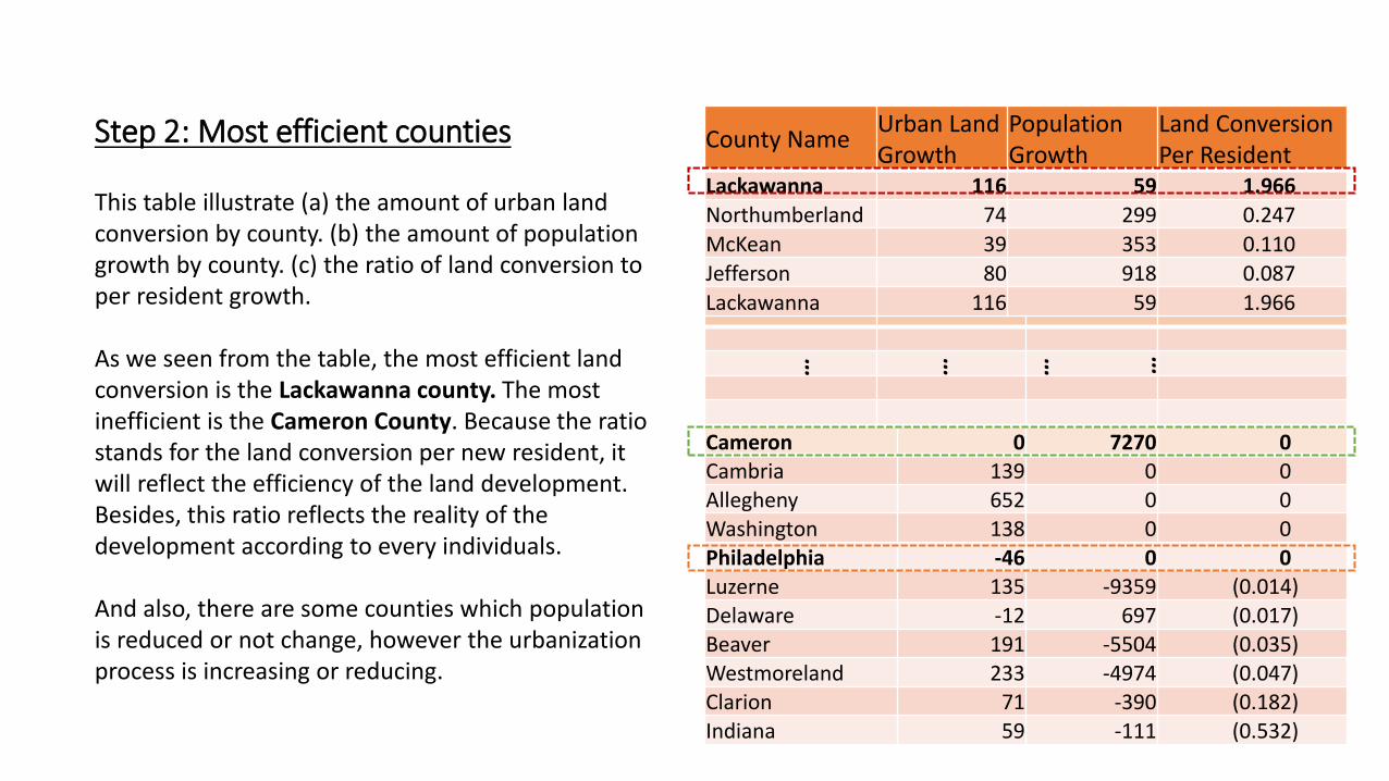
This table illustrate (a) the amount of urban land conversion by county. (b) the amount of population growth by county. (c) the ratio of land conversion to per resident growth.
As we seen from the table, the most efficient land conversion is the Lackawanna county. The most inefficient is the Cameron County. Because the ratio stands for the land conversion per new resident, it will reflect the efficiency of the land development. Besides, this ratio reflects the reality of the development according to every individuals.
And also, there are some counties which population is reduced or not change, however the urbanization process is increasing or reducing.
County NameUrban Land Growth
Population Growth
Land Conversion Per Resident
Lackawanna 116 59 1.966
Northumberland 74 299 0.247
McKean 39 353 0.110
Jefferson 80 918 0.087
Lackawanna 116 59 1.966
Cameron 0 7270 0
Cambria 139 0 0 Allegheny 652 0 0 Washington 138 0 0 Philadelphia -46 0 0
Luzerne 135 -9359 (0.014)
Delaware -12 697 (0.017)Beaver 191 -5504 (0.035)Westmoreland 233 -4974 (0.047)Clarion 71 -390 (0.182)
Indiana 59 -111 (0.532)
…
Step 2: Most efficient counties
… … …

Step 3: The Sensitive Lands in PA Counties (1992)
• Combine raster layers ( water, farm, pasture & forest)
• Use Raster Calculator to combine the different 1992 environmental rasters into a composite “1992 sensitive lands” raster.
• Reclassify this new sensitive lands raster which consist of two values, 0 and 1, where 1 is sensitive land areas and 0 is not sensitive.
• Sum sensitive lands by county in 1992
• Use the Zonal Statistics (as Table) command to summarize the amount of sensitive lands by county in 1992
sensitive land in 1992

Step 4: The Sensitive Lands developed in 2001
• Combine raster layers (new urbanized locations between 1992 and 2001 & sensitive land in 1992)
• Use Raster Calculator to combine the grid from step 1 (areas that changed from non-urban to urban) with the sensitive lands grid of 1992
• Reclassify this new sensitive lands raster which consist of two values, 0 and 1, where 1 is the places where recent urban growth was most threatening to sensitive lands in 1992
Layer1: New urbanized locations between 1992 and 2001 from step 1-1: non-urban0: urban or non-urban1: urbanized
Layer2: Sensitive lands grid of 1992 from step 3
0: not sensitive land; 1: sensitive land areas
Raster Calculator
-1; 0; 1; 2
0
Reclassify
1: Developed Sensitive Land in 1992

Step 4: The Sensitive Lands developed in 2001
• Summarize the number of grid cells that sensitive lands developed
• Use Zonal Statistics (as Table) to Summarize the results by county
• From the table, we can easily find the Allegheny is the County which has recent urban growth was most threatening to sensitive lands in 1992.
• Also the total number of the grid cells that were sensitive lands developed upon in 2001 is the 4677.

Step 5: The Urban Land Use in 2001 - Urbanization
• Factor 1: distance to existing urban (Weight: 4)
• Within 6km of urban development in 2001 in PA counties
• Use the Euclidean Distance Tool to develop the maximum distance of 6km to existing area
• Reclassify the value of 1 and 0. Value of 1 means that area within 6km
• Factor2: slope <=2 (Weight: 3)
• slope less than 2% grade in 2001 in PA counties.
• Use the Raster Calculator to figured out "pa_slope_" <= 2
• Factor3: distance to highways (Weight: 2)
• within 10KM of 4-lane highways in 2001 in PA counties
• Use the Euclidean Distance Tool to develop the maximum distance of 10km to highway area
• Reclassify the value of 1 and 0. Value of 1 means that the area of distance to highways within 0km
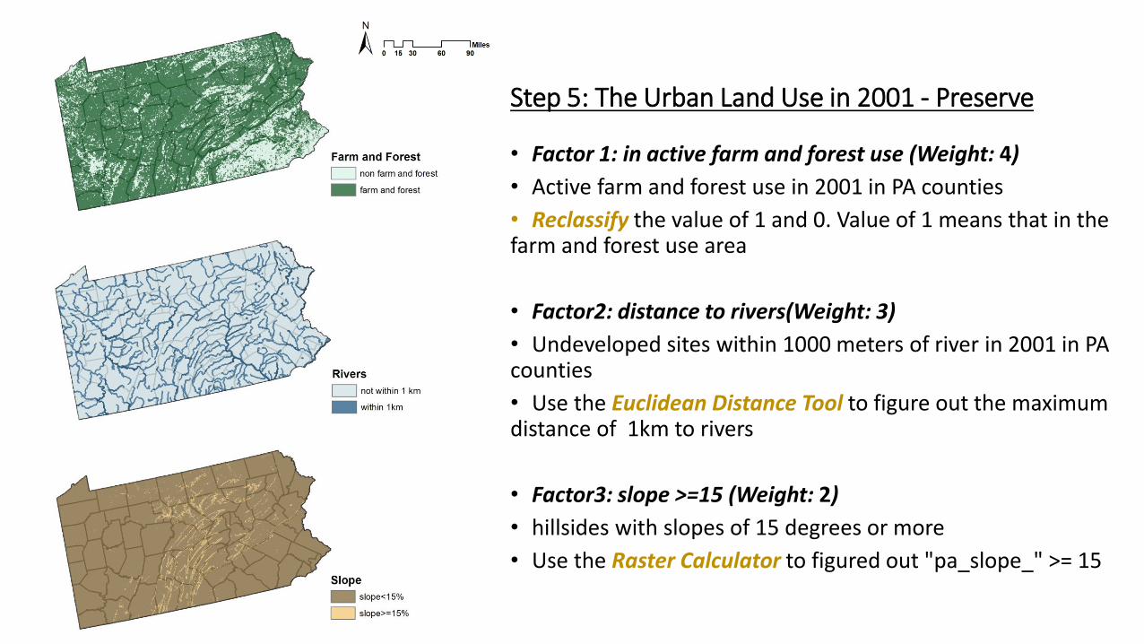
Step 5: The Urban Land Use in 2001 - Preserve
• Factor 1: in active farm and forest use (Weight: 4)
• Active farm and forest use in 2001 in PA counties
• Reclassify the value of 1 and 0. Value of 1 means that in the farm and forest use area
• Factor2: distance to rivers(Weight: 3)
• Undeveloped sites within 1000 meters of river in 2001 in PA counties
• Use the Euclidean Distance Tool to figure out the maximum distance of 1km to rivers
• Factor3: slope >=15 (Weight: 2)
• hillsides with slopes of 15 degrees or more
• Use the Raster Calculator to figured out "pa_slope_" >= 15

• Use the Raster Calculator to develop a “Future Urbanization Index Map”• " distance to existing urban " * 4 + " slope <=2 " * 3 + " distance to highways " * 2• 5 Quantile breaks.
• Future Urbanization Index Map
Step 5: The Urban Land Use in 2001 – Urbanization & Preserve
• Environmental Sensitivity Index map
• Use the Raster Calculator to develop a “Environmental Sensitivity Index map”
• "slope >=15 " * 2 + "distance to rivers" * 3 + "in active farm use" * 4 + "in active forest use " * 4
• 5 Quantile breaks.
0 - 3
3 - 4
4 - 5
5 - 6
6 - 9
0
0 - 2
2 - 4
4 - 5
5 - 9

• In Urban Urbanization Index and Environment Sensitivity Map, Reclassify index where the top 3rd
highest values are deemed ‘most likely to be urbanized or sensitivity’ (give these values a ‘1’) and remaining values a ‘0’
• Reclassify Urban Urbanization Index map from 0 and 1 to 0 and 10.
• Use the Raster Calculator to combine Urban Urbanization Index map with environmentally sensitive index, have a new grid that contains the values 0, 1, 10 and 11.
Step 6: Four categories of Environment Sensitivity Index and Future Urbanization
0 to 0
0 to 10
0 10 10
0 1 10 11
Urbanization Sensitivity

Four categories of Environment Sensitivity Index
and Future Urbanization Map
• The four categories stands for:
• (0) -Area not environmentally sensitive And might not be developed.
• (1) -Area that are environmentally sensitive And might not be developed.
• (10)-Area that are not sensitive And might be developed.
• (11)-Area that are sensitive And might be developed.
Step 6: Four categories of Environment Sensitivity Index and Future Urbanization
0 10 10
0 1 10 11
Urbanization Sensitivity

• Not environmentally sensitive and might be developed area
• Environmentally sensitive and might be developed area
Step 7: Two important type pf developed area
Supply-sideDemand-side
According to this two maps, the trend for the development we can see from the above map is mainly located in the eastern and western part of PA counties. The trend of the environmental sensitive we can see from the right map is mainly located in the central part of the PA counties.
