urban growth drivers and spatial inequalities: europe - a case with

A New Concept of European Federalism

LSE ‘Europe in Question’ Discussion Paper Series

Urban Growth Drivers and Spatial

Inequalities: Europe - a Case with

Geographically Sticky People

Paul C. Cheshire and Stefano Magrini

LEQS Paper No. 11/2009

October 2009

All views expressed in this paper are those of the author and do not necessarily represent the

views of the editors or the LSE.

© Paul C. Cheshire and Stefano Magrini

Editorial Board

Dr. Joan Costa-i-Font

Dr. Vassilis Monastiriotis

Dr. Jonathan White

Ms. Katjana Gattermann

Paul C. Cheshire & Stefano Magrini




Paul C. Cheshire* and Stefano Magrini**

Abstract

Analysts of regional growth differences in the US tend to assume full spatial equilibrium

(Glaeser et al, 1995). Flows of people thus indicate changes in the distribution of spatial

welfare more effectively than differences in incomes. Research in Europe, however, shows

that people tend to be immobile. Even mobility within countries is restricted compared to the

US but national boundaries offer particular barriers to spatial adjustment. Thus it is less

reasonable to assume full spatial equilibrium in a European context and differences in per

capita incomes may persist and signal real spatial welfare differences. Furthermore, it implies

that the drivers of what population movement there is, may differ from the drivers of spatial

differences in productivity or output growth. This paper analyses the drivers of differential

urban growth in the EU both in terms of population and output growth. The results show

significant differences in the drivers as well as common ones. They also reveal the extent to

which national borders still impede spatial adjustment in Europe. This has important

implications for policy and may apply more generally to countries – for example China - less

homogeneous than the USA.

* London School of Economics European Institute, Department of Geography & Environment, Houghton St, London

WC2A 2AE, UK

Email: [email protected]

**Università Ca' Foscari di Venezia Dipartimento di Scienze Economiche, Cannaregio, 873 S. Giobbe, 30121 Venezia, IT


Fiscal Decentralization and Economic Growth

Table of Contents

Abstract

1. Introduction 1

2. Meaningful Data for Useful Regions 3

Our regions 3

Why FURs not NUTS? 4

Implications for Conventional Analyses of Spatial Disparities 5

Our Approach to ‘Growth Regressions’ and Spatial Dependence 6

3. Results 7

Common Features of Models of Population and Economic Growth 7

4. Results for Population Growth (1980 to 2000) 9

Localized adjustments 12

Better weather attracts 14

Spatial dependence 16

5. Analysis and Results for GDP Growth per Capita (1978 to 1994) 18

Many of the drivers of economic growth differ 18

Controlloing for ‘national’ factors 20

Growth: agglomeration good; density bad 21

Spatial dependence – introducing a spatial lag 21

Human capital, R&D and local growth promotion with spatial spillovers 22

Systematic spatial influences on growth 26

6. Comparing and Contrasting the Drivers of Population and

Economic Growth 28

References

Appendix


1




1. Introduction

Much work has been done on regional growth processes in the U.S. (e.g., Rey and

Montouri, 1999; Glaeser et al, 1995). However, this work has been based on an

explicit or implicit underlying assumption of full spatial equilibrium. This is

explicitly the case with Glaeser et al (1995). They argue that since, if there is full

spatial equilibrium, people are unable to improve their welfare by moving from one

place to another, flows of people indicate changes in the distribution of spatial

welfare (as people move to places offering superior opportunities or lifestyles) more

directly than do changes in income levels or rates of growth of income.

In contrast, research in Europe shows that people tend to be quite immobile. Net

migration between similarly sized geographic regions in the U.S. is 15 times greater

than in Europe (Cheshire and Magrini, 2006). This is despite the fact that differences

in real incomes and employment opportunities are substantially greater and

geographic distances smaller in Europe than in the U.S. Even mobility within

countries is limited compared to the U.S. But as we will illustrate here, national

boundaries offer particular barriers to spatial adjustment. Thus it seems

unreasonable to assume full inter-regional or inter-urban equilibrium in a European

context; differences in per capita incomes are persistent and likely to signal real

spatial welfare differences. Furthermore, the reluctance of people to move countries

or apparently even move inter-regionally in Europe suggests that the drivers of

whatever population movement there is in Europe may differ from the drivers of

spatial differences in productivity or output growth.

Urban Growth Drivers and Spatial Inequalities

2

This paper combines theory with empirical analysis to investigate the drivers of

spatial growth processes, welfare, and disparities in a context in which people are

markedly immobile. Drawing on two of our recent papers (Cheshire and Magrini,

2006 and 2009), we review the evidence on the drivers of differential urban growth in

the European Union (EU), both in terms of population and Gross Domestic Product

(GDP) per capita growth. We conclude that while environmental ‘goods’, in the form

of climate differences, are significant influences on urban population growth, there is

no general process of the European population ‘moving to the sun’. Climate

differences are significant only as they vary from national values: not as they

systematically vary from European values. Moreover, while there do appear to be

some Europe-wide economic drivers of population movement, we find that their

influence is less than in the case of economic growth differences. Analysis of spatial

dependence and its determinants also reveals substantial national boundary barriers

to both population and economic adjustment. Together, these findings suggest that

one cannot reasonably maintain the assumption of full spatial equilibrium in a

European context.

In Section 2 we give some technical detail and explanation about our units of analysis

– Functional Urban Regions (FURs). These are a ‘core-based’ type of urban region

similar to the Standard Metropolitan Statistical Areas which provide the units for

much applied urban economics in the U.S. Readers may want to skip this section at a

first reading although the use of data for FURs is central to our approach. In Section

3 we summarize the results concerning the drivers of population growth, reported in

detail in Cheshire and Magrini (2006), and then summarize the results of a more

recent analysis of the drivers of growth in FUR GDP per capita (Cheshire and

Magrini, 2009).We find strong indications of population immobility and sluggish

migration response across national borders and also find that economic adjustment

between neighboring city-regions is strongly impeded by national borders. In

analyzing the drivers of economic growth, we pay particular attention to the role of

highly skilled human capital, concentrations of R&D, and the potential role of

differences in systems of local government in a (‘non-Tiebout’) world of sticky


3

people and territorial spillovers with local public goods. Although when analyzing

the determinants of urban population and economic growth there are some drivers

in common and these apparently reflect the immobility of Europeans, we also find

important differences. The final section offers an interpretation of why there are such

differences and what they suggest both for spatial adjustment, spatial equilibrium

and policy.

2. Meaningful Data for Useful Regions

Our regions

Our units of analysis are core-based urban regions – or Functional Urban Regions

(FURs) – similar in concept to the Standard Metropolitan Statistical Areas (SMSAs)

familiar from the U.S. literature. These FURs were originally defined in Hall and Hay

(1980), but some of their boundaries were slightly updated and revised in Cheshire

and Hay (1989). Since then, the data set relating to these FURs has been continuously

updated, although their boundaries remain fixed as at 1971. The urban cores are

identified on the basis of concentrations of jobs. Using the smallest spatial units in

each country for which the basic data were available, all contiguous units with job

densities exceeding 12.35 per hectare were combined to identify the FUR core-city.

The FUR hinterland was then identified by combining all the contiguous units from

which more people commuted to jobs in the given core than commuted elsewhere,

with a minimum cut-off of 10 percent. This definitional method was used for the

great majority of countries, but in some cases critical data were unavailable, so

alternative methods had to be used. The most extreme case was Italy, where

previously defined retail areas were substituted for the FUR boundaries. Because of

the difficulties of estimating comparable data for the FURs, we analyze patterns of

growth only for the largest 121 FURs. All of these FURs are in the former EU-121 –

1 That is, in the countries of Belgium, Denmark, France, Germany, Greece, Ireland, Italy,

Luxembourg, The Netherlands, Portugal, Spain and the United Kingdom.


4

excluding Berlin – and all had a total population of more than one third of a million

and a core city of more than 200,000 at some date since 1951.

Why FURs not NUTS?

There are significant advantages of using functionally, as opposed to adminis-

tratively, defined regions as the units of analysis. Even across a country as consti-

tutionally unified and developmentally homogeneous as the U.S., states, counties

and cities vary considerably in how they relate to patterns of behavior or economic

conditions. In Europe the official regions (the NUTS2) are far more disparate since

they combine within one system very different national systems. Even within one

country – Germany – the largest NUTS Level 1 regions vary from hangovers from

the Middle Ages – such as Bremen (population 0.7 million) or Hamburg (1.7 million)

- to regions such as Bavaria, with a population of 12.3 million and the size of several

smaller European countries combined. In terms of administrative competence,

Germany has 16 of the functionally very disparate Länder (NUTS Level 1 regions),

each with substantial powers and constituting the elements of its Federal system;

below that are the Kreise (NUTS Level 3) – 439 of them in 2003. Britain has 12 NUTS

1 regions, corresponding in mean size to the Länder, but only one of them – Scotland

- has any real administrative or fiscal independence. In Britain, there are only 133 of

the smaller units supposedly equivalent to the Kreise. Bavaria, despite including

major cities such as Munich, had a population density of only 174 people per square

km, compared to 4,539 in the NUTS Level 1 region of London or 2,279 in Hamburg

(CEC, 2004).

More significant than their heterogeneity in size and administrative powers is the

fact that the official NUTS regions are economically heterogeneous. In some cases

2 Nomenclature des Unités Territoriales Statistiques (N.U.T.S.) regions. This is a nesting set of

regions based on national territorial divisions. The largest are Level 1 regions; the smallest for

which a reasonable range of data is available are Level 3. Historically Level 3 NUTS regions

corresponded to Counties in the UK, Départements in France; Provincies in Italy or Kreise in

Germany.


5

they contain very different local economies within the same statistical unit (for

example, Glasgow and Edinburgh in Scotland or Lille and Valenciennes in Nord-Pas-

de-Calais) and in others a single city-region is divided among as many as three

separate units. The functional reality of Hamburg, for example, is divided among

three different Länder: Hamburg, Schleswig-Holstein, and Niedersachsen. There are

thus many NUTS regions with large scale and systematic cross border commuting

and some contain mainly bedroom communities near large cities. Others (for

example, Brussels, London, Bremen or Hamburg) are effectively urban cores or only

small parts of urban cores. This means that residential segregation influences the

value of variables such as unemployment, health or skills if measured on the basis of

the boundaries of NUTS. Moreover, measures of Gross Domestic Product (GDP),

Value Added or productivity per capita can be grotesquely distorted since output is

measured at workplaces and people are counted where they live.

Even measured growth in GDP per capita can be seriously distorted since over time

residential (de)centralization may occur at different rates to job (de)centralization.

The reported growth in GDP per capita for the NUTS region of Bremen during the

1980s, for example, was 40 percent higher than for the Bremen functionally defined

region. This was because of strong residential relative to job decentralization during

that decade. These problems of statistical distortion are concentrated in the larger

cities, because these tend to spill over their administrative boundaries; they are also

concentrated in richer regions. This last facet of the distortions to official regional

statistics results not only because richer regions tend to include larger cities but

because a significant proportion of larger cities extend functionally beyond their

administrative boundaries, so their recorded GDP (or GVA) per capita is overstated.

Implications for Conventional Analyses of Spatial Disparities

These are obvious points, causing us to have serious reservations about the many

published analyses of regional growth rates in Europe that use official Eurostat data

for NUTS regions. This means that official measures of so-called ‘regional disparities’


6

– which show, for example, that in 2001 the ‘region’ of Inner London was 2.5 times as

‘rich’ in per capita GDP as the mean for the EU-15 and 3.2 times as ‘rich’ as the UK’s

poorest region - are in essence completely invalid.

It is for these reasons that we rely on our own data for FURs. There is one additional

advantage of this choice in the present context. FURs are the most economically

independent divisions of national territories that can be constructed. They represent

concentrations of jobs and all those people who depend on those jobs – the economic

spheres of influence of major cities. As a result, the benefits of additional

employment or output are confined as much as possible to those who live within a

given FUR.

Our Approach to ‘Growth Regressions’ and Spatial Dependence

Two idiosyncrasies of our approach should be noted. First, in our analysis of growth

in GDP per capita we do not include the initial level of GDP per capita. So this

analysis does not contribute to the regional growth regression literature stemming

from the work of Barro and Sala-i-Martin (Barro, 1990; Barro and Sala-i-Martin, 1991;

1992 or 1995). We find this literature to be both theoretically (see the discussion in

Cheshire and Malecki, 2004) and empirically suspect. Empirically when we include

the initial level of GDP per capita in our models, it clearly introduces

multicollinearity and leads to very unstable parameter estimates for the variable –

even signs flip. In essence, it is possible to generate either apparent β-convergence or

β-divergence in equally respectable looking models. However, in all of our better

specified models, the effect, if included, of initial GDP per capita on subsequent

growth performance is statistically insignificant.

The second idiosyncrasy of our approach is in our interpretation of any finding of

spatial dependence. That the growth performance of cities or regions close to each

other should interact is not in itself surprising, so we should expect to find systematic

spatial patterns in growth. These might be caused by common factors (e.g. some


7

shared structural or institutional features) but we should also expect to find localized

interactions to be more pervasive and responsive than those between cities or regions

that are widely separated or – given the findings on population mobility – separated

by national borders. If, therefore, we can find variables that reflect spatial adjustment

mechanisms between neighboring regions we should be able to ‘explain’ remaining

spatial patterns in the data. In other words a finding of spatial dependence is really

an indicator of an omitted variables problem and if the model(s) can be more fully

and appropriately specified then any indicated problems of spatial dependence

should be resolved. In testing for spatial dependence and formulating our variables

to reflect spatial adjustment processes, we also find that results critically depend on

how the spatial weights matrix is formulated. Following standard procedures to

specify the spatial weights matrix, we experiment with contiguity, geographic and

time-distance and find test statistics which reveal no apparent problems of spatial

dependence in the theoretically more satisfying models. Problems of spatial

dependence are only indicated when an additional time-distance penalty for national

borders is introduced. This is consistent with our other findings, which show, for

example, that climatic differences only influence population mobility if expressed

relative to a country’s mean. These findings indicate that national borders in Europe

present a continuing barrier to processes of spatial adjustment - even for localized

economic adjustment.

3. Results

Common Features of Models of Population and Economic Growth

Appendix Tables 1a & b define the main variables used. Models for both population

and GDP per capita growth apply the same basic approach. We first build a ‘base’

model and test it for standard specification problems and for spatial dependence. In

the latter tests we pay particular attention to the specification of the spatial weights

matrix - choosing weights which maximize the indicated sensitivity to problems of


8

spatial dependence while conforming to obvious economic logic. For both sets of

models we use OLS. The exception is the estimation of models with a spatial lag

where we use maximum likelihood. We try to minimize problems of endogeneity.

Although we recognize that our efforts do not necessarily entirely eliminate all such

problems, we believe that any remaining endogeneity problems do not significantly

influence the results.

There are two families of models in our analysis: 1) those that use the FUR rate of

change of population from 1980 to 2000 as the dependent variable and 2) those that

use the FUR rate of growth of GDP per capita at purchasing power standard (PPS)

measured from the mean of 1978-80 to the mean of 1992-94 as the dependent

variable. The main control variables in the two families of models are similar. We

have consistently found that specific measures of reliance on old, resource-based

industries (e.g., the coal industry, port activity, agriculture) perform better than more

generalized measures such as employment in industry or unemployment at the start

of the period (although each of these is included in one model and is marginally

useful). Since reliance on the coal industry is measured with a geological indicator, it

seems safe to assume it is exogenous. Port activity is measured very early – 1969 –

before the main transformation of the industry to modern methods and before any

likely integration effects of creating the European Union would be apparent.

Concentration on agriculture is not in the FUR itself but in the larger region

containing the FUR – again well before the start of the period covered by the

dependent variable. These control variables reflect economic factors and work in

very similar ways, whether FUR population or GDP per capita growth is the

dependent variable.

One result of using the major FURs as our spatial units of analysis is that a large

proportion of the territory of each country is outside their area. In 2001, the total

population of the EU-12, excluding Berlin, was about 340.5 million. At that time,

almost exactly half – 169.2 million – lived in its major FURs as defined here. This

property of the FURs allows us to define two additional control variables: the rate of

natural growth of population in the area of each country that is outside its major


9

FURs and the rate of growth of GDP per capita in the same area. In each case, we

calculate these control variables over the same period as our dependent variable. By

including the rate of non-FUR natural population growth as an independent variable

in the population models, we effectively model quasi-net migration.

In cross-sectional analyses of regional growth the conventional control for all

country-specific factors (notably the incidence of the national economic cycles but

also institutional and policy differences between countries) has been national

dummies. However, this would be problematic with our data set since Denmark,

Greece, Ireland and Portugal each have only one or two major FURs. This means we

would have to arbitrarily choose which countries to pool to construct national

dummies. More interestingly, since we wish to infer causation, our underlying

assumption must be that our observational units – the major FURs of Western

Europe – are in statistical terms a homogeneous population. A more elegant solution

to control for national factors not explicitly included as independent variables is,

therefore, to include ‘non-FUR growth’ as a continuous control variable.

4. Results for Population Growth (1980 to 2000)

Table 1 shows the ‘Base’ model for FUR population growth. All variables are

significant and have the expected signs. There are two variables, in addition to those

discussed above, that reflect expectations about systematic spatial patterns of

growth. The first of these is taken directly from Clark et al, 1969 (with values

extended to cover Spain and Portugal, using Keeble et al, 1988). The process of

European integration, in combination with falling transport costs, was expected to

lead to systematic changes in regional economic potential, favoring ‘core’ regions.

Clark et al estimated for each region of the original six member countries, plus

Denmark, Ireland, Norway and the UK, the impact of European integration on


10

‘economic potential.’3 We have added our own estimates for the major FURs of

Greece. Clark et al’s expectation was that changes in economic potential so measured

would indicate the regional patterns of systematic gains and losses from the creation

and enlargement of the EU. Although the original theoretical underpinnings were

somewhat ad hoc, such a prediction seems entirely compatible with New Economic

Geography models.

3 This is measured as the accessibility costs to total GDP at every point, allowing for the costs of

trade and transport and how those would change with the elimination of tariffs, EU enlargement,

and transport improvements to include containerisation and roll-on roll-off ferries.


11

Table 1 Dependent Variable: FUR Population Growth Rate 1980 to 2000 - The Base Model

Model 1 2 3 4 5 6 ‘Base’

R-squared 0.2460 0.3101 0.3830 0.4818 0.5014 0.5180

Constant

0.006886

5

0.006600

6

0.008491

5

0.005555

3

0.005351

3 0.005074

T 4.15 4.02 4.77 3.76 3.51 3.31

Agric Emp.’75

0.000343

1

0.000243

2 0.0001806

0.000381

8

0.000396

6

0.000410

2

T 3.59 2.57 1.93 4.04 4.07 4.21

(Agric Emp.’75)2 -0.000009

-

0.000006

5 -0.000005

-

0.000009

2

-

0.000009

2

-

0.000009

4

T -3.50 -2.47 -2.04 -3.62 -3.52 -3.61

Ind. Emp.’75

-

0.000145

6

-

0.000112

3 -0.000134

-

0.000156

4

-

0.000171

6

-

0.000169

3

T -3.93 -2.78 -3.25 -3.81 -4.11 -4.07

Coalfield: core

-

0.002659

1

-

0.002909

5

-

0.002837

1

-

0.002450

7

-

0.002114

3

T -2.75 -3.31 -3.27 -2.90 -2.43

Coalfield: hint’land

-

0.002092

2

-

0.002318

2

-

0.002289

2

-

0.002724

5

-

0.002054

8

T -3.60 -2.88 -3.14 -3.65 -2.48

Port size ’69

-

0.001026

7

-

0.000861

7

-

0.000821

6

-

0.000727

8

T -3.08 -2.90 -2.98 -2.56

(Port size ’69)2

0.000056

9

0.000047

8

0.000041

2

0.000036

6

T 3.36 3.21 2.91 2.51

Nat Non-FUR Pop Growth ’80-

’00

0.473166

1

0.455977

1

0.441785

2

T 4.38 4.15 3.95

(Integration Gain)2

0.001100

8

0.001127

8

T 2.30 2.48

Interaction ’79-’91

0.044080

6

T 2.11

Parameter estimates shown in italics are significant only at 10%: all other parameter estimates

are significant at 5% or better

Variables are defined in Appendix Tables 1a and 1b. Sources for all variables are shown in

Cheshire and Magrini, 2006 and 2009. Parameter values in the above table are the authors’

estimates.


12

Localized adjustments

There are likely to be other systematic spatial patterns between FUR population growth

rates because of interaction between contiguous FURs. People in Europe may be very

immobile, but in the specific conditions of dense urbanization there are alternative

forms of spatial labor market adjustment. In the EU, there are swathes of densely

urbanized territory where FURs are not just tightly clustered; their boundaries and

commuting hinterlands touch and, at the ‘commuter shed’, there is still substantial

cross-border commuting. In such conditions, if the economic attractions of one FUR

increase relative to its neighbors, that FUR will attract additional commuters. Since

changes in commuting patterns are cheap – particularly if there are good transport links

– such adjustments between adjacent FURs should be expected to respond to small

changes in the spatial distribution of opportunities.

If changes in commuting patterns act as spatial adjustment mechanisms between

neighboring FURs, then we would expect there to be a ‘growth shadow effect’. That is, a

FUR growing economically faster than neighboring FURs will initially attract additional

workers from those FURs. Over time, a proportion of these long distance commuters

attracted to work in the faster growing FUR may move there and become short distance

inter-FUR ‘migrants,’ which would lead to population growth in the subsequent period

in the economically more dynamic FUR. Moreover, since long distance commuters have

higher human capital and perhaps favorable unmeasured productivity characteristics,

there would also be a composition effect. This means the productivity of the labor force

of the FUR that has attracted additional commuters would grow relative to that of its

neighbor(s). Finally, there might also be dynamic agglomeration effects favoring

productivity growth in the faster growing FUR. It was shown in Cheshire et al, 2004,

that commuting flows between FURs do in fact adjust to differential employment

opportunities in the way indicated above and that the response of net commuting to

differential growth in employment opportunities is subject to a quite sharp distance

decay effect.


13

We represent this localized interaction through the medium of labor market

adjustment using the “Interaction” variable. This is measured as the sum of the

differences in the employment growth rates in each FUR and in all other FURs

within 100 minutes traveling time, weighted by the inverse of time-distance over the

period 1979-1991. It thus proxies for net commuters attracted to employment in each

FUR over the first half of the period. The estimated parameter for the variable is

significant and positive, supporting the interpretation that commuters attracted to a

FUR in one period reinforce the dynamism of the more successful FUR relative to its

neighbors and generate differential population growth over the period as a whole.

Although not reported here, it is also worth mentioning that compared to models

that do not include this “Interaction” variable, problems of spatial dependence are

much reduced.

Table 2

Dependent Variable: FUR Population Growth Rate 1980 to 2000 - Base

Model plus Geographic and Climate Variables

Base + geographical variables Base model + climate variables

Linear Quadratic

West or

South

within

country

South

within

country

West or

South

within EU

Wet day

frequency

ratio:

country

Wet day

frequency

ratio:

country

Mean

Temperat

ure ratio:

country

Maximum

Temperatur

e ratio:

country

Model 7 8 9 10 11 12 13

R2 0.6012 0.5951 0.5258 0.5940 0.6090 0.5863 0.5946

West

-

0.00000

2

1β̂ x

-

0.00789

-

0.02615

-

0.04805

6

-

0.076058

T -1.44 t -4.70 -3.98 -2.37 -2.29

South

0.00000

5

0.00000

5 2β̂ x2 0.00938

7

0.02607

6 0.041133

T 4.02 4.69 t 2.91 2.74 2.58

EUwest

0.00000

08

T 0.99

EUsouth

0.00000

04

T 0.66

Parameter estimates shown in italics are not significant at 10%



estimates.


14

Better weather attracts

Table 2 shows what happens if we include geographic and climatic variables in the

base model. Two conclusions clearly emerge. The first is that FURs further south

grew faster, but this effect was only within countries. When the position of a FUR is

measured relative to a fixed point in the EU- 12 (taken arbitrarily as the centroid of

the FUR of Brussels) then its geographic position is statistically insignificant.

However, there was still a strong effect of being further south within each country.

Being further west within a country had a minor but insignificant effect on

population growth: being further west within the EU as a whole had no significant

impact on population growth. Numerous studies in the US (e.g., Graves, 1976, 1979,

1980 & 1983; Rappaport, 2004) have shown that - other things equal - migration is

sensitive to better weather. Likewise in the ‘Quality of Life’ literature (e.g., Blomquist

et al, 1988; Gyourko and Tracey, 1991) climate is an important driver of quality of life.

The data do not allow us to estimate full ‘Quality of Life’ models in Europe.

However, the results of including measures of weather are shown in the last four

columns of Table 2. We can see that these weather variables are statistically highly

significant and, if anything, perform rather better than the geographic position of a

FUR. The functional form that is most appropriate seems to be quadratic, although

the relationship is quite close to linear. These results confirm that it is only the

climate of a FUR relative to the mean for its country that is significant. Again,

expressing climatic differences relative to the mean for the EU as a whole proves

entirely insignificant. Table 3 shows the results for some better performing models

and shows that the best results are achieved if measures of both dryness and warmth

relative to national means are included.


15

Table 3

Dependent Variable: FUR Population Growth Rate 1980 to 2000 - Best Models Model 14 15 16

R-squared 0.6325 0.6326 0.6405

Constant plus:

Agric Emp.’75 0.0003127 0.0004266 0.0004079

t 3.02 4.32 4.42

(Agric Emp.’75)2 -0.0000056 -0.0000083 -0.0000075

t -2.09 -3.31 -3.06

Industrial Emp.’75 -0.0000962 -0.0001457 -0.0001213

t -2.55 -3.71 -3.55

Coalfield: core -0.0015896 -0.001655 -0.001812

t -2.21 -2.10 -2.42

Coalfield: hint’land -0.0020415 -0.001682 -0.0018028

t -2.47 -2.12 -2.37

Port size ’69 -0.0005831 -0.0006274 -0.0006521

t -2.30 -2.59 -2.64

(Port size ’69)2 0.0000291 0.0000294 0.0000315

t 2.31 2.39 2.55

Nat Non-FUR Pop Growth ’80-’00 0.3029144 0.5536141 0.4710524

t 2.41 4.91 4.38

(Integration Gain)2 0.0015988 0.0020954 0.0020679

t 3.41 4.54 4.50

Interaction ’79-’91 0.0539774 0.0532723 0.0519908

t 2.69 2.70 2.73

South within EU 0.0000032

t 2.80

Frost frequency ratio : country -0.0039281

t -2.50

(Frost frequency ratio : country)2 0.0020628

t 3.36

Maximum temperature ratio :

country -0.0752656

t -2.33

(Maximum temperature ratio :

country)2 0.0379645

t 2.51

Wet day frequency ratio : country -0.0214449 -0.0247 -0.0202854

t -3.77 -3.76 -3.58

(Wet day frequency ratio : country)2 0.0082249 0.008621 0.0069708

t 2.78 2.81 2.37

All parameter estimates significant at 5% or better



estimates.


16

Spatial dependence

The results of diagnostic tests on these models are reported in Cheshire and Magrini,

2006. These results suggest that there are no problems of either heteroskedasticity or

non-normality of errors. The value of the multicollinearity condition number is

relatively high in most of the models in which climate variables are included in

quadratic form. However, since the parameter estimates are stable and the functional

form (effectively suggesting that it is asymptotic to an upper value) seems sensible,

this does not seem to be a cause for concern.

As is well known, the major practical issue in testing for problems of spatial

dependence is the choice of measures of ‘distance’. There is no ‘theoretically correct’

measure that one should select a priori. The spatial econometrics literature provides

examples of many measures: contiguity; linear geographic distance; time-distance; or

the inverse of time distance. Our view is that any indicators of spatial dependence

should in principle be reflections of underlying spatial processes. This suggests two

points: one should select the distance weights in a way that makes sense in terms of

spatial economics and spatial economic adjustment processes; and a reasonable

criterion for choosing the weights is that, assuming they make sense in economic terms,

they maximize sensitivity to spatial dependence.

With these points in mind, we measured distance between FURs as the transit time by

road, including any ferry crossings and using the standard commercial software for

road freight. We tested for both the inverse of time distance and the inverse of time

distance squared. Given that we had already found that national frontiers constituted

strong barriers to spatial mobility (from the results on climate and geographical

variables), we also experimented with an added time distance for all FURs separated by

a national border. We found that the greatest sensitivity in the tests for spatial depen-

dence was achieved if the time cost of a national border was set at 120 minutes.


17

Table 4

Inclusion of Spatially Lagged Population Growth 1980 to 2000

Model 17 Model 18 Model 19

R-squared 0.5416 0.6418 0.6468

Loglikelihood 554.986 568.97 569.604

Spatially lagged pop growth 1980-

‘00 0.37939 0.25415 0.21369

prob 0.0004 0.0196 0.0540

Agric Emp.’75 0.00033 0.00037 0.00036

prob 0.0003 0.0000 0.0000

(Agric Emp.’75)2 -0.00001 -0.00001 -6.6E-06

prob 0.0018 0.0027 0.0056

Industrial Emp.’75 -0.00013 -0.00013 -0.00011

prob 0.0001 0.0003 0.0013

Coalfield: core -0.00169 -0.00141 -0.0016

prob 0.0214 0.0357 0.0154

Coalfield: hint’land -0.00177* -0.00150* -0.00165*

prob 0.0774* 0.0984* 0.0668*

Port size ’69 -0.00069 -0.00061 -0.00064

prob 0.0032 0.0050 0.0024

(Port size ’69)2 0.00003 0.00003 3.04E-05

prob 0.0236 0.0427 0.0233

(Integration Gain)2 0.00077 0.00175 0.00178

prob 0.1146 0.0002 0.0002

Interaction ’79-’91 0.04829 0.05532 0.05378

prob 0.0194 0.0029 0.0037

Nat Non-FUR Pop Growth ’80-’00 0.37956 0.50526 0.43847

prob 0.0000 0.0000 0.0000

Wet day frequency ratio : country -0.02122 -0.01743

prob 0.0130 0.0391

(Wet day frequency ratio : country)2 0.00715* 0.00563

prob 0.0937* 0.1853

Frost frequency ratio : country -0.00350

prob 0.0401

(Frost frequency ratio : country)2 0.00193

prob 0.0097

Max. Temperature : country -0.07122

prob 0.0060

(Max. Temperature : country)2 0.03555

prob 0.0042

* Estimated parameters significant at 10%. All other estimates significant at 5% or better except

those in italics which are not significant at 10%.



estimates.

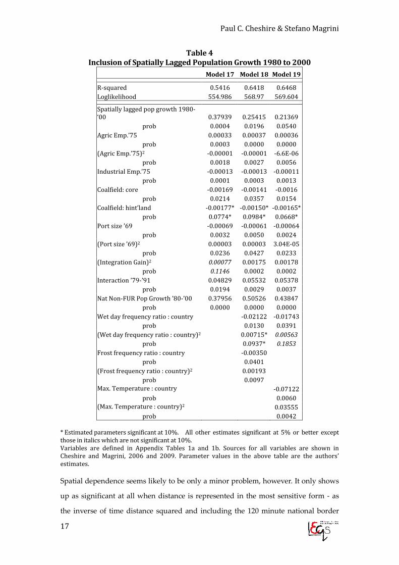
Spatial dependence seems likely to be only a minor problem, however. It only shows

up as significant at all when distance is represented in the most sensitive form - as

the inverse of time distance squared and including the 120 minute national border


18

effect. Indeed, if no time-distance penalty for national borders is included, then, in

the better models, no problems of spatial dependence were indicated. Even then, in

Model 16 (in Table 3), indicated spatial dependence was only on the margins of

significance at 10%. Nevertheless, it seemed safer to re-estimate including a spatial

lag of the dependent variable. Selected (and representative) results of this re-

estimation are reported in Table 4. The spatially lagged value of population growth is

significant. All signs remain appropriate and – except for the spatial effects of EU

integration in the ‘base’ model - all variables are significant at least at 10%. A few

variables, however, cease to be significant at 5%, although the diagnostics remain

reassuring. Perhaps most reassuring of all, and again consistent with the conclusion

that problems of spatial dependence are for practical purposes very minor, the

coefficient estimates for equivalent models are numerically very similar in the

spatially lagged estimates (Table 4) and the robust standard error OLS estimates

reported in Tables 1, 2 and 3.

5. Analysis and Results for GDP Growth per Capita (1978

to 1994)

Many of the drivers of economic growth differ

The analysis of FUR per capita GDP growth draws on Cheshire and Magrini (2009).

Although we use similar controls to those in the models of population growth, we

learn from that process by dividing our variables more strictly between those

designed to reflect specific drivers - such as inheritance of old, resource-based

industries - and those designed to reflect systematic spatial patterns and adjustment

processes. We are particularly interested in investigating the role of concentrations of

highly skilled human capital and the localized impact of concentrations of R&D.

However, we are also interested in seeing whether the evidence is consistent with

dynamic agglomeration economies and what the impact of density may be,


19

independent of agglomeration. Finally, we are interested in testing hypotheses about

the impact of governmental arrangements on urban economic growth.

In our models analyzing population growth, our main interest was on the impact of

climate and the extent to which there appeared to be a single unified European urban

system. For completeness, however, all the variables relating to human capital

concentrations, R&D, and urban government were included in the population

models. None proved to be significant. In a complementary way, for completeness,

we included climate variables in the economic growth models, but, again, none was

significant (although having a wetter climate relative to the national mean came

quite close to being significantly and positively related to economic growth). The

evidence is strong that many of the most significant drivers of economic growth are

entirely different from those of population growth. However, there are also some

similarities: both processes reveal the continued importance of national boundaries

in Europe and that they are significant barriers to spatial adjustment other than

across wider densely urbanized regions. There are also some controls that are

common to both processes.


20

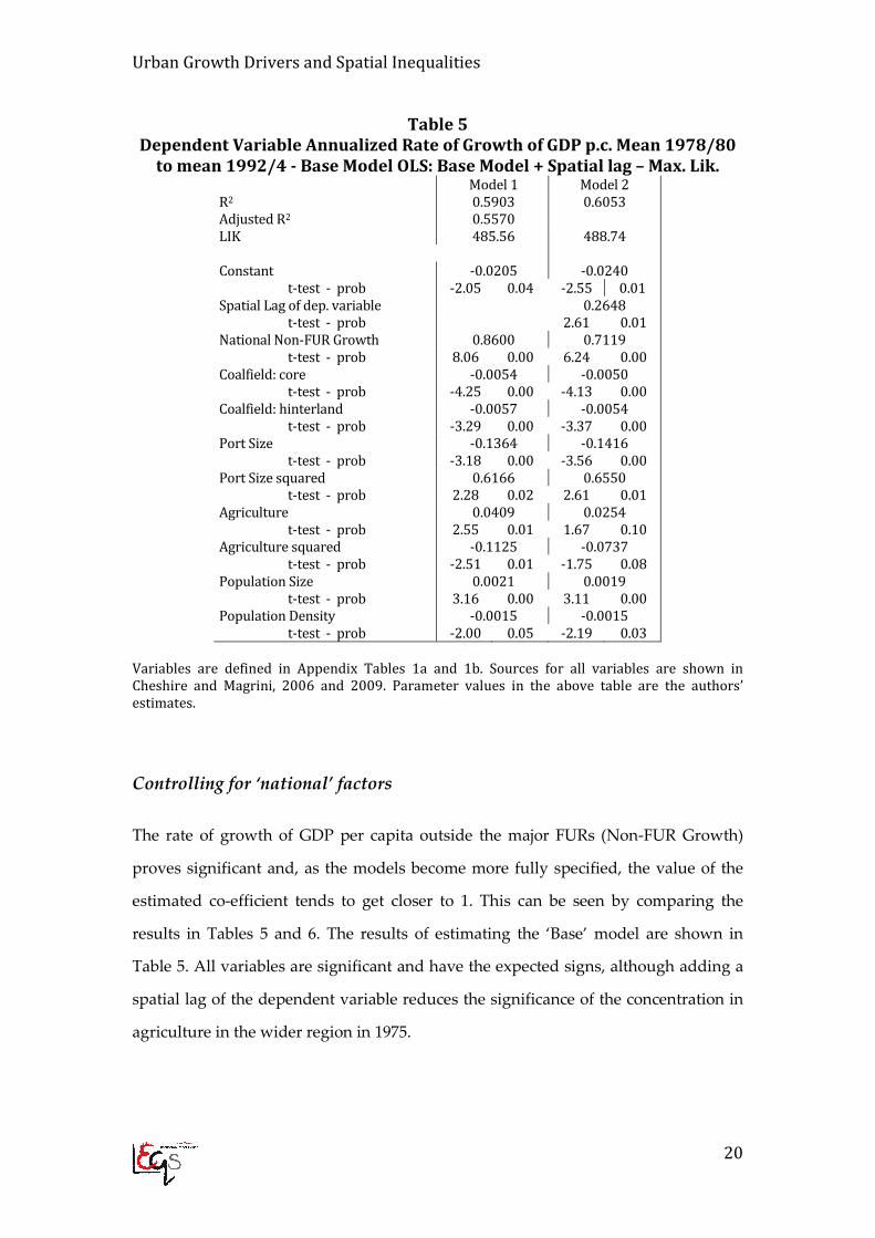
Table 5

Dependent Variable Annualized Rate of Growth of GDP p.c. Mean 1978/80

to mean 1992/4 - Base Model OLS: Base Model + Spatial lag – Max. Lik. Model 1 Model 2

R2 0.5903 0.6053

Adjusted R2 0.5570

LIK 485.56 488.74

Constant -0.0205 -0.0240

t-test - prob -2.05 0.04 -2.55 0.01

Spatial Lag of dep. variable 0.2648

t-test - prob 2.61 0.01

National Non-FUR Growth 0.8600 0.7119

t-test - prob 8.06 0.00 6.24 0.00

Coalfield: core -0.0054 -0.0050

t-test - prob -4.25 0.00 -4.13 0.00

Coalfield: hinterland -0.0057 -0.0054

t-test - prob -3.29 0.00 -3.37 0.00

Port Size -0.1364 -0.1416

t-test - prob -3.18 0.00 -3.56 0.00

Port Size squared 0.6166 0.6550

t-test - prob 2.28 0.02 2.61 0.01

Agriculture 0.0409 0.0254

t-test - prob 2.55 0.01 1.67 0.10

Agriculture squared -0.1125 -0.0737

t-test - prob -2.51 0.01 -1.75 0.08

Population Size 0.0021 0.0019

t-test - prob 3.16 0.00 3.11 0.00

Population Density -0.0015 -0.0015

t-test - prob -2.00 0.05 -2.19 0.03



estimates.

Controlling for ‘national’ factors

The rate of growth of GDP per capita outside the major FURs (Non-FUR Growth)

proves significant and, as the models become more fully specified, the value of the

estimated co-efficient tends to get closer to 1. This can be seen by comparing the

results in Tables 5 and 6. The results of estimating the ‘Base’ model are shown in

Table 5. All variables are significant and have the expected signs, although adding a

spatial lag of the dependent variable reduces the significance of the concentration in

agriculture in the wider region in 1975.


21

Growth: agglomeration good; density bad

There are indications of dynamic agglomeration economies – larger FURs grew faster

when other factors were controlled for. However, once FUR size was controlled for,

those FURs that were denser grew more slowly. The rationale for including both

FUR size and initial population density is that the factors generating agglomeration

economies are distinct from density itself. Agglomeration economies arise as a result

of the number and net value of productive interactions between economic agents,

and these are larger in larger cities. Population density also rises with city size and in

studies of agglomeration economies, density of employment or population has often

been used as the ‘explanatory’ variable. While this approach is not inappropriate in

unregulated conditions, in a number of EU countries where there are very strong

urban containment policies, population density and population size will to some

extent vary independently of each other. Once size has been controlled for, higher

density should be associated with both higher space costs (see Cheshire and Hilber,

2008) and more congestion, and is thus expected to be associated with less favorable

conditions for economic activity. The results reported in Tables 5 and 6 are entirely

consistent with this reasoning.

Spatial dependence – introducing a spatial lag

Although we do not report the test statistics in Tables 5 and 6, those for the standard

problems of heteroskedasticity, non-normality of errors, multicollinearity and

functional form were all within acceptable ranges (see Cheshire and Magrini, 2009).

So, too, were tests for spatial dependence, except for the case where an additional

time-distance penalty for national borders was included. Further experimentation

showed that spatial dependence problems were maximized if this national border

penalty was set at 600 minutes. The indicated textbook solution was to include the

spatially lagged dependent variable as an additional independent variable. The

results of doing so are shown for model 2 reported in the final column of Table 5. The

spatially lagged dependent variable is significant but has little effect on the other


22

estimated parameters except for reducing the significance of past specialization in

agriculture in the wider region.

As noted above, our preferred approach to problems of spatial dependence is to treat

a significant result as indicating a problem of omitted variables: in the present case,

those driving systematic spatial patterns of FUR growth. Table 6 shows the results of

including such variables, plus additional variables designed to test specific

hypotheses.

Human capital, R&D and local growth promotion with spatial spillovers

The idea that concentrations of highly skilled human capital should be associated

with faster rates of real GDP per capita growth (itself very closely related to

productivity growth) is not new. It is represented here as the ratio of university

students to total employees at the very start of the period (to help reduce any

possible problems of endogeneity which would certainly be a danger if, for example,

the variable was defined as university graduates in the labor force at the end of the

period). There is a large literature on the tendency for patents to be applied closer to

their points of origin (see e.g., Audretsch, 1998, or, for a recent application to a

European context, Barrios et al., 2008). So we would expect FURs with greater

concentrations of R&D activity at the start of the period to have grown faster. This is

measured as R&D facilities of the largest firms per 1000 inhabitants – again at the

start of the period.

The third variable designed to test hypotheses about the drivers of economic growth

is rather more novel. Tiebout (1956) is one of the most cited papers in local public

finance. It shows that, under certain conditions, if there are many competing local

jurisdictions, then the provision of local public goods will match the structure of

demand as people vote with their feet to find the best combination of tax rates and

public goods available to them. The ‘certain conditions’ assumed to prevail are that

people are perfectly mobile and that there are no spillovers of public goods from one


23

jurisdiction to another. It is easy, however, to think of local public goods, such as

crime reduction or pollution control, which are likely to involve jurisdictional

spillovers. Moreover, as already noted here, people in Europe are far from perfectly

mobile.

Therefore we consider an ‘anti-Tiebout’ world in which the provision of a local

public good may involve jurisdictional spillovers and where mobility is expensive. In

this case, the implications are that a more efficient provision of local public goods

may result if jurisdictional boundaries coincide with the set of households/agents

affected by the local public good(s). One of the notable recent trends in Europe is the

spread of local growth promotion efforts by authorities or agencies representing

cities and regions. Now, if we suspend our disbelief and allow for the possibility that

such policies4 may have some positive impact, then local growth promotion policies

would consist of the provision of a pure local public good. Extra local growth would

have zero opportunity costs in consumption and be non-excludable. If, my rents go

up because of additional local growth, that imposes no cost on other owners of real

estate. Moreover, if a local growth promotion agency is successful, it will not be

possible to exclude residents from outside the jurisdiction from benefiting from the

better job opportunities or higher wages.

Since FURs are intentionally defined to be economically self-contained, their boundaries

should minimize spillovers of local growth. Those who benefit from any jobs or

incomes created within a FUR live within its boundaries (although there may be

external owners of assets). So the more closely a local jurisdiction’s boundaries

correspond to the extent of a FUR, the smaller - other things equal - will be the spillover

losses from successful growth promotion efforts. The other factor determining the

4 We are not here concerned with the particular form such policies may take. Clearly much of the

effort of local growth promotion agencies goes into trying to attract mobile investment. This is

not necessarily a policy with much payoff. More effective policies may include simple efficiency in

public administration, transparent regulation, flexible land use policies with quick and cheap

decisions, and effective co-ordination of public infrastructure provision with private investment.

None of these policies will necessarily be measured in higher local expenditures - so total

spending – even if data were available - by either local government or local development

agencies will not too effectively capture the efficiency of local growth promotions efforts.

Moreover since the functions of local government compared to national and, where it exists,

regional government, vary so much across Europe, it is impractical to use local spending as an

indicator of local growth promotion efforts.


24

incentive to establish local growth promotion agencies will be the transaction costs

incurred. Such agencies typically consist of public-private partnerships initiated and

facilitated by local government. The fewer the total number of jurisdictions and the

larger is the central local jurisdiction, the lower will be the transaction costs, and so the

greater will be the net payoff from establishing a growth promotion agency.

Arguments such as these prompted Cheshire and Gordon (1996, page 389) to

hypothesize that growth promotion policies would be more likely to appear and be

more energetically pursued where ‘there are a smaller number of public agencies

representing the functional economic region, with the boundaries of the highest tier

authority approximating to those of the region…’.

A variable that captures this idea is simply a measure of how closely each FUR’s

boundaries match those of the central jurisdiction, defined as the ratio of jurisdiction to

FUR population at the start of the period. The hypothesis is that the more closely these

match, the greater will be the payoff to forming an effective growth promotion agency,

other things being equal. It could be that the advantage increases as the governmental

unit becomes bigger than the FUR itself (as happens in some European countries in

which there is an effective regional tier of government – Madrid might be an example)

because the resources and clout of the governmental unit will be greater. But if the

governmental unit is too large, the interests of the main FUR within it may get diluted

by those of outlying smaller cities and rural areas. Assuming that growth promotion

agencies are able to have any impact on local economic growth, this implies a positive

(perhaps quadratic) relationship between the variable we call the ‘policy incentive’ and

GDP per capita growth, since a regional tier of government that too greatly exceeds the

size of the economic region or FUR may dilute the positive impact on growth.


25

Table 6

Dependent Variable Annualized Rate of Growth of GDP p.c. Mean 1978/80

to mean 1992/4 – Models excluding and including ‘Spatial Variables’

Model 3 Model 4 Model 5

R2 0.6765 0.7413 0.7555

Adjusted R2 0.6372 0.6986 0.7095

LIK 499.86 513.38 516.80

Constant -0.0320 -0.0233 -0.0261

t-test - prob -3.14 0.00 -3.52 0.01 -2.84 0.01

National Non-FUR Growth 0.9442 0.8975 0.9050

t-test - prob 9.22 0.00 9.07 0.00 9.31 0.00

Coalfield: core -0.0062 -0.0051 -0.0051

t-test - prob -5.18 0.00 -3.99 0.00 -4.00 0.00

Coalfield: hinterland -0.0042 -0.0034 -0.0032

t-test - prob -2.61 0.01 -2.23 0.03 -2.06 0.04

Port Size -0.1474 -0.1003 -0.0932

t-test - prob -3.69 0.00 -2.62 0.01 -2.46 0.02

Port Size squared 0.7634 0.4871 0.4669

t-test - prob 3.04 0.00 2.02 0.05 1.97 0.05

Agriculture 0.0508 0.0384 0.0478

t-test - prob 3.22 0.00 2.48 0.01 3.02 0.00

Agriculture squared -0.1345 -0.1126 -0.1231

t-test - prob -3.21 0.00 -2.82 0.01 -3.12 0.00

Unemployment -0.0332 -0.0312

t-test - prob -2.45 0.02 -2.29 0.02

Population Size 0.0021 0.0016 0.0016

t-test - prob 3.53 0.00 2.90 0.00 2.87 0.01

Population Density -0.0015 -0.0015 -0.0013

t-test - prob -2.25 0.03 -2.36 0.02 -2.07 0.04

Integration Gain 0.0073 0.0082

t-test - prob 3.20 0.00 3.61 0.00

University Students 0.0309 0.0367 0.0303

t-test - prob 2.67 0.01 3.62 0.00 2.87 0.01

R&D Facilities 0.8079 0.8947 0.8512

t-test - prob 2.84 0.01 3.26 0.00 3.10 0.00

Policy Incentive 0.0075 0.0026 0.0086 a

t-test - prob 2.24 0.03 2.45 0.02 2.49 0.01

Policy Incentive squared -0.0021 -0.0027 a

t-test - prob -1.32 0.19 -1.72 0.09

R&D Facilities Density 0.0531 0.0703

t-test - prob 2.19 0.03 2.70 0.01

Peripherality Dummy 0.0059 0.0054

t-test - prob 4.51 0.00 4.10 0.00

University Student Density -0.0025 -0.0030

t-test - prob -2.46 0.02 -2.93 0.00

Unemployment Density -0.0036

t-test - prob -1.92 0.06

Note: a Test of joint significance: χ2(2) = 10.4333 (0.01).

Variables are defined in Appendix Tables 1a and 1b. Sources for all variables are shown

in Cheshire and Magrini, 2006 and 2009. Parameter values in the above table are the

authors’ estimates.


26

Model 3 in Table 6 includes all these variables. Including these variables, which are all

significant, improves the fit of the model without significantly changing the estimated

parameter values of the existing variables. Only the functional form of the policy

incentive variable is unclear, since the quadratic term, although it has the expected sign,

is not significant. Testing for spatial dependence (see Cheshire and Magrini, 2009 for

details), however, reveals apparent problems if the 600 minute time-distance penalty is

included for national borders. This suggests that variables reflecting systematic spatial

patterns are omitted.

Systematic spatial influences on growth

Models 4 and 5 in Table 6 show the impact of including variables designed to capture

such spatial influences. The first two relate to Europe-wide influences on spatial

patterns of urban growth. The first is the “Integration Gain” variable, which is intended

to capture the spatial effect of European integration. Partly as a response to the

perceived advantage accruing to ‘core’ regions from European integration, starting in

the mid-1970s, Europe developed stronger policies aimed at redistributing economic

activity to ‘peripheral’ regions. In 1972, such policies accounted for 4 percent of

spending by the European Commission but increased to 15 percent by 1980 and about

30 percent by 1994. Although its impact has been questioned (see, Midelfart and

Overman, 2002; Rodriguez-Pose and Fratesi, 2004), a variable for ‘peripherality’ still

seems worth including. To avoid any apparent subjectivity in selecting ‘peripheral’

regions, this variable is arbitrarily defined as being all FURs more than 600 minutes

time-distance from Brussels.

It is also plausible that in the more densely urbanized parts of Europe conditions in

FURs will influence each other. That is, there will be interaction between neighboring

cities. Drawing on the literature on spatial labor markets and the distance decay effect

of innovations, we include three variables to try to capture these interactions. There is

evidence, particularly from the spatial applications of patents, that new innovations are

subject to a distance decay effect, and we have already seen that concentrations of R&D


27

favor FUR growth. Thus, if there are concentrations of R&D in a FUR, one would expect

it to favor growth in FURs close by, subject to a distance decay effect. This is reflected in

the design of the “R&D Facilities Density” variable. Similarly, if a concentration of

highly skilled labor favors a FUR’s growth, then a higher concentration in neighboring

FURs would be expected to reduce the FUR’s growth since the faster growth generated

in the surrounding FURs will tend to attract highly skilled commuters away from the

slower growing FUR. This is reflected in the “University Student Density” variable.

Finally, some studies (e.g., Glaeser et al, 1995) suggest that a higher initial level of

unemployment inhibits subsequent growth. Therefore, models 4 and 5 include both the

initial level of unemployment in FURi and an “Unemployment Density” variable,

calculated as the distance-weighted level of unemployment in all neighboring FURsj-n

with up to 120 minutes between centroids. The time distance cut-off applied to the R&D

Facilities and University Students Density variables is higher – 150 minutes. These

differential cut-offs provide better statistical performance, but are also consistent with

underlying reasoning. The unemployed, who are biased towards the least skilled, are

likely to have a geographically more confined influence than either the most highly

skilled workers or innovation. For each FUR, the 600 minute time-distance penalty for

national borders is applied to calculate the value of these spatial interaction variables

implying that the processes of adjustment between the economies of neighboring FURs

are severely impeded if a national border separates them. This is consistent with the

logic underlying our choice for the spatial weights matrix but it also fits the data better.

That is according to the test statistics a finding of spatial dependence becomes even

more improbable if the 600 minute time distance penalty is included in the calculation

of these localized spatial adjustment variables. This version of the model not only

performs better statistically but is consistent with our other findings (see Table 6).

As shown in Table 6, all variables have the expected sign and are significant at at least

the 10 percent level. Tests for joint significance provide further evidence that the

underlying functional form of the policy incentive variable is quadratic, with the

maximum favorable impact of the relationship between FURs and their administrative

boundaries appearing when the administrative jurisdiction containing the FUR is about


28

1.5 times its size. Even more encouraging is the fact that all signs of spatial dependence

are eliminated (see Cheshire and Magrini, 2009, for details). As before, no conventional

econometric problems are indicated.

In the context of understanding the main drivers of the rate of FUR GDP per capita

growth, these results suggest the existence of dynamic agglomeration economies, but

that other things equal, higher population density is bad for growth. The results also

suggest that while the process of European integration does indeed favor ‘core’ regions,

policies to reduce ‘spatial disparities’ (the official aim of European regional policies)

may have at least partially offset this tendency. The results are certainly consistent with

the hypothesis that concentrations of highly skilled human capital and R&D favor local

growth. Perhaps more surprisingly, they suggest that local growth promotion policies

may have some positive impact because we find significant evidence that the incentives

regional actors face in developing such policies are themselves influential in explaining

urban growth performance. It helps if local jurisdictional boundaries coincide more

closely with those of self-contained economic regions – FURs – because when there are

spillovers and transactions costs associated with forming effective growth promotion

agencies, such a coincidence of boundaries increases the expected gains to actors.

Finally, we find strong evidence that national boundaries are still a barrier to the

processes of spatial adjustment in Europe.

6. Comparing and Contrasting the Drivers of Population

and Economic Growth

Given the reluctance of Europeans to migrate in response to changing patterns of

opportunity or follow the sun beyond their national boundaries, it does not seem

appropriate to assume that Europe is characterized by full spatial equilibrium. This has

implications both for the persistence of spatial disparities in welfare and for the

processes driving spatial differences in population and economic growth. Controlling

for differences in the natural rate of population growth, we find some economic drivers

of population growth - such as an inheritance of an old, resource-based local economy


29

or the systematic impacts of European integration. But these Europe-wide drivers are

quite weak and only the impact of European integration can really be classed as

‘Europe-wide’. When we analyze the impact of climate on population growth, we find

compelling evidence of a purely national impact. It is not differences in climate relative

to some European mean that is significant: it is only relative to national conditions that

climate drives FUR population growth. Moreover, in analyzing the sources of spatial

dependence, we find strong evidence that while population growth in one FUR

influences its neighbor(s), if a national border separates two FURs, that influence is

much diminished.

When we examine the drivers of economic growth, we also find a powerful national

border barrier to spatial interaction between neighboring FURs. But in other ways, the

drivers of economic growth are significantly different from the drivers of population

growth. Dynamic agglomeration economies and concentrations of R&D and highly

skilled labor are significant in driving GDP per capita growth but not in driving

population growth. Moreover, the ‘policy incentive’ variable designed to reflect the

incentives faced by local actors to promote local growth is highly significant in

accounting for differences in economic growth rates between FURs but not at all

significant in accounting for differences in population growth.

It has been asserted that climate and environmental factors have become more

important in influencing firm location because of their supposed influence on the

locational choices of highly skilled labor (the so-called ‘new location factors’5).

However, our findings provide no support for this view. Climatic differences – the most

obvious environmental factor – are not statistically significant in models of GDP per

capita growth; the closest they come, indeed, runs counter to the supposed role of the

alleged ‘new location factors’. When we include the number of wet days relative to the

national mean in the model, the variable has a positive sign and is on the verge of being

significant, suggesting that for economic growth, wetter is better.

Overall, both the differences and similarities between the drivers of population growth

5 See for example http://geographyfieldwork.com/HighTechLocationFactors.htm


30

and economic growth broadly reflect theory. In a world of “sticky” people, we would

expect sluggish adjustment to spatial differences in opportunity. We would also expect

national boundaries to represent additional obstacles to spatial adjustment. Both

expectations are supported by this analysis. We might also expect there to be a

systematic adjustment process between FURs in densely populated regions and FURs

in wider urbanized regions. The literature on labor market search and on induced

commuting tells us that these processes tend to even out spatial opportunities as they

occur in sets of labor markets linked by significant (potential) commuting flows.

Although FUR boundaries are designed to delimit self-contained labor markets, where

the boundaries are contiguous, people living in the suburban hinterlands can alter their

commuting patterns over time to take advantage of opportunities in neighboring FURs.

As a result of vacancy chains - that is the fact that if a person leaves a job in one location

to fill a vacancy somewhere else they create a vacant job to be filled by someone living

elsewhere - opportunities will tend to be equalized over the set of linked local labor

markets (Morrison, 2005). The condition for this opportunity equalization between

neighboring areas appears to be simply that cross-boundary commuting flows exceed

some threshold (see Gordon and Lamont, 1982). Thus, without conventional geographic

mobility, spatial equilibrium may be produced through local labor market interactions

when geography and transport systems facilitate adjustment in commuting patterns. If

we include variables designed to reflect this process (and other spatial interactions),

spatial dependence problems are eliminated but we also find strong evidence that

adjustment is greatly impeded across European borders. This is true for both

population growth and economic growth, reinforcing the conclusion that spatial

differences in Europe are persistent, not just because people are geographically

immobile but because, if national borders intervene, people tend not to take advantage

of even those opportunities they could reach without re-locating.

Apart from increasing our understanding of the drivers of spatial growth and

adjustment processes, the evidence presented in this paper has a number of wider

implications. It suggests that differences in real incomes in Europe – and more

generally where populations are relatively immobile – are likely troublesomely to


31

persist and that they are likely to indicate real differences in welfare, certainly if

prices do not fully adjust. Although the evidence does not indicate how significant

inter-regional income differences are relative to other sources of welfare difference

between individuals, it does imply that people of similar personal characteristics

may have different life chances simply because they are born in one region rather

than another. Contrary to some recent assertions (e.g., Kresl, 2007), our findings also

suggest that there is no evidence of a unified European urban system, but rather of a

set of national systems, with weak responses to variations in local economic

opportunities when national boundaries intervene. We also find that there are

significant, but theoretically consistent, differences in the drivers of population

compared to economic growth. Agglomeration economies, concentrations of research

and development (R&D) activity and highly skilled human capital, and systems of

urban governance play a significant role in driving spatial economic growth

differences, but no role when it comes to population growth. And, in contrast, while

there is strong evidence of environmental factors driving population growth, they do

not seem to influence economic growth differences. Finally, we might speculate that

the findings for Western Europe may be more applicable than those for the U.S. to

conditions in Asia, with its long history of settlement, its patchwork of languages

and cultures, and, particularly to China, where, in addition, there are deliberate

restrictions on population mobility.


32

References

Audretsch, D. B. (1998), ‘Agglomeration and the Location of Innovative Activity’, Oxford Review of

Economic Policy, 14 (2), 18-29.

Barro, R.J. (1990) ‘Government Spending in a Simple Model of Endogenous Growth’, Journal of

Political Economy, 98, S103-S125.

Barro, R. J. and Sala-i-Martin, X. (1991), ‘Convergence across States and Regions’, Brooking Papers on

Economic Activity, 1: 107-182.

Barro, R. J. and Sala-i-Martin, X. (1992), ‘Convergence’, Journal of Political Economy 100 (2), 223-251.

Barro, R.J. and X. Sala-i-Martin (1995), Economic Growth, New York: McGraw-Hill.

Barrios, S., Bertinelli, L., Heinen, A. and E. Strobl (2007): Exploring the Link between Local and Global

Knowledge Spillovers, MPRA No 6301.

Blomquist, G.C., M. C. Berger and J. P. Hoehn (1988) ‘New estimates of the Quality of Life in Urban

Areas’, American Economic Review, 78, 89-107.

Cheshire, P.C. and D. G. Hay, (1989), Urban Problems in Western Europe: an economic analysis, Unwin

Hyman: London.

Cheshire, P.C. and I.R. Gordon (1996) ‘Territorial Competition and the Logic of Collective (In)action’,

International Journal of Urban and Regional Research, 20, 383-99.

Cheshire P.C. and C. Hilber, (2008) ‘Office Space Supply Restrictions in Britain: the political economy

of market revenge’, Economic Journal, 118, (June) F185-F221.

Cheshire, P.C. and S. Magrini, (2000) ‘Endogenous Processes in European Regional Growth:

Implications for Convergence and Policy’, Growth and Change, 32, 4, 455-79.

Cheshire, P.C. and S. Magrini, (2006) ‘Population Growth in European Cities: weather matters – but

only nationally’, Regional Studies, 40, 1, 23-37.

Cheshire, P.C. and S. Magrini, (2009) ‘Urban Growth Drivers in a Europe of Sticky People and Implicit

Boundaries’, Journal of Economic Geography, 9, 1, 85-115.

Cheshire, P.C., S. Magrini, F. Medda and V. Monastiriotis (2004) ‘Cities are not Isolated States’ in

Boddy, M. and M. Parkinson (eds) City Matters, Bristol: The Policy Press.

Cheshire, P.C and E.J .Malecki (2004) ‘Growth, Development and Innovation: a look backward and

forward’, Papers in Regional Science, 83, 249-267.

Clark, C., F. Wilson, and J. Bradley, (1969) ‘Industrial location and economic potential in Western

Europe’ Regional Studies, 3, 197-212.

Commission of the European Communities (CEC) (2004) Third Report on Social and Economic

Cohesion: Main Regional Indicators, Luxembourg,

Glaeser, E.L., J.A. Scheinkman and A. Shleifer (1995) ‘Economic Growth in a Cross-Section of Cities’,

Journal of Monetary Economics, 36, 117-43.

Gordon, I. and Lamont, D. (1982) ‘A model of Labor-market Interdependencies in the London

Region’, Environment and Planning A, 14, 238-64.


33

Graves, P.E., 1976. A reexamination of migration, economic opportunity, and the quality of life,

Journal of Regional Science, 16, 107-112.

Graves, P.E., 1979. A life-cycle empirical analysis of migration and climate, by race, Journal of

Urban Economics, 6, 135-147.

Graves, P.E., 1980. Migration and climate, Journal of Regional Science, 20, 227-237.

Graves, P.E., 1983. Migration with a composite amenity: the role of rents, Journal of Regional

Science, 23,541-546.

Gyourko, J. and J. Tracy (1991) ‘The structure of local public finance and the quality of life’,

Journal of Political Economy, 99, 774-806.

Hall, P.G. and D. G. Hay (1980) Growth Centres in the European Urban System, London: Heinemann

Educational.

Keeble, D., J. Offord and S. Walker (1988) Peripheral Regions in a Community of Twelve Member

States, Office of Official Publications, Luxembourg.

Kresl, P. K. (2007) Planning Cities for the Future: The Successes and Failures of Urban Economic

Strategies in Europe, Cheltenham: Edward Elgar.

Midelfart, K.H and H.G.Overman (2002) ‘Delocation and European Integration: Is European

Structural Spending Justified?’, Economic Policy, 35, 321-359.

Morrison, P. S. (2005) ‘Unemployment and Urban Labor Markets’, Urban Studies, 42, 12, 2261-2288.

Rappaport, J. (2004) Moving to Nice Weather, Working Paper, Federal Reserve Bank of Kansas

City.

Rey, S.J. and B.D. Montuori (1999) ‘US regional income convergence: a spatial economic perspective’,

Regional Studies, 33:143-156.

Rodriguez-Pose and U. Fratesi (2004) ‘Between Development and Social Policies: The Impact of

European Structural Funds in Objective 1 Regions’, Regional Studies, 38, 1, 97-113.

Tiebout, C. (1956) A pure theory of local expenditures, Journal of Political Economy, 64, 416-24.


34

Appendix

Table 1a

Variable Definitions - Rate of FUR Population Growth 1980 to 2000 =

Dependent Variable

Industrial Emp.’75 Percentage of labor force in industry in surrounding level 2 region in 1975: source

Eurostat

Coalfield: core A dummy=1 if the core of the FUR is located within a coalfield

Coalfield:

hinterland A dummy=1 if the hinterland of the FUR is located within a coalfield

Port size ’69* Volume of port trade in 1969 in tons

Agric Emp.’75* Percentage of labor force in agriculture in surrounding Level 2 region in 1975

Integration Gain*

Change in economic potential for FUR resulting from pre-Treaty of Rome EEC to

post enlargement EU with reduced transport costs (estimated from Clark et al

1969 and Keeble et al 1988)

Interaction ’79-91

The sum of the differences in the growth rates of employment each FUR and in all

other FURs within 100 minutes traveling time weighted by distance over the

period 1979-1991.

West Distance west of centre of FUR from national capital city (Amsterdam taken as

capital of Netherlands; Bonn of Germany)

South Distance south of centre of FUR from national capital city (Amsterdam taken as

capital of Netherlands; Bonn of Germany)

EUwest Distance west of centre of FUR from Brussels

EUsouth Distance south of centre of FUR from Brussels

Nat Non-FUR Pop

Growth ’80-’00

Annualized rate of growth of population in territory of country outside major

FURs between 1980 and 2000

Wet day

frequency ratio :

country*

Ratio of wet day frequency between FUR and national average (1970s and 1980s)

Frost frequency

ratio : country*

Ratio of ground frost frequency between FUR and national average (1970s and

1980s)

Maximum

temperature ratio

: country*

maximum temperature percentage difference between FUR and national average

(1970s and 1980s)

Cloud cover ratio:

country* Ratio of cloud cover days between FUR and national averages (1970s and 1980s)

Minimum

temperature ratio:

country*

Ratio of minimum temperatures between FUR and national average (1970s and

1980s)

Mean

temperature ratio:

country*

Ratio of mean temperature between FUR and national average (1970s and 1980s)

Max temperature

ratio: country*

Ratio of maximum temperature between FUR and national average (1970s and

1980s)

Note: * denote variables tried with a quadratic specification for reasons explained in the text:

never entered as squared value alone.

All climate variables were also expressed as the ratio of the FUR value to the EU mean.

Sources for all variables are shown in Cheshire and Magrini, 2006 and 2009.


35

Table 1b

Variable Definitions – Rate of Growth of GDP per capita at PPS 1978/80 to

1992/94 = Dependent Variable

Note: * denote variables tried with a quadratic specification for reasons explained in the text.

Never entered as squared value alone.

Sources for all variables are shown in Cheshire and Magrini, 2006 and 2009.

No Variable Name Description

Constant

1 Population Size Population size in 1979 (natural logarithm)

2 Population Density Density of population in FUR in 1979 (1000

inhabitants/Km2)

3 Coalfield Dummy: core Dummy = 1 if the core of the FUR is located within a coalfield

4 Coalfield Dummy: hinterland Dummy = 1 if the hinterland of the FUR is located in a

coalfield

5 Port size * Volume of port trade in 1969 (100 tons)

6 Agriculture * Share of labor force in agriculture in surrounding NUTS 2 in

1975

7 Unemployment * Unemployment rate (average rate between 1977 and 1981 –

from Eurostat NUTS3 data)

8 National Non-FUR Growth Growth of GDP p.c. in the territory of each country outside

the FURs (annualized rate between 1978/80 and 1992/94)

9 Policy Incentive *

Ratio of the population of the largest governmental unit

associated with the FUR to that of the FUR in 1981 (see

below for details)

10 Integration Gain

Change in economic potential for FUR resulting from pre-

Treaty of Rome EEC to post enlargement EU with reduced

transport costs (estimated from Clark et al 1969 and Keeble

et al 1988)

11 Peripherality Dummy Dummy = 1 if the FUR is more than 10 hours away from

Brussels

12 University Students * Ratio of university students (1977-78) to total employment

(1979)

13 R&D Facilities * R&D laboratories of Fortune 500 companies per 1000

inhabitants in 1980

14 Unemployment Density

Sum of differences between the unemployment rate (average

between 1977 and 1981) of a FUR and the rates in

neighboring FURs (within 2 hours), discounted by distance

(with 10 hours time penalty for national borders)

15 University Student Density

Sum of university students per employees in neighboring

FURs (within 2.5 hours), discounted by distance (with 10

hours time penalty for national borders)

16 R&D Facilities Density

Sum of R&D laboratories per 1000 inhabitants in

neighboring FURs (within 2.5 hours), discounted by distance

(with 10 hours time penalty for national borders)

Recent LEQS papers

Rodríguez-Pose, Andrés & Krøijer, Anne. ‘Fiscal Decentralization and Economic

Growth in Central and Eastern Europe’. LEQS Paper No. 12, October 2009

Cheshire, Paul C. & Magrini, Stefano. ‘Urban Growth Drivers and Spatial

Inequalities: Europe - a Case with Geographically Sticky People. LEQS Paper No.

11, October 2009

McCrea, Ronan. ‘The Recognition of Religion within the Constitutional and Political

Order of the European Union’. LEQS Paper No. 10, September 2009

Bertola, Guiseppe & Mola, Lorenza. ‘Services Provision and Temporary Mobility:

Freedoms and Regulation in the EU’ LEQS Paper No. 9, September 2009

Walker, Neil. ‘Multilevel Constitutionalism: Looking Beyond the German Debate’.

LEQS Paper No. 8, June 2009

Frankel, Jeffrey. ‘The Estimated Trade Effects of the Euro: Why Are They Below

Those From Historical Monetary Unions Among Smaller Countries?’. LEQS Paper

No. 7, June 2009

Colomer, Josep M.. 'On Building the American and the European Empires'. LEQS

Paper No. 6, June 2009

Boeri, Tito. 'Immigration to the Land of Redistribution'. LEQS Paper No. 5, June

2009

Jones, Erik. ‘They Have No Idea… Decision-making and Policy Change in the Global

Financial Crisis’. LEQS Paper No. 4, May 2009

Frey, Bruno. ‘A New Concept of European Federalism’. LEQS Paper No. 3, May 2009

Chalmers, Damian. ‘Gauging the Cumbersomeness of EU Law’. LEQS Paper No. 2,

May 2009

Bellamy, Richard. ‘The Liberty of the Post-Moderns? Market and Civic Freedom

within the EU’. LEQS Paper No. 1, May 2009


38

LEQS

European Institute

London School of Economics

Houghton Street

WC2A 2AE London


http://www2.lse.ac.uk/europeanInstitute/LEQS/Home.aspx

urban growth drivers and spatial inequalities: europe - a case with

Documents