urban forest inventory and assessment pilot project phase
TRANSCRIPT

Urban Forest Inventory and Assessment Pilot Project
Phase Two Report
March 25, 2013
Submitted to: Mary Klaas-Schultz, Chris Keithley, John Melvin, Tiffany Meyer, and Mark Rosenberg, CalFire
Submitted by: Drs. Qingfu Xiao, Julia Bartens, and Chelsea Wu, Department of Land, Air, and Water Resources, University of California, Davis
Drs. Greg McPherson and James Simpson, Urban Ecosystems and Social Dynamics, USDA Forest Service
Dr. Jarlath O’Neil-Dunne, Spatial Analysis Laboratory, University of Vermont
All Images: Courtesy of City of San Jose

2
Acknowledgements
We thank CalFire FRAP for funding this project and the guidance provided by their staff (Mary Klaas-Schultz, Chris Keithley, Tiffany Meyer, Mark Rosenberg) and John Melvin (Cal Fire) throughout the process.
The City of San Jose staff was a much appreciated help. Dorothy Abeyta and Ralph Mize were wonderful to work with and great partners when it comes to determining canopy cover targets and planning the outreach event. Thanks to William Harmon for help with GIS and LiDAR data.
Advice from Zhanfeng (Leo) Liu, Lisa Fischer, Matthew Bokach (State and Private Forestry, USDA Forest Service, Davis, CA), Paula Peper (PSW Research Station, Davis, CA), and Jim Baldwin (Station Statistician, PSW Research Station, Albany, CA) during design and analysis of the project was very helpful and much appreciated.
Field assistance was invaluable to this project. We thank Mary Klaas-Schultz and Tiffany Meyer (CalFire FRAP), Jimi Scheid and Glenn Flamik (CalFire), Zuha Lambert, Elizabeth Lanham, and Ralph Mize (City of San Jose), and Louren Kotow for their help.
3
Table of Contents
ACKNOWLEDGEMENTS ..................................................................................................................................... 2
TABLE OF CONTENTS ......................................................................................................................................... 3
FIGURES .................................................................................................................................................................... 5
TABLES ...................................................................................................................................................................... 6
GLOSSARY ................................................................................................................................................................ 8
EXECUTIVE SUMMARY ....................................................................................................................................... 9
BACKGROUND ..................................................................................................................................................... 14
PROJECT PROCESS............................................................................................................................................. 15
DATA & SOFTWARE .......................................................................................................................................... 16
Study Site ...................................................................................................................................... 16
Source Data ................................................................................................................................... 17
Software ........................................................................................................................................ 17
Hardware ...................................................................................................................................... 17
Other GIS Data .............................................................................................................................. 17
Definitions ..................................................................................................................................... 19
LAND COVER CLASSIFICATION .................................................................................................................... 20
Classification Approach ................................................................................................................. 20
Data Preparation ........................................................................................................................... 21
Tree Canopy Mapping ................................................................................................................... 21
Land Cover mapping ..................................................................................................................... 23
Results and Discussion .................................................................................................................. 25
Accuracy Assessment .................................................................................................................... 31
EXISTING TREE NUMBERS............................................................................................................................. 32
Results & Discussion ..................................................................................................................... 32
POTENTIAL TREE PLANTING SITES (PTPS) ........................................................................................... 34
Off-Street Pervious Surfaces .................................................................................................................. 34
PTPS Adjustment Factors (Pervious) ...................................................................................................... 34
PTPS Streets ............................................................................................................................................ 35
Results & Discussion ..................................................................................................................... 36
PTPS ........................................................................................................................................................ 36

4
URBAN TREE CANOPY TARGETS ................................................................................................................ 40
Results & Discussion ..................................................................................................................... 41
ECOSYSTEM SERVICE AND PROPERTY VALUE ASSESSMENT ........................................................ 46
Calculation Process ................................................................................................................................. 47
Energy Effects ......................................................................................................................................... 50
Atmospheric Carbon Dioxide Reduction ................................................................................................ 52
Air Pollutants .......................................................................................................................................... 53
Rainfall Interception ............................................................................................................................... 54
Property Value ........................................................................................................................................ 55
Results & Discussion ..................................................................................................................... 56
Ecosystem services and property value increases provided by existing UTC ........................................ 56
Ecosystem services and property value increases provided by additional UTC .................................... 58
Asset value of San Jose’s urban forest ................................................................................................... 58
CONCLUSION ....................................................................................................................................................... 62
Limitations to the study ................................................................................................................ 64
DELIVERABLES AND RESOURCES .............................................................................................................. 65
REFERENCES ....................................................................................................................................................... 66
APPENDIX I PARKING LOT DEMONSTRATION ...................................................................................... 70
Results & Discussion ..................................................................................................................... 71
APPENDIX II COUNCIL DISTRICTS SUMMARY DATA .......................................................................... 75

5
Figures
Figure 1. Project process overview. .............................................................................................. 15
Figure 2. The study area. ............................................................................................................... 16
Figure 3. Study area and council districts. .................................................................................... 18
Figure 4. Workflow diagram showing the source data, processing steps, intermediate output, and deliverables. .................................................................................................................... 20
Figure 5. Customized import for tree-canopy mapping. .............................................................. 21
Figure 6. eCognition workspace in which each project represents a 2000-ft x 2000-ft raster data stack and associated intersecting vector layers. ................................................................... 22
Figure 7.eCognition rule set for tree-canopy mapping. ............................................................... 22
Figure 8. Segmented tree-canopy objects generated to facilitate manual review and correction. ............................................................................................................................................... 24
Figure 9. Final land-cover raster dataset. ..................................................................................... 24
Figure 10. Current urban tree canopy cover by council district. .................................................. 26
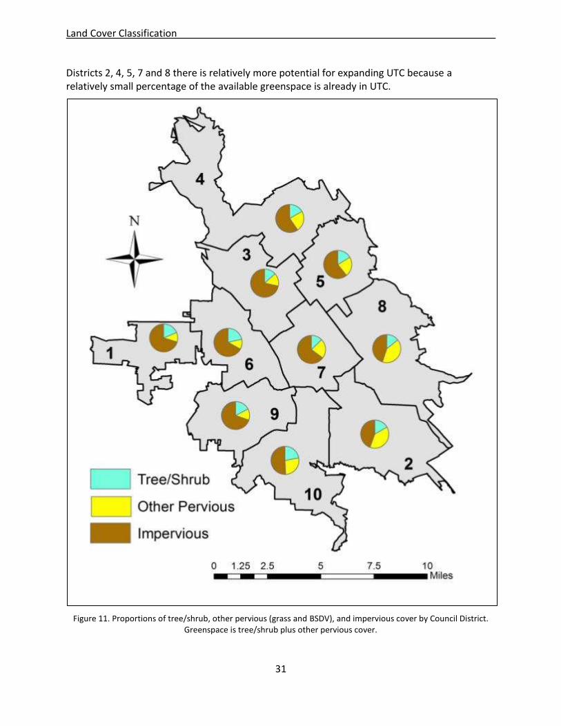
Figure 11. Proportions of tree/shrub, other pervious (grass and BSDV), and impervious cover by Council District. Greenspace is tree/shrub plus other pervious cover. ................................. 30
Figure 12. Relationships between existing tree numbers and potential tree planting site numbers, where the size of each pie is scaled according to relative number of tree sites. . 38
Figure 13. Relationships between the number of off-street and on-street sites for 100,000 additional trees, where the size of each pie is scaled according to relative number of tree sites. ....................................................................................................................................... 42
Figure 14. Number of existing and additional trees by council district. ....................................... 45
Figure 15. Annual value of ecosystem services and property value increases for the existing and additional UTC by Council District. ........................................................................................ 59
Figure 16. Appendix I PTPS parking lot demonstration site is the HP Pavilion parking lot at 525 West Santa Clara St., San Jose. .............................................................................................. 71
Figure 17. Appendix I Three types of planting areas for parking lot trees are recommended; left: 1.5 by 1.5m diamonds; center: 1.5 planting strip, right: 2.4m wells (1-tree or 2-tree) created by converting standard to compact spaces right (City of San Jose, 1990). .............. 71
Figure 18. Appendix I Medium tree design for the parking lot PTPS demonstration. PTPS locations (light green dots), their 30ft-diameter crowns (dark green circles), and existing canopy (delineated in red) are shown. .................................................................................. 73
Figure 19. Appendix I Large tree parking lot PTPS demonstration. PTPS locations (light green dots), and their 50-ft diameter crowns (dark green cirlces), and existing canopy (delineated in red) are shown. .................................................................................................................. 74

6
Tables
Table 1. Existing and additional urban tree canopy (UTC), estimated tree numbers, and monetized value of ecosystem services produced. ............................................................... 13
Table 2.Dataset description and source organization. ................................................................. 17
Table 3. Zoning classes cross-walk table. ...................................................................................... 18
Table 4. Land cover classes used for land cover mapping. ........................................................... 19
Table 5. Human populations, land use (acres) by Council District, and proportions of land area. ............................................................................................................................................... 27
Table 6. Proportion of land cover by Council District. .................................................................. 28
Table 7. Land cover (%) by land use class. .................................................................................... 28
Table 8. Example of land cover by census block group, submitted in digital form. ..................... 28
Table 9. Land cover percentages for selected cities from remote sensing studies. .................... 29
Table 10. Error matrix for the final land-cover dataset. ............................................................... 31
Table 11. Numbers of trees by Council District in the public ROW (street) and off-street. ......... 33
Table 12. Measures of urban forest structure for San Jose and selected cities*. ........................ 33
Table 13. Numbers of existing trees and adjusted number of potential tree planting sites. ...... 37
Table 14. Accuracy assessment for street PTPS analysis by land cover class. .............................. 39
Table 15. Numbers of trees to plant by land use class and Council District. ............................... 43
Table 16. Urban tree canopy of the existing trees and additional (100,000) trees at maturity. . 44
Table 17. Percent full stocking for existing and additional trees, along with change in stocking level. ....................................................................................................................................... 44
Table 18. Transfer functions (Resource Unit ac-1 UTC; in lbs unless otherwise specified) for San Jose from the San Francisco Bay Area Report (Simpson and McPherson, 2007) and San Jose field survey data. ................................................................................................................... 49
Table 19. Prices used to value ecosystem services in San Jose. ................................................... 50
Table 20. Distribution of matched species used for energy calculations. .................................... 51
Table 21. Number of sample trees by location relative to closest building. ................................ 52
Table 22. Estimated annual ecosystem services (tons unless otherwise specified) and property values (acre of annual increase in leaf area) provided by existing UTC. ............................... 57
Table 23. Estimated annual monetary value ($1,000) of ecosystem services and property value increase provided by existing UTC. ........................................................................................ 57
Table 24. Estimated annual ecosystem services (tons unless otherwise specified) and property values (acre of annual increase in leaf area) provided by additional UTC. ........................... 60
Table 25. Estimated annual monetary value ($1,000) of ecosystem services and property value increase provided by additional UTC. .................................................................................... 60
Table 26.Urban forest asset value at two discount rates. ............................................................ 61
Table 27. Appendix I Number of trees and canopy cover for two parking lot designs. Medium trees have 30-ft and large trees have 50-ft crown diameters. ............................................. 72

7
Table 28. Appendix II Council District Summary Data: Geographics. ........................................... 75
Table 29. Appendix II Council District Summary Data: Current UTC and existing tree statistics. 76
Table 30. Appendix II Council District Summary Data: Additional UTC and tree statistics. ......... 76

8
Glossary
AFUE Annual fuel utilization efficiency
Agri Agriculture land use
BLD Building
BS Bare soil land cover
BSDV Bare-soil and dry (non-woody) vegetation land cover combined
BVOC Biogenic volatile organic compounds
Comm Commercial land use
ESRI Environmental Systems Research Institute, Inc., Redlands, CA
GIS Geographic Information System
HDR High-density or multi-family residential
Ind Industrial land use
LiDAR Light Detection And Ranging
Mixed Mixed uses land
MMU Minimum mapping unit
MultiFam Multi-family or high-density residential land use
NAIP National Agricultural Imagery Program
NDVI Normalized Difference Vegetation Index
NO2 Nitrogen dioxide
O3 Ozone
OBIA Object-based image analysis
OpenSpace Open Space (OS) land use (excludes parks)
Other Imp Other impervious surfaces that are not in the building or road class
PM10 Particulate matter of <10 micron diameter
PQP Public/Quasi-Public land
PTPS Potential tree planting sites
PUTC Potential UTC
ROW Right-of-way
RS Remote Sensing
RU Resource unit
SEER Seasonal energy efficiency ratio
SingleFam Low-density residential (LDR) land use
TF Transfer function
UFORE Urban Forest Effects Model
UTC Urban tree canopy
VOC Volatile organic compound

Executive Summary
9
Executive Summary
The City of San Jose is the 3rd largest city in California, the 10th largest city in the US, and home to nearly 1 million people (www.city-data.com). Because it is such an attractive place to live, work, and play it is experiencing rapid growth, especially in outlying areas, which is accelerating air pollution along with water and energy demand problems. More sustainable infill growth is placing higher concentrations of people in urban environments where green space is a critical component to quality of life. Finding adequate space for trees in these densely engineered developments is a challenge. These problems urgently need solutions. Urban forestry is integral to land use planning, water shortage mitigation, energy conservation, air quality improvement, public health program enhancement, land value and local tax base increases, job training and employment opportunity provision, city services cost reduction, and public safety increases. Expanding the urban forest through judicious tree planting and stewardship activities can insure long term environmental, economic, and health benefits to local communities and maximum return on investment in planning and management.
In 2007, San Jose’s council adopted the Green Vision which will “transform San Jose into the world center of Clean Technology, promote cutting-edge sustainable practices, and demonstrate that the goals of economic growth, environmental stewardship and fiscal responsibility are inextricable linked” (City of San Jose, 2009). The council plans to reduce energy use through the conversion of all street lights to zero emission lighting as well as converting 100% of the electric power to clean, renewable energy sources. In addition, they decided to plant 100,000 trees by 2022. In so doing, the council recognized the potential of trees to improve the urban environment by helping clean the air by filtering out pollutants, providing shade, and storing carbon. Just as important, through partnerships with NGOs like Our City Forest, the urban forest message has reached an unprecedented number of residents. Now that program participation and visibility are growing, it is time to reaffirm the relevance of San Jose’s urban forest and to plan for its future.
This study provides up-to-date information on the extent and potential of San Jose’s urban forest. It quantifies the distribution of current tree canopy cover and maps locations of potential tree planting sites. Also, the study estimates the dollar value of ecosystem services provided by the current and future urban forest.
Urban tree canopy (UTC), defined as the “layer of leaves, branches and stems that cover the ground” (Raciti et al., 2006), is the metric used to quantify the extent, function, and value of San Jose’s urban forest. To calculate benefits of the urban forest canopy, field survey data were combined with UTC mapped across the city from remote sensing. The ecosystem services and property value increases associated with UTC were calculated with numerical models developed by the US Forest Service. Services per unit UTC were applied to the measured UTC and monetized to calculate their annual value for existing and additional UTC (i.e., runoff reduction, air quality, carbon dioxide removal, property values, and building energy use savings).
San Jose’s urban forest is extensive, covering 15.4% of the 151 square mile study area (

Executive Summary
10
Table 1). Urban tree canopy ranged from lows of 12% in Council Districts 4 and 7 to greater than 20% in 6 and 10. Council Districts 2 and 8 also had low UTC, but relatively high proportions of grass and dry vegetation, indicating good potential for tree planting. Impervious surfaces such as roads, buildings, and parking lots accounted for 59% of the land area, while irrigated grass, bare soil and dry vegetation covered 25%. The Spatial Analysis Laboratory’s accuracy assessment found that the overall accuracy was 93%, above the 90% standard set for the study.
There are approximately 1.6 million trees in San Jose’s urban forest, assuming an average crown diameter of 22.75-ft per tree found from field measurements in San Francisco, Los Angeles, and Sacramento, CA. The average number of trees per acre in San Jose is 16.5, which compares favorably with values reported for Sacramento (16.1) and Los Angeles (19.9), but is less than cities with similar population densities such as Pasadena (24.1) and Minneapolis (26.4). The average number of trees per capita is 1.6, also less than Pasadena (2.7) and Minneapolis (2.6), but comparable to higher density cities such as Los Angeles (1.3), Chicago (1.3) and Philadelphia (1.4).
San Jose’s urban forest produces ecosystem services and property value increases valued at $239.3 million annually. The largest benefit, $154.6 million, is for increased property values and other intangible services. Building shade and air temperature decreases from trees reduce residential air condition demand by 415,000 MWh, saving $77 million in cooling costs each year. The existing urban forest intercepts 1.2 billion gallons of rainfall annually, which reduces stormwater runoff management costs valued at $6.7 million. If carbon dioxide sequestered and emissions avoided from cooling savings by the existing trees, a total of 100,181 tons, were sold at $10 per ton, the revenue would be $1 million. Finally, San Jose’s urban forest filters a net total of 403 tons of air pollutants from the air annually.
The City of San Jose contains approximately 2.1 million potential tree planting sites (PTPS), with 94% of these off-street (private/institutional lands). This number assumes plantable space for a 22.75-ft crown diameter tree and that about 30% of the vacant sites are not plantable because of physical limitations such as utilities. Some vacant sites located in northern San Jose near the airport and sewage treatment plant are not plantable for safety reasons. About 42% of the PTPS are in irrigated grass, where planting is most cost-effective. Nearly all of the remaining sites are in non-irrigated grasslands, where trees will require watering during establishment. There are an estimated 124,472 PTPS along streets, excluding sites in sidewalks. Approximately 77% of these sites are in irrigated grass, the rest are in bare soil/dry vegetation. The estimate of 124,472 street PTPS is greater than the 2009 i-Tree sample estimate of 87,580 vacant sites. This may be because this study’s estimates were not adjusted to account for all planting obstructions that were observed in the field during the i-Tree survey, such as street lights, utility lines, fire hydrants, sewer inlets, and intersections. Therefore, it is unlikely that all of the street PTPS reported here are actually plantable.
Setting realistic targets for additional UTC is not straightforward because each Council District has a different land use mix as well as different existing UTC and potential UTC (PUTC) that reflect historic patterns of development and tree stewardship. After discussing alternative planting scenarios with the city forester, the research team determined to “plant” 80,000 tree

Executive Summary
11
sites in the street ROW and the remaining 20,000 off-street in irrigated grass. These sites were distributed among the Council Districts proportionate to the availability of vacant sites.
Filling 100,000 sites will increase UTC from 15.4% to 16.3%, assuming that current UTC remains stable and program tree sites remain fully stocked with 22.75-ft crown diameter trees. There is adequate space in irrigated lawn areas to achieve 98% of the 100,000 tree target. The number of vacant sites to be planted ranges from 6,812 in the relatively well-treed Council District 1 (UTC is 18.8%) to 14,585 in the sparsely-treed Council District 8 (UTC is 12.9%) (
Table 1).
Achieving the targeted 1% UTC increase will pay dividends. The annual value of ecosystem services and property values will increase by nearly 7% or $16.4 million, from $239.3 million to $255.8 million. The worth of increased annual property values and other intangible services is projected to be $10.6 million alone. Reduced demand for 28,699 MWh of electricity for air conditioning is expected to save another $5.3 million in cooling costs. Annual savings for lowered stormwater management costs from an additional 74 million gallons of rainfall interception is projected to be $426,489. Trees in the additional sites will diminish atmospheric carbon dioxide by 6,485 tons, valued at $65,000 annually. The additional UTC will reduce another 27 tons of pollutants from the air.
Expansion of the UTC from 15.4 to 16.3% is projected to result in total services valued at $255.8 billion annually from approximately 1.7 million trees. The average annual value of $153 per tree is comparable to results for the same services reported for other cities. This is a very conservative estimate of service value as it does not fully capture all benefits associated with increased UTC, such as job creation, improved human health and fitness, wildlife habitat, and biodiversity.
The values for these services have been expressed in annual terms, but trees provide benefits across many generations. Moreover, the benefits trees provide become increasingly scarce and more valuable with time. To enable tree planting and stewardship to be seen as a capital investment, the asset value of trees in San Jose was calculated. The annual flows of realized benefits from trees were converted into their net present value, which is a discounted sum of annual future benefits. Discounting future services to their present value incorporates the time value of money and the opportunity cost of investment. The farther ahead in time one goes, the less value a dollar has. A benefit derived in 50 years is worth far less than the same benefit today. By applying this method to the future stream of ecosystem services, the urban forest’s asset value is calculated in today’s dollars.
Discount rates of 4.125%, which is applied by the US Army Corps of Engineers for large projects, and 0% were used over 100 years for Existing UTC, Additional UTC and Existing plus Additional UTC. Some economists argue that natural capital has a lower discount rate because the benefit stream is more certain over longer periods of time.
The asset value of San Jose’s existing urban forest is $5.7 billion, or $3,634 per tree, calculated at a 4.125% discount rate for the next 100 years. At zero discount rate, the region’s urban forest asset value is estimated at $23.9 billion. If UTC is increased to 16.3% over the next 30 years, the urban forest’s asset value increases to $6.1 billion and $25.2 billion, assuming 4.125%

Executive Summary
12
and 0% discount rates, respectively. Hence, the ecosystem services produced by the region’s urban forest provide a considerable stream of benefits over time, just as a freeway or other capital infrastructure does. Quantifying the asset value of this “green infrastructure” can help guide advancement towards a sustainable green economy by shifting investments towards the enhancement of natural capital.
Results from this study can be used to:
Communicate the ecological and economic value of the existing urban forest
Establish tree planting and UTC targets for Council Districts
Describe the level of benefits obtained by reaching these targets
Track changes in UTC that reflect progress made reaching targets
Link changes in UTC to causal drivers such as levels of community tree planting,
drought, pests, storms, and vandalism
San Jose is a vibrant city that has invested in its urban forest as it has grown. The task ahead is to better integrate the green infrastructure with the gray infrastructure by targeting tree planting and stewardship activities to maximize their environmental and human health impacts. This study provides information that can be used to plan, prioritize and implement new urban forestry programs. In so doing, San Jose’s regional urban forest will become larger, more resilient, and better able to meet the challenges that loom ahead.

Table 1. Existing and additional urban tree canopy (UTC), estimated tree numbers, and monetized value of ecosystem services produced.
Council
District
No.
Existing
Trees
No.
Additional
Sites
Planted
Total Tree
Sites
Planted
Existing
Stocking
Level (%)
Future
Stocking
Level (%)
Change in
Stocking
(%)
Existing
UTC (%)
Future
UTC (%)
Annual Value
of Existing
Ecosystem
Services ($1M)
Annual Value
of Additional
Ecosystem
Services ($1M)
Existing +
Additional
Ecosystem Services
($1M)
1 124,227 6,812 131,039 67.6 71.3 3.7 18.8 19.8 23.3 1.2 24.6
2 165,669 11,452 177,121 29.8 31.9 2.1 13.6 14.6 26.1 2.0 28.2
3 118,608 9,885 128,493 51.8 56.1 4.3 13.3 14.4 15.1 1.3 16.4
4 196,885 12,786 209,671 38.4 40.9 2.5 12.2 13.0 26.0 1.8 27.8
5 124,303 8,249 132,552 45.6 48.6 3.0 15.8 16.9 20.9 1.6 22.5
6 178,868 8,465 187,333 69.4 72.6 3.3 21.4 22.4 32.5 1.4 34.0
7 92,295 7,304 99,599 39.3 42.4 3.1 12.1 13.0 13.8 1.2 15.0
8 175,366 14,585 189,951 27.7 30.0 2.3 12.9 13.9 20.7 2.3 23.0
9 148,019 8,596 156,615 61.2 64.8 3.6 17.0 18.0 29.0 1.6 30.6
10 244,441 11,866 256,307 47.6 49.9 2.3 20.4 21.4 31.8 2.0 33.8
Total 1,568,681 100,000 1,668,681 43.1 45.9 2.8 15.4 16.3 239.3 16.4 255.8
13

Background
14
Background
The 2008 Farm Bill requires that states assess their forest resources, trends, and threats to receive funds for Cooperative Forestry Assistance Act programs. The California Department of Forestry and Fire Protection’s 2010 Forests and Rangelands Assessment (CalFire, 2010) included an assessment of its urban forests. It used an asset-threat approach for energy and air quality to evaluate conditions and identify priority areas for urban tree planting and maintenance. However, the approach did not incorporate detailed mapping of existing urban tree canopy (UTC), which is defined as the “layer of leaves, branches and stems that cover the ground” (Raciti et al., 2006). As part of a national study, the USDA Forest Service used National Land Cover Data (NLCD) to estimate tree canopy cover for urban areas in California (Nowak and Greenfield, 2010). Existing UTC was tabulated by city and county and priority areas for planting were based on population density, green space, and canopy per capita. Although this information filled a gap in public knowledge, its accuracy was poor because NLCD data were found to significantly underestimate UTC. Moreover, estimates of carbon dioxide storage were based on a national average that did not reflect local urban forest structure.
There is need for mapping the state’s urban forests at a higher resolution to establish baselines for quantifying carbon stocks and other ecosystem services, detecting and tracking UTC change, determining potential for large-scale tree planting projects, planning tree management activities, and educating residents about the health and extent of their community forests. Because cities account for 8% (35,000 km2 or 13,514 sq. miles) of California’s land area and 95% of its population, mapping UTC statewide is a considerable effort. A goal of this study is to develop and demonstrate a feasible approach for mapping the state’s urban forests and quantifying the value of ecosystem services they provide.
The goal of Phase One was to quantify the time and accuracy required to classify and map UTC and potential tree planting sites using a variety of approaches. Together with FRAP staff, it was concluded that the object-based approach using LiDAR was the best method to use. The objective of Phase Two was to demonstrate the application of this approach for the entire study area through mapping and quantification of ecosystem services. Land cover distributions, existing UTC, potential tree planting sites and UTC targets were made spatially explicit through mapping. Annual value of ecosystem services and property value increases were quantified and mapped for the existing UTC and additional UTC after planting 100,000 sites. The primary outcome of this study is an approach that can be replicated by FRAP and others to map and quantify urban forest services. The Spatial Analysis Lab at the University of Vermont was contracted to conduct the land cover classification for the entire study area while the University of California, Davis and the USDA Forest Service, PSW Research Station conducted the analyses of ecosystem services and UTC targets.

Data & Software
15
Project Process
The process started with baseline mapping to quantify land cover conducted by the Spatial Analysis Lab at the University of Vermont (Figure 1). This stage also utilized aerial images and GIS data. The second step consisted of an analysis of the urban forest structure to determine the current state and the potential or capacity of the urban forest. This included quantifying the current tree cover as well as vacant planting sites. The final steps were to quantify, monetize and map annual ecosystem services and property value increases provided by the existing and future urban forest. The development of transfer functions and respective prices for each service led to the mapping of service values. Asset values were calculated as the present value of the 100 year stream of future services from the existing and future urban forest at two discount rates. Data were normalized to compare results among Council Districts of different sizes and to assess change. Examples of normalized metrics include percentage UTC, trees per capita, tree density (i.e., trees per acre) and stocking level (i.e., percentage of existing trees plus vacant sites filled with trees).
Figure 1. Project process overview.
GIS DataZoning/Land use, roads, Census, buildings, Parcels, hydrography
Remote Sensing ImageryNAIP, LiDAR, Orthophotographs
Existing Urban Forest • UTC by Council District & Census Block
Group (CBG)• Tree numbers, density, stocking• Vacant planting sites (ROW and off-
street)
Land Cover Mapping• Data preparation• Urban tree canopy (UTC) • Other land cover types• Accuracy assessment
Assess Change• Change in UTC and tree numbers• Change in trees per capita and
stocking levels• Change in ecosystem services and
value
Urban Tree Canopy Targets• Numbers to plant (100,000 sites, 80,000
ROW & 20,000 off-street)• Where to plant (proportional to vacant
sites)• Map new UTC by Council District & CBG
Ecosystem Services • Develop transfer functions
(RU/ac UTC) by land use • Apply to mapped UTC • Calculate asset value (PVB for 100
years at 0 and 4.125% discount rates)
Value• Price each service• Apply priced transfer functions to
mapped UTC • Calculate asset value (PVB for 100
years at 0 and 4.125% discount rates)
Baseline MappingAnalysis of Urban Forest
Structure
Analysis of Function & Value

Data & Software
16
Data & Software
Study Site
The study area (Figure 2) for Phase II, covers 95,288 acres or 149 sq. miles (386 km2) of urbanized area within the City of San Jose, CA. The urbanized area was identified based on 2010 census data.
Figure 2. The study area.

Data & Software
17
Source Data
The list of datasets used for the land-cover classification is presented in
Table 2.
Table 2.Dataset description and source organization.
Software
Image preparation tasks such as mosaicking and clipping were performed in ERDAS IMAGINE 2011.
All vector processing and editing tasks were performed using ArcGIS 10.1.
LiDAR datasets were prepared in Quick Terrain Modeler 7.1.6.
eCognition 8.8 was used for all object-based classification work.
Numerical models in i-Tree were used to calculate ecosystem services and property values.
Hardware
Image processing and vector processing/editing were performed using a variety of Dell
workstations with 6-12GB of RAM and dual/quad-core processors.
LiDAR preparation and object-based classification were performed on a Dell Precision T7500 workstation with 96GB of RAM and dual XEON quad core processors.
Other GIS Data
Land use/zoning data were provided by the City of San Jose. Zoning data were summarized to 8 applicable categories (Table 3). Council District (Figure 3) and Census data were used to summarize and map the results.
Hydrography polygons USGS
LiDAR 2006 Normalized Digital Surface Model (nDSM) City of San Jose
LiDAR 2006 point cloud City of San Jose
Data Source
Road data (centerline, curb edge, sidewalk)
Property parcel polygons
Orthophotographs 2011 3-band imagery
NAIP 2010 4-band imagery
City of San Jose
City of San Jose
City of San Jose
USDA
Building polygons City of San Jose
Census data (population, block, tract, block group) Census
Council District boundaries City of San Jose

Data & Software
18

Data & Software
19
Table 3. Zoning classes cross-walk table.
Figure 3. Study area and council districts.
Zoning Class Definition Total area (acre) %
Agriculture (Agri)agricultural land, including
nurseries and orchards4,241 4.4
Commercial (Comm)small, large, and mixed
commercial6,309 6.5
Industrial (Ind)light, heavy, and mixed
industrial12,536 13.0
Single Family Residential
(SingleFam)low density residential 53,762 55.7
Mixed Uses (Mix) multiple land uses 1,273 1.3
Multi-Family Residential
(MultiFam)
medium, high, and mixed
density residential6,443 6.7
Open Space (OpenSpace) open space, excluding parks 10,525 10.9
Public-Quasi Public (PQP)
roads/highways, water ways,
schools, sports fields and
golf courses, cemeteries,
airports, parks, etc.
1,470 1.5

Data & Software
20
Definitions
- Remote Sensing minimum mapping unit (MMU): 4 pixels (4 square meters)
- GIS mapping units: census block group
- Reporting units: San Jose City Council Districts and census block groups
The nine land cover classes are described in
Table 4.
Table 4. Land cover classes used for land cover mapping.
Level I Definition PlantableDenoted
as
Linear/long, concrete or asphalt,
with vehicular or pedestrian
(through) traffic; also parking lots
<5,000 ft2
No Road
Lakes/ponds/river No Water
Other impervious not in the
building, road or sidewalk class
such as sidewalks, driveways,
patios etc
No Imp
Woody plant, DBH ≥ 2.5 cm or
height ≥ 3 mNo Tree
Woody plant, DBH < 2.5 cm or
height < 3 mNo Shrub
Irrigated grass/herbaceous Yes Grass
Non-irrigated grass/herbaceous Yes Dry Grass
Pervious surface (soil, gravel,
pavers, etc) without vegetation
or frequent vehicular or
pedestrian traffic
Yes Bare Soil
Level II
Bld
Built-up
land/Impervious
No
Vegetation/Pervious
Trees
Shrubs
Irrigated non-woody plant
Bare soil
Any 3-dimensional permanent
structure
Non-irrigated non-woody plant
Water bodies
Building
Roads or paths
Other impervious

Land Cover Classification
21
Land Cover Classification
The Spatial Analysis Lab at the University of Vermont performed the land cover classification using an object-based approach and a combination of remotely-sensed data and vector GIS datasets.
Classification Approach
The workflow for land cover mapping is presented in Figure 4. In general, the project was comprised of four phases: 1) data preparation; 2) tree-canopy mapping; 3) land-cover mapping; and 4) accuracy assessment.
Figure 4. Workflow diagram showing the source data, processing steps, intermediate output, and deliverables.

Land Cover Classification
22
Data Preparation
During the data-preparation phase both the 2010 NAIP and 2011 orthophotographs were mosaicked into composite image datasets. A composite raster Normalized Digital Surface Model (nDSM) representing the height of features relative to ground was generated from the LiDAR data. The nDSM was further processed to remove spurious high and low values. Road vector data were edited to form a composite street polygon dataset reflecting 2011 ground conditions. Building polygons and hydrography polygons were similarly edited to reflect the 2011 imagery. Given the known difficulty of mapping shrubs and bare soil in automated processing, these features were manually digitized using the 2011 orthophotographs. Only the most obvious clumps of shrubs or expanses of bare soil were digitized; an intensive review of these features at very fine scales (e.g., suburban backyards) would have been prohibitively time-consuming. For loading into eCognition, the raster datasets (NAIP mosaic, orthophoto mosaic, and LiDAR nDSM) were diced into tiles measuring 2000ft x 2000ft with 200-ft overlap between tiles.
Tree Canopy Mapping
The vector layers and tiled rasters were loaded into eCognition using a customized import routine (Customized Import San Jose Tree Canopy.xml,
Figure 5), producing an individual eCognition project for each tile (Figure 6).
Figure 5. Customized import for tree-canopy mapping.

Land Cover Classification
23
Figure 6. eCognition workspace in which each project represents a 2000-ft x 2000-ft raster data stack and associated intersecting vector layers.
Within eCognition, a rule set (San Jose Tree Canopy.dcp) was developed to automatically extract tree canopy from the source datasets using an expert systems approach (Figure 7).
Figure 7.eCognition rule set for tree-canopy mapping.

Land Cover Classification
24
The output from the eCognition rule set consisted of binary raster tiles containing one class representing tree canopy and a second class representing all other features (i.e., not tree canopy). These tiles were mosaicked and loaded into a new eCognition project in which the tree canopy was segmented into smaller polygons using a new rule set (San Jose Resegment Tree Canopy.dcp). The re-segmentation rule set worked by first dividing the entire area into smaller tiles and then sub-dividing the tree-canopy class into polygons based on the spectral and spatial properties of the NAIP data (Figure 8).
The tiled tree-canopy data were then subjected to quality assurance/quality control (QA/QC) procedures. This analysis focused on manual review of draft tree-canopy segments at a scale of 1:1,000; existing segments were manually modified or removed as required and new segments were added where tree canopy had not been detected. The corrections made to each tile were independently checked by a second GIS technician. Once all edits were complete, the vector tiles were assembled into a single tree-canopy vector feature class.
Land Cover mapping
For land-cover mapping, the customized import routine (Customized Import San Jose Land Cover.xml) was modified to incorporate the tree-canopy vector layer produced in the previous step into the data stacks. A new rule set (San Jose Land Cover.dcp) was constructed to extract nine land-cover types from the source data: (1) tree canopy; (2) shrubs; (3) irrigated grass; (4) non-irrigated grass; (5) bare earth; (6) water; (7) buildings; (8) roads; and (9) other paved surfaces. The eCognition rule set produced raster tiles that were then mosaicked into a single raster dataset. QA/QC for the draft land-cover map was conducted by GIS technicians who digitized polygons on top of the land-cover raster; each polygon was assigned a “from” class and a “to” class. The actual process of modifying the draft land-cover map was subsequently performed in eCognition using a routine that re-classified individual objects according to each manually-digitized corrections polygon. In this process, all pixels encompassed by a corrections polygon and belonging to the “from” class were converted to the “to” class. If no “from” class was present all pixels in the polygon were converted to the “to” class. The corrections process produced tiled raster output, which was subsequently merged into a single raster land-cover mosaic (Figure 9).

Land Cover Classification
25
Figure 8. Segmented tree-canopy objects generated to facilitate manual review and correction.
Figure 9. Final land-cover raster dataset.

Land Cover Classification
26
Results and Discussion
The urbanized study area covered 149 square miles or 53% of the entire city. Because the study area was limited to urbanized areas, some land in most Council Districts was excluded from the analysis. The majority of land in the study area belonged to single family and multifamily residential land uses (62%). Other land uses were industrial (13%), open space (11%), commercial (7%), agricultural (4%), and public-quasi public and mixed (< 2% each) (Table 5). Twenty six percent of the land area was classified as other impervious, such as parking lots and driveways, followed by buildings (17.5%), trees (15.4%), dry vegetation and roads (13% each) and irrigated grass (10.3%) (Table 6). Water, shrubs, and bare soil were less than 3% each. The highest percentage of irrigated grass cover was in the single family land use class, while shrubs and dry vegetation cover were highest in open space (
Table 7).
Although UTC averaged 15.4% (14,644 ac) citywide, it ranged from lows of about 12% in Council Districts 4 and 7 to greater than 20% in 6 and 10. Council District 6, located in the western part of the study, had 21.4% UTC. The lowest canopy cover was in District 4 to the north and 7 in the center of the study area (Figure 10). Council Districts 2 and 8 had low UTC and relatively high proportions of grass and dry vegetation, indicating good potential for tree planting. However, these areas also include parts of the Diablo foothills, where afforestation might not directly benefit large numbers of residents. Table 8 shows an example of land cover types by census block group. Detailed tables like this can be found for all of the datasets in digital form submitted with this report.

Land Cover Classification
27
Figure 10. Current urban tree canopy cover by council district.

Table 5. Human populations, land use (acres) by Council District, and proportions of land area.
Agri Comm Ind SingleFam Mix MultiFam OS PQP
1 6,223 95,817 68 698 0 4,436 10 935 0 35 6,183 99.4
2 27,875 91,379 572 359 1,430 6,661 64 210 1,918 150 11,363 40.8
3 8,353 97,003 58 1,272 3,098 1,438 203 2,223 24 29 8,344 99.9
4 26,006 99,892 2,055 397 5,669 5,875 45 289 734 25 15,090 58.0
5 10,888 97,510 155 464 211 5,130 1 555 624 200 7,340 67.4
6 7,823 91,837 43 913 424 5,195 101 910 41 192 7,819 99.9
7 7,144 99,030 326 566 1,406 3,761 24 485 555 21 7,144 100.0
8 46,616 97,336 434 379 134 6,801 799 112 3,877 188 12,726 27.3
9 8,125 90,714 70 788 49 6,596 0 456 86 68 8,112 99.8
10 30,307 92,094 460 401 105 7,201 14 267 2,327 392 11,167 36.8
Total 179,359 952,612 4,241 6,236 12,526 53,094 1,262 6,443 10,186 1,300 95,288 53.1
Land use Percent Land
Area Included
Project
Area Total
Council
District Area Population
27

Land Cover Classification
29
Table 6. Proportion of land cover by Council District.
Table 7. Land cover (%) by land use class.
Table 8. Example of land cover by census block group, submitted in digital form.
Tree Shrub Grass DryGrass BS Other Imp Building Road Water
1 18.8 0.0 9.7 0.6 0.6 30.8 24.2 15.3 0.1 6.5
2 13.6 3.1 8.3 30.0 0.5 18.8 13.3 11.4 0.9 11.9
3 13.3 0.2 6.4 6.9 1.6 32.3 19.4 19.7 0.2 8.8
4 12.2 4.5 7.5 14.1 2.1 25.1 14.4 9.6 10.5 15.8
5 15.8 0.6 13.1 9.1 0.6 28.7 17.9 13.9 0.2 7.7
6 21.4 0.1 8.4 2.3 0.7 29.0 23.1 15.0 0.1 8.2
7 12.1 0.7 9.9 10.8 1.8 31.2 19.7 13.7 0.1 7.5
8 12.9 1.4 13.8 26.5 0.5 21.5 13.0 9.8 0.6 13.4
9 17.0 0.2 10.5 1.7 0.8 30.6 23.0 15.7 0.5 8.5
10 20.4 1.7 15.0 10.9 1.3 21.9 15.9 11.9 1.0 11.7
Total 15.4 1.6 10.3 13.1 1.1 26.0 17.5 13.0 2.1 100.0
Council
District
Land cover (%)Total (%)
Land useBare
SoilBuilding
Irrigated
GrassWater
Dry
Grass
Other
ImpRoads
Tree
CanopyShrubs Total
Agri 0.1 0.1 0.4 0.9 1.4 0.4 0.2 0.5 0.3 4.5
Comm 0.1 1.3 0.2 0.0 0.3 2.7 1.2 0.7 0.0 6.5
Ind 0.2 2.1 0.6 0.7 1.9 4.4 1.7 1.3 0.2 13.1
SingleFam 0.4 11.9 6.6 0.2 3.9 15.0 8.1 9.5 0.4 55.7
Mix 0.0 0.2 0.1 0.0 0.1 0.5 0.2 0.1 0.0 1.3
MultiFam 0.0 1.6 0.6 0.0 0.2 1.8 1.1 1.3 0.1 6.8
OpenSpace 0.2 0.1 1.5 0.2 5.1 0.8 0.3 1.7 0.6 10.7
PQP 0.1 0.1 0.2 0.0 0.2 0.3 0.1 0.2 0.0 1.4
Total 1.1 17.5 10.3 2.1 13.1 26.0 13.0 15.4 1.6 100.0
Bare Soil Building Grass DryGrass Other
Imp Roads Shrubs Tree Water
060855001001 0.6 49.5 5.6 3.8 81.6 37.3 0.0 15.5 0.0 8.0 1,661
060855001002 0.1 16.3 5.5 0.3 22.0 16.6 0.0 8.4 0.0 12.2 904
060855001003 0.0 21.8 8.4 0.2 27.9 17.7 0.0 12.9 0.0 14.6 1,386
060855001004 0.3 36.9 11.6 0.1 47.3 20.8 0.0 13.9 0.0 10.6 1,492
060855002001 0.3 34.3 12.4 2.0 92.7 34.9 0.7 49.8 0.0 21.9 5,333
060855002002 0.0 8.9 1.6 0.0 10.1 6.0 0.0 2.0 0.0 6.9 209
060855002003 0.0 17.0 3.6 0.0 23.5 14.0 0.0 18.5 0.0 24.1 1,980
060855002004 0.1 20.2 7.1 3.2 21.8 21.7 0.0 13.9 0.0 15.8 1,488
060855003001 12.4 66.7 34.1 112.3 167.2 99.2 0.7 64.0 2.0 11.5 6,858
060855003002 2.6 41.7 7.4 0.5 57.9 31.6 0.0 24.6 0.0 14.8 2,635
060855004001 0.4 24.1 12.1 1.7 40.2 16.9 0.0 38.2 0.0 28.6 4,097
060855004002 0.0 22.0 8.7 2.4 28.5 15.2 0.0 39.9 0.0 34.2 4,279
060855005001 0.3 27.9 12.8 0.0 38.6 14.2 0.0 29.5 0.0 24.0 3,165
060855005002 0.0 30.3 5.4 0.4 35.4 11.5 0.0 29.1 0.0 26.0 3,122
…. …. ….. …. …. …. …. …. …. …. …. …..
Land cover (ac) UTC
(%)
Number
Existing
Tree
Census Block
Group ID

Land Cover Classification
30
When comparing the study city to previously researched cities, San Jose’s UTC is greater than Los Angeles’ (14%), but less than Sacramento’s (18%) (Table 9). All three cities share a Mediterranean climate. San Jose has an average annual temperature of 57⁰F with 18” of precipitation compared to Sacramento (73⁰F and 17.2”) and Los Angeles (64⁰F and 17") (www.city-data.com). Although the amount of UTC in San Jose is similar to the 15.7% reported for Metro Denver, the percentage of impervious surfaces is much higher (58.3% vs. 36.6%) (McPherson et al., 2013). However, the Denver study area (721 sq. miles) was much larger than the San Jose study area and included more agricultural land and open space.
Greenspace, defined as the sum of tree, shrub, grass, and bare soil cover types, accounted for 42% of the land area in San Jose (Table 9). This value is more than reported for Los Angeles (39%) and less than San Francisco (46%), both more densely populated than San Jose. Pasadena, a city with similar density, has relatively more greenspace (54%), as do other less densely populated cities like Escondido and Bakersfield. Not surprisingly, total greenspace in Metro Denver was 63% compared to 42% in San Jose. Development patterns in San Jose exhibit higher building densities than Denver. As a result, San Jose has relatively less greenspace and its associated potential for tree planting. The relatively high percentage of impervious surfaces in San Jose suggests that there is need for tree plantings to mitigate urban heat islands and excessive stormwater runoff generated by these surfaces.
Table 9. Land cover percentages for selected cities from remote sensing studies.
The potential for adding new greenspace is limited by the relative amount of impervious surfaces, which varies considerably among Council Districts (Figure 11). In three Council Districts (1, 3, 9) the percentages of impervious are 70% or more and in three (2, 8, 10) it is 50% or less. The extent to which the remaining pervious surfaces are in UTC reveals the relative potential for adding UTC. For example, Council Districts that have filled 50% or more of their overall greenspace with UTC are 1, 6 and 9 (Figure 11). Their potential for increasing UTC is limited because they have successfully filled much of the available greenspace. In Council
City
Human
Population
Density
(people/ac)
Tree
Cover
(%)
Other
Greenspace
(%)
Total
Greenspace
(%)
Impervious
(%)
San Jose, CA 9.9 15.4 26.3 41.7 58.3
San Francisco, CA 27.6 11.9 34.0 45.9 54.1
Los Angeles, CA 15.3 13.8 24.9 38.7 61.3
Sacramento Metro, CA 5.8 18.2 29.6 47.8 52.2
Pasadena, CA 8.9 22.5 31.4 53.9 46.1
Metro Denver, CO 5.9 15.7 47.7 63.4 36.6
Escondido, CA 4.8 18.1 52.1 70.2 29.8
Bakersfield, CA 1.1 5.7 72.1 77.8 22.2
Land Cover Classification
31
Districts 2, 4, 5, 7 and 8 there is relatively more potential for expanding UTC because a relatively small percentage of the available greenspace is already in UTC.
Figure 11. Proportions of tree/shrub, other pervious (grass and BSDV), and impervious cover by Council District. Greenspace is tree/shrub plus other pervious cover.

Land Cover Classification
32
Accuracy Assessment
The Spatial Analysis Laboratory conducted the land-cover classification accuracy assessment from 2,000 randomly placed points. Each point was independently assigned to a reference land-cover class based on the 2011 orthophotographs and 2010 NAIP. Of the original points, 348 were removed because of uncertainty in the reference land cover data due to obscuration (e.g. shadow) or misalignment between the NAIP data and the city orthophotos. These points were
replaced with 348 points from a separately generated random points dataset. The points were
then combined with the land-cover datasets, producing “reference” and “map” land-cover classifications for each point. This information was used to construct an error matrix in which the overall accuracy was computed along with the producer’s and user’s accuracies for each class (Table 10). The overall accuracy was 93%, slightly exceeding the original specification of 90%. Tree canopy had the highest overall user’s accuracy for vegetation at 97%. This is not surprising given that the QA/QC effort focused primarily on this class. In contrast, the shrub class had the lowest user’s accuracies at 73%. This class was difficult to detect in automated feature extraction because it lacked distinct spectral, textural, and physical properties in the source datasets that would facilitate discrimination from other classes. The manually-digitized polygons representing the most notable shrub and bare-soil objects missed smaller, isolated features, contributing to the lower observed accuracies. Inaccuracies were particularly evident in residential areas, where shadows and heterogeneous cover types were ubiquitous.
Table 10. Error matrix for the final land-cover dataset.
This project succeeded in mapping land cover for the San Jose urbanized area with greater than 90% overall accuracy. The project was able to achieve its goals largely due to the availability of the source datasets, particularly LiDAR and 4-band imagery. It is anticipated that other land-cover projects in California could be performed with similar success. Lower costs could be achieved by reducing the number of land-cover classes, specifically consolidation of the shrub class with the grass classes.
Bare soil Buildings Irrigated grass Dry grass OtherImp Roads Shrub Tree Water Grand Total
Bare soil 14 3 17 0.82
Buildings 357 3 2 362 0.99
Irrigated grass 2 194 7 25 3 231 0.84
Dry grass 4 4 252 9 2 3 274 0.92
OtherImp 3 6 442 2 453 0.98
Roads 2 2 1 3 262 1 271 0.97
Shrub 2 6 7 16 3 2 36 0.44
Tree 1 6 7 7 5 1 295 322 0.92
Water 1 33 34 0.97
Grand Total 19 369 216 274 492 269 22 304 35 2,000
0.74 0.97 0.90 0.92 0.90 0.97 0.73 0.97 0.94 0.93
SAL LCC
Consumer's Accuracy
Producer's
Accuracy
SAL
Re
fere
nce
Dat
a

Existing Trees
33
Existing Tree Numbers
To estimate the number of trees in the San Jose study area the UTC, 14,644 acres, was divided by the average crown projection area (CPA; i.e., area under the dripline of the crown) of existing trees. Lacking a sufficient number of trees sampled throughout San Jose, a weighted average CPA was calculated for trees measured during UFORE studies in Los Angeles (Nowak et al., 2011), San Francisco (Nowak et al., 2007b), and Sacramento (Xiao et al., 2009). The weighted average tree crown diameter and CPA were 22.75-ft and 406.5-ft2, respectively. The area classified as UTC was divided by the weighted mean CPA to approximate tree numbers.
Results & Discussion
There are 1.6 million trees in the San Jose study area (

Existing Trees
34
Table 11). Council Districts 10 (16%), 4 (13%), 8, 6 and 2 (11%) host the most trees, while Council Districts 7 (6%), 1, 3 and 5 (8%) contain the fewest trees. Most trees, 1.27 million (81%), are off-street on private land and parks. There are approximately 302,618 street trees. This estimate is higher than the 2009 estimate of 242,650 street trees from the i-Tree sample. One possible cause for discrepancy is the tree size (CPA) used with UTC to calculate tree numbers. In this case, the weighted average from three other California cities may not accurately reflect conditions in San Jose.
For all trees citywide, 70% are on residential land, offering potential for energy savings from shade because a single large tree may shade several residential buildings (Maco et al., 2005). Also, unit energy consumption is higher for single-family buildings than for other building types, so residential trees provide potentially greater energy savings. Energy savings, however, depend on the location of the respective tree to the building (Simpson, 2002). Large trees on the west side of a building usually provide the highest cooling energy savings for California climates (McPherson and Simpson, 2003, Simpson and McPherson, 2001).
The average number of trees per acre in San Jose is 16.5, which compares favorably with values reported for Sacramento (16.1), but is less than cities with similar population densities such as Pasadena (24.1) and Minneapolis (26.4) (Table 12). The average number of trees per capita is 1.6, also less than Pasadena (2.7) and Minneapolis (2.6), but comparable to higher density cities such as Los Angeles (1.3).

Existing Trees
35
Table 11. Numbers of trees by Council District in the public ROW (street) and off-street.
Table 12. Measures of urban forest structure for San Jose and selected cities*.
*(McPherson et al., in review, McPherson et al., 2013, Nowak and Crane, 2002, Nowak, 2006, Nowak et al., 2007a,
Nowak et al., 2010) # Study area boundaries were city limits
CD Street Off-Street Total Tree/capita Trees/ac
1 31,800 92,427 124,227 1.3 20.1
2 31,882 133,787 165,669 1.8 14.6
3 35,595 83,013 118,608 1.2 14.2
4 33,317 163,568 196,885 2.0 13.0
5 21,159 103,144 124,303 1.3 16.9
6 47,292 131,576 178,868 1.9 22.9
7 16,569 75,726 92,295 0.9 12.9
8 19,686 155,680 175,366 1.8 13.8
9 35,780 112,239 148,019 1.6 18.2
10 29,538 214,903 244,441 2.7 21.9
Total 302,618 1,266,063 1,568,681 1.6 16.5
City PopulationStudy Area
(sq miles)
Human
Population
Density
(people/ac)
Tree
Cover
(%)
TreesTrees/
Capita
Tree Density
(trees/ac)
San Jose, CA 952,612 149 9.9 15.4 1,568,681 1.6 16.5
Chicago, IL# 2,700,000 231 18.3 17.2 3,585,000 1.3 24.2
Los Angeles, CA# 3,792,621 387 15.3 13.8 4,915,068 1.3 19.9
Metro Denver, CO 2,700,000 721 5.9 15.7 10,713,292 4.0 23.2
Minneapolis, MN# 382,000 58 10.3 26.4 979,000 2.6 26.4
Pasadena, CA 131,591 23 8.9 22.5 354,803 2.7 24.1
Philadelphia, PA# 1,526,000 132 18.1 15.7 2,113,000 1.4 25.0
Sacramento Metro, CA 2,500,000 669 5.8 18.2 6,889,000 2.8 16.1
San Francisco, CA# 776,733 44 27.6 11.9 669,000 0.9 23.8

Potential Tree Planting Sites
36
Potential Tree Planting Sites (PTPS)
Potential or vacant tree plantings sites were calculated for streets (public right-of-way or ROW) and off-street (private/institutional lands) locations. PTPS in pervious areas (i.e., non-woody plant and bare soil land cover classes) can be planted at less expense than PTPS in sidewalks along streets. The goal of this analysis was to provide a first-order approximation of the number of vacant planting sites along streets and in pervious areas on private and institutional property. The exact X-Y coordinates of each potential site were not determined because actual tree planting decisions will be made by people inspecting the sites.
Off-Street Pervious Surfaces
PTPS were assessed for two types of pervious areas in off-street locations. Irrigated grass areas were analyzed because they can be planted without installing irrigation. The second type of pervious area was bare soil and dry vegetation. The number of PTPS was calculated on an area basis. It was assumed that the size of each PTPS was the same as each existing tree, 22.75-ft crown diameter or a crown projection area of 406.5-ft2. Polygons classified as plantable (grass, BSDV) were divided by this crown projection area to calculate the number of PTPS (polygon area / 406.5-ft2).
PTPS Adjustment Factors (Pervious)
There are many types of physical obstacles to tree planting that are not easily discernible from aerial imagery. Such obstacles include overhead power lines, underground sewer lines, vegetable gardens, sports fields, and pathways. Little research has documented the extent to which these obstacles limit planting in otherwise plantable sites (Wu et al., 2008). During Phase I of this project a random sample of pervious polygons was taken to record the number and type of obstacles present in the landscape. PTPS were drawn on a field map for each polygon within the pervious land cover classes identified for field assessment. During field reconnaissance the obstacles were recorded for each PTPS drawn on the map.
Two hundred and eleven potential tree planting sites were field assessed for physical limitations. The field assessment involved noting the number and type of physical limitations to tree planting on field maps (NAIP images with 3.3-ft resolution and/or natural color 1-ft resolution) where each PTPS was drawn in the lab. Adjustment factors were calculated as the fraction of PTPS determined not plantable due to physical limitations. Adjustment factors of 0.83 for irrigated grass and 0.64 for bare soil/dry vegetation were calculated. Net PTPS were calculated as the product of adjustment factors and gross PTPS (2 and 3 below). It was found that existing trees, other vegetation, and grey infrastructure (mainly sidewalks and buildings) were the most common physical limitations.
# PTPS = polygon area (ft2) / 406.5 (ft2) (1)
# PTPS adjusted for physical limitations (PTPSPL) Grass = PTPSGL * 0.83 (2)
# PTPS adjusted for physical limitations (PTPSPL) BSDV = PTPSGL * 0.64 (3)

Potential Tree Planting Sites
37
PTPS Streets
The number of vacant planting sites within the public ROW can be used to calculate current stocking level and plan future plantings. The PTPS analysis was conducted for each parcel bordering a street in the study area using the following assumptions:
Each parcel had a 20-ft wide driveway
Each PTPS had to be large enough to accommodate a medium sized tree (22.75-ft crown diameter) without the PTPS crown overlapping with other trees or buildings
Three GIS layers were used: land cover classification, ROW, and the buildings layer. First, building and ROW masks were created by applying a 10-ft buffer to buildings (BLDbuf) and a 20-ft buffer to ROW street side (ROWbuf). The ROW area of interest (AOI) was defined as the ROWbuf excluding any overlap with the BLDbuf.
Five land cover types (i.e., existing trees, shrubs, buildings, roads, and water) were then excluded from ROW AOI PTPS calculation. Three land cover types (i.e., irrigated grass, bare soil, and dry vegetation) were defined as plantable. Although some tree plantings along streets are in sidewalk cutouts, these types of sites were excluded from this analysis. Thus, the number of PTPS calculated for each ROW parcel was conducted for irrigated grass, bare soil and dry vegetation.
The land cover map and the ROW AOI were then overlaid and the PTPS analysis conducted. The maximum number of trees within the ROW for each parcel was:
Max # trees = (Parcel width [ft] – driveway width [ft]) / 22.75-ft crown diameter
The number of existing tree crown polygons within the ROW was counted. This number was counted as the number of tree polygons from the land cover map, assuming each existing tree crown did not extend into a neighboring parcel. If the number of existing tree crown polygons was equal to or greater than the max # trees, then this parcel was “saturated” and the next parcel was analyzed. Otherwise, the maximum number of PTPS was calculated as:
Max # PTPS = Max # trees - # existing trees
If the area of irrigated grass (Aig) was equal to or greater than 16-ft2, the minimum supporting soil area, then:
# PTPSgrass = Aig/91-ft2*
*91-ft2 is the area of a 22.75-ft crown diameter PTPS that is included in the 4-ft wide right-of-way planting strip.
The number of PTPSgrass was compared to the maximum # PTPS. If # PTPSgrass exceeded the max # PTPS, the number was adjusted to meet the max # PTPS. Otherwise, the next land cover class, bare soil, was analyzed using the same method and PTPSgrass and PTPSbare soil summed. The same process was followed for dry vegetation and other impervious land cover classes. The total number of PTPS was noted per parcel by land cover class. An accuracy assessment using a random sample of 1,000 parcel ROWs was conducted based on the same rules described above for the ROW PTPS analysis.

Potential Tree Planting Sites
38
Results & Discussion
PTPS
There are approximately 2.1 million PTPS in San Jose, with 94% (1.9 million) on off-street and institutional land and the remainder along public ROWs (streets) (
Table 13). Of the PTPS that are off-street, 40% are in irrigated grass, where planting is most cost-effective. Nearly all of the remaining sites are in non-irrigated grasslands, where trees will require watering during establishment. The number of these vacant sites is overestimated because some are located in northern San Jose near the airport and sewage treatment plant where trees are not plantable for safety reasons.
Council Districts 2, 4, and 8 have the largest number of off-street PTPS, while 1, 6 and 9 have the least. Although overall numbers are lowest in Districts 1, 6 and 9, a relatively high percentage of PTPS are in irrigated grass (Figure 12). Building energy savings from tree shade is location specific. Prioritizing tree plantings to focus on large-stature trees to the west side of buildings in irrigated grass will maximize energy benefits for cooling at minimal cost for irrigation.

Table 13. Numbers of existing trees and adjusted number of potential tree planting sites.
* (BSDV = Bare Soil and Dry vegetation)
Existing
TreesGrass BSDV*
Total
PTPS
Existing
TreesGrass BSDV*
Total
PTPS
Existing
TreesGrass BSDV*
Total
PTPS
1 31,800 8,545 340 8,885 92,427 44,451 6,334 50,785 124,227 52,996 6,674 59,670
2 31,882 9,171 5,804 14,975 133,787 73,954 301,113 375,067 165,669 83,125 306,917 390,042
3 35,595 7,383 3,234 10,617 83,013 39,969 59,840 99,809 118,608 47,352 63,074 110,426
4 33,317 11,114 4,817 15,931 163,568 88,894 211,297 300,191 196,885 100,008 216,114 316,122
5 21,159 10,428 2,244 12,672 103,144 74,642 60,851 135,493 124,303 85,070 63,095 148,165
6 47,292 8,114 1,589 9,703 131,576 50,318 18,973 69,291 178,868 58,432 20,562 78,994
7 16,569 6,885 1,907 8,792 75,726 55,889 77,867 133,756 92,295 62,774 79,774 142,548
8 19,686 12,859 4,247 17,106 155,680 142,553 298,943 441,496 175,366 155,412 303,190 458,602
9 35,780 7,904 1,192 9,096 112,239 67,745 16,888 84,633 148,019 75,649 18,080 93,729
10 29,538 13,342 3,353 16,695 214,903 134,883 117,265 252,148 244,441 148,225 120,618 268,843
Total 302,618 95,745 28,727 124,472 1,266,063 773,298 1,169,371 1,942,669 1,568,681 869,043 1,198,098 2,067,141
Street TotalOff-StreetCouncil
District
37

Potential Tree Planting Sites
40
Figure 12. Relationships between existing tree numbers and potential tree planting site numbers, where the size of each pie is scaled according to relative number of tree sites.

Potential Tree Planting Sites
41
There are 124,472 PTPS along streets in San Jose (
Table 13). This number excludes the approximately 194,113 PTPS that would need to be planted in sidewalk cutouts if street trees were spaced to form a continuous canopy along both sides of every street, with the exceptions of intersections and driveways. Of the 124,472 PTPS, 77% are in irrigated grass and 23% are in bare soil/dry vegetation (BSDV).
The 2009 i-Tree sample estimated that there were 87,580 vacant PTPS along San Jose streets. The estimate of 124,472 sites reported here is substantially larger, although planting sites in sidewalks have been excluded. This may be because the i-Tree survey excluded sites near street lights, utility lines, fire hydrants, sewer inlet basins, and intersections. The remote sensing-based estimate of 124,472 sites was not adjusted for these unseen physical obstructions to planting. In reality, tree planting is avoided near these features to prevent conflicts between trees and infrastructure. Therefore, an undetermined number of the PTPS reported here are not plantable.
The accuracy assessment found that the overall accuracy for this approach was 92% (Table 14). The lowest accuracy was for PTPS in bare soil, while PTPS in other impervious and irrigated grass had the highest accuracy.
Table 14. Accuracy assessment for street PTPS analysis by land cover class.
Grass Bare Soil Dry Veg Other Imp Total
Grass 262 1 0 1 264 0.99
Bare Soil 3 10 0 0 13 0.77
Dry Veg 0 0 77 0 77 1.00
Other Imp 2 0 2 568 572 0.99
Not plantable 37 1 8 28 74
Total 304 12 87 597 1,000
0.86 0.83 0.89 0.95 0.92
Producer's
Accuracy
Consumer's Accuracy
SAL LCCLand cover
Re
fere
nce

Urban Tree Canopy Targets
42
Urban Tree Canopy Targets
Communities set UTC targets as measurable goals that inform policies, ordinances, and specifications for land development, tree planting, and preservation. Targets should respond to the regional climate and local land use patterns. Cities in regions where the amount of rainfall favors tree growth tend to have the most UTC. Within a city, land use patterns affect the amount of space available for vegetation: for example, residential land tends to have higher capacity than commercial/industrial land for potential tree planting (McPherson and Rowntree, 1993).
McPherson (1993) differentiated between two other terms related to UTC, technical potential and market potential. Technical potential is the total amount of planting space—existing UTC plus pervious surfaces that could have trees—whereas market potential is the amount of UTC plus the amount of PUTC that is plantable given physical or preferential barriers that preclude planting. Physical barriers include conflicts between trees and other higher priority existing or future uses, such as sports fields, vegetable gardens, and development. Another type of market barrier is personal preference to keep certain locations free of UTC. Whereas technical potential is easily measured, market potential is a complex sociocultural phenomenon that has not been well studied. Setting UTC targets requires collaboration between local planners, policy makers, and urban forestry professionals and usually will be linked to planting certain percentages of potential tree planting sites. Additional UTC is the amount of UTC that is needed to add to existing UTC to achieve the target UTC.
In 2007, San Jose’s council adopted the Green Vision which will “transform San Jose into the world center of Clean Technology, promote cutting-edge sustainable practices, and demonstrate that the goals of economic growth, environmental stewardship and fiscal responsibility are inextricable linked” (City of San Jose, 2009). The council plans to reduce energy use through the conversion of all street lights to zero emission lighting as well as converting 100% of the electric power to clean, renewable energy sources. In addition, they decided to plant 100,000 trees by 2022. In so doing, the council recognized the potential of trees to improve the urban environment by helping clean the air by filtering out pollutants, providing shade, and storing carbon.
City of San Jose and PSW/UC Davis staff collaborated to develop planting targets for the study area. To distribute these 100,000 additional trees across the 10 Council Districts in urbanized San Jose, it was determined to “plant” 80,000 trees in pervious sites within the public street ROW. These trees will fill nearly all of the vacant street tree sites. The remaining 20,000 trees would be “planted” on private property in areas classified as irrigated grass. The target number for each Council District was proportional to the District’s number of PTPS. Hence, if a District contained 10% of the city’s total PTPS in irrigated grass, its planting target was to plant 10% of the 20,000 trees, or 2,000 sites. This method acknowledged that:
Each Council District is unique because it has a different land use mix, as well as
different existing UTC and Potential UTC that reflects historical patterns of development
and tree stewardship.

Urban Tree Canopy Targets
43
Each Council District can do its “fair share” by filling the same percentage of its available
tree planting sites, thus contributing to a shared region wide goal. This aspect of the
approach is attractive because it addresses issues of equity and environmental justice
across San Jose.
Council Districts with the most available planting sites will achieve the greatest relative
increase in UTC, whereas those with higher stocking levels will obtain less enhancement.
This approach meets four important criteria for UTC target setting. It is easily applied in a systematic manner across a diverse group of Council Districts with readily available data. It is easily communicated and readily understood by a variety of stakeholders, such as elected officials, planners, business community, non-profit tree groups, and interested residents. Progress towards reaching the UTC targets can be repeatedly measured in a standardized fashion over time. The UTC targets are set at a scale that is locally relevant and logistically feasible.
Results & Discussion
By filling 100,000 of net PTPS (Table 15), Jan Jose’s UTC will increase by 1% to 16.3%. Once additional trees mature the UTC will exceed 13% in all Council Districts (

Urban Tree Canopy Targets
44
Table 16). The number of vacant sites to be planted ranges from 6,812 in relatively well-treed Council District 1 (UTC is 18.8%) to 14,585 in sparsely-treed Council District 8 (UTC is 12.9%). Council District 4, with UTC of only 12.2%, is targeted for 12,786 trees (Figure 13 and Figure 14).

Urban Tree Canopy Targets
45
Figure 13. Relationships between the number of off-street and on-street sites for 100,000 additional trees, where
the size of each pie is scaled according to relative number of tree sites.

Urban Tree Canopy Targets
46
The change in stocking level associated with planting additional trees sites is an indicator of the extent to which new plantings are distributed to enhance urban forest services where they are most needed (
Table 17). Stocking level changes are measured in terms of percentage of full stocking and range from 2.3 to 3.7% among the 10 Council Districts. Overall, the 100,000 additional trees will increase stocking by 2.8%. Increases in stocking exceed 3% for half of the Council Districts, namely 1, 3, 6, 7, and 9.
Approximately 74% of the additional tree sites are in residential land uses where their location relative to surrounding buildings could accentuate energy saving and property value benefits (Maco et al., 2005). Locating trees in PTPS on the west side of buildings will maximize their energy benefits (McPherson and Rowntree, 1993). Of the remaining additional tree sites, 9% are in industrial and 6% are in commercial lands. All of the additional sites are in pervious surfaces and only 1,474 street tree sites are in bare soil/dry vegetation, where irrigation is not in place.
Table 15. Numbers of trees to plant by land use class and Council District.
CD Agri Comm Ind LDR Mix MultiFam OS PQP Total % Total
1 21 839 0 4,704 8 1,215 0 25 6,812 6.8
2 78 385 911 8,865 0 435 610 168 11,452 11.5
3 90 1,041 2,014 2,436 45 4,240 13 6 9,885 9.9
4 573 344 4,471 6,762 226 256 152 2 12,786 12.8
5 43 180 40 6,979 0 740 149 118 8,249 8.2
6 4 1,099 607 5,557 25 1,075 29 69 8,465 8.5
7 179 524 882 4,338 4 1,036 335 6 7,304 7.3
8 339 293 106 8,648 2,556 141 2,252 250 14,585 14.6
9 360 642 22 6,938 0 572 22 40 8,596 8.6
10 412 301 46 8,763 2 492 1,817 33 11,866 11.9
Total 2,099 5,648 9,099 63,990 2,866 10,202 5,379 717 100,000 100.0
% Total 2.1 5.6 9.1 64.0 2.9 10.2 5.4 0.7 100.0

Urban Tree Canopy Targets
47
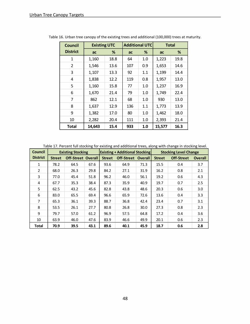
Urban Tree Canopy Targets
48
Table 16. Urban tree canopy of the existing trees and additional (100,000) trees at maturity.
Table 17. Percent full stocking for existing and additional trees, along with change in stocking level.
Street Off-Street Overall Street Off-Street Overall Street Off-Street Overall
1 78.2 64.5 67.6 93.6 64.9 71.3 15.5 0.4 3.7
2 68.0 26.3 29.8 84.2 27.1 31.9 16.2 0.8 2.1
3 77.0 45.4 51.8 96.2 46.0 56.1 19.2 0.6 4.3
4 67.7 35.3 38.4 87.3 35.9 40.9 19.7 0.7 2.5
5 62.5 43.2 45.6 82.8 43.8 48.6 20.3 0.6 3.0
6 83.0 65.5 69.4 96.6 65.9 72.6 13.6 0.4 3.3
7 65.3 36.1 39.3 88.7 36.8 42.4 23.4 0.7 3.1
8 53.5 26.1 27.7 80.8 26.8 30.0 27.3 0.8 2.3
9 79.7 57.0 61.2 96.9 57.5 64.8 17.2 0.4 3.6
10 63.9 46.0 47.6 83.9 46.6 49.9 20.1 0.6 2.3
Total 70.9 39.5 43.1 89.6 40.1 45.9 18.7 0.6 2.8
Existing Stocking Existing + Additional Stocking Stocking Level ChangeCouncil
District
ac % ac % ac %
1 1,160 18.8 64 1.0 1,223 19.8
2 1,546 13.6 107 0.9 1,653 14.6
3 1,107 13.3 92 1.1 1,199 14.4
4 1,838 12.2 119 0.8 1,957 13.0
5 1,160 15.8 77 1.0 1,237 16.9
6 1,670 21.4 79 1.0 1,749 22.4
7 862 12.1 68 1.0 930 13.0
8 1,637 12.9 136 1.1 1,773 13.9
9 1,382 17.0 80 1.0 1,462 18.0
10 2,282 20.4 111 1.0 2,393 21.4
Total 14,643 15.4 933 1.0 15,577 16.3
Council
District
Existing UTC Additional UTC Total

Urban Tree Canopy Targets
49
Figure 14. Number of existing and additional trees by council district.

Ecosystem Service Assessment
50
Ecosystem Service and Property Value Assessment
Urban trees provide ecosystem services by regulating climate and conserving building energy use, filtering pollutants from air and water, reducing soil erosion, and creating habitat for plants and animals. The natural beauty of trees plays an important role making communities attractive places to work and play. Urban forests produce shaded streets and trails that promote fitness from outdoor exercise like walking and biking. Planting and maintaining trees creates jobs and provides environmental education opportunities for youth.
This study evaluated ecosystem services values including energy, carbon, air quality, storm runoff, and property value effects for existing UTC and additional UTC. Benefits of carbon storage, carbon sequestration, air quality, and property values were based on transfer functions calculated for the San Francisco Bay Area State of the Urban Forest study (Simpson and McPherson, 2007), while the energy effects were estimated based on data collected in the 2012 San Jose field campaign.
Transfer function is a term used to describe the transfer of data for a particular “study site” to a “policy site” for which little or no data exist (Brookshire and Neill, 1992, Downing and Ozuna Jr, 1996). In this study, transfer functions are defined as field plot-based measures of a service (e.g., gallons of rainfall intercepted) per acre UTC (gal ac-1 UTC) that are aggregated and applied to a region by land use class. We express ecosystem services in terms of resource units (RUs), or engineering units, per unit UTC. Previous research found that this approach provided higher accuracy, greater precision, and improved spatial detail compared to services derived by land use class alone.
Different transfer function values reflect different stand structures and dynamics that influence the provision of ecosystem services. For instance, the C storage transfer function for an acre of UTC in an old residential neighborhood will be relatively high when the stand consists of closely spaced mature oaks (Quercus spp.) and a lush understory. In contrast, the transfer function for an acre of UTC in a new residential area will be lower when the stand is characterized by juvenile pear (Pyrus spp.) trees with a sparse understory. Hence, the value of a transfer function reflects species composition and attributes of stand structure, such as tree and basal area densities. Species type is important because of its influence on the tree’s biomass and partitioning into roots, bole, branches, stems, and foliage. Stand attributes, such as the vertical layering of biomass in strata, tree density, and bole size also influence the amount of woody and foliar biomass per acre UTC and the resulting value of a transfer function.
The transfer function for each land use class is transferred to the UTC and delineated for the corresponding land use. Using GIS capabilities, services are mapped and values are summed based on the amount of UTC in each land use class. These maps provide spatially explicit information on the distribution of ecosystem services for planning and management purposes.

Ecosystem Service Assessment
51
Calculation Process
There were two options for generating transfer functions from existing tree inventory and ecosystem services information. One approach was to use average values from several reference cities, such as San Francisco, Berkeley, and Modesto. This was the most straightforward approach, but did not produce transfer functions for each land use because RUs were for street trees only. A second limitation was that the species composition and structure of street tree populations often differs from the structure of the overall urban forest. For example, in Guangzhou, China the street tree population was less diverse, contained more large-stature taxa, and exhibited higher levels of spatial continuity than park and campus trees (Jim and Liu, 2001). For these reasons it was decided that transfer functions generated from street trees without land use designations was not the best approach.
The second approach was applied in a study of the San Francisco Bay Area urban forest (Simpson and McPherson, 2007). It involved first selecting the reference city that best matched San Jose in terms of its tree species, growth and management, as well as climate. Then, RUs were converted from a per tree basis to an UTC basis and dependencies on tree size and species were eliminated. Finally, land use dependence was added. The resulting transfer functions could be directly applied to UTC polygons with values changing by land use.
Calculating RUs for carbon, air quality, rainfall interception, and property values involved four steps. First, RUs per tree were calculated using tree data from reference city research in Modesto, CA (McPherson and Simpson, 1999, 2002). After examining regional climate data and speaking with San Jose city arborist Ralph Mize, it was determined that the tree species and benefit data from Modesto were a better fit for San Jose than data from Berkeley and San Francisco. For example, street trees in San Francisco were heavily pruned for bus clearance, which made for a poor match with fuller-crowned trees in San Jose. Information used in the Modesto analysis included climate, building types, benefit prices, air quality, and other environmental data. In “Modesto Municipal Forest Resource Assessment” (McPherson et al., 1999), RUs per tree and Crown Projection Area or UTC per tree were calculated as a function of species and size class from a stratified random sample of 22 species. About 30 to 50 trees of each species were measured in Modesto to establish relations between tree age, size, leaf area, and biomass (Peper et al., 2001). Trees were selected so as to represent as wide a range of sizes/ages as possible; 9 DBH size classes were used.
The second step was to convert RUs per tree to RUs per unit UTC for each species and size class represented:
RUs/UTCj,k = RUs/treej,k UTC/treej,k,
where j is DBH size class 1 to 9, and k is species 1 to n, where n was 22 tree species for Modesto. In the third step, tree size dependence was removed by weighting RUs/UTC by the distribution of tree numbers by species and size class based on the Modesto tree inventory. In the final step, species dependence was removed and land use dependence added based on UTC by species and land use data derived from an earlier study (McPherson, 1998). Results were applied to the land cover/land use maps to calculate the values of ecosystem services across the City of San Jose.

Ecosystem Service Assessment
52
Urban tree canopy was converted to estimates of tree numbers based on the average tree canopy diameter (D) of 16.4-ft (5 m) found for Sacramento (McPherson, 1998). Field data from Sacramento were used to estimate average crown size because the sample was citywide and results would be applied citywide.
Canopy diameter was converted to horizontal UTC by assuming a circular crown, where UTC = πr2 and r = D/2, so that average UTC = 406.6-ft2 (37.8 m2).
Calculation of benefits from GIS polygons for each land use (m = 1 to 7 land use types) was a straightforward process as the product of RUs per unit UTC, tree size class distribution (TDist) and UTC summed over size class (j = 1 to 9) and species (k = 1 to 22) for Modesto:
Benefitm = 22
1
[k
9
1
[j
RUs/UTCj,k x TDistj,k] x UTCk,m]
The transfer functions and prices used to value each ecosystem service and property value are shown in Table 18 and Table 19.
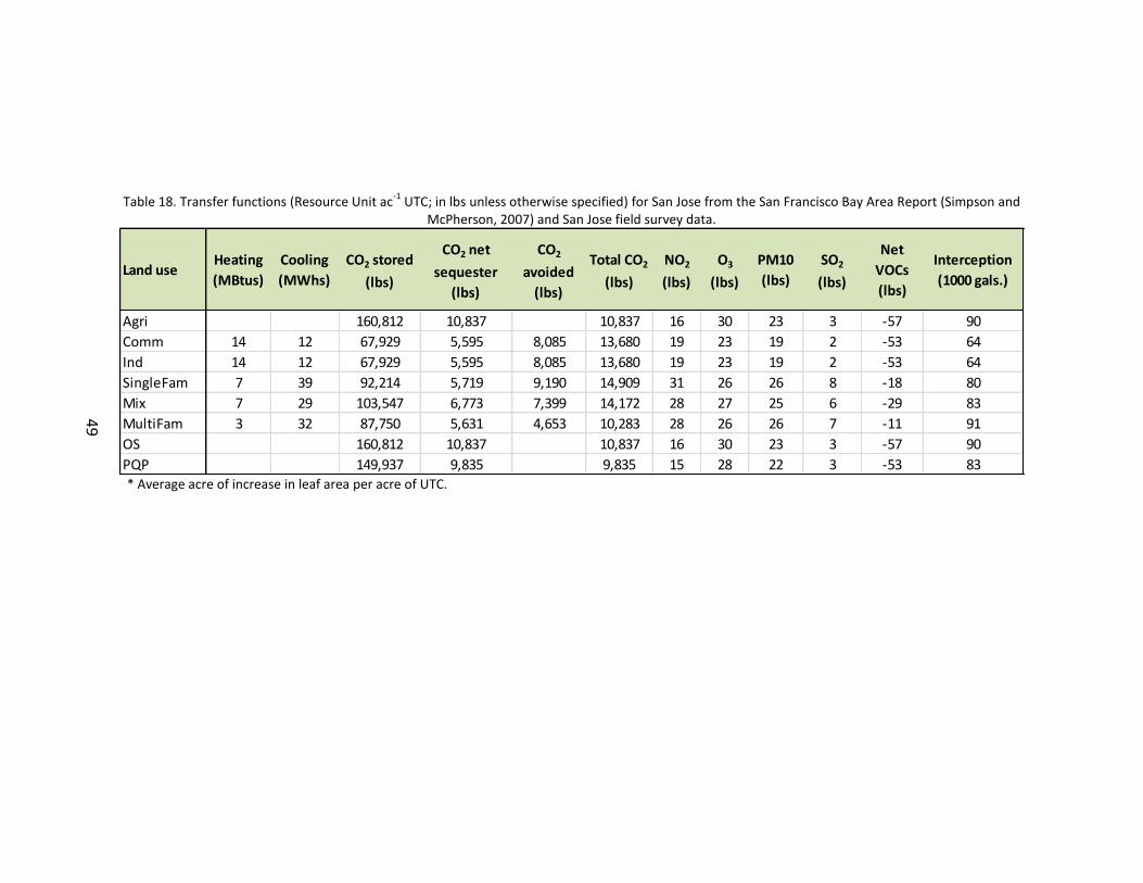
Table 18. Transfer functions (Resource Unit ac-1
UTC; in lbs unless otherwise specified) for San Jose from the San Francisco Bay Area Report (Simpson and McPherson, 2007) and San Jose field survey data.
* Average acre of increase in leaf area per acre of UTC.
Land useHeating
(MBtus)
Cooling
(MWhs)
CO2 stored
(lbs)
CO2 net
sequester
(lbs)
CO2
avoided
(lbs)
Total CO2
(lbs)
NO2
(lbs)
O3
(lbs)
PM10
(lbs)
SO2
(lbs)
Net
VOCs
(lbs)
Interception
(1000 gals.)
Agri 160,812 10,837 10,837 16 30 23 3 -57 90
Comm 14 12 67,929 5,595 8,085 13,680 19 23 19 2 -53 64
Ind 14 12 67,929 5,595 8,085 13,680 19 23 19 2 -53 64
SingleFam 7 39 92,214 5,719 9,190 14,909 31 26 26 8 -18 80
Mix 7 29 103,547 6,773 7,399 14,172 28 27 25 6 -29 83
MultiFam 3 32 87,750 5,631 4,653 10,283 28 26 26 7 -11 91
OS 160,812 10,837 10,837 16 30 23 3 -57 90
PQP 149,937 9,835 9,835 15 28 22 3 -53 83
49

Ecosystem Service Assessment
54
Table 19. Prices used to value ecosystem services in San Jose.
Energy Effects
The effect of trees on building energy use has been studied using varying approaches (Carver et al., 2004, Jo and McPherson, 2001, McPherson and Simpson, 2003). Our approach used a prototypical building for simulations with tree distributions based on results from our San Jose field campaign. The prototype building was typical of post-1980 construction practices and represented approximately one-third of the total single-family residential housing stock in the Northern California Coast region. The house was a one-story, wood-frame building with a basement and total conditioned floor area of 2,180-ft2. Window area (double-glazed) was 262-ft2. Wall and ceiling insulation was R11 and R25, respectively. The central cooling system had a seasonal energy efficiency ratio (SEER) of 10, the natural-gas furnace had an annual fuel utilization efficiency (AFUE) of 78%. Building footprints were square, reflecting average impacts for a large number of buildings (McPherson and Simpson, 1999). Buildings were simulated with 1.5-ft overhangs. Blinds had a visual density of 37% and were assumed to be closed when the air conditioner was operating. Summer thermostat settings were 78°F; winter settings were 68°F during the day and 60°F at night. Because the prototype building was larger, but more energy efficient than most other construction types, our projected energy savings could be considered similar to those for older, less thermally efficient, but smaller buildings. The energy simulations relied on typical meteorological data from Sunnyvale, CA (Marion and Urban, 1995). The total energy effects per tree were the combined shade and climate effect calculated for its size, species, and location to surrounding buildings. The dollar value of energy savings was based on regional average residential electricity and natural-gas prices of $0.186/kWh and $0.01/kBtu, respectively (Table 19). Electricity and natural-gas prices were from Pacific Gas and Electric’s 2012 rate schedule.
Benefit Value
Heating ($/kBtu) 0.010
Cooling ($/kWh) 0.186
CO2 ($/lb) 0.005
NO2 ($/lb) 0.005
O3 ($/lb) 3.340
PM10 ($/lb) 3.340
SO2 ($/lb) 4.458
Net VOCs ($/lb) 9.661
Interception ($/gal) 0.006
Property value ($/acre of UTC)
Commercial 4,471
Industrial 4,471
SingleFamily 14,859
Mix 10,918
MultiFamily 8,358
Public/Quasi-Public 4,300

Ecosystem Service Assessment
55
Calculating shade effects As part of Phase I, we identified 100 stratified random samples for each land cover class based on the object-based classification with LiDAR. These points were visually classified using 2010 NAIP images. All points that showed uncertainty were field visited plus 10% of the certain points. To determine the distribution of trees to buildings we used the 55 field sample points from the tree land cover class. This sample was unbiased because points were identified at random and independent of surrounding building locations. Because the focus of energy savings was on the residential zoning class, 49 tree points within the single-family and multi-family zoning class were included in tree-building distribution analyses for energy savings calculations. Out of these 49 trees, 45 were within 60-ft of buildings and 4 were outside 60-ft, where no shading occurred.
Each tree was identified and measured (diameter at breast height, height, and canopy dimensions) in the field. In the lab, the trees’ distances and orientations to surrounding buildings were determined using the GIS buildings layer. Each tree’s distance was calculated using the building polygons while its orientation was determined based on the building polygon’s centroid to avoid any confusion based on the shape of the building. For both distance and orientation, the ‘generate near table’ function in ArcGIS was used.
To calculate the cooling and heating transfer functions (Table 18) for the 49 sample trees, DBH, species, distance, and orientation data were used to locate the appropriate resource unit from energy lookup tables (Simpson, 2002) for San Jose (McPherson et al., 2008). The lookup tables contained the energy effects for a number of species at a range of sizes, distances, and orientations to single-family residential buildings. Because not all tree species are included in the lookup tables, the species that best matched taxonomically to the one measured in the field was chosen. The distribution of species used for energy calculations can be seen in Table 20.
Table 20. Distribution of matched species used for energy calculations.
Botanical name Common name Tree count
Acer saccharinum Silver maple 6
Betula pendula European white birch 1
Fraxinum angustifolia Raywood ash 1
Fraxinus excelsior Hesse ash 3
Fraxinus pennsylvanica Marshall ash 6
Koelreuteria paniculata Goldenrain tree 1
Lagerstroemia indica Common crapemyrtle 6
Liquidamber styraciflua Sweetgum 1
Phoenix dactylifera Date palm 3
Pinus radiata Monterey pine 1
Pinus thunbergiana Japanese black pine 1
Pyrus kawakamii Evergreen pear 8
Quercus ilex Holly oak 7
Zelkova serrata Japanese zelkova 4
49Total

Ecosystem Service Assessment
56
Table 21. Number of sample trees by location relative to closest building.
In addition to localized shade effects, an increase in neighborhood tree cover also lowered air temperatures and wind speeds. These are referred to as climate effects and can produce a net decrease in demand for winter heating and summer cooling. Depending on the circumstances, reduced wind speeds alone may increase or decrease cooling demand. Climate effects on energy use, air temperature, and wind speed as a function of neighborhood canopy cover were estimated from published values (McPherson and Simpson, 1999). Existing tree canopy cover for San Jose was 15.4% and building cover was estimated to be 17.5%. Climate effects were estimated by simulating the effects of air temperature and wind reductions on energy use.
Atmospheric Carbon Dioxide Reduction
Calculating reduction in CO2 emissions from power plants Conserving energy in buildings can reduce electricity demand for air conditioning and carbon dioxide (CO2) emissions from power plants. These avoided emissions were calculated as the product of energy savings for heating and cooling based on PG&E’s CO2 production of 651 lbs per MWh for electricity and 11.8 lbs per MBtu for natural gas (McPherson et al., 2010).
Calculating carbon storage Sequestration, the net rate of CO2 storage in above- and belowground biomass over the course of one growing season, was calculated by using tree height and DBH data with biomass equations (Pillsbury et al., 1998). Volume estimates were converted to green and dry-weight estimates (Markwardt, 1930) and divided by 78% to incorporate root biomass. Dry-weight biomass was converted to carbon (50%) and these values were converted to CO2. The amount of CO2 sequestered each year is the annual increment of CO2 stored as biomass each year. The monetary value of sequestered and avoided CO2 was $0.005/lb based on average high and low estimates for emerging carbon trading markets.
<20ft 20-40ft 40-60ft >60ft Total
E 3 1 2 6
N 2 3 2 7
NE 2 1 2 5
NW 1 1 2 4
S 2 3 1 6
SE 2 1 3
SW 2 2 2 6
W 4 2 2 8
Climate only 4 4
Total 16 15 14 4 49
AzimuthDistance class
Calculating climate effects

Ecosystem Service Assessment
57
Air Pollutants
Calculating reduction in air pollutant emissions Reductions in building energy use also result in reduced emission of air pollutants from power plants and space-heating equipment. Volatile organic hydrocarbons (VOCs) and nitrogen dioxide (NO2)—precursors of ozone (O3) formation—as well as sulfur dioxide (SO2) and particulate matter of <10 micron diameter (PM10) were considered. Changes in average annual emissions and their monetary values were calculated in the same way as for CO2, by using PG&E-specific emissions factors for electricity and heating fuels (U.S. Environmental Protection Agency, 1998). The price of emissions savings were derived from models that calculate the marginal damage cost of different pollutants to meet air quality standards (Wang and Santini, 1995). Emissions concentrations were obtained from US EPA (2003) and population estimates from the 2010 US Census (US Census Bureau, 2013).
Calculating pollutant uptake by trees Trees also remove pollutants from the atmosphere. The modeling method we applied was developed by Scott et al. (1998). It calculates hourly pollutant dry deposition per tree expressed as the product of deposition velocity (Vd = 1/[Ra + Rb + Rc]), pollutant concentration (C), canopy-projection area (CP), and a time step. In this equation Ra, Rb, and Rc are aerodynamic, boundary layer, and stomatal resistances. Hourly deposition velocities for each pollutant were calculated during the growing season by using estimates for the resistances (Ra + Rb + Rc ) for each hour throughout the year. Hourly concentrations for 2001 were selected as representative for modeling deposition based on a review of mean PM10 and O3 concentrations for the years 1996 through 2004. The O3, NO2, and SO2 data were from Oakland and PM10 from San Pablo (California Air Resources Board, 2004). Hourly air temperature and wind speed data were obtained for Berkeley (California Air Resources Board, 2004). To set a value for pollutant uptake by trees, we used the procedure described above for emissions reductions. The monetary value for NO2 was also used for O3.
Estimating BVOC emissions from trees Annual emissions for biogenic volatile organic compounds (BVOCs) were estimated for each tree species by using the algorithms of Guenther et al. (1991, 1993). Annual emissions were simulated during the growing season. The emission of carbon as isoprene was expressed as a product of the base emission rate (micrograms of carbon per gram of dry foliar biomass per hour), adjusted for sunlight, temperature, and the amount of dry foliar biomass present in the tree. Monoterpene emissions were estimated by using a base emission rate adjusted for temperature. The base emission rates were based on values reported in the literature (Benjamin and Winer, 1998). Hourly emissions were summed to get monthly and annual emissions.
Annual dry foliar biomass was derived from field data. The amount of foliar biomass present for each year of the simulated tree’s life was unique for each species. Hourly air temperature and solar radiation data were used as model inputs.
Calculating net air quality benefits Net air quality benefits were calculated by subtracting the costs associated with BVOC emissions from benefits owing to pollutant uptake and avoided power plant emissions. The O3

Ecosystem Service Assessment
58
reduction benefit from lowering summertime air temperatures, thereby reducing hydrocarbon emissions from anthropogenic and biogenic sources, were estimated as a function of canopy cover following McPherson and Simpson (1999). They used peak summer air temperatures reductions of 0.2°F for each percentage of increase in canopy cover. Hourly changes in air temperature were calculated by reducing this peak air temperature at every hour based on hourly maximum and minimum temperatures for that day, as well as maximum and minimum values of total global solar radiation for the year. However, this analysis does not incorporate the effects of lower summer air temperatures on O3 formation rates owing to atmospheric processes. The value of ecosystem services for air quality were monetized using models that calculated the marginal cost of controlling different pollutants to meet air quality standards (Wang and Santini, 1995). All air pollutant prices are shown in Table 19.
Rainfall Interception
Urban trees can reduce the amount of runoff and pollutant loading in receiving waters by intercepting and storing rainfall on leaves and branch surfaces. Root growth and decomposition can also increase the capacity and rate of soil infiltration by rainfall and reduce overland flow. Studies of urban forest impacts on stormwater reported an annual runoff reduction of 2 to 7% (Xiao et al., 1998a).
Estimating rainfall interception by tree canopies A numerical simulation model was used to estimate annual rainfall interception (Xiao et al., 2000). The interception model accounted for water intercepted by the tree as well as throughfall and stem flow. Intercepted water is stored temporarily on canopy leaf and bark surfaces. Rainwater drips from leaf surfaces, flows down the stem surface to the ground or evaporates. Tree-canopy parameters that affect interception include species, leaf and stem surface areas, shade coefficients (visual density of the crown), foliation periods, and tree dimensions (e.g., tree height, crown height, crown diameter, and DBH). Tree-height data were used to estimate wind speed at different heights above the ground and resulting rates of evaporation.
The volume of water stored in the tree crown was calculated from the crown-projection area (area under tree dripline), leaf area indices (LAI, the ratio of leaf surface area to crown projection area), and the depth of water captured by the canopy surface. Gap fractions, foliation periods, and tree surface saturation storage capacity influence the amount of projected throughfall. Tree surface saturation was 0.04 in for all trees. Hourly meteorological and rainfall data for 2001 from the CIMIS (California Irrigation Management Information System, 2004) San Jose Station (ID #69; latitude 37°19' N, longitude 121°95' W) were used for this simulation. Annual precipitation during 2001 was 16.7 in (424.4 mm). Storm events less than 0.1 in were assumed to not produce runoff and were removed from the analysis. More complete descriptions of the interception model can be found in Xiao et al. (1998b).
Calculating water quality protection and flood control benefit The benefit of runoff reduction was estimated using costs associated with collection, conveyance, and treatment of stormwater from sewer service fees, a conservative proxy for a

Ecosystem Service Assessment
59
desired level of service. Interception was priced based on mean fees for San Francisco, Berkeley, and Modesto (Simpson and McPherson, 2007). The price of $0.006 per gallon is comparable to the average price for stormwater runoff reduction ($0.01/gallon) reported in similar studies (McPherson et al., 2005).
Property Value
Many benefits attributed to urban trees are difficult to translate into economic terms. Beautification, privacy, wildlife habitat, sense of place, and well-being are services that are difficult to price. However, the value of some of these benefits may be captured in the property values of the land on which trees stand. To estimate the value of these “other” benefits, we applied results of research that compared differences in sales prices of houses to statistically quantify the difference associated with trees. All else being equal, the difference in sales price reflects the willingness of buyers to pay for the benefits and costs associated with trees. This approach has the virtue of capturing in the sales price both the benefits and costs of trees as perceived by the buyers. Limitations to this approach include; difficulty determining the value of individual trees on a property, the need to extrapolate results from studies done years ago in the East and South to this region, and the need to extrapolate results from front-yard trees on residential properties to trees in other locations (e.g., back yards, streets, parks, and non-residential land) and UTC.
Anderson and Cordell (1988) surveyed 844 single-family residences in Athens, GA and found that each large front-yard tree was associated with a 0.88% increase in the average home sales price. This percentage of sales price was utilized as an indicator of the additional value a resident in San Jose would gain from selling a home with a large tree. The sales price of residential properties varied widely by location within San Jose, but the median was $645,000 (Simpson and McPherson, 2007). Therefore, the value of a large tree that added 0.88% to the sales price of such a home was $5,688. To estimate annual benefits, the total added value was divided by the leaf surface area of a mature shade tree ($5,688/3,348-ft2) to yield the base value of $0.16/ft2 of leaf surface area. This value was multiplied by the amount of leaf surface area added to the tree during 1 year of growth.
To adapt and apply the base value to San Jose’s urban forest, a land use reduction factor was applied because the value of trees located in back yards and non-residential property will have less impact on sales price and other intangible benefits compared to front-yard trees (Richards et al., 1984). Lacking specific research findings and wanting to be conservative, it was assumed that single family residential UTC had less impact than a front-yard tree. Overall, the reduction factor of 0.834 was applied based on tree distributions among land uses (Simpson and McPherson, 2007).

Ecosystem Service Assessment
60
Results & Discussion
Ecosystem services and property value increases provided by existing UTC
The annual value of ecosystem services and property value increase (Table 22) provided by existing UTC was $239 million (
Table 23). UTC was estimated to increase property values and provide other intangible benefits valued at $154.7 million annually or 65% of the total. Energy savings and rainfall interception accounted for $78 million (33%) and 6.7 million (3%), respectively. Atmospheric carbon dioxide reduction was valued at $1 million. San Jose’s urban forest removes 610 tons of air pollutants from the atmosphere, valued at $2.9 million. However, this benefit is offset because the urban forest emits 207 tons of BVOCs valued at -$4 million. As a result, the net annual cost is $1.1 million. A number of the most common trees species in San Jose are high-emitters of BVOCs (e.g., eucalyptus, sweet gum, sycamore, and oak) (Nowak, 2000).
These are very conservative estimates of service provided because they do not fully capture all benefits associated with urban tree canopy such as job creation, improved human health and fitness, wildlife habitat, and biodiversity.

Table 22. Estimated annual ecosystem services (tons unless otherwise specified) and property values (acre of annual increase in leaf area) provided by existing UTC.
Table 23. Estimated annual monetary value ($1,000) of ecosystem services and property value increase provided by existing UTC.
Council
District UTC (ac)
Heating
(MBtus)
Cooling
(MWhs)
CO2
stored
CO2 net
sequester
CO2
avoided
Total
CO2
NO2 O3 PM10 SO2
Net
VOCs
Interception
(1,000 gal)
Property
value (ac)
1 1,160 7,721 40,993 52,442 3,333 4,816 8,149 17 15 15 4 -11 93,243 478
2 1,547 10,095 44,864 76,914 5,019 5,768 10,787 21 20 19 5 -22 123,003 541
3 1,107 8,667 28,646 46,225 3,190 3,791 6,981 14 14 13 3 -16 87,246 359
4 1,838 16,445 44,791 81,794 5,661 7,172 12,833 23 23 21 5 -33 137,174 593
5 1,160 6,561 35,949 59,006 3,773 4,244 8,017 16 15 15 4 -14 94,403 426
6 1,670 11,653 56,778 75,443 4,843 6,920 11,764 24 21 21 6 -18 132,730 675
7 862 5,516 24,169 42,502 2,792 3,060 5,852 11 11 11 3 -12 69,049 290
8 1,637 6,783 34,916 98,249 6,432 4,275 10,706 20 22 20 4 -29 136,431 419
9 1,382 9,322 50,110 63,569 4,008 5,990 9,998 21 18 18 5 -14 110,261 585
10 2,282 9,762 53,741 133,557 8,676 6,418 15,094 29 31 28 7 -37 189,619 643
Total 14,645 92,524 414,956 729,702 47,726 52,455 100,181 195 190 180 44 -207 1,173,158 5,009
Council
District Heating Cooling
CO2 net
sequester
CO2
avoided
Total
CO2
NO2 O3 PM10 SO2
Net
VOCsInterception
Property
valueTotal
1 73.6 7,620.6 33.3 48.2 81.5 0.2 99.2 98.8 36.6 -221.0 536.1 15,012.0 23,337.6
2 96.3 8,340.2 50.2 57.7 107.9 0.2 133.9 127.5 42.4 -421.9 707.3 16,987.7 26,121.3
3 82.7 5,325.2 31.9 37.9 69.8 0.1 92.6 86.7 26.0 -307.2 501.7 9,246.0 15,123.5
4 156.8 8,326.7 56.6 71.7 128.3 0.2 152.8 141.7 40.9 -632.5 788.7 16,876.0 25,979.8
5 62.6 6,682.9 37.7 42.4 80.2 0.2 101.6 97.8 34.1 -277.4 542.8 13,590.7 20,915.5
6 111.1 10,555.1 48.4 69.2 117.6 0.2 142.3 140.6 50.7 -352.3 763.2 21,014.6 32,543.2
7 52.6 4,493.0 27.9 30.6 58.5 0.1 74.6 70.5 23.0 -236.0 397.0 8,869.2 13,802.6
8 64.7 6,490.8 64.3 42.7 107.1 0.2 148.9 133.4 39.3 -559.9 784.5 13,461.4 20,670.3
9 88.9 9,315.4 40.1 59.9 100.0 0.2 118.4 118.6 44.6 -264.7 634.0 18,889.9 29,045.3
10 93.1 9,990.4 86.8 64.2 150.9 0.3 206.2 187.8 58.0 -722.8 1,090.3 20,746.8 31,801.1
Total 882.5 77,140.3 477.3 524.5 1,001.8 1.9 1,270.3 1,203.4 395.6 -3,995.6 6,745.7 154,694.4 239,340.2
57

Ecosystem Service Assessment
62
Ecosystem services and property value increases provided by additional UTC
Planting 100,000 trees will increase UTC from 15.4% to 16.3% (assuming a 22.75-ft mature crown diameter). An additional 1% of UTC is projected to increase the annual value of ecosystem services and property values (
Table 24) by $16.4 million (

Ecosystem Service Assessment
63
Table 25 and

Ecosystem Service Assessment
64
Figure 15). The majority of these additional benefits are from increased property values ($10.6 million, 65%) and energy savings ($5.4 million, 33%). The calculation assumes that current UTC remains stable and program tree sites remain fully stocked with 22.75-ft crown diameter trees. Because some program trees will die and need to be replaced, more than 100,000 trees will need to be planted to keep additional sites fully stocked. It will take 20 to 30 years to achieve the projected level of canopy cover after planting.
The approximate annual value of ecosystem services and property value increases provided per tree is $153 for San Jose’s 1.57 million existing trees and $164 for additional trees. The average annual benefit per tree from approximately 1.67 million trees is $153, comparable to results for the same services reported for other cities (Maco et al., 2005). The annual value per acre UTC is approximately $17,000.
Asset value of San Jose’s urban forest
The values for ecosystem services have been expressed in annual terms, but trees provide benefits across many generations. Moreover, the benefits trees provide become increasingly scarce and more valuable with time. To enable tree planting and stewardship to be seen as a capital investment, the asset value of trees in San Jose was calculated. The annual flows of realized benefits from trees were converted into their net present value, which is a discounted sum of annual future benefits. Discounting future services to their present value incorporates the time value of money and the opportunity cost of investment. The farther ahead in time one goes, the less value a dollar has. A benefit derived in 50 years is worth far less than the same benefit today. By applying this method to the future stream of ecosystem services, the urban forest’s asset value is calculated in today’s dollars.
The asset value was calculated as the net present value using discount rates of 4.125%, which are used by the US Corps of Engineers for large projects, and 0% over 100 years were used for Existing UTC, Additional UTC, and Existing plus Additional UTC. Some economists argue that natural capital has a lower discount rate because the benefit stream is more certain over longer periods of time.
The asset value of San Jose’s existing urban forest is $5.7 billion or $3,634 per tree, calculated at a 4.125% discount rate for the next 100 years (Table 26). At a zero discount rate, the urban forest asset value is estimated at $23.9 billion. If UTC is increased to 16.3% over the next 30 years by planting 100,000 trees, the urban forest’s asset value increases to $6.1 billion and $25.2 billion, assuming 4.125% and 0% discount rates, respectively. Hence, the ecosystem services produced by San Jose’s urban forest provide a stream of benefits over time, just as a freeway or other capital infrastructure does.

Ecosystem Service Assessment
65
Figure 15. Annual value of ecosystem services and property value increases for the existing and additional UTC by Council District.
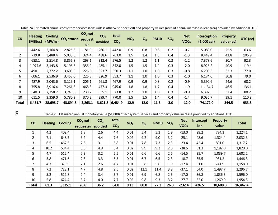
Table 24. Estimated annual ecosystem services (tons unless otherwise specified) and property values (acre of annual increase in leaf area) provided by additional UTC.
Table 25. Estimated annual monetary value ($1,000) of ecosystem services and property value increase provided by additional UTC.
CDHeating
(MBtus)
Cooling
(MWhs)CO2 stored
CO2 net
sequest
er
CO2
avoided
total
CO2
NO2 O3 PM10 SO2
Net
VOCs
Interception
(1,000 gal)
Property
value (ac)UTC (ac)
1 442.6 2,164.8 2,825.3 181.9 260.1 442.0 0.9 0.8 0.8 0.2 -0.7 5,080.0 25.5 63.6
2 739.8 3,488.4 5,038.5 324.4 438.6 763.0 1.5 1.4 1.3 0.4 -1.3 8,449.4 41.8 106.9
3 683.1 2,514.8 3,856.8 263.1 313.4 576.5 1.2 1.2 1.1 0.3 -1.2 7,378.6 30.7 92.3
4 1,074.6 3,143.8 5,196.6 356.9 485.1 842.0 1.5 1.5 1.4 0.3 -2.0 8,925.2 40.9 119.4
5 490.1 2,772.2 3,603.3 226.6 323.7 550.3 1.1 1.0 1.0 0.3 -0.8 6,205.5 32.3 77.0
6 606.1 2,536.9 3,458.0 226.8 326.9 553.7 1.1 1.0 1.0 0.3 -1.0 6,174.0 30.8 79.0
7 487.9 2,043.6 3,129.1 206.1 261.8 467.9 0.9 0.9 0.8 0.2 -0.9 5,390.6 24.6 68.2
8 755.8 3,916.4 7,261.3 468.3 477.3 945.6 1.8 1.8 1.7 0.4 -1.9 11,134.7 46.5 136.1
9 540.3 2,758.7 3,745.6 238.7 335.1 573.8 1.2 1.0 1.0 0.3 -0.9 6,397.5 32.4 80.2
10 611.5 3,359.0 5,780.2 370.2 399.7 770.0 1.5 1.5 1.4 0.4 -1.4 9,036.7 39.1 110.8
Total 6,431.7 28,698.7 43,894.8 2,863.1 3,621.8 6,484.9 12.9 12.0 11.6 3.0 -12.0 74,172.0 344.5 933.5
CD Heating CoolingCO2 net
sequester
CO2
avoided
total
CO2
NO2 O3 PM10 SO2
Net
VOCs
Intercept
ion
Property
valueTotal
1 4.2 402.4 1.8 2.6 4.4 0.01 5.4 5.3 1.9 -13.0 29.2 784.1 1,224.1
2 7.1 648.5 3.2 4.4 7.6 0.02 9.2 9.0 3.2 -25.1 48.6 1,324.4 2,032.3
3 6.5 467.5 2.6 3.1 5.8 0.01 7.8 7.3 2.3 -23.4 42.4 801.0 1,317.2
4 10.2 584.4 3.6 4.9 8.4 0.02 9.9 9.3 2.8 -38.5 51.3 1,182.0 1,820.0
5 4.7 515.4 2.3 3.2 5.5 0.01 6.6 6.6 2.5 -14.5 35.7 1,039.7 1,602.2
6 5.8 471.6 2.3 3.3 5.5 0.01 6.7 6.5 2.3 -18.7 35.5 931.2 1,446.3
7 4.7 379.9 2.1 2.6 4.7 0.01 5.8 5.6 1.9 -17.4 31.0 741.9 1,158.0
8 7.2 728.1 4.7 4.8 9.5 0.02 12.1 11.4 3.8 -37.1 64.0 1,497.7 2,296.7
9 5.2 512.8 2.4 3.4 5.7 0.01 6.9 6.8 2.5 -17.0 36.8 1,036.3 1,596.0
10 5.8 624.4 3.7 4.0 7.7 0.02 9.8 9.3 3.2 -27.7 52.0 1,269.9 1,954.5
Total 61.3 5,335.1 28.6 36.2 64.8 0.13 80.0 77.2 26.3 -232.4 426.5 10,608.3 16,447.4
60

Ecosystem Service Assessment
67
Table 26.Urban forest asset value at two discount rates.
0% 4.125%
Existing UTC 23,934,024,906 5,700,307,526
Additional UTC 1,266,066,519 419,541,147
Existing + Additional UTC 25,200,091,425 6,119,848,672
UTCDiscount Rate

Conclusion
68
Conclusion
San Jose’s urban forest is extensive, covering 15.4% of the 149 square mile region. Urban tree canopy for the 10 Council Districts ranged from 12% to 21%. Impervious surfaces, such as roads, buildings, and parking lots accounted for 58% of the land area. Irrigated grass, bare soil, and dry vegetation covered only 26%. Of comparable cities, only Los Angeles had a higher percentage of impervious surface (61%). The potential for UTC is limited by the relative amount of impervious surfaces, which varies considerably among Council Districts. In three Council Districts the percentages of impervious are 70% or more. In three Council Districts more than 50% of the remaining greenspace is filled with UTC. As a result, their potential for increasing UTC is more limited than it is in the other districts where less than 50% of the available greenspace is already canopied.
There are approximately 1.6 million trees in San Jose’s urban forest, assuming an average crown diameter of 22.75-ft per tree found from field measurements in San Francisco, Los Angeles, and Sacramento, CA. Approximately 19% are street trees and the remainder are off-street. The average number of trees per acre in San Jose is 16.5 and varies from 13.0% to 22.9% among Council Districts. San Jose’s average tree density compares favorably with values reported for Sacramento (16.1) and Los Angeles (19.9), but is less than cities with similar population densities such as Pasadena (24.1) and Minneapolis (26.4). The average number of trees per capita is 1.6, also less than Pasadena (2.7) and Minneapolis (2.6), but comparable to higher density cities such as Los Angeles (1.3). The number of trees per capita ranges from 0.9 to 2.0 among Council Districts.
San Jose’s urban forest produces ecosystem services valued at $239.3 million annually. The largest benefit, $154.6 million, is for increased property values and other intangible services. Lowered air temperature from evapotranspirational cooling and building shade reduce residential air condition demand by 415,000 MWh, saving $77 million in cooling costs each year. The existing urban forest intercepts 1.1 billion gallons of rainfall that reduces stormwater runoff management costs valued at $6.7 million. If carbon dioxide sequestered and emissions avoided from cooling savings by the existing trees (100,000 tons) were sold at $10 per ton, the revenue would be $1 million. Finally, San Jose’s urban forest filters a net total of 403 tons of air pollutants from the air annually.
The City of San Jose contains approximately 2.1 million vacant planting sites, with 94% of these off-street. This number assumes plantable space for a 22.75-ft crown diameter and that about 30% of the vacant sites are not plantable because of physical limitations such as utilities. About 42% of the PTPS are in irrigated grass, where planting is most cost-effective. Nearly all of the remaining sites are in non-irrigated grasslands, where trees will require watering during establishment. There are an estimated 124,472 PTPS along street ROWs, excluding sites in sidewalks where concrete cutting is required to plant trees. Approximately 77% (95,745) of these street tree sites are in irrigated grass, the rest are in bare soil/dry vegetation. The 2009 i-Tree sample estimated that there were 87,580 vacant PTPS along San Jose streets. The estimate of 124,472 sites reported here is substantially larger. This may be because estimates have not been adjusted for unseen physical obstructions to planting, such as proximity to street lights,

Conclusion
69
utility lines, fire hydrants, sewer inlet basins, and intersections. During the i-Tree survey these obstructions were considered when vacant sites were identified.
Setting realistic targets for additional UTC is not straightforward because each Council District has a different land use mix, as well as different existing UTC and potential UTC (PUTC) that reflects historical patterns of development and tree stewardship. After discussing alternative planting scenarios with the city arborist, the research team determined to “plant” 80,000 additional trees sites in the street ROW and the remaining 20,000 on private land in irrigated grass. The target number for each Council District was proportional to the District’s number of PTPS.
Filling 100,000 additional sites will increase UTC from 15.4% to 16.3% assuming that current UTC remains stable and program tree sites remain fully stocked with 22.75-ft crown diameter trees. There is adequate space in irrigated lawn areas to achieve 98% of the 100,000 tree target. The number of vacant sites to be planted ranges from 6,812 in relatively well-treed Council District 1 (UTC is 18.8%) to 14,585 in sparsely-treed Council District 8 (UTC is 12.9%).
Achieving the targeted 1% UTC increase will pay dividends. The value of ecosystem services will increase by nearly 7% or $16.4 million, from $239.3 million to $255.8 million. The value of increased annual property values and other intangible services is projected to be $10.6 million. Reduced demand for 28,699 MWh of electricity for air conditioning is expected to save another $5.3 million in cooling costs. Annual savings for reduced stormwater management costs from an additional 74 million gallons of rainfall interception is projected to be $426,489. Trees in the additional sites will reduce atmospheric carbon dioxide by 6,485 tons, valued at $65,000 annually. The additional UTC will reduce another 27 tons of pollutants from the air. Expansion of the UTC from 15.4 to 16.3% is projected to result in provisioning of ecosystem services valued at $255.8 billion annually from approximately 1.7 million trees. The average annual value of $153 per tree is comparable to results for the same services reported for street and park trees in Berkeley (Maco et al., 2005). This is a very conservative estimate of service value, as it does not fully capture all benefits associated with increased UTC, such as job creation, improved human health and fitness, wildlife habitat, and biodiversity. The asset value of San Jose’s existing urban forest is $5.7 billion, or $3,634 per tree, calculated at a 4.125% discount rate for the next 100 years. At zero discount rate, the region’s urban forest asset value is estimated at $23.9 billion. If UTC is increased to 16.3% over the next 30 years, the urban forest’s asset value increases to $6.1 billion and $25.2 billion, assuming 4.125% and 0% discount rates, respectively. Hence, the ecosystem services produced by the region’s urban forest provides a considerable stream of benefits over time, just as other capital infrastructure does. Quantifying the asset value of this “green infrastructure” can help guide advancement towards a sustainable green economy by shifting investments towards the enhancement of natural capital.
The City of San Jose is a vibrant community that has invested in its urban forest as it has grown. The task ahead is to better integrate the green infrastructure with the gray infrastructure by targeting tree planting and stewardship activities to maximize their environmental and human

Conclusion
70
health impacts. This study provides information that can be used to plan, prioritize and implement new urban forestry programs. In so doing, San Jose’s urban forest will become larger, more resilient, and better able to meet the challenges of tomorrow.
Limitations to the study
This study is one of the first to integrate valuation of urban forest services with delineation of UTC. As a pioneering effort it is not surprising that it encountered obstacles and limitations. Future research, development and application is needed to overcome some of these challenges. Several of the most significant limitations are listed.
Estimates of existing and PTPS are based on field data from previous studies in other California cities because data were lacking for San Jose. Similarly, most transfer functions were based on numerical modeling of tree effects for locations such as Modesto, instead of San Jose. Ideally, a study such as this will have access to recently collected field data for more accurate estimation of tree sizes, numbers and services.
Estimates of existing and PTPS could be improved through field verification and closer scrutiny of areas unlikely to be planted, such as airports.
Time gaps between acquisition of remotely sensed data and field sampling can result in inaccurate land cover maps and benefit estimation. Up-to-date data that overlap spatially and temporally can improve the accuracy of land cover classification and subsequent ecosystem service modeling.
Lookup tables developed by Dr. Jim Simpson (PSW, now retired) were used to model energy effects. These tables did not include all species found within the study area. Access to more detailed data on energy savings by species and location may also improve the accuracy of ecosystem service results.
Estimates of ecosystem services are subject to multiple sources of uncertainty. Sampling and measurement error influence the accuracy of data from field plots. Errors are introduced in the derivation, parameterization and application of numerical models used to estimate effects of trees. For example, annual carbon sequestration estimates are limited by uncertainty inherent in sampling and measurements of trees that were the source of tree growth models. Estimates of avoided emissions rely on a numerical model and multiple sources of error associated with model parameterization and application. Mapping UTC and ecosystem services is subject to errors associated with land cover classification, as well as land use designations. Sensitivity analysis can be used to characterize uncertainty distributions for each type of error, but is beyond the scope of this study.

Conclusion
71
Deliverables and Resources
Products that this project will deliver to the City of San Jose and CalFire are as follows:
1. High-resolution land-cover raster dataset
2. High-resolution land-cover vector dataset 3. GIS datasets (land use, roads, buildings, water, CBGs, etc.) 4. Excel tables (by Council District and CBG)
a. Land use and cover b. PTPS (street & off-street) c. Additional 100,000 trees d. Ecosystem services (RUs and monetary values) e. Outreach event to present results and gather feedback
City of San Jose staff in conjunction with UC Davis organized an outreach event to present project findings to stakeholders in San Jose. The event took place on February 20th from 10 am to noon at San Jose City Hall.
Greg McPherson presented the project and its outcomes and facilitated discussion. About 20 people attended from entities that included the Department of Transportation, Parks and Recreation, GIS, Public Works, and ESD.
5. Final report 6. Executive summary 2-page handout 7. Council District handouts (1 for each)
References
72
References
Anderson, L. M. and H. K. Cordell. 1988. Influence of trees on residential property values in Athens, Georgia (USA): a survey based on actual sales prices. Landscape and Urban Planning. 15:153-164.
Benjamin, M. T. and A. M. Winer. 1998. Estimating the ozone-forming potential of urban trees and shrubs. Atmospheric Environment:Urban Atmospheres. 32:53-68.
Bicknell, J., L. Prickett, V. Atre and Q. Lu. 2012. C.3 Stormwater Handbook. City of San Jose, California Retrieved from http://www.scvurppp-w2k.com/pdfs/1112/C3_Handbook_Chapters-042012-Web.pdf.
Brookshire, D. S. and H. R. Neill. 1992. Benefit transfers: conceptual and empirical issues. Water Resources Research. 28:651-655.
CalFire. 2010. California's Forests and Rangelands: 2010 Assessment.California Department of Forestry and Fire Protection. Sacramento, CA.
California Air Resources Board. 2004. California air quality data (CD-ROM PTSD-04-019-CD). State of California, California Environmental Protection Agency. Retrieved March 14, 2004, from http://www.arb.ca.gov/aqd/aqdcd/aqdcd.htm.
California Irrigation Management Information System. 2004. CIMIS data. Retrieved October 27, 2004, from http://wwwcimis.water.ca.gov/cimis/data.jsp.
Carver, A. D., D. R. Unger and C. L. Parks. 2004. Modeling energy savings from urban shade trees: An assessment of the CITYgreen® energy conservation module. Environmental management. 34:650-655.
City of San Jose. 1990. Commercial design guidelines. City of San Jose. 2009. San Jose's Green Vision: Annual Report. Retrieved March 5, 2013, from
https://ca-sanjose.civicplus.com/DocumentCenter/View/9217. City of San Jose. 2011. Council policy: Post-construction urban runoff management Retrieved
from http://www3.sanjoseca.gov/clerk/cp_manual/CPM_6_29.pdf. Downing, M. and T. Ozuna Jr. 1996. Testing the reliability of the benefit function transfer
approach. Journal of environmental economics and management. 30:316-322. Guenther, A. B., R. K. Monson and R. Fall. 1991. Isoprene and monoterpene emission rate
variability: observations with eucalyptus and emission rate algorithm development. 96:10799-10808.
Guenther, A. B., P. R. Zimmerman, P. C. Harley, R. K. Monson and R. Fall. 1993. Isoprene and monoterpene emission rate variability: model evaluations and sensitivity analyses. Journal of Geophysical Research. 98:12609-12617.
Jim, C. Y. and H. T. Liu. 2001. Species diversity of three major urban forest types in Guangzhou City, China. Forest Ecology and Management 146:99-114.
Jo, H. K. and E. G. McPherson. 2001. Indirect carbon reduction by residential vegetation and planting strategies in Chicago, USA. Journal of Environmental Management. 61:165-177.
Maco, S. E., E. G. McPherson, J. R. Simpson, P. J. Peper and Q. Xiao. 2005. City of Berkeley, California Municipal Tree Resource Analysis. USDA Forest Service, Pacific Southwest Research Station, Center for Urban Forest Research. Davis, CA.
Marion, W. and K. Urban. 1995. Users manual for TMY2s: Derived from the 1961--1990 National Solar Radiation Data Base. National Renewable Energy Lab., Golden, CO (United States).

References
73
Markwardt, L. J. 1930. Comparative strength properties of woods grown in the United States. USDA Forest Service, Washington, DC. 1.
McPherson, E., Q. Xiao and E. Aguaron. in review. Transfer functions for mapping urban forest carbon dioxide storage in Los Angeles and Sacramento, California. Landscape and Urban Planning.
McPherson, E. G. 1993. Evaluating the cost effectiveness of shade trees for demand-side management. The Electricity Journal. 6:57-65.
McPherson, E. G. and R. A. Rowntree. 1993. Energy conservation potential of urban tree planting. Journal of Arboriculture. 19:321-331.
McPherson, E. G. 1998. Structure and sustainability of Sacramento's urban forest. Journal of Arboriculture 24:174-190.
McPherson, E. G. and J. R. Simpson. 1999. Carbon Dioxide Reductions Through Urban Forestry: Guidelines for Professional and Volunteer Tree Planters. (Gen. Tech. Rep. PSW-GTR-171). Albany, CA: USDA Forest Service, Pacific Southwest Research Station.
McPherson, E. G., J. R. Simpson, P. J. Peper and Q. Xiao. 1999. Benefit-cost analysis of Modesto's municipal urban forest. Journal of Arboriculture. 25:235-248.
McPherson, E. G. 2001. Sacramento’s parking lot shading ordinance: environmental and economic costs of compliance. Landscape and Urban Planning. 57:105-123.
McPherson, E. G. and J. R. Simpson. 2002. A comparison of municipal forest benefits and costs in Modesto and Santa Monica, California, U.S.A. Urban Forestry & Urban Greening Urban Forestry & Urban Greening. 1:61-74.
McPherson, E. G. and J. R. Simpson. 2003. Potential energy savings in buildings by an urban tree planting programme in California. Urban Forestry & Urban Greening. 2:73-86.
McPherson, E. G., J. R. Simpson, P. J. Peper, S. E. Maco and Q. Xiao. 2005. Municipal forest benefits and costs in five U.S. cities. Journal of Forestry 103:411-416.
McPherson, E. G., J. R. Simpson, P. J. Peper, A. Crowell and X. Xiao. 2010. Northern California Coast Community Tree Guide: Benefits, Costs and Strategic Planting. (PSW-GTR-228). Albany, CA: USDA Forest Service, Pacific Southwest Research Station.
McPherson, G., J. Simpson, D. Marconett, P. Peper and E. Aguaron. 2008. Urban Forestry and Climate Change. Retrieved March, 2012, from http://www.fs.fed.us/ccrc/topics/urban-forests/.
McPherson, G., Q. Xiao, C. Wu and J. Bartens. 2013. Metro Denver Urban Forest Assessment. Submitted to the Parks and Recreation Department, City and County of Denver, Co.
Nowak, D. J. 2000. Tree species selection, design, and management to improve air quality. pp. In: Proc. of conf. on 2000 ASLA annual meeting proceedings. Washington, DC: American Society of Landscape Architects.
Nowak, D. J. and D. E. Crane. 2002. Carbon storage and sequestration by urban trees in the USA. Environmental Pollution. 116:381-389.
Nowak, D. J. 2006. Assessing Urban Forest Effects and Values: Minneapolis' Urban Forest. DIANE Publishing,
Nowak, D. J., R. Hoehn, D. E. Crane, J. C. Stevens and J. T. Walton. 2007a. Assessing Urban Forest Effects and Values: Philadelphia's Urban Forest (Res. Bull. NRS-7). Newtown Square, PA: U.S. Department of Agriculture, Forest Service, Northern Research Station.

References
74
Nowak, D. J., R. E. Hoehn, D. E. Crane, J. C. Stevens and J. T. Walton. 2007b. Assessing Urban Forest Effects and Values, San Francisco’s Urban Forest. (Resource Bulletin NRS-8). Newtown Square, PA: Northeastern Research Station, USDA Forest Service.
Nowak, D. J. and E. J. Greenfield. 2010. Evaluating the national land cover database tree canopy and impervious cover estimates across the conterminous United States: a comparison with photo-interpreted estimates. Environmental management. 46:378-390.
Nowak, D. J., R. E. Hoehn III, D. E. Crane, J. C. Stevens and C. Leblanc Fisher. 2010. Assessing urban forest effects and values: Chicago's urban forest. US Department of Agriculture, Forest Service, Northern Research Station,
Nowak, D. J., R. E. Hoehn III, D. E. Crane, L. Weller and A. Davila. 2011. Assessing Urban Forest Effects and Values: Los Angeles' Urban Forest. United States Department of Agriculture, Forest Service, Northern Research Station,
Peper, P. J., E. G. McPherson and S. M. Mori. 2001. Equations for predicting diameter, height, crown width and leaf area of San Joaquin Valley street trees. Journal of Arboriculture 27:306-317.
Pillsbury, N., J. L. Reimer and R. Thompson. 1998. Tree Volume Equations for Fifteen Urban Species in California. Urban Forest Ecosystems Institute, California Polytechnic State University, San Luis Obispo.
Raciti, S., M. Galvin, J. Grove, J. O'Neil-Dunne, A. Todd and S. Clagett. 2006. Urban tree canopy goal settings - A guide for Chesapeake Bay communities. USDA Forest Service, Northern State & Private Forestry, Chesapeake Bay Program Office, Annapolis, MD.
Richards, N. A., J. R. Mallette, R. J. Simpson and E. A. Macie. 1984. Residential greenspace and vegetation in a mature city: Syracuse, New York. Urban Ecology. 8:99-125.
Schiavo, K. 1991. Mitigation of summer urban heat islands in medeterranean climate zones through development of urban forests in parking lots. san Jose State University. 129.
Scott, K. I., E. G. McPherson and J. R. Simpson. 1998. Air pollutant uptake by Sacramento's urban forest. Journal of Arboriculture. 24:224-234.
Simpson, J. and E. McPherson. 2001. Tree planting to optimize energy and CO2 benefits. pp. In: Proc. of conf. on Investing in natural capital: proceedings of the 2001 national urban forest conference.
Simpson, J. R. 2002. Improved estimates of tree-shade effects on residential energy use. Energy and Buildings. 34:1067-1076.
Simpson, J. R. and E. G. McPherson. 2007. San Francisco Bay Area: State of the Urban Forest: Final Report. Center for Urban Forest Research, USDA Forest Service, Pacific Southwest Research Station,
U.S. Environmental Protection Agency. 1998. AP 42. Compilation of Air Pollutant Emission Factors, Volume 1: Stationary Point and Area Sources. Fifth. Retrieved Jan 9, 2008
US Census Bureau. 2013. State & County QuickFacts: San Jose (city), California. Retrieved Nov 21, 2012, from http://quickfacts.census.gov/qfd/states/06/0668000.html.
US EPA. 2003. E-GRID (E-GRID2002 Edition). Retrieved June 2, 2004, from http://www.epa.gov/cleanenergy/egrid/index.htm.
Wang, M. Q. and D. J. Santini. 1995. Monetary values of air pollutant emissions in various U.S. regions. Transportation Research Record 1475
References
75
Wu, C., Q. Xiao and E. G. McPherson. 2008. A method for locating potential tree-planting sites in urban areas: A case study of Los Angeles, USA. Urban Forestry & Urban Greening. 7:65-76.
Xiao, Q., E. G. McPherson, J. R. Simpson and S. L. Ustin. 1998a. Rainfall interception by Sacramento's urban forest. Journal of Arboriculture. 24:235-244.
Xiao, Q., E. G. McPherson, S. L. Ustin, M. E. Grismer and Agu. 1998b. A new approach to model canopy ranifall interception. pp F261. 1998 Fall Meeting: American Geophysical Union. AGU. Washington, D.C.
Xiao, Q., E. G. McPherson, S. L. Ustin and M. E. Grismer. 2000. A new approach to modeling tree rainfall interception. Journal of Geographical Research Atmospheres Journal of Geographical Research Atmospheres. 105:29,173-29,188.
Xiao, Q., C. Wu, J. Simpson and E. G. McPherson. 2009. Urban Forests for Clean Air Demonstration Project - Land Cover, Land Use and Urban Forest Analysis. (Final Report). Davis, CA: Department of Land, Air and Water Resources, UC Davis.

Appendix I Parking Lot Demonstration
76
Appendix I Parking Lot Demonstration
Trees in parking lots help alleviate the urban heat island effect through shade provision, evaporation, and rainfall interception while providing other benefits important to the urban environment. To provide a high level of these benefits 50% tree cover in parking lots is a goal for California communities. Determining the number of PTPS in parking lots throughout a city is difficult because each lot is different. For this study, two designs were created to demonstrate the planting potential for a demonstration parking lot, the HP Pavilion parking lot at 525 West Santa Clara St. in San Jose (Figure 16).
To determine the number of trees needed to reach 50% canopy cover, the area of the parking lot as well as the existing canopy were measured. In ArcGIS, the parking lot was delineated using boundaries discerned from aerial imagery, as well as the parcel GIS layer. Then the existing canopy was delineated using a combination of NAIP 2010, Google Earth 2012, and Google Maps 2012 images. These images were used to estimate the existing canopy as closely to current conditions as possible. Area for both GIS layers, parking lot and existing canopy, was calculated. The amount of UTC required to achieve 50% UTC was calculated as: (Parking lot area/2) – sum of existing UTC.
The first design used medium-sized trees (30-ft crown diameter) and one large-statured tree (50-ft crown diameter). The second design used large-stature trees, which required fewer concrete cuts and provided greater benefits than smaller trees. They are recommended when it comes to stormwater credits (Bicknell et al., 2012, City of San Jose, 2011), but they also require large soil volumes to support their growth. Root-zone expanding designs, such as structural soil, are more expensive than traditional designs. The two designs show some of the challenges and possibilities associated with the design of canopy-rich parking lots.
To maximize the number of tree locations, avoid large canopy overlap, and maximize shade, trees for the medium-tree design were placed at a density of one tree per 4 stalls while trees for the large-tree design were spaced at a 1:8 ratio. Medium trees were placed at 2 trees per cutout whereas large trees were placed 1 tree per cutout. Cutouts in the center of the parking lot were 2-stall wells (Figure 17), converting 4 stalls into stalls for compact vehicles. Along the parking lot perimeter, single trees were placed into tree wells.
After tree locations were identified, 15-ft and 25-ft buffers were applied to depict tree crowns. To exclude any crown overlap from the canopy cover calculations these crown circles were merged together and crown areas outside the parking lot boundary was excluded. This GIS layer was then used to calculate the percent potential canopy cover for both designs.

Appendix I Parking Lot Demonstration
77
Figure 16. Appendix I PTPS parking lot demonstration site is the HP Pavilion parking lot at 525 West Santa Clara St., San Jose.
Figure 17. Appendix I Three types of planting areas for parking lot trees are recommended; left: 1.5 by 1.5m diamonds; center: 1.5 planting strip, right: 2.4m wells (1-tree or 2-tree) created by converting standard to
compact spaces right (City of San Jose, 1990).
Results & Discussion
Parking lots cover an estimated 10% of urban land area, providing parking spaces at home and work and those needed for social, commercial, and recreational activities (Schiavo, 1991). Their expanses of pavement are sources of thermal pollution and runoff. Tree shade is one means of mitigating their adverse impacts on the environment. McPherson (2001) found that increasing Sacramento’s parking lot UTC from 22% to 50% would double the annual benefits.

Appendix I Parking Lot Demonstration
78
The costs for tree planting and care could be amortized within less than 10 years, while trees could potentially last decades longer, providing a higher level of benefit as they aged.
Designing a parking lot so that its canopy cover reaches 50% of the paved area without losing any parking stalls can be a challenge. The demonstration parking lot chosen for this project covers an area of 10.6 acres with a current canopy cover of 4% from the existing 44 trees (Figure 18). To reach the 50% target this parking lot required another 4.9 acres of UTC. Approximately 303 medium-sized (30-ft crown diameter) trees would have to be planted to reach the goal and 108 large trees (50-ft diameter) (Table 27).
The maximum number of PTPS that was feasible to plant was 304 and 106, respectively, for the medium and large tree designs (Figure 18 and Figure 19). The designs intentionally restricted canopy overlap and conflicts with existing parking lot lighting and the adjacent railroad ROW. Initially, the medium and large tree designs resulted in 4.9 acre and 4.8 acre of UTC. However, after excluding crown overlap and UTC polygons outside the parking lot boundary the UTC was reduced to 3.4 acre and 4.2 acres. Hence, the final designs were 1.5 acre and 0.7 acre short of the 4.9 acre target to reach 50% UTC. Combining the existing canopy 0.4 acres and the results from the designs resulted in a total UTC of 36% and 43%, respectively.
One of the biggest design challenges was canopy overlap. Because PTPS could only be placed between double-loaded rows and along the perimeter, adding more 30-ft diameter PTPS did not significantly increase UTC. Using fewer, but larger trees did result in a higher UTC because they extended over traffic lanes. However, larger trees require more soil volume thus the 2-stall wide planting wells are needed to support their growth. Overall, large-statured trees are recommended to optimize UTC in such parking lots.
Table 27. Appendix I Number of trees and canopy cover for two parking lot designs. Medium trees have 30-ft and
large trees have 50-ft crown diameters.
* overlapping canopy as well as canopy outside the parking lot boundary is excluded
Design
Existing
canopy
(%)
Canopy needed
to reach 50%
UTC (%)
Number of
trees
needed
Number of
trees
accomodated
% canopy
(existing +
additional)*
Med. Trees 303 304 35.6
Large trees 108 106 43.33.8 46.2

Appendix I Parking Lot Demonstration
79
Figure 18. Appendix I Medium tree design for the parking lot PTPS demonstration. PTPS locations (light green dots), their 30ft-diameter crowns (dark green circles), and existing canopy (delineated in red) are shown.

Appendix I Parking Lot Demonstration
80
Figure 19. Appendix I Large tree parking lot PTPS demonstration. PTPS locations (light green dots), and their 50-ft diameter crowns (dark green cirlces), and existing canopy (delineated in red) are shown.

Appendix II Council District Summary Data
81
Appendix II Council Districts Summary Data
Table 28. Appendix II Council District Summary Data: Geographics.
Council
District
land area
(ac)
land area
included in
study (ac)
% land
area
included
population
of land area
included
population
density
(no./ac)
1 6,223 6,183 1.0 95,817 15.5
2 27,875 11,363 0.4 91,379 8.0
3 8,353 8,344 1.0 97,003 11.6
4 26,006 15,090 0.6 99,892 6.6
5 10,888 7,340 0.7 97,510 13.3
6 7,823 7,819 1.0 91,837 11.7
7 7,144 7,144 1.0 99,030 13.9
8 46,616 12,726 0.3 97,336 7.6
9 8,125 8,112 1.0 90,714 11.2
10 30,307 11,167 0.4 92,094 8.2
Total 179,359 95,288 0.5 952,612 10.0

Table 29. Appendix II Council District Summary Data: Current UTC and existing tree statistics.
Table 30. Appendix II Council District Summary Data: Additional UTC and tree statistics.
Council
DistrictUTC (ac) UTC % No. Trees
Trees/
capita
Tree
density
(No/ac)
PTPS
(ROW)
PTPS
(Off-
street)
PTPS Total
Techincal
Potential
(No Sites)
% Full Stocking
(Existing +
Add'l)
Annual Value
Ecosystem Services
($1,000)
1 1,160 18.8 124,227 1.3 20.1 8,885 50,785 59,670 183,897 67.6 23,338
2 1,547 13.6 165,669 1.8 14.6 14,975 375,067 390,042 555,711 29.8 26,121
3 1,107 13.3 118,608 1.2 14.2 10,617 99,809 110,426 229,034 51.8 15,124
4 1,838 12.2 196,885 2.0 13.0 15,931 300,191 316,122 513,007 38.4 25,980
5 1,160 15.8 124,303 1.3 16.9 12,672 135,493 148,165 272,468 45.6 20,916
6 1,670 21.4 178,868 1.9 22.9 9,703 69,291 78,994 257,862 69.4 32,543
7 862 12.1 92,295 0.9 12.9 8,792 133,756 142,548 234,843 39.3 13,803
8 1,637 12.9 175,366 1.8 13.8 17,106 441,496 458,602 633,968 27.7 20,670
9 1,382 17.0 148,019 1.6 18.2 9,096 84,633 93,729 241,748 61.2 29,045
10 2,282 20.4 244,441 2.7 21.9 16,695 252,148 268,843 513,284 47.6 31,801
Total 14,644 15.4 1,568,681 1.6 16.5 124,472 1,942,669 2,067,141 3,635,822 43.1 239,340
Council
District
No.
Existing
Trees
No.
Additional
Sites Planted
Total Tree
Sites
Planted
Future
Stocking
Level (%)
Change in
Stocking
(%)
Existing
UTC (%)
Future
UTC (%)
Annual Value of
Existing
Ecosystem
Services ($1M)
Annual Value of
Additional
Ecosystem
Services ($1M)
Existing +
Additional
Ecosystem
Services ($1M)
1 124,227 6,812 131,039 65.5 3.4 18.8 19.8 23.3 1.2 24.6
2 165,669 11,452 130,060 24.8 2.2 13.6 14.6 26.1 2.0 28.2
3 118,608 9,885 206,770 62.3 3.0 13.3 14.4 15.1 1.3 16.4
4 196,885 12,786 137,089 29.6 2.8 12.2 13.0 26.0 1.8 27.8
5 124,303 8,249 187,117 54.8 2.4 15.8 16.9 20.9 1.6 22.5
6 178,868 8,465 100,760 52.4 4.4 21.4 22.4 32.5 1.4 34.0
7 92,295 7,304 182,670 54.9 2.2 12.1 13.0 13.8 1.2 15.0
8 175,366 14,585 162,604 25.8 2.3 12.9 13.9 20.7 2.3 23.0
9 148,019 8,596 253,037 70.3 2.4 17.0 18.0 29.0 1.6 30.6
10 244,441 11,866 177,535 39.0 2.6 20.4 21.4 31.8 2.0 33.8
Total 1,568,681 100,000 1,668,681 43.6 2.6 15.4 16.3 239.3 16.4 255.8
76