Urban and Rural Area Definitions for

Policy Purposes in England and Wales:

Methodology (v1.0)

Published on 28th August 2013

Authors: Peter Bibby, Department of Town and Regional Planning, University of

Sheffield and Paul Brindley, School of Computer Science, University of Nottingham

© Crown copyright 2013

2

You may re-use this information (not including logos) free of charge in any format or medium, under

the terms of the Open Government Licence. To view this licence, visit

www.nationalarchives.gov.uk/doc/open-government-licence/ or write to the Information Policy

Team, The National Archives, Kew, London TW9 4DU, or e-mail: psi@nationalarchives.gsi.gov.uk

With thanks to the Steering Group:

Bill South (ONS), Stephen Hall (Defra), Monika Krzykawska (Defra), Justin Martin

(Defra), Simon Roberts (DCLG) and Stuart Neil (Welsh Government).

3

Contents

1. Introduction ................................................................................................. 4 2. Overview ..................................................................................................... 4 3. Some Urban-Rural Distinctions.................................................................... 6 4. Implementing RUC: Settlement Morphology................................................ 8 5. Implementing RUC: Adding Context............ ...............................................21 6. The Classification of Statistical Units.......................................................... 22 7. Conclusion. ................................................................................................ 32 8. References ................................................................................................. 33 9. Annex 1: Rules for Identifying Settlement Morphology .............................. 34

4

1. Introduction

1.1 In 2012, a Consortium of government agencies comprising the Department for the

Environment, Food and Rural Affairs (Defra), the Department of Communities and Local

Government (DCLG), the Welsh Government (WG) and the Office of National Statistics

(ONS) commissioned the University of Sheffield to update a typology of urban and rural

areas, and apply it to classification of small statistical units. The original typology had been

developed following the 2001 Census to classify such units (ie Output Areas, Super-Output

Areas and Wards) for policy purposes. The updated work classifies the corresponding units

for which 2011 Census data are made available. This document outlines both the construction

of the original typology and assignment and the minor changes introduced for the update.

Much of the discussion of the original methodology provided by Bibby and Shepherd (2004)

is reproduced here to ensure that both the original principles and necessary changes may be

readily apprehended.

2. Overview

2.1 The key principle underlying the Rural-Urban Definition for Small Area Geographies (RUC)

in both its original (RUC2001) and updated (RUC2011) forms is its reliance on the

identification and characterisation of physical settlements. This principle was explicitly

introduced in what is referred to below as the 2001 Review of urban and rural definitions in

use by government agencies. The 2001 Review was undertaken in that year for what was then

the Department of Transport Local Government and the Regions (now Department of

Communities and Local Government). A summary of its key findings is most readily

available in DCLG (2006).

2.2 The 2001 Review recommended that for consistency in statistical reporting physical

settlements with a population of 10,000 or more should be treated as ‘urban’ in the absence of

particular reasons for setting a different level. All smaller settlements were to be treated as

rural. This carried forward a principle applied since 1981 and allowed for compatibility with

other constituent countries of the UK. Alongside this, a particular method was identified as

appropriate to the delimitation of urban settlements starting from the identification of ‘..areas

of built up land with a minimum area of 20 hectares and an associated population of 1,000’.

The challenge of RUC was to develop an approach based on the physical principle but which

stretched right down the settlement hierarchy to include small villages, hamlets and isolated

dwellings.

2.3 The identification of settlements within RUC depends on laying a grid of hectare cells (100m

x100m) over England and Wales. Individual residential properties inferred from Royal Mail’s

Postcode Address File (PAF) are assigned to cells of this grid providing a representation of

dwelling densities that is used as a proxy for residential land use at a high degree of

resolution. Residential densities are then calculated for a set of increasing radii around each

cell, defining for each a ‘density profile.’ Comparison with standard profiles allows each

hectare cell in England and Wales to be assigned to one of a series of settlement types (such

as ‘village,’ ‘town’ and ‘urban fringe’). The rules which define the standard profiles are set

5

out in Appendix 1. This assignment (referred to below as the ‘underlying settlement

classification’) having been made, RUC then relies on digital boundaries due to Ordnance

Survey to delimit the larger settlements, associating particular cells with specific settlements

named by OS. Significant differences between the specifications of the digital boundaries

used in RUC2001 and RUC2011 are discussed below.

2.4 The next step is to overlay the Census Output Areas (OAs) on the hectare grid. At this stage,

the population of each OA is known, and so it is possible to identify cells within physical

settlements with an associated population of 10,000 or more. This allows for revision of the

settlement classes to which the cells are assigned, identifying those to be treated as ‘urban’

cells, overriding whatever settlement type might have been suggested by the density profiles.

This allows the final morphology grid to be constructed. Each Output Area is then itself

assigned to a morphological class based upon the mix of settlements types within it. Within

RUC2011 (but not RUC2001), density profiles are used to subdivide urban settlements into

those forming parts of conurbations and others.

2.5 The second dimension of RUC concerns the context in which physical settlements are found.

Estimation of residential densities at broader geographic scales (10km, 20kms and 30kms)

provides the basis for a measure of population ‘sparsity’. Classification of Output Areas by

settlement type and context together provides a two level typology of rural areas as shown in

Figure1 below:

Figure 1: RUC2011 Typology Output Area Level: Rural Domain

6

2.6 Super Output Areas and wards are in turn classified by reference to their mix of settlement

types and by context on the basis of the assignment of OAs which they comprise. The design

of these units is such that very few are characterized by predominantly dispersed settlement.

For this reason, only five morphological categories are distinguished at these levels. This

provides a simpler two-level typology of rural areas as follows:

Figure 2: RUC2011 Typology Higher Levels: Rural Domain

2.7 Within RUC2011 the urban domain (at both Output Area and higher reporting levels) is

similarly sub-divided as shown in Figure 3. A distinction between major conurbations, lesser

conurbations and other urban areas is introduced which was not present in RUC2001.The

entire typology at Output Area level is shown in Figure 4.

Figure 3: RUC2011 Typology: Urban Domain

3. Some Urban-Rural Distinctions

3.1 RUC distinguishes urban and rural milieux, but makes no attempt to identify any broader

economic, cultural, or social distinctions. Urban and rural domains are distinguished solely

by physical criteria. The question of whether it is any longer valid to try to distinguish

Not

Sparse

Not

Sparse

7

Figure 4: RUC2011 Typology; Output Area Level

8

between the ‘urban’ and the ‘rural’ in any broader sense is not considered further here,

although this is not presumed.

3.2 Some further comments may be useful in understanding the approach to definition and

classification on which RUC depends. Bibby and Shepherd (2004) drew attention to three

different senses or dimensions of the term ‘urban’ (and by extension of the term ‘rural’)

evident in their use by Government agencies in the 2001 Review. The first is the apparently

simple distinction between land that is built over and land which is not. Usually, however,

this dimension is also associated with some threshold population size, which might serve to

distinguish between larger (urban) and smaller (rural) settlements.

3.3 The second broad sense of the term ‘urban’ evident during the 2001 Review had concerned

the wider context of particular physically defined settlements. For example, reference might

be made to an urban centre within an essentially ‘rural’ hinterland, leading to the apparently

contradictory notion of a ‘rural town’. Concern with context might also extend to the broader

settlement structure in which a rural place is located: its setting for example within a

landscape of nucleated villages or a mix of hamlets and isolated dwellings.

3.4 This contextual sense of is of potential significance to policy because it might indicate the

costs of delivering key services such as health and education. The importance of context is,

for example, reflected in the inclusion of measures of population ‘sparsity’ in the local

government revenue support grant formula. A concern to capture this sense has since been

taken forward through Defra’s (2005, 2009) Urban-Rural classification of local authorities,

which forms a complementary part of the overall Rural Urban Classification

3.5 Thirdly, the term ‘urban’ has traditionally denoted economic separation from the land. This,

functional dimension of ‘urban’ is at least as important as the other two and is dominant

within the social sciences. Within government agencies in the 2001 Review it was reflected

in the Countryside Agency’s classification of rural and urban administrative areas which was

based on a range of socio-economic characteristics of the population at local authority and

ward levels.

3.6 Different physical settlement forms, of course, tend to be associated with different services,

although this relationship changes over time. It is for this reason that RUC emphasises firstly

the morphology of settlements (i.e. their physical form) and secondly their wider geographic

context. This approach ensures that the focus remains clearly on the most enduring – physical

- aspects of settlement. An important advantage of this approach is that it allows the

functional role of the rural domain to be measured rather than assumed.

4. Implementing RUC : Settlement Morphology

4.1 The process of classification adopted within RUC2001 and continued in RUC2011 begins by

identifying physical settlement of whatever size. This is achieved by reference to the precise

location of individual dwellings (referred to here as Self Contained Units of Occupation or

9

SCUOs). A SCUO most frequently takes the form of a single residential property standing on

a house plot, but may often be a flat in a block or a self-contained flat in a divided house. A

regular grid of cells each 100m x 100m is cast over England and Wales and the number of

SCUOs in each cell is estimated on the basis of information provided in Royal Mail’s

‘Postcode Address File’ (PAF). Each cell represents an area of one hectare (ie 10,000 square

metres or 2.47 acres). These units are referred to below as 'hectare cells'.

4.2 While PAF data were used to form estimates of the number of SCUOs in each hectare cell in

both RUC2001 and RUC2011, changes in Royal Mail’s operational procedures required

detailed modifications to the method. For RUC2001, the number of SCUOs in any area in

2001 was estimated by the number of ‘residential delivery points’ at any unit (full) postcode

recorded within Royal Mail’s Address Manager (a product derived from PAF) and the

associated grid reference. By 2011, however, Royal Mail’s practice in many areas was more

likely to treat a substantial house divided into self-contained flats as a single delivery point

rather than several. Hence the count of ‘households’ at any delivery point included on PAF

by 2011 played an important part in estimating the number of SCUOs in RUC2011.

4.3 Nevertheless, in constructing RUC2011, provision had to be made for a range of

circumstances in which a PAF ‘household’ cannot serve as a proxy for a SCUO (eg the count

refers to individual residents in a residential institution, or most frequently to individual

students in a hall of residence). The SCUO counts for 2011 rest on procedures which attempt

to distinguish those delivery points with multiple ‘households’ which genuinely appear to

refer to self-contained units of occupation from others by making adjustments to exclude:

student accommodation of various forms, institutions (eg nurses homes, prisons, hostels),

homes for the elderly, units on caravan sites, and non-residential units (eg accommodation

addresses, units in managed workspace).

4.4 The allocation of residential addresses to a regular grid immediately allows examination of

the density of SCUOs at the 1ha cell level. A grid based on PAF for the Second Quarter of

2011 version (part of which is illustrated in Figure 5a) shows the distribution of SCUOs at the

time of the population Census. This shows a very close relationship to the distribution of

households revealed by the 2011 Census as shown in Figure 5b and for many purposes the

distribution of SCUOs can be used as a proxy for the distribution of households.

4.5 Densities are partly a function of the scale at which they are measured, and this property is

critical to the assessment of settlement type within RUC. Density is estimated by dividing a

numerator (the number of dwellings) by a denominator (representing the area which they

occupy). Most commonly, references to dwelling densities concern the density at which new

units are constructed on particular sites, and indeed an emphasis of planning policy through

most of the period between the 2001 and 2011 Censuses lay in ensuring that such densities

exceeded 30 dwellings to the hectare (dph). This is somewhat different from what might be

thought of as the ‘ambient’ dwelling density within a particular physical settlement (which

depends also on other land uses including parks and open spaces) or density across arbitrary

administrative areas.

10

4.6 Having assigned dwellings to the grid (rather than estimating density for administrative or

statistical units) it is possible to estimate density across circles of varying radius around any

cell. This is referred to below as estimating density at different scales by way of shorthand.

As the radius around the focal cell changes, the area used in the denominator changes, the

character of residential property included changes and estimated density will also change.

Figure 5a: Distribution of SCUOs from PAF 2011; Second Quarter

Figure 5b: Distribution of Households from the 2011 Census of Population

Birmingham

Coventry

Leicester

Coventry

Birmingham

Leicester

11

4.7 Importantly, this property - which gives different typical densities at different scales – can be

used to identify and classify settlements. Following Bibby and Shepherd (2004), the term

‘density profile’ is used to refer to a series of density measures focused on a given 1ha cell,

but calculated at a series of increasing scales. Different settlement forms can be shown to

have different typical density ‘profiles’.

4.8 Consider, for example, a situation where 50 houses stand on a hectare of land- a single cell in

the grid- perhaps constituting a very compact village, with no other dwellings within 1km. If

one were to calculate density over a broader area centred on that same cell (say, for 200m

radius around the centre of that cell), then the density measure calculated over this wider area

would not be 50 dph, but only 4 dph. In this idealized circumstance, if one were to then

measure density over an area 400m around the cell, the density would fall by a factor of four,

to 1 dwelling per hectare.

4.9 The rate at which density changes as the area around the ‘focus’ cell is increased is a function

of local settlement structure. Thus, in contrast to the village example discussed above, within

a conurbation where densities are sustained at (say) 30 dwellings to the hectare over a

broader area, such falls will not occur.

4.10 ‘Density profiles’ can thus be created using a series of different areas or radii. Within RUC

they are estimated by calculating densities at a series of fixed scales - 200m, 400m, 800m and

1600m - around each cell (Figure 6). Actual settlement patterns, of course, are not composed

of compact villages surrounded by entirely undeveloped agricultural land. In practice, as the

measurement scale increases, the fall in estimated density around villages is less marked. A

‘village’ as defined for RUC has the following properties: a density of greater than 0.18

dwellings per hectare at the 800m scale, a density at least double that at the 400m scale and a

density at the 200m scale at least 1.5 times the density at the 400m scale. This serves as an

example of a rule used to identify settlement morphology both in RUC2001 and RUC2011.

Classes of larger settlements such as those described as rural ‘towns’ in RUC also have

distinct profiles. The nature of the rules is discussed in more detail in Annex 1.

Figure 6: Areas for Calculating Density

12

4.11 Bibby and Shepherd (2004) use the examples of Great Rissington in Gloucestershire (a

village) and Henley-in-Arden in Warwickshire (a town) to illustrate how these principles

work and their illustrations are reproduced here (see Figures 7 and 8). Great Rissington in

2001comprised about 170 dwellings, increasing to 175 by 2011. At the 800m scale the typical

Figure 7: A Compact Village Identified by Density Profiles, RUC2011

Figure 8: A Rural Town Identified By Density Profiles, RUC2011

Burford

Stow-on-the-

Wold

Chipping

Norton

Northleach

Bourton-on-the-

Water

Great

Rissington

Warwick Henley-in-Arden

Alcester

Stratford-upon-

Avon

Redditch

13

density for a hectare cell within the village was estimated at 0.73 dph in 2001(0.89 dph in

2011); while at the 400m scale the corresponding density was 2.94 dph in 2001 and 3.02 dph

in 2011. The peak density at the 200m scale exceeded 10dph at the time of both Censuses.

While minor change occurred over the decade, the ‘village’ rule was satisfied by the Great

Rissington cells under RUC2011 exactly as under RUC2001.

4.12 Rules to identify rural ‘towns’ depend upon densities at the 400m, 800m and 1600m scales

(see Annex 1). Bibby and Shepherd (2004) used Henley-in-Arden in Warwickshire to

illustrate this (see Figure 8), and under RUC2011 it satisfies the same rule in a similar

manner. Its dwelling stock appeared to increase from 1400 to 1460 dwellings over the inter-

censal decade. At the 400m scale, cells within Henley typically had a density of 18 dwellings

to the hectare both in in 2001 and 2011, falling to 7.3 at the 800m scale in 2001 (7.2 in 2011)

and to 2.0 at the 1600m scale. Once again, despite minor changes the same rule is satisfied.

4.13 The use of profiles including density measures at these specific geographic scales (200m,

400m, 800m and 1600m) can identify a range of elements within the urban and rural

settlement structure. Such elements include not only ‘towns’ and nucleated villages, but also

‘envelopes’ around villages, an ‘urban fringe’ (where there are abrupt changes of density

between scales), and areas of scattered dwellings. Areas of higher density dispersed

settlement around cities also have a distinct ‘peri-urban’ density profile. This rule-based

approach generates most classes within the ‘underlying settlement classification’ referred to

by Bibby and Shepherd (2004). Comparison of Figures 9a and 9b which show this underlying

classification for 2001 and 2011 respectively demonstrate the evident stability of this aspect

of RUC.

4.14 Figures 9a and 9b show alongside the underlying settlement classification the urban areas

identified for 2001. The red tone on both Figures includes the ‘generalised urban area’

approximating the urban areas whose actual definition depends upon OS boundaries.

Comparison of Figures 9a and 9b highlights areas of urban expansion most markedly around

Swindon and Milton Keynes. Although Bibby and Shepherd (2004) barely mention the

‘generalised urban area’ identified as part of RUC2001, this class has subsequently proved

important in understanding the extent to which changes between RUC2001 and RUC2011

result from physical development as distinct from changes in Ordnance Survey settlement

delimitation.

4.15 In RUC2011 density profiles are also used for the first time to distinguish conurbations

within the urban domain. Reference to the 1600m density (using a cut-off of 3.75 dph) picks

out contiguous (or quasi-contiguous) urban agglomerations as a first step (see Figure 10).

Recourse to the 10km density serves to distinguish free standing urban areas of greater and

lesser size; and reference to densities at the 20km scale serves to distinguish areas of

sustained substantial dwelling density of greater extent.

14

Figure 9a: South Midlands Morphology: 2001

Worcester

Gloucester

Swindon

Banbury

Northampton

Milton Keynes

Oxford

15

Figure 9b: South Midlands Morphology: 2011

Northampton

Swindon

Milton Keynes Banbury

Worcester

Gloucester

Oxford

16

Figure 10: England and Wales: Contiguous Urban Agglomerations

Quasi contiguous urban agglomerations are defined where dwelling density exceeds 3.75 dph at the 1600m scale. The

largest such areas are highlighted in blue.

GREATER

LONDON

WEST MIDLANDS

WEST

YORKSHIRE

South

Yorkshire

Greater

Nottingham

conurbation

MERSEYSIDE

TYNE & WEAR

GREATER

MANCHESTER

17

4.16 All urban agglomerations where dwelling density exceeds 3.75 dph at the 1600m are shown

on Figure 10 with the areas of greatest extent highlighted in blue. Their density

characteristics at the three scales are summarized in Table 1. Table 1 additionally shows the

geographic extent of the areas and a score used to assist assessment of whether they might be

considered to represent 'conurbations.' RUC2011 identifies the six major conurbations

traditionally considered (eg Freeman 1966). These are London, the West Midlands, West

Yorkshire, Tyneside, Merseyside and Greater Manchester (the latter two forming a

continuous Mersey Belt using the density rule above). Determining cut-offs for

agglomerations to be included as lesser conurbations is not as straightforward. Of the areas

listed in Table 1 only Greater Nottingham and South Yorkshire were ultimately included as

lesser conurbations within RUC2011.

Table 1: Areas Considered as Potential Conurbations

Area Mean Densities (dph) Ranks

Score

(has) 10km 20km Conurbation Area 10km

Density

20km

Density

Cardiff 11644 5.5 2.8 10.7 12 10 11 3

Derby 9567 4.4 3.2 12.9 14 14 8 2

Greater Bristol 19731 7.4 3.1 12.8 8 6 9 6

Gtr Nottingham 24793 7.0 4.1 10.3 7 7 6 7

London 202239 16.2 14.0 18.3 1 1 1 10

Mersey Belt 141822 9.0 6.5 11.0 2 3 3 10

North Staffordshire 16137 4.9 2.2 9.8 10 11 14 2.5

Portsmouth 19328 4.9 2.9 10.4 9 12 10 3.5

South Yorkshire 51427 5.6 3.8 9.3 6 9 7 8

Southampton 14174 5.6 2.5 11.5 11 8 12 3.5

Teeside 13951 4.5 2.3 10.9 13 13 13 1

Tyneside 44899 7.5 4.6 10.9 5 4 5 10

West Midlands 80497 9.8 7.0 12.9 3 2 2 10

West Yorkshire 67235 7.4 5.4 10.1 4 5 4 10

4.17 Two further settlement types which are not identified by density profiles also formed part of

the underlying settlement classification both in RUC2001 and RUC2011. Use of the textual

elements of addresses within PAF allows for elements of the settlement structure to be

identified based on historic function. Thus within the broad category of ‘dispersed

settlements’, isolated farmsteads are identified by applying natural language processing. A

tiny grammar of noun phrases is used identifying individual building names such as 'X Farm,'

'X Farm Cottage', and 'X Farm Barn,' as pointers to a farmstead, but ignoring terms such as

'Farm Lane Stores', 'Cantrill Farm Housing Office', 'Sewage Farm', 'Bassetts Farm Primary

School' or 'Raspberry Hill Health Farm'. Then, in the tradition of rural settlement analysis

exemplified by Roberts (1996), hamlets are identified as larger settlement units of 3-8

historic farmsteads within 250m of each other. Where a farmstead or hamlet is found in a cell

occupied by a higher order settlement (identified by density profiles), the cell is considered to

form part of the higher order settlement.

18

Incorporating Ordnance Survey Settlement Boundaries

4.18 Having produced the underlying settlement classification, the next step in generating the

settlement morphology involves reference to Ordnance Survey settlement boundaries. The

2001 Review had explicitly recommended that definitions of urban areas were based on a

specific set of physical settlement boundaries – those generated by Ordnance Survey for use

with the decennial Census (which prior to the review had been styled ‘urban areas’ and which

from 2001 were referred to as ‘urban settlements’). As indicated above, a key motivation for

the development of the ‘underlying settlement classification’ described was to provide a

consistent supplement to these map-based definitions. Thus in the RUC2001 definition, the

underlying settlement classification of hectare cells was overridden by the OS urban

settlement definition where the population of the relevant settlement was above the 10,000

threshold.

4.19 To support RUC2011, the Consortium commissioned new physical settlement definitions

from Ordnance Survey, referred to here as 2011 ‘built-up areas’. In contrast to the hand-

digitised vector boundaries used to capture physical settlements for use with the 1981,1991

and 2001 Censuses, the 2011 built-up areas were algorithmically produced using the OS

MasterMap Topography Layer and Named Extents Settlements, supplemented by hand-

digitized representations of large industrial areas and areas of mobile homes (OS 2012).

Being automatically generated, the rules defining the limits of physical settlements can be

strictly and systematically applied. Moreover, updated built-up areas might be readily

constructed on a similar basis. A key element of the OS specification carried forward in

principle from earlier versions entails that built-up areas will be combined where the distance

between them is less than 200m. There are, however, significant differences between the

areas admitted as built-up under the earlier and later definitions. Although the aggregate area

of the 2011 built-up areas is much greater than that of the 2001 urban settlements, substantial

areas of land treated as urban in 2001 are now regarded as rural (see Figure 11).

4.20 In generating RUC2011, the ‘built-up area’ boundaries produced by Ordnance Survey were

used in precisely the same way as the previous work had used the OS ‘urban settlement’

boundaries for 2001. Thus, the underlying settlement classification based on density profiles

was modified wherever a hectare cell fell within the boundary of an OS built-up area with an

associated population of 10,000 or more. Although the procedures applied by the University

of Sheffield in the update were identical to those used in constructing the RUC2001, the

substantive implications of following this procedure are quite different. Many areas

previously assigned to the rural domain pass to the urban domain in the updated definition as

a result of the change in Ordnance Survey mapping specifications.

4.21 Given this difficultly it appears important to distinguish those cells (and subsequently

statistical units) which have been assigned to different settlement categories as a result of

changes in OS specification from those which result from physical change. To achieve this,

hectare cell assignments for 2001 and 2011 were examined to determine firstly whether

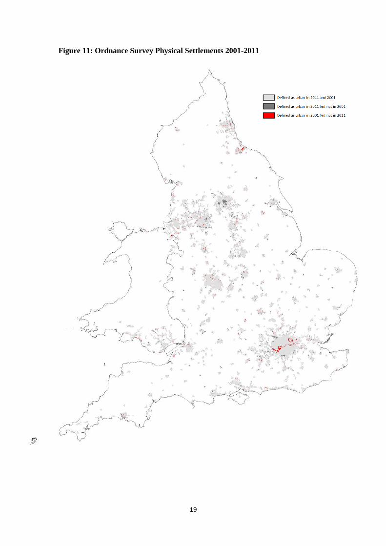
19

Figure 11: Ordnance Survey Physical Settlements 2001-2011

20

numbers of properties in a particular cell and neighbouring cells increased over the decade,

and secondly whether a particular cell fell within the generalised urban area (defined on the

basis of density profiles) in 2001 and in 2011. This forms the basis for identifying the reasons

for change in classification of Output Areas flagged on the RUC2011 assignment.

4.22 On the basis of underlying settlement classification together with the Ordnance Survey

settlement boundaries it is possible to provide indicative densities at each scale for the

various morphological types settlement types, and to show how they changed over the decade

as shown in Table 2. This shows the typical density of SCUOs at each of the key scales and

represents the numerical outcome of applying the procedures to all hectare cells for England

and Wales. It should be stressed that some of the categories shown are not based on the

density profile rules (urban areas, isolated farmsteads, hamlets and scattered dwellings (this

last being a residual class)). Differences over time reflect a complex combination of effects,

but intensification of urban areas over the decade is clear.

Table 2 Mean Densities at Key Scales for Settlements of Different Morphological Type

Settlement Form Density of SCUOs (mean)

2001 At 200m At 400m At 800m At 1600m

Town 8.23 8.99 8.29 5.59

Fringe (urban, town) 6.46 7.21 5.90 4.68

Village 3.81 2.28 0.83 0.58

Peri-urban 0.30 0.59 1.57 2.80

Village envelope 0.94 1.15 1.31 0.59

Village envelope (in peri-urban) 2.96 3.27 1.81 2.13

Hamlet 0.65 0.21 0.13 0.20

Scattered dwellings 0.39 0.17 0.15 0.23

Urban Areas (above 10k) 16.09 15.17 13.78 11.89

2011

Town 8.16 9.13 8.53 6.34

Fringe (urban, town) 5.90 7.10 6.09 4.68

Village 3.68 2.18 0.79 0.46

Peri-urban 0.36 0.68 1.61 2.80

Village envelope 0.83 1.37 1.57 0.68

Village envelope (in peri-urban) 6.16 2.97 1.67 1.85

Hamlet 0.93 0.29 0.18 0.24

Scattered dwellings 0.47 0.22 0.20 0.26

Urban Areas (above 10k) 16.32 15.38 13.93 11.99

21

5. Implementing RUC: Adding Context

5.1 The second dimension of the Rural Urban Classification for small area geographies is

‘context’. This refers to the broader setting in which settlements (including isolated dwellings)

are located. In this sense, context may be interpreted in general terms as the wider

accessibility of a settlement, the sparsity of population within a broad area and, in a general

way, the potential costs of overcoming distance to supply that settlement with various public

and private services.

5.2 The density of dwellings (SCUOs) at much broader scales forms the basis for characterising

aspects of accessibility and population sparsity. RUC2001 and RUC2011 both achieved this

by calculating for each 1ha cell the density of dwellings across areas with radii of 10kms,

20kms and 30kms centred on that cell. Use of the 10km scale was intended to reflect typical

commuting distances, while the broader scales, were intended to be pertinent to the delivery

of ‘high level’ services to rural areas. Maps for the 10km and 30km scales are shown in

Figure 12. The relation between the extent of sparsity at the three different scales, and the

numbers of dwellings associated with sparsity at each scale is summarised in Table 3.

RUC2011 followed RUC2001 in identifying as ‘sparse’ those hectare cells which appear

most sparse at all three scales (see Figure 13).

Table 3 Extent of Sparsity at Different Geographic Scales

Characteristic Area Dwellings Figure 13 Assignment

sq kms 000s

Not Sparse at any scale 87,089 22,234 ..

Sparse at 10km only 16,554 447 ‘Sparse' at 10km scale

Sparse at 20km only 1,740 101 ‘Sparse' at 20km scale

Sparse at 30km only 2,558 244 ‘Sparse' at 30km scale

Sparse at 10km and 20km 6,640 172 ‘Sparse' at 20km scale

Sparse at 20km and 30km 3,638 390 ‘Sparse' at 20km and 30km scales

Sparse at 10km and 30km 1,835 32 ‘Sparse' at 30km scale

Sparse at all three scales 34,099 562 ‘Sparse' at 10km, 20km and 30km scales

5.3 The overall inertia in the settlement pattern- that is the relatively limited addition to the

dwelling stock that typically occurs in a single decade- implies very substantial stability in

sparsity measures between 2001 and 2011.

22

6. The Classification of Statistical Units

6.1 Having classified individual cells, the next step within RUC is to categorise the settlement

characteristics of statistical units. This is intended to facilitate the use of a range of statistical

data, particularly those from the decennial population census. The smallest of the units

classified are Census Output Areas. At a broader scale, two levels of Super Output Areas and

wards are also classified. Classification depends on identifying the proportion of OAs in each

urban/rural class within the area concerned.

(a) Census Output Areas: Morphological Classes

6.2 At Census Output Area level, within RUC2011 units are assigned to one of six morphological

types on the basis of their predominant settlement component:

Urban

Major conurbation

Lesser conurbation

City and town

Rural

Town and fringe

Village, and

Dispersed (hamlets and isolated dwellings).

6.3 Output Areas are treated as ‘urban’ or ‘rural’ simply on the basis of their geographic

relationship to settlements of 10,000 or more population. More specifically, the principle

deployed derives from the 2001 Review and is that where the majority of the population of an

Output Area lives within settlements with a population of more than 10,000 people, that

Output Area is treated as urban. All other Output Areas are treated as rural.

6.4 For the purposes of RUC2001, assignment of OAs to the urban domain rested on an

allocation of individual dwellings to urban areas by ONS. Where the majority of an OA’s

population fell within an urban settlement boundary provided by OS whose associated

population was above the 10,000 threshold, the OA was treated as urban. For RUC2011,

assignment of population to built-up areas depended on the use of population-weighted

centroids for OAs estimated by ONS; those OAs whose centroids fell within a built-up area

with an associated population above the 10,000 threshold were treated as urban.

6.5 Outside the urban domain, the guiding principle in RUC is that an OA should be assigned to

the morphological class most typical of the hectare cells within it. Given the small numbers

of dwellings in individual Output Areas and the degree of mixing of morphological types

within Output Areas within the rural domain, settlement types may be broadly balanced.

Moreover, there are some conceptual difficulties in identifying typicality in a satisfactory

23

way. On one hand, it might seem consistent with the overall approach to assign an OA to that

morphological class which accommodates the majority of its dwellings. On the other, such

an approach would not fully capture significant and deeply-rooted distinctions between areas

of nucleated and dispersed settlement charted for example in English Heritage’s Settlement

Atlas (Roberts and Wrathmell 2000; Lowerre 2011) and which remain important within

physical planning (Owen and Herlin 2009). Because dwelling densities (at say the 200m

scale) in dispersed settlement are only around one eighth of those in villages, assignment by

reference to dwellings alone obscures the physical significance of dispersed settlement. RUC,

therefore, considers both numbers of dwellings in settlements of different form and the

footprint of those settlements.

6.6 Within RUC2001 assignment was made by area, but where components were equally

balanced a principle of ‘hierarchical privileging’ was used to assign an OA to the higher

order class (eg village rather than dispersed). (The design of OAs with its strong tendency to

population equalization is such that those which impinge on rural ‘towns’ tend to be

geographically small and homogenous with respect to settlement type). In preparing

RUC2011, the sensitivity of the area-based assignment procedure to recently built scattered

dwellings became clear. To offset this, assignment in RUC2011 was based on the weighted

mix of hectare cells given over to different settlement types; cells assigned to the village or

town category being assigned a weight of four, with those assigned to the dispersed

categories assigned a weight of one. This procedure substantially reduced the number of OAs

at risk of shifting from the village to dispersed categories. Nevertheless, the question of the

most appropriate manner of combining information about dwelling stocks and residential

footprint in gauging rural settlement structure remains a matter for further investigation.

(b) Census Output Areas: Sparsity

6.7 On the basis of the three sparsity measures (10kms, 20kms, 30kms) calculated at cell level, it

is possible to identify cells where population is ‘sparse’ at a particular scale. By calculating

these three measures for each cell in a 2011 Census Output Area, weighted averages for each

OA can be found. (The weights used are the number of SCUOs in a cell). By focusing on the

sparsest 5 percent for each measure, three indicators of ‘sparsity’ are obtained for each OA.

Output Areas are classified as ‘sparse’ if they fall within the sparsest 5 percent of Output

Areas at all three scales, and are classified as ‘less sparse’ if they do not fall within this

threshold. The fifth percentile ‘cut-offs’ used in applying this rule to 2011 data are shown in

Table 4 with 2001 values included for comparison.

6.8 Overall with the development of new residential property in the inter-censal decade the value

of the fifth percentiles in 2011 are higher than those for 2001. In identifying sparse OAs,

however, reference has been made to the fifth percentile consistently (ie the relative measure

rather than the absolute measure).

24

Figure 12: Dwelling Densities Calculated at 10km and 30km;2011

a) 10km b) 30km

Dwellings per hectare

25

Figure 13: Hectare Cells Sparse at all Three Scales (10km, 20km and 30km);2011

‘sparse’ at 10km scale ‘sparse’ at 20km scale ‘sparse’ at 30km scale ‘sparse’ at 20km and 30km scales ‘sparse’ at 10km, 20km and 30km scales

26

Table 4: Fifth Percentile Measures for Defining ‘Sparsity’

Category Fifth Percentile 2001

SCUOs per ha

Fifth Percentile 2011

SCUOs per ha

Sparse at the 10km scale < 0.393 < 0.432

Sparse at the 20km scale < 0.410 < 0.450

Sparse at the 30km scale < 0.422 < 0.473

6.9 Finally, classifications on the ‘morphology’ and ‘context’ dimensions are combined as

indicated in the ‘tree diagram’ (Figure 4). The distribution of OAs between categories of

the typology of RUC2011 is summarised in Table 5 and mapped as Figure 14.

Table 5: Distribution of 2011 Census Output Areas between Categories; RUC2011

(c) Super Output Areas and Census Wards: Morphological classes

6.10 The design of Super Output Areas (both Lower Layer – LSOAs and Middle Layer -

MSOAs) and Wards is such that very few are characterized by predominantly dispersed

settlement. For this reason, only five morphological categories are distinguished at this

level:

Urban

Major conurbation

Minor conurbation

City and Town

Rural

Town and fringe

Village and Dispersed.

OA Class Frequency %

Urban: Major Conurbation 59,199 32.6

Urban: Minor Conurbation 6,277 3.5

Urban: City and Town 81,004 44.7

Urban: City and Town in a Sparse Setting 490 0.3

Rural: Town and Fringe 15,850 8.7

Rural: Town and Fringe in a Sparse Setting 1,044 0.6

Rural: Village 9,646 5.3

Rural: Village in a Sparse Setting 1,042 0.6

Rural: Hamlets and Isolated Dwellings 5,969 3.3

Rural: Hamlets and Isolated Dwellings in a Sparse Setting 887 0.5

27

Figure 14: England &Wales; 2011 Census Output Areas: Rural-Urban Typology

(RUC2011)

28

Figure 15: England & Wales; 2011 LSOAs: Rural-Urban Typology (RUC2011)

29

Figure 16: England & Wales; 2011 MSOAs: Rural-Urban Typology (RUC2011)

30

Figure 17: England & Wales; 2011 Wards: Rural-Urban Typology (RUC2011)

31

6.11 Higher level statistical units are assigned to one of these categories on the basis on what

might be termed the ‘OA count approach’ that is to say on the basis of the corresponding

category occurring most frequently amongst its constituent OAs. Thus:

i) a higher level unit is considered urban if the number of urban OAs it contains is greater

than or equal to the number of rural OAs,

ii) remaining higher level statistical units are then classified as being small town/fringe if the

number of small town/fringe OAs is greater than or equal to the number of village and

dispersed OAs, and then

iii) remaining higher level statistical units are classified as village and dispersed.

(d) Super Output Areas and Wards: Sparsity

6.12 Because context measures vary smoothly from one hectare cell to the next, there is little

difficulty in estimating measures for higher level statistical units that are consistent with those

measured for Output Areas. The OA count approach is used to calculate the context measure

higher level units as follows :

i) a higher level statistical unit is less sparse if the number of less sparse OAs it contains is

greater than or equal to the number of sparse OAs, and

ii) the remaining level statistical units are classified as sparse.

6.13 Finally, classifications on the ‘morphology’ and ‘context’ dimensions are combined. The

distribution of LSOAs between categories of the typology of RUC2011 is summarised in

Table 6 and that of MSOAs in Table 7. Assignments to 2011 electoral wards are made on the

basis of best fit OAs (provided by ONS (http://www.ons.gov.uk/ons/guide-

method/geography/products/census/lookup/2011/index.html). The geographic distribution of LSOA,

MSOA and ward assignments is mapped as Figures 15, 16 and 17 respectively.

Table 6: Distribution of 2011 LSOAs between Categories; RUC2011

LSOA Class Frequency %

Urban: Major Conurbation 11,523 33.16

Urban: Minor Conurbation 1,208 3.48

Urban: City and Town 15,724 45.25

Urban: City and Town in a Sparse Setting 94 0.27

Rural: Town and Fringe 3,189 9.18

Rural: Town and Fringe in a Sparse Setting 197 0.57

Rural: Village and Dispersed 2,490 7.16

Rural: Village and Dispersed in a Sparse Setting 328 0.94

32

Table 7: Distribution of 2011 MSOAs between Categories; RUC2011

MSOA Class Frequency %

Urban: Major Conurbation 2,399 33.31

Urban: Minor Conurbation 249 3.46

Urban: City and Town 3,206 44.52

Urban: City and Town in a Sparse Setting 21 0.29

Rural: Town and Fringe 645 8.96

Rural: Town and Fringe in a Sparse Setting 29 0.4

Rural: Village and Dispersed 566 7.86

Rural: Village and Dispersed in a Sparse Setting 86 1.19

7. Conclusion

7.1 The foregoing discussion demonstrates the possibility of building a typology of statistical units

based on the form and context of associated settlement. It reiterates much of the explanation of

principles provided by Bibby and Shepherd (2004) and demonstrates the robust nature of what

they describe as the ‘underlying settlement classification’.

7.2 The principles underlying the methodology of RUC lend the typology and the assignments

some important qualities. They can be used in a consistent manner to treat settlements at any

level of the hierarchy and at a range of scales from the hectare cell to MSOAs. A user-guide to

RUC2011 draws attention to some practical implications of both strengths and limitations

deriving from the underlying method.

7.3 The methodology is such that the RUC (for small area geographies) takes no explicit account

of economic function. While this might be seen as a weakness, its offsetting strength is that it

allows the economic function of the rural domain to be explained and measured rather than

presumed.

7.4 The focus on settlement type to the exclusion of other aspects of land cover implies further

strengths and weaknesses which users may find more troublesome in practice. It is particularly

important to appreciate that RUC is designed to support the use of social and economic

statistics, and the methodology of its construction implies that on its own it is badly suited to

support the administration of agro-environment schemes or to analyse their take up.

7.5 Updating RUC for use with the 2011 Census has demonstrated the robustness of an approach

based on density profiles, and demonstrated that changes in the detailed character of the postal

data used have been successfully accommodated by minor changes in method. Re-specification

of Ordnance Survey polygons representing the larger physical settlements, however, carries

serious implications for the interpretation of shifts between the urban and rural divisions of the

typology between 2001 and 2011. Although this implies that such changes in OA assignment

cannot be used directly to track physical development, it has proved quite feasible to rely on

33

other elements of the method (including identification of the generalised urban area) to

distinguish changes arising from difference in protocols from those attributable to underlying

physical change.

References

Bibby, P R, Shepherd, JW, 2004, ‘Developing a New Classification of Urban and Rural Areas

for Policy Purposes – the Methodology’ Available at:

https://www.gov.uk/government/uploads/system/uploads/attachment_data/file/137655/rural-

urban-definition-methodology-technical.pdf Last Accessed: 5th

July 2013

Defra, 2005/2009 ‘Defra Classification of Local Authority Districts and Unitary Authorities in

England: An Introductory Guide’ Available at:

https://www.gov.uk/government/uploads/system/uploads/attachment_data/file/137661/la-class-

updated-technical.pdf Last Accessed: 21st August 2013

DCLG, 2006, ‘Urban and Rural Area Definitions: a User Guide’, London, Department of

Communities and Local Government. Available at

https://www.gov.uk/government/uploads/system/uploads/attachment_data/file/142430/urbanrur

al-user-guide.pdf Last Accessed: 5th

July 2013

Freeman, T.W, 1966, Conurbations of Great Britain, 2nd edition, Manchester, Manchester

University Press

Lowerre A, 2001, ‘The Atlas of Settlement in England GIS’. English Heritage Research News

16, 32-35

Ordnance Survey, 2012, Built-up Areas Core Specification v2.0, unpublished

Owen,S; Herlin, I S; 2009, ‘A Sustainable Development Framework for a Landscape of

Dispersed Historic Settlement’, Landscape Research,34, 33-54

Roberts, B. K, 1996 , Landscapes of Settlement: Prehistory to the Present, New York:

Routledge

Roberts, B. K., and Wrathmell, S, 2000, An Atlas of Rural Settlement in England, London

English Heritage

34

Annex 1: Rules for Identifying Settlement Morphology.

The settlement morphology element of RUC is derived from the classification of 1ha grid

squares according to a set of rules. Many slightly different rule-sets pick out the same features,

and a complete illustrative set is provided here.

The rules in this set and similar sets result from empirically adjusted elaborations of principles

based on idealised settlement forms (concerned with typical plot densities, neighbourhood

densities areal extents and rates of change). The discussion of the idealized village in paras 4.8-

4.10 of this document provides an example of the type of elementary thought experiment with

which they originate. Once a 'proto-rule' is articulated comparison with settlement features

held a hectare grid allow divergences to be observed and additional rules elaborated. These

settlement features include for example OS urban areas from 1981, 1991 and 2001 and groups

of cells away from urban settlements whose individual residential addresses include the same

locality).

The illustrative hectare cell classification rules are applied to all cells in the order given below.

For any hectare cell, a rule appearing later in the series is not tested if one appearing earlier in

the series is satisfied. Different rules identifying the same class of settlement ‘fringe’ may

have different parameters, but will identify the same settlement type.

Densities are calculated over a series of radii. The density over a 1600m radius around a cell is

referred to as the D1600 measure for that cell. The terms ‘D800’, ‘D400’, and ‘D200’ are

defined in a similar manner.

Rule 1:

If

D800 > 8

a cell is deemed to form part of the generalised urban area. This category does not appear in

the final assignment. Nearly all cells assigned to this class are expected to be re-assigned to the

urban category on the basis of OS boundaries.

Rule 2:

If

D400 > 8 and

D800 < 4

a cell is deemed to form part of a fringe.

35

Rule 3:

If

D800 > 2.5 and

D800 > 2.5*D1600,

a cell is deemed to form part of a town.

Rule 4:

If

D800 > 4 and

D400 > 4 and

D800 < 8,

a cell square is deemed to form part of a fringe.

Rule 5:

If

D800 < 8 and

D400 > 8,

a cell is deemed to form part of a town.

Rule 6:

If

D800 > 0.18 and

D400 > 2*D800 and

D200 > 1.5*D800,

a cell is deemed to form part of a village.

36

Rule 7:

If

D1600 > 1.0 and

D400 > 1.5*D800 and

D400 < 2*D800 and

D200 > 0,

a cell is deemed to form part of a village envelope (in peri-urban).

Rule 8:

If

D1600 > 1.0,

a cell is deemed to form part of a peri-urban zone.

Rule 9:

If

D1600 =< 1.0 and

D800 >= 0.5,

a cell is deemed to form part of a village envelope.