AUNATIONAL ENVIRONMENTAL RESEARCH INSTITUTEAARHUS UNIVERSITY

PhD Thesis, 2010 Ngo Tho Hung

URbAN AIR QUALITY MODELLINg AND MANAgEMENT IN HANOI, VIETNAM

[Blank page]

AU

URBAN AIR QUALITY MODELLING AND MANAGEMENT IN HANOI, VIETNAMPhD Thesis 2010

Ngo Tho Hung

NATIONAL ENVIRONMENTAL RESEARCH INSTITUTEAARHUS UNIVERSITY

Data sheet

Title: Urban air quality modelling and management in Hanoi, Vietnam Subtitle: PhD Thesis

Author: Ngo Tho Hung Department(s): Aarhus University, National Environmental Research Institute, Department of Atmospheric

Environment. University: The PhD was matriculated at the Roskilde University (RUC), Graduate School of Environmental

Stress Studies (GESS) Publisher: National Environmental Research Institute ©

Aarhus University, Denmark URL: http://www.neri.dk

Year of publication: 2010 Editing completed: June 2010 Referee(s): Steen Solvang Jensen, Matthias Ketzel, Helge Rørdam Olesen.

Financial support: Project 322 - VOSP Vietnam, DANIDA.

Please cite as: Ngo Tho Hung, 2010: Urban air quality modelling and management in Hanoi, Vietnam. PhD Thesis, Aarhus University, National Environmental Research Institute, Denmark. 211 pp

Reproduction permitted provided the source is explicitly acknowledged

Abstract: A systematic evaluation of dispersion models as a tool for air quality assessment and manage-ment in a Vietnamese context was conducted with focus on technical as well as management aspects. The research studied the application of dispersion models in line with the Integrated Monitoring and Assessment (IMA) concept. The research mainly focused on the application and evaluation of Operational Street Pollution Model (OSPM) and Operational Meteorological Air Quality Model (OML) which are operational and applicable dispersion models for assessment of street and urban background air quality. An evaluation of model calculations against available measurements was carried out. This study contributed to a systematic evaluation of air pollution conditions in Hanoi and identified factors that influence air quality.

Keywords: Air quality, Dispersion model, OSPM model, OML model, model evaluation, Integrated Monitor-ing and Assessment, Hanoi, Vietnam.

Layout of front page: Britta Munter ISBN: 978-87-7073-183-6

Number of pages: 211

Internet version: The report is available in electronic format (pdf) at NERI's website http://www.dmu.dk/pub/phd_nth.pdf

Contents

Preface 7

Acknowledgement 8

9

10

1212

1518

1819

19

2020

2122

232.1.6 Integrated Monitoring and Assessment of air pollution 28

291

31

3132

32

3636

373940

4245

50

51

5253

5353

Abstract

List of abbreviations

1 INTRODUCTION 1.1 Motivation 1.2 Related studies in Vietnam 1.3 Aims 1.4 Research questions 1.5 Applications of the research 1.6 Demarcation,

2 CONCEPTUAL FRAMEWORKS AND METHODOLOGY DESIGN 2.1 Conceptual frameworks

2.1.1 Air pollution 20 2.1.2 Meteorology of air pollution 20 2.1.3 Classification of air pollution sources 2.1.4 Dispersion modelling of Air pollution 2.1.5 Urban Air Quality Management

2.1.7 DPSIR framework 2.2 Methodology design 3

2.2.1 DPSIR analysis of UAQM in Vietnam 2.2.2 Approach for the Application of Dispersion models in Urban Air Quality

Assessment 2.2.3 Capacity building on Technology transfer within UAQM 2.2.4 Introduction to the case study 2.2.5 Outline Hanoi case study 33

3 AIR QUALITY ASSESSMENT AND MANAGEMENT – CASE STUDY IN HANOI 3.1 DPSIR framework design for a case study of Hanoi 3.2 Driving forces of air pollution in Hanoi 3.3 Pressure of air pollution in Hanoi 3.4 State of air environment in Hanoi 3.5 Impacts of air pollution in Hanoi 3.6 Response to air pollution in Hanoi 3.7 Summary 49

4 SELECTION OF DISPERSON MODELS 4.1 Selection of air quality models 50 4.2 Introduction to Danish air quality assessment

4.2.1 Air Quality Monitoring Program 51 4.2.2 Urban air quality modelling systems by Dispersion models 4.2.3 Danish legislative system for UAQM

4.3 Operational Street Pollution Model (OSPM) as Street Scale model 4.3.1 Structure of OSPM

4.3.2 Traffic produced turbulence 5757

5859

606061

6363

6465

666667

68697071

7172

7979

8183

8486

8889

9090

9395

97

100100

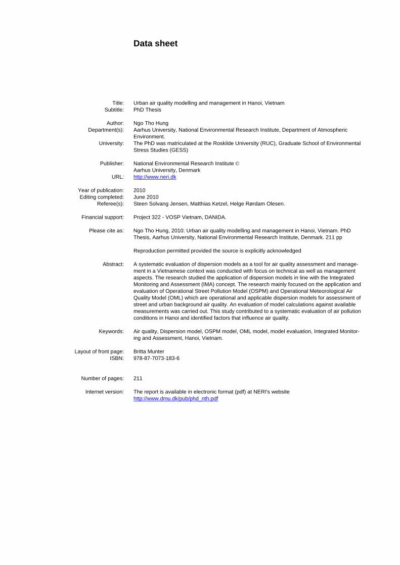
106108

115115

116117

120120

1233

124129

131135

135137

4.3.3 NO2 chemistry 4.3.4 Input and output data 4.3.5 OSPM applications

4.4 Operational Meteorological Air Quality Models (OML) as a local scale model

4.4.1 Structure of OML 4.4.2 OML applications

5 APPLICATION OF THE OPERATIONAL STREET POLLUTION MODEL (OSPM) IN HANOI 5.1 Introduction 5.2 Air quality modelling at street level in Hanoi, Vietnam using the OSPM 5.3 Locations of measurements 5.4 Street configurations

5.4.1 TruongChinh Street 5.4.2 DienBienPhu Street 5.4.3 NguyenTrai Street 5.4.4 LeTrongTan Street 5.4.5 ToVinhDien Street

5.5 Traffic and emission data 5.5.1 Vehicle classification 5.5.2 Diurnal traffic variation 5.5.3 Vehicle distribution 5.5.4 Average daily traffic 5.5.5 Emission data

5.6 Meteorology data 5.6.1 Wind speed 5.6.2 Wind direction 5.6.3 Temperature 5.6.4 Global radiation 5.6.5 Summary

5.7 Urban background measurements 5.7.1 Measurement campaign using passive sampling techniques 91 5.7.2 Hourly data at Lang Station 5.7.3 Analysis and adjustment

5.8 Street measurements 5.9 Correlation between CO and BNZ 99 5.10 Comparison of measured and model results

5.10.1 The Year of 2004: TC Street, DBS Street and NT Street: 5.10.2 The Year of 2007: LTT Street, TVD Street:

5.11 Results and discussions 5.12 Summary 114

6 EVALUATION OF OPERATIONAL METEOROLOGYCAL AIR QUALITY MODEL (OML) IN HANOI 6.1 Introduction 6.2 Emission data from a pilot area of ThanhXuan district

6.2.1 Point sources 6.2.2 Line sources 6.2.3 Area sources

6.3 Estimation of emissions for the OML modelling in Hanoi. 6.3.1 Introduction 12 6.3.2 Emissions from traffic 6.3.3 Emissions from Industries 6.3.4 Emissions from domestic

6.4 OML Meteorological Preprocessor 6.4.1 Hourly surface based meteorological data 6.4.2 Radiosonde data

6.4.3 Topographical data 138138

141141143

143143

147154

1599

159160

161163

163

167167

167169

170171

172172

175

182

207

208

210

6.5 Regional air pollution background data 6.6 Urban background measurements

6.6.1 Campaign using passive sampling 6.6.2 Hourly data from the Lang Station

6.7 Evaluation of model results against observations 6.7.1 Dry season and wet season in 2007 6.7.2 Evaluation of model results for the Lang station in 2007 6.7.3 Spatial variation annual city in 2007

6.8 Summary 157

7 DPSIR analysis of application of dispersion models in Hanoi 7.1 Approach 15 7.2 Driving forces in relation to dispersion modelling 7.3 Pressure in relation dispersion model 7.4 State in relation with dispersion model tasks 7.5 Impacts in relation to dispersion models 7.6 Responses in relation to dispersion models 7.7 Summary 165

8 CONCLUSIONS 8.1 Summary of the research 8.2 Answers to research questions 8.3 Contributions of the research

8.3.1 Contributions from OSPM modelling 8.3.2 Contributions from OML modelling 8.3.3 Contributions from Integrated Monitoring and Assessment analysis

8.4 Recommendations

Reference List

Appendix 1: Science paper – Journal of Air & Waste Management Association – A&WMA, USA

Appendix 2: Presentation on the Seventeenth International Conference on Modelling, Monitoring and Management of Air Pollution, July 2009 – WIT, UK.

Appendix 3: Presentation on the Better Air Quality conference in Asia (BAQ2010), November, 2010, Singapore

Appendix 4: Science paper on dissemination the research results in Vietnam, November, 2009 (in Vietnamese)

Preface

This dissertation is submitted to Roskilde University as part of a PhD degree in Environmental Science.

The research is carried out studying air pollution assessment and management of urban areas of Hanoi, Vietnam and how air quality is affected by climatic, meteorological, topographical and geographical conditions. The study investigates ways to apply dispersion models as a tool for air quality assessment and management in Vietnam. This research will potentially contribute to Vietnam in protecting the air quality in urban areas. It could also contribute to the technology transfers and international cooperation between developed and developing countries for environmental protection and sustainable development.

This study will allow me to return to Vietnam with the capacity and confidence to further build and enrich air quality assessment and management. On my return, I will be able to offer colleagues and students in Vietnam advice and support in air pollution modelling and urban environment management and development and I will be able to assist the Vietnamese government and other organizations to develop strong and successful policies and programs in this area.

This PhD dissertation is dedicated to my parents.

7

Acknowledgement

This PhD project is funded by the Vietnamese government (project 322) together with supplemental supports from the Danish International Development Agency (DANIDA) and the National Environmental Research Institute (NERI), Denmark.

The author would like to express profound thanks to his advisor, Prof. Henning Schroll (RUC) and his co-advisor Dr. Steen Solvang Jensen (NERI - ATMI) as well as to Dr. Matthias Ketzel and Dr. Olesen Helge Rørdam (NERI - ATMI) for key supports. They have provided whole hearted supports, guidance and advices throughout this research. Their constant encouragements, enthusiasm and intellectual supports have been a great help.

Thanks and highest appreciations are extended to A.Prof/Dr. Nguyen Thi Kim Oanh (SERD – AIT, Thailand) for her valuable suggestions, comments, and encouragements in solving problems related to input data from Hanoi, Vietnam.

The author would like to thank: Dr. Ruwim Berkowicz (NERI) and Professors at Department of Environmental Engineering, National University of Civil Engineering, Vietnam for supports in the initial phase of the project; Mr. Martin Hvidberg (NERI) and Mr. Thomas Becker (NERI) for their support on building up a GIS data set for Hanoi; Dr. Ole Hertel as a mentor at NERI for his encouragements on my work.

The author would like to thank: Mr. Michael Rudolf Baechlin, Mr. Do Quang Trung at the Swiss Vietnamese Clean Air Program (SVCAP), Dr. M. Hangartner, PASSAM (Switzerland), colleagues at Institute of Meteorology, Hydrology and Environment (IMHEN), Mr. Duong Hoang Long at the Hydro Meteorological and Environmental Station Network Center (Hanoi, Vietnam), Ms. Vo Thi Quynh Truc (AIT, Thailand) for their valuable contributions to the data collection for this study. Thanks are also sent to Dr. Hoang Duong Tung (CEMDI, Vietnam), Mr. Nguyen Minh Tan (CENMA, Hanoi), Prof/Dr. Hoang Xuan Co (HUS, Vietnam) and many other colleagues from Vietnam for their assistance in the field trip activities.

Last but not least, my sincerely gratitude is to all of my family. I would like to thank them for their love, care and encouragements. All friends who have given support deserve my sincerest thanks, especially my colleague, Ms. Quynh Nguyen, who encouraged me during the finalisation of this PhD study.

8

Abstract

A systematic evaluation of dispersion models as a tool for air quality assessment and management in a Vietnamese context was conducted with focus on technical as well as management aspects. The research studied the application of dispersion models in line with the Integrated Monitoring and Assessment (IMA) concept. The research mainly focused on the application and evaluation of Operational Street Pollution Model (OSPM) and Operational Meteorological Air Quality Model (OML) which are operational and applicable dispersion models for assessment of street and urban background air quality. An evaluation of model calculations against available measurements was carried out. This study contributed to a systematic evaluation of air pollution conditions in Hanoi and identified factors that influence air quality.

9

List of abbreviations

ADB Asian Development Bank ADT Average Daily Traffic AIRPET Improving Air Quality in Asian Developing Countries

Project – Asian Institute of Technology AIT Asian Institute of Technology, Thailand ATMI Department of Atmospheric Environment, National

Environmental Research Institute, Denmark. BNZ Benzene CAI ASIA Clean Air Initiative - ASIA CEETIA Centre for Environment Engineering of Towns and

Industrial Areas CENMA Hanoi Centre for Environmental and Natural

Resources Monitoring and Analysis (Hanoi city council)

CEMDI Centre of Monitoring and Environmental Data (VEPA) CIDA Canadian International Development Agency CO Carbon Monoxide CO2 Carbon Dioxide DANIDA Danish International Development Agency DONREH Department of Natural Resources, Environment and Housing EMBARQ: The global network catalyzes environmentally and

financially sustainable transport solutions to improve quality of life in cities.

GDP Gross Domestic Product GIS Geographic Information System IMA Integrated Monitoring and Assessment HCMC HoChiMinh city HEPA HoChiMinh City Environmental Protection Agency HUS Hanoi University of Science JICA Japan International Cooperation Agency LFA Logical Framework Approach MONRE Ministry of Natural Resource and Environment N/A Not available NAP National Action Plan NERI National Environmental Research Institute, Denmark. NORAD Norwegian Agency for Development Cooperation NO2 Nitrogen Dioxide NOx Nitrogen Oxides

10

OSPM Operational Street Pollution Model OML Operational Meteorological Air Quality Model PM Particle Matter RUC Roskilde University, Denmark SDC Swiss Agency for Development and Cooperation SIDA Swedish International Development Agency SERD–AIT School of Environment, Resources and Development,

Asian Institute of Technology, Thailand SO2 Sulphur Dioxide SVCAP Swiss Vietnamese Clean Air Program TCVN Vietnam National Standards TSP Total Suspended Particulate UAQM Urban Air Quality Management System US-AEP US-Asia Environmental Program VEPA Vietnam Environmental Protection Agency VOC Volatile Organic Compounds VR Vietnam Register WB World Bank WHO World Health Organization WRI World Resources Institute

11

1 INTRODUCTION

In this chapter, the aims and motivations for the research are defined. The tasks of this study are also related to other relevant studies in a Vietnamese context. How the research can contribute to potential implementations of dispersion models for air quality assessment and management in urban areas in a developing country is also discussed.

1.1 Motivation

Urbanization is an unavoidable process in the world. According to the United Nation (UN), more than 90% of urbanization is taking place in the developing world (UN-Habitat, 2006). The urban populations in the developing countries will reach 2 billion in the next 20 years, increasing about 70 million per year. The populations in the urban areas of Africa and Asia will be double at that time. By 2030, 80% of the total world’s urban population will be living in developing countries. Vietnam is also rapidly urbanized. It is estimated that 57% of the population will be living in the cities in 2050 compared to 20% in 1990 (Figure 1.1). This will put more pressure on the air environment (World Bank, 2009b).

Figure 1.1. Urbanization in Vietnam from 1990-2005, forecast up to 2050 Source: United Nation (VCAP and CAI-Asia, 2008)

Vietnam is undergoing a rapid process of industrialization and modernization process (World Bank, 2009a). Currently, there is a critical need for environmental specialists with qualified professional knowledge who can be responsible for improving the environmental conditions, especially in urban and industrial areas. In most urban centres, there are many environmental problems and the air pollution problems in particularly are also accelerating.

12

The environment is seriously polluted and this has significant public health impacts. A solution to minimize the effect of air pollution is, hence, pressing. However, the questions are which appropriate air pollution models should be selected? And there have been many diverse proposals but none has been proved to be the most optimal (Sivertsen and The, 2006; ADB and CAI-Asia, 2006).

According to previous studies, most urban air pollution originates from traffic, industries and domestic cooking. Vehicles, in particular motorbikes, are the important sources of air pollution in cities in Vietnam. Vehicles discharge PM (particulate matter), NOX, CO, SO2, VOC (volatile organic compounds) e.g. Benzene (BNZ) to the urban air environments (Dang, 2005). It is estimated that 70% of air pollution in the cities come from vehicles (Hoang, 2004). The number of vehicles in Vietnam is increasing rapidly, especially for motorbikes. Motorbikes increased more than 400% from 1996 to 2006. Passenger cars are also increasing in recent years in Hanoi and HoChiMinh city (see more in Figure 3.3) (VCAP and CAI-Asia, 2008). In larger cities, re-suspended dust from construction activities also presents an air pollution problem as visibility is reduced. According to the Department of Natural Resources, Environment and Housing in Hanoi (DONREH) 70% of Total Suspended Particulate (TSP) comes from construction activities (MONRE, 2008).

As other Asian megacities, Hanoi is polluted by PM10 (particles less than 10 micron), TSP, SO2, NOx, CO, BNZ etc. Poor air quality impacts human health in the cities. Air pollution increases mortality and morbidity. Air pollution causes, induces or aggravate health effects such as cardiovascular diseases, lung cancer, asthma, bronchitis, respiratory illness, and allergy. There are studies of health impacts due to air pollution in Vietnam. The Labour Health and Environmental Hygiene Institute has estimated the annual losses caused by air pollution as high as 20 millions USD for Hanoi and 50 millions USD for HoChiMinh city. They also accounted for 626 deaths and 1,500 incidences of respiratory infection caused by urban air pollution in Vietnam. Dust also reduces the photosynthesis of vegetation (VCAP and CAI-Asia, 2008).

In Vietnam, only limited monitoring of air quality is conducted in few locations. In the two largest cities (HoChiMinh City and Hanoi), some air quality models have been applied in some specific cases but they have not been validated against monitored air quality data. A monitoring network should ideally provide air pollution data of high temporal solution and high accuracy. Monitoring data is useful to follow trends and assess compliance with air quality standards. Analysis of data can also provide insight into the sources of air pollution. However, the establishment and operation of monitor stations are expensive and

13

can only be expected to be established in few locations. Therefore, modelling is a powerful tool because it can estimate the pollution level at any locations (ADB and CAI-Asia, 2006).

Air pollution modelling has proved successful as a management technique. Air quality models attempt to simulate the physical and chemical processes in the atmosphere that may involve transport, dispersion, deposition and chemical reactions that occur in the atmosphere to estimate pollutant concentrations at a downwind receptor location. Fundamentally different models have been developed in the way they parameterize the physical and chemical processes. They have been developed for different scales from transboundary air pollution, to urban background and street scale, and for different sources: traffic or industrial sources (Fenger, 1999; Vardoulakis et al., 2003).

In developed countries a strategy that combines monitoring and modelling so-called “integrated monitoring” (Hertel et al., 2007; Hertel, 2009) can provide a good understanding of information about air pollution conditions in a cost-effective way. My research uses this concept to do a research on air pollution assessment and management in the urban areas in the context of Hanoi, Vietnam. The impacts of climatic, meteorological, topographical and geographical conditions are also considered. This study also investigates ways to ensure successful implementation of air quality assessment and management by air quality models. The research provides a potential tool of assessment and management of air quality for Vietnam in protecting the urban areas from air pollutions.

The research mainly focuses on dispersion models that are operational and applicable in the urban background to street scale as there is a particular need to improve capacities in this area. Air quality models can be used to map concentrations where there are no measurements. The combination of monitoring and modelling (integrated monitoring and assessment) can be useful for a spatial description of air quality. Since models establish a link between emissions and concentrations they can be used to analyze the pollution contributed from different source (e.g. traffic sources emitting at ground level versus sources emitting at elevated level as industrial chimneys). Being a potential tool in air quality assessment and management, air quality modelling requires a lot of input data on meteorology, emissions, topology etc. which is difficult to fulfil in Vietnam. Models can be used for backcast, nowcast and forecast, and air quality models may also be used to evaluate different control options in scenario analysis.

14

1.2 Related studies in Vietnam

This research will make use and establish contacts to other ongoing activities in Vietnam (see Figure 1.2). At present, Vietnam is attending the Network of Clean Air Initiative for Asian Cities (CAI-Asia) (CAI ASIA, 2010). CAI-Asia is a multi-stakeholder initiative set up by Asian Development Bank, World Bank and United States-Asia Environmental Partnership (US-AEP) to promote better air quality management in Asia. The ultimate success of CAI-Asia will be determined by the success of its local networks. CAI-Asia undertakes knowledge management, capacity building, and regional dialogues and promotes air quality management policies, pilot programs and workshops. Air quality models were also applied in selected locations in the network countries (Huizenga, 2006).

CAI-Asia has been helping Vietnam to achieve better understanding of air pollution and air quality management (ADB and CAI-Asia, 2006). In Vietnam, Vietnam Register (VR) (VR Vietnam, 2010) is an organization that provides technical supervisions and certifications for quality and safety on means of transports including motorbike. VR services are for the promotion of safety of life, property and protection of the environment from pollution. VR, for its part, has acknowledged the CAI-Asia's direct or indirect influence in the following activities: Integrated Action Plan for Reduction of Vehicle Emissions (NAP-VE) (driver manual: Section of environmental issues), developing a platform for achieving European standards in new vehicles and fuels to improve air quality in Vietnam (US-AEP), clean motorcycle pilot project (Swiss contact), vehicle emission inventory and measures focusing on motorcycles, buses, and trucks (World Bank) (SVCAP, 2005).

Danish International Development Agency (DANIDA) has also supported a project on Environmental Information and Reporting (2003 - 2006). The aim of the project was to achieve environmental information and reporting system in Vietnam to support environmental management and policy. Therefore, decisions are based on the best possible knowledge. As the results of the project, the information management system was improved on three subjects: marine coastal pollution, air pollution and water pollution (DANIDA, 2002).

Swiss Vietnamese Clean Air Program (SVCAP) is a project funded by the Swiss Agency for Development and Cooperation (SDC) through Swiss Contact. The overall goal of SVCAP is to contribute to the prevention of a possible further degradation of the air quality in Hanoi. The first phase (2004 –2007) is to support the conditions for the reduction of air pollution by means of the definition and implementation of an integrated air quality management system on Hanoi. Previous activities related to air

15

quality management in Vietnam listed by SVACP is shown in the Figure 1.2.

For this modelling study, data were collected from databases of other projects: Hanoi Urban Transport project 2006 (World Bank), Swiss-Vietnamese Clean Air Program 2007 (SVCAP), US-AEP 2005 and others. The emission inventory conducted by SVCAP in a pilot area (ThanhXuan district) is used to extrapolate the emission data for the whole city (Hanoi). The information of traffic including emission factors, vehicle distributions was collected from Hanoi Urban Transport project 2006 (World Bank), Assessment of VOC levels from motor vehicle exhaust and potential health effects in Hanoi, Vietnam (AIT project), monitoring vehicle air pollution in Hanoi by mobile station for air quality monitoring US-AEP Project (CENMA and SVCAP, 2008; Sivertsen and The, 2006; Truc, 2005; Dang, 2005). Other supplement data and information was also consulted such as improving air quality in Vietnam - AIRPET (SIDA/AIT project) (Hoang, 2008), Environmental Information and Reporting (DANIDA, 2002).

16

Figure 1.2. Previous international funded projects related to air quality management in Vietnam. Source (CENMA and SVCAP, 2008)

In Hanoi, the Swiss Vietnamese Clean Air Program (SVCAP) and Hanoi Centre for Environmental and Natural Resources Monitoring and Analysis (CENMA) put a significant contribution into air quality management including a pilot emission inventory (CENMA and SVCAP, 2008). The pilot emission inventory was conducted in ThanhXuan district and it will be used as input data for this air quality modelling study.

17

In addition, air quality models should also be used as an approach to facilitate small and local urban areas to ensure a more effective air pollution management in Vietnam. Air pollution modelling needs to have emission data (emission inventory) together with other parameters such as meteorological and topographical.

Thus, this PhD study will further contribute to an integrated analysis on how air quality modelling can work in a Vietnamese context with the current input data. It also emphasizes the needs to promote the quality control of input data for air pollution modelling in Vietnam.

1.3 Aims

The aims of the PhD study are to

• conduct a systematic analysis on the conditions that are necessary for a potential implementation of air quality models as an assessment and management technique in the context of urban air pollution in Vietnam.

• understand and determine how and why local climatology, meteorology, emission, topographical, and geographical conditions influence air pollution problems in urban areas in Vietnam, and evaluate the application of dispersion models for potential implementation in air quality assessment and management.

1.4 Research questions

The key research question is how to apply the air quality dispersion models as an assessment and management technique in the context of urban air pollution in Vietnam using Hanoi as a case study.

The study will look into the following detailed questions:

1. What are the most important factors influencing air quality in the urban areas? And how does this affect the choice of appropriate air quality models?

2. What are the most important technical factors and institutional factors for successful adaptation and application of air quality models in a Vietnamese context?

18

1.5 Applications of the research

Environmental management in general and the management of air quality in particular are new in Vietnam, while the human resources available in this field are limited regarding technical skills and knowledge.

This PhD study is dedicated to understand and determine the technical and institutional factors upon which the successful applications of air quality models depend. It will also contribute to identify, develop and demonstrate solutions that will lay the foundation for successful adaptation and applications of air quality models in Vietnam.

The study will also contribute to a systematic evaluation of the current and future air pollution conditions in Vietnam and identify factors that influence air quality. A systematic evaluation of dispersion models as a tool for air quality assessment and management in a Vietnamese context. This will be carried out with focus on technical as well as management aspects.

This PhD work will further facilitate the links between advanced institutions in Denmark and institutions in Vietnam on which future partnership and capacity building may develop on an institutional level.

1.6 Demarcation,

The study focuses on dispersion modelling of air pollution within urban areas with selected critical air pollutants. The case study area is in Hanoi, Vietnam. The case study focuses on traffic, industry and domestic cooking as air pollution sources.

On May 29, 2008, it was decided that HaTay province, VinhPhuc's MeLinh district and 3 communes of Luong Son district, HoaBinh should merged into the metropolitan area of Hanoi from August 1, 2008. Hanoi's total area was increased three times to 334,470 hectares, and is divided into 29 subdivisions (Decision number: 15/2008/QH12 by Vietnamese National Assembly, 2008) . The new population is 6,232,940 compare to 3,398,889 in 2007. The case study of this PhD project still keeps in the area of Hanoi before merging, the so called “Hanoi 1” now, as indicated in the approved PhD proposal in 2006.

19

2 CONCEPTUAL FRAMEWORKS AND METHODOLOGY DESIGN

The objective of this chapter is to provide the concepts, definitions and methodology frameworks leading to the applications of air dispersion models for urban air quality management in Hanoi, Vietnam as an example of a developing country.

2.1 Conceptual frameworks

2.1.1 Air pollution

Air pollution describes the concentrations that cause damage to humans, plant, animal life, human-made materials and structures. According to US EPA the air pollution and air pollutant are defined (US EPA, 2009):

“An air pollutant is any substance in the air that can cause harm to humans or the environment. Pollutants may be natural or man-made and may take the form of solid particles, liquid droplets or gases. These pollutants are divided into various groups, including particulate matter, volatile organic compounds (VOCs) and halogen compounds. Also included are commonly-known pollutants such as lead, mercury and asbestos.”

“Air pollution is the degradation of air quality resulting from unwanted chemicals or other materials, which are higher than its own natural concentration, occurring in the atmosphere that may result in adverse effects on humans, animals, vegetation, and/or materials”.

2.1.2 Meteorology of air pollution

With respect to Urban Air Pollution, the meteorological conditions which effect transport and dispersion take place in the so-called planetary boundary layer (Ekman layer), roughly the lower 1000 m of the atmosphere. Within this layer, wind speed and wind direction are influenced by the roughness of the surface and the vertical height of flows (Seinfeld and Pandis, 1998).

In the past, the most common way to classify the atmospheric turbulence was a method developed by Pasquill in 1961. The atmospheric turbulence was categorized into six stability classes named A, B, C, D, E and F with class A being the most unstable or most turbulent class, and class F the most stable or least turbulent class. Table 2.1 presents the six classes of atmospheric stability (Turner, 1969).

20

Table 2.1. The Pasquill stability classes. (Turner, 1969). Stability class Definition Stability class Definition A very unstable D neutral B unstable E slightly stable C slightly unstable F stable

Table 2.2 provides the meteorological conditions that define each class.

Table 2.2. Meteorological conditions that define the Pasquill stability classes. (Turner, 1969).

Surface wind speed Daytime incoming solar radiation Night time cloud cover

m/s m/h Strong Moderate Slight > 50% < 50%

< 2 < 5 A A – B B E F

2 – 3 5 – 7 A – B B C E F

3 – 5 7 – 11 B B – C C D E

5 – 6 11 – 13 C C – D D D D

> 6 > 13 C D D D D Note: Class D applies to heavily overcast skies, at any wind speed day or night

For a long time in the past, the Pasquill stability classes are commonly used to distinguish the atmospheric turbulence. Recently, many of the more advanced air pollution dispersion models do not categorize atmospheric turbulence by using the simple meteorological parameters commonly used in defining the six Pasquill classes as shown in Table 2.1. The more advanced models used some form of Monin-Obukhov similarity theory like in OML and in AERMOD, ADMS 3 (Seinfeld and Pandis, 1998).

2.1.3 Classification of air pollution sources

Air pollution emission sources can be classified into point, line, area or volume sources:

1. A point source is normally used to identify a stack of a factory; Point sources are characterized by the volume of emission, stack height, and stack diameter.

2. A line source is used to locate the emissions of vehicles from street or road. It is a one-dimensional source of air pollutant emissions.

3. An area source is a two-dimensional source of air pollutant emissions. In the urban area it is used to identify the emission from a particularly area like domestic emissions from households.

4. A volume source is a three dimensional source of diffuse air pollutant emissions. A volume source is used to

21

describe emissions from three dimensional sources such as an open lime stone mine (Milton R.Beychok, 2006).

2.1.4 Dispersion modelling of Air pollution

Dispersion modelling of air pollution is a mathematical simulation of how air pollutants disperse in ambient air. The model is used to describe the physical and chemical processes to be able to calculate the pollution level at all locations (Vardoulakis et al., 2003). The dispersion models are used to estimate or to predict the concentration of air pollutants emitted from sources such as vehicles, industrial stacks etc. The amount of released emission can be determined from knowledge of the process or actual measurements.

There are five general types of air dispersion models: Box model, Gaussian model, Lagrangian model, Eulerian model, and computational fluid dynamics (CFD) model (Holmes and Morawska, 2006).

Box models are based on the conservation of mass. It assumes the airshed (an airshed is a part of the atmosphere that behaves in a coherent way with respect to the dispersion of emissions) in the shape of a box. It also assumes that the air pollutants inside the box are homogeneously distributed and used that assumption to estimate the average pollutant concentrations anywhere within the airshed. This model has a limited use due to the assumption of homogeneous pollutant distribution which is often too simplistic. Examples of box models are AURORA and CPB. AURORA is an integrated model, AURORA is used to model the concentration of inert and reactive gases and particles in an urban environment (Mensink et al., 2003). The CPB is an urban canyon box model that has been designed for urban canyons (Holmes and Morawska, 2006). The OSPM model uses a box model to describe the contri-bution to concentrations of the re-circulation zone generated by the wind flow in a street canyon and concentrations are computed assuming equality of the incoming and outcoming pollution flux. The Gaussian model is the most commonly used model type. It assumes that the air pollutant dispersion has a Gaussian distribution, it is normally used for predicting the dispersion of continuous, buoyant air pollution plumes originating from ground-level or elevated sources. Gaussian models may also be used for predicting the dispersion of non-continuous air pollution plumes. Examples of Gaussian models are: OSPM, UBM, CALINE4, AERMOD, and UK-ADMS. They can be used to calculate the dispersion of vehicle emissions. The Gaussian models are only valid for shorter distances (up to about 20-30 km) as they assume a constant wind speed and direction within a time step, and they can not give a proper description of complex terrain.

22

They are not recommended for modelling of very low wind speed conditions as they require a wind direction and wind speed to be defined. However, they have been applied in many studies, mainly because they are simple to operate and have fast computation (Holmes and Morawska, 2006).

A Lagrangian model is a mathematical model (e.g. SPRAY models). It follows pollution plume parcels as the parcels move in the atmosphere and they model the motion of the parcels as a random walk process. It calculates the air pollution dispersion by computing the statistics of the trajectories of a large number of the pollution plume parcels. The model is used to calculate the transport and dispersion of pollutants over long distances (Holmes and Morawska, 2006).

Eulerian model is similar to a Lagrangian model. It also tracks the movement of a large number of pollution plume parcels. The difference is that Eulerian model uses a fixed three-dimensional cartesian grid as a frame of reference rather than a moving frame of reference as a Lagrangian model (a cartesian coordinate system specifies each point uniquely in a plane by a pair of numerical coordinates, which are the signed distances from the point to two fixed perpendicular directed lines, measured in the same unit of length). Examples of Eulerian models are CALGRID model and ARIA Regional model or the Danish Eulerian Hemispheric Model (DEHM). Like Lagrangian models, the Eulerian models are usually used to calculate the transport and dispersion over long distances (Holmes and Morawska, 2006).

Computational fluid dynamics (CFD) modelling is a general term used to describe the analysis of systems involving fluid flow, heat transfer and associated phenomena (e.g. chemical reactions) by means of computer-based numerical methods (Vardoulakis et al 2003). CFD models can also be used to calculate the dispersion of air pollution from traffic in urban areas with a very high grid resolution. They are particularly useful to describe the flow on a fine scale and in complex terrain like a street canyon. It is a very computer demanding model where calculations take a very long time which is not suitable for practical application. An example of a CFD model is MISKAM. A CFD model is an advanced model but it is also a demanding model which requires many detailed input data and it is more difficult to use and therefore not applicable in developing countries for assessment and management of air quality.

2.1.5 Urban Air Quality Management

Urban air quality management (UAQM) is a system for the design and implementation of monitoring, management and policies within air quality in urban areas (Steinar et al., 1997). Air quality measurements combined with models, dose-response functions

23

and effect/cost estimates may produce a list of the most cost effective actions. Figure 2.1 shows a chart for UAQM that is applicable for developing countries. In developing countries, increased air pollution by human activities is a great threat to public health and the environment in urban areas. It is important to design an air quality management system as part of urban planning and management. UAQM can be used to make an action plan for improving air quality through urban management and development.

24

Figure 2.1. Urban air quality management system. (Steinar et al., 1997)

In an urban air quality management system, the assessment component includes monitoring of air quality as well as emission inventories and air quality modelling. The emission and monitoring modules may be considered as starting points for a systematic analysis of air quality.

25

Air pollution dispersion models are a part of the assessment component. It is used to estimate the concentration of pollutants from the emission sources in certain locations according e.g. as hourly time series. Models can calculate air quality where the air measurements are not carried out e.g. due to lack of financial and technical resources. As the first important part of UAQM, air quality assessment is to provide input data for the analysis part. Air quality assessment includes the air quality data, meteorological data, emission inventory, air quality models and measurements. Data collected as part of air quality assessment may also be used for evaluation of impacts of air pollutions. For this study dispersion models are used as assessment tools to describe the relationship between air pollutants and the related emission sources within the urban area.

Emission inventory refers to the volume of pollutants discharged into the atmospheric environment. An emission inventory includes the emissions of pollutants from all sources in a certain area. Such information provides crucial data for the modelling process and for investigating potential environmental pollution.

Air quality models calculate concentrations of pollutants based on emission inventory of pollution sources and meteorological data to predict air quality at any location in the area where. Data from the model output can be compared to and validated against actual measurements to evaluate the performance of models as a prediction tool.

Measurements are the key tool for monitoring air quality to comply with air quality standards. However, data from the network of monitoring stations cannot fully represent the condition of a larger city especially those with complex urban areas, which require a comprehensive model system to fulfil the task (Sivertsen, 2007; Fenger, 1999). In developing countries, lack of financial and technical capacities also create further uncertainties on the quality of measurements.

The action components are the air pollution control parts that aim to develop the institutional and regulatory mechanisms together with a control strategy. The components of air quality assessment, environmental damage assessment and abatement options assessment are the inputs for cost benefit analysis (CBA), or cost effectiveness analysis (CEA). CBA and CEA are also guided by established air quality objectives such as air quality standards and guidelines and economic objectives such as reducing damage costs. The assessment phase includes collecting air quality and meteorological data as well as emission data and assessment of impacts. The results of these analyses are used to obtain an optimum control strategy with prioritized abatement measures. Selecting the appropriate abatement measures aim to reduce the emissions from different sources and regulate new sources

26

towards the use of cleaner fuels, increased energy efficiencies and renewable energy sources (Steinar et al., 1997).

An UAQM depends on technical and analytical tasks. According to (Sivertsen, 2007)), that also applies to developing countries, the UAQM includes the following activities:

• Creating an inventory of polluting activities and emissions; • Monitoring air pollution and dispersion parameters; • Calculating air pollution concentrations with dispersion models; • Assessing exposure and damage; • Estimating the effect of abatement and control measures; • Establishing and improving air pollution regulations and policy objectives.

These activities and the institutions are necessary to carry out, constitute the prerequisites for establishing the air quality assessment. Figure 2.2 presents a simple visualization of urban air quality management system (UAQM) elements and the flow of information among them.

Figure 2.2. The elements of urban air quality management (Sivertsen, 2007),

All listed components possess an integrated interaction within a complex system. This study focuses on how dispersion models will be used as an assessment tool in the integrated monitoring and assessment method.

27

2.1.6 Integrated Monitoring and Assessment of air pollution

Urban Air Quality Assessment requires a method to analyze the relations between air quality models and actual measurements.

The Integrated Monitoring and Assessment (IMA) tool is defined as the combined use of measurements and model calculations. This concept has been analyzed and validated with model and measurement data for the past 20 years in the Department of Atmospheric Environment (ATMI), National Environmental Research Institute (NERI), Denmark. It is now widely applied in NERI’s works. IMA uses the best data both from modelling and measurements. The combined results are found to reflect the actual situation more precisely compared to a situation where only modelling or measurements were used. Measurements are important for evaluation of air quality and measurement data is very crucial for validation of models. On the other hand, model calculations are also used in interpretation of measurements to identify measurement errors. The main advantages of IMA in air quality management are to improve the data quality, enhance the understanding of processes and optimize allocated resources (Hertel et al., 2007; Hertel, 2009) (See Figure 2.3).

Integrated Monitoring

Measurements

Model calculations

Environmental Management

Policy making

Laboratory and fieldStudies

Process understanding

Mapping, scenarios, & source allocation

Abatement strategies

Assessment &Evaluation

New initiatives

Figure 2.3. Integrated Monitoring and Assessment Framework. (Hertel et al., 2007)

IMA can provide optimal use of resources and the best basis for environmental management and decision making. It is a useful tool to study processes and optimize allocated resources for urban air pollution assessment. Integrated air quality monitoring is based upon atmospheric measurement results usually from fixed stations and those calculated from air quality models.

In this research, the concept of IMA is used within:

28

• The ambient air concentrations at the monitoring sites; • Source apportionments; and • Validation of air quality models.

The model calculations are used to provide air quality levels at locations where measurements are not available. The results from the air pollution models are used in the interpretation of actual measurements, and also to provide information on pollution sources.

Within this study, the model calculations are also used to obtain the followings:

• Mapping of pollutant concentrations in GIS map (OML model)

• Distribution among local contributing sources • Distribution among different contributing sectors

2.1.7 DPSIR framework

The urban air quality management system must be based on condensed and aggregated information. Considerable attention has been given to the development of environmental indicators, which by definition are parameters or values that provide information on the state of the environment. Such indicators can provide information on environmental problems, identify key factors (that cause pressure on the environment), support policy development and priority setting and finally monitor the effects of policy responses (Hanne Bach, 2005).

The Driving force–Pressure–State–Impact–Response (DPSIR) framework is a tool to guide environmental indicators. The model is powerful in analyzing a complex environmental problem. The DPSIR model was developed by the European Environmental Agency (EEA, 1999) based on a simple Pressure–Status–Response (PSR) framework which was earlier developed by the Organization for Economic Cooperation and Development (OECD, 1993). NERI has also adapted DPSIR in research programs as part of an integrated environmental information system (Kristensen, 2004; Hanne Bach, 2005).

The DPSIR framework provides a comprehensive approach in analyzing environmental problems. In DPSIR analysis, the economic and social factors are divided into: Driving forces (D), Pressures (P) on the environment, and as a result, the State (S) of the environment. These changes subsequently have Impacts (I) on the environment, human health and materials. Due to these impacts, the society Responds (R) to the driving forces, or directly to the pressure, state or impacts through preventive, adaptive or curative solutions (Hanne Bach, 2005; Jago-on et al., 2009). The

29

DPSIR elements are shown in Figure 2.4 followed by details of each element.

Figure 2.4. DPSIR elements adapted from (Hanne Bach, 2005)

DRIVING FORCES PRESSURES

RESPONSES STATES

IMPACTS

The DPSIR framework is used to investigate environmental indicators in a flexible framework. It can improve the understanding of the complexity of linkages and feedbacks between the causes and effects within environmental issues and identify indicators to explain and quantify these linkages and feedbacks. DPSIR contains 5 components. In relation to urban air pollution they described as below:

1. Driving forces

The social driving forces that causes degradation of urban air quality is urbanisation, industrialisation and motorisation and all the activities that follow.

2. Pressures

The emissions from the driving forces create pressures on the state of urban air quality. The main air pollutant emissions in urban area are Total Suspended Particles (TSP), NOx (NO2 and NO), CO, SO2, BNZ, and VOCs.

3. State

The state is the concentration of air pollutants such as TSP, NOX CO, SO2, BNZ and VOCs in the atmospheric

30

environment. It can be assessed by measured and modelled data.

4. Impacts

An important impact of urban air pollution is health effects. People living in urban areas are exposed to air pollutants which create adverse health effects. Poor people in urban areas are subject to pollution because of their inadequate living conditions. Old people and children are among the most sensitive to air pollutions. Building materials and vegetation in urban areas are also damaged by air pollution.

5. Responses:

The responses are the actions that society and humans take to reduce the negative impacts of urban air pollution. The response may be legislation that can prevent urban air pollution. In general, it could be government and local authority policies like air quality standards and urban planning towards a more environmental friendly and sustainable development of cities.

2.2 Methodology design

2.2.1 DPSIR analysis of UAQM in Vietnam

The DPSIR framework (Hanne Bach, 2005) has been used to analyze different environmental problems as only a few studies have focused on the problems of the air quality management (Hanne Bach, 2005; Jago-on et al., 2009). For this study, the DPSIR framework is used to analyze the current problems of the air pollution management system and to suggest solutions to improve air quality management for the future. A case study was conducted in Hanoi, Vietnam as an example of a developing city.

An analysis of different air quality assessment and management strategies focusing on application of air quality dispersion models (OSPM and OML) in particular will be carried out using the above mentioned methodological framework (Figure 2.4).

2.2.2 Approach for the Application of Dispersion models in Urban Air Quality Assessment

Modelling of air pollution based on operational dispersion models has been applied in many countries as an assessment technique. They are used to estimate the pollution level from street canyon scale to the regional scale (Holmes and Morawska, 2006). The main purpose of this PhD study focuses on how to apply dispersion

31

models (OSPM, OML) to a city (Hanoi) where model input data and data from air quality monitoring stations are limited and of varying quality. It could also contribute to the technology transfers and international cooperation between developed and developing countries for protection of the environment and for sustainable development.

The cities of developed countries and developing countries are very different. Nevertheless, developing countries could learn from experiences of developed countries. Such experiences still require some modifications to match with the local conditions. The first step towards formulating the concept is to design a case study that applies to a certain situation.

The United Nations Conference on Environment and Development (UNCED) in Rio during 1992 proposed Agenda 21 for achieving ‘Sustainable Development.’ Chapter 6 on ‘Human Health and Environmental Pollution’ (UNCED, 1992) suggests that nationally determined action programs in this area, with international assistance, should support and coordinate the management of urban air pollution by:

• develop an applicable pollution control technology based on the risk assessment and epidemiological research for the introduction of environmentally sound production process and suitable safe mass transport.

• develop air pollution control capacities in mega cities, emphasizing enforcement programs and using monitoring networks, as appropriate.

• international assistances could provide an optimum support, if it addresses the local issues through local initiatives, rather than bringing in the recipes from developed countries or by using a universal solution.

2.2.3 Capacity building on Technology transfer within UAQM

An analysis of institutional and capacity building aspects of air quality assessment and management will be conducted to investigate the required conditions for potential implementing of air quality dispersion models as a tool for air quality assessment in the context of urban air pollution in Vietnam.

2.2.4 Introduction to the case study

A case study has been conducted in Hanoi, Vietnam as a case study of urban air assessment and management in a developing country. A systematic analysis of the current air pollution conditions has been performed using the DPSIR concept (Figure

32

2.4). This analysis focuses on identification of critical pollutants, evaluation of air quality in relation with air quality standards, geographic areas, emission sources, and assessment of potential health and environmental effects. An analysis is conducted of the current institutional capacity within air quality assessment and management based on framework of the study as outlined in Figure 2.5.

Targets for future improved air quality in Hanoi will be defined based on international standards and recommendations of the CAI-Asia initiative (Huizenga, 2006). A systematic analysis of the technical and institutional requirements to develop from the current to the future situation will be conducted. The transition will focus on required changes in air quality assessment and management strategies and techniques with special focus on selection, adaptation and application of air quality models.

The OSPM and OML models are applied and adapted to the conditions in Hanoi based on available input data. Validation studies will be conducted by comparing model results and measurements. Potentials and shortcomings of the models and input data will be analyzed. The spatial variation of urban background concentrations as well as detailed modelling in specific streets will be carried out. Different emission types (traffic, industry, domestic) will be evaluated to demonstrate linkages between emissions and concentrations.

One field trip was conducted in July-August 2008 and two workshops on dissemination of results to Vietnamese stakeholders were conducted in December, 2009. These consultation workshops for consultants and stakeholders of involved institutions were held in order to evaluate findings and recommendations. A summary of the findings and recommendations for the study was prepared taking into account the feedback from stakeholders. The workshop minutes were recorded for analysis of the feedback.

2.2.5 Outline Hanoi case study

An analysis of the current Vietnamese air quality management system has been conducted with emphasis on identification of critical characteristics to build up an UAQM development plan. The DPSIR framework will be used to analyze the current problems of the air pollution management system and to improve air quality management in the future. The methodology framework for a case study is described in Figure 2.5.

33

Figure 2.5. Outline Hanoi case study

The data of emission sources, pollution concentration measurements and other supplemental data (geographical, meteorological data, GIS maps) were collected to analyze the current situation of air pollution and air quality management. The emission sources and meteorology data are analyzed and evaluated for the purpose of dispersion modelling with the OSPM and OML models. Air quality measurements in Hanoi are also used validate the models (SVCAP and Fabian, 2007; JICA and TEDI, 2006; Truc, 2005; CENMA and SVCAP, 2008).

The dispersion models (OSPM and OML) are employed as the urban air quality assessment tool in:

34

• Mapping of air quality: The spatial variation of air quality in Hanoi will be modelled based on dispersion models, emission inventories and meteorological data (OML).

• Assessment of the modelled concentrations against the standard limit values. In this PhD project the assessment focuses on these pollutants: NOX, SO2, CO, Benzene (BNZ).

• Introduction of the use of models for air quality management.

• Validation of dispersion models: Dispersion models will be evaluated by comparing calculated and measured air quality levels.

• Estimation of vehicle emissions: Backward (Inverse) modelling will be used to estimate vehicle emissions using a street dispersion model (OSPM), air quality measurements and meteorological data.

The outputs from the air quality models after being validated against measurements are also used to demonstrate the application of air quality models. The feedbacks of model applications from consultants and stakeholder workshops in Hanoi in December 2009 are used to discuss air quality management for the future.

35

3 AIR QUALITY ASSESSMENT AND MANAGEMENT – CASE STUDY IN HANOI

This chapter analysis the current situation of air quality assessment and management based on the DPSIR framework including: Driving forces, Pressures, States, Impacts and Responses.

3.1 DPSIR framework design for a case study of Hanoi

In this study, a DPSIR diagram has been designed (Figure 3.1) for analysis of the urban air pollution situation in Hanoi.

Figure 3.1. DPSIR diagram for urban air pollution of Hanoi

The Driving forces, Pressures, States, Impacts and Responses related to air pollution in Hanoi are systematically analyzed in section 3.2 – 3.6.

36

3.2 Driving forces of air pollution in Hanoi

The driving forces are the general trends in the society that create pressures on the air quality. In general, urbanization, economic growth, fossil fuel usages and motorization are the main driving forces of air pollution. Vietnam is rapidly urbanizing (see Figure 1.1) leading to an increased population. In 2007, Hanoi has approximately 3.5 millions registered inhabitants with a population density of 3,740 persons/km2 (Hanoi statistical office, 2008). However, the actual population is estimated to be more than 5.0 millions if unregistered inhabitants are included. This creates heavy pressures on the environments and urban infrastructure. It also causes problems of immigration; and traffic congestion and it creates demand for more public services which put even more pressure on the air environment.

In Hanoi, air pollution is particularly caused by traffic, industries and domestic activities (NEA Vietnam, 2009). Therefore, they are the direct driving forces for the urban air pollution which can potentially cause severe damages to health due to the human exposures (Figure 3.2).

1. Pollution from traffic 2. Pollution from Industries 3. Pollution from Domestic

cooking Figure 3.2. Driving force of Urban air pollution in Hanoi. (NEA Vietnam, 2009)

Transport is the main driving force affecting urban air pollution. It has been estimated that approximately 70-75 % of air pollutants of PM10, SO2, NOX, and CO comes from traffic (Hoang, 2004; Son D.H et al., 2008). Figure 3.3 shows the trend of vehicles in Vietnam.

37

Figure 3.3. Increasing trend of vehicle in Vietnam. (VCAP and CAI-Asia, 2008)

The number of vehicles in Vietnam is rapidly increasing, especially in the two major cities: Hanoi and HoChiMinh City. The average vehicular fleet has grown at 11.8% annually in the period 1992–2001 while motorcycles increased at 14.9% in the same period. Before 1980 approximately 80–90% of the population in the city used bicycles whereas today the same percentage of people now travel by motorbike. Motorbikes increased 400% from 1996 to 2006. The total number of motor vehicles in Hanoi is continuously increasing every year (10% for cars and 15% for motorbike). This growth significantly contributes to the degrading of air quality in the city (VCAP and CAI-Asia, 2008).

The vehicle number is increasing rapidly (Figure 3.3) in Vietnam. The number of cars and motorbikes in Hanoi are also increased. Table 3.1 shows the trend of vehicles in Hanoi from 1990-2020.

Table 3.1. Number of vehicle in Hanoi 1990-2006, estimated for 2010 and 2020 Year Cars Motorbikes Total 1990 34,222 195,447 229,669 1995 60,231 498,468 558,699 2000 96,679 785,969 759,029 2003 126,478 1,179,166 1,323,644 2006 157,000 1,700,000 1,857,000

2010 (estimated) 219,800 2,720,000 2,939,800 2020 (estimated) 307,720 6,800,000 3,027,720

1990-2003: Source (ADB et al., 2005) 2006, 2010, 2020: Source (Son D.H et al., 2008)

38

In addition to transport, the industry is another driving force. Industries emit, among others, SO2 and NOx within the areas where the factory is located. Domestic activities, such as the common use of coal for cooking, also contribute to air pollution. This source causes high exposures as it is close to the human life. Therefore it also creates severe effects on human health (Hoang, 2004; Son D.H et al., 2008). The economic development continues to increase and leads to increase energy usage in both the industrial and domestic sector. Figure 3.4 shows the relation between economic growth (GDP) and energy usage in Vietnam.

Figure 3.4. . Increase in energy usage in relation to development in GDP 1990 – 2006. (VCAP and CAI-Asia, 2008)

3.3 Pressure of air pollution in Hanoi

In the DPSIR framework, the pressures are the emissions of air pollutants. The main pollutants in Hanoi are Total Suspended Particles (TSP), NOX, CO, SO2, and BNZ. The emissions from sources mentioned under driving forces are the pressures that affect the state of urban air quality.

The estimated emissions from traffic were calculated based on the number of vehicles which is shown in the Table 3.2:

39

Table 3.2. Traffic emission in Hanoi 2003 - 2020 (tons/year) (Son D.H et al., 2008) Year NO2 SO2 CO VOC 2003 35,0 12,0 61,0 22,0 2006 49,0 16,8 85,4 30,8

2010 68,6 23,5 119,5 43,1

2020 96,0 32,92 167,3 60,3

The traffic emission data in 2003 is collected from Environment annual report 2003 (Hoang, 2004). Emissions in 2006, 2010, 2020 was calculated based the on the emission factors in 2003 and the development of total vehicles in Table 3.1. This estimation is obviously a simple assumption and may not reflect the real situation since it did not consider the future development of emission factors.

Table 3.3 shows the trend of pressures from industrial emissions in Hanoi 1997-2020:

Table 3.3. Industrial emissions in Hanoi 1997-2020 (tons/year) (Son D.H et al., 2008) Year Industrial

areas (ha) SO2 NOX CO TSP PM10

1997 441.3 2,4 1,9 489 8,1 6,0 2010 1,642.7 10,4 7,0 1,820 30,1 22,6 2020 2,537.7 16,1 10,9 2,812 46,6 35,0

According to the Annual Environment Report 2007 (Hanoi DONREH), the industrial sector contributes to the majority of NOX, SO2, CO and TSP emissions in the proximity of factories.

The total amount of domestic emissions is insignificant comparing to traffic and industry sources. As this source is a local source, they can severely affect indoor air quality. Table 3.4 shows the trend of domestic emissions in Hanoi 1997-2010:

Table 3.4. Domestic emissions in Hanoi 1997-2020 (tons/year) (Son D.H et al., 2008) Year NOX CO TSP 1997 315 8,908 1,483 2010 360 10,339 1,721

The emissions from traffic, industry and domestic activities in the urban areas are vastly increasing following the rapid urbanization rate leading to heavy pressures of the air environment.

3.4 State of air environment in Hanoi

The state is the concentration of air pollutants (TSP, NOX, CO, SO2, BNZ) in the atmospheric environment. It can be analyzed based on modelled and measured data.

40

In Hanoi the air quality is measured hourly at some monitoring stations. Hanoi Department of Natural Resources, Environment and Housing (DONREH) is a lead agency mandated to regulate and manage air quality in Hanoi. There are 5 automatic fixed air quality monitoring stations and 2 mobile stations. Table 3.6 shows the hourly average concentration of PM10; NO2; SO2; CO; O3 at the urban background station of the Lang monitoring station in 2007:

Table 3.5. Urban background monthly average concentrations in 2007 (Lang station). (µg/m3) Month PM10 NO2 SO2 CO O3 January 141.0 26.38 24.26 728.68 14.54 February 144.6 18.95 19.07 569.85 18.75 March 132.4 17.09 14.05 581.68 18.99 April 138.4 19.32 16.86 413.52 29.50 May 129.8 10.41 8.92 382.03 27.57 June 140.8 7.78 8.47 335.88 42.59 July 129.9 7.63 8.47 313.72 41.06 August 149.9 12.06 8.29 377.88 43.14 September 160.6 26.25 6.03 530.42 43.92 October 152.9 23.88 8.26 522.57 43.08 November 155.5 39.14 26.03 738.92 23.54 December 141.1 37.62 16.90 489.65 18.13 Mean 139.5 20.53 13.75 498.06 30.45

The Lang station was originally designed for measuring urban background pollutants. Due to the urbanization, it is now more representative for roadside conditions rather than the urban background. The quality assessment and quality control (QA/QC) at this station is not in good order (Long D.H., 2009). Therefore, the data from this station must be checked and validated against other site measurements (e.g passive samples) data.

From a health point of view, PM10 and TSP are important pollutants in Hanoi and also in other cities in Vietnam. PM10 concentrations are also high as can be seen from Table 3.5. Reliable emission factors for exhaust are available but the uncertainty on non-exhaust is very large. The main sources to PM10 and TSP are from road surface and pavement (non exhaust sources). There is likely a large contribution from the regional background that also is unknown. Furthermore, measurements of PM10 and TSP were not available for the 45 sites of the campaign using passive sampling. Therefore, it is not possible to compare model results with measurements. Therefore, PM10 modelling is not conducted in this study.

A number of site measurements were also conducted to evaluate the state of air quality in Hanoi. They showed increasing pollution level. In 2007, the SVCAP project conducted a sampling campaign covering 100 measurement points in Hanoi using passive samplers (Dang, 2005; Truc, 2005; SVCAP and Fabian, 2007). The average concentrations of NO2, SO2 and BTX are shown in Table 3.6:

41

Table 3.6. Average concentrations of air pollutants in Hanoi using passive samplers (January and February 2007), (µg/m3) (Hien, 2007; SVCAP and Fabian, 2007) District NO2 SO2 BTX BaDinh 47.7 32.3 9.3 CauGiay 44.0 36.3 10.3 DongDa 47.8 38.4 15.9 HaiBaTrung 50.7 44.5 11.4 HoangMai 28.7 29.5 6.8 HoanKiem 64.2 36.5 18.4 TayHo 28.4 23.8 6.8 ThanhXuan 47.0 52.9 12.4 Vietnamese Standard (TCVN 5937 – 2005: Ambient Air Quality)

40.0 50.0 10.0 (for BNZ concentration)

EU Standard 40.0 20.0 5.0 (for BNZ concentration)

WHO Standard 40.0 20.0 --

The data in Table 3.6 shows that most areas in Hanoi are highly polluted by NO2, SO2 and BTX and exceeding EU and WHO air quality standards. The regulated values of SO2 and BNZ according to Vietnamese standards are approximately 2.0-2.5 times higher than the WHO standards.

The pollution concentration at street level in Hanoi is very high indicated a bad state of air environment. Table 3.7 shows the pollution level of NO2, SO2, CO at the street level during congestion times in 2004:

Table 3.7. Concentration of pollutants in selected streets in the city centre during congestion time, 2004 (µg/m3) by Nguyen Thi Ha (Son D.H et al., 2008) Locations NO2 SO2 CO VOC NgaTuVong intersection 390 360 360 170 NgaTuKimLien intersection 370 350 350 160 NgaTuSo intersection 380 370 355 165 Vietnamese Standard (TCVN 5937 - 2005)

40 50 40 5.0

The air quality in streets during congestion times (Table 3.7) are approximately 10 times higher than Vietnamese standards indicating serious air pollution conditions.

In summary, the state of air environment in Hanoi indicates a serious pollution level almost all over the city. It makes a potential impact on human health, materials and green parks.

3.5 Impacts of air pollution in Hanoi

The most serious impact of urban air pollution is damage to human health (WHO, 2000). People living in urban areas are exposed to air pollutions which seriously affect their health. In

42

Hanoi, poor people in the central urban areas are the most damaged by air pollution (Sumi et al., 2007). The children and old people also have difficulty in coping with air pollution. (Figure 3.5) Building materials and green areas are also affected by urban air pollutions (MONRE, 2008).

Figure 3.5. Humans are exposed to air pollution (NEA Vietnam, 2009)

Exposure to air pollution may cause various diseases. Long time exposure to air pollutions causes respiratory disease, throat inflammation, cardiovascular disease, chest pain, and congestion. Chemical and radioactive substances can cause cancers. Table 3.8 shows the most common diseases related to air pollutions in Vietnam (MONRE, 2008).

Table 3.8. The most common diseases related to air pollutions in Vietnam. by Ministry of Health, 2005 (MONRE, 2008)

Rank Disease Cases per 100.000 inhabitants1 Pneumonia 415 2 Throat symptoms 309 3 Chronic Bronchitis 305

According to records of Vietnam Ministry of Health in 2007, respiratory diseases related to air pollution is a serious disease in Vietnam. Recent studies in Hanoi show further evidence between air pollution and respiratory diseases. The percentage of respiratory disease cases of people living in the ThuongDinh Industrial area is 14% (Table 3.9). It is 2.3 times higher than a control group in the rural area of KimBang, HaNam province. (MONRE, 2008).

43

Table 3.9. The percentage of disease cases in industrial areas (ThuongDinh) in comparison with the control sample in rural area (PhuThuy, GiaLam). (MONRE, 2008) Disease % in ThuongDinh % in GiaLam Chronic bronchitis 6.4 2.8 Upper respiratory infection 36.1 13.1 Lower respiratory infection 17.9 15.5 Optical symptoms 28.5 16.1 Nose symptoms 17.5 13.7 Throat symptoms 31.4 26.3 Skin symptoms 17.6 6.6 Vegetative nervous symptoms 30.6 21.5 Nervous response symptoms 40.7 37.7 Ventilate function disorder 29.4 22.8

The percentage of respiratory infection cases in this industrial area is 1.9-7.6 times higher compared to the rural areas (Table 3.9). It indeed shows an obvious link between human effect and air pollutions.

According to the global environment outlook (GEO-4) released by the United Nations Environment Program, Hanoi and HoChiMinh city are among the six cities suffering the most from severe air pollution in the world.. Dr. Hoang Duong Tung, Director of the Environment Observatory and Information Centre (CEMDI), of the Vietnam Environmental Protection Agency (VEPA) Ministry of Natural Resources and the Environment (MONRE), Vietnam has contributed in the report. For the dust concentration in the air, Hanoi and HoChiMinh cities rank only behind Beijing, Shanghai of China, New Delhi of India and Dhaka of Bangladesh. Experts say that Vietnam’s current GDP growth is estimated to 8%, but if the environmental losses caused by the development process are taken into account, the real growth rate would be 3-4% (UNEP, 2007).

According to a research study in Hanoi, incomes are reduced 20% and health of citizen also by 20% in Hanoi due to air pollution. The survey was conducted in five typical areas: the ThuongDinh Industrial zone, PhapVan highway, DongXuan Market, KimLien apartment quarter and TayHo. More than 2,200 households with 10,100 members, 6,020 students, and 1,370 workers in those areas participated in the survey. Among 2,200 households, 73% have had illnesses due to air pollution (Pham, 2007).

On March 6, 2007, in a workshop of air pollution from motorbikes conducted by Vietnam Register (VR) and Swiss-Vietnamese Clean Air Program (SVCAP), it was an estimated that Hanoi losses one billion Vietnam dong/day (eq. 50.000 USD/day) because of air pollution (Vietnam Register and SVCAP, 2007).

44

It is obvious that Vietnamese authorities already realizes that air pollution is an issue in Vietnam, especially in the urban areas (Thomas Fuller, 2007).

3.6 Response to air pollution in Hanoi

As define earlier, the responses are the actions that government and others take to mitigate the negative changes of urban air pollution. Responses can be legal works that can prevent urban air pollutions. It could be regulated by setting standards for emissions of vehicles or industrial activities such as developing standards for fuel used, cleaning the emitted air by introducing catalytic converters on cars, introducing environmentally friendly cars e.g hybrid cars. Ambient air quality standards are built-up to protect the state of the environment from air pollutants like: TSP, PM10, SO2, NO2, and CO. In general, the response is the governmental policies of managing emissions and air quality in urban areas and city authorities’ effort in urban planning towards an environmentally friendly and sustainable development of cities.

In response to the awareness of the negative effects of air pollution on the social and economic development, the Vietnamese government has issued a system of policies relevant to air quality management. Table 3.10 show the most important legal documents related to air quality management at the country level and Hanoi level.

45

Table 3.10. Legal decisions passed for air quality management in Vietnam - Country level.(Sarath et al., 2008) Legal Documents by Vietnamese government

Contents Related to AQM

Environmental Protection Law (2005) Article 83 on Management and Control of Dust and Air Emission stipulates that all sources including establishments, industries, transports, and construction activities must have solutions to meet air environmental standards.

Decision No. 256/2003 issued by the Prime Minister on Approval of the National Environment Protection Strategy up to 2010 and vision to 2020

- By 2010, to improve the environmental quality in large cities including Hanoi and by 2020, to achieve better air quality. - 36 national prioritized programs/plans are to be implemented in order to concretize the set objectives of the national strategy, of which Program No. 23 is about ”Urban Air Quality Improvement”, administered by Ministry of Transport in coordination with relevant ministries and localities.

Decision No. 4121/2005 issued by the Minister of Transport on Approval of overall framework on implementing Urban Air Quality Improvement Program – the 23rd program within the National Environment Protection Strategy

The overall goals are: Restrict air pollution in urban areas due to transportation, industry and construction operation. Gradually improve and raise urban air quality. Control air pollution caused by the mentioned activities, especially those caused by transportation • Specific targets on Hanoi include: - 2006: Trial application of emission reduction technology and fuel saving for road vehicles - 2007: control and reduce dust amount to 40% and to 20% emission in comparison with 2005 - 2008: Control and decrease to 60% dust amount and to 40% emission in comparison with 2005; develop sustainable urban transportation systems - 2009: control and limit to 80% dust amount and 60% emission in comparison with 2005 • 8 prioritized projects under this program are identified; all of which are directly related to Hanoi.

Decision No. 249/2005 issued by the Prime Minister on Roadmap of Implementation of Emission Standards for Road Vehicles

Application of Euro2-equivalent standards for vehicle emissions.

Decision No. 64/2003 issued by the Prime Minister on Plan for Thorough Treatment of Seriously Environmentally Polluted Facilities

2007 target: Thorough treatment of 439 seriously environmentally polluted facilities among 4295 identified facilities 2012 target: Continue the treatment of 3856 remaining facilities

Decision No. 79/2006 issued by the Prime Minister on the National Program for Saving and Efficient Use of Energy

One of the overall goals during the period 2006-2015 is to reduce the energy amount used, contributing to environmental protection. • Under the program, 6 topics and 11 national projects are identified, among which 2 topics and 3 projects are directly related to air pollution reduction

National Environmental Standards • TCVN 5937:2005 – Ambient Air Quality • TCVN 5938:2005 – Maximum Allowable Concentration of a number of Hazardous Air Pollutants • TCVN 5939:2005 – Industrial Air Emission for Inorganic Matters including Dust • TCVN 5940:2005 - Industrial Air Emission for Organic Matters • TCVN 6438:2005 – Air Emission for Vehicles (Euro2 equivalent)

46

Legal Documents by Hanoi city council Dust Reduction Program in Construction Field issued in 2005 by Hanoi People’s Committee

• Requiring individuals and organizations involved in construction and waste disposal activities to ensure that the transport of construction materials does not cause dust pollution • Construction sites should be covered • Road washing to prevent dust pollution

Hanoi Action Plan for Environment Protection up to 2010 and vision to 2020 issued by Hanoi People’s Committee

Program No. 3 on Air Quality Improvement administered by Hanoi Department of Natural Resources, Environment and Housing

Decision numbered 02/2004/QĐ-UB dated 10th January, 2005 issued by Hanoi PPC

Program recommends solutions for dust reduction in the construction sector within Hanoi area.

The legal documents and national environmental standards are developed mostly based on the international regulation and law. However, there are some alterations to adjust to Vietnamese conditions. For example the Vietnamese air quality limit value of SO2 (TCVN – 5937 - 2005) is 50 (µg/m3) compared to 20 (µg/m3) in EU and also recommended by WHO (Table 3.6).

Vietnam does not have an air quality monitoring network system that links all the cities in the country but there are some fragmental activities on air quality monitoring in some large cities. Currently, air quality monitoring is managed by the environmental units of city or province. The Ministry of Environment and Natural Resources (MONRE) is responsible for strategic supports and technical supervisions (ADB and CAI-Asia, 2006; ADB et al., 2005).

In Hanoi, there are 7 monitoring stations and belonged to different owners. They are operated individually and not connected with each other in one manage system (Table 3.11).

47

Table 3.11. Air quality monitoring Stations in Hanoi. (ADB and CAI-Asia, 2006)

No Type of Air quality Stations Location Parameter Operator

Fixed stations 1 Automatic continuous

monitoring (rooftop station, on 4th floor)

55 GiaiPhong Road SO2, NO, NO2, NOx, O3, CO CETTIA

2 Automatic continuous monitoring (rooftop station, on 7th floor)

285 LacLongQuan Str. SO2, NO, NO2, NOx, O3, CO, TSP CTET

3 Automatic continuous monitoring (rooftop station, on 5th floor)

334 NguyenTrai Str. SO2, NO, NO2, NOx, O3, CO, TSP DONREH

4 Automatic continuous monitoring (rooftop station, on 2nd floor)

35 PhamVanDong Str SO2, NO, NO2, NOx, O3, CO DONREH

5 Automatic continuous monitoring (ground level) (Lang Station)

18 NguyenChiThanh Str. SO2, NO, NO2, NOx, O3, CO, PM10, CH4, MMHC, NH3

Institute of Meteo-Hydrology

Mobile stations 6 Continuous monitoring Mobile, Street level SO2, NO, NO2, NOx, O3,

CO CEETIA

7 Continuous monitoring Mobile, Street level SO2, NO, NO2, NOx, O3, CO

Centre for Tropical Architecture

These stations measure concentrations of PM10, CO, SO2, NOx, ozone (O3), TSP and meteorological conditions. The stations are managed and operated separately by different organizations where the stations are located. The monitoring data exits in different formats that make the assessment of air quality difficult (ADB and CAI-Asia, 2006). In summary, AQM activities are only at a basic level in Hanoi.

It is obviously that air quality management is Hanoi is inadequate. The functions, responsibilities, and organizational arrangement in urban air quality management is not clear since there is no clear allocation of responsibility for air quality management at the country level. Legal documents on environmental protections and specific regulations for urban air quality are still lacking. Emission sources, monitoring and auditing systems are weak: The plan for the National Monitoring Network has not been introduced in practice; the network is lacking modern equipment, data, investment and effective QA/QC system. The auditing of polluting sources has not been widely applied in provinces but only limited research and pilot projects have been carried out.

The research and education do not meet requirements. Recently, the number of people graduating from environmental disciplines is continuously rising but still lack qualifications. There are only few research studies on air quality and no comprehensive assessment of the state of air quality in general and state of urban air quality in particular. Many important aspects of air quality

48

research are being neglected (Sarath et al., 2008; VCAP and CAI-Asia, 2008).

In Hanoi, the participation of the public in AQM related activities is very limited. Information to the public from monitoring stations is limited. There is only some information in newspaper, radio, television, and internet. At present, the operation of electronic information boards that display real time pollutant levels at DONREH and Department of Transportation is very sporadic and unreliable. As a result, community participation in air quality protection is limited due to low awareness and knowledge on the matter and due to inadequate support from government agencies. In general, non-governmental organisations (NGOs), civil society, and advocacy groups are not common, not only for air quality related issues but for most environmental issues (Sarath et al., 2008; Sarath et al., 2008). There is a need to develop a master strategy plan for air quality management in Vietnam. It requires a long term commitment for air quality issues in the urban areas (ADB et al., 2005).

3.7 Summary

Vietnam has a limited system for Air Quality Management (AQM). The biggest problem is the insufficient performance and enforcement of the legal documents. There has been no systematic reviews of such policies and legal decisions have had limited impact on the air quality in Hanoi.

In the air quality assessment system, estimation of air quality levels by dispersion models is important because they can assess air quality in locations with no measurements. All pre-feasibility studies in Hanoi also suggest that dispersion models for AQM should be applied in Hanoi. From this point of view, a systematic study on dispersion models application in Hanoi can potentially contribute to the urban air quality management activities. This study may be applicable to other cities in Vietnam and other cities in South East Asia that have similar conditions. As a result, academic results from this study can be applicable beyond the present case study. It is the main goal of this PhD study.

49

4 SELECTION OF DISPERSON MODELS

This chapter describes the choice of dispersion models and their applications. It will also discuss the advantages of the Danish air quality management system in comparison with the current Vietnamese system for the applications of dispersion models in Vietnam as an example of transferring technology to the developing world.

4.1 Selection of air quality models

The dispersion models for UAQM have a good chance to be applied in the developing world (Hoang, 2004; ADB and CAI-Asia, 2006; Sivertsen and The, 2006; VCAP and CAI-Asia, 2008) since they are reliable and the inputs requirements are not too complicated. For this study, special attention will be devoted to the air quality models: Operational Street Pollution Model (OSPM) and Operational Meteorological Air Quality Models (OML) developed at the National Environmental Research Institute in Denmark. They are operational, user-friendly and developed for practical application for air quality assessment and management. The advantage for this choice is also due to the available supports within NERI and the opportunity for international cooperation and technology transfer between developed countries and developing countries. The OSPM and OML models have been applied to many cases in Denmark and other places such as: St. Petersburg, Stockholm, Helsinki, Amsterdam, USA and China (Fu et al., 2000; Ziv et al., 2002; Aquilina and Micallef, 2004; Mensink et al., 2006; Vardoulakis et al., 2007; Jensen et al., 2009). The OSPM model is a street canyon model and it can be used to assess pollution resulting from traffic in streets (Berkowicz, 2000b; Berkowicz et al., 2008). The OML model is an operational short-range atmospheric dispersion model that has been specifically developed for assessment of air pollution from industrial chimneys and is also applied for regulatory purposes in Denmark. Besides regulatory studies, the OML model can also be used for environmental assessments where air pollution has to be mapped for an entire urban area (Løfstrøm and Olesen, 1994).

For this study the OSPM model is used to estimate the concentration of pollutants in five streets. The OML model is used to estimate the concentration of pollutants in the urban background based on data on GIS map.

50

4.2 Introduction to Danish air quality assessment

4.2.1 Air Quality Monitoring Program

NOVANA is the National Monitoring and Assessment Program for the Aquatic and Terrestrial Environment in Denmark and includes two air quality monitoring networks with focus on urban and rural air pollution, respectively: The Danish Air Quality Monitoring Program for urban areas and the other network for rural areas (the Danish Background Monitoring Program). The pollutant measurements are performed at six stations, and various ions are determined in precipitation collected at 9 sites (Kemp and Palmgren, 2003; Kemp et al., 2008).

The Danish Air Quality Monitoring Program is designed for an urban network. It has been constructed in accordance with the Directive 2008/50/EC of the European Parliament and of the Council of 21 May 2008 on ambient air quality and cleaner air for Europe (EU Directive 2008). The program has a monitoring network with stations in the four largest Danish cities. Figure 4.1 shows the locations of the air quality monitoring stations in Denmark (Kemp et al., 2008).

Figure 4.1. The air quality monitoring stations networks in Denmark (Kemp et al., 2008).

The program is managed by the National Environmental Research Institute (NERI) in co-operation with the Danish Environmental Protection Agency, and the Municipalities of Copenhagen, Aarhus,

51

Aalborg and Odense. The monitoring data are used for assessment of the air pollution in urban areas (Kemp and Palmgren, 2003; Kemp et al., 2008).

The measuring is normally carried out by two stations (a pair) in each city. One of the stations is located close (at the sidewalk) to a street lane with a high traffic density (street station). The other is located within a few hundred meters from the street station, and is representative for the urban background pollution. The background stations are normally placed on rooftops (urban background stations). It should not be influenced by a single or a few streets or other nearby sources. For the rural background data, two rural stations from the Danish Background Monitoring Program are used to monitor the pollution outside city areas (regional background stations) (Kemp et al., 2008).

4.2.2 Urban air quality modelling systems by Dispersion models

Dispersion models are simple and reliable for air pollution estimation and prediction. Thus they are applied in many cities as an assessment tool for UAQM. Urban air pollution description and appropriate dispersion models applied is described in the Figure 4.2:

Figure 4.2. Urban air pollution description and Dispersion models applied. (Berkowicz et al., 1997)

In Denmark, NERI has developed and maintains several atmospheric dispersion models applicable to the urban context.

The OSPM model (Operational Street Pollution Model) is a street canyon model, and the UBM model (Urban Background Model) is a simple operational urban background model for area sources (Berkowicz, 2000a). AirGIS is a GIS-based human exposure modelling system for traffic air pollution for application in urban air quality assessment and management. The AirGIS applies the OSPM and UBM models to be able to model air quality in many

52

locations in an efficient way (Jensen et al., 2001). The OML model is an operational short-range atmospheric dispersion model that has been specifically developed for assessment of air pollution from industrial chimneys and is applied for regulatory purposes in Denmark. On the regional scale the DEHM (Danish Eulerean Hemispheric Model) is a state-of-the-art air chemistry transport model for assessment of regional air quality. NERI has also developed an air pollution forecast system consisting of several air pollution models (DEHM, UBM, OSPM) and a weather forecast model. The forecast system produces operational 3-day air pollution forecasts, four times every day. The integrated system can be used for forecasting, nowcasting, emission reduction scenarios, retrospective analyses and air pollution assessments and management. The system can also be used for information and warning of the public in cases of high air pollution levels and for policy management (e.g. by emission reduction or traffic scenarios) of many different chemical compounds. The system can be applied operationally for any location all over the world (Brandt et al., 2000).

Some of the models have a relatively large user community, while others mainly are for research. These dispersion models have been used to describe the level of air pollution in cities in Denmark and in many other countries.

4.2.3 Danish legislative system for UAQM

The Danish system for urban air quality management is based on the EU legal system. The EU legislation provides a directive for regulation of ambient air, namely, the Directive 2008/50/EC of the European Parliament and of the Council of 21 May 2008 on ambient air quality and cleaner air for Europe (EU Directive 2008). The Danish air quality limit values are based on the EU directives. The limit values are adapted based on recommendations from the World Health Organization based on the health effects of the pollutants (WHO, 2000).

4.3 Operational Street Pollution Model (OSPM) as Street Scale model

4.3.1 Structure of OSPM

The OSPM model is a practical street pollution model developed by the National Environmental Research Institute, Department of Atmospheric Environment. Concentrations of exhaust gases are calculated using a combination of a plume model (Gaussian) for the direct contribution and a box model for the recalculating part of the pollutants in the street (Figure 4.3). It is one of many other

53

Gaussian models (CALINE4, HIWAY2, CAR-FMI, OSPM, CALPUFF, AEROPOL, AERMOD, UK-ADMS and SCREEN3) (Holmes and Morawska, 2006).

Figure 4.3. Schematic illustration of the basic model principles in OSPM. (Berkowicz et al., 1997).

For the direct contribution the OSPM model assumes traffic emissions to be uniformly distributed across the street canyon (between building facades). The emission field is treated as a number of infinitesimal line sources, with thickness dx, that are aligned perpendicular to the wind direction at street level. The wind direction at the street level is assumed to be mirror reflected with respect to the roof level wind. Outside the circulation zone, the wind direction is the same as that at roof level. The direct contribution is calculated using a simple plume model. The OSPM model disregards the cross wind diffusion and the line sources are treated as infinite line sources.

The emission density for such a line source is

dxWQdQ *=

where: Q is the emission in the street (g.m-1.s-1) W (m) is the width of the street canyon. dx (m) is the perpendicular line to the street axis.

54

Figure 4.4. Illustration of the wind flow and formation of the recirculation zone in the street canyon (horizontal view). (Berkowicz et al., 1997).

The contribution to the concentration at a point located at a distance x from the line source is given by:

where: Cd: Concentration from the direct contribution ub is the wind speed at the street level; σz(x) is the vertical dispersion parameter at a downwind distance x.

For the recirculation of pollutants, the contribution is calculated based on simple box model. The concentration in the recirculation zone is calculated by assuming that the inflow rate of the pollutants into the recirculation zone is equal to the outflow rate and that the pollutants are well mixed inside the zone. A vortex is generated when the wind is perpendicular to the street orientation, see Figure 4.3. The vortex explains the upwind accumulation of the pollutant concentration within the street canyon. The street canyon vortex maintains the higher pollutant concentrations at leeward side compared to windward side despite that emissions are the same at both sides of the street.

55

Figure 4.5. Geometry of the recirculation zone. (Berkowicz et al., 1997).

The box model is illustrated in Figure 4.4. It is assumed that the canyon vortex has the shape of a trapeze, with the maximum length of the upper edge being half of the vortex length Lvortex.

The inflow rate per unit length is given by,

INFLOW = (Q/W)*Lrec

where: Lrec is the width of the recirculation zone (Figure 4.5).

The outflow rate through the top and side edges is calculated with flux velocities given by: σwt - the top edge, ut - the upper half of the side edge and ub - the lower half of the side edge.

OUTFLOW = Crec*( σwt*Lt + ut *Ls1 + u*Ls2)

Lt, Ls1 and Ls2 are calculated taking into account the canyon geometry and the extension of the recirculation zone (Figure 4.5) (Berkowicz et al., 1997).

56

4.3.2 Traffic produced turbulence

The turbulence within the canyon is calculated taking into account the traffic produced turbulence (TPT). The traffic induced turbulence plays a crucial role in determination of pollution levels in street canyons. During windless conditions the ambient turbulence vanishes and the only dispersion mechanism is due to the turbulence created by traffic. Thereby, the traffic produced turbulence becomes the critical factor determining the highest pollution levels in a street canyon (Berkowicz et al., 1997).

The turbulence caused by vehicle moving has been subject to several theoretical and experimental investigations (Eskridge et al., 1991; Thompson and Eskridge, 1987). A simpler approach is applied in the OSPM model suggested by Hertel and Berkowicz (Hertel and Berkowicz, 1989):

where:

σwo is the traffic produced turbulence b is an empirical constant, b = 0.3 Nveh is the number of cars passing the street per time unit, S2 is the horizontal area occupied by a single car W is the width of the street

The traffic produced turbulence (TPT) increases with the square root of the traffic flow (Nveh*V) and it decreases with increasing canyon width. The empirical constant, b = 0.3, are used in the present version of the OSPM model. For low wind conditions the only dispersion mechanism is due to the turbulence created by traffic. Thus, the traffic produced turbulence is a critical factor determining the pollution levels in a street canyon (Berkowicz et al., 1997).

4.3.3 NO2 chemistry

The NO2 concentrations are calculated taking into account NO-NO2-O3 chemistry and the residence time of pollutants in the street. The presence of NO2 in ambient air is mainly due to the chemical oxidation of the emitted NO by background ozone. Under sunlight conditions (and also influenced by temperature), photo dissociation of NO2 leads to partial reproduction of NO and ozone (O3).

NO + O3 <=> NO2 + O2

57

Figure 4.6. Relationship between NO2 and NOx concentrations based on O3 concentration (Berkowicz et al., 1997)

The relationship between NO2 and NOx concentrations in ambient air is non-linear and depends on the concentrations of ozone. The time scales characterizing these reactions are of the order of tens of seconds, thus comparable with residence time of pollutants in a street canyon. Consequently, the chemical transformations and exchange of street canyon air with the ambient air are of importance for NO2 formation (Berkowicz et al., 1997).

4.3.4 Input and output data

The OSPM model requires information about street configuration (e.g. street orientation, street width, building height), hourly traffic emissions, hourly meteorological parameters and hourly urban background concentrations. The European Emission Model COPERT IV (EEA, 2007) is integrated into the OSPM model as an emission module. Emissions are calculated based on car fleet and fuel characteristics and emission factors together with information about the traffic flow for the different vehicle categories and the diurnal variation of traffic. The percentage of directly emitted NO2 is also required (Figure 4.7).

58

Figure 4.7. OSPM Model structure (Berkowicz et al., 1997)

The outputs from the modelling are used to provide pollutant concentrations at locations where measurements are not performed. It is also used to compare the model results with air quality limit values. The model outputs of the OSPM model are hourly time-series. It is possible to create a file with various statistical parameters. The results from the OSPM model may also be used in the interpretation of measurements and for validation of the model comparing calculations and measurements (Berkowicz et al., 1997; Berkowicz, 2000b).

4.3.5 OSPM applications

• For this study, the OSPM model is used for air quality assessments for five streets where measurements were available. It is also used for:

• Estimation of emissions per vehicle category.

• Estimation of average vehicle fleet emission factors.

• Model evaluation by comparison of model results against of measurements.

• Sensitivity analysis on Traffic Produced Turbulence (TPT)

• and challenges of future application of the OSPM model in Hanoi.

59

4.4 Operational Meteorological Air Quality Models (OML) as a local scale model

The Operational Meteorological Air Quality Model (OML) is an atmospheric dispersion model. It is used to assess air pollution from sources such as stacks and area sources. The OML model is similar to the model AERMOD (US EPA) and the ADMS (United Kingdom) in respect to the theory underlying the model (Olesen et al., 2007).

The OML model is a modern Gaussian plume model, based on boundary layer scaling instead of relying on Pasquill stability classification. The OML model is a time series model. It computes an hourly time series of concentrations at user-specified receptor points, from which statistics are extracted and presented to the user. A basic assumption underlying the model is that the plume disperses according to a Gaussian distribution (Løfstrøm and Olesen, 1994; Olesen et al., 2007).

The OML model can be used for air quality assessment on an urban scale including point, area and line sources. The OML model is frequently applied for regulatory purposes in Denmark using a standard set of Danish meteorological data. The model can be used for environmental assessments where air quality has to be mapped for an entire urban area. It has been applied successful for case studies in Latvia and Rumania (Jensen et al., 2002; Jensen et al., 2003).

4.4.1 Structure of OML

The OML model is frequently applied for industrial sources. In addition, the model can be used for environmental assessments where concentrations have to be mapped for an entire urban area. For this study, the OML model is used to estimate the pollution for an urban area mapping the concentrations of pollutants on a GIS map.

The Figure 4.8 shows the structure of the OML model.

60

Figure 4.8. OML Model structure. (Olesen et al., 2007)

Meteorological surface measurements - e.g. standard synoptic observations

Routineradiosondes

Weatherforecast model

Meteorological preprocessorcalculating

micro-meteorologicalparameters

Terraindata

Emissiondata

Friction velocity, Monin-Obukhovlength, mixing heigh etc.

Time series ofpredicted concentrations

OMLdispersion model

The OML model is used with a standard set of Danish meteorological data. This standard set is normally used for regulatory purposes in Denmark and the set is a meteorological time series with at least one year data from Copenhagen airport (Kastrup). Meteorological data needs to be treated by the OML meteorological pre-processor. Hourly data for one year at a local station are required to perform realistic calculations. The OML meteorological pre-processor uses hourly surface-based meteorological data and radiosonde data to create the turbulence parameters and mixing height (Olesen, 2007). Pre-processed hourly meteorological data from a meteorology station and vertical temperature profiles from radiosonde data was collected for a case study in Hanoi.

The terrain height describes the surface data. Hanoi is located in the Red river delta on low land, and the terrain height is set to zero for all sources and receptors.

The emission data for the Hanoi case study is collected from previous studies (CENMA and SVCAP, 2008). The emission sources are distributed on a grid of 1 km x 1 km. It includes the traffic sources, industrial sources and domestic sources.

4.4.2 OML applications

For this study, the OML model is used for environmental assessments for an entire urban area. It is used in:

61

• Mapping of air quality: The spatial variation of air quality in Hanoi will be modelled based on emission inventories and meteorological data.

• Comparison and validating: the OML model will be evaluated by comparing calculated and measured air quality levels by passive samples.

• Assessing the modelled concentrations against the standard air quality limit values

62

5 APPLICATION OF THE OPERATIONAL STREET POLLUTION MODEL (OSPM) IN HANOI

There is a particular need for Vietnam to improve capacities in street scale air pollution modelling. In this study, the OSPM model was applied in Hanoi for five selected streets and evaluated against air quality measurements. This study also emphasizes the possibility to further eliminate the uncertainties in input data for street canyon air pollution modelling in Vietnam.

5.1 Introduction

In many metropolitan areas, traffic is the main source of air pollution. Estimation of air pollution levels near streets is required for health impact assessment. This task has been conducted very well in many developed countries by combining air quality measurements and modelling. This study focuses on how to apply a dispersion model to Hanoi, the capital of Vietnam, which was selected as a typical city in the developing world where model input data and data from air quality monitoring stations are limited or of varying quality.

In the urban areas of Vietnam, motor vehicles, particularly motorbikes, are the main sources of air pollution. In addition, re-suspended dust from construction activities in the larger cities also presents an urgent air pollution problem as it causes reduction in visibility. The air pollution in Hanoi has severe impacts on human health (Hien, 2007; Truc and Kim Oanh, 2007; Saksena et al., 2008; Son D.H et al., 2008). Limited monitoring of air quality is carried out only in a few places in some of the largest cities. However, in the biggest cities such as HoChiMinh City and Hanoi emission inventories do exist. They cover all sectors and major pollutants, which are managed in a geographic information system (GIS) and include a reliable forecast on future emission loads. Some air quality models have been applied in some specific cases but have not been validated against measured air quality data (ADB and CAI-Asia, 2006).

Hanoi is located in the centre of the northern part of Vietnam. It covers an area of 921 km2 and has a registered population of about 3.5 millions. The mean temperature is 24.5oC, the mean humidity is 77% (Hanoi statistical office, 2008), and the mean wind speed is 1.16 m/s (Lang Station in Hanoi). Low wind speeds in combination with high temperatures and sunlight and high emissions cause elevated air pollution levels. This study uses the

63

Operational Street Pollution Model (OSPM) developed by NERI, Denmark for a case study in Hanoi. The Operational Street Pollution Model (OSPM) is based on a Gaussian plume model for the direct contribution from the vehicles and a box model for the well-mixed recirculation of air pollution inside the street canyon (Berkowicz et al., 1997). It was successfully validated in Copenhagen, St. Petersburg, Stockholm, Helsinki, Amsterdam, USA and China (Fu et al., 2000; Ziv et al., 2002; Aquilina and Micallef, 2004; Mensink et al., 2006; Vardoulakis et al., 2007; Berkowicz et al., 2008; Jensen et al., 2009). OSPM model predictions were evaluated against air quality measurements from five streets of Hanoi. Hourly data from a urban background station named Lang Station (in combining with data from a passive sample campaign) is used for urban background input. Hourly measurements and passive sample measurements collected over three-week periods were used for comparisons with the model outputs. In addition, backward calculations (invert modelling) were performed to correct the initially assumed emission factors. Average fleet emission factors that can be used for emission calculations at other streets in Hanoi and in other locations in South-East Asia with similar vehicle types were also estimated. This study also highlights the need to further eliminate the uncertainties in input data for the street canyon air pollution modelling in Vietnam, namely providing reliable emission factors and hourly air pollution measurements of high quality.

5.2 Air quality modelling at street level in Hanoi, Vietnam using the OSPM

The OSPM model calculates hourly concentrations of air pollution at the street level. The OSPM model requires input information of street configuration (e.g. street orientation, street width, building height), hourly traffic emissions, hourly meteorological parameters and hourly urban background concentrations. The OSPM model also includes simple photochemistry involving NO, NO2 and O3 for estimation of NO2 concentrations. The European Emission Model COPERT IV (EEA, 2007) is integrated into the OSPM model as an emission module. Emissions are calculated based on car fleet and fuel characteristics and emission factors together with information on the traffic flow for different vehicle categories and the diurnal variation of traffic. The percentage of directly emitted NO2 is also required (Berkowicz et al., 1997; Berkowicz, 2000b).

In this study, we provided emission data that reflects conditions in Hanoi based on previous studies. Traffic data originates from traffic counts and street configuration data were measured on site. Hourly meteorological data (e.g. wind speed, wind direction, global radiation, and temperature) and the urban background air pollution contributions were obtained from an urban background

64

monitoring station in the centre of Hanoi (Lang Station) including a correction by data from a passive sample campaign in 2007.

5.3 Locations of measurements

The model study was carried out in the central part of Hanoi. It has been reported that 1.86 million motorcycles and 200,000 cars are in operation in the city (Hanoi statistical office, 2008). The number of cars is increasing by 11% per year and motorbikes are increasing by 15% per year. Motorbikes, mainly 100-110 cm3 four-stroke engines, are by far the most dominant type of the vehicle fleet (Son D.H et al., 2008).

Measurements of air quality from one urban background monitoring station and five typical streets in the centre of the Hanoi metropolitan region were selected for the model evaluations. The measurements of pollutant concentrations come from the AIT project (2005) and the SVCAP project (2007) (Truc, 2005; SVCAP and Fabian, 2007). The locations of the five streets and the urban background monitoring station are shown in Figure 5.1:

Figure 5.1. Location of the five selected hotspots and the urban background monitoring station (Lang station) in Hanoi (based on Google map).

5 km

The five selected streets are representative for the traffic condition in Hanoi. TruongChinh (TC) is the outer ring road level 2 of the city road transport system. NguyenTrai (NT) is the main road (arterial road) that connects Hanoi centre to the south west areas. DienBienPhu (DBP) is another main street in the centre of the BaDinh district of Hanoi; LeTrongTan (LTT) and ToVinhDien (TVD) are located in ThanhXuan district representing inner city streets. The Lang Station is an urban background monitor station which is located in the central part of Hanoi (Figure 5.1).

65

5.4 Street configurations

The configurations of the buildings adjacent to a particular street, the so-called street configurations, affect the air flow in the street and hence influence the dispersion and dilution of air pollutants. The street configurations of the five streets in Hanoi were obtained using on-site measurements, paper maps and Google map. Details on street configuration data of the five streets are shown in Table 5.1:

Table 5.1. Street configurations of five streets in Hanoi

Building Height (m) No

Street name in short

Street name in full Side 1 Side 2

Street Width (m)

Street Orientation

1 TC Street TruongChinh Street 4.0 4.0 12.0 107o

2 DBP Street DienBienPhu Street 2.0 2.0 14.0 135o 3 NT Street NguyenTrai Street 4.0 4.0 60.0 55o 4 LTT Street LeTrongTan Street 7.5 2.1 8.9 150o 5 TVD Street ToVinhDien Street 10.0 10.0 9.1 37o

Source: Site Measurements. The street configuration data in Table 5.1 show that LTT street and TVD street can be considered as street canyons while TC street, DBP street and NT street are more open streets with low buildings/walls. Side 1 and side 2 refer to opposite sides of the street, the street width is the distance between opposite building facades, and the street orientation is given in relation to north. Side 1 is in the OSPM model defined as the side of the street that is the first encountered when going from north in a clockwise direction. OSPM requires the length of the street to indicate the distance from the receptors to the beginning and the end of the street section. The OSPM model only considers emissions from a single road and none of the five hot spots has major intersections close to the measurement locations that could jeopardize this assumption.

5.4.1 TruongChinh Street

TC street is the outer ring road level 2 of the city transport system, connecting Lang street to DaiLa street which is frequently dominated by trucks, and buses from the outskirt to the downtown. TC street is also the border line between DongDa and ThanhXuan district, connecting the two crowded crossroads: NgaTuVong and NgaTuSo. It is a 12 meter wide street. The street orientation is almost East-West, about 107o in relation to North, (Truc, 2005). The street location and its configuration are presented in Figure 5.2 and Figure 5.3. Side 1 and side 2 of the street have buildings with average height 4.0 meter.

66

Figure 5.2. The sampling site – TC street (based on Google map). * S1 is the calculation point of side 1 and S2 is the calculation point of side 2 according to OSPM convention.

Figure 5.3. The Street configuration – TC street. View toward the East.

5.4.2 DienBienPhu Street

DBP street is in the centre of BaDinh district of Hanoi. The north-west part is the West Lake, the biggest natural lake of the city with a surface area of 176 ha, one kilometre from the DBP street site. The large sidewalks, pavements and traffic control systems are the characteristics of this site, and traffic jam rarely occurs. The street has four lanes, a width of around 18 m and a street orientation of North West – South West or 135o in relation to north - south line (Truc, 2005). Side 1 and side 2 of the street are fenced with buildings with average height of 2.0 meters (Figure 5.4 and Figure 5.5).

67

Figure 5.4. The sampling site – DBP street (based on Google map).

Figure 5.5. The Street configuration – DBP street. View toward the north west.

5.4.3 NguyenTrai Street

NT street is the avenue running from north to south of the ThanhXuan district. This is a busy street located in an industrial zone. It is a 60 meter wide street with six lanes for auto vehicles including a bus-lane, and 2-lane roads for non auto vehicles. The street orientation is North-east to South-west, or about 55o in relation to north (Truc, 2005). Side 1 and side 2 of the street have buildings with an average height of 4.0 meter. The street location and it’s configuration are presented in Figure 5.6 and Figure 5.7.

68

Figure 5.6. The sampling site – NT street (based on Google map).

Figure 5.7. The Street configuration – NT street. View toward the North East.

5.4.4 LeTrongTan Street

LTT street is a local street in ThanhXuan district. This is an 8.9 meter wide street with traffic both directions for all vehicles. The street orientation is about 150o in relation to North. Side 1 of the street has buildings with an average height of 7.5 m while side 2 has a 2.1 m tall fence belonging to an old army airport, see in Figure 5.8 and Figure 5.9.

69

Figure 5.8. The sampling site – LTT street (based on Google map)

Figure 5.9. The street configuration – LTT street. View toward the South.

5.4.5 ToVinhDien Street

TVD street is a small local street in ThanhXuan district. This is a 9.0 meter wide street with traffic in both directions for all vehicles. The street orientation is estimated about 37o in relation to North. Side 1 and side 2 have buildings with an average height of 10.0 meters, see Figure 5.10 and Figure 5.11.

70

Figure 5.10. The sampling site – TVD street (based on Google map)

Figure 5.11. The street configuration – TVD street. View toward the North East.

5.5 Traffic and emission data

5.5.1 Vehicle classification

The vehicle fleet is categorized into different types of vehicles. These vehicle categories are used for both traffic counts in the streets and estimation of emissions in the OSPM model. The vehicle classification defined by the Swiss Vietnamese Clean Air Program (SVCAP) and the Hanoi Centre for Environmental and Natural Resources Monitoring and Analysis (CENMA) was selected for OSPM calculation since the emission factors were available for this classification (CENMA and SVCAP, 2008). According to SVCAP and CENMA, the fleet is classified into six vehicle categories: Motorbike, Car 4-16 seats, Car >24 seats, Bus, Truck, and Container (Figure 5.12).

71

Figure 5.12. Vehicles classified by SVCAP & CENMA Source: (CENMA and SVCAP, 2008)

Most of the motorbikes in Hanoi have 4-stroke engines with capacity of about 100–110 cm3. The category “Car 4-16 seats” consists almost completely of cars with 4 or 7 seats using petrol, although some of them (Sport Utility Vehicle - SUVs) use diesel. The category “Car >24 seats” consists of mini buses and vans. Based on the survey data from the SVCAP project - 2007, it is estimated that 50% of “Car >24 seats” use diesel and 50% use petrol (Do, 2009; Vu, 2009). The category “Bus” includes buses and coaches that use diesel. The category “Truck” stands for trucks that are mostly used for goods delivery. Most of them use diesel. “Container” is all articulated trucks of which all use diesel (CENMA and SVCAP, 2008).

5.5.2 Diurnal traffic variation

The diurnal variation of traffic describes the hourly variation in the traffic flow during a 24 hour period and might depend on the day of the week and the specific location of the street within the city. This variation usually does not change much with time for one location i.e. within one year or between years, since it reflects the daily habits and routines of the population. For this study, the diurnal traffic variations are based on the traffic counts collected in the Hanoi Transport Project carried out by the Japan International Cooperation Agency (JICA) and the Transport Engineering Design Incorporated (TEDI) – Ministry of Transport, Vietnam (JICA and TEDI, 2006).

Under the JICA Project’s framework, traffic variations in several streets of Hanoi were recorded in June 2006. Traffic flow was monitored over 24 hours in 2 locations of GiaiPhong and VanDien which were located to the south of Hanoi. In addition traffic flow during 6h00 - 19h00 for 17 locations, during 6h00 - 8h00, 11h00 - 13h00 and during 16h00 - 18h00 for 16 locations, and during 6h00 - 9h00 and 16h00 - 19h00 for 9 locations were also monitored (Table 5.2).

72

Table 5.2. Locations and time periods for measurements of traffic flow June, 2006. (JICA & TEDI, 2006). Monitoring

time 24/24 6h00 - 19h00 6h00 - 8h00, 11h00 - 13h00

and 16h00 - 18h00 6h00 - 9h00 and 16h00 - 19h00

1 VanDien Batrieu 1 CatLinh Buoi Str 1 2 GiaiPhong Batrieu 2 Cuanam Buoi Str 2 3 DCViet DBPhu Kim Ma 4 GiangVo DCviet2 Lang Str 5 Hadong1 DDAnh HQViet 6 HBTrung Giaiphong2 PVDong 7 Hue2 Giangvo1 HHTham 8 KhamThien Giangvo2 Thuykhue 9 LangHa2 HaDong2 LLQuan 10 Lathanh HangBong 11 NgocKhanh HBTrung 12 NTHoc2 KDTien 13 NVCu LeDuan 14 TaySon NTSo 15 TDThang NTHoc1 16 TrangThi PBChau 17 TranPhu

Figure 5.13 shows the difference in the vehicle classifications by JICA 2006 (JICA and TEDI, 2006) and by SVCAP 2007 (CENMA and SVCAP, 2008).

Vehicles classifications by JICA 2006

Car 30-60 seatsMotorbike Truck 2 & 3 tons

Car <9 seats Car 12-9 seats Truck 4 tons

Car 4-16 seats Motorbike Bus Truck ContainerCar >24 seats

Due to the differences between vehicle fleet classified by the SVCAP project and the JICA project, the following assumptions have been made to make use of both studies:

- The traffic variation of car 4-16 seats in the SVCAP project is equivalent to the variation of car < 9 seats in the JICA Project.

- The traffic variation of car >24 seats in the SVCAP project is equivalent to the variation of car 12-9 seats in the JICA Project.

Figure 5.13. Comparable traffic variation between SVCAP 2007 and JICA 2006 vehicle classifications

Vehicles classifications by SVCAP 2007

73

- The traffic variation of Bus in the SVCAP project is equivalent to the variation of Car 30-60 seats in the JICA Project.

- The traffic variation of Truck in the SVCAP project is equivalent to the variation of the sum of Truck 2tons + Truck 3tons in the JICA Project.

- The traffic variation of Container in the SVCAP project is equivalent to the variation of Truck >4tons in the JICA Project.

For the calculations with the OSPM model in this study, the diurnal traffic variation for each vehicle category is assumed to be similar from year to year.

Based on the observed traffic data at a total of 43 locations in June 2006 presented in the Table 5.2 (JICA and TEDI, 2006), the diurnal traffic variations were developed. The results are shown in Figure 5.14 - Figure 5.19. All figures show the observed data for the different vehicle categories and the average (marked with OSPM) as well as the range of standard deviation (dashed lines).

74

Motorbike fraction of daily total

0

2

4

6

8

10

12

14

16

18

20

0 1 2 3 4 5 6 7 8 9 10 11 12 13 14 15 16 17 18 19 20 21 22 23 24

Hour

Perc

entiv

e of

dai

ly to

tal %

OSPM VanDien GiaiPhong Batrieu 1Batrieu 2 DCViet GiangVo Hadong1HBTrung Hue2 KhamThien LangHa2Lathanh NgocKhanh NTHoc2 NVCuTaySon TDThang TrangThi TranPhuCatLinh Cuanam DBPhu DCviet2DDAnh Giaiphong2 Giangvo1 Giangvo2HaDong2 HangBong HBTrung KDTienLeDuan NTSo NTHoc PBChauBuoi Str 1 Buoi Str 2 Kim Ma Lang StrHQViet PVDong HHTham ThuykhueLLQuan Upper line of StdDev Lower line of StdDev

Figure 5.14. Motorbike fraction of daily total (June 2006)

Car 4-16 seats fraction of daily total

0

2

4

6

8

10

12

14

16

18

20

0 1 2 3 4 5 6 7 8 9 10 11 12 13 14 15 16 17 18 19 20 21 22 23 24

Hour

Per

cent

ive

of d

aily

tota

l %

OSPM VanDien GiaiPhong Batrieu 1Batrieu 2 DCViet GiangVo Hadong1HBTrung Hue2 KhamThien LangHa2Lathanh NgocKhanh NTHoc2 NVCuTaySon TDThang TrangThi TranPhuCatLinh Cuanam DBPhu DCviet2DDAnh Giaiphong2 Giangvo1 Giangvo2HaDong2 HangBong HBTrung KDTienLeDuan NTSo NTHoc PBChauBuoi Str 1 Buoi Str 2 Kim Ma Lang StrHQViet PVDong HHTham ThuykhueLLQuan Upper line of StdDev Lower line of StdDev

Figure 5.15. Car 4-16 seats fraction of daily total (June 2006)

Car >24 seats fraction of daily total

0

2

4

6

8

10

12

14

16

18

20

22

24

0 1 2 3 4 5 6 7 8 9 10 11 12 13 14 15 16 17 18 19 20 21 22 23 24

Hour

Perc

entiv

e of

dai

ly to

tal %

OSPM VanDien GiaiPhong DCVietGiangVo Hadong1 HBTrung Hue2KhamThien LangHa2 Lathanh NgocKhanhNTHoc2 NVCu TaySon TDThangTrangThi TranPhu CatLinh CuanamDBPhu DCviet2 DDAnh Giaiphong2Giangvo1 Giangvo2 HaDong2 HangBongHBTrung KDTien LeDuan NTSoNTHoc PBChau Buoi Str 1 Buoi Str 2Kim Ma Lang Str HQViet PVDongHHTham Thuykhue LLQuan Upper line of StdDev Lower line of StdDev

Figure 5.16. Car >24 seats fraction of daily total (June 2006)

75

Bus fraction of daily total

0

2

4

6

8

10

12

14

16

18

20

0 1 2 3 4 5 6 7 8 9 10 11 12 13 14 15 16 17 18 19 20 21 22 23 24

Hour

Per

cent

ive

of d

aily

tota

l %

OSPM VanDien GiaiPhong Batrieu 1Batrieu 2 DCViet GiangVo Hadong1HBTrung Hue2 KhamThien LangHa2Lathanh NgocKhanh NTHoc2 NVCuTaySon TDThang TrangThi TranPhuCatLinh Cuanam DBPhu DCviet2DDAnh Giaiphong2 Giangvo1 Giangvo2HaDong2 HangBong HBTrung KDTienLeDuan NTSo NTHoc PBChauBuoi Str 1 Buoi Str 2 Kim Ma Lang StrHQViet PVDong HHTham ThuykhueLLQuan Upper line of StdDev Lower line of StdDev

Figure 5.17. Bus fraction of daily total (June 2006)

Truck fraction of daily total

0

2

4

6

8

10

12

14

16

18

20

22

24

0 1 2 3 4 5 6 7 8 9 10 11 12 13 14 15 16 17 18 19 20 21 22 23 24

Hour

Per

cent

ive

of d

aily

tota

l %

OSPM VanDien GiaiPhong Batrieu 1Batrieu 2 DCViet GiangVo Hadong1HBTrung Hue2 KhamThien LangHa2Lathanh NgocKhanh NTHoc2 NVCuTaySon TDThang TrangThi TranPhuCatLinh Cuanam DBPhu DCviet2DDAnh Giaiphong2 Giangvo1 Giangvo2HaDong2 HangBong HBTrung KDTienLeDuan NTSo NTHoc PBChauBuoi Str 1 Buoi Str 2 Kim Ma Lang StrHQViet PVDong HHTham ThuykhueLLQuan Upper line of StdDev Lower line of StdDev

Figure 5.18. Truck fraction of daily total (June 2006)

Container fraction of daily total

0

2

4

6

8

10

12

14

16

18

20

22

24

26

28

30

0 1 2 3 4 5 6 7 8 9 10 11 12 13 14 15 16 17 18 19 20 21 22 23 24

Hour

Perc

entiv

e of

dai

ly to

tal %

OSPM VanDien GiaiPhong Hadong1

LangHa2 Lathanh NVCu Giangvo1

HaDong2 KDTien LeDuan NTSo

Buoi Str 1 Buoi Str 2 Kim Ma Lang Str

HQViet PVDong HHTham Thuykhue

LLQuan Upper line of StdDev Lower line of StdDev

Figure 5.19. Container fraction of daily total (June 2006)

76

The diurnal traffic variations for vehicle fleet in Hanoi defined by the mean values of hourly fraction distributions (from Figure 5.14 to Figure 5.19) are summarized in Figure 5.20:

Hourly fraction of daily total for all vehicle fleets

0

2

4

6

8

10

12

1h 2h 3h 4h 5h 6h 7h 8h 9h 10h 11h 12h 13h 14h 15h 16h 17h 18h 19h 20h 21h 22h 23h 24hHour

Perc

enta

ge p

er d

ay (%

)

Motorbicle

Car 4-16 seats

Car > 24 seatsBus

Truck

Container

Figure 5.20. Hourly Fraction of daily total (June 2006)

The traffic variations used for the OSPM calculations are described in Table 5.1:

The relative variation of traffic counting undertaken by AIT project (2004) (Truc, 2005) indicated that the diurnal traffic variations of vehicle categories in Hanoi are not much different from weekday to the weekend (see Figure 5.21).

Motobike variation 2004- Truong Chinh Str

0

2000

4000

6000

8000

10000

12000

14000

16000

18000

20000

7-8am 8-9 am 11-12am 12-13pm 16-17pm 17-18pm 18-19pmhour

Vehi

cle

per

hou

r

Monday 2004 Oct 08

Tuesday 2004 Oct 09

Wednesday 2004 Oct 10

Thursday 2004 Oct 11

Friday 2004 Oct 12

Saturday 2004 Oct 13

Sunday 2004 Oct 14

Monday 2004 Oct 15

Tuesday 2004 Oct 16

Figure 5.21. Motorbike variation 2004 – TC Street (Truc, 2005)

The vehicle counting by SVCAP 2007 at NguyenTrai street and TruongChinh street indicated that no different between weekdays and weekends (CENMA and SVCAP, 2008). The JICA report (JICA and TEDI, 2006) did not record the day of vehicle observation.

77

However, the variations of vehicle fleet are assumed indifferent based on the data from AIT Project (2004) and SVCAP project (2007). OSPM will use the average variations of fraction of daily total from this project to generate the hourly distribution of vehicles from the average daily traffic for each street.

In this model study, the diurnal traffic variations of different streets are assumed to be the same throughout the week (CENMA and SVCAP, 2008; JICA and TEDI, 2006; Truc, 2005). Figure 5.21 illustrates that there is not much day-to-day differences in the diurnal variation. Therefore, one day case from Monday to Sunday has been created for application in the OSPM model for Hanoi.

Table 5.3. Diurnal traffic variation for the 6 vehicle categories. Values are in percent of the total traffic within each vehicle category.

Time Motorbike 4-16 seats > 24 seats Bus Truck Container1h 1.84 1.67 1.13 0.38 1.41 8.93 2h 1.35 1.32 0.92 0.06 1.16 10.02 3h 1.23 1.33 0.78 0.22 1.34 11.10 4h 1.72 1.61 1.21 0.50 1.36 8.11 5h 2.22 1.88 1.64 2.09 1.38 5.11 6h 3.49 3.73 5.26 6.06 2.06 1.27 7h 7.99 5.82 6.12 6.27 1.78 1.11 8h 6.26 6.39 6.39 6.78 5.22 1.91 9h 4.69 6.76 6.75 6.22 9.69 3.21 10h 5.61 6.71 7.35 6.52 9.70 1.04 11h 5.37 6.16 5.92 6.90 9.49 2.47 12h 3.80 4.07 4.82 7.00 7.00 1.22 13h 4.28 5.23 5.14 6.29 7.54 1.22 14h 4.25 6.45 6.27 5.25 10.06 4.32 15h 4.48 5.87 5.76 4.98 9.97 3.84 16h 6.45 6.00 6.30 6.52 3.97 1.99 17h 8.55 5.99 6.03 7.23 2.09 1.30 18h 5.37 5.26 6.27 6.52 1.92 2.23 19h 4.50 4.27 3.69 5.40 2.02 1.30 20h 4.30 3.39 3.43 2.95 2.68 3.48 21h 3.81 3.05 2.94 2.33 2.42 4.57 22h 3.32 2.70 2.45 1.70 2.17 5.66 23h 2.82 2.36 1.96 1.13 1.92 6.75 24h 2.33 2.01 1.48 0.69 1.66 7.84 Sum 100.0 100.0 100.0 100.0 100.0 100.0

The travel habits of Hanoi’s citizens are dominated by motorbikes as about 90-96% of traffic flow is motorbikes. The diurnal variation of motorbikes in Hanoi shows a peak during 7h00-8h00 in the morning when people go to work. There are two small peaks at 11h00 and 13h00 when people go out for lunch and then come back to work. The other peak is at 17h30 when they come back home from work.

78

4-16 seats and >24 seats cars are the main four-wheel vehicles running inside the city. They are normally running during the daytime and have a diurnal variation with long rush hours during the morning and afternoon/evening.

Buses have their own weekly schedule and has a priority in some streets.

The truck does not have the permission to run in rush hours (7h00-9h00; 16h00-18h00). The container (large truck) only runs on the main roads e.g. VanDien, GiaPhong.

5.5.3 Vehicle distribution

The vehicle distribution defines the share (percentage) that every vehicle class has in relation to the total sum of all vehicles during a day.

For this model study, the vehicle distribution for each of the five model streets is based on the reported data from 2007. The observations were divided into 6 vehicle categories: Motorbike, 4-16 seats, 24 seats, Bus, Truck, and Container based on data from 42 streets in the ThanhXuan district in October 2007. For the main roads: NT and TC, vehicles were counted on a 24h basis and for three representative days during the week: Monday, Wednesday and Sunday. The counting of vehicles in 3 different days of the week provides an opportunity to check the difference of traffic flow at the beginning, the middle of the week and at the weekend. The results show that there is no difference among those days concerning the vehicle distribution. For other streets, vehicles on each street were counted at 3 periods of the day: 7h00 – 9 h00, 10h00– 11h00, and 13h00 - 15h00 (CENMA and SVCAP, 2008).

Since the traffic for DBP street is not covered by SVCAP project, the vehicle distribution was calculated based on the reported data in 2006 by JICA project (JICA and TEDI, 2006). The overall vehicle distributions are presented in Table 5.4:

Table 5.4. Vehicle distribution for each street (%)

Street name Motorbike Car 4-16 seats

Car > 24 seats Bus Truck Container Sum

TC 91.26 6.05 0.34 0.39 1.92 0.03 100 DBP 93.56 5.58 0.36 0.40 0.09 0.00 100 NT 90.09 5.53 0.53 0.82 2.94 0.09 100 LTT 96.09 3.29 0.08 0.23 0.31 0.00 100 TVD 95.29 3.84 0.00 0.00 0.87 0.00 100

5.5.4 Average daily traffic

The Average Daily Traffic (ADT) is the sum of all vehicles passing through a street during a year divided by 365 days (unit: vehicles per day). In this study, daily traffic flow data is calculated from

79

the observations from previous studies (JICA and TEDI, 2006; Truc, 2005; CENMA and SVCAP, 2008; SVCAP and Fabian, 2007).

In 2004, the AIT project (Truc, 2005) reported traffic counts in some specific hours of the day in different periods for 3 streets: TC, DBP, NT. The average daily traffic of motorbikes for those streets were calculated based on the observed data at 7h, 8h, 11h, 12h, 16h, 17h and 18h in October and December 2004 and for missing hours the faction for each hour (%) is taken from the JICA project (JICA and TEDI, 2006), see Table 5.4.

The average daily traffic (ADT) was calculated based on the number of motorbikes. As reported by Truc (Truc, 2005), during the time of monitoring, motorbike represents 95.7% in TC Street, 90.2% in DBP Street, 96.1% in NT Street. Details are presented in Table 5.5

Table 5.5. Average daily traffic in TC street, DBP street and NT street (2004) Observed time 7h 8h 11h 12h 16h 17h 18h Sum

Equivalent fraction of daily relative distributions (%) – (JICA, 2006)

7.987 6.263 5.366 3.804 6.446 8.546 5.368 43.78

TC Street Number of observed motorbike 12,49212,650 9,817 7,14312,34212,157 9,815 76,415Total motorbike in 24 hours 174,540Total vehicles in 24 hours (ADT) (based on 95.7% is motorbike)

182,382

DBP Street Number of observed Motorbike 1,021 1,210 2,045 925 460 1,674 1,882 9,217Total motorbike in 24 hours 21 053Total vehicles in 24 hours (ADT) (based on 90.2% is motorbike)

23,340

NT Street Number of observed motorbike 23,82019,79514,38410,57824,03224,107 22,333139,382Total motorbike in 24 hours 318,364Total vehicles in 24 hours (ADT) (based on 96.1% is motorbike)

331,284

With regard to LTT and TVD streets, ADT for each vehicle category was observed in October 2007 (CENMA and SVCAP, 2008). For the other streets (TC, DBP, NT) ADT given in Table 5.5 was broken down on vehicle categories based on the vehicle distribution derived in Table 5.4. ADT for the five streets and attribution to the 6 vehicle categories are shown in the Table 5.6:

80

Table 5.6. Average daily traffic for each vehicle class (veh/day) Street name Motorbike Car 4-16

seats Car > 24

seats Bus Truck Container Sum (ADT)

TC (2004) 166,449 11,040 620 707 3511 56 182,382DBP (2004) 21,838 1,302 84 94 22 0 23,340NT (2004) 298,462 18,314 1,755 2,728 9,737 288 331,284LTT (2007) 82,821 2,836 72 195 271 0 86,195TVD (2007) 9,528 384 0 0 87 0 9,999

From Table 5.6 it is seen that motorbikes are the dominant vehicle class in the streets followed by “car 4-16 seats”. The ADT can reach very high values (more than 300,000 vehicles/day) in Hanoi. The “container” is only allowed in the main roads, and not in the inner city streets.

ADT, the vehicle distribution and the diurnal variation of traffic are used in the OSPM model to calculate hourly emissions.

5.5.5 Emission data

The emission factor gives the mass of a specific pollutant that is emitted by a vehicle per distance, e.g. in units: g km-1 veh-1. The emission factor typically depends on vehicle type as well as driving speed, fuel, road conditions, etc. For instance, an “average fleet emission factor” can be estimated for a street accounting for all the conditions of that street.

The emission factors are required for calculating the total emissions based on traffic data. In the original OSPM model, emission factors are calculated based on the European COPERT IV method (EEA, 2007). However, in this study, emission factors are derived based on previous studies in East Asia.

In Hanoi, there is a lack of emission measurements available for emission factors of traffic, especially for motorbikes. The average emission factors are used to estimate annual average emission rates for the vehicle fleet in Hanoi. Emission factors have been studied in previous projects. Due to the lack of emission factors for air pollutants, some specific values had to be estimated from older Danish vehicles based on COPERT IV, which are comparable with Vietnamese condition. The emission factors selected for OSPM calculations are shown in Table 5.7.

Table 5.7. Emission factors for OSPM performance in Hanoi Emission factor (g/km) Vehicle classes

PM105 SO2 NOx CO Benzene

Motorbike 0.101 0.032 0.301 3.623 0.0234 Car 4-16 Seats 0.101 0.172 1.501 3.623 0.0463 Car >24 Seats 0.481 0.252 8.551 5.623 0.0603 Bus 1.501 0.642 7.601 3.103 0.0323 Truck 0.801 0.402 11.001 2.753 0.0453 Container 3.281 1.062 17.001 3.103 0.0253

81

1Sivertsen and The, 2006 2 CENMA and SVCAP, 2008 3 1999 data set for Denmark 4 HuongGiang, 2008 5 PM represent for the exhaust sources

As previously mentioned, emission factors in this study were obtained from previous projects (See footnotes in Table 5.7) and the emission factors for Hanoi are based on those sources for NOx and PM10. For the directly emitted NO2 fraction we assume a value of 5% as typical in Europe before 2000. This is because the recent development in Europe with increasing NO2 fractions due to more diesel passenger cars using oxidizing catalysts and also due to some particle filters with CRT technology (also increasing the NO2 fraction) has not yet taken place in Hanoi (Truc, 2005). Emission factors for SO2 were obtained from a US EPA study under the SCVAP project (2007) (CENMA and SVCAP, 2008).

Emission factors for benzene for motorbikes originate from a study in HoChiMinh city (HuongGiang, 2008). The benzene emission factors of other vehicle types and emission factors for CO are based on a 1999 data set for Denmark according to COPERT IV (EEA, 2007). The vehicle fleet composition in 1999 in Denmark is comparable to the condition in Vietnam in 2007 (vehicle emissions are dominated by the EURO II emission standard and older vehicles). For the Danish conditions, the emission factor of benzene is calculated based on 1.0% content of benzene in petrol. According to TCVN 6776 – 2005, the content of benzene in Vietnamese petrol is 2.5% (Vu, 2009) and a correction of the emission factors in Vietnam has been carried out and is discussed later on section 5.9.

The contribution to the emission of air pollutions from each vehicle class can be generated from the ADT for each vehicle class in the Table 5.6 multiplying with the emission factors in Table 5.7. The results are presented in Table 5.8:

82

Table 5.8. Average daily pollution emission contribution from each vehicle class (%) Street name Motorbike Car 4-16

seats Car > 24

seats Bus Truck Container Total

Average PM10 emission contribution (%) from exhausted source (vehicle) TC (2004) 83.0 5.5 1.5 5.3 4.0 0.9 100.0 DBP (2004) 87.4 5.2 1.6 5.6 0.2 0.0 100.0 NT (2004) 75.1 4.6 2.1 10.3 5.6 2.4 100.0 LTT (2007) 92.4 3.2 0.4 3.3 0.7 0.0 100.0 TVD (2007) 94.3 3.8 0.0 0.0 2.0 0.0 100.0 Average 86.4 4.5 1.1 4.9 2.5 0.7 100.0 Average SO2 emission contribution (%) TC (2004) 55.9 21.0 1.7 5.1 15.7 0.7 100.0 DBP (2004) 68.5 23.1 2.2 6.3 0.9 0.0 100.0 NT (2004) 48.3 16.8 2.4 9.4 21.0 1.6 100.0 LTT (2007) 77.9 15.1 0.6 3.9 3.4 0.0 100.0 TVD (2007) 73.3 16.7 0.0 0.0 8.9 0.0 100.0 Average 64.8 18.6 1.4 4.9 10.0 0.5 100.0 Average NOx emission contribution (%) TC (2004) 42.8 14.2 4.5 4.6 33.1 0.8 100.0 DBP (2004) 64.4 19.2 7.1 7.0 2.4 0.0 100.0 NT (2004) 33.8 10.4 5.7 7.8 40.5 1.8 100.0 LTT (2007) 72.6 12.4 1.8 4.3 8.7 0.0 100.0 TVD (2007) 65.1 13.1 0.0 0.0 21.8 0.0 100.0 Average 55.7 13.9 3.8 4.8 21.3 0.5 100.0 Average CO emission contribution (%) TC (2004) 91.6 6.1 0.5 0.3 1.5 0.0 100.0 DBP (2004) 93.5 5.6 0.6 0.3 0.1 0.0 100.0 NT (2004) 90.6 5.6 0.8 0.7 2.2 0.1 100.0 LTT (2007) 96.1 3.3 0.1 0.2 0.2 0.0 100.0 TVD (2007) 95.5 3.8 0.0 0.0 0.7 0.0 100.0 Average 93.5 4.9 0.4 0.3 0.9 0.0 100.0 Average BNZ emission contribution (%) TC (2004) 87.5 5.8 0.8 0.5 3.6 0.0 100.0 DBP (2004) 93.6 5.6 0.9 0.6 0.2 0.0 100.0 NT (2004) 86.3 5.3 1.3 1.1 5.5 0.1 100.0 LTT (2007) 96.1 3.3 0.2 0.3 0.6 0.0 100.0 TVD (2007) 95.3 3.8 0.0 0.0 1.7 0.0 100.0 Average 91.7 4.8 0.7 0.5 2.3 0.0 100.0

Results on the Table 5.8 show that most of pollutants in Hanoi’s streets originate from motorbikes. This is caused by the dominant amount of motorbike in the streets of Hanoi.

5.6 Meteorology data

The OSPM model requires inputs of hourly meteorological data: wind speed, wind direction, global radiation, and temperature. Global radiation and temperature are used to estimate the chemistry reactions between pollutants (NO + O3 <=> NO2 + O2).

In Hanoi, currently, the Lang monitoring station is the local national meteorological station. Lang station is the one of six air monitoring stations located around Hanoi (Figure 5.22). Lang Station is situated at the Institute of Meteorology, Hydrology and Environment (IMHEN), the address is N 18 NguyenChiThanh street, in the centre of Hanoi. It is the only station under permanent operation in Hanoi, that provides hourly wind speed

83

and wind direction above roof level, temperature and global radiation besides background concentration of pollutants.

For comparison, meteorology data measured at Hanoi Airport (Noibai airport) is taken into consideration in order to validate the meteorology inputs for OSPM. The airport site, so called "Ha Noi", is located within 45 km from Hanoi Centre (Figure 5.22). The latitude and longitude is 21.02N/105.48E and the elevation at the site is 6 m (William Brown, 2009). It provides half hourly data for wind speed, wind direction, temperature and other meteorology parameters for aviation.

Figure 5.22. Airport meteorology station in Hanoi, Vietnam (based on Google map)

50 km

The meteorology data from the airport are synchronized with the data at the Lang station for a comparison and analysis.

5.6.1 Wind speed

The airport data for this study were obtained from NOAA, United States. There are two types of wind speed data from the airport station as given below:

1. SY-MT is defined as Synoptic and METAR merged report.

2. FM-15 is defined as METAR Aviation routine weather report.

The wind speed data from the airport is provided based on the SY-MT method every 3 hours at the times: 00, 03, 06, 09, 12, 18, 21 hours and based on the FM-15 method for all other hours (Table 5.9).

84

Table 5.9. Hourly average wind speed (m/s) (local time: GMT+7). Data for 2004 and 2007 at the Lang Station and the airport. The corrections for the different measurement units at the airport are included.

2004 2007 Hour Lang St. Airport St. Airport St

Corrected Lang St. Airport St.

Uncorrected Airport St Corrected

Measurement method

Uncorrected

0 1.43 1.97 1.01 0.91 2.50 1.29 FM-15 1 0.94 1.50 1.50 1.25 1.67 1.67 SY-MT 2 1.01 2.00 1.03 0.94 2.67 1.37 FM-15 3 1.05 1.83 0.94 1.00 2.93 1.51 FM-15 4 0.80 1.67 1.67 1.23 1.53 1.53 SY-MT 5 1.07 2.17 1.11 1.16 2.87 1.47 FM-15 6 0.83 2.40 1.23 1.05 3.11 1.60 FM-15 7 0.90 1.61 1.61 0.97 1.81 1.81 SY-MT 8 0.98 2.48 1.28 1.32 2.84 1.46 FM-15 9 1.22 2.71 1.39 1.24 3.45 1.78 FM-15

10 1.25 1.87 1.87 1.63 2.03 2.03 SY-MT 11 1.34 2.84 1.46 1.62 3.57 1.83 FM-15 12 1.24 2.84 1.46 1.58 3.77 1.94 FM-15 13 1.33 1.74 1.74 1.66 2.23 2.23 SY-MT 14 1.47 2.77 1.43 1.31 3.13 1.61 FM-15 15 1.34 3.13 1.61 1.31 3.26 1.68 FM-15 16 1.19 1.81 1.81 1.26 1.55 1.55 SY-MT 17 1.39 2.77 1.43 0.97 3.13 1.61 FM-15 18 1.09 2.81 1.44 0.97 2.83 1.46 FM-15 19 0.99 1.90 1.90 0.85 1.50 1.50 SY-MT 20 1.05 2.71 1.39 0.91 2.61 1.34 FM-15 21 1.11 2.48 1.28 0.99 2.61 1.34 FM-15 22 1.09 1.58 1.58 0.83 1.48 1.48 SY-MT 23 0.87 2.10 1.08 0.89 2.30 1.18 FM-15

Mean 1.12 2.24 1.43 1.16 2.56 1.59

The average diurnal wind speed variation at the airport station (uncorrected) was abnormal in comparison with the data at the Lang Station. The observed values occurring at the local time: 1, 4, 7, 10, 13, 16, 19, 22 hours by the SY-MT method at the airport at the year of 2004 and 2007 are systematically lower than the other values obtained by the FM-15 method (Table 5.9).

Annual diurnal w ind speed variation - 2004

00.20.40.60.8

11.21.41.61.8

2

0 1 2 3 4 5 6 7 8 9 10 11 12 13 14 15 16 17 18 19 20 21 22 23

hour

WS

(m/s

)

Average of WS at Lang St. (m/sec)

Average WS corection at Airport St

Figure 5.23. Annual diurnal wind speed variation – 2004 (m/s)

85

Annual diurnal wind speed variation - 2007

0

0.5

1

1.5

2

2.5

0 1 2 3 4 5 6 7 8 9 10 11 12 13 14 15 16 17 18 19 20 21 22 23hour

WS

(m/s

)Average of WS at Lang St. (m/sec)

Average of WS at Airport St (m/sec)

Figure 5.24. Annual diurnal wind speed variation – 2007 (m/s)

We contacted the meteorology data provider (NOAA) to check the problematic issues concerning the measured unit SY-MT (meters/second) and FM-15 (knot). The definitions of SY-MT and FM-15 are not clear. All measurements of wind speed are assumed to be measurements in meters/second in the data management system (William Brown, 2009). Because of the obviously systematic error, William Brown recommended that it is better to connect directly to the person in charge in Hanoi airport, Vietnam. After a long time of contacts, the confirmation from Hanoi airport is that SY-MT is based on meters/second, while FM-15 is based on knot (1 knot = 1mile/hour = 1852/3600 meters/second) (Long D.H., 2009).

After correcting for the different wind speed units the diurnal variations look more reasonable especially for 2007, while in 2004 there is still some small variations appearing in connection with the changing measuring method (Table 5.9 and Figures 5.23 and 5.24). In general the wind speed at the airport is higher than at the Lang station because it is situated in an open areas and it is not affected by building like insides the city. Compared to the Beaufort scale of wind speeds, wind speed in Hanoi is mostly calm and light.

5.6.2 Wind direction

Wind speed and wind direction influence the vortex of the air flow in the street canyon. Figure 5.25 to Figure 5.28 present frequency distribution of wind speed and wind direction.

86

0

45

90

135

180

225

270

315

ANNUAL WIND ROSE 2004 LANG STATION

0% 4% 8% 12%

Wind Speed (m/sec)>0 - 1>1 - 2>2 - 3>3 - 4>4

0

45

90

135

180

225

270

315

ANNUAL WIND ROSE 2004 AIRPORT STATION

0% 4% 8% 12%

Wind Speed (m/sec)>0 - 1>1 - 2>2 - 3>3 - 4>4

Figure 5.25. Annual wind rose in 2004 at the Lang Station and the Airport Station

Figure 5.26. Wind rose in 2004 at the Lang Station during 8 November 2004 – 24 November 2004. (The same time period with measurements at the TC street)

87

Figure 5.27. Annual wind rose in 2007 at the Lang Station and the Airport Station

Figure 5.28. Wind rose in 2007 at the Lang station during 12 January 2007 – 5 February 2007 (The same time period as the measurement period conducted by SVCAP 2007 using passive sampling devices)

There are two main wind directions in Hanoi: North East in the winter and South East in the summer. The wind directions at the Lang station are less concentrated at certain wind directions compared to the Airport station. The buildings and street canyon inside the city make the distribution of wind direction inside the city smoother. Therefore, the wind direction at the Airport station is more representative for the regional scale and the Lang station is more representative for a rooftop station in the city centre.

5.6.3 Temperature

The annual diurnal temperature variation in the Lang Station and the Airport Station are similar. The annual diurnal values for 2004 and 2007 are presented in the Figure 5.29.

88

1. Annual diurnal temperature variation - 2004

0

5

10

15

20

25

0 1 2 3 4 5 6 7 8 9 1011 1213141516171819 2021222324

hour

Tem

p (o

C)

Average of Temp(degC)

Average of Airport Temp( C)

Annual diurnal temperature variation - 2007

0

5

10

15

20

25

0 1 2 3 4 5 6 7 8 9 10 111213 141516 171819 202122 2324hour

Tem

p (o

C)

Average of Temp(degC)Average of Airport Temp (oC)

Figure 5.29. Annual diurnal temperature variation – 2004 and 2007 (oC)

5.6.4 Global radiation

In the OSPM model, the global (solar) radiation is a very important input (in combination with temperature) for NO2 chemistry in the atmospheric (NO + O3 <=> NO2 + O2). Figure 5.30 shows the annual diurnal variation of global radiation in 2004 and 2007.

89

Annual diurnal global radiation variation - 2004 (W/m2)

0

50

100

150

200

250

0 1 2 3 4 5 6 7 8 9 10 11 1213 1415 16 1718 19 2021 2223 24

Global Radiation(W/m2)

Annual diurnal global radiation variation - 2007 (W/m2)

-50

0

50

100

150

200

250

300

350

0 1 2 3 4 5 6 7 8 9 10 1112 1314 1516 1718 1920 2122 2324

Global radiation (W/m2)

Figure 5.30. Annual diurnal global radiation variation 2004 and 2007 (W/m2)

5.6.5 Summary

The meteorological data, from the Lang Station represent the rooftop conditions inside the city. Thus this meteorological data will be used as the rooftop station data for the selected streets: TC, DBP, NT, LTT, and TVD. Hence, monitoring data at the Lang station will be used for the required meteorological data for hourly wind speed and wind direction above roof level, and temperature and global radiation for OSPM calculations.

5.7 Urban background measurements

The OSPM model requires hourly urban background air quality data. In Hanoi, air quality data are neither systematically collected nor well documented. Therefore, it is a challenge to provide urban background data for the OSPM model. The quality assurance and quality control (QA/QC) are not well maintained. In this

90

modelling study, data from a measurement campaign using passive sampling techniques (SVCAP 2007) are used to analyze the current air pollution situation, and to validate the hourly data from the Lang station for OSPM input data.

5.7.1 Measurement campaign using passive sampling techniques

In 2007, as a subcomponent activity of the SVCAP Project, the Laboratory for Environmental Research (PASSAM) Switzerland and CENMA, Vietnam have conducted a measurement campaign with passive sampling devices at 100 points all over the city. A passive or diffusive sampler is a tube with an absorbing medium which is exposed to the ambient air during a time period of e.g. one to four weeks. When absorbed the air pollutant remains in the absorbing medium. Its mass can thereafter be determined in a laboratory and the pollution concentration of the air can be calculated. The QA/QC was managed by PASSAM. Thus it is the most valuable data reflecting the current situation of air pollution level in Hanoi.

Originally, these sites were classified into 6 categories: traffic hot spots (6 points), industrial hot spots (8 points), rural areas (5 points) and city background (81 points) inside eight inner districts covering an area of about 120 km2 (SVCAP and Fabian, 2007). In this model study, the locations of measured points are placed on GIS maps and Google maps based on the available information from the site reports. The traffic hot spots, industrial hot spots, and rural areas are well documented and representative for their type. Among the 81 urban background points, the points which are significantly influenced by air pollution from streets should be considered as roadside points while the other points are classified as urban background (Hien, 2007).

Adapted from that concept, the road side points (36 points) for this model study are defined as those located within 15 meters from the streets. The other 45 points were not affected by the air pollution directly from streets and thus are considered as actual urban background. The location is also validated in a paper map, a GIS map and a Google map for Hanoi according to the information given in campaign reports to ensure that each point is accurately representing the class it belongs to. The location of the urban background points are shown in Figure 5.31.

91

Figure 5.31. Urban background measurement points from a measurement campaign using passive sampling techniques during Jan-Feb 2007. Adapted from SVCAP 2007 (SVCAP and Fabian, 2007)

50 km

Based on the classification of the measuring points, an assessment of air pollution levels in Hanoi is now possible. The average concentrations of NO2, SO2 and benzene (BNZ) for the 5 categories are presented in Table 5.10 .

Table 5.10. Mean concentrations from measurement campaign using passive sampling techniques during 12 January 2007 – 5 February 2007 (µg/m3) NO2 SO2 BNZ No of Sites Traffic hot spots 64.3 47.4 14.1 6 Road side 47.9 38.8 13.3 36 Industry 34.7 46.1 7.3 3 Urban background 29.0 25.9 7.4 45 Rural site 21.3 22.6 6.9 6

The annual average value of Ambient Standards for Air Quality is set up by EU, WHO and also Vietnam respectively for controlling the air pollution. The annual limit values for selected pollutants are given in Table 5.11.

Table 5.11. Ambient Standards for Air Quality - Annual average value. (µg/m3) Annual mean value EU WHO Vietnam BNZ 5 - 10 NO2 40 40 40 SO2 20 20 50 PM10 40 20 50

It can be seen that at the traffic hot spots and road sides the NO2 levels are an average higher than the level regulated by

92

Vietnamese, EU and WHO Standards. For the other location classes the NO2 standards are not exceeded (Figure 5.32).

The concentrations of SO2 are not exceeding the regulated level of the Vietnamese standard, although concentrations at all points are higher than the WHO and EU standards (Figure 5.32). The high concentrations of SO2 at hot spots and road sides show that traffic is also a source of SO2 emission. Diesel fuel in Hanoi can contain sulphur in up to 2500 mg/kg fuel and Gasoline fuel in Hanoi can contain up to 500 mg/kg fuel (according to Vietnamese standard: TCVN 5689-2005).

All the areas exceed the EU standard for BNZ, while only at the hot spots and road side the concentration of BNZ are higher than the Vietnamese standard (Figure 5.32, Table 5.11).

Passive Sampling during the period of 11 January - 6 Febuary 2007

0

5

10

15

20

25

30

35

40

45

50

55

60

65

70

75

Con

cent

ratio

n (µ

g/m

3 )

Hot Spots of TrafficRoad SideIndustrial AreasUrban BackgroundRural Areas

EU/WHOTCVN

EU

TCVN

TCVN

EU/WHO

NO2 SO2 Benzene

Figure 5.32. Mean concentrations and standard deviation of NO2, SO2 and Benzene for five site categories in the passive sampling 2007 in Hanoi compared to Vietnamese standard TCVN 5937-2005, WHO and EU air quality limit values.

In summary, in Hanoi the average SO2 and benzene concentrations are all over the city above the EU and the WHO standards. NO2 concentrations are above the EU standard for the street sites but not for the other areas.

5.7.2 Hourly data at Lang Station

Hourly data of urban background concentrations are required for OSPM calculations.

Data from the Lang monitoring station will be used for the urban background concentrations for modelling in the 5 selected streets. The area around the Lang station is densely populated and surrounded with busy streets (Figure 5.33). The Lang station provides concentrations of total suspended particulates (TSP), PM10 that is particles less than 10 microns, sulphur dioxide (SO2),

93

nitrogen monoxide (NO), nitrogen dioxide (NO2), carbon monoxide (CO), ozone (O3), ammonia (NH3), methane CH4, Non methane hydrocarbons (NMHC).

Figure 5.33. Locations of the Lang Station and nearby points from the measurement campaign using passive sample devices from 2007

1 km

Concentrations of NOX, NO2, NO, O3, SO2, CO, BNZ and the mean value are presented in Table 5.12.

Table 5.12. Average urban background data at Lang Station at the same periods as street measurements (CO in mg/m3 all other compounds in (µg/m3) )

Measurement period NOX NO2 NO O3 SO2 CO TC Str. (8th-24th, Nov 2004) 39.9 34.7 3.4 5.2 49.4 1.2 DBP Str. (2nd-4th, Nov 2004) 32.3 31.3 0.6 8.2 53.8 1.3 NT Str. (16th-17th, Dec 2004) 63.4 51.3 7.8 3.5 92.9 1.4 LTT Str. & TVD Str. (12th Jan – 5th Feb 2007)

49.9 41.8 5.3 14.0 57.3 0.7

At the Lang station, BNZ was not measured. The benzene concentration of urban background is created by OSPM based on the correlation of BNZ concentration with CO concentration. The correlation is based on 1% BNZ in gasoline, however, for Vietnamese conditions benzene in gasoline fuel is 2.5% (see more under section 5.4.6).

The mean values of NO2, and SO2 at the Lang Station are higher than those at the nearby locations from the measurement campaign using passive sample techniques during January - February 2007 (Figure 5.33, Table 5.13). These locations are representative for road sides (VT21, VT22, VT29, and VT30) and hotspot s (VT99).

94

Table 5.13. Mean value of air pollutants at the Lang Station compared to nearby locations from the measurement campaign using passive sample devices (Figure 5.33), Jan-Feb 2007, (µg/m3)

Pollutant Lang St. VT21 VT22 VT29 VT30 VT99 Mean of all 45 urban background points by passive sample 2007

NO2 41.8 43.0 40.2 33.9 51.8 48.4 29.0 SO2 57.3 28.5 20.5 33.5 37.9 39.8 25.9 BNZ - - - - 11.6 12.1 7.4

The data in Table 5.13 show that the Lang station is more representative for a road side location than an urban background location. Based on the location of the Lang station, and in comparison with the measurement campaign with passive sample techniques during January - February 2007, it is a necessity to apply a scaling of the air pollution data from the Lang station before it can be used as urban background input data for OSPM.

5.7.3 Analysis and adjustment

Data from the campaign using passive sampling techniques in 2007 was used to analyze the current air pollution level and also to scale the urban background pollution data. The measured hourly data of CO and BNZ at TC street in 2004 (Truc, 2005) was also used to investigate the experimental correlation between CO and BNZ.

The original urban background mean values at the Lang station compared to mean values the campaign using passive sampling technique in 2007 are shown in Table 5.14

Table 5.14. Original urban background mean value at the Lang station compared to mean value in campaign using passive sampling technique in 2007 (CO in mg/m3 all other compounds in µg/m3)

Time periods SO2 CO BNZ Lang station from 8 to 24, Nov 2004 (a period according to TC Street site measurements)

49.4 1.2 -

Lang station from 2 to 4, Nov 2004 (a period according to DBT Street site measurements)

53.8 1.3 -

Lang station from 16 to 17, Dec 2004 (a period according to NT Street site measurements)

92.9

1.4

-

Lang station from 12 Jan to 5 Feb, Dec 2007 (a period according to LTT & TVD streets site measurement)

41.8 57.3 -

Urban Background based on campaign using passive sampling techniques from 12 January to 5 February 2007.

25.9

7.4

Based on the data in Table 5.13 and Table 5.14, hourly measurements of the Lang Station are representative for the road side points rather than the urban background due to the following reasons:

• It is located in the vicinity of busy streets: LangHa street and NguyenChiThanh street.

95

• The efficient quality control and quality assurance system for the output data is not adequate (Long D.H., 2009)

The campaign using passive sampling techniques in 2007 can be regarded as trustworthy considering the following (Hien, 2007):

• The agreement within 10% of concentration values for duplicate measurements by PASSAM.

• The significant correlation coefficient, R = 0.83, between NO2 and BTX concentration values, as expected.

• The consistency of average concentrations for roadside, background, rural and hot spots sites.

• A reasonable frequency distribution of concentration values.

Therefore, the data from the campaign using passive sampling technique in 2007 is used to scale the hourly variation data of pollutants at the Lang Station.

Urban background data for OSPM calculations is generated based on the hourly data from the Lang station: A scaling ratio was applied based on the urban background values from the campaign using passive sampling technique in 2007 divided by the mean value of the urban background data at the Lang Station at the same time.

The scaling process of NO2 in 2007 is illustrated in Figure 5.34:

Average diurnal variation of NO2 at Lang station (12 January - 5 February 2007)

0

10

20

30

40

50

60

70

80

0 1 2 3 4 5 6 7 8 9 10 11 12 13 14 15 16 17 18 19 20 21 22 23

Hour

Con

cent

ratio

n (µ

g/m

3 )

Original average value of cNO2_bCorrected average value of cNO2_b Mean value by passive sample in 2007

Figure 5.34. Illustration of the construction of hourly urban background data for the OSPM.

96

This scaling ratio was applied to the original hourly data of the Lang station in order to scale the data for each hour to enable to have a mean value equal to the value of the campaign using passive sampling techniques. The scaled data is then used as urban background concentrations in the OSPM calculations. The hourly NO2 monitoring data at Lang station were adjusted within the same time period as the time period for the street measurements. It was only possible to do this adjustment for NO2 as NOx and O3 were not measured in the campaign using passive sampling techniques. In principle the NOx and O3 concentrations should also have been scaled as NO2, NOx and O3 are interrelated due to photochemistry.

5.8 Street measurements

Available street measurements in Hanoi from 5 locations were used to evaluate the model outputs calculated by the OSPM model (Table 5.15).

The street measurements in 2004 were obtained during a project by AIT (Truc, 2005). The measurements mainly focused on the BZN concentrations on both sides of the streets (S1 and S2). The project also measured NOX, NO2, NO, SO2, and CO in some hours of the day. The hourly traffic was counted at the same time as air pollutants were measured.

The street measurements in 2007 were carried out by the SVCAP project. The campaign using passive sampling technique focused on NO2, SO2, and BNZ. The campaign was used to compare with the mean value of the OSPM model outputs. Two campaigns using passive sampling techniques were conducted in 2007: from 12 January to 5 February 2007 (dry season) and from 18 August to 12 September 2007 (wet season). The average daily traffic (ADT) was measured in October 2007 during another subcomponent of the SVCAP project by CENMA (CENMA and SVCAP, 2008).

First campaign from 12 January to 5 February 2007 is representative for the dry season and it was used to compare with OSPM model outputs from 2007 during the same period.

97

Table 5.15. Average of street measurements (CO in mg/m3 all other compounds in µg/m3) NOX NO2 NO SO2 CO BNZ

S1 S2 S1 S2 S1 S2 S1 S2 S1 S2 S1 S2 TC Str. (8-24, Nov 2004) by hourly measurement

6.4 7.4 1.1 1.5 3.4 3.9 35.3 8.1 5.7 87.2 71.4

DBP Str. (2-4, Nov 2004) by hourly measurement

3.3 3.6 0.8 0.9 1.6 1.8 23.9 6.6 7.1 28.7 39.2

NT Str. (16-17, Dec 2004) by hourly measurement

80.8 31.9 39.1 39.1 7.8 74.0 59.1

LTT Str. (12 Jan – 5 Feb 2007) by passive sample measurement

39.5

32.9

TVD Str. (12 Jan – 5 Feb 2007) by campaign using passive sampling

39.2 27.6

The collected data in 2004 was hourly measurements during selected hours of the day. The collected data in 2007 was by passive sampling and had only one mean value for the whole period. The measurements of NO2 and NO concentrations in 2004 seem too low. TC and DBP are too low compared to the passive sampling in 2007 (also compared to data from Copenhagen, Denmark). There should be some potential problem during the data collection. Thus, such data are not used for modelling evaluation (Table 5.15). The measurements of NO2 and NO in NT street data were high and also not considered for a comparison in order to avoid a systematic error from the same measurement equipments.

In summary, the hourly measurement data of CO, SO2 and BNZ in 2004 and the measurement campaign using passive sampling of NO2 and SO2 during January – February, 2007 will be used for the modelling evaluation.

98

5.9 Correlation between CO and BNZ

At the Lang station, BNZ is not measured. OSPM, however, requires the urban background concentration of BZN to be able to calculate the BZN concentration in the street.

With regard to the air pollutants emitted from traffic, CO and benzene concentrations have a very good correlation since they are emitted from petrol engines (Palmgren et al., 1999). Therefore, benzene concentrations of the urban background can be estimated by the OSPM model based on the correlation with CO concentrations according the equation below:

C_BNZ = 3.90*C_CO (5.1) (C_CO in mg/m3 and C_BNZ in µg/m3)

This correlation is calculated based on 1% BNZ in gasoline in Demark. However, in Vietnam the content of BZN in petrol is 2.5%. Therefore, the new ratio is:

3.90*2.5/1 = 9.75

Then for Vietnamese conditions, equation 5.1 will be:

C_BNZ = 9.75 *C_CO (5.2)

The ratio of 9.75 is also close to the actual ratio measured at TC street and NT Street. However, the ratio for DBP street is much lower compared to the ratio in equation 5.2 (Table 5.16). A possible explanation for this could be that the vehicle distribution applied for DBP does not reflect the actual vehicle distribution. The vehicle distribution was calculated based on the reported data in 2006 by the JICA project and not by the SVCAP project as for other streets (see more on section 5.5.3 vehicle distribution).

99

Table 5.16. CO-BNZ correlations for street measurements in 2004. CO in mg/m3 all other compounds in µg/m3. CO BNZ Ratio: BNZ/CO

TC S1 (High traffic Volume: 182,382 veh/day)

8.1 87.2 10.77

TC S2 5.7 71.4 12.53 DBP S1 (Low traffic Volume: 23,340 veh/day)

6.6 28.7 4.35

DBP S2 7.0 39.1 5.59 NT S1 (High traffic Volume: 331,284 veh/day)

7.7 74.0 9.61

Average 7.0 60.1 8.56 Standard Deviation 3.11 Standard Error 1.27

The equation 5.2 could be a good approximation for deriving of Benzene concentrations from CO concentrations for modelling studies.

5.10 Comparison of measured and model results

Meteorological data and the scaled air quality data from the Lang station are used as urban background data in the OSPM calculations. Other input data are street configuration and traffic data. The modelling was performed for the same time periods as the street measurement data.

5.10.1 The Year of 2004: TC Street, DBS Street and NT Street:

Urban background data from the campaign using passive sampling techniques in 2007 is used to scale the background concentration from the Lang Station for NO2 and SO2. For BNZ, the content benzene in fuel of 2.5% (TCVN 6776-2005) is applied instead of 1% which was used in Copenhagen. The corrected mean values of outputs are presented in Table 5.17.

100

Table 5.17. Mean values of model outputs 2004, using the scaled background data from the Lang Station. CO in mg/m3 other compounds in µg/m3.

SO2 CO BNZ 1. TC Str. (8-24, Nov 2004) Urban Background from Lang station after the scaling by passive sampling in 2007.

22.3 1.2 11.9

Modelling outputs by OSPM (S1/S2) 67.6/67.2 4.6/4.6 34.1/33.9 Measurements (S1/S2) NA/35.34 8.1/5.7 87.2/71.4 2. DBP Str. (2-4, Nov 2004) Urban Background from Lang station after the scaling by passive sampling in 2007.

24.3 1.3 12.2

Modelling outputs by OSPM (S1/S2) 34.4/34.4 2.1/2.1 17.9/17.0 Measurements (S1/S2) 23.9/NA 6.6/7.1 28.7/39.2 3. NT Str. (16-17, Dec 2004) Urban Background from Lang station after the validation by passive sampling in 2007

25.9 1.4 13.4

Modelling outputs by OSPM (S1/S2) 53.3/51.3 3.2/3.1 25.4/24.4 Measurements (S1/S2) 31.9/NA 7.8/NA 74.0/59.1 4. Passive sampling in 2007 (from table 5.14) Urban background 25.9 - 7.4 Road side 38.8 - 13.3 Traffic hot spots 47.4 - 14.1

Note: NA = not available, BNZ urban background data is a model output of OSPM based on the correlation with CO (equation 5.2).

For all streets the modelled mean value of SO2 is higher than the measured values. In DBP street SO2 measurements are even a little lower than the scaled urban background. Compared to the average value of the campaign using passive sampling in 2007 (from Table 5.10) all the modelling outputs of SO2 are in the range of measured values for traffic hot spots and road side types. This indicates that hourly site measurements of SO2 in 2004 may be too low.

The modelled mean values of BNZ (and CO) are much lower than the site measurements which could be explained by the uncertainties of the method of estimation of the urban background of BNZ and the emission factors taken from Danish condition.

The average diurnal variation of OSPM outputs of SO2, CO and BZN is presented in Figure 5.35 – Figure 5.43.

The modelled average diurnal variation of SO2 concentration (Figure 5.35 to Figure 5.37) follows a similar pattern as the diurnal variation of motorbike traffic (Figure 5.20) and hence emissions from motorbikes. However, the diurnal variation of measured SO2 concentration does not correspond to the traffic flow variation. The measurement point may be more influenced by other sources rather than the vehicle contribution.

101

TC Str. (8-24, Nov 2004) (ug/m3)

0

20

40

60

80

100

120

0 1 2 3 4 5 6 7 8 9 10 11 12 13 14 15 16 17 18 19 20 21 22 23 24

Hour

SO2

Con

cent

ratio

n

Average of cSO2_b

Average of cSO2_mod_1

Average of cSO2_mod_2

Average of cSO2_obs_2

Figure 5.35. Average diurnal variation of SO2 in TC Str. 8-24 Nov 2004

DBP Str. (2-4, Nov 2004) (ug/m3)

0

5

10

15

20

25

30

35

40

45

50

0 1 2 3 4 5 6 7 8 9 10 11 12 13 14 15 16 17 18 19 20 21 22 23 24

Hour

SO2

Con

cent

ratio

n

Average of cSO2_b

Average of cSO2_mod_1

Average of cSO2_mod_2

Average of cSO2_obs_1

Figure 5.36. Average diurnal variation of SO2 in DBP Str. 2-4 Nov 2004

102

NT Str. (16-17, Dec 2004) (ug/m3)

0

10

20

30

40

50

60

70

80

0 1 2 3 4 5 6 7 8 9 10 11 12 13 14 15 16 17 18 19 20 21 22 23 24

Hour

SO2

Con

cent

ratio

n

Average of cSO2_b

Average of cSO2_mod_1

Average of cSO2_mod_2

Average of cSO2_obs_1

Figure 5.37. Average diurnal variation of SO2 in NT Str. 16-17 Dec 2004

The modelled diurnal variation of CO concentrations (Figure 5.38 to Figure 5.40) is also correlated to the traffic variation (Figure 5.20) and also to the total CO emission from motorbikes.

The measured hourly variation at site 2 on TC street is correlated to the modelled value from 6h00 to 19h00 (Figure 5.38). For other locations at DBP and NT streets, the measurements are much higher than model outputs. This could be caused by underestimated emission factors. Alternatively the measurement point might be affected by other source(s) rather than traffic contribution.

TC Str. (8-24, Nov 2004) (mg/m3)

0

2

4

6

8

10

12

14

0 1 2 3 4 5 6 7 8 9 10 11 12 13 14 15 16 17 18 19 20 21 22 23 24

Hour

CO

Con

cent

ratio

n

Average of cCO_bAverage of cCO_mod_1Average of cCO_mod_2Average of cCO_obs_1Average of cCO_obs_2

Figure 5.38. Average diurnal variation of CO in TC Str. 8-24 Nov 2004

103

DBP Str. (2-4, Nov 2004) (mg/m3)

0

2

4

6

8

10

12

14

16

0 1 2 3 4 5 6 7 8 9 10 11 12 13 14 15 16 17 18 19 20 21 22 23 24

Hour

CO

Con

cent

ratio

n

Average of cCO_b

Average of cCO_mod_1

Average of cCO_mod_2

Average of cCO_obs_1

Average of cCO_obs_2

Figure 5.39. Average diurnal variation of CO in DBP Str. 2-4 Nov 2004

NT Str. (16-17, Dec 2004) (mg/m3)

0

2

4

6

8

10

12

14

0 1 2 3 4 5 6 7 8 9 10 11 12 13 14 15 16 17 18 19 20 21 22 23 24

Hour

CO

Con

cent

ratio

n

Average of cCO_b

Average of cCO_mod_1

Average of cCO_mod_2

Average of cCO_obs_1

Figure 5.40. Average diurnal variation of CO in NT Str. 16-17 Dec 2004

The modelled diurnal variation of BNZ concentrations (Figure 5.41 to Figure 5.43) is as well related to the diurnal variation of motorbikes (Figure 5.20) and also with the total emission of motorbikes (Table 5.8).

The measurements for BNZ for all locations are higher than the model outputs. This might be caused by underestimated emission factors. It could also be because the measurement location was affected by other pollution source(s) than traffic.

104

TC Str. (8-24, Nov 2004) (ug/m3)

0

50

100

150

200

250

0 1 2 3 4 5 6 7 8 9 10 11 12 13 14 15 16 17 18 19 20 21 22 23 24

Hour

BN

Z C

once

ntra

tion

Average of cBNZ_b

Average of cBNZ_mod_1

Average of cBNZ_mod_2

Average of cBNZ_obs_1

Average of cBNZ_obs_2

Figure 5.41. Average diurnal variation of BNZ in TC Str. 8-24 Nov 2004

DBP Str. (2-4, Nov 2004) (ug/m3)

0

10

20

30

40

50

60

70

0 1 2 3 4 5 6 7 8 9 10 11 12 13 14 15 16 17 18 19 20 21 22 23 24

Hour

BN

Z C

once

ntra

tion

Average of cBNZ_b

Average of cBNZ_mod_1

Average of cBNZ_mod_2

Average of cBNZ_obs_1

Average of cBNZ_obs_2

Figure 5.42. Average diurnal variation of BNZ in DBP Str. 2-4 Nov 2004

NT Str. (16-17, Dec 2004) (ug/m3)

0

20

40

60

80

100

120

140

160

180

200

0 1 2 3 4 5 6 7 8 9 10 11 12 13 14 15 16 17 18 19 20 21 22 23 24

Hour

BN

Z C

once

ntra

tion

Average of cBNZ_b

Average of cBNZ_mod_1

Average of cBNZ_mod_2

Average of cBNZ_obs_1

Average of cBNZ_obs_2

Figure 5.43. Average diurnal variation of BNZ in NT Str. 16-17 Dec 2004

105

5.10.2 The Year of 2007: LTT Street, TVD Street:

Urban background data from the campaign using passive sampling in 2007 was used in the same way as described earlier to scale the urban background hourly data of the Lang Station as input for the OSPM model. The outputs are presented in Table 5.18.

Table 5.18. Mean value of model outputs 2007 using scaled urban background data from the Lang Station. (CO in mg/m3 all other compounds in µg/m3.

NO2 SO2 CO BNZ 1. LTT Str. (12 Jan – 5 Feb 2007) Urban Background from Lang station after the scaling by campaign using passive sampling in 2007

29.0 25.9 0.7 7.2

Modelling outputs by OSPM (S1/S2) 61.3/63.9 66.2/70.1 4.7/5.0 32.5/34.9 Measurements (S1/S2) (12 Jan – 5 Feb 2007) 35.9 / NA 32.9 / NA

2. TVD Str. (12 Jan – 5 Feb 2007) Urban Background from Lang station after scaling by campaign using passive sampling in 2007

29.0 25.9 0.7 7.2

Modelling outputs by OSPM (S1/S2) 43.5/43.9 35.9/36.1 1.7/1.7 13.3/13.5 Measurements (S1/S2) (12 Jan – 5 Feb 2007) NA / 39.2 NA / 27.6

3. Campaign using passive sampling in 2007 (from table 5.14) Urban background 29.0 25.9 7.4 Road side 47.9 38.8 13.3 Traffic hot spots 64.3 47.4 14.1

Note: NA = not available, BNZ urban background data is a model output of OSPM based on the correlation with CO in equation 5.2.

There is no measured data for BNZ at LTT and TVD streets. However, compared to the campaign using passive sampling for NO2 and SO2, model output data in TVD street is corresponding to levels measured for road sides, and model output at LTT street is corresponding to measured levels at traffic hotspots.

The model output data is higher than the hourly measurements. One reason might be that applied emission factors are overestimated. Another reason might be that the locations of sites are not typically for street canyons (except TVD street) and the OSPM model may not fully describe these conditions.

The modelled diurnal variation of SO2 and NO2 (Figure 5.44 to Figure 5.47) are correlated with the diurnal variation of motorbikes which is a dominant vehicle class in the street (Figure 5.20) and also with emissions of motorbikes (Table 5.8).

It is not possible to present diurnal variations of SO2 and BNZ due to the very limited number of observations.

106

LTT Str. (12 Jan – 5 Feb 2007) (ug/m3)

0

10

20

30

40

50

60

70

80

90

0 1 2 3 4 5 6 7 8 9 10 11 12 13 14 15 16 17 18 19 20 21 22 23 24

Hour

NO

2 C

once

ntra

tion

Average of cNO2_b

Average of cNO2_mod_1Average of cNO2_mod_2

Average of cNO2_obs_1

Figure 5.44. Average diurnal variation of NO2 in LTT Str. 12 Jan – 5 Feb 2007

TVD Str. (12 Jan – 5 Feb 2007) (ug/m3)

0

10

20

30

40

50

60

70

0 1 2 3 4 5 6 7 8 9 10 11 12 13 14 15 16 17 18 19 20 21 22 23 24

Hour

NO

2 C

once

ntra

tion

Average of cNO2_b

Average of cNO2_mod_1Average of cNO2_mod_2

Average of cNO2_obs_2

Figure 5.45. Average diurnal variation of NO2 in TVD Str. 12 Jan – 5 Feb 2007

LTT Str. (12 Jan – 5 Feb 2007) (ug/m3)

0

20

40

60

80

100

120

0 1 2 3 4 5 6 7 8 9 10 11 12 13 14 15 16 17 18 19 20 21 22 23 24

Hour

SO2

Con

cent

ratio

n

Average of cSO2_b

Average of cSO2_mod_1Average of cSO2_mod_2

Average of cSO2_obs_1

Figure 5.46. Average diurnal variation of SO2 in LTT Str. 12 Jan – 5 Feb 2007

107

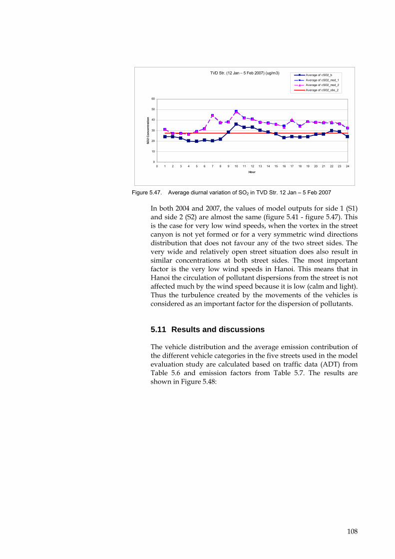
TVD Str. (12 Jan – 5 Feb 2007) (ug/m3)

0

10

20

30

40

50

60

0 1 2 3 4 5 6 7 8 9 10 11 12 13 14 15 16 17 18 19 20 21 22 23 24

Hour

SO2

Con

cent

ratio

n

Average of cSO2_b

Average of cSO2_mod_1Average of cSO2_mod_2

Average of cSO2_obs_2

Figure 5.47. Average diurnal variation of SO2 in TVD Str. 12 Jan – 5 Feb 2007

In both 2004 and 2007, the values of model outputs for side 1 (S1) and side 2 (S2) are almost the same (figure 5.41 - figure 5.47). This is the case for very low wind speeds, when the vortex in the street canyon is not yet formed or for a very symmetric wind directions distribution that does not favour any of the two street sides. The very wide and relatively open street situation does also result in similar concentrations at both street sides. The most important factor is the very low wind speeds in Hanoi. This means that in Hanoi the circulation of pollutant dispersions from the street is not affected much by the wind speed because it is low (calm and light). Thus the turbulence created by the movements of the vehicles is considered as an important factor for the dispersion of pollutants.

5.11 Results and discussions

The vehicle distribution and the average emission contribution of the different vehicle categories in the five streets used in the model evaluation study are calculated based on traffic data (ADT) from Table 5.6 and emission factors from Table 5.7. The results are shown in Figure 5.48:

108

Figure 5.48. Average contribution (%) of emissions of NOx, SO2, CO, BZN and PM10 from each vehicle category for five streets in this model evaluation study. The vehicle distribution (%) is also shown in the top left chart.

Motorbikes are the dominant type of vehicle in Hanoi. They contribute 92-95% of all vehicles. They are also the main source of emissions in the streets. Motorbikes contribute 56% of NOx, 65% of SO2, 94% of CO, 92% of BNZ, and 86 % of PM10 exhaust emissions. The “Trucks” and the “Car 4-16 seats” also have relatively large contributions to NOx and SO2 emissions. Trucks contribute 21% of NOx and 10% of SO2 emissions, and “Car 4-16 seats” contribute 14% NOx and 19% of SO2 (Figure 5.48).

Observed and modelled CO concentrations for TC Street have similar variation corresponding to the diurnal variation of CO emissions (Figure 5.38). The modelled diurnal variation of CO concentrations shows peaks in the morning and afternoon rush hours and also relatively high concentrations during the evening. This diurnal variation fits well with the diurnal variation of motorbikes which are the dominant source to CO emissions (Figure 5.38). The model predicts almost the same concentrations for opposite sides of the street (S1 and S2). This is also expected due to the long modelling period, the low buildings on both sides (height of 4 m) and the low wind speeds. It is also seen that the street increment (difference between street and urban background concentrations) is considerable. The observed diurnal variation of CO concentrations of side 2 show a similar diurnal pattern as the modelled variation although observations are somewhat higher during the day and lower during the evening. The observed CO concentrations of side 1 during the morning and night fit well with that of side 2 but during 16h-18h concentrations are much higher for no obvious reason, probably due to special traffic or meteorological conditions during the measurements or uncertainties in the measured data. BNZ concentrations were also

109

measured for this street and concentrations levels are the same for both sides (Figure 5.38 and Figure 5.49).

The modelled diurnal concentrations of SO2 and BNZ show similar patterns as for CO. It is not possible to present diurnal variations of SO2 and BNZ due to the very limited number of observations.

Modelled and observed daily mean concentrations of SO2, CO and BNZ for the TC, DBP and NT streets, and SO2, NO2 and BNZ for the LTT and TVD streets are shown in Figure 5.49.

Figure 5.49. Modelled and observed mean concentrations for the five selected streets. Urban background concentrations are also provided for reference.

Modelled concentrations overestimate observations up to a factor of two for SO2. The smallest overestimation is for the two streets with low traffic levels (DBP and TVD). However, for DBP street the SO2 street observations are lower than the background concentrations, which are not consistent and can never be reproduced by the model. The systematic overestimation indicates that the SO2 emission factors may be too high. Analysis of the limited data on diurnal variation of observed SO2 concentrations also shows that other sources than vehicles may contribute to SO2 concentrations.

For CO the modelled concentrations underestimate observations up to a factor of two for the streets of DBP and NT and less for TC. The systematic underestimation indicates that the CO emission factors might be too low.

For NO2 the modelled concentrations overestimate observations up to a factor of two for the busy LTT Street whereas modelled and observed levels are similar for the TVD street that has low traffic levels. It is not logical that the observed street

110

concentrations are similar at the LTT and TVD streets when the LTT street has about 10 times higher traffic levels than the TVD street. This indicates uncertainly on the NO2 measurements.

For BNZ the modelled concentrations underestimate observations up to a factor of about two for the busy streets of TC and NT and less for DBF that has lower traffic levels. The systematic underestimation indicates that the BNZ emission factors may be too low. Furthermore, the urban background concentration of BNZ was estimated based on observed correlations between BNZ and CO in Denmark and transferred to Hanoi taking into account differences in the content of BNZ in petrol. In addition, the assumptions of BNZ emission factors for other vehicles than motorbikes for Vietnam conditions are based on a 1999 data set for Denmark according to emissions from COPERT. It is obvious that these assumptions about the urban background and emission factors are highly uncertain.

The OSPM model includes the impact of Traffic Produced Turbulence (TPT) on dispersion parameters. In the OSPM model, TPT is depending on the number of vehicles, the speed, the frontal area of a vehicle, and inversely depending on the width of the street (Berkowicz et al., 1997). An increase of TPT, while leaving all other parameters constant, will lower the modelled concentrations especially under conditions of low wind speeds. In the present version of the OSPM model, TPT of all vehicle types except motorbikes is taken into account. Since motorbikes are the dominant vehicle type in Hanoi they certainly contribute to TPT although their horizontal area is small compared to passenger cars. TPT is also important due to the low wind speed conditions in Hanoi. A sensitivity analysis was carried out where it was assumed that each motorbike contributes with the same TPT as a passenger car. OSPM model calculations showed that concentrations were lowered by 33% for street concentrations under these assumptions. The frontal impact area (width multiplied by height) for a popular motorbike (Honda Future) is about 27% of the frontal area of a popular car (Honda Civic). It illustrates that it is important to take into account TPT also for motorbikes.

A comparison of emission factors (g.km-1) for the different vehicle categories in this study and selected studies from the literature is shown in Table 5.19.

111

Table 5.19. Comparison of emission factors (g km-1) for different vehicle categories in different studies PM10 SO2 NOx CO Benzene

1. Motorbike Hanoi ( from table 4) 0.10 0.03 0.30 3.62 0.023 Bangkok (Kim Oanh et al., 2008) 32.8±8.9

Bangkok (Ittipol P., 2004) Chassis dynamometer 0.08±0.07 2.23±2.2

Bangkok (Ittipol P., 2004) Mobile 6 0.48 0.85 13.3 (Chan L.M and Weaver C.S, 1994) 19.0 China 2009 (Yung-Chen Yao, Jiun-Horng Tsai, and Hui-Fen Ye) -hot start 0.08±0.02 2.17±0.78

2. Car 4-16 seats Hanoi ( from table 4) 0.10 0.17 1.50 3.62 0.023 Bangkok (Kim Oanh et al., 2008) 1.5±0.91

Bangkok (Ittipol P., 2004) Chassis dynamometer 1.37±1.0 5.12±5.65

Bangkok (Ittipol P., 2004) Mobile 6 0.48 0.49 5.41 Copenhagen 1997 - (Palmgren et al., 1999) 0.9±0.1 17.3±0.7 0.11±0.01China 2007 (Zhiliang Yao, Qidong Wang, Kebin He, Hong Huo, Yongliang Ma, and Qiang Zhang)

1. Carburetor vehicles 2.17 24.08 2. Electronic injection vehicles 2.23 12.91 3. Euro I vehicles 1.33 6.21 4. Euro II vehicles 0.81 3.32

3. Bus Hanoi ( from table 4) 1.50 0.64 7.60 3.10 0.032

Bangkok (Ittipol P., 2004) Chassis dynamometer 1.25 12.55 21.99

Bangkok (Ittipol P., 2004) Mobile 6 1.15 23.12 8.89 Copenhagen 1997 (Palmgren et al., 1999) 12.5±3.0 9.6±4 0.05±0.05

4. Truck Hanoi ( from table 4) 0.80 0.40 11.00 2.75 0.045

Bangkok (Ittipol P., 2004) Chassis dynamometer 1.25 12.55 21.99 Bangkok (Ittipol P., 2004) Mobile 6 1.15 23.12 8.89

Copenhagen 1997 (Palmgren et al., 1999) 12.5±3.0 9.6±4 0.05±0.05

It is difficult to compare emission factors across countries due to differences in the vehicle fleet, emission standards, maintenance etc. CO emission factors vary up to a factor of 10 for motorbikes and up to a factor of 3 for other categories among the different studies. This study has applied relatively low emission factors compared to other studies and the model evaluation against observed CO concentrations also indicates that the applied emission factors for CO may be too low. For NOx emission factors there is less variation across the different studies.

The average vehicle emission factors have been estimated using the OSPM model for backward calculations based on the hourly concentration data from 2004 available for three out the five selected streets. The results are shown in Table 5.20:

112

Table 5.20. Average vehicle emission factors of 3 selected streets by backward calculation

Emission factor (g.km-1) SO2 CO Benzene

TC – 2004 (a ring road) 0.038 4.0 0.051

DBP – 2004 (an inner city road) 0.022 16.9 0.125 NT – 2004 (an arterial road) 0.026 10.4 0.079 Mean 0.029 10.4 0.085

The average vehicle emission factors in Table 5.20 can be used to estimate the emissions from other streets if the traffic volume is known according to the road type (arterial road, ring road, inner city road) or the mean may be used to estimate emissions from traffic for a whole city knowing the average traffic volumes and length of the road network.

The estimated average vehicle emission factors by backward calculations have been compared to other studies, see Table 5.21.

Table 5.21. Average vehicle emission factors from different studies Emission factor (g/km)

PM10 SO2 NOX CO BenzeneThis study for TC, DBT, and NT streets, backward calculations (Table 5.20) 0.029 10.4 0.085

This study, average vehicle emission factors for 5 selected streets (by OSPM). 0.108 0.044 0.547 3.6 0.024

HoChiMinh city (Belalcazar et al., 2009) 0.0067 OSPM emission module for the street of Jagtvej, Copenhagen in 2004 1.47 9.3 0.046

The estimated average vehicle emission factor for SO2 by backward calculation is considerable lower than the applied emission factor for OSPM calculations. Lower SO2 emission factor would reduce the overestimation by the OSPM model for SO2 concentrations.

The estimated average vehicle emission factor for CO by backward calculation is three times higher than the applied emission factor for OSPM calculations. Higher CO emission factors would cause less underestimation by the OSPM model for CO concentrations. The emission factor estimated by backward calculations is similar to that of a busy street in Copenhagen in 2004.

The estimated average vehicle emission factor for BNZ by backward calculation is 3-4 times higher than the applied emission factor for OSPM calculations. Higher BNZ emission factors would cause less underestimation by the OSPM model for BNZ concentrations. The emission factor estimated by backward calculations is about two times higher than a busy street in Copenhagen in 2004, among others, due to higher content of

113

benzene in petrol in Hanoi. The estimated average emission factor for BNZ by backward calculation is about 10 times higher compared to the tracer study carried out by Belalcazar in HoChiMinh city (Belalcazar et al., 2009).

5.12 Summary

In this study, the OSPM model was applied in Hanoi for five selected streets and evaluated against air quality measurements. The model was also used to estimate average vehicle emission factors based on backward calculations.

The motorbike is the dominant vehicle type in Hanoi as it constitutes 92-95% of all vehicles. It is also the main source of emissions in the streets.

Analysis of the modelled and observed diurnal variation of CO for one street showed that the OSPM model generally reproduced the diurnal variation.

The model evaluation also showed that the OSPM model, given the applied input data, overestimated daily mean concentrations of SO2 and CO and underestimated concentrations of NO2 and benzene. The most likely reason is uncertainties in emission factors. However, NO2 measurements are also likely to be uncertain.

Traffic Produced Turbulence is neglected in OSPM for motorbikes that are usually a minor vehicle class under West or North European conditions. If TPT for motorbikes was taken into account it would further reduce modelled concentrations. In the future, it is important to incorporate TPT for motorbikes into the OSPM model.

This study also illustrates the challenges of applying dispersion models in a context where high quality model input data and high quality measurements are missing and still need further improvements.

114

6 EVALUATION OF OPERATIONAL METEOROLOGYCAL AIR QUALITY MODEL (OML) IN HANOI

The objective of this chapter is to evaluate the Operational Meteorological Air Quality Model (OML) for a case study in Hanoi, Vietnam. This study uses OML as a modelling tool to map air quality levels on the urban background scale. Emissions from all over the city were categorized in 3 types: traffic source, industrial source and domestic source. In this chapter, the emissions from traffic sources are calculated based on the results of emissions incorporated into the OSPM model in chapter 5. Air quality levels calculated by the OML model was mapped in a GIS spatial map. Model results are also compared with hourly urban background air quality measurements at the Lang station and measurements from a campaign using passive sampling techniques in 2007. The study focuses on NOX, NO2, SO2 and CO.

6.1 Introduction

Operational Meteorological Air Quality Models (OML) was originally designed for industrial sources. The model can also estimate the spatial pollutions on an urban scale from point, area and line sources (Olesen et al., 2007). The OML model has also been applied outside Denmark such as in Latvia and Romania (Jensen et al., 2003; Jensen et al., 2002).

In this study, the OML model is used to map the concentrations of air pollutants on a GIS based map. The spatial variation of air quality in Hanoi is calculated and the model outputs are evaluated by comparison with measured air quality. The model results were evaluated against urban background measurement based on a campaign using passive sampling (45 site measured points) and hourly data at Lang station in the centre of Hanoi.

The OML model requires input data of meteorology, regional background concentrations and emissions.

The hourly meteorological data are based on data from the urban background station of the Lang Station. As no regional background stations exist it was necessary to generate hourly regional background concentrations. This was done based on data from the Lang Station but downscaled to represent regional conditions based on measurements from a campaign using passive sampling in 2007 that gave the average level of the regional air pollution out side Hanoi.

115

The emission data for Hanoi are calculated based on previous studies (CENMA and SVCAP, 2008; Truc, 2005). The emission sources are distributed on a grid of 1 km x 1 km. It includes traffic sources, industrial sources and domestic sources. The emission inventory is based on the data collected from a pilot project in a representative area (ThanhXuan district). ThanhXuan is a small district (in area) and it includes all typical sectors that cause urban air pollution. Therefore, ThanhXuan district was selected for case studies of many projects concerning air quality management. This data base has been extrapolated to the whole city based on indicators such as population, land use, traffic data, and industry before used for OML calculations. The model calculations focus on concentration of NOX, NO2, SO2 and CO and comparison with measurements of the same air pollutants.

6.2 Emission data from a pilot area of ThanhXuan district

This emission inventory was carried out during September - December 2007 as part of the SVCAP project. It was carried out by Hanoi Centre for Environmental and Natural Resources Monitoring and Analysis (CEMMA), Hanoi. The survey was conducted in the whole area of ThanhXuan district ( Figure 6.1).

Figure 6.1. Location of ThanhXuan district in the Hanoi metropolitan area (TuAnh, 2008)

ThanhXuan district is a small but representative zone in Hanoi metropolitan area that has all of the typical types of air pollution sources: domestic, industry and traffic. ThanhXuan is located in the South-West of Hanoi and covers about 9.11 square kilometres. The district has 11 wards (communes) with a population of 214,900 registered citizens. (Table 6.1)

116

Table 6.1. Population distribution in ThanhXuan District 2007 (Hanoi statistical office, 2008)

No Name Area (km2)

Population Population Density (pers/sq.km)

No of Communes

1 ThanhXuan 9.11 214,900 23,589 11 2 Hanoi Total 920.97 3,444,600 3,740 226

The emission campaign was carried out in September to December 2007. the methodology for data collection was designed by Thoan Christopher Nguyen and Patrick Gaffney – experts from the California Air Resources Board (ARB) - based on experiences from consulting and training experience in Asia developing countries (CENMA and SVCAP, 2008).

The emission inventory in ThanhXuan classifies pollution sources into: industrial sources, construction, domestic cooking, commercial activities (petrol stations) and focus on the air pollutants: PM, NOX, SO2, CO, and VOC. Emissions data were collected by CENMA for industrial, domestic, traffic sources. The campaign has surveyed about 200 production and service businesses, 13 petrol stations, 2 hospitals, 42 roads, 105 residential construction sites and 4 commercial construction sites, 3,297 households in 11 wards of ThanhXuan district. For industrial sources, some key parameters were measured for the modelling purposes in the future integrated air quality management system (CENMA and SVCAP, 2008). Emissions from the different sources in ThanhXuan district are summarized in Table 6.2:

Table 6.2. Emissions from different sources in ThanhXuan district in 2007 (tons/year) (CENMA and SVCAP, 2008)

Source PM10 SO2 NOx CO VOCTraffic exhaust 148.8 59.0 733.81 - -Paved road (suspended dust) 2,438.9 - - - -Industries 20.1 324.0 45.0 4.98 0.24Domestic cooking 45.1 676.8 26.0 780.9 86.76Petrol station - - - - 0,006Residential construction 179 - - - -Commercial construction 120.9 - - - -Total 2,952.9 1,059.8 804.9 785.9 87.0

The highest emission load is for PM10 and is dominated by emissions from paved roads.

6.2.1 Point sources

The OML model accepts a maximum of 3,000 point sources. There is a maximum of 3 substances. The OML model requires physical parameters in relation to emissions from point sources: stack height, diameter, gas flow rate, time variation.

117

The pilot emission inventory makes a survey of 22 factories in ThanhXuan District. The parameters of emissions from point sources are presented in Table 6.3:

Table 6.3. Parameters of point sources in ThanhXuan district (CENMA and SVCAP, 2008)

Fuel consumption Source ID

Factory name Stack height

Stack Diameter Type kg/hour

11 Joint-stock SaoVang Rubber Company 32.0 0.8 DO Fuel 583.33

12 22.5 0.5 DO Fuel 123.2213 22.5 0.5 Gas 123.2214 22.5 0.5 DO Fuel 123.2215 22.5 0.5 Coal 123.2216 22.5 0.5 DO Fuel 123.2221 QuangTrung Mechanical company 20.0 0.5 FO Fuel 0.7631 Institute of paper & Cellulose 15.0 0.4 FO Fuel 40.00

41 Joint-stock company for building and glass building 20.0 0.5 DO Fuel 34.72

42 20.0 0.5 DO Fuel 0.3051 Lix soap powder Company 20.0 0.5 DO Fuel 287.5552 20.0 0.5 DO Fuel 287.5553 20.0 0.8 Coal 21.29

61 Thongnhat printing Joint-stock company 20.0 0.5 Coal 1.49

71 19-5 Fabric Company 20.0 0.5 Coal 62.5081 Hanoi soap powder company 20.0 0.5 Coal 1.2391 ThuongDinh Shoes Company 20.0 0.5 Gas 115.28100 DongTien rubber limited Company 15.0 0.3 DO fuel 1.67101 DaiKim Joint-stock company 20.0 0.5 DO Fuel 1.39

102 AnhThinh foodstuff limited Company 20.0 0.5 Coal 1.11

103 RangDong Light Source And Vacuum Flask Joint Stock Company 20.0 0.5 Coal 111.11

104 VIHA company 20.0 0.5 DO Fuel 4.46

105 MuaDong Woollen Knitwear Company 20.0 0.5 Coal 83.33

161 ThangLong Tobacco Company 20.0 0.54 DO Fuel 107.64162 32.0 1.05 DO Fuel 107.64

171 Pharmaceutical Dept - National Hospital for Traditional Medicine 20.0 0.5 Gas 0.30

181 HaNoi Dying limited Company 20.0 0.5 DO fuel 4.17191 HaViet Printing Company 20.0 0.5 DO Fuel 138.89201 TranPhu electromechanical 20.0 0.5 DO Fuel 2.04211 SonHan mechanical company 20.0 0.5 Gas 3.70221 KimSon Company 20.0 0.5 DO Fuel 94.69

118

Note: FO is fuel oil, DO is diesel oil and gas is natural gas.

In Table 6.3, source ID is used to locate the source in a GIS map. Sources that do not have the detailed physical parameters are assumed to have the average stack height of 20 m and the dimension of outlets of 0.5 m. For fuel consumption the average fuel consumption (kg/hour) is assumed.

In the SVCAP project, the emission factor for fuel was calculated based on the methodology of U.S.EPA AP-42, section 13.2.1, March, 1996: Uncontrolled emission factor listing of criteria air pollutants, chapter 14, volume II and California Air Resources Board, California 1999 (CENMA and SVCAP, 2008). The emissions from industries in ThanhXuan District were calculated based on the survey data (Table 6.3) and emission factors from U.S EPA.

However, the survey data was limited. It only provided emission data for some sources. It did not cover all point sources in the region. In an alternative way, the emission was calculated by a software (SPC.PAS) based on the mass balance of combustion. It calculated the air emissions based on the combustion of fuel consumption for each stack which was collected by CENMA (CENMA, 2008). A sample of calculation for source ID No 1.1 (Table 6.3) is described in Figure 6.2:

Figure 6.2. Modelled emissions for industrial source ID No 1.1

119

This software is developed by Tran Ngoc Chan at the Department of Environmental Engineering, National University of Civil Engineering, Hanoi, Vietnam and it has been applied in many cases in Vietnam to calculate the emissions from industries. Thus, this provides sufficient input data for industrial sources in ThanhXuan district.

The average emissions calculated based on the total emission (g/s) from ThanhXuan district and the total industrial area (km2). The average emissions in ThanhXuan district are used to estimate the emissions from the other industrial areas in Hanoi where detailed emission data of the factories is not available.

6.2.2 Line sources

The SVCAP project conducted a counting of vehicles at 42 streets in ThanhXuan district. Vehicles on each road were counted during 24 hours at 3 representative days in the week: Monday, Wednesday and Sunday (CENMA and SVCAP, 2008). Table 6.4 presents the emissions from typical streets in ThanhXuan district:

Table 6.4. Estimated emission for typical streets in ThanhXuan district (tons/year) (CENMA and SVCAP, 2008)

NguyenTrai Street TruongChinh Street Date

PM10 NOX SO2 PM10 NOX SO2 Monday 39.19 219.83 16.02 25.93 125.45 10.50 Wednesday 57.77 288.60 22.17 22.50 112.59 9.16 Sunday 52.25 255.50 20.29 23.50 110.62 9.72

The data in Table 6.4 shows that there is no significant difference between emissions on those three days of the week as traffic levels and vehicle distribution is more or less the same (see more in chapter 5).

6.2.3 Area sources

Domestic cooking is considered as an area source in the ThanhXuan district. The two main types of fuels which are widely used for domestic cooking in ThanhXuan district are hand-fired coal and gas. The emissions of SO2, NO2, and CO from combustion of gas are very small and therefore neglected (data calculated by SVCAP project) (CENMA and SVCAP, 2008). Therefore, for input to the OML model, the emissions of SO2, NOx, and CO from domestic sources are calculated based on hand-fired coal (“Than tổ ong” in Vietnamese) combustions. The amount of coal usage in ThanhXuan district (47,074 households) was estimated based on the data. The coal consumption for domestic cooking from a survey of 3,202 households in ThanhXuan is shown in Table 6.5:

120

Table 6.5. Coal consumption for domestic cooking in a Pilot project in ThanhXuan district (CENMA and SVCAP, 2008).

Ward Number of Households Coal consumption (kg/day)Kim Giang 297 99.5 Khuong Mai 301 154.5

Phuong Liet 300 150.5

Ha Dinh 261 138.5 Thuong Dinh 300 173

Nhan Chinh 300 147

Khuong Trung 291 196 Khuong Dinh 300 580.5 Thanh Xuan Bac 299 114.5 Thanh Xuan Nam 296 131 Thanh Xuan Trung 257 123

Total 3,202 2,008

The data in Table 6.5 confirmed a value of coal usage in a household of 0.627 kg/day. The amount of coal usage in ThanhXuan district with total 47,074 households was estimated based on the data from a survey of 3,202 households and the 25% of 47,074 households in ThanhXuan district used hand-fired coal, the rest of the households uses gas and electricity for cooking (source: Mr. Dang Thanh Trung, CENMA and Mr. Bui Quang Trung, SVCAP– persons in charge of Emission inventory for ThanhXuan district) (CENMA and SVCAP, 2008). The consumption of coal usage is presented in Table 6.6:

Table 6.6. Coal consumption for domestic cooking in ThanhXuan. (CENMA and SVCAP, 2008)

Coal usage in ThanhXuan district District Number of

Households

Average coal usage in a household

(kg/day) (kg/day) (kg/h) ThanhXuan 47,074 0.627 7,383 308

The pilot emission inventory has build-up some data for the emissions of domestic cooking (Table 6.2). However, this data sheet is not sufficient to be the input data for OML modelling. The emissions from domestic sources for OML modelling were also calculated by the SPC.PAS software based on the mass balance of combustion as shown below (Figure 6.3):

121

Figure 6.3. Modelling emissions for domestic sources in ThanhXuan District

The emissions for one km2 of domestic sources in ThanhXuan are calculated based on the total emissions calculated above divided by the summary of the area of residential areas. Emissions for one km2 of domestic sources are presented in Table 6.7:

Table 6.7. Unit emissions for domestic sources for ThanhXuan District Emissions for 1 km2 (g/s)/km2 District Residential area

(km2) NOX SO2 CO ThanhXuan 3.15 0.08 0.27 0.03

This data is the first data set that was systematically collected in Hanoi for an emission inventory of domestic sources and it represents the current situation of domestic cooking in Hanoi. It will be used to estimate the emission from domestic sources for the whole city based on information of residential areas (building foot prints) on a GIS map.

122

6.3 Estimation of emissions for the OML modelling in Hanoi.

6.3.1 Introduction

The emissions for OML modelling is estimated based on land-use and population data from Hanoi. Table 6.8 shows the land-use data of Hanoi (2007):

Table 6.8. Land-use data in Hanoi in 2007(km2) (Vu Tuan Vinh, 2009)

District Total Area Industrial Area

Land for Traffic

Land for Resident

Other emission

BaDinh 9.25 0.61 1.65 3.25 3.75HoanKiem 5.29 0.45 1.03 1.63 2.19TayHo 24.00 0.64 1.97 4.17 17.22LongBien 59.53 4.49 4.70 10.79 39.55CauGiay 12.04 0.68 2.10 4.23 5.03DongDa 9.96 0.50 2.13 4.42 2.91HaiBaTrung 10.09 1.07 1.81 3.53 3.69HoangMai 39.51 2.24 4.78 8.97 23.52ThanhXuan 9.11 1.36 1.54 3.15 3.06SocSon 306.51 4.55 24.32 34.80 242.84DongAnh 182.30 8.38 13.29 21.32 139.31GiaLam 114.79 3.75 9.35 12.55 89.14TuLiem 75.32 2.12 6.74 12.74 53.72ThanhTri 63.27 2.19 4.30 8.14 48.64Summary of Hanoi 920.97 32.40 78.07 130.42 680.07

Table 6.9 shows the population data in Hanoi (2007):

123

Table 6.9. Population data in Hanoi – 2007 (Hanoi statistical office, 2008).

District Name Population (persons) Population Density (pers/ km2)

BaDinh 242,400 26,205

HoanKiem 180,700 34,159 TayHo 117,900 4,913 LongBien 210,300 3,533 CauGiay 192,200 15,963

DongDa 387,400 38,896 HaiBaTrung 325,000 32,210 HoangMai 265,700 6,725

ThanhXuan 214,900 23,589 SocSon 277,600 906 DongAnh 316,100 1,734 GiaLam 224,000 1,953

TuLiem 296,000 3,930 ThanhTri 194,400 3,073 Summary of Hanoi total 3,444,600 3,740

Based on these data assigned to a GIS map, the data from the pilot emission inventory in ThanhXuan district was used to extrapolate to the whole city.

Emissions were categorized in three sources: traffic, industry and domestic. How the emissions for the whole city are estimated is described in the following.

6.3.2 Emissions from traffic

As previously indicated, emissions from traffic are the main source of air pollution in Hanoi and pollution from traffic is considered a line source. The necessary parameters for estimating this source are emission factors, number of vehicle, vehicle kilometre travelled (VKT), and the length of roads. The OML model requires that the line sources are converted into area sources. In this study a GIS based road network is available that includes three types of streets. This information was utilized to generate emission on a grid of 1 km x 1 km for the whole city area.

Streets in Hanoi were categorized in 3 types (Tu Anh, 2008):

Street type 1 (named Pho cap 1 in GIS data base) is the main roads that have the Vietnamese name “đường”. They are defined as arterial road or ring roads. The traffic flows on these streets are very high (100,000 – 300,000 vehicle/day). NguyenTrai Street and TruongChinh street represent this type (see more in chapter 5) (Truc, 2005; CENMA and SVCAP, 2008). This data is used to estimate the emission from traffic for this type of street.

Street type 2 (named Pho cap 2 in GIS data base) is the inner streets in the Hanoi traffic system. It includes all streets having a name

124

starting with “phố”. DienBienPhu street, LeTrongTan Street and ToVinhDien street present this type (see more in chapter 5). The traffic level on these streets (43 streets) is about 30,000 vehicles/day (CENMA and SVCAP, 2008).

Street type 3 (named Pho cap 3 in GIS data base) is the minor streets and lanes that do not an official name on the map. These streets are normally small and motorbikes may only be allowed. According to Mr. Do Quang Trung (SVCAP project, 2007) the average vehicle volume for this type is estimated to about 10,000 motorbikes/day.

The emission factors for three street types have been estimated based on emission factors generated for the OSPM model (in chapter 5). The results are summarized in the Table 6.10:

Table 6.10. Average emission factors for streets from OSPM study in chapter 5 Emission factor (g.km-1)

Mean value by OSPM Mean value by Backward Cal.

NOX SO2 CO NOX SO2 COStreet type 1 - - - TruongChinh 0.64 0.05 3.61 - 0.038 3.99 NguyenTrai 0.80 0.06 3.60 - 0.026 10.43 Mean 0.72 0.06 3.61 - 0.032 7.21 Street type 2 DienBienPhu 0.44 0.04 3.62 - 0.022 - LeTrongTan 0.40 0.04 3.62 - - - ToVinhDien 0.44 0.04 3.61 - Mean 0.43 0.04 3.62 - - - Street type 3 - - - Lane (for motorbikes) 0.30 0.03 3.62 - - -

Applied emission factors and the average daily traffic (ADT) for traffic sources used in OML model are presented in Table 6.11:

Table 6.11. Emission factors for OML’s traffic sources ADT Emission factor (g/km) Category

(veh./day) SO2 NOX COStreet type 1 150,000 0.032 0.72 7.21 Street type 2 30,000 0.022 0.43 7.21 Street type 3 10,000 0.030 0.30 3.62

The road network were originally based on a MapInfo data set for each district (Tu Anh, 2008). The traffic network was converted to a Shape file for use in ArcGIS. Table 6.12 shows the total length of streets according to the types for each district:

125

Table 6.12. The total length of streets according to the street types (km) No Districts Street type 1 Street type 2 Street type 3 1 BaDinh 16.05 37.82 30.41 2 HoanKiem 1.39 48.80 1.65 3 TayHo 4.24 24.24 23.19 4 LongBien 22.33 8.66 33.35 5 CauGiay 13.44 30.00 19.13 6 DongDa 12.19 25.20 41.33 7 HaiBaTrung 10.17 43.42 33.03 8 HoangMai 23.48 39.69 54.63 9 ThanhXuan 15.55 26.36 33.42

10 SocSon 53.76 41.70 84.62 11 DongAnh 28.97 9.03 98.09 12 GiaLam 15.74 17.03 15.74 13 TuLiem 45.08 35.90 58.82 14 ThanhTri 11.99 40.49 97.52

Summary 274.38 428.34 624.94

The road network and summary of km travelled on a 1km2 grid on a GIS map is shown in Figure 6.4.

126

Figure 6.4. Road network and districts

The emissions of pollutants from each cell (1 km x 1 km) are calculated based on the total length of each street type multiplied by the emission factor from Table 6.11. Emissions of NOX derived from traffic are shown in Figure 6.5.

127

Figure 6.5. Spatial distribution of NOX emissions from traffic on a 1x1 km2 grid (g/s)

The time variation for traffic sources is obtained from OSPM study in chapter 5 (Table 5.3 Diurnal variation of vehicles).

128

Based on the diurnal variation of motorbikes (the most dominated vehicle type) in table 5.3 the time variation for traffic sources are distributed in each hour in a day and presented in Figure 6.6:

Figure 6.6. The time variation for traffic sources

The monthly factors and day of the week factor were assumed constant.

6.3.3 Emissions from Industries

There is no complete emission inventory for industrial emissions in Hanoi. A pilot project in the ThanhXuan district is given some data for point sources. It is used to estimate the average emission from the other industrial areas in Hanoi where no detailed emission data is available.

The mean values of emissions density were calculated based on the total emissions (g/s) from industries in the ThanhXuan District (Table 6.2) divided by the summary of industrial areas (km2) within the ThanhXuan district. The results are presented in Table 6.13:

129

Table 6.13. Emission factors for OML’s industrial sources Emissions for 1 km2 (g/s)/km2)

NOX SO2 COHanoi 7.50 1.04 0.12

The time variation for industries sources is assumed to be constant in the absents of any information about the time variation (Figure 6.7).

Figure 6.7. The time variation for industries sources

Based on the data for industrial sources in ThanhXuan District, the stacks of factories in Hanoi are not high (15 m -20 m) and the emission volume for each stack is not very large (CENMA and SVCAP, 2008). Therefore, it is possible to estimate the emission from those factories as an area source. The total area of industries in Hanoi was distributed on a grid of 1 km x 1 km in a GIS map (Figure 6.8). The industrial emissions for each cell was calculated by the emissions of 1 km2 [(g/s)/km2] in Table 6.13 multiplied by the total area of industries of each cell. The spatial distribution of industrial areas in Hanoi was shown in Figure 6.8.

130

Figure 6.8. Spatial distribution of industrial areas on a GIS map (grid is 1 km x 1 km)

6.3.4 Emissions from domestic

Emissions from domestic sources contribute significantly to SO2 and CO pollution in the residential areas due to the usage of coal for cooking. The emission load is small compared to traffic and

131

industrial sources but the emissions are close to the human life and causes high exposures. Therefore, it causes severe damage to human health.

The emissions from domestic sources were calculated based on the emission inventory of the ThanhXuan District by the SVCAP project in 2007. This emission inventory (from Table 6.7) is extrapolated to the whole city based on the population density for each district (Hanoi statistical office, 2008). The results are presented in Table 6.14:

Table 6.14. Emissions for domestic sources for districts of Hanoi

No District Population

Density (pers/sq.km)

Ratio of Pollution Density compared to

ThanhXuan

NOx (g/s)

SO2 (g/s)

CO (g/s)

1 BaDinh 26,205 1.11 0.0882 0.0356 0.30182 HoanKiem 34,159 1.45 0.1150 0.0465 0.39343 TayHo 4,913 0.21 0.0165 0.0067 0.05664 LongBien 3,533 0.15 0.0119 0.0048 0.04075 CauGiay 15,963 0.68 0.0537 0.0217 0.18386 DongDa 38,896 1.65 0.1310 0.0529 0.44797 HaiBaTrung 32,210 1.37 0.1085 0.0438 0.37098 HoangMai 6,725 0.29 0.0226 0.0091 0.07749 ThanhXuan 23,589 1.00 0.0794 0.0321 0.2716

10 SocSon 906 0.04 0.0031 0.0012 0.010411 DongAnh 1,734 0.07 0.0058 0.0024 0.020012 GiaLam 1,953 0.08 0.0066 0.0027 0.022513 TuLiem 3,930 0.17 0.0132 0.0053 0.045314 ThanhTri 3,073 0.13 0.0103 0.0042 0.0354

The spatial distributions of domestic emissions are calculated based on locations of residential areas in Hanoi which was shown in Figure 6.9:

132

Figure 6.9. Residential areas and districts

Emissions of SO2 derived from domestic cooking are shown in Figure 6.10.

133

Figure 6.10. Distribution of SO2 emission from domestic cooking (g/s)

The time variation for domestic sources is obtained from the actual habits of cooking in Hanoi based on information from a survey (Do, 2009). The monthly factors and day of the week factors for domestic source were assumed constant. The hourly factor for the diurnal variation was distributed in 24 hours based a information from SVCAP project (Do, 2009), see (Figure 6.11).

134

Figure 6.11. The time variation for domestic source

6.4 OML Meteorological Preprocessor

Meteorological data need to be processed before they are suitable for use by the OML model. The OML meteorological preprocessor is a software package to take care of this task. The preprocessor requires hourly surface-based meteorological data and radiosonde data to calculate turbulence parameters and mixing height. The OML model needs hourly data to perform calculations, and typically one year of data are used (Olesen, 2007). These data describes the meteorological characteristics of the boundary layer where the mixing of air pollutants mixing is taking place. The Lang station is provided surface-based meteorology data for 2007, while radiosonde soundings for 2007 have been taken from Hanoi airport. The data set from 2007 is sufficient for an integrated air quality assessment. Dr. Helge Rørdam Olesen, NERI has contributed to this project by running the meteorological preprocessor for the Hanoi case study.

6.4.1 Hourly surface based meteorological data

Hourly metrological data from the Lang Station were used as hourly surface-based meteorological data for modelling. Wind speed and wind direction is shown in Figure 6.12:

135

Figure 6.12. Annual wind rose 2007 for Lang Station

For OML modelling, the aerodynamic roughness has to been set to 0.3 m as an empirical constant for urban areas, both for the area with the Lang station and for the modelling area in general.

The monthly average rainfall and temperature of Hanoi in 2007 are presented in Table 6.15.

Table 6.15. Monthly average rainfall and temperature of Hanoi in 2007 (Lang Station) Monthly Rainfall (mm) Monthly Temperature (oC)

Month Average Average Max Min

Jan 4.8 16.6 25.8 11.1 Feb 32.7 21.6 28.5 13.1 Mar 34.7 20.6 28.7 11.3 Apr 119.5 23.2 33.5 14.0

May 135.8 27.0 38.1 19.7 Jun 249.0 29.8 37.7 22.9 Jul 300.4 30.1 36.4 24.9

Aug 359.8 28.9 36.0 23.4 Sep 354.5 27.0 33.1 22.1 Oct 160.8 25.6 32.5 19.3 Nov 4.6 21.5 28.2 13.2 Dec 28.1 20.0 27.6 14.4

Based on the rainfall in Table 6.15, the dry season in this study is defined from May to October, and the wet season is the other months. The dry and wet seasons will be used in comparison of model results and observations.

136

For Hanoi, turbulence parameters are calculated based on the so-called resistance method. The resistance method uses measurement data performed on a routine basis based on national meteorological stations (so called synoptic stations). Input data for Hanoi are the data from Lang meteorology station. The parameters used from the mast are wind direction and speed, temperature, relative humidity, cloud cover and global radiation. Information on rainfall also comes from the Lang Station.

The OML meteorological preprocessor does not accept a wind speed of zero. A program to prepare wind data takes care of this problem and some other tasks. It replaces missing wind directions with values generated based on wind direction for the previous, the current and the next hour (Olesen, 2007). Missing data for wind speed are filled in with interpolated values. The program defines a default wind speed of 0.5 m/s in the case that wind speed is zero. The OML model requires a parameter indicating the change of wind direction from one hour to the next, which is also computed in this step.

The central component of the preprocessor computes turbulence parameters from ordinary meteorological data, using the resistance method. The input are the data listed above, and the output includes the turbulence parameters u* (friction velocity), H (sensible heat flux), L (Monin-Obukhov length), all of which carry important information on dispersion (Olesen, 2007).

6.4.2 Radiosonde data

The OML model needs information of mixing height. Mixing height is derived from the surface based meteorological data, combined with radiosonde data, which provides a vertical profile of various parameters. The radiosonde data provide information at 00 and 12 GMT. The parameters required by the OML meteorological preprocessor are: Pressure, temperature and relative humidity at as many vertical positions as possible (Olesen, 2007). The radiosonde data for Hanoi was collected from the websit of the University of Wyoming (University of Wyoming, 2008). The code for the Hanoi Station is 48820 VVNB Hanoi.

A program in the preprocessor package (READSOND.FOR) has been used to process radiosonde data and prepare them in a format appropriate for the OML preprocessor. Next, the so-called ZI program of the preprocessor was executed in order to compute mixing height for all hours of 2007. An adjusted version of this program was created by Helge Rørdam Olesen in order to be applicable for Vietnamese conditions.

The pre-processor package was applied successfully to produce one year of hourly meteorological data (2007).

137

6.4.3 Topographical data

The OML model has simple procedures for terrain effects on dis-persion of air pollutions. The effect from the terrain on concentra-tions depends on terrain height and the largest terrain inclination. In Hanoi the terrain is flat and the terrain height is set to zero. The aerodynamic roughness length is assumed to be 0.3 meters. The roughness length represents the overall roughness of the terrain in the OML model. Often, a value of 0.1 m is used in the countryside and 0.3 m in urban areas. This roughness length is based on a sur-vey from 2007 (Son D.H et al., 2008).

6.5 Regional air pollution background data

Among the meteorological station network nearby Hanoi, there are 2 meteorological stations which have been considered as regional background stations for meteorological and air quality data (Long D.H., 2009):

1. Phulien Station: Located about 100 km to the north east of Hanoi. It is also located close to the city of Haiphong. Therefore, this station is not representative for the regional background. The NOX concentration of this station is even higher than at the Lang Station which is an urban background station.

2. CucPhuong Station: Located in the national forest also named CucPhuong, situated around 100 km to the south of Hanoi. The monitoring data is fragmented due to unstable power supply in 2007. Therefore the data is not sufficient for modelling. However, the concentrations of O3 and CO from this station are considered for estimating the average concentration of the regional background.

In order to create a data set with hourly values for the regional background air pollution, the average concentrations from locations representative for regional conditions obtained from the campaign using passive sampling in 2007 are used and the diurnal variation is obtained from the hourly data from the Lang Station. The mean value for correction of NO2 and SO2 are shown in Table 6.16:

Table 6.16. Regional background mean concentrations in 2007 (µg/m3) Dry season 12/1/07-5/2/07 Wet season 18/8/07 -12/9/07

Pollutant Lang station

Regional site Passive sample

Lang station Regional site

Passive sample NO2 43.7 21.3 58.3 14.0 SO2 61.8 22.6 27.0 6.3

The campaign using passive sampling was conducted during two time periods in 2007. The measurements from 12 January to 5 February 2007 are representative for the dry season and the

138

measurements from 18 August to 12 September 2007 are representative for the wet season. Based on the information in Table 6.15, those months which belong to the dry season (November, December, January, February, March and April) will be adjusted by measurements from 12 January to 5 February 2007. The other months from May to October which belong to the wet season will be adjusted by measurements from 18 August to 12 September 2007.

The adjusted time series will have the mean value equivalent to the mean value of the campaign using passive sampling is the real rural data. A sample of the correction was presented in Figure 6.13:

Average diurnal variation of NO2 at Lang station for regional background (12 January - 5 February 2007)

0

10

20

30

40

50

60

70

80

0 1 2 3 4 5 6 7 8 9 10 11 12 13 14 15 16 17 18 19 20 21 22 23

Hour

Con

cent

ratio

n (µ

g/m

3 )

Original average value of cNO2_bCorrected average value of cNO2_b Mean value by passive sample in 2007

Figure 6.13. Annual diurnal variation of NO2 (12 January to 5 February 2007)

The OML model also requires hourly O3 concentration from the regional background for simple photo chemistry calculations. Available O3 concentrations in Vietnam were collected together with O3 data from Bangkok, Thailand. The mean values of all collected data are shown on Table 6.17:

139

Table 6.17. Annual O3 concentrations from different stations (µg/m3) No Monitoring Station Time No of

Measurement /year

O3 Mean Max Min

1 Vietnam (Long D.H., 2009) 1.1 Lang, Hanoi

(Urban Background) 1/2007-12/2007 8670/8670

24.7 114 1.96

6/2007-12/2007 29.6 114 1.961.2 CucPhuong (Regional

site) 6/2007-12/2007 4471/8670 36.4 110 8

1.3 GiaLam, Hanoi 1/2010-3/2010 2188/2188 33.0 258 02 Thailand: Bangkok (Le, 2008)

2.1 BMR (Urban background)

2004 -- 32.5 384

2.2 Eastern, (Regional background)

2004 -- 39.0 272

2.3 Northern, (Regional background)

2004 -- 40.4 247

2.4 Northern Eastern, (Regional background)

2004 -- 45.7 241

Compared to the ozone data from Bangkok (GiaLam station) the mean ozone concentration at CucPhuong (regional site) in Table 6.17 seems to represent regional conditions. However, this station has only hourly ozone data for half of the year in 2007. Therefore, the mean value for this half year was assumed as the annual mean value of ozone concentration at the CucPhuong station. This mean was used to represent the average regional ozone concentrations for the OML modelling. To construct hourly regional O3 concentration data, a scaling was introduced based on the hourly variation of O3 at the Lang station. It is obviously a very crude assumption as the hourly variation in regional ozone concentrations will not be the same as the hourly variation at the urban background site of the Lang Station as O3 concentrations here will be influenced by the NOx emissions of the city.

Measurements of CO concentrations in 2007 are not available for Hanoi. The mean value (59.0 µg.m-3) of all available data of CO concentrations in 2007 at the CucPhuong station was assumed to be representative for the regional background concentration of CO. It was applied as a constant value for all hours for the whole year for the OML model calculations.

The OML model requires the hourly input data in µg.m-3. The conversion factors between ppb and µg.m-3 and ppm and mg.m-3 is normally based on European conditions (EC 20 oC and 1013mb). Due to the hot weather in Hanoi, the appropriate conversion factors at 25oC and 1013mb are used (Table 6.18).

140

Table 6.18. Conversional factors between ppb and µg.m-3 and ppm and mg.m-3 Pollutant EC 20 oC and 1013mb WHO 25 oC and 1013mb

Ozone 1 ppb = 2.00 μg.m-3 1 ppb = 1.96 μg.m-3 Nitrogen dioxide 1 ppb = 1.91 μg.m-3 1 ppb = 1.88 μg.m-3 Carbon monoxide 1 ppm = 1.16 mg.m-3 1 ppm = 1.15 mg.m-3 Sulphur dioxide 1 ppb = 2.66 μg.m-3 1 ppb = 2.62 μg.m-3 Benzene 1 ppb 1 ppb = 3.25 μg.m-3 1 ppb = 3.19 μg.m-3

NOx in µg.m-3 is expressed as NO2. i.e. (NO ppb + NO2 ppb) * 1.91 = NOx in µg.m-3.

6.6 Urban background measurements

6.6.1 Campaign using passive sampling

As already mentioned in section 5.1.7 chapter 5 (page 84), 45 measured points which were not affected by the pollutants directly from streets are considered as actual urban background. The location of urban background points are shown in Figure 5.31.

The measurements will be used to evaluate the modelling outputs: Measurements from 12 January to 5 February 2007 are representative for the dry season and the measurements from 18 August to 12 September 2007 are representative for the wet season. The measurements together with ID codes are presented in Table 6.19:

141

Table 6.19. Pollutant concentrations of urban background sites from campaign using passive sampling in 2007(μg.m-3) (SVCAP and Fabian, 2007)

GPS Coordinates - WGS_1984_UTM_Zone_48N

Dry season 12/1/07-5/2/07

Wet season 18/8/07-12/9/07

Code

North East NO2 SO2 NO2 SO2 VT1 583039 2332121 26.6 21.2 20.1 9.7 VT2 584624 2331835 27.9 22.5 27.1 11.8 VT3 585302 2331023 26.4 22.7 13.8 21.4 VT4 584423 2330327 31.3 19.5 19.3 5.2 VT5 585887 2330024 27.8 19.7 22.7 10.1 VT6 586907 2329348 21.9 20.0 15.6 5.1 VT7 583871 2328821 27.3 25.4 19.4 7.5 VT8 585580 2329387 23.8 15.2 17.0 6.8 VT9 586541 2329607 21.6 17.6 38.9 10.1

VT11 583264 2327804 24.2 25.0 20.7 20.0 VT12 584232 2328013 27.4 34.5 17.4 7.7 VT15 582771 2326411 29.7 22.1 20.3 14.1 VT16 583941 2326624 32.2 26.5 23.7 16.3 VT23 585289 2325723 38.6 30.7 27.7 15.2 VT24 586559 2325572 50.1 26.5 35.3 11.6 VT27 581655 2324564 25.2 14.1 25.6 13.3 VT30 585528 2324709 36.1 30.4 26.4 8.3 VT32 587759 2324518 49.6 36.4 37.4 17.7 VT35 583690 2323748 32.5 30.5 26.2 13.9 VT46 588931 2321977 35.7 44.3 28.8 17.3 VT52 585402 2320846 26.2 27.7 27.7 12.5 VT53 586627 2320406 33.6 29.1 26.9 20.5 VT56 590098 2320926 28.8 35.2 25.2 171.6 VT57 591340 2320460 41.5 26.3 26.1 17.0 VT58 592422 2320714 23.5 24.0 23.4 10.1 VT59 593522 2320773 19.2 23.1 16.0 13.9 VT61 585264 2319725 28.7 42.3 19.1 15.6 VT62 586715 2319405 31.5 34.6 24.4 20.7 VT63 587800 2319564 29.9 27.7 18.5 13.7 VT64 589062 2319831 24.5 26.7 19.4 17.3 VT65 590126 2319578 26.8 23.8 17.7 9.4 VT66 591032 2320540 28.5 34.0 26.7 15.5 VT68 585340 2318422 23.2 23.6 15.9 11.7 VT69 586930 2318626 30.8 28.9 19.7 11.7 VT71 589128 2318426 43.2 25.7 32.8 9.5 VT72 583039 2332121 30.2 26.5 21.8 14.6 VT73 584624 2331835 29.1 22.1 29 13.4 VT74 585302 2331023 24.7 20.9 19.9 8.8 VT75 584423 2330327 20.8 23.7 12.7 10.2 VT76 585887 2330024 24.4 19.4 24.3 8.1 VT77 586907 2329348 24.9 24.7 17.4 21.2 VT78 583871 2328821 23.1 23.1 18 7.3 VT79 585580 2329387 25.7 19.0 15.7 8.8 VT85 586541 2329607 21.0 21.1 11.4 9.4 VT96 583264 2327804 27.3 26.3 34.2 11.9 Mean 29.0 25.9 22.8 16.2

142

6.6.2 Hourly data from the Lang Station

The hourly monitoring data of NO2, SO2 and CO for the whole year of 2007 was also used for evaluation of the model outputs.

6.7 Evaluation of model results against observations

The OML model uses meteorological data produced by meteorological preprocessor program and the emissions from traffic, industrial and domestic sources which was managed in a GIS data base. The OML model was run for the same periods as the available measurements for comparison and evaluation of the model results.

6.7.1 Dry season and wet season in 2007

The OML model was used to model the concentrations of NO2 and SO2 with 45 receptor points for the locations of the campaign using passive sampling in the dry season (from 12 January 2007 to 5 February 2007) and wet season (18 August 2007 to 12 September 2007) (CENMA and SVCAP, 2008). The mean values of model outputs will be compared to the values from the corresponding periods from the campaign using passive sampling in Table 6.19 for an evaluation of the model data.

The correlation between modelled and observed NO2 for dry and wet season are presented in Figure 6.14- Figure 6.17:

Comparison between observed and modeledmean concentrations of NO2 - Dry season 2007 (12 Jan - 5 Feb 2007)

0

10

20

30

40

50

60

1 2 3 4 5 6 7 8 9 10 11 12 13 14 15 16 17 18 19 20 21 22 23 24 25 26 27 28 29 30 31 32 33 34 35 36 37 38 39 40 41 42 43 44 45

Measurement points

Con

cent

ratio

n (µ

g/m

3)

ObservedModeled

Figure 6.14. Mean concentration of NO2 for 45 measurement points– Dry season 2007 (µg/m3).

143

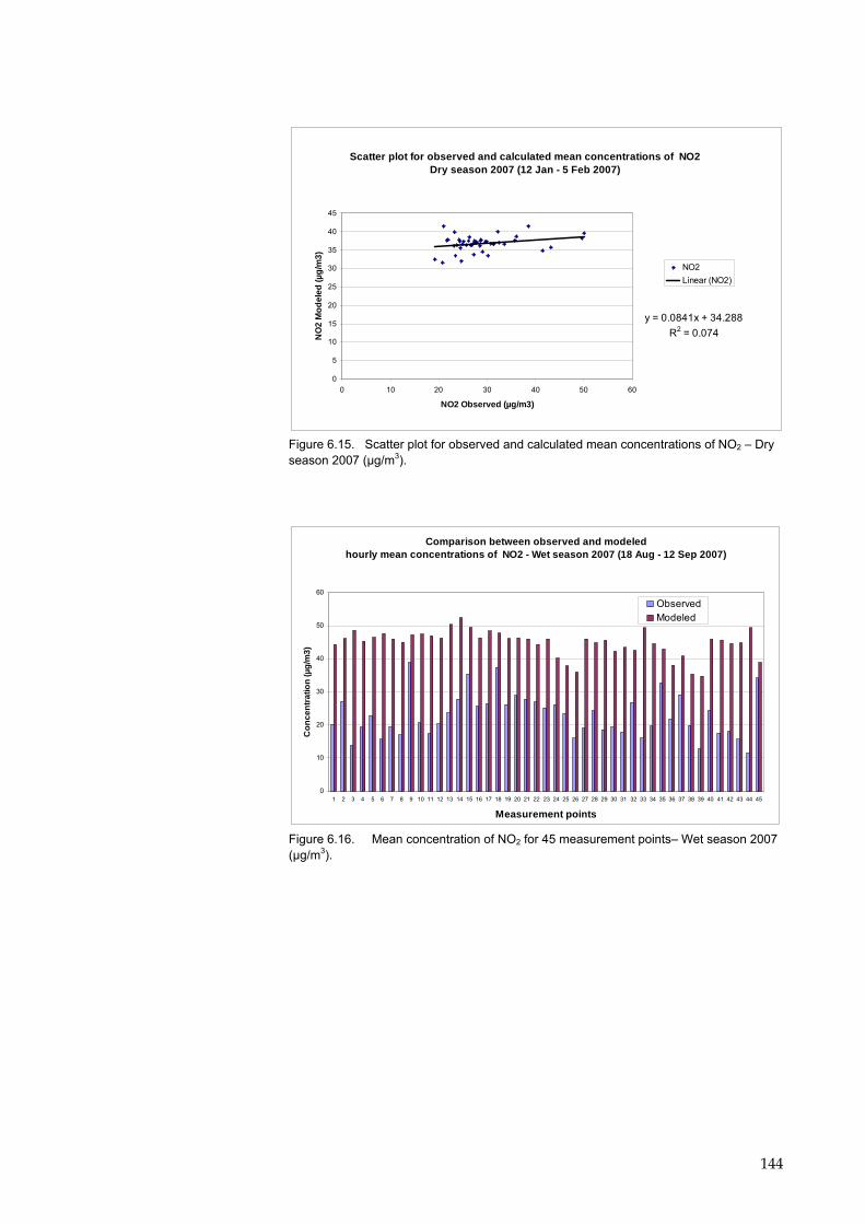
Scatter plot for observed and calculated mean concentrations of NO2 Dry season 2007 (12 Jan - 5 Feb 2007)

y = 0.0841x + 34.288R2 = 0.074

0

5

10

15

20

25

30

35

40

45

0 10 20 30 40 50 60

NO2 Observed (µg/m3)

NO

2 M

odel

ed (µ

g/m

3)

NO2Linear (NO2)

Figure 6.15. Scatter plot for observed and calculated mean concentrations of NO2 – Dry season 2007 (µg/m3).

Comparison between observed and modeledhourly mean concentrations of NO2 - Wet season 2007 (18 Aug - 12 Sep 2007)

0

10

20

30

40

50

60

1 2 3 4 5 6 7 8 9 10 11 12 13 14 15 16 17 18 19 20 21 22 23 24 25 26 27 28 29 30 31 32 33 34 35 36 37 38 39 40 41 42 43 44 45

Measurement points

Con

cent

ratio

n (µ

g/m

3)

ObservedModeled

Figure 6.16. Mean concentration of NO2 for 45 measurement points– Wet season 2007 (µg/m3).

144

Scatter plot for observed and calculated mean concentrations of NO2 Wet season 2007 (18 Aug - 12 Sep 2007)

y = 0.07x + 43.13R2 = 0.01

0

10

20

30

40

50

60

0 5 10 15 20 25 30 35 40 45

NO2 Observed (µg/m3)

NO

2 M

odel

ed (µ

g/m

3)

NO2Linear (NO2)

Figure 6.17. Scatter plot for observed and calculated mean concentrations of NO2– Wet season 2007 (µg/m3).

Model results overestimate observations and the spatial variation in observations is not very well reproduced. The mean value of measured data for NO2 from the 45 urban background points is 80% of the modelled mean for the dry season. For the wet season it is 50% and further studies are needed to understand why. NO2 is not affected much by wet deposition so deposition processes can not explain that NO2 is lower during the wet season. Differences in mean monthly wind speeds do not seem to explain why modelled NO2 concentrations are substantially lower during the wet season. However, the correlation between modelled and observed concentrations according to the scatter plots is poor with r2 of only 0.01-0.07 (Figure 6.15, Figure 6.17). It indicates a further need to improve the emission inventory for the modelling inputs in terms of the level and spatial distribution. Regional background ozone concentrations were crudely assumed to be constant which make little variation in modelled NO2. More precise input data will make better correlation between modelled and observed data.

The correlation between modelled and observed SO2 for the dry and wet seasons are presented in Figure 6.18 and Figure 6.20:

145

Comparison between observed and calculatedmean concentrations of SO2 - Dry season 2007 (12 Jan - 5 Feb 2007)

0

5

10

15

20

25

30

35

40

45

50

1 2 3 4 5 6 7 8 9 10 11 12 13 14 15 16 17 18 19 20 21 22 23 24 25 26 27 28 29 30 31 32 33 34 35 36 37 38 39 40 41 42 43 44 45

Measurement points

Con

cent

ratio

n (µ

g/m

3)

ObservedModeled

Figure 6.18. Mean concentration of SO2 for 45 measured points– Dry season 2007 (µg/m3).

Scatter plot for observed and calculated hourly concentrations of SO2 Dry season 2007 (12 Jan - 5 Feb 2007)

y = 0.24x + 28.02R2 = 0.13

0

5

10

15

20

25

30

35

40

45

50

0 10 20 30 40 50

SO2 Observed (µg/m3)

SO2

Mod

eled

(µg/

m3)

SO2Linear (SO2)

Figure 6.19. Scatter plot for observed and calculated mean concentrations of SO2 – Dry season 2007 (µg/m3).

146

Comparison between observed and modeledmean concentrations of SO2 - Wet season 2007 (18 Aug - 12 Sep 2007)

0

5

10

15

20

25

30

35

40

45

1 2 3 4 5 6 7 8 9 10 11 12 13 14 15 16 17 18 19 20 21 22 23 24 25 26 27 28 29 30 31 32 33 34 35 36 37 38 39 40 41 42 43 44 45

Measurement points

Con

cent

ratio

n (µ

g/m

3)

ObservedModeled

Figure 6.20. Mean concentration of NO2 for 45 measured points– Wet season 2007 (µg/m3).

Scatter plot for observed and calculated mean concentrations of SO2 Wet season 2007 (18 Aug - 12 Sep 2007)

y = 0.20x + 11.43R2 = 0.12

0

5

10

15

20

25

30

0 5 10 15 20 25 30 35 40 45

SO2 Observed (µg/m3)

SO2

Mod

eled

(µg/

m3)

SO2Linear (SO2)

Figure 6.21. Scatter plot for observed and calculated mean concentrations of SO2 – Wet season 2007 (µg/m3).

The model slightly overestimates during the dry season and slightly underestimates during the wet season. The correlation between modelled and observed SO2 concentration according to the scatter plots (Figure 6.19, Figure 6.21) is also poor but slightly better compared to NO2. 12-13 % of measurements are explained by the model (r2=0.12-0.13). It also indicates that there is a need to improve the emission inventory for the modelling inputs.

6.7.2 Evaluation of model results for the Lang station in 2007

The OML model was also used to model the hourly concentrations of NO2, SO2 and CO at location of the Lang station. The values of model outputs for NO2, SO2, CO at the Lang Station are compared

147

with the monitoring data from the Lang station for an evaluation of the performance of the model.

The correlation between modelled and observed NO2 concentrations for the Lang station location is presented in Figure 6.22:

148

Scatter plot for observed and modeled hourly concentrations of NO2 at Lang Station

y = 0.46x + 19.71R2 = 0.36

0

50

100

150

200

250

300

350

400

0 50 100 150 200 250 300 350 400

NO2 Observed (µg/m3)

NO2

Mod

eled

(µg/

m3)

NO2 ModeledLinear (NO2 Modeled)

NO2 hourly variation at Lang Station

0

10

20

30

40

50

60

70

1 2 3 4 5 6 7 8 9 10 11 12 13 14 15 16 17 18 19 20 21 22 23 24

Hour

Con

cent

ratio

n (µ

g/m

3)

0.00

0.20

0.40

0.60

0.80

1.00

1.20

1.40

1.60

Win

d Sp

eed

(m/s

)

Average of NO2 ModeledAverage of NO2 ObservedAverage of WS(m/sec)

TCVN 5937-2005

NO2 monthly variation at Lang Station

0.00

10.00

20.00

30.00

40.00

50.00

60.00

70.00

80.00

01 02 03 04 05 06 07 08 09 10 11 12

Months

Con

cent

ratio

n (µ

g/m

3)

0.00

0.20

0.40

0.60

0.80

1.00

1.20

1.40

Win

d Sp

eed

(m/s

)Average of NO2 ObservedAverage of NO2 ModeledAverage of WS(m/sec)

TCVN 5937-2005

Figure 6.22. NO2 modelled vs. NO2 observed at the Lang Station in 2007 (µg/m3). The dry season in this study is defined from May to October, and the wet season is the other months.

149

The correlation between modelled and observed NO2 concentrations at the Lang station location according to the scatter plot (Figure 6.22) is much better than for the campaign using passive sampling. The model explains 36% of the variation in measurements (r2=0.36). When compared to the Vietnamese standard 5937-2005: Air quality – Ambient air quality standards (equivalent to EU and WHO level) the limit value (40 μg/m3) as an annual mean is just exceeded. The diurnal and monthly variations of NO2 are influenced by the meteorology conditions. As expected the concentration is low when the wind speed is high and vice versa but the picture is not clear as other factors also play a role. In the modelling it was assumed that the seasonal and day of the week variation in emissions was constant but this may not be the case and may partly explain difference in modelled and observed results.

The correlation between modelled and observed SO2 concentrations for the Lang station location is presented in Figure 6.23:

150

Scatter plot for observed and modeled hourly concentrations of SO2 at Lang Station

y = 0.39x + 7.73R2 = 0.30

0

50

100

150

200

0 50 100 150 200

SO2 Observed (µg/m3)

SO2

mod

eled

(µg/

m3)

SO2 ModeledLinear (SO2 Modeled)

SO2 hourly variation at Lang Station

0.00

10.00

20.00

30.00

40.00

50.00

60.00

1 2 3 4 5 6 7 8 9 10 11 12 13 14 15 16 17 18 19 20 21 22 23 24

Hour

Con

cent

ratio

n (µ

g/m

3)

0.00

0.20

0.40

0.60

0.80

1.00

1.20

1.40

1.60

Win

d Sp

eed

(m/s

)

Average of SO2 ObservedAverage of SO2 ModeledAverage of WS(m/sec)

SO2 monthly variation at Lang Station

0.00

10.00

20.00

30.00

40.00

50.00

60.00

70.00

01 02 03 04 05 06 07 08 09 10 11 12

Months

Con

cent

ratio

n (µ

g/m

3)

0.00

0.20

0.40

0.60

0.80

1.00

1.20

1.40Average of SO2 ObservedAverage of SO2 ModeledAverage of WS(m/sec)

Figure 6.23. SO2 modelled vs. SO2 observed at Lang Station – 2007 (µg/m3)

EU Standard

TCVN 5937-2005

EU standard

TCVN 5937-2005

The correlation between modelled and observed SO2 concentrations at the Lang station location (according to the scatter plots) is also better than for locations representing the campaign using passive sampling. 30 % of the measurements are explained by the model. When compared to Vietnamese standard 5937-2005: Air quality – Ambient air quality standards, SO2 concentrations are below the standard at the Lang station (Figure 6.23). However, compared to EU and WHO Standards, the average measured and modelled concentrations are higher than the standard.

The correlation between modelled and observed CO concentrations for the Lang station location is presented in Figure 6.24:

Scatter plot for observed and modeled mean concentrations of CO at Lang Station

y = 0.37x + 0.61R2 = 0.04

0.0

0.5

1.0

1.5

2.0

2.5

3.0

3.5

4.0

4.5

0 1 2 3 4 5

CO Observed (mg/m3)

CO m

odel

ed (m

g/m

3)

CO ModeledLinear (CO Modeled)

CO hourly variation Station

0.00

0.50

1.00

1.50

2.00

2.50

1 2 3 4 5 6 7 8 9 10 11 12 13 14 15 16 17 18 19 20 21 22 23 24

Hour

Con

cent

ratio

n (m

g/m

3)

0.00

0.20

0.40

0.60

0.80

1.00

1.20

1.40

1.60

Win

d Sp

eed

(m/s

)

Average of CO ObservedAverage of CO ModeledAverage of WS(m/sec)

CO monthly variation at Lang Station

0.00

0.20

0.40

0.60

0.80

1.00

1.20

01 02 03 04 05 06 07 08 09 10 11 12

Months

Con

cent

ratio

n (m

g/m

3)

0.00

0.20

0.40

0.60

0.80

1.00

1.20

1.40

Win

d Sp

eed

(m/s

)

Average of CO ObservedAverage of CO ModeledAverage of WS(m/sec)

Figure 6.24. CO modelled vs. CO observed at the Lang Station in 2007 (mg/m3)

153

For this modelling study, CO measurements were not available for the campaign using passive sampling or for the regional background. The correlation between modelled and observed CO concentrations for Lang station receptor point is poor as the model only explains 4% the monitoring data in a scatter plot (r2=0.04). The hourly mean values and monthly mean value however correlated to the wind speed data.

6.7.3 Spatial variation annual city in 2007

The OML model was also run with the receptor points for all the centre points of 1 km x 1km grid applied to the whole city. This data is used to describe the spatial variation of the annual mean concentration of NO2 and SO2 in Hanoi. The spatial variation of modelled results for NO2 and SO2 are shown in Figure 6.25 and Figure 6.26.

154

Figure 6.25 Spatial variation for annual urban background concentrations of NO2 in Hanoi in 2007

155

Figure 6.26 Spatial variation for annual urban background concentrations of SO2 in Hanoi in 2007

156

The spatial distribution of the yearly mean values in Figure 6.25 and Figure 6.26 show that the city centre is highly polluted by NO2 and SO2. The pollution is higher in the locations where the industrial areas are located. NO2 is mostly emitted from traffic. In fact, emission of NO2 was shown to closely relate to the spatial distribution of traffic (Figure 6.5). SO2 emission represents the domestic cooking source and was also found to correlate to the spatial distribution of residential areas (Figure 6.10). Such strong correlations between pollutant concentrations and the distribution of emission sources indicate the dependence of pollution level upon the proximity to emission sources.

6.8 Summary

In this model study, OML modelled urban background air quality calculations were compared with measurements from a campaign using passive sampling including 45 sites, and with hourly measurements from the urban background monitor station of Lang Station. The model was also used to calculate air quality at receptor points in a 1x1 km2 grid over Hanoi to give the spatial distribution of air quality in the city. The results show a potential to estimate the air pollution level in the city based on the data from a pilot project that was extrapolated to the rest of the city based on various land-use data.

The OML modelled pollution results based on the estimated emission inventory gives a first attempt to describe the air quality levels at the urban background scale. The OML model reproduced the general air quality levels for NO2 and SO2 at the 45 campaign sites but did not fully capture the geographic variation in the measurements as the correlation between modelled and measured data was poor (r2=0.12-0.13). The correlation between hourly modelled and observed NO2 and SO2 concentrations at the Lang station location was much better than for the campaign using passive sampling. The model explains 36% of the variation in the measurements for NO2 and 30% for SO2, r2=0.36 and 0.30, respectively. The general trends in the diurnal and monthly variations of NO2 and SO2 are reproduced fairly well and it is clearly seen that the variation is influenced by the meteorology conditions. The model output will be much better if an emission inventory was systematically built up and managed by a single institution in Vietnam. In this study, the variations of air quality in the regional background were created by an urban background data set. Therefore the variation may not be representative for the regional conditions.

The air quality data set from the Lang station also needs better quality assurance and quality control.

157

The modelled spatial variation of air pollution is a useful result based on a combination of emission data on GIS, modelled output results and measurement. Based on these data, environmental authorities and policymakers can describe the environmental status (air pollution level) and the driving forces of air pollution (the sources and its developments) for the environmental management and sustainable development of urban planning.

158

7 DPSIR analysis of application of dispersion models in Hanoi

This chapter presents the shortcomings and potentials for application of the OSPM model and the OML model in Hanoi, Vietnam for air quality assessments. The DPSIP framework is used to analyze dispersion model applications in the future.

7.1 Approach

Modelling provides a link between the emission inventory data and the monitoring data. If the emission inventory, meteorology data and all of its inputs were perfect, the air quality model would predict measured pollutant concentrations from high quality monitor stations with high certainty. In Hanoi, as a case study of a developing country, these perfect conditions can not be expected, so the three components (emission inventory, monitoring, and modelling) are used together in an integrated approach of adjustment, evaluation, and refinement. Each tool is used to help in identifying the shortcomings of the others and to identify what improvements are needed. The DPSIP framework is used as a tool to analyze the complexity of linkages and feedbacks between the DPSIR components within the application of dispersion models (OSPM and OML models).

7.2 Driving forces in relation to dispersion modelling

The driving forces are the social forces leading to the emissions. For the dispersion modelling applications in the cities, the information of urbanization (Figure 1), motorization (table 3.1), and industrialization are required. Those data is used for uptrend analysis. The dispersion modelling can predict the pollution level based on the different scenario analysis for the future. The urban development also puts more pressure on the emissions leading to increase in pollution levels. Therefore, these developments are important to evaluate to be able to assess air quality in the future. The growing in transport, industry, and household activities in Hanoi must be well documented in order to estimate the development in emissions. As experienced in the past, the data is fragmentarily collected with varying quality and collected by different institutions. If only one institution was assigned this task then the data would be more well managed in one system for modelling purposes. In Hanoi, CENMA would be a suitable institution in charge of this task. The data of road networks must be managed in a GIS based data. The industrial source data is expected to be documented precisely for each stack. However, this

159

task needs an enforcement legal framework and also time to be build-up. For immediate results, the estimation of emissions from industries can be estimated based on the fuel consumption or product amount. A method for this was applied in the OML model study in chapter 6. For the emissions from domestic sources, a GIS based map of residential areas and the fuel consumption for domestic cooking in the whole city is sufficient to estimate the emission from domestic sources. Those data if collected and managed in a systematically way would be very helpful for pollution prediction by modelling. The information of pollution levels predicted by dispersion models from different scenarios can provide feedback to the authorities about the development in the driving forces and suggest adjustments to be made. This may help to control the driving forces for better an urban sustainable development.

7.3 Pressure in relation dispersion model

The pressure is the emissions of air pollutants (e.g. TSP, NOX, CO, SO2 and VOC) in the city. Each emission source emits certain pollutants. Concerning air quality modelling it is necessary to identify the most important sources for each pollutant. Then authorities can manage a suitable emission inventory for them. An emission inventory is an efficient tool to manage emission source activities. It is used to produce the input data for dispersion model.

In Hanoi, the TSP comes mainly from non-exhaust sources: re-suspension of dusts from streets, road wear, tyre wear and break wear. For particulate matter, it is important to estimate the vehicle volume and distribution as they affect non-exhaust. Construction activities also contribute to coarse particulate matter. The relative humidity and rain also have an effect on the concentration of particulate matter in the air. In order to model particulate matter this information is important.

Vehicles use fuel and emit pollutants such as PM10, NOX, CO, SO2, VOC. Concerning vehicle emissions, the emission factors (g.km-1) are the most uncertain due to the usage of old cars. Apart from emission factors, the necessary parameters to estimate emissions are information about the vehicle fleet, vehicle kilometre travelled, and the road network. The study of the OSPM model in Hanoi (chapter 5) shows that it is important to have experimental studied on emission factors for each vehicle category in Hanoi. It is recommended from this study to categorize the different road types according to traffic flows and manage a road network in a GIS to be able to predict the spatial distribution of emissions from streets for easy handling in models.

Combustion activities from industries emit many air pollutants such as: NOX, CO, SO2, VOC, and PM10. The following fuels: Coal,

160

fuel oil (FO), diesel oil (DO) are mainly used in factories in Hanoi. Concerning the estimation of emissions from point sources, the necessary parameters are amount of fuel consumed per day (or per year), yearly production schedule, parameters for stacks such as volume, height, and diameter. The emission inventory of industries needs to be located by GPS and placed in a GIS map for modelling purpose.

Domestic cooking produces pollutants such as CO, SO2, NOx, VOC, and PM10. In the city, this source is assigned as an area source. The application study of the OML model in Hanoi (chapter 6) shows that it is important to have geographic information about the residential areas and population density to be able to assign domestic emissions to the areas where these emissions are released. Then emissions can be distributed in an emission grid (1 km x 1 km) in a GIS map for air quality modelling. The emission inventory for domestic emissions is based on the population density that also needs to be build-up with the parameters suitable for each particularly area. Middle class and upper classes of urban citizens are moving towards usage of natural gas instead of FO, DO fuel and coal. The detailed survey information available for the ThanhXuan district was used to extrapolate to the rest of the city. This means that the emission data from the pilot project in ThanhXuan district may not be representative for the domestic sources applied to the whole city since the ThanhXuan district is dominated by middle and upper class citizens.

From an institutional point of view, human resources at CENMA should be able to analyze the trends in pressures of emissions and the effect on air quality in the city. Then CENMA can recommend solutions to manage and reduce the emissions from the sources. Currently, only the actual state of air quality is assessed through limited air quality monitoring.

In summary, to improve air quality modelling, it is necessary to identify the sources of air pollution and locate them on a GIS map and build-up an emissions inventory system.

7.4 State in relation with dispersion model tasks

The state indicates the air quality in the urban area. It can be analyzed by an integrated air quality monitoring system. Integrated air quality monitoring is monitoring based on results from air quality measurements from fixed monitoring stations, and results obtained from calculations with air quality models.

For application and evaluation of dispersion models, monitoring stations must be in a system and all the observed data must be managed in a central data base. Some monitoring stations at street

161

level and at urban background and at least one rural background station must be included in the monitoring networks to reflect the different air environments inside and outside the city. The data from the monitoring stations is the basic data that presents the actual level of air pollution in the city. It was visualized in Figure 4.2. Monitoring data of regional background stations represents concentration of rural areas and it is the input to calculate the urban background level when adding pollution contributions from urban areas. A regional background monitoring station representative for upwind conditions for Hanoi is lacking at present. The urban background monitoring station data represents the concentrations of urban background, that is, concentrations at roof tops or in a park not affected by a single strong source. It is used to evaluate and validate the urban background calculations by the OML model. Due to the cost implications, monitoring can only be carried out in selected locations but the OML model can provide the spatial distribution of air quality for the entire city. Urban background monitoring data may also be used as model input data for calculation of street pollution levels by the OSPM model. Data in street stations can be used to estimate the pollution contribution directly from traffic by OSPM modelling.

Environmental authorities and managers can estimate the pollution level by a combination of model results and data from the monitoring network to set up the regulations needed for managing the air quality in the city.

Available data at monitoring stations should be managed and linked to a central database of the city. This data can be presented in some pollution information boards in streets showing the air quality levels to the public to raise awareness. CENMA is the suitable institution for this task. Human resources of CENMA should be trained to maintain the monitoring network and air quality data management.

Temporal campaign measurements using passive sampling can supplement fixed monitoring stations in combining with the modelling data in an Integrated Monitoring and Assessment (IMA) framework. The campaign measurements should be carried out in Hanoi at several locations in a program for environmental monitoring. The campaign measurements can be carried out at representative places such as road side, urban background, and regional background. The quality control and quality assurance must be carried out with professional calibration of instruments and sufficient checking of data to provide for high quality measurement data. This requirement is a necessity to be able to use measurement data for evaluation and validation of results from dispersion models. Vice versa, the model calculations can provide the pollutant concentrations at locations that are not covered by the limited number of campaign measurements or the fixed

162

monitoring stations. The results from the air pollution models are also used in the interpretation of measurements.

In summary, dispersion models play an important role in the integrated air quality monitoring system. Dispersion models can provide the information at any place in the city to describe the state of urban air quality.

7.5 Impacts in relation to dispersion models

Human health effects are important impacts of urban air pollutions. Other impacts are related to materials, green areas or such.

Dispersion models are a sufficient tool to estimate human exposure to air pollution. The information needed to estimate human exposure (in the whole city) is the spatial distribution of pollutant concentrations and population data through the city area. The health impacts can be estimated by information about pollution level and exposure, dose-response relations, and health effect baseline data for key health effect outcomes. In Vietnam, particularly in Hanoi, an assessment of the health impacts of air pollution has not been carried out. However, there is a lot of international studies on health effects related to urban air pollution from which assessments for Hanoi could be based.

7.6 Responses in relation to dispersion models

The responses are the actions that the government, institutions, companies and individuals etc. decide to make to react to the negative change in urban air pollution. Responses are actions taken to protect human health and reduce the damage to the environment, buildings etc.

As already mentioned under State and Impact, dispersion models can provide information about air quality and they can provide input to estimation of the impacts of air pollution. The air pollution models are also used to provide information about the pollution source and their relative contribution to air quality. Furthermore, scenario studies are ‘what if’ studies that examine different abatement measures and their effects on air quality. Based on this information authorities and citizens can decide on which actions to take.

The most important response is to reduce the emissions. Based on the information provided by modelling data, environmental authorities such as the city council can make an action plan to reduce emission sources. Technology plays an important role in reducing emissions. For example, one way to reduce emissions, is

163

to shift to cleaner fuels like natural gas for domestic cooking instead of using polluting fuels like coal and kerosene. Another example of emission reduction is end-of-pipe treatment e.g. filters on stacks or catalytic converters on cars. In Hanoi, the main pollution comes from traffic. Authorities could define a low emission zone in Hanoi to protect the urban centre area from air pollution from traffic by requiring certain emission standards for vehicles to enter the low emission zone.

Another response is dilution. Although this response does not reduce overall emissions the impacts of air pollution is reduced due to dilution. For an example, in Denmark regulation of industrial air pollution is regulated with a combination of emission limits and limit values for the contribution to the ambient concentrations. Once the emission limits are met the remaining emissions have to be diluted to meet limit values for the contribution to ambient concentrations.

The final solution as a response is to separate the emission sources and the sensitive receptors e.g. by removing people from pollution if there is no way to stop the harmful emissions. An example is to move the factories out of residential areas. The new location should be downwind of the prevailing wind directions to minimize population exposure. Dispersion models can be used to estimate those conditions that cause potential air pollution problems in certain locations.

All those responses must be considered in a complex social and economic context. Parallel with the economic development, the emissions from business activities (traffic, industries, domestic) in the urban area will increase rapidly. There is no ways to stop this process but there are efficient ways to minimize emissions and their negative effects.

The air quality based on the integrated monitoring and assessment should be managed in a systematic way. The lesson learnt can be taken from the diagram of the structure of the framework directive by the European Union on ambient air quality assessment and management (Figure 7.1) (EU directive 2008). The idea is that authorities can set up legislation with ambient air quality limit values and require actions to be taken if they are not met.

164

Figure 7.1. Schematic diagram of structure of the framework directive (EU directive 2008;Palmgren, 2000)

The groups in Figure 7.1 are the different environmental zones related to different pollution levels. The authorities have to report to the EU Commission for all the zones about the pollution level every year or every third year depending on the air pollution levels. For zones where the pollution level does not meet the limit value (group 1) authorities have to maintain and improve the air quality based on an action plan. Zones where pollution levels are between the limit values and the limit value plus margin of tolerance (group 2) must report annually to the EU Commission to ensure that the limit value is met by an attainment date. The idea of the margin of tolerance is to make sure that some actions are carried out before the date in which a limit value must be met is reached. Zones belonging to group 3 where air quality is below the limit value only have to report every third year and ensure that the good air quality is maintained until the attainment date (EU directive 2008; Palmgren, 2000).

7.7 Summary

In summary, the selected dispersion models are operational, user-friendly and reliable to use provided availability of high quality input data. They have a good chance to be applied in developing cities as a predicted tool to supplement costly operation of fixed monitoring stations and campaign measurements. In the Integrated Monitoring and Assessment (IMA) framework, dispersion models can provide the information of pollution level at any location as required. The result from air pollution models can be used in the interpretation of monitoring and campaign measurement data. Dispersion model also can provide information

165

about the contribution to concentrations of the different pollution sources; and furthermore, link the pollution levels to health effects caused by air pollution.

166

8 CONCLUSIONS

8.1 Summary of the research

A systematic evaluation of dispersion models as a tool for air quality assessment and management in a Vietnamese context was conducted with focus on technical as well as management aspects. The research studied the application of dispersion models in line with the Integrated Monitoring and Assessment (IMA) concept. The research mainly focused on the application and evaluation of Operational Street Pollution Model (OSPM) and Operational Meteorological Air Quality Model (OML) which are operational and applicable dispersion models for assessment of street and urban background air quality. An evaluation of model calculations against available measurements was carried out. This study contributed to a systematic evaluation of air pollution conditions in Hanoi and identified factors that influence air quality.

8.2 Answers to research questions

The answers to the research questions are dedicated to apply dispersion models as an assessment tool for urban air quality assessment and management in Hanoi as the case study.

1. The first question: What are the most important factors influencing air quality in the urban areas and how does this affect the choice of appropriate air quality models?

The answer:

The most important factor influencing air quality in Hanoi is traffic emissions. Parallel with the rapid increase in population in urban areas, traffic demand is also increasing rapidly which leads to increase in emissions and degradation of air quality. Other important sources affecting air quality are industry and residential cooking. The industrial factories use coal in Hanoi which lead to severe local air pollution in the area where the factories are located. Hand-fired coal used for cooking in Hanoi cause air pollution indoors.

The second important factor is meteorological conditions. The meteorological conditions in Hanoi are not advantageous to the dispersion of air pollutants. Low wind speeds combined with high temperatures cause elevated air pollution level in the city centre. In the monsoon season, the air near ground surface cools faster than the upper layer. Therefore, it prevents emissions from rising and

167

be diluted. The nocturnal radiation inversion also causes the air pollution levels at night to be 2-3 times higher compared to the daytime.

Thirdly, typographical factors play a role. The flat terrain in Hanoi is an advantage for air pollution dispersion. Furthermore, the street building facades are generally low and the street canyon effect leading to elevated air pollution levels is therefore also limited. Traffic Produced Turbulence (TPT) is an important factor for the dispersion of pollutants at the street scale especially under low wind speed conditions.

Based on the available information of emission inventories together with meteorological, and topographical conditions in Hanoi, dispersion models are suitable for air quality modelling purposes since they are simple, operational, user-friendly and reliable.

For this study, the Operational Street Pollution Model (OSPM) and Operational Meteorological Air Quality Models (OML) were selected as dispersion models as they fulfil the above criteria. They are developed at the National Environmental Research Institute in Denmark. The advantage for this choice is also due to the available technical supports within NERI. In this research, the OSPM model is applied to evaluate the air pollution level at street scale. The OML model together with a data base in GIS is used to calculate and map the air pollution level at the urban scale in Hanoi. The research, however, also illustrated the challenges of applying dispersion models under the conditions in Hanoi and recommends for further improvements for dispersion model applications.

2. The second question: What are the most important technical factors and institutional factors for successful adaptation and application of air quality models in a Vietnamese context?

The answer:

The most important technical factor that influences the efficiency of dispersion models is the reliability of traffic and vehicle emission data. Ideally, a GIS data set with detail parameters of the road network, vehicle volume for each street and studies of emission factors for each vehicle category must be in place.

With regard to industries, emission sources should be managed in an emission inventory with detailed information of each factory. However, in Hanoi as a developing city, it is a challenge to make such a data set. In this study, industrial emissions were estimated based on the fuel consumption from a pilot project in ThanhXuan district and extrapolated to other areas based on land-use information on a GIS map about industrial sectors in Hanoi.

168

The domestic sources in Hanoi can be considered as area sources due to the many sources of low height. In this study, domestic emissions were estimated based on the fuel consumption for household cooking activities in ThanhXuan district and land-use information on a GIS map of the area of the domestic sector in the rest of Hanoi. The emission from domestic sources could also be estimated based on the emissions per capita. The population density for each commune or district will make the mapping of emissions from domestic more precisely.

The evaluation of the existing monitoring network revealed that the monitoring network should be systematically set up and managed. At least one regional background monitoring station must be included in the monitoring network to provide for assessment of regional background concentrations and also to serve as input for urban background modelling. The urban background station must be relocated to better represent the urban background pollution level. Permanent street level monitoring stations with rooftop meteorology is also required for validation of modelling at street level.

The current institutions in Hanoi are not sufficient for handling monitoring and modelling tasks as a part of an integrated monitoring and assessment strategy. An emission inventory must be developed and annually updated for modelling purpose. The monitoring network must be connected and a central data base should be built up. The competence of the involved staff must also be improved. The enforcement of legal documents and standards should be applied to all emission sectors. The collaboration between the environmental managers of the city council and professionals from e.g. universities, academic institutions etc. must be strengthened. More research activities must also be based on the needs and problems within air pollution in Vietnam.

Citizens are currently inadequately informed about the health effects of air pollution. They should be more informed about the effect of air pollution on human health, and how changes in behaviour can reduce air pollution e.g. use of different fuels for cooking and different means of transportation.

8.3 Contributions of the research

This study has evaluated the applications of dispersion models (OSPM and OML) for air quality assessment in Hanoi, Vietnam as a developing city, where input data for modelling was limited and of varying quality.

169

8.3.1 Contributions from OSPM modelling

The OSPM model was applied in Hanoi for five selected streets and evaluated against actual air quality measurements. The research used the passive sampling data from 2007 to adjust the hourly data at the Lang station to obtain sufficient hourly concentration data of urban background concentrations for OSPM modelling. Since the quality control and quality assurance at the Lang station is insufficient, the meteorological data from Hanoi airport was used to evaluate the quality of the Lang station data. The research created an average diurnal traffic variation for six vehicle categories. The average vehicle volume for three street types, representative for the road network in Hanoi, was estimated from the traffic data and used together with emission factors for calculation of the emission from entire road network. The study also established the correlation between CO and BNZ concentrations for Vietnamese conditions to be able to model urban background concentrations as no measurements of BNZ were available. Urban background concentrations are a requirement for modelling of street concentrations with the OSPM model. Model outputs of NO2, SO2, CO, and BNZ were evaluated with the hourly measurements and passive sample measurements for the first time in Hanoi. Backward calculations were also used to estimate average emission factors of the vehicle fleet in Hanoi.

Emission factors were established for PM10, SO2, NOX, CO and BNZ based on literature values and implemented into the emission module of the OSPM model. Average fleet emission factors of PM10, SO2, NOX, CO, BNZ were estimated which can be used for emission calculations at other streets in Hanoi and South-East Asia cities with similar vehicle composition.

According to the emission factors implemented motorbikes are the main source of emissions in the streets constituting 92-95% of all vehicle emissions. Motorbikes contribute 56% of NOx, 65% of SO2, 94% of CO, 92% of BNZ, and 86% of PM10 street emissions.

Both modelled and observed diurnal variations of CO concentrations were similar to the diurnal variation in traffic. The model evaluation also showed the model overestimated daily mean measured concentrations of SO2 and CO and underestimated measured concentrations of NO2 and benzene. The main reason is properly attributed to uncertainties in emission factors.

Backward calculations were performed to estimate average emission factors of SO2, CO and BNZ for three street types. Emission factors estimated based on backward calculations were about 3-4 higher for CO and BNZ and about at the same level for SO2.

170

8.3.2 Contributions from OML modelling

The OML model was applied to evaluate the air pollution level of NO2, SO2 and CO at urban background scale. OML modelled outputs were evaluated against passive sampling measurements and hourly data from the Lang Station. The OML model was also used to map the spatial distribution of air pollution for the whole Hanoi. The annual average concentrations of NO2 and SO2 were mapped in a GIS spatial map on a 1x1 km2 grid resolution as an example of predicting the pollution levels related to the emission sources and meteorological conditions.

For OML modelling, the emission inputs were categorized in 3 types: traffic sources, industrial sources and domestic sources and the emission data for these sources were calculated separately. The traffic emissions are calculated based on the total length of each street type multiply by the emission factor. The emissions were distributed in a grid of 1 km x 1 km. The industrial sources in ThanhXuan district were based on surveyed data from a previous study and for the other districts emissions were extrapolated using land-use data for industrial areas. The domestic emissions were calculated based on the emissions collected from the ThanhXuan district and extrapolated to the whole city based on population density for each district.

All the emission data were built and managed in a GIS for this research. The study showed that it was possible to develop a simple emission data base for modelling purpose. This method would have significant application in developing cities where emission inventory is not available and the characterizations of emission sources are usually limited and of varying quality.

OML predicted average air quality levels of NO2 and SO2 in the dry season of 2007 overestimate levels in comparison with the passive sample measurements. Measurements were 80% of the predictions for the mean value for the 45 measurement points. In the wet season of 2007 the measurements were 50% of the predictions for NO2 and 70% for SO2.

The correlations between hourly modelled and observed values of NO2 and SO2 were 0.36 and 0.30, respectively. The annual average diurnal variation and the seasonal variation (monthly means) showed similar patterns between modelled and observed data and NO2 levels were about the same but the model underestimated SO2 concentrations. The results correlate well with the meteorological conditions during the dry and wet season. The concentrations are systematically low while wind speed is higher and vice versa.

The modelled spatial variation of SO2 and NO2 presents the possibility of using a simple model like the OML model with a GIS map as a sufficient tool for mapping of air pollution levels. The

171

OML model can also be used to predict future concentrations if the future emissions can be predicted.

8.3.3 Contributions from Integrated Monitoring and Assessment analysis

The DPSIR framework was employed to analyse the current situation of the air quality in Hanoi. The DPSIR framework was also used to analyse shortcomings and potential applications of the OSPM model and the OML model in Hanoi, Vietnam in context of the integrated monitoring and assessment approach.

In Hanoi, the input data is not systematically collected and managed. Time and resources are required to build-up a sufficient emission inventory for modelling of air quality and a sufficient monitoring network in Hanoi. Therefore all the available data from different sources should be used to identify the shortcoming of different information sources. Site measurements can be good sources for evaluation of the hourly data from fixed monitoring stations. At the same time, systematic yet simple surveys for each main emission sources can enable operation of air dispersion modelling. IMA can also provide the best basic information of emission sources and air pollution levels to environmental authorities and policy makers. However, it is necessity to establish a central database capable of managing all the emission sources and air pollution monitoring data for the whole city. An action plan for air quality control thus should also be developed to reduce the impacts of air pollution.

8.4 Recommendations

The OSPM model study for streets in Hanoi also revealed the challenges of applying dispersion models in a context where high quality model input data and high quality measurements are unavailable. Better input data will indeed enable the model describes the actual pollution level better at street scale.

The emission factors of vehicles in developing countries are inadequately managed compared to emission models such as COPERT 4 (EU) or Mobile 6 (USA). An experimental study on the emission factors for all vehicle categories reflecting the Vietnamese conditions should be conducted. The street types should be categorised according to their corresponding vehicle volume. Such data must be annually updated to a GIS database.

Due to the low wind speed condition and street configurations, Traffic produced turbulence (TPT) is a significant contributor to the circulating of air pollution at the street scale. More studies should be conducted on the influence of motorbikes on TPT as motorbikes are the dominant vehicle category in Hanoi.

172

The traffic and other relevant data for the road network must be regularly managed and maintained on a GIS map for local scale modelling (OML model) of air pollution from traffic. The analysed trend of traffic development should be updated annually for sustainable urbanization.

Fuel used in the industry should be changed from fossil coal and kerosene oil to gas as this is a cleaner fuel. The detail parameters of those sources should be well updated and documented annually for dispersion modelling. It is possible to manage the industrial sources (due to the low stack height) as an area sources. Before an adequate emission inventory can be developed, the emissions can be estimated based on the fuel consumptions or production amount reported by industries. Using the emissions from industries based on production is more adequate in estimation the emission from this source since those data are reported annually to the municipality authorities. The ideal solution for this is to stop using fossil fuel to reduce the emissions. The other possible solution to this is to move polluting factories out of the residential areas. New location of polluting factories should be downwind. In Hanoi, the main wind directions are South East and North East. Therefore, from a meteorological point of view, new and existing factories using polluting fuels should be relocated to areas North West or South West from Hanoi centre.

The emission from domestic cooking by household fuel consumption is not fully representative for all areas in Hanoi. Only low income groups use “hand-fired coal” for cooking whereas high income groups use natural gas and electricity for cooking. These richer households produce less emissions and less degradation of air quality. Estimation of the emissions per capital in Hanoi based on each residential area is recommended. The hand-fired coal should not be used for domestic cooking in the urban areas and incentives to reduce the use of this fuel should be developed.

In this research, the directly emitted NO2 fraction of vehicle NOx emission was assumed to be 5% following the European conditions in the 1990s similar to the conditions in Vietnam in 2010s. Studies should be undertaken to estimate the directly emitted NO2 fraction more accurately.

Taking the sunny and hot weather in Hanoi into account, a study on the relation between NOX, NO2, NO and O3 are also recommended to evaluate if the simple photo chemistry assumed in the OSPM and OML models are sufficient for Hanoi conditions.

The validation studies of air quality models using updated emission inventory and high quality measurement must be made.

173

Modelling human exposure and estimation of the heath impacts of air pollution in Hanoi need to be carried out soon. After all above mentioned activities are done.

Hanoi also requires more studies on the institutional aspects of air quality management especially with regard to developing a platform for air quality management activities, capacity building, legal framework and enforcement.

174

Reference List

ADB and CAI-Asia (2006): Vietnam - Country Synthesis Report on Urban Air Quality Management (a report from Asian Development Bank (ADB); Clean Air Initiative - Asia (CAI-Asia)). ADB Publisher, Philippines.

ADB, HPC and WRI (2005): Partnership for sustainable transport in Asia, Hanoi city (a report of Asian Development Bank (ADB); Hanoi People Committee (HPC); World Resources Institute (WRI)), Vietnam. WRI Publisher.

Aquilina, N. and Micallef, A. (2004): Evaluation of the Operational Street Pollution Model Using Data from European Cities. Environmental Monitoring and Assessment 95, 75-96.

Berkowicz, R. (2000a): A simple model for urban background pollution. Environmental Monitoring and Assessment 65, 259-267.

Berkowicz, R. (2000b): OSPM - A parameterised street pollution model. Environmental Monitoring and Assessment 65, 323-331.

Berkowicz, R., Hertel, O., Larsen, S. E., Sørensen, N. N. and Nielsen, M. (1997): Modelling traffic pollution in streets. National Environmental Research Institute, Roskilde, Denmark. ISBN: 87-7772-307-4.

Berkowicz, R., Ketzel, M., Jensen, S. S., Hvidberg, M. and Raaschou-Nielsen, O. (2008): Evaluation and application of OSPM for traffic pollution assessment for a large number of street locations. Environmental Modelling & Software 23, 296-303.

Brandt, J., Christensen, J., Frohn, L. M., Berkowicz, R. and Palmgren, F. (2000): THOR Air Pollution Forecast System - System description. National Environmental Research Institute.

Brandt, J., Christensen, J., Frohn, L. M. and Zlatev, Z. (2001): Operational air pollution forecast modelling by using the THOR system. Physics and Chemistry of the Earth (B) Vol.26, No. 2, pp. 117-122, 2001.,

CAI ASIA (2010): CAI ASIA web page: http://www.cleanairnet.org/caiasia/1412/propertyvalue-13734.html.

CENMA and SVCAP (2008): Pilot Emission Inventory in Hanoi. CENMA Publisher, Vietnam.

175

Chan L.M and Weaver C.S (1994): Motorcycle emission standards and emission control technology. Asia Technical Department. World Bank Press.

Dang, P. N. (2005): Report of monitoring vehicle air pollution in Hanoi by mobile station for air quality monitoring.

DANIDA (2002): Environmental Information and Reporting (J.nr. 104. Vietnam 1.MFS.22).

Decision number: 15/2008/QH12 by Vietnamese National Assembly (2008): http://en.wikipedia.org/wiki/Hanoi.

EEA (1999): Environmental indicators: typology and overview, report no. 25. Copenhagen. European Environment Agency; 1999.

EEA (2007): EMEP/CORINAIR Atmospheric Emissions Inventory Guidebook. EEA.

Eskridge, R. E., Petersen, W. B. and Rao, S. T. (1991): Turbulent diffusion behind vehicles Effect of traffic speed on pollutant concentrations. JAWMA, 41, 312-317.

EU Directive (2008): Directive 2008/50/EC of the European Parliament and of the Council of 21 May 2008 on ambient air quality and cleaner air for Europe Web page: http://eur-lex.europa.eu/LexUriServ/LexUriServ.do?uri=CELEX:32008L0050:EN:NOT.

Fenger, J. (1999): Urban air quality. Atmospheric Environment 33, 4877-4900.

Fu, L. X., Hao, J. M., Hertel, O. and Berkowicz, R. (2000): Modeling traffic-related air pollution in street canyons of Beijing. Journal of the Air & Waste Management Association 50, 2060-2066.

Hanne Bach (2005): Methodology and process for indicator development. DEA - Vietnam.

Hanoi statistical office (2008): Hanoi statistical yearbook 2007. KhuyenHoc Co, Limited, Vietnam.

Hertel, O. and Berkowicz, R. (1989): Operational Street Pollution Model (OSPM). Evaluation of the model on data from S. Olavs Street in Oslo. National Environmental Research Institute.

Hertel, O., Ellermann, T., Palmgren, F., Berkowicz, R., Lofstrom, P., Frohn, L. M., Geels, C., Skjoth, C. A., Brandt, J., Christensen, J., Kemp, K. and Ketzel, M. (2007): Integrated air-quality monitoring - combined use of measurements and models in monitoring programmes. Environmental Chemistry 4, 65-74.

176

Hertel, O. (2009): Integrated Monitoring and Assessment of Air Pollution. Dr.Sc Thesis, NERI

Hien, P. D. (2007): The first passive sampling campaign in Hanoi. SVCAP Publisher.

Hoang, D. T. (2004): Current state of Air Pollution in Vietnam. Vietnam Environmental Protection Agency (VEPA).

Hoang, X. C. (2008): Improving air quality in Vietnam. SIDA & AIT.

Holmes, N. S. and Morawska, L. (2006): A review of dispersion modelling and its application to the dispersion of particles: An overview of different dispersion models available. Atmospheric Environment 40, 5902-5928.

Huizenga, C. (2006): Introduction to CAI-Asia.

HuongGiang, N. T. (2008): Roadside air quality in Ho Chi Minh City and vehicle emission estimation by back calculation, Master thesis, Asian Institute of Technology (AIT), Thailand.

Ittipol P. (2004): Development of mobile source emission factors for Bangkok using modeling and emission testing tools. Master thesis, Asian Institute of Technology (AIT), Thailand.

Jago-on, K. A. B., Kaneko, S., Fujikura, R., Fujiwara, A., Imai, T., Matsumoto, T., Zhang, J., Tanikawa, H., Tanaka, K., Lee, B. and Taniguchi, M. (2009): Urbanization and subsurface environmental issues: An attempt at DPSIR model application in Asian cities. Science of The Total Environment 407, 3089-3104.

Jensen, S. S., Berkowicz, R., Sten Hansen, H. and Hertel, O. (2001): A Danish decision-support GIS tool for management of urban air quality and human exposures. Transportation Research Part D: Transport and Environment 6, 229-241.

Jensen, S. S., Larson, T., Deepti, K. C. and Kaufman, J. D. (2009): Modeling traffic air pollution in street canyons in New York City for intra-urban exposure assessment in the US Multi-Ethnic Study of atherosclerosis and air pollution. Atmospheric Environment 43, 4544-4556.

Jensen, S. S., Mihai George Mocioaca and Daniela Zizu (2003): Preliminary Assessment based on AQ Modelling. Ploiesti Agglomeration in Romania. Ministry of the Environment, National Environmental Research Institute.

Jensen, S. S., Palmgren, F., Allan, B. J. and Edgars, S. (2002): Preliminary assessment of air quality in Latvia. Ministry of the Environment, National Environmental Research Institute.

177

JICA and TEDI (2006): Hanoi Urban Transport Development Project (a report from Japan International Cooperation Agency (JICA); Transport Engineering Design Incorporated (TEDI)). TEDI Publisher, Vietnam.

Kemp, K., Ellermann, T., Brandt, J., Christensen, J. and Ketzel, M. &. J. S. S. (2008): The Danish Air Quality Monitoring Programme. Annual Summary for 2007.

Kemp, K. and Palmgren, F. (2003): The Danish Air Quality Monitoring Programme. Annual Report for 2002. National Environmental Research Institute, Roskilde, Denmark. NERI Technical Report No. 450.

Kim Oanh, N. T., Martel, M., Pongkiatkul, P. and Berkowicz, R. (2008): Determination of fleet hourly emission and on-road vehicle emission factor using integrated monitoring and modeling approach. Atmospheric Research 89, 223-232.

Kristensen, P. (2004): The DPSIR Framework. National Environmental Research Institute.

Le, H. N. (2008): Photochemical modeling for simulation of ground level ozone over the continental Southeast Asian region to assess potential impacts on rice crop. PhD Thesis, AIT, Thailand

Løfstrøm, P. and Olesen, H. R. (1994): User's guide for OML-Multy. NERI, Denmark.

Long D.H. (2009): Personal communication: Meteorological data in Hanoi.

Mensink, C., Colles, A., Janssen, L. and Cornelis, J. (2003): Integrated air quality modelling for the assessment of air quality in streets against the council directives. Atmospheric Environment 37, 5177-5184.

Mensink, C., Lefebre, F., Janssen, L. and Cornelis, J. (2006): A comparison of three street canyon models with measurements at an urban station in Antwerp, Belgium. Environmental Modelling & Software 21, 514-519.

Milton R.Beychok (2006): Air dispersion modeling Terminology.

MONRE (2008): Annual report on National Air Environmental state of 2007. Ministry of Natural Resource and Environment.

NEA Vietnam (2009): Current state of air pollution in Hanoi: http://www.nea.gov.vn/onkk/hientrang.html.

OECD (1993): OECD core set of indicators for environmental performance reviews. Organization for Economic Cooperation and Development (OECD).

178

Olesen, H. R. (2007): Using the OML meteorological pre-processor – a practical guide. National Environmental Research Institute, Denmark.

Olesen, H. R., Berkowicz, R. and Løfstrøm, P. (2007): OML: Review of model formulation. National Environmental Research Institute.

Palmgren, F. (2000): Air quality directive. National Environmental Research Institute, Denmark.

Palmgren, F., Berkowicz, R., Ziv, A. and Hertel, O. (1999): Actual car fleet emissions estimated from urban air quality measurements and street pollution models. The Science of The Total Environment 235, 101-109.

Pham, L. T. (2007): Research programme on diseases related to air pollution in the inner Hanoi area, Hanoi Department of Health: http://english.vietnamnet.vn/social/2007/03/674470/.

Saksena, S., Quang, T. N., Nguyen, T., Dang, P. N. and Flachsbart, P. (2008): Commuters' exposure to particulate matter and carbon monoxide in Hanoi, Vietnam. Transportation Research Part D: Transport and Environment 13, 206-211.

Sarath, G., Nguyen Quoc Tuan, QuynhNhu Pham, Duong Hong Son and Luu Duc Cuong (2008): A 2020 Vision: An Integrated Policy Reform for Air Quality Management in Hanoi, Viet Nam.

Seinfeld, J. H. and Pandis, S. N. (1998): Atmospheric Chemistry and Physics: From Air Pollution to Climate Change. John Wiley and Sons, New York.

Sivertsen, B. (2007): How the Scandinavian air pollution research institutes can improve air quality in growing urban spheres in the developing countries.

Sivertsen, B. and The, N. T. (2006): Support for the Review of Air Quality Management Sub-component for the Hanoi Urban Transport and Development Project. NILU Scientific Report NO. NILU OR 78/2006.

Son D.H, Le Van Sy and others (2008): Air quality report (in Vietnamese). Ministry of Natural Resources and Environment, Vietnam.

Steinar, L., Knut Erik Grønskei, M.C.Hannegraaf, Huib Jansen, O.J.Kuik, F.H Oosterhuis, Xander A.Olsthoorn, Jitendra, J. S., Tanvi, N. and Carter, J. B. (1997): Urban air quality management strategy in Asia - Guidebook. The World Bank Press.

Sumi, M., Le, T. G., Vu, X. D. and others (2007): Air Pollution, Poverty, and Health in Ho Chi Minh City.

179

SVCAP (2005): Concept for an improved air quality monitoring system and emission inventory for Hanoi. SVCAP.

SVCAP and Fabian, S. (2007): Report on the first Air Quality Measuring Campaign in Hanoi using the Passive Sampling Method. SVCAP Publisher.

Thomas Fuller (2007): Air pollution fast becoming an issue in booming Vietnam. New York Times Journal

Thompson, R. S. and Eskridge, R. E. (1987): Turbulent diffusion behind vehicles: Experimentally determined influence of vortex pair in vehicle wake. Atmospheric Environment (1967) 21, 2091-2097.

Truc, V. T. Q. (2005): Assessment of VOC levels from motor vehicle exhaust and potential health effects in Hanoi, Vietnam, Master thesis, Asian Institute of Technology (AIT), Thailand.

Truc, V. T. Q. and Kim Oanh, N. T. (2007): Roadside BTEX and other gaseous air pollutants in relation to emission sources. Atmospheric Environment 41, 7685-7697.

Tu Anh (2008): GIS data for Hanoi.

Turner, D. B. (1969): Workbook of Atmospheric Diffusion Estimates. USEPA 999-AP-26. U.S. Environmental Protection Agency, Washington, DC.

UN-Habitat (2006): State of the World's Cities 2006/7. London and Sterling, Virginia Earthscan.

UNCED (1992): The United Nations Conference on Environment and Development (UNCED) in Rio during 1992 proposed Agenda 21 for achieving 'Sustainable Development.' Chapter 6 on 'Human Health and Environmental Pollution': http://www.c-fam.org/docLib/20080625_Rio_Declaration_on_Environment.pdf.

UNEP (2007): Global Environment Outlook GEO4. United Nations Environment Programme (UNEP).

University of Wyoming (2008): Radiosonde data: http://weather.uwyo.edu/upperair/sounding.html.

US EPA (2009): Air pollution definition: http://www.epa.gov/ebtpages/airairpollutants.html.

Vardoulakis, S., Fisher, B. E. A., Pericleous, K. and Gonzalez-Flesca, N. (2003): Modelling air quality in street canyons: a review. Atmospheric Environment 37, 155-182.

Vardoulakis, S., Valiantis, M., Milner, J. and ApSimon, H. (2007): Operational air pollution modelling in the UK--Street canyon

180

applications and challenges. Atmospheric Environment 41, 4622-4637.

VCAP and CAI-Asia (2008): Clean Air in Vietnam: Summary of Progress on improving air quality. Vietnam Clean Air Partnership (VCAP) - Clean Air Initiative, Asian Center (CAI-Asia).

Vietnam Register and SVCAP (2007): Hanoi loss one billion per day by air pollution (in Vietnamese).

VR Vietnam (2010): Vietnam Register web page: http://www.vr.org.vn/vre/HomeNE.aspx .

Vu Tuan Vinh (2009): Land use data in Hanoi - 2007 (Hanoi Urban Planning Institute).

Vu, N. H. (2009): Personal communication: Dr Nguyen Hoang Vu, Head of Engine Laboratory, Vietnam Military Technical Academy, Vietnam.

WHO (2000): Air Quality Guidelines for Europe, Second Edition. WHO Regional Publications, European Series.

William Brown (2009): Hanoi Airport meteorology data 2004-2007. NOAA's National Climatic Data Center.

World Bank (2009a): Country forecasts: http://web.worldbank.org/WBSITE/EXTERNAL/EXTDEC/EXTDECPROSPECTS/EXTGBLPROSPECTS/0,,contentMDK:20672485~menuPK:612532~pagePK:2904583~piPK:2904598~theSitePK:612501,00.html?cid=GS_GEP2010_2121. World Bank web site.

World Bank (2009b): The World bank urban & local government strategy: Concept & Issues note. World Bank Publisher.

Y., Tsai, J., Ye, H., & Chiang, H.. (2009). Comparison of Exhaust Emissions Resulting from Cold- and Hot-Start Motorcycle Driving Modes. Journal of the Air & Waste Management Association 2010, 59(11), 1339-1346.

Z., Wang, Q., He, K., Huo, H., Ma, Y., & Zhang, Q.. (2007). Characteristics of Real-World Vehicular Emissions in Chinese Cities. Journal of the Air & Waste Management Association 2010, 57(11), 1379-1386.

Ziv, A., Berkowicz, R., Genikhovich, E., Palmgren, F. and Yakovleva, E.

(2002): Analysis of the St. Petersburg Traffic Data using the OSPM Model. Water, Air, & Soil Pollution: Focus 2, 297-310.

181

[Blank page]

182

Appendix 1: Science paper – Journal of Air & Waste Management Association – A&WMA, USA

Air pollution modelling at road sides using the OSPM model - A case study in Hanoi, Vietnam

(Submitted on 22 February 2010, Accepted for publication on 8 July, 2010)

Ngo Tho Hung a,b,*; Matthias Ketzel a; Steen Solvang Jensen a; Nguyen Thi Kim Oanh c; a: National Environmental Research Institute (NERI), Department of Atmospheric Environment, Aarhus University, Denmark b: Graduate School of Environmental Stress Studies, Roskilde University, Denmark c: Environmental Engineering and Management, School of Environment, Resources and Development, Asian Institute of Technology, Thailand * Corresponding author: email nth@dmu.dk ; Phone: +45 4630 1105; Fax: +45 4630 1214

ABTRACT

In many metropolitan areas, traffic is the main source of air pollution. The high concentra-tions of pollutants in streets have the potential to affect human health. Therefore, estimation of air pollution at street level is required for health impact assessment. This task has been carried out in many developed countries by a combination of air quality measurements and modeling. This study focuses on how to apply a dispersion model to cities in the developing world, where model input data and data from air quality monitoring stations are limited or of varying quality. We use the Operational Street Pollution Model (OSPM) developed by NERI, Denmark (http://ospm.dmu.dk/) for a case study in Hanoi, the capital of Vietnam. OSPM pre-dictions from five streets were evaluated against air pollution measurements of NOx, SO2, CO, Benzene (BNZ), available from previous studies. Hourly measurements and passive sample measurements collected over three-week periods were compared with model outputs, applying emission factors from previous studies. In addition, so-called backward calculations were performed to adapt the emission factors for Hanoi conditions. The average fleet emis-sion factors estimated can be used for emission calculations at other streets in Hanoi and in other locations in South-East Asia with similar vehicle types. This study also emphasizes the need to further eliminate uncertainties in input data for the street scale air pollution modeling in Vietnam, namely by providing reliable emission factors and hourly air pollution measure-ments of high quality.

IMPLICATION

There is a particular need in Vietnam to improve capacities in street scale air pollution model-ing. In this study, the OSPM was applied in Hanoi for five selected streets and evaluated against air pollution measurements of NOX, SO2, CO, Benzene (BNZ). This study also em-phasizes the need to further eliminate uncertainties in input data for street scale air pollution modeling in Vietnam.

183

INTRODUTION

In the urban areas of Vietnam, motor vehicles, particularly motorbikes, are the main source of air pollution. Especially in larger cities, re-suspended dust from construction activities also presents an urgent air pollution problem as it causes reduction in visibility.1,2 The air pollu-tion in Hanoi has severe effects on human health.1,3-5 Limited monitoring of air quality is car-ried out only in a few places in some of the largest cities in Vietnam. However, in a few cities such as HoChiMinh city and Hanoi emission inventories do exist. They cover all sectors and major pollutants, are managed in a geographic information system (GIS) and include a reli-able forecast on future emissions6. The emission inventory data is being gathered but this process has not been completed yet.7 In Hanoi, some receptor modeling studies have been conducted by Nguyen Duy Hien based on measured data.3,8

For this study, we selected the OSPM. It is based on a Gaussian plume model for the direct contribution from the vehicles and a box model for the well-mixed air pollution recirculating inside the street due to the presence of buildings.9 It has been successfully validated in Co-penhagen, Stockholm, Helsinki, Amsterdam, USA and China.10-16

This study investigates how the OSPM can be applied in Hanoi with limited input data of varying quality. In a first step, the available data relevant for air pollution modeling (NOX, SO2, CO, BNZ) 2,17-19 are collected, assessed and compiled and later prepared as input for the OSPM. PM10 is one of severe pollutants in Hanoi. However, PM10 concentrations at the street scale are caused by suspended dust from road surface rather than from vehicle. Therefore, the PM10 emission factor based on vehicle emissions is not sufficient for PM10 modeling in this study. Moreover no PM10 measurements were available.

In the following step, the OSPM is applied with Hanoi data and evaluated against measure-ments. In addition, so-called backward calculations were performed to adapt the initial emis-sion factors. Average vehicle fleet emission factors of NOx, SO2, CO, BNZ were estimated based on the compositions of vehicle fleet, the adapted emission factors and the backward calculations. Estimated fleet emission factors can be used for emission calculations at other streets in Hanoi and in other locations in South-East Asia with similar vehicle types.

AIR QUALITY MODELING IN HANOI, VIETNAM USING THE OSPM

In the following, we give a brief introduction to the OSPM and describe the input data gener-ated for the model and the five measurement sites in Hanoi that were used for evaluation of the OSPM predictions.

Model description

The OSPM calculates hourly concentrations of air pollution at the street level. The OSPM requires information about street configuration (e.g. street orientation, street width, building height), hourly traffic emissions, hourly meteorological parameters and hourly urban back-ground concentrations.

The OSPM also includes simple photochemistry involving NO, NO2 and O3 for estimation of NO2 concentrations. The European Emission Model COPERT IV (EEA, 2007)20 is integrated

184

into the OSPM as an emission module. Emissions are calculated based on vehicle fleet, fuel characteristics, emission factors together, traffic flow information for the different vehicle categories and the diurnal variation of traffic. The percentage of directly emitted NO2 is also required.9,21 The OSPM includes the impact of traffic produced turbulence (TPT) on the dis-persion process. In the OSPM, TPT is modeled as increasing with the number of vehicles, the speed and the frontal area of a vehicle, and decreasing with the width of the street.9 An in-crease of TPT, while leaving all other parameters constant, will lower the modeled concentra-tions especially under conditions of low wind speeds.

Location of measurements

Hanoi is located in the centre of the northern part of Vietnam. In 2007, it covers an area of 921 km2 and has a registered population of about 3.5 million inhabitants. The annual average temperature was 24.5oC, with annual average relative humidity of 77% (Hanoi statistical yearbook, 2007)22, and annual average wind speed of 1.16 m/s (Lang Station, Hanoi). Low wind speeds in combination with high temperatures and sunlight and high emissions cause elevated air pollution levels (photochemical smog).

This modeling exercise was carried out in the centre of Hanoi. There are about 1.86 million motorbikes and 200,000 cars in the city. The number of four wheeled vehicles is increasing by 11% per year and the number of motorbikes is increasing by 15% per year. Motorbikes, mainly 100-110 cc four-stroke engines, are the dominant type of the vehicle fleet. 1 Meas-urements of NOX, SO2, CO and BNZ concentrations from one urban background monitoring station and five typical streets in the centre of the Hanoi metropolitan region were selected for the model evaluation. The measurements of pollutants and traffic data are based on previous studies. 2,17,23 The locations of the five streets and the urban background monitoring station are shown in Figure 1.

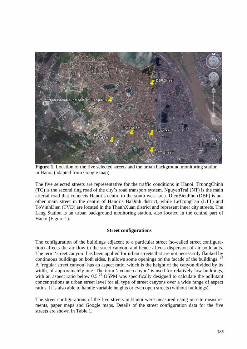
185

Figure 1. Location of the five selected streets and the urban background monitoring station in Hanoi (adapted from Google map).

The five selected streets are representative for the traffic conditions in Hanoi. TruongChinh (TC) is the second ring road of the city’s road transport system. NguyenTrai (NT) is the main arterial road that connects Hanoi’s centre to the south west area. DienBienPhu (DBP) is an-other main street in the centre of Hanoi’s BaDinh district, while LeTrongTan (LTT) and ToVinhDien (TVD) are located in the ThanhXuan district and represent inner city streets. The Lang Station is an urban background monitoring station, also located in the central part of Hanoi (Figure 1).

Street configurations

The configuration of the buildings adjacent to a particular street (so-called street configura-tion) affects the air flow in the street canyon, and hence affects dispersion of air pollutants. The term ‘street canyon’ has been applied for urban streets that are not necessarily flanked by continuous buildings on both sides. It allows some openings on the facade of the buildings. 24 A ‘regular street canyon’ has an aspect ratio, which is the height of the canyon divided by its width, of approximately one. The term ‘avenue canyon’ is used for relatively low buildings, with an aspect ratio below 0.5.24 OSPM was specifically designed to calculate the pollutant concentrations at urban street level for all type of street canyons over a wide range of aspect ratios. It is also able to handle variable heights or even open streets (without buildings).9

The street configurations of the five streets in Hanoi were measured using on-site measure-ments, paper maps and Google maps. Details of the street configuration data for the five streets are shown in Table 1.

Table 1. Street configurations of 5 streets in Hanoi. Source: Site measurements performed within this study.

Building Height (m) No Street name

in short Street name in full Side 1 Side 2

Street Width (m)

Street

Orientation

1 TC Street TruongChinh Street 4.0 4.0 12.0 107o

2 DBP Street DienBienPhu Street 2.0 2.0 14.0 135o

3 NT Street NguyenTrai Street 4.0 4.0 60.0 55o

4 LTT Street LeTrongTan Street 7.5 2.1 8.9 150o

5 TVD Street ToVinhDien Street 10.0 10.0 9.1 37o

1 TC Street TruongChinh Street 4.0 4.0 12.0 107o

2 DBP Street DienBienPhu Street 2.0 2.0 14.0 135o

Side 1 and side 2 refer to opposite sides of the street, the street width is the distance between opposite building facades, and the street orientation is given in relation to north. Side 1 is in the OSPM defined as the side of the street that is the first encountered when going from north in a clockwise direction. The data in table 1 show that LTT street and TVD street can be con-sidered as regular street canyons while TC street, DBP street and NT street are consider as avenue canyons, or even close to open streets.

Traffic and emission data

In Hanoi, the vehicle fleet is classified into six vehicle categories: Motorbike, Car 4-16 seats, Car >24 seats, Bus, Truck and Container (Figure 2). This vehicle classification was defined by the Swiss Vietnamese Clean Air Program (SVCAP) and the Hanoi Centre for Environ-mental and Natural Resources Monitoring and Analysis (CENMA). It was selected for OSPM calculation since the emission factors were available for this vehicle classification. These ve-hicle categories are used for traffic counting in the streets, as well as to estimate emissions in the OSPM. 2

186

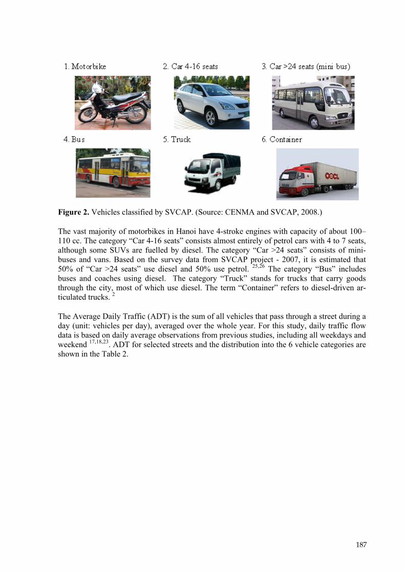
Figure 2. Vehicles classified by SVCAP. (Source: CENMA and SVCAP, 2008.)

The vast majority of motorbikes in Hanoi have 4-stroke engines with capacity of about 100–110 cc. The category “Car 4-16 seats” consists almost entirely of petrol cars with 4 to 7 seats, although some SUVs are fuelled by diesel. The category “Car >24 seats” consists of mini-buses and vans. Based on the survey data from SVCAP project - 2007, it is estimated that 50% of “Car >24 seats” use diesel and 50% use petrol. 25,26 The category “Bus” includes buses and coaches using diesel. The category “Truck” stands for trucks that carry goods through the city, most of which use diesel. The term “Container” refers to diesel-driven ar-ticulated trucks. 2

The Average Daily Traffic (ADT) is the sum of all vehicles that pass through a street during a day (unit: vehicles per day), averaged over the whole year. For this study, daily traffic flow data is based on daily average observations from previous studies, including all weekdays and weekend 17,18,23. ADT for selected streets and the distribution into the 6 vehicle categories are shown in the Table 2.

187

Table 2. Average Daily Traffic for each vehicle class (vehicles/day). Source: Truc, V. T. Q. (2005), CENMA and SVCAP, 2008

Street name Motorbike

Car 4-16 seats

Car > 24 seats

Bus Truck Container Sum (ADT)

TC 166,449 11,040 620 707 3511 56 182,382

DBP 21,838 1,302 84 9 22 0 23,340

NT 298,462 18,314 1,755 2,728 9,737 288 331,284

LTT 82,821 2,836 72 195 271 0 86,195

TVD 9,528 384 0 87 0 9,999

Table 2 shows that ‘Motorbikes’ are the dominant vehicle class in the streets, followed by “Car 4-16 seats”. The ADT can reach very high values of more than 300,000 vehicles/day in Hanoi.

Besides the ADT for the different vehicle classes, the OSPM also needs the diurnal variation of traffic in order to calculate hourly emissions.

The diurnal variation of traffic describes the hourly variation in the traffic flow during a 24 hour period, and might depend on the day of the week. This variation usually does not change much with time (i.e. within one year or between years), since it reflects the daily habits and routines of the population. For this study, the diurnal traffic variations are based on traffic counts collected in the Hanoi Transport Project carried out by the Japan International Coop-eration Agency (JICA) and the Transport Engineering Design Incorporated (TEDI) – Ministry of Transport, Vietnam.18 In this project, traffic flow was estimated in 43 locations. Our analy-sis of traffic counts from these studies indicates that there is no significant difference in traffic flow on different workdays (Monday-Friday) or between workdays and weekends.17,18,23 Therefore we assume in this modeling study, that the diurnal traffic variations of different streets for the different vehicle categories are the same for all days of the week (Figure 3).

188

Hourly fraction of daily total for all vehicle fleets

0

2

4

6

8

10

12

1h 2h 3h 4h 5h 6h 7h 8h 9h 10h 11h 12h 13h 14h 15h 16h 17h 18h 19h 20h 21h 22h 23h 24hHour

Perc

enta

ge p

er d

ay (%

)

MotorbicleCar 4-16 seatsCar > 24 seatsBusTruckContainer

Figure 3. Average diurnal variation of the six vehicle categories plotted as hourly fraction (in %) of the daily total of each vehicle category. Based on data from 43 locations. (Source: JICA & TEDI, 2006)

For the motorbike category, there are two large peaks in traffic flow, corresponding to the morning and evening rush hours, and two smaller peaks at 11:00 and 13:00 when people go out for lunch and then come back to work. The “Car 4-16 seats” and “Car > 24 seats” have very similar variations but with less pronounced rush hour peaks. The ‘Bus’ category has its own daily schedule. The ‘Truck’ category does not have permission to drive during rush hours (7h-9h; 16h-18h) and trucks normally circulate on roads from 10:00 to 15:00. ‘Con-tainer’ category vehicles are only allowed to drive on the main roads: TC and NT (Table 2) and are most active during the night (Figure 3).

The vehicle specific emission factors (unit: g km-1 vehicle-1) are needed together with the traffic data for calculation of the emissions. In the OSPM, emission factors are usually based on the European emission model COPERT IV (EEA, 2007). 20 However, in this study, emis-sion factors are derived in a different way since COPERT IV is not applicable for Hanoi. The applied emission factors and references to where they originate from are given in Table 3.

189

Table 3. Applied emission factors for OSPM calculation in Hanoi.

Emission factor ( g km-1) Vehicle classes PM5 SO2 NOx CO Benzene

Motorbike 0.101 0.032 0.301 3.623 0.0234 Car 4-16 Seats 0.101 0.172 1.501 3.623 0.0463 Car >24 Seats 0.481 0.252 8.551 5.623 0.0603 Bus 1.501 0.642 7.601 3.103 0.0323 Truck 0.801 0.402 11.001 2.753 0.0453 Container 3.281 1.062 17.001 3.103 0.0253 1Sivertsen and The, 2006 2 CENMA and SVCAP, 2008 3 1999 data set for Denmark 4 HuongGiang, 2008

5 PM represent for the exhaust source

For Hanoi, no measurements of vehicle emission factors were available. Emission factors were reported in previous projects and the emission factors for Hanoi are based on those sources for NOx and PM10.6 The directly emitted NO2 fraction is assumed to be 5% of total NOX (i.e. the sum of NO2 + NO) by mass. This value was representative for Europe before 2000. After 2000 the NO2 fractions has increased in Europe due to much higher share of die-sel passenger cars and particle filters with CRT technology. Since this development has not taken place in Hanoi the value of 5% for the directly emitted NO2 fraction is assumed for this study. The emission factor for SO2 was calculated by Thoan Christopher Nguyen and Patrick Gaffney - California Air Resources Board (ARB), based on consulting and training experi-ence in Asia developing countries and the US EPA data base (SVCAP project 2007) 2. Emis-sion factors of benzene for motorbikes originate from a study in HoChiMinh city.19 The ben-zene emission factors of other vehicle types and emission factors for CO are based on a 1999 data set for Denmark according to COPERT. The vehicle fleet composition in 1999 in Den-mark is comparable to the condition of Vietnam in 2007, since the Vietnamese vehicle fleet is dominated by cars with the EURO II emission standard and older vehicles27. For the Danish conditions, the emission factor of benzene is calculated based on 1.0% content of benzene in petrol. However, the content of benzene in Vietnamese petrol is 2.5% (according to Vietnam-ese standard: TCVN 6776-2005) 26 and a correction of the emission factors in Vietnam was carried out and is discussed later.

Meteorology data

The OSPM requires hourly meteorological data for calculations. The required data are wind speed, wind direction, temperature and global radiation. Wind speed and wind directions should be provided at rooftop level in the city, in order for OSPM to estimate the wind speed and wind direction inside the street canyon (channeling effect). Temperature and global radia-tion are used to calculate the chemical transformation between NO, NO2 and O3. In this study, meteorological data from the Lang station were used. The wind roses for the modeling peri-ods in 2004 and 2007 are shown in Figure 4:

190

Figure 4. Wind rose during the two modeling periods in 2004 (left) and 2007 (right) for a background station (Lang Station) in Hanoi.

Due to its central location and after some comparison with data from the airport station, the meteorological data at Lang station were considered to be representative for the rooftop con-ditions at the 5 selected streets.

Urban background measurements

The OSPM requires hourly urban background concentrations. The urban background repre-sents conditions at rooftop level in a city or at ground level away from local sources (e.g. in a park area). Hourly monitoring data from the Lang Station was the first choice to represent the urban background for the five selected street sites. However, analysis of the air pollution level at the Lang Station compared to air pollution levels from a campaign using passive samplers at many urban background sites revealed that the air pollution levels measured at the Lang Station in 2007 were approximately 1.5 times higher compared to the passive sample meas-urements by SVCAP project in 2007. This indicates that the Lang station overestimates the urban background concentrations. The Lang Station is located close to the busy LangHa street and NguyenChiThanh Street. Thus the data are more representative for road sides than for urban background conditions. Furthermore, the air pollution data are not systematically col-lected and documented, and the quality control (QC) is often inadequate.

For this study, 4 week averages from passive sample measurements are used to represent the general air pollution level in the urban background (Figure 5) and to down-scale (adjust) the hourly measurements at the Lang Station (Figure 6).

191

Passive Sampling during the period of 11 January - 6 Febuary 2007

0

5

10

15

20

25

30

35

40

45

50

55

60

65

70

75C

once

ntra

tion

(µg/

m3 )

Hot Spots of TrafficRoad SideIndustrial AreasUrban BackgroundRural Areas

EU/WHOTCVN

EU

TCVN

TCVN

EU/WHO

NO2 SO2 Benzene

Figure 5. Mean concentrations and standard deviation of NO2, SO2 and Benzene for five site categories in 2007 using passive sampling compared to Vietnamese standard TCVN 5937-2005, WHO and EU air quality limit values (Measured data was obtained from SVCAP 2007)23

The 100 locations of measurement points in the passive sample campaign were plotted on a GIS map and Google maps, based on the available information from site reports 2,3. The traf-fic hotspots (6 points), industrial hotspots (8 points), rural areas (5 points) are all representa-tive for their types. The other 81 points, are divided in two groups: the 36 points which lie within 15 m from a street are influenced by pollution from streets are considered as roadside points and the rest (45) are considered as urban backgrounds.3 Averages in each category are plotted in Figure 5, together with air quality standards defined by Vietnam, the WHO and the EU.

Mean NO2 concentrations exceed the limit value for traffic hotspots and roadsides, whereas other categories are lower than the EU limit values (the same as the Vietnamese standard and WHO limit value). The concentrations of SO2 have not exceeded the Vietnamese Standard (TCVN 5937-2005), however they are more than double the EU limit value (same as WHO) for traffic and industrial hotspots and roadsides, and other categories also exceed the EU/WHO limit value. The hotspots and roadside the concentration of BNZ are higher than the Vietnamese Standard, and also three times higher than the EU limit value, and other site categories also exceed the EU limit.

The hourly urban background air quality data for the OSPM have been constructed by com-bining the hourly variation at the Lang Station and the mean value of the “real” urban back-ground sites in the passive sample campaign in 2007 (Figure 6).

192

Average diurnal variation of NO2 at Lang station (12 January - 5 February 2007)

0

10

20

30

40

50

60

70

80

0 1 2 3 4 5 6 7 8 9 10 11 12 13 14 15 16 17 18 19 20 21 22 23

Hour

Con

cent

ratio

n (µ

g/m

3 )

Original average value of cNO2_bCorrected average value of cNO2_b Mean value by passive sample in 2007

Figure 6. Illustration of the construction of hourly urban background data for the OSPM.

Benzene concentrations (BNZ) are not measured at the Lang Station. However, the OSPM requires urban background concentration of BNZ to calculate the concentration in the street. For the pollutants emitted from traffic, CO and BNZ concentrations have a strong correlation since they are both emitted from petrol-powered engines.28 Therefore, it is possible to esti-mate BNZ concentrations based on a correlation with CO concentrations. This correlation is based on a benzene content of 1% in petrol in Demark. 28 In Vietnam, the benzene content in petrol is 2.5% (Vietnamese standard: TCVN 6776-2005) The motorbikes and Car 4-16 seats which are using petrol are dominating the vehicle fleet (Table 2). We therefore consider only petrol vehicles in the correlation. Equation 1 was adapted for Vietnamese benzene content and is used to calculate BNZ from CO concentrations in the urban background:

C_BNZ = 9.75 *C_CO (1)

where C_BNZ is in µg/m3 and C_CO is in mg/m3.

The roadsides observations of CO and BNZ in NT street and TC street, DBP street17 (Table 5) are used to check equation 1 and they agree with this relationship. The average coefficient for this is 8.56, which is in good agreement with equation 1.

Street air pollutant measurements

Measurements of NOx, NO2, NO, SO2 CO and BNZ from the five street locations were col-lected to evaluate the model outputs calculated by the OSPM. In 2004, hourly street meas-urements were carried out in a project by the Asian Institute of Technology (AIT)17. The measurements, performed at both sides of the streets (S1 and S2), focused mainly on the BNZ contribution from vehicles. The project also measured NOx, NO2, NO, SO2 and CO for some

193

hours of the day. Hourly traffic counts were carried out during the same time periods as air pollutant measurements.

In 2007 street measurements were carried out by PASSAM, Switzerland and CENMA, Viet-nam 2 using passive sample measurements for NO2, SO2, and BNZ. This 3 week average data was compared with the mean value of the model predictions during the same period. The measurements are summarized in Table 4.

Table 4. Average of air quality measurements in five streets in Hanoi. Source: Truc, V. T. Q. (2005), CENMA and SVCAP, 2008

NOx NO2 NO SO2 CO BNZ

S1 S2 S1 S2 S1 S2 S1 S2 S1 S2 S1 S2

µg/m3 µg/m3 µg/m3 µg/m3 mg/m3 µg/m3 TC Street (8-24, Nov 2004) - hourly measurement

6.4 7.4 1.1 1.5 3.4 3.9 35.3 8.1 5.7 87.2 71.4

DBP Street (2-4, Nov 2004) - hourly measurement 3.3 3.6 0.8 0.9 1.6 1.8 23.9 6.6 7.1 28.7 39.2

NT Street (16-17, Dec 2004) - hourly measurement 80.8 31.9 39.1 39.1 7.8 74.0 59.1

LTT Street (12 Jan - 5 Feb 2007) - passive sample measurement

39.5

32.9

TVD Street (12 Jan - 5 Feb 2007) - passive sample measurement 39.2 27.6

The measurements of NO2 and NO concentrations in the TC and DBP streets seem unrealisti-cally low compared to the passive sample campaign in 2007. Therefore, these data are not used for model evaluation. In summary, the hourly data of CO, SO2 and BNZ in 2004 and the passive sample data for NO2 and SO2 in January – February, 2007 are used for model evalua-tion.

ESTIMATE OF AVERAGE FLEET VEHICLE EMISSION USING BACKWARD CALCULATIONS

The average vehicle fleet emission factors were also estimated using the OSPM by backward calculations to assess and adapt the applied vehicle emission factors from previous studies given in Table 3. This methodology assumes that the OSPM gives a nearly perfect description of the dispersion process between vehicle emissions and the street increment in concentra-tions. The methodology is described below.

The fleet emissions can be calculated from the concentration of a particular non-reactive pol-lutant in the street in the following way 29,30:

194

(2)

Qh: Hourly vehicle emission in g m-1 s-1.

Ch: Hourly concentration of a pollutant in the street in g m-3.

Ch, background: Hourly concentration of a pollutant in the urban background in g m-3.

Fh (meteorology): Dispersion function given by the OSPM in s m-2.

The total emission Qh can alternatively be expressed as:

(3)

Nk,h : Hourly traffic flow of the kth vehicle category (vehicle hour-1).

qk: Emission factor of the kth vehicle category (g veh-1 km-1).

Then the average fleet vehicle emission factors qaverage (g veh-1 km-1) can be estimated from the total emission Qh by equation 2 divided by the total number of vehicles Nh (sum over all vehicle categories).

RESULT AND DISCUSSION

Air pollutant emissions per vehicle category

The average vehicle distribution and the average emission contribution from the different vehicle categories are shown in Figure 7. The estimates are based on traffic data from Table 2, the emission factors from Table 3 and averaged over the 5 streets.

195

Figure 7. Average contribution (%) to emission of NOx, SO2, CO, BZN and PM10 from each vehicle category for five streets in this model evaluation study. The vehicle distribution (%) is shown in the top left chart.

Motorbikes are the dominant vehicle type in Hanoi as they constitute 92-95% of all vehicles. They are also the main source of emissions in the streets. Motorbikes contribute 56% of NOx, 65% of SO2, 94% of CO, 92% of BNZ, and 86 % of PM10 emissions. The “trucks” and the “car 4-16 seats” also have relatively large contributions to NOx and SO2 emissions. Trucks contribute 21% of NOx and 10% of SO2 emissions, and “Car 4-16 seats” contribute 14% NOx and 19% of SO2 (Figure 7).

Measurements and model results

Observed and modeled CO concentrations for the TC Street are shown as diurnal variation in Figure 8.

196

CO diurnal variation at TC Str. (8-24, Nov 2004) (mg/m3)

0

2

4

6

8

10

12

14

1 2 3 4 5 6 7 8 9 10 11 12 13 14 15 16 17 18 19 20 21 22 23 24

Hour

CO

con

cent

ratio

n (m

g/m3 )

Average of cCO_obs_1

Average of cCO_obs_2

Average of cCO_mod_1

Average of cCO_mod_2

Average of cCO_b

Figure 8. Modeled and observed diurnal variation of CO concentrations for the TC Street in Hanoi. “mod” refers to modeled street concentrations, “obs” to observed street concentra-tions and “b” to urban background concentrations.

The modeled diurnal variation of CO concentrations shows peaks in the morning and after-noon rush hours, and also relatively high concentrations during the evening. This diurnal variation fits well with the diurnal variation of motorbike traffic (Figure 3), since motorbikes are the dominant source to CO emissions from vehicles (Figure 7). The model predicts almost the same concentrations for the two opposite sides of the street (S1 and S2). This has several reasons: 1) at low wind speeds (below 3 m/s), which are very common in Hanoi and which give the highest concentrations, the dispersion is dominated by the TPT, and the wind direc-tion has only a minor influence on the relative concentrations at the two sides of the street; 2) the low building heights and the symmetric canyon (4m height at both sides) will, even for higher wind speeds, lead to similar concentration levels at both sides; and 3) during the rela-tively long modeling period with variable wind directions, the differences between the two sides are averaged out. Figure 8 shows that the street increment (difference between street and urban background concentrations) is considerable. The observed diurnal variation in CO con-centrations of side 2 shows a similar diurnal pattern to the modeled variation, although obser-vations are somewhat higher during the day and lower during the evening. The observed CO concentrations of side 1 during the morning and night fits well with that of side 2, but during 16:00-18:00 concentrations are much higher for no obvious reason, probably due to special traffic or meteorological conditions during the measurement period or uncertainties in the measured data. BNZ concentrations were also measured for this street and concentrations levels are the same for both sides (Figure 9).

The modeled diurnal concentrations of SO2 and BNZ show a similar pattern as for CO. It is however not possible to present measured diurnal variations of SO2 and BNZ, due to the very limited number of observations.

197

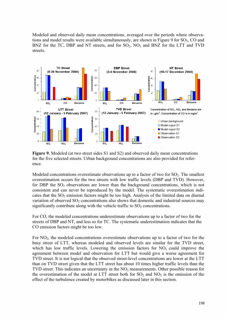
Modeled and observed daily mean concentrations, averaged over the periods where observa-tions and model results were available simultaneously, are shown in Figure 9 for SO2, CO and BNZ for the TC, DBP and NT streets, and for SO2, NO2 and BNZ for the LTT and TVD streets.

Figure 9. Modeled (at two street sides S1 and S2) and observed daily mean concentrations for the five selected streets. Urban background concentrations are also provided for refer-ence.

Modeled concentrations overestimate observations up to a factor of two for SO2. The smallest overestimation occurs for the two streets with low traffic levels (DBP and TVD). However, for DBP the SO2 observations are lower than the background concentrations, which is not consistent and can never be reproduced by the model. The systematic overestimation indi-cates that the SO2 emission factors might be too high. Analysis of the limited data on diurnal variation of observed SO2 concentrations also shows that domestic and industrial sources may significantly contribute along with the vehicle traffic to SO2 concentrations.

For CO, the modeled concentrations underestimate observations up to a factor of two for the streets of DBP and NT, and less so for TC. The systematic underestimation indicates that the CO emission factors might be too low.

For NO2, the modeled concentrations overestimate observations up to a factor of two for the busy street of LTT, whereas modeled and observed levels are similar for the TVD street, which has low traffic levels. Lowering the emission factors for NOx could improve the agreement between model and observation for LTT but would give a worse agreement for TVD street. It is not logical that the observed street-level concentrations are lower at the LTT than on TVD street given that the LTT street has about 10 times higher traffic levels than the TVD street. This indicates an uncertainty in the NO2 measurements. Other possible reason for the overestimation of the model at LTT street both for SO2 and NO2 is the omission of the effect of the turbulence created by motorbikes as discussed later in this section.

198

For BNZ, the modeled concentrations underestimate observations up to a factor of about two for the busy streets of TC and NT, and less so for DBF, which has low traffic levels. The sys-tematic underestimation indicates that the BNZ emission factors may be too low. Further-more, the urban background concentration of BNZ was estimated based on observed correla-tions between BNZ and CO (see above). In addition, the assumptions of BNZ emission fac-tors for vehicles other than motorbikes for Vietnamese condition are based on a 1999 data set for Denmark according to COPERT. It is obvious that these assumptions about the urban background and emission factors are highly uncertain.

Traffic Produced Turbulence (TPT)

In the present version of the OSPM, TPT of all vehicle types except motorbikes is taken into account. Since motorbikes are the dominant vehicle type in Hanoi they certainly contribute to TPT although their horizontal area is small compared to passenger cars. TPT is also espe-cially important during the frequently observed low wind speed conditions in Hanoi. A sensi-tivity analysis was carried out where it was assumed that each motorbike contributes with the same TPT as a passenger car. OSPM calculations showed that concentrations were lowered by 33% under these assumptions. However, the frontal area of a popular motorbike (Honda Future) is only about 27% (including the driver) of the frontal impact area (width multiply by height) of a popular car (Honda Civic). It is therefore to be expected that including TPT con-tribution from motorbike in OSMP will lower the modeled concentrations by approximately 10%. It illustrates that it is important to take into account TPT also for motorbikes.

Vehicle emission factors

A comparison of emission factors (g km-1 vehicle-1) for the different vehicle categories in this study and selected studies from the literature is shown in Table 5.

Table 5. Comparison of emission factors (g km-1 vehicle-1) for the different vehicle categories in different studies PM SO2 NOx CO Benzene

1. Motorbike Hanoi (from table 3) 0.10 0.03 0.30 3.62 0.023 Bangkok 31 32.8±8.9 Bangkok (Chassis dynamometer)32 0.08±0.07 2.23±2.2 Bangkok (Mobile 6)32 0.48 0.85 13.3 Chan and Weaver 33 19.0 China 2009 34 0.08±0.02 2.17±0.78

2. Car 4-16 seats Hanoi (from table 3) 0.10 0.17 1.50 3.62 0.023 Bangkok 31 1.5±0.91 Bangkok (Chassis dynamometer)32 1.37±1.0 5.12±5.65 Bangkok (Mobile 6)32 0.48 0.49 5.41 Copenhagen 1997 29 0.9±0.1 17.3±0.7 0.11±0.01

199

China - 200735 1. Carburetor vehicles 2.17 24.08 2. Electronic injection vehicles 2.23 12.91 3. Euro I vehicles 1.33 6.21 4. Euro II vehicles 0.81 3.32

3. Bus Hanoi (from table 3) 1.50 0.64 7.60 3.10 0.032 Bangkok (Chassis dynamometer)32 1.25 12.55 21.99 Bangkok (Mobile 6)32 1.15 23.12 8.89 Copenhagen 1997 29 12.5±3.0 9.6±4 0.05±0.05

4. Truck Hanoi (from table 3) 0.80 0.40 11.00 2.75 0.045 Bangkok (Chassis dynamometer)32 1.25 12.55 21.99 Bangkok (Mobile 6)32 1.15 23.12 8.89 Copenhagen 1997 29 12.5±3.0 9.6±4 0.05±0.05

It is difficult to compare emission factors across countries due to differences in the vehicle fleet, emission standards, maintenance, etc. CO emission factors vary up to a factor of 10 for motorbikes and up to a factor of 3 for other categories among the different studies. This study has applied relatively low emission factors compared to other studies and the model evalua-tion against observed CO concentrations also indicates that the applied emission factors for CO may be too low. For NOx emission factors, there is less variation across the different stud-ies.

The average fleet vehicle emission factors have been estimated using the OSPM for backward calculations based on the hourly concentration data from 2004 available for three out the five selected streets. Calculation of average fleet vehicle emission factors is done according to the equations 2 and 3. The results are shown in Table 6.

Table 6. Average fleet vehicle emission factors of 3 selected streets by backward calculation

Emission factor (g km-1 vehicle-1) SO2 CO Benzene

TC – 2004 (a ring road) 0.038 4.0 0.051 DBP – 2004 (an inner city road) 0.022 16.9 0.125 NT – 2004 (an arterial road) 0.026 10.4 0.079 Mean 0.029 10.4 0.085

The average fleet vehicle emission factors in Table 6 can be used to estimate the emissions from other streets if the traffic volume is known according to the road type (arterial road, ring road, inner city road) or the mean may be used to estimate emissions from traffic for a whole city, if one knows the average traffic volumes and length of the road network.

The average vehicle fleet emission factors, estimated by backward calculations, have been compared to other studies, see Table 7.

200

Table 7. Average fleet vehicle emission factors from different studies Emission factor (g km-1 vehicle-1)

PM10 SO2 NOx CO BenzeneThis study, backward calculations (Table 6) 0.029 10.4 0.085

This study, average fleet vehicle emission factors for 5 selected streets (by OSPM).

0.108 0.044 0.547 3.6 0.024

HoChiMinh city36 0.0067OSPM emission module for the street of Jagtvej, Copenhagen in 1999

1.41 5.8 0.041

The average vehicle fleet emission factor for SO2, estimated by backward calculation, is con-siderably lower than the applied emission factor for OSPM calculations. A lower SO2 emis-sion factor would reduce the overestimation by the OSPM for SO2 concentrations.

The average vehicle fleet emission factor for CO, estimated by backward calculation, is three times higher than the applied emission factor for OSPM calculations. Higher CO emission factors would cause less underestimation by the OSPM for CO concentrations. The emission factor estimated by backward calculations is about a factor of 2 higher than was estimated for Copenhagen in 1999 (comparable car fleet age). This might be due to motorbike emissions, which are not represented in the Copenhagen vehicle fleet.

The average vehicle fleet emission factor for BNZ, estimated by backward calculation, is 3-4 times higher than the applied emission factor for OSPM calculations. Higher BNZ emission factors would cause less underestimation by the OSPM for BNZ concentrations. The emission factor estimated by backward calculations is about two times higher than a busy street in Co-penhagen in 1999, among others, due to higher content of benzene in petrol in Hanoi. The estimated average emission factor for BNZ by backward calculation is about 10 times higher compared to the tracer study carried out by Belalcazar30 in HoChiMinh city showing ex-tremely small values compared also to other literature (Table 5).

Challenges and future work for applying a dispersion model (OSPM) in Hanoi

This modeling study at street level in Hanoi also shows the challenges of applying dispersion models in a context where high quality model input data and high quality measurements are missing and still need further improvements. Higher quality input data will enable OSPM to more accurately describe the actual pollution level at street scale.

The emission factors of vehicles in developing countries are inadequately represented in an emission model such as COPERT 4 (EU) or Mobile 6 (US). An experimental study of the emission factors for all vehicle categories reflecting “real” Vietnamese conditions should be conducted.

201

In this research, the direct emission of NO2 was assumed to be 5% from total NOX emission in mass, as in European conditions before 2000. This assumption should be verified using detailed hourly air quality measurements of NO, NO2 and O3. Also the important pollutants PM10 and PM2.5

need to be addressed in future measurement and modeling studies.

Due to the prevailing low wind speeds in Hanoi, traffic produced turbulence (TPT) is the sig-nificant dispersion mechanism in OSPM for air pollution in street scale. However the very sunny and hot weather in Hanoi might lead to some heat induced dispersion (unstable condi-tions) presently not represented in OSPM. More research based on high quality measurements is needed on this issue.

For larger scale calculations, the street types are to be categorized systematically for a larger area in Hanoi in a scientific way according to street function, the vehicle volume in different categories and the street width and building heights, and updated information is needed pref-erably in a GIS database. Such a database should be updated annually and will be useful for trend analysis of traffic development and for plans towards sustainable urbanization and traf-fic management.

CONCLUSIONS

In this study, the OSPM was applied in Hanoi for five selected streets and evaluated against concentration measurements of NO2, SO2, CO and BNZ. The model was also used to estimate average fleet vehicle emission factors based on backward calculations.

The motorbike is the dominant vehicle type in Hanoi, as it constitutes 92-95% of all vehicles. It is also the main source of emissions in the streets.

Analysis of the modeled and observed diurnal variation of CO for one street showed that the OSPM generally reproduced the diurnal variation.

The model evaluation also showed that the OSPM, given the applied input data, overesti-mated daily mean concentrations of SO2 and CO and underestimated concentrations of NO2 and benzene. Among the reason are uncertainties in the emission factors and the missing TPT contribution from motorbikes. However, NO2 measurements are also likely to be uncertain.

The evaluation study illustrates that it is important to incorporate TPT for motorbikes into the OSPM. TPT is neglected in OSPM for motorbikes, which are usually a minor vehicle class in West or North European conditions. If TPT for motorbikes were taken into account, it would further reduce modeled concentrations. It is expected that including TPT contribution from motorbike in OSPM will reduce the modeled concentrations approximately 10%.

This study also illustrates some of the challenges and future needs for air pollution modeling in Hanoi. In the previous section we outlined the shortcomings of the present study and sug-gested directions for further investigations and air pollution research in Hanoi.

202

ACKNOWLEDGMENTS

This work is part of a PhD study funded by the Vietnamese Government (project 322) to-gether with supplemental supports from the Danish International Development Agency (DANIDA) and the National Environmental Research Institute (NERI), Aarhus University, Denmark. The authors would like to thank colleagues at CENMA, SVCAP, CENRE (IM-HEN), CEMDI, (from Vietnam), PASSAM (Switzerland) and AIT (Thailand) for their valu-able contribution to the data collections for this model study. The authors also would like to thank the anonymous reviewers for their valuable comments on this paper.

REFERENCE LIST

1. Son D.H; Le Van Sy; others Air quality report (in Vietnamese); Ministry of Natural Re-sources and Environment, Vietnam, 2008.

2. CENMA; SVCAP Pilot Emission Inventory in Hanoi; CENMA Publisher, Vietnam, 2008.

3. Hien, P. D. The first passive sampling campaign in Hanoi, SVCAP Publisher, Vietnam, 2007.

4. Truc, V. T. Q.; Kim Oanh, N. T. Roadside BTEX and other gaseous air pollutants in relation to emission sources. Atmospheric Environment 2007, 41 (36), 7685-7697.

5. Saksena, S.; Quang, T. N.; Nguyen, T.; Dang, P. N.; Flachsbart, P. Commuters' expo-sure to particulate matter and carbon monoxide in Hanoi, Vietnam. Transportation Re-search Part D: Transport and Environment 2008, 13 (3), 206-211.

6. Sivertsen, B.; The, N. T. Support for the Review of Air Quality Management Sub-component for the Hanoi Urban Transport and Development Project; NILU Scientific Report NO. NILU OR 78/2006

7. SVCAP Concept for an improved air quality monitoring system and emission inventory for Hanoi; SVCAP: Hanoi, Vietnam, 2005.

8. Hien, P. D.; Bac, V. T.; Thinh, N. T. H. PMF receptor modelling of fine and coarse PM10 in air masses governing monsoon conditions in Hanoi, northern Vietnam. Atmos-pheric Environment 2004, 38 (2), 189-201.

9. Berkowicz, R.; Hertel, O.; Larsen, S. E.; Sørensen, N. N.; Nielsen, M. Modelling traffic pollution in streets.; National Environmental Research Institute, Roskilde, Denmark: 1997.

10. Fu, L. X.; Hao, J. M.; Hertel, O.; Berkowicz, R. Modeling traffic-related air pollution in street canyons of Beijing. Journal of the Air & Waste Management Association 2000, 50 (12), 2060-2066.

203

11. Ziv, A.; Berkowicz, R.; Genikhovich, E. L.; Palmgren, F.; Yakovleva, E. Analysis of the St. Petersburg traffic data using the OSPM. Water, Air, & Soil Pollution: Focus 2002, 2, 297-310.

12. Aquilina, N.; Micallef, A. Evaluation of the operational street pollution model using data from European cities. Environmental Monitoring and Assessment 2004, 95 (1-3), 75-96.

13. Mensink, C.; Lefebre, F.; Janssen, L.; Cornelis, J. A comparison of three street canyon models with measurements at an urban station in Antwerp, Belgium. Environmental Modelling & Software 2006, 21 (4), 514-519.

14. Vardoulakis, S.; Valiantis, M.; Milner, J.; ApSimon, H. Operational air pollution model-ling in the UK--Street canyon applications and challenges. Atmospheric Environment 2007, 41 (22), 4622-4637.

15. Berkowicz, R.; Ketzel, M.; Jensen, S. S.; Hvidberg, M.; Raaschou-Nielsen, O. Evalua-tion and application of OSPM for traffic pollution assessment for a large number of street locations. Environmental Modelling & Software 2008, 23 (3), 296-303.

16. Jensen, S. S.; Larson, T.; Deepti, K. C.; Kaufman, J. D. Modeling traffic air pollution in street canyons in New York City for intra-urban exposure assessment in the US Multi-Ethnic Study of atherosclerosis and air pollution. Atmospheric Environment 2009, 43 (30), 4544-4556.

17. Truc, V. T. Q. Assessment of VOC levels from motor vehicle exhaust and potential health effects in Hanoi, Vietnam, Master thesis, Asian Institute of Technology (AIT), Thailand. 2005.

18. JICA & TEDI Hanoi Urban Transport Development Project; TEDI Publisher, Vietnam: 2006.

19. HuongGiang, N. T. Roadside air quality in Ho Chi Minh City and vehicle emission es-timation by back calculation, Master thesis, Asian Institute of Technology (AIT), Thai-land 2008.

20. EEA EMEP/CORINAIR Atmospheric Emissions Inventory Guidebook; EEA 2007.

21. Berkowicz, R. OSPM - A parameterised street pollution model. Environmental Monitor-ing and Assessment 2000, 65 (1-2), 323-331.

22. Hanoi statistical office Hanoi statistical yearbook 2007; KhuyenHoc Co, Limited, Viet-nam: Hanoi, 2008.

23. SVCAP; Fabian, S. Report on the first Air Quality Measuring Campaign in Hanoi using the Passive Sampling Method; SVCAP Publisher, Vietnam: 2007.

204

24. Vardoulakis, S.; Fisher, B. E. A.; Pericleous, K.; Gonzalez-Flesca, N. Modelling air quality in street canyons: a review. Atmospheric Environment 2003, 37, 155-182.

25. Do, Quang Trung, Personal communications: Mr Do Quang Trung Person in charge of Emission Inventory of SVCAP Project 2007, Vietnam, 2009.

26. Vu, Nguyen Hoang, Personal communications: Dr Nguyen Hoang Vu, Head of Energy laboratory, Vietnam Military Technical Academy, Vietnam 2009.

27. EEA Environmental indicators: typology and overview, report no. 25. Copenhagen; European Environment Agency; 1999.

28. Palmgren, F.; Hansen, A. B.; Berkowicz, R.; Skov, H. Benzene emission from the actual car fleet in relation to petrol composition in Denmark. Atmospheric Environment 2001, 35 (1), 35-42.

29. Palmgren, F.; Berkowicz, R.; Ziv, A.; Hertel, O. Actual car fleet emissions estimated from urban air quality measurements and street pollution models. The Science of The Total Environment 1999, 235 (1-3), 101-109.

30. Ketzel, M.; Wåhlin, P.; Berkowicz, R.; Palmgren, F. Particle and trace gas emission factors under urban driving conditions in Copenhagen based on street and roof-level ob-servations. Atmospheric Environment 2003, 37, 2735-2749.

31. Kim Oanh, N. T.; Martel, M.; Pongkiatkul, P.; Berkowicz, R. Determination of fleet hourly emission and on-road vehicle emission factor using integrated monitoring and modeling approach. Atmospheric Research 2008, 89 (3), 223-232.

32. Ittipol P. Development of mobile source emission factors for Bangkok using modeling and emission testing tools. Master thesis, Asian Institute of Technology (AIT), Thai-land; 2004.

33. Chan L.M; Weaver C.S Motorcycle emission standards and emission control technol-ogy. Asia Technical Department. World Bank Press. 1994.

34. Y., Tsai, J., Ye, H., & Chiang, H.. (2009). Comparison of Exhaust Emissions Resulting from Cold- and Hot-Start Motorcycle Driving Modes. Journal of the Air & Waste Man-agement Association 2010, 59(11), 1339-1346.

35 Z., Wang, Q., He, K., Huo, H., Ma, Y., & Zhang, Q.. (2007). Characteristics of Real-World Vehicular Emissions in Chinese Cities. Journal of the Air & Waste Management Association 2010, 57(11), 1379-1386.

36. Belalcazar, L. C.; Fuhrer, O.; Ho, M. D.; Zarate, E.; Clappier, A. Estimation of road traffic emission factors from a long term tracer study. Atmospheric Environment 2009, 43 (36), 5830-5837.

205

206

ABOUT THE AUTHOR

Ngo Tho Hung is a researcher in Urban Environment and Infrastructure Engineering, Vietnam. From 2007-2010, he was a PhD research scholar at National Environmental Research Institute (NERI), Department of Atmospheric Environment, Aarhus Univer-sity and Denmark and Graduate School of Environmental Stress Studies (GESS), Roskilde University, Denmark. Corresponding author: email nth@dmu.dk; Phone: +45 4630 1105; Fax: +45 4630 1214. Dr. Steen Solvang Jensen and Dr. Matthias Ketzel are senior scientists on Atmospheric Environment at National Environmental Research Institute (NERI), Department of Atmospheric Environment. Dr. Nguyen Thi Kim Oanh is a professor at School of Environment, Resources and Development, Asian Institute of Technology, Thailand.

[Blank page]

Appendix 2: Presentation on the Seventeenth International Conference on Modelling, Monitoring and Management of Air Pollution, July 2009 – WIT, UK.

Air pollution modelling at road sides in Hanoi, Vietnam using the OSPM model – Ways of handling limitations in

input data

Ngo Tho Hung a,b,*; Matthias Ketzel a; Steen Solvang Jensen a; a: National Environmental Research Institute (NERI), Department of Atmospheric Environment, Aarhus University, Denmark b: Graduate School of Environmental Stress Studies, Roskilde University, Denmark * Corresponding author: email nth@dmu.dk ; Phone: +45 4630 1105; Fax: +45 4630 1214

Abstract:

In many metropolitan areas, traffic is the main source of air pollution. Estimation of air pollution levels near streets is needed for impact assessment of human health effects. This work has been carried out very well in many developed countries by a combination of air quality measurements and modelling. This study focused on how to use the “western model” for the cities in the developing world where data from air quality monitoring stations are limited or of varying quality. The study uses the Operational Street Pollution Model (OSPM) developed by NERI, Denmark (http://ospm.dmu.dk/) for a case study in Hanoi, the capital of Vietnam. OSPM model predictions were evaluated against air quality measurements at five busy streets. The emission contribution from traffic is calculated based on the number of vehicles per hour estimated in six vehicle categories and their emission factors. The urban background contribution is based on the diurnal variation in air quality measurements from a urban background monitoring station and adjusted to reflect a representative air pollution level based on measurements from a passive sample campaign performed at urban background locations. Meteorological data are from an urban meteorology monitoring station. Hourly measurement and passive sample measurements over three week periods are available at the street sides and were used for comparisons with model outputs. Additionally so-called backward calculations were performed to correct the initially assumed emission factors. An output of this study is average fleet emission factors that can be used for emission calculations at other streets in Hanoi and locations in South-East-Asia with similar vehicle types. This study also emphasizes the need to further eliminate the uncertainties in input data for street canyon air pollution modelling in Vietnam, namely providing reliable emission factors and hourly air pollution measurements of high quality.

207

Appendix 3: Presentation on the Better Air Quality conference in Asia (BAQ2010), November, 2010, Singapore

Integrated Monitoring and Assessment for air quality management – A case study in Hanoi, Vietnam

(Submitted abstract)

Ngo Tho Hung a,b,*; Steen Solvang Jensen a; a: National Environmental Research Institute (NERI), Department of Atmospheric Environment, Aarhus University, Denmark b: Graduate School of Environmental Stress Studies, Roskilde University, Denmark * Corresponding author: email nth@dmu.dk ; Phone: +45 4630 1105; Fax: +45 4630 1214

Abstract:

In relation to air quality management (AQM), Integrated Monitoring and Assessment (IMA) is defined as a combined usage of measurements and model calculations1. Integrated air quality monitoring is monitoring based on results from air quality measurements from fixed monitoring stations, and results obtained from calculations with air quality models. IMA combines data from both modelling and measurements to improve assessment of air quality. This concept has been developed, applied and evaluated for the past 20 years at NERI in Denmark.

A PhD study has been conducted during 2007-2010 with the aim to evaluate air quality models developed at NERI in the context of AQM in Vietnam with Hanoi as case study area2. The OSPM model3 was adapted to the traffic and vehicle emission conditions in Hanoi, and model results were compared to measurement campaigns at three streets where limited measurement data were available. The OSPM model was also used for backward modelling to estimate average vehicle emission factors based on the air quality measurement data. The OML model4 was used to assess the geographic distribution of air pollution in Hanoi based on an emission inventory for vehicle, domestic and industrial sources. OML model results for urban background conditions were compared to measurements from a passive sample measurement campaign and also for hourly pollutant data from an urban background station. The analysis showed many limitations in input data and measurement data but also many opportunities for improving air quality assessment with the use of air quality models in combination with measurements.

The presentation will outline the concept of IMA and present results from the case study in Hanoi and further provide recommendations for future implementation of IMA in AQM in Hanoi with focus on the role of air quality models.

References

[1] Hertel, O., Ellermann, T., Palmgren, F., Berkowicz, R., Løfstrøm, P., Frohn, L.M., Geels, C., Ambelas Skjøth, C., Brandt, J., Christensen, J.,

208

Kemp, K., Ketzel, M. 2007, 'Integrated air-quality monitoring - combined use of measurements and models in monitoring programmes', Environmental Chemistry, vol. 4 no. 2, pp. 65-74.

[2] Ngo Tho Hung, 2010, “Urban Air Quality Modeling and Management in Hanoi, Vietnam”, PhD thesis, National Environmental Research Institute, Denmark (in preparation)

[3] Berkowicz, R. 2000. OSPM - A parameterised street pollution model, Environmental Monitoring and Assessment, Volume 65, Issue 1/2, pp. 323-331.

[4] Olesen, H.R., Berkowicz, R.B, Løfstrøm, P., 2007: OML: Review of model formulation. National Environmental Research Institute, Denmark. 130pp. -NERI Technical Report No. 609, http://www.dmu.dk/Pub/FR609.

Keywords: Urban air quality, Developing country, Dispersion model applications, OSPM model, OML model.

Tag: Air Quality Management & Climate Change Mitigation (covering all sources)

209

[Blank page]

Appendix 4: Science paper on dissemination the research results in Vietnam, November, 2009 (in Vietnamese)

(Journal of Building Science & Technology, Page 111-118, No 6 - December/2009)

Ứng dụng mô hình tính lan tỏa ô nhiễm môi trường khí OSPM trong tính toán hệ số phát thải dòng xe tại Hà Nội. (Estimate the

average fleet vehicle emission factors using OSPM model in Hanoi)

PhD Student. MSc. Ngo Tho Hung (corresponding author) - National Environmental Research Institute (NERI), Aarhus University, Denmark and Graduate School of Environmental Stress Studies, Roskilde University, Denmark. A.Prof.Dr Bui Sy Ly – Institute of Science & Environmental Engineering, Hanoi University of Civil Engineering, Vietnam

Tóm tắt: Bài báo này đề cập đến nghiên cứu ứng dụng mô hình tính khuyếch tán ô nhiễm không khí từ đường phố Operational Street Pollution Model (OSPM) cho các đô thị của các nước đang phát triển nơi mà các số liệu đầu vào cho việc tính toán mô hình hạn chế và có dung sai lớn. Nghiên cứu này sử dụng mô hình tính khuyếch tán OSPM để tính toán kiểm tra thí điểm cho 3 đường phố tại Hà Nội. Kết quả nghiên cứu kiến nghị về hệ số phát thải cho dòng xe trong điều kiện Hà nội và có thể dùng để tính toán cho các thành phố khác của Việt Nam và các đô thị trong khu vực có điều kiện giao thông tương tự. Nghiên cứu cũng kiến nghị các giải pháp loại trừ các sai số của số liệu đầu vào, các giải pháp để có kểt quả dự báo từ mô hình chính xác hơn trong tương lai.

Summary: This paper uses the Operational Street Pollution Model (OSPM) for cities of developing countries where model input data and data from air quality monitoring stations are limited or of varying quality. OSPM model predictions were evaluated against air quality measurements from three streets. One output of this study is average fleet emission factors that can be used for emission calculations at other streets in Hanoi and in other locations in Vietnam or in the South-East Asia with similar vehicle types. This study also emphasizes the need to further eliminate the uncertainties in input data for the street canyon air pollution modelling for better outputs of modelling for air pollution for the future.

References

[1] Berkowicz, R. (2000): OSPM - A parameterised street pollution model. Environmental Monitoring and Assessment 65, 323-331.

[2] Hanoi Center for Environmental and Natural Resources Monitoring and Analysis (CENMA) and Swiss Vietnames Clean Air Program (SVCAP) (2008): Pilot Emission Inventory in Hanoi.

210

211

[3] Japan International Cooperation Agency (JICA) and Transport Engineering Design Incorporated (TEDI) (2006): Hanoi Urban Transport Development Project.

[4] Sivertsen, B. and The, N. T. (2006): Support for the Review of Air Quality Management Sub-component for the Hanoi Urban Transport and Development Project.

[5] Ittipol P. (2004): Development of mobile source emission factors for Bangkok using modeling and emission testing tools. Master thesis, Asian Institute of Technology (AIT), Thailand.

National Environmental Research Institute, NERI, is a part of Aarhus University.

NERI undertakes research, monitoring and consultancy

within environment and nature.

At NERI’s website www.neri.dk you’ll fi nd information regarding ongoing research and development projects.

Furthermore the website contains a database of publications including scientifi c articles, reports, conference contributions etc. produced by NERI staff members.

National Environmental Research InstituteDanmarks Miljøundersøgelser

NERIDMU

Further information: www.neri.dk

National Environmental Research Institute Management Frederiksborgvej 399 Department of Arctic Environment PO Box 358 Department of Atmospheric Environ ment DK-4000 Roskilde Department of Environmental Chemistry and Microbiology Denmark Department of Marine Ecology Tel: +45 4630 1200 Department of Policy Analysis Fax: +45 4630 1114 National Environmental Research Institute Department of Freshwater Ecology Vejlsøvej 25 Department of Terrestrial Ecology PO Box 314 DK-8600 Silkeborg Denmark Tel: +45 8920 1400 Fax: +45 8920 1414

National Environmental Research Institute Department of Wildlife Ecology and Biodiversity Grenåvej 14, Kalø DK-8410 Rønde Denmark Tel: +45 8920 1700 Fax: +45 8920 1514

[Blank page]

ISBN: 978-87-7073-183-6

UrBaN aIr QUalIty ModellINg aNd MaNageMeNt IN HaNoI, VIetNaMa systematic evaluation of dispersion models as a tool for air quality assessment and management in a Vietnamese context was conducted with focus on technical as well as management aspects. the research studied the applica-tion of dispersion models in line with the Integrated Moni-toring and assessment (IMa) concept. the research mainly focused on the application and evaluation of operational Street Pollution Model (oSPM) and operational Meteo-rological air Quality Model (oMl) which are operational and applicable dispersion models for assessment of street and urban background air quality. an evaluation of model calculations against available measurements was carried out. this study contributed to a systematic evaluation of air pollution conditions in Hanoi and identified factors that influence air quality.