upper bounds on the values of the positive roots...
TRANSCRIPT

UNIVERSITY OF THESSALY
SCHOOL OF ENGINEERING
Department of Computer and Communications Engineering
UPPER BOUNDS ON THE VALUES OF THE POSITIVE ROOTS OF POLYNOMIALS
by
Panagiotis S. Vigklas
A dissertation submitted in partial fulfillment of the requirements for the degree of
Doctor of Philosophy
University of Thessaly Volos, Greece
2010

Supervisor Dr Alkiviadis Akritas, Associate Professor, University of Thessaly
Co-supervisors Dr Elias Houstis, Professor, University of Thessaly Dr Michalis Hatzopoulos, Professor, University of Athens
Doctoral Committee Dr Elias Houstis, Professor, University of Thessaly Dr Michalis Hatzopoulos, Professor, University of Athens Dr Panagiotis Sakkalis, Professor, Agricultural University of Athens Dr Evangelos Fountas, Professor, University of Piraeus Dr Alkiviadis Akritas, Associate Professor, University of Thessaly Dr Maria Gousidou-Koutita, Associate Professor, Aristotle Univ. of Thessaloniki Dr Panagiota Tsompanopoulou, Assistant Professor, University of Thessaly

To my parents
ii

ACKNOWLEDGEMENTS
Heartfelt thanks go to my scientific adviser, Prof. Alkiviadis Akritas for making
me familiar with computer algebra systems and root isolation methods, for his patient
support and his indefatigable interest in my thesis and for his friendship.
I am deeply indebted to Adam Strzebonski and Prof. Doru Stefanescu for their
significant contributions towards the completion of this research.
I am grateful to Prof. Elias Houstis and Prof. Michael Hatzopoulos for serving
on my thesis committee.
Last but not least I want to thank my parents who encourage me to complete this
study.
iii

TABLE OF CONTENTS
DEDICATION . . . . . . . . . . . . . . . . . . . . . . . . . . . . . . . . . . ii
ACKNOWLEDGEMENTS . . . . . . . . . . . . . . . . . . . . . . . . . . iii
LIST OF FIGURES . . . . . . . . . . . . . . . . . . . . . . . . . . . . . . . vi
LIST OF TABLES . . . . . . . . . . . . . . . . . . . . . . . . . . . . . . . . vii
ABSTRACT . . . . . . . . . . . . . . . . . . . . . . . . . . . . . . . . . . . viii
ABSTRACT . . . . . . . . . . . . . . . . . . . . . . . . . . . . . . . . . . . x
CHAPTER
I. Introduction . . . . . . . . . . . . . . . . . . . . . . . . . . . . . . 1
1.1 Historical Note . . . . . . . . . . . . . . . . . . . . . . . . . . 1
II. Bounds . . . . . . . . . . . . . . . . . . . . . . . . . . . . . . . . . . 4
2.1 Definitions . . . . . . . . . . . . . . . . . . . . . . . . . . . . 42.1.1 Univariate Polynomials . . . . . . . . . . . . . . . . 42.1.2 Bounds on the Values of the Roots of Polynomials . 5
2.2 Classical Methods for Computing Bounds . . . . . . . . . . . 62.2.1 Cauchy’s Method . . . . . . . . . . . . . . . . . . . 62.2.2 The Lagrange–MacLaurin Method . . . . . . . . . . 72.2.3 Kioustelidis’ Method . . . . . . . . . . . . . . . . . 8
III. A General Theorem for Computing Bounds on the PositiveRoots of Univariate Polynomials . . . . . . . . . . . . . . . . . . 10
3.1 Preliminaries . . . . . . . . . . . . . . . . . . . . . . . . . . . 103.2 Stefanescu’s Theorem and its Extension . . . . . . . . . . . . 103.3 Algorithmic Implementations of the Generalized
Theorem . . . . . . . . . . . . . . . . . . . . . . . . . . . . . 14
iv
3.4 Linear Complexity Bounds . . . . . . . . . . . . . . . . . . . 163.4.1 The Pseudocode . . . . . . . . . . . . . . . . . . . . 203.4.2 Testing Linear Complexity Bounds . . . . . . . . . . 243.4.3 Sage Session Demonstration of New Bounds . . . . 26
3.5 Quadratic Complexity Bounds . . . . . . . . . . . . . . . . . 283.5.1 The Pseudocode . . . . . . . . . . . . . . . . . . . . 323.5.2 Testing Quadratic Complexity Bounds . . . . . . . 353.5.3 Mathematica Session Demonstration of New Bounds 37
IV. Application of the New Bounds to Real Root Isolation Methods 39
4.1 Introduction . . . . . . . . . . . . . . . . . . . . . . . . . . . 394.2 Algorithmic Background of the VAS Method . . . . . . . . . . 40
4.2.1 Description of the VAS-Continued Fractions Algorithm 414.2.2 The Pseudocode of the VAS-Continued Fractions Al-
gorithm . . . . . . . . . . . . . . . . . . . . . . . . . 424.2.3 Example of the Real Root Isolation Method . . . . 43
4.3 Benchmarking VAS with New Bounds . . . . . . . . . . . . . . 45
V. Conclusions . . . . . . . . . . . . . . . . . . . . . . . . . . . . . . . 54
5.1 Final Note . . . . . . . . . . . . . . . . . . . . . . . . . . . . 54
APPENDICES . . . . . . . . . . . . . . . . . . . . . . . . . . . . . . . . . . 56A.1 Number of Real Roots of a Polynomial in an Interval . . . . . 57
A.1.1 Sturm’s Theorem (1827) . . . . . . . . . . . . . . . 59A.1.2 Fourier’s Theorem (1819) . . . . . . . . . . . . . . . 61A.1.3 Descartes’ Theorem (1637) . . . . . . . . . . . . . . 62A.1.4 Budan’s Theorem (1807) . . . . . . . . . . . . . . . 64
B.1 Mathematical Formulas of the Benchmark Polynomials . . . . 65
BIBLIOGRAPHY . . . . . . . . . . . . . . . . . . . . . . . . . . . . . . . . 67
v

LIST OF FIGURES
Figure
3.1 Screen capture of Sage software calculating bounds using the algorithms
proposed in (Akritas, Strzebonski, and Vigklas, 2006). . . . . . . . . . . 27
3.2 Screen capture of Mathematica software using the proposed bounds in
various commands. . . . . . . . . . . . . . . . . . . . . . . . . . . . . 38
4.1 Tree-diagram of the VAS-CF Real Root Isolation Algorithm 9, forthe polynomial 8x4 − 18x3 + 9x− 2. . . . . . . . . . . . . . . . . . . 44
4.2 The average speed−up of the VAS algorithm for each Table (4.1–4.8) using
the min(ubFL, ubLM ) and ubLMQ against Cauchy’s bound, ubC . . . . . . 51
4.3 Computation times for the Laguerre polynomials of degree (100...1000).
The VAS-CF(LM), VAS-CF(LMQ), (LM), and (LMQ) are described above in
the text. Note that the bars are scaled to the left Y axis whereas the lines
to the right one. . . . . . . . . . . . . . . . . . . . . . . . . . . . . . 53
A.1 A polynomial with three positive real roots. . . . . . . . . . . . . . . . 58
vi

LIST OF TABLES
Table
3.1 Linear complexity bounds of positive roots for various types of polynomials. 25
3.2 Quadratic complexity bounds of positive roots for various types of poly-
nomials. . . . . . . . . . . . . . . . . . . . . . . . . . . . . . . . . . . 36
4.1 Special polynomials of some indicative degrees. . . . . . . . . . . . . . 47
4.2 Polynomials with random 10-bit coefficients. . . . . . . . . . . . . . . . 48
4.3 Polynomials with random 1000-bit coefficients. . . . . . . . . . . . . . . 48
4.4 Monic polynomials with random 10-bit coefficients. . . . . . . . . . . . 49
4.5 Monic polynomials with random 1000-bit coefficients. . . . . . . . . . . 49
4.6 Products of terms x20 − r, with random 20-bit r. . . . . . . . . . . . . 50
4.7 Products of terms x20 − r, with random 1000-bit r. . . . . . . . . . . . 50
4.8 Products of terms x− r with random integer r. . . . . . . . . . . . . . 51
vii

ABSTRACT
This thesis describes new results on computing bounds on the values of the positive
roots of polynomials. Bounding the roots of polynomials is an important sub-problem
in many disciplines of scientific computing.
Many numerical methods for finding roots of polynomials begin with an estimate
of an upper bound on the values of the positive roots. If one can obtain a more
accurate estimate of the bound, one can reduce the amount of work used in searching
within the range of possible values to find the root (e.g. using a bisection method).
Also, the computation of the real roots of higher degree univariate polynomials
with real coefficients is based on their isolation. Isolation of the real roots of a
polynomial is the process of finding real disjoint intervals such that each contains one
real root and every real root is contained in some interval. To isolate the real positive
roots, it is necessary to compute, in the best possible way, an upper bound on the
value of the largest positive root. Although, several bounds are known, the first of
which were obtained by Lagrange and Cauchy, this thesis revealed that there was
much room for improvement on this topic. Today, two of the algorithms presented
in this thesis, are regarded as the best (one of linear computational complexity and
the other of quadratic complexity) and have already been incorporated in the source
code of major computer algebra systems such as Mathematica and Sage.
A certain part of this thesis is also devoted to the analytical presentation of the
continued fraction real root isolation method. Its algorithm and its underlying com-
ponents are presented thoroughly along with a new implementation of the method
using the above mentioned bounds. Intensive computational tests verify that this
viii

implementation makes the continued fraction real root isolation method the fastest
among its rivals.
After almost thirty years of usage and development, the continued fractions real
root isolation algorithm, introduced back in 1976 by A. Akritas, continues today to
efficiently tackle a basic but still important mathematical problem, the solution of a
polynomial equation. The revived interest in this algorithm is motivated by the need
to solve, in real time, polynomial equations of higher degrees in such diverse scien-
tific fields as control theory, financial theory, signal processing, robotics, computer
vision, computer-aided-design, geometric modeling, industrial problems, to name a
few. The usage of the continued fraction real root isolation algorithm from major
commercial and open source mathematical solvers proves its robustness. This thesis
has contributed towards this direction.
ix

x
ABSTRACT (in greek)
Αυτή η διατριβή παρουσιάζει νέα αποτελέσματα σε ότι αφορά τον
υπολογισμό των άνω ορίων των τιμών των θετικών ριζών των πολυωνυμικών
εξισώσεων. Ο υπολογισμός αυτών των άνω ορίων αποτελεί ένα σημαντικό
πρόβλημα σε πολλά διαφορετικά πεδία των επιστημονικών υπολογισμών και
εφαρμογών.
Υπάρχουν σήμερα πολλές αριθμητικές μέθοδοι για την εύρεση των ριζών
των πολυωνυμικών εξισώσεων που ξεκινούν με μια εκτίμηση του άνω ορίου των
τιμών των θετικών ριζών. Αν κάποιος μπορούσε να υπολογίσει με μεγαλύτερη
ακρίβεια αυτό το άνω όριο, θα μείωνε δραστικά των αριθμό των υπολογισμών που
θα χρειαζόταν για την αναζήτηση της ρίζας του πολυωνύμου μέσα σε ένα
συγκεκριμένο εύρος τιμών, (π.χ. κάνοντας χρήση μιας μεθόδου διχοτόμησης).
Επίσης, ο υπολογισμός των πραγματικών ριζών πολυωνυμικών εξισώσεων
μιας μεταβλητής μεγάλου βαθμού με πραγματικούς συντελεστές βασίζεται στη
μέθοδο απομόνωσής τους. Η απομόνωση των πραγματικών ριζών πολυωνυμικών
εξισώσεων αφορά στην εύρεση πραγματικών μη συνεχόμενων διαστημάτων
τέτοιων ώστε καθένα από αυτά να περιέχει μια ρίζα και κάθε πραγματική ρίζα να
περιέχεται σε κάποιο από αυτά. Για να απομονώσουμε τις πραγματικές θετικές
ρίζες, είναι απαραίτητο καταρχάς, να υπολογίσουμε, με τον καλύτερο δυνατό
τρόπο, ένα άνω όριο στη τιμή της μεγαλύτερης θετικής ρίζας. Αν και υπάρχουν
αρκετές τέτοιες μέθοδοι υπολογισμού, (μερικές από τις οποίες είχαν προταθεί
αρχικά από το Lagrange και τον Cauchy), αυτή η διατριβή αποδεικνύει ότι
υπάρχουν αρκετά περιθώρια βελτίωσης αυτών των μεθόδων. Σήμερα, δυο από τις
αλγοριθμικές μεθόδους που παρουσιάζονται σε αυτή τη διατριβή, θεωρούνται οι

xi
καλύτερες που υπάρχουν (η μια με γραμμική και η άλλη με τετραγωνική
υπολογιστική πολυπλοκότητα) και έχουν ήδη ενσωματωθεί στον πηγαίο κώδικα
πολύ γνωστών συστημάτων λογισμικού επιστημονικών υπολογισμών όπως π.χ. το
Mathematica, Sage, Mathemagix, κ.α.
Ένα μέρος της παρούσας διατριβής περιλαμβάνει επίσης και την
αναλυτική παρουσίαση της μεθόδου απομόνωσης πραγματικών ριζών με συνεχή
κλάσματα. Ο αλγόριθμος της μεθόδου περιγράφεται διεξοδικά μαζί με μια νέα
υλοποίησή του που ενσωματώνει τις παραπάνω νέες μεθόδους υπολογισμού των
ορίων. Εξαντλητικές υπολογιστικές δοκιμές επιβεβαιώνουν ότι η νέα αυτή
υλοποίηση του αλγορίθμου κάνει τη μέθοδο απομόνωσης πραγματικών ριζών με
συνεχή κλάσματα την ταχύτερη ανάμεσα σε άλλες.
Μετά από τριάντα σχεδόν χρόνια εφαρμογής και ανάπτυξης, η μέθοδος
απομόνωσης πραγματικών ριζών με συνεχή κλάσματα, που προτάθηκε το 1976
από τον Α. Ακρίτα, συνεχίζει και σήμερα να αντιμετωπίζει αποτελεσματικά ένα
βασικό αλλά ωστόσο πολύ σημαντικό μαθηματικό πρόβλημα, αυτό της επίλυσης
της πολυωνυμικής εξίσωσης. Το έντονο ενδιαφέρον που έδειξε η ερευνητική
κοινότητα τελευταία για τη μέθοδο αυτή, πηγάζει από την ανάγκη ύπαρξης μιας
αξιόπιστης και αποδοτικής μεθόδου για τη λύση, σε πραγματικό χρόνο,
πολυωνυμικών εξισώσεων μεγάλου βαθμού σε ποικίλα επιστημονικά πεδία όπως
η θεωρία ελέγχου, οικονομική θεωρία, επεξεργασία σήματος, ρομποτική,
υπολογιστική όραση, γραφικά υπολογιστών, υπολογιστική γεωμετρία,
βιομηχανικά προβλήματα, κλπ. Η υιοθέτηση της μεθόδου απομόνωσης
πραγματικών ριζών με συνεχή κλάσματα από μεγάλα εμπορικά και ανοικτού
κώδικα μαθηματικά πακέτα λογισμικού αποδεικνύει τη δύναμή της και τις
δυνατότητές της. Δύναμη και δυνατότητες που οφείλονται εν μέρει και στα
αποτελέσματα αυτής της διατριβής.
CHAPTER I
Introduction
1.1 Historical Note
One of the oldest and maybe for centuries the only area of study in Algebra had
been polynomial equations. The problem was to find formulas that could give the
roots of polynomials in terms of their coefficients.
It has been found, from historical searches, that the ancient Babylonians, who
created their civilization in 2000 B.C. in Mesopotamia, knew how to find the roots
of 1st and 2nd degree polynomials. Also they could approximate the square roots of
numbers. They formulated the problems and their solutions mostly verbally.
The next big step was done by the ancient Greeks. A group of mathematicians
called Pythagoreans (5th century B.C.), proved that the square roots that appeared
in the study of 2nd degree equations resulted in irrational numbers.
The ancient Greeks were using geometrical designs for solving polynomial equa-
tions of the 1st, 2nd and 3rd degree. That is geometrical designs made with a ruler
and a pair of compasses. Traces of algebraic representation for solving 2nd degree
equations did not exist until 100 B.C. The mathematician Diofante in 250 B.C. in-
troduced a form of algebraic symbolism. The arithmetic of Diofante is for algebra of
the same importance as the elements of Euclid for geometry. The Arabians improved
algebraic calculus but did not manage to solve 3rd degree equations.
1

In the Middle Age, European mathematicians improved the things they learned
from the Arabs, the most famous of them being Al-Khwarismi and introduced new
symbols. During the Renaissance, the development of algebra was remarkable, like
all other branches of mathematics.
Approximately at the end of the 15th century the University of Bologna in Italy,
was one of the most famous in Europe. This fame was related with the attempt of
the Bolognese mathematicians to solve 3rd and 4th degree equations.
It seems that Professor Scipio del Ferro, who died in 1526 managed to solve the
equation of the 3rd degree, without ever publishing his work. Niccolo Fontana known
as Tartaglia found again the solution of the 3rd degree equation. This particular
project of Fontana was published in 1545 from a polymath doctor in Milan, Hieronimo
Cardano in his work Ars Magna (The Great Art). Ars Magna also includes a method
for solving polynomial equations of degree four, by reducing them to equations of
degree three.
Of course, after that discovery, the effort was concentrated in finding formulas
which would give the roots of equations of degree 5 or greater than 5.
In the 18th century Josheph Louis Lagrange, influenced drastically the theory
of equations and approximately three years later C.F. Gauss (1777-1855) based on
Lagrange’s conclusions proved The Fundamental Theorem of Algebra.
The proof of the fact that there is not a formula to compute the roots of equations
of degree 5 was given by Paolo Ruffini (1804), who preceded Horner by about 15 years.
The Norwegian mathematician, N.H. Abel (1802-1829), in 1824, generalized Ruffini‘s
work by showing the impossibility of solving the general quintic equation by means of
radicals, thus finally put to rest a difficult problem that had puzzled mathematicians
for many years. Of course there was still the problem of finding the conditions that
such an equation must satisfy in order to be solved. Abel was working on this problem
until his death in 1829.
2

Eventually this problem was solved by the young French mathematician Evariste
Galois (1811-1832). His theory virtually contains the solution of this problem. Galois
wrote his conclusions in an illegible manuscript 31 pages long, the night before he
died at the age of 20. This manuscript became well known when Joseph Liouville
presented it in the French Academy in 1843.
Since then (and for some time before in fact), researchers have concentrated on
numerical (iterative) methods such as the famous Newton’s method of the 17th cen-
tury, Bernoulli’s method of the 18th, and Graeffe’s method of the early 19th. During
the same period, Fourier conceived the idea to split the problem, of the higher degree
equation solving, in two subproblems; that is, fist to isolate the real roots, and then
to approximate them to any desired degree of accuracy. The major problem was iso-
lation, which attracted immediately the attention of the mathematicians. To isolate
the roots two theorems were initially proposed: Budan’s (1807) and Fourier’s (1820)
theorems on which Vincent’s (1836) and Sturm’s (1829) theorems were based later
on. Vincent’s (1836) theorem, was, in turn, the foundation of the Akritas’ continued
fractions method of 1978, a method that is considered the most efficient today1.
1For Descartes’, Budan’s, Fourier’s, Vincent’s and Sturm’s theorems, see the Appendix. Fordetails on Vincent’s theorem, see Chapter IV.
3

CHAPTER II
Bounds
2.1 Definitions
2.1.1 Univariate Polynomials
A polynomial is a mathematical expression of the form
p(x) = α0xn + α1x
n−1 + ...+ αn−1x+ αn, (α0 > 0) (2.1)
If the highest power of x is xn, the polynomial is said to be of degree n. It was proved
by Gauss in the early 19th century that every polynomial of positive degree has at
least one zero (i.e. a value z which makes p(z) equal to zero), and that a polynomial
of degree n has n zeros (not necessarily distinct). Often we use x for a real variable,
and z for a complex one. A zero of a polynomial is synonymous to the “root” of the
equation p(x) = 0. A zero may be real or complex, and if the “coefficients” αi are
all real, then complex zeros occur in conjugate pairs α + iβ, α− iβ. The purpose of
the first part of this study is to describe methods which have been developed to find
bounds for the real positive roots of polynomials with real coefficients.
4

2.1.2 Bounds on the Values of the Roots of Polynomials
In attempting to find the roots of a polynomial equation it is advantageous to
narrow the region within which they must be sought. So, our aim is to establish
sharp bounds, for the positive and negative roots x1, x2, ..., xm, 1 ≤ m ≤ n, of the
equation p(x) = 0. It is sufficient to restrict ourselves to finding the upper bound,
ub, of only the positive roots of polynomials of type (2.1). Here is why:
Consider along with (2.1) the transformed equations
p1(x) ≡ xnp(1
x) = 0 (2.2a)
p2(x) ≡ xnp(−x) = 0 (2.2b)
p3(x) ≡ xnp(−1
x) = 0 (2.2c)
and let the upper bounds of their positive roots be ub1, ub2 and ub3 respectively.
Then the number 1ub1
is clearly a lower bound on the values of the positive roots of
equation (2.1), that is, all positive roots x+ of this equation, if they exist, satisfy the
inequality
1
ub1
≤ x+ ≤ ub (2.3)
Similarly, the numbers −ub2 and − 1ub3
are, respectively, lower and upper bounds of
the negative roots of (2.1), that is, all negative roots x− of this equation, if they exist,
satisfy the inequality
−ub2 ≤ x− ≤ − 1
ub3
(2.4)
It should be emphasized here that bounds on the values of just the positive roots of
polynomials are scarce in the literature. Especially, in the English literature, only
5

bounds on the absolute values (positive and negative) of the roots existed until 1978.
As Akritas points out, he was able to find Cauchy’s bound (described below) on the
values of the positive roots in Obrechkoff’s book, (Obreschkoff , 1963). Bounds on
the values of the positive roots of polynomials are important, because it is only those
bounds that can be used in the root isolation process described in Chapter IV.
2.2 Classical Methods for Computing Bounds
In this section we first present the two classical theorems by Cauchy and Lagrange-
MacLaurin. Until recently, the first was the only method used for computing the
bounds, on the values of the positive roots of polynomials. In addition, we in-
clude, Kioustelidis’ bound, (Kioustelidis , 1986), which is closely related to the one by
Cauchy.
2.2.1 Cauchy’s Method
Theorem II.1. Let p(x) be a polynomial as in (2.1), of degree n > 0, with αn−k < 0
for at least one k, 1 ≤ k ≤ n. If λ is the number of negative coefficients, then an
upper bound on the values of the positive roots of p(x) is given by
ub = max{1≤k≤n:αn−k<0}
k
√−λαkα0
Note that if λ = 0 there are no positive roots.
Proof. From the definition above we have
ubk ≥(−λαn−k
α0
)
6
for every k such that αn−k < 0. For these k, the inequality above could be written
ubn ≥(−λαn−k
α0
)ubn−k
Summing for all k’s we have
λubn ≥ λ∑
1≤k≤n:αn−k<0
(−αn−k
α0
)ubn−k
or
ubn ≥∑
1≤k≤n:αn−k<0
(−αn−k
α0
)ubn−k
i.e., dividing p(x) = 0 by α0, making unitary the leading coefficient, and replacing x
with ub, x← ub, the first term, i.e. ubn, would be greater than, or equal to, the sum
of the absolute values of the terms with negative coefficient. Hence, for all x > ub,
p(x) > 0.
Even though the proof is sound, and easy to follow, it gives us no insight on what is
going on. Hence, we cannot improve on it. The same holds for the following theorem.
2.2.2 The Lagrange–MacLaurin Method
Theorem II.2. Suppose αn−k, k ≥ 1, is the first of the negative coefficients1 of a
polynomial p(x), as in (2.1). Then an upper bound on the values of the positive roots
of p(x) is given by
ub = 1 + k
√B
α0
,
where B is the largest absolute value of the negative coefficients of the polynomial
p(x).
1If there is no negative coefficient then p(x) has no positive roots.
7

Proof. Set x > 1. If in p(x) each of the nonnegative coefficients α1, α2, . . . ,
αk−1 is replaced by zero, and each of the remaining coefficients αk, αk+1, . . . , αn is
replaced by the negative number −B, we obtain
p(x) ≥ α0xn −B(xn−k + xn−k−1 + . . .+ 1) = α0x
n −Bxn−k+1 − 1
x− 1
Hence for x > 1 we have
p(x) > α0xn − B
x− 1xn−k+1 =
xn−k+1
x− 1(α0x
k−1(x− 1)−B)
>xn−k+1
x− 1(α0(x− 1)k −B)
Consequently for
x ≥ 1 + k
√B
α0
= ub
we have p(x) > 0 and all the positive roots x+ of p(x) satisfy the inequality
x+ < ub.
2.2.3 Kioustelidis’ Method
Theorem II.3. Let p(x) be a polynomial as in (2.1), of degree n > 0, with αn−k < 0
for at least one k, 1 ≤ k ≤ n. Then an upper bound on the values of the positive roots
of p(x) is given by
ub = 2 max{1≤k≤n:αn−k<0}
k
√−αn−k
α0
.
Proof. From the definition above we have
ubk ≥ 1
2k
(−αn−k
α0
)
8

for every k such that αn−k < 0. For these k, the inequality above could be written
ubn ≥ 1
2k
(−αn−k
α0
)ubn−k
Summing for all k’s we have
ubn ≥∑
1≤k≤n:αn−k<0
1
2k
(−αn−k
α0
)ubn−k
or
ubn ≥ (1− 1
2n)
∑1≤k≤n:αn−k<0
(−αn−k
α0
)ubn−k
and because (1− 2−n) < 1 we get
ubn ≥∑
1≤k≤n:αn−k<0
(−αn−k
α0
)ubn−k
i.e., dividing p(x) = 0 by α0, making unitary the leading coefficient, and replacing x
with ub, x← ub, the first term, i.e. ubn, would be greater than, or equal to, the sum
of the absolute values of the terms with negative coefficient. Hence, for all x > ub,
p(x) > 0.
In the next chapter, we will present a theorem by Stefanescu, (Stefanescu, 2005),
that gives some insight into the nature of how these bounds are computed. Extending
Stefanescu’s theorem, (Akritas and Vigklas , 2006), (Akritas, Strzebonski, and Vigklas ,
2006), we obtain a general theorem, which includes the above three methods as special
cases, and from which new, sharper, bounds can be derived.
9
CHAPTER III
A General Theorem for Computing Bounds on the
Positive Roots of Univariate Polynomials
3.1 Preliminaries
In the following discussion we shall consider polynomials with integer or ratio-
nal coefficients of any (arbitrary) bit–length. The methods that will be presented
here are methods of infinite precision (based on exact arithmetic) and must not be
confused with numerical or other approximate methods where someone has to take
under consideration various types of errors that infiltrate the computation process
and progressively degrade the final results.
3.2 Stefanescu’s Theorem and its Extension
Despite the fact that in the literature one can find many formulas1 that estimate
an upper bound on the largest absolute value of the real or complex roots, (Yap,
2000), (Mignotte, 1992), the most recent addition for a method to compute bound on
the positive roots of polynomials, that is of importance to us, has been by Stefanescu.
Namely, in (Stefanescu, 2005), the following theorem is proved:
1A bibliographical search till 2005 gives over 50 articles or books which give such bounds.
10
Theorem III.1 (Stefanescu’s, 2005). Let p(x) ∈ R[x] be such that the number of
variations of signs of its coefficients is even. If
p(x) = c1xd1 − b1x
m1 + c2xd2 − b2x
m2 + . . .+ ckxdk − bkxmk + g(x), (3.1)
with g(x) ∈ R+[x], ci > 0, bi > 0, di > mi > di+1 for all i, the number
B3(p) = max
{(b1
c1
)1/(d1−m1)
, . . . ,
(bkck
)1/(dk−mk)}
(3.2)
is an upper bound for the positive roots of the polynomial p for any choice of c1, . . . , ck.
We point out that Stefanescu’s theorem introduces the concept of matching or pairing
a positive coefficient with a negative coefficient of a lower order term. That is, to
obtain an upper bound, we match each negative coefficient–in fact we match a nega-
tive term, with a positive one, but for short we mention coefficient–with a preceding
positive one, and take the maximum. Clearly, Stefanescu’s theorem has limited use
since it works only for polynomials with an even number of sign variations2.
The following theorem generalizes Theorem III.1, in the sense that it applies to
polynomials with any number of sign variations. To accomplish this, we introduce
the new concept of breaking-up a positive coefficient into several parts to be paired
with negative coefficients (of lower order terms)3.
2In (Tsigaridas and Emiris, 2006), Tsigaridas and Emiris mention slightly different the sametheorem “Moreover, when the number of negative coefficients is even then a bound due to Stefanescucan be used which is much better”. Unfortunately, still with this version of the theorem its weaknessremains.
3After the publication of this work, (Akritas, Strzebonski, and Vigklas, 2006), Stefanescu alsoextended Theorem III.1 in (Stefanescu, 2007).
11
Theorem III.2. Let
p(x) = αnxn + αn−1x
n−1 + . . .+ α0, (αn > 0) (3.3)
be a polynomial with real coefficients and let d(p), t(p) denote the degree and the
number of its terms, respectively. Moreover, assume that p(x) can be written as
p(x) = q1(x)− q2(x) + q3(x)− q4(x) + . . .+ q2m−1(x)− q2m(x) + g(x), (3.4)
where all polynomials qi(x), i = 1, 2, . . . , 2m and g(x) have only positive coefficients.
In addition, assume that for i = 1, 2, . . . ,m we have
q2i−1(x) = c2i−1,1xe2i−1,1 + . . .+ c2i−1,t(q2i−1)x
e2i−1,t(q2i−1) (3.5)
and
q2i(x) = b2i,1xe2i,1 + . . .+ b2i,t(q2i)x
e2i,t(q2i) , (3.6)
where e2i−1,1 = d(q2i−1) and e2i,1 = d(q2i) and the exponent of each term in q2i−1(x)
is greater than the exponent of each term in q2i(x). If for all indices i = 1, 2, . . . ,m,
we have
t(q2i−1) ≥ t(q2i), (3.7)
then an upper bound of the values of the positive roots of p(x) is given by
ub = max{i=1,2,...,m}
{(b2i,1
c2i−1,1
) 1e2i−1,1−e2i,1
, . . . ,
(b2i,t(q2i)
c2i−1,t(q2i)
) 1e2i−1,t(q2i)
−e2i,t(q2i)
}, (3.8)
for any permutation of the positive coefficients c2i−1,j, j = 1, 2, . . . , t(q2i−1). Other-
12

wise, for each of the indices i for which we have4
t(q2i−1) < t(q2i) (3.9)
we break-up one of the coefficients of q2i−1(x) into t(q2i)− t(q2i−1) + 1 parts, so that
now t(q2i) = t(q2i−1) and apply the same formula (3.8) given above.
Proof. Suppose x > 0. We have
|p(x)| ≥ c1,1xe1,1 + . . .+ c1,t(q1)x
e1,t(q1) − b2,1xe2,1 − . . .− b2,t(q2)x
e2,t(q2)
+
...
+ c2m−1,1xe2m−1,1 + . . .+ c2m−1,t(q2m−1)x
e2m−1,t(q2m−1)
− b2m,1xe2m,1 − . . .− b2m,t(q2m)x
e2m,t(q2m) + g(x)
= xe2,1(c1,1xe1,1−e2,1 − b2,1) + . . .
+ xe2m,t(q2m)(c2m−1,t(q2m)xe2m−1,t(q2m)−e2m,t(q2m) − b2m,t(q2m)) + g(x)
which is strictly positive for
x > max{i=1,2,...,m}
{(b2i,1
c2i−1,1
) 1e2i−1,1−e2i,1
, . . . ,
(b2i,t(q2i)
c2i−1,t(q2i)
) 1e2i−1,t(q2i)
−e2i,t(q2i)
}
Remark 1. Pairing positive with negative coefficients and breaking-up a positive
coefficient into the required number of parts—to match the corresponding number of
negative coefficients—are the key ideas of this theorem. In general, formulae analo-
gous to (3.8) hold for the cases where: (a) we pair coefficients from the non-adjacent
polynomials q2l−1(x) and q2i(x), for 1 ≤ l < i, and (b) we break-up one or more
4A partial extension of Theorem III.1, presented in (Akritas and Vigklas, 2007), does not treatthe case t(q2i−1) < t(q2i).
13

positive coefficients into several parts to be paired with the negative coefficients of
lower order terms. In the following section we present several implementations of
Theorem III.2.
3.3 Algorithmic Implementations of the Generalized
Theorem
Theorem III.2 is stated in such a way, that it is amenable to several implementa-
tions; to wit, the positive-negative coefficient pairing is not unique and can be done
in several ways5.
Moreover, we have quite a latitude in choosing the positive coefficient to be broken
up; and once that choice has been made, we can break it up in equal or unequal parts.
We explore some of these choices below.
We begin with the most straightforward approach for implementing Theorem III.2,
which is to first take care of all the cases where t(q2i−1) < t(q2i), and then, for all
i = 1, 2, . . . ,m, to pair a positive coefficient of q2i−1(x) with a negative coefficient of
q2i(x)—starting with the coefficients c2i−1,1 and b2i,1 and moving to the right (in non-
increasing order of exponents), until the negative coefficients have been exhausted.
Example 1. Consider the polynomial
p1(x) = x9 + 3x8 + 2x7 + x6 − 4x4 + x3 − 4x2 − 3
5An example of the worst possible pairing strategy is the rule by Lagrange and MacLaurin,(Akritas and Vigklas, 2006), that was mentioned in (§ 2.2.2)
14
for which we have
q1(x) = x9 + 3x8 + 2x7 + x6
−q2(x) = −4x4
q3(x) = x3
−q4(x) = −4x2 − 3.
A direct application of Theorem III.2 pairs the terms {x9,−4x4} of q1(x) and q2(x),
and ignores the last three terms of q1(x). It then splits the coefficient of x3 into two,
say equal parts to account for the two negative terms of q4(x) and forms the pairs
{x32,−4x2} and {x3
2,−3}. The resulting upper bound is 8, whereas the maximum
positive real root of the polynomial is 1.06815.
Another way of applying Theorem III.2 would be to pair each of the terms of q1(x)
with −4x4 of q2(x), and pick the minimum; that is, we pick the minimum of the terms
{x9,−4x4}, {3x8,−4x4}, {2x7,−4x4} and {x6,−4x4}, which is 4√
4/3 = 1.07457.
Then, we pair each of the negative terms of q4(x) with all of the unmatched positive
terms of q1(x) and q3(x) and pick the minimum. That is, for the term −4x2 we
pick the minimum of {x9,−4x2}, {2x7,−4x2}, {x6,−4x2} and {x3,−4x2} which is
5√
2 = 1.1487, whereas for the term−3 we pick the minimum of {x9,−3}, {x6,−3} and
{x3,−3} which is 9√
3 = 1.12983. Finally, the bound is the max{ 4√
4/3, 5√
2, 9√
3} =
1.1487.
This last approach is also encountered in (Hong , 1998) and (Stefanescu, 2005).
The computed bound is close to the optimal value, due to the quadratic complexity
of this method, whereas the first one was linear. In the sequel, we first present imple-
mentation methods of Theorem III.2 that are linear in complexity and the computed
bounds are close to the optimal value.
15

3.4 Linear Complexity Bounds
Bounds that we meet most often in the literature, such as Cauchy’s and Kiouste-
lidis’, (§ 2.2.1, § 2.2.3), are of linear complexity.
The General Idea of the Linear Complexity Bounds: These bounds are
computed as follows:
• each negative coefficient of the polynomial is paired with one of the preceding
unmatched positive coefficients;
• the maximum of all the computed radicals is taken as the estimate of the bound.
In general, we can obtain better bounds if we pair coefficients from non-adjacent
polynomials q2l−1(x) and q2i(x), for 1 ≤ l < i. The earliest known implementation of
this type is Cauchy’s rule, that was described in (§ 2.2.1). Using Theorem III.2 we
obtain the following interpretation of Cauchy’s and Kioustelidis’ theorems:
Definition 1: Cauchy’s “leading–coefficient” implementation of Theorem III.2.
For a polynomial p(x), as in Eq. (2.1), with λ negative coefficients, Cauchy’s method
first breaks-up its leading coefficient, αn, into λ equal parts and then pairs each part
with the first unmatched negative coefficient. That is, we have:
ubC = max{1≤k≤n:αn−k<0}
k
√−λαn−k
α0
or, equivalently,
ubC = max{1≤k≤n:αn−k<0}
k
√−αn−kα0
λ
.
So, in Example 1 we form the pairs {x93,−4x4}, {x9
3,−4x2} and {x9
3,−3}, and
obtain as upper bound the value 1.64375. This improvement in the estimation of the
16

bound is due to the fact that the radicals that come into play, namely 5√
12, 7√
12,
and 9√
9, (obtained from the pairs mentioned above) are of higher order and hence
the numbers computed are smaller.
From (§ 2.2.3) we obtain the following:
Definition 2: Kioustelidis’ “leading–coefficient” implementation of Theorem III.2.
For a polynomial p(x), as in Eq. (2.1), Kioustelidis’ method matches the coefficient
−αn−k of the term −αn−kxn−k in p(x) with αn
2k, the leading coefficient divided by 2k.
ubK = 2 max{1≤k≤n:αn−k<0}
k
√−αn−k
α0
or, equivalently,
ubK = max{1≤k≤n:αn−k<0}
k
√−αn−kα0
2k
.
Kioustelidis’ “leading-coefficient” implementation of Theorem III.2, differs from
that of Cauchy’s only in that the leading coefficient is now broken up in unequal parts,
by dividing it with different powers of 2, Kioustelidis (1986).
So, in Example 1 with Kioustelidis’ method we form the pairs {x925,−4x4}, {x9
27,−4x2}
and {x929,−3}, and obtain as upper bound the value 2.63902.
We can still improve the estimation of the upper bound, if we use Remark 1 and
we pair the two negative terms of q4(x) with the first two (of the three) ignored
positive terms of q1(x). In this way, we obtain an upper bound of 1.31951, which is
very close to 1.06815, the maximum positive root of p1(x). This new improvement
is explained by the fact that the radicals 5√
4, 6√
4/3, and 7√
3/2, obtained from the
pairs {x9,−4x4}, {3x8,−4x2} and {2x7,−3}, yield even smaller numbers.
Moreover, extensive experimentation confirmed that by pairing coefficients from
the non-adjacent polynomials q2l−1(x) and q2i(x) of p(x), where 1 ≤ l < i, we ob-
17
tain bounds which are the same as, or better than, the bounds obtained by direct
implementation of Theorem III.2, and in most cases better than those obtained by
Cauchy’s and Kioustelidis’ rules.
Therefore, using Theorem III.2, a new linear complexity method, first–λ, was
developed for computing upper bounds on the values of the positive roots of polyno-
mials.
Definition 3: “first–λ” implementation of Theorem III.2.
For a polynomial p(x), as in (3.3), with λ negative coefficients we first take care of
all cases for which t(q2i) > t(q2i−1), by breaking-up the last coefficient c2i−1,t(q2i), of
q2i−1(x), into t(q2i)− t(q2i−1)+ 1 equal parts. We then pair each of the first λ positive
coefficients of p(x), encountered as we move in non-increasing order of exponents,
with the first unmatched negative coefficient.
Although this bound is a significant improvement over the other two bounds by
Cauchy and Kioustelidis, even this approach can lead, in some cases, to an overes-
timation of the upper bound, as seen in the following example, which highlights the
importance of suitable pairing of negative and positive coefficients.
Example 2. Consider the polynomial
p(x) = x3 + 10100x2 − 10100x− 1.
which has one sign variation and, hence, only one positive root, x = 1.
Cauchy’s “leading–coefficient” implementation of Theorem III.2 forms the pairs
{x32,−10100x} and {x3
2,−1}, and taking the maximum of the radicals computed, we
obtain a bound estimate of 1.41421× 1050; Kioustelidis’ “leading–coefficient” imple-
mentation of Theorem III.2 forms the pairs {x322,−10100x} and {x3
23,−1} yielding an
upper bound of 2 × 1050; and finally our “first–λ” implementation pairs the terms
{x3,−10100x} and {10100x2,−1} yielding an upper bound of 1050.
18

A “possible solution” to this problem could also be to scan the positive coef-
ficients backwards (in non-decreasing order of exponents) in which case the pairs
{10100x2,−10100x} and {x3,−1} are formed, yielding an upper bound of 1.
From the above example, it becomes obvious that in addition to the already
presented implementations of Theorem III.2 we also need another, different pairing
strategy to take care of cases in which these three approaches perform poorly.
However, the “possible solution” outlined above, may well take care of Example
2, but it picks coefficients from the adjacent polynomials q2i−1(x) and q2i(x) of p(x),
with all the associated weaknesses, mentioned above.
Therefore, we did not pick this “possible solution” as our fourth implementation
of Theorem III.2. Instead, we chose the “local-max” pairing strategy, which is defined
as follows:
Definition 4: “local-max” implementation of Theorem III.2.
For a polynomial p(x), as in (3.3), the coefficient −αk of the term −αkxk in p(x) —as
given in Eq. (3.3)— is paired with the coefficient αm
2t, of the term αmx
m, where αm is
the largest positive coefficient with n ≥ m > k and t indicates the number of times
the coefficient αm has been used.
Note that our “local-max” strategy can pair coefficients of p(x) from the non-
adjacent polynomials q2l−1(x) and q2i(x) of p(x), where 1 ≤ l < i, and breaks-up
positive coefficients also in unequal parts. Moreover, binary fractions of only the
coefficient αm get paired with each negative coefficient; this process continues until
we encounter a greater positive coefficient.
Applying our “local-max” implementation to Example 2 we form two pairs {10100
2x2,
− 10100x} and {10100
22x2,−1}, from which we obtain an upper bound of 2. Therefore,
we return the value 2 = min{1050, 2}, which is the minimum of our “first–λ” and
“local-max” implementations.
19

3.4.1 The Pseudocode
Below we present the pseudocode for the four different implementations of Theo-
rem III.2. Cauchy’s “leading–coefficient” implementation is described in Algorithm 1,
lines 1–14, and the output is ubC . Kioustelidis’ “leading–coefficient” implementation
is described in Algorithm 2, lines 1–14, and the output is ubK . (These two bounds
are presented here for completion.) The “local-max” implementation is described in
Algorithm 3, lines 1–20, and the output is ubLM . The “first–λ” implementation is
described in Algorithms 4 & 5, lines 1–77, and the output is ubFL. The final upper
bound is ub = min{ubFL, ubLM}.
Input: A univariate polynomial p(x) = α0xn + α1xn−1 + . . .+ αn, (α0 > 0)
Output: An upper bound, ubC , on the values of the positive roots of the polynomial
initializations;1
cl←− {α0, α1, α2, . . . , αn−1, αn};2
λ←− the number of negative elements of cl;3
if n+ 1 <= 1 or λ = 0 then return ubC = 0;4
j = n+ 1;5
for i = 1 to n do77
if cl(i) < 0 then99
tempub = (λ(−cl(i)/cl(j)))1/(j−i);10
if tempub > ub then ub = tempub;11
end12
end13
ubC = ub14
Algorithm 1: Cauchy’s “leading–coefficient” implementation of Theorem III.2.
20

Input: A univariate polynomial p(x) = α0xn + α1xn−1 + . . .+ αn, (α0 > 0)
Output: An upper bound, ubK , on the values of the positive roots of the polynomial
initializations;1
cl←− {α0, α1, α2, . . . , αn−1, αn};2
λ←− the number of negative elements of cl;3
if n+ 1 <= 1 or λ = 0 then return ubK = 0;4
j = n+ 1;5
for i = 1 to n do77
if cl(i) < 0 then99
tempub = 2((−cl(i)/cl(j)))1/(j−i);10
if tempub > ub then ub = tempub;11
end12
end13
ubK = ub14
Algorithm 2: Kioustelidis’ “leading–coefficient” implementation of Thm. III.2.
Input: A univariate polynomial p(x) = αnxn + αn−1xn−1 + . . .+ α0, (αn > 0)
Output: An upper bound, ubLM , on the values of the positive roots of the polynomial
initializations;1
cl←− {α0, α1, α2, . . . , αn−1, αn};2
if n+ 1 <= 1 then return ubLM = 0;3
j = n+ 1;4
t = 1;5
for i = n to 1 step −1 do77
if cl(i) < 0 then99
tempub = (2t(−cl(i)/cl(j)))1/(j−i);10
if tempub > ub then ub = tempub;11
t+ +;12
else13
if cl(i) > cl(j) then14
j = i;15
t = 116
end17
end18
end19
ubLM = ub20
Algorithm 3: The “local-max” implementation of Theorem III.2.
21

Input: A univariate polynomial p(x) = αnxn + αn−1xn−1 + . . .+ α0, (αn > 0)
Output: An upper bound, ubFL, on the values of the positive roots of the polynomial
initializations;1
cl←− {α0, α1, α2, . . . , αn−1, αn};2
λ←− the number of negative elements of cl;3
if n+ 1 <= 1 or λ = 0 then return ubFL = 0;4
j = n+ 1;5
while j > 1 do // make sure t(q2i−1) ≥ t(q2i) holds for all i77
while j > 1 and (cl(j) = 0 or cl(j) > 0) do // compute t(q2i−1)99
flag = 0;1111
while j > 1 and cl(j) > 0 do12
flag = 1;13
posCounter + +;14
j −−15
end16
if flag = 1 then LastPstvCoef = j + 1;17
while j > 1 and cl(j) = 0 do18
j −−19
end20
end21
if j = 1 and cl(j) > 0 then posCounter + +;22
while j > 1 and (cl(j) = 0 or cl(j) < 0) do // compute t(q2i)23
while j > 1 and cl(j) < 0 do2525
negCounter + +;26
j −−27
end28
while j > 1 and cl(j) = 0 do29
j −−30
end31
end32
if j = 1 and cl(j) < 0 then negCounter + +;33
if negCounter > posCounter then // replace last coefficient by a list34
cl(LastPstvCoef) = {cl(LastPstvCoef)
negCounter − posCounter + 1, . . .︸ ︷︷ ︸
negCounter−posCounter+1
}
35
end36
negCounter = 0;37
posCounter = 0;38
end39
Algorithm 4: The first part of the “first–λ” implementation of Theorem III.2.
22

i = j = n+ 1;40
while i > 0 and j > 0 and λ > 0 do // pair coefficients and process pairs4242
while cl(j) ≤ 0 do4444
j −−45
end46
if cl(j) is a list element then // cl(j) is a list element4848
while (cl(i) ≥ 0 or cl(i) is a list) and i > 1 do49
i−−50
end51
tempub = (−cl(i)/cl(j))1/(j−i);52
λ−−;53
if tempub > ub then ub = tempub;54
i−−;55
j −−;56
end57
end58
if cl(j) is a list then // cl(j) is a list59
k = the number of elements of cl(j);60
temp = cl(j, 1);61
if k > λ then6363
k = λ64
end65
for ν = 1 to k do66
while (cl(i) ≥ 0 or cl(i) is a list) and i > 1 do67
i−−68
end69
tempub = (−cl(i)/temp)1/(j−i);70
λ−−;71
if tempub > ub then ub = tempub;72
i−−;73
end74
j −−;75
end76
ubFL = ub77
Algorithm 5: The second part of the “first–λ” implementation of Theorem III.2.
23
3.4.2 Testing Linear Complexity Bounds
In this section, we present some examples using the same classes of polynomials,
as in (Akritas and Strzebonski , 2005) in order to evaluate our new combined imple-
mentation, min{“first–λ”, “local-max”}, of Theorem III.2 and to compare it with
Cauchy’s and Kioustelidis’ “leading–coefficient” implementations.
Table 3.1, “uRandom” indicates a random polynomial whose leading coefficient
is one6, whereas “sRandom” indicates a random polynomial obtained with the ran-
domly chosen seed 1001; the average size of the coefficients ranges from −220 to 220.
Additionally, Kioustelidis’ name was shortened to “K” and a “star” indicates that
the bound obtained by “local-max” was the minimum of the two. MPR stands for
the maximum positive root, computed numerically.
6For exact mathematical formulas of the benchmark polynomials, please see the Appendix.
24

Tab
le3.
1:L
inea
rco
mp
lexit
yb
oun
ds
ofp
osit
ive
root
sfo
rva
riou
sty
pes
of
poly
nom
ials
.D
egre
esP
oly
nom
ial
Bou
nd
s10
100
200
300
400
500
600
700
800
900
Lagu
erre
Cau
chy(ub C
)500
5×
105
4×
106
1.3
5×
107
3.2×
107
6.2
5×
107
1.0
8×
108
1.7
2×
108
2.5
6×
108
3.6
5×
108
K(ub K
)200
2×
104
8×
104
18×
104
32×
104
50×
104
72×
104
98×
104
1.2
8×
106
1.6
2×
106
min
(ub F
L,ub L
M)
100
1×
104
4×
104
9×
104
16×
104
25×
104
36×
104
49×
104
64×
104
81×
104
MP
R29.9
2374.9
8767.8
21162.8
1558.8
11955.4
42352.5
2749.8
73147.4
83545.2
9
Ch
ebysh
evI
Cau
chy(ub C
)2.7
425
50
75
100
125
150
175
200
225
K(ub K
)3.1
610
14.1
417.3
220
22.3
624.4
926.4
628.2
830
min
(ub F
L,ub L
M)
1.5
85
7.0
78.6
610
11.1
812.2
513.2
314.1
415
MP
R0.9
87688
0.9
99877
0.9
99969
0.9
99986
0.9
99992
0.9
99995
0.9
99997
0.9
99997
0.9
99998
0.9
99998
Ch
ebysh
evII
Cau
chy(ub C
)2.6
024.8
749.8
774.8
799.8
7124.8
6149.8
8174.8
8199.8
8224.8
8K
(ub K
)3
9.9
514.1
117.2
919.9
822.3
424.4
726.4
428.2
729.9
8min
(ub F
L,ub L
M)
1.5
4.9
77.0
58.6
59.9
911.1
712.2
413.2
214.1
314.9
9M
PR
0.9
59493
0.9
99516
0.9
99878
0.9
99945
0.9
99969
0.9
9998
0.9
99986
0.9
9999
0.9
99992
0.9
99994
Wilkin
son
Cau
chy(ub C
)275
252500
2.0
1×
106
6.7
7×
106
1.6×
107
3.1
3×
107
5.4×
107
8.5
9×
107
1.2
8×
108
1.8
2×
108
K(ub K
)110
10100
40200
90300
160400
250500
360600
490700
640800
810900
min
(ub F
L,ub L
M)
55
5050
20100
45150
80200
125250
180300
245350
320400
405450
MP
R10
100
200
300
400
500
600
700
800
900
Mig
nott
e
Cau
chy(ub C
)1.7
78
1.0
48
1.0
24
1.0
16
1.0
12
1.0
09
1.0
08
1.0
07
1.0
06
1.0
05
K(ub K
)3.2
62.0
81
2.0
40
2.0
26
2.0
20
2.0
16
2.0
13
2.0
11
2.0
098
2.0
087
min
(ub F
L,ub L
M)
1.6
31.0
41
1.0
20
1.0
13
1.0
099
1.0
079
1.0
066
1.0
056
1.0
049
1.0
044
MP
R1.5
763
1.0
362
1.0
177
1.0
117
1.0
088
1.0
070
1.0
058
1.0
050
1.0
044
1.0
039
uR
an
dom
Cau
chy(ub C
)1892
42535
7.0
4×
106
5282.2
9.6
2×
107
11801.2
5.2
5×
107
17389
17199.7
513.4
K(ub K
)1892
1810
135426
2001.7
31.0
1×
106
1441.7
5373400
1851.0
51746.3
7133.8
min
(ub F
L,ub L
M)
946
1810
135426*
4.9
2*
506494
29.3
*186700
20.4
*3.0
8*
2.5
7*
MP
R944.9
62
905.5
28
67721.9
1.4
0192
506493
13.7
921
186698
10.6
972
0.9
98305
1.2
1821
Ran
dom
Cau
chy(ub C
)2.0
252
11.6
2156.9
57.1
5122.6
258.6
45.8
10.4
8993.1
K(ub K
)2.2
32.2
42.2
82.0
42.4
12.3
23.4
94.8
82.0
84.5
4min
(ub F
L,ub L
M)
3.1
1*
2.1
5*
1.4
1.9
8*
1.6
8*
2.4
3*
3.4
72.4
41.8
2*
4.5
4*
MP
R1.1
843
1.6
4514
1.0
0699
1.2
2919
1.0
0248
1.3
9784
2.6
9568
1.0
0576
1.0
2541
3.3
9394
usR
an
dom
Cau
chy(ub C
)602.6
17.6
1205.1
1.5
0×
108
100.4
13574
7.3
1×
107
6.2
8×
107
2.2
0×
108
636.6
K(ub K
)602.6
18.6
191.1
92.0
6×
106
54.1
71752.4
493872
364264
1.1
2×
106
165.9
min
(ub F
L,ub L
M)
1.4
8*
1.9
0*
1.7
3*
1.0
3163×
106
1.9
9*
17.3
7*
493872*
364264*
557783
1.9
9*
MP
R@(
-0.2
36)
@(-0
.236)
@(-0
.236)
1.0
3162×
106
1.2
0669
9.6
9017
246938
182136
557782
1.0
6084
sRan
dom
Cau
chy(ub C
)13.6
152.5
303.1
458.9
87.2
513
6.0
35.1
618.3
68.6
5K
(ub K
)4.5
45.6
55.5
66.3
32.1
83.9
52.8
92.3
82.0
02.2
5min
(ub F
L,ub L
M)
4.5
4*
5.6
5*
5.5
63.1
71.6
13.6
41.4
41.6
7*
1.9
9*
1.9
9*
MP
R2.4
0372
4.8
321
3.5
684
2.7
936
1.0
2576
1.0
1633
1.0
0183
1.0
038
1.0
1238
1.0
0061
25

From Table 3.1, we see that Kioustelidis’ method is, in general, better (or much
better) than that of Cauchy. This is not surprising given the fact that Kioustelidis
breaks-up the leading coefficient in unequal parts, whereas Cauchy breaks it up in
equal parts.
Our “first–λ” implementation, as the name indicates, uses additional coefficients
and, therefore, it is not surprising that it is, in general, better (or much better) than
both previous methods. In the few cases where Kioustelidis’ method is better than
“first–λ”, the “local-max” method takes again the lead.
Therefore, given their linear cost of execution, we propose that one could safely
use only the last two implementations of Theorem III.2 in order to obtain the best
bounds possible. Certainly, this is worth trying in the continued fractions real root
isolation method in order to further improve its performance. We will carry on this
endeavor in Chapter IV of this study.
Last but not least, it should be noted that these new bounds, “first–λ”, “local-
max”, as well as the min{“first–λ”, “local-max”} have already been implemented
into one of the newest open-source7 mathematics software system, “SAGE”, (SAGE ,
2004–2010). A demonstration of a “SAGE” session calculating bounds on the values
of the positive roots of some polynomials can be found in the next section.
3.4.3 Sage Session Demonstration of New Bounds
In Sage reference manual, (SAGE , 2004–2010), three methods are defined as:
sage.rings.polynomial.real roots.cl_maximum_root_first_lambda(cl),
sage.rings.polynomial.real roots.cl_maximum_root_local_max(cl),
sage.rings.polynomial.real roots.cl_maximum_root(cl)
7Another implementation of our bounds can be found in the computer algebra systemMathemagix, (Hoeven, Lecerf, Mourrain, and Ruatta, 2008).
26

implementing our linear complexity bounds “first–λ”, “local-max” and min{“first–
λ”, “local-max”}, described earlier, (Akritas, Strzebonski, and Vigklas , 2006). Given
a polynomial represented by a list of its coefficients, (cl) (as RealIntervalFieldEle-
ments, RIF ), an upper bound on its largest real root is being computed. Computing
for instance the upper bound of the polynomial equation:
x5 − 10x4 + 15x3 + 4x2 − 16x+ 400 = 0
we have
Figure 3.1: Screen capture of Sage software calculating bounds using the algorithms pro-posed in (Akritas, Strzebonski, and Vigklas, 2006).
The bounds above correspond to ubFL = 10, ubLM = 20, min{ubFL, ubLM} =
10 respectively, whereas the maximum positive root of the polynomial computed
numerically is MPR = 7.9945.
27

3.5 Quadratic Complexity Bounds
To further investigate the new proposed bounds it was decided to define, in addi-
tion, new bounds of quadratic complexity this time (based on the linear complexity
counterparts), hoping that their improved estimates should compensate for the extra
time needed to compute them. These bounds are based on the following idea:
The General Idea of the Quadratic Complexity Bounds: These bounds
are computed as follows:
• each negative coefficient of the polynomial is paired with all the preceding
positive coefficients and the minimum of the computed values is taken;
• the maximum of all those minimums is taken as the estimate of the bound.
In general, the estimates obtained from the quadratic complexity bounds are less
than or equal to those obtained from the corresponding linear complexity bounds, as
the former are computed after much greater effort and time. The quadratic complexity
bounds described below are all extensions of their linear complexity counterparts.
Thus, we have:
Definition 5: “Cauchy Quadratic” implementation of Theorem III.2.
For a polynomial p(x), as in Eq. (2.1), each negative coefficient ai < 0 is “paired”
with each one of the preceding positive coefficients aj divided by λi — that is, each
positive coefficient aj is “broken up” into equal parts, as is done with just the leading
coefficient in Cauchy’s bound; λi is the number of negative coefficients to the right of,
and including, ai — and the minimum is taken over all j; subsequently, the maximum
is taken over all i.
That is, we have:
28

ubCQ = max{ai<0}
min{aj>0:j>i}
j−i
√−aiaj
λi
.
Example 2, continued: For Cauchy Quadratic we first compute
• the minimum of the two radicals obtained from the pairs of terms
{x32,−10100x} and {10100x2
2,−10100x} which is 2,
• the minimum of the two radicals obtained from the pairs of terms {x32,−1} and
{10100x2
2,−1} which is
√2
1050,
and we then obtain as a bound estimate the value max{2,√
21050} = 2.
Definition 6: “Kioustelidis’ Quadratic” implementation of Theorem III.2.
For a polynomial p(x), as in Eq. (2.1), each negative coefficient ai < 0 is “paired”
with each one of the preceding positive coefficients aj divided by 2j−i — that is, each
positive coefficient aj is “broken up” into unequal parts, as is done with just the
leading coefficient in Kioustelidis’ bound — and the minimum is taken over all j;
subsequently, the maximum is taken over all i.
That is, we have:
ubKQ = 2 max{ai<0}
min{aj>0:j>i}
j−i
√−aiaj,
or, equivalently,
ubKQ = max{ai<0}
min{aj>0:j>i}
j−i
√− ai
aj2j−i
.
Example 2, continued: For Kioustelidis’ Quadratic we first compute
• the minimum of the two radicals obtained from the pairs of terms
{x322,−10100x} and {10100x2
2,−10100x} which is 2,
29
• the minimum of the two radicals obtained from the pairs of terms {x323,−1} and
{10100x2
22,−1} which is 2
1050,
and we then obtain as a bound estimate the value max{2, 21050} = 2.
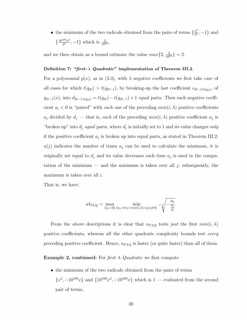
Definition 7: “first–λ Quadratic” implementation of Theorem III.2.
For a polynomial p(x), as in (3.3), with λ negative coefficients we first take care of
all cases for which t(q2`) > t(q2`−1), by breaking-up the last coefficient c2`−1,t(q2`), of
q2`−1(x), into d2`−1,t(q2`) = t(q2`)− t(q2`−1) + 1 equal parts. Then each negative coeffi-
cient ai < 0 is “paired” with each one of the preceding min(i, λ) positive coefficients
aj divided by dj — that is, each of the preceding min(i, λ) positive coefficient aj is
“broken up” into dj equal parts, where dj is initially set to 1 and its value changes only
if the positive coefficient aj is broken up into equal parts, as stated in Theorem III.2;
u(j) indicates the number of times aj can be used to calculate the minimum, it is
originally set equal to dj and its value decreases each time aj is used in the compu-
tation of the minimum — and the minimum is taken over all j; subsequently, the
maximum is taken over all i.
That is, we have:
ubFLQ = max{ai<0}
min{aj>0:j>min(i,λ):u(j)6=0}
j−i
√−aiaj
dj
.
From the above descriptions it is clear that uFLQ tests just the first min(i, λ)
positive coefficients, whereas all the other quadratic complexity bounds test every
preceding positive coefficient. Hence, uFLQ is faster (or quite faster) than all of them.
Example 2, continued: For first–λ Quadratic we first compute
• the minimum of the two radicals obtained from the pairs of terms
{x3,−10100x} and {10100x2,−10100x} which is 1 — evaluated from the second
pair of terms,
30

• the minimum of the two radicals obtained from the pairs of terms {x3,−1} and
{10100x2,−1} which is 1,
and we then obtain as a bound estimate the value max{1, 1} = 1. Note that once a
term with a positive coefficient has been used in obtaining the minimum, it cannot
be used again!
Definition 8: “local-max Quadratic” implementation of Theorem III.2.
For a polynomial p(x), as in (3.3), each negative coefficient ai < 0 is “paired” with
each one of the preceding positive coefficients aj divided by 2tj — that is, each
positive coefficient aj is “broken up” into unequal parts, as is done with just the
locally maximum coefficient in the local max bound; tj is initially set to 1 and is
incremented each time the positive coefficient aj is used — and the minimum is taken
over all j; subsequently, the maximum is taken over all i.
That is, we have:
ubLMQ = max{ai<0}
min{aj>0:j>i}
j−i
√− ai
aj
2tj
.
Since 2tj ≤ 2j−i — where i and j are the indices realizing the max of min; equality
holds when there are no missing terms in the polynomial — it is clear that the
estimates computed by “local-max Quadratic” are sharper by the factor 2j−i−tj
j−i
than those computed by “Kioustelidis’ Quadratic”.
Example 2, continued: For “local-max Quadratic” we first compute
• the minimum of the two radicals obtained from the pairs of terms
{x32,−10100x} and {10100x2
2,−10100x} which is 2,
• the minimum of the two radicals obtained from the pairs of terms {x322,−1} and
{10100x2
22,−1} which is 2
1050,
31

and we then obtain as a bound estimate the value max{2, 21050} = 2.
3.5.1 The Pseudocode
Below we present the pseudocode for ubLMQ and ubFLQ quadratic implementations
of Theorem III.2. We decided to omit ubCQ and ubKQ implementations since both
previous theoretical analysis and empirical data establish the better performance of
ubLMQ and ubFLQ over these two in every case. The ubLMQ, “local-max Quadratic”
implementation is described in Algorithm 6, lines 1–18, whereas the ubFLQ, “first–λ
Quadratic” implementation is described in Algorithms 7 and 8, lines 1–66.
Input : A univariate polynomial p(x) = anxn + an−1xn−1 + . . .+ a0, (an > 0)
Output: An upper bound ubLMQ, on the values of the positive roots of the polynomial
initializations;1
cl←− {a0, a1, a2, . . . , an−1, an};2
timesused←− {1, 1, 1, . . . , 1};3
ub = 0;4
if n+ 1 ≤ 1 then return ub = 0;5
for m←− n to 1 do6
if cl(m) < 0 then7
tempub =∞;8
for k ←− n+ 1 to m+ 1 do9
temp = (−cl(m)cl(k)
2timesused(k)
)1
k−m ;10
timesused(k) + +;11
if tempub > temp then tempub = temp;12
end13
if ub < tempub then ub = tempub;14
end15
end16
ubLMQ = ub;17
return ubLMQ;18
Algorithm 6: The “local-max Quadratic” implementation of Theorem III.2.
32

Input : A univariate polynomial p(x) = anxn + an−1xn−1 + . . .+ a0, (an > 0)
Output: An upper bound ubFLQ, on the values of the positive roots of the polynomial
initializations;1
cl←− {a0, a1, a2, . . . , an−1, an};2
λ←− number of negative elements of cl;3
usedV ector ←− {0, 0, 0, . . . , 0};4
for i←− 1 to n+ 1 do5
if cl(i) > 0 then usedV ector(i) = 1;6
end7
if n+ 1 ≤ 1 or λ = 0 then return ub = 0;8
i = n+ 1;9
templamda = 0;10
flag = 0;11
while templamda < λ do // make sure t(q2i−1) ≥ t(q2i) holds for all i12
if cl(i) > 0 then13
if flag = 0 then posCounter + +;14
else if flag = 1 then15
if negCounter > posCounter then16
usedV ector(positionLastPositiveCoef) = negCounter − posCounter + 1;17
end18
negCounter = 0;19
posCounter = 1;20
flag = 0;21
end22
positionLastPositiveCoef = i;23
else if cl(i) < 0 then24
flag = 1;25
negCounter + +;26
templamda+ +;27
end28
i−−;29
end30
if negCounter > posCounter then31
usedV ector(positionLastPositiveCoef) = negCounter − posCounter + 1;32
end33
Algorithm 7: 1st part of “first–λ Quadratic” implementation of Theorem III.2.
33

sumPosCoeff = 0;34
i = n+ 1;35
// Last of the first-λ coefficients
while sumPosCoeff < λ do36
if usedV ector(i) 6= 0 then37
sumPosCoeff+ = usedV ector(i);38
flPos = i;39
end40
i−−;41
end42
/* If the last of the first-λ coefficients is a broken one (usedV ector(flPos) > 1), there might
be a chance that the sum of the positive coefficients (including broken ones) is more than
λ. For Example: Let the signs of p be + + + - + + - - - + + + - the 5th positive
coefficient will be broken into 2 pieces (usedV ector(8) = 2). However, the sum of the
first-λ (5 non broken) positive coefficients is 6 (incl. broken). As a result we are going
to use the last of the positive first-λ coefficients timesToUse(8)− (sum− λ) = 1 time only.
*/
timesToUse(flpos)− = (sumPosCoeff − λ);43
denomV ector ←− usedV ector;44
m = n;45
ub = 0;46
while λ > 0 do47
if cl(m) < 0 then48
tempub =∞;49
for k = n+ 1 to max(m+ 1, f lPos) do50
if usedV ector(k) > 0 then51
tempB = (−cl(m)cl(k)
denomV ector(k)
)1
k−m ;52
if tempub > tempB then53
tempub = tempB;54
tempN = k;55
end56
end57
end58
usedV ector(tempN)−−;59
λ−−;60
if ub < tempub then ub = tempub;61
end62
m−−;63
end64
ubFLQ = ub;65
return ubFLQ;66
Algorithm 8: 2nd part of “first–λ Quadratic” implementation of Theorem III.234

3.5.2 Testing Quadratic Complexity Bounds
In this section, we present some results using the same classes of polynomials8, as
in (Akritas and Strzebonski , 2005) in order to compare “first–λ Quadratic” and
“local-max Quadratic” implementation of Theorem III.2.
In Table 3.2, “first–λ Quadratic” and “local-max Quadratic” names were
shortened to ubFLQ and ‘ubLMQ respectively. Also, in parenthesis the respective
computation time is given for each algorithm, whereas MPR stands for the maximum
positive root, computed numerically.
8For exact mathematical formulas of the benchmark polynomials, please see the Appendix.
35

Tab
le3.
2:Q
uad
rati
cco
mp
lexit
yb
oun
ds
ofp
osit
ive
root
sfo
rva
riou
sty
pes
of
poly
nom
ials
.D
egre
esP
oly
nom
ial
Bou
nd
s10
100
200
300
400
500
600
700
800
900
Lagu
erre
ub L
MQ
200
2×
104
8×
104
18×
104
32×
104
50×
104
72×
104
98×
104
128×
104
162×
104
(0.)
(0.5
63)
(3.5
62)
(11.1
87)
(25.5
94)
(49.7
82)
(87.3
44)
(142.4
53)
(220.7
66)
(329.7
19)
ub F
LQ
100
104
4×
104
9×
104
16×
104
25×
104
36×
104
49×
104
64×
104
81×
104
(0.)
(0.0
15)
(0.0
31)
(0.0
78)
(0.1
09)
(0.1
72)
(0.2
5)
(0.3
28)
(0.4
06)
(0.5
)M
PR
29.9
2374.9
8767.8
21162.8
1558.8
11955.4
42352.5
2749.8
73147.4
83545.2
9
Ch
ecysh
evI
ub L
MQ
2.2
3607
7.0
7107
10
12.2
474
14.1
421
15.8
114
17.3
205
18.7
083
20
21.2
132
(0.)
(0.0
78)
(0.5
15)
(1.5
47)
(3.4
53)
(6.4
53)
(10.6
88)
(15.8
91)
(23.4
06)
(33.7
5)
ub F
LQ
1.5
8114
57.0
7107
8.6
6025
10
11.1
803
12.2
474
13.2
88
14.1
421
15
(0.)
(0.)
(0.0
15)
(0.0
47)
(0.6
2)
(0.1
1)
(0.1
41)
(0.1
72)
(0.2
34)
(0.2
81)
MP
R0.9
87688
0.9
99877
0.9
99969
0.9
99989
0.9
99992
0.9
99995
0.9
99997
0.9
99997
0.9
99998
0.9
99998
Ch
ecysh
evII
ub L
MQ
2.1
2132
7.0
3562
9.9
7497
12.2
27
14.1
244
15.7
956
17.3
061
18.6
949
19.9
875
21.2
014
(0.0
15)
(0.0
79)
(0.5
31)
(1.5
63)
(3.4
53)
(6.4
68)
(10.7
19)
(16.6
87)
(24.6
56)
(34.7
34)
ub F
LQ
1.5
4.9
7494
7.0
5337
8.6
4581
9.9
8749
11.1
692
12.2
372
13.2
193
14.1
333
14.9
917
(0.)
(0.0
16)
(0.0
15)
(0.0
47)
(0.0
78)
(0.1
09)
(0.1
41)
(0.1
87)
(0.2
19)
(0.2
65)
MP
R0.9
59493
0.9
99516
0.9
99878
0.9
99945
0.9
99969
0.9
9998
0.9
99986
0.9
9999
0.9
99992
0.9
99994
Wilkin
son
ub L
MQ
110
10100
40200
90300
160400
250500
360600
490700
640800
810900
(0.)
(6.3
91)
(52.2
34)
(179.7
5)
(438.5
16)
(878.)
(1549.8
9)
(2508.5
2)
(3833.5
2)
(5569.4
2)
ub F
LQ
55
5050
20100
45150
80200
125250
180300
245350
320400
405450
(0.)
(0.0
16)
(0.0
47)
(0.0
78)
(0.0
14)
(0.2
03)
(0.2
82)
(0.3
59)
(0.5
16)
(0.6
56)
MP
R10
100
200
300
400
500
600
700
800
900
Mig
nott
e
ub L
MQ
1.7
7828
1.0
4811
1.0
2353
1.0
1557
1.0
1164
1.0
0929
1.0
0773
1.0
0662
1.0
0579
1.0
0514
(0.)
(0.)
(0.0
15)
(0.)
(0.)
(0.0
16)
(0.)
(0.)
(0.)
(0.0
15)
ub F
LQ
1.6
3069
1.0
4073
1.0
1995
1.0
1321
1.0
0988
1.0
0789
1.0
0656
1.0
0562
1.0
0491
1.0
0437
(0.)
(0.0
16)
(0.)
(0.0
16)
(0.1
5)
(0.0
16)
(0.0
16)
(0.0
15)
(0.0
16)
(0.0
15)
MP
R1.5
763
1.0
362
1.0
177
1.0
117
1.0
088
1.0
070
1.0
058
1.0
050
1.0
044
1.0
039
sRan
dom
ub L
MQ
2.0
1011
14.3
673
1.3
9904
3.5
4546
3.6
5744
7.7
5602
2.5
257
1.5
3975
1.7
0317
1.6
5478
(0.)
(0.2
19)
(1.0
16)
(2.1
1)
(3.8
28)
(6.)
(8.6
25)
(11.7
35)
(14.7
65)
(18.7
34)
ub F
LQ
2.4
5417
25.1
062
1.0
4472
3.5
4546
2.5
862
7.7
5602
2.0
3158
1.6
409
1.4
8873
1.1
7328
(0.)
(0.0
31)
(0.1
57)
(0.2
81)
(0.5
47)
(0.8
43)
(1.1
57)
(1.6
56)
(1.5
)(2
.375)
MP
R1.6
173
8.1
5106
0.9
82276
1.1
221
1.7
1921
1.0
12339
0.9
83633
0.9
83628
1.0
10844
0.9
83628
usR
an
dom
ub L
MQ
1.5
7532
1916790
1.4
0849
1.7
8915
105264
1272940
1803160
12.6
533
1197500
790432
(0.)
(0.2
5)
(1.0
32)
(2.1
25)
(3.7
97)
(5.8
91)
(8.5
)(1
1.5
31)
(14.8
75)
(18.7
65)
ub F
LQ
3.1
6629
1916790
1.0
6293
15.6
504
105264
1272940
901580
6.3
2665
598750
790432
(0.0
16)
(0.0
47)
(0.1
56)
(0.2
66)
(0.5
31)
(0.8
28)
(1.1
56)
(1.6
41)
(2.0
46)
(2.3
28)
MP
R0.9
25381
1.0
18871
0.9
82509
0.9
841
1.0
26689
1.0
11621
1.3
31235
1.7
55769
1.0
13423
1.2
28396
pR
an
dom
ub L
MQ
5984.5
58818.6
314435.4
(10.2
97)
(75.4
53)
(1053.5
5)
ub F
LQ
4231.7
25555.3
99093.7
5(0
.562)
(1.4
53)
(21.1
56)
MP
R998
998
1019
36

From the data presented in the Table 3.2, it becomes obvious that the sharpness
of the estimates of both ubFLQ and ubLMQ is about the same, but ubFLQ in most cases
runs faster (or quite faster) than ubLMQ. So, when it comes to quadratic complexity
bounds the ubFLQ algorithm is undoubtedly the best choice regarding sharpness to
speed of computation, ratio. However, examining both Table 3.2 and Table 3.1,
one must be very careful in his choice of quadratic versus linear complexity bounds
because then he has to trade-off between a slightly better bound estimation and a
greater algorithmic complexity and execution time. This last remark seems to have
been exploited by the commercial computational software program, Mathematica,
(Wolfram Research, 2008), as we can see in the following section.
3.5.3 Mathematica Session Demonstration of New Bounds
The Mathematica’s real root isolation source code, by default, uses the better
bound from each category, i.e. “first–λ”, ubFL, from the linear complexity bounds
and “local-max Quadratic”, ubLMQ from the quadratic complexity ones, (Strzebonski ,
2010). However, its source code also contains implementations of Cauchy’s, (§ 2.2.1),
and Hong’s bound, (Hong , 1998), which we call “Kioustelidis’ Quadratic” in our
work as well as the “local-max”, ubLM and “first–λ Quadratic”, ubFLQ, bounds.
There is an undocumented system variable which allows to change the bound used to
any combination of those bounds. The new bounds have been added in Mathematica
version 7.
These bounds are always implicity used for calculating intervals isolating polyno-
mial real roots. Intervals are given by command RootIntervals. Real root isolation
is used by any Mathematica function that requires real algebraic number computa-
tion.
See the following examples:
37

Fig
ure
3.2:
Scr
een
cap
ture
ofMathematica
soft
war
eu
sin
gth
ep
rop
osed
bou
nd
sin
vari
ou
sco
mm
and
s.
38

CHAPTER IV
Application of the New Bounds to Real Root
Isolation Methods
4.1 Introduction
In this chapter we apply the newly proposed linear and quadratic complexity (up-
per) bounds on the values of the positive roots of polynomials on a method for the
isolation of real roots of polynomials. Although there are many root isolations meth-
ods (based on continued fractions, bisection, exclusion, etc) that could greatly benefit
from our new sharper bounds we decided to study their impact on the performance of
the Vincent-Akritas-Strzebonski (VAS) method for the isolation of real roots of poly-
nomials. The VAS real root isolation method is based on continued fractions and till
today is considered the fastest among its rivals, having already being incorporated in
major mathematical software packages.
Computing (lower) bounds on the values of the positive roots of polynomials is a
crucial operation in the VAS method. Therefore, we begin by reviewing some basic
facts about this method, which is based on Vincent’s theorem1, (Vincent , 1836):
1For a complete overview of Vincent’s theorem of 1836 and its implications to root isolation, see(Akritas, 2010).
39

Theorem IV.1 (Vincent, 1836). If in a polynomial, p(x), of degree n, with rational
coefficients and without multiple roots we perform sequentially replacements of the
form
x← α1 +1
x, x← α2 +
1
x, x← α3 +
1
x, . . .
where α1 ≥ 0 is an arbitrary non negative integer and α2, α3, . . . are arbitrary positive
integers, αi > 0, i > 1, then the resulting polynomial either has no sign variations or
it has one sign variation. In the last case the equation has exactly one positive root,
which is represented by the continued fraction
α1 +1
α2 + 1α3+ 1
...
whereas in the first case there are no positive roots.
The thing to note is that the quantities αi (the partial quotients of the continued
fraction) are computed by repeated application of a method for estimating lower
bounds2 on the values of the positive roots of a polynomial.
Therefore, the efficiency of the VAS continued fractions method heavily depends
on how good these estimates are.
4.2 Algorithmic Background of the VAS Method
In the sequel we present the VAS algorithm –as found in (Akritas and Strzebonski ,
2005)– and correct a misprint in Step 5 that had appeared in that presentation;
moreover, we explain where the new bound on the positive roots is used.
2A lower bound, `b, on the values of the positive roots of a polynomial f(x), of degree n, isfound by first computing an upper bound, ub, on the values of the positive roots of xnf( 1
x ) and thensetting `b = 1
ub , see (§ 2.1.2).
40

4.2.1 Description of the VAS-Continued Fractions Algorithm
Using the notation of the paper Akritas and Strzebonski (2005), let f ∈ Z[x]\{0}.
By sgc(f) we denote the number of sign changes in the sequence of nonzero coefficients
of f . For nonnegative integers a, b, c, and d, such that ad− bc 6= 0, we put
intrv(a, b, c, d) := Φa,b,c,d((0,∞))
where
Φa,b,c,d : (0,∞) 3 x −→ ax+ b
cx+ d∈ (min(
a
c,b
d),max(
a
c,b
d))
and by interval data we denote a list
{a, b, c, d, p, s}
where p is a polynomial such that the roots of f in intrv(a, b, c, d) are images of
positive roots of p through Φa,b,c,d, and s = sgc(p).
The value of parameter α0 used in step 4 below needs to be chosen empirically.
In our implementation α0 = 16.
Algortihm Continued Fractions (VAS).
Input: A squarefree polynomial f ∈ Z[x] \ {0}
Output: The list rootlist of the isolation intervals of the positive roots of f .
1. Set rootlist to an empty list. Compute s ← sgc(f). If s = 0 return an empty
list. If s = 1 return {(0,∞)}. Put interval data {1, 0, 0, 1, f, s} on intervalstack.
2. If intervalstack is empty, return rootlist, else take interval data {a, b, c, d, p, s}
off intervalstack.
3. Compute a lower bound α ∈ Z on the positive roots of p.
41

4. If α > α0 set p(x)← p(αx), a← αa, c← αc, and α← 1.
5. If α ≥ 1, set p(x) ← p(x + α), b ← αa + b, and d ← αc + d. If p(0) = 0, add
[b/d, b/d] to rootlist, and set p(x)← p(x)/x. Compute s← sgc(p). If s = 0 go
to step 2. If s = 1 add intrv(a, b, c, d) to rootlist and go to step 2.
6. Compute p1(x) ← p(x + 1), and set a1 ← a, b1 ← a + b, c1 ← c, d1 ← c + d,
and r ← 0. If p1(0) = 0, add [b1/d1, b1/d1] to rootlist, and set p1(x)← p1(x)/x,
and r ← 1. Compute s1 ← sgc(p1), and set s2 ← s− s1− r, a2 ← b, b2 ← a+ b,
c2 ← d, and d2 ← c+ d.
7. If s2 > 1, compute p2(x) ← (x + 1)mp( 1x+1
), where m is the degree of p. If
p2(0) = 0, set p2(x)← p2(x)/x. Compute s2 ← sgc(p2).
8. If s1 < s2, swap {a1, b1, c1, d1, p1, s1} with {a2, b2, c2, d2, p2, s2}.
9. If s1 = 0 goto step 2. If s1 = 1 add intrv(a1, b1, c1, d1) to rootlist, else put
interval data {a1, b1, c1, d1, p1, s1} on intervalstack.
10. If s2 = 0 goto step 2. If s2 = 1 add intrv(a2, b2, c2, d2) to rootlist, else put
interval data {a2, b2, c2, d2, p2, s2}on intervalstack. Go to step 2.
Please note that the lower bound3, α, on the positive roots of p(x) is computed
in Step 3, and used in Step 5.
4.2.2 The Pseudocode of the VAS-Continued Fractions Algorithm
We present the pseudocode of the VAS-Continued Fractions Root Isolation Method,
below in Algorithm 9, lines 1–13. Note the repeated use of the lower bound lb in lines
4–5.
3As mentioned in (§ 2.2), Cauchy’s bound was the only one known and the first one to be usedin VAS, in 1978. This of course changed, in 2006, after we developed the new bounds.
42

Input: The square-free polynomial p(x) ∈ Z[x], p(0) 6= 0, and the Mobius transformation
M(x) = ax+bcx+d
= x, a, b, c, d ∈ Z
Output: A list of isolating intervals of the positive roots of p(x)
var ←− the number of sign changes of p(x);1
if var = 0 then RETURN ∅;2
if var = 1 then RETURN {]a, b[} // a = min(M(0),M(∞)), b = max(M(0),M(∞));3
`b←− a lower bound on the positive roots of p(x);4
if `b > 1 then {p←− p(x+ `b),M ←−M(x+ `b)};5
p01 ←− (x+ 1)deg(p)p( 1x+1
),M01 ←−M( 1x+1
) // Look for real roots in ]0, 1[ ;6
m←−M(1) // Is 1 a root? ;7
p1∞ ←− p(x+ 1),M1∞ ←−M(x+ 1) // Look for real roots in ]1,+∞[ ;8
if p(1) 6= 0 then9
RETURN VAS(p01,M01)⋃
VAS(p1∞,M1∞)10
else11
RETURN VAS(p01,M01)⋃{[m,m]}
⋃VAS(p1∞,M1∞)12
end13
Algorithm 9: VAS-Continued Fractions Algorithm.
4.2.3 Example of the Real Root Isolation Method
Executing Algorithm 9 for the polynomial 8x4 − 18x3 + 9x − 2 which has one
negative, −√
2/2 and three positive real roots, 1/4,√
2/2 and 2, we have:
43
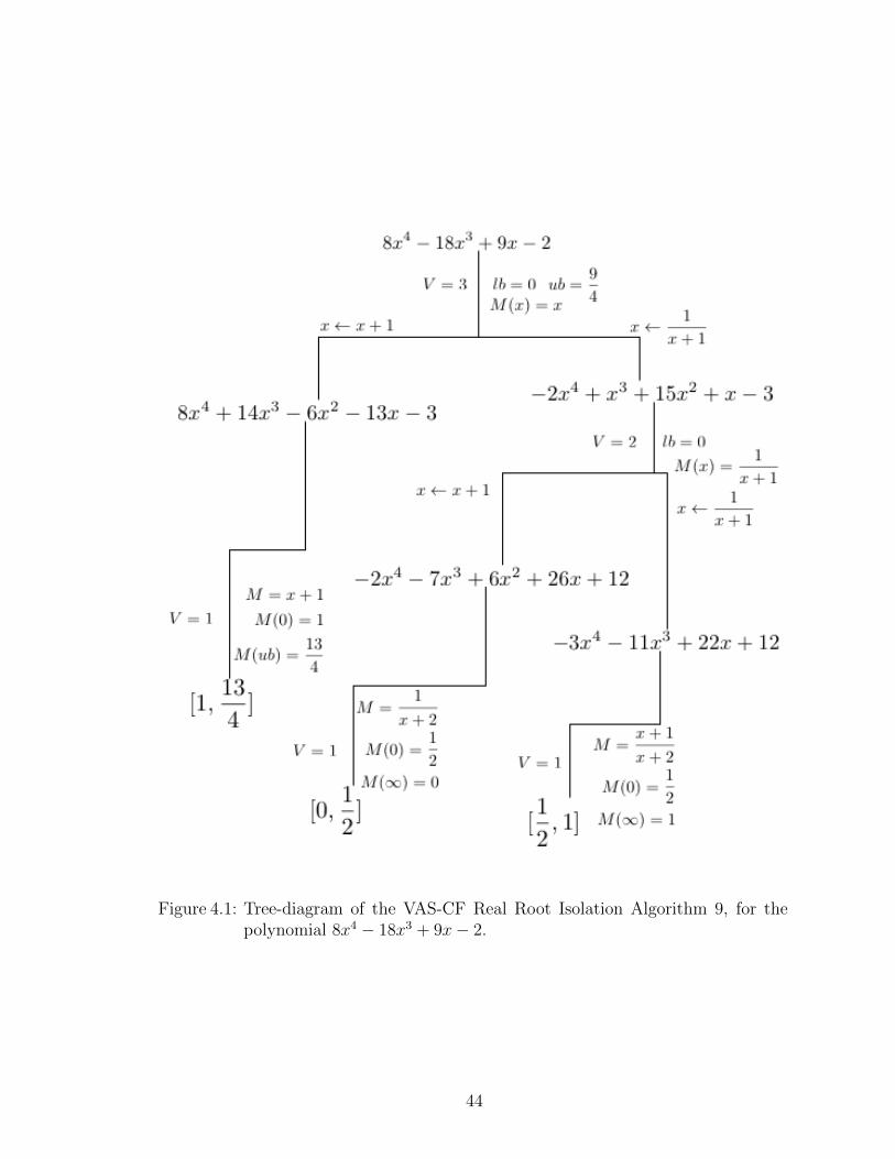
Figure 4.1: Tree-diagram of the VAS-CF Real Root Isolation Algorithm 9, for thepolynomial 8x4 − 18x3 + 9x− 2.
44

4.3 Benchmarking VAS with New Bounds
In this section we compare four implementations of the VAS real root isolation
method using two linear and two quadratic complexity bounds on the values of the
positive roots of polynomials.
The two linear complexity bounds are: Cauchy’s, ubC and min(ubFL, ubLM), the
minimum of “first–λ” and “local-max” bounds, (Akritas, Strzebonski, and Vigklas ,
2006), whereas the two quadratic complexity ones are: ubKQ, the Quadratic complex-
ity variant of K ioustelidis’ bound, studied by Hong, (Hong , 1998), and ubLMQ, the
Quadratic complexity version of the “local-max” bound, (Akritas, Strzebonski, and
Vigklas , 2008a).
Our choice of the various bounds in the implementations of VAS is justified as
follows:
1. From the linear complexity bounds we included:
(a) Cauchy’s bound, ubC , to be used as a point of reference, since it has been
in use for the past 30 years, and
(b) min(ubFL, ubLM) bound, (Akritas, Strzebonski, and Vigklas , 2006), which
is the best among the linear complexity bounds, in order to see when
it’s implementation will outperform that of the two quadratic complexity
bounds.
2. From the quadratic complexity bounds we included:
(a) Kioustelidis’ bound, ubKQ and
(b) ubLMQ bound in order to compare their performance; as explained in the
previous chapter ubLMQ computes sharper estimates than ubKQ.
45

They all use the same implementation of Shaw and Traub’s algorithm for Taylor
shifts (von zur Gathen and Gerhard , 1997). We followed the standard practice and
used as benchmark the Laguerre, Chebyshev (first and second kind), Wilkinson and
Mignotte polynomials4, as well as several types of randomly generated polynomials of
degrees {100, 200, 300, 400, 500, 600, 700, 800, 900, 1000, 1500, 2000}. For the random
polynomials the size of the coefficients ranges from −220 to 220.
4For exact mathematical formulas of the benchmark polynomials, please see the Appendix.
46

Table 4.1: Special polynomials of some indicative degrees.
Polynomial Degree ubC min(ubFL, ubLM) ubKQ(Hong) ubLMQ
Class Time(s) Time(s) Time(s) Time(s)
Laguerre 100 0.23 0.19 0.19 0.17Laguerre 1000 979 665 729 633Laguerre 1500 7194 4903 5356 4569Laguerre 2000 27602 21007 22712 19277
ChebyshevI 100 0.19 0.17 0.16 0.11ChebyshevI 1000 517 460 496 299ChebyshevI 1500 3681 3333 3381 2188ChebyshevI 2000 16697 15010 14571 10473
ChebyshevII 100 0.42 0.17 0.15 0.10ChebyshevII 1000 529 437 443 296ChebyshevII 1500 3772 3198 3190 2166ChebyshevII 2000 16559 14492 14370 10184
Wilkinson 100 0.03 0.03 0.03 0.03Wilkinson 1000 54.6 44.5 43.7 43.3Wilkinson 1500 339 295 270 265Wilkinson 2000 1361 1305 1241 1242
Mignotte 100 0.008 0.004 0.008 0.004Mignotte 1000 0.79 0.78 0.81 0.66Mignotte 1500 2.05 2.12 2.06 1.77Mignotte 2000 4.52 4.37 4.47 3.69
47

Table 4.2: Polynomials with random 10-bit coefficients.
Degree No. of roots ubC min(ubFL, ubLM) ubKQ(Hong) ubLMQ
Time(s) Time(s) Time(s) Time(s)Avg(Min/Max) Avg(Min/Max) Avg(Min/Max) Avg(Min/Max) Avg(Min/Max)
100 4.4 (2/6) 0.01 (0.00/0.01) 0.01 (0.01/0.02) 0.01 (0.01/0.02) 0.01 (0.01/0.01)200 4.0 (2/8) 0.06 (0.02/0.18) 0.06 (0.03/0.16) 0.05 (0.03/0.14) 0.04 (0.03/0.09)300 4.8 (4/6) 0.14 (0.07/0.24) 0.12 (0.06/0.22) 0.13 (0.07/0.19) 0.09 (0.07/0.13)400 4.4 (4/6) 0.17 (0.12/0.21) 0.18 (0.12/0.25) 0.17 (0.12/0.20) 0.16 (0.12/0.20)500 4.8 (2/8) 0.70 (0.21/1.96) 0.54 (0.20/1.22) 0.35 (0.21/0.56) 0.32 (0.20/0.50)600 5.2 (4/6) 0.96 (0.46/1.41) 0.86 (0.51/1.25) 0.60 (0.42/0.84) 0.53 (0.42/0.72)700 4.0 (2/6) 0.95 (0.45/1.68) 0.81 (0.44/1.33) 0.82 (0.44/1.25) 0.69 (0.50/0.91)800 5.2 (4/8) 1.97 (0.67/4.09) 1.68 (0.74/3.33) 1.22 (0.71/2.25) 1.02 (0.72/1.70)900 3.6 (2/6) 2.56 (0.68/7.15) 2.27 (0.72/6.13) 1.44 (0.71/2.55) 1.19 (0.67/1.87)1000 6.4 (4/8) 4.07 (1.63/9.02) 3.56 (1.54/7.64) 2.86 (1.57/4.51) 2.06 (1.38/3.18)1500 4.0 (2/6) 10.6 (2.73/26.1) 7.51 (2.33/13.9) 5.78 (2.35/10.1) 5.24 (2.43/7.77)2000 6.8 (4/12) 53.8 (7.54/137) 45.5 (7.90/118) 23.3 (7.67/53.9) 19.1 (7.61/40.2)
Table 4.3: Polynomials with random 1000-bit coefficients.
Degree No. of roots ubC min(ubFL, ubLM) ubKQ(Hong) ubLMQ
Time(s) Time(s) Time(s) Time(s)Avg(Min/Max) Avg(Min/Max) Avg(Min/Max) Avg(Min/Max) Avg(Min/Max)
100 4.0 (4/4) 0.01 (0.00/0.02) 0.01 (0.00/0.02) 0.01 (0.00/0.02) 0.01 (0.00/0.02)200 3.6 (2/6) 0.06 (0.03/0.12) 0.05 (0.02/0.10) 0.04 (0.02/0.06) 0.03 (0.01/0.06)300 4.8 (2/8) 0.12 (0.04/0.32) 0.11 (0.04/0.28) 0.10 (0.04/0.23) 0.09 (0.04/0.17)400 4.4 (2/6) 0.29 (0.06/0.54) 0.25 (0.06/0.44) 0.24 (0.06/0.44) 0.16 (0.06/0.25)500 5.2 (4/8) 0.68 (0.16/1.20) 0.55 (0.17/0.95) 0.45 (0.21/0.92) 0.32 (0.21/0.48)600 3.6 (2/4) 0.76 (0.19/2.09) 0.54 (0.18/0.96) 0.43 (0.19/0.66) 0.39 (0.18/0.52)700 3.6 (0/6) 1.26 (0.25/2.82) 1.28 (0.19/2.51) 0.85 (0.19/1.54) 0.68 (0.19/1.29)800 4.4 (2/6) 3.03 (0.29/5.50) 2.53 (0.26/4.76) 1.08 (0.34/1.68) 0.93 (0.27/1.53)900 5.6 (4/8) 4.55 (1.05/9.32) 3.72 (1.02/7.53) 2.23 (1.00/3.09) 1.59 (0.76/2.68)1000 3.6 (2/6) 2.42 (0.46/4.62) 2.06 (0.44/3.92) 1.27 (0.40/2.00) 1.04 (0.42/1.68)1500 5.6 (4/8) 16.1 (2.30/40.2) 9.41 (1.99/18.2) 7.17 (2.10/11.9) 5.63 (1.96/10.8)2000 5.2 (4/6) 23.3 (4.12/79.8) 19.4 (4.08/65.4) 13.2 (4.33/33.4) 10.4 (4.11/20.2)
48

Table 4.4: Monic polynomials with random 10-bit coefficients.
Degree No. of roots ubC min(ubFL, ubLM) ubKQ(Hong) ubLMQ
Time(s) Time(s) Time(s) Time(s)Avg(Min/Max) Avg(Min/Max) Avg(Min/Max) Avg(Min/Max) Avg(Min/Max)
100 4.8 (2/8) 0.01 (0.01/0.02) 0.01 (0.00/0.02) 0.01 (0.01/0.02) 0.01 (0.00/0.02)200 5.6 (4/6) 0.08 (0.03/0.16) 0.06 (0.03/0.13) 0.06 (0.03/0.09) 0.05 (0.03/0.08)300 4.8 (4/6) 0.12 (0.08/0.22) 0.12 (0.08/0.21) 0.12 (0.08/0.15) 0.10 (0.08/0.15)400 4.8 (4/6) 0.19 (0.19/0.29) 0.19 (0.16/0.26) 0.18 (0.15/0.26) 0.17 (0.16/0.20)500 5.2 (4/10) 0.44 (0.18/1.38) 0.42 (0.18/1.19) 0.33 (0.18/0.74) 0.32 (0.19/0.63)600 5.6 (4/8) 0.99 (0.30/2.04) 0.76 (0.30/1.21) 0.65 (0.31/0.94) 0.49 (0.30/0.72)700 5.2 (4/8) 1.14 (0.43/1.63) 0.99 (0.42/1.47) 0.92 (0.46/1.30) 0.73 (0.49/0.94)800 5.6 (4/8) 1.45 (0.66/1.99) 1.29 (0.64/1.62) 1.22 (0.65/1.42) 0.90 (0.69/1.03)900 4.4 (2/6) 1.01 (0.74/1.18) 1.01 (0.71/1.31) 1.05 (0.69/1.36) 1.09 (0.72/1.33)1000 5.6 (4/8) 3.40 (1.18/7.09) 3.02 (1.03/5.94) 2.41 (1.10/4.28) 1.72 (1.10/2.70)1500 6.8 (6/8) 14.8 (6.06/27.3) 11.8 (5.86/17.1) 8.43 (5.98/12.9) 6.80 (4.90/9.24)2000 7.6 (4/14) 54.8 (6.12/137) 47.6 (6.09/120) 23.9 (6.15/56.0) 19.4 (6.03/42.2)
Table 4.5: Monic polynomials with random 1000-bit coefficients.Degree No. of roots ubC min(ubFL, ubLM) ubKQ(Hong) ubLMQ
Time(s) Time(s) Time(s) Time(s)Avg(Min/Max) Avg(Min/Max) Avg(Min/Max) Avg(Min/Max) Avg(Min/Max)
100 6.0 (4/8) 0.03 (0.02/0.04) 0.01 (0.01/0.03) 0.01 (0.00/0.02) 0.01 (0.00/0.02)200 5.2 (4/8) 0.09 (0.02/0.22) 0.07 (0.02/0.19) 0.04 (0.02/0.11) 0.04 (0.03/0.06)300 5.6 (4/8) 0.19 (0.06/0.46) 0.14 (0.07/0.28) 0.12 (0.06/0.24) 0.14 (0.07/0.26)400 5.2 (4/8) 0.41 (0.08/1.00) 0.24 (0.06/0.54) 0.21 (0.06/0.44) 0.15 (0.06/0.28)500 5.6 (4/8) 0.62 (0.18/1.00) 0.39 (0.12/0.68) 0.45 (0.12/0.74) 0.26 (0.12/0.37)600 4.8 (4/6) 1.03 (0.24/3.09) 0.52 (0.17/1.21) 0.37 (0.17/0.68) 0.32 (0.17/0.59)700 5.2 (2/10) 1.27 (0.20/2.67) 1.02 (0.21/1.84) 0.86 (0.19/1.43) 0.65 (0.19/1.09)800 5.6 (4/8) 2.92 (0.43/5.41) 2.40 (0.39/4.46) 1.02 (0.38/2.02) 0.79 (0.38/1.38)900 6.0 (4/8) 4.22 (0.84/9.86) 2.67 (0.80/5.78) 1.84 (0.88/2.47) 1.43 (0.74/2.22)1000 5.6 (4/6) 4.23 (2.21/5.86) 2.90 (1.34/4.21) 2.23 (1.34/3.52) 1.44 (1.15/1.84)1500 6.8 (6/8) 17.1 (26.06/41.8) 11.4 (5.25/28.2) 8.28 (4.86/15.7) 5.44 (3.30/10.4)2000 6.4 (6/8) 30.6 (4.80/102) 24.0 (4.59/80.9) 16.7 (4.60/47.4) 12.6 (5.02/35.9)
49
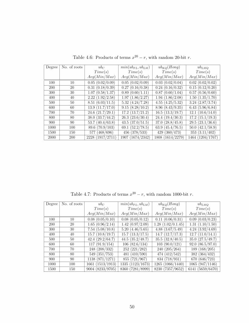
Table 4.6: Products of terms x20 − r, with random 20-bit r.
Degree No. of roots ubC min(ubFL, ubLM) ubKQ(Hong) ubLMQ
Time(s) Time(s) Time(s) Time(s)Avg(Min/Max) Avg(Min/Max) Avg(Min/Max) Avg(Min/Max)
100 10 0.05 (0.02/0.09) 0.05 (0.02/0.09) 0.03 (0.02/0.04) 0.02 (0.02/0.02)200 20 0.31 (0.18/0.39) 0.27 (0.16/0.38) 0.24 (0.16/0.32) 0.15 (0.12/0.20)300 30 1.07 (0.58/1.37) 0.89 (0.60/1.11) 0.87 (0.60/1.04) 0.57 (0.56/0.60)400 40 2.22 (1.92/2.58) 1.97 (1.86/2.27) 1.94 (1.86/2.08) 1.50 (1.35/1.70)500 50 8.51 (6.03/11.5) 5.32 (4.24/7.28) 4.55 (4.25/5.32) 3.24 (2.87/3.74)600 60 13.9 (11.7/17.0) 9.15 (8.28/10.2) 8.96 (8.43/9.35) 6.43 (5.96/6.84)700 70 24.6 (21.7/29.1) 17.2 (13.7/21.2) 16.5 (13.3/19.7) 12.1 (10.6/14.0)800 80 38.0 (33.7/44.2) 26.3 (23.6/30.4) 24.4 (19.4/30.3) 17.2 (15.1/19.3)900 90 53.7 (40.4/63.8) 43.5 (37.0/51.5) 37.0 (28.8/45.8) 29.5 (23.1/36.6)1000 100 89.6 (70.9/103) 69.1 (52.2/78.5) 63.9 (45.4/76.5) 50.0 (42.1/58.9)1500 150 577 (468/696) 456 (378/533) 429 (360/473) 353 (3.11/402)2000 200 2228 (1917/2711) 1907 (1674/2342) 1808 (1614/2279) 1464 (1204/1767)
Table 4.7: Products of terms x20 − r, with random 1000-bit r.
Degree No. of roots ubC min(ubFL, ubLM) ubKQ(Hong) ubLMQ
Time(s) Time(s) Time(s) Time(s)Avg(Min/Max) Avg(Min/Max) Avg(Min/Max) Avg(Min/Max)
100 10 0.08 (0.05/0.10) 0.08 (0.05/0.12) 0.11 (0.06/0.31) 0.09 (0.03/0.23)200 20 1.65 (0.96/2.14) 1.42 (0.97/2.09) 1.28 (1.02/0.1.45) 1.31 (1.10/1.50)300 30 7.54 (5.08/10.8) 5.20 (4.46/5.65) 4.88 (3.67/5.49) 4.24 (3.92/4.69)400 40 15.7 (10.8/19.7) 15.7 (13.3/17.5) 14.7 (12.7/17.3) 12.7 (11.0/14.1)500 50 42.4 (29.2/64.7) 44.5 (35.2/48.7) 35.5 (32.8/40.5) 35.0 (27.5/49.7)600 60 117 (91.9/154) 106 (82.6/134) 103 (90.0/121) 92.0 (86.5/97.0)700 70 248 (208/332) 252 (221/282) 240 (205/264) 189 (168/205)800 80 549 (351/753) 481 (410/590) 474 (412/542) 382 (364/432)900 90 1138 (971/1271) 855 (721/967) 834 (718/931) 670 (646/723)1000 100 1661 (1513/1913) 1335 (1123/1673) 1265 (1066/1440) 1065 (947/1146)1500 150 9004 (8233/9705) 8360 (7281/8999) 8230 (7357/9652) 6141 (5659/6470)
50

Table 4.8: Products of terms x− r with random integer r.
Bit-length Degree ubC min(ubFL, ubLM) ubKQ(Hong) ubLMQ
Time(s) Time(s) Time(s) Time(s)of roots Avg(Min/Max) Avg(Min/Max) Avg(Min/Max) Avg(Min/Max)
10 100 0.46 (0.28/0.94) 0.24 (0.18/0.28) 0.34 (0.27/0.41) 0.34 (0.30/0.41)10 200 1.46 (1.24/1.85) 1.40 (1.28/1.69) 1.41 (1.26/1.71) 1.40 (1.20/1.69)10 500 18.1 (16.5/18.9) 18.1 (16.6/18.8) 21.2 (17.5/24.4) 22.1 (18.7/24.2)
1000 20 0.07 (0.04/0.14) 0.02 (0.02/0.03) 0.03 (0.02/0.04) 0.03 (0.02/0.04)1000 50 3.69 (2.38/6.26) 0.81 (0.60/1.28) 0.88 (0.52/1.28) 0.81 (0.52/1.11)1000 100 47.8 (37.6/56.9) 13.8 (10.3/19.2) 17.6 (12.4/25.9) 15.8 (11.3/21.3)
Figure 4.2: The average speed−up of the VAS algorithm for each Table (4.1–4.8) using themin(ubFL, ubLM ) and ubLMQ against Cauchy’s bound, ubC .
51

Summarizing the testing results5 from Tables 4.1 through 4.8 above we have
the Figure 4.2. The time gain for min(ubFL, ubLM) and ubLMQ against Cauchy’s
bound, ubC , was calculated for every row using the formulas: Speed − up = 100 ·
|min(ubFL, ubLM)−ubC |/ubC and Speed−up = 100 · |ubLMQ−ubC |/ubC , respectively.
Then, for every Table, the average value of Speed− up was computed giving a rough
overall estimation on time gain that VAS algorithm received after the incorporation
of the new bounds.
Taking these test results into consideration, one could safely conclude that us-
ing the new proposed bounds (linear or quadratic) in VAS real root isolation algo-
rithm would see a average overall improvement in computation time of about 20%
for min(ubFL, ubLM) and about 40% for ubLMQ bound.
Also, notice that ubLMQ is fastest for all classes of polynomials tested, except for
the case of very many very large roots, Table 4.8. In the case of very many very
large roots VAS using ubLMQ is a very close second to VAS using our linear complexity
bound min(ubFL, ubLM)6.
We end this chapter by presenting the following graph, Figure 4.3. This graph
depicts the overall time of VAS-CF in comparison with the time spent for computing
bounds. Especially, the left scale shows the total time in seconds (bars) needed by
VAS-CF to isolate the roots of a certain class of polynomials (Laguerre) using both
ubLM , the “local-max” bound, and ubLMQ, its quadratic version. The right scale
is associated with the two curves which show the total time spent by VAS-CF in
computing just these bounds.
5The change in memory use was negligible in every case, and hence, it is not included. Also,timing results are subject to measurement error, which especially affect small timings.
6For additional discussion on these conclusions, see (Akritas, Strzebonski, and Vigklas, 2007),(Akritas, Strzebonski, and Vigklas, 2008b) and (Akritas, 2009).
52

Figure 4.3: Computation times for the Laguerre polynomials of degree (100...1000). TheVAS-CF(LM), VAS-CF(LMQ), (LM), and (LMQ) are described above in the text.Note that the bars are scaled to the left Y axis whereas the lines to the rightone.
53

CHAPTER V
Conclusions
5.1 Final Note
This thesis was motivated by an old, but still important for many modern scientific
fields, problem in polynomial algebra, namely, the determination of upper bounds on
the values of the positive roots of polynomials. The widespread development and use
of computer algebra systems, (CAS ), along with an increasing interest in root isolation
methods, provided a fruitful context for reexamination of this classical problem.
We have presented and analyzed a variety of algorithms both of linear and quadratic
computational complexity that take advantage of a theorem that we extended, in or-
der to establish a unified general framework in which the classical ones fitted perfectly
and new ones came out naturally. These algorithms are simple in implementation, and
in most cases outperform in speed and accuracy the established preexisting methods.
The incorporation of these new bounds in the Vincent-Akritas-Strzebonski, (VAS),
continued fractions polynomial real root isolation algorithm offered a significant speed-
up to an already fast method extending significant the range of its applicability and
its robustness.
The immediate adoption of our new algorithms by major mathematical software
systems, such as Mathematica and Sage, bear witness to their usefulness and their
effectiveness. However, this thesis is by no means exhaustive and questions such as:
54

• Is there an optimal way to break up the coefficients in the“first–λ” method?
• Is it possible to extend these bounds to multivariate polynomials with similar
success?
• Can these bounds be suitably modified to constitute a complex analogue for
polynomials with complex coefficients?
and many others, seek to be answered by our long term on-going research.
55

APPENDICES
56

APPENDIX A
Theorems on the Number of Real Roots of a
Polynomial
A.1 Number of Real Roots of a Polynomial in an Interval
After the bounds of the positive and negative real roots of the polynomial equation
p(x) = 0 have been calculated according to the methods presented in Chapter 3.2
the next question that arises concerns the number of real roots of a polynomial in a
given interval (a, b). A picture of the number of real roots of equation p(x) = 0 in
an interval (a, b) is shown in Figure A.1, for the function y = p(x), where the roots
x1, x2, x3 are found as the points of intersection of the graph with the x-axis. We note
that (a) If p(a)p(b) < 0, then on the interval (a, b) there is an odd number of roots of
p(x), counting multiplicities, (b) If p(a)p(b) > 0, then on the interval (a, b) there are
either no roots of p(x) or there is an even number of such roots. The question of the
number of real roots of an algebraic equation in a given interval is solved completely
by the Sturm method, (Kurosh, 1988). Before going into that let us introduce the
notion of the number of sign changes in a set of numbers.
57

Figure A.1: A polynomial with three positive real roots.
Definition A.1. Suppose we have an ordered finite set of real numbers different from
zero:
r1, r2, ...rl (l ≥ 2) (A.1)
We say that there is a change of sign for a pair of two successive elements rk, rk+1 of
(A.1) if these elements have opposite signs, that is,
rkrk+1 < 0 (A.2)
and there is no change of sign if the signs are the same:
rkrk+1 > 0 (A.3)
The total number of changes of sign in all pairs of successive elements rk, rk+1(k =
1, 2, ...l−1) of (A.1) is called the number of sign changes or variations of sign, (V ar),
in (A.1).
Example A.2. Consider the polynomial p(x) = x3 − 7x2 + 7. The sequence of its
coefficients is {1,−7, 0, 7} which shows a number of sign variations equal 2, (V ar = 2).
58
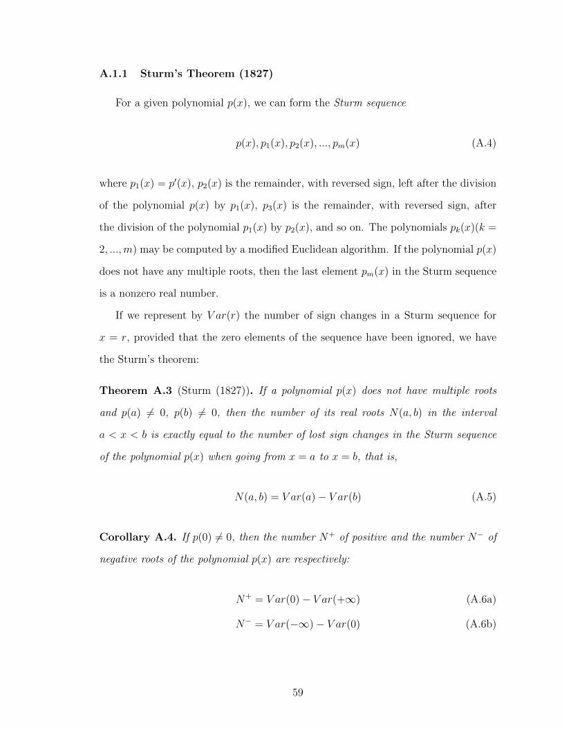
A.1.1 Sturm’s Theorem (1827)
For a given polynomial p(x), we can form the Sturm sequence
p(x), p1(x), p2(x), ..., pm(x) (A.4)
where p1(x) = p′(x), p2(x) is the remainder, with reversed sign, left after the division
of the polynomial p(x) by p1(x), p3(x) is the remainder, with reversed sign, after
the division of the polynomial p1(x) by p2(x), and so on. The polynomials pk(x)(k =
2, ...,m) may be computed by a modified Euclidean algorithm. If the polynomial p(x)
does not have any multiple roots, then the last element pm(x) in the Sturm sequence
is a nonzero real number.
If we represent by V ar(r) the number of sign changes in a Sturm sequence for
x = r, provided that the zero elements of the sequence have been ignored, we have
the Sturm’s theorem:
Theorem A.3 (Sturm (1827)). If a polynomial p(x) does not have multiple roots
and p(a) 6= 0, p(b) 6= 0, then the number of its real roots N(a, b) in the interval
a < x < b is exactly equal to the number of lost sign changes in the Sturm sequence
of the polynomial p(x) when going from x = a to x = b, that is,
N(a, b) = V ar(a)− V ar(b) (A.5)
Corollary A.4. If p(0) 6= 0, then the number N+ of positive and the number N− of
negative roots of the polynomial p(x) are respectively:
N+ = V ar(0)− V ar(+∞) (A.6a)
N− = V ar(−∞)− V ar(0) (A.6b)
59

Corollary A.5. For all the roots of a polynomial p(x) of degree n to be real, in the
absence of multiple roots, it is necessary and sufficient that the following condition
holds:
V ar(−∞)− V ar(+∞) = n (A.7)
Example A.6. Let us determine the number of positive and negative roots of the
equation p(x) = x7 − 7x+ 1. The Sturm sequence is
p(x) = x7 − 7x+ 1 (A.8a)
p1(x) = x6 − 1 (A.8b)
p2(x) = 6x− 1 (A.8c)
p3(x) = 46655 (A.8d)
so
V ar(−∞) = 3, V ar(0) = 2, V ar(+∞) = 0 (A.9)
We find that equation p(x) = x7 − 7x+ 1 has
N+ = 2− 0 = 2 positive roots (A.10a)
N− = 3− 2 = 1 negative roots (A.10b)
and its rest four roots are complex roots. We can easily deduce here a way to isolate
the roots of algebraic equations by using Sturm sequence in order to partition the
interval (a, b) containing all the real roots of the equation into a finite number of
subintervals (α, β) such that V ar(α)− V ar(β) = 1.
60

A.1.2 Fourier’s Theorem (1819)
Sturm arrived at his method (1827) by extending an earlier theorem by Fourier
(1819). Let us return to the method described above (A.1) for the counting of the
number variations of sign in a sequence of numbers:
Definition A.7. Suppose we have a finite ordered sequence of real numbers:
r1, r2, ..., rl (A.11)
where r1 6= 0 and rl 6= 0. We define: (a) lower number of variations of sign V arlo
of the sequence (A.11) for the number of sign changes in an appropriate subsequence
that does not contain zero elements and (b) upper number of variations of sign V arup
of a sequence of numbers (A.11) for the number of sign changes in a transformed
sequence of (A.11) where the zero elements
rk = rk+1 = ... = rk+m−1 = 0 (A.12)
(rk−1 6= 0, rk+m 6= 0) are replaced by the elements rk+i(i = 0, 1, 2, ...,m− 1) such that
sgn(rk+i) = (−1)m−isgn(rk+m) (A.13)
It is clear that if (A.11) has no zero elements, then the number V ar of sign changes
in the sequence coincides with its lower V arlo and upper V arup number of variation
of sign: V ar = V arlo = V arup whereas generally V arup ≥ V arlo.
Example A.8. Let us determine the lower and upper number of changes of sign in
the sequence 1, 0, 0,−1, 1. Omitting the zeros, we have V arlo = 2. To calculate V arup
using (A.13), we form the sequence 1,−σ, σ,−1, 1 where σ > 0, and V arup = 4.
Theorem A.9 (Fourier, 1820). If the numbers a and b (a < b) are not roots of a
polynomial p(x) of degree n, then the number N(a, b) of real roots of the equation
61

p(x) = 0 lying between a and b is equal to the minimal number ∆V ar of the sign
changes lost in the sequence of successive derivatives
p(x), p′(x), ..., pn−1(x), pn(x) (A.14)
when going from x = a to x = b, or less that ∆V ar by an even number: N(a, b) =
∆V ar − 2k where ∆V ar = V arlo(a)− V arup(b) and V arlo(a) is the lower number of
variations of sign in the sequence (A.14) for x = a, V arup(b) is the upper number of
variations of sign in that sequence for x = b [k = 0, 1, ..., E(∆V ar2
)]
Fourier’s theorem is the only one found in the literature under the names: Budan,
Budan-Fourier, Fourier or Fourier-Budan. We expalin why in the sequel. In the
above theorem it is assumed that each root of the equation p(x) = 0 is counted
according to its multiplicity. If the derivatives pk(x) (k = 1, 2, ..., n) do not vanish
at x = a and x = b, then counting the signs is simplified and ∆V ar becomes ∆V ar =
V ar(a)− V ar(b).
Corollary A.10. . If ∆V ar = 0, then there are no real roots of the equation p(x) = 0
between a and b.
Corollary A.11. . If ∆V ar = 1, then there is exactly one real root of the equation
p(x) = 0 between a and b.
A.1.3 Descartes’ Theorem (1637)
Somewhat easier in applications, but still unable to determine precisely the num-
ber of roots, is Descartes’ rule of signs (given in his work Geometrie in 1637 and
proved by Gauss in 1828), (Bartolozzi and Franci , 1993).
Theorem A.12 (Descartes’ rule of signs, 1637). The number of positive roots of an
algebraic equation p(x) = 0 such that a root of multiplicity m being counted as m
roots, is equal to the nummber of variations in sign in the sequence of coefficients
62

an, an−1, an−2, ..., a0 (A.15)
(where the coefficients equal to zero are not counted) or less than that by an even
integer.
Clearly, Descartes’ rule of sign is an application of the Fourier theorem to the
interval (0,+∞). Since
p(x) = anxn + ...+ a0 (A.16a)
p′(x) = nanxn−1 + ...+ a1 (A.16b)
p(2)(x) = n(n− 1)anxn−2 + ...+ 2a2 (A.16c)
... (A.16d)
... (A.16e)
... (A.16f)
p(n)(x) = n!an (A.16g)
sequence (A.15) is, to within positive factors, a collection of derivatives p(k)(0) (k =
0, 1, 2..., n) written in ascending order, i.e. a0, a1, 2a2, ..., n!an, therefore, the number
of variations in sign in the sequence (A.15) is equal to V arlo(0), zero coefficients not
counted. On the other hand, the derivatives p(k)(+∞) (k = 0, 1, 2..., n) have no sign
variations and follows that V arup(+∞) = 0. Then, we have
∆V ar = V arlo(0)− V arup(+∞) = V arlo(0) (A.17)
and on the basis of the Fourier theorem, the number of positive roots of p(x) = 0 is
either equal to ∆V ar or is less than that by an even integer.
Corollary A.13. If the coefficients of p(x) = 0 are different from zero, then the
63

number of negative roots of p(x) = 0, counting multiplicities, is equal to the number
of non-variations of sign in the sequence (A.15) of its coefficients or is less than that
by an even integer. The proof of this follows directly from the application of Descartes’
rule to the polynomial p(−x).
A.1.4 Budan’s Theorem (1807)
Budan’s theorem of 1807 is equivalent to, but not the same, as, Fourier’s theo-
rem. Due to this equivalence, it was not considered essential and therefore, it was
only Fourier’s theorem that gained popularity among researchers. Budan’s theorem
appears in the literature only in Vincent’s paper, (Vincent , 1836) and in Akritas’
work, (Akritas , 1982). Budan’s theorem despite its similarity to Fourier’s, leads in a
different direction. It states:
Theorem A.14 (Budan, 1807). If in an algebraic equation p(x) = 0, we make two
distinct substitutions x = α+x′ and x = β+x′′, where α and β are real numbers and
α < β, getting the equations A(x′) =∑aix
i = 0 and B(x′′) =∑bix
i = 0. Then
• V ar(ai) ≥ V ar(bi)
• The number of real roots of p(x) = 0 between α and β is: N(α, β) = V ar(ai)−
V ar(bi)− 2k, where as above k is an integer and k ≥ 0.
To see that this theorem is equivalent to Fourier’s theorem we must replace, in
Fourier’s sequence, x by any real number c. Then, the n + 1 resulting numbers are
proportional to the corresponding coefficients of the transformed polynomial equation
p(x + c) =∑
0≤i≤n[p(i)(c)/i!]xi obtained by Taylor’s expansion theorem. Budan’s
theorem is the base of Vincent’s theorem that plays an important role to the real
root isolation algorithms.
64

APPENDIX B
Mathematical Formulas of Testing Polynomials
B.1 Mathematical Formulas of the Benchmark Polynomials
Below we present the exact mathematical formulas of the polynomials that were
used for the tests, during the computational evaluation of the various bounds. We
followed the standard practice and used as benchmark the Laguerre polynomials
recursively defined as:
L0(x) = 1 (B.1a)
L1(x) = 1− x (B.1b)
Ln+1(x) =1
n+ 1((2n+ 1− x)Ln(x)− nLn−1(x)) (B.1c)
ChebyshevI of the first kind recursively defined as:
T0(x) = 1 (B.2a)
T1(x) = x (B.2b)
Tn+1(x) = 2xTn(x)− Tn−1(x) (B.2c)
65

ChebyshevII of the second kind recursively defined as:
U0(x) = 1 (B.3a)
U1(x) = 2x (B.3b)
Un+1(x) = 2xUn(x)− Un−1(x) (B.3c)
Wilkinson recursively defined as:
W (x) =n∏i=1
(x− i) (B.4a)
Mignotte recursively defined as:
Mn(x) = xn − 2(5x− 1)2 (B.5a)
as well as several types of randomly generated polynomials of degrees {100, 200, 300,
400, 500, 600, 700, 800, 900, 1000, 1500, 2000}. For the random polynomials the size of
the coefficients ranges from −220 to 220. “uRandom” indicates a random polynomial
whose leading coefficient is one, whereas ‘“sRandom” indicates a random polynomial
obtained with the randomly chosen seed 1001; also “pRandom” denotes products of
factors (x-randomly generated integer root p(x) =∏
degree(x− n)).
66

BIBLIOGRAPHY
67

BIBLIOGRAPHY
Akritas, A. G. (1982), Reflections on a pair of theorems by budan and fourier, Math-ematics Magazine, 55 (5), 292–298.
Akritas, A. G. (2009), Linear and quadratic complexity bounds on the values of thepositive roots of polynomials, Journal of Universal Computer Science, 15 (3), 523–537.
Akritas, A. G. (2010), Vincent’s theorem of 1836: overview and future research,Journal of Mathematical Sciences, 168 (3), 309–325.
Akritas, A. G., and A. Strzebonski (2005), A comparative study of two real rootisolation methods, Nonlinear Analysis, Modelling and Control, 10 (4), 297–304.
Akritas, A. G., and P. Vigklas (2006), Comparison of various methods for comput-ing bounds for positive roots of polynomials, Abstracts of the 12th InternationalConference on Applications of Computer Algebra, ACA, p. 32.
Akritas, A. G., and P. Vigklas (2007), A comparison of various methods for computingbounds for positive roots of polynomials, Journal of Universal Computer Science,13 (4), 455–467.
Akritas, A. G., A. Strzebonski, and P. Vigklas (2006), Implementations of a newtheorem for computing bounds for positive roots of polynomials, Computing, 78,355–367.
Akritas, A. G., A. Strzebonski, and P. Vigklas (2007), Advances on the continuedfractions method using better estimations of positive root bounds, Proceedings ofthe 10th International Workshop on Computer Algebra in Scientific Computing,CASC, pp. 24–30.
Akritas, A. G., A. Strzebonski, and P. Vigklas (2008a), Quadratic complexity boundson the values of positive roots of polynomials, Abstracts of the International Con-ference on Polynomial Computer Algebra, PCA 2008, p. 6.
Akritas, A. G., A. Strzebonski, and P. Vigklas (2008b), Improving the performanceof the continued fractions method using new bounds of positive roots, NonlinearAnalysis Modelling and Control, 13 (3), 265–279.
68

Bartolozzi, M., and R. Franci (1993), La regola dei segni dall enunciato di r. descartes(1637) alla dimostrazione di c.f. gauss (1828)., Archive for History of Exact Sci-ences, 45 (4), 335–374.
Stefanescu, D. (2005), New bounds for positive roots of polynomials, Journal of Uni-versal Computer Science, 11 (12), 2132–2141.
Stefanescu, D. (2007), Bounds for real roots and applications to orthogonal polynomi-als, in Proceedings of Computer Algebra in Scientific Computing, 10th InternationalWorkshop, Lecture Notes in Computer Science, CASC 2007, vol. 4770, edited byM. W. E. Ganzha G. V. and V. V. E., pp. 377–391, Springer, Bonn, Germany.
Hoeven, J., G. Lecerf, B. Mourrain, and O. Ruatta (2008), Mathemagix computeralgebra system,: Version 0.2,URL http://www.mathemagix.org/.
Hong, H. (1998), Bounds for absolute positiveness of multivariate polynomials, Jour-nal of symbolic Computation, 25 (5), 571–585.
Kioustelidis, B. (1986), Bounds for positive roots of polynomials, Journal of Compu-tational and Applied Mathematics, 16 (2), 241–244.
Kurosh, A. (1988), Higher Algebra, Mir Publishers, Moscow.
Mignotte, M. (1992), Mathematics for Computer Algebra, Springer-Verlag, New York.
Obreschkoff, N. (1963), Verteilung und Berechnung der Nullstellen reeller Polynome,VEB Deutscher Verlag der Wissenschaften, Berlin.
SAGE (2004–2010), Sage, open-source mathematics software, version 4.6,URL http://www.sagemath.org/.
Strzebonski, A. (2010), Wolfram research, inc. personal communication. 23 november.
Tsigaridas, P. E., and Z. I. Emiris (2006), Univariate polynomial real root isola-tion: continued fractions revisited, in Proceedings of the 14th conference on AnnualEuropean Symposium - Volume 14, (ESA, LNCS 4168), edited by Y. Azar andT. Erlebach, pp. 817–828, Springer-Verlag, London, UK.
Vincent, A. J. H. (1836), Sur la resolution des equations numeriques, Journal deMathematiques Pures et Appliquees, 1, 341–372.
von zur Gathen, J., and J. Gerhard (1997), Fast algorithms for taylor shifts andcertain difference equations, in Proceedings of the 1997 international symposiumon Symbolic and algebraic computation, ISSAC ’97, pp. 40–47, ACM, New York,NY, USA.
Wolfram Research, I. (2008), Mathematica edition: Version 7.0,URL http://www.wolfram.com/.
69

Yap, C. K. (2000), Fundamental Problems of Algorithmic Algebra, Oxford UniversityPress, Oxford.
70