updated users guide for sammy: multilevel r-matrix …
TRANSCRIPT

ORNL/TM-9179/R8 ENDF-364/R2
UPDATED USERS= GUIDE FOR SAMMY: MULTILEVEL R-MATRIX FITS TO NEUTRON DATA USING BAYES= EQUATIONS
October 2008 Prepared by Nancy M. Larson Nuclear Science and Technology Division

DOCUMENT AVAILABILITY Reports produced after January 1, 1996, are generally available free via the U.S. Department of Energy (DOE) Information Bridge. Web site http://www.osti.gov/bridge Reports produced before January 1, 1996, may be purchased by members of the public from the following source. National Technical Information Service 5285 Port Royal Road Springfield, VA 22161 Telephone 703-605-6000 (1-800-553-6847) TDD 703-487-4639 Fax 703-605-6900 E-mail [email protected] Web site http://www.ntis.gov/support/ordernowabout.htm Reports are available to DOE employees, DOE contractors, Energy Technology Data Exchange (ETDE) representatives, and International Nuclear Information System (INIS) representatives from the following source. Office of Scientific and Technical Information P.O. Box 62 Oak Ridge, TN 37831 Telephone 865-576-8401 Fax 865-576-5728 E-mail [email protected] Web site http://www.osti.gov/contact.html
This report was prepared as an account of work sponsored by an agency of the United States Government. Neither the United States Government nor any agency thereof, nor any of their employees, makes any warranty, express or implied, or assumes any legal liability or responsibility for the accuracy, completeness, or usefulness of any information, apparatus, product, or process disclosed, or represents that its use would not infringe privately owned rights. Reference herein to any specific commercial product, process, or service by trade name, trademark, manufacturer, or otherwise, does not necessarily constitute or imply its endorsement, recommendation, or favoring by the United States Government or any agency thereof. The views and opinions of authors expressed herein do not necessarily state or reflect those of the United States Government or any agency thereof.
ORNL/TM-9179/R8
ENDF-364/R2
Nuclear Science and Technology Division
UPDATED USERS= GUIDE FOR SAMMY: MULTILEVEL R-MATRIX FITS TO
NEUTRON DATA USING BAYES= EQUATIONS
Nancy M. Larson
Date of First Publication: August 1984Date of Revision 1: April 1985Date of Revision 2: June 1989Date of Revision 3: September 1996Date of Revision 4: December 1998Date of Revision 5: October 2000Date of Revision 6: July 2003Date of Revision 7: September 2006Date of Revision 8: October 2008
Prepared by the OAK RIDGE NATIONAL LABORATORY
Oak Ridge, TN 37831 managed by
UT-BATTELLE, LLC for the
U.S. DEPARTMENT OF ENERGY under contract DE-AC05-00OR22725


Table of Contents, page 1 (R8) Page iii
Table of Contents, page 1 (R8) Page iii
CONTENTS LIST OF TABLES......................................................................................................................... ix LIST OF FIGURES ..................................................................................................................... xiii ACKNOWLEDGMENTS .............................................................................................................xv ABSTRACT................................................................................................................................ xvii I. INTRODUCTION ..................................................................................................................1
A. MODIFICATIONS AND ADDITIONS IN REVISION 8 .............................................3 II. SCATTERING THEORY ......................................................................................................5
A. EQUATIONS FOR SCATTERING THEORY ..............................................................7 1. R-Matrix and A-Matrix Equations.........................................................................11 2. Derivation of Scattering Theory Equations ...........................................................15 a. Relating the scattering matrix to the cross sections .......................................23
B. VERSIONS OF MULTILEVEL R-MATRIX THEORY .............................................25 1. Reich-Moore Approximation to Multilevel R-Matrix Theory...............................27
a. Energy-differential cross sections ..................................................................29 i. One-level two-channel case......................................................................31 b. Angular distributions......................................................................................35 c. Specifying individual reaction types ..............................................................39 d. External R-function ........................................................................................41
2. Simulation of Full R-Matrix ..................................................................................43 3. Breit-Wigner Approximations ...............................................................................47
a. Single and multilevel Breit-Wigner cross sections ........................................49 4. Direct Capture Component ....................................................................................51
C. DETAILS AND CONVENTIONS USED IN SAMMY ..............................................53 1. Spin and Angular Momentum Conventions ..........................................................55
a. Quantum vector algebra .................................................................................59 2. Kinematics .............................................................................................................61
a. Derivation of kinematics equations ................................................................65 b. Kinematics for elastic scattering ....................................................................71
3. Evaluation of Hard-Sphere Phase Shift .................................................................73 4. Modifications for Charged Particles ......................................................................75
a. Charged-particle initial states .........................................................................77 5. Inverse Reactions (Reciprocity).............................................................................79
D. DERIVATIVES.............................................................................................................83 1. Derivatives for Reich-Moore Approximation........................................................85
a. Derivatives with respect to R-matrix .............................................................87 b. Derivatives with respect to resonance parameters .........................................91 c. Derivatives with respect to channel radius.....................................................93 d. Derivatives of logarithmic external R-function..............................................97 e. Derivatives with respect to p-parameters .......................................................99
2. Derivatives for MLBW and SLBW Approximations ..........................................105 3. Details Involving Derivatives ..............................................................................107

Table of Contents, page 2 (R8) Page iv
Table of Contents, page 2 (R8) Page iv
III. CORRECTIONS FOR EXPERIMENTAL CONDITIONS...............................................111
A. THEORETICAL FOUNDATION FOR NUMERICAL BROADENING .................113 1. Analyst’s Responsibility for Auxiliary Energy Grid ...........................................115 2. Choose Auxiliary Energy Grid ............................................................................117 3. Perform Numerical Integration ............................................................................121
B. DOPPLER BROADENING........................................................................................125 1. Free-Gas Model of Doppler Broadening .............................................................127
a. Derivatives with respect to effective temperature T.....................................129 2. Leal-Hwang Doppler Broadening........................................................................131 3. High-Energy Gaussian Approximation to Doppler Broadening..........................135 4. Crystal-Lattice Model of Doppler Broadening ....................................................137
C. RESOLUTION BROADENING ................................................................................139 1. Gaussian plus Exponential Resolution Broadening.............................................141
a. Resolution broadening: Gaussian................................................................143 b. Resolution broadening: exponential ............................................................149 c. Resolution broadening: convolution of Gaussian and
exponential ...................................................................................................151 2. Oak Ridge Resolution Function (ORR)...............................................................153
a. Individual components of the ORR resolution function ..............................155 b. Converting length to time dependence.........................................................159 c. Convolution of components of ORR resolution function ............................161
3. RPI (and GELINA and nTOF) Resolution Broadening.......................................163 a. Components of the RPI/GELINA/nTOF resolution
function.........................................................................................................165 b. Input for the RPI/GELINA/nTOF resolution function.................................169
4. Straight-Line Energy Average .............................................................................173 5. User-Defined Numerical Resolution Function ....................................................175
D. SELF-SHIELDING AND MULTIPLE-SCATTERING CORRECTIONS................177
E. OTHER EXPERIMENTAL CORRECTIONS ...........................................................183 1. Transmission Experiments...................................................................................185 a. Transmission through a non-uniform sample ...............................................187 2. Combining Several Nuclides in a Single Sample ................................................189 3. Data-Reduction Parameters .................................................................................191
a. Explicit normalization and/or background functions ...................................193 b. User-supplied data-reduction parameters .....................................................197
4. Paramagnetic Cross Section.................................................................................199 5. Detector Efficiency ..............................................................................................201 6. Self-Indication Measurements .............................................................................203 7. Corrections for Angular Distributions .................................................................205 8. Energy Scale Dependence on t0 and L .................................................................207
Table of Contents, page 3 (R8) Page v
Table of Contents, page 3 (R8) Page v
IV. THE FITTING PROCEDURE ...........................................................................................211
A. DERIVATION OF BAYES= EQUATIONS ...............................................................213 1. Derivation of SAMMY’s Solution Schemes .......................................................217 2. Chi-Squared and Weighted Residuals .................................................................221 3. Iteration Scheme ..................................................................................................225
B. IMPLEMENTATION OF BAYES= EQUATIONS ....................................................227 1. Solving Bayes= Equations: N+V Inversion Scheme ...........................................229 2. Solving Bayes= Equations: I+Q Inversion Scheme .............................................231 3. Solving Bayes= Equations: M+W Inversion Scheme..........................................233
C. CONSTRUCTING THE PARAMETER SET ............................................................235 D. TREATMENT OF DATA COVARIANCE MATRICES ..........................................237
1. Derivation of Data Covariance Matrix Equation .................................................243 2. Propagated Uncertainty Parameters.....................................................................253 3. Implicit Data Covariance Matrix .........................................................................257
E. MISCELLANEOUS TOPICS RELATED TO COVARIANCES..............................261 1. Simultaneous Fitting to Several Data Sets ..........................................................263 2. Retroactive Parameter Covariance Matrix Method .............................................265
3. Least Squares and Other Extensions of SAMMY’s Methodology......................267 4. Covariances for Calculated Cross Sections .........................................................269 5. Calculating Average Values and Uncertainties for Resonance
Widths ..................................................................................................................271 6. Augmenting the Resonance Parameter Covariance Matrix .................................273
a. Modifying the parameter uncertainties.........................................................277
V. POST-PROCESSORS AND OTHER MISCELLANEOUS TOPICS ...............................279
A. RECONSTRUCTING POINT-WISE CROSS SECTIONS .......................................281 B. INTEGRAL QUANTITIES ........................................................................................285
1. User-Supplied Flux for Watt Spectrum Average.................................................289 C. AVERAGING THE CROSS SECTIONS...................................................................293
1. Energy- or Time-Weighted Averages for Experimental Data .............................295 2. Bondarenko-Weighted Averages .........................................................................297 3. Unweighted Energy Average...............................................................................299
D. STELLAR-AVERAGED CAPTURE CROSS SECTIONS .......................................301 E. PSEUDO CROSS SECTIONS FOR TESTING .........................................................305 F. SUMMED STRENGTH FUNCTION ........................................................................307

Table of Contents, page 4 (R8) Page vi
Table of Contents, page 4 (R8) Page vi
VI. INPUT TO SAMMY ..........................................................................................................309 A. THE INPut FILE .........................................................................................................311
1. Alphanumeric Commands ...................................................................................331 B. THE PARameter FILE ................................................................................................381 C. THE DATa AND Data CoVariance FILES ................................................................435
1. Experimental Data ...............................................................................................437 2. Explicit Data Covariance Matrices ......................................................................439 3. Implicit Data Covariance (IDC) Matrices............................................................441
a. Input for propagated uncertainty parameters................................................443 b. User-supplied implicit data covariance matrix.............................................445 c. Implicit data covariance for normalization and
background ...................................................................................................447 D. INTEGRAL DATA FILE ...........................................................................................449 E. INTERACTIVE INPUT TO SAMMY .......................................................................451 F. OTHER INPUT FILES FOR SAMMY ......................................................................455
1. The AVeraGe File................................................................................................457 2. Input to Produce Files in ENDF File 2 or File 32 Format ...................................461 3. Using ENDF File 2 as input to SAMMY.............................................................467 4. Format of the MXW file ......................................................................................469 5. Crystal-Lattice Model File...................................................................................471
VII. OUTPUT FROM SAMMY ................................................................................................473
A. LINE-PRINTER OUTPUT .........................................................................................477 B. OUTPUT TO BE USED AS INPUT ..........................................................................479 C. PLOT OUTPUT ..........................................................................................................483 D. COMPLETE SET OF PARTIAL DERIVATIVES FOR RESONANCE
PARAMETERS...........................................................................................................487 E. COMPACT FORMAT FOR PARAMETER COVARIANCE
INFORMATION .........................................................................................................489 F. PUBLICATION AIDS ................................................................................................491 G. OTHER OUTPUT FILES ...........................................................................................493
Table of Contents, page 5 (R8) Page vii
Table of Contents, page 5 (R8) Page vii
VIII. UNRESOLVED RESONANCE REGION.........................................................................495
A. EQUATIONS FOR UNRESOLVED RESONANCE REGION.................................497 1. Derivation of Non-Elastic Average Cross Section ..............................................503
B. INPUT FOR ANALYSIS OF DATA IN UNRESOLVED RESONANCE REGION......................................................................................................................509
C. OUTPUT FROM ANALYSIS IN UNRESOLVED RESONANCE REGION ..........523 D. CONVERTING SAMMY/URR PARAMETERS TO ENDF/B
PARAMETERS...........................................................................................................525 1. Relation of SAMMY/URR Radius to ENDF/B Radius.......................................527
IX. THE ENDF CONNECTION ..............................................................................................531
A. CSEWG CONSTANTS ..............................................................................................535
X. AUXILIARY PROGRAMS ...............................................................................................537
A. ANGODF: CONVERT FROM ENERGY/ANGLE TO ANGLE/ENERGY............541 B. CONVRT: CONVERT FROM REFIT INPUT TO SAMMY OR VICE
VERSA........................................................................................................................543 C. SAMAMR: ADD, MIX, OR RECOVER VARIABLES............................................545 D. SAMAMX: MODIFY A SINGLE VALUE ...............................................................557 E. SAMCPR: COMPARE RESULTS............................................................................559 F. SAMDIS: STATISTICAL DISTRIBUTIONS ..........................................................561 G. SAMFTZ: FIX TZERO...............................................................................................563 H. SAMORT: PLOT THE OAK RIDGE RESOLUTION FUNCTION .........................565 I. SAMPLT: ALTERNATIVE FORM FOR PLOT FILES...........................................567 J SAMQUA: RESONANCE QUANTUM NUMBERS...............................................569 K. SAMRPT: PLOT RPI RESOLUTION FUNCTION .................................................573 L. SAMRST: PLOT RESOLUTION FUNCTION.........................................................575 M. SAMSMC: MONTE CARLO MULTIPLE SCATTERING ......................................577 N. SAMSTA: STAIRCASE PLOTS...............................................................................579 O. SAMTHN: THINNING DATA .................................................................................581 P. SUGGEL: ESTIMATING L AND J ...........................................................................583 Q. SAMRML: CALCULATE CROSS SECTIONS FROM ENDF FILE 2....................587 R. SAMGY2: SMOOTH THE TABULATED Y2 FUNCTION.....................................589

Table of Contents, page 6 (R8) Page viii
Table of Contents, page 6 (R8) Page viii
XI. HELPFUL HINTS FOR RUNNING SAMMY..................................................................591 A. STRATEGY FOR DATA EVALUATION WITH SAMMY.....................................593
B. PROCEDURES TO FOLLOW WHEN YOU HAVE PROBLEMS ..........................601 C. MISCELLANEOUS COMMENTS AND SUGGESTIONS ......................................605
XII. EXAMPLES .......................................................................................................................611
A. TUTORIAL .................................................................................................................613 B. TEST CASES..............................................................................................................615 C. MONTE CARLO SIMULATIONS OF MULTIPLE-SCATTERING
CORRECTIONS .........................................................................................................625 XIII. DESCRIPTION OF THE COMPUTER CODE SAMMY.................................................627
A. DYNAMIC ALLOCATION OF ARRAY STORAGE...............................................629 B. USE OF TEMPORARY DATA FILES TO STORE INTERMEDIATE
RESULTS....................................................................................................................632 C. DIVISION OF THE PROGRAM INTO AUTONOMOUS SEGMENTS .................643 D. COMPUTER-SPECIFIC FEATURES........................................................................653 E. ORELA DATA FORMAT..........................................................................................655 F. CONFIGURATION AND DISTRIBUTION SYSTEM.............................................657
REFERENCES ............................................................................................................................663 APPENDIX A. VERSIONS OF THIS MANUAL................................................................673
A.1 MODIFICATIONS AND ADDITIONS IN REVISION 1 .........................................675 A.2 MODIFICATIONS AND ADDITIONS IN REVISION 2 .........................................677 A.3 MODIFICATIONS AND ADDITIONS IN REVISION 3 .........................................679 A.4 MODIFICATIONS AND ADDITIONS IN REVISION 4 .........................................681 A.5 MODIFICATIONS AND ADDITIONS IN REVISION 5 .........................................685 A.6 MODIFICATIONS AND ADDITIONS IN REVISION 6 .........................................687 A.7 MODIFICATIONS AND ADDITIONS IN REVISION 7 .........................................691
APPENDIX B. ACKNOWLEDGMENTS FROM EARLIER VERSIONS ..............................697
List of Tables, page 1 (R8) Page ix
List of Tables, page 1 (R8) Page ix
LIST OF TABLES Table Page II A.1 Hard-sphere penetrability (penetration factor) P, level shift factors S, and
potential-scattering phase shifts φ for orbital angular momentum l, wave number k, and channel radius ac, with ρ = kac ...............................................................9
II B2.1 Parameter values used to illustrate Reich-Moore vs. full R-matrix calculations ..................................................................................................................44
II C1.1 Spin and angular momentum conventions used in SAMMY ......................................56
II C1 a.1 Allowed values for the sum of two quantized vectors.................................................60
III C1.1 Resolution-broadening input parameters ...................................................................141
III C3 b.1 Default values for parameters for RPI resolution function........................................171
III C3 b.2 Parameters suitable for use with experimental data from GELINA at IRMM and from nTOF at CERN...............................................................................172
III C5.1 Format for numerical UDR function file. ..................................................................175
III E4.1 Default parameter values for paramagnetic cross sections. .......................................199
IV D2.1 Types of parameters that may be PUP’d....................................................................253
VI.1 SAMMY input files ...................................................................................................309
VI A.1 Format of the INPut file.............................................................................................313
VI A1.1 Categories for alphanumeric commands....................................................................332
VI A1.2 Alphanumeric statements for use in the INPut file, card set 3...................................334
VI A1.3 Alphabetical list of acceptable commands for card set 3...........................................373
VI B.1 Header lines for card sets in the PARameter file.......................................................385
VI B.2 Format of the PARameter file....................................................................................389
VI B.3 Format of the PARameter file when spin group information is included here.............................................................................................................................433
VI C1.1 MULTI-style format for the DATa file .....................................................................438
VI C2.1 Format of the explicit data covariance file ................................................................440

List of Tables, page 2 (R8) Page x
LIST OF TABLES (continued) Table Page
List of Tables, page 2 (R8) Page x
VI C3 b.1 Format for user-supplied IDC file..............................................................................446
VI D.1 Types of integral data.................................................................................................449
VI D.2 Format of the NTG file ..............................................................................................450
VI E.1 Input for a typical SAMMY run starting with a new PARameter file.......................451
VI E.2 Complete list of input files for SAMMY runs, in the order in which they will occur ...................................................................................................................452
VI F1.1 Format of the AVG file..............................................................................................458
VI F1.2 Format of the BONdarenko file .................................................................................459
VI F2.1 File needed for generated ENDF File 2 output..........................................................463
VI F2.2 Key-word-based file needed for generating ENDF File 2 output..............................464
VI F4.1 Format for File 3 cross sections to be added for stellar averages ..............................470
VI F5.1 Format of the SAMMY CLM file (Crystal-Lattice Model).......................................471
VII.1 SAMMY output files .................................................................................................473
VII B.1 Binary COVariance file .............................................................................................480
VII C.1 Sections of the ODF file generated by SAMMY, for transmission or total cross-section data .......................................................................................................483
VII C.2 Sections of the ODF file generated by SAMMY, for energy-differential data that are neither transmission nor total cross section...........................................484
VII C.3 Sections of SAMMY.ODF when data are angular distributions ...............................485
VII C.4 Sections of the ODF file SAMMY.DAT generated by SAMMY when data are angular distributions.............................................................................................485
VII D.1 Contents of the output file SAMMY.PDS .................................................................488
VII E.1 Map from true correlation coefficient C to integer M and back to approximate coefficient c for compact format...........................................................490
VII F.1 Columns of SAMMY.PUB file..................................................................................491

List of Tables, page 3 (R8) Page xi
LIST OF TABLES (continued) Table Page
List of Tables, page 3 (R8) Page xi
VII F.2 Converting SAMMY.PUB into a spreadsheet ...........................................................492
VIII B.1 Formats for original PARameter file for treatment of the unresolved resonance region ...................................................................................................... 513
VIII B.2 Formats for annotated PARameter file for treatment of the unresolved resonance region .......................................................................................................515
VIII B.3 Energy ranges encountered in the unresolved resonance region ...............................520
IX.1 Key-word-based file needed for generating ENDF File 3 output..............................533
IX A.1 Exact values of constants as used in the current version of SAMMY.......................536
X.1 SAMMY auxiliary codes ...........................................................................................537
X A.1 Contents of the ODF file SAMMY.DAT ..................................................................541
X A.2 Contents of the ODF file SAMMY.ODF for angular distribution data.....................541
X A.3 Contents of the ODF file created by program ANGODF..........................................542
X C.1 Commands to analyze data from three samples of different thicknesses at two different temperatures .........................................................................................549
X C.2 The initial PARameter file t007a.par for the example of Section X.C ......................552
X C.3 Intermediate PARameter file raa.par .........................................................................552
X C.4 Intermediate PARameter file rcc.par .........................................................................552
X C.5 Intermediate PARameter file rdd.par.........................................................................553
X C.6 Intermediate PARameter file ree.par .........................................................................553
X C.7 Intermediate PARameter file rff.par ..........................................................................553
X C.8 Intermediate PARameter file rgg.par.........................................................................554
X C.9 PARameter file rhh.par, containing final results for the example of Section X.C................................................................................................................554
X C.10 PARameter file rii.par, which is a permutation of the file rhh.par ............................554
X C.11 PARameter file rkk.par, which is a permutation of the file rhh.par...........................555

List of Tables, page 4 (R8) Page xii
LIST OF TABLES (continued) Table Page
List of Tables, page 4 (R8) Page xii
X C.12 The PARameter file r1l.par, which is a permutation of the file hh.par......................555
X F.1 Input for program SAMDIS.......................................................................................562
X J.1 Input options for SAMQUA in particle-pair mode....................................................570
X N.1 Input for Program SAMSTA .....................................................................................579
X P.1 Variables appearing in the “suggel.inp” file ..............................................................584
XI B.1 Possible solutions to some common problems ..........................................................603
XII A.1 Computer exercises for the student............................................................................614
XII B.1 SAMMY test cases ....................................................................................................616
XII C.1 Sample Monte Carlo simulations...............................................................................625
XIII A.1 Illustration of dynamic allocation of array storage ....................................................629
XIII B.1 Files used by SAMMY ..............................................................................................634
XIII C.1 Segments of the code SAMMY .................................................................................644
XIII E.1 Arguments for ODF subroutines................................................................................656
XIII F.1 Installation instructions for SAMMY, as given in the INSTALL file.......................658

List of Figures (R7) Page xiii
List of Figures (R7) Page xiii
LIST OF FIGURES Figure Page II.1 Schematic of entrance and exit channels as used in scattering theory...........................6
II B2.1 Reich-Moore approximation vs. full R-matrix for artificial example of test case tr110 .....................................................................................................................44
II C2.1 Schematic of particle pairs for kinematics calculation ................................................61
II C5.1 Schematic of kinematics for inverse reactions............................................................ 80
III A1.1 Unbroadened cross section calculated with too few points in the auxiliary grid .............................................................................................................................115
III A1.2 Incorrect Doppler-broadened cross section calculated with too few points in the auxiliary grid....................................................................................................115
III A1.3 Unbroadened cross section calculated with an adequate number of points in the auxiliary grid....................................................................................................116
III A1.4 Doppler-broadened cross section calculated with an adequate number of points in the auxiliary grid .........................................................................................116
III D.1 Geometry for the single-scattering correction to capture or fission yield, for a neutron incident on the flat surface of a cylindrical sample..............................179
XIII C.1 Flow chart for commonly used SAMMY modules....................................................651


Acknowledgments (R8) Page xv
Acknowledgments (R8) Page xv
ACKNOWLEDGMENTS FOR REVISION 8 The author once again acknowledges the significant contributions and encouragement from SAMMY users throughout the world. Special thanks go to Kazuyoshi Furutaka for his careful reading of Revision 7 of this manual and of the exercises and test cases. His comments have helped considerably in removal of errors of omission and commission from this document, from the exercises and test cases, and from the code itself. Additional typographical errors in the manual were noted by Christophe Suteau and Cyrille De Saint Jean; the author is grateful for their comments as well.
Acknowledgments from previous revisions of this manual are found in Appendix B.


Abstract (R8) Page xvii
Abstract (R8) Page xvii
ABSTRACT
In 1980 the multilevel multichannel R-matrix code SAMMY was released for use in analysis of neutron-induced cross section data at the Oak Ridge Electron Linear Accelerator. Since that time, SAMMY has evolved to the point where it is now in use around the world for analysis of many different types of data. SAMMY is not limited to incident neutrons but can also be used for incident protons, alpha particles, or other charged particles; likewise, Coulomb exit channels can be included. Corrections for a wide variety of experimental conditions are available in the code: Doppler and resolution broadening, multiple-scattering corrections for capture or reaction yields, normalizations and backgrounds, to name but a few. The fitting procedure is Bayes= method, and data and parameter covariance matrices are properly treated within the code. Pre- and post-processing capabilities are also available, including (but not limited to) connections with the Evaluated Nuclear Data Files. Though originally designed for use in the resolved resonance region, SAMMY also includes a treatment for data analysis in the unresolved resonance region.
This document serves as a users= guide for SAMMY and many of its auxiliary codes. Citations: Citations for use of the SAMMY code should refer to this manual as N. M. Larson, Updated Users’ Guide for SAMMY: Multilevel R-Matrix Fits to Neutron Data Using Bayes’ Equations, ORNL/TM-9179/R8, Oak Ridge National Laboratory, Oak Ridge, TN, USA (2008). Also ENDF-364/R2. The manual is available on the SAMMY web site at http://www.ornl.gov/sci/nuclear_science_technology/nuclear_data/sammy/

Section I, page 1 (R8) Page 1
Section I, page 1 (R8) Page 1
I. INTRODUCTION This document serves as a users’ guide to the multilevel multichannel R-matrix code SAMMY. Beginning with Revision 6, the organization of this manual has been redesigned in an effort to make it more legible, logical, and useful. A summary of the structure of this document is given here.
Introductions for the original version of this manual through the previous revision are available in Appendix A. An introduction specifically for the current revision, describing recent modifications and additions to the code and the manual, is found immediately following this general introduction. All SAMMY users are encouraged to read Section I.A for an overview of recent developments.
Analysis of neutron cross-section data in the resolved resonance region (RRR) has three distinct aspects, each of which must be included in any analysis code: First, an appropriate formalism is needed for generating theoretical cross sections. Second, a plausible mathematical description must be provided for every experimental condition that affects the values of the quantities being measured. Third, a fitting procedure must be available to determine the parameter values which provide the “best” fit of theoretical to experimental numbers. These three aspects of the SAMMY code are described in Sections II, III, and IV of this manual, respectively.
Calculation of the cross sections in the RRR is described in Section II, with emphasis on the Reich-Moore approximation to R-matrix theory. Explicit equations are given for the various types of energy-differential cross sections (total, elastic, capture, fission, other reaction) and for the angle and energy-differential cross sections (elastic, reaction). Both Coulomb and non-Coulomb (neutron) formulae are shown.
Experimental modifications to the theoretical cross sections in the RRR are described in Section III. Included here are such effects as Doppler and resolution broadening, normalization and backgrounds, finite-size corrections, and treatment of more than one nuclide in the target sample.
SAMMY’s fitting procedure is described in Section IV. Bayes’ equations are derived from Bayes’ theorem plus assumptions about normality and linearity. The relationship between Bayes’ equations and the more familiar least-squares equations is described. Emphasis is placed on methodologies for properly including all measurement uncertainty in the analysis process, including the many SAMMY options for inclusion of data covariance information.
Section V describes such topics as post-processor options (calculating multigroup cross sections or other averages) and other miscellaneous features.
The input to SAMMY is detailed in Section VI. Output is described in Section VII.
SAMMY’s treatment of the unresolved resonance region (URR) is discussed in Section VIII. The theoretical treatment was borrowed directly from Fritz Fröhner’s FITACS program; subsequently, input/output and certain details of the calculation have been augmented to increase the functionality of this code.
Section I, page 2 (R8) Page 2
Section I, page 2 (R8) Page 2
Section IX describes the relationship of SAMMY to the Evaluated Nuclear Data Files (ENDF). Certain types of ENDF files can be used to provide resonance parameters, parameter covariance matrices, or experimental data as input to SAMMY. Likewise, SAMMY can produce ENDF files containing resonance parameters, point-wise cross sections, or uncertainty information.
A number of auxiliary programs are available for use with SAMMY input or output. Section X contains a brief description of those for which the SAMMY author has maintenance responsibility.
Advice for running SAMMY is presented in Section XI. Even experienced SAMMY users are encouraged to read this section, as it contains information about recent developments that may be unfamiliar (but potentially useful) to long-time users. Novices are likely to find valuable suggestions in this section. Anyone requesting the author’s help is expected to have read and followed the procedures outlined in Section XI.B.
Sample runs are described in Section XII. These include (1) tutorial exercises (designed to familiarize a novice user with running the code), (2) test cases (designed for quality control, to ensure that the code gives consistent answers from one platform to another and from one version to another, but also useful as examples of input for specific features of the code), and (3) simulations (Monte Carlo simulations of multiple-scattering corrections, designed to test the accuracy of the SAMMY treatment for those corrections).
Section XIII provides an introduction to the computer code itself, for the benefit of the code managers at various sites. The casual user will probably not need the information from this section.

Section I.A, page 1 (R8) Page 3
Section I.A, page 1 (R8) Page 3
I.A. MODIFICATIONS AND ADDITIONS IN REVISION 8
Modifications, additions, and improvements to SAMMY subsequent to the publication of Revision 7 of this manual are summarized here. Because the time elapsed after the release of Revision 7 is relatively short, and this author is now officially retired, there are relatively few changes to be reported here.
New features have been added to SAMMY.
1. The value of ν (NU) for η (ETA) calculations can now be energy dependent. See card set 11 in Table VI B.2 (PARameter file) for details. See also test case tr176.
2. Extensive revisions have been made to the self-shielding multiple-scattering (ssm) module of the code. Corrections have been made in the computation of derivatives. More input options are available; see card set 11 in Table VI.A.1 (INPut file).
3. Tabulated values (from Monte Carlo calculations) can be used instead of SAMMY-generated double-plus scattering corrections. See Section III.D for the description and simulation sim009 for examples.
4. The “simple” resolution function may include a Gaussian whose width is a linear function of energy. See Section III.C.1.a for details, card set 4 of Table VI B.2 for input, and test case tr022 runs e and f for examples.
5. Input resonance parameters can now be presented as reduced width amplitudesγ instead of partial widths 22PγΓ = . In this case, resonance energies are given as Eλ , and all
quantities are in units of eV . See card set 1a of Table VI.B.2 for input and test case tr002 run k for an example. This feature should be especially useful for situations in which a resonance is very near threshold, particularly in the case of Coulomb interactions.
6. For transmission measurements, the sample thickness may be non-uniform. In Section III.E.1.a, the sample thickness is assumed to be a piecewise linear function of radius.
7. SAMMY now produces a third type of output file from which plots may be made. In addition to the ORELA Data Format file (with extension “ODF”) and the generic binary file (with extension “PLT”), an ASCII file (with extension “LST”) is created containing the same information. Details are in Section VII.C.
Other features on the SAMMY “wish list” are itemized in [NL06b]. These will be added to the code as time permits.

Section I.A, page 2 (R8) Page 4
Section I.A, page 2 (R8) Page 4
Additional changes have been made in the manual. 1. Section V.A, “RECONSTRUCTING POINT-WISE CROSS SECTIONS,” has been
rewritten to clarify its meaning. 2. Section IV.E.6, “Modifying the parameter uncertainties,” has been modified slightly and
demoted to Section IV.E.6a. A new Section IV.E.6, “Augmenting the Resonance Parameter Covariance Matrix,” has been created to describe the rationale underlying the use of additional terms (beyond those obtained from the resonance parameter covariance matrix) in generating the evaluated cross section covariance matrix.
Bugs have been repaired in the FORTRAN coding. Generally these bugs affected only highly specific combinations of features; many were corrected for release sammy-7.0.1. A brief description of some of these corrections is given here.
1. The option to insert BROADening parameters into the INPut file rather than the PARameter file now functions properly.
2. Likewise, the use of MISCEllaneous parameters in INPut file now works properly.
3. When a pseudo cross section type (constant, linear, quadratic, Dirac, or 1/v) is specified, a single pass is now made through SAMMY.
4. A bug was corrected in multiple scattering corrections with several nuclides, in situations where the nuclide definitions are ordered differently from the spin group definitions.
5. Use of the “RETROACTIVE” command simultaneously with “DROP SMALL VALUES OF correlation matrix” is now allowed.
6. The RECONSTRUCT and MAXWELLIAN options can now be used together.
7. Significant digits for ENDF file 32 are more properly recorded.
8. Proper representation of ENDF File2 and File 32 is now given, even when threshold reaction channels exist.
9. The detector efficiency parameters are now written into the PARameter file only if they are in the original PARameter file.
14. The logic for adding direct capture for more than one nuclide is now correct.

Section II, page 1 (R7) Page 5
Section II, page 1 (R7) Page 5
II. SCATTERING THEORY
Details of scattering theory have been well understood since the middle of the previous century, when they were summarized in a review article by Lane and Thomas [AL58]. A wealth of additional reference material is available to the student of scattering theory; only a few are listed here. The text by Foderaro [AF71] provides a more elementary introduction to the subject. One publication by Fröhner [FF80] is based on lectures presented at the International Centre for Theoretical Physics (ICTP) Winter Courses on Nuclear Physics and Reactors, 1978; this is a comprehensive and useful guide to applied neutron resonance theory. It includes a variety of topics, including preparation of data, various approximations to scattering theory, Doppler broadening, experimental complications, data-fitting procedures, and statistical tests. Another Fröhner paper [FF00] is somewhat more theoretical, and covers many aspects of data fitting in the resonance region.
The particular aspect of scattering theory with which we are concerned is the R-matrix formalism. A summary of the underlying principles is given here.
R-matrix theory is a mathematically rigorous phenomenological description of what is actually seen in an experiment (i.e., the measured cross section). The theory is not a model of neutron-nucleus interaction, in the sense that it makes no assumptions about the underlying physics of the interaction. Instead it parameterizes the measurement in terms of quantities such as the interaction radii and boundary conditions, resonance energies and widths, and quantum numbers; values for these parameters may be determined by fitting theoretical calculations to observed data. The theory is mathematically correct, in that it is analytic, unitary, and rigorous; nevertheless, in practical applications, the theory is always approximated in some fashion.
R-matrix theory is based on the following assumptions: (1) the applicability of non-relativistic quantum mechanics; (2) the absence or unimportance of all processes in which more than two product nuclei are formed; (3) the absence or unimportance of all processes of creation or destruction; and (4) the existence of a finite radial separation beyond which no nuclear interactions occur, although Coulomb interactions are given special treatment. [In practical applications two of these four assumptions may be violated in one degree or another: (1) The theory may be used for relativistic neutron energies, and corrected for relativistic effects; nevertheless, non-relativistic quantum mechanics is assumed. (2) A fission experiment with more than two final products is treated as a two-step process. That is, the immediate result of the neutron-nuclide interaction is assumed to be limited to two final products, at least one of which decays prior to detection.]
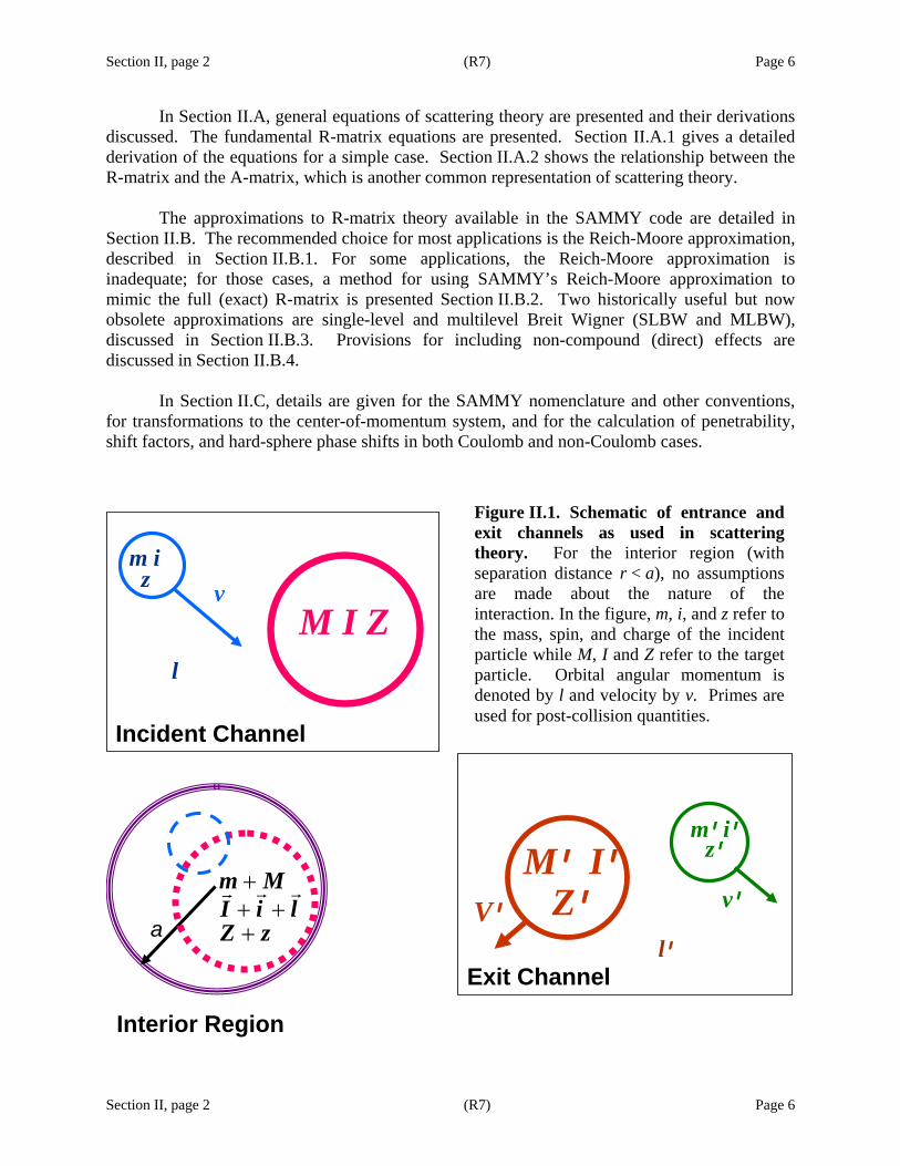
R-matrix theory is expressed in terms of channels, where a channel is defined as a pair of (incoming or outgoing) particles, plus specific information relevant to the interaction between the two particles. A schematic depicting entrance and exit channels is shown in Figure II.1. Note that entrance channels can also occur as exit channels, but some exit channels (e.g., fission channels) do not occur as entrance channels. Two interacting particles are shown in the portion of the figure that is labeled “Interior Region”; here the particles are separated by less than the interaction radius a.
Section II, page 2 (R7) Page 6
Section II, page 2 (R7) Page 6
In Section II.A, general equations of scattering theory are presented and their derivations discussed. The fundamental R-matrix equations are presented. Section II.A.1 gives a detailed derivation of the equations for a simple case. Section II.A.2 shows the relationship between the R-matrix and the A-matrix, which is another common representation of scattering theory. The approximations to R-matrix theory available in the SAMMY code are detailed in Section II.B. The recommended choice for most applications is the Reich-Moore approximation, described in Section II.B.1. For some applications, the Reich-Moore approximation is inadequate; for those cases, a method for using SAMMY’s Reich-Moore approximation to mimic the full (exact) R-matrix is presented Section II.B.2. Two historically useful but now obsolete approximations are single-level and multilevel Breit Wigner (SLBW and MLBW), discussed in Section II.B.3. Provisions for including non-compound (direct) effects are discussed in Section II.B.4.
In Section II.C, details are given for the SAMMY nomenclature and other conventions, for transformations to the center-of-momentum system, and for the calculation of penetrability, shift factors, and hard-sphere phase shifts in both Coulomb and non-Coulomb cases.
Incident Channel
m i z
M I Zv
l
a
++ ++
m MI i lZ z
Exit Channel
V’
M’ I’Z’
m’i’z’
v’
l’
Figure II.1. Schematic of entrance and exit channels as used in scattering theory. For the interior region (with separation distance r < a), no assumptions are made about the nature of the interaction. In the figure, m, i, and z refer to the mass, spin, and charge of the incident particle while M, I and Z refer to the target particle. Orbital angular momentum is denoted by l and velocity by v. Primes are used for post-collision quantities.
Interior Region
Section II.A, page 1 (R7) Page 7
Section II.A, page 1 (R7) Page 7
II. A. EQUATIONS FOR SCATTERING THEORY
In this section, equations for scattering theory are presented but not derived. Specifics for the R-matrix formulation of scattering theory are presented in Section II.A.1, which provides a discussion of an alternative formulation (the A-matrix). Readers interested in the derivation of the equations for scattering theory are referred to the Lane and Thomas article [AL58] for a detailed derivation in the general case, or to Section II.A.2 of this document for a simplified version. In scattering theory, a channel may be defined by c = (α, l, s, J), where the following definitions apply: • α represents the two particles making up the channel; α includes mass (m and M), charge (z
and Z), spin (i and I ) with associated parities, and all other quantum numbers for each of the two particles, plus the Q-value (equivalent to the negative of the threshold energy in the center of momentum system).
• l is the orbital angular momentum of the pair, and the associated parity is given by (-1) l. • s represents the channel spin (including the associated parity); that is, s is the quantized
vector sum of the spins of the two particles of the pair: Iis += . • J is the total angular momentum (and associated parity); that is, J is the quantized vector sum
of l and s: slJ += . Only J and its associated parity π are conserved for any given interaction. The other quantum numbers may differ from channel to channel, as long as the sum rules for spin and parity are obeyed. Within this document and within the SAMMY code, the set of all channels with the same J and π are called a “spin group.” In all formulae given below, spin quantum numbers (e.g., J ) are implicitly assumed to include the associated parity. Quantized vector sum rules are implicitly assumed to be obeyed. Readers unfamiliar with these sum rules are referred to Section II.C.1.a for a mini-tutorial on the subject. Let the angle-integrated cross sections from entrance channel c to exit channel c' with total angular momentum J be represented by σcc'. This cross section is given in terms of the scattering matrix U cc' as
22
' ' ' '2 ,ci wcc J cc cc JJ
a
g e Uk απσ δ δ= − (II A.1)
where kα is the wave number (and K kα α= = center-of-mass momentum) associated with incident particle pair α, gJα is the spin statistical factor, and wc is the Coulomb phase-shift difference. Note that wc is zero for non-Coulomb channels. (Details for the charged-particle case are presented in Section II.C.4.) The spin statistical factor g is given by
Section II.A, page 2 (R7) Page 8
Section II.A, page 2 (R7) Page 8
2 1 ,(2 1) (2 1)J
Jgi Iα
+=
+ + (II A.2)
and center-of-mass momentum Kα by
( )( )
222
22 .m MK k Em Mα α= =+
(II A.3)
Here E is the laboratory kinetic energy of the incident (moving) particle. A derivation of this value for Kα is given in Section II.C.2. The scattering matrix U can be written in terms of matrix W as ' ' ' ,cc c cc cU W= Ω Ω (II A.4) where Ω is given by
( ) .c ci wc e ϕ−Ω = (II A.5)
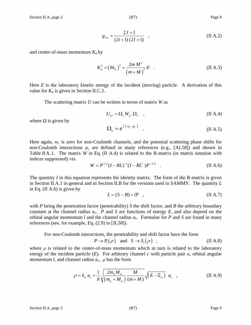
Here again, wc is zero for non-Coulomb channels, and the potential scattering phase shifts for non-Coulomb interactions φc are defined in many references (e.g., [AL58]) and shown in Table II A .1. The matrix W in Eq. (II A.4) is related to the R-matrix (in matrix notation with indices suppressed) via 1/ 2 1 * 1/ 2( ) ( ) .W P I RL I RL P− −= − − (II A.6) The quantity I in this equation represents the identity matrix. The form of the R-matrix is given in Section II.A.1 in general and in Section II.B for the versions used in SAMMY. The quantity L in Eq. (II A.6) is given by ( ) ,L S B iP= − + (II A.7) with P being the penetration factor (penetrability) S the shift factor, and B the arbitrary boundary constant at the channel radius ac. P and S are functions of energy E, and also depend on the orbital angular momentum l and the channel radius ac. Formulae for P and S are found in many references (see, for example, Eq. (2.9) in [JL58]). For non-Coulomb interactions, the penetrability and shift factor have the form ( ) ( ) and ,l lP P S Sρ ρ→ → (II A.8) where ρ is related to the center-of-mass momentum which in turn is related to the laboratory energy of the incident particle (E). For arbitrary channel c with particle pair α, orbital angular momentum l, and channel radius ac, ρ has the form
( ) ( )21 ,
( )c cm M Mk a E a
m M m Mα α
α αα α
ρ = = −Ξ+ +
(II A.9)

Section II.A, page 3 (R7) Page 9
Section II.A, page 3 (R7) Page 9
as shown in Section II.C.2. Here αΞ is the energy threshold for particle pair α, mα and Mα are the masses of the two particles of particle pair α, and m and M are the masses of the incident particle and target nuclide, respectively. Appropriate formulae for P, S, and φ in the non-Coulomb case are shown in Table IIA.1. For two charged particles, formulae for the penetrabilities are given in Section II.C.4. The energy dependence of fission and capture widths is negligible over the energy range of these calculations. Therefore, a penetrability of unity may be used.
Table II A .1. Hard-sphere penetrability (penetration factor) P, level shift factor S, and potential-scattering phase shift φ for orbital angular momentum l, wave number k, and
channel radius ac, with ρ = kac
l Pl Sl lϕ
0
ρ 0 ρ
1
ρ3/(1 + ρ2) -1 / (1 + ρ2) ρ-tan-1 ρ
2
ρ5 / (9 + 3 ρ2 + ρ4) -(18 + 3 ρ2) / (9 + 3 ρ2 + ρ4) ρ-tan-1[3ρ / (3 - ρ2)]
3
ρ7 / (225 + 45 ρ2) + 6ρ4 + ρ6)
-(675 + 90 ρ2 + 6 ρ4) / (225 + 45 ρ2 + 6 ρ4 + ρ6)
ρ-tan-1[ρ(15-ρ2) / (15-6 ρ2)]
4
ρ9 / (11025 + 1575 ρ2 + 135ρ4 + 10ρ6 + ρ8
-(44100 + 4725 ρ2 + 270 ρ4 + 10 ρ6) / (11025 + 1575 ρ2 + 135 ρ4 + 10 ρ6 + ρ8)
ρ-tan-1[ρ(105 - 10 ρ2) / (105 – 45 ρ2 + ρ4)]
l
( ) 21
21
12
−−
−
+− ll
l
PSlPρ
21
2 21 1
( )( )
l
l l
l Sl
l S Pρ −
− −
−−
− + ( )1
1 1 1tan ( ( )/l l lP l Sϕ −− − −− −
or )( 1 lll XBB += −
1(1 )/ l lB X−− with
tan( )l lB ρ ϕ= − and
1 1( ) ( )/l l lX P l S− −= −

Section II.A, page 4 (R7) Page 10
Section II.A, page 4 (R7) Page 10
Formulae for a particular cross section type can be derived by summing over the terms in Eq. (II A.1). For the total cross section, the sum over all possible exit channels and all spin groups gives
( )
( )( )
2
' '2
'
2*' ' ' ' ' '2
'
2
2 1 Re .
totalcc cc
incident all Jchannels channels
c c
J cc cc cc cc cc ccJ incident all
channels channelsc c
J ccJ incident
channelsc
g Uk
g U U Uk
g Uk
αα
α
α
πσ δ
π δ δ δ
π
= −
= − − +
= −
∑ ∑ ∑
∑ ∑ ∑
∑ ∑
(II A.10)
For non-charged incident particles, the elastic (or scattering) cross section is given by
( ) 2
'2'
1 2Re .J cc ccJ c incident c incident
channel channel
g U Ukααα
πσ= =
⎛ ⎞⎜ ⎟= − +⎜ ⎟⎜ ⎟⎝ ⎠
∑ ∑ ∑ (II A.11)
Similarly, the cross section for any non-elastic reaction can be written
2
'2'
.reactionJ cc
J c incident c reactionchannel channel
g Ukαα
πσ= =
= ∑ ∑ ∑ (II A.12)
In particular, the capture cross section could be written as the difference between the total and all other cross sections,
2
'2'
1 .captureJ cc
J c incident c all channelschannel except capture
g Ukα
πσ= =
⎛ ⎞⎜ ⎟= −⎜ ⎟⎜ ⎟⎝ ⎠
∑ ∑ ∑ (II A.13)
(This form will be used later, in Section II.B.1.a, when the capture channels are treated in an approximate fashion.)
Section II.A.1, page 1 (R7) Page 11
Section II.A.1, page 1 (R7) Page 11
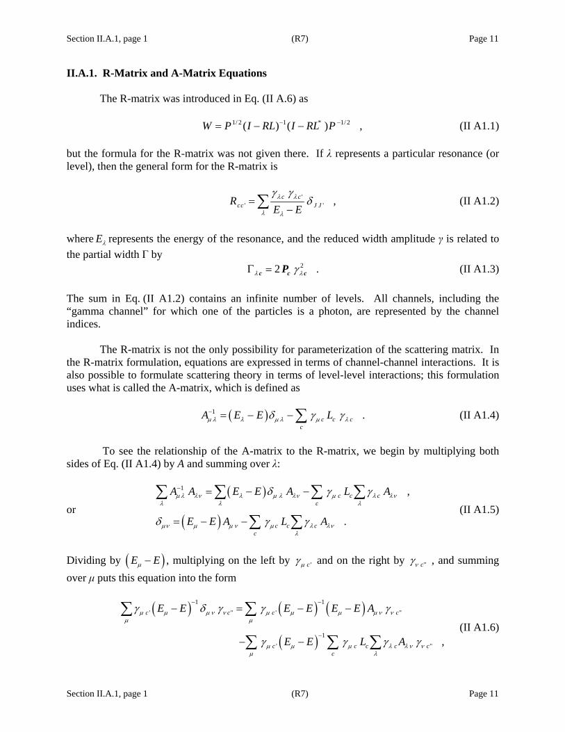
II.A.1. R-Matrix and A-Matrix Equations The R-matrix was introduced in Eq. (II A.6) as 1/ 2 1 * 1/ 2( ) ( ) ,W P I RL I RL P− −= − − (II A1.1) but the formula for the R-matrix was not given there. If λ represents a particular resonance (or level), then the general form for the R-matrix is
'' ' ,c c
cc J JRE Eλ λ
λ λ
γ γδ=
−∑ (II A1.2)
where Eλ represents the energy of the resonance, and the reduced width amplitude γ is related to the partial width Γ by 22 .λ λγΓ =c c cP (II A1.3) The sum in Eq. (II A1.2) contains an infinite number of levels. All channels, including the “gamma channel” for which one of the particles is a photon, are represented by the channel indices.
The R-matrix is not the only possibility for parameterization of the scattering matrix. In the R-matrix formulation, equations are expressed in terms of channel-channel interactions. It is also possible to formulate scattering theory in terms of level-level interactions; this formulation uses what is called the A-matrix, which is defined as
( )1 .c c c
cA E E Lμ λ λ μ λ μ λδ γ γ− = − −∑ (II A1.4)
To see the relationship of the A-matrix to the R-matrix, we begin by multiplying both
sides of Eq. (II A1.4) by A and summing over λ:
or ( )
( )
1 ,
.
c c cc
c c cc
A A E E A L A
E E A L A
μλ λν λ μ λ λν μ λ λνλ λ λ
μν μ μ ν μ λ λνλ
δ γ γ
δ γ γ
− = − −
= − −
∑ ∑ ∑ ∑
∑ ∑ (II A1.5)
Dividing by ( )E Eμ − , multiplying on the left by 'cμγ and on the right by "cνγ , and summing over μ puts this equation into the form
( ) ( ) ( )
( )
1 1
' " ' "
1
' " ,
c c c c
c c c c cc
E E E E E E A
E E L A
μ μ μ ν ν μ μ μ μ ν νμ μ
μ μ μ λ λν νμ λ
γ δ γ γ γ
γ γ γ γ
− −
−
− = − −
− −
∑ ∑
∑ ∑ ∑ (II A1.6)

Section II.A.1, page 2 (R7) Page 12
Section II.A.1, page 2 (R7) Page 12
which can be reduced to
( )
( )
1' " ' "
1
' " .
c c c c
c c c c cc
E E A
E E L A
ν ν ν μ μ ν νμ
μ μ μ λ λν νμ λ
γ γ γ γ
γ γ γ γ
−
−
− =
⎡ ⎤− −⎢ ⎥
⎣ ⎦
∑
∑ ∑ ∑ (II A1.7)
Summing over ν puts this into the form
( )
( )
1' " ' "
1
' " ,
c c c c
c c c c cc
E E A
E E L A
ν ν ν μ μ ν νν μ ν
μ μ μ λ λ ν νμ λν
γ γ γ γ
γ γ γ γ
−
−
⎡ ⎤− =⎢ ⎥⎣ ⎦
⎡ ⎤− −⎢ ⎥
⎣ ⎦
∑ ∑
∑ ∑ ∑ (II A1.8)
in which we can replace the quantities in square brackets by the R-matrix, giving
' " ' " ' "
' ' " .
c c c c c c c c cc
c c c c c c cc
R A R L A
R L A
μ μν ν λ λν νμ ν λν
λ λν νλν
γ γ γ γ
δ γ γ
= −
⎡ ⎤= −⎣ ⎦
∑ ∑ ∑
∑ ∑ (II A1.9)
Solving for the summation, this equation can be rewritten as ( ) 1
""
.c ccc
I RL R Aλ λν νλν
γ γ−⎡ ⎤− =⎣ ⎦ ∑ (II A1.10)
To relate this to the scattering matrix, we note that Eq. (II A.6) can be rewritten using Eq. (II A .7) into the form
( ) ( )( ) ( )( ) ( ) ( )
( )( )
11/ 2 * 1/ 2
11/ 2 1/ 2
1 11/ 2 1/ 2
11/ 2 1/ 2 1/ 2 1/ 2
11/ 2 1/ 2
2
2
2
2 .
W P I RL I RL P
P I RL I RL iRP P
P I RL I RL i I RL RP P
P P iP I RL RPP
I iP I RL RP
− −
− −
− − −
−− −
−
= − −
= − − +
⎡ ⎤= − − + −⎣ ⎦
= + −
= + −
(II A1.11)
Comparing Eq. (II A1.10) to Eq. (II A1.11) gives, in matrix form, 1/ 2 1/ 22 .W I iP A Pγ γ= + (II A1.12)
These equations are exact; no approximations have been made.
Section II.A.1, page 3 (R7) Page 13
Section II.A.1, page 3 (R7) Page 13
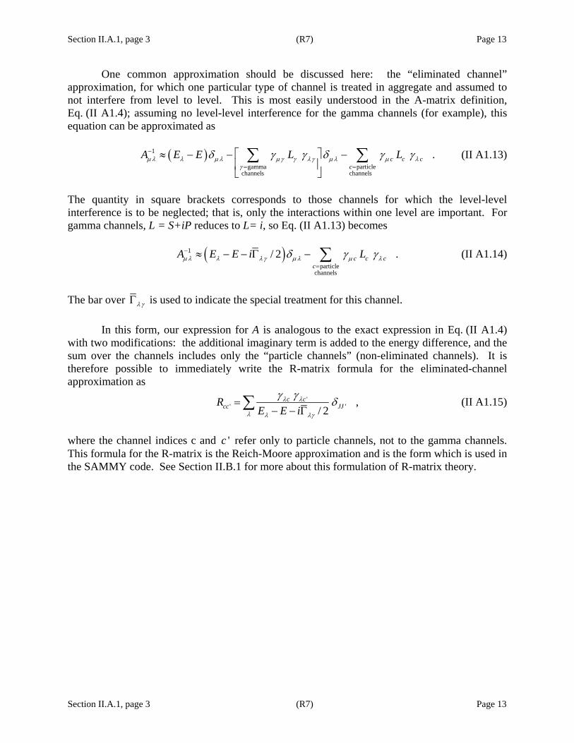
One common approximation should be discussed here: the “eliminated channel” approximation, for which one particular type of channel is treated in aggregate and assumed to not interfere from level to level. This is most easily understood in the A-matrix definition, Eq. (II A1.4); assuming no level-level interference for the gamma channels (for example), this equation can be approximated as
( )1
gamma particle channels channels
.c c cc
A E E L Lμλ λ μ λ μγ γ λγ μ λ μ λγ
δ γ γ δ γ γ−
= =
⎡ ⎤≈ − − −⎢ ⎥⎣ ⎦∑ ∑ (II A1.13)
The quantity in square brackets corresponds to those channels for which the level-level interference is to be neglected; that is, only the interactions within one level are important. For gamma channels, L = S+iP reduces to L= i, so Eq. (II A1.13) becomes ( )1
particle channels
/ 2 .c c cc
A E E i Lμλ λ λγ μ λ μ λδ γ γ−
=
≈ − − Γ − ∑ (II A1.14)
The bar over λγΓ is used to indicate the special treatment for this channel.
In this form, our expression for A is analogous to the exact expression in Eq. (II A1.4) with two modifications: the additional imaginary term is added to the energy difference, and the sum over the channels includes only the “particle channels” (non-eliminated channels). It is therefore possible to immediately write the R-matrix formula for the eliminated-channel approximation as
'' ' ,
/ 2c c
cc JJRE E i
λ λ
λ λ λγ
γ γ δ=− − Γ∑ (II A1.15)
where the channel indices c and 'c refer only to particle channels, not to the gamma channels. This formula for the R-matrix is the Reich-Moore approximation and is the form which is used in the SAMMY code. See Section II.B.1 for more about this formulation of R-matrix theory.


Section II.A.2, page 1 (R7) Page 15
Section II.A.2, page 1 (R7) Page 15
II.A.2. Derivation of Scattering Theory Equations Many authors have given derivations of the equations for the scattering matrix in terms of the R-matrix. Sources for the derivation shown here are unpublished lecture notes of Fröhner [FF02], presented at the SAMMY workshop in Paris in 2002, and Foderaro [AF71]. This derivation is valid for only the simple case of spinless projectiles and target nuclei, assuming only elastic scattering and absorption. For the general case, the reader is referred to Lane and Thomas [AL58]. Schrödinger equation The Schrödinger equation with a complex potential is
2
2 ,2
V iW Em
ψ ψ⎛ ⎞−
∇ + + =⎜ ⎟⎝ ⎠
(II A2.1)
in which one can consider that V causes scattering and W causes absorption. The wave function can be expanded in the usual fashion,
( ) ( )0
( , cos ) cos ,ll
l
u rr P
rψ θ θ
∞
=
= ∑ (II A2.2)
for which the radial portion obeys the equation
( ) ( )22
2 2 2
12 0 ,ll
d u l lmk V iW ud r r
+⎡ ⎤+ − + − =⎢ ⎥
⎣ ⎦ (II A2.3)
subject to the conditions that 2ψ is everywhere finite and that
( )0 0 .lu r = = (II A2.4) In the external region, r a> , the nuclear forces are zero (V = W = 0), so the solution has the form ( ) ( ) ( ) .l l l lu r I r U O r= − (II A2.5) Il represents an incoming free wave, and Ol represents an outgoing free wave. Ul is the “collision function” or “S function” that describes the effects of the nuclear interaction, giving both the attenuation and the phase shift of the outgoing wave:
and 2
2
1 for 0 ,
1 for 0 .l
l
U W
U W
= =
< ≠ (II A2.6)
Our goal is to determine an appropriate analytic form for Ul.

Section II.A.2, page 2 (R7) Page 16
Section II.A.2, page 2 (R7) Page 16
Orthogonal eigenvectors in interior region
For the interior region r a< , we define eigenfunctions ( )lw rλ and eigenvalues Eλ ,
2 2
,2
kEmλ
λ = (II A2.7)
for the wave equation without absorption (W = 0),
( )22
2 2 2
12 0 ,ll
d w l lmk V wd r r
λλ λ
+⎡ ⎤+ − − =⎢ ⎥⎣ ⎦
(II A2.8)
for which the boundary conditions are
( ) ( )0 0 and .l
l ll r a
d waw r Bw a d r
λλ
λ =
= = = (II A2.9)
Note that ( )lw rλ is real if the boundary parameter Bl is chosen to be real. The eigenfunctions are orthogonal, since
( ) ( ) [ ]
( ) ( ) ( ) ( )
22
2 20 0
0
0
0 ,
a al ll l
l l l l
all
l l
lll l
r a r a
ll l l l
d w d wd w d wdw w dr w w drdr dr dr d r d r
d wd w w wd r d r
d wd w w a w ad r d r
B w a w a w a w aa
μ μλ λμ λ μ λ
μλμ λ
μλμ λ
λ μ λ μ
= =
⎛ ⎞ ⎛ ⎞− = −⎜ ⎟ ⎜ ⎟⎜ ⎟ ⎝ ⎠⎝ ⎠
⎡ ⎤= −⎢ ⎥
⎣ ⎦
= − −
⎡ ⎤= − =⎣ ⎦
∫ ∫
(II A2.10)
in which both equations of (II A2.9) have been invoked. The integral in Eq. (II A2.10) can also be evaluated using Eq. (II A2.8), giving

Section II.A.2, page 3 (R7) Page 17
Section II.A.2, page 3 (R7) Page 17
( )
( )
2 2
2 20
2 22 2
0
2 2
0
2 2
0
2 2
.
al l
l l
a
l l l l
a
l l l l
a
l l
d w d ww w dr
d r d r
mV mVk w w w k w dr
k w w k w w dr
k k w w dr
λ μμ λ
λ λ μ λ μ λ
λ λ μ μ λ μ
λ μ λ μ
⎛ ⎞−⎜ ⎟⎜ ⎟
⎝ ⎠⎛ ⎞⎡ ⎤ ⎡ ⎤= − − − − −⎜ ⎟⎢ ⎥ ⎢ ⎥⎣ ⎦ ⎣ ⎦⎝ ⎠
= − +
= − −
∫
∫
∫
∫
(II A2.11)
Equating Eq. (II A2.10) to Eq. (II A2.11) gives
( )2 2
0
0 .a
l lk k w w drλ μ λ μ− =∫ (II A2.12)
For λ μ≠ , assuming no degenerate states, it therefore follows that
0
0 if .a
l lw w drλ μ λ μ= ≠∫ (II A2.13)
The orthogonality of the eigenvectors is therefore established. We assume that these wave functions are normalized such that
0
.a
l lw w drλ μ λ μδ=∫ (II A2.14)
Matching at the surface
The internal wave function for the true potential (including the imaginary part iW ) can be expanded in terms of the eigenfunctions as
( ) ( ) for ,l l lu r c w r r aλ λλ
= ≤∑ (II A2.15)
with
0
.a
l l lc u w drλ λ= ∫ (II A2.16)
This equation for lcλ is derived by multiplying Eq. (II A2.15) by ( )lu rλ , integrating, and applying Eq. (II A2.14).

Section II.A.2, page 4 (R7) Page 18
Section II.A.2, page 4 (R7) Page 18
Consider now the integral
2 2
2 2
0
,a
l ll l
d u d ww u dr
d r d rλ
λ
⎛ ⎞−⎜ ⎟⎜ ⎟
⎝ ⎠∫ (II A2.17)
which can be expanded by use of Eqs. (II A2.3) and (II A2.8) to give
( ) ( ) ( )
( )
2 2
2 2
0
2 22 2 2 2
0
2 22
0 0
1 12 2
2 .
a
l ll l
a
l l l l
a a
l l l l
d u d ww u dr
d r d r
l l l lm mk V iW u w u k V w drr r
mk k u w dr W u w dr
λλ
λ λ λ
λ λ λ
⎛ ⎞−⎜ ⎟⎜ ⎟
⎝ ⎠
⎛ ⎞+ +⎡ ⎤ ⎡ ⎤= − − + − + − −⎜ ⎟⎢ ⎥ ⎢ ⎥⎜ ⎟⎣ ⎦ ⎣ ⎦⎝ ⎠
= − +∫ ∫
∫
∫ (II A2.18)
Defining lWλ as
0 0
a a
l l l l lW W u w dr u w drλ λ λ= ∫ ∫ (II A2.19)
permits rewriting Eq. (II A2.18) in the form
2 2
2 22 2 2
00
2 .a a
l ll l l l l
d u d w mw u dr k k i W u w drd r d r
λλ λ λ λ
⎛ ⎞ ⎛ ⎞− = − +⎜ ⎟ ⎜ ⎟⎜ ⎟ ⎝ ⎠⎝ ⎠∫∫ (II A2.20)
Integrating the left-hand side of this equation gives
( )
2 2
2 200
,
a al l l ll l
l l l l l lr a
ll l ll l l l l
r a r a
d u d w d w d wdu duw u dr w u w ud r d r d r d r d r d r
w adu B duw u w a u Bd r a d r a
λ λ λλ λ λ
λλ λ
=
= =
⎛ ⎞ ⎡ ⎤ ⎡ ⎤− = − = −⎜ ⎟ ⎢ ⎥ ⎢ ⎥⎜ ⎟ ⎣ ⎦ ⎣ ⎦⎝ ⎠
⎡ ⎤ ⎡ ⎤= − = −⎢ ⎥ ⎢ ⎥⎣ ⎦ ⎣ ⎦
∫ (II A2.21)
in which we have again made use of the boundary condition of Eq. (II A2.9). Integrating the right-hand side of Eq. (II A2.20) by applying Eq. (II A2.16) gives
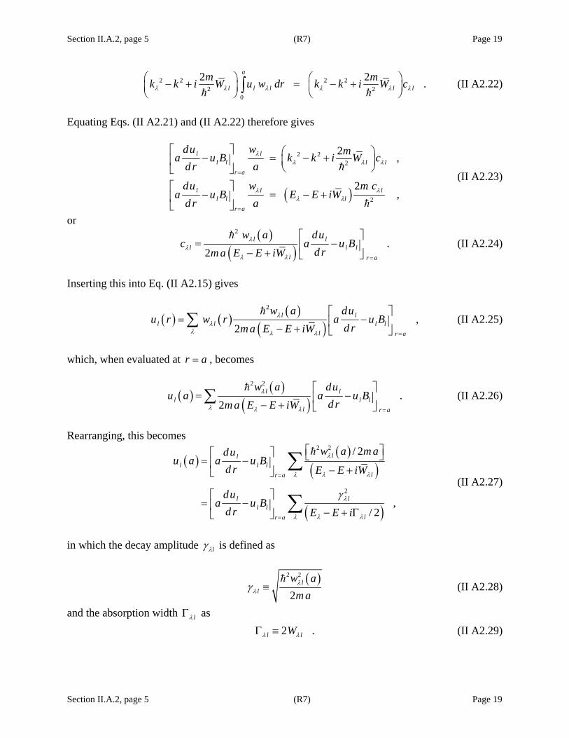
Section II.A.2, page 5 (R7) Page 19
Section II.A.2, page 5 (R7) Page 19
2 2 2 22 2
0
2 2 .a
l l l l lm mk k i W u w dr k k i W cλ λ λ λ λ λ
⎛ ⎞ ⎛ ⎞− + = − +⎜ ⎟ ⎜ ⎟⎝ ⎠ ⎝ ⎠∫ (II A2.22)
Equating Eqs. (II A2.21) and (II A2.22) therefore gives
( )
2 22
2
2 ,
2,
l ll l l l
r a
l l ll l l
r a
du w ma u B k k i W cd r a
du w m ca u B E E iW
d r a
λλ λ λ
λ λλ λ
=
=
⎡ ⎤ ⎛ ⎞− = − +⎢ ⎥ ⎜ ⎟⎝ ⎠⎣ ⎦
⎡ ⎤− = − +⎢ ⎥
⎣ ⎦
(II A2.23)
or
( )
( )2
.2
l ll l l
l r a
w a duc a u B
d rm a E E iWλ
λλ λ =
⎡ ⎤= −⎢ ⎥− + ⎣ ⎦
(II A2.24)
Inserting this into Eq. (II A2.15) gives
( ) ( ) ( )( )
2
,2
l ll l l l
l r a
w a duu r w r a u B
d rm a E E iWλ
λλ λ λ =
⎡ ⎤= −⎢ ⎥− + ⎣ ⎦∑ (II A2.25)
which, when evaluated at r a= , becomes
( ) ( )( )
2 2
.2
l ll l l
l r a
w a duu a a u B
d rm a E E iWλ
λ λ λ =
⎡ ⎤= −⎢ ⎥− + ⎣ ⎦∑ (II A2.26)
Rearranging, this becomes
( )( )
( )
( )
2 2
2
/ 2
,/ 2
lll l l
lr a
l ll l
lr a
w a m aduu a a u B
d r E E iW
dua u B
d r E E i
λ
λ λλ
λ
λ λλ
γ
=
=
⎡ ⎤⎡ ⎤ ⎣ ⎦= −⎢ ⎥ − +⎣ ⎦
⎡ ⎤= −⎢ ⎥ − + Γ⎣ ⎦
∑
∑ (II A2.27)
in which the decay amplitude lλγ is defined as
( )2 2
2l
l
w am aλ
λγ ≡ (II A2.28)
and the absorption width lλΓ as 2 .l lWλ λΓ ≡ (II A2.29)
Section II.A.2, page 6 (R7) Page 20
Section II.A.2, page 6 (R7) Page 20
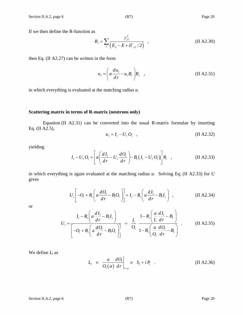
If we then define the R-function as
( )2
,/ 2
ll
l
RE E i
λ
λ λ λ
γ=
− + Γ∑ (II A2.30)
then Eq. (II A2.27) can be written in the form
,ll l l l
duu a u B R
d r⎛ ⎞
= −⎜ ⎟⎝ ⎠
(II A2.31)
in which everything is evaluated at the matching radius a. Scattering matrix in terms of R-matrix (neutrons only)
Equation (II A2.31) can be converted into the usual R-matrix formulae by inserting Eq. (II A2.5), ,l l l lu I U O= − (II A2.32) yielding
( ) ,l ll l l l l l l l l
d I dOI U O a U B I U O Rd r d r
⎡ ⎤⎛ ⎞− = − − −⎢ ⎥⎜ ⎟
⎝ ⎠⎣ ⎦ (II A2.33)
in which everything is again evaluated at the matching radius a. Solving Eq. (II A2.33) for U gives
,l ll l l l l l l l l
dO d IU O R a B O I R a B Id r d r
⎡ ⎤⎛ ⎞ ⎛ ⎞− + − = − −⎢ ⎥⎜ ⎟ ⎜ ⎟
⎝ ⎠ ⎝ ⎠⎣ ⎦ (II A2.34)
or
1
.1
lll ll l l l
lll
l lll ll l l l
l
d Iad I R BI R a B II d rd r IU
O dOadO R BO R a B OO d rd r
⎛ ⎞⎛ ⎞− −− − ⎜ ⎟⎜ ⎟
⎝ ⎠ ⎝ ⎠= =⎡ ⎤ ⎛ ⎞⎛ ⎞ − −− + − ⎜ ⎟⎢ ⎥⎜ ⎟
⎝ ⎠⎝ ⎠⎣ ⎦
(II A2.35)
We define Ll as
( )
.ll l l
l r a
dOaL S i PO a d r
=
≡ ≡ + (II A2.36)

Section II.A.2, page 7 (R7) Page 21
Section II.A.2, page 7 (R7) Page 21
For spinless particles, *l lI O= , so that
( )
*ll l l
l r a
d Ia L S iPI a d r
=
= = − (II A2.37)
and
*
2 .i
il li
l l
O eI O eO O O e
ϕϕ
ϕ
−−= = = (II A2.38)
Therefore Eq. (II A2.34) becomes
( )( )
*2
1,
1l l li
ll l l
R L BU e
R L Bϕ−
− −=
− − (II A2.39)
which is the usual form for the scattering matrix in terms of the R-matrix in this simple case.

Section II.A.2.a, page 1 (R7) Page 23
Section II.A.2.a, page 1 (R7) Page 23
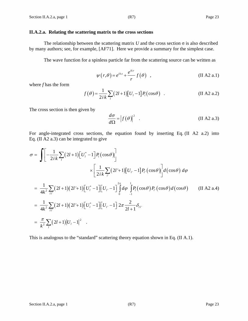
II.A.2.a. Relating the scattering matrix to the cross sections The relationship between the scattering matrix U and the cross section σ is also described by many authors; see, for example, [AF71]. Here we provide a summary for the simplest case. The wave function for a spinless particle far from the scattering source can be written as
( ) ( ), ,i k r
i k z er e fr
ψ θ θ= + (II A2 a.1)
where f has the form
( ) ( )[ ] ( )1 2 1 1 cos .2 l l
l
f l U Pi k
θ θ= + −∑ (II A2 a.2)
The cross section is then given by
( ) 2.d f
dσ θ=Ω
(II A2 a.3)
For angle-integrated cross sections, the equation found by inserting Eq. (II A2 a.2) into Eq. (II A2 a.3) can be integrated to give
( ) ( )
( )[ ] ( ) ( )
( )( ) ( ) ( ) ( )
( )( )
( )
*
' ''
2 1*
' '2' 0 1
*' '2
'
2
2
1 2 1 1 cos2
1 2 ' 1 1 cos cos2
1 2 1 2 ' 1 1 1 cos cos cos4
1 22 1 2 ' 1 1 1 22 14
2 1 1 .
l ll
l ll
l l l ll l
l l l ll l
ll
l U Pi k
l U P d di k
l l U U d P P dk
l l U Ulk
l Uk
π
σ θ
θ θ ϕ
ϕ θ θ θ
π δ
π
−
⎡ ⎤⎡ ⎤= − + −⎢ ⎥⎣ ⎦
⎣ ⎦⎡ ⎤
× + −⎢ ⎥⎣ ⎦
⎡ ⎤ ⎡ ⎤= + + − −⎣ ⎦ ⎣ ⎦
⎡ ⎤ ⎡ ⎤= + + − −⎣ ⎦ ⎣ ⎦ +
= + −
∑
∑
∑ ∫ ∫
∑
∑
∫
(II A2 a.4)
This is analogous to the “standard” scattering theory equation shown in Eq. (II A.1).


Section II.B, page 1 (R7) Page 25
Section II.B, page 1 (R7) Page 25
II. B. VERSIONS OF MULTILEVEL R-MATRIX THEORY
Many representations of multilevel R-matrix theory have been developed over the years. For a summary of the more common versions, the reader is referred to the works of Fröhner [FF80, FF00]. Four versions of R-matrix theory are available in SAMMY: the Reich-Moore approximation (Section II.B.1), the single-level (SLBW) and multilevel Breit-Wigner (MLBW) approximations (Section II.B.3), and a variant on the Reich Moore which mimics the full R-matrix (Section II.B.2). An option to include a direct capture component is also provided (Section II.B.4).
The Reich-Moore approximation is the preferred method for most modern evaluations; it is the default formalism for SAMMY runs.
Fröhner, in fact, suggests that the Reich-Moore approximation is universally applicable to
all cases: “Experience has shown that with this approximation [Reich Moore] all resonance cross section data can be described in detail, in the windows as well as in the peaks, even the weirdest multilevel interference patterns . . . It works equally well for light, medium-mass and heavy nuclei, fissile and nonfissile.” [FF00, page 60]
For most purposes, Reich Moore is indeed indistinguishable from the exact formulation.
Notable exceptions are situations where interference effects exist between capture and other channels. For those cases, small modifications to the SAMMY input will permit the user to mimic the effect of the non-approximated R-matrix; see Section II.B.2 for details.
Occasionally it is not possible to properly describe a cross section within the confines of
R-matrix theory, because the reaction includes a direct component. SAMMY has provisions for the user to provide a numerical description of this component; see Section II.B.4 for details. Also available within SAMMY are both the SLBW and the MLBW formulations (Section II.B.3); these are included for the sake of completeness, for comparison purposes, and because many of the evaluations in the nuclear data files were performed with Breit-Wigner formulae. However, it is strongly recommended that only Reich Moore be used for new evaluations, for several reasons: MLBW is often inadequate; SLBW is almost always inadequate. When it is correct, MLBW gives identical results to Reich Moore. “Ease of Programming” is no longer a valid excuse for using MLBW, since the programming has already been accomplished. Similarly, a slow computer is no longer a legitimate excuse, since modern computers can readily handle the more rigorous formulae. Finally, it should be noted that SAMMY’s implementation of MLBW does not correspond to the usual definition of MLBW. Instead, SAMMY uses the ENDF [ENDF-102] convention in which only the elastic cross section is truly multilevel, and all other types of cross section are single level.

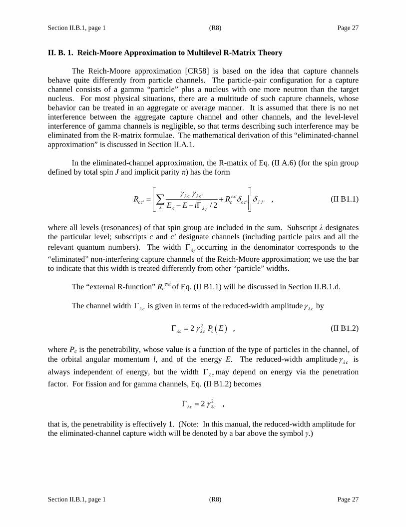
Section II.B.1, page 1 (R8) Page 27
Section II.B.1, page 1 (R8) Page 27
II. B. 1. Reich-Moore Approximation to Multilevel R-Matrix Theory The Reich-Moore approximation [CR58] is based on the idea that capture channels behave quite differently from particle channels. The particle-pair configuration for a capture channel consists of a gamma “particle” plus a nucleus with one more neutron than the target nucleus. For most physical situations, there are a multitude of such capture channels, whose behavior can be treated in an aggregate or average manner. It is assumed that there is no net interference between the aggregate capture channel and other channels, and the level-level interference of gamma channels is negligible, so that terms describing such interference may be eliminated from the R-matrix formulae. The mathematical derivation of this “eliminated-channel approximation” is discussed in Section II.A.1. In the eliminated-channel approximation, the R-matrix of Eq. (II A.6) (for the spin group defined by total spin J and implicit parity π) has the form
'' ' ' ,
/ 2c c ext
cc c cc J JR RE E i
λ λ
λ λ λγ
γ γδ δ
⎡ ⎤= +⎢ ⎥
− − Γ⎢ ⎥⎣ ⎦∑ (II B1.1)
where all levels (resonances) of that spin group are included in the sum. Subscript λ designates the particular level; subscripts c and c' designate channels (including particle pairs and all the relevant quantum numbers). The width λγΓ occurring in the denominator corresponds to the “eliminated” non-interfering capture channels of the Reich-Moore approximation; we use the bar to indicate that this width is treated differently from other “particle” widths. The “external R-function” Rc
ext of Eq. (II B1.1) will be discussed in Section II.B.1.d. The channel width cλΓ is given in terms of the reduced-width amplitude cλγ by ( )22 ,c c cP Eλ λγΓ = (II B1.2) where Pc is the penetrability, whose value is a function of the type of particles in the channel, of the orbital angular momentum l, and of the energy E. The reduced-width amplitude cλγ is always independent of energy, but the width cλΓ may depend on energy via the penetration factor. For fission and for gamma channels, Eq. (II B1.2) becomes 22 ,c cλ λγΓ = that is, the penetrability is effectively 1. (Note: In this manual, the reduced-width amplitude for the eliminated-channel capture width will be denoted by a bar above the symbol γ.)
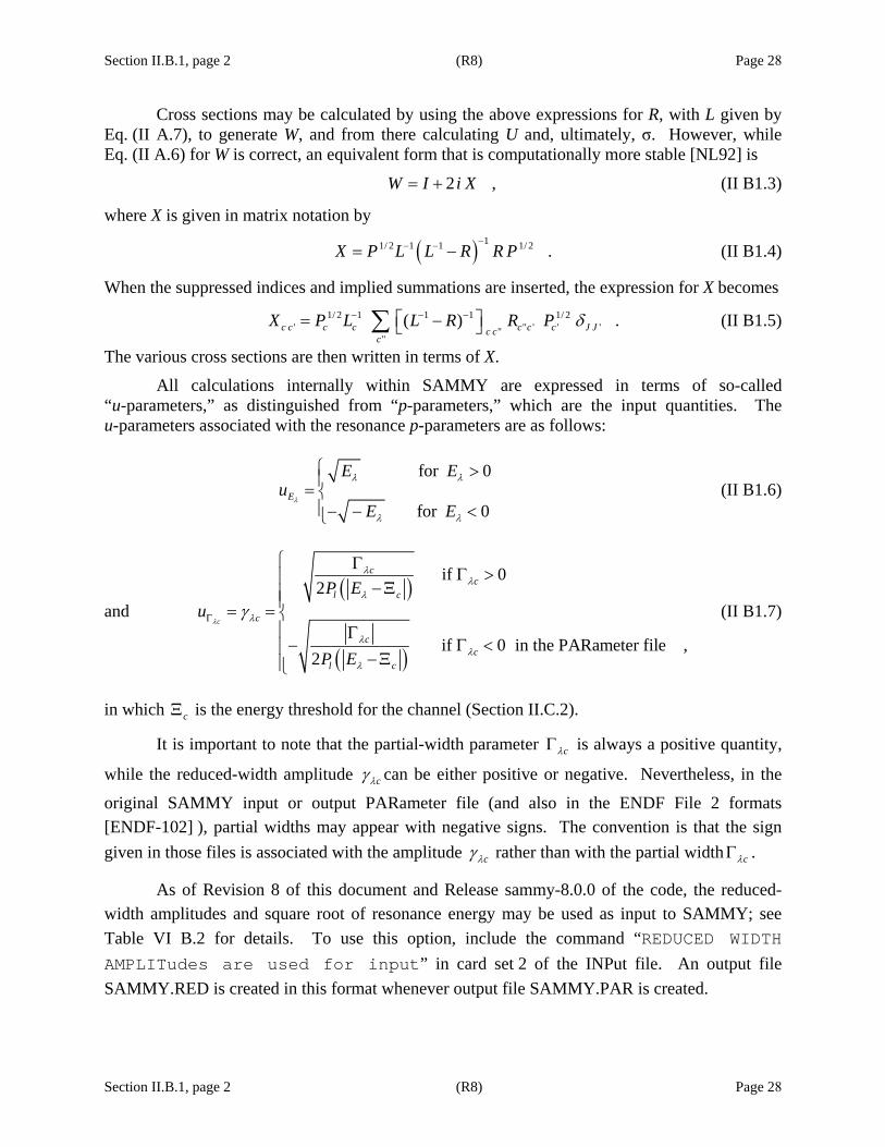
Section II.B.1, page 2 (R8) Page 28
Section II.B.1, page 2 (R8) Page 28
Cross sections may be calculated by using the above expressions for R, with L given by Eq. (II A.7), to generate W, and from there calculating U and, ultimately, σ. However, while Eq. (II A.6) for W is correct, an equivalent form that is computationally more stable [NL92] is
2 ,W I i X= + (II B1.3)
where X is given in matrix notation by
( ) 11/ 2 1 1 1/ 2 .X P L L R R P−− −= − (II B1.4)
When the suppressed indices and implied summations are inserted, the expression for X becomes
1/ 2 1 1 1 1/ 2' " ' ' '"
"( ) .c c c c c c c J Jc c
cX P L L R R P δ− − −⎡ ⎤= −⎣ ⎦∑ (II B1.5)
The various cross sections are then written in terms of X.
All calculations internally within SAMMY are expressed in terms of so-called “u-parameters,” as distinguished from “p-parameters,” which are the input quantities. The u-parameters associated with the resonance p-parameters are as follows:
for 0
for 0E
E Eu
E Eλ
λ λ
λ λ
⎧ >⎪= ⎨⎪− − <⎩
(II B1.6)
and ( )
( )
if 02
if 0 in the PARameter file ,2
c
cc
l c
c
cc
l c
P Eu
P E
λ
λλ
λ
λ
λλ
λ
γΓ
⎧ ΓΓ >⎪
−Ξ⎪⎪= = ⎨⎪ Γ− Γ <⎪
−Ξ⎪⎩
(II B1.7)
in which cΞ is the energy threshold for the channel (Section II.C.2).
It is important to note that the partial-width parameter cλΓ is always a positive quantity,
while the reduced-width amplitude cλγ can be either positive or negative. Nevertheless, in the
original SAMMY input or output PARameter file (and also in the ENDF File 2 formats [ENDF-102] ), partial widths may appear with negative signs. The convention is that the sign given in those files is associated with the amplitude cλγ rather than with the partial width cλΓ .
As of Revision 8 of this document and Release sammy-8.0.0 of the code, the reduced-width amplitudes and square root of resonance energy may be used as input to SAMMY; see Table VI B.2 for details. To use this option, include the command “REDUCED WIDTH AMPLITudes are used for input” in card set 2 of the INPut file. An output file SAMMY.RED is created in this format whenever output file SAMMY.PAR is created.
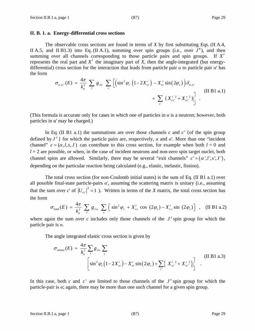
Section II.B.1.a, page 1 (R7) Page 29
Section II.B.1.a, page 1 (R7) Page 29
II. B. 1. a. Energy-differential cross sections The observable cross sections are found in terms of X by first substituting Eqs. (II A.4, II A.5, and II B1.3) into Eq. (II A.1), summing over spin groups (i.e., over J π ), and then summing over all channels corresponding to those particle pairs and spin groups. If X r represents the real part and X i the imaginary part of X, then the angle-integrated (but energy-differential) cross section for the interaction that leads from particle pair α to particle pair α' has the form
( ) ( )( )2
, ' , '2
2 2' '
'
4( ) sin 1 2 sin 2
.
i rJ c cc cc c
J c
i rcc cc
c
E g X Xk
X X
α α α α αα
πσ ϕ ϕ δ⎡= − −⎣
⎤+ + ⎥⎦
∑ ∑
∑ (II B1 a.1)
(This formula is accurate only for cases in which one of particles in α is a neutron; however, both particles in α' may be charged.) In Eq. (II B1 a.1) the summations are over those channels c and c′ of the spin group defined by J π for which the particle pairs are, respectively, α and α'. More than one “incident channel” ( , , , )c l s Jα= can contribute to this cross section, for example when both l = 0 and l = 2 are possible, or when, in the case of incident neutrons and non-zero spin target nuclei, both channel spins are allowed. Similarly, there may be several “exit channels” ( )' ', ', ', 'c l s Jα= , depending on the particular reaction being calculated (e.g., elastic, inelastic, fission). The total cross section (for non-Coulomb initial states) is the sum of Eq. (II B1 a.1) over all possible final-state particle-pairs α', assuming the scattering matrix is unitary (i.e., assuming that the sum over c' of 2
' 1ccU = ). Written in terms of the X matrix, the total cross section has the form
22
c
4( ) sin cos (2 ) sin (2 ) ,i rtotal J c cc c cc c
J
E g X Xk αα
πσ ϕ ϕ ϕ⎡ ⎤= + −⎣ ⎦∑ ∑ (II B1 a.2)
where again the sum over c includes only those channels of the J π spin group for which the particle pair is α. The angle integrated elastic cross section is given by
( ) ( )
2
2 2 2' '
'
4( )
sin 1 2 sin 2 .
elastic JJ c
i r i rc cc cc c cc cc
c
E gk
X X X X
αα
πσ
ϕ ϕ
=
⎡ ⎤− − + +⎢ ⎥⎣ ⎦
∑ ∑
∑ (II B1 a.3)
In this case, both c and 'c are limited to those channels of the J π spin group for which the particle-pair is α; again, there may be more than one such channel for a given spin group.
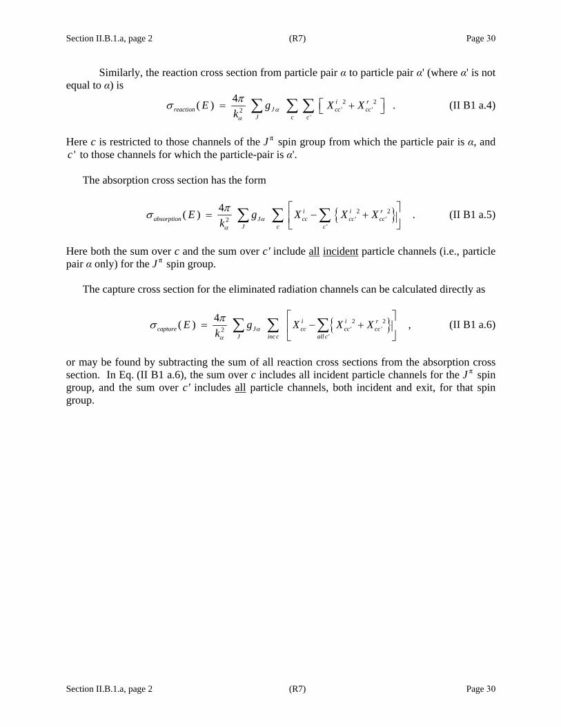
Section II.B.1.a, page 2 (R7) Page 30
Section II.B.1.a, page 2 (R7) Page 30
Similarly, the reaction cross section from particle pair α to particle pair α' (where α' is not equal to α) is
2 2' '2
'
4( ) .i rreaction J cc cc
J c c
E g X Xk αα
πσ ⎡ ⎤= +⎣ ⎦∑ ∑ ∑ (II B1 a.4)
Here c is restricted to those channels of the J π spin group from which the particle pair is α, and
'c to those channels for which the particle-pair is α'. The absorption cross section has the form
2 2' '2
'
4( ) .i i rabsorption J cc cc cc
J c c
E g X X Xk αα
πσ ⎡ ⎤= − +⎢ ⎥⎣ ⎦∑ ∑ ∑ (II B1 a.5)
Here both the sum over c and the sum over c′ include all incident particle channels (i.e., particle pair α only) for the J π spin group. The capture cross section for the eliminated radiation channels can be calculated directly as
2 2' '2
'
4( ) ,i i rcapture J cc cc cc
J incc all cE g X X X
k αα
πσ⎡ ⎤
= − +⎢ ⎥⎣ ⎦
∑ ∑ ∑ (II B1 a.6)
or may be found by subtracting the sum of all reaction cross sections from the absorption cross section. In Eq. (II B1 a.6), the sum over c includes all incident particle channels for the J π spin group, and the sum over c′ includes all particle channels, both incident and exit, for that spin group.

Section II.B.1.a.i, page 1 (R7) Page 31
Section II.B.1.a.i, page 1 (R7) Page 31
II.B.1.a.i. One-level two-channel case For a simple one-level, two-channel case for which the shift factor is set to zero, the various cross sections defined in Section II.B.1.a can easily be expressed in terms of resonance parameters. Users are reminded that SAMMY is by no means restricted to this simple case and can be used with as many levels and as many channels as are needed to describe the particular physical situation. Nevertheless, it is useful to examine the cross section equations for this simple case: while these equations are a crude over-simplification for most physical situations, there is often physical insight to be gained by examination of these equations.
For this simple case, the X matrix of Eq. (II B1.4) takes the form
( ) 11 1
12 21 1 1 2 1 1 2
11 12 2
1 2 2 1 2 2 22
22
100
,1 0
0
X PL L R R P
PPiP iP D D D D
PPD iP D D DiP
γ γ γ γ γ γ
γ γ γ γ γ γ
−− −
−
= −
⎡ ⎤ ⎡ ⎤ ⎡ ⎤− −⎢ ⎥ ⎢ ⎥ ⎢ ⎥ ⎡ ⎤⎢ ⎥ ⎢ ⎥ ⎢ ⎥= ⎢ ⎥⎢ ⎥ ⎢ ⎥ ⎢ ⎥ ⎢ ⎥⎣ ⎦⎢ ⎥ − −⎢ ⎥ ⎢ ⎥⎣ ⎦⎢ ⎥ ⎣ ⎦⎣ ⎦
(II B1 ai.1)
in which the subscript on the penetrabilities denotes the channel number (not the angular momentum), the symbol D has been used for 2E E iλ λγγ− − , and the subscript λ has been omitted from the reduced-width amplitudes for simplicity’s sake. This equation can be rewritten as
( )( )
( )( )
12 22 1 1 1 2 1 21 11 1 21 2
221 2 2 21 2 1 2 1 2 2
2
21 2 2 1 2 1 211 2
2 2 21 2 1 1 2 2 1 2 1 2 2 1
2
1 00
1 00
1 0
10
P D iP iPPP PiPP DXiD PiPP P D iP
P
P D iP iPPPPPPP D iP D iP D iPP P D iP
P
γ γ γ γ γ γγ γ γγ γ γ
γ γ γ
γ γ γ γ
−⎡ ⎤⎢ ⎥ ⎡ ⎤− − ⎡ ⎤⎡ ⎤⎢ ⎥ ⎢ ⎥= ⎢ ⎥⎢ ⎥⎢ ⎥ ⎢ ⎥− − ⎢ ⎥⎣ ⎦ ⎣ ⎦⎣ ⎦⎢ ⎥⎢ ⎥⎣ ⎦
⎡ ⎤⎢ ⎥ −⎢ ⎥=⎢ ⎥− − −⎢ ⎥⎢ ⎥⎣ ⎦
( )21
211 1 2
21 2 2 2
0,
0
P
P
γ
γ γ γγ γ γ
⎡ ⎤⎢ ⎥⎢ ⎥⎣ ⎦
⎡ ⎤⎡ ⎤× ⎢ ⎥⎢ ⎥
⎢ ⎥⎣ ⎦ ⎣ ⎦
or

Section II.B.1.a.i, page 2 (R7) Page 32
Section II.B.1.a.i, page 2 (R7) Page 32
( )1
2 2 21 1 2 2
2
2 2 2 2 2 3 311 1 1 2 1 2 1 2 1 2 1 1 2 1 2 1 2 1 2 1 2
3 3 2 2 2 2 21 2 1 2 2 1 2 1 2 1 2 1 2 1 2 2 2 1 2 1 2 2
2 21 1 2 2
1 01
10
0
0
1
PX
D iP D iP DP
PP D iPP iPP PD iPP iPPiPP P D iPP iPP P D iPP P
D iP D iP
γ γ
γ γ γ γ γ γ γ γ γ γ γγ γ γ γ γ γ γ γ γ γ γ
γ γ
⎡ ⎤⎢ ⎥⎢ ⎥=⎢ ⎥− −⎢ ⎥⎢ ⎥⎣ ⎦
⎡ ⎤⎡ ⎤− + − +× ⎢ ⎥⎢ ⎥+ − + − ⎢ ⎥⎣ ⎦ ⎣ ⎦
=− −( )
( )
21 11 1 1 1 2
222 1 2 2 2 2
2
21 1 1 2 1 2
2 2 21 1 2 2 1 2 1 2 2 2
1 00
1 00
1 ,
P PP D PDP D P DD P
P
P PPD iP iP PP P
γ γ γγ γ γ
γ γ γ
γ γ γ γ γ
⎡ ⎤⎢ ⎥ ⎡ ⎤⎡ ⎤⎢ ⎥ ⎢ ⎥⎢ ⎥⎢ ⎥ ⎢ ⎥⎣ ⎦ ⎣ ⎦⎢ ⎥⎢ ⎥⎣ ⎦
⎡ ⎤= ⎢ ⎥
− − ⎢ ⎥⎣ ⎦ or, finally,
( )
( )
21 1 1 2 1 2
2 2 2 21 1 2 2 1 2 1 2 2 2
1 1 2
1 2 2
1
/ 2 / 21 ,/ 2 / 2 / 2
P PPX
E E i iP iP PP P
E E i
λ γ
λ
γ γ γ
γ γ γ γ γ γ
⎡ ⎤= ⎢ ⎥
− − − − ⎢ ⎥⎣ ⎦
⎡ ⎤Γ Γ Γ= ⎢ ⎥
− − Γ Γ Γ Γ⎢ ⎥⎣ ⎦
(II B1 ai.2)
in which Γ is the sum of the partial widths 1 2 γΓ + Γ +Γ .
In this form, X can be substituted into the equations for the various cross sections. Assuming the second channel is a reaction channel, Eq. (II B1 a.2) for the total cross section becomes
( )
( )
12 12
112
4( ) sin cos (2 ) sin (2 )4 2
2 1 1 cos (2 ) sin (2 ) ,2
total J c c c
J c c
E EE g
k d d
E Eg
k d d
λ
α
λ
α
πσ ϕ ϕ ϕ
π ϕ ϕ
− Γ⎡ ⎤ΓΓ= + −⎢ ⎥
⎣ ⎦− Γ⎡ ⎤ΓΓ⎛ ⎞= − − −⎢ ⎥⎜ ⎟
⎝ ⎠⎣ ⎦
(II B1 ai.3)
in which d has been used to represent ( ) ( ) ( )2 2 2/ 2 / 2E E i E Eλ λ− − Γ = − + Γ . Similarly, the elastic cross section, Eq. (II B1 a.3), can be expressed as
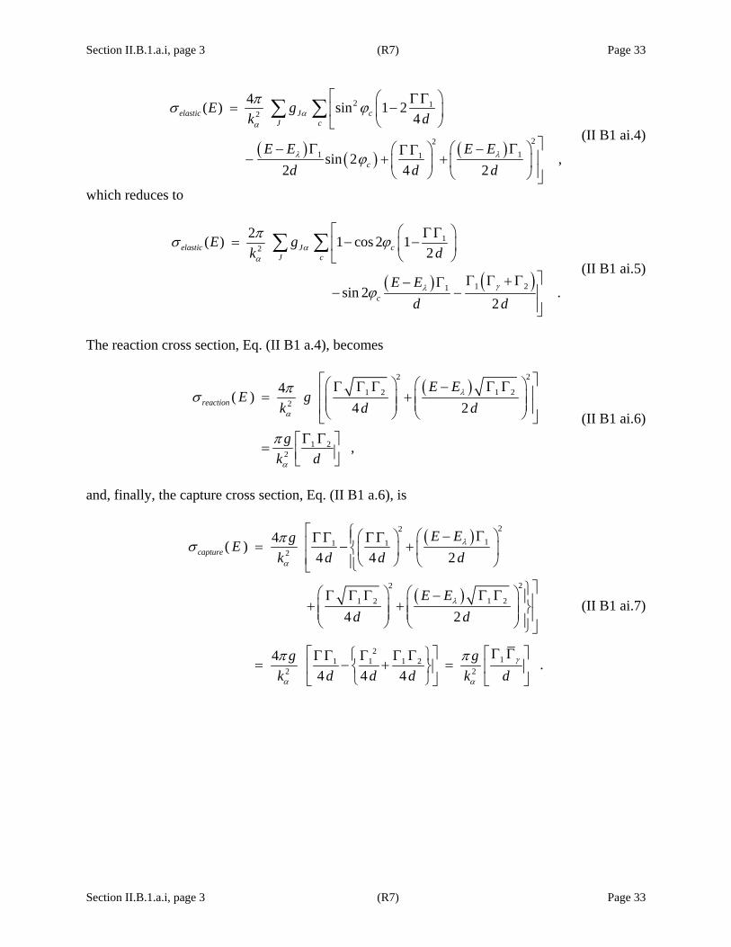
Section II.B.1.a.i, page 3 (R7) Page 33
Section II.B.1.a.i, page 3 (R7) Page 33
( ) ( ) ( )
2 12
221 11
4( ) sin 1 24
sin 2 ,2 4 2
elastic J cJ c
c
E gk d
E E E Ed d d
αα
λ λ
πσ ϕ
ϕ
⎡ ⎛ ⎞ΓΓ= −⎢ ⎜ ⎟
⎝ ⎠⎣⎤− Γ − Γ⎛ ⎞⎛ ⎞ΓΓ ⎥− + +⎜ ⎟⎜ ⎟⎥⎝ ⎠ ⎝ ⎠ ⎦
∑ ∑ (II B1 ai.4)
which reduces to
( ) ( )
12
1 21
2( ) 1 cos 2 12
sin 2 .2
elastic J cJ c
c
E gk d
E Ed d
αα
γλ
πσ ϕ
ϕ
⎡ ⎛ ⎞ΓΓ= − −⎢ ⎜ ⎟
⎝ ⎠⎣⎤Γ Γ +Γ− Γ
− − ⎥⎥⎦
∑ ∑ (II B1 ai.5)
The reaction cross section, Eq. (II B1 a.4), becomes
( )22
1 21 22
1 22
4( )4 2
,
reaction
E EE g
k d d
gk d
λ
α
α
πσ
π
⎡ ⎤⎛ ⎞⎛ ⎞ − Γ ΓΓ Γ Γ⎢ ⎥= + ⎜ ⎟⎜ ⎟⎜ ⎟ ⎜ ⎟⎢ ⎥⎝ ⎠ ⎝ ⎠⎣ ⎦Γ Γ⎡ ⎤= ⎢ ⎥⎣ ⎦
(II B1 ai.6)
and, finally, the capture cross section, Eq. (II B1 a.6), is
( )
( )
2211 1
2
22
1 21 2
211 1 1 2
2 2
4( )4 4 2
4 2
4 .4 4 4
capture
E EgEk d d d
E Ed d
g gk d d d k d
λ
α
λ
γ
α α
πσ
π π
⎡ ⎧ − Γ⎛ ⎞⎛ ⎞ΓΓ ΓΓ⎪⎢= − +⎨ ⎜ ⎟⎜ ⎟⎢ ⎝ ⎠ ⎝ ⎠⎪⎩⎣⎤⎫⎛ ⎞⎛ ⎞ − Γ ΓΓ Γ Γ ⎪⎥+ + ⎜ ⎟⎜ ⎟ ⎬⎜ ⎟ ⎜ ⎟ ⎥⎪⎝ ⎠ ⎝ ⎠ ⎭⎦
⎡ ⎤ ⎡Γ Γ ⎤⎧ ⎫ΓΓ Γ Γ Γ= − + =⎨ ⎬⎢ ⎥ ⎢ ⎥
⎩ ⎭ ⎣ ⎦⎣ ⎦
(II B1 ai.7)

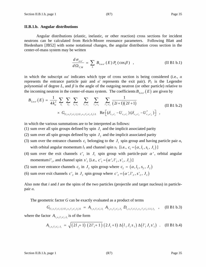
Section II.B.1.b, page 1 (R7) Page 35
Section II.B.1.b, page 1 (R7) Page 35
II.B.1.b. Angular distributions Angular distributions (elastic, inelastic, or other reaction) cross sections for incident neutrons can be calculated from Reich-Moore resonance parameters. Following Blatt and Biedenharn [JB52] with some notational changes, the angular distribution cross section in the center-of-mass system may be written
'' ( ) ( cos ) ,L L
LC M
dB E P
dαα
αα
σβ=
Ω ∑ (II B1 b.1)
in which the subscript αα' indicates which type of cross section is being considered (i.e., α represents the entrance particle pair and α' represents the exit pair). PL is the Legendre polynomial of degree L, and β is the angle of the outgoing neutron (or other particle) relative to the incoming neutron in the center-of-mass system. The coefficients ( )'LB Eαα are given by
( ) ( )( )1 2 1 1 1 1 2 2 2 2
1 1 1 1 1 2 2 2 2 2 1 1 1 1 2 2 2 2
' 2' ' ' '
* ' ' ' ' ' ' ' '
1 14 2 1 2 1
Re ( ) ( ) ,
LJ J l s l s l s l s
l s l s J l s l s J L c c c c c c c c
B Ek i I
G U U
ααα
δ δ
=+ +
⎡ ⎤× − −⎣ ⎦
∑ ∑ ∑ ∑ ∑ ∑ (II B1 b.2)
in which the various summations are to be interpreted as follows: (1) sum over all spin groups defined by spin 1J and the implicit associated parity (2) sum over all spin groups defined by spin 2J and the implicit associated parity (3) sum over the entrance channels 1c belonging to the 1J spin group and having particle pair α,
with orbital angular momentum l1 and channel spin s1 [i.e., ( )1 1 1 1, , ,c l s Jα= ] (4) sum over the exit channels 1'c in 1J spin group with particle-pair 'α , orbital angular
momentum 1'l , and channel spin 1's [i.e., ( )1 1 1 1' ', ' , ' ,c l s Jα= ]
(5) sum over entrance channels 2c in 2J spin group where ( )2 2 2 2, , ,c l s Jα=
(6) sum over exit channels 2'c in 2J spin group where ( )2 2 2 2' ', ' , ' ,c l s Jα= Also note that i and I are the spins of the two particles (projectile and target nucleus) in particle-pair α.
The geometric factor G can be exactly evaluated as a product of terms
1 1 1 1 1 2 2 2 2 2 1 1 1 1 1 2 2 2 2 2 1 1 1 1 2 2 2 2 1 2 ' ' ' ' ' ' ; ' ' ; ' ' ' ' ; ,l s l s J l s l s J L l s l s J l s l s J l s l s l s l s L J JG A A D= (II B1 b.3)
where the factor 1 1 1 1 1' ' ;l s l s JA is of the form
( ) ( ) ( ) ( ) ( )1 1 1 1 1' ' ; 1 1 1 1 1 1 1 1 12 1 2 ' 1 2 1 ' ' .l s l s JA l l J l J s l J s= + + + Δ Δ (II B1 b.4)
Section II.B.1.b, page 2 (R7) Page 36
Section II.B.1.b, page 2 (R7) Page 36
The expression for D is
( ) ( ) ( ) ( )( ) ( ) ( )
( )( ) ( ) ( )
( )( ) ( ) ( )
1 1 1 1 2 2 2 2 1 2 1 2
1 1
1 2 1 2
2 2 2 ' '' ' ' ' ; 1 2 1 2
'1 1 2 2 1 1 1 2 2 1 ' '
'
1 2 1 2
2 1
, ' ' , ' 1
! 1 ' ! 1,
! ! ! ' ' ! ' ' ! ' !
l s l s l s l s L J J
s ss s s s
n n
D L J J L l l L l l L
w l J l J s L w l J l J s L
n nn l n l n L n l n l n L
δ δ −
= + Δ Δ Δ
× −
− −×
− − − − − −
(II B1 b.5)
in which n is defined by 1 22 ;n l l L= + + (II B1 b.6) D is zero if l1+l2+L is an odd number. A similar expression defines n′. The Δ2 term is given by
( ) ( ) ( ) ( )( )
2 ! ! !,
1 !a b c a b c a b c
abca b c
+ − − + − + +Δ =
+ + + (II B1 b.7)
for which the arguments a, b, and c are to be replaced by the appropriate values given in Eqs. (II B1 b.4) and (II B1 b.5). The expression for ( )2 abcΔ implicitly includes a selection rule for the arguments; that is, the quantized vector sum must hold, or a b c a b c a b+ = − ≤ ≤ + (II B1 b.8) with c being either integer or half-integer. The quantity w in Eq. (II B1 b.5) is defined as
( ) ( )( )( ) ( )( )
( )( ) ( )( )
( ) ( ) ( )
1 1 2 2
1 1 2 21 1 2 2
1 2 1 2
1 1 2 2 1 2 2 1
1 1 !( , )
! !
1! !
1! ! !
k l J l Jkmax
k kmin
kw l J l J s L
k l J s k l J s
k l l L k J J L
l J l J k l J s L k l J s L k
+ + + +
=
− += Σ
− + + − + +
×− + + − + +
×+ + + − + + + − + + + −
(II B1 b.9)
(and similarly for the primed expression), where kmin and kmax are chosen such that none of the arguments of the factorials are negative. That is,
( ) ( ) ( ) ( ) ( ) ( ) ( )
1 1 2 2 1 2 1 2
1 1 2 2 1 2 2 1
max , , ,
min , , .
kmin l J s l J s l l L J J L
kmax l J l J l J s L l J s L
= + + + + + + + +
= + + + + + + + + + (II B1 b.10)
Section II.B.1.b, page 3 (R7) Page 37
Section II.B.1.b, page 3 (R7) Page 37
Single-channel case For some situations, these equations can be greatly simplified. When the target spin is zero and there are no possible reactions (no fission, no inelastic, no other reactions), then each spin group will consist of a single channel (the elastic channel). In this case, the coefficients
( )'LB Eαα reduce to
1 1 1 1 1 2 2 2 2 2
1 2 1 1 1 1 2 2 2 2
1 1 2 2
2( ) ( )
*
1( )4
1 Re (1 ) (1 ) ,( 2 1) ( 2 1)
L l s l s J l s l s J LJ J c l s J c l s J
c c c ca b
B E Gk
U Ui i
ααα αα = =
=
⎡ ⎤× − −⎣ ⎦+ +
∑ ∑ ∑ ∑(II B1 b.11)
where the existence of only one channel requires that the primed quantities of Eq.(II B1 b.2) be equal to the unprimed (e.g., 'α α= ). The geometric factor G becomes
1 1 1 1 1 2 2 2 2 2 1 1 1 1 1 2 2 2 2 2 1 1 1 1 2 2 2 2 1 2 ; ; ; ,l s l s J l s l s J L l s l s J l s l s J l s l s l s l s L J JG A A D= (II B1 b.12) in which the factor A reduces to the simple form
1 1 1 1 1
2; 1 1 1 1 1( 2 1) ( 2 1) ( ) ,l s l s JA l J l J s= + + Δ (II B1 b.13)
and the expression for D reduces to
1 1 1 1 2 2 2 2 1 2
1 2
2 4; 1 2 1 2
22
1 1 2 2 11 2
( 2 1) ( ) ( )
!( , ) ,( )! ( )! ( )!
l s l s l s l s L J J
s s
D L J J L l l L
nw l J l J s Ln l n l n L
δ
= + Δ Δ
⎡ ⎤× ⎢ ⎥− − −⎣ ⎦
(II B1 b.14)
in which n is again defined as in Eq. (II B1 b.6).


Section II.B.1.c, page 1 (R7) Page 39
Section II.B.1.c, page 1 (R7) Page 39
II. B.1.c. Specifying individual reaction types
Early versions of SAMMY permitted users to specify “inelastic”, “fission”, and “reaction” data. However, the tacit assumption was that all the exit channels are relevant to the type of data being used. If, for example, three exit channels were specified as (1) inelastic, (2) first fission channel, and (3) second fission channel, then any calculation for “inelastic”, “fission”, or “reaction” data types would automatically include all three exit channels in the final state.
Hence, in early versions of SAMMY, true inelastic cross sections (for example) would be calculated only if all of the following conditions were met: 1. Either “inelastic”, “fission”, or “reaction” was specified as the data type in the INPut file, card
set 8. 2. The exit channel description was appropriate for inelastic channels: The INPut file noted that
penetrabilities were to be calculated (LPENT = 1 on line 2 of card set 10.1) and also provided a non-zero value for the excitation energy.
3. No fission channel (or other exit channel) was defined in the INPut file (and PARameter file).
Beginning with release M5 of the SAMMY code, it is now possible to include only a subset of the exit channels in the outgoing final state. The third condition in the list above is no longer necessary, but is replaced by another (less restrictive) condition: 3. Exit channels that are not inelastic have a flag (“1” in column 18 of line 2 of card set 10.1 or
card set 10.2 of the INPut file), denoting that this channel does not contribute to the final state. (Similar considerations hold, of course, for any other reaction type, not only for inelastic.)
With release 7.0.0 of the SAMMY code in 2006, a more intuitive input is possible. When channels are specified using either of the particle-pair options (see card set 4 or 4a of Table VIA.1), then the data type line (card set 8 of Table VIA.1) may be used to specify the name(s) of the particle pair(s) to be included in the final-state reaction. Specifically, beginning in the first column of card set 8, include the phrase
FINAL-state particle pairs are or
PAIRS in final state = (Only the first five characters are required, the others are optional.) Elsewhere on the same line, give the eight-character designation of the particle pair(s) to be included in the final-state reaction. Only channels involving those particle pairs will be included in the final state; any channels not involving those particle pairs will not be included. (Caution: The particle pair name must be exactly as it appears in the INPut file, including capitalization.) The same two command lines may be used for angular distributions with specific final states, provided the phrase “ANGULar distribution” is given later on the same line.

Section II.B.1.c, page 1 (R7) Page 40
Section II.B.1.c, page 1 (R7) Page 40
See test case tr159 for an example which includes three reactions, one being (n,α) and the
other two inelastic (n,n'). Various options for input are given in this test case. Run “k” of test case tr112 shows an example for the angular distribution of a reaction cross
section.

Section II.B.1.d, page 1 (R7) Page 41
Section II.B.1.d, page 1 (R7) Page 41
II.B.1.d. External R-function
When generating cross sections via R-matrix theory, it is important to include contributions from all resonances, even those outside the energy range of the data. Tails from negative-energy resonances (which may correspond to bound states) and from higher-lying resonances can contribute significantly to the “background” of the R-matrix and must therefore not be omitted. There are infinitely many of these resonances, so approximations must be made.
The usual approximation is to use pseudo or dummy resonances to approximate the effect of
the infinite number of outlying resonances. The energy associated with a dummy resonance must be outside the energy region for which the analysis is valid.
For discussion regarding two different philosophies for determining appropriate choices of
dummy resonances, see Leal et al. [LL99] and Fröhner and Bouland [FF01]. Any number of additional possibilities exist for approximating the contribution of the
external resonances to the tail of the R-matrix. A logarithmic parameterization of the R-function is implemented in SAMMY; note that this is properly denoted as a function rather than a matrix, because it is diagonal with respect to the channels. The form used in the code is
( ) ( )
( )
2
ln
ext up downc c clin,ccon,c lin,c q ,c
upc
con,c lin,c downc
E = E + E sR E ER R R
E E E .s s E E
+ − −
−⎡ ⎤− + ⎢ ⎥−⎣ ⎦
(II B1 d.1)
Any or all of the seven free parameters may be varied during a SAMMY analysis (see Table VI B.2, card set 3, and card set 3a). Note that ext
cR is strictly real in this parameterization.
The u-parameters (i.e., the parameters on which Bayes= equations will operate, as described in Section IV.C) associated with the external R-function are given by
( ) ( )( ) ( ) ( )( ) ( )
, , , , , ,
, , , , .
down down up upc c c c
con c con c lin c lin c q c q c
con c con c lin c lin c
u E E u E E
u R R u R R u R R
u s s u s s
= =
= = =
= =
(II B1 d.2)
Of the current ENDF formats [ENDF-102], only new LRF = 7 format permits this type of parameterization of the R-function. The more commonly used LRF = 3 format (the so-called Reich Moore format) allows only the dummy-resonance option.

Section II.B.2, page 1 (R8) Page 43
Section II.B.2, page 1 (R8) Page 43
II.B.2. Simulation of Full R-Matrix
While SAMMY does not yet have the ability to calculate the full (unapproximated) R-matrix of Lane and Thomas [AL58], it is possible to use the Reich-Moore approximation in such a way that it mimics the full R-matrix with a high degree of accuracy. This is necessary, for example, in cases where there are interference effects between the (incident) neutron channel and a gamma channel – that is, for some low-mass nuclides.
The Reich-Moore approximation involves an aggregate treatment (“eliminated channels”) for the gamma widths (capture widths). Therefore, to approximate the full R-matrix, one sets the Reich-Moore gamma width to a very small number and uses an exit channel to define the actual gamma channel: 1. Set the SAMMY gamma-channel widths to a very small number, perhaps 0.001. 2. Define an exit channel to be the actual capture channel and assign appropriate values for the
widths. Quantum numbers for this channel will be the same as those for fission channels (in particular, set LPENT = 0).
3. When calculating capture cross sections, set the IFEXCL flag to 1 for all other (non-gamma) exit
channels. (See Section II.B.1.c and card set 10.1 or 10.2 of Table VIA.1 for details.) When calculating other reaction cross sections, set the IFEXCL flag to 0 for the reaction channels of interest, to 1 for the capture channels, and to 1 for any other reaction channels to be excluded.
When utilizing this option, SAMMY users should take care that results are not unduly
influenced by the approximation in step 1 above. To test this, make radical changes in the value used for the gamma widths (e.g., set the value to 100.0 or 10−6) and recalculate the cross section. Note that it is not possible to set these values to zero; doing so results in numerical overflow problems (because computers do not know how to calculate zero divided by zero).
Comparisons between cross sections calculated by SAMMY and those generated by the R-matrix code EDA [GH75] using the same R-matrix parameters have shown agreement to ~5 significant digits [INDC03]. Some of the runs for those comparisons are now assembled into SAMMY test case tr125.
Test case tr110 shows an artificial but extreme example of a situation in which use of the
Reich-Moore approximation gives very different results from those obtained via the full R-matrix. For this example, there are two resonances with parameter values as shown in Table II B2.1; plots of the curves calculated with those parameters are shown in Figure II B2.1. As evident from the figure, the Reich-Moore curve lies between the two extreme R-matrix curves which show constructive (dashed curve) and destructive (dot-dash curve) interference.

Section II.B.2, page 2 (R8) Page 44
Section II.B.2, page 2 (R8) Page 44
Table II B2.1. Parameter values used to illustrate Reich-Moore vs. full R-matrix calculations
λ Energy (MeV) λγΓ (eV) nλΓ (eV) Sign
× λγΓ (eV)a
Reich Moore 1 1.0 1.0 10000. 2 1.1 1.1 11000.
Pseudo-full R-matrix # 1 1 1.0 810 − 10000. 1.0 2 1.1 810 − 11000. 1.1 Pseudo-full R-matrix # 2 1 1.0 810 − 10000. 1.0 2 1.1 810 − 11000. −1.1 a Remember that the value given in the SAMMY PARameter file is not the partial width Γ (which is always a positive number); rather, it is the sign of the reduced-width amplitude γ multiplied by the partial width Γ. Hence, the negative sign in the final entry of this table is actually associated with the reduced-width amplitude for the capture channel. See Section II.B.1 for further discussion.
Figure II B2.1. Reich-Moore approximation vs. full R-matrix for artificial example of test case tr110.
Solid line = Reich MooreDot-dash = full R-matrix # 1Dash = full R-matrix # 2
Section II.B.2, page 3 (R8) Page 45
Section II.B.2, page 3 (R8) Page 45
Different treatments for different capture channels Occasionally it may be convenient to treat certain gamma widths individually while treating most gamma widths in aggregate fashion. This can be accomplished by defining “particle” channels for the individual widths (as described above) and using the Reich-Moore capture channel (eliminated width) for the aggregate width. To calculate the capture cross section in this situation, it is not sufficient to specify the data type as “CAPTURE”, because that would give only the contribution from the aggregate width. To obtain the contribution from the individual widths, specify the data type as “REACTION” or (preferably) as “FINAL state pairs =” followed by the exact names specified for the gamma-channel particle-pairs. (See card sets 4 and 8 of Table VI A.1 and Section II.B.1.c for details.) To calculate the complete capture cross section, use “FINAL state pairs =” for the data type and add the command line ADD ELIMINATED CAPTUre channel to final state
This will cause SAMMY to add the contributions from the individual capture channels plus the contribution from the aggregate channels. The formula used to calculate the capture cross section is similar to Eq. (II B1 a.6), with only the non-capture exit channels included in the summation over 'c :
2 2' '2
'= non-capture exit channels
4( ) .i i rcapture J cc cc cc
J c cE g X X X
k αα
πσ⎡ ⎤⎢ ⎥= − +⎢ ⎥⎢ ⎥⎣ ⎦
∑ ∑ ∑ (II B2.1)


Section II.B.3, page 1 (R8) Page 47
Section II.B.3, page 1 (R8) Page 47
II.B.3. Breit-Wigner Approximations In addition to the preferred Reich-Moore formalism, SAMMY also offers the option to calculate cross sections using either the multilevel Breit-Wigner (MLBW) or the single-level Breit-Wigner (SLBW) [GB36] approximation. These approximations have the advantage that the calculation occurs more rapidly because fewer computations are required; however, they also have the disadvantage that unphysical cross sections may be generated. Use of these options is discouraged for new analyses; the options are included within SAMMY for the sake of completeness, to permit use of SAMMY with most ENDF resonance parameter information, and to facilitate comparisons with older codes such as SIOB [GD78]. Formulae for MLBW and SLBW cross sections are presented in Section II.B.3.a; these are identical to those used in ENDF files [ENDF-102], although they are not necessarily programmed in this fashion. Formulae for derivatives are given in Section II.D.2.
The reader should be aware that the ENDF version of MLBW (and hence, SAMMY’s version of MLBW) does not correspond to the usual definition of multilevel Breit Wigner. Instead, only the elastic cross section is calculated with the multilevel formula; other partial cross sections for the MLBW format are actually single level. A note regarding broadening: Historically, the Breit-Wigner formulations had the great advantage that the cross sections could be Doppler broadened analytically, using the high-energy approximation to the free-gas model of Doppler broadening (Section III.B.3). Results were written in terms of χ and ψ functions, and computation was relatively rapid. However, with the advent of modern computers, more accurate cross sections and more accurate Doppler-broadening computations can be accomplished rapidly, without resorting to these rather crude approximations. In SAMMY, Doppler and resolution broadening are accomplished numerically, in the same manner for MLBW and SLBW cross sections as for Reich-Moore cross sections, as described in Section III of this manual.

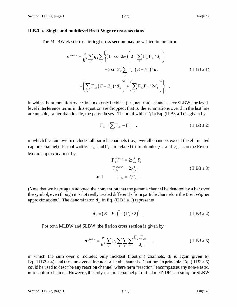
Section II.B.3.a, page 1 (R7) Page 49
Section II.B.3.a, page 1 (R7) Page 49
II.B.3.a. Single and multilevel Breit-Wigner cross sections
The MLBW elastic (scattering) cross section may be written in the form
( )
( )
( )
2
2 2
1 cos 2 2 /
2sin 2 /
/ / 2 ,
elasticJ c
J c
c
c c
g dk
E E d
E E d d
λ λ λλ
λ λ λλ
λ λ λ λ λ λλ λ
πσ ϕ
ϕ
⎧ ⎛ ⎞= − − Γ Γ⎨ ⎜ ⎟
⎝ ⎠⎩
+ Γ −
⎫⎛ ⎞ ⎛ ⎞ ⎪+ Γ − + Γ Γ ⎬⎜ ⎟ ⎜ ⎟⎝ ⎠ ⎝ ⎠ ⎪⎭
∑ ∑ ∑
∑
∑ ∑
(II B3 a.1)
in which the summation over c includes only incident (i.e., neutron) channels. For SLBW, the level-level interference terms in this equation are dropped; that is, the summations over λ in the last line are outside, rather than inside, the parentheses. The total width Γλ in Eq. (II B3 a.1) is given by ,c
cλ λ λγΓ = Γ +Γ∑ (II B3 a.2)
in which the sum over c includes all particle channels (i.e., over all channels except the eliminated capture channel). Partial widths cλΓ and λγΓ are related to amplitudes cλγ and λγ , as in the Reich-Moore approximation, by
2
2
2
2
2
and 2 .
neutronc c c
fissionc c
Pλ λ
λ λ
λγ λγ
γ
γ
γ
Γ =
Γ =
Γ =
(II B3 a.3)
(Note that we have again adopted the convention that the gamma channel be denoted by a bar over the symbol, even though it is not really treated differently from particle channels in the Breit Wigner approximations.) The denominator dλ in Eq. (II B3 a.1) represents ( ) ( )2 2/ 2 .d E Eλ λ λ= − + Γ (II B3 a.4)
For both MLBW and SLBW, the fission cross section is given by
'2
'
,c cfissionJ
J c c
gk d
λ λ
λ λ
πσΓ Γ
= ∑ ∑∑∑ (II B3 a.5)
in which the sum over c includes only incident (neutron) channels, dλ is again given by Eq. (II B3 a.4), and the sum over c´ includes all exit channels. Caution: In principle, Eq. (II B3 a.5)could be used to describe any reaction channel, where term “reaction” encompasses any non-elastic, non-capture channel. However, the only reaction channel permitted in ENDF is fission; for SLBW
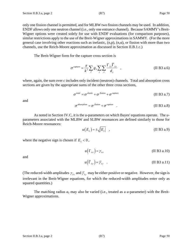
Section II.B.3.a, page 2 (R7) Page 50
Section II.B.3.a, page 2 (R7) Page 50
only one fission channel is permitted, and for MLBW two fission channels may be used. In addition, ENDF allows only one neutron channel (i.e., only one entrance channel). Because SAMMY’s Breit-Wigner options were created solely for use with ENDF evaluations (for comparison purposes), similar restrictions apply to the use of the Breit-Wigner approximations in SAMMY. (For the more general case involving other reactions such as inelastic, (n,p), (n,α), or fission with more than two channels, use the Reich-Moore approximation as discussed in Section II.B.1.c.)
The Breit-Wigner form for the capture cross section is
2 ,ccaptureJ
J cg
k dλ λγ
λ λ
πσΓ Γ
= ∑ ∑∑ (II B3 a.6)
where, again, the sum over c includes only incident (neutron) channels. Total and absorption cross sections are given by the appropriate sums of the other three cross sections,
total elastic fission captureσ σ σ σ= + + (II B3 a.7)
and .absorption fission captureσ σ σ= + (II B3 a.8)
As noted in Section IV.C, it is the u-parameters on which Bayes' equations operate. The u-
parameters associated with the MLBW and SLBW resonances are defined similarly to those for Reich-Moore resonances: ( ) ,u E Eλ λ= ± (II B3 a.9) where the negative sign is chosen if 0Eλ < ,
( )c cu λ λγΓ = (II B3 a.10) and
( ) .u λγ λγγΓ = (II B3 a.11) (The reduced-width amplitudes and c λ λγγ γ may be either positive or negative. However, the sign is irrelevant in the Breit-Wigner equations, for which the reduced-width amplitudes enter only as squared quantities.)
The matching radius ac may also be varied (i.e., treated as a u-parameter) with the Breit-Wigner approximations.

Section II.B.4, page 1 (R7) Page 51
Section II.B.4, page 1 (R7) Page 51
II.B.4. Direct Capture Component
An externally generated direct capture component may be added to the appropriate cross section types (capture, absorption, and total) by including the phrase ADD DIRECT CAPTURE Component to capture, total, and absorption cross section in the alphanumeric command section of the INPut file. When this command is present, the direct capture component for at least one of the nuclides is provided as a numerical function of energy, in a separate file (the ADRC file”). SAMMY will linearly interpolate as needed between the energy points given.
The format of the DRC file is as follows: First line: key word “NUClide Number”, followed by an equal sign “=”, followed by the
nuclide number as specified in the PARameter file. Second line: energy (eV), value of direct capture component (barn), in 2F20 format. Third line: repeat second line as many times as needed. Last line: blank. These lines may be repeated for each nuclide as needed. Not all nuclides need to be included, but those which are included should be given in the same order as in the PARameter file. (For example, give the direct capture component for nuclides number 2, 4, and 7, rather than 4, 7, and 2.)
The actual value of the direct capture component added to the capture (and total and absorption) cross section for any given nuclide is the product of the value determined from the DRC file and a constant (energy-independent) coefficient whose value is specified as miscellaneous parameter DRCAP. See Table VI B.2 for details.
Test case tr076 contains examples.


Section II.C, page 1 (R8) Page 53
Section II.C, page 1 (R8) Page 53
II.C. DETAILS AND CONVENTIONS USED IN SAMMY
Details of cross section evaluation are often a matter of convention: for example, should one use l-s or j-j coupling for spin assignments? The spin conventions used in SAMMY are described in Section II.C.1.
Section II.C.2 describes the conversion of energy and momentum from the laboratory reference system to the center-of-mass system.
The method used for computing sin2φ and cos2φ, where φ is the hard-sphere phase shift,
is described in Section II.C.3. Modifications are needed to the cross section equations when a channel contains two
charged particles. These are described in Section II.C.4. When data from an inverse reaction are used in an evaluation, modifications to either the
measured data or the R-matrix parameters are needed. These are described in Section II.C.5.

Section II.C.1, page 1 (R7) Page 55
Section II.C.1, page 1 (R7) Page 55
II.C.1. Spin and Angular Momentum Conventions
For any analysis or evaluation, the analyst bears ultimate responsibility for including the proper spin-group definitions.
This is not the responsibility of the SAMMY program nor of the SAMMY author. SAMMY
will issue warnings for obvious errors, but it is the responsibility of the user to notice and heed those warnings. It is also the responsibility of the user to ensure that the set of spin groups is complete; program SAMQUA, described in Section X.J, can be used for guidance in that effort.
It is worthwhile to discuss what is meant by “complete.” Clearly, it is neither necessary nor
possible to include all legitimate values of all of the quantum numbers (l, s, and J), because an infinite number of spin groups is available. Generally, one should include low values of l, l = 0 being always required and l = 1, 2, 3, … being included when the experimental data require their inclusion. For each l, the user should determine (using SAMQUA or by hand) all possible s-values leading to all possible J-values. In general, all such channels and spin groups should be included in the analysis. When the hard-sphere phase shift values are sufficiently large that there is a noticeable contribution to the cross section from the hard-sphere phase shift, all such channels must be included. On rare occasions, there may be one resonance (or several) whose high l-value dictates the presence of a particular channel in a particular spin group, but for which the hard-sphere phase shift is negligible for all energies of interest in this experiment. In this case, it would be reasonable to omit other channels and spin groups with this same l-value, without degrading the quality of the evaluation.
The spin and angular momentum conventions used in SAMMY (and in its predecessor MULTI [GA74]) are described in Table II C1.1. Recall that the word “channel” refers to the physical configuration (e.g., the particular particles involved) as well as to the quantum numbers given here. For example, an incident channel might consist of a neutron (intrinsic spin i = 2) impinging on a target (sample) whose spin is I, so that the channel spin is s, where Ii = s + . The relative orbital angular momentum of this channel (neutron plus target) is l, and total spin is J, where
lsJ += . For elastic scattering, the exit channel is the same as the entrance channel. For a reaction such as (n,p), the exit channel contains a proton (spin i' = ½) and another nuclide (spin 'I ); the channel spin is 's , where ''' Iis += . The relative angular momentum proton-nuclide system is 'l , and the total J must satisfy '' lsJ += .
Readers unfamiliar with vector sum rules are referred to Section II.C.1.a for a short summary of the basic principles.
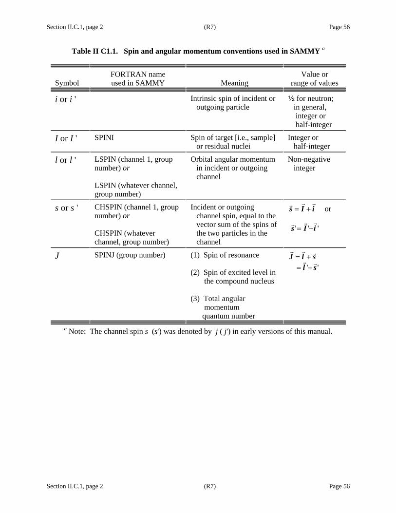
Section II.C.1, page 2 (R7) Page 56
Section II.C.1, page 2 (R7) Page 56
Table II C1.1. Spin and angular momentum conventions used in SAMMY a
Symbol FORTRAN name used in SAMMY Meaning
Value or range of values
i or i ' Intrinsic spin of incident or outgoing particle
2 for neutron; in general, integer or half-integer
I or I ' SPINI Spin of target [i.e., sample] or residual nuclei
Integer or half-integer
l or l ' LSPIN (channel 1, group number) or LSPIN (whatever channel, group number)
Orbital angular momentum in incident or outgoing channel
Non-negative integer
s or s ' CHSPIN (channel 1, group number) or CHSPIN (whatever channel, group number)
Incident or outgoing channel spin, equal to the vector sum of the spins of the two particles in the channel
iIs += or ''' iIs +=
J SPINJ (group number) (1) Spin of resonance (2) Spin of excited level in the compound nucleus (3) Total angular momentum quantum number
slJ += '' sl +=
a Note: The channel spin s (s') was denoted by j ( j') in early versions of this manual.
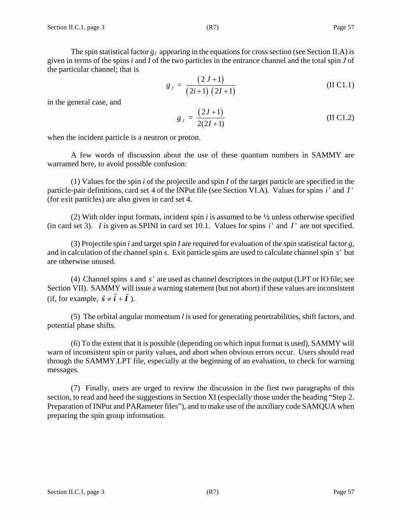
Section II.C.1, page 3 (R7) Page 57
Section II.C.1, page 3 (R7) Page 57
The spin statistical factor gJ appearing in the equations for cross section (see Section II.A) is given in terms of the spins i and I of the two particles in the entrance channel and the total spin J of the particular channel; that is
( )( ) ( )
2 12 1 2 1J
J = g
i I+
+ + (II C1.1)
in the general case, and
( )2 12(2 1)J
J = g
I++
(II C1.2)
when the incident particle is a neutron or proton.
A few words of discussion about the use of these quantum numbers in SAMMY are warranted here, to avoid possible confusion:
(1) Values for the spin i of the projectile and spin I of the target particle are specified in the particle-pair definitions, card set 4 of the INPut file (see Section VI.A). Values for spins 'i and 'I (for exit particles) are also given in card set 4.
(2) With older input formats, incident spin i is assumed to be 2 unless otherwise specified
(in card set 3). I is given as SPINI in card set 10.1. Values for spins 'i and 'I are not specified.
(3) Projectile spin i and target spin I are required for evaluation of the spin statistical factor g, and in calculation of the channel spin s. Exit particle spins are used to calculate channel spin s' but are otherwise unused.
(4) Channel spins s and 's are used as channel descriptors in the output (LPT or IO file; see Section VII). SAMMY will issue a warning statement (but not abort) if these values are inconsistent (if, for example, Iis +≠ ).
(5) The orbital angular momentum l is used for generating penetrabilities, shift factors, and potential phase shifts.
(6) To the extent that it is possible (depending on which input format is used), SAMMY will warn of inconsistent spin or parity values, and abort when obvious errors occur. Users should read through the SAMMY.LPT file, especially at the beginning of an evaluation, to check for warning messages. (7) Finally, users are urged to review the discussion in the first two paragraphs of this section, to read and heed the suggestions in Section XI (especially those under the heading “Step 2. Preparation of INPut and PARameter files”), and to make use of the auxiliary code SAMQUA when preparing the spin group information.

Section II.C.1.a, page 1 (R7) Page 59
Section II.C.1.a, page 1 (R7) Page 59
II.C.1.a. Quantum vector algebra For a complete description of sum rules for quantum vectors, the reader is referred to textbooks on elementary quantum mechanics. Here we simply state the vector sum rules without detailed explanation. Let a be a quantized vector. The value of this vector, generally written either a or a , is either a positive half-integer or a positive integer. That is to say, a can have any of the values 0, 1/2, 1, 3/2, 2, 5/2, etc. For example, the spin of a neutron or proton is 1/2, and the spin of an alpha particle is 0. The orbital angular momentum l for a pair of particles is integral, l = 0, 1, 2, 3, etc.
Given two quantized vectors a and b , and let c a b= + be the sum of the two vectors. The possible values for c are then
,a b c a b− ≤ ≤ + (II C1 a.1) where the allowed values of c are separated by one unit. Examples are shown in Table II C1 a.1. Values of a and b are in the left-most column and the uppermost row; values for c are in the other cells of the table. Because Eq. (II C1 a.1) is symmetric with respect to a and b, entries are made only in the lower triangular half of the table. Each spin vector has an associated parity, which can be positive or negative. For example, protons, neutrons, and alpha particles have positive parity; many nuclides have negative parity. The parity associated with angular momentum l is ( )1 l− . Parity is conserved when two vectors are added; the product of the parities of the two components is the parity of the resulting vector. A vector which is formed as the sum of two positive-parity vectors will have positive parity, a vector which is formed as the sum of two negative-parity vectors will have positive parity, and a vector which is formed as the sum of one positive-parity vector and one negative-parity vector will have negative parity. In other words, if a and b have the same parity, c has positive parity. If f a and b have different parity, c has negative parity.
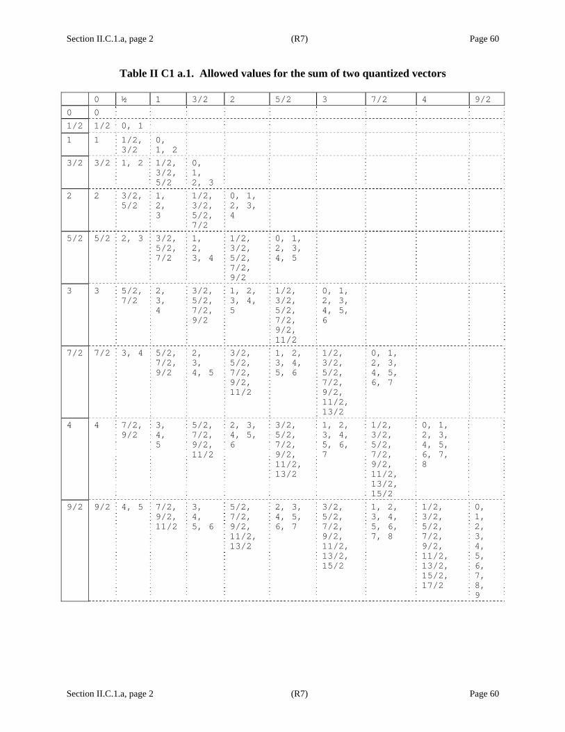
Section II.C.1.a, page 2 (R7) Page 60
Section II.C.1.a, page 2 (R7) Page 60
Table II C1 a.1. Allowed values for the sum of two quantized vectors 0 ½ 1 3/2 2 5/2 3 7/2 4 9/2 0 0 1/2 1/2 0, 1 1 1 1/2,
3/2 0, 1, 2
3/2 3/2 1, 2 1/2, 3/2, 5/2
0, 1, 2, 3
2 2 3/2, 5/2
1, 2, 3
1/2, 3/2, 5/2, 7/2
0, 1, 2, 3, 4
5/2 5/2 2, 3 3/2, 5/2, 7/2
1, 2, 3, 4
1/2, 3/2, 5/2, 7/2, 9/2
0, 1, 2, 3, 4, 5
3 3 5/2, 7/2
2, 3, 4
3/2, 5/2, 7/2, 9/2
1, 2, 3, 4, 5
1/2, 3/2, 5/2, 7/2, 9/2, 11/2
0, 1, 2, 3, 4, 5, 6
7/2 7/2 3, 4 5/2, 7/2, 9/2
2, 3, 4, 5
3/2, 5/2, 7/2, 9/2, 11/2
1, 2, 3, 4, 5, 6
1/2, 3/2, 5/2, 7/2, 9/2, 11/2, 13/2
0, 1, 2, 3, 4, 5, 6, 7
4 4 7/2, 9/2
3, 4, 5
5/2, 7/2, 9/2, 11/2
2, 3, 4, 5, 6
3/2, 5/2, 7/2, 9/2, 11/2, 13/2
1, 2, 3, 4, 5, 6, 7
1/2, 3/2, 5/2, 7/2, 9/2, 11/2, 13/2, 15/2
0, 1, 2, 3, 4, 5, 6, 7, 8
9/2 9/2 4, 5 7/2, 9/2, 11/2
3, 4, 5, 6
5/2, 7/2, 9/2, 11/2, 13/2
2, 3, 4, 5, 6, 7
3/2, 5/2, 7/2, 9/2, 11/2, 13/2, 15/2
1, 2, 3, 4, 5, 6, 7, 8
1/2, 3/2, 5/2, 7/2, 9/2, 11/2, 13/2, 15/2, 17/2
0, 1, 2, 3, 4, 5, 6, 7, 8, 9
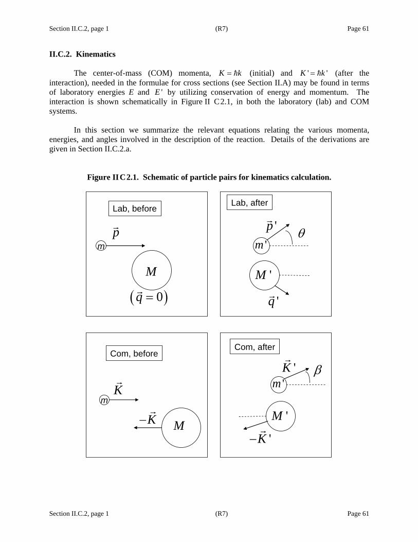
Section II.C.2, page 1 (R7) Page 61
Section II.C.2, page 1 (R7) Page 61
II.C.2. Kinematics The center-of-mass (COM) momenta, K k= (initial) and ' 'K k= (after the interaction), needed in the formulae for cross sections (see Section II.A) may be found in terms of laboratory energies E and 'E by utilizing conservation of energy and momentum. The interaction is shown schematically in Figure II C2.1, in both the laboratory (lab) and COM systems.
In this section we summarize the relevant equations relating the various momenta, energies, and angles involved in the description of the reaction. Details of the derivations are given in Section II.C.2.a.
Figure IIC2.1. Schematic of particle pairs for kinematics calculation.
mp
Lab, before
( )0q =
mK
Com, before
K−
'p
'q
'mθ
'M
Lab, after
'K
'K−
β'm
'M
Com, after
M
M
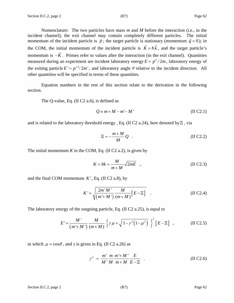
Section II.C.2, page 2 (R7) Page 62
Section II.C.2, page 2 (R7) Page 62
Nomenclature: The two particles have mass m and M before the interaction (i.e., in the incident channel); the exit channel may contain completely different particles. The initial momentum of the incident particle is p ; the target particle is stationary (momentum 0q = ); in the COM, the initial momentum of the incident particle is K k= , and the target particle’s momentum is K− . Primes refer to values after the interaction (in the exit channel). Quantities measured during an experiment are incident laboratory energy 2 / 2E p m= , laboratory energy of the exiting particle 2' ' / 2 'E p m= , and laboratory angle θ relative to the incident direction. All other quantities will be specified in terms of these quantities. Equation numbers in the rest of this section relate to the derivation in the following section.
The Q-value, Eq. (II C2 a.6), is defined as
' 'Q m M m M≡ + − − (II C2.1) and is related to the laboratory threshold energy , Eq. (II C2 a.24), here denoted byΞ , via
.m M QM+
Ξ = − (II C2.2)
The initial momentum K in the COM, Eq. (II C2 a.2), is given by
2 ,MK k mEm M
= =+
(II C2.3)
and the final COM momentum 'K , Eq. (II C2 a.8), by
( ) [ ]2 ' '' .
' ' ( )m M MK E
m M m M= −Ξ
+ + (II C2.4)
The laboratory energy of the outgoing particle, Eq. (II C2 a.25), is equal to
( ) ( ) [ ]
22 2'' 1 1 ,
' ' ( )M ME E
m M m Mγ μ γ μ= + − − −Ξ
+ + (II C2.5)
in which cosμ θ= , and γ is given in Eq. (II C2 a.26) as
2 ' ' ' .'
m m m M EM M m M E
γ +=
+ −Ξ (II C2.6)
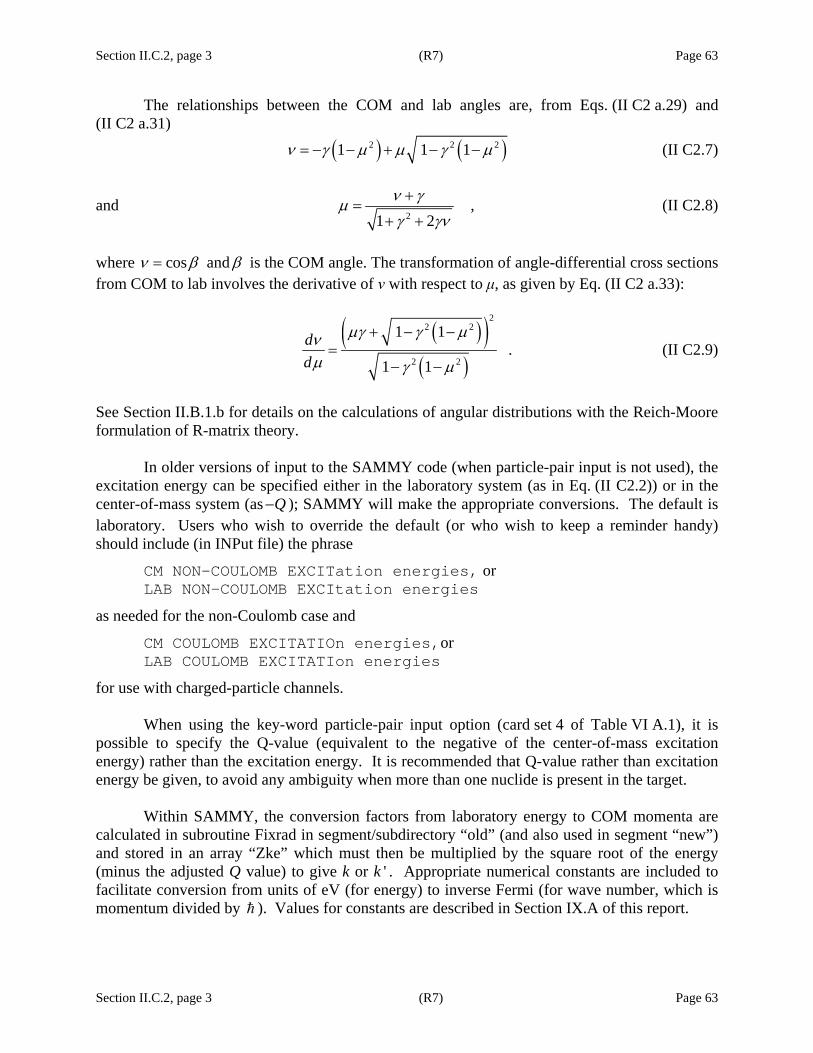
Section II.C.2, page 3 (R7) Page 63
Section II.C.2, page 3 (R7) Page 63
The relationships between the COM and lab angles are, from Eqs. (II C2 a.29) and (II C2 a.31)
( ) ( )2 2 21 1 1ν γ μ μ γ μ= − − + − − (II C2.7)
and 2
,1 2ν γμγ γν+
=+ +
(II C2.8)
where cosν β= andβ is the COM angle. The transformation of angle-differential cross sections from COM to lab involves the derivative of ν with respect to μ, as given by Eq. (II C2 a.33):
( )( )
( )
22 2
2 2
1 1.
1 1
dd
μγ γ μνμ γ μ
+ − −=
− − (II C2.9)
See Section II.B.1.b for details on the calculations of angular distributions with the Reich-Moore formulation of R-matrix theory.
In older versions of input to the SAMMY code (when particle-pair input is not used), the excitation energy can be specified either in the laboratory system (as in Eq. (II C2.2)) or in the center-of-mass system (as Q− ); SAMMY will make the appropriate conversions. The default is laboratory. Users who wish to override the default (or who wish to keep a reminder handy) should include (in INPut file) the phrase
CM NON-COULOMB EXCITation energies, or LAB NON-COULOMB EXCItation energies
as needed for the non-Coulomb case and
CM COULOMB EXCITATIOn energies,or LAB COULOMB EXCITATIon energies
for use with charged-particle channels.
When using the key-word particle-pair input option (card set 4 of Table VI A.1), it is possible to specify the Q-value (equivalent to the negative of the center-of-mass excitation energy) rather than the excitation energy. It is recommended that Q-value rather than excitation energy be given, to avoid any ambiguity when more than one nuclide is present in the target.
Within SAMMY, the conversion factors from laboratory energy to COM momenta are
calculated in subroutine Fixrad in segment/subdirectory “old” (and also used in segment “new”) and stored in an array “Zke” which must then be multiplied by the square root of the energy (minus the adjusted Q value) to give k or k ' . Appropriate numerical constants are included to facilitate conversion from units of eV (for energy) to inverse Fermi (for wave number, which is momentum divided by ). Values for constants are described in Section IX.A of this report.

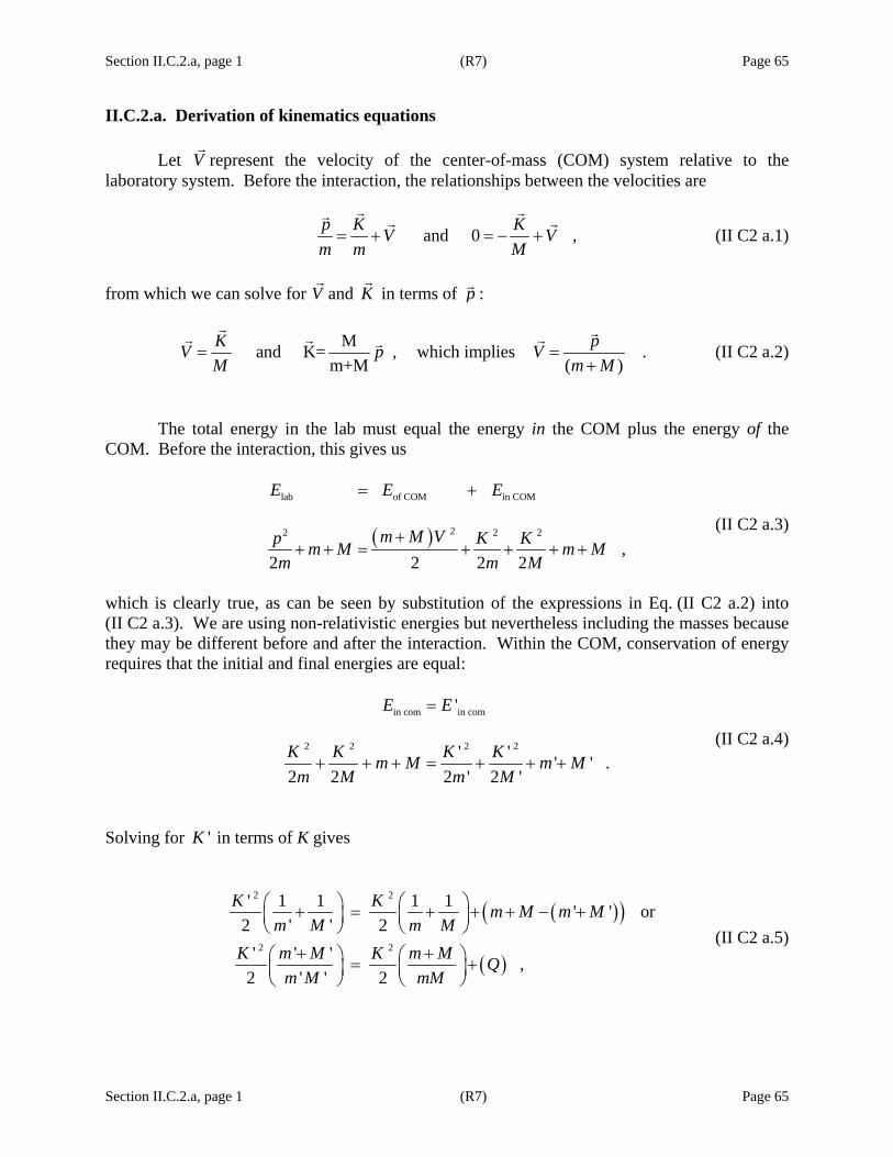
Section II.C.2.a, page 1 (R7) Page 65
Section II.C.2.a, page 1 (R7) Page 65
II.C.2.a. Derivation of kinematics equations Let V represent the velocity of the center-of-mass (COM) system relative to the laboratory system. Before the interaction, the relationships between the velocities are
and 0 ,p K KV Vm m M= + = − + (II C2 a.1)
from which we can solve for V and K in terms of p :
M and K= , which implies .m+M ( )
K pV p VM m M
= =+
(II C2 a.2)
The total energy in the lab must equal the energy in the COM plus the energy of the COM. Before the interaction, this gives us
( )
lab of COM in COM
22 2 2
,2 2 2 2
E E E
m M Vp K Km M m Mm m M
= +
++ + = + + + +
(II C2 a.3)
which is clearly true, as can be seen by substitution of the expressions in Eq. (II C2 a.2) into (II C2 a.3). We are using non-relativistic energies but nevertheless including the masses because they may be different before and after the interaction. Within the COM, conservation of energy requires that the initial and final energies are equal:
in com in com
2 2 2 2
'
' ' ' ' .2 2 2 ' 2 '
E E
K K K Km M m Mm M m M
=
+ + + = + + + (II C2 a.4)
Solving for 'K in terms of K gives
( )( )
( )
2 2
2 2
' 1 1 1 1 ' ' or 2 ' ' 2
' ' ' ,2 ' ' 2
K K m M m Mm M m M
K m M K m M Qm M mM
⎛ ⎞ ⎛ ⎞+ = + + + − +⎜ ⎟ ⎜ ⎟⎝ ⎠ ⎝ ⎠
+ +⎛ ⎞ ⎛ ⎞= +⎜ ⎟ ⎜ ⎟⎝ ⎠ ⎝ ⎠
(II C2 a.5)

Section II.C.2.a, page 2 (R7) Page 66
Section II.C.2.a, page 2 (R7) Page 66
in which we have defined the Q-value as ' ' .Q m M m M= + − − (II C2 a.6) Rewriting Eq. (II C2 a.5) using the value for K from Eq. (II C2 a.2) gives
2 2
2
2
2 ' ''' ' 2
2 ' '' ' 2
2 ' ' .' ' 2 ( )
m M m MK K Qm M mM
m M M m Mp Qm M m M mM
m M p M Qm M m m M
⎡ + ⎤⎛ ⎞= +⎜ ⎟⎢ ⎥+ ⎝ ⎠⎣ ⎦⎡ ⎤+⎧ ⎫ ⎛ ⎞= +⎢ ⎥⎨ ⎬ ⎜ ⎟+ +⎩ ⎭ ⎝ ⎠⎢ ⎥⎣ ⎦⎡ ⎤
= +⎢ ⎥+ +⎣ ⎦
(II C2 a.7)
This can also be written as
2 2 ' '' ,' ' ( )m M MK E Q
m M m M⎡ ⎤
= +⎢ ⎥+ +⎣ ⎦ (II C2 a.8)
in which E is equal to the kinetic energy of the incident particle in the laboratory system,
2
.2pEm
= (II C2 a.9)
This definition of E is used throughout this manual; cross sections are always specified in terms of this energy unless otherwise noted explicitly. The transformation from COM to laboratory gives values for momenta after the interaction. Again, we add velocities, similar to Eq. (II C2 a.1), using Eq. (II C2 a.2) for V :
' ' ' .' ' ' ( )
p K K pVm m m m M
= + = ++
(II C2 a.10)
(An analogous set of equations holds for the second particle,
' ,' ( )
q K K pVM M M m M
= − + = − ++
(II C2 a.11)
but we shall not be concerned with this particle now.)
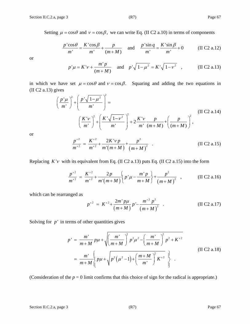
Section II.C.2.a, page 3 (R7) Page 67
Section II.C.2.a, page 3 (R7) Page 67
Setting cos and cos ,μ θ ν β= = we can write Eq. (II C2 a.10) in terms of components
'cos 'cos 'sin 'sin and 0' ' ( ) ' '
p K p p q Km m m M m m
θ β β= + = +
+ (II C2 a.12)
or
2 2'' ' and ' 1 ' 1 ,( )
m pp K p Km M
μ ν μ ν= + − = −+
(II C2 a.13)
in which we have set cos and cos .μ θ ν β= = Squaring and adding the two equations in (II C2 a.13) gives
22 2
2 22 2
' 1'' '
' 1' '2 + ,' ' ' ( ) ( )
ppm m
KK K p pm m m m M m M
μμ
νν ν
⎛ ⎞−⎛ ⎞ ⎜ ⎟+ =⎜ ⎟ ⎜ ⎟⎝ ⎠ ⎝ ⎠
⎛ ⎞− ⎛ ⎞⎛ ⎞ ⎜ ⎟+ + ⎜ ⎟⎜ ⎟ ⎜ ⎟ + +⎝ ⎠ ⎝ ⎠⎝ ⎠
(II C2 a.14)
or
( ) ( )
2 2 2
22 2
' ' 2 ' + .' ' '
p K K p pm m m m M m M
ν= +
+ + (II C2 a.15)
Replacing 'K ν with its equivalent from Eq. (II C2 a.13) puts Eq. (II C2 a.15) into the form
( ) ( )
2 2 2
22 2
' ' 2 '' + ,' ' '
p K p m p ppm m m m M m M m M
μ⎧ ⎫= + −⎨ ⎬+ +⎩ ⎭ + (II C2 a.16)
which can be rearranged as
( ) ( )
2 22 2
22 ' '' ' ' .m p m pp K pm M m M
μ= + −
+ + (II C2 a.17)
Solving for 'p in terms of other quantities gives
( )
2 22 2 2 2
22 2 2
' ' '' '
' 1 ' .'
m m mp p p p Km M m M m M
m m Mp p Km M m
μ μ
μ μ
⎛ ⎞ ⎛ ⎞= + − +⎜ ⎟ ⎜ ⎟+ + +⎝ ⎠ ⎝ ⎠
⎧ ⎫+⎪ ⎪⎛ ⎞= + − +⎨ ⎬⎜ ⎟+ ⎝ ⎠⎪ ⎪⎩ ⎭
(II C2 a.18)
(Consideration of the p = 0 limit confirms that this choice of sign for the radical is appropriate.)
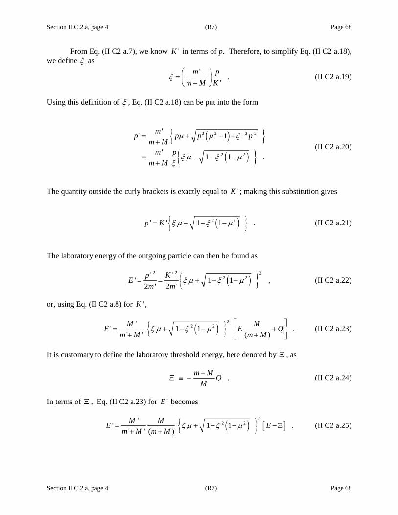
Section II.C.2.a, page 4 (R7) Page 68
Section II.C.2.a, page 4 (R7) Page 68
From Eq. (II C2 a.7), we know 'K in terms of p. Therefore, to simplify Eq. (II C2 a.18), we define ξ as
' .'
m pm M K
ξ ⎛ ⎞= ⎜ ⎟+⎝ ⎠ (II C2 a.19)
Using this definition of ξ , Eq. (II C2 a.18) can be put into the form
( )
( )
2 2 2 2
2 2
'' 1
' 1 1 .
mp p p pm M
m pm M
μ μ ξ
ξ μ ξ μξ
−= + − ++
= + − −+
(II C2 a.20)
The quantity outside the curly brackets is exactly equal to 'K ; making this substitution gives
( ) 2 2' ' 1 1 .p K ξ μ ξ μ= + − − (II C2 a.21)
The laboratory energy of the outgoing particle can then be found as
( ) 2 2 22 2' '' 1 1 ,
2 ' 2 'p KEm m
ξ μ ξ μ= = + − − (II C2 a.22)
or, using Eq. (II C2 a.8) for 'K ,
( ) 22 2'' 1 1 .
' ' ( )M ME E Q
m M m Mξ μ ξ μ
⎡ ⎤= + − − +⎢ ⎥+ +⎣ ⎦
(II C2 a.23)
It is customary to define the laboratory threshold energy, here denoted by Ξ , as
.m M QM+
Ξ ≡ − (II C2 a.24)
In terms of Ξ , Eq. (II C2 a.23) for 'E becomes
( ) [ ]2
2 2'' 1 1 .' ' ( )M ME E
m M m Mξ μ ξ μ= + − − −Ξ
+ + (II C2 a.25)

Section II.C.2.a, page 5 (R7) Page 69
Section II.C.2.a, page 5 (R7) Page 69
Equation (II C2 a.19) for ξ can also be written in terms ofΞ , using Eq. (II C2 a.8), as
2
2
' 2' ' ' .'2 ' '
' ' ( )
m mEm m m M Em MM M m M Em M ME Q
m M m M
ξ
⎛ ⎞⎜ ⎟ ++⎝ ⎠= =
+ −Ξ⎡ ⎤+⎢ ⎥+ +⎣ ⎦
(II C2 a.26)
Next, we consider the transformation of angle from laboratory θ to COM β and vice versa. From Eq. (II C2 a.13) we have
'' ' ' ' ,( )
m pp K K Km M
μ ν ν ξ= + = ++
(II C2 a.27)
in which we have made use of Eq. (II C2 a.19). Substituting Eq. (II C2 a.21) into this equation gives
( ) 2 2' ' 1 1 ' ' ,p K K Kμ ξ μ ξ μ μ ν ξ= + − − = + (II C2 a.28)
which reduces to ( ) ( )2 2 21 1 1 .ν ξ μ μ ξ μ= − − + − − (II C2 a.29)
This equation can be inverted to give μ in terms of ν as follows:
( ) ( )( ) ( )
( )
( )
22 2 2 2
2 2 2 2 4 2 2 2 2 4
2 2 2 2
2 22
2
1 1 1 ,
2 1 1 2 ,
1 2 2 ,
2 ,1 2
ν ξ μ μ ξ μ
ν ξν μ ξ μ μ μ ξ μ ξ μ
μ ξ ξν ν ξν ξ
ν ξν ξμξ ξν
⎡ ⎤ ⎡ ⎤+ − = − −⎣ ⎦ ⎣ ⎦
+ − + − + = − +
+ + = + +
+ +=
+ +
(II C2 a.30)
or, finally, as
2
.1 2
ν ξμξ ξν+
=+ +
(II C2 a.31)
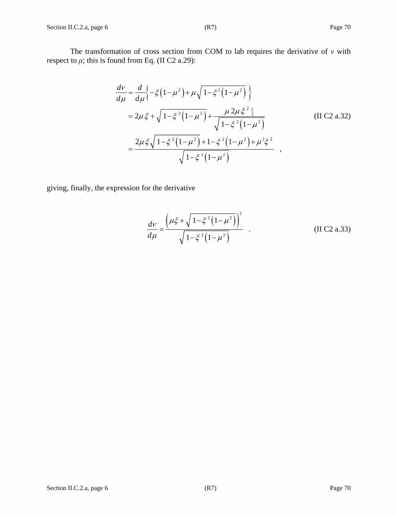
Section II.C.2.a, page 6 (R7) Page 70
Section II.C.2.a, page 6 (R7) Page 70
The transformation of cross section from COM to lab requires the derivative of ν with respect to μ; this is found from Eq. (II C2 a.29):
( ) ( ) ( )
( )( ) ( )
( )
2 2 2
2 12 2 2
2 2
2 2 2 2 2 2
2 2
1 1 1
22 1 11 1
2 1 1 1 1,
1 1
d dd dν ξ μ μ ξ μμ μ
μ μξμξ ξ μξ μ
μξ ξ μ ξ μ μ ξ
ξ μ
= − − + − −
= + − − +− −
− − + − − +=
− −
(II C2 a.32)
giving, finally, the expression for the derivative
( )( )
( )
22 2
2 2
1 1.
1 1
dd
μξ ξ μνμ ξ μ
+ − −=
− − (II C2 a.33)
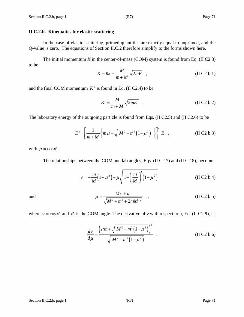
Section II.C.2.b, page 1 (R7) Page 71
Section II.C.2.b, page 1 (R7) Page 71
II.C.2.b. Kinematics for elastic scattering In the case of elastic scattering, primed quantities are exactly equal to unprimed, and the Q-value is zero. The equations of Section II.C.2 therefore simplify to the forms shown here.
The initial momentum K in the center-of-mass (COM) system is found from Eq. (II C2.3) to be
2 ,MK k mEm M
= =+
(II C2 b.1)
and the final COM momentum 'K is found in Eq. (II C2.4) to be
' 2 .MK mEm M
=+
(II C2 b.2)
The laboratory energy of the outgoing particle is found from Eqs. (II C2.5) and (II C2.6) to be
( ) 2
2 2 21' 1 ,E m M m Em M
μ μ⎡ ⎤= + − −⎢ ⎥+⎣ ⎦ (II C2 b.3)
with cosμ θ= .
The relationships between the COM and lab angles, Eqs. (II C2.7) and (II C2.8), become
( ) ( )2
2 21 1 1m mM M
ν μ μ μ⎛ ⎞= − − + − −⎜ ⎟⎝ ⎠
(II C2 b.4)
and 2 2
,2
M mM m mM
νμν
+=
+ + (II C2 b.5)
where cosν β= and β is the COM angle. The derivative of ν with respect to μ, Eq. (II C2.9), is
( )( )
( )
22 2 2
2 2 2
1.
1
m M mdd M m
μ μνμ μ
+ − −=
− − (II C2 b.6)


Section II.C.3, page 1 (R7) Page 73
Section II.C.3, page 1 (R7) Page 73
II.C.3. Evaluation of Hard-Sphere Phase Shift
Formulae for the hard-sphere phase shift (otherwise known as the potential-scattering phase shift) are given in Table II A.1 for non-Coulomb interactions. What is actually needed in SAMMY is not, however, the phase shifts φ themselves but rather cos(2φ) and sin(2φ). Since evaluation of φ requires the inverse tangent function, results for cos(2φ) and sin(2φ) are more readily generated with fewer computer round-off errors by using trigonometric relationships to generate formulae for cos(2φ) and sin(2φ) directly.
For all l, it is clear from Table II A.1 that φ may be written in the form ,φ Xρ= − (II C3.1) where 1tanX f−= (II C3.2) and f is a different function of ρ for each value of l. From Eq. (II C3.1), using elementary trigonometric relationships, we find cos cos cos sin sinX Xϕ ρ ρ= + (II C3.3) and
sin cos sin sin cos .X Xϕ ρ ρ= − + (II C3.4) Thus, ( )cos 2 φ becomes
( ) ( )
( )
22 2 2
22
2
cos 2 2cos 1 2cos cos 1 tan tan 1
cos2 1 tan 1 .1
φ φ = X X
= f + f
ρ ρ
ρ ρ
= − + −
+ − (II C3.5)
Similarly, ( )sin 2 φ can be written
( ) ( ) ( )
( ) ( )
2 2
2
2
sin 2 2 cos sin 2 cos cos 1 tan tan tan tan
cos2 1 tan tan1
φ = φ φ = X X X
= f f .f
ρ ρ ρ
ρ ρ ρ
+ − +
+ − ++
(II C3.6)
Equations (II C3.5) and (II C3.6) are the form used in SAMMY to evaluate the hard-sphere phase shift terms for non-Coulomb situations.

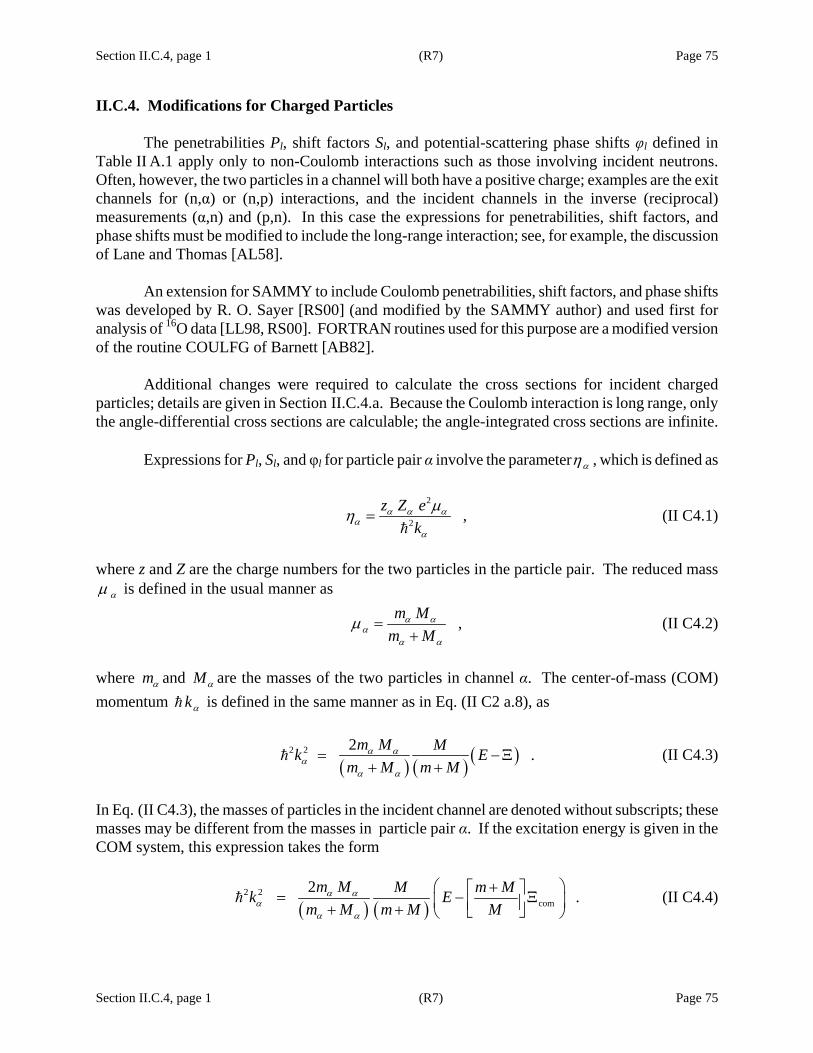
Section II.C.4, page 1 (R7) Page 75
Section II.C.4, page 1 (R7) Page 75
II.C.4. Modifications for Charged Particles
The penetrabilities Pl, shift factors Sl, and potential-scattering phase shifts φl defined in Table II A.1 apply only to non-Coulomb interactions such as those involving incident neutrons. Often, however, the two particles in a channel will both have a positive charge; examples are the exit channels for (n,α) or (n,p) interactions, and the incident channels in the inverse (reciprocal) measurements (α,n) and (p,n). In this case the expressions for penetrabilities, shift factors, and phase shifts must be modified to include the long-range interaction; see, for example, the discussion of Lane and Thomas [AL58].
An extension for SAMMY to include Coulomb penetrabilities, shift factors, and phase shifts was developed by R. O. Sayer [RS00] (and modified by the SAMMY author) and used first for analysis of 16O data [LL98, RS00]. FORTRAN routines used for this purpose are a modified version of the routine COULFG of Barnett [AB82].
Additional changes were required to calculate the cross sections for incident charged
particles; details are given in Section II.C.4.a. Because the Coulomb interaction is long range, only the angle-differential cross sections are calculable; the angle-integrated cross sections are infinite.
Expressions for Pl, Sl, and φl for particle pair α involve the parameter αη , which is defined as
2
2 ,z Z ek
α α αα
α
μη = (II C4.1)
where z and Z are the charge numbers for the two particles in the particle pair. The reduced mass
αμ is defined in the usual manner as
,m Mm M
α αα
α α
μ =+
(II C4.2)
where mα and Mα are the masses of the two particles in channel α. The center-of-mass (COM) momentum kα is defined in the same manner as in Eq. (II C2 a.8), as
( ) ( ) ( )2 2 2 .m M Mk Em M m M
α αα
α α
= −Ξ+ +
(II C4.3)
In Eq. (II C4.3), the masses of particles in the incident channel are denoted without subscripts; these masses may be different from the masses in particle pair α. If the excitation energy is given in the COM system, this expression takes the form
( ) ( )
2 2com
2 .m M M m Mk Em M m M M
α αα
α α
⎛ + ⎞⎡ ⎤= − Ξ⎜ ⎟⎢ ⎥+ + ⎣ ⎦⎝ ⎠ (II C4.4)
Section II.C.4, page 2 (R7) Page 76
Section II.C.4, page 2 (R7) Page 76
In the SAMMY input, the user can specify the value of the excitation energy either in the laboratory system [as in Eq. (II C4.3)] or in the COM system; SAMMY will make the appropriate conversions. The default is laboratory. Users who wish to provide COM values should include the phrase “CM COULOMB EXCITATION ENERGIES” as needed.
The reaction Q-value is the negative of variable COMΞ = ECHAN (in the COM system) in
card set 10.1 or 10.2 of Table VI A.1. When using the particle-pair input, card set 4 or 4a of Table VIA.1, it is possible to give the Q-value directly; this is the recommended input format.
Recall that a channel is defined by the particle pair (with mass, spin, and charge for each of
the two particles, plus the Q-value) plus the spin quantum numbers l, s, and J. Quantities defined above in Eqs. (II C4.1) through (II C4.4) depend only on the particle pair α and not on the spin quantum numbers. Other quantities (below) depend also on the value of l.
If ac is the channel radius for this channel, we again define ρ as ck aαρ = (II C4.5) The penetrabilities ( )lP η, ρ , shift factors ( )lS η, ρ , and phase shifts ( ),lϕ η ρ are then calculated as
functions of ( )lF η, ρ and ( )lG η,ρ , the regular and irregular Coulomb wave functions, respectively. The equations are as follows:
2 , , and cos ,l ll l l
l l l
A GP S
A A Aρ ρ ϕ
ρ∂
= = =∂
(II C4.6)
where 2 2 2 .l l lA F G= + (II C4.7)
In Eqs. (II A.1) and (II A.5), the Coulomb phase-shift difference wc is required for charged-
particle interactions. From Lane and Thomas [AL58], this quantity has the value
1
1
0 0
0 .tanlc
n
lw
lnαη−
=
=⎧⎪= ⎨ ⎛ ⎞ ≠⎪ ⎜ ⎟⎩ ⎝ ⎠∑
(II C4.8)
Finally, we note that an alternative version of the Coulomb functions is available in SAMMY. This alternative, modified from files provided by Hale [GH02], requires longer run time but appears to be more accurate at low values of ρ (and corresponding high values of η). SAMMY will automatically switch to the more accurate version when it discerns the need. To invoke this alternative for all calculations, include the phrase
USE ALTERNATIVE COULomb functions in the INPut file.
Section II.C.4.a, page 1 (R7) Page 77
Section II.C.4.a, page 1 (R7) Page 77
II.C.4.a. Charged-particle initial states
To derive the equations for the angle-differential cross sections for charged-particle incident channels, we begin with the Lane and Thomas [AL58] expression [page 292, Eq. (2.6)]. When this expression is corrected (for a missing complex conjugate, a missing minus sign, and missing delta functions), summed over the exit channel spins 's , and averaged over the incident channel spins s, the resulting equation for the angle-differential cross section is
( ) ( ) ( )
( )
2'' '2
2*
'2
cos
4Re cos .
2
l
L LLC M
i wcc
J lJ sl
dB E P C
d k
e Ug i C P
k
α
αααα α αα
α
α ααα
σ πβ β δ
πβ δ
= +Ω
⎡ ⎤⎛ ⎞−⎢ ⎥+ − ⎜ ⎟
⎜ ⎟⎢ ⎥⎝ ⎠⎣ ⎦
∑
∑ (II C4 a.1)
Here we have again used the convention that , , ,c l s Jα= . For the charged-particle case, the
definition of ( )'LB Eαα is modified slightly from the non-Coulomb case [Eq. (II B1 b.2)] to give
( )
( )( )
1 2 1 1 1 1 2 2 2 2
1 1 1 1 1 2 2 2 2 2
1 1 1 1 2 2 2 2
' 2' ' ' '
' ' ' '
2 2 *' ' ' '
14
12 1 2 1
Re ( ) ( ) .l l
LJ J l s l s l s l s
l s l s J l s l s J L
i w i wc c c c c c c c
B Ek
Gi I
e U e Uα α
ααα
δ δ−
=
×+ +
⎡ ⎤× − −⎣ ⎦
∑ ∑ ∑ ∑ ∑ ∑
(II C4 a.2)
In the final line of Eq. (II C4 a.2), the quantity c1 is substituted for the expression 1 1 1, , ,l s Jα ,
c2 for 2 2 2, , ,l s Jα , 1'c for 1 1 1', ' , ' ,l s Jα , and 2'c for 2 2 2', ' , ' ,l s Jα . The geometric term G in
Eq. (II C4 a.2) is the same as for the non-Coulomb case and is defined in Eqs. (II B1 b.3) to (II B1 b.10). Notation for summation indices is the same as in the non-Coulomb case.
What is different here is the presence of the exponential involving the Coulomb phase-shift difference wlα, defined in Eq. (II C4.7) . Also, the scattering matrix contains the wlα in the definition of Ω; the Sommerfeld parameter ηα in Eq. (II C4.1) is defined as
2
2 .z Z ek
αα
α
μη = (II C4 a.3)
Section II.C.4.a, page 2 (R7) Page 78
Section II.C.4.a, page 2 (R7) Page 78
The additional terms in Eq. (II C4 a.1) involve the function Cα , which is defined as
2 ln sin
221 cosec .24
iC e
αβη
α αβη
π
⎡ ⎤⎛ ⎞− ⎜ ⎟⎢ ⎥⎝ ⎠⎣ ⎦⎛ ⎞= ⎜ ⎟⎝ ⎠
(II C4 a.4)
It is this term which is infinite at 0β = (forward scattering) and which causes the (angle-integrated) elastic-scattering cross section to be infinite. Center-of-mass vs Laboratory
Angular distribution cross sections are sometimes reported as if measured in the center-of-mass system rather than in the laboratory system; hence, SAMMY can calculate either version. To specify which is wanted, insert one of the phrases
USE CENTER OF MASS Cross sections USE LABORATORY CROSS sections
into your INPut file (see Tables VI A.1 and VI A1.2). Center-of-mass is the default. Acknowledgements The author is grateful to SAMMY users Jeff Blackmon and Olivier Bouland for uncovering bugs in early implementations of charged-particle elastic scattering, and to Eric Berthoumieux (author of the ANARKI R-matrix code) for providing calculations to assist in debugging this portion of SAMMY.
Section II.C.5, page 1 (R7) Page 79
Section II.C.5, page 1 (R7) Page 79
II.C.5. Inverse Reactions (Reciprocity) Occasionally a user may wish to include data from an inverse reaction in the same evaluation as the forward reaction. For example, for an evaluation of the 16O resonance parameters, Sayer [RS00] wanted to include 16O(n,α)13C data. No such data existed, but 13C(α,n)16O data were available.
Unfortunately SAMMY does not have the capability of including reciprocal data in the same evaluation (using the same resonance parameters). SAMMY was designed with the intent of treating one incident particle (originally a neutron) and many different types of nuclides within the target. Other codes (e.g., EDA [GH75]) were designed with a different philosophy: to simultaneously treat all interactions leading to the same compound nucleus. Eventually the SAMMY author hopes to add similar capabilities to the SAMMY code. Meanwhile, two alternatives are available: (1) The SAMMY user can convert the data using reciprocal relationships, and include the converted data within his or her evaluation. (2) If there is no need for simultaneous∗ fitting, resonance parameter values can be converted to those appropriate for the reciprocal reaction. Either of these two can be accomplished by application of the principle of detailed balance.
To convert the cross section from the ( )' ',A a a Areaction to the ( ), ' 'A a a A reaction, we first consider the center-of-mass (COM) system, in which the energies are easily related by ' .COM COME E Q= − (II C5.1) Elementary kinematics (as illustrated in Figure II C5.1) gives the conversion to the laboratory values E and E',
', ' ' , ,' 'COM COM lab
M M ME E E E Qm M m M m M
= = = − Ξ+ + +
(II C5.2)
and algebra then gives
( ) ' '' .'lab
M m ME Em M M
+= −Ξ
+ (II C5.3)
∗ By “simultaneous” is meant either (1) truly simultaneous or (2) “sequential using the covariance matrix from one SAMMY run fitting one data set as input to another run fitting another data set.” See Section IV of this manual for details of both possibilities.
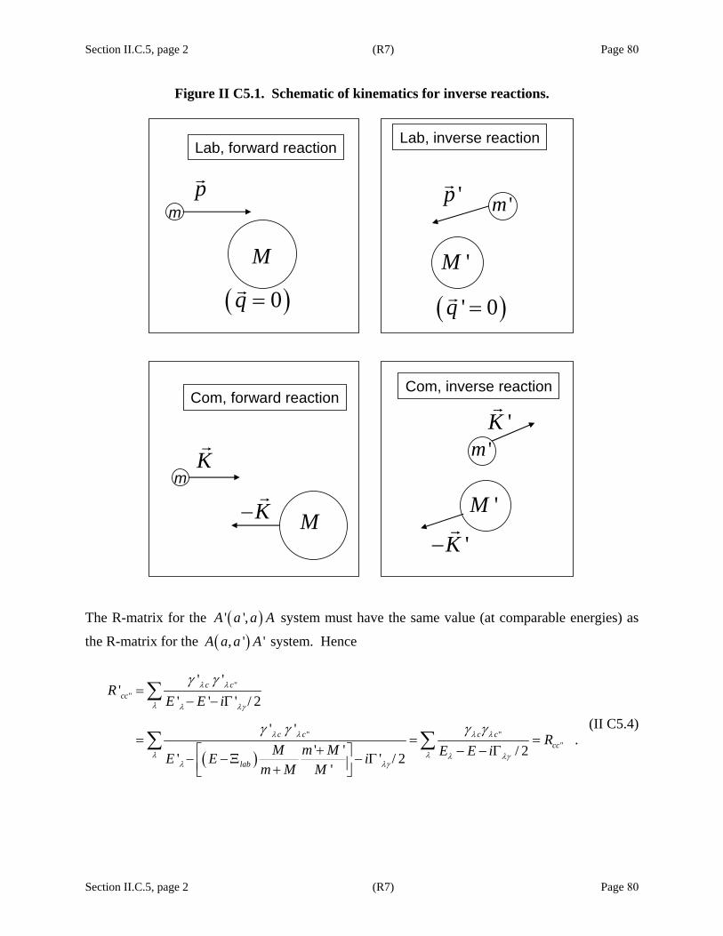
Section II.C.5, page 2 (R7) Page 80
Section II.C.5, page 2 (R7) Page 80
Figure II C5.1. Schematic of kinematics for inverse reactions.
The R-matrix for the ( )' ',A a a A system must have the same value (at comparable energies) as
the R-matrix for the ( ), ' 'A a a A system. Hence
( )
""
" ""
' ''
' ' ' / 2
' '.
' ' / 2' ' / 2'
c ccc
c c c ccc
lab
RE E i
RM m M E E iE E i
m M M
λ λ
λ λ λγ
λ λ λ λ
λ λ λ λγλ λγ
γ γ
γ γ γ γ
=− − Γ
= = =+ − − Γ⎡ ⎤− −Ξ − Γ⎢ ⎥+⎣ ⎦
∑
∑ ∑ (II C5.4)
mp
Lab, forward reaction
( )0q =
mK
Com, forward reaction
K−
'p
( )' 0q =
'm
'M
Lab, inverse reaction
'K
'K−
'm
'M
Com, inverse reaction
M
M

Section II.C.5, page 3 (R7) Page 81
Section II.C.5, page 3 (R7) Page 81
In order for the equality on the bottom line of Eq. (II C5.4) to hold, the unprimed resonance parameters must be defined as follows: ' , ' , ' ,lab c c c cE E q q qλ λ λ λ λ λγ γ= +Ξ Γ = Γ = (II C5.5) where
'' '
m M MqM m M+⎡ ⎤ ⎡ ⎤= ⎢ ⎥ ⎢ ⎥+⎣ ⎦ ⎣ ⎦
(II C5.6)
(for c = any channel, for example neutron, fission, or capture). These equations may be used to convert the resonance parameters.
To convert the experimental data, recall that there is a multiplicative kinematic factor of 1/K2, where K is the momentum of the incident particle in the COM frame. For ( )' ',A a a A , this term is
( )( )
2
22
' '1 ,' 2 ' ' '
m MK m M E
+= (II C5.7)
and for ( ), ' 'A a a A , the term is
( )2
2 2
1 .2m M
K mM E+
= (II C5.8)
The experimental cross sections must be multiplied by the ratio of these two values, and appropriate energy substitutions made.
Another multiplicative factor that must be adjusted is the spin statistical factor, which also reflects the parameters of the incident channel. Since the compound nuclear spin J is the same in either system, the correct multiplier is the ratio of the two:
( )
( )
( ) ( )( )( )
: ' '
: ' '
2 ' 1 2 ' 1.
2 1 2 1J A aa A
J A a a A
g i Ig i I
+ +=
+ + (II C5.9)
With these changes, the cross section for the ( ), ' 'A a a A reaction may be written in terms of the
cross section for the ( )' ',A a a A reaction as
( ) ( ) ( )( )( )( )
( )( ) ( ) ( )
22
' ' ' '22
2 ' 1 2 1 ' ' ' ' .2 1 2 1 ' 'A aa A A a a A
i I m Mm M EE Ei I mM Em M
σ σ+ + +
=+ + +
(II C5.10)

Section II.D, page 1 (R7) Page 83
Section II.D, page 1 (R7) Page 83
II.D. DERIVATIVES In order to make use of sophisticated fitting procedures such as Bayes’ equations (Section IV of this manual), it is necessary to know the partial derivatives of the theory with respect to the parameters to be fitted (the “varied parameters”). The easiest method for calculating derivatives of cross sections with respect to resonance parameters is to use a numerical difference approximation, of the form
( ) ( ) ,P P P
P Pσ σσ + Δ −∂
≈∂ Δ
(II D.1)
or, to avoid problems from the asymmetry of that approximation,
( ) ( ) .2
P P P PP P
σ σσ + Δ − −Δ∂≈
∂ Δ (II D.2)
Numerical methods, however, are neither as accurate nor as efficient or rapid as analytic derivatives. For that reason, SAMMY uses analytic derivatives wherever possible. In particular, derivatives of cross sections with respect to resonance parameters are all calculated analytically. To reiterate: SAMMY does NOT use numerical derivatives of the form (II D.1). When a numerical derivative is absolutely necessary, the form (II D.2) is used. For R-matrix parameters, analytic derivatives are always used. (The only exception to this rule is for charged-particle shift factors and penetrabilities, for which calculations of both the functions and the derivatives require numerical techniques.) The R-matrix equations are expressed in terms of the reduced-width amplitude γ rather than the partial width Γ. In the SAMMY code, the amplitudes are the parameters to be varied. In general, SAMMY distinguishes between “u-parameters” and “p-parameters”: The u-parameter is the variable whose value is sought by the fitting procedure. The p-parameter is the parameter whose value is given in the SAMMY input and output files. There is a well-defined relationship between the two, but the relationship is not necessarily one to one. For example, the value for the neutron width specified in the input PARameter file (see Table VI B.2 in Section VI.B) is related to three parameters, any or all of which might be varied:
22 ( ) ,
,
and 2 .
n l n
n
P
k a
Mk mEm M
λ λ
λ λ
λ λ
ρ γ
ρ
Γ =
=
=+
(II D.3)
Here , , andna Eλ λγ all may be varied parameters. In the SAMMY input, varied parameters are indicated by a flag, whose value (0, 1, or 3) indicates how that parameter is to be treated. The convention is that a flag on Γ denotes the status of the γ parameter, because the other two (the radius and the energy) are separately flagged.

Section II.D, page 2 (R7) Page 84
Section II.D, page 2 (R7) Page 84
Throughout this document, when the varied u-parameter is different from the flagged p-parameter, the equations relating the two are given explicitly. For the R-matrix (in all its various guises), the u-parameter associated with the resonance energy is ( ) ,u E Eλ λ= ± (II D.4) where the negative sign is chosen if Eλ is negative, and the u-parameter associated with the width is ( ) .c cu λ λγΓ = (II D.5) In the following sections, equations are given for the derivatives of the cross section with respect to the R-matrix parameters for the Reich-Moore approximation (Section II.D.1) and for the Breit-Wigner approximations (Section II.D.2). Additional details are in Section II.D.3.

Section III.D.1, page 1 (R7) Page 85
Section III.D.1, page 1 (R7) Page 85
II.D.1. Derivatives for Reich-Moore Approximation The derivative of the cross section with respect to a resonance parameter is found by making use of the chain rule:
,i i
R W U σ σ = u u R W U
μν ωτ ωτ
μ ν μν ωτ ωτω τ≤≤
∂ ∂ ∂∂ ∂∂ ∂ ∂ ∂ ∂∑ (II D1.1)
where the index J has been suppressed, since it is fixed for a given parameter u. Each term in this expression is evaluated separately.
Derivatives of cross sections with respect to the scattering matrix U, derivatives of U with respect to W, and derivatives of W with respect to R are found in Section II.D.1.a. Derivatives of R with respect to resonance parameters are given in Section II.D.1.b.
Derivatives of the cross sections with respect to the channel radius require additional terms
beyond those in Eq. (II D1.1), because the radius is also used to determine the hard-sphere phase shift. These derivatives are discussed in Section II.D.1.c.
Derivatives of R with respect to the variables of the logarithmic parameterization of the
external R-function (defined in Section II.B.1.d) are given in Section II.D.1.d.

Section III.D.1.a, page 1 (R7) Page 87
Section III.D.1.a, page 1 (R7) Page 87
II.D.1.a. Derivatives with respect to R-matrix
For resonance and Rext parameters, the derivative of the cross section may be written as
,c d e f e f
c di i c d e f e fe f
R W U σ σ =u u R W U≤
≤
∂ ∂ ∂∂ ∂∂ ∂ ∂ ∂ ∂
∑ (II D1 a.1)
where the index J has been suppressed, since it is fixed for a given parameter u. Indices c, d, e, and f denote channels. The restriction c d≤ indicates that the sum includes, for example, only terms with indices 1 2c c and not terms with indices 2 1c c (for 1 2c c≠ ); this restriction results from the symmetry of R and W (or X) with respect to interchange of indices.
Each term in the expression (II D1 a.1) will be evaluated separately, starting with the right-most term. All except /R u∂ ∂ are evaluated in this section; /R u∂ ∂ is discussed in subsequent sections.
The derivatives of cross section with respect to the real part of U can be expressed as
*
* * 2 Rer r r
σ σ U σ U σ σ= + = = ,U U U U U U U U
σ∂ ∂ ∂ ∂ ∂ ∂ ∂ ∂⎡ ⎤+ ⎢ ⎥∂ ∂ ∂ ∂ ∂ ∂ ∂ ∂⎣ ⎦ (II D1 a.2)
where the asterisk implies complex conjugate, and U and U* are treated as independent entities. Similarly the derivative with respect to the imaginary part of U is given by
*
* * 2 Imi i i
σ σ U σ U σ σ σ= = i i = .U U U U U U U U
⎡ ⎤∂ ∂ ∂ ∂ ∂ ∂ ∂ ∂+ − − ⎢ ⎥∂ ∂ ∂ ∂ ∂ ∂ ∂ ∂⎣ ⎦
(II D1 a.3)
It follows that the derivative of the cross section with respect to U can be written as
1Re Im .2 r i
σ σ σ σ σ= i iU U U U U
⎡ ⎤ ⎡ ⎤ ⎛ ⎞∂ ∂ ∂ ∂ ∂+ = −⎜ ⎟⎢ ⎥ ⎢ ⎥∂ ∂ ∂ ∂ ∂⎣ ⎦ ⎣ ⎦ ⎝ ⎠
(II D1 a.4)
Using Eq. (II D1 a.4), values for the partial derivative of σ with respect to U are found from
Eqs. (II A.8) to (II A.11), which give
2
total
e fe f
π g ,U kσ δ∂
= −∂
(II D1 a.5)
( )*2 ,e f e f
e f
g UU k
αασ π δ∂
= − −∂
(II D1 a.6)
Section III.D.1.a, page 2 (R7) Page 88
Section III.D.1.a, page 2 (R7) Page 88
' *2 for 'e f
e f
π g= U ,U kαασ
α α∂
≠∂
(II D1 a.7)
and
*2
capture
e fe f
g U .U k
σ π∂= −
∂ (II D1 a.8)
Derivatives of a complex variable (such as U ) with respect to another complex variable
(such as W ) may be generated directly, without separately considering the real and imaginary parts of each variable; this is demonstrated explicitly in Section II.D.3. Here, we make use of this result to evaluate U / W∂ ∂ and W / R∂ ∂ .
Derivatives of Ue f with respect to We f are formed directly from Eq. (II A.4), which may be expressed as ,e f e e f fU W= Ω Ω (II D1 a.9) so that
.e fe f
e f
UW∂
= Ω Ω∂
(II D1 a.10)
Derivatives of W with respect to R are formed from Eqs. (II B1.3) and (II B1.4), which we
rewrite as
( )( )( )( ) ( )
( )
11 1
11 1 1 1
1 11 1 1 1 1 1
11 1 1 1
2 2
2
2 2
2 2 .
W I iX I i PL L R R P
I i PL L R R L L P
I i PL L R R L P i PL L R L P
I i PL P i PL L R L P
−− −
−− − − −
− −− − − − − −
−− − − −
= + = + −
⎡ ⎤= + − − +⎣ ⎦
⎡ ⎤ ⎡ ⎤= + − − + −⎣ ⎦ ⎣ ⎦
= − + −
(II D1 a.11)
Explicitly displaying the indices, Eq. (II D1 a.11) takes the form 1 1 12 2 ,e f e f e f e e e f f fW I i P L i P L Y L Pδ − − −= − + (II D1 a.12) where we have set ( ) 11 .e f
e f L RY
−−⎡ ⎤= −⎢ ⎥⎣ ⎦ (II D1 a.13)
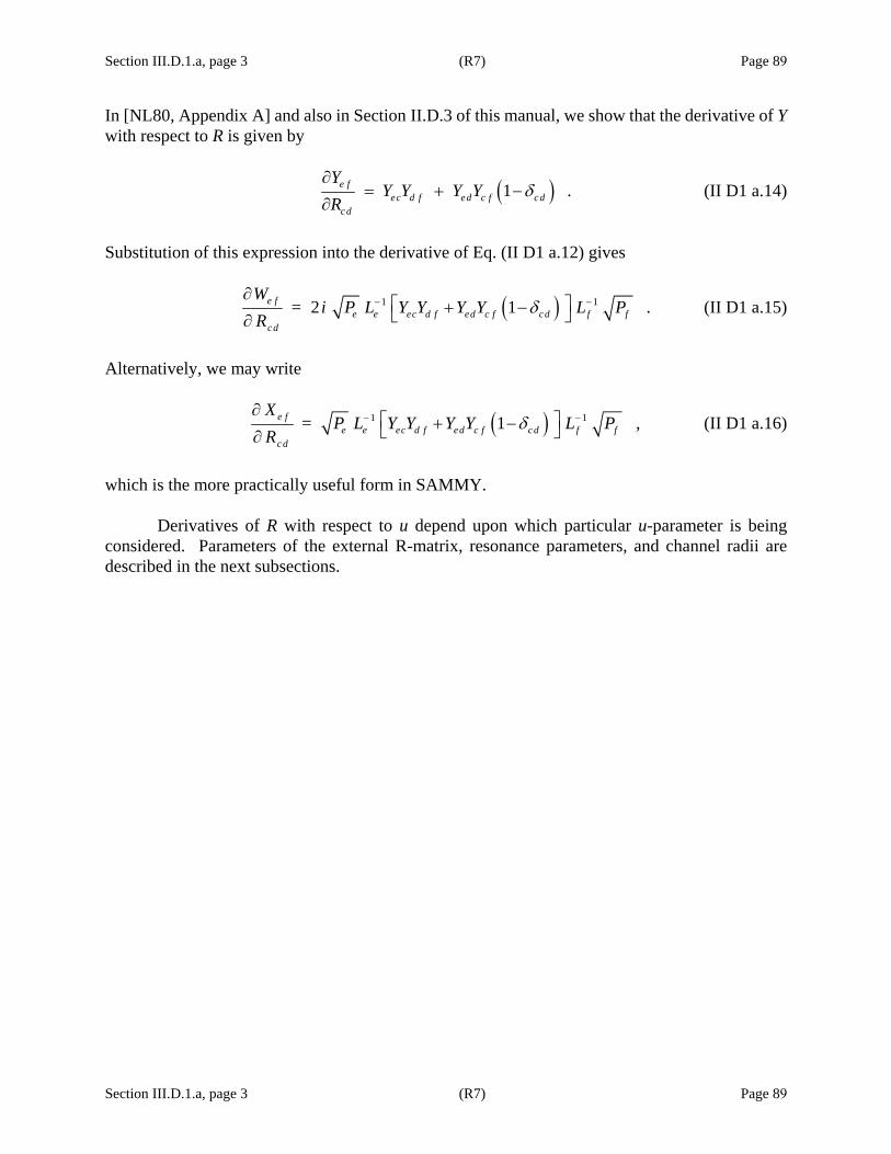
Section III.D.1.a, page 3 (R7) Page 89
Section III.D.1.a, page 3 (R7) Page 89
In [NL80, Appendix A] and also in Section II.D.3 of this manual, we show that the derivative of Y with respect to R is given by
( )1 .e fec d f ed c f cd
cd
YY Y Y Y
Rδ
∂= + −
∂ (II D1 a.14)
Substitution of this expression into the derivative of Eq. (II D1 a.12) gives
( )1 12 1 .e fe e ec d f ed c f cd f f
cd
W= i P L Y Y Y Y L P
Rδ− −∂
⎡ ⎤+ −⎣ ⎦∂ (II D1 a.15)
Alternatively, we may write
( )1 11 ,e fe e ec d f ed c f cd f f
c d
X= P L Y Y Y Y L P
Rδ− −∂
⎡ ⎤+ −⎣ ⎦∂ (II D1 a.16)
which is the more practically useful form in SAMMY.
Derivatives of R with respect to u depend upon which particular u-parameter is being considered. Parameters of the external R-matrix, resonance parameters, and channel radii are described in the next subsections.


Section II.D.1.b, page 1 (R8) Page 91
Section II.D.1.b, page 1 (R8) Page 91
II.D.1.b. Derivatives with respect to resonance parameters
From Eq. (II B1.1), the derivatives of the real and imaginary part of R with respect to the resonance u-parameter associated with the resonance energy are
( ) ( ) 22 2 2Re
2 /R
E E E dE
μνλ μ λν λ λ λγ λ
λ
γ γ γ⎡ ⎤∂ ⎣ ⎦ ⎡ ⎤⎡ ⎤= − − +⎣ ⎦ ⎢ ⎥⎣ ⎦∂
(II D1 b.1)
and
( ) 2 2Im
4 / .R
E E E dE
μ νλ μ λν λ λ λγ λ
λ
γ γ γ⎡ ⎤∂ ⎣ ⎦ ⎡ ⎤⎡ ⎤= − −⎣ ⎦ ⎣ ⎦∂
(II D1 b.2)
The derivatives of R with respect to the u-parameter associated with the eliminated capture width can be written as
( ) 2 2Re
4 /R
E E dμνλ μ λν λγ λ λγ λ
λγ
γ γ γ γγ
⎡ ⎤∂ ⎣ ⎦ ⎡ ⎤⎡ ⎤= − −⎣ ⎦ ⎣ ⎦∂ (II D1 b.3)
and
( ) ( ) 22 2 2Im
2 / .R
E E dμ νλ μ λν λγ λ λγ λ
λγ
γ γ γ γγ
⎡ ⎤∂ ⎣ ⎦ ⎡ ⎤⎡ ⎤= − −⎣ ⎦ ⎢ ⎥⎣ ⎦∂ (II D1 b.4)
The derivatives for the particle widths are
( ) ( )Re
1 /R
E E dμ νλν μ ν λ λ
λ μ
γ δγ
⎡ ⎤∂ ⎣ ⎦ ⎡ ⎤ ⎡ ⎤= + −⎣ ⎦⎣ ⎦∂ (II D1 b.5)
and
( ) 2Im
1 / .R
dμνλν μ ν λγ λ
λ μ
γ δ γγ
⎡ ⎤∂ ⎣ ⎦ ⎡ ⎤ ⎡ ⎤= + ⎣ ⎦⎣ ⎦∂ (II D1 b.6)
In the expressions above, the denominator term d is defined as
( )2 4 .d E Eλ λ λγγ= − + (II D1 b.7)
In each of these equations, the first square bracket contains an energy-independent factor; in the code SAMMY, this factor (times 2) is evaluated outside the energy loop in subroutine BABB and is stored as BR(μv,i) for the derivative of the real part of Rμv with respect to the ith parameter, and BI(μv,i) for the derivative of the imaginary part of Rμv. The quantity in the second square bracket is energy dependent but channel independent. Therefore, it must be generated for each energy and is temporarily stored as UPR(i) and UPI(i) in subroutine ABPART.
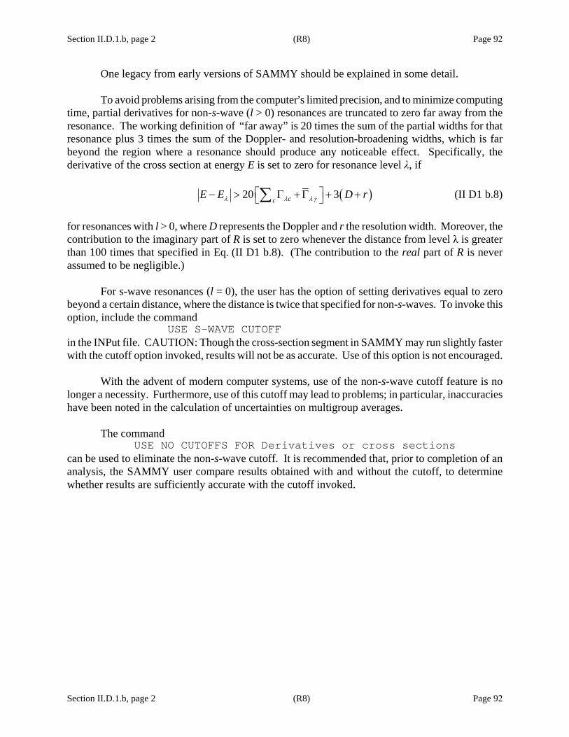
Section II.D.1.b, page 2 (R8) Page 92
Section II.D.1.b, page 2 (R8) Page 92
One legacy from early versions of SAMMY should be explained in some detail. To avoid problems arising from the computer=s limited precision, and to minimize computing
time, partial derivatives for non-s-wave (l > 0) resonances are truncated to zero far away from the resonance. The working definition of “far away” is 20 times the sum of the partial widths for that resonance plus 3 times the sum of the Doppler- and resolution-broadening widths, which is far beyond the region where a resonance should produce any noticeable effect. Specifically, the derivative of the cross section at energy E is set to zero for resonance level λ, if
( )20 3cc
E E D rλ λ λγ⎡ ⎤− > Γ +Γ + +⎣ ⎦∑ (II D1 b.8)
for resonances with l > 0, where D represents the Doppler and r the resolution width. Moreover, the contribution to the imaginary part of R is set to zero whenever the distance from level λ is greater than 100 times that specified in Eq. (II D1 b.8). (The contribution to the real part of R is never assumed to be negligible.)
For s-wave resonances (l = 0), the user has the option of setting derivatives equal to zero beyond a certain distance, where the distance is twice that specified for non-s-waves. To invoke this option, include the command
USE S-WAVE CUTOFF in the INPut file. CAUTION: Though the cross-section segment in SAMMY may run slightly faster with the cutoff option invoked, results will not be as accurate. Use of this option is not encouraged.
With the advent of modern computer systems, use of the non-s-wave cutoff feature is no
longer a necessity. Furthermore, use of this cutoff may lead to problems; in particular, inaccuracies have been noted in the calculation of uncertainties on multigroup averages.
The command
USE NO CUTOFFS FOR Derivatives or cross sections can be used to eliminate the non-s-wave cutoff. It is recommended that, prior to completion of an analysis, the SAMMY user compare results obtained with and without the cutoff, to determine whether results are sufficiently accurate with the cutoff invoked.
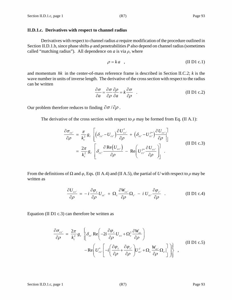
Section II.D.1.c, page 1 (R7) Page 93
Section II.D.1.c, page 1 (R7) Page 93
II.D.1.c. Derivatives with respect to channel radius
Derivatives with respect to channel radius a require modification of the procedure outlined in Section II.D.1.b, since phase shifts φ and penetrabilities P also depend on channel radius (sometimes called “matching radius”). All dependence on a is via ρ, where
,k aρ = (II D1 c.1) and momentum k in the center-of-mass reference frame is described in Section II.C.2; k is the wave number in units of inverse length. The derivative of the cross section with respect to the radius can be written
.ka aσ σ ρ σ
ρ ρ∂ ∂ ∂ ∂
= =∂ ∂ ∂ ∂
(II D1 c.2)
Our problem therefore reduces to finding /σ ρ∂ ∂ .
The derivative of the cross section with respect to ρ may be formed from Eq. (II A.1):
( ) ( )
( )
*' ' '*
' ' ' '2
' '*' '2
Re2 Re .
cc cc ccJc cc cc cc cc
c
cc ccJc cc cc
c
U Ug U U
k
U Ug U
k
σ π δ δρ ρ ρ
π δρ ρ
⎡ ⎤∂ ∂ ∂= − + −⎢ ⎥
∂ ∂ ∂⎢ ⎥⎣ ⎦⎡ ⎤∂ ⎛ ⎞∂⎢ ⎥= − ⎜ ⎟⎜ ⎟∂ ∂⎢ ⎥⎝ ⎠⎣ ⎦
(II D1 c.3)
From the definitions of Ω and φ, Eqs. (II A.4) and (II A.5), the partial of U with respect to ρ may be written as
' ' '' ' ' .cc c cc c
cc c c cc
U Wi U i Uϕ ϕ
ρ ρ ρ ρ∂ ∂ ∂ ∂
= − + Ω Ω −∂ ∂ ∂ ∂
(II D1 c.4)
Equation (II D1 c.3) can therefore be written as
' 2'2
'* '' ' '
2 Re 2
Re ,
cc c ccc cc cc c
c
c c J cccc cc c c
Wg i Uk
WU i U
σ ϕπ δρ ρ ρ
ϕ ϕρ ρ ρ
⎧∂ ∂⎛ ⎞∂⎪= − +Ω⎨ ⎜ ⎟∂ ∂ ∂⎪ ⎝ ⎠⎩⎫⎛ ⎞⎡ ⎤∂ ∂⎛ ⎞ ⎪− − + +Ω Ω⎜ ⎟ ⎬⎢ ⎥⎜ ⎟⎜ ⎟∂ ∂ ∂⎝ ⎠⎣ ⎦ ⎪⎝ ⎠ ⎭
(II D1 c.5)
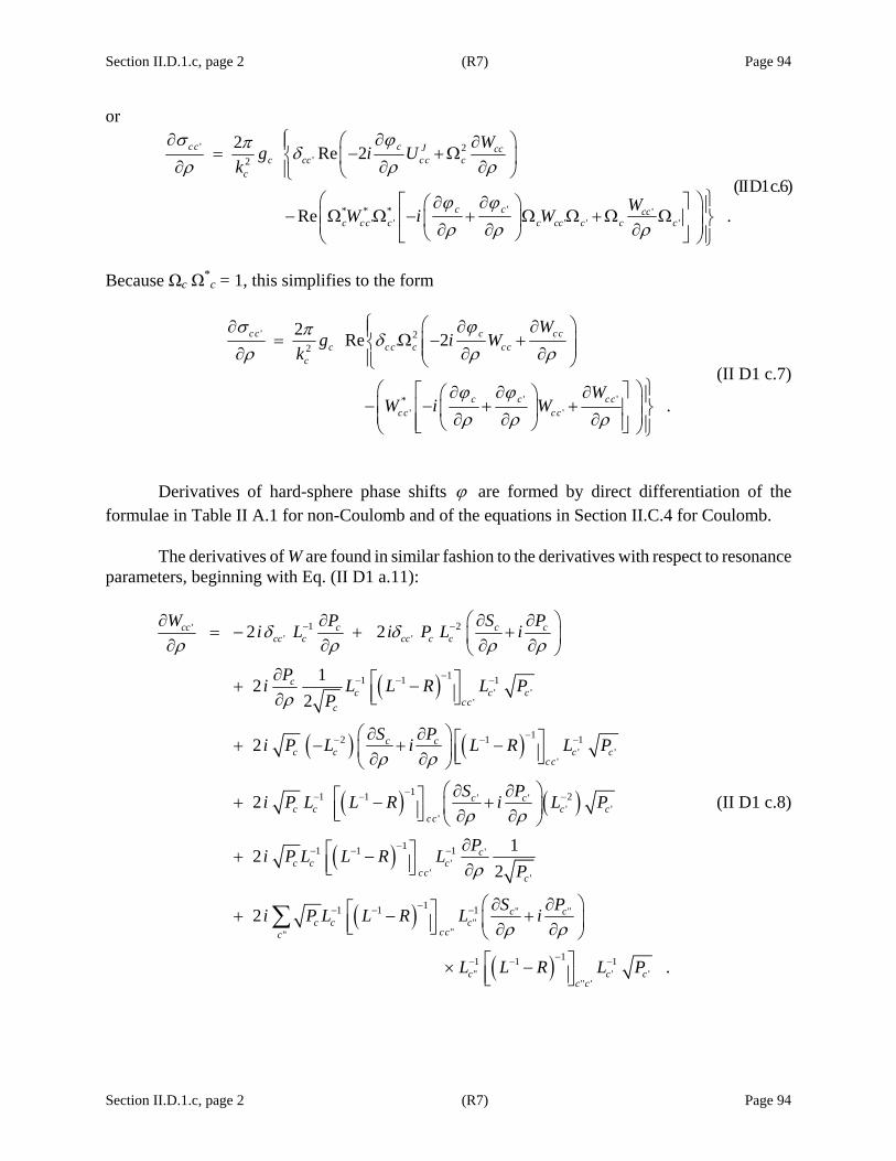
Section II.D.1.c, page 2 (R7) Page 94
Section II.D.1.c, page 2 (R7) Page 94
or
' 2'2
'* * * '' ' ' ' '
2 Re 2
Re .
cc c J ccc cc cc c
c
c c ccc cc c c cc c c c
Wg i Uk
WW i W
σ ϕπ δρ ρ ρ
ϕ ϕρ ρ ρ
⎧∂ ∂⎛ ⎞∂⎪= − +Ω⎨ ⎜ ⎟∂ ∂ ∂⎪ ⎝ ⎠⎩⎫⎛ ⎞⎡ ⎤∂ ∂⎛ ⎞ ⎪− Ω Ω − + Ω Ω +Ω Ω⎜ ⎟ ⎬⎢ ⎥⎜ ⎟⎜ ⎟∂ ∂ ∂⎝ ⎠⎣ ⎦ ⎪⎝ ⎠ ⎭
(II D1 c.6)
Because Ωc Ω*
c = 1, this simplifies to the form
' 2'2
' '*' '
2 Re 2
.
cc c ccc cc c cc
c
c c cccc cc
Wg i W
k
WW i W
σ ϕπ δρ ρ ρ
ϕ ϕρ ρ ρ
⎧ ⎛ ⎞∂ ∂ ∂⎪= Ω − +⎜ ⎟⎨ ⎜ ⎟∂ ∂ ∂⎪ ⎝ ⎠⎩⎫⎛ ⎞⎡ ⎤∂ ∂ ∂⎛ ⎞ ⎪− − + +⎜ ⎟⎢ ⎥ ⎬⎜ ⎟⎜ ⎟∂ ∂ ∂⎢ ⎥⎝ ⎠ ⎪⎣ ⎦⎝ ⎠ ⎭
(II D1 c.7)
Derivatives of hard-sphere phase shifts ϕ are formed by direct differentiation of the
formulae in Table II A.1 for non-Coulomb and of the equations in Section II.C.4 for Coulomb.
The derivatives of W are found in similar fashion to the derivatives with respect to resonance parameters, beginning with Eq. (II D1 a.11):
( )
( ) ( )
( ) ( )
1 2'' '
11 1 1' '
'
12 1 1' '
'
11 1 2' '' '
'
2 2
122
2
2
cc c c ccc c cc c c
cc c c
ccc
c cc c c c
cc
c cc c c c
cc
W P S Pi L i P L i
Pi L L R L PP
S Pi P L i L R L P
S Pi P L L R i L P
δ δρ ρ ρ ρ
ρ
ρ ρ
ρ ρ
− −
−− − −
−− − −
−− − −
⎛ ⎞∂ ∂ ∂ ∂= − + +⎜ ⎟∂ ∂ ∂ ∂⎝ ⎠
∂ ⎡ ⎤+ −⎢ ⎥⎣ ⎦∂
⎛ ⎞∂ ∂ ⎡ ⎤+ − + −⎜ ⎟ ⎢ ⎥⎣ ⎦∂ ∂⎝ ⎠
⎛ ⎞∂ ∂⎡ ⎤+ − +⎜ ⎟⎢ ⎥⎣ ⎦ ∂ ∂⎝ ⎠
( )
( )
( )
11 1 1 ''
' '
11 1 1 " ""
""
11 1 1" ' '
" '
122
2
.
cc c c
cc c
c cc c c
ccc
c c cc c
Pi P L L R LP
S Pi P L L R L i
L L R L P
ρ
ρ ρ
−− − −
−− − −
−− − −
∂⎡ ⎤+ −⎢ ⎥⎣ ⎦ ∂
⎛ ⎞∂ ∂⎡ ⎤+ − +⎜ ⎟⎢ ⎥⎣ ⎦ ∂ ∂⎝ ⎠
⎡ ⎤× −⎢ ⎥⎣ ⎦
∑
(II D1 c.8)

Section II.D.1.c, page 3 (R7) Page 95
Section II.D.1.c, page 3 (R7) Page 95
This expression can be greatly simplified by setting
( ) 11 1 1 1' ' ' '
',cc c c c c c c cc
ccP L L R L P P Lϑ δ
−− − − −⎡ ⎤= − −⎢ ⎥⎣ ⎦ (II D1 c.9)
which gives
' '' '
'
1 " "" " " '
"
1 1
2 .
Jcc c c
cc ccc c
c ccc c c c
c
W P Pi iP P
S Pi P i
ϑ ϑρ ρ ρ
ϑ ϑρ ρ
−
∂ ∂ ∂= + +
∂ ∂ ∂
⎛ ⎞∂ ∂+ +⎜ ⎟∂ ∂⎝ ⎠
∑ (II D1 c.10)
Derivatives of penetrabilities Pc and shift factors Sc are found by direct differentiation of the formulae in Table II A.1 for non-Coulomb and Section II.C.4 for Coulomb. Derivatives of the cross sections with respect to ρ are then found by substituting results from Eq. (II D1 c.10) into Eq. (II D1 c.7).


Section II.D.1.d, page 1 (R7) Page 97
Section II.D.1.d, page 1 (R7) Page 97
II.D.1.d. Derivatives of logarithmic external R-function
Derivatives of Rext with respect to the u-parameters are found from Eqs. (II B1 d.1) and (II B1 d.2) to be of the form
, , ,ext upc con c lin c cup upc c
R s s EE E E∂ +
= −∂ −
(II D1 d.1)
, , ,ext downc con c lin c c
down downc c
R s s EE E E∂ +
= −∂ −
(II D1 d.2)
,
1 ,extc
con c
RR∂
=∂
(II D1 d.3)
,
,extc
lin c
RE
R∂
=∂
(II D1 d.4)
2
,
,extc
q c
RE
R∂
=∂
(II D1 d.5)
,,
2 ln ,ext upc c
con c downccon c
R E EsE Es
∂ ⎡ ⎤−= − ⎢ ⎥−∂ ⎣ ⎦ (II D1 d.6)
and
( ),
ln .ext upc up down c
c c downlin c c
R E EE E Es E E∂ ⎡ ⎤−
= − − − ⎢ ⎥∂ −⎣ ⎦ (II D1 d.7)

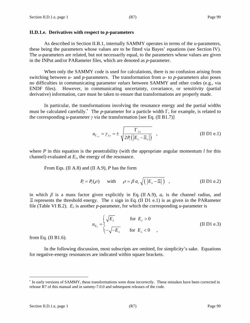
Section II.D.1.e, page 1 (R7) Page 99
Section II.D.1.e, page 1 (R7) Page 99
II.D.1.e. Derivatives with respect to p-parameters As described in Section II.B.1, internally SAMMY operates in terms of the u-parameters, these being the parameters whose values are to be fitted via Bayes’ equations (see Section IV). The u-parameters are related, but not necessarily equal, to the parameters whose values are given in the INPut and/or PARameter files, which are denoted as p-parameter. When only the SAMMY code is used for calculations, there is no confusion arising from switching between u- and p-parameters. The transformation from u- to p-parameters also poses no difficulties in communicating parameter values between SAMMY and other codes (e.g., via ENDF files). However, in communicating uncertainty, covariance, or sensitivity (partial derivative) information, care must be taken to ensure that transformations are properly made. In particular, the transformations involving the resonance energy and the partial widths must be calculated carefully.∗ The p-parameter for a particle width Γ, for example, is related to the corresponding u-parameter γ via the transformation [see Eq. (II B1.7)]
( ) ,2c
cc
l c
uP Eλ
λλ
λ
γΓ
Γ= = ±
−Ξ (II D1 e.1)
where P in this equation is the penetrability (with the appropriate angular momentum l for this channel) evaluated at Eλ, the energy of the resonance.
From Eqs. (II A.8) and (II A.9), P has the form
( )( ) with ,l l cP P a Eλρ ρ β= = −Ξ (II D1 e.2) in which β is a mass factor given explicitly in Eq. (II A.9), ac is the channel radius, and Ξ represents the threshold energy. The ± sign in Eq. (II D1 e.1) is as given in the PARameter file (Table VI B.2). Eλ is another p-parameter, for which the corresponding u-parameter is
for 0
for 0 ,E
E Eu
E Eλ
λ λ
λ λ
⎧ >⎪= ⎨⎪− − <⎩
(II D1 e.3)
from Eq. (II B1.6).
In the following discussion, most subscripts are omitted, for simplicity’s sake. Equations for negative-energy resonances are indicated within square brackets.
∗ In early versions of SAMMY, these transformations were done incorrectly. These mistakes have been corrected in release R7 of this manual and in sammy-7.0.0 and subsequent releases of the code.

Section II.D.1.e, page 2 (R7) Page 100
Section II.D.1.e, page 2 (R7) Page 100
Consider a function f of the two u-parameters γ and u (which we take to be the u-parameter associated with the resonance energy). This function might be the cross section, or some other function such as transmission or average cross section. The equations of transformation to the two p-parameters Γ and Eλ are given above. The derivatives of f with respect to the p-parameters are therefore
f f u fu
γγ
∂ ∂ ∂ ∂ ∂= +
∂Γ ∂Γ ∂ ∂Γ ∂ (II D1 e.4)
and
.f f u fE E E uλ λ λ
γγ
∂ ∂ ∂ ∂ ∂= +
∂ ∂ ∂ ∂ ∂ (II D1 e.5)
The partial derivatives of the u-parameters with respect to the p-parameter Γ can readily be found from Eqs. (II D1 e.1) and (II D1 e.3) as
1/ 21 1 1 1 ,2 2 2 22 PP
γ γ−∂ Γ= ± Γ = ± =
∂Γ Γ Γ (II D1 e.6)
and
0 .u∂=
∂Γ (II D1 e.7)
The derivative of u with respect to Eλ is relatively straight forward:
( )
1/ 2
1/ 2
1 12 2 2
1 1 if 0 .2 2 2
u uEE u E
u uE EE u E
λλ λ
λ λλ λ
−
−
∂= = =
∂
⎡ ⎤∂= − = − = <⎢ ⎥∂⎣ ⎦
(II D1 e.8)
The derivative of γ with respect to Eλ is somewhat more complicated, having the form
3/ 21 1 ' ' ,2 2 2 2 2
dP P PPE d E P P E P Eλ λ λ λ
γ ρ ρ γ ρρ
−∂ Γ ∂ Γ ∂ ∂⎛ ⎞= ± − = = −⎜ ⎟∂ ∂ ∂ ∂⎝ ⎠∓ (II D1 e.9)
in which we have defined 'P to be dP dρ . From Eq. (II D1 e.2), for Eλ > Ξ , it follows that
( ) ( )
' ' .2 42P a P
E P P EEλ λλ
γ γ β γ ρ∂= − = −
∂ −Ξ−Ξ (II D1 e.10)

Section II.D.1.e, page 3 (R7) Page 101
Section II.D.1.e, page 3 (R7) Page 101
Similarly, for Eλ < Ξ , we find
( ) ( )( )
( )( ) ( )
1' '2 2 2
' ' .4 4
aP Pa EE P E P E
a EP PP E P E
λλ λ λ
λ
λ λ
βγ γ γβ
βγ γ ρ
−∂ ∂= − − −Ξ = −
∂ ∂ − −Ξ
− −Ξ= + = −
− −Ξ −Ξ
(II D1 e.11)
Equations (II D1 e.4) and (II D1 e.5) can therefore be rewritten as
02
f fγγ
∂ ∂= +
∂Γ Γ ∂ (II D1 e.12)
and
( )
' .4 2
f P f u fE P E E uλ λ λ
γ ργ
∂ ∂ ∂= − +
∂ −Ξ ∂ ∂ (II D1 e.13)
Similarly, if the function f is defined in terms of p-parameters, the derivatives of f with respect to the u-parameters are given by
Ef f fE
λ
λγ γ γ∂∂ ∂Γ ∂ ∂
= +∂ ∂ ∂Γ ∂ ∂
(II D1 e.14)
and
.Ef f fu u u E
λ
λ
∂∂ ∂Γ ∂ ∂= +
∂ ∂ ∂Γ ∂ ∂ (II D1 e.15)
That is, the inverse transformation (from p-space to u-space) requires the use of the partial derivatives of p-parameters with respect to the u-parameters. These derivatives have the form
22 2 4 ,P Pγ γγ γ∂Γ Γ
= ± = ± =∂
(II D1 e.16)
0 ,Eλ
γ∂
=∂
(II D1 e.17)
and
2 22 2 if 0 .E E E Eu u Eu u u uλ λ λ λ
λ∂ ∂⎡ ⎤= = = − = <⎢ ⎥∂ ∂⎣ ⎦
(II D1 e.18)

Section II.D.1.e, page 4 (R7) Page 102
Section II.D.1.e, page 4 (R7) Page 102
The partial derivative of Γ with respect to u requires special care to evaluate correctly. For 2u Eλ= > Ξ , this derivative has the form
( )( )
( )( )( ) ( )
22 2
2
2
2 '2
' 2 ' '= .2
P P dP P a uu u P d u P u
a u u EP a u P PP P E P E uu
λ
λ λ
γ ργ βρ
ββ ρ
∂Γ ∂ ∂ ∂= = = Γ −Ξ
∂ ∂ ∂ ∂
−Ξ= Γ Γ = Γ
−Ξ −Ξ−Ξ
(II D1 e.19)
If 20 E uλ< = < Ξ , this partial derivative takes the form
( )( )( )( )
( ) ( )( )
( )
22 2
2
22
2 '2
2' '=2
' .
P P dP P a uu u P d u P u
a u ua uP PP P uu
EPP E u
λ
λ
γ ργ βρ
ββ
ρ
∂Γ ∂ ∂ ∂= = = Γ − −Ξ
∂ ∂ ∂ ∂
− −Ξ −−= Γ Γ
− −Ξ− −Ξ
= Γ−Ξ
(II D1 e.20)
[Finally, if 20 E uλ> = − , then
( )( )( )
( )( )
( )( )
( )
22 2
2
22
2 '2
2' '=2
'= ,
P P dP P a uu u P d u P u
a u ua uP PP P uu
EPP E u
λ
λ
γ ργ βρ
ββ
ρ
∂Γ ∂ ∂ ∂= = = Γ − − −Ξ
∂ ∂ ∂ ∂
+Ξ= Γ Γ
− − −Ξ+Ξ
Γ−Ξ
(II D1 e.21)
in a form which is compatible with the other versions.]
Substituting Eqs. (II D1 e.16) through (II D1 e.19) into Eqs. (II D1 e.14) and (II D1 e.15) gives
2 0f fγ γ
∂ Γ ∂= +
∂ ∂Γ (II D1 e.22)
and
( )
2' .E Ef P f fu P E u u E
λ λ
λ λ
ρ∂ ∂ ∂= Γ +
∂ −Ξ ∂Γ ∂ (II D1 e.23)
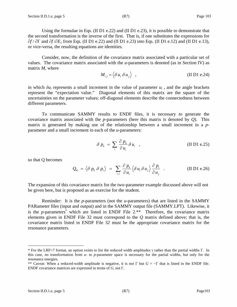
Section II.D.1.e, page 5 (R7) Page 103
Section II.D.1.e, page 5 (R7) Page103
Using the formulae in Eqs. (II D1 e.22) and (II D1 e.23), it is possible to demonstrate that the second transformation is the inverse of the first. That is, if one substitutes the expressions for ∂f / ∂Γ and ∂f /∂Eλ from Eqs. (II D1 e.22) and (II D1 e.23) into Eqs. (II D1 e.12) and (II D1 e.13), or vice-versa, the resulting equations are identities. Consider, now, the definition of the covariance matrix associated with a particular set of values. The covariance matrix associated with the u-parameters is denoted (as in Section IV) as matrix M, where ,i j i jM u uδ δ= (II D1 e.24) in which δui represents a small increment in the value of parameter ui , and the angle brackets represent the “expectation value.” Diagonal elements of this matrix are the square of the uncertainties on the parameter values; off-diagonal elements describe the connectedness between different parameters. To communicate SAMMY results to ENDF files, it is necessary to generate the covariance matrix associated with the p-parameters (here this matrix is denoted by Q). This matrix is generated by making use of the relationship between a small increment in a p-parameter and a small increment in each of the u-parameters:
,kk i
i i
pp uu
δ δ∂
=∂∑ (II D1 e.25)
so that Q becomes
,
.k lkl k l i j
i j i j
p pQ p p u u
u uδ δ δ δ
∂ ∂= =
∂ ∂∑ (II D1 e.26)
The expansion of this covariance matrix for the two-parameter example discussed above will not be given here, but is proposed as an exercise for the student. Reminder: It is the p-parameters (not the u-parameters) that are listed in the SAMMY PARameter files (input and output) and in the SAMMY output file (SAMMY.LPT). Likewise, it is the p-parameters∗ which are listed in ENDF File 2.** Therefore, the covariance matrix elements given in ENDF File 32 must correspond to the Q matrix defined above; that is, the covariance matrix listed in ENDF File 32 must be the appropriate covariance matrix for the resonance parameters.
* For the LRF=7 format, an option exists to list the reduced width amplitudes γ rather than the partial widths Γ. In this case, no transformation from u- to p-parameter space is necessary for the partial widths, but only for the resonance energies. ** Caveat: When a reduced-width amplitude is negative, it is not Γ but G = −Γ that is listed in the ENDF file. ENDF covariance matrices are expressed in terms of G, not Γ.

Section II.D.1.e, page 6 (R7) Page 104
Section II.D.1.e, page 6 (R7) Page 104
When the cross section is calculated as a function of the u-parameters, a small increment in the calculated cross section is given by
.nn n
uuσδ σ δ∂
=∂∑ (II D1 e.27)
Therefore the covariance matrix jiC for the cross section is found from
,
,
,
jii j i j n m
n mn m
jin m
n m n m
jinm
n m n m
C u uu u
u uu u
Mu u
σσδ σ δ σ δ δ
σσ δ δ
σσ
∂⎛ ⎞ ⎛ ⎞∂= = ⎜ ⎟ ⎜ ⎟∂ ∂⎝ ⎠ ⎝ ⎠
∂∂=
∂ ∂
∂∂=
∂ ∂
∑ ∑
∑
∑
(II D1 e.28)
in which M is again defined as the covariance matrix for the u-parameters. In order to print the covariance matrix resonance parameters for the p-parameters into the ENDF formats, it is necessary to transform the parameter covariance matrix from M to Q. That transformation is made by inserting the formulae
i k i
kn n k
pu u pσ σ∂ ∂ ∂
=∂ ∂ ∂∑ (II D1 e.29)
and
j jl
lm m l
pu u pσ σ∂ ∂∂
=∂ ∂ ∂∑ (II D1 e.30)
into the previous expression, Eq. (II D1 e.28), yielding
, , ,
ji k lij nm
n m k l k n m l
p pC Mp u u p
σσ ∂∂ ∂ ∂=
∂ ∂ ∂ ∂∑ (II D1 e.31)
or
,
,jiij kl
k l k l
C Qp p
σσ ∂∂=
∂ ∂∑ (II D1 e.32)
where Q is given by
,
.k lkl nm
n m n m
p pQ Mu u
∂ ∂=
∂ ∂∑ (II D1 e.33)
For the case in which only one elastic width contains an energy-dependent penetrability, the p-parameter covariance matrix must be modified for all elements involving a width having energy-dependent penetrability.

Section II.D.2, page 1 (R8) Page 105
Section II.D.2, page 1 (R8) Page 105
II.D.2. Derivatives for MLBW and SLBW Approximations
From the form of the cross sections in Eqs. (II B3 a.1), (II B3 a.5), and (II B3 a.6), we note that there are only four expressions in which the resonance energies or widths occur. These expressions are denoted as follows:
( )1 / ,c cA E E dλ λ λ λ= Γ − (II D2.1) 2 / ,c cA dλ λ λγ λ= Γ Γ (II D2.2) 3 ' ' / ,cc c cA dλ λ λ λ= Γ Γ (II D2.3) and 4 / ,c cA dλ λ λ λ= Γ Γ (II D2.4) where d is given by Eq. (II B3 a.4) as
( ) ( )2 2/ 2 .d E Eλ λ λ= − + Γ (II D2.5)
Equation (II D2.4) is actually redundant, since
4 3 ' 2'
.c cc cc
A A Aλ λ λ= +∑ (II D2.6)
As discussed in Section II.D, the assumption in the SAMMY code is that the u-parameters
are independent and the p-parameters are derived quantities. Thus we need only evaluate partial derivatives of 1 2 3 ', , and c c ccA A Aλ λ λ with respect to the u-parameters (i.e., with respect to the partial-width amplitudes and to the square root of the resonance energy). These derivatives may be written as follows:
( ) 21 2 1 2 / / ,cc
AE E E d d
Eλ
λ λ λ λ λλ
∂= Γ − + −
∂ (II D2.7)
( )2 24 / ,cc
AE E E d
Eλ
λ λ λγ λ λλ
∂= Γ Γ −
∂ (II D2.8)
( )3 ' 2'4 / ,cc
c c
AE E E d
Eλ
λ λ λ λ λλ
∂= Γ Γ −
∂ (II D2.9)
( )1 22 / ,cc
AE E dλ
λγ λ λ λ λλγ
γγ
∂= − Γ − Γ
∂ (II D2.10)

Section II.D.2, page 2 (R8) Page 106
Section II.D.2, page 2 (R8) Page 106
2 2 2 / / ,cc
Ad dλ
λγ λ λγ λ λ λλγ
γγ
∂= Γ −Γ Γ
∂ (II D2.11)
3 ' 2'2 / ,cc
c c
Adλ
λγ λ λ λ λλγ
γγ
∂= − Γ Γ Γ
∂ (II D2.12)
( ) ( ) 1" " "
"
2 / 2 / ,cc cc c c
c
AE E d dλ
λ λ λ λ λ λ λλ
δ γγ∂
= Γ − −Γ Γ∂
(II D2.13)
( ) 2" " "
"
2 / 2 / ,cc cc c c
c
Ad dλ
λ λγ λ λ λ λ λλ
δ γγ
∂= Γ Γ −Γ Γ
∂ (II D2.14)
and
( ) 3 "' " ' " " "
"
2 / 2 / .ccc c cc c c c c
c
Ad dλ
λ λ λ λ λ λ λλ
δ δ γγ
∂= Γ Γ + −Γ Γ
∂ (II D2.15)
All other derivatives are zero.
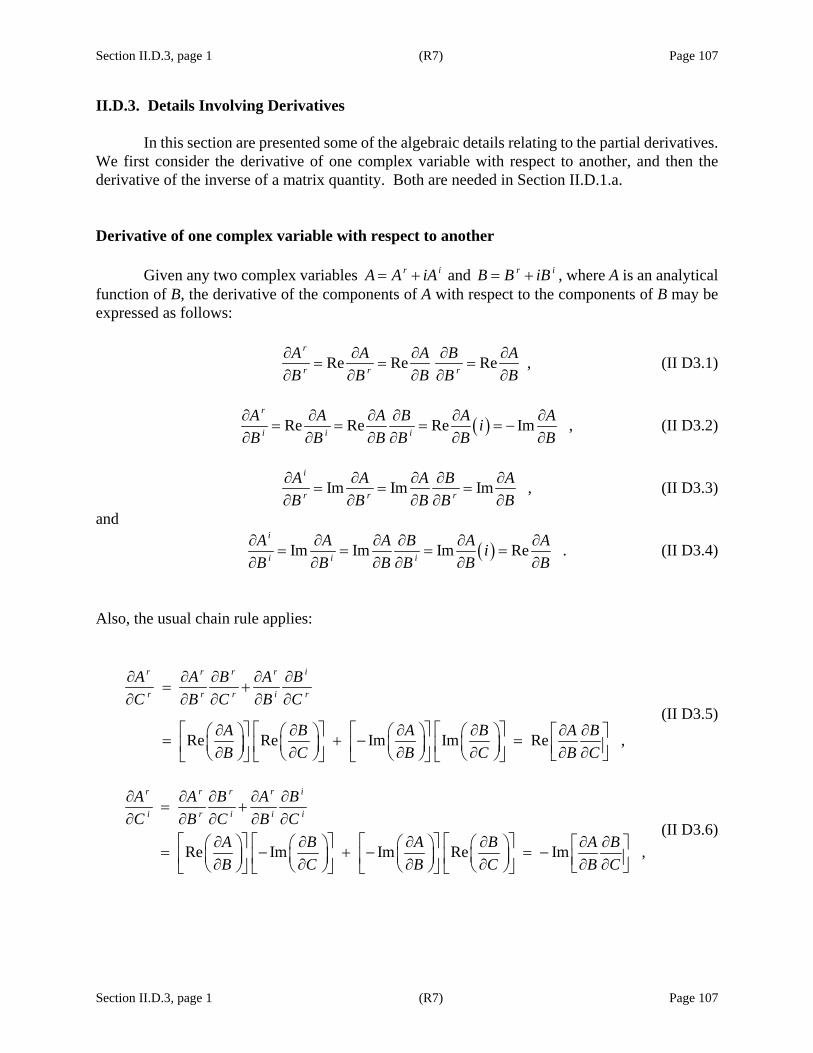
Section II.D.3, page 1 (R7) Page 107
Section II.D.3, page 1 (R7) Page 107
II.D.3. Details Involving Derivatives In this section are presented some of the algebraic details relating to the partial derivatives. We first consider the derivative of one complex variable with respect to another, and then the derivative of the inverse of a matrix quantity. Both are needed in Section II.D.1.a. Derivative of one complex variable with respect to another
Given any two complex variables r iA A iA= + and r iB B iB= + , where A is an analytical function of B, the derivative of the components of A with respect to the components of B may be expressed as follows:
Re Re Re ,r
r r r
A A A B AB B B B B∂ ∂ ∂ ∂ ∂
= = =∂ ∂ ∂ ∂ ∂
(II D3.1)
( )Re Re Re Im ,r
i i i
A A A B A AiB B B B B B∂ ∂ ∂ ∂ ∂ ∂
= = = = −∂ ∂ ∂ ∂ ∂ ∂
(II D3.2)
Im Im Im ,i
r r r
A A A B AB B B B B∂ ∂ ∂ ∂ ∂
= = =∂ ∂ ∂ ∂ ∂
(II D3.3)
and
( )Im Im Im Re .i
i i i
A A A B A AiB B B B B B∂ ∂ ∂ ∂ ∂ ∂
= = = =∂ ∂ ∂ ∂ ∂ ∂
(II D3.4)
Also, the usual chain rule applies:
Re Re Im Im Re ,
r r r r i
r r r i r
A A B A BC B C B C
A B A B A BB C B C B C
∂ ∂ ∂ ∂ ∂= +
∂ ∂ ∂ ∂ ∂
⎡ ∂ ⎤ ⎡ ∂ ⎤ ⎡ ∂ ⎤ ⎡ ∂ ⎤ ∂ ∂⎛ ⎞ ⎛ ⎞ ⎛ ⎞ ⎛ ⎞ ⎡ ⎤= + − =⎜ ⎟ ⎜ ⎟ ⎜ ⎟ ⎜ ⎟⎢ ⎥ ⎢ ⎥ ⎢ ⎥ ⎢ ⎥ ⎢ ⎥∂ ∂ ∂ ∂ ∂ ∂⎝ ⎠ ⎝ ⎠ ⎝ ⎠ ⎝ ⎠ ⎣ ⎦⎣ ⎦ ⎣ ⎦ ⎣ ⎦ ⎣ ⎦
(II D3.5)
Re Im Im Re Im ,
r r r r i
i r i i i
A A B A BC B C B C
A B A B A BB C B C B C
∂ ∂ ∂ ∂ ∂= +
∂ ∂ ∂ ∂ ∂⎡ ∂ ⎤ ⎡ ∂ ⎤ ⎡ ∂ ⎤ ⎡ ∂ ⎤ ∂ ∂⎛ ⎞ ⎛ ⎞ ⎛ ⎞ ⎛ ⎞ ⎡ ⎤= − + − = −⎜ ⎟ ⎜ ⎟ ⎜ ⎟ ⎜ ⎟⎢ ⎥ ⎢ ⎥ ⎢ ⎥ ⎢ ⎥ ⎢ ⎥∂ ∂ ∂ ∂ ∂ ∂⎝ ⎠ ⎝ ⎠ ⎝ ⎠ ⎝ ⎠ ⎣ ⎦⎣ ⎦ ⎣ ⎦ ⎣ ⎦ ⎣ ⎦
(II D3.6)

Section II.D.3, page 2 (R7) Page 108
Section II.D.3, page 2 (R7) Page 108
Im Re Re Im Im ,
i i r i i
r r r i r
A A B A BC B C B C
A B A B A BB C B C B C
∂ ∂ ∂ ∂ ∂= +
∂ ∂ ∂ ∂ ∂
⎡ ∂ ⎤ ⎡ ∂ ⎤ ⎡ ∂ ⎤ ⎡ ∂ ⎤ ∂ ∂⎛ ⎞ ⎛ ⎞ ⎛ ⎞ ⎛ ⎞ ⎡ ⎤= + =⎜ ⎟ ⎜ ⎟ ⎜ ⎟ ⎜ ⎟⎢ ⎥ ⎢ ⎥ ⎢ ⎥ ⎢ ⎥ ⎢ ⎥∂ ∂ ∂ ∂ ∂ ∂⎝ ⎠ ⎝ ⎠ ⎝ ⎠ ⎝ ⎠ ⎣ ⎦⎣ ⎦ ⎣ ⎦ ⎣ ⎦ ⎣ ⎦
(II D3.7)
and
Im Im Re Re Re .
i i r i i
i r i i i
A A B A BC B C B C
A B A B A BB C B C B C
∂ ∂ ∂ ∂ ∂= +
∂ ∂ ∂ ∂ ∂⎡ ∂ ⎤ ⎡ ∂ ⎤ ⎡ ∂ ⎤ ⎡ ∂ ⎤ ∂ ∂⎛ ⎞ ⎛ ⎞ ⎛ ⎞ ⎛ ⎞ ⎡ ⎤= − + =⎜ ⎟ ⎜ ⎟ ⎜ ⎟ ⎜ ⎟⎢ ⎥ ⎢ ⎥ ⎢ ⎥ ⎢ ⎥ ⎢ ⎥∂ ∂ ∂ ∂ ∂ ∂⎝ ⎠ ⎝ ⎠ ⎝ ⎠ ⎝ ⎠ ⎣ ⎦⎣ ⎦ ⎣ ⎦ ⎣ ⎦ ⎣ ⎦
(II D3.8)
Derivative of the inverse of a matrix In Eq. (II D1 a.13), the quantity Y is defined as
( ) 11 .e fe f
L RY−−⎡ ⎤= −⎢ ⎥⎣ ⎦
(II D3.9)
To find the derivative of Y with respect to R, we first note that 1 ,ea ab eb
aY Y δ− =∑ (II D3.10)
so that the derivative is zero; that is,
( )
11 1
1
0
1 .
ea abea ab ab ea
a a ac d cd c d
eaab ea ac bd a d bc c d
a ac d
Y YY Y Y Y
R R R
YY Y
Rδ δ δ δ δ
−− −
−
∂ ∂∂ ⎡ ⎤= = +⎢ ⎥∂ ∂ ∂⎣ ⎦
∂= + − − −
∂
∑ ∑ ∑
∑ ∑ (II D3.11)
The quantity in curly brackets comes from the symmetry of the R-matrix and from the stipulation that only unique matrix elements are to be considered [ ,c d e f≤ ≤ in Eq. (II D1.1) and Eq. (II D1 a.1)]. Multiplying both terms by b fY , summing over b, and rearranging give
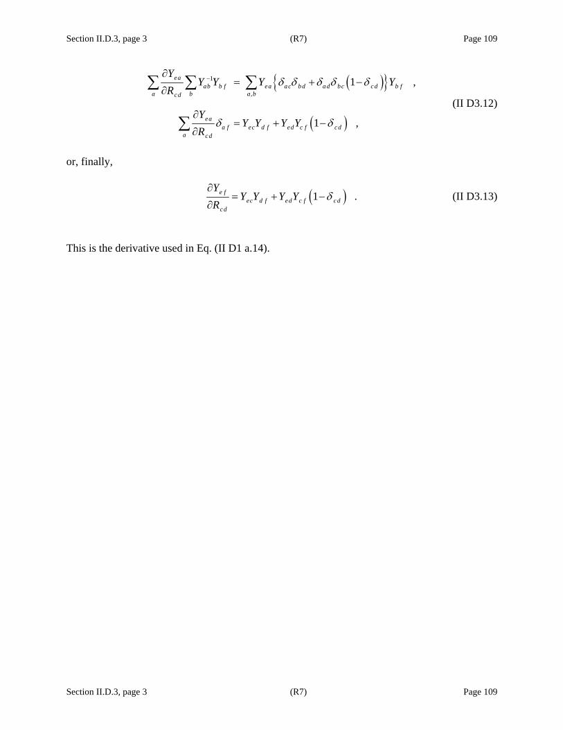
Section II.D.3, page 3 (R7) Page 109
Section II.D.3, page 3 (R7) Page 109
( )
( )
1
,1 ,
1 ,
eaab b f ea ac bd a d bc cd b f
a b a bcd
eaa f ec d f ed c f cd
a c d
YY Y Y Y
R
YY Y Y Y
R
δ δ δ δ δ
δ δ
−∂= + −
∂
∂= + −
∂
∑ ∑ ∑
∑ (II D3.12)
or, finally,
( )1 .e fec d f ed c f c d
c d
YY Y Y Y
Rδ
∂= + −
∂ (II D3.13)
This is the derivative used in Eq. (II D1 a.14).


Section III, page 1 (R7) Page 111
Section III, page 1 (R7) Page 111
III. CORRECTIONS FOR EXPERIMENTAL CONDITIONS
In general it is not possible to directly compare the cross sections extracted from experiments to those generated via R-matrix theory (or via any other theory). This is because “perfect” experimental conditions do not exist: (1) individual nuclei within the sample are not at rest; (2) finite time intervals are required both for the neutron beam and for the detecting apparatus; (3) the flight-path length traversed by a neutron depends on its position of origin within the neutron-producing target, on its position of interaction within the sample, and on the position at which it is detected; (4) the finite size of the sample causes interactions beyond those described by the cross section for individual nuclei. The first of these conditions leads to the effect known as Doppler broadening, the second and third lead to resolution broadening, and the fourth to multiple-scattering and self-shielding effects. There are other effects as well, not included in this enumeration. To compare theory to experiment, either the theory must include these effects or corrections must be applied to the experimental data. Often the former is easier, or the latter is impossible. SAMMY therefore includes options to simulate a great many of these effects, and modify the theoretical calculations appropriately.
To simulate Doppler or resolution broadening (i.e., to “broaden the theory”), it is necessary to first have a mathematical description of the broadening (generally, as an integral of the unbroadened cross section times a broadening function), and then to evaluate those integrals analytically if possible or numerically if necessary.
In Section III.A, the scheme used in SAMMY for most of the numerical integrations is described in some detail. It is important to note that it is the user, not the code author, who is responsible for ensuring that the numerical integrations are performed sufficiently well; this is discussed in Section III.A.1, which should be read and carefully considered before analysis results are published.
SAMMY contains four distinct procedures for Doppler broadening, which are described in Section III.B. The various available methodologies for resolution broadening are discussed in Section III.C. Section III.D is devoted to multiple-scattering effects, and other phenomena are treated in Section III.E.


Section III.A, page 1 (R7) Page 113
Section III.A, page 1 (R7) Page 113
III. A. THEORETICAL FOUNDATION FOR NUMERICAL BROADENING
The primary method used in SAMMY for evaluating the integrals required in Doppler and resolution broadening involves several operations for which details are given in the subsequent subsections. The method was borrowed originally from the MULTI code [GA74] and subsequently modified as the need arose. Note that in SAMMY, broadening is applied both to the cross sections and to the partial derivatives, while in MULTI, it was applied only to the cross sections. A summary of the operations is given here. 1. Choose an appropriate “auxiliary energy grid” at which to evaluate the integrands. The
auxiliary grid consists of (a) the original energy grid (i.e., the energies at which experimental data are given), (b) points below the minimum energy of the experimental data and above the maximum energy, and (c) additional points sufficient to describe the structure of any “narrow” resonance. See Section III.A.2 for more details regarding the choice of auxiliary grid and Section III.A.3 for details regarding the integration scheme. (Different criteria are required for Leal-Hwang Doppler broadening; see Section III.B.2.)
2. A discussion of pitfalls that can arise when insufficient care is devoted to the choice of
auxiliary grid is given in Section III.A.1. While Sections III.A.2 and III.A.3 may safely be regarded as “black boxes” by some analysts, all SAMMY users are encouraged to pay careful attention to issues raised in Section III.A.1.
3. For each energy in the auxiliary grid, evaluate the theoretical cross sections and derivatives
thereof, as described in Section II. 4. Determine Doppler-broadened cross section and derivatives wherever possible (i.e., for all
but the highest and the lowest energies in the auxiliary grid). Generate derivatives with respect to Doppler temperature. See Section III.B for details.
5. Transform from cross section to transmission as needed; apply transformation to derivatives
also. See Section III.E.1. Generate derivative with respect to sample thickness. 6. Apply self-shielding and multiple-scattering corrections as needed, both to cross sections and
to derivatives. See Section III.D for details. 7. For each energy in the original (experimental) grid, determine the resolution-broadened cross
section (or transmission) and derivatives thereof. Also generate derivatives with respect to resolution-broadening parameters. See Section III.C.
8. If needed, transform from transmission back to cross section; transform derivatives also. 9. Multiply by normalization and add backgrounds, as needed. Generate derivatives with
respect to normalization and background. See Section III.E.3.a.

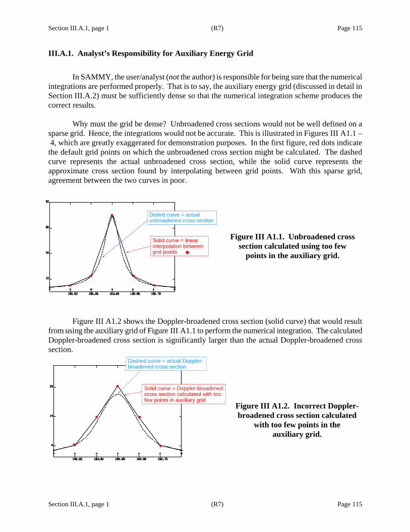
Section III.A.1, page 1 (R7) Page 115
Section III.A.1, page 1 (R7) Page 115
III.A.1. Analyst’s Responsibility for Auxiliary Energy Grid
In SAMMY, the user/analyst (not the author) is responsible for being sure that the numerical
integrations are performed properly. That is to say, the auxiliary energy grid (discussed in detail in Section III.A.2) must be sufficiently dense so that the numerical integration scheme produces the correct results.
Why must the grid be dense? Unbroadened cross sections would not be well defined on a sparse grid. Hence, the integrations would not be accurate. This is illustrated in Figures III A1.1 – 4, which are greatly exaggerated for demonstration purposes. In the first figure, red dots indicate the default grid points on which the unbroadened cross section might be calculated. The dashed curve represents the actual unbroadened cross section, while the solid curve represents the approximate cross section found by interpolating between grid points. With this sparse grid, agreement between the two curves in poor.
Figure III A1.1. Unbroadened cross section calculated using too few
points in the auxiliary grid.
Figure III A1.2 shows the Doppler-broadened cross section (solid curve) that would result from using the auxiliary grid of Figure III A1.1 to perform the numerical integration. The calculated Doppler-broadened cross section is significantly larger than the actual Doppler-broadened cross section.
Figure III A1.2. Incorrect Doppler-broadened cross section calculated
with too few points in the auxiliary grid.
Dotted curve = actual unbroadened cross section
Solid curve = linear interpolation between grid points
Dashed curve = actual Doppler-broadened cross section
Solid curve = Doppler-broadened cross section calculated with too few points in auxiliary grid
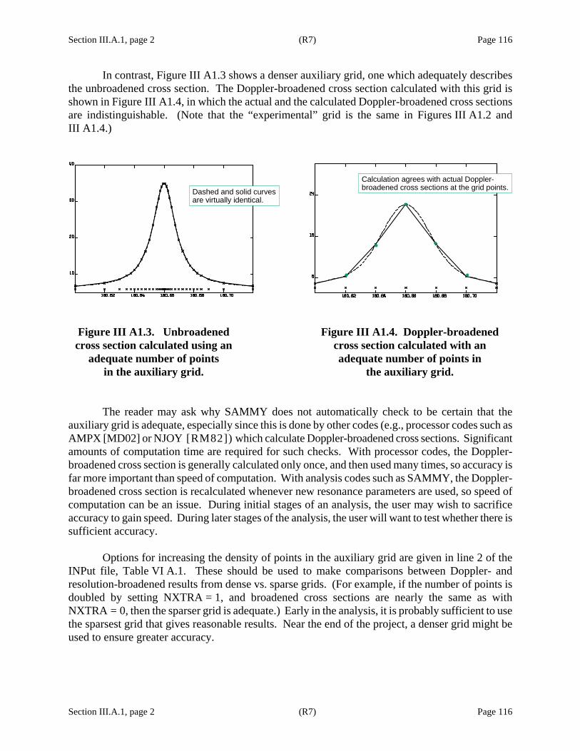
Section III.A.1, page 2 (R7) Page 116
Section III.A.1, page 2 (R7) Page 116
In contrast, Figure III A1.3 shows a denser auxiliary grid, one which adequately describes the unbroadened cross section. The Doppler-broadened cross section calculated with this grid is shown in Figure III A1.4, in which the actual and the calculated Doppler-broadened cross sections are indistinguishable. (Note that the “experimental” grid is the same in Figures III A1.2 and III A1.4.)
Figure III A1.3. Unbroadened cross section calculated using an
adequate number of points in the auxiliary grid.
Figure III A1.4. Doppler-broadened cross section calculated with an adequate number of points in
the auxiliary grid. The reader may ask why SAMMY does not automatically check to be certain that the auxiliary grid is adequate, especially since this is done by other codes (e.g., processor codes such as AMPX [MD02] or NJOY [RM82]) which calculate Doppler-broadened cross sections. Significant amounts of computation time are required for such checks. With processor codes, the Doppler-broadened cross section is generally calculated only once, and then used many times, so accuracy is far more important than speed of computation. With analysis codes such as SAMMY, the Doppler-broadened cross section is recalculated whenever new resonance parameters are used, so speed of computation can be an issue. During initial stages of an analysis, the user may wish to sacrifice accuracy to gain speed. During later stages of the analysis, the user will want to test whether there is sufficient accuracy.
Options for increasing the density of points in the auxiliary grid are given in line 2 of the INPut file, Table VI A.1. These should be used to make comparisons between Doppler- and resolution-broadened results from dense vs. sparse grids. (For example, if the number of points is doubled by setting NXTRA = 1, and broadened cross sections are nearly the same as with NXTRA = 0, then the sparser grid is adequate.) Early in the analysis, it is probably sufficient to use the sparsest grid that gives reasonable results. Near the end of the project, a denser grid might be used to ensure greater accuracy.
Dashed and solid curves are virtually identical.
Calculation agrees with actual Doppler-broadened cross sections at the grid points.
Section III.A.2, page 1 (R7) Page 117
Section III.A.2, page 1 (R7) Page 117
III.A.2. Choose Auxiliary Energy Grid
We wish to evaluate integrals of the form
( ) ( ) ( )max
min
' , ' ' ,E
i iE
f E f E B E E d E= ∫ (III A2.1)
where ( ')f E represents the unbroadened theoretical cross section (or transmission) and ( )if E the
broadened. B represents the appropriate broadening function as described in Section III.B or III.C. The set of points Ei are the original grid, for which data are available and at which theoretical values are required.
Standard practice for evaluating integrals such as those in Eq (III A2.1) is to choose a set of points ' jE and associated weights jW in such a way that
( ) ( ) ( ) ( )' , ' ' ' , ' ,b
i j i j jja
f E B E E dE f E B E E W≅∑∫ (III A2.2)
where the approximation is exact if the product ( ) ( )' , 'j i jf E B E E is a polynomial of some
specified degree, say n. Use of these points and weights to evaluate the integral over a non-
polynomial function [such as ( ) ( )' , 'if E B E E in Eq. (III A2.1)] will give a result that is accurate to
the extent that the function can be approximated by a polynomial of degree n. In practice, if one divides the integration region [Emin, Emax] into sufficiently small subregions [a, b], the polynomial approximation will be quite accurate within each subregion.
The choice of points ' jE is, to some extent, arbitrary. (Once ' jE is fixed, weights
jW are determined from Eq. (III A2.2).) Because it is necessary to integrate Eq. (III A2.1) many
times (i.e., once for each Ei), it is expedient to have the set ' jE be the same for each Ei in order to
minimize the total number of evaluations of ( )' jf E . These points ' jE will hereafter be
designated collectively as the “auxiliary grid,” and the points iE for which data are given will be designated as the “original grid.”
Several types of points contribute to the auxiliary grid:
a. All points in the original grid are included in the auxiliary grid.

Section III.A.2, page 2 (R7) Page 118
Section III.A.2, page 2 (R7) Page 118
b. “Extra” points are added between each point in the original grid. The number “NXTRA” of such points is specified by the user in the INPut file (see card set 2 of Table VIA.1). (See Section III.A.1 for a discussion of why this may be necessary.)
c. Points are added at the extremities of the data region, to be used in broadening the cross sections at the end points. The relative spacing of these points is similar to that of points inside the energy region being analyzed. The grid is chosen in one of two ways:
1. Points from the data set, but outside the energy region being analyzed, are added to the auxiliary grid.
2. If (1) is not possible because the data set contains no such points, then the spacing Δ between data points E1 and E 2 is used to locate other points equally spaced at 1 1 1, , ,2 3 E E E− − −Δ Δ Δ ... ; a sufficient number of points are chosen to cover the integration region for E1.
d. Equation (III A2.2) is a good approximation only if the integrand closely resembles a low-order polynomial. Therefore, it may be necessary to add points over the width of narrow resonances so that the structure of the integrand will be properly represented. Also, the auxiliary grid must vary smoothly to avoid numerical difficulties in evaluating the integrals. This problem can be broken into several pieces:
1. Decide which resonances require additional points. IPTDOP is the number of points required across a resonance; the default value for IPTDOP is 9, but the user may increase this as desired (see Table VI A.1, card set 2). If there are fewer than IPTDOP points between (Eλ - D) and (Eλ + D), where D is the sum of the absolute values of the gamma and particle widths, then more points must be added near this resonance.
2. For each narrow resonance, add auxiliary points at Eλ and at positions ( )2 / IPTDOP 1jE Dλ ± − , where j ranges from 1 to IPTDOP.
3. Add points at 1.5 and 2E D E Dλ λ± ± .
4. If IPTWID is positive (but smaller than 7), add additional points at positions ( )3 , 4 , and IPTWID 1E D E D E Dλ λ λ± ± ± + , where the input quantity IPTWID is
specified in Table VI A.1, card set 2.
5. If IPTWID is negative, add points as in #4, and also at 10E Dλ ± and at 20E Dλ ± .
6. Test the resulting auxiliary grid to see that no two neighboring points are either very close together (relative to neighboring spacing) or very far apart. Drop or add points as needed.

Section III.A.2, page 3 (R7) Page 119
Section III.A.2, page 3 (R7) Page 119
Caveat: If the original (MULTI-style) Doppler broadening is used, and energy points in the auxiliary grid fall at negative energy, SAMMY will issue a warning and abort execution. For subsequent runs, the analyst has several options: either choose a higher Emin, specify “NO LOW-ENERGY BROADEning is to be used” in the INPut file (see Tables VI A.1 and VI A.2 for details), specify “USE LEAL,HWANG DOPPLer broadening” for the low-energy region (see Section III.B.2), or specify “USE FREE GAS MODEL Of doppler broadening.” The final option (i.e., the free-gas model) is the default and is the author=s recommendation for most calculations; see Section III.B.1.


Section III.A.3, page 1 (R8) Page 121
Section III.A.3, page 1 (R8) Page 121
III.A.3. Perform Numerical Integration
The numerical integration scheme used in SAMMY to evaluate the integrals shown in Eqs. (III A2.1) and (III A2.2) is borrowed from MULTI [GA74] and is based on the four-point progressive interpolation method of Mintz and Jordan [MM64]. For the value of an integral from x2 to x3 of some function ( )y x , where the value of y is known only at the four values of x
1 2 3( , , ,x x x x= or 4 )x , this method uses the approximation
( ) ( )3
2
4
1,
x
i iix
y x dx y x w=
≅ ∑∫ (III A3.1)
in which the weights wi are given by
( )( )( )
( ) ( )( )
( )( )
( ) ( )( )
( )( )
( )( )( )
32 3
11 2 1 3
2 3 1 3 4 32
2 1 2 4
3 2 1 2 4 23
3 1 3 4
32 3
44 2 4 3
,12
4 ,12
4 ,12
.12
x xw
x x x x
x x x x x xw
x x x x
x x x x x xw
x x x x
x xw
x x x x
−=
− −
⎡ ⎤− − −= + −⎢ ⎥− −⎢ ⎥⎣ ⎦
⎡ ⎤− − −= − −⎢ ⎥− −⎢ ⎥⎣ ⎦
−=
− −
(III A3.2)
These equations give the exact result if y ( x) is a polynomial of degree 2 or less [i.e., if y ( x) is a
quadratic, linear, or constant function of x].
What is required for the broadening integrals is, however, a function of the form
( )1'1
'
' ' ( ') ' ,max max
minmin
j
j
EE j
j jE E
y E d E y E d E+−
=
≅∫ ∫∑ (III A3.3)
in which jmin and jmax are chosen such that 1' '
min minj min jE E E +≤ ≤ and 1' 'max maxj max jE E E− ≤ ≤ . Each
integral on the right-hand side of Eq. (III A3.3) may be evaluated using Eq. (III A3.1), with
1 1 2 3 1 4 2, , , and .j j j jxx E E x E x E− + += = = = (III A3.4)
Section III.A.3, page 2 (R8) Page 122
Section III.A.3, page 2 (R8) Page 122
Define wij as “wi from Eq. (III A3.2) with the xi given by Eq. (III A3.4),” or more precisely,
2' .i j j ix E + −= (III A3.5) Equation (III A3.3) can then be put into the form
( ) ( )4
21
' ' ' .max max
minmin
E j
i j j iij jE
y E d E w y E + −==
≅ ∑∫ ∑ (III A3.6)
Performing the summation over i gives
( ) ( )' ' ' ,max max
minmin
E j
j jj jE
y E dE W y E=
≅∫ ∑ (III A3.7)
where the weight Wj is given by
( )
4
21
.j i j ii
W w + −=
= ∑ (III A3.8)
The summation in Eq. (III A3.8) may be evaluated explicitly using Eq. (III A3.1) with Eq. (III A3.4), yielding
( ) ( )
( ) ( )( )
( ) ( )( )
1 1 2 2
2 2 2 2
1 2 1 1 1 2
1 1
' ' / 3 ' ' /12
' ' ' ' ' ' ' '1 .12 ' ' ' '
j j j j j
j j j j j j j j
j j j j
W E E E E
E E E E E E E E
E E E E
+ − + −
− + + + − −
+ −
= − + −
⎡ ⎤− − − − − −⎢ ⎥+ +⎢ ⎥− −⎣ ⎦
(III A3.9)
SAMMY uses the values given by Eq. (III A3.9) even for j = jmin and j = jmax, even though they implicitly require the use of 1'
minjE − and 1'maxjE + , which technically are outside the range of
integration ( ) to min maxE E ; this is legitimate because the range of integration is chosen so that the
integrand ( )'y E is effectively zero outside that range. Thus, the values of ( )1'minjy E − and
( )1'maxjy E + are zero and are implicitly included in the above formulation. In contrast, the code
MULTI performed extra calculations to end exactly at ( )' to 'min maxj jE E ; our studies have found this
an unneeded complication.

Section III.A.3, page 3 (R8) Page 123
Section III.A.3, page 3 (R8) Page 123
The scheme described above is used in SAMMY only if there are more than twelve points between ' and '
min maxj jE E , inclusive. If there are fewer than twelve but more than five points, Simpson's rule is used. For five or fewer points, it is assumed that the broadened value is equal to the unbroadened value, and no integration is performed.
It should be noted that there are situations in which it is imperative to end the integration
precisely at the specified limits. At least two examples occur in the SAMMY code.
1. Multiple-scattering corrections for capture or fission experiments (Section III.D) involve integration over the scattering angle, from 0 to 180 degrees. When “integration over angle” is converted to “integration over energy of the scattered neutron,” one might be tempted to extend the energy integral to the nearest grid point. However, to obtain accurate results, the integration clearly must not extend beyond the energies corresponding to back-angle scattering or forward-angle scattering.
2. Absolute limits are also required for the calculation of average cross sections (Section V.C).
In situations in which the integrand does not smoothly approach zero outside the limits of the integration, Eq. (III A3.9) is modified to give the appropriate weights to define an absolute integration limit.


Section III.B, page 1 (R7) Page 125
Section III.B, page 1 (R7) Page 125
III. B. DOPPLER BROADENING
Four options are available within SAMMY to accomplish Doppler broadening; three are based on the free-gas model (FGM), and the fourth is a solid-state model.
SAMMY=s free-gas model is described in Section III.B.1. This model was introduced into SAMMY in order to overcome shortcomings of the two earlier versions (Sections III.B.2 and III.B.3), and is now the default method. This is the option that should be used for most calculations. For additional details, see [NL98].
A second method, described in Section III.B.2, is an elegant and rigorous adaptation of the FGM based on work by Leal and Hwang [LL85]. This method works best with smooth cross sections, and thus has limitations for use in the resonance region.
SAMMY=s original method, a high-energy Gaussian approximation (HEGA) to the FGM, is based on an adaptation of the method used by George Auchampaugh in his code MULTI [GA74]. This method is described in Section III.B.3. Because this is a high-energy approximation, it cannot be used for very low-energy computations.
A fourth option is available for use in those situations in which the FGM is inadequate. The crystal-lattice model (CLM) of Doppler broadening, added to SAMMY for Release M6 of the code, is described in Section III.B.4. SAMMY=s implementation is based on the DOPUSH model of Naberejnev [DN99, DN99a].

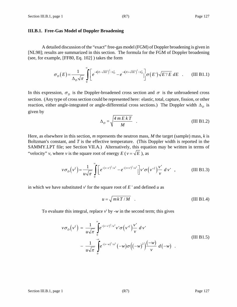
Section III.B.1, page 1 (R7) Page 127
Section III.B.1, page 1 (R7) Page 127
III.B.1. Free-Gas Model of Doppler Broadening
A detailed discussion of the “exact” free-gas model (FGM) of Doppler broadening is given in [NL98]; results are summarized in this section. The formula for the FGM of Doppler broadening (see, for example, [FF80, Eq. 102] ) takes the form
( ) ( ) ( ) ( )2 22 24 ' / 4 ' /
0
1 ' '/ .D DE EE E EED
D
E e e E E E dEσ σπ
∞
− − Δ − + Δ⎡ ⎤= −⎢ ⎥Δ ⎣ ⎦∫ (III B1.1)
In this expression, Dσ is the Doppler-broadened cross section and σ is the unbroadened cross section. (Any type of cross section could be represented here: elastic, total, capture, fission, or other reaction, either angle-integrated or angle-differential cross sections.) The Doppler width DΔ is given by
.D4 m E k T=
MΔ (III B1.2)
Here, as elsewhere in this section, m represents the neutron mass, M the target (sample) mass, k is Boltzman=s constant, and T is the effective temperature. (This Doppler width is reported in the SAMMY.LPT file; see Section VII.A.) Alternatively, this equation may be written in terms of “velocity” v, where v is the square root of energy E ( v E= ), as
( ) ( ) ( ) ( )2 22 2' / ' /2 2
0
1 '' ' ' ,v v u v v uD
vv v e e v v d vvu
σ σπ
∞
− − − +⎡ ⎤= −⎢ ⎥⎣ ⎦∫ (III B1.3)
in which we have substituted v' for the square root of E ' and defined u as / .u m k T M= (III B1.4)
To evaluate this integral, replace v' by -w in the second term; this gives
( ) ( ) ( )
( ) ( ) ( )( ) ( ) ( )
2 2
2 2
' /2 2
0
2/
0
1 '' ' '
1 .
v v uD
v w u
vv v e v v d vvu
we w w d w
vu
σ σπ
σπ
∞
− −
−∞
− −
=
−− − − −
∫
∫ (III B1.5)

Section III.B.1, page 2 (R7) Page 128
Section III.B.1, page 2 (R7) Page 128
Replacing v' by w in the first term of Eq. (III B1.5), rearranging the second term, and defining
( )( )
( )
2
2
for 0
0 for 0
for 0
w w
s w w
w w
σ
σ
⎧ >⎪⎪= =⎨⎪ − <⎪⎩
(III B1.6)
puts this equation into the form
( ) ( ) ( )2 2/2 1 .v w u
Dwv v e w s w d wvu
σπ
∞
− −
−∞
= ∫ (III B1.7)
In the form of Eq. (III B1.7) with definition (III B1.6), the Doppler-broadening integration can be accomplished readily within SAMMY using the same numerical techniques used for other integrations, without having to give special consideration to “the second term” of Eq. (III B1.1). The integration scheme of Section III A.3 is used directly. The auxiliary energy grid is chosen as described in Section III.A.2, with the exception that the additional low-energy points are equally spaced in velocity rather than in energy. Negative velocities are included as needed, in order to properly evaluate the integral at low values of E.
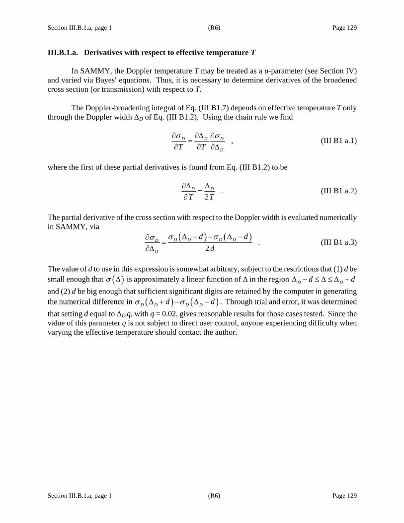
Section III.B.1.a, page 1 (R6) Page 129
Section III.B.1.a, page 1 (R6) Page 129
III.B.1.a. Derivatives with respect to effective temperature T
In SAMMY, the Doppler temperature T may be treated as a u-parameter (see Section IV) and varied via Bayes= equations. Thus, it is necessary to determine derivatives of the broadened cross section (or transmission) with respect to T.
The Doppler-broadening integral of Eq. (III B1.7) depends on effective temperature T only through the Doppler width ΔD of Eq. (III B1.2). Using the chain rule we find
,D D D
DT Tσ σ∂ ∂Δ ∂
=∂ ∂ ∂Δ
(III B1 a.1)
where the first of these partial derivatives is found from Eq. (III B1.2) to be
.2
D D
T T∂Δ Δ
=∂
(III B1 a.2)
The partial derivative of the cross section with respect to the Doppler width is evaluated numerically in SAMMY, via
( ) ( ) .2
D D D DD
D
d dd
σ σσ Δ + − Δ −∂=
∂Δ (III B1 a.3)
The value of d to use in this expression is somewhat arbitrary, subject to the restrictions that (1) d be small enough that ( )σ Δ is approximately a linear function of Δ in the region D Dd dΔ − ≤ Δ ≤ Δ + and (2) d be big enough that sufficient significant digits are retained by the computer in generating the numerical difference in ( ) ( )D D D Dd dσ σΔ + − Δ − . Through trial and error, it was determined that setting d equal to ΔD q, with q = 0.02, gives reasonable results for those cases tested. Since the value of this parameter q is not subject to direct user control, anyone experiencing difficulty when varying the effective temperature should contact the author.

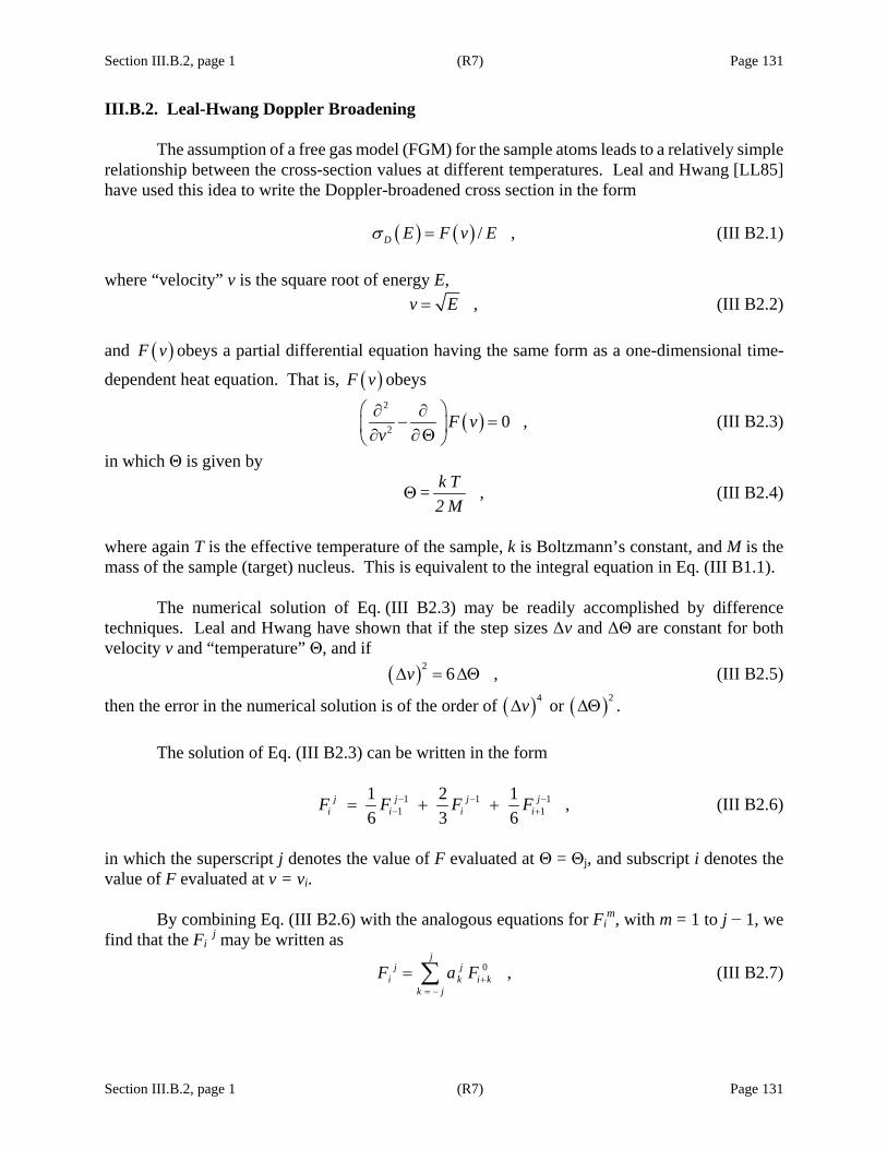
Section III.B.2, page 1 (R7) Page 131
Section III.B.2, page 1 (R7) Page 131
III.B.2. Leal-Hwang Doppler Broadening
The assumption of a free gas model (FGM) for the sample atoms leads to a relatively simple relationship between the cross-section values at different temperatures. Leal and Hwang [LL85] have used this idea to write the Doppler-broadened cross section in the form ( ) ( ) / ,D E F v Eσ = (III B2.1) where “velocity” v is the square root of energy E,
,v E= (III B2.2) and ( )F v obeys a partial differential equation having the same form as a one-dimensional time-
dependent heat equation. That is, ( )F v obeys
( )2
2 0 ,F vv
⎛ ⎞∂ ∂− =⎜ ⎟∂ ∂Θ⎝ ⎠
(III B2.3)
in which Θ is given by
,k T = 2 M
Θ (III B2.4)
where again T is the effective temperature of the sample, k is Boltzmann’s constant, and M is the mass of the sample (target) nucleus. This is equivalent to the integral equation in Eq. (III B1.1).
The numerical solution of Eq. (III B2.3) may be readily accomplished by difference techniques. Leal and Hwang have shown that if the step sizes Δv and ΔΘ are constant for both velocity v and “temperature” Θ, and if ( )2 6 ,vΔ = ΔΘ (III B2.5)
then the error in the numerical solution is of the order of ( )4vΔ or ( )2ΔΘ .
The solution of Eq. (III B2.3) can be written in the form
1 1 11 1
1 2 1 ,6 3 6
j j j ji i i iF F F F− − −
− += + + (III B2.6)
in which the superscript j denotes the value of F evaluated at Θ = Θj, and subscript i denotes the value of F evaluated at v = vi.
By combining Eq. (III B2.6) with the analogous equations for Fim, with m = 1 to j − 1, we
find that the Fi j may be written as
0 ,j
j ji k i k
k jF a F +
= −
= ∑ (III B2.7)
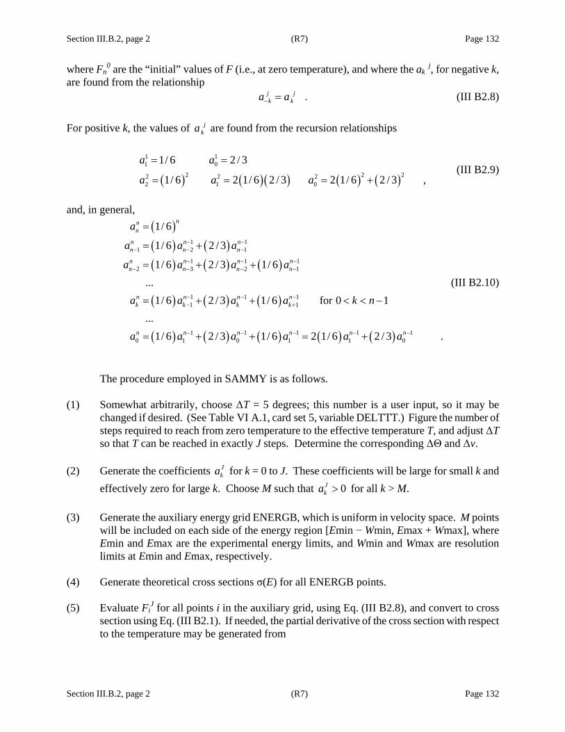
Section III.B.2, page 2 (R7) Page 132
Section III.B.2, page 2 (R7) Page 132
where Fn0 are the “initial” values of F (i.e., at zero temperature), and where the ak
j, for negative k, are found from the relationship
.j jk ka a− = (III B2.8)
For positive k, the values of j
ka are found from the recursion relationships
( ) ( )( ) ( ) ( )
1 11 0
2 2 22 2 22 1 0
1/ 6 2 / 3
1/ 6 2 1/ 6 2 / 3 2 1/ 6 2 / 3 ,
a a
a a a
= =
= = = + (III B2.9)
and, in general,
( )( ) ( )( ) ( ) ( )
( ) ( ) ( )
( ) ( ) ( ) ( ) ( )
1 11 2 1
1 1 12 3 2 1
1 1 11 1
1 1 1 1 10 1 0 1 1 0
1/ 6
1/ 6 2 / 3
1/ 6 2 / 3 1/ 6...
1/ 6 2 / 3 1/ 6 for 0 1...
1/ 6 2 / 3 1/ 6 2 1/ 6 2 / 3 .
nnn
n n nn n n
n n n nn n n n
n n n nk k k k
n n n n n n
a
a a a
a a a a
a a a a k n
a a a a a a
− −− − −
− − −− − − −
− − −− +
− − − − −
=
= +
= + +
= + + < < −
= + + = +
(III B2.10)
The procedure employed in SAMMY is as follows. (1) Somewhat arbitrarily, choose ΔT = 5 degrees; this number is a user input, so it may be
changed if desired. (See Table VI A.1, card set 5, variable DELTTT.) Figure the number of steps required to reach from zero temperature to the effective temperature T, and adjust ΔT so that T can be reached in exactly J steps. Determine the corresponding ΔΘ and Δv.
(2) Generate the coefficients J
ka for k = 0 to J. These coefficients will be large for small k and effectively zero for large k. Choose M such that 0J
ka > for all k > M. (3) Generate the auxiliary energy grid ENERGB, which is uniform in velocity space. M points
will be included on each side of the energy region [Emin − Wmin, Emax + Wmax], where Emin and Emax are the experimental energy limits, and Wmin and Wmax are resolution limits at Emin and Emax, respectively.
(4) Generate theoretical cross sections σ(E) for all ENERGB points. (5) Evaluate Fi
J for all points i in the auxiliary grid, using Eq. (III B2.8), and convert to cross section using Eq. (III B2.1). If needed, the partial derivative of the cross section with respect to the temperature may be generated from

Section III.B.2, page 3 (R7) Page 133
Section III.B.2, page 3 (R7) Page 133
( )1
,
1 .J i
J Ji i
v v
F Fσ +
Θ=Θ =
∂= −
∂Θ ΔΘ (III B2.11)
Using the chain rule with Eq. (III B2.4), combined with Eqs. (III B2.6) and (III B2.11), gives
1 1,
1 1 16 3 6
J i
J J Ji i i
v v
T F F FT Eσ
− +Θ=Θ =
∂ Θ ⎡ ⎤= − +⎢ ⎥∂ ΔΘ ⎣ ⎦ (III B2.12)
for the derivatives of the cross section with respect to the temperature.
(6) From here on, follow the prescription given in Section III.A, beginning at step 4.
Finally, we recall from the discussion of the free-gas model (Section III.B.1) that the integral equation for Doppler broadening [Eq. (III B1.1) or (III B1.7)] is symmetric with respect to the transformation 'v → 'v− , provided ( )'vσ − is defined as ( )'vσ− as in Eq. (III B1.6). In a similar manner, the Leal-Hwang option permits the direct evaluation of the broadened cross section even for points near E = 0.
[In earlier versions of SAMMY (prior to the 2006 release, sammy-7.0.0), studies suggested
that results obtained for very low energies (well below thermal) were not completely accurate; specifically, Doppler-broadened 1/v cross sections did not retain the 1/v shape at these very low energies, and the step size ΔT was critically important. This was found to be due to a mistake in the coding, which was corrected for the sammy-7.0.0 release.]
To minimize the number of points required for use in the auxiliary grid, SAMMY users are
encouraged to rely on the FGM (see Section III.B.1) for most calculations. The Leal-Hwang model is useful for double-checking results at low energies, and in other situations that call for accurate calculation of Doppler broadening of smooth cross sections.
To use the Leal-Hwang Doppler broadening, include in your INPut file a line which reads
USE LEAL,HWANG DOPPLER BROADENING and specify the step size ΔT on card set 5 of the INPut file, Table VIA.1.

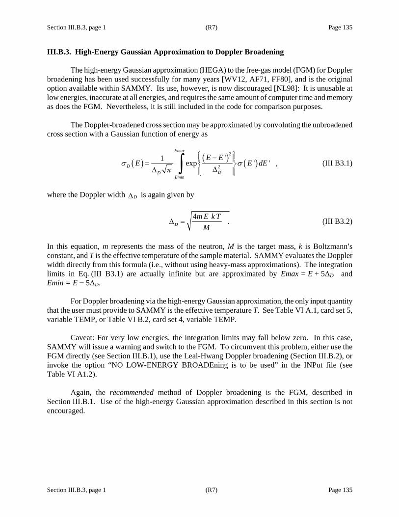
Section III.B.3, page 1 (R7) Page 135
Section III.B.3, page 1 (R7) Page 135
III.B.3. High-Energy Gaussian Approximation to Doppler Broadening
The high-energy Gaussian approximation (HEGA) to the free-gas model (FGM) for Doppler broadening has been used successfully for many years [WV12, AF71, FF80], and is the original option available within SAMMY. Its use, however, is now discouraged [NL98]: It is unusable at low energies, inaccurate at all energies, and requires the same amount of computer time and memory as does the FGM. Nevertheless, it is still included in the code for comparison purposes.
The Doppler-broadened cross section may be approximated by convoluting the unbroadened cross section with a Gaussian function of energy as
( ) ( ) ( )2
2
'1 exp ' ' ,
Emax
DDD
Emin
E EE E dEσ σ
π
⎧ ⎫−⎪ ⎪= ⎨ ⎬ΔΔ ⎪ ⎪⎩ ⎭∫ (III B3.1)
where the Doppler width DΔ is again given by
4 .Dm E k T
MΔ = (III B3.2)
In this equation, m represents the mass of the neutron, M is the target mass, k is Boltzmann=s constant, and T is the effective temperature of the sample material. SAMMY evaluates the Doppler width directly from this formula (i.e., without using heavy-mass approximations). The integration limits in Eq. (III B3.1) are actually infinite but are approximated by Emax = E + 5ΔD and Emin = E − 5ΔD.
For Doppler broadening via the high-energy Gaussian approximation, the only input quantity that the user must provide to SAMMY is the effective temperature T. See Table VI A.1, card set 5, variable TEMP, or Table VI B.2, card set 4, variable TEMP.
Caveat: For very low energies, the integration limits may fall below zero. In this case, SAMMY will issue a warning and switch to the FGM. To circumvent this problem, either use the FGM directly (see Section III.B.1), use the Leal-Hwang Doppler broadening (Section III.B.2), or invoke the option “NO LOW-ENERGY BROADEning is to be used” in the INPut file (see Table VI A1.2).
Again, the recommended method of Doppler broadening is the FGM, described in Section III.B.1. Use of the high-energy Gaussian approximation described in this section is not encouraged.


Section III.B.4, page 1 (R7) Page 137
Section III.B.4, page 1 (R7) Page 137
III.B.4. Crystal-Lattice Model of Doppler Broadening
The crystal-lattice model (CLM) of Doppler broadening used in SAMMY is based on the DOPUSH model of Naberejnev [DN99, DN99a], which in turn is based on the LEAPR model of NJOY [RM82]. Only the continuous and the discrete modes were developed further in DOPUSH.
(Readers are encouraged to consult the references for a description of the physics; a later revision of the SAMMY manual will include more detail. Alternative descriptions can be found in works by Meister [AM94].)
The algorithm used in SAMMY is virtually identical to the algorithm used in the DOPUSH code, where “identical” implicitly implies “for the examples that were available.” No attempt has yet been made by this author to extend the validity of the model beyond ensuring agreement between DOPUSH and SAMMY when run with the same input.
Prior to implementing the DOPUSH CLM into SAMMY, this author created a modified version of DOPUSH (denoted DOPUSHx) which uses the same input and runs in the same manner as DOPUSH but whose coding is streamlined and more readily portable than the original DOPUSH code. Below is an itemization of the changes made for DOPUSHx (and also incorporated into SAMMY). 1. Values of physical and mathematical constants conform to ENDF standards. See
Section IX.A of this document. 2. One or two “trivial” errors were corrected [notably, mass-factor self-consistency is ensured
by using (M+m)/M not (M+1)/M with M and m in units of amu]. 3. Redundant calculations were moved outside the energy loops; many of the intermediate
computations required for convolving the phonon distributions are energy independent and do not need to be repeated for each energy. This change resulted in a significant decrease in computer processor unit (cpu) time.
4. More efficient sorting algorithms are employed; in general, FORTRAN operations have been
made more efficient. Changes made from DOPUSHx to SAMMY include the following. 1. Nomenclature has been modified to conform to SAMMY conventions. 2. Savings in cpu time from DOPUSHx to SAMMY are primarily the result of SAMMY's
organizational scheme, in which the unbroadened cross sections are first calculated on an energy grid designed to describe the curvature of the cross section with reasonable accuracy, assuming a quadratic interpolation scheme. When the unbroadened cross section is required at a different energy, interpolation is used. In contrast, DOPUSH and DOPUSHx re-calculate the unbroadened cross section whenever it is needed, using algorithms similar to those employed in NJOY. (The cost which SAMMY users must pay for this increased speed

Section III.B.4, page 2 (R7) Page 138
Section III.B.4, page 2 (R7) Page 138
is that the accuracy of integrations cannot be tested during the integration process, as it is in NJOY. SAMMY users are reminded to make such tests themselves in order to have full confidence in their results.)
The examples of input for DOPUSH which were provided by Naberejnev have been
organized into SAMMY test case tr124. For those examples that run on all three programs (DOPUSH, SAMMY, & DOPUSHx), the three codes give virtually the same results. The time required for the computations is significantly shorter with the newer codes (details available from the author upon request). This is true even when the number of points in SAMMY's auxiliary grid was increased dramatically (NXTRA was changed from 0 to 99), as a double-check on the accuracy of SAMMY's calculation. Accuracy was not significantly affected by the additional energy points, indicating that SAMMY=s original grid is sufficiently dense.
For this release of SAMMY, no attempts have been made to improve or expand upon the model as provided by Naberejnev. One improvement that will likely be made for a subsequent release is the ability to treat the temperature as a search parameter in the fitting procedure.
For a description of the input to SAMMY=s CLM, see Section VI.F.5.
Section III.C, page 1 (R7) Page 139
Section III.C, page 1 (R7) Page 139
III.C. RESOLUTION BROADENING
Unlike Doppler broadening, for resolution broadening there is no “standard” or “best” function that is appropriate everywhere. Instead, each analysis code has its own version of resolution broadening, with specific formulations for specific experimental sites or setups. For this reason, many distinct types of resolution broadening are available in SAMMY.
Readers interested in a detailed study of resolution broadening, with emphasis on the 200-m flight path at the Oak Ridge Electron Linear Accelerator (ORELA), are referred to the paper by Larson, Larson, and Harvey [DL84].
The original resolution-broadening function in SAMMY is a combination of Gaussian plus exponential. This formulation is based upon the method used in the MULTI code [GA74] and is described in Section III.C.1.
A second option is a more realistic function — the ORR or “Oak Ridge Resolution function,” which uses mathematical descriptions of the components in the experimental broadening as determined from careful studies of ORELA experiments. Section III.C.2 gives specifics about this resolution function.
Another option is a realistic function designed to describe the experimental situation for the linac at Rensselaer Polytechnic Institute; this “RPI resolution function” is described in Section III.C.3. This option has been expanded to include features which may make it also useful for data from the Geel Electron Linear Accelerator (GELINA) at the Institute for Reference Materials and Measurements (IRMM) in Belgium or for data from the neutron time-of-flight (nTOF) facility at the European Council for Nuclear Research (CERN) in Switzerland.
A straight-line energy average resolution function is available, primarily for use with charged-particle or angular distribution data. See Section III.C.4.
A numerical user-defined resolution (UDR) function is described in Section III.C.5.
It is possible to include more than one of the above resolution functions for a single SAMMY run. To use this feature, include the command
TWO RESOLUTION FUNCTions together in your INPut file. With this command, you are permitted to use the following combinations of resolution functions:
1. one occurrence of the Gaussian plus exponential function; and/or 2. one straight-line energy average resolution function; and/or 3. at most one of the ORR, RPI, or UDR resolution functions.


Section III.C.1, page 1 (R8) Page 141
Section III.C.1, page 1 (R8) Page 141
III. C. 1. Gaussian plus Exponential Resolution Broadening
To understand how a resolution broadening may be described mathematically, we first consider the formula that describes how the neutron=s energy is extracted from measured quantities:
2
21 1 ,2 2
LE mv mt
⎛ ⎞= = ⎜ ⎟⎝ ⎠
(III C1.1)
where m is the neutron mass and v its velocity. The velocity is equal to the flight-path length L divided by travel time t. From this definition, it is clear that different types of resolution broadening are possible —due to distributions in time, distributions in length, and distributions in energy.
Several factors may contribute to each of the types of resolution broadening. In this version of SAMMY=s resolution function, the following components of the resolution function are treated explicitly: (1) a rectangular distribution‡ in flight-path length (due, for example, to the neutron moderator and/or detector), (2) a rectangular distribution in time (channel width), (3) a Gaussian distribution in time (burst width), and (4) a Gaussian distribution whose width is constant in energy. Each is expressed as an approximate Gaussian distribution in energy, using approximations if necessary (see Section III.C.1.a), and then convoluted to give the final Gaussian distribution in energy. An exponential distribution may also be included, as described in Section III.C.1.b.
Table III C1.1 shows relationships between input parameters and the resolution width associated with various types of resolution distribution functions. This table is included here as an aid in determining appropriate values to use as input to SAMMY. Note that “equivalent,” as used in the following pages, indicates only that the first and second moments of the distributions are identical, not that the distributions have the same shapes.
For a detailed discussion of resolution broadening with emphasis on flight path 1 at ORELA, see [DL84].
Table III C1.1. Resolution-broadening input parameters
SAMMY input variable
“Equivalent” quantity
Description
ΔL or DELTAL (Section III.C.1.a)
ΔL is the full width of a rectangular distribution in flight-path length.
12 Lσ Lσ is the standard deviation of a Gaussian distribution in flight-path length.
32 ln 2 LF
FL is the full width at half maximum of a Gaussian distribution in flight-path length.
‡ In previous versions of this document, what we here refer to as a “rectangular function” was denoted a “square function.” Clearly, “rectangular” is the more accurate nomenclature.
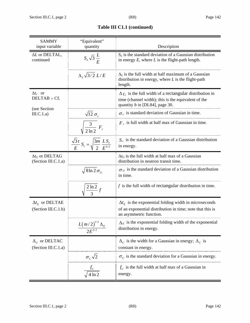
Section III.C.1, page 2 (R8) Page 142
Table III C1.1 (continued)
Section III.C.1, page 2 (R8) Page 142
SAMMY input variable
“Equivalent” quantity
Description
ΔL or DELTAL, continued 3L
LSE
SL is the standard deviation of a Gaussian distribution in energy E, where L is the flight-path length.
3 / 2 /L L EΔ ΔL is the full width at half maximum of a Gaussian distribution in energy, where L is the flight-path length.
ctΔ is the full width of a rectangular distribution in time (channel width); this is the equivalent of the quantity b in [DL84], page 30.
Δtc or DELTAB H Cfi (see Section III.C.1.a) 12 cσ cσ is standard deviation of Gaussian in time.
32 ln 2 cF
cF is full width at half max of Gaussian in time.
3/ 2
3 32
cc
L St mSE E
= cS is the standard deviation of a Gaussian distribution
in energy.
ΔtG or DELTAG (Section III.C.1.a)
ΔtG is the full width at half max of a Gaussian distribution in neutron transit time.
8ln 2 Gσ
Gσ is the standard deviation of a Gaussian distribution in time.
2 ln 23
f f is the full width of rectangular distribution in time.
EtΔ or DELTAE (Section III.C.1.b)
EtΔ is the exponential folding width in microseconds
of an exponential distribution in time; note that this is an asymmetric function.
( )1/ 2
3/ 2
/ 22
EL mE
Δ
EΔ is the exponential folding width of the exponential distribution in energy.
CΔ or DELTAC (Section III.C.1.a)
CΔ is the width for a Gaussian in energy; CΔ is
constant in energy.
2Cσ Cσ is the standard deviation for a Gaussian in energy.
4 ln 2Cf Cf is the full width at half max of a Gaussian in
energy.
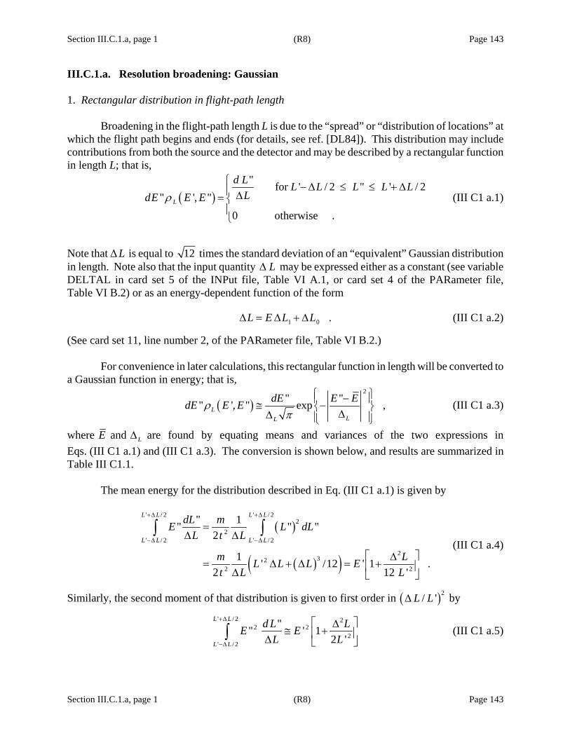
Section III.C.1.a, page 1 (R8) Page 143
Section III.C.1.a, page 1 (R8) Page 143
III.C.1.a. Resolution broadening: Gaussian 1. Rectangular distribution in flight-path length
Broadening in the flight-path length L is due to the “spread” or “distribution of locations” at which the flight path begins and ends (for details, see ref. [DL84]). This distribution may include contributions from both the source and the detector and may be described by a rectangular function in length L; that is,
( )" for ' / 2 " ' / 2
" ', "0 otherwise .
L
d L L L L L LLdE E Eρ
⎧ −Δ ≤ ≤ + Δ⎪ Δ= ⎨⎪⎩
(III C1 a.1)
Note that ΔL is equal to 12 times the standard deviation of an “equivalent” Gaussian distribution in length. Note also that the input quantity LΔ may be expressed either as a constant (see variable DELTAL in card set 5 of the INPut file, Table VI A.1, or card set 4 of the PARameter file, Table VI B.2) or as an energy-dependent function of the form
1 0 .L E L LΔ = Δ + Δ (III C1 a.2)
(See card set 11, line number 2, of the PARameter file, Table VI B.2.)
For convenience in later calculations, this rectangular function in length will be converted to a Gaussian function in energy; that is,
( )2
" "" ', " exp ,LLL
dE E EdE E Eρπ
⎧ ⎫−⎪ ⎪≅ −⎨ ⎬ΔΔ ⎪ ⎪⎩ ⎭ (III C1 a.3)
where E and LΔ are found by equating means and variances of the two expressions in Eqs. (III C1 a.1) and (III C1 a.3). The conversion is shown below, and results are summarized in Table III C1.1.
The mean energy for the distribution described in Eq. (III C1 a.1) is given by
( )
( )( )
' / 2 ' / 22
2' / 2 ' / 2
232
2 2
" 1" " "2
1 ' /12 ' 1 .2 12 '
L L L L
L L L L
dL mE L dLL t L
m LL L L Et L L
+Δ +Δ
−Δ −Δ
=Δ Δ
⎡ ⎤Δ= Δ + Δ = +⎢ ⎥Δ ⎣ ⎦
∫ ∫ (III C1 a.4)
Similarly, the second moment of that distribution is given to first order in ( )2/ 'L LΔ by
' / 2 2
2 22
' / 2
"" ' 12 '
L L
L L
d L LE EL L
+Δ
−Δ
⎡ ⎤Δ≅ +⎢ ⎥Δ ⎣ ⎦
∫ (III C1 a.5)

Section III.C.1.a, page 2 (R8) Page 144
Section III.C.1.a, page 2 (R8) Page 144
so that the variance of the rectangular distribution is given by
( ) ( ) ( )22 2 22 2 2' 1 / ' / 2 ' 1 / ' /12 ' / ' / 3 .E L L E L L E L L⎡ ⎤ ⎡ ⎤ ⎡ ⎤+ Δ − + Δ ≅ Δ⎣ ⎦ ⎣ ⎦ ⎣ ⎦ (III C1 a.6)
Since the mean of the Gaussian distribution in Eq. (III C1 a.3) is E and the variance is 2 / 2LΔ , the parameters of the Gaussian are given (to lowest order) by 'E E= (III C1 a.7) and
( )2 / 3 ' / ' .L E L LΔ = Δ (III C1 a.8) 2. Rectangular distribution in time
Finite channel width is one contributor to broadening in time (for details, see [DL84]). The channel width is represented by a rectangular function in time of width ctΔ as
( )' for / 2 ' / 2
' , '
0 otherwise .
c ccc
d t t t t t ttdE E Eρ
⎧ − Δ ≤ ≤ + Δ⎪Δ= ⎨⎪⎩
(III C1 a.9)
Generally the channel width is constant for a certain energy range but changes from one range to the next. SAMMY input accommodates this characteristic: values for ctΔ are given as a constant DELTAB times a “crunch factor” CFi for energies between Bci-1 and Bci. Details are given in Table VI A.1, card set 6.
This component of the resolution function also will be converted to an equivalent Gaussian function in the energy variable. Arguments similar to those given above for Eqs. (III C1 a.3) through (III C1 a.8) show that this Gaussian has the form
( ) ( )2
2
''' , ' expccc
E EdEdE E EWW
ρπ
⎧ ⎫−⎪ ⎪= −⎨ ⎬⎪ ⎪⎩ ⎭
(III C1 a.10)
where 2 / 3 / .c cW E t t= Δ (III C1 a.11)
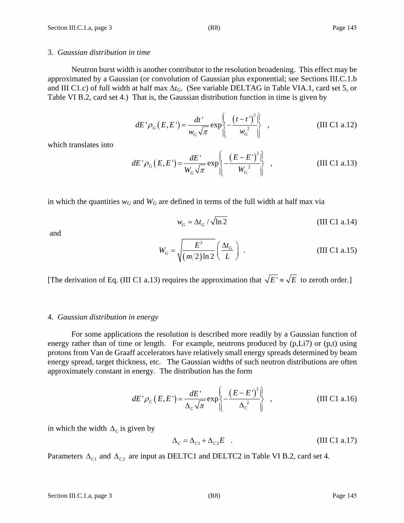
Section III.C.1.a, page 3 (R8) Page 145
Section III.C.1.a, page 3 (R8) Page 145
3. Gaussian distribution in time
Neutron burst width is another contributor to the resolution broadening. This effect may be approximated by a Gaussian (or convolution of Gaussian plus exponential; see Sections III.C.1.b and III C1.c) of full width at half max ΔtG. (See variable DELTAG in Table VIA.1, card set 5, or Table VI B.2, card set 4.) That is, the Gaussian distribution function in time is given by
( ) ( )2
2
''' , ' exp ,GGG
t tdtdE E Eww
ρπ
⎧ ⎫−⎪ ⎪= −⎨ ⎬⎪ ⎪⎩ ⎭
(III C1 a.12)
which translates into
( ) ( )2
2
''' , ' exp ,GGG
E EdEdE E EWW
ρπ
⎧ ⎫−⎪ ⎪= −⎨ ⎬⎪ ⎪⎩ ⎭
(III C1 a.13)
in which the quantities wG and WG are defined in terms of the full width at half max via
/ ln 2G Gw t= Δ (III C1 a.14) and
( )
3
.2 ln 2
GG
tEWm L
Δ⎛ ⎞= ⎜ ⎟⎝ ⎠
(III C1 a.15)
[The derivation of Eq. (III C1 a.13) requires the approximation that 'E E≈ to zeroth order.] 4. Gaussian distribution in energy
For some applications the resolution is described more readily by a Gaussian function of energy rather than of time or length. For example, neutrons produced by (p,Li7) or (p,t) using protons from Van de Graaff accelerators have relatively small energy spreads determined by beam energy spread, target thickness, etc. The Gaussian widths of such neutron distributions are often approximately constant in energy. The distribution has the form
( ) ( )2
2
''' , ' exp ,CCC
E EdEdE E Eρπ
⎧ ⎫−⎪ ⎪= −⎨ ⎬ΔΔ ⎪ ⎪⎩ ⎭
(III C1 a.16)
in which the width CΔ is given by
1 2 .C C C EΔ = Δ + Δ (III C1 a.17)
Parameters 1CΔ and 2CΔ are input as DELTC1 and DELTC2 in Table VI B.2, card set 4.

Section III.C.1.a, page 4 (R8) Page 146
Section III.C.1.a, page 4 (R8) Page 146
5. Convolution of the pieces
The resolution-broadened cross section (or other function) is expressed as the convolution of the resolution function(s) with the unbroadened cross section, as
( ) ( )
( )
( )
( ) ( )
21
1 2
22 1
2 2
23 2
3 2
24 3
4 42
1 exp
1 exp
1 exp
1 exp ,
allcc
LL
GG
CC
E Ef E dE
WW
E EdE
E EdE
WW
E EdE f E
π
π
π
π
+∞
−∞
+∞
−∞
+∞
−∞
+∞
−∞
⎧ ⎫−⎪ ⎪= −⎨ ⎬⎪ ⎪⎩ ⎭
⎧ ⎫−⎪ ⎪× −⎨ ⎬ΔΔ ⎪ ⎪⎩ ⎭
⎧ ⎫−⎪ ⎪× −⎨ ⎬⎪ ⎪⎩ ⎭⎧ ⎫−⎪ ⎪× −⎨ ⎬
ΔΔ ⎪ ⎪⎩ ⎭
∫
∫
∫
∫
(III C1 a.18)
in which we have combined Eqs. (III C1 a.3), (III C1 a.10), (III C1 a.13), and (III C1 a.16). This formula can be written in the form
( ) ( ) ( )2
2
'1 'exp ' ,allallall
E Ef E dE f E
π
+∞
−∞
⎧ ⎫−⎪ ⎪= −⎨ ⎬ΔΔ ⎪ ⎪⎩ ⎭
∫ (III C1 a.19)
in which the combined resolution function is found from
( )
( ) ( )
( ) ( )
2
2
2 21 2 1
1 22 2
2 23 2 3
3 2 2
'1 exp
1 1exp exp
'1 1exp .
allall
c Lc L
G CG C
E E
E E E EdE dE
WW
E E E EdE
WW
π
π π
π π
+∞ +∞
−∞ −∞
+∞
−∞
⎧ ⎫−⎪ ⎪− =⎨ ⎬ΔΔ ⎪ ⎪⎩ ⎭
⎧ ⎫ ⎧ ⎫− −⎪ ⎪ ⎪ ⎪− × −⎨ ⎬ ⎨ ⎬ΔΔ⎪ ⎪ ⎪ ⎪⎩ ⎭ ⎩ ⎭
⎧ ⎫ ⎧ ⎫− −⎪ ⎪ ⎪ ⎪× − × −⎨ ⎬ ⎨ ⎬ΔΔ⎪ ⎪ ⎪ ⎪⎩ ⎭ ⎩ ⎭
∫ ∫
∫
(III C1 a.20)
It is well known that the convolution of two or more Gaussians is also a Gaussian, with the
variance given by the sum of the variances of the components. This could also be demonstrated by direct integration of Eq. (III C1 a.20).

Section III.C.1.a, page 5 (R8) Page 147
Section III.C.1.a, page 5 (R8) Page 147
[In our situation, this is strictly true only if the width LΔ of the second Gaussian is independent of the variable of integration 1E of the first Gaussian. Nevertheless, we may approximate 'E and 'L in our expression for LΔ , Eq. (III C1 a.8), by E and L since the integrand of Eq. (III C1 a.20) is large only near 'E E≅ (i.e., 'L L≅ ).] The variance for the combined resolution function of Eq. (III C1 a.20) may therefore be written as
2 22 3
2 2 22 .3 ln 2
2
c Gall C
t tL EE mt L L
⎡ ⎤Δ Δ⎛ ⎞ ⎛ ⎞Δ⎛ ⎞⎢ ⎥Δ = + + + Δ⎜ ⎟ ⎜ ⎟⎜ ⎟⎝ ⎠⎢ ⎥⎝ ⎠ ⎝ ⎠⎣ ⎦
(III C1 a.21)
Replacing t in Eq. (III C1 a.21) by its equivalent in terms of E and L and rearranging give
2 22
2 2 3 3 22 2 2 2 1 ,3 3 ln 2
c Gall C
t tLE E EL m L m L
Δ ΔΔ ⎛ ⎞ ⎛ ⎞⎛ ⎞Δ = + + + Δ⎜ ⎟ ⎜ ⎟ ⎜ ⎟⎝ ⎠ ⎝ ⎠ ⎝ ⎠
(III C1 a.22)
which may be rewritten in the form
2 2 3 3 2 ,all CaE bE cEΔ = + + + Δ (III C1 a.23) with
2 222 2 2 2 1, ,and .
3 3 ln 2c Gt tLa b c
L m L m LΔ ΔΔ ⎛ ⎞ ⎛ ⎞⎛ ⎞= = =⎜ ⎟ ⎜ ⎟ ⎜ ⎟
⎝ ⎠ ⎝ ⎠ ⎝ ⎠ (III C1 a.24)
If E is in units of eV, GtΔ in μsec, and L in meters, then neutron mass m may be expressed as
( )22 72.3 .m ≅ (III C1 a.25)
This follows directly from 241.67482 10m g−= × and 2 2 111erg cm /s 6.2418 10 eVg= = × . With this value for the mass, the parameters in Eq. (III C1 a.23) become
( )2
2
2 21/2
221/2
2 0.81650 / ,3
2 2 0.011293 ,3
2 0.01661 .ln 2
c c
GG
La L LL
t tb
m L L
ttcLm L
⎛ ⎞Δ= ≅ Δ⎜ ⎟⎜ ⎟⎝ ⎠
⎛ ⎞Δ Δ⎛ ⎞⎛ ⎞= ≅⎜ ⎟ ⎜ ⎟⎜ ⎟⎜ ⎟⎝ ⎠ ⎝ ⎠⎝ ⎠
Δ⎛ ⎞⎛ ⎞Δ⎛ ⎞= ≅ ⎜ ⎟⎜ ⎟⎜ ⎟⎝ ⎠⎝ ⎠ ⎝ ⎠
(III C1 a.26)
It should be noted that more accurate values than these are used in the SAMMY code, as discussed in Section IX.A.
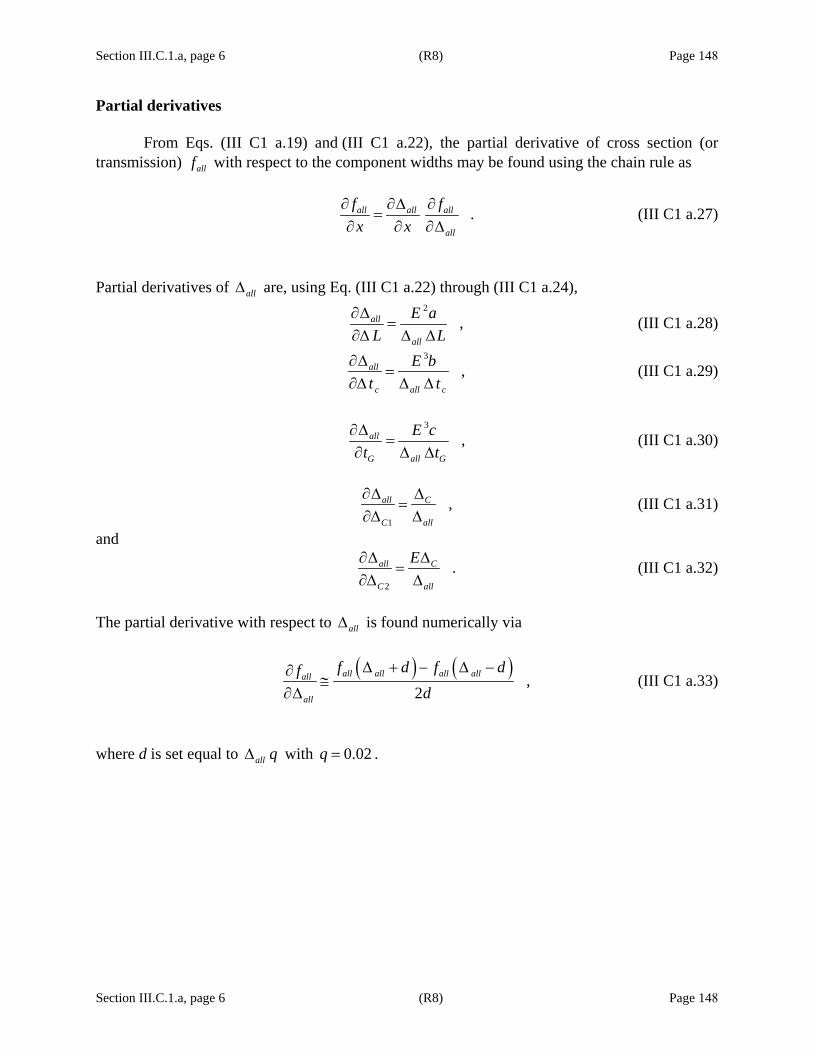
Section III.C.1.a, page 6 (R8) Page 148
Section III.C.1.a, page 6 (R8) Page 148
Partial derivatives
From Eqs. (III C1 a.19) and (III C1 a.22), the partial derivative of cross section (or transmission) allf with respect to the component widths may be found using the chain rule as
.all all all
all
f fx x
∂ ∂Δ ∂=
∂ ∂ ∂Δ (III C1 a.27)
Partial derivatives of allΔ are, using Eq. (III C1 a.22) through (III C1 a.24),
2
,all
all
E aL L
∂Δ=
∂Δ Δ Δ (III C1 a.28)
3
,all
c all c
E bt t
∂Δ=
∂Δ Δ Δ (III C1 a.29)
3
,all
G all G
E ct t
∂Δ=
∂ Δ Δ (III C1 a.30)
1
,all C
C all
∂Δ Δ=
∂Δ Δ (III C1 a.31)
and
2
.all C
C all
E∂Δ Δ=
∂Δ Δ (III C1 a.32)
The partial derivative with respect to allΔ is found numerically via
( ) ( )
,2
all all all allall
all
f d f dfd
Δ + − Δ −∂≅
∂Δ (III C1 a.33)
where d is set equal to all qΔ with 0.02q = .
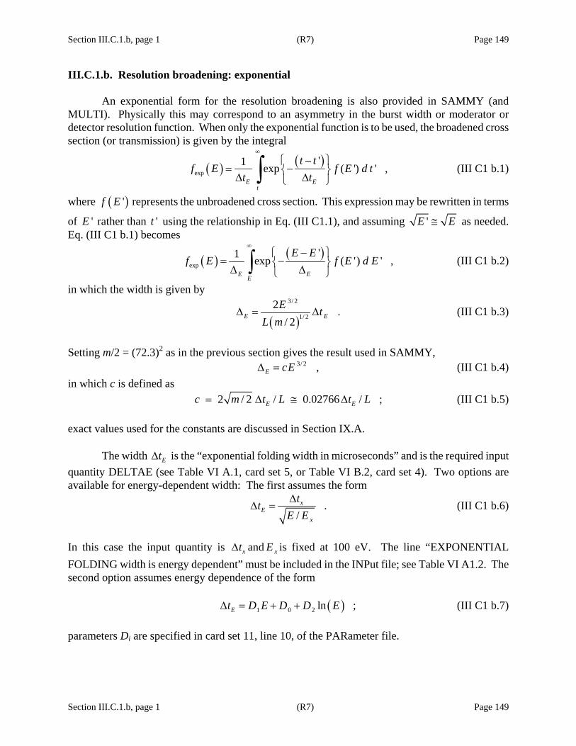
Section III.C.1.b, page 1 (R7) Page 149
Section III.C.1.b, page 1 (R7) Page 149
III.C.1.b. Resolution broadening: exponential
An exponential form for the resolution broadening is also provided in SAMMY (and MULTI). Physically this may correspond to an asymmetry in the burst width or moderator or detector resolution function. When only the exponential function is to be used, the broadened cross section (or transmission) is given by the integral
( ) ( )exp
'1 exp ( ') ' ,E E
t
t tf E f E d t
t t
∞
−⎧ ⎫= −⎨ ⎬Δ Δ⎩ ⎭∫ (III C1 b.1)
where ( )'f E represents the unbroadened cross section. This expression may be rewritten in terms
of 'E rather than 't using the relationship in Eq. (III C1.1), and assuming 'E E≅ as needed. Eq. (III C1 b.1) becomes
( ) ( )exp
'1 exp ( ') ' ,E EE
E Ef E f E d E
∞−⎧ ⎫
= −⎨ ⎬Δ Δ⎩ ⎭∫ (III C1 b.2)
in which the width is given by
( )
3/ 2
1/ 22 .
/ 2E EE t
L mΔ = Δ (III C1 b.3)
Setting m/2 = (72.3)2 as in the previous section gives the result used in SAMMY, 3/ 2 ,E cEΔ = (III C1 b.4) in which c is defined as 2 / 2 / 0.02766 / ;E Ec m t L t L= Δ ≅ Δ (III C1 b.5) exact values used for the constants are discussed in Section IX.A.
The width EtΔ is the “exponential folding width in microseconds” and is the required input quantity DELTAE (see Table VI A.1, card set 5, or Table VI B.2, card set 4). Two options are available for energy-dependent width: The first assumes the form
./
xE
x
ttE EΔ
Δ = (III C1 b.6)
In this case the input quantity is xtΔ and xE is fixed at 100 eV. The line “EXPONENTIAL FOLDING width is energy dependent” must be included in the INPut file; see Table VI A1.2. The second option assumes energy dependence of the form ( )1 0 2 ln ;Et D E D D EΔ = + + (III C1 b.7) parameters Di are specified in card set 11, line 10, of the PARameter file.
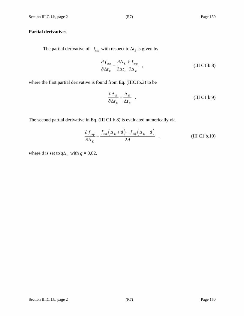
Section III.C.1.b, page 2 (R7) Page 150
Section III.C.1.b, page 2 (R7) Page 150
Partial derivatives
The partial derivative of expf with respect to EtΔ is given by
exp exp ,E
E E E
f ft t
∂ ∂Δ ∂=
∂Δ ∂Δ ∂Δ (III C1 b.8)
where the first partial derivative is found from Eq. (IIIC1b.3) to be
.E E
E Et t∂Δ Δ
=∂Δ Δ
(III C1 b.9)
The second partial derivative in Eq. (III C1 b.8) is evaluated numerically via
( ) ( )exp expexp ,
2E E
E
f d f dfd
Δ + − Δ −∂=
∂Δ (III C1 b.10)
where d is set to EqΔ with q = 0.02.
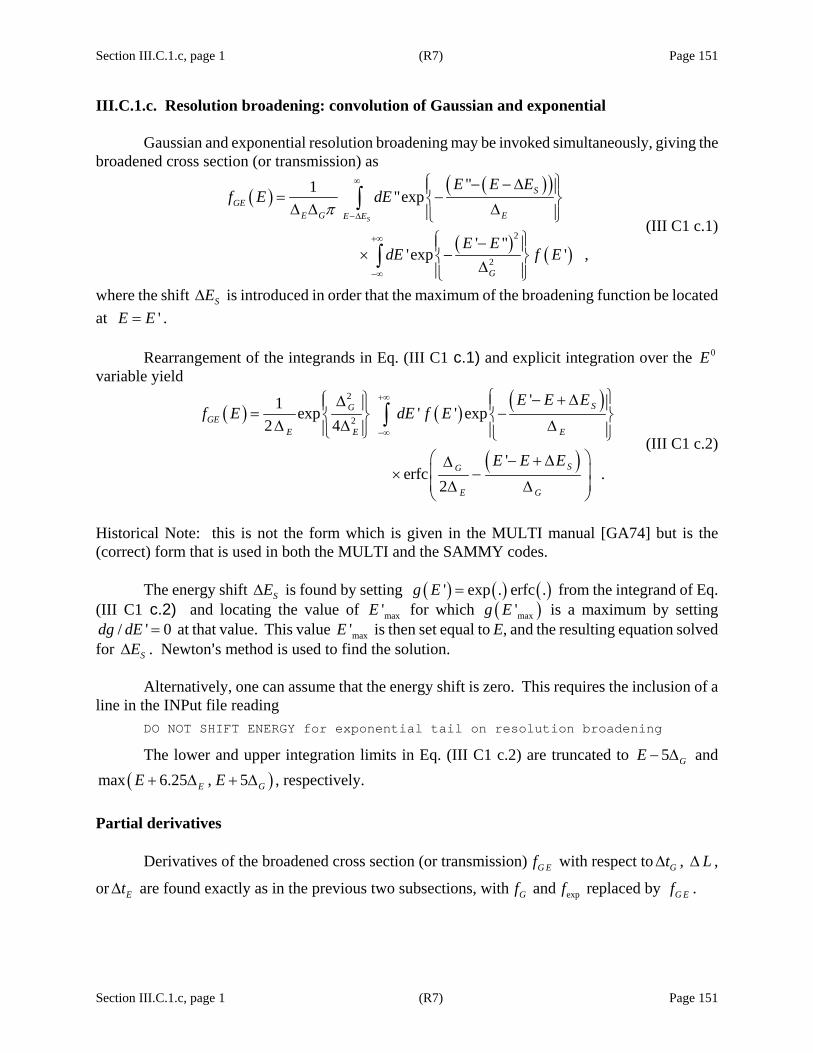
Section III.C.1.c, page 1 (R7) Page 151
Section III.C.1.c, page 1 (R7) Page 151
III.C.1.c. Resolution broadening: convolution of Gaussian and exponential
Gaussian and exponential resolution broadening may be invoked simultaneously, giving the broadened cross section (or transmission) as
( ) ( )( )
( ) ( )2
2
"1 "exp
' "'exp ' ,
S
SGE
E G EE E
G
E E Ef E dE
E EdE f E
π
∞
−Δ
+∞
−∞
⎧ ⎫− − Δ⎪ ⎪= −⎨ ⎬Δ Δ Δ⎪ ⎪⎩ ⎭⎧ ⎫−⎪ ⎪× −⎨ ⎬Δ⎪ ⎪⎩ ⎭
∫
∫ (III C1 c.1)
where the shift SEΔ is introduced in order that the maximum of the broadening function be located at 'E E= .
Rearrangement of the integrands in Eq. (III C1 c.1) and explicit integration over the 0E variable yield
( ) ( ) ( )
( )
2
2
'1 exp ' ' exp2 4
'erfc .
2
SGGE
E E E
SG
E G
E E Ef E dE f E
E E E
+∞
−∞
⎧ ⎫− + Δ⎧ ⎫Δ⎪ ⎪ ⎪ ⎪= −⎨ ⎬ ⎨ ⎬Δ Δ Δ⎪ ⎪ ⎪ ⎪⎩ ⎭ ⎩ ⎭⎛ ⎞− + ΔΔ⎜ ⎟× −⎜ ⎟Δ Δ⎝ ⎠
∫ (III C1 c.2)
Historical Note: this is not the form which is given in the MULTI manual [GA74] but is the (correct) form that is used in both the MULTI and the SAMMY codes.
The energy shift SEΔ is found by setting ( ) ( ) ( )' exp . erfc .g E = from the integrand of Eq. (III C1 c.2) and locating the value of max'E for which ( )max'g E is a maximum by setting
/ ' 0dg dE = at that value. This value max'E is then set equal to E, and the resulting equation solved for SEΔ . Newton=s method is used to find the solution.
Alternatively, one can assume that the energy shift is zero. This requires the inclusion of a line in the INPut file reading
DO NOT SHIFT ENERGY for exponential tail on resolution broadening The lower and upper integration limits in Eq. (III C1 c.2) are truncated to 5 GE − Δ and
( )max 6.25 , 5E GE E+ Δ + Δ , respectively. Partial derivatives
Derivatives of the broadened cross section (or transmission) G Ef with respect to GtΔ , LΔ ,
or EtΔ are found exactly as in the previous two subsections, with Gf and expf replaced by G Ef .


Section III.C.2, page 1 (R7) Page 153
Section III.C.2, page 1 (R7) Page 153
III.C.2. Oak Ridge Resolution Function (ORR)
For ORELA data, the resolution-broadening functions described in Section III.C.1 are not especially accurate approximations. We have therefore developed a more realistic mathematical description of the experimental situation at ORELA, based on concepts described by D. C. Larson et al. [DL84] and initially derived by F. G. Perey [FP89].
The resolution function has four components: the electron burst, the ORELA moderator, the neutron detector, and the time-of-flight channel width. Experimentally, the resolution-broadened cross section ( )Eσ is formed when each contributing feature provides its own broadening; the combined effect of the several components is all that is actually noticed. Mathematically, this may be viewed as follows: Each component is modeled separately as a function of flight time (rather than energy), and then each is convoluted in turn with the unbroadened (or partially broadened) cross section; the convolution process is performed analytically where possible and numerically where necessary. That is, the resolution-broadened cross section ( )tσ may be expressed as
( ) ( ) ( ) ( ) ( ) ( )1 1 1 2 1 2 2 3 2 3 3 4 3 4 4 4 ,t I t t dt I t t dt I t t dt I t t dt tσ σ= − − − −∫ ∫ ∫ ∫ (III C2.1) where Ii is our mathematical model for the ith component. This expression may then be rearranged into the form
( ) ( ) ( )' ' ' ,t I t t t dtσ σ= −∫ (III C2.2) where the resolution function ( )'I t t− is defined as
( ) ( ) ( ) ( ) ( )1 1 1 2 1 2 2 3 2 3 3 4 3' ' .I t t I t t dt I t t dt I t t dt I t t− = − − − −∫ ∫ ∫ (III C2.3) Because SAMMY deals with cross sections as functions of energy, rather than time, the relationship
2
22
1 12 2
LE mv mt
= = (III C2.4)
is used to convert from energy to time (or time to energy) in Eq. (III C2.2), yielding ( ) ( )( ) ( )( )' ' ' ' ' .E I t E t E t dtσ σ= −∫ (III C2.5)
In the following sections we describe the components Ii and the convolution procedure. Input for using this resolution function is described in card set 9, Table VI B.2. See also Section X.H, which describes program SAMORT, used for plotting the individual pieces and the complete ORR function at a specified energy.


Section III.C.2.a, page 1 (R7) Page 155
Section III.C.2.a, page 1 (R7) Page 155
III.C.2.a. Individual components of the ORR resolution function 1. Electron burst
The electron burst from ORELA is closely approximated by a square function in time:
( )1
1/ for 00 otherwise ,
p t pI t
< <⎧= ⎨⎩
(III C2 a.1)
where p is the burst width in nanoseconds. The value 1/ p for this function gives a normalization of unity. 2. Neutron sources
Experiments at ORELA can utilize neutrons from a tantalum target, or collimate on the water moderator surrounding the tantalum target. The two are modeled separately; experiments are assumed to use predominantly one or the other, rather than a mixture of both. (The implications to this representation if neutrons are emitted from both the tantalum target and the water moderator will be studied as time and funding permit.) ORELA water moderator
The distribution of flight-path lengths of neutrons in the ORELA water moderator that has the most physical basis [SC92] is the chi-square distribution with 2( 1)m+ degrees of freedom, where m is an integer. (Originally m = 4 or 5, but any integer from 1 to 10 will now work; the default value is m = 4.)
( )2 1' exp ,!
m
a m
l lI lm +
⎛ ⎞= −⎜ ⎟Λ Λ⎝ ⎠ (III C2 a.2)
where l is the flight-path-length variable and where the moderation distance Λ is a mean free path. The value of Λ varies with energy as ( ) ( )( )2
0 1 2ln lnE EΛ = Λ +Λ +Λ [CC83]. Default values for the Λi are chosen to give agreement with [SC92].
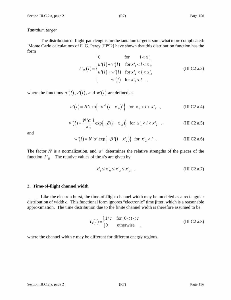
Section III.C.2.a, page 2 (R7) Page 156
Section III.C.2.a, page 2 (R7) Page 156
Tantalum target
The distribution of flight-path lengths for the tantalum target is somewhat more complicated: Monte Carlo calculations of F. G. Perey [FP92] have shown that this distribution function has the form
( )( ) ( )( ) ( )
( )
1
1 22
2 3
3 ,
0 for '' ' for ' '
'' ' for ' '
' for '
b
l xu l v l x l x
I lu l w l x l x
w l x l
<⎧⎪ + < <⎪= ⎨ + < <⎪⎪ <⎩
(III C2 a.3)
where the functions ( )'u l , ( )'v l , and ( )'w l are defined as ( ) ( ) 22
0 1 3' 'exp ' ' for ' ' ,u l N l x x l xε= − − < < (III C2 a.4)
( ) ( ) 2 1 22
' '' exp ' for ' ' ,'
N lv l l x x l xxα β= − − < < (III C2 a.5)
and ( ) ( ) 2 2' ' 'exp ' ' for ' .w l N l x x lα β= − − < (III C2 a.6) The factor N' is a normalization, and 'α determines the relative strengths of the pieces of the function 2' bI . The relative values of the x=s are given by 1 0 2 3' ' ' ' .x x x x≤ ≤ ≤ (III C2 a.7) 3. Time-of-flight channel width
Like the electron burst, the time-of-flight channel width may be modeled as a rectangular distribution of width c. This functional form ignores “electronic” time jitter, which is a reasonable approximation. The time distribution due to the finite channel width is therefore assumed to be
( )3
1/ for 00 otherwise ,
c t cI t
< <⎧= ⎨⎩
(III C2 a.8)
where the channel width c may be different for different energy regions.

Section III.C.2.a, page 3 (R7) Page 157
Section III.C.2.a, page 3 (R7) Page 157
4. Detectors
Two types of neutron detectors are commonly used for transmission measurements at ORELA: the NE110 (a recoil proton detector) and the lithium glass (for which moderation of neutrons in the detector plays an important role). NE110 detector
If δ is the thickness of the NE110 detector, then the resolution function appropriate for that detector is
( ) ( )4
exp for 0'
0 otherwise .a
l lI l
λσ δΔ − < <⎧⎪= ⎨⎪⎩
(III C2 a.9)
where λ is the number of molecules per volume (molecules per millimeter barn) of the detector (0.0047 for NE110), and ( )Eσ is the total cross section of the detector material (CH1.104 for NE110). The normalization factor Δ is found by setting the integral over all space of 4' aI equal to 1. Lithium glass detector
For the lithium glass detector, the resolution function is assumed to have the form
( ) ( )( )4
for 0
exp for ,b
Dg t dI l
D f t d d t
< <⎧⎪= ⎨ − − <⎪⎩ (III C2 a.10)
where g, f, and d are constants, and D is chosen to give an integral of unity.


Section III.C.2.b, page 1 (R7) Page 159
Section III.C.2.b, page 1 (R7) Page 159
III.C.2.b. Converting length to time dependence
The relationship between energy E, flight time t, and flight-path length l may be used to convert from a function of l to a function of t (assuming E is fixed):
2
2 ,2m lE
t= (III C2 b.1)
which may be rearranged to give
2 ,El t btm
= = (III C2 b.2)
in which we have defined b as the square root of 2 /E m . A distribution function in l may then be converted to a distribution function in t by (a) replacing l by bt everywhere and (b) replacing dl by b dt. In particular, the distances 'ix (tantalum target) translate to the time dimension via ' / ,i ix x b= (III C2 b.3) and, similarly, δ (NE110 detector) translates via
/ .d bδ= (III C2 b.4) For the NE110 detector, we also define f via .f bλσ= (III C2 b.5)

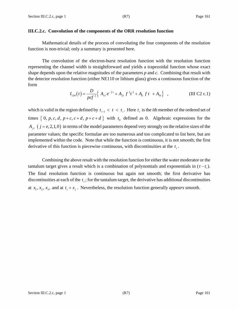
Section III.C.2.c, page 1 (R7) Page 161
Section III.C.2.c, page 1 (R7) Page 161
III.C.2.c. Convolution of the components of the ORR resolution function
Mathematical details of the process of convoluting the four components of the resolution function is non-trivial; only a summary is presented here.
The convolution of the electron-burst resolution function with the resolution function representing the channel width is straightforward and yields a trapezoidal function whose exact shape depends upon the relative magnitudes of the parameters p and c. Combining that result with the detector resolution function (either NE110 or lithium glass) gives a continuous function of the form
( ) 2 2134 2 1 02 ,f t
ei i i iDI t A e A f t A f t A
pcf−= + + + (III C2 c.1)
which is valid in the region defined by 1i it t t− < < . Here it is the ith member of the ordered set of
times 0, , , , , ,p c d p c c d p c d+ + + + with 0t defined as 0. Algebraic expressions for the
( ), 2,1,0j iA j e= in terms of the model parameters depend very strongly on the relative sizes of the parameter values; the specific formulae are too numerous and too complicated to list here, but are implemented within the code. Note that while the function is continuous, it is not smooth; the first derivative of this function is piecewise continuous, with discontinuities at the it .
Combining the above result with the resolution function for either the water moderator or the tantalum target gives a result which is a combination of polynomials and exponentials in ( it t− ). The final resolution function is continuous but again not smooth; the first derivative has discontinuities at each of the it ; for the tantalum target, the derivative has additional discontinuities
at 1 2 3, , ,x x x and at i jt x+ . Nevertheless, the resolution function generally appears smooth.


Section III.C.3, page 1 (R7) Page 163
Section III.C.3, page 1 (R7) Page 163
III.C.3. RPI (and GELINA and nTOF) Resolution Broadening
Researchers at Rensselaer Polytechnic Institute (RPI) have carefully measured the resolution function associated with the “bounce target” and the transmission detector (lithium glass) for the LINAC at RPI [BM96]. This resolution function may be described by the sum of a chi-squared function (with six degrees of freedom) plus two exponential terms. The total resolution function appropriate for data measured on that machine is then the convolution of the target-detector resolution function, with a Gaussian function representing the electron burst and a square function representing the channel width.
An extension to the RPI resolution function has been shown by Gunsing [FG05] to provide a
reasonable description for the resolution functions for two other time-of-flight facilities: the Geel Electron Linear Accelerator (GELINA) at IRMM in Belgium and the neutron time of flight (nTOF) facility at CERN in Switzerland. This extension (discussed in the next section) has been implemented in SAMMY.
Within SAMMY, the RPI resolution function is formed in much the same manner as described for the realistic resolution function of Section III.C.2, that is, the resolution-broadened cross section ( )tσ may be expressed as
( ) ( ) ( ) ( ) ( )1 1 1 2 1 2 2 3 2 3 3 3 ,t I t t dt I t t dt I t t dt tσ σ= − − −∫ ∫ ∫ (III C3.1) where Ii is our mathematical model for the ith component. This expression may then be rearranged into the form ( ) ( ) ( )' ' ' ,t I t t t dtσ σ= −∫ (III C3.2) where the resolution function ( )'I t t− is defined as ( ) ( ) ( ) ( )1 1 1 2 1 2 2 3 2' ' .I t t I t t dt I t t dt I t t− = − − −∫ ∫ (III C3.3) Because SAMMY deals with cross sections as functions of energy, rather than time, the relationship
2
22
1 12 2
LE = m = m vt
(III C3.4)
is used to convert from energy to time and vice versa in Eq. (IIIC3.2), yielding ( ) ( )( ) ( )( )' ' ' ' ' .E I t E t E t dtσ σ= −∫ (III C3.5)
In the following section (Section III.C.3.a), the component functions Ii are described, along with the parameters for those components.

Section III.C.3, page 2 (R7) Page 164
Section III.C.3, page 2 (R7) Page 164
Test cases tr053, tr054, tr094, and tr095 show several examples using the RPI resolution function, with parameter values suitable for RPI data and candidate parameters for use with GELINA data. More recently, the RPI resolution function has been extended to give a more suitable energy-dependent form for use with both GELINA and nTOF data; this form was suggested by Gunsing [FG05], who also provided preliminary parameter values. Testing for the extension is given in test cases tr104 and tr107; Gunsing’s parameter values are used in tr108.
To make plots of this resolution function and the individual components, see Section X.K.
Also see test case tr107 for examples of another method of plotting the RPI resolution function, using the Dirac delta function option for pseudo cross section with uniform energy grid (Section V.E).
Section III.C.3.b discusses the various input options for the RPI/GELINA/nTOF resolution
function.

5ection III.C.3.a, page 1 (R7) Page 165
Section III.C.3.a, page 1 (R7) Page 165
III.C.3.a. Components of the RPI / GELINA / nTOF resolution function 1. Electron burst
The electron burst from the RPI linac may be described by a Gaussian function in time, of the form:
( ) 2 2
1 ,w twI t eπ
−= (III C3 a.1)
where 2 ln 2 / w p= is the full width at half max of the burst. Normalization is unity for this function. 2. Target plus detector
The RPI transmission resolution function, which represents the combined components for the “bounce target” and transmission detector, has been found by RPI researchers [BM96] to be best described by the sum of a chi-squared function with six degrees of freedom plus two exponential terms. A similar function (with different values for the parameters) describes the bounce target plus capture detector.
The original RPI function had constant values for A3 and A5. The GELINA and nTOF
resolution functions proposed by Gunsing [FG05] use energy dependent values of the A3 and A5 parameters.
Specifically, the RPI resolution function has the form
( ) ( ) ( ) ( ) ( ) ( )
( )
3 0 5 0
2 0
2/
2 0 1 2 43
5
2 11
2!
,i
A t t A t tt
B t ti
i
tI t A e A A e A e X t
B e
ττ − + − +− + Λ
− +−
=
⎧ +⎪ ⎡ ⎤= + +⎨ ⎣ ⎦Λ⎪⎩⎫+ ⎬⎭
∑ (III C3 a.2)
in which the function ( )X t is zero if the quantity within the square brackets (the sum of the exponential terms) is negative, and unity otherwise. Likewise the χ2 function is assumed to have zero value when the exponent is positive (i.e., when 0t τ+ < ). The value of A0 is chosen to give an overall normalization of unity for this function. Parameters Λ, τ, A1, A3, and A5 are functions of energy, the specific forms being, respectively, ( ) ( ) ( ) 4
20 1 2 3ln ln ,E E E EΛΛ = Λ +Λ +Λ +Λ⎡ ⎤⎣ ⎦ (III C3 a.3)
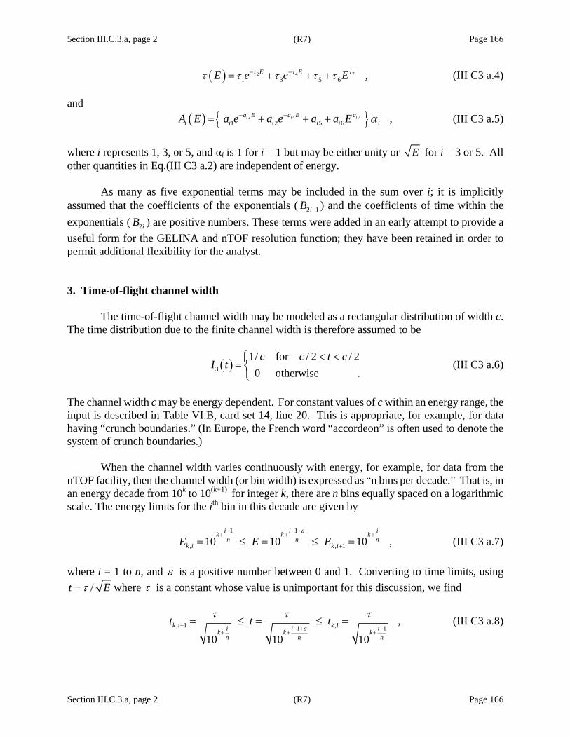
5ection III.C.3.a, page 2 (R7) Page 166
Section III.C.3.a, page 2 (R7) Page 166
( ) 72 41 3 5 6 ,E EE e e Eττ ττ τ τ τ τ− −= + + + (III C3 a.4)
and
( ) 2 4 71 2 5 6 ,i i ia E a E a
i i i i i iA E a e a e a a E α− −= + + + (III C3 a.5) where i represents 1, 3, or 5, and αi is 1 for i = 1 but may be either unity or E for i = 3 or 5. All other quantities in Eq.(III C3 a.2) are independent of energy.
As many as five exponential terms may be included in the sum over i; it is implicitly assumed that the coefficients of the exponentials ( 2 1iB − ) and the coefficients of time within the exponentials ( 2iB ) are positive numbers. These terms were added in an early attempt to provide a useful form for the GELINA and nTOF resolution function; they have been retained in order to permit additional flexibility for the analyst. 3. Time-of-flight channel width
The time-of-flight channel width may be modeled as a rectangular distribution of width c. The time distribution due to the finite channel width is therefore assumed to be
( )3
1/ for / 2 / 20 otherwise .c c t c
I t− < <⎧
= ⎨⎩
(III C3 a.6)
The channel width c may be energy dependent. For constant values of c within an energy range, the input is described in Table VI.B, card set 14, line 20. This is appropriate, for example, for data having “crunch boundaries.” (In Europe, the French word “accordeon” is often used to denote the system of crunch boundaries.) When the channel width varies continuously with energy, for example, for data from the nTOF facility, then the channel width (or bin width) is expressed as “n bins per decade.” That is, in an energy decade from 10k to 10(k+1) for integer k, there are n bins equally spaced on a logarithmic scale. The energy limits for the ith bin in this decade are given by
1 1
, , 110 10 10 ,i i ik k kn n n
k i k iE E Eε− − +
+ + +
+= ≤ = ≤ = (III C3 a.7) where i = 1 to n, and ε is a positive number between 0 and 1. Converting to time limits, using
/t Eτ= where τ is a constant whose value is unimportant for this discussion, we find
, 1 ,1 1,
10 10 10k i k ii i ik k k
n n n
t t tε
τ τ τ+ − + −
+ + +
= ≤ = ≤ = (III C3 a.8)
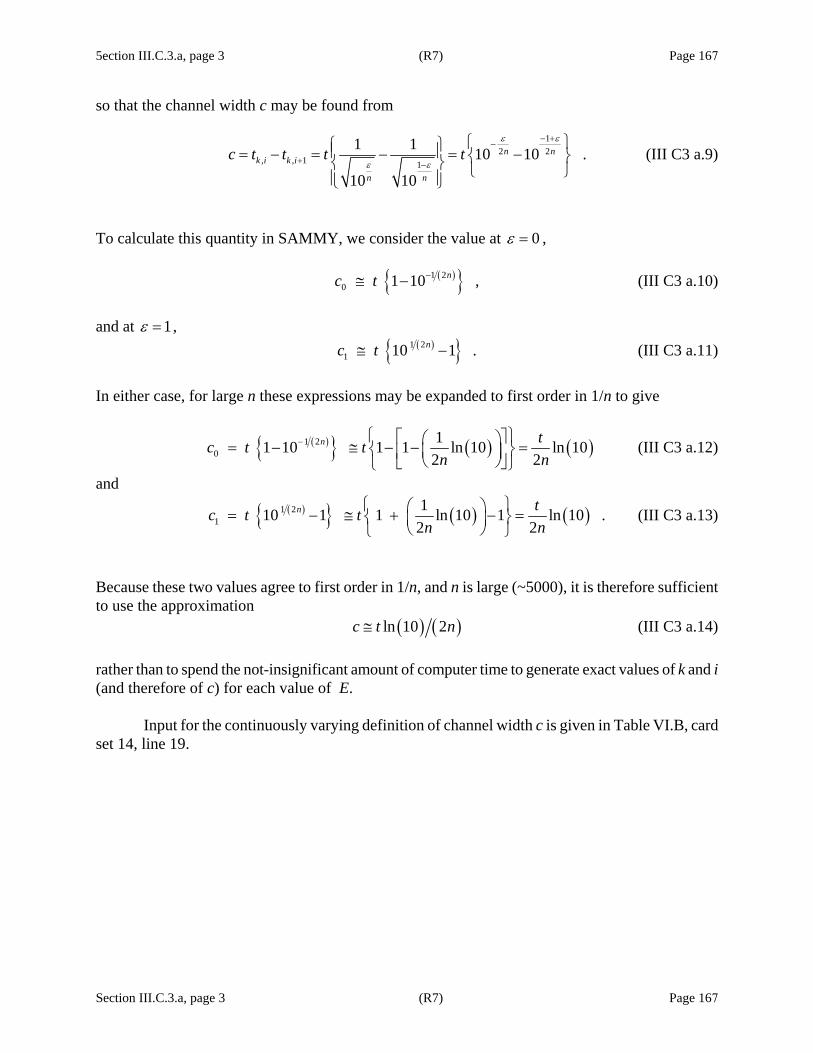
5ection III.C.3.a, page 3 (R7) Page 167
Section III.C.3.a, page 3 (R7) Page 167
so that the channel width c may be found from
1
2 2, , 1 1
1 1 10 10 .
10 10
n nk i k i
n n
c t t t tε ε
ε ε
− +−
+ −
⎧ ⎫⎧ ⎫⎪ ⎪= − = − = −⎨ ⎬⎨ ⎬ ⎩ ⎭⎪ ⎪⎩ ⎭
(III C3 a.9)
To calculate this quantity in SAMMY, we consider the value at 0ε = ,
( ) 1 20 1 10 ,nc t −≅ − (III C3 a.10)
and at 1ε = , ( ) 1 2
1 10 1 .nc t≅ − (III C3 a.11)
In either case, for large n these expressions may be expanded to first order in 1/n to give
( ) ( ) ( )1 20
11 10 1 1 ln 10 ln 102 2
n tc t tn n
− ⎧ ⎫⎡ ⎤⎛ ⎞= − ≅ − − =⎨ ⎬⎜ ⎟⎢ ⎥⎝ ⎠⎣ ⎦⎩ ⎭ (III C3 a.12)
and
( ) ( ) ( )1 21
110 1 1 ln 10 1 ln 10 .2 2
n tc t tn n
⎧ ⎫⎛ ⎞= − ≅ + − =⎨ ⎬⎜ ⎟⎝ ⎠⎩ ⎭
(III C3 a.13)
Because these two values agree to first order in 1/n, and n is large (~5000), it is therefore sufficient to use the approximation
( ) ( )ln 10 2c t n≅ (III C3 a.14) rather than to spend the not-insignificant amount of computer time to generate exact values of k and i (and therefore of c) for each value of E. Input for the continuously varying definition of channel width c is given in Table VI.B, card set 14, line 19.

Section III.C.3.b, page 1 (R7) Page 169
Section III.C.3.b, page 1 (R7) Page 169
III.C.3.b. Input for the RPI/GELINA/nTOF resolution function
Input formats for all parameters of the RPI/GELINA/NTOF resolution function are given in Table VI B.2, card set 14. Note that zero values are assumed to actually be zero and are not replaced by default values. The first line of this card set contains one of the following phrases (which are treated as equivalent):
RPI Resolution function GELINa resolution function NTOF resolution function
As usual, only those characters in capital letters are required; those in lower case letters are optional.
In Table III C3 b.1, default values for the constants from Eqs. (III C3 a.2) through (III C3 a.5) are defined for transmission and capture measurements. To invoke these defaults (without the option to flag them for varying), the user must specify the appropriate phrase
RPI Transmission resolution function or RPI Capture resolution function
on the first line of card set 14.
Table III C3 b.2, provided courtesy of Frank Gunsing of Saclay [FG05], gives parameter values that may be suitable for use with data from the Geel Electron Linear Accelerator (GELINA) at IRMM and with data from the neutron time-of-flight facility (nTOF) at CERN. Note that these values are preliminary; they are reasonable starting values which should be fine-tuned on measurements of well-known resonances (i.e., on resonances that have been measured many times at different installations). To invoke these values automatically (without the option to flag them for varying), use one of the following phrases for the first line of card set 14:
GEEL DEFAUlt values for resolution parameters GELINa DEFAUlt values NTOF DEFAUlt values
With the RPI/GELINA/nTOF resolution function, it is necessary to specify whether the resolution function should be used exactly as given in the input or whether, instead, it should be shifted so that it is centered on the current energy. To center the function, include one of the phrases
SHIFT RPI RESOLUTION function to center SHIFT GEEL RESOLUTIOn function to center SHIFT GELINA RESOLUtion function to center SHIFT NTOF RESOLUTIOn function to center
in the command section of the INPut file. To use the function exactly as given in the input, include one of the phrases

Section III.C.3.b, page 2 (R7) Page 170
Section III.C.3.b, page 2 (R7) Page 170
DO NOT SHIFT RPI RESolution function to center
DO NOT SHIFT GEEL Resolution function to center DO NOT SHIFT GELINA resolution function to center DO NOT SHIFT NTOF Resolution function to center
Many test cases provide examples of input for the RPI resolution function; see, for example,
tr053, tr054, tr090, tr094, tr095, tr115, or tr136. For examples using the GELINA and nTOF resolution function, see test cases tr104, tr107, and (especially) tr108.
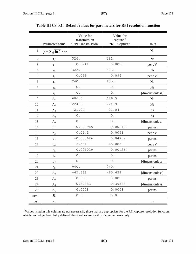
Section III.C.3.b, page 3 (R7) Page 171
Section III.C.3.b, page 3 (R7) Page 171
Table III C3 b.1. Default values for parameters for RPI resolution function
Parameter name
Value for transmission
“RPI Transmission”
Value for capture a
“RPI Capture” Units
1 2 ln 2p = / w Ns
2 τ1 326. 381. Ns 3 τ2 0.0241 0.0058 per eV 4 τ3 323. 323. Ns 5 τ4 0.029 0.094 per eV 6 τ5 240. 105. Ns 7 τ6 0. 0. Ns 8 τ7 0. 0. [dimensionless] 9 Λ0 686.5 686.5 Ns
10 Λ1 -224.9 -224.9 Ns 11 Λ2 21.04 21.04 ns 12 Λ3 0. 0. ns 13 Λ4 0. 0. [dimensionless] 14 a1 -0.000985 -0.001106 per ns 15 a2 0.0241 0.0058 per eV 16 a3 -0.000626 0.04752 per ns 17 a4 3.531 65.083 per eV 18 a5 0.001029 0.001264 per ns 19 a6 0. 0. per ns 20 a7 0. 0. [dimensionless] 21 t 0 940. 940. ns 22 A2 -65.638 -65.638 [dimensionless] 23 A3 0.005 0.005 per ns 24 A4 0.39383 0.39383 [dimensionless] 25 A5 0.0008 0.0008 per ns
next Bi 0.0 0.0 last c ns
a Values listed in this column are not necessarily those that are appropriate for the RPI capture resolution function, which has not yet been fully defined; these values are for illustrative purposes only.

Section III.C.3.b, page 4 (R7) Page 172
Section III.C.3.b, page 4 (R7) Page 172
Table III C3 b.2. Parameters suitable for use with experimental data from GELINA at IRMM and from nTOF at CERN. Values are from preliminary work of F. Gunsing [FG05]. Parameters not listed in this table have value zero. Test case tr108 contains these values
Parameter name Value for GELINA
90-degree flight patha Values for
nTOF Units
τ5 -0.7722 -3.7004 ns
τ6 1363.85 -684.39 ns
τ7 -0.5322 -0.5189 [dimensionless]
Λ0 1.4460 3.8457 ns
Λ3 454.9720 502.9930 ns
Λ4 -0.5077 -0.4155 [dimensionless]
a1 0.0 -0.0381 per ns
a2 0.0 9.974×10⁻⁶ per eV
a3 0.04152 -0.01172 per ns
a4 -5.847×10⁻⁶ 0.0001019 per eV
a5 -0.0415 0.05009 per ns
a6 9.247×10⁻⁶ 0.0 per ns
a7 0.5961 0.0 [dimensionless]
A2 1.0 1.0 [dimensionless]
A4 -1.0 -1.0 [dimensionless]
A3SQE (A3): a35 0.0003047 -0.0001689 per [ns ×(eV)1/2]
A3SQE (A3): a36 7.818×10⁻⁵ 0.0004254 per [ns ×(eV)1/2]
A3SQE (A3): a37 -2.011 -0.06043 [dimensionless]
A3SQE (A5): a55 0.007331 0.0002766 per [ns ×(eV)1/2]
aThe GELINA resolution function refers to the beam only and does not include a contribution from a detection system.
Section III.C.4, page 1 (R7) Page 173
Section III.C.4, page 1 (R7) Page 173
III.C.4. Straight-Line Energy Average
This relatively simple resolution function takes the form
( )1
1/ for ''
0 otherwise ,D E D E
I E− <⎧
= ⎨⎩
(III C4.1)
so that the broadened cross section is given by
( ) ( )1 ' ' .E
E D
E E dED
σ σ−
= ∫ (III C4.2)
Note that the apparent position of a resonance is altered (shifted to a higher energy) by the use of this resolution function.
It is also possible to use this resolution function without shifting the apparent position of the resonances. To invoke this option, include the phrase
CENTER THE CONSTANT ENERGY RESOLUTION FUNCTION in the INPut file. In this case, the resolution function of Eq. (III C4.1) is replaced by
( )1
1/ for / 2 ' / 2'
0 otherwise ,D E D E E D
I E− < < +⎧
= ⎨⎩
(III C4.3)
and the broadened cross section is given by
( ) ( )/ 2
/ 2
1 ' ' .E D
E D
E E dED
σ σ+
−
= ∫ (III C4.4)
Input for the value of D is variable DDDEEE in card set 5 of the INPut file. See test case
tr105 for examples. Note that this parameter cannot be fitted (i.e., it cannot be treated as a search parameter in the fitting procedure).
CAUTION: Difficulties have been experienced in using this resolution function in the neighborhood of extremely narrow resonances (probably due to the discontinuous nature of the function). When results look very odd (abrupt changes in value of cross section as a function of energy, for example), try increasing the number of mesh points in the auxiliary grid (see Sections III.A.1 and III.A.2). If problems persist, contact the SAMMY author.

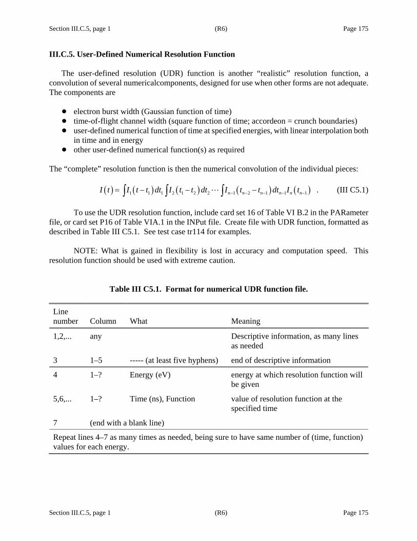
Section III.C.5, page 1 (R6) Page 175
Section III.C.5, page 1 (R6) Page 175
III.C.5. User-Defined Numerical Resolution Function
The user-defined resolution (UDR) function is another “realistic” resolution function, a convolution of several numericalcomponents, designed for use when other forms are not adequate. The components are
! electron burst width (Gaussian function of time) ! time-of-flight channel width (square function of time; accordeon = crunch boundaries) ! user-defined numerical function of time at specified energies, with linear interpolation both
in time and in energy ! other user-defined numerical function(s) as required
The “complete” resolution function is then the numerical convolution of the individual pieces: ( ) ( ) ( ) ( ) ( )1 1 1 2 1 2 2 1 2 1 1 1 .n n n n n nI t I t t dt I t t dt I t t dt I t− − − − −= − − −∫ ∫ ∫ (III C5.1)
To use the UDR resolution function, include card set 16 of Table VI B.2 in the PARameter file, or card set P16 of Table VIA.1 in the INPut file. Create file with UDR function, formatted as described in Table III C5.1. See test case tr114 for examples.
NOTE: What is gained in flexibility is lost in accuracy and computation speed. This resolution function should be used with extreme caution.
Table III C5.1. Format for numerical UDR function file. Line number Column What Meaning
1,2,... any Descriptive information, as many lines as needed
3 1–5 ----- (at least five hyphens) end of descriptive information
4 1–? Energy (eV) energy at which resolution function will be given
5,6,... 1–? Time (ns), Function value of resolution function at the specified time
7 (end with a blank line)
Repeat lines 4–7 as many times as needed, being sure to have same number of (time, function) values for each energy.

Section III.D, page 1 (R8) Page 177
Section III.D, page 1 (R8) Page 177
III.D. SELF-SHIELDING AND MULTIPLE-SCATTERING CORRECTIONS TO CAPTURE OR FISSION YIELDS
The theoretical capture, fission, and other cross sections may be calculated directly from the
equations in Section II using the Reich-Moore (or other) approximation to the multilevel R-matrix. However, in order to compare with experimental results, corrections must often be made for the finite (non-infinitesimal) size of the sample. Both “self-shielding” and “multiple-scattering” effects must be included in the calculation. These corrections are most often needed for capture experiments; however, they may also be needed for fission, absorption, or other partial cross sections. For the rest of this section, “capture” will be taken to indicate whichever type of cross section is under investigation; the corrections described here apply in any case.
Derivation of the appropriate expressions for self-shielding and multiple-scattering corrections, including details of the methods of calculation, is non-trivial and will not be presented here. Results of comparison tests with Monte Carlo calculations indicate good agreement between Monte Carlo results and results obtained via SAMMY, as reported in [NL02]. See Section X.M for a description of the Monte Carlo code used for such comparisons.
The capture yield ( )Y E can be written as the sum of four components, each of which is
described separately below; that is, ( ) ( ) ( ) ( ) ( )0 1 2 .nsY E Y E Y E Y E Y E= + + + (III D.1) Self-shielding
Self-shielding is the reduction in the observed capture cross section due to interactions of incident neutrons with other nuclei in front of the current position. The probability that capture will occur at depth z (within dz) can be written as
/ ,tn z Dc
n e dzD
σ σ− (III D.2)
where n is the sample thickness in atoms/barn and D is the sample thickness in the same units as z. Subscripts t and c denote total and capture cross sections, respectively. Integrating over z (from 0 to D) gives the self-shielded capture yield
0 1 .tn c
t
Y e σ σσ
− ⎛ ⎞= − ⎜ ⎟
⎝ ⎠ (III D.3)
(See the end of this section for a discussion of the normalization options for capture yields.) Single scattering
The scattering correction is the increase in the observed capture cross section due to capture of neutrons that have been scattered out of the original beam path. Calculation of the scattering effect is more complicated than the self-shielding because it involves the product of (1) the
Section III.D, page 2 (R8) Page 178
Section III.D, page 2 (R8) Page 178
probability of reaching a position (x,y,z) inside the sample, (2) the probability of scattering from that position into solid angle Ω within d Ω, (3) the probability of those scattered nuclei reaching position q within dq along that direction, and (4) the probability of being captured at that location. This product is then integrated over the position q, over solid angle, and over the sample volume, giving the single-scattering result. If the z axis is defined by the beam line, this expression can be reduced to the form
( )11 exp ' exp ' ,t c t
n n d n n Y E dx dy dz z d dq qS D D d D D
σσ σ σ⎛ ⎞ ⎛ ⎞= − Ω −⎜ ⎟ ⎜ ⎟Ω⎝ ⎠ ⎝ ⎠∫ ∫ ∫ ∫ ∫ (III D.4)
in which primes indicate evaluation at the scattered energy, rather than at the incident energy of the neutron. The scattered energy is given by
( ) ( )
( )2
2
2 2cos 1 sin' ,1 1 1/ 1
E E Er r rθ θ ε θ
⎡ ⎤⎢ ⎥= + − =
+ + +⎢ ⎥⎣ ⎦ (III D.5)
where r is the ratio of the mass of the target nuclide† to the mass of the neutron. [See Section II.C.2 and especially Eq. (II C2 b.3) for a derivation of this equation.]
Explicit evaluation of the expression in Eq. (III D.4) requires detailed knowledge of the geometry of the sample and its positioning relative to the neutron beam, as shown in the sketch in Figure III D.1. In the case where the sample is a round disk, with a flat surface perpendicular to the beam, the expression can be reduced to
( )1 1 1 1 1 ,f b cf cbY E Y Y Y Y∞ ∞= + + + (III D.6) where the subscripts “f ” and “b” refer to forward and backward scattering, respectively. The subscript “∞ ” indicates that this term assumes the sample extends to infinity in the dimensions perpendicular to the beam; subscript “c” indicates that this term is the correction for finite size.
The “infinite” terms in Eq. (III D.6) are one-dimensional integrals,
( )1 ' /
10
'1 12 ' ' /
tot tot totn n ncap
ftot tot tot tot
d e e eY E dd
σ σ σ μσσμσ σ σ σ μ
− − −
∞
⎛ ⎞− −= +⎜ ⎟Ω −⎝ ⎠∫ (III D.7)
and
( )( )0 ' /
11
'1 1 1 ,2 ' ' /
tot tottot nncap
btot tot tot tot
d e eY E dd
σ σ μσσσμσ σ σ σ μ
− −−
∞−
⎛ ⎞− −= −⎜ ⎟⎜ ⎟Ω −⎝ ⎠∫ (III D.8)
† There may, of course, be several different types of target nuclide, each with a different mass. While the equations in this section assume only one nuclide, the implementation in the SAMMY code includes summations over all nuclides in the sample.

Section III.D, page 3 (R8) Page 179
Section III.D, page 3 (R8) Page 179
in which μ = cos(θ). The “finite” corrections involve four-dimensional integrals of the form
( ) ( )1
10
'1 , , '2 '
capc f f tot tot
tot
dY E d Qd
σσμ μ σ σσ
=Ω∫ (III D.9)
and
( ) ( )0
11
'1 , , ' .2 '
capcb b tot tot
tot
dY E d Qd
σσμ μ σ σσ−
=Ω∫ (III D.10)
Here the three-dimensional integral Qf is given by ( ) ( ) ( )( )/' / 2 /, , ' n D z Dn D z n L D
fQ dz e d S e eσ μσ σμ σ σ − −− −= −∫ ∫ (III D.11)
and Qb by ( ) ( ) ( ) ( )( )' / /2 /, , ' ,n D z z n D z D n L D
bQ dz e d S e eσ σ μ σμ σ σ − − − − −= −∫ ∫ (III D.12)
where L is the actual path length, within the sample, available for travel by the scattered neutron; note that L is geometry dependent. The integration over d 2 S in this expression for Q is over the beam cross section; the integration over z is over the thickness of the sample. SAMMY evaluates Q on a separate grid and interpolates to produce the required values for Eqs. (III D.9) and (III D.10).
Values for Q are generated in advance (in segment SAMPAR) and stored in a file named SAMMY.SSM. This file may be renamed and reused for subsequent runs, as long as the geometry remains the same.
Figure III D.1. Geometry for the single-scattering correction to capture or fission yield, for a neutron incident on the flat surface of a cylindrical sample.
RsRφ
LθZ
z
Incident neutron beam
Exit path for scattered neutron if not captured inside sample
D
Section III.D, page 4 (R8) Page 180
Section III.D, page 4 (R8) Page 180
More than one scatter
Derivation of the effect of two or more scatters followed by capture is accomplished in a similar manner to the derivation of the single-scattering effect. The exact expression for k scatters involves ( )3 3k + embedded integrations; it is therefore necessary to make severe approximations in order to derive an expression that can be calculated in a finite amount of time. The approximation currently employed by SAMMY is borrowed from Moxon [MM89], based on a derivation by Case et al. [KC53]; an independent derivation was developed in preparation for implementation into the SAMMY code. The approximation assumes that after two scatterings, neutrons are uniformly distributed both in direction of motion and in position within the sample.‡ To quantify this approximation, we assume that the escape probability for a neutron after k scatterings (i.e., at energy E (k) ) depends only on the energy; specifically, the escape probability is given by the formula
( )( ) ( )( )
( )
( )3
1
1 21 1 ,2 21
1 /
kk
k n u totescape k k
tot
np E u e dun n
Z R
σ σσ σ
∞− −⎡ ⎤ +
= −⎢ ⎥⎣ ⎦ +
+
∫ (III D.13)
where R is the radius of the sample. With this approximation, one can recursively define a function y via
( )
( )( ) ( )( )( )1
1 1 ,j
j jj j c j escape
j
dy d y p Edσ σ
−
− = Ω + −Ω∫ (III D.14)
in which the superscript denotes the energy at which the cross section is to be calculated. The initial estimate for a neutron scattered k times is
( )
( ) ( )( )( )1
1 2 1 .k
k kk k c escape
k
dy d p Edσπ μ σ
−
− ≈ −Ω∫ (III D.15)
This function y can then be used to estimate the capture yield for two or more scatterings:
( )'
21 .tot tot
n nz qD D
ln d nY E dx dy dz e d y dq e
S E d Dσ σσ− −
= ΩΩ∫ ∫ ∫ ∫ ∫ (III D.16)
In this form the multiple-scattering capture yield has the same mathematical properties as the single-scattering capture yield of Eq. (III D.4). Similar computational techniques can therefore be used to evaluate both quantities.
‡ This approximation has the effect of decoupling 2k of the embedded integrals, so that they can be performed separately from the others.

Section III.D, page 5 (R8) Page 181
Section III.D, page 5 (R8) Page 181
Alternative for more than one scatter
For very thick samples and/or very strong resonances, the crude approximation described above for double-plus scattering may be woefully inadequate. For those situations, tabulated values can be for Y2. The tabulated values are generated with a series of three runs, first SAMMY with the command
PREPARE INPUT FOR MOnte carlo simulation, or simply MONTE CARLO
Next, the SAMSMC code is run to perform the Monte Carlo calculation. Then SAMGY2 reads the output from SAMSMC, smooths the Y2 curve, and creates a file named SAMY2.DAT that contains the tabulated Y2 values for use in the next SAMMY run. For that run, the command
Y2 VALUES ARE TABULAted
is inserted into the INPut file, and the name of the file must be included in the input stream. Only the values of Y2 are given in this manner; derivatives are still generated as though the original form were used. Caution must be exercised when using this option, especially when varying resonance parameters, since (1) the tabulated values of Y2 do not change unless the entire process is repeated and (2) derivatives are inaccurate. Simulation sim009 makes use of this option. Neutron sensitivity In capture experiments, not only gamma rays but also scattered neutrons reach the detector. The detector is not always able to distinguish between the two; hence, it may be necessary to make corrections for the neutron sensitivity of the detector. These corrections are temporarily unavailable in SAMMY, pending further study. Normalization and input options
Capture yield data may be normalized in a variety of ways; therefore, SAMMY allows the user to choose which normalization is to be taken. The normalization generally referred to as capture Ayield” is the one shown in the equations in this section; this choice has the property that values are in the range from 0 to 1. Another commonly used normalization requires dividing by thickness n; in this case, the value approaches the capture cross section in the limit of zero thickness. Finally, the data may be normalized as ( )1 totn
tote σ σ−− , that is, by multiplying the yield by the total
cross section. To use these options, the appropriate phrase must be included in the alphanumeric section of the INPut file:
NORMALIZE AS CROSS Section rather than yield NORMALIZE AS YIELD Rather than cross section NORMALIZE AS (1-E)SIgma

Section III.D, page 6 (R8) Page 182
Section III.D, page 6 (R8) Page 182
No default is assumed for normalization; instead, SAMMY requires that one of the above options be specified by the user.
The default mode in SAMMY is to not include self-shielding and multiple-scattering corrections; therefore, to invoke these corrections, users will need to include one or more of the following phrases in their INPut file. For self-shielding but no multiple-scattering correction:
USE SELF SHIELDING Only, no scattering, or SELF SHIELD
For self-shielding, single-scattering (with edge-effects), and no double-scattering correction: USE SINGLE SCATTERINg plus self shielding, or SINGLE
For self-shielding, single-scattering (infinite slab approximation), and no double-scattering corrections, two commands are required:
SINGLE and INFINITE SLAB
For self-shielding, single-scattering (with edge-effects correction), and multiple-scattering corrections:
INCLUDE DOUBLE SCATTering plus single scattering, or MULTIPLE SCATTERING or DOUBLE
For self-shielding, single-scattering (infinite-slab approximation), and multiple-scattering corrections, two commands are needed:
DOUBLE and INFINITE SLAB
When finite-size corrections (for single scattering) are wanted, additional input is needed to
express the geometric properties of the beam and of the sample. These include the dimensions of the sample, the cross-sectional dimensions of the beam if smaller than the sample, and integers that determine the accuracy to which the function Q will be calculated. Details are given in Table VI A.1, card set 11.
Examples using multiple-scattering corrections can be found in test cases tr039, tr052, tr064, tr099, and others.

Section III.E, page 1 (R7) Page 183
Section III.E, page 1 (R7) Page 183
III.E. OTHER EXPERIMENTAL CORRECTIONS
This section contains information about a variety of other corrections for experimental conditions not covered in earlier portions of Section III. Included here are the following: 1. Modifications needed for analyzing transmission measurements are covered in
Section III.E.1. 2. The means by which one may analyze samples containing multiple nuclides (multiple
isotopes, chemical compounds, contaminants) is discussed in Section III.E.2. 3. Two methods of including data-reduction parameters (such as normalizations or
backgrounds) within the SAMMY analysis are described in Section III.E.3. 4. Paramagnetic cross sections are discussed in Section III.E.4 5. A treatment of l-dependent detector efficiencies is outlined in Section III.E.5. 6. Self-indication measurements are discussed in Section III.E.6. 7. Attenuation and angle-averaging for angular-distribution data are described in
Section III.E.7.


Section III.E.1, page 1 (R8) Page 185
Section III.E.1, page 1 (R8) Page 185
III.E.1. Transmission Experiments
The analysis of transmission (or total cross section) data requires an extension to the description given in Section III.A, since what is actually measured (and thus what is to be “fitted”) is not cross section σ but transmission T, where .nT e σ−= (III E1.1) Here n is the sample thickness, measured independently and expressed in units of atoms/barn. In this section we consider the case of uniform thickness; for the case of non-uniform thickness, see the next section (Section III .E.1.a).
Theoretical values of T and T u∂ ∂ are generated in SAMMY according to the following procedure:
1. Generate total cross section σ and partial derivatives uσ∂ ∂ as described in Section II.
2. Doppler broaden the cross section and derivatives as described in Section III.B.
3. Convert to transmission using Eq. (III E1.1) for the value and
nT n eu u
σ σ−∂ ∂= −
∂ ∂ (III E1.2)
for the derivatives.
4. If thickness n is a varied parameter, generate /T n∂ ∂ from
.nT e Tn
σσ σ−∂= − = −
∂ (III E1.3)
5. Resolution broaden the transmission and derivatives, as described in Section III.C.
6. If total cross sections are to be fitted, rather than transmissions, convert the broadened
transmissions and derivatives thereof back to cross section. NOTE: Experience has shown that fewer numerical difficulties are encountered if transmissions, rather than cross sections, are used for the fitting procedure.
The total cross section determined using the above procedure corresponds to the actual
unbroadened total cross section. It may differ considerably from the “cross section” extracted directly from the measured transmission using the relationship
( )measured1" " ln .Tn
σ = − (III E1.4)

Section III.E.1, page 2 (R8) Page 186
Section III.E.1, page 2 (R8) Page 186
In the study of transmission data, the distinction is made between “effective cross section” effσ and “true cross section” trueσ . The effective cross section is defined by first resolution
broadening the transmission, ( ) ( ) ( )'Tr ' ' ,Dn EE e R E E d Eσ−= −∫ (III E1.5)
where ( )'D Eσ is the Doppler-broadened total cross section and ( )'R E E− is the resolution function, and then converting to cross section,
( ) ( )( )1 ln Tr .eff E En
σ = − (III E1.6)
The so-called true cross section, on the other hand, is defined by resolution-broadening the Doppler-broadened total cross section directly (i.e., by omitting the conversion to and from transmission):
( ) ( ) ( )' ' ' .true DE E R E E d Eσ σ= −∫ (III E1.7) The difference between effσ and trueσ corresponds to the “self-shielding effect” in transmission measurements.
In SAMMY, the “true cross section” can be generated (i.e., the conversion to and from transmission can be omitted from the calculations) by including the command
USE TRUE TOTAL CROSS section for resolution broadening in the INPut file. With this command invoked, the treatment of transmission and total cross section (as outlined on the previous page) is replaced with the following:
1. Generate total cross section σ and partial derivatives / uσ∂ ∂ as described in Section II. 2. Doppler broaden the cross section and derivatives, as described in Section III.B. 3. Resolution broaden the cross section and derivatives, as described in Section III.C.
Fitting to experimental data is inappropriate with this command, since Eq. (III E1.7) does not correspond to data measured by any practical experiment.

Section III.E.1.a., page 1 (R8) Page 187
Section III.E.1.a., page 1 (R8) Page 187
III.E.1.a. Transmission through a non-uniform sample Occasionally the sample is known to be non-uniform in thickness, generally thicker in the center and thinner on the edges. To model this situation, we assume that the sample is a circular disk of average thickness n (atoms/barn) or Z (cm), with n N Z= . Actual thickness is specified by the user in piece-wise fashion as a function of distance R from the center, as ( ) 1 for 1 to , with 0 ,i i iZ R Z i M R == = = (III E1 a.1)
where the units on the iR and iZ are unimportant since SAMMY will rescale these. At arbitrary values of R, the thickness is given by linear interpolation between the specified points:
( ) 11
1 1
,i ii i i i
i i i i
R R R RZ R Z Z a b R
R R R R+
++ +
− −= + = +
− − (III E1 a.2)
where 1 1 1
1 1
and .i i i i i ii i
i i i i
R Z R Z Z Za b
R R R R+ + +
+ +
− −= =
− − (III E1 a.3)
Under these assumptions, the measured transmission may be modeled as the average over the area of the sample, as
( )
( )( ) ( )1
2
20 0
1222
1
2 1 1 1 .
M
i i
RN Z R
M
MN Z N Z
i i i iiM i
T R dR d eR
e N b R e N b RR N b
πσ
σ σ
ϕπ
σ σσ
−
−
− −−
=
=
⎡ ⎤= + − +⎣ ⎦
∫ ∫
∑ (III E1 a.4)
When ib is small, the result in Eq. (III E1 a.4) must be modified to avoid singularities. Rewriting this equation slightly gives a convenient form for small ib :
( )
( ) ( ) ( )1
1222
2 1 1 .i
i i i
N ZMN b R R
i i i iiM i
eT e N b R N b RR N b
σσ σ σ
σ−
−−
−=
⎡ ⎤= + − +⎢ ⎥⎣ ⎦∑ (III E1 a.5)
For small arguments, an exponential can be written in the form
1 12 61 1 .xe Ax A Bx B Cx C Dx= + = + = + = + (III E1 a.6)
Using this form for the second exponential puts Eq. (III E1 a.5) into the form
( ) ( )1 1 122
2 .iM
N Zi i i i i
iM
T e R R R A R R BR
σ−− − −
=
⎡ ⎤= − + −⎣ ⎦∑ (III E1 a.7)
As one test to see whether this form is correct, consider the case for which all iZ are exactly equal. For this situation, 1A→ and 1
2B → , and the transmission becomes
( ) ( ) 11 1 1 22
2
2 .M
N Z ni i i i i
iM
T e R R R R R eR
σ σ− −− − −
=
⎡ ⎤→ − + − =⎣ ⎦∑ (III E1 a.8)
This is identical to the uniform-sample case. QED.

Section III.E.1.a., page 2 (R8) Page 188
Section III.E.1.a., page 2 (R8) Page 188
Input for this option is accomplished in the same manner as for the multiple-scattering correction in the case of non-uniform sample (not yet implemented in the code). The user provides values for iR and iZ of Eq. (III E1 a.1). It is not necessary for the iZ to be normalized
so that the average is Z , only that the ratios be correct; SAMMY will take care of normalization. Details for input of the non-uniform thickness are given in card set 11 of the PARameter file.
The derivative of the transmission with respect to the total cross section σ is also needed. From Eq. (III E1 a.4), it is clear that this derivative is
( )( ) ( )
( )( ) ( )
( )( ) ( )
( ) ( )
1
1
1
1
1222
1 12
12
2
1 12
2 2 / 1 1
1 1 1
1
1 2 1
i i
i i
i i
i
MN Z N Z
i i i iiM i
N Z N Zi i i i i i
i
N Z N Zi i i i
i
N Zi i i i
M
dT e N b R e N b Rd R N b
NZ e N b R NZ e N b RN b
e Nb R e Nb RN b
N b e N Z N b RR
σ σ
σ σ
σ σ
σ
σ σ σσ σ
σ σσ
σ
σ σ σσ
−
−
−
−
− −−
=
− −− −
− −−
− −− −
⎧ −⎪ ⎡ ⎤= + − +⎨ ⎣ ⎦⎪⎩
⎡ ⎤+ − + + +⎣ ⎦
⎫⎪⎡ ⎤+ −⎣ ⎦⎬⎪⎭
= − + +
∑
( )( ) ( )
12
2
1 2 .i
M
ii
N Zi i i i
N Z
e N Z N b R N Zσ
σ
σ σ σ
−=
−
⎡ ⎤+⎣ ⎦
⎡ ⎤+ + + +⎣ ⎦
∑
(III E1 a.9)
The small-b expansion for this expression is
( ) ( ) ( ) ( )
( ) ( )
12
1 1 122
1 2 1 2
1 2 ,
i i iiM
N b R RN Zi i i i i
iM
i i i i
dT N b e e N Z N b R N Zd R
N Z N b R N Z
σσσ σ σ σσ σ
σ σ σ
−− −−
− − −=
⎡ ⎤= − + + +⎣ ⎦
⎡ ⎤+ + + +⎣ ⎦
∑
which becomes
( ) ( )
( )( ) 2 2
1 1 1 1220
1
2 2
2 .
iM
N Zi i i i i i i
i
i i i
dT e R R R R A R N Z Rd R
B N a R R
σ σσ σ
σ
−− − − −
=
−
⎡= − − − +⎣
⎤+ + − ⎦
∑ (III E1 a.10)
In the limit as all the ib become zero, this is
( ) ( ) ( )( )
( )
2 2 11 1 1 1 122
2
2 212
2
2 2 2
.
Mn
i i i i i i i iiM
Mn n
i iiM
dT e R R R R R n R n R Rd R
n e R R n eR
σ
σ σ
σ σσ σ
−− − − − −
=
− −−
=
⎡ ⎤→ − − − + + + −⎣ ⎦
−→ − = −
∑
∑
(III E1 a.11) Again, this is identical to the uniform-sample case. QED.
Test case tr178 has examples of this feature.
Section III.E.2, page 1 (R7) Page 189
Section III.E.2, page 1 (R7) Page 189
III.E.2. Combining Several Nuclides in a Single Sample
Because the samples used in neutron experiments are often made from natural materials rather than isotopically pure materials and may contain chemical combinations of elements and/or impurities, the SAMMY INPut and PARameter files may need to describe resonances corresponding to several different nuclides. A number of features of SAMMY have evolved to deal with this consideration; these features are described below. In addition, users are referred to test case tr060, which treats multiple isotopes of barium as well as oxygen and carbon. The user must provide abundances for each nuclide; however, if the exact composition of a diluent is unknown, abundances may be flagged (varied) so that SAMMY can determine the optimal values to fit the experimental data.
The SAMMY features relevant to multiple nuclides in a single sample are as follows:
1. Spin groups may be specified in one of two ways, either of which may contain information about abundances of isotopes or elements. See Section VI.A, Table VI A.1, card sets 10.1 and 10.2, for details. The nuclear spin (as well as mass and isotopic abundance) can be specified for each nuclide separately.
2. When using a multi-nuclide PARameter file, flags on the appropriate spin groups in the
INPut file will eliminate the use of those spin groups in performing the calculation of cross sections; thus, the same PARameter file may be used both for the analysis of data from an isotopically pure sample and for the analysis of data from a “natural” sample, or for data from a specific nuclide and for a chemical combination. Input details are again given in Table VIA.1.
3. Channel radii (see Section II.A.1) for the different nuclei (and for different spin groups) may
be specified separately. In addition, the channel radius (PAREFF) used in evaluation of the potential-scattering phase shift φl may differ from the channel radius (PARTRU) used in evaluation of penetration factor Pl and level shift factor Sl,; this is included for compatibility with ENDF [ENDF-102]. Input details are given in card set 7a of Table VI B.2; alternatively, one may use the older and more cumbersome card set 7. Any or all of these radii may be varied in a SAMMY run.
4. To specify a single abundance and the correct mass for all spin groups corresponding to a
given nucleus, use card set 10 of the PARameter file (see Section VI.B.). Abundances, but not masses, may be varied.
SAMMY will confirm that the sets of spin groups corresponding to a given nuclide are
defined consistently between the INPut and the PARameter files.

Section III.E.2, page 2 (R7) Page 190
Section III.E.2, page 2 (R7) Page 190
SAMMY is no longer restricted to a small number of spin groups. Previously, there were two limitations:
1. Only two digits are permitted for the spin group number in the format for the resonance parameters (card set 1 of Table VI B.2). Furthermore, spin group numbers greater than 50 (or negative) are used to designate resonances to be omitted from the calculation. When more than 50 spin groups are needed, an alternative (4-digit) format can now be used; see Table VI B.2 for details. (The maximum permitted number of spin groups is now 500, because the format in the INPut file permits only 3 digits.)
2. The second limitation relates to the itemization of spin groups associated with channel radii
or with nuclide abundance in the PARameter file. Originally, this itemization used a two-digit format and required that all spin groups be listed on one line. It is now possible to use a five-digit format (when there are more than 99 spin groups) and to continue the itemization on other lines if needed. Details are given in Table VI B.2. (A better method of input for channel radii is available in card set 7a of the PARameter file, which uses key-word-based input without fixed format.)
Section III.E.3, page 1 (R7) Page 191
Section III.E.3, page 1 (R7) Page 191
III.E.3. Data-Reduction Parameters
Analysis of experimental data requires, first of all, a reduction of raw data to cross section (or transmission). Values of the parameters for the data-reduction process may not be perfectly known, and the effects of these uncertainties should be incorporated into the data analysis. Within SAMMY there are several methods of doing this:
1. The uncertainties can be carefully propagated through the data-reduction process, so that the full off-diagonal covariance matrix of the reduced data is generated. This covariance matrix is then explicitly input to SAMMY; see Section VI.C.2 for input details.
2. The user-supplied implicit data covariance (IDC) matrix may be used. See Section IV.D.3
for a description of the IDC method and Section VI.C.3.b for input for this option.
3. Another method of incorporating data-reduction parameters into the SAMMY analysis is to perform the background subtraction and/or normalization process explicitly, analytically, within SAMMY. In this case the operations are applied to the theoretical calculations, not to the experimental data. Section III.E.3.a discusses this option in detail.
4. The PUP (Propagated Uncertainty Parameter) method is perhaps the easiest method for the
analyst to use for incorporating measurement-related uncertainties into the analysis process. See Sections IV.D.1 for derivation of the PUP method, Section IV.D.2 for a summary and description of its use in SAMMY, and Section VI.C.3.a for input information. The PUP method is applicable only for parameters for which SAMMY has derivatives internally available; therefore, it is more restrictive than # 1 or # 2 (but more general than # 3).
5. Partial derivatives of the (reduced) data with respect to the data-reduction parameters can be
generated externally, and these derivatives read into SAMMY, which will then generate the explicit data covariance matrix. Details are given in Section III.E.3.b. (The code ALEX [NL84] can be used to generate the needed partial derivatives.) While this method requires similar input to # 2 above (though in different format), it is an older formulation and has not been extensively tested. Probably this option will be eliminated in the near future.
The computer code ALEX was designed to generate the data covariance matrix for ORELA data and can therefore be used to prepare input for options # 1, 2, or 5. For a description of ALEX and a detailed discussion on the role of uncertainties in the data-reduction process, see [DL83] and [NL84]. An update of this code, to be more directly applicable for option # 2, is planned.
See test case tr140 for equivalent examples of many of these options.


Section III.E.3.a., page 1 (R8) Page 193
Section III.E.3.a., page 1 (R8) Page 193
III.E.3.a. Explicit normalization and/or background functions A constant overall normalization and a variety of different analytical models for backgrounds may be applied to the theoretical values (cross sections, transmissions, etc.) generated within SAMMY. These corrections are applied to the theory, not to the data. Normalization is applied first, followed by background corrections, so that the backgrounds are not multiplied by the normalization.
Let Tu represent the uncorrected theoretical value (for cross section, transmission, etc.); then the corrected value is given by ( ) ( ) ( ) ,uT E aT E b E= + (III E3 a.1) in which energy dependences have been explicitly displayed.
Input for the normalization a and four specific backgrounds is specified in card set 6 of the PARameter file. The four backgrounds are
( )( )( )( )
1
2
3
4
,
,
.
/ ,
and exp /
a
b
c
d f
b E B
b E B E
b E B E
b E B B E
=
=
=
= −
(III E3 a.2)
With this format, the user provides one value (which may be zero) for each of the five background parameters Ba through Bf. It is not possible, however, to give more than one value for any of the backgrounds; hence, one cannot, with this format, specify two exponential decay rates for the background.
A second, more general, format for background functions is given in card set 13 of the PARameter file. Here there are nine different types of background functions; however, unlike those given above, any number of each type may be included, so that the actual background is the sum of all such functions. The functional forms for the first four of these backgrounds are, respectively, constant, exponential, power, and exponential of a logarithmic function. An energy range (Emin to Emax) may be specified for each of these functions. Explicitly, these functions are
( )( )( )( )( )( ) ( )
1
2
3
4
,
,
,
and exp / ln ,
Bt
B
b A
b E t Ae
b E t At
b E t A Bt C t
−
=
=
=
= + +
(III E3 a.3)
in which the flight time t is derived from the energy in the usual manner,

Section III.E.3.a., page 2 (R8) Page 194
Section III.E.3.a., page 2 (R8) Page 194
2
,2mLt
E= (III E3 a.4)
where L is the flight-path length. If the value for L is already given (e.g., for transmission data), that value can be used here. Otherwise, L can be specified along with the other parameters for these functions. The fifth type of background function is a point-wise linear function in time. This function has the form
( )( ) 1 15 1
1 1
,i ii i
i i i i
t t t tb E t A At t t t+ +
++ +
− −= +
− − (III E3 a.5)
in which the value of ( )( )5 i ib E t A= is specified at two or more particular times ti.
Equation (III E3 a.5) is valid for 1i it t t +≤ ≤ . For time t outside the range of times given for this background type, the value of ( )( )5b E t is set to zero. As with the other types of background function, the flight-path length L may be given with the input for this function if it is not already specified.
The sixth type of background is a point-wise linear function in energy. Specifically,
( ) 1 16 1
1 1
,i ii i
i i i i
E E E Eb E A A
E E E E+ +
++ +
− −= +
− − (III E3 a.6)
in which the value of ( )6 i ib E A= is specified at two or more particular energies Ei.
Equation (III E3 a.6) is valid for 1i iE E E +≤ ≤ . For energy E outside the range of energies given
for this background type, the value of ( )6b E is set to zero. The seventh type of background is again a point-wise linear function in time, with essentially the same form as type 5 except for a multiplicative factor B:
( )( ) 1 17 1
1 1
.i ii i
i i i i
t t t tb E t B A At t t t+ +
++ +
⎡ ⎤− −= +⎢ ⎥− −⎣ ⎦
(III E3 a.7)
Likewise, the eighth type of background is a point-wise linear function in energy, with essentially the same form as type 6 except for a multiplicative factor B:
( ) 1 18 1
1 1
.i ii i
i i i i
E E E Eb E B A A
E E E E+ +
++ +
⎡ ⎤− −= +⎢ ⎥
− −⎢ ⎥⎣ ⎦ (III E3 a.8)
Section III.E.3.a., page 3 (R8) Page 195
Section III.E.3.a., page 3 (R8) Page 195
For both type 7 and type 8, the point-wise values are listed in a separate file and cannot be varied. The multiplicative factor can, however, be varied. Details are given in Table VI B.2.
Because most of these parameters [excluding Emin, Emax, ti, Ei, and L, and the Ai of Eqs. (III E3 a.7) and (III E3 a.8)] can be varied, partial derivatives of the theoretical values T are required. These derivatives are found directly from Eqs. (III E3 a.1) through (III E3 a.4) and are not listed explicitly here. Derivatives generated prior to these corrections (e.g., derivatives with respect to resonance parameters or broadening parameters) are also corrected by the normalization factor, as needed.
The ninth type of background is of the form
( )9 ,Bb E AE−= (III E3 a.9) where both A and B may be varied. For examples of the use of normalization and/or background functions, the reader is referred to the test cases that are distributed with the SAMMY code. Test cases tr032 and tr045 (among others) include normalization and constant background in card set 6 of the PARameter file. Test case tr056 specifically addresses the use of more general background functions (types 1 through 9) provided in card set 13 of the PARameter file.

Section III.E.3.b, page 1 (R7) Page 197
Section III.E.3.b, page 1 (R7) Page 197
III.E.3.b. User-supplied data-reduction parameters
When uncertainties inherent in the parameters of the data-reduction process are carefully propagated through that process, the covariance matrix associated with the reduced data is off-diagonal. While SAMMY can handle off-diagonal data covariance matrices, it is often more convenient as well as more informative to treat the data covariance matrix as diagonal and incorporate the uncertainty information directly into the solution of Bayes' equations.
To understand how this is done, let d represent the raw (unreduced) data and D the reduced data. The relationship between D and d is ( ), ,i iD f d q= (III E3 b.1) where f i is some function of d (which represents the entire set of raw data) and of q (which represents the set of data-reduction parameters). A small increment in D may then be written as
.i ii j k
j kj k
f fD d qd q
δ δ δ∂ ∂= +
∂ ∂∑ ∑ (III E3 b.2)
Squaring this expression, taking expectation values, and noting that the jd and kq are mutually independent give
2 ' '' '
, ' '
i i i ii i j k k
j k kj j k k
f f f fD D d q qd d q q
δ δ δ δ∂ ∂ ∂ ∂= Δ +
∂ ∂ ∂ ∂∑ ∑ (III E3 b.3)
for the covariance between iD and 'iD . In Eq. (III E3 b.3), use has been made of the uncorrelated nature of the raw data: 2
' ' .j j j j jd d dδ δ δ= Δ (III E3 b.4)
The first term in Eq. (III E3 b.3) represents the statistical uncertainty on D i . Generally, it is diagonal with respect to i and i', since f i will usually depend only on d i and not on other di', but we have included off-diagonal terms for the sake of completeness. The second term contains information from the data-reduction process. Generally, this term is off-diagonal with respect to i and i'; that is, the reduced data D i all depend upon the same parameters qk, and thus are correlated. Thus the data covariance matrix Vi i= to be used in Bayes' equations involves off-diagonal terms.
It is possible for the full covariance matrix to be calculated from Eq. (III E3 b.3) and read
directly into SAMMY (see Section VI.C.2). However, all data points that are connected by off-diagonal terms need to be included in the same analysis. Because typical time-of-flight experiments may involve thousands of data points, this process is often impractical computationally.
An alternative method of handling uncertainties on data-reduction parameters is to treat those parameters as variables whose value is to be determined by the analysis process, that is, to treat them in the same fashion as the resonance parameters.

Section III.E.3.b, page 2 (R7) Page 198
Section III.E.3.b, page 2 (R7) Page 198
In the development of Bayes’ equations (Section IV), the conditional probability p(D|PX) was needed. Since the data-reduction parameters q are now considered to be a part of the set P, Eq. (IV A1.3) requires the probability of D being true given that q are exactly the correct values. That is, we use the data covariance matrix V formed from only the first term in Eq. (III E3 b.3), the second term giving zero if the values forq are exact.
Since data D, as well as theory T, now depend on parameters P, Eq. (II A1.4) must be expanded to include ( ) ( ) ( ) ( ) ,T P D q T D G P P g q q− = − + − − − (III E3 b.5) in which we have set the partial derivative of Di with respect to qk equal to gik; that is,
.ii k
k
Dg
q∂
=∂
(III E3 b.6)
Therefore, by expanding the set of parameters P to include the data-reduction parameters q, and by redefining Gik, the partial derivative of the theory Ti with respect to the parameter Pk , to be the partial derivative of (Ti − Di ) with respect to P k , the equations take on the exact form discussed in Section IV.A.
To use this method in SAMMY, the analyst must generate the partial derivatives gik prior to the SAMMY runs, and provide the values to SAMMY. (The code ALEX [DL83 and NL84] may be used for this purpose.) Input details are given in Section VI.C of this report.
Caveat: This option has been available in SAMMY almost from the beginning, but it has (to
the author’s knowledge) never been used extensively and hence never been thoroughly tested. Moreover, the techniques used are not optimal. Unless there is demand for this option, it will probably be discontinued with the next release of the code.
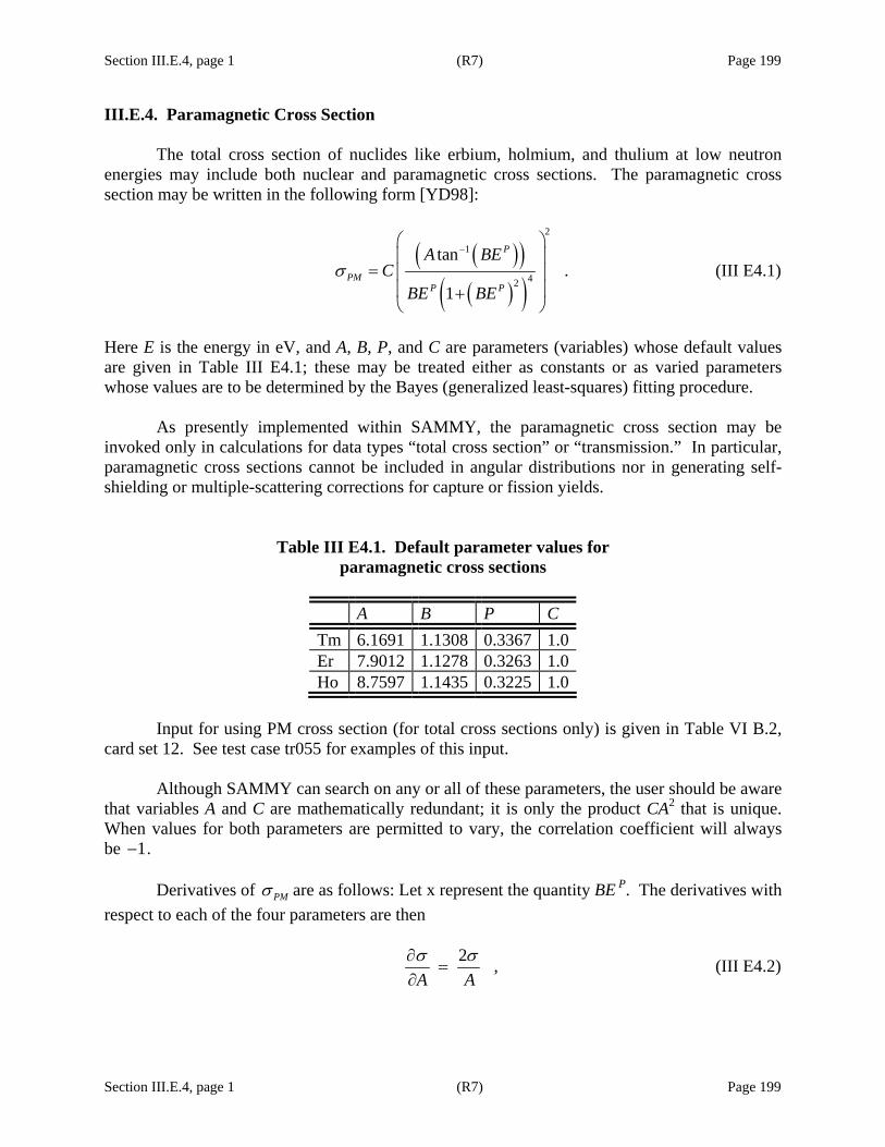
Section III.E.4, page 1 (R7) Page 199
Section III.E.4, page 1 (R7) Page 199
III.E.4. Paramagnetic Cross Section
The total cross section of nuclides like erbium, holmium, and thulium at low neutron energies may include both nuclear and paramagnetic cross sections. The paramagnetic cross section may be written in the following form [YD98]:
( )( )( )( )
2
1
42
tan.
1
P
PMP P
A BEC
BE BEσ
−⎛ ⎞⎜ ⎟
= ⎜ ⎟⎜ ⎟+⎝ ⎠
(III E4.1)
Here E is the energy in eV, and A, B, P, and C are parameters (variables) whose default values are given in Table III E4.1; these may be treated either as constants or as varied parameters whose values are to be determined by the Bayes (generalized least-squares) fitting procedure. As presently implemented within SAMMY, the paramagnetic cross section may be invoked only in calculations for data types “total cross section” or “transmission.” In particular, paramagnetic cross sections cannot be included in angular distributions nor in generating self-shielding or multiple-scattering corrections for capture or fission yields.
Table III E4.1. Default parameter values for paramagnetic cross sections
A B P C Tm 6.1691 1.1308 0.3367 1.0Er 7.9012 1.1278 0.3263 1.0Ho 8.7597 1.1435 0.3225 1.0
Input for using PM cross section (for total cross sections only) is given in Table VI B.2,
card set 12. See test case tr055 for examples of this input.
Although SAMMY can search on any or all of these parameters, the user should be aware that variables A and C are mathematically redundant; it is only the product CA2 that is unique. When values for both parameters are permitted to vary, the correlation coefficient will always be 1− .
Derivatives of PMσ are as follows: Let x represent the quantity BE P. The derivatives with respect to each of the four parameters are then
2 ,A Aσ σ∂
=∂
(III E4.2)

Section III.E.4, page 2 (R7) Page 200
Section III.E.4, page 2 (R7) Page 200
2 2 ,d f xC A fB d x Bσ∂
=∂
(III E4.3)
( )2 ln ,d fC A f x EP d xσ∂
=∂
(III E4.4)
and
.C Cσ σ∂
=∂
(III E4.5)
In these equations we have made the substitution
( )
1
42
tan ,1
xfx x
−
=+
(III E4.6)
so that
( )
21
52
1 1 91 tan .1
d f x xd x xx x
−⎡ ⎤−= −⎢ ⎥
⎣ ⎦+ (III E4.7)
Section III.E.5, page 1 (R7) Page 201
Section III.E.5, page 1 (R7) Page 201
III.E.5. Detector Efficiency
For measurements of capture or fission yields, the detectors may have different efficiencies for different l-values. SAMMY is equipped with a spin-group-dependent detector efficiency (multiplicative factor), which can be used to model this effect. The user may specify as many different efficiencies as needed, and delineate the spin groups to which those efficiencies apply. (See Table VI B.2, card set 15, for input details.) SAMMY will multiply the calculated capture or fission partial cross sections by the efficiencies prior to applying self-shielding and multiple-scattering corrections; these efficiencies can also be used with self-indication data. Note that the total and elastic cross sections (used in the calculation of self-shielding and multiple-scattering effects) are not multiplied by the efficiencies.
Test case tr078 contains examples of the use of spin-group-dependent detector efficiencies.


Section III.E.6, page 1 (R6) Page 203
Section III.E.6, page 1 (R6) Page 203
III.E.6. Self-Indication Measurements
Self-indication experiments involve a combination of both capture and transmission measurements. Two samples are used: the one closer to the source is used for transmission and the other is used for capture. Both samples contain the nuclide of interest. Such an experiment preferentially removes neutrons near the peak of the resonances for this nuclide, thus focusing on the shoulders or wings of a resonance.
Analysis of a self-indication experiment requires both calculation of transmission through the first sample and calculation of capture yield with self-shielding and multiple-scattering corrections for the second sample. Transmission is calculated as described in Section III.E.1, using parameters appropriate for that sample (for thickness, nuclide abundances, contaminants, temperature, etc.). Essentially, transmission T is given by ( ) ,T tnT E e σ−= (III E6.1) in which nT represents the sample thickness and σt the total cross section (appropriately Doppler broadened). Subscript T indicates that the thickness is that of the transmission sample; subscript t refers to the total cross section. The capture yield Y (E ) is calculated as described in Section III.D, using parameters appropriate for the capture sample; note that any of the three normalizations (as cross section, as yield, or as yield times total cross section) described in that section may be applied to the capture “yield” calculation here. The self-indication result is the product of the transmission and the capture yield, ( ) ( ) ( ) ,SI E T E Y E= (III E6.2) followed by resolution broadening.
Parameters such as “isotopic” (nuclide) abundances, effective temperature, and thickness, which are input in the usual fashion into SAMMY, are assumed to be those of the capture sample. Input of parameters appropriate for the transmission sample is via card set 11, line 7 of the PARameter file (see Table VI B.2). The phrase “self-indication” must occur in the INPut file (card set 8).
Test case tr057 has examples, using artificial data, for self-indication experiments.
[Note that the option to calculate the self-indication ratio is not yet implemented into SAMMY. This quantity is defined as the resolution-broadened SI(E) divided by the resolution-broadened capture yield Y(E); implementation of this feature is one of many “on the drawing board” for future work.]


Section III.E.7, page 1 (R7) Page 205
Section III.E.7, page 1 (R7) Page 205
III.E.7. Corrections for Angular Distributions Angular distribution measurements may require additional treatments for experimental conditions beyond those required by angle-integrated measurements. Two kinds of treatment are currently available in SAMMY; as experiments improve and the need arises for more sophisticated treatments, others will be added to the code. Attenuation
One type of correction for finite sample size in angular distributions is handled in much the same manner as in the code RFUNC, which was developed by F. G. Perey [FP89a] for calculating elastic angular distributions using the R-function approximation for spin-zero samples. Two effects are included, which are denoted “incident neutron attenuation” and “scattered neutron attenuation,” respectively.
Incident neutron attenuation is accomplished by multiplying the cross section by the factor
( ) ( ) ,exp ,in tot Dn Eθ σ− (III E7.1) where the “thickness” or attenuation ( )inn θ may be specified independently for each angle and may be treated as a search parameter. The cross section appearing in Eq. (III E7.1) is the Doppler-broadened total cross section.
The so-called “scattered neutron attenuation” is used to approximately describe three distinct effects: (1) Neutrons initially scattered in the direction of the detector may be re-scattered (or captured, or involved in some other reaction). (2) Neutrons not initially scattered toward the detector may, after two or more scatterings, ultimately reach the detector. (3) Both the sample and the detectors have large angular spreads.
To describe these effects, the cross section is multiplied by the attenuation factor ( ) ( ) ,exp ' .out tot xn Eθ σ− (III E7.2) Here the attenuation ( )outn θ again may be different for each angle and may be treated as a search parameter. The cross section in this equation is evaluated at the scattered energy for the particular angle and has been broadened (using a triangular resolution function) to approximate the effects of the angular spread of the detector and sample.
See Table VI B.2, card set 11, line 4, for details of the input for these attenuation factors.

Section III.E.7, page 2 (R7) Page 206
Section III.E.7, page 2 (R7) Page 206
Angle Average Another available correction for the finite sample size is a straight-line average over solid
angle, of the form
( )
( )
( )
( )cos cos
cos cos
,D D
D D
d d d ddd
θ θ θ θ
θ θ θ θ
σ σ μ μ− −
+ +
=ΩΩ ∫ ∫ (III E7.3)
in which the differential elastic cross section is assumed to be a function of cos(θ) but a constant with respect to the azimuthal angle φ.
The actual calculation in SAMMY is carried out in a relatively crude approximation which implicitly assumes that the angular spread is not large. The cross section is calculated at three angles: Dθ θ+ , θ , and Dθ θ− . Quadratic interpolation in cos(θ) is used so that the cross section at other angles is assumed to be given by
( ) ( )( )( )( )
( )( )( )( )
( )( )( )( )
,b c a c a b
A B Ca b a c b a b c c a c bμ μ μ μ μ μ
σ μ− − − − − −
= + +− − − − − −
(III E7.4)
in which we have set ( ) ( ) ( )cos cos cosa D b D cθ θ θ θ θ= + = − = (III E7.5) and
( ) ( ) ( ) .d a d b d c
A B Cd d dσ σ σ
= = =Ω Ω Ω
(III E7.6)
Substituting Eq. (III E7.4) into Eq. (III E7.3) and integrating gives the resulting average cross section
( )( )( )
21 3 2 3 2 .6
b ad c b a c b aA B Cd c a b a c a b cσ ⎡ ⎤−− − − + +
= + +⎢ ⎥Ω − − − −⎢ ⎥⎣ ⎦
(III E7.7)
To invoke this option, include the phrase
ANGLE-AVERAGE FOR DIfferential cross sections in the command section of the INPut file. The angles θ and angular spreads Dθ are given in card set 8 of that file (see Table VI A.1).
Section III.E.8, page 1 (R7) Page 207
Section III.E.8, page 1 (R7) Page 207
III.E.8. Energy-Scale Dependence on t0 and L
When analyzing two or more independent data sets, the problem of displacement between energy scales often arises. Proper alignment of energy scales has traditionally been a task for the analyst; however, help is available from SAMMY. Two methods are described here. First method:
In time-of-flight measurements, the energy of the incident neutron is determined from the
flight-path length L, the flight time t, and the initial time t0 as
( )
2
20
.2m LE
t t=
− (III E8.1)
By treating L and t0 as variables (parameters) and searching for those values of L and t0 which provide the best fit of experimental measurement to the calculated cross section, it is possible to adjust the energy scales to provide agreement between different data sets. See card set 11, line 6, of the PARameter file, Section VI, for input details.
Derivatives of the cross section with respect to flight-path length L and initial time t0 are given in terms of the derivative with respect to energy as
( )0 0 0
2E Et t E t t Eσ σ σ∂ ∂ ∂ ∂
= =∂ ∂ ∂ − ∂
(III E8.2)
and
2 .E EL L E L Eσ σ σ∂ ∂ ∂ ∂
= =∂ ∂ ∂ ∂
(III E8.3)
Recall that the cross section σ is given in terms of the scattering matrix U. The energy-dependence of σ is therefore that of U (via ρ) and of the ( )21/ k multiplicative factor. That is, this derivative is given by
2 ,k kE k E k Eσ σ ρ σ
ρ∂ ∂ ∂ ∂ ∂
= −∂ ∂ ∂ ∂ ∂
(III E8.4)
which can be rewritten as
2 .2ka
E k Eσ σ σ
ρ⎛ ⎞∂ ∂
= −⎜ ⎟∂ ∂⎝ ⎠ (III E8.5)
Section III.E.8, page 2 (R7) Page 208
Section III.E.8, page 2 (R7) Page 208
Combining this equation with Eqs.(III E8.2) and (III E8.3) gives
( ) ( )0 0 0
2t t t t tσ ρ σ σ
ρ∂ ∂
= −∂ − ∂ −
(III E8.6)
and
2 .L L Lσ ρ σ σ
ρ∂ ∂
= −∂ ∂
(III E8.7)
The derivative of the cross section with respect to ρ is again, as in Section II.D.1.c, found by substituting Eq. (II D1 c.9) into Eq. (II D1 c.6).
Note that relativistic corrections are often added to the expression in Eq. (III E8.1); such corrections are ignored in SAMMY's treatment of the t0 dependence.
Within SAMMY the value of L is not varied directly; rather, L is set equal to the product of the “initial” value Li times a dimensionless quantity L0. This dimensionless multiplier is generally given an initial value of 1.0, and the value is varied in the SAMMY run.
In preliminary studies, what has been found practical is to use this option somewhat apart from the mainstream of SAMMY analyses. The procedure that worked best in our trials was to first obtain a reasonably good fit to the “best” data set (the data set which, in the analyst’s judgment, has the “most correct” energy scale), with particular emphasis on obtaining accurate resonance energies. Next, modify the parameter file to vary only L0 and t0 (i.e., do not vary resonance energies or other resonance parameters) and make a SAMMY run to determine the best values for L0 and t0 for the data set in which the energy scale is “wrong.” Once those values have been determined, generate a modified data set which has the corrected energy scale and use the modified set in subsequent work. The code SAMFTZ, described in Section X.G of this manual, can be used to generate the modified data set. Second method:
Begin by fitting each data set separately from the others, establishing in particular appropriate energies for the largest resonances. Choose one data set (probably the transmission measurement with the longest flight path) as the standard. For each other data set, compare energies for individual resonances to those in the standard data set. By considering the relative energy difference as a function of resonance energy, a fit can be made to the functional form
' ,E E E a b EE E− Δ
= = + (III E8.8)

Section III.E.8, page 3 (R7) Page 209
Section III.E.8, page 3 (R7) Page 209
in which E is the energy of the resonance in the standard data set, and 'E the energy in the other data set. Equation (III E8.8) is the appropriate functional form, as can be seen by taking increments of Eq. (III E8.1),
( )0 0
0 0
2 2 ,E E E EE L t L tL t L t t
∂ ∂Δ = Δ + Δ = Δ + Δ
∂ ∂ − (III E8.9)
or
00
2 2 / 2 2 /2 2 .E m t mE L Lt E
E L L L L⎛ ⎞ΔΔ Δ Δ
= + Δ = + ⎜ ⎟⎜ ⎟⎝ ⎠
(III E8.10)
Once appropriate values are determined for a and b, all energies in the non-standard data set can be modified by replacing the original (incorrect) energy 'E by "E , where ( )' " " " .E E a b E E= + + (III E8.11)
Solution of this equation for "E can be done iteratively, with " 'E E≈ as starting value.

Section IV, page 1 (R8) Page 211
Section IV, page 1 (R8) Page 211
IV. THE FITTING PROCEDURE
In order to determine the parameter values that give the “best fit” of theoretical values to experimental measurements, a fitting procedure is needed. The procedure must properly incorporate all uncertainties in the measured data, including both statistical and systematic uncertainties, and should provide appropriate uncertainties and correlations for the resulting set of parameter values.∗
The fitting procedure must be able to deal with nonlinear systems. The procedure used in SAMMY is Bayes’ method, sometimes denoted “generalized least
squares.” See Section XI.C for a philosophical discussion of the implications of the use of Bayes’ method.
(In the limit of infinite prior uncertainty, under the customary assumptions of normality,
Bayes’ method reduces to the more familiar least-squares method. SAMMY contains provisions for using the least-squares method rather than the more powerful generalized least squares; see Section IV.E.3 for details.)
Section IV.A is devoted to a formal description of the relevant equations for Bayes’ method. Starting from Bayes= theorem [HJ61] and three basic assumptions, formulae are derived for updating parameter values and parameter covariance matrix elements based on information contained in the data currently being analyzed. These formulae, in their several guises, are hereafter referred to as Bayes= equations. The three versions used in the SAMMY code are derived in Section IV.A.1, and the iterative versions thereof (for use with nonlinear systems) in Section IV.A.3. Formulae for chi squared are developed and discussed in Section IV.A.2.
Implementation of each of the three versions of Bayes’ equations in SAMMY is described in Section IV.B.
Most input parameters may be fitted in the SAMMY code, though the actual fitted parameter
is not always the variable given in the input. For example, though values for the resonance energies are given in the PARameter file, the variable used in the fitting procedure is the square root of the resonance energy. In Section IV.C, parameters that may be varied are listed.
Section IV.D contains a discussion of the Data Covariance Matrix (DCM), its role in Bayes’ equations, and SAMMY’s various treatments of the DCM. SAMMY has the ability to read, store, and invert a full off-diagonal DCM; however, the reader should be aware that this is a highly inefficient method for treating experimental uncertainties. Instead, when components of the DCM are generated external to SAMMY, those components (rather than the DCM itself) should be used as input to the code via the User-Supplied Implicit DCM option (Section VI.C.3.b has input details for this option). To include the contribution from uncertainties on SAMMY input parameters, the Propagated Uncertainty Parameter (PUP) option is available; see the discussion in Section IV.D.2
∗ Uncertainties determined by R-matrix codes are often deemed to be too small. It is this author’s opinion that the resonance parameter uncertainties are correct but that the resonance parameter covariance matrix alone is insufficient to describe all the uncertainty in the evaluated cross sections. For further discussion on this topic, the reader is referred to Section IV.E.6.

Section IV, page 2 (R8) Page 212
Section IV, page 2 (R8) Page 212
and the input details in Section VI.C.3.a. In both cases, the full DCM is not calculated; instead, the treatment is via SAMMY’s Implicit Data Covariance (IDC) method, described in Section IV.D.3.
Section IV.E contains information about a variety of topics related to covariances. For a discussion of simultaneous (rather than sequential) fitting of several data sets, see Section IV.E.1. In Section IV.E.2, information is found on SAMMY’s retroactive covariance method, whereby a parameter covariance matrix can be generated that is approximately correct for a given parameter set. To use an infinite prior parameter covariance matrix (i.e., to use the least-squares equations), see Section IV.E.3. Generating the covariance matrix associated with the theoretical cross section is described in Section IV.E.4. Section IV.E.5 describes SAMMY’s method for calculating average values and uncertainties for certain classes of resonance parameters (e.g., the average capture or neutron width for all resonances in a particular spin group). Finally, Section IV.E.6 contains a discussion of the capability of the resonance parameter covariance matrix (RPCM) to produce credible cross section covariance matrices and describes available methods for altering or augmenting the SAMMY-produced RPCM, in preparation for reporting to ENDF and/or publishing results.
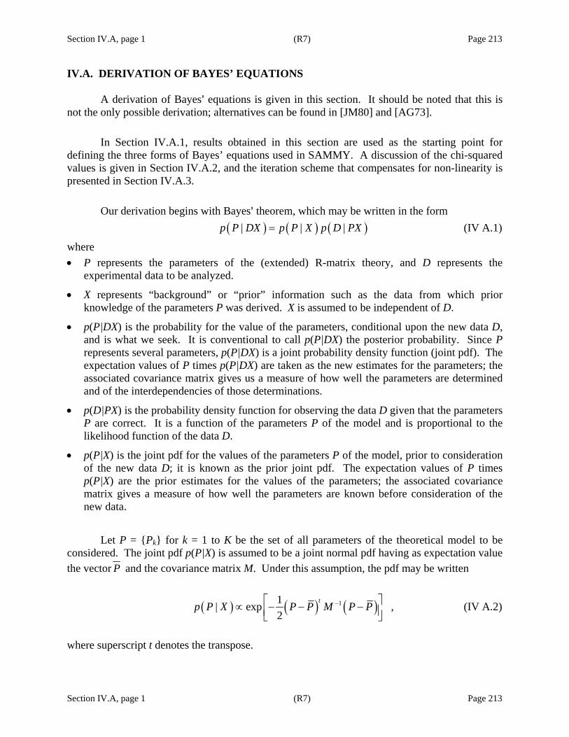
Section IV.A, page 1 (R7) Page 213
Section IV.A, page 1 (R7) Page 213
IV.A. DERIVATION OF BAYES’ EQUATIONS
A derivation of Bayes= equations is given in this section. It should be noted that this is not the only possible derivation; alternatives can be found in [JM80] and [AG73].
In Section IV.A.1, results obtained in this section are used as the starting point for
defining the three forms of Bayes’ equations used in SAMMY. A discussion of the chi-squared values is given in Section IV.A.2, and the iteration scheme that compensates for non-linearity is presented in Section IV.A.3.
Our derivation begins with Bayes= theorem, which may be written in the form ( ) ( ) ( )| | |p P DX p P X p D PX= (IV A.1)
where • P represents the parameters of the (extended) R-matrix theory, and D represents the
experimental data to be analyzed.
• X represents “background” or “prior” information such as the data from which prior knowledge of the parameters P was derived. X is assumed to be independent of D.
• p(P|DX) is the probability for the value of the parameters, conditional upon the new data D, and is what we seek. It is conventional to call p(P|DX) the posterior probability. Since P represents several parameters, p(P|DX) is a joint probability density function (joint pdf). The expectation values of P times p(P|DX) are taken as the new estimates for the parameters; the associated covariance matrix gives us a measure of how well the parameters are determined and of the interdependencies of those determinations.
• p(D|PX) is the probability density function for observing the data D given that the parameters P are correct. It is a function of the parameters P of the model and is proportional to the likelihood function of the data D.
• p(P|X) is the joint pdf for the values of the parameters P of the model, prior to consideration of the new data D; it is known as the prior joint pdf. The expectation values of P times p(P|X) are the prior estimates for the values of the parameters; the associated covariance matrix gives a measure of how well the parameters are known before consideration of the new data.
Let P = Pk for k = 1 to K be the set of all parameters of the theoretical model to be
considered. The joint pdf p(P|X) is assumed to be a joint normal pdf having as expectation value the vector P and the covariance matrix M. Under this assumption, the pdf may be written
( ) ( ) ( )11| exp ,2
tp P X P P M P P−⎡ ⎤∝ − − −⎢ ⎥⎣ ⎦
(IV A.2)
where superscript t denotes the transpose.

Section IV.A, page 2 (R7) Page 214
Section IV.A, page 2 (R7) Page 214
The experimental data are represented by a data vector D whose components Di are the L data points. The experimental conditions are assumed to be such that the data D (i.e., the Di=s) have a joint normal distribution with mean ( )D T T P= = and covariance matrix V. The likelihood function is then
( ) ( ) ( )11| ~ exp .2
tp D PX D T V D T−⎡ ⎤− − −⎢ ⎥⎣ ⎦ (IV A.3)
Here T represents theory (i.e., calculated values of cross section or transmission plus corrections), and the covariance matrix V represents not only the experimental “errors” of the data but also any theoretical “errors” resulting from approximations used in calculating T. Obviously V need not be diagonal.
Combining Eqs. (IV A.1), (IV A.2), and (IV A.3) gives an expression for the pdf of P after consideration of new data D [i.e., for p (P|DX ) ], expressed in terms of the “true” value T. What is needed, however, is an expressions for p (P|DX ) expressed in terms of the parameters P. This is obtained formally by considering T a function of P, performing a Taylor expansion about P [the expectation value of p (P|X ) ], and keeping only the linear terms:
( ) ( ) . . . ,T P T G P P= + − + (IV A.4)
where ( )T T P= . The elements of G, often denoted the “sensitivity matrix,” are the partial
derivatives of Tn with respect to the parameters Pk , evaluated at P P= :
= 1 to
for = 1 to .
nnk
k P P
n LTGk KP
=
⎧∂= ⎨∂ ⎩
(IV A.5)
Because T is a vector of dimension L (equal to the number of data points), and P is a vector of dimension K (equal to the number of parameters), the sensitivity matrix G has dimension L H K.
Substituting Eq. (IV A.4) into Eq. (IV A.3) and using Eq. (IV A.2), we obtain for the posterior joint pdf [Eq. (IV A.1)]
( ) ( ) ( )
( )( ) ( )( )
1
1
1| ~ exp2
.
t
t
p P DX P P M P P
D T G P P V D T G P P
−
−
⎡− − − +⎢⎣⎤− − − − − − ⎥⎦
(IV A.6)
Because of the three basic assumptions we have made, that is,
i. the prior joint pdf is a joint normal, Eq. (IV A.2), ii. the likelihood function is a joint normal, Eq. (IV A.3), and iii. the true value is a linear function of the parameters, Eq. (IV A.4) with (IV A.5),

Section IV.A, page 3 (R7) Page 215
Section IV.A, page 3 (R7) Page 215
it follows that the posterior joint pdf is also a joint normal. Denoting its expectation value by 'P and its covariance matrix by 'M , we may write
( ) ( ) ( ) ( ) 11| ~ exp ' ' ' .2
tp P DX P P M P P−⎡ ⎤− − −⎢ ⎥⎣ ⎦
(IV A.7)
Substituting Eqs. (IV A.2), (IV A.3), and (IV A.7) into (IV A.1) gives
( ) ( ) ( ) ( ) ( )
( ) ( )
1 1
1
1 1exp ' ' ' ~ exp2 2
1exp ,2
t t
t
P P M P P P P M P P
D T V D T
− −
−
⎡ ⎤ ⎡ ⎤− − − − − −⎢ ⎥ ⎢ ⎥⎣ ⎦ ⎣ ⎦⎡ ⎤× − − −⎢ ⎥⎣ ⎦
(IV A.8)
which is valid up to a normalization constant. To simplify this expression, we substitute Eq. (IV A.4) for T, obtaining
( ) ( ) ( ) ( ) ( )
( )( ) ( )( )
1 1
1
1 1exp ' ' ' ~ exp2 2
1exp .2
t t
t
P P M P P P P M P P
D T G P P V D T G P P
− −
−
⎡ ⎤ ⎡ ⎤− − − − − −⎢ ⎥ ⎢ ⎥⎣ ⎦ ⎣ ⎦⎡ ⎤× − − − − − − −⎢ ⎥⎣ ⎦
(IV A.9)
In this form, the theoretical function T is treated as strictly linear with respect to the parameters. (In Section.IV.A.3, this formula will be generalized for nonlinear T.) Rearranging the exponents gives
( ) ( ) ( )( ) ( )( )( ) ( ) ( ) ( )( ) ( )
1
1 1
1 1
1
1exp ' ' '2
constant,
t
t t
t tt
t
P P M P P
P P M G V G P P
P P G V D T D T V G P P
D T V D T
−
− −
− −
−
⎡− − −⎢⎣
− − + −
+ − − + − −
⎤− − − =⎥⎦
(IV A.10)
where the value of the constant depends upon the unspecified normalizations. After setting ' 'P P P P P P− = − + − (IV A.11) and rearranging, Eq. (IV A.10) becomes

Section IV.A, page 4 (R7) Page 216
Section IV.A, page 4 (R7) Page 216
( ) ( ) ( ) ( ) ( ) ( )( ) ( ) ( ) ( ) ( ) ( )( ) ( )( )( ) ( ) ( ) ( )( ) ( )
1 1
1 1
1 1
1 1
1
1exp ' ' '2
' ' ' ' '
constant,
t t
t t
t t
t tt
t
P P M P P P P M P P
P P M P P P P M P P
P P M G V G P P
P P G V D T D T V G P P
D T V D T
− −
− −
− −
− −
−
⎡− − − + − −⎢⎣
+ − − + − −
− − + −
+ − − + − −
⎤− − − =⎥⎦
(IV A.12)
or
( ) ( ) ( ) ( )( ) ( ) ( ) ( )
( ) ( ) ( ) ( )
( ) ( ) ( ) ( ) ( )
1 1 1
1 1
1 1
1 1
1exp '2
' '
' '
' ' ' constant.
t t
t t
t t
t t
P P M M G V G P P
P P M P P G V D T
P P M D T V G P P
P P M P P D T V D T
− − −
− −
− −
− −
⎡ ⎡ ⎤− − − + −⎢ ⎣ ⎦⎣⎡ ⎤+ − − + −⎣ ⎦
⎡ ⎤+ − + − −⎣ ⎦
⎤+ − − − − − =⎥⎦
(IV A.13)
In order for Eq. (IV A.13) to be valid for all P, the exponent must be constant. For this to happen, the terms linear and quadratic in ( )P P− must separately be equal to zero. This gives us two equations relating the primed (posterior) values to the unprimed (prior) values:
( ) ( )1 1 1' 0tM M G V G− − −− + = (IV A.14)
and ( ) ( ) ( )1 1' ' 0 ,tM P P G V D T− −− + − = (IV A.15)
which can be rewritten in the form
( ) 1 1 1' tM M G V G− − −= + (IV A.16)
and ( )1' ' .tP P M G V D T−= + − (IV A.17)
Equations (IV A.16) and (IV A.17) are denoted “Bayes’ Equations,” sometimes called
“generalized least squares” for reasons which shall be discussed later. Three distinct but equivalent versions of these equations are used within the SAMMY code, as described in the next section of this manual (Section IV.A.1).

Section IV.A.1, page 1 (R7) Page 217
Section IV.A.1, page 1 (R7) Page 217
IV.A.1. Derivation of SAMMY’s Solution Schemes Three distinct versions of Bayes’ equations are used in the SAMMY computer code. More specifically, it is the equation for M ' that differs in the three versions. Each has computational advantages and disadvantages for particular situations; these are described in Section IV.B. In this section, the three versions are derived from the forms found in Eqs. (IV A.16) and (IV A.17), which are repeated here: ( ) 1 1 1' tM M G V G− − −= + (IV A1.1) and ( )1' ' .tP P M G V D T−= + − (IV A1.2) Here the bars have been dropped for simplicity of notation. For readers who may be unfamiliar with matrix notation, the final equations are given at the end of this section with indices and summations explicitly displayed. M+W Version The version of Bayes’ Equations which uses Eqs. (IV A1.1) and (IV A1.2) directly is denoted the “M+W” version,
( )( )
11
1 1
' ' '
,t t
M M W P P M Y
W G V G Y G V D T
−−
− −
= + = +
= = − (IV A1.3)
in which the matrix quantities Y and W have been introduced to simplify later discussion. (See especially Section IV.E.1.)
In this form, the relationship of Bayes’ equations to the more common least-squares equations is transparent: If the prior parameter covariance matrix M is infinite on the diagonal ( )1 0M − = , then the equations in Eq. (IV A1.3) become the least-squares equations; the only difference is in the first equation. Hence the least-squares equations may be considered to be a special case of Bayes’ equations; alternatively, Bayes’ Equations may be viewed as generalized least squares.
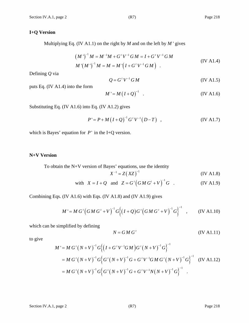
Section IV.A.1, page 2 (R7) Page 218
Section IV.A.1, page 2 (R7) Page 218
I+Q Version Multiplying Eq. (IV A1.1) on the right by M and on the left by M ' gives
( )
( ) ( )
1 1 1 1
1 1
'
' ' ' .
t t
t
M M M M G V G M I G V G M
M M M M M I G V G M
− − − −
− −
= + = +
= = + (IV A1.4)
Defining Q via 1tQ G V G M−= (IV A1.5) puts Eq. (IV A1.4) into the form ( ) 1' .M M I Q −= + (IV A1.6) Substituting Eq. (IV A1.6) into Eq. (IV A1.2) gives ( ) ( )1 1' ,tP P M I Q G V D T− −= + + − (IV A1.7) which is Bayes’ equation for 'P in the I+Q version. N+V Version To obtain the N+V version of Bayes’ equations, use the identity ( ) 11X Z XZ −− = (IV A1.8)
( ) 1with and .t tX I Q Z G G M G V G
−= + = + (IV A1.9)
Combining Eqs. (IV A1.6) with Eqs. (IV A1.8) and (IV A1.9) gives
( ) ( ) ( ) 11 1' ,t t t tM M G G M G V G I Q G G M G V G
−− −= + + + (IV A1.10)
which can be simplified by defining tN G M G= (IV A1.11) to give
( ) ( ) ( ) ( ) ( ) ( ) ( ) ( ) ( )
11 11
11 1 11
11 1 11
'
.
t t t
t t t t
t t t
M M G N V G I G V G M G N V G
M G N V G G N V G G V G M G N V G
M G N V G G N V G G V N N V G
−− −−
−− − −−
−− − −−
= + + +
= + + + +
= + + + +
(IV A1.12)

Section IV.A.1, page 3 (R7) Page 219
Section IV.A.1, page 3 (R7) Page 219
Rearranging gives
( ) ( ) ( )( ) ( ) ( ) ( )( )( ) ( ) ( ) ( )( ) ( ) ( ) ( ) ( )
( )( )
11 1 11
11 1 11
11 1 11
11 1
11 1 1
11 1 1
11 1 1
1
' t t
t t
t t
t t
t t
t t
t t
t
M M G N V G G N V V N N V G
M G N V G G N V V N V V N V G
M G N V G G N V V N V G
M G N V G G V G
M G N V V V G G V G
M G N V N V N V G G V G
M G I N V N V G G V G
M G V G N
−− − −−
−− − −−
−− − −−
−− −
−− − −
−− − −
−− − −
−
= + + + +
= + + + + − +
= + + + − +
= +
= +
= + + −
⎡ ⎤= − +⎣ ⎦
= − ( )( ) ( )( )
( )
11 1 1
111 1 1
1 .
t t
t t t t
t
V G M G V G G V G
M G V G G N V G M G V G G V G
M M G N V G M
−− − −
−−− − −
−
+
= − +
= − + (IV A1.13) This is the N+V version of Bayes’ Equation for 'M : ( ) 1' .tM M M G N V G M−= − + (IV A1.14) The N+V version of Bayes’ equation for 'P is found by inserting Eq. (IV A1.14) into Eq. (IV A1.2) and rearranging:
( ) ( )
( ) ( )
( ) ( )
( ) [ ] ( )
( ) ( ) ( ) ( )
( ) ( )
( ) ( )
1 1
1 1
1 1
1 1
1 1 1
1 1
1
'
.
t t
t t t
t
t
t
t
t
P P M M G N V G M G V D T
P M G M G N V G MG V D T
P M G I N V N V D T
P M G I N V N V V V D T
P M G I N V N V N V V V D T
P M G I I N V V V D T
P M G N V D T
− −
− −
− −
− −
− − −
− −
−
⎡ ⎤= + − + −⎣ ⎦⎡ ⎤= + − + −⎣ ⎦
⎡ ⎤= + − + −⎣ ⎦⎡ ⎤= + − + + − −⎣ ⎦⎡ ⎤= + − + + + + −⎣ ⎦⎡ ⎤= + − + + −⎣ ⎦
= + + −
(IV A1.15)
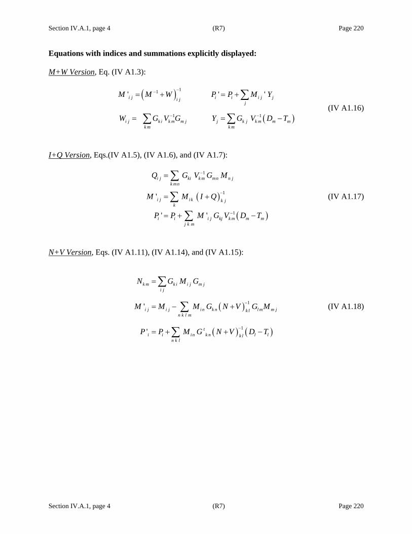
Section IV.A.1, page 4 (R7) Page 220
Section IV.A.1, page 4 (R7) Page 220
Equations with indices and summations explicitly displayed: M+W Version, Eq. (IV A1.3):
( )
( )
11
1 1
' ' 'i j i i i j ji jj
i j k i k m m j j k j k m m mk m k m
M M W P P M Y
W G V G Y G V D T
−−
− −
= + = +
= = −
∑
∑ ∑ (IV A1.16)
I+Q Version, Eqs.(IV A1.5), (IV A1.6), and (IV A1.7):
( )
( )
1
1
1
'
' '
i j ki k m mn n jk mn
i j i k k jk
i i i j kj k m m mj k m
Q G V G M
M M I Q
P P M G V D T
−
−
−
=
= +
= + −
∑
∑
∑
(IV A1.17)
N+V Version, Eqs. (IV A1.11), (IV A1.14), and (IV A1.15):
( )
( ) ( )
1
1
'
'
k m k i i j m ji j
i j i j i n k n l m m jk ln k l m
ti i i n k n l lk l
n k l
N G M G
M M M G N V G M
P P M G N V D T
−
−
=
= − +
= + + −
∑
∑
∑
(IV A1.18)
Section IV.A.2, page 1 (R7) Page 221
Section IV.A.2, page 1 (R7) Page 221
IV.A.2. Chi-Squared and Weighted Residuals The negative of the constant term (the P-independent term) in the exponent of Eq. (IVA.13), which we shall label as 2
Bayesχ and denote the “Bayesian chi squared,” is of the form ( ) ( ) ( ) ( ) ( )12 1
Bayes ' ' ' .t t
P P M P P D T V D Tχ − −= − − − + − − (IV A2.1) The second term in this expression is exactly the usual χ2 value, defined as ( ) ( )2 1
LS .t
D T V D Tχ −= − − (IV A2.2) The least-squares χ2 is always larger than the Bayesian χ2 because the difference [the first term in the right-hand side of Eq.(IV A2.1)] is the negative of a squared quantity. What is observed during a successful Bayes fit is that the value of the least-squares 2
LSχ decreases with
each iteration, while the value of the Bayesian 2Bayesχ changes very little. In fact, the value of
2LSχ becomes very close to the value of 2
Bayesχ as the iterations proceed. (See Section IV.A.3 for a discussion of iteration as compensation for nonlinearity.) Hence, the Bayesian χ2 is, in some sense, a measure of the “best fit” that can be found between this theoretical formulation and these experimental data. When a very small 2
LSχ value
is considered to be a goal of the analysis process, but the value of 2Bayesχ is relatively large, the
analyst may find it prudent to look for problems with either the theory or the data before attempting to find a good fit. For example, spin assignments might be incorrect (Section II.C.1), background might not have been properly included (Section III.E.3.a), or multiple-scattering corrections might be needed (Section III.D).
The expression for 2Bayesχ can be written in terms of known quantities as follows:
Replacing ( )'P P− by its value as given in the expression in Eq. (IV.A.16) gives
( ) ( ) ( ) ( ) ( )( )( )( ) ( )( ) ( ) ( )( ) ( ) ( ) ( )( ) ( )
12 1Bayes
11 1 1
1 1 1
1 1 1
' ' '
' ' '
'
' .
t t
tt t
tt t
t t
P P M P P D T V D T
D T V G M M M G V D T D T V D T
D T V G M G V D T D T V D T
D T V G M G V V D T
χ − −
−− − −
− − −
− − −
= − − − + − −
= − − − + − −
= − − − + − −
= − − + −
(IV A2.3)
In the M+W version for M ', 2
Bayesχ therefore becomes

Section IV.A.2, page 2 (R7) Page 222
Section IV.A.2, page 2 (R7) Page 222
( ) ( ) ( )12 1 1 1 1Bayes ,
t tD T V G M W G V V D Tχ−− − − −= − − + + − (IV A2.4)
where W is again defined as 1tG V G− .
In the I+Q version, 2Bayesχ takes the form
( ) ( ) ( )12 1 1 1
Bayes ,t tD T V G M I Q G V V D Tχ −− − −= − − + + − (IV A2.5)
where Q is 1tG V G M− .
Finally, in the N+V version,
( ) ( ) ( )12 1 1 1Bayes ,
t t tD T V G M M G N V G M G V V D Tχ −− − −⎡ ⎤= − − − + + −⎣ ⎦ (IV A2.6)
in which N is equal to tG M G . The expression in the curly brackets in Eq. (IV A2.6) can be simplified significantly as
( )
( )( )
( )
( )( )
( )
( ) ( )
11 1 1
11 1 1 1 1
11 1 1 1 1
11 1
11 1
11 1
11 1
1
t t
t t t
V G M M G N V G M G V V
V G M G V V G M G N V G M G V V
V N V V N N V N V V
V N N N V N V V
V N N V V N V N V V
V N N V N V N V V
V V N V N V V V V
V V
−− − −
−− − − − −
−− − − − −
−− −
−− −
−− −
−− −
−
⎡ ⎤= − − + +⎣ ⎦
= − + + +
= − + + +
⎡ ⎤= − + + +⎣ ⎦⎡ ⎤= − + + − + +⎣ ⎦⎡ ⎤= − + − + +⎣ ⎦⎡ ⎤= − + + − +⎣ ⎦
= − ( )
( ) ( )
1 1
1 11 1 .
V N V V V V
V V N V V V N V
− −
− −− −
⎡ ⎤+ + +⎣ ⎦⎡ ⎤= + = +⎣ ⎦
(IV A2.7)
Making this substitution into Eq. (IV A2.6) gives ( ) ( ) ( )12
Bayest
D T N V D Tχ −= − + − (IV A2.8) for the N+V version of 2
Bayesχ .
Section IV.A.2, page 3 (R7) Page 223
Section IV.A.2, page 3 (R7) Page 223
Values for χ2 (of both types) are reported in the SAMMY output file SAMMY.LPT (see Section VII.A). It should be noted, however, that SAMMY does not report χ2/ dof (where dof = degrees of freedom = NDAT − NPAR, with NDAT being the number of data points and NPAR the number of varied parameters), since with Bayes= method dof can be zero or negative. Instead SAMMY will report χ2 and χ2/NDAT. Caveat: In the past (prior to the release of sammy-7.0.0 in 2006), the value of 2
LSχ , as reported in the SAMMY.LPT file, was calculated under the implicit assumption that the data covariance matrix V was diagonal. This is no longer true; 2
LSχ is now calculated using the actual data covariance matrix, including off-diagonal elements if they are present. Another quantity that the analyst will often find useful to examine is the so-called weighted residual, which is the difference between measured value and theoretical value weighted (divided) by the uncertainty on the measured value. Specifically, the weighted residual at point i is defined as ( )LS ,i i i iiR D T V= − (IV A2.9) a formula that implicitly assumes that the data covariance matrix is diagonal, since off-diagonal elements are ignored. To ask for this array to be printed, the user should specify “PRINT WEIGHTED RESIDuals” in the command section of the INPut file; see Table VI A1.2. The array will be printed, however, only if the data covariance matrix is diagonal. SAMMY recognizes another array related to the weight residuals and denotes it as the “Bayesian weighted residual,” ( ) ( )1B .i j ji j
j
R N V D T−= + −∑ (IV A2.10)
No particular physical interpretation is applied to this quantity. To calculate and print this array, insert the command “PRINT BAYES WEIGHTED residuals” into the INPut file. If the command “PRINT WEIGHTED RESIDuals” is given, and this array is generated in the normal course of solving Bayes’ equations, then it will be printed even though it was not explicitly called for.

Section IV.A.3, page 1 (R8) Page 225
Section IV.A.3, page 1 (R8) Page 225
IV.A.3. Iteration Scheme
The linearity hypothesis, that is, the assumption that the Taylor expansion of the theoretical values around the prior expectation value truncates after the linear term, is in general only approximately true. Therefore, the parameter values 'P resulting from application of Bayes= equations are also only approximately correct. To obtain more accurate values, the Taylor expansion, Eq. (IV A.4), may be performed not around P but around the new (intermediate) values ( )nP , where n represents the nth iteration and ( )0P P= . That is, we assume
( ) ( ) ( )( ) ( ) ( ) ( ) ( ) ( )( )( ) ( ) ( ) ( )( ) ( ) ( )( )
0 0
0 0 .
n n n n n n
n n n n
T T G P P T G P P P P
T G P P G P P
≅ + − = + − + −
= + − + − (IV A3.1)
Here the sensitivity matrix ( )nG and the theoretical values ( )nT are evaluated at ( )nP P= . With Eq. (IV A3.1) for T, the formula analogous to Eq. (IV A.13) is
( )( ) ( )( ) ( ) ( )( ) ( )( )( )( ) ( )( ) ( ) ( )( )
( ) ( ) ( ) ( ) ( )( )( )( ) ( )( ) ( )( )
( ) ( ) ( ) ( )( )( ) ( ) ( )( )( )( ) ( )( ) ( ) ( )( )
( ) ( ) ( ) ( )( )( ) ( ) ( ) ( ) ( )( )( )
10 1 01 1
10 1 0 1
01
10 1 1
0 01
11 1 0 10
0 01
1exp2
constant .
t n n t n
t n n
n t n n n
tn n
tn n n n
tn n n
tn n n n n n
P P M M G V G P P
P P M P P
G V D T G P P
P P M
D T G P P V G P P
P P M P P
D T G P P V D T G P P
−+ − −
−+ +
−
−+ +
−
−+ + +
−
⎡ ⎡ ⎤− − − + −⎢ ⎢ ⎥⎣ ⎦⎣⎡+ − −⎢⎣
⎤− − − − ⎥⎦⎡+ −⎢⎣
⎤− − − − −⎥⎦
+ − −
⎤− − − − − − − ⎥⎦=
(IV A3.2)
The iterative forms of Bayes= equations follow immediately, by replacing G by ( )nG and T
by ( ) ( ) ( ) ( )( )0n n nT G P P− − in the equations of Section IV A.1. Note that again we have dropped
the bars to simplify the notation. Explicitly, the equations are as follows: For the M+W version, Eq. (IV A1.3) becomes
( ) ( )( ) ( ) ( ) ( ) ( )
( ) ( ) ( ) ( ) ( ) ( ) ( ) ( ) ( )( )( )
11 1 0 11
01 1 .
n n n n n
n n t n n n t n n n
M M W P P M Y
W G V G Y G V D T G P P
−+ + +−
− −
= + = +
= = − − −(IV A3.3)
Section IV.A.3, page 2 (R8) Page 226
Section IV.A.3, page 2 (R8) Page 226
For the I+Q version, the covariance equations, Eqs. (IV A1.5) and (IV A1.6), take the form
( ) ( ) ( ) ( ) ( )( ) 111 and ,n n t n n nQ G V G M M M I Q−+−= = + (IV A3.4)
and for the N+V version, Eqs. (IV A1.10) and (IV A1.13) become
( ) ( ) ( )( ) ( ) ( ) ( )11 with .n n t n n n n tM M M G N V G M N G M G−+ = − + = (IV A3.5)
For all versions, the parameter equation is
( ) ( ) ( ) ( ) ( ) ( ) ( ) ( )( )( )1 0 1 01 .n n n t n n nP P M G V D T G P P+ + −= + − − − (IV A3.6)
To control the number of iterations When running SAMMY, the default number of iterations is 2; that is, SAMMY stops after calculating ( ) ( )2 2 and P M . This value was chosen based on early experience which suggested that, for many practical applications, little was gained from additional iterations: After two iterations, the value of a parameter would generally be accurate to within the uncertainty on that parameter. To illustrate, suppose the “true” value of a parameter was 1.23456789 ± 0.03456789. After two iterations, the value was found to be approximately 1.23500000 ± 0.03500000, so no useful new information is gained by continuing the computations.
Nevertheless, especially during early stages of an analysis, the user will often find it helpful to iterate more times. To increase the number of iterations, specify ITMAX in columns 46–50 of line 2 (i.e., card set 2) of the INPut file, Table VIA.1.
Caveat: Setting ITMAX = 0 in the INPut file will cause the default value ITMAX = 2 to be used. In order to obtain zero iterations (i.e., to evaluate the cross section but not update the parameter values), the user must specify “DO NOT SOLVE BAYES Equations” in the command section of the INPut file.
Caveat: Some older compilers interpret “1” (one) in column 49 as “10” (ten). To avoid undue difficulties caused by having misplaced a number by one column, SAMMY assumes that a value of ITMAX greater than 9 was an input error. If more than 9 iterations are wanted, the user must insert the negative of the correct value into the INPut file.
At present there are no criteria in SAMMY for stopping the iterations when convergence is reached. These may be added in the future.

Section IV.B, page 1 (R7) Page 227
Section IV.B, page 1 (R7) Page 227
IV.B. IMPLEMENTATION OF BAYES= EQUATIONS
Each of the three forms of Bayes’ equations has its own strengths and weaknesses.
In the original version of SAMMY (circa 1978), only the N+V method was available. This method requires inversion of a symmetric square matrix whose size is the number of experimental data points – a prohibitive requirement, in the case where off-diagonal data covariance matrix elements exist. The I+Q method requires inversion of a non-symmetric square matrix whose size is the number of varied parameters; in its original form, however, I+Q also required that the data covariance matrix be diagonal. The M+W method also requires inversion of a matrix whose size is the number of varied parameters; in this case, the matrix is symmetric.
SAMMY=s method of solution of Bayes= equations for N+V inversion scheme is described in Section IV.B.1, and the solution for the I+Q scheme in Section IV.B.2. The M+W solution method is discussed in Section IV.B.3.
By default, analyses in the resolved resonance region (RRR) use either the N+V or the I+Q method, and SAMMY will choose the method requiring the least amount of computer memory. In general, this means that analyses involving a large number of parameters and/or an off-diagonal data covariance matrix will use N+V, and analyses involving relatively few parameters and a diagonal data covariance matrix will use I+Q.
Under certain circumstances, it is possible for the user to override SAMMY’s default choice of which method to use. (This is accomplished by inserting the command “NPV” or “IPQ” in the INPut file; see Table VI A1.2.) When both N+V and I+Q are possible, they give the same results but consume different amounts of computer resources (memory and time).
Analyses in the unresolved resonance region use only the M+W method. For truly simultaneous fitting of a number of data sets in the RRR, the M+W is used and can
be made to behave as a least-squares process. The retroactive covariance matrix generation scheme also uses M+W. See Section IV.E for discussions of these topics.
Certain types of off-diagonal data covariance matrices can be accommodated by any of the three forms of Bayes’ equations. See Section IV.D for a discussion of the implicit data covariance (IDC) techniques and propagated uncertainty parameters (PUPs).


Section IV.B.1, page 1 (R7) Page 229
Section IV.B.1, page 1 (R7) Page 229
IV.B.1. Solving Bayes= Equations: N+V Inversion Scheme
SAMMY uses coding similar to that in the code BAYES [NL82] to solve Bayes= equations in the N+V inversion scheme. In matrix notation, the noniterative form of Bayes= equations can be written ( ) ( )1' tP P M G N V D T−− = + − (IV B1.1) and ( ) 1' ,tM M M G N V G M−= − + (IV B1.2) where N is given by .tN G M G= (IV B1.3) Solving these equations is equivalent to solving AX Y= (IV B1.4) K + 1 times (where K is the number of parameters for the problem), with A the L H L symmetric matrix N + V (where L is the number of data points), and Y a column matrix equal to ( )D T− in Eq. (IV B1.1) or equal to each of the K columns of the rectangular matrix GM in Eq. (IV B1.2).
The inverse of matrix A is not evaluated directly. Rather, A is first factorized as tA U BU= (IV B1.5) where B is a block-diagonal matrix and U is the product of elementary unit triangular and permutation matrices, so that inverses of U and B are immediately available. The solution X to Eq.(IV B1.4) is then found from ( )1 1 1 .
tX U B U Y− − −= (IV B1.6)
In SAMMY, the factorization of Eq. (IV B1.5) is performed by the LINPACK [JD79] subroutine SSPCO, and the (K + 1) solutions are obtained by LINPACK subroutine SSPSL (with the SAMMY author=s updates for double precision). Subroutine NEWPAR oversees these operations.
As explained earlier, it is necessary to modify this procedure slightly to account for the approximations built into Bayes= equations. Details are given in Section IV.A.3.


Section IV.B.2, page 1 (R7) Page 231
Section IV.B.2, page 1 (R7) Page 231
IV.B.2. Solving Bayes= Equations: I+Q Inversion Scheme
In matrix notation, the noniterative form of Bayes= equations for the I+Q inversion scheme can be written ( ) ( )1 1' tP P M I Q G V D T− −− = + − (IV B2.1) and ( ) 1' ,M M I Q −= + (IV B2.2) where Q is given by 1 .tQ G V G M−= (IV B2.3) Although Q (and thus I + Q) is not symmetric, nevertheless MN is symmetric. This can be shown by noting that ( ) ( ) 11 1' tM M I Q M M M G V G M M
−− −= + = + (IV B2.4) provided that 1M − exists. In the form of Eq.(IV B2.4), MN is clearly symmetric.
The inversion of ( )I Q+ is found by using NAG [NAG] routine F01AAF. When MN is needed (i.e., for the final iteration), Eq. (IV B2.2) is solved first and the array MN used in Eq. (IV B2.1) to find 'P . When MN is not needed, the quantity ( ) ( )1 1tI Q G V D T− −+ − is first generated and then the multiplication by M is performed. Fewer computer operations and thus faster run time result from performing the multiplications in this order.
As with the N+V inversion scheme, two iterations is the default in SAMMY.
The user has the option to choose which inversion scheme to use (as defined in a command line in the INPut file). If the user makes no choice, SAMMY will choose I+Q or N+V based on which method requires the smaller array size. However, if the data covariance matrix V is neither diagonal nor separable (see Section IV.D.3), then the N+V inversion scheme must be used.

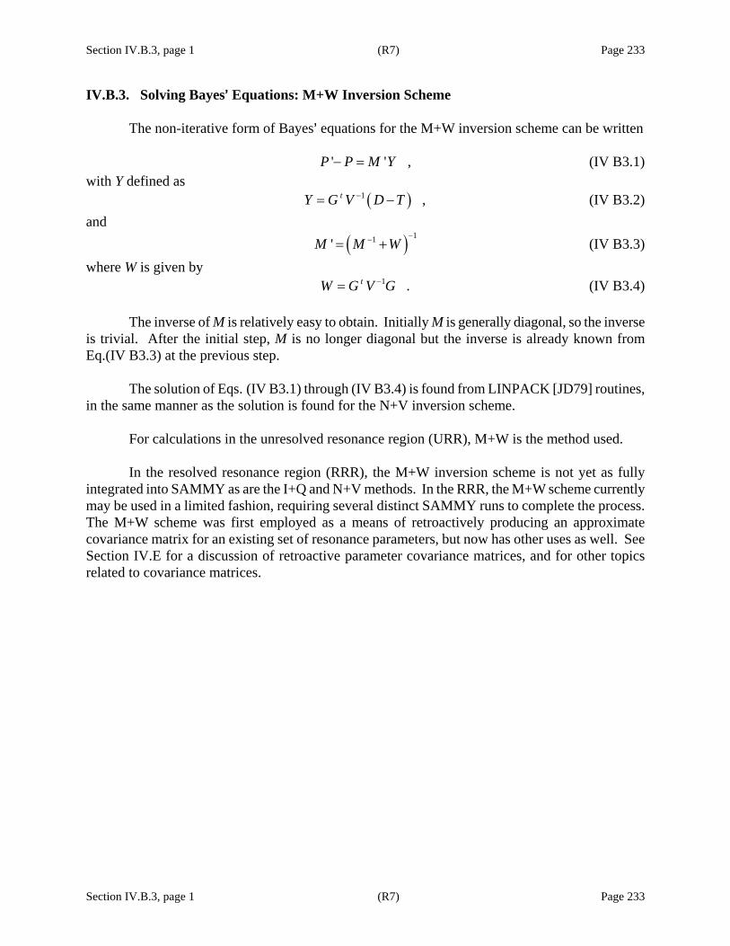
Section IV.B.3, page 1 (R7) Page 233
Section IV.B.3, page 1 (R7) Page 233
IV.B.3. Solving Bayes= Equations: M+W Inversion Scheme
The non-iterative form of Bayes= equations for the M+W inversion scheme can be written ' ' ,P P M Y− = (IV B3.1) with Y defined as ( )1 ,tY G V D T−= − (IV B3.2) and ( ) 11'M M W
−−= + (IV B3.3) where W is given by 1 .tW G V G−= (IV B3.4)
The inverse of M is relatively easy to obtain. Initially M is generally diagonal, so the inverse is trivial. After the initial step, M is no longer diagonal but the inverse is already known from Eq.(IV B3.3) at the previous step.
The solution of Eqs. (IV B3.1) through (IV B3.4) is found from LINPACK [JD79] routines, in the same manner as the solution is found for the N+V inversion scheme.
For calculations in the unresolved resonance region (URR), M+W is the method used. In the resolved resonance region (RRR), the M+W inversion scheme is not yet as fully
integrated into SAMMY as are the I+Q and N+V methods. In the RRR, the M+W scheme currently may be used in a limited fashion, requiring several distinct SAMMY runs to complete the process. The M+W scheme was first employed as a means of retroactively producing an approximate covariance matrix for an existing set of resonance parameters, but now has other uses as well. See Section IV.E for a discussion of retroactive parameter covariance matrices, and for other topics related to covariance matrices.


Section IV.C, page 1 (R7) Page 235
Section IV.C, page 1 (R7) Page 235
IV.C. CONSTRUCTING THE PARAMETER SET
Several distinct types of parameters may be varied (i.e., “fitted” or “searched on” in least-squares jargon) in SAMMY. Alternatively, these parameters may be treated as PUPs (propagated uncertainty parameters, as described in Section IV.D.2). Input values for all varied parameters are given in the PARameter file, Table VI B.2; input values for PUPs may generally be given in either the PARameter file or the INPut file. The different types of parameters are listed below; the list is not necessarily all-inclusive.
! Resonance energies and widths: that is, the Reich-Moore R-matrix parameters as described in Section II.B.1 (or the Breit-Wigner parameters as discussed in Section II.B.3). Values for energies and widths are provided via card set 1 of Table VI B.2.
! The matching radii (or channel radii) for the different spin groups and/or potential scattering vs. penetrabilities and shift factors. Values for the matching radii are given in card set 7 or card set 7a of Table VI B.2.
! The seven parameters of the external R-function. These are described in Section II.B.1.d; values are input to the code as shown in card set 3 of Table VI B.2.
! Effective temperature for Doppler broadening, as described in Section III.B. Input is in card set 4 of Table VI B.2.
! Resolution-broadening parameters. For the original formulation (Gaussian and/or exponential) of resolution broadening, Section III.C.1, input is in card set 4 of Table VI B.2. For the Oak Ridge Resolution Function of Section III.C.2, input is in card set 9. For the RPI/GELINA/nTOF Resolution Function of Section III.C.3, input is in card set 14.
[The parameter for the straight-line energy average resolution function, Section III.C.4, is not variable. Until the author is able to do more extensive testing, it is recommended that parameters of the user-defined resolution function, Section III.C.5, also not be considered variable.]
! Normalization and background functions. See Section III.E.3.a for description and card sets 6 and 13 for input details.
! Abundances for the various nuclides. See card set 10 of Table VI B.2.
! Sample thickness n. See card set 4 of Table VI B.2.
! Any of the miscellaneous parameters in card set 11 of Table VI B.2.
! Detector efficiencies, card set 15 of Table VI B.2.
For each parameter of each type, the user sets a flag that specifies whether that particular parameter is to be treated as a constant number (flag = 0), varied (flag = 1), or PUP’d (flag = 3). SAMMY counts the number NFPALL of flagged (varied + PUP’d) parameters and sets up an array U of dimension NFPALL. The initial values P needed in Bayes= equations [see, for example,
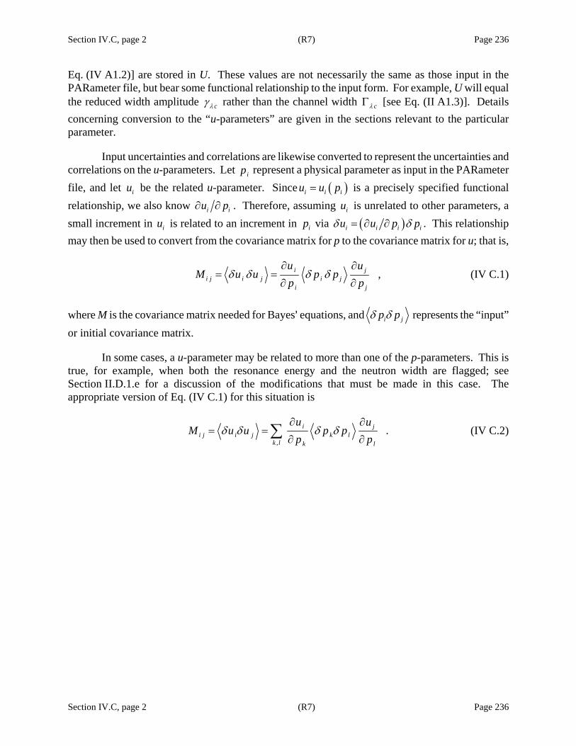
Section IV.C, page 2 (R7) Page 236
Section IV.C, page 2 (R7) Page 236
Eq. (IV A1.2)] are stored in U. These values are not necessarily the same as those input in the PARameter file, but bear some functional relationship to the input form. For example, U will equal the reduced width amplitude cλγ rather than the channel width cλΓ [see Eq. (II A1.3)]. Details concerning conversion to the “u-parameters” are given in the sections relevant to the particular parameter.
Input uncertainties and correlations are likewise converted to represent the uncertainties and correlations on the u-parameters. Let ip represent a physical parameter as input in the PARameter file, and let iu be the related u-parameter. Since ( )i i iu u p= is a precisely specified functional relationship, we also know i iu p∂ ∂ . Therefore, assuming iu is unrelated to other parameters, a small increment in iu is related to an increment in ip via ( )i i i iu u p pδ δ= ∂ ∂ . This relationship may then be used to convert from the covariance matrix for p to the covariance matrix for u; that is,
,i ji j i j i j
i j
u uM u u p p
p pδ δ δ δ
∂ ∂= =
∂ ∂ (IV C.1)
where M is the covariance matrix needed for Bayes= equations, and i jp pδ δ represents the “input” or initial covariance matrix.
In some cases, a u-parameter may be related to more than one of the p-parameters. This is true, for example, when both the resonance energy and the neutron width are flagged; see Section II.D.1.e for a discussion of the modifications that must be made in this case. The appropriate version of Eq. (IV C.1) for this situation is
,
.i ji j i j k l
k l k l
u uM u u p p
p pδ δ δ δ
∂ ∂= =
∂ ∂∑ (IV C.2)
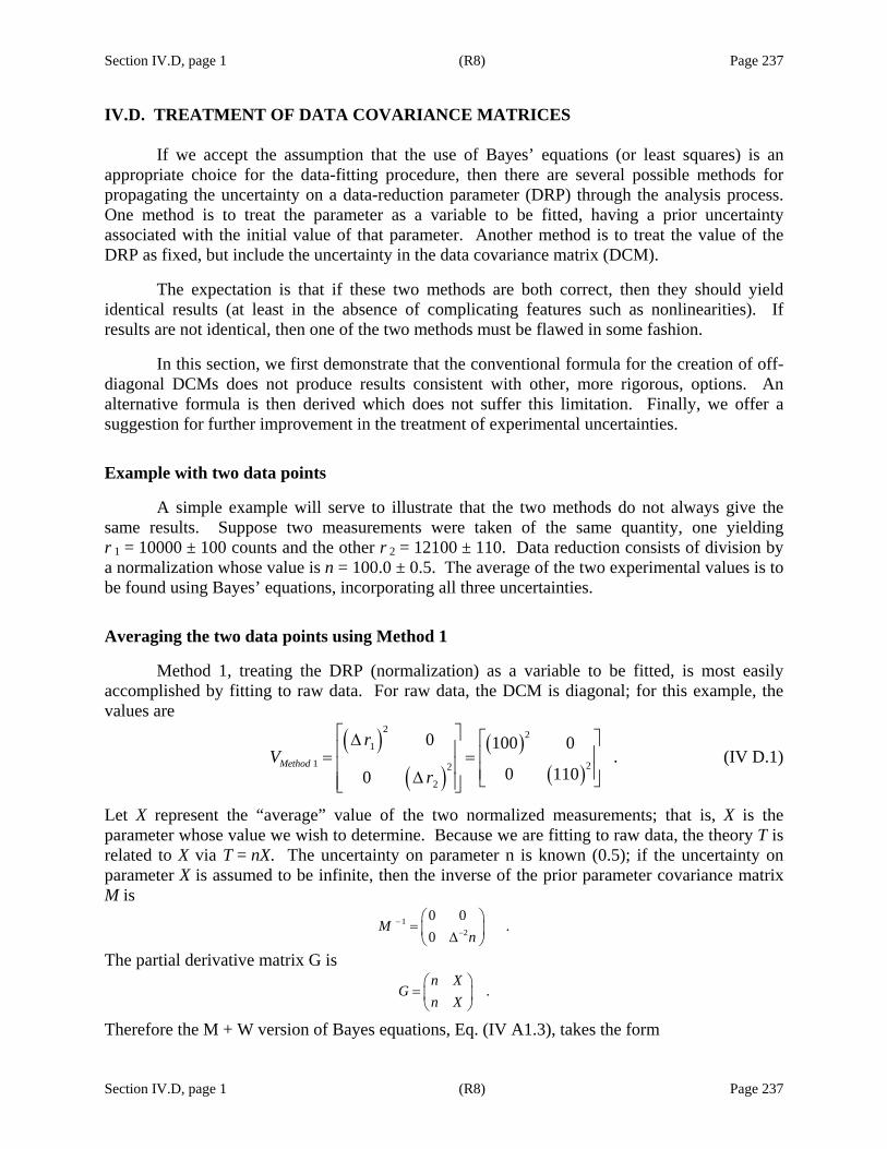
Section IV.D, page 1 (R8) Page 237
Section IV.D, page 1 (R8) Page 237
IV.D. TREATMENT OF DATA COVARIANCE MATRICES If we accept the assumption that the use of Bayes’ equations (or least squares) is an appropriate choice for the data-fitting procedure, then there are several possible methods for propagating the uncertainty on a data-reduction parameter (DRP) through the analysis process. One method is to treat the parameter as a variable to be fitted, having a prior uncertainty associated with the initial value of that parameter. Another method is to treat the value of the DRP as fixed, but include the uncertainty in the data covariance matrix (DCM).
The expectation is that if these two methods are both correct, then they should yield identical results (at least in the absence of complicating features such as nonlinearities). If results are not identical, then one of the two methods must be flawed in some fashion.
In this section, we first demonstrate that the conventional formula for the creation of off-diagonal DCMs does not produce results consistent with other, more rigorous, options. An alternative formula is then derived which does not suffer this limitation. Finally, we offer a suggestion for further improvement in the treatment of experimental uncertainties.
Example with two data points
A simple example will serve to illustrate that the two methods do not always give the same results. Suppose two measurements were taken of the same quantity, one yielding r 1 = 10000 ± 100 counts and the other r 2 = 12100 ± 110. Data reduction consists of division by a normalization whose value is n = 100.0 ± 0.5. The average of the two experimental values is to be found using Bayes’ equations, incorporating all three uncertainties.
Averaging the two data points using Method 1
Method 1, treating the DRP (normalization) as a variable to be fitted, is most easily accomplished by fitting to raw data. For raw data, the DCM is diagonal; for this example, the values are
( )
( )( )
( )
2 21
1 22
2
0 100 0.
0 1100Method
rV
r
⎡ ⎤ ⎡ ⎤Δ⎢ ⎥ ⎢ ⎥= =⎢ ⎥ ⎢ ⎥Δ ⎣ ⎦⎢ ⎥⎣ ⎦
(IV D.1)
Let X represent the “average” value of the two normalized measurements; that is, X is the parameter whose value we wish to determine. Because we are fitting to raw data, the theory T is related to X via T = nX. The uncertainty on parameter n is known (0.5); if the uncertainty on parameter X is assumed to be infinite, then the inverse of the prior parameter covariance matrix M is
12
0 0.
0M
n−
−
⎛ ⎞= ⎜ ⎟Δ⎝ ⎠
The partial derivative matrix G is
.n X
Gn X⎛ ⎞
= ⎜ ⎟⎝ ⎠
Therefore the M + W version of Bayes equations, Eq. (IV A1.3), takes the form
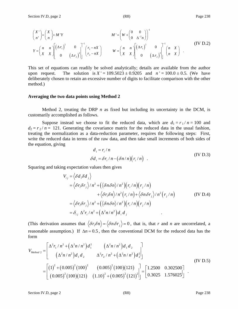
Section IV.D, page 2 (R8) Page 238
Section IV.D, page 2 (R8) Page 238
( )( )
( )( )
1
2
1 12 2
1 11
2 22
2 2
' 0 0' '
' 0
0 0.
0 0
X XM Y M W
n n n
r rr nXn n n n n XY W
r nXX X X X n Xr r
−
−
− −
⎛ ⎞⎛ ⎞ ⎛ ⎞ ⎛ ⎞= + = +⎜ ⎟⎜ ⎟ ⎜ ⎟ ⎜ ⎟Δ⎝ ⎠ ⎝ ⎠ ⎝ ⎠⎝ ⎠
⎡ ⎤ ⎡ ⎤Δ Δ−⎛ ⎞⎛ ⎞ ⎛ ⎞ ⎛ ⎞⎢ ⎥ ⎢ ⎥= =⎜ ⎟⎜ ⎟ ⎜ ⎟ ⎜ ⎟⎢ ⎥ ⎢ ⎥−⎝ ⎠ ⎝ ⎠ ⎝ ⎠⎝ ⎠Δ Δ⎢ ⎥ ⎢ ⎥⎣ ⎦ ⎣ ⎦
(IV D.2)
This set of equations can readily be solved analytically; details are available from the author upon request. The solution is X ' = 109.5023 ± 0.9205 and n ' = 100.0 ± 0.5. (We have deliberately chosen to retain an excessive number of digits to facilitate comparison with the other method.)
Averaging the two data points using Method 2
Method 2, treating the DRP n as fixed but including its uncertainty in the DCM, is customarily accomplished as follows.
Suppose instead we choose to fit the reduced data, which are d1 = r 1 / n = 100 and d2 = r 2 / n = 121. Generating the covariance matrix for the reduced data in the usual fashion, treating the normalization as a data-reduction parameter, requires the following steps: First, write the reduced data in terms of the raw data, and then take small increments of both sides of the equation, giving
( )( )
/
/ / / .i i
i i i
d r n
d r n n n r nδ δ δ
=
= − (IV D.3)
Squaring and taking expectation values then gives
( )( )( )( ) ( )
( )( )( )( )
2 2
2 2
2 2
2 2 2 2
/ / / /
/ / / /
/ / / /
/ / .
i j i j
i j i j
i i j j
i j i j
i j i i j
V d d
r r n n n n r n r n
r n n r n n r n r n
r r n n n n r n r n
r n n n d d
δ δ
δ δ δ δ
δ δ δ δ
δ δ δ δ
δ
=
= +
+ +
= +
= Δ + Δ
(IV D.4)
(This derivation assumes that 0i jr n n rδ δ δ δ= = , that is, that r and n are uncorrelated, a reasonable assumption.) If 0.5nΔ = , then the conventional DCM for the reduced data has the form
( ) ( )( ) ( )
( ) ( ) ( ) ( ) ( )( )( ) ( )( ) ( ) ( ) ( )
2 2 2 2 2 2 21 1 1 2
2 2 2 2 2 2 2 21 2 2 2
2 2 2 2
2 2 2 2
/ / /
/ / /
1 0.005 100 0.005 100 121 1.2500 0.302500.
0.3025 1.5760250.005 100 121 1.10 0.005 121
Method
r n n n d n n d dV
n n d d r n n n d
⎡ ⎤Δ + Δ Δ⎢ ⎥=⎢ ⎥Δ Δ + Δ⎣ ⎦
⎡ ⎤+ ⎡ ⎤⎢ ⎥= = ⎢ ⎥⎢ ⎥+ ⎣ ⎦⎣ ⎦
(IV D.5)
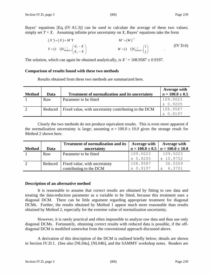
Section IV.D, page 3 (R8) Page 239
Section IV.D, page 3 (R8) Page 239
Bayes’ equations [Eq. (IV A1.3)] can be used to calculate the average of these two values; simply set T = X. Assuming infinite prior uncertainty on X, Bayes’ equations take the form
( ) ( ) ( )
( ) ( )
1
11 12 2
2
' ' '
11 1 1 1 .
1Method Method
X X M Y M W
d XY V W V
d X
−
− −
= + =
−⎛ ⎞ ⎛ ⎞= =⎜ ⎟ ⎜ ⎟− ⎝ ⎠⎝ ⎠
(IV D.6)
The solution, which can again be obtained analytically, is X ' = 108.9587 ± 0.9197.
Comparison of results found with these two methods
Results obtained from these two methods are summarized here.
Method Data Treatment of normalization and its uncertainty Average with n = 100.0 ± 0.5
1 Raw Parameter to be fitted 109.5023 ± 0.9205
2 Reduced Fixed value, with uncertainty contributing to the DCM 108.9587 ± 0.9197
Clearly the two methods do not produce equivalent results. This is even more apparent if the normalization uncertainty is large; assuming n = 100.0 ± 10.0 gives the strange result for Method 2 shown here.
Method Data Treatment of normalization and its
uncertainty Average with n = 100.0 ± 0.5
Average with n = 100.0 ± 10.0
1 Raw Parameter to be fitted 109.5023 ± 0.9205
109.5023 ± 10.9752
2 Reduced Fixed value, with uncertainty contributing to the DCM
108.9587 ± 0.9197
36.5559 ± 6.3701
Description of an alternative method
It is reasonable to assume that correct results are obtained by fitting to raw data and treating the data-reduction parameter as a variable to be fitted, because this treatment uses a diagonal DCM. There can be little argument regarding appropriate treatment for diagonal DCMs. Further, the results obtained by Method 1 appear much more reasonable than results obtained by Method 2, especially for the extreme value of normalization uncertainty.
However, it is rarely practical and often impossible to analyze raw data and thus use only diagonal DCMs. Fortunately, obtaining correct results with reduced data is possible, if the off-diagonal DCM is modified somewhat from the conventional approach discussed above.
A derivation of this description of the DCM is outlined briefly below; details are shown
in Section IV.D.1. (See also [NL04a], [NL04b], and the SAMMY workshop notes. Readers are

Section IV.D, page 4 (R8) Page 240
Section IV.D, page 4 (R8) Page 240
also encouraged to see the discussion regarding creation, storage, communicating, and usage of DCM in [NL08], in which it is noted that only the pieces of the DCM need to be generated.)
We begin with Bayes’ equations written in terms of the raw data. Simple (albeit extensive) algebra is then used to re-express the equations in terms of the reduced data; details are presented in Section IV.D.1. The resulting formulae are
( ) 11
1 1
' ' '
( ) ,t t
P P M Y M W M
Y G V D T W G V G
−−
− −
− = = +
= − = (IV D.7)
in which V has the form ,tV v g m g= + (IV D.8)
with g expressed in terms of the theoretical values for the quantity to be fitted (e.g., the cross section). The only difference between these formulae (which we will denote Method 2a) and those used in the conventional approach (Method 2) is that Method 2 calculates g in terms of the experimental values.
Averaging the two data points using Method 2a For our example, the DCM takes the form
( ) ( )
( ) ( )
2 2 2 2 2 2 2 21
2 2 2 2 2 2 2 2 22
/ / /.
/ / /Method a
r n n n X n n XV
n n X r n n n X
⎡ ⎤Δ + Δ Δ⎢ ⎥=⎢ ⎥Δ Δ + Δ⎣ ⎦
(IV D.9)
Substituting this into Eq. (IV D.7) gives us expressions similar in form to that for Method 2, Eq. (IV D.6),
( ) ( ) ( )
( ) ( )
1
11 12 2
2
' ' '
11 1 1 1 .
1Method a Method a
X X M Y M W
d XY V W V
d X
−
− −
= + =
−⎛ ⎞ ⎛ ⎞= =⎜ ⎟ ⎜ ⎟− ⎝ ⎠⎝ ⎠
(IV D.10)
for which the solution is X ' = 109.5023 ± 0.9205, identical to that obtained with Method 1. Likewise, with the larger uncertainty for the normalization, this method gives exact agreement with Method 1.
Method Data
Treatment of normalization and its
uncertainty
Values used to generate the DCM
Average with n = 100.0 ± 0.5
Average with n = 100.0 ± 10.0
1 Raw Parameter to be fitted 109.5023 ± 0.9205
109.5023 ± 10.9752
2 Reduced Fixed value, DCM Experimental 108.9587 ± 0.9197
36.5559 ± 6.3701
2a Reduced Fixed value, DCM Theoretical 109.5023 ± 0.9205
109.5023 ± 10.9752
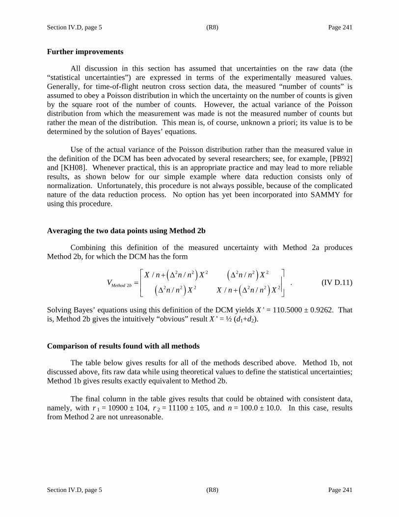
Section IV.D, page 5 (R8) Page 241
Section IV.D, page 5 (R8) Page 241
Further improvements
All discussion in this section has assumed that uncertainties on the raw data (the “statistical uncertainties”) are expressed in terms of the experimentally measured values. Generally, for time-of-flight neutron cross section data, the measured “number of counts” is assumed to obey a Poisson distribution in which the uncertainty on the number of counts is given by the square root of the number of counts. However, the actual variance of the Poisson distribution from which the measurement was made is not the measured number of counts but rather the mean of the distribution. This mean is, of course, unknown a priori; its value is to be determined by the solution of Bayes’ equations. Use of the actual variance of the Poisson distribution rather than the measured value in the definition of the DCM has been advocated by several researchers; see, for example, [PB92] and [KH08]. Whenever practical, this is an appropriate practice and may lead to more reliable results, as shown below for our simple example where data reduction consists only of normalization. Unfortunately, this procedure is not always possible, because of the complicated nature of the data reduction process. No option has yet been incorporated into SAMMY for using this procedure. Averaging the two data points using Method 2b
Combining this definition of the measured uncertainty with Method 2a produces Method 2b, for which the DCM has the form
( ) ( )
( ) ( )
2 2 2 2 2 2
2 2 2 2 2 2 2
/ / /.
/ / /Method b
X n n n X n n XV
n n X X n n n X
⎡ ⎤+ Δ Δ⎢ ⎥=⎢ ⎥Δ + Δ⎣ ⎦
(IV D.11)
Solving Bayes’ equations using this definition of the DCM yields X ' = 110.5000 ± 0.9262. That is, Method 2b gives the intuitively “obvious” result X ' = ½ (d1+d2). Comparison of results found with all methods
The table below gives results for all of the methods described above. Method 1b, not discussed above, fits raw data while using theoretical values to define the statistical uncertainties; Method 1b gives results exactly equivalent to Method 2b. The final column in the table gives results that could be obtained with consistent data, namely, with r 1 = 10900 ± 104, r 2 = 11100 ± 105, and n = 100.0 ± 10.0. In this case, results from Method 2 are not unreasonable.

Section IV.D, page 6 (R8) Page 242
Section IV.D, page 6 (R8) Page 242
M Data Norm
Statistical uncer-tainties
Values for
DCM n = 100. ± 0.5
n = 100.0 ± 10.0
Consistent data,
Δn = 10.0 1 Raw Parameter
to be fitted Exper. 109.5023
± 0.9205 109.5023 ±10.9752
109.9904 ±11.0238
1b Raw Parameter to be fitted
Theory 110.5000 ± 0.9262
110.5000 ±11.0750
110.5000 ±11.0250
2 Reduced Fixed value, DCM
Exper. Exper. 108.9587 ± 0.9197
36.5559 ± 6.3701
108.0123 ±10.9247
2a Reduced Fixed value, DCM
Exper. Theory 109.5023 ± 0.9205
109.5023 ±10.9752
109.9904 ±11.0238
2b Reduced Fixed value, DCM
Theory Theory 110.5000 ± 0.9262
110.5000 ±11.0750
110.5000 ±11.0250
Discussion
In SAMMY, any parameter for which derivatives are available (i.e., any parameter that is capable of being fitted) can be treated as a contributor to the DCM. Such parameters are denoted “propagated uncertainty parameters,” or PUPs. In Section IV.D.2, application of the PUP method within SAMMY is described; a list is given of those parameters that may be treated as PUPs. Section IV.D.3 deals with methods of generating and inverting the DCM. In particular, the “implicit data covariance” (IDC) method is introduced, which has many advantages over explicitly generating, storing, and inverting the full DCM. Further discussion on this topic is available in [NL08].
Even though the method is known to be flawed,∗ it was seen above that Method 2 can produce reasonable results as long as the data are consistent. With consistent data and good statistics,† use of Method 2 is generally preferable to another common practice, totally ignoring the off-diagonal elements of the DCM. SAMMY includes several options for input of DCMs which have been generated in the usual fashion; these are detailed in Section VI.C. Many SAMMY test cases give examples of the various treatments of DCM. See Section XII.B for the list of test cases.
∗ These flaws include inconsistency with the fit-to-raw-data method; excessive computer time and memory requirements for explicitly creating, storing, and inverting the full DCM; potential problems with discrepant data; and possible loss of accuracy and associated numerical difficulties if using ASCII formats to communicate values for the matrix elements. † Experience has shown that it is necessary to exercise caution when basing the DCM on experimental values alone. Whenever possible, it is preferable to calculate the DCM with theoretical values as in Method 2a.

Section IV.D.1, page 1 (R8) Page 243
Section IV.D.1, page 1 (R8) Page 243
IV.D.1. Derivation of Data Covariance Matrix Equation In this section, we derive the equation for the data covariance matrix (DCM) in terms of the data-reduction parameters and derivatives with respect to those parameters, as discussed in Section IV.D. See also references [NL04a] and [NL04b]. Readers uninterested in details of the derivation may safely bypass these pages.
Matrix notation is used in this derivation, with indices omitted. We begin with definitions of terms:
• P = theory parameters − R-matrix widths and energies, channel radii − may also include some measurement-related parameters (Doppler widths, etc.) if
not included in p • p = data-reduction parameter
− normalization or backgrounds − resolution or Doppler widths − others
• d = experimental measurement (raw data) − related to cross section but exactly as measured by the experiment
• d = experimental measurement after data reduction (reduced data) − a function of d and p
• M = initial covariance matrix for parameters P − can be diagonal or off-diagonal − can be very large (suggesting little a priori information) or quite small (suggesting
the parameters are well known) • m = initial (measured) covariance matrix for p
− can be diagonal or off-diagonal − are determined during the measurement or data-reduction process
• v = covariance matrix for raw data d − no assumption regarding diagonality is made yet, though generally the covariance
matrix for measured data is diagonal • t = theoretical cross section
− a function of R-matrix parameters in P − the quantities whose values are to be determined by this experiment and analysis
• t = theory corresponding to the measured data − a function of t and p
• g = partial derivative of theory t with respect to data-reduction parameters p • G = partial derivative of theory t with respect to theory parameters P
The theory t is a complicated function of the cross section. This function incorporates
such effects as beam intensity, duration of the experiment, cosmic and room backgrounds, Doppler- and resolution-broadening, detector dead time, finite-size corrections, and others. The ultimate goal of the measurement and analysis is to learn what that cross section is as a function of energy. In general, one can write ( , ) ,t f t p= (IV D1.1)

Section IV.D.1, page 2 (R8) Page 244
Section IV.D.1, page 2 (R8) Page 244
where t represents the cross section and p represents any parameters involved in the transformation. Again we consider Bayes’ equations (M+W version), using slightly different notation,
( )( )
11
1 1
' ' '
,
−−
− −
= + = +
= − =t t
P P M Y M M W
Y G V D T W G V G (IV D1.2)
where P represents all parameters, M the full covariance matrix for all parameters, D the measured data, T the corresponding theoretical calculation, G the partial derivative of T with respect to P, and V the DCM. Primes represent updated values for P and M. Superscript t, as usual, indicates transpose. In Eq. (IV D1.2), substitute D = d and T = t, and V = v; in addition, substitute the matrix identities
[ ]0, , .
0P M
G gp m
⎡ ⎤ ⎡ ⎤= = =⎢ ⎥ ⎢ ⎥⎣ ⎦ ⎣ ⎦
P M G (IV D1.3)
The inverse of M is then
1
11
0.
0M
m
−−
−
⎡ ⎤= ⎢ ⎥⎣ ⎦
M (IV D1.4)
1−= tW G V G is therefore found from
1 1 1
1 11 1 1
and ,t t t
t t t
G v G v G G v gg v g v G g v g
− − −− −
− − −
⎡ ⎤ ⎡ ⎤= =⎢ ⎥ ⎢ ⎥⎣ ⎦ ⎣ ⎦
t tG V G V G (IV D1.5)
so that ( ) 1' −M becomes
( )1 1 1
1 1 11 1 1
.t t
tt t
G v G M G v gg v G g v g m
− − −− − −
− − −
⎡ ⎤+= ⎢ ⎥
+⎣ ⎦M' = G V G + M (IV D1.6)
M' is found by inverting that equation. For matrix X of the form
,tA C
XC B⎡ ⎤
= ⎢ ⎥⎣ ⎦
(IV D1.7)

Section IV.D.1, page 3 (R8) Page 245
Section IV.D.1, page 3 (R8) Page 245
the inverse of X can be shown to be
( ) ( )
( ) ( )
1 11 1 1
11 11 1 1
,t t t
t t
A C B C A C B C C BX
B C A C CA B C A C
− −− − −
−
− −− − −
⎡ ⎤− − −⎢ ⎥=⎢ ⎥− − −⎢ ⎥⎣ ⎦
(IV D1.8)
in which the off-diagonal terms are the transpose of each other:
( ) ( )( ) ( ) ( )( ) ( )( ) ( )( )
1 11 1 1 1
1 11 1 1 1
1 11 1 1 1
1 11 1 1 1
11 1 .
tt t t
t t t t
t t t t t
t t t t
t t
B C A C CA A C B C A C
A C B C A C B C A C B C A C
A C B C C C B CA C B C A C
A C B C C B B CA C B C A C
A C B C C B
− −− − − −
− −− − − −
− −− − − −
− −− − − −
−− −
⎡ ⎤− = −⎢ ⎥⎣ ⎦
= − − −
⎡ ⎤= − − −⎣ ⎦
⎡ ⎤= − − −⎣ ⎦
= −
(IV D1.9)
That Eq. (IV D1.8) is a correct form for the inverse can readily be verified by calculating
1 1X X X X I− −= = = the identity matrix, using Eq. (IV D1.9) as necessary. Substituting the pieces of Eq. (IV D1.6) for M' into Eq. (IV D1.8) and (IV D1.9) gives
( )( )
( )
11 1 1 1 1 1 1
11 1 1 1 1 1
1 1 .
t t t t t
t t t
t t
A C B C G v G M G v g g v g m g v G
G v v g g v g m g v G M
G v g m g G M
−− − − − − − −
−− − − − − −
− −
− = + − +
= − + +
= + +
(IV D1.10)
If we then define H as ,tH v g m g= + (IV D1.11) then Eq. (IV D1.10) takes the form 1 1 1 .t tA C B C G H G M− − −− = + (IV D1.12) Analogously, define h as ,th v G M G= + (IV D1.13) so that ( ) 11 1 1 1 .t t t tB CA C g v G M G g m g h g m
−− − − −− = + + = + (IV D1.14) Also, since 1 1 1 1 and ,t tA G v G M B g v g m− − − −= + = + (IV D1.15) it follows that 1 1 1 1 and .t tA M M G h G M B m m g H g m− − − −= − = − (IV D1.16)

Section IV.D.1, page 4 (R8) Page 246
Section IV.D.1, page 4 (R8) Page 246
Making those substitutions into Eq.(IV D1.8) for 1X − gives the following for M ':
( )
( )
11 1 1 11 1
1
11 1 1 1
11 11
' .
t tt
t
t t
tt
G H G M G v gG H G M
m m g H gm
g h g m g v G
g h g mM MG h GM
−− − − −− −
−
−− − − −
−− −−
⎡ ⎤− ++⎢ ⎥⎢ ⎥× −⎢ ⎥= ⎢ ⎥− +⎢ ⎥⎢ ⎥+× −⎢ ⎥⎣ ⎦
M (IV D1.17)
Similarly, for Y from Eq. (IV D1.2) we find
1
1
( ),
( )
t
t
G v d tg v d t
−
−
⎡ ⎤−= ⎢ ⎥
−⎣ ⎦Y (IV D1.18)
which leads to
( )
( )
11 1 1
11 1 1 1 1
11 1 1 1 1
11 1 1
( )...
( )'
.'
( )...
( )
t t
t t t t
t t t t
t t
G H G M G v d t
G H G M G v g m m g H g m g v d tP Pp p
g h g m g v G M MG h G M G v d t
g h g m g v d t
−− − −
−− − − − −
−− − − − −
−− − −
⎡ ⎤+ −⎢ ⎥⎢ ⎥− + − −⎢ ⎥−⎡ ⎤ ⎢ ⎥=⎢ ⎥ ⎢ ⎥−⎣ ⎦ ⎢ ⎥− + − −⎢ ⎥⎢ ⎥+ + −⎢ ⎥⎣ ⎦
(IV D1.19)
Rearranging, this becomes
( ) ( )
( ) ( )
( )
( )
11 1 1 1 1
11 1 1 1 1
11 1 1 1 1 1
11 1 1 1 1 1
1'' 1
1
1
t t t t
t t t t
t t t t t
t t t t t
G H G M G v g m m g H g m g v d tP Pp p g h g m g v G M M G h G M G v d t
G H G M G v g m g v g m g H g m g v d t
g h g m g v GM G v GM G h GM G v d t
−− − − − −
−− − − − −
−− − − − − −
−− − − − − −
⎡ ⎤+ − − −−⎡ ⎤ ⎢ ⎥=⎢ ⎥ ⎢ ⎥−⎣ ⎦ + − − + −⎢ ⎥⎣ ⎦
⎡ ⎤+ − + −⎢ ⎥=⎢ + − + + −⎢⎣ ⎦
11 1 1 1
11 1 1 1
( ),
( )
t t
t t
G H G M G v v H d t
g h g m g v vh d t
−− − − −
−− − − −
⎥⎥
⎡ ⎤+ −⎢ ⎥=⎢ ⎥+ −⎢ ⎥⎣ ⎦
(IV D1.20)
or
11 1 1
11 1 1
( )'.
' ( )
t t
t t
G H G M G H d tP Pp p g h g m g h d t
−− − −
−− − −
⎡ ⎤+ −−⎡ ⎤ ⎢ ⎥=⎢ ⎥ ⎢ ⎥−⎣ ⎦ + −⎢ ⎥⎣ ⎦
(IV D1.21)
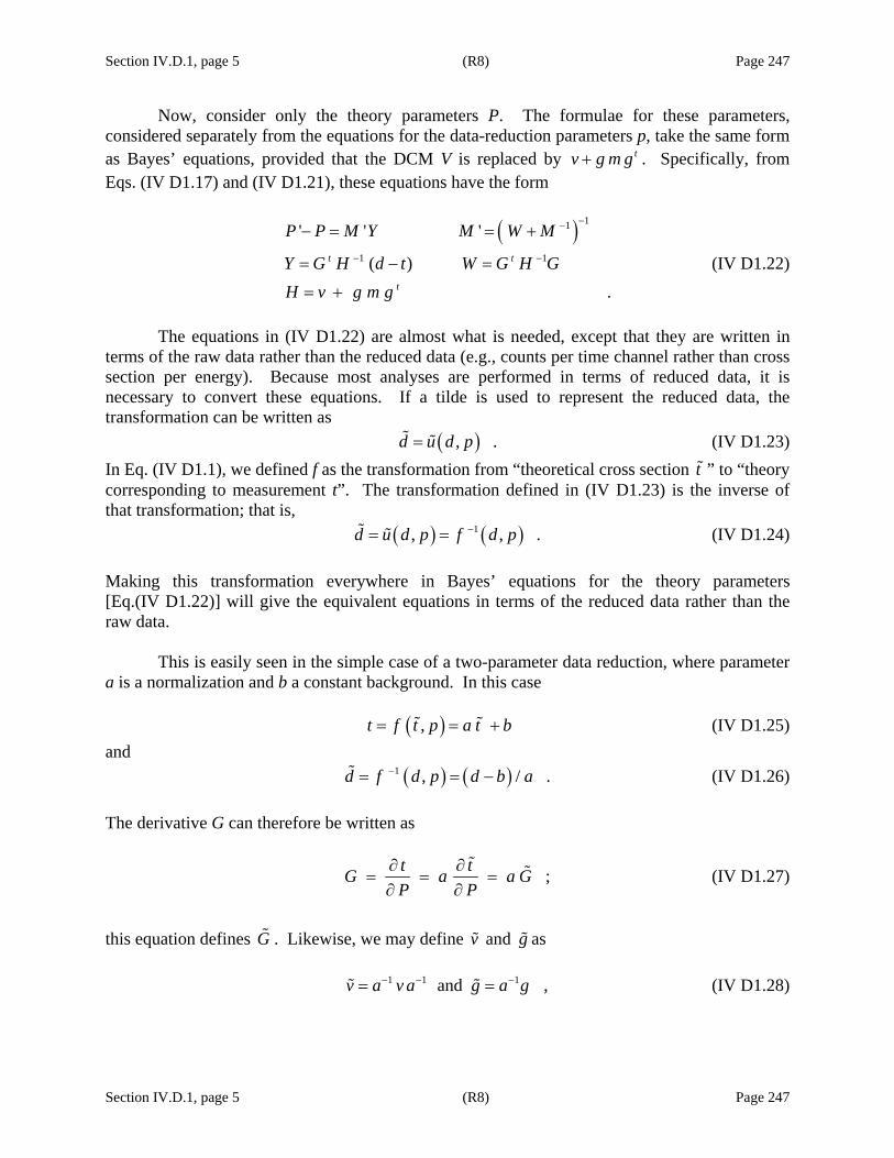
Section IV.D.1, page 5 (R8) Page 247
Section IV.D.1, page 5 (R8) Page 247
Now, consider only the theory parameters P. The formulae for these parameters, considered separately from the equations for the data-reduction parameters p, take the same form as Bayes’ equations, provided that the DCM V is replaced by tv g m g+ . Specifically, from Eqs. (IV D1.17) and (IV D1.21), these equations have the form
( ) 11
1 1
' ' '
( ) .
t t
t
P P M Y M W M
Y G H d t W G H GH v g m g
−−
− −
− = = +
= − =
= +
(IV D1.22)
The equations in (IV D1.22) are almost what is needed, except that they are written in terms of the raw data rather than the reduced data (e.g., counts per time channel rather than cross section per energy). Because most analyses are performed in terms of reduced data, it is necessary to convert these equations. If a tilde is used to represent the reduced data, the transformation can be written as ( ), .d u d p= (IV D1.23) In Eq. (IV D1.1), we defined f as the transformation from “theoretical cross section t ” to “theory corresponding to measurement t”. The transformation defined in (IV D1.23) is the inverse of that transformation; that is, ( ) ( )1, , .d u d p f d p−= = (IV D1.24) Making this transformation everywhere in Bayes’ equations for the theory parameters [Eq.(IV D1.22)] will give the equivalent equations in terms of the reduced data rather than the raw data. This is easily seen in the simple case of a two-parameter data reduction, where parameter a is a normalization and b a constant background. In this case ( ),t f t p a t b= = + (IV D1.25) and ( ) ( )1 , / .d f d p d b a−= = − (IV D1.26) The derivative G can therefore be written as
;t tG a a GP P∂ ∂
= = =∂ ∂
(IV D1.27)
this equation defines G . Likewise, we may define v and g as 1 1 1 and ,v a v a g a g− − −= = (IV D1.28)

Section IV.D.1, page 6 (R8) Page 248
Section IV.D.1, page 6 (R8) Page 248
and therefore rewrite H in the form
.t tH v g m g a v a a g m g a a H a= + = + = (IV D1.29) Substituting into Eq. (IV D1.22) for Y and W gives
( ) ( ) ( ) ( )( )
1 1 1 1
1
t t
t
Y G H d t G a a H a a d b a t b
G H d t
− − − −
−
= − = + − −
= − (IV D1.30)
and ( ) ( ) ( )1 1 1 1 1 .t t t W G H G G a a H a a G G H G− − − − −= = = (IV D1.31)
The form of the equation is the same, with or without tildes. In the general case with more than one parameter, equations analogous to (IV D1.25) and (IV D1.26) are
( )( )
, at
or , at
t u x p x t
t f x p x t
= =
= = (IV D1.32)
and
( )( )
, at
or , at .
d u x p x d
d f x p x d
= =
= = (IV D1.33)
The function u is the inverse of the function f :
( ) ( )( )( ) ( )( )
, , ,
or , , , .
x f x p f u x p p
x u x p u f x p p
= =
= = (IV D1.34)
Relationships between various partial derivatives can be established by using the chain rule:
( )( ) ( ) ( ), , , ,
1f u x p p f x p u x px
x x x x∂ ∂ ∂∂
= = =∂ ∂ ∂ ∂
(IV D1.35)
or ( ) ( ) 1
, ,.
u x p f x px x
−⎡ ⎤∂ ∂
= ⎢ ⎥∂ ∂⎣ ⎦ (IV D1.36)
Note that both t and d are independent of the data-reduction parameters p: t is calculated directly from the theory parameters P, and d is measured directly with no corrections. Taking the derivative with respect to p of the first line in Eq. (IV D1.34) with x d= and x d= gives
0 ;x d x d x d
d f f up p x p
= = =
∂ ∂ ∂ ∂= = +
∂ ∂ ∂ ∂ (IV D1.37)

Section IV.D.1, page 7 (R8) Page 249
Section IV.D.1, page 7 (R8) Page 249
likewise, the derivative of the second line of Eq. (IV D1.34) with x t= and x t= is
0 .x t x t x t
t u u fp p x p
= = =
∂ ∂ ∂ ∂= = +
∂ ∂ ∂ ∂ (IV D1.38)
The last term ( )/f p∂ ∂ , however, is exactly equal to our definition of g at the beginning of this section.
We now consider a Taylor expansion of ( ),x d
d f x p=
= in the neighborhood of ,t for
fixed p:
( ) ( ) , , .x t x t
f fd f d p f t p d t t d tx x
= =
∂ ∂= ≈ + − ≈ + −
∂ ∂ (IV D1.39)
For simplicity, define F as
;x t
fFx
=
∂=
∂ (IV D1.40)
it follows that .d t t F d t t F d t− ≈ + − − = − (IV D1.41)
In similar fashion, the derivative with respect to the R-matrix parameters can be written as
.t t tG F GP t P∂ ∂ ∂
= = =∂ ∂ ∂
(IV D1.42)
Substituting those expressions into Eq. (IV D1.22) for Y and W gives ( ) ( ) 1 1 1t t t t tY G H d t G F H F d t G F H F d t− − −= − ≈ − = − (IV D1.43)
and ( ) ( )1 1 1 .t t t t t W G H G G F H F G G F H F G− − −= = = (IV D1.44)
Inserting the definition of H from Eq. (IV D1.11) gives
( )( ) ( )
( ) ( )
( ) ( ) ( )
111 11 1 1
11 11 1
111 1 1 ,
t t t t
t t t
tt
F H F F H F F v g m g F
F v F F g m g F
F v F F g m F g
−−− −− − −
−− −− −
−−− − −
⎡ ⎤= = +⎢ ⎥⎣ ⎦
⎡ ⎤= +⎢ ⎥⎣ ⎦
⎡ ⎤= +⎢ ⎥⎣ ⎦
(IV D1.45)
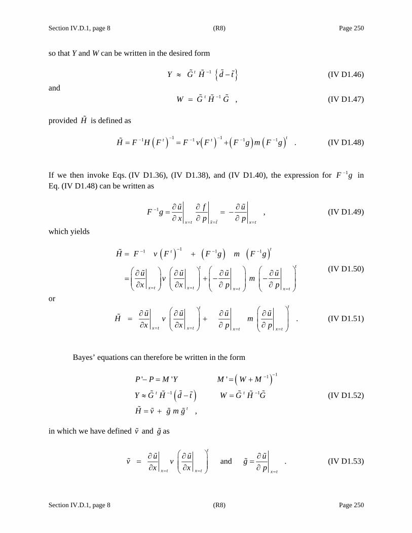
Section IV.D.1, page 8 (R8) Page 250
Section IV.D.1, page 8 (R8) Page 250
so that Y and W can be written in the desired form 1tY G H d t−≈ − (IV D1.46)
and 1 ,tW G H G−= (IV D1.47) provided H is defined as ( ) ( ) ( ) ( )1 11 1 1 1 .
tt tH F H F F v F F g m F g− −− − − −= = + (IV D1.48)
If we then invoke Eqs. (IV D1.36), (IV D1.38), and (IV D1.40), the expression for 1F g− in Eq. (IV D1.48) can be written as
1 ,x t x t x t
u f uF gx p p
−
= = =
∂ ∂ ∂= = −∂ ∂ ∂
(IV D1.49)
which yields
( ) ( ) ( )11 1 1 tt
tt
x t x t x t x t
H F v F F g m F g
u u u uv mx x p p
−− − −
= = = =
= +
⎛ ⎞ ⎛ ⎞⎛ ⎞ ⎛ ⎞∂ ∂ ∂ ∂⎜ ⎟ ⎜ ⎟= + − −⎜ ⎟ ⎜ ⎟⎜ ⎟ ⎜ ⎟ ⎜ ⎟ ⎜ ⎟∂ ∂ ∂ ∂⎝ ⎠ ⎝ ⎠ ⎝ ⎠ ⎝ ⎠
(IV D1.50)
or
.tt
x t x t x t x t
u u u uH v mx x p p= = = =
⎛ ⎞⎛ ⎞∂ ∂ ∂ ∂⎜ ⎟= +⎜ ⎟⎜ ⎟ ⎜ ⎟∂ ∂ ∂ ∂⎝ ⎠ ⎝ ⎠
(IV D1.51)
Bayes’ equations can therefore be written in the form
( )( )
11
1 1
' ' '
,
t t
t
P P M Y M W M
Y G H d t W G H G
H v g m g
−−
− −
− = = +
≈ − =
= +
(IV D1.52)
in which we have defined v and g as
and .t
x t x t x t
u u uv v gx x p= = =
⎛ ⎞∂ ∂ ∂= =⎜ ⎟⎜ ⎟∂ ∂ ∂⎝ ⎠
(IV D1.53)
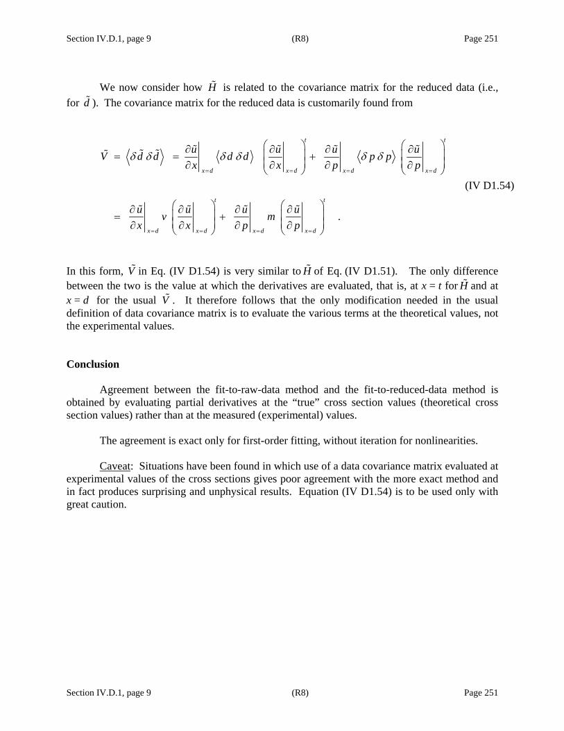
Section IV.D.1, page 9 (R8) Page 251
Section IV.D.1, page 9 (R8) Page 251
We now consider how H is related to the covariance matrix for the reduced data (i.e.,
for d ). The covariance matrix for the reduced data is customarily found from
.
t t
x d x d x d x d
t t
x d x d x d x d
u u u uV d d d d p px x p p
u u u uv mx x p p
δ δ δ δ δ δ= = = =
= = = =
⎛ ⎞ ⎛ ⎞∂ ∂ ∂ ∂⎜ ⎟ ⎜ ⎟= = +⎜ ⎟ ⎜ ⎟∂ ∂ ∂ ∂⎝ ⎠ ⎝ ⎠
⎛ ⎞ ⎛ ⎞∂ ∂ ∂ ∂⎜ ⎟ ⎜ ⎟= +⎜ ⎟ ⎜ ⎟∂ ∂ ∂ ∂⎝ ⎠ ⎝ ⎠
(IV D1.54)
In this form, V in Eq. (IV D1.54) is very similar to H of Eq. (IV D1.51). The only difference between the two is the value at which the derivatives are evaluated, that is, at x = t for H and at x = d for the usual V . It therefore follows that the only modification needed in the usual definition of data covariance matrix is to evaluate the various terms at the theoretical values, not the experimental values. Conclusion
Agreement between the fit-to-raw-data method and the fit-to-reduced-data method is obtained by evaluating partial derivatives at the “true” cross section values (theoretical cross section values) rather than at the measured (experimental) values.
The agreement is exact only for first-order fitting, without iteration for nonlinearities. Caveat: Situations have been found in which use of a data covariance matrix evaluated at
experimental values of the cross sections gives poor agreement with the more exact method and in fact produces surprising and unphysical results. Equation (IV D1.54) is to be used only with great caution.

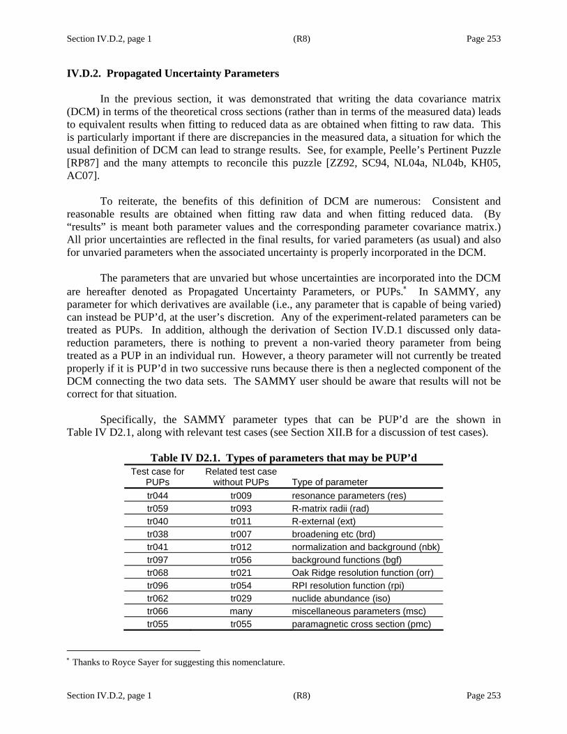
Section IV.D.2, page 1 (R8) Page 253
Section IV.D.2, page 1 (R8) Page 253
IV.D.2. Propagated Uncertainty Parameters In the previous section, it was demonstrated that writing the data covariance matrix (DCM) in terms of the theoretical cross sections (rather than in terms of the measured data) leads to equivalent results when fitting to reduced data as are obtained when fitting to raw data. This is particularly important if there are discrepancies in the measured data, a situation for which the usual definition of DCM can lead to strange results. See, for example, Peelle’s Pertinent Puzzle [RP87] and the many attempts to reconcile this puzzle [ZZ92, SC94, NL04a, NL04b, KH05, AC07]. To reiterate, the benefits of this definition of DCM are numerous: Consistent and reasonable results are obtained when fitting raw data and when fitting reduced data. (By “results” is meant both parameter values and the corresponding parameter covariance matrix.) All prior uncertainties are reflected in the final results, for varied parameters (as usual) and also for unvaried parameters when the associated uncertainty is properly incorporated in the DCM.
The parameters that are unvaried but whose uncertainties are incorporated into the DCM are hereafter denoted as Propagated Uncertainty Parameters, or PUPs.∗ In SAMMY, any parameter for which derivatives are available (i.e., any parameter that is capable of being varied) can instead be PUP’d, at the user’s discretion. Any of the experiment-related parameters can be treated as PUPs. In addition, although the derivation of Section IV.D.1 discussed only data-reduction parameters, there is nothing to prevent a non-varied theory parameter from being treated as a PUP in an individual run. However, a theory parameter will not currently be treated properly if it is PUP’d in two successive runs because there is then a neglected component of the DCM connecting the two data sets. The SAMMY user should be aware that results will not be correct for that situation. Specifically, the SAMMY parameter types that can be PUP’d are the shown in Table IV D2.1, along with relevant test cases (see Section XII.B for a discussion of test cases).
Table IV D2.1. Types of parameters that may be PUP’d Test case for
PUPs Related test case
without PUPs Type of parameter tr044 tr009 resonance parameters (res) tr059 tr093 R-matrix radii (rad) tr040 tr011 R-external (ext) tr038 tr007 broadening etc (brd) tr041 tr012 normalization and background (nbk) tr097 tr056 background functions (bgf) tr068 tr021 Oak Ridge resolution function (orr) tr096 tr054 RPI resolution function (rpi) tr062 tr029 nuclide abundance (iso) tr066 many miscellaneous parameters (msc) tr055 tr055 paramagnetic cross section (pmc)
∗ Thanks to Royce Sayer for suggesting this nomenclature.

Section IV.D.2, page 2 (R8) Page 254
Section IV.D.2, page 2 (R8) Page 254
Extensive testing has been done for each type of parameter, to ensure that the PUP theory and implementation are indeed correct. The tests consisted primarily of running the code with as many different options as possible for treating the parameter uncertainty, and comparing the resulting values and covariance matrices for the varied parameters. The available options are
1. varying the parameter, 2. treating the parameter as a PUP, 3. giving an explicit DCM, 4. providing user-supplied implicit DCM (see Section VI.C.3.b for details), and 5. treating via SAMMY’s original IDC parameter method (Section VI.C.3.c), available
for normalization and background parameters. In the tests, options #1 and #2 gave identical results for the first iteration. When available, options #2 and #5 gave exactly identical results for all iterations. Options #3 and #4 gave almost identical results, as long as each element of the explicit DCM was specified with a sufficient number of significant digits. When the data are not discrepant (so that a “fixed” DCM is a good approximation), all methods gave similar results. To designate that a parameter is a PUP, the SAMMY user must simply set the flag for that parameter equal to “3” rather than “0” (to hold constant) or “1” (to vary). Uncertainties are provided in the same manner as for varied parameters; details are given in Table VI B.2. In the SAMMY.LPT output file, the ordinal numbers for PUPs are given in angle brackets, for example, <38>, while numbers for varied parameters are given in parentheses, for example (38). Card sets for most types of parameters may be put into the INPut file (Table VI A.1) rather than the PARameter file (Table VI B.2), provided none of that type of parameter is flagged for varying. Varied parameters must always be in the PARameter file. PUP’d parameters, on the other hand, may be in either the PARameter file or the INPut file. (A card set, however, can occur in at most one of the two files.) A flag = 1 in the INPut file will be ignored; a flag = 3 in either the INPut or the PARameter file will signify that the parameter is to be PUP’d. Values (and corresponding uncertainties) for most PUP’d data-related parameters may be different from one run to the next in a series for which the covariance matrix is carried along.
The exception to the above paragraph is any R-matrix parameter, all of which must be in the PARameter file. Values and uncertainties for PUP’d R-matrix parameters may NOT be changed from one run to the next in a sequential series. Furthermore, the current implementation neglects the DCM component (caused by PUP’ing the theory parameter) relating one data set to another. Hence, even though the option to PUP the R-matrix parameters is available, its use is not encouraged.
Uncertainties for PUP’d parameters may be input to SAMMY in the same fashion as uncertainties on the varied parameters. The user should be aware, however, that the “EXPLIcit” option (card set “Last B” of the PARameter file) is not appropriate for PUPs because it cannot be used when a COVariance file exists (card set “Last A”) for the varied parameters. (Therefore,

Section IV.D.2, page 3 (R8) Page 255
Section IV.D.2, page 3 (R8) Page 255
for example, the final no-Bayes computation would not understand the EXPLIcit uncertainty for PUP’d parameter.) Instead, the uncertainty for the parameter should be input in the card set containing the parameter value itself. For the 2006 revision of the code (sammy-7.0.0), options to include the uncertainties have been added to several of the card sets (e.g., card set 4, the BROADening parameters).
When off-diagonal elements of the PUP covariance matrix exist, input of the covariance
matrix for some or all of the PUP’d parameters can be accomplished by means of a separate file. This file can be created by the analyst using available information, or it can be created by preliminary SAMMY runs. Details are given in Section VI.C.3.a.

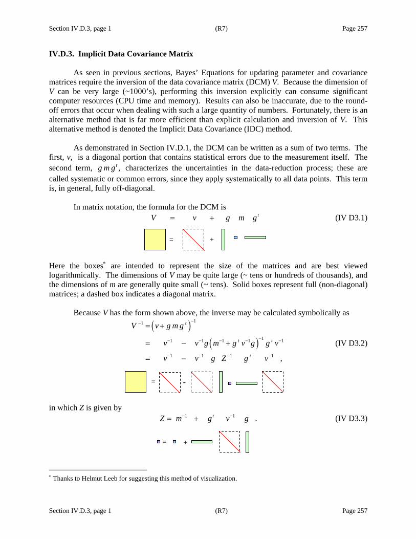
Section IV.D.3, page 1 (R7) Page 257
Section IV.D.3, page 1 (R7) Page 257
IV.D.3. Implicit Data Covariance Matrix
As seen in previous sections, Bayes’ Equations for updating parameter and covariance matrices require the inversion of the data covariance matrix (DCM) V. Because the dimension of V can be very large (~1000’s), performing this inversion explicitly can consume significant computer resources (CPU time and memory). Results can also be inaccurate, due to the round-off errors that occur when dealing with such a large quantity of numbers. Fortunately, there is an alternative method that is far more efficient than explicit calculation and inversion of V. This alternative method is denoted the Implicit Data Covariance (IDC) method.
As demonstrated in Section IV.D.1, the DCM can be written as a sum of two terms. The
first, v, is a diagonal portion that contains statistical errors due to the measurement itself. The second term, ,tg m g characterizes the uncertainties in the data-reduction process; these are called systematic or common errors, since they apply systematically to all data points. This term is, in general, fully off-diagonal.
In matrix notation, the formula for the DCM is
tV v g m g= + (IV D3.1)
Here the boxes∗ are intended to represent the size of the matrices and are best viewed logarithmically. The dimensions of V may be quite large (~ tens or hundreds of thousands), and the dimensions of m are generally quite small (~ tens). Solid boxes represent full (non-diagonal) matrices; a dashed box indicates a diagonal matrix. Because V has the form shown above, the inverse may be calculated symbolically as
( )( )
11
11 1 1 1 1
1 1 1 1 ,
t
t t
t
V v g m g
v v g m g v g g v
v v g Z g v
−−
−− − − − −
− − − −
= +
= − +
= −
(IV D3.2)
in which Z is given by 1 1 .tZ m g v g− −= + (IV D3.3)
∗ Thanks to Helmut Leeb for suggesting this method of visualization.
= +
= -
+=
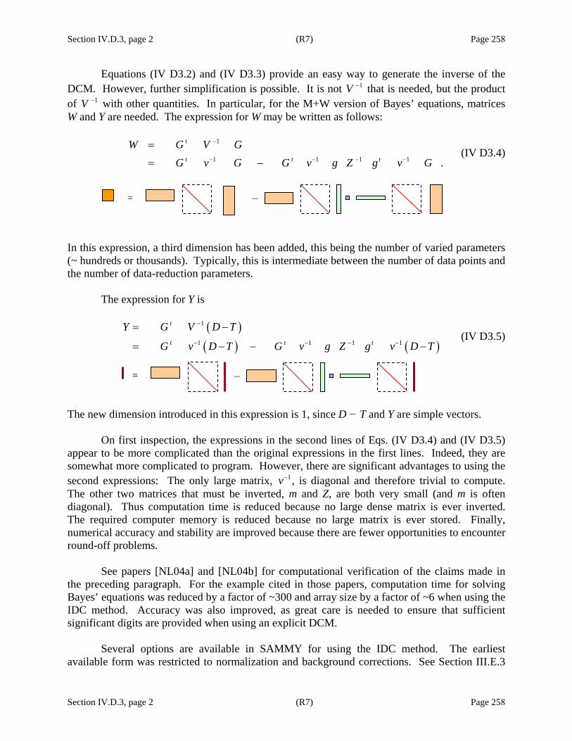
Section IV.D.3, page 2 (R7) Page 258
Section IV.D.3, page 2 (R7) Page 258
Equations (IV D3.2) and (IV D3.3) provide an easy way to generate the inverse of the DCM. However, further simplification is possible. It is not 1V − that is needed, but the product of 1V − with other quantities. In particular, for the M+W version of Bayes’ equations, matrices W and Y are needed. The expression for W may be written as follows:
1
1 1 1 1 .
t
t t t
W G V GG v G G v g Z g v G
−
− − − −
=
= − (IV D3.4)
In this expression, a third dimension has been added, this being the number of varied parameters (~ hundreds or thousands). Typically, this is intermediate between the number of data points and the number of data-reduction parameters. The expression for Y is
( )( ) ( )
1
1 1 1 1
t
t t t
Y G V D T
G v D T G v g Z g v D T
−
− − − −
= −
= − − − (IV D3.5)
The new dimension introduced in this expression is 1, since D − T and Y are simple vectors. On first inspection, the expressions in the second lines of Eqs. (IV D3.4) and (IV D3.5) appear to be more complicated than the original expressions in the first lines. Indeed, they are somewhat more complicated to program. However, there are significant advantages to using the second expressions: The only large matrix, 1v− , is diagonal and therefore trivial to compute. The other two matrices that must be inverted, m and Z, are both very small (and m is often diagonal). Thus computation time is reduced because no large dense matrix is ever inverted. The required computer memory is reduced because no large matrix is ever stored. Finally, numerical accuracy and stability are improved because there are fewer opportunities to encounter round-off problems. See papers [NL04a] and [NL04b] for computational verification of the claims made in the preceding paragraph. For the example cited in those papers, computation time for solving Bayes’ equations was reduced by a factor of ~300 and array size by a factor of ~6 when using the IDC method. Accuracy was also improved, as great care is needed to ensure that sufficient significant digits are provided when using an explicit DCM. Several options are available in SAMMY for using the IDC method. The earliest available form was restricted to normalization and background corrections. See Section III.E.3
= −
= −

Section IV.D.3, page 3 (R7) Page 259
Section IV.D.3, page 3 (R7) Page 259
for a discussion of these corrections and Section VI.C.3.c for a description of the original IDC-relevant input. For the release of sammy-7.0.0 in 2006, two additional options were made available: The first is the PUP option, discussed in Sections IV.D.1 and IV.D.2. The second is for the user to provide externally generated values for g and m. Input details are provided in Section VI.C.3.b.


Section IV.E, page 1 (R8) Page 261
Section IV.E, page 1 (R8) Page 261
IV.E. MISCELLANEOUS TOPICS RELATED TO COVARIANCES For a summary of many of the available SAMMY options related to covariances, the reader is referred to presentations [NL04a], [NL04b], and especially [NL06a].
Section IV.E.1 provides information regarding simultaneous fitting of several data sets.
SAMMY’s so-called “retroactive covariance method” is a particular application of the simultaneous fitting procedure of Section IV.E.1. This retroactive method is a means of generating a parameter covariance matrix that is approximately correct for a given (pre-determined) parameter set. See Section IV.E.2 for details.
For a means to set the prior parameter covariance matrix to infinity, thereby reducing Bayes’ equations to the usual least-squares equations, see Section IV.E.3. Other topics (such as fitting to multiple data sets while including iteration for nonlinearities) are also covered here.
Generating the covariance matrix associated with the theoretical cross section is
described in Section IV.E.4. For each spin group and channel, the average resonance width and associated uncertainty
are calculated and printed in the SAMMY.LPT file. In Section IV.E.5, the algorithm used to generate those values is described.
Section IV.E.6 describes the rationale and methodology for modifying the SAMMY
output resonance parameter covariance matrix prior to reporting the values or using them for post-processing (e.g., for calculating multigroup averages).

Section IV.E.1, page 1 (R7) Page 263
Section IV.E.1, page 1 (R7) Page 263
IV.E.1. Simultaneous Fitting to Several Data Sets The M+W scheme can be used for truly simultaneous fitting to several independent data sets in the resolved-resonance region. Any number of data sets of any type (capture, fission, integral, transmission, etc.) may be included. The procedure requires a series of separate SAMMY runs, first to generate the information separately for each data set and then to solve Bayes’ Equations once for the entire system. The procedure is as follows:
Step a. Create a single PARameter file containing only R-matrix parameters and no measurement-specific information. Flag all variables of interest; PUP no parameters. This parameter file will be used as the prior parameter set for all runs in steps b through d below.
Step b. For each independent data set, create an INPut file as usual. Put all measurement-related information into the INPut file (see the end of Table VI A.1); PUP parameters as needed (Section IV.D.2). Include the command
GENERATE Y AND W MATrices or YW in the INPut file. Run SAMMY with this INPut file, the PARameter file from step a, and the appropriate DATa file, SAMMY will produce sub-matrices Yi and Wi , which are this data set’s contribution to Y and W needed in Bayes’ Equations (Section IV.B.3). Arrays Yi and Wi are defined as
( )1 1 and ,t ti i i i i i i iY G V D T W G V G− −= − = (IV E1.1)
in which the subscript i denotes the specific data set. These values are stored in file SAMMY.YWY, which the user should rename and keep for use in step d.
Step c. Repeat step b as many times as needed, once for each data set.
Step d. Once Yi and Wi are known for each set of experimental data, they can be summed over the data sets i, giving
and .i ii i
Y Y W W= =∑ ∑ (IV E1.2)
These matrices will be used in Bayes= equations, Eq. (IV B3.2) and Eq. (IV B3.4), respectively, to solve for updated parameter values and covariance matrix. This step is accomplished by an additional SAMMY run in which the INPut file includes the phrase
READ Y AND W MATRICEs or WY The PARameter file from step a is used, and a dummy name may be given for the data set. Names of the files containing the sub-matrices Yi and Wi are specified, one per line, immediately following the dummy data-file name in the input stream. This run produces the SAMMY.PAR and SAMMY.COV files. Be sure to rename these to use in later steps.

Section IV.E.1, page 2 (R7) Page 264
Section IV.E.1, page 2 (R7) Page 264
If iteration for nonlinearities is to be used, an additional command is required in the INPut file in step d: REMEMBER ORIGINAL PArameter values This command causes a file REMORI.PAR to be created; this file contains values for (0)P and 1M − , as needed in the iterative form of Bayes’ equations for M+W [Eq. (IV A3.3)].
Step e. To iterate for nonlinearities, create a second INPut file for each data set identical to the INPut file created in step b but containing one additional command:
USE REMEMBERED ORIGInal parameter values This command does not tell SAMMY to calculate theoretical cross sections at the original parameter values but rather to use (0)P , as specified in the REMORI.PAR file, for generating Y via the iterative form of Bayes’ equations [Eq. (IV A3.3)]. That file (with that name) must be available in the subdirectory in which these runs are made.
Run SAMMY with this INPut file and the appropriate data file, using the PARameter file
and COVariance matrix created in step d. This will cause SAMMY to generate a new Yi and Wi using the parameter values determined in Step b.
Step f. Repeat step e as many times as needed, once for each data set.
Step g. Fit the data sets using the M+W scheme using the commands USE REMEMBERED ORIGInal parameter values
READ Y AND W MATRICES, or WY The “use remembered…” command will cause SAMMY to use the (0)P and 1M − from REMORI.PAR when solving for updated parameter values and covariance matrix, as in Eq. (IV A3.3).
Step h. Repeat steps e, f, and g as many times as desired, or until convergence (i.e., until there are no more changes in the 2χ values for any of the data sets).
Step i. To obtain plot files with the final fits to the data, it is necessary to make another set of runs, one for each data set. In these runs, the INPut files should include the command
GENERATE PLOT FILE Automatically
Test cases tr082, tr089, tr131, and tr149 give examples of steps a through d of this procedure. A slight variation of this procedure is used for least-squares runs in test case tr163; see Section IV.E.3 for details.
Section IV.E.2, page 1 (R8) Page 265
Section IV.E.2, page 1 (R8) Page 265
IV.E.2. Retroactive Parameter Covariance Matrix Method Occasionally it is necessary to produce an approximate covariance matrix associated with a pre-existing set of resonance parameters.
For example, most current evaluated nuclear data files (ENDF) contain resonance parameters but not uncertainties / covariances for those parameters. The ideal cure for this situation would be to reanalyze the experimental data, including all appropriate uncertainties (those associated with both measurement and theory), thus producing a new set of resonance parameters and the corresponding covariance matrix. However, it is not possible to immediately produce complete new evaluations for all nuclides in the ENDF. Therefore, a method is needed to generate an approximate covariance matrix appropriate for the current ENDF resonance parameters.
This may be accomplished using a scheme called the “retroactive parameter covariance matrix method”: First, create representative data sets covering the energy range of the R-matrix evaluation. This may be done by running SAMMY in the no-Bayes mode with suitable energy grids and using the calculated cross sections as the “experimental data” in later runs. Make reasonable choices for the covariance matrix for this set of data. Do a simultaneous fit to all those data sets, taking the ENDF File 2 parameter set for initial values and varying all resonance parameters. Check to be sure the output parameter values are not very different from the input values. If that is the case (as it should be, with the artificial experimental data in use here), then the output parameter covariance matrix (PCM) may safely be assumed to be a reasonable approximation for the covariance matrix associated with the input parameter values.
Test case tr149 gives an example of the procedure for retroactively producing an approximate covariance matrix.
After the retroactive covariance matrix has been produced, it is possible to use that
covariance matrix with the original parameter values in another SAMMY run. To do this, include one of the following (equivalent) commands RETROACTIVE OLD PARAmeter file new covariance or RETROACTIVE or U COVARIANCE MATRIX is correct, p is not in the INPut file. In addition, make a new file identical to the original PARameter file but containing the phrase “COVARiance matrix exists” at the end of the file (after the final blank line signifying the end of the previous card set, or immediately after card set 2 if there are no other card sets). This new file and the now-renamed SAMMY.COV file from the run that created the retroactive parameter covariance file are used as the input *.par and *.cov file for this run. See test case tr083, step r, for which the PARameter file t083r.par is identical to the original file tr082a.par except for the final line. Variations on this procedure are possible. Instead of assuming that the u- PCM is correct, one could assume that the p-PCM is correct. (For a discussion of u- vs. p-parameters, see the end of Section IV.C.) Ideally, there should be virtually no differences in results obtained from the two
Section IV.E.2, page 2 (R8) Page 266
Section IV.E.2, page 2 (R8) Page 266
assumptions, since only insignificant changes should occur to the value of the parameters in the retroactive process. In practice there will be small differences. To use the p-PCM instead of the u-PCM from the *.cov file, include the command P COVARIANCE MATRIX is correct, u is not The user may wish to modify (increase) the uncertainties on some of the parameters. To give explicit values for the uncertainties, while maintaining the correlation matrix currently in the *.cov file, include both of these commands in the INPut file: P COVARIANCE MATRIX is correct, u is not and MODIFY P COVARIANCE matrix before using In addition, create a file (the “new uncertainty” file) containing, in free format, the values you want for the uncertainties for all of the varied parameters (p-parameters), in the numerical order as indicated in the LPT file. An uncertainty equal to zero in this file indicates that SAMMY should use the uncertainty from the *.cov file. The name of this file is given at the end of the input stream. See also Table VI E.2 for a complete listing of the ordering of input files. It is possible to use the “MODIFY P COVARIANCE” option with “U COVARIANCE MATRIX” rather than “P COVARIANCE MATRIX.” In this case, the u-PCM is taken from the *.cov file and transformation is made to give the associated p-PCM; this matrix is then modified using the uncertainties from the new uncertainty file. The reverse transformation then gives the u-PCM to be used in the SAMMY calculations. For additional details on modifying the SAMMY-produced PCMs, see Section IV.E.6.
Section IV.E.3, page 1 (R7) Page 267
Section IV.E.3, page 1 (R7) Page 267
IV.E.3. Least Squares and Other Extensions of SAMMY’s Methodology The least-squares method can be considered as a special case of Bayes’ equations, in which the initial parameter covariance matrix (PCM) M is diagonal and infinite (so that the inverse 1M − is zero). Nonetheless, in practice it is not easy to reach that limit when creating input for SAMMY. The usual technique is to provide a very large prior uncertainty for each parameter, large enough to be “effectively infinite.” Using this technique, however, can lead to numerical problems. In particular, large prior uncertainties on resonance energies will often permit two resonances to interchange positions – an untenable feature. To circumvent this difficulty and to facilitate comparisons with other codes that do assume a diagonal and infinite prior PCM, several options have been added to SAMMY. The relevant test case is tr163; the procedure is outlined below. Step a. For each of the data sets, generate Yi and Wi as described in the previous section. The
command line
GENERATE Y AND W MATrices or YW
must be in the input file for each run. Step b. Fit the data sets using the M+W scheme, including the following commands in the INPut
file: USE LEAST SQUARES TO give pcm for initial parameters REMEMBER ORIGINAL PArameter values
READ Y AND W MATRICEs or WY
The first of these directs SAMMY to assume that the inverse of the prior covariance matrix is zero; this command is optional (though required if one wishes to do least squares). The second command causes a file REMORI.PAR to be created; this file contains values for (0)P and 1M − , as needed in the iterative form of Bayes’ equations for M+W [Eq. (IV A3.3)]. The third command is always needed when invoking the M+W method in the resolved resonance region.
If values of starting parameters are not extremely close to the “true” results, there may be divergence problems. In that case, it may also be necessary to include the command
TAKE BABY STEPS WITH least squares method
in the INPut file. This command will cause the change in the parameter increment ( )'P P− to be 1/10 the calculated value of 'M Y [see Eq. (IV A3.1) or Eq. (IV B3.1)], and will often alleviate the divergence problems.

Section IV.E.3, page 2 (R7) Page 268
Section IV.E.3, page 2 (R7) Page 268
Step c. For each data set, generate a new Yi and Wi using the parameter values determined in step b. Include these command lines
GENERATE Y AND W MATrices or YW USE REMEMBERED ORIGInal parameter values
The second of these lines does not tell SAMMY to calculate theoretical cross sections at the original parameter values but rather to use (0)P , as specified in the REMORI.PAR file, for generating Y via the iterative form of Bayes’ equations [Eq. (IV A3.3)]. That file (with that name) must be available in the subdirectory in which these runs are made.
Step d. Fit the data sets using the M+W scheme, with the commands
USE REMEMBERED ORIGInal parameter values READ Y AND W MATRICEs or WY
The “use remembered . . .” command will cause SAMMY to use the (0)P and 1M − from REMORI.PAR when solving for updated parameter values and covariance matrix, as in Eq. (IV A3.3). Again, it may be necessary to include the “take baby steps . . .” command.
Step e. Repeat steps c and d, as many times as desired, or until convergence (i.e., until there are no more changes in the 2χ values for any of the data sets).
Test case tr163 has been set up to repeat steps c and d twice more (steps e and f, h and i). In addition, two command files (test163_many and test163hi) allow the user to rerun steps h and i 20 more times, each time overwriting the previous results (to avoid keeping so many intermediate files) while keeping track of the changes in the 2χ values. These options were implemented by the author to facilitate intercomparisons among three R-matrix codes (SAMMY, EDA [GH75], and RAC [CZ95]), as part of an IAEA Cooperative Research Project on Light-Element Standards [AC05, INDC02, INDC03, INDC04,VP04].
Section IV.E.4, page 1 (R8) Page 269
Section IV.E.4, page 1 (R8) Page 269
IV.E.4. Covariances for Calculated Cross Sections
Let Ti represent the theoretical cross section (or transmission), at energy point Ei, as calculated from the “final” set of resonance parameters and parameter covariance matrix. The covariance matrix element connecting theory point Ti with point Tj is found from
,
,i jk n
k n k n
T TM
u u∂ ∂
∂ ∂∑ (IV E4.1)
where Mkn is the covariance matrix element connecting parameter uk with parameter un . The theoretical uncertainty on theory Ti is the square root of the diagonal element; that is,
2
,
.i ii i k n
k n k n
T TT T M
u u∂ ∂
Δ = Δ =∂ ∂∑ (IV E4.2)
When the phrase
INCLUDE THEORETICAL uncertainties in plot file
is given in the command section of the INPut file, values of ΔT i will be reported in the plot file. See Section VII.C for specific details about where to find which uncertainties.
To create an ASCII listing of cross section (or transmission), uncertainty, and correlation matrix, include the phrase
CROSS SECTION COVARIance matrix is wanted in the command section of the INPut file. The desired listing will be given in the SAMMY.LPT file. This is a no-Bayes run (i.e., no fitting can be accomplished in the same SAMMY run). Using this command will also give the cross-section covariance matrix formatted into a “publishable” file named SAMCOV.PUB. This file is formatted with values separated by tabs so that it can be easily ported to a spreadsheet or other program, for example, to be plotted in three dimensions. This SAMCOV.PUB file contains the following information:
Row 1: three tabs, followed by the Ti separated by tabs Row 2: three tabs, followed by the ΔTi separated by tabs Row 3: three tabs, followed by the Ei separated by tabs Row 4: T1, Δ T1, E1, followed by the first row of the covariance matrix separated by tabs Row 5: T2, Δ T2, E2, followed by the second row of the covariance matrix separated by tabs . . . Row N+3: TN, Δ TN, EN, followed by the Nth row of the covariance matrix separated by tabs
In this format, it is easily possible to manipulate the results in a spreadsheet program. For example, the correlation matrix is found by dividing the covariance matrix element by the uncertainty in the same column in Row 2 and by the uncertainty in the same row in Column 2. See test case tr010, run e, for an example of this. (Caution: The user should exercise caution in porting this file to a spreadsheet, as the number of data points can easily become too large to fit into a normal spreadsheet.)

Section IV.E.4, page 2 (R8) Page 270
Section IV.E.4, page 2 (R8) Page 270
The SAMMY user should note that the covariance matrix constructed in this fashion is not a complete representation of the evaluated cross section covariance matrix. Detail arguments concerning this assertion are presented in Section IV.E.6.
Section IV.E.5, page 1 (R7) Page 271
Section IV.E.5, page 1 (R7) Page 271
IV.E.5. Calculating Average Values and Uncertainties for Resonance Widths In the SAMMY.LPT file (discussed in Section VII.A), the average value and uncertainty
are reported for the various channel widths for every spin group. These averages are generated from the p-parameter covariance matrix by invoking Bayes’ equations over a different set of variables from those used in earlier sections of this manual.
To calculate an average over a set of correlated parameters, we recognize that “average” can be interpreted as “most likely value for a group of numbers.” Bayes’ equations therefore are applicable, where the theoretical model is a simple function equal to the average whose value is needed. Explicitly, we can rewrite Bayes’ equations [see, for example, Eq. (IV A 1.1)] into the form
1' ' tA K G M −= Γ (IV E5.1)
and ( ) 11' .tK G M G−−= (IV E5.2)
Here A' represents the needed average (for example, for the neutron widths for spin group number 3), and Γ represents the individual values (for each of those widths). The prior value for the average is set to zero. K ' is the needed variance for the average, and the prior variance is set to infinity. M represents that portion of the parameter covariance matrix which corresponds to this set of widths. Finally, G is the partial derivative of the function to be fitted with respect to the average A, so that G is 1 for parameters in the set of interest and 0 for all other parameters. With these definitions, Eq. (IV E5.2) reduces to
( )1
1' ,i j
i j
K M−
−⎡ ⎤= ⎢ ⎥⎣ ⎦∑ (IV E5.3)
in which the summation includes all parameters within the set to be averaged. The average value from Eq. (IV E5.1) then becomes
( )1' ' ,ji ji j
A K M −= Γ∑ (IV E5.4)
again summing over only the relevant parameters.
In the SAMMY.LPT file, two different average values and uncertainties are reported for each channel width for each spin group:
The first is labeled “Expected Value” in the LPT file and includes all varied widths in the summations in Eqs. (IV E5.3) and (IV E5.4).
The second is labeled “EV changed parameters” and attempts to include only those widths whose values have been affected (changed) by the data analysis. However, the criterion used to determine which parameters are to be included is rather naive: the uncertainty on the individual widths must be less than 9% of the value of the parameter.
In either case, if there are no parameters fitting the requirements, the printed average and uncertainty are zero.


Section IV.E.6, page 1 (R8) Page 273
Section IV.E.6, page 1 (R8) Page 273
IV.E.6. Augmenting the Resonance Parameter Covariance Matrix The posterior resonance parameter covariance matrix (RPCM) produced by SAMMY is a accurate representation of the uncertainties in the R-matrix evaluation.† Nevertheless, uncertainties for evaluated cross sections reproduced by propagating the RPCM have historically been regarded as “too small.” In fact, cross section uncertainties based solely on the RPCM are indeed too small, because it is not possible for the RPCM to convey complete information concerning the evaluated cross section covariance matrix (ECSCM). There are at least three reasons for this inability: (1) computation of the RPCM is based on assumptions which are not fully valid; (2) Bayes’ equation for the RPCM contains no information about the validity of the fit of theory to data; (3) the experimental data base is not unique. These three reasons are discussed more fully below.
(1) Assumptions underlying computation of the RPCM. The RPCM would indeed provide a complete description of the ECSCM, if all underlying assumptions of the evaluation procedure were to have no uncertainty associated with them. However, most underlying assumptions are suspect to some degree. The most basic assumption is that R-matrix theory provides a correct and complete description of the interactions for which data are being evaluated. All resonances are included, even very small experimentally invisible resonances and even the (infinite number of) resonances lying outside the energy region under analysis. All spin assignments are correct; there is no unresolved ambiguity. No direct components or other extensions to R-matrix theory exist. Further, everything has been calculated correctly; there are no bugs in the computer code. Another important assumption is that all experimental conditions are properly understood and included in the analysis. Corrections are accurately made for Doppler and resolution broadening, multiple-scattering, normalization, and backgrounds. No corrections, however minor, have been omitted; each experiment is completely understood and correctly simulated in the code. Everything has been calculated correctly; there are no bugs in the computer code. Clearly, not one of the assumptions listed in the previous two paragraphs is absolutely valid; each has some non-readily-quantifiable uncertainty associated with it. None of those uncertainties will be reflected in the RPCM. (2) Validity of the fit. The non-iterative form of Bayes’ equation for the RPCM can be written as
( ) 11 1' ,tM G V G M−− −= + (1.1)
† This has been confirmed by at least two independent researchers, who compared the SAMMY-produced results with Monte Carlo simulations. Unfortunately, neither of those studies has been published.

Section IV.E.6, page 2 (R8) Page 274
Section IV.E.6, page 2 (R8) Page 274
where M is the prior resonance parameter covariance matrix (usually assumed to be large or infinite, so that 1 0M − ≈ ), G is the sensitivity matrix (partial derivatives of theory with respect to the parameters), and V is the experimental data covariance matrix. Nowhere in this equation is there any information about the goodness of the fit between theory and measurement. Therefore the RPCM does not contain any information about poor fits, nor can it reflect any discrepancies among the various data sets. (3) Non-unique data base. For every evaluation, the evaluator considers all available relevant measurements and accepts or rejects each measurement based on his/her determination of the quality of the data. This determination is based on a study of the documentation for the measurement (e.g., whether or not sufficient information is provided to understand the uncertainties associated with the experiment) and on preliminary analyses of the individual data sets. The evaluator may find the need to renormalize the data, subtract a background, or rescale the energies for certain measurements in order to make them consistent with other measurements. Even though the evaluator can and should attempt to incorporate all known uncertainties into the evaluation (e.g., including normalization uncertainty as a PUP parameter), there is no well-defined methodology for including uncertainties related to the choice of data base. Those uncertainties will therefore not be reflected in the output RPCM.
The logical conclusion is that the resonance parameter covariance matrix alone cannot
provide complete information on the uncertainty in the evaluated cross section. Something else is clearly needed. It is not obvious how one could quantize the effects described above. Nevertheless, the attempt should be made, and some approximate contribution be added to the ECSCM in addition to the contribution from the RPCM. Historically, what has been done is to increase the RPCM in a rather arbitrary fashion, based on the nuclear data community’s judgment of what the ECSCM should look like. For example, for the light element standards for ENDF/B-VI, the ESCSM uncertainties were adjusted upwards so that “… if a modern day experiment were performed today on a given standard using the best techniques, those results should fall within these expanded uncertainties (2/3 of the time).”† For the first release of ENDF/B-VII and for early subsequent evaluations, the usual procedure was for the evaluator to increase either the diagonal elements of the RPCM or (more commonly) increase the uncertainties while maintaining the correlation matrix, while attempting to conform to the evaluator’s opinion of what the multigroup cross section covariance matrix should look like. (Various options for accomplishing this task were implemented in SAMMY; these are described in Subsection IV.E.6.a.) This technique, however, is highly subjective and
† As quoted by A. D. Carlson at the 2002 Research Coordination Meeting of the IAEA Coordinated Research Project on light element standards.

Section IV.E.6, page 3 (R8) Page 275
Section IV.E.6, page 3 (R8) Page 275
awkward to use, as the link between the RPCM and the ESCSM (or multigroup covariance matrix) is sufficiently indirect that much trial-and-error is required to achieve the desired result. More recently, it was recognized by Herve Derrien that normalization and/or background uncertainty components could be added to the RPCM component in order to provide a seemingly realistic description of the expected ECSCM. While these components certainly do not completely reflect all the various types of uncertainties discussed above, they nevertheless may provide a reasonable first approximation for the previously omitted components. The link between normalization and background uncertainty and ESCSM is direct, making this a more satisfying solution than arbitrary increases in the RPCM. An additional positive feature of this option is that it may be implemented directly into ENDF files, without new format requirements, by using ENDF File 33 normalization and background descriptions [NL07c].

Section IV.E.6.a, page 1 (R8) Page 277
Section IV.E.6.a, page 1 (R8) Page 277
IV.E.6.a. Modifying the parameter uncertainties In response to analysts’ requests for automated methods to increase the uncertainties on the resonance parameters, a variety of options have been created. With the exception of Option #2 below, these will be used with runs that perform post-processing operations (e.g., calculate multigroup averages as described in Section V.C or create ENDF File 32 descriptions of the PCM as discussed in Section IX). All of these methods assume that uncertainties are to be modified but the correlation coefficients will remain the same. Option #1. A simple INPut file command will cause every uncertainty for every resonance parameter to be multiplied by the same value, that is, every element of the PCM to be multiplied by the square of that value. This command is INITIAL UNCERTAINTY multiplier = value The equal sign must be present, and “value” is replaced by a positive real number. At the beginning of this SAMMY run, each element of the PCM obtained from the input COVariance file is multiplied by the square of the value. See test case tr019, run d. Option #2. A related command is FINAL UNCERTAINTY MUltiplier = value Here it is the output PCM that is modified; see test case tr019, run e, for an example of the use of this command. Use of this option is not recommended because it requires the analyst to decide before viewing the PCM that the PCM must be changed. Option #1 can be used to produce the same result without permanently changing the SAMMY.COV file (produced directly from the data analysis process) via multiplication by a preconceived value. Option #3. To multiply the PCM by a value which varies with energy, and may also be spin group dependent, use the command
E-DEPENDENT INITIAL uncertainty multiplier or E-DEPENDENT UNCERTAInty multiplier. (The hyphen is optional here.) A separate EDU (energy-dependent uncertainty) file is needed with this command; the EDU file contains the following information:
1. Alphanumeric title 2. Second title line, or blank 3. Spin group = 1 [only the equal sign and the number are absolutely necessary] 4. Energy, value of multiplier in 2F10.1 format (i.e., one value in the first ten columns and
the second in the next ten columns) 5. Repeat line 4 as many times as needed 6. End with a blank line 7. Repeat lines 3 through 6 as many times as needed
Energies (line 4) must be in order of increasing energy. For resonances in the specified spin group, SAMMY will linearly interpolate to give the value of the multiplier at the resonance

Section IV.E.6.a, page 2 (R8) Page 278
Section IV.E.6.a, page 2 (R8) Page 278
energy. If the resonance energy is outside the specified energies (below the first or above the last), the multiplier is assumed to be unity. Likewise, if a spin group is omitted from this listing, the multiplier will be unity for all resonances in that group. Note that the same multiplier is used for all parameters (energy and widths) for a particular resonance. The name of the EDU file is given after the name of the COVariance file in the input stream. Note that this option works only if you are using a pre-existing COVariance file, not if starting from scratch. Examples are given in test case tr019, runs f and g. Option #4. To modify the uncertainty on each parameter separately and independently from the modification of the uncertainties on other parameters (while maintaining the original correlation coefficients), insert the commands
P COVARIANCE MATRIX is correct, u is not MODIFY P COVARIANCE matrix before using
into the INPut file. Create a file containing the new values for the uncertainties, in the same order in which they appear in the LPT file, in free format. For those parameters for which you do not wish to change the uncertainty, it is not necessary to copy the value of the uncertainty into this file; instead, the value in this file can be set to zero. The name of this file is given to SAMMY directly following the name of the COVariance file. For examples, see test case tr149, runs l, m, o, and p.
Option #5. The RSAP program [RS03] contains options to read the SAMMY-produced SAMMY.PUB file (see Section VII.F) and create plots showing the effects of modifying the parameter values within the bounds of the uncertainties on the parameters. The uncertainties can be scaled, in which case RSAP produces a new file rsap.PUB in the same format as SAMMY.PUT, containing, however, the scaled uncertainties.
To report the scaled uncertainties back to SAMMY for additional computations, an auxiliary code PUB2COV was written by D. Wiarda. (This code will be made available as part of the RADCOP program under development by R. O. Sayer. [RS06a] ) Input to the PUB2COV code consists of the original SAMMY PARameter and COVariance files, the original PUB file, and the modified PUB file. Output is a hybrid SAMMY COVariance file containing the original parameter values, the modified p-PCM, and the original u-PCM. (The modified p-PCM has the new uncertainties but the original correlation coefficients.)
To use the hybrid SAMMY COVariance file in a new SAMMY run (e.g., to generate ENDF Files 2 and 32), include the command
P COVARIANCE MATRIX is correct, u is not in the INPut file.

Section V, page 1 (R7) Page 279
Section V, page 1 (R7) Page 279
V. POST-PROCESSORS AND OTHER MISCELLANEOUS TOPICS
In addition to fitting energy- and angle-differential data in the resolved (and unresolved) resonance region, SAMMY has capabilities for other tasks such as reproducing cross sections directly from resonance parameters, calculating average cross sections, or creating portions of ENDF files. Some of these features are described in this section. For a discussion of SAMMY’s interactions with ENDF files, see Section IX.
Methods for reconstructing point-wise cross sections without having to specify an energy
grid are given in Section V.A.
Section V.B includes a discussion SAMMY’s calculation of certain integral quantities. The code can also fit to these quantities where data or standard values are available.
Section V.C describes how SAMMY may be used to average cross sections (both theoretical and experimental) over particular energy range. The corresponding covariance matrix is also generated.
SAMMY=s calculation of Maxwellian averages of capture cross sections (sometimes called “stellar averages”) is discussed in Section V.D.
Section V.E describes various “pseudo cross sections” (simple functional forms) that can be generated by SAMMY, for use primarily in debugging Doppler or resolution functions.
Section V.F describes a method for generating the summed strength function for
resonance parameters in a particular spin group.


Section V.A, page 1 (R8) Page 281
Section V.A, page 1 (R8) Page 281
V.A. RECONSTRUCTING POINT-WISE CROSS SECTIONS
SAMMY’S main purpose is to analyze neutron-induced cross section data by fitting to R-matrix parameters; in that mode, the user provides an energy grid (the experimental grid) from which an auxiliary grid can be constructed as discussed in Sections III.A.1 and III.A.2. To calculate a cross section directly from the resonance parameters without any pre-defined energy grid, one would use a nuclear data processor code such as AMPX [MD02], NJOY [RM82], or PREPRO [DC04]; these codes were designed to create energy grids that would describe the unbroadened cross sections with sufficient accuracy for essentially any purpose.
Occasionally, however, it is desirable to have SAMMY generate point-wise cross sections without a pre-existing energy grid. SAMMY has two methods of accomplishing this, as described below. The user should be aware that the energy grids generated in SAMMY will provide a means of viewing the cross sections but are not intended to be highly accurate representations of all the structure in the cross sections.
Method 1
The first method, borrowed almost directly from the processing code NJOY [RM82], uses a convergence algorithm to choose an energy grid sufficiently dense to properly define total, elastic, and capture cross sections, as well as fission if needed. The output plot files (SAMMY.ODF, SAMMY.LST, SAMM.PLT) contains energies in section 1, total cross section in section 2, elastic cross section in section 3, capture cross section in section 4, and reaction cross section in section 5 if needed; section 6 holds the absorption cross section (sum of capture plus reaction cross sections). These cross sections are unbroadened (zero temperature). To invoke this option, include the phrase
RECONSTRUCT CROSS SEctions from resonance parameters
in card set 3 of the INPut file (see Section VI.A of this report). SAMMY will ask for the data file name, as always, but a dummy name may be given since that information is never used.
Caveat: This method makes use of the Reich-Moore approximation to R-Matrix theory. It cannot be used with MLBW or SLBW resonance parameters.
Several criteria are used in the RECONSTRUCT option to ensure that the energy grid is sufficiently dense. An initial grid consists of beginning and ending points plus all resonance energies within the specified energy range. Beginning at the lowest energy, each pair of points
( )a aEσ σ= and ( )b bEσ σ= is examined to see whether these two points alone can describe the
midpoint between those two points ( )( )12m m a bE E Eσ σ= = + . Convergence is assumed only if each
type of cross section (elastic, capture, and reaction) separately meets one of the criteria.
Criterion # 1. If both aσ and bσ are smaller than SIGMIN, points a and b are sufficient.
The value for SIGMIN is an input parameter whose default is 610 − barns.
Section V.A, page 2 (R8) Page 282
Section V.A, page 2 (R8) Page 282
Criterion # 2. For large changes in the cross sections ( 1.4a bσ σ> or 1.4b aσ σ> ), the midpoint is added to the energy grid.
Criterion # 3. Let ,intmσ represent the interpolated cross section at mE ; ,intmσ is given by
,int .b m m am a b
b a b a
E E E EE E E E
σ σ σ− −
= +− −
(V A.1)
If mσ is smaller than both aσ and bσ (so that the midpoint is near a minimum in the cross section), the convergence requirement is
,int ERRXC2 /10 .b b bσ σ σ− ≤ × (V A.2)
where ERRXC2 is an input parameter whose default value is 0.005.
Criterion # 4. If mσ is not smaller than both aσ and bσ , the criterion is less stringent.
,int ERRXC2 .b b bσ σ σ− ≤ × (V A.3)
The convergence parameters ERRXC2 and SIGMIN may be specified by the user to have different values from the default values of 0.005 and 610 − barns, respectively. See card set 7 of the INPut file (Table VI A.1).
For examples using Method 1, see test case tr037 and others.
Method 2
SAMMY’s second option for generating point-wise cross sections without specifying an energy grid a priori makes use of SAMMY=s ability to choose an auxiliary grid that properly defines the unbroadened cross section (see Section III.A). The user must provide some kind of a “data file,” but it need not necessarily be appropriate for the nuclide(s) being considered; it is used only as a starting point for the auxiliary grid. SAMMY first sets up a grid of NEPNTS from EMIN to EMAX; NEPNTS is specified on card set 2 of the INPut file (see Table VI A.1). This grid is evenly spaced in velocity space (i.e., in the square root of energy). SAMMY then chooses additional points for the auxiliary grid as though broadening were to occur.
To invoke this option include the phrases ARTIFICIAL ENERGY GRid is needed
and PUT UNBROADENED CROSs sections into plot file
in the INPut file. An output plot file SAMMY.UNB† contains energies in section 1 and cross section in section 2. A second file, SAMMY.DAT, contains the same information in SAMMY’s TWENTY data format.
† Note that the name of this file is no longer SAMXAC.ODF, to avoid confusion about which file is produced when.

Section V.A, page 3 (R8) Page 283
Section V.A, page 3 (R8) Page 283
Unlike the RECONSTRUCT method of generating an energy grid, this method evaluates only the one type of cross section specified in the INPut file. Also unlike the first method, any of the several R-matrix approximations may be used, as specified in the INPut file.
Both methods
Examples of reconstructing point-wise cross sections using both of these methods can be found in several test cases. See, specifically, tr037 for “pure” reconstruction and tr042, tr049, and tr175 for reconstruction followed by computation of stellar (Maxwellian) averages (see Section V.D).
Finally, it should be noted that, prior to release 7.0.1 of the SAMMY code, the implementation of method 1 would occasionally produce unrealistic values of stellar averages.

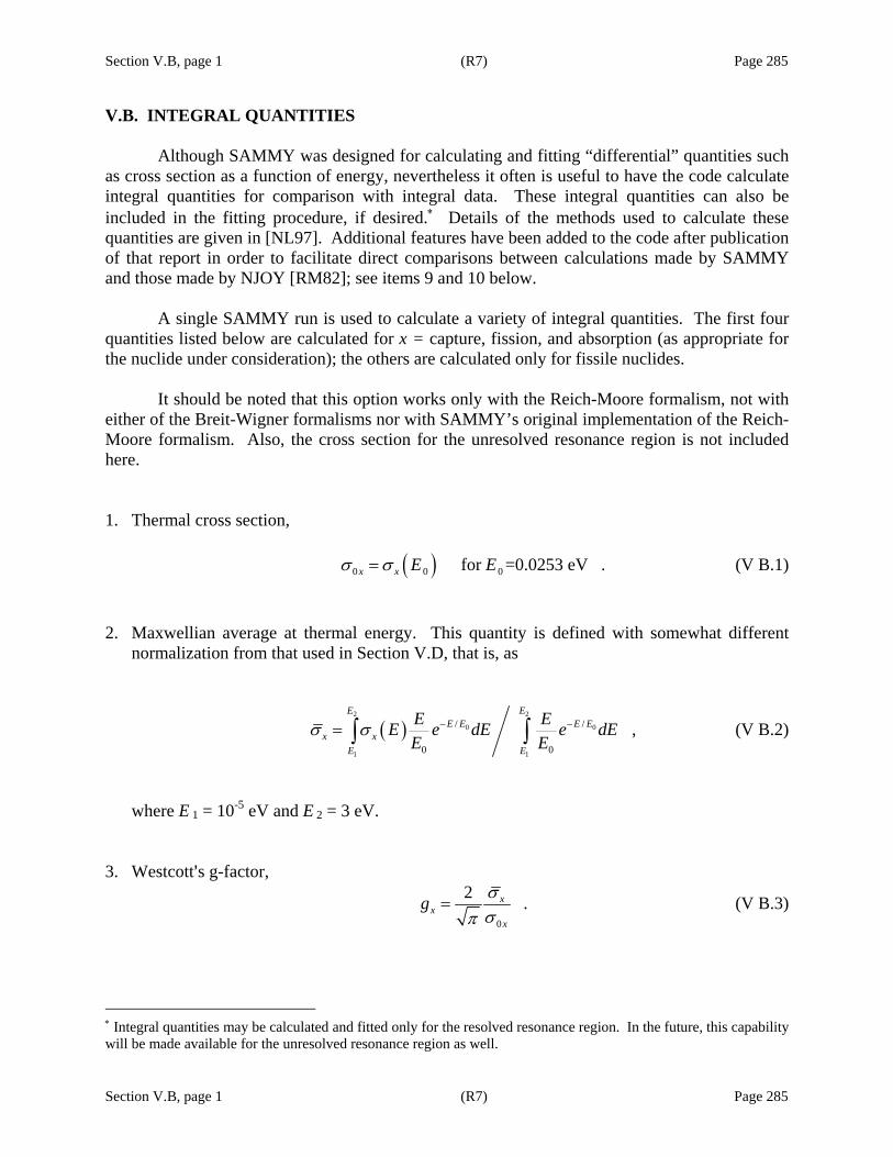
Section V.B, page 1 (R7) Page 285
Section V.B, page 1 (R7) Page 285
V.B. INTEGRAL QUANTITIES
Although SAMMY was designed for calculating and fitting “differential” quantities such as cross section as a function of energy, nevertheless it often is useful to have the code calculate integral quantities for comparison with integral data. These integral quantities can also be included in the fitting procedure, if desired.∗ Details of the methods used to calculate these quantities are given in [NL97]. Additional features have been added to the code after publication of that report in order to facilitate direct comparisons between calculations made by SAMMY and those made by NJOY [RM82]; see items 9 and 10 below.
A single SAMMY run is used to calculate a variety of integral quantities. The first four quantities listed below are calculated for x = capture, fission, and absorption (as appropriate for the nuclide under consideration); the others are calculated only for fissile nuclides.
It should be noted that this option works only with the Reich-Moore formalism, not with either of the Breit-Wigner formalisms nor with SAMMY’s original implementation of the Reich-Moore formalism. Also, the cross section for the unresolved resonance region is not included here. 1. Thermal cross section,
( )0 0 0 for =0.0253 eV .x x E Eσ σ= (V B.1) 2. Maxwellian average at thermal energy. This quantity is defined with somewhat different
normalization from that used in Section V.D, that is, as
( )2 2
0 0
1 1
/ /
0 0
,E E
E E E Ex x
E E
E EE e dE e dEE E
σ σ − −= ∫ ∫ (V B.2)
where E 1 = 10-5 eV and E 2 = 3 eV.
3. Westcott=s g-factor,
0
2 .xx
x
g σσπ
= (V B.3)
∗ Integral quantities may be calculated and fitted only for the resolved resonance region. In the future, this capability will be made available for the unresolved resonance region as well.
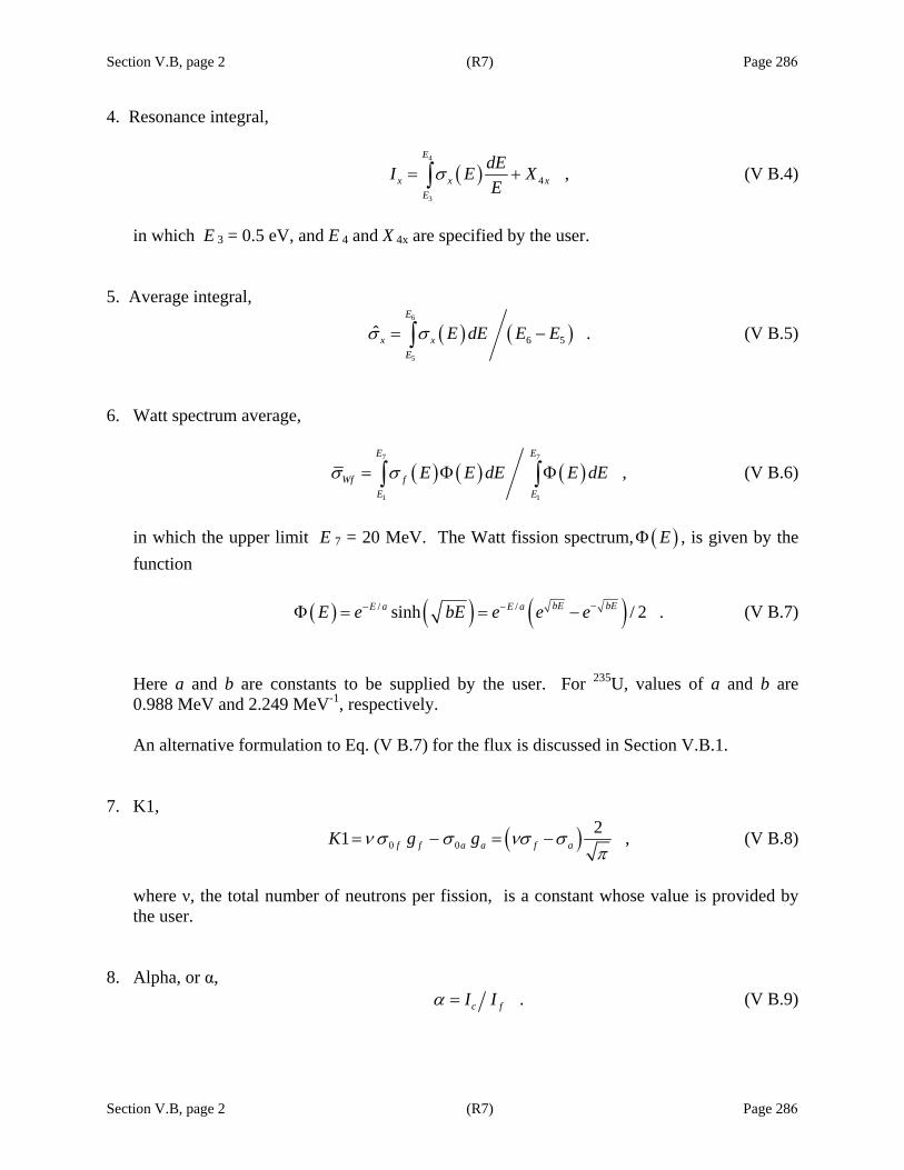
Section V.B, page 2 (R7) Page 286
Section V.B, page 2 (R7) Page 286
4. Resonance integral,
( )4
3
4 ,E
x x xE
dEI E XE
σ= +∫ (V B.4)
in which E 3 = 0.5 eV, and E 4 and X 4x are specified by the user.
5. Average integral,
( ) ( )6
5
6 5ˆ .E
x xE
E dE E Eσ σ= −∫ (V B.5)
6. Watt spectrum average,
( ) ( ) ( )7 7
1 1
,E E
Wf fE E
E E dE E dEσ σ= Φ Φ∫ ∫ (V B.6)
in which the upper limit E 7 = 20 MeV. The Watt fission spectrum, ( )EΦ , is given by the function ( ) ( ) ( )/ /sinh / 2 .bE bEE a E aE e bE e e e−− −Φ = = − (V B.7)
Here a and b are constants to be supplied by the user. For 235U, values of a and b are 0.988 MeV and 2.249 MeV-1, respectively. An alternative formulation to Eq. (V B.7) for the flux is discussed in Section V.B.1.
7. K1,
( )0 021 ,f f a a f aK g gν σ σ νσ σπ
= − = − (V B.8)
where ν, the total number of neutrons per fission, is a constant whose value is provided by the user.
8. Alpha, or α,
.c fI Iα = (V B.9)
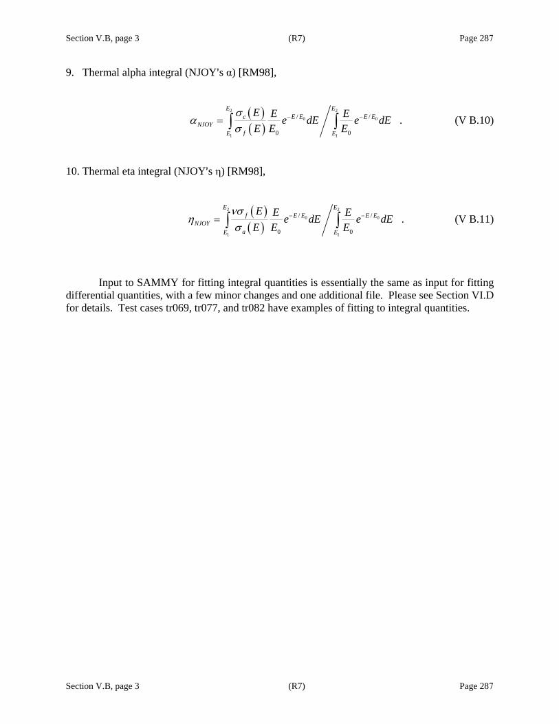
Section V.B, page 3 (R7) Page 287
Section V.B, page 3 (R7) Page 287
9. Thermal alpha integral (NJOY=s α) [RM98],
( )( )
2 2
0 0
1 1
/ /
0 0
.E E
E E E EcNJOY
fE E
E E Ee dE e dEE E E
σα
σ− −= ∫ ∫ (V B.10)
10. Thermal eta integral (NJOY=s η) [RM98],
( )( )
2 2
0 0
1 1
/ /
0 0
.E E
f E E E ENJOY
aE E
E E Ee dE e dEE E E
νση
σ− −= ∫ ∫ (V B.11)
Input to SAMMY for fitting integral quantities is essentially the same as input for fitting differential quantities, with a few minor changes and one additional file. Please see Section VI.D for details. Test cases tr069, tr077, and tr082 have examples of fitting to integral quantities.

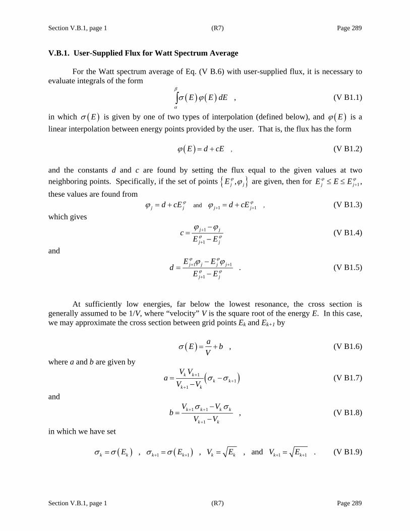
Section V.B.1, page 1 (R7) Page 289
Section V.B.1, page 1 (R7) Page 289
V.B.1. User-Supplied Flux for Watt Spectrum Average
For the Watt spectrum average of Eq. (V B.6) with user-supplied flux, it is necessary to evaluate integrals of the form
( ) ( ) ,E E dEβ
α
σ ϕ∫ (V B1.1)
in which ( )Eσ is given by one of two types of interpolation (defined below), and ( )Eϕ is a linear interpolation between energy points provided by the user. That is, the flux has the form ( ) ,E d cEϕ = + (V B1.2) and the constants d and c are found by setting the flux equal to the given values at two neighboring points. Specifically, if the set of points ,j jE ϕ ϕ are given, then for 1j jE E Eϕ ϕ
+≤ ≤ , these values are found from 1 1and ,j j j jd cE d cEϕ ϕϕ ϕ + += + = + (V B1.3) which gives
1
1
j j
j j
cE Eϕ ϕ
ϕ ϕ+
+
−=
− (V B1.4)
and
1 1
1
.j j j j
j j
E Ed
E E
ϕ ϕ
ϕ ϕ
ϕ ϕ+ +
+
−=
− (V B1.5)
At sufficiently low energies, far below the lowest resonance, the cross section is generally assumed to be 1/V, where “velocity” V is the square root of the energy E. In this case, we may approximate the cross section between grid points Ek and Ek+1 by
( ) ,aE bV
σ = + (V B1.6)
where a and b are given by
( )11
1
k kk k
k k
V Va
V Vσ σ+
++
= −−
(V B1.7)
and
1 1
1
,k k k k
k k
V Vb
V Vσ σ+ +
+
−=
− (V B1.8)
in which we have set ( ) ( )1 1 1 1, , , and .k k k k k k k kE E V E V Eσ σ σ σ+ + + += = = = (V B1.9)
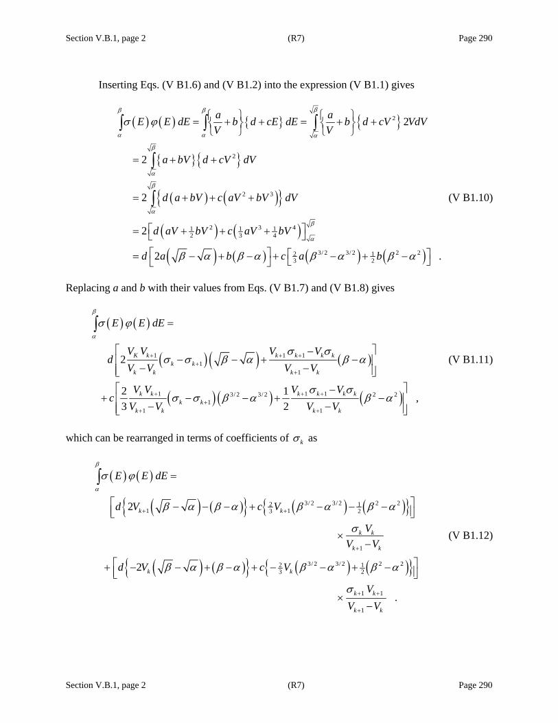
Section V.B.1, page 2 (R7) Page 290
Section V.B.1, page 2 (R7) Page 290
Inserting Eqs. (V B1.6) and (V B1.2) into the expression (V B1.1) gives
( ) ( )
( ) ( )
( ) ( )( ) ( ) ( ) ( )
2
2
2 3
2 3 41 1 12 3 4
3/ 2 3/ 2 2 22 13 2
2
2
2
2
2 .
a aE E dE b d cE dE b d cV VdVV V
a bV d cV dV
d a bV c aV bV dV
d aV bV c aV bV
d a b c a b
ββ β
α α α
β
α
β
α
β
α
σ ϕ
β α β α β α β α
⎧ ⎫ ⎧ ⎫= + + = + +⎨ ⎬ ⎨ ⎬⎩ ⎭ ⎩ ⎭
= + +
= + + +
⎡ ⎤= + + +⎣ ⎦
⎡ ⎤ ⎡ ⎤= − + − + − + −⎣ ⎦⎣ ⎦
∫ ∫ ∫
∫
∫ (V B1.10)
Replacing a and b with their values from Eqs. (V B1.7) and (V B1.8) gives
( ) ( )
( ) ( ) ( )
( ) ( ) ( )
1 1 11
1
1 1 13/ 2 3/ 2 2 21
1 1
2
2 1 ,3 2
K k k k k kk k
k k k k
k k k k k kk k
k k k k
E E dE
V V V Vd
V V V V
V V V Vc
V V V V
β
α
σ ϕ
σ σσ σ β α β α
σ σσ σ β α β α
+ + ++
+
+ + ++
+ +
=
⎡ ⎤−− − + −⎢ ⎥
− −⎢ ⎥⎣ ⎦⎡ ⎤−
+ − − + −⎢ ⎥− −⎢ ⎥⎣ ⎦
∫
(V B1.11)
which can be rearranged in terms of coefficients of kσ as
( ) ( )
( ) ( ) ( ) ( )
( ) ( ) ( ) ( )
3/ 2 3/ 2 2 22 11 13 2
1
3/ 2 3/ 2 2 22 13 2
1 1
1
2
2
.
k k
k k
k k
k k
k k
k k
E E dE
d V c V
VV V
d V c V
VV V
β
α
σ ϕ
β α β α β α β α
σ
β α β α β α β α
σ
+ +
+
+ +
+
=
⎡ ⎤− − − + − − −⎢ ⎥⎣ ⎦
×−
⎡ ⎤+ − − + − + − − + −⎢ ⎥⎣ ⎦
×−
∫
(V B1.12)
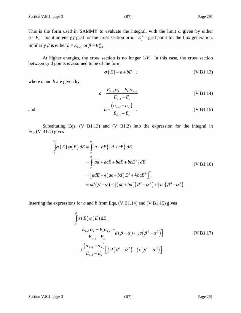
Section V.B.1, page 3 (R7) Page 291
Section V.B.1, page 3 (R7) Page 291
This is the form used in SAMMY to evaluate the integral, with the limit α given by either α = kE = point on energy grid for the cross section or α = jE ϕ = grid point for the flux generation.
Similarly β is either β = 1kE + or β = 1jE ϕ+ .
At higher energies, the cross section is no longer 1/V. In this case, the cross section
between grid points is assumed to be of the form
( ) ,E a bEσ = + (V B1.13)
where a and b are given by
1 1
1
k k k k
k k
E Ea
E Eσ σ+ +
+
−=
− (V B1.14)
and ( )1
1
.k k
k k
bE Eσ σ+
+
−=
− (V B1.15)
Substituting Eqs. (V B1.13) and (V B1.2) into the expression for the integral in Eq. (V B1.1) gives
( ) ( )
( )( ) ( )( ) ( )
2
2 31 12 3
2 2 3 31 12 3 .
E E dE a bE d cE dE
ad acE bdE bcE dE
adE ac bd E bcE
ad ac bd bc
β β
α α
β
α
β
α
σ ϕ
β α β α β α
= + +
= + + +
⎡ ⎤= + + +⎣ ⎦
= − + + − + −
∫ ∫
∫ (V B1.16)
Inserting the expressions for a and b from Eqs. (V B1.14) and (V B1.15) gives
( ) ( )
( ) ( )
( ) ( ) ( )
1 1 2 212
1
1 2 2 3 31 12 3
1
.
k k k k
k k
k k
k k
E E dE
E Ed c
E E
d cE E
β
α
σ ϕ
σ σβ α β α
σ σβ α β α
+ +
+
+
+
=
−⎡ ⎤− + −⎣ ⎦−
−⎡ ⎤+ − + −⎣ ⎦−
∫
(V B1.17)
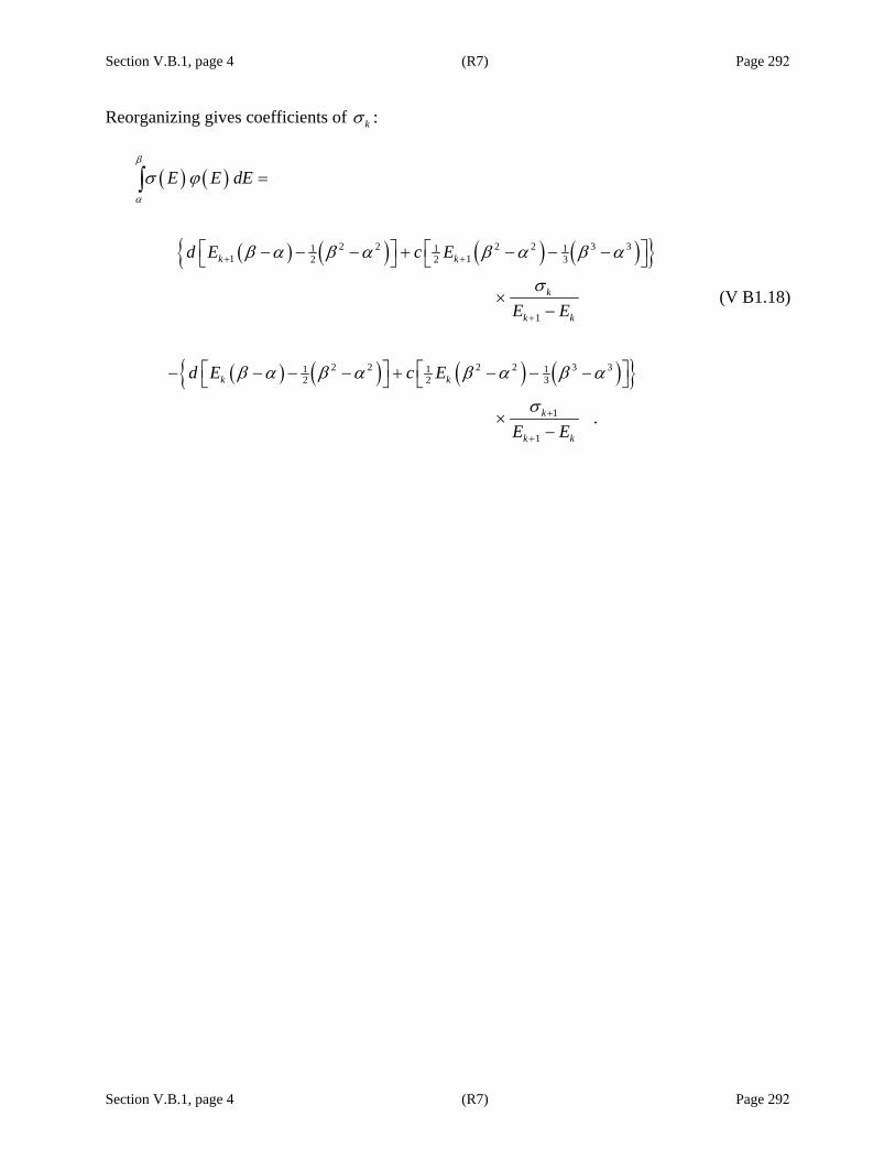
Section V.B.1, page 4 (R7) Page 292
Section V.B.1, page 4 (R7) Page 292
Reorganizing gives coefficients of kσ :
( ) ( )
( ) ( ) ( ) ( )
( ) ( ) ( ) ( )
2 2 2 2 3 31 1 11 12 2 3
1
2 2 2 2 3 31 1 12 2 3
1
1
.
k k
k
k k
k k
k
k k
E E dE
d E c E
E E
d E c E
E E
β
α
σ ϕ
β α β α β α β α
σ
β α β α β α β α
σ
+ +
+
+
+
=
⎡ ⎤ ⎡ ⎤− − − + − − −⎣ ⎦ ⎣ ⎦
×−
⎡ ⎤ ⎡ ⎤− − − − + − − −⎣ ⎦ ⎣ ⎦
×−
∫
(V B1.18)

Section V.C, page 1 (R8) Page 293
Section V.C, page 1 (R8) Page 293
V. C. AVERAGING THE CROSS SECTIONS
Once the SAMMY analysis is completed, the analyst may wish to average the theoretical curves produced by SAMMY over an energy range (or ranges) in order to more directly compare results with those from other experiments or analyses. Alternatively, the analyst may wish to produce multi-group cross sections plus covariance matrix for use in further calculations.
Three options are available in SAMMY for averaging the cross section: The original option uses an energy or time average and treats the quantity to be averaged as a
histogram. Hence it is useful for averaging experimental data that have been binned into channels but is not so useful for accurate averaging of theoretical cross sections. See Section V.C.1 for details on this option.
The second option uses the Bondarenko [IB64] narrow-resonance scheme for weighting the
cross section. Sophisticated integration techniques are used to accurately and rapidly calculate the averages. See Section V.C.2 for details.
The third is an unweighted energy average similar to the first option but uses the same
techniques to evaluate the integrals as are used in the Bondarenko option; see Section V.C.3. In all cases, uncertainties are propagated through the entire procedure. Uncertainties and
correlation matrix are printed for the multi-group cross sections. To ensure accurate uncertainties for the multi-group cross sections, it may be necessary to
eliminate the cutoff for non-s-wave resonances (Section II.D.1.b). This is accomplished by inserting the command
USE NO CUTOFFS FOR Derivatives or cross sections into the INPut file.

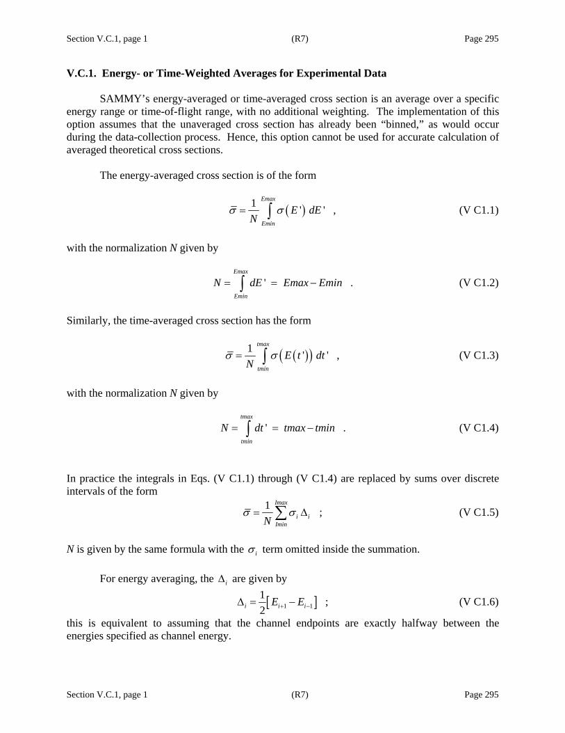
Section V.C.1, page 1 (R7) Page 295
Section V.C.1, page 1 (R7) Page 295
V.C.1. Energy- or Time-Weighted Averages for Experimental Data SAMMY’s energy-averaged or time-averaged cross section is an average over a specific energy range or time-of-flight range, with no additional weighting. The implementation of this option assumes that the unaveraged cross section has already been “binned,” as would occur during the data-collection process. Hence, this option cannot be used for accurate calculation of averaged theoretical cross sections.
The energy-averaged cross section is of the form
( )1 ' ' ,Emax
Emin
E dEN
σ σ= ∫ (V C1.1)
with the normalization N given by
' .Emax
Emin
N dE Emax Emin= = −∫ (V C1.2)
Similarly, the time-averaged cross section has the form
( )( )1 ' ' ,tmax
tmin
E t dtN
σ σ= ∫ (V C1.3)
with the normalization N given by
' .tmax
tmin
N dt tmax tmin= = −∫ (V C1.4)
In practice the integrals in Eqs. (V C1.1) through (V C1.4) are replaced by sums over discrete intervals of the form
1 ;Imax
i iIminN
σ σ= Δ∑ (V C1.5)
N is given by the same formula with the iσ term omitted inside the summation.
For energy averaging, the iΔ are given by
[ ]1 11 ;2i i iE E+ −Δ = − (V C1.6)
this is equivalent to assuming that the channel endpoints are exactly halfway between the energies specified as channel energy.
Section V.C.1, page 2 (R7) Page 296
Section V.C.1, page 2 (R7) Page 296
For time-average cross sections, the iΔ are given by the difference between the time at the end of a channel and the time at the beginning. This assumes that the specified experimental energies are stated at the center of the channel, that is, that the time associated with channel i is
2
2ii
m LtE
= (V C1.7)
and iΔ is given by
1 11 .2i i it t+ −⎡ ⎤Δ = −⎣ ⎦ (V C1.8)
In both cases described above, corrections are made to ensure that the range included in the summation does not extend beyond the minimum and maximum energies, which are not likely to be channel boundaries. Note that neither of these approximations is exactly correct when compared to the experimental situation, since the endpoints of the time-of-flight channels are estimated based on center-time information. A more correct procedure would be to use the exact information from the experimental time-of-flight channels; unfortunately such information is not available to the analysis.
To determine the uncertainties associated with σ , we consider a small increment in σ , which can be written as
1 ,ii j
j i j
uN u
σδσ δ∂= Δ
∂∑∑ (V C1.9)
where ju are the u-parameters (see Section IV.C). Squaring this quantity and taking expectation values give the variance on σ as
( ) ( )2 '' '
' ' '
1 .i ii i j j
i i j j j j
Var u uN u u
σ σσ δσ δ δ∂ ∂= = Δ Δ
∂ ∂∑∑∑∑ (V C1.10)
Note that the quantity 'j ju uδ δ is just the parameter covariance matrix 'j jM , which is known from the earlier analysis. The partial derivatives in Eq. (V C1.10) are readily evaluated within SAMMY, and the iΔ are known. Thus, the uncertainty on the average cross section σ may be found directly from this equation.
The input needed to use this option is described in Section VI.F.1. Examples are given in test cases tr014 and tr075.
Section V.C.2, page 1 (R7) Page 297
Section V.C.2, page 1 (R7) Page 297
V.C.2. Bondarenko-Weighted Averages
The general definition of the flux-weighted multigroup cross section is
( ) ( ) ( )1 1
, ,g gi i
t ti i
E E
x i xE E
E E dE E dEσ σ+ +
= Φ Φ∫ ∫ (V C2.1)
in which subscript x indicates the particular type of cross section (e.g. capture, fission, total). (Superscript g on the energy limits is used to distinguish these energies from the energies Ei of the experimental grid.) The flux Φ(E) is the energy-dependent neutron flux. Since this flux is not known, the Bondarenko narrow-resonance scheme [IB64] is often used. This scheme is defined as
( ) ( )( )
( )( )
1 1
,0 0
,g gi i
g gi i
E Ex
x itot totE E
E C E C EdE dE
E Eσ
σσ σ σ σ
+ +
=+ +∫ ∫ (V C2.2)
in which totσ is the total cross section, 0σ is an energy-independent constant, and C(E) is a smooth function of energy. Currently in SAMMY, C(E) may be expressed as a piece-wise linear function of energy; see Section VI.F.1 for input options.
(The limit in which C is constant and 0σ is effectively infinite, while it has little practical application, may be useful for comparison purpose. This limit may be written as
( )1 1
, ;g gi i
g gi i
E E
x i xE E
E dE dEσ σ+ +
= ∫ ∫ (V C2.3)
this is the form discussed in Section V.C.3 as the “unweighted energy average” option. While a large value of 0σ and constant C can be used with the Bondarenko option to calculate this quantity, that method is highly inefficient. Instead, it is recommended that the option described in Section V.C.3 be used.) Evaluation of the integrals in Eq. (V C2.2) is performed in similar manner to that described in Section III.A for numerical integration of the Doppler and resolution-broadening functions. However, unlike the integrations needed for those operations, here the integrand does not approach zero at the end points. The integration scheme is therefore modified at the end points to use the exact limit.
In addition to the calculating the multigroup cross sections, it is also necessary to generate the associated covariance matrix. This is accomplished by first taking small increments
,, ,x i
x i kk k
uuσ
δ σ δ∂
=∂∑ (V C2.4)
Section V.C.2, page 2 (R7) Page 298
Section V.C.2, page 2 (R7) Page 298
where u represents the resonance parameters. The covariance matrix is then found by taking expectation values
, ',' , ', '
, ' '
, ','
, ' '
,
x i x jxx i j x i x j k k
k k k k
x i x jk k
k k k k
C u uu u
Mu u
σ σδ σ δ σ δ δ
σ σ
∂ ∂= =
∂ ∂
∂ ∂=
∂ ∂
∑
∑ (V C2.5)
in which ' 'k k k kM u uδ δ= (V C2.6) is the (known) covariance matrix for the resonance parameters.
Derivatives of the multigroup cross sections with respect to the resonance parameters are found using the chain rule, in the usual fashion.
Input needed to generate Bondarenko-weighted averages (multigroup cross sections) and the associated covariance matrix using SAMMY is described in Section VI.F.1 of this document. Examples are given in test cases tr083 and tr085; included in these examples are validity tests where the Bondarenko scheme of Eq. (V C2.2) is used to mimic the energy-average scheme of Section V.C.1 and the unweighted average of Section V.C.3.
Section V.C.3, page 1 (R7) Page 299
Section V.C.3, page 1 (R7) Page 299
V.C.3. Unweighted Energy Average
The unweighted energy average is defined as
( )1 1
, .g gi i
g gi i
E E
x i xE E
E dE dEσ σ+ +
= ∫ ∫ (V C3.1)
This form is mathematically equivalent to the limit of Eq. (V C2.2) in which C is constant and σ 0 is effectively infinite. However, it would be highly inefficient to use Eq. (V C2.1) to calculate Eq. (V C3.1), because in the Bondarenko method, (a) the total cross section (as well as the cross section of interest) must be computed and (b) not only the numerator but also the denominator requires numerical integration. Hence, the unweighted energy average is calculated via a separate implementation in SAMMY. The multigroup covariance matrix is calculated in the same fashion as described in Section V.C.2 for the Bondarenko averaging scheme. Input details are presented in Section VI.F.1. For examples, see test cases tr071, tr085, and tr146.


Section V.D, page 1 (R5) Page 301
Section V.D, page 1 (R5) Page 301
V.D. STELLAR-AVERAGED CAPTURE CROSS SECTIONS
Stellar-averaged capture cross sections∗ may be generated for nuclear astrophysics applications. These are similar to the Maxwellian average used in reactor applications (see Section V.B on Integral Quantities) but defined in a somewhat different fashion. They are obtained from the stellar reaction rate formula [KW84],
( ) ( ) ( )0
, ,capturekTE E E E W E kT d Eσ σ
∞
= ∫ (V D.1)
where W(E,kT) is the Maxwellian weighting factor
( )( )
/
2
2, ,E kTE eW E kT
kTπ
−
= (V D.2)
and the capture cross section σcapture is generated from the resolved resonance parameters. The integration is performed numerically in SAMMY, using techniques similar to those described in Section III.A for the broadening integrals.
Energies in the above equations are center of mass. The cross sections generated from resonance parameters are, however, expressed in terms of laboratory energy. The conversion from center of mass to laboratory is
,labME E
m M=
+ (V D.3)
where m is the mass of the incident neutron and M is the mass of the target nucleus. The integration variable is changed from E to Elab before the integral is evaluated.
The numerical integration technique is used to evaluate Eq. (V D.1) instead of the analytical approximation which may be more familiar to nuclear astrophysicists, because the assumptions underlying the analytical approximation are not always valid (see below). SAMMY does, however, calculate and print the approximate value in addition to the numerical result and provides a comparison between the two. (In addition to printing these in the LPT file output, SAMMY also generates an output file SAM16.DAT which contains only the table of stellar averages.)
The assumptions under which the analytical approximation is derived are the following: (1) The function /E kTe− is constant across the width of a resonance. (2) The neutron width Γnλ is constant across the width of a resonance. (3) The multilevel Breit-Wigner approximation provides an adequate description for the cross section. (4) The lower-energy limit may be extended from 0 to negative infinity. Under these assumptions, the Maxwellian average has the approximate value
∗ Only the resolved resonance parameters, not the unresolved, are used in the calculation of Eq. (V D.1). However, point-wise cross sections from ENDF File 3 may be added, as described at the end of this section.
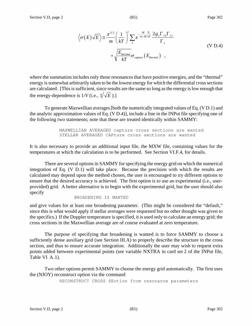
Section V.D, page 2 (R5) Page 302
Section V.D, page 2 (R5) Page 302
( )
( )
23/ 2 21
,
EMnm M kT
thermalcapture thermal
gE E e
m kT
E EkT
λλ λ λγ
λ λ
πσ
σ
−+
Γ Γ⎛ ⎞≅ ⎜ ⎟ Γ⎝ ⎠
+
∑ (V D.4)
where the summation includes only those resonances that have positive energies, and the “thermal” energy is somewhat arbitrarily taken to be the lowest energy for which the differential cross sections are calculated. [This is sufficient, since results are the same so long as the energy is low enough that the energy-dependence is 1/V (i.e., 1 E ).]
To generate Maxwellian averages [both the numerically integrated values of Eq. (V D.1) and the analytic approximation values of Eq. (V D.4)], include a line in the INPut file specifying one of the following two statements; note that these are treated identically within SAMMY:
MAXWELLIAN AVERAGED capture cross sections are wanted STELLAR AVERAGED CAPture cross sections are wanted
It is also necessary to provide an additional input file, the MXW file, containing values for the temperatures at which the calculation is to be performed. See Section VI.F.4, for details.
There are several options in SAMMY for specifying the energy grid on which the numerical integration of Eq. (V D.1) will take place. Because the precision with which the results are calculated may depend upon the method chosen, the user is encouraged to try different options to ensure that the desired accuracy is achieved. The first option is to use an experimental (i.e., user-provided) grid. A better alternative is to begin with the experimental grid, but the user should also specify
BROADENING IS WANTED and give values for at least one broadening parameter. (This might be considered the “default,” since this is what would apply if stellar averages were requested but no other thought was given to the specifics.) If the Doppler temperature is specified, it is used only to calculate an energy grid; the cross sections in the Maxwellian average are of course evaluated at zero temperature.
The purpose of specifying that broadening is wanted is to force SAMMY to choose a sufficiently dense auxiliary grid (see Section III.A) to properly describe the structure in the cross section, and thus to ensure accurate integration. Additionally the user may wish to request extra points added between experimental points (see variable NXTRA in card set 2 of the INPut file, Table VI A.1).
Two other options permit SAMMY to choose the energy grid automatically. The first uses the (NJOY) reconstruct option via the command
RECONSTRUCT CROSS SEction from resonance parameters
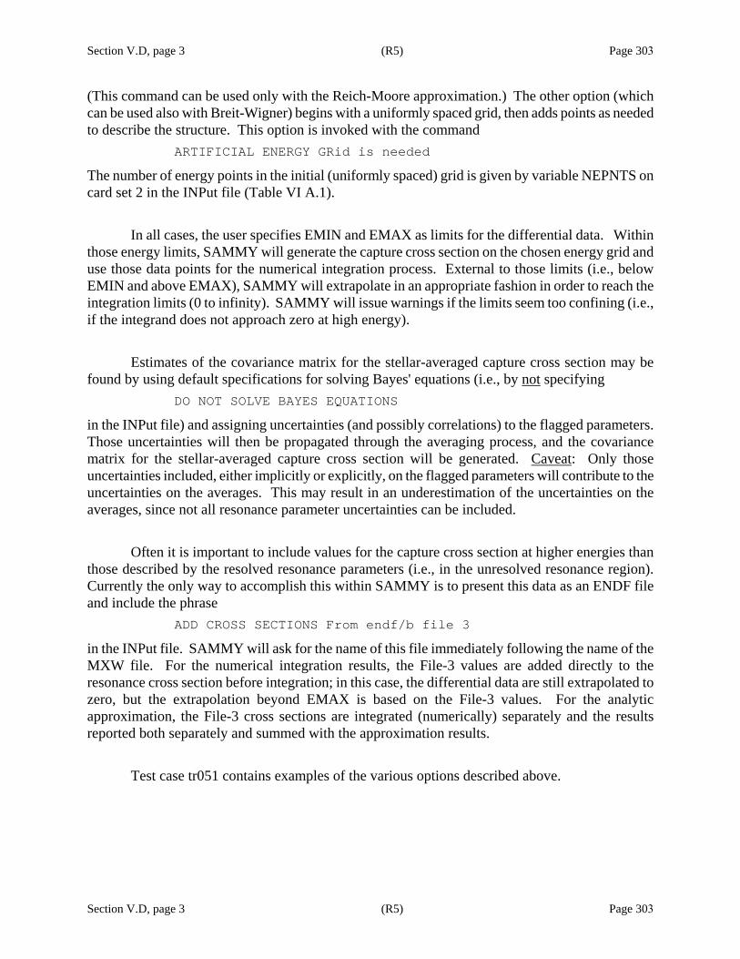
Section V.D, page 3 (R5) Page 303
Section V.D, page 3 (R5) Page 303
(This command can be used only with the Reich-Moore approximation.) The other option (which can be used also with Breit-Wigner) begins with a uniformly spaced grid, then adds points as needed to describe the structure. This option is invoked with the command
ARTIFICIAL ENERGY GRid is needed The number of energy points in the initial (uniformly spaced) grid is given by variable NEPNTS on card set 2 in the INPut file (Table VI A.1).
In all cases, the user specifies EMIN and EMAX as limits for the differential data. Within those energy limits, SAMMY will generate the capture cross section on the chosen energy grid and use those data points for the numerical integration process. External to those limits (i.e., below EMIN and above EMAX), SAMMY will extrapolate in an appropriate fashion in order to reach the integration limits (0 to infinity). SAMMY will issue warnings if the limits seem too confining (i.e., if the integrand does not approach zero at high energy).
Estimates of the covariance matrix for the stellar-averaged capture cross section may be found by using default specifications for solving Bayes' equations (i.e., by not specifying
DO NOT SOLVE BAYES EQUATIONS
in the INPut file) and assigning uncertainties (and possibly correlations) to the flagged parameters. Those uncertainties will then be propagated through the averaging process, and the covariance matrix for the stellar-averaged capture cross section will be generated. Caveat: Only those uncertainties included, either implicitly or explicitly, on the flagged parameters will contribute to the uncertainties on the averages. This may result in an underestimation of the uncertainties on the averages, since not all resonance parameter uncertainties can be included.
Often it is important to include values for the capture cross section at higher energies than those described by the resolved resonance parameters (i.e., in the unresolved resonance region). Currently the only way to accomplish this within SAMMY is to present this data as an ENDF file and include the phrase
ADD CROSS SECTIONS From endf/b file 3
in the INPut file. SAMMY will ask for the name of this file immediately following the name of the MXW file. For the numerical integration results, the File-3 values are added directly to the resonance cross section before integration; in this case, the differential data are still extrapolated to zero, but the extrapolation beyond EMAX is based on the File-3 values. For the analytic approximation, the File-3 cross sections are integrated (numerically) separately and the results reported both separately and summed with the approximation results.
Test case tr051 contains examples of the various options described above.


Section V.E, page 1 (R7) Page 305
Section V.E, page 1 (R7) Page 305
V.E. PSEUDO CROSS SECTIONS FOR TESTING
It is possible to generate a fictitious theoretical “cross section” that exhibits constant, linear, delta-function, or 1/V (inverse velocity) behavior. These pseudo cross sections are useful for testing the effect of resolution functions or Doppler broadening.
To invoke these functions, in the INPut file, in the location where you would normally provide the data type (“transmission”, “capture”, “differential elastic”, etc.), give one of the following phrases:
CONSTANT LINEAR QUADRATIC DIRAC 1/V
SAMMY will then calculate, instead of the Reich-Moore cross section, the following: $ a constant cross section [everywhere equal to 1] $ a linear-in-energy cross section [=1 at Emin, 2 at Emax, but see below] $ a quadratic-in-energy cross section [=1 at Emin, 2 at Emid=(Emin+Emax)/2, 1 at Emax] $ an approximation to the Dirac delta function [= 0 everywhere except 1 at Emid] $ a 1/V cross section [whereV E= with E = Energy]
In the output plot file (SAMMY.ODF or SAMMY.PLT , as described in Section VII.C of this document), the pseudo cross section is stored in section 2 (which would normally contain the experimental data). Section 4 contains the “corrected” cross sections that have been Doppler or resolution broadened, normalized, or otherwise corrected as specified in the user’s INPut and PARameter file.
Along with these pseudo cross sections, it is often useful to have SAMMY choose an energy grid according to certain well-defined specifications (such as uniform in energy or uniform in flight time). To invoke these options, include one of the following lines in the alphanumeric command section of the INPut file: UNIFORM ENERGY GRID UNIFORM VELOCITY GRId UNIFORM TIME GRID
In the first case, the code will provide an “experimental” energy grid that is equally spaced in energy E. The default number of points in this grid is 1001, though you may overwrite this number by specifying NEPNTS in columns 41 to 45 of line 2 of the INPut file.
For the uniform velocity grid, SAMMY uses 1001 points equally spaced in V E= ; for the uniform time grid there will be 1001 points equally spaced in 1T E= (which is proportional to time of flight t). Again, NEPNTS can be specified if you wish a different number of points.
Section V.E, page 2 (R7) Page 306
Section V.E, page 2 (R7) Page 306
(Note that, for the SAMMY run, you must include a name for a data file, but the file does not need to exist; it will be ignored.)
When using a fictitious cross section with a uniform grid (in energy, velocity, or time), SAMMY assumes that you want the LINEAR or QUADRATIC or whatever cross section to be LINEAR or QUADRATIC , etc., in the variable in which the grid is given. That is, if you specify for a example a “UNIFORM TIME GRID” and ask for QUADRATIC cross section, it will be quadratic in the time variable (in 1 1T V E= = ).
See test case tr115 for examples of these features.
[CAVEAT: While using the DIRAC delta function option with only resolution broadening, the calculated curve in section 4 of the SAMMY.ODF or SAMMY.PLT file will closely resemble the resolution function. The user should, however, be aware that it is NOT the resolution function. If the resolution function has discontinuities (as, for example, a square function in time whose width changes abruptly at a certain energy between Emin and Emax), those discontinuities will manifest themselves as odd shapes in the calculated curve.]

Section V.F, page 1 (R7) Page 307
Section V.F, page 1 (R7) Page 307
V.F. SUMMED STRENGTH FUNCTION The summed strength function, as defined by Mughabghab [SM06] for incident neutrons and converted to SAMMY notation, is
( ) ( ) ( )
( )
1
2
1
12 1
2 .2 1
cn
l
cn
gSl E E P
gl E E
λλ λ
λλ λ
ρρ
ρ γ
Λ
=Λ
Λ
=Λ
Λ = Γ+ Δ
=+ Δ
∑
∑ (V F.1)
Only the first elastic (neutron) channel c = n is considered here. The summation is over all resonances of the one or two particular spin groups (where Λ is the total number of such resonances) in an energy interval ΔEΛ. The convention for ΔEΛ, taken from [HD02], is that ΔE is the energy difference between the first and last resonances, plus one average spacing between resonances, that is,
( ) ( ) ( )1 1 11 .
1 1E E E E E E EΛ Λ Λ Λ
ΛΔ = − + − = −
Λ − Λ − (V F.2)
To calculate ( )1S through ( )S N , for resonances within a specified energy range in one or
two spin groups (for which the first elastic channels must have the same value of l), include the following command in card set 3 of the INPut file:
SUMMED STRENGTH FUNCtion is wanted In the interactive input, immediately following the name of the PARameter file, give the name of the COVariance file. On the next line, give two spin group numbers (the second of which can be zero if only one is required) and the energy range (minimum and maximum energies) for which you want the summed strength function to be calculated, in free format. Subsequent lines may contain the same information for other combinations of spin groups and energy ranges, if desired. See test case tr019, run h, for examples.
[There are two differences here from the usual SAMMY input: (1) No DATa file is needed, and no dummy name should be supplied. (2) This option works ONLY when a previous SAMMY run has generated a SAMMY.COV file.] For each input line, SAMMY will calculate ( )S Λ for Λ=1 to N, where N is the total number of resonances in the energy interval specified. SAMMY will also calculate the uncertainties for each ( )S Λ , and the covariance matrix for the set of ( )S Λ . See test case tr019, run h.


Section VI, page 1 (R7) Page 309
Section VI, page 1 (R7) Page 309
VI. INPUT TO SAMMY
Input to SAMMY consists of three or more files, which may be user generated or (sometimes) produced by earlier SAMMY runs. These files are summarized in Table VI.1 and described in detail in the sections listed in the table. Test case numbers (see Section XII.B) are given for those files that are infrequently used.
Table VI.1. SAMMY input files
Description Contents
Section(s) / table(s) containing details
Test case using this
file
Interactive input Interactive input to SAMMY (file names, energy ranges)
Section VI.E
INPut file Details about the interaction being studied, including SAMMY control information
Section VI.A Tables VI A.1 and VI A.2
PARameter file Initial values for resonance and other parameters, flags defining which are to be varied, uncertainty information
Section VI.B Table VI B.2
DATa file Experimental data, including energy, cross section (or transmission, for example), and uncertainty
Section VI.C.1 Table VI C1.1
COVariance file Covariance matrix for the parameters as output by an earlier SAMMY run
Section VII.B
DCV (Data CoVariance)
Covariance information for the data Section VI.C.2
tr007, tr118
IDC (Implicit Data Covariance) for normalization and backgrounds only
Information on data-reduction parameters to be used to generate implicit data covariance matrix
Section VI.C.3.c
tr070
IDC (User supplied)
Information on data-reduction parameters to be used to generate implicit data covariance matrix
Section VI.C.3.b
tr118 tr140 (*.dcv)
NTG file Integral data file Section VI.D tr069, tr077

Section VI, page 2 (R7) Page 310
Table VI.1 (continued)
Section VI, page 2 (R7) Page 310
Description Contents
Section(s) / table(s) containing details
Test case using this
file
AVG file or BON file
Information needed by SAMMY in order to produce energy-averaged or Bondarenko-averaged cross sections
Section VI.F.1 tr014, tr083, tr084, tr085
NDF file Information needed by SAMMY in order to generate an output file in ENDF-6 File 2 format
Section VI.F.2 tr023
ENDF resonance parameter file
File 2 from ENDF, to be used instead of the usual SAMMY PARameter file (and for part of the SAMMY INPut file)
Section VI.F.3 tr049, tr050, tr086, tr091, tr102, tr129
ENDF File 3 Smooth cross sections to be added to the cross section calculated from resonance parameters, for use in calculating the stellar (Maxwellian) averages
Section V.D tr051
MXW file Temperatures at which the stellar (Maxwellian) averages are to be evaluated
Sections V.D and VI.F.4
tr042, tr049, tr051
SSM file Edge-effects corrections to single-scattering correction for capture cross sections (file is generated by a previous SAMMY run)
Section III.D tr039 and many others
URR PAR file Input information for unresolved resonance region
Section VIII tr073, tr088
YWY file W and Y matrices from a single data set, when analyzing several data sets simultaneously, e.g., for creating a retroactive parameter covariance matrix (files are generated by previous SAMMY runs)
Sections IV.E.1 and IV.E.2
tr082, tr089, tr131, tr149

Section VI.A, page 1 (R8) Page 311
Section VI.A, page 1 (R8) Page 311
VI.A. THE INPut FILE SAMMY’s INPut file contains essentially three types of information. The first is a set of command statements that define the particular case to be run; these are discussed in detail in Section VI.A.1. The second type consists of spin group and channel definitions, and the third is miscellaneous other information. Table VI A.1 gives details about the second and third types. Information in the INPut file is categorized into “card sets.” One or more lines of input are included in each card set. The categories are described here, and details are given in Table VI A.1.
Card set 1 of the table contains a title, which is reproduced in the output LPT file (see Section VII.A) but is otherwise unused.
Card set 2 contains miscellaneous information, including the mass of the sample, the energy range, and a flag to indicate how many iterations of Bayes= equations are to be run. Some of the information given here may also be input elsewhere, in which case, values given here are ignored. Card set 3 contains the command statements; see Section VI.A.1 for details.
Card set 4 contains particle-pair definitions, an alternative method of providing information (masses, spins and parities, charges, threshold values) for the two particles in the channel, in key-word format. This is the preferred format.
Card set 4a contains the same information as in card set 4, but in fixed format. Card set 4.5 exists only if the command “PLOT RESOLUTION FUNCtion” is given in
card set 3.
Card sets 5 and 6 describe the original input for the Doppler- and resolution-broadening functions (see Sections III B.1 and III C.1). (See also card set P4.)
Card set 7 gives the matching radius for the R-matrix formalism, sample thickness, and various other parameters. Values for many of these parameters may, however, be superseded by values specified in the PARameter file (Section VI.B) or elsewhere in the INPut file (card set P4).
Card set 8 specifies the type of data to be analyzed (e.g., capture cross section, transmission). When the data are angular distributions, angles are also specified here.
Card set 9 was originally used to specify the spin and parity of the nucleus in the sample. For Version M6 and subsequent versions, this card is no longer required and should be removed from INPut files. Currently, this card set will be ignored if it exists in the INPut file; however, future versions of SAMMY may require that this line be removed.
Card set 10 had previously been used to describe the quantum numbers for the various spin groups. For Version M6 and subsequent versions, the original format is deemed to be obsolete and is no longer supported. Users should convert their INPut files to use either the “NEW SPIN GROUP
Section VI.A, page 2 (R8) Page 312
Section VI.A, page 2 (R8) Page 312
FORMAT” (previously called “Alternative to card set 10” and now denoted “card set 10.1” in Table VIA.1) or the new “card set 10.2,” which makes use of the particle-pair definitions given in card set 4 or 4a. In either case, SAMMY provides assistance in converting the INPut files; users can simply begin a SAMMY run using the obsolete INPut file and follow the instructions on the screen.
Card set 11 is needed only when analyzing capture cross sections using self-shielding and multiple-scattering corrections, or when analyzing transmission data with a non-uniform sample. Dimensions of the sample, plus interpolation and integration parameters, are specified in this card set.
Finally, many of the parameter types that are normally given in the PARameter file (see Table VI B.2) may now be given in the INPut file instead. This is convenient, for example, when an evaluation involves data from many different experiments, in which case the same resonance parameters but different measurement-specific parameters are needed for each data set. Caution: Parameters that are specified in the INPut file cannot be varied; any flags equal to 1 will be ignored here. The parameters can, however, be PUP’d (see Section IV.D.2 for a discussion of the Propagated Uncertainty Parameter option). Flags equal to 3 will be understood in both the INPut and the PARameter files. Note that each of these card sets can occur in at most one of the two files; SAMMY will abort with an error message if the same card set is found in both files.
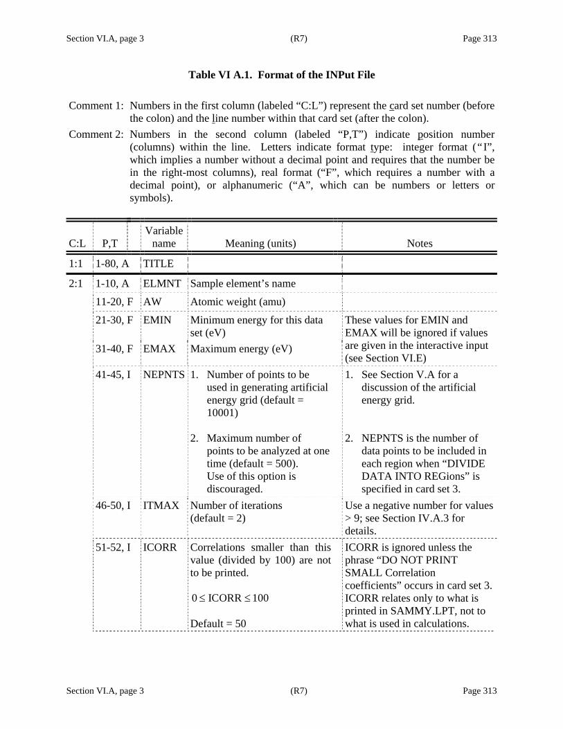
Section VI.A, page 3 (R7) Page 313
Section VI.A, page 3 (R7) Page 313
Table VI A.1. Format of the INPut File
Comment 1: Numbers in the first column (labeled “C:L”) represent the card set number (before the colon) and the line number within that card set (after the colon).
Comment 2: Numbers in the second column (labeled “P,T”) indicate position number(columns) within the line. Letters indicate format type: integer format (“I”, which implies a number without a decimal point and requires that the number be in the right-most columns), real format (“F”, which requires a number with a decimal point), or alphanumeric (“A”, which can be numbers or letters or symbols).
C:L P,T Variable
name Meaning (units) Notes
1:1 1-80, A TITLE
2:1 1-10, A ELMNT Sample element’s name
11-20, F AW Atomic weight (amu)
21-30, F EMIN Minimum energy for this data set (eV)
31-40, F EMAX Maximum energy (eV)
These values for EMIN and EMAX will be ignored if values are given in the interactive input (see Section VI.E)
41-45, I NEPNTS 1. Number of points to be used in generating artificial energy grid (default = 10001)
2. Maximum number of
points to be analyzed at one time (default = 500). Use of this option is discouraged.
1. See Section V.A for a discussion of the artificial energy grid.
2. NEPNTS is the number of
data points to be included in each region when “DIVIDE DATA INTO REGions” is specified in card set 3.
46-50, I ITMAX Number of iterations (default = 2)
Use a negative number for values > 9; see Section IV.A.3 for details.
51-52, I ICORR Correlations smaller than this value (divided by 100) are not to be printed. 0 ICORR 100≤ ≤ Default = 50
ICORR is ignored unless the phrase “DO NOT PRINT SMALL Correlation coefficients” occurs in card set 3. ICORR relates only to what is printed in SAMMY.LPT, not to what is used in calculations.
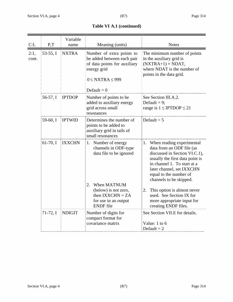
Section VI.A, page 4 (R7) Page 314
Table VI A.1 (continued)
Section VI.A, page 4 (R7) Page 314
C:L P,T Variable
name Meaning (units) Notes
2:1, cont.
53-55, I NXTRA Number of extra points to be added between each pair of data points for auxiliary energy grid 0 NXTRA 999≤ ≤ Default = 0
The minimum number of points in the auxiliary grid is (NXTRA+1) × NDAT, where NDAT is the number of points in the data grid.
56-57, I IPTDOP Number of points to be added to auxiliary energy grid across small resonances
See Section III.A.2. Default = 9; range is 1 ≤ IPTDOP ≤ 21
59-60, I IPTWID Determines the number of points to be added to auxiliary grid in tails of small resonances
Default = 5
61-70, I IXXCHN 1. Number of energy channels in ODF-type data file to be ignored
2. When MATNUM
(below) is not zero, then IXXCHN = ZA for use in an output ENDF file
1. When reading experimental data from an ODF file (as discussed in Section VI.C.1), usually the first data point is in channel 1. To start at a later channel, set IXXCHN equal to the number of channels to be skipped.
2. This option is almost never
used. See Section IX for more appropriate input for creating ENDF files.
71-72, I NDIGIT Number of digits for compact format for covariance matrix
See Section VII.E for details. Value: 1 to 6 Default = 2

Section VI.A, page 5 (R7) Page 315
Table VI A.1 (continued)
Section VI.A, page 5 (R7) Page 315
C:L P,T Variable
name Meaning (units) Notes
2:1, cont.
73-74, I IDROPP The input resonance-parameter covariance matrix will be modified before being used in the fitting procedure. Correlations smaller than this % will be set to zero.
Value: 1 to 99; default = 2 This variable is ignored unless the phrase “DROP SMALL VALUES OF correlation matrix” occurs in the command section of the INPut file (card set 3).
75-80, I MATNUM ENDF Material Number This value is almost never used. See Section IX for more appropriate input for creating ENDF files.
3:?
1-20, A
WHAT
Alphanumeric information concerning program options.
See Table VI A1.2 for a listing of valid commands.
3:Last (blank)
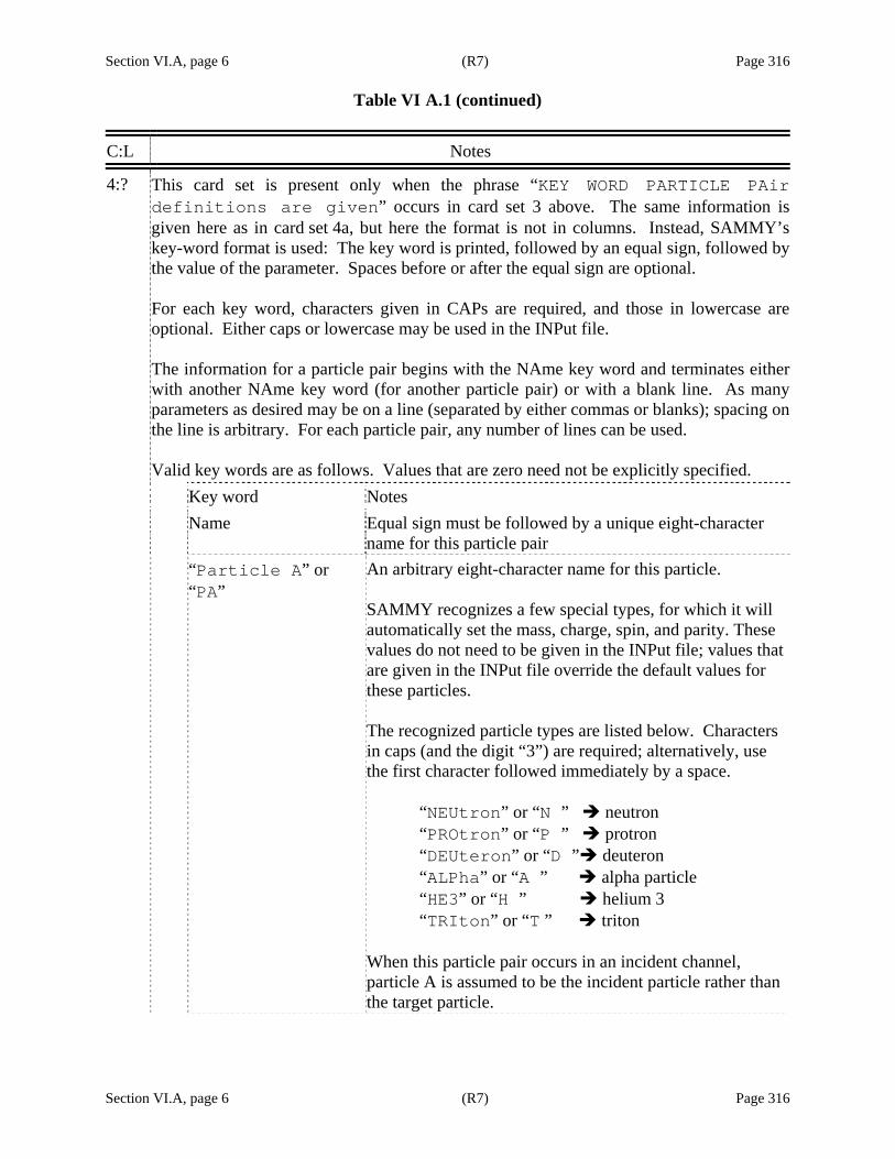
Section VI.A, page 6 (R7) Page 316 Table VI A.1 (continued)
Section VI.A, page 6 (R7) Page 316
C:L Notes
4:? This card set is present only when the phrase “KEY WORD PARTICLE PAir definitions are given” occurs in card set 3 above. The same information is given here as in card set 4a, but here the format is not in columns. Instead, SAMMY’s key-word format is used: The key word is printed, followed by an equal sign, followed by the value of the parameter. Spaces before or after the equal sign are optional. For each key word, characters given in CAPs are required, and those in lowercase are optional. Either caps or lowercase may be used in the INPut file. The information for a particle pair begins with the NAme key word and terminates either with another NAme key word (for another particle pair) or with a blank line. As many parameters as desired may be on a line (separated by either commas or blanks); spacing on the line is arbitrary. For each particle pair, any number of lines can be used. Valid key words are as follows. Values that are zero need not be explicitly specified.
Key word Notes Name Equal sign must be followed by a unique eight-character
name for this particle pair “Particle A” or
“PA” An arbitrary eight-character name for this particle. SAMMY recognizes a few special types, for which it will automatically set the mass, charge, spin, and parity. These values do not need to be given in the INPut file; values that are given in the INPut file override the default values for these particles. The recognized particle types are listed below. Characters in caps (and the digit “3”) are required; alternatively, use the first character followed immediately by a space.
“NEUtron” or “N ” neutron “PROtron” or “P ” protron “DEUteron” or “D ” deuteron “ALPha” or “A ” alpha particle “HE3” or “H ” helium 3 “TRIton” or “T ” triton
When this particle pair occurs in an incident channel, particle A is assumed to be the incident particle rather than the target particle.

Section VI.A, page 7 (R7) Page 317 Table VI A.1 (continued)
Section VI.A, page 7 (R7) Page 317
C:L Notes
4:?, cont.
“Particle B” or “PB”
When this particle pair occurs in an incident channel, particle B is the target particle.
“Mass A” or “MA” Mass of particle A, in amu “Mass B” or “MB” Mass of particle B, in amu
“Charge A” or “ZA” Charge of particle A “Charge B” or “ZB” Charge of particle B “Spin A” or “SA” Spin of particle A; if non-zero, may include sign for parity “Spin B” or “SB” Spin of particle B; if non-zero, may include sign for parity “PARIty A” Parity of particle A; needed only if the spin of particle A is
zero and the parity is negative “PARIty B” Parity of particle B; needed only if the spin of particle B is
zero and the parity is negative “PEnetrability” “Yes” or “No” or “1” or “0” “Shift” “Yes” or “No” or “1” or “0” “Q-value” or
“THreshold” Note: If the Q-value is given, it is implicitly assumed to be in the center-of-mass system. If, instead, the excitation energy (threshold energy) is given, it is assumed to be in the laboratory unless overridden with one of the commands “CM NON COULOMB EXCITation” or “CM COULOMB EXCITATIOn”.
“EFfective radius” or “RE”
“TRue radius” or “RT”
Channel radii may be given here if they are appropriate for all channels in which this particle pair appears. However, if channel radii are given in card set 7 or 7a of the parameter file, the values given here are ignored.
4:Last (end this card set with one blank line)
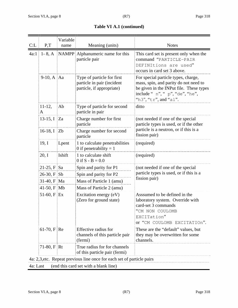
Section VI.A, page 8 (R7) Page 318 Table VI A.1 (continued)
Section VI.A, page 8 (R7) Page 318
C:L P,T Variable
name Meaning (units) Notes
4a:1 1- 8, A NAMPP Alphanumeric name for this particle pair
This card set is present only when the command “PARTICLE-PAIR DEFINItions are used” occurs in card set 3 above.
9-10, A Aa Type of particle for first particle in pair (incident particle, if appropriate)
For special particle types, charge, mass, spin, and parity do not need to be given in the INPut file. These types include “ n”, “ p”, “de”, “he”, “h3", “tr”, and “al”.
11-12, A
Ab Type of particle for second particle in pair
ditto
13-15, I Za Charge number for first particle
16-18, I Zb Charge number for second particle
(not needed if one of the special particle types is used, or if the other particle is a neutron, or if this is a fission pair)
19, I Lpent 1 to calculate penetrabilities0 if penetrability = 1
(required)
20, I Ishift 1 to calculate shift 0 if S - B = 0.0
(required)
21-25, F Sa Spin and parity for P1 26-30, F Sb Spin and parity for P2 31-40, F Ma Mass of Particle 1 (amu) 41-50, F Mb Mass of Particle 2 (amu)
(not needed if one of the special particle types is used, or if this is a fission pair)
51-60, F Ex Excitation energy (eV) (Zero for ground state)
Asssumed to be defined in the laboratory system. Override with card-set 3 commands “CM NON COULOMB EXCITation” or “CM COULOMB EXCITATIOn”.
61-70, F Re Effective radius for channels of this particle pair (fermi)
These are the “default” values, but they may be overwritten for some channels.
71-80, F Rt True radius for for channels of this particle pair (fermi)
4a: 2,3,etc. Repeat previous line once for each set of particle pairs 4a: Last (end this card set with a blank line)

Section VI.A, page 9 (R7) Page 319 Table VI A.1 (continued)
Section VI.A, page 9 (R7) Page 319
C:L P,T Variable
name Meaning (units) Notes
4.5:1 1-10, F 11-20, F … 71-80, F
ERESOL Energies at which to plot the resolution function
This card set is present only if “PLOT RESOLUTION FUNCtion” is specified in card set 3. See Section X.L for details.

Section VI.A, page 10 (R7) Page 320
Table VI A.1 (continued)
Section VI.A, page 10 (R7) Page 320
C:L P,T Variable
name Meaning (units) Notes
5:1 1-10, F TEMP Effective temperature of the sample (K); zero for no Doppler broadening. This value may be overwritten in PARameter card set 4 (see Table VI B.2).
This card set is omitted when “BROADENING IS NOT WAnted” is specified in card set 3. (SAMMY will abort if this rule not followed.)
11-20, F DIST Flight-path length (m) 21-30, F DELTAL That portion of the Gaussian
resolution width attributed to the flight-path length (m).
Value may be overwritten in PARameter card set 4 (see Table VI B.2).
31-40, F DELTAE E-folding width of exponential resolution function (μs); (0 for pure Gaussian resolution function).
This value may be overwritten in PARameter card set 4 (see Table VI B.2).
See Section III.C.1.b. If the line “EXPONENTIAL FOLDING width is energy-dependent” is specified in card set 3 of the INPut file, then see Eq. (III C1 b.6) for details of the energy dependence.
41-50, F DELTAG The absolute value of DELTAG is the FWHM (μs) of a Gaussian resolution function representing the burst width. (DELTAG = 0 for a purely exponential resolution function.)
See Section III.C.1.a, Eqs. (III C1 a.13) and (III C1 a.15). If DELTAG is negative, channel widths are given in card set 6.
51-60, F DELTTT Approximate step size for the Effective Temperature for the Leal-Hwang method of Doppler broadening (K). Value > 0; default = 5.0
See Section III.B.2. If DELTTT < 0.0, an error message will be printed and the code will cease operation.
61-70, F ELOWBR The energy below which no broadening is wanted, for high-energy Gaussian approximation to Doppler broadening (eV)
Default = 0.0
71-80, F DDDEEE Range for straight-line energy average resolution function (eV)
See Section III.C.4.

Section VI.A, page 11 (R8) Page 321
Table VI A.1 (continued)
Section VI.A, page 11 (R8) Page 321
C:L P,T Variable
name Meaning (units) Notes
6:1 1-10, F DELTAB Minimum channel width for interval from EMIN to EMAX (μs)
This card set is included only if DELTAG < 0 in card set 5.
11-15, I NCF Number of crunch boundaries (energy intervals)
6:2 1-10, F 11-20, F etc.
(BCF(I), CF(I), I=1,NCF)
BCF(I) = maximum energy for this crunch factor (read in order of increasing energy) (eV) CF(I) = crunch factors (integer units of DELTAB)
The value of Δtc to be used in the energy range BCF(I-1) < E < BCF(I) is CF(I)×DELTAB. See Eq. (III C1 a.9) and the following.
7:1 1-10, F CRFN Channel radius (fermi) If CRFN is input as zero, its value is computed as 1.45 × (1.008665 +AW)1/3.
Value may be overwritten in card set 4 or 7 of the PARameter file (see Table VI B.2).
11-20, F THICK Sample thickness (atoms/barn) Needed only for TRANSmission or for TOTAL cross section or for multiple-scattering corrections.
21-30, F DCOVA or ERRXC2
DCOVA = Constant term in data covariance (default = 0.0)
31-40, F DCOVB or SIGMIN
DCOVB = Linear term in data covariance (default = 0.0) For a description of ERRXC2 and SIGMIN, see Section V.A on reconstructing point-wise cross sections.
Data covariance matrix has additional term of the form (DCOVA + Ei × DCOVB) × (DCOVA + Ej × DCOVB). Usually these terms will be set to zero.
41-50, F VMIN Minimum absolute uncertainty (standard deviation) on experimental data Often set to zero
If an experimental uncertainty in the DATa file is smaller than VMIN, SAMMY will increase the value to VMIN.
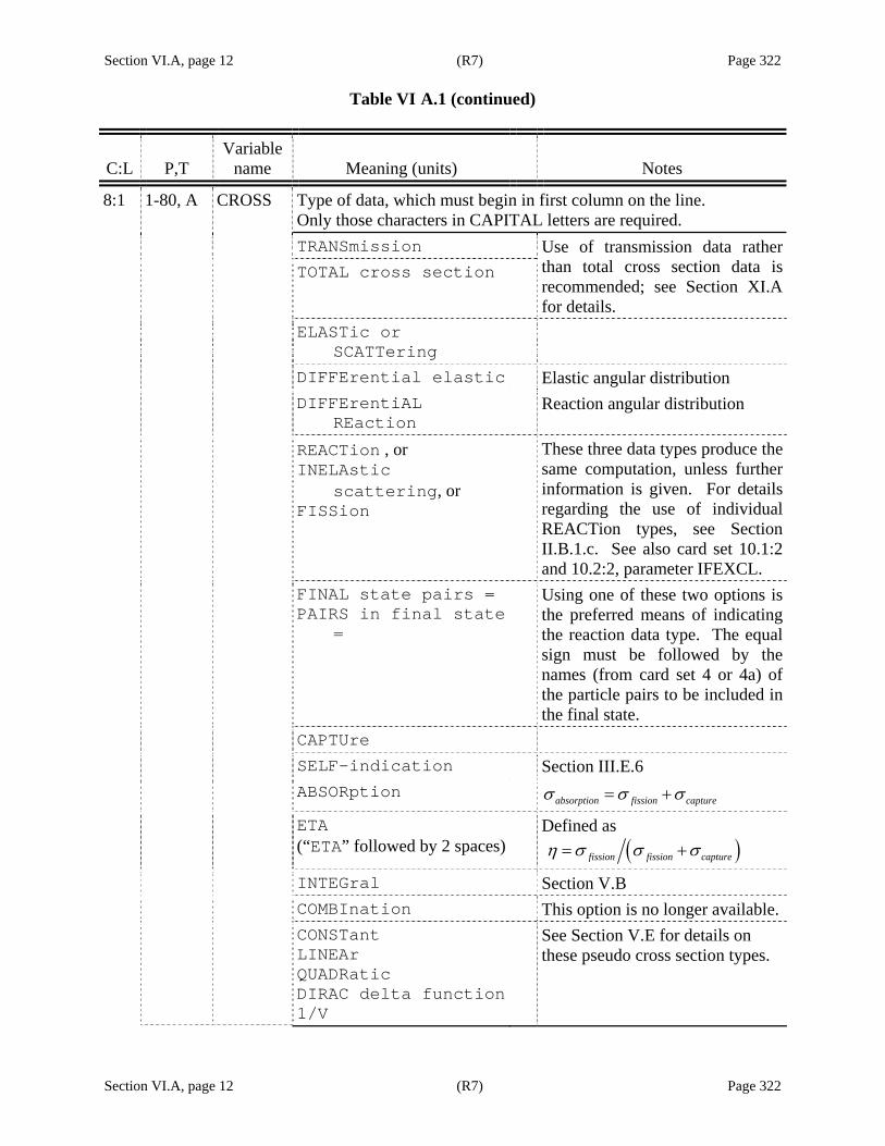
Section VI.A, page 12 (R7) Page 322 Table VI A.1 (continued)
Section VI.A, page 12 (R7) Page 322
C:L P,T Variable
name Meaning (units) Notes
8:1 1-80, A CROSS Type of data, which must begin in first column on the line. Only those characters in CAPITAL letters are required.
TRANSmission TOTAL cross section
Use of transmission data rather than total cross section data is recommended; see Section XI.A for details.
ELASTic or SCATTering
DIFFErential elastic Elastic angular distribution DIFFErentiAL
REaction Reaction angular distribution
REACTion , or INELAstic
scattering, or FISSion
These three data types produce the same computation, unless further information is given. For details regarding the use of individual REACTion types, see Section II.B.1.c. See also card set 10.1:2 and 10.2:2, parameter IFEXCL.
FINAL state pairs = PAIRS in final state
=
Using one of these two options is the preferred means of indicating the reaction data type. The equal sign must be followed by the names (from card set 4 or 4a) of the particle pairs to be included in the final state.
CAPTUre SELF-indication Section III.E.6 ABSORption absorption fission captureσ σ σ= +
ETA (“ETA” followed by 2 spaces)
Defined as ( )fission fission captureη σ σ σ= +
INTEGral Section V.B COMBInation This option is no longer available. CONSTant
LINEAr QUADRatic DIRAC delta function 1/V
See Section V.E for details on these pseudo cross section types.

Section VI.A, page 13 (R7) Page 323 Table VI A.1 (continued)
Section VI.A, page 13 (R7) Page 323
C:L P,T Variable name Meaning (units) Notes
8:2 1- 5, I NANGLE Number of angles 11-20, F ANGLE(1) First angle, in laboratory;
between 0 and 180 degrees 21-30, F ANGLE(2) Second angle (degrees) ... 71-80, F ANGLE(7) Seventh angle
This line and those following are present only for data types “DIFFErential elastic cross sections” or “DIFFErentiAL REaction.” See Section II.B.1.b for details.
8:3 etc.
1-10, F 11-20, F etc.
ANGLE(8) ANGLE(9) etc.
Other angles, for a total of NANGLE
These lines are absent if NANGLE < 8.
8:4 11-20, F DANGLE(1) Angular spread of detector at ANGLE(1) (degrees)
... DANGLE(7) Spread at ANGLE(7) 8:6 etc.
1-10, F 11-20, F etc.
DANGLE(8) DANGLE(9) etc.
Spread at other angles, for a total of NANGLE
These lines are absent if NANGLE < 8.
9 This card set, which originally contained the spin of the target nuclide, is no longer needed and should be removed from INPut files. The spin of the target nuclide is now given either in card set 10.1 or in card set 4 or 4a. Currently, SAMMY will ignore this card if it is present. However, that capability will not necessarily be maintained in future releases of the code.
10 The original card set 10 is obsolete and must be replaced by either card set 10.1 or card set 10.2. To convert your old INPut files, begin a SAMMY run using that file; SAMMY will generate a file INPUT.NEW containing card set 10.1. Caution: Information in INPUT.NEW may not be entirely correct, as information in the obsolete format can be misinterpreted. It is the user’s responsibility to ensure that the conversion is correct.
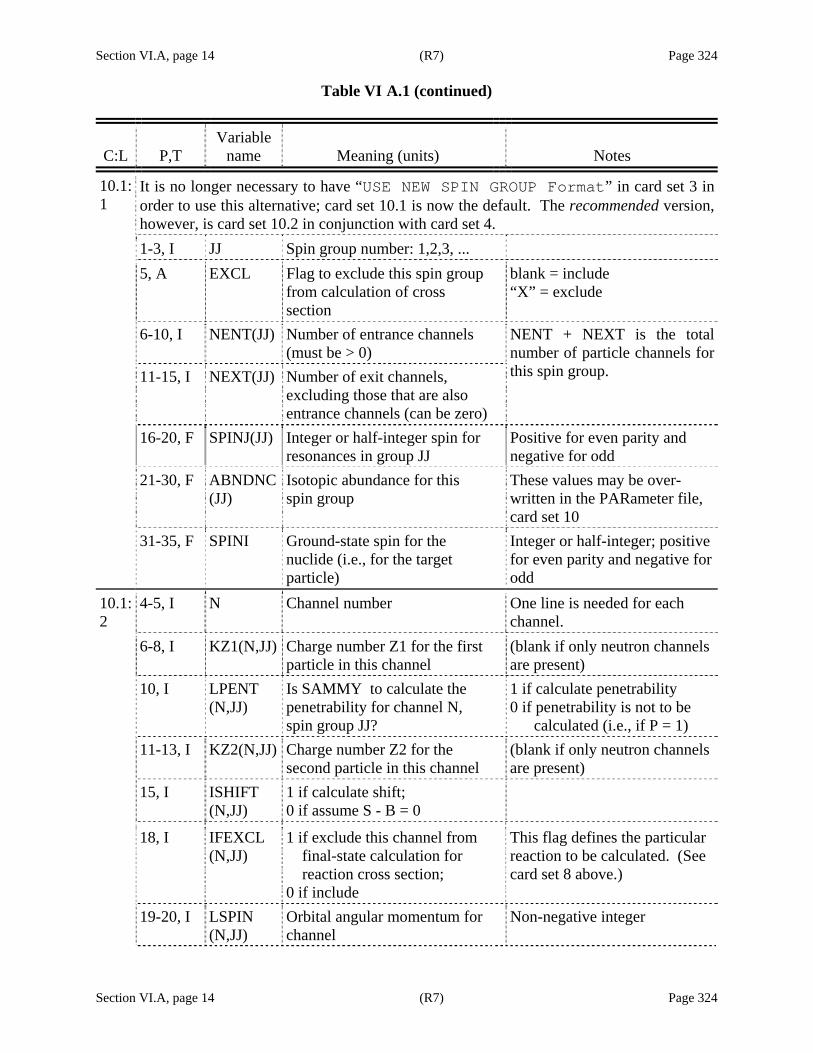
Section VI.A, page 14 (R7) Page 324 Table VI A.1 (continued)
Section VI.A, page 14 (R7) Page 324
C:L P,T Variable
name Meaning (units) Notes
10.1: 1
It is no longer necessary to have “USE NEW SPIN GROUP Format” in card set 3 in order to use this alternative; card set 10.1 is now the default. The recommended version, however, is card set 10.2 in conjunction with card set 4.
1-3, I JJ Spin group number: 1,2,3, ... 5, A EXCL Flag to exclude this spin group
from calculation of cross section
blank = include “X” = exclude
6-10, I NENT(JJ) Number of entrance channels (must be > 0)
11-15, I NEXT(JJ) Number of exit channels, excluding those that are also entrance channels (can be zero)
NENT + NEXT is the total number of particle channels for this spin group.
16-20, F SPINJ(JJ) Integer or half-integer spin for resonances in group JJ
Positive for even parity and negative for odd
21-30, F ABNDNC (JJ)
Isotopic abundance for this spin group
These values may be over-written in the PARameter file, card set 10
31-35, F SPINI Ground-state spin for the nuclide (i.e., for the target particle)
Integer or half-integer; positive for even parity and negative for odd
10.1: 2
4-5, I N Channel number One line is needed for each channel.
6-8, I KZ1(N,JJ) Charge number Z1 for the first particle in this channel
(blank if only neutron channels are present)
10, I LPENT (N,JJ)
Is SAMMY to calculate the penetrability for channel N, spin group JJ?
1 if calculate penetrability 0 if penetrability is not to be calculated (i.e., if P = 1)
11-13, I KZ2(N,JJ) Charge number Z2 for the second particle in this channel
(blank if only neutron channels are present)
15, I ISHIFT (N,JJ)
1 if calculate shift; 0 if assume S - B = 0
18, I IFEXCL (N,JJ)
1 if exclude this channel from final-state calculation for reaction cross section; 0 if include
This flag defines the particular reaction to be calculated. (See card set 8 above.)
19-20, I LSPIN (N,JJ)
Orbital angular momentum for channel
Non-negative integer
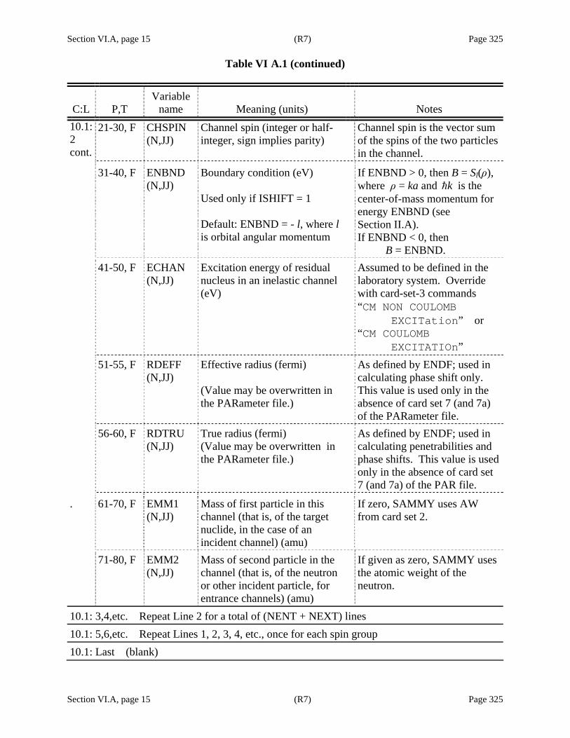
Section VI.A, page 15 (R7) Page 325 Table VI A.1 (continued)
Section VI.A, page 15 (R7) Page 325
C:L P,T Variable
name Meaning (units) Notes
21-30, F CHSPIN (N,JJ)
Channel spin (integer or half-integer, sign implies parity)
Channel spin is the vector sum of the spins of the two particles in the channel.
10.1: 2 cont.
31-40, F ENBND (N,JJ)
Boundary condition (eV) Used only if ISHIFT = 1 Default: ENBND = - l, where l is orbital angular momentum
If ENBND > 0, then B = Sl(ρ), where ρ = ka and k is the center-of-mass momentum for energy ENBND (see Section II.A). If ENBND < 0, then B = ENBND.
41-50, F ECHAN (N,JJ)
Excitation energy of residual nucleus in an inelastic channel (eV)
Assumed to be defined in the laboratory system. Override with card-set-3 commands “CM NON COULOMB
EXCITation” or “CM COULOMB
EXCITATIOn” 51-55, F RDEFF
(N,JJ) Effective radius (fermi) (Value may be overwritten in the PARameter file.)
As defined by ENDF; used in calculating phase shift only. This value is used only in the absence of card set 7 (and 7a) of the PARameter file.
56-60, F RDTRU (N,JJ)
True radius (fermi) (Value may be overwritten in the PARameter file.)
As defined by ENDF; used in calculating penetrabilities and phase shifts. This value is used only in the absence of card set 7 (and 7a) of the PAR file.
. 61-70, F EMM1 (N,JJ)
Mass of first particle in this channel (that is, of the target nuclide, in the case of an incident channel) (amu)
If zero, SAMMY uses AW from card set 2.
71-80, F EMM2 (N,JJ)
Mass of second particle in the channel (that is, of the neutron or other incident particle, for entrance channels) (amu)
If given as zero, SAMMY uses the atomic weight of the neutron.
10.1: 3,4,etc. Repeat Line 2 for a total of (NENT + NEXT) lines 10.1: 5,6,etc. Repeat Lines 1, 2, 3, 4, etc., once for each spin group 10.1: Last (blank)
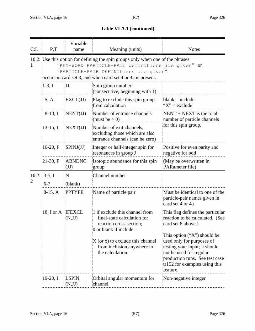
Section VI.A, page 16 (R7) Page 326 Table VI A.1 (continued)
Section VI.A, page 16 (R7) Page 326
C:L P,T Variable
name Meaning (units) Notes
10.2: 1
Use this option for defining the spin groups only when one of the phrases “KEY-WORD PARTICLE-PAir definitions are given” or “PARTICLE-PAIR DEFINItions are given”
occurs in card set 3, and when card set 4 or 4a is present. 1-3, I JJ Spin group number
(consecutive, beginning with 1)
5, A EXCL(JJ) Flag to exclude this spin group from calculation
blank = include “X” = exclude
8-10, I NENT(JJ) Number of entrance channels (must be > 0)
13-15, I NEXT(JJ) Number of exit channels, excluding those which are also entrance channels (can be zero)
NENT + NEXT is the total number of particle channels for this spin group.
16-20, F SPINJ(JJ) Integer or half-integer spin for resonances in group J
Positive for even parity and negative for odd
21-30, F ABNDNC (JJ)
Isotopic abundance for this spin group
(May be overwritten in PARameter file)
3-5, I N Channel number 10.2: 2 6-7 (blank)
8-15, A PPTYPE Name of particle pair Must be identical to one of the particle-pair names given in card set 4 or 4a
18, I or A IFEXCL (N,JJ)
1 if exclude this channel from final-state calculation for reaction cross section; 0 or blank if include. X (or x) to exclude this channel from inclusion anywhere in the calculation.
This flag defines the particular reaction to be calculated. (See card set 8 above.) This option (“X”) should be used only for purposes of testing your input; it should not be used for regular production runs. See test case tr152 for examples using this feature.
19-20, I LSPIN (N,JJ)
Orbital angular momentum for channel
Non-negative integer

Section VI.A, page 17 (R7) Page 327 Table VI A.1 (continued)
Section VI.A, page 17 (R7) Page 327
C:L P,T Variable
name Meaning (units) Notes
10.2: 2 cont.
21-30, F CHSPIN (N,JJ)
Channel spin (integer or half-integer, sign implies parity)
Channel spin is the vector sum of the spins of the two particles in the channel.
31-40, F ENBND (N,JJ)
Boundary condition (eV) Used only if ISHIFT = 1 or SHift = Yes. Default: ENBND = - LSPIN
If ENBND > 0, then B = Sl(ρ), where ρ = ka and k is the center-of-mass momentum for energy ENBND (Section II). If ENBND < 0, then B = ENBND.
41-50, F RDEFF (N,JJ)
Effective radius (fermi) Needed here only if different from the value of the effective radius given in the particle-pair definitions. Is ignored if Radius parameters are given in the PARameter file.
51-60, F RDTRU (N,JJ)
True radius (fermi) Needed here only if different from the value of the true radius given in the particle-pair definitions. Is ignored if Radius parameters are given in the PARameter file.
10.2: 3,4,etc. Repeat Line 2 for a total of (NENT + NEXT) lines
10.2: 5,6,etc. Repeat Lines 1,2,3,4,etc, once for each spin group
10.2: Last (blank)
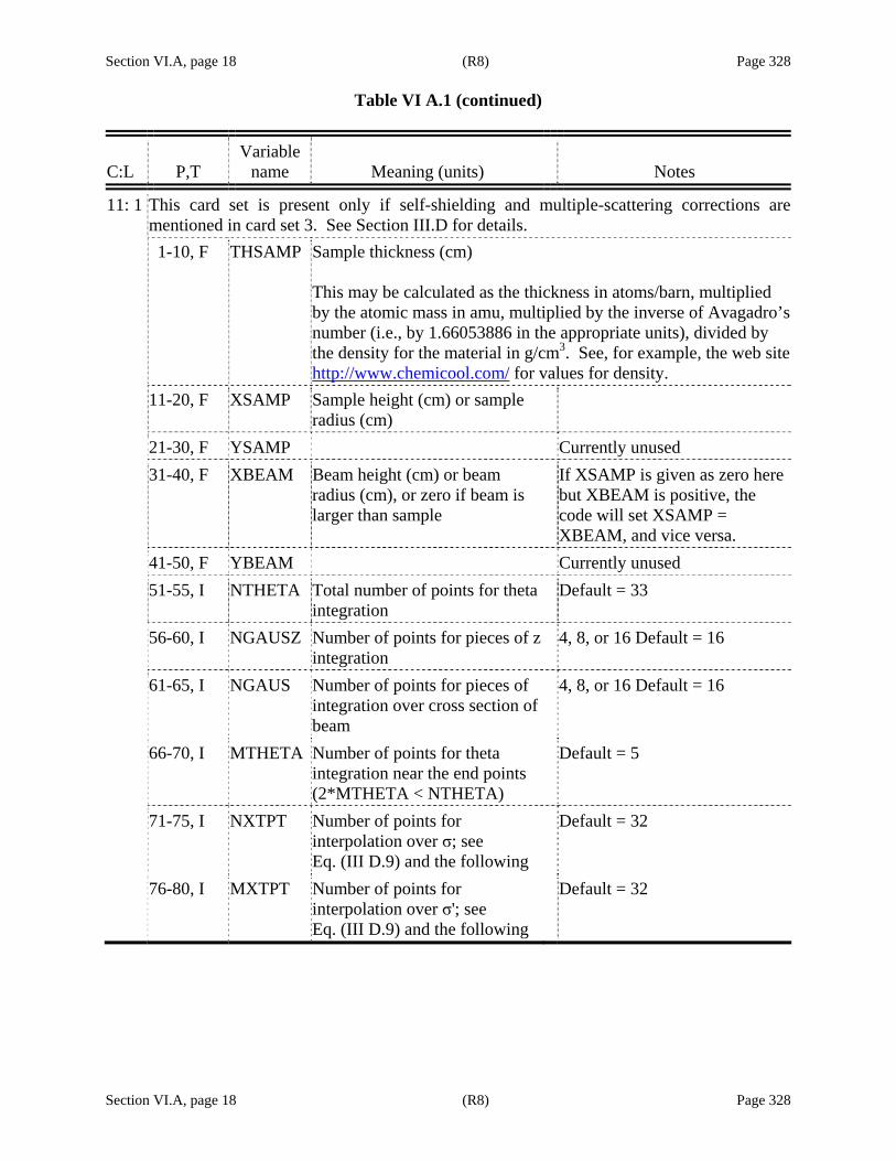
Section VI.A, page 18 (R8) Page 328 Table VI A.1 (continued)
Section VI.A, page 18 (R8) Page 328
C:L P,T Variable
name Meaning (units) Notes
11: 1 This card set is present only if self-shielding and multiple-scattering corrections are mentioned in card set 3. See Section III.D for details.
1-10, F THSAMP Sample thickness (cm) This may be calculated as the thickness in atoms/barn, multiplied by the atomic mass in amu, multiplied by the inverse of Avagadro’s number (i.e., by 1.66053886 in the appropriate units), divided by the density for the material in g/cm3. See, for example, the web sitehttp://www.chemicool.com/ for values for density.
11-20, F XSAMP Sample height (cm) or sample radius (cm)
21-30, F YSAMP Currently unused 31-40, F XBEAM Beam height (cm) or beam
radius (cm), or zero if beam is larger than sample
If XSAMP is given as zero here but XBEAM is positive, the code will set XSAMP = XBEAM, and vice versa.
41-50, F YBEAM Currently unused 51-55, I NTHETA Total number of points for theta
integration Default = 33
56-60, I NGAUSZ Number of points for pieces of zintegration
4, 8, or 16 Default = 16
61-65, I NGAUS Number of points for pieces of integration over cross section of beam
4, 8, or 16 Default = 16
66-70, I MTHETA Number of points for theta integration near the end points (2*MTHETA < NTHETA)
Default = 5
71-75, I NXTPT Number of points for interpolation over σ; see Eq. (III D.9) and the following
Default = 32
76-80, I MXTPT Number of points for interpolation over σ'; see Eq. (III D.9) and the following
Default = 32

Section VI.A, page 19 (R8) Page 329 Table VI A.1 (continued)
Section VI.A, page 19 (R8) Page 329
C:L P,T Variable
name Meaning (units) Notes
11: 2 This line is optional 1-10, F XTMIN Lowest value of log of total
cross section to be used in evaluating Q for single-scattering correction (barns). See Section III.D for details.
Default = -20.0
11-20, F XTMAX Largest value of log of total cross section to be used in evaluating Q
Default = 20.0
21-50 Currently unused 51-55, I JTHETA Number of points in theta
integration near cos(theta) = 1 Default = 5
56-60, I KTHETA Number of points in theta integration near cos(theta) = 0
Default = 5
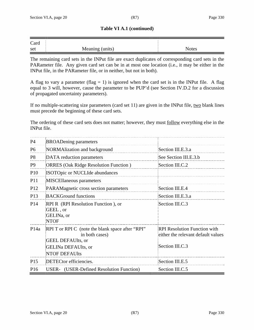
Section VI.A, page 20 (R7) Page 330 Table VI A.1 (continued)
Section VI.A, page 20 (R7) Page 330
Card set Meaning (units) Notes
The remaining card sets in the INPut file are exact duplicates of corresponding card sets in the PARameter file. Any given card set can be in at most one location (i.e., it may be either in the INPut file, in the PARameter file, or in neither, but not in both). A flag to vary a parameter (flag = 1) is ignored when the card set is in the INPut file. A flag equal to 3 will, however, cause the parameter to be PUP’d (see Section IV.D.2 for a discussion of propagated uncertainty parameters). If no multiple-scattering size parameters (card set 11) are given in the INPut file, two blank lines must precede the beginning of these card sets. The ordering of these card sets does not matter; however, they must follow everything else in the INPut file. P4 BROADening parameters P6 NORMAlization and background Section III.E.3.a P8 DATA reduction parameters See Section III.E.3.b P9 ORRES (Oak Ridge Resolution Function ) Section III.C.2 P10 ISOTOpic or NUCLIde abundances P11 MISCEllaneous parameters P12 PARAMagnetic cross section parameters Section III.E.4 P13 BACKGround functions Section III.E.3.a P14 RPI R (RPI Resolution Function ), or
GEEL , or GELINa, or NTOF
Section III.C.3
P14a RPI T or RPI C (note the blank space after “RPI” in both cases) GEEL DEFAUlts, or GELINa DEFAUlts, or NTOF DEFAUlts
RPI Resolution Function with either the relevant default values Section III.C.3
P15 DETECtor efficiencies. Section III.E.5 P16 USER- (USER-Defined Resolution Function) Section III.C.5
Section VI.A.1, page 1 (R7) Page 331
Section VI.A.1, page 1 (R7) Page 331
VI.A.1. Alphanumeric Commands SAMMY relies on the use of alphanumeric commands to govern the operations it will perform. These commands, which are in English, are located in card set 3 of the INPut file. Commands are divided into 23 different categories, which are summarized in Table VI A1.1.
Valid commands are listed by category in Table VI A1.2; some commands may be listed in more than one category. A second listing, with the commands in alphabetical order, is given in Table VI A1.3.
Any of the valid statements listed in Tables VI A1.2 and VI A1.3 may be included in card set 3 of the INPut file, in any order. Usually only the first 20 characters of the statement are required; occasionally other information must be given either in specific columns or following an equal sign, as indicated in the “notes” column of the table. Characters shown in lowercase letters are optional in the INPut file but are included here for clarity. In Table VI A1.2, mutually exclusive options are grouped together, and groups are divided by a solid line. Options within a group are divided by dashed lines.
In the event that contradictory statements are included in an INPut file, the last to appear is
the instruction that SAMMY will honor. Default instructions (denoted by “D” in the appropriate column) need not be included explicitly. Options that are described “for debug purposes” (denoted “B” in Table VI A1.3) should generally be avoided because these cause considerable output to be generated, especially when many data points are included. Improper commands (misspellings, etc.) will be noted as such both in the LPT file and on screen, but will otherwise be ignored.
The first 20 characters of a command are shown in the table in uppercase; nevertheless, they may be included as either uppercase or lowercase in the INPut file. Cases may be intermixed within a command (early releases of the code required consistent case within a command).
A command may be “commented out” by insertion of a pound sign (#) in the first column; in
that case, SAMMY will simply ignore the command. Hyphens within a command can be replaced by a blank, except when preceded or followed by a number; similarly, a blank between two letters may be replaced by hyphen.
An entire row (20 characters) of hyphens indicates that the next rows are to be treated as
comments; a second row of twenty hyphens is needed to end this comment section.
Numbers in the final column of Table VI A1.2 relate to the position of the command in the common block, as stored in program file blk/BGZYX. Generally, the SAMMY user can ignore this column.

Section VI.A.1, page 2 (R7) Page 332 Table VI A1.1. Categories for alphanumeric commands
Section VI.A.1, page 2 (R7) Page 332
Category Description of commands in this category
Abbreviation used for this category in Table VI A1.3
General Is this run to use resolved or unresolved resonance formulae; how to insert comments among the commands
General
R-matrix approximation Define which approximation to the R-matrix is to be used for this calculation
RM
Parameters – input control for quantum numbers, etc.
Define which type of input is to be used for spin group information and other parameters
Param
Parameters – input control for prior covariance matrix
Define the prior parameter covariance matrix
PCM in
Parameters – output control for parameter covariance matrix
Define the method of output for the parameter covariance matrix
PCM out
Experimental data – input control
Define the format for the experimental data
Data
Experimental data – input control for covariance matrix
Define the format for input of data covariance matrix
DCM
Experimental data – angular distribution
Define frames of references and other details for angle-differential calculations
Angle
Broadening options Is broadening wanted Broad
Broadening – Doppler Define which version of Doppler broadening is to be used
Doppler
Broadening – resolution Provide some of the details about the resolution broadening function (most information is given along with parameter values rather than here)
Resol
Multiple-scattering corrections
Define how the multiple-scattering corrections are to proceed
MSC
Bayes’ solution Define details of the fitting procedure Bayes

Section VI.A.1, page 3 (R7) Page 333 Table VI A1.1 (continued)
Section VI.A.1, page 3 (R7) Page 333
Category Description of commands in this category
Abbreviation used for this category in Table VI A1.3
Options for printing into SAMMY.LPT
Define what information will be printed in output file SAMMY.LPT
LPT
ENDF as input Provide details about the ENDF files to be used as input to SAMMY
ENDF in
ENDF output Provide details about the particular ENDF output that is to be generated
ENDF out
Plot file control Define units for energy in the plot file; ask for specialized plot-file output
Plot
Averages, etc. Define which post-processing procedure is to be used
Average
Constants Define which set of values are to be used for the physical constants
Constant
Cross section calculation details
Give miscellaneous details about the cross section calculation
CS calc
No pre-defined energy grid Provide instructions concerning the method to be used in generating an energy grid on which the cross section is to be calculated
Grid
Special options Miscellaneous options that do not fit other categories
Special
URR controls Give details regarding calculations in the unresolved resonance region
URR

Section VI A.1, page 4 (R7) Page 334
Section VI A.1, page 4 (R7) Page 334
Table VI A1.2. Alphanumeric statements acceptable for use in the INPut file, card set 3. See text for a description of the columns
Category D Statements Notes #
General D (none needed) Resolved resonance region (RRR) R-matrix calculation Unless otherwise specified, all alphanumeric commands refer to RRR.
UNRESOLVED RESONANCE region, or
FRITZ FROEHNERS FITAcs, or FITACS
Use the SAMMY version of Fritz Froehner’s code FITACS for analysis of the unresolved resonance region (URR). See Section VIII.
2
34
-------------------- Two lines of hyphens may be used to separate commands from comments.
5
# Alternatively, begin each comment line with a pound sign (#).
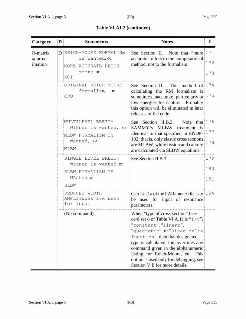
Section VI.A.1, page 5 (R8) Page 335
Table VI A1.2 (continued)
Section VI.A.1, page 5 (R8) Page 335
Category D Statements Notes #
R-matrix approx-imation
D REICH-MOORE FORMALISm is wanted, or MORE ACCURATE REICH- moore, or XCT
See Section II. Note that “more accurate” refers to the computational method, not to the formalism.
171
172
173
ORIGINAL REICH-MOORE formalism, or CRO
See Section II. This method of calculating the RM formalism is sometimes inaccurate, particularly at low energies for capture. Probably this option will be eliminated in later releases of the code.
174
175
MULTILEVEL BREIT- WIGner is wanted, or MLBW FORMALISM IS WAnted, or MLBW
See Section II.B.3. Note that SAMMY’s MLBW treatment is identical to that specified in ENDF-102; that is, only elastic cross sections are MLBW, while fission and capture are calculated via SLBW equations.
176
177
178
SINGLE LEVEL BREIT- Wigner is wanted, or SLBW FORMALISM IS WAnted, or SLBW
See Section II.B.3. 179
180
181
REDUCED WIDTH AMPLITudes are used for input
Card set 1a of the PARameter file is to be used for input of resonance parameters.
184
(No command) When “type of cross section” (see card set 8 of Table VI A.1) is “1/v”, “constant”, “linear”, “quadratic”, or “Dirac delta function”, then that designated type is calculated; this overrides any command given in the alphanumeric listing for Reich-Moore, etc. This option is used only for debugging; see Section V.E for more details.
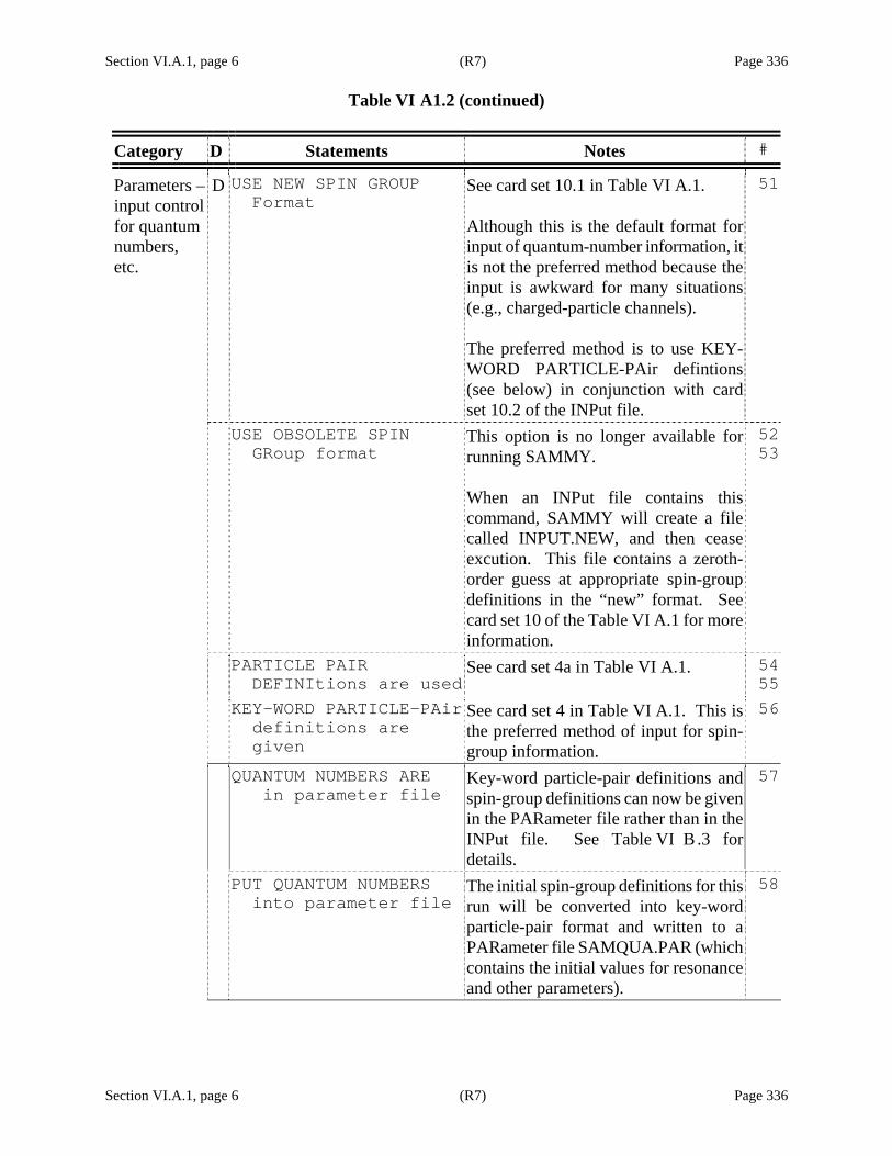
Section VI.A.1, page 6 (R7) Page 336 Table VI A1.2 (continued)
Section VI.A.1, page 6 (R7) Page 336
Category D Statements Notes # D USE NEW SPIN GROUP Format
See card set 10.1 in Table VI A.1. Although this is the default format for input of quantum-number information, it is not the preferred method because the input is awkward for many situations (e.g., charged-particle channels). The preferred method is to use KEY-WORD PARTICLE-PAir defintions (see below) in conjunction with card set 10.2 of the INPut file.
51Parameters – input control for quantum numbers, etc.
USE OBSOLETE SPIN GRoup format
This option is no longer available for running SAMMY. When an INPut file contains this command, SAMMY will create a file called INPUT.NEW, and then cease excution. This file contains a zeroth-order guess at appropriate spin-group definitions in the “new” format. See card set 10 of the Table VI A.1 for more information.
5253
PARTICLE PAIR DEFINItions are used
See card set 4a in Table VI A.1. 5455
KEY-WORD PARTICLE-PAir definitions are given
See card set 4 in Table VI A.1. This is the preferred method of input for spin-group information.
56
QUANTUM NUMBERS ARE in parameter file
Key-word particle-pair definitions and spin-group definitions can now be given in the PARameter file rather than in the INPut file. See Table VI B .3 for details.
57
PUT QUANTUM NUMBERS into parameter file
The initial spin-group definitions for this run will be converted into key-word particle-pair format and written to a PARameter file SAMQUA.PAR (which contains the initial values for resonance and other parameters).
58
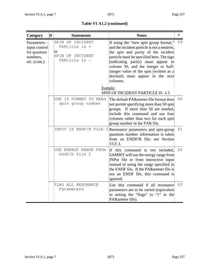
Section VI.A.1, page 7 (R7) Page 337 Table VI A1.2 (continued)
Section VI.A.1, page 7 (R7) Page 337
Category D Statements Notes # Parameters – input control for quantum numbers, etc. (cont.)
SPIN OF INCIDENT PARticle is + or SPIN OF INCIDENT PARticle is -
If using the “new spin group format,” and the incident particle is not a neutron, the spin and parity of the incident particle must be specified here. The sign (indicating parity) must appear in column 30, and the integer or half-integer value of the spin (written as a decimal) must appear in the next columns.
59
Eample: SPIN OF INCIDENT PARTICLE IS -1.5
USE I4 FORMAT TO REAd spin group number
The default PARameter file format does not permit specifying more than 50 spin groups. If more than 50 are needed, include this command and use four columns rather than two for each spin group number in the PAR file.
60
INPUT IS ENDF/B FILE 2 Resonance parameters and spin-group quantum number information is taken from an ENDF/B file; see Section VI.F.3.
61
USE ENERGY RANGE FROm endf/b file 2
If this command is not included, SAMMY will use the energy range from INPut file or from interactive input instead of using the range specified in the ENDF file. If the PARameter file is not an ENDF file, this command is ignored.
62
FLAG ALL RESONANCE Parameters
Use this command if all resonance parameters are to be varied (equivalent to setting the “flags” to “1” in the PARameter file).
63
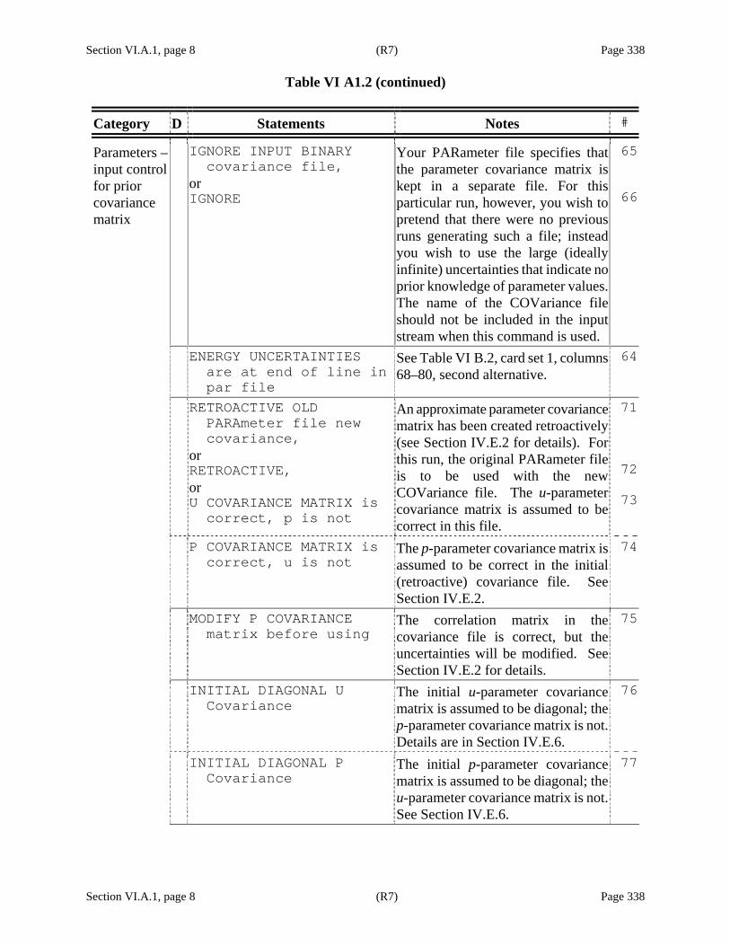
Section VI.A.1, page 8 (R7) Page 338 Table VI A1.2 (continued)
Section VI.A.1, page 8 (R7) Page 338
Category D Statements Notes #
Parameters – input control for prior covariance matrix
IGNORE INPUT BINARY covariance file, or IGNORE
Your PARameter file specifies that the parameter covariance matrix is kept in a separate file. For this particular run, however, you wish to pretend that there were no previous runs generating such a file; instead you wish to use the large (ideally infinite) uncertainties that indicate no prior knowledge of parameter values.The name of the COVariance file should not be included in the input stream when this command is used.
65
66
ENERGY UNCERTAINTIES are at end of line in par file
See Table VI B.2, card set 1, columns 68–80, second alternative.
64
RETROACTIVE OLD PARAmeter file new covariance, or RETROACTIVE, or U COVARIANCE MATRIX is correct, p is not
An approximate parameter covariance matrix has been created retroactively (see Section IV.E.2 for details). For this run, the original PARameter file is to be used with the new COVariance file. The u-parameter covariance matrix is assumed to be correct in this file.
71
72
73
P COVARIANCE MATRIX is correct, u is not
The p-parameter covariance matrix is assumed to be correct in the initial (retroactive) covariance file. See Section IV.E.2.
74
MODIFY P COVARIANCE matrix before using
The correlation matrix in the covariance file is correct, but the uncertainties will be modified. See Section IV.E.2 for details.
75
INITIAL DIAGONAL U Covariance
The initial u-parameter covariance matrix is assumed to be diagonal; the p-parameter covariance matrix is not. Details are in Section IV.E.6.
76
INITIAL DIAGONAL P Covariance
The initial p-parameter covariance matrix is assumed to be diagonal; the u-parameter covariance matrix is not.See Section IV.E.6.
77
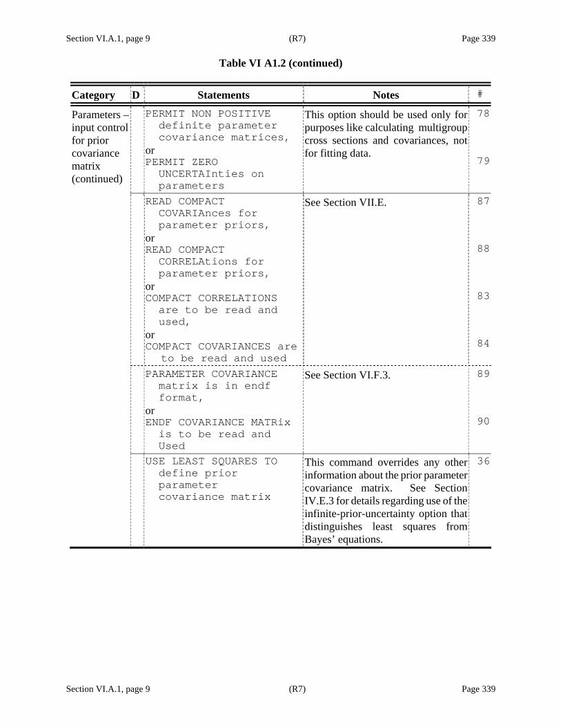
Section VI.A.1, page 9 (R7) Page 339 Table VI A1.2 (continued)
Section VI.A.1, page 9 (R7) Page 339
Category D Statements Notes # PERMIT NON POSITIVE definite parameter covariance matrices, or PERMIT ZERO UNCERTAInties on parameters
This option should be used only for purposes like calculating multigroup cross sections and covariances, not for fitting data.
78
79
Parameters – input control for prior covariance matrix (continued)
READ COMPACT COVARIAnces for parameter priors, or READ COMPACT CORRELAtions for parameter priors, or COMPACT CORRELATIONS are to be read and used, or COMPACT COVARIANCES are
to be read and used
See Section VII.E. 87
88
83
84
PARAMETER COVARIANCE matrix is in endf format, or ENDF COVARIANCE MATRix is to be read and Used
See Section VI.F.3. 89
90
USE LEAST SQUARES TO define prior parameter covariance matrix
This command overrides any other information about the prior parameter covariance matrix. See Section IV.E.3 for details regarding use of the infinite-prior-uncertainty option that distinguishes least squares from Bayes’ equations.
36
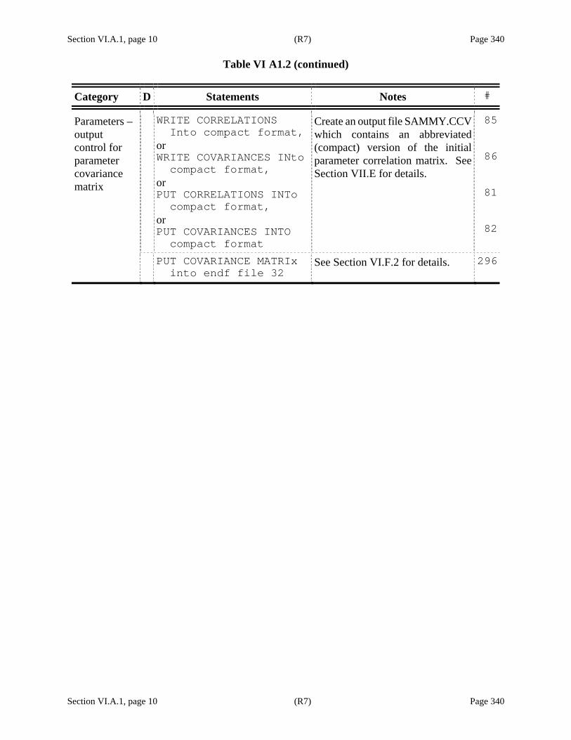
Section VI.A.1, page 10 (R7) Page 340 Table VI A1.2 (continued)
Section VI.A.1, page 10 (R7) Page 340
Category D Statements Notes #
Parameters – output control for parameter covariance matrix
WRITE CORRELATIONS Into compact format, or WRITE COVARIANCES INto compact format, or PUT CORRELATIONS INTo compact format, or PUT COVARIANCES INTO compact format
Create an output file SAMMY.CCV which contains an abbreviated (compact) version of the initial parameter correlation matrix. See Section VII.E for details.
85
86
81
82
PUT COVARIANCE MATRIx into endf file 32
See Section VI.F.2 for details. 296
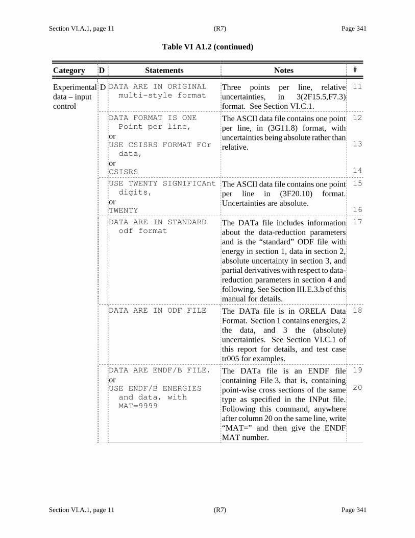
Section VI.A.1, page 11 (R7) Page 341 Table VI A1.2 (continued)
Section VI.A.1, page 11 (R7) Page 341
Category D Statements Notes #
D DATA ARE IN ORIGINAL multi-style format
Three points per line, relative uncertainties, in 3(2F15.5,F7.3) format. See Section VI.C.1.
11Experimental data – input control
DATA FORMAT IS ONE Point per line, or USE CSISRS FORMAT FOr data, or CSISRS
The ASCII data file contains one point per line, in (3G11.8) format, with uncertainties being absolute rather than relative.
12
13
14 USE TWENTY SIGNIFICAnt
digits, or TWENTY
The ASCII data file contains one point per line in (3F20.10) format. Uncertainties are absolute.
15
16 DATA ARE IN STANDARD
odf format The DATa file includes information about the data-reduction parameters and is the “standard” ODF file with energy in section 1, data in section 2, absolute uncertainty in section 3, and partial derivatives with respect to data-reduction parameters in section 4 and following. See Section III.E.3.b of this manual for details.
17
DATA ARE IN ODF FILE The DATa file is in ORELA Data Format. Section 1 contains energies, 2 the data, and 3 the (absolute) uncertainties. See Section VI.C.1 of this report for details, and test case tr005 for examples.
18
DATA ARE ENDF/B FILE, or USE ENDF/B ENERGIES and data, with MAT=9999
The DATa file is an ENDF file containing File 3, that is, containing point-wise cross sections of the same type as specified in the INPut file. Following this command, anywhereafter column 20 on the same line, write “MAT=” and then give the ENDF MAT number.
19
20

Section VI.A.1, page 12 (R7) Page 342 Table VI A1.2 (continued)
Section VI.A.1, page 12 (R7) Page 342
Category D Statements Notes # DIFFERENTIAL DATA ARe in ascii file
See Section VI.C.1 for details; note that the default for angle-differential data is ODF file.
22
D DO NOT DIVIDE DATA Into regions
Include entire energy range in a single SAMMY run.
23
Experimental data – input control (cont.)
DIVIDE DATA INTO REGions with a fixed number of data points per region
SAMMY will automatically choose energy regions of NEPNTS data points each, for sequential analysis. (See card set 2, Table VI A.1 for input for NEPNTS.)
24
Warning: SAMMY merely counts; it does not consider carefully whether a dividing point is located in a region where the theoretical values (σ or T) are nonlinear with respect to the parameters. Dividing in such a location (at or near a resonance) will invalidate the linearity assumption used in deriving Bayes' equation, and thus lead to spurious results. Users are urged to use this option only on the “zeroth pass,” as an aid in deciding where to divide the data, and not for final runs. With high-capacity computer systems available today, this option is seldom needed.

Section VI.A.1, page 13 (R8) Page 343 Table VI A1.2 (continued)
Section VI.A.1, page 13 (R8) Page 343
Category D Statements Notes #
IMPLICIT DATA COVARIance is wanted, or IDC
See Section VI.C.3.c. 31
32
Experimental data – input control for covariance matrix USER SUPPLIED IMPLICit
data covariance matrix, or USER IDC
See Section VI.C.3.b. 33
34 PUP COVARIANCE IS IN an
ascii file The covariance matrix for all or some of the Propagated Uncertainty Parameters (PUPs) is in an ASCII file. See Sections IV.D.2 and VI.C.3.a for details.
35
CREATE PUP FILE FROM varied parameters used in this run
Use this run, in which only parameters to be PUP’d in later runs are varied, to generate a file containing the PUP covariance matrix for future runs. See Sections IV.D.2 and VI.C.3.a for additional information.
21
ADD CONSTANT TERM TO data covariance or ADD CONSTANT TO DATA covariance matrix
39
40
D DO NOT ADD CONSTANT term to data covariance
41
USE DEFAULT FOR CONStant term to add to data covariance
These three statements refer to the option of adding a constant to the data covariance matrix, both on- and off-diagonal, over the energy region in which the effect of the non-s-wave resonance is felt. The magnitude of this constant is specified in columns 68–80 in the PARameter file, for each resonance. For the third option, the default value of this constant is set at 1.0E−6 for every non-s-wave resonance.
42

Section VI.A.1, page 14 (R8) Page 344 Table VI A1.2 (continued)
Section VI.A.1, page 14 (R8) Page 344
Category D Statements Notes # USE TEN PERCENT DATA uncertainty, or ADD TEN PERCENT DATA uncertainty
The “experimental uncertainty” is assumed by SAMMY to be 10% of the “measured value”. This option should not be used for analyses of real data.
43
44
Experimental data – input control for covariance matrix (cont.) D DATA COVARIANCE IS
Diagonal The explicit data covariance matrix is diagonal. Nevertheless, the actual data covariance matrix may include implicit contributions, either from propagated uncertainty parameters (see Section IV.D.2 or VI.C.3.a) or from a user-supplied implicit data covariance matrix (see Section VI.C.3.b).
45
DATA HAS OFF-DIAGONAl contribution to covariance matrix of the form (a+bEi) (a+bEj)
a and b are specified as DCOVA and DCOVB in the INP file, card set 7 in Table VI A.1.
46
DATA COVARIANCE FILE is named YYYYYY.YYY
Substitute your own file name for YYYYYY.YYY in columns 31–40. See Table VI C2.1 for the format for this file. Note that only ten characters are allowed for this file name.
47
FREE FORMAT DATA COVariance YYYYYY.YYY
Substitute your own file name for YYYYYY.YYY in columns 31–40.Note that only ten characters are allowed for this file name. Values in this file are in free format.
48
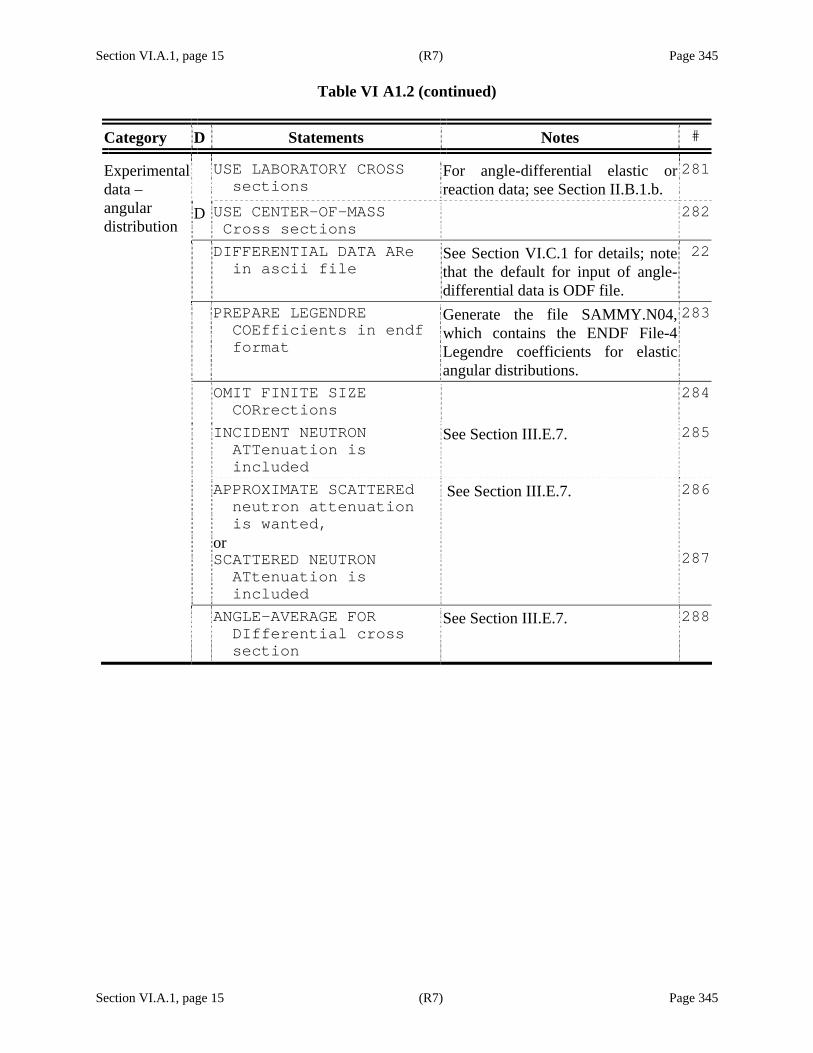
Section VI.A.1, page 15 (R7) Page 345 Table VI A1.2 (continued)
Section VI.A.1, page 15 (R7) Page 345
Category D Statements Notes #
USE LABORATORY CROSS sections
For angle-differential elastic or reaction data; see Section II.B.1.b.
281Experimental data – angular distribution
D USE CENTER-OF-MASS Cross sections
282
DIFFERENTIAL DATA ARe in ascii file
See Section VI.C.1 for details; note that the default for input of angle-differential data is ODF file.
22
PREPARE LEGENDRE COEfficients in endf format
Generate the file SAMMY.N04,which contains the ENDF File-4 Legendre coefficients for elastic angular distributions.
283
OMIT FINITE SIZE CORrections
284
INCIDENT NEUTRON ATTenuation is included
See Section III.E.7. 285
APPROXIMATE SCATTEREd neutron attenuation is wanted, or SCATTERED NEUTRON ATtenuation is included
See Section III.E.7. 286
287
ANGLE-AVERAGE FOR DIfferential cross section
See Section III.E.7. 288

Section VI.A.1, page 16 (R7) Page 346 Table VI A1.2 (continued)
Section VI.A.1, page 16 (R7) Page 346
Category D Statements Notes #
Broadening options
D BROADENING IS WANTED Some form of broadening is to be used; see Sections III.B and III.C.
201
BROADENING IS NOT WAnted
If you do not wish to have SAMMY Doppler or resolution broaden the theoretical values, be sure to remove card sets 5 and 6 (see Table VI A.1) from the INP file, as well as include this line.
202

Section VI.A.1, page 17 (R7) Page 347 Table VI A1.2 (continued)
Section VI.A.1, page 17 (R7) Page 347
Category D Statements Notes #
Broadening – Doppler
D USE FREE GAS MODEL Of doppler broadening, or FGM
The free-gas model of Doppler broadening, as described in Section III.B.1, is to be used.
211
212 USE LEAL-HWANG DOPPLer
broadening The Doppler-broadening method of Leal and Hwang, as described in Section III.B.2, is to be used.
213214
HIGH ENERGY GAUSSIAN approximation for Doppler broadening, or USE MULTI-STYLE DOPPler broadening, or HEGA
High-energy Gaussian approximation to the free-gas model is to be used for Doppler broadening, as described in Section III.B.3.
215
216217218
USE CRYSTAL LATTICE model of doppler broadening, or CLM
Use the crystal lattice (DOPUSH) model of Doppler broadening, as described in Section III.B.4.
219
220
NO LOW-ENERGY BROADEning is to be used
Theoretical values are not to be broadened below the energy value ELOWBR given in card set 5 of Table VI A.1 (the INPut file). This option works only with the high-energy Gaussian approximation for Doppler broadening.
221
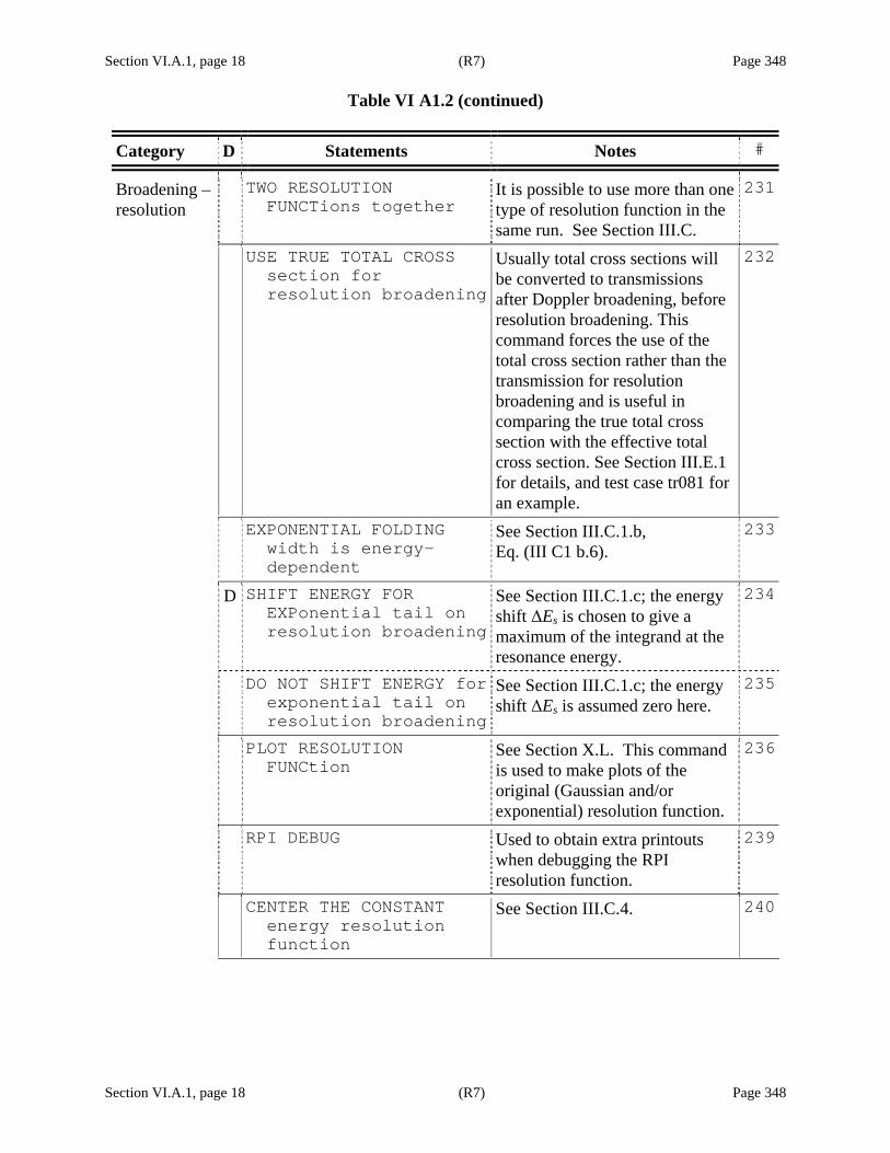
Section VI.A.1, page 18 (R7) Page 348
Table VI A1.2 (continued)
Section VI.A.1, page 18 (R7) Page 348
Category D Statements Notes #
Broadening – resolution
TWO RESOLUTION FUNCTions together
It is possible to use more than one type of resolution function in the same run. See Section III.C.
231
USE TRUE TOTAL CROSS section for resolution broadening
Usually total cross sections will be converted to transmissions after Doppler broadening, before resolution broadening. This command forces the use of the total cross section rather than the transmission for resolution broadening and is useful in comparing the true total cross section with the effective total cross section. See Section III.E.1 for details, and test case tr081 for an example.
232
EXPONENTIAL FOLDING width is energy- dependent
See Section III.C.1.b, Eq. (III C1 b.6).
233
D SHIFT ENERGY FOR EXPonential tail on resolution broadening
See Section III.C.1.c; the energy shift ΔEs is chosen to give a maximum of the integrand at the resonance energy.
234
DO NOT SHIFT ENERGY for exponential tail on resolution broadening
See Section III.C.1.c; the energy shift ΔEs is assumed zero here.
235
PLOT RESOLUTION FUNCtion
See Section X.L. This command is used to make plots of the original (Gaussian and/or exponential) resolution function.
236
RPI DEBUG Used to obtain extra printouts when debugging the RPI resolution function.
239
CENTER THE CONSTANT energy resolution function
See Section III.C.4. 240
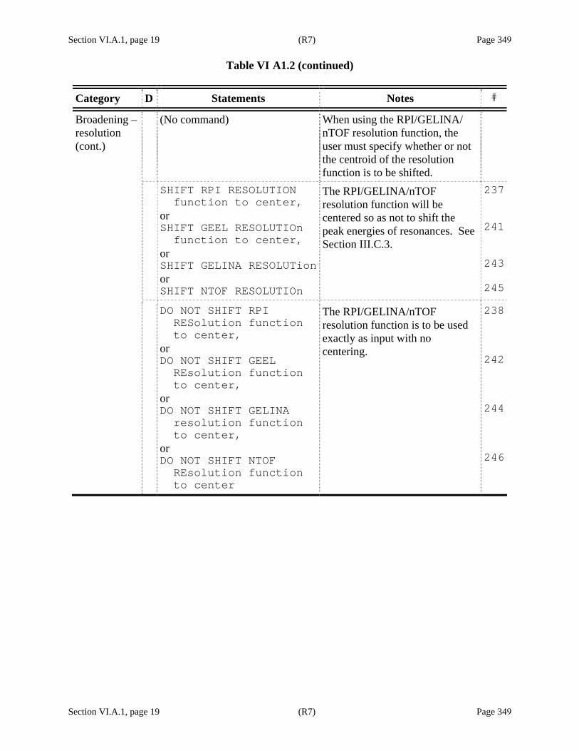
Section VI.A.1, page 19 (R7) Page 349
Table VI A1.2 (continued)
Section VI.A.1, page 19 (R7) Page 349
Category D Statements Notes # Broadening – resolution (cont.)
(No command) When using the RPI/GELINA/ nTOF resolution function, the user must specify whether or not the centroid of the resolution function is to be shifted.
SHIFT RPI RESOLUTION function to center, or SHIFT GEEL RESOLUTIOn function to center, or SHIFT GELINA RESOLUTionor SHIFT NTOF RESOLUTIOn
The RPI/GELINA/nTOF resolution function will be centered so as not to shift the peak energies of resonances. See Section III.C.3.
237
241
243
245
DO NOT SHIFT RPI RESolution function to center, or DO NOT SHIFT GEEL REsolution function to center, or DO NOT SHIFT GELINA resolution function to center, or DO NOT SHIFT NTOF REsolution function to center
The RPI/GELINA/nTOF resolution function is to be used exactly as input with no centering.
238
242
244
246

Section VI.A.1, page 20 (R8) Page 350 Table VI A1.2 (continued)
Section VI.A.1, page 20 (R8) Page 350
Category D Statements Notes #
Multiple-scattering corrections
D DO NOT INCLUDE SELF- shielding or multiple-scattering corrections, or NO SELF-SHIELDING ANd multiple-scattering corrections
Calculate the cross section but do not include any self-shielding or multiple-scattering corrections.
251
252
USE SELF SHIELDING Only, no scattering, or SELF SHIELD, or INCLUDE ONLY SELF SHielding and not Multiple scattering
Only self-shielding is to be included; no single- or double-scattering (see Section III.D).
253
254
255
USE SINGLE SCATTERINg plus self shielding, or SINGLE
Include self-shielding plus single-scattering corrections.
256
257
INCLUDE DOUBLE SCATTering corrections, or USE MULTIPLE SCATTERing plus single scattering,or DOUBLE, or MULTIPLE
Include self-shielding, single-scattering, and double-scattering corrections (see Section III.D).
258
259
261
260 INFINITE SLAB,
or NO FINITE-SIZE CORREctions to single scattering
Single-scattering correction does not include edge effects.
263
262
D FINITE SLAB, or FINITE SIZE CORRECTIons to single scattering
Edge effects corrections are included for single scattering.
265
264

Section VI.A.1, page 21 (R8) Page 351 Table VI A1.2 (continued)
Section VI.A.1, page 21 (R8) Page 351
Category D Statements Notes # Multiple-scattering corrections (cont.)
D MAKE NEW FILE WITH Edge effects
See Section III.D. This statement is ignored if “INFINITE SLAB” is specified. Be sure to rename and save the SAMMY.SSM file if you wish to reuse it.
266
FILE WITH EDGE EFFECts already exists
Use this option to conserve run time. Include the name of this file (which was generated by a previous SAMMY run) after the name of your DATa file.
267
MAKE PLOT FILE OF MUltiple scattering pieces
Store Y0, Y1, and Y2 in file SAM53.DAT, to be read by program SAMCPR.
268269
NORMALIZE AS CROSS Section rather than yield, or CROSS SECTION
270
271
NORMALIZE AS YIELD Rather than cross section, or YIELD
272
273
NORMALIZE AS (1-E)SIgma
See Section III.D. Note than normalization must be specified explicitly. SAMMY will abort if the INPut file does not specify which normalization is to be used.
274 PRINT MULTIPLE SCATTering
corrections Create a table of E, Y0, Y1, Y2, and Y (energy plus components of the corrected yield) in file SAM012.DAT.
275
PREPARE INPUT FOR MOnte carlo simulation, or MONTE CARLO
This is the initial SAMMY run to generate cross sections for use in Monte Carlo simulation of multiple-scattering effects.
276277
Y2 VALUES ARE TABULAted When SAMMY’s calculation of double-plus scattering is inadequate, tabulated values for Y2, can be used. See Section III.D for information on creating and using tabulated values.
247
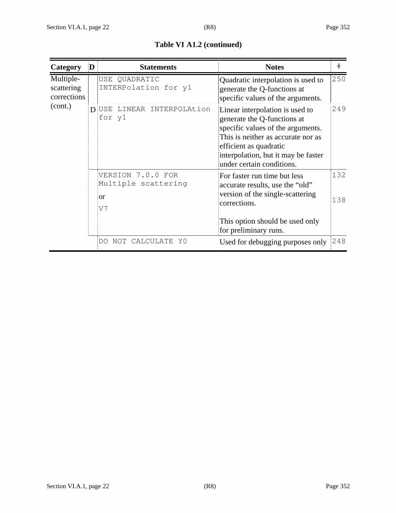
Section VI.A.1, page 22 (R8) Page 352 Table VI A1.2 (continued)
Section VI.A.1, page 22 (R8) Page 352
Category D Statements Notes # USE QUADRATIC INTERPolation for y1
Quadratic interpolation is used to generate the Q-functions at specific values of the arguments.
250Multiple-scattering corrections (cont.) D USE LINEAR INTERPOLAtion
for y1 Linear interpolation is used to generate the Q-functions at specific values of the arguments. This is neither as accurate nor as efficient as quadratic interpolation, but it may be faster under certain conditions.
249
VERSION 7.0.0 FOR Multiple scattering or V7
For faster run time but less accurate results, use the “old” version of the single-scattering corrections. This option should be used only for preliminary runs.
132
138
DO NOT CALCULATE Y0 Used for debugging purposes only 248
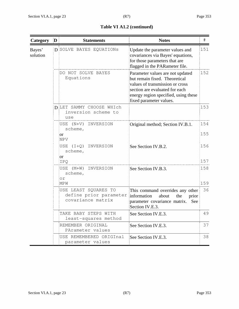
Section VI.A.1, page 23 (R7) Page 353 Table VI A1.2 (continued)
Section VI.A.1, page 23 (R7) Page 353
Category D Statements Notes #
Bayes’ solution
D SOLVE BAYES EQUATIONs Update the parameter values and covariances via Bayes' equations, for those parameters that are flagged in the PARameter file.
151
DO NOT SOLVE BAYES Equations
Parameter values are not updated but remain fixed. Theoretical values of transmission or cross section are evaluated for each energy region specified, using these fixed parameter values.
152
D LET SAMMY CHOOSE WHIch inversion scheme to use
153
USE (N+V) INVERSION scheme, or NPV
Original method; Section IV.B.1. 154
155
USE (I+Q) INVERSION scheme, or IPQ
See Section IV.B.2. 156
157 USE (M+W) INVERSION
scheme, or MPW
See Section IV.B.3. 158
159 USE LEAST SQUARES TO
define prior parameter covariance matrix
This command overrides any other information about the prior parameter covariance matrix. See Section IV.E.3.
36
TAKE BABY STEPS WITH least-squares method
See Section IV.E.3. 49
REMEMBER ORIGINAL PArameter values
See Section IV.E.3. 37
USE REMEMBERED ORIGInal parameter values
See Section IV.E.3. 38

Section VI.A.1, page 24 (R7) Page 354 Table VI A1.2 (continued)
Section VI.A.1, page 24 (R7) Page 354
Category D Statements Notes #
D DO NOT PRINT ANY INPut parameters
9192
PRINT ALL INPUT PARAmeters
All resonances parameters are printed in SAMMY.LPT.
93
Options for printing into SAMMY. LPT PRINT VARIED INPUT
Parameters Resonances for which no parameters are flagged will not be printed. Use this option for direct comparison with output parameters, which are always printed in this mode.
94
D DO NOT PRINT INPUT Data 95 PRINT INPUT DATA,or
PRINT EXPERIMENTAL Values
9697
D DO NOT PRINT THEORETical values
98
PRINT THEORETICAL VAlues, or PRINT THEORETICAL CRoss sections
“Input data” refers to experimental values of the measured cross section (or transmission, etc.), as read from the DATa file (see Section VI.C). “Theoretical values” refers to the calculated cross sections (as broadened and otherwise corrected). Often these are available in the plot file (see Table VII C.1), so they need not be printed in the LPT file.
99
100
D DO NOT PRINT PARTIAL derivatives
101
PRINT PARTIAL DERIVAtives Use this option only for debug purposes.
102
SUPPRESS INTERMEDIATe printout
Updated parameter values and covariance matrix elements are printed only upon completion of entire run.
103
DO NOT SUPPRESS INTErmediate printout
Updated parameter values and covariance matrix elements are printed after completion of each energy region.
104
D DO NOT SUPPRESS ANY intermediate printout
Updated parameter values are printed after each iteration of Bayes' equations (i.e., typically twice for each energy region). Updated covariance matrix elements are evaluated and printed only upon completion of an energy region.
105
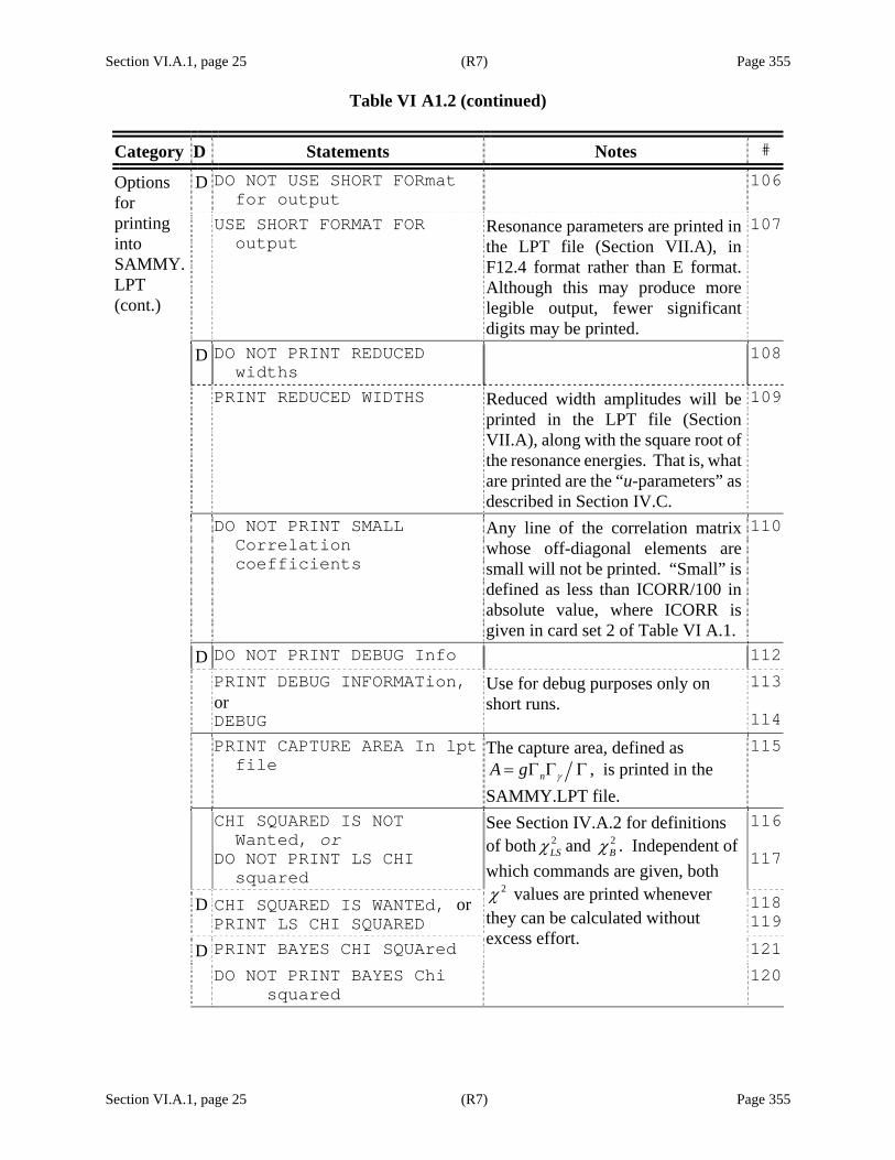
Section VI.A.1, page 25 (R7) Page 355 Table VI A1.2 (continued)
Section VI.A.1, page 25 (R7) Page 355
Category D Statements Notes # D DO NOT USE SHORT FORmat for output
106Options for printing into SAMMY. LPT (cont.)
USE SHORT FORMAT FOR output
Resonance parameters are printed in the LPT file (Section VII.A), in F12.4 format rather than E format. Although this may produce more legible output, fewer significant digits may be printed.
107
D DO NOT PRINT REDUCED widths
108
PRINT REDUCED WIDTHS Reduced width amplitudes will be printed in the LPT file (Section VII.A), along with the square root of the resonance energies. That is, what are printed are the “u-parameters” as described in Section IV.C.
109
DO NOT PRINT SMALL Correlation coefficients
Any line of the correlation matrix whose off-diagonal elements are small will not be printed. “Small” is defined as less than ICORR/100 in absolute value, where ICORR is given in card set 2 of Table VI A.1.
110
D DO NOT PRINT DEBUG Info 112 PRINT DEBUG INFORMATion,
or DEBUG
Use for debug purposes only on short runs.
113
114 PRINT CAPTURE AREA In lpt
file The capture area, defined as
nA g γ= Γ Γ Γ , is printed in the SAMMY.LPT file.
115
CHI SQUARED IS NOT Wanted, or DO NOT PRINT LS CHI squared
116
117
D CHI SQUARED IS WANTEd, or PRINT LS CHI SQUARED
118119
D PRINT BAYES CHI SQUAred
See Section IV.A.2 for definitions of both 2
LSχ and 2Bχ . Independent of
which commands are given, both 2χ values are printed whenever
they can be calculated without excess effort. 121
DO NOT PRINT BAYES Chi squared
120

Section VI.A.1, page 26 (R7) Page 356 Table VI A1.2 (continued)
Section VI.A.1, page 26 (R7) Page 356
Category D Statements Notes # D DO NOT PRINT WEIGHTEd Residuals, or DO NOT PRINT LS WEIGhted residuals
See Section IV.A.2 for definitions of weighted residuals.
122
123
Options for printing into SAMMY. LPT (cont.)
PRINT WEIGHTED RESIDuals,or PRINT LS WEIGHTED REsiduals
124
125
PRINT BAYES WEIGHTED residuals
126
D DO NOT PRINT BAYES Weighted residuals
127
D DO NOT PRINT PHASE Shifts 130 PRINT PHASE SHIFTS For
input parameters Hard-sphere phase shifts are defined in Section II.A.
131
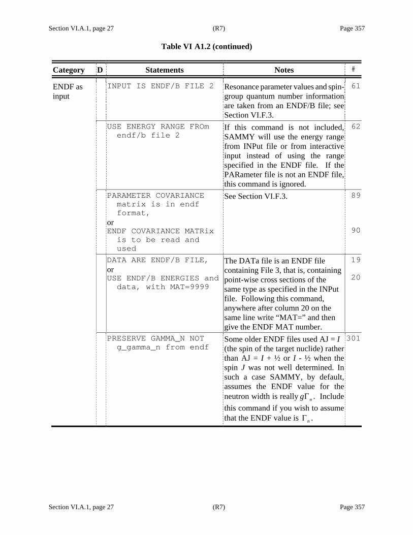
Section VI.A.1, page 27 (R7) Page 357 Table VI A1.2 (continued)
Section VI.A.1, page 27 (R7) Page 357
Category D Statements Notes #
ENDF as input
INPUT IS ENDF/B FILE 2 Resonance parameter values and spin-group quantum number information are taken from an ENDF/B file; see Section VI.F.3.
61
USE ENERGY RANGE FROm endf/b file 2
If this command is not included, SAMMY will use the energy range from INPut file or from interactive input instead of using the range specified in the ENDF file. If the PARameter file is not an ENDF file, this command is ignored.
62
PARAMETER COVARIANCE matrix is in endf format, or ENDF COVARIANCE MATRix is to be read and used
See Section VI.F.3. 89
90
DATA ARE ENDF/B FILE, or USE ENDF/B ENERGIES and data, with MAT=9999
The DATa file is an ENDF file containing File 3, that is, containing point-wise cross sections of the same type as specified in the INPut file. Following this command, anywhere after column 20 on the same line write “MAT=” and then give the ENDF MAT number.
19
20
PRESERVE GAMMA_N NOT g_gamma_n from endf
Some older ENDF files used AJ = I (the spin of the target nuclide) rather than AJ = I + ½ or I - ½ when the spin J was not well determined. In such a case SAMMY, by default, assumes the ENDF value for the neutron width is really ngΓ . Include this command if you wish to assume that the ENDF value is nΓ .
301
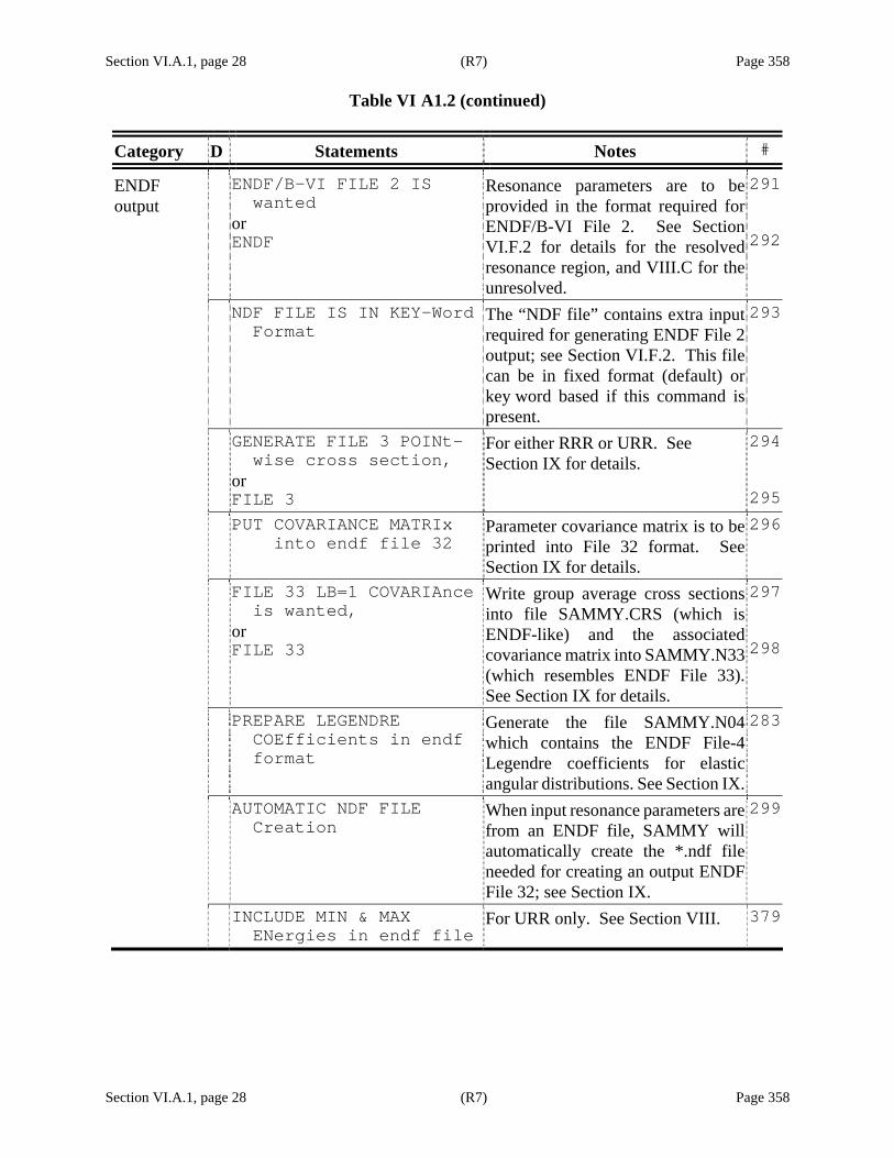
Section VI.A.1, page 28 (R7) Page 358 Table VI A1.2 (continued)
Section VI.A.1, page 28 (R7) Page 358
Category D Statements Notes # ENDF output
ENDF/B-VI FILE 2 IS wanted or ENDF
Resonance parameters are to be provided in the format required for ENDF/B-VI File 2. See Section VI.F.2 for details for the resolved resonance region, and VIII.C for the unresolved.
291
292
NDF FILE IS IN KEY-Word Format
The “NDF file” contains extra input required for generating ENDF File 2 output; see Section VI.F.2. This file can be in fixed format (default) or key word based if this command is present.
293
GENERATE FILE 3 POINt- wise cross section, or FILE 3
For either RRR or URR. See Section IX for details.
294
295 PUT COVARIANCE MATRIx
into endf file 32 Parameter covariance matrix is to be printed into File 32 format. See Section IX for details.
296
FILE 33 LB=1 COVARIAnce is wanted, or FILE 33
Write group average cross sections into file SAMMY.CRS (which is ENDF-like) and the associated covariance matrix into SAMMY.N33 (which resembles ENDF File 33). See Section IX for details.
297
298
PREPARE LEGENDRE COEfficients in endf format
Generate the file SAMMY.N04which contains the ENDF File-4 Legendre coefficients for elastic angular distributions. See Section IX.
283
AUTOMATIC NDF FILE Creation
When input resonance parameters are from an ENDF file, SAMMY will automatically create the *.ndf file needed for creating an output ENDF File 32; see Section IX.
299
INCLUDE MIN & MAX ENergies in endf file
For URR only. See Section VIII. 379
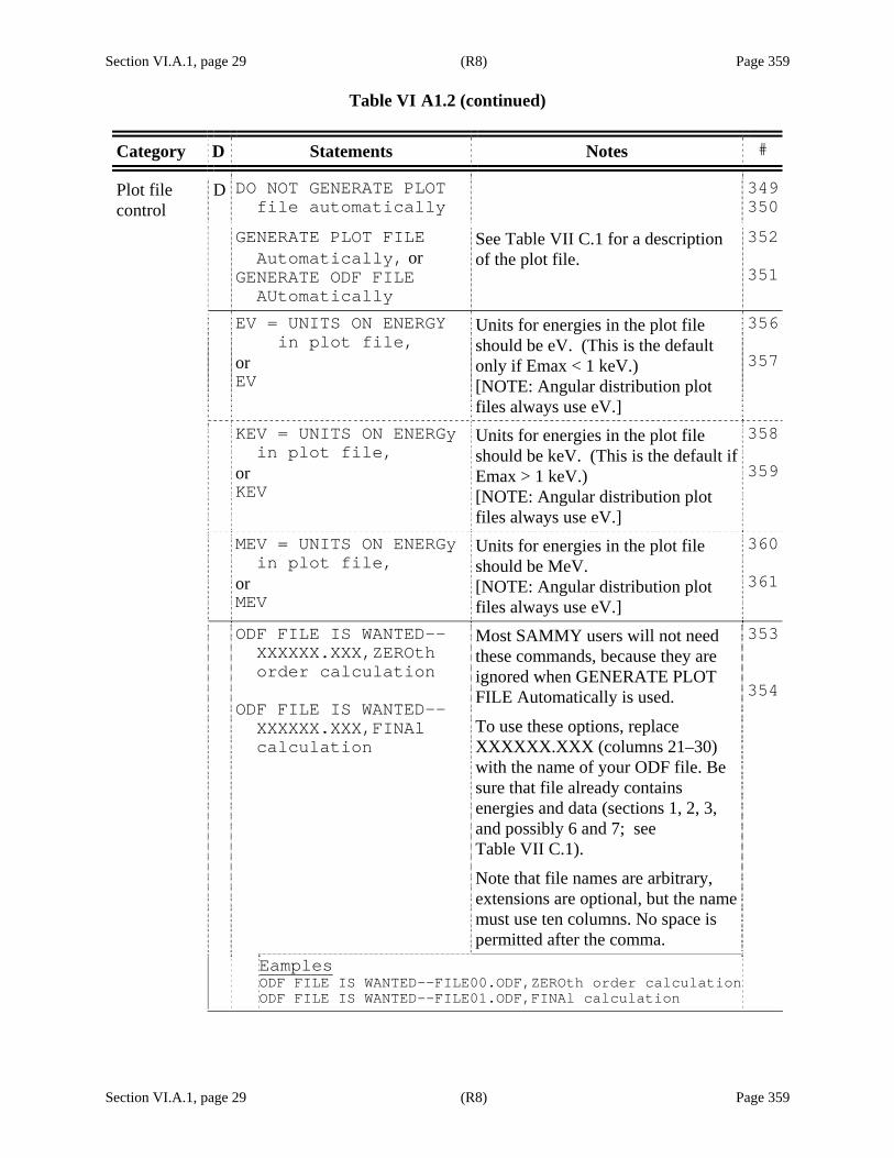
Section VI.A.1, page 29 (R8) Page 359 Table VI A1.2 (continued)
Section VI.A.1, page 29 (R8) Page 359
Category D Statements Notes #
Plot file control
D DO NOT GENERATE PLOT file automatically
349350
GENERATE PLOT FILE Automatically, or GENERATE ODF FILE AUtomatically
See Table VII C.1 for a description of the plot file.
352
351
EV = UNITS ON ENERGY in plot file, or EV
Units for energies in the plot file should be eV. (This is the default only if Emax < 1 keV.) [NOTE: Angular distribution plot files always use eV.]
356
357
KEV = UNITS ON ENERGy in plot file, or KEV
Units for energies in the plot file should be keV. (This is the default if Emax > 1 keV.) [NOTE: Angular distribution plot files always use eV.]
358
359
MEV = UNITS ON ENERGy in plot file, or MEV
Units for energies in the plot file should be MeV. [NOTE: Angular distribution plot files always use eV.]
360
361
ODF FILE IS WANTED-- XXXXXX.XXX,ZEROth order calculation ODF FILE IS WANTED-- XXXXXX.XXX,FINAl calculation
Most SAMMY users will not need these commands, because they are ignored when GENERATE PLOT FILE Automatically is used.
To use these options, replace XXXXXX.XXX (columns 21–30) with the name of your ODF file. Be sure that file already contains energies and data (sections 1, 2, 3, and possibly 6 and 7; see Table VII C.1).
Note that file names are arbitrary, extensions are optional, but the name must use ten columns. No space is permitted after the comma.
353
354
Eamples ODF FILE IS WANTED--FILE00.ODF,ZEROth order calculationODF FILE IS WANTED--FILE01.ODF,FINAl calculation
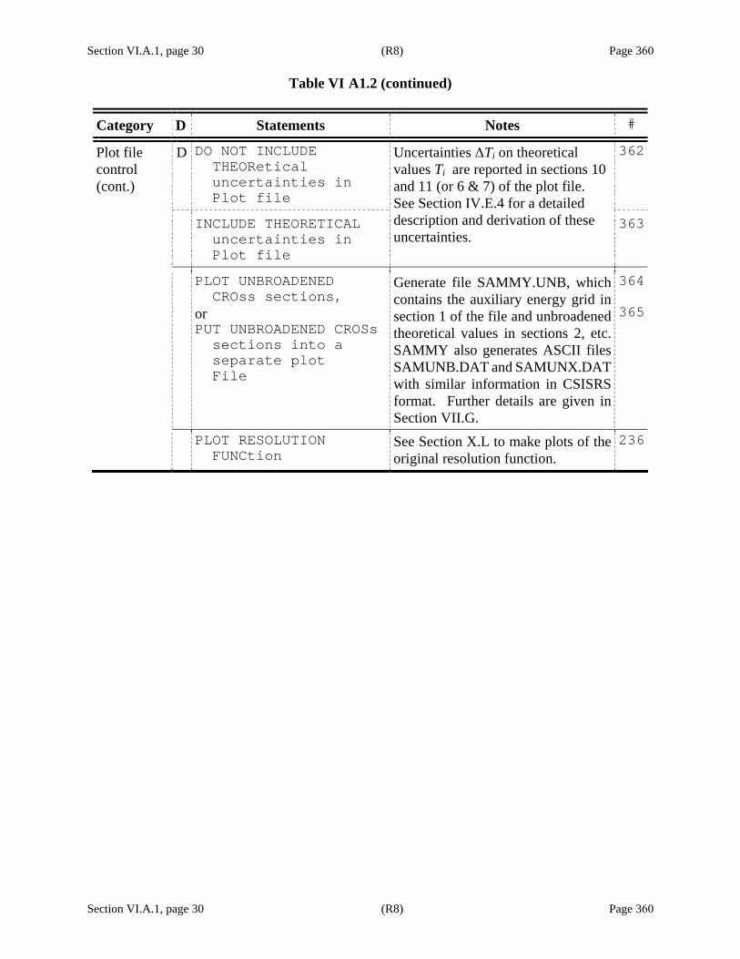
Section VI.A.1, page 30 (R8) Page 360 Table VI A1.2 (continued)
Section VI.A.1, page 30 (R8) Page 360
Category D Statements Notes # Plot file control (cont.)
D DO NOT INCLUDE THEORetical uncertainties in Plot file
362
INCLUDE THEORETICAL uncertainties in Plot file
Uncertainties ΔTi on theoretical values Ti are reported in sections 10 and 11 (or 6 & 7) of the plot file. See Section IV.E.4 for a detailed description and derivation of these uncertainties.
363
PLOT UNBROADENED CROss sections, or PUT UNBROADENED CROSs sections into a separate plot File
Generate file SAMMY.UNB, which contains the auxiliary energy grid in section 1 of the file and unbroadened theoretical values in sections 2, etc. SAMMY also generates ASCII filesSAMUNB.DAT and SAMUNX.DATwith similar information in CSISRS format. Further details are given in Section VII.G.
364
365
PLOT RESOLUTION FUNCtion
See Section X.L to make plots of the original resolution function.
236

Section VI.A.1, page 31 (R7) Page 361 Table VI A1.2 (continued)
Section VI.A.1, page 31 (R7) Page 361
Category D Statements Notes #
D (none needed ) Do not average over energy ranges. Averages, etc. AVERAGE OVER ENERGY
Ranges or AVERAGE OVER ENERGIEs
Produce energy-averaged experi-mental data and theoretical values, using output parameters from an earlier SAMMY analysis. See Section V.C.1 for details.
311
312
CAUTION: The integration scheme used here is histogram based, suitable for averaging experimental data but not suitable for averaging theoretical cross sections. Use “ENERGY AVERAGE USING constant flux” option instead.
GROUP AVERAGE OVER Energy ranges, or GROUP or BONDARENKO AVERAGE Over energy ranges
Produce Bondarenko averages, using output parameters from an earlier SAMMY analysis. See Section V.C.2 for details.
313
314
315
ENERGY AVERAGE USING constant flux, or UNWEIGHTED ENERGY AVerage
This is the appropriate scheme to use when averaging theoretical cross sections with constant flux; see Section V.C.3.
325
MAXWELLIAN-AVERAGED capture cross sections are wanted, or STELLAR-AVERAGED CAPture cross sections are wanted, or MXW
Generate stellar averaged capture cross section; see Section V.D.
316
317
318 CALCULATE MAXWELLIAN
averages after reconstructing cross sections
This option provides stellar averaged capture cross sections (Section V.D) using reconstructed energy grid (Section V.A, NJOY method).
319
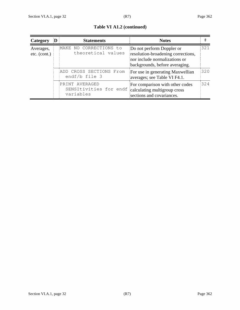
Section VI.A.1, page 32 (R7) Page 362 Table VI A1.2 (continued)
Section VI.A.1, page 32 (R7) Page 362
Category D Statements Notes # Averages, etc. (cont.)
MAKE NO CORRECTIONS to theoretical values
Do not perform Doppler or resolution-broadening corrections, nor include normalizations or backgrounds, before averaging.
321
ADD CROSS SECTIONS From endf/b file 3
For use in generating Maxwellian averages; see Table VI F4.1.
320
PRINT AVERAGED SENSItivities for endf variables
For comparison with other codes calculating multigroup cross sections and covariances.
324
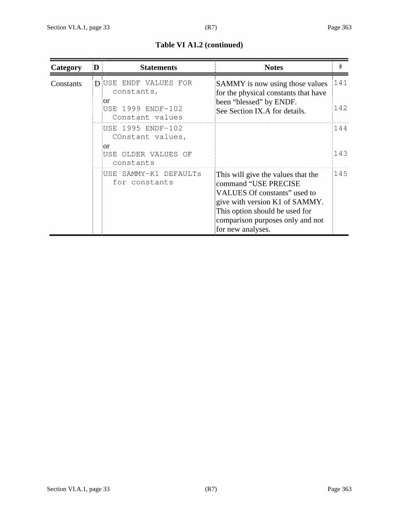
Section VI.A.1, page 33 (R7) Page 363 Table VI A1.2 (continued)
Section VI.A.1, page 33 (R7) Page 363
Category D Statements Notes #
Constants D USE ENDF VALUES FOR constants, or USE 1999 ENDF-102 Constant values
SAMMY is now using those values for the physical constants that have been “blessed” by ENDF. See Section IX.A for details.
141
142
USE 1995 ENDF-102 COnstant values, or USE OLDER VALUES OF constants
144
143
USE SAMMY-K1 DEFAULTs for constants
This will give the values that the command “USE PRECISE VALUES Of constants” used to give with version K1 of SAMMY. This option should be used for comparison purposes only and not for new analyses.
145
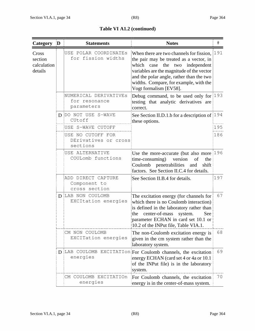
Section VI.A.1, page 34 (R8) Page 364 Table VI A1.2 (continued)
Section VI.A.1, page 34 (R8) Page 364
Category D Statements Notes #
Cross section calculation details
USE POLAR COORDINATEs for fission widths
When there are two channels for fission, the pair may be treated as a vector, in which case the two independent variables are the magnitude of the vector and the polar angle, rather than the two widths. Compare, for example, with the Vogt formalism [EV58].
191
NUMERICAL DERIVATIVEs for resonance parameters
Debug command, to be used only for testing that analytic derivatives are correct.
193
D DO NOT USE S-WAVE CUtoff
194
USE S-WAVE CUTOFF 195 USE NO CUTOFF FOR
DErivatives or cross sections
See Section II.D.1.b for a description of these options.
186
USE ALTERNATIVE COULomb functions
Use the more-accurate (but also more time-consuming) version of the Coulomb penetrabilities and shift factors. See Section II.C.4 for details.
196
ADD DIRECT CAPTURE Component to cross section
See Section II.B.4 for details. 197
D LAB NON COULOMB EXCItation energies
The excitation energy (for channels for which there is no Coulomb interaction) is defined in the laboratory rather than the center-of-mass system. See parameter ECHAN in card set 10.1 or 10.2 of the INPut file, Table VIA.1.
67
CM NON COULOMB EXCITation energies
The non-Coulomb excitation energy is given in the cm system rather than the laboratory system.
68
D LAB COULOMB EXCITATIon energies
For Coulomb channels, the excitation energy ECHAN (card set 4 or 4a or 10.1 of the INPut file) is in the laboratory system.
69
CM COULOMB EXCITATIOn energies
For Coulomb channels, the excitation energy is in the center-of-mass system.
70

Section VI.A.1, page 35 (R8) Page 365 Table VI A1.2 (continued)
Section VI.A.1, page 35 (R8) Page 365
Category D Statements Notes # Cross section calculation details, continued
ADD ELIMINATED CAPTUre channel to final state
When some capture channels are treated individually and others in aggregate, this command will include both in the calculation of capture cross section. See Section II.B.2 for details.
10

Section VI.A.1, page 36 (R7) Page 366 Table VI A1.2 (continued)
Section VI.A.1, page 36 (R7) Page 366
Category D Statements Notes #
No pre-defined energy grid
RECONSTRUCT CROSS SEction from resonance parameters
SAMMY will automatically choose an appropriate grid and evaluate total, elastic, capture, and fission cross sections on that grid, using NJOY method. See Section V.A.
306
ARTIFICIAL ENERGY Grid is needed
SAMMY will automatically choose an appropriate grid and evaluate, using SAMMY method. See Section V.A.
307

Section VI.A.1, page 37 (R7) Page 367 Table VI A1.2 (continued)
Section VI.A.1, page 37 (R7) Page 367
Category D Statements Notes #
Special options
RELEVANT PARAMETERS are chosen via uncertainty ratio
Solve Bayes’ equations one time. Then, based on the ratio of u-parameter uncertainties, choose which of the R-matrix parameters are relevant. Create file SAMMY.REL, which contains the original parameter values with only the relevant parameters flagged to be varied. See test case tr166 for examples.
327
CROSS SECTION COVARIance matrix is wanted
Calculate the covariance matrix for the theoretical cross sections.
328
INITIAL UNCERTAINTY multiplier =
All prior parameter uncertainties (square roots of diagonal elements of parameter covariance matrix) are to be multiplied by the specified number. See Section IV.E.6 for further discussion, and test case tr019 for examples.
329
FINAL UNCERTAINTY MUltiplier =
All output parameter uncertainties (square roots of diagonal elements of parameter covariance matrix) are to be multiplied by the specified number. See Section IV.E.6 for further discussion, and test case tr019 for examples.
330
E-DEPENDENT INITIAL Uncertainty multiplier, or E-DEPENDENT UNCERTAInty multiplier
All prior parameter uncertainties are to be multiplied by an energy- and spin-group-dependent multiplier. Details are give in Section IV.E.6, and test casetr019 contains examples.
6
7
SUMMED STRENGTH FUNCtion is wanted
Evaluate and print the summed strength function and corresponding covariance matrix. See Section V.F for details.
331

Section VI.A.1, page 38 (R7) Page 368 Table VI A1.2 (continued)
Section VI.A.1, page 38 (R7) Page 368
Category D Statements Notes # Special options (cont.)
GENERATE PARTIAL DERivatives only
SAMMY will assume all resonance parameters, and only resonance para-meters, are to be varied; that Bayes' equations are not to be solved; and that the partial derivatives of the theoretical values with respect to those parameters are to be written into file SAMMY.PDS .
332
GENERATE SPIN GROUP cross sections
Generate the ODF (Plot) file containing the energy (from auxiliary grid) in section 1, the unbroadened cross section in section 2, the spin-group-1 contribution to the unbroadened cross section in section 3, spin-group-2 contribution in section 4, etc.
333
REFORMULATE DATA FOR implicit data covariances
See Sections IV.D.3 and VI.C.3. 334
COMPARE EXPERIMENT To theory
See Section X.E; results are reported in binary file SAM53.DAT.
335
GENERATE Y AND W MATrices, or YW
336
337
READ Y AND W MATRICEs, or WY
See Section IV for a description of the M+W form of Bayes’ Equations. See test case tr089 for examples of the use of this option.
338
339 STOP abc n
(Note that there are two spaces before “n” in this command; n is replaced with an integer value.)
Cease execution prior to the n th occurrence of segment abc. Used only for debug (Section XI.B) and for preparation for Monte Carlo calculations (Section X.M).
340
WRITE CALCULATED CROss sections into ascii file
Write energies and theoretical values into ascii file SAMTHE.DAT in 2F20.10 format.
341

Section VI.A.1, page 39 (R7) Page 369 Table VI A1.2 (continued)
Section VI.A.1, page 39 (R7) Page 369
Category D Statements Notes # Special options (cont.)
PRINT MULTIPLE SCATTering corrections
Create a table of E, Y0, Y1, Y2, and Y(energy plus components of the corrected yield) in file SAM012.DAT.
275
UNIFORM ENERGY GRID Instead of using the energies from the experimental data set to define the energy grid, SAMMY will create a grid of 1001 points uniformly space in energy. This is for testing purposes only, so this grid must be used only for “no Bayes” runs. See Section V.E for details.
342
UNIFORM VELOCITY GRId
SAMMY will create a grid of 1001 points uniformly spaced in velocity (square root of energy). To be used for testing purposes only. See Section V.E.
343
UNIFORM TIME GRID SAMMY will create a grid of 1001 points uniformly spaced in time (1 over the square root of energy). To be used for testing purposes only. See Section V.E for details.
344
CREATE PUBLISHABLE List of parameters, or PUBLISH
The file SAMMY.PUB will be created, which contains resonance parameters and uncertainties in columns, with each value separated by tabs. This file can be ported to spreadsheet programs to be formatted for publication purposes. See Section VII.F for details.
345
346
DO NOT TEST FOR EIGEnvalues
Do not test whether the parameter covariance matrix is positive-definite (i.e., whether all eigenvalues are greater than zero).
347

Section VI.A.1, page 40 (R7) Page 370 Table VI A1.2 (continued)
Section VI.A.1, page 40 (R7) Page 370
Category D Statements Notes #
URR controls
EXPERIMENTAL DATA ARe in separate files
See Section VIII.B for details of input to unresolved resonance region (URR) calculations.
371
NO ANNOTATED PARAMETer file for urr input
Input for URR is essentially the original format as in the FITACS code; see Table VIII.B.1.
372
D ANNOTATED PARAMETER file for urr, or ANNOTATED
Input for URR is “annotated file”, which contains key words and phrases to make the input more human-legible. See Section VIII.B and Table VIII.B.2 for details.
373
374
D OUTPUT IN ANNOTATED parameter file for urr
Output parameter file is annotated. (This is always true; SAMMY now contains no option for writing non-annotated output, although that can still be used as input).
375
ENDF/B-VI FILE 2 IS wanted, or ENDF
Resonance parameters are to be written into the format required for ENDF/B-VI File 2. See Section VI.F.2 for details.
291
292 D USE ALL EXPERIMENTAL
data points, or DO NOT USE ENERGY LImits as given in the input file
All data points appearing in the initial URR PARameter file (see Section VIII.B) are to be fitted during the analysis. Energy limits given in the INPut file will be ignored.
376
377
USE ENERGY LIMITS AS Given in the input file
The energy range specified in card set 2 of the INPut file will be used to define which data points are to be included in the analysis.
378
INCLUDE MIN & MAX ENergies in endf file
When creating ENDF File 2 for LRU= 2, include Emin and Emax from the SAMMY run as part of the energy list. Examples are in test cases tr127, tr128, tr133, and tr134.
379
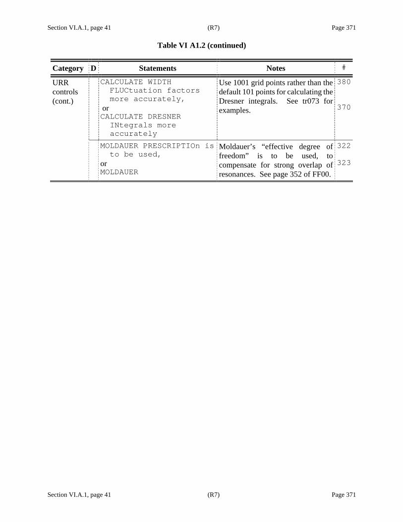
Section VI.A.1, page 41 (R7) Page 371 Table VI A1.2 (continued)
Section VI.A.1, page 41 (R7) Page 371
Category D Statements Notes # URR controls (cont.)
CALCULATE WIDTH FLUCtuation factors more accurately, or CALCULATE DRESNER INtegrals more accurately
Use 1001 grid points rather than the default 101 points for calculating the Dresner integrals. See tr073 for examples.
380
370
MOLDAUER PRESCRIPTIOn is to be used, or MOLDAUER
Moldauer’s “effective degree of freedom” is to be used, to compensate for strong overlap of resonances. See page 352 of FF00.
322
323


Section VI.A.1, page 43 (R8) Page 373 Table VI A1.3. Alphabetic list of acceptable commands for card set 3 Abbreviations in the “Category” column are defined in Table VI A1.1 and refer to the location in Table VI A1.2 in which a description of this command can be found. “P” in the column labeled “Parameter” indicates that additional values are required on this line. “D” in the column labeled “Default” indicates that this is a default command and so may be safely omitted. “B” in the “deBug” column indicates that this command should be only for debugging and not for production runs. “A” in the “Archaic” column indicates a command that will likely soon be eliminated.
Section VI.A.1, page 43 (R8) Page 373
Command statement Category Para
met
er
Def
ault
deB
ug
Arc
haic
ADD CONSTANT TERM TO data covariance DCM ADD CROSS SECTIONS From endf/b file 3 Average ADD DIRECT CAPTURE Component… CS calc ADD ELIMINATED CAPTUre channel to final state CS calc ADD TEN PERCENT DATA uncertainty DCM ANGLE-AVERAGE FOR DIfferential cross section Angle ANNOTATED URR D ANNOTATED PARAMETER file for urr URR D APPROXIMATE SCATTEREd neutron attenuation… Angle ARTIFICIAL ENERGY GRid is needed Grid AUTOMATIC NDF FILE Creation ENDF out AVERAGE OVER ENERGY ranges Average BONDARENKO AVERAGE Over energy ranges Average BROADENING IS NOT WAnted Broad BROADENING IS WANTED Broad D CALCULATE DRESNER INtegrals more accurately URR CALCULATE MAXWELLIAN averages after reconst… Average CALCULATE WIDTH FLUCtuation factors more… URR CENTER THE CONSTANT energy resolution function Resol CHI SQUARED IS NOT Wanted LPT CHI SQUARED IS WANTEd LPT D CLM Doppler CM COULOMB EXCITATIOn energies CS calc CM NON COULOMB EXCITation energies CS calc

Section VI.A.1, page 44 (R8) Page 374 Table VI A1.3 (continued)
Section VI.A.1, page 44 (R8) Page 374
Command statement Category Para
met
er
Def
ault
deB
ug
Arc
haic
COMPACT CORRELATIONS are to be read and used PCM in COMPACT COVARIANCES are to be read and used PCM in COMPARE EXPERIMENT To theory Special CREATE PUBLISHABLE List of parameters Special CREATE PUP FILE FROM varied parameters used… DCM CRO RM ACROSS SECTION MSC CROSS SECTION COVARIance matrix is wanted Special CSISRS Data DATA ARE ENDF/B FILE Data DATA ARE IN ODF FILE Data DATA ARE IN ORIGINAL multi-style format Data D DATA ARE IN STANDARD odf format Data DATA COVARIANCE FILE is named YYYYYY.YYY DCM P DATA COVARIANCE IS Diagonal DCM D DATA FORMAT IS ONE Point per line Data DATA HAS OFF-DIAGONAl contribution to cov... DCM DEBUG LPT B DIFFERENTIAL DATA ARe In ascii file Data DIFFERENTIAL DATA ARe in ascii file Angle DIVIDE DATA INTO REGions with a fixed number… Data DO NOT ADD CONSTANT term to data covariance DCM D DO NOT ALLOW VALUES for data-related param… Special DO NOT DIVIDE DATA Into regions Data D DO NOT GENERATE PLOT file automatically Plot D DO NOT INCLUDE SELF-shielding or multiple-scat… MSC D DO NOT INCLUDE THEORetical uncertainties in… Plot DO NOT PRINT ANY INPut parameters LPT D DO NOT PRINT BAYES Chi squared LPT DO NOT PRINT BAYES Weighted residuals LPT D
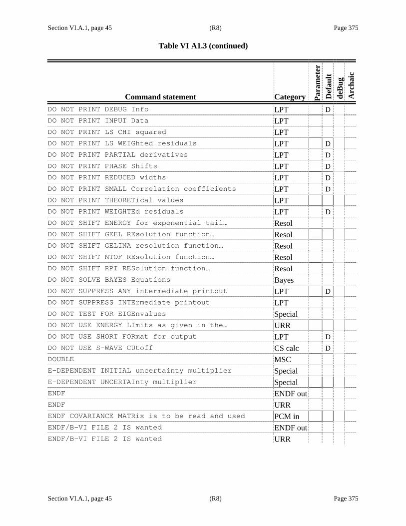
Section VI.A.1, page 45 (R8) Page 375 Table VI A1.3 (continued)
Section VI.A.1, page 45 (R8) Page 375
Command statement Category Para
met
er
Def
ault
deB
ug
Arc
haic
DO NOT PRINT DEBUG Info LPT D DO NOT PRINT INPUT Data LPT DO NOT PRINT LS CHI squared LPT DO NOT PRINT LS WEIGhted residuals LPT D DO NOT PRINT PARTIAL derivatives LPT D DO NOT PRINT PHASE Shifts LPT D DO NOT PRINT REDUCED widths LPT D DO NOT PRINT SMALL Correlation coefficients LPT D DO NOT PRINT THEORETical values LPT DO NOT PRINT WEIGHTEd residuals LPT D DO NOT SHIFT ENERGY for exponential tail… Resol DO NOT SHIFT GEEL REsolution function… Resol DO NOT SHIFT GELINA resolution function… Resol DO NOT SHIFT NTOF REsolution function… Resol DO NOT SHIFT RPI RESolution function… Resol DO NOT SOLVE BAYES Equations Bayes DO NOT SUPPRESS ANY intermediate printout LPT D DO NOT SUPPRESS INTErmediate printout LPT DO NOT TEST FOR EIGEnvalues Special DO NOT USE ENERGY LImits as given in the… URR DO NOT USE SHORT FORmat for output LPT D DO NOT USE S-WAVE CUtoff CS calc D DOUBLE MSC E-DEPENDENT INITIAL uncertainty multiplier Special E-DEPENDENT UNCERTAInty multiplier Special ENDF ENDF out ENDF URR ENDF COVARIANCE MATRix is to be read and used PCM in ENDF/B-VI FILE 2 IS wanted ENDF out ENDF/B-VI FILE 2 IS wanted URR
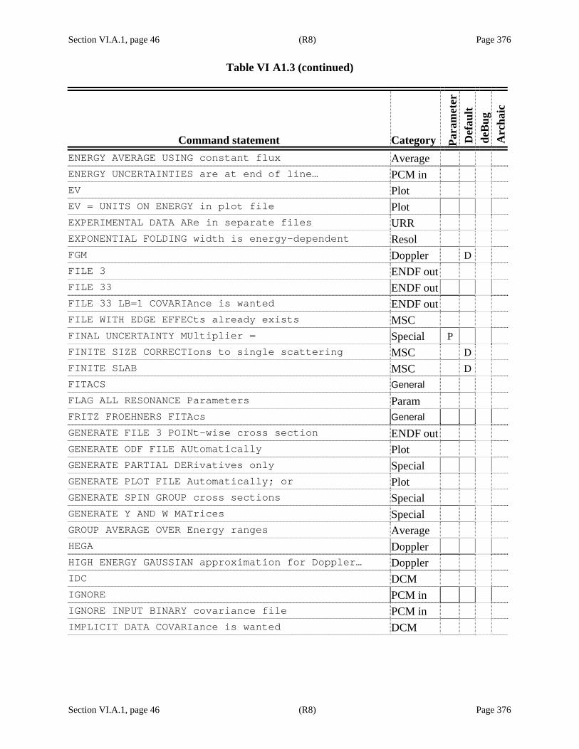
Section VI.A.1, page 46 (R8) Page 376 Table VI A1.3 (continued)
Section VI.A.1, page 46 (R8) Page 376
Command statement Category Para
met
er
Def
ault
deB
ug
Arc
haic
ENERGY AVERAGE USING constant flux Average ENERGY UNCERTAINTIES are at end of line… PCM in EV Plot EV = UNITS ON ENERGY in plot file Plot EXPERIMENTAL DATA ARe in separate files URR EXPONENTIAL FOLDING width is energy-dependent Resol FGM Doppler D FILE 3 ENDF out FILE 33 ENDF out FILE 33 LB=1 COVARIAnce is wanted ENDF out FILE WITH EDGE EFFECts already exists MSC FINAL UNCERTAINTY MUltiplier = Special P FINITE SIZE CORRECTIons to single scattering MSC D FINITE SLAB MSC D FITACS General FLAG ALL RESONANCE Parameters Param FRITZ FROEHNERS FITAcs General GENERATE FILE 3 POINt-wise cross section ENDF out GENERATE ODF FILE AUtomatically Plot GENERATE PARTIAL DERivatives only Special GENERATE PLOT FILE Automatically; or Plot GENERATE SPIN GROUP cross sections Special GENERATE Y AND W MATrices Special GROUP AVERAGE OVER Energy ranges Average HEGA Doppler HIGH ENERGY GAUSSIAN approximation for Doppler… Doppler IDC DCM IGNORE PCM in IGNORE INPUT BINARY covariance file PCM in IMPLICIT DATA COVARIance is wanted DCM

Section VI.A.1, page 47 (R8) Page 377 Table VI A1.3 (continued)
Section VI.A.1, page 47 (R8) Page 377
Command statement Category Para
met
er
Def
ault
deB
ug
Arc
haic
INCIDENT NEUTRON ATTenuation is included Angle INCLUDE DOUBLE SCATTering corrections MSC INCLUDE MIN & MAX ENergies in endf file ENDF out INCLUDE MIN & MAX ENergies in endf file URR INCLUDE ONLY SELF SHielding and not multiple… MSC INCLUDE THEORETICAL uncertainties in plot file Plot INFINITE SLAB MSC INITIAL DIAGONAL P Covariance PCM in INITIAL DIAGONAL U Covariance PCM in INITIAL UNCERTAINTY multiplier = Special P INPUT IS ENDF/B FILE 2 Param INPUT IS ENDF/B FILE 2 ENDF in IPQ Bayes KEV Plot KEV = UNITS ON ENERGy in plot file Plot KEY-WORD PARTICLE-PAir definitions are given Param LAB COULOMB EXCITATIon energies CS calc D LAB NON COULOMB EXCItation energies CS calc D LET SAMMY CHOOSE WHIch inversion scheme… Bayes D LINEAR MSC D MAKE NEW FILE WITH Edge effects MSC D MAKE NO CORRECTIONS to theoretical values Average MAKE PLOT FILE OF MUltiple scattering pieces MSC MAXWELLIAN AVERAGED capture cross sections… Average MEV Plot MEV = UNITS ON ENERGy in plot file Plot MLBW RM MLBW FORMALISM IS WAnted RM MODIFY P COVARIANCE matrix before using PCM in MOLDAUER URR MOLDAUER PRESCRIPTIOn is to be used URR

Section VI.A.1, page 48 (R8) Page 378 Table VI A1.3 (continued)
Section VI.A.1, page 48 (R8) Page 378
Command statement Category Para
met
er
Def
ault
deB
ug
Arc
haic
MONTE CARLO MSC MORE ACCURATE REICH-moore RM MPW Bayes MULTILEVEL BREIT-WIGner is wanted RM MULTIPLE MSC MXW Average NDF FILE IS IN KEY-Word Format ENDF out NO ANNOTATED PARAMETer file for urr input URR NO FINITE-SIZE CORREctions to single scattering MSC NO LOW-ENERGY BROADEning is to be used Doppler NO SELF-SHIELDING ANd multiple-scattering… MSC D NORMALIZE AS (1-E)SIgma MSC NORMALIZE AS CROSS Section rather than yield MSC NORMALIZE AS YIELD Rather than cross section MSC NPV Bayes NUMERICAL DERIVATIVEs for resonance parameters CS calc B ODF FILE IS WANTED-- XXXXXX.XXX, FINAl guess Plot P ODF FILE IS WANTED-- XXXXXX.XXX, ZEROth order… Plot P OMIT FINITE SIZE CORrections Angle ORIGINAL REICH-MOORE formalism RM AOUTPUT IN ANNOTATED parameter file for urr URR D P COVARIANCE MATRIX is correct, U is not PCM in PARAMETER COVARIANCE matrix is in endf format PCM in PARTICLE PAIR DEFINItions are given Param PERFORM SUMMARY ANALysis Special PERMIT NON POSITIVE definite parameter cov… PCM in PERMIT ZERO UNCERTAInties on parameters PCM in PLOT RESOLUTION FUNCtion Resol PLOT RESOLUTION FUNCtion Plot PLOT UNBROADENED CROss sections Plot
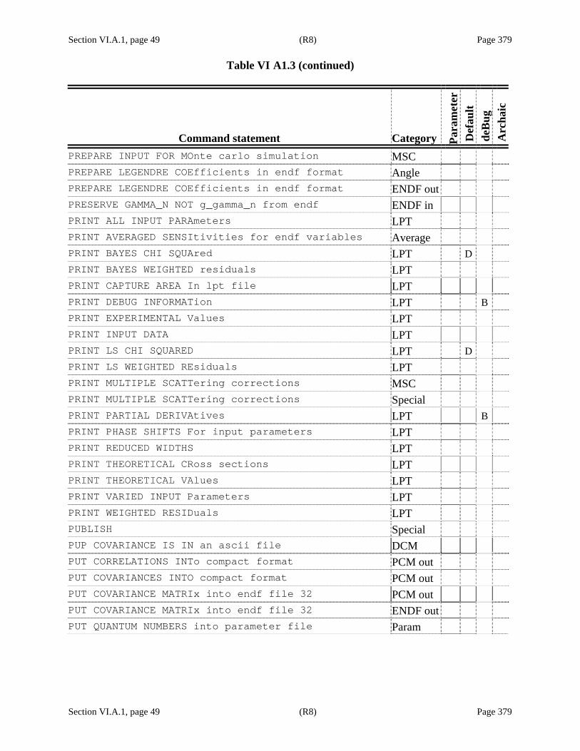
Section VI.A.1, page 49 (R8) Page 379 Table VI A1.3 (continued)
Section VI.A.1, page 49 (R8) Page 379
Command statement Category Para
met
er
Def
ault
deB
ug
Arc
haic
PREPARE INPUT FOR MOnte carlo simulation MSC PREPARE LEGENDRE COEfficients in endf format Angle PREPARE LEGENDRE COEfficients in endf format ENDF out PRESERVE GAMMA_N NOT g_gamma_n from endf ENDF in PRINT ALL INPUT PARAmeters LPT PRINT AVERAGED SENSItivities for endf variables Average PRINT BAYES CHI SQUAred LPT D PRINT BAYES WEIGHTED residuals LPT PRINT CAPTURE AREA In lpt file LPT PRINT DEBUG INFORMATion LPT B PRINT EXPERIMENTAL Values LPT PRINT INPUT DATA LPT PRINT LS CHI SQUARED LPT D PRINT LS WEIGHTED REsiduals LPT PRINT MULTIPLE SCATTering corrections MSC PRINT MULTIPLE SCATTering corrections Special PRINT PARTIAL DERIVAtives LPT B PRINT PHASE SHIFTS For input parameters LPT PRINT REDUCED WIDTHS LPT PRINT THEORETICAL CRoss sections LPT PRINT THEORETICAL VAlues LPT PRINT VARIED INPUT Parameters LPT PRINT WEIGHTED RESIDuals LPT PUBLISH Special PUP COVARIANCE IS IN an ascii file DCM PUT CORRELATIONS INTo compact format PCM out PUT COVARIANCES INTO compact format PCM out PUT COVARIANCE MATRIx into endf file 32 PCM out PUT COVARIANCE MATRIx into endf file 32 ENDF out PUT QUANTUM NUMBERS into parameter file Param

Section VI.A.1, page 50 (R8) Page 380 Table VI A1.3 (continued)
Section VI.A.1, page 50 (R8) Page 380
Command statement Category Para
met
er
Def
ault
deB
ug
Arc
haic
PUT UNBROADENED CROSs sections into plot file Plot QUADRATIC MSC QUANTUM NUMBERS ARE in parameter file Param READ COMPACT CORRELAtions for parameter priors PCM in READ COMPACT COVARIAnces for parameter priors PCM in READ Y AND W MATRICEs Special RECONSTRUCT CROSS SEction from resonance… Grid REFORMULATE DATA FOR implicit data covariances Special REICH-MOORE FORMALISm is wanted RM D RELEVANT PARAMETERS are chosen via uncert… Special REMEMBER ORIGINAL PArameter values Bayes RETROACTIVE PCM in RETROACTIVE OLD PARAmeter file new cov… PCM in RPI DEBUG Resol B SCATTERED NEUTRON ATtenuation is included Angle SELF SHIELD MSC SHIFT ENERGY FOR EXPonential tail on resolution… Resol D SHIFT GEEL RESOLUTIOn function to center Resol SHIFT GELINA RESOLUTion Resol SHIFT NTOF RESOLUTIOn Resol SHIFT RPI RESOLUTION function to center Resol SINGLE MSC SINGLE LEVEL BREIT-Wigner is wanted RM SLBW RM SLBW FORMALISM IS WAnted RM SOLVE BAYES EQUATIONs Bayes D SPIN OF INCIDENT PARTICLE IS - Param P SPIN OF INCIDENT PARTICLE IS + Param P STELLAR AVERAGED CAPture cross sections… Average STOP abc n Special B SUMMED STRENGTH FUNCtion is wanted Special

Section VI.A.1, page 51 (R8) Page 381 Table VI A1.3 (continued)
Section VI.A.1, page 51 (R8) Page 381
Command statement Category Para
met
er
Def
ault
deB
ug
Arc
haic
SUPPRESS INTERMEDIATe printout LPT TAKE BABY STEPS WITH least squares method Bayes TWENTY Data TWO RESOLUTION FUNCTions together Resol U COVARIANCE MATRIX is correct, P is not PCM in UNIFORM ENERGY GRID Special UNIFORM TIME GRID Special UNIFORM VELOCITY GRId Special UNRESOLVED RESONANCE region General UNWEIGHTED ENERGY AVerage Average USE (I+Q) INVERSION scheme Bayes USE (M+W) INVERSION scheme Bayes USE (N+V) INVERSION scheme Bayes USE 1995 ENDF-102 COnstant values Constant USE 1999 ENDF-102 COnstant values Constant USE ALL EXPERIMENTAL data points URR D USE ALTERNATIVE COULomb functions CS calc USE ALTERNATIVE COULomb functions CS calc USE CENTER-OF-MASS Cross sections Angle D USE CRYSTAL LATTICE model of doppler broadening Doppler USE CSISRS FORMAT FOr data Data USE DEFAULT FOR CONStant term to add to… DCM USE ENDF VALUES FOR constants Constant D USE ENDF/B ENERGIES and data, with MAT=9999 Data P USE ENERGY LIMITS AS given in the input file URR USE ENERGY RANGE FROm endf/b file 2 Param USE ENERGY RANGE FROm endf/b file 2 ENDF in USE FREE GAS MODEL Of doppler broadening Doppler D USE I4 FORMAT TO REAd spin group number Param USE LABORATORY CROSS sections Angle

Section VI.A.1, page 52 (R8) Page 382 Table VI A1.3 (continued)
Section VI.A.1, page 52 (R8) Page 382
Command statement Category Para
met
er
Def
ault
deB
ug
Arc
haic
USE LEAL-HWANG DOPPLer broadening Doppler USE LEAST SQUARES TO define prior par cov… Bayes USE LEAST SQUARES TO define prior par… cov… PCM in USE LINEAR INTERPOLAtion for y1 MSC D USE MULTIPLE SCATTERing plus single scattering MSC USE MULTI-STYLE DOPPler broadening Doppler USE NEW SPIN GROUP Format Param D USE NO CUTOFF FOR DErivatives or cross sections CS calc USE OBSOLETE SPIN GRoup format Param AUSE OLDER VALUES OF constants Constant USE POLAR COORDINATEs for fission widths CS calc USE QUADRATIC INTERPoltion for y1 MSC USE REMEMBERED ORIGInal parameter values Bayes USE SAMMY-K1 DEFAULTs for constants Constant USE SELF SHIELDING Only, no scattering MSC USE SHORT FORMAT FOR output LPT USE SINGLE SCATTERINg plus self shielding MSC USE S-WAVE CUTOFF CS calc USE TEN PERCENT DATA uncertainty DCM USE TRUE TOTAL CROSS section for resolution… Resol USE TWENTY SIGNIFICAnt digits Data USER IDC DCM USER SUPPLIED IMPLICit data covariance matrix DCM VERSION 7.0.0 FOR MUltiple scattering or V7 MSC WRITE CALCULATED CROss sections into ascii file Special WRITE CORRELATIONS Into compact format PCM out WRITE COVARIANCES INto compact format PCM out WY Special XCT RM Y2 VALUES ARE TABULAted MSC YIELD MSC YW Special
Section VI.B, page 1 (R8) Page 383
Section VI.B, page 1 (R8) Page 383
VI.B. THE PARameter FILE
The PARameter file contains initial values for all those parameters that are to be varied, as well as others that may be held fixed or treated as propagated-uncertainty parameters (see Section IV.D.2 for details concerning PUPs). In addition, this file may contain a priori uncertainties or covariances for the varied parameters.
Various types of data can be included in the PARameter file. These are organized into “card sets,” with each card set consisting of one or more lines of information. Most card sets begin with a header line and end with a blank line. The header lines are listed in Table VI B.1, along with key words for some of the card sets. Details about each card set are given in Table VI B.2 and summarized here.
Card set 1 contains resonance parameters, ending in a blank line.
Beginning with Revision 8 of this document and Release sammy-7.0.2, the square root of resonance energies and reduced-width amplitudes may be used for input in place of resonance energies and partial widths. Input for this option is described in card set 1a. To use this option, include the command “REDUCED WIDTH AMPLITudes are used for input” in card set 2 of the INPut file.
For all SAMMY runs for which resolved-resonance-region parameters are fitted, two output parameter files are created. The first, SAMMY.PAR, is in the original format with resonance energies and partial widths; units are eV for energies and meV for partial widths. The second, SAMMY.RED, contains the square root of resonance energies and reduced-width amplitudes; units for both types of parameters are the square root of eV.
Card set 2 contains a single number, called FUDGE, which is the “fudge factor” by which a parameter may multiplied to give the initial uncertainty for that parameter. This option is used only if the parameter’s uncertainty is not specified elsewhere.
Only card set 1 is required to be in the file. If any of card sets 3 through “Last” are present, then card set 2 must also be present.
Card set 3 gives values for parameters of the external R-function (see Section II.B.1.d). Two alternate formats are available for this.
Card set 4 gives values for some broadening (and other) parameters.
Card set 5 gives values of “unused” parameters, that is, of those data-reduction parameters that are not directly affected by the data set to be analyzed but that are coupled via the covariance matrix to other parameters that are directly affected. An example of such a parameter would be the thickness of a thin sample, for which the data have already been analyzed via SAMMY, while the current data set is from a measurement with a thick sample. The auxiliary code SAMAMR must be used between the two SAMMY runs to ensure that the correct thickness is used with the appropriate data set (see Section X.C).
Card set 6 gives values for normalization and background parameters, as described in Eqs. (III E3a.1) and (III E3 a.2) of Section III.E.3.a

Section VI.B, page 2 (R8) Page 384
Section VI.B, page 2 (R8) Page 384
Card set 7 contains values for the two channel radii (as used for potential scattering and for penetrability and shift factor). Key-word format for the channel radii is described in card set 7a. See item 3 in Section III.E.2 for discussion of effective vs. true radius.
Card set 8 gives names and values for data reduction parameters, as described in Section III.E.3.b.
Card set 9 gives values of parameters for the Oak Ridge resolution function (ORR) parameters, as described in Section III.C.2.
Card set 10 contains isotopic mass and abundance values, as described in Section III.E.2.
Card set 11 contains values for miscellaneous parameters, described in various locations throughout this manual.
Card set 12 provides parameter values for paramagnetic cross sections; see Section III.E.4.
Card set 13 contains values for parameters of the background functions described in Section III.E.3.a.
Card set 14 gives parameters of the RPI resolution function (Section III.C.3).
Card set 15 provides values for l- and isotope-dependent detector efficiencies (Section III.E.5).
Card set 16 gives input for the numerical user-defined resolution function. This is described in more detail in Section III.C.5.
The last card set defines the prior covariance matrix for the parameters. Three alternative methods are given: Card set Last A assumes a covariance matrix has been prepared by a previous SAMMY run; the presence of this card set eliminates the possibility of any others being used. Card sets Last B (“explicit uncertainties”) and Last C (“relative uncertainties”) may be interchanged at will, as long as each occurs at most once in any given PARameter file. A fourth alternative is available for resonance energies only (see card set 1, columns 68–80, option 3). A fifth is to omit this card set entirely, in which case, default uncertainties are used for every parameter.
Note that each card set in the PAR file (except for card sets 1 and 2) begins with an alphanumeric description of what follows. Note also that each card set (except card set 2) terminates with a blank card. A blank line at the very end of the file may be omitted, but all others must be present.
Quantum numbers included in PARameter file
Beginning with Release M6 of the SAMMY code, it is possible to include all information relevant to the R-matrix within the PARameter file rather than have partial information (spin group definitions) in the INPut file. Details are given in Table VI B.3.

Section VI.B, page 3 (R7) Page 385
Section VI.B, page 3 (R7) Page 385
Table VI B.1. Header lines for card sets in the PARameter file Card
set Alphanumeric header line Notes 1 Resonance parameters. No header
line; card set ends in a blank line. 2 Fudge factor for default uncertainties;
no header line, no blank line. 3 EXTERnal R-function parameters
follow
3a R-EXTernal parameters follow
Only one of card sets 3 and 3a is permitted.
4 BROADening parameters may be varied
5 UNUSEd but correlated variables Card set is created by SAMAMR run. 6 NORMAlization and background 7 RADIUs parameters follow
(two versions: usual for fewer than 99 channels and spin groups, alternative version for greater than 99 channels or spin groups.
Card set 7a is the preferred method.
7a RADII are in KEY-WORD format or CHANNel radius parameters follow
Valid key words for channel radius: RADIus or RADIi EFfective radius TRue radius
Valid key words for uncertainty: RElative ABsolute or UNcertainty
Valid key words for particle-pair names: PARTicle-pair or PP
Valid key words for orbital angular momentum: L or ORbital angular momentum
with ODd, EVen, or ALl after equal sign Valid key word for flags:
FLags with Yes, 1, No, 0, 2, or −1 Valid key word for spin groups:
GRoup followed by a group number or All CHannels =, followed by channel numbers
8 DATA reduction parameters are next Seldom used

Section VI.B, page 4 (R7) Page 386
Table VI B.1 (continued)
Section VI.B, page 4 (R7) Page 386
Card set Alphanumeric header line Notes
9 ORRES
Valid subheadings for first five columns of subsequent lines: BURST WATER or TANTA (not both) LITHI or NE110 (not both) CHANN
10 ISOTOpic abundances and masses, or NUCLIde abundances and masses
11 MISCEllaneous parameters follow Valid subheadings for first five columns of subsequent lines:
DELTA ETA FINIT GAMMA TZERO SIABN SELFI EFFIC DELTE DRCAP
12 PARAMagnetic cross section parameters follow
In first five columns of next line, use one of “TM ”, “ER ”, “HO ”
13 BACKGround functions Valid subheadings for first five columns of subsequent lines:
CONST EXPON POWER EXPLN T-PNT E-PNT TFILE EFILE
14 RPI Resolution function, or GEEL resolution function, or GELINa resolution, or NTOF resolution function
Valid subheadings for first five columns of subsequent lines: BURST TAU LAMBD A1 EXPON A3 A5 XXPON BINS CHANN
14a RPI Transmission resolution function, or RPI Capture resolution function, or GEEL DEFAUlts, or GELINa DEFAUlts, or NTOF DEFAUlts
Valid subheadings for first five columns of subsequent lines: BURST BINS CHANN
15 DETECtor efficiencies

Section VI.B, page 5 (R7) Page 387
Table VI B.1 (continued)
Section VI.B, page 5 (R7) Page 387
Card set Alphanumeric header line Notes 16 USER-Defined resolution function
Valid subheadings for first five columns of subsequent lines: BURST CHANN FILE=
Last COVARiance matrix is in binary form in another file
Last B
EXPLIcit uncertainties and correlations follow
Last C
RELATive uncertainties follow
Last D
PRIOR uncertainties follow in key-word format See Table VI B.2 for details.
Valid key words are: RELAtive, ABSOlute, or UNCErtainty EMIN or EMAX GRoup with number or All Channel with number or All Energy or Gamma PP or PARTicle pair L or Orbital angular momentum

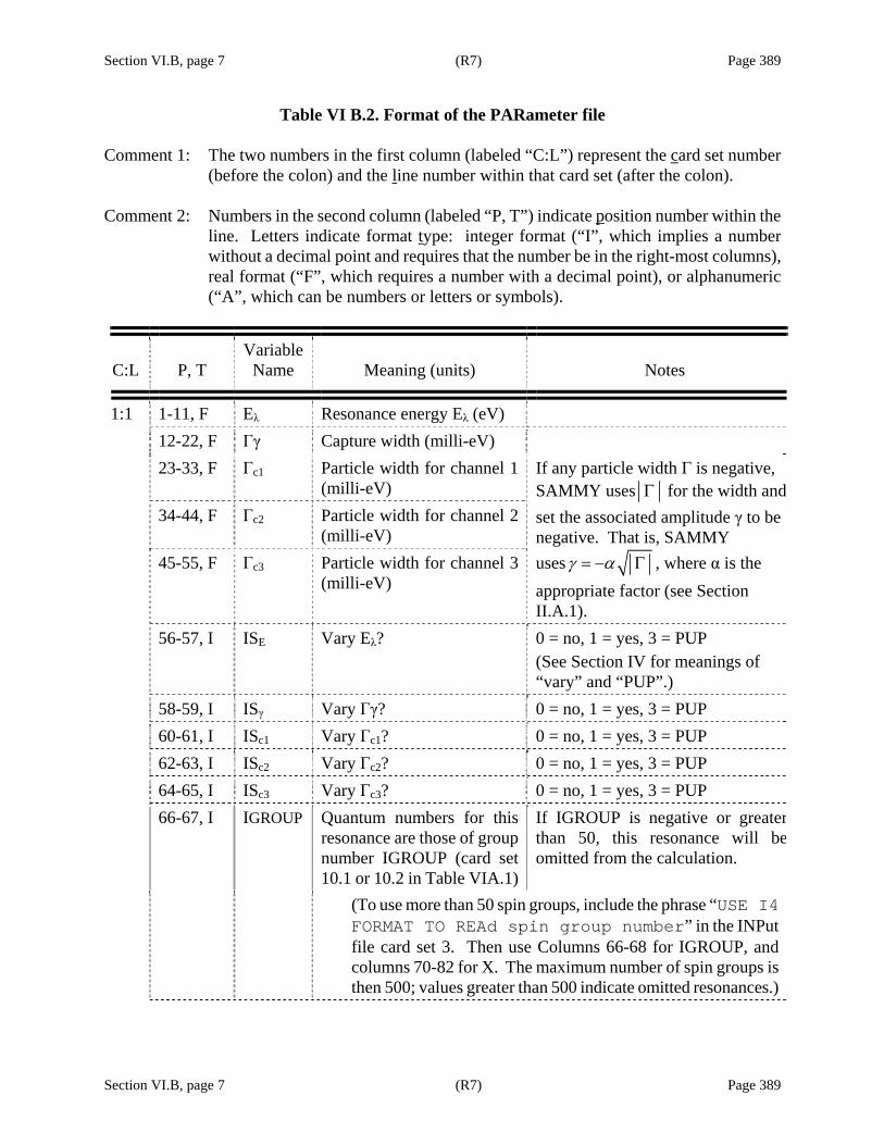
Section VI.B, page 7 (R7) Page 389
Section VI.B, page 7 (R7) Page 389
Table VI B.2. Format of the PARameter file
Comment 1: The two numbers in the first column (labeled “C:L”) represent the card set number (before the colon) and the line number within that card set (after the colon).
Comment 2: Numbers in the second column (labeled “P, T”) indicate position number within the
line. Letters indicate format type: integer format (“I”, which implies a number without a decimal point and requires that the number be in the right-most columns), real format (“F”, which requires a number with a decimal point), or alphanumeric (“A”, which can be numbers or letters or symbols).
C:L P, T Variable
Name Meaning (units) Notes
1:1 1-11, F Eλ Resonance energy Eλ (eV) 12-22, F Γγ Capture width (milli-eV) 23-33, F Γc1 Particle width for channel 1
(milli-eV) 34-44, F Γc2 Particle width for channel 2
(milli-eV) 45-55, F Γc3 Particle width for channel 3
(milli-eV)
If any particle width Γ is negative, SAMMY uses Γ for the width and set the associated amplitude γ to be negative. That is, SAMMY usesγ α= − Γ , where α is the appropriate factor (see Section II.A.1).
56-57, I ISE Vary Eλ? 0 = no, 1 = yes, 3 = PUP (See Section IV for meanings of “vary” and “PUP”.)
58-59, I ISγ Vary Γγ? 0 = no, 1 = yes, 3 = PUP 60-61, I ISc1 Vary Γc1? 0 = no, 1 = yes, 3 = PUP 62-63, I ISc2 Vary Γc2? 0 = no, 1 = yes, 3 = PUP 64-65, I ISc3 Vary Γc3? 0 = no, 1 = yes, 3 = PUP 66-67, I IGROUP Quantum numbers for this
resonance are those of group number IGROUP (card set 10.1 or 10.2 in Table VIA.1)
If IGROUP is negative or greaterthan 50, this resonance will beomitted from the calculation.
(To use more than 50 spin groups, include the phrase “USE I4 FORMAT TO REAd spin group number” in the INPut file card set 3. Then use Columns 66-68 for IGROUP, and columns 70-82 for X. The maximum number of spin groups is then 500; values greater than 500 indicate omitted resonances.)

Section VI.B, page 8 (R7) Page 390
Table VI B.2 (continued)
Section VI.B, page 8 (R7) Page 390
C:L P, T Variable
Name Meaning (units) Notes
1:1 cont.
68-80, F X For many cases, this variable is not used (columns may be left blank). However, there are three possible uses for this variable:
(1) If X < 0, then values of Γ for other particle channels are included on the following line.
(2) If X is positive and the statement “ENERGY UNCERTAINTIES are at end of line” is included in card set 3 of the INPut file (see Table VI A1.2), then X is the prior absolute uncertainty on Eλ (eV).
(3) If X is positive, and the expression “ADD CONSTANT TERM TO data covariance” is included in the INPut file (see Table VI A1.2), then a constant on-and-off diagonal contribution to the data covariance matrix (DCM) is to be used under this resonance. In this case X should be ≤ (Δd)2, where Δd is the absolute uncertainty on data near this resonance. NOTE: This option is seldom used.
1:2 1-11, F Γc4 Particle width for channel 4 (milli-eV)
This line is present only if X < 0 on the preceding line
12-22, F Γc5 Width for ch 5 (milli-eV) 23-33, F Γc6 Width for ch 6 (milli-eV) 34-44, F Γc7 Width for ch 7 (milli-eV) 45-55, F Γc8 Width for ch 8 (milli-eV) 56-57, I ISc4 Vary Γc4? 0 = no, 1 = yes, 3 = PUP 58-59, I ISc5 Vary Γc5? 0 = no, 1 = yes, 3 = PUP 60-61, I ISc6 Vary Γc6? 0 = no, 1 = yes, 3 = PUP 62-63, I ISc7 Vary Γc7? 0 = no, 1 = yes, 3 = PUP 64-65, I ISc8 Vary Γc8? 0 = no, 1 = yes, 3 = PUP 66-67, I IGROUP must be same as previous line 68-80, F X As above, negative to indicate continuation line. Positive for
uncertainty on resonance energy, or for off-diagonal DCM. 1:3,4, etc Repeat line 2 as needed, until all non-zero channel widths have been defined. 1:5 etc, Repeat lines 1 – 4 as many times as needed, until all resonances are specified. 1:Last End with a blank line.

Section VI.B, page 9 (R8) Page 391
Table VI B.2 (continued)
Section VI.B, page 9 (R8) Page 391
C:L P, T Variable
Name Meaning (units) Notes
1a:1 When this format is used for input of resonance parameters, the command “REDUCED WIDTH AMPLITudes are used for input” must be included in the INPut file.
1-11, F Eλ Square root of the resonance energy Eλ ( )eV
When 0Eλ < , the quantity to be
given here is Eλ− − .
12-22, F γγ Reduced-width amplitude for the eliminated capture channel
( )eV
23-33, F 1cγ Reduced-width amplitude for channel 1 ( )eV
34-44, F 2cγ Reduced-width amplitude for channel 2 ( )eV
45-55, F 3cγ Reduced-width amplitude for channel 3 ( )eV
56-57, I ISE Vary Eλ ? 0 = no, 1 = yes, 3 = PUP (See Section IV for meanings of “vary” and “PUP”.)
58-59, I ISγ Vary γγ ? 0 = no, 1 = yes, 3 = PUP
60-61, I ISc1 Vary 1cγ ? 0 = no, 1 = yes, 3 = PUP
62-63, I ISc2 Vary 2cγ ? 0 = no, 1 = yes, 3 = PUP
64-65, I ISc3 Vary 3cγ ? 0 = no, 1 = yes, 3 = PUP
66-67, I IGROUP Quantum numbers for this resonance are those of group number IGROUP (card set 10.1 or 10.2 in Table VIA.1).
If IGROUP is negative or greaterthan 50, this resonance will beomitted from the calculation.
(To use more than 50 spin groups, include the phrase “USE I4 FORMAT TO REAd spin group number” in the INPut file card set 3. Then use Columns 66–68 for IGROUP, and columns 70–82 for X. The maximum number of spin groups is then 500; values greater than 500 indicate omitted resonances.)

Section VI.B, page 10 (R8) Page 392
Table VI B.2 (continued)
Section VI.B, page 10 (R8) Page 392
C:L P, T Variable
Name Meaning (units) Notes
1a:1 cont.
68-80, F X For many cases, this variable is not used (columns may be left blank). However, if X < 0, then values of γ for other particle channels are included on the following line. For other possible meanings for X, see card set 1.
1a:2 1-11, F 4cγ Reduced-width amplitude for channel 4 ( )eV
This line is present only if X < 0 on the preceding line.
12-22, F 5cγ Reduced-width amplitude for channel 5 ( )eV
23-33, F 6cγ Reduced-width amplitude for channel 6 ( )eV
34-44, F 7cγ Reduced-width amplitude for channel 7 ( )eV
45-55, F 8cγ Reduced-width amplitude for channel 8 ( )eV
56-57, I ISc4 Vary 4cγ ? 0 = no, 1 = yes, 3 = PUP
58-59, I ISc5 Vary 5cγ ? 0 = no, 1 = yes, 3 = PUP
60-61, I ISc6 Vary 6cγ ? 0 = no, 1 = yes, 3 = PUP
62-63, I ISc7 Vary 7cγ ? 0 = no, 1 = yes, 3 = PUP
64-65, I ISc8 Vary 8cγ ? 0 = no, 1 = yes, 3 = PUP
66-67, I IGROUP must be same as previous line 68-80, F X As above, negative to indicate continuation line. Positive for
uncertainty on resonance energy, or for off-diagonal DCM. 1a:3,4, etc Repeat line 2 as needed, to include all non-zero reduced-width amplitudes. 1a:5 etc, Repeat lines 1–4 as many times as needed, until all resonances are specified. 1a:Last End with a blank line.

Section VI.B, page 11 (R7) Page 393
Table VI B.2 (continued)
Section VI.B, page 11 (R7) Page 393
C:L P,T Variable
Name Meaning (units) Notes
2:1 1-11, F Fudge Fudge = initial relative uncertainty for varied parameters whose initial uncertainty is not specified elsewhere. Default = 0.1
One exception: The value of FUDGE will not affect the resonance energy Eλ. The default initial uncertainty for Eλ is set at 2 times the sum of all widths (including Doppler and resolution widths).
3:1 1-80, A WHAT “EXTERnal R-function parameters follow”
Alphanumeric indicator of what comes next; only the first five characters are read.
3:2 1-3, I IGROUP Spin group number 4-5, I ICHN Channel number If zero, SAMMY assumes 1. 6-16, F Eαdown Logarithmic singularity
below energy range (eV) 17-27, F Eαup Logarithmic singularity
above energy range (eV) 28-38, F Rcon, α Constant term 39-49, F Rlin, α Linear Term 50-60, F sα Coefficient of logarithmic
term (must be non-negative)
Parameters of the logarithmic parameterization of the external R-matrix for quantum numbers α (i.e., for IGROUP and ICHN), of the form given in Eq. (II B1 d.1).
62, I ISEαdown Vary Eαdown ? 0 = no, 1 = yes, 3 = PUP 64, I ISEαup Vary Eαup ? 0 = no, 1 = yes, 3 = PUP 66, I ISRcon, α Vary Rcon, α ? 0 = no, 1 = yes, 3 = PUP 68, I ISRlin, α Vary Rlin, α ? 0 = no, 1 = yes, 3 = PUP 70, I ISsα Vary sα ? 0 = no, 1 = yes, 3 = PUP
3:3 etc.
Repeat line 2 as many times as desired. Include only those spin groups and channels for which you wish to parameterize the external R-matrix in this manner.
3:Last (blank)

Section VI.B, page 12 (R7) Page 394
Table VI B.2 (continued)
Section VI.B, page 12 (R7) Page 394
C:L P, T Variable
Name Meaning (units) Notes
3a:1 1-80, A WHAT “R-EXTernal parameters follow”. This card set 3a is an alternative, not a supplement, to card set 3. It is not permitted to use both.
3a:2 1-2, I IGROUP Spin group number 3, I ICHN Channel number If zero, SAMMY assumes 1. 4, I ISEαdown Vary Eαdown ? 0 = no, 1 = yes, 3 = PUP 5, I ISEαup Vary Eαup ? 0 = no, 1 = yes, 3 = PUP 6, I ISRcon, α Vary Rcon, α ? 0 = no, 1 = yes, 3 = PUP 7, I ISRlin, α Vary Rlin, α ? 0 = no, 1 = yes, 3 = PUP 8, I ISscon, α Vary scon,α ? 0 = no, 1 = yes, 3 = PUP 9, I ISslin, α Vary slin, α ? 0 = no, 1 = yes, 3 = PUP 10, I ISRq, α Vary Rq, α ? 0 = no, 1 = yes, 3 = PUP 11-20, F Eαdown Logarithmic singularity
below energy range (eV) 21-30, F Eαup Logarithmic singularity
above energy range (eV) 31-40, F Rcon, α Constant term 41-50, F Rlin, α Linear Term (eV-1) 51-60, F scon, α Constant coefficient of
logarithmic term (must be non-negative)
61-70, F slin, α Linear coefficient of logarithmic term
71-80, F Rq,α Quadratic term
Parameters of the logarithmic parameterization of the external R-matrix for quantum numbers α (i.e., for IGROUP and ICHN), of the form given in Eq. (IIB1d.1).
3a:3 etc.
Repeat line 2 as many times as desired. Include only those spin groups and channels for which you wish to parameterize the external R-matrix in this manner.
3a: Last (blank)
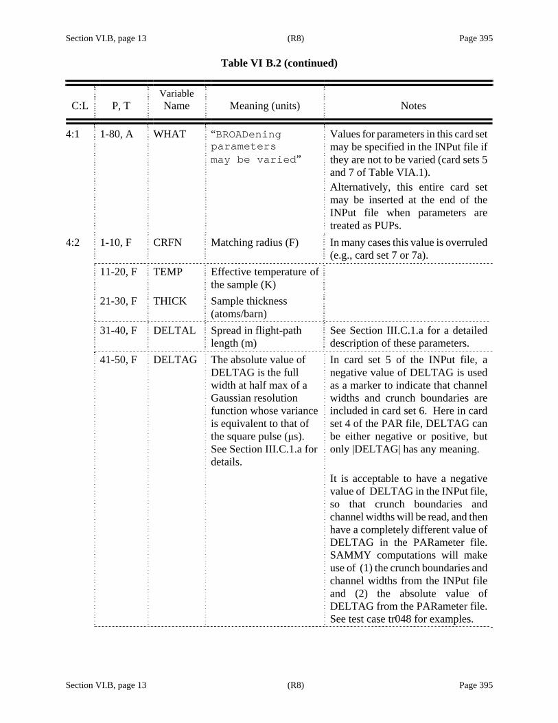
Section VI.B, page 13 (R8) Page 395
Table VI B.2 (continued)
Section VI.B, page 13 (R8) Page 395
C:L P, T Variable Name Meaning (units) Notes
4:1 1-80, A WHAT “BROADening parameters may be varied”
Values for parameters in this card set may be specified in the INPut file if they are not to be varied (card sets 5 and 7 of Table VIA.1). Alternatively, this entire card set may be inserted at the end of the INPut file when parameters are treated as PUPs.
4:2 1-10, F CRFN Matching radius (F) In many cases this value is overruled (e.g., card set 7 or 7a).
11-20, F TEMP Effective temperature of the sample (K)
21-30, F THICK Sample thickness (atoms/barn)
31-40, F DELTAL Spread in flight-path length (m)
See Section III.C.1.a for a detailed description of these parameters.
41-50, F DELTAG The absolute value of DELTAG is the full width at half max of a Gaussian resolution function whose variance is equivalent to that of the square pulse (μs). See Section III.C.1.a for details.
In card set 5 of the INPut file, a negative value of DELTAG is used as a marker to indicate that channel widths and crunch boundaries are included in card set 6. Here in card set 4 of the PAR file, DELTAG can be either negative or positive, but only |DELTAG| has any meaning. It is acceptable to have a negative value of DELTAG in the INPut file, so that crunch boundaries and channel widths will be read, and then have a completely different value of DELTAG in the PARameter file. SAMMY computations will make use of (1) the crunch boundaries and channel widths from the INPut file and (2) the absolute value of DELTAG from the PARameter file. See test case tr048 for examples.
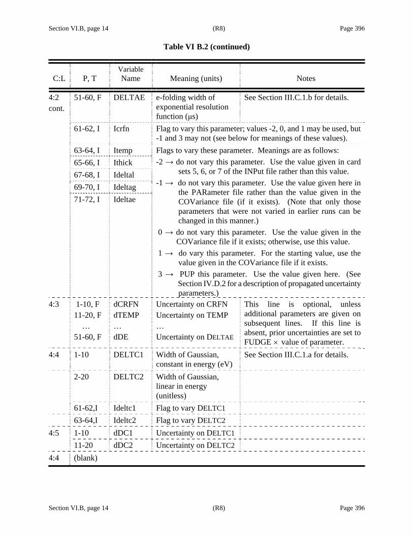
Section VI.B, page 14 (R8) Page 396
Table VI B.2 (continued)
Section VI.B, page 14 (R8) Page 396
C:L P, T Variable Name Meaning (units) Notes
4:2 cont.
51-60, F DELTAE e-folding width of exponential resolution function (μs)
See Section III.C.1.b for details.
61-62, I Icrfn Flag to vary this parameter; values -2, 0, and 1 may be used, but -1 and 3 may not (see below for meanings of these values).
63-64, I Itemp 65-66, I Ithick 67-68, I Ideltal 69-70, I Ideltag 71-72, I Ideltae
Flags to vary these parameter. Meanings are as follows: -2 → do not vary this parameter. Use the value given in card sets 5, 6, or 7 of the INPut file rather than this value. -1 → do not vary this parameter. Use the value given here in the PARameter file rather than the value given in the COVariance file (if it exists). (Note that only those parameters that were not varied in earlier runs can be changed in this manner.) 0 → do not vary this parameter. Use the value given in the COVariance file if it exists; otherwise, use this value. 1 → do vary this parameter. For the starting value, use the value given in the COVariance file if it exists. 3 → PUP this parameter. Use the value given here. (See Section IV.D.2 for a description of propagated uncertainty parameters.)
4:3 1-10, F 11-20, F … 51-60, F
dCRFN dTEMP … dDE
Uncertainty on CRFN Uncertainty on TEMP … Uncertainty on DELTAE
This line is optional, unless additional parameters are given on subsequent lines. If this line is absent, prior uncertainties are set to FUDGE × value of parameter.
4:4 1-10 DELTC1 Width of Gaussian, constant in energy (eV)
See Section III.C.1.a for details.
2-20 DELTC2 Width of Gaussian, linear in energy (unitless)
61-62,I Ideltc1 Flag to vary DELTC1 63-64,I Ideltc2 Flag to vary DELTC2
4:5 1-10 dDC1 Uncertainty on DELTC1 11-20 dDC2 Uncertainty on DELTC2
4:4 (blank)

Section VI.B, page 15 (R7) Page 397
Table VI B.2 (continued)
Section VI.B, page 15 (R7) Page 397
C:L P, T Variable
Name Meaning (units) Notes
5:1 1-80, A WHAT “UNUSEd but correlated variables come next”
Parameter files using this card set arenever generated directly by aSAMMY user; rather, they resultfrom using the code SAMAMR (seeSection X.C).
5:2 1-5, A NUSED1 Name of first unused variable
11-15, A NUSED2 Name of 2nd unused variable . . . 71-75, A NUSED8 Name of 8th unused variable
5:3 1-10, F UNUSED1 Value of first unused variable
11-20, F UNUSED2 Value of 2nd unused variable . . . 71-80, F UNUSED8 Value of 8th unused variable
5:4, 5, etc. Repeat lines 2 and 3 as many times as needed 5:Last (blank)

Section VI.B, page 16 (R7) Page 398
Table VI B.2 (continued)
Section VI.B, page 16 (R7) Page 398
C:L P, T Variable
Name Meaning (units) Notes
6:1 1-80, A WHAT “NORMAlization and background are next”
See Section III.E.3.a. This card set could be put into the INPut file rather than PARameter file if no values are to be varied.
6:2 1-10, F ANORM a = normalization (dimensionless)
Value ~ 1
11-20, F BACKA Ba = constant background (dimensionless if data are transmission, barns if c.s.)
21-30, F BACKB Bb = background proportional to1 E or linear in time ( eV or barns eV× )
31-40, F BACKC Bc = background proportional to E or linear in inverse time (1 eV or barns eV )
41-50, F BACKD Bd = coefficient for exponential background (dimensionless or barns)
51-60, F BACKF Bf = exponential decay constant ( eV )
61-62, I Ianorm 63-64, I Ibacka 65-66, I Ibackb 67-68, I Ibackc 69-70, I Ibackd 71-72, I Ibackf
Flag for these parameters: -1, 0, 1, or 3 -1 → do not vary or PUP this parameter. Use the value given here in the PAR file rather than the value given in the COVariance file if it exists. (Note that only those parameters that were not varied in earlier runs can be changed in this manner).
0 → do not vary or PUP this parameter. Use the value given in the COVariance file if it exists; otherwise, use the value given here.
1 → do vary this parameter. For the starting value, use the value given in the COVariance file if it exists.
3 → PUP this parameter, using this value.

Section VI.B, page 17 (R7) Page 399
Table VI B.2 (continued)
Section VI.B, page 17 (R7) Page 399
C:L P, T Variable
Name Meaning (units) Notes
6:3 1-10, F Danorm uncertainty on ANORM 11-20, F Dbacka uncertainty on BACKA 21-30, F Dbackb uncertainty on BACKB 31-40, F Dbackc uncertainty on BACKC 41-50, F Dbackd uncertainty on BACKD 51-60, F Dbackf uncertainty on BACKF
This line is optional for angle-integrated data but not for angular distributions. When the line is omitted, the uncertainty is assumed to be FUDGE × value of parameter.
6:4, 6:5, etc.
When the data are angular distributions, line 2 contains normalization and backgrounds for the first angle and line 3 the corresponding uncertainties. Line 4 contains values for the second angle, etc.
6:Last (blank)
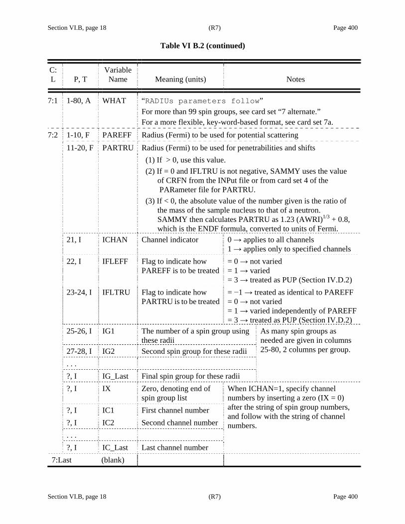
Section VI.B, page 18 (R7) Page 400
Table VI B.2 (continued)
Section VI.B, page 18 (R7) Page 400
C:L P, T
Variable Name Meaning (units) Notes
7:1 1-80, A WHAT “RADIUs parameters follow” For more than 99 spin groups, see card set “7 alternate.” For a more flexible, key-word-based format, see card set 7a.
7:2 1-10, F PAREFF Radius (Fermi) to be used for potential scattering 11-20, F PARTRU Radius (Fermi) to be used for penetrabilities and shifts (1) If > 0, use this value.
(2) If = 0 and IFLTRU is not negative, SAMMY uses the value of CRFN from the INPut file or from card set 4 of the PARameter file for PARTRU. (3) If < 0, the absolute value of the number given is the ratio of the mass of the sample nucleus to that of a neutron. SAMMY then calculates PARTRU as 1.23 (AWRI)1/3 + 0.8, which is the ENDF formula, converted to units of Fermi.
21, I
ICHAN Channel indicator 0 → applies to all channels 1 → applies only to specified channels
22, I
IFLEFF Flag to indicate how PAREFF is to be treated
= 0 → not varied = 1 → varied = 3 → treated as PUP (Section IV.D.2)
23-24, I
IFLTRU Flag to indicate how PARTRU is to be treated
= −1 → treated as identical to PAREFF = 0 → not varied = 1 → varied independently of PAREFF = 3 → treated as PUP (Section IV.D.2)
25-26, I IG1 The number of a spin group using these radii
27-28, I IG2 Second spin group for these radii . . . ?, I IG_Last Final spin group for these radii
As many spin groups as needed are given in columns 25-80, 2 columns per group.
?, I IX Zero, denoting end of spin group list
?, I IC1 First channel number ?, I IC2 Second channel number . . . ?, I IC_Last Last channel number
When ICHAN=1, specify channel numbers by inserting a zero (IX = 0) after the string of spin group numbers, and follow with the string of channel numbers.
7:Last (blank)
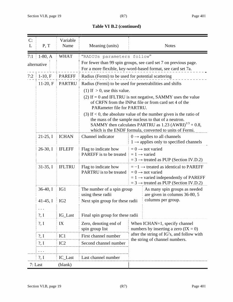
Section VI.B, page 19 (R7) Page 401
Table VI B.2 (continued)
Section VI.B, page 19 (R7) Page 401
C:L P, T
Variable Name Meaning (units) Notes
7:1 1-80, A
alternative
WHAT “RADIUs parameters follow” For fewer than 99 spin groups, see card set 7 on previous page. For a more flexible, key-word-based format, see card set 7a.
7:2 1-10, F PAREFF Radius (Fermi) to be used for potential scattering 11-20, F PARTRU Radius (Fermi) to be used for penetrabilities and shifts (1) If > 0, use this value.
(2) If = 0 and IFLTRU is not negative, SAMMY uses the value of CRFN from the INPut file or from card set 4 of the PARameter file for PARTRU. (3) If < 0, the absolute value of the number given is the ratio of the mass of the sample nucleus to that of a neutron. SAMMY then calculates PARTRU as 1.23 (AWRI)1/3 + 0.8, which is the ENDF formula, converted to units of Fermi.
21-25, I
ICHAN Channel indicator 0 → applies to all channels 1 → applies only to specified channels
26-30, I IFLEFF Flag to indicate how PAREFF is to be treated
= 0 → not varied = 1 → varied = 3 → treated as PUP (Section IV.D.2)
31-35, I IFLTRU Flag to indicate how PARTRU is to be treated
= −1 → treated as identical to PAREFF = 0 → not varied = 1 → varied independently of PAREFF = 3 → treated as PUP (Section IV.D.2)
36-40, I IG1 The number of a spin group using these radii
41-45, I IG2 Next spin group for these radii . . . ?, I IG_Last Final spin group for these radii
As many spin groups as needed are given in columns 36-80, 5 columns per group.
?, I IX Zero, denoting end of spin group list
?, I IC1 First channel number ?, I IC2 Second channel number . . . ?, I IC_Last Last channel number
When ICHAN=1, specify channel numbers by inserting a zero (IX = 0) after the string of IG=s, and follow with the string of channel numbers.
7: Last (blank)

Section VI.B, page 20 (R7) Page 402
Table VI B.2 (continued)
Section VI.B, page 20 (R7) Page 402
C:L P, T Variable Name Meaning (units) Notes
7a:1 1-80, A WHAT “RADII are in KEY-WORD format”, or “CHANNel radius parameters follow”
If using the first option, the phrase “key-word” must occur somewhere on the line.
See Table VI B.1 for an itemized list of the valid key words used in this card set. Many test cases contain examples of this card set: tr041,tr043,tr119, tr151. Below is one example from test case tr059, file t059cz.par : Channel RADIUS PARAMETERS FOLLOW Radius= 3.200 3.200 Flags=1 3 PP=n+16O L=all Radius= 3.200 3.200 Flags=3 -1 PP=alf+13C L=all Radius= 3.200 3.200 Flags=3 1 PP=n+16O 1 L=all Radius= 3.200 3.200 Flags=3 3 PP=n+16O 2 L=all
7a:2 Channel radii parameters are given in key word format, with the key word followed by an equal sign followed by the value. Radii values must be specified first, prior to the information regarding which channels are associated with these radii. Valid key words for radii: RADIus, RADIi, EFfective radius, TRue radius. Only those letters in caps must be included; they may be either caps or lowercase in the file. If key word RADIus is used, it can be followed by one or two values (separated by space or comma); the first is the effective radius, and the second is the true radius. In any case, if only one radius value is specified, the other is assumed to be equal to that same value. No other key words may be included on this line.
7a:3 Uncertainties may be given for the radii. Use the key word RElative to specify relative uncertainties, and ABsolute or UNcertainty to provide absolute uncertainties. Give two values after the equal sign, the first for the effective radius and the second for the true radius. It is permitted to give only one value, in which case that value is used for both radii. However, if only one value is given, it must be the last item on this line.
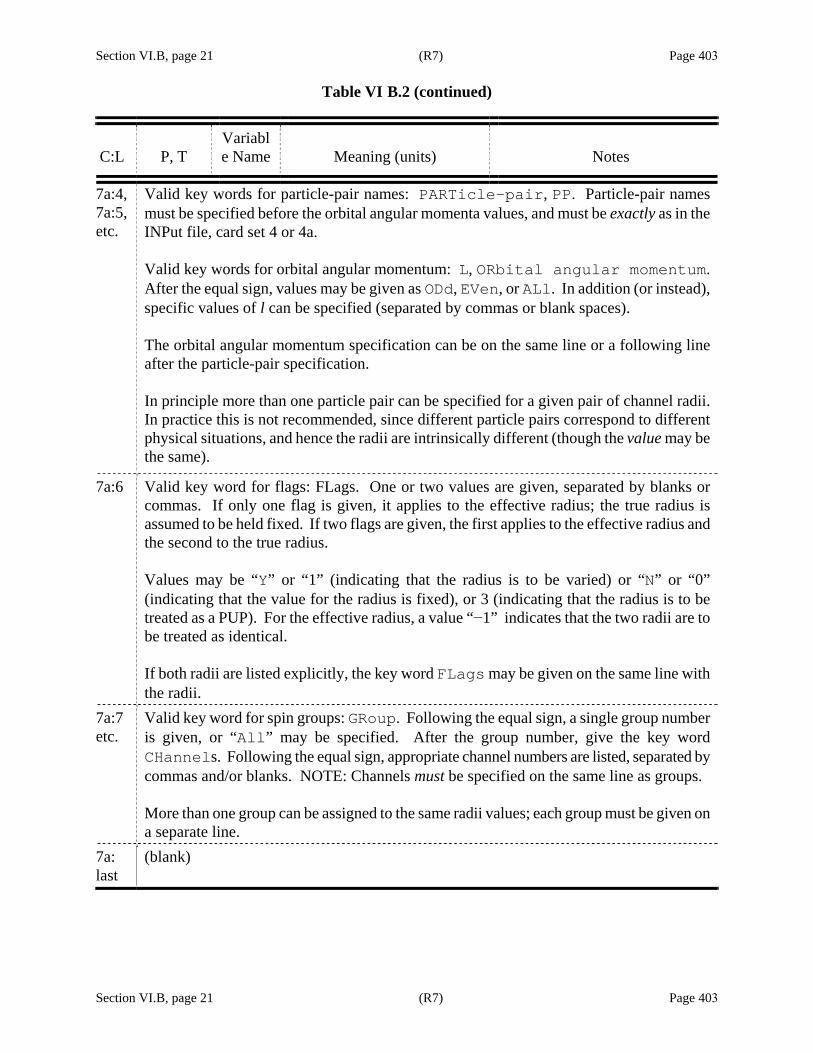
Section VI.B, page 21 (R7) Page 403
Table VI B.2 (continued)
Section VI.B, page 21 (R7) Page 403
C:L P, T Variable Name Meaning (units) Notes
7a:4, 7a:5, etc.
Valid key words for particle-pair names: PARTicle-pair, PP. Particle-pair names must be specified before the orbital angular momenta values, and must be exactly as in the INPut file, card set 4 or 4a. Valid key words for orbital angular momentum: L, ORbital angular momentum. After the equal sign, values may be given as ODd, EVen, or ALl. In addition (or instead), specific values of l can be specified (separated by commas or blank spaces). The orbital angular momentum specification can be on the same line or a following line after the particle-pair specification. In principle more than one particle pair can be specified for a given pair of channel radii. In practice this is not recommended, since different particle pairs correspond to different physical situations, and hence the radii are intrinsically different (though the value may be the same).
7a:6 Valid key word for flags: FLags. One or two values are given, separated by blanks or commas. If only one flag is given, it applies to the effective radius; the true radius is assumed to be held fixed. If two flags are given, the first applies to the effective radius and the second to the true radius. Values may be “Y” or “1” (indicating that the radius is to be varied) or “N” or “0” (indicating that the value for the radius is fixed), or 3 (indicating that the radius is to be treated as a PUP). For the effective radius, a value “−1” indicates that the two radii are to be treated as identical. If both radii are listed explicitly, the key word FLags may be given on the same line with the radii.
7a:7 etc.
Valid key word for spin groups: GRoup. Following the equal sign, a single group number is given, or “All” may be specified. After the group number, give the key word CHannels. Following the equal sign, appropriate channel numbers are listed, separated by commas and/or blanks. NOTE: Channels must be specified on the same line as groups. More than one group can be assigned to the same radii values; each group must be given on a separate line.
7a: last
(blank)
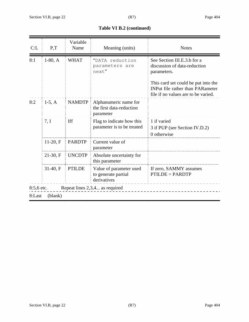
Section VI.B, page 22 (R7) Page 404
Table VI B.2 (continued)
Section VI.B, page 22 (R7) Page 404
C:L P,T Variable
Name Meaning (units) Notes
8:1 1-80, A WHAT “DATA reduction parameters are next”
See Section III.E.3.b for a discussion of data-reduction parameters. This card set could be put into the INPut file rather than PARameter file if no values are to be varied.
8:2 1-5, A NAMDTP Alphanumeric name for the first data-reduction parameter
7, I Iff Flag to indicate how this parameter is to be treated
1 if varied 3 if PUP (see Section IV.D.2) 0 otherwise
11-20, F PARDTP Current value of parameter
21-30, F UNCDTP Absolute uncertainty for this parameter
31-40, F PTILDE Value of parameter used to generate partial derivatives
If zero, SAMMY assumes PTILDE = PARDTP
8:5,6 etc. Repeat lines 2,3,4... as required 8:Last (blank)
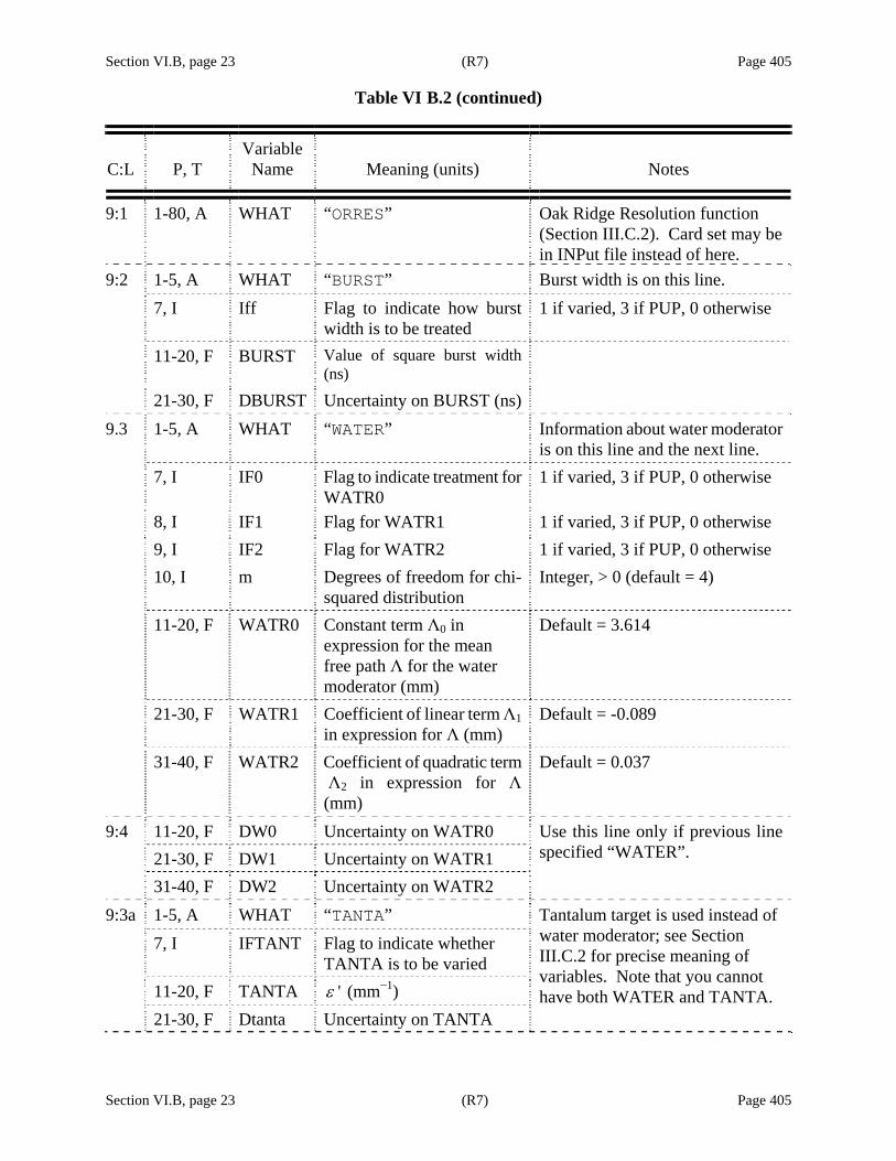
Section VI.B, page 23 (R7) Page 405
Table VI B.2 (continued)
Section VI.B, page 23 (R7) Page 405
C:L P, T Variable
Name Meaning (units) Notes
9:1 1-80, A WHAT “ORRES” Oak Ridge Resolution function (Section III.C.2). Card set may be in INPut file instead of here.
9:2 1-5, A WHAT “BURST” Burst width is on this line. 7, I Iff Flag to indicate how burst
width is to be treated 1 if varied, 3 if PUP, 0 otherwise
11-20, F BURST Value of square burst width (ns)
21-30, F DBURST Uncertainty on BURST (ns) 9.3 1-5, A WHAT “WATER” Information about water moderator
is on this line and the next line. 7, I IF0 Flag to indicate treatment for
WATR0 1 if varied, 3 if PUP, 0 otherwise
8, I IF1 Flag for WATR1 1 if varied, 3 if PUP, 0 otherwise 9, I IF2 Flag for WATR2 1 if varied, 3 if PUP, 0 otherwise 10, I m Degrees of freedom for chi-
squared distribution Integer, > 0 (default = 4)
11-20, F WATR0 Constant term Λ0 in expression for the mean free path Λ for the water moderator (mm)
Default = 3.614
21-30, F WATR1 Coefficient of linear term Λ1 in expression for Λ (mm)
Default = -0.089
31-40, F WATR2 Coefficient of quadratic term Λ2 in expression for Λ (mm)
Default = 0.037
9:4 11-20, F DW0 Uncertainty on WATR0 21-30, F DW1 Uncertainty on WATR1 31-40, F DW2 Uncertainty on WATR2
Use this line only if previous line specified “WATER”.
9:3a 1-5, A WHAT “TANTA” 7, I IFTANT Flag to indicate whether
TANTA is to be varied 11-20, F TANTA 'ε (mm−1) 21-30, F Dtanta Uncertainty on TANTA
Tantalum target is used instead of water moderator; see Section III.C.2 for precise meaning of variables. Note that you cannot have both WATER and TANTA.
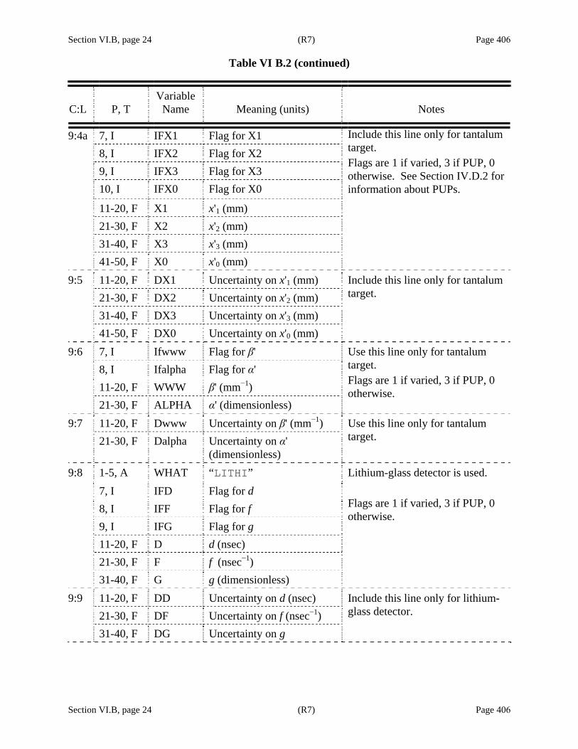
Section VI.B, page 24 (R7) Page 406
Table VI B.2 (continued)
Section VI.B, page 24 (R7) Page 406
C:L P, T Variable
Name Meaning (units) Notes
9:4a 7, I IFX1 Flag for X1 8, I IFX2 Flag for X2 9, I IFX3 Flag for X3 10, I IFX0 Flag for X0
Include this line only for tantalum target. Flags are 1 if varied, 3 if PUP, 0 otherwise. See Section IV.D.2 for information about PUPs.
11-20, F X1 x'1 (mm) 21-30, F X2 x'2 (mm) 31-40, F X3 x'3 (mm) 41-50, F X0 x'0 (mm)
9:5 11-20, F DX1 Uncertainty on x'1 (mm) 21-30, F DX2 Uncertainty on x'2 (mm)
Include this line only for tantalum target.
31-40, F DX3 Uncertainty on x'3 (mm) 41-50, F DX0 Uncertainty on x'0 (mm)
9:6 7, I Ifwww Flag for β' 8, I Ifalpha Flag for α' 11-20, F WWW β' (mm−1) 21-30, F ALPHA α' (dimensionless)
Use this line only for tantalum target. Flags are 1 if varied, 3 if PUP, 0 otherwise.
9:7 11-20, F Dwww Uncertainty on β' (mm−1) 21-30, F Dalpha Uncertainty on α'
(dimensionless)
Use this line only for tantalum target.
9:8 1-5, A WHAT “LITHI” 7, I IFD Flag for d 8, I IFF Flag for f 9, I IFG Flag for g 11-20, F D d (nsec) 21-30, F F f (nsec−1) 31-40, F G g (dimensionless)
Lithium-glass detector is used. Flags are 1 if varied, 3 if PUP, 0 otherwise.
9:9 11-20, F DD Uncertainty on d (nsec) 21-30, F DF Uncertainty on f (nsec−1)
Include this line only for lithium-glass detector.
31-40, F DG Uncertainty on g
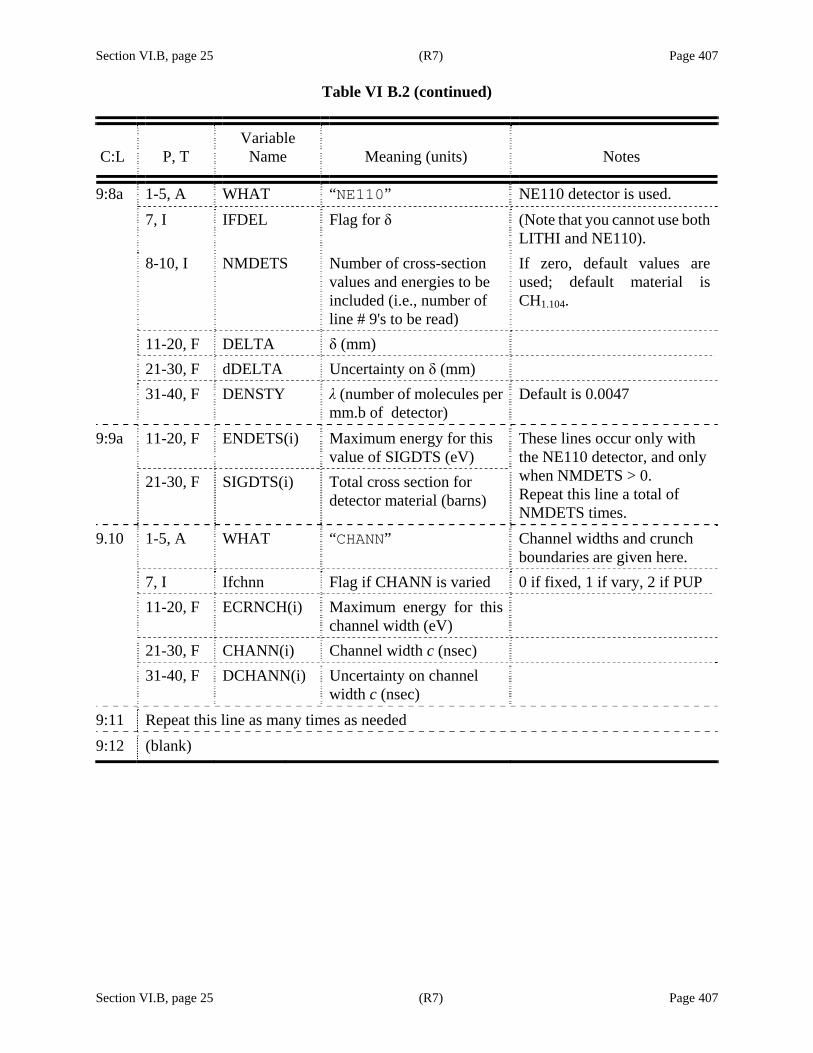
Section VI.B, page 25 (R7) Page 407
Table VI B.2 (continued)
Section VI.B, page 25 (R7) Page 407
C:L P, T Variable
Name Meaning (units) Notes
9:8a 1-5, A WHAT “NE110” NE110 detector is used. 7, I IFDEL Flag for δ (Note that you cannot use both
LITHI and NE110). 8-10, I NMDETS Number of cross-section
values and energies to be included (i.e., number of line # 9's to be read)
If zero, default values are used; default material is CH1.104.
11-20, F DELTA δ (mm) 21-30, F dDELTA Uncertainty on δ (mm) 31-40, F DENSTY λ (number of molecules per
mm.b of detector) Default is 0.0047
9:9a 11-20, F ENDETS(i) Maximum energy for this value of SIGDTS (eV)
21-30, F SIGDTS(i) Total cross section for detector material (barns)
These lines occur only with the NE110 detector, and only when NMDETS > 0. Repeat this line a total of NMDETS times.
9.10 1-5, A WHAT “CHANN” Channel widths and crunch boundaries are given here.
7, I Ifchnn Flag if CHANN is varied 0 if fixed, 1 if vary, 2 if PUP 11-20, F ECRNCH(i) Maximum energy for this
channel width (eV)
21-30, F CHANN(i) Channel width c (nsec) 31-40, F DCHANN(i) Uncertainty on channel
width c (nsec)
9:11 Repeat this line as many times as needed 9:12 (blank)

Section VI.B, page 26 (R7) Page 408
Table VI B.2 (continued)
Section VI.B, page 26 (R7) Page 408
C:L P, T Variable
Name Meaning (units) Notes
10:1 1-80, A WHAT “ISOTOpic abundances and masses”, or “NUCLIde abundances and masses”
Each nuclide in the sample should have an entry here.
10:2 1-10, F AMUISO (1) Atomic mass (amu) 11-20, F PARISO (1) Fractional abundance
for this nuclide (dimensionless)
21-30, F DELISO (1) Uncertainty on abundance (dimensionless)
31-32, I (or 31-35, I if > 99 groups)
IFLISO (1) Flag whether treatment for the abundance
−2 → use value of isotopic abundance given in INPut file 1 → vary 0 → do not vary 3 → treat as PUP (Section IV.D.2)
33-34, I or 36-40, I
IGRISO (1,1) Number of the first spin group belonging to this nuclide
35-36, I or 41-50, I
IGRISO (2,1) Number of second spin group
etc.
If more than 24 spin groups are needed, insert “-1” in Columns 79-80, and continue on the next line. When there are more than 99 spin groups altogether, each integer entry on this line requires five columns.
10:3 1-5, I IGRISO (24,1) or (9,1)
Number of the next spin group belonging to this nuclide
This line is needed only if the final entry on the previous line was −1.
6-10, I etc. As many as needed 10:4 Repeat previous line as many times as needed. 10:5 etc. Repeat Lines 2 – 4 as many times as needed. 10:6 (blank)

Section VI.B, page 27 (R8) Page 409
Table VI B.2 (continued)
Section VI.B, page 27 (R8) Page 409
C:L P,T Variable
Name Meaning (units) Notes
11:1 1-80, A WHAT “MISCEllaneous parameters follow”
Any line in this card set may be omitted when not needed. This card set may be in INPut file.
11:2 1-5, A WHAT “DELTA” 7, I IFLAG1 Flag to indicate treatment
for parameter 1LΔ
9, I IFLAG0 Flag to indicate treatment for parameter 0LΔ
11-20, F DELL11 1LΔ = Coeff. of E (m/eV)
1 0L E L LΔ = Δ + Δ is used instead of DELTAL from card set 4 of this file, or instead of DELTAL from card set 5 of the INPut file. Flags = 1 to vary, 3 to PUP, and 0 to hold fixed.
21-30, F D1 Uncertainty on 1LΔ (m/eV)
31-40, F DELL00 0LΔ = Constant term (m)
41-50, F D0 Uncertainty on 0LΔ (m)
11:3 1-5, A WHAT “ETA ” (“eta” plus two blank spaces)
Use if type of data (see card set 8 of INput file) is ETA.
7, I IFLAGN Flag to indicate treatment for parameter ν
11-20, F NU Normalization coefficient NU = ν (dimensionless) as in ETA = NU H (fission /absorption)
21-30, F DNU Uncertainty on NU 31-40, F ENU Energy for which this value
of NU applies (eV) If a constant value of NU is wanted, the energy value can be omitted. If more than one ETA line is present, all must be together in the file and in increasing energy order. SAMMY will linearly interpolate to obtain the value of NU between the specified energies.
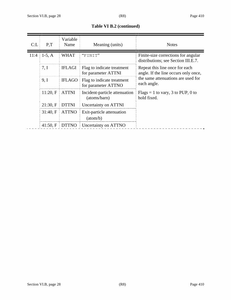
Section VI.B, page 28 (R8) Page 410
Table VI B.2 (continued)
Section VI.B, page 28 (R8) Page 410
C:L P,T Variable
Name Meaning (units) Notes
11:4 1-5, A WHAT “FINIT” Finite-size corrections for angular distributions; see Section III.E.7.
7, I IFLAGI Flag to indicate treatment for parameter ATTNI
9, I IFLAGO Flag to indicate treatment for parameter ATTNO
Repeat this line once for each angle. If the line occurs only once, the same attenuations are used for each angle.
11:20, F ATTNI Incident-particle attenuation (atoms/barn)
Flags = 1 to vary, 3 to PUP, 0 to hold fixed.
21:30, F DTTNI Uncertainty on ATTNI 31:40, F ATTNO Exit-particle attenuation
(atom/b)
41:50, F DTTNO Uncertainty on ATTNO
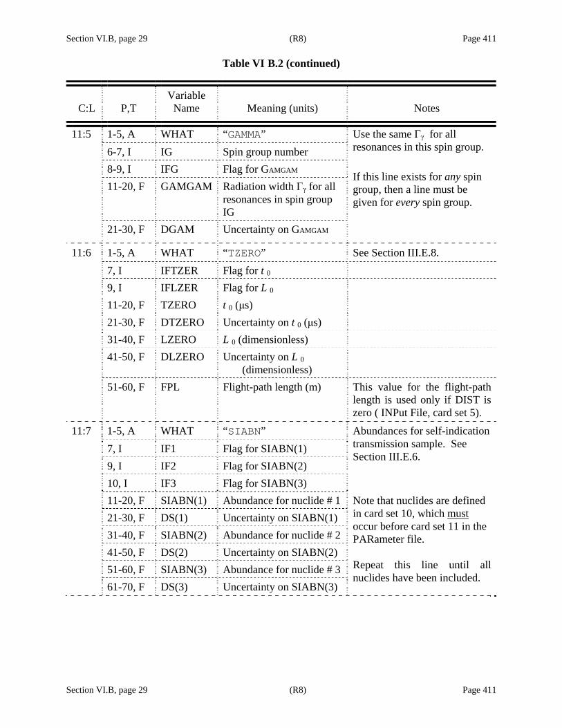
Section VI.B, page 29 (R8) Page 411
Table VI B.2 (continued)
Section VI.B, page 29 (R8) Page 411
C:L P,T Variable
Name Meaning (units) Notes
11:5 1-5, A WHAT “GAMMA” 6-7, I IG Spin group number 8-9, I IFG Flag for GAMGAM 11-20, F GAMGAM Radiation width Γγ for all
resonances in spin group IG
21-30, F DGAM Uncertainty on GAMGAM
Use the same Γγ for all resonances in this spin group. If this line exists for any spin group, then a line must be given for every spin group.
11:6 1-5, A WHAT “TZERO” See Section III.E.8. 7, I IFTZER Flag for t 0 9, I IFLZER Flag for L 0 11-20, F TZERO t 0 (μs) 21-30, F DTZERO Uncertainty on t 0 (μs) 31-40, F LZERO L 0 (dimensionless) 41-50, F DLZERO Uncertainty on L 0
(dimensionless)
51-60, F FPL Flight-path length (m) This value for the flight-path length is used only if DIST is zero ( INPut File, card set 5).
11:7 1-5, A WHAT “SIABN” 7, I IF1 Flag for SIABN(1) 9, I IF2 Flag for SIABN(2)
Abundances for self-indication transmission sample. See Section III.E.6.
10, I IF3 Flag for SIABN(3) 11-20, F SIABN(1) Abundance for nuclide # 1 21-30, F DS(1) Uncertainty on SIABN(1) 31-40, F SIABN(2) Abundance for nuclide # 2 41-50, F DS(2) Uncertainty on SIABN(2) 51-60, F SIABN(3) Abundance for nuclide # 3 61-70, F DS(3) Uncertainty on SIABN(3)
Note that nuclides are defined in card set 10, which must occur before card set 11 in the PARameter file. Repeat this line until all nuclides have been included.
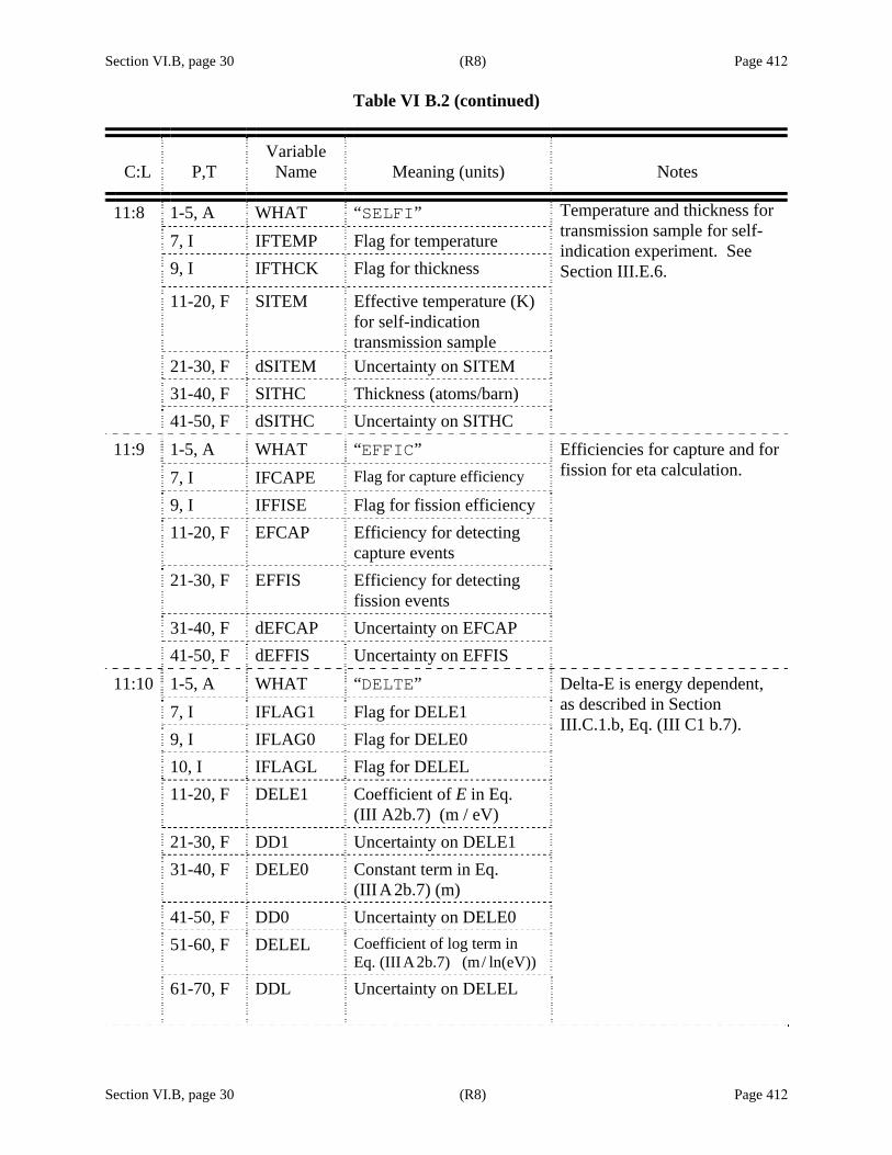
Section VI.B, page 30 (R8) Page 412
Table VI B.2 (continued)
Section VI.B, page 30 (R8) Page 412
C:L P,T Variable
Name Meaning (units) Notes
11:8 1-5, A WHAT “SELFI” 7, I IFTEMP Flag for temperature 9, I IFTHCK Flag for thickness
Temperature and thickness for transmission sample for self-indication experiment. See Section III.E.6.
11-20, F SITEM Effective temperature (K) for self-indication transmission sample
21-30, F dSITEM Uncertainty on SITEM 31-40, F SITHC Thickness (atoms/barn) 41-50, F dSITHC Uncertainty on SITHC 11:9 1-5, A WHAT “EFFIC” 7, I IFCAPE Flag for capture efficiency
9, I IFFISE Flag for fission efficiency
Efficiencies for capture and for fission for eta calculation.
11-20, F EFCAP Efficiency for detecting capture events
21-30, F EFFIS Efficiency for detecting fission events
31-40, F dEFCAP Uncertainty on EFCAP 41-50, F dEFFIS Uncertainty on EFFIS
1-5, A WHAT “DELTE” 11:10 7, I IFLAG1 Flag for DELE1
9, I IFLAG0 Flag for DELE0 10, I IFLAGL Flag for DELEL
Delta-E is energy dependent, as described in Section III.C.1.b, Eq. (III C1 b.7).
11-20, F DELE1 Coefficient of E in Eq. (III A2b.7) (m / eV)
21-30, F DD1 Uncertainty on DELE1 31-40, F DELE0 Constant term in Eq.
(III A2b.7) (m)
41-50, F DD0 Uncertainty on DELE0 51-60, F DELEL Coefficient of log term in
Eq. (III A2b.7) (m / ln(eV))
61-70, F DDL Uncertainty on DELEL

Section VI.B, page 31 (R8) Page 413
Table VI B.2 (continued)
Section VI.B, page 31 (R8) Page 413
C:L P,T Variable
Name Meaning (units) Notes
11:11 1-5, A WHAT “DRCAP” 7, I IFLAG1 Flag to vary COEF(Nuc) 9, I NUC Nuclide Number 11-20, F COEF Coefficient of the value
given in the DRC file 21-30, F dCOEF Uncertainty on COEF 21-30, F DSENSN Uncertainty on A
Numerical direct capture component for nuclide number NUC is read from DRC file; COEF (NUC) multiplies that value. Note that this line may be included as many times as needed, to a maximum of once per nuclide. See Section II.B.4 for details.
11:13 1-5,A WHAT “NONUN” or “NON U” 21-30, F 1 0R = Radius at which thickness
is to be given 31-40, F 1Z Positive value for the
sample thickness at this radius
41-50, F 1dZ Uncertainty on thickness
Non-uniform sample; thickness is a function of radius (see Section III.E.1.a for transmission). At least two lines must be given, all together in one location in the card set; the first line must have zero radius (the center of the sample), and the last must be at the outer edge of the sample. No fitting is yet permitted with these parameters. See test case tr176 for examples.
11:Last (blank)
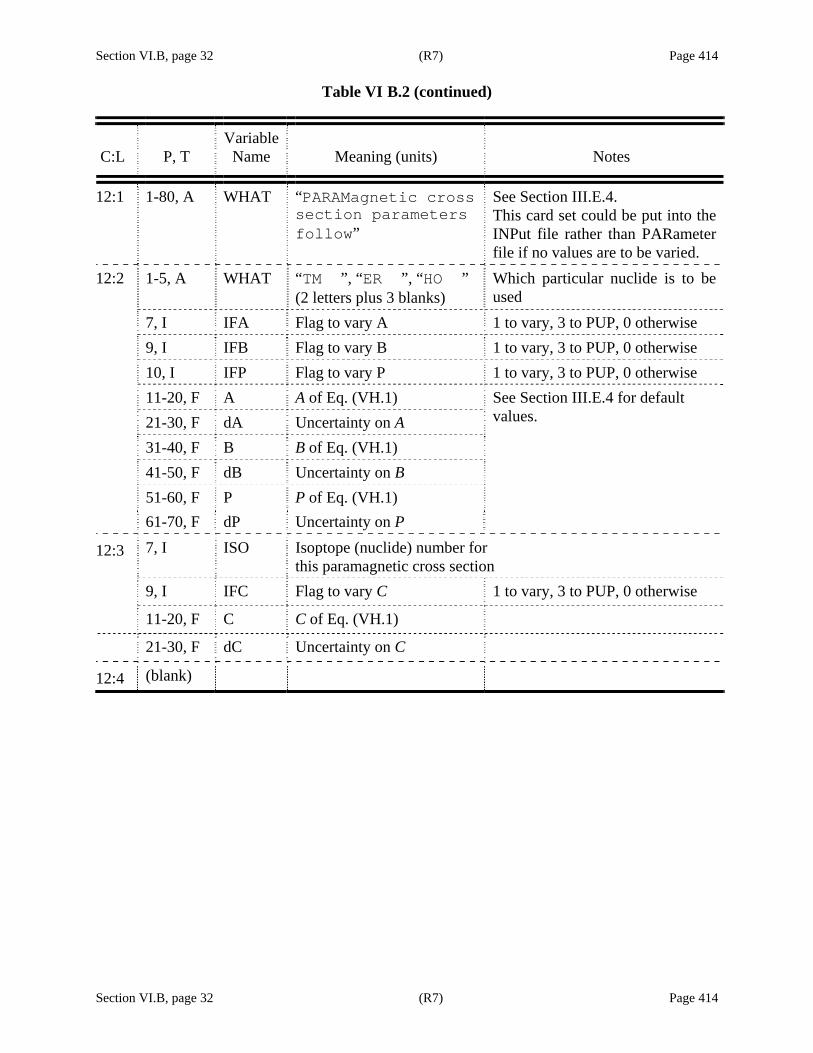
Section VI.B, page 32 (R7) Page 414
Table VI B.2 (continued)
Section VI.B, page 32 (R7) Page 414
C:L P, T Variable
Name Meaning (units) Notes
12:1 1-80, A WHAT “PARAMagnetic cross section parameters follow”
See Section III.E.4. This card set could be put into the INPut file rather than PARameter file if no values are to be varied.
12:2 1-5, A WHAT “TM ”, “ER ”, “HO ” (2 letters plus 3 blanks)
Which particular nuclide is to be used
7, I IFA Flag to vary A 1 to vary, 3 to PUP, 0 otherwise 9, I IFB Flag to vary B 1 to vary, 3 to PUP, 0 otherwise 10, I IFP Flag to vary P 1 to vary, 3 to PUP, 0 otherwise 11-20, F A A of Eq. (VH.1) 21-30, F dA Uncertainty on A 31-40, F B B of Eq. (VH.1) 41-50, F dB Uncertainty on B 51-60, F P P of Eq. (VH.1) 61-70, F dP Uncertainty on P
See Section III.E.4 for default values.
12:3 7, I ISO Isoptope (nuclide) number for this paramagnetic cross section
9, I IFC Flag to vary C 1 to vary, 3 to PUP, 0 otherwise
11-20, F C C of Eq. (VH.1)
21-30, F dC Uncertainty on C
12:4 (blank)

Section VI.B, page 33 (R8) Page 415
Table VI B.2 (continued)
Section VI.B, page 33 (R8) Page 415
C:L P, T Variable
Name Meaning (units) Notes
13:1 1-80, A WHAT “BACKGround functions”
See Section III.E.3.a. This card set could be put into the INPut file rather than PARameter file if no values are to be varied.
13:2 1-5, A WHAT “CONST” Type 1 in Eq. (III E3 a.3)
Line is present only if needed and may be repeated as needed.
7, I IFA Flag to vary or PUP A 1 to vary, 3 to PUP, 0 otherwise 11-20, F A Constant background (same
units as data)
21-30, F dA Uncertainty on background 31-40, F Emin Minimum energy for which
this background applies (eV)41-50, F Emax Maximum energy (eV)
Default energies are entire range of analysis.
51-60, F FPL Flight-path length (m) This value of the flight-path length is used only if DIST was not given in card set 5 of INPut file or elsewhere.
13:3 1-5, A WHAT “EXPON” 7, I IFA Flag to vary or PUP A 9, I IFB Flag to vary or PUP B
This line is present only if needed, and may be repeated as needed. Type 2 in Eq. (III E3 a.3)
11-20, F A Coefficient of exponential (units same as data)
21-30, F dA A priori uncertainty on A 31-40, F B Coefficient of time in exp (ns)
41-50, F dB A priori uncertainty on B
See Section III.E.3.a for an explanation of this background function.
51-60, F Emin Minimum energy for which this background applies (eV)
61-70, F Emax Maximum energy (eV)
Default energies are entire range of analysis.
71-80, F FPL Flight-path length (m) This value of the flight-path length is used only if DIST was not given in card set 5 of the INPut file (or elsewhere).

Section VI.B, page 34 (R8) Page 416
Table VI B.2 (continued)
Section VI.B, page 34 (R8) Page 416
C:L P, T Variable
Name Meaning (units) Notes
13:4 1-5, A WHAT “POWER” 7, I IFA Flag to vary or PUP A 9, I IFB Flag to vary or PUP B
This line is present only if needed and may be repeated as needed.
Type 3 in Eq. (III E3 a.3)
11-20, F A Coeff. of power of time (units are [data]H[ns-B] )
21-30, F dA A priori uncertainty on A 31-40, F B Power (dimensionless) 41-50, F dB A priori uncertainty on B
See Section III.E.3.a for an explanation of this background function.
51-60, F Emin Minimum energy for which this background applies (eV)
61-70, F Emax Maximum energy (eV)
Default energies are entire range of analysis.
71-80, F FPL Flight-path length (m) This value of L is used only if flight-path length was not given earlier.
13:5 1-5, A WHAT “EXPLN” 7, I IFA Flag to vary or PUP A 9, I IFB Flag to vary or PUP B 10, I IFC Flag to vary or PUP C
This line is present only if needed and is always followed by line # 6. The pair of lines may be repeated as needed. Type 4 in Eq. (III E3 a.3).
11-20, F A Constant term in exponential (dimensionless)
21-30, F dA A priori uncertainty on A
See Section III.E.3.a for an explanation of this background function.
31-40, F B Coef. of t in exponential (ns−1) 41-50, F dB A priori uncertainty on B 51-60, F C Coefficient of [ln(t)] −1 in
exponential (ln(nsec))
61-70, F dC A priori uncertainty on C 13:6 11-20, F Emin Minimum energy for which
this background applies (eV)21-30, F Emax Maximum energy (eV)
Line 6 must follow each and every occurrence of line 5.
31-40, F FPL Flight-path length (m) This value of L is used only if flight-path length was not given earlier.

Section VI.B, page 35 (R8) Page 417
Table VI B.2 (continued)
Section VI.B, page 35 (R8) Page 417
C:L P, T Variable
Name Meaning (units) Notes
13:7 1-5, A WHAT “T-PNT” Type 5 in Eq. (III E3 a.5)
Point-wise linear function of time. If this line is present, it must occur at least twice. All occurrences must be contiguous in the file, and the times “T” must be increasing monotonically.
7, I IFA Flag to vary or PUP A 1 to vary, 3 to PUP, 0 otherwise 11-20, F A Value of this background at
time T (same units as data) 21-30, F dA Uncertainty on A
Section III.E.3.a provides an explanation of this background function.
31-40, F T Flight time for which this value of A applies (ns)
41-50, F FPL Flight-path length (m) This value of the flight-path length is used only if DIST was not given in card set 5 of INPut file or elsewhere.
13:8 1-5, A, F WHAT “E-PNT” Type 6 in Eq. (III E3 a.6)
Point-wise linear function of energy. If this line is present, it must occur at least twice. All occurrences must be contiguous in the file, and the energies “E” must be increasing monotonically.
7, I IFA Flag to vary or PUP A 1 to vary, 3 to PUP, 0 otherwise 11-20, F A Value of this background at
energy E (same units as data)21-30, F dA Uncertainty on A
Section III.E.3.a provides an explanation of this background function.
31-40, F E Energy for which this value of A applies (eV)
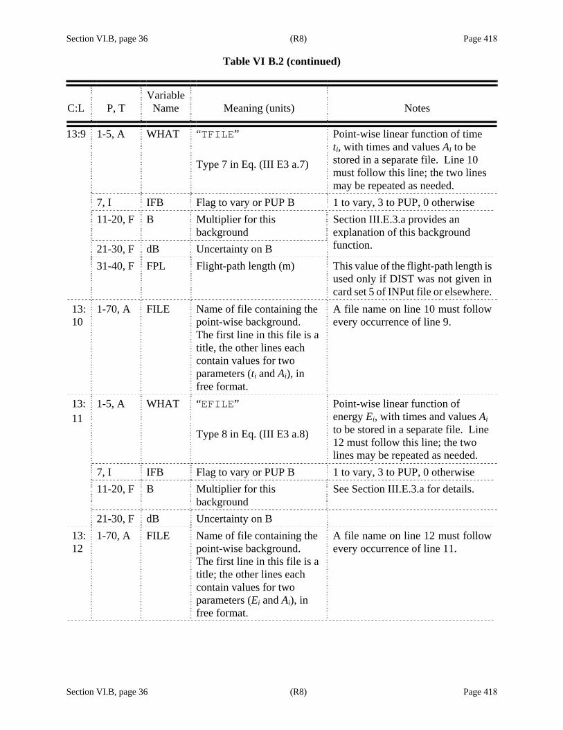
Section VI.B, page 36 (R8) Page 418
Table VI B.2 (continued)
Section VI.B, page 36 (R8) Page 418
C:L P, T Variable
Name Meaning (units) Notes
13:9 1-5, A WHAT “TFILE” Type 7 in Eq. (III E3 a.7)
Point-wise linear function of time ti, with times and values Ai to be stored in a separate file. Line 10 must follow this line; the two lines may be repeated as needed.
7, I IFB Flag to vary or PUP B 1 to vary, 3 to PUP, 0 otherwise 11-20, F B Multiplier for this
background 21-30, F dB Uncertainty on B
Section III.E.3.a provides an explanation of this background function.
31-40, F FPL Flight-path length (m) This value of the flight-path length is used only if DIST was not given in card set 5 of INPut file or elsewhere.
13:10
1-70, A FILE Name of file containing the point-wise background. The first line in this file is a title, the other lines each contain values for two parameters (ti and Ai), in free format.
A file name on line 10 must follow every occurrence of line 9.
13: 11
1-5, A WHAT “EFILE” Type 8 in Eq. (III E3 a.8)
Point-wise linear function of energy Ei, with times and values Ai to be stored in a separate file. Line 12 must follow this line; the two lines may be repeated as needed.
7, I IFB Flag to vary or PUP B 1 to vary, 3 to PUP, 0 otherwise 11-20, F B Multiplier for this
background See Section III.E.3.a for details.
21-30, F dB Uncertainty on B 13:12
1-70, A FILE Name of file containing the point-wise background. The first line in this file is a title; the other lines each contain values for two parameters (Ei and Ai), in free format.
A file name on line 12 must follow every occurrence of line 11.
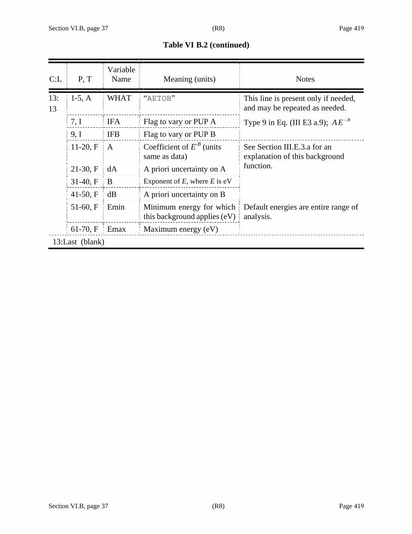
Section VI.B, page 37 (R8) Page 419
Table VI B.2 (continued)
Section VI.B, page 37 (R8) Page 419
C:L P, T Variable
Name Meaning (units) Notes
13: 13
1-5, A WHAT “AETOB”
7, I IFA Flag to vary or PUP A 9, I IFB Flag to vary or PUP B
This line is present only if needed, and may be repeated as needed.
Type 9 in Eq. (III E3 a.9); BA E −
11-20, F A Coefficient of E-B (units same as data)
21-30, F dA A priori uncertainty on A 31-40, F B Exponent of E, where E is eV
41-50, F dB A priori uncertainty on B
See Section III.E.3.a for an explanation of this background function.
51-60, F Emin Minimum energy for which this background applies (eV)
61-70, F Emax Maximum energy (eV)
Default energies are entire range of analysis.
13:Last (blank)
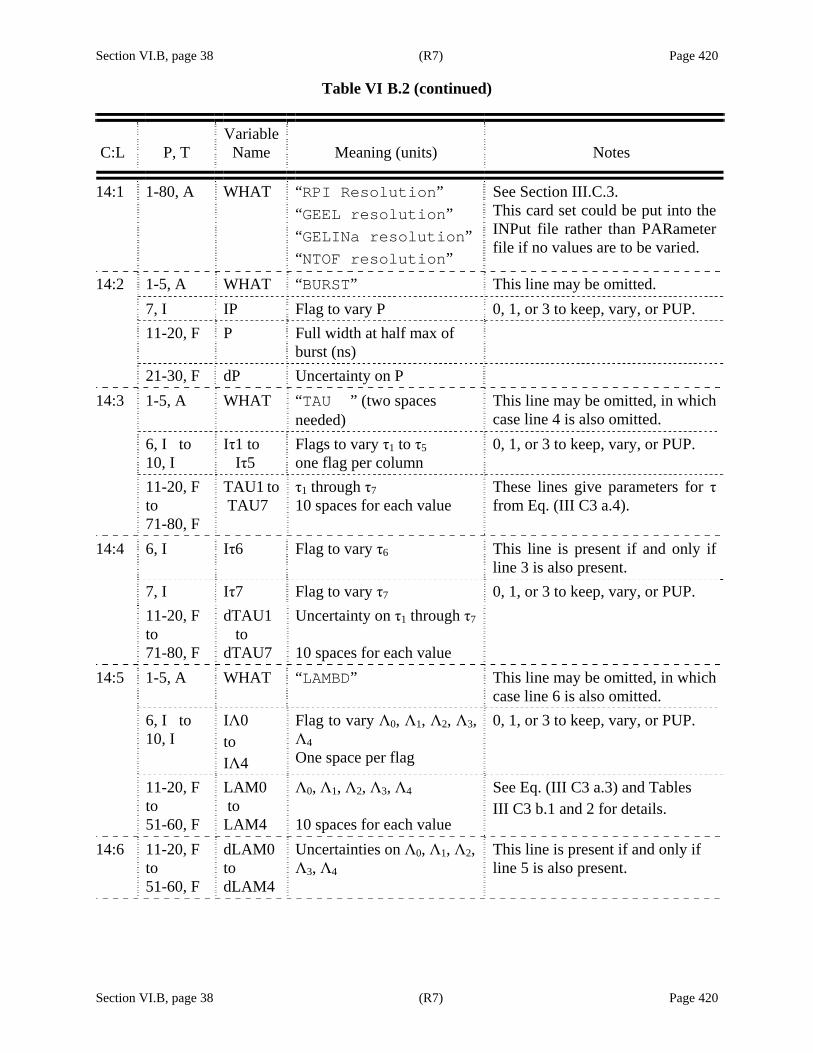
Section VI.B, page 38 (R7) Page 420
Table VI B.2 (continued)
Section VI.B, page 38 (R7) Page 420
C:L P, T Variable
Name Meaning (units) Notes
14:1 1-80, A WHAT “RPI Resolution” “GEEL resolution” “GELINa resolution” “NTOF resolution”
See Section III.C.3. This card set could be put into the INPut file rather than PARameter file if no values are to be varied.
14:2 1-5, A WHAT “BURST” This line may be omitted. 7, I IP Flag to vary P 0, 1, or 3 to keep, vary, or PUP. 11-20, F P Full width at half max of
burst (ns)
21-30, F dP Uncertainty on P 14:3 1-5, A WHAT “TAU ” (two spaces
needed) This line may be omitted, in which case line 4 is also omitted.
6, I to 10, I
Iτ1 to Iτ5
Flags to vary τ1 to τ5 one flag per column
0, 1, or 3 to keep, vary, or PUP.
11-20, F to 71-80, F
TAU1 to TAU7
τ1 through τ7 10 spaces for each value
These lines give parameters for τ from Eq. (III C3 a.4).
14:4 6, I Iτ6 Flag to vary τ6 This line is present if and only if line 3 is also present.
7, I Iτ7 Flag to vary τ7 0, 1, or 3 to keep, vary, or PUP. 11-20, F to 71-80, F
dTAU1 to dTAU7
Uncertainty on τ1 through τ7 10 spaces for each value
14:5 1-5, A WHAT “LAMBD” This line may be omitted, in which case line 6 is also omitted.
6, I to 10, I
IΛ0 to IΛ4
Flag to vary Λ0, Λ1, Λ2, Λ3, Λ4 One space per flag
0, 1, or 3 to keep, vary, or PUP.
11-20, F to 51-60, F
LAM0 to LAM4
Λ0, Λ1, Λ2, Λ3, Λ4 10 spaces for each value
See Eq. (III C3 a.3) and Tables III C3 b.1 and 2 for details.
14:6 11-20, F to 51-60, F
dLAM0 to dLAM4
Uncertainties on Λ0, Λ1, Λ2, Λ3, Λ4
This line is present if and only if line 5 is also present.

Section VI.B, page 39 (R7) Page 421
Table VI B.2 (continued)
Section VI.B, page 39 (R7) Page 421
C:L P, T Variable
Name Meaning (units) Notes
14:7 1-5, A WHAT “A1 ” (That’s “A One, blank blank blank”)
This line may be omitted, in which case line 8 is also omitted.
6, I to 10, I
IAA1 to IAA5
Flag to vary a1, a2, a3, a4, a5 (one space per flag)
0, 1, or 3 to keep, vary, or PUP.
11-20, F to 71-80, F
AA1 to AA7
Values for a1, a2, a3, a4, a5, a6, a7 from Eq. (III C3 a.5) 10 spaces for each value
See Eq. (III C3 a.5) and Tables III C3 b.1 and 2 for details.
14:8 6, I IAA6 Flag to vary a6 7, I IAA7 Flag to vary a7
This line is present if and only if line 7 is also present.
11-20, F to 71-80, F
dAA1 to dAA7
Uncertainties on a1, a2, a3, a4, a5, a6, a7
14:9 1-5, A WHAT “EXPON” 6, I to 10, I
IT0, IA2 to IA5
Flag to vary t0, A2, A3, A4, A5 One space per flag
11-20, F to 51-60, F
T0, A2 to A5
Values for t0, A2, A3, A4, A5 from Eq. (III C3 a.2) 10 spaces for each value
This line may be omitted (in which case line 10 is also omitted).
See Eq. (III C3 a.2) and Tables III C3 b.1 and 2 for details.
If lines 11 and 12 are present, the value for A3 given here will be ignored. Likewise, when lines 13 and 14 are present, the value for A5 given here will be ignored.
14: 10
11-20, F to 51-60, F
dT0, dA2 to dA5
Uncertainties on t0, A2, A3, A4, A5 10 spaces for each value
This line is present if and only if line 9 is also present.
14: 11
1-5, A WHAT “A3SQE” or “A3 ” ( “A 3 blank blank blank”)
6, I to 10, I
IAA31 to IAA35
Flag to vary a31, a32, a33, a34, a35. One space per flag
11-20, F to 71-80, F
AA31 to AA37
Values for a31, a32, a33, a34, a35, a36, and a37 from Eq. (III C3 a.5), 10 spaces for each.
This line may be omitted, in which case line 12 is also omitted and A3 is equal to the value given in line 9.
With WHAT=“A3SQE”, the value of α3 is sqrt(E).
With WHAT=“A3 ”, α3 = 1.
See Eq. (III C3 a.5) for details.
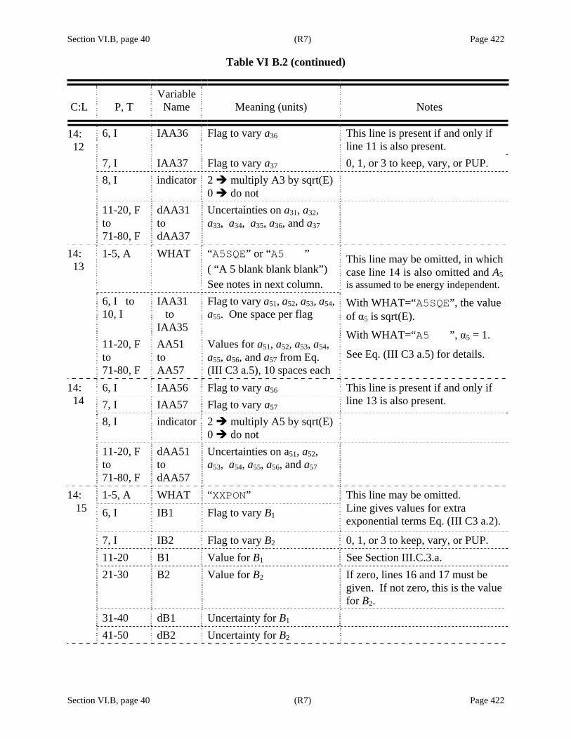
Section VI.B, page 40 (R7) Page 422
Table VI B.2 (continued)
Section VI.B, page 40 (R7) Page 422
C:L P, T Variable
Name Meaning (units) Notes
6, I IAA36 Flag to vary a36 This line is present if and only if line 11 is also present.
14: 12
7, I IAA37 Flag to vary a37 0, 1, or 3 to keep, vary, or PUP. 8, I indicator 2 multiply A3 by sqrt(E)
0 do not
11-20, F to 71-80, F
dAA31 to dAA37
Uncertainties on a31, a32, a33, a34, a35, a36, and a37
14: 13
1-5, A WHAT “A5SQE” or “A5 ” ( “A 5 blank blank blank”) See notes in next column.
6, I to 10, I
IAA31 to IAA35
Flag to vary a51, a52, a53, a54, a55. One space per flag
11-20, F to 71-80, F
AA51 to AA57
Values for a51, a52, a53, a54, a55, a56, and a57 from Eq. (III C3 a.5), 10 spaces each
This line may be omitted, in which case line 14 is also omitted and A5 is assumed to be energy independent.
With WHAT=“A5SQE”, the value of α5 is sqrt(E).
With WHAT=“A5 ”, α5 = 1.
See Eq. (III C3 a.5) for details.
6, I IAA56 Flag to vary a56 14: 14 7, I IAA57 Flag to vary a57
This line is present if and only if line 13 is also present.
8, I indicator 2 multiply A5 by sqrt(E) 0 do not
11-20, F to 71-80, F
dAA51 to dAA57
Uncertainties on a51, a52, a53, a54, a55, a56, and a57
1-5, A WHAT “XXPON” 14: 15
6, I IB1 Flag to vary B1 This line may be omitted. Line gives values for extra exponential terms Eq. (III C3 a.2).
7, I IB2 Flag to vary B2 0, 1, or 3 to keep, vary, or PUP. 11-20 B1 Value for B1 See Section III.C.3.a. 21-30 B2 Value for B2 If zero, lines 16 and 17 must be
given. If not zero, this is the value for B2.
31-40 dB1 Uncertainty for B1 41-50 dB2 Uncertainty for B2
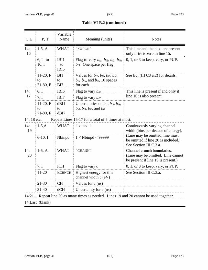
Section VI.B, page 41 (R7) Page 423
Table VI B.2 (continued)
Section VI.B, page 41 (R7) Page 423
C:L P, T Variable
Name Meaning (units) Notes
14: 16
1-5, A WHAT “XXPON” This line and the next are present only if B2 is zero in line 15.
6, I to 10, I
IBI1 to IBI5
Flag to vary bi1, bi2, bi3, bi4, bi5. One space per flag
0, 1, or 3 to keep, vary, or PUP.
11-20, F to 71-80, F
BI1 to BI7
Values for bi1, bi2, bi3, bi4, bi5. bi6, and bi7, 10 spaces for each.
See Eq. (III C3 a.2) for details.
6, I IBI6 Flag to vary bi6 14: 17 7, I IBI7 Flag to vary bi7
This line is present if and only if line 16 is also present.
11-20, F to 71-80, F
dBI1 to dBI7
Uncertainties on bi1, bi2, bi3, bi4, bi5. bi6, and bi7
14: 18 etc. Repeat Lines 15-17 for a total of 5 times at most. 14: 19
1-5,A
WHAT “BINS ”
6-10, I Nbinpd 1 < Nbinpd < 99999
Continuously varying channel width (bins per decade of energy). (Line may be omitted; line must be omitted if line 20 is included.) See Section III.C.3.a.
14: 20
1-5, A WHAT “CHANN” Channel crunch boundaries. (Line may be omitted. Line cannot be present if line 19 is present.)
7, I ICH Flag to vary c 0, 1, or 3 to keep, vary, or PUP. 11-20 ECRNCH Highest energy for this
channel width c (eV) See Section III.C.3.a.
21-30 CH Values for c (ns) 31-40 dCH Uncertainty for c (ns)
14:21... Repeat line 20 as many times as needed. Lines 19 and 20 cannot be used together. 14:Last (blank)
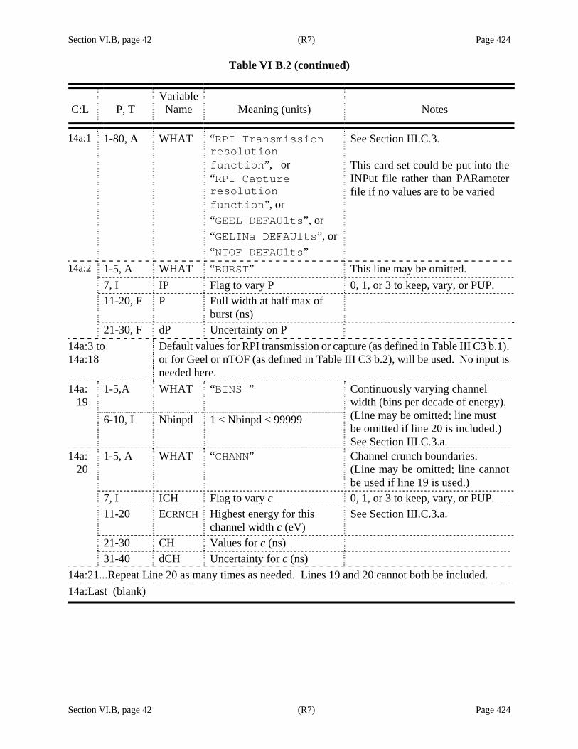
Section VI.B, page 42 (R7) Page 424
Table VI B.2 (continued)
Section VI.B, page 42 (R7) Page 424
C:L P, T Variable
Name Meaning (units) Notes
14a:1 1-80, A WHAT “RPI Transmission resolution function”, or “RPI Capture resolution function”, or “GEEL DEFAUlts”, or “GELINa DEFAUlts”, or “NTOF DEFAUlts”
See Section III.C.3. This card set could be put into the INPut file rather than PARameter file if no values are to be varied
14a:2 1-5, A WHAT “BURST” This line may be omitted. 7, I IP Flag to vary P 0, 1, or 3 to keep, vary, or PUP. 11-20, F P Full width at half max of
burst (ns)
21-30, F dP Uncertainty on P 14a:3 to 14a:18
Default values for RPI transmission or capture (as defined in Table III C3 b.1), or for Geel or nTOF (as defined in Table III C3 b.2), will be used. No input is needed here.
14a: 19
1-5,A
WHAT “BINS ”
6-10, I Nbinpd 1 < Nbinpd < 99999
Continuously varying channel width (bins per decade of energy). (Line may be omitted; line must be omitted if line 20 is included.) See Section III.C.3.a.
14a: 20
1-5, A WHAT “CHANN” Channel crunch boundaries. (Line may be omitted; line cannot be used if line 19 is used.)
7, I ICH Flag to vary c 0, 1, or 3 to keep, vary, or PUP. 11-20 ECRNCH Highest energy for this
channel width c (eV) See Section III.C.3.a.
21-30 CH Values for c (ns) 31-40 dCH Uncertainty for c (ns)
14a:21... Repeat Line 20 as many times as needed. Lines 19 and 20 cannot both be included. 14a:Last (blank)

Section VI.B, page 43 (R7) Page 425
Table VI B.2 (continued)
Section VI.B, page 43 (R7) Page 425
C:L P, T Variable Name Meaning (units) Notes
15:1 1-80, A WHAT “DETECtor efficiencies”
See Section III.E.5. This card set could be put into the INPut file rather than PARameter file if no values are to be varied.
15:2 1-10, F PARDET (1) Detector efficiency appropriate for these spin groups
11-20, F DELDET (1) Uncertainty on this detector efficiency
21-22, I or 21-25, I
IFLDET (1) Flag whether to vary this detector efficiency
23-24, I or 26-30, I
IGRDET (1,1) Number of the first spin group belonging to this isotope
25-26, I or 31-35, I
IGRDET (2,1) Number of second spin group belonging to this isotope
etc.
If more than 29 spin groups are needed, insert “−1” in Columns 79-80 and continue on the next line with five columns for each entry. When there are more than 99 spin groups altogether, use 5 columns for each integer entry in this line .
15:3 1-5, I IGRDET (29,1) Number of next spin group belonging to this isotope
This line is present only if the final entry on line 3 is “−1”
2-10, I IGRDET (30,1) Etc.
15:4 Repeat line 2 (and 3 if needed) for second (third, etc.) detector efficiency. Any spin groups which are not included in this listing will be assigned the final efficiency given in the list.
15:Last (blank)
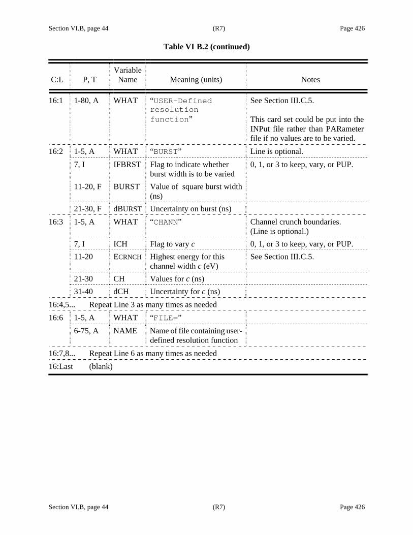
Section VI.B, page 44 (R7) Page 426
Table VI B.2 (continued)
Section VI.B, page 44 (R7) Page 426
C:L P, T Variable
Name Meaning (units) Notes
16:1 1-80, A WHAT “USER-Defined resolution function”
See Section III.C.5. This card set could be put into the INPut file rather than PARameter file if no values are to be varied.
16:2 1-5, A WHAT “BURST” Line is optional. 7, I IFBRST Flag to indicate whether
burst width is to be varied 0, 1, or 3 to keep, vary, or PUP.
11-20, F BURST Value of square burst width (ns)
21-30, F dBURST Uncertainty on burst (ns) 16:3 1-5, A WHAT “CHANN” Channel crunch boundaries.
(Line is optional.) 7, I ICH Flag to vary c 0, 1, or 3 to keep, vary, or PUP. 11-20 ECRNCH Highest energy for this
channel width c (eV) See Section III.C.5.
21-30 CH Values for c (ns) 31-40 dCH Uncertainty for c (ns)
16:4,5... Repeat Line 3 as many times as needed 16:6 1-5, A WHAT “FILE=”
6-75, A NAME Name of file containing user-defined resolution function
16:7,8... Repeat Line 6 as many times as needed 16:Last (blank)
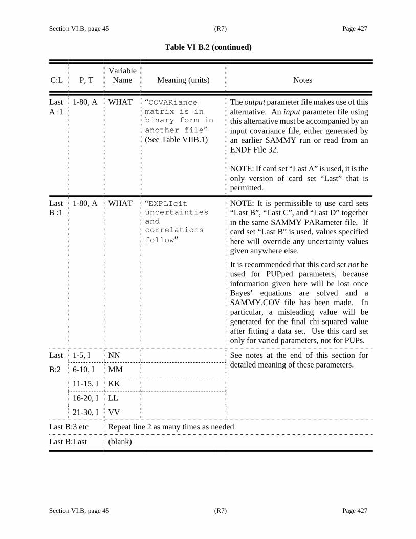
Section VI.B, page 45 (R7) Page 427
Table VI B.2 (continued)
Section VI.B, page 45 (R7) Page 427
C:L P, T Variable
Name Meaning (units) Notes
Last A :1
1-80, A WHAT “COVARiance matrix is in binary form in another file” (See Table VIIB.1)
The output parameter file makes use of this alternative. An input parameter file using this alternative must be accompanied by an input covariance file, either generated by an earlier SAMMY run or read from an ENDF File 32. NOTE: If card set “Last A” is used, it is the only version of card set “Last” that is permitted.
Last B :1
1-80, A WHAT “EXPLIcit uncertainties and correlations follow”
NOTE: It is permissible to use card sets “Last B”, “Last C”, and “Last D” together in the same SAMMY PARameter file. If card set “Last B” is used, values specified here will override any uncertainty values given anywhere else.
It is recommended that this card set not be used for PUPped parameters, because information given here will be lost once Bayes’ equations are solved and a SAMMY.COV file has been made. In particular, a misleading value will be generated for the final chi-squared value after fitting a data set. Use this card set only for varied parameters, not for PUPs.
Last 1-5, I NN
B:2 6-10, I MM
11-15, I KK
16-20, I LL
21-30, I VV
See notes at the end of this section for detailed meaning of these parameters.
Last B:3 etc Repeat line 2 as many times as needed
Last B:Last (blank)
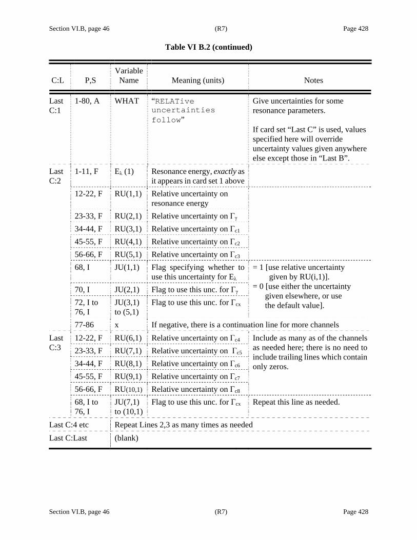
Section VI.B, page 46 (R7) Page 428
Table VI B.2 (continued)
Section VI.B, page 46 (R7) Page 428
C:L P,S Variable
Name Meaning (units) Notes
Last C:1
1-80, A WHAT “RELATive uncertainties follow”
Give uncertainties for some resonance parameters. If card set “Last C” is used, values specified here will override uncertainty values given anywhere else except those in “Last B”.
Last C:2
1-11, F Eλ (1) Resonance energy, exactly as it appears in card set 1 above
12-22, F RU(1,1) Relative uncertainty on resonance energy
23-33, F RU(2,1) Relative uncertainty on Γγ 34-44, F RU(3,1) Relative uncertainty on Γc1 45-55, F RU(4,1) Relative uncertainty on Γc2 56-66, F RU(5,1) Relative uncertainty on Γc3
68, I JU(1,1)
Flag specifying whether to use this uncertainty for Eλ
70, I JU(2,1) Flag to use this unc. for Γγ 72, I to 76, I
JU(3,1) to (5,1)
Flag to use this unc. for Γcx
= 1 [use relative uncertainty given by RU(i,1)]. = 0 [use either the uncertainty given elsewhere, or use the default value].
77-86 x If negative, there is a continuation line for more channels 12-22, F RU(6,1) Relative uncertainty on Γc4 Last
C:3 23-33, F RU(7,1) Relative uncertainty on Γc5 34-44, F RU(8,1) Relative uncertainty on Γc6 45-55, F RU(9,1) Relative uncertainty on Γc7 56-66, F RU(10,1) Relative uncertainty on Γc8
Include as many as of the channels as needed here; there is no need to include trailing lines which contain only zeros.
68, I to 76, I
JU(7,1) to (10,1)
Flag to use this unc. for Γcx Repeat this line as needed.
Last C:4 etc Repeat Lines 2,3 as many times as needed Last C:Last (blank)

Section VI.B, page 47 (R7) Page 429
Table VI B.2 (continued)
Section VI.B, page 47 (R7) Page 429
C:L P,S Variable
Name Meaning (units) Notes
Last D:1
1-80, A WHAT “PRIOR uncertainties follow in key word format”
Give uncertainties for some resonance parameters, in key word format. Examples are given in test case tr151. In all cases below, an equal sign must appear between the key word and the value of the parameter.
Last D:2
Valid key word for uncertainty: RELAtive uncertainty. The absolute uncertainty will be the product of this value times the absolute value of the parameter. Other valid key words for uncertainty: ABSOlute uncertainty or UNCErtainty. These are both treated as absolute uncertainties. To give an energy range, use key words EMIN or EMAX followed by equal sign and value. This uncertainty will be applied only to parameters for resonances within this energy range. (Warning: a zero-value will be interpreted as undefined. To give values of EMIN or EMAX as zero, use instead a small but non-zero value.)
To specify which parameters will have this uncertainty, two options are available; one or more of these can be used with each value of uncertainty. (1) Use key word GRoup followed (after equal sign) by a single group number, or by the word “All” (which indicates that this uncertainty applies to resonances in all spin groups). On the same line, use key word CHannel followed (after equal sign) by one or more channel numbers, and/or by the key word Energy or Gamma (indicating, respectively, the resonance energy and the capture width). Caution: SAMMY will not read beyond column 80 on a line. If there are too many channels to fit everything on the same line, it is possible to simply repeat the GRoup information with the remainder of the CHannel numbers on an additional line. Another option is to put all of the GRoup and CHannel information on a line separate from the other key word information.

Section VI.B, page 48 (R7) Page 430
Table VI B.2 (continued)
Section VI.B, page 48 (R7) Page 430
C:L P,S Variable
Name Meaning (units) Notes
Last D:2 cont.
(2) If quantum numbers were defined using the particle-pair option, then it is possible to use the key word PP or PARTicle pair followed (after equal sign) by the name of the particle pair exactly as given in the INPut (or PARameter) file. Use key word “L” or “Orbital angular momentum” followed by an equal sign and one or more integer values (separated by commas or spaces), to specify the spin groups and channels (those with this particle pair and these values of angular momentum) for which this uncertainty should apply. It is possible (though not necessarily practical!) to use PP=Energy or PP=gamma to give the uncertainty on resonance energies or capture widths. In this case, values of l need not be given, and the uncertainty is assumed to apply to all spin groups. Conflicting input is permitted here. In the case of conflicts, SAMMY will assume that the first uncertainty to be specified is the one to be used. See Table VI B.1 for a simple itemization of valid key words.
Last D:3 etc Repeat Line 2 as many times as needed. Last D:Last (blank)
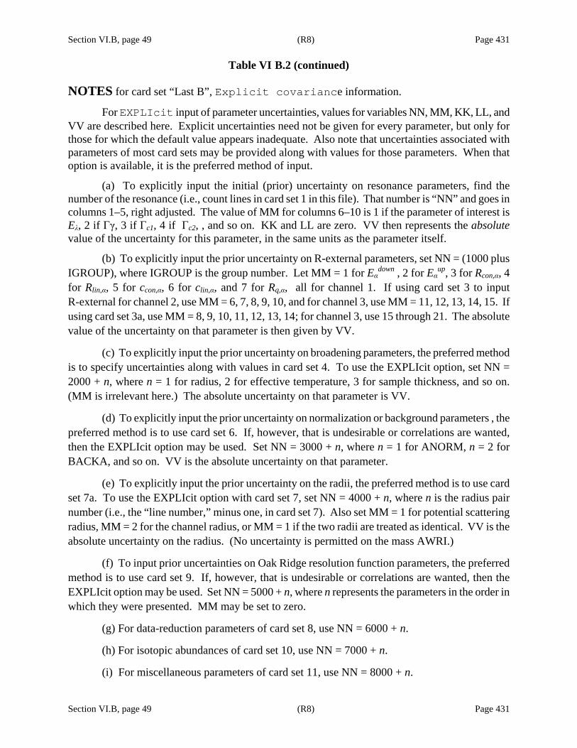
Section VI.B, page 49 (R8) Page 431
Table VI B.2 (continued)
Section VI.B, page 49 (R8) Page 431
NOTES for card set “Last B”, Explicit covariance information.
For EXPLIcit input of parameter uncertainties, values for variables NN, MM, KK, LL, and VV are described here. Explicit uncertainties need not be given for every parameter, but only for those for which the default value appears inadequate. Also note that uncertainties associated with parameters of most card sets may be provided along with values for those parameters. When that option is available, it is the preferred method of input.
(a) To explicitly input the initial (prior) uncertainty on resonance parameters, find the number of the resonance (i.e., count lines in card set 1 in this file). That number is “NN” and goes in columns 1–5, right adjusted. The value of MM for columns 6–10 is 1 if the parameter of interest is Eλ, 2 if Γγ, 3 if Γc1, 4 if Γc2, , and so on. KK and LL are zero. VV then represents the absolute value of the uncertainty for this parameter, in the same units as the parameter itself.
(b) To explicitly input the prior uncertainty on R-external parameters, set NN = (1000 plus IGROUP), where IGROUP is the group number. Let MM = 1 for Eαdown , 2 for Eαup, 3 for Rcon,α, 4 for Rlin,α, 5 for ccon,α, 6 for clin,α, and 7 for Rq,α, all for channel 1. If using card set 3 to input R-external for channel 2, use MM = 6, 7, 8, 9, 10, and for channel 3, use MM = 11, 12, 13, 14, 15. If using card set 3a, use MM = 8, 9, 10, 11, 12, 13, 14; for channel 3, use 15 through 21. The absolute value of the uncertainty on that parameter is then given by VV.
(c) To explicitly input the prior uncertainty on broadening parameters, the preferred method is to specify uncertainties along with values in card set 4. To use the EXPLIcit option, set NN = 2000 + n, where n = 1 for radius, 2 for effective temperature, 3 for sample thickness, and so on. (MM is irrelevant here.) The absolute uncertainty on that parameter is VV.
(d) To explicitly input the prior uncertainty on normalization or background parameters , the preferred method is to use card set 6. If, however, that is undesirable or correlations are wanted, then the EXPLIcit option may be used. Set NN = 3000 + n, where n = 1 for ANORM, n = 2 for BACKA, and so on. VV is the absolute uncertainty on that parameter.
(e) To explicitly input the prior uncertainty on the radii, the preferred method is to use card set 7a. To use the EXPLIcit option with card set 7, set NN = 4000 + n, where n is the radius pair number (i.e., the “line number,” minus one, in card set 7). Also set MM = 1 for potential scattering radius, MM = 2 for the channel radius, or MM = 1 if the two radii are treated as identical. VV is the absolute uncertainty on the radius. (No uncertainty is permitted on the mass AWRI.)
(f) To input prior uncertainties on Oak Ridge resolution function parameters, the preferred method is to use card set 9. If, however, that is undesirable or correlations are wanted, then the EXPLIcit option may be used. Set NN = 5000 + n, where n represents the parameters in the order in which they were presented. MM may be set to zero.
(g) For data-reduction parameters of card set 8, use NN = 6000 + n.
(h) For isotopic abundances of card set 10, use NN = 7000 + n.
(i) For miscellaneous parameters of card set 11, use NN = 8000 + n.

Section VI.B, page 50 (R8) Page 432
Table VI B.2 (continued)
Section VI.B, page 50 (R8) Page 432
(j) For background function parameters of card set 13, use NN = 13000 + n.
(k) To explicitly input correlations between the uncertainties on two parameters, let NN and MM indicate the first parameter, as in (a) through (j) above. The second parameter is indicated by KK and LL (analogous to NN and MM, respectively). The correlation coefficient is then given by VV. Note that VV is in the range from −1 to +1.
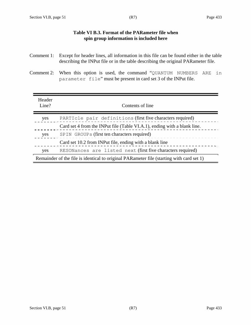
Section VI.B, page 51 (R7) Page 433
Section VI.B, page 51 (R7) Page 433
Table VI B.3. Format of the PARameter file when spin group information is included here
Comment 1: Except for header lines, all information in this file can be found either in the table
describing the INPut file or in the table describing the original PARameter file. Comment 2: When this option is used, the command “QUANTUM NUMBERS ARE in
parameter file” must be present in card set 3 of the INPut file.
Header Line? Contents of line
yes PARTIcle pair definitions (first five characters required)
Card set 4 from the INPut file (Table VI.A.1), ending with a blank line. yes SPIN GROUPs (first ten characters required)
Card set 10.2 from INPut file, ending with a blank line yes RESONances are listed next (first five characters required)
Remainder of the file is identical to original PARameter file (starting with card set 1)


Section VI.C, page 1 (R8) Page 435
Section VI.C, page 1 (R8) Page 435
VI.C. THE DATa and Data CoVariance FILES
Several possible formats are offered for inputting experimental data into the current version of SAMMY; these are described in Subsection VI.C.1. ASCII versions include the original (MULTI-style) data file with three data points per line, a format consistent with CSISRS data, and a 20-significant-digit format to meet the need for high precision.
Several different options are provided for input of the data covariance matrix (DCM). One commonly used method is to assume that the DCM contains only diagonal components, in which case the uncertainty (square root of the diagonal covariance matrix element) provided in the DATa file is used. As discussed in Section IV, this is not the optimal treatment of data uncertainties, as it is not the correct treatment for the important systematic experimental uncertainties. Instead, the user is encouraged to use one or another of several forms for including off-diagonal data covariance information.
The DCM may be calculated external to SAMMY and provided explicitly in ASCII format,
as described in Section VI.C.2. When using this “explicit DCM” option, the user must take great care to ensure that as many significant digits as possible are printed in the file in order to avoid numerical difficulties in the calculations. Because this method uses only experimental information, with no input regarding theoretical cross sections, it is the least rigorous method available here.
A better option is for the user to provide the components of the DCM, as discussed in
Section VI.C.3. This is preferable to the explicit DCM, for two reasons: (1) The input is both shorter and simpler for the user to generate. (2) Internal to SAMMY, matrix manipulation can be accomplished via the efficient “implicit data covariance” treatment as described in Section IV. The disadvantage is that this version of the DCM relies exclusively on experimental data; this option is therefore less rigorously correct than the method of the next paragraph. Nevertheless, this is the best available option for parameters whose derivatives are not calculated in SAMMY.
Finally, components of the off-diagonal DCM often are derived from uncertainties on parameters that are directly involved in the SAMMY analysis (e.g., the normalization or the resolution-function parameters might be viewed as contributing to the DCM). In these cases, there is now an option in SAMMY to simply flag these parameters with the number “3” to indicate that these are PUPs (Propagated Uncertainty Parameters). SAMMY will then make use of the uncertainties on the PUP’d parameters in deriving the implicit data covariance matrix. Details are discussed in Section IV.D.2. The PUP method is the recommended approach when using a data covariance matrix; only the option of directly varying a parameter is more rigorous.

Section VI.C.1, page 1 (R7) Page 437
Section VI.C.1, page 1 (R7) Page 437
VI.C.1. Experimental Data
The original format for the DATa file is shown in Table VI C1.1; this version is borrowed directly from MULTI [GA74]. Three data points, including energy, experimental value for cross section (or transmission, eta, etc.), and relative uncertainty appear on each line. Energies may be ordered from high to low or low to high, but the ordering must be monotonic. The data file may contain points that are not within the range [EMIN,EMAX] specified for this run; such points will be ignored (or, possibly, used for determining the auxiliary grid. See Section III.A).
A second ASCII format permits one data point per line, in (3F11) or (3E11) format, with uncertainties being absolute (rather than relative as in the “original” format). To use this option, the phrase “USE CSISRS FORMAT FOr data” or an equivalent must appear in card set 3 of the INPut file (See Table VI A1.2).
A third ASCII format is useful when many significant digits are needed (e.g., when comparing cross sections calculated by SAMMY with those calculated by other codes). This format has one data point per line, in (3F20) or (3E20) format, and uncertainties are absolute. The phrase “USE TWENTY SIGNIFICAnt digits for experimental data” (or simply “TWENTY”) must appear in card set 3 of the INPut file (Table VI A1.2).
The energies and cross sections from an ENDF/B File 3 listing may be used for the “experimental data” in a SAMMY run. The command for this option is “USE ENDF/B ENERGIES and cross sections MAT=abcd”, in which “abcd” is replaced by the ENDF MAT (material) number. See test case tr086 for examples.
For ORNL-ORELA staff and others who use the plotting package FORODF [JC78] with their version of SAMMY, there are several possible methods of supplying data in ORELA Data Format (ODF): For the first, you must specify “DATA ARE IN ODF FILE” in card set 3 of the INPut file (see Tables VI A.1 and VI A1.2). In this ODF data file, section 1 contains the energy (which can be either high-to-low or low-to-high), section 2 contains the data, and 3 contains the absolute uncertainty. Use of this alternative is discouraged, because SAMMY handles it awkwardly, copying to a temporary file in the usual DATa file format of Table VI C1.1. See test case tr005 for an example using this option.
The second ODF format is the “standard ODF format,” for which you must specify “DATA ARE IN STANDARD odf format” in your input file. In this ODF file, unlike the version in the previous paragraph, the energies must be ordered high to low. Again energies are stored in section 1, data in section 2, and absolute uncertainties in section 3. The standard ODF file contains additional sections not in the other version: sections 4, 5, and so forth are used to store the partial derivatives of the data with respect to the data-reduction parameters. (See Section III.E.3 of this report for a discussion of data-reduction parameters.) Note that section 4 of the ODF file must correspond to data-reduction parameter number 1, section 5 to parameter number 2, etc. As with all varied parameters, initial values are given in the PARameter file (card set 8 of Table VI B.2). This method has not been used very much and will likely be dropped in future releases.

Section VI.C.1, page 2 (R7) Page 438
Section VI.C.1, page 2 (R7) Page 438
Two options are available for specifying differential elastic scattering data. The first is via an ODF file. Section 1 of this file contains the energy; section 2, the measured cross sections for the first angle; section 3, the absolute uncertainties on the cross sections in section 2; sections 4 and 5, the cross sections and uncertainties for the second angle; and so forth. In general, section 2n contains data for the nth angle; and section 2n+1 contains the uncertainties. Angles are specified in the INPut file, card set 8 (see Table VI A.1). (This option has seen little use and will likely be dropped in future revisions.)
The second option for differential elastic data is via an ASCII file, all in (8F10.1) format, with at least two lines per energy. The first line contains the energy in the first ten columns, cross section at first angle in columns 11-20, cross section at second angle in columns 21-30, etc.; if there are more than seven angles, the eighth appears in columns 1-10 of the next line. The second line (or set of lines) is blank in columns 1-10, contains the (absolute) uncertainty in the cross section at the first angle in columns 11-20, uncertainty for the second angle in columns 11-20, etc.; again, if there are more than seven angles, then values for the 8th and subsequent angles are on additional lines, beginning in column 1. These two (sets of) lines are repeated once for each energy. To use this option, it is necessary to include the phrase “DIFFERENTIAL DATA ARE IN ascii file” in the INPut file. See test cases tr033, tr043, tr109, and others for examples.
Table VI C1.1. MULTI-Style Format for the DATa file
Line Column Variable Format Meaning (units)
1,2,etc. 1-15 ENERGY1 F15 Energy (eV) 16-30 DATA1 F15 Experimental cross section
(barns), transmission, yield, or other type of data
31-37 FRACT1 F7 Fractional uncertainty in DATA1 38-52 ENERGY2 F15 53-67 DATA2 F15 68-74 FRACT2 F7 75-89 ENERGY3 F15 90-104 DATA3 F15 105-111 FRACT3 F7
Note that although F formats are specified above, input can be in either E or F format. Numbers must, however, be within the columns specified, and a decimal point is required. If using E format, the exponent is in the right-most columns.

Section VI.C.2, page 1 (R8) Page 439
Section VI.C.2, page 1 (R8) Page 439
VI.C.2. Explicit Data Covariance Matrices
It is possible, but not optimal, to generate an approximate off-diagonal data covariance matrix (DCM) using knowledge of the experimental data only. Information about such DCM may be communicated to SAMMY either explicitly (generating the entire DCM external to SAMMY and preparing an ASCII file containing the matrix elements) or implicitly (providing only the components of the DCM, not the full matrix).
An explicit DCM is treated as a regular off-diagonal covariance matrix; see the description of Bayes= equations, Section IV. Use of the explicit data covariance matrix thus requires inversion of an N H N array, where N is the number of data points. Use of the explicit DCM is permitted but not recommended.
An implicit data covariance matrix (described in Section IV.A.1.a) makes use of the specific mathematical form for the covariance matrix,
,tV v g m g= + (VI C2.1) where v is the diagonal statistical portion, m is the covariance matrix for the data-reduction parameters, and g represents the partial derivatives of the theoretical values with respect to the data-reduction parameters. (See Section IV.D for more details.) With the user-supplied implicit DCM, the components (v, g, and m) are generated external to SAMMY and provided to the code; V itself is not needed. The implicit DCM is treated by a more sophisticated mathematical process that does not require inversion of such a large matrix. See Section VI.C.3 for input details for the implicit DCM; this is the recommended approach.
When either an explicit or an implicit DCM could be used, the implicit DCM is recommended because the treatment within SAMMY is far more efficient and often more accurate.
Table VI C2.1 shows the original format for a Data CoVariance (DCV) file, to be included when each covariance matrix element is given explicitly in fixed format. The name of this file must be specified in card set 3 of the INPut file (Tables VI A.1 and VI A1.2) in columns 31–40 of the line reading “DATA COVARIANCE FILE is named ...” Because the matrix is symmetric, only the lower triangular half of this matrix is given in the file; matrix elements are read across the columns, as illustrated here.
V11 V21 V22 V31 V32 V33 V41 V42 V43 V44 V51 V52 V53 V54 V55
CAUTION: When creating an explicit DCV file, it is important to provide as many significant digits as possible for each matrix element, in order to ensure reasonably accurate results and avoid numerical problems associated with singular matrices. Often it is simply not possible to provide an adequate number of digits in a ten-column format.
A second option for input of the explicit DCM is now available, using free format. In this case, the input file must include the command “FREE FORMAT DATA COVariance” with the file name in columns 31–40 of the same line. Again, the recommended procedure for input of an

Section VI.C.2, page 2 (R8) Page 440
Section VI.C.2, page 2 (R8) Page 440
externally generated covariance matrix is via the IDC method of Section VI.C.3.b, rather than via explicit calculation of the full data covariance matrix.
Occasionally it may be convenient to introduce a constant on- and off-diagonal data covariance in the neighborhood of a non-s-wave resonance, permitting effective decoupling of any underlying l = 0 state from the non-s waves. This is effective because an additive constant covariance is mathematically equivalent to a constant, coherent correction term for either the data or the theory. (Algebraic details are presented in Appendix A of the original SAMMY report [NL80].) This type of off-diagonal data covariance matrix can be generated automatically by SAMMY; details for input are given in Table VI A1.2 under the category “Experimental data – input control for covariance matrix” and in card set 1, columns 68 to 80, of Table VI B.2.
Another type of explicit off-diagonal data covariance matrix that can be automatically generated by SAMMY is of the form ( )( ) ,i j i j i jV V a bE a bE= + + + (VI C2.2)
where i jV is provided by the user, iE is the energy for data point i , and a and b are constants chosen by the user. This type of covariance is useful if there are energy-dependent coherent uncertainties in the data, for example, if a subtracted background is imperfectly known. Input for this option is given in card set 7 of Table VI A.2, and the “Input Control” statement “DATA HAS OFF-DIAGONAL contribution ...” of Table VI A1.2.
Table VI C2.1. Format of the explicit data covariance file This file contains the lower triangular half of the matrix, reading across the columns
Line Column Variable Format Meaning
1 1-10 VARDAT(1,1) F10.1 Variance for data point 1
2 1-10 11-20
VARDAT(2,1) VARDAT(2,2)
F10.1 F10.1
Covariance between data points 1 and 2 Variance for data point 2
3 1-10 11-20 21-30
VARDAT(3,1) VARDAT(3,2) VARDAT(3,3)
F10.1 F10.1 F10.1
Covariance between data points 1 and 3 Covariance between data points 2 and 3 Variance for data point 3
4 1-10 ... VARDAT(4,1) etc.
F10.1
…
Last 1-10 ... VARDAT(Last,1) etc.
F10.1
Note that the ordering of data points is low to high (independent of the ordering in the DATa file), and only those data points actually used in the calculation can be referenced in the DCV file. A maximum of eight matrix elements are to be included on one line; thus, “line number 11,” for example, will actually be two lines, with eight numbers on the first and three on the second.

Section VI.C.3, page 1 (R7) Page 441
Section VI.C.3, page 1 (R7) Page 441
VI.C.3. Implicit Data Covariance (IDC) Matrices
The data-reduction process, which is generally performed by the experimentalist who measured the data, includes background subtraction and normalization, as well as other corrections (for deadtime, self-shielding, etc.). This process introduces systematic errors, which lead to an off-diagonal data covariance matrix (DCM). This off-diagonal portion of the DCM should be included along with the diagonal portion (statistical errors) in the analysis process.
As described in Section IV (The Fitting Procedure) and, in particular, Section IV.D.3 (Implicit Data Covariance Matrix), it is possible for SAMMY to treat data covariances without actually ever generating, storing, or inverting the complete off-diagonal DCM. There are several possibilities for inputting the necessary information into SAMMY.
The Propagated Uncertainty Parameter (PUP) option is described in detail in Sections IV.D.1 and IV.D.2. Input for PUPs is discussed in Section VI.C.3.a.
A second option for input of data covariance information is for the user to externally generate
the pieces g (derivatives with respect to data-reduction parameters) and m (covariance matrix for the data-reduction parameters) of the DCM. See Section VI.C.3.b for details. Finally, in Section VI.C.3.c, SAMMY’s original version of IDC methodology is discussed. Though this option is still available, in practice it provides the exact same results as the PUP method and is somewhat more awkward to use.

Section VI.C.3.a, page 1 (R7) Page 443
Section VI.C.3.a, page 1 (R7) Page 443
VI.C.3.a. Input for propagated uncertainty parameters
The Propagated Uncertainty Parameter (PUP) option is described in detail in Sections IV.D.1 and IV.D.2. Essentially, the PUP method takes any of the SAMMY parameters (either R-matrix parameters or parameters from the experiment-related corrections to the cross sections) and incorporates the uncertainty on that parameter into the data covariance matrix (DCM). The value of the parameter is held fixed.
As indicated in Table VI B.2, SAMMY input parameters generally have both a flag and an
uncertainty associated with them. If that flag is zero, the parameter is treated as a constant and the uncertainty is ignored. When the flag is 1, the value of that parameter is refined (“fitted” or “searched on”) during the analysis process; the uncertainty is taken as the “prior” uncertainty on that parameter (unless, of course, a prior COVariance file is used). If the flag is 3, the parameter value remains fixed, but the uncertainty becomes a component of the DCM.
Nearly all the data-related card sets of the PARameter file (Table VI B.2) can now be
inserted into the INPut file (see the end of Table VI A.1). When the card set is in the INPut file, flags = 1 will be ignored but flags = 3 will be honored.
Sometimes it is desirable to provide an off-diagonal covariance matrix for the PUP’d
parameters. For example, the set of resolution-function parameters may be determined altogether, by fitting a functional form to measured data; those parameters are then correlated. To input such information to SAMMY, create an ASCII file containing the following information:
1. A title on the first line. 2. A line containing “Number of parameters = #”, where # is replaced by the integer
number of PUP parameters for which covariances will be provided. [In fact, only the equal sign and the number are absolutely necessary on this line.]
3. One or more lines containing the exact values of the PUPs, in free-format. These values must be within 0.1 % of the actual value of the parameters as given in the PARameter or INPut file. (Caution: if there are two PUPs whose values are nearly identical, and it is the second one that you are intending to use here, SAMMY might misinterpret the information. To avoid this problem, include the first PUP, and all in between, in the PUP covariance matrix.)
4. One or more lines containing the lower triangular covariance matrix elements for those parameters (reading across the matrix from the left-hand side to the diagonal in the usual SAMMY fashion), in free format.
It is NOT necessary to include every PUP in this file, but those that are included must be
consecutively located in the SAMMY.LPT listing; that is, the PUP numbers inside the pointed brackets must be consecutive, as in <6> and <7>. For example, one might have a covariance matrix for the resolution-function parameters but wish to PUP the Doppler width plus the normalization and background parameters as well. See test case tr168 for examples.
To use the PUP covariance file in a SAMMY run, include the phrase “PUP COVARIANCE IS IN an ascii file” in the command section of the INPut file.
Section VI.C.3.a, page 2 (R7) Page 444
Section VI.C.3.a, page 2 (R7) Page 444
It is possible to use SAMMY to generate PUP covariance information and write it into a file to be used as input for subsequent runs. For example, to predetermine resolution-function parameters, a SAMMY run (or series of runs) might be made on “clean” data with well-defined resonance parameters. Only the resolution parameters would be flagged. The command “CREATE PUP FILE FROM varied parameters used in this run” would be included in the INPut file for this run (or for the final run of the series). The output file SAMPUP.COV is in the appropriate format for use as the input PUP covariance file for future runs. Again, see test case tr168 for an example of this. Caveat: The implementation of the PUP covariance input option is new and has not been extensively tested. Because there are so many possibilities for parameters to be PUP’d, it has not been possible for the author to test each and every potential combination. The user is therefore strongly advised to carefully examine the SAMMY.LPT output file to be sure that the PUP covariance matrix information has been properly interpreted by the code. In particular, look at the array printed following the phrase “Correlation matrix for PUPped parameters” and check that the uncertainties and correlations correspond to the appropriate PUPs.
For sequential runs in which the varied-parameter COVariance file from one run is used as input to the next run, values and uncertainties for varied parameters cannot be modified. (The exception is via the use of program SAMAMR; see Section X.C.) However, values and uncertainties for PUPs can be modified, since they are associated with the data set rather than with the parameters whose values are being determined. (The exception is that the treatment of R-matrix parameters may not be changed during a sequence of runs.) If the user wishes to be certain that values for PUPs do not change, s/he can insert the command “DO NOT ALLOW VALUES for data-related parameters to change” into the INPut file.
R-matrix parameters should not be PUP’d during sequential runs: One of the assumptions
underlying the use of sequential analysis is that the data sets being analyzed are completely independent of each other, that is, they are not united via a common DCM. Therefore, if a parameter (e.g., a channel radius) is PUP’d for two data sets, the associated components of the DCM uniting the two data sets will be ignored. This would violate the assumption of independent data sets. The same is also true for simultaneous runs of two or more data sets, as described in Section IV.E.1, because the scheme described there also assumes that the data sets are independent.
It is expected that future development work will provide a means of properly including the
effect of a PUP’d variable that connects two otherwise-independent data sets.

Section VI.C.3.b, page 1 (R7) Page 445
Section VI.C.3.b, page 1 (R7) Page 445
VI.C.3.b. User-supplied implicit data covariance matrix
After reducing experimental data from raw counts to a form resembling a cross section, the experimentalist has available all information needed to produce the covariance matrix for the reduced data. This covariance matrix would have the form given in Eq. (IVD.1): ' '
'i j i i j i k k k j k
k k
V v g m gδ= +∑ (VI C3 b.1)
where i kg is the partial derivative of the expression for data point i (in terms of the measured quantity and the data-reduction parameters) with respect to data-reduction parameter k. The covariance matrix for the data-reduction parameters is m. (For a concrete example of this, see the paper by Gunsing [FG98] detailing the derivation of the covariance matrix for data measured at the GELINA facility.)
Rather than generating the entire covariance matrix V, the SAMMY user can prepare a file containing the partial derivatives that SAMMY will then use for the Implicit Data Covariance Matrix. The SAMMY INPut file should contain the command “USER-SUPPLIED IMPLICIt data covariance matrix”, and the name of the file must be given directly after the name of the data file.
The format for the user-supplied implicit data covariance file is as shown in Table VI C3 b.1. Examples
For examples on the use of IDC, see test cases tr070, tr118, and tr140. Case tr118 contains equivalent examples of normalization and background included in the fitting (case a), implicit covariance matrix (cases c and i), user-supplied implicit data covariance matrix (cases g and h), and explicit data covariance matrix (case j).

Section VI.C.3.b, page 2 (R7) Page 446
Section VI.C.3.b, page 2 (R7) Page 446
Table VI C3 b.1. Format for user-supplied IDC file
Card set: Line
Variable
Meaning
1:1 Alpha At least the first two characters (and the equal sign) of the phrase “NUmber of data-reduction parameters =”, followed by an integer number Kwhich indicates how many partial derivatives are to be read. Example: NU=7
1:2 (blank) 2:1 Alpha At least the first ten characters of the phrase “PARTIAL DErivatives” or
“FREE-FORMAt partial derivatives” 2:2 X(i,1) If “PARTIAL DErivatives”, then the K partial derivatives for the first data
point, eight values per line, continuing on the next lines if needed, in 8F10 format, or If “FREE-FORMAt partial derivatives”, then this line contains the energy, the statistical uncertainty on the first data point, and the K partial derivatives for the first data point, in free format
2:3 X(i,2) The K partial derivatives for the second data point in 8F10 format, or Energy, statistical uncertainty, and partial derivatives in free format
etc. 2: N + 1 X(i,N) The K partial derivatives for the Nth data point (where N is the total number of
data points in the SAMMY run), in 8F10 format. Energy, statistical uncertainty, and K partial derivatives, in free format.
2: N + 2 (blank) 3:1 Alpha At least the first ten characters of the phrase “UNCERTAINTies on data-
reduction parameters”. NOTE: This card set is optional and may be omitted if the uncertainties are multiplied into X, that is, if X(i,k) from card set 2 contains X k
i times the square root of wk rather than just X k i itself.
3:2 X(i,1) Uncertainties for the K data-reduction parameters, continuing on the next lines if needed. Format is 8F10 or free-format as specified in card set 2, line 1.
3: 3 (blank) 4:1 Alpha At least the first ten characters of the phrase “CORRELATIOns for
data-reduction parameters”. This card set is optional and may be omitted if values for the data-reduction parameters were independently determined (i.e., if parameters are uncorrelated).
4:2 C(1,2) Correlation between parameter number 1 and parameter number 2. Format is F10 or free format, as specified in card set 2 line 1.
4:3 C(1,3), C(2,3)
Correlation between parameters 1 and 3, and between 2 and 3; format is 2F10 or free format.
etc. 4: K + 1 C(i,K) Correlation between parameters i (for i = 1 to K−1) and K, in 8F10 format or
free format, continuing on additional lines if needed. 4: K + 2 (blank)
Section VI.C.3.c, page 1 (R7) Page 447
Section VI.C.3.c, page 1 (R7) Page 447
VI.C.3.c. Implicit data covariance for normalization and background
To determine the covariance matrix due to the background and normalization corrections, SAMMY assumes that the “corrected” data D and the “original” data R are related via
( ) ( ) ( ) ,R E b E
D Ea−
= (VI C3 c.1)
in which a and b are defined as in Section III.E.3.a (Explicit Normalization and/or Background Functions). Note that for the IDC, corrections are applied to the experimental data and therefore are opposite to those applied to the theory as in Section III.E.3.a.
Values and uncertainties (as well as possible correlations) for the normalization and background parameters should be determined by the experimentalist. However, the analyst may find it necessary to apply further corrections to the data. In this case, the analyst can run SAMMY, including normalization and/or background functions in the parameter file with the parameters flagged (varied) in order to determine the correct values for the parameters. The next step would be to produce a modified data file; this step can be accomplished with SAMMY by including a command line “REFORMULATE DATA FOR implicit data covariance” in the INPut file. SAMMY will then produce a file SAMMY.DA2 in the same format as the analyst’s DATa file, with the data values corrected according to Eq. (VI C3 c.1). Note that uncertainties in this data file will not be changed (except to divide by the normalization a, if the uncertainties in the file are absolute rather than relative): This file, like the original, contains only statistical, but not systematic, errors. SAMMY will also produce a file SAMMY.IDC that contains the normalization and broadening information, and a new parameter file SAMMY.PA2 identical to the analyst=s PAR file except for the absence of the normalization and broadening information. The uncertainties in SAMMY.IDC can then be modified (or added) to be the proper experimental uncertainties on the normalization and broadening parameters, to be used in further SAMMY runs.
In subsequent SAMMY runs for that data set, the INPut file contains the command line “IMPLICIT DATA COVARIance matrix is to be used.” SAMMY then looks for the IDC file, which uses the same formats as portions of the PARameter file. In particular, card set 6 (NORMAlization and background) and card set 13 (BACKGround functions) can be included in this file; see Section III.E.3.a for a description of these functions. Any correlations between values should also be given here, using again the formats of the PARameter file for EXPLIcit uncertainties (card set Last, alternative B).
NOTE: This use of the implicit data covariance (IDC) with normalization and background
parameters was the earliest implementation of the more general IDC construction, as outlined in Section IV.D.3. The PUP concept (Section IV.D.2) is applicable to more parameter types, and is easier for the analyst to use but (when used with the same parameters) gives identical results to the original normalization-and-background IDC described in this section. It is likely, therefore, that this original version will eventually be phased out. Analysts are encouraged to use the PUP option instead.


Section VI.D, page 1 (R7) Page 449
Section VI.D, page 1 (R7) Page 449
VI.D. INTEGRAL DATA FILE
When the data type is specified as “INTEGral quantities” (see card set 8 of the INPut file), two kinds of data files are needed. The first is an experimental differential data file, which is used only to generate the energy grid on which the integrals are to be calculated; the type of data and values of the cross sections in this file are ignored. The second kind of data file contains the experimental integral data and is designated as the “NTG” file.
In the NTG file, each type of integral data is specified by a unique five-character name, which is given in Columns 1 to 5 of the appropriate line. Names can be either uppercase or lowercase, and the ordering is arbitrary. Only those data types for which experimental measurements exist need to be specified; others can simply be omitted from this file.
Table VI D.1 shows the various types of integral data available in SAMMY. Note that underscore _ in a name denotes a blank space.
When the INPut and PARameter files specify more than one nuclide (isotope), SAMMY will calculate the integral quantities for each nuclide separately, ignoring the abundances specified in INPut and/or PARameter files. Integral data are assumed to be for a specific nuclide; it is important to note that the ordering of the nuclides must be the same in the NTG file as in the PAR file.
Correlations between experimental data are also given in the NTG file.
The name of the integral data file is given directly after the name of the differential data file, in the “interactive input to SAMMY.” Details for the format of the NTG file are given in Table VI D.2.
Table VI D.1. Types of integral data
Name as used in NTG file Description
THABS, THFIS, THCAP Absorption, fission, or capture cross section, respectively, at thermal energy (E = 0.0253 eV)
MXABS, MXFIS, MXCAP Maxwellian average absorption, fission, or capture cross section
WGABS, WGFIS, WGCAP
Westcott=s g factor for absorption, fission, or capture cross section
RIABS, RIFIS, RICAP
Resonance integral for absorption, fission, or capture cross section
AVABS, AVFIS, AVCAP
Average integral for absorption, fission, or capture cross section
WATTS
Watt spectrum average
K1_ _ _
[ v (MXFIS) - (MXABS) ] 2 / π
ALPHA
α = (RICAP) / (RIFIS)
NJALF
NJOY=s α
NJETA
NJOY=s η

Section VI.D, page 2 (R7) Page 450
Section VI.D, page 2 (R7) Page 450
Table VI D.2. Format of the NTG file
Line No. Column Variable Name Meaning
1 1-70 TITLE Title for the file; is printed in LPT file but never used
2 1-5 NUCLID Nuclide number (default = 1); nuclides must be in the same order as in PAR file
3, 4, etc. 1- 5 WHAT Type of integral data, from list in Table VI D.1
11-20 DATA Experimental value for this data type
21-30 UNC Experimental uncertainty for this data type
31-40 CONST
41-50 CONST2
For resonance integral data, CONST is the maximum energy for integrand, and CONST2 is the remainder to be added to the integrated value
For average integral data, CONST is the lower limit on the integral and CONST2 the upper
For K1, CONST is the value of v For Watt spectrum average, CONST = a and
CONST2 = b
5 (blank)
6, etc. Repeat lines 2 through 5 as many times as needed
7 (blank)
8 1-5 WHAT CORRElations follow
9 1-5 WHAT1 Type of integral data
6-10 NUC1 Nuclide number
11-15 WHAT2 Type of integral data
16-20 NUC2 Nuclide number
21-30 CORR Correlation between data of type WHAT1 for nuclide number NUC1, and WHAT2 for Nuc2
10, 11, etc. Repeat line 9 as many times as needed
12 (blank)
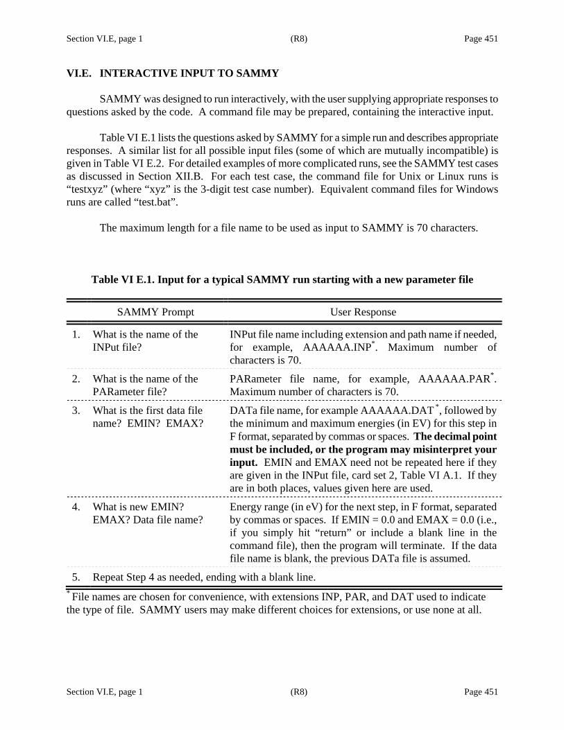
Section VI.E, page 1 (R8) Page 451
Section VI.E, page 1 (R8) Page 451
VI.E. INTERACTIVE INPUT TO SAMMY
SAMMY was designed to run interactively, with the user supplying appropriate responses to questions asked by the code. A command file may be prepared, containing the interactive input. Table VI E.1 lists the questions asked by SAMMY for a simple run and describes appropriate responses. A similar list for all possible input files (some of which are mutually incompatible) is given in Table VI E.2. For detailed examples of more complicated runs, see the SAMMY test cases as discussed in Section XII.B. For each test case, the command file for Unix or Linux runs is “testxyz” (where “xyz” is the 3-digit test case number). Equivalent command files for Windows runs are called “test.bat”. The maximum length for a file name to be used as input to SAMMY is 70 characters.
Table VI E.1. Input for a typical SAMMY run starting with a new parameter file
SAMMY Prompt User Response
1. What is the name of the INPut file?
INPut file name including extension and path name if needed, for example, AAAAAA.INP*. Maximum number of characters is 70.
2. What is the name of the PARameter file?
PARameter file name, for example, AAAAAA.PAR*. Maximum number of characters is 70.
3. What is the first data file name? EMIN? EMAX?
DATa file name, for example AAAAAA.DAT *, followed by the minimum and maximum energies (in EV) for this step in F format, separated by commas or spaces. The decimal point must be included, or the program may misinterpret your input. EMIN and EMAX need not be repeated here if they are given in the INPut file, card set 2, Table VI A.1. If they are in both places, values given here are used.
4. What is new EMIN? EMAX? Data file name?
Energy range (in eV) for the next step, in F format, separated by commas or spaces. If EMIN = 0.0 and EMAX = 0.0 (i.e., if you simply hit “return” or include a blank line in the command file), then the program will terminate. If the data file name is blank, the previous DATa file is assumed.
5. Repeat Step 4 as needed, ending with a blank line. * File names are chosen for convenience, with extensions INP, PAR, and DAT used to indicate the type of file. SAMMY users may make different choices for extensions, or use none at all.

Section VI.E, page 2 (R8) Page 452
Section VI.E, page 2 (R8) Page 452
Table VI E.2. Complete list of input files for SAMMY runs, in the order in which they will occur. Only a subset of the SAMMY prompts will occur for any given SAMMY run.
SAMMY prompt What is needed Invoking command
1. What is the name of the INPut file?
INPut file name plus extension. Maximum number of characters is 70.
2. What is the name of the PARameter file?
PARameter file name. Maximum number of characters is 70.
3. What is the first data file name? EMIN? EMAX?
DATa file name followed by the minimum and maximum energies (in EV) for this step in F format, separated by commas or spaces.
4. What is name of input file for ENDF output?
The name of the “ndf” file, described in Section VI.F.2.
ENDF/B-VI FILE 2 IS wanted, or ENDF
5. What are names of WY files?
Names of the files produced by “YW” runs (described in Section IV.E.1) in preparation for simultaneous fitting to be accomplished in this run. Each file is specified on a separate input line, ending with a blank line.
READ Y AND W MATRICEs or WY
6. What is name of file with values of direct capture?
See Section II.B.4 for details. ADD DIRECT CAPTURE Component
7. What is name of parameter COVariance file?
See Section VII.B and Table VII B.1 for details.
8. What is name of file for edge effects?
This SAMMY-produced file contains geometric information for single-scattering corrections. See Section III.D for more information.
FILE WITH EDGE EFFECts already exists
9. What is name of implicit data covariance file?
Section VI.C.3.c has details. IMPLICIT DATA COVARIance matrix is to be used
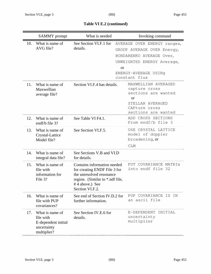
Section VI.E, page 3 (R8) Page 453
Table VI E.2 (continued)
Section VI.E, page 3 (R8) Page 453
SAMMY prompt What is needed Invoking command
10. What is name of AVG file?
See Section VI.F.1 for details.
AVERAGE OVER ENERGY ranges, GROUP AVERAGE OVER Energy, BONDARENKO AVERAGE Over, UNWEIGHTED ENERGY Average, or ENERGY-AVERAGE USINg constant flux
11. What is name of Maxwellian average file?
Section VI.F.4 has details. MAXWELLIAN AVERAGED capture cross sections are wanted or STELLAR AVERAGED CAPture cross sections are wanted
12. What is name of endf/b file 3?
See Table VI F4.1. ADD CROSS SECTIONS From endf/b file 3
13. What is name of Crystal-Lattice Model file?
See Section VI.F.5. USE CRYSTAL LATTICE model of doppler broadening, or CLM
14. What is name of integral data file?
See Sections V.B and VI.D for details.
15. What is name of file with information for File 3?
Contains information needed for creating ENDF File 3 for the unresolved resonance region. (Similar to *.ndf file, # 4 above.) See Section VI.F.2.
PUT COVARIANCE MATRIx into endf file 32
16. What is name of file with PUP covariances?
See end of Section IV.D.2 for further information.
PUP COVARIANCE IS IN an ascii file
17. What is name of file with E-dependent initial uncertainty multiplier?
See Section IV.E.6 for details.
E-DEPENDENT INITIAL uncertainty multiplier
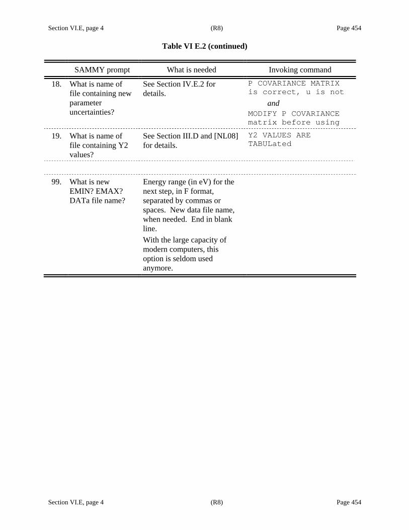
Section VI.E, page 4 (R8) Page 454
Table VI E.2 (continued)
Section VI.E, page 4 (R8) Page 454
SAMMY prompt What is needed Invoking command
18. What is name of file containing new parameter uncertainties?
See Section IV.E.2 for details.
P COVARIANCE MATRIX is correct, u is not and MODIFY P COVARIANCE matrix before using
19. What is name of file containing Y2 values?
See Section III.D and [NL08] for details.
Y2 VALUES ARE TABULated
99. What is new EMIN? EMAX? DATa file name?
Energy range (in eV) for the next step, in F format, separated by commas or spaces. New data file name, when needed. End in blank line. With the large capacity of modern computers, this option is seldom used anymore.

Section VI.F, page 1 (R7) Page 455
Section VI.F, page 1 (R7) Page 455
VI.F. OTHER INPUT FILES FOR SAMMY In addition to the INPut, PARameter, and DATa files, several special-purpose input files exist for various options available in SAMMY. These are discussed in the following sections:
1. The AVG file, described in Section VI.F.1, contains the energy ranges for calculation of multigroup cross sections.
2. In order for SAMMY to generate output in appropriate formats for the Evaluated Nuclear
Data Files (ENDF), ENDF-specific information is required. This is provided in the NDF file, described in Section VI.F.2.
3. ENDF Files 2 and/or 32 are sometimes used as input to SAMMY. See Section VI.F.3 for
details. 4. The calculation of Maxwellian or stellar-averaged capture cross sections requires
information about which temperatures are to be used for the calculation. Section VI.F.4 provides information about this input file.
5. The Crystal Lattice Model of Doppler broadening requires additional input, as shown in
Section VI.F.5.


Section VI.F.1, page 1 (R7) Page 457
Section VI.F.1, page 1 (R7) Page 457
VI.F.1. The AVeraGe File
In Section V.C, descriptions are given of the way SAMMY can be used to produce energy- averaged, time-averaged, Bondarenko-averaged, or unweighted energy-averaged cross sections and the associated covariance matrix. To invoke these options, alphanumeric command lines must be included in the INPut file. For energy- or time-averaging (Section V.C.1), the command is
AVERAGE OVER ENERGY ranges.
For Bondarenko averaging, the command is
GROUP AVERAGE OVER Energy ranges, or BONDARENKO AVERAGE Over energy ranges.
For unweighted energy-averaging, the command is
UNWEIGHTED ENERGY Average, or ENERGY-AVERAGE USINg constant flux
One or more additional files are required, which are denoted the AVG (AVeraGe) files or
BON (BONdarenko) files; their names are given to SAMMY as interactive input (see Table VI E .1), directly following the name of the first data file, or, if a COVariance file is used, directly after the name of the COVariance file . Formats for AVG files are given in Table VI F1.1, and for the BON files in Table VI F1.2. The two types of files follow very much the same format, except the BON files require additional input parameter values. For unweighted energy-averaging, either file may be used (the “TYPE” line is ignored). For all types of multigroup averaging, it is possible to print the partial derivatives (sensitivities) of the multigroup cross sections with respect to the resonance parameters and to print the associated multigroup covariance matrix. The command
PRINT AVERAGED SENSItivities for endf parameters will cause the creation of several files, all in ASCII format:
SAMAVG.COV contains the multigroup covariance matrix.
SAMSEN.DAT contains partial derivatives of all multigroup cross sections with respect to resonance parameters of the five lowest-lying resonances. These derivatives are with respect to the p-parameters (see Section IV.C) rather than u-parameters, that is, with respect to the “endf parameters” as suggested in the command line.
SAMMY.LLL contains the same information as the multigroup-average portion of the SAMMY.LPT file, but in reverse energy order to facilitate comparison with results from some processor codes.
SAMMY.MGS contains the multigroup cross section (and nothing else), again in reverse energy order, to facilitate porting to spreadsheets for comparisons with output from other codes.

Section VI.F.1, page 2 (R7) Page 458
Section VI.F.1, page 2 (R7) Page 458
Table VI F1.1. Format of the AVG file
Line Number
Col-umn
Variable Name Format
Meaning (units)
Possible Values Notes
1 1-80 TITLE A80
2 1-10 TYPE A10 Type of averaging to be used
“ENERGY-AVErage” or “TIME-AVERAge”
energy- or time- average
3 1-10 EMIN F10 Minimum energy for this range (eV)
11-20 EMAX F10 Maximum energy for this range (eV)
If EMAX = 0, use EMAX equal to the value given for EMIN on the next line
4, 5, ... (repeat line 3 as many times as needed)
last (blank)
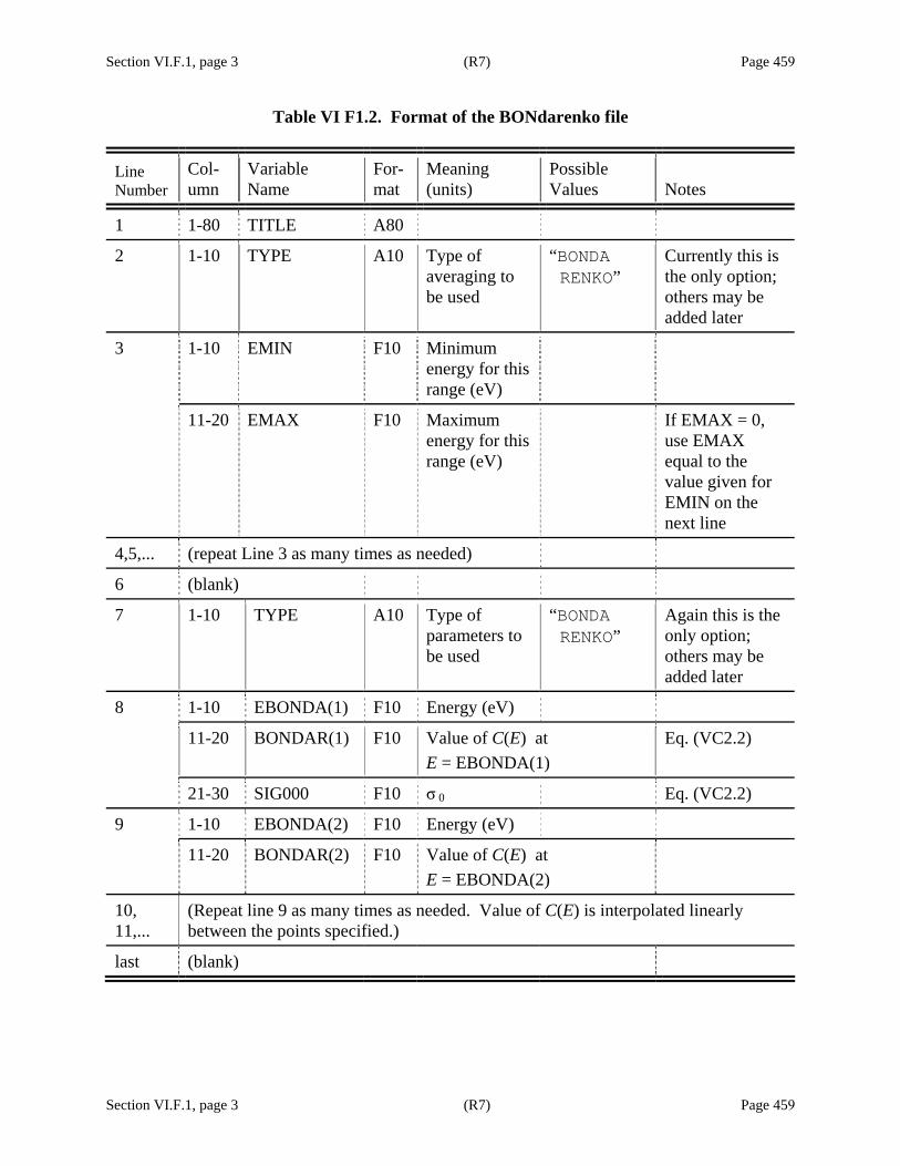
Section VI.F.1, page 3 (R7) Page 459
Section VI.F.1, page 3 (R7) Page 459
Table VI F1.2. Format of the BONdarenko file
Line Number
Col-umn
Variable Name
For-mat
Meaning (units)
Possible Values Notes
1 1-80 TITLE A80
2 1-10 TYPE A10 Type of averaging to be used
“BONDA RENKO”
Currently this is the only option; others may be added later
3 1-10 EMIN F10 Minimum energy for this range (eV)
11-20 EMAX F10 Maximum energy for this range (eV)
If EMAX = 0, use EMAX equal to the value given for EMIN on the next line
4,5,... (repeat Line 3 as many times as needed)
6 (blank)
7 1-10 TYPE A10 Type of parameters to be used
“BONDA RENKO”
Again this is the only option; others may be added later
8 1-10 EBONDA(1) F10 Energy (eV)
11-20 BONDAR(1) F10 Value of C(E) at E = EBONDA(1)
Eq. (VC2.2)
21-30 SIG000 F10 σ 0 Eq. (VC2.2)
9 1-10 EBONDA(2) F10 Energy (eV)
11-20 BONDAR(2) F10 Value of C(E) at E = EBONDA(2)
10, 11,...
(Repeat line 9 as many times as needed. Value of C(E) is interpolated linearly between the points specified.)
last (blank)


Section VI.F.2, page 1 (R7) Page 461
Section VI.F.2, page 1 (R7) Page 461
VI.F.2. Input to Produce Files in ENDF File 2 or File 32 Format
SAMMY is capable of converting information obtained from the usual SAMMY INPut and PARameter files (plus a modest amount of additional input) into ENDF File 2 format, in several of the many versions of that format. To invoke this option, the following line must be included in the INPut file:
ENDF/B-VI FILE 2 IS wanted (This may be shortened to “ENDF” if desired.)
One additional file is required, denoted the “ndf” file, whose name is supplied to SAMMY in the site in which SAMMY would normally expect the DATa file name (see Section VI.E). Contents of this file are shown in Table VI F2.1.
There is a more convenient version of the ndf file, which is used when the INPut file contains the command line
NDF FILE IS IN KEY-Word format This is the preferred version for the ndf file. Formats for the file are key word based; see Table VI F2.2 for details. Below are two examples of key word files:
235U 23Na
Z=92 A=235 Isotope # 1 Spi=7.5 L=0,Group=1,2
Z=11 A=23 Mat=1125 Isotope=1 Spin=1.5 L=0,GROUP=1,2 L=1,GROUP=3,4,5,6,7,8 L=2,GROUP=9,10,11,12,13,14,15,16
In either case, SAMMY will produce a file called SAMMY.NDF, which contains the appropriate lines for ENDF/B File 2. See test cases tr023, tr086, tr126, tr137, tr154 for examples.
In SAMMY.NDF, resonance energies are given in F format, to as many significant digits as possible within the limitation of eleven columns. Widths are given in E format, with, however, the “E” suppressed and the exponent given as one digit if possible.

Section VI.F.2, page 2 (R7) Page 462
Section VI.F.2, page 2 (R7) Page 462
To produce ENDF File 32 (covariance matrix for resonance parameters), include the command
PUT COVARIANCE MATRIx into endf file 32 Only the key word version of the ndf file is acceptable for this option. Parameters such as “LCOmp”, “DIAgonal” and “DEfault uncertainty” are relevant here; see Table VI F2.2. The output file, to be used as ENDF File 32, is called SAMMY.N32.
When the command DEBUG is given in the INPut file, then additional “annotated” files will be produced by SAMMY, to aid the reader in understanding what is where in the ENDF file. The file SAMMY.NDX is identical to file SAMMY.NDF, except that it also contains annotations (lines beginning with #) describing the information in the file. Similarly, the file SAMMY.N3X is identical to the first portion of SAMMY.N32 except for the annotations.
NOTE: The ENDF File 2 LRF=3 convention for the angular momentum parameter AJ is as follows: AJ is defined as " J, where the sign denotes the channel spin s; AJ = − J denotes s = I − i, with i = 1/2 for neutron; AJ = +J denotes s = I + i . This is in compliance with the format change approved by the Cross Section Evaluation Working Group at the 1999 meeting [ENDF 99].
CAUTION: SAMMY’s original implementation of the LRF=7 format was not entirely correct for 0− nuclides; the negative parity was not specified properly. To the best of the author’s knowledge, no official ENDF files were created with this version of SAMMY. Nevertheless, anyone using very early examples of LRF=7 ENDF files for 0− nuclides should check to be certain that the file behaves as expected.
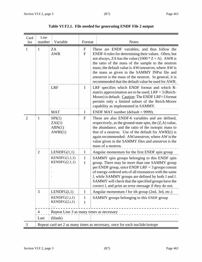
Section VI.F.2, page 3 (R7) Page 463
Section VI.F.2, page 3 (R7) Page 463
Table VI F2.1. File needed for generating ENDF File 2 output
Card Set
Line number Variable Format Notes
1 1 ZA AWR
F F
These are ENDF variables, and thus follow the ENDF-6 rules for determining their values. Often, but not always, ZA has the value (1000 * Z + A). AWR is the ratio of the mass of the sample to the neutron mass; the default value is AW/aneutron, where AW is the mass as given in the SAMMY INPut file and aneutron is the mass of the neutron. In general, it is recommended that the default value be used for AWR.
LRF I LRF specifies which ENDF format and which R-matrix approximation are to be used; LRF = 3 (Reich-Moore) is default. Caution: The ENDF LRF=3 format permits only a limited subset of the Reich-Moore capability as implemented in SAMMY.
MAT I ENDF MAT number (default = 9999). 2 1 SPI(1)
ZAI(1) ABN(1) AWRI(1)
F These are also ENDF-6 variables and are defined, respectively, as the ground-state spin, the (Z,A) value, the abundance, and the ratio of the isotopic mass to that of a neutron. Use of the default for AWRI(i) is again recommended: AW/aneutron, where AW is the value given in the SAMMY files and aneutron is the mass of a neutron.
2 LENDFG(1,1) I Angular momentum for the first ENDF spin group KENDFG(1,1,1)
KENDFG(2,1,1) . . .
I I
SAMMY spin groups belonging to this ENDF spin group. There may be more than one SAMMY group per ENDF group, since ENDF LRF = 3 groups consist of energy-ordered sets of all resonances with the same l, while SAMMY groups are defined by both J and l. SAMMY will check that the specified groups have the correct l, and print an error message if they do not.
3 LENDFG(i,1) I Angular momentum l for ith group (2nd, 3rd, etc.) KENDFG(1,i,1)
KENDFG(2,i,1) . . .
I I
SAMMY groups belonging to this ENDF group
4 Repeat Line 3 as many times as necessary Last (blank)
3 Repeat card set 2 as many times as necessary, once for each nuclide/isotope

Section VI.F.2, page 4 (R8) Page 464
Section VI.F.2, page 4 (R8) Page 464
Table VI F2.2. Key-word-based file needed for generating ENDF File 2 output. For each key word used, only those few characters written as capitals in the table are required; those in lowercase are optional. Key words may be given as capital, lower-case, or mixed case letters.
Card set
Key word variable Notes
1 Z Z for target nucleus
A Atomic mass number
ZA If different from (1000 * Z + A), then this value must be inserted directly.
AWr Ratio of the mass of the sample nucleus to the neutron mass. AWR is the ratio of the mass of the sample to the neutron mass; the default value is AW/mn where AW is the mass as given in the SAMMY INPut file and mn is the mass of the neutron. In general, it is recommended that the default value be used for AWR.
Mat ENDF MAT number (default = 9999)
MT ENDF reaction number, for file 3 output
LRF Which ENDF file 2 format and which R-matrix approximation are to be used (1 = SLBW, 2 = MLBW, 3 = RM, 7 = RML). If LRF is not specified, SAMMY will choose the appropriate value.
LCOmp Which ENDF file 32 format is to be used:
LCOMP = 0 can be used only for LRF = 1 or 2; results are not guaranteed to be correct. Use of this format is discouraged.
LCOMP = 1 can be used for LRF = 1, 2, 3, or 7, or for URR.
LCOMP = 2 (“compact”) can be used for LRF = 1, 2, 3, or 7, or for URR. However, this format should be used with extreme caution as it is a crude approximation.
(The format for LCOMP = 1, LRF = 7, was accepted as an official ENDF format in November, 2006.)
NDigit Number of digits to be used for LCOMP = 2. NDigit = 2,3,4,5,6 are approved ENDF formats.
DIAgonal If LCOmp = 1 and DIAgonal = Yes, then only the diagonal pieces of the covariance matrix will be specified in File 32.
NUmber Number of energies to be included (for URR only)
E Energy (for URR)

Section VI.F.2, page 5 (R8) Page 465
Table VIF.2 (continued)
Section VI.F.2, page 5 (R8) Page 465
Card set
Key word variable Notes
1 cont.
DEfault uncertainty or DU
Relative uncertainty for unflagged parameters. The value of the uncertainty to be printed in File 32 is this value times the value of the parameter.
FLagged Only resonances with flagged parameters (flag = 1) will be included in file 32. (No value needs to be given here.)
ALl All resonances are to be included in file 32. (No value needs to be given here.)
(blank) Terminate this card set with a blank line.
2 ISOtope or NUClide
(No value needs to be given here.)
3 Z Z for target nucleus (this isotope)
A Atomic mass number (this isotope)
ZA If different from (1000 * Z + A), then this value must be inserted directly.
AWr Ratio of the mass of the sample nucleus (this isotope) to the neutron mass. Again, it is recommended that the default value be used rather than giving the value here explicitly.
ABn Abundance for this isotope
SPin Ground state spin for this isotope
(blank) Terminate this card set with a blank line.
4 L (card set is not needed for LRF = 7)
Orbital angular momentum for this ENDF spin group. On the same line, give key word “GROUP” and specify the SAMMY group numbers that contribute to this l for this isotope. Example: L=0, Group=1,2,3
5 Repeat card set 4 as many times as needed, ending with a blank line.
6 Repeat from card set 2 through card set 5, as many times as needed. (CAUTION: The author does not guarantee that the program will work properly for more than one isotope.)
7 SHort For LCOMP = 1, LRF = 3, the “short-range section information” follows this line; see the ENDF-102 description of File 32 input for details. Be sure that at least two blank lines precede this line.

Section VI.F.2, page 6 (R8) Page 466
Table VIF.2 (continued)
Section VI.F.2, page 6 (R8) Page 466
Card set
Key word variable Notes
8 N Ordinal number for this short-range section. (This number is for your use only, so the value is arbitrary.) On the same line, give key word “Spin group” and specify the ordinal numbers for the spin groups to be included in this section. Example: N=1 S=1,3,4
9 energy range On the line immediately following card set 8, give the energy range (minimum to maximum) for resonances to be included in the short-range section. No key word is required, but an equal sign must be present. Example: Energy range = -10. 20.
10 Repeat card sets 8–9 as many times as needed. End with a blank line.
Section VI.F.3, page 1 (R7) Page 467
Section VI.F.3, page 1 (R7) Page 467
VI.F.3. Using ENDF File 2 as input to SAMMY
Instead of manually creating a SAMMY-type PARameter file and an entire SAMMY-type INPut file, a user may retrieve resonance parameters (File 2) from the Evaluated Nuclear Data Files (ENDF) Library at the National Nuclear Data Center [NNDC] and use that file directly as input to SAMMY. The first portion of a SAMMY-type INPut file is still required; this file contains card sets 1–8 but no others (see Table VI A .1). Included in card set 3 of the INPut file must be the line
INPUT IS ENDF/B FILE MAT=abcd , in which “abcd” is to be replaced by the ENDF MAT (material) number. The name of the ENDF/B file is included in the input stream where the name of the PARameter file is called for.
Prior to Release M6 of the SAMMY code, it was necessary for the user to edit the ENDF file and extract File 2 for the material of interest. This is no longer needed; SAMMY will now search through a long ENDF file and use the relevant portion. However, if the command line reads only
INPUT IS ENDF/B FILE without the MAT number, then SAMMY will assume (as in the past) that the ENDF file contains only File 2 for the material of interest.
With either of the commands given above, only resonance parameters and spin-group quantum numbers are retrieved from the ENDF File 2. If the energy range from the ENDF file is to be used for the SAMMY run, then the command
USE ENERGY RANGE FROm endf/b file 2 is given in the INPut file.
(Note that additional commands may be required for the experimental data and associated energy grid. In general, the user must provide a separate file for the experimental data in the customary fashion as described in Section VI C.1.)
Output from a run using an ENDF file for input includes several additional files not usually found in SAMMY output. The first is SAMNDF.INP which is a SAMMY-type INPut file containing the spin group information in card set 10.1 format. The second, SAMNDF.PAR, is a SAMMY-type PARameter file containing the resonance parameter information from the ENDF file, translated into SAMMY formats. These two files can then be modified as needed and used for subsequent SAMMY runs.
A third member of this list of additional output files is SAMQUA.PAR, a PARameter file that contains quantum number information as well as resonance parameters. See Table VI B.3 for a detailed explanation of this file.

Section VI.F.3, page 2 (R7) Page 468
Section VI.F.3, page 2 (R7) Page 468
Caveat # 1: Only isotopic ENDF files can be used as input for SAMMY runs. For example, one could use the file for 28Si but not the file for natural silicon.
Caveat # 2: The file SAMNDF.INP contains a command (card set 3) specifying which type of R-matrix approximation was used for the ENDF file. For example, if the ENDF File 2 indicates LRF=1, then the resonance parameters were determined by a procedure that used the single-level Breit-Wigner approximation; SAMNDF.INP therefore will contain the command line “SLBW FORMALISM IS WANTED”. Similarly LRF = 2 indicates multilevel Breit Wigner, and LRF = 3 indicates the ENDF Reich-Moore approximation.
If the intent of the user is simply to use SAMMY to create a plot of the evaluated cross sections, then the SAMMY runs should indeed use the same approximation as was used to define the ENDF file.
However, if the intent is to use the ENDF File 2 parameters as starting values for analysis of new data, or for a new evaluation, then the user is encouraged to modify (or remove) the command in the INPut file for subsequent runs. New analyses should use the Reich-Moore approximation, which is the default option for SAMMY.

Section VI.F.4, page 1 (R5) Page 469
Section VI.F.4, page 1 (R5) Page 469
VI.F.4. Format of the MXW File
In order to generate stellar (Maxwellian) averages of capture cross sections (see Section V.D), two pieces of input are needed. In the alphanumeric portion (card set 3) of the INPut file, the line
MAXWELLIAN AVERAGED capture cross sections are wanted
or STELLAR AVERAGED CAPture cross sections are wanted
must be included (the two phrases are treated identically within the code). It is also necessary to specify the temperatures at which the stellar averages are to be calculated; these are given in a “MXW” file whose name is specified immediately following the name of the DATa file in the input stream. The format of the MXW file is one temperature per line, in F10.1 format, in units of eV.
When calculating stellar averages, it is often desirable to include cross sections at energies above the resolved resonance region. In SAMMY, this may be done by providing the “smooth cross section” in the ENDF File 3 format. Users must also include the following line
ADD CROSS SECTIONS From endf/b file 3 in the alphanumeric portion of the INPut file.
For users unfamiliar with ENDF formats, a description of the relevant portions of File 3 is presented in Table VI F4.1. Note that the parameter INT specifies an interpolation scheme for NBT energy points. For INT = 1, the cross section from Ei to Ei+1 is constant and equal to Ci. For INT = 2, the cross section for Ei < E < Ei+1 is linearly interpolated between the two values. (Note that other options are available in ENDF but only these two have been implemented in SAMMY.)
Examples for stellar averaging are given in test cases tr042, tr049, and tr051.
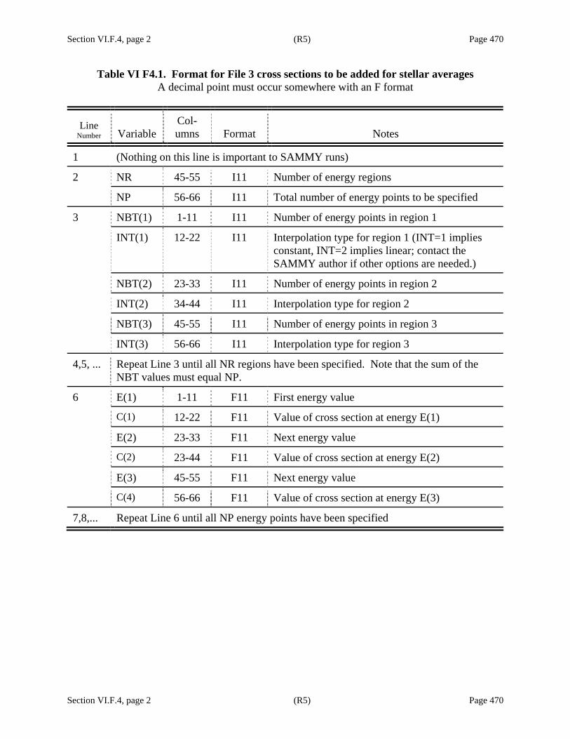
Section VI.F.4, page 2 (R5) Page 470
Section VI.F.4, page 2 (R5) Page 470
Table VI F4.1. Format for File 3 cross sections to be added for stellar averages A decimal point must occur somewhere with an F format
Line Number Variable
Col-umns Format Notes
1 (Nothing on this line is important to SAMMY runs)
2 NR 45-55 I11 Number of energy regions
NP 56-66 I11 Total number of energy points to be specified
3 NBT(1) 1-11 I11 Number of energy points in region 1
INT(1) 12-22 I11 Interpolation type for region 1 (INT=1 implies constant, INT=2 implies linear; contact the SAMMY author if other options are needed.)
NBT(2) 23-33 I11 Number of energy points in region 2
INT(2) 34-44 I11 Interpolation type for region 2
NBT(3) 45-55 I11 Number of energy points in region 3
INT(3) 56-66 I11 Interpolation type for region 3
4,5, ... Repeat Line 3 until all NR regions have been specified. Note that the sum of the NBT values must equal NP.
6 E(1) 1-11 F11 First energy value
C(1) 12-22 F11 Value of cross section at energy E(1)
E(2) 23-33 F11 Next energy value
C(2) 23-44 F11 Value of cross section at energy E(2)
E(3) 45-55 F11 Next energy value
C(4) 56-66 F11 Value of cross section at energy E(3)
7,8,... Repeat Line 6 until all NP energy points have been specified

Section VI.F.5, page 1 (R7) Page 471
Section VI.F.5, page 1 (R7) Page 471
VI.F.5. Crystal-Lattice Model File
The crystal-lattice model of Doppler broadening, discussed in Section III.B.4, requires additional input beyond that needed by other Doppler models: (1) In the INPut file, include one of these alphanumeric commands:
USE CRYSTAL LATTICE model of doppler broadening or CLM (2) Provide the location/name of the CLM file in the input stream, directly after the name of the
DATa file. The format for the CLM file is given in Table VI F5.1, where we have again used the convention that “C:L” implies “card set number: line number” and the notation “f-f ” refers to “free format.”
Table VI F5.1. Format of the SAMMY CLM file (crystal-lattice model) Note: “f-f” indicates “free-format”
C:L Variable Name Format
Possible Values
Default Value Meaning
1:1 Title A80 Alphanumeric title
2:1 Mode_ S_Norm
f-f integer 0 or 1 0 Mode of normalization 0 do not correct the S function 1 correct the S function
Nphon f-f integer > 0 Phonon-expansion order
Sub f-f real > 0.0 1.0 Number of subdivisions between the spectrum points for beta mesh
Xdop f-f real > 0.0 1.0 Initial Doppler cut of beta mesh
Eps f-f real > 0.0, small
0.08 Precision over normalization and sum rule check of scattering law
Epsc f-f real > 0.0, small
0.001 Precision of convolution integral calculation
2:2 (blank)
3:1 What A5 CONTI Continuous distribution parameters follow
3:2 Del_Phonon f-f real > 0.0 Interval (in eV) between points of the phonon distribution
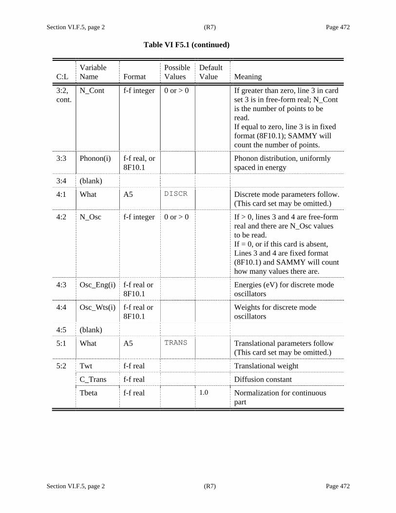
Section VI.F.5, page 2 (R7) Page 472 Table VI F5.1 (continued)
Section VI.F.5, page 2 (R7) Page 472
C:L Variable Name Format
Possible Values
Default Value Meaning
3:2, cont.
N_Cont f-f integer 0 or > 0 If greater than zero, line 3 in card set 3 is in free-form real; N_Cont is the number of points to be read. If equal to zero, line 3 is in fixed format (8F10.1); SAMMY will count the number of points.
3:3 Phonon(i) f-f real, or 8F10.1
Phonon distribution, uniformly spaced in energy
3:4 (blank)
4:1 What A5 DISCR Discrete mode parameters follow. (This card set may be omitted.)
4:2 N_Osc f-f integer 0 or > 0 If > 0, lines 3 and 4 are free-form real and there are N_Osc values to be read. If = 0, or if this card is absent, Lines 3 and 4 are fixed format (8F10.1) and SAMMY will count how many values there are.
4:3 Osc_Eng(i) f-f real or 8F10.1
Energies (eV) for discrete mode oscillators
4:4 Osc_Wts(i) f-f real or 8F10.1
Weights for discrete mode oscillators
4:5 (blank)
5:1 What A5 TRANS Translational parameters follow (This card set may be omitted.)
5:2 Twt f-f real Translational weight
C_Trans f-f real Diffusion constant
Tbeta f-f real 1.0 Normalization for continuous part
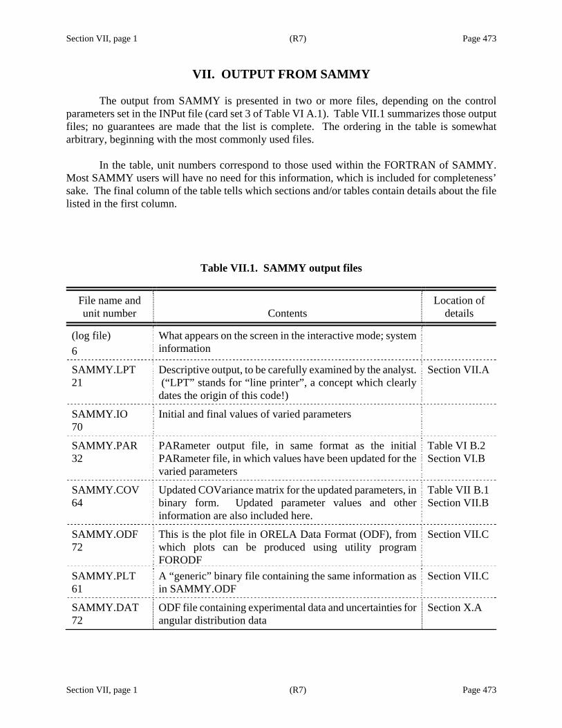
Section VII, page 1 (R7) Page 473
Section VII, page 1 (R7) Page 473
VII. OUTPUT FROM SAMMY
The output from SAMMY is presented in two or more files, depending on the control parameters set in the INPut file (card set 3 of Table VI A.1). Table VII.1 summarizes those output files; no guarantees are made that the list is complete. The ordering in the table is somewhat arbitrary, beginning with the most commonly used files.
In the table, unit numbers correspond to those used within the FORTRAN of SAMMY.
Most SAMMY users will have no need for this information, which is included for completeness’ sake. The final column of the table tells which sections and/or tables contain details about the file listed in the first column.
Table VII.1. SAMMY output files
File name and unit number Contents
Location of details
(log file) 6
What appears on the screen in the interactive mode; system information
SAMMY.LPT 21
Descriptive output, to be carefully examined by the analyst. (“LPT” stands for “line printer”, a concept which clearly dates the origin of this code!)
Section VII.A
SAMMY.IO 70
Initial and final values of varied parameters
SAMMY.PAR 32
PARameter output file, in same format as the initial PARameter file, in which values have been updated for the varied parameters
Table VI B.2 Section VI.B
SAMMY.COV 64
Updated COVariance matrix for the updated parameters, in binary form. Updated parameter values and other information are also included here.
Table VII B.1 Section VII.B
SAMMY.ODF 72
This is the plot file in ORELA Data Format (ODF), from which plots can be produced using utility program FORODF
Section VII.C
SAMMY.PLT 61
A “generic” binary file containing the same information as in SAMMY.ODF
Section VII.C
SAMMY.DAT 72
ODF file containing experimental data and uncertainties for angular distribution data
Section X.A
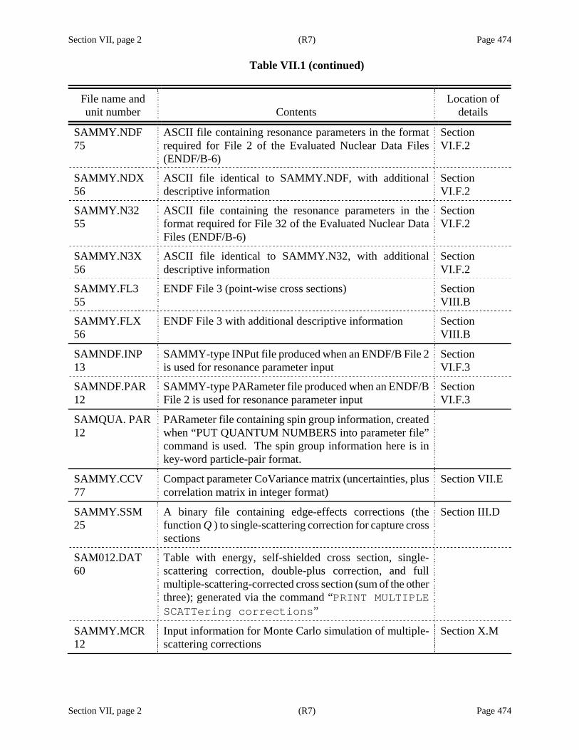
Section VII, page 2 (R7) Page 474
Table VII.1 (continued)
Section VII, page 2 (R7) Page 474
File name and unit number Contents
Location of details
SAMMY.NDF 75
ASCII file containing resonance parameters in the format required for File 2 of the Evaluated Nuclear Data Files (ENDF/B-6)
Section VI.F.2
SAMMY.NDX 56
ASCII file identical to SAMMY.NDF, with additional descriptive information
Section VI.F.2
SAMMY.N32 55
ASCII file containing the resonance parameters in the format required for File 32 of the Evaluated Nuclear Data Files (ENDF/B-6)
Section VI.F.2
SAMMY.N3X 56
ASCII file identical to SAMMY.N32, with additional descriptive information
Section VI.F.2
SAMMY.FL3 55
ENDF File 3 (point-wise cross sections) Section VIII.B
SAMMY.FLX 56
ENDF File 3 with additional descriptive information Section VIII.B
SAMNDF.INP 13
SAMMY-type INPut file produced when an ENDF/B File 2 is used for resonance parameter input
Section VI.F.3
SAMNDF.PAR 12
SAMMY-type PARameter file produced when an ENDF/B File 2 is used for resonance parameter input
Section VI.F.3
SAMQUA. PAR 12
PARameter file containing spin group information, created when “PUT QUANTUM NUMBERS into parameter file” command is used. The spin group information here is in key-word particle-pair format.
SAMMY.CCV 77
Compact parameter CoVariance matrix (uncertainties, plus correlation matrix in integer format)
Section VII.E
SAMMY.SSM 25
A binary file containing edge-effects corrections (the function Q ) to single-scattering correction for capture cross sections
Section III.D
SAM012.DAT 60
Table with energy, self-shielded cross section, single-scattering correction, double-plus correction, and full multiple-scattering-corrected cross section (sum of the other three); generated via the command “PRINT MULTIPLE SCATTering corrections”
SAMMY.MCR 12
Input information for Monte Carlo simulation of multiple-scattering corrections
Section X.M

Section VII, page 3 (R7) Page 475
Table VII.1 (continued)
Section VII, page 3 (R7) Page 475
File name and unit number Contents
Location of details
SAMXAC.ODF
No longer available (replaced with SAMMY.UNB, to eliminate redundancy in the code)
SAMMY.UNB 9
Binary file in ODF format, containing energy in Section 1 and unbroadened cross section in other sections, created when command “PUT UNBROADENED CROSs sections into plot file” is invoked
Section VII.G
SAMUNB.DAT 9
ASCII file containing auxiliary energy grid and unbroadened cross section in TWENTY format, created when command “PUT UNBROADENED CROSs sections into plot file” is invoked
Section VII.G
SAMUNX.DAT 9
ASCII file containing auxiliary energy grid and unbroadened cross sections in CSISRS format, created when command “PUT UNBROADENED CROSs sections into plot file” is invoked, for those cases where more than one type of cross section is available
Section VII.G
SAMMY.LEG 99
ASCII file containing energy and Legendre coefficients for all possible L for each energy in the auxiliary grid. In older versions, this file was called “legendre.dat”
SAMMY.N04 97
Legendre coefficients in format for ENDF File 4. In older versions, this file was called “endf_legendre.dat”
Section IX
SAMJNK.DAT 96
The same information as SAMMY.LEG or SAMMY.N04, in expanded format
Section IX
SAMMY.LLL 69
Average cross sections and uncertainties Section VI.F.1
SAMAVG.COV 29
ASCII file containing covariance matrix for multigroup average cross sections
Section VI.F.1
SAMSEN.DAT 29
Partial derivatives of averaged cross section with respect to some of the R-matrix parameters
Section VI.F.1
SAMMY.CRS 55
Multigroup average cross sections, in ENDF-like file Section IX
SAMMY.N33 55
Covariance matrix for multigroup average cross sections, in ENDF File 33 format
Section IX

Section VII, page 4 (R7) Page 476
Table VII.1 (continued)
Section VII, page 4 (R7) Page 476
File name and unit number Contents
Location of details
SAMMY.PUB 37
Tabulated file containing all resonance parameters and uncertainties, in a form suitable for porting to spreadsheets for formatting for publication
Section VII.F
SAMCOV.PUB 37
Tabulated file containing the calculated cross sections and the associated covariance matrix. The cross sections are “point-wise” (i.e., given at specific energies).
Section IV.E.4
SAMMY.PA2 33
Modified PARameter file when “REFORMULATE DATA FOR implicit data covariance”
Section VI.C.3.c
SAMMY.IDC 34
File containing normalization and background information when “REFORMULATE DATA FOR implicit data covariance”
Section VI.C.3.c
SAMMY.DA2 15
Modified DATa file in which normalization and background corrections have been made, when “REFORMULATE DATA FOR implicit data covariance”
Section VI.C.3.c
SAMCOV.PUP 40
File containing values and covariances for varied u-parameters (to be used as PUPs in later runs), created when the command “CREATE PUP FILE FROM varied parameters used in this run” is given in the INPut file
Section VI.C.3.a
SAMMY.REL 12
PARameter file in which only the “relevant” parameters have been flagged
Table VI A1.2
INPUT.NEW 22
Spin group information in the format of card set 10.1, provided as a possible alternative to the obsolete format used in the INPut file
REMORI.PAR 25
Binary file containing original parameter file and inverse of original parameter covariance matrix, when needed for iterations with M+W method of solution of Bayes’ equations
Section IV.E.3
SAMMY.YWY 32
Binary file containing contribution of one data set to the Y and W matrices needed in M+W method of solution of Bayes’ equations
Section IV.E.1
SAMMY.PDS 71
Partial derivatives of the theoretical values with respect to every resonance parameter
Section VII.D

Section VII.A, page 1 (R7) Page 477
Section VII.A, page 1 (R7) Page 477
VII.A. LINE-PRINTER OUTPUT
The first two output files (the “LPT” and the “IO” files) are intended for visual inspection. The LPT file contains full output, detailed to the extent specified by the user in the INPut file (see Tables VI A.1 and VI A1.2).
The IO file merely lists initial and final parameter values.
The LPT file contains a wealth of information with which users should become familiar. Here you find, among other things, $ Input file names; $ Title for the run (taken from your INPut file); $ Values for varied and fixed parameters; $ Verbatim alphanumeric commands (with notification if the command is not recognized); $ Chronological listing of the SAMMY segments used in the run; $ Updated parameter values, uncertainties, and correlation values; $ Chi-squared values; $ Error messages, if applicable. Sample LPT files may be found among the output for the test cases or tutorial exercises; see Section XII.
It is strongly recommended that novice SAMMY users examine the LPT file for each run, to be sure SAMMY is interpreting input as the user intended. Even experienced SAMMY users should regularly look at the LPT file, especially when output parameter values or chi-squared values are puzzling or when the run ends abnormally. Such problems are often the result of user input errors, which can frequently be discovered by comparing intended input values with the values as listed in the LPT file. In addition, the LPT file often provides error messages to guide the user into fixing an input error. Error messages are also provided for abnormal aborts for common input errors. (Please notify the author if you have suggestions for a more informative error message for your favorite mistake.)


Section VII.B, page 1 (R7) Page 479
Section VII.B, page 1 (R7) Page 479
VII.B. OUTPUT TO BE USED AS INPUT
Two output files (the “PAR” and the “COV” files) are intended to be used as input to another SAMMY run. The PAR file is as described in Section VI.B, with the “Last A” alternative chosen for the “last” card set of Table VI B.2.
In very early versions of SAMMY, the output “binary COVariance file” contained only the new (updated) covariance matrix for physical parameters (i.e., not for the u-parameters; see Section IV.C). Output parameter values were stored in the output PARameter file. When these two files were used as input to another run, the covariance matrix for the u-parameters was generated from Eq. (IV C.1).
Two drawbacks to this scheme led to expansion of the COV file. First, unnecessary computer time was spent in making the conversion back to u-parameters. Second, and more important, was the loss of precision between runs. In converting from u-parameters to physical parameters, storing these in ASCII format, reading them back in for the next run, and converting back to u-parameters, often the last several significant digits were lost. One would expect that analysis of two energy regions, first in two separate executions of SAMMY, then in one execution but still analyzing the two regions sequentially, should give identical results. With the early storage scheme, small differences occurred; with the current scheme, no discrepancies are found.
SAMMY users should keep in mind the following:
If a COVariance file is specified, SAMMY will use parameter values given in the (binary) COVariance file rather than those given in the PARameter file.
That is, all parameter values are taken from the values stored in the binary COVariance file; these values are more precise than those in the PARameter file. (See, however, the end of this section for exceptions to this rule.)
Table VII B.1 shows which variables are written in what order in the COVariance file. Dotted lines separate values kept in separate records.
Occasionally a user may wish to modify the contents of the COVariance file (and associated PARameter file), in order to de-activate a measurement-related parameter (e.g., sample thickness or Doppler temperature) and activate the comparable parameter for the measurement to be analyzed next. This may be accomplished using the program SAMAMR; see Section X.C for details.
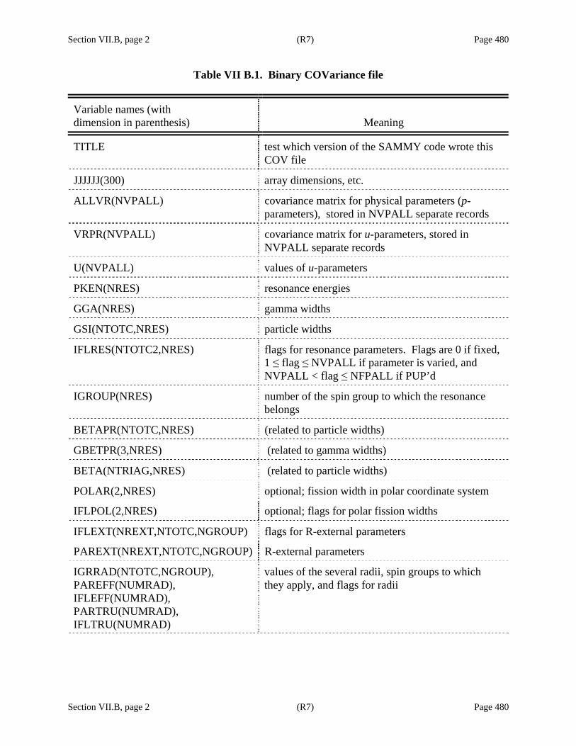
Section VII.B, page 2 (R7) Page 480
Section VII.B, page 2 (R7) Page 480
Table VII B.1. Binary COVariance file
Variable names (with dimension in parenthesis) Meaning
TITLE
test which version of the SAMMY code wrote this COV file
JJJJJJ(300) array dimensions, etc.
ALLVR(NVPALL) covariance matrix for physical parameters (p-parameters), stored in NVPALL separate records
VRPR(NVPALL) covariance matrix for u-parameters, stored in NVPALL separate records
U(NVPALL) values of u-parameters
PKEN(NRES) resonance energies
GGA(NRES) gamma widths
GSI(NTOTC,NRES) particle widths
IFLRES(NTOTC2,NRES) flags for resonance parameters. Flags are 0 if fixed, 1 ≤ flag ≤ NVPALL if parameter is varied, and NVPALL < flag ≤ NFPALL if PUP’d
IGROUP(NRES) number of the spin group to which the resonance belongs
BETAPR(NTOTC,NRES) (related to particle widths)
GBETPR(3,NRES) (related to gamma widths)
BETA(NTRIAG,NRES) (related to particle widths)
POLAR(2,NRES) optional; fission width in polar coordinate system
IFLPOL(2,NRES) optional; flags for polar fission widths
IFLEXT(NREXT,NTOTC,NGROUP) flags for R-external parameters
PAREXT(NREXT,NTOTC,NGROUP) R-external parameters
IGRRAD(NTOTC,NGROUP), PAREFF(NUMRAD), IFLEFF(NUMRAD), PARTRU(NUMRAD), IFLTRU(NUMRAD)
values of the several radii, spin groups to which they apply, and flags for radii
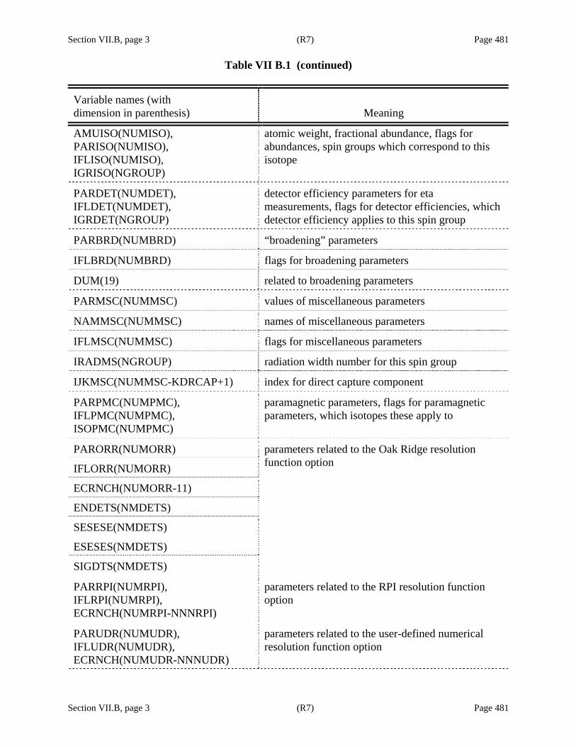
Section VII.B, page 3 (R7) Page 481 Table VII B.1 (continued)
Section VII.B, page 3 (R7) Page 481
Variable names (with dimension in parenthesis) Meaning
AMUISO(NUMISO), PARISO(NUMISO), IFLISO(NUMISO), IGRISO(NGROUP)
atomic weight, fractional abundance, flags for abundances, spin groups which correspond to this isotope
PARDET(NUMDET), IFLDET(NUMDET), IGRDET(NGROUP)
detector efficiency parameters for eta measurements, flags for detector efficiencies, which detector efficiency applies to this spin group
PARBRD(NUMBRD) “broadening” parameters
IFLBRD(NUMBRD) flags for broadening parameters
DUM(19) related to broadening parameters
PARMSC(NUMMSC) values of miscellaneous parameters
NAMMSC(NUMMSC) names of miscellaneous parameters
IFLMSC(NUMMSC) flags for miscellaneous parameters
IRADMS(NGROUP) radiation width number for this spin group
IJKMSC(NUMMSC-KDRCAP+1) index for direct capture component
PARPMC(NUMPMC), IFLPMC(NUMPMC), ISOPMC(NUMPMC)
paramagnetic parameters, flags for paramagnetic parameters, which isotopes these apply to
PARORR(NUMORR)
IFLORR(NUMORR)
ECRNCH(NUMORR-11)
ENDETS(NMDETS)
SESESE(NMDETS)
parameters related to the Oak Ridge resolution function option
ESESES(NMDETS)
SIGDTS(NMDETS)
PARRPI(NUMRPI), IFLRPI(NUMRPI), ECRNCH(NUMRPI-NNNRPI)
parameters related to the RPI resolution function option
PARUDR(NUMUDR), IFLUDR(NUMUDR), ECRNCH(NUMUDR-NNNUDR)
parameters related to the user-defined numerical resolution function option
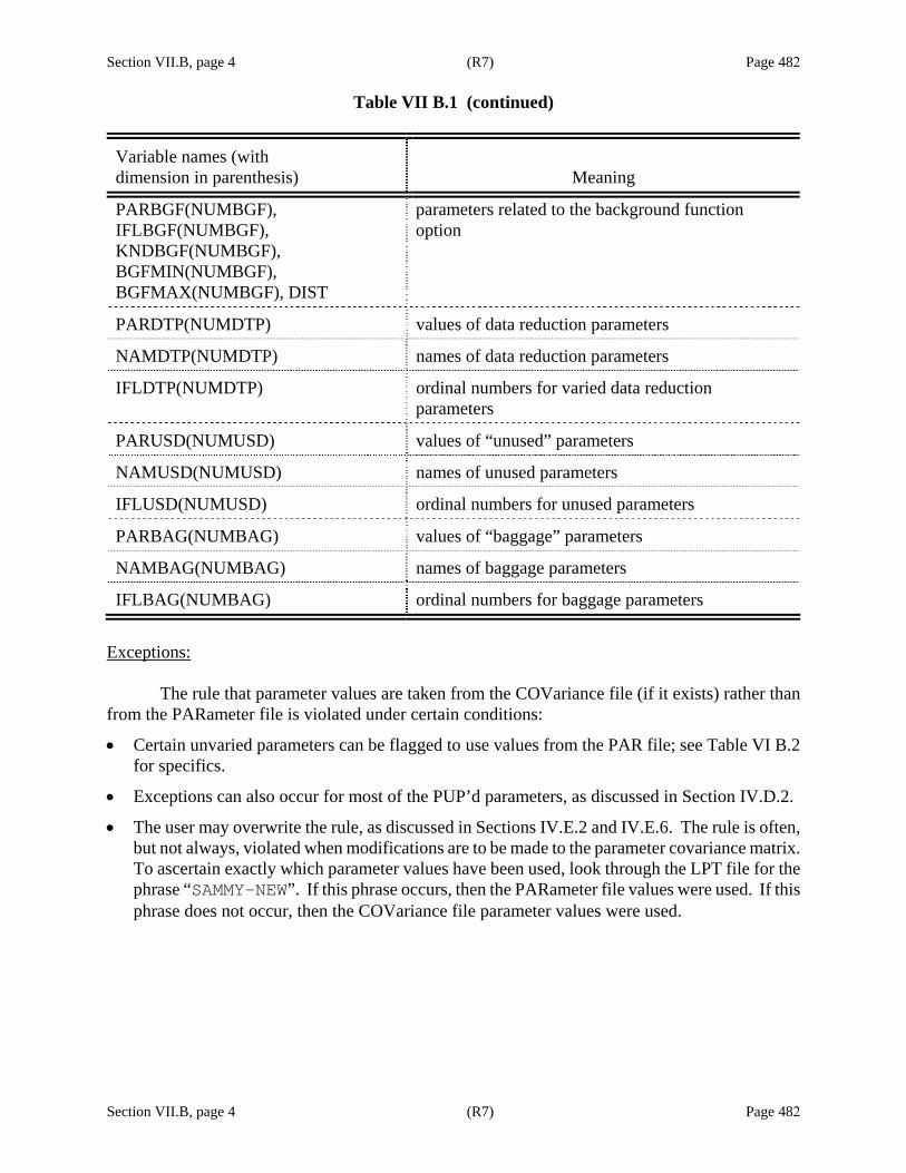
Section VII.B, page 4 (R7) Page 482 Table VII B.1 (continued)
Section VII.B, page 4 (R7) Page 482
Variable names (with dimension in parenthesis) Meaning
PARBGF(NUMBGF), IFLBGF(NUMBGF), KNDBGF(NUMBGF), BGFMIN(NUMBGF), BGFMAX(NUMBGF), DIST
parameters related to the background function option
PARDTP(NUMDTP) values of data reduction parameters
NAMDTP(NUMDTP) names of data reduction parameters
IFLDTP(NUMDTP) ordinal numbers for varied data reduction parameters
PARUSD(NUMUSD) values of “unused” parameters
NAMUSD(NUMUSD) names of unused parameters
IFLUSD(NUMUSD) ordinal numbers for unused parameters
PARBAG(NUMBAG) values of “baggage” parameters
NAMBAG(NUMBAG) names of baggage parameters
IFLBAG(NUMBAG) ordinal numbers for baggage parameters
Exceptions: The rule that parameter values are taken from the COVariance file (if it exists) rather than from the PARameter file is violated under certain conditions:
• Certain unvaried parameters can be flagged to use values from the PAR file; see Table VI B.2 for specifics.
• Exceptions can also occur for most of the PUP’d parameters, as discussed in Section IV.D.2.
• The user may overwrite the rule, as discussed in Sections IV.E.2 and IV.E.6. The rule is often, but not always, violated when modifications are to be made to the parameter covariance matrix. To ascertain exactly which parameter values have been used, look through the LPT file for the phrase “SAMMY-NEW”. If this phrase occurs, then the PARameter file values were used. If this phrase does not occur, then the COVariance file parameter values were used.

Section VII.C, page 1 (R8) Page 483
Section VII.C, page 1 (R8) Page 483
VII.C. PLOT OUTPUT
The output file SAMMY.ODF is in the ORELA DATA FORMAT [JC78] and is intended for use with the plotting program FORODF to produce plots of the results of SAMMY calculations. Table VII C.1 shows what is stored in each section of the SAMMY.ODF file, for the case when the experimental data are either total cross section or transmission. Table VII C.2 describes the ODF file for other types of energy-differential data, and Table VII C.3 shows the SAMMY.ODF file for angular-distribution (angle- and energy-differential) data. In the case of angular-distribution data, when the input data are provided in an ASCII file, SAMMY will produce a second output ODF file (SAMMY.DAT) that contains the experimental values; if the input data are given in an ODF file, the SAMMY.DAT file is not generated. A description of the SAMMY.DAT file is shown in Table VII C.4.
For computer systems using other plotting routines, SAMMY provides two additional files containing the same information as that in the ODF file. One is an ASCII file and the other is a “generic” binary file; names for the two files are derived from the name of the ODF file with extensions “LST” or “PLT”, respectively. For example, the files corresponding to SAMMY.ODF are SAMMY.LST and SAMMY.PLT. The files corresponding to SAMMY.DAT are SAMMYX.LST and SAMMYX.PLT. Details for reading PLT files are presented in Section X.I.
Table VII C.1. Sections of the ODF file generated by SAMMY, for transmission or total
cross-section data
Sect. No. Contents and units 1 Energy (Units are as specified by input command. If not specified, then units
are eV if appropriate, otherwise keV.) 2 Experimental cross section (barns) 3 Absolute uncertainty in experimental cross section (barns) 4 Zeroth-order theoretical cross section as evaluated by SAMMY (barns) 5 Final theoretical cross section as evaluated by SAMMY (barns) 6 Experimental transmission (dimensionless) 7 Absolute uncertainty in experimental transmission 8 Zeroth-order theoretical transmission as evaluated by SAMMY 9 Final theoretical transmission as evaluated by SAMMY
10 a Theoretical uncertainty on section 4 if data were total cross section, or on section 8 if data were transmission
11 a Theoretical uncertainty on section 5 or section 9 12 b Adjusted energy initially, when t0 and L0 are to be varied. See Section III.E.8 of
this manual. 13 b Adjusted energy finally, when t0 and L0 are to be varied. See Section III.E.8 of
this manual. a These sections are filled only if the phrase “INCLUDE THEORETICAL errors” occurs in the INPut file (Table VI A1.2). b These sections are filled only if t0 and/or L0 is to be varied.

Section VII.C, page 2 (R8) Page 484
Section VII.C, page 2 (R8) Page 484
Table VII C.2. Sections of the ODF file generated by SAMMY, for energy-differential data that are neither transmission nor total cross section
Sect. No. Contents and units
1 Energy (Units are as specified by input command. If not specified, then units are eV if appropriate, otherwise keV)
2 Experimental cross section (barns) 3 Absolute uncertainty in experimental cross section (barns) 4 Zeroth-order theoretical cross section as evaluated by SAMMY
(barns) 5 Final theoretical cross section as evaluated by SAMMY (barns) 6 a Theoretical uncertainty on section 4 (barns) 7 a Theoretical uncertainty on section 5 (barns) 8 b Adjusted energy initially, when t0 and L0 are to be varied. See
Section III.E.8 of this report 9 b Adjusted energy finally, when t0 and L0 are to be varied. See
Section III.E.8 of this report a These sections are filled only if the phrase “INCLUDE THEORETICAL errors” occurs in the INPut file (Table VI A1.2). b These sections are filled only if t0 and/or L0 is to be varied.

Section VII.C, page 3 (R8) Page 485
Section VII.C, page 3 (R8) Page 485
Table VIIC.3. Sections of SAMMY.ODF when data are angular distributions (energy- and
angle-differential elastic scattering or reaction data)
Sect. No. Contents and units
1 Energy (eV) 2 Zeroth-order theoretical cross section for the first angle (barns) 3 Final theoretical cross section for the first angle (barns) 4 Zeroth-order theoretical cross section for the second angle (barns) 5 Final theoretical cross section for the second angle (barns) ... 2n Zeroth-order theoretical cross section for the nth angle (barns)
2n + 1 Final theoretical cross section for the nth angle (barns)
Table VIIC.4. Sections of the ODF file SAMMY.DAT generated by SAMMY when data are angular distributions
Sect. No. Contents and units
1 Energy (eV) 2 Experimental cross section for the first angle (barns) 3 Uncertainty on experimental cross section for the first angle (barns) 4 Experimental cross section for the second angle (barns) 5 Uncertainty on experimental cross section for the second angle (barns) ... 2n Experimental cross section for the nth angle (barns)
2n + 1 Uncertainty on experimental cross section for the nth angle (barns)


Section VII.D, page 1 (R7) Page 487
Section VII.D, page 1 (R7) Page 487
VII.D. COMPLETE SET OF PARTIAL DERIVATIVES FOR RESONANCE PARAMETERS
It is possible for SAMMY to generate an ASCII file containing partial derivatives of the cross sections with respect to all resonance parameters. This option was added to SAMMY for one specialized application, when the results of a SAMMY analysis were to be used as the starting point for a study of integral quantities; it is not expected to be a generally useful option for other applications.
To invoke this SAMMY option, include the statement
GENERATE PARTIAL DERIVATIVES ONLY in the INPut file. The output file SAMMY.PDS will then be produced; contents of this file are shown in Table VII D.1.
For this file, resonance parameters are numbered as follows: First, resonances are ordered according to spin groups. Next, resonances are energy ordered within spin groups. Finally, for each resonance, the u-parameters associated with the energy, the reduced-gamma-width amplitude, the reduced-neutron-width amplitude, and other reduced width amplitudes (if they exist), are, respectively, the first, second, third, and possibly fourth and fifth parameters. (See Section II.D.1.e for a description of u-parameters for the Reich-Moore approximation.)

Section VII.D, page 2 (R7) Page 488
Section VII.D, page 2 (R7) Page 488
Table VII D.1. Contents of output file SAMMY.PDS
Line Number Variable Columns Format Meaning
1 NPAR 1-10 I10 total number of resonance parameters
2, etc. U(1) to U(NPAR)
6G13.6 value of the parameters
3 DATA(1) 1-13 F first experimental data value
DELD(1) 14-26 F uncertainty on data
THEORY(1) 27-39 F theoretical value for first data point
G(1,1) 40-52 F partial derivative of THEORY with respect to parameter number 1
G(1,2) 53-65 F partial derivative of THEORY with respect to parameter number 2
G(1,3) 66-79 F partial derivative of THEORY with respect to parameter number 3
4 etc. G(1,4) to G(1,NPAR)
6G13.6 partial derivative of THEORY with respect to parameter number 4
5 DATA(i) 1-13 F ith experimental data value
DELD(i) 14-26 F uncertainty on data
THEORY(i) 27-39 F theoretical value for ith data point
G(i,1) 40-52 F partial derivative of THEORY with respect to parameter number 1
G(i,2) 53-65 F partial derivative of THEORY with respect to parameter number 2
G(i,3) 66-79 F partial derivative of THEORY with respect to parameter number 3
6 etc G(i,4) to G(i,NPAR)
6G13.6 partial derivative of THEORY with respect to parameter number 4
Repeat lines 5 and 6 for each data point.
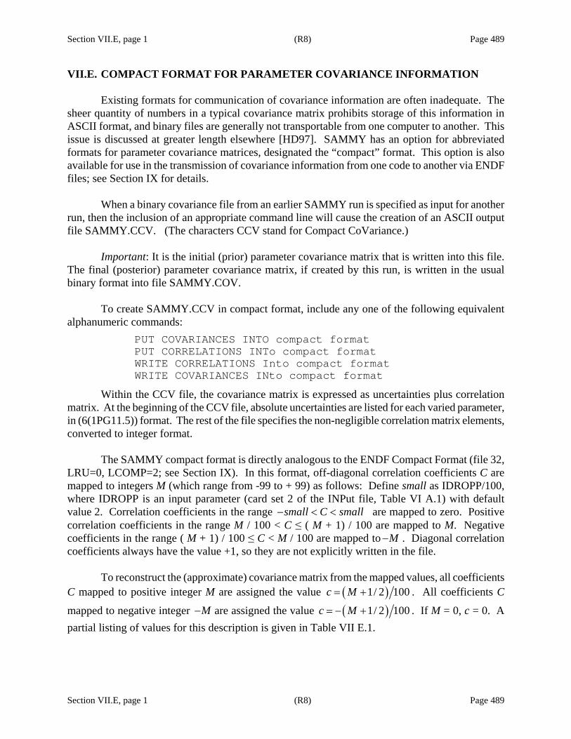
Section VII.E, page 1 (R8) Page 489
Section VII.E, page 1 (R8) Page 489
VII.E. COMPACT FORMAT FOR PARAMETER COVARIANCE INFORMATION
Existing formats for communication of covariance information are often inadequate. The sheer quantity of numbers in a typical covariance matrix prohibits storage of this information in ASCII format, and binary files are generally not transportable from one computer to another. This issue is discussed at greater length elsewhere [HD97]. SAMMY has an option for abbreviated formats for parameter covariance matrices, designated the “compact” format. This option is also available for use in the transmission of covariance information from one code to another via ENDF files; see Section IX for details.
When a binary covariance file from an earlier SAMMY run is specified as input for another run, then the inclusion of an appropriate command line will cause the creation of an ASCII output file SAMMY.CCV. (The characters CCV stand for Compact CoVariance.)
Important: It is the initial (prior) parameter covariance matrix that is written into this file. The final (posterior) parameter covariance matrix, if created by this run, is written in the usual binary format into file SAMMY.COV.
To create SAMMY.CCV in compact format, include any one of the following equivalent alphanumeric commands:
PUT COVARIANCES INTO compact format PUT CORRELATIONS INTo compact format WRITE CORRELATIONS Into compact format WRITE COVARIANCES INto compact format
Within the CCV file, the covariance matrix is expressed as uncertainties plus correlation matrix. At the beginning of the CCV file, absolute uncertainties are listed for each varied parameter, in (6(1PG11.5)) format. The rest of the file specifies the non-negligible correlation matrix elements, converted to integer format.
The SAMMY compact format is directly analogous to the ENDF Compact Format (file 32, LRU=0, LCOMP=2; see Section IX). In this format, off-diagonal correlation coefficients C are mapped to integers M (which range from -99 to + 99) as follows: Define small as IDROPP/100, where IDROPP is an input parameter (card set 2 of the INPut file, Table VI A.1) with default value 2. Correlation coefficients in the range small C small− < < are mapped to zero. Positive correlation coefficients in the range M / 100 < C ≤ ( M + 1) / 100 are mapped to M. Negative coefficients in the range ( M + 1) / 100 ≤ C < M / 100 are mapped to M− . Diagonal correlation coefficients always have the value +1, so they are not explicitly written in the file.
To reconstruct the (approximate) covariance matrix from the mapped values, all coefficients C mapped to positive integer M are assigned the value ( )1/ 2 100c M= + . All coefficients C
mapped to negative integer M− are assigned the value ( )1/ 2 100c M= − + . If M = 0, c = 0. A partial listing of values for this description is given in Table VII E.1.
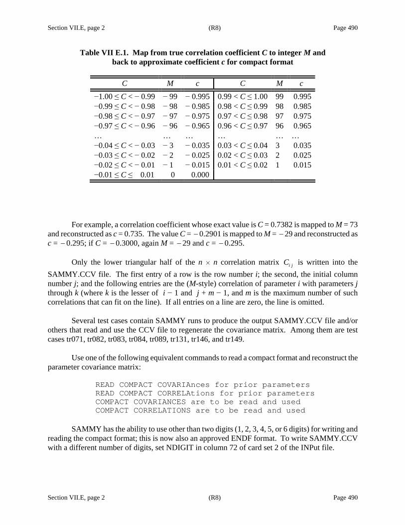
Section VII.E, page 2 (R8) Page 490
Section VII.E, page 2 (R8) Page 490
Table VII E.1. Map from true correlation coefficient C to integer M and back to approximate coefficient c for compact format
C M c C M c
−1.00 ≤ C < − 0.99 − 99 − 0.995 0.99 < C ≤ 1.00 99 0.995 −0.99 ≤ C < − 0.98 − 98 − 0.985 0.98 < C ≤ 0.99 98 0.985 −0.98 ≤ C < − 0.97 − 97 − 0.975 0.97 < C ≤ 0.98 97 0.975 −0.97 ≤ C < − 0.96 − 96 − 0.965 0.96 < C ≤ 0.97 96 0.965 … … … … … … −0.04 ≤ C < − 0.03 − 3 − 0.035 0.03 < C ≤ 0.04 3 0.035 −0.03 ≤ C < − 0.02 − 2 − 0.025 0.02 < C ≤ 0.03 2 0.025 −0.02 ≤ C < − 0.01 − 1 − 0.015 0.01 < C ≤ 0.02 1 0.015 −0.01 ≤ C ≤ 0.01 0 0.000
For example, a correlation coefficient whose exact value is C = 0.7382 is mapped to M = 73 and reconstructed as c = 0.735. The value C = −0.2901 is mapped to M = −29 and reconstructed as c = −0.295; if C = −0.3000, again M = −29 and c = −0.295.
Only the lower triangular half of the n H n correlation matrix i jC is written into the SAMMY.CCV file. The first entry of a row is the row number i; the second, the initial column number j; and the following entries are the (M-style) correlation of parameter i with parameters j through k (where k is the lesser of i − 1 and j + m − 1, and m is the maximum number of such correlations that can fit on the line). If all entries on a line are zero, the line is omitted.
Several test cases contain SAMMY runs to produce the output SAMMY.CCV file and/or others that read and use the CCV file to regenerate the covariance matrix. Among them are test cases tr071, tr082, tr083, tr084, tr089, tr131, tr146, and tr149.
Use one of the following equivalent commands to read a compact format and reconstruct the
parameter covariance matrix:
READ COMPACT COVARIAnces for prior parameters READ COMPACT CORRELAtions for prior parameters COMPACT COVARIANCES are to be read and used COMPACT CORRELATIONS are to be read and used
SAMMY has the ability to use other than two digits (1, 2, 3, 4, 5, or 6 digits) for writing and reading the compact format; this is now also an approved ENDF format. To write SAMMY.CCV with a different number of digits, set NDIGIT in column 72 of card set 2 of the INPut file.
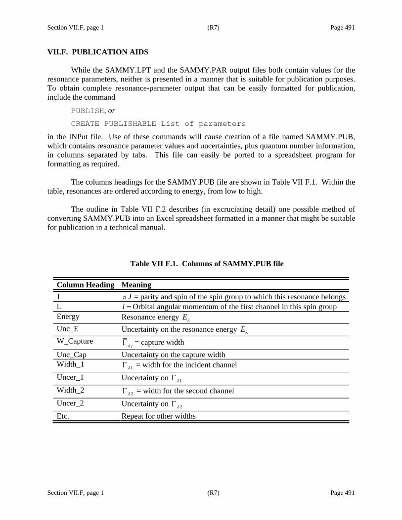
Section VII.F, page 1 (R7) Page 491
Section VII.F, page 1 (R7) Page 491
VII.F. PUBLICATION AIDS While the SAMMY.LPT and the SAMMY.PAR output files both contain values for the resonance parameters, neither is presented in a manner that is suitable for publication purposes. To obtain complete resonance-parameter output that can be easily formatted for publication, include the command
PUBLISH, or CREATE PUBLISHABLE List of parameters
in the INPut file. Use of these commands will cause creation of a file named SAMMY.PUB, which contains resonance parameter values and uncertainties, plus quantum number information, in columns separated by tabs. This file can easily be ported to a spreadsheet program for formatting as required.
The columns headings for the SAMMY.PUB file are shown in Table VII F.1. Within the table, resonances are ordered according to energy, from low to high.
The outline in Table VII F.2 describes (in excruciating detail) one possible method of
converting SAMMY.PUB into an Excel spreadsheet formatted in a manner that might be suitable for publication in a technical manual.
Table VII F.1. Columns of SAMMY.PUB file
Column Heading Meaning J Jπ = parity and spin of the spin group to which this resonance belongsL l =Orbital angular momentum of the first channel in this spin group Energy Resonance energy Eλ Unc_E Uncertainty on the resonance energy Eλ W_Capture
λγΓ = capture width Unc_Cap Uncertainty on the capture width Width_1 1λΓ = width for the incident channel Uncer_1 Uncertainty on 1λΓ Width_2 2λΓ = width for the second channel Uncer_2 Uncertainty on 2λΓ Etc. Repeat for other widths

Section VII.F, page 2 (R7) Page 492
Section VII.F, page 2 (R7) Page 492
Table VII F.2. Converting SAMMY.PUB into a spreadsheet 1. copy SAMMY.PUB onto a Windows directory 2. bring up Excel, perhaps via
a. Start i. Programs
1. Excel 3. data (one of the menus across top of page)
a. import external data i. import data
1. all files (box at bottom) 2. highlight the SAMMY.PUB file 3. Open
a. Next b. Next c. Finish d. OK
4. put the curser in the grey box above “1” and to the right of “A” 5. format (another of menus at top)
a. cells i. number
1. decimal places (2 or 3 or whatever) a. OK
6. put the curser above the “J” column 7. format
a. cells i. number
1. decimal places = 1 a. OK
8. put the curser above the “L” column 9. format
a. cells i. number
1. decimal places = 0 a. OK
10. put the curser in the grey box above “1” and to the right of “A” 11. format
a. column i. autofit selection
12. other options of interest: a. to add or delete a row or column … need icons on tool bar
i. tools/customize/command/edit/ and /insert/; move icons to tool bar ii. once icons are there, put curser in column or row to delete (or after position to
add column or row), and click the icon b. to move a column
i. highlight the column (click on letter above column) ii. click scissors (cut)
iii. highlight the (empty) column into which you want to move this one iv. hit “enter”

Section VII.G, page 1 (R8) Page 493
Section VII.G, page 1 (R8) Page 493
VII.G. OTHER OUTPUT FILES Often it is useful to have the unbroadened cross section values in a separate file rather than embedded within the SAMMY.LPT file. To obtain such a file, include the phrase
PUT UNBROADENED CROSs sections into plot file into the command section of the INPut file. This will cause two or three files to be generated, SAMMY.UNB, SAMUNB.DAT, and possibly SAMUNX.DAT.
File SAMMY.UNB is an ODF plot file (Section VII.C) that contains two or more sections. Section 1 contains the energy in eV, and section 2 contains the cross section.
When more than one type of cross section is used for the particular calculation, then section 3, 4, etc., contain the other cross sections. For example, in the case when the data type (card set 8 of the INPut file) is “CAPTUre” and multiple-scattering corrections are requested, then sections 2 through Lmax + 1 will contain Legendre coefficients for L = 0 through Lmax − 1, respectively, section Lmax + 2 will contain the total cross section, and Lmax + 3 will contain the capture cross section. When the data type is “INTEGral quantities” for a fissile nuclide, section 2 will be fission and section 3 absorption.
File SAMUNB.DAT is an ASCII file in TWENTY format (Section VI.C.1) with three columns. The first is energy in eV, and the second is the cross section. (When more than one type of cross section is used, it is the final type in the paragraph above that appears in this position.) The third column is the value 0.1; this number is a placeholder for the uncertainty on this cross section, included because it is sometimes desirable to use this file as dummy “experimental” data for other SAMMY runs.
File SAMUNX.DAT is another ASCII file, in CSISRS format (1P7G11.4). This file appears only when more than one type of cross section is used in the calculation. The file contains energy in column 1 and the cross sections in the remaining columns, in the order as described above.1
For all of these files, negative-energy data points and cross sections may appear in the file. These arise from the velocity-grid requirements for Doppler broadening, as discussed in Section III.B.1.
1 Prior to Version 7.1.4, placeholders for the uncertainty on the cross section(s) were included in SAMUNX.DAT; these placeholders have been eliminated because they serve no useful purpose.


Section VIII, page 1 (R7) Page 495
Section VIII, page 1 (R7) Page 495
VIII. UNRESOLVED RESONANCE REGION
As a first step towards expansion into the unresolved resonance region, Fritz Fröhner=s code FITACS [FF89] has been obtained and inserted into SAMMY. FITACS uses Hauser-Feshbach theory with width fluctuations. The adjustable parameters are neutron strength functions, distant-level parameters, average radiation widths (at E = 0), and average fission widths (at E = 0). The energy dependence of the radiation widths is specified via the giant dipole model, of the fission widths via Hill-Wheeler fission barrier transmission coefficients, and of the mean level spacing for s-waves via the Gilbert-Cameron composite formula. Mean spacings for l > 0 are given via the Bethe formula. Moldauer’s prescription is used for partial cross sections. Details of the theory are presented in Section VIII.A.
Initially (for release M2 of the code), FITACS was incorporated into SAMMY (as segments SAMFFF and SAMACS) in a limited fashion only. Internal changes were made, to be consistent with SAMMY notation and to use dynamic dimensioning of arrays. The M + W version of Bayes’ method has replaced the fitting procedure used in FITACS. Calculation of penetrabilities was extended to all l values (FITACS had used only s, p, d, and f-waves). The output included files from which plots can be made. Results were reported in SAMMY.PAR in the same format as is used in the input file (as well as in more human-legible fashion in SAMMY.LPT).
Subsequently, additional modifications, improvements, and new features have been made in the SAMMY URR treatment: • Partial derivatives with respect to varied parameters are calculated exactly rather than
approximately. • A more efficient integration routine has been written for the Dresner integral, Eq. (VIII A.5). • It is possible to include (and vary, if desired) a normalization for each data set. • Elastic cross section data may be fitted. • There is no limit on the number or type of experimental data sets. Data may be kept in separate
files rather than appended to the parameter file. • The output has been modified to conform more closely to SAMMY conventions. • An “annotated” PARameter file, including key-word-based input, is the default input option, and
the only option available for output. (Files in the original format can still be used for input, but options are limited with that format.)
• Different sets of average resonance parameters can be used in different energy ranges.

Section VIII, page 2 (R7) Page 496
Section VIII, page 2 (R7) Page 496
• Output can be produced in ENDF/B format, for both File 2 (resonance parameters) and File 32 (covariance matrices). ENDF files cannot be used for input, because the ENDF format requires a more limited theoretical description than does FITACS/SAMMY.
• The fitting procedure can be performed sequentially, in similar fashion as in the resolved
resonance region. That is, output PARameter and COVariance files from the fit to one data set may be used as input to another run which fits another data set. [Initially, only simultaneous fitting of all data sets was permitted.]
• “No-Bayes” runs can be made: cross sections will be calculated from the resonance parameters,
but no fitting will be done.
Additions being considered for future revisions of the code include the following: • Multiple nuclides in the sample • An option to calculate multigroup cross sections and covariances • An option to include integral quantities in the fit • Extensions to the theory • Additional ENDF capability (requiring ENDF format changes) • A link between the resolved resonance parameters and those for the unresolved region, in order
to provide more consistent evaluated cross sections • Methodologies for retroactive generation of covariance matrices, similar to that used in the
resolved resonance region
Input for analysis of data in the unresolved resonance region is described in Section VIII.B. Output is described in Section VIII.C. The relationship between ENDF parameters and SAMMY/URR parameters is discussed in Section VIII.D.
For an example of the use of SAMMY/URR, see [HD00] and test cases 73, 88, 127, 133,
134, 142, and 145.
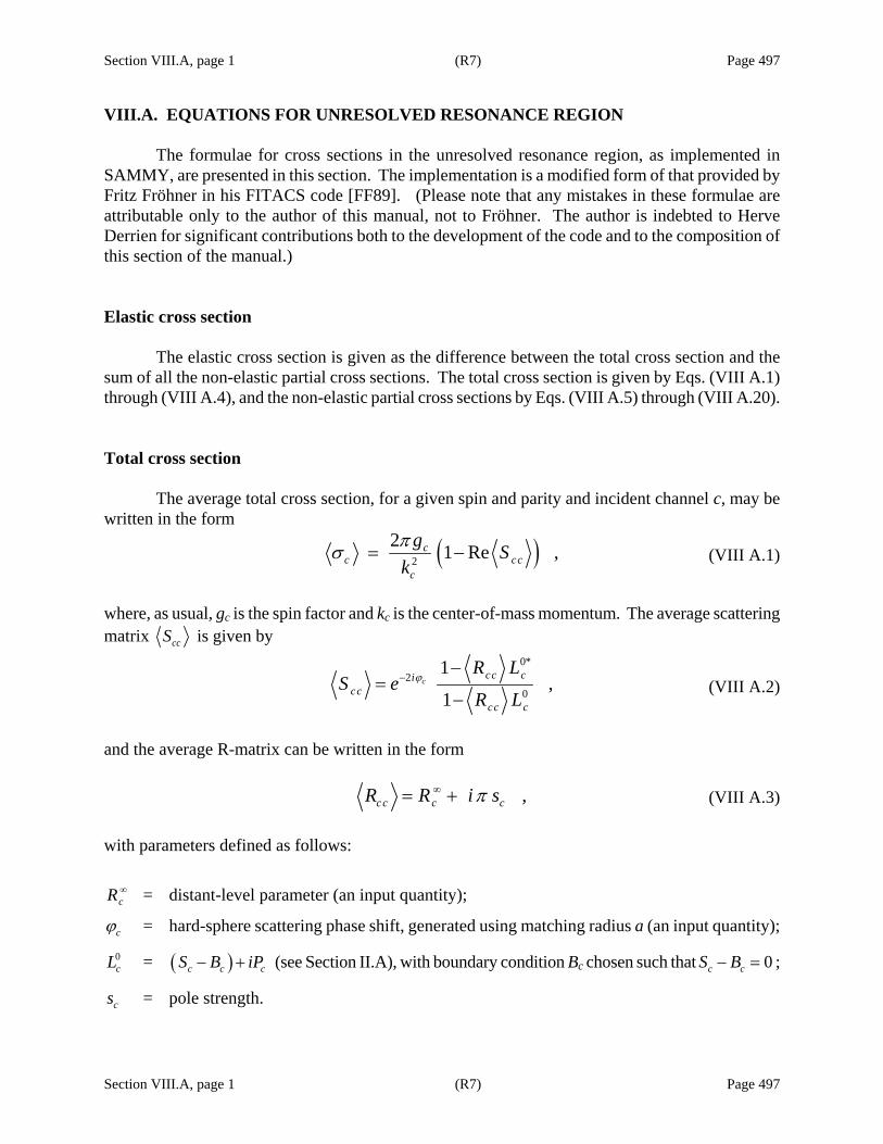
Section VIII.A, page 1 (R7) Page 497
Section VIII.A, page 1 (R7) Page 497
VIII.A. EQUATIONS FOR UNRESOLVED RESONANCE REGION
The formulae for cross sections in the unresolved resonance region, as implemented in SAMMY, are presented in this section. The implementation is a modified form of that provided by Fritz Fröhner in his FITACS code [FF89]. (Please note that any mistakes in these formulae are attributable only to the author of this manual, not to Fröhner. The author is indebted to Herve Derrien for significant contributions both to the development of the code and to the composition of this section of the manual.) Elastic cross section The elastic cross section is given as the difference between the total cross section and the sum of all the non-elastic partial cross sections. The total cross section is given by Eqs. (VIII A.1) through (VIII A.4), and the non-elastic partial cross sections by Eqs. (VIII A.5) through (VIII A.20). Total cross section
The average total cross section, for a given spin and parity and incident channel c, may be written in the form
( )2
2 1 Re ,cc cc
c
g Skπσ = − (VIII A.1)
where, as usual, gc is the spin factor and kc is the center-of-mass momentum. The average scattering matrix ccS is given by
0*
20
1,
1c
cc cicc
cc c
R LS e
R Lϕ−
−=
− (VIII A.2)
and the average R-matrix can be written in the form ,cc c cR R i sπ∞= + (VIII A.3) with parameters defined as follows:
cR ∞ = distant-level parameter (an input quantity);
cϕ = hard-sphere scattering phase shift, generated using matching radius a (an input quantity); 0cL = ( )c c cS B iP− + (see Section II.A), with boundary condition Bc chosen such that 0c cS B− = ;
cs = pole strength.
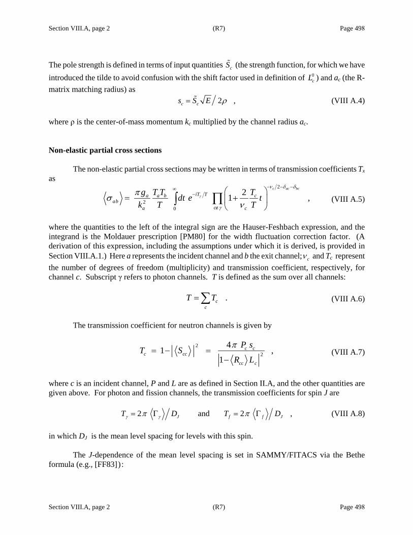
Section VIII.A, page 2 (R7) Page 498
Section VIII.A, page 2 (R7) Page 498
The pole strength is defined in terms of input quantities cS (the strength function, for which we have introduced the tilde to avoid confusion with the shift factor used in definition of 0
cL ) and ac (the R-matrix matching radius) as 2 ,c cs S E ρ= (VIII A.4) where ρ is the center-of-mass momentum kc multiplied by the channel radius ac. Non-elastic partial cross sections
The non-elastic partial cross sections may be written in terms of transmission coefficients Tx as
2
20
21 ,c ac bc
iT Ta a b cab
ca c
g T T Tdt e tk T T
γ
ν δ δ
γ
πσν
− − −∞−
∉
⎛ ⎞= +⎜ ⎟
⎝ ⎠∏∫ (VIII A.5)
where the quantities to the left of the integral sign are the Hauser-Feshbach expression, and the integrand is the Moldauer prescription [PM80] for the width fluctuation correction factor. (A derivation of this expression, including the assumptions under which it is derived, is provided in Section VIII.A.1.) Here a represents the incident channel and b the exit channel; cν and Tc represent the number of degrees of freedom (multiplicity) and transmission coefficient, respectively, for channel c. Subscript γ refers to photon channels. T is defined as the sum over all channels: .c
c
T T=∑ (VIII A.6)
The transmission coefficient for neutron channels is given by
2
2
41 ,1
c cc cc
cc c
P sT SR L
π= − =
− (VIII A.7)
where c is an incident channel, P and L are as defined in Section II.A, and the other quantities are given above. For photon and fission channels, the transmission coefficients for spin J are 2 and 2 ,J f f JT D T Dγ γπ π= Γ = Γ (VIII A.8) in which DJ is the mean level spacing for levels with this spin.
The J-dependence of the mean level spacing is set in SAMMY/FITACS via the Bethe formula (e.g., [FF83]):
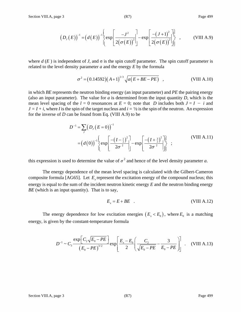
Section VIII.A, page 3 (R7) Page 499
Section VIII.A, page 3 (R7) Page 499
( )( ) ( )( )( )( )
( )( )( )
221 1
2 2
1exp exp ,
2 2J
JJD E d EE Eσ σ
− −⎧ ⎫⎡ ⎤ ⎡ ⎤− +−⎪ ⎪⎢ ⎥ ⎢ ⎥= −⎨ ⎬
⎢ ⎥ ⎢ ⎥⎪ ⎪⎣ ⎦ ⎣ ⎦⎩ ⎭ (VIII A.9)
where d (E ) is independent of J, and σ is the spin cutoff parameter. The spin cutoff parameter is related to the level density parameter a and the energy E by the formula ( )( ) ( )2/32 0.14592 1 ,A a E BE PEσ = + + − (VIII A.10) in which BE represents the neutron binding energy (an input parameter) and PE the pairing energy (also an input parameter). The value for a is determined from the input quantity D, which is the mean level spacing of the l = 0 resonances at E = 0; note that D includes both J = I − i and J = I + i, where I is the spin of the target nucleus and i = 2 is the spin of the neutron. An expression for the inverse of D can be found from Eq. (VIII A.9) to be
( )( )
( )( ) ( ) ( )
11
22 311 2 2
2 2
0
0 exp exp ;2 2
JJ
D D E
I Id
σ σ
−−
−
= =
⎧ ⎫⎡ ⎤⎡ ⎤− − − +⎪ ⎪= − ⎢ ⎥⎢ ⎥⎨ ⎬⎢ ⎥⎢ ⎥⎪ ⎪⎣ ⎦ ⎣ ⎦⎩ ⎭
∑ (VIII A.11)
this expression is used to determine the value of σ 2 and hence of the level density parameter a.
The energy dependence of the mean level spacing is calculated with the Gilbert-Cameron composite formula [AG65]. Let xE represent the excitation energy of the compound nucleus; this energy is equal to the sum of the incident neutron kinetic energy E and the neutron binding energy BE (which is an input quantity). That is to say, .xE E BE= + (VIII A.12)
The energy dependence for low excitation energies ( )0xE E< , where 0E is a matching energy, is given by the constant-temperature formula
( )
2 01 0 23 3/ 2
000
exp 3~ exp .2
xC E PE E E CD C
E PEE PEE PE−
⎡ ⎤− ⎡ ⎤⎛ ⎞−⎣ ⎦ −⎢ ⎥⎜ ⎟⎜ ⎟−−− ⎢ ⎥⎝ ⎠⎣ ⎦ (VIII A.13)
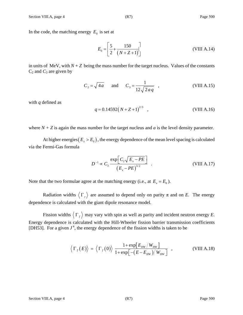
Section VIII.A, page 4 (R7) Page 500
Section VIII.A, page 4 (R7) Page 500
In the code, the matching energy 0E is set at
( )0
5 1502 1
EN Z
⎡ ⎤= +⎢ ⎥+ +⎣ ⎦
(VIII A.14)
in units of MeV, with N + Z being the mass number for the target nucleus. Values of the constants C2 and C3 are given by
2 314 and ,
12 2C a C
a q= = (VIII A.15)
with q defined as ( )2/30.14592 1 ,q N Z= + + (VIII A.16) where N + Z is again the mass number for the target nucleus and a is the level density parameter.
At higher energies ( )0xE E> , the energy dependence of the mean level spacing is calculated via the Fermi-Gas formula
( )
213 3/ 2
exp.
x
x
C E PED C
E PE−
⎡ ⎤−⎣ ⎦∝−
(VIII A.17)
Note that the two formulae agree at the matching energy (i.e., at 0xE E= ).
Radiation widths γΓ are assumed to depend only on parity π and on E. The energy dependence is calculated with the giant dipole resonance model.
Fission widths fΓ may vary with spin as well as parity and incident neutron energy E. Energy dependence is calculated with the Hill-Wheeler fission barrier transmission coefficients [DH53]. For a given J π, the energy dependence of the fission widths is taken to be
( ) ( ) [ ]( )
1 exp0 ,
1 expHW HW
f fHW HW
E WE
E E W+
Γ = Γ+ − −⎡ ⎤⎣ ⎦
(VIII A.18)
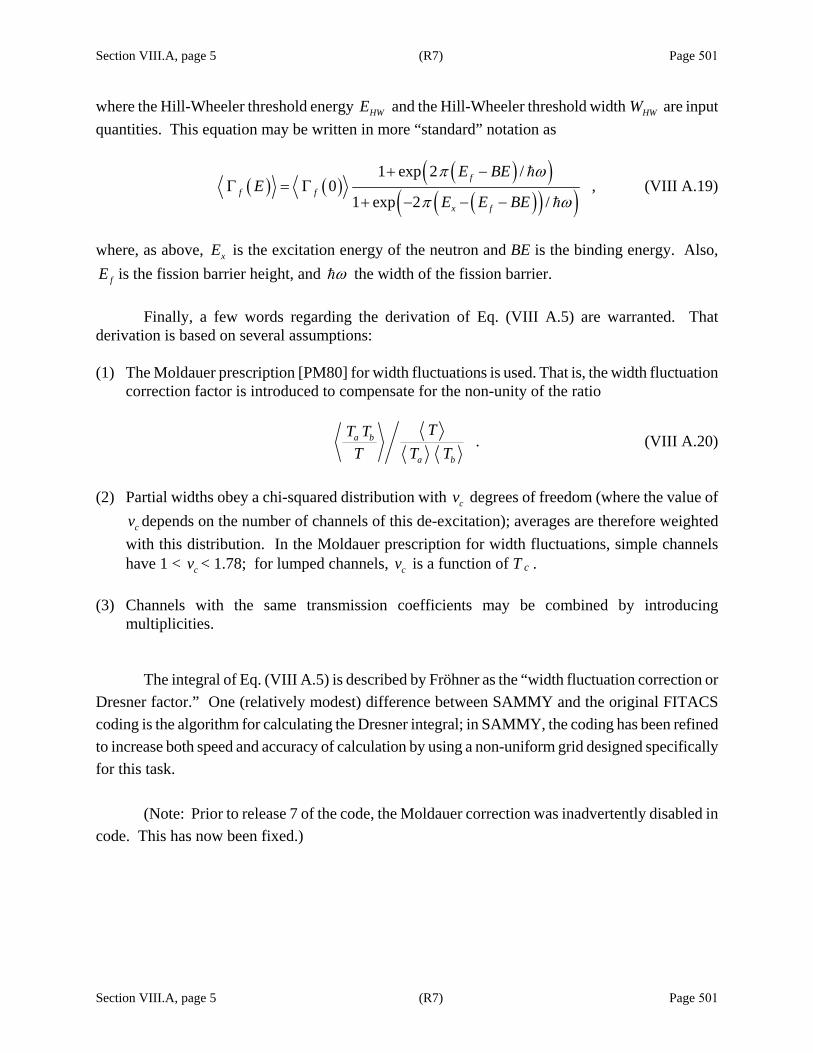
Section VIII.A, page 5 (R7) Page 501
Section VIII.A, page 5 (R7) Page 501
where the Hill-Wheeler threshold energy HWE and the Hill-Wheeler threshold width HWW are input quantities. This equation may be written in more “standard” notation as
( ) ( )( )( )
( )( )( )1 exp 2 /
0 ,1 exp 2 /
ff f
x f
E BEE
E E BE
π ω
π ω
+ −Γ = Γ
+ − − − (VIII A.19)
where, as above, xE is the excitation energy of the neutron and BE is the binding energy. Also,
fE is the fission barrier height, and ω the width of the fission barrier.
Finally, a few words regarding the derivation of Eq. (VIII A.5) are warranted. That derivation is based on several assumptions: (1) The Moldauer prescription [PM80] for width fluctuations is used. That is, the width fluctuation
correction factor is introduced to compensate for the non-unity of the ratio
.a b
a b
TT TT T T
(VIII A.20)
(2) Partial widths obey a chi-squared distribution with cv degrees of freedom (where the value of
cv depends on the number of channels of this de-excitation); averages are therefore weighted with this distribution. In the Moldauer prescription for width fluctuations, simple channels have 1 < cv < 1.78; for lumped channels, cv is a function of T c .
(3) Channels with the same transmission coefficients may be combined by introducing
multiplicities.
The integral of Eq. (VIII A.5) is described by Fröhner as the “width fluctuation correction or Dresner factor.” One (relatively modest) difference between SAMMY and the original FITACS coding is the algorithm for calculating the Dresner integral; in SAMMY, the coding has been refined to increase both speed and accuracy of calculation by using a non-uniform grid designed specifically for this task.
(Note: Prior to release 7 of the code, the Moldauer correction was inadvertently disabled in
code. This has now been fixed.)


Section VIII.A.1, page 1 (R7) Page 503
Section VIII.A.1, page 1 (R7) Page 503
VIII.A.1. Derivation of Non-Elastic Average Cross Section
Derivations shown in this section are based on (1) notes provided by Fritz Fröhner [FF99] and (2) discussions with Herve Derrien [HD00a]. Any errors in these pages are the responsibility of the SAMMY author alone.
The interpretation of the transmission coefficient Tc in terms of average resonance parameters is straightforward if one assumes that the resonant cross section can be approximated by the single-level Breit Wigner formula, i.e.,
( ) ( )2 22 ,
2a a b
aba
gk E E
λ λ
λ λ λ
πσ
Γ Γ=
− + Γ∑ (VIII A1.1)
in which total width Γλ is the sum of all partial widths. The corresponding average cross section in an energy interval containing a large number of resonances may be written as
2 2 ,a a bab a
a
gkπ
σ π ρ Γ Γ=
Γ (VIII A1.2)
where ρ is the level density, and the brackets refer to averages. (Note that the subscript λ has been dropped for simplicity’s sake.) The calculation of the average quantity /a bΓ Γ Γ is not
straightforward, since the known parameters are aΓ and bΓ (from the statistical properties of the resonance parameters). One has to take into account the fluctuations of the partial widths of the resonances from the chi-squared distribution of the parameters.
A method of calculating the average /a bΓ Γ Γ from the known entities a bΓ Γ Γ was proposed by Dresner [FF99]. He suggested making the substitution
0
exp ,a b a ba b c
ccall c
dq q∞
Γ Γ Γ Γ ⎛ ⎞= = Γ Γ − Γ⎜ ⎟Γ Γ ⎝ ⎠
∑∑ ∫ (VIII A1.3)
which follows from the identity
00
1 1 .qQ yd q e d y eQ Q
∞ ∞− −= =∫∫ (VIII A1.4)
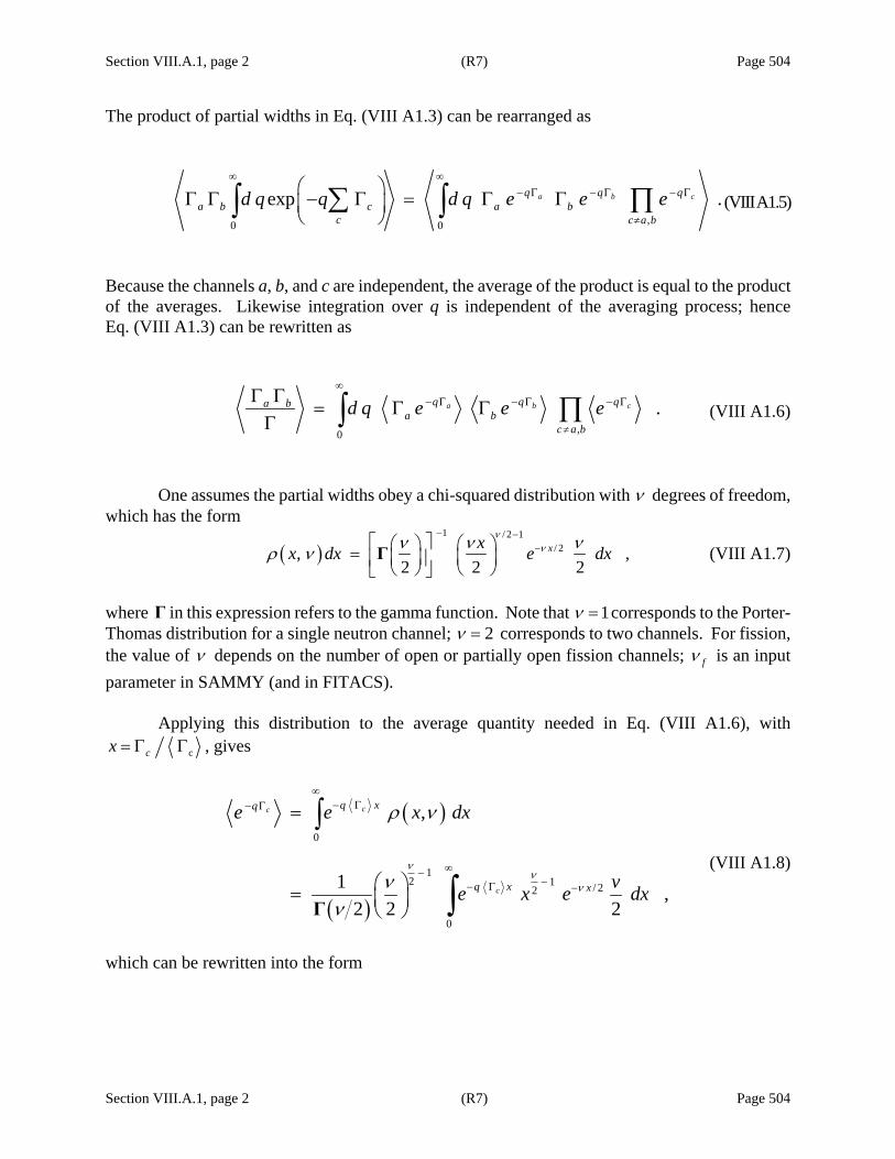
Section VIII.A.1, page 2 (R7) Page 504
Section VIII.A.1, page 2 (R7) Page 504
The product of partial widths in Eq. (VIII A1.3) can be rearranged as
,0 0
exp .a b cq q qa b c a b
c c a b
d q q d q e e e∞ ∞
− Γ − Γ − Γ
≠
⎛ ⎞Γ Γ − Γ = Γ Γ⎜ ⎟⎝ ⎠∑ ∏∫ ∫ (VIII A1.5)
Because the channels a, b, and c are independent, the average of the product is equal to the product of the averages. Likewise integration over q is independent of the averaging process; hence Eq. (VIII A1.3) can be rewritten as
,0
.a b cq q qa ba b
c a b
d q e e e∞
− Γ − Γ − Γ
≠
Γ Γ= Γ Γ
Γ ∏∫ (VIII A1.6)
One assumes the partial widths obey a chi-squared distribution with ν degrees of freedom, which has the form
( )1 / 2 1
/ 2, ,2 2 2
xxx dx e dxν
νν ν νρ ν− −
−⎡ ⎤⎛ ⎞ ⎛ ⎞= ⎜ ⎟ ⎜ ⎟⎢ ⎥⎝ ⎠ ⎝ ⎠⎣ ⎦Γ (VIII A1.7)
where Γ in this expression refers to the gamma function. Note that 1ν = corresponds to the Porter-Thomas distribution for a single neutron channel; 2ν = corresponds to two channels. For fission, the value of ν depends on the number of open or partially open fission channels; fν is an input parameter in SAMMY (and in FITACS).
Applying this distribution to the average quantity needed in Eq. (VIII A1.6), with ccx = Γ Γ , gives
( )
( )
0
12 1 / 22
0
,
1 ,2 2 2
cc
c
q xq
q x x
e e x dx
ve x e dxν
νν
ρ ν
νν
∞− Γ− Γ
∞−−− Γ −
=
⎛ ⎞= ⎜ ⎟⎝ ⎠
∫
∫Γ
(VIII A1.8)
which can be rewritten into the form

Section VIII.A.1, page 3 (R7) Page 505
Section VIII.A.1, page 3 (R7) Page 505
( )( )
( )
( ) ( )
2 1/ 2 2
0
2 2 12
0
2 2
12 2
12 2 2
1 2 21 2 1 .2
cc q xq
wc
c c
e e x dx
q e w dw
q q
νν
ν
ν νν
ν ν
νν
ν νν
νν ν ν
∞−− Γ +− Γ
∞−−−
− −
⎛ ⎞= ⎜ ⎟⎝ ⎠
⎛ ⎞ ⎛ ⎞= + Γ⎜ ⎟ ⎜ ⎟⎝ ⎠ ⎝ ⎠
⎛ ⎞ ⎛ ⎞= + Γ Γ = + Γ⎜ ⎟ ⎜ ⎟⎝ ⎠ ⎝ ⎠
∫
∫
Γ
Γ
Γ
(VIII A1.9)
Likewise, aq
a e − ΓΓ from Eq. (VIII A1.6) has the form
( )
( )
( )
( )
( )
0
12 / 22
0
12 2
2
0
12 2
12 2
,
2 2 2
2 2 2
12 2 2 2
2 2 2 2 2
aa
a
q xqa a
q xa x
a wa
aa
aa
e x e x dx
ve x e dx
q e w d w
q
q
νν
ν
ν νν
ν ν
ν ν
ρ ν
νν
ν νν
ν ν νν
ν ν ν νν
∞− Γ− Γ
∞−− Γ −
∞− −−
− −
− −
Γ = Γ
Γ ⎛ ⎞= ⎜ ⎟⎝ ⎠
Γ ⎛ ⎞ ⎛ ⎞= + Γ⎜ ⎟ ⎜ ⎟⎝ ⎠ ⎝ ⎠
Γ ⎛ ⎞ ⎛ ⎞ ⎛ ⎞= + Γ +⎜ ⎟ ⎜ ⎟ ⎜ ⎟⎝ ⎠ ⎝ ⎠ ⎝ ⎠
Γ ⎛ ⎞ ⎛ ⎞ ⎛ ⎞= + Γ⎜ ⎟ ⎜ ⎟ ⎜ ⎟⎝ ⎠ ⎝ ⎠ ⎝ ⎠
= Γ
∫
∫
∫
Γ
Γ
ΓΓ
ΓΓ
1221a aqν
ν
− −⎛ ⎞+ Γ⎜ ⎟⎝ ⎠ (VIII A1.10)
and similarly for bq
b e − ΓΓ . Hence Eq. (VIII A1.6) can be expressed as
/ 2
0
21 ,c ac bc
a ba b c
c c
dq q
ν δ δ
ν
− − −∞⎛ ⎞Γ Γ
= Γ Γ + Γ⎜ ⎟Γ ⎝ ⎠∏∫ (VIII A1.11)
in which the correspondence of ν with channel c is made explicit by the addition of the subscript.
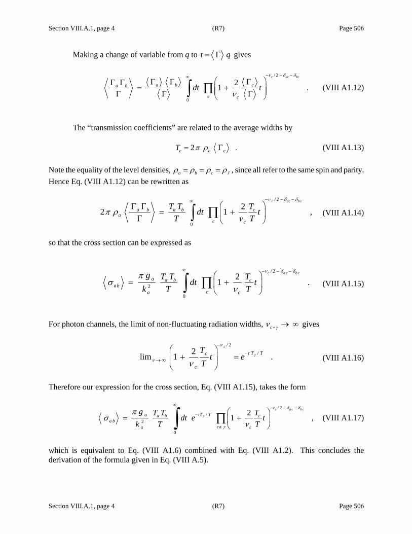
Section VIII.A.1, page 4 (R7) Page 506
Section VIII.A.1, page 4 (R7) Page 506
Making a change of variable from q to t q= Γ gives
/ 2
0
21 .c ac bc
a b ca b
c c
dt t
ν δ δ
ν
− − −∞⎛ ⎞Γ Γ ΓΓ Γ
= +⎜ ⎟⎜ ⎟Γ Γ Γ⎝ ⎠∏∫ (VIII A1.12)
The “transmission coefficients” are related to the average widths by
2 .c c cT π ρ= Γ (VIII A1.13) Note the equality of the level densities, a b c Jρ ρ ρ ρ= = = , since all refer to the same spin and parity. Hence Eq. (VIII A1.12) can be rewritten as
/ 2
0
22 1 ,c ac b c
a b a b ca
c c
T T Tdt tT T
ν δ δ
π ρν
− − −∞⎛ ⎞Γ Γ
= +⎜ ⎟Γ ⎝ ⎠∏∫ (VIII A1.14)
so that the cross section can be expressed as
/ 2
2
0
21 .c a c b c
a a b cab
ca c
g T T Tdt tk T T
ν δ δπσ
ν
∞ − − −⎛ ⎞
= +⎜ ⎟⎝ ⎠
∏∫ (VIII A1.15)
For photon channels, the limit of non-fluctuating radiation widths, c γν = → ∞ gives
/ 2
/2lim 1 .c
t T Tc
c
Tt e
Tγ
ν
ν ν
−
−→ ∞
⎛ ⎞+ =⎜ ⎟⎜ ⎟
⎝ ⎠ (VIII A1.16)
Therefore our expression for the cross section, Eq. (VIII A1.15), takes the form
/ 2
/2
0
21 ,c a c b c
iT Ta a b ca b
ca c
g T T Tdt e tk T T
γ
ν δ δ
γ
πσ
ν
∞− − −
−
∉
⎛ ⎞= +⎜ ⎟
⎝ ⎠∏∫ (VIII A1.17)
which is equivalent to Eq. (VIII A1.6) combined with Eq. (VIII A1.2). This concludes the derivation of the formula given in Eq. (VIII A.5).
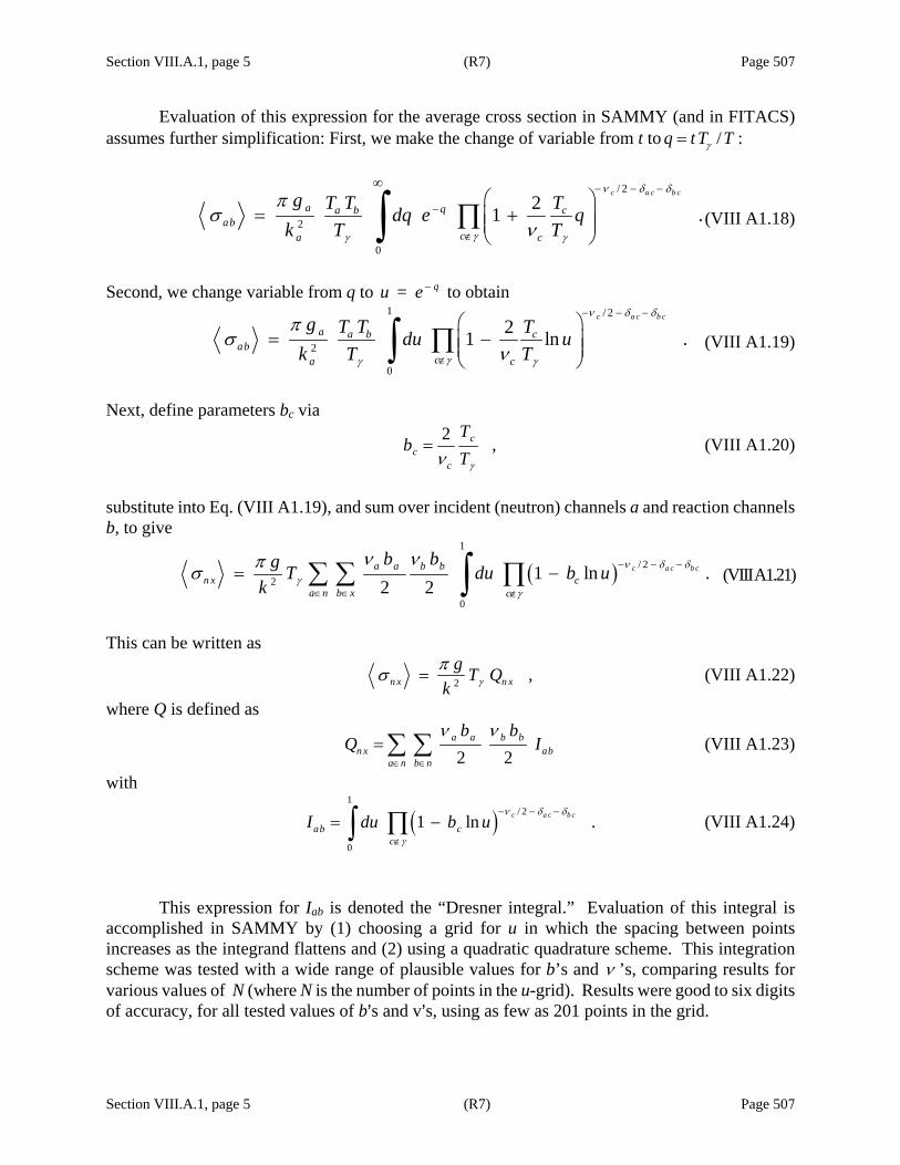
Section VIII.A.1, page 5 (R7) Page 507
Section VIII.A.1, page 5 (R7) Page 507
Evaluation of this expression for the average cross section in SAMMY (and in FITACS) assumes further simplification: First, we make the change of variable from t to /q t T Tγ= :
/ 2
2
0
21 .c a c b c
a qa b cab
ca c
g T T Tdq e qk T T
ν δ δ
γγ γ
πσ
ν
− − −
−
∉
∞⎛ ⎞
= +⎜ ⎟⎜ ⎟⎝ ⎠
∏∫ (VIII A1.18)
Second, we change variable from q to qu = e − to obtain
1 / 2
2
0
21 ln .c a c b c
a a b cab
ca c
g T T Tdu uk T T
ν δ δ
γγ γ
πσ
ν
− − −
∉
⎛ ⎞= −⎜ ⎟⎜ ⎟
⎝ ⎠∏∫ (VIII A1.19)
Next, define parameters bc via
2 ,cc
c
Tb
Tγν= (VIII A1.20)
substitute into Eq. (VIII A1.19), and sum over incident (neutron) channels a and reaction channels b, to give
( )1
/ 22
0
1 ln .2 2
c a c b ca a b bn x c
a n b x c
b bg T du b uk
ν δ δγ
γ
ν νπσ − − −
∈ ∈ ∉
= −∑ ∑ ∏∫ (VIII A1.21)
This can be written as
2 ,n x n xg T Q
k γπσ = (VIII A1.22)
where Q is defined as
2 2
a a b bn x ab
a n b n
b bQ I
ν ν
∈ ∈
=∑ ∑ (VIII A1.23)
with
( )1
/ 2
0
1 ln .c a c b c
ab cc
I du b uν δ δ
γ
− − −
∉
= −∏∫ (VIII A1.24)
This expression for Iab is denoted the “Dresner integral.” Evaluation of this integral is accomplished in SAMMY by (1) choosing a grid for u in which the spacing between points increases as the integrand flattens and (2) using a quadratic quadrature scheme. This integration scheme was tested with a wide range of plausible values for b’s and ν ’s, comparing results for various values of N (where N is the number of points in the u-grid). Results were good to six digits of accuracy, for all tested values of b=s and v=s, using as few as 201 points in the grid.

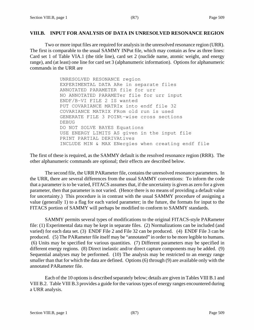
Section VIII.B, page 1 (R7) Page 509
Section VIII.B, page 1 (R7) Page 509
VIII.B. INPUT FOR ANALYSIS OF DATA IN UNRESOLVED RESONANCE REGION
Two or more input files are required for analysis in the unresolved resonance region (URR). The first is comparable to the usual SAMMY INPut file, which may contain as few as three lines: Card set 1 of Table VIA.1 (the title line), card set 2 (nuclide name, atomic weight, and energy range), and (at least) one line for card set 3 (alphanumeric information). Options for alphanumeric commands in the URR are
UNRESOLVED RESONANCE region EXPERIMENTAL DATA ARe in separate files ANNOTATED PARAMETER file for urr NO ANNOTATED PARAMETer file for urr input ENDF/B-VI FILE 2 IS wanted PUT COVARIANCE MATRIx into endf file 32 COVARIANCE MATRIX FRom old run is used GENERATE FILE 3 POINt-wise cross sections DEBUG DO NOT SOLVE BAYES Equations USE ENERGY LIMITS AS given in the input file PRINT PARTIAL DERIVAtives INCLUDE MIN & MAX ENergies when creating endf file
The first of these is required, as the SAMMY default is the resolved resonance region (RRR). The other alphanumeric commands are optional; their effects are described below.
The second file, the URR PARameter file, contains the unresolved resonance parameters. In the URR, there are several differences from the usual SAMMY conventions: To inform the code that a parameter is to be varied, FITACS assumes that, if the uncertainty is given as zero for a given parameter, then that parameter is not varied. (Hence there is no means of providing a default value for uncertainty.) This procedure is in contrast with the usual SAMMY procedure of assigning a value (generally 1) to a flag for each varied parameter; in the future, the formats for input to the FITACS portion of SAMMY will perhaps be modified to conform to SAMMY standards.
SAMMY permits several types of modifications to the original FITACS-style PARameter
file: (1) Experimental data may be kept in separate files. (2) Normalizations can be included (and varied) for each data set. (3) ENDF File 2 and File 32 can be produced. (4) ENDF File 3 can be produced. (5) The PARameter file itself may be “annotated” in order to be more legible to humans. (6) Units may be specified for various quantities. (7) Different parameters may be specified in different energy regions. (8) Direct inelastic and/or direct capture components may be added. (9) Sequential analyses may be performed. (10) The analysis may be restricted to an energy range smaller than that for which the data are defined. Options (6) through (9) are available only with the annotated PARameter file.
Each of the 10 options is described separately below; details are given in Tables VIII B.1 and VIII B.2. Table VIII B.3 provides a guide for the various types of energy ranges encountered during a URR analysis.
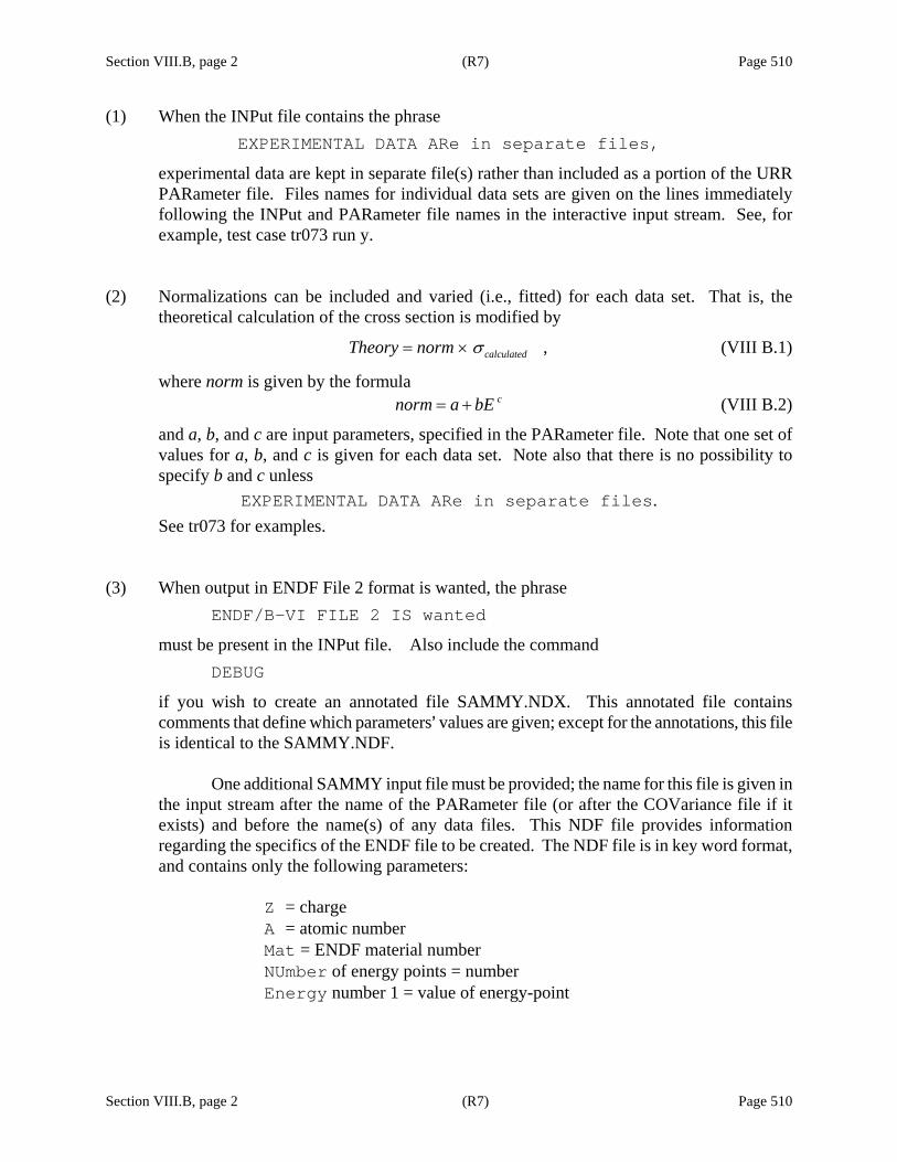
Section VIII.B, page 2 (R7) Page 510
Section VIII.B, page 2 (R7) Page 510
(1) When the INPut file contains the phrase EXPERIMENTAL DATA ARe in separate files,
experimental data are kept in separate file(s) rather than included as a portion of the URR PARameter file. Files names for individual data sets are given on the lines immediately following the INPut and PARameter file names in the interactive input stream. See, for example, test case tr073 run y.
(2) Normalizations can be included and varied (i.e., fitted) for each data set. That is, the
theoretical calculation of the cross section is modified by
,calculatedTheory norm σ= × (VIII B.1)
where norm is given by the formula cnorm a bE= + (VIII B.2)
and a, b, and c are input parameters, specified in the PARameter file. Note that one set of values for a, b, and c is given for each data set. Note also that there is no possibility to specify b and c unless
EXPERIMENTAL DATA ARe in separate files. See tr073 for examples.
(3) When output in ENDF File 2 format is wanted, the phrase
ENDF/B-VI FILE 2 IS wanted
must be present in the INPut file. Also include the command DEBUG
if you wish to create an annotated file SAMMY.NDX. This annotated file contains comments that define which parameters= values are given; except for the annotations, this file is identical to the SAMMY.NDF.
One additional SAMMY input file must be provided; the name for this file is given in
the input stream after the name of the PARameter file (or after the COVariance file if it exists) and before the name(s) of any data files. This NDF file provides information regarding the specifics of the ENDF file to be created. The NDF file is in key word format, and contains only the following parameters:
Z = charge A = atomic number Mat = ENDF material number NUmber of energy points = number Energy number 1 = value of energy-point

Section VIII.B, page 3 (R7) Page 511
Section VIII.B, page 3 (R7) Page 511
Only the one or two characters in capitals are required; others are optional. The value is given following the equal sign. One or the other of “NU...=” and “E...=” must be present. (If both are present, “NU...=” will be ignored.)
The number of energy points specifies at how many equally spaced points per energy
region the parameter values will be printed into the ENDF file. Values may also be printed at Emin and Emax, the limits of the analysis, if the phrase
INCLUDE MIN & MAX ENergies in endf file is given in the INPut file. For example, for 3 points per region and 5 regions, a total of 3 H 5 + 2 = 17 sets of values would be given in the ENDF file.
If, instead of having a certain number of points for each energy range, specific values
of energy are wanted in the ENDF file, then the alternative “E...=” should be specified. Subsequent energies are given one per line, with or without the key word “E...=” prior to the value. These energy values should be the last entries in this file.
See test cases tr073 and tr127 for examples. Runs a, b, e, and f of tr127 use
“NU...=” key word, while run g uses the “E...=” key word.
To also obtain the associated covariance file (ENDF File 32), include the phrase PUT COVARIANCE MATRix into endf file 32
in the INPut file. See test case tr128 runs j and k for examples. (4) ENDF File 3 output (point-wise cross sections, in file SAMMY.FL3) can be generated when
the command GENERATE FILE 3 POINt-wise cross sections
is included in the INPut file. The energy grid for this cross section is as defined by the input data sets. If the DEBUG command is also used, an annotated ENDF File 3 (SAMMY.FLX) output file is also produced. See test case tr073, runs n through t, for examples.
(5) Two modes, annotated and unannotated, are available for the URR PARameter file:
The unannotated mode is essentially equivalent to Fröhner=s original FITACS file (which includes both parameters and data). Formats for this file are described in Table VIII B .1; all numbers, both integer and real, are specified with F10 formats. To use this mode, the INPut file must contain the command
NO ANNOTATED PARAMETer file for urr input
Test case tr073 has examples of this input mode.
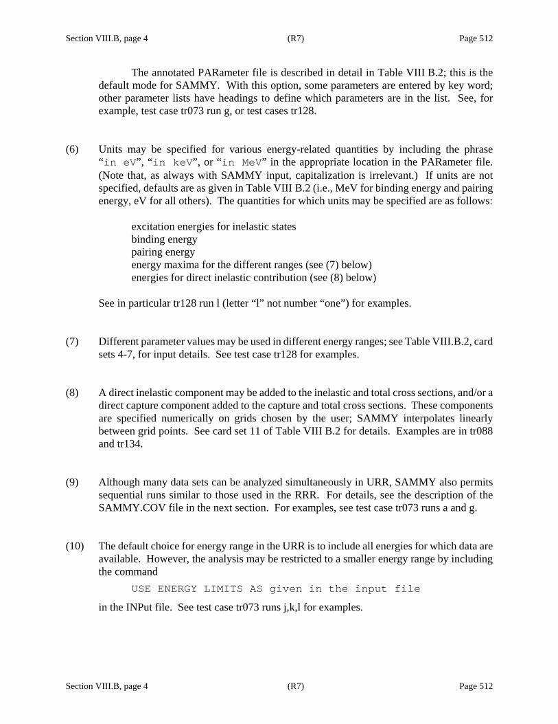
Section VIII.B, page 4 (R7) Page 512
Section VIII.B, page 4 (R7) Page 512
The annotated PARameter file is described in detail in Table VIII B.2; this is the default mode for SAMMY. With this option, some parameters are entered by key word; other parameter lists have headings to define which parameters are in the list. See, for example, test case tr073 run g, or test cases tr128.
(6) Units may be specified for various energy-related quantities by including the phrase
“in eV”, “in keV”, or “in MeV” in the appropriate location in the PARameter file. (Note that, as always with SAMMY input, capitalization is irrelevant.) If units are not specified, defaults are as given in Table VIII B.2 (i.e., MeV for binding energy and pairing energy, eV for all others). The quantities for which units may be specified are as follows:
excitation energies for inelastic states binding energy pairing energy energy maxima for the different ranges (see (7) below) energies for direct inelastic contribution (see (8) below)
See in particular tr128 run l (letter “l” not number “one”) for examples.
(7) Different parameter values may be used in different energy ranges; see Table VIII.B.2, card
sets 4-7, for input details. See test case tr128 for examples. (8) A direct inelastic component may be added to the inelastic and total cross sections, and/or a
direct capture component added to the capture and total cross sections. These components are specified numerically on grids chosen by the user; SAMMY interpolates linearly between grid points. See card set 11 of Table VIII B.2 for details. Examples are in tr088 and tr134.
(9) Although many data sets can be analyzed simultaneously in URR, SAMMY also permits
sequential runs similar to those used in the RRR. For details, see the description of the SAMMY.COV file in the next section. For examples, see test case tr073 runs a and g.
(10) The default choice for energy range in the URR is to include all energies for which data are
available. However, the analysis may be restricted to a smaller energy range by including the command
USE ENERGY LIMITS AS given in the input file
in the INPut file. See test case tr073 runs j,k,l for examples.

Section VIII.B, page 5 (R7) Page 513
Section VIII.B, page 5 (R7) Page 513
Table VIII B.1. Formats for original PARameter file for treatment of the unresolved resonance region
Card set
Line No. Description
1 1–4 First four lines are alphanumeric title
2 1 Number of iterations, fitting tolerance (essentially delta chi squared). Note that integers are to be specified as real numbers. All formats are F10.
2 Mass in amu, radius in Fermi (or use default), neutron binding energy in MeV, pairing energy PE in MeV. Again, formats are F10; note that the energy units are MeV, as opposed to the usual SAMMY standard of eV.
3 1,2,... Center-of-mass excitation energy (in eV), spin, and parity for the nth target level (beginning with ground state). Repeat as many times as needed.
Last (Blank)
4 1 Strength function Sc, uncertainty, distant-level parameter cR∞ , uncertainty,
radiation width γΓ in eV, uncertainty, mean level spacing D in eV for l = 0
2 Strength function, uncertainty, distant-level parameter, uncertainty, radiation width in eV, uncertainty, for l = 1
3 Strength function, uncertainty, distant-level parameter, uncertainty, radiation width in eV, uncertainty, for l = 2
4,5,... As above, for higher l values as needed
Last (Blank)
5 1 For the lowest J value for l = 0, Average fission width fΓ (eV)
Degree of freedom fν for fission width distribution
Hill-Wheeler threshold energy H WE
Hill-Wheeler threshold width H WW
Uncertainty on the average fission width
2,3,… Repeat line 1 for each possible value of J for l = 0.

Section VIII.B, page 6 (R7) Page 514
Table VIII B.1 (continued)
Section VIII.B, page 6 (R7) Page 514
Card set
Line No. Description
5, cont.
4,5,… Repeat lines 1-3 for each possible value of J for l = 1, 2, ...
For a given spin J and parity (even or odd l), only one set of values is actually used for fΓ and the other parameters. Nevertheless, all J and l must be included in this list. Only the values associated with the lowest l value will be used for the calculations; the other values will be ignored.
For example, the ground state of 235U is 7/2−. For l = 0, J π = 3−, 4−. For l = 1, J π = 2+, 3+, 4+, 5+. For l = 2, J π = 1−, 2−, 3−, 4−, 5−, 6−. The 3−and 4− values used in the calculations will be those given for l = 0. The values given for J π = 3−and 4− with l = 2 will be ignored.
Last (Blank)
6 1 Type of cross-section data (TOTAl, CAPTure, FISSion, or INELastic)
2 Uncertainties are RELAtive or ABSOlute
3 Energy, cross section, and uncertainty for first data point. Normalization and uncertainty (a and Δa) for this data set.
4,... Energy, cross section, uncertainty. (Note: if RELAtive then these need to be specified only for first data point; the others are assumed to be the same.)
Last (Blank)
6x All Repeat card set 6 as many times as needed, in any order
7 1 The single word “NORMALIZATION”. (Card set 7 is present only if the command “EXPERIMENTAL DATA ARe in separate files” appears in card set 3 of the INPut file.)
2 Type of cross section, normalization parameters a, Δa, b, Δb, c, Δc, where the normalization for this data set is given by cnorm = a + b E
3,etc. Repeat Line 2 once for each data set. Normalizations must appear in the same order in which the data sets appear. SAMMY will check to be sure the data types are consistent.
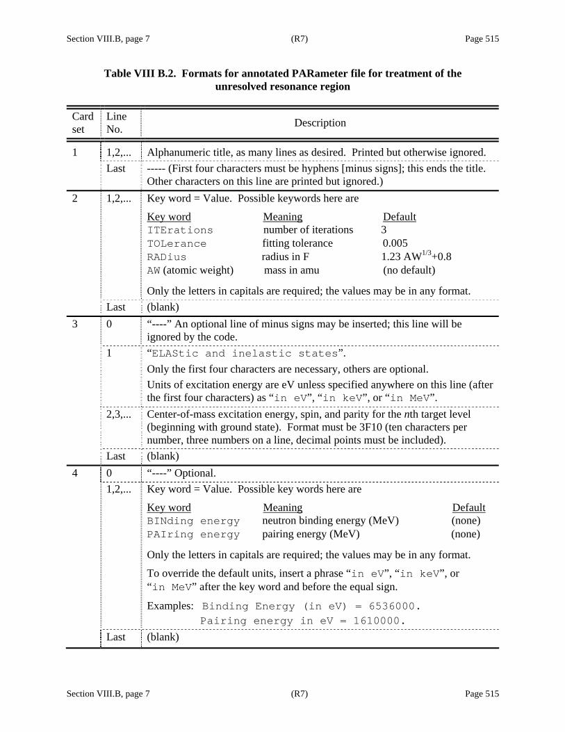
Section VIII.B, page 7 (R7) Page 515
Section VIII.B, page 7 (R7) Page 515
Table VIII B.2. Formats for annotated PARameter file for treatment of the unresolved resonance region
Card set
Line No. Description
1 1,2,... Alphanumeric title, as many lines as desired. Printed but otherwise ignored. Last ----- (First four characters must be hyphens [minus signs]; this ends the title.
Other characters on this line are printed but ignored.) 2 1,2,... Key word = Value. Possible keywords here are
Key word Meaning Default ITErations number of iterations 3 TOLerance fitting tolerance 0.005 RADius radius in F 1.23 AW1/3+0.8 AW (atomic weight) mass in amu (no default)
Only the letters in capitals are required; the values may be in any format. Last (blank) 3 0 “----” An optional line of minus signs may be inserted; this line will be
ignored by the code. 1 “ELAStic and inelastic states”.
Only the first four characters are necessary, others are optional. Units of excitation energy are eV unless specified anywhere on this line (after the first four characters) as “in eV”, “in keV”, or “in MeV”.
2,3,... Center-of-mass excitation energy, spin, and parity for the nth target level (beginning with ground state). Format must be 3F10 (ten characters per number, three numbers on a line, decimal points must be included).
Last (blank) 4 0 “----” Optional. 1,2,... Key word = Value. Possible key words here are
Key word Meaning Default BINding energy neutron binding energy (MeV) (none) PAIring energy pairing energy (MeV) (none)
Only the letters in capitals are required; the values may be in any format.
To override the default units, insert a phrase “in eV”, “in keV”, or “in MeV” after the key word and before the equal sign.
Examples: Binding Energy (in eV) = 6536000. Pairing energy in eV = 1610000.
Last (blank)
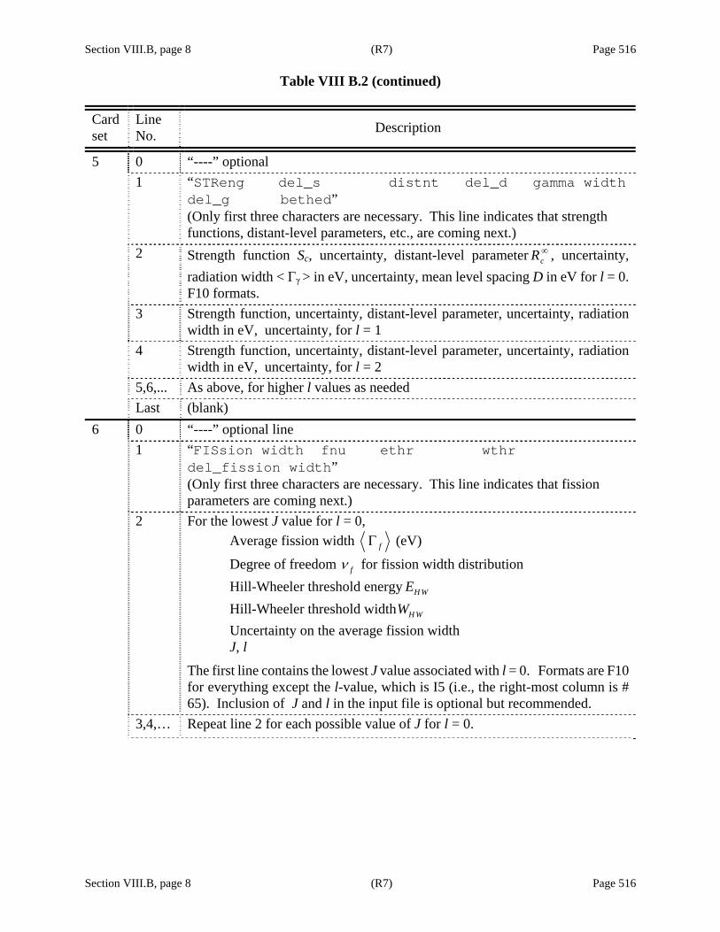
Section VIII.B, page 8 (R7) Page 516 Table VIII B.2 (continued)
Section VIII.B, page 8 (R7) Page 516
Card set
Line No. Description
5 0 “----” optional 1 “STReng del_s distnt del_d gamma width
del_g bethed” (Only first three characters are necessary. This line indicates that strength functions, distant-level parameters, etc., are coming next.)
2 Strength function Sc, uncertainty, distant-level parameter cR∞ , uncertainty, radiation width < Γγ > in eV, uncertainty, mean level spacing D in eV for l = 0. F10 formats.
3 Strength function, uncertainty, distant-level parameter, uncertainty, radiation width in eV, uncertainty, for l = 1
4 Strength function, uncertainty, distant-level parameter, uncertainty, radiation width in eV, uncertainty, for l = 2
5,6,... As above, for higher l values as needed Last (blank) 6 0 “----” optional line 1 “FISsion width fnu ethr wthr
del_fission width” (Only first three characters are necessary. This line indicates that fission parameters are coming next.)
2 For the lowest J value for l = 0, Average fission width fΓ (eV)
Degree of freedom fν for fission width distribution Hill-Wheeler threshold energy H WE Hill-Wheeler threshold width H WW Uncertainty on the average fission width J, l
The first line contains the lowest J value associated with l = 0. Formats are F10 for everything except the l-value, which is I5 (i.e., the right-most column is # 65). Inclusion of J and l in the input file is optional but recommended.
3,4,… Repeat line 2 for each possible value of J for l = 0.
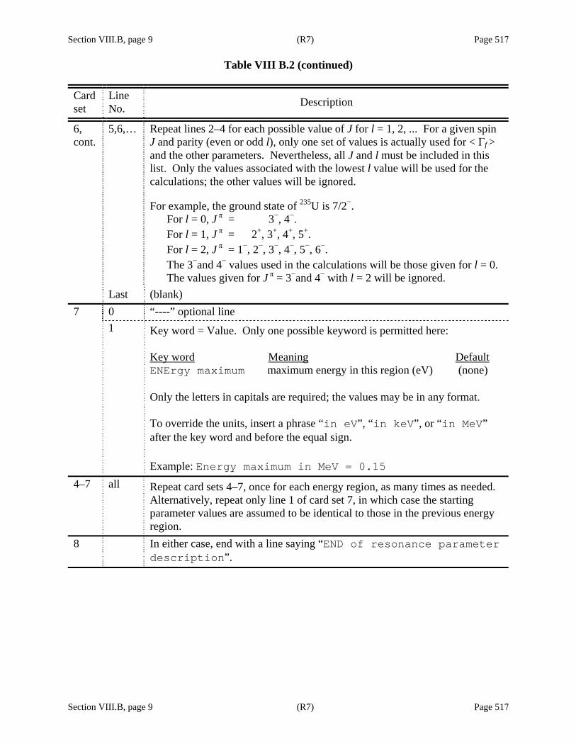
Section VIII.B, page 9 (R7) Page 517 Table VIII B.2 (continued)
Section VIII.B, page 9 (R7) Page 517
Card set
Line No. Description
6, cont.
5,6,… Repeat lines 2–4 for each possible value of J for l = 1, 2, ... For a given spin J and parity (even or odd l), only one set of values is actually used for < Γf > and the other parameters. Nevertheless, all J and l must be included in this list. Only the values associated with the lowest l value will be used for the calculations; the other values will be ignored.
For example, the ground state of 235U is 7/2−. For l = 0, J π = 3−, 4−. For l = 1, J π = 2+, 3+, 4+, 5+. For l = 2, J π = 1−, 2−, 3−, 4−, 5−, 6−. The 3−and 4− values used in the calculations will be those given for l = 0. The values given for J π = 3−and 4− with l = 2 will be ignored.
Last (blank) 7 0 “----” optional line 1
Key word = Value. Only one possible keyword is permitted here: Key word Meaning Default ENErgy maximum maximum energy in this region (eV) (none) Only the letters in capitals are required; the values may be in any format. To override the units, insert a phrase “in eV”, “in keV”, or “in MeV” after the key word and before the equal sign. Example: Energy maximum in MeV = 0.15
4–7 all Repeat card sets 4–7, once for each energy region, as many times as needed. Alternatively, repeat only line 1 of card set 7, in which case the starting parameter values are assumed to be identical to those in the previous energy region.
8 In either case, end with a line saying “END of resonance parameter description”.
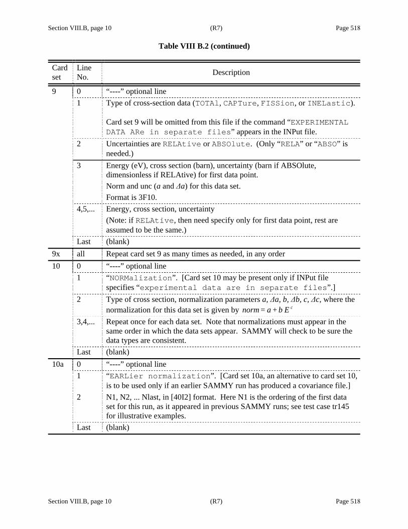
Section VIII.B, page 10 (R7) Page 518 Table VIII B.2 (continued)
Section VIII.B, page 10 (R7) Page 518
Card set
Line No. Description
9 0 “----” optional line 1 Type of cross-section data (TOTAl, CAPTure, FISSion, or INELastic).
Card set 9 will be omitted from this file if the command “EXPERIMENTAL DATA ARe in separate files” appears in the INPut file.
2 Uncertainties are RELAtive or ABSOlute. (Only “RELA” or “ABSO” is needed.)
3 Energy (eV), cross section (barn), uncertainty (barn if ABSOlute, dimensionless if RELAtive) for first data point. Norm and unc (a and Δa) for this data set. Format is 3F10.
4,5,... Energy, cross section, uncertainty (Note: if RELAtive, then need specify only for first data point, rest are assumed to be the same.)
Last (blank) 9x all Repeat card set 9 as many times as needed, in any order 10 0 “----” optional line 1 “NORMalization”. [Card set 10 may be present only if INPut file
specifies “experimental data are in separate files”.] 2 Type of cross section, normalization parameters a, Δa, b, Δb, c, Δc, where the
normalization for this data set is given by cnorm = a + b E 3,4,... Repeat once for each data set. Note that normalizations must appear in the
same order in which the data sets appear. SAMMY will check to be sure the data types are consistent.
Last (blank) 10a 0 “----” optional line 1 “EARLier normalization”. [Card set 10a, an alternative to card set 10,
is to be used only if an earlier SAMMY run has produced a covariance file.] 2 N1, N2, ... Nlast, in [40I2] format. Here N1 is the ordering of the first data
set for this run, as it appeared in previous SAMMY runs; see test case tr145 for illustrative examples.
Last (blank)

Section VIII.B, page 11 (R7) Page 519 Table VIII B.2 (continued)
Section VIII.B, page 11 (R7) Page 519
Card set
Line No. Description
11 0 “----” optional line 1 “DIRECT Inelastic contribution”, or “DIRECT Capture
contribution”. Note that eight characters (rather than the usual four) are required here.
2 Energy = value, Sigma = value. Both key words (and both values) must be on the same line. Key word Meaning Energy Energy in (eV) Sigma Direct inelastic cross section (b) at that energy To use different units on energy, insert a phrase “in eV”, “in keV”, or “in MeV” after the key word “Energy”.
3,4,... etc.
Repeat line 2 as many times as required. Note that card set 11 may be omitted if the contribution of the direct inelastic cross section is negligible or unknown.

Section VIII.B, page 12 (R7) Page 520
Section VIII.B, page 12 (R7) Page 520
Table VIII B.3. Energy ranges encountered in the unresolved resonance region
EMIN and EMAX for this run – • EMIN & EMAX refer to the min and max energies of the data to be fitted. • EMIN & EMAX can be given in the INPut file.
o “USE ENERGY LIMITS AS GIVEN IN THE INPUT FILE” must be specified (otherwise the values are ignored).
o The same EMIN & EMAX apply to all data sets. • If EMIN & EMAX are not given in the INPut file (or the command line is not used), then
EMIN & EMAX are set to the min and max energies occurring in the data sets. For each data set i – • Actual range for which data exist = Emini and Emaxi
o never defined in the SAMMY input but seen in the data file • Range to be used in this calculation
o All data points (from Emini to Emaxi) will be used unless EMIN & EMAX are specified in INPut file [and command line is there]. The same EMIN & EMAX are used for all data sets.
For the parameters, there are Numurr regions – • Energy limits are specified in the PARameter file.
o Engur0 is the “MINImum energy” for the first region. If Engur0 is not given, then it will be set equal to EMIN.
o Engurr(n) is the “Energy Maximum” for the nth region. If a “MINImum energy” is specified for region n (n>1), the code will check
whether it is equal to Engurr(n-1) and abort if it isn’t.
Region number
Energy at start of region
Energy at end of region
1 Engur0 Engurr(1) 2 Engurr(1) Engurr(2) 3 Engurr(2) Engurr(3) … Numurr Engurr(Numurr-1) Engurr(Numurr)
• If EMAX > Engurr(Numurr)
o If data are to be used above Engurr(Numurr), the code will print an error message and abort, because parameters are not defined above Engurr(Numurr).
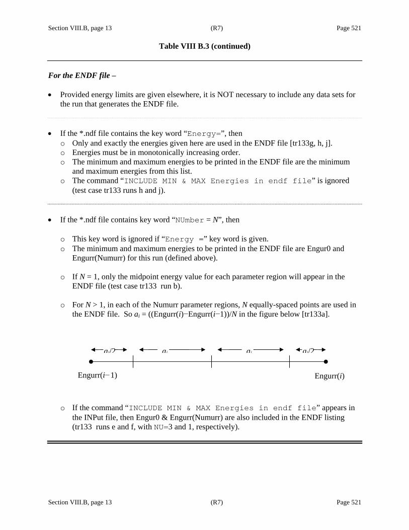
Section VIII.B, page 13 (R7) Page 521 Table VIII B.3 (continued)
Section VIII.B, page 13 (R7) Page 521
For the ENDF file – • Provided energy limits are given elsewhere, it is NOT necessary to include any data sets for
the run that generates the ENDF file. • If the *.ndf file contains the key word “Energy=”, then
o Only and exactly the energies given here are used in the ENDF file [tr133g, h, j]. o Energies must be in monotonically increasing order. o The minimum and maximum energies to be printed in the ENDF file are the minimum
and maximum energies from this list. o The command “INCLUDE MIN & MAX Energies in endf file” is ignored
(test case tr133 runs h and j).
• If the *.ndf file contains key word “NUmber = N”, then
o This key word is ignored if “Energy =” key word is given. o The minimum and maximum energies to be printed in the ENDF file are Engur0 and
Engurr(Numurr) for this run (defined above). o If N = 1, only the midpoint energy value for each parameter region will appear in the
ENDF file (test case tr133 run b). o For N > 1, in each of the Numurr parameter regions, N equally-spaced points are used in
the ENDF file. So ai = ((Engurr(i)−Engurr(i−1))/N in the figure below [tr133a].
o If the command “INCLUDE MIN & MAX Energies in endf file” appears in the INPut file, then Engur0 & Engurr(Numurr) are also included in the ENDF listing (tr133 runs e and f, with NU=3 and 1, respectively).
Engurr(i−1) Engurr(i)
ai aiai/2 ai/2

Section VIII.C, page 1 (R7) Page 523
Section VIII.C, page 1 (R7) Page 523
VIII.C. OUTPUT FROM ANALYSIS IN UNRESOLVED RESONANCE REGION
As with the resolved resonance region, each SAMMY/URR run may produce several output files: (1) The SAMMY.LPT file contains details of the calculations. (2) For runs which involve the solution of Bayes’ equations and hence the generation of updated
parameter values (a “Bayes run” as opposed to a “no-Bayes run” which simply calculates cross sections), an output file SAMMY.PAR is provided in the annotated form described in Table VIII B.2. (This file, of course, is quite different from the file by the same name produced in a resolved resonance region run.)
(3) For Bayes runs, a COVariance file SAMMY.COV is produced, which contains (among other
things) the final parameter covariance matrix; see below for more detail. (4) Files SAMMY.NDF and SAMMY.N32 contain the URR portion of ENDF File 2 and 32,
respectively; these files are produced when the appropriate command is in the INPut file. (5) Files SAMMY.NDX and SAMMY.N3X contain the same information as in SAMMY.NDF
and SAMMY.N32 respectively, but also include comment lines defining the parameters whose values are given. Only the uncertainty values are given in SAMMY.N3X; correlations are printed only in SAMMY.N32.
The binary COVariance file SAMMY.COV can be used as input to a subsequent SAMMY
run that uses the same R-matrix parameters but different data sets and different normalizations, in a similar fashion to sequential runs in the RRR. There are slight differences, however, in the usage of this COVariance file; no auxiliary program comparable to SAMAMR is required here, as there is only one type of data-reduction parameter (the normalizations). The user must simply rename and modify the SAMMY.PAR file to contain the appropriate normalization parameters for the data sets about to be analyzed. The output PARameter file will contain card set 10a of Table VIII B.2; PARameter files to be used as input will use either card set 10 (for new data sets for which the normalizations have not yet been defined) or card set 10a (to re-use normalizations already defined for the current data sets). See test case tr145 for examples.
To use an output SAMMY.PAR file as input to a new run without the accompanying COV file, it is necessary to delete the first line of the file; this line reads as follows:
COVARIANCE MATRIX FRom old run is used When the COV file is to be used (for sequential runs), keep this line in the PARameter file. Test cases tr073, tr088, tr127, tr128, tr133, tr145, and others provide sample input and output for URR calculations.

Section VIII.D, page 1 (R7) Page 525
Section VIII.D, page 1 (R7) Page 525
VIII.D. CONVERTING SAMMY/URR PARAMETERS TO ENDF/B PARAMETERS
Parameters required by the ENDF formats [ENDF-102] are related to the SAMMY (FITACS) input parameters but are not identical. Likewise the cross sections calculated by ENDF processor codes such as NJOY [RM82] may have somewhat different values from those calculated by SAMMY [HD03] because the exact same formulae are not used. (Formulae in SAMMY and FITACS are more accurate than those supported by ENDF.)
The correspondence between the SAMMY and the ENDF parameter values is described below. Channel radius
The R-matrix channel radius a used in SAMMY is related the ENDF scattering radius AP via ( )AP ' 1 cR a R∞= = − (VIII D.1) Note that a is input to SAMMY in units of Fermi; AP is specified for ENDF in units of 10−12 cm. Degrees of freedom
ENDF formats require that the number of degrees of freedom be explicitly stated for each channel), for each l and J. For SAMMY, only for fission channels is the number of degrees of freedom fν explicitly given in the input; for neutron channels, nν is calculated by the code to be either 1 or 2 (depending on the number of available channel spin values). For capture channels, γν is infinite and therefore not given in the input. [See Eq. (VIII A.5) for use of nν .] Level spacing
In SAMMY the mean level spacing D for l = 0 is specified in the input, and the energy- and J-dependent mean level spacing DJ (E) is derived as described in Section VIII.A, Eqs. (VIII A.9–16). For ENDF, DJ (E) is reported at particular energies. Neutron widths
In SAMMY the strength function is used to generate the transmission coefficient for neutron channels, according to Eq. (VIII A.7) with the pole strength sc defined in terms of the input strength function cS . Using the analogous form from Eq. (VIII A.8) and equating to Eq. (VIII A.7), we find

Section VIII.D, page 2 (R7) Page 526
Section VIII.D, page 2 (R7) Page 526
2
42 ,1
c cn J
cc c
P sDR L
ππ Γ =−
(VIII D.2)
or
( )( )( ) 2
2 2,
1 2
c cn J
c c c
P S ED
R i S E L
ρ
π ρ∞Γ =
− + (VIII D.3)
in which the expression for pole strength sc in terms of strength function cS , Eq. (VIII A.4), has been substituted. The ENDF manual [ENDF-102, page D18] specifies that it is the reduced neutron width which is to be reported. This width is related to the neutron width via
on n nE P ρΓ = Γ (VIII D.4)
or (with c = n)
( )( ) 2 ,
1 2
con J
c c c
SD
R i S E Lπ ρ∞Γ =
− + (VIII D.5)
which is the quantity reported in the ENDF file for a particular energy E.
Inelastic widths
The ENDF manual [ENDF-102] is exceedingly vague with regard to the inelastic widths. Two gross approximations are clearly required by the format: (1) Only a single inelastic width is permitted. (2) Only a single value of orbital angular momentum may be used. To work within these limitations, we have chosen to provide information only for the first inelastic channel, and to use the lowest value of orbital angular momentum l ' consistent with the specified l (of the elastic channel) and J. The contribution from the other inelastic channels can be given in File 3. The contribution from higher l ' must simply be ignored. No guarantee is made that SAMMY’s implementation of ENDF’s format is correct here.
Radiation widths
Radiation widths γΓ are input to SAMMY at E = 0. For ENDF, the widths are reported at particular energies as calculated by the giant dipole resonance model.
Fission widths
Fission widths fΓ are likewise input into SAMMY at E = 0, and reported in ENDF at particular energies. The energy dependence is given by Eqs. (VIII A .17–18).
Section VIII.D.1, page 1 (R7) Page 527
Section VIII.D.1, page 1 (R7) Page 527
VIII.D.1. Relation of SAMMY/URR Radius to ENDF/B Radius
To understand the rationale for the choice of R ' as the input radius for ENDF, we consider the value of the cross section in the limit in which the effect of resonances is negligible. From Eq. (VIII A.2), the average scattering matrix is given by
0*
20
1,
1c
cc cicc
cc c
R LS e
R Lϕ−
−=
− (VIII D1.1)
in which the average R-matrix is .cc c cR R i sπ∞= + (VIII D1.2) Substituting iP for L, dropping subscripts for simplicity, and rearranging give
( )( )( )( )
( ) ( ) ( )( ) ( )
( ) ( )
2 2
2
22 2 2
22
2 2 2
1 1
11
1 1
1 1
1 2cos 2 sin 2
1
cos 2 1
i icc
i
R i s i P Ps iPRS e e
Ps iPRR i s i P
Ps iPR Ps iPRe
Ps iPR Ps iPR
P s PR iPRi
Ps PR
P s PR
ϕ ϕ
ϕ
π π
ππ
π π
π π
πϕ ϕ
π
ϕ π
∞ ∞− −
∞∞
∞ ∞−
∞ ∞
∞ ∞
∞
∞
⎡ ⎤− + − ⎡ ⎤− +⎣ ⎦ ⎣ ⎦= =⎡ ⎤ ⎡ ⎤+ −− + + ⎣ ⎦⎣ ⎦
⎡ ⎤ ⎡ ⎤− + + +⎣ ⎦ ⎣ ⎦=⎡ ⎤ ⎡ ⎤+ − + +⎣ ⎦ ⎣ ⎦
− − += −⎡ ⎤⎣ ⎦
+ +
− −
=
( ) ( ) ( ) ( )
( ) ( )
2
22 2 2
22
sin 2 2
sin 2 1 sin 2 2.
1
PR
i P s PR PR
Ps PR
ϕ
ϕ π ϕ
π
∞
∞ ∞
∞
⎡ ⎡ ⎤ +⎢ ⎢ ⎥⎣ ⎦⎣⎤⎡ ⎤+ − − − + ⎥⎢ ⎥⎣ ⎦ ⎦
+ +
(VIII D1.3) The cross section can then be expressed as
( )( ) ( ) ( )
( ) ( )
2
22 2 2
22 2
2 1 Re
cos 2 1 sin 2 22 1 .1
c ccg S
k
P s PR PRgk Ps PR
πσ
ϕ π ϕπ
π
∞ ∞
∞
= −
⎛ ⎞⎡ ⎤− − +⎢ ⎥⎜ ⎟⎣ ⎦= −⎜ ⎟+ +⎜ ⎟
⎝ ⎠
(VIII D1.4)
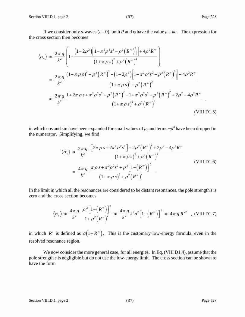
Section VIII.D.1, page 2 (R7) Page 528
Section VIII.D.1, page 2 (R7) Page 528
If we consider only s-waves (l = 0), both P and φ have the value ρ = ka. The expression for the cross section then becomes
( ) ( )( ) ( )
( ) ( ) ( ) ( )( ) ( )( ) ( )( ) ( )
22 2 2 2 2 2
22 2 2
2 22 2 2 2 2 2 2 2
22 2 2
2 22 2 2 2 2 2 2 2 2 2
22 2 2
1 2 1 42 11
1 1 2 1 42
1
1 2 1 2 42 ,1
c
s R Rgk s R
s R s R Rgk s R
s s R s R Rgk s R
ρ π ρ ρ ρπσπ ρ ρ
π ρ ρ ρ π ρ ρ ρπ
π ρ ρ
π ρ π ρ ρ π ρ ρ ρ ρπ
π ρ ρ
∞ ∞
∞
∞ ∞ ∞
∞
∞ ∞ ∞
∞
⎛ ⎞⎡ ⎤− − − +⎢ ⎥⎜ ⎟⎣ ⎦≈ −⎜ ⎟+ +⎜ ⎟
⎝ ⎠⎡ ⎤+ + − − − − −⎢ ⎥⎣ ⎦=
+ +
+ + + − + + + −≈
+ +
(VIII D1.5) in which cos and sin have been expanded for small values of ρ, and terms ~ρ4 have been dropped in the numerator. Simplifying, we find
( )( ) ( )
( )( ) ( )
22 2 2 2 2 2
22 2 2
22 2 2 2
22 2 2
2 2 2 2 42
1
14 .1
c
s s R Rgk s R
s s Rgk s R
π ρ π ρ ρ ρ ρπσπ ρ ρ
π ρ π ρ ρπ
π ρ ρ
∞ ∞
∞
∞
∞
⎡ ⎤+ + + −⎣ ⎦≈+ +
⎡ ⎤+ + −⎣ ⎦=+ +
(VIII D1.6)
In the limit in which all the resonances are considered to be distant resonances, the pole strength s is zero and the cross section becomes
( )( )
( )22
22 2 222 22
14 4 1 4 ' ,1
c
Rg g k a R g Rk kR
ρπ πσ πρ
∞
∞
∞
⎡ ⎤−⎣ ⎦ ⎡ ⎤≈ ≈ − =⎣ ⎦+ (VIII D1.7)
in which 'R is defined as ( )1a R ∞− . This is the customary low-energy formula, even in the resolved resonance region.
We now consider the more general case, for all energies. In Eq. (VIII D1.4), assume that the pole strength s is negligible but do not use the low-energy limit. The cross section can be shown to have the form
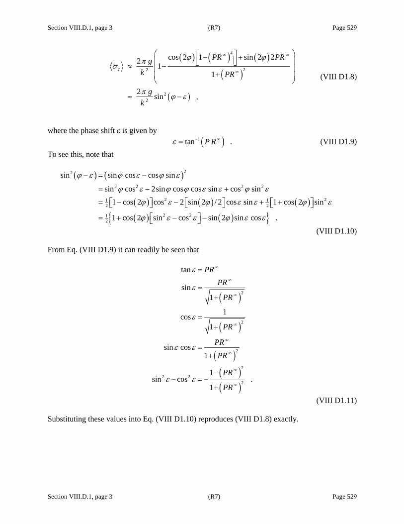
Section VIII.D.1, page 3 (R7) Page 529
Section VIII.D.1, page 3 (R7) Page 529
( ) ( ) ( )
( )
( )
2
22
22
cos 2 1 sin 2 22 11
2 sin ,
c
PR PRgk PR
gk
ϕ ϕπσ
π ϕ ε
∞ ∞
∞
⎛ ⎞⎡ ⎤− +⎢ ⎥⎜ ⎟⎣ ⎦≈ −⎜ ⎟+⎜ ⎟
⎝ ⎠
= −
(VIII D1.8)
where the phase shift ε is given by ( )1tan .P Rε − ∞= (VIII D1.9) To see this, note that
( ) ( )
( ) ( ) ( )( ) ( )
22
2 2 2 2
2 21 12 2
2 212
sin sin cos cos sin
sin cos 2sin cos cos sin cos sin
1 cos 2 cos 2 sin 2 / 2 cos sin 1 cos 2 sin
1 cos 2 sin cos sin 2 sin cos .
ϕ ε ϕ ε ϕ ε
ϕ ε ϕ ϕ ε ε ϕ ε
ϕ ε ϕ ε ε ϕ ε
ϕ ε ε ϕ ε ε
− = −
= − +
= − − + +⎡ ⎤ ⎡ ⎤ ⎡ ⎤⎣ ⎦ ⎣ ⎦ ⎣ ⎦
⎡ ⎤= + − −⎣ ⎦
(VIII D1.10) From Eq. (VIII D1.9) it can readily be seen that
( )
( )
( )( )( )
2
2
2
2
2 22
tan
sin1
1cos1
sin cos1
1sin cos .
1
PRPR
PR
PR
PR
PR
PR
PR
ε
ε
ε
ε ε
ε ε
∞
∞
∞
∞
∞
∞
∞
∞
=
=+
=+
=+
−− = −
+
(VIII D1.11) Substituting these values into Eq. (VIII D1.10) reproduces (VIII D1.8) exactly.

Section IX, page 1 (R8) Page 531
Section IX, page 1 (R8) Page 531
IX. THE ENDF CONNECTION
Analyses accomplished with SAMMY often find their way into one or more of the evaluated nuclear data files [ENDF (United States), JEFF (European), CENDL (Chinese), JENDL (Japanese), BROND (Russian), FOND (Russian), ...]. Resonance parameters from the evaluated nuclear data files or experimental data from the EXFOR files are sometimes used as input for SAMMY analyses. Many options are available within SAMMY to expedite this information interchange; a summary is available in [NL07a]. Options described elsewhere in this document are merely noted here; other options are described in detail in this section. See also Section XI.C for miscellaneous comments regarding ENDF format conventions. Details of ENDF formats are given in [ENDF-102]; SAMMY users can more readily obtain information about resolved-resonance ENDF formats from [NL07b].
SAMMY command statements related to using ENDF formats as either input or output are summarized in Table VI A1.2 under the categories “ENDF as input” or “ENDF output.” See also Sections VI.F.2 and VI.F.3 for other input requirements.
(In the following comments, “endf” in lowercase letters refers to “evaluated nuclear data files” in general, and “ENDF” in capital letters refers to the United States’ Evaluated Nuclear Data Files [ENDFw] as housed at the National Nuclear Data Center [NNDC] at Brookhaven National Laboratory.)
In 1998 the Cross Section Evaluation Working Group (CSEWG), an advisory group for the ENDF, appointed a “constants” task force subcommittee whose purpose was to ensure that each code contributing to or using data from the evaluated files would use the same values for mathematical and physical constants. The final report of that subcommittee is found in Section IX.A of this document. Also included there is Table IXA.1, which gives values for the physical constants used in the current version of SAMMY.
In the resolved resonance region (RRR), SAMMY can read resonance parameters directly from File 2 (extracted from an endf file), or from an entire endf file if the MAT (material) number is provided. Test cases tr049, tr050, tr086, tr102, and tr129 provide examples of this use of endf files. See Section VI.F.3 for details.
SAMMY can also write the R-matrix parameters into endf file 2 formats. For the RRR, see Section VI.F.2 for details. For the unresolved resonance region (URR), see Section VIII.D. Note that SAMMY can produce two output files corresponding to endf File 2, named SAMMY.NDF and SAMMY.NDX. The first of these is suitable for direct use within a complete endf file. The second (which is produced if the command “DEBUG” is included in the INPut file) contains the identical information but also includes comment lines (beginning with ####) that may be helpful in understanding the contents of the file.
When creating File 2, it is also possible to create File 32, which contains covariance information for the resonance parameters. The necessary command line is “PUT COVARIANCE MATRIx into endf file 32”. The output file is named SAMMY.N32, and the corresponding annotated file (containing comment lines) is SAMMY.N3X. Test case tr126 has numerous examples with LCOMP = 0, 1, and 2. Test case tr128 gives examples in the URR.
Section IX, page 2 (R8) Page 532
Section IX, page 2 (R8) Page 532
When the input resonance parameters are in endf File 2 format (RRR), and the intent is to generate an estimated covariance matrix for endf File 32, SAMMY can automatically generate the input *.ndf file for that purpose. To invoke, include the command “AUTOMATIC NDF FILE Creation” in the INPut file. See test case tr137 (k and l) for examples. Note that other commands are also necessary:
AUTOMATIC NDF FILE Creation INPUT IS ENDF/B FILE MAT=9446 FLAG ALL RESONANCE Parameters ENDF/B-VI FILE 2 IS wanted NDF FILE IS IN KEY Word format (optional) PUT COVARIANCE MATRIx into endf file 32
It is important to note that the resonance parameter covariance matrix alone is not capable of conveying complete information regarding the evaluated cross section covariance matrix, as discussed in Section IV.E.6. Additional information (normalization or background uncertainty) can be introduced via the use of endf File 33.
Point-wise cross sections can be printed in endf File 3 formats, in both the RRR and the URR. To invoke this option, include the phrase “GENERATE FILE 3 POINt-wise cross section”, or “FILE 3”, in the INPut file. An annotated *.ndf file, similar to that described in Section VI.F.2 for File 2, is also needed; see Table IX.1 for details. (Note that most entries in this table are optional.) The output file is named SAMMY.FL3, and the corresponding annotated file is SAMMY.FLX. For examples, see test case tr086 (w) in the RRR, and test case tr073 (n) in the URR.
It is possible to use ENDF File 3 as the “experimental data file”. To do so, include one of these commands in the INPut file: “DATA ARE ENDF/B FILE MAT=1234” or “USE ENDF/B ENERGIES MAT=1234”, where the spacing before “MAT=” is not important (but there must be at least one space), and the endf MAT (material) number is used instead of “1234”.
When calculating group averages, results can be reported in an endf-like format, similar to File 3, and the associated covariance matrix into a file with a format similar to File 33. Include the command “FILE 33 LB=1 COVARIAnce is wanted” (or just “FILE 33”) to write the average cross sections into file SAMMY.CRS and covariance information into file SAMMY.N33. † See test case tr089 (h and i) for examples. It is important to note that this is not the standard use for Files 3 and 33; these files should not be used for inclusion in official ENDF files.
Legendre coefficients for angular distributions may be reported in endf File 4 format by including the command “PREPARE LEGENDRE COEfficients in endf format”. The output file is called endf_legendre.dat. (File SAMJNK.DAT contains the same information in an expanded format.) The version of File 4 used here is that described in Section 4.2.2 of [ENDF-102], LTT = 1, LVT = 0, and LI = 0 (that is to say, the Legendre expansion coefficients Al(E) are given, no transformation matrix is given, and the angular distributions are not all isotropic). See test case tr112 for examples. † Historical note: SAMMY.N33 was once called SAMMY.NDF, but the name has been changed to avoid confusion with other files of the same name.

Section IX, page 3 (R8) Page 533
Section IX, page 3 (R8) Page 533
CAVEAT: It is the responsibility of the analyst (and not only of the SAMMY author) to ensure that any endf files produced by SAMMY runs are correct. In particular, SAMMY users are strongly encouraged to compare those files with the requirements of the endf formats. Likewise, when endf files are used for input to SAMMY, users are urged to look carefully at all output to be sure that SAMMY is properly interpreting the input. When discrepancies are found, please notify the SAMMY author so that adjustments can be made.
Table IX.1. Key-word-based file needed for generating ENDF File 3 output
Card Set
Key-word variable Notes
1 Z Z for target nucleus.
A Atomic mass number.
ZA If different from (1000 * Z + A), then value must be inserted directly.
AW Ratio of the mass of the sample nucleus to the neutron mass (if absent, will be calculated from the SAMMY input).
MAT ENDF MAT number (default = 9999).
(blank)
2 NUclide or ISOtope
No value need be given here; this word simply indicates that information for the next nuclide will follow. For the URR, card sets 2 and 3 are not used, as the present implementation of the URR in SAMMY permits only one nuclide at a time.
3 Z Z for target nucleus (this isotope); not needed here if same as above.
A Atomic mass number (this isotope); not needed if same as above.
ZA If different from (1000 * Z + A), then value must be inserted directly.
AW Ratio of mass of sample nucleus (this isotope) to neutron mass.
ABN Abundance for this isotope, if different from unity.
SPIN Spin of this isotope.
(blank)


Section IX.A, page 1 (R7) Page 535
Section IX.A, page 1 (R7) Page 535
IX.A. CSEWG CONSTANTS
Recommendation of the CSEWG Constants Task Force October 20, 1998
CSEWG participants: Mark Chadwick, Maurice Greene, Richard Hwang, Nancy Larson (chair), Robert
MacFarlane, Vicki McLane, John White Other participants: Dermott Cullen, Mick Moxon In order to eliminate the use of different values for physical and mathematical constants as a source of discrepancy between calculations using different computer codes, CSEWG should take the following actions: (1) Formally designate as official CSEWG constants the values reported in “1986 CODATA Internationally
recommended values of the Fundamental Physical Constants” on the Web site http://physics.nist.gov/cuu/Constants/. This is the “NIST Reference on Constants, Units, and Uncertainty, one of the technical activities of the Fundamental Constants Data Center of the NIST Physics Laboratory. The contents of this site have been prepared by Barry N. Taylor of the Data Center in close collaboration with Peter J. Mohr of the Physics Laboratory=s Atomic Physics Division.”
a. Relevant numbers from the CODATA list will be published in ENDF-102. b. Evaluators and code developers should use the values published in ENDF-102, updating only when
that document is updated. (2) Within the text of the next update of ENDF-102, remove numerical values for physical constants and
replace by variable names; provide numerical values (and units) in a list in an appendix. This list should include (but is not limited to) the following:
a. mn = mass of neutron in atomic mass units (u)
[Remove values from pages 0.18 and D.4 of the Nov. 1995 version of ENDF-102]. Recommended value from CODATA: mn = 1.008 664 904 u
b. Boltzmann=s constant k.
Recommended value from CODATA: k = 8.617 385 H 10-5 eV K-1
c. 2 nm = sqrt (2 mass of neutron) / Plank=s constant. [Remove value from p. D.3.]
Recommended value based on information in CODATA:
2 nm = 0.002 196 807 122 623 / (10-12 cm eV )
d. 2 (amu) / 2 . [Remove value from Eq. (6.9).]
Recommended value based on information in CODATA: 2 (amu) / 2 = 4.784 504 258 066 H 10-6 / ( [10-12 cm]2 eV ).
e. (e2 / )2 amu. [Remove value from Eq. (6.10).]
Recommended value based on CODATA: (e2 /• )2 amu = 2.480 167 060 319 H 104 eV.
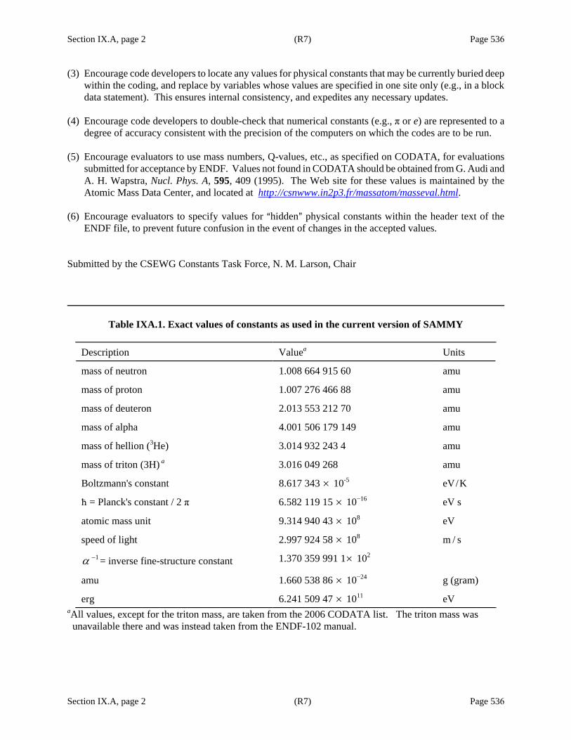
Section IX.A, page 2 (R7) Page 536
Section IX.A, page 2 (R7) Page 536
(3) Encourage code developers to locate any values for physical constants that may be currently buried deep within the coding, and replace by variables whose values are specified in one site only (e.g., in a block data statement). This ensures internal consistency, and expedites any necessary updates.
(4) Encourage code developers to double-check that numerical constants (e.g., π or e) are represented to a
degree of accuracy consistent with the precision of the computers on which the codes are to be run. (5) Encourage evaluators to use mass numbers, Q-values, etc., as specified on CODATA, for evaluations
submitted for acceptance by ENDF. Values not found in CODATA should be obtained from G. Audi and A. H. Wapstra, Nucl. Phys. A, 595, 409 (1995). The Web site for these values is maintained by the Atomic Mass Data Center, and located at http://csnwww.in2p3.fr/massatom/masseval.html.
(6) Encourage evaluators to specify values for Ahidden@ physical constants within the header text of the
ENDF file, to prevent future confusion in the event of changes in the accepted values. Submitted by the CSEWG Constants Task Force, N. M. Larson, Chair
Table IXA.1. Exact values of constants as used in the current version of SAMMY
Description Valuea Units
mass of neutron 1.008 664 915 60 amu
mass of proton 1.007 276 466 88 amu
mass of deuteron 2.013 553 212 70 amu
mass of alpha 4.001 506 179 149 amu
mass of hellion (3He) 3.014 932 243 4 amu
mass of triton (3H) a 3.016 049 268 amu
Boltzmann's constant 8.617 343 × 10-5 eV/K
• = Planck's constant / 2 π 6.582 119 15 × 10−16 eV s
atomic mass unit 9.314 940 43 × 108 eV
speed of light 2.997 924 58 × 108 m / s 1α − = inverse fine-structure constant 1.370 359 991 1× 10²
amu 1.660 538 86 × 10−24 g (gram)
erg 6.241 509 47 × 1011 eV aAll values, except for the triton mass, are taken from the 2006 CODATA list. The triton mass was unavailable there and was instead taken from the ENDF-102 manual.

Section X, page 1 (R8) Page 537
Section X, page 1 (R8) Page 537
X. AUXILIARY PROGRAMS
A number of “auxiliary” programs, not an integral part of SAMMY itself, are designed to be used in conjunction with SAMMY. These programs manipulate SAMMY PARameter and/or COVariance files, aid in interpreting or illustrating SAMMY input or output, or offer a means of comparing SAMMY results with other calculations. The codes are listed in alphabetical order in Table X.1, which also provides a brief description of the purpose of the code, and the section number in which details can be found.
Table X.1. SAMMY auxiliary codes
Code name Description Section
ANGODF Convert PLOT file from energy/angle to angle/energy X.A CONVRT Convert from REFIT input to SAMMY or vice versa X.B SAMAMR Add, mix, or recover variables in COVariance file X.C SAMAMX Alter the value of one non-varied parameter in the COVariance
file after completion of an analysis X.D
SAMCPR Compare SAMMY calculations to those from other sources X.E SAMDIS Calculate statistical distributions for resonance parameters X.F SAMFTZ Modify the experimental energies with t0 and L0 X.G SAMGY2 Smooth the Y2 function for multiple-scattering calculations X.R SAMORT Plot the ORR resolution function X.H SAMPLT Alternative form for plot files X.I SAMQUA Generate resonance quantum numbers for particle pairs X.J SAMRML Read ENDF File 2; calculate cross sections and derivatives X.Q SAMRPT Plot RPI resolution function X.K SAMRST Plot Gaussian plus exponential resolution function X.L SAMSMC Monte Carlo calculation of multiple scattering corrections X.M SAMSTA Generate staircase plots of resonance widths X.N SAMTHN Thin experimental data X.O SUGGEL Estimate quantum numbers for resonances X.P

Section X, page 2 (R8) Page 538
Section X, page 2 (R8) Page 538
When angular distribution data are analyzed, results are reported in an ODF file [JC78] from which plots of cross section vs. energy at a fixed angle can be made. To plot cross section vs. angle at fixed energy, it is necessary to reorganize the ODF file; this reorganization is accomplished with the program ANGODF, discussed in Section X.A.
The task of converting from REFIT to SAMMY input can be eased by use of the program CONVRT, discussed in Section X.B.
In Section X.C the program SAMAMR is described; this program is used to rearrange PARameter and COVariance files to facilitate analyses of disparate data sets with the same resonance parameter set. (Note that SAMAMR replaces the two codes SAMADD and SAMMIX described in early versions of this report.)
Program SAMAMX is used to alter the value of one non-varied parameter in the covariance file after completion of an analysis. See Section X.D.
For assistance in comparing results of calculations performed by different computer codes, use program SAMCPR; see Section X.E for details.
Program SAMDIS (elsewhere named SAMDIST) is used for calculating statistical distributions for R-matrix resonance parameters; see ref. [LL95]. Level spacing distributions are calculated according to the Wigner distribution law, distributions for widths are calculated via χ2 distributions, and long-range correlations of the energies are tested via the Δ3 statistic of Mehta-Dyson. A summary of features of this code is given in Section X.F, along with recent modifications of the input to the code.
Program SAMFTZ is used to modify the experimental energies in a DATa file, in order to align them more accurately with other experimental data. See Section X.G for details.
Program SAMORT, described in Section X.H, is used for plotting the components of the Oak Ridge resolution function. Similar plots can be made for the RPI resolution function using program SAMRPT (Section X.K) and for the original Gaussian-plus-exponential resolution function (Section X.L).
Program SAMPLT, which provides an alternative methodology for generating plots, is discussed in Section X.I. (Note: This program has been renamed from SAMBIN.)
Quantum numbers can be generated using program SAMQUA, described in Section X.J. This program has recently been updated by Olivier Bouland et al. [OB03] to include more complicated cases.
Program SAMSMC may be used for Monte Carlo calculations of the self-shielding and multiple-scattering corrections to capture and fission yields. See Section X.M.
The program SAMSTA, described in Section X.N, is used to create a file from which “staircase plots” of the resonance from a SAMMY PARameter file can be generated.

Section X, page 3 (R8) Page 539
Section X, page 3 (R8) Page 539
Section X.O describes program SAMTHN, a simple program for averaging data files used as input to SAMMY runs.
Soo Youl Oh and Luiz Leal=s SUGGEL code, used to provide initial estimates for the quantum numbers of resonances, is described in Section X.P.
Section X.Q describes SAMRML, a program designed as an aid for people wishing to implement the ENDF File 2 LRU=1 LRF=7 format. This code calculates cross sections and derivatives as SAMMY does but without the considerable overhead relating to comparisons to experimental data.
Program SAMY2C reads double-plus scattering corrections as generated by SAMSMC and smooths them for use in place of the SAMMY-generated values in future SAMMY calculations. Details are given in Section III.D and in Section X.R.

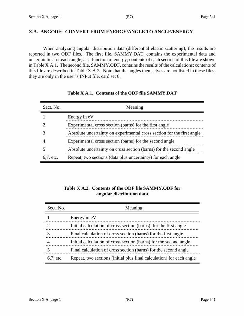
Section X.A, page 1 (R7) Page 541
Section X.A, page 1 (R7) Page 541
X.A. ANGODF: CONVERT FROM ENERGY/ANGLE TO ANGLE/ENERGY
When analyzing angular distribution data (differential elastic scattering), the results are reported in two ODF files. The first file, SAMMY.DAT, contains the experimental data and uncertainties for each angle, as a function of energy; contents of each section of this file are shown in Table X A.1. The second file, SAMMY.ODF, contains the results of the calculations; contents of this file are described in Table X A.2. Note that the angles themselves are not listed in these files; they are only in the user’s INPut file, card set 8.
Table X A.1. Contents of the ODF file SAMMY.DAT
Sect. No. Meaning
1 Energy in eV
2 Experimental cross section (barns) for the first angle
3 Absolute uncertainty on experimental cross section for the first angle
4 Experimental cross section (barns) for the second angle
5 Absolute uncertainty on cross section (barns) for the second angle
6,7, etc. Repeat, two sections (data plus uncertainty) for each angle
Table X A.2. Contents of the ODF file SAMMY.ODF for angular distribution data
Sect. No. Meaning
1 Energy in eV
2 Initial calculation of cross section (barns) for the first angle
3 Final calculation of cross section (barns) for the first angle
4 Initial calculation of cross section (barns) for the second angle
5 Final calculation of cross section (barns) for the second angle
6,7, etc. Repeat, two sections (initial plus final calculation) for each angle
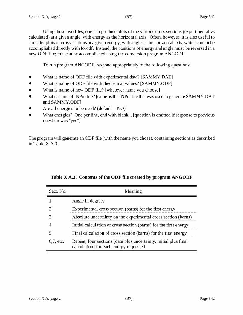
Section X.A, page 2 (R7) Page 542
Section X.A, page 2 (R7) Page 542
Using these two files, one can produce plots of the various cross sections (experimental vs calculated) at a given angle, with energy as the horizontal axis. Often, however, it is also useful to consider plots of cross sections at a given energy, with angle as the horizontal axis, which cannot be accomplished directly with forodf. Instead, the positions of energy and angle must be reversed in a new ODF file; this can be accomplished using the conversion program ANGODF.
To run program ANGODF, respond appropriately to the following questions: ! What is name of ODF file with experimental data? [SAMMY.DAT] ! What is name of ODF file with theoretical values? [SAMMY.ODF] ! What is name of new ODF file? [whatever name you choose] ! What is name of INPut file? [same as the INPut file that was used to generate SAMMY.DAT
and SAMMY.ODF] ! Are all energies to be used? (default = NO) ! What energies? One per line, end with blank... [question is omitted if response to previous
question was Ayes@] The program will generate an ODF file (with the name you chose), containing sections as described in Table X A.3.
Table X A.3. Contents of the ODF file created by program ANGODF
Sect. No. Meaning
1 Angle in degrees
2 Experimental cross section (barns) for the first energy
3 Absolute uncertainty on the experimental cross section (barns)
4 Initial calculation of cross section (barns) for the first energy
5 Final calculation of cross section (barns) for the first energy
6,7, etc. Repeat, four sections (data plus uncertainty, initial plus final calculation) for each energy requested

Section X.B, page 1 (R4) Page 543
Section X.B, page 1 (R4) Page 543
X.B. CONVRT: CONVERT FROM REFIT INPUT TO SAMMY OR VICE VERSA
During his 1996 visit to Oak Ridge, Mick Moxon and the SAMMY author made preliminary attempts to provide an interface between Moxon’s code REFIT [MM89] and SAMMY. The result is a program CONVRT, which is intended to read the input files for one code and write the corresponding input files for the other code. Beginning from REFIT input files, program CONVRT is able to generate appropriate SAMMY-style INPut and PARameter files; similarly, beginning from SAMMY-style files, CONVRT can generate portions of the REFIT input files. In either case, the user will likely need to edit the new files to provide complete input. Note that CONVRT is not yet able to translate resolution parameters nor experimental data from one code to the other, because definitions are not completely compatible between SAMMY and REFIT.
Input to program CONVRT consists of one command line (either “sammy” if converting from SAMMY to REFIT, or “refit” if converting from REFIT to SAMMY), followed by names of input files.
When converting from SAMMY to REFIT, file names are given in the usual order (INPut, PARameter, and DATa file names). Output consists of a SAMMY.LPT file, plus files containing portions of the REFIT input files; these are named REFITx.DAT where “x” is a digit from 0 to 9. One file is given for each nuclide type; it is the user=s responsibility to combine these properly into the REFIT input file.
When converting from REFIT to SAMMY, output consists of three files: SAMMY.LPT, SAMMY.INP, and SAMMY.PAR. The user should rename these files and check to be sure they are complete before using the INPut or PARameter file as input to SAMMY runs.

Section X.C, page 1 (R7) Page 545
Section X.C, page 1 (R7) Page 545
X.C. SAMAMR: ADD, MIX, OR RECOVER VARIABLES Because the fitting procedure in SAMMY is Bayes= method (Section IV) rather than ordinary least squares, SAMMY may be used for general evaluation purposes, that is, for determining a set of parameters that simultaneously describe a large number of different types of experimental data taken at different times and/or at different laboratories.
Performing such evaluations with SAMMY originally required sequential analyses of the various data sets,∗ with the output parameter and covariance matrix from the first analyses used as input to the second, output from the second used as input to the third, and so forth. If none of the broadening parameters are varied during the analyses, and if no data-reduction parameters are included, this procedure poses no undue difficulty; the analyst simply changes the values of the thickness and/or of the broadening parameters in the INPut file to correspond to the data currently being analyzed. However, when any of the broadening parameters are varied, and/or when normalization or background is included in the analysis, the PARameter and COVariance files must also correspond to the current data set. The code SAMAMR performs the appropriate modifications to the PARameter and COVariance files.
For example, data may come from two or more samples of different thicknesses and at
different temperatures. The initial PARameter file is set up to include thickness and temperature appropriate for the first sample; thickness and temperature for the other samples are simply omitted. After the analysis of the first data set, code SAMAMR is used to incorporate the second thickness (as yet uncorrelated to any other parameters) and to “mothball” the correlated but now-to-be-unused first thickness; a second run of SAMAMR introduces the new temperature parameter and mothballs the old. The resulting PARameter file can then be used as input for the SAMMY analysis of the second data set. If, for a subsequent SAMMY run, one of the “UNUSED” parameters must be used again, SAMAMR will interchange the current BROADening parameter with the appropriate UNUSED parameter.
To illustrate, suppose three data sets are available, taken from three samples at two
different temperatures:
Data Set 1: Sample 1 (thickness n1, Temperature T1) Data Set 2: Sample 2 (thickness n2, Temperature T2) Data Set 3: Sample 3 (thickness n3, Temperature T1)
The sequence of commands required to properly analyze these data is shown in
Table X C.1. The input PARameter file (t007a.par) is listed in Table X C.2. Output PARameter files are listed in Tables X C.3 through X C.12. (Data and analysis are courtesy of F. G. Perey [FP84].) Note that values (and covariances) of the unused parameters are updated in each SAMMY run, even though the data have no direct effect on those parameters. Rather, the effect
∗ This is still the “standard mode” of operation for SAMMY. However, it is also now possible to simultaneously analyze more than one data set (Section IV.E.1), so long as none of the data-specific parameters are varied. The uncertainties on the data-specific parameters can, however, be included in the data covariance matrix, via the PUP option as described in Section IV.D.2.
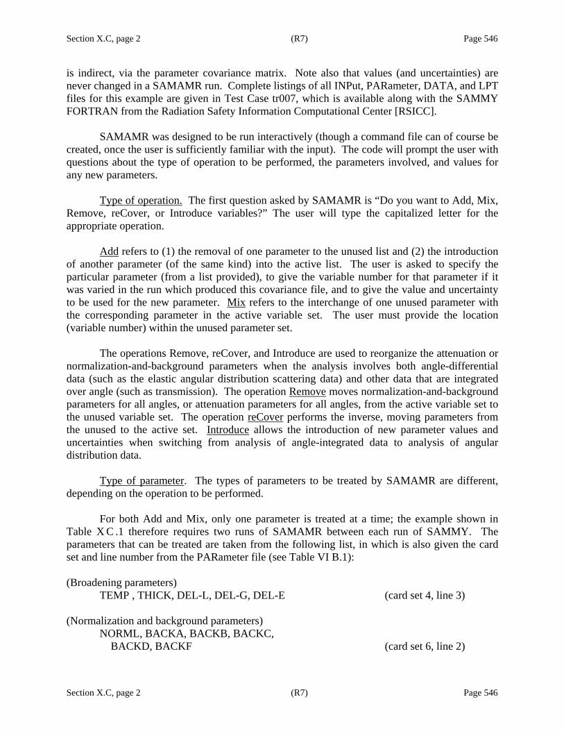
Section X.C, page 2 (R7) Page 546
Section X.C, page 2 (R7) Page 546
is indirect, via the parameter covariance matrix. Note also that values (and uncertainties) are never changed in a SAMAMR run. Complete listings of all INPut, PARameter, DATA, and LPT files for this example are given in Test Case tr007, which is available along with the SAMMY FORTRAN from the Radiation Safety Information Computational Center [RSICC].
SAMAMR was designed to be run interactively (though a command file can of course be
created, once the user is sufficiently familiar with the input). The code will prompt the user with questions about the type of operation to be performed, the parameters involved, and values for any new parameters.
Type of operation. The first question asked by SAMAMR is “Do you want to Add, Mix,
Remove, reCover, or Introduce variables?” The user will type the capitalized letter for the appropriate operation.
Add refers to (1) the removal of one parameter to the unused list and (2) the introduction
of another parameter (of the same kind) into the active list. The user is asked to specify the particular parameter (from a list provided), to give the variable number for that parameter if it was varied in the run which produced this covariance file, and to give the value and uncertainty to be used for the new parameter. Mix refers to the interchange of one unused parameter with the corresponding parameter in the active variable set. The user must provide the location (variable number) within the unused parameter set.
The operations Remove, reCover, and Introduce are used to reorganize the attenuation or
normalization-and-background parameters when the analysis involves both angle-differential data (such as the elastic angular distribution scattering data) and other data that are integrated over angle (such as transmission). The operation Remove moves normalization-and-background parameters for all angles, or attenuation parameters for all angles, from the active variable set to the unused variable set. The operation reCover performs the inverse, moving parameters from the unused to the active set. Introduce allows the introduction of new parameter values and uncertainties when switching from analysis of angle-integrated data to analysis of angular distribution data.
Type of parameter. The types of parameters to be treated by SAMAMR are different,
depending on the operation to be performed. For both Add and Mix, only one parameter is treated at a time; the example shown in
Table X C .1 therefore requires two runs of SAMAMR between each run of SAMMY. The parameters that can be treated are taken from the following list, in which is also given the card set and line number from the PARameter file (see Table VI B.1): (Broadening parameters)
TEMP , THICK, DEL-L, DEL-G, DEL-E (card set 4, line 3) (Normalization and background parameters)
NORML, BACKA, BACKB, BACKC, BACKD, BACKF (card set 6, line 2)

Section X.C, page 3 (R7) Page 547
Section X.C, page 3 (R7) Page 547
(ORR resolution parameters) BURST (card set 9, line 2) WATR0, WATR1, WATR2 (card set 9, line 3) TANTA (card set 9, line 3) X1, X2, X3, X0 (card set 9, line 4) WWW, ALPHA (card set 9, line 6) D, F, G (card set 9, line 8) DELTA (card set 9, line 8) CHANN (card set 9, line 10)
(Miscellaneous parameters, with alternative names in square brackets)
DELTA, DELT2 [DELL1, DELL0] (card set 11, line 2) NU [ETA] (card set 11, line 3) ATTNI, ATTNO [FINIT, FINI2] (card set 11, line 4) TZERO, LZERO (card set 11, line 6) SIABN (card set 11, line 7) SITEM, SITHC [SELFI] (card set 11, line 8) EFFIC, FISEF [EFCAP, EFFIS] (card set 11, line 9) DELTE, DELE0, DELE2 [DELE1, DELE0, DELE2] (card set 11, line 10) CONCR, CONTR (card set 11, line 11)
(RPI/GELINA/nTOF resolution function parameters)
BURST (card set 14, line 2) TAU (card set 14, line 3) LAMBD (card set 14, line 5) A1 (card set 14, line 7) EXPON (card set 14, line 9) CHANN (card set 14, line 11)
In addition to giving the parameter name, as given in the above list, the user will
sometimes also need to specify which parameter of this type is to be used. The name is given in the first five columns (be sure to leave blanks if the name is fewer than five characters), and an integer number is then given. For the RPI resolution parameters, the second, third, etc., variables on the line (in the PARameter file) are specified by “2”, “3”, etc., in the SAMAMR input. See test case tr087 for examples of this.
For the operations Remove, reCover, and Introduce, only the parameters ATTEN and ALLNB may be specified. When ATTEN is specified, all attenuation parameters (both incident and outgoing, from card set 11, line 4 of the PARameter file) are involved. When ALLNB is specified, all normalization and background parameters are involved (see card set 6, line 2). Again, only one type can be treated during one run of SAMAMR.
When the operation Introduce is used, attenuation or normalization/background parameters are assumed to be given in a separate file in the same format as used in the PARameter file (either with or without the “MISCEllaneous parameters” or “NORMAlization and background” header lines of card sets 11 and 6; however, if they are included, the first five

Section X.C, page 4 (R7) Page 548
Section X.C, page 4 (R7) Page 548
characters must be either all caps or all lowercase). SAMMY will ask for the file name instead of the parameter values. Test case tr036 shows examples of the use of this feature.
An additional restriction for operations Remove, reCover, and Introduce stems from the
connection between the attenuation parameters and the number of angles: SAMAMR assumes that removal of attenuation parameters implies changing from angular-distribution data to angle-integrated data, and that recovery or introduction of attenuation parameters implies the reverse change. Removal of attenuation parameters, therefore, must be accomplished after removal of normalization and background parameters, and recovery or introduction of attenuation parameters must be accomplished prior to recovery or introduction of normalization and background parameters.
Test cases tr007, tr032, tr036, tr079, and tr087 all have examples of the use of program
SAMAMR.
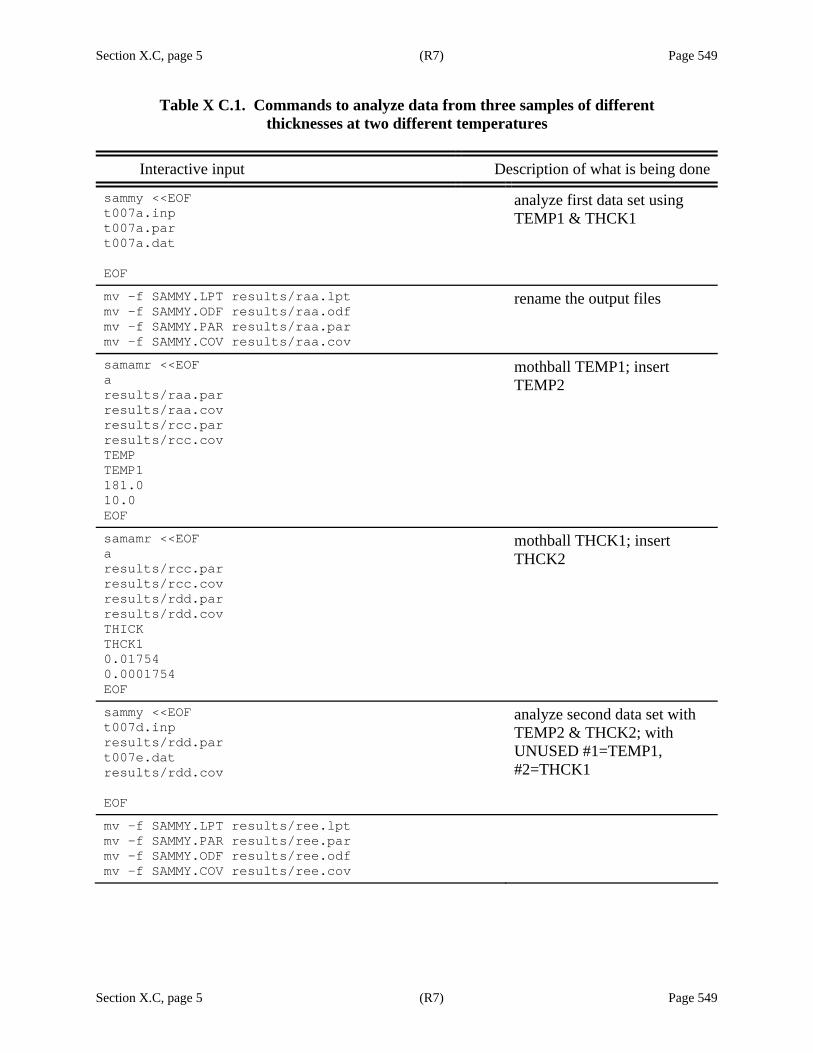
Section X.C, page 5 (R7) Page 549
Section X.C, page 5 (R7) Page 549
Table X C.1. Commands to analyze data from three samples of different thicknesses at two different temperatures
Interactive input Description of what is being done
sammy <<EOF t007a.inp t007a.par t007a.dat EOF
analyze first data set using TEMP1 & THCK1
mv -f SAMMY.LPT results/raa.lpt mv –f SAMMY.ODF results/raa.odf mv –f SAMMY.PAR results/raa.par mv –f SAMMY.COV results/raa.cov
rename the output files
samamr <<EOF a results/raa.par results/raa.cov results/rcc.par results/rcc.cov TEMP TEMP1 181.0 10.0 EOF
mothball TEMP1; insert TEMP2
samamr <<EOF a results/rcc.par results/rcc.cov results/rdd.par results/rdd.cov THICK THCK1 0.01754 0.0001754 EOF
mothball THCK1; insert THCK2
sammy <<EOF t007d.inp results/rdd.par t007e.dat results/rdd.cov EOF
analyze second data set with TEMP2 & THCK2; with UNUSED #1=TEMP1, #2=THCK1
mv –f SAMMY.LPT results/ree.lpt mv –f SAMMY.PAR results/ree.par mv –f SAMMY.ODF results/ree.odf mv –f SAMMY.COV results/ree.cov

Section X.C, page 6 (R7) Page 550
Table X C.1 (continued)
Section X.C, page 6 (R7) Page 550
Interactive input Description of what is being done samamr <<EOF m results/ree.par results/ree.cov results/rff.par results/rff.cov TEMP TEMP2 1 EOF
interchange so USED=TEMP1, UNUSED#1=TEMP2
samamr <<EOF a results/rff.par results/rff.cov results/rgg.par results/rgg.cov THICK THCK2 0.01319 0.0001319 EOF
mothball THCK2, insert THCK3
sammy <<EOF # tr7hhh t007h.inp results/rgg.par t007h.dat results/rgg.cov EOF
analyze third data set with TEMP1 & THCK3; with UNUSED #1=TEMP2, #2=THCK1, #3=THCK2
mv SAMMY.LPT results/rhh.lpt mv SAMMY.PAR results/rhh.par mv SAMMY.ODF results/rhh.odf mv SAMMY.COV results/rhh.cov
rename files
samamr <<EOF m results/rhh.par results/rhh.cov results/rii.par results/rii.cov THICK THCK3 2 EOF
interchange THICK and UNUSED#2 (so will use TEMP1 & THCK1)
sammy <<EOF t007j.inp results/rii.par t007a.dat results/rii.cov EOF
generate cross section for first data set with TEMP1 & THCK1; with UNUSED #1=TEMP2, #2=THCK3, #3=THCK2
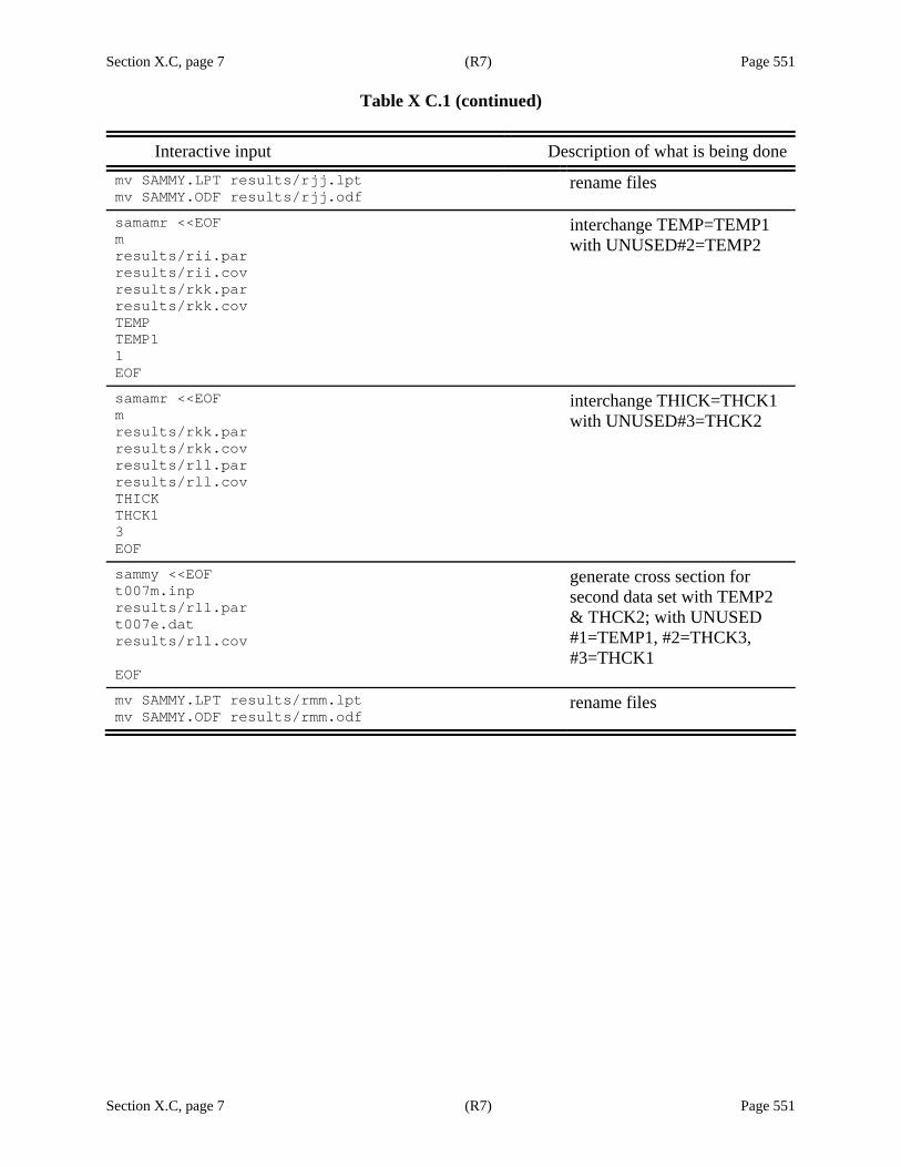
Section X.C, page 7 (R7) Page 551
Table X C.1 (continued)
Section X.C, page 7 (R7) Page 551
Interactive input Description of what is being done mv SAMMY.LPT results/rjj.lpt mv SAMMY.ODF results/rjj.odf
rename files
samamr <<EOF m results/rii.par results/rii.cov results/rkk.par results/rkk.cov TEMP TEMP1 1 EOF
interchange TEMP=TEMP1 with UNUSED#2=TEMP2
samamr <<EOF m results/rkk.par results/rkk.cov results/rll.par results/rll.cov THICK THCK1 3 EOF
interchange THICK=THCK1 with UNUSED#3=THCK2
sammy <<EOF t007m.inp results/rll.par t007e.dat results/rll.cov EOF
generate cross section for second data set with TEMP2 & THCK2; with UNUSED #1=TEMP1, #2=THCK3, #3=THCK1
mv SAMMY.LPT results/rmm.lpt mv SAMMY.ODF results/rmm.odf
rename files

Section X.C, page 8 (R7) Page 552
Section X.C, page 8 (R7) Page 552
Table X C.2. The initial PARameter file t007a.par for the example of Section X.C -2070. 1450. 186600. 0. 0. 0 0 0 0 0 1 27650. 1400. 1480000. 0. 0. 1 0 1 0 0 1 1151.07 600. 62. 0. 0. 1 1 1 0 0 2 BROADENING 6.00 329.00 0.2179 0.025 0.022 0.022 1 1 1 1 1 1 EXPLICIT 2001 0.5 2002 5.0 2003 0.002179 2004 0.005 2005 0.005 2006 0.005 2 1 400. 2 3 100000. 3 1 5. 3 2 300. 3 3 15.
Table X C.3. Intermediate PARameter file raa.par
-2070.00000 1450.00000 186600.000 0 0 0 1 27652.54913 1400.00000 1478023.10 1 0 1 1 1151.115961 582.738578 58.8204626 1 1 1 2 .100000000 BROADENING PARAMETERS FOLLOW 6.00413005 328.76010 .21794422 .02489528 .02195479 .02179978 1 1 1 1 1 1 COVARIANCE MATRIX IS IN BINARY FORM
Table X C.4. Intermediate PARameter file rcc.par
-2070.00000 1450.00000 186600.000 0 0 0 1 27652.54913 1400.00000 1478023.10 1 0 1 1 1151.115961 582.738578 58.8204616 1 1 1 2 .100000000 BROADENING PARAMETERS FOLLOW 6.00413005 181.00000 .21794422 .02489528 .02195479 .02179978 1 1 1 1 1 1 UNUSED PARAMETERS FOLLOW TEMP1 328.760096 COVARIANCE MATRIX IS IN BINARY FORM
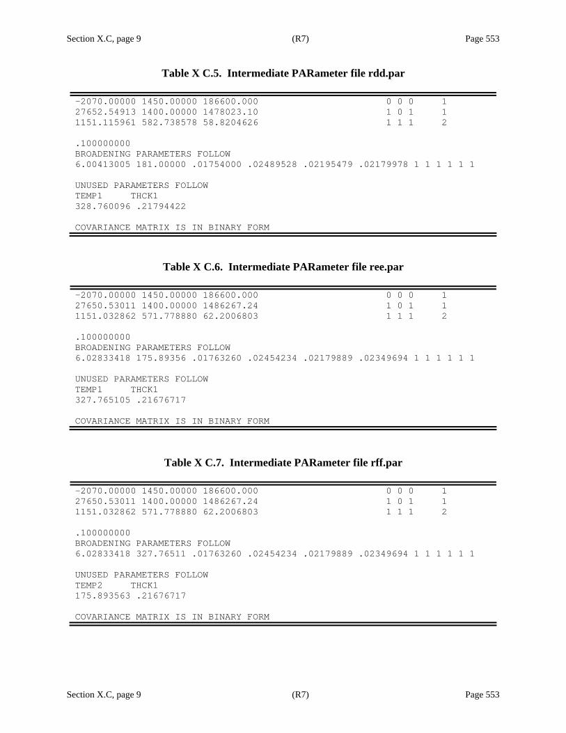
Section X.C, page 9 (R7) Page 553
Section X.C, page 9 (R7) Page 553
Table X C.5. Intermediate PARameter file rdd.par
-2070.00000 1450.00000 186600.000 0 0 0 1 27652.54913 1400.00000 1478023.10 1 0 1 1 1151.115961 582.738578 58.8204626 1 1 1 2 .100000000 BROADENING PARAMETERS FOLLOW 6.00413005 181.00000 .01754000 .02489528 .02195479 .02179978 1 1 1 1 1 1 UNUSED PARAMETERS FOLLOW TEMP1 THCK1 328.760096 .21794422 COVARIANCE MATRIX IS IN BINARY FORM
Table X C.6. Intermediate PARameter file ree.par
-2070.00000 1450.00000 186600.000 0 0 0 1 27650.53011 1400.00000 1486267.24 1 0 1 1 1151.032862 571.778880 62.2006803 1 1 1 2 .100000000 BROADENING PARAMETERS FOLLOW 6.02833418 175.89356 .01763260 .02454234 .02179889 .02349694 1 1 1 1 1 1 UNUSED PARAMETERS FOLLOW TEMP1 THCK1 327.765105 .21676717 COVARIANCE MATRIX IS IN BINARY FORM
Table X C.7. Intermediate PARameter file rff.par
-2070.00000 1450.00000 186600.000 0 0 0 1 27650.53011 1400.00000 1486267.24 1 0 1 1 1151.032862 571.778880 62.2006803 1 1 1 2 .100000000 BROADENING PARAMETERS FOLLOW 6.02833418 327.76511 .01763260 .02454234 .02179889 .02349694 1 1 1 1 1 1 UNUSED PARAMETERS FOLLOW TEMP2 THCK1 175.893563 .21676717 COVARIANCE MATRIX IS IN BINARY FORM

Section X.C, page 10 (R7) Page 554
Section X.C, page 10 (R7) Page 554
Table X C.8. Intermediate PARameter file rgg.par
-2070.00000 1450.00000 186600.000 0 0 0 1 27650.53011 1400.00000 1486267.24 1 0 1 1 1151.032862 571.778880 62.2006803 1 1 1 2 .100000000 BROADENING PARAMETERS FOLLOW 6.02833418 327.76511 .01319000 .02454234 .02179889 .02349694 1 1 1 1 1 1 UNUSED PARAMETERS FOLLOW TEMP2 THCK1 THCK2 175.893563 .21676717 .01763260 COVARIANCE MATRIX IS IN BINARY FORM
Table X C.9. PARameter file rhh.par, containing final results for example of Section X.C
-2070.00000 1450.00000 186600.000 0 0 0 1 27651.00483 1400.00000 1487173.71 1 0 1 1 1151.033783 565.790617 61.6726510 1 1 1 2 .100000000 BROADENING PARAMETERS FOLLOW 6.03414731 326.86586 .01317133 .02392383 .02155364 .02207008 1 1 1 1 1 1 UNUSED PARAMETERS FOLLOW TEMP2 THCK1 THCK2 178.166780 .21674113 .01765984 COVARIANCE MATRIX IS IN BINARY FORM
Table X C.10. PARameter file rii.par, which is a permutation of the file rhh.par
-2070.00000 1450.00000 186600.000 0 0 0 1 27651.00483 1400.00000 1487173.71 1 0 1 1 1151.033783 565.790617 61.6726510 1 1 1 2 .100000000 BROADENING PARAMETERS FOLLOW 6.03414731 326.86586 .21674113 .02392383 .02155364 .02207008 1 1 1 1 1 1 UNUSED PARAMETERS FOLLOW TEMP2 THCK3 THCK2 178.166777 .01317133 .01765984 COVARIANCE MATRIX IS IN BINARY FORM

Section X.C, page 11 (R7) Page 555
Section X.C, page 11 (R7) Page 555
Table X C.11. PARameter file rkk.par, which is a permutation of the file rhh.par
-2070.00000 1450.00000 186600.000 0 0 0 1 27651.00483 1400.00000 1487173.71 1 0 1 1 1151.033783 565.790617 61.6726510 1 1 1 2 .100000000 BROADENING PARAMETERS FOLLOW 6.03414731 178.16678 .21674113 .02392383 .02155364 .02207008 1 1 1 1 1 1 UNUSED PARAMETERS FOLLOW TEMP1 THCK3 THCK2 326.865860 .01317133 .01765984 COVARIANCE MATRIX IS IN BINARY FORM
Table X C.12. The PARameter file rll.par, which is a permutation of the file rhh.par
-2070.00000 1450.00000 186600.000 0 0 0 1 27651.00483 1400.00000 1487173.71 1 0 1 1 1151.033783 565.790617 61.6726510 1 1 1 2 .100000000 BROADENING PARAMETERS FOLLOW 6.03414731 178.16678 .01765984 .02392383 .02155364 .02207008 1 1 1 1 1 1 UNUSED PARAMETERS FOLLOW TEMP1 THCK3 THCK1 326.865860 .01317133 .21674113 COVARIANCE MATRIX IS IN BINARY FORM


Section X.D, page 1 (R7) Page 557
Section X.D, page 1 (R7) Page 557
X.D. SAMAMX: MODIFY A SINGLE VALUE
Program SAMAMX is used to alter the value of one non-varied parameter in the covariance file after completion of an analysis.
Development of SAMAMX was prompted by the need to change the value of λγΓ for a low-lying (negative-energy) resonance in order to obtain the correct thermal values but without having to reanalyze the higher-energy regions.
The program is to be used only on rare occasions and with extreme caution!
The program is designed to run interactively; SAMAMX will prompt you for the information that you need to provide to it.
For a sample run of SAMAMX, see test case tr007. Look near the end of the command file test007 for the SAMAMX run, which alters the value of λγΓ in raa.cov for the second resonance, and puts the result in ryy.cov.
BEWARE: SAMAMX does not change resonance parameter values in the PAR file; changes in value occur only in the COV file. You may, if you wish, manually change them in the PAR file; however, it is not necessary to do so. SAMMY will use the values given in the COV file, not those in the PAR file; you can verify this by looking at the values given in the LPT file from the SAMMY run (file rzz.lpt in the example).


Section X.E, page 1 (R7) Page 559
Section X.E, page 1 (R7) Page 559
X.E. SAMCPR: COMPARE RESULTS
Program SAMCPR is an aide in comparing cross sections calculated by one computer code (e.g., NJOY [RM82] or REFIT [MM89] ) with those calculated by SAMMY. First, a no-Bayes SAMMY run is made using the other code’s calculations as the DATa file, and including the alphanumeric command “COMPARE EXPERIMENT To theory” in the INPut file. SAMMY generates a binary file SAM53.DAT, which can then be read by program SAMCPR to produce the ODF file SAMCPR.ODF.
The contents of the various sections of the output file SAMCPR.ODF are as follows:
S1 = energy S2 = X = “data,” which may be a calculation from another code S3 = S = “theory,” which is the SAMMY calculation S4 = X − S S5 = ( X − S ) / S S6 = ( X − S ) / S H 103 S7 = ( X − S ) / S H 104 S8 = ( X − S ) / S H 105 S9 = ( X − S ) / S H 106 S10 = S5 adjusted for small cross sections S11 = S10 H 103 S12 = S10 H 104 S13 = S10 H 105 S14 = S10 H 106
For section 10, the quantity ( X − S ) / S is replaced by 10−25 if both X and S are smaller than 0.0001. Thus the values in S10 through S14 will be sizeable only when the cross sections themselves are reasonably large.
Note that early versions of this program were called SAMCMP. However, “cmp” is a special word on Unix systems; hence, the name has been changed.


Section X.F, page 1 (R7) Page 561
Section X.F, page 1 (R7) Page 561
X.F. SAMDIS: STATISTICAL DISTRIBUTIONS
The code SAMDIS a slightly modified version of the code SAMDIST [LL95], which is used to verify the consistency of a resonance parameter set with the predicted theoretical statistical distribution. Three different tests can be performed: 1. Level spacing distributions are compared with the Wigner distribution law. 2. Neutron-, radiation-, and fission-width distributions are calculated and compared with the χ2
distribution with the appropriate number of degrees of freedom (ν = 1 for the Porter-Thomas distribution of neutron widths, ν = 2 or 3 for fission, and ν = infinity for capture widths).
3. Long-range correlations of the energies are tested via the Δ3 statistic of Mehta and Dyson. Details of the three tests are given in the SAMDIST manual.
One modification to the code (and to the input; see Table XF.1) has been made subsequent to the publication of the SAMDIST manual: The calculation of distribution of neutron widths now includes penetrabilities. Hence it is necessary to define the orbital angular momentum and to give the atomic mass of the target nucleus.

Section X.F, page 2 (R7) Page 562
Section X.F, page 2 (R7) Page 562
Table X F.1. Input for program SAMDIS
Line number SAMDIST prompt Response Notes
1 Type d (for spacing), w (for width), or d3 (for delta3)
“d”, “w”, or “d3” Line 3 appears only for “w” in line 1
2 Parameter file name name of file 30 characters or less 3 (“w” only) Enter particle channel “neutron”,
“fission”, or “gamma”
only lowercase is permitted; note also that this line appears only for type 2 (“w” in line 1)
4 Spin group, initial and final energies
SAMMY spin group number, Emin and Emax
free format, separate by commas
5 (“w” and “neutron” only)
Enter l and awr integer value of orbital angular momentum, mass of target nucleus
This line is absent unless line 1 is “w” and line 3 is “neutron”
6 (“d” or “w” only)
Bin width for sampling
in units of energy This line is absent for “d3”
7 (“w” only) Degrees of freedom degrees of freedom for chi-squared distribution
This line is here for “w” only (not for “d” or “d3”)
Section X.G, page 1 (R7) Page 563
Section X.G, page 1 (R7) Page 563
X.G. SAMFTZ: FIX TZERO
When the energy grids of two or more data sets are misaligned, SAMMY has an option to treat initial time t0 and the flight-path length L as search parameters, in order to provide consistent energy grids; see Section III.E.8 for details.
Once appropriate values for t0 and L are determined, it is often useful to adjust the experimental data set accordingly before proceeding with further analysis. This is accomplished using the auxiliary code SAMFTZ.
To run SAMFTZ, provide answers to the following questions:
What are tzero & Lzero? (default = 0.0 & 1.0) What is the flight-path length in meters? What is name of original data file? What is name of new data file? Are data in csisrs format? (default = yes)
Only CSISRS or TWENTY format is permitted for the “original data file;” answer “yes” to the final question if the original file is in CSISRS format and “no” if the file is TWENTY. The “new data file” will be in TWENTY format.
For an example of the use of SAMFTZ, see test case tr122.


Section X.H, page 1 (R8) Page 565
Section X.H, page 1 (R8) Page 565
X.H. SAMORT: PLOT THE OAK RIDGE RESOLUTION FUNCTION
When using the realistic resolution function (see Section III.C.2), it may be useful to plot both the individual components of the resolution function and the final composite function. This can be accomplished using program SAMORT, which requires only the PARameter file and three other numbers (energy, mass, and flight-path length) as input. Output consists of one descriptive ASCII file plus several plot files.
The descriptive file, named SAMMY.ORR, gives details of the case being run, including for example centroids for each component of the resolution function.
Four plot files give time vs. resolution function for each component, and a fifth gives energy, resolution function, and time for the composite function (so that one can plot the resolution as a function of either energy or time). As with other plot files produced by SAMMY, these are in ODF format. For the benefit of SAMMY users who do not have the ORNL plotting package FORODF, the same information is also given in ASCII files with extension “LST” and in “generic” binary files with extension “PLT”.1
A sample interactive (Unix) run of program SAMORT is accomplished with the following lines of input:
samort a.par 180000.,57.935,201.578
Here the energy at which the functions are to be evaluated is 180000 eV, the mass of the sample is 57.935 amu, and the flight-path length is 201.578 m.
The file a.par can be either the complete PARameter file or may contain only the ORRES portion thereof. The file may look similar to the following (see test case tr021, file t021tlo.par):
BURST 1 1.775 .5 TANTA 1 0.200 0.1 TANTA 1111 0.010 0.050 0.090 0.040 TANTA 0.005 .005 0.005 0.005 TANTA 11 0.079 1.000 TANTA 0.04 0.5 LITHI 111 5.000 0.392235 1.009 LITHI 2.000 0.200000 0.500 CHANN 1 200000.000 7.179 4.000
(See card set 9 of the PARameter file, Table VI B.2, for interpretation of these numbers.)
1 Prior to version 7.1.5 of the SAMMY code, the “PLT” extension was used to denote the ASCII files produced by program SAMORT. The change from “PLT” to “LST” for the ASCII files and the addition of “PLT” binary files were made to conform with usage elsewhere in the SAMMY code. (See, for example, Section VII.C.)
Section X.H, page 2 (R8) Page 566
Section X.H, page 2 (R8) Page 566
Output plot files are as follows: The file SAM_ORR.ODF contains energies in section 1, resolution function in section 2, and time of flight in section 3. File SAM_ORR_BURST.ODF contains time of flight in section 1 and the burst-width component of the resolution function in section 2. File SAM_ORR_TANTA.ODF contains time in section 1 and the tantalum target component of the resolution function in section 2. File SAM_ORR_CHANN.ODF contains time in section 1 and the channel-width component in section 2. Finally, the file SAM_ORR_LITHI.ODF contains time in section 1 and the lithium-glass detector resolution function in section 2.
If the water moderator or the NE110 detector had been used instead, the respective file names would be SAM_ORR_WATER.ODF and SAM_ORR_NE110.ODF.
For a description of the contents of the ASCII LST files, substitute “column” for “section” in the above description. The one exception to that is file SAM_ORR.LST, for which column 1 contains time of flight, column 2 the resolution function, and column 3 energy.
What follows is the output ASCII file SAMMY.ORR produced by running the example described above: p ---------------------------- 1.7750E-03 a, w, x1, x2, x3, x0, alpha -- 1174. 463.6 1.7041E-06 8.5204E-06 1.5337E-05 6.8163E-06 1.000 c ---------------------------- 7.1790E-03 d, f, g ---------------------- 5.0000E-03 392.2 1.009 <t>, t1, t2, t3, t4 ---------- 1.0224E-02 8.8750E-04 1.5522E-03 3.5895E-03 4.1951E-03 tlow, time, tup -------------- 34.252758 34.350628 34.360852 eup , em , elow ------------- 181030.09 180000.00 179892.89 #########################

Section X.I, page 1 (R8) Page 567
Section X.I, page 1 (R8) Page 567
X.I. SAMPLT: ALTERNATIVE FORM FOR PLOT FILES
Plotting with SAMMY at Oak Ridge may be accomplished by means of a set of utility programs FORODF [JC78]. SAMMY produces an “ODF” or “plot” file named SAMMY.ODF which contains the information (such as energies and cross sections) from which plots may be made using FORODF. (See, for example, Section VII.C.) An alternative plotting program RSAP [RS03] is currently under development and will be made available at a future time.
Users on other systems will likely use other plotting packages. For that purpose, SAMMY produces two additional output files containing the same information as SAMMY.ODF but in different formats. One is an ASCII file named SAMMY.LST (new with Revision 8 of the manual and code). The other, named SAMMY.PLT, is a “generic” binary file to be read by the SAMPLT code.
One version of code SAMPLT (file mplt.f) is provided with the SAMMY FORTRAN; this version of SAMPLT reads the binary file and produces at least one ASCII file (SAM_ASCII.PLT). The local SAMMY manager may wish to modify the file mplt.f to accommodate his or her system=s needs; mplt.f contains extensive comment cards to aid in making the needed modifications.
Caution: There may be problems associated with the creation of PLT files for certain configurations of SAMMY runs, notably those for which more than one PLT file is produced by an individual run, and possibly in other situations. Generally such problems should be immediately obvious to the user; when in doubt, cross sections can be printed in the LPT file for comparison with the PLT file. (See “options for printing into SAMMY.LPT” in Table VI A1.2 to learn how this can be done.) Most such problems should have been eliminated with revision 8 of the manual and code. Nevertheless, users are encouraged to contact the SAMMY development team at [email protected] if they encounter difficulties with these files.


Section X.J, page 1 (R7) Page 569
Section X.J, page 1 (R7) Page 569
X.J. SAMQUA: RESONANCE QUANTUM NUMBERS
The code SAMQUA can serve as an aide to generating the correct (and complete) set of resonance spin quantum numbers for any given set of incident and exit channels. The original version of this program was quite limited, assuming a neutron incident on a single nuclide, and including only elastic channels. In 2003 Bouland and Babut of Cadarache, in collaboration with the SAMMY author, developed a more general version of this code [OB03]. This version of SAMQUA treats the general case of elastic, inelastic, reaction, and fission channels, including charged particles as needed.
Two distinct modes of input are available for SAMQUA. The first (the Cadarache input mode) uses free-format values interspersed with descriptive information, and is described in detail in the SAMQUA documentation [OB03]. The second (the Particle-Pair mode) uses essentially the particle-pair information from SAMMY’s card set 4 of Table VI.A.1. In both cases, the output consists of portions of the SAMMY INPut file: Output file “quantum2.dat” contains card sets 4 and 10.2, as well as the necessary commands (to be included in card set 3 of the INPut file) for use of those input options. Output file “quanpar.dat” may be used (perhaps with modifications) for card set 7 (radius parameters) and card set 10 (isotopic abundances) of the SAMMY PARameter file. Another output file, “table.dat”, gives the spin group information in tabular form.
One additional output file, “quantum.dat”, contains card set 10.1 (for SAMMY’s INPut file) plus command lines. However, use of this option in SAMMY runs is discouraged as the format is crowded, awkward, and non-intuitive and will eventually be disallowed. SAMMY users are encouraged to convert to card set 10.2 (as given in quantum2.dat of SAMQUA output).
Subsequent to publication of the SAMQUA manual [OB03], the code has again been upgraded [OB04] with options to provide additional information to the user, and to reorganize the output. For each run, another output file (“quantum3.dat”) is created. This file contains the same information as quantum2.dat, with extra lines following each channel descriptor in card set 10.2; the extra lines give penetrability and hard-sphere cross section at specified energies. (The hard-sphere cross section is that cross section that would be calculated if there were no resonances.) By default these energies are 1.0 eV, 500 keV, and 1 MeV, but (for the particle-pair input mode) there are other options:
(1) The user can specify values Emin and Emax, and SAMQUA will calculate penetrabilities
and cross sections at Emin, (Emin+Emax)/2, and Emax. (2) A list of energies can be given in a separate file; this can be a SAMMY PARameter file
or a simple list of energies. Because the calculation of penetrabilities and cross sections requires knowledge of radii, and
the radii used in an evaluation may differ from SAMQUA’s default values, the user may also provide radii values.

Section X.J, page 2 (R7) Page 570
Section X.J, page 2 (R7) Page 570
Finally, a single input command will alter the ordering of the spin groups from J, π as in the 2003 version to L, J (where L here indicates the orbital angular momentum of the first entrance channel for any given spin group, and J and π indicate the total angular momentum and parity for the spin group).
Table X J.1 summarizes the input options for the particle-pair mode.
Test case tr143 gives numerous examples of the use of this code. Cases whose names end in “a” use the Cadarache mode of SAMQUA input, and cases whose names end in “b” use the particle-pair mode. Cases labeled with “c” include the option to read channel radii from a separate file, and cases labeled with “d” provide reordered output. Cases labeled “e” read from a parameter file to learn energies on which to calculate penetrabilities and hard-sphere cross sections.
Table X J.1. Input options for SAMQUA in particle-pair mode
Line Contents Notes Required?
1 Title 1. Alphanumeric title, will be printed but not used.
Yes
2,3, …
Blank, or containing # in first column.
1. Blank or # lines may be inserted almost anywhere into the file.
No
4, 5 “EMIN =” or “EMAX =”, followed by the real value.
1. The penetrability and hard-sphere cross section will be calculated at Emin, (Emin+Emax)/2, and Emax.
2. If either Emin or Emax is unspecified, the default values (1 eV, 1 MeV respectively) will be used.
3. The equal sign must be included.
No
Alt. 4 (no 5)
“ENERgy file =”, followed by name of file in which energies are stored
1. Energies are listed one per line, in the first eleven columns.
2. A SAMMY-style resonance PARameter file can be used here (in which case negative energies and continuation lines will be ignored).
No
6 “RADius file =”, followed by the name of the file in which the radii are stored
1. The “radius file” defines values for the channel radii, which are needed for calculating the penetrabilities and hard-sphere cross sections. The format for the radius file is the same as card set 7a of the PARameter file, with the caveat that only particle-pair and orbital angular momentum information can be given, and not spin group and channels (since these will be determined by the samqua run).
No

Section X.J, page 3 (R7) Page 571
Table X J.1 (continued)
Section X.J, page 3 (R7) Page 571
Line Contents Notes Required?
6, cont.
2. If channel radii are not specified (i.e., if this line is absent and no “radius file” exists), the SAMQUA default values are used.
3. Only the first three characters of “radius file” are needed; however, the equal sign must be included.
4. This line may be interchanged with line 7.
7 “REOrder according to LJ not Jpi” or “ORDer by LJ”.
1. If this line is present, the spin groups will be listed in the output files in order of increasing L, where L here refers to the orbital angular momentum of the first (incident) channel for each spin group. If two spin groups have the same value of L, the one with the smaller value of J will be listed first.
2. If this line is absent, the spin groups are ordered by increasing J, with negative-parity spin groups listed before those with positive parity.
3. This line may be interchanged with line 6.
No
8 “NUclide, Lmax=” or “First nuclide, Lmax=”, followed by integer value for Lmax. Line may also contain “Number of fission channels =”, followed by integer value
1. Indicates the beginning of information for the first nuclide. Only the first two characters (NU) and the first equal sign are required.
2. Lmax is the maximum value of the orbital
angular momentum. 3. If a second equal sign is present, the integer
value following that equal sign is the number of fission channels to be included.
Yes
9 “Abundance =”, followed by real value
1. Indicates the abundance of this isotope. Printed in file quanpar.dat for use in card set 10 of the SAMMY PARameter file.
2. No blank line (or # line) is permitted between Line 8 and Line 9.
Yes
10, etc.
1. These lines give the particle-pair information, exactly as in card set 4 of the INPut file.
2. End with a blank line (not a # line)
Yes

Section X.J, page 4 (R7) Page 572
Table X J.1 (continued)
Section X.J, page 4 (R7) Page 572
Line Contents Notes Required?
11 “NUCLide, Lmax=” or “NEXT nuclide, Lmax=” or “NEW nuclide, Lmax=” Line may also contain “Number of fission channels =”, followed by integer value
Like line 8 for another nuclide: 1. Indicates the beginning of information for the
new nuclide. Only the first four characters and the first equal sign (plus the value of Lmax for this nuclide) are required.
2. Lmax is the maximum value of the orbital
angular momentum. 3. If a second equal sign is present, the integer
value following that equal sign is the number of fission channels to be included.
No
12,13 Repeat lines 9 and 10 for this nuclide 14 … Repeat lines 11 through 14 as needed
Section X.K, page 1 (R8) Page 573
Section X.K, page 1 (R8) Page 573
X.K. SAMRPT: PLOT RPI RESOLUTION FUNCTION
To plot the components and the total RPI resolution function (see Section III.C.3) at a given energy, use program SAMRPT. Input to SAMRPT consists of two lines of information: The first is the name of the PARameter file. Alternatively, it could be the name of a file containing the RPI portion of the PARameter file; the header line (“RPI Resolution function”) may or may not be present. The second line contains the energy in eV, mass in atomic mass units (amu), and flight-path length in meters (m), in 3F format (separated by commas or spaces); alternatively, the same information may be given as the first line in the RPI file. (Default values for these three quantities are 150.0, 183.85, and 25.604, respectively.)
Output from a run of SAMRPT consists of one ASCII file, SAMMY.RPI, which gives derived quantities such as the time-width associated with each component of the resolution function, as many as four plot (ODF) files, four “generic” (PLT) binary files, and four additional ASCII files:
SAM_RPI.ODF - S1 = energy, S2 = (total) resolution function, S3 = time SAM_RPI_BURST.ODF - S1 = time, S2 = burst-width component SAM_RPI_TDXXX.ODF - S1 = time, S2 = target-plus-detector component SAM_RPI_CHANN.ODF - S1 = time, S2 = channel-width component
The four binary files have similar names with extension “ODF” replaced by extension “PLT”. The four ASCII files have extension “ODF” replaced by “LST”. Information from the various sections of the ODF files is given in the corresponding columns of the LST files and in the binary PLT files.1
Test case tr053 gives numerous examples (not all of which make physical sense!) for the use of this program.
1 Prior to version 7.1.5 of the SAMMY code, the “PLT” extension was used to denote the ASCII files produced by program SAMRPT. The change from “PLT” to “LST” for the ASCII files and the addition of “PLT” binary files were made to conform with usage elsewhere in the SAMMY code. (See, for example, Section VII.C.)

Section X.L, page 1 (R7) Page 575
Section X.L, page 1 (R7) Page 575
X.L. SAMRST: PLOT RESOLUTION FUNCTION
Even though program SAMRST is actually a module of SAMMY, it is covered in this section because comparable programs (SAMORT and SAMRPT) are also presented here.
To generate a plot file containing the Gaussian plus exponential resolution function (see Section III.C.1) at specific energies, insert the command line
PLOT RESOLUTION FUNCtion in the INPut file. Also in the INPut file, directly after the blank line signifying the end of the alphanumeric commands (card set 3), insert one line specifying the energies (in 8F10.1 format) at which the resolution function is to be reported; a maximum of eight such energies are allowed. This line is card set 4.5 of the INPut file.
Program SAMRST will generate one plot file (ODF file) per energy; these files are named SAMRSx.ODF, where “x” is a digit from 1 to 8; these files contain energy in S1 and resolution function in S2. In the event that there are too few points to resolution broaden at the specified energy, an error message is printed and the plot file is not generated.
An example using SAMRST is given in test case tr018.


Section X.M, page 1 (R7) Page 577
Section X.M, page 1 (R7) Page 577
X.M. SAMSMC: MONTE CARLO MULTIPLE SCATTERING
In Section III.D, SAMMY=s method of calculating the multiple-scattering corrections to the capture and fission yields is presented. Because these calculations involve complicated expressions as well as approximations whose legitimacy can be questioned, it is desirable to have an independent means of testing the calculations. Monte Carlo is suitable for this task, as the method is completely different from the analytic-with-approximations approach taken in Section III.D.
The precursor to the code SAMSMC was written during the 1980's by Gerard de Saussure [GD80] and subsequently modified by Francis Perey. More recently, the SAMMY author has modified this code to include anisotropic scattering (non-s-waves) and more than one nuclide. In addition, an interface was developed with the SAMMY code, in order for SAMSMC to read and use the same Doppler-broadened cross sections and energies that are used in SAMMY.
Use of the SAMSMC code is a multi-step process, described below. 1. Run SAMMY with a line in the alphanumeric section of the INPut file which says
PREPARE INPUT FOR MONte carlo simulation
This command causes the code to stop at the point where it would otherwise begin execution of segment SAMSSM. Two or three files are produced that are needed for the Monte Carlo simulation: File SAM54.DAT contains the unbroadened cross sections and SAM51.DAT contains Doppler-broadened cross sections (assuming the INPut file specified that Doppler broadening was to be done). Rename these file for use in later steps. The third file is SAMMY.MCR, which contains most of the information to be given to SAMSMC (as specified in # 2 below). Some of this information you will use as is; other values may be modified.
2. Run program SAMSMC (SAM-Ssm-Monte-Carlo), with the following lines of input:
a. Title (whatever you wish) b. Energy-mesh information (Emin, Emax, 0.) c. Name of file with energy mesh (here only if Emin = 0 in part a) d. THSAMP, XSAMP, YSAMP, XBEAM, YBEAM (like card set 11 in INPut file for the
regular SAMMY run) e. Thickness (in atoms/barn), Mass (in amu) f. Maximum number of histories g. Number of scatterings to include h. Name of the file generated by SAMMY run of step 1 (renamed from SAM51.DAT) i. Maximum L-value in that file (where L is the vector sum of the orbital angular momentum
for the individual levels); number of nuclides j. Normalize as yield (Y) or cross section (C) or other (O) k. If more than one nuclide, give masses of each l. If more than one nuclide, give abundance for each

Section X.M, page 2 (R7) Page 578
Section X.M, page 2 (R7) Page 578
Two output files are produced by the SAMSMC run. MC_1.DAT holds the various cross sections, and MC_2.DAT contains results from 0 scattering, 1 scattering, two-or-more scatterings, and the sum of those three. Rename these, if desired.
3. Run program SAMSMX (SAMSMc-fiX), with the following input:
a. Name of the cross section file produced by SAMSMC (MC_1.DAT) b. Name of the second file produced by SAMSMC (MC_2.DAT)
Four output files are produced by this run. Three are ASCII files name MC_Y0.DAT, MC_Y1.DAT, and MC_Y2.DAT; these contain the self-shielded yield, the self-shielded plus single-scattering-corrected yield, and the full multiple-scattering-corrected yield, respectively. These files are in a form suitable for use as SAMMY DATa files, in the TWENTY format (see Section VI.C.1).
The other output file produced by this procedure is named MC.ODF. This file is an ODF file (see Section VII.C) with the following sections:
S1. energy in eV S2. 0 scattering (self-shielding) only S3. 1 scattering S4. 2 scatterings S5. 0 + 1 S6. 0 + 1 + 2 S7. capture cross section S8. total cross section S9. (1-exp(-thickness H total cross section)) H capture / total
Sections of this file can be compared to output in section 4 of the ODF file produced by the corresponding SAMMY runs. For example, output from a SAMMY run that includes single scattering (finite disk) but not double scattering would be compared to Section 5 in MC.ODF.

Section X.N, page 1 (R3) Page 579
Section X.N, page 1 (R3) Page 579
X.N. SAMSTA: STAIRCASE PLOTS
To produce an ODF file from which can be made staircase plots of SAMMY resonances for specified spin groups, use the program SAMSTA. Input to SAMSTA is shown in Table X N.1. Output consists of a single file in ORELA Data FORMAT (ODF) (or binary, depending on the system); Section 1 of that file contains resonance energies, and Section 2 contains the number of resonances (from the specified spin groups) at or below the corresponding energy.
Note that the SAMMY INPut file is not read by SAMSTA; the only information required from that file is the l-value associated with the given spin groups, and that information is provided directly to SAMSTA. The user should therefore take care to provide correct input, since SAMSTA cannot make consistency checks (l-value vs. spin group number, for example).
Table X N.1 Input for Program SAMSTA
Question Response
1. What is name of parameter file? Name of SAMMY PARameter file
2. What is spin (l)? What are spin group numbers?
Orbital angular momentum for channel 1, as specified by the variable LSPIN in card set 10 of the INPut file; spin group numbers for those groups have this l-value. Format is “6I3”
3. What is name for ODF file? Name for the output ODF file to be produced by SAMSTA
Questions 2 and 3 are repeated until the user enters “0” for spin and group numbers.

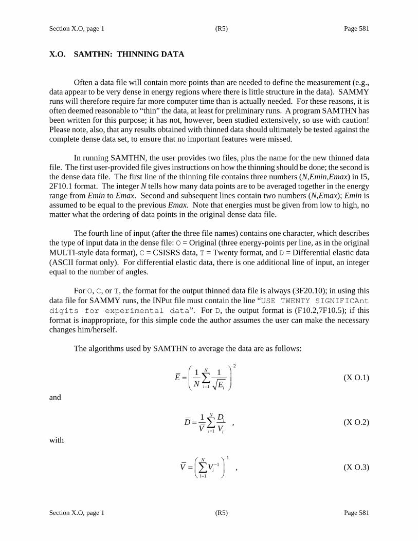
Section X.O, page 1 (R5) Page 581
Section X.O, page 1 (R5) Page 581
X.O. SAMTHN: THINNING DATA
Often a data file will contain more points than are needed to define the measurement (e.g., data appear to be very dense in energy regions where there is little structure in the data). SAMMY runs will therefore require far more computer time than is actually needed. For these reasons, it is often deemed reasonable to “thin” the data, at least for preliminary runs. A program SAMTHN has been written for this purpose; it has not, however, been studied extensively, so use with caution! Please note, also, that any results obtained with thinned data should ultimately be tested against the complete dense data set, to ensure that no important features were missed.
In running SAMTHN, the user provides two files, plus the name for the new thinned data file. The first user-provided file gives instructions on how the thinning should be done; the second is the dense data file. The first line of the thinning file contains three numbers (N,Emin,Emax) in I5, 2F10.1 format. The integer N tells how many data points are to be averaged together in the energy range from Emin to Emax. Second and subsequent lines contain two numbers (N,Emax); Emin is assumed to be equal to the previous Emax. Note that energies must be given from low to high, no matter what the ordering of data points in the original dense data file.
The fourth line of input (after the three file names) contains one character, which describes the type of input data in the dense file: O = Original (three energy-points per line, as in the original MULTI-style data format), C = CSISRS data, T = Twenty format, and D = Differential elastic data (ASCII format only). For differential elastic data, there is one additional line of input, an integer equal to the number of angles.
For O, C, or T, the format for the output thinned data file is always (3F20.10); in using this data file for SAMMY runs, the INPut file must contain the line “USE TWENTY SIGNIFICAnt digits for experimental data”. For D, the output format is (F10.2,7F10.5); if this format is inappropriate, for this simple code the author assumes the user can make the necessary changes him/herself.
The algorithms used by SAMTHN to average the data are as follows:
2
1
1 1N
i i
EN E
−
=
⎛ ⎞= ⎜ ⎟⎜ ⎟⎝ ⎠∑ (X O.1)
and
1
1 ,N
i
i i
DDV V=
= ∑ (X O.2)
with
1
1
1,
N
ii
V V−
−
=
⎛ ⎞= ⎜ ⎟⎝ ⎠∑ (X O.3)

Section X.O, page 2 (R5) Page 582
Section X.O, page 2 (R5) Page 582
in which E represents the energy, D the data, and V the variance (i.e., the square of the uncertainty). Quantities with subscripts are from the original dense data set, and quantities with bars represent the averaged values.
Test case tr072 has two examples for thinning data.

Section X.P, page 1 (R7) Page 583
Section X.P, page 1 (R7) Page 583
X.P. SUGGEL: ESTIMATING L AND J
Often when beginning an analysis, the SAMMY user will start from spin assignments and resonance parameters already available in the literature or in the ENDF files. Sometimes, however, such information is either nonexistent, inadequate, or unavailable through the entire energy range. In such situations, the analyst must use alternative methods to obtain starting parameter values. The computer program SUGGEL [SO01], written by S. Y. Oh and L. C. Leal, provides one such method. The following description is taken from the abstract to that document:
“The SUGGEL computer code has been developed to suggest a value for the orbital angular momentum of a neutron resonance that is consistent with the magnitude of its neutron width. The suggestion is based on the probability that a resonance having a certain value of gΓn is an l-wave resonance. The probability is calculated by using Bayes’ theorem on the conditional probability. The probability density functions (pdf=s) of gΓn for up to d-wave (l = 2) have been derived from the χ2 distribution of Porter and Thomas. The pdf =s take two possible channel spins into account.”
“This code is a tool which evaluators will use to construct resonance parameters and help to
assign resonance spin. The use of this tool is expected to reduce time and effort in the evaluation procedure, since the number of repeated runs of the fitting code (e.g., SAMMY) may be reduced.”
SAMMY test case tr141 gives three examples of SUGGEL runs.
Readers are referred to the documentation [SO01] for details concerning the use of this code. That document’s description of the input to the code is repeated here (below the line, and in Table X P.1). Note that the second of the two input files is the resonance-parameter portion of a SAMMY-style PARameter file, and the name for this file is provided in the suggel.inp file discussed below.
The program requires two input files and generates two output files. The basic data, as well as some control options, for the calculation are included in a file named “suggel.inp”, while sets of resonance energy and neutron width are provided in the other input file. One of the output files shows calculation results, and the other file contains resonance parameters in SAMMY.PAR format. Input Description
The file “suggel.inp” is prepared in the name-list type of input. This file consists of: The first line: “&indata” from column 2 to 8, In the second to the (last-1) lines: data section with the name-list key words (each line shall
have the first column blank), and The last line: “&end” from column 2 to 5. Some notes can be added after this line for user’s
convenience.

Section X.P, page 2 (R6) Page 584
Section X.P, page 2 (R6) Page 584
Table X P.1. Variables appearing in the “suggel.inp” file
Key word Units Description
Parin Input resonance parameter data file name. In the file, the resonance energy is given in eV and Γn (or gΓn) in meV.
Partyp Type of neutron width in ‘parin= file. If partyp = 0, the parin file is in SAMMY.PAR file format and Γn=s are given; otherwise, the file is in rsap.gamma format and gΓn=s are given. Concerning the rsap.gamma file, see following this table.
Fout Output list file name. Parout File name of the output resonance parameter file, which is in
SAMMY.PAR format. Awri Atomic mass of target nuclide divided by the neutron mass. Spin Spin of the target nuclide (I). Scattr fermi Scattering radius (R').
If scattr = 0.0, the program calculates it as R' = 0.123 (awri)1/3 +0.08 [10−12 cm]
Disp Spin dispersion parameter (s). If disp = 0.0, the program calculates the value. Very large ‘disp= value (e.g., 999.) implies to use (2J+1) law, with which the level density is proportional to 2J+1. See further discussion following the table.
Bn MeV Neutron separation energy of (A+1) nuclide Pair MeV Pairing energy Denpar MeV−1 Level density parameter Eini eV Lower energy boundary under the analysis Efin eV Upper energy boundary under the analysis Pcut Probability cutoff.
The suggested orbital angular momentum is adopted for a resonance for which the probability is higher than this value. If it is not the case, the l value is not altered from its original assignment as given in ‘parin= file. It is not effective with the input rsap.gamma file.
Optj Method of J assignment. If optj = 0, the most probable J value is adopted; otherwise, the J value is assigned randomly. Regardless of this option, the original J value is maintained if the original l value is maintained due to the probability cutoff. See Section 2.6 of [SO01].

Section X.P, page 3 (R6) Page 585 Table X P.1 (continued)
Section X.P, page 3 (R6) Page 585
Key word Units Description
Stn(i), i=1,2,3
10−4 Neutron strength functions for s-, p-, and d-waves, respectively
Dzero eV Average level spacing of s-wave resonance. Level spacings of p- and d-waves are calculated in the program.
Frac(i), i=1,2,3
A priori probability correction factors for s-, p-, and d-waves, respectively. See Section 2.2 of [SO01].
Sam(i), i=1~max.18
l value of spin group i in ‘parin’ file. This definition shall be kept in subsequent SAMMY run. The number of spin groups can be more than 18 in SAMMY run (e.g., in case of the analysis of a natural element), and it is also possible to define the spin group not to begin with 1 in SAMMY. However, the SUGGEL assumes that the spin group starts at 1.
Ajsam(i), i=1~max.18
J value of spin group i in ‘parin’ file. This definition shall be kept in subsequent SAMMY run.
Note from SAMMY author: This program does not run under the VMS operating systems. In general, portability of SUGGEL is not guaranteed.


Section X.Q, page 1 (R7) Page 587
Section X.Q, page 1 (R7) Page 587
X.Q. SAMRML: CALCULATE CROSS SECTIONS FROM ENDF FILE 2 The program SAMRML was created as an aid for persons wishing to implement the ENDF File 2 LRF=7 (R-Matrix Limited) Format. SAMRML can be used in at least two ways: This coding may be inserted directly into a processor code (after appropriate re-writes). When independent coding is developed, SAMRML can be used to test the results. The stand-alone code SAMRML was derived from the cross-section-calculation portion of SAMMY, with the following changes: Experiment-related pieces were removed from this code; only one nuclide is considered at a time, and no corrections are made for any measurement-related effects. All cross section types are generated in a single SAMRML run. SAMRML calculates energy-differential (angle-integrated) elastic, absorption, and reaction cross sections. If requested, SAMRML will also calculate elastic angular distributions. In addition, an option exists for generating partial derivatives of the angle-integrated cross sections with respect to the resonance parameters. The code will calculate one of two versions of the partial derivatives: In the default mode, derivatives are with respect to the resonance widths Γλx and energies Eλ, as they appear in the ENDF files. Alternatively, the derivatives can be given with respect to SAMMY’s u-parameters as defined in Section II of this report; this option is useful for ensuring that SAMRML is indeed working properly. The default option is currently the more useful one for processor codes that make more direct use of the ENDF files than does SAMMY. Two input files are needed for SAMRML. The first contains a list of energies (one per line, ending with a blank line) and angles (one per line, ending with a blank line) at which the calculation is to be performed. If no angles are given, no angular distributions will be calculated. The second file is an ENDF file in which File 2 uses LRF=1 (single-level Breit Wigner), 2 (multilevel Breit Wigner), 3 (the so-called Reich-Moore format), or 7 (the R-matrix limited format). Four lines of input are needed following the “samrml” run command:
1. name of energy/angle file 2. name of ENDF File 2 file 3. the ENDF material number (MATNUM); if MATNUM is zero, only the File 2 portion of the
ENDF file is to be included in the file specified in the previous line. 4. two characters, in the first two columns of this line. If the first character is “y” or “Y” (for
“yes”), then partial derivatives will be generated. If the second character is “s” or “S”, then those derivatives will be with respect to the SAMMY u-parameters.

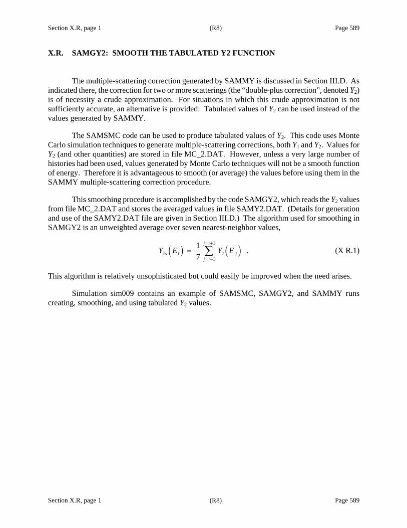
Section X.R, page 1 (R8) Page 589
Section X.R, page 1 (R8) Page 589
X.R. SAMGY2: SMOOTH THE TABULATED Y2 FUNCTION
The multiple-scattering correction generated by SAMMY is discussed in Section III.D. As indicated there, the correction for two or more scatterings (the “double-plus correction”, denoted Y2) is of necessity a crude approximation. For situations in which this crude approximation is not sufficiently accurate, an alternative is provided: Tabulated values of Y2 can be used instead of the values generated by SAMMY.
The SAMSMC code can be used to produce tabulated values of Y2. This code uses Monte Carlo simulation techniques to generate multiple-scattering corrections, both Y1 and Y2. Values for Y2 (and other quantities) are stored in file MC_2.DAT. However, unless a very large number of histories had been used, values generated by Monte Carlo techniques will not be a smooth function of energy. Therefore it is advantageous to smooth (or average) the values before using them in the SAMMY multiple-scattering correction procedure.
This smoothing procedure is accomplished by the code SAMGY2, which reads the Y2 values from file MC_2.DAT and stores the averaged values in file SAMY2.DAT. (Details for generation and use of the SAMY2.DAT file are given in Section III.D.) The algorithm used for smoothing in SAMGY2 is an unweighted average over seven nearest-neighbor values,
( ) ( )3
2 23
1 .7
j i
s i jj i
Y E Y E= +
= −
= ∑ (X R.1)
This algorithm is relatively unsophisticated but could easily be improved when the need arises. Simulation sim009 contains an example of SAMSMC, SAMGY2, and SAMMY runs creating, smoothing, and using tabulated Y2 values.


Section XI, page 1 (R7) Page 591
Section XI, page 1 (R7) Page 591
XI. HELPFUL HINTS FOR RUNNING SAMMY
This section covers a multitude of topics, all designed to facilitate the smooth operation of SAMMY. Careful attention to the ideas covered here should make your job (and the author=s!) a lot easier.
Section XI.A describes an agenda for performing a SAMMY evaluation. Even experienced SAMMY users might benefit from reading this section, as it includes mention of useful features of the SAMMY code which might be unfamiliar to them.
Section XI.B offers suggestions for solving common problems encountered by SAMMY
users. The procedure to be used in obtaining the author=s help is also discussed. Section XI.C contains discussions on a variety of topics related to running the SAMMY
code. Included are such topics as Bayes’ method, spin-group definitions, negative reduced-width amplitudes, and transmission vs total cross section.

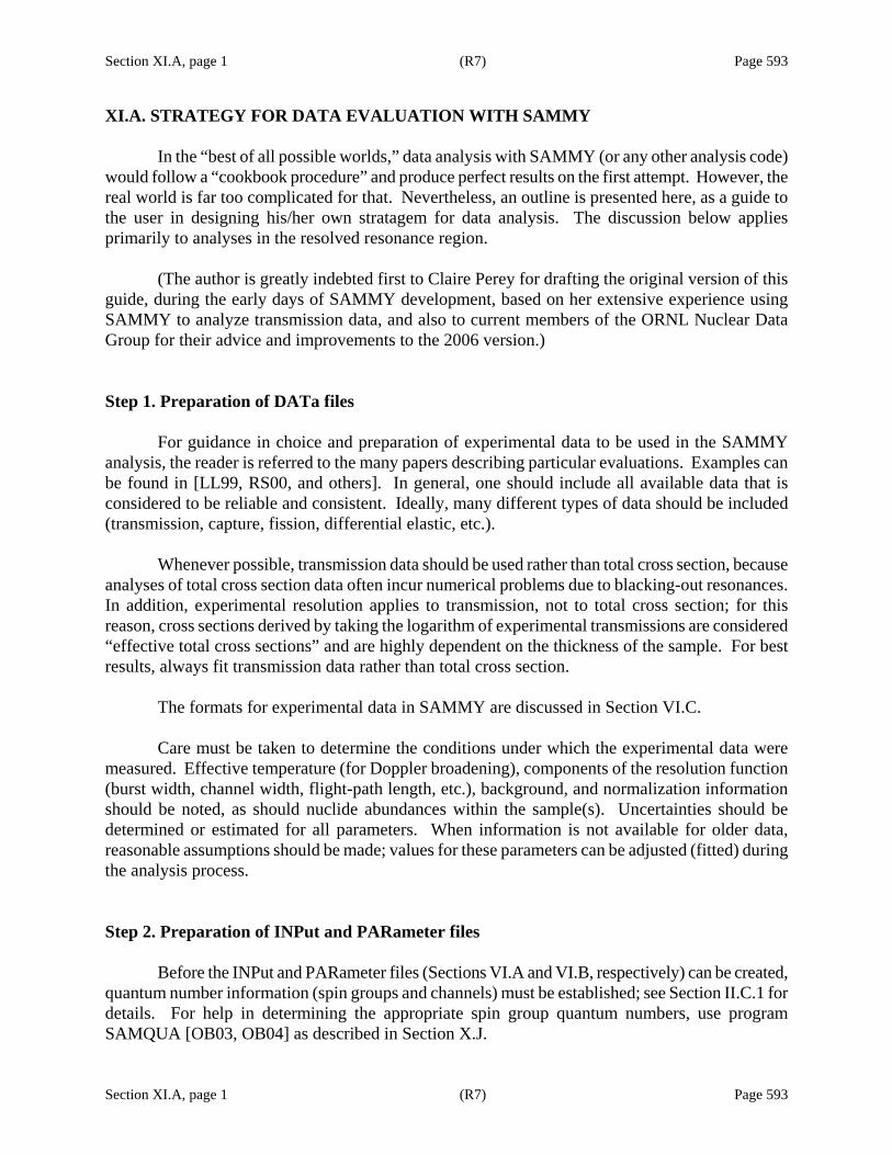
Section XI.A, page 1 (R7) Page 593
Section XI.A, page 1 (R7) Page 593
XI.A. STRATEGY FOR DATA EVALUATION WITH SAMMY
In the “best of all possible worlds,” data analysis with SAMMY (or any other analysis code) would follow a “cookbook procedure” and produce perfect results on the first attempt. However, the real world is far too complicated for that. Nevertheless, an outline is presented here, as a guide to the user in designing his/her own stratagem for data analysis. The discussion below applies primarily to analyses in the resolved resonance region.
(The author is greatly indebted first to Claire Perey for drafting the original version of this guide, during the early days of SAMMY development, based on her extensive experience using SAMMY to analyze transmission data, and also to current members of the ORNL Nuclear Data Group for their advice and improvements to the 2006 version.)
Step 1. Preparation of DATa files For guidance in choice and preparation of experimental data to be used in the SAMMY analysis, the reader is referred to the many papers describing particular evaluations. Examples can be found in [LL99, RS00, and others]. In general, one should include all available data that is considered to be reliable and consistent. Ideally, many different types of data should be included (transmission, capture, fission, differential elastic, etc.).
Whenever possible, transmission data should be used rather than total cross section, because analyses of total cross section data often incur numerical problems due to blacking-out resonances. In addition, experimental resolution applies to transmission, not to total cross section; for this reason, cross sections derived by taking the logarithm of experimental transmissions are considered “effective total cross sections” and are highly dependent on the thickness of the sample. For best results, always fit transmission data rather than total cross section. The formats for experimental data in SAMMY are discussed in Section VI.C. Care must be taken to determine the conditions under which the experimental data were measured. Effective temperature (for Doppler broadening), components of the resolution function (burst width, channel width, flight-path length, etc.), background, and normalization information should be noted, as should nuclide abundances within the sample(s). Uncertainties should be determined or estimated for all parameters. When information is not available for older data, reasonable assumptions should be made; values for these parameters can be adjusted (fitted) during the analysis process. Step 2. Preparation of INPut and PARameter files Before the INPut and PARameter files (Sections VI.A and VI.B, respectively) can be created, quantum number information (spin groups and channels) must be established; see Section II.C.1 for details. For help in determining the appropriate spin group quantum numbers, use program SAMQUA [OB03, OB04] as described in Section X.J.

Section XI.A, page 2 (R7) Page 594
Section XI.A, page 2 (R7) Page 594
In many cases, results of earlier evaluations for some of the relevant nuclides are available in the evaluated nuclear data files (ENDF). ENDF File 2 (which contains resonance parameters) can be used as input to SAMMY, greatly simplifying the SAMMY setup procedure. (See Section IX of this manual for details concerning the use of ENDF files as input to SAMMY.) Do not, however, rely entirely on the information in the ENDF files, for the following reasons:
• Older files sometimes did not give proper descriptions of the spin groups and channels.
• Except for the new LRF = 7 format, ENDF formats do not have provision for defining parity. Do not assume that the spins and parities extracted from ENDF files are correct.
• Many older files used one of the Breit-Wigner approximations, which should not be used for new evaluations. (When reading an ENDF file, SAMMY produces a comparable SAMMY-style INPut file called SAMNDF.INP; be sure to remove any command lines referring to Breit-Wigner from this file before using it as input to future SAMMY runs.)
• Small resonances observable in new measurements may not have been seen in the early measurements.
• New measurements may permit extension of the resolved resonance region to higher energies, requiring the use of higher l-values.
Therefore, even when preliminary information is available from ENDF File 2, it is recommended that SAMQUA be used to ensure that all possible spin groups and channels are considered for inclusion in the analysis. If R-matrix parameters are not available from ENDF, results from resonance parameter analyses may be found in the EXFOR files [EXFOR]. Users should be aware that these are not full evaluations but are closely tied to individual measurements. Information concerning individual resonances may be available in the literature. See, for example, the Mughabghab compilation [SM06].
Information from data bases or the literature will probably need to be augmented with information available only in the new data you are preparing to analyze. Program SUGGEL (Section X.P) was designed to provide guidance in making spin-group assignments for resonances. Program RSAP [RS03] also has features that aid in PARameter-file preparation. One such feature is a peak search procedure that “finds” resonances in new data and generates starting PARameter-file entries. A certain amount of trial and error on the analyst’s part will also be needed but will pay dividends in the future. The R-matrix is a complicated function, involving long-range interference. At any given energy, the “background” R-matrix has contributions from nearby small resonances, from large resonances within the region being analyzed, and from resonances outside the region of analysis. The effect of the outside resonances is approximated either by fictitious or “dummy” resonances or by a parameterized external R-function. (For more on this topic, see Section II.B.1.d and references [LL99] and [FF01].) Be sure to include either dummy resonances or another description of the external levels in your PARameter file, as it will not be possible to fit the data without this.
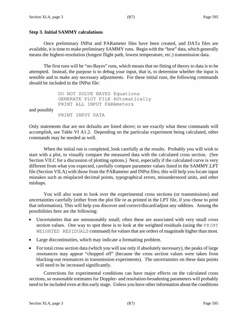
Section XI.A, page 3 (R7) Page 595
Section XI.A, page 3 (R7) Page 595
Step 3. Initial SAMMY calculations Once preliminary INPut and PARameter files have been created, and DATa files are available, it is time to make preliminary SAMMY runs. Begin with the “best” data, which generally means the highest-resolution (longest flight path, lowest temperature, etc.) transmission data.
The first runs will be “no-Bayes” runs, which means that no fitting of theory to data is to be attempted. Instead, the purpose is to debug your input, that is, to determine whether the input is sensible and to make any necessary adjustments. For these initial runs, the following commands should be included in the INPut file:
DO NOT SOLVE BAYES Equations GENERATE PLOT FILE AUtomatically PRINT ALL INPUT PARAmeters
and possibly PRINT INPUT DATA
Only statements that are not defaults are listed above; to see exactly what these commands will accomplish, see Table VI A1.2. Depending on the particular experiment being calculated, other commands may be needed as well.
When the initial run is completed, look carefully at the results. Probably you will wish to start with a plot, to visually compare the measured data with the calculated cross section. (See Section VII.C for a discussion of plotting options.) Next, especially if the calculated curve is very different from what you expected, carefully compare parameter values listed in the SAMMY.LPT file (Section VII.A) with those from the PARameter and INPut files; this will help you locate input mistakes such as misplaced decimal points, typographical errors, misunderstood units, and other mishaps.
You will also want to look over the experimental cross sections (or transmissions) and uncertainties carefully (either from the plot file or as printed in the LPT file, if you chose to print that information). This will help you discover and correct/discard/adjust any oddities. Among the possibilities here are the following:
• Uncertainties that are unreasonably small; often these are associated with very small cross section values. One way to spot these is to look at the weighted residuals (using the PRINT WEIGHTED RESIDUALS command) for values that are orders of magnitude higher than most.
• Large discontinuities, which may indicate a formatting problem.
• For total cross section data (which you will use only if absolutely necessary), the peaks of large resonances may appear “chopped off” (because the cross section values were taken from blacking-out resonances in transmission experiments). The uncertainties on these data points will need to be increased significantly.
Corrections for experimental conditions can have major effects on the calculated cross sections, so reasonable estimates for Doppler- and resolution-broadening parameters will probably need to be included even at this early stage. Unless you have other information about the conditions

Section XI.A, page 4 (R7) Page 596
Section XI.A, page 4 (R7) Page 596
under which these data were measured, initial attempts should assume room temperature (300 K) for the Doppler broadening (Section III.B.1), and the simple Gaussian resolution function with reasonable parameter values (Section III.C.1.a). By performing a few successive no-Bayes runs, you will eventually reach the stage where the calculated cross sections are roughly consistent with the measured data. That is, you will find
• good approximations for the values of the energy parameters for the large resonances seen in the region you are planning to analyze and
• a combination of parameters for your external R-function (or outside dummy resonances) and for the widths of the large resonances in your energy range to give reasonable estimates of the effect of outside resonances.
For some of the data sets, you may also discover energy-scale misalignments and/or normalization or background problems. Energy re-alignment of all the experimental data sets should be performed at this stage, using the transmission experiment with the longest flight path as the standard. See Section III.E.8 for guidance for correcting the energy scale, and Section III.E.3 for normalization and background options.
Step 4. Preliminary analysis: gross features
Perform a preliminary analysis on each individual data set (again beginning with the “best” data set), using Bayes= theorem to adjust the most relevant parameters. At this stage it is recommended that you assign • small but realistic uncertainties on the energy parameters of the large resonances inside your
energy range and
• fairly large uncertainties on the widths of these resonances and on the parameters outside your range of analysis.
Table VI B.2 provides many options for input of prior uncertainties on resonance and other parameters.
In a few runs you will have generated a theoretical cross section that roughly agrees with your data. (In earlier years, when computation time was prohibitive, these runs were often made using severely averaged data sets to speed up the calculation. With today’s high-speed computers, averaging is almost never necessary.)
For these runs, you will need to modify your INPut files by disabling the command that prohibits fitting. This command line can either be removed, or it can be commented-out with a pound sign (#) in the first column, as shown here:
#DO NOT SOLVE BAYES Equations
One default command should be noted: DO NOT SUPPRESS ANY intermediate printout

Section XI.A, page 5 (R7) Page 597
Section XI.A, page 5 (R7) Page 597
When things go wrong, the additional printout (in the SAMMY.LPT file, as described in Section VII.A) provided by this command is helpful in detecting where, and possibly why, the trouble started. If everything goes right, use of this option allows you to follow the path of the parameters’ adjustments. Step 5. Further analysis: small energy regions
Small regions should now be studied individually, with all the necessary details, progressively including narrow resonances. At this stage you will want to refine the resolution function for each data set, and include other corrections (multiple scattering, background, etc.); see Section III for details.
Care should be taken to include enough points in the auxiliary energy grid to properly
describe the unbroadened cross section, in order to perform the Doppler and resolution integrations accurately. (See the discussion in Section III.A.1 regarding the density of points in the auxiliary grid.) One simple test you can make to see whether your grid is sufficiently dense is to double the number of points used (i.e., set NXTRA = 1 in card set 2 of the INPut file). If values for the Doppler- and resolution-broadened cross sections change appreciably, then the grid is not sufficiently dense. If values remain approximately the same, then the original grid is acceptable. Remember that it is the analyst’s responsibility (not the SAMMY author’s) to ensure that the auxiliary grid is adequate for your purposes. Step 6. Final fitting runs
At the end of this final step you will obtain the complete and consistent parameter and covariance files for all data sets included in the analysis. Therefore, none of the input parameter values or their uncertainties, nor the data points or their uncertainties, should be manually changed at any time during this final step. If changes are needed, the entire process should begin anew.
All relevant parameters should be varied in this step: set the flag = 1 in the PARameter file.
Some parameters may be held fixed: (1) Values for some parameters are well determined from other experiments but have little effect for the current data; these should be held fixed or perhaps PUPped (see Section IV.D.2) so that their uncertainty contributes to the data covariance matrix. (2) If necessary to conserve computer resources, some parameters may be held fixed at the values found in earlier steps. Care should be taken to hold fixed only those parameters whose effect is short range. (3) In some cases, a parameter may be essentially irrelevant for the data being analyzed and therefore need not be flagged.
All measurement uncertainties should be included at this stage. Statistical uncertainties are
defined in the DATa file, but systematic uncertainties require different treatments. The simplest way for the user to take care of systematic measurement uncertainties is to PUP the data-reduction parameters (normalization, background, sample thickness, etc.) by setting the flag = 3 in either the PARameter or (more likely) the INPut file. When additional systematic uncertainties are available,
Section XI.A, page 6 (R7) Page 598
Section XI.A, page 6 (R7) Page 598
these should be included via the user-supplied implicit data covariance option (see Section IV.D.3 for a discussion and VI.C.3.b for input details).
Two options are now available in SAMMY for analyzing several data sets together. The first
(SAMMY’s original) method involves sequential analyses, one data set after another, using the output parameter covariance matrix (PCM) from one run as input to the next run. The other is to analyze all data sets simultaneously. There are advantages and disadvantages to each.
Sequential analyses: Final results from sequential analyses would be exactly equivalent to
final results from simultaneous analysis, provided the theory were linear with respect to the varied parameters. Since R-matrix theory is exceedingly non-linear, exact equivalence is not possible. Further, the ordering of the data sets in the sequence can be important. Generally, one would include the best data sets first, to firmly establish values for the most important parameters, before moving on to less reliable data.
Often the analyst will take the final PARameter and COVariance file from the entire
sequence of runs, and repeat the sequence using those files as initial input. This process may be repeated several times, until convergence is reached. Generally, the criterion for convergence is that parameter values (and hence chi-squared values) no longer change very much. (Caution: When this kind of repetition is used a total of N times through the sequence, the final parameter covariance matrix is diminished by a factor of N. That is, the uncertainty on any parameter must be multiplied by N to obtain the “true” uncertainty as determined by this sequential analysis.)
A major advantage of sequential analysis is the ability to locate data sets which are
inconsistent with the other data. When such a data set is encountered in the sequence, parameter values will always be modified, so it is unlikely that convergence will be reached. By studying the sequence of runs, the analyst will be able to determine which data set is causing the problem, and make adjustments as needed.
Simultaneous analysis: It is now possible, although still a bit awkward, for SAMMY to do
simultaneous analysis of even very large data sets. (Details are presented in Section IV.E.1.) A series of runs is made, one for each data set. The contributions to the Y and W matrices (needed for Bayes’ equations) are generated in those runs and saved in binary files. An additional SAMMY run then reads those files and solves Bayes’ Equations to determine the updated parameter values and associated parameter covariance matrix. Iteration for non-linearities is also possible with simultaneous analysis, although each iteration requires another complete series of K+1 runs (where K is the number of data sets). Details are given in Section IV.E.1.
With simultaneous analyses, it is possible to calculate the true least-squares solution, in which the prior parameter covariance matrix is assumed to be diagonal and infinite. (See Section IV.E.3 for details.) This feature was added primarily to facilitate comparison with other codes, most of which use least squares rather than the more general Bayes’ equations used in SAMMY.

Section XI.A, page 7 (R7) Page 599
Section XI.A, page 7 (R7) Page 599
Step 7. Obtaining the parameter covariance matrix
The procedure described in step 6 produces both a “good” set of parameter values and the associated parameter covariance matrix (PCM). Ideally, this is the PCM which would be included in the analyst’s final report. In practice, this PCM is widely regarded as too small, which means that the uncertainties (the square root of the diagonal of the covariance matrix) are deemed to be smaller than expected. In reality, not all sources of uncertainty are included in the analysis, even when the analyst goes to great pains to include all known sources of experimental uncertainty. (See Section IV.E.6 for further discussion.)
Analysts therefore usually wish to adjust (increase) the SAMMY-produced PCM in some fashion, to better conform to their expectations regarding the correct PCM. A variety of techniques have been developed to assist in this process; these are described in Section IV.E.6.
Given the recent surge in perception of the importance of uncertainty information in all aspects of nuclear data, it is important that anyone reporting the results of data analysis should include information about the PCM. Do not neglect this aspect of your analysis. Step 8. Statistical studies Most reports regarding resonance parameters also include discussion of statistical properties of those parameters. See, for example, references [HD90], [OB97], [LL99], [RS06]. The code SAMDIS (Section X.F) can be used for some of those studies. Step 9. Reporting results
To create a table of resonance parameters, including uncertainties, use SAMMY’s command PUBLISH, or CREATE PUBLISHABLE List of parameters
which creates a file called SAMMY.PUB. This file can be ported to a spreadsheet to be formatted as needed for publication. See Section VII.F for details.
To write the resonance parameters and covariance matrix into an ENDF file, see Section IX. The SAMMY author would appreciate receiving preprints or reprints of any publications
describing work using the SAMMY code. Kindly e-mail these to [email protected].


Section XI.B, page 1 (R7) Page 601
Section XI.B, page 1 (R7) Page 601
XI.B. PROCEDURES TO FOLLOW WHEN YOU HAVE PROBLEMS
(Most of this section is taken almost directly from the SAMMY workshop material. The procedure described here has proven to be useful in helping users debug their input and in helping the author debug the code when that is needed.)
What to do when SAMMY does not work?! 1. Do not panic – this happens to everyone. 2. Is this run really the same as the one that worked last week? Think carefully — exactly what
did you change? 3. Look at the SAMMY.LPT file in detail:
a. Did SAMMY understand all of your instructions? Maybe you had a typographical error. b. Is SAMMY using the same parameter values that you intended? Maybe you had a typo.
Look for factors of ten, for example. c. Would additional information help? Maybe you need to ask SAMMY to print out more
initial values, or more intermediate steps. d. Did SAMMY give you an error message? Look at the very end of the file.
4. Can you simplify and/or isolate the problem?
a. Use a smaller energy range. b. Vary fewer parameters. c. Drop normalization & background options. d. Do no broadening. e. Find the smallest case for which the error occurs, and try to understand what is unique
about that case. 5. See Table XIB.1 for additional suggestions. 6. If the problem persists, ask for help. (See the next page.)

Section XI.B, page 2 (R7) Page 602
Section XI.B, page 2 (R7) Page 602
Help is available 1. Talk to your office-mate or the person next door. Perhaps you have simply been looking at it
for too long, and someone else can see immediately what you can no longer see. 2. Talk to the most experienced SAMMY user in the neighborhood. It does get easier with
practice. 3. Send an e-mail to the author at [email protected].
a. First, send information but not files. Describe the problem in some detail: i. What version of SAMMY are you using? (If you are not using the most recent
release, your bug may already be fixed.) ii. What features are in use? iii. Did the code bomb or “merely” give wrong answers? iv. How do you know that the answers are wrong? v. In which module did the bomb occur?
• For example, SAMMY-RSL might be the last thing in the LPT file. • Or M6-SAMMY-SSM might appear on the screen right before the bomb.
vi. What error message did SAMMY give you? vii. Does a minor perturbation of this case work properly?
b. When requested, send very small files from the simplest case that illustrates the problem: command file, INPut file, PARameter file, DATa file, and any other necessary input files. i. Send these files as attachments if possible, otherwise as separate e-mail messages. ii. See item # 4 on the previous page for suggestions on how to simplify the run.
NOTE: If you should find an error in your version of SAMMY (either the code or the manual), please tell the author about it so that it can be corrected in the “official” version. ALSO: When you encounter a SAMMY error message that does not convey appropriate information, can you suggest a more informative message? If so, please contact the author with your suggestion.
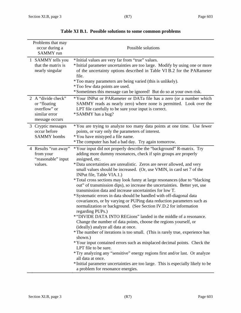
Section XI.B, page 3 (R7) Page 603
Section XI.B, page 3 (R7) Page 603
Table XI B.1. Possible solutions to some common problems
Problems that may occur during a SAMMY run
Possible solutions
1 SAMMY tells you that the matrix is nearly singular
* Initial values are very far from “true” values. * Initial parameter uncertainties are too large. Modify by using one or more
of the uncertainty options described in Table VI B.2 for the PARameter file.
* Too many parameters are being varied (this is unlikely). * Too few data points are used. * Sometimes this message can be ignored! But do so at your own risk.
2 A “divide check” or “floating overflow” or similar error message occurs
* Your INPut or PARameter or DATa file has a zero (or a number which SAMMY reads as nearly zero) where none is permitted. Look over the LPT file carefully to be sure your input is correct.
* SAMMY has a bug?
3 Cryptic messages occur before SAMMY bombs
* You are trying to analyze too many data points at one time. Use fewer points, or vary only the parameters of interest.
* You have mistyped a file name. * The computer has had a bad day. Try again tomorrow.
4 Results “run away” from your “reasonable” input values.
* Your input did not properly describe the “background” R-matrix. Try adding more dummy resonances, check if spin groups are properly assigned, etc.
* Data uncertainties are unrealistic. Zeros are never allowed, and very small values should be increased. (Or, use VMIN, in card set 7 of the INPut file, Table VIA.1.)
* Total cross sections may look funny at large resonances (due to “blacking out” of transmission dips), so increase the uncertainties. Better yet, use transmission data and increase uncertainties for low T.
* Systematic errors in data should be handled with off-diagonal data covariances, or by varying or PUPing data reduction parameters such as normalization or background. (See Section IV.D.2 for information regarding PUPs.)
* “DIVIDE DATA INTO REGions” landed in the middle of a resonance. Change the number of data points, choose the regions yourself, or (ideally) analyze all data at once.
* The number of iterations is too small. (This is rarely true, experience has shown.)
* Your input contained errors such as misplaced decimal points. Check the LPT file to be sure.
* Try analyzing any “sensitive” energy regions first and/or last. Or analyze all data at once.
* Initial parameter uncertainties are too large. This is especially likely to be a problem for resonance energies.

Section XI.C, page 1 (R8) Page 605
Section XI.C, page 1 (R8) Page 605
XI.C. MISCELLANEOUS COMMENTS AND SUGGESTIONS Bayes’ method
Users should bear in mind that there is a fundamental difference between SAMMY and most other data analysis programs with which they might be familiar: SAMMY was designed to use Bayes= equations rather than least-squares equations to update parameter values. The approach taken to data analysis can be quite different from that taken with least squares. Some of these differences are indicated here. • SAMMY can be used sequentially† to obtain results valid over extremely large energy regions
or over many different data sets. One need not do a series of independent analyses followed by much labor to provide consistency over all the data; consistency is a by-product of Bayes= equations. Parameters relevant to all data sets being analyzed should be flagged for fitting.
• Parameters irrelevant to the data currently being analyzed (e.g., energies or widths for far-away
resonances) may be varied (flagged for fitting) without ill effect. These parameter values will not be changed significantly, nor will their uncertainties. (This feature, in particular, is quite different from many implementations of the least-squares method, in which significant computation time is often consumed looking for the “best” value of parameters about which the current data have no information.)
• During the initial stages of an analysis, when starting values are poorly known,‡ SAMMY may
be used much like least-squares programs are used, analyzing the same data with different starting values, varying different parameters, etc., until reasonable parameter values are found for the data being studied. The user should bear in mind that those values are accurate if the parameters that are not varied are known exactly; hence, it is necessary to later do a global fitting of all parameters.
• Occasionally a user may find it convenient to include a data set more than once during a
sequential fit. However, in this case, the parameter covariance matrix (PCM) produced by the sequential analyses must not be considered to be accurate: This is equivalent to including the same data twice in a simultaneous fit, that is, to reducing the uncertainty on each data point by
2 . Sometimes this can be used to advantage: For example, to obtain extremely accurate parameter values, one might run sequentially through all data sets 100 times. Upon completion, the final PCM must be multiplied by 100 (the uncertainties multiplied by 10) to give the actual PCM.
† A “sequential fit” is one in which the output PARameter and COVariance file from one run (analyzing one energy region or one of the data sets) are used as input to the next run (using another energy range or another data set), analyzing each and every data point once and only once.
‡ When starting values are far from true values, the assumption of linearity (implicit in both Bayes’ equations and the least-squares equations) is not even approximately true. Hence the blind use of even the iterative form of either set of equations will often not produce a good fit of theory to data.

Section XI.C, page 2 (R8) Page 606
Section XI.C, page 2 (R8) Page 606
• It is possible to use an output PARameter file as input to a future run without using the COVariance file. To do this, the user may either (i) edit the PARameter file, deleting the final line which states “COVariance matrix is in binary form” and using instead an initial (prior) large uncertainty on each parameter, (ii) include in the input file a card that says “IGNORE INPUT BINARY covariance matrix file”, which will cause the default prior uncertainties to be used, or (iii) answer “IGNORE” when SAMMY requests the name of the binary file.
• Prior (initial) uncertainties for each varied parameter are required as input to SAMMY (although
they will be assigned default values if not stated explicitly). In the case where it may be assumed that we have no prior knowledge about the value of a certain parameter (i.e., usually), the value for the uncertainty should ideally be infinite. (Recall that Bayes= equations, in the limit of infinite prior uncertainty, reduce to the familiar least-squares equations.) Computers, however, require finite numbers. Moreover, it has not been possible to program SAMMY to operate via least squares for some parameters and via Bayes= equations for others. Compromise is therefore necessary. A convenient and practical compromise is that formulated in SAMMY=s default values for prior uncertainties (see Section V1.B). As far as Bayes= equations are concerned, these default uncertainties are effectively infinite, yet they are usually not so large as to cause singularity problems in inverting the matrix.§ A major exception is the default uncertainty on resonance energy, which may be much too large, especially for large s-wave resonances.
• The ratio of the output uncertainty for a given parameter to its initial (prior) uncertainty is a
measure of the effect the data have on that parameter. An unchanged or slightly changed uncertainty implies that the data have little or no effect on the parameter. A drastic reduction in the uncertainty (i.e., a ratio which is, say, less than 0.05 or 0.10) implies that this is an important parameter for these data, and, further, that the prior value was effectively infinite. An increase (a ratio > 1.0 ) perhaps indicates that numerical problems exist.
• Occasionally there are significant changes in values of parameters which should be unaffected in
the region being analyzed. This might be the case, for example, for the width of a large s-wave resonance. If, however, the uncertainty on that parameter remains large and the correlations between it and other parameters are also large, possibly the value of that parameter will resume its expected magnitude once data directly affecting it are analyzed. Values of correlated parameters will be altered to ensure that the fit to the data analyzed earlier is not degraded. On the other hand, it may happen that SAMMY is unable to recover from major changes in parameter values. In this case, the analyst should carefully consider whether some data are inconsistent with the others and make appropriate changes. If all data are deemed to be good, it will likely be necessary to alter the sequential order in which data are analyzed or to decrease prior uncertainties on parameters. Alternatively, one could do simultaneous runs, as described in Section IV.E.1.
§ Experience has shown that the choice of prior uncertainties can, in fact, make some difference in the final results, both for parameter values and for parameter uncertainties. This has often been stated as a deficiency in Bayes’ method, since the output depends upon the input. The analyst should keep in mind, however, that output from least-squares analyses also depends upon the input, but with least squares the user has no choices regarding that particular piece of input – the prior uncertainties are always infinite.

Section XI.C, page 3 (R8) Page 607
Section XI.C, page 3 (R8) Page 607
Spin group definitions
It is legitimate to specify a spin group in the INPut file without giving any resonance for that spin group in the PARameter file. Potential scattering (via hard-sphere phase shifts) will be calculated for that spin group. It is not permitted, however, to request a spin group or channel in the PARameter file without specifying that group in the INPut file.† The ENDF so-called “Reich Moore” format (LRF=3), however, does not allow spin groups to be defined without at least one resonance in the spin group. (See the next paragraph for the exception to this rule.) Evaluators who require an “empty” spin group are encouraged to use the new, less restrictive “R Matrix Limited” format (LRF=7). The original ENDF LRF=3 format made the implicit but unwarranted assumption that all resonances having a given l and J would have the same s. Because this assumption is not always valid, the format was modified in 1999 to specify which channel spin would be used; see Section VI.F.2 for details. The format also requires that “the other” channel spin be added if it is absent, in order to obtain the correct hard-sphere-phase-shift cross section.
A critic has suggested that SAMMY should require that all analyses always use all possible spin groups and channels (up to a user-determined value of l, presumably); the critic is recalling an early ENDF evaluation for which “the other channel spin” was omitted during the analysis, causing great consternation when processor codes reconstructed a cross section which differed from the original. Nevertheless, the SAMMY author has chosen not to hamstring the SAMMY user in this fashion, relying instead on the expertise of today’s evaluators to avoid repetition of a single 25-year-old mistake.
There are legitimate reasons for giving the analyst the ability to define spin groups as s/he
chooses: (1) Only the analyst understands all aspects of the evaluation, so only he or she should be responsible for including all relevant information. (2) Forcing the inclusion of spin groups or channels with negligible contribution will add nothing of value to the calculation, and only increase the CPU time used for calculating zero. (3) It is often useful for the analyst to consider the effect of an individual spin group without including the others. To be sure that your final evaluation includes the “complete” set of spin groups and channels (and to justify the SAMMY author’s faith in the thoroughness of today’s evaluators), users are strongly encouraged to make use of program SAMQUA for assistance in determining spin groups.
† When the command “QUANTUM NUMBERS ARE in parameter file” is given and the spin-group definitions are at the beginning of the PARameter file rather than in the INPut file, the same arguments hold. A channel or spin group cannot be used in the resonance-parameter list if it is not first defined in the spin-group list.

Section XI.C, page 4 (R8) Page 608
Section XI.C, page 4 (R8) Page 608
Negative reduced-width amplitudes
In Section II.B.1, in the paragraph following Eq. (II B1.7), it is stated that reduced-width amplitudes can be either positive or negative. However, the reduced-width amplitude itself is usually not printed in either SAMMY or ENDF files.† Instead, the partial width (related to the square of the reduced-width amplitude) is printed; if the value in the file is given as negative, the sign is assumed to belong to the amplitude rather than to the partial width. (This potentially confusing convention is standard practice, is unambiguous, and soon becomes second-nature to experienced R-matrix practitioners.) In light of the previous paragraph, one might ask why so few negative signs are observed in SAMMY or ENDF files. There are several reasons: • The “natural” thing to do is to use positive signs until and unless the need for a negative sign
becomes apparent. Because it is the easy thing to do, we assign all the amplitudes as positive unless there is evidence to the contrary.
• The sign is irrelevant for widely spaced resonances of the same spin groups (and for resonances of different spin groups). Even for neighboring resonances of the same spin group, only the relative sign is sometimes observable.
• Interferences between neutron widths are often effectively invisible under experimental conditions, lost in the noise and the Doppler and the resolution broadening, etc.
• Negative signs are most often observed for fission widths, when two or more fission widths are specified for each resonance. These signs appear naturally as needed during the course of an analysis – but again, they only appear when needed, and they are not needed very often.
• Rather than starting with all positive amplitudes, a more realistic approach would be to assign the signs randomly for the starting parameters. This is rarely done, most often with fission widths.
• A basic assumption underlying the Reich-Moore approximation is that the signs of the gamma-width amplitudes are randomly distributed. This randomness plus the sheer number of capture channels allow us to treat the gamma width as an average, non-interfering, positive quantity.
Transmission vs. total cross section Analysts will want to make use of transmission data rather than total cross section data whenever possible. Total cross section data are typically derived from transmission data, which cannot reliably be translated to cross section data for all resonances for any given sample thickness. Ideally, transmission data from several different-thickness samples should be included in the evaluation, in order to determine the peaks for resonances of widely differing widths.
† Reduced width amplitudes may be used as input for SAMMY when the command “REDUCED WIDTH AMPLITudes are used for input” is given in the INPut file; details are in card set 1a of the PARameter file.
Section XI.C, page 5 (R8) Page 609
Section XI.C, page 5 (R8) Page 609
ENDF files
The official manual for ENDF formats is [ENDF-102]. A subset of that manual relevant to the resolved-resonance region, with additional comments of interest to SAMMY users, is given in an ENDF-for-SAMMY-users guide [NL07b]. Anyone creating or using ENDF files for the resolved resonance region should be aware of idiosyncrasies in the ENDF formats. • The ENDF multilevel Breit-Wigner format (LRF = 2) is “multi” only for elastic scattering.
Other cross sections are single level. • The so-called Reich-Moore format (LRF = 3) permits only a limited subset of options available
in Reich-Moore. The newer “R-Matrix Limited format” (LRF = 7) is appropriate for situations that do not fit the LRF = 3 format. That is, the LRF = 7 format can be used for more than one entrance channel, for more than two fission channels, for other reaction channels (inelastic, proton, alpha, etc.), for combinations of orbital angular momenta and/or channel spins, and for other generalizations.
• The so-called Reich-Moore format (LRF = 3) requires that, for a given l and J, any non-
identified (i.e., missing) channel spin s must be added to the configuration as a new spin group. With this format, it is not possible to explicitly define a spin group or channel for which there are no resonances. Hence, missing channels are implicitly assumed to be present so that the hard-sphere phase shift contribution will be added to the cross sections.
• In contrast, the R-Matrix Limited format (LRF = 7) requires that each and every spin group and
channel be explicitly defined. It is the evaluator’s responsibility to be sure that all non-negligible spin groups and channels are included.
• Except for the LRF = 7 format, no ENDF formats have provision for defining parity explicitly.
Hence, for example, the ENDF file for 235U suggests that the ground state is 7/2+ when it is in fact 7/2−.
• The ENDF formats, like the SAMMY PARameter file format, use ( )22G A A Pγ= Γ = , where A
is the sign ofγ , for the input quantity. • Unlike SAMMY, ENDF resonance parameter covariance matrices (RPCM) are written in terms
of the input quantity G rather than of the more physical quantityΓ . (As of this writing, this topic is not addressed in the ENDF-102 manual, though it is expected to be included in future releases of that document. The convention that ENDF RPCM be written in terms of G is used in SAMMY to create ENDF File 32, is used in the two covariance processor codes ERRORJ [GC04] and PUFF-IV [DW06], and has been recommended to CSEWG. In contrast, the RPCM printed in the SAMMY.LPT file has always been expressed in terms of Γ rather than G.)


Section XII, page 1 (R7) Page 611
Section XII, page 1 (R7) Page 611
XII. EXAMPLES
Three quite different types of examples are provided with the SAMMY code. The first is a series of tutorial exercises, designed as a learning aid for novice users. These
were originally designed for use in the SAMMY workshops but have been successfully used for independent study as well. For a description of the tutorial exercises, see Section XII.A.
The second type, described in Section XII.B, is a series of test cases that are designed to test
the various features of the code to ensure consistent behavior over time and across computer platforms. A second, equally useful, function of these test cases is to provide users with examples of input for the different features available in the code. Prior to release of the code, all these test cases are run on a variety of platforms. Users who are having difficulty with particular features of the code are strongly encouraged to run the relevant test cases prior to contacting the author for assistance.
Some of the examples that previously were part of the test cases of Section XII.B have now been moved∗ into a category called “simulations,” described in Section XII.C. These are Monte Carlo simulations of the multiple-scattering corrections for capture or fission data.
∗ The move was prompted by the author’s propensity to absentmindedly rerun the simulations, even when nothing was changed with respect to the simulations. Putting these very long runs into a separate category ensured that they will be rerun only when necessary.


Section XII.A, page 1 (R8) Page 613
Section XII.A, page 1 (R8) Page 613
XII.A. TUTORIAL
A series of computer exercises has been developed as an aide to persons wishing to learn how to run SAMMY. Novice users are urged to work their way through the entire series of exercises in numerical order; experienced SAMMY users may find particular exercises helpful when beginning to use an unfamiliar feature.
Files for each exercise are located in a separate subdirectory; instructions for the exercise are given in the text file README.FIRST, located in that subdirectory. The author’s results from running the exercise are in subdirectory “answers”.
Table XII A.1 explains which SAMMY features are addressed in the exercises. Note that each exercise assumes that the user has knowledge of features described in earlier exercises. Also note that the first exercise (ex000) teaches the use of the ORNL plotting packages FORODF [JC78] and RSAP [RS03]. (The RSAP code is not yet available for public release.) For users at facilities not using these plotting packages, this exercise should be modified.

Section XII.A, page 2 (R8) Page 614
Section XII.A, page 2 (R8) Page 614
Table XII A.1. Computer exercises for the student
No. Description of feature emphasized in this example
000 Use of plotting package FORODF 001 Simple one-resonance nonfissile nucleus; capture experiment 002 Fissile nucleus, several resonances; capture experiment 003 Different kinds of cross sections 004 l > 0 (s, p, d waves); I > 0 005 Doppler broadening 006 Resolution broadening (Gaussian) 007 Resolution broadening (ORR) 008 Resolution broadening (RPI) 009 Normalization 010 Backgrounds 011 More than one channel radius 012 Multiple nuclides within a single sample 013 Uncertainties on parameters 014 Angular distributions 015 Sequential vs. simultaneous fitting of data 016 Sequential fitting of three data sets; parameter covariance matrix
as input 017 Several data sets; varying data-reduction parameters 018 Data covariances (implicit and explicit) 019 Self-shielding and multiple-scattering corrections to capture yields 020 Integral quantities 021 Almost real data: W transmission with many complications 022 Almost real data: 235U. How to do an evaluation 023 Finding input errors 024 Run program LADDER 025 Run program SAMDIS 026 Create ENDF File 2 027 Running SAMMY with ENDF files for input

Section XII.B, page 1 (R8) Page 615
Section XII.B, page 1 (R8) Page 615
XII.B. TEST CASES
The SAMMY quality assurance program involves a series of “test cases,” each of which is designed to test a particular feature of the code. Whenever a new feature is added to SAMMY or a major bug exterminated, a new test case is developed. Prior to the release of a new version of the code, all test cases are run on several computer platforms, to ensure that recent changes have not adversely affected the behavior of older features. These test cases, both input and output, are released, along with the source codes (e.g., from RSICC); anyone wishing to port SAMMY to his or her own computer is advised to run a significant number of test cases, compare output, and resolve major differences before beginning new analyses. In particular, a user should run the test cases which contain those features that are used in her/his own research.
Table XII B.1 gives a brief description of the test cases, which are numbered in arbitrary order. Cases 1 through 180 are labeled “tr001” through “tr180” where “tr” denotes “trial”.
Each test case is contained in a separate subdirectory named .../samtry/trxyz, where xyz
represents the three-digit case number. The Unix command file for each test case is denoted “testxyz”; the comparable command file for Windows is named “test.bat”. Running this file will cause several SAMMY (or auxiliary code) runs to be made with results written into subdirectory .../samtry/trxyz/results. A second additional command file, named “check”, is provided for each test case; this file can be used to compare new results (those run on the user’s computer) to the standard results (found in subdirectory .../samtry/trxyz/answers). A third command file, named “t”, runs both “testxyz” and “check”. The command file “zzauto” (found in subdirectory …/samtry) can be used to run all test cases automatically.
For version 7.0.0 of SAMMY, the test cases were reorganized from previous versions. Certain of the old test cases (e.g., tr038) were incomplete or used non-portable input; these cases were eliminated and the numbers reassigned to newer examples. Test cases involving Monte Carlo simulations of multiple-scattering corrections were relocated into “samsim” instead of “samtry”; see Section XII.C for details.
IMPORTANT: All experimental data used in the test cases are to be treated as “dummy” data, not to be used for any purpose other than to verify the accuracy of the SAMMY calculations. The same is true of resonance parameters used in the test cases. Neither data nor parameters should ever be assumed to have any physical validity.
In addition to providing the basis for SAMMY’s quality assurance program, the test cases fill another role: They serve as examples of input for the various features of the code. Persons wishing to begin using an unfamiliar feature of the code may consult the test cases for guidance in preparing input.
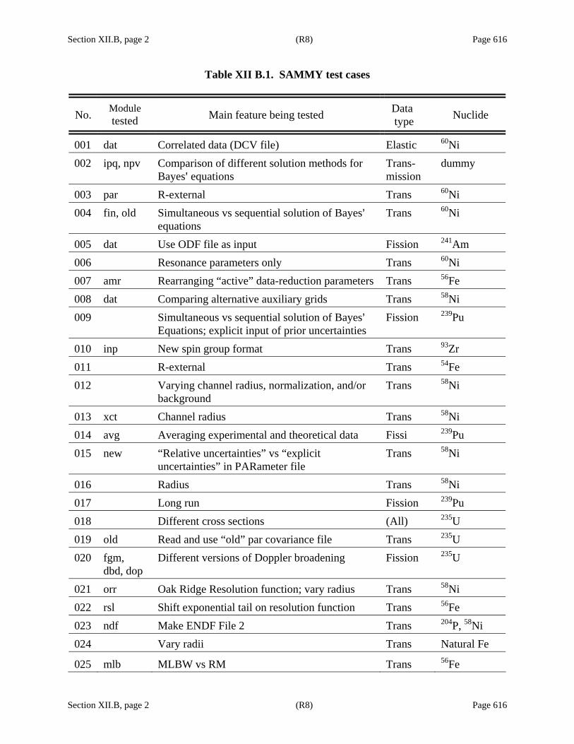
Section XII.B, page 2 (R8) Page 616
Section XII.B, page 2 (R8) Page 616
Table XII B.1. SAMMY test cases
No. Module tested Main feature being tested Data
type Nuclide
001 dat Correlated data (DCV file) Elastic 60Ni 002 ipq, npv Comparison of different solution methods for
Bayes= equations Trans-mission
dummy
003 par R-external Trans 60Ni 004 fin, old Simultaneous vs sequential solution of Bayes=
equations Trans 60Ni
005 dat Use ODF file as input Fission 241Am 006 Resonance parameters only Trans 60Ni 007 amr Rearranging “active” data-reduction parameters Trans 56Fe 008 dat Comparing alternative auxiliary grids Trans 58Ni 009 Simultaneous vs sequential solution of Bayes=
Equations; explicit input of prior uncertainties Fission 239Pu
010 inp New spin group format Trans 93Zr 011 R-external Trans 54Fe 012 Varying channel radius, normalization, and/or
background Trans 58Ni
013 xct Channel radius Trans 58Ni 014 avg Averaging experimental and theoretical data Fissi 239Pu 015 new “Relative uncertainties” vs “explicit
uncertainties” in PARameter file Trans 58Ni
016 Radius Trans 58Ni 017 Long run Fission 239Pu 018 Different cross sections (All) 235U 019 old Read and use “old” par covariance file Trans 235U 020 fgm,
dbd, dop Different versions of Doppler broadening Fission 235U
021 orr Oak Ridge Resolution function; vary radius Trans 58Ni 022 rsl Shift exponential tail on resolution function Trans 56Fe 023 ndf Make ENDF File 2 Trans 204P, 58Ni 024 Vary radii Trans Natural Fe
025 mlb MLBW vs RM Trans 56Fe
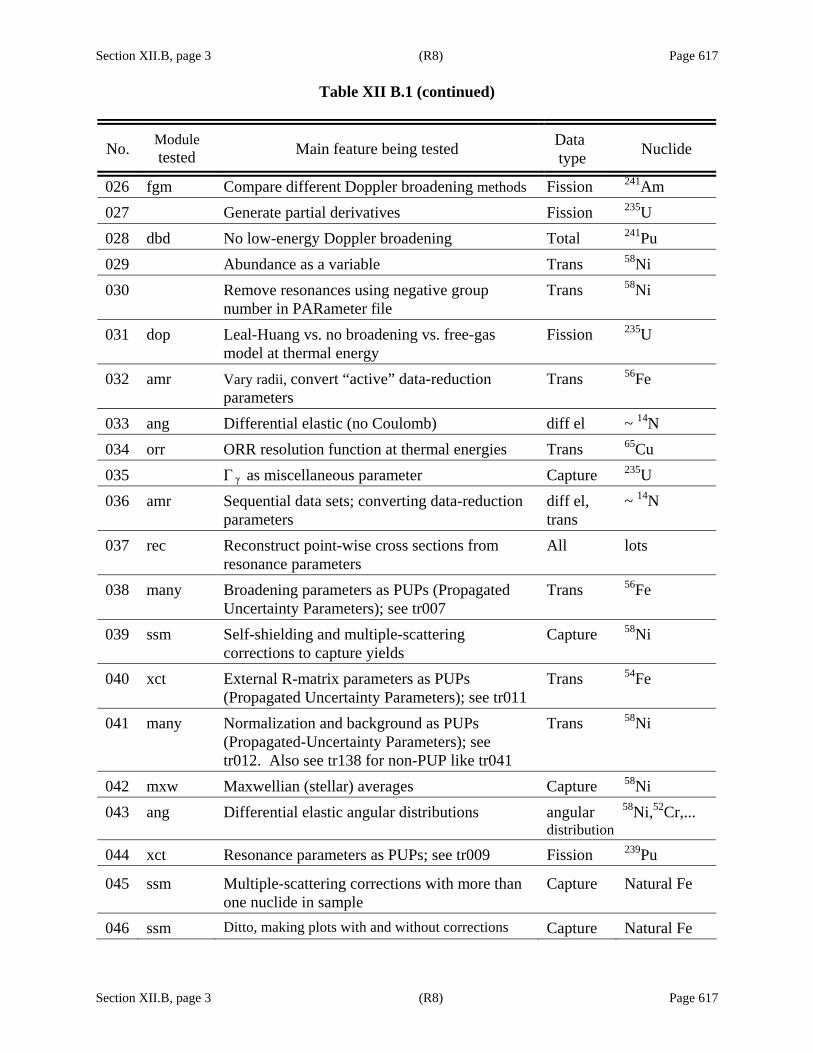
Section XII.B, page 3 (R8) Page 617 Table XII B.1 (continued)
Section XII.B, page 3 (R8) Page 617
No. Module tested Main feature being tested Data
type Nuclide
026 fgm Compare different Doppler broadening methods Fission 241Am 027 Generate partial derivatives Fission 235U 028 dbd No low-energy Doppler broadening Total 241Pu 029 Abundance as a variable Trans 58Ni 030 Remove resonances using negative group
number in PARameter file Trans 58Ni
031 dop Leal-Huang vs. no broadening vs. free-gas model at thermal energy
Fission 235U
032 amr Vary radii, convert “active” data-reduction parameters
Trans 56Fe
033 ang Differential elastic (no Coulomb) diff el ~ 14N 034 orr ORR resolution function at thermal energies Trans 65Cu 035 Γ γ as miscellaneous parameter Capture 235U 036 amr Sequential data sets; converting data-reduction
parameters diff el, trans
~ 14N
037 rec Reconstruct point-wise cross sections from resonance parameters
All lots
038 many Broadening parameters as PUPs (Propagated Uncertainty Parameters); see tr007
Trans 56Fe
039 ssm Self-shielding and multiple-scattering corrections to capture yields
Capture 58Ni
040 xct External R-matrix parameters as PUPs (Propagated Uncertainty Parameters); see tr011
Trans 54Fe
041 many Normalization and background as PUPs (Propagated-Uncertainty Parameters); see tr012. Also see tr138 for non-PUP like tr041
Trans 58Ni
042 mxw Maxwellian (stellar) averages Capture 58Ni 043 ang Differential elastic angular distributions angular
distribution 58Ni,52Cr,...
044 xct Resonance parameters as PUPs; see tr009 Fission 239Pu
045 ssm Multiple-scattering corrections with more than one nuclide in sample
Capture Natural Fe
046 ssm Ditto, making plots with and without corrections Capture Natural Fe

Section XII.B, page 4 (R8) Page 618 Table XII B.1 (continued)
Section XII.B, page 4 (R8) Page 618
No. Module tested Main feature being tested Data
type Nuclide
047 Vary t0 and L0 Trans 56Fe 048 rsl Channel resolution varies with energy Fission 239Pu 049 rec, mxw Reconstruct point-wise cross sections; use
results to calculate stellar averages Capture 54Fe
050 mas Use ENDF File2 for input to SAMMY Trans 59Co 051 mxw Various ways to generate stellar averages Capture 136Ba 052 ssm Self-shielding and multiple-scattering
corrections Capture 134Ba
053 rpt Generate RPI resolution function none none 054 rpi Use RPI resolution function Trans W 055 xct Paramagnetic cross section (including PUPs) Total Dummy 056 Background function Dummy Dummy 057 ssm Self-indication data Self-
indication Dummy
058 dop, fgm Very-low-energy Doppler broadening Capture Dummy 059 xct Channel radii as PUPs; see tr093 Reaction 16O 060 ssm Self-shielding and multiple-scattering
corrections Capture 136Ba
061 ref Convert REFIT input to SAMMY and vice versa
062 Abundances as PUPs Trans 58Ni 063 Constant cross section Dummy 064 Fission yields, polar coordinates Fission 235U 066 many Miscellaneous parameters as PUPs many many 067 dat Twenty significant digits for data Dummy 068 orr ORR parameters as PUPs. See tr117 for related
unPUP case. Trans 58Ni
069 ntg Integral quantities All 235U 070 idc, fdc Implicit data covariances 235U 071 Write covariance matrix in compact ASCII format 235U 072 thn Thinning data 073 fff Unresolved resonance region many 235U
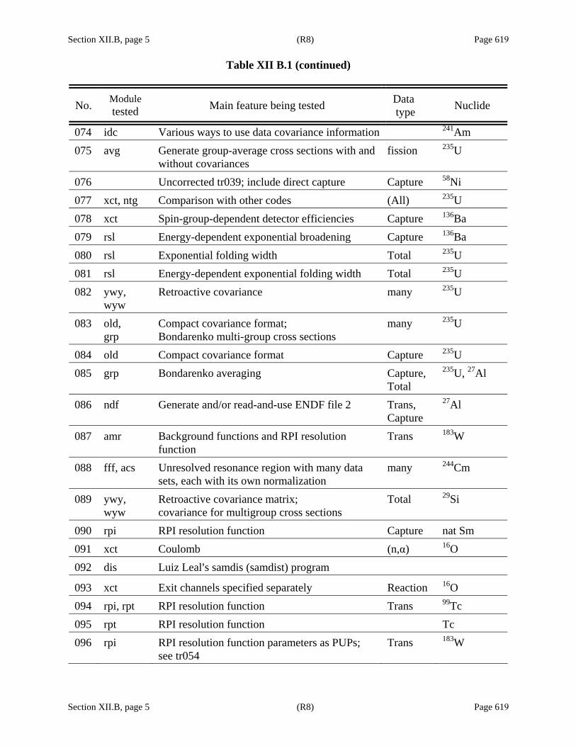
Section XII.B, page 5 (R8) Page 619 Table XII B.1 (continued)
Section XII.B, page 5 (R8) Page 619
No. Module tested Main feature being tested Data
type Nuclide
074 idc Various ways to use data covariance information 241Am 075 avg Generate group-average cross sections with and
without covariances fission 235U
076 Uncorrected tr039; include direct capture Capture 58Ni 077 xct, ntg Comparison with other codes (All) 235U 078 xct Spin-group-dependent detector efficiencies Capture 136Ba 079 rsl Energy-dependent exponential broadening Capture 136Ba 080 rsl Exponential folding width Total 235U 081 rsl Energy-dependent exponential folding width Total 235U 082 ywy,
wyw Retroactive covariance many 235U
083 old, grp
Compact covariance format; Bondarenko multi-group cross sections
many 235U
084 old Compact covariance format Capture 235U 085 grp Bondarenko averaging Capture,
Total 235U, 27Al
086 ndf Generate and/or read-and-use ENDF file 2 Trans, Capture
27Al
087 amr Background functions and RPI resolution function
Trans 183W
088 fff, acs Unresolved resonance region with many data sets, each with its own normalization
many 244Cm
089 ywy, wyw
Retroactive covariance matrix; covariance for multigroup cross sections
Total 29Si
090 rpi RPI resolution function Capture nat Sm 091 xct Coulomb (n,α) 16O 092 dis Luiz Leal=s samdis (samdist) program
093 xct Exit channels specified separately Reaction 16O 094 rpi, rpt RPI resolution function Trans 99Tc 095 rpt RPI resolution function Tc 096 rpi RPI resolution function parameters as PUPs;
see tr054 Trans 183W
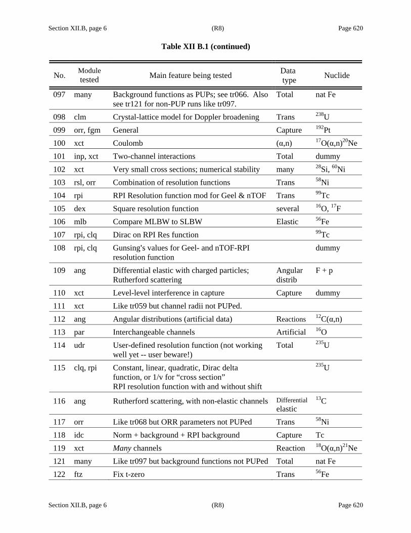
Section XII.B, page 6 (R8) Page 620 Table XII B.1 (continued)
Section XII.B, page 6 (R8) Page 620
No. Module tested Main feature being tested Data
type Nuclide
097 many Background functions as PUPs; see tr066. Also see tr121 for non-PUP runs like tr097.
Total nat Fe
098 clm Crystal-lattice model for Doppler broadening Trans 238U 099 orr, fgm General Capture 192Pt 100 xct Coulomb (α,n) 17O(α,n)20Ne 101 inp, xct Two-channel interactions Total dummy 102 xct Very small cross sections; numerical stability many 28Si, 60Ni 103 rsl, orr Combination of resolution functions Trans 58Ni 104 rpi RPI Resolution function mod for Geel & nTOF Trans 99Tc 105 dex Square resolution function several 16O, 17F 106 mlb Compare MLBW to SLBW Elastic 56Fe 107 rpi, clq Dirac on RPI Res function 99Tc 108 rpi, clq Gunsing=s values for Geel- and nTOF-RPI
resolution function dummy
109 ang Differential elastic with charged particles; Rutherford scattering
Angular distrib
F + p
110 xct Level-level interference in capture Capture dummy 111 xct Like tr059 but channel radii not PUPed. 112 ang Angular distributions (artificial data) Reactions 12C(α,n) 113 par Interchangeable channels Artificial 16O 114 udr User-defined resolution function (not working
well yet -- user beware!) Total 235U
115 clq, rpi Constant, linear, quadratic, Dirac delta function, or 1/v for “cross section” RPI resolution function with and without shift
235U
116 ang Rutherford scattering, with non-elastic channels Differential elastic
13C
117 orr Like tr068 but ORR parameters not PUPed Trans 58Ni 118 idc Norm + background + RPI background Capture Tc 119 xct Many channels Reaction 18O(α,n)21Ne 121 many Like tr097 but background functions not PUPed Total nat Fe 122 ftz Fix t-zero Trans 56Fe

Section XII.B, page 7 (R8) Page 621 Table XII B.1 (continued)
Section XII.B, page 7 (R8) Page 621
No. Module tested Main feature being tested Data
type Nuclide
123 ang Angle average Diff elas 17F+p 124 clm Crystal lattice model for Doppler broadening
(DOPUSH) several dummy 238U
125 xct, ang Running as pseudo R-matrix (no Reich-Moore approximation); Coulomb; many channels
many 16O
126 ndf Prepare compact covariance file in ENDF File 32 format
Fission, Total
235U, 27Al, 23Na, 242Pu, 240Pu, 241Am
127 lru Create File 2 for unresolved resonance region all 235U, 244Cm 128 fff Use several energy regions in URR calculation all 235U 129 mas Read all of ENDF file, not just File 2 242Pu, 23Na,
240Pu, 241Am 130 new Read ENDF File 32 as generated in tr126
131 ndf Write compact covariance matrix in ENDF format
152Gd
132 ndf, new Create PAR & COV file, generate ENDF File 2 and File 32, read them back
dummy like 27Al
133 lru Write ENDF File 2 and File 32 for URR all 235U 134 lru Write ENDF File 2 for URR; options for
energies in ENDF file 238U
135 inp, par More than fifty spin groups Total dummy (Si) 136 rpi Derivatives with respect to RPI resolution
function parameters Trans Gd
137 ndf Create File 32 original ENDF formats (LCOMP = 0 or 1)
242Pu, 23Na, 240Pu, 241Am
138 many Like tr041 but normalization and background are not PUPs
Trans 58Ni
139 xct, xxx Calculate hard-sphere phase shift at high energy Reaction 9Be(α,n)12C 140 idc User-supplied implicit data covariance matrix Trans 129I 141 suggel Estimate quantum numbers for resonances 142 fit, fff Sequential runs in URR all 233U

Section XII.B, page 8 (R8) Page 622 Table XII B.1 (continued)
Section XII.B, page 8 (R8) Page 622
No. Module tested Main feature being tested Data
type Nuclide
143 qua Prepare spin group quantum number information in SAMMY input format
58Ni, 99Tc, 26Fe, 241Am, 235U, 16O, 17O, 13C
144 inp, par Treat channels properly: 10 spin groups vs. 18; 2 or 3 channels vs. 1
Trans 27Al
145 fff, acs Covariances, normalizations in URR Total, Fission
235U
146 avg, grp, fin
“Compact” format for ENDF Capture 235U
147 rml Read and use LRF=7 ENDF format; test SAMRML program (see tr147a for SAMRML runs with no SAMMY runs)
Elastic, Absorp-tion, Fission
27Al, 16O, 235U
148 rml Test SAMRML program, including derivatives and angular distributions (see tr148a for only SAMRML runs, no SAMMY runs)
many 52Cr
149 many Create retroactive covariance matrix for ENDF File 32
many 233U
150 rml Extension of tr147 with fewer resonances and parameters but more features (see tr150a for SAMRML without SAMMY)
Angular distribs, derivatvs
16O
151 par Additional possibilities for input of prior uncertainty on resonance parameters
input 58Ni
152 par, xct Exclude channels from entire calculation Trans 19F 153 inp, par Input data-related parameters via the INPut file
rather than PARameter file Trans 19F
154 ndf Prepare covariance file in ENDF File 32 format. Like tr126 but use default uncertainty option (“def = value” in *.ndf file; see Section VI.F.2 for details). All resonances appear in File 32.
235U, 27Al, 23Na, 242Pu, 240Pu, 241Am
155 ang Angular distribution of reaction cross sections Differential reaction
9Be
156 grp Bondarenko averaging with Doppler broadening and resolution broadening
Capture 238U
157 inp, par Broadening parameters in INPut file Trans 238U
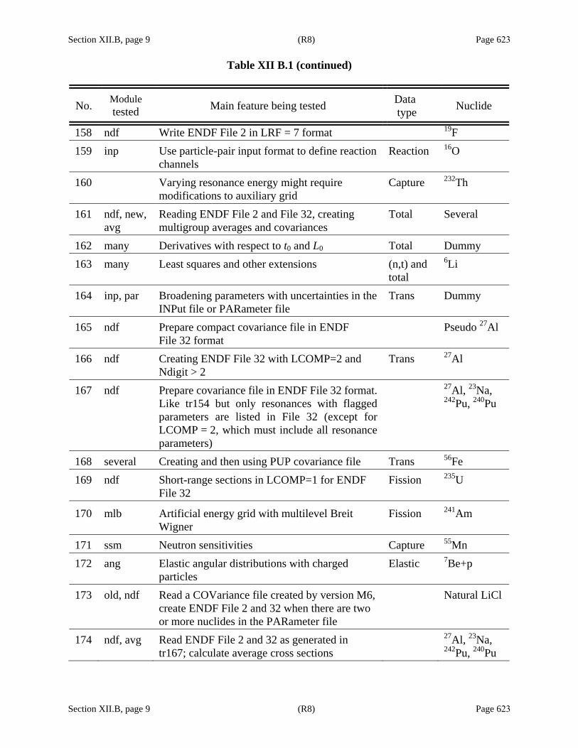
Section XII.B, page 9 (R8) Page 623 Table XII B.1 (continued)
Section XII.B, page 9 (R8) Page 623
No. Module tested Main feature being tested Data
type Nuclide
158 ndf Write ENDF File 2 in LRF = 7 format 19F 159 inp Use particle-pair input format to define reaction
channels Reaction 16O
160 Varying resonance energy might require modifications to auxiliary grid
Capture 232Th
161 ndf, new, avg
Reading ENDF File 2 and File 32, creating multigroup averages and covariances
Total Several
162 many Derivatives with respect to t0 and L0 Total Dummy 163 many Least squares and other extensions (n,t) and
total 6Li
164 inp, par Broadening parameters with uncertainties in the INPut file or PARameter file
Trans Dummy
165 ndf Prepare compact covariance file in ENDF File 32 format
Pseudo 27Al
166 ndf Creating ENDF File 32 with LCOMP=2 and Ndigit > 2
Trans 27Al
167 ndf Prepare covariance file in ENDF File 32 format. Like tr154 but only resonances with flagged parameters are listed in File 32 (except for LCOMP = 2, which must include all resonance parameters)
27Al, 23Na, 242Pu, 240Pu
168 several Creating and then using PUP covariance file Trans 56Fe 169 ndf Short-range sections in LCOMP=1 for ENDF
File 32 Fission 235U
170 mlb Artificial energy grid with multilevel Breit Wigner
Fission 241Am
171 ssm Neutron sensitivities Capture 55Mn
172 ang Elastic angular distributions with charged particles
Elastic 7Be+p
173 old, ndf Read a COVariance file created by version M6, create ENDF File 2 and 32 when there are two or more nuclides in the PARameter file
Natural LiCl
174 ndf, avg Read ENDF File 2 and 32 as generated in tr167; calculate average cross sections
27Al, 23Na, 242Pu, 240Pu

Section XII.B, page 10 (R8) Page 624 Table XII B.1 (continued)
Section XII.B, page 10 (R8) Page 624
No. Module tested Main feature being tested Data
type Nuclide
175 rec, mxw Calculating Maxwellian averages with and without using the RECONSTRUCT command
19F
176 xct Energy-dependent “nu” Eta 235U 177 xct Including both the Reich-Moore eliminated
capture channel and an explicit capture channel Many 16O
178 Several Non-uniform sample for transmission data Trans 204P 179 ndf, mas Creating and reading ENDF File 2 and 32 with
LRF = 3, LCOMP = 1, when different spin groups have a different number of fission channels and/or a different number of flags
240Pu
180 ndf, mas Creating and reading ENDF File 2 and 32 with LRF = 7, LCOMP = 1, when some resonances are below inelastic threshold
19F

Section XII.C, page 1 (R8) Page 625
Section XII.C, page 1 (R8) Page 625
XII.C. MONTE CARLO SIMULATIONS OF MULTIPLE-SCATTERING CORRECTIONS
One aspect of the SAMMY quality assurance program is the use of any and all available methods for double-checking the implementation of the various features in the code. For the multiple-scattering corrections for capture or fission data described in Section III.D, the most reliable checking method is Monte Carlo simulation of those corrections. The code SAMSMC (Section X.M) is used for these simulations. Sample simulations are stored in subdirectories samsim/sim001 through samsim/sim009; details are shown in Table XII C.1. The command file in each subdirectory is called simxyz, where xyz is the three-digit simulation number. The number of Monte Carlo iterations in simxyz is unrealistically small; for a more reasonable number (and hence a far longer run time), see file simxyz_intense. Results in the answers subdirectory were created using the larger number of iterations.
Table XII C.1. Sample Monte Carlo simulations
Simulation number Sample composition
Related test case number
sim001 58Ni tr039 sim002 natural Sm plus heavy water sim003 137Ba tr060 sim004 natural Si sim005 28Si; artificial data sim006 Natural Li Cl sim007 35Cl with proton channel sim008 W sim009 55Mn
(uses tabulated Y2 values)


Section XIII, page 1 (R7) Page 627
Section XIII, page 1 (R7) Page 627
XIII. DESCRIPTION OF THE COMPUTER CODE SAMMY
The computer code SAMMY was originally developed to run efficiently on the DECSystem-10 (PDP-10) at the Oak Ridge Electron Linear Accelerator (ORELA). Because memory rather than CPU time was the limiting factor on the PDP10, a number of techniques were used to conserve memory, occasionally at the expense of run time. These techniques include dynamic allocation of array storage (Section XIII.A), use of temporary data files to store intermediate results (Section XIII.B), and division of the program into substantially independent segments (Section XIII.C).
In 1985 ORELA replaced its PDP10 with a VAX785, and SAMMY migrated to the system. Since the mid 1990's, the primarily operating system for SAMMY development has been UNIX or LINUX. Currently the author maintains the code under UNIX (f77 on IBM and VAX-Alpha workstations) and LINUX operating systems; the same version also works on Windows under Compaq FORTRAN. Portability to VMS operating systems is no longer maintained.
Prior to release M5 of the code in 2000, the “division of the program into substantially independent segments” was significantly altered; see Section XIII.C for details. Future plans call for continued modernization of the coding, including conversion to FORTRAN 90; this will eliminate the rather archaic (but nevertheless useful) “dynamic allocation of array storage” currently in use (Section XIII.B).
For the 2006 release 7.0.0 of SAMMY, the use of temporary data files has been significantly
lessened but not yet completely eliminated.
For the benefit of persons wishing to port SAMMY to a new computer system, a brief discussion is included in Section XIII.D regarding routines and statements specific to a given computer. The discussion is not expected to cover all conversion problems but merely to point out a few problems of which the author is aware.
The ODF (ORELA Data Format) plotting package in use at Oak Ridge is not easily portable to most machines. See Section XIII.E for a discussion of this topic, and Section X.I for a discussion of alternatives.
In 2005 a modern configuration and distribution system was designed by ORNL researcher
Dorothea Wiarda. This system, described in Section XIII.F, makes it significantly simpler for a user to install SAMMY.

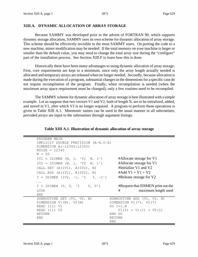
Section XIII.A, page 1 (R7) Page 629
Section XIII.A, page 1 (R7) Page 629
XIII.A. DYNAMIC ALLOCATION OF ARRAY STORAGE
Because SAMMY was developed prior to the advent of FORTRAN 90, which supports dynamic storage allocation, SAMMY uses its own scheme for dynamic allocation of array storage. This scheme should be effectively invisible to the most SAMMY users. On porting the code to a new machine, minor modification may be needed: If the total memory on your machine is larger or smaller than the default value, you may need to change the total array size during the “configure” part of the installation process. See Section XIII.F to learn how this is done.
Historically there have been many advantages to using dynamic allocation of array storage. First, core requirements are kept to a minimum, since only the array length actually needed is allocated and temporary arrays are released when no longer needed. Secondly, because allocation is made during the execution of a program, substantial changes in the dimensions for a specific case do not require recompilation of the program. Finally, when recompilation is needed (when the maximum array space requirement must be changed), only a few routines need to be recompiled.
The SAMMY scheme for dynamic allocation of array storage is best illustrated with a simple example. Let us suppose that two vectors V1 and V2, both of length N, are to be initialized, added, and stored in V1, after which V2 is no longer required. A program to perform these operations is given in Table XIII A.1. Mnemonic names can be used in the usual manner in all subroutines, provided arrays are input to the subroutines through argument listings.
Table XIII A.1. Illustration of dynamic allocation of array storage
PROGRAM MAIN IMPLICIT DOUBLE PRECISION (A-H,O-Z) DIMENSION A(-12345:12345) NSIZE = 12345 N = 50 IV1 = IDIMEN (N, 1, ‘V1 N, 1’) #Allocate storage for V1 IV2 = IDIMEN (N, 1, ‘V2 N, 1’) #Allocate storage for V1 CALL SET (A(IV1), A(IV2), N) #Initialize V1 and V2 CALL ADD (A(IV1), A(IV2), N) #Add V1 = V1 + V2 I = IDIMEN (IV2, -1, ‘I I, -1’) #Release storage for V2 . . . I = IDIMEN (0, 0, ‘I 0, 0’) #Request that IDIMEN print out theSTOP # maximum length usedEND SUBROUTINE SET (V1, V2, N) DIMENSION V1(N), V2(N) READ (11) V1 READ (11) V2 RETURN END
SUBROUTINE ADD (V1, V2, N) DIMENSION V1(*), V2(*) DO I=1,N V1(I) = V1(I) + V2(I) END DO RETURN END
Section XIII.A, page 2 (R7) Page 630
Section XIII.A, page 2 (R7) Page 630
What follows is a brief description of the scheme currently in use in SAMMY for dynamic allocation of array storage. Most users of the code will not need to be concerned with the remainder of this section. The information is included here for completeness’ sake, and for the benefit of anyone who may need to modify the code.
The current scheme is essentially the same as in previous releases of the SAMMY code, though different in detail. All arrays required by the computer program are stored in one array A, dimensioned A(-n:n) where n is a large number. [Use of this form, rather than the more common A(n), makes use of the negative integers and thus effectively doubles the maximum size of the array available with the largest possible 8-byte (32-bit) integer (231-1 = 2 147 483 647, since the 32nd bit is used for the sign). For a very few applications, this large size is needed and can be accommodated on computers with sufficient memory.] The precise value to be used for n is machine dependent. The SAMMY default is 65 million, but this can be overwritten when the code is configured for a specific machine, as described in Section XIII.F.
As shown in Table XIII A.1, allocation of space in this array is accomplished via a call to FUNCTION IDIMEN, which keeps track of the last location allocated, and appends the new array to that position. When an array is no longer needed, its space is released via another call to IDIMEN. At the end of each segment, IDIMEN is called one more time to report the maximum size actually used in that segment. IDIMEN also issues a warning if more than 2n words are required in the array A(-n:n), and then aborts the run.
Three arguments are used for IDIMEN (m1, m2, a3): The third, a3, is an arbitrary alphanumeric phrase used by the author for debugging. The second, m2, tells IDIMEN what to do with the first, m1. If m2 > 0, an array of size m1 is allocated. If m2 < 0, everything in A(-n:n) beyond position A(m1) is released for reuse. If m2 = 0, the total amount of storage used since the previous such call is reported (written into the SAMMY.LPT file).
Users familiar with the array storage system in earlier versions of SAMMY will note some differences in the 7.0.0 release of the code, especially with respect to the array sizes printed in the SAMMY.LPT file.
First, the storage requirement for segment XCT will generally be twice the size for the same segment in previous versions of the code; nevertheless, the largest requirement (for all segments) remains approximately the same. At the beginning of segment XCT, the new array-storage system allots all of the storage (for theory and derivatives, original and Doppler broadened, for example) needed to store intermediate results. SAMMY reuses those same storage locations as it goes from segment to segment. For a typical run including both Doppler and resolution broadening, after completion of segment FGM (Doppler), the “original” array positions will be re-used to hold the resolution-broadened values.
In the old version of the code, only the arrays needed in segment XCT were defined in XCT; these were then written to a temporary file and the space released. Then in FGM, space was allocated for the original arrays and for the Doppler-broadened arrays; the original values were read in from the temporary file. When the FGM calculations finished, the Doppler-broadened values were written to a temporary file and the space (for all these arrays) was released. This process was repeated in every module of the code.

Section XIII.A, page 3 (R7) Page 631
Section XIII.A, page 3 (R7) Page 631
Hence, the new system uses essentially the same total storage space but eliminates the reads and writes to the temporary files. Total time for a SAMMY run is therefore decreased. (Future development will likely eliminate nearly all of the temporary files. For more on the use of temporary files, see Section XIII.B.)
As indicated above, SAMMY allocates the array space for storing the values and derivatives at the beginning of segment XCT. However, it does not allocate all array space needed for all of the processes involved in calculating those values and derivatives. Thus, for example, the SSM segment (which calculates self-shielding and multiple-scattering corrections) requires many auxiliary calculations, for which it needs extra array space.

Section XIII.B, page 1 (R7) Page 633
Section XIII.B, page 1 (R7) Page 633
XIII.B. USE OF TEMPORARY DATA FILES TO STORE INTERMEDIATE RESULTS
Output to and input from temporary files is a time-honored method of saving memory at the expense of run time. In versions of SAMMY prior to M5, the use of temporary files also provided the necessary linkage from one module to another; I/O for this purpose has now been eliminated, since the segments of the code are now united into one large code. Nevertheless there are still many temporary files created by a SAMMY run; these are being phased out as modernization of the code proceeds. For now, upon successful completion of a SAMMY run, the temporary files may be deleted.
It is still occasionally possible for the author to debug the code in a piece-wise fashion, one segment at a time. However, it now requires a bit more planning. First, a SAMMY run is made that includes the alphanumeric line
STOP xyz n in the INPut file, where n is a one-digit integer preceded by two spaces, and xyz is the name of the segment for which debugging is needed. This line is a command to SAMMY to cease execution just prior to the beginning of the nth pass through segment xyz and generate the temporary files that permit restart of that segment alone. After this run finishes, those temporary files can, in principle, be used as input for debugging on segment samxyz. However, with modern high-speed computers, it is now generally more trouble to ensure that the one segment runs properly than to run the entire program. This capability is gradually being eliminated, and the additional routines necessary for reading the temporary files and starting a run in the middle are no longer distributed with the code.
The temporary files generated by SAMMY are listed in Table XIII B .1. “Standard” names referenced in the third column of the table are “SAMxx.DAT,” where “xx” is replaced by the unit number. Caution: The list in Table XIII B .1 may not be completely accurate.
Input and output files are also included in Table XIII B .1, without detailed explanation. For
a more comprehensive list of input files, see Table VI.1. For a list of output files, see Table VII.1.

Section XIII.B, page 2 (R8) Page 634
Section XIII.B, page 2 (R8) Page 634
Table XIII B.1. Files used by SAMMY. The letter A, B, or O in the second column indicates whether the file is written as ASCII, binary, or ODF file. Only SAMMY files (not those for
auxiliary codes) are listed here.
Unit No.
A, B, O
File name if not standard
Subdirectory: subroutines in which
this file is written
Subdirectory: subroutines in which
this file is read Content
5 A Interactive input
mas: many places See Table VI E .1
6 A Log file [Many places] 10 A CLM file clm: Readclm_0,
Find_Osc, Readclm
Crystal lattice information; see Section III.B.4
10 A ENDF/B-VI file 2
mas: Rcontx, Rcont, Rtab1, Rlist, Read_Pp7, Endf7
Resonance parameters in ENDF formats
10 A ENDF/B file 3
rec: Read3, Rdndf3 File 3 contribution to cross section
10 A MXW file mxw: Rktxxx, Readkt See Section V.D and VI.F.4
10 A NDF file ndf: Rdndf7, Read_ndf, Rdndf
See Section VI.F.2
10 A NTG file ntg: Rdntgq_0, Rdntgq
Integral data; see Sections V.B and VI.D
11 A INPut file mas: Finpx, Finp, New_Input_File, Newinp
See Tables VI A.1 and VI A1.2
12, 32
A Initial PARameter file
mas: Fpar_If_Cov inp: many places par: many places fdc: Paramf
See Table VI B.2
12 A SAMNDF. PAR
mas: several SAMMY-style PAR file generated from ENDF/B file 2
13 A SAMNDF. INP
mas: several SAMMY-style INPut file generated from ENDF/B file 2

Section XIII.B, page 3 (R8) Page 635 Table XIII B.1 (continued)
Section XIII.B, page 3 (R8) Page 635
Unit No.
A, B, O
File name if not standard
Subdirectory: subroutines in which
this file is written
Subdirectory: subroutines in which
this file is read Content
13, 14
A or O
DATa file mas: Ascidt, Ascxdt odf: many dat: many fdc: Rddat0_Fdc,
Rddat1_Fdc
See Table VIC.1
14 A SAMEXP.DAT
mas: odfdat odf: many dat: many
ASCII version of ODF data file
14 A SAMNDF. PAR or SAMMY. PAR
mas: Rewrite_12 Rewriting output PARameter file
15 A SAMMY. FFF
fff: many FITACS input file, see Section VIII
16 A mas: Sumstr, Wrt16x, Writ16, File2x,
inp: Saminp_0, Files, Filesx, Qcova
old: Addup fff: Pass
Controls for passes 1 and 2 through SAMMY
17 18 A mas: finp, writ19,
file2x odf: chck18
odf: Chck18, Read18 Controls for running ODF segment
19 A mas: Writ19 inp: Saminp_0, Files, Filesx, Qcova
old: Addup fff: Pass
Controls for pass 3 through SAMMY
20 21 A SAMMY.
LPT many places never “Line Printer”
output giving details for this SAMMY run
22 A INPUT. NEW
inp: Rdspnx Error message when using obsolete input

Section XIII.B, page 4 (R8) Page 636 Table XIII B.1 (continued)
Section XIII.B, page 4 (R8) Page 636
Unit No.
A, B, O
File name if not standard
Subdirectory: subroutines in which
this file is written
Subdirectory: subroutines in which
this file is read Content
22 A mas: New_Input_File, Sett, Set, Write_Alpha
inp: many places fff: Pass
Copy of INPut file, with appropriate modifications for first pass through SAMMY
23, 24
A Like 22, for passes 2 and 3
25 B SAMMY. SSM
inp: Qqqwrt ssm: Qqqxxx, Qqqget Edge effects for single-scattering corrections to capture or fission yields
25 B REMORI. PAR
wyw: Getywy
wyw: Getywy ywy: Get_Dminth_
Gppn
Original parameter covariance matrix for retroactive method
26, 27
A inp: Saminp_0, Rdspno
fin: Find_More_Data avg: Again
fin: Find_More_Data avg: Tryrng,
Test_If_Data, Again
mxw:Rktxxx ndf: Endfb6
Similar to SAM16.DAT
28 A AVG file avg: Tryrng, Qrange See Section VI.F.1
29 30 B acs: Wrt30 mpw: Readwx Arrays W and Y
for M+W inversion scheme (see Section IV.B.3)
30 A (user-supplied)
idc: Wrt30_Idc ipq: Estx, estipq, findxx
npv: Get_Idc_1, Findxx, Read_Cov_Idc
Implicit data covariance information

Section XIII.B, page 5 (R8) Page 637 Table XIII B.1 (continued)
Section XIII.B, page 5 (R8) Page 637
Unit No.
A, B, O
File name if not standard
Subdirectory: subroutines in which
this file is written
Subdirectory: subroutines in which
this file is read Content
30 B ntg: Wrntgq, Wrntgx npv: Rdntg1, Prepare_Storage
ywy: Rdntg1_Ywy
Integral data information
31 32 A mas: Datcov wyw: Getywy File names for Yi
and Wi for data set i; see Section IV.E.1
32 A SAMMY. PAR
fit: Writep Updated PAR file for the URR (unresolved resonance region); see Section VIII.C
33 A SAMMY. PA2
fdc: Paramf Modified PAR file; see Section VI.C.3.c
34 A SAMMY. IDC
fdc: Paramf idc: many places See Section VI.C.3.c
33-35
A Debug printout
36 A fin: many fin: Rewrite_12 Temporary file for creating SAMMY.RED
37 B npv: Get_W_Idc old: Rdcov_Pup
inp: Reorg_Cov old: Rparfl_Pup end: Outvs
Covariance matrix for Propagated-Uncertainty Parameters
38 A mas: Endf2, Endf7 fin: Oldord
mas: Rewrite_12 Temporary site for storing parameters prior to rewriting
39 A mas: Read_Pp7 mas: Rewrite_12 SAMMY-style input file created from ENDF File 2
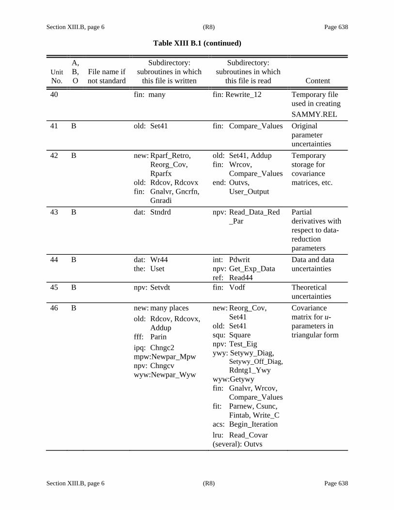
Section XIII.B, page 6 (R8) Page 638 Table XIII B.1 (continued)
Section XIII.B, page 6 (R8) Page 638
Unit No.
A, B, O
File name if not standard
Subdirectory: subroutines in which
this file is written
Subdirectory: subroutines in which
this file is read Content
40 fin: many fin: Rewrite_12 Temporary file used in creating SAMMY.REL
41 B old: Set41 fin: Compare_Values Original parameter uncertainties
42 B new: Rparf_Retro, Reorg_Cov, Rparfx
old: Rdcov, Rdcovx fin: Gnalvr, Gncrfn,
Gnradi
old: Set41, Addup fin: Wrcov,
Compare_Values end: Outvs,
User_Output
Temporary storage for covariance matrices, etc.
43 B dat: Stndrd npv: Read_Data_Red _Par
Partial derivatives with respect to data-reduction parameters
44 B dat: Wr44 the: Uset
int: Pdwrit npv: Get_Exp_Data ref: Read44
Data and data uncertainties
45 B npv: Setvdt fin: Vodf Theoretical uncertainties
46 B new: many places old: Rdcov, Rdcovx,
Addup fff: Parin ipq: Chngc2 mpw:Newpar_Mpw npv: Chngcv wyw:Newpar_Wyw
new: Reorg_Cov, Set41
old: Set41 squ: Square npv: Test_Eig ywy: Setywy_Diag,
Setywy_Off_Diag, Rdntg1_Ywy
wyw:Getywy fin: Gnalvr, Wrcov,
Compare_Values fit: Parnew, Csunc,
Fintab, Write_C acs: Begin_Iteration lru: Read_Covar (several): Outvs
Covariance matrix for u-parameters in triangular form
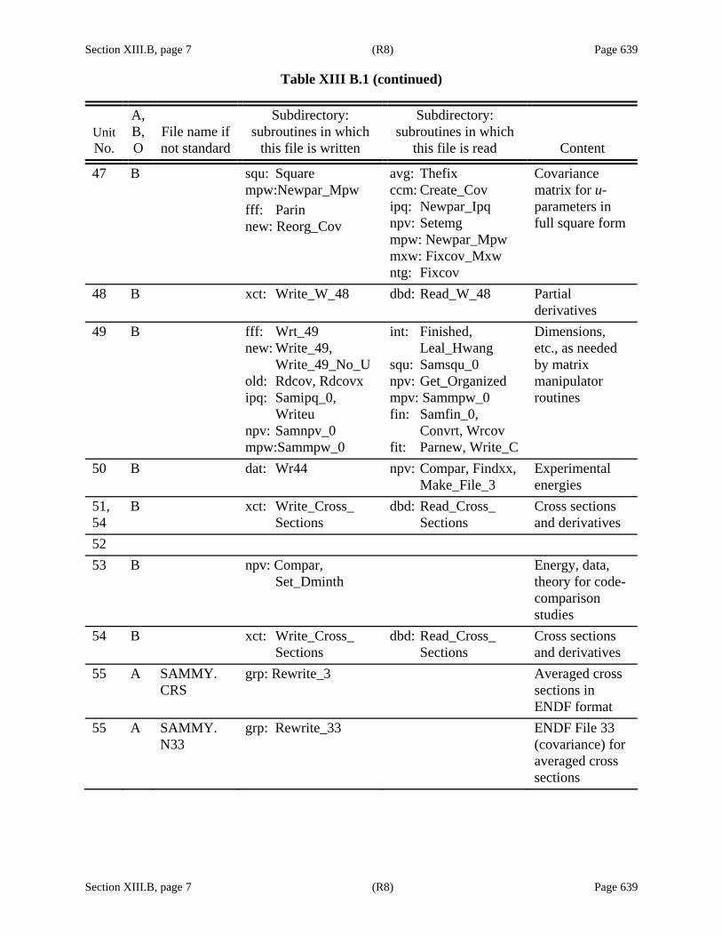
Section XIII.B, page 7 (R8) Page 639 Table XIII B.1 (continued)
Section XIII.B, page 7 (R8) Page 639
Unit No.
A, B, O
File name if not standard
Subdirectory: subroutines in which
this file is written
Subdirectory: subroutines in which
this file is read Content
47 B squ: Square mpw:Newpar_Mpw fff: Parin new: Reorg_Cov
avg: Thefix ccm: Create_Cov ipq: Newpar_Ipq npv: Setemg mpw: Newpar_Mpw mxw: Fixcov_Mxw ntg: Fixcov
Covariance matrix for u-parameters in full square form
48 B xct: Write_W_48
dbd: Read_W_48
Partial derivatives
49 B fff: Wrt_49 new: Write_49,
Write_49_No_U old: Rdcov, Rdcovx ipq: Samipq_0,
Writeu npv: Samnpv_0 mpw:Sammpw_0
int: Finished, Leal_Hwang
squ: Samsqu_0 npv: Get_Organized mpv: Sammpw_0 fin: Samfin_0,
Convrt, Wrcov fit: Parnew, Write_C
Dimensions, etc., as needed by matrix manipulator routines
50 B dat: Wr44 npv: Compar, Findxx, Make_File_3
Experimental energies
51,54
B xct: Write_Cross_ Sections
dbd: Read_Cross_ Sections
Cross sections and derivatives
52 53 B npv: Compar,
Set_Dminth Energy, data,
theory for code-comparison studies
54 B xct: Write_Cross_ Sections
dbd: Read_Cross_ Sections
Cross sections and derivatives
55 A SAMMY. CRS
grp: Rewrite_3 Averaged cross sections in ENDF format
55 A SAMMY. N33
grp: Rewrite_33 ENDF File 33 (covariance) for averaged cross sections
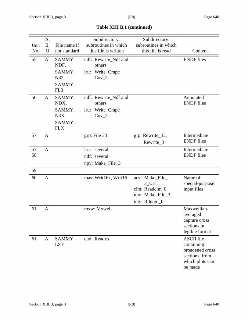
Section XIII.B, page 8 (R8) Page 640 Table XIII B.1 (continued)
Section XIII.B, page 8 (R8) Page 640
Unit No.
A, B, O
File name if not standard
Subdirectory: subroutines in which
this file is written
Subdirectory: subroutines in which
this file is read Content
55 A SAMMY. NDF, SAMMY. N32, SAMMY. FL3
ndf: Rewrite_Ndf and others
lru: Write_Cmpc_ Cov_2
ENDF files
56 A SAMMY. NDX, SAMMY. N3X, SAMMY. FLX
ndf: Rewrite_Ndf and others
lru: Write_Cmpc_ Cov_2
Annotated ENDF files
57 A grp: File 33 grp: Rewrite_33, Rewrite_3
Intermediate ENDF files
57,58
A lru: several ndf: several npv: Make_File_3
Intermediate ENDF files
59 60 A mas: Writ16x, Writ16 acs: Make_File_
3_Urr clm: Readclm_0 npv: Make_File_3 ntg: Rdntgq_0
Name of special-purpose input files
61 A mxw: Mxwell Maxwellian-averaged capture cross sections in legible format
61 A SAMMY. LST
end: Readxx
ASCII file containing broadened cross sections, from which plots can be made

Section XIII.B, page 9 (R8) Page 641 Table XIII B.1 (continued)
Section XIII.B, page 9 (R8) Page 641
Unit No.
A, B, O
File name if not standard
Subdirectory: subroutines in which
this file is written
Subdirectory: subroutines in which
this file is read Content
61 A SAMMXW. FIG
end: Readxx Ascii file containing stellar-averaged cross sections
62 B fin: Gnalvr fin: several old: many
Binary covariance matrix for P-parameters
63 A DCV file dat: Qdatcv Explicit data covariance matrix
64 B SAMMY. COV
fin: Wrcov Output binary covariance matrix for P-parameters
65 66 A fort.66 ssm: Ssssds Debug printout
of corrections to capture yield
67-69 70 A SAMMY.
IO end: Outpar Like
SAMMY.LPT (unit 21), except contains only input and output
71 A SAMMY. PDS
new: Opnpds int: Pdwrit
Partial deriva-tives, for use in generating parameter covariance matrix
72 O SAMMY. ODF
odf: several int: Thodf fin: Vodf
int: Thodf fin: Vodf
ODF file containing broadened cross sections, from which plots can be made

Section XIII.B, page 10 (R8) Page 642 Table XIII B.1 (continued)
Section XIII.B, page 10 (R8) Page 642
Unit No.
A, B, O
File name if not standard
Subdirectory: subroutines in which
this file is written
Subdirectory: subroutines in which
this file is read Content
73
O SAMMXW. ODF
grp: Mxwodf ODF file containing stellar-averaged cross sections
77 A SAMMY. CCV
old:Covnd3 Covariance matrix in ENDF compact format (LCOMP = 2)
82 (60)
B SAMMY. PLT
odf: several int: Thodf fin: Vodf
int: Thodf fin: Vodf end: Readxx
Binary file containing broadened cross sections, to be read by program samplt
83 (60)
B SAMMXW. PLT
grp: Mxwodf end: Readxx Binary file containing stellar-averaged cross sections
Section XIII.C, page 1 (R7) Page 643
Section XIII.C, page 1 (R7) Page 643
XIII.C. DIVISION OF THE PROGRAM INTO AUTONOMOUS SEGMENTS
Prior to version M5 of SAMMY (in the year 2000), the code SAMMY was actually a system of ~50 semi-autonomous codes that executed sequentially and that communicated with each other via I/O from/to temporary files. This structure was originally necessary when computer memory was small and virtual memory nonexistent, and it also had the great virtue of permitting the author to debug each segment independently of the others.
With the advent of modern computers, this independent nature of the segments became obsolete and has therefore been eliminated. The various pieces have been assembled into one code. Many (but not yet all) of the read and write operations have also been eliminated. Users will notice two immediate benefits from this modernization of the code:.
(1) Porting SAMMY to a new platform is considerably easier than in the past. Subroutine execv, the C-language (or system) routine which permitted one FORTRAN routine to initiate execution of another, was a major source of difficulty in porting the program; execv is no longer used. Also, the location (path name) of the executable files must no longer be specified within the code prior to compilation.
(2) Execution time is shortened. The author has noted improvement by as much as 70% on the test cases, though more modest gains are likely on routine runs.
The basic structure of the code has not changed, however: SAMMY still consists of semi-independent segments that are now called sequentially by a main routine. There are approximately fifty segments (or modules), not all of which are used for every SAMMY run. Table XIII C.1 describes the functions of each segment and indicates the calling sequence. The order of the segments in the table is alphabetical.
A flow chart (Figure XIII C.1) shows the order in which the most commonly used modules
are invoked. The path shown across the top of the table is used for unresolved resonance region runs, and the downward path is for resolved resonance runs. Dotted boxes on the flow chart indicate modules that may be omitted in some runs; multiple entries inside a box indicate that only one of those modules is used in a particular run.
By convention, the segment name is “samabc” where abc is replaced by the three characters listed in the table. For most of the segments, relevant files are contained within a subdirectory of the same three-character name (in lowercase, on UNIX operating systems). (Most segments also make use of subroutines in files stored in other subdirectories.) The name and location conventions are not, however, rigidly followed. Some subdirectories store files used in many segments but do not themselves constitute a segment. Other subdirectories hold coding for several segments.
In addition to the segments that operate within a SAMMY run, a number of auxiliary programs are available to be used in conjunction with SAMMY. These programs are described in Section X; most are also included in Table XIII C.1.
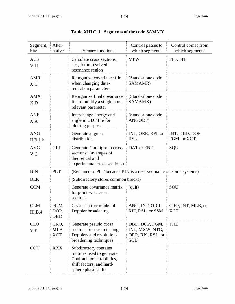
Section XIII.C, page 2 (R6) Page 644
Table XIII C .1. Segments of the code SAMMY
Section XIII.C, page 2 (R6) Page 644
Segment; Site
Alter-native
Primary functions
Control passes to which segment?
Control comes from which segment?
ACS VIII
Calculate cross sections, etc., for unresolved resonance region
MPW FFF, FIT
AMR X.C
Reorganize covariance file when changing data-reduction parameters
(Stand-alone code SAMAMR)
AMX X.D
Reorganize final covariance file to modify a single non-relevant parameter
(Stand-alone code SAMAMX)
ANF X.A
Interchange energy and angle in ODF file for plotting purposes
(Stand-alone code ANGODF)
ANG II.B.1.b
Generate angular distribution
INT, ORR, RPI, or RSL
INT, DBD, DOP, FGM, or XCT
AVG V.C
GRP Generate “multigroup cross sections” (averages of theoretical and experimental cross sections)
DAT or END SQU
BIN PLT (Renamed to PLT because BIN is a reserved name on some systems)
BLK (Subdirectory stores common blocks)
CCM Generate covariance matrix for point-wise cross sections
(quit) SQU
CLM III.B.4
FGM, DOP, DBD
Crystal-lattice model of Doppler broadening
ANG, INT, ORR, RPI, RSL, or SSM
CRO, INT, MLB, or XCT
CLQ V.E
CRO,MLB, XCT
Generate pseudo cross sections for use in testing Doppler- and resolution-broadening techniques
DBD, DOP, FGM, INT, MXW, NTG, ORR, RPI, RSL, or SQU
THE
COU XXX Subdirectory contains routines used to generate Coulomb penetrabilities, shift factors, and hard-sphere phase shifts
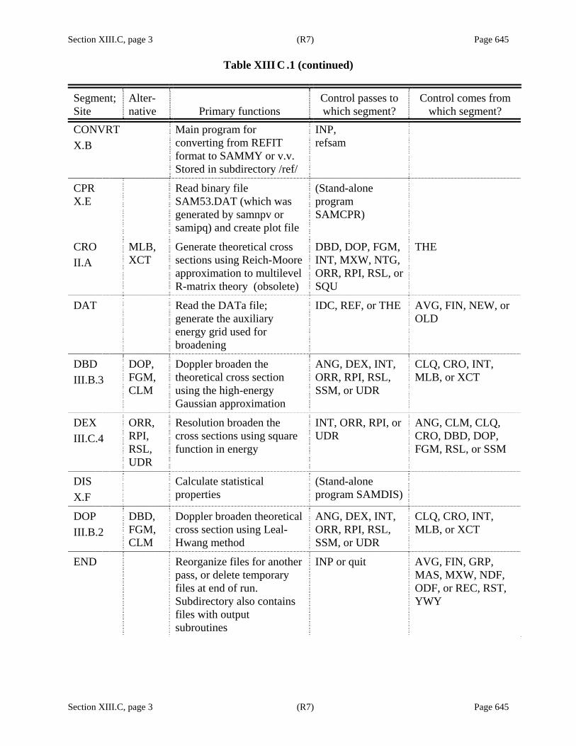
Section XIII.C, page 3 (R7) Page 645
Table XIII C .1 (continued)
Section XIII.C, page 3 (R7) Page 645
Segment; Site
Alter-native
Primary functions
Control passes to which segment?
Control comes from which segment?
CONVRT X.B
Main program for converting from REFIT format to SAMMY or v.v. Stored in subdirectory /ref/
INP, refsam
CPR X.E
Read binary file SAM53.DAT (which was generated by samnpv or samipq) and create plot file
(Stand-alone program SAMCPR)
CRO II.A
MLB, XCT
Generate theoretical cross sections using Reich-Moore approximation to multilevel R-matrix theory (obsolete)
DBD, DOP, FGM, INT, MXW, NTG, ORR, RPI, RSL, or SQU
THE
DAT Read the DATa file; generate the auxiliary energy grid used for broadening
IDC, REF, or THE AVG, FIN, NEW, or OLD
DBD III.B.3
DOP, FGM, CLM
Doppler broaden the theoretical cross section using the high-energy Gaussian approximation
ANG, DEX, INT, ORR, RPI, RSL, SSM, or UDR
CLQ, CRO, INT, MLB, or XCT
DEX III.C.4
ORR, RPI, RSL, UDR
Resolution broaden the cross sections using square function in energy
INT, ORR, RPI, or UDR
ANG, CLM, CLQ, CRO, DBD, DOP, FGM, RSL, or SSM
DIS X.F
Calculate statistical properties
(Stand-alone program SAMDIS)
DOP III.B.2
DBD, FGM, CLM
Doppler broaden theoretical cross section using Leal-Hwang method
ANG, DEX, INT, ORR, RPI, RSL, SSM, or UDR
CLQ, CRO, INT, MLB, or XCT
END Reorganize files for another pass, or delete temporary files at end of run. Subdirectory also contains files with output subroutines
INP or quit AVG, FIN, GRP, MAS, MXW, NDF, ODF, or REC, RST, YWY

Section XIII.C, page 4 (R7) Page 646
Table XIII C .1 (continued)
Section XIII.C, page 4 (R7) Page 646
Segment; Site
Alter-native
Primary functions
Control passes to which segment?
Control comes from which segment?
FDC VI.C.3.c
Update data file with implicit data covariance information
(quit) INP
FFF VIII
Read input for analysis of unresolved resonance region
ACS MAS
FGM III.B.1
CLM, DBD, DOP
Doppler-broaden via the free-gas model
ANG, DEX, INT, NTG, ORR, RPI, RSL, SQU, SSM, or UDR
CLQ, CRO, MLB, or XCT
FIN Convert results from u-parameters to physical parameters; print results
DAT, END, or THE
IPQ, MPW, or NPV
FIT VIII
Print results for unresolved resonance region
ACS MPW
FNC (Subdirectory contains coding for frequently used mathematical functions)
FTZ X.G
Modify data by adjusting t_zero and L_zero
(Stand-alone code SAMFTZ)
GRP V.C.2 V.C.3
AVG Generate multigroup cross sections using Bondarenko narrow-resonance weighting scheme, also for unweighted average
END SQU
IDC VI.C.3. c
Read and sort implicit data covariance information
REF, RST, THE DAT
INP Read INPut file for control commands and for information about the data set; read through PARameter file to set array sizes
FDC, PAR END or MAS

Section XIII.C, page 5 (R7) Page 647
Table XIII C .1 (continued)
Section XIII.C, page 5 (R7) Page 647
Segment; Site
Alter-native
Primary functions
Control passes to which segment?
Control comes from which segment?
INT Print theoretical cross sections and/or partial derivatives; put values into parts of plot file
ANG, CLM, DBD, DOP, FGM, MXW, NPV, NTG, ORR, RPI, RSL, SQU, SSM, WYW, or YWY
ANG, CRO, CLM, CLQ, DBD, DOP, FGM, MLB, ORR, RPI, RSL, SSM, or XCT
IPQ IV.B.2
MPW, NPV
Solve I+Q form of Bayes= equations
FIN SQU
LRU VIII
Write ENDF File2 for Unresolved Resonance Region
(end) FFF
MAS Read input commands and file names; read portions of INPut and other files; organize the manner in which SAMMY runs
END, FFF, INP, or ODF
SAMMY
MLB II.B.3
CLQ, CRO, XCT
Generate theoretical cross sections using the single or multilevel Breit-Wigner theory
CLM, DBD, DEX, DOP, FGM, INT, MXW, NTG, ORR, RPI, RSL, SQU, or UDR
THE
MPW IV.B.3
IPQ, NPV
Solve Bayes= equations via the M+W method
FIN, FIT ACS, SQU, WYW
MXW V.D
Generate stellar (Maxwellian) average capture cross section
END CLQ, CRO, MLB, REC, SQU, XCT
NDF VI.F.2
Write resolved resonance parameters into ENDF-6 file 2 format
END NEW or OLD
NEW OLD Generate the initial covariance matrix for the parameters
DAT, NDF, REC, REF, WYW
PAR
NPV IV.B.1
IPQ, MPW
Solve N+V form of Bayes= equations
FIN INT, NTG, or SQU
NTG V.B
Calculate integral quantities NPV CRO, FGM, MLB, REC, SQU, XCT

Section XIII.C, page 6 (R7) Page 648
Table XIII C .1 (continued)
Section XIII.C, page 6 (R7) Page 648
Segment; Site
Alter-native
Primary functions
Control passes to which segment?
Control comes from which segment?
ODF VII.C
Initialize the plot (ODF) output file by writing energies into section 1, data into sections 2 and 6, and uncertainties into sections 3 and 7. See Section VII.C of this document for a description of ODF “sections.”
END MAS
OLD VII.B
NEW Read the initial parameter covariance matrix from binary file generated by an earlier SAMMY run
DAT, NDF, or REC, WYW
PAR
ORR III.C.2
DEX, RPI, RSL, UDR
Resolution broaden the theoretical cross section using Oak Ridge resolution function
INT ANG, CLM, CRO, DBD, DEX, DOP, FGM, INT, MLB, RSL, SSM, or XCT
ORT X.H
Study ORR resolution function
(Stand-alone code SAMORT)
PAR VI.B
Read parameters from PARameter file
NEW or OLD INP
PLT X.I
Convert from binary plot file to another option
(Stand-alone code SAMPLT)
QUA X.J
Generate spin group information for given particle-pair quantum numbers and orbital angular momenta
(Stand-alone program SAMQUA)
REC V.A
Reconstruct point-wise cross section from resonance parameters
END, MXW, or NTG
NEW or OLD
REF X.B
Convert resonance parameters from SAMMY to REFIT format; a part of program CONVRT, not program SAMMY
DAT, IDC

Section XIII.C, page 7 (R7) Page 649
Table XIII C .1 (continued)
Section XIII.C, page 7 (R7) Page 649
Segment; Site
Alter-native
Primary functions
Control passes to which segment?
Control comes from which segment?
REFSAM X.B
Convert resonance parameters from REFIT to SAMMY format; a part of program convrt; files in subdirectory /ref/
CONVRT
RML X.Q
Calculate R-matrix cross sections and derivatives
(Stand-alone code SAMRML)
RPI III.C.3
DEX,ORR, RSL,UDR
Resolution-broaden the theoretical cross section using the RPI resolution function
INT ANG, CLM, CLQ, CRO, DBD, DOP, FGM, INT, MLB, SSM, or XCT
RPT X.K
Study RPI resolution function
(Stand-alone code SAMRPT)
RSL III.C.1
DEX,ORR, RPI, UDR
Resolution-broaden theoretical cross section using the original method
INT ANG, CLM, CLQ, CRO, DBD, DOP, FGM, INT, MLB, SSM, or XCT
RST X.L
Study RSL resolution function
(Stand-alone code SAMRST)
SAMMY Begin, get organized MAS
SMC III.D, X.M
Generate multiple-scattering correction to capture or fission yields via Monte Carlo method
(Stand-alone program SAMSMC)
SQU Expand the triangular storage of the covariance matrix to full square form
AVG, IPQ, MPW, MXW, NTG, or NPV
CLM, CLQ, CRO, INT, MLB, or XCT
SSM III.D
Perform self-shielding and multiple-scattering calculation for capture yields
INT, ORR, RPI, or RSL
CLM, CLQ, DBD, DOP, FGM, INT, or XCT
STA X.N
Generate staircase plots (Stand-alone code SAMSTA)
THE Perform bookkeeping related to cross-section calculations
CLQ, CRO, MLB, or XCT
DAT, FIN, IDC
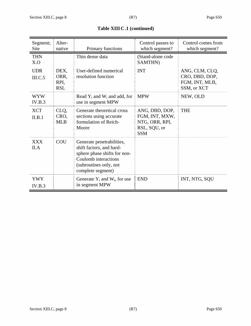
Section XIII.C, page 8 (R7) Page 650
Table XIII C .1 (continued)
Section XIII.C, page 8 (R7) Page 650
Segment; Site
Alter-native
Primary functions
Control passes to which segment?
Control comes from which segment?
THN X.O
Thin dense data (Stand-alone code SAMTHN)
UDR III.C.5
DEX, ORR, RPI, RSL
User-defined numerical resolution function
INT ANG, CLM, CLQ, CRO, DBD, DOP, FGM, INT, MLB, SSM, or XCT
WYW IV.B.3
Read Yi and Wi and add, for use in segment MPW
MPW NEW, OLD
XCT II.B.1
CLQ, CRO, MLB
Generate theoretical cross sections using accurate formulation of Reich-Moore
ANG, DBD, DOP, FGM, INT, MXW, NTG, ORR, RPI, RSL, SQU, or SSM
THE
XXX II.A
COU Generate penetrabilities, shift factors, and hard-sphere phase shifts for non-Coulomb interactions (subroutines only, not complete segment)
YWY IV.B.3
Generate Yi and Wi, for use in segment MPW
END INT, NTG, SQU
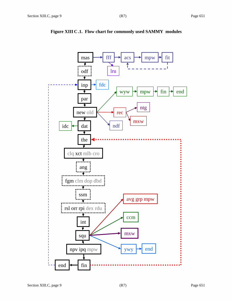
Section XIII.C, page 9 (R7) Page 651
Figure XIII C .1. Flow chart for commonly used SAMMY modules
Section XIII.C, page 9 (R7) Page 651
mas
odf
inp
par
new old
dat
the
clq xct mlb cro
fgm clm dop dbd
ssm
rsl orr rpi dex rdu
npv ipq mpw
finend
ang
fff acs mpw fit
wyw mpw fin end
avg grp mpw
ywy end
ccmint
fdc
ndf
recntg
mxwidc
mxw
lru
squ


Section XIII.D, page 1 (R8) Page 653
Section XIII.D, page 1 (R8) Page 653
XIII.D. COMPUTER-SPECIFIC FEATURES
The current version of SAMMY is compatible with most UNIX operating systems, with LINUX, and with Compaq Visual Fortran under Windows.1 Details about specific machines on which the code has been tested are available from the Radiation Safety Information Computational Center [RSICC].
Input/Output statements are the most likely sources of incompatibility from one computer platform to another. To mitigate problems associated with portability, most of SAMMY=s file-OPEN statements are localized in one file, end/msamxx.f, which can be modified as necessary to suit the particular platform.
SAMMY is designed to provide CPU timing information as it passes through the various segments during a run. However, because the routine which generates this information is computer dependent, function jstime in file end/jstime.c is not guaranteed to provide correct results on all platforms. (Function jstime is the only C-language routine used in SAMMY.)
The output file SAMMY.LPT is written (added to) in numerous subroutines in nearly every segment of the code. Many of the WRITE statements for SAMMY.LPT (unit number 21) and for SAMMY.IO (unit 70) occur in subroutines whose names begin with the characters “OUT”. The output file SAMMY.IO contains only Input and Output values of the parameters. Originally these files were designed to be sent to the line-printer for printing and examination by the analyst. Over the years, as work habits have evolved to include less hard-copy printing and more on-line viewing, the format for these files has also evolved to become compatible with an eighty-character screen. Portability should not be a problem with these files.
See the next section (Section XIII.E) for a discussion of plot files, for which portability may be a problem.
1 Because Compaq Visual Fortran is no longer available commercially, the availability of Windows executables may be curtailed in future releases of SAMMY.

Section XIII.E, page 1 (R7) Page 655
Section XIII.E, page 1 (R7) Page 655
XIII.E. ORELA DATA FORMAT
Plotting of results in SAMMY may be accomplished by first generating a “plot file,” named SAMMY.ODF, and using program FORODF [JC78] to produce plots. The code FORODF has both advantages and disadvantages for the user; advantages include data-manipulation capabilities not readily available in other plotting packages. The major disadvantages are the age, the lack of routine maintenance, the use of single precision, and the difficulties in porting this program. Because of these disadvantages, FORODF is no longer distributed along with the SAMMY code.
For information on alternative plotting packages, see Sections VII.C and X.I.
Calls to three different ODF routines occur in the coding for SAMMY. Names and arguments for these routines are
Odfio (Iu,File,Ifb,New,Ins,Incmx,Mode,Ndstrt,Iener,Irun) Outodf(Iu,Ifb,Ins,Isn,Mode,Ndstrt,Isc,Inc,Array(J),N) Inodf (Iu,Ifb,Ins,Isn,Mode,Ndstrt,Isc,Inc,Array(J),N)
The first subroutine (ODFIO) is used to open or create the plot file; the second (OUTODF), to write INC elements of ARRAY into section number ISN of the file; and the last (INODF), to read from the file. Access to the plot file is random rather than sequential. Meanings for the arguments of these subroutines are given in Table XIII E.1. Note that many of the arguments are irrelevant to SAMMY, either because they are unused or because only one value is used. These are marked as “irrelevant” in the table.

Section XIII.E, page 2 (R7) Page 656
Section XIII.E, page 2 (R7) Page 656
Table XIII E.1. Arguments for ODF subroutines
Argument name Included in which routine Meaning of argument
IU All three: ODFIO, OUTODF, and INODF
FORTRAN unit number
FILE ODFIO File name for plot file
IFB All three Irrelevant to SAMMY
NEW ODFIO Irrelevant
INS All Number of sections in the file (see Table VII C.1)
ISN OUTODF, INODF Which section is being written or read now
INCMAX ODFIO Total number of data points for this plot file
MODE All Irrelevant
NDSTRT All Irrelevant (equal to zero)
IENER ODFIO Irrelevant
IRUN ODFIO Irrelevant
ISC OUTODF, INODF This “write” or “read” begins with the ISCth data point
INC OUTODF, INODF This “write” or “read” includes a total of INC data points
ARRAY(j) OUTODF, INODF This subroutine will write from or read into the array elements ARRAY(j) through ARRAY(j+INC-1)
N OUTODF, INODF Irrelevant
Section XIII.F, page 1 (R7) Page 657
Section XIII.F, page 1 (R7) Page 657
XIII.F. CONFIGURATION AND DISTRIBUTION SYSTEM
In 2005, ORNL researcher Dorothea Wiarda created a modern configuration and distribution system for SAMMY. This system makes it significantly easier for a user to install SAMMY on another computer. SAMMY is distributed as a set of four *.gz files. The primary file, sammy-7.0.0.tar.gz, contains the FORTRAN plus installation commands. To unpack this file, type the command
gunzip -c sammy-7.0.0.tar.gz|tar xvf - This command will create a subdirectory named sammy-7.0.0/, which contains a number of command and comment files, plus three subdirectories doc/, obj/, and src/. Subdirectory doc/ contains this document (the SAMMY users’ manual) in pdf format. Subdirectory src/ contains 68 subdirectories, each of which hold several FORTRAN files. Subdirectory obj/ contains only two files initially but after compilation holds the object files (compiled version of the FORTRAN files). Before creating the SAMMY executables, decide where you want to store them; you must have write privileges for that directory. To create the executables, type the following commands (substituting, of course, your chosen location for the directory name):
cd sammy-7.0.0 ./configure --bindir=/xxx/sammydir --with-array=32500000 make
In this example, we have arbitrarily chosen “/xxx/sammydir” to represent the directory name. The absolute path name must be used. The number 32500000 represents one-half of the array size and may need to be modified (increased∗ or decreased) for your particular installation; see Section XIII.A for more information. If no change is needed in this value, the second line above can be shortened by dropping “--with-array=32500000”.
The “make” command will compile the FORTRAN files and place the results as *.o into the sammy-7.0.0/obj directory. It will also create executable files, placing them in the same directory. After this step is successfully completed, type the command
make install , which copies the executables to subdirectory /xxx/sammydir. The executable files are as follows:
∗ The maximum possible value for this number is 231-1 = 2147483647 on a 32-bit machine. It is recommended to use smaller values than these unless absolutely necessary. If the number is too big for your compiler, compilation may fail. Alternatively, installation may appear to be complete, but the program will not run. In either case, try a smaller value.
angodf convrt dopushx
sam012 samamr samamx
samcpr samdis samftz
sammy samort samplt
samplx samqua samrml
samrpt samsmc samsmx
samsta samthn suggel
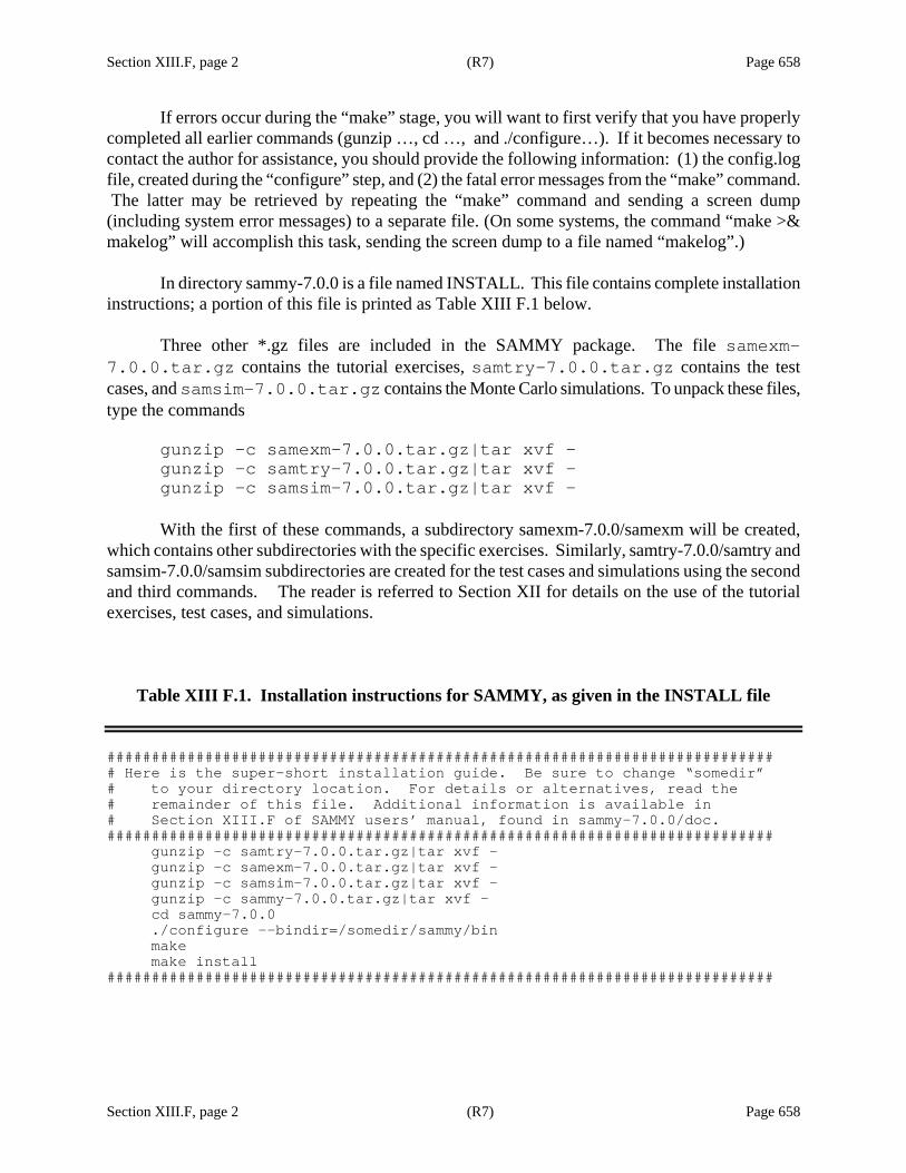
Section XIII.F, page 2 (R7) Page 658
Section XIII.F, page 2 (R7) Page 658
If errors occur during the “make” stage, you will want to first verify that you have properly completed all earlier commands (gunzip …, cd …, and ./configure…). If it becomes necessary to contact the author for assistance, you should provide the following information: (1) the config.log file, created during the “configure” step, and (2) the fatal error messages from the “make” command. The latter may be retrieved by repeating the “make” command and sending a screen dump (including system error messages) to a separate file. (On some systems, the command “make >& makelog” will accomplish this task, sending the screen dump to a file named “makelog”.)
In directory sammy-7.0.0 is a file named INSTALL. This file contains complete installation instructions; a portion of this file is printed as Table XIII F.1 below.
Three other *.gz files are included in the SAMMY package. The file samexm-
7.0.0.tar.gz contains the tutorial exercises, samtry-7.0.0.tar.gz contains the test cases, and samsim-7.0.0.tar.gz contains the Monte Carlo simulations. To unpack these files, type the commands
gunzip -c samexm-7.0.0.tar.gz|tar xvf - gunzip -c samtry-7.0.0.tar.gz|tar xvf - gunzip -c samsim-7.0.0.tar.gz|tar xvf -
With the first of these commands, a subdirectory samexm-7.0.0/samexm will be created,
which contains other subdirectories with the specific exercises. Similarly, samtry-7.0.0/samtry and samsim-7.0.0/samsim subdirectories are created for the test cases and simulations using the second and third commands. The reader is referred to Section XII for details on the use of the tutorial exercises, test cases, and simulations.
Table XIII F.1. Installation instructions for SAMMY, as given in the INSTALL file
########################################################################### # Here is the super-short installation guide. Be sure to change “somedir” # to your directory location. For details or alternatives, read the # remainder of this file. Additional information is available in # Section XIII.F of SAMMY users’ manual, found in sammy-7.0.0/doc. ########################################################################### gunzip -c samtry-7.0.0.tar.gz|tar xvf - gunzip -c samexm-7.0.0.tar.gz|tar xvf - gunzip -c samsim-7.0.0.tar.gz|tar xvf - gunzip -c sammy-7.0.0.tar.gz|tar xvf - cd sammy-7.0.0 ./configure --bindir=/somedir/sammy/bin make make install ###########################################################################
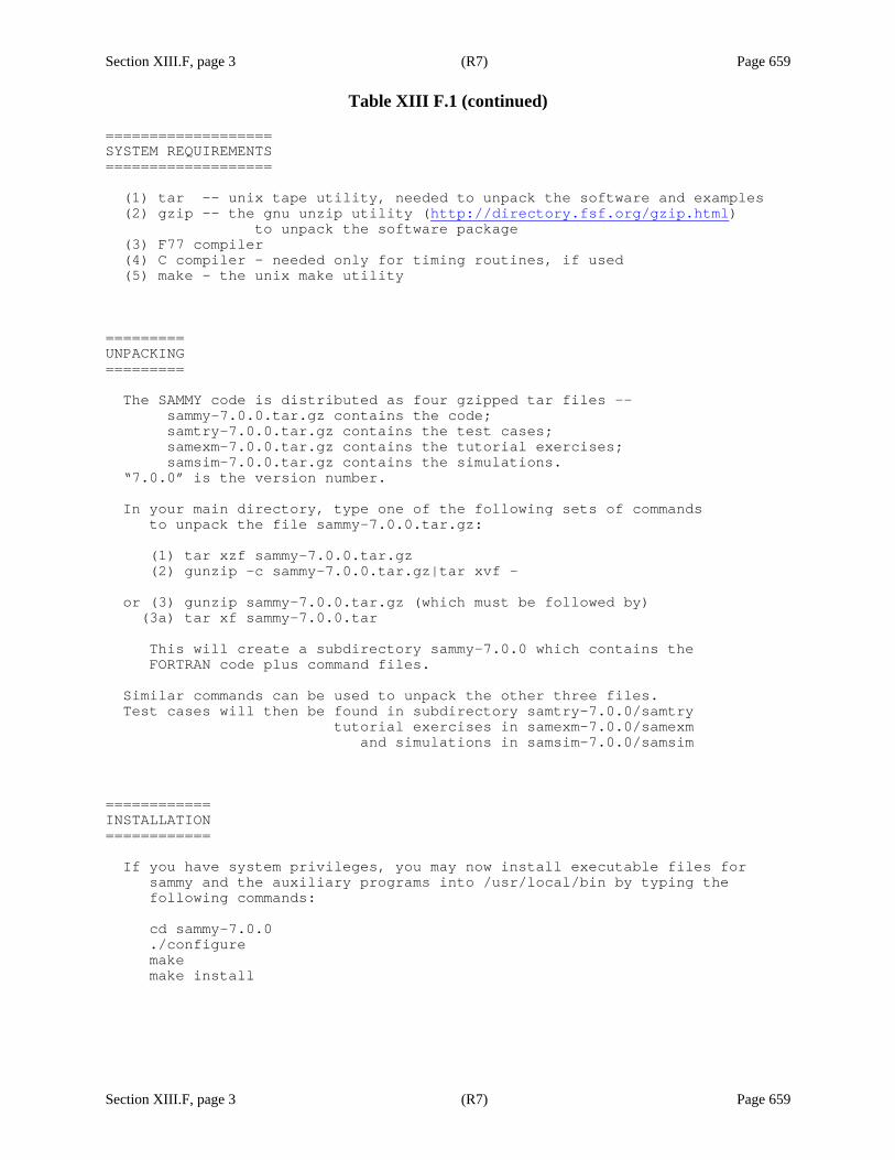
Section XIII.F, page 3 (R7) Page 659
Table XIII F.1 (continued)
Section XIII.F, page 3 (R7) Page 659
=================== SYSTEM REQUIREMENTS =================== (1) tar -- unix tape utility, needed to unpack the software and examples (2) gzip -- the gnu unzip utility (http://directory.fsf.org/gzip.html) to unpack the software package (3) F77 compiler (4) C compiler – needed only for timing routines, if used (5) make – the unix make utility ========= UNPACKING ========= The SAMMY code is distributed as four gzipped tar files -- sammy-7.0.0.tar.gz contains the code; samtry-7.0.0.tar.gz contains the test cases; samexm-7.0.0.tar.gz contains the tutorial exercises; samsim-7.0.0.tar.gz contains the simulations. “7.0.0” is the version number. In your main directory, type one of the following sets of commands to unpack the file sammy-7.0.0.tar.gz: (1) tar xzf sammy-7.0.0.tar.gz (2) gunzip -c sammy-7.0.0.tar.gz|tar xvf - or (3) gunzip sammy-7.0.0.tar.gz (which must be followed by) (3a) tar xf sammy-7.0.0.tar This will create a subdirectory sammy-7.0.0 which contains the FORTRAN code plus command files. Similar commands can be used to unpack the other three files. Test cases will then be found in subdirectory samtry-7.0.0/samtry tutorial exercises in samexm-7.0.0/samexm and simulations in samsim-7.0.0/samsim ============ INSTALLATION ============ If you have system privileges, you may now install executable files for sammy and the auxiliary programs into /usr/local/bin by typing the following commands: cd sammy-7.0.0 ./configure make make install

Section XIII.F, page 4 (R7) Page 660
Table XIII F.1 (continued)
Section XIII.F, page 4 (R7) Page 660
===================== A DIFFERENT DIRECTORY ===================== Alternatively, you may wish to install the executables into another directory, for example /somedir/sammy/bin. To do this, first be certain you have write authority for the subdirectory. Then execute the following commands, being sure to use the correct complete path name for the subdirectory: ./configure --bindir=/somedir/sammy/bin make make install These commands would install sammy and auxiliary-code executable files into /somedir/sammy/bin. ======================= CHANGING THE ARRAY SIZE ======================= Dynamic dimensioning is achieved in SAMMY by assigning and de-assigning space in a large container array, designated as A(-N:N). The default value for N is 32500000. To use a different value, modify the configure line as shown here, substituting the appropriate value for your computer system: ./configure --with-array=100000000 or ./configure --bindir=/somedir/sammy/bin --with-array=210000000 ====================== COMPILER OPTIONS, ETC. ====================== If you want to use a different FORTRAN compiler, for example f90, then set the environment variable F77=f90 in bash: export F77=f90 in csh: setenv F77 f90 and then do the above install sequence. If you want to set compiler flags, for example -Wall, then use in bash: export FFLAGS=-Wall in csh: setenv FFLAGS -Wall and then do the above install sequence. ===================== Other useful commands ===================== make clean <- removes all generated object and source files make distclean <- cleans the tree for a new invocation of configure make dist <- creates a new *.gz file which includes any updates that you may have made to the FORTRAN files

Section XIII.F, page 5 (R7) Page 661
Table XIII F.1 (continued)
Section XIII.F, page 5 (R7) Page 661
======================== PC (WINDOWS) EXECUTABLES ======================== For those who wish to run SAMMY in a Windows environment on a pc, executable files for SAMMY and the auxiliary programs are provided in subdirectory sammy-7.0.0/Windows/ and can be copied from there to the pc. ====================== RUNNING THE TEST CASES ====================== ------------- Unix or Linux ------------- The command file “zzauto” (found in samtry-7.0.0/samtry) can be used to run all of the test cases on a Unix or Linux system. Command file “zzauto_short” runs a representative sample of thirteen test cases. Individual test cases can be run by using the command file “t” or “test???” in the subdirectory for that test case. See Section XII.B of the SAMMY manual for details. ------- Windows ------- Command file “test.bat” in the subdirectory tr??? can be used to run the individual test case under Windows. ================ THE SAMMY MANUAL ================ The SAMMY manual is found in subdirectory sammy-7.0.0/doc in pdf format. Two versions are given there. SAMMY7.pdf is the version to use on screen. SAMM7_print.pdf is the version to use if you wish to print a double-sided listing of the manual; it contains extra blank pages as needed to make the pagination come out correctly.


References, page 1 (R8) Page 663
References, page 1 (R8) Page 663
REFERENCES
AB82 A. R. Barnett, Comp. Phys. Comm. 27, 147 (1982); Comp. Phys. Comm. 21, 297 (1981).
AC05 A. D. Carlson, S. A. Badikov, Chen Zhenpeng, E. Gai, G. M. Hale, F.-J. Hambsch, H. M. Hofmann, T. Kawano, N. M. Larson, S. Y. Oh, V. G. Pronyaev, D. L. Smith, S. Tagesen, H. Vonach, “An International Evaluation of the Neutron Cross Section Standards,” 12th International Symposium on Reactor Dosimetry, May 8–13, 2005, Gatlinburg, TN.
AC07 A. D. Carlson, S. A. Badikov, Chen Zhenpeng, E. Gai, G. M. Hale, F.-J. Hambsch, H. M. Hofmann, T. Kawano, N. M. Larson, S. Y. Oh, V. G. Pronyaev, D. L. Smith, S. Tagesen, H. Vonach, “International Evaluation of Neutron Cross-Section Standards,” IAEA Report STI/PUB/1291, November 2007, available at
http://www-pub.iaea.org/MTCD/publications/PDF/Pub1291_web.pdf
AF71 A. Foderaro, The Elements of Neutron Interaction Theory, MIT Press, 1971.
AG65 A. Gilbert and A. G. W. Cameron, Can. J. Phys. 43, 1446 (1965).
AG73 A. Gandini, Nuclear Data and Integral Measurements Correlations for Fast Reactors, Parts I and II, Comitato Nazionale Energia Nucleare, Casaccia, Italy, 1973, RT/FI(73)5 and 22 (1973).
AL58 A. M. Lane and R. G. Thomas, Rev. Mod. Phys. 30, 257 (1958).
AM94 A. Meister, Calculations on lattice vibration effects in the Doppler broadening of the 0.18eV Cd neutron resonance cross section, CE/R/VG/78/94 (January 1994).
BM96 B. E. Moretti, Molybdenum Neutron Transmission Measurements and the Development of an Enhanced Resolution Neutron Target, Ph.D. Thesis in Nuclear Engineering and Science, Rensselaer Polytechnic Institute, Troy, NY, August 1996.
CC83 C. Coceva, R. Simonini, and D. K. Olsen, “Calculaton of the ORELA Neutron Moderator Spectrum and Resolution Function,” Nucl. Inst. Meth. 211, 459 (1983).
CR58 C. W. Reich and M. S. Moore, Phys. Rev. 111, 929 (1958).
CZ95 Chen Z. P., “Reduced R-Matrix Analysis for 17O system,” Atomic Energy Science and Technology 29 (4), 366–371 (1995).
DC04 D. Cullen, PREPRO 2004, IAEA-NDS-39, Rev. 12, Nov. 22, 2004. Also see http://www-nds.iaea.org/ndspub/endf/prepro/.
DH53 D. L. Hill and J. A. Wheeler, Phys. Rev. 89, 1102 (1953).
References, page 2 (R8) Page 664
References, page 2 (R8) Page 664
DL83 D. C. Larson, N. M. Larson, J. A. Harvey, N. W. Hill, and C. H. Johnson, Application of New Techniques to ORELA Neutron Transmission Measurements and their Uncertainty Analysis: the Case of Natural Nickel from 2 keV to 20 MeV, ORNL/TM-8203, ENDF-333, Oak Ridge National Laboratory, October 1983.
DL84 D. C. Larson, N. M. Larson, and J. A. Harvey, ORELA Flight Path 1: Determinations of Its Effective Length vs Energy, Experimental Energies, and Energy Resolution Function and Their Uncertainties, ORNL/TM-8880, Oak Ridge National Laboratory, June 1984.
DN99 D. G. Naberejnev, “Etude de L’Influence des Liaisons Chimiques sur L’Absorption et la Diffusion de Neutrons aux Energies de Resonance,” Ph.D. Thesis, ISSN 0429-3460, CEA-N-2840 (Fevrier 1999).
DN99a D. G. Naberejnev, C. Mounier, and R. Sanchez, “The Influence of Crystalline Binding on Resonant Absorption and Reaction Rates,” Nucl. Sci. Eng. 131, 222–220 (1999).
DW06 D. Wiarda and M. E. Dunn, PUFF-IV: A Code for Processing ENDF Uncertainty Data Into Multigroup Covariance Matrices, ORNL/TM-2006/147, Oak Ridge National Laboratory, 2006.
ENDF-102 ENDF-102, Data Formats and Procedures for the Evaluated Nuclear Data File, ENDF-6, written by the Members of the Cross Section Evaluation Working Group, ed. V. McLane, C. L. Dunford, P. F. Rose, BNL-NCS-4495, Brookhaven National Laboratory, April 2001. Updated BNL-NCS-4495/04-Rev, ed. M. Herman, June 2005.
ENDFw Web site for Cross Section Evaluation Working Group http://www.nndc.bnl.gov/exfor7/endf00.htm .
EV58 E. Vogt, Phys. Rev. 112, 203 (1958).
EXFOR Experimental Nuclear Reaction Data Files at Brookhaven National Laboratory (EXFOR/CSISRS), http://www.nndc.bnl.gov/exfor3/exfor00.htm.
FF80 F. H. Fröhner, Applied Neutron Resonance Theory, reprinted from Nuclear Theory for Applications, p. 59 ff., International Centre for Theoretical Physics, Trieste (1980). Available as KFK 2669 (1978). See also “Applied Theory of Resolved and Unresolved Resonances,” p. 70 in Applied Nuclear Theory and Nuclear Model Calculations for Nuclear Technology Applications, M. K. Mehta and J. J. Schmidt, eds., World Scientific, Singapore, 1989.
FF83 F. H. Fröhner, B. Goel, and U. Fischer, “Calculation of Average on Capture Cross Sections for Actinides – Level-Statistical vs Global Approach,” p. 116 in Proc. Mtg. Fast Neutron Capture Cross Sections, Argonne, Illinois, April 20–23, 1982, ANL-83-4, Argonne National Laboratory (1983).
FF89 F. H. Fröhner, “Evaluation of the Unresolved Resonance Range of 238U,” Nucl. Sci. Eng. 103, 119–128 (1989).

References, page 3 (R8) Page 665
References, page 3 (R8) Page 665
FF99 F. H. Fröhner, Kernforschungszentrum Karlsruhe, Germany, private communication, 1999.
FF00 F. H. Fröhner, Evaluation and Analysis of Nuclear Resonance Data, JEFF Report 18, NEA/OECD (2000).
FF01 F. H. Fröhner and O. Bouland, “Treatment of External Levels in Neutron Resonance Fitting: Application to the Nonfissile Nuclide 52Cr,” Nucl. Sci. Eng. 137, 70–88 (2001).
FF02 F. H. Fröhner, lecture notes on R-Matrix theory, presented at the SAMMY workshop of February 18–22, 2002, at the NEA Headquarters in Paris, France (2002).
FG98 F. Gunsing, CEA Saclay, France, private communication, 1998.
FG05 F. Gunsing, CEA Saclay, France, private communication, 2005.
FP84 F. G. Perey, Oak Ridge National Laboratory, private communication, 1984.
FP89 F. G. Perey, Oak Ridge National Laboratory, private communication, 1989.
FP89a F. G. Perey, RFUNC — A Code to Analyze Differential Elastic-Scattering Data, ORNL/TM-11112, Oak Ridge National Laboratory, March 1989.
FP92 F. G. Perey, Oak Ridge National Laboratory, private communication, 1992.
GA74 G. F. Auchampaugh, MULTI, A FORTRAN Code for Least-Squares Shape Fitting of Neutron Cross-Section Data Using the Reich-Moore Multilevel Formalism, LA-5473-MS, Los Alamos Scientific Laboratory, l974.
GB36 G. Breit and E. Wigner, “Capture of Slow Neutrons,” Phys. Rev. 49, 519 (1936).
GC04 G. Chiba, ERRORJ–Covariance Processing Code System for JENDL, Version 2, JNC TN9520 2003-008; also G. Chiba and M. Ishikawa, “Revision and Application of Covariance Data Processing Code, ERRORJ,” pp. 486–471 in ND2004 (International Conference on Nuclear Data for Science and Technology), Sept. 26–Oct. 1, 2004, edited by R. C. Haight et al., AIP Conf. Proc. 769, 2005.
GD78 G. deSaussure, D. K. Olsen, and R. B. Perez, SIOB: A FORTRAN Code for Least-Squares Shape Fitting Several Neutron Transmission Measurements Using the Breit-Wigner Multilevel Formula, ORNL/TM-6286, ENDF-261, Oak Ridge National Laboratory, 1978.
GD80 G. deSaussure and F. G. Perey, Oak Ridge National Laboratory, private communication, 1980.
GH75 G. M. Hale, D. C. Dodder, and K. Witte, Los Alamos National Laboratory, Los Alamos, New Mexico, USA, private communication, 1975.
GH02 G. M. Hale, Los Alamos National Laboratory, Los Alamos, New Mexico, USA, private communication, 2002.
References, page 4 (R8) Page 666
References, page 4 (R8) Page 666
HD90 H. Derrien, G. de Saussure, and R. B. Perez, “R Matrix Analysis of the 239Pu Neutron Cross Sections in the Energy Range Up to 1000 eV,” Nucl. Sci. Eng. 106, 434–51 (1990).
HD97 H. Derrien, N. M. Larson, and L. C. Leal, Covariance Matrices for Use in Criticality Safety Predictability Studies, ORNL/TM-13492, Oak Ridge National Laboratory, September 1997.
HD00 H. Derrien, J. A. Harvey, N. M. Larson, L. C. Leal, and R. Q. Wright, Neutron Total Cross Sections of 235U from Transmission Measurements in the Energy Range 2 keV to 300 keV and Statistical Model Analysis of the Data, ORNL/TM-2000/129, May 2000.
HD00a H. Derrien, Oak Ridge National Laboratory, private communication, 2000.
HD02 H. Derrien, L. C. Leal, K. H. Guber, T. Valentine, N. M. Larson, and T. Rauscher, Evaluation of Silicon Neutron Resonance Parameters in the Energy Range Thermal to 1800 keV, ORNL/TM-2001/271, August 2002.
HD03 H. Derrien, Oak Ridge National Laboratory, private communication, 2003.
HJ61 H. Jeffreys, Theory of Probability, Third Edition, Oxford University Press, London, 1961.
IB64 I. I. Bondarenko, ed., Group Constants for Nuclear Reactor Calculations, Consultant Bureau, New York, 1964.
INDC02 Summary Report of the First Research Co-ordination Meeting on Improvement of the Standard Cross Sections for Light Elements, 23–27 Sept. 2002, IAEA Nuclear Data Section, Vienna, Austria, ed. A. D. Carlson, G. M. Hale, and V. G. Pronyaev, INDC(NDS)-438, January 2003.
INDC03 Summary Report of the Second Research Co-ordination Meeting on Improvement of the Standard Cross Sections for Light Elements, 13–17 Oct. 2003, IAEA Nuclear Data Section, Vienna, Austria, ed. A. D. Carlson, G. M. Hale, and V.G. Pronyaev, INDC(NDS)-438, March 2004.
INDC04 Summary Report of the Third Research Co-ordination Meeting on Improvement of the Standard Cross Sections for Light Elements, 18–22 Oct., 2004, IAEA Nuclear Data Section, Vienna, Austria, ed. A. D. Carlson, G. M. Hale, and V. G. Pronyaev, INDC(NDS)-453, November 2004.
JB52 J. M. Blatt and L. C. Biedenharn, “The Angular Distribution of Scattering and Reaction Cross Sections,” Rev. Mod. Phy. 24, 258 (1952).
JC78 J. G. Craven, OPRODF, A DECsystem-10 Data Manipulation Program for ORELA Data Formatted Files, ORNL/CSD/TM-45, Oak Ridge National Laboratory, May 1978.
JD79 J. J. Dongarra, C. B. Moler, J. R. Bunch, G. W. Stewart, LINPACK User=s Guide, SIAM (1979).
References, page 5 (R8) Page 667
References, page 5 (R8) Page 667
JL58 J. E. Lynn, The Theory of Neutron Resonance Reactions, Clarendon Press, Oxford (1958).
JM80 J. H. Marable, C. R. Weisbin, and G. deSaussure, “Combination of Differential and Integral Data” in Sensitivity and Uncertainty Analysis of Reactor Performance Parameters, Adv. Nucl. Sci. and Technology, Plenum Press, New York, ed. Martin Becker, 1980.
KC53 K. M. Case, F. de Hoffman, and G. Placzek, Introduction to the Theory of Neutron Diffusion, Los Alamos Scientific Laboratory, 1953.
KH05 K. M. Hanson, T. Kawano, and P. Talou, “Probabilistic interpretation of Peelle’s pertinent puzzle and its resolution,” pp. 304–307 in Int. Conf. Nuclear Data for Science and Technology, edited by R. C. Haight et al., AIP Conf. Proc. 769, 2005.
KH08 K. M. Hanson, Los Alamos National Laboratory, private communication, 2008.
KW84 K. Wisshak, F. Kappeler, G. Reffo, and F. Fabbri, “Neutron Capture in s-Wave Resonances of Iron-56, Nickel-58, and Nickel-60,” Nucl. Sci. Eng. 86, 168 (1984).
LL85 L. C. Leal, Oak Ridge National Laboratory, private communication, 1985.
LL95 L. C. Leal and N. M. Larson, SAMDIST, A Computer Code for Calculating Statistical Distributions for R-Matrix Resonance Parameters, ORNL/TM-13092, Oak Ridge National Laboratory, September 1995.
LL98 L. C. Leal, R. O. Sayer, N. M. Larson, and R. R. Spencer, “R-Matrix Evaluation of 16O Neutron Cross Sections up to 6.3 MeV,” ANS Winter Meeting, Washington, D.C., Nov. 16–20, 1998.
LL99 L. C. Leal, H. Derrien, N. M. Larson, and R. Q. Wright, “R-Matrix Analysis of 235U Neutron Transmission and Cross Sections in the Energy Range 0 to 2.25 keV,” Nucl. Sci. Eng. 131, 230 (February 1999); also published as ORNL/TM-13516 (November 1997).
MD02 M. E. Dunn and N. M. Greene, “AMPX-2000: A Cross-Section Processing System for Generating Nuclear Data for Criticality Safety Applications,” Trans. Am. Nucl. Soc. (2002).
MM64 M. D. Mintz and D. P. Jordan, A >Progressive= Interpolation Scheme for Hand and Digital Computer Analysis of Tabulated Data, Report UCRL-7681, Lawrence Livermore Laboratory, 1964.
MM89 M. C. Moxon, REFIT2: A Least Squares Fitting Program for Resonance Analysis of Neutron Transmission and Capture Data, NEA-0914/02, July 1989.
NAG Numerical Algorithms Group (USA) Inc., Suite 220,1431 Opus Place, Downers Grove, IL 60515-1362, USA; http://www.techexpo.com/firms/numeralg.html. Modified versions of NAG subroutines from ~1980 are used in SAMMY.

References, page 6 (R8) Page 668
References, page 6 (R8) Page 668
NL80 N. M. Larson and F. G. Perey, User=s Guide for SAMMY: A Computer Model for Multilevel R-matrix Fits to Neutron Data Using Bayes= Equations, ORNL/TM-7485, ENDF-297, Oak Ridge National Laboratory, November 1980.
NL82 N. M. Larson, User's Guide for BAYES: A General-Purpose Computer Code for Fitting a Functional Form to Experimental Data, ORNL/TM-8185, ENDF-323, Oak Ridge National Laboratory, August 1982.
NL84 N. M. Larson, User=s Guide for ALEX: Uncertainty Propagation from Raw Data to Final Results for ORELA Transmission Measurements, ORNL/TM-8676, ENDF-332, Oak Ridge National Laboratory, February 1984.
NL92 N. M. Larson, “Cross Section Parameterization in the Resolved Resonance Region,” invited paper presented October 12–16, 1992, at Brookhaven National Laboratory and published in International Symposium on Nuclear Data Evaluation Methodology, ed. Charles L. Dunford, pp. 285–294, 1993.
NL97 N. M. Larson, L. C. Leal, and H. Derrien, Integral Data Analysis for Resonance Parameters Determination, ORNL/TM-13495, Oak Ridge National Laboratory, September 1997. Also Nucl. Sci. and Eng. 131, 254 (February 1999).
NL98 N. M. Larson, M. C. Moxon, L. C. Leal, and H. Derrien, Doppler Broadening Revisited, ORNL/TM-13525, Oak Ridge National Laboratory, 1998.
NL98a N. M. Larson, “Introduction to the Theory and Analysis of Resolved (and Unresolved) Neutron Resonances via SAMMY,” in Proceedings of the IAEA Workshop on “Nuclear Reaction Data and Nuclear Reactors: Physics, Design and Safety, held at the International Centre for Theoretical Physics, Trieste, Italy, 23 February–27 March 1998, published by World Scientific, 1999. Also published as ORNL/M-6576, July 1998. See also the SAMMY lecture notes at
http://www.ornl.gov/sci/nuclear_science_technology/nuclear_data/sammy/
NL02 N. M. Larson and K. N. Volev, “Validation of Multiple-Scattering Corrections in the Analysis Code SAMMY,” Paper A0203 of the International Conference on the New Frontiers of Nuclear Technology: Reactor Physics, Safety and High- Performance Computing (Physor 2002), October 2002 in Seoul, South Korea. Published on CD rom.
NL04a N. M. Larson, “Treatment of Data Uncertainties,” pp. 374–377 in ND2004 (International Conference on Nuclear Data for Science and Technology), Sept. 26–Oct. 1, 2004, edited by R. C. Haight et al., AIP Conf. Proc. 769, 2005.
NL04b N. M. Larson, “On the Efficient Treatment of Data Covariance Matrices,” 71st Annual Meeting of the Southeastern Section of the APS, Oak Ridge, TN, November 11–13, 2004.
NL06a N. M. Larson, “Use of Covariance Matrices in SAMMY,” Workshop on Nuclear Data Evaluation for Reactor Application (WONDER 2006) held at the Chateau de Cadarache, October 9–11, 2006.

References, page 7 (R8) Page 669
References, page 7 (R8) Page 669
NL06b N. M. Larson, “Future Developments for SAMMY,” Workshop on Nuclear Data Evaluation for Reactor Application (WONDER 2006) held at the Chateau de Cadarache, October 9–11, 2006.
NL07a N. M. Larson, L. C. Leal, R. O. Sayer, H. Derrien, D. Wiarda, G. Arbanas, “Current Status of the R-Matrix Code SAMMY, with Emphasis on the Relationship to ENDF Formats,” pp. 641 ff in ND2007 (International Conference on Nuclear Data for Science and Technology), April 22–27, 2007.
NL07b N. M. Larson, SAMMY User Guidance for ENDF Formats, ORNL/TM-2007/23 (also ENDF-367), Oak Ridge National Laboratory, Oak Ridge, TN, April 2007. Available by clicking on “ENDF Formats Guide” at
http://www.ornl.gov/sci/nuclear_science_technology/nuclear_data/sammy/.
NL07c N. M. Larson, H. Derrien, L. C. Leal, D. Wiarda, G. Arbanas, “Paradigm Shift for Resonance-Region Uncertainties,” presented at the November 2007 meeting of the Cross Section Evaluation Working Group (CSEWG), http://www.nndc.bnl.gov/proceedings/2007csewgusndp/Thursday/CSEWG/LarsonParadigm.pdf .
NL08 N. M. Larson, A Concise Method for Storing and Communicating the Data Covariance Matrix, ORNL/TM-2008/104, Oak Ridge National Laboratory, 2008. Available by clicking on “Data Covariance Matrices” at
http://www.ornl.gov/sci/nuclear_science_technology/nuclear_data/sammy/.
NNDC The National Nuclear Data Center at Brookhaven National Laboratory, http://www.nndc.bnl.gov/.
OB97 O. Bouland, H. Derrien, N. M. Larson, and L. C. Leal, “R-Matrix Analysis of the 240Pu neutron Cross Sections in the Thermal to 5700-eV Energy Range,” Nuclear Science and Engineering 127, 105–129 (1997). Also published as ORNL/TM-13450, Oak Ridge National Laboratory, August 1997.
OB03 O. Bouland, R. Babut, and N. M. Larson, SAMQUA B A Program for Generating All Possible Combinations of Quantum Numbers Leading to the Same Compound Nucleus State in the Framework of the R-Matrix Code SAMMY, JEF-DOC 929 OECD/NEA Publications (2003) and ENDF-363 (October 2003).
OB04 O. H. Bouland, R. Babut, N. M. Larson, “SAMQUA - A Program for Generating All Possible Combinations of Quantum Numbers Leading to the Same Compound Nucleus State in the Framework of the R-Matrix Code SAMMY,” pp. 414–417 in ND2004 (International Conference on Nuclear Data for Science and Technology), Sept. 26–Oct. 1, 2004, edited by R. C. Haight et al., AIP Conf. Proc. 769, 2005.
PB92 P R. Bevington and D. K. Robinson, Data Reduction and Error Analysis for the Physical Sciences, WCB-McGraw-Hill, Boston (1992).
PM80 P. A. Moldauer, Nucl. Phys. A344, 185 (1980).
RH87 R. Hwang, Nucl. Sci. Eng. 96, 192 (1987).
References, page 8 (R8) Page 670
References, page 8 (R8) Page 670
RM82 R. E. MacFarlane, D. W. Muir, and R. M. Boicourt, The NJOY Nuclear Data Processing System, Volume II: The NJOY, RECONR, BROADR, HEATR, and THERMR Modules, LA-9303-M, Vol. II (ENDF-324) (May 1982). Also R. E. MacFarlane, Introducing NJOY 89, LA-UR 89-2057, June 1989.
RM98 R. E. MacFarlane, Los Alamos National Laboratory, Los Alamos, New Mexico, private communication, 1998.
RP87 R. W. Peelle, Oak Ridge National Laboratory, private communication, 1987.
RS00 R. O. Sayer, L. C. Leal, N. M. Larson, R. R. Spencer, and R. Q. Wright, R-Matrix Evaluation of 16O Neutron Cross Sections up to 6.3 MeV, ORNL/TM-2000/212, Oak Ridge National Laboratory, Oak Ridge, TN, August 2000.
RS03 R. O. Sayer, Updated Users= Guide for RSAP—A Code for Display and Manipulation of Neutron Cross Section Data and SAMMY Fit Results, ORNL/TM-2003/133, Oak Ridge National Laboratory, Oak Ridge, TN.
RS06 R. O. Sayer, K. H. Guber, L. C. Leal, N. M. Larson, and T. Rauscher, “R-Matrix Analysis of Cl neutron cross sections up to 1.2 MeV,” Phys. Rev. C 73, 044603 (2006).
RS06a R. O. Sayer and D. Wiarda, Oak Ridge National Laboratory, private communication, 2006.
RSICC Radiation Safety Information Computational Center (formerly the Radiation Shielding Information Center), Oak Ridge National Laboratory, Bldg 6025, MS-6362, P.O. Box 2008, Oak Ridge, TN 37831-6362. See also http://www-rsicc.ornl.gov/.
SC92 S. N. Cramer and F. G. Perey, “Time-Dependent Monte Carlo Calculations of the Oak Ridge Electron Linear Accelerator Target Neutron Spectrum,” Nucl. Sci. Eng. 111, 102–111 (1992).
SC94 S. Chiba and D. L. Smith, Some Comments on Peelle’s Pertinent Puzzle,” AERI-M 94-068, 1994.
SO01 S. Y. Oh and L. C. Leal, SUGGEL: A Program Suggesting the Orbital Angular Momentum of a Neutron Resonance from the Magnitude of its Neutron Width, ORNL/TM-2000/314, Oak Ridge National Laboratory, February 2001.
SM06 S. F. Mughabghab, Atlas of Neutron Resonances, 5th edition, published by Elsevier, Amsterdam, The Netherlands, 2006.
VP04 V. G Pronyaev (IAEA, Austria), S. A. Badikov (IPPE, Russia), Chen Zhenpeng (Tsinghua University, China), A. D. Carlson (NIST, USA), E.V. Gai (IPPE, Russia), G. M. Hale (LANL, USA), F.-J. Hambsch (IRMM, Belgium), H. M. Hofmann (ITP III, Erlangen-Nürnberg University, Germany), N. M. Larson (ORNL, USA), D. L. Smith (ANL, USA), Soo Youl Oh (KAERI, Republic of Korea), S. Tagesen (IIK, Wien University, Austria), H. Vonach (IIK, Wien University, Austria), “Status of the International Neutron Cross Section Standards File,” International Conference on Nuclear Data for Science and Technology, Sept. 26–Oct. 1, 2004.

References, page 9 (R8) Page 671
References, page 9 (R8) Page 671
WV12 W. Voigt, Sitz-Ber. Bayer. Akad. Wiss., p. 603, (1912).
YD98 Y. Danon et al., “Neutron Total Cross Section Measurements and Resonance Parameter Analysis of Ho, Tm, and Er from 0.001 eV to 20 eV,” Nucl. Sci. Eng. 128, 61–69 (1998).
ZZ92 Z. Zhao and F. G. Perey, The Covariance Matrix of Derived Quantities and Their Combination, ORNL/TM-12106, Oak Ridge National Laboratory, 1992.


Appendix A, page 1 (R7) Page 673
Appendix A, page 1 (R7) Page 673
APPENDIX A. VERSIONS OF THIS MANUAL (This page is taken from the Introduction to the original document ORNL/TM-9179, published in 1984, with strikeouts and inserts to clarify topics that might otherwise cause confusion.)
In 1980 the multilevel multichannel R-matrix code SAMMY [NL80] was released for use in analysis of neutron data at the Oak Ridge Electron Linear Accelerator (ORELA). At its inception, SAMMY was a severely altered version of George Auchampaugh=s multilevel R-matrix code MULTI [GA74], the fundamental difference being that SAMMY uses Bayes= method while MULTI uses a least-squares method to update parameter values. Since that time, significant modifications and improvements have been incorporated into SAMMY: (1) User-friendly options have been introduced to streamline common operations and to protect a run from common user errors. (2) The Reich-Moore formalism has been extended to include an optional logarithmic parameterization of the external R-matrix, for which any or all parameters may be varied. (3) The ability to vary sample thickness, effective temperature, matching radius, and/or resolution-broadening parameters has been incorporated. (4) To avoid loss of information (i.e., computer round-off errors) between runs, the “covariance file” now includes precise values for all variables. (5) Unused but correlated variables may be included in the analysis.
Because of these and earlier changes, the 1980 SAMMY manual is now hopelessly obsolete. This report is intended to be complete documentation for the current version of SAMMY. Its publication in loose-leaf form pdf format will permit updates to the manual to be made concurrently with updates to the code itself, thus eliminating most of the time lag between update and documentation.
Because Bayes= method is a new concept to many users, its derivation and implementation are described in some detail in Section II IV of this report. Though a similar discussion is included in both the earlier SAMMY report [NL80] and the BAYES report [NL82], it is repeated here for completeness sake.
The evaluation of theoretical cross sections is described in Section III II. Doppler- and resolution-broadening are discussed in Section IV III. Special data types (such as transmission or combinations) are discussed in Section V.
Section VI describes the input to SAMMY, with tables detailing each file the user must create. A discussion of the output is given in Section VII.
In Section VIII X.C the auxiliary codes SAMADD and SAMMIX are SAMAMR is described: these codes are this code is to be used in conjunction with SAMMY when multiple experiments are analyzed sequentially.
Two examples of SAMMY runs are presented in Section IX; these runs are typical of runs required for analysis of transmission and fission data.

Appendix A, page 2 (R7) Page 674
Appendix A, page 2 (R7) Page 674
“Helpful hints for running SAMMY” are given in Section X XI. It is hoped that this section can be considerably expanded in the future: ideas from users would be appreciated here. This section was completely rewritten for Revision 7.
Section XI XIII gives a general description of the computer code, more for the benefit of someone wishing to convert SAMMY to another computer than for a physicist wishing to use SAMMY to perform data analyses.
A FORTRAN listing of the code is provided in the appendix in microfiche form. Input and output for several test cases are also given there.
Appendix A.1, page 1 (R7) Page 675
Appendix A.1, page 1 (R7) Page 675
Appendix A.1. MODIFICATIONS AND ADDITIONS IN REVISION 1 (This page is taken from the Introduction to Revision 1 of this manual, with strikeouts and inserts to clarify topics that might otherwise cause confusion.)
Changes documented in this revision are as follows: 1. An alternative matrix-manipulation method, the (I+Q) inversion scheme, has been devised
(see Sect. II IV). Use of this scheme requires that the data covariance matrix be diagonal, and that the number of data points be much larger than the number of varied parameters. When these two requirements are met, the (I+Q) inversion scheme uses significantly less computer core than does the original method, the (N+V) inversion scheme.
2. Cross-section calculations and broadening operations are now performed in two separate stand-alone segments of the computer code, since they are in fact two distinct operations. Within the broadening segment, the various broadening procedures have been sufficiently disentangled that one can, e.g., Doppler-broaden but not resolution-broaden.
3. The multilevel Breit-Wigner approximation may be used to generate cross sections; see Sect. III.C Section II.B.3.
4. New input options are explained in the tables of Section VI. NOTE: No input has been changed; a user need not fear that his or her old INP or PAR tiles are obsolete.
5. All temporary files are now called SAM??.DAT with the question marks replaced by FORTRAN unit numbers. Thus if a run bombs or is aborted, all SAMMY files may be deleted with the single command “DEL SAM??.DAT” or the equivalent command on modern computer systems. CAUTION: If you wish to discuss with the author why your job bombed, it would be best not to delete these files first. See Sect. X.B XI.B.
6. It is now sometimes possible to analyze very large data sets, of a thousand or more points, in one shot. This is due to the invention of a sophisticated “bookkeeping” system to use temporary files rather than in-core storage for larger arrays. To decide whether your particular case will fit into the PDP10, run the code SAMEST; i.e., type >R SAMEST= interactively and answer the questions asked. Caveat: array sizes given are estimates only, not to be trusted absolutely.
7. The internal FORTRAN coding of SAMMY, version O, is considerably different from version P. (While users of the code will not notice these changes, anyone wishing to implement SAMMY on his or her own computer is warned to use one version or the other and not intermix them.) A consistent nomenclature for the several types of varied parameters has been developed. Subroutines have been subdivided so that each routine deals with a single well-defined operation. Attempts have been made to standardize FORTRAN usage, to minimize necessary changes when converting to another computer. Many of these changes were designed in preparation for future revisions, including (a) more correct treatment of resolution broadening, (b) inclusion of data parameters (such as normalization or background subtraction) as varied parameters, and (c) proper treatment of multiple isotopes.


Appendix A.2, page 1 (R7) Page 677
Appendix A.2, page 1 (R7) Page 677
Appendix A.2. MODIFICATIONS AND ADDITIONS IN REVISION 2 (This page is taken from the Introduction to Revision 2 of this manual, with strikeouts and inserts to clarify topics that might otherwise cause confusion.)
Version C of SAMMY, documented in this Revision, is currently operational on the VAX computer, on the FPS (Floating Point Systems, Inc.) AP (Array Processor) computer, and on the IBM computer. Version C incorporates all features of earlier versions of SAMMY, as documented in previous reports. Additional features of version C include:
1. Internal structural changes in the coding to accommodate VAX, FPS, and IBM computers (and hopefully to ease the transition to other computer systems).
2. Streamlining of portions of the coding to increase computation speed and decrease array storage.
3. Separation of broadening segments into logical components; e.g., Doppler broadening is now performed in a separate segment from resolution broadening.
4. A more careful choice of “auxiliary grid” for use in Doppler broadening. This new choice of grid alleviates many of the problems encountered when the experimental grid was not sufficiently dense; for such data, earlier versions of SAMMY did not include enough points in the auxiliary grid to correctly evaluate the integrals required for generating the Doppler-broadened cross section. For details, the reader is referred to Section IV Section III.A.
5. Additional user-defined options in choosing the auxiliary grid; that is, the user may inform SAMMY that the experimental grid is not dense and thus require introduction of extra points between each experimental point, or he may require even more points added near small resonances. For details, see Section IV Section III on broadening and Section VI.A for input.
6. An option to use an entirely different scheme for Doppler broadening, based on work by Luiz Leal and Richard Hwang. Details are given in Section IV.D III.B.2.
7. An option to generate averaged theoretical cross sections (or transmissions) using parameters determined from previous SAMMY runs. Details are given in Section V.C.
8. The possibility to omit one or more spin groups from a particular calculation, while retaining parameters associated with the excluded spin groups in the set of varied parameters. Thus one can analyze two disparate experimental situations and obtain one parameter set appropriate for both. See Section V.D III.E.2 for details.
9. An option to suppress output of small correlation coefficients, to minimize line-printer output; see Section VI.A for input.
10. An option to input resonance energy uncertainties at the end of the line in the PARameter file; see Table VI B.1 VI B.2, card set 1, for input.
11. An option to use energy-independent normalization and/or any of five different energy-dependent backgrounds; normalization and background parameters may be varied, if desired. Details are given in Section V.E.l III.E.3.a.

Appendix A.2, page 2 (R7) Page 678
Appendix A.2, page 2 (R7) Page 678
12. The ability to include data reduction parameters (such as numerically-defined backgrounds or dead-time correction parameters) among the set of varied parameters. Details may be found in Section V.E.2 III.E.3.a.
13. The possibility of using separate radii for potential scattering vs. penetrability and shift factor; also, the possibility of using different radii for different spin groups. Any or all of the radii may be varied. Details are given in Section V.D III.E.2 and VI.B.
14. A more realistic resolution broadening function, designed especially for ORELA data but hopefully useful for analysis of data from other facilities as well; see Section IV.E III.C.2
15. An option to vary the isotopic abundances within an analysis; see Section V.D III.E.2
16. The ability to output resonance parameters to ENDF/B-VI File 2 format; see Section VI.F VI.F.2.
One major item remaining on the “wish list” for future work is the incorporation of multiple-scattering effects for capture cross sections. This was accomplished by Revision 3.)
Appendix A.3, page 1 (R7) Page 679
Appendix A.3, page 1 (R7) Page 679
Appendix A.3. MODIFICATIONS AND ADDITIONS IN REVISION 3 (This page is taken from the Introduction to Revision 3 of this manual, with strikeouts and inserts to clarify topics that might otherwise cause confusion.)
Major modifications and improvements to SAMMY have been incorporated subsequent to the publication of Revision 2 of this manual; these changes are documented in Revision 3.
Chief among the improvements is the incorporation of self-shielding and multiple-scattering corrections in the calculation of capture yields. Self-shielding is included exactly. Single-scattering is included exactly for specific geometries (a disk or flat rectangular sample inserted perpendicular to the neutron beam), or may be approximated (by pretending the radius of the disk or dimensions of the rectangle are infinite) in order to shorten computer run time. (Double-scattering in approximate form is “on the drawing board” still.) See Section III.F III.Dfor a more complete description of these corrections.
The ability to calculate angular distributions (double differential elastic cross sections) was initially a by-product of the single-scattering correction, but is also useful in its own right. SAMMY can now be used to analyze angular distributions of elastic cross sections for samples of any spin. Separate normalizations, backgrounds, and attenuation factors can be applied to each angle. A formal description of differential elastic scattering and other angular distributions is given in Section III.E Section II.B.1.b, and input is described in Section VI.
Mixtures of different isotopes or even nuclei with different Z can now be treated properly in SAMMY; thus data from oxides or other chemical combinations, with impurities, and/or samples with natural isotopic abundances can all be analyzed properly. Spins, abundances, masses, and scattering radii are individually given for each separate nucleus. Abundances and radii may be varied if desired. See Section VI for input information and Section V.D III.E.2 for a description of the options.
“Simultaneous analyses” (i.e., sequential analyses connected via the parameter covariance matrix) of different data sets is often hindered because of slightly offset energy scales for the two data sets. To compensate for this, SAMMY now permits the user to vary t0 and L. See Section III.A.2.c III.E.8 for details and Table VIB.1 VI B.2, card set 11, for input.
Reconstruction of point-wise cross sections from resonance parameters can now be done automatically in SAMMY, without the user having to provide an energy grid. Details are in Section V.G V.A.
SAMMY can now accept ENDF/B File 2 as input, replacing part of the usual SAMMY INPut file and all of the PARameter file. Details are given in Section VI.G VI.F.3.
An alternative method for calculating the Reich-Moore R-matrix cross sections is described in Section III.D Section II.B. This method was programmed for two reasons: First, accurate calculation of low-energy absorption or capture cross sections required revisions of the coding, since the original method produced numerical instabilities. Secondly, restructuring of the coding was

Appendix A.3, page 2 (R7) Page 680
Appendix A.3, page 2 (R7) Page 680
required in order to facilitate incorporation of some of the other new features (multiple-scattering, angular distributions, reconstruction of point-wise cross sections).
Maxwellian (or stellar) averages of capture cross sections may be calculated from resonance parameters alone, or with resonance parameters plus point-wise cross sections for the unresolved region. See Section V.F V.D for details and VI.H VI.F.4 for input.
The Oak Ridge Resolution function was available at the printing Revision 2 of this manual; documentation, however, was not, but is provided here (see Section IV.E III.C.2). The implementation of the ORR function within SAMMY has been modified somewhat, notably in changing all input parameters to consistent units, and introducing energy-dependence into the mean free path for the water moderator. In addition, the auxiliary program SAMORT (Section VIII.C X.H) was created to view individual components as well as the complete Oak Ridge Resolution function.
The data-reading segment in SAMMY has been modified to (1) take the “even grid for broadening at end points” as the default in designing the auxiliary grid, and (2) streamline the coding. The user retains the option to use the original version should the need arise; however this “original version” (segment DAX) is not being carefully maintained, so is useful only in simple cases. Segment DAX is no longer available.
Auxiliary program SAMAMR replaces SAMADD and SAMMIX (see Section VIII.A X.C). In addition to those features contained in SAMADD and SAMMIX, SAMAMR also facilitates simultaneous analysis of angular distributions with angle-integrated data by Adding, Mixing, or Removing data-set-dependent varied parameters from the “active” list.
Computer systems which choose not to use the ORELA “ODF” plotting package are encouraged to make use of SAMMY=s alternative, which is to write the information into a “generic” binary file and process this file via a modification of the program SAMBIN SAMPLT. Details are given in Section VIII.F X.I
Finally, the input/output protocols for temporary storage within SAMMY have been extensively altered as a means of improving run time. This is possible because memory on modern computers has vastly increased; it is no longer necessary, e.g., to read derivatives at only one energy while keeping all others in temporary files. This change should be invisible to most users, except as manifested in increased speed of computation.

Appendix A.4, page 1 (R7) Page 681
Appendix A.4, page 1 (R7) Page 681
Appendix A.4. MODIFICATIONS AND ADDITIONS IN REVISION 4 (This page is taken from the Introduction to Revision 4 of this manual, with strikeouts and inserts to clarify topics that might otherwise cause confusion.)
Modifications and improvements to SAMMY subsequent to the publication of Revision 3 of this manual are documented here. These changes fall into several categories: (1) Significant additions to the code were requested (and funded) to ensure compatibility with experimental conditions of the linac at Renssaelar Polytechnic Institute (RPI). (2) Other features were designed to facilitate interaction between differential and integral data analysis; this work was funded primarily by the Nuclear Criticality Predictability Program (NCPP). (3) Miscellaneous new features and/or new descriptions of old features. (4) Modifications that fall under the general heading of “routine maintenance.” (5) Planned future modifications and improvements. Even though the features are itemized in this section under these categories, the reader is encouraged to read the entire introduction, because features developed for one purpose are often suitable for use for another. 1. RPI Options
Further options have been added for background functions. See Section V.E.1, page 98g III.E.3.a.
A resolution function has been added which was designed specifically for use with data taken at the Gaerttner LINAC at RPI, but is presumably useful for data taken on other machines as well. See Section IV.G, page 92s III.C.3. Note that this resolution function is not necessarily the “final word” for RPI data, but may be updated for the next revision of SAMMY.
The ability to analyze self-indication experiments has been implemented; composition and temperature of the transmission and capture samples need not be identical. See Section III.G III.E.6.
A truly multiple multiple-scattering correction has been developed for capture and fission yields, and implemented in the code; see Section III.F III.D. Detailed documentation is being prepared, to describe precisely what approximations are used for this important correction factor.
An option has been added to use l-dependent detector efficiencies for capture or fission yields or for self-indication experiments. See Section V.K III.E.5.
An option has been added to include paramagnetic cross section in addition to the total cross section calculated from the resonance parameters. See Section V.H III.E.4. 2. Integral/differential features
Average theoretical cross sections can now be calculated accurately, using SAMMY=s
auxiliary energy grid, without generating experimental corrections (Doppler and resolution

Appendix A.4, page 2 (R7) Page 682
Appendix A.4, page 2 (R7) Page 682
broadening, etc.) on the theoretical values. The inability to do so was a shortcoming overlooked until recently and therefore not included in earlier versions of the code. Use the command “MAKE NO CORRECTIONS To theoretical values” in the INPut file (see Section VI.A., Table VIA.2), and do include some broadening parameters (which will not be used, but will force SAMMY to generate and use the dense auxiliary grid).
In addition to the energy-differential (and angle-differential) data that SAMMY was designed to analyze, some types of integral data can now be fitted directly with SAMMY. These are described in Section VI.I, page 130m V.B, and in greater detail in a separate document [NL97]. (Note that two additional types of integral data have been added to SAMMY subsequent to the release of that document.)
Most experimental data have both statistical errors (for which the covariance matrix is diagonal) and systematic errors (for which the covariance matrix is decidedly off-diagonal). Often analyses include only the statistical errors, or only the diagonal portion of the systematic errors, even though this practice is known to give inaccurate results. To make it easier for SAMMY users to use the correct covariance matrix, SAMMY now contains an option to include Implicit Data Covariance (IDC) information, for which the user must provide only minimal input; see Section VI.C.3. For an application of this technique, see ref. [HD97].
In an effort to improve communication with data processing codes, and to encourage such codes to make use of covariance information for resonance parameters, SAMMY can now provide output of the resonance parameter covariance matrix in a format that may be efficient for transmittal to those codes. See Section V.K (page 98u) VII.E. 3. Miscellaneous New Features
Values for fundamental physical and mathematical constants have been sited at one location only within the code, to ensure that the exact same values are used consistently throughout the code. Default values have been modified to conform to the current ENDF standards; see Appendix E, page 241 Section IX, for the Cross Section Evaluation Working Group recommendations regarding values of constants.
Test cases (both input and output) have always been available for quality control with SAMMY and can also be useful in learning to use a new feature. A table describing the various test cases has been added to this manual (see Section XI.D, Table XID.1 XII.B), and many sections now include references to the appropriate test cases.
For the Workshop on Nuclear Reaction Data and Nuclear ReactorsCPhysics, Design and Safety (held February 23 through March 27, 1998, at the International Centre for Theoretical Physics, Trieste, Italy), a series of exercises was developed as an aid in learning how to run SAMMY. These exercises are now included in the standard SAMMY package when the code is requested from the Radiation Safety Information Computational Center (RSICC) (formerly the Radiation Shielding Information Center) or other data centers. See Section X.D (page 206a)

Appendix A.4, page 3 (R7) Page 683
Appendix A.4, page 3 (R7) Page 683
XII.A for information about these exercises. The companion lecture notes are available as [NL98a].
Generating the appropriate set of spin groups for the nuclide of interest can be a confusing task. See Section VIII.I (page 150o) X.J for guidance.
Converting from REFIT input [MM89] to SAMMY input (or vice versa) is discussed in Section VIII.J (page 150w) X.B.
Direct comparison of theoretical cross sections calculated by SAMMY with those calculated by other codes is facilitated by the use of program SAMCMP. See Section VIII.K, page 150y X.E.
SAMMY now automatically calculates average resonance widths and uncertainties thereon. These widths and uncertainties are reported in the LPT file, along with the updated resonance parameters, after data are fitted.
For guidance on the analysis of experimental data for which the sample contains more than one nuclide (multiple isotopes, chemical compounds, contaminants), see Section V.D on page 98c III.E.2.
Previously, when varying channel radii, SAMMY has implicitly assumed that reduced width amplitudes are held constant; hence the various partial widths (neutron widths, in particular) would be modified even if they were not explicitly varied. The user now has an option to override this assumption by specifying “DO NOT MODIFY UNVARied widths” in the INPut file; see Table VIA.2, page 114c. 4. Routine Maintenance
The entire code has been converted to double precision; previously, only those pieces deemed critical utilized double precision.
Output in the LPT file has been modified to (usually) fit 80 columns rather than 120; this change was driven by the current habit of viewing files on a screen rather than making hard (paper) copy of each file.
A few of the defaults have been changed:
USE 1999 ENDF-102 CONSTANT VALUES now replaces USE PRECISE VALUES OF CONSTANTS. This change ensures that SAMMY results are consistent both with ENDF conventions and with results obtained from other Reich-Moore codes such as NJOY [RM82], PREPRO [DC04] MULTIPOLE [RH87], and REFIT [MM89]. Internally, values for the constants are now sited in only one location in the coding, to ensure self-consistency and to facilitate future changes. See Appendix E Section IX.A for the CSEWG recommendations regarding values for

Appendix A.4, page 4 (R7) Page 684
Appendix A.4, page 4 (R7) Page 684
physical constants and Table VI A1.2 VIA.2 (page 114) for description of how “older” values of the constants may be obtained.
The free-gas model (FGM) of Doppler broadening has been shown [NL98] to be a better choice for all energies, rather than the high-energy Gaussian approximation to the free-gas model. FGM is now the default option for Doppler broadening.
The “new” spin group format is more versatile and contains more information than the original format, and is now the default. Users whose INPut files do not use this format will receive error messages from SAMMY, along with suggestions about the necessary changes. [Note: The obsolete spin group format has been found to produce erroneous results when used in conjunction with angle-differential calculations (e.g., multiple-scattering corrections for capture or fission yields). Use of the obsolete spin group option is therefore not permitted in cases where it would produce errors.]
Minor bugs have been fixed; a partial list is given here:
The ASCII option for reading differential elastic scattering data now works consistently.
Integration limits for Doppler broadening have been extended somewhat to ensure more accurate results in those situations where the end of the integration region falls in the middle of a resonance. In addition, the algorithm for choosing the auxiliary grid near small resonances has been improved.
Errors in the documentation of the differential elastic cross section (Section III.E II.B.1.b) have been corrected. These errors were only in the documentation, not in the coding.
A correction has been made for programming error affecting only reaction (inelastic or fission) cross sections, in the case when there are more than two reaction channels. 5. Future Plans
Among the features planned for addition to SAMMY in the near future are: (1) More integral quantities, particularly those appropriate for intermediate energies. (2) Charge-dependent penetrabilities, to more accurately describe outgoing fission channels and to extend the capability of the code from neutron-induced reactions to charged-particle-induced reactions. See Section II.C.4. (3) Interface with other codes for use of covariance matrix. (4) Resolution function appropriate for use with Geel data (in collaboration with Saclay and Cadarache). See Section III.C.3. (5) Restructuring of the code to permit truly simultaneous analysis of any and all data sets; see Appendix F for details.
Appendix A.5, page 1 (R7) Page 685
Appendix A.5, page 1 (R7) Page 685
Appendix A.5. MODIFICATIONS AND ADDITIONS IN REVISION 5 (This page is taken from the Introduction to Revision 5 of this manual, with strikeouts and inserts to clarify topics that might otherwise cause confusion.)
Modifications and improvements to SAMMY subsequent to the publication of Revision 4 of this manual are summarized here. (1) The ability to calculate Coulomb penetrabilities, shift factors, and phase shifts will extend the applicability of SAMMY to other types of data such as (n,α), (n,p), (p,n), (α,n). Section III.H II.C.4 provides details on the Coulomb implementation in SAMMY. (2) One change which is essentially invisible to the SAMMY user is the combination of the various segments into one large program. In addition to easing portability problems, this change has resulted in increased computation speed; SAMMY runs with Version M5 will require less CPU time than the same runs with earlier versions. Details are found in Section XI XIII.C. (3) From the equations for Doppler broadening (Sect. IV.A.1 and IV.F Section III.B ), it is clear that the Doppler width is mass dependent, and therefore changes from nuclide to nuclide. Unfortunately this detail was overlooked in prior versions of SAMMY (M2a and earlier). That oversight has been corrected for Version M5. For most experimental conditions, this will be a small effect. For cases in which two nuclides, both with large abundances, have vastly different masses, the effect will be more pronounced. SAMMY users will want to be aware of this error and consider what impact it might have on their evaluations. (4) It is now possible to calculate individual reaction types or individual fission channels. For example, one might wish to know the (n,α) cross section separately from (n,p) or (n,n`). [In prior versions of SAMMY, all “exit channels” were automatically included in the outgoing final state whenever the data was specified as inelastic, fission, or reaction.] Details on how this is accomplished are given in Sect. V.L, page 98w Section II.B.1.c. (5) A bug was discovered (and exterminated) in the derivatives with respect to resonance parameters. This bug was found while the author was playing with artificial data, and occurred only when the penetrability was very small, that is, for low energies and non-zero angular momentum. Hence it is highly unlikely to have affected calculations relating to physical data. (6) Errors in implementation of the RPI resolution function have been corrected, and the form of the function generalized. Preliminary values of resolution parameters suitable for use with Geel data are provided. See Sect. IV.G. Section III.C.3. (7) Values of parameters for either the RPI resolution function or the ORR resolution function can now be given in either the INPut file or the PARameter file. If any parameter is to be varied, the PARameter file must be used.

Appendix A.5, page 2 (R7) Page 686
Appendix A.5, page 2 (R7) Page 686
(8) Improvements in the treatment of the unresolved-resonance region include more exact calculation of partial derivatives, normalization options for the experimental data, and increased flexibility for input of experimental data. Details are given in Section V.J (page 98s) VIII . (9) Derivatives with respect to the matching radius (channel radius) are now generated in a self-consistent and logical manner. When the matching radius is varied but the neutron width is held fixed, the width Γn and not the partial-width amplitude γn remains unchanged. This is true also for other widths with non-unit penetrabilities (including Coulomb penetrabilities). (10) It is now possible to utilize the MPW M+W solution for Bayes= equations in the resolved resonance region in a limited fashion. Individual SAMMY runs can generate Wi and Yi for several data sets, and an additional SAMMY run will read those arrays, add them appropriately, and update the parameter values and covariance matrix (i.e., solve Bayes= equations via MPW M+W method). See Sect. II.B.1.c (page 20c) Section IV.B.3 for more details. This scheme was initially devised for retroactively generating an approximate covariance matrix for a pre-existing set of resonance parameters Section IV.E.2. (11) Bondarenko averaging is now available for the generation of multigroup cross sections; see Section V.C.2 for details. (12) Output covariance matrices for the resonance parameters can now be provided in an abbreviated “concise” “compact” ASCII file, which the author intends to propose for adoption as an ENDF format. Details are given in Section VII.E. (13) SAMMY can utilize ENDF File 2 (LRU=1, LRF=3, i.e. the Reich-Moore format) for input of resonance parameters (see Sect. VI.G Section VI.F.3), and can also provide output in ENDF File 2 format (see Sect. VI.F Section VI.F.2). The format change approved at the November 1999 CSEWG meeting is included; this format change permits specification of channel spin as well as resonance spin and orbital angular momentum for each resonance. (14) Additional output files, in legible (ASCII) format, are now provided by the auxiliary programs SAMORT (Sect. VIII.C Section X.H) and SAMRPT (Sect. VIII.M Section X.K). These new files, with extensions PLT, are intended for use where the ORNL plotting package FORODF is replaced by another package. (15) Auxiliary code SAMSMC can be used to generate Monte Carlo simulations of the multiple-scattering corrections to capture and/or fission yields. See Sect. VIII.O page 150z.7 Section X.M.

Appendix A.6, page 1 (R7) Page 687
Appendix A.6, page 1 (R7) Page 687
Appendix A.6. MODIFICATIONS AND ADDITIONS IN REVISION 6 (This section is modified slightly from Appendix A.6 in Revision 6 of this manual, with strikeouts and inserts to clarify topics that might otherwise cause confusion.)
Modifications, additions, and improvements to SAMMY subsequent to the publication of Revision 5 of this manual are summarized here. New Input Options 1. The “obsolete spin group format” is no longer supported. Current formats are described in Table
VI.A.1, card sets 10.1 and 10.2. (For help in converting to one of those formats, users can attempt to make a SAMMY run with the obsolete INPut file and then follow the instructions which SAMMY provides.)
2. Key-word-based input is now available as an alternative to the sometimes-confusing earlier
possibilities: particle-pair and spin group definitions (See Section VI.A, Table VI A.1, card set 4.1 4), information needed when writing an ENDF File 2 output file (VI.F VI.F.2), and input to unresolved resonance calculations (VIII).
3. Input for R-matrix parameters has traditionally been provided in two locations, with spin-group
definitions in the INPut file and resonance parameters in the PARameter file. Eventually the intent is to have one file for each nuclide, and that file would give all R-matrix information for only that one nuclide. As an intermediate step in that direction, version M6 of SAMMY includes the possibility to store all R-matrix information (for all nuclides) in the PARameter file rather than splitting it between INPut and PARameter files. SAMMY can also provide guidance for making the conversion. See Section VI on input.
4. Mistakes in command lines in the INPut file are now reported “live” as well as in the LPT file.
(By “live” is meant “on screen”, or “in the file to which the on-screen information is printed.”) Command lines may be “commented out” (so that SAMMY ignores them) by inserting a pound sign (#) in the first column. See Table VI.A.2 VI A1.2.
5. Previous versions of SAMMY permitted at most 50 spin groups, due to restrictions in the input
format. An alternate format now makes it possible to use up to 500 spin groups. See Table VI A .1 and VI B.1 VI B.2 for details.
6. When using an ENDF file to obtain resonance parameters for SAMMY, it is no longer necessary
to edit and extract File 2; instead, the complete ENDF file may be used as input to SAMMY. See Sections IX (“the ENDF Connection”) and VI.G VI.F.3 (input).
7. Units may be specified by the user for the energies in the plot file (SAMMY.PLT or
SAMMY.ODF). See Table VI.A.2 VI A1.2. A flag indicating which units are used is reported in both versions of the plot file (see the FORTRAN file plt/mplt.f), and can be used for printing column headings for example.
Appendix A.6, page 2 (R7) Page 688
Appendix A.6, page 2 (R7) Page 688
Output Changes 1. An effort has been made to eliminate inconsistencies in output in the SAMMY.LPT file. Users
are requested to report any remaining inconsistencies to the author. 2. The formulae used to generate chi-squared values printed in the LPT file have been modified
somewhat: When off-diagonal data covariances are given (either explicitly or implicitly), they are now included in the calculation of χ2.
3. To ease your publication efforts, an option exists for generating a listing of resonance parameters
and uncertainties in a format suitable for porting to a spreadsheet program, which can then be used to arrange the information in publishable form. See Table VIA.2 for details.
4. ENDF files can be created for analyses in the unresolved resonance region (URR) as well as in
the resolved. See Sections VIII (URR) and IX (ENDF) for details. New Features 1. Angular distributions for reaction cross sections can be generated; previously, only elastic
angular distributions were permitted. See Section III.E II.B.1.c. 2. Angular distributions can be angle-averaged; see Section III.E.3 III.E.7. 3. A crystal-lattice model (CLM) of Doppler broadening has been added, based on the DOPUSH
model of Naberejnev [DN99]; see Section IV.B.4 III.B.4. 4. For testing purposes, fictitious cross sections can be generated (in lieu of actual Reich-Moore
cross sections) in the form of constant, linear, quadratic, Dirac-delta, or 1/v functions. Along with these, specific types of energy grids (uniform in energy, time, or velocity) may be used. See Section V.E for details.
5. Enhancements have been made to the RPI resolution function, Section IV.C.3 III.C.3. 6. A straight-line energy-average resolution function “DEX” has been added; see Section IV.C.4
III.C.4for details. 7. The resolution function can now be specified numerically; see Section IV.C.5 III.C.5 for a
description of this UDR resolution function. (Use with extreme caution, as this is a preliminary implementation and is known to be flawed.)
8. More than one type of resolution function may be used during a single SAMMY run. For
details, see Section IV.C III.C. 9. Numerous enhancements have been made in the unresolved resonance region, described in
Section VIII. “Annotated” input files may be used to increase the legibility and reduce the risk

Appendix A.6, page 3 (R7) Page 689
Appendix A.6, page 3 (R7) Page 689
of input errors; output parameter files are given in annotated format. Output parameters and covariance matrix can be used as input to another run, in similar fashion to that used for sequential runs in the RRR. Parameters and covariance matrix, or point-wise cross sections, can be written in ENDF format.
10. Experience has shown that it is possible to use SAMMY=s Reich-Moore approximation in a
manner which mimics full (unapproximated) R-matrix behavior. See Section III.I II.B.2 for details.
11. When appropriate, covariance matrices are now tested to ensure that they are positive-definite.
Error messages are written if they are not. (Note: For virtually all the SAMMY test cases, the parameter covariance matrices are positive definite. The notable exceptions are those involving approximate covariance matrices.)
Debugging the Code 1. Bugs were uncovered and resolved in the calculation of the partial derivatives with respect to the
resolution parameters, for both the ORR and RPI resolution functions. Attempts to include these parameters in the fitting procedure should now meet with far more success than previously.
2. Other less-obvious bugs have also been corrected; these will not be itemized here. Users are
encouraged to contact the author when they suspect their problems to be due to a bug in the code. See Section XI.B for suggested procedures for resolving problems and for contacting the author.
Modifications to the Manual 1. Irrelevant and outdated material from the earlier releases has been eliminated:
APPENDIX A. FORTRAN LISTING OF SAMMY. A listing of the coding for SAMMY, currently ~ 120,000 140,000 lines, is no longer provided in the manual. See Table XIII.C.1 for a description of the various segments of the code. APPENDIX B. EXAMPLES. Please see Section XII for a description of the SAMMY tutorial exercises and test cases, which provide examples of input and output for most features of the code. APPENDIX C. POSSIBLE JCL FOR IBM VERSION OF SAMMY. This information is no longer relevant.

Appendix A.6, page 4 (R7) Page 690
Appendix A.6, page 4 (R7) Page 690
APPENDIX D. ANALYSES USING SAMMY. Revision 5 (and earlier versions) of this manual contained a listing of publications describing SAMMY analyses. Because it is impossible to maintain an accurate and complete listing, this appendix is discontinued with Revision 6. Information from the old “APPENDIX E. CONSTANTS” is now included in a new section (Section IX. THE ENDF CONNECTION), which summarizes SAMMY features related to the Evaluated Nuclear Data Files. APPENDIX F, detailing future plans for restructuring of the SAMMY code and input, has been repositioned to Appendix B removed.
2. The structure of much of the manual has been reorganized in a more logical fashion. (Sections II
and III will be reorganized at a later date. Sections II, III, and IV are reorganized for Revision 7.)
3. Tables in Section VI (Input) have been redesigned. 4. The page numbering system (for Section IV through the appendix) has been revised to use
sequential integer numbers. Some numbers are skipped, to ease future expansion efforts. References to page numbers are generally omitted throughout the manual; instead, the references are to section numbers.
5. The manual is no longer published on paper, but only as a pdf file. Readers wishing to have hard
copy of the manual can print from the pdf file.

Appendix A.7, page 1 (R8) Page 691
Appendix A.7, page 1 (R8) Page 691
Appendix A.7 MODIFICATIONS AND ADDITIONS IN REVISION 7
(This section is modified slightly from Section I.A in Revision 7 of this manual, with strikeouts and inserts to clarify topics that might otherwise cause confusion.)
Modifications, additions, and improvements to SAMMY subsequent to the publication of Revision 6 of this manual are summarized here.
New or expanded options in the resolved resonance region (RRR)
1. The ability to quickly and efficiently generate and use the data covariance matrix (DCM) has been greatly enhanced with the development of two features: a. The Propagated Uncertainty Parameter (PUP) option allows the uncertainty associated with
any parameter to be incorporated into the data covariance matrix, while holding the value for that parameter constant. Sections IV.D.1 and IV.D.2 give details; input is described in Section VI.C.3.a.
b. The User-Supplied Implicit Data Covariance (IDC) option allows the components of the DCM to be generated external to SAMMY. See Sections IV.D.3 and VI.C.3.b.
2. Covariances associated with point-wise cross sections can now be calculated and printed; see Section IV.E.4 for details.
3. Techniques have been improved for simultaneous fitting using the M+W scheme for solution of Bayes’ Equations. For example, either explicit or implicit data covariance matrices may be used for the individual data sets. Details regarding simultaneous fitting are in Section IV.E.1.
4. Options have been introduced to perform true least-squares fitting (as opposed to Bayes techniques, which require estimation of finite prior parameter uncertainties). Least-squares fitting implicitly assumes infinite prior parameter uncertainties. See Section IV.E.3.
5. The “retroactive covariance method” has received considerable attention to ensure that it is working properly. Also, it is now possible to make a SAMMY run using the original parameter values together with the retroactive covariance matrix to test whether the combination is reasonable. See Section IV.E.2 for details.
6. Ad hoc methods have been created for modifying the output uncertainties in the parameter covariance matrix, in order to report more realistic uncertainties in ENDF files or other publications. These methods are discussed in Section IV.E.6 IV.E.6.a.
7. The RPI resolution function has been extended in order to provide capabilities to simulate the GELINA and nTOF resolution functions. Extensions include a continuously varying time-channel width. Thanks to Frank Gunsing for providing appropriate forms and parameter values for those. Details are given in Section III.C.3.
8. An option has been created to efficiently calculate unweighted energy-averaged cross sections (Section V.C.3).
9. As an alternative to the energy dependence of the flux used in the Watt spectrum average [Section V.B, Eq. (V B.7)], the user may specify the flux numerically on an energy grid. Details are given in Section V.B.1.
10. An optional correction for neutron sensitivity has been added to the multiple-scattering correction for capture yields. See Section III.D for details.
Appendix A.7, page 2 (R8) Page 692
Appendix A.7, page 2 (R8) Page 692
11. An externally generated direct capture component may be added to the R-matrix cross section, with a variable normalization on this component. See Section II.B.4.
12. The ENDF connection has been strengthened: a. A new ENDF format for File 2 resonance parameters (LRU = 1, LRF = 7, titled “R-Matrix
Limited”) was developed by the SAMMY author and approved by the Cross Section Evaluation Working Group in November of 2004. This format provides capability for reporting virtually any SAMMY R-matrix parameterization (for incident neutrons) into the evaluated nuclear data files. SAMMY can both read and write this format. Sections VI.F.2, VI.F.3, and IX discuss this and other ENDF formats.
b. To facilitate use of the new R-matrix format, the auxiliary code SAMRML was developed as an aid to processor-code developers. This code calculates cross sections and derivatives from the R-matrix parameters, much as SAMMY itself does, but does not contain any of the measurement-related capabilities (e.g., Doppler or resolution broadening, multiple-scattering corrections) found in SAMMY. See Section X.Q for details.
c. A second new ENDF format, for File 32 (covariances for resonance parameters), was developed by the SAMMY author and approved by CSEWG in 2004. This format (denoted the Compact Covariance Format, and defined by parameter LCOMP = 2 allows the parameter uncertainties and an abbreviated correlation matrix to be stored in the ENDF file. Again, SAMMY can both read and write this format; see Sections VI.F.2, VI.F.3, and IX.
d. SAMMY can also read and write other ENDF File 32 covariance formats (LCOMP = 0 for Breit Wigner; LCOMP = 1 for any of the Breit Wigner, Reich Moore, and R-matrix limited formats), though not in all possible permutations. See Section IX for details.
e. For comparison purposes, it is now possible to read and write ENDF File 2 (resonance parameters) in either of the Breit-Wigner formats (LRF = 1 or 2). SAMMY users are reminded, however, that these crude approximations should not be used for new evaluations.
Input and output improvements in RRR
1. Most of the data-related parameters (e.g., abundances, Doppler temperature, resolution-broadening parameters) can now be specified in the INPut file rather than the PARameter file. See the end of Table VI A.1 for a list of parameter types (card sets) that can be moved to the INPut file.
2. A flag to include the uncertainty on a parameter while holding the parameter fixed (i.e., to treat the parameter as a PUP, as described in Section IV.D.2) will be acknowledged in either the INPut file or the PARameter file. A flag to vary a parameter will be ignored in the INPut file. The option to PUP a parameter in the INPut file makes it far easier for the user to organize a sequence of SAMMY runs involving several different data sets.
3. To specify reactions such as inelastic or (n,p), the input has been somewhat cumbersome. With this release, a more intuitive key-word-based input is available. See Section II.B.1.c and card sets 4 and 8 of Table VIA.1 for details.
4. The PUBLISH command was updated to include spins J and L. See Section VII.F for details.
5. Simpler options have been created for the input of prior uncertainties for various classes of resonance parameters. See card set “Last D” in Table VI B.2.

Appendix A.7, page 3 (R8) Page 693
Appendix A.7, page 3 (R8) Page 693
6. Simpler options have been created for input of prior uncertainties for broadening parameters (card set 4 of the PARameter file) and for channel radii (card set 7a).
Streamlining and modernization changes
1. A new distribution system was created for SAMMY by Dorothea Wiarda. For details, see Section XIII.F.
2. The use of temporary data files has been substantially lessened but not yet completely eliminated. The functions previously performed by “reads to” and “writes from” the temporary files are now performed within the code.
3. Array sizes have been reduced where possible.
4. Modifications were introduced to make it easy to use extremely large arrays, for those rare situations in which those modifications are necessary. Thanks to Goran Arbanas for his work on this feature. For details, see Section XIII.A.
5. Sections II, III, and IV of this manual have been reorganized into a more sensible and legible ordering with greatly expanded descriptions.
6. Section XI of this manual, “Helpful Hints for Running SAMMY,” has been completely rewritten. Both novice and experienced users are encouraged to read this section.
Bugs eliminated in the RRR
1. The conversion of the covariance matrix from u-parameters to p-parameters had previously ignored the dependence of the neutron (or other) widths on the resonance energy. This deficiency has now been corrected; details are in Section II.D.1.e.
2. The RPI resolution function (Section III.C.3) has been corrected to work properly at low energy.
3. Bondarenko averaging (Section V.C.2) now works with “make no corrections,” that is, when the unaveraged cross sections were not Doppler- or resolution-broadened prior to averaging.
4. For average cross sections:
a. The energy- or time-weighted average (Section V.C.1) had been working correctly but also had great potential for abuse: The implementation of this feature assumed that the “unaveraged” cross sections had been averaged over the time-channel width –that is, the implementation assumed that these are measured values, not theoretical cross sections. Therefore this method should not be used when accurate averages of theoretical cross sections are wanted.
b. To obtain accurate averages of theoretical cross sections, one can use the Bondarenko averaging technique (Section V.C.2). However, for more efficient calculations of unweighted (weighted with a constant) averages, the new unweighted energy average described in Section V.C.3 is the method of choice.
5. The Watt spectrum average (Section V.B) was previously calculated incorrectly; this has been fixed.

Appendix A.7, page 4 (R8) Page 694
Appendix A.7, page 4 (R8) Page 694
6. Kinematics equations for angular distributions with non-zero Q value have been derived and implemented in the code. (See Section II.C.2.b.) It therefore is now possible to properly calculate angular distribution reaction cross sections. (Previously, these cross sections had been calculated incorrectly.)
7. In some cases, especially those involving high orbital angular momentum, elastic scattering angular distributions for incident charged particles (Section II.C.4.a) had been calculated incorrectly. This is now corrected.
8. A bug affecting very-low-energy cross sections has been eliminated from the Leal-Hwang Doppler-broadening method (Section III.B.2). This method now produces virtually the same results as does the free-gas model of Section III.B.1.
9. A bug has been corrected in the “RECONSTRUCT CROSS SEctions from resonance parameters” option, so that fission cross sections are also correctly generated.
Auxiliary programs 1. The SAMQUA program has been enhanced to additional information, useful in determining
whether a particular spin group and/or channel must be included. See Section X.J. 2. Input for and output from the SAMMY run which prepares input for the Monte Carlo simulation
code SAMSMC has been changed, to eliminate redundancies and reduce mistakes; see Section X.M for details.
3. The SUGGEL program is now portable to LINUX systems. See Section X.P. 4. A code SAMRML was developed to calculate cross sections and partial derivatives at any
specified energy, starting from ENDF File 2. See Section X.Q. Improvements in the unresolved resonance region (URR) 1. Elastic data may be fitted. Previously, only total, inelastic, fission, or capture were allowed. 2. The ability to perform a “no-Bayes” run (calculation of cross section with no fitting to data) was
added. 3. Calculation of the Dresner integration was upgraded. 4. The Moldauer prescription for width fluctuations was implemented. Previously, it had been
inadvertently disabled in the coding. 5. Options were added to include direct capture and/or direct inelastic. 6. Options for interfacing with ENDF were enhanced. 7. The interior of the code was redesigned (modernized) a bit. 8. Bugs related to sequential runs were found and eliminated.
9. Previously, the value of fΓ would occasionally become negative during an analysis; when this
happens, the value is now set to the absolute value of fΓ .
Appendix A.7, page 5 (R8) Page 695
Appendix A.7, page 5 (R8) Page 695
10. The PARameter file has been modified for increased human legibility. Spin and orbital angular momentum may be added to the listing of fΓ to reduce possibilities for confusion.
11. Usage of the parameter covariance matrix has been generalized to include features previously available only in the RRR.
Prognostication Though it is never possible to precisely predict the path forward, it is possible to itemize options under consideration for future implementation into the code. Below are listed some of these options for the resolved resonance region. (For a similar list in the unresolved resonance region, see Section VIII.) Comments on these options, suggestions for prioritization, and proposals for additional items are always welcome. 1. Put each nuclide’s R-matrix information into a separate file. Analysis of measurements with
multiple nuclides in the sample would then use multiple PARameter files rather than one combined file.
2. Provide measurement-related information (e.g., thickness, temperature, resolution function, background) in a separate file for each data set. Information concerning the measurement would then be thoroughly isolated from information concerning the R-matrix.
3. Implement a technique for analyzing inverse reaction data without rewriting the resonance parameters or the experimental data. This would allow, for example, n+16O data to be analyzed simultaneously with α + 13C data.
4. Implement convergence criteria when iterating for non linearity (Section IV.A.3). 5. Simplify the simultaneous fitting of more than one data set (Section IV.E.1) and the use of least-
squares (Section IV.E.3). 6. Invent methodologies for incorporating uncertainty in the theory into the analysis. For example,
what is the effect of our limited knowledge of spin assignments for the very small resonances? 7. When two mostly independent measurements are marginally related (e.g., by having used the
same physical sample), provide options for incorporating uncertainties from that relationship into the analysis.
8. Currently, the auxiliary grid (Section III.A) is generated only once during the fitting procedure. When resonance energies are varied, and the values change significantly in early iterations, the original auxiliary grid may not be adequate. Implement an option to regenerate this grid for each iteration.
9. Currently, corrections for experimental effects in angular-distribution data are rather unsophisticated. Is there a need for improvement here?
10. Create a graphical user interface. 11. Introduce a modern configuration control and archival system for the code. 12. Introduce modern matrix-manipulation techniques, especially for very large runs. Preliminary
studies have indicated that this will significantly reduce the time requirements for extremely large runs.


Appendix B, page 1 (R7) Page 697
Appendix B, page 1 (R7) Page 697
APPENDIX B. ACKNOWLEDGMENTS FROM EARLIER VERSIONS Acknowledgments from earlier versions of this manual are repeated in this appendix.
ACKNOWLEDGMENTS FOR ORIGINAL VERSION Impetus for the development of a comprehensive users= guide for SAMMY was provided
by those brave souls who struggled through a SAMMY analysis without benefit of such a guide. Foremost on this list of data analysts are Claire Perey, Bob Carlton, and Berger Folgelberg, whose comments, suggestions, and error-detection abilities have greatly enhanced both the user-friendly aspects and the accuracy of SAMMY. Other users, too numerous to mention, have also contributed to the continuing process of maintaining and upgrading the code.
Programming help from Jack Craven and Connie Malarkey is gratefully acknowledged: Jack, for devising a method of automatically increasing array sizes as needed, and Connie, for converting SAMMY to the ORIC VAX computer, and in the process discovering a few obscure bugs.
The assistance of Francis Perey in interpreting results and understanding subtleties of Bayes= method has proven invaluable. Francis has also contributed ideas for extension of the code, some of which have already been incorporated into the present version and others of which are being studied for incorporation into the next version of SAMMY.
Thanks to Claire Perey, Francis Perey, and Gerard de Saussure for permitting the use of their preliminary analyses as examples of SAMMY runs. Special thanks to Claire Perey for a careful review of this report. Her efforts have resulted in elimination of a number of obscurities, ambiguities, and just plain errors.
Lastly, the author wishes to thank Bobbie Roth for her patient efforts in typing this manuscript and especially for producing the complicated tables presented in the later sections of this report. ACKNOWLEDGMENTS FOR REVISION 1
Special thanks go to Sue Damewood for typing and assembling this document, and to Gerard de Saussure, without whose patient insistence many of the improvements described in this report would not have been made.

Appendix B, page 2 (R7) Page 698
Appendix B, page 2 (R7) Page 698
ACKNOWLEDGMENTS FOR REVISION 2
The scientists and researchers who collectively constitute the SAMMY users group provide the author with a seemingly unending source of inspiration and (at times) frustration. Without the persistent encouragement of Claire Perey, Gerard de Saussure, Mike Moore, Herve Derrien, Ron Winters, Francis Perey, and Duane Larson (among others), this code would never have reached its current state. Special thanks go to Claire Perey and Ron Winters for carefully reviewing the pages of this revision.
Encouragement and financial support for implementation of an IBM version of SAMMY were provided by the Linac group at the Central Bureau for Nuclear Measurements (GELINA) in Geel, Belgium.
Once again the author gratefully acknowledges the able assistance of Sue Damewood in the preparation of the many tables and pages of text for this manual. ACKNOWLEDGMENTS FOR REVISION 3
SAMMY users throughout the world continue to provide inspiration, encouragement, and support for the author=s endeavors to improve and extend the code; the author is grateful for their interest. Among these are Luiz Leal of ORNL and the research staff of ORELA. In addition the author wishes to thank Ann McCoy, who patiently typed the first drafts of most pages in this revision. ACKNOWLEDGMENTS FOR REVISION 4
Encouragement from and collaboration with the research staff at Renssaelar Polytechnic Institute are gratefully acknowledged. The continued support from colleagues here at Oak Ridge National Laboratory (notably Luiz Leal and Herve Derrien) and around the world is also appreciated. Thanks to SAMMY users who report problems with coding or documentation (John Burke, Olivier Bouland, Klaus Guber, Bob Spencer, Albert Popov). Thanks to Luiz Leal and Royce Sayer for careful proofreading of equations, and to Cecil Lubitz and Norm Francis for thorough reading of this and other documents. Finally, the author wishes to thank M. C. Moxon for numerous interesting conversations relevant to the further development of data analysis tools such as SAMMY and Moxon=s code REFIT.
This work was sponsored by the U.S. Department of Energy (DOE), under contract DE-AC05-96OR22464 with Lockheed Martin Energy Research Corporation. The author is particularly indebted to D. Cabrilla, Environmental Management, U.S. Department of Energy, Washington, D.C., for his support.

Appendix B, page 3 (R7) Page 699
Appendix B, page 3 (R7) Page 699
ACKNOWLEDGMENTS FOR REVISION 5
The encouragement and support of SAMMY users is gratefully acknowledged. I am indebted first to ORNL researchers (Luiz Leal, Herve Derrien, Royce Sayer, Klaus Guber, Paul Koehler) and then to outside users (Frank Gunsing, Olivier Bouland, Soo Youl Oh, Kun Joong Yoo, Greg Leinweber, Yaron Danon) for their helpful suggestions and for their skill in uncovering my programming errors. Royce Sayer=s work was invaluable in adding the Coulomb capability to the code. Special thanks must go to Ali Nouri of NEA, Paris, for organizing the SAMMY workshop held in September of 1999 and for maintaining the Web site at http://www.nea.fr/html/dbdata/sammy.htm. Finally, my apologies to the many SAMMY users whose names are not mentioned here, but whose contributions are important to the development and maintenance of this code. ACKNOWLEDGMENTS FOR REVISION 6
As always, the development of SAMMY is heavily influenced by the many SAMMY users throughout the world who provide their suggestions, comments, criticisms, and even occasional praise for the code and the manual. In addition to those persons mentioned in earlier acknowledgments (most of whom are still contributing but whose names will not be repeated here), several newcomers have recently made important contributions: among these are Dan Bardayan, Jeff Blackmon, Michael Heil, Gilles Noguere, and Arjan Plompen. Again my apologies for inadvertent omissions from this list.
Special thanks must also go to (1) Olivier Bouland and Richard Babut from Cadarache, for development of an update to the auxiliary code SAMQUA, (2) the research staff at Rensselaer Polytechnic Institute for their strong encouragement in eradicating errors in SAMMY=s ORR and RPI resolution functions, and to (3) Peter Siegler et al. at Geel for financial support for incorporation into SAMMY of the DOPUSH crystal-lattice model of Doppler broadening.
This work was sponsored by the Office of Environmental Management, U. S. Department of Energy, under contract DE-AC05-00OR22725 with UT-Battelle, LLC.

Appendix B, page 4 (R7) Page 700
Appendix B, page 4 (R7) Page 700
ACKNOWLEDGMENTS FOR REVISION 7
Nearly three decades of my life have been devoted to the development of the SAMMY code. This endeavor has proven to be often challenging, sometimes exciting, seldom boring, occasionally frustrating, frequently bewildering, but always worthwhile. This revision of the SAMMY manual will likely be the final one for which I am sole author. While the code is expected to remain in widespread use, future development will require ventures into arenas foreign to my innate abilities and training: graphical user interfaces, modern programming languages, sophisticated data storage and retrieval systems, and other unforeseeable innovations. People younger and more energetic than I will become involved in those ventures.
Enough about the future. With regard to the present work, ideas from many people have contributed to this effort. Special thanks go to the members of the ORNL Nuclear Data Group, who have never shied from asking for new or upgraded features in the code and who willingly and happily accept the responsibility of testing those features after they are implemented. In alphabetical order, members of the ORNL NDG are Goran Arbanas, Herve Derrien, Mike Dunn, Maurice Greene, Klaus Guber, Liuz Leal, Royce Sayer, and Dorothea Wiarda.
There is one other group whose joint contribution must be acknowledged. During the
past several years, I was privileged to serve as a member of the IAEA Coordinated Research Project on Light Element Standards; my contribution to this effort was primarily to use SAMMY’s treatment of covariances to facilitate comparison between the two R-matrix codes used for the light-element evaluations. The lively discussions and interactions among the group members provided significant insight into the use and propagation of measurement uncertainties throughout the data-fitting process. Many of the innovations described in Section IV of this manual owe their conception to ideas discussed during meetings of this group.
Reviewing a document like this one is a formidable task, and the author is deeply
indebted to everyone who participated in that effort. David Davis, who carefully read the first draft of Section II and politely pointed out my mistakes, has earned my gratitude (as well as my admiration for his endless patience). Official peer reviews of the various pieces of this document were performed by the following ORNL personnel (in alphabetical order): Goran Arbanas, Jeff Blackmon, Herve Derrien, Maurice Greene, Paul Koehler, Luiz Leal, Royce Sayer, and Dorothea Wiarda. Each of these people offered valuable suggestions which have improved the accuracy, legibility, and usefulness of this document, and I am grateful for their conscientiousness. Thanks also go to Joyce Echols, who carefully checked all the links in the pdf file; any remaining problems with the links were introduced by this author after Joyce completed her testing. Finally, thanks to technical editors Debbie Stevens and Marsha Savage, whose advice and assistance were invaluable in producing a high-quality document.
Support from the National Nuclear Security Administration (NNSA) Nuclear Criticality Safety Program (NCSP) for both the SAMMY software development and preparation of the manual is gratefully acknowledged.