updated analysis on cost of equity for pr19 - ofwat.gov.uk · ddm approach, whereas lower relative...
TRANSCRIPT
PwC Economics
Updated analysis on cost of equity for PR19
December 2017
Updated analysis on cost of equity for PR19 Updated analysis on cost of equity for PR19
1
Table of Contents
Summary .................................................................................................................................. 2
1. Introduction ......................................................................................................................... 6
2. Methodological considerations as a consequence of a lower for longer interest rate
environment ............................................................................................................................. 7
A lower for longer interest rate environment ............................................................................................... 7
Methodological considerations ..................................................................................................................... 9
3. Decomposition of Total Market Return .............................................................................. 10
Issue 3a Low forecast interest rates and low equity returns ..................................................................... 10
Issue 3b Implications of a negative real-risk free rate ................................................................................ 11
4. Dividend Discount Model ....................................................................................................13
Issue 4a Averaging methodologies for DDM calculations and volatility adjustments ............................. 13
Issue 4b GDP as an assumption of growth in dividends ............................................................................ 17
Issue 4c Difference in results compared to other DDM models ................................................................ 19
Issue 4d Predictive power of DDM modelling ........................................................................................... 20
Updated DDM analysis ................................................................................................................................. 21
5. Analysis of Market to Asset Ratios...................................................................................... 23
Issue 5a Impact of regulatory capital growth and non-regulated revenues in MAR analysis ................. 23
Issue 5b TMR as an economy wide variable ............................................................................................... 24
Issue 5c Sample used for MAR analysis as a representation of the water industry ................................. 25
Issue 5d Cost of debt in MAR analysis........................................................................................................ 26
Issue 5e Updating MAR analysis using current data ................................................................................. 26
Refined MAR analysis ................................................................................................................................. 27
6. Approach used to deflate nominal TMR .............................................................................. 28
Issue 6a Consistency of inflation and the approach for obtaining the TMR estimate ............................. 28
7. Conclusion .......................................................................................................................... 29
Updated analysis on cost of equity for PR19 Updated analysis on cost of equity for PR19
2
Summary
To support the production of its final methodology in December 2017, Ofwat has commissioned PwC to provide
a report which updates the total market return (“TMR”) analysis which was included in our earlier report on
‘Refining the balance of incentives for PR19’ (“PwC report” or “previous report”).
Specifically, Ofwat requires an “an updated view on the total market return in a lower for longer interest rate
environment on a fully forward looking basis”. It can then incorporate this analysis in forming its views of the
initial estimate of WACC for PR19.
Ofwat has commissioned this work to incorporate:
A review of consultation responses – the report reviews comments from the consultation on its
draft methodology and compares with other academic and market evidence. Following this review we
conclude on whether the methodology for preparing the total market return in a lower for longer interest
rate environment on a fully forward looking basis needs to be refined.
Updated analysis – the report then takes into account our views on methodological refinements and
uses latest market data to update the analysis.
After a short introductory Section 1, this report is structured in four further sections. In Section 2, we review
the current interest rate and return environment. We conclude that little has changed since our previous report
and that both market participants and commentators are still expecting an extended period of low interest rates
and low returns. The increase in Bank of England base rates to 0.5% on November 2nd was accompanied with
guidance from the Monetary Policy Committee that “all members agree that any prospective increases in bank
rate would be expected to be at a gradual pace and to a limited extent”1. We therefore consider there is sufficient
market-based and projection-based evidence to point towards the persistence of a lower for longer interest rate
environment with sufficiently high certainty at the beginning of the next price control period in 2020.
We acknowledge there is greater uncertainty around interest rate conditions towards the end of the next price
control period. However, Ofwat needs to set a price control for the whole of the 2020-2025 period and should
therefore place more emphasis on interest rate and return conditions at the beginning of the price control
where there is greater certainty. For the price control starting in 2025, Ofwat will be able to revisit its
assessment of the WACC, drawing upon the interest rate and return environment at that time as well as all
forms of evidence which is helpful in determining an appropriate TMR estimate – both historical and
contemporaneous forward-looking market evidence.
In Section 3, we set out evidence of the linkage between the low interest rate environment and forward-
looking equity return expectations. With the magnitude of the movements in interest rates which have been
observed since the financial crisis (particularly forward looking long-term interest rate expectations which
dropped significantly in 2014), we do not consider the TMR can be assumed to be fixed. However, neither is the
equity market risk premium a fixed addition to the varying risk-free rate. Rather, our evidence suggests there is
negative correlation between the risk-free rate and the equity market risk premium, so that periods of low
interest rates are accompanied by periods of elevated equity market risk premium. This negative correlation is
high but not perfect (so not ‘-1’), which means that a low interest rate environment is accompanied by reduced
total market return expectations. Our empirical analysis using the Dividend Discount Model (DDM) suggests a
correlation factor of 0.65, so a three percentage point reduction in nominal interest rates is consistent with a
one percentage point reduction in nominal equity returns (the correlation factor is similar when measured in
both nominal and real terms). The important implication of a less-than-perfect negative relationship between
the risk-free rate and equity market risk premium (EMRP), is that historical analysis of equity returns has to be
used carefully as a benchmark, and the weight placed on the use of historical averages should be reduced in
favour of more contemporaneous market techniques.
1 Bank of England (2017) ”Inflation Report”, November, Page 5

Updated analysis on cost of equity for PR19 Updated analysis on cost of equity for PR19
3
We therefore prepare forward-looking market evidence on expected equity returns. We acknowledge that such
estimates require more data and assumptions and are both more volatile and more uncertain than the use of
historical data. This means that Ofwat has to utilise its regulatory judgment in assessing the trade-offs from
relying on different evidence and the possible implications on both company financing and customer bills (as
we set out in our previous report).
In Section 4, we review and update our DDM methodology. A number of respondents to Ofwat’s draft
methodology consultation suggested that our DDM estimates need to be adjusted because they implicitly use a
geometric averaging approach. The need for, and scale of, adjustment is dependent on: (i) the relative volatility
of capital growth in comparison to dividend growth and (ii) the length of investment horizon2. High relative
volatility of capital growth combined with a short-term investment horizon warrants a larger adjustment to the
DDM approach, whereas lower relative volatility of capital growth combined with a long-term investment
horizon warrants a smaller adjustment.
Following the approach used by Fama and French in their 2002 study3, we analyse capital price returns and
dividend growth returns using FTSE all share data from 2000 to 2017. We find that capital price volatility is
greater than dividend growth volatility, but not by the same extent found by Fama and French in their study
(based upon US data). In our DDM modelling approach, we also adjust the dividend yield (upwards) for share
buybacks. As a consequence we also review capital price volatility in comparison to volatility in dividend and
share buyback growth combined (total equity yield). Here we find that total equity yield volatility is greater than
capital volatility. This has occurred as share price volatility has reduced in recent decades (with a notable
exception around the time of the financial crisis), but dividend and share buyback volatility has increased, and
when viewed together they are not necessarily the reliable, constant stream of returns investors used to expect.
This negates the need for a relative volatility adjustment.
We also review other DDM models, for example the Bank of England and Bloomberg. These typically use
analyst projections of earnings and dividends rather than GDP growth which we used. Our concern with such
approaches is that analyst forecasts have been well documented to be optimistic or upwardly biased. This is not
a primary concern for the Bank of England, which is using its DDM as a tool for decomposing market
parameters and is interested in whether analysts are upgrading or downgrading their forecasts and the
movement in risk premia. Ofwat, however, is more concerned with setting the level of the expected returns and
therefore needs a more balanced source of dividend growth assumptions. We observe that historical dividend
growth rates have lagged GDP growth, but this is difficult to maintain over the long-term.4 So we continue to
consider the use of expected GDP growth as a reasonable, and stable source of dividend growth assumptions.
We update our DDM estimates to the end of October 2017, which shows little movement from the end of 2016.
As well as providing updated spot estimates and 5-year estimates, we also show an average since January 2014.
This period is shown because January 2014 marks the point when future long-term interest rates expectations
began to fall markedly. On the basis of our updated DDM estimates we suggest an appropriate range for the
forward-looking nominal TMR is 8.4% to 8.7%.
In Section 5, we review the Market Asset Ratio (MAR) approach to assessing forward-looking return
expectations. This approach seeks to deconstruct observed premia for the market value of listed water
companies above their regulatory values. We have made three updates to our analysis:
Following peer review of our calculations, we also now inflate the whole of the PR14 real cost of equity
(including the EMRP) by inflation, whereas previously we had only inflated the risk-free rate. This then
provides a nominal cost of equity which is used to discount nominal equity cash flows. This makes a small
0.0 to 0.1 percentage point impact on our implied TMR figures;
2 As suggested by Fama, E F and French, K R, ‘The Equity Premium’, Journal of Finance, April 2002 3 Fama, E F and French, K R, ‘The Equity Premium’, Journal of Finance, April 2002 4 If dividend growth has been low due to investment, then such deferred would be expected to increase future dividends. If dividend growth has been low because the corporate share of profits in national income has been falling then this would also be expected to revert to a long-term equilibrium.

Updated analysis on cost of equity for PR19 Updated analysis on cost of equity for PR19
4
We include the impact of the CIS indexation RCV log-down that will affect the industry at the end of
AMP6. This reduces the RCV and therefore increases the market valuation premium to market values
and thereby reduces our implied cost of equity; and
We include an estimate for non-regulated values for Severn Trent, based upon their share of capital
employed in non-regulated activities (similar information is not available for United Utilites).
Following these updates, we calculate an updated TMR range of 7.5% to 8.2%. It should be noted that the
bottom end of this range is drawn from United Utilities data and does not include any adjustment for non-
regulated activities, so is likely to be a slight underestimate.
We continue to consider investor surveys as a helpful supplementary source of information on required returns.
The most recent 2017 survey carried out by Fernandez suggest UK investors and practitioners are using a figure
for the TMR of 8.1%.
Our updated analysis is summarised in the table below:
Dividend Discount Model
Measure Spot Return Average since
January 2014 5 year average
Original Estimate in
Balance of Incentives (Dec-16) 8.3% Not provided 8.8%
October 2017 update
(as at 31/10/2017) 8.4% 8.6% 8.7%
October 2017 DDM range 8.4%-8.7%
Market Asset Ratios
SVT UU
Measure Estimate low Estimate high Estimate low Estimate high
Original Estimate
Balance of Incentives 7.6% 7.9% 7.8% 8.1%
Add: October 2017 update
Fisher effect on EMRP 7.7% 8.0% 7.8% 8.2%
Add: October 2017 update
Incorporate CIS adjustment to
2020 RCV 7.4% 7.8% 7.5% 7.9%
Add: October 2017 update
Incorporate non-regulated
activities (using 3% of SVT
capital employed as proxy for
non-regulated activities)5
7.9% 8.2% N/A N/A
October 2017 MAR range 7.5% to 8.2%
Investor surveys
Fenandez 2017 8.1%
Source: PwC analysis
5 Based on KPMG estimate for SVT. See KPMG (2017), ‘A review of Ofwat’s proposed approach to total market returns’, P32

Updated analysis on cost of equity for PR19 Updated analysis on cost of equity for PR19
5
Based upon our updated methodology and analysis, we conclude that a reasonable range for the total market
return in a lower for longer interest rate environment on a fully forward-looking basis is 8.0% to 8.6% in
nominal terms. This discounts the very top end of the DDM analysis (which uses data which pre-date the
significant drop in long-term interest rate expectations) and the bottom end of the TMR analysis (which risks
omitting other explanatory factors of listed water company market value).

Updated analysis on cost of equity for PR19 Updated analysis on cost of equity for PR19
6
1. Introduction
1.1 Ofwat is shaping its approach to the 2019 price review (PR19). This will involve providing an initial
estimate of the weighted average cost of capital (“WACC”) for the purpose of preparing water company
business plans.
1.2 As part of the consultation on the draft methodology for PR19, Ofwat has received a number of
responses from water companies, investors and stakeholders from other sectors. This includes a report6
commissioned from KPMG by Anglian Water, Affinity Water and Northumbrian Water (“KPMG
report”) and a report7 commissioned from EY by United Utilities (“EY report”).
1.3 To support the production of the final methodology in December 2017, Ofwat has commissioned PwC to
provide a report which updates the total market return (“TMR”) analysis which was included in our
July 2017 report on ‘Refining the balance of incentives for PR19’ (“PwC report” or “previous report”).
Specifically, Ofwat requires “an updated view on the total market return in a lower for longer interest
rate environment on a fully forward looking basis”. It can then incorporate this analysis in forming its
views of the initial estimate of WACC for PR19.
1.4 Ofwat has commissioned this work to incorporate:
A review of consultation responses – the report reviews comments from the consultation
and compares with other academic and market evidence. Following this review we conclude on
whether the methodology for preparing the total market return in a lower for longer interest rate
environment on a fully forward looking basis needs to be refined.
Updated analysis – the report then takes into account our views on methodological
refinements and uses latest market data to update the analysis.
1.5 Each section of this report focusses on a broad area of comments received, summarises the issues
raised, presents our additional market and academic evidence which we consider relevant and then
updates our analysis. The report is structured as follows:
Section 2 sets out methodological considerations for assessing the total market return
assumption in a lower for longer interest rate environment;
Section 3 reviews the decomposition of total market returns;
Section 4 sets out estimation issues surrounding the use of the Dividend Discount Model
(DDM) and updates the DDM analysis;
Section 5 sets out the issues regarding the market to asset ratios (MARs) analysis and updates
the MARs analysis; and
Section 6 sets out our views on the inflation approach to deflating the nominal total market
return.
6 KPMG (2017), “A review of Ofwat’s proposed approach to total market returns”, August 2017 7 EY(2017), “The cost of equity at PR19”

Updated analysis on cost of equity for PR19 Updated analysis on cost of equity for PR19
7
2. Methodological considerations as a consequence of a lower for longer interest rate environment
A lower for longer interest rate environment
2.1 A lower for longer interest rate environment reflects the current as well as the future likely period of low
interest rates. In our previous report, we set out some of the structural and cyclical factors which have
been identified as drivers of this low interest rate environment.
2.2 While most respondents acknowledge that we are currently in a low interest rate regime (both in terms
of Bank of England base rates and longer term interest rates, as demonstrated in long-term UK
government bond yields), KPMG and EY point to recent commentary and market interest rate
expectations, which suggests a rise in interest rate expectations during 2017. They, and others, caution
that the interest rate outlook for the next price control period 2020-2025 is far from certain and Ofwat
cannot assume that the current low interest rate environment will persist until 2025.
2.3 We need to be cautious in overreacting to relatively modest increases8 in interest rate expectations and
the increase in the Bank of England base rate to 0.5% on 2 November 2017. Such changes in
expectations need to be considered in the context of the scale of interest rate reductions, which
distinguish the low interest rate environment (Bank of England base rates falling from 5.75% in July
2007 to 0.25% in August 2016, and 20-year nominal government bond yields falling from above 4% in
2011 to below 2% in 2017)9.
2.4 While the interest rate rise on 2 November 2017 (which unwound the emergency response following the
EU referendum) was well trailed by the Bank of England, very gradual future interest rate movements
have also been signalled.
2.5 The MPC dropped their guidance that the Bank Rate may need to rise more than markets imply.
Governor Mark Carney said two additional 25bp rate hikes over three years “are consistent with”
inflation falling back towards target by the end of the forecasting horizon. The Bank of England
November Inflation Report concludes that “all members agree that any prospective increases in bank
rate would be expected to be at a gradual pace and to a limited extent”10, and sees “considerable risks to
the outlook, which include the response from households, businesses and financial markets to
developments related to the process of EU withdrawal”11.
2.6 The impact of Quantitative Easing (QE) on long-term interest rates and other non-conventional
monetary policies is difficult to assess definitively, but the policies themselves were clear and bond
markets would be expected to incorporate expectations as to their effect. The Bank of England has not
provided any timetable for unwinding QE, stating only that this would start after interest rates have
risen a few times12. This, therefore, places any unwinding of Quantitative Easing well into and probably
beyond the 2020 to 2025 price control period.
8 Figure 3 and Figure 4 in the KPMG report show upward movements in interest rate expectations of 20 basis points over a five year forecast period. 9 PwC (2017), Figure 19 10 Bank of England (2017) ”Inflation Report”, November, Page 5 11 Bank of England (2017) ”Inflation Report”, November, Page ii 12 Ian McCafferty (2017), 'Twenty years of Bank of England independence: the evolution of monetary policy', P14.

Updated analysis on cost of equity for PR19 Updated analysis on cost of equity for PR19
8
2.7 Market expectations are also pointing towards a slow trajectory of rising interest rates into the future.
Currently, two-year UK government bond yields (a maturity with one of the highest sensitivities
to base rate changes) stand at 0.48%, which is marginally lower than the 0.5% base rate (as of 2
November 2017).
The BoE conditioning path for short-term market interest rates implies a rate of 0.89 by Q1
202013.
The OBR base rate forecast from November 2017 shows the base-rate is expected to remain
below 1.0% through the beginning of the AMP 2020 period to reach 1.25% in five years’ time by
Q1 2022. This still represents a low interest rate environment when compared to the pre-
financial crisis levels.
2.8 The measure which we focussed on for assessing long-term expectations of long-term interest rates was
the 10 year forward 10 year gilt rate. This represents the evolving market expectation of 10 year gilt
rates in 10 years’ time. In Figure 1, we update to the end of October 2017.
Figure 1: Evolution of the 10 year forward 10 year gilt rate (2000-2017)
Source: Datastream and PwC analysis
2.9 Figure 1 shows there has been a sustained decrease in the expectations of future real interest rates in
recent years, with a particular structural change in interest rate expectations that began in January
2014. Expectations for nominal interest rates have followed a similar trend, which suggests that the
underlying real interest rate is driving future expectation of nominal rates rather than any changes in
expected future inflation. Updating for 2017 market data does not change this conclusion.
2.10 We therefore consider there is sufficient market-based and projection based evidence to point towards
the persistence of a lower for longer interest rate environment with sufficiently high certainty at the
13 Bank of England (November 2017), Inflation Report, page 4
-3.0%
-2.0%
-1.0%
0.0%
1.0%
2.0%
3.0%
4.0%
5.0%
6.0%
7.0%
Oct 00
Oct 01
Oct 02
Oct 03
Oct 04
Oct 05
Oct 06
Oct 07
Oct 08
Oct 09
Oct 10
Oct 11
Oct 12
Oct 13
Oct 14
Oct 15
Oct 16
Oct 17
UK NominalForward Yield
UK RealForward Yield
Updated analysis on cost of equity for PR19 Updated analysis on cost of equity for PR19
9
beginning of the next price control period in 202014 and with a reasonable probability towards the end
of the price control period in 2025.
2.11 We agree there is greater uncertainty around interest rate conditions towards the end of the next price
control period. However, Ofwat needs to set a price control for the whole of the 2020-2025 period and
should therefore place more emphasis on interest rate and return conditions at the beginning of the
price control where there is greater certainty.
2.12 The determination of an EMRP and a TMR requires consideration of all forms of evidence. It is
important to recognise weaknesses in data and triangulate the evidence and, as a regulator, Ofwat’s role
is to attach appropriate weight to different forms of evidence. We consider the current return
environment warrants a higher weight applied to current market approaches. For the price control
starting in 2025, Ofwat will be able to revisit its assessment of the WACC, drawing upon the interest
rate and return environment at that time as well as weighing all forms of evidence – both historical and
contemporaneous forward-looking market evidence.
Methodological considerations
2.13 The lower for longer interest rate environment presents clear methodological challenges in estimating
the TMR and hence the cost of equity. Firstly, there is a need to establish whether there is a relationship
between low interest rates (and long-term government bond yields) and required equity returns. We
examine this issue in Section 3.
2.14 If there is a relationship between interest rates and required equity returns (i.e. total market returns are
not invariant with respect to underlying interest rates), then this presents a problem with using a long-
term historical averages approach for estimating the total market returns assumption. In this situation,
the balance of weight placed on the use of historical averages should be reduced in favour of more
contemporaneous market techniques. We recognise historical estimates still provide a useful
benchmark, as contemporaneous market estimate should evolve around historical averages15.
2.15 We acknowledge that contemporaneous market based techniques require greater judgement in terms of
input assumptions and set out some of the policy trade-offs in our previous report.
2.16 However, Ofwat can reduce the uncertainty around the use of current market measures by:
Establishing an expected range around market estimates for the TMR, aided by the fact that it is
now possible to calibrate for the likely low point in the interest rate cycle;
Setting out expected long-term cycle-neutral total market return assumptions, and possibly
producing an approximate sliding scale for how the TMR assumption reverts to such cycle-
neutral assumptions; i.e. the relationship between long-term interest rates and the total market
return assumption. Setting out this expected relationship between long-term interest rates and
total market returns will provide investors with some guide for how future total return
assumptions may evolve. Such an approach is unlikely to be totally mechanical, as there may be a
requirement for Ofwat to consider likely future market disruptions, as Ofwat did in PR09; and
By clearly communicating the assumptions and ranges used in the various approaches and
triangulating the evidence.
14 Ofwat should monitor market conditions during PR19 and can update its assessment of WACC up to the final determinations. 15 Historical return estimates should also consider structural (as opposed to cyclical) factors, which suggest forward looking cycle-neutral returns may not be the same as historical averages.

Updated analysis on cost of equity for PR19 Updated analysis on cost of equity for PR19
10
3. Decomposition of Total Market Return
3.1 This section presents relevant background to the issues raised on the decomposition of total market
return estimates. Specifically, we address:
The relationship between low forecast interest rates and low equity returns; and
Implications of negative real-risk free rates.
Issue 3a Low forecast interest rates and low equity returns
Issue Overview
3.2 A number of respondents to Ofwat’s consultation suggested that low interest rates do not necessarily
imply low equity returns and that our TMR estimate does not take into account the negative correlation
between interest rates and market risk premia16. A range of responses suggested that academic papers
and regulatory precedents consider the TMR assumption should be reasonably constant and not
responsive to movements in the underlying interest rate. A similar conclusion was reflected in the work
of Wright and Smithers for Ofgem in 201417.
Comments and Response
3.3 We support the view that there is greater stability of TMR assumptions compared to bond yields18. This
has resulted in the shift in emphasis in regulatory cost of capital calculations away from estimating the
risk-free rate separately from the equity market risk premium and instead estimating the TMR and then
deconstructing into its constituent elements. This approach also means that the precise selection of the
RFR and EMRP are of lesser importance.
3.4 Our approach is consistent with a negative relationship between the risk-free rate and the equity market
risk premium, so that as interest rates have fallen, the equity market risk premium has risen, resulting
in smaller movements in the TMR. By illustration, assuming long-term nominal bond yields of around
2%, the implied equity market risk premium within our TMR range of 8.0% to 8.5% is 6.0% to 6.5%.
This is markedly higher than the EMRP assumption typically used by regulators before the current era
of low interest rates.
3.5 We consider there is a range of evidence which supports a lower TMR estimate than historical averages
would suggest and supports a less than perfect negative correlation between bond yields and TMR:
i) Qualitative industry commentary anticipating a low equity return outlook in the low interest rate
environment.19
ii) Quantitative Easing (through reducing long-term bond yields) has increased equity values showing some reduction in the equity discount rate.20
iii) For water stocks specifically, there is a positive historic correlation21 between water company
equity prices and gilt prices of 0.59 over the past five years. This is higher than the five year
correlation between water company equity prices and the FTSE all share price index of 0.52. As
16 See KPMG (2017), ‘A review of Ofwat’s proposed approach to total market returns’, P 5; Allianz Appendix B 17 See Wright and Smithers (2014), ‘ The cost of Equity for Regulated Companies: A review for Ofgem’ 18 PwC (2017), Table 14 19 PwC (2017), Page 74 20 Bank of England (2012),’Working Paper No. 442: The impact of QE on the UK economy’ - some supportive monetarist arithmetic - Jonathan Bridges and Ryland Thomas’
Updated analysis on cost of equity for PR19 Updated analysis on cost of equity for PR19
11
such water stocks are sometimes referred to as ‘bond proxies’. This means that water stocks are
higher, and therefore their implied cost of equity is lowest, when bond yields are also lower.
iv) The relationship between the implied equity risk premium (taken from DDM analysis) and the
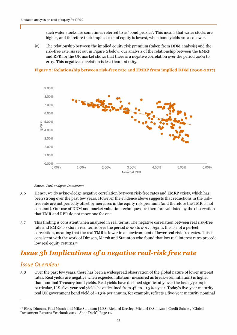
risk-free rate. As set out in Figure 2 below, our analysis of the relationship between the EMRP
and RFR for the UK market shows that there is a negative correlation over the period 2000 to
2017. This negative correlation is less than 1 at 0.65.
Figure 2: Relationship between risk-free rate and EMRP from implied DDM (2000-2017)
Source: PwC analysis, Datastream
3.6 Hence, we do acknowledge negative correlation between risk-free rates and EMRP exists, which has
been strong over the past few years. However the evidence above suggests that reductions in the risk-
free rate are not perfectly offset by increases in the equity risk premium (and therefore the TMR is not
constant). Our use of DDM and market valuation techniques are therefore validated by the observation
that TMR and RFR do not move one for one.
3.7 This finding is consistent when analysed in real terms. The negative correlation between real risk-free
rate and EMRP is 0.62 in real terms over the period 2000 to 2017. Again, this is not a perfect
correlation, meaning that the real TMR is lower in an environment of lower real risk-free rates. This is
consistent with the work of Dimson, Marsh and Staunton who found that low real interest rates precede
low real equity returns.22
Issue 3b Implications of a negative real-risk free rate
Issue Overview
3.8 Over the past few years, there has been a widespread observation of the global nature of lower interest
rates. Real yields are negative when expected inflation (measured as break-even inflation) is higher
than nominal Treasury bond yields. Real yields have declined significantly over the last 15 years; in
particular, U.S. five-year real yields have declined from 4% to –1.3% a year. Today’s five-year maturity
real UK government bond yield of –1.3% per annum, for example, reflects a five-year maturity nominal
22 Elroy Dimson, Paul Marsh and Mike Staunton | LBS, Richard Kersley, Michael O'Sullivan | Credit Suisse , “Global Investment Returns Yearbook 2017 - Slide Deck”, Page 11.
0.00%
1.00%
2.00%
3.00%
4.00%
5.00%
6.00%
7.00%
8.00%
9.00%
0.00% 1.00% 2.00% 3.00% 4.00% 5.00% 6.00%
EM
RP
Nominal RFR

Updated analysis on cost of equity for PR19 Updated analysis on cost of equity for PR19
12
yield of 0.7% and expected inflation of 2.0%. Only at much longer maturities are real government bond
yields positive today, although even those yields are still well below historical levels.
3.9 Respondents to Ofwat’s consultation suggest the use of real risk-free rates (RFR) in negative territory is
‘unprecedented’ and ‘a major departure from regulatory precedent’.
Comments and Response
3.10 The decline of real interest rates into negative territory is readily observable, particularly when using
RPI as the basis of indexation. Market expectations suggest this is likely to persist for the foreseeable
future (as we set out in the section above). Additionally, asset purchases of gilts between 2012 and 2016
have been relatively minimal, yet real risk-free rates have structurally declined. This implies that
market forces other than externally-influenced policies such as QE have been the more significant
driver of real risk-free rates into the negative territory.
3.11 Our recommendation is to use inputs into the cost of capital calculation which are broadly market
aligned. This is clearly done for the cost of debt assumption in regulatory calculations. If the risk-free
rate assumption is not based upon market observations, then this would lead to an inconsistency in the
credit spread between the risk-free rate and the cost of debt. By way of illustration, the yield for recently
issued water company long-term bonds is around 2.75%23, which is around or below long-term
expectations for RPI, so in RPI terms, water company new cost of debt is already around or below zero.
In the presence of a credit risk premium, this means that the risk-free rate must be below the cost of
debt and therefore must be negative.
3.12 We consider that our focus on the overall TMR means that the precise selection of the RFR is less
important. Were Ofwat to use low or negative market aligned risk-free rate assumptions, then the
EMRP would be commensurately higher to provide the overall TMR.
23 For example, Thames Water issued a £250 million bond with a coupon of 2.875% in May 2017 and Anglian Water issued a £200 million bond with a coupon of 2.625% in March 2017.
Updated analysis on cost of equity for PR19 Updated analysis on cost of equity for PR19
13
4. Dividend Discount Model
4.1 Having set out our views on the lower for longer interest rate environment and its implications for how
to estimate the total market return, this section of the report addresses specific issues raised about our
dividend discount model (DDM) approach, including:
The geometric average calculation and need for an upward volatility adjustment;
The GDP growth rate as a proxy for the growth in dividends;
Variance across other DDM models; and
Predictive power of DDM models.
4.2 We conclude this section by providing an update to the DDM analysis as at the end of October 2017.
Issue 4a Averaging methodologies for DDM calculations and volatility adjustments
Issue Overview
4.3 One of the material issues for appraisers in setting the cost of equity is the use of arithmetic versus
geometric means of estimating the equity risk premium. Historical averages can be calculated using
both arithmetic and geometric averages. Using the forward-looking DDM implicitly uses a geometric
approach, as the growth in dividends is assumed to be constant. This method has been challenged on
the basis that it does not “compensate investors for volatility of within year TMR, due to changes in
market price”24.
Comments and Response
Arithmetic vs Geometric based returns
4.4 There has been a wide ranging debate on the use of arithmetic and geometric averages in setting
forward looking return requirements.
4.5 Some practitioners prefer an arithmetic average as a measure of forward looking returns, based on the
justification that it represents an unbiased estimate25. The CMA in their determination for NIE in 2014
also noted that “The simplest approach is to calculate the arithmetic average of historical returns…
Since annual returns have been highly variable this approach requires looking at a long run of
historical data.” (para 13.139)
4.6 Other practitioners prefer the use of a geometric average. Their justification is based on a number of
reasons. Firstly, empirical studies seem to indicate that returns on stock are negatively correlated over a
long period26. Consequently, the arithmetic average method is more likely to overstate the forward
looking required risk premium. Secondly, while asset pricing models like the Capital Asset Pricing
Model (CAPM) are single period models, these models are used to estimate expected equity returns
over longer periods. In this context, there is a stronger preference to use the geometric average
methodology. These views are presented by Professor Aswarth Damodaran:
24 See KPMG (2017), ‘A review of Ofwat’s proposed approach to total market returns’, P 5 25 Kolbe, L.A., Read J.A. and Hall, G.R. (1984) ‘The cost of capital, Estimating the Rate of Return for Public Utilities’ 26 Negative serial correlation means good return years are more likely to be followed by poor return years, and vice versa. The evidence on negative serial correlation is widely cited, including analysis conducted by Fama and French (1988). While one year serial correlation is low, they find that five year correlations are strongly negative across all size classes. Fama, E.F. and K.R. French, 1992, The Cross-Section of Expected Returns, Journal of Finance, Vol 47, 427-466.
Updated analysis on cost of equity for PR19 Updated analysis on cost of equity for PR19
14
"There are, however, strong arguments that can be made for the use of geometric
averages. First, empirical studies seem to indicate that returns on stocks are
negatively correlated over time. Consequently, the arithmetic average return is likely
to overstate the premium. Second, while asset pricing models may be single period
models, the use of these models to get expected returns over long periods (such as five
or ten years) suggests that the estimation period may be much longer than a year. In
this context, the argument for geometric average premiums becomes stronger… In
closing, the averaging approach used clearly matters. Arithmetic averages will yield
higher risk premiums than geometric averages, but using these arithmetic average
premiums to obtain discount rates, which are then compounded over time, seems
internally inconsistent. In corporate finance and valuation, at least, the argument for
using geometric average premiums as estimates is strong."27
4.7 Lastly, some practitioners suggest a blend between the two. This view is consistent with Indro and Lee
(1997) who argue for a weighted average of the arithmetic and geometric premiums, with the weight on
a geometric premium progressively increasing with a longer time horizon. Such an approach was also
reflected in the CMA (2014) work where short-term investments were modelled based on the arithmetic
average while long-term investment returns justified the use of a geometric average. Fama and French
(2002) also explored the role of volatility in explaining the difference between historical average risk
premiums and forward-looking geometric techniques.28
4.8 Hence, what drives the opinions of practitioners on their choice of methodology depends on:
Forward looking return volatility assumptions; and
The investment holding period.
4.9 So for appraising an investment with a one year holding period and high expected volatility, use of an
arithmetic average approach can be justified, whereas low expected volatility and a longer investment-
holding period warrants the use of a geometric average. This helps to explain why investment
professionals providing long-term forward-looking equity return assumptions use figures that typically
are below the figures used by regulators to set required equity returns.29
Relative volatility adjustment
4.10 Volatility in returns can be decomposed into volatility in dividend growth and volatility in equity price
growth. As a result, investors require compensation for volatility in dividends and share prices. Fama
and French (2002) and KPMG (2017) argue that under the DDM approach, the mean forward-looking
return only takes into account the dividend yield volatility through the dividend growth input (where
the growth assumption is calculated using an arithmetic average of historical dividend growth rates30).
Hence, the two papers imply that the DDM approach understates expected returns by failing to
recognise that volatility in capital price growth has been higher than volatility in dividend growth –
thereby requiring a relative volatility adjustment. This adjustment could be applied in order to convert
a DDM approach to the equivalent of a simple one-period discount rate/arithmetic average.
4.11 Fama and French (2002) investigate the volatility in growth rates by comparing the standard deviation
of the annual simple rate of capital gain to the standard deviation of the annual dividend growth rate
and recommend an adjustment of half of the difference between the historic variances of the growth
27 Damodaran, Aswarth, “Equity Risk Premiums (ERP): Determinants, Estimation and Implications”, September 2008 28 Fama, E F and French, K R, ‘The Equity Premium’, Journal of Finance, April 2002 29 JP Morgan widely use the geometric average method for long-term investment return assumptions. November (2011), ‘Price/Earnings investing’. A selection of long-term equity return assumptions can be found in: BlackRock Investment Institute (April 2017). J.P. Morgan “2017 Long-term capital market assumptions” (September 2016). Morgan Stanley “Inputs for GIC asset allocation” (March 2017). BNY Mellon Fiduciary Solutions “10-year capital market return assumptions” (Jan 2017). Callan Associates “2017 Capital Market Projections”. Schroders “Long-run asset class performance: 30 years return forecasts (2017-2046)” (March 2017) *Large cap only 30 Our dividend growth assumption is taken from GDP growth forecasts which are typically higher than arithmetic means of historical dividend growth rates.

Updated analysis on cost of equity for PR19 Updated analysis on cost of equity for PR19
15
rates of dividends and capital gains. Based on US data from 1951-2000, they estimate the standard
deviation of annual capital price growth is 3.29 times the standard deviation of annual dividend growth.
4.12 We investigate these results further by:
Preparing more up to date, equivalent data for the UK, by analysing capital price returns and
dividend growth returns using FTSE all share data from 2000 to 2017. This uses the same
methodology employed by Fama and French; and
Restating Fama and French’s approach by investigating growth in total equity yield (dividend
and share repurchase) instead of purely growth in dividends.31
UK equivalent data
4.13 The table below shows the difference between our standard deviation measure and the results from
Fama-French (2002).
Table 1: Capital Price and Dividend Growth volatility
Measure Fama-French (2002) estimate
using 1951-2000 US data
PwC estimate
using 2000-2017 UK data
Capital price growth standard deviation 16.77% 15.6%
Dividend growth standard deviation 5.09% 8.1%
Standard deviation ratio 3.29x 1.92x
Capital price growth variance 2.81% 2.45%
Dividend growth variance 0.26% 0.66%
Variance adjustment 1.28% 0.89%
Source: Datastream and PwC analysis
4.14 Part of the reason for the lower relative volatility in the UK has been a period of lower equity price
volatility in recent years (see Figure 3 below).
Incorporating share buybacks
4.15 Another limitation of the Fama-French approach and consequently the suggestion for a volatility
adjustment made by KPMG is the focus on dividend growth rates. Given that the PwC DDM includes
total equity yield i.e. growth in dividends and share buybacks, a like for like analysis should incorporate
buybacks to estimate the overall dividend volatility and volatility adjustment.
4.16 Nominal rates of growth of dividends and buybacks is estimated as GCt = Ct/Ct-1, where GCt is the
growth in cash yield, and Ct is the total equity yield (cash value of dividends and share buybacks) at the
end of year t. Nominal rates of growth in capital price is estimated as GPt = Pt/Pt-1, where GPt is the
growth in stock price index, and Pt is the stock price at the end of year t. The evolution of the volatility
in capital price and total equity yield is set out in Figure 3 below:
31 This is consistent with our DDM model which incorporates equity buybacks as an equivalent to dividend return.
Updated analysis on cost of equity for PR19 Updated analysis on cost of equity for PR19
16
Figure 3: Total equity yield and Capital Price Y-o-Y Growth Variance 5-year average
Source: Datastream, Capital IQ, PwC analysis
4.17 Figure 3 suggests that total equity yield volatility has been higher than equity price volatility in almost
all years since 2006 except for the last few months of 2017. The volatility for total equity yield is
particularly influenced by strong dividend and share buyback activity running up to the financial crisis
and then reducing markedly afterwards.
4.18 The table below compares estimates from Fama-French (2002), our updated results incorporating
dividend growth only for 2000-2017 data, and our updated results incorporating total equity yield
growth.
Table 2: Capital price, Dividend growth and Total equity yield volatility
Measure
Fama-French (2002)
estimate
using 1951-2000 US data
PwC estimate (only
dividend growth)
using 2000-2017 US
data
PwC estimate (total
equity yield growth)
using 2000-2017 UK
data
Capital price growth
variance 2.81% 2.45% 2.45%
Dividend growth variance 0.26% 0.66% N/A
Total equity yield growth
variance N/A N/A 4.47%
Variance adjustment 1.28% 0.89% -1.01%
Source: Datastream and PwC analysis
4.19 The table above suggests that when we incorporate the impact of share buybacks in total equity yield,
the variance adjustment for the period 2000 to 2017 drops to a negative 1.01%. The negative
adjustment is due to a higher total equity yield growth volatility compared to total nominal capital
growth volatility. Hence, based on more up to date data, but using the Fama and French approach, it is
unclear that we need to make their bias adjustment to the DDM for forward-looking purposes. We note
0%
1%
2%
3%
4%
5%
6%
7%
8%
9%
Oct 2006 Oct 2007 Oct 2008 Oct 2009 Oct 2010 Oct 2011 Oct 2012 Oct 2013 Oct 2014 Oct 2015 Oct 2016 Oct 2017
Capital Volatility - Total Equity Yield Growth Volatility
Capital Price Volatility
Total Equity Yield Growth Volatility

Updated analysis on cost of equity for PR19 Updated analysis on cost of equity for PR19
17
that the current difference between the variances of equity price and total equity yields is small and
therefore do not incorporate any adjustment to our DDM analysis.
Holding Period
4.20 In the 2014 NIE case, the CMA noted that, in the context of a difference in the relative volatility of
equity capital values, the arithmetic mean would be appropriate where the holding period was close to
one-year, and a geometric mean would be appropriate for a longer time horizon. Were a relative
volatility adjustment required, then according to this finding by the CMA, a long holding period
assumption would mitigate much of the need for a volatility adjustment.
4.21 In any case, however, our analysis above suggests that there is no need for a volatility adjustment when
estimating total market returns. Hence, we do not need to further investigate the relationship between a
volatility adjustment and the length of holding period assumed.
Issue 4b GDP as an assumption of growth in dividends
Issue Overview
4.22 A key input to the DDM is an estimate of the expected growth of future dividends.
4.23 The expected short-term and long-term growth rates used in our DDM analysis represent nominal
growth rates from forecast real GDP growth and forecast inflation. Our argument for this growth
assumption was based on the premise that “we are applying this DDM approach to the market as a
whole, i.e. the entire FTSE All Share, GDP growth serves as a reasonable proxy for expected dividend
growth.”32 KPMG have challenged the use of GDP as an assumption for growth in dividends by implying
that the “relationship between dividends and GDP has historically been highly imperfect, and there is
no robust means to test whether this assumption truly reflects investors’ expectations.”
4.24 Water investors make a further recommendation - that the dividend growth assumption should be
based on a measure of global GDP growth rather than UK GDP. This is based on the observation that
the shares traded on the FTSE All Share Index come from many global companies.
Comments and Response
GDP as a measure of future growth in dividends
4.25 Academics and practitioners have proposed a variety of approaches to estimate the future expected
dividend growth rate. There are three options:
Historical analysis of dividend growth rates;
Bottom up approaches which use analyst forecasts for dividend growth at a firm level. These are
then aggregated to provide the overall dividend growth expectations for the market; and
Macroeconomic proxies, such as GDP growth.
4.26 Fama-French (2002) cite a real historical dividend growth rate of 0.5% for the US, well below the
average rate of growth in the economy. The CMA found a similar result for the UK, noting growth in
dividends from 1980 had averaged 1.6% compared to 2.3% for real GDP growth. This helps to illustrate
some of the challenges in using historical dividend growth averages, which are likely to understate
expectations of future dividend growth. One reason why historical growth rates may be lower than
broader economic growth is that companies have increased their use of share-buybacks as a tax efficient
32 PwC (2017), ‘Refining the balance of incentives’
Updated analysis on cost of equity for PR19 Updated analysis on cost of equity for PR19
18
way of returning value to shareholders.. For these reasons we rejected the use of historical averages as a
way of estimating future dividend growth.
4.27 Analyst forecasts are often used as an input into DDM models. In fact, the Bank of England uses survey
data from equity analyst forecasts to estimate short-term horizon dividend payments. However, it does
explicitly cite that the accuracy of equity analyst forecasts is ‘a key source of potential error in the
DDM’33. It can be argued that analyst forecasts may be an imperfect variable for actual expectations, for
example if they lag changes in actual dividend estimations or if analysts are overly optimistic in their
estimates (which can be a common driver of bias as analyst expectations are tied directly with
management goals). Hence, relying on analyst forecasts might not enable the elimination of any
systematic bias.
4.28 Our rationale for using GDP growth as our assumption for dividend growth is based on three reasons:
If part of the reason that dividend growth has been kept low is due to investment (i.e. deferred
dividends), then we expect dividend growth to return to typical rates of GDP growth in the
future;
If dividend growth has been low because dividends have been falling as a share of national
income, then this trend is unlikely to continue and dividends should find an equilibrium share of
national income, and then grow in line with national income; and
The GDP measure of growth provides stability in the DDM model. It draws on forecasts of real
GDP and inflation from Consensus Economics, which is a widely sourced provider of consensus
forecast macroeconomic data. This avoids large swings in analyst short-term forecasts (e.g. at
turning points in the economic cycle) overly influencing the DDM results.
4.29 We therefore consider the use of GDP forecasts as a reasonable proxy for dividend growth expectations.
Hence, our use of GDP growth rates lies in the middle of the spectrum of options as it is not
downwardly bias by omitted sources of growth (historical measures) and not upwardly biased by using
analyst dividend forecasts. In order to capture long-term dividend growth variations, the BoE ties its
estimate to long-term GDP projections. Specifically, the BoE DDM model assumes that beyond five
years, dividends are expected to grow in line with five year-ahead GDP projections34. This is in line with
our DDM approach for long-term DDM growth expectations.
Use of the UK GDP growth rate
4.30 We acknowledge that many FTSE All share listed companies derive a substantial portion of their
earnings from outside the UK, where GDP growth rates may be higher than in the UK. Use of global
growth rates, or a blend of global and UK growth rates in our DDM model would be expected to
produce higher TMR estimates.
4.31 However, Ofwat requires cost of capital assumptions which are sufficient to enable UK water companies
to finance their activities. This typically requires use of UK input parameters to cost of capital estimates.
If we were to use global growth assumptions, or a blend of UK and global growth, then we would need
to consider whether the global/UK blended TMR should then be deconstructed into a UK figure and a
non-UK figure. As the differential growth rates between the UK and the rest of the world are likely to be
an important consideration in both the calculation of the blended rate and the deconstruction into UK
and non-UK figures, this approach seems unnecessary. Rather, our preference is to use UK based
parameters, and proxies, wherever possible as it avoids the need for further adjustments.
Use of the Global GDP growth rate and global cost of capital assumptions
4.32 A further suggestion from respondents to Ofwat’s consultation is to move to a more global basis of
estimating the cost of capital, so using global equity market performance as a guide to historic equity
33 Bank of England (2017), ‘An improved model for understanding equity prices’ 34 Bank of England (2017), ‘An improved model for understanding equity prices’

Updated analysis on cost of equity for PR19 Updated analysis on cost of equity for PR19
19
returns, and use of global equity yields and global growth rates as assumptions in DDM modelling. This
raises a number of issues:
Selection of a global index - a global based equity index such as the MSCI world index could be
used. However, the MSCI world index covers representation across 23 developed market countries.
This moves away from UK financing conditions.
Estimation challenges - it is harder to estimate global parameters for cost of capital calculations,
due to the need for more information and reduced quality of information. For example, betas
calculated with respect to global indices typically exhibit much larger confidence intervals.
Consistent estimation across all cost of capital parameters - a global approach would require
estimating a water asset beta against the MSCI world index. It is notable that the asset beta of UK
water companies regressed against the MSCI World Index (proxy for global market index) is 7 basis
points lower than when it is regressed against the FTSE All share index35. A higher TMR would
therefore be used with a lower beta assumption. As well as being less certain, this means it is
unclear whether such an approach provides a definitively different answer.
4.33 So a global cost of capital approach moves the focus from a UK based cost of capital measure and hence
makes the estimate less relevant for water companies in the UK and Ofwat.
Issue 4c Difference in results compared to other DDM models
Issue Overview
4.34 The adoption of the DDM model to understand equity market conditions has been widespread,
including by the Bank of England and Bloomberg, which provide a DDM tool on its platform. These
models operate on different assumptions compared to the PwC DDM model, which drives some of the
difference between TMR estimates.
4.35 This forms the basis of KPMG’s observation that ‘the results of DDM are sensitive to the dividend
growth assumption and time period’ and that PwC’s DDM model ‘ultimately relies on assumptions
around dividend forecasts into perpetuity, which introduces significant judgement to the analysis’36.
Other respondents note the different results we obtained compared to the Bank of England and
Bloomberg which therefore raises the issue of the relative suitability of the different approaches and
assumptions used.
Comments and Response
4.36 The differences in EMRP/TMR estimates proposed by other institutions and practitioners largely arise
due to differences in their input assumptions.
4.37 The latest Bank of England approach uses the net present value relationship by equating equity prices
to the present value of all future dividends discounted by a risk-free rate and an EMRP estimate. It uses
a combination of analyst forecasts and GDP growth to estimate future short-term and long-term
dividend growth rates respectively. Its use of long-term GDP figures to estimate the long-term dividend
growth rates has enabled the BoE to capture the long-term variation in investor growth expectations
and that ‘improves the accuracy of the model’s ERP estimates’.
35 The UK water company price returns were regressed against the FTSE 100 (UK) and MSCI World Index (global) over a five year period since 31/10/2017 to estimate UK water company 5 yr equity betas. The equity betas were de-levered using the 5 yr gearing ratios of the respective companies. The resulting figure represent UK water company asset betas benchmarked against UK and Global price indices. 36 See KPMG (2017), ‘A review of Ofwat’s proposed approach to total market returns’, Page 5

Updated analysis on cost of equity for PR19 Updated analysis on cost of equity for PR19
20
4.38 The Bloomberg model is based on a three-stage dividend growth model. Unlike the Bank of England
and PwC DDM models, this version includes a transitionary growth period between short-term and
long-term dividend growth estimates, both of which are based on analyst growth forecasts. More
specifically, the dividend numbers are based on the dividend payout ratios37 (dividends per share /
earnings per share). Hence, the growth in dividends is pegged to the growth in earnings.
4.39 Work done in the Bank in the past found that IBES38 aggregate forecasts of earnings and dividend
growth in both the United Kingdom and the United States for the first, second and third year (fixed-
event forecasts) are biased (non-zero average error) and inefficient (errors correlated with past
information)39. In particular, analyst based forecasts are excessively optimistic during economic
downturns and too pessimistic in recoveries. Harris (1999) found also that analysts’ long-run earnings
forecasts for US companies are biased and inefficient.
4.40 This finding is relevant when considering the purpose of the different DDM models. The Bank of
England DDM model has been created to help it in “monitoring of equity price moves in support of its
policy objectives”40. It is interested whether risk premia are rising, or whether analysts are cutting their
forecasts of earnings and dividends and this is instructive for both managing monetary policy and
financial stability. For the Bank of England’s purposes, it wants to incorporate analyst views into its
model as it wants to pick up movements in analyst expectations. It is less concerned with the absolute
level of the equity return predicted in its model (around 11% in nominal terms). For the regulatory
purpose of setting the level of equity returns the potential for analyst optimism is more problematic,
and we do not require a model which picks up day to day variations in analyst expectations. For this
reason we do not consider using analyst forecasts of dividend growth is not suited to Ofwat’s purposes.
Issue 4d Predictive power of DDM modelling
Issue Overview
4.41 One of the responses to Ofwat’s consultation on the DDM model was its instability and its poor
predictive ability for outturn equity returns. KPMG suggest that the PwC DDM model ‘implicitly relies
on its spot rate ex-ante forecast to determine TMR over the next eight years, as opposed to its five year
average’.
Comments and Response
4.42 The predictive power of DDM models, in contrast to the use of historical averages, was reviewed in the
paper by Fama-French (2002). They concluded that “the dividend and earnings growth estimates of
the equity risk premium from 1951 to 2000 are closer to the true expected value” and “Based upon this
and other evidence, our main message is that the unconditional expected equity premium of the last
50 years is probably far below the realised premium”. Additionally, recent academic work has found
that the predictive power of market implied approaches such as this when fitted to actual returns are
higher than competing methodologies. Specifically, using data for the US market, Professor Aswarth
Damodaran found the technique with the best predictive power of actual returns over the following 5-
years was recent averages of implied outputs such as DDM41. A 2015 working paper by the Bank of
England also found a similar result, which is that DDM can significantly forecast returns.42
4.43 We therefore consider the DDM approach has validity for use in estimating forward-looking return
requirements.
37 Equity Markets and Portfolio Analysis, R.Stafford Johnson 38 IBES – Institutional Brokers’ Estimate System 39 Bank of England Quarterly Bulletin Spring 2002 40 Bank of England (2017), ‘An improved model for understanding equity prices’ 41 Equity Risk Premiums: Determinants, Estimation and Implications – The 2017 Edition, pp122-123 including Table 24 42 Chin and Polk (2015), ‘A forecast evaluation of expected equity return measures’, Working Paper No.520

Updated analysis on cost of equity for PR19 Updated analysis on cost of equity for PR19
21
4.44 There is then the issue whether to rely on a spot estimate, or some form of longer period average. We
acknowledge that a spot or current rate runs the risk of being unhelpfully volatile. However, this is
mitigated by the use of GDP forecasts as proxies for dividend growth, which change much more slowly
than other sources of growth assumptions. We also caution the use of longer averaging periods, as the
purpose of using the DDM is to move away from techniques which depend upon historical data. Even
the five year average extends back to when expectations of future long-term interest rates were much
higher than they are today. For this reason our five year average DDM figure was outside of our overall
TMR range in our previous report.
4.45 We do consider it is helpful to calculate an average DDM figure from January 2014. This period marks
the beginning of a structural decline in long-term interest rate expectations, so is more aligned to the
low interest rate environment. This is evident in Figure 1 which depicts a sustained decrease in the
expectations of future real interest rates in recent years, with a particular structural change in interest
rate expectations that began in January 2014. This can be seen as a drop in 10 year forward rates on 10
year real and nominal UK government yields.
Updated DDM analysis
4.46 The outputs from our monthly DDM analysis are shown in Figure 4 below. The TMR spot rate as of the
end of October 2017 is 8.4% (in nominal terms), while the 5-year average of DDM outputs has been
8.7%.
Figure 4: Monthly DDM outputs, 2000 to 2017
Source: PwC analysis, Datastream, Consensus Economics, Bank of England
4.47 The table below presents the updated evidence of DDM outputs against the evidence from our Balance
of Incentives work.
0%
2%
4%
6%
8%
10%
12%
14%
Oct-
00
Oct-
01
Oct-
02
Oct-
03
Oct-
04
Oct-
05
Oct-
06
Oct-
07
Oct-
08
Oct-
09
Oct-
10
Oct-
11
Oct-
12
Oct-
13
Oct-
14
Oct-
15
Oct-
16
Oct-
17
Nom
inal T
MR
5-year average 8.7%
Oct-17 spot 8.4%

Updated analysis on cost of equity for PR19 Updated analysis on cost of equity for PR19
22
Table 3: TMR returns based on PwC DDM model
Dividend Discount Model
Measure Spot Return Average since January
2014 5 year average
Original Estimate
Balance of Incentives (Dec-16) 8.3% Not provided 8.8%
October 2017 update
(as at 31/10/2017) 8.4% 8.6% 8.7%
October 2017 DDM range 8.4%-8.7%
Source: PwC analysis, Datastream, Consensus Economics, Bank of England
4.48 The October 2017 update of the PwC DDM model shows a 0.1% reduction in TMR in the 5 year average,
whilst a 0.1% increase in the spot return compared to the estimates from our Balance of Incentives
work. The lack of movement in DDM based returns suggests that the model results are relatively stable.

Updated analysis on cost of equity for PR19 Updated analysis on cost of equity for PR19
23
5. Analysis of Market to Asset Ratios
5.1 In our previous report, one source of current market evidence reviewed was evidence from RCV premia
(otherwise referred to as market-to-asset ratios or MARs).
5.2 As set out in our report, wherever the use of current market approaches is applied, there are advantages
and disadvantages of the approach. For example, a key advantage can be that required returns are
better matched to prevailing market expectations, while disadvantages can include greater estimation
challenges and a greater degree of judgement.
5.3 The use of evidence from RCV premia is no exception to these advantages and disadvantages. For
example, there is a degree of judgement involved in ascribing observed premia between different
sources of value, and the relative contributions of these sources can change over time.
5.4 As such, we recommended that the outputs from the review of this evidence be used in conjunction with
the outputs from other techniques such as DDM modelling. Furthermore, we also noted that where
some potential drivers of the RCV premia were not fully accounted for in the analysis, the approach
should be used as a reference point for the lower end of return requirements (rather than a central
estimate).
Issue 5a Impact of regulatory capital growth and non-regulated revenues in MAR analysis
Issue Overview
5.5 A response to Ofwat’s consultation posited the presence of downward bias in the inferred cost of equity
using the MAR evidence we provided from two sources. Firstly, from an assumption of zero RCV
growth, and secondly, from not controlling for non-regulated activities.
5.6 The first issue raised, regarding RCV growth, stated that, “PwC’s analysis does not control for RCV
growth, and implicitly assumes a constant nominal RCV in perpetuity.”43 Given this, the response then
sought to quantify the impact of two scenarios. Based on this analysis, an increase in nominal TMR of
approximately 1 percentage point (pp) was found to be the difference between the two scenarios.
5.7 The second issue raised, regarding non-regulated revenues, highlighted that a proportion of enterprise
value is attributable to non-regulated activities and that this element had been excluded from the
analysis. Based on SVT’s financial statements, a deduction of 3% from the observed MAR for SVT was
made. This was in turn used to support an increase in estimated nominal TMR of approximately 0.3
pps.
Comments and Response
5.8 With regards to the first issue, positive nominal RCV growth was included in the estimation of the
implied TMR from RCV premia for both companies. The nominal present value of outperformance was
estimated on the basis of a given % RoRE outperformance applied to notional regulated equity value
(which was in turn linked to this growing nominal RCV). There is therefore no requirement for an
adjustment for “constant nominal RCV in perpetuity”
5.9 With regards to the second issue, we noted that non-regulated activities were not ascribed any value in
the estimates presented in our July 2017 report.
43 KPMG (2017), ‘A review of Ofwat’s proposed approach to total market returns’, Page 30

Updated analysis on cost of equity for PR19 Updated analysis on cost of equity for PR19
24
5.10 Our report did however note that these sources of income were likely to be small relative to regulated
income. Moreover, our report noted that as there remained some potential for other sources of value,
that the RCV premia estimates presented should be used to calibrate the lower end of return
requirements. Where an attempt is made to specifically account for other drivers of enterprise value,
removing them from the observed RCV premium, the estimates presented become closer to central
estimates for the assumption.44
5.11 In order to incorporate value for non-regulated activities, we have used the KPMG suggestion of a 3%
deduction from enterprise value in order to account for the impact of non-regulated activities45. We
find, holding all else equal, there is approximately a 0.3pp to 0.4pp increase in the implied nominal
TMR.
5.12 There are however countervailing impacts to this increase if specific treatment of other regulatory items
are also included. One other regulatory item, not included in our July 2017 analysis, is the impact of the
CIS indexation RCV log-down that will affect the industry at the end of AMP6.
5.13 In terms of accounting for this RCV log-down46, we apply a three step approach:
The scale of the MAR at FY16 end is adjusted for the scale of the RCV log-down in nominal terms
(+0.02x to both the SVT and UU MAR);
Outperformance for AMP6 continued to be estimated with reference to an unadjusted RCV, as
the log-down occurs at the end of AMP6; and
Outperformance for AMP7 onwards is applied to the logged-down asset base.
5.14 Where this item is applied, we find that the impact on the implied TMR is a decrease of approximately
0.2pp to 0.3pp.
5.15 In summary, the estimates in our July 2017 report can be supplemented with additional analysis. Above
we set out two supplementary items, non-regulated revenues and the CIS indexation RCV log-down.
The net effect of these two supplementary items is small. Therefore we do not consider that there is a
downward bias in the RCV premia analysis presented in our July 2017 report.
Issue 5b TMR as an economy wide variable
Issue Overview
5.16 One response highlighted that TMR estimates have been produced by a sample of water companies that
are unlikely to be representative of the broader economy.
5.17 The essence of this response is that company specific data is being used to inferred parameters for the
equity market as a whole. As the sample of listed water companies is small (only two WaSCs were used
as Pennon Group has a substantial non-regulated business), the response challenges the strength of the
conclusions that can be drawn for equities more widely.
Comments and Response
5.18 Firstly, it is important to note that the key output from the RCV premia analysis was an inferred
investor discount rate for equity, by calculating the discount rate required to reach an RCV premium of
44 We specifically use the term ‘closer to’, as there potentially remain other unquantified value drivers such as optimism bias, valuation of potential future opportunities and flight to safety effects. 45 Based on KPMG estimate for SVT. See KPMG (2017), ‘A review of Ofwat’s proposed approach to total market returns’, Page 32 46 The RCV log-down amounts are set out in Section 7 in the PR14 reconciliation rulebook http://www.ofwat.gov.uk/wp-content/uploads/2016/10/PR14-reconcilliation-rulebook1.pdf
Updated analysis on cost of equity for PR19 Updated analysis on cost of equity for PR19
25
zero (after adjusting for the expected value of outperformance).47 In other words, the analysis could
have closed at this juncture, focusing on this inferred cost of equity for WaSCs.48 Extra steps were
needed to transform this inferred cost of equity into a total market returns figure.
5.19 We note that there is uncertainty in this transformation. This uncertainty arises predominantly from
the asset beta assumption applied. We therefore acknowledge the need to check the consistency of this
transformation with the asset beta approach Ofwat uses in the initial WACC for PR19 (the number itself
may be different if Ofwat considers forward looking risk exposure will change as a consequence of its
regulatory methodology). We have used the PR14 asset beta estimate, applicable at the time period used
for our analysis.
5.20 Were Ofwat to receive sufficient evidence that other water companies required higher returns, relative
to the two large WASCs used in our analysis, then it would be able to separately adjust for this.49
Issue 5c Sample used for MAR analysis as a representation of the water industry
Issue Overview
5.21 Responses highlighted that the companies used for RCV premia analysis may not be representative of
the wider industry on the basis of both size and activities.
5.22 As highlighted above, the core output of the RCV premia analysis was an inferred, sector specific, cost
of equity. The issue raised here is whether this figure is only suited to a subset of the industry.
Specifically, the responses posit that it is more suited to larger WaSCs, and less suited to smaller
companies and WoCs.
Comments and Response
5.23 Firstly, on the issue of company size, we have previously found that there is little academic consensus
on the need for a change to the cost of equity on the basis of size alone.50 Furthermore, in the 2010
determination of Bristol Water, the CC (now the CMA) found that:51
“Size alone did not support the need for an uplift. While there was theoretical
evidence that small companies required a higher return on capital (such as the
Fama-French model), there was insufficient evidence to show that small water
companies had higher systematic risk.”
5.24 Small water companies face the same regulatory framework compared to larger water and wastewater
companies. Additionally, as Professor Damodaran states. “risk ultimately has to come from something
fundamental (and size is not a fundamental factor)”52.
47 The nature of setting regulated charges via a regulatory asset base provides a convenient setting for ascribing changes in market value to different sources. Where company specific factors are appropriately account for, the remaining factors are broader market variables. 48 In the analysis incorporated into our Balance of Incentives work, the implied nominal cost of equity was 6.7% for Severn Trent and 6.8% for United Utilities. 49 In PR14, Ofwat made no company specific adjustments to the cost of equity. We also found no difference between WaSC and WoC transaction multiples. See Page 37 of PwC (2014), ‘Company specific adjustments to the WACC: A report prepared for Ofwat’. 50 PwC (2014), ‘Company specific adjustments to the WACC: A report prepared for Ofwat’. 51 CMA (2014), ‘Bristol Water plc: A reference under section 12(3)(a) of the Water Industry Act 1991’, A10(1)-24. 52 Aswath Damodaran, ‘Equity risk premiums (ERP): determinants, estimation and implications – the 2016 edition’, March 2016

Updated analysis on cost of equity for PR19 Updated analysis on cost of equity for PR19
26
5.25 Given these findings, we do not agree that the cost of equity inferred from listed WaSC RCV premia
would be unrepresentative for the wider industry.
5.26 Secondly, on the issue of different activities, both we and the CMA have reviewed the potential impact
of different activities on the capital intensity of companies, producing differences in ‘operational
leverage’.53 We have previously found that there is not conclusive evidence to support an adjustment to
asset beta for differences in operational leverage. However, the CMA in its 2010 and 2014 reviews of the
asset beta for Bristol Water (a WoC) did apply an adjustment for operational leverage to asset beta.
5.27 Given this, the representativeness of the cost of equity inferred from listed WaSCs will depend on the
view taken by Ofwat on the magnitude of any differences in asset betas across the water sector.
Issue 5d Cost of debt in MAR analysis
Issue Overview
5.28 One response stated an issue with our analysis of RCV premia was that outperformance of the allowed
cost of debt had not been taken into account.
5.29 Historically, the ability of companies to outperform the notional cost of debt assumption applied by
Ofwat in the setting of charges has contributed significantly to total outperformance. Therefore,
accounting for this source of outperformance, alongside others, is important when understanding
drivers of value.
Comments and Response
5.30 The analysis set out in our July 2017 report included outperformance associated with:
Total expenditure;
Outcome delivery incentives;
The Service Incentive Mechanism; and
The cost of debt (referred to in our report as “financing outperformance”).
5.31 For each of the four elements set out above, a percentage point outperformance in RoRE terms was
applied to a stream of regulatory equity. The cost of debt outperformance was therefore taken into
account.
Issue 5e Updating MAR analysis using current data
Issue Overview
5.32 One response highlighted an issue with the use of RCV premia (from FY16 end), which was that stock
prices of the listed WaSCs declined over the period 31st May 2017 to 24th August 2017.
5.33 The issue raised is that over the time period highlighted the magnitude of RCV premia declined as
market valuations fell. All else equal, this would suggest that the post-outperformance RCV premia was
lower, and therefore, the inferred TMR higher.
Comments and Response
5.34 Using more up to date time periods suffers from significant circularity issues. This is especially
pertinent for any RCV premia observed following the publication of Ofwat’s methodology consultation -
53 WaSCs on average have higher capital intensity than WoCs, this is associated with lower ‘operational leverage’.
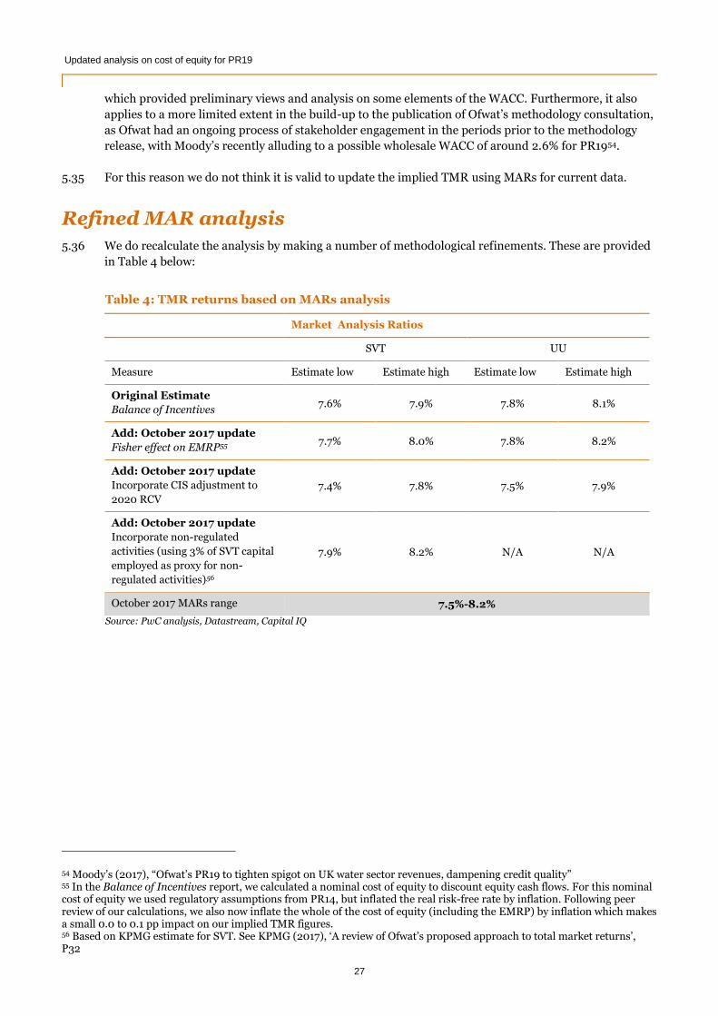
Updated analysis on cost of equity for PR19 Updated analysis on cost of equity for PR19
27
which provided preliminary views and analysis on some elements of the WACC. Furthermore, it also
applies to a more limited extent in the build-up to the publication of Ofwat’s methodology consultation,
as Ofwat had an ongoing process of stakeholder engagement in the periods prior to the methodology
release, with Moody’s recently alluding to a possible wholesale WACC of around 2.6% for PR1954.
5.35 For this reason we do not think it is valid to update the implied TMR using MARs for current data.
Refined MAR analysis
5.36 We do recalculate the analysis by making a number of methodological refinements. These are provided
in Table 4 below:
Table 4: TMR returns based on MARs analysis
Market Analysis Ratios
SVT UU
Measure Estimate low Estimate high Estimate low Estimate high
Original Estimate
Balance of Incentives 7.6% 7.9% 7.8% 8.1%
Add: October 2017 update
Fisher effect on EMRP55 7.7% 8.0% 7.8% 8.2%
Add: October 2017 update
Incorporate CIS adjustment to
2020 RCV
7.4% 7.8% 7.5% 7.9%
Add: October 2017 update
Incorporate non-regulated
activities (using 3% of SVT capital
employed as proxy for non-
regulated activities)56
7.9% 8.2% N/A N/A
October 2017 MARs range 7.5%-8.2%
Source: PwC analysis, Datastream, Capital IQ
54 Moody’s (2017), “Ofwat’s PR19 to tighten spigot on UK water sector revenues, dampening credit quality” 55 In the Balance of Incentives report, we calculated a nominal cost of equity to discount equity cash flows. For this nominal cost of equity we used regulatory assumptions from PR14, but inflated the real risk-free rate by inflation. Following peer review of our calculations, we also now inflate the whole of the cost of equity (including the EMRP) by inflation which makes a small 0.0 to 0.1 pp impact on our implied TMR figures. 56 Based on KPMG estimate for SVT. See KPMG (2017), ‘A review of Ofwat’s proposed approach to total market returns’, P32

Updated analysis on cost of equity for PR19 Updated analysis on cost of equity for PR19
28
6. Approach used to deflate nominal TMR
Issue 6a Consistency of inflation and the approach for obtaining the TMR estimate
Issue Overview
6.1 In our previous report, we calculated TMR in nominal terms, as market data (DDM, market values and
surveys) typically incorporates inflation. We then explored three approaches to adjust the nominal cost
of equity in order to calculate real figures for use in regulatory financial models.
6.2 The KPMG and EY report suggest that there was no clarity on the approach that will be used to deflate
the TMR.
Comments and Response
6.3 In order to estimate a real cost of equity, the inflation approach should be consistent with Ofwat’s
methodology of estimating the TMR.
6.4 In our balance of incentives work, we set out three approaches:
Approach 1: Retains all components of the cost of equity in nominal terms, calculates nominal
cost of equity and deflating the nominal cost of equity figure at the end;
Approach 2: Estimates the EMRP using the nominal TMR and nominal RFR, and subsequently
applies the EMRP that’s been calculated to a real RFR when calculating the real cost of equity;
and
Approach 3: Estimates the EMRP using the real TMR and real RFR, and subsequently applies the
EMRP calculated to a real RFR when calculating the real cost of equity.
6.5 We consider that approach 1 and 3 are in line with Ofwat’s current methodology, which derives an
EMRP using a real risk-free rate and a real TMR. Given the TMR is set using a forward looking
approach (DDM methodology), our nominal estimate should be deflated using a forward-looking
inflation expectation.
6.6 It is important to note that the inflation approach should be based on the underlying approach used to
obtain the TMR estimate. This consideration is required to ensure consistency in the cost of equity and
inflation approaches.
6.7 In the event of a material difference between the current inflation forecast and the trailing forecast
inflation average (embedded into an average TMR estimate over a period of time), we recommend
Ofwat should allow for an adjustment for this. However, such adjustments should be based upon long-
term inflation expectations, which move slowly and have, to date, been heavily anchored around 2.0%
for CPI. This means the size of any such adjustment is likely to be small.

Updated analysis on cost of equity for PR19 Updated analysis on cost of equity for PR19
29
7. Conclusion
7.1 Our report has set out the responses to specific comments made by KPMG and EY (on behalf of water
companies) and by other water investors. We have also augmented our responses with updates from
recent market developments and academic studies where required.
7.2 Based on our responses and recent market information, we have updated our TMR range as of the end
of October 2017 using both the DDM, MARs analysis and investor surveys57. We provide the updated
TMR range in the table below. The one change has been to increase the top end of the TMR range to
include the average DDM result since January 2014.
Table 5: Recommended updated TMR range (as of October 2017)
Measure TMR range
Original Range
Balance of Incentives (Dec-16)
8.0% - 8.5%
October 2017 update
DDM range (as at 31/10/2017)
8.4% - 8.7%
October 2017 update
MARs range (as at 31/10/2017)
7.5% - 8.2%
Recommended updated range using
DDM, MARs and investor surveys58 (as
at 31/10/2017)
8.0%-8.6%
57 Fernandez, Pablo and Pershin, Vitaly and Fernández Acín, Isabel, Discount Rate (Risk-Free Rate and Market Risk Premium) Used for 41 Countries in 2017: A Survey (April 17, 2017). Available at SSRN: https://ssrn.com/abstract=2954142 58 Top end of DDM range is not appropriate, as this uses data prior to structural break. Top end of range therefore uses DDM average since January 2014. Bottom end of MAR range is not appropriate due to potential omission of other factors, with likely small positive impact on inferred TMR.

Updated analysis on cost of equity for PR19 Updated analysis on cost of equity for PR19
30
This document has been prepared only for Water Services Regulation Authority
(Ofwat), solely for the purpose, and on the terms agreed with Water Services
Regulation Authority (Ofwat) in our agreement dated 12 October 2017 (SER/
0713).
We accept no liability (including for negligence) to anyone else in connection with
this document, and it may not be provided to anyone else.
© 2017 PricewaterhouseCoopers LLP. All rights reserved. In this document, 'PwC'
refers to the UK member firm, and may sometimes refer to the PwC network.
Each member firm is a separate legal entity. Please see www.pwc.com/structure
for further details.