CONSAT

Stabilisation and Control of

Small Satellites

April 1999

Update on Status of

Satellite Simulator

Pedro Tavares

Robert Clements

Contents

1. Introduction..................................................................................................... 3

2. Modifications to Core Structure...................................................................... 4

2.1 Simsat Executive Structure ............................................................... 4

2.2 Changes to Incorporate an Estimator ................................................ 6

3. PoSat-1 Type Actuator.................................................................................... 9

4. Predictive Controller..................................................................................... 12

5. Sensors .......................................................................................................... 13

5.1 Sun Sensor....................................................................................... 13

5.2 Earth Horizon Sensor ...................................................................... 17

6. Estimator ....................................................................................................... 21

7. Automatic Results Analysis.......................................................................... 22

7.1 Controller Data Analysis................................................................. 22

7.2 Estimator Data Analysis.................................................................. 23

8. Bibliography ................................................................................................. 24

2

1. Introduction

Since previous reports some significant modifications having been made to the ConSat Satellite

Simulator. These include modification to the structure to allow an attitude estimator to be used and the

ability to run batches of simulations; the actuators used in the simulator have been updated in the light

of new information; new versions of the Predictive Controller and Sensors have been added and an

Estimator has been incorporated. This reports aims to summarise all these modifications to bring the

reader up to date with the current status of the simulator.

3

2. Modification of the Core Structure 2.1 Simsat Executive Structure

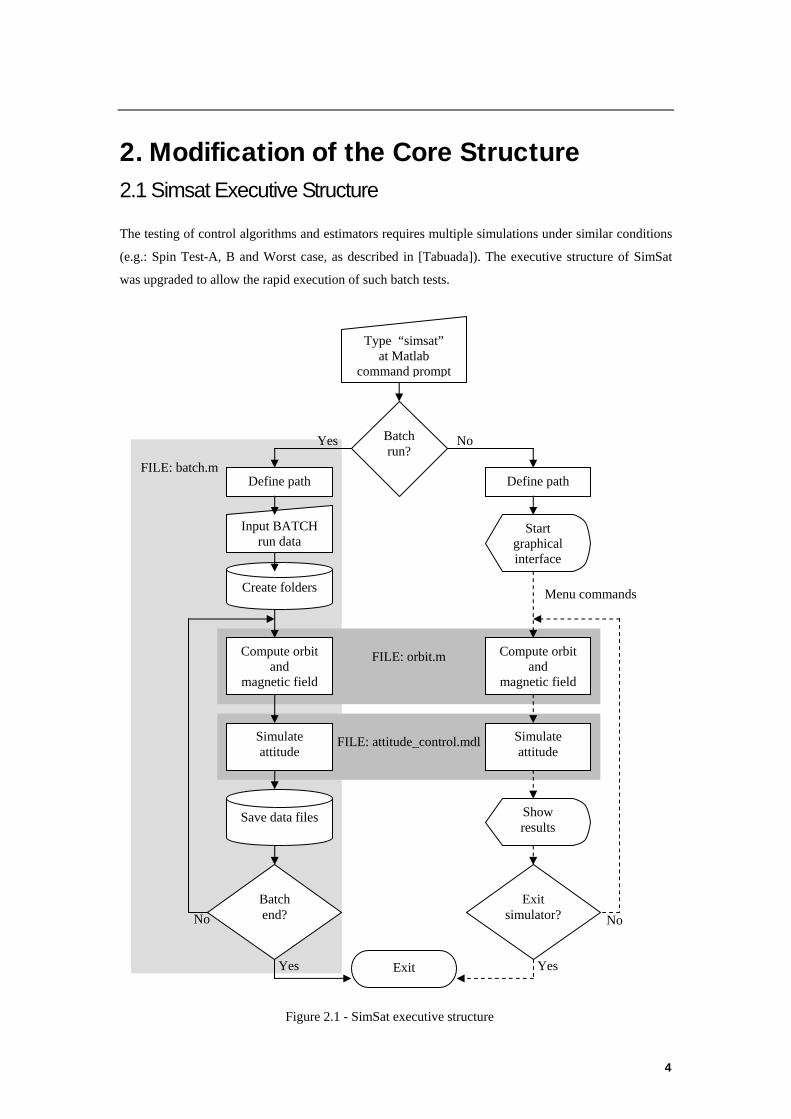
The testing of control algorithms and estimators requires multiple simulations under similar conditions

(e.g.: Spin Test-A, B and Worst case, as described in [Tabuada]). The executive structure of SimSat

was upgraded to allow the rapid execution of such batch tests.

FILE: batch.m

FILE: attitude_control.mdl

FILE: orbit.m

Menu commands

Batch run?

Define path Define path

Yes No

Input BATCH run data

Create folders

Compute orbit and

magnetic field

Simulate attitude

Save data files

Exit

Compute orbit and

magnetic field

Simulate attitude

Start graphical interface

Show results

Exit simulator?

Yes Yes

Batch end? No No

Type “simsat” at Matlab

command prompt

Figure 2.1 - SimSat executive structure

4

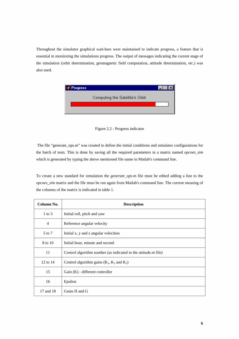
Throughout the simulator graphical wait-bars were maintained to indicate progress, a feature that is

essential in monitoring the simulations progress. The output of messages indicating the current stage of

the simulation (orbit determination, geomagnetic field computation, attitude determination, etc.) was

also used.

Figure 2.2 - Progress indicator

The file “generate_ops.m” was created to define the initial conditions and simulator configurations for

the batch of tests. This is done by saving all the required parameters in a matrix named opcoes_sim

which is generated by typing the above mentioned file name in Matlab's command line.

To create a new standard for simulation the generate_ops.m file must be edited adding a line to the

opcoes_sim matrix and the file must be run again from Matlab's command line. The current meaning of

the columns of the matrix is indicated in table 1.

Column No. Description

1 to 3 Initial roll, pitch and yaw

4 Reference angular velocity

5 to 7 Initial x, y and z angular velocities

8 to 10 Initial hour, minute and second

11 Control algorithm number (as indicated in the attitude.m file)

12 to 14 Control algorithm gains (K1, K2 and K3)

15 Gain (K) - different controller

16 Epsilon

17 and 18 Gains H and G

5

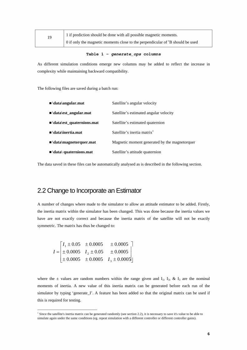
19 1 if prediction should be done with all possible magnetic moments.

0 if only the magnetic moments close to the perpendicular of cB should be used

Table 1 - generate_ops columns

As different simulation conditions emerge new columns may be added to reflect the increase in

complexity while maintaining backward compatibility.

The following files are saved during a batch run:

\data\angular.mat Satellite’s angular velocity

\data\est_angular.mat Satellite’s estimated angular velocity

\data\est_quaternions.mat Satellite’s estimated quaternion

\data\inertia.mat Satellite’s inertia matrix1

\data\magnetorquer.mat Magnetic moment generated by the magnetorquer

\data\ quaternions.mat Satellite’s attitude quaternion

The data saved in these files can be automatically analysed as is described in the following section.

2.2 Change to Incorporate an Estimator

A number of changes where made to the simulator to allow an attitude estimator to be added. Firstly,

the inertia matrix within the simulator has been changed. This was done because the inertia values we

have are not exactly correct and because the inertia matrix of the satellite will not be exactly

symmetric. The matrix has thus be changed to:

⎥⎥⎥

⎦

⎤

⎢⎢⎢

⎣

⎡

±±±±±±±±±

=0005.00005.00005.0

0005.005.00005.00005.00005.005.0

3

2

1

II

II

where the ± values are random numbers within the range given and I1, I3, & I3 are the nominal

moments of inertia. A new value of this inertia matrix can be generated before each run of the

simulator by typing ‘generate_I’. A feature has been added so that the original matrix can be used if

this is required for testing.

1 Since the satellite's inertia matrix can be generated randomly (see section 2.2), it is necessary to save it's value to be able to simulate again under the same conditions (eg. repeat simulation with a different controller or different controller gains).

6

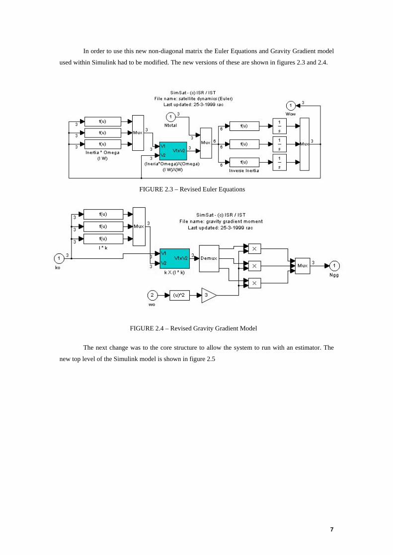
In order to use this new non-diagonal matrix the Euler Equations and Gravity Gradient model

used within Simulink had to be modified. The new versions of these are shown in figures 2.3 and 2.4.

FIGURE 2.3 – Revised Euler Equations

FIGURE 2.4 – Revised Gravity Gradient Model

The next change was to the core structure to allow the system to run with an estimator. The

new top level of the Simulink model is shown in figure 2.5

7

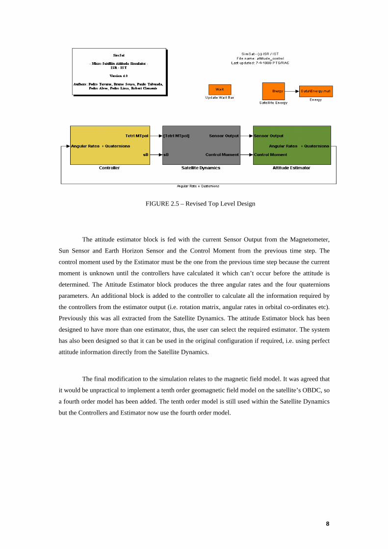
FIGURE 2.5 – Revised Top Level Design

The attitude estimator block is fed with the current Sensor Output from the Magnetometer,

Sun Sensor and Earth Horizon Sensor and the Control Moment from the previous time step. The

control moment used by the Estimator must be the one from the previous time step because the current

moment is unknown until the controllers have calculated it which can’t occur before the attitude is

determined. The Attitude Estimator block produces the three angular rates and the four quaternions

parameters. An additional block is added to the controller to calculate all the information required by

the controllers from the estimator output (i.e. rotation matrix, angular rates in orbital co-ordinates etc).

Previously this was all extracted from the Satellite Dynamics. The attitude Estimator block has been

designed to have more than one estimator, thus, the user can select the required estimator. The system

has also been designed so that it can be used in the original configuration if required, i.e. using perfect

attitude information directly from the Satellite Dynamics.

The final modification to the simulation relates to the magnetic field model. It was agreed that

it would be unpractical to implement a tenth order geomagnetic field model on the satellite’s OBDC, so

a fourth order model has been added. The tenth order model is still used within the Satellite Dynamics

but the Controllers and Estimator now use the fourth order model.

8

3. PoSat-1 Type Actuators

SimSat’s implementation of the magnetic satellite actuators was reviewed after new

information on the nature of PoSat-1’s hardware was available to the group. These changes make the

simulated PoSat-1 actuators more accurate and thus enable the test of control algorithms designed

specifically for this satellite in a realistic fashion.

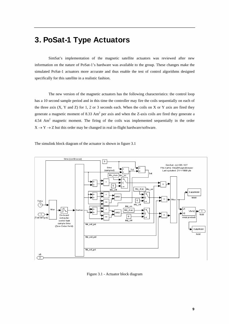
The new version of the magnetic actuators has the following characteristics: the control loop

has a 10 second sample period and in this time the controller may fire the coils sequentially on each of

the three axis (X, Y and Z) for 1, 2 or 3 seconds each. When the coils on X or Y axis are fired they

generate a magnetic moment of 8.33 Am2 per axis and when the Z-axis coils are fired they generate a

4.54 Am2 magnetic moment. The firing of the coils was implemented sequentially in the order

X → Y → Z but this order may be changed in real in-flight hardware/software.

The simulink block diagram of the actuator is shown in figure 3.1

Figure 3.1 - Actuator block diagram

9

The figure 3.2 shows the magnetic moment generated by the magnetorquer in a nominal control

situation.

Figure 3.2 - Magnetorquer output

As the inputs of the magnetorquer block are the three firing duration’s and three coils

polarities (see Figure 3.1 - Actuator block diagram), a further block had to be added to the system to

convert the desired magnetic moment required by the controller into the times and polarities required

by the magnetorquer. This block first extracts the part of the desired magnetic moment (cMd) that is

perpendicular to the geomagnetic field vector (cB). The resulting vector is then resized so that it can be

generated (i.e all 3 components are smaller or equal to the maximum moment possible in each of the

three coils). The resizing is done using the same factor for all three components so that the direction of

the vector isn't changed. Each of the components of the resulting vector is then converted to a time

duration (a simple scalar factor multiplication) and discretized into a value in the set {1,2,3} [second].

The sign of each of the 3 vector components is also extracted at this stage and outputted as polarity of

the coils. This block also saves to the file "Data\Mg.mat" the (generatable) magnetic moment, prior to

discretization.

10

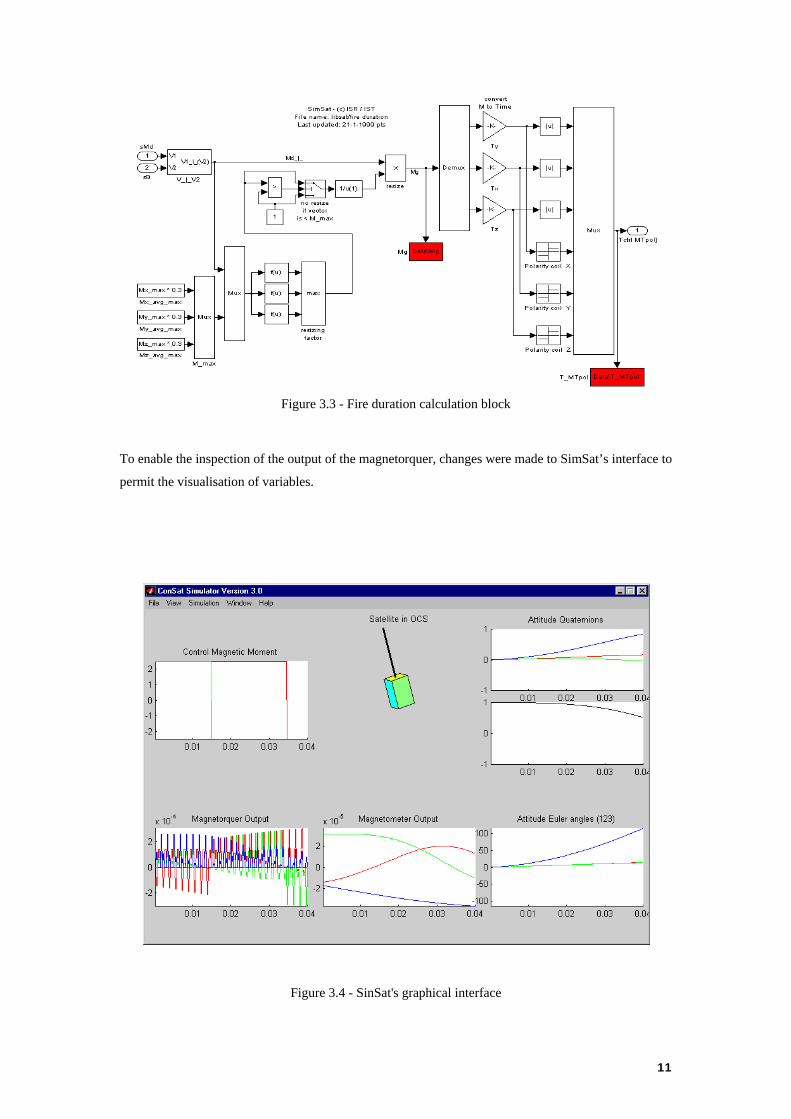
Figure 3.3 - Fire duration calculation block

To enable the inspection of the output of the magnetorquer, changes were made to SimSat’s interface to

permit the visualisation of variables.

Figure 3.4 - SinSat's graphical interface

11

4. Predictive Controller Upgrade

The predictive (or brute-force) controller described in [Tavares-98b] and implemented in

[Tabuada] was reviewed in order to take into account the changes made to the magnetorquer. Basically

these changes meant the increase in the number of magnetic moments that can be generated by the

torquer and the dismissal of the previously used 100-second back-off.

As the coils on each of the satellite’s axis can be fired for 0, 1, 2 or 3 seconds and as the coils

polarity can be reversed, the number of possible different magnetic moments that can be generated per

axis is seven. This means that the number of magnetic moment vectors (X, Y and Z coils) that can be

generated is 73 = 343.

As this number is high, an attempt must be made to reduce the number of vectors searched in

the optimisation of the predictive controller’s cost function which is accomplished excluding the

vectors that are not close to the perpendicular of the geomagnetic field vector. This orthogoanality can

be checked by comparing the dot product of any normalised magnetic moment vector and the

normalised geomagnetic field vector with a threshold. In the present case a threshold of 0.1 was used

and thus a “waste” factor of 10% was deemed acceptable.

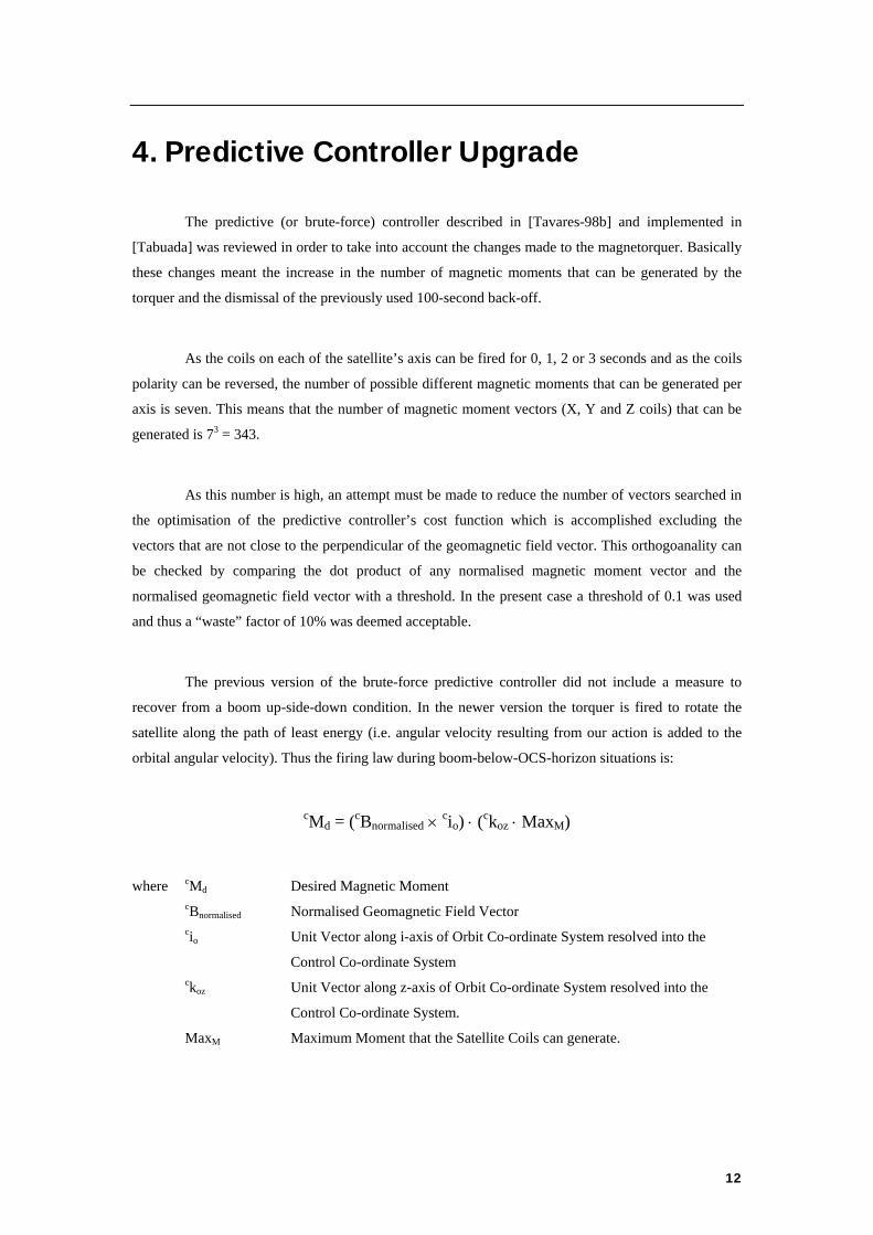
The previous version of the brute-force predictive controller did not include a measure to

recover from a boom up-side-down condition. In the newer version the torquer is fired to rotate the

satellite along the path of least energy (i.e. angular velocity resulting from our action is added to the

orbital angular velocity). Thus the firing law during boom-below-OCS-horizon situations is:

cMd = (cBnormalised × cio) ⋅ (ckoz ⋅ MaxM)

where cMd Desired Magnetic Moment

cBnormalised Normalised Geomagnetic Field Vector

cio Unit Vector along i-axis of Orbit Co-ordinate System resolved into the

Control Co-ordinate System

ckoz Unit Vector along z-axis of Orbit Co-ordinate System resolved into the

Control Co-ordinate System.

MaxM Maximum Moment that the Satellite Coils can generate.

12

5. Sensors 5.1 Sun Sensor

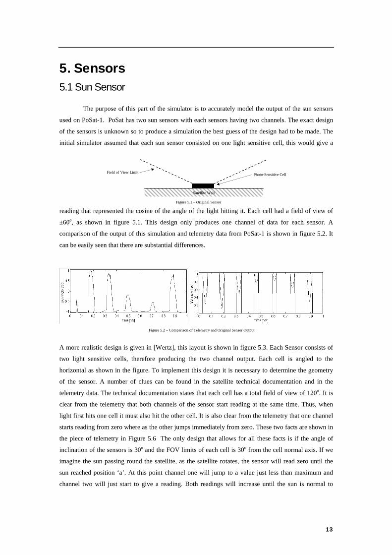
The purpose of this part of the simulator is to accurately model the output of the sun sensors

used on PoSat-1. PoSat has two sun sensors with each sensors having two channels. The exact design

of the sensors is unknown so to produce a simulation the best guess of the design had to be made. The

initial simulator assumed that each sun sensor consisted on one light sensitive cell, this would give a

reading that represented the cosine of the angle of the light hitting it. Each cell had a field of view of

±60o, as shown in figure 5.1. This design only produces one channel of data for each sensor. A

comparison of the output of this simulation and telemetry data from PoSat-1 is shown in figure 5.2. It

can be easily seen that there are substantial differences.

Satellite Wall

Field of View Limit

Figure 5.1 – Original Sensor

Photo-Sensitive Cell

Figure 5.2 – Comparison of Telemetry and Original Sensor Output

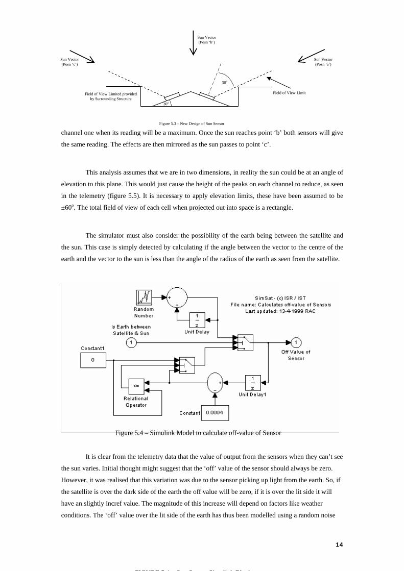
A more realistic design is given in [Wertz], this layout is shown in figure 5.3. Each Sensor consists of

two light sensitive cells, therefore producing the two channel output. Each cell is angled to the

horizontal as shown in the figure. To implement this design it is necessary to determine the geometry

of the sensor. A number of clues can be found in the satellite technical documentation and in the

telemetry data. The technical documentation states that each cell has a total field of view of 120o. It is

clear from the telemetry that both channels of the sensor start reading at the same time. Thus, when

light first hits one cell it must also hit the other cell. It is also clear from the telemetry that one channel

starts reading from zero where as the other jumps immediately from zero. These two facts are shown in

the piece of telemetry in Figure 5.6 The only design that allows for all these facts is if the angle of

inclination of the sensors is 30o and the FOV limits of each cell is 30o from the cell normal axis. If we

imagine the sun passing round the satellite, as the satellite rotates, the sensor will read zero until the

sun reached position ‘a’. At this point channel one will jump to a value just less than maximum and

channel two will just start to give a reading. Both readings will increase until the sun is normal to

13

Sun Vector (Posn ‘c’)

Sun Vector (Posn ‘b’)

Sun Vector (Posn ‘a’)

30o

30o

Field of View Limited provided by Surrounding Structure

Field of View Limit

Figure 5.3 – New Design of Sun Sensor

channel one when its reading will be a maximum. Once the sun reaches point ‘b’ both sensors will give

the same reading. The effects are then mirrored as the sun passes to point ‘c’.

This analysis assumes that we are in two dimensions, in reality the sun could be at an angle of

elevation to this plane. This would just cause the height of the peaks on each channel to reduce, as seen

in the telemetry (figure 5.5). It is necessary to apply elevation limits, these have been assumed to be

±60o. The total field of view of each cell when projected out into space is a rectangle.

The simulator must also consider the possibility of the earth being between the satellite and

the sun. This case is simply detected by calculating if the angle between the vector to the centre of the

earth and the vector to the sun is less than the angle of the radius of the earth as seen from the satellite.

Figure 5.4 – Simulink Model to calculate off-value of Sensor

It is clear from the telemetry data that the value of output from the sensors when they can’t see

the sun varies. Initial thought might suggest that the ‘off’ value of the sensor should always be zero.

However, it was realised that this variation was due to the sensor picking up light from the earth. So, if

the satellite is over the dark side of the earth the off value will be zero, if it is over the lit side it will

have an slightly incref value. The magnitude of this increase will depend on factors like weather

conditions. The ‘off’ value over the lit side of the earth has thus been modelled using a random noise

14

FIGURE 5 4 S S Si li k Bl k

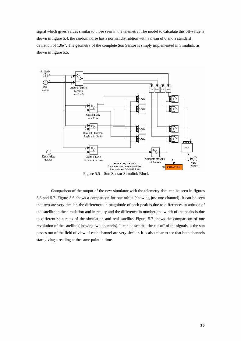
signal which gives values similar to those seen in the telemetry. The model to calculate this off-value is

shown in figure 5.4, the random noise has a normal distrubtion with a mean of 0 and a standard

deviation of 1.0e-5. The geometry of the complete Sun Sensor is simply implemented in Simulink, as

shown in figure 5.5.

Figure 5.5 – Sun Sensor Simulink Block

Comparison of the output of the new simulator with the telemetry data can be seen in figures

5.6 and 5.7. Figure 5.6 shows a comparison for one orbits (showing just one channel). It can be seen

that two are very similar, the differences in magnitude of each peak is due to differences in attitude of

the satellite in the simulation and in reality and the difference in number and width of the peaks is due

to different spin rates of the simulation and real satellite. Figure 5.7 shows the comparison of one

revolution of the satellite (showing two channels). It can be see that the cut-off of the signals as the sun

passes out of the field of view of each channel are very similar. It is also clear to see that both channels

start giving a reading at the same point in time.

15

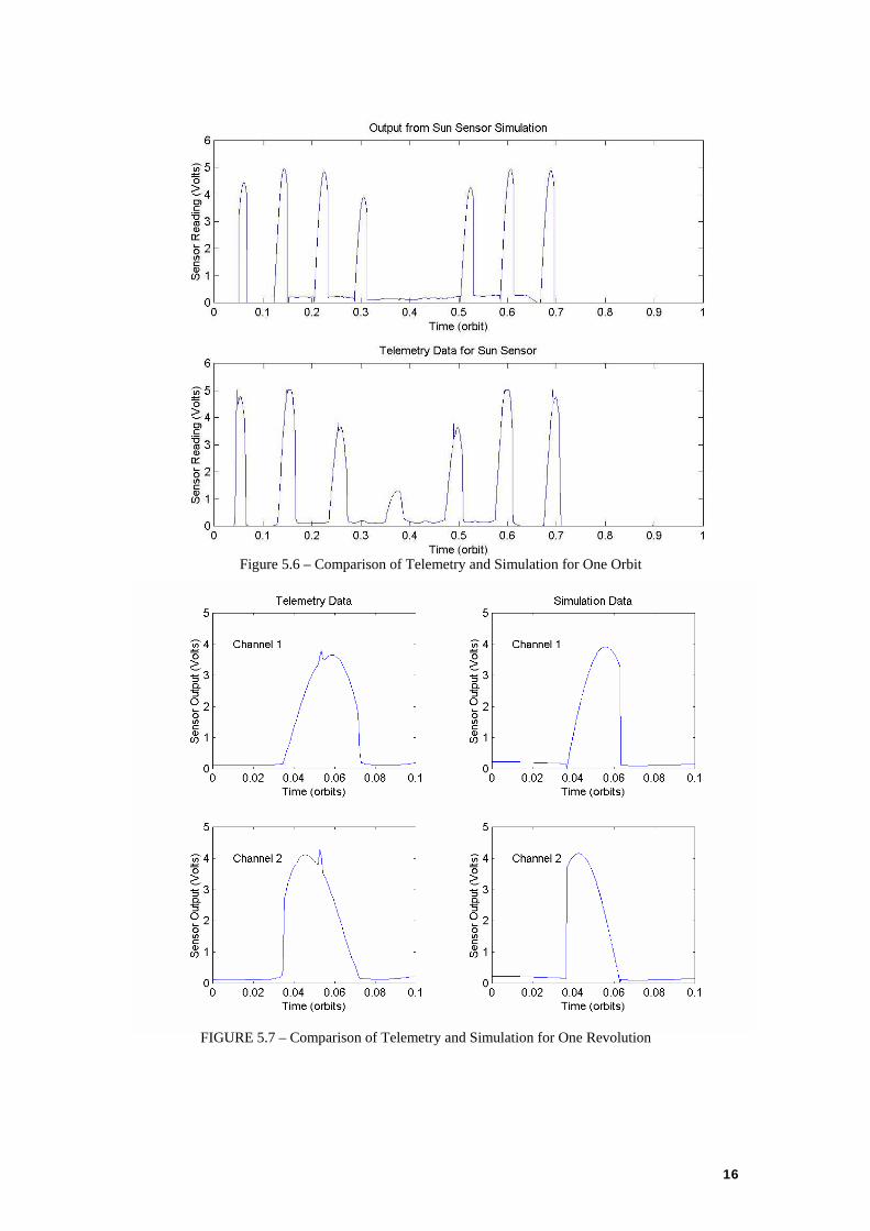
Figure 5.6 – Comparison of Telemetry and Simulation for One Orbit

FIGURE 5.7 – Comparison of Telemetry and Simulation for One Revolution

16

5.2 Earth Horizon Sensor

PoSat-1 has two Earth Horizon Sensors (EHS). Each EHS is a camera which looks down at the earth

horizon. The view of the camera is a narrow slot, the output of the sensor is related to the amount of

that slot that is lit, i.e., the sensor would read 1 if the slot was looking totally at the earth, 0 if it was

looking into space and somewhere in between if the horizon line falls somewhere across that slot.

The initial version of the EHS simulator made two assumptions: 1) The earth underneath the satellite

was always fully lit, this is clearly only true for one part of the orbit; 2) The view of the sensor will

always be aligned with a diameter of the earth, this is only true if the OCS is aligned with the SCS.

The key to an accurate simulation is to determine, given the relative positions of the sun, earth and

satellite, the current view of the earth from the satellite (this is like viewing the moon from the earth).

The earth may appear fully lit, total dark or somewhere in between. Once the view of the earth is

determined the slot that the EHS camera looks through can be projected onto this view and the amount

of that slot which is seeing light can be determined.

Vector of Lower Field of

View Limit

Vector of Upper Field

of View Limit

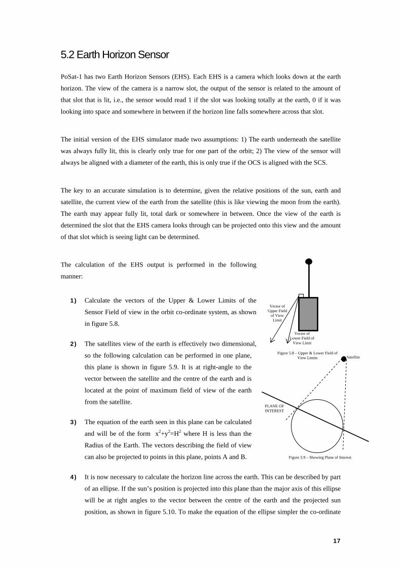
The calculation of the EHS output is performed in the following

manner:

1) Calculate the vectors of the Upper & Lower Limits of the

Sensor Field of view in the orbit co-ordinate system, as shown

in figure 5.8.

2) The satellites view of the earth is effectively two dimensional,

so the following calculation can be performed in one plane,

this plane is shown in figure 5.9. It is at right-angle to the

vector between the satellite and the centre of the earth and is

located at the point of maximum field of view of the earth

from the satellite.

Figure 5.8 – Upper & Lower Field of View Limits

PLANE OF INTEREST

Satellite

Figure 5.9 – Showing Plane of Interest

3) The equation of the earth seen in this plane can be calculated

and will be of the form x2+y2=H2 where H is less than the

Radius of the Earth. The vectors describing the field of view

can also be projected to points in this plane, points A and B.

4) It is now necessary to calculate the horizon line across the earth. This can be described by part

of an ellipse. If the sun’s position is projected into this plane than the major axis of this ellipse

will be at right angles to the vector between the centre of the earth and the projected sun

position, as shown in figure 5.10. To make the equation of the ellipse simpler the co-ordinate

17

system can now be rotated to align with this major axis (new

system u,v). The points A and B can also be determined in

the new co-ordinate system

5) The equation of the ellipse is thus 222

Rvau

=+⎟⎠⎞

⎜⎝⎛

where

R is the radius of the earth and ‘a’ relates to the size of the

ellipse. This value ‘a’ is determined by the angle of

elevation of the sun from this plane. If the elevation angle

was 90o or 270o then a must be 1, if the elevation angle was

0o or 180o then a must be 0. The value of a is, thus, given by

the cosine of the sun elevation angle. If ‘a’ is less than 0.001

then the ellipse is assumed to be a straight line.

SUN projected onto plane

Major Axis of Ellipse

Earth as view from Satellite

Figure 5.10 – Showing Ellipse that describes the Horizon Line

Ellipse describing

Horizon Line

(c)

(b)

(a)

Figure 5.11 – Showing Light and Dark parts of Earth

6) The current picture is shown in figure 5.11. The earth is now

divided into three parts by the ellipse. It is necessary to

determine which of these parts are lit and which are in

darkness. This is depended on whether the sun is above of

below the plane. If the sun, in figure 5.11, was above the

plane then parts (a) and (b) would be lit, however, if the sun

was below the plane only part (a) would be lit.

7) The equation of the line connecting points A and B can easily

be found. With this equation, the equation of the circle and

ellipse intersection points can be calculated. There will be a

maximum of four intersection points. An example of one

possibility is shown in figure 5.12. Knowing the positions of A

and B and each of these intersections it is relatively simple to calculate if the line between A

and B is full lit, full dark, or if it crosses a horizon line. In the last case the output value can be

found as the percentage of the line that is lit.

Figure 5.12 – Showing View of Sensor with Horizon Line

A

B

View of Sensor

Dark Side of the Earth

The EHS is very sensitive to attitude. Perturbations greater that ±5o will saturate the sensor. For this

reason to get a good comparison between telemetry and simulation it is important that the attitude is

very similar. The attitude of the satellite is unknown for the period of the telemetry data so accurate

comparison is not possible. Figure 5.13 shows a comparison with different attitude. Although they are

quite different whilst the sensor is ‘on’ it shows the peaks that occur as the satellite passes over the

earth horizon. i.e. as the satellite is over the horizon line, during one revolution the sensor will see a

dark earth on one half and a lit earth on the other half of the revolution. This gives the single peak

either side of the main ‘on’ part which is seen in both the telemetry and the simulation. It also shows

the sensor switches off whilst over the dark side of the earth.

18

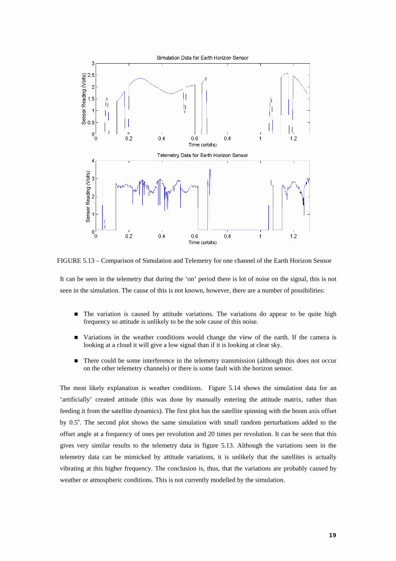
FIGURE 5.13 – Comparison of Simulation and Telemetry for one channel of the Earth Horizon Sensor

It can be seen in the telemetry that during the ‘on’ period there is lot of noise on the signal, this is not

seen in the simulation. The cause of this is not known, however, there are a number of possibilities:

The variation is caused by attitude variations. The variations do appear to be quite high frequency so attitude is unlikely to be the sole cause of this noise.

Variations in the weather conditions would change the view of the earth. If the camera is looking at a cloud it will give a low signal than if it is looking at clear sky.

There could be some interference in the telemetry transmission (although this does not occur on the other telemetry channels) or there is some fault with the horizon sensor.

The most likely explanation is weather conditions. Figure 5.14 shows the simulation data for an

‘artificially’ created attitude (this was done by manually entering the attitude matrix, rather than

feeding it from the satellite dynamics). The first plot has the satellite spinning with the boom axis offset

by 0.5o. The second plot shows the same simulation with small random perturbations added to the

offset angle at a frequency of ones per revolution and 20 times per revolution. It can be seen that this

gives very similar results to the telemetry data in figure 5.13. Although the variations seen in the

telemetry data can be mimicked by attitude variations, it is unlikely that the satellites is actually

vibrating at this higher frequency. The conclusion is, thus, that the variations are probably caused by

weather or atmospheric conditions. This is not currently modelled by the simulation.

19

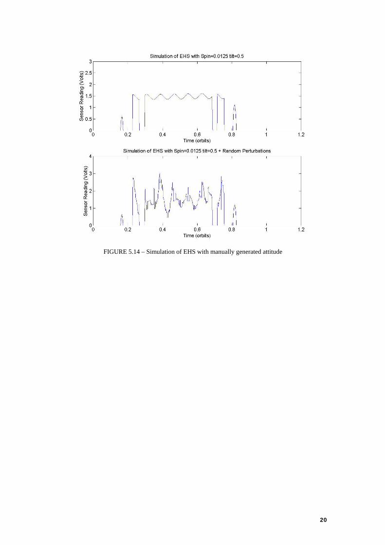
FIGURE 5.14 – Simulation of EHS with manually generated attitude

20

6. Estimator The current estimator is based on the Kalman Filter method as proposed in [W.H.Steyn]. The method

used by [Steyn] has been modified so that the quaternions are normalised after a new measurement has

been added. This method only uses the magnetometer output. Future versions of this estimator will also

incorporate the Sun and Earth Horizon Sensors. The estimator uses a 4TH Order Geomagnetic Field

model. The inertia matrix used within the estimator is the nominal diagional matrix.

The estimator currently requires knowledge of the initial state of the satellite. The true initial state is

known within the simulator, this is augmented with a 20% error factor. This augmented state is then

used to provide initial data to the estimator.

The estimator is currently predicting attitude to a mean error of 2.5o. The goal is to tune the covariance

matrices to improve this value. The target is to bring it below 0.5o

21

7. Automated Result Analysis Two functions have been written to analysis the results produced by the simulator. The first is designed

to analysis the performance of the controller, the second is designed to analysis the performance of the

estimator.

7.1 Controller Data Analysis

The data generated by SimSat can be automatically analysed by the Matlab script in the file

“results.m”. When run the script will require the user to specify the batch simulation starting and

ending numbers, ask if the data analysed is to be plotted (individually) and if a table of results is to be

generated.

The script determines the following from the saved data:

Gamma angle (between the boom and oZ)

Gamma settling time to within 5 degrees

Gamma settling time to within 1 degree

Gamma after 3 and 5 orbits

Pointing accuracy

Angular velocity settling time within 0.0005 radians

Accuracy error (as a percentage relative to the 0.02 rad/s reference)

These results are saved in a MAT file called “resultX.mat” in the “sim_results” folder, where X stands

for the simulation number.

If a table was required, one will be saved in a file named “tableX1_X2.txt”, where X1 is the starting

simulation number and X2 the ending simulation number. This file will be created below the

“sim_results” folder and will contain a line with the results listed above for every simulation analysed

and the mean, standard deviation and worst case for every result. The values on this file are stored in

ASCII and are delimited with tabs to facilitate the importing of the data to spreadsheets and word

processors.

22

7.2 Estimator Data Analysis

The file ‘est_results’ has been written to determine the performance of the estimator. It calculates from

the files produced by the simulation the following information:

The mean angle between the z-axis of the true satellite co-ordinate system and the estimated co-ordinate system.

The standard deviation of the angle between the z-axis of the true satellite co-ordinate system and the estimated co-ordinate system.

The percentage error in the estimation of the spin rate.

The standard deviation of the percentage error in the estimation of the spin rate.

The maximum quaternion error and the time at which it occurred

The maximum angular rate error and the time at which it occurred.

23

8. Bibliography [Tabuada] Tabuada, Paulo; Alves, Pedro; Tavares, Pedro; Lima, Pedro.

(1998). Attitude Control Strategies for Small Satellites. Institute for Systems and Robotics / IST internal report.

[Tavares-98a] Tavares, Pedro; Sousa, Bruno; Lima, Pedro. (1998). A Simulator of Satellite Attitude Dynamics. Proc. of the 3rd Portuguese Conference on Automatic Control, Vol. II, pp. 459-464, Coimbra, Portugal.

[Tavares-98b] Tavares, Pedro; Tabuada, Paulo; Lima, Pedro. (1998). Project ConSat: Control of Small Satellites. Control of Complex Systems Annual Joint Workshop, Ohrid, FYR of Macedonia.

[Wertz, J.R.] Spacecraft Attitude Determination and Control

[Steyn, W.H.] Full Satellite State Determination from Vector Observations

24