NBER WORKING PAPER SERIES

UPCODING: EVIDENCE FROM MEDICARE ON SQUISHY RISK ADJUSTMENT

Michael GerusoTimothy Layton

Working Paper 21222http://www.nber.org/papers/w21222

NATIONAL BUREAU OF ECONOMIC RESEARCH1050 Massachusetts Avenue

Cambridge, MA 02138May 2015

We thank Colleen Carey, Joshua Gottlieb, and Amanda Kowalski for serving as discussants, as wellas seminar participants at the 2014 Annual Health Economics Conference, the 2014 American Societyof Health Economists Meeting, the BU/Harvard/MIT Health Economics Seminar, Boston University,Harvard Medical School, the NBER Public Economics Meeting 2015, the University of Illinois atChicago, RTI, the Southeastern Health Economics Study Group, and the University of Texas at Austinfor useful comments. We also thank Chris Afendulis, Marika Cabral, Vilsa Curto, David Cutler, FrancescoDecarolis, Liran Einav, Randy Ellis, Keith Ericson, Amy Finkelstein, Austin Frakt, Craig Garthwaite,Jonathan Gruber, Jonathan Kolstad, Tom McGuire, Hannah Neprash, Joe Newhouse, and Daria Pelechfor assistance with data and useful conversations. We gratefully acknowledge financial support fromthe National Institute of Mental Health (Layton, T32-019733). The views expressed herein are thoseof the authors and do not necessarily reflect the views of the National Bureau of Economic Research.

NBER working papers are circulated for discussion and comment purposes. They have not been peer-reviewed or been subject to the review by the NBER Board of Directors that accompanies officialNBER publications.

© 2015 by Michael Geruso and Timothy Layton. All rights reserved. Short sections of text, not toexceed two paragraphs, may be quoted without explicit permission provided that full credit, including© notice, is given to the source.

Upcoding: Evidence from Medicare on Squishy Risk AdjustmentMichael Geruso and Timothy LaytonNBER Working Paper No. 21222May 2015JEL No. H42,H51,I1,I13,I18

ABSTRACT

Diagnosis-based subsidies, also known as risk adjustment, are widely used in US health insurancemarkets to deal with problems of adverse selection and cream-skimming. The widespread use of thesesubsidies has generated broad policy, research, and popular interest in the idea of upcoding—the notionthat diagnosed medical conditions may reflect behaviors of health plans and providers to game thepayment system, rather than solely characteristics of patients. We introduce a model showing thatcoding differences across health plans have important consequences for public finances and consumerchoices, whether or not such differences arise from gaming. We then develop and implement a novelstrategy for identifying coding differences across insurers in equilibrium in the presence of selection.Empirically, we examine how coding intensity in Medicare differs between the traditional fee-for-serviceoption, in which coding incentives are weak, and Medicare Advantage, in which insurers receive diagnosis-basedsubsidies. Our estimates imply that enrollees in private Medicare Advantage plans generate 6% to16% higher diagnosis-based risk scores than the same enrollees would generate under fee-for-serviceMedicare. Consistent with a principal-agent problem faced by insurers attempting to induce their providersto upcode, we find that coding intensity increases with the level of vertical integration between insurersand the physicians with whom they contract. Absent a coding inflation correction, our findings implyexcess public payments to Medicare Advantage plans of around $10 billion annually. This differentialsubsidy also distorts consumers' choices toward private Medicare plans and away from fee-for-serviceMedicare.

Michael GerusoUniversity of Texas at AustinDepartment of Economics1 University Station C3100Austin, TX 78712and NBERmike.geruso@austin.utexas.edu

Timothy LaytonDepartment of Health Care PolicyHarvard Medical School180 Longwood AvenueBoston, MA 02115layton@hcp.med.harvard.edu

1 Introduction

Diagnosis-based subsidies have become an increasingly important regulatory tool in US health in-

surance markets. Between 2003 and 2014, the number of consumers enrolled in a market where an

insurer’s payment is based on the consumer’s diagnosed health state increased from almost zero

to around 50 million, including in Medicare, Medicaid, and state and federal Health Insurance Ex-

changes. These diagnosis-based payments to insurers are typically known as risk adjustment. By

compensating insurers for enrolling high expected-cost consumers, risk adjustment weakens insurer

incentives to engage in cream-skimming—that is, inefficiently distorting insurance product charac-

teristics to attract lower-cost enrollees as in Rothschild and Stiglitz (1976).1 It also works to solve the

Akerlof (1971) problem of high-cost enrollees driving up contract prices, leading to market unravel-

ling.

The intuition underlying risk adjustment is straightforward, but the mechanism relies on a reg-

ulator’s ability to generate an accurate measure of each consumer’s health state. In practice in health

insurance markets, the diagnoses used to determine insurer payment are reported by physicians and

then aggregated into a risk score that reflects the consumer’s expected claims cost. A higher score

yields a higher net payment to the insurer, in many settings at a cost to the public. Therefore, insurers

are incentivized to influence physicians to “upcode” diagnosis information in the patient’s record to

maximize the insurer subsidy, for instance by paying physicians on the basis of the codes they assign.

The extent to which they do so in practice is of considerable policy, industry, and popular interest.2

Nonetheless, relatively little is known about the extent of upcoding in these contexts or its impacts in

terms of public costs or consumer choices.3

In this paper, we characterize the distortions and excess public spending created by coding dif-

ferences across insurers, and then quantify these impacts in the context of the Medicare program.

We begin by constructing a simple framework that assumes a risk score is generated by an enrollee

× insurer match, and therefore would vary for the same individual depending on her choice of in-

1For instance, in Medicare Advantage a diagnosis of the condition Diabetes with Acute Complications generates apayment for the private insurer that enrolls the patient that is incrementally larger by about $3,390 per year, the averageincremental cost incurred by individuals diagnosed with Diabetes with Acute Complications in the traditional fee-for-service Medicare program.

2See, for example, CMS, 2010; Government Accountability Office, 2013; Kronick and Welch, 2014; Schulte, 2014.3There has been substantial research into the statistical aspects of diagnosis-based risk adjustment models in the health

services literature, but such studies do not allow the possibility that there could be endogenous insurer responses to thecoding incentive or differences across insurers for any reason.

1

surance plan. We show that if risk scores vary across insurers for the same consumers, then even

when risk adjustment is successful in counteracting both the Rothschild and Stiglitz (1976) and Ak-

erlof (1971) selection inefficiencies, it introduces a new distortion by differentially subsidizing plans

with higher coding intensity. This differential payment for intensive coding has two effects: First,

in a partially privatized public spending program like Medicare, upcoding impacts the program’s

cost to taxpayers. Second, because the differential payment implicitly creates a voucher that is larger

when consumers choose a plan with higher coding intensity, consumer choices can be inefficiently

tilted toward these plans. This choice distortion has not been previously noted, though we show it

operates in any risk-adjusted market, including Medicare, many state Medicaid programs, and the

Affordable Care Act (ACA) Health Insurance Exchanges.

We investigate the empirical importance of upcoding in Medicare. For hospital and physician

coverage, Medicare beneficiaries can choose between a traditional fee-for-service (FFS) option and

enrolling with a private insurer through Medicare Advantage (MA). In the FFS system, most re-

imbursement is independent of recorded diagnoses. Payments to private MA plans, however, are

capitated with risk adjustment based on the recorded diagnoses of their enrollees. This provides MA

plans with direct and strong financial incentives to code intensely. Although the incentive for MA

plans to code intensely is strong, the ability of the plans to respond to this incentive depends on the

plans’ ability to influence the providers that assign diagnosis codes.4 Thus, whether and to what

extent coding differs between the MA and FFS segments of the market is an empirical question.

The key challenge in identifying coding intensity differences between FFS and MA, or within

the MA market segment among competing insurers, is that upcoding estimates are potentially con-

founded by adverse selection. An insurer might report an enrollee population with higher-than-

average risk scores either because the consumers who choose the insurer’s plan are in worse health

(selection) or because for the same individual, the insurer’s coding practices result in higher risk

scores (upcoding). Effects of coding and selection are therefore observationally equivalent at the plan

level. We develop an approach to separately identify selection and coding differences in equilibrium.

The core insight of our identification approach is that if the same individual would generate a differ-

ent risk score under two insurers and if we observe an exogenous shift in the market shares of the

two insurers, then we should also observe changes in the market-level average of reported risk scores.

4In addition, if generating higher risk scores requires more (costly) contact with patients, then MA plans face a counter-vailing incentive because the plan is the residual claimant on any dollars not spent on patient care.

2

Such a pattern could not be generated by selection, because selection can affect only the sorting of

risk types across insurers within the market, not the overall market-level distribution of reported risk

scores. Our strategy is related to that of Chetty, Friedman and Rockoff (2014), who identify teacher

value-added via changes in the composition of teaching staff within a grade over time. These authors

analogously avoid biases introduced by endogenous student sorting across teachers by examining

changes in outcomes aggregated up to the grade level, rather than at the teacher level.5 A key advan-

tage of our strategy is that the data requirements are minimal, and it could be easily implemented in

future assessments of coding in Health Insurance Exchanges or state Medicaid programs.6

We exploit large and geographically diverse increases in MA enrollment that began in 2006 in

response to the Medicare Modernization Act in order to identify variation in MA penetration that

was plausibly uncorrelated with changes in real underlying health at the market (county) level.7 We

simultaneously exploit an institutional feature of the MA program that causes risk scores to be based

on prior year diagnoses. This yields sharp predictions about the timing of effects relative to chang-

ing penetration in a difference-in-diferences framework. Using the rapid within-county changes in

penetration that occurred over our short panel, we find that a 10 percentage point increase in MA

penetration leads to a 0.64 percentage point increase in the reported average risk score in a county.

This implies that MA plans generate risk scores for their enrollees that are on average 6.4% larger

than what those same enrollees would have generated under FFS. Further, we show that the size of

this coding difference is related to the vertical relationship between insurers and providers. Health

maintenance organizations (HMOs) have the highest coding intensity of all plan types operating in

the Medicare Advantage market, and fully vertically integrated (i.e., physician owned) plans gen-

erate 16% higher risk scores for the same patients compared to FFS, nearly triple the effect of non-

integrated plans.

The identifying assumption driving our results is that true population health did not vary con-

temporaneously with these penetration changes within markets. In addition to providing a series of

5A closer analog of our method to the educational context would be for use in separating selection and program effectsin other contexts where, within a geographic market, a fixed population chooses between public and private providers of aservice. For example, our method could be used to estimate causal effects of charter schools on student outcomes in a waythat is robust to endogenous sorting of students across schools.

6The key advantages here are that market-level average risk scores and plan enrollment data are sufficient for analysisand that the strategy does not rely on a natural experiment that changes how particular codes are reimbursed. Onlyexogenous shifts in plan market shares are needed for identification.

7The current risk adjustment system was implemented in MA in 2004 and fully phased in by 2007. Data on risk scoresin MA are available from the regulator beginning in 2006.

3

tests that support our parallel trends assumption, we show it is difficult to rationalize our results by

the alternative explanation that they reflect changes in underlying health. First, the precise timing

of the response (with a one-year lag) corresponds exactly to the institutional feature that causes risk

scores to be based on prior year diagnoses. Second, the effect is large: a 7% increase in the average risk

score is equivalent to 7% of all consumers in the market becoming paraplegic, 12% of all consumers

developing Parkinson’s disease, or 43% becoming diabetics. While these effects would be implausi-

bly large if they captured rapid changes to true population health, these effects are not implausibly

large as manifestations of coding behavior.8 And, finally, for a small sample of Massachusetts resi-

dents, we provide individual-level evidence, tracking risk scores within consumers as they transition

from an employer plan to an MA plan or FFS Medicare at the age 65 eligibility threshold. This alter-

native identification strategy based on person fixed effects yields results closely consistent with our

main analysis.

We view our results as addressing an important gap in the literature on adverse selection and

the public finance of healthcare. The most closely related prior work on coding has shown that pa-

tients’ reported diagnoses vary with the local practice style of physicians (Song et al., 2010) and that

coding responds to changes in how particular codes are reimbursed by FFS Medicare for inpatient

hospital stays (Dafny, 2005; Sacarny, 2014). Ours is the first study to model the implications of dif-

ferential coding patterns across insurers and to provide empirical evidence of such differences. The

recent surge in applied theoretical and empirical work on inefficient selection in insurance markets

(see Einav, Finkelstein and Levin, 2010 and Chetty and Finkelstein, 2013 for overviews) has largely

ignored risk adjustment and the potential it introduces for upcoding, even though risk adjustment

is the most widely implemented regulatory response to selection. And while there has been sub-

stantial research into the statistical aspects of diagnosis-based risk adjustment models in the health

services literature, the distortionary implications of coding heterogeneity have received little atten-

tion.9 Our work highlights these distortions and traces several implications that have not previously

been considered.

8Our estimates are in line with the stated beliefs of regulators and government analysts. CMS began deflating MArisk scores by 3.41% in 2010 because of suspected differential coding, while the Government Accountability Office hasconsistently argued for a larger deflation. In 2014, the CMS deflation increased to 4.91%, and it is slated to rise to 5.91% in2015, consistent with our findings.

9The few recent papers that have examined the distortionary implications of risk adjustment include Brown et al. (2014),Carey (2014), Geruso and McGuire (2015), and Einav et al. (2015), though none of these has explored the phenomenon ofinterest here: whether risk scores are endogenous to the insurer, rather than a fixed characteristic of the insured.

4

For example, our framework shows (i) that the differential reimbursement to more intensely

coded plans can distort consumer choices, (ii) that increasing the competitiveness of the market can

actually worsen this distortion and reduce net efficiency—increased competition tips the incidence

of the subsidy away from producers and toward consumers, but this shift in incidence more strongly

distorts consumers’ choices—and (iii) that it is not necessary to take a stand on which insurer’s coding

regime is objectively correct for many questions related to the public finance and consumer choice im-

plications of differential coding. In our empirical setting, this means that it does not matter whether

physicians billing under FFS Medicare pay too little attention to coding or whether MA insurers pay

too much attention to coding. It also implies that even if the higher coding intensity is valued by

consumers—for example, because higher intensity is associated with better continuity of care—the

differential reimbursement is nonetheless distortionary.

Our empirical findings have specific implications for Medicare as well as broader implications

for the regulation of private insurance markets. Medicare is the costliest public health insurance

program in the world and makes up a significant fraction of US government spending. Absent a

coding correction, our estimates imply excess payments of around $10.5 billion to Medicare Advan-

tage plans annually, or about $640 per MA enrollee per year.10 To put the magnitude in context, this

is about twice as large as the Brown et al. (2014) estimate of the increase in excess payments to MA

plans due to uncompensated favorable selection following the implementation of risk adjustment. It

is also more than three times the size of the excess government payments in Medicare Part D that Ho,

Hogan and Scott Morton (2014) estimate arise from consumers’ inattention to health plan choice and

insurers’ endogenous responses to that inattention. Although, similar to Brown et al. (2014) and Ho,

Hogan and Scott Morton (2014), our identifying variation is not suited to performing a full welfare

analysis, we note that the public spending implications of upcoding in Medicare are significant.11

More broadly, our findings are directly relevant for risk adjustment in other US markets, includ-

10In 2010, toward the end of our study period, CMS began deflating MA risk scores by 3.41% due to concerns aboutupcoding. Our results indicate that the 2010 deflation adjustment is both too small and fails to account for large codingdifferences across insurance contract types. In 2015, the deflation is slated to increase to a uniform 5.91%.

11Our findings also contribute to the growing policy literature on the broader welfare impacts of the MA program.In addition to the benefits of expanding choice, one popular argument in favor of MA is that it might create importantspillover effects for FFS Medicare. Studies of physician and hospital behavior in response to the growth of managed caresuggest the possibility of positive externalities in which the existence of managed care plans lowers costs for all localinsurers (see for example, Baker, 1997; Glied and Zivin, 2002; Glazer and McGuire, 2002; Frank and Zeckhauser, 2000).Most recently, Baicker, Chernew and Robbins (2013) find that the expansion of MA resulted in lower hospital costs inFFS Medicare. Our findings indicate that these benefits of privatized Medicare do not come without costs. Any positivespillovers should be balanced alongside the additional costs (the deadweight loss of taxation plus welfare losses due tochoice distortions) of upcoding in MA.

5

ing the state and federal Health Insurance Exchanges created by the ACA. Payments to Exchange

plans are risk adjusted using a model very similar to the Medicare Advantage risk adjustment model.

In the Exchanges, where there is no public option, risk adjustment is budget neutral: Payments to

insurers that report sicker enrollees are funded by transfers from insurers that report healthier en-

rollees. In such an environment, differential coding across insurers would have no effect on public

finances but would result in transfers from plans with less intensive coding to plans with more in-

tensive coding. The evidence in this paper implies that these transfers will distort consumer choices

toward more integrated plans.

Finally, our results provide a rare insight into the insurer-provider relationship. Because diag-

nosis codes ultimately originate from provider visits, insurers face a principal-agent problem in con-

tracting with physicians. Our findings suggest that, in the context of coding, insurers have largely

been able to solve this principal-agent problem. Further, we show that coding intensity varies signif-

icantly according to the contractual relationship between the physician and the insurer, suggesting

that the cost of aligning physician incentives with insurer objectives may be significantly lower in

vertically integrated firms. These results connect to a long literature concerned with the internal

organization of firms and the application of these ideas to the healthcare industry (e.g., Gaynor, Reb-

itzer and Taylor, 2004), as well as to the study of the intrinsic (Kolstad, 2013) and extrinsic (Clemens

and Gottlieb, 2014) motivations of physicians. These results also represent the first direct evidence of

which we are aware that vertical integration between insurers and providers facilitates the “gaming”

of health insurance payment systems. However, these results likewise represent evidence that strong

insurer-provider contracts may also facilitate other, more socially beneficial, insurer objectives, in-

cluding quality improvements through “pay-for-performance” initiatives and cost containment via

capitation contracts. This is an issue of significant policy interest, but for which there is relatively

little prior evidence.12

The outline for the remainder of the paper is as follows. In Section 2, we provide a brief overview

of how insurers can influence the diagnoses assigned to their enrollees, and the implications for

consumer choices and public spending. In Section 3, we explain our strategy for estimating upcoding

in the presence of selection. In Section 4, we discuss our data and empirical setting. In sections 5 and

6, we present results, and in Section 7 we discuss several implications of our findings for policy and

12For a discussion of this literature, see Gaynor, Ho and Town (2015).

6

economic efficiency. We discuss our conclusions in Section 8.

2 Model of Risk Adjustment with Endogenous Coding

2.1 Risk Adjustment

We begin by briefly describing the functioning of a risk-adjusted payment system in a regulated pri-

vate insurance market. Plans receive payment from a regulator for each individual they enroll, which

supplements or replaces premiums paid by the enrollee. The net payment R after risk adjustment

for enrolling individual i is equal to the individual’s risk score, ri, multiplied by some benchmark

amount, φ, set by the regulator: Ri = φ · ri.13 The regulator distributes risk adjustment payments

from a fund, or enforces transfers across plans.14 The risk score itself is calculated by multiplying a

vector of risk adjusters, xi, by a vector of risk adjustment coefficients, Λ. Net payments are therefore

Ri = φ · xiΛ. By compensating the insurer for an enrollee’s expected cost, risk adjustment makes all

potential enrollees appear equally profitable to the insurer, in principle, since all enrollees have the

same net expected cost. This removes incentives to distort contracts to attract lower-cost enrollees,

as in Rothschild and Stiglitz (1976). Because risk adjustment does not compensate for realized costs,

insurers still bear all risk and remain the residual claimants on lower patient healthcare spending.

In health insurance markets, risk adjusters, xi, typically consist of a set of indicators for demo-

graphic groups (age-by-sex cells) and a set of indicators for condition categories, which are based

on diagnosis codes contained in health insurance claims. In Medicare, as well as the federal Health

Insurance Exchanges, these indicators are referred to as Hierarchical Condition Categories (HCCs).

Below, we refer to xi as conditions for simplicity. The coefficients, Λ, capture the incremental impact

of each condition on the insurer’s expected costs, as estimated by the regulator in a regression of total

spending on the vector xi in some reference population. Coefficients Λ are normalized by the regula-

tor so that the average risk score is equal to one in the relevant population. One implicit assumption

underlying the functioning of risk adjustment is that conditions, xi, do not vary according to the plan

in which a consumer is enrolled. In other words, diagnosed medical conditions are properties of

individuals, not individual-plan matches.

13The benchmark payment can be equal to the average premium paid in the full population of enrollees, as in the ACAExchanges, or some statutory amount, as in Medicare Advantage.

14The fund can be financed via tax revenues or via fees assessed to health plans by the regulator. In Medicare Advantage,the fund is financed by tax revenues, while in the Exchanges the fund is financed by health plan fees.

7

2.2 Coding Intensity and Public Spending

To explore the implications of upcoding for public spending, we relax the assumption that risk scores

are invariant to an enrollee’s plan choice by allowing the reported conditions for individual i to vary

by plan j. More specifically, we model risk scores as generated in the following way15:

rij = ri + α(γj, ψj), (1)

where α(γ, ψ) describes a plan-specific coding factor that is a function of plan characteristics.16 We

define characteristics γ as not valued by consumers, despite their impact on risk scores. For exam-

ple, insurers may implement automated retrospective chart reviews to identify missing codes within

the insurer’s systems, with no effect on the consumer’s experience. Characteristics ψ are valued

by consumers and could include features like home health visits, which impact recorded diagnoses

and patient utility via utilization. We define differential coding intensity—or relative “upcoding”—

between plans as any (valued or non-valued) difference across plans that would result in the same

individual generating different risk scores across plans, or α(γj, ψj) 6= α(γk, ψk). This allows differ-

ences to arise from an insurer response to the financial incentive to code intensely, as well as from

any other source.

This plan-dependent definition of the risk score generates an analogous plan-dependent defini-

tion of the risk-adjusted payment:

Rij = φ · rij = φ · (ri + α(γj, ψj)). (2)

It directly follows that if plan j codes more intensively than k in the sense of generating a higher

α, then j would receive a larger payment than k for enrolling the same individual. We refer to the

difference φrij − φrik = φ(α(γj, ψj)− α(γk, ψk)) as the differential voucher. It is measured in dollars.

To understand the potential impact of this differential voucher on public spending, it is useful

to apply the idea to our empirical setting. For hospital and physician coverage, Medicare benefi-

ciaries can choose between using the public fee-for-service option, where individual providers are

15Section 2.4 provides institutional details about how risk scores are generated in practice.16Note that this assumption requires that coding differences across plans be the same for all enrollees. Here, we maintain

this assumption for tractability. In the next section, we relax this assumption and show that it is not necessary for manyempirical applications of the model.

8

reimbursed based on procedures performed, and enrolling with a private insurance plan under the

Medicare Advantage option. Under Medicare Advantage, insurers are paid by Medicare on a risk-

adjusted, capitated basis as in Eq. 2. Private insurers then make payments to their providers under

various arrangements.

The regulator attempts to set benchmarks (φ) and risk adjustment coefficients (Λ) so that the pay-

ment to the Medicare Advantage insurer for consumer i would just equal the total cost of reimbursing

providers for procedures if i were enrolled under fee-for-service Medicare.17 Importantly, the risk ad-

justment coefficients Λ are generated using fee-for-service data on total costs and conditions (xi) and

thus reflect the relationship between costs and conditions under fee-for-service Medicare. Therefore,

if an individual is assigned more condition codes under a Medicare Advantage plan, she will generate

a larger insurer payment relative to her counterfactual FFS cost. Specifically, government spending

on Medicare Advantage is higher by the amount φ(ri,MA − ri,FFS) = φ(α(γMA, ψMA)− α(γFFS, ψFFS)).

Summing over the entire population, the extra government spending due to coding differences be-

tween FFS and MA is equal to:

N

∑i=1

(φ(α(γMA, ψMA)− α(γFFS, ψFFS)) · 1[MAi]) , (3)

where 1[MAi] is an indicator for choosing a Medicare Advantage plan. However, if coding is iden-

tical in MA and FFS, the differential voucher is zero, and government spending on individual i is

unaffected by plan choice. Note that the source of the coding differences (valued versus non-valued

plan characteristics) plays no role in this calculation: If α(γMA, ψMA) > α(γFFS, ψFFS), government

spending will be higher in MA.

2.3 Coding Intensity and Consumer Choice

We next turn to the implications of differential coding intensity for consumer choices. Our goal

in the empirical portion of this paper is to identify coding intensity differences across insurers in

equilibrium, not to estimate the welfare impacts of manipulable coding. Nonetheless, in this section

we introduce a framework for structuring discussion of the potential welfare impacts. We show

that consumer choice distortions arise from differences in coding intensity across insurers. This is

17In practice, during this period the process by which φ is set is more complicated and involves urban and rural “floors”that do not allow φ to go below statutory minimum values.

9

true even in markets like the state and federal Health Insurance Exchanges, where the regulator

implements risk adjustment by enforcing transfers between plans, so that there is no taxpayer cost to

differential coding.

Consider a general setting where consumers choose between two insurance contracts. Contract j

consists of the characteristic set {γj, ψj, δj}. As above, γj is a vector of attributes that affect risk scores

but are not valued by consumers, and ψj is a vector of attributes that affect risk scores and are valued

by consumers. We define δj as a third vector of consumer-valued plan attributes that do not affect

risk scores. δj could include characteristics like network quality.

Define utility over plan j as vij = ui(ψj, δj). Following the literature, we rule out income effects

and assume price is additively separable from the utility derived from other plan characteristics.18

With appropriate scaling of the ui function, we can then describe the consumer choice problem be-

tween plans j and k as one of choosing j over k if and only if:

ui(ψj, δj)− pj > ui(ψk, δk)− pk. (4)

where p gives the price that the consumer faces.

Next, consider the allocative efficiency condition, which requires that a consumer chooses plan

j if and only if it represents the greatest utility net of the consumer’s marginal cost in the plan

(cij(γj, ψj, δj)).19 In Section 7, we discuss differential coding in the presence of multiple simulta-

neous market failures, but we narrow attention here to just the inefficiency introduced by differen-

tial diagnosis coding. To illustrate the impacts of differential coding even when risk adjustment

works perfectly in counteracting selection inefficiencies, we make two simplifying assumptions.

First, we assume marginal costs are additively separable in the plan and individual components:

cij(γj, ψj, δj) = cj(γj, ψj, δj) + ci. This parameterization intentionally rules out phenomena like ineffi-

18Many of the recent empirical studies of selection in insurance markets, including Einav, Finkelstein and Cullen (2010),Handel (2013), and Handel and Kolstad (2015) assume CARA preferences, a form which nests the assumption of no incomeeffects.

19The (standard) welfare function is W = ∑Ni=1{(ui(ψj, δj)− cij)1[Choose j] + (ui(ψk, δk)− cik)1[Choose k]}.

10

cient selection on moral hazard (Einav et al., 2013).20 The efficiency condition is then:

ui(ψj, δj)− cj(γj, ψj, δj) > ui(ψk, δk)− ck(γk, ψk, δk), (5)

where ci has canceled from both sides of the inequality, and the remaining c is a function only of plan

characteristics.

Second, we assume that in the absence of differential coding, equilibrium prices net of the risk ad-

justment subsidy would sort consumers across plans efficiently. This implies pj − pk = cj(γj, ψj, δj)−

ck(γk, ψk, δk) whenever αj = αk.21 This assumption asserts that risk adjustment succeeds in flattening

the insurer’s perceived cost curve in a competitive equilibrium setting, consistent with the regulatory

intention of risk adjustment. Under these assumptions, the consumer choice problem from Eq. 4 then

becomes choose j if and only if22:

ui(ψj, δj)− cj(γj, ψj, δj) + φα(γj, ψj) > ui(ψk, δk)− ck(γk.ψk, δk) + φα(γk, ψk). (6)

The expression for choice in Eq. 6 differs from the efficiency condition in Eq. 5 by the term

φα(γ, ψ), which captures the portion of the risk adjustment payment that depends on plan, rather

than person, characteristics. To illustrate the source of the inefficiency, consider the consumer choice

problem under three scenarios: (a) Plans differ in characteristics that do not affect risk scores (δj 6= δk);

(b) plans differ in characteristics that affect risk scores, but not consumer utility (γj 6= γk); and (c)

plans differ in characteristics that simultaneously affect risk scores and consumer utility (ψj 6= ψk).

20This assumption also has the effect of generating identical first-best prices for every consumer, allowing us to abstractfrom forms of selection that cause no single price to sort consumers efficiently across plans as in Bundorf, Levin andMahoney (2012) and Geruso (2012). Such forms of selection add complexity to describing the choice problem withoutproviding additional insights into the consequences of coding differences for consumer choices.

21This efficient price differential could be supported in a competitive equilibrium. The zero profit condition requiresthat prices are set equal to average costs net of risk adjustment. For example, let pj = E[cij(γj, ψj, δj)− φRij | Choose j] =E[cj(γj, ψj, δj) + ci − φri | Choose j]. If risk adjustment succeeds in flattening the firm’s cost curve exactly as policymakersintend (and with no upcoding), then the person-specific components of plan costs are exactly compensated by the person-specific component of the risk adjustment payment (ci = φri), and the last terms cancel. In that case pj = cj(γj, ψj, δj),which satisfies zero profits.

22Specifically, we assume that φri = cij(γj, ψj, δj)− cj(γj, ψj, δj). That is, we assume that the person component of therisk score exactly compensates the person component of marginal costs. This is the intention of risk adjustment. Then thenet marginal cost the insurer perceives is cij(γj, ψj, δj)− φ(ri + α(γj, ψj)) = cj(γj, ψj, δj)− φα(γj, ψj). This assumption isnot necessary to derive the results in this section, but allows us significant economy of notation.

11

Under these scenarios, the consumer choice problems from Eq. 6 are to choose j when:

ui(δj)− cj(δj) +��φα > ui(δk)− ck(δk) +��φα no coding differences (7a)

��ui − cj(γj) + φα(γj) >��ui − ck(γk) + φα(γk) valueless, costly coding differences (7b)

ui(ψj)− cj(ψj) + φα(ψj) > ui(ψk)− ck(ψk) + φα(ψk), valued, costly coding differences (7c)

where notation is suppressed wherever characteristics are identical across plans. Only for the case

in which coding is identical across plans, (a), does the choice problem match the efficiency condition

in Eq. 5. In (b), differential coding affects the insurer’s costs and risk-adjusted payments but does

not affect consumer valuation. Therefore, consumers value both plans equally and simply choose the

plan with the lowest net price, c − φα. In (c), the plan characteristics that consumers value simulta-

neously affect coding. This would be the case, for example, if lower copays impacted utilization and

thus also affected the probability that a diagnosis was recorded. In (b) and (c), the φα(γ, ψ) terms

distort the choice away from the efficiency condition.

Note that comparing across the three scenarios, the optimal allocations of consumers to plans,

defined by ui(·)− cj(·), would differ. This is because the coding activity changes the plans’ marginal

costs as well as the consumers’ valuations. Nevertheless, in (b) and (c) the differential subsidy

(α(γj, ψj) − α(γk, ψk)) distorts away from whatever is the relevant optimum. This is true for case

(c) even though the coding differences there are due entirely to plan attributes that consumers value.

The intuition here is straightforward: Like any other market setting, differentially subsidizing

a particular consumer choice reduces total surplus unless the subsidy counteracts another market

failure. In principle, the distortion of consumer choices toward more intensely coded plans could

be efficient (in a second-best sense) if it counteracted other distortions operating simultaneously that

caused under-subscription of consumers to those same intensely coded plans. We discuss this possi-

bility in Section 7 for some commonly considered market failures in Medicare, though the point here

is that there is no a priori reason to think subsidizing high coding intensity is first or second best.

Finally, the model shows that with respect to consumer choice distortions, an important parame-

ter is the complete differential voucher, φrij − φrik = φ(α(γj, ψj)− α(γk, ψk)), which can be calculated

given the observed benchmark, φ, and an estimate of the coding differential, rij − rik. Identifying this

parameter does not require identifying whether the driver of differential coding is worthless from the

12

consumer perspective (γ) or valued (ψ). This differential voucher is the same parameter necessary

to characterize the public spending consequences of upcoding by Medicare Advantage plans, and is

the focus of our estimation strategy.

2.4 Coding in Practice

In most markets with risk adjustment, regulators recognize the potential for influencing diagnosis

codes and attempt to respond by placing restrictions on which diagnosis codes can be used to de-

termine an individual’s risk score. Typically, the basis for all valid diagnosis codes is documentation

from a face-to-face encounter between the provider and the patient. During an encounter like an

office visit, a physician takes notes, which are passed to the billing/coding staff in the physician’s

office. Billers use the notes to generate a claim, including diagnosis codes, that is sent to the insurer

for payment.23 The insurer pays the claims and over time aggregates all of the diagnoses associated

with an enrollee to generate a risk score on which the payment from the regulator is based.

In Figure 1, the various mechanisms insurers employ to affect diagnosis coding, and in turn

risk scoring, are outlined.24 We exclude any mechanisms that involve illegal action on the part of

insurers.25 First, and before any patient-provider interaction, insurers can structure contracts with

physician groups such that the payment to the group is a function of the risk-adjusted payment

that the insurer itself receives from the regulator, directly passing coding incentives through to the

groups. Insurers may also choose to selectively contract with providers who code more aggressively.

Additionally, the insurer can influence coding during the medical exam by providing tools to the

physician that pre-populate his notes with information on prior-year diagnoses for the patient. Since

risk adjustment in many settings, including MA, is based solely on the diagnoses from a single year,

this increases the probability that diagnoses, once added, are retained indefinitely. Insurers also

routinely provide training to the physician’s billing staff on how to assign codes to ensure the coding

is consistent with the insurer’s financial incentives. Finally, even after claims and codes are submitted

to the insurer for an encounter, the insurer may automatically or manually review claims, notes, and

charts and either request a change to the coding by the physician’s billing staff, or directly alter the

23Traditionally, the diagnoses were included on the claim to provide justification for the service for which the providerwas billing the insurer.

24Insights in the figure come from investigative reporting by the Center for Public Integrity, statements by CMS, and ourown discussions with MA insurers and physician groups.

25While fraud is a known problem in health insurance markets, it is clear that coding differences can arise without anyexplicitly illegal actions on the part of the insurer.

13

codes itself.26

In addition to these interventions with physicians and their staffs, insurers directly incentivize

their enrollees to take actions that result in more intensive coding. Insurers may incentivize or require

enrollees to complete annual evaluation and management visits or “risk assessments,” which are

inexpensive to the insurer, but during which codes can be added that would otherwise have gone

undiscovered. Further, if an insurer observes that an enrollee whose expected risk score is high

based on medical history has not visited a physician in the current plan year, the insurer can directly

intervene by proactively contacting the enrollee or sending a physician or nurse to the enrollee’s

home. The visit is necessary in order to add the relevant, reimbursable diagnoses for the current plan

year and relatively low cost. There is substantial anecdotal evidence and lawsuits related to such

behavior in Medicare Advantage,27 and regulators have expressed serious concern that such visits

primarily serve to inflate risk scores.28

None of these insurer activities take place in FFS because providers under the traditional system

are paid directly by the government, and, in the outpatient setting, these payments are based on

procedures, not diagnoses.29 In FFS, diagnoses are instead used for the sole purpose of providing

justification for the services for which the providers are requesting reimbursement. This difference in

incentive structure between FFS and MA naturally suggests that coding is less intensive under FFS,

especially with respect to the codes that are relevant for payment in MA.

3 Identifying Upcoding in Selection Markets

The central difficulty of identifying upcoding arises from selection on risk scores. At the health plan

level, average risk scores can differ across plans competing in the same market because either coding

26Insurers use various software tools to scan medical records and determine for each enrollee the set of codes—consistentwith the medical record—that delivers the highest risk score.

27See, for example, Schulte (2015).28In a 2014 statement, CMS noted that home health visits and risk assessments “are typically conducted by healthcare

professionals who are contracted by the vendor and are not part of the plan’s contracted provider network, i.e., are notthe beneficiaries’ primary care providers.” CMS also noted that there is “little evidence that beneficiaries’ primary careproviders actually use the information collected in these assessments or that the care subsequently provided to beneficiariesis substantially changed or improved as a result of the assessments.”

29Under FFS, hospitals are compensated for inpatient visits via the diagnosis-related groups (DRG) payment system,in which inpatient stays are reimbursed partially based on inpatient diagnoses and partially based on procedures. Itis nonetheless plausible that overall coding intensity in FFS and MA differs significantly. For one, the set of diagnosescompensated under the inpatient DRG payment system differs from that of the MA HCC payment system. In addition, themajority of FFS claims are established in the outpatient setting, in which physician reimbursement depends on procedures,not diagnoses.

14

for identical patients differs, or patients with systematically different health conditions select into

different plans. At the individual level, the counterfactual risk score that a person would generate in

a non-chosen plan during the same plan year is unobservable.

Our solution to the identification problem is to focus on market-level risk. Consider a large geo-

graphic market in which the population distribution of actual health conditions is stationary. In such

a setting, market-level reported risk scores could nonetheless change if market shares shift between

plans with higher and lower coding intensity.

3.1 Graphical Intuition

Figure 2 provides the graphical intuition for this idea. We depict two plans, or market segments,

labeled j and k. They are intended to align with TM and MA, respectively. All consumers choose

either j or k. Plan k is assumed to be advantageously selected on risk scores, so that the risk score of

the marginal enrollee is higher than that of the average enrollee.30 The top panel shows three curves:

the average risk in j (rj), the average risk in k (rk), and the average risk of all enrollees in the market

(r).

In the top panel of Figure 2, we plot the baseline case of no coding differences across plans. The

market share of k, denoted by θk, increases along the horizontal axis. Average risk in k is low at low

levels of θk because the few beneficiaries selecting into k are the lowest risk. As long as there is no

coding difference between j and k, the market-level risk (r), which is averaged over enrollees in both

plans, is constant in θk. This is because reshuffling enrollees across plans within a market does not

affect the market-level distribution of underlying health conditions.

The bottom panel of Figure 2 incorporates differential coding: For any individual, plan k is as-

sumed to assign a risk score higher than that assigned under j by some constant factor as in Eq. 1. For

reference, the dashed line in the figure represents the counterfactual average risk that plan k enrollees

would have been assigned under j’s coding intensity, rjk. The key insight is that in the bottom panel

where coding intensity differs, the slope of market-level risk r with respect to k’s market share (θk)

is non-zero. Intuitively,∂r

∂θkreveals upcoding because the marginal consumer switching from j to k

increases θk and simultaneously increases the average reported risk (r) in the market by moving to a

30Note that this figure does not describe selection on costs net of risk adjustment, but rather selection on risk scores.This is because our goal here is to distinguish between risk score differences due to coding and risk score differences due toselection. If selection existed only along net costs (and not risk scores), then estimating coding intensity differences wouldbe trivial. One could directly compare the means of risk scores across plans.

15

plan that assigns her a higher score. Although the bottom panel of Figure 2 depicts the empirically

relevant case in which the advantageously selected plan or market segment is more intensely coded,

we show next that the same intuition applies regardless of the presence or direction of selection.31

3.2 Model

We now generalize this graphical analysis to allow for consumer preferences, consumer risk scores,

and plan characteristics that generate arbitrary patterns of selection. We also allow for a more general

representation of coding differences across plans.

Continue to assume that all consumers choose between two plans or market segments, labeled

j and k. As in Section 2, rik − rij represents i’s differential risk score. θk is defined as above, and

1[ki(θk)] is an indicator function for choosing k. This expresses, for any level of k’s market share, the

plan choice of consumer i. Then, the average risk score in the market can be expressed as

r =1

N ∑(

rij + 1[ki(θk)](rik − rij)

)

. (8)

The top panel of Figure 2 illustrates that when coding is homogenous across insurers, the market-

level average risk does not vary with market shares. To see that this holds generally under any

pattern of selection between plans, note that if coding is identical in plans j and k, then rik = rij for

every enrollee, implying r =1

N ∑(

rij

)

and∂r

∂θk= 0.

The bottom panel of Figure 2 suggests that if coding differs between plans (rij 6= rik), then∂r

∂θk6=

0. Under the assumption from Section 2 that an individual’s risk score rik is composed of a plan-

independent individual risk component ri plus a plan-dependent component α(γj, ψj), the slope of

the market average risk curve r exactly pins down the coding difference between j and k:

∂r

∂θk= α(γk, ψk)− α(γj, ψj). (9)

With additive separability of the individual and plan-specific components of the risk score, Equation

9 holds for any distribution of risks and for any form of selection across plans.32 In Appendix A.3,

31For illustration, in Appendix Figure A1, we depict a case in which the advantageously selected plan codes less intensely,a case where coding differences exist absent any selection on the risk score, and a case in which selection is both nonlinearand non-monotonic.

32Proof: Recall that rij = ri + α(γj, ψj). Then∂r

∂θ=

∂

∂θ

1

N ∑(

ri + αj + 1[ki(θ)](αk − αj))

= (αk − αj) ·∂

∂θ

1

N ∑ 1[ki(θ)] =

16

we allow for heterogeneity in coding at the individual × plan level (rij = ri + α(γj, ψj) + ǫij) so that

individuals are heterogeneous in the extent to which their risk scores differ across plans. We show

that in this case, Eq. 9 still identifies the mean difference in risk scores across plans (α(γk, ψk) −

α(γj, ψj)) under the weaker assumption that any heterogeneity in coding at the individual × plan

level is orthogonal to θk.

Eq. 9 implies that in the typical risk adjustment scheme in which risk scores are normed to one,

if plan k generates risk scores 10% of the mean higher than what j would generate for the same con-

sumers, then the slope of the market-level risk curve with respect to k’s market share would be 0.10.

If these assumptions fail to hold (i.e., coding heterogeneity at the individual × plan level, ǫij, is sys-

tematically related to θk), then the market-level average risk curve will be nonlinear in θk because the

marginal and average coding differences will not be equal. In that case,∂r

∂θkis a local approxima-

tion that identifies the coding difference among the marginal enrollees. Our aggregate, market-level

data (which do not include individual risk scores) cannot be used to identify heterogeneity across

individual enrollees, though we discuss in Section 7 how this kind of heterogeneity would affect the

interpretation of our estimates of the public spending implications. We also show empirically in Sec-

tion 6 how coding manipulability differs across disease conditions, using a supplementary dataset

and strategy.

4 Setting and Empirical Framework

We apply the identification insights from Section 3 to examine coding differences between Medi-

care Advantage (MA) plans and the traditional fee-for-service (FFS) program. We begin with a brief

overview of the institutional features of payments to private plans in MA. Then we describe our data

and discuss our identifying variation and empirical framework in detail.

4.1 Medicare Advantage Payments

Individuals who are eligible for Medicare can choose between the FFS program administered by the

federal government or coverage through a private MA plan. MA plans are attractive to Medicare

beneficiaries because, compared to the traditional system, these plans offer more comprehensive fi-

αk − αj. This makes no assumption on the distribution of ri or on joint distribution of risks and preferences that generatethe selection curves rj(θ) and rk(θ).

17

nancial coverage, such as lower deductibles and coinsurance rates, as well as additional benefits,

such as dental care and vision care. The tradeoff faced by beneficiaries in choosing an MA plan is

that most are managed care plans, which restrict enrollees to a particular network of doctors and may

impose referral requirements and utilize other mechanisms to limit access to specialists.

The regulator, the Centers for Medicare and Medicaid Services (CMS), makes monthly capitation

payments to MA plans for each beneficiary enrolled. In 2004, CMS began transitioning from risk ad-

justment that was based primarily on demographics to risk adjustment based on diagnoses obtained

during inpatient hospital stays and outpatient encounters. By 2007, diagnosis-based risk adjustment

was fully phased-in.

As described in Section 2, the capitation payment is the product of the benchmark rate φc, which

varies across counties c, and a person-specific risk score rij, which may be endogenous to the choice

of plans (j). From the consumer’s perspective, Medicare-eligible consumers face the same menu of

MA plan options at the same prices within each county. Historically, county benchmarks have been

set to capture the cost of covering the “national average beneficiary” in the FFS program in that

county, though Congress has made many ad-hoc adjustments over time.33 CMS sets risk adjustment

coefficients nationally using claims data from FFS.

4.2 Data

Estimating the slope∂r

∂θMAfrom Figure 2 requires observing market-level risk scores at varying levels

of MA penetration. We obtained yearly county-level averages of risk scores and MA enrollment

by plan type from CMS for 2006 through 2011.34 MA enrollment is defined as enrollment in any

MA plan type, including managed care plans like Health Maintenance Organizations (HMOs) and

Preferred Provider Organizations (PPOs), private fee-for-service (PFFS) plans, and employer MA

plans.35 Average risk scores within the MA and FFS market segments are weighted by the fraction

of the year each beneficiary was enrolled in the segment. We define MA penetration (θMA) as the

fraction of all beneficiary-months of a county-year spent in an MA plan. For most of our analysis,

we collapse all MA plans together and consider the markets as divided between the MA and FFS

segments, though we also analyze the partial effects of increased penetration among various subsets

33In practice, benchmarks can vary somewhat by plan. See Appendix A.1 for full details.34Similar data are unavailable before 2006, since diagnosis-based risk scores were not previously generated by the regu-

lator.35We exclude only enrollees in the Program of All-inclusive Care for the Elderly (PACE) plans.

18

of MA plan types.

All analysis of risk scores is conducted at the level of market averages, as the regulator does

not generally release individual-specific risk adjustment data for MA plans.36 We supplement these

county-level aggregates with administrative data on demographics for the universe of Medicare en-

rollees from the Medicare Master Beneficiary Summary File (MBSF) for 2006-2011. These data allow

us to construct county-level averages of the demographic (age and gender) component of risk scores,

which we use in a falsification test.37

Table 1 displays summary statistics for the balanced panel of 3,128 counties that make up our

analysis sample. The columns compare statistics from the introduction of risk adjustment in 2006

through the last year for which data are available, 2011. These statistics are representative of counties,

not individuals, since our unit of analysis is the county-year. The table shows that risk scores, which

have an overall market mean of approximately 1.0, are lower within MA than within FFS, implying

that MA selects healthier enrollees.38 Table 1 also shows the dramatic increase in MA penetration

over our sample period, which comprises one part of our identifying variation.

4.3 Identifying Variation

4.3.1 MA Penetration Changes

We exploit the large and geographically heterogenous increases in MA penetration that followed

implementation of the Medicare Modernization Act of 2003. The Act introduced Medicare Part D,

which was implemented in 2006 and added a valuable new prescription drug benefit to Medicare.

Because Part D was available solely through private insurers and because insurers could combine

Part D drug benefits and Medicare Advantage insurance under a single contract known as an MA-

Part D plan, this drug benefit was highly complementary to enrollment in MA. Additionally, MA

plans were able to “buy-down” the Part D premium paid by all Part D enrollees. This led to fast

growth in the MA market segment (Gold, 2009). In the top panel of Figure 3, we put this timing in

36CMS has not traditionally provided researchers with individual-level risk scores for MA enrollees (two exceptions areBrown et al. (2014) and Curto et al. (2014)). A strength of our identification strategy, which could easily be applied in othersettings like Medicaid Managed Care and Health Insurance Exchanges, is that it does not require individual-level data.

37The regulator’s algorithm specifies that the demographic components (rAi ) and diagnostic components (rDX

ij ) of in-

dividual risk scores are additively separable, which implies that the county averages are also additively separable:

r = 1Nc ∑

i∈Ic

(

rAi + rDX

ij

)

= rA + rDX .

38For estimation, we normalize the national average to be exactly 1.0 in each year.

19

historical context, charting the doubling of MA penetration nationally between 2005 and 2011. The

bottom panel of the figure shows that within-county penetration changes were positive in almost

all cases, though the size of these changes varied widely. Figure 4 shows that this MA penetration

growth was not limited to certain regions or to urban areas. Each county is shaded according to its

quartile of penetration changes.

Our main identification strategy relies on year-to-year variation in penetration within geographic

markets to trace the slope of the market average risk curve,∂r

∂θMA. The identifying assumption in our

difference-in-differences framework is that these changes in MA enrollment are not correlated with

changes in actual underlying population health. In particular, in the county fixed-effects models we

estimate below, this implies that year-to-year growth in MA enrollment in the county did not track

year-to-year variation in the county’s actual population-level health. The assumption is plausible,

given that county population health, reflected in the incidence of chronic conditions used in risk

scoring, such as diabetes and cancer, is unlikely to change sharply year-to-year. In contrast, reported

risk can change instantaneously due to coding differences when a large fraction of the Medicare

population moves to MA.39 Further, we can test the assumption of no correlated underlying health

trends for a variety of independently observable demographic, morbidity, and mortality outcomes at

the county level.

4.3.2 Timing

We also exploit an institutional feature of how risk scores are calculated in MA to more narrowly

isolate the identifying variation that arises from post-Medicare Modernization Act increases in en-

rollment. Because risk scores are calculated based on the prior year’s diagnoses, upcoding should be

apparent only with a lag relative to penetration changes.

We illustrate the timing in Figure 5. The individual’s risk score that is reported and used for

39We offer the following additional arguments for the plausibility of this identifying assumption. On the supply side,the assumption implies that insurers do not selectively enter counties or alter plan benefits based on year-to-year changesin the average health of the county. This seems sensible, since the penetration growth over our period appears to be drivenby regulatory changes to Medicare embodied in the Medicare Modernization Act of 2003. We would spuriously estimateupcoding effects in MA only if insurers expanded market share by lowering prices or increasing benefits in places wherethe population was simultaneously becoming sicker or older. In terms of consumer choice, our assumption implies thatindividuals’ demand for MA does not increase as the average health in the county declines. This also seems plausible,as the literature suggests that if there is a relationship between demand for MA and health status, it is that as healthdeteriorates demand for MA decreases rather than increases (Brown et al. (2014), Newhouse et al. (2012)). Additionally, thewithin-county changes in MA penetration appear as large shocks rather than slow shifts in enrollment trends, suggestingsupply-side rather than demand-side factors are responsible for the variation in MA penetration we exploit.

20

payment throughout the calendar year t+ 1 is based on diagnoses from calendar year t. This implies,

for example, that if an individual moves to MA from FFS during open enrollment in January of a

given year, the risk score for her entire first year in MA will be based on diagnoses she received while

in FFS during the prior calendar year. Only after the first year of MA enrollment will the risk score

of the switcher include diagnoses she received while enrolled with her MA insurer. Therefore, in the

first year following a net change in MA enrollment due to switching, the overall market-level risk

should remain constant.

The timing is slightly more complex for newly-eligible Medicare beneficiaries choosing to enroll

in MA. In order for an MA enrollee to be assigned a diagnosis-based risk score, CMS requires the

enrollee to have accumulated a full calendar year of diagnoses. This restriction causes all new MA

enrollees to be assigned demographic risk scores during their first calendar year of MA enrollment.

Additionally, many individuals first enroll in MA when they become eligible for Medicare on their

65th birthday. This results in most new MA enrollees joining MA partway through a calendar year,

causing them to also have an incomplete set of diagnoses from their first calendar year of enrollment.

These enrollees receive a demographic risk score during their first and second years of MA enrollment.

This is illustrated in Figure 5, and it implies that if coding intensity is higher in MA, changes in MA

penetration due to newly-eligible 65-year-olds should affect reported coding with up to a two-year

lag. We exploit these timing features below.

4.4 Econometric Framework

The slope of the market-level average risk score with respect to MA penetration identifies coding

intensity in MA relative to FFS. To control for any unobserved local factors that could simultaneously

affect population health and MA enrollment, such as physician practice styles, medical infrastructure,

or consumer health behaviors, we exploit the panel structure of our data and estimate difference-in-

differences models of the form:

rsct = γc + γt + ∑τ∈T

βτ · θMAscτ + f (Xsct) + ǫsct, (10)

where rsct is the average market-level risk in county c of state s at time t, and θMA denotes MA pen-

etration, which ranges from zero to one. County and year fixed effects are captured by γc and γt,

so that coefficient estimates for β are identified within counties across time and scaled to the level

21

of the continuous treatment variable (θMA). Xsct is a vector of time-varying county characteristics

described in more detail below. The subscript τ in the summation indicates the timing of the pene-

tration variable relative to the timing of the reported risk score. This specification allows flexibility

in identifying post-penetration change effects as well as pre-trends (placebos). Coefficients βτ mul-

tiply contemporaneous MA penetration (τ = t), leads of MA penetration (τ > t), and lags of MA

penetration (τ < t).

The coefficients of interest are βt−1 and βt−2 because of the institutional feature described above

in which risk scores are calculated based on the prior full year’s medical history, so that upcoding

could plausibly affect risk scores only after the first year of MA enrollment for prior FFS enrollees and

after the second year of MA enrollment for newly-eligible beneficiaries. Because of the short panel

nature of the data—the regulator’s data start in 2006 and our extract ends in 2011—in our main spec-

ification, we estimate β for only a single lag. Later, we report alternative specifications that include a

second lag, though these necessarily decrease the sample size, limiting statistical precision. A positive

coefficient on lagged penetration indicates more intensive coding in MA relative to FFS. Under our

additive coding intensity assumption, βt−1 + βt−2 is exactly equal to α(γMA, ψMA)− α(γFFS, ψFFS),

the difference between the risk scores that the same individual would generate under the two sys-

tems.

We include the placebo regressor that captures contemporaneous effects of MA enrollment changes

(θMAsc, τ=t) in all specifications. The coefficient on the placebo reveals any source of contemporane-

ous correlation between MA penetration and unobservable determinants of underlying population

health that could generate spurious results. The contemporaneous effect of penetration changes on

market-level risk reflected in βt should be zero. Similar placebo tests can be performed for leads of

penetration(

θMAsc τ>t

)

, again subject to the caveat of reducing the panel length.

In addition to these placebo tests, we perform a series of falsification tests, described below, to

show that at the county level, MA penetration does not predict other time-varying county charac-

teristics. Most importantly, we test whether MA penetration changes are correlated only with the

portion of the risk scores derived from diagnoses. Risk scores are partly determined by demographic

characteristics, which are not plausibly manipulated by insurer behavior.

22

5 Results

We begin by presenting the results on coding that include all Medicare Advantage (MA) plan types.40

After reporting on a series of falsification and placebo tests in support of our identifying assumption,

we examine how coding differences vary according to the level of integration between the insurer

and providers.

5.1 Main Results

Table 2 reports our main results. The coefficient of interest is on lagged MA penetration. In column

1, we present estimates of the baseline model controlling for only county and year fixed effects. The

difference-in-differences coefficient indicates that the market-level average risk score in a county in-

creases by about 0.07—approximately one standard deviation—as lagged MA penetration increases

from 0% to 100%. Because risk scores are scaled to have a mean of one, this implies that an indi-

vidual’s risk score in MA is about 7% higher than it would have been under fee-for-service (FFS)

Medicare. In column 2, we add linear state time trends, and in column 3, we add time-varying con-

trols for county demographics.41 Across specifications, the coefficient on lagged MA penetration is

stable.

To put the size of these coding effects in context, a 0.07 increase in market-level risk is equivalent

to 7% of all consumers in the market becoming paraplegic, 12% of all consumers developing Parkin-

son’s disease, or 43% becoming diabetics. If, contrary to our identifying assumption, these estimates

were capturing a spurious correlation between actual changes in underlying health in the local mar-

ket and changes to MA penetration, large negative shocks to population health that closely tracked

enrollment changes would be required. This would imply that insurers’ contract design and pricing

was changed to become more attractive at the times and in the places where population health was

rapidly deteriorating.

Although these effects are large, they are not inconsistent with widely held beliefs about coding

in MA. Since 2010, CMS has applied a 3.41% deflation factor to MA risk scores when determining

40In Appendix A.4, we perform an analogous exercise examining how the within-FFS and within-MA average risk scoresvary with MA penetration to provide evidence on selection. We find weak evidence consistent with the common findingof (compensated) advantageous selection into MA on the risk score (e.g., Newhouse et al., 2012), though estimates areimprecise.

41These controls consist of 18 variables that capture the fraction of Medicare beneficiaries in the county-year in five-yearage bins from 0 to 85 and 85+.

23

payments to private plans in the MA program, under the assumption that private plans code the

same patients more intensively. The Government Accountability Office has expressed concerns that

coding differences between MA and FFS are likely much higher, in the range of 5% to 7% (Govern-

ment Accountability Office, 2013). However, neither agency—nor any other study—has been able to

provide econometrically identified estimates of this coding difference.

As a robustness check, we also estimate versions of the main regressions that isolate different

sources of year-to-year variation in MA enrollment. MA-Part D plans combined MA with the new

Medicare prescription drug benefit introduced in 2006. In Appendix Table A2, we re-estimate our

regressions controlling for changes in MA penetration in any plan type other than MA-Part D. This

identifies effects using only the penetration growth directly attributable to growth in the MA-Part D

market. We alternatively control for the complement of this variation: changes in penetration by MA-

Part D plans. This identifies estimates using only changes in MA penetration arising from enrollment

in plans that did not offer a Part D drug benefit. All results are closely consistent with Table 2, which

uses all within-county across-time variation.

5.2 Placebo/Parallel Trends Tests

The coefficient estimates for contemporaneous MA penetration in Table 2, which are close to zero

and insignificant across all specifications, support our placebo test. These coefficients imply that the

health of the population was not drifting in a way that was spuriously correlated with changes in

penetration in the relevant pre-period. Effects appear only with a lag. In principle, we could extend

the placebo test of our main regressions by examining leads in addition to the contemporaneous

effect. In practice, we are somewhat limited by our short panel, which becomes shorter as more leads

or lags are included in the regression. Due to the length of time diagnosis-based risk adjustment has

existed in Medicare, the data extend back only to 2006. The most recent data year available is 2011.

Therefore, including two leads and one lag of penetration restricts our panel to just the three years

from 2007 to 2009. Nonetheless, in columns 1 through 3 of Table 3, we repeat the main analysis with

additional leads, under the intuition that significant coefficients on contemporaneous effects or leads

would provide evidence against the parallel trends assumption.

The column headers in Table 3 describe the panel years, which necessarily change across columns.

Standard errors increase due to the smaller sample sizes, but the patterns on the placebo variables

24

(θMAt , θMA

t+1 , and θMAt+2 ) show no consistent evidence that contemporaneous or future values of MA

penetration are correlated with market-level changes in time t risk scores, supporting the parallel

trends assumption implicit in our identification strategy. Because true population characteristics, es-

pecially the prevalence of the chronic conditions that determine risk scores, tend to change gradually

rather than discretely, the large and precisely timed response with a lag of at least one year is more

consistent with a mechanical coding effect than a change in true population health.

As discussed in the context of Figure 5, switchers from FFS to MA carry forward their old risk

scores for one plan-year, but newly-eligible consumers aging into Medicare and choosing MA will not

have risk scores based on diagnoses that were assigned by their MA plan until after two plan years.42

Column 4, which includes a second lag, provides evidence consistent with this. Each coefficient in

the table represents an independent effect, so that point estimates in column 4 indicate a cumulative

upcoding effect of 8.7% (=4.1+4.6) after two years. In the short panel, we are limited in estimating the

effects of longer lags or leads with any precision. Nonetheless, we report on an extended set of leads

and lags in Appendix Table A3, which supports the robustness of our findings.

5.3 Falsification Tests

In Tables 4 through 6, we conduct a series of falsification tests intended to uncover any correlation

between changes in MA penetration and changes in other time-varying county characteristics. In

particular, we focus on county demographics, mortality, and morbidity, since correlations between

these characteristics and MA penetration could undermine the identifying assumption.

Table 4 replicates the specifications in columns 1 through 3 of Table 2, but with the demographic

portion of the risk score as the dependent variable. The demographic portion of the risk score is

based only on age and gender, and unlike diagnoses is not manipulable by the insurer because CMS

retrieves this information from Social Security data. The coefficients, which are near zero and in-

significant in all specifications, show no impact of lagged (or contemporaneous) MA penetration,

consistent with the mechanism we describe in which enrollees are assigned more, or more severe,

medical conditions.43

42Additionally, some of the insurer strategies for coding, such as prepopulating physician notes with past diagnoses andmaking home health visits to enrollees who had been previously coded with generously reimbursed conditions, wouldsuggest that upcoding effects may ratchet up the longer an individual is enrolled in MA. Even for switchers from FFS, thiscould result in positive coefficients for more than a single lag of MA penetration.

43An additional implication of the results in Table 4 (also consistent with our identifying assumption) is that conditionalon county fixed effects, MA plans were not differentially entering counties in which the population structure was shifting

25

In Table 5, we test whether changes in MA penetration are correlated with mortality or morbid-

ity. Columns 1 through 3 show the relationship between changes in a county’s mortality rate among

county residents age 65 and older and changes in MA penetration. For morbidity, finding illness data

that is not potentially contaminated by the insurers’ coding behavior is challenging. We use cancer

incidence data from the Surveillance, Epidemiology, and End Results (SEER) Program of the National

Cancer Institute, which operates an independent data collection enterprise and does not rely on in-

surer claims to determine diagnoses. Columns 4 through 6 show the relationship between cancer

incidence among county residents age 65 and older and MA penetration. Cancer data is limited to

the subset of counties monitored by SEER, which accounted for 27% of the US population in 2011

and 25% of the population over 65. Across both outcomes in Table 5 and for all specifications, coeffi-

cients on contemporaneous and lagged MA penetration are consistently close to zero and statistically

insignificant.

Finally, we test whether changes in MA penetration are correlated with changes in the county’s

Medicare enrollee age distribution. In Table 6, the dependent variables measure the fraction of a

county’s Medicare population within each specified age range. The estimates show no consistent

evidence of a systematic relationship between MA penetration and the Medicare enrollee age distri-

bution. In sum, each falsification test supports our identifying assumption of no correlation between

MA penetration and actual underlying population health or demographics.

5.4 Insurer-Provider Integration

Because diagnoses originate with providers rather than insurers, insurers face an agency problem

regarding coding. Plans that are physician owned, selectively contract via physician networks, or

follow managed care models (i.e., HMOs and PPOs) may have more tools available for influencing

provider coding patterns. For example, our conversations with MA insurers and physician groups

indicated that vertically integrated plans often pay their physicians (or physician groups) partly or

wholly as a function of the risk score that physicians’ diagnoses generate. In such cases, within large

physician groups, leadership may use monthly “conferences” to display the risk scores generated by

individual physicians and place workplace pressure on low-scoring physicians to bring scores into

line with the group. Additionally, insurers may be able to use the threat of removal from their net-

to older ages, which are more generously reimbursed in the risk adjustment formula.

26

works to generate adherence to their coding objectives. Integration, broadly defined by the closeness

of insurers and providers, could therefore influence a plan’s capacity to affect coding.

To investigate this possibility, in Table 7 we separate the effects of market share increases among

HMO, PPO, and private fee-for-service (PFFS) plans. HMOs may be the most likely to exhibit integra-

tion, followed by PPOs. PFFS plans are fundamentally different. During most of our sample period,

PFFS plans did not have provider networks. Instead, PFFS plans reimbursed Medicare providers

based on procedure codes (not diagnoses) at standard Medicare rates. Thus, PFFS plans had access

to only a subset of the tools available to managed care plans to influence diagnoses recorded within

the physician’s practice. In particular, PFFS insurers could not arrange a contract with providers

that directly rewarded intensive coding, and PFFS insurers would not be likely to train a physician’s

billing staff on coding. PFFS plans could, nonetheless, affect the probability of diagnoses via con-

sumer incentives for contact with physicians: PFFS plans routinely set lower copays for routine and

specialist visits than beneficiaries faced under FFS. PFFS plans could also utilize home visits from

nurses employed by the insurer to capture codes that otherwise may have been missed.

As in the main analysis, the coefficients of interest in Table 7 are on lagged penetration, while con-

temporaneous penetration coefficients comprise our standard placebo (parallel trends) test.44 Point

estimates in the table show that the strongest coding intensity is associated with managed care plans

generally, and HMOs in particular. Risk scores in HMO plans are around 10% higher than they would

have been for the same Medicare beneficiaries enrolled in FFS. PPO coding intensity is around 7%

higher than FFS. Risk scores in PFFS plans, while intensely coded relative to FFS, exhibit relatively

smaller effects.

In Table 8, we report on a complementary analysis that classifies MA plans according to whether

the plan was physician-owned, using data collected by Frakt, Pizer and Feldman (2013).45 The anal-

ysis uses physician ownership as an alternative definition of insurer-provider integration. Table 8

yields a similar insight as Table 7: Physician-owned MA plans display differential coding intensity

that is larger than the overall mean among MA plans by a factor of 2.5. Our estimates imply that

the small set of plans identified as physician-owned by Frakt, Pizer and Feldman (2013) generate risk

scores that are about 16% higher than FFS Medicare, while the average among all other plans is a 6%

44These regressions also separately control for penetration by employer-sponsored MA plans and for penetration by theremaining plan types. The MA program includes various specialized alternative plan types, serving a small minority ofthe Medicare market. These include Cost Plans, Special Needs Plans, and other temporary CMS demonstration plans.

45We describe these data in Appendix A.5.

27

coding difference.

Although the internal organization of the MA plan strongly predicts coding intensity, local adop-

tion of electronic health records (EHRs) appears not to play a significant role. We investigated this

possibility using data on adoption of EHR by office-based physicians available from the Office of the

National Coordinator for Health Information Technology in the Department of Health and Human

Services. The exercise is described in detail in Appendix A.6, and the results are displayed in Table

A4. Interactions between lagged penetration and an indicator for high EHR adoption by physician

offices in the local (county) market yield coefficients very close to zero, though the standard errors

do not rule out small effects.

6 Additional Evidence from Massachusetts

Our main dataset does not include any information on diagnoses other than the average risk score in

the county × year. We next turn to individual-level data that includes diagnoses. This allows us to (i)

provide additional evidence supporting our key result via a complementary identification strategy

and (ii) investigate the diagnosis margins along which upcoding occurs. Specifically, we track how

reported conditions change differentially within consumers when 64-year-olds age into Medicare and

choose either FFS or MA.

6.1 Evidence at the Person Level

In the prior literature, it had not been possible to track the diagnoses of individuals aging into Medi-

care. Insurer claims data are proprietary, and even conditional on obtaining insurer data, there has

generally been no way to link the same individual in different insurers’ databases in any market.

However, as part of the its regulatory activity, the state of Massachusetts has recently begun col-

lecting and linking claims files from private insurers. For 2011 and 2012 only, the Massachusetts

All-Payer Claims Dataset (APCD) includes an individual identifier that allows us to follow people

across health insurance plans. It covers all private insurer claims data, including Medicare Advan-

tage, Medigap, employer, and individual-market commercial insurers. This allows us to observe a

consumer in her employer plan at age 64 and then again in her MA plan at age 65.

FFS claims are not directly captured as they are exempted from the regulator’s reporting require-

28

ments. However, we use an approach developed by Song and Wallace (2015) to identify which claims

belong to FFS enrollees using data from private Medigap plans. Because Medigap plans pay some

fraction of almost every FFS claim (and no MA claims), we can identify the claims of FFS enrollees

indirectly.46 These Medigap claims include all the relevant diagnosis information needed to construct

a risk score for the FFS population.

We focus on two groups of consumers in the data: all individuals who join an MA plan within

one month of their 65th birthday and all individuals who join a Medigap plan within one month

of their 65th birthday.47 We limit the sample to individuals with at least six months of data before

and after joining MA or Medigap. Our final sample includes 4,724 Medigap enrollees and 1,347 MA

enrollees. We use diagnoses from the claims data to generate two risk scores for each individual

based on the diagnosed conditions pre- and post-Medicare enrollment. The levels of our calculated

risk scores are lower than in the main analysis above because these data capture less than a full year

of claims and diagnosis experience.48 Risk scores are calculated according to the same Medicare

Advantage HCC model regardless of the plan type in which the consumer is enrolled (i.e., employer,

individual market, FFS, or MA).49 These risk scores do not share the lagged property (see Figure 5) of

the scores from the administrative data used in Sections 4 and 5 as we calculate the scores ourselves

based on current-year diagnoses.

In Figure 6, we show how risk scores change differentially for consumers entering MA versus

consumers entering FFS. The figure plots means of reported chronic conditions and risk scores at age

64 and 65, stratified by whether the beneficiary enters MA or FFS at age 65.50 The intuition for this

strategy is straightforward: If underlying health in the two groups of Medicare beneficiaries follows

a similar age trend within a very short window around age 65, then any differential change in risk

46The only claims that Medigap does not pay any part of are hospital readmissions and lab claims (paid in full by FFS).Our analysis assumes these types of claims contain no relevant diagnoses that are not also recorded on another claim forthe beneficiary. For hospital readmissions, it is obviously unlikely that the new admission will include relevant diagnosesthat did not appear in a prior admission. For lab claims, it is unlikely that the lab claim itself includes a diagnosis that doesnot appear on the claim for the office visit corresponding to the lab test.

47In each group, we remove everyone who is not continuously enrolled in MA/Medigap after her 65th birthday andeveryone who is not continuously enrolled in a (non-Medicare) employer or commercial plan prior to her 65th birthday.

48Because the data are limited to the 2011 and 2012 plan years, the only enrollees for whom we have close to a full yearof data in the pre- and post-65 plan year are those with a January birthday.

49For each individual, we construct the longest possible pre- and post- periods given the individual’s enrollment dateand a restriction that the pre- and post- periods include the same months from 2011 and 2012. For example, if an individualenrolleed in MA/Medigap in July 2011, her pre-period would consist of January-June 2011, and her post period wouldconsist of January-June 2012. However, if an individual enrolled in MA/Medigap in February 2012, her pre-period wouldconsist of February-December 2011 and her post period would consist of February-December 2012.

50All statistics are based on risk scores that are adjusted for an individual’s month of enrollment (and thus the length ofthe pre- and post- periods), gender, and the region of Massachusetts in which she resides.

29

scores at age 65 between the two groups will be evidence of differential coding in MA vs. FFS.

Evidence that coding intensity is higher in MA than in FFS is apparent by comparing the changes

across the age 65 threshold. Figure 6 shows that the reported health status of MA enrollees appears to

immediately and dramatically worsen at the time of enrollment, relative to the reported trajectory of

FFS enrollees. This holds for the probability of being coded with at least one chronic condition that

forms the basis for MA risk scores (panel A), the count of these chronic conditions (panel B), and the

risk score (panel C). We also note that consistent with many studies of advantageous selection into

MA (Newhouse et al., 2012; Brown et al., 2014), all three panels of Figure 6 suggest that individuals

who choose to enroll in MA are unconditionally healthier at age 64 than individuals who choose to

enroll in FFS, as reflected in their pre-Medicare diagnoses.

The corresponding difference-in-differences regression results are displayed in Table 9 in speci-

fications that allow for person fixed effects. Column headers indicate the dependent variables. The

results in columns 1, 3, and 5 control for individual covariates such as gender, the region of Mas-

sachusetts in which the individual resides, and the month the individual enrolled in Medicare. The

results in columns 2, 4, and 6 include individual fixed effects to control for any unobserved individual

characteristics, including the pre-65 commercial plan choice.

Consistent with the figure, all regressions show a differentially large increase in risk scores and

diagnoses at age 65 for new MA enrollees. Columns 1 and 2 indicate that at age 65 the risk scores

of new MA enrollees increase by 0.044 more than the increase among new FFS enrollees. These

point estimates align very closely with the results presented above in our main dataset and empirical

strategy: The coefficient on Post-65 × Selected MA is equal to 8% of the mean (= .044.550 ). Columns

3 through 6 show that this differential increase in risk scores is due to a differential increase in the

number of chronic conditions of 0.123 (22% of the mean) and in the probability of being coded for

at least one chronic condition of 0.06 (18% of the mean). All results in Table 9 are statistically and

economically significant and robust to the inclusion of individual fixed effects.

This person-level evidence supports our main results in Table 2, though it is important to un-

derstand the limitations of this analysis. Unlike our main strategy, the person-fixed effects strategy

would not be robust to selection on health trajectory. The limited time dimension of the data com-

bined with a difference around the age 65 birthday also means that we observe pre- and post-65

diagnoses for less than a full plan year, which drives all risk scores down relative to official statistics.

30

Finally, unlike our main identification strategy that has national coverage at all ages of Medicare en-

rollment, we cannot exploit the same heterogeneity across plan types or estimate coding differences

at ages other than 65.

6.2 Coding Margins

Despite the potential limitations of the person-level analysis, these data offer a distinct advantage

over our market-level risk score data: They allow us to examine in more detail which diagnosis

codes drive the effect we document. To investigate which health conditions contribute to explaining

the risk score effect, we estimate difference-in-differences regressions similar to those presented in

Table 9 but with indicators for specific chronic conditions that enter the risk-scoring algorithm as the

dependent variables. For parsimony, we collapse the 70 condition categories used to generate risk

scores into 24 mutually exclusive categories, following Pope et al. (2011).

In Figure 7, we plot the coefficients on Post-65 × Selected MA for the 24 condition groups, with

each bar representing a separate regression with a different dependent variable. Conditions are or-

dered by the size of the coefficient estimate. The chronic condition categories displaying the largest

differential prevalence in MA vs. FFS are infections, neoplasms (cancers and tumors), diabetes, and

heart conditions. Although the results suggest substantial heterogeneity in upcoding across condi-

tions, we detect no generalizable pattern.51

For two disease groups, diabetes and neoplasms, the regulator’s risk-scoring algorithm defines

levels of severity of the disease that generate different payments—for example, “Diabetes without

Complication” versus “Diabetes with Acute Complications.”52 For diabetes, these levels are deter-

mined by the presence of diagnosed comorbidities and complications. For neoplasms, the levels of

severity are determined by the site and malignancy, with the lowest severity category including non-

malignant tumors. In Appendix Figure A2, we investigate whether the coding intensity effects we

find for diabetes and neoplasms occur along the extensive margin of obtaining any code within the

51Regarding neoplasms, whereas our analysis of the independently-collected SEER cancer data shows no evidence ofcancer incidence responding to our identifying variation (Table 5), the cancer diagnoses as coded by the MA plans them-selves show a significant effect here.

52In order of increasing severity, the cancer condition categories are Breast, Prostate, Colorectal, and Other Cancers andTumors; Lymphatic, Head and Neck, Brain, and Other Major Cancers; Lung, Upper Digestive Tract, and Other SevereCancers; and Metastatic Cancer and Acute Leukemia. In order of increasing severity, the diabetes condition categories areDiabetes without Complication; Diabetes with Ophthalmologic or Unspecified Manifestation; Diabetes with Acute Com-plications; Diabetes with Neurologic or Other Specified Manifestation; and Diabetes with Renal or Peripheral CirculatoryManifestation.

31

group, or along the intensive margin of increased severity within the group. The figure shows that

the largest effects occur along the extensive margin—that is, diagnosis at the lowest severity level.

This suggests that an important margin along which coding intensity varies may be the recording of

a marginal disease, rather than increasing the reported severity within a disease category.

7 Discussion

7.1 Public Finance Impacts

Our coefficients can be used to calculate the implicit differential voucher available for enrolling in

Medicare Advantage (MA) plans during our study period and today. As discussed in Section 2,

this differential voucher implies a taxpayer-financed subsidy to more intensely-coded plans. The

per-enrollee subsidy is equal to the benchmark rate multiplied by the difference in coding intensity

(ri,MA − ri,FFS), which we estimate to be 6.4% (0.064 in column 3, Table 2).

In 2014, the average annual benchmark was about $10,000, implying that the additional costs to

the government of MA enrollment would be around $640 per person or $10.5 billion total annually

absent any correction.53 In 2010, toward the end of our study period, CMS began deflating MA risk

scores by 3.41% due to concerns about upcoding. In 2014, the deflation increased to 4.91%. 2014

risk scores thus remain on average 1.2% higher in MA compared to FFS after the deflation.54 With

16 million Medicare beneficiaries choosing MA, even with the larger 2014 deflation this implies an

excess public cost of $120 per MA enrollee or approximately $2 billion in total in 2014.55 While these

2014 excess costs are substantial, during our study period there was no coding adjustment (pre-2010)

or a smaller adjustment (2010 and 2011), and the excess public cost of MA enrollment was much

higher.

Our results in Tables 7 and 8 indicate that the policy of uniformly deflating MA risk scores fails to

account for large coding differences across insurance contract types. Whereas PFFS MA plans differ

in coding intensity by 5-6% relative to FFS, HMOs, which comprise the largest category of MA plans,

inflate risk scores by 10%. And physician-owned plans inflate scores by 16%. This translates into

53The mean benchmark rate across counties for 2014 was $10,020 for a plan with a 4-star (of 5) quality rating.54The deflation is applied by multiplying the risk score by one minus the deflation factor: 1.064 × (1 − 0.0491) = 1.012.

In 2015, the deflation is slated to increase again to 5.91%, close to our estimates.55Based on September 2014 enrollment of 16,347,808 beneficiaries in MA, reported in Monthly SCC Enrollment Files

provided by CMS.

32

an incremental implicit subsidy of about $460 and $1,030 per MA enrollee annually to HMOs and

physician-owned plans, respectively, after the 2014 deflation.56

These costs of differential coding are substantial. Brown et al. (2014) study the uncompensated

advantageous selection into MA after the implementation of risk adjustment in 2004. They show that

the introduction of risk adjustment led to $317 per enrollee in additional annual overpayments to

MA, relative to the cost of insuring beneficiaries under FFS, because MA plans attracted relatively

low-cost enrollees conditional on their risk scores. Our results, which would add to this $317, imply

that the Brown et al. (2014) estimate, while large and important in itself, dramatically understates

the problem of implicit overpayments to MA plans arising from risk adjustment because it does not

consider the possibility of manipulable coding.

We have generally assumed that ri,MA − ri,FFS is constant across consumers or varies in a way that

is uncorrelated with MA penetration, θMA. If, contrary to our maintained assumption, individual-

level heterogeneity in ri,MA − ri,FFS were correlated with θMA, then our main results would capture

coding differences only for the individuals marginal to our variation. In practice, these marginal

types are likely to be close to the average MA enrollee. This is because the variation in θMA we

exploit in our empirical analysis covers most of the relevant range of MA penetration, as it arises

from a period of massive expansion in the MA market segment. Therefore, even if the individual-

specific coding differences are systematically different for beneficiaries who choose MA versus FFS,

our estimates likely reflect the parameter necessary to calculate the excess public spending, which is

the coding difference conditional on choosing MA, or E[ri,MA − ri,FFS | MAi = 1].

Recent changes to Medicare intended to improve quality of care in FFS are likely to have the

unintended consequence of encouraging higher coding intensity by FFS providers when treating

FFS patients. Interestingly, this might have the benefit of reducing excess payments to MA plans.

Newly established Accountable Care Organizations (ACOs) under FFS are intended to incentivize

cost savings by making providers the residual claimants on a portion of the healthcare savings the

providers generate for their patients. In the Medicare Shared Savings Program, the most popular

ACO program, regulators compensate FFS physician and hospital groups when patients under their

care use relatively fewer resources relative to their risk-adjusted health state, potentially incentivizing

56Coding differences net of the 2014 deflation are 4.6% for HMOs and 10.3% for physician-owned plans. Coding differ-ences net of the smaller 2010-2013 deflation are 6.2% for HMOs and 12% for physician-owned plans.

33

more intense coding in order to maximize payments under this metric.57 If FFS coding intensity

increases to come closer to parity with MA coding, then the differential voucher would be reduced

by the amount φ(αnewFFS − αold

FFS), following Eq. 2.58 Such a possibility illustrates that only relative

coding intensity matters for many questions of public finance.

7.2 Consequences for Consumer Choice

While we document the impact on public spending, it is beyond the scope of this paper and outside

the limits of our identification strategy to estimate the full welfare consequences of heterogeneous

coding. This is because we examine equilibrium coding behaviors in the presence of a stable risk

adjustment policy, while welfare estimation would necessarily involve a counterfactual in which

consumers make plan choices under a different risk adjustment regime. Our variation gives no in-

sight into such a counterfactual. However, we expect future work on welfare in insurance markets

with multiple market failures to build on this paper’s findings regarding manipulable coding.59 To

give guidance to future research, here we draw on the framework in Section 2 to describe in detail the

main pathway by which upcoding could conceivably affect social welfare: distortions to consumer

choices.

Our empirical results above combined with the framework in Section 2 indicate that consumers

are differentially subsidized to choose an MA plan over the FFS option, and differentially subsi-

dized among the plans within the MA segment of the market. The same phenomenon is relevant in

other risk-adjusted markets, such as the ACA Exchanges. In the Exchanges, private insurers do not

compete with a public option. In these markets, risk adjustment has no first-order impact on pub-

lic budgets because a regulator simply enforces transfers from plans with lower average risk scores

to plans with higher average risk scores.60 Nonetheless, even budget-neutral transfers generate the

same kind of differential implicit subsidies discussed in the context of Medicare. Our result that MA

57It is possible in principle that the ACO program could cause coding intensity in FFS to surpass the level of intensityin MA due to the principal-agent complexity inherent in the relationship between the MA insurers that are incentivized toupcode and the providers who ultimately do most of the coding.

58In order for this change in FFS coding intensity to impact overpayments to MA plans due to MA upcoding, CMSwould have to recalibrate the MA risk adjustment coefficients using FFS data from the post-ACO period. Currently, CMSrecalibrates MA risk adjustment coefficients approximately every two years.

59Curto et al. (2014) take a step in this direction, estimating the welfare impacts of the MA program in a way that buildson our findings regarding upcoding.

60A caveat is that in markets such as the Exchanges where the government pays subsidies based on the premiums set byinsurers, there could still be public finance consequences from upcoding. Investment by health plans in coding intensitycould conceivably result in higher premiums and—because government subsidies are based on these premium—highersubsidies and additional government spending.

34

plans with higher levels of insurer-provider integration display higher coding intensity suggests that

there will be asymmetric coding among Exchange plans as well, with HMOs and other integrated

insurer-provider organizations coding most intensely. This will distort the choices of Exchange en-

rollees toward the more integrated plans.

Thus far, we have considered the differential coding distortion in isolation. In a setting with

multiple simultaneous market failures, the question of efficiency depends on whether the coding

distortion counteracts some other opposing market failure. For example, if MA insurers have market

power (Cabral, Geruso and Mahoney, 2014; Curto et al., 2014), then markups may raise prices above

costs. In this case, the differential voucher due to the unrelated phenomenon of upcoding could be

welfare-improving. Of course, this offsetting relationship between “under-enrollment” in MA due

to imperfect competition and “over-enrollment” in MA due to the coding subsidy would be purely

coincidental. There is no reason a priori to expect that the coding subsidy specifically counteracts MA

insurer market power or any of the other important market failures documented in the context of

Medicare Advantage, such as inertia (Sinaiko, Afendulis and Frank, 2013), spillovers between MA

and FFS (Baicker, Chernew and Robbins, 2013), or the choice salience of non-cash rebates (Stockley

et al., 2014).

One non-obvious welfare implication of differential coding worth highlighting is that stronger

competition may actually exacerbate the choice distortion. If competition is strong, then insurers will

pass-through the higher subsidy to consumers in the form of lower premiums or additional benefits

(Cabral, Geruso and Mahoney, 2014).61 While higher pass-through increases consumer surplus at

the cost of producer surplus, this higher pass-through could also decrease net efficiency by distorting

choices. On the other hand, if competition is weak, insurers will pass-through a smaller fraction of

the overpayment, resulting in a smaller distortion to consumers’ choices between FFS and MA. In

summary, increased competition tilts the incidence of the transfer/subsidy toward consumers but

can simultaneously worsen the choice distortion caused by the differential voucher.

61Because the FFS subsidy is very large and MA plans cannot offer negative premiums, MA plans may be unable tocharge a price low enough to induce efficient sorting. However, MA plans are allowed to (and often do in practice) “buy-down” seniors’ Part B and Part D premiums. This is economically equivalent to offering a negative premium. See AppendixSection A.1 for additional information about the MA payment system.

35

8 Conclusion

The manipulability of the risk adjustment system via diagnosis coding is an issue of significant prac-

tical importance, given the large and growing role of risk adjustment in regulated insurance markets

for Medicare, Medicaid, and Exchange plans. Our results demonstrate wide scope for upcoding

in Medicare Advantage, the largest risk-adjusted health insurance market in the US, relative to the

fee-for-service option. The estimates imply significant overpayments to private insurers at a cost to

the taxpayer, as well as distortions to consumer choices. We also find strong evidence that coding

intensity is increasing in a plan’s level of insurer-provider integration.

Nonetheless, risk adjustment addresses an important problem of asymmetric information in in-

surance markets. Therefore, in the second-best world in which adverse selection is an inherent feature

of competitive insurance markets, the optimal payment mechanism may include some kind of risk

adjustment despite the costs and distortions of manipulable coding that we document. Our study

offers some insight into potential improvements in risk adjustment mechanism design: From the per-

spective of this paper, the risk adjustment literature focusing on the predictive content of risk scores

is pursuing the wrong objective function. Glazer and McGuire (2000) show that to induce efficient

health plan benefit design, risk adjustment must focus on generating insurer incentives rather than

predicting expected costs. Applied to our findings, this insight suggests that the (second-best) opti-

mal payment policy may include risk adjustment, but with coefficients on risk adjusters that account

for the susceptibility of each code to differential coding (of which we provide evidence in Figure 7).

In principle, with information on the upcoding susceptibility of various conditions, it would be

possible to estimate optimal payment coefficients by minimizing a loss function that includes cod-

ing distortions. In practice, because the upcoding susceptibility of risk adjusters (especially new risk

adjusters) may be difficult to observe, fewer and coarser diagnosis groups might be a preferable fea-

sible alternative to current risk adjustment systems. Another simple change that could reduce the

impact of coding heterogeneity across insurers would be to expand the look-back period over which

risk scores are calculated. Insurers increase risk scores in part by attempting to reassign prior-year

diagnoses—for example, by reviewing charts automatically, prompting providers with past diag-

noses, and/or by proactively sending providers to the homes of patients with particular medical

histories. A longer look-back period would reduce heterogeneity in coding along this margin, par-

ticularly in FFS Medicare (in which providers have little incentive to retain prior diagnoses) versus

36

MA.

Even with significant reform, it may not be possible to achieve perfect parity of coding intensity

across the Medicare Advantage and FFS market segments or within MA, among its competing plans.

In that case, any benefits of the MA program in terms of generating consumer surplus or creating

cost-saving externalities within local healthcare markets (as in Baicker, Chernew and Robbins (2013))

should be weighed against the additional taxpayer costs and consumer choice distortions generated

by a regulatory system in which the parameters determining payment are squishy.

37

References

Akerlof, George A. 1971. “The Market for “Lemons”: Quality Uncertainty and the Market Mecha-nism.” The Quarterly Journal of Economics, 84(3): 488–500.

Baicker, Katherine, Michael E. Chernew, and Jacob A. Robbins. 2013. “The spillover effects of Medi-care managed care: Medicare Advantage and hospital utilization.” Journal of Health Economics,32(6): 1289 – 1300.

Baker, Laurence. 1997. “HMOs and Fee-For-Service Health Care Expenditures: Evidence from Medi-care.” Journal of Health Economics, 16: 453–482.

Brown, Jason, Mark Duggan, Ilyana Kuziemko, and William Woolston. 2014. “How does risk se-lection respond to risk adjustment? Evidence from the Medicare Advantage program.” AmericanEconomic Review, 104(10): 3335–3364.

Bundorf, M. Kate, Jonathan Levin, and Neale Mahoney. 2012. “Pricing and Welfare in Health PlanChoice.” American Economic Review, 102(7): 3214–48.

Cabral, Marika, Michael Geruso, and Neale Mahoney. 2014. “Does Privatized Health InsuranceBenefit Patients or Producers? Evidence from Medicare Advantage.” NBER Working Paper.

Carey, Colleen. 2014. “Government Payments and Insurer Benefit Design in Medicare Part D.”

Chetty, Raj, and Amy Finkelstein. 2013. “Social Insurance: Connecting Theory to Data.” Handbookof Public Economics, 5: 111.

Chetty, Raj, John N. Friedman, and Jonah E. Rockoff. 2014. “Measuring the Impacts of TeachersI: Evaluating Bias in Teacher Value-Added Estimates.” American Economic Review, 104(9): 2593–2632.

Clemens, Jeffrey, and Joshua D Gottlieb. 2014. “Do Physicians’ Financial Incentives Affect MedicalTreatment and Patient Health?” The American economic review, 104(4): 1320.

CMS. 2010. “Announcement of Calendar Year (CY) 2010 Medicare Advantage Capitation Rates andMedicare Advantage and Part D Payment Policies.” Centers for Medicare and Medicaid Services.

Curto, Vilsa, Liran Einav, Jonathan Levin, and Jay Bhattacharya. 2014. “Can Health InsuranceCompetition Work? Evidence from Medicare Advantage.” National Bureau of Economic ResearchWorking Paper 20818.

Dafny, Leemore S. 2005. “How Do Hospitals Respond to Price Changes?” American EconomicReview, 1525–1547.

Einav, Liran, Amy Finkelstein, and Jonathan Levin. 2010. “Beyond Testing: Empirical Models ofInsurance Markets.” Annual Review of Economics, 2: 311–36.

Einav, Liran, Amy Finkelstein, and Mark R. Cullen. 2010. “Estimating Welfare in Insurance MarketsUsing Variation in Prices.” The Quarterly Journal of Economics, 125(3): 877–921.

Einav, Liran, Amy Finkelstein, Raymond Kluender, and Paul Schrimpf. 2015. “Beyond statistics:the economic content of risk scores.” MIT.

Einav, Liran, Amy Finkelstein, Stephen P. Ryan, Paul Schrimpf, and Mark R. Cullen. 2013. “Selec-tion on Moral Hazard in Health Insurance.” American Economic Review, 103(1): 178–219.

38

Frakt, Austin B, Steven D Pizer, and Roger Feldman. 2013. “Plan–Provider Integration, Premiums,and Quality in the Medicare Advantage Market.” Health Services Research, 48(6pt1): 1996–2013.

Frank, Richard G, and Zeckhauser. 2000. “Custom-made versus ready-to-wear treatments: Behav-ioral propensities in physicians’ choices.” Journal of Health Economics, 26(6): 1101–1127.

Gaynor, Martin, James B Rebitzer, and Lowell J Taylor. 2004. “Physician incentives in health main-tenance organizations.” Journal of Political Economy, 112(4): 915–931.

Gaynor, M., K. Ho, and R. Town. 2015. “The Industrial Organization of Health Care Markets.”Journal of Economic Literature, 53(2).

Geruso, Michael. 2012. “Selection in Employer Health Plans: Homogeneous Prices and Heteroge-neous Preferences.”

Geruso, Michael, and Thomas McGuire. 2015. “Tradeoffs in the Design of Health Plan PaymentSystems: Fit, Power and Balance.” NBER Working Paper.

Glazer, Jacob, and Thomas G McGuire. 2000. “Optimal risk adjustment in markets with adverseselection: an application to managed care.” The American Economic Review, 90(4): 1055–1071.

Glazer, Jacob, and Thomas G McGuire. 2002. “Setting health plan premiums to ensure efficientquality in health care: minimum variance optimal risk adjustment.” Journal of Public Economics,84(2): 153–173.

Glied, Sherry, and Joshua Graff Zivin. 2002. “How do doctors behave when some (but not all) oftheir patients are in managed care?” Journal of Health Economics, 21(2): 337–353.

Gold, Marsha. 2009. “Medicare’s Private Plans: A Report Card On Medicare Advantage.” HealthAffairs, 28(1): w41–w54.

Government Accountability Office. 2013. “Substantial Excess Payments Underscore Need forCMS to Improve Accuracy of Risk Score Adjustmnets.” Accessed on Oct 8, 2013 athttp://www.gao.gov/assets/660/651712.pdf.

Handel, Benjamin R. 2013. “Adverse selection and inertia in health insurance markets: When nudg-ing hurts.” The American Economic Review, 103(7): 2643–2682.

Handel, Benjamin R, and Jonathan T Kolstad. 2015. “Health Insurance for “Humans”: InformationFrictions, Plan Choice, and Consumer Welfare.” American Economic Review, (forthcoming).

Ho, Kate, Joseph Hogan, and Fiona Scott Morton. 2014. “The Impact of Consumer Inattention onInsurer Pricing in the Medicare Part D Program.”

Kolstad, Jonathan T. 2013. “Information and Quality When Motivation Is Intrinsic: Evidence fromSurgeon Report Cards.” American Economic Review, 103(7): 2875–2910.

Kronick, Richard, and W. Pete Welch. 2014. “Measuring Coding Intensity in the Medicare Advan-tage Program.” Medicare and Medicaid Research Review, 4(2): E1–E19.

Newhouse, Joseph P, Mary Price, Jie Huang, J Michael McWilliams, and John Hsu. 2012. “Stepsto reduce favorable risk selection in Medicare advantage largely succeeded, boding well for healthinsurance exchanges.” Health Affairs, 31(12): 2618–2628.

39

Pope, Gregory C, John Kautter, Melvin J Ingber, Sara Freeman, Rishi Sekar, and Cordon Newhart.

2011. “Evaluation of the CMS-HCC Risk Adjustment Model.” CMS Division of Risk Adjustmentand Payment Policy Final Report March.

Rothschild, Michael, and Joseph Stiglitz. 1976. “Equilibrium in Competitive Insurance Markets: AnEssay on the Economics of Imperfect Information.” The Quarterly Journal of Economics, 90(4): 629–649.

Sacarny, Adam. 2014. “Technological Diffusion Across Hospitals: The Case of a Revenue-GeneratingPractice.” MIT.

Schulte, Fred. 2014. “Judgment calls on billing make upcoding prose-cutions rare.” The Center for Public Integrity, May 19, 2014. Available:http://www.publicintegrity.org/2012/09/15/10835/judgment-calls-billing-make-upcoding-prosecutions-rare [Last accessed: 15 April 2015].

Schulte, Fred. 2015. “More Whistleblowers Say Health Plans Are Goug-ing Medicare.” National Public Radio, May 19, 2014. Available:http://www.npr.org/blogs/health/2015/04/23/401522021/more-whistleblowers-say-health-plans-are-gouging-medicare [Last accessed: 15 April 2015].

Sinaiko, Anna D, Christopher C Afendulis, and Richard G Frank. 2013. “Enrollment in MedicareAdvantage Plans in Miami-Dade County Evidence of Status Quo Bias?” INQUIRY: The Journal ofHealth Care Organization, Provision, and Financing, 50(3): 202–215.

Song, Yunjie, Jonathan Skinner, Julie Bynum, Jason Sutherland, John E Wennberg, and Elliott S

Fisher. 2010. “Regional variations in diagnostic practices.” New England Journal of Medicine,363(1): 45–53.

Song, Zurui, and Jacob Wallace. 2015. “The Impact of Turning 65 on Spending, Volume and Price.”

Stockley, Karen, Thomas McGuire, Christopher Afendulis, and Michael E. Chernew. 2014. “Pre-mium Transparency in the Medicare Advantage Market: Implications for Premiums, Benefits, andEfficiency.” NBER Working Paper.

40

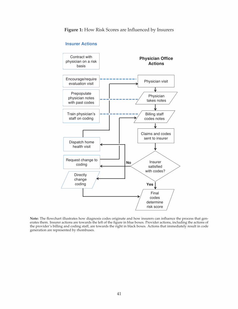
Figure 1: How Risk Scores are Influenced by Insurers

!

!

!

!

!

!

!

!

!

!

!

!

!

!

!

!

!

!

!

!

!

!

!

!

!

!

!

!

!

!

!

!

!

!

!

!

!

!

!

!

!

Yes

!

No

Dispatch home health visit

Contract with

physician on a risk

basis

Prepopulate

physician notes

with past codes

Train physician’s staff on coding

Request change to coding

Physician visit

Physician takes notes

Claims and codes

sent to insurer

Insurer

satisfied

with codes?

Encourage/require

evaluation visit

Final

codes

determine risk score

Insurer Actions

Physician Office

Actions

!

!

Directly

change

coding

Billing staff

codes notes

Note: The flowchart illustrates how diagnosis codes originate and how insurers can influence the process that gen-erates them. Insurer actions are towards the left of the figure in blue boxes. Provider actions, including the actions ofthe provider’s billing and coding staff, are towards the right in black boxes. Actions that immediately result in codegeneration are represented by rhombuses.

41

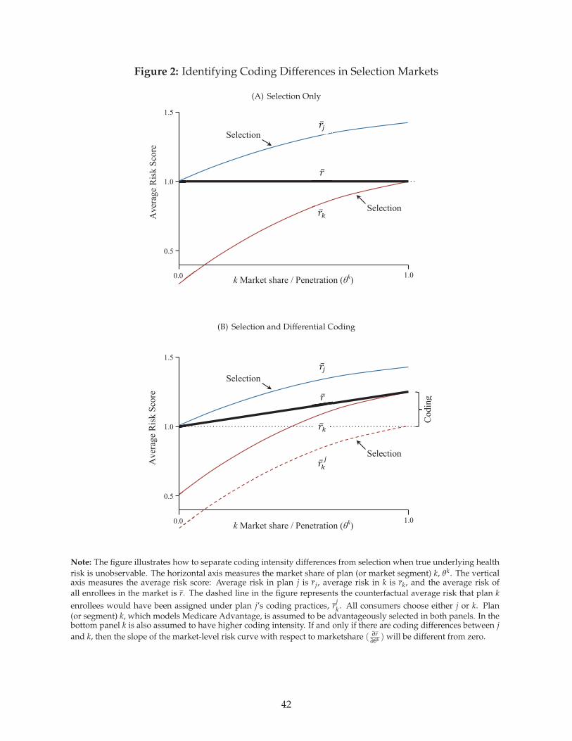
Figure 2: Identifying Coding Differences in Selection Markets

(A) Selection Only!

!

!

!

!

!

!

!

!

!

!

!

!

!

!

!

!

!

!

!

!

!

!

!

1.5

!1.0

0.5

1.0 0.0

1.5

!

.0

Codin

g

k Market share / Penetration (θk)

Aver

age

Ris

k S

core

!!

!!

!!

Selection

Selection

Selection

Selection

!!! !

!!! !

!!! !

!!! !

(B) Selection and Differential Coding

!

!

!

!

!

!

!

!

!

!

!

!

!

!

!

!

!

!

!

!

!

!

!

!

1.5

!1.0

0.5

1.0 0.0

Codin

g

Aver

age

Ris

k S

core

k Market share / Penetration (θk)

!!!

!

!!

Selection

Selection

!!! !

!!! !

Note: The figure illustrates how to separate coding intensity differences from selection when true underlying health

risk is unobservable. The horizontal axis measures the market share of plan (or market segment) k, θk. The verticalaxis measures the average risk score: Average risk in plan j is rj, average risk in k is rk, and the average risk ofall enrollees in the market is r. The dashed line in the figure represents the counterfactual average risk that plan k

enrollees would have been assigned under plan j’s coding practices, rjk. All consumers choose either j or k. Plan

(or segment) k, which models Medicare Advantage, is assumed to be advantageously selected in both panels. In thebottom panel k is also assumed to have higher coding intensity. If and only if there are coding differences between j

and k, then the slope of the market-level risk curve with respect to marketshare ( ∂r∂θk ) will be different from zero.

42

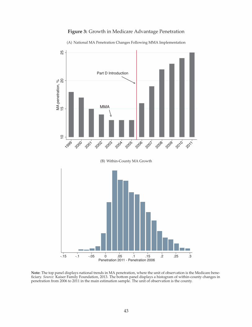
Figure 3: Growth in Medicare Advantage Penetration

(A) National MA Penetration Changes Following MMA Implementation

MMA

Part D Introduction

10

15

20

25

MA

penetr

ation, %

1999

2000

2001

2002

2003

2004

2005

2006

2007

2008

2009

2010

2011

(B) Within-County MA Growth

-.15 -.1 -.05 0 .05 .1 .15 .2 .25 .3

Penetration 2011 - Penetration 2006

Note: The top panel displays national trends in MA penetration, where the unit of observation is the Medicare bene-ficiary. Source: Kaiser Family Foundation, 2013. The bottom panel displays a histogram of within-county changes inpenetration from 2006 to 2011 in the main estimation sample. The unit of observation is the county.

43

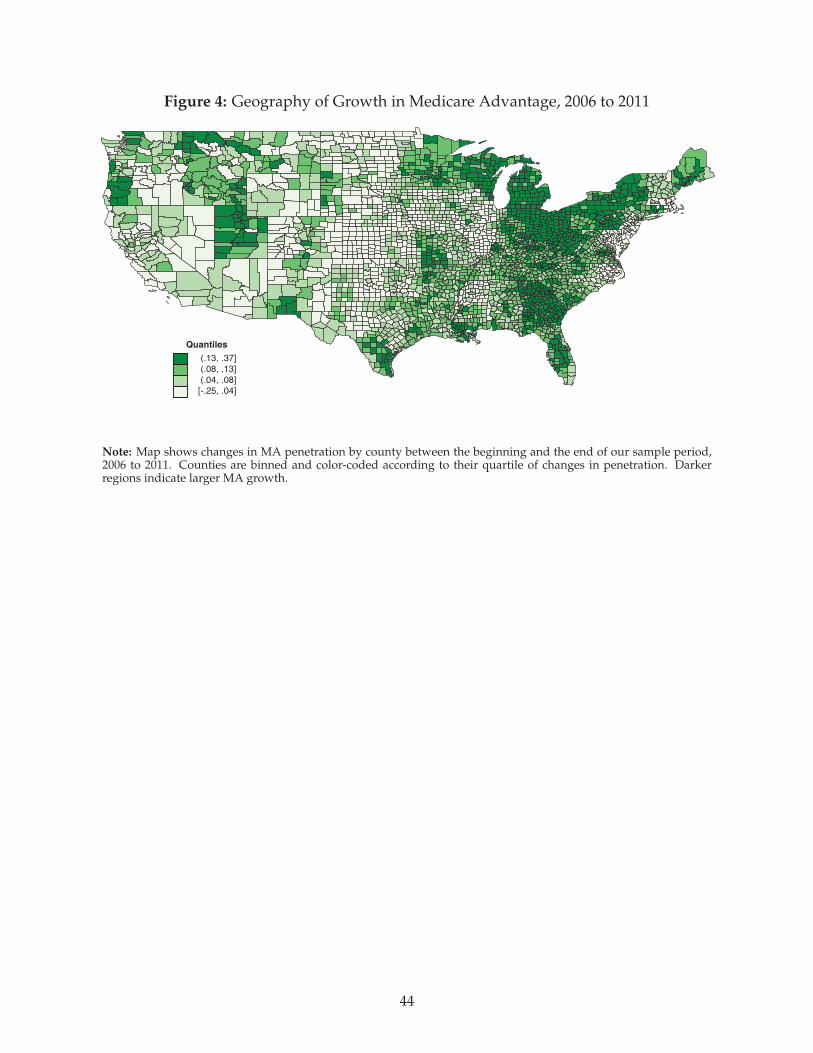
Figure 4: Geography of Growth in Medicare Advantage, 2006 to 2011

(.13, .37]

(.08, .13]

(.04, .08]

[-.25, .04]

Quantiles

Note: Map shows changes in MA penetration by county between the beginning and the end of our sample period,2006 to 2011. Counties are binned and color-coded according to their quartile of changes in penetration. Darkerregions indicate larger MA growth.

44

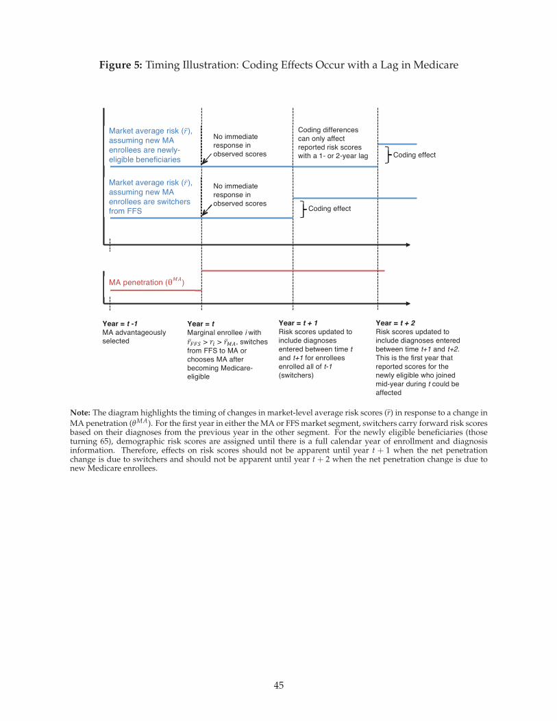
Figure 5: Timing Illustration: Coding Effects Occur with a Lag in Medicare!

!

!

!

!

!

!

!

!

!

!

!

!

!

!

!

!

!

!

!

!

!

!

!

!

!

!

!

!

!

!

!

!

!

!

MA penetration (!!"

)

Year = t

Marginal enrollee i with

!!!!" > !! > !!!", switches

from FFS to MA or

chooses MA after

becoming Medicare-eligible

Year = t + 2

Risk scores updated to

include diagnoses entered

between time t+1 and t+2.

This is the first year that

reported scores for the

newly eligible who joined

mid-year during t could be

affected

Year = t -1

MA advantageously selected

Coding effect

Market average risk (!!),

assuming new MA

enrollees are newly-

eligible beneficiaries

Coding differences

can only affect

reported risk scores with a 1- or 2-year lag

No immediate

response in

observed scores

Year = t + 1

Risk scores updated to

include diagnoses

entered between time t

and t+1 for enrollees

enrolled all of t-1

(switchers)

Market average risk (!!),

assuming new MA

enrollees are switchers

from FFS

No immediate

response in

observed scores

Coding effect

Note: The diagram highlights the timing of changes in market-level average risk scores (r) in response to a change in

MA penetration (θMA). For the first year in either the MA or FFS market segment, switchers carry forward risk scoresbased on their diagnoses from the previous year in the other segment. For the newly eligible beneficiaries (thoseturning 65), demographic risk scores are assigned until there is a full calendar year of enrollment and diagnosisinformation. Therefore, effects on risk scores should not be apparent until year t + 1 when the net penetrationchange is due to switchers and should not be apparent until year t + 2 when the net penetration change is due tonew Medicare enrollees.

45

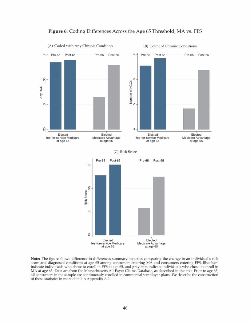
Figure 6: Coding Differences Across the Age 65 Threshold, MA vs. FFS

(A) Coded with Any Chronic Condition

Pre-65 Post-65 Pre-65 Post-65

.25

.3.3

5.4

Any H

CC

Electedfee-for-service Medicare

at age 65

ElectedMedicare Advantage

at age 65

(B) Count of Chronic Conditions

Pre-65 Post-65 Pre-65 Post-65

.4.5

.6.7

Num

ber

of H

CC

s

Electedfee-for-service Medicare

at age 65

ElectedMedicare Advantage

at age 65

(C) Risk Score

Pre-65 Post-65 Pre-65 Post-65

.45

.5.5

5.6

Ris

k S

core

Electedfee-for-service Medicare

at age 65

ElectedMedicare Advantage

at age 65

Note: The figure shows difference-in-differences summary statistics comparing the change in an individual’s riskscore and diagnosed conditions at age 65 among consumers entering MA and consumers entering FFS. Blue barsindicate individuals who chose to enroll in FFS at age 65, and gray bars indicate individuals who chose to enroll inMA at age 65. Data are from the Massachusetts All-Payer Claims Database, as described in the text. Prior to age 65,all consumers in the sample are continuously enrolled in commercial/employer plans. We describe the constructionof these statistics in more detail in Appendix A.2.

46

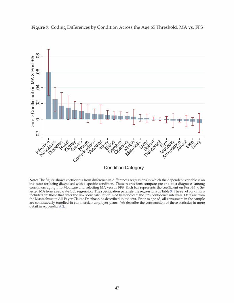
Figure 7: Coding Differences by Condition Across the Age 65 Threshold, MA vs. FFS

-.0

20

.02

.04

.06

.08

D-in

-D C

oe

fficie

nt o

n M

A X

Po

st-

65

Infe

ction

Neo

plas

m

Diabe

tes

Hea

rt

Kidne

y

Gas

tro

Neu

ro

Com

plicat

ions

Vascu

lar

Injury

Blood

Cer

ebro

Ope

ning

MHSA

Met

abolicLive

r

Spina

l

Tran

splant

Eye

Mus

culo

Amup

tatio

n

Arrest

SkinLu

ng

Condition Category

Note: The figure shows coefficients from difference-in-differences regressions in which the dependent variable is anindicator for being diagnosed with a specific condition. These regressions compare pre and post diagnoses amongconsumers aging into Medicare and selecting MA versus FFS. Each bar represents the coefficient on Post-65 × Se-lected MA from a separate OLS regression. The specification parallels the regressions in Table 9. The set of conditionsincluded are those that enter the risk score calculation. Red bars indicate the 95% confidence intervals. Data are fromthe Massachusetts All-Payer Claims Database, as described in the text. Prior to age 65, all consumers in the sampleare continuously enrolled in commercial/employer plans. We describe the construction of these statistics in moredetail in Appendix A.2.

47

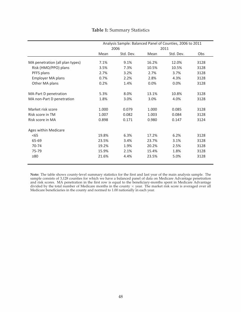
Table 1: Summary Statistics

!"#$ %&'()*"+( !"#$ %&'()*"+( ,-.

!/)0"$"&1#&23$)4#55)05#$)&60".7 8(9: ;(9: 9<(=: 9=(>: ?9=@

A2.B)4C!,DEE,7)05#$. ?(F: 8(?: 9>(F: 9>(F: ?9=@

EGG%)05#$. =(8: ?(=: =(8: ?(8: ?9=@

HI0536"1)!/)05#$. >(8: =(=: =(@: J(?: ?9=@

,&K"1)!/)05#$. >(=: 9(J: >(>: >(>: ?9=@

!/LE#1&)*)0"$"&1#&23$ F(?: @(>: 9?(9: 9>(@: ?9=@

!/)$3$LE#1&)*)0"$"&1#&23$ 9(@: ?(>: ?(>: J(>: ?9=@

!#1B"&)12.B).M31" 9(>>> >(>8; 9(>>> >(>@F ?9=@

A2.B).M31")2$)N! 9(>>8 >(>@= 9(>>? >(>@J ?9=@

A2.B).M31")2$)!/ >(@;@ >(989 >(;@> >(9J8 ?9=J

/O".)P2&K2$)!"'2M#1"

Q<F 9;(@: <(?: 98(=: <(=: ?9=@

<FL<; =?(F: ?(J: =?(8: ?(9: ?9=@

8>L8J 9;(=: 9(;: =>(=: =(F: ?9=@

8FL8; 9F(;: =(9: 9F(J: 9(@: ?9=@

R@> =9(<: J(J: =?(F: F(>: ?9=@

/$#56.2.)%#I05"S)T#5#$M"')E#$"5)3U)V3W$&2".X)=>><)&3)=>99

=>99=>><

Note: The table shows county-level summary statistics for the first and last year of the main analysis sample. Thesample consists of 3,128 counties for which we have a balanced panel of data on Medicare Advantage penetrationand risk scores. MA penetration in the first row is equal to the beneficiary-months spent in Medicare Advantagedivided by the total number of Medicare months in the county × year. The market risk score is averaged over allMedicare beneficiaries in the county and normed to 1.00 nationally in each year.

48

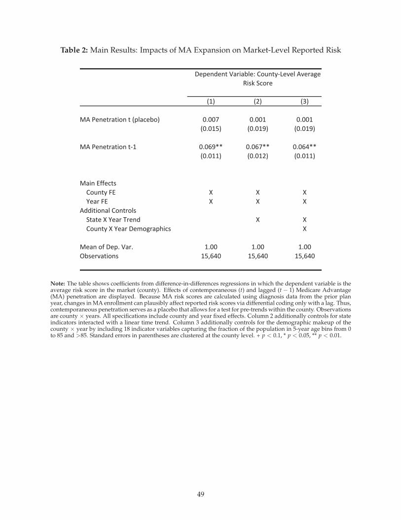
Table 2: Main Results: Impacts of MA Expansion on Market-Level Reported Risk

!"# !$# !%#

&'()*+*,-.,/0+(,(!12.3*40# 56557 5655" 5655"

!565"8# !565"9# !565"9#

&'()*+*,-.,/0+(,:" 565;9<< 565;7<< 565;=<<

!565""# !565"$# !565""#

&./+(>??*3,@

A0B+,C(D> E E E

F*.-(D> E E E

'GG/,/0+.2(A0+,-02@

H,.,*(E(F*.-(I-*+G E E

A0B+,C(E(F*.-(J*K0L-.1M/3@ E

&*.+(0?(J*16(N.-6 "655 "655 "655

O4@*-P.,/0+@ "8Q;=5 "8Q;=5 "8Q;=5

J*1*+G*+,(N.-/.42*R(A0B+,C:S*P*2('P*-.L*(

T/@U(H30-*

Note: The table shows coefficients from difference-in-differences regressions in which the dependent variable is theaverage risk score in the market (county). Effects of contemporaneous (t) and lagged (t − 1) Medicare Advantage(MA) penetration are displayed. Because MA risk scores are calculated using diagnosis data from the prior planyear, changes in MA enrollment can plausibly affect reported risk scores via differential coding only with a lag. Thus,contemporaneous penetration serves as a placebo that allows for a test for pre-trends within the county. Observationsare county × years. All specifications include county and year fixed effects. Column 2 additionally controls for stateindicators interacted with a linear time trend. Column 3 additionally controls for the demographic makeup of thecounty × year by including 18 indicator variables capturing the fraction of the population in 5-year age bins from 0to 85 and >85. Standard errors in parentheses are clustered at the county level. + p < 0.1, * p < 0.05, ** p < 0.01.

49

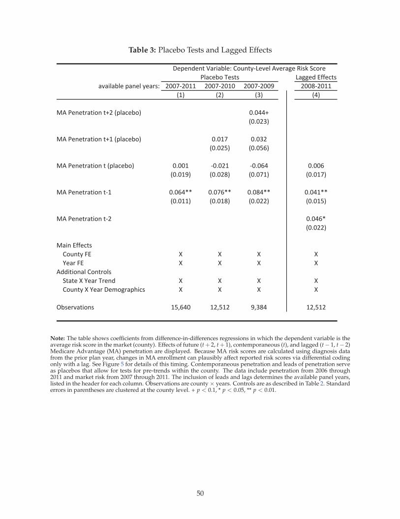
Table 3: Placebo Tests and Lagged Effects

!"##$%&'(($)*+

","-."/.$&0"1$.&2$"3+4 566785699 566785696 56678566: 566;85699

<9= <5= <>= <?=

@A&B$1$*3"*-C1&*D5&<0.")$/C= 6E6??D

<6E65>=

@A&B$1$*3"*-C1&*D9&<0.")$/C= 6E697 6E6>5

<6E65F= <6E6FG=

@A&B$1$*3"*-C1&*&<0.")$/C= 6E669 86E659 86E6G? 6E66G

<6E69:= <6E65;= <6E679= <6E697=

@A&B$1$*3"*-C1&*89 6E6G?HH 6E67GHH 6E6;?HH 6E6?9HH

<6E699= <6E69;= <6E655= <6E69F=

@A&B$1$*3"*-C1&*85 6E6?GH

<6E655=

@"-1&'(($)*+

ICJ1*2&K' L L L L

M$"3&K' L L L L

A%%-*-C1".&IC1*3C.+

N*"*$&L&M$"3&O3$1% L L L L

ICJ1*2&L&M$"3&P$QC#3"0R-)+ L L L L

S/+$3,"*-C1+ 9FTG?6 95TF95 :T>;? 95TF95

P$0$1%$1*&U"3-"/.$4&ICJ1*28!$,$.&A,$3"#$&V-+W&N)C3$

B.")$/C&O$+*+

Note: The table shows coefficients from difference-in-differences regressions in which the dependent variable is theaverage risk score in the market (county). Effects of future (t+ 2, t+ 1), contemporaneous (t), and lagged (t− 1, t− 2)Medicare Advantage (MA) penetration are displayed. Because MA risk scores are calculated using diagnosis datafrom the prior plan year, changes in MA enrollment can plausibly affect reported risk scores via differential codingonly with a lag. See Figure 5 for details of this timing. Contemporaneous penetration and leads of penetration serveas placebos that allow for tests for pre-trends within the county. The data include penetration from 2006 through2011 and market risk from 2007 through 2011. The inclusion of leads and lags determines the available panel years,listed in the header for each column. Observations are county × years. Controls are as described in Table 2. Standarderrors in parentheses are clustered at the county level. + p < 0.1, * p < 0.05, ** p < 0.01.

50

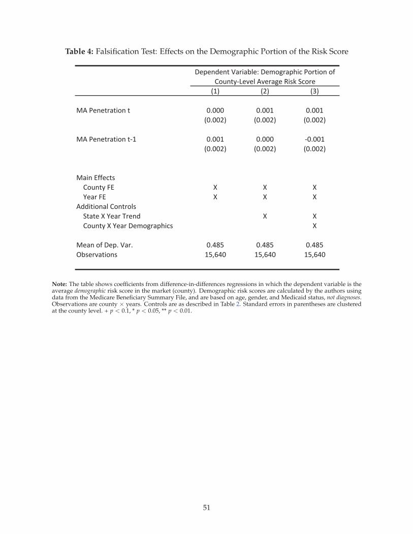
Table 4: Falsification Test: Effects on the Demographic Portion of the Risk Score

!"# !$# !%#

&'()*+*,-.,/0+(, 12111 1211" 1211"

!1211$# !1211$# !1211$#

&'()*+*,-.,/0+(,3" 1211" 12111 31211"

!1211$# !1211$# !1211$#

&./+(455*6,7

809+,:(;4 < < <

=*.-(;4 < < <

'>>/,/0+.?(80+,-0?7

@,.,*(<(=*.-(A-*+> < <

809+,:(<(=*.-(B*C0D-.EF/67 <

&*.+(05(B*E2(G.-2 12HIJ 12HIJ 12HIJ

KL7*-M.,/0+7 "JNOH1 "JNOH1 "JNOH1

B*E*+>*+,(G.-/.L?*P(B*C0D-.EF/6()0-,/0+(05(

809+,:3Q*M*?('M*-.D*(R/7S(@60-*

Note: The table shows coefficients from difference-in-differences regressions in which the dependent variable is theaverage demographic risk score in the market (county). Demographic risk scores are calculated by the authors usingdata from the Medicare Beneficiary Summary File, and are based on age, gender, and Medicaid status, not diagnoses.Observations are county × years. Controls are as described in Table 2. Standard errors in parentheses are clusteredat the county level. + p < 0.1, * p < 0.05, ** p < 0.01.

51

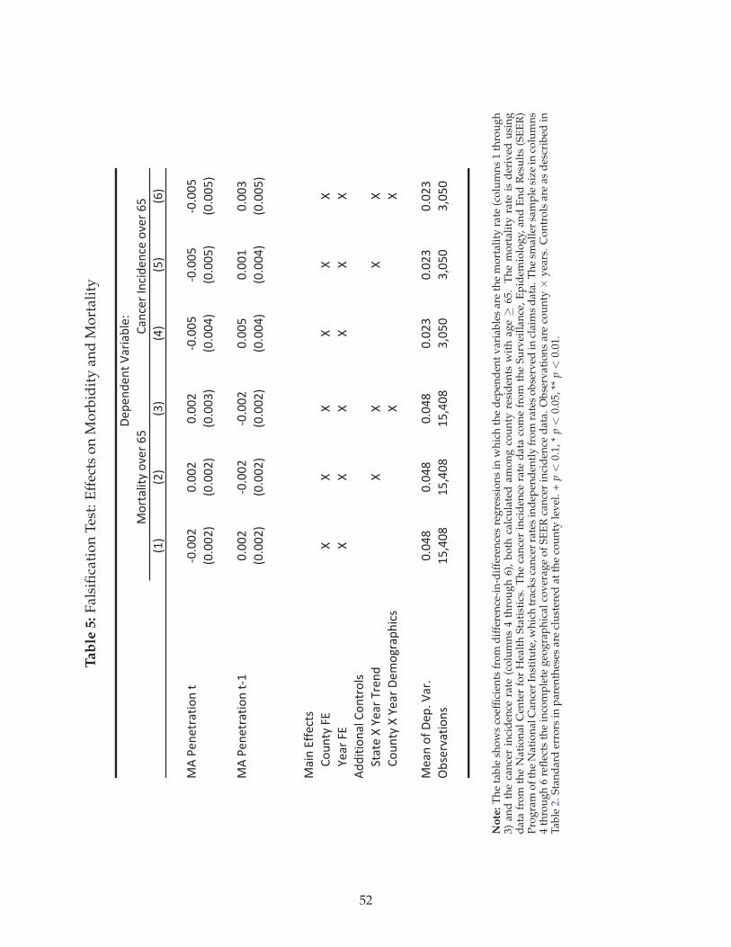
Tab

le5:

Fal

sifi

cati

on

Tes

t:E

ffec

tso

nM

orb

idit

yan

dM

ort

alit

y

!"#

!$#

!%#

!&#

!'#

!(#

)*+,-.-/01/23.+/

45655$

5655$

5655$

45655'

45655'

45655'

!5655$#

!5655$#

!5655%#

!5655&#

!5655'#

!5655'#

)*+,-.-/01/23.+/4"

5655$

45655$

45655$

5655'

5655"

5655%

!5655$#

!5655$#

!5655$#

!5655&#

!5655&#

!5655'#

)12.+788-9/:

;3<./=+>7

??

??

??

@-10+>7

??

??

??

*AA2/23.1B+;3./03B:

C/1/-+?+@-10+D0-.A

??

??

;3<./=+?+@-10+E-F3G01HI29:

??

)-1.+38+E-H6+J106

565&K

565&K

565&K

565$%

565$%

565$%

LM:-0N1/23.:

"'O&5K

"'O&5K

"'O&5K

%O5'5

%O5'5

%O5'5

E-H-.A-./+J1021MB-P

)30/1B2/=+3N-0+('

;1.9-0+Q.92A-.9-+3N-0+('+

No

te:

Th

eta

ble

sho

ws

coef

fici

ents

fro

md

iffe

ren

ce-i

n-d

iffe

ren

ces

reg

ress

ion

sin

wh

ich

the

dep

end

ent

var

iab

les

are

the

mo

rtal

ity

rate

(co

lum

ns

1th

rou

gh

3)an

dth

eca

nce

rin

cid

ence

rate

(co

lum

ns

4th

rou

gh

6),

bo

thca

lcu

late

dam

on

gco

un

tyre

sid

ents

wit

hag

e≥

65.

Th

em

ort

alit

yra

teis

der

ived

usi

ng

dat

afr

om

the

Nat

ion

alC

ente

rfo

rH

ealt

hS

tati

stic

s.T

he

can

cer

inci

den

cera

ted

ata

com

efr

om

the

Su

rvei

llan

ce,

Ep

idem

iolo

gy,

and

En

dR

esu

lts

(SE

ER

)P

rog

ram

of

the

Nat

ion

alC

ance

rIn

stit

ute

,wh

ich

trac

ks

can

cer

rate

sin

dep

end

entl

yfr

om

rate

so

bse

rved

incl

aim

sd

ata.

Th

esm

alle

rsa

mp

lesi

zein

colu

mn

s4

thro

ug

h6

refl

ects

the

inco

mp

lete

geo

gra

ph

ical

cov

erag

eo

fS

EE

Rca

nce

rin

cid

ence

dat

a.O

bse

rvat

ion

sar

eco

un

ty×

yea

rs.

Co

ntr

ols

are

asd

escr

ibed

inT

able

2.S

tan

dar

der

rors

inp

aren

thes

esar

ecl

ust

ered

atth

eco

un

tyle

vel

.+

p<

0.1,

*p<

0.05

,**

p<

0.01

.

52

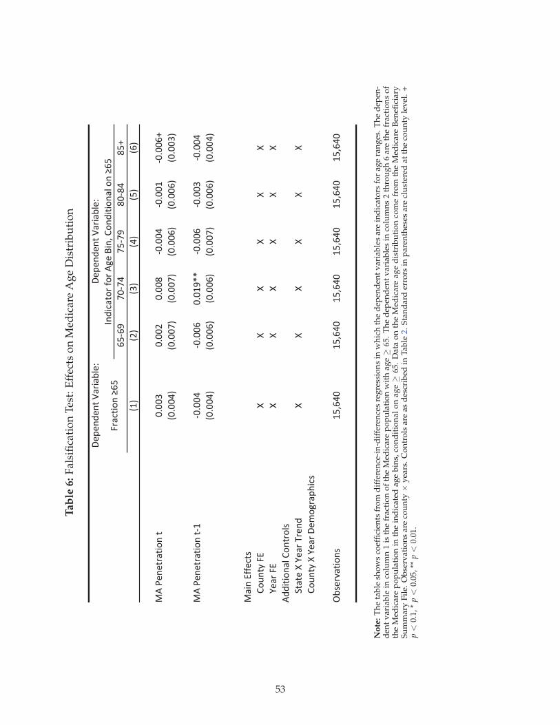
Tab

le6:

Fal

sifi

cati

on

Tes

t:E

ffec

tso

nM

edic

are

Ag

eD

istr

ibu

tio

n

!"#"$%"$&'()*+),-".

/01/2

34135

30132

64165

607

89:

8;:

8<:

85:

80:

8/:

=>'?"$"&*)&+@$'&

4A44<

4A44;

4A446

14A445

14A449

14A44/7

84A445:

84A443:

84A443:

84A44/:

84A44/:

84A44<:

=>'?"$"&*)&+@$'&19

14A445

14A44/

4A492BB

14A44/

14A44<

14A445

84A445:

84A44/:

84A44/:

84A443:

84A44/:

84A445:

=)+$'CDD"E&F

G@H$&I'JC

KK

KK

KK

L")*'JC

KK

KK

KK

>%%+&+@$)-'G@$&*@-F

M&)&"'K'L")*'N*"$%

KK

KK

KK

G@H$&I'K'L")*'!"O@P*)#Q+EF

R,F"*S)&+@$F

90T/54

90T/54

90T/54

90T/54

90T/54

90T/54

U$%+E)&@*'D@*'>P"'V+$T'G@$%+&+@$)-'@$'W/0

J*)E&+@$'W/0

!"#"$%"$&'()*+),-".

No

te:

Th

eta

ble

sho

ws

coef

fici

ents

fro

md

iffe

ren

ce-i

n-d

iffe

ren

ces

reg

ress

ion

sin

wh

ich

the

dep

end

ent

var

iab

les

are

ind

icat

ors

for

age

ran

ges

.T

he

dep

en-

den

tv

aria

ble

inco

lum

n1

isth

efr

acti

on

of

the

Med

icar

ep

op

ula

tio

nw

ith

age≥

65.

Th

ed

epen

den

tv

aria

ble

sin

colu

mn

s2

thro

ug

h6

are

the

frac

tio

ns

of

the

Med

icar

ep

op

ula

tio

nin

the

ind

icat

edag

eb

ins,

con

dit

ion

alo

nag

e≥

65.

Dat

ao

nth

eM

edic

are

age

dis

trib

uti

on

com

efr

om

the

Med

icar

eB

enefi

ciar

yS

um

mar

yF

ile.

Ob

serv

atio

ns

are

cou

nty

×y

ears

.C

on

tro

lsar

eas

des

crib

edin

Tab

le2.

Sta

nd

ard

erro

rsin

par

enth

eses

are

clu

ster

edat

the

cou

nty

lev

el.

+p<

0.1,

*p<

0.05

,**

p<

0.01

.

53

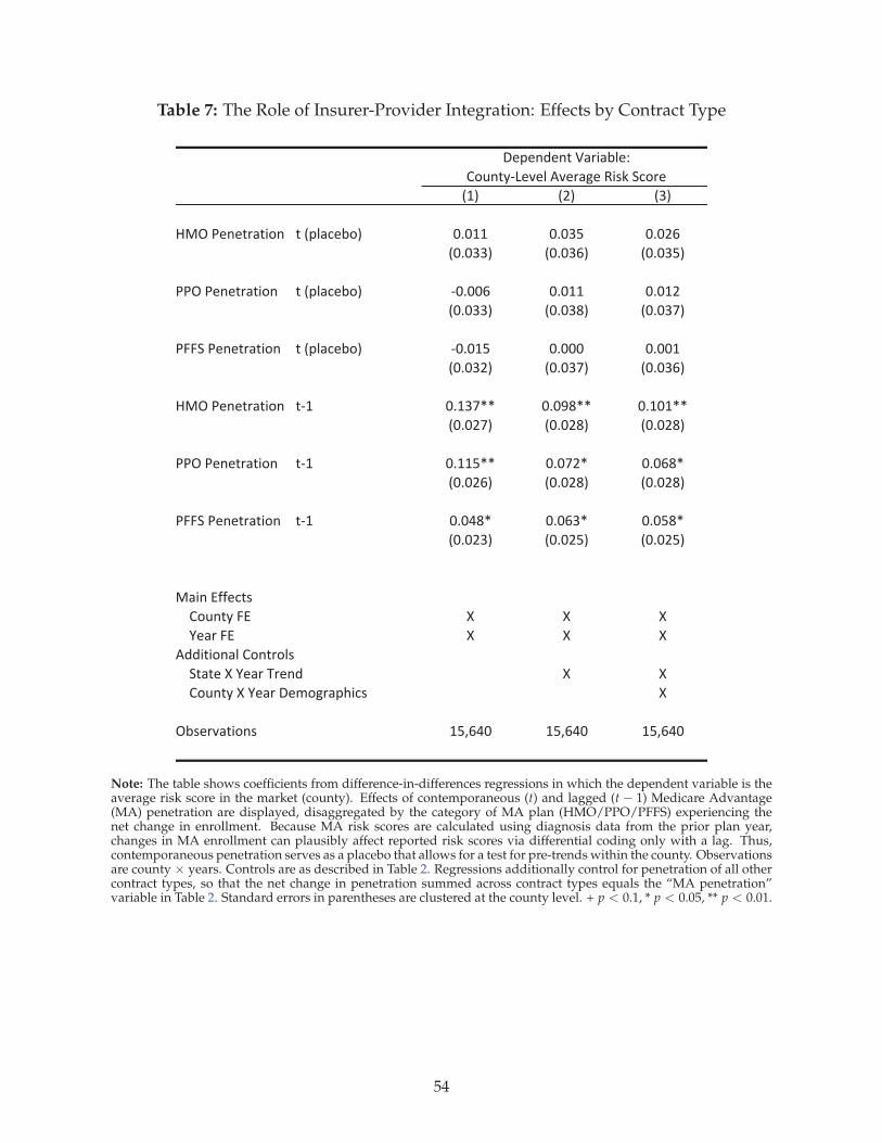
Table 7: The Role of Insurer-Provider Integration: Effects by Contract Type

!"# !$# !%#

&'()*+,+-./-01, -)!23/4+51# 676"" 676%8 676$9

!676%%# !676%9# !676%8#

**()*+,+-./-01, -)!23/4+51# :67669 676"" 676"$

!676%%# !676%;# !676%<#

*==>)*+,+-./-01, -)!23/4+51# :676"8 67666 6766"

!676%$# !676%<# !676%9#

&'()*+,+-./-01, -:" 67"%<?? 676@;?? 67"6"??

!676$<# !676$;# !676$;#

**()*+,+-./-01, -:" 67""8?? 676<$? 6769;?

!676$9# !676$;# !676$;#

*==>)*+,+-./-01, -:" 676A;? 6769%? 6768;?

!676$%# !676$8# !676$8#

'/0,)BCC+4-D

E1F,-G)=B H H H

I+/.)=B H H H

JKK0-01,/3)E1,-.13D

>-/-+)H)I+/.)L.+,K H H

E1F,-G)H)I+/.)M+N1O./2P04D H

(5D+.Q/-01,D "8R9A6 "8R9A6 "8R9A6

M+2+,K+,-)S/.0/53+T)))))))))))))))))))))))))))))))))

E1F,-G:U+Q+3)JQ+./O+)V0DW)>41.+

Note: The table shows coefficients from difference-in-differences regressions in which the dependent variable is theaverage risk score in the market (county). Effects of contemporaneous (t) and lagged (t − 1) Medicare Advantage(MA) penetration are displayed, disaggregated by the category of MA plan (HMO/PPO/PFFS) experiencing thenet change in enrollment. Because MA risk scores are calculated using diagnosis data from the prior plan year,changes in MA enrollment can plausibly affect reported risk scores via differential coding only with a lag. Thus,contemporaneous penetration serves as a placebo that allows for a test for pre-trends within the county. Observationsare county × years. Controls are as described in Table 2. Regressions additionally control for penetration of all othercontract types, so that the net change in penetration summed across contract types equals the “MA penetration”variable in Table 2. Standard errors in parentheses are clustered at the county level. + p < 0.1, * p < 0.05, ** p < 0.01.

54

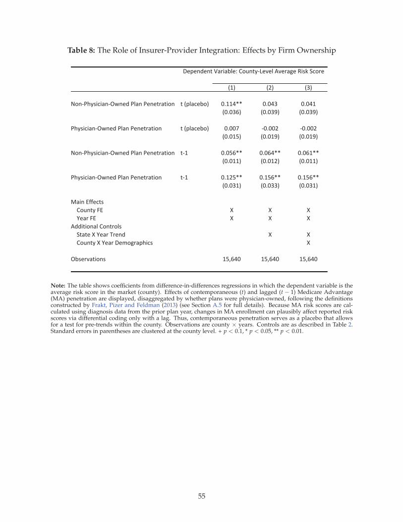
Table 8: The Role of Insurer-Provider Integration: Effects by Firm Ownership

!"# !$# !%#

&'()*+,-./.0()12(345*60(5*3(37807.'( 75!960/3:'# ;<""=>> ;<;=% ;<;="

!;<;%?# !;<;%@# !;<;%@#

*+,-./.0()12(345*60(5*3(37807.'( 75!960/3:'# ;<;;A );<;;$ );<;;$

!;<;"B# !;<;"@# !;<;"@#

&'()*+,-./.0()12(345*60(5*3(37807.'( 7)" ;<;B?>> ;<;?=>> ;<;?">>

!;<;""# !;<;"$# !;<;""#

*+,-./.0()12(345*60(5*3(37807.'( 7)" ;<"$B>> ;<"B?>> ;<"B?>>

!;<;%"# !;<;%%# !;<;%"#

C0.(5DEE3/7-

F'G(7,5HD I I I

J3085HD I I I

K44.7.'(065F'(78'6-

L70735I5J3085M83(4 I I

F'G(7,5I5J3085N3O'P809+./- I

1:-38Q07.'(- "BR?=; "BR?=; "BR?=;

N393(43(75S08.0:63T5F'G(7,)U3Q365KQ380P35V.-W5L/'83

Note: The table shows coefficients from difference-in-differences regressions in which the dependent variable is theaverage risk score in the market (county). Effects of contemporaneous (t) and lagged (t − 1) Medicare Advantage(MA) penetration are displayed, disaggregated by whether plans were physician-owned, following the definitionsconstructed by Frakt, Pizer and Feldman (2013) (see Section A.5 for full details). Because MA risk scores are cal-culated using diagnosis data from the prior plan year, changes in MA enrollment can plausibly affect reported riskscores via differential coding only with a lag. Thus, contemporaneous penetration serves as a placebo that allowsfor a test for pre-trends within the county. Observations are county × years. Controls are as described in Table 2.Standard errors in parentheses are clustered at the county level. + p < 0.1, * p < 0.05, ** p < 0.01.

55

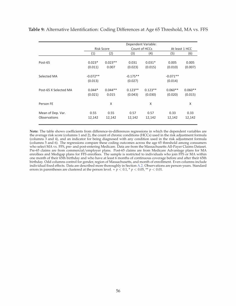
Table 9: Alternative Identification: Coding Differences at Age 65 Threshold, MA vs. FFS

!"# !$# !%# !&# !'# !(#

)*+,-(' ./.$%0 ./.$%00 ./.%" ./.%"0 ./..' ./..'

!./.""# ./..1 !./.$%# !./."'# !./.".# !./..1#

23435,36789 -./.1$00 -./"1'00 -./.1"00

!./."%# !./.$1# !./."&#

)*+,-('7:723435,36789 ./.&&0 ./.&&00 ./"$%00 ./"$%00 ./.(.00 ./.(.00

!./.$"# ./."' !./.&%# !./.%.# !./.$.# !./."'#

)3;+*<7=> : : :

83?<7*@7A3B/7C?;/ ./'' ./'' ./'1 ./'1 ./%% ./%%

DE+3;F?,G*<+ "$H"&$ "$H"&$ "$H"&$ "$H"&$ "$H"&$ "$H"&$

9,743?+,7"7IJJJ*K<,7*@7IJJ+LG+M725*;3

A3B3<63<,7C?;G?E43N7

Note: The table shows coefficients from difference-in-differences regressions in which the dependent variables arethe average risk score (columns 1 and 2), the count of chronic conditions (HCCs) used in the risk adjustment formula(columns 3 and 4), and an indicator for being diagnosed with any condition used in the risk adjustment formula(columns 5 and 6). The regressions compare these coding outcomes across the age 65 threshold among consumerswho select MA vs. FFS, pre- and post-entering Medicare. Data are from the Massachusetts All-Payer Claims Dataset.Pre-65 claims are from commercial/employer plans. Post-65 claims are from Medicare Advantage plans for MAenrollees and Medigap plans for FFS enrollees. The sample is restricted to individuals who join FFS or MA withinone month of their 65th birthday and who have at least 6 months of continuous coverage before and after their 65thbirthday. Odd columns control for gender, region of Massachusetts, and month of enrollment. Even columns includeindividual fixed effects. Data are described more thoroughly in Section A.2. Observations are person-years. Standarderrors in parentheses are clustered at the person level. + p < 0.1, * p < 0.05, ** p < 0.01.

56

Appendix

APPENDIX

A.1 Background on MA Risk-Adjusted Payments

Medicare Advantage (MA) insurance plans are given monthly capitated payments for each enrolledMedicare beneficiary. The levels of these county-specific payments are tied to historical fee-for-service (FFS) Medicare costs in the county. County captitation rates were originally intended tocapture the cost of enrolling the “national average beneficiary” in the FFS Medicare program in thecounty, though Congress has made many ad-hoc adjustments over time.

Before 2004, there was relatively minimal risk adjustment of capitation payments, relying pri-marily on demographics.62 In 2004, CMS began transitioning to risk adjustment based on diagnosesobtained during inpatient hospital stays and outpatient encounters. By 2007, diagnosis-based riskadjustment was fully phased-in. During our study period (2006-2011), risk adjusted capitation pay-ments were equal to Rijc = φjc · xicΛ, where i indexes beneficiaries, j indexes plans, and c indexescounties (markets). The basis φj was approximately equal to the county “benchmark” φc, though φjc

could vary across plans within the same county.φ could vary within counties because since 2006 MA plans have been required to submit bids to

CMS. These bids are compared to the uniform county benchmark φc. If the bid is below the countybenchmark set by the regulator, the plan receives 75% of the difference between the bid and thebenchmark, which the plan is required to fold back into its premium and benefits as a “rebate” tobeneficiaries. Importantly for our purposes, this 75% is still paid out by CMS into the MA program.This implies that any estimation of coding subsidies should be based on the capitation payment toplans inclusive of any “rebate.”

A.2 Data Used in Section 6

For the analysis in Section 6, we obtained data on Medicare Advantage and Medigap claims fromthe new Massachusetts All-Payer Claims Dataset (Mass APCD). The Mass APCD is mantained bythe Massachusetts Center for Health Information and Analysis (CHIA). The database includes theuniverse of health insurance claims for individuals receiving medical services in the state of Mas-sachusetts. Payers, along with third-party claims administrators and pharmacy benefit managers,report all claims to the state of Massachusetts. These claims are then aggregated into a large, compre-hensive dataset. To identify individuals, we use an individual ID generated by the state using SocialSecurity numbers, names, and addresses. This ID is available only for 2011-12.

We identify two groups of individuals in the Mass APCD. The first group consists of all indi-viduals enrolling in a product identified as a Medicare Advantage plan within one month of their65th birthday. We identify Medicare Advantage plans using an identifier provided by CHIA. Weverify that the CHIA identifier for Medicare Advantage products is accurate by matching the namesof the payers in the Mass APCD data to publicly available Medicare Advantage enrollment data pro-vided by CMS. We also check the age distribution of enrollees in these plans to ensure that there is adiscontinuous spike in the density at age 65.

The second group consists of all individuals enrolling in a product identified as a Medigap planwithin one month of their 65th birthday. We identify Medigap plans using an identifier providedby CHIA. Again, we verify that the CHIA identifier for Medigap plans is accurate by matching the

62From 2001-2003 inpatient diagnoses were used in risk adjustment, but in order to weaken insurer incentives to sendmore enrollees to the hospital, CMS only gave these diagnoses a 10% weight in the risk adjustment payment, leaving theother 90% of the payment based on demographics only.

57

Appendix

names of the payers in the Mass APCD data to publicly available information about the insurers com-peting in the Massachusetts Medigap market. Additionally, we observe the portion of total spendingpaid by Medicare. For almost all of the plans identified as Medigap plans, this value was between70% and 90%, confirming that these products are Medigap plans.

For both groups, we identify the subset of individuals with some form of coverage for everymonth of 2011 and 2012. We drop any individuals with some form of Medicare coverage prior tojoining MA or Medigap at 65. This removes, for example, Medicare enrollees who gain coverage viadisability rather than automatically becoming eligible at age 65. Because Medicaid data is excludedfrom our version of the Mass APCD, this results in a sample of individuals with continuous commer-cial/employer coverage prior to their 65th birthday and continuous Medigap/MA coverage aftertheir 65th birthday. To ensure that we have enough claims data to calculate risk scores, we restrict thesample to individuals with at least six months of data prior to joining Medigap/MA and six monthsof data after joining Medigap/MA. This effectively eliminates anyone joining Medigap/MA beforeJuly 2011 and after July 2012.

For the resulting set of individuals, we restrict attention to claims from medical plans only, ex-cluding prescription drug plans.63 We then assign individuals to cohorts based on the month inwhich they joined Medigap/MA. We specify separate “pre-65” and “post-65” periods for each co-hort. We require that the pre-65 and post-65 periods be of equal length and that they consist of thesame months from different years. Given these restrictions, we choose the longest possible period foreach cohort. For example, for the individuals joining Medigap/MA in July 2011, we specify the pre-65 period to be January-June 2011 and the post-65 period to be January-June 2012. For the individualsjoining Medigap/MA in February 2012, we specify the pre-65 period to be February-December 2011and the post-65 period to be February-December 2012.64

For each individual, we calculate a pre-65 and a post-65 risk score. The pre-65 (post-65) risk scoreis calculated by identifying all diagnoses from medical claims incurred during the pre-65 (post-65)period and running those diagnoses through the 2011 version of the CMS-HCC SAS risk scoringprogram. The program is freely available from CMS. It maps each individual’s diagnoses to a set of70 chronic conditions. It then multiplies indicators for these chronic conditions by a set of weightsestimated by CMS using claims data from fee-for-service Medicare. The product of the individual’schronic conditions indicators and the weights is the risk score. We also calculate each individual’snumber of chronic conditions and construct a dummy variable indicating whether the individual hasat least one chronic condition.

A.3 Linearity of Market-level Average Risk Curve

Throughout much of Section 3 we impose the assumption that coding differences across plans canbe represented by the difference between two additive plan-dependent coding factors. Under thisassumption, the slope of the average risk curve in the market is exactly equal to the average codingdifference in the population. This relationship ( ∂r

∂θ = αk − αj) also holds under the weaker assump-tion that any individual-specific heterogeneity in the plan-dependent component of the risk score isorthogonal to plan k’s market share (θk). In that case the slope of the average risk curve in the marketis exactly equal to the average coding difference across plans.

To formalize this statement, let individual i’s risk score in plan j be equal to rij = ri + α(γj, ψj),and let i’s risk score in plan k be equal to rik = ri + α(γk, ψk) + ǫik where ǫik has mean ǫ = 0 and

63The CMS-HCC risk adjustment model used for MA payments is based only on diagnoses from medical claims.64Alternatively, we could have required that the pre-65 and post-65 periods be contiguous. For example, for individuals

joining Medigap/MA in July 2011, we could specify the pre-65 period to be January-June 2011 and the post-65 period to beJuly-December 2011. This alternative specification produces results nearly identical to those produced by the specificationoutlined above.

58

Appendix

represents individual-specific heterogeneity in the relative coding intensity between plans j and k.For individual i, this generates a differential risk score of α(γk, ψk) + ǫik − α(γj, ψj). This produces an

average upcoding factor of1

N ∑(

α(γk, ψk) + ǫik − α(γj, ψj)))

= α(γk, ψk)− α(γj, ψj).

Letting 1[ki(θ)] represent the indicator function for choosing k, market average risk can be ex-

pressed as r =1

N ∑(

ri + α(γj, ψj) + 1[ki(θ)](α(γk, ψk) + ǫik − α(γj, ψj)))

. Assuming that ǫk is or-

thogonal to θ, differentiating r with respect to θ produces:

∂r

∂θ=

∂

∂θ

1

N ∑(

ri + α(γj, ψj) + 1[ki(θ)](α(γk, ψk) + ǫik − α(γj, ψj)))

= α(γk, ψk)− α(γj, ψj). (11)

Therefore, in the case of individual-level heterogeneity in the differential risk score, the slope of themarket-level risk curve still identifies the mean coding difference across plans or market segments.

A.4 Estimates of Selection

Section 5 describes the results of the main analysis in which we regress county-level averages of riskscores on lagged MA penetration in the county to estimate coding differences. For completeness, herewe estimate selection on risk scores, using an analogous set of regressions. Under the assumptionthat MA penetration changes are exogenous to changes in underlying population health conditionalon our controls, selection on risk scores can be estimated by regressing either the average risk scorewithin FFS or the average risk score within MA on contemporaneous and lagged penetration. Notethat this reveals only compensated selection, not uncompensated selection as estimated in Brownet al. (2014) and Cabral, Geruso and Mahoney (2014).

Table A1 presents the selection results. Coefficients on contemporaneous MA penetration iden-tify pure selection effects. If selection were monotonic (such as in Figure 2), then positive contem-poraneous coefficients in both markets would indicate that as penetration increased, the marginalbeneficiary choosing MA was high risk relative to the MA average and low risk relative to the FFSaverage (according to prior-year diagnoses), increasing the average risk score in both pools. In TableA1, estimates for both FFS and MA risk are imprecise, yielding confidence intervals consistent witha broad range of selection effects, including the findings in Newhouse et al. (2012) of advantageousselection into MA of 4 to 9% of the risk score in 2008.

An important component of selection effects may be captured by the lagged penetration coeffi-cient: Research on MA enrollment by Sinaiko, Afendulis and Frank (2013) shows that the majority ofnew MA enrollees are age 65, implying that most of the shift in MA penetration is likely occurringamong the newly Medicare-eligible. In Table A1, this would cause a significant fraction of selectioneffects to be captured by the lagged coefficient, as new MA enrollees aren’t assigned diagnosis-basedrisk scores until their second year. However, interpreting selection effects in Table A1 is difficult be-cause coefficients on lagged MA penetration are affected by: (i) selection on risk score trajectory and(ii) selection on the unobserved contemporaneous risk score for new enrollees who are not assigneda diagnosis-based score until their second year.

It is important to note that unlike these within-market-segment results, the regressions compris-ing our main analysis, which examine the effect of lagged penetration on overall county risk, areunaffected by selection and yield a straightforward identification of pure coding effects.

A.5 Supplemental Analysis on Plan Ownership

In Section 5 we described results that identified heterogeneity in coding practices across plans withdifferent levels of insurer-provider integration. For our results in Table 8, we calculated MA pene-

59

Appendix

tration separately for physician-owned plans, using data constructed by Frakt, Pizer and Feldman(2013). Here, we describe those data and results in more detail.

Frakt, Pizer and Feldman (2013) gathered data on provider ownership of plans via plan websitesand governance documents for plan year 2009. They limited attention to coordinated care MA-PartD plans (e.g. HMOs and PPOs), excluding employer plans, PFFS plans, and MA plans withoutdrug coverage. We apply their integration flag to our data covering years 2006-2011, using publiclyavailable CMS plan crosswalk files to link the 2009 plan IDs across years. The restriction of Frakt,Pizer and Feldman (2013) to exclude non-drug plans from classification and our implicit assumptionthat physician ownership was constant from 2006 to 2011 could introduce measurement error, whichwould bias against our finding of a difference in coding between plans classified as physician-ownedand not.

A.6 The Role of Electronic Health Record (EHR) Adoption

Regressions in Table A4 analyze the extent of coding intensity differences across markets classifiedby differences in the local adoption of electronic health records (EHRs). Here we describe the dataused to classify local markets by EHR adoption.

CMS, in cooperation with the Office of the National Coordinator for Health Information Tech-nology, has collected data on meaningful use of EHR systems within physician office settings. Since2011, physician offices serving Medicare patients have been incentivized with financial bonuses to re-port on meaningful EHR use to CMS. We use reports of EHR use during the first year of the incentiveprogram (2011) as a proxy for the existing local EHR infrastructure during our sample period (2006-2011). Within each county, we normalize the count of physicians reporting office EHR adoption bythe county Medicare population. Then we define an indicator for high EHR adoption by splitting thismetric at the median. Interaction terms in Table A4 between lagged penetration and this indicatorfor high EHR adoption yield coefficients very close to zero.

60

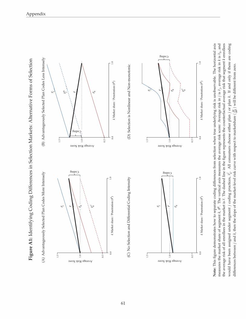
Appendix

Fig

ure

A1:

Iden

tify

ing

Co

din

gD

iffe

ren

ces

inS

elec

tio

nM

ark

ets:

Alt

ern

ativ

eF

orm

so

fS

elec

tio

n

(A)

Ad

van

tag

eou

sly

Sel

ecte

dP

lan

Co

des

Mo

reIn

ten

sely

! ! ! ! ! ! ! ! ! !

! !

! ! ! ! ! ! ! ! ! ! ! ! ! !

1.5

!

.0

1.5

!1

.0

0.5

1.0

0

.0

Coding

Average Risk Score

k M

ark

et s

hare

/ P

enet

rati

on

(θk)

!!!

!!!

!!

!! !!

!!

!! !!

!! !!

(B)

Ad

van

tag

eou

sly

Sel

ecte

dP

lan

Co

des

Les

sIn

ten

sely

! ! ! ! ! ! ! ! ! !

! !

! ! ! ! ! ! ! ! ! ! ! !

1.5

!

.0

1.5

!1

.0

0.5

1.0

0

.0

Average Risk Score

k M

ark

et s

hare

/ P

enet

rati

on

(θk)

!!

!! !!

!!

Coding

!! !!

!! !!

!! !!

!! !!

(C)

No

Sel

ecti

on

and

Dif

fere

nti

alC

od

ing

Inte

nsi

ty

! ! ! ! ! !

! !

! ! ! ! ! ! ! ! ! ! ! !

1.5

!1

.0

0.5

1.0

0

.0

k M

ark

et s

hare

/ P

enet

rati

on

(θk)

Average Risk Score

!!

Coding

!! !!

!! !!

(D)

Sel

ecti

on

isN

on

lin

ear

and

No

n-m

on

oto

nic

! ! ! ! ! ! ! ! !

! !

! ! ! ! ! ! ! ! ! ! ! !

1.5

!1

.0

0.5

1.0

0

.0

Coding

Average Risk Score

k M

ark

et s

hare

/ P

enet

rati

on

(θk)

!!

!! !!

!! !!

!! !!

No

te:

Th

isfi

gu

red

emo

nst

rate

sh

ow

tose

par

ate

cod

ing

dif

fere

nce

sfr

om

sele

ctio

nw

hen

tru

eu

nd

erly

ing

risk

isu

no

bse

rvab

le.

Th

eh

ori

zon

tal

axis

mea

sure

sth

em

ark

etsh

are

of

seg

men

tk,

θk.

Th

ev

erti

cal

axis

mea

sure

sth

eav

erag

eri

sksc

ore

:A

ver

age

risk

inj

isr j

,av

erag

eri

skin

kis

r k,

and

the

aver

age

risk

of

all

enro

llee

sin

the

mar

ket

isr.

Th

ed

ash

edli

ne

inth

efi

gu

rere

pre

sen

tsth

eco

un

terf

actu

alav

erag

eri

skth

atse

gm

ent

ken

roll

ees

wo

uld

hav

eb

een

assi

gn

edu

nd

erse

gm

ent

jco

din

gp

ract

ices

,rj k

.A

llco

nsu

mer

sch

oo

seei

ther

pla

nj

or

pla

nk.

Ifan

do

nly

ifth

ere

are

cod

ing

dif

fere

nce

sb

etw

een

jan

dk,

then

the

slo

pe

of

the

mar

ket

-lev

elri

skcu

rve

wit

hre

spec

tto

mar

ket

shar

e(

∂r ∂θk)

wil

lb

ed

iffe

ren

tfr

om

zero

.

61

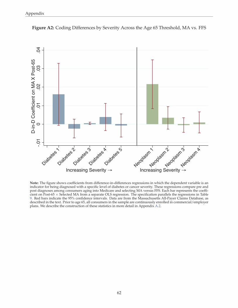
Appendix

Figure A2: Coding Differences by Severity Across the Age 65 Threshold, MA vs. FFS

-.0

10

.01

.02

.03

.04

D-in

-D C

oe

fficie

nt o

n M

A X

Po

st-

65

Diabe

tes 1

Diabe

tes 2

Diabe

tes 3

Diabe

tes 4

Diabe

tes 5

Neo

plas

m 1

Neo

plas

m 2

Neo

plas

m 3

Neo

plas

m 4

Increasing Severity → Increasing Severity →

Note: The figure shows coefficients from difference-in-differences regressions in which the dependent variable is anindicator for being diagnosed with a specific level of diabetes or cancer severity. These regressions compare pre andpost diagnoses among consumers aging into Medicare and selecting MA versus FFS. Each bar represents the coeffi-cient on Post-65 × Selected MA from a separate OLS regression. The specification parallels the regressions in Table9. Red bars indicate the 95% confidence intervals. Data are from the Massachusetts All-Payer Claims Database, asdescribed in the text. Prior to age 65, all consumers in the sample are continuously enrolled in commercial/employerplans. We describe the construction of these statistics in more detail in Appendix A.2.

62

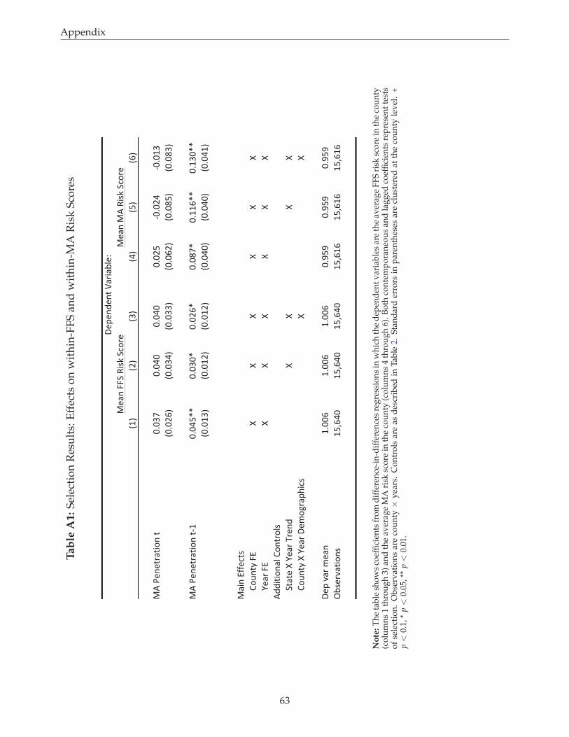
Appendix

Tab

leA

1:

Sel

ecti

on

Res

ult

s:E

ffec

tso

nw

ith

in-F

FS

and

wit

hin

-MA

Ris

kS

core

s

!"#

!$#

!%#

!&#

!'#

!(#

)*+,-.-/01/23.+/

454%6

454&4

454&4

454$'

7454$&

7454"%

!454$(#

!454%&#

!454%%#

!454($#

!4548'#

!4548%#

)*+,-.-/01/23.+/7"

454&'99

454%49

454$(9

454869

45""(99

45"%499

!454"%#

!454"$#

!454"$#

!454&4#

!454&4#

!454&"#

)12.+:;;-</=

>3?./@+A:

BB

BB

BB

C-10+A:

BB

BB

BB

*DD2/23.1E+>3./03E=

F/1/-+B+C-10+G0-.D

BB

BB

>3?./@+B+C-10+H-I3J01KL2<=

BB

H-K+M10+I-1.

"544(

"544(

"544(

45N'N

45N'N

45N'N

OP=-0M1/23.=

"'Q(&4

"'Q(&4

"'Q(&4

"'Q("(

"'Q("(

"'Q("(

)-1.+AAF+R2=S+F<30-

)-1.+)

*+R2=S+F<30-

H-K-.D-./+T1021PE-U

No

te:

Th

eta

ble

sho

ws

coef

fici

ents

fro

md

iffe

ren

ce-i

n-d

iffe

ren

ces

reg

ress

ion

sin

wh

ich

the

dep

end

ent

var

iab

les

are

the

aver

age

FF

Sri

sksc

ore

inth

eco

un

ty(c

olu

mn

s1

thro

ug

h3)

and

the

aver

age

MA

risk

sco

rein

the

cou

nty

(co

lum

ns

4th

rou

gh

6).

Bo

thco

nte

mp

ora

neo

us

and

lag

ged

coef

fici

ents

rep

rese

nt

test

so

fse

lect

ion

.O

bse

rvat

ion

sar

eco

un

ty×

yea

rs.

Co

ntr

ols

are

asd

escr

ibed

inT

able

2.S

tan

dar

der

rors

inp

aren

thes

esar

ecl

ust

ered

atth

eco

un

tyle

vel

.+

p<

0.1,

*p<

0.05

,**

p<

0.01

.

63

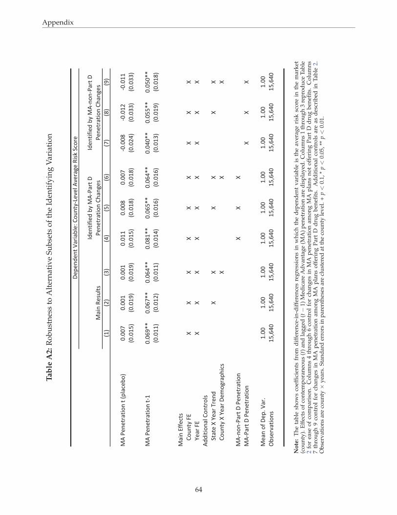
Appendix

Tab

leA

2:

Ro

bu

stn

ess

toA

lter

nat

ive

Su

bse

tso

fth

eId

enti

fyin

gV

aria

tio

n

!"#

!$#

!%#

!&#

!'#

!(#

!)#

!*#

!+#

,-./0102342561.2.!78490:6#

;<;;)

;<;;"

;<;;"

;<;""

;<;;*

;<;;)

=;<;;*

=;<;"$

=;<;""

!;<;"'#

!;<;"+#

!;<;"+#

!;<;"'#

!;<;"*#

!;<;"*#

!;<;$&#

!;<;%%#

!;<;%%#

,-./0102342561.2="

;<;(+>>

;<;()>>

;<;(&>>

;<;*">>

;<;('>>

;<;(&>>

;<;&;>>

;<;''>>

;<;';>>

!;<;""#

!;<;"$#

!;<;""#

!;<;"&#

!;<;"(#

!;<;"(#

!;<;"%#

!;<;"+#

!;<;"*#

,451.?@@092A

B6C12D.E?

FF

FF

FF

FF

F

G043.E?

FF

FF

FF

FF

F

-HH5256148.B612368A

I2420.F.G043.J301H

FF

FF

FF

B6C12D.F.G043.K0L6M347N59A

FF

F

,-=161=/432.K./0102342561

FF

F

,-=/432.K./0102342561

FF

F

,041.6@.K07<.O43<

"<;;

"<;;

"<;;

"<;;

"<;;

"<;;

"<;;

"<;;

"<;;

P:A03Q42561A

"'R(&;

"'R(&;

"'R(&;

"'R(&;

"'R(&;

"'R(&;

"'R(&;

"'R(&;

"'R(&;

,451.S0AC82A

TH0125@50H.:D.,

-=/432.K.

/0102342561.BN41M0A

K0701H012.O4354:80U.B6C12D=V0Q08.-Q034M0.S5AW.I9630

TH0125@50H.:D.,

-=161=/432.K.

/0102342561.BN41M0A

No

te:

Th

eta

ble

sho

ws

coef

fici

ents

fro

md

iffe

ren

ce-i

n-d

iffe

ren

ces

reg

ress

ion

sin

wh

ich

the

dep

end

ent

var

iab

leis

the

aver

age

risk

sco

rein

the

mar

ket

(co

un

ty).

Eff

ects

of

con

tem

po

ran

eou

s(t

)an

dla

gg

ed(t−

1)M

edic

are

Ad

van

tag

e(M

A)

pen

etra

tio

nar

ed

isp

lay

ed.

Co

lum

ns

1th

rou

gh

3re

pro

du

ceT

able

2fo

rea

seo

fco

mp

aris

on

.C

olu

mn

s4

thro

ug

h6

con

tro

lfo

rch

ang

esin

MA

pen

etra

tio

nam

on

gM

Ap

lan

sn

ot

off

erin

gP

art

Dd

rug

ben

efits

.C

olu

mn

s7

thro

ug

h9

con

tro

lfo

rch

ang

esin

MA

pen

etra

tio

nam

on

gM

Ap

lan

so

ffer

ing

Par

tD

dru

gb

enefi

ts.

Ad

dit

ion

alco

ntr

ols

are

asd

escr

ibed

inT

able

2.O

bse

rvat

ion

sar

eco

un

ty×

yea

rs.

Sta

nd

ard

erro

rsin

par

enth

eses

are

clu

ster

edat

the

cou

nty

lev

el.

+p<

0.1,

*p<

0.05

,**

p<

0.01

.

64

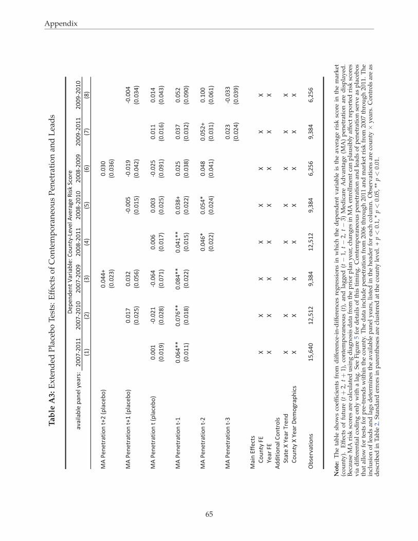
Appendix

Tab

leA

3:

Ex

ten

ded

Pla

ceb

oT

ests

:E

ffec

tso

fC

on

tem

po

ran

eou

sP

enet

rati

on

and

Lea

ds

!"!#$!%$&'(!)&$'*&!+,-

.//01./22

.//01./2/

.//01.//3

.//41./22

.//41./2/

.//41.//3

.//31./22

.//31./2/

526

5.6

576

586

596

5:6

506

546

;<'=&)&>+!>#?)'>@.'5($!A&%?6

/B/88@

/B/7/

5/B/.76

5/B/7:6

;<'=&)&>+!>#?)'>@2'5($!A&%?6

/B/20

/B/7.

1/B//9

1/B/23

1/B//8

5/B/.96

5/B/9:6

5/B/296

5/B/8.6

5/B/786

;<'=&)&>+!>#?)'>'5($!A&%?6

/B//2

1/B/.2

1/B/:8

/B//:

/B//7

1/B/.9

/B/22

/B/28

5/B/236

5/B/.46

5/B/026

5/B/206

5/B/.96

5/B/326

5/B/2:6

5/B/876

;<'=&)&>+!>#?)'>12

/B/:8CC

/B/0:CC

/B/48CC

/B/82CC

/B/74@

/B/.9

/B/70

/B/9.

5/B/226

5/B/246

5/B/..6

5/B/296

5/B/..6

5/B/746

5/B/7.6

5/B/3/6

;<'=&)&>+!>#?)'>1.

/B/8:C

/B/98C

/B/84

/B/9.@

/B2//

5/B/..6

5/B/.86

5/B/826

5/B/726

5/B/:26

;<'=&)&>+!>#?)'>17

/B/.7

1/B/77

5/B/.86

5/B/736

;!#)'DEE&A>,

F?G)>*'HD

II

II

II

II

J&!+'HD

II

II

II

II

<KK#>#?)!$'F?)>+?$,

L>!>&'I'J&!+'M+&)K

II

II

II

II

F?G)>*'I'J&!+'N&O?P+!(Q#A,

II

II

II

II

R%,&+"!>#?),

29S:8/

2.S92.

3S748

2.S92.

3S748

:S.9:

3S748

:S.9:

N&(&)K&)>'T!+#!%$&-'F?G)>*1U&"&$'<"&+!P&'V#,W'LA?+&

No

te:

Th

eta

ble

sho

ws

coef

fici

ents

fro

md

iffe

ren

ce-i

n-d

iffe

ren

ces

reg

ress

ion

sin

wh

ich

the

dep

end

ent

var

iab

leis

the

aver

age

risk

sco

rein

the

mar

ket

(co

un

ty).

Eff

ects

of

futu

re(t+

2,t+

1),

con

tem

po

ran

eou

s(t

),an

dla

gg

ed(t−

1,t−

2,t−

3)M

edic

are

Ad

van

tag

e(M

A)

pen

etra

tio

nar

ed

isp

lay

ed.

Bec

ause

MA

risk

sco

res

are

calc

ula

ted

usi

ng

dia

gn

osi

sd

ata

fro

mth

ep

rio

rp

lan

yea

r,ch

ang

esin

MA

enro

llm

ent

can

pla

usi

bly

affe

ctre

po

rted

risk

sco

res

via

dif

fere

nti

alco

din

go

nly

wit

ha

lag

.S

eeF

igu

re5

for

det

ails

of

this

tim

ing

.C

on

tem

po

ran

eou

sp

enet

rati

on

and

lead

so

fp

enet

rati

on

serv

eas

pla

ceb

os

that

allo

wfo

rte

sts

for

pre

-tre

nd

sw

ith

inth

eco

un

ty.

Th

ed

ata

incl

ud

ep

enet

rati

on

fro

m20

06th

rou

gh

2011

and

mar

ket

risk

fro

m20

07th

rou

gh

2011

.T

he

incl

usi

on

of

lead

san

dla

gs

det

erm

ines

the

avai

lab

lep

anel

yea

rs,

list

edin

the

hea

der

for

each

colu

mn

.O

bse

rvat

ion

sar

eco

un

ty×

yea

rs.

Co

ntr

ols

are

asd

escr

ibed

inT

able

2.S

tan

dar

der

rors

inp

aren

thes

esar

ecl

ust

ered

atth

eco

un

tyle

vel

.+

p<

0.1,

*p<

0.05

,**

p<

0.01

.

65

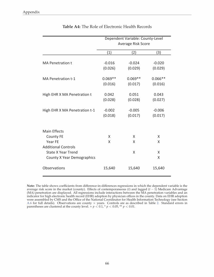
Appendix

Table A4: The Role of Electronic Health Records

!"# !$# !%#

&'()*+*,-.,/0+(,( 1232"4 1232$5 1232$2

!232$4# !232$6# !232$6#

&'()*+*,-.,/0+(,1" 2324677 2324677 2324477

!232"4# !232"8# !232"4#

9/:;(<9=(>(&'()*+*,-.,/0+(, 2325$ 232?" 2325%

!232$@# !232$@# !232$8#

9/:;(<9=(>(&'()*+*,-.,/0+(,1" 12322$ 12322? 123224

!232"@# !232"8# !232"8#

&./+(<AA*B,C

D0E+,F(G< > > >

H*.-(G< > > >

'II/,/0+.J(D0+,-0JC

K,.,*(>(H*.-(L-*+I > >

D0E+,F(>(H*.-(M*N0:-.O;/BC >

PQC*-R.,/0+C "?S452 "?S452 "?S452

M*O*+I*+,(T.-/.QJ*U(D0E+,F1V*R*J(

'R*-.:*(=/CW(KB0-*

Note: The table shows coefficients from difference-in-differences regressions in which the dependent variable is theaverage risk score in the market (county). Effects of contemporaneous (t) and lagged (t − 1) Medicare Advantage(MA) penetration are displayed. All regressions include interactions between the MA penetration variables and anindicator for high electronic health record (EHR) adoption by physician offices in the county. Data on EHR adoptionwere assembled by CMS and the Office of the National Coordinator for Health Information Technology (see SectionA.6 for full details). Observations are county × years. Controls are as described in Table 2. Standard errors inparentheses are clustered at the county level. + p < 0.1, * p < 0.05, ** p < 0.01.

66