unveiling the mandelbrot set - fractal · 2582016 unveiling the mandelbrot set | plus.maths.org ...
TRANSCRIPT

2582016 Unveiling the Mandelbrot set | plus.maths.org
https://plus.maths.org/content/os/issue40/features/devaney/index 1/14
By Robert L. Devaney
Back in the 1970s and 1980s, mathematicians working in an area called dynamical systemsmade use of the everadvancing computing power to draw computer images of the objects theywere working on. What they saw blew their minds: fractallike structures whose beauty andcomplexity is only rivalled by Nature itself. At the heart of them lay the Mandelbrot set, whichtoday has achieved fame even outside the field of dynamics. This article describes where itcomes from and explores its infinite intricacies.
IterationThe Mandelbrot set is generated by what is called iteration, which means to repeat a processover and over again. In mathematics this process is most often the application of amathematical function. For the Mandelbrot set, the functions involved are some of the simplestimaginable: they all are what is called quadratic polynomials and have the form f(x) = x + c,where c is a constant number. As we go along, we will specify exactly what value c takes.
To iterate x + c, we begin with a seed for the iteration. This is a number which we write as x .Applying the function x + c to x yields the new number
x = x + c.Now, we iterate using the result of the previous computation as the input for the next. That is
x = x + c
x = x + c
x = x + c
x = x + cand so forth. The list of numbers x , x , x ,... generated by this iteration has a name: it is calledthe orbit of x under iteration of x + c.
The theory of iterated functions is motivated by questions from real life. Modelling the growth ofa population of animals is an example. The size of the population after one breeding cycledepends on how many animals there are at present, so mathematical models of populationgrowth typically consist of a function f in a variable x, where x represents the present populationsize, and f(x) gives the expected population size after one breeding cycle. To work out the size ofthe population after any number of breeding cycles you need to iterate the function.Incidentally, the functions used in a standard model of population growth are quadraticpolynomials very similar to the ones we will consider here, and this is what first motivated theirstudy.
This leads to one of the principal questions in this area of mathematics: what is the fate oftypical orbits? Do they converge or diverge? Do they cycle or behave erratically? The Mandelbrotset is a geometric version of the answer to this question.
Let's begin with a few examples. Suppose we start with the constant c = 1. Then, if we choosethe seed 0, the orbit is
Unveiling the Mandelbrot set
Submitted by plusadmin on September 1, 2006
2
20
20
1 02
2 12
3 22
4 32
5 42
0 1 2
02

2582016 Unveiling the Mandelbrot set | plus.maths.org
https://plus.maths.org/content/os/issue40/features/devaney/index 2/14
x = 0
x = 0 + 1 = 1
x = 1 + 1 = 2
x = 2 + 1 = 5
x = 5 + 1 = 26
x = 26 + 1 = BIG
x = BIGGER
x = REALLY BIG,and we see that points in this orbit get bigger and bigger — the orbit tends to infinity.
As another example, choose c = 0. Now the orbit of the seed 0 is quite different: it remains fixedfor all iterations.
x = 0
x = 0 + 0 = 0
x = 0 + 0 = 0
x = 0 + 0 = 0 .If we now choose c = 1, something else happens. For the seed 0, the orbit is
x = 0
x = 0 1 = 1
x = (1) 1 = 0
x = 0 1 = 1
x = (1) 1 = 0.Here we see that the orbit bounces back and forth between 0 and 1. This is a cycle of period 2.
To understand the fate of orbits, it is most often easiest to proceed geometrically: a time seriesplot of the orbit often gives more information about its fate. In the plots below, we havedisplayed the time series for x + c where c = 1.1, 1.3, 1.38, and 1.9. In each case we havecomputed the orbit of 0 and marked the points in it by dots which are connected by straight linesegments. Note that the fate of the orbit changes with c. For c = 1.1, we see that the orbitapproaches a 2cycle. For c = 1.3, the orbit tends to a 4cycle. For c = 1.38, we see an 8cycle.And when c = 1.9, there is no apparent pattern for the orbit; mathematicians use the wordchaos for this phenomenon.
0
12
22
32
42
52
6
7
0
12
22
32
0
12
22
32
42
2

2582016 Unveiling the Mandelbrot set | plus.maths.org
https://plus.maths.org/content/os/issue40/features/devaney/index 3/14
Figure 1: the orbit of 0 for iteration of x 1.1 . The orbit approaches a 2cycle.
Figure 2: the orbit of 0 for iteration of x 1.3. The orbit approaches a 4cycle.
Figure 3: the orbit of 0 for iteration of x 1.38. The orbit approaches an 8cycle.
Figure 4: the orbit of 0 for iteration of x 1.9. There is no apparent pattern, we see chaos.
To see additional time series plots for other values of c, select a c value from the options below:
c = 0.65 (/issue40/features/devaney/time1.html) (Tends to a fixed point)c = 1.6 (/issue40/features/devaney/time2.html) (Chaotic behaviour)c = 1.75 (/issue40/features/devaney/time3.html) (Tends to period 3)c = 1.8 (/issue40/features/devaney/time4.html) (Chaotic behaviour close to 3cycle,sometimes called intermittency)c = 1.85 (/issue40/features/devaney/time5.html) (Chaotic behaviour)c = 0.2 (/issue40/features/devaney/time6.html) (Tends to a fixed point).
Before proceeding, let us make a seemingly obvious and uninspiring observation. Under iterationof x + c, either the points in the orbit of 0 get larger and larger so that the orbit tends toinfinity, or they do not. When the orbit does not go to infinity, it may behave in a variety ofways. It may be fixed or cyclic or behave chaotically, but the fundamental observation is that
2
2
2
2
2

2582016 Unveiling the Mandelbrot set | plus.maths.org
https://plus.maths.org/content/os/issue40/features/devaney/index 4/14
there is a dichotomy: sometimes the orbit goes to infinity, other times, it does not. TheMandelbrot set is a picture of precisely this dichotomy in the case where 0 is used as the seed.Thus the Mandelbrot set is a record of the fate of the orbit of 0 under iteration of x + c: thenumbers c are represented graphically and coloured a certain colour depending on the fate ofthe orbit of 0.
Complex numbersHow, then, is the Mandelbrot set a picture in the plane, rather than on the number line on whichall the cvalues we have considered lie? The answer is, instead of considering only real values ofc, we also allow c to be a complex number. If you are not familiar with complex numbers, thenread this brief introduction (/issue40/features/devaney/complex.html) or read Plus articleCurious quaternions (/issue32/features/baez) for more detail.
Let's look at some examples of the iteration of x + c when c is a complex number: if c=i, thenthe orbit of 0 under x + i is given by
x = 0
x = 0 + i = i
x = i + i = 1 + i
x = (1+i) + i = i
x = (i) + i = 1 + i
x = (1+i) + i = i
x = (i) + i = 1+iand we see that this orbit eventually cycles with period 2. If we change c to 2i, then the orbitbehaves very differently
x = 0
x = 0 + 2i = 2i
x = (2i) + 2i = 4 + 2i
x = (4 + 2i) + 2i = 12 14i
x = (12 14i) + 2i = 52 334i
x = BIG (meaning far away from the point 0)
x = BIGGERand we see that this orbit tends to infinity in the complex plane (the numbers comprising theorbit recede further and further from the point 0, which has coordinates (0,0)). Again we makethe fundamental observation that either the orbit of 0 under x + c tends to infinity, or it doesnot.
The Mandelbrot set
2
2
2
0
12
22
32
42
52
62
0
12
22
32
42
5
5
2

2582016 Unveiling the Mandelbrot set | plus.maths.org
https://plus.maths.org/content/os/issue40/features/devaney/index 5/14
Figure 5: the black region is the Mandelbrot set —pick any cvalue from this black reason and you willfind that when you iterate x +c the orbit of zerodoes not escape to infinity. The Mandelbrot set issymmetric with respect to the xaxis in the plane,and its intersection with the xaxis occupies theinterval from 2 to 1/4. The point 0 lies within the'main cardioid', and the point 1 lies within the'bulb' attached to the left of the main cardioid.
The Mandelbrot set puts some geometry into the fundamental observation above. Here is itsprecise definition:
The Mandelbrot set consists of all of those (complex) cvalues for which the corresponding orbitof 0 under x + c does not escape to infinity.
From our previous calculations, we see that c = 0, 1,1.1, 1.3, 1.38, and i all lie in the Mandelbrot set,whereas c = 1 and c = 2i do not. We will representthe Mandelbrot set by the letter M. It is named afterthe mathematician Benoit Mandelbrot (http://wwwhistory.mcs.standrews.ac.uk/Biographies/Mandelbrot.html) who wasone of the first to study it in 1980.
At this point, a natural question is: why would anyonecare about the fate of the orbit of 0 under x + c?Why not the orbit of i? Or 2 + 3i? Or any other seed,for that matter? As we will see below, there is a verygood reason for inquiring about the fate of the orbit of0; amazingly, the orbit of 0 somehow tells us atremendous amount about the fate of all other orbitsunder x + c.
We remark at this point that our definition of theMandelbrot set gives quite an easy way of drawing itusing a computer, which is described in the Plusarticle Computing the Mandelbrot set.(/issue9/features/mandelbrot)
Bulbs and antennasComputer images of the Mandelbrot set, like the one above, give a hint of how incrediblyintricate it is. It is known that, no matter how closely you zoom in on its boundary, it will alwaysappear just as crinkly as it did before. The exact nature of the boundary's crinkliness is still oneof the major open questions in maths. There are, however, quite a lot of things we can say aboutthe Mandelbrot set, and these things reveal that its structure is by no means coincidental:every little piece of it is loaded with mathematical meaning.
So let's have a close look at it. You can see that it consists of a main body, which looks a bit likea heart lying on its side and is therefore called the main cardioid of M (from the Greek kardia,meaning heart). Attached to the main cardioid are myriad "decorations". Closer inspection ofthese shows that all of them are different in shape.
2
2
2
2

2582016 Unveiling the Mandelbrot set | plus.maths.org
https://plus.maths.org/content/os/issue40/features/devaney/index 6/14
The point c = 1.01 is marked inwhite..
Figure 6: decorations of the Mandelbrot set in closeup. The two 'bulbs' shown here are directly attached to the main cardioid.
The decorations directly attached to the main cardioid in M are called primary bulbs or primarydecorations. Any primary bulb in turn has infinitely many smaller decorations attached, as wellas what appear to be antennas. In particular, as is clearly visible in figure 6, the "main antenna"attached to each decoration seems to consist of a number of spokes which varies from decorationto decoration.
There is a beautiful relationship between the number of spokes on these antennas and thedynamics of x + c for c lying inside the primary bulb. To see this, let's take a c value inside thebig bulb that is attached to the main cardioid on the left, for example c=1.01. Starting with theseed 0.0099, you can calculate that this function has a cycle of period two:
x = 0.0099
x = 0.0099 1.01 = 1.0099
x = (1.0099) 1.01 = 0.0099
x = 0.0099 1.01 = 1.0099.The Mandelbrot set keeps track of the orbit of 0, and if we use 0 asa seed we get:
x = 0,x = 1.01,x = 0.0101,
x = 1.00989799,x = 0.00989395,x = 1.00990210,x = 0.00990227,
and so forth. The points in the orbit get closer and closer to the 2cycle, without ever landingright on it — mathematicians say that the orbit of zero is attracted to the two cycle.This is the case not only for c=1.01: for any c value that lies inside the same bulb as 1.01 thefunction x + c has a 2cycle and the orbit of zero is attracted to it.
2
0
12
22
32
0
1
2
3
4
5
6
2
2582016 Unveiling the Mandelbrot set | plus.maths.org
https://plus.maths.org/content/os/issue40/features/devaney/index 7/14
Something similar happens for every primary bulb: if c lies in the interior of such a primarybulb, then the orbit of 0 is attracted to a cycle of some period n. The number n is the same forany c inside this primary bulb, and it is called the period of the bulb. To see that this is reallytrue, open the Mandelbrot set iterator applet (http://math.bu.edu/DYSYS/applets/MsetIteration.html) on my website, which was written by James Denvir. Clicking on a point in theMandelbrot set shown in this applet will display the orbit of zero on the left. You will see thatafter a few iterations this orbit cycles.
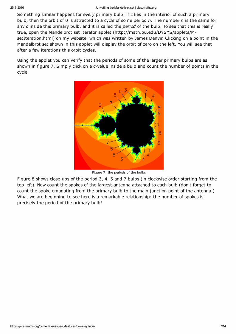
Using the applet you can verify that the periods of some of the larger primary bulbs are asshown in figure 7. Simply click on a cvalue inside a bulb and count the number of points in thecycle.
Figure 7: the periods of the bulbs
Figure 8 shows closeups of the period 3, 4, 5 and 7 bulbs (in clockwise order starting from thetop left). Now count the spokes of the largest antenna attached to each bulb (don't forget tocount the spoke emanating from the primary bulb to the main junction point of the antenna.)What we are beginning to see here is a remarkable relationship: the number of spokes isprecisely the period of the primary bulb!

2582016 Unveiling the Mandelbrot set | plus.maths.org
https://plus.maths.org/content/os/issue40/features/devaney/index 8/14
Figure 8: various bulbs and their periods. Clockwise from top left: period 3 bulb, period 4 bulb, period 5 bulb, period 7 bulb.Note that the period of the bulb is equal to the number of spokes on the main antenna.
A similar result is true for nonprimary bulbs that are not directly attached to the main cardioid.In this case, the period of the bulb is a multiple of the number of spokes attached to itsantenna.
Filled Julia setsBut the remarkable relationships don't end here. There is a second, more dynamic way tocalculate the periods of these primary bulbs in M. To explain this, we have to introduce thenotion of a filled Julia set. The filled Julia set for x + c is subtly different from the Mandelbrotset. For M, we calculated only the orbit of 0 for each cvalue and then displayed the result. A cvalue lies in M if the corresponding orbit of 0 does not escape to infinity. The Mandelbrot set is apicture in the cplane.
For the filled Julia sets, we fix a cvalue and then consider the fate of all possible seeds for thatfixed value of c. Those seeds whose orbits do not escape form the filled Julia set of x + c.Putting it formally:
Fix a value of c. The filled Julia set of x + c is the collection of seeds whose orbit does not tendto infinity.
2
2
2

2582016 Unveiling the Mandelbrot set | plus.maths.org
https://plus.maths.org/content/os/issue40/features/devaney/index 9/14
(Caution: There is also a notion of the Julia set. This term is used to describe the boundary ofthe filled Julia set.)From our examples above we see that the point 0 lies in the filled Julia set of x + 0, because itis fixed and does not go anywhere. But 0 is not in the filled Julia set of x + 1, because itescapes to infinity.
Thus, we get a different filled Julia set for each different choice of c. We write J for the filledJulia set of x + c. In figures 9 to 12 we have displayed the filled Julia sets for a variety of cvalues.
Figure 9: the filled Julia set for c = 1.037 + 0.17i, which lies in a period 2 bulb.
Figure 10: the filled Julia set for c = 0.52 + 0.57i, which lies in a period 5 bulb.
2
2
c2
2582016 Unveiling the Mandelbrot set | plus.maths.org
https://plus.maths.org/content/os/issue40/features/devaney/index 10/14
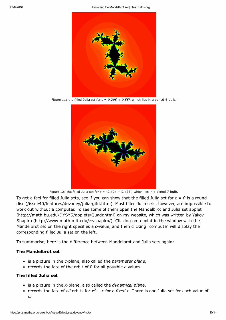
Figure 11: the filled Julia set for c = 0.295 + 0.55i, which lies in a period 4 bulb.
Figure 12: the filled Julia set for c = 0.624 + 0.435i, which lies in a period 7 bulb.
To get a feel for filled Julia sets, see if you can show that the filled Julia set for c = 0 is a rounddisc (/issue40/features/devaney/juliagifd.html). Most filled Julia sets, however, are impossible towork out without a computer. To see some of them open the Mandelbrot and Julia set applet(http://math.bu.edu/DYSYS/applets/Quadr.html) on my website, which was written by YakovShapiro (http://wwwmath.mit.edu/~yshapiro/). Clicking on a point in the window with theMandelbrot set on the right specifies a cvalue, and then clicking "compute" will display thecorresponding filled Julia set on the left.
To summarise, here is the difference between Mandelbrot and Julia sets again:
The Mandelbrot set
is a picture in the cplane, also called the parameter plane,records the fate of the orbit of 0 for all possible cvalues.
The filled Julia set
is a picture in the xplane, also called the dynamical plane,records the fate of all orbits for x + c for a fixed c. There is one Julia set for each value ofc.
The fundamental dichotomy
2

2582016 Unveiling the Mandelbrot set | plus.maths.org
https://plus.maths.org/content/os/issue40/features/devaney/index 11/14
This Julia set is a Cantor set. It is made upof the black points. Every such point formsa separate component, and these pointcomponents pile up on each other.
The fundamental dichotomyAll the filled Julia sets we have displayed here have onething in common: they are connected sets, in other wordsthey consist of just one piece. But not all filled Julia sets areconnected. One of the most beautiful results in all ofcomplex dynamics dates back to 1919 and was provedindependently by both Gaston Julia (http://wwwhistory.mcs.standrews.ac.uk/Biographies/Julia.html) andPierre Fatou (http://wwwhistory.mcs.standrews.ac.uk/Biographies/Fatou.html). It states that eithera Julia set is connected, or it consists of infinitely manypieces, each of which is a single point. These points pile upon each other creating something resembling a cloud."Cloud sets" like these are called Cantor sets (see Plus articleHow big is the milky way? (/issue15/features/oneil) for moreon Cantor sets).
So the fundamental dichotomy says that filled Julia sets for x + c come in one of two varieties:connected sets (one piece) or Cantor sets (infinitely many pieces). There is no inbetween: thereare no cvalues for which J consists of 10 or 20 or 756 pieces.
How do we decide what shape a given J assumes, whether it is connected or a Cantor set?Amazingly, it is the orbit of 0 that determines this. For if the orbit of 0 tends to infinity underiteration of x + c, then the fact is that J is a Cantor set. On the other hand, if the orbit of 0does not tend to infinity, then J is a connected set.
A visual way to view this dichotomy is given by the Mandelbrot set. If c lies in M, then we knowthat the orbit of 0 does not escape to infinity under iteration of x + c, so J must be connected.If c does not lie in M then J is a Cantor set. This dichotomy thus gives us a secondinterpretation of the Mandelbrot set.
The Mandelbrot set consists of all cvalues for which
J is connected, or, equivalentlythe orbit of 0 under x + c does not tend to infinity.
To see how the filled Julia sets "fall apart" into infinitely many pieces as the cvalue leaves theMandelbrot set have a look at these movies (http://math.bu.edu/DYSYS/explorer/tour4.html) onmy website.
It is amazing that the orbit of 0 "knows" the shape of the filled Julia set for x + c. There aresome deeper mathematical reasons for this, which we'll not go into here.
Back to the Mandelbrot setBut the shapes of the filled Julia set and the Mandelbrot set are connected in more ways thanthis. The appearance of the Julia set belonging to a cvalue inside one of the decorations of Mgives us a way of telling the period of that decoration, and vice versa. In figure 13 we havedisplayed the filled Julia set for c = 0.12 + 0.75i. This filled Julia set is often called Douady'srabbit, after Adrien Douady who is one of the pioneers in this area of maths. Note that theimage looks like a "fractal rabbit." The rabbit has a main body with two ears attached.Everywhere you look you see other pairs of ears.
2
c
c
2c
c
2c
c
c2
2

2582016 Unveiling the Mandelbrot set | plus.maths.org
https://plus.maths.org/content/os/issue40/features/devaney/index 12/14
Figure 13: the fractal rabbit.
Another way to say this is that the filled Julia set contains infinitely many "junction points" atwhich 3 distinct black regions in J are attached. In figure 14 we have magnified a portion of thefractal rabbit to illustrate this.
Figure 14: a magnification of the fractal rabbit.
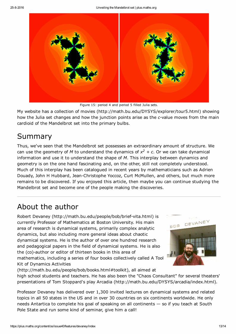
The fact that each junction point in this filled Julia set has 3 pieces attached is no surprise tothose in the know, since this cvalue lies in a primary period 3 bulb in the Mandelbrot set. Thisis another fascinating fact about M. If you choose a cvalue from one of the primary decorationsin M, then, first of all, J must be a connected set, and secondly, J contains infinitely manyspecial junction points and each of these points has exactly n regions attached to it, where n isexactly the period of the bulb. Figure 15 illustrates this for periods 4 and 5.
c
c c
2582016 Unveiling the Mandelbrot set | plus.maths.org
https://plus.maths.org/content/os/issue40/features/devaney/index 13/14
Figure 15: period 4 and period 5 filled Julia sets.
My website has a collection of movies (http://math.bu.edu/DYSYS/explorer/tour5.html) showinghow the Julia set changes and how the junction points arise as the cvalue moves from the maincardioid of the Mandelbrot set into the primary bulbs.
SummaryThus, we've seen that the Mandelbrot set possesses an extraordinary amount of structure. Wecan use the geometry of M to understand the dynamics of x + c. Or we can take dynamicalinformation and use it to understand the shape of M. This interplay between dynamics andgeometry is on the one hand fascinating and, on the other, still not completely understood.Much of this interplay has been catalogued in recent years by mathematicians such as AdrienDouady, John H Hubbard, JeanChristophe Yoccoz, Curt McMullen, and others, but much moreremains to be discovered. If you enjoyed this article, then maybe you can continue studying theMandelbrot set and become one of the people making the discoveries.
About the authorRobert Devaney (http://math.bu.edu/people/bob/briefvita.html) iscurrently Professor of Mathematics at Boston University. His mainarea of research is dynamical systems, primarily complex analyticdynamics, but also including more general ideas about chaoticdynamical systems. He is the author of over one hundred researchand pedagogical papers in the field of dynamical systems. He is alsothe (co)author or editor of thirteen books in this area ofmathematics, including a series of four books collectively called A ToolKit of Dynamics Activities(http://math.bu.edu/people/bob/books.html#toolkit), all aimed athigh school students and teachers. He has also been the "Chaos Consultant" for several theaters'presentations of Tom Stoppard's play Arcadia (http://math.bu.edu/DYSYS/arcadia/index.html).
Professor Devaney has delivered over 1,300 invited lectures on dynamical systems and relatedtopics in all 50 states in the US and in over 30 countries on six continents worldwide. He onlyneeds Antartica to complete his goal of speaking on all continents — so if you teach at SouthPole State and run some kind of seminar, give him a call!
2

2582016 Unveiling the Mandelbrot set | plus.maths.org
https://plus.maths.org/content/os/issue40/features/devaney/index 14/14
Professor Devaney's website (http://math.bu.edu/people/bob/index.html) contains a number ofinteresting applets, articles and interactive papers on dynamical systems. Have a look.
Add new comment (/content/comment/reply/2288#commentform)
Comments
Julia sets (/content/comment/2727#comment2727)Permalink (/content/comment/2727#comment2727) Submitted by Anonymous on September 2, 2011
Thank you for a brilliant web page that helped me understand more clearly the connectionbetween Julia sets and the Mandelbrot set.Jill Russell
reply (/content/comment/reply/2288/2727)
Thank you (/content/comment/2877#comment2877)Permalink (/content/comment/2877#comment2877) Submitted by Anonymous on October 17, 2011
Thank you so much i have a mathematics c assignment on Fractals and the Mandelbrot setand i am so grateful i found this i understand the whole thing now, Thank you!
reply (/content/comment/reply/2288/2877)
This was great! (/content/comment/5980#comment5980)Permalink (/content/comment/5980#comment5980) Submitted by Anonymous on January 9, 2015
That you for making such a clear and indepth guide to this concept
reply (/content/comment/reply/2288/5980)
What an amazing article (/content/comment/6989#comment6989)
Permalink (/content/comment/6989#comment6989) Submitted by Anonymous on December 12, 2015
I found this article quite in depth and informative to say the least. The Mandelbrot Set istruly a thing of beauty.
reply (/content/comment/reply/2288/6989)