unrooted genealogical tree probabilities in the infinitely-many

Unrooted Genealogical Tree Probabilities in the Infinitely-Many-Sites Model

R. C. GRIFFITHS Deparhent of Mathematics, Monash University, Clayton 3168, Australia

AND

SIMON TAVARE Department of Mathematics and Biological Sciences, University of Southern California, Los Angeles, California 90089-1 113

Received 2 Februury 1994; revised 11 Juiy 1994

ABSTRACT

The infinitely-many-sites process is often used to model the sequence variability observed in samples of DNA sequences. Despite its popularity, the sampling theory of the process is rather poorly understood. We describe the tree structure underlying the model and show how this may be used to compute the probability of a sample of sequences. We show how to produce the unrooted genealogy from a set of sites in which the ancestral labeling is unknown and from this the corresponding rooted genealogies. We derive recursions for the probability of the configuration of sequences (equivalently, of trees) in both the rooted and unrooted cases. We give a computational method based on Monte Carlo recursion that provides approximants to sampling probabilities for samples of any size. Among several applications, this algorithm may be used to find maximum likelihood estimators of the substitution rate, both when the ancestral labeling of sites is known and when it is unknown.

1. INTRODUCTION The infinitely-many-sites model is extremely popular in the popula-

tion genetics literature as a description of the DNA sequence variability observed in samples of genes. Hudson [SI provides an excellent overview. For the most part, inference for this process has been based on the distribution of summary statistics of the sequences. One such is the number of segregating sites, which is the number of DNA sequence locations in the aligned sequences in which more than one nucleotide is represented. While this statistic is simple, it clearly does not make full use of the data. Strobeck [lo] showed that certain genealogical trees play an important role in defining the probability distribution of the sample configuration. He showed how such probabilities could be calculated for samples that contained at most three distinct haplotypes.

MATHEMATICAL BIOSCIENCES 12777-98 (1995) 0 Elsevier Science Inc., 1995 655 Avenue of the Americas, New York, NY 10010

0025-5564/95/$9.50 SSDI 0025-5564(94)00044-2

78 R. c. GRIFFITHS AND s. TAVARE

In this paper, we develop the theory of the genealogical trees that underpin the model and show how this theory can be used to calculate probabilities for samples of any size. One novel application of the theory is a way to compute maximum likelihood estimators of the substitution rate.

From a practical point of view, there are two important new aspects to our results. The first shows how sample configuration probabilities can be found when the ancestral labeling of the sites is unknown. The second is the development of a computationally feasible numerical algorithm for calculating such probabilities. This algorithm is based on the principles described by Griffiths and TavarC [6], in which the probability of interest is represented as the mean of a functional of a particular Markov chain that can readily be simulated.

1.1. THE COALESCENT

The genealogy of a sample of n genes drawn at random from a large Wright-Fisher population of approximately constant size N individuals is often described by the coalescent [91. The time Ti during which the sample has j distinct ancestors has an exponential distribution with mean [ E T i = 2/(j(j - l)), j = 2,3,. . . , n, times for different j being independent. Time is conventionally measured in units of 2 N generations. For reviews of the basic structure of the coalescent, see [8, 111, for example.

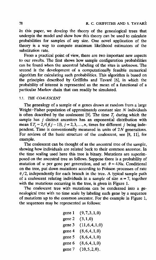
The coalescent can be thought of as the ancestral tree of the sample, showing how individuals are related back to their common ancestor. In the time scaling used here this tree is binary. Mutations are superim- posed on the ancestral tree as follows. Suppose there is a probability of mutation of u per gene per generation, and set 8 = 4Nu. Conditional on the tree, put down mutations according to Poisson processes of rate 8 / 2 , independently for each branch in the tree. A typical sample path of a coalescent relating individuals in a sample of size n = 7, together with the mutations occurring in the tree, is given in Figure 1.

The coalescent tree with mutations can be condensed into a genealogical tree with no time scale by labeling each gene by a sequence of mutations up to the common ancestor. For the example in Figure 1, the sequences may be represented as follows:

gene 1 (9,7,3,1,0) gene 2 (3,1,0) gene 3 (11,6,4,1,0) gene 4 (8,6,4,1,0) gene 5 (8,6,4,1,0) gene 6 (8,6,4,1,0) gene 7 (10,5,2,0).

GENEALOGICAL TREES 79

7

9

2

5

10

) FIG. 1. Coalescent tree with mutations. 0 denotes mutation, 0 denotes individuals.

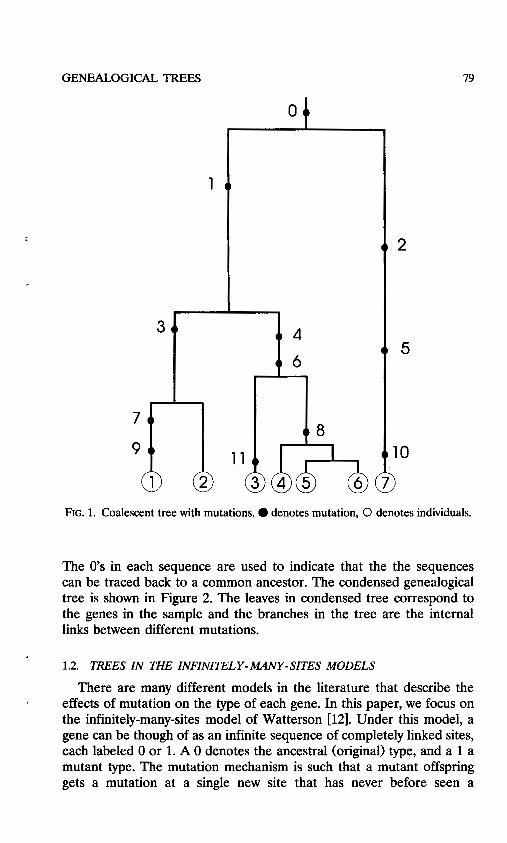
The 0's in each sequence are used to indicate that the the sequences can be traced back to a common ancestor. The condensed genealogical tree is shown in Figure 2. The leaves in condensed tree correspond to the genes in the sample and the branches in the tree are the internal links between different mutations.

1.2. TREES IN THE INFINITELY-u4Ny-SITES MODELS

There are many different models in the literature that describe the effects of mutation on the type of each gene. In this paper, we focus on the infinitely-many-sites model of Watterson [12]. Under this model, a gene can be though of as an infinite sequence of completely linked sites, each labeled 0 or 1. A 0 denotes the ancestral (original) type, and a 1 a mutant type. The mutation mechanism is such that a mutant offspring gets a mutation at a single new site that has never before seen a

.


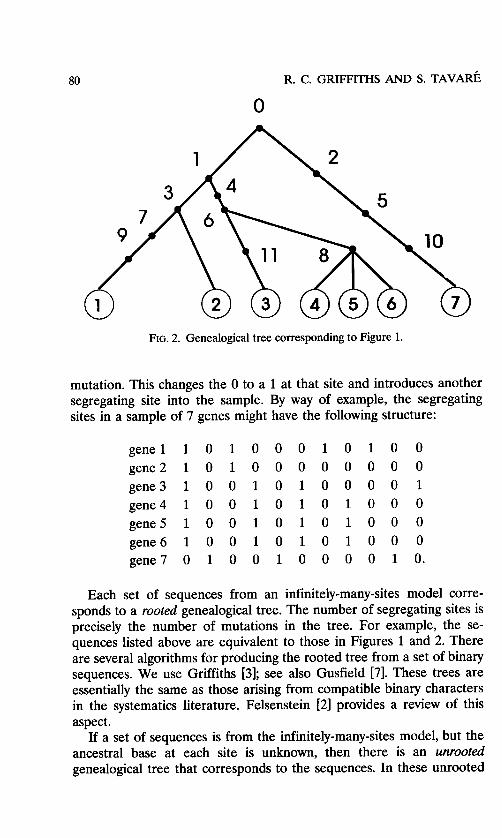
trees, the vertices represent sequences and the number of mutations between sequences are represented by numbers along the edges.

Given a single rooted tree, the unrooted genealogy and therefore all other rooted trees, corresponding to other possible rootings, can be found. The constructive way to do this from a given rooted tree is to put in vertices corresponding to sequences, and also inferred sequences at each vertex of degree greater than two. A mutation at a vertex is counted in the unrooted tree edge leading toward the root in the given rooted tree. If there is no root type in the sample and the root is of degree two, then it is removed from the unrooted genealogy (as in our example). The unrooted tree constructed from any of these rooted trees is unique. It is convenient to label the vertices as to the genes they represent. The unrooted tree for the example sequences is shown in Figure 3.

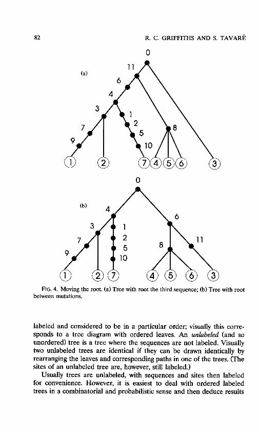
Conversely, the class of rooted trees produced from an unrooted genealogy may be constructed by placing the root at one of the sequences or between mutations along an edge. Two examples are given in Figure 4. In the first the root corresponds to the third sequence, labeled 3 in Figures 1 and 3, and in the second it is between the two mutations between the two inferred sequences.

Trees are called labeled if the sequences are labeled. Two labeled trees are identical if there is a renumbering of the sites so that they are identical. An ordered labeled tree is one where the sequences are

FIG. 3. Unrooted genealogical tree corresponding to Figure 1. The unlabeled circles are inferred individuals.


0

0

FIG. 4. Moving the root. (a) Tree with root the third sequence; (b) Tree with root between mutations.

labeled and considered to be in a particular order; visually this corresponds to a tree diagram with ordered leaves. An unlabeled (and so unordered) tree is a tree where the sequences are not labeled. Visually two unlabeled trees are identical if they can be drawn identically by rearranging the leaves and corresponding paths in one of the trees. (The sites of an unlabeled tree are, however, still labeled.)

Usually trees are unlabeled, with sequences and sites then labeled for convenience. However, it is easiest to deal with ordered labeled trees in a combinatorial and probabilistic sense and then deduce results


about unlabeled trees from labeled trees. If there are (Y sequences (including the inferred sequences) with m1,m2,. . . mutations along the edges and s segregating sites, then there are

a + + ( m j - l ) = s + l i

rooted trees when the sequences are labeled. There may be fewer unlabeled rooted trees, as some can be identical after unlabeling the sequences. In the example there are 11 segregating sites, and so 12 labeled rooted trees, which correspond to distinct unlabeled rooted trees as well.

The class of rooted trees corresponds to those constructed from toggling the ancestor labels 0 and 1 at sites. The number of the 2s possible relabelings that are consistent with the sequences having come from a tree is

.

mi-1

j k = l

This follows from the observation that if there is a collection of m segregating sites which correspond to mutations between sequences, then the corresponding data columns of the 0-1 sequences (with 0 the ancestral state) are identical or complementary. Any of the configurations of k identical and m - k complementary columns correspond to the same labeled tree with a root placed after the kth mutation. The correspondence between different rooted labeled trees and the matrix of segregating sites can be described as follows: in order to move the root from one position to another, just toggle those sites that occur on the branches between the two roots.

Ethier and Griffiths [ l ] provide a simulation algorithm to generate the rooted genealogical tree of a sample of size n from the infinitely- many-sites model, starting from a common ancestor. The simulation proceeds as follows:

(1) Start with a tree with two leaves. (2) At successive time instants where there are r leaves, either

(i) grow a leaf (with probability ( r - l)/(r + 8 - 1)); or

(a

(ii) grow a branch (with probability 8 / ( r + 8 - 1)). (3) (3) Stop when there are n + 1 leaves in the tree, and delete the last leaf.

It is possible to simulate an unrooted tree using the same algorithm, by finding the unrooted tree that corresponds to the simulated rooted tree.

84

1.3. INFERENCE ABOUT e Watterson [12] was interested in estimating the parameter 0 using

the number K of segregating sites in the sample. Since the mean number of segregating sites in a sample of size n is 0Z7:;jf1, he proposed the unbiased estimator

R. c. GRIFFITHS AND s. TAVARE

This estimator does not make full use of the data since it ignores the genealogical relationships among the genes in the sample. It might be expected to be less efficient than an estimator that does. A start on the theory of likelihood methods for unlabeled genealogical trees was made by Strobeck [lo]. In this paper, we extend the exact recursive method of Griffiths [4] to unrooted trees, and we develop a Markov chain Monte Carlo method for computing probabilities of either rooted or unrooted trees. This technique complements the recursive method and allows such probabilities to be computed for arbitrary data sets, which may have both large numbers of individuals and many segregating sites.

2. GENEALOGICAL, TREE PROBABILITIES The type of a gene i in the sample is described by a sequence

yi = ( y i o , y i l , ... ) of positive integers. Suppose that in a sample of n genes there are d distinct sequences, xl ,xz, . . . , xdy grouped according to their multiplicities n = ( q , . . . , nd). We write the data in the form (xl, ..., xd,n) =(T,n), where T represents a rooted tree and n the multiplicities of the leaves. In the example discussed earlier, there are d = 5 distinct sequences that can be represented as

Note that the label 0 is common to all sequences because we are assuming that the individuals in the sample can be traced back to a common ancestor.

Let '(xly.. . ,x,J and (.yl,. . . ,yJ be collections of sequences, not neces- sarily distinct. Define equivalence relations - and = on trees by


(xl,.. . , x n ) - (yl,. ..,y,) if there exists a bijection 7: Z, + Z, = { O , l , 2 ,... } with y,, = q ( x i j ) for i = l , . . ., n and j = 0,1,. . . and (xl,. . .,xJ = (yl,...,yn ) if there exists a bijection 7: Z, -+ Z, and a permutation r E S,, the set of permutations of (1,. . ., n>, such that yw( i ) j = 7 ( x i j ) for i = 1,. . . , n and j = O , l , . . . . Equivalence classes under N correspond to labeled trees, and those under = to unlabeled trees.

Let p(T ,n) be the probability, under the stationary distribution of the process, of obtaining a particular ordered sample of distinct sequences T = (x,,. . . , x d ) with multiplicities n = (n,,. . . , nd) in a sample of size n under equivalence N . Ethier and Griffiths [l] prove that p ( T , n) satisfies the equation

In (5), ej is the jth unit vector, 9 is a shift operator which deletes the first coordinate of a sequence, Y k T deletes the first coordinate of the kth sequence of T , 9 k T removes the kth sequence of T , and “ x k 0 distinct” means that xko # xi, for all (xl,. . .,xd) and (i, j) # (k,O). In the inner summation in the last term of (5) there is at most one j such that Y x k = xi. The boundary condition is p(T, ,e , ) = 1. The system (5) is recursive in the quantity {n - 1 +the number of vertices in TI. Equation (5) can be validated by a simple coalescent argument by looking back- wards in time for the first event in the ancestry of the sample. The first term on the right of (5) corresponds to a coalescence occurring first, while the last two terms correspond to mutations. There are two mutation terms, the first corresponding to the ancestor not being in the sample, the second to the ancestor being in the sample.

For the purposes of an algorithm for computing these probabilities, it is more convenient to consider the recursion satisfied by the quantities po(T,n) defined by

po(T,n) is the probability of the labeled tree T without regard to the order of the sequences in the sample. Using (3, this may be written in

86 R. c. GRIFFITHS AND s. TAV&

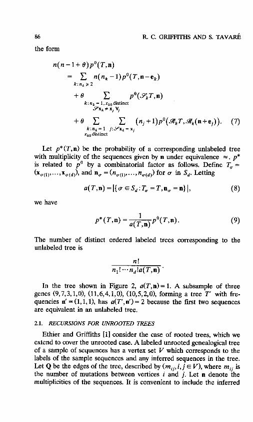
the form

n ( n - l + e ) p o ( T , n )

= n(nk -l)pO(T,n-e,) k : n k 2 2

+ e c pO(%T,n) k : n k = 1,xkOdistinct

9 X k # xi vj

+ e C ( n j + l ) p O ( ~ k T , ~ k ( n + e j ) ) . (7) k : n k = l j : 9 ’ x k = x j

xko distinct

Let p*(T,n) be the probability of a corresponding unlabeled tree with multiplicity of the sequences given by n under equivalence = . p* is related to p o by a combinatorial factor as follows. Define Tu =

(xu(1) , . . . ,xu(,)) , and nu = . , n , ( d ) ) for (T in s d . Letting

a( T,n) = I{ (T E s d : Tu = T , n , = n} 1, (8)

we have

The number of distinct ordered labeled trees corresponding to the unlabeled tree is

In the tree shown in Figure 2, a(T,n)= 1. A subsample of three genes (9,7,3,1,0), (11,6,4,1,0), (10,5,2,0), forming a tree T’ with frequencies n’ = (1,1,1), has a(T’, n’) = 2 because the first two sequences are equivalent in an unlabeled tree.

2.1. RECURSIONS FOR UNROOTED TREES

Ethier and Griffiths [ l ] consider the case of rooted trees, which we extend to cover the unrooted case. A labeled unrooted genealogical tree of a sample of sequences has a vertex set V which corresponds to the labels of the sample sequences and any inferred sequences in the tree. Let Q be the edges of the tree, described by (mi j , i7 j E V ) , where mij is the number of mutations between vertices i and j. Let n denote the multiplicities of the sequences. It is convenient to include the inferred

.


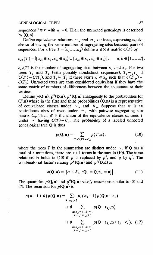
sequences 1 E V with n, = 0. Then the unrooted genealogy is described by (Q,n>.

Define equivalence relations - and = on trees, expressing equivalence of having the same number of segregating sites between pairs of sequences. For a tree T = (xl,.. .,xd) define a d X d matrix C ( T ) by

cUb(T) is the number of segregating sites between xu and xb. For two trees Tl and T2 (with possibly nondistinct sequences), Tl - if C(Tl) = C(T2), and Tl = if there exists u E S, such that C(Tl,) = C(T, 1. Unrooted trees are thus considered equivalent if they have the same matrix of numbers of differences between the sequences at their vertices.

Define p(Q, n), po(Q, n), p* (Q, n) analogously to the probabilities for (T,n) where in the first and third probabilities (Q,n) is a representative of equivalence classes under N,, and zU. Suppose that 12 is an equivalence class of trees under - with pairwise segregating site matrix C,. Then B is the union of the equivalence classes of trees T under - having C(T)=C, . The probability of a labeled unrooted genealogical tree Q is thus

p(Q,n)= p ( T , n ) , (10) T : C ( T ) = c,

where the trees T in the summation are distinct under - . If Q has a total of s mutations, there are s + 1 terms in the sum in (10). The same relationship holds in (10) if p is replaced by p o , and q by qo. The combinatorial factor relating p* (Q, n) and po(Q, n) is

a(Q,n) =I{a ESIVI:Qa =Q,n, =.}I. (11)

The quantities p(Q,n) and po(Q,n) satisfy recursions similar to (5) and (7). The recursion for p(Q,n) is

n ( n - l + O)p(Q,n> = C nk(nk-l)p(Q,n-e,) k : n k a 2

+ e P(Q-e,j,n) k: n k = l , lk l= 1 k + j , m k j > l

+ 6 ~(Q-e , j ,n+ej -e , ) , (12) k : n k = l , lk l= 1 k + j , m k j = l


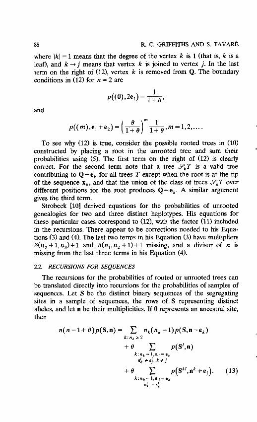
where Ikl = 1 means that the degree of the vertex k is 1 (that is, k is a leaf), and k + j means that vertex k is joined to vertex j . In the last term on the right of (12), vertex k is removed from Q. The boundary conditions in (12) for n = 2 are

and

To see why (12) is true, consider the possible rooted trees in (10) constructed by placing a root in the unrooted tree and sum their probabilities using (5). The first term on the right of (12) is clearly correct. For the second term note that a tree 9,T is a valid tree contributing to Q-e, for all trees T except when the root is at the tip of the sequence x k , and that the union of the class of trees YkT over different positions for the root produces Q - ek. A similar argument gives the third term.

Strobeck [ 101 derived equations for the probabilities of unrooted genealogies for two and three distinct haplotypes. His equations for these particular cases correspond to (121, with the factor (11) included in the recursions. There appear to be corrections needed to his Equa- tions (3) and (4). The last two terms in his Equation (3) have multipliers S(n, + 1, n,)+ 1 and S(n,, n2 + 1)+ 1 missing, and a divisor of n is missing from the last three terms in his Equation (4).

2.2. RECURSIONS FOR SEQUENCES

The recursions for the probabilities of rooted or unrooted trees can be translated directly into recursions for the probabilities of samples of sequences. Let S be the distinct binary sequences of the segregating sites in a sample of sequences, the rows of S representing distinct alleles, and let n be their multiplicities. If 0 represents an ancestral site, then

+ e p(Sk',nk+ej). (13) k : n k = l , s . l = e k

s i . = sj.


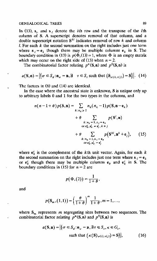
In (13), si. and s.[ denote the ith row and the transpose of the lth column of S. A superscript denotes removal of that column, and a double superscript notation Ski indicates removal of row k and column 1. For each k the second summation on the right includes just one term where s . ~ = e k though there may be multiple columns ek in S. The boundary condition in (13) is p(@,(l)) = 1, where @ is an empty matrix which may occur on the right side of (13) when n = 2.

The combinatorial factor relating p* (S, n) and po(S, n) is

a(S,n) = I[ (+ E Sd :nu = n , 3 T E S , such that (Su(i),T(j)) = S} I. (14)

The factors in (8) and (14) are identical.

to arbitrary labels 0 and 1 for the two types in the columns, and In the case where the ancestral state is unknown, S is unique only up

n ( n - ~ + e)p(S,n) = n k ( n k -I)p(S,n-e,) k : n k , 2

+ e C p(s' ,n) k : n k = l , ~ , ~ = e k

o r e i , s i . # s j . , k + j

where e; is the complement of the kth unit vector. Again, for each k the second summation on the right includes just one term where s . ~ = ek or e; though there may be multiple columns ek and e; in S. The boundary conditions in (15) for n = 2 are

and

where S, represents rn segregating sites between two sequences. The combinatorial factor relating p*(S,n) and pO(S,n) is -

90 R. c. GRIFFITHS AND s. T A V ~

where K is one of the 2, functions in G, which map d X s 0 - 1 matrices to the same class of matrices by toggling 0 and 1 entries in columns. The factors in (16) and (11) are identical.

Equation (13) and (15) have the benefit that they do not require a knowledge of the genealogical tree structure of a sample, and are possibly easier to code than the corresponding tree recursions. However whatever inference can be drawn about the genealogy of a sample is of great interest in practice.

2.3. A NUMERICAL EXAMPLE

In this example we suppose that the ancestral states are unknown and that the sequences, each with multiplicity unity, are:

1 0 0 0 0 0 0 1 0 1 1 0

For convenience, label the segregating sites 1, 2, 3, and 4 starting from the left. When 0 is the ancestral state, a possible rooted tree for these sequences has paths to the root of (l,O), (2,3,0), and (4,O). It is then straightforward to construct the corresponding unrooted genealogy, which is shown in Figure 5. The central sequence is inferred.

There are five possible labeled rooted trees constructed from the unrooted genealogy, corresponding to the root being at one of the sequences, or between the two mutations on the edge between the inferred individual and gene 3. These five trees are shown in Figure 6, together with their probabilities p(T , n), computed exactly from the recursion (5) when 8 = 2.0. p(Q,n) is the sum of these probabilities, 0.00497256. The factor in (11) is 2, and the multinomial coefficient 3!/1!1!1! = 6 so p*(Q,n) = 3 X0.00497256 = 0.0149177. Note that the trees (b) and (e) are identical unlabeled rooted trees, but are distinct labeled rooted trees, so are both counted in calculating p*(Q,n).

1

2

1

FIG. 5. Unrooted genealogy for numerical example.

0.00291 0.00026 0.00 1 20 0.00034 0.00026 FIG. 6. Labeled rooted tree probabilities.

The genealogy in Figure 5 fits into Strobeck’s [lo] genealogy in his Figure l(c), and his (revised) algorithm gives the same probability.

In this small genealogy the coalescent trees with four mutations can be enumerated to find the probability of the genealogy. The trees which produce the tree in Figure 5 are shown in Figure 7, with correspondence to the trees in Figure 6 highlighted.

Let T3 be the time during which the sample has three ancestors and T2 the time during which it has two. T3 and T2 are independent exponential random variables with rates 3 and 1, respectively. By considering the Poisson nature of the mutations along the edges of the coalescent tree and adding the probabilities of the trees in Figure 7 we find that

p*(Q,n) = E e-(3T3+2Tz)e/2(T,2(T2 + T3)’ /2!+2T;(T2 + T 3 ) / 2 !

+2T;T2 /2! + T,2T2(T2 + T3) + T:T. /2! ) )

(( *)1

Evaluating this expectation gives the correct probability 0.0149176.

(a> (a> (b>,(e> (C> (dl FIG. 7. Possible coalescent trees producing Figure 6 trees.


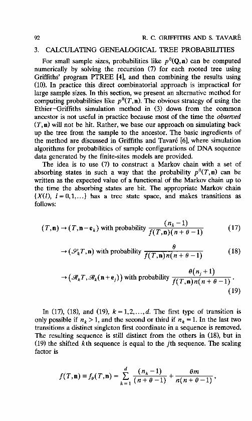
3. CALCULATING GENEALOGICAL TREE PROBABILITIES For small sample sizes, probabilities like po(Q,n) can be computed

numerically by solving the recursion (7) for each rooted tree using Griffiths' program FTREE [4], and then combining the results using (10). In practice this direct combinatorial approach is impractical for large sample sizes. In this section, we present an alternative method for computing probabilities like po(T,n) . The obvious strategy of using the Ethier-Griffiths simulation method in (3) down from the common ancestor is not useful in practice because most of the time the observed (T,n) will not be hit. Rather, we base our approach on simulating back up the tree from the sample to the ancestor. The basic ingredients of the method are discussed in Griffiths and TavarC [6], where simulation algorithms for probabilities of sample configurations of DNA sequence data generated by the finite-sites models are provided.

The idea is to use (7) to construct a Markov chain with a set of absorbing states in such a way that the probability po(T,n) can be written as the expected value of a functional of the Markov chain up to the time the absorbing states are hit. The appropriate Markov chain {XU), I = 0, 1, ...} has a tree state space, and makes transitions as follows:

( I Z k - l ) f (T,n) (n + e -1)

( T , n) + ( T , n - e k ) with probability

e ( n j + 1) f ( T , n ) n ( n + e-1) *

+ ( 9 k T , 9k( n + e j ) ) with probability

(19)

In (17), (18), and (19), k = 1,2,. . ., d. The first type of transition is only possible if nk > 1, and the second or third if nk = 1. In the last two transitions a distinct singleton first coordinate in a sequence is removed. The resulting sequence is still distinct from the others in (181, but in (19) the shifted kth sequence is equal to the j th sequence. The scaling factor is

~

:

GENEALOGICAL TREES

where m is given by

93

m=I{k:nk=l ,Xk ,od i s t inc t ,~Xk # x j v j } I

+ c C ( n j + 1 ) * k : nk = 1

xk , , distinct j : 9 x k = xi

The idea is to simulate the X process starting from an initial tree (T ,n ) until the time T at which there are two sequences (xl0,...,xli) and (x,,, ..., x Z j ) with x l i = x Z j (corresponding to the root of the tree) representing a tree T,. The probability of such a tree is

The representation of po(T,n) is now r7--1 1

where X(1) = (T( l ) ,n( l ) ) is the tree at time 1. Equation (20) may be used to produce an estimate of po(T,n) by simulating independent copies of the tree process {XU), I = 0,1,. . .), and computing [ IIT:if(T(I), n(I))]pO(Tz) for each run. The average over all runs is then an unbiased estimator of po(T,n) . An estimate of p*(T,n) can then be found by dividing by a(T,n).

It is possible to construct a simulation method to find the likelihood of an unrooted genealogy based on (12). However, it seems best to proceed by finding all the possible rooted labeled trees corresponding to an unrooted genealogy and their individual likelihoods.

3.1. COMPUTING A LIKELIHOOD SURFACE

The method of Griffiths and TavarC [6] can be modified to compute po(T,n) for fixed (T,n) as a function of 8 from a single realization of the process { X ( f ) , f = 0,1,. . .}. In the context of estimating 8, this provides a Monte Carlo approximant to a likelihood surface. This method is as follows: Simulate the chain {XU), I = 0,1,. . .} with a particular value 8, as parameter and obtain the likelihood surface for other values of 8 using the representation

7 - 1

I = O

94

bY

R. c. GRIFFITHS AND s. TAVARE

where (as before) (T(l),n(l)) is the tree at time 1, and h is determined

and

this last holding both for transitions of the form (181, when (T’,n’) =

(P,T,n), and of the form (191, when (T’,n’) = (9,T,9fk(n+ei)).

3.2. CHECKING THE ALGORITHM

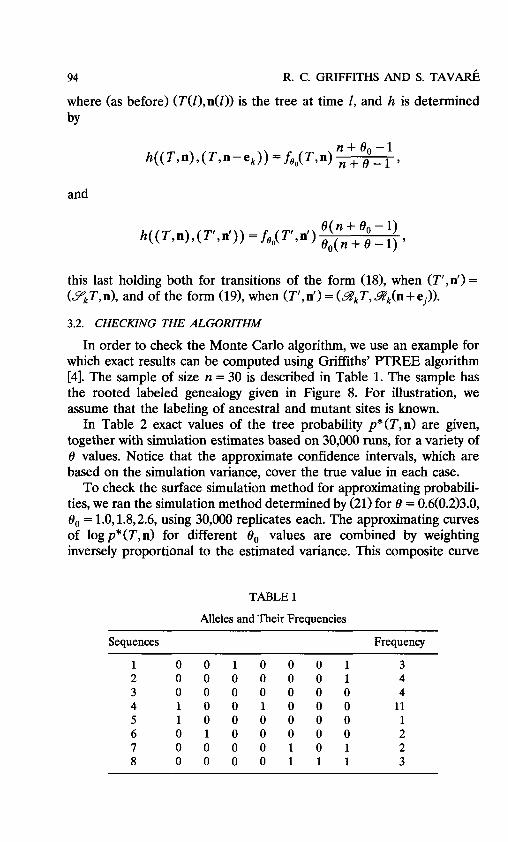
In order to check the Monte Carlo algorithm, we use an example for which exact results can be computed using Griffiths’ PTREE algorithm [4]. The sample of size n = 30 is described in Table 1. The sample has the rooted labeled genealogy given in Figure 8. For illustration, we assume that the labeling of ancestral and mutant sites is known.

In Table 2 exact values of the tree probability p*(T,n) are given, together with simulation estimates based on 30,000 runs, for a variety of 8 values. Notice that the approximate confidence intervals, which are based on the simulation variance, cover the true value in each case.

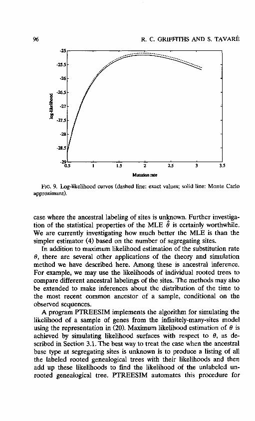
To check the surface simulation method for approximating probabilities, we ran the simulation method determined by (21) for 8 = 0.6(0.2)3.0, 8, = 1.0,1.8,2.6, using 30,000 replicates each. The approximating curves of logp*(T,n) for different 8, values are combined by weighting inversely proportional to the estimated variance. This composite curve

TABLE 1

Alleles and Their Frequencies

Sequences Frequency

0 0 1 0 0 0 1 3 0 0 0 0 0 0 1 4 0 0 0 0 0 0 0 4 1 0 0 1 0 0 0 11 1 0 0 0 0 0 0 1 0 1 0 0 0 0 0 2 0 0 0 0 1 0 1 2 0 0 0 0 1 1 1 3


FIG. 8. Genealogical tree corresponding to Table 1.

and the true curve computed by Griffiths' algorithm are shown in Figure 9. The agreement is extremely good. If the ancestral labeling is unknown, then the probabilities of the different rooted trees can be computed individually and summed according to (10) to approximate the probability of the unrooted tree.

4. DISCUSSION One important application of the theory we have developed here is

maximum likelihood estimation of the substitution rate 8 in the typical

TABLE 2

Exact and Estimated Tree Probabilities

True Estimated 95% Confidence e scale probability probability interval

1.0 10-12 4.77 4.25 (3.52,4.97) 2.0 10-11 1.27 1.35 (1.13,1.58) 4.0 3.33 3.22 (2.85,3.59) 6.0 10-13 3.85 4.01 (3.42,4.60) 8.0 10-14 4.12 3.57 (2.95'4.20) 10.0 10-15 4.75 4.28 (2.81,5.75)


FIG. 9. Log-likelihood curves (dashed line: exact values; solid line: Monte Carlo approximant).

case where the ancestral labeling of sites is uneown. Further investiga- tion of the statistical properties of the MLE 8 is certainly worthwhile. We are currently investigating how much better the MLE is than the simpler estimator (4) based on the number of segregating sites.

In addition to maximum likelihood estimation of the substitution rate 8, there are several other applications of the theory and simulation method we have described here. Among these is ancestral inference. For example, we may use the likelihoods of individual rooted trees to compare different ancestral labelings of the sites. The methods may also be extended to make inferences about the distribution of the time to the most recent common ancestor of a sample, conditional on the observed sequences.

A program PTREESIM implements the algorithm for simulating the likelihood of a sample of genes from the infinitely-many-sites model using the representation in (20). Maximum likelihood estimation of 8 is achieved by simulating likelihood surfaces with respect to 8, as described in Section 3.1. The best way to treat the case when the ancestral base type at segregating sites is unknown is to produce a listing of all the labeled rooted genealogical trees with their likelihoods and then add up these likelihoods to find the likelihood of the unlabeled unrooted genealogical tree. PTREESIM automates this procedure for

I

:


single likelihoods and for surface simulation. Checking consistency of a collection of sequences with the infinitely-many-sites model, and the production of a (rooted or unrooted) tree from these sequences is an option in PTREESIM. The algorithm used is that in Griffiths [31. PTREESIM is available from the authors on request in portable C source code and in executable form for a PC.

The infinitely-many-sites process described here is certainly an over- simplified picture of the variability observed in DNA sequence data. The assumption that once a mutation has occurred at a site there may be no further mutation there is clearly in conflict with the occurrence of back substitutions, for example. Griffiths and TavarC [6] show how the Monte Carlo recursion technique can be used to approximate the likelihood of samples from coalescent models which allow for back substitutions. These techniques are considerably more expensive computationally than the present ones.

The sampling theory developed here applies to samples from populations that have maintained approximately constant size for many generations, an assumption that is clearly unreasonable in some cases. The effects of deterministically varying population size can be incorporated into the analysis; see Griffiths and TavarC [SI. The combinatorial and topological structure of the tree (T,n) is precisely the same as that described here, but the probabilistic structure has to be modified to account for the fact that the times T,. while the sample has j distinct ancestors are dependent random variables.

'

-

1

The authors were supported in part by NSF grant DMS 90-05833, and by the IMA ut the University of Minnesota.

REFERENCES

1 S. N. Ethier and R. C. Griffiths, The infinitely-many-sites model as a measure valued diffusion, Ann. Probab. 15:414-545 (1987).

2 J. Felsenstein, Numerical methods for inferring evolutionaIy trees, Quart. Rev. Biol. 57:379-404 (1982).

3 R. C. Griffiths, An Algorithm for Constructing Genealogical Trees, Statistics Research Report #163, Department of Mathematics, Monash University, 1987.

4 R. C. Griffiths, Genealogical-tree probabilities in the infinitely-many-site model, J . Math. Biol. 27:667-680 (1989).

5 R. C. Griffiths and S. Tavar6, Sampling theory for neutral alleles in a varying environment, Phil. Trans. Roy. Sac. London B, 344:403-410 (1994).

6 R. C. Griffiths and S. Tavar6, Simulating probability distributions in the coalescent, Theor. Pop. Biol. 46:131-159 (1994).


7 D. Gusfield, Efficient algorithms for inferring evolutionary trees, Netwok

8 R. R. Hudson, Gene genealogies and the coalescent process, in Oxford Surveys in Euolutionaly Biology, vol. 7, D. Futuyma and J. Antonovics, eds., Oxford University Press, 1991, pp. 1-44.

9 J. F. C. Kingman, On the genealogy of large populations, J. Appl. h b a b .

10 C. Strobeck, Estimation of the neutral mutation rate in a finite population from DNA sequence data, Theor. Pop. Bwl. 24:160-172 (1983).

11 S. TavarC, Calibrating the clock Using stochastic processes to measure the rate of evolution, in Molecular Biology and Mathematics, E. S . Lander, ed., National Academy Press, to appear.

12 G. A. Watterson, On the number of segregating sites in genetical models without recombination, Theor. Pop. Bwl. 7556-276 (1975).

21:19-28 (1991).

19A27-43 (1982).

. . "

unrooted genealogical tree probabilities in the infinitely-many

Documents