university of twente - universiteit twenteessay.utwente.nl/56922/1/010ce2005_schutyser.pdf · at...
TRANSCRIPT

University of Twente
EEMCS / Electrical Engineering Control Engineering
An optimal controller for Desdemona for an optimal feeling
Pieter Schutyser
M.Sc. Thesis
Supervisors prof.dr.ir. J. van Amerongen
dr.ir. S. Stramigioli dr.ir. M.Wentink, ir. V. Duindam
March 2005
Report nr. 010CE2005 Control Engineering
EE-Math-CS University of Twente
P.O. Box 217 7500 AE Enschede
The Netherlands

ii

Public version
In this report confidential figures and tables are not displayed. For more information see [2].

iv
Summary
Desdemona is a new prototype disorientation simulator which can generate acceleration profiles. In this report thedesign of an optimal controller for Desdemona is described.An optimal controller calculates the optimal move-ments of Desdemona within the limits of Desdemona. The limitations are caused by maximum displacement ofthe joints and a maximum in the power/torque of the motors, where a dynamic model is used to calculate the powerand torque of the motors. The optimal controller optimizes the complete trajectory if it is known beforehand oruntil a limited time horizon if the trajectory can only be estimated for a limited time horizon.
The optimal controller is realized and tested for Desdemonawith one degree of freedom (d.o.f.), calleddy-namic flight simulatoralso with two d.o.f. where the central yaw and the vertical sledge are controlled. And finallywith three d.o.f where yaw of the cabin is also included. If the d.o.f. is one then the optimization can be solved forthe case the trajectory can only be estimated for a certain time horizon. This is the case for example withman inthe loop.
The results show that the optimization works especially forlimited d.o.f. An increased number of d.o.f. makesthe problem much harder to solve, which causes a decrease in performance. The performance can be increasedby choosing smart initial values. Initial values for the optimization can be generated with the existing controllers.The results of the optimization will be better or equal to theresults of the initial values from the controller. Thismakes the optimization method an interesting extension forthe existing controllers. For Desdemona asdynamicflight simulatorthis is shown.
The off-line optimization is ready to be implemented for simulations. Some work has to be done for realizingthe on-line optimization. The path of the simulated model has to be estimated in the future and the calculation timehas to be reduced.

vi

Preface
After a couple of studies I thought I was ready and went to the University. Now almost six yeas later Im writingthe last pages of my final thesis for completing my Master of Science study in the field of Electrical Engineeringat the University of Twente. The thesis is about a subject that has my interest from the beginning of my technicalstudy. It is about a moving object which is controlled by a controller which looks complex but is, if you look tothe mathematics, quite simple. I have no idea why I’m interested in theoretical mathematics, moving objects andthe complete area between. But it is for me fascinating to seethat all these things together can result in a piece ofadvanced technology.
I would like to thank some people for their support during this assignment. First I would like to thank dr.ir.Stefano Stramigioli, he deserves a lot of appreciation for all the advice he gave during my work. I also would likethank dr.ir. Mark Wentink for all the enthusiastic support he has given me by phone and ’live’ discussions. Also Iwould like to thank him for introducing me in the fascinatingworld of disorientation simulators.
The last but not the least, I also would like to thank my family, who always give support and courage duringmy studies. And my friends who make life much better in and outside Enschede. Thanks to all of you.

viii

Nomenclature
Symbols
p Acceleration in the origin of the cabin , see equation (3.2)
pd Desired acceleration in the cabin , see equation (3.1)
τ Torque of the motors
τmax Maximum torque of the motors
T i,jk Twist fromk to j seen from coordinatesi
C(q, q) Coriolis matrix
en n-axis of the coordination frame. Withn asx,y,z
f0 Cost function in the analytical optimization
ffeas Feasibility function, the part in the cost function that represent the constraints
G Gravity , see equation (3.2)
g Gravity constant
Hnm Matrix that expresses a general change of Cartesian coordinates from coordinatesm to n
hn Step-size (sample time) withn as the sampled item (Sd,q...)
I0,i Generalized inertia matrix of bodyi expressed in coordinate frame0
iemn
Inertia in directionn of elementm
J Cost function
Jn Jacobian matrix (linear relationship between the joint velocities and the end-effectorn twist)
k Discrete time step
K() End cost
M Modulus of the path of Desdemona , page 46
M(q) Mass matrix
Me Modulus of the estimated path in the future , page 46
Mn Mass of elementn
N Conservative force
On nth Coordinates frame

x
p Translation vector
Pmax Maximum power of the motors
Q (Weighing matrix)Matrix which give to some extent the importance of the optimization per d.o.f. of thepath
q Joints of Desdemona
qn max Maximum positionqn can have
R Rotation matrix
S Path of Desdemona , see equation (3.2)
Sd Desired path , page 7
Sd,perc PerceivedSd
Sperc PerceivedS
Tc Calculation time
Th Horizon Time
V Potential energy
ns Sampled n
Abbreviations and used terms
d.o.f. degree of freedom
dom Domain
ips Neural discharge rate (impulses per second)
Iteration A iteration is one step in the optimization routine
MPC Model Predictive Control
RMS Root Mean Square
Run A run is a complete optimization, which includes a numberof iterations

Contents
1 Introduction 11.1 Desdemona in comparison with other disorientation simulators . . . . . . . . . . . . . . . . . . . 21.2 Description of the problem . . . . . . . . . . . . . . . . . . . . . . . . .. . . . . . . . . . . . . 31.3 Outline . . . . . . . . . . . . . . . . . . . . . . . . . . . . . . . . . . . . . . . . .. . . . . . . 3
2 Objectives 5
3 Problem definition for an optimal controller 73.1 Defining the path to be followed . . . . . . . . . . . . . . . . . . . . . .. . . . . . . . . . . . . 73.2 Physical bounds of Desdemona . . . . . . . . . . . . . . . . . . . . . . .. . . . . . . . . . . . . 73.3 Time horizon . . . . . . . . . . . . . . . . . . . . . . . . . . . . . . . . . . . . .. . . . . . . . 83.4 Mathematical formulation of the optimization problem .. . . . . . . . . . . . . . . . . . . . . . 83.5 Example of the optimization . . . . . . . . . . . . . . . . . . . . . . . .. . . . . . . . . . . . . 9
4 Numerical optimization 114.1 Introduction to numerical optimization . . . . . . . . . . . . .. . . . . . . . . . . . . . . . . . . 114.2 Redefining the analytical optimization to a numerical problem . . . . . . . . . . . . . . . . . . . 114.3 Classifying the numerical optimization problem . . . . . .. . . . . . . . . . . . . . . . . . . . . 124.4 Methods for solving nonlinear least-squares optimization problems . . . . . . . . . . . . . . . . . 124.5 Limitations to the numerical optimization . . . . . . . . . . .. . . . . . . . . . . . . . . . . . . 134.6 Converting a constrained to an unconstrained optimal problem . . . . . . . . . . . . . . . . . . . 134.7 Example of numerical optimization . . . . . . . . . . . . . . . . . .. . . . . . . . . . . . . . . . 14
5 Practical extensions of the numerical optimization 175.1 Barrier functions . . . . . . . . . . . . . . . . . . . . . . . . . . . . . . . .. . . . . . . . . . . 175.2 Optimizing initial position and speed of Desdemona . . . .. . . . . . . . . . . . . . . . . . . . . 185.3 Optimizing with different step size . . . . . . . . . . . . . . . . .. . . . . . . . . . . . . . . . . 195.4 Different stopping criterions . . . . . . . . . . . . . . . . . . . . .. . . . . . . . . . . . . . . . 205.5 Evaluating different profiles . . . . . . . . . . . . . . . . . . . . . .. . . . . . . . . . . . . . . 215.6 Desdemona with three degrees of freedom . . . . . . . . . . . . . .. . . . . . . . . . . . . . . . 285.7 Improving the performance . . . . . . . . . . . . . . . . . . . . . . . . .. . . . . . . . . . . . . 335.8 Discussion three d.o.f. results . . . . . . . . . . . . . . . . . . . .. . . . . . . . . . . . . . . . . 35
6 Including human perception model 376.1 Introduction . . . . . . . . . . . . . . . . . . . . . . . . . . . . . . . . . . . .. . . . . . . . . . 376.2 Human perception . . . . . . . . . . . . . . . . . . . . . . . . . . . . . . . . .. . . . . . . . . . 376.3 Vestibular system . . . . . . . . . . . . . . . . . . . . . . . . . . . . . . . .. . . . . . . . . . . 386.4 Including model of the semi-circular canals and the otoliths . . . . . . . . . . . . . . . . . . . . . 406.5 Results . . . . . . . . . . . . . . . . . . . . . . . . . . . . . . . . . . . . . . . . .. . . . . . . . 41
xii CONTENTS
7 Predictive optimal control 437.1 The principle of on-line optimization . . . . . . . . . . . . . . .. . . . . . . . . . . . . . . . . . 437.2 Desdemona as a dynamic flight simulator . . . . . . . . . . . . . . .. . . . . . . . . . . . . . . 447.3 The on-line control method . . . . . . . . . . . . . . . . . . . . . . . . .. . . . . . . . . . . . . 467.4 Reducing the optimization time . . . . . . . . . . . . . . . . . . . . .. . . . . . . . . . . . . . . 467.5 On-line examples . . . . . . . . . . . . . . . . . . . . . . . . . . . . . . . . .. . . . . . . . . . 477.6 Discussion of the results . . . . . . . . . . . . . . . . . . . . . . . . . .. . . . . . . . . . . . . 48
8 Conclusion and recommendations 518.1 Conclusions . . . . . . . . . . . . . . . . . . . . . . . . . . . . . . . . . . . . .. . . . . . . . . 518.2 Recommendations . . . . . . . . . . . . . . . . . . . . . . . . . . . . . . . . .. . . . . . . . . . 52
References 53
A Notation and Model 55A.1 Notation . . . . . . . . . . . . . . . . . . . . . . . . . . . . . . . . . . . . . . . .. . . . . . . . 55A.2 Model . . . . . . . . . . . . . . . . . . . . . . . . . . . . . . . . . . . . . . . . . . .. . . . . . 56A.3 Calculating the path of Desdemona. . . . . . . . . . . . . . . . . . .. . . . . . . . . . . . . . . 58A.4 Euler Lagrangian equations and Dynamic model . . . . . . . . .. . . . . . . . . . . . . . . . . . 58A.5 Parameters of Desdemona . . . . . . . . . . . . . . . . . . . . . . . . . . .. . . . . . . . . . . 59
B Model with two degrees of freedom 61B.1 Analytical optimization . . . . . . . . . . . . . . . . . . . . . . . . . .. . . . . . . . . . . . . . 62
C Optimization methods and definitions 65C.1 Convex . . . . . . . . . . . . . . . . . . . . . . . . . . . . . . . . . . . . . . . . . .. . . . . . 65C.2 Newton and Quasi-Newton methods . . . . . . . . . . . . . . . . . . . .. . . . . . . . . . . . . 66
D Implementation of the optimization problem 67D.1 Optimization program . . . . . . . . . . . . . . . . . . . . . . . . . . . . .. . . . . . . . . . . . 67D.2 Different cost functions that are used in this report . . .. . . . . . . . . . . . . . . . . . . . . . . 70D.3 Reference list from the used files . . . . . . . . . . . . . . . . . . . .. . . . . . . . . . . . . . . 72

Chapter 1
Introduction
Human beings sense movements of their bodies. The interpretation of the sensed movements is a complex processand a broad research topic. For new research topics Desdemona is developed, it is a new kind of motion platform.With Desdemona it is possible to do research on the human perception model and to use the gained knowledge forapplied research and applications. Some examples are the training for flying a plane, driving a car and steering aship.
Figure 1.1: Desdemona at TNO
Current motion platforms are limited in their simulation ofsustained acceleration. Desdemona has an innov-ative kinematic design (see figure 1.1) so that it is less limited than conventional simulators. Because the controlsystem of existing motion platforms are not optimal for Desdemona, a new kind of controller is discussed in thisreport.

2 1. INTRODUCTION
1.1 Desdemona in comparison with other disorientation simulators
The 1 most common motion platform is the Stewart six-pod platform, which allows all six degrees of freedom.Despite the fact that accelerations can be induced only for ashort time, for many applications such as training fortransport aircraft this platform is sufficient. However, for fighter aircraft with pulling high sustained G-loads, thisplatform is not sufficient for realistic mission rehearsal.Present developments show that for flight simulation withhigher G-loads, centrifuges are built with roll and pitch options of the gondola. Problem with these simulatorsis that they are able to simulate the G-load, but that the corresponding angular accelerations during the onset,introduce conflicting motion information to the pilot’s equilibrium system. This may lead to unwanted side effectssuch as disorientation and motion sickness. Desdemona is a research simulator, which combines the possibilities ofcommon Stewart platform with the possibility of the sustained G-load, however, without the co-varying rotationalaccelerations.
Figure 1.2: Desdemona movements
The Desdemona concept was developed by TNO Human Factors in co-operation with AMST Systemtechnik[2]. Figure 1.2 shows the concept. It consists of a fully gimbaled cockpit, which allows for unlimited rotation in alldirections. The pilot with his head in the center of rotation, controls the (flight) instruments and has a view outsidevia up-to-date visuals. For simulation purposes differentmodels and databases are available. The cockpit can movealong an 8 meter horizontal track. The cockpit can also move vertically over 2 meter. Finally, the horizontal trackis rotated around a vertical axis, which means that centrifuging is also possible. The working principle of a normalcentrifuge is a variation on the angular velocity with constant eccentricity resulting in a varying G-load. However,keeping the angular velocity constant and varying the amount of eccentricity is another way of varying the G-load.Desdemona applies both with a maximal G-load of 3g. The main characteristic of the concept, i.e. the variationof the G-load by varying the eccentricity, has consequencesfor simulation. It means that the onset of a sustainedG-load is not necessarily accompanied with a strong angularacceleration, as is the case in the conventional cen-trifuge. It is possible to start the rotator subliminal up tothe desired speed with the cockpit in the center position,and subsequently move the cockpit away from the axis withoutvarying the angular velocity. It is obvious that oneshould take into account the linear Coriolis accelerationsduring the movement of the cockpit on the track. This
1This part is mainly based on [2]
DESCRIPTION OF THE PROBLEM 3
example also shows the difficulty of controlling Desdemona.It is possible to simulate a transversal accelerationby moving the cockpit on the horizontal track while possiblyrotating the horizontal track. The choice depends onthe magnitude and the duration of the desired acceleration.
1.2 Description of the problem
The control problem of the Desdemona is significantly different from that of the Steward platform, because thedirections of movement of the Steward platform are in general the same as the model movements. Desdemona onthe other hand can also use rotation to simulate a linear acceleration.
To find the optimal acceleration and rotation path, an optimal controller is needed. The optimal path is definedasthe path that is as close as possible to the desired path.The optimal controller decides which movements of Des-demona give the best simulation of the desired path with taking constraints such as maximum power in account.
In this report an optimal controller is designed for the cases in which the acceleration trajectory is known andunknown beforehand.
1.3 Outline
The outline of this report is as follows. In chapter 2, the objectives of this report are given. Then in chapter 3 theoptimization problem is defined which forms the basis of the optimization. In chapter 4 the numerical optimizationmethods are discussed and the problem is solved for the most basic off-line case. Then in chapter 5 the numericaloptimization is redefined to make it more practically applicable. In chapter 6 the human perception model isincluded. In chapter 7 an on-line optimization for Desdemona as dynamic flight simulator is done. Finally, inchapter 8 conclusions and recommendations of this researchare drawn.

4 1. INTRODUCTION

Chapter 2
Objectives
Desdemona combines the degrees of freedom (d.o.fs) of a centrifuge simulator, used for sustained G-load simula-tion, with additional d.o.f.’s to give it the full 6 d.o.f. motion cueing possibilities of a standard hexapod simulator.In centrifuge mode, Desdemona rotates around its central yaw axis while in hexapod mode this axis, in combinationwith the main arm, is used to simulate linear accelerations.In both modes, attitude is simulated with the gimbaledsystem. The combination of a centrifuge and hexapod simulation mode provides huge advantages in simulations ofhighly agile maneuvers with sustained G-load (e.g.: F16 combat simulation, unusual attitude recoveries, etc.). Themain objective of this report is to design an optimal motion cueing and control algorithm that takes full advantageof the available d.o.f’s of Desdemona.
Goal
The simulation of high frequency, agile motion in hexapod mode in combination with, or followed by, sustainedG-loads in centrifuge mode requires advanced motion cueingand control algorithms. Although algorithms for thecentrifuge and hexapod mode are developed by AMST separately, an algorithm that combines the two has not yetbeen developed. The goal of this work is to develop an optimalcontrol algorithm that combines the centrifuge andhexapod capabilities of Desdemona during the simulation ofhighly agile maneuvers (high frequency accelerations)in combination with, or followed by, sustained G-loads (lowfrequency accelerations). In this scope, optimal isdefined as:
• minimization of the perception of differences in the simulator
• minimization of false cues,
• within the limits of Desdemona (structural limits and drivelimits).
Although pre-defined maneuvers will be used first, the ultimate, long-term goal is an optimal control algorithmthat can be implemented in pilot-in-the-loop simulations (which will result in maneuvers that are hard to predictbeforehand).
Methods
In order to reach the stated goal, the following sub-goals are defined:
• Study of literature on: modeling and simulation of robotic dynamics, optimal control concepts, Desdemonaspecifications, motion cueing in conventional flight simulation,
• Developing a dynamic simulation model of Desdemona,
• evaluating suitable optimal control concepts,

6 2. OBJECTIVES
• defining an optimization cost function (incorporating perception of difference, false cues, drive performanceparameters, etc.)
• developing & implementing of optimal control algorithms inthe dynamic simulation model
• evaluating the optimal control algorithm, especially the ’optimal’ motion characteristics during the transitionfrom hexapod motion types to centrifuge motion types (and vice versa).
• Working towards a real-time optimal control algorithm thatcan be used duringman in the loopsimulations.

Chapter 3
Problem definition for an optimalcontroller
The main goal of the optimal controller is to find optimal movements for the jointsq(t) of Desdemona within thephysical constraints such as motor power, dimensions etc.
To define the optimal control problem, the path and the error will be defined first and then the physical con-straints. At the end of this chapter a simplified model of Desdemona will be outlined.
3.1 Defining the path to be followed
Desdemona is a simulator, in which one feels the acceleration from the simulated model. The model gives outputinformation on the rotation speedω(t) and the translation accelerationp(t) and gravityG(t). The calculated pathfrom the model is the desired path for Desdemona and is indicated with:
Sd(t) =
(ωd(t)
pd(t) + G(t)
)(3.1)
The mechanical part of Desdemona has to follow that path. Themovement of Desdemona can be written in thesame way as the movement of the model, but now as function of the joints and it derivativesq(t), q(t), q(t).
S(t) =
(ω(q(t), q(t))
p(q(t), q(t), q(t)) + G(q(t))
)(3.2)
Where omega can be extracted from the twist (see also A.6):Thead,earthhead =
(ωv
)andp can be calculated
with equation A.18. The gravity vectorG(q(t)) can be calculated with the help of the rotation matrix (see A.19).
The goal of Desdemona is to follow the path of the model. The error that Desdemona makes can be written as:∆S(q(t), q(t), q(t), t) = Sd(t)−S(q(t), q(t), q(t)). The error that the pilot will observe is not∆S(q(t), q(t), q(t), t)because the vestibular nerve system in combination with thevisual input does not give an exact impression of∆S(q(t), q(t), q(t), t). It is important to keep this in mind designing the optimum controller. This fact will bediscussed later (chapter 6 ). But at this point it will be assumed that the pilot is observing∆S(q(t), q(t), q(t), t) asfault in the path.
3.2 Physical bounds of Desdemona
Some of the movements of Desdemona are physically limited because of the finite stroke of the joints. Thislimitation is given in equation (3.3). The joints of the vertical sledge and heave, respectivelyq2(t) andq3(t), are

8 3. PROBLEM DEFINITION FOR AN OPTIMAL CONTROLLER
Optimization Desdemona
+
-
Error
Sd
Figure 3.1: Optimal control problem
limited because they are the only two translation joints. The others are unbounded joint rotation movements.
−q2max≤ q2(t) ≤ q2 max−q3max≤ q3(t) ≤ q3 max
(3.3)
Other bounds on the velocities and accelerations prevent large mechanical stress and vibrations to occur in thesystem.
−qmax ≤ q(t) ≤ qmax
−qmax ≤ q(t) ≤ qmax(3.4)
Desdemona is actuated by a number of motors and every motor has limited power and torque.
−Pi,max ≤ τi(t)qi(t) ≤ Pi,max
−τmax ≤ τ(t) ≤ τmax(3.5)
The power and torque relations are calculated in section A.4
3.3 Time horizon
Time horizon (Th) is defined as the amount of time in the future for which the desired path,Sd(t), is known.The time horizons depend on the purpose the Desdemona is used. They can be grouped in two categories:man inthe loopandno man in the loop(for example a roller coaster). If Desdemona works withman in the loop, the timehorizon will be short although it is possible to predict a fewseconds. This depends of course on the model whichDesdemona is simulating. For example the path of a car which is driving on a road with no side lanes is easier topredict then a car on a road with side lanes. If there is noman in the loopthen the time horizon runs till the end ofthe simulation, because the path is predefined.
3.4 Mathematical formulation of the optimization problem
Figure 3.1 shows the optimization problem. The problem can be calculated off-line for cases where there is noman in the loop. In case there is aman in the loopsimulation, then the state at the end of the time horizon (finalstate) of Desdemona is important, since future simulation errors need to be avoided1. Because the pathSd can notbe calculated in advance, the optimization should be done online.
The definition of the problem is divided an on-line and off-line optimization.
1With man in the loopthe simulation time is longer than the time horizon and the path of Desdemona is optimized with several optimizationswhich start after each other. An end cost avoids that at the end of an optimization Desdemona comes in a certain position whichlimits theaccelerations that can be simulated. This can happen if a gimble lock occurs or if the vertical sledge reach the end of the vertical track. Inchapter 7 this is discussed

EXAMPLE OF THE OPTIMIZATION 9
The off-line optimization problem can be written as:
minq
J =
∫ te
t0
∆S(q(t), q(t), q(t), t)T Q∆S(q(t), q(t), q(t), t) dt (3.6)
subject to the Dynamical system:q(t) = f(q(t), q(t), τ(q(t), q(t), q(t))) (see section A.4), and the constraints:
|q2(t)| − q2 max ≤ 0
|q3(t)| − q3 max ≤ 0
|q(t)| − qmax ≤ 0
|q(t)| − qmax ≤ 0
|τ(t)| − τmax ≤ 0∣∣τi(t)qi(t)T∣∣− Pi,max ≤ 0 (3.7)
whereQ is a semi-positive definite weighing matrix. The elements ofthe matrix give to some extent the impor-tance of the optimization per direction of the path.q andτ are calculated in A.27 and A.26
The on-line (real time) optimization problem can be writtenas:
minq
J = K(q(te), q(te), te) +
∫ te
t0
∆S(q(s), q(s), q(s), s)T Q∆S(q(s), q(s), q(s), s) ds (3.8)
And is subjected to the same constants as in the off-line optimization. WhereK(q, q, te) gives the inverse ofthe quality of the state of Desdemona atte. Quality of the state is defined as the possible accelerations Desdemonacan simulate at that point. If Desdemona is in a singular point thenK will be large and if Desdemona can simulateall accelerations thenK will be small.
3.5 Example of the optimization
3.5.1 Introduction
The problem of finding the right path for Desdemona can be madea bit easier by reducing it to a problem with twodegrees of freedom. The problem itself will be the same ”find the optimal path”.
In this example only jointsq1 andq2 are considered. The other joints are fixed and for the fixed parts the inertiais zero. The acceleration that the pilot should feel is takenas a cosine in they direction of the cockpit. At this pointthe other accelerations (false cues) are not include in the optimization. The pathSd can be defined by:
y = cos(wt) (3.9)
Sd(t) =
0000y0
(3.10)
For the error only the acceleration in theey direction is taken into account. Thus
Q =
0 0 0 0 0 00 0 0 0 0 00 0 0 0 0 00 0 0 0 0 00 0 0 0 1 00 0 0 0 0 0

10 3. PROBLEM DEFINITION FOR AN OPTIMAL CONTROLLER
The constraints which are mentioned in paragraph 3.2 are valid.The optimal controller should calculate the movements of the joints. The expectation is that if the frequency
of y is high enough, the linear sled will make sine movements and the rotation of the central yaw will remain zero.But for low frequencies the linear sled will not have enough space to move. It will reach the end of the verticalaxis. Desdemona will use the central yaw to generate an acceleration in they direction of the cockpit by centrifugalacceleration.
3.5.2 Mathematical formulation
The problem can be formulated as:
minq
J =
∫ te
t0
∆S(q(t), q(t), q(t), t)T Q∆S(q(t), q(t), q(t), t) dt (3.11)
|q2(t)| − q2 max ≤ 0
|q(t)| − qmax ≤ 0
|q(t)| − qmax ≤ 0
|τ(t)| − τmax ≤ 0∣∣τ(t)q(t)T∣∣− Pmax ≤ 0
TheS and theτ vector are calculated in appendix B
3.5.3 Outline of analytical solution
One of the basic methods to solve optimal problems is theMinimum Principle of Pontryagin[18]. To solve theoptimal problem with the minimumprinciple of Pontryagin, the dynamic equation has to be rewritten as a firstorder differential equation and the constraints are rewritten as extra cost. The solution of the problem can then berewritten as8 ODE’s (ordinary differential equations) where 4 ODE’s havean initial value and 4 a final value. Thisis done in Appendix B.1.
The ODE’s can not be solved analytically with symbolic computer programs like Maple. It is possible to solvethe equations numerically with the Matlab functionode45which is based on an explicitRunge-Kutta[7]. Thedifficulty is that the method can only handle initial values.So the initial values have to be chosen in such a waythatp (the co-state, see section B.1) is zero atte. For somex0 and some trivial weight functions of the cost functionthis is possible. With theNewtonmethod [11] a solution could be found. This is one of the numerical methods tosolve an optimal problem, that will be described in the next chapter.

Chapter 4
Numerical optimization
4.1 Introduction to numerical optimization
In this section the analytical optimization problem will beredefined as a numerical optimization problem. Thisnumerical problem will be compared to other standard optimization problems to determine the right numericaloptimization method. After that, the optimization method and their limitations will be discussed. At the end of thischapter the example from section 3.5.3 is solved using numerical optimization.
4.2 Redefining the analytical optimization to a numerical problem
The off-line optimization problem is given in equation 3.6.For the numerical case the cost function has to bewritten in a discrete form because integrating and differentiating are done in continues time and discrete timedifferently.The integral of the joint vectorsq(k) is calculated with the discrete method Runge-kutta [7], where q(k) is takenas input.Thereafter the cost function and the constraints are be calculated. The integral in the cost function can be replacedwith a sum operator, since the integral only integrates discrete values. This is elaborated in section D.2.
The input for the discrete cost function isq ∈ RM×N , whereM is the number of d.o.f ofq, and N the number
of time steps. All the time steps have to be optimized, therefore the number of parameters which have to be opti-mized isM × N .
The discrete optimization problem can now be written as:
minq
J =
te∑
k=t0
∆S(q(k), q(k), q(k), t(k))T Q∆S(q(k), q(k), q(k), k) (4.1)
subject to
|q2(k)| − q2 max ≤ 0
|q3(k)| − q3 max ≤ 0
|q(k)| − qmax ≤ 0
|q(k)| − qmax ≤ 0
|τ(q(k), q(k), q(k))| − τmax ≤ 0∣∣τi(q(k), q(k), q(k))qi(k)T∣∣− Pi,max ≤ 0 (4.2)

12 4. NUMERICAL OPTIMIZATION
Another way of writingJ is
J =
te∑
k=t0
‖f(t(k), q(k)‖2 (4.3)
withf(t(k), q(k)) =
√Q∆S(q(k), q(k), q(k), k) (4.4)
and√
Q such that(√
Q)T√
Q = Q
4.3 Classifying the numerical optimization problem
The optimization problem can be grouped in two differed classes [17]. The first group is where the cost functiondepends on integer values. Examples where the cost functiondepends on an integer are routing in batch processesor path-length problems. The second group, is where the costfunction depends on parameters with a real value,can be separated in the following subgroups.
Linear programming problem The cost function is linear or affine1
Quadratic programming problem The cost function is quadratic and the constraints are linear or affine.
Nonlinear optimization problem The cost function is nonlinear, non-convex.
Convex optimization The cost function is a convex function. (A convex function has one local optimum (theglobal minimum), see section C.1.3)
The numerical Desdemona optimization problem can be placedin the group nonlinear optimization problems.The numerical cost function defined in 4.1 is nonlinear and not quadratic because∆S is not linear and the costfunction is not a quadratic function of the inputs. Another reason is that the cost function is non-convex and weexpect local minima. A nonlinear optimization problems canbe grouped in several classes. From equation 4.3 itis obvious that the Desdemona problem has the form which is called a least-squares (data-fitting) problem. Theleast-squares (data-fitting) problem has the from of:
minx
J(x) = f1(x) + f2(x) + . . . + fn(x)
4.4 Methods for solving nonlinear least-squares optimization problems
Most of the numerical optimization techniques work in combination with theNewtonmethod (see appendix C.2).TheNewtonmethod in combination with the line search algorithm is selected for nonlinear least-squares optimiza-tion problems because it is used in [17] and [8], in [9] this method is also mentioned as option. In [4] this methodis described for solving a Model Predictive Control (MPC) problem. A MPC problem is a online optimizationproblem. A global overview of the complete optimization method can be found in section D.1.1.
4.4.1 Methods with direction determination and line search
Each iteration step of these methods consists of a directiondetermination followed by a line search, i.e., an opti-mization along this determined direction. The basic idea isto choose a search directiondk at an initial pointxk,and then to minimize the objective function J(x) along a line
xk+1 = xk + dks s ∈ R
Wherexk andds are vector ands is a scalar.Now a one dimensional minimization problem can be obtained.
mins
J(x(k) + d(k)s)
1Example: the functionf(x) = Ax + B is linear ifB = 0 and affine ifB 6= 0
LIMITATIONS TO THE NUMERICAL OPTIMIZATION 13
The starting point for the next iteration is then given by
x(k + 1) = x(k) + d(k)sopt(k)
where
sopt(k) = mins
J(x(k) + d(k)s)
The search direction can be calculated with theNewtonmethodd(k) = −H−1(x(k))∇T J(x(k)), or any otherquasi-Newtonmethod.
For the determination of the step size ofs are several methods available [17].
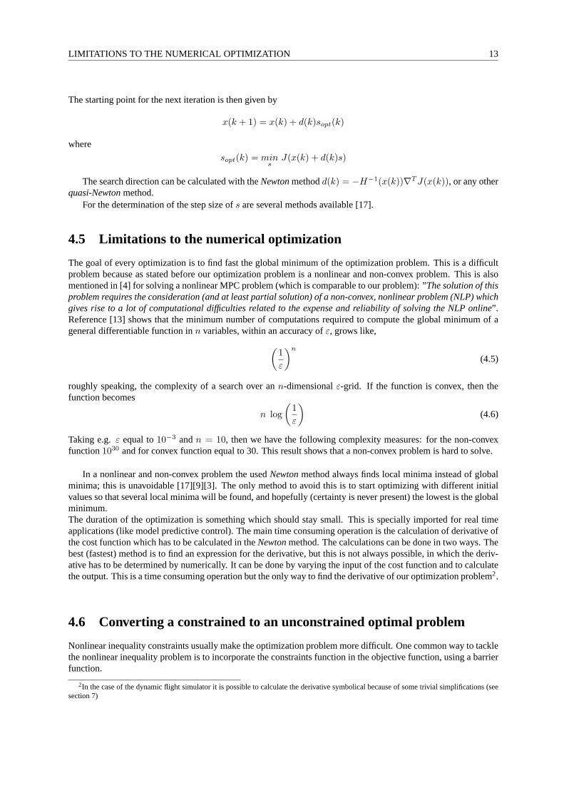
4.5 Limitations to the numerical optimization
The goal of every optimization is to find fast the global minimum of the optimization problem. This is a difficultproblem because as stated before our optimization problem is a nonlinear and non-convex problem. This is alsomentioned in [4] for solving a nonlinear MPC problem (which is comparable to our problem): ”The solution of thisproblem requires the consideration (and at least partial solution) of a non-convex, nonlinear problem (NLP) whichgives rise to a lot of computational difficulties related to the expense and reliability of solving the NLP online”.Reference [13] shows that the minimum number of computations required to compute the global minimum of ageneral differentiable function inn variables, within an accuracy ofε, grows like,
(1
ε
)n
(4.5)
roughly speaking, the complexity of a search over ann-dimensionalε-grid. If the function is convex, then thefunction becomes
n log
(1
ε
)(4.6)
Taking e.g.ε equal to10−3 andn = 10, then we have the following complexity measures: for the non-convexfunction1030 and for convex function equal to 30. This result shows that a non-convex problem is hard to solve.
In a nonlinear and non-convex problem the usedNewtonmethod always finds local minima instead of globalminima; this is unavoidable [17][9][3]. The only method to avoid this is to start optimizing with different initialvalues so that several local minima will be found, and hopefully (certainty is never present) the lowest is the globalminimum.The duration of the optimization is something which should stay small. This is specially imported for real timeapplications (like model predictive control). The main time consuming operation is the calculation of derivative ofthe cost function which has to be calculated in theNewtonmethod. The calculations can be done in two ways. Thebest (fastest) method is to find an expression for the derivative, but this is not always possible, in which the deriv-ative has to be determined by numerically. It can be done by varying the input of the cost function and to calculatethe output. This is a time consuming operation but the only way to find the derivative of our optimization problem2.
4.6 Converting a constrained to an unconstrained optimal problem
Nonlinear inequality constraints usually make the optimization problem more difficult. One common way to tacklethe nonlinear inequality problem is to incorporate the constraints function in the objective function, using a barrierfunction.
2In the case of the dynamic flight simulator it is possible to calculate the derivative symbolical because of some trivial simplifications (seesection 7)

14 4. NUMERICAL OPTIMIZATION
If the optimization function has the constraintg(x) ≤ 0 then the basic idea of the barrier function is to introduce afeasibility functionJfeas of the form
Jfeas(x) =
{0 g(x) ≪ 0∞ g(x) → 0
and add this function to the original cost function
minx
[J(x) + Jfeas(x)]
In this way the cost function will increase significantly if the inequality constraints is not met, an example is:
Jfeas = − 1
βg(x)
with β > 1
4.7 Example of numerical optimization
The example which was drawn up analytically (see section 3.5.3) is now solved numerically. The pathSd (eq. 3.9)will be redefined, namelyy = 5 cos(2t)The constraints will be included using a feasibility function. It is taken the same as in the analytical optimization(eq. B.13).
The used parameters are:M1 = 1 ie1z
= 1 M2 = 2 ie2z
= 2 (the other elements of Desdemona are assumedweightless)a = 0.1 b = 1e−3 c = 1e−5 (These parameters are taken as example, they are not realistic). Thestep-size is taken0.1 sec and the total time is 5 sec.
The initialsq(t0), q(t0)) are taken random just asq(t0), q(t1), . . . , q(te). Now the optimization can be done,using 40 iterations in combination with the line search method.
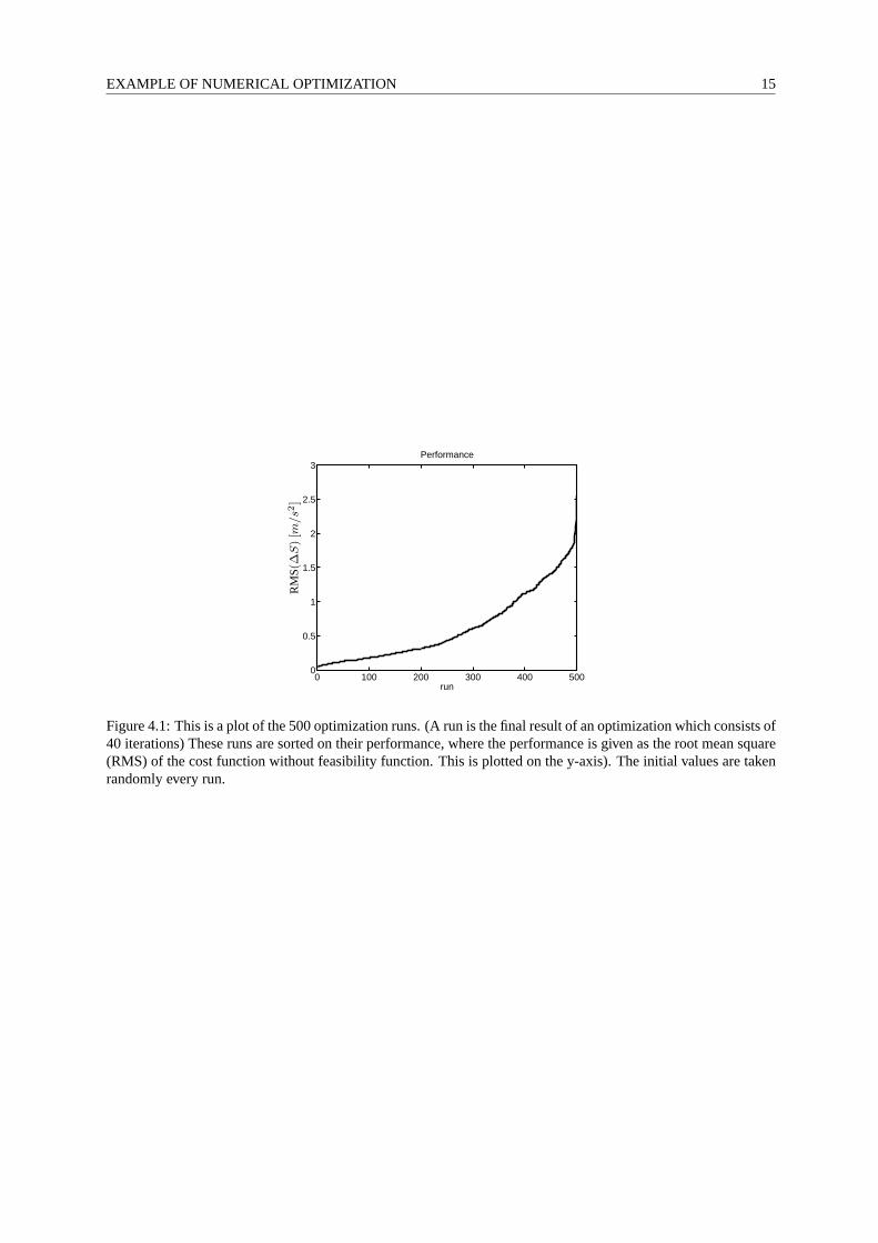
This optimization has been done 500 times (runs), every run with different initial values. This is done becausethe line search method finds a local optimum and this way it wastried to find the global minimum. These runs aresorted on performance (see figure 4.1), where the performance is the cost function without feasibility function . Itcan be seen that the initial values have an influence on the final results of the optimization.In figure 4.2 the results are given for run 300, so there are thus 299 runs with a better performance. The movementDesdemona is making is rotating and making small sinus movements around the origin with the vertical sledge. Itcan be seen that the accelerationsS are almost the same asSd. The values of joint vectorq2 are bounded. Theruns with a better performance have a similar behavior, the∆S becomes smaller andq2 remains small. The maindifference is that the size of∆S is smaller in the beginning of a run. This is due to better initial values.The numerical optimal control is thus working properly.
EXAMPLE OF NUMERICAL OPTIMIZATION 15
0 100 200 300 400 5000
0.5
1
1.5
2
2.5
3
run
Performance
RM
S(∆
S)[m
/s2
]
Figure 4.1: This is a plot of the 500 optimization runs. (A runis the final result of an optimization which consists of40 iterations) These runs are sorted on their performance, where the performance is given as the root mean square(RMS) of the cost function without feasibility function. This is plotted on the y-axis). The initial values are takenrandomly every run.

16 4. NUMERICAL OPTIMIZATION
0 1 2 3 4 5−6
−4
−2
0
2
4
6S
time
acce
lera
tion
m/s
2
Sd
S
0 1 2 3 4 5−3
−2
−1
0
1
2
3
4acceleration of q
time
met
er/s
ec2 a
nd r
ad/s
ec2
(a) (b)
0 1 2 3 4 5−100
0
100
200
300
400
500
time
degr
ee
q1
0 1 2 3 4 5−1.5
−1
−0.5
0
0.5
1
1.5
time
met
er
q2
(c) (d)
Figure 4.2: In (a) theS (doted line) andSd (Solid line) are plotted. In (b) the vectorq1 (solid line) andq2
the (doted line) are plotted. In (c) and (d) the vectorq1 and respectivelyq2 are plotted. The initial velocity isq = [63.6 degree/s 1.13m/s] (These results are not based on real parameters).

Chapter 5
Practical extensions of the numericaloptimization
In the previous chapter the optimization problem is solved for the most basic case. In this chapter the optimizationproblem is redefined to make it a more practical applicable optimization problem. Therefore the feasibility functionis changed and the initial values of Desdemona (q(t0), q(t0)) are included as optimization parameter. The sampletimes and stop criteria are chosen more carefully. At the endof this chapter some more realistic paths are definedand Desdemona is optimized with real parameters for the two and three d.o.f. cases.
In this chapter the following terminology is used: withrun, a complete optimization. A complete optimizationconsists of a number of iterations. The performance of a run is given as the root mean Square (RMS) of∆S.
RMS(∆S) =
√∑ni=1 ∆S2
i
n(5.1)
These RMS sorted with the best run first is plotted in the next sections for a number of runs to compare severaldifferent optimization configurations.
5.1 Barrier functions
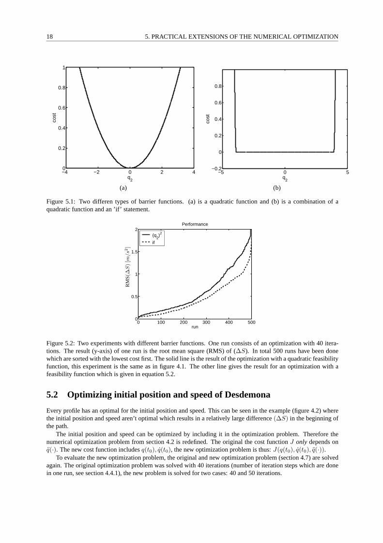
The barrier function (see section 4.6) is taken quadratic inthe example (section 3.5 or 4.7). This is not a realisticbarrier function because it results in costs when there is noreason for. This results in unwanted restriction of thejoins and motor. This can be seen forq2 in figure 5.1.a. ifq2 = 2 then it is not near the end of the track but there isalready a cost.
A good cost function is a cost function where the cost is low and constant if the constraints are not violated,if the constraints are (almost) violated then the cost function should increase significantly. The function should becontinuous which is important when taking the derivative intheNewtonmethod.
An example of a good barrier function is given in eq. 5.2 and can be seen in figure 5.1.b.
Jfeas(q2) =
{((q2)
2 − 3.72)2 |q2| > 3.70 |q2| ≤ 3.7
(5.2)
To evaluate the cost function the experiment from section 4.7 is repeated, but now with the barrier functionwhich is given in equation 5.2. The results are given in figure5.2. The number of runs is chosen in such awaythe calculation time is reasonable and the results can be justified statistically and the number of iterations is takenbig enough so that the results are satisfying. Further in this chapter there is discussed how to determine the rightnumber.
In figure 5.2 it can be seen that the cost of the optimization with a ’if’ barrier function is lower then the costof the optimization with a quadratic barrier function. So there can be concluded that the ’if’ barrier function givesbetter results then the quadratic barrier function.
18 5. PRACTICAL EXTENSIONS OF THE NUMERICAL OPTIMIZATION
−4 −2 0 2 40
0.2
0.4
0.6
0.8
1
q2
cost
−5 0 5−0.2
0
0.2
0.4
0.6
0.8
q2
cost
(a) (b)
Figure 5.1: Two differen types of barrier functions. (a) is aquadratic function and (b) is a combination of aquadratic function and an ’if’ statement.
0 100 200 300 400 5000
0.5
1
1.5
2
run
Performance
(q2)2
if
RM
S(∆
S)[m
/s2
]
Figure 5.2: Two experiments with different barrier functions. One run consists of an optimization with 40 itera-tions. The result (y-axis) of one run is the root mean square (RMS) of (∆S). In total 500 runs have been donewhich are sorted with the lowest cost first. The solid line is the result of the optimization with a quadratic feasibilityfunction, this experiment is the same as in figure 4.1. The other line gives the result for an optimization with afeasibility function which is given in equation 5.2.
5.2 Optimizing initial position and speed of Desdemona
Every profile has an optimal for the initial position and speed. This can be seen in the example (figure 4.2) wherethe initial position and speed aren’t optimal which resultsin a relatively large difference(∆S) in the beginning ofthe path.
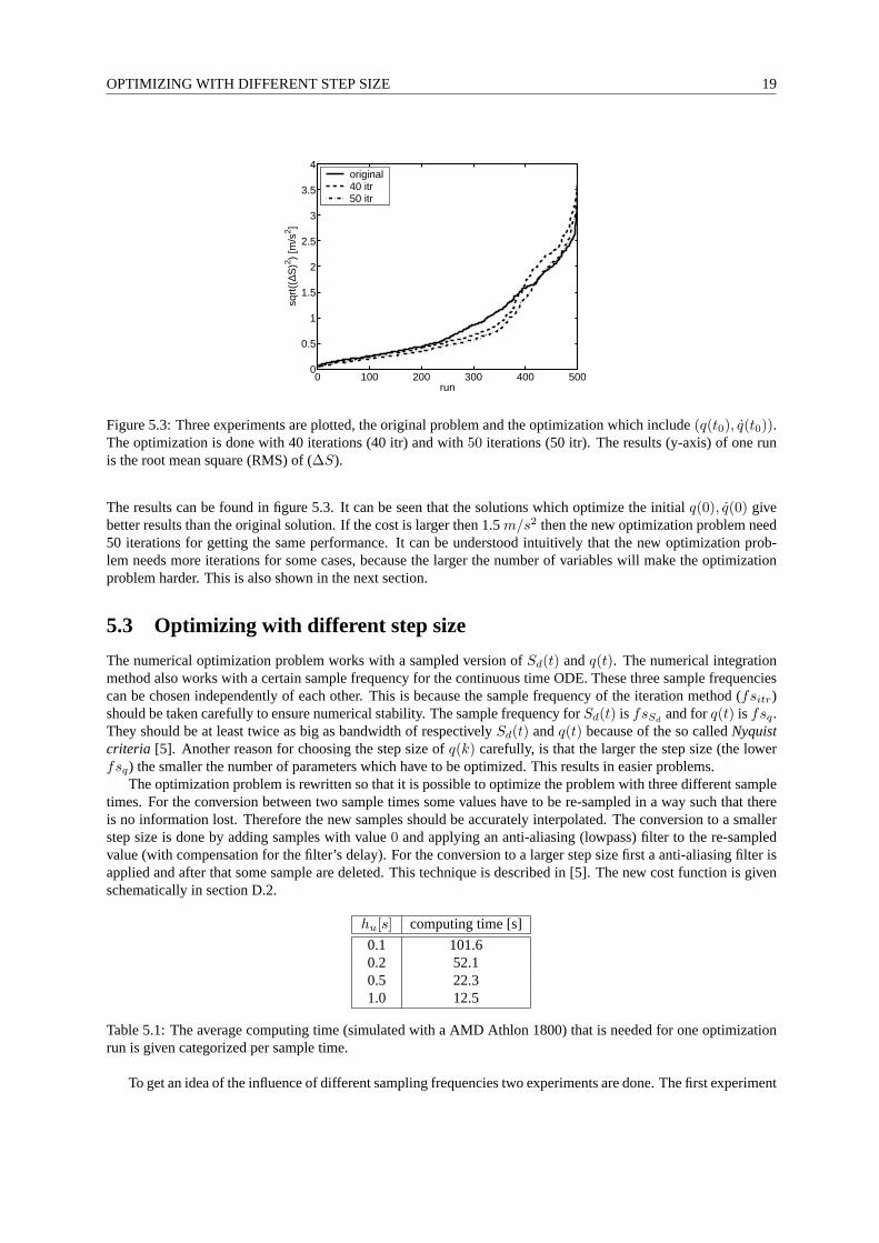
The initial position and speed can be optimized by includingit in the optimization problem. Therefore thenumerical optimization problem from section 4.2 is redefined. The original the cost functionJ only depends onq(·). The new cost function includesq(t0), q(t0), the new optimization problem is thus:J(q(t0), q(t0), q(·)).
To evaluate the new optimization problem, the original and new optimization problem (section 4.7) are solvedagain. The original optimization problem was solved with 40iterations (number of iteration steps which are donein one run, see section 4.4.1), the new problem is solved for two cases: 40 and 50 iterations.
OPTIMIZING WITH DIFFERENT STEP SIZE 19
0 100 200 300 400 5000
0.5
1
1.5
2
2.5
3
3.5
4
run
sqrt
((∆S
)2 ) [m
/s2 ]
original40 itr50 itr
Figure 5.3: Three experiments are plotted, the original problem and the optimization which include(q(t0), q(t0)).The optimization is done with 40 iterations (40 itr) and with50 iterations (50 itr). The results (y-axis) of one runis the root mean square (RMS) of (∆S).
The results can be found in figure 5.3. It can be seen that the solutions which optimize the initialq(0), q(0) givebetter results than the original solution. If the cost is larger then 1.5m/s2 then the new optimization problem need50 iterations for getting the same performance. It can be understood intuitively that the new optimization prob-lem needs more iterations for some cases, because the largerthe number of variables will make the optimizationproblem harder. This is also shown in the next section.
5.3 Optimizing with different step size
The numerical optimization problem works with a sampled version ofSd(t) andq(t). The numerical integrationmethod also works with a certain sample frequency for the continuous time ODE. These three sample frequenciescan be chosen independently of each other. This is because the sample frequency of the iteration method (fsitr)should be taken carefully to ensure numerical stability. The sample frequency forSd(t) is fsSd
and forq(t) is fsq.They should be at least twice as big as bandwidth of respectively Sd(t) andq(t) because of the so calledNyquistcriteria [5]. Another reason for choosing the step size ofq(k) carefully, is that the larger the step size (the lowerfsq) the smaller the number of parameters which have to be optimized. This results in easier problems.
The optimization problem is rewritten so that it is possibleto optimize the problem with three different sampletimes. For the conversion between two sample times some values have to be re-sampled in a way such that thereis no information lost. Therefore the new samples should be accurately interpolated. The conversion to a smallerstep size is done by adding samples with value0 and applying an anti-aliasing (lowpass) filter to the re-sampledvalue (with compensation for the filter’s delay). For the conversion to a larger step size first a anti-aliasing filter isapplied and after that some sample are deleted. This technique is described in [5]. The new cost function is givenschematically in section D.2.
hu[s] computing time [s]
0.1 101.60.2 52.10.5 22.31.0 12.5
Table 5.1: The average computing time (simulated with a AMD Athlon 1800) that is needed for one optimizationrun is given categorized per sample time.
To get an idea of the influence of different sampling frequencies two experiments are done. The first experiment

20 5. PRACTICAL EXTENSIONS OF THE NUMERICAL OPTIMIZATION
0 100 200 300 4000
0.5
1
1.5
2
run
Performance
hq=0.1s
hq=0.2s
hq=0.5s
hq=1s
RM
S(∆
S)[m
/s2
]
Figure 5.4: Four experiments optimizing with different step sizes, in the legends the sample time is given. Theresults (y-axis) of one run is the root mean square (RMS) of (∆S).
is the same as the original experiment (section 4.7) but now with different step size and number of iterations (seefor the definition of iteration section 4.4.1). The step sizeof Sd(k) is taken ashSd
= 0.1s and the step size of thenumerical integration method is changed tohitr = 0.05s. The step-size of the numerical integration is not changedduring the experiment. The step size ofq(k) is changed during the experiment betweenhq = 1s andhq = 0.1s(original optimization problem). The optimization is donewith 20 iterations.
In figure 5.4 and table 5.1 the results are given. The originaloptimization problem with sample timehSd= 0.1s
has the worst performance. This can be seen from the high costand computing time. This is due to the number ofvariables which have to be optimized. The fewer variables (the larger the step size) that have to be optimized, theeasier (faster) it is to optimize. The is that the sample frequency ofq can not be taken to low because then it is notpossible to include the high frequency accelerations. Thiswill be shown in the next experiment.
From the previous paragraph it is clear that for a last optimization the lowest possible sample frequency ofq(t)should be determined prior to the optimization. When the pathof Desdemona is a linear function of the states of thejointsS(q(t), q(t), q(t), t), then the sample frequencies ofS andq can be taken the same. But because Desdemonais nonlinear this is not the case1. The only relation is that the higher the frequencies inSd(t) the higher the samplefrequency has to be forq(t).
In the following experiment it will be shown that there is a relationship between the step-size ofq(k) and thefrequency inSd(k). The following step sizes are used:hSd
= 0.1s, hitr = 0.05s andhq = 1s. The frequency ofthe accelerations inSd(k) is changed from 2 to 5rad/s, the results are shown in figure 5.5. If the frequency ofSd
is above 3 rad/s the cost is increasing enormously. This is due to a too low sample frequency forq(k). So it can beconcluded that the frequency ofSd(k) has an influence on the neededfsq.
5.4 Different stopping criterions
In previous experiments the number of iterations in a optimization run is fixed. This is not a logic stop criteriabecause if the optimization method finds the (local) optimumin fewer steps, the additional steps do not doesn’tbenefit the performance. Therefore the optimization shouldbe stopped if the optimum is reached. If the optimiza-tion has reached its optimum then the change in the cost function will remain small in the next iteration steps. So,a good extension of the stop criteria is adding a minimum for the change of the cost function. If the cost functionis changing less then the minimum, the optimization will be stopped.
This extended stop criterium has been tested in the following experiment. The minimum change for the stopcriteria is taken0.1. The results are given in figure 5.6. The performance is almost the same hence the extra stop
1It is possible for some nonlinear filter cases to calculate theoutput frequency for a given input frequency. But for Desdemona this is notpossible, due to used sinuses and limiters in the transfer function

EVALUATING DIFFERENT PROFILES 21
0 5 10 15 200
0.5
1
1.5
2
2.5
3
3.5
4Performance
run
ω=2ω=3ω=4ω=5
RM
S(∆
S)[m
/s2
]
Figure 5.5: Four times the experiment of section 4.7 is done with four differentSd(k). TheSd(k) in equation 3.9is defined asy = 5 cos(ωk) with ω changing between 2 and 5 rad/s. The results (y-axis) of one run is the rootmean square (RMS) of (∆S).
criterium is not influencing the results. But there is a30% saving of computing time, hence the extended stopcriterium is useful.
0 100 200 300 400 5000
0.2
0.4
0.6
0.8
1
1.2
1.4
1.6
1.8
2Performance
run
originalstop criteria
RM
S(∆
S)[m
/s2
]
Figure 5.6: Different stopping criterions, the results of the original experiment (section 4.7) with 40 iterations andthe same experiment with extra stop criterium. The extra stop criterium will stop the optimization if the changingof cost function(inclusive feasibility function) is below0.1. The results (y-axis) of one run is the root mean square(RMS) of (∆S).
5.5 Evaluating different profiles
The final step in the two degrees optimization problem is to combine the new techniques described in this chapter.Another step is to use the real parameters (see section A.5) for dimensioning Desdemona and the motors. Thisoptimization problem is tested with some realistic paths.
To get an idea of the performance of Desdemona the two degree Dynamic model assumes that the degrees offreedom which are not used have become rigid connections. Itmeans that the mass and inertia (see section A.5) ofthe whole Desdemona are taken into account.

22 5. PRACTICAL EXTENSIONS OF THE NUMERICAL OPTIMIZATION
In this optimization problem all the constraints (see section 3.4) will be taken into account. For the feasibilityfunction the barrier function in the form of equation 5.2 is chosen. The parameters which determine the bounds ofthe constraints can be found in section A.5.
5.5.1 Cosine path
To be able to compare the new realistic system with previous experiments the original cosine path will be used forthe first experiment. The initial position is also optimized, and the stop criterium is taking the change of the costfunction in account. The results for the best run is given in figure 5.7. The result is good because the constraintsare met andS is very close toSd
5.5.2 Catapult start
This profile describes the start of an airplane from a aircraft carrier. It is a very strong acceleration in one (ey)direction. The optimization also optimized the initial position as well. The results for the best run is given in figure5.8. As can be seen there is a difference betweenS andSd although the flanks ofS are steep.
5.5.3 Triple pulse
The initial position is also optimized, and the stop criterium is taking the change of the cost function in account.The results for the best run (figure 5.9) are the same as the results of the catapult start, there is a difference betweenS andSd but the flanks are steep.
5.5.4 Fast care
In this experiment the data from a real car is used. The accelerations are measured during 35 second while the caris doing the track from figure 5.10.
The best run is given in figure 5.11. As can be seen the results are good.

EVALUATING DIFFERENT PROFILES 23
plaatjes_two/COS_TWO_output_S.eps
(a)
plaatjes_two/COS_TWO_output_q1.eps plaatjes_two/COS_TWO_output_q2.eps
(b) (c)
plaatjes_two/COS_TWO_output_tau.eps plaatjes_two/COS_TWO_output_power.eps
(d) (e)
Figure 5.7: The best results for the cosines experiment. In (a) theS (doted line) andSd (Solid line) are plotted.(b) and (c) are the positions of the jointsq1 andq2 respectively are plotted. In (d) and (e) the normalized forceand power respectively are plotted. They are normalized by dividing the force and power by its maximum allowedvalue. If the normalized force or power is larger than one, then one of of the motors will be damaged. The initialvelocity is q = [109.5 degree/s 0.18m/s]

24 5. PRACTICAL EXTENSIONS OF THE NUMERICAL OPTIMIZATION
plaatjes_two/CAT_TWO_output_S.eps
(a)
plaatjes_two/CAT_TWO_output_q1.eps plaatjes_two/CAT_TWO_output_q2.eps
(b) (c)
plaatjes_two/CAT_TWO_output_tau.eps plaatjes_two/CAT_TWO_output_power.eps
(d) (e)
Figure 5.8: The best results for the catapult start. In (a) the S (doted line) andSd (Solid line) are plotted. (b)and (c) are the positions of the joints are plotted. In (d) and(e) the normalized force and power respectivelyare plotted. It is normalized by dividing the force and powerrespectively by its maximum allowed value. If thenormalized force or power is larger, then one, than one of themotors will be damaged. The initial velocity isq = [−82.6 degree/s − 0.04m/s]

EVALUATING DIFFERENT PROFILES 25
plaatjes_two/DUB_TWO_output_S.eps
(a)
plaatjes_two/DUB_TWO_output_q1.eps plaatjes_two/DUB_TWO_output_q2.eps
(b) (c)
plaatjes_two/DUB_TWO_output_tau.eps plaatjes_two/DUB_TWO_output_power.eps
(d) (e)
Figure 5.9: The best results for the double pulse experiment. In (a) theS (doted line) andSd (Solid line) are plotted.(b) and (c) the positions of the joints are plotted. In (d) and(e) the normalized force and power respectively areplotted. It is normalized by dividing the force and power respectively by its maximum allowed value. If thenormalized force or power is larger then one, than the motorswill be damaged. The initial velocities are isq = [2.82 rad/s − 0.11m/s]

26 5. PRACTICAL EXTENSIONS OF THE NUMERICAL OPTIMIZATION
plaatjes_alg/track.eps
Figure 5.10: The track of the fast care, done in 35 seconds
EVALUATING DIFFERENT PROFILES 27
plaatjes_two/AUTO_TWO_output_S.eps
(a)
plaatjes_two/AUTO_TWO_output_q1.eps plaatjes_two/AUTO_TWO_output_q2.eps
(b) (c)
plaatjes_two/AUTO_TWO_output_tau.eps plaatjes_two/AUTO_TWO_output_power.eps
(d) (e)
Figure 5.11: The best results for the fast care experiment. In (a) theS (doted line) andSd (Solid line) are plotted.(b) and (c) the positions of the joints are plotted. In (d) and(e) the normalized force and power respectivelyare plotted. It is normalized by dividing the the force and power respectively by its maximum allowed value. Ifthe normalized force or power is larger then one, than the motors will be damaged. The initial velocities are isq = [−9.4 degree/s − 0.4m/s]

28 5. PRACTICAL EXTENSIONS OF THE NUMERICAL OPTIMIZATION
5.6 Desdemona with three degrees of freedom
A logical step to make the optimization problem more realistic is to increase the number of d.o.f. Thereforeq5 theyaw of the cabin is included. With this extra d.o.f. it is possible to place the cabin in every position in theex ey
plane of the fixed world and to simulate any desired acceleration profile (that is within bounds). In this sectionthe same experiments are done as in section 5.5. All the experiments optimize also the initial position, and thestop criterium is taking the change of the cost function in account. In the pathSd the linear translation inex ey
direction are defined, the rotation is not taken into account. The rotation is not taken into account because forexample the catapult start path demands for almost 2 secondsan acceleration of20m/s2 which result in a linear 40meter displacement or a combination of a small displacementand rotation. Desdemona isn’t 40 meter long, so weexpect the optimal controller to force Desdemona to start rotating. Q is defined so that the rotation isn’t includedin the optimization.
The results of the experiments are discuss in section 5.8.
5.6.1 Cosine path
To be able to compare the new realistic system with previous experiments the original cosines path will be used forthe first experiment. The results for the best run is given in figure 5.12. The result is good because the constraintsare met andS is very close toSd.
5.6.2 Catapult Start
This profile is from the start of an airplane from a aircraft carrier. It is very strong acceleration in one (ey) direction.The optimization also optimized the initial position. The weight matrixQ (see section 3.4) is taken so that an errorin ex direction result in a three times larger cost than iney direction. The results for the best run is given in figure5.13. It can be seen that the results aren’t so good as the two degree problem, this is to be expected because it isa much harder problem. The false cue (Sx) is smaller then the wanted acceleration (Sy) which is one of the basicrequirements to make the simulation realistic.
5.6.3 Double pulse
This is just a test profile with twice an step acceleration in theey direction. The results for the best run is given infigure 5.14. The weight matrixQ (see section 3.4) is taken so that an error inex direction result in a three timeslarger cost then iney direction.
5.6.4 Fast car
In this experiment the data from a real care is used (the car isdoing the track from figure 5.10). The results for thebest run is given in figure 5.15. It can be seen there is a large difference betweenS andSd. But on the other handSd is high frequent, and hence difficult to follow.

DESDEMONA WITH THREE DEGREES OF FREEDOM 29
plaatjes_THREE/COS_THREE_output_Sx.eps plaatjes_THREE/COS_THREE_output_Sy.eps
(a) (b)
plaatjes_THREE/COS_THREE_output_q1.eps plaatjes_THREE/COS_THREE_output_q2.eps
(c) (d)
plaatjes_THREE/COS_THREE_output_q5.eps
(e)
Figure 5.12: The best results for the three d.o.f. cosines experiment. In (a) and (b) theSx and respectivelySy
are plotted. In (c), (d) and (e) the positions of the jointsq1, q2 respectivelyq5 are plotted. The constraints are notplotted but they are all met. The initial velocities are[q1 q2 q5] = [37.3 degree/s − 1.0m/s 0.5 degree/s]

30 5. PRACTICAL EXTENSIONS OF THE NUMERICAL OPTIMIZATION
plaatjes_THREE/CAT_THREE_output_Sx.eps plaatjes_THREE/CAT_THREE_output_Sy.eps
(a) (b)
plaatjes_THREE/CAT_THREE_output_q1.eps plaatjes_THREE/CAT_THREE_output_q2.eps
(c) (d)
plaatjes_THREE/CAT_THREE_output_q5.eps
(e)
Figure 5.13: The best results for the three degree catapult start experiment. In (a) and (b) theSx andSy respectivelyare plotted. In (c), (d) and (e) the positions of the jointsq1, q2 andq5 respectively are plotted. The constraints arenot plotted but they are all met. The initial velocities are[q1 q2 q5] = [−74.9 degree/s −1.5m/s 10.0 degree/s]

DESDEMONA WITH THREE DEGREES OF FREEDOM 31
plaatjes_THREE/DUB_THREE_output_Sx.eps plaatjes_THREE/DUB_THREE_output_Sy.eps
(a) (b)
plaatjes_THREE/DUB_THREE_output_q1.eps plaatjes_THREE/DUB_THREE_output_q2.eps
(c) (d)
plaatjes_THREE/DUB_THREE_output_q5.eps
(e)
Figure 5.14: The best results for the three degree catapult start experiment. In (a) and (b) theSx andSy respectivelyare plotted. In (c), (d) and (e) the positions of the jointsq1, q2 andq5 respectively are plotted. The constraints are notplotted but they are all met. The initial velocities are[q1 q2 q5] = [−52.9 degree/s − 1.5m/s − 39.2 degree/s]

32 5. PRACTICAL EXTENSIONS OF THE NUMERICAL OPTIMIZATION
plaatjes_THREE/AUTO_THREE_output_Sx.eps plaatjes_THREE/AUTO_THREE_output_Sy.eps
(a) (b)
plaatjes_THREE/AUTO_THREE_output_q1.eps plaatjes_THREE/AUTO_THREE_output_q2.eps
(c) (d)
plaatjes_THREE/AUTO_THREE_output_q5.eps
(e)
Figure 5.15: The best results for the fast care experiment. In (a) and (b) theSx andSy respectively are plotted. In(c), (d) and (e) the positions of the jointsq1, q2 andq5 respectively are plotted. The constraints are not plotted butthey are all met. The initial velocities are[q1 q2 q5] = [7.8 degree/s − 1.7m/s − 6.5 degree/s]

IMPROVING THE PERFORMANCE 33
5.7 Improving the performance
In previous section Desdemona simulated with three d.o.f. The results can be increased by simplifying the dynamicmodel of Desdemona and by taking initial values not randomlybut by selecting promising values. This is explainedin this section.
Simplifying the dynamic model
The parameters of the dynamic are given in appendix A.5. The center of mass is not always in the origin ofDesdemona coordinates. This makes the dynamic model more complex because it increases the number of jointsthat are influencing each other torques. By assuming the the center of the mass is always in the origin, some smallerrors are introduced in the optimization. The result is that the calculation time is shorter. The fact that some smallerrors are introduced can be eliminated by an extra optimization with the full dynamic model at the end. Thus thismethod is increasing the performance.
Smart Guess
All the experiments are until now done with random initial values (randomq(0), q(0), q(·)). But due to otherresearch2 about Desdemona there are ideas of good performing inial values. Some experiments are done withthese inial values. The idea is that a initial values that arechosen with prior knowledge give better results.
For example, if we expect anSd in theey direction, where at the begin no accelerations and later some highacceleration occur, then three groups of sensible initial parameters can be chosen, see table 5.2.
q2 q1 q2
0 ↑ -↑ 0 0
small ↑ ↓
Table 5.2: The three possible initial parameters. The↑ means a large value. The acceleration will be low for alimited time and thereafter high. This can be found from equation B.5
5.7.1 Catapult start
The catapult start is repeated but now with a simplified dynamics and smartly guessed initials values.q(0), q(0):
[q1 q2 q5] = [0 degree − 0.01m 0 degree]
[q1 q2 q5] = [86 degree/s − 1.4m/s 0 degree/s]
The results are given in figure 5.16. The optimization with the simplified dynamics is done first and thereafter anoptimization with the real dynamic is done to ensure the results are applicable to the Desdemona.
2Mark, heb je nog referencies??todo

34 5. PRACTICAL EXTENSIONS OF THE NUMERICAL OPTIMIZATION
plaatjes_THREE/CAT_THREE_smart_Sx.eps plaatjes_THREE/CAT_THREE_smart_Sy.eps
(a) (b)
plaatjes_THREE/CAT_THREE_smart_q1.eps plaatjes_THREE/CAT_THREE_smart_q2.eps
(c) (d)
plaatjes_THREE/CAT_THREE_smart_q5.eps
(e)
Figure 5.16: The best results for the smart catapult experiment. In (a) and (b) theSx andSy respectively areplotted. In (c), (d) and (e) the positions of the jointsq1, q2 andq5 respectively are plotted. The constraints are notplotted but they are all met. The initial velocities are[q1 q2 q5] = [95.2 degree/s − 0.4m/s − 21.9 degree/s]
DISCUSSION THREE D.O.F. RESULTS 35
5.8 Discussion three d.o.f. results
The results are good for the cosines experiment (figure 5.12). Thus the method is working. For the other exper-iments (figure 5.13, 5.14 and 5.15) the result are not as good.This is because the cost function is non-linear andnon-convex, which result in a large number of local minima. In the two degree optimizations cases the problem isless nonlinear and therefore there are fewer local optimums.
For finding a low local minimum you need a huge number of trials. This number can be reduced by usingpromising initial values and by simplifying the dynamic model. But then you need a way to find these values. Anexample can can be found in section 5.7.
The cosines experiment has the best result, this is because the lower the existing frequencies inSd(t) are, theeasier to solve the optimization problem. One reason is you can resample the problem, and solve easier (see section5.3). Or in other words, a change at a certain time of the joints of Desdemona will not only influence the error(∆S) at the same time interval but also in later intervals. This is particular the case ifSd(t) contains only lowerfrequencies since there is more correlation between two sample next to each other.
Another difficulty is that the optimization has to deal with ahuge number of input variables, for the fast carexperiment (figure 5.15) 450 variables, which cause a huge complexity for the problem (see section 4.5).
Thus the results could be expected because of the known limitations and complexity (see section 4.5). Someoptions give better results by choosing better initial values, and to avoid high frequencies inSd(t)
If the optimization find a local minima, a method that possibly can be used to find other local minima in theneighborhood can be applied. The method redefines theSd(·) as
Sdnew(·) = λSd(·) + (1 − λ)S(·)
with λ ∈< 0 . . . 1 > andS(t) is the path from the previous found optimum. Then with a new optimization runtheSdnew(t) can be used to find other local minima. This method has been implemented with severalλ and testedwith the three d.o.f. catapult start experiment (section 5.6.2). The results is that the average performance decreases.Thus there can be concluded that the method is in our case not useful for improving the optimization performance.

36 5. PRACTICAL EXTENSIONS OF THE NUMERICAL OPTIMIZATION

Chapter 6
Including human perception model
6.1 Introduction
As stated before, the main goal of Desdemona is to let the person in Desdemona observe the same movementsas in the simulated vehicle. Sometimes a human observes different movements than the human body it is makingdue to measurement faults. Therefore it is not always necessary that Desdemona makes the same movements asthe simulated vehicle. By taking this into account it is possible to filter out irrelevant movements (movements ahuman doesn’t observe) and concentrate on the movements that a human does percept. To achieve this, a humanperception model is included in the optimization problem, this is given in figure 6.1.
DesdemonaHuman
perseption
+
-
Error
Human
perseption
OptimizationSd
Figure 6.1: A schematic model of the optimization problem with human perception model
6.2 Human perception
There are three main sensory systems involved in spatial orientation and disorientation: the visual system, thevestibular system (inner ear), the somatosensory system (”seat of the pants”)[1]. To a smaller degree, the auditorysystem is also involved. Of these, vision is by far the most important sensory system providing spatial orientationduring flight. In the absence of vision, orientation must be derived solely from the vestibular or somatosensorysystems, and these systems do not always provide accurate motion and position cues.
The primary role of the vestibular system is to enhance vision. It provides angular and linear accelerationinformation to stabilize the eyes when motion of the head andbody would otherwise result in blurred vision. It’ssecondary role, in the absence of vision, is to provide a sense of position and motion.
The nerve system and brain are interpreting and combining the information from the sensors and let a personobserve the movements which the person is making. But sometimes a person observe another movements that it ismaking. This is due to measurement and interpretation faults. This and other effects from the human perceptionmodel are still a subject for ongoing research. An example isthat you don’t feel constant rotations, or another

38 6. INCLUDING HUMAN PERCEPTION MODEL
example, if you sit in the train, you think it is leaving but instead it is nearby a train that is leaving
A fixed simulator involves virtual and auditory simulation and a moving simulator also involves the vestibularand somatosensory simulation. This work only deals with themoving part of Desdemona and in dialogue withTNO there has been decided to include the vestibular system in the optimization problem.
6.3 Vestibular system
Figure 6.2: The Vestibular system (from [12])
The vestibular system can be divided in the semi-circular canals and otoliths see 6.2. With these two perceptionmodels it is possible to measure rotation and linear acceleration. These models will be included in the cost functionof the optimization and the new optimization will minimize the error in perception.
6.3.1 The semi-circular canals
The semicircular canals are part of the vestibular system. There are three semicircular canals located in the innerear on each side of the head. Fluid within the canals moves relative to the canal walls when angular accelerationsare applied to the head. This fluid movement bends sensory hair filaments in specialized portions of the canals,which send nerve impulses to the brain resulting in the perception of rotary motion. Each canal is oriented suchthat it responds differently from the others to angular accelerations in the pitch, roll and yaw spatial planes (seefigure 6.3).
Figure 6.3: The pitch, roll and yaw canals (from [12])

VESTIBULAR SYSTEM 39
The relative responses from all three canals are integratedby the brain to determine the actual plane in whichthe motion is occurring.
Dynamic model of the semi-circular canals
The model of the semi-circular canals are based on an overdamped-torsion-pendulum with transfer function
Hscc(ω) =neural discharge rate
angular acceleration=
K
(1 + τ1jω)(1 + τ2jω)(6.1)
The technique to measure the neural discharge rate (impulses per second, ips) of the primary neurons in the vestibu-lar nerve, made the determination of the transfer function of the semi canals possible [6]. The transfer functionbecomes:
Hscc(ω) =K(1 + τLjω)
(1 + τ1jω)(1 + τ2jω)(6.2)
With the following parameters given in the table 6.1.
K 2 ips/m/s2
τn 0.11sτ1 5.9sτ2 0.005s
Table 6.1: The parameters of the model (eq. 6.2) of the semi-circular canals. (ips stands for the Neural dischargerate (impulses per second)
Because in the used pathS the angular displacement is given as omega and not as acceleration the transferfunctionHscc has to be differentiated. This is done with a lead filter [14] because a pure differentiator is difficult
to implement. The transfer function of the lead filter isjωjω
α+1
whereα is chosen larger than the bandwidth of
Desdemona (see section A.5) so the lead compensation doesn’t have influence in the relevant frequency domain.The final transfer function can be found in eq. 6.3 and is plotted in figure 6.4.
Hscc(velocity)(ω) =K(1 + τLjω)
(1 + τ1jω)(1 + τ2jω)
jωjωα
+ 1(6.3)
10−2
10−1
100
101
102
−90
0
90
Pha
se (
deg)
−30
−25
−20
−15
−10
−5
Mag
nitu
de (
dB)
Figure 6.4: The frequent response of the semi-circular canals (from [12])

40 6. INCLUDING HUMAN PERCEPTION MODEL
6.3.2 The otoliths
The otolith organs are one of the sensory components of the vestibular system. They translate gravitational andinertial forces into spatial orientation information - specifically, information about angular position (tilt) and linearmotion of the head. The otolith organs (see figure 6.5) contain top-heavy hair-like cells that bend in response togravitational or linear acceleration forces. The bending of the sensory hairs relative to the membranes / structuresto which they are attached are transformed into orientationsignals to the brain. Inertial forces associated with themovement of the human body, combined with gravity, act upon the otolith organs.
Figure 6.5: The otholits (from [12])
Dynamic model of the otoliths
Considering their physical structure, each otolith can be modelled as an acceleration meter with over-dampedmass-spring-dashpot characteristics [6]. The transfer function is given as:
Hoto(ω) =neural discharge rate
linear acceleration=
K
(1 + τ1jω)(1 + τ2jω)(6.4)
It has been very difficult to identify the time constants. Themain reason is the lack of adequate experimentalinstallations to generate necessary linear acceleration stimuli. Based on different arguments, researchers concludedthat the numerator of equation (6.4) should be extended witha first-order term [6] to:
Hoto(ω) =K(1 + τnjω)
(1 + τ1jω)(1 + τ2jω)(6.5)
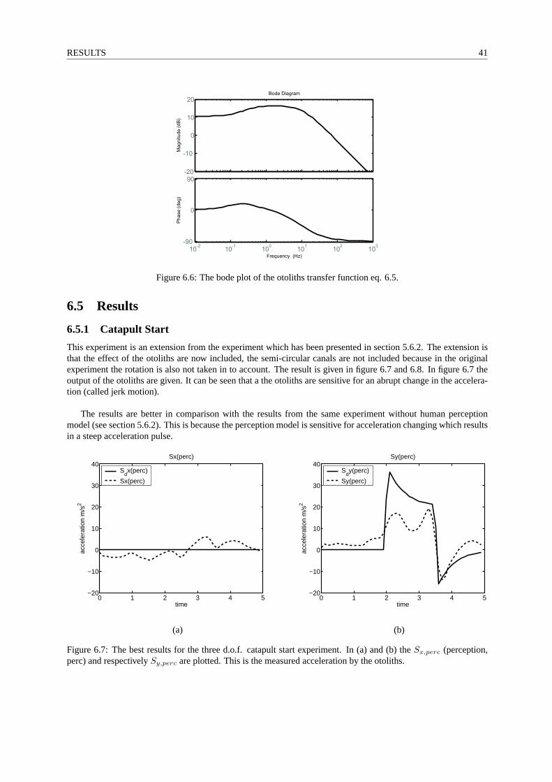
with the following parameters given in table 6.2. The transfer function is plotted in figure 6.6. It can be seen thatthe otolith is most sensitive to movements between 0.1 and 10hertz.
K 3.4 ips/m/s2
τn 1sτ1 0.5sτ2 0.016s
Table 6.2: The parameters of the model (eq. 6.5) of the otoliths. (ips stand for the Neural discharge rate (impulsesper second, ips)
6.4 Including model of the semi-circular canals and the otoliths
Both the transfer functions are scaled so that|H(ω → 0)| = 1 to make it easier to interpret the results. The transferfunctions are rewritten as a state space model and are included in the cost function. The new calculation scheme isgiven in section D.2.
RESULTS 41
10-2
10-1
100
101
102
103
-90
0
90P
hase (
deg)
-20
-10
0
10
20
Magnitude (
dB
)
Bode Diagram
Frequency (Hz)
Figure 6.6: The bode plot of the otoliths transfer function eq. 6.5.
6.5 Results
6.5.1 Catapult Start
This experiment is an extension from the experiment which has been presented in section 5.6.2. The extension isthat the effect of the otoliths are now included, the semi-circular canals are not included because in the originalexperiment the rotation is also not taken in to account. The result is given in figure 6.7 and 6.8. In figure 6.7 theoutput of the otoliths are given. It can be seen that a the otoliths are sensitive for an abrupt change in the accelera-tion (called jerk motion).
The results are better in comparison with the results from the same experiment without human perceptionmodel (see section 5.6.2). This is because the perception model is sensitive for acceleration changing which resultsin a steep acceleration pulse.
0 1 2 3 4 5−20
−10
0
10
20
30
40Sx(perc)
time
acce
lera
tion
m/s
2
Sdx(perc)
Sx(perc)
0 1 2 3 4 5−20
−10
0
10
20
30
40Sy(perc)
time
acce
lera
tion
m/s
2
Sdy(perc)
Sy(perc)
(a) (b)
Figure 6.7: The best results for the three d.o.f. catapult start experiment. In (a) and (b) theSx,perc (perception,perc) and respectivelySy,perc are plotted. This is the measured acceleration by the otoliths.

42 6. INCLUDING HUMAN PERCEPTION MODEL
plaatjes_OOR/CAT_OOR_output_Sx.eps plaatjes_OOR/CAT_OOR_output_Sy.eps
(a) (b)
plaatjes_OOR/CAT_OOR_output_q1.eps plaatjes_OOR/CAT_OOR_output_q2.eps
plaatjes_OOR/CAT_OOR_output_q5.eps
(e)
Figure 6.8: The best results for the three d.o.f. catapult start experiment. In (a) and (b) respectivelySx andSy areplotted. In (c),(d) and (e) the positions of the joints respectively q1, q2 andq5 are given. The constraints are notplotted but they are all met. The initial velocities are[q1 q2 q5] = [−37.8 degree/s 0.1m/s − 12.7 degree/s].

Chapter 7
Predictive optimal control
7.1 The principle of on-line optimization
In some cases there is a need for on-line optimization. An example isman in the loop(see figure 7.1). Since humanbehavior can not be predicted,Sd can not be determined prior to the optimization. Therefore the optimization hasto be done online (see also 3.4).
Vehicle
dynamicsOptimization Desdemona
+
-
Error
Sd
Figure 7.1: The calculation and horizon time.
The on-line optimization needs an estimated path with a certain time horizonTh to calculate the path of thejoints of Desdemona. The time necessary to calculate the optimization is the calculation timeTc (see figure 7.2).The determined path of the joints of Desdemona will be used asinput duringt = Tc . . . 2Tc and meanwhile theon-line optimization will determine the path again for the next time step.
Horizon time
Calculation time
Relevant output
Tc 2Tc Tht0
Figure 7.2: The calculation and horizon time.
The time of calculation should be short, at most half ofTh. They only way to make an on-line optimizationis to configure Desdemona as a dynamic flight simulator, because with this configuration it is possible to realize acalculation that is short enough .
44 7. PREDICTIVE OPTIMAL CONTROL
7.2 Desdemona as a dynamic flight simulator
In the following part of this chapter, Desdemona is considered as a dynamic flight simulator. This means thevertical sledge is fixed in its outer position and the horizontal sledge is fixed in its lowest position. Desdemonaworks like a centrifuge-based simulator. The main benefit ofthe dynamic flight simulator configuration is that thesimulated acceleration can be higher than in other configurations of Desdemona [2].
The angle of the acceleration vector working on the pilot canbe changed with the gimbles. The optimizationproblem has to be redefined because the new goal is to optimizethe path of the accelerationmodulus.
Md =√
S2dx + S2
dy + S2dz (7.1)
M =√
S2x + S2
y + S2z (7.2)
To give an impression of the possibilities of the dynamic flight simulator an off-line optimization is made for acatapult start. The results are given in figure 7.3.

DESDEMONA AS A DYNAMIC FLIGHT SIMULATOR 45
plaatjes_graat1/PULSE_ONE_output_M.eps plaatjes_graat1/PULSE_ONE_output_dM.eps
(a) (b)
plaatjes_graat1/PULSE_ONE_output_Sx.eps plaatjes_graat1/PULSE_ONE_output_Sy.eps
(c) (d)
plaatjes_graat1/PULSE_ONE_output_tau.epsplaatjes_graat1/PULSE_ONE_output_power.eps
(e) (f)
Figure 7.3: The results of the off-line catapult start. In (a) modulusMd, M andMorg are given.Morg representsthe original results of a non-optimized method (see section7.4.2). (b) shows the error betweenMd andM , andbetweenMd andMorg. In (c) and (d) respectivelySx andSy are plotted. (e) and (f) show the motor force andpower.

46 7. PREDICTIVE OPTIMAL CONTROL
7.3 The on-line control method
The goal of the on-line control method is to generate in real time the path of the joints by using an estimated path(Me). Since the estimated path is used as a criteria in the optimization it is important that the path is realistic. Themethod to estimate the path depends on the vehicle to be simulated and the mission of the pilot. In this report it isassumed that the path can be fully estimated. An overview of the optimization method is found in section D.1.2.
In equation 3.8 an online optimization algorithm with end cost is given. For the end cost of the dynamic flightsimulator value zero can be taken, because the movements of the simulator are not limited. An example of limitedmovements of Desdemona are its horizontal movements.
The cost function of the dynamic flight simulator is almost the same as in equation 4.1. The discrete optimiza-tion problem is written as:
minq
J =
te∑
k=t0
∆M(q(k), q(k), k)2 (7.3)
where∆M(q(k), q(k), k) = Me(k) − M(q(k), q(k)) and with constrains:
|q1(k)| − q1 max ≤ 0
|q1(k)| − q1 max ≤ 0
|τ(q1(k))| − τmax ≤ 0
|τ(q1(k))q1(k)| − Pmax ≤ 0 (7.4)
The torque depends onq2, so the constraint (q) andτ(q1(k)) can be rewritten as one constraint.
Another way of writingJ is
J =
te∑
k=t0
f(q1(k), q1(k), k)2 (7.5)
withf(q1(k), q1(k), k) = ∆M(q1(k), q(k), k) (7.6)
M(q1(k), q(k)) can be calculated by combining equation B.5 and 7.2 and the parametersq2 = −4, q2 = 0 andq2 = 0. Then
M(q1(k), q(k)) =√
(4q1(k))2 + (4q1(k)2)2 + g2 (7.7)
The nature of the optimization problem described in the previous section is the same as the one described inchapter 4. This is because both problems have the form of a least-squares (data-fitting) problem and are nonlinearand non-convex. Therefore, the same optimization algorithm as in section 4.3 can be selected.
7.4 Reducing the optimization time
The calculation time can be reduced by speeding up the optimization and by choosing the initial values smartly.First a fast method of calculating the Jacobian is introduced. Thereafter, the method to choose the initial values isdiscussed.
7.4.1 Calculation of the Jacobian
The optimization method iterates to its optimum as explained in section C.2. Therefore the Jacobian has to becalculated at every iteration. This can be done numerically, but in this case it is faster to calculate the Jacobiananalytically.

ON-LINE EXAMPLES 47
The Jacobian can be calculated by integrating theq(k) with the explicit Euler method and∆M(k) with equa-tion 7.7
q(k) = q(0) + hk∑
n=1
q(n)
∆M(q(k), q(k), k) = Me(k) − M(q(k), q(k))
Then the cost functionf(k) = (∆M(q(k), q(k), k))2 can be calculated analytically. Thus the Jacobian is:Jacobian(i, j) = ∂f(i)
∂q(j) , which results in:
Jacobian(i, j) =
0 i < j∆M(i)R22[2hq(i)3+q(j)]
M(i) i = j∆M(i)R24hq(i)3
M(i) i > j
(7.8)
Thus for aN × N Jacobian matrix the number of calculations is2N .
7.4.2 Smart guessing of the initial values
The optimization time can be reduced by choosing the initialvalues closely to the optimal values. Therefore asmall number of optimization (iteration) steps can be takenwithout having a worse performance. The new initialvalues (q1(k)) can be calculated with a small error by neglecting the accelerationq1 in equation 7.7. This can bedone becauseM(q(k), q(k)) mainly depends onq andg. The new equation isM(q(k)) =
√(4q(k)21)
2 + g2 or
rewritten1 q1(k) =
√√M(k)2−g2
4 . The estimated path can be used to calculateq1 thusq1(k) =
√√Me(k)2−g2
4 .With a control loop it is possible to calculate the new input (q1) for the optimization and taking care of the constraint|q1(k)| − q1max≤ 0 (see figure 7.4).This method is a common method to control dynamic flight simulators.
Figure 7.4: The schematic representation of calculatingq1 that is used for the initial value of the optimization
7.5 On-line examples
The catapult start and roller coaster experiments discussed in this section both have the same calculationTc =0.4 sec, horizonTh = 1 sec, and sample timehq = 0.1 sec.
As can be understood intuitively, larger horizons give better results. Experiments also verify this, but the resultsof these are not displayed here.
The calculation time of the optimization algorithm has to besmaller or equalTc to be useful in practicalapplications. When using anAMD Athlon 1800the calculation time of the optimization algorithm is smaller thanTc. So, theAMD Athlon 1800is suitable to do this optimization in practice.
The control loop method from section 7.4.2 (see figure 7.4) isoriginally used in dynamic flight simulators forcalculating the central yaw [15]. To be able to compare the optimized results with the original results, the latter arealso given.
1Without influencing the optimization results,q can be assumed positive.

48 7. PREDICTIVE OPTIMAL CONTROL
7.5.1 Catapult start
For the on-line optimization example a path (Md) is chosen that consists of a pulse superposition at a constantacceleration. The results can be found in figure 7.5. The average calculation time anAMD Athlon 1800needs is0.23 second.
7.5.2 Roller coaster
The roller coaster experiment is given in figure 7.6. TheMd is specified by measured data from a real roller coasterto which halve of the gravity is added. This gravity is added to be able to simulate accelerations that are smallerthen gravity2. ThereafterMd is limited by the limits of Desdemona and filtered with a low pass filter of5hz. Theaverage calculation time anAMD Athlon 1800needs is 0.23 second.
7.6 Discussion of the results
To evaluate the results two criteria will be considered: theperformance and the calculation time. Both criteria haveto be satisfied to be useful in a real time situation.
The performance of the optimal control algorithm is better then the original control loop method (see section7.4.2). This is due to the fact that the optimization method is anticipating on the future. This results in a smallerdelay betweenMd andM .
The calculation time is small enough to make it applicable inpractical situations. To conclude, the optimizationmethod is a useful extension on current systems. When the pathcan be estimated for limited time (Th) in the futurethen the method can be implemented. If the calculation timeTc is reduced thenTh can be reduced without a lossof performance. This can be useful for cases in which it is difficult to estimate the path.
2This way also allows for steeper acceleration to be made. [15]

DISCUSSION OF THE RESULTS 49
plaatjes_graat1/PULSE_ONE_online_M.eps plaatjes_graat1/PULSE_ONE_online_dM.eps
(a) (b)
plaatjes_graat1/PULSE_ONE_online_Sx.eps plaatjes_graat1/PULSE_ONE_online_Sy.eps
(c) (d)
plaatjes_graat1/PULSE_ONE_online_tau.epsplaatjes_graat1/PULSE_ONE_online_power.eps
(e) (f)
Figure 7.5: The results of the catapult start. In (a) modulusMd, M andMorg are given. Morg represents theoriginal results of a non-optimized method (see section 7.4.2). (b) shows the error betweenMd and M , andbetweenMd andMorg. In (c) and (d) respectivelySx andSy are plotted. (e) and (f) show the motor force andpower.

50 7. PREDICTIVE OPTIMAL CONTROL
plaatjes_graat1/ROLLERCOASTER_ONE_online_M.epsplaatjes_graat1/ROLLERCOASTER_ONE_online_dM.eps
(a) (b)
plaatjes_graat1/ROLLERCOASTER_ONE_online_Sx.epsplaatjes_graat1/ROLLERCOASTER_ONE_online_Sy.eps
(c) (d)
plaatjes_graat1/ROLLERCOASTER_ONE_online_tau.epsplaatjes_graat1/ROLLERCOASTER_ONE_online_power.eps
(e) (f)
Figure 7.6: The results of the roller coaster experiment.In(a) modulusMd, M andMorg are given.Morg representsthe original results of a non-optimized method (see section7.4.2). (b) shows the error betweenMd andM , andbetweenMd andMorg. In (c) and (d) respectivelySx andSy are plotted. (e) and (f) show the motor force andpower.
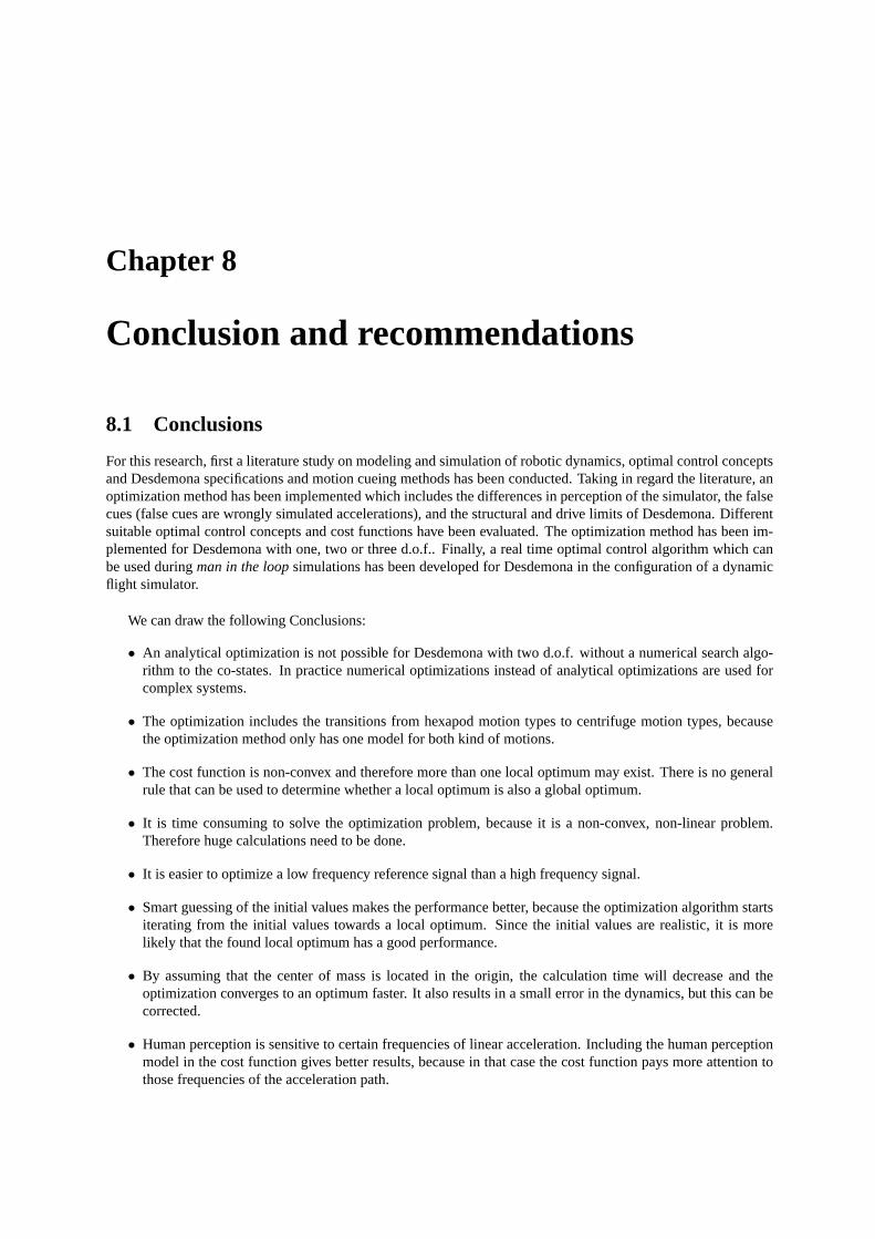
Chapter 8
Conclusion and recommendations
8.1 Conclusions
For this research, first a literature study on modeling and simulation of robotic dynamics, optimal control conceptsand Desdemona specifications and motion cueing methods has been conducted. Taking in regard the literature, anoptimization method has been implemented which includes the differences in perception of the simulator, the falsecues (false cues are wrongly simulated accelerations), andthe structural and drive limits of Desdemona. Differentsuitable optimal control concepts and cost functions have been evaluated. The optimization method has been im-plemented for Desdemona with one, two or three d.o.f.. Finally, a real time optimal control algorithm which canbe used duringman in the loopsimulations has been developed for Desdemona in the configuration of a dynamicflight simulator.
We can draw the following Conclusions:
• An analytical optimization is not possible for Desdemona with two d.o.f. without a numerical search algo-rithm to the co-states. In practice numerical optimizations instead of analytical optimizations are used forcomplex systems.
• The optimization includes the transitions from hexapod motion types to centrifuge motion types, becausethe optimization method only has one model for both kind of motions.
• The cost function is non-convex and therefore more than one local optimum may exist. There is no generalrule that can be used to determine whether a local optimum is also a global optimum.
• It is time consuming to solve the optimization problem, because it is a non-convex, non-linear problem.Therefore huge calculations need to be done.
• It is easier to optimize a low frequency reference signal than a high frequency signal.
• Smart guessing of the initial values makes the performance better, because the optimization algorithm startsiterating from the initial values towards a local optimum. Since the initial values are realistic, it is morelikely that the found local optimum has a good performance.
• By assuming that the center of mass is located in the origin, the calculation time will decrease and theoptimization converges to an optimum faster. It also results in a small error in the dynamics, but this can becorrected.
• Human perception is sensitive to certain frequencies of linear acceleration. Including the human perceptionmodel in the cost function gives better results, because in that case the cost function pays more attention tothose frequencies of the acceleration path.

52 8. CONCLUSION AND RECOMMENDATIONS
• Optimization the Desdemona configured with one instead of three d.o.f. needs less computing power, be-cause the number of optimization variables is smaller and the dynamics is less complex. The number ofjoints directly influence the number of variables: a one d.o.f. problem compared to a three d.o.f. problemhas three times fewer input variables for the optimization.The dynamic is less complex because there arefewer joints which are coupled. Also the expression for the acceleration the pilot makes is less complex.
• If Desdemona is configured with only one d.o.f instead of morethan one d.o.f. (see previous point), then itis easier to compute the optimization problem. In that case the optimization problem can be implemented asa real time application for Desdemona as dynamic flight simulator.
8.2 Recommendations
As stated before, the on-line optimal control algorithm which can be used duringman in the loopsimulationshas been implemented for Desdemona configured as a dynamic flight simulator. To implement the algorithm, anestimator needs to be designed to predict the path in the future. The model for the estimator is dependent on thesimulated model. The time that needs to be estimated can be reduced by reducing the time of calculation of theoptimization algorithm. This could be done by optimizing the implementation code.
The recommendation for off-line optimization of Desdemonawith more then one d.o.f is to apply an optimiza-tion method with smart chosen initial values. The results will be better than or equal to the results produced by theinitial values. Implementing the optimization algorithm is especially recommended for cases in which the resultsof the initial values are not sufficient.
Including all the d.o.f. in the optimizing problem of the Desdemona will result in needs of huge computerpower and probably with poor performance. It is not always necessary to include all the d.o.f. of Desdemona inthe optimization, because by combining the optimized joints and the desired path (Sd), it is possible to calculatethe positions of the other joints. This has been done when Desdemona configured as a dynamic flight simulator.Therefore, more research should be done to redefine the optimization problem for Desdemona was configured with(almost) all the d.o.f. to a configuration with a reduced number of d.o.f.

Bibliography
[1] M. B. Bannach.Air Force Manual 11-217, Instrument Flight Procedures. U. S. Air Force, volume 1 edition,December 2000.
[2] W. Bles, R. J. A. W. Hosman, and B. de Graaf. Desdemona: Advanced disorientation trainer and (sustained-g) flight simulator. volume AIAA-2000-4176 ofAIAA Modeling and Simulation Technologies Conference,Soesterberg, Netherlands, August 2000. TNO Human Factors,American Institute of Aeronautics and Astro-nautics.
[3] S. Boyd and L. Vandenberghe.Convex Optimization. Cambridge University Press, 2004.
[4] E.F. Camacho.Model predictive control, volume 2. Springer-Verlag, 2003.
[5] S. Haykin.An Introduction to Analog and Digital Communications. John Wiley & Sons, 1989.
[6] R.J.A.W. Hosman.Pilot’s perception and control of aircraft motions. PhD thesis, Delft University of Tech-nology, 1996.
[7] E. Kreyszig. Advanced Engineering Mathematics. eighth edition (Special Indian Edition). John Wiley &Sons, 1999.
[8] F. Martinsen, L. T. Biegler, and B. A. Foss. A new optimization algorithm with application to nonlinear mpc.Journal of Process Control 14 (2004) 853-865, 2004.
[9] The Mathworks, Inc, 3 Apple Hill Drive Natick, MA 01760-2098.Matlab optimization toolbox user’s guide,version 3 edition, Oktober 2004. online only, http://www.mathworks.com.
[10] Richard M. Murray, Zexiang Li, and S.Shankar Sastry.A Mathematical Introduction to Robotic Manipulation.CRC Press, 1994.
[11] Y. Nakamura.Advanced Robotics: Redundancy and optimization. Addison-Wesely Publising Company, Inc.,1991.
[12] National Aeronautics and Space Administration (NASA). Educational Brief, The Effects of Space Flight onthe Human Vestibular System, eb-2002-09-011-ksc edition, September 2002.
[13] A.S. Nemirovsky and D.B. Yudin. Problem complexity and method efficiency in optimization. Wiley-Interscience Series in Discrete Mathematics. John Wiley and Sons Ltd, 1983.
[14] N.S.Nise. Control Systems Engineering, volume 2. The Benjamin/Cummings Publishing Company, Inc.,1995.
[15] C. H. Spenny, B. S. Liebst, T. L. Chelette, C. Folescu, and J. Sigda. Development of a sustainable-g dynamicflight simulator. AIAA-2000-4075. American Institute of Aeronautics and Astronautics, 2000.
[16] S. Stramigioli. Modeling and IPC control of interactive mechanical: a co-ordinate free approach. LNCISserie of Springer. Springer-Verlag London, 2001.

54 BIBLIOGRAPHY
[17] T. van den Boom and B. Schutter.Optimization in Systems and Constrol. Delft University of Technology,Mekelweg 2 2628CD Delft, The Netherlands, August 2004.
[18] H.J. Zwart and J.W. Polderman.Optimal Control (Systeem- en besturingstheorie). University of Twente,Drienerlolaan 5 7522NB Enschede, The Netherlands, August 2001.

Appendix A
Notation and Model
A.1 Notation
The notation which is used in this report is based on [16]. It is a geometrical and global method. In this appendixsome of the notations are explained and the parameters of Desdemona are given.
A.1.1 The homogeneous transformation matrix
A general change Cartesian coordinates from coordinates1 into 2 can be expressed with a matrix of the form:
H21 =
(R2
1 p21
0T3 1
)(A.1)
In this matrixR is the rotation matrix andp the translation vector.With a serial robot like Desdemona, it is possible to first define the transformation matrices for each joint, and
then combine them. For exampleHij = Hi
kHkj .
Rotations around the x,y and z axis can be defined as followed.
Hx axis(α) =
1 0 0 00 cos(α) − sin(α) 00 sin(α) cos(α) 00 0 0 1
(A.2)
Hy axis(β) =
cos(β) 0 sin(β) 00 1 0 0
− sin(β) 0 cos(β) 00 0 0 1
(A.3)
Hz axis(γ) =
cos(γ) − sin(γ) 0 0sin(γ) cos(γ) 0 0
0 0 1 00 0 0 1
(A.4)
Translations can be written as:
Htranslation(x, y, z) =
1 0 0 x0 1 0 y0 0 1 z0 0 0 1
(A.5)

56 A. NOTATION AND MODEL
A.1.2 Twist
The twist is defined asT = [ω v]T and can also be written in matrix notation.
T i,ji = Hj
i Hij (A.6)
The indices inT i,jk mean a twist fromk to j expressed in from coordinatesi. The coordinates from the twist can
also be changed with help from the adjoint matrix [16]T j,ji = Ad
Hj
iT i,j
i .
A.2 Model
In figure A.1 the axis from Desdemona are defined. The numbering of the axis is done from earth to cabin withthe coordinate system of earth as number zero, and the cabin number six. The anglesq have the same order ofnumbering withq1 as the angle between the earth and the central yaw. The transformation matrices are definedas:
H01 = Hz axis(q1)
H12 = Htranslation(0, q2, 0)
H23 = Htranslation(0, 0, q3)
H34 = Hx axis(q4)
H45 = Hz axis(q5)
H56 = Hy axis(q6)
(A.7)
The twists are defined as:T 0,0
1 = [0 0 1 0 0 0]T
T 1,12 = [0 0 0 0 1 0]T
T 2,23 = [0 0 0 0 0 1]T
T 3,34 = [1 0 0 0 0 0]T
T 4,45 = [0 0 1 0 0 0]T
T 5,56 = [0 1 0 0 0 0]T
(A.8)
The Jacobian matrixJn gives the linear relationship between the joint velocitiesand the end-effectorn twist.This can be written asT 0,n
1 = Jn(q)qThe Jacobian matrix can be calculated with
Jn(q) = [T 0,01 . . . T 0,n−1
n ] (A.9)
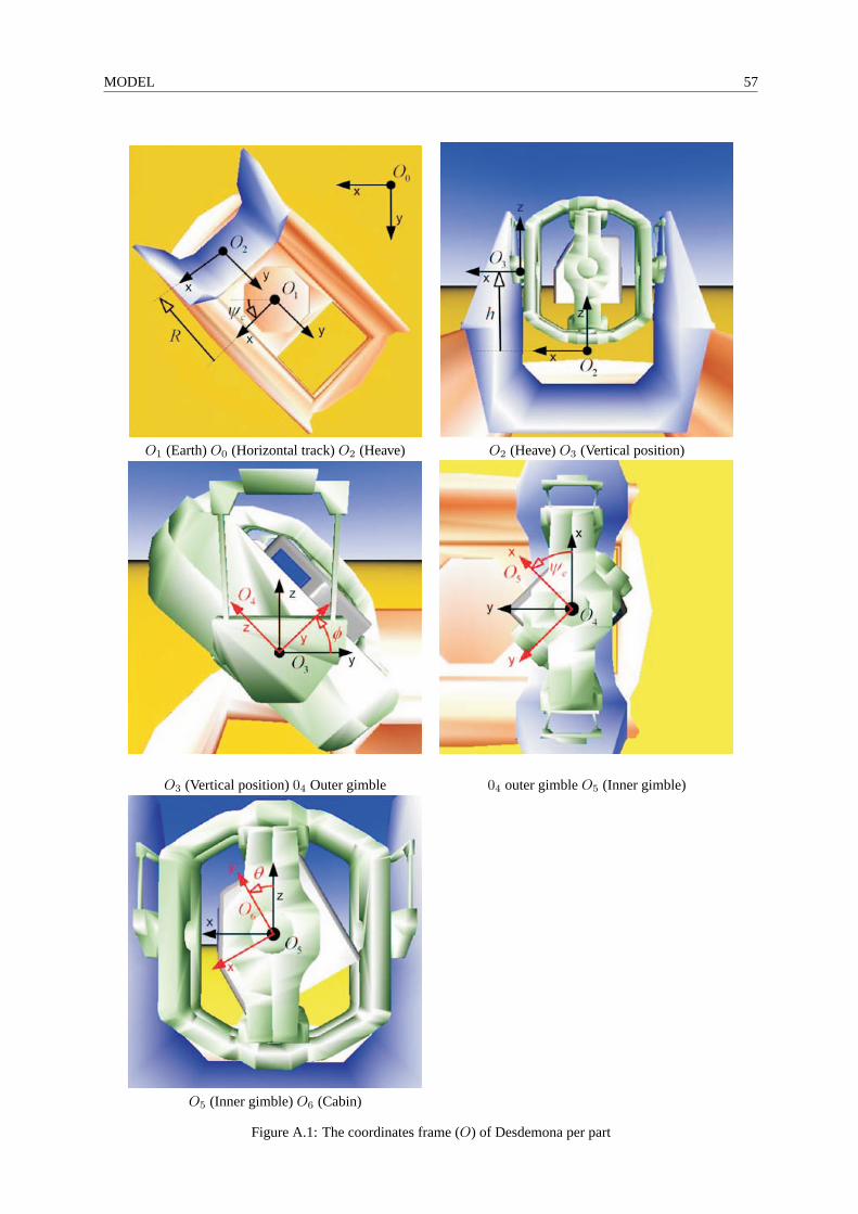
MODEL 57
O1 (Earth)O0 (Horizontal track)O2 (Heave) O2 (Heave)O3 (Vertical position)
O3 (Vertical position)04 Outer gimble 04 outer gimbleO5 (Inner gimble)
O5 (Inner gimble)O6 (Cabin)
Figure A.1: The coordinates frame (O) of Desdemona per part
58 A. NOTATION AND MODEL
A.3 Calculating the path of Desdemona.
The path which Desdemona has to follow is given in translation acceleration and rotation speeds in the origin ofthe head. It is also possible to express the trajectory of Desdemona in the same way. The expression is
S =
(ω(t)
P (t) + G(t)
)(A.10)
whereω is the rotation of the head.P the acceleration andG the gravity.To calculateP , first the twist and his derivative has to be calculated as follows:
T 0,06 = H0
6H60 (A.11)
T 6,06 = AdH6
0T 0,0
6 (A.12)
˙T6,0
6 (q, q)ij =6∑
k=1
(∂(T 6,0
6 )ij
∂qk
qk +∂(T 6,0
6 )ij
∂qk
qk
)(A.13)
The p ∈ R3 consists of the three upper elements ofP ∈ R
4 and can be calculated with the help of thebasic equationP 0 = H0
6P 6. The accelerationP 0 can then be expressed as:P 0 = H06P 6 or rewritten as:
P 0 = H06H6
0P 0
H06H6
0 ↔ ˙(H06 )H6
0 (A.14)
↔ ˙(T 0,0
6 H06 )H6
0 (A.15)
↔ ˙T0,0
6 + T 0,06 H0
6H60 (A.16)
hence
P 0 = ˙T0,0
6 P 0 + T 0,06 P 0 (A.17)
For calculating the acceleration of pointP 0 you need the twistT 0,06 and his derivative˙T
0,0
6 . If you want theacceleration seen from coordinate frame6 then the equation becomes:
(P 0)6 = ˙T6,0
6 P 0 + T 6,06 P 0 (A.18)
The gravity vector can be calculated with:
G = {G ∈ R3|
(G0
)= H6
0
00g0
} (A.19)
whereg the gravity constant is.
A.4 Euler Lagrangian equations and Dynamic model
Definitions of the necessary quantities
The manipulator inertia matrix [10] can be calculated with:
M(q) =
n∑
i=1
(J i)T I0,iJ i (A.20)
PARAMETERS OF DESDEMONA 59
With I0,i the generalized inertia matrix of bodyi expressed in coordinate frame0. The parameters can be foundat the end of this section.The potential energy in the system can be calculated with
V (q) =
n∑
i=1
mighi(q) (A.21)
wheremi andhi(q) as respectively the mass and the height of theith link and g is the gravitational constant. Thenthe conservative force can be defined as
Ni(q) =∂V (q)
∂qi
(A.22)
The Coriolis matrixC(q, q) gives the Coriolis and centrifugal terms in the equation of motion.
Cij(q, q) =1
2
n∑
k=1
(∂Mij(q)
∂qk
+∂Mik(q)
∂qj
− ∂Mkj(q)
∂qi
)qk (A.23)
Euler Lagrangian equations
To make a dynamical model of Desdemona the Euler Lagrangian equations are used. The Lagrangian for the rigidbody is written [10] in terms of the joint angles and velocities. The Lagrangian is given in equation A.24 .
L(q, q) =1
2qT M(q)q − V (q) (A.24)
The equation of motion can be acquired by using the Lagrange’s equation. (eq A.25).
τi =d
dt
∂L
∂qi
− ∂L
∂qi
(A.25)
The equation of motion can now be rewritten as:
τ = M(q)q + C(q, q)q + N(q, q) (A.26)
whereM(q)as the inertia matrix,C(q, q) as the Coriolis matrixC, N(q, q) as vector for the Conservative forcesand friction.
The power that is exchanged between the actuating motor and the joint can be calculated withP = τT q
The inverse dynamic model
The equation of motion A.26 can be rewritten asq = f(q, q, τ) which give the inverse dynamic equation asfunction ofτ .
M−1τ = M−1M(q)q + M−1C(q, q)q + M−1N(q, q)
q = M−1τ − M−1C(q, q)q − M−1N(q, q) (A.27)
A.5 Parameters of Desdemona
All the parameters that are used in this report are mentionedin this section. In table A.1 the motor limits aregiven. In table A.2 and A.3 the mass and respectively inertiaare given. Table A.4 gives the limits of the body ofDesdemona.

60 A. NOTATION AND MODEL
This report is a public version, therefor this table is not displayed. For more information [2].
Table A.1: This are the effective motor limits.
This report is a public version, therefor this table is not displayed. For more information [2].
Table A.2: This are the mass and the center of gravity in Desdemona coordinates (’-’ is not important in thedynamic model)
This report is a public version, therefor this table is not displayed. For more information [2].
Table A.3: The moment of inertia in the origin of Desdemona coordinate system. (’-’ is not known or not importantin the dynamic model, and taken as zero). The units that are used are[kg m2]
The center of gravity and the origin of Desdemona coordinatesystem are not the same in case of the Innergimble and cabin. For taking this effect into account the mass is rewritten as a generalized mass ((Imass)
m =(0 00 mI
)) and the coordinates are transfer to the same coordinates asthe moment of inertia.(Imass)
0 =
(AdH0
m
)TImAdH0
m. Now the generalized inertia of the total body in the origin of Desdemona coordinates is
I = (Imass)0 +
(J 00 0
)WhereJ is the moment of inertia of the body
This report is a public version, therefor this table is not displayed. For more information [2].
Table A.4: The physical limits, due to limited dimensions, stiffness and forces of Desdemona body.For Desde-mona as dynamic flight simulator (section 7) another maximumis valid: q1max = 155.4◦/s
This report is a public version, therefor the bandwidth of the cockpit is not given.

Appendix B
Model with two degrees of freedom
In this appendix a model of Desdemona configured with only thejoints q1 andq2 (the central yaw respectivelyvertical sledge) will be defined. The other joints are fixed. For this system it is possible to define a problem whichis similar to the full Desdemona, but because it has fewer decrees of freedom, it is easier (faster) to solve the prob-lem. The reason for choosingq1 andq2 as joints is that both joins can generate an acceleration in theey directionin the cockpit.
B.0.1 Basic equations
The equation of motion (eq. A.26) is for this case
τ =
(ie1
z+ ie2
z+ m2(q2)
2 00 m2
)q +
(q2m2q2 q2m2q1
−q2m2q1 0
)q +
(00
)(B.1)
The twist vectorT 2,02 (eq. A.8 )is.
T 2,02 =
00q1
−q2q1
q2
0
(B.2)
The acceleration vectorP (eq. A.18 )is.
P =
−q2q1 − 2q1q2
q2 − q21q2
00
(B.3)
The gravity vectorG (eq. A.18 )is.
G =
00g
(B.4)
The path vectorS is.
S =
00q1
−q2q1 − 2q1q2
q2 − q21q2
g
(B.5)

62 B. MODEL WITH TWO DEGREES OF FREEDOM
B.1 Analytical optimization
B.1.1 The used theory
The analytical optimization is based on theMinimum Principle of Pontryagin[18]. It solves the following opti-mization problem:
minτ
J = K(x(te)) +
∫ te
t0
f0(x(t, t0, x0, u), u(t), t) dt (B.6)
subject tox = f(x(t), u(t)) andx(t0) = x0
With the hamiltonian the condition for optimality can be deduced. An hamiltonian is defined as:H = p(t)T f(x(t), u(t))+f0(t, x(t), u(t)) (with p(x(t), u(t)) as co-state,f(x(t), u(t)) the dynamic system andf0(t, x(t), u(t)) the costfunction)
Then with theMinimum Principle of Pontryagincan be found that for an optimal control minimizing equationB.6, the following equations hold.
xopt(t) =∂H
∂p(popt(t), xopt(t), uopt(t))
T (B.7)
xopt(0) = x0 (B.8)
popt(t) = −∂H
∂x(popt(t), xopt(t), uopt(t))
T (B.9)
popt(te) =∂K
∂x(xopt(te))
T (B.10)
If there exists an optimal solution then
∂H
∂u(popt(t), xopt(t), uopt(t)) = 0
B.1.2 Solving the example with the Minimum Principle of Pontryagin
The problem statement is given in section 3.5.
For getting the optimal problem in the same form as the Minimum Principle of Pontryagin, it has to be rewrittenas a first order problem.
Therefore it is necessary to introducex =
{x ∈ R
4, q ∈ R2, q ∈ R
2|x =
)}. With x the dynamic of Des-
demona can be rewritten asq(t) = f(x(t), τ(t)) and finally as first order differential equation.
x(t) =
x3(t)x4(t)
f(x(t), τ(t))
(B.11)
= R((x(t), u(t)) (B.12)
whereu = τ .
To avoid violation of the constraints, the error functionf0 is not only including∆S but also the constraints.The extra addition in the cost function is called a feasibility function, which is explained for the numerical part insection 4.6. To ensure the torque will be constrained a feasibility function is taken asbτ2
1 andcτ22 , whereb andc
are weight coefficients. The position ofq2 will be included asaq22 (with a as weight coefficient). The rest of the
constraints are not taken into account. The total error function becomes:
ffeas = aq22 + bτ2
1 + cτ22 (B.13)
f0 =(cos(wt) − R4((x(t), u(t)) − (x3)
2x2
)2+ ffeas (B.14)

ANALYTICAL OPTIMIZATION 63
There are no final costs defined, thusK(x(te)) = 0
Now it is possible to calculate the ODE’s for the example:
x =
)=
q1
q2
− p3
2(iz 1+iz 2+q22M2)
2b− 2 q2M 2q2q1
iz 1+iz 2+q22M 2
−12
p4−2 cos(wt)+4q2
1q2
2+cM 22 + q21q2
p =
0
(2 τ1q2M2
(iz 1+iz 2+q22M2)
2 + 4 q22M 22q2q1
(iz 1+iz 2+q22M2)
2 − 2 M2q2q1
iz 1+iz 2+q22M2
)p3 . . .
. . . − q21p4 + 4
(cos (wt) − τ2
M2
− 2q21q2
)q21 − 2aq2
−p1 + 2 q2M2q2p3
iz 1+iz 2+q22M2
− 2q2q1p4 + 8(cos (wt) − τ2
M2
− 2q21q2
)q2q1
−p2 + 2 q2M2q1p3
iz 1+iz 2+q22M2
and
τ =
( −1/2 p3
(iz 1+iz 2+q22M2)b
−1/2M2(p4−2 cos(wt)+4q2
1q2)
1+cM22
)
The begin value is given byxopt(t0) = x0 and the end value bypopt(te)=0.
Hence to solve the 8 nonlinear differential equations with 4end and 4 begin condition analytical is very difficult.Therefore the the problem is rewritten as a numerical problem. This has been done in section 4.2.

64 B. MODEL WITH TWO DEGREES OF FREEDOM

Appendix C
Optimization methods and definitions
In this appendix the properties of a convex function are given and theNewtonoptimization method is explained.
C.1 Convex
C.1.1 Convex set
A setC in R is convex if for each pairx, y ∈ C and for allΘ ∈ [0, 1] the next property holds:
(1 − Θ)x + Θy ∈ C
C.1.2 Convex function
A function J is convex if [3]
1. The domain dom(J) is a convex set
2. The next inequality holds for allx, y ∈ dom(J) andΘ ∈ [0, 1]
J ((1 − Θ)x + Θy) ≤ (1 − Θ)J(x) + ΘJ(y)
Geometrically, this inequality means that the line segmentbetween [x, J(x)] and [y, J(y)], which is the chordfrom x to y, lies above the graph of f (see figure. C.1 )
[ , ( )]x J x
[ , ( )]y J y
Figure C.1: 1 Graph of a convex function. The chord (i.e., line segment) between any two points on the graph liesabove the graph.

66 C. OPTIMIZATION METHODS AND DEFINITIONS
C.1.3 First-order conditions
SupposeJ is differentiable (i.e., its gradient∇J exists at each point in dom(J)). Then as can be seen in [3] J isconvex if and only if dom(J) is convex and
J(y) ≥ J(x) + ∇J(x)T (y − x) (C.1)
holds for allx, y ∈ dom(J)As one simple example, the inequality C.1 shows that if∇J(x) = 0, then for ally ∈ domJ ,J(y) ≥ J(x), i.e.,
x is a global minimizer of the functionJ . This example shows also that there is only one local minimum[3].
C.2 Newton and Quasi-Newton methods
The Newtonmethod [17] is based on a second-order Taylor series expansion of the cost functionJ . If the costfunction isJ(x) then the Taylor series aroundx0 is
J(x) = J(x0) + ∇T J(x0)(x − x0) +1
2(x − x0)
T H(x0)(x − x0)
The higher order terms are neglected and the Jacobian (gradient) is∇T J(x0) and the Hessian isH(x0).
For the (local) minimum the derivative of the cost function is zero.
minx
J(x) ⇒ ∇J(x) = 0
Thus for the Taylor function∇J(x) = 0 ⇒ ∇J(x0) + H(x0)(x − x0) = 0. An estimate for the optimum of theoriginal problem is given by
xopt = x0 − H−1(x0)∇J(x0).
To improve the results we can repeat this procedure and so we obtainNewton’s algorithm, which is characterizedby the following iteration step:
xk+1 = xk − H−1(xk)∇T J(xk)
The estimatexk+1 will be good if the higher order terms in the Taylor series aresmall. The closer we are to theoptimumxopt, the smaller the higher order terms will be. This means that ,if the initial guessx0 is close enoughto xopt, the approximation will become better each step and the algorithm converges.
The Newtonalgorithm does not always perform well, e.q. the inversion of the Hessian matrix may becomenumerical ill-conditioned if the Hessian matrix is almost singular. Another problem is that the computation of theHessian matrixH(xk) is time consuming. Therefore there are several algorithms to avoid these problems [17].

Appendix D
Implementation of the optimizationproblem
In this chapter way of the optimization program works is described. First the off-line and on-line optimizations aredescribed and thereafter the used cost functions. In the last section the reference list from the used Matlab files isgiven.
D.1 Optimization program
D.1.1 Off-line optimization
The implementation of the off-line optimization is given inthe flow diagram of figure D.1.The program starts inthe block ’start’ where it loads some basic information like: mass, max motor power,Sd, etc. Then the programgoes to the block ’initial’ where it loads the initial valuesfor the optimization. Thereafter the real optimizationtakes place. Then a choice is made (in block ’Another optimization?’) if the number of optimizations is enough orif another run is required. If not, then the best optimization with the best result is displayed.
The most important part of the program is the optimizing parttherefore some details are given (see the zoom infigure D.1). First the Jacobian (The Jacobian is explained insection C.2) is calculated from the cost function(Theused cost functions can be found in section D.2). Then the jacobian is used for the line optimization (see section4.4.1). Then one optimization step (iteration) is done. If the stop criteria is satisfied then the optimization isfinished, or else another step is done.

68 D. IMPLEMENTATION OF THE OPTIMIZATION PROBLEM
Start
Initial
Optimizing
Display
Another
optimization?Yes
No
Calculation the
Jacobian
Line
optimalization
Stop Criteria
Satisfied?No
Yes
Figure D.1: The off-line optimization program

OPTIMIZATION PROGRAM 69
D.1.2 on-line optimization
Start
Optimizing
Display
Simulation
finished?No
Predicting path
Estimate Input
Selecting relevant
Input for Desdemona
Yes
Figure D.2: The on-line control program
The implementation of the on-line optimization is plotted in a flow diagram see figure D.2.The program startsin the block ’start’ where it loads some basic information like: mass, max motor power,Sd, etc. Then the programgoes the block ’Predicting path’ where the path is predictedTh in the future. This path is used to estimate the inputfor the optimization. (The optimization is described in detail in the previous section.) After the optimization therelevant1 input for Desdemona is selected. If the simulation is not finished then the hole process is repeated, orelse the final results are displayed. One cycle costsTc of time.
1With relevant is mentioned the input samples that are valid at the time the optimization is finished untilTc in the future
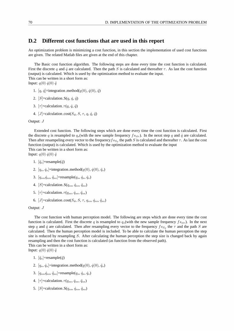
70 D. IMPLEMENTATION OF THE OPTIMIZATION PROBLEM
D.2 Different cost functions that are used in this report
An optimization problem is minimizing a cost function, in this section the implementation of used cost functionsare given. The related Matlab files are given at the end of thischapter.
The Basic cost function algorithm. The following steps are done every time the cost function is calculated.First the discreteq andq are calculated. Then the pathS is calculated and thereafterτ . As last the cost function(output) is calculated. Which is used by the optimization method to evaluate the input.This can be written in a short form as:Input: q(0) q(0) q
1. [q, q]=integrationmethod(q(0), q(0), q)
2. [S]=calculationS(q, q, q)
3. [τ ]=calculationτ (q, q, q)
4. [J ]=calculationcost(Sd, S, τ , q, q, q)
Output:J
Extended cost function. The following steps which are done every time the cost function is calculated. Firstthe discreteq is resampled toqs(with the new sample frequencyfsitr). In the nexst stepq and q are calculated.Then after resampeling every vector to the frequencyfsSd
the pathS is calculated and thereafterτ . As last the costfunction (output) is calculated. Which is used by the optimization method to evaluate the inputThis can be written in a short form as:Input: q(0) q(0) q
1. [qs]=resample(q)
2. [qs, qs]=integrationmethod(q(0), q(0), qs)
3. [qss,qss, qss]=resample(qs, qs, qs)
4. [S]=calculationS(qss, qss, qss)
5. [τ ]=calculationτ (qss, qss, qss)
6. [J ]=calculationcost(Sd, S, τ , qss, qss, qss)
Output:J
The cost function with human perception model. The following are steps which are done every time the costfunction is calculated. First the discreteq is resampled toqs(with the new sample frequencyfsitr). In the nextstepq and q are calculated. Then after resampling every vector to the frequencyfsSd
the τ and the pathS arecalculated. Then the human perception model is included. Tobe able to calculate the human perception the stepsite is reduced by resamplingS. After calculating the human perception the step size is changed back by againresampling and then the cost function is calculated (as function from the observed path).This can be written in a short form as:Input: q(0) q(0) q
1. [qs]=resample(q)
2. [qs, qs]=integrationmethod(q(0), q(0), qs)
3. [qss,qss, qss]=resample(qs, qs, qs)
4. [τ ]=calculationτ (qss, qss, qss)
5. [S]=calculationS(qss, qss, qss)

DIFFERENT COST FUNCTIONS THAT ARE USED IN THIS REPORT 71
6. [Ss]=resample(S)
7. [S percs]=humanperseptionmodel(Ss)
8. [S perc]=resample(S perss)
9. [J ]=calculationcost(S percd, S perc, τ , qss, qss, qss)
Output:J
The Online cost function and Jacobian. The following are steps which are done every time the cost functionis calculated. Firstq is calculated. Thereafter the pathS is calculated and thereafter the jacobian. As last the costfunction (output) is calculated.This can be written in a short form as:Input: q(0) q
1. [q1]=integrationmethod(q1(0), q1)
2. [S]=calculationS(q1, q1, q1)
3. [Jacobian]=calculationJacobian(M , q1, q1)
4. [J ]=calculationcost(Me, M , τ , q1, q1)
Output:J

72 D. IMPLEMENTATION OF THE OPTIMIZATION PROBLEM
D.3 Reference list from the used files
In this section the structure and the filenames are given for the optimization program. It is the same structure foron-line and off-line optimization but the code inside the files is different.
start main file.m
Loading parameters parameters.m
Loading Sd Load Sd.m
Prepare the optimizing optimizing ini.m
Optimizing lsqnonlin
cost function costfunction.m
resample resample.m
ODE45 integration method.m
S andτ Spath.m
(Possible) Human perception modelHuman perseption model.m
(Possible) JacobianJacobian.mCalculation of the cost function The cost.m
Display Output.m