university of trieste - units.it€¦ · university of trieste doctoral school in physics european...
TRANSCRIPT

University of Trieste
Doctoral School in Physics
European Social Fund
(S.H.A.R.M. project, Regional Operative Program 2007/2013)
List S.p.A.
Applications of Large Deviations Theory and
Statistical Inference to Financial Time Series
Ph.D. Candidate:
Mario Filiasi
School Director:
Paolo Camerini
Supervisor:
Erik Vesselli
Co-Supervisor:
Maria Peressi
Company Supervisor:
Elia Zarinelli
Academic Year 2013/2014

Abstract
The correct evaluation of financial risk is one of the most active domain of financial research,
and has become even more relevant after the latest financial crisis. The recent developments of
econophysics prove that the dynamics of financial markets can be successfully investigated by
means of physical models borrowed from statistical physics. The fluctuations of stock prices are
continuously recorded at very high frequencies (up to 1ms) and this generates a huge amount
of data which can be statistically analysed in order to validate and to calibrate the theoretical
models. The present work moves in this direction, and is the result of a close interaction between
the Physics Department of the University of Trieste with List S.p.A., in collaboration with the
International Centre for Theoretical Physics (ICTP).
In this work we analyse the time-series over the last two years of the price of the 20 most traded
stocks from the Italian market. We investigate the statistical properties of price returns and we
verify some stylized facts about stock prices. Price returns are distributed according to a heavy-
tailed distribution and therefore, according to the Large Deviations Theory, they are frequently
subject to extreme events which produce abrupt price jumps. We refer to this phenomenon as
the condensation of the large deviations. We investigate condensation phenomena within the
framework of statistical physics and show the emergence of a phase transition in heavy-tailed
distributions. In addition, we empirically analyse condensation phenomena in stock prices: we
show that extreme returns are generated by non-trivial price fluctuations, which reduce the
effects of sharp price jumps but amplify the diffusive movements of prices.
Moving beyond the statistical analysis of the single-stock prices, we investigate the structure
of the market as a whole. In financial literature it is often assumed that price changes are due to
exogenous events, e.g. the release of economic and political news. Yet, it is reasonable to suppose
that stock prices could also be driven by endogenous events, such as the price changes of related
financial instruments. The large amount of available data allows us to test this hypothesis and
to investigate the structure of the market by means of the statistical inference. In this work
we propose a market model based on interacting prices: we study an integrate & fire model,
inspired by the dynamics of neural networks, where each stock price depends on the other stock
prices through some threshold-passing mechanism. Using a maximum likelihood algorithm, we
apply the model to the empirical data and try to infer the information network that underlies
the financial market.
1

Acknowledgements
I acknowledge financial support from the European Social Fund (S.H.A.R.M. project, Re-
gional Operative Program 2007/2013), from LIST S.p.A., and from the NETADIS Marie Curie
Training Network (European Commission, FP7, Grant 290038).
I also acknowledge LIST S.p.A. for logistic and technical support and for data providing, and
M. Marsili (the Abdus Salam International Centre for Theoretical Physics – ICTP) for constant
collaboration to the research project.
I thank the supervisors E. Vesselli, M. Peressi, and E. Zarinelli for their careful tutoring and
continuous encouragement; M. Marsili for his precious collaboration; E. Dameri, E. Melchioni and
D. Davio for fostering the present project. I also thank L. Caniparoli, G. Dovier, R. Monasson,
G. Livan, and S. Saccani for the fruitful discussions, and all staff of the University of Trieste,
LIST S.p.A., and ICTP for providing a friendly and inspiring environment.
2

Contents
1 Introduction 6
1.1 About Stock Prices . . . . . . . . . . . . . . . . . . . . . . . . . . . . . . . . . . . 8
1.2 First Issue: Power-Law Distributions . . . . . . . . . . . . . . . . . . . . . . . . . 9
1.3 Second Issue: Auto-Correlation Effects . . . . . . . . . . . . . . . . . . . . . . . . 11
I Large Deviations Theory and Condensation Phenomena 14
2 Large Deviations Theory 15
2.1 Large Deviations Principle . . . . . . . . . . . . . . . . . . . . . . . . . . . . . . . 15
2.2 Derivation of the LDT . . . . . . . . . . . . . . . . . . . . . . . . . . . . . . . . . 17
2.3 Sample Mean of i.i.d. Random Variables . . . . . . . . . . . . . . . . . . . . . . . 21
2.4 Equivalence between LDT and SM . . . . . . . . . . . . . . . . . . . . . . . . . . 23
2.4.1 First Scenario . . . . . . . . . . . . . . . . . . . . . . . . . . . . . . . . . . 24
2.4.2 Second Scenario . . . . . . . . . . . . . . . . . . . . . . . . . . . . . . . . 26
2.4.3 Remarks . . . . . . . . . . . . . . . . . . . . . . . . . . . . . . . . . . . . . 29
3 Condensation Phenomena 30
3.1 Breaking the Assumptions of the LDT . . . . . . . . . . . . . . . . . . . . . . . . 30
3.2 Heavy-Tailed Distributions . . . . . . . . . . . . . . . . . . . . . . . . . . . . . . 31
3.3 LDT for Heavy-Tailed Distributions . . . . . . . . . . . . . . . . . . . . . . . . . 33
3.4 Condensation Phase Transition . . . . . . . . . . . . . . . . . . . . . . . . . . . . 37
3.5 The Order Parameter . . . . . . . . . . . . . . . . . . . . . . . . . . . . . . . . . 39
4 The Density Functional Method 43
4.1 The Fluid Phase . . . . . . . . . . . . . . . . . . . . . . . . . . . . . . . . . . . . 44
4.2 The Condensed Phase . . . . . . . . . . . . . . . . . . . . . . . . . . . . . . . . . 48
4.3 Simultaneous Deviations of Two Observables . . . . . . . . . . . . . . . . . . . . 51
3

II Extreme Events in Stock Prices 56
5 Stock Prices Dataset 57
5.1 The Order Book . . . . . . . . . . . . . . . . . . . . . . . . . . . . . . . . . . . . 58
5.2 Description of the Dataset . . . . . . . . . . . . . . . . . . . . . . . . . . . . . . . 60
5.3 Measuring Times and Prices . . . . . . . . . . . . . . . . . . . . . . . . . . . . . . 64
6 Stylized Facts about Stock Prices 68
6.1 The Geometric Brownian Motion . . . . . . . . . . . . . . . . . . . . . . . . . . . 68
6.2 Global Properties of Stocks . . . . . . . . . . . . . . . . . . . . . . . . . . . . . . 71
6.3 Probability Distribution of Price Returns . . . . . . . . . . . . . . . . . . . . . . 73
6.4 Diffusivity of Prices . . . . . . . . . . . . . . . . . . . . . . . . . . . . . . . . . . 76
6.5 Auto-Correlation of Price Returns . . . . . . . . . . . . . . . . . . . . . . . . . . 79
7 Large Deviations in Price Returns 84
7.1 Large Deviations in Price Returns . . . . . . . . . . . . . . . . . . . . . . . . . . 84
7.2 Extreme Events in Power-Law Distributions . . . . . . . . . . . . . . . . . . . . . 87
7.3 Preliminary Remarks . . . . . . . . . . . . . . . . . . . . . . . . . . . . . . . . . . 88
7.4 Condensation Phenomena in Stock Prices . . . . . . . . . . . . . . . . . . . . . . 90
8 Modelling Extreme Price Returns 95
8.1 Beyond the Geometric Brownian Motion . . . . . . . . . . . . . . . . . . . . . . . 95
8.1.1 The Jump-Diffusion Model . . . . . . . . . . . . . . . . . . . . . . . . . . 96
8.1.2 Stochastic-volatility Models . . . . . . . . . . . . . . . . . . . . . . . . . . 96
8.1.3 ARCH & GARCH Models . . . . . . . . . . . . . . . . . . . . . . . . . . . 97
8.1.4 The Multi-Fractal Random Walk . . . . . . . . . . . . . . . . . . . . . . . 99
8.2 Condensation Phenomena and Volatility Clustering . . . . . . . . . . . . . . . . . 100
III Statistical Inference of the Market Structure 103
9 The Financial Network 104
9.1 Cross-Stock Correlations in Financial Markets . . . . . . . . . . . . . . . . . . . . 105
10 A Model for Interactive Stock Prices 111
10.1 Micro-Structural Noise . . . . . . . . . . . . . . . . . . . . . . . . . . . . . . . . . 112
10.2 The Dynamics of Effective Prices . . . . . . . . . . . . . . . . . . . . . . . . . . . 112
10.3 The Dynamics of Observed Prices . . . . . . . . . . . . . . . . . . . . . . . . . . . 115
10.4 Analogy with Neural Networks . . . . . . . . . . . . . . . . . . . . . . . . . . . . 117
4

11 Bayesian Inference of the Financial Network 119
11.1 Bayesian Inference . . . . . . . . . . . . . . . . . . . . . . . . . . . . . . . . . . . 119
11.2 Evaluation of the Likelihood Function . . . . . . . . . . . . . . . . . . . . . . . . 122
11.3 Weak-Noise Approximation . . . . . . . . . . . . . . . . . . . . . . . . . . . . . . 125
12 Testing and Results 132
12.1 Statistical Errors . . . . . . . . . . . . . . . . . . . . . . . . . . . . . . . . . . . . 132
12.2 Testing the Algorithm . . . . . . . . . . . . . . . . . . . . . . . . . . . . . . . . . 135
12.2.1 First Test – Homogeneous Network . . . . . . . . . . . . . . . . . . . . . . 135
12.2.2 Second Test – Heterogeneous Network . . . . . . . . . . . . . . . . . . . . 137
12.2.3 Third Test – Random Network . . . . . . . . . . . . . . . . . . . . . . . . 140
12.2.4 Fourth Test – No Network . . . . . . . . . . . . . . . . . . . . . . . . . . . 140
12.3 Inferring the Real Financial Structure . . . . . . . . . . . . . . . . . . . . . . . . 143
13 Conclusions 149
13.1 Part I . . . . . . . . . . . . . . . . . . . . . . . . . . . . . . . . . . . . . . . . . . 149
13.2 Part II . . . . . . . . . . . . . . . . . . . . . . . . . . . . . . . . . . . . . . . . . . 151
13.3 Part III . . . . . . . . . . . . . . . . . . . . . . . . . . . . . . . . . . . . . . . . . 152
Bibliography 153
5

Chapter 1
Introduction
What is “econophysics”? Econophysics is an interdisciplinary branch of physics that applies
methods and models from conventional physics to financial and economic subjects. Although
the interest of physicists in social and economic sciences is not new, econophysics has become an
established field of physical research only in the last few decades, thanks to the growing number of
works in this sector and to the increasing employment of physicists in the financial industry. The
birthday of econophysics can be symbolically traced back to 1995 when, in a statistical physics
conference at Kolkata, H. E. Stanley coined the term “econophysics” to denote the new front of
physical research on economic subjects [59]. The same year, R. N. Mantegna and H. E. Stanley
themselves published an inspiring paper on Nature [90], investigating the scaling properties of
stock prices with a rigorous empirical approach, and signing what is now celebrated as the first,
large-audience work in econophysics.
The main idea that induced an increasing number of researchers to explore the financial world
with the eyes of a natural scientist is that markets and economies can be described as complex
systems, where a large number of agents, such as traders, industries, financial institutions, and
governments, continuously interact by exchanging goods, services, labour, and money. According
to the words by J.-P. Bouchaud [22]:
[. . . ] modelling the madness of people is more difficult than the motion of planets,
as Newton once said. But the goal here is to describe the behaviour of large popu-
lations, for which statistical regularities should emerge, just as the law of ideal gases
emerge from the incredibly chaotic motion of individual molecules.
In this context, one of the most studied cases in econophysics is the financial market, where
a dense network of interactions between trading agents processes and digests the large hetero-
geneity of trading strategies into unique numbers, namely, prices, interest rates, and exchange
rates, referring to several financial instruments such as stock shares, derivatives, currencies, etc.
Starting from the 1980s, the financial markets underwent a technological revolution that led to
the automatic management of the trading operations by means of electronic systems. The pos-
6

sibility of algorithmic trading, enhanced by the speculative advantages of short reaction times,
led to an overall acceleration of trading activities and gave rise to what is now denoted as High-
Frequency Trading (HFT) [91]. In addition, the prices of each financial instrument started to
be continuously monitored, keeping trace of all offers and trades in virtual registers that can be
recovered for statistical analyses. In conclusions, modern financial markets produce gigabytes of
data every day, recording price fluctuations, trading volumes, order flows, stock liquidity, and
so on. Such volume of information is a precious tool for the academic research, allowing a deep
historical analysis and a careful validation and calibration of theoretical models.
Yet, the quickening of trading activity has its perilous drawbacks. In the last century, the
number of financial crises has significantly increased, pointing out the inadequacy of market
regulations and the inability of existing economic models in describing and predicting financial
crashes. The increased volatility in stock prices, financial indices, interest rates, and exchange
rates, has stressed the importance of a correct evaluation of the financial risk, which is now one
of the greatest concerns of the financial industry [74]. Econophysics, then, finds its ultimate
rationale in this scenario. The empirical observation of financial time-series is an imperative
step in the formulation of new methods for financial risk evaluation. Finally, by capturing the
underlying mechanisms of price fluctuations, econophysics could achieve a deeper understanding
in the generation of financial crashes, supporting modern economics with new models to predict
(or avoid) economic crises, with obvious advantages for the global society.
The success of econophysics along the pre-existing financial research is probably due to the
different approach of physicists towards the research subjects with respect to the previous sci-
entific community composed of economists and mathematicians. The classical framework of
economic theories is based on very strong assumptions, such as the perfect rationality of trading
agents and the information efficiency of financial markets, which are usually developed in order
to simplify the theoretical models rather than to reproduce the empirical observations. The
inadequacy of this approach in forecasting and managing the latest economic crises has pointed
out the weakness of the existing methods, leaving room to new perspectives [22]. Physicists
dedicate to financial issues a more pragmatic approach, trying to adapt models and theories
to empirical observations and rising doubts about traditional axioms, favouring the reality of
facts over the beauty of concepts. Doing so, econophysicists unveiled the presence of complex
dynamics in modern economies, where financial markets are out of equilibrium and prices are
highly susceptible to small excitations [75]. Although econophysics is far from having found a
universal theory for global and local economies, there are strong beliefs that the new empirical
approach on the traditional economic problems could provide a more profound knowledge about
the financial world.
7

1.1 About Stock Prices
The main subjects of the present work are stock prices. In this thesis, we review the most
important and universal features of stock prices according to the existing financial literature,
and present new empirical analyses performed on a real dataset (courtesy of LIST S.p.A). The
available data refer to the historical prices of the 20 most traded stocks from the Italian equity
market, recorded with high time resolution (0.01 secs), over a period of two years, from July
2012 to June 2014.
According to a widely accepted theoretical framework, stock prices are described by stochastic
processes, and are intrinsically unpredictable random quantities [91, 20]. The stochasticity of
stock prices was postulated for the first time in 1900 by L. Bachelier, in his celebrated PhD thesis
named “Theorie de la speculation” [3], where he originally developed the random walk theory
five years before Einstein. Since then, the idea that stock prices can be successfully described
as intrinsically random quantities has always been at the basis of the most important economic
theories. In 1970, E. F. Fama affirmed this concept in rigorous form by developing the so-
called Efficient Market Hypothesis [53], stating that financial markets should be “informationally
efficient”. Loosely speaking, this means that stock prices should instantaneously react to the
release of new information, such as political and economical news, and should reflect the pure
randomness of the information flow. During the last century, the original theory developed by
Bachelier has been gradually refined through a large variety of stochastic models [91]. Among
the most important ones, we mention the Black-Scholes-Merton model (1973) [14, 95], the Auto-
Regressive Conditional Heteroskedatic (ARCH) models (1982) [49], the Heston model (1993)
[69], and the Multi-Fractal Random Walk (2001) [4].
In the statistical analysis of stock prices, the role of fundamental random step at the basis
of the price-fluctuation process is played by the price return xτ (t), i.e. the relative increment of
prices at the instant t, after a specific time-lag τ (see Section 6.1 for more details). In a zero-th
order approximation, price returns can be considered as independent normal random variables,
namely:
xτ (t) ∼ N (µτ , σ2τ ) ,
where µτ and σ2τ denote the mean and the variance of xτ (t), respectively, at the specific time-lag
τ [20]. The assumption of statistical independence is justified by the Efficient Market Hypothesis,
and is partially supported by the lack of linear auto-correlation in empirical returns (although
different forms of statistical dependence are clearly recognizable [20]). The normality of price
returns, instead, is usually invoked as a mathematical simplification in order to describe stock
price as continuous stochastic processes with scale-invariant properties. Indeed, thanks to the
stability and to the infinite divisibility of the normal distribution, stock prices (or, rather, the
logarithm of stock prices) can be defined as continuous Wiener processes whose increments obey
the diffusive law:
xτ (t) ∼ N (µτ, σ2τ) ,
8

where τ is any time-scale, and µ and σ2 are the characteristic mean and variance of the process.
This simplification has been widely used in earliest theoretical models and, above all, it provided
the mathematical background for the celebrated Black & Scholes formula [14], a milestone of
modern financial theories, developed in 1973 in order to define the price of stock options.
The above vision, which depicts stock prices as Wiener processes and price returns as sta-
tistically independent normal variables, is far from being a faithful description of reality. In
our opinion, according to the discussion presented in the following chapters, the most relevant
discrepancies between this “toy model” and the empirical observations on stock prices are the
following [91, 20]:
• Price returns xτ (t) are not normal random variables, but are rather described by some
power-law distribution with much larger tails.
• Price returns xτ (t) at subsequent times t are not statistically independent, but their mag-
nitude is strongly auto-correlated over time.
The interplay of these two features strongly affects the price-fluctuation process and, above
all, enhance the generation of extreme price changes, with obvious consequences in the field of
financial-risk management. These properties of stock prices will be the main ingredients of the
following work and are worth a specific discussion.
1.2 First Issue: Power-Law Distributions
Power-law distributions naturally arise in a large variety of contexts in both natural and social
sciences [124, 123]. The first appearance of a power-law distribution is probably due to V. Pareto,
who, in 1897, analysed the empirical distribution of wealth in stable economies, discovering a
power-law distribution with a slow decaying behaviour. Since then, power-law distributions have
been empirically observed in the most disparate sectors of scientific research in relation to several
observables [117, 87, 109, 138, 108, 136], such as:
• magnitude of earthquakes;
• intensity of forest-fires;
• intensity of rains;
• size of cities;
• intensity of wars;
• frequency of words in a text;
• variety of biological species;
• diameters of moon craters;
9

• intensity of solar flares;
• activity of neural cells;
• fluctuations of stock prices and other financial instruments, such as interest rates, derivative
prices, financial indices, and exchange rates.
The ubiquity of power-laws in almost all sectors of natural and social sciences is often claimed
as the fingerprint of self-organized criticality in complex systems [122]. Indeed, power-laws
naturally emerge in presence of critical phenomena, where different systems with heterogeneous
dynamics exhibit a common behaviour due to the universal scaling-laws of their observables. The
widespread of power-law distributions in almost every sector of everyday life, and the resulting
impact of large-scale events, give rise to the so-called black swan theory [127], denoting the
importance of a correct statistical treatment of rare events (the “black swan” is a metaphor
describing the occurrence of a rare event which can easily lead to an inappropriate ex-post
rationalization).
It is an empirical fact that price returns are distributed according to a power-law distribution,
but what are the direct consequences of this fact? The first, most obvious consequence is that
extreme price returns (i.e. large gains and losses in stock prices) are not as rare as one would
expect on the basis of normal returns, and this is a crucial point if we consider that extreme price
returns are relevant sources of financial risk. Yet, the statement that price returns are power-
law random variables is much stronger than this, and implies the existence of precise scaling
properties in the occurrence of extreme events [123].
Let us consider a generic random variable x described by the probability density function
Px(x). The distribution Px(x) is a power-law distribution if it decays as:
Px(x) ' A
xα+1,
where A is a normalization constant and α is the tail index of the distribution (α > 0). The
fundamental properties of power-law distributions is the lack of a characteristic scale, which is
reflected in the scale-invariance of extreme events. Indeed, if we consider the rescaling x 7→ λx
and focus on the tail of the distribution, we simply find:
Pλx(x) ' λαPx(x) ,
for any scale factor λ. Loosely speaking, the relative probability of two large event xA and
xB does not depend on their individual values, but only on the ratio xA/xB . As a result, the
concept of extreme event in power-law distributions becomes counter-intuitive. Since the tail of
the distribution is not characterized by any reference scale, it is not easy to distinguish “rare
events” form “typical events”. Moreover, this scale-invariance suggests that any extreme event in
the outcomes of power-law random variables should not be considered as an outlier, but should
10

rather be analysed in relation to all other outcomes as a natural extension of the statistical
sample to larger sizes [123].
In our opinion, one of the most striking features of power-law distributions is the emergence
of condensation phenomena in the rare outcomes of power-law random variables [55, 83]. Let
us introduce this concept with an example. Suppose to observe an anomalous price-drop in the
historical time-series of some financial stock. Assume that the price-drop has been recorded
on a daily time-scale and imagine to investigate the detailed movement of the stock price on
finer sampling-times, say, at 5 minutes. What should we expect to find? A naive guess could
suggest that the price-drop has been obtained as the sum of many negative returns, leading
to a continuous negative drift of the stock price. Yet, if we assume that price returns are
independent random variables with power-law distribution, the most likely realization of the
final daily-return is a concentration of the whole price-drop in a single 5-minute return. This
mechanism is known in literature as the condensation of large deviations in the sum of random
variables [55, 83]. The emergence of condensation phenomena in statistical samples of power-law
random variables can be described in a statistical-mechanics approach as a second-order phase
transition, from a fluid phase (the regime of typical fluctuations) to a condensed phase (the regime
of large deviations), characterized by a spontaneous symmetry breaking [55]. This mechanism
is reminiscent of the phase transition occurring in the Bose-Einstein condensate [110], and can
be observed in other physical systems with power-law distributions [11, 83, 105]. In this work,
we examine condensation phenomena in deep details by invoking both the statistical mechanics
and the Large Deviation Theory [128], developed to analyse the probability of rare events in
statistical samples, then we perform an empirical measurement of condensation phenomena in
financial time-series and we show how the specific dynamics of stock prices affects the generation
of large price returns.
1.3 Second Issue: Auto-Correlation Effects
Besides their power-law distribution, the second important feature of price returns is the presence
of strong auto-correlation effects [91, 20]. This auto-correlation does not affect the returns
themselves, but rather their unsigned magnitudes. As explained by B. Mandelbrot [88], who
first reported this empirical fact in 1963, “large changes tend to be followed by large changes –
of either sign – and small changes tend to be followed by small changes”.
In most theoretical models developed in recent years [49, 69, 4], price returns xτ (t) have been
described as the composition of two separate stochastic processes, namely:
xτ (t) = στ (t) · ητ (t) ,
where ητ (t) are the rescaled returns and στ (t) are the instantaneous values of the price volatility,
which measures the characteristic scale of price fluctuation. The rescaled returns ητ (t) are
11
assumed to be statistically independent and are often defined as normal random variables; on
the contrary, the volatilities στ (t) are (positive) auto-correlated random variables and should
reproduce the correlation effects in the magnitude of price returns. Depending on the specific
form of the volatility auto-correlation, the above decomposition could replicate the power-law
behaviour of price returns even when the rescaled returns are chosen to be normally distributed
(consider, for instance, the Multi-Fractal Random Walk described in Section 8.1).
This picture naturally accounts for the heteroskedasticity of price returns (i.e. the variable
range of price fluctuations [49]), and could be the first step towards a more faithful description
of the complex price behaviour. The financial time-series of stock prices are characterized by
heterogeneous regimes where fluctuations can be relatively small or large, with sudden volatility
changes spaced out by constant-volatility regimes with variable duration. This effect is often
denoted as volatility clustering [33, 20], suggesting that price returns with different magnitudes
are not homogeneously distributed in time. Surprisingly, the irregular behaviour of the volatility
can be detected on several time-scales, from few minutes to many days, and exhibits the typical
scale-invariance of fractal processes [17]. Indeed, the volatility changes over a given observation
time can be sharpened or smoothed just by changing the sampling times of the examined prices,
and even the constant-volatility regimes may hide abrupt volatility burst or quenches that are
visible only on smaller time-scales. As a result, the auto-correlation function of the volatility
exhibits a slowly decaying behaviour that is often comparable to a power-law with a small
exponent, and this is usually claimed to be a sign of long-memory effects in price dynamics[17].
At this stage, the real question is: why does such correlation emerge? In financial literature,
price changes are usually classified as either exogenous or endogenous, depending on their origin
[72, 75]. According to the traditional economic explanation, price fluctuations are mainly exoge-
nous and depend on the information flow from the external world to the financial market. As a
matter of fact, many changes in stock prices can be traced back to the release of some political
or economic news, or to the price change of some fundamental asset. Yet, this explanation could
be not enough. In recent years, it has been frequently claimed that the volatility of stock prices
is too high to be entirely explained by exogenous factors, and that some endogenous mechanisms
of price fluctuation is indeed necessary to explain the empirical observations. This statement
is often denoted as the “excess volatility puzzle” and is clearly in contrast with the common
assumptions of the Efficient Market Hypothesis [75, 120]. In addition, it has been noticed that
the intermittent behaviour of volatility, characterized by long-memory effects, is typical of many
physical systems with non-linear dynamics [81, 29]. In turbulent flows, for instance, the velocities
measured at different length-scales exhibit the same intermittent and power-law behaviour that
is observed in the returns of stock prices [4, 17]. The comparison of the financial markets with
non-linear physical systems suggests that the fluctuation-process of stock prices could be driven
by some self-exciting feedback that causes trades to induce further trades [75]. In the worst
scenario, this noise-amplification feedback could escalate in avalanche-like dynamics that may
eventually lead to financial crashes, as it probably happened in the infamous Flash Crash (May
12

6, 2010), where the Dow Jones index lost almost the 9% of its value in very few minutes [131].
In financial literature, the presence of self-exciting mechanisms in trading activity and in the
price-fluctuation dynamics is usually addressed as the self-reflexivity of financial market, and is
currently an active research front for econophysics [30, 68]. In the present work, we move along
this research line and we develop a new model for the financial markets where price changes in
specific stocks may induce further price changes in correlated stocks. This model defines the
financial market as an interaction network connecting several financial assets. In the following,
using the probabilistic framework of the Bayesian inference [62], we apply the theoretical model
to our dataset and we try to infer the topology of the financial network on the basis of the
empirical observations.
13

Part I
Large Deviations Theory and
Condensation Phenomena
14

Chapter 2
Large Deviations Theory
In this chapter we introduce the formalism of Large Deviations Theory (LDT), which studies
the asymptotic probability distribution of averaged observables defined over large sets of random
variables [128]. The origin of the LDT can be traced back to the works of H. Cramer in the
early 1930s [37], but the theory has been formalized by S. R. S. Varadhan only in 1966 [133]. In
spite of this, some essential results of the LDT were already known by statistical physicists in
some specific contexts before their rigorous mathematical statements, and settled the basis for
the classical formulation of statistical physics [128].
The following discussion reviews the fundamental concepts of the LDT, focusing on a classical
case: the sample mean of a large number of independent and identically distributed random
variables. In this context, the LDT can be considered as a generalization to the Central Limit
Theorem (CLT) and to the Law of Large Numbers (LLN), describing the statistical deviations
of the sample mean from its expected value beyond their respective range of validity. The main
goal of the following sections is to introduce the theoretical framework required for the analysis
of condensation phenomena, which are one of the main subjects of the present work.
2.1 Large Deviations Principle
Let us consider a set of N random variables {x1, . . . ,xN} (which we denote simply as {x})described by the joint p.d.f. P{x}(x1, . . . , xN ). Given this set, let us define the random variable:
y = f(x1, . . . ,xN ) ,
where f is a generic function of the random set. The p.d.f. of y can be defined in terms of the
joint p.d.f. of {x} by the equation:
Py(y) =
∫dNxP{x}(x1, . . . , xN ) δ
(f(x1, . . . , xN )− y
). (2.1)
15

We assume that the random variable y obeys the Law of Large Numbers (LLN) [65]. This
means that there is a typical value y0 such that, in the limit N →∞, the probability that y = y0
remains strictly positive, while the probability that y 6= y0 tends to zero. Loosely speaking,
y0 is the only likely outcome for y in the limit N → ∞. As long as N remains finite, y may
deviate from y0. We call small deviations all possible outcomes of y in the proximity of y0 whose
probability is relatively large, and we call large deviations all other outcomes. In the following, we
will often use the terms small and large deviations as synonymous of typical and rare outcomes,
respectively. The boundary between the two kind of deviations is not sharp and depends on the
number of variables N . Indeed, as N increases, the range of small deviations becomes narrower
and narrower, leaving place to large deviations and eventually reducing to the single point y0.
The main purpose of the LDT is to find a good approximation for Py(y) for large values of
N which holds for both small and large deviations. This is different, for instance, from the usual
results of the Central Limit Theorem, which holds only around the centre of the distribution.
According to the LDT, we say that the random variable y satisfies the Large Deviation Principle
[128] if the limit
Iy(y) = − limN→∞
1
NlogPy(y) (2.2)
exists and is not trivial (i.e. it is almost everywhere different from zero). In this case, the function
Iy(y) is called the rate function of the variable y, and Py(y) can be approximated, for large N ,
by the asymptotic relation:
Py(y) ∼ e−NIy(y) . (2.3)
The last equation sums up the whole LDT in just one formula. According to the LLN, as long
as the number of variables N increases, the non-typical outcomes of y become less and less likely
and the whole probability measure Py(y) is absorbed by y0. The eq. (2.3) quantifies this idea,
asserting that the probability of non-typical outcomes is exponentially suppressed in N at a speed
defined by the rate function Iy(y). Since y0 is the only likely outcome in the limit N → ∞, we
expect that Iy(y) = 0 for y = y0 and that Iy(y) > 0 for all y 6= y0 (this expectation will be
confirmed in the next section). Under this considerations, the LDT turns out to be a finite-size
correction of the LLN that extends the law to the case of large but finite N .
It is worth to notice that, even if the definition (2.2) is rigorous, it is useless for practical
purposes. Indeed, one would like to use the rate function to approximate Py(y), which is supposed
to be unknown, but the definition of the rate function requires the knowledge of Py(y) itself. In
the next section we will overcome this problem by presenting an alternative way to evaluate the
rate function Iy(y). This will be the chance to clarify the mathematical foundation of the LDT
and to take a deeper insight into the theory.
16

2.2 Derivation of the LDT
Let us study the definition (2.1) of Py(y). By exploiting the Laplace representation of the delta
function we can write:
Py(y) =
∫dNxP{x}(x1, . . . , xN )× 1
2πi
∫=
ds esf(x1,...,xN )−sy ,
where the symbol = means that the integration over s must be performed along the imaginary
axis. Then, inverting the integrals, we get:
Py(y) =1
2πi
∫=
ds
[∫dNxP{x}(x1, . . . , xN ) esf(x1,...,xN )
]e−sy ,
which can be shortened in:
Py(y) =1
2πi
∫=
ds 〈esy〉 e−sy . (2.4)
The last integral has exactly the form of an inverse Laplace transform, and proves that 〈esy〉is the Laplace transform of Py(y). In order to be more rigorous, let us introduce the moment
generating function Φy(s) and the cumulant generating function Ψy(s), which are defined as:
Φy(s) = 〈esy〉 , Ψy(s) = log〈esy〉 . (2.5)
As stated before, the moment generating function Φy(s) is exactly the Laplace transform of
the p.d.f. Py(y) (this can be easily proved from the definition itself). The cumulant generating
function Ψy(s), instead, is simply defined as the logarithm of Φy(s). The names of the functions
are due to the asymptotic expansions:
Φy(s) =
∞∑n=0
〈yn〉 sn
n!, Ψy(s) =
∞∑n=0
〈yn〉csn
n!, (2.6)
which allow us to evaluate all moments and cumulants of the distribution Py(y) respectively as:
〈yn〉 =dn
dsnΦy(s)
∣∣∣∣s=0
, 〈yn〉c =dn
dsnΨy(s)
∣∣∣∣s=0
.
It is important to stress that the functions Φy(s) and Ψy(s) are not guaranteed to exist for any
s ∈ R. Indeed, depending on the features of the distribution Py(y), the expected value 〈esy〉 may
diverge. If the generating functions exist for some point s on the real axis, then they can be also
extended to the complex plane along the line s+ it, for any t ∈ R. By definition, we always have
Φy(0) = 1 and Ψy(0) = 0, therefore, the functions Φy(it) and Ψy(it) are always well-defined
and turns out to be the characteristic function of Py(y) and its logarithm, respectively. This
property ensures that the inverse Laplace transform in eq. (2.4) is always convergent.
From now on, we focus on the cumulant generating function Ψy(s) and we assume that Ψy(s)
17

exist for any s ∈ R (the case where Ψy(s) is not defined will be addressed in Chapter 3). By
definition, Ψy(s) is an analytic and convex1 function of s [128]. Since y is defined over the set
{x1, . . . ,xN}, the function Ψy(s) implicitly depends on the number of variables N . The LDT
assumes that the behaviour of Ψy(s) for large N is described by the following scaling law:
Ψy(Ns) ' NΛy
(s) , (2.7)
where Λy(s) is independent on N . This assumptions is based on the typical behaviour of y when
the random variables {x1, . . . ,xN} are independent and identically distributed (see Section 2.3
for a specific example). According to the scaling law (2.7), we can define Λy(s) as:
Λy(s) = limN→∞
Ψy(Ns)
N. (2.8)
The function Λy(s) is called the rescaled cumulant generating function of the variable y. Like
Ψy(s), the function Λy(s) is convex, yet, for the sake of simplicity, we assume that Λy(s) is also
analytic and strictly convex, which means that the second derivative Λ′′y(s) exists and is strictly
positive for all s ∈ R [128].
At this stage, we can return to the inverse Laplace transform (2.4) and apply the new defi-
nitions. We can write:
Py(y) =1
2πi
∫=
ds eΨy(s)−sy ,
then, after the rescaling s→ Ns, we get:
Py(y) =N
2πi
∫=
ds eΨy(Ns)−Nsy ,
and finally, recalling the scaling law (2.7), we obtain:
Py(y) =N
2πi
∫=
ds e−N [sy−Λy(s)]+o(N) .
We arrived now at the fundamental step of the whole LDT. If N is large, we can try to
evaluate the above integral by means of the saddle-point approximation. We assume that the
function sy−Λy(s) has a unique stationary point s∗, which depends on y and is implicitly defined
by the equation Λ′y(s∗) = y. Since Λy(s) is strictly convex, the function Λ′y(s) can be inverted
and s∗ exists for any y in the domain of Py(y). The stationary point s∗ defines the saddle-point
of the integrand function. According to the saddle-point approximation, we can move the path
of integration across the complex plane in order to pass through the saddle-point, then, if N
is large, the whole integration can be approximated by a unique evaluation of the integrand
1The convexity of Ψy(s) means that Ψy(w1s1 +w2s2) ≤ w1Ψy(s1) +w2Ψy(s1) for any s1, s2 ∈ R and for anyw1, w2 ∈ [0, 1] such that w1 + w2 = 1. This can be proved by means of the Holder’s inequality, asserting that〈e(w1s1+w2s2)y〉 ≤ 〈es1y〉w1 〈es2y〉w2 .
18

s
Λy(s)
Λy(0) = 0
Λ′y(0) = y0
s
Λ′y(s) = y
y
Iy(y)
Iy(y0) = 0
I′y(y0) = 0
y
I′y(y) = s
Figure 2.1 – Schematic representation of the rescaled cumulant generating function Λy(s)
(left) and of the rate function Iy(y) (right), showing the correspondence between the
derivatives Λ′y(s) and I ′y(y) and the conjugate arguments y and s, as defined by the
Legendre transformation.
function at the saddle-point itself. The result is:
Py(y) ∼ e−N [s∗y−Λy(s∗)] .
Comparing last equation to eq. (2.3), it becomes clear that the rate function Iy(y) is equal to
s∗y−Λy(s∗) under the constraint Λ′y(s∗) = y. Therefore, Iy(y) is exactly the Legendre transform
of Λy(s) and can be expressed as:
Iy(y) = maxs∈R{sy − Λy(s)} . (2.9)
As we can see, the evaluation of the rate function Iy(y) does not require the knowledge of the
p.d.f. Py(y), but it can be directly computed from the (rescaled) cumulant generating function
by means of a Legendre transformation. In many cases (see Section 2.3, for instance) this is a
much simpler task than the evaluation of the p.d.f. Py(y) itself.
Since Λy(s) is assumed to be strictly convex, the Legendre transformation (2.9) can be in-
verted. Therefore, Λy(s) is also the Legendre transform of Iy(y), and we can write:
Λy(s) = maxy∈R{sy − Iy(y)} . (2.10)
Because of the relations (2.9) and (2.10), the functions Iy(y) and Λy(s) are said to be convex
conjugates [128]. This correspondence allows us to analyse the rate function Iy(y) just by knowing
Λy(s). Under the above assumptions, both functions Λy(s) and Iy(y) are analytic and strictly
19

Logarithm N →∞
Logarithm N →∞
Lapla
ce
transf
orm
Legendre
transfo
rm
Φy(s) Ψy(s) Λy(s)
Py(y) logPy(y) Iy(y)
Figure 2.2 – Relations between the fundamental functions in LDT.
convex. The rate function Iy(y) has a global minimum at the point y0 = Λ′y(0), and one gets
Iy(y) = 0 for y = y0 and Iy(y) > 0 for y 6= y0. According to the definition (2.8) and the
properties of the cumulant generating function, the minimum point y0 is:
y0 = limN→∞
〈y〉 .
These results are in full agreement with the LLN and confirm our previous expectations about
the rate function Iy(y). The correspondence between Λy(s) and Iy(y) and their typical shapes
are shown if Fig. 2.1.
The content of this section has been outlined in Fig. 2.2, showing the main ingredient of the
LDT and the mathematical relations connecting them. Now, in order to conclude this section,
we would like to present the above result in a more rigorous form by invoking the so-called
Gartner-Ellis theorem, developed by J. Gartner and R. S. Ellis in 1977 and 1984, respectively
[60, 47].
Gartner-Ellis theorem: Consider the random variable y as a function of the random
set {x1, . . . ,xN}, and consider the rescaled cumulant generating function Λy(s) defined in
(2.8), namely:
Λy(s) = limN→∞
1
Nlog⟨eNsy
⟩.
If Λy(s) exists and is differentiable for all s ∈ R, then y satisfies the Large Deviation Principle
(2.3) and its rate function Iy(y) is the Legendre-Fenchel tranform of Λy(s), namely:
Iy(y) = sups∈R{sy − Λy(s)} .
20

2.3 Sample Mean of i.i.d. Random Variables
In the previous sections we presented the LDT in its more general framework. In this section,
instead, we restrict our analysis to a simpler and more specific case, namely, the sample mean
of i.i.d. random variables. This is a classical topic in probability theory that found its historical
establishment in the Central Limit Theorem (CLT) [64]. Yet, it is worth to address this issue
with the new formalism of LDT: this will generalize the classical findings of the CLT and will
set the problem into a different light.
Let us consider a random set {x1, . . . ,xN} and let us assume that the components of the set
are i.i.d. This means that:
P{x}(x1, . . . , xN ) =
N∏n=1
Px(xn) ,
where x denotes a unique arbitrary variable in the set. Now, instead of the generic variable
y = f(x1, . . . ,xN ), let us consider the sample mean:
m =1
N
N∑n=1
xn .
According to eq. (2.1), the p.d.f. Pm(m) can be written as:
Pm(m) =
∫dNx
(N∏n=1
Px(xn)
)δ
(1
N
N∑n=1
xn −m
). (2.11)
Now, we can invoke the general results of the previous section to work out the LDT of the
sample mean m. The main difference between the considered case and the general case is that
the scaling law (2.7) is not just an approximation, but is exact. This is due to the equivalence
〈eNsm〉 = 〈esx〉N , which leads to:
Ψm(Ns) = NΨx(s) ,
and thus:
Λm(s) = Ψx(s) .
Therefore, the behaviour of the sample mean m in the limitN →∞ is equivalent to the behaviour
of an average variable x of the set. The final result is that the rate function Im(m) can be directly
evaluated as the Legendre transform of the cumulant generating function Ψx(s).
This result can be formalized into the Cramer’s theorem [37], which has been developed by
H. Cramer early in 1938 and can be considered as a special case of the more general Gartner-Ellis
theorem (see Section 2.2).
21
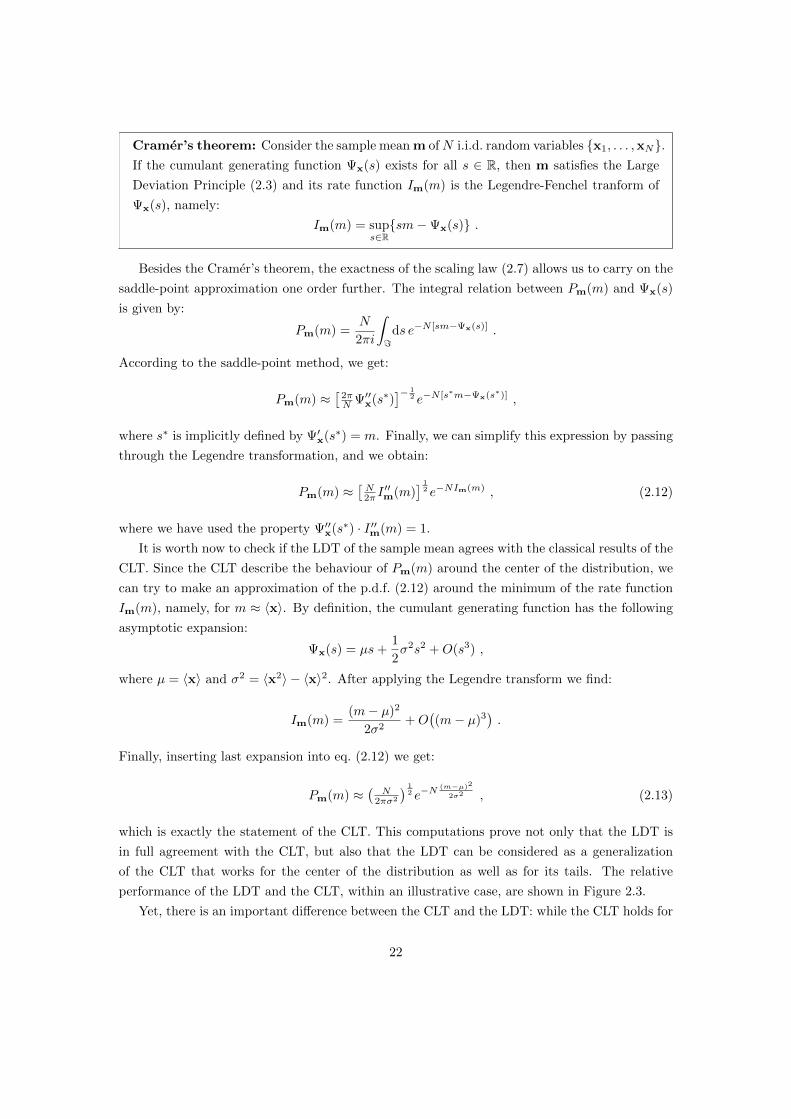
Cramer’s theorem: Consider the sample mean m ofN i.i.d. random variables {x1, . . . ,xN}.If the cumulant generating function Ψx(s) exists for all s ∈ R, then m satisfies the Large
Deviation Principle (2.3) and its rate function Im(m) is the Legendre-Fenchel tranform of
Ψx(s), namely:
Im(m) = sups∈R{sm−Ψx(s)} .
Besides the Cramer’s theorem, the exactness of the scaling law (2.7) allows us to carry on the
saddle-point approximation one order further. The integral relation between Pm(m) and Ψx(s)
is given by:
Pm(m) =N
2πi
∫=
ds e−N [sm−Ψx(s)] .
According to the saddle-point method, we get:
Pm(m) ≈[
2πN Ψ′′x(s∗)
]− 12 e−N [s∗m−Ψx(s∗)] ,
where s∗ is implicitly defined by Ψ′x(s∗) = m. Finally, we can simplify this expression by passing
through the Legendre transformation, and we obtain:
Pm(m) ≈[N2π I′′m(m)
] 12 e−NIm(m) , (2.12)
where we have used the property Ψ′′x(s∗) · I ′′m(m) = 1.
It is worth now to check if the LDT of the sample mean agrees with the classical results of the
CLT. Since the CLT describe the behaviour of Pm(m) around the center of the distribution, we
can try to make an approximation of the p.d.f. (2.12) around the minimum of the rate function
Im(m), namely, for m ≈ 〈x〉. By definition, the cumulant generating function has the following
asymptotic expansion:
Ψx(s) = µs+1
2σ2s2 +O(s3) ,
where µ = 〈x〉 and σ2 = 〈x2〉 − 〈x〉2. After applying the Legendre transform we find:
Im(m) =(m− µ)2
2σ2+O
((m− µ)3
).
Finally, inserting last expansion into eq. (2.12) we get:
Pm(m) ≈(
N2πσ2
) 12 e−N
(m−µ)2
2σ2 , (2.13)
which is exactly the statement of the CLT. This computations prove not only that the LDT is
in full agreement with the CLT, but also that the LDT can be considered as a generalization
of the CLT that works for the center of the distribution as well as for its tails. The relative
performance of the LDT and the CLT, within an illustrative case, are shown in Figure 2.3.
Yet, there is an important difference between the CLT and the LDT: while the CLT holds for
22

-1 0 1 2 3 4 5
0.0
0.2
0.4
0.6
0.8
1.0
1.2
-1 0 1 2 3 4 5
0.0
0.2
0.4
0.6
0.8
1.0
1.2
-1 0 1 2 3 4 5
0.0
0.2
0.4
0.6
0.8
1.0
1.2
-1 0 1 2 3 4 5
-12
-10
-8
-6
-4
-2
0
2
-1 0 1 2 3 4 5
-12
-10
-8
-6
-4
-2
0
2
-1 0 1 2 3 4 5
-12
-10
-8
-6
-4
-2
0
2
m m m
Pm
(m)
logPm
(m)
Figure 2.3 – The p.d.f. Pm(m) of the sample mean of N i.i.d. random variables with
exponential distribution Px(x) = e−x (x > 0), for N = 5. The dotted lines show the exact
p.d.f. Pm(m) = NNmN−1e−Nm/Γ(N). The red lines show (from left to right) different
approximations of Pm(m) with increasing goodness, namely: the CLT approximation
(2.13) (left); the standard LDT approximation (2.3) (center); and the full LDT approx-
imation (2.12) (right). Plots are shown twice, both in linear scale (top) and logarithmic
scale (bottom). The rate function of the sample mean is Im(m) = m− logm− 1. In the
case of the standard LDT approximation, the distribution has been normalized to unity.
any distribution with finite mean and variance, the LDT is based on the existence of the entire
generating function Ψx(s), which is a much stronger requirement. There is a large variety of
probability distributions with finite mean and variance whose generating functions do not exist.
In this cases, the CLT still holds, but it cannot be considered any more as a consequence of the
Large Deviations Principle. This is a very interesting scenario and will be specifically addressed
in the following sections (see Chapter 3).
2.4 Equivalence between LDT and SM
Up to now, the LDT may seem a purely mathematical toolbox to be used in the computation
of probabilities. Yet, the theory acquires a strong physical meaning when it is compared to
the classical results of the Statistical Mechanics (SM) [70]. The main ingredients of the LDT,
like the rate functions and the moment/cumulant generating functions, can be defined also for
thermodynamic systems and take the name of entropies, free energy, partition functions, and so
on. Even if the LDT is younger then the SM, it is at the very foundation of this physical theory.
Quoting H. Touchette [128], “physicists have been using LDT for more then a hundred years,
end are even responsible for writing down the very first large deviation results”.
In the following, we present two different scenarios in SM, inspired by [128], and based on
23

the micro-canonical and canonical ensembles, respectively. We are going to establish a one-to-
one correspondence between mathematical quantities in LDT and physical observables in SM,
showing that, to some extent, the two theories are equivalent.
2.4.1 First Scenario
Consider a system of N particles, which can be atoms, molecules, spins, etc. and suppose that
the state of the n-th particle is fully identified by a unique real-valued observable, say, xn. This
can be, for instance, the position of the particle or its magnetic moment. We analyse this system
in the micro-canonical ensemble [70], which is based on the postulate of equal a-priori probability.
This means that the probability of finding the system in a given configuration {x1, . . . , xN} is:
Pconf(x1, . . . , xN ) = constant .
Without loss of generality, we can set the constant to unity. This is always possible by choosing
a suitable unit of measure for the observables xn.
Now we assume that the dynamic of the system is driven by the Hamiltonian H(x1, . . . , xN ).
In order to define the thermodynamics of this system, we need to evaluate its entropy S(E) at
fixed energy E. This is defined as:
S(E) = logW (E) ,
where W (E) is the number of configurations whose energy is equal to E, namely:
W (E) =
∫dNx δ
(H(x1, . . . , xN )− E
).
Last integral can be analysed by means of the saddle-point method. By using the Laplace
representation of the delta function we obtain:
W (E) =
∫dNx
1
2πi
∫=
dβ e−β[H(x1,...,xN )−E] ,
which yields:
W (E) =1
2πi
∫=
dβ
[∫dNx e−βH(x1,...,xN )
]eβE .
The quantity in square brackets is exactly the partition function of the system in the canonical
ensemble [70], namely:
Z(β) =
∫dNx e−βH(x1,...,xN ) ,
then we can write:
W (E) =1
2πi
∫=
dβ Z(β) eβE .
24

Finally, recalling the definition of the free energy in the canonical ensemble:
F (β) = − 1
βlogZ(β) ,
we arrive to the last equation:
eS(E) =1
2πi
∫=
dβ eβ[E−F (β)] .
Since E and F (β) are extensive quantities, last integral can be evaluated via the saddle point
method.
Even if we used different names, the above computations are exactly the same performed in
Section 2.2. Therefore, we can try to make a correspondence between thermodynamic observables
and probabilistic quantities. Reminding that Pconf(x1, . . . , xN ) = 1, the result is:
• W (E) = PH(E);
• Z(β) = ΦH(−β);
• F (β) = −β−1ΨH(−β).
This means that we are actually considering the large deviations of the HamiltonianH(x1, . . . , xN ),
which is now considered as a random variable depending on the random configuration {x1, . . . , xN}.In order to complete this picture, we still have to find a correspondence with the rate function
IH and the rescaled cumulant generating function ΛH, which are the most important ingredients
of the LDT. Obviously, the LDT cannot be directly applied to the Hamiltonian H, because it is
an extensive quantity and do not obeys the Law of Large Numbers. Yet, even if H does not obey
the law, the average Hamiltonian H/N does. It is clear now that we must turn from extensive
to intensive quantities, and move towards the thermodynamic limit N → ∞. Let us define the
entropy density s(e) and the free energy density f(β) as:
s(e) = limN→∞
S(Ne)
N, f(β) = lim
N→∞
F (β)
N,
where e = E/N is the average energy per particle. Now it is easy to find that:
• f(β) = −β−1ΛH/N (−β);
• s(e) = −IH/N (e);
and the correspondence between the LDT and the SM is complete. The main consequence of
this correspondence is that s(e) and f(β) are conjugated by a Legendre transformation (except
for a factor β). Thus we can write:
s(e) = minβ
{β[e− f(β)]
}, f(β) = min
e
{e− β−1s(e)
}.
25

1st Scenario
Logarithm N →∞
Logarithm N →∞
Lapla
ce
transf
orm
Legendre
transfo
rm
Z(β) F (β) f(β)
W (E) S(E) s(e)
Figure 2.4 – Relations between the fundamental thermodynamic quantities described in
Sec. 2.4.1, in analogy with the LDT represented in Fig. 2.2.
If the number of particle is large and the finite size effects are negligible, then we can make
the approximations S(E) ' Ns(E/N) and F (β) ' Nf(β). This allows us to rewrite the above
equivalences in extensive form, namely:
S(E) ' minβ
{β[E − F (β)]
}, F (β) ' min
E
{E − β−1S(E)
}.
Therefore, if we define the temperature of the system as t = 1/β, we find that the LDT prin-
ciple reproduces exactly the common thermodynamic law F = E − tS, with all its consequent
results [70]. It is worth to remind that we mixed the micro-canonical definition for S(E) with
the canonical definition for F (β), concluding that the two quantities are linked by a Legendre
transformation. Thus, the above results also proved the equivalence of the two ensembles in the
thermodynamic limit.
2.4.2 Second Scenario
Since in the previous scenario we proved the equivalence between the micro-canonical and canon-
ical ensembles, for this scenario we start straight from the canonical ensemble. The probability
Pconf(x1, . . . , xN ) of finding the system in a specific state {x1, . . . , xN} is given by:
Pconf(x1, . . . , xN ) =1
Z(β)e−βH(x1,...,xN ) ,
where Z(β) is the canonical partition function. We assume that the only interaction between the
system and the environment is through the thermal bath, therefore the HamiltonianH(x1, . . . , xN )
describes a fully isolated system.
In this scenario we would like to study the behaviour of some extensive observableM(x1, . . . , xN ),
26

which depends on the state of the system. Specifically, we ask what is the probability PM(M) of
finding the system in a state such that M(x1, . . . , xN ) is equal to M . Under these assumptions,
we are not observing a free system, but rather a system at fixed M (whatever is the physical
quantity denoted by M). For practical purposes, we can imagine that xn is the magnetic moment
of the n-th particle and that M is the value assumed by the total magnetization of the system,
namely, M(x1, . . . , xN ) = x1 + · · ·+ xN . The probability PM(M) can be written as:
PM(M) =1
Z(β)
∫dNx e−βH(x1,...,xN ) δ
(M(x1, . . . , xN )−M
).
Once again, we can try to evaluate this integral by means of the saddle-point method. We begin
by expressing the delta function in its Laplace representation:
PM(M) =1
Z(β)
∫dNx e−βH(x1,...,xN ) × β
2πi
∫=
dh eβh[M(x1,...,xN )−M ] ,
then, by inverting the integrals, we get:
PM(M) =β
2πi
1
Z(β)
∫=
dh
[∫dNx e−βH
′(x1,...,xN )
]e−βhM ,
where:
H′(x1, . . . , xN ) = H(x1, . . . , xN )− hM(x1, . . . , xN ) .
Therefore, this approach naturally suggest to substitute the original Hamiltonian H whith the
new Hamiltonian H − hM, where h plays the role of an external parameter (in the case where
M is the total magnetization, h is the external magnetic field). With the new Hamiltonian,
the system ceases to be isolated ad start interacting with the environment. Now, it is worth to
re-define the partition function as:
Z(β, h) =
∫dx e−β[H(x1,...,xN )−hM(x1,...,xN )] ,
which yields:
PM(M) =β
2πi
∫=
dhZ(β, h)
Z(β, 0)e−βhM .
At this stage, we can introduce the free energies of the system, namely, the Helmholtz free energy
at fixed field h, and the Gibbs free energy at fixed observable M . As usual, the Helmholtz free
energy F (β, h) is defined from the partition function as:
F (β, h) = − 1
βlogZ(β, h) .
On the contrary, the Gibbs free energy G(β,M) can be directly defined from the p.d.f. PM(M),
27

namely:
G(β,M) = − 1
βlogPM(M) + constant ,
where the constant defines the zero of the free energy (it is arbitrary and has to be defined).
With this definitions we get:
e−β[G(β,M)−const.] =β
2πi
∫=
dh e−β[F (β,h)−F (β,0)] e−βhM .
The most natural choice is to set the arbitrary constant to F (β, 0), and this finally leads to:
e−βG(β,M) =β
2πi
∫=
dh e−β[F (β,h)+hM ] .
Now, the whole LDT structure of the system becomes clear, and we find:
• Z(β, h) = Z(β, 0) · ΦM(βh);
• F (β, h) = F (β, 0)− β−1ΨM(βh);
• f(β, h) = f(β, 0)− β−1ΛM/N (βh);
• g(β,m) = f(β, 0) + β−1IM/N (m);
where f(β, h) and g(β,m) are the free energy densities in the thermodynamic limit, i.e.:
f(β, h) = limN→∞
F (β, h)
N, g(β,m) = lim
N→∞
G(β,Nm)
N.
Therefore, the analysis of the system at fixed M is equivalent to the analysis of the large de-
viations of M(x1, . . . , xN ). The correspondence between the free energy densities f(β, h) and
g(β,m) and the functions IM/N and ΛM/N allows us to write:
g(β,m) = maxh
{f(β, h) + hm
}, f(β, h) = min
m
{g(β,m)− hm
},
which, in extensive form, become:
G(β,M) ' maxh
{F (β, h) + hM
}, F (β, h) ' min
M
{G(β,M)− hM
}.
Once again, the application of the LDT to the physical system allows us to recover a thermo-
dynamic law, namely, F = G − hM . This law is well-known in the case of magnetic systems,
where M is the total magnetization of the system and h the external magnetic field [70], yet, we
just proved that it holds in general for any observable M(x1, . . . , xN ) (although the parameter
h may not have a physical meaning and may not be measurable).
Very often, the thermodynamic potentials F and G are defined through the structure of
Legendre transforms, and their rigorous definition is ignored. Here we show that F and G may
28

2nd Scenario
Logarithm N →∞
Logarithm N →∞
Lapla
ce
transf
orm
Legendre
transfo
rm
Z(β, h) F (β, h) f(β, h)
PM(M) G(β,M) g(β,m)
Figure 2.5 – Relations between the fundamental thermodynamic quantities described in
Sec. 2.4.2, in analogy with the LDT represented in Fig. 2.2.
have an independent definition, and that their conjugation by means of a Legendre transformation
is a result rather than an assumption. As we have shown, the Gibbs energy G(β,M) can be
defined from the logarithm of PM(M) so, basically, it plays the role of an entropy (except for
the sign). This considerations are at the basis of the so-called Einstein’s fluctuation theory [128].
2.4.3 Remarks
As we have proved in the previous scenarios, the LDT can be considered the mathematical
foundation of the SM and can be invoked to obtain rigorous thermodynamic laws [128]. The
equivalence of the statistical ensembles in the thermodynamic limit and the Legendre structure
of the thermodynamic potentials are standard consequences of the LDT. The Large Deviation
Principle can be translated in physical language by stating that the thermodynamic potentials
of the system exist and are extensive. Indeed, the relations:
PH(E) ∝ eS(E) ∼ eNs(E/N) , (1st scenario)
PM(M) ∝ e−βG(β,M) ∼ e−Nβg(β,M/N) , (2nd scenario)
which have been obtained from the analysis of the two previous scenarios, are of the same kind
of the expression (2.3) from the LDT. The equivalence between thermodynamic potentials and
rate functions proves that the physical principles of minimum energy and maximum entropy for
systems at the equilibrium are just the physical translation of the LLN.
The scenarios presented above are not comprehensive and can be mixed and generalized.
The LDT can be exploited to create new thermodynamic potentials depending on the physical
observables that are under investigation and on the interactions between the system and the
environment, enforcing the resulting thermodynamics with a rigorous mathematical foundation.
29

Chapter 3
Condensation Phenomena
With the term “condensation phenomenon” we denote a particular state of complex systems,
where some microscopic observable exhibits an extremely large deviation from its expected value,
breaking the intrinsic symmetry of the system and altering its behaviour at a macroscopic level.
The most famous example of condensation phenomena in physics is probably the Bose-Einstein
condensate [110], the low-temperature state of a boson-gas where a finite fraction of particles
are trapped in the lowest quantum state, giving raise to macroscopic quantum phenomena. Yet,
condensation phenomena are not peculiar of the physical world and can appear in several context
of natural and social sciences. Indeed, such phenomena can be induced by purely statistical
properties, regardless of the specific kind of interactions between the condensing elements of the
system, and are generally induced by a heavy-tailed (or power-law) distribution of the underlying
observables [55, 83].
Condensation phenomena can be better understood within the theoretical framework of the
LDT as a “negative case”. Indeed, the appearance of condensation phenomena in a set of random
variables requires the violation of some basic assumptions, leading to the failure of the Large
Deviation Principle. Various examples of condensation phenomena have been already studied
in literature in several contexts [11, 83, 105]. In this chapter, we review the most important
results about this topic by presenting an original discussion based on the LDT and its breaking
mechanisms.
3.1 Breaking the Assumptions of the LDT
The LDT approach described in Chapter 2 is based on many assumptions. Obviously, the most
important requirement is that the deviating variable, say, y, must satisfy the large deviation
principle as prescribed in eq. (2.3). There is not a general criterion to understand whether the
principle is satisfied or not, so, in practice, one must verify that:
1. the cumulant generating function Ψy(s) exists;
30

2. the rescaled cumulant generating function Λy(s) exists;
3. the rescaled cumulant generating function Λy(s) is differentiable.
If all these points are satisfied, then we can invoke the Gartner-Ellis theorem: this ensures that
the rate function Iy(y) exists and is the convex conjugate of Λy(s), thus completing the whole
LDT picture. We stress that the points in the above list are not just mathematical requirements
but, if we interpret the random variable y as an observable of a physical system, they also express
some specific physical properties. Let us examine these points in more details.
Let us start from the 2nd point. This point requires that the function Ψy(s) obeys the scaling
law (2.7). Physically speaking, it just means that the free energy of the system is extensive, and
this is true for a large variety of cases. Regardless of the investigated system, this requirement
is very likely to be satisfied for any system composed of non-interacting or weakly-interacting
elements.
The 3rd point is more subtle: it may happen that both functions Iy(y) and Λy(s) exist but
have some singularities, namely, one or more points where the functions become non-analytic. In
this case, the Gartner-Ellis theorem cannot be applied: it is not guaranteed that the two functions
are convex conjugates, and the rate function Iy(y) could be non-convex at all. The emergence of
singularities brings us into the rich world of phase transitions [128]. In physical terms, a point of
non-analyticity in the free energy of a system identifies the critical point where a phase transition
occurs, and the order of the transition corresponds to its degree of non-analyticity [70]. Although
interesting, a comprehensive analysis of these cases goes beyond the purposes of this work.
Now, let us focus on the 1st point of the list, namely, the existence of the cumulant generating
function. When Ψy(s) does not exist or, equivalently, the free energy of the system diverges,
then the whole machinery of LDT breaks down from the very first step. Although this problem
may seem very rare, it is actually related to a very common type of probability distributions (the
so-called heavy-tailed distributions) and occurs in a large variety of mathematical and physical
systems [124]. This is a fundamental issue in probability theory and leads to a core topic of this
work, namely, the condensation phanomena.
In the following sections, we precisely consider this issue. We investigate the case in which the
cumulant generating function Ψy(s) does not exist; we explain how and why the Gartner-Ellis
theorem fails and we describe the results from a physical point of view. As in Section 2.3, we
focus on the sample mean of i.i.d. random variables: although it might seem a well-established
topic in probability theory, it has a wide range of applications and provides the best training
ground to introduce and understand condensation phenomena [55].
3.2 Heavy-Tailed Distributions
Before investigating the condensation phenomena, let us introduce the concept of light-tailed and
heavy-tailed distributions. Let us consider a generic p.d.f. Px(x) and the corresponding direct
31

and inverse cumulative distribution functions, namely:
Fx(x) =
∫ x
−∞dx′ Px(x′) , Fx(x) =
∫ +∞
x
dx′ Px(x′) , (3.1)
where Fx(x) = 1−Fx(x). The distribution Px(x) is said to be light-tailed on its left or right tail
if there is some strictly positive s such that:
limx→−∞
Fx(x) e−sx <∞ , (left tail)
limx→+∞
Fx(x) e+sx <∞ . (right tail)
On the contrary, if one of the above limits diverges for any strictly positive s, then the distribution
Px(x) is said to be heavy-tailed on that tail. The two definitions are specific of each tail, therefore
any distribution can be light-tailed, heavy-tailed, or both (it can be light-tailed on the left side
and heavy-tailed on the right side, or vice-versa). Loosely speaking, a distribution is light-tailed
only if the p.d.f. Px(x) decays as an exponential or faster than an exponential, otherwise it
is heavy-tailed. For example, the normal distribution is a light-tailed distribution, while the
Student’s t-distribution is always heavy-tailed, regardless of its degrees of freedom.
The most important difference between light-tailed and heavy-tailed distributions is that the
generating functions Φx(s) and Ψx(s) defined in (2.5) exist only if the distribution Px(x) is light-
tailed. Indeed, the p.d.f. Px(x) must decay at least as en exponential in order for the expected
value 〈esx〉 to converge. Let us be more rigorous. If Px(x) is light-tailed on its right tail, then
there is some value ssup > 0 (possibly ssup = ∞) such that the expected value 〈esx〉 converges
for any 0 ≤ s < ssup. The same is true if Px(x) is light-tailed on its left tail but, in this case, the
convergence of 〈esx〉 occurs for any sinf < s ≤ 0. On the other hand, if Px(x) is heavy-tailed on
its right or left tail, then the expected value 〈esx〉 diverges for any positive or negative value of
s, respectively. These convergence rules have been represented in Fig. 3.1.
As we showed in Chapter 2, the LDT is based on the existence of the cumulant generating
functions Ψx(s), which allows us to extract the asymptotic behaviour of Px(x) in the limit N →∞ by means of the saddle-point approximation. When Ψx(s) does not exist, the mathematical
framework of the LDT collapse, and the common results of the LDT, such as the Large Deviation
Principle and the Gartner-Ellis theorem, are not guaranteed any more. For these reasons, heavy-
tailed distributions play a special role in LDT, and deserve a specific and detailed treatment.
One of the most important and wide class of heavy-tailed distributions is the class of power-
law distributions. We say that the distribution Px(x) has a power-law tail if there is some α > 0
such that:lim
x→−∞Fx(x) |x|α = constant , (left tail)
limx→+∞
Fx(x) |x|α = constant . (right tail)
The exponent α is called the tail-index of the distribution. A distribution may have power-law
32

0s
Ψx(s)
0s
Ψx(s)
0s
Ψx(s)
0x
Px(x)
0x
Px(x)
0x
Px(x)
Figure 3.1 – Convergence domain of the cumulant generating function (top) for different
probability distributions (bottom). Three cases are shown: a light-tailed distribution
(left); a heavy-tailed distribution (right); and the hybrid case with both type of tails
(centre).
tails on one or both sides and, in the latter case, it may have two different tail indexes, say, α+
and α−. The main property of power-law distributions concerns its moments: if Px(x) has a
power-law tail, then the expected value 〈xn〉 is finite for all n < α and diverges for all n ≥ α.
This remains true also for distributions with two different tail indexes α+ and α−, as long as
α = min{α+, α−}. The most common examples of power-law distributions are listed in Table
3.1. Even if all power-law distributions are heavy-tailed, the vice-versa is not true: there are
some distributions Px(x) such that the expected value 〈esx〉 diverges even though all moments
〈xn〉 are finite. The best example is given by the stretched exponential distribution, defined as
Px(x) ∝ exp(−|x|c), with 0 < c < 1.
3.3 LDT for Heavy-Tailed Distributions
In this section, we consider again the sample mean m of N i.i.d. random variables described by
the p.d.f. Px(x). Thanks to the Cramer’s theorem (see Section 2.3) we can compute the rate
function Im(m) as the convex conjugate of the cumulant generating function Ψx(s). Yet, if Px(x)
is heavy-tailed, the generating function Ψx(s) does not exist. In this case, it is reasonable to
assume that Im(m) is either undefined or degenerate, otherwise we could recover Ψx(s) as the
convex conjugate of Im(m). Therefore, we are not sure that the sample mean m still satisfies
the Large Deviations Principle until we are able to estimate Im(m) in some other way.
Let us go back to the definition (2.11) for the p.d.f. Pm(m). The delta function works as a
constraint over the N variables of the integration, reducing the dimensionality of the integral
from N to N − 1. Integrating over all variables but one, we can rewrite (2.11) as a recursive
33

Name Definition Constraints
Pareto Distribution: Px(x) =α xαmin
xα+1
x ≥ xmin
xmin > 0
Frechet Distribution: Px(x) =α
xα+1e−1/xα x ≥ 0
Student’s t-Distribution: Px(x) =Γ(α+1
2
)√απ Γ
(α2
) (1 +x2
α
)−α+12
–
Levy Stable Distribution: φx(t) = exp{− |t|α
(1− iβfα(t)
)} 0 < α < 2−1 < β < +1
Table 3.1 – Examples of power-law distributions with tail index α. The Levy stable
distribution is defined in terms of the characteristic function φx(t), namely, the Fourier
transform of the p.d.f. Px(x). The function fα(t) is equal to tan(απ/2) sign(t) for α 6= 1,
and − 2π sign(t) log |t| for α = 1.
equation. Let us denote by m′ the sample mean of all variables but one. Since the variables are
identically distributed, we do not need to specify which variable has been excluded. After the
partial integration we find:
Pm(m) =N
N − 1
∫dxPm′
(Nm− xN − 1
)Px(x) ,
then, with the change of variable x = m′ +N(m−m′), we obtain:
Pm(m) = N
∫dm′ Pm′(m
′)Px
(m′ +N(m−m′)
). (3.2)
The meaning of this integral is clear: suppose that the mean of all N variables is fixed to m;
the first N − 1 variables are free and may attain any mean m′, but then the last variable is
constrained and must carry the whole deviation between the desired mean m and the realized
mean m′, namely, N(m−m′) [83].
When Px(x) is a heavy-tailed distribution, we can find a good approximation of Pm(m) for
large N with the following argument. Let us assume that x has a finite mean, say, 〈x〉 = m0,
and let us investigate the large deviations of m, which means that either m� m0 or m� m0.
For N →∞, both terms in the integral (3.2) tend to a delta function, indeed:
Pm′(m′)→ δ(m′ −m0) , NPx
(m′ +N(m−m′)
)→ δ(m′ −m) . (3.3)
The first limit is due to the LLN, whereas the second limit is obtained by keeping the argument
m′ +N(m−m′) at a finite value. We would like to use these limits to simplify the integral and
34

get an estimate of Pm(m) for large N . Yet, since m 6= m0, we must first understand which delta
function is approached faster. According to the CLT and the LDT (see eqs. (2.12) and (2.13)),
the first limit is exponentially fast and is driven by the central moments of Px(x) rather than by
its tails. On the contrary, the second limit depends on the tails of Px(x), and is exponentially
fast only if Px(x) is light-tailed. Therefore, if Px(x) is a heavy-tailed distribution, the first limit
should be faster than the second, and Pm′(m′) can be reasonably approximated by δ(m′ −m0).
The result is:
Pm(m) ≈ NPx
(m0 +N(m−m0)
), (3.4)
and holds for either m� m0 or m� m0, depending on whether Px(x) is heavy-tailed on its right
or left tail, respectively. The approximation (3.4) clearly shows that the mean of heavy-tailed
random variables is again heavy-tailed and that, in this case, the tails of Pm(m) decay exactly
as the tails of Px(x) [83].
Now we have a way to estimate the rate function Im(m) in the case of heavy-tailed distribu-
tions. According to the approximation (3.4) we get:
Im(m) = − limN→∞
1
NlogPx
(m0 +N(m−m0)
),
and then, since Px(x) is heavy-tailed, we get Im(m) = 0 for any m� m0 and/or any m� m0.
This results is not only an approximation, but can be exactly obtained from the integral (3.2) by
means of the saddle-point approximation and can be extended to all values of m. In conclusion,
if the distribution Px(x) is heavy-tailed on its right (left) tail, then the rate function Im(m)
is degenerate and is identically zero in the whole region at the right (left) of the typical point
m = 〈x〉. Even though Im(m) = 0 is formally a rate function, this does not allow us to say
that the sample mean m satisfies the Large Deviations Principle. Indeed, if Im(m) is zero over
the whole axis (or semi-axis), then the expression (2.3) becomes non-normalizable and has no
sense. Therefore, the sample mean of random variables with heavy-tailed distributions breaks
the Large Deviations Principle, and the approximation (3.4) is the best we can say about the
large deviations of simple mean in the case of heavy-tailed distributions.
What can we infer from the above results? When Px(x) is light-tailed, the Large Deviations
Principle asserts that:
Pm(m) ∼[e−Im(m)
]N.
Loosely speaking, this means that a large deviations of the sample mean requires N simultaneous
deviations, whose probability is roughly e−Im(m). In some sense, this takes into account that
all variables {x1, . . . ,xN} must deviate from their typical value in order to realize an overall
deviation of m. Within this perspective, the Large Deviations Principle naturally describes a
democratic realization of large deviations, meaning that the total deviation m − 〈x〉 is equally
distributed among all variables {x1, . . . ,xN}. The failure of the Large Deviations Principle with
the heavy-tailed distributions somehow suggest that large deviations of the sample mean are
35
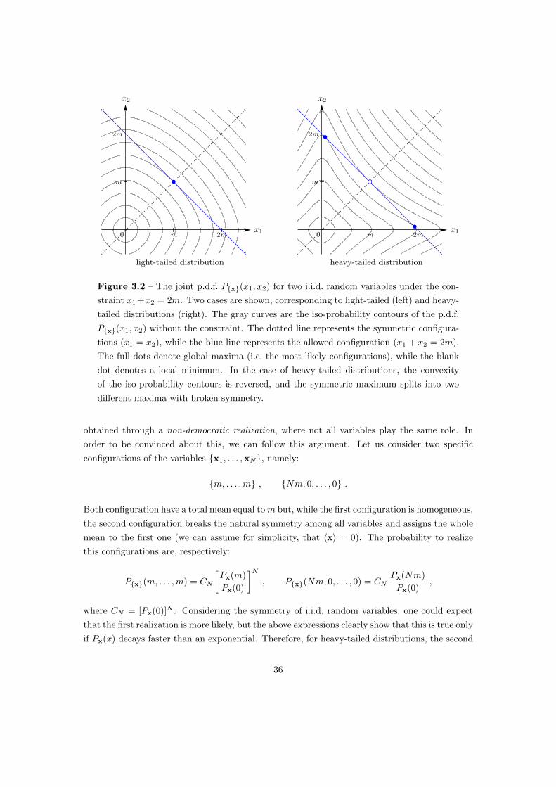
light-tailed distribution
x1
x2
0 m 2m
m
2m
heavy-tailed distribution
x1
x2
0 m 2m
m
2m
Figure 3.2 – The joint p.d.f. P{x}(x1, x2) for two i.i.d. random variables under the con-
straint x1 +x2 = 2m. Two cases are shown, corresponding to light-tailed (left) and heavy-
tailed distributions (right). The gray curves are the iso-probability contours of the p.d.f.
P{x}(x1, x2) without the constraint. The dotted line represents the symmetric configura-
tions (x1 = x2), while the blue line represents the allowed configuration (x1 + x2 = 2m).
The full dots denote global maxima (i.e. the most likely configurations), while the blank
dot denotes a local minimum. In the case of heavy-tailed distributions, the convexity
of the iso-probability contours is reversed, and the symmetric maximum splits into two
different maxima with broken symmetry.
obtained through a non-democratic realization, where not all variables play the same role. In
order to be convinced about this, we can follow this argument. Let us consider two specific
configurations of the variables {x1, . . . ,xN}, namely:
{m, . . . ,m} , {Nm, 0, . . . , 0} .
Both configuration have a total mean equal tom but, while the first configuration is homogeneous,
the second configuration breaks the natural symmetry among all variables and assigns the whole
mean to the first one (we can assume for simplicity, that 〈x〉 = 0). The probability to realize
this configurations are, respectively:
P{x}(m, . . . ,m) = CN
[Px(m)
Px(0)
]N, P{x}(Nm, 0, . . . , 0) = CN
Px(Nm)
Px(0),
where CN = [Px(0)]N . Considering the symmetry of i.i.d. random variables, one could expect
that the first realization is more likely, but the above expressions clearly show that this is true only
if Px(x) decays faster than an exponential. Therefore, for heavy-tailed distributions, the second
36

light-tailed distribution
m0
m
x1 x2 x3 · · · · · · · · · xN
heavy-tailed distribution
m0
m
x1 x2 x3 · · · · · · · · · xN
Figure 3.3 – Schematic representation of condensation phenomena. The plots show the
most likely realization of a large deviation of the sample mean for a light-tailed (left) and
a heavy-tailed distribution (right). The values m and m0 denote the realized mean and
the typical mean, respectively.
realization is more likely, and large deviations of the sample mean tends to be distributed in non-
democratic ways. In conclusion, heavy-tailed distributions lead to a mechanism of spontaneous
symmetry breaking, where the natural symmetry between i.i.d. variables is destroyed. This
phenomenon is extremely clear in the simple case N = 2 and has been illustrated in Fig. 3.2.
In order to conclude this picture, let us go back to the recursive relation (3.2) and re-interpret
the above results on the basis of the new considerations. The limits (3.3) represent a non-
democratic and a democratic realization of the sample mean, respectively. In the case of light-
tailed distributions the second limit is stronger, then the realized mean m′ tends to the desired
mean m and all variables fluctuate around the same value, i.e. m. On the contrary, in the case
of heavy-tailed distributions, the first limit is stronger, then N − 1 variables fluctuate around
the typical mean m0 (namely, 〈x〉), and the remaining variable carries the whole deviation
between m and m0. The latter mechanism is called condensation, because the large deviation is
concentrating in just one (randomly chosen) variable, which is denoted as the condensate [83].
This phenomenon is responsible for the failure of the Large Deviation Principle and has been
schematically illustrated in Fig. 3.3.
3.4 Condensation Phase Transition
In this section we try to translate the results of the previous section in physical language. As
usual, let us consider the sample mean m of the i.i.d. random variables {x1, . . . ,xN} described
37

by the p.d.f. Px(x). According to the scenario presented in Section 2.4.2, this mathematical
framework is equivalent to a thermodynamic system composed of N particles and described by
the Hamiltonian:
H(x1, . . . , xN ) = −N∑n=1
logPx(xn) ,
where xn denotes the state of the n-th particle. In this picture, we assume that the system is at
fixed (inverse) temperature β = 1, and we ignore the dependencies of all physical quantities on
β. In order to evaluate the rate function Im(m) we need to consider the observable:
M(x1, . . . , xN ) =
N∑n=1
xn ,
then, the rate function Im(m) is equal to the Gibbs free-energy density g(m) evaluated under
the constraint M(x1, . . . , xN ) = Nm. As explained in Section 2.4.2, this picture becomes more
tangible if we think of M(x1, . . . , xN ) as the total magnetization of a system composed of N
independent magnetic spins.
Now, let us assume that the p.d.f. Px(x) is both light-tailed and heavy-tailed on its left and
right tails, respectively, and that its first moment is finite, that is 〈x〉 = m0. In this case, the
large deviations of the sample mean m are realized both democratically (for m � m0) and
non-democratically (for m � m0), so we have the chance to investigate both cases in physical
terms. The rate function Im(m) or, equivalently, the Gibbs free-energy density g(m), is strictly
positive for m < m0, vanishes at m = m0, and becomes identically zero for m > m0. The
resulting function is continuous and analytic for all m ∈ R, with the exception of the single point
m = m0 where it becomes non-analytic. Physically, the non-analyticity of g(m) at the point
m = m0 implies the presence of a phase transition. The point m = m0 denotes the critical point
of the system and separates two different phases, which we call the fluid phase (for m < m0) and
the condensed phase (for m > m0) [83]. Since g(m) is continuous, this is a second-order phase
transition. Like many other second-order phase transitions in the physical world, this transition
is driven by a mechanism of spontaneous symmetry breaking (see also the previous section). The
breaking pattern is:
SN 7→ SN−1 ⊗ 1 ,
where SN denotes the permutation group over N elements. In the fluid phase, indeed, the N
particles have the same behaviour and can be exchanged without modify the macroscopic state
of the system. On the contrary, in the condensed phase, the condensate carries a macroscopic
amount of the deviation m−m0 and cannot be exchanged with the other N − 1 particles.
Even if we are able to identify the exact point of the phase transition, we are able to define
the thermodynamics of the system only in the fluid phase. Indeed, in the whole range m ≥ m0,
the Gibbs free energy g(m) has neither definite convexity nor a unique global minimum. The
reason is that the density g(m) has been defined only for systems with extensive free energy,
38

but, according to the final shape of g(m), this system is extensive in the fluid phase, and sub-
extensive in the condensed phase. This is in agreement with our previous considerations about
the democratic and non-democratic realizations of the large deviations.
It is worth to stress that the investigated system is entirely composed of non-interacting
particles. Yet, in spite of its simplicity, it exhibits a quite rich phenomenology, showing a phase
transitions, a spontaneous symmetry breaking, and a non-extensive thermodynamic potential.
The above considerations prove that the classical problem of the sample mean of i.i.d. random
variables is much more complex than expected and does not reduce to the simple statements of
the CLT.
3.5 The Order Parameter
Since condensation phenomena appears through a phase transition with spontaneous symmetry
breaking, it is useful to define an order parameter to obtain a more precise description of the phase
transition. Let us consider a random variable q as a function of the random set {x1, . . . ,xN}and let us assume that q, in some sense, is able to quantify the amount of condensation in the
outcomes of the random set. Such variable is a good candidate for being an order parameter for
the condensation phase transition. In the previous section, we argued that the phase transition
is driven by the sample mean m and therefore, in order to use the observable q as an order
parameter, we need to consider the conditional probability distribution:
Pq|m(q|m) =Pm,q(m, q)
Pm(m), (3.5)
where Pm,q(m, q) denotes the joint probability distribution of both m and q. The above proba-
bility distribution fully describes the behaviour of q when m is fixed, and can be used to explore
both the fluid and condensed phase of the system. In the limit N → ∞ the conditional proba-
bility distribution Pq|m(q|m) is usually peaked around some typical value. In this case, we can
define the order parameter of the phase transition as the expected value of q at fixed m, namely:
〈q〉m=m =
∫dq q Pq|m(q|m) . (3.6)
In the limit N →∞ the order parameter should tend to zero in the symmetric phase, and should
remain different from zero in the symmetry-broken phase. If the observable q has been chosen
such that 〈q〉m=m obeys this property, then it is a good order parameter for the phase transition.
Generally, the probability distributions appearing in (3.5) and (3.6) can be handled by means of
the Large Deviation Principle. By applying the definition (2.2) to eq. (3.5) we can rewrite the
above relation in terms of rate function, and we get:
Iq|m(q|m) = Im,q(m, q)− Im(m) .
39

Finally, by applying the Large Deviation Principle to eq. (3.6), we end up with the simple formula:
limN→∞
〈q〉m=m = arg minq
{Im,q(m, q)− Im(m)
}, (3.7)
which links the order parameter to the rate functions Im(m) and Im,q(m, q). As we argued in
the previous sections, the Large Deviations Principle does not hold when the system is in the
condensed phase, and then we expect that eq. (3.7) is valid only in the fluid phase. Yet, we can
still use eq. (3.7) to analyse the behaviour of the order parameter in the fluid phase and to detect
the phase boundary between the fluid and the condensed phases.
Now, we need to define an observable that can quantify the amount of concentration in a set
of variables. In agreement with [55], in this work we exploit the generalized inverse participation
ratio (IPR). This is defined as:
IPRk =
[N∑n=1
[w(xn)
]k] 1k−1
, (3.8)
where w(xn) is a statistical weight attached to the variable xn. The weights must be non-negative
and their sum must be equal to one. There is not a unique way to define these weights: in some
sense, the more important a variable, the largest its weight. The simplest choice for w(x) is:
w(x) =|x− x0|η∑n |xn − x0|η
, (3.9)
where x0 is some reference outcome for x and η is some non-negative exponent. According to
this definition, the statistical weight of a variable depends on how much it deviates from x0 with
respect to the other variables. When 〈x〉 is finite, the most natural choice for the parameters
x0 and η is x0 = 〈x〉 and η = 2, which is the smallest exponent yielding analytical weights. As
an alternative choice, if x is always greater than some minimum outcome xmin, then we can set
x0 = xmin and η = 1. The advantage of the latter choice is that, when the mean m is fixed, the
weight w(x) becomes a linear function of x.
In order to understand the behaviour of the IPR, let us consider a simple case. Suppose that
the sample mean m is deviating from the reference value x0 and that the deviation is realized by a
partially democratic configuration. This means that the deviation m 6= x0 is equally distributed
among M variables, while the other N−M variables are exactly at x0. In this case, the statistical
weights of the deviating variables are equal to 1/M , while the other weights vanish. According
to the definitions (3.8) and (3.9), the IPR is always equal to 1/M , therefore, it (inversely) counts
the number of participant to the total deviation m 6= x0. When the number of participants is not
so clearly defined, the IPR assumes intermediate values, yet, it always stays between the values
1/N and 1, corresponding to a fully democratic and a fully condensed realization, respectively.
The IPR becomes a good order parameter in the limit N → ∞. In the fluid phase, indeed, the
deviations of the sample mean are equally distributed among N participant and we expect that
40

IPRk → 0. On the contrary, in the condensed phase, the statistical weight of the condensate
remains much larger than the others, and we expect that IPRk remains strictly positive. It is
worth to notice that:
IPRk = e−Hk[w(x1),...,w(xN )] ,
where Hk[w1 . . . , wN ] is the Renyi entropy of the probability distribution defined by the statistical
weights {w1 . . . , wN}. Both the IPR and the Renyi entropy are well-known in literature as
measures of the concentration in discrete probability distributions [43, 113, 129].
Among all possible values of the parameters k appearing in the definition (3.8), there are
some interesting choices. First of all, we stress that the IPR is defined also in the limits k → 1
and k →∞. For k → 1 the Renyi entropy reduces to the classical Shannon entropy [35, 98] and
the result is:
IPR1 =
N∏n=1
[w(xn)
]w(xn).
On the other hand, for k →∞, only the largest weight survives in the sum (3.8) and we get:
IPR∞ = max{w(x1), . . . , w(xN )
}.
Beyond the limit k → 1 and k → ∞, another interesting choice for k is given by k = 2, which
yields the classical definition of the IPR, i.e.:
IPR2 =
N∑n=1
[w(xn)
]2.
The quantity IPR2 is also known in literature as purity, and has the advantage of being an
independent sum over the statistical weights.
In this work, we define the order parameter for the condensation phase transition by selecting
k = 2. We define the weights w(x) according to eq. (3.9) by setting x0 = 0 and either η = 1
or η = 2, depending on the properties of the random variable x (the case x0 6= 0 can be easily
recovered through the substitution x → x + constant). This choice lead us to define the two
following order parameters:
q1 =m2
Nm21
, q2 =m4
Nm22
, (3.10)
where mk denotes the k-th sample moment of the set {x1, . . . ,xN}, namely:
mk =1
N
N∑n=1
xkn . (3.11)
The variable q2 is an IPR for any set of random variables, and is specifically intended for random
variables with zero mean. On the contrary, the variable q1 is an IPR only when the random
variable x is non-negative, but it explicitly depends on the first moment m1 and allows an easier
41
investigation of large deviations of the sample mean. Therefore, one can exploit q1 for the analysis
of non-negative random variables, and q2 for the other cases (an explicit application of the order
parameter q2 to the financial case is shown in Section X). The statistical characterization of the
observables q1 and q2 can be carried out in terms of the moments mk. Indeed, according to eq.
(3.5), the conditional probabilities Pq1|m(q|m) and Pq2|m(q|m) can be rewritten as:
Pq1|m(q|m) =N m2
Pm(m)Pm1,m2(m,Nqm2) ,
Pq2|m(q|m) =
∫dv
N v2
Pm(m)Pm1,m2,m4(m, v,Nqv2) ,
As a result, the joint probabilities of the moments mk contains all the information required
for the statistical analysis of the order parameters q1 and q2 (recall that Pq1|m(q|m) and
Pq2|m(q|m) must be intended as function of q and that the denominator Pm(m) plays the role
of a simple normalization factor). Yet, the analysis of joint probability distributions of the form
Pma,mb,...(ma,mb, . . . ) is not an easy task and could require more sophisticated techniques. This
will be the main subject of the following chapter, where we apply the theoretical framework
of the Density Functional Method to the analysis of condensation phenomena in i.i.d. random
variables.
42

Chapter 4
The Density Functional Method
In this chapter we introduce a different mathematical approach to analyse a large set of random
variables: the Density Functional Method. This method is based on a continuous description
of the random set in the limit of an infinite number of variables, and it recalls the typical
computations performed by physicist in the context of classical and quantum field theories. This
approach allows us to recover all results presented in the previous chapters with a direct and
intuitive procedure, and can be easily extended to address more complicated cases.
The Density Functional Method is a quite common formalism in physical research and is
widely applied in a large variety of contexts, where it can be addressed with different names.
In Random Matrix Theory, for instance, this approach is usually denoted as the Coulomb Gas
Method, in relation to the effective interactions between the eigenvalues of random matrices
[39, 105, 134]. In quantum mechanics and in physical chemistry, instead, it gives rise to the
Density Functional Theory, developed to analyse the electronic structure of many-body quantum
systems. Finally, this formalism can be recognized at the basis of common Field Theories, playing
a fundamental role in both high-energy and condensed-matter physics. In the context of i.i.d.
random variables, the presented method is not identified with any specific name, and it will be
addressed here as the “Density Functional Method” in relation to the fundamental mathematical
objects introduced by the formalism.
The Density Functional Method has been already applied to the fluid phase of i.i.d. random
variables to recover the classical results of the LDT [98]. In some other works, this method
has also been exploited for the investigation of interacting system with condensed phases [105].
Yet, at the best of our knowledge, a comprehensive analysis of condensation phenomena in
i.i.d. random variables within the Density Functional Method is still missing. In our opinion,
the analysis of this specific system without any form of interaction is a fundamental tool to
understand the emergence of condensation phenomena as a purely statistical mechanism, and
the Density Functional Method could provide the best theoretical framework for a systematic
analysis of this system from both a qualitative and a quantitative point of view.
43

In the following sections, we introduce the Density Functional Method by investigating both
the fluid phase and the condensed phase of i.i.d. random variables under large deviations of
their sample mean. Then, in Section 4.3, we extend the same procedure to a more general case
by considering simultaneous deviations of the sample mean and another sample moment. The
latter case refers to an original analysis, and characterizes the statistical properties of the order
parameter for the phase transition (see Section 3.5).
4.1 The Fluid Phase
In Section 2.3 we considered the sample mean m of N i.i.d. random variables {x1, . . . ,xN}. We
defined the p.d.f. Pm(m) in eq. (2.11) and we analysed it by means of the standard LDT. In
this section, we try to recover the same results within the formalism of the Density Functional
Method. The idea at the basis of this new approach is that, in the limit N → ∞, the discrete
set {x1, . . .xN} can be described in continuous form by means of some continuous function. Let
us define the density profile of the random variables as:
ρ(x) =1
N
N∑i=1
δ(x− xi) . (4.1)
The distribution ρ(x) is also called the type of the sequence {x1, . . .xN}. It is a random variable
itself and has been defined such that 〈ρ(x)〉 = Px(x). Thanks to the new definition, we can
re-express the multiple integral (2.11) over the N variables {x1, . . . , xN} as a unique functional
integral over a density function ρ(x). First of all, we need to rewrite the quantities∑n xn and∏
n Px(xn) in terms of ρ(x). By applying the definition (4.1) and the property∏
= exp∑
log,
it is easy to verify that:
N∑n=1
xn = N
∫dxx ρ(x) ,
N∏n=1
Px(xn) = exp
(N
∫dx ρ(x) logPx(x)
).
Therefore we can write:
Pm(m) =
∫Dρ J [ρ] eN
∫dx ρ(x) logPx(x) δ
(∫dxx ρ(x)−m
),
where J [ρ] is the Jacobian involved in the change of variables from the set {x1, . . . , xN} to the
density ρ(x). This can be written as:
J [ρ(x)] =
∫dNx δ
[ρ(x)− 1
N
N∑i=1
δ(x− xi)
],
44

where δ[ · ] denotes the functional equivalent of the Dirac delta-function1. In practice, the Jaco-
bian J [ρ] counts the number of configurations {x1, . . . , xN} described by a specific distribution
ρ(x). Since we are considering the above integral in the limit N → ∞, we can simplify J [ρ] by
means of the saddle-point approximation [40]. The result is:
J [ρ] ' Ae−N∫
dx ρ(x) log ρ(x) δ(∫
dx ρ(x)− 1),
where A is an unimportant normalization constant. Inserting last equation back in the functional
integral we find:
Pm(m) ' A∫Dρ e−N
∫dx ρ(x) log ρ(x)
Px(x) ×
× δ(∫
dx ρ(x)− 1)δ(∫
dxx ρ(x)−m).
At is stage, it is worth to borrow some definitions from the context of Information Theory
[35, 98]. Let us introduce the Shannon entropy :
HS[P ] = −∫
dxP (x) logP (x) ,
and the Kullback-Leibler divergence:
DKL[P1||P2] =
∫dxP1(x) log
P1(x)
P2(x).
The entropy HS[P ] quantifies the amount of uncertainty related to the distribution P (x). In
some sense, it (logarithmically) counts the number of possible outcomes of a random variable
described by the distribution P (x), according to their probability. In the investigated case, for
any normalized distribution, we found J [ρ] ∼ exp(NHS[ρ]). The Kullback-Leibler divergence
DKL[P1||P2], instead, defines a non-symmetric distance between the distributions P1(x) and
P2(x). Loosely speaking, it quantifies the amount of information lost when P2(x) is used to
approximate P1(x).
After the introduction of the Kullback-Leibler divergence, we can rewrite the functional
integral for Pm(m) as:
Pm(m) ' A∫Dρ e−NDKL[ρ||Px] δ
(〈1〉ρ − 1
)δ(〈x〉ρ −m
), (4.2)
where 〈f(x)〉ρ =∫
dx f(x) ρ(x). Hence, in order to evaluate Pm(m), we have to integrate over
all possible normalized distributions ρ(x) whose mean is exactly equal to m. Those distributions
are not equally important, but are exponentially weighted according to their similarity to the
original distribution Px(x). It is clear that, for N → ∞, the only distribution that survives to
the integration is the closest to Px(x). This means that we can again perform the saddle-point
1For any functional F [ρ], the delta-functional δ[ρ] obeys the rule∫DρF [ρ] δ[ρ− ρ′] = F [ρ′].
45

Px(x)
ρ∗(x)
〈1〉ρ = 1
〈x〉ρ = m
all distributions
distributionswith mean m
Figure 4.1 – Visual representation of the integral (4.2). The ellipses represents the
constraints 〈1〉ρ = 1 and 〈x〉ρ = m and the coloured region denotes the integration domain.
In the limit N →∞ the only contribute to the integral comes from the distribution ρ∗(x),
which is the closest distribution to Px(x) in terms of the Kullback-Leibler divergence
DKL[ρ∗||Px].
approximation and write:
Pm(m) ∼ e−NDKL[ρ∗||Px] ,
where ρ∗(x) is the probability density that minimize the Kullbak-Leibler divergence with Px(x)
among all distributions whose mean is m (see Fig. 4.1). The constrained minimization of the
Kullback-Leibler divergence can be carried out with the method of Lagrange multipliers, which
yields:
ρ∗(x) =Px(x) esx∫
dxPx(x) esx, (4.3)
where s is a Lagrange multiplier which depends on m and is implicitly defined by the equation:∫dxxPx(x) esx∫dxPx(x) esx
= m . (4.4)
The above procedure proves that the rate function Im(m) is exactly equivalent to the Kullback-
Leibler divergence DKL[ρ∗||Px]. This is in perfect agreement with the standard result of the LDT
(see Section 2.3). Indeed, the equations (4.3) and (4.4) can be respectively rewritten as:
Ψx(s) = sx− logρ∗(x)
Px(x), Ψ′x(s) = m ,
then, recalling the definition of the Kullback-Leibler divergence DKL[ρ∗||Px], one finds that
DKL[ρ∗||Px] = maxs{sm − Ψx(s)}, as prescribed by the LDT. It may seems that the density
46

functional method did not provide any additional result with respect to the LDT described in
Chapter 2, yet, there is one main difference: now we are able to express the LDT in terms of the
optimal density ρ∗(x). In order to understand the difference, let us consider a generic random
variable y = f(x1, . . . ,xN ) and its conditional expectation 〈y〉m=m, namely:
〈y〉m=m =
∫dNx f(x1, . . . , xn)
(∏n Px(xn)
)δ(
1N
∑n xn −m
)∫dNx
(∏n Px(xn)
)δ(
1N
∑n xn −m
) .
If we are able to rewrite the function f(x1, . . . , xn) as a functional f [ρ] over the density ρ(x),
then, for large N , we can write:
〈y〉m=m '∫Dρ f [ρ] e−NDKL[ρ||Px] δ
(〈1〉ρ − 1
)δ(〈x〉ρ −m
)∫Dρ e−NDKL[ρ||Px] δ
(〈1〉ρ − 1
)δ(〈x〉ρ −m
) .
Thanks to the saddle-point approximation, it is easy to see that:
limN→∞
〈y〉m=m = f [ρ∗] . (4.5)
Therefore, in the limit N → ∞, any expected value can be expressed in terms of the optimal
density ρ∗(x), and the knowledge of ρ∗(x) is sufficient to determine the behaviour of the system
under the constraint m = m. As a special case of the eq. (4.5), we can write:
limN→∞
〈ρ(x)〉m=m = ρ∗(x) ,
then, the optimal density ρ∗(x) is exactly the marginal distribution of a generic variable x under
the constraint m = m in the limit N →∞.
The existence of the optimal density ρ∗(x), together with the relation (4.5), proves that
large deviations of the mean are realized through democratic outcomes. Specifically, in the limit
N → ∞, the random variables {x1, . . . ,xN} behaves as if they were drawn from the optimal
distribution ρ∗(x) instead of their original distribution Px(x). As a consequence, all variables
fluctuates in the same way, and their sample mean m tends to the expected value of ρ∗(x), which
is equal to m by definition. It is worth to notice that the results presented in this section are
exactly equivalent to the ones expressed by the Sanov’s theorem for discrete random variables
[35, 98] and that, in some sense, the Density Functional Method extends the validity of the
theorem also to continuous random variables. Yet, this picture is valid only when the random
variables are in the fluid phase: the condensed phase violate the statement of the Sanov’s theorem
and requires an alternative description based on different assumptions.
47

4.2 The Condensed Phase
The Density Functional Method presented in the previous section has a limited range of validity,
which can be determined ex-post by checking that all involved quantities are well-defined. The
cornerstone equation of the method is the saddle-point condition (4.4), which defines the existence
of the Lagrange multiplier s as a function of the sample mean m. Indeed, this equation does not
have a solution for all values of m and all possible shapes of the p.d.f. Px(x). In order to find a
solution for eq. (4.4), the system must verify one of the following conditions:
• Px(x) is a light-tailed distribution, whatever m.
• Px(x) is a hybrid light-tailed and heavy-tailed distribution with finite mean and either
m ≥ 〈x〉 or m ≤ 〈x〉, depending on whether the heavy tail is on the left or right side,
respectively.
• Px(x) is a hybrid light-tailed and heavy-tailed distribution with infinite mean, whatever m
(this can be considered a generalization of the previous case for 〈x〉 → ∞).
• Px(x) is a heavy-tailed distribution with finite mean and m = 〈x〉.
If none of the above conditions is verified, the Lagrange multiplier s cannot be defined and
the optimal density ρ∗(x) does not exist. In this case, large deviations of the sample mean m
cannot be explained any more as democratic deviations of the random variables {x1, . . . ,xN}.Therefore, the saddle-point equation (4.4) defines the phase boundary between the fluid phase
and the condensed phase of the system, and the fluid phase coincides with the existence domain
of its solution.
In order to extend the Density Functional Method to the condensed phase, the formalism
presented in Section 4.1 must be modified at its very assumptions. Indeed, by writing the p.d.f.
Pm(m) as a unique functional integral over the density profile ρ(x), we are implicitly assum-
ing that the random variables {x1, . . . ,xN} obey the same scaling-law and can be described by
a unique continuous function. Basically, this corresponds to a democratic ansatz. In order to
investigate the non-democratic realizations of the large deviations, we should break this ansatz
and let the random variables fluctuate with different scaling-laws. As argued in Chapter 3,
condensation phenomena are determined by the anomalous fluctuation of a single random vari-
able, which becomes macroscopically large. This results in the spontaneous symmetry breaking
SN 7→ SN−1⊗ 1, where SN is the permutation group of N elements (see Section 3.4). Therefore,
the characterization of the condensed phase should be achieved by dividing the set {x1, . . . ,xN}in two different subset: the condensate, identified with a single random variable xc, and the
bulk, composed of all other N − 1 variables and described by the density profile ρb(x). This new
description corresponds to a condensed ansatz, in contrast with the democratic ansatz presented
in the previous section.
Now, let us go back to eq. (2.11), which defines the p.d.f. Pm(m) as a multiple integral over
the random variables {x1, . . . ,xN}, and let us factorize out the contribution of one variable, say,
48

xN . The result is:
Pm(m) =N
N − 1
∫dxN Px(xN )×
×∫
dN−1x
(N−1∏i=1
Px(xn)
)δ
(1
N − 1
N−1∑i=1
xn −Nm− xNN − 1
).
In order to describe the condensed phase of the system, in agreement with the condensed ansatz,
we should apply the Density Functional Method just to the latter integral, setting the N -th
variable aside. By writing the results in terms of the condensate xc and of the bulk density
ρb(x), we obtain:
Pm(m) ' N
N − 1
∫dxc Px(xc)×
×A∫Dρb e
−(N−1)DKL[ρb||Px] δ(〈1〉ρb − 1
)δ(〈x〉ρb − Nm−xc
N−1
).
The next step in the Density Functional Method should be the saddle-point approximation of
this compound integral in the limit N → ∞. Yet, before that, we must rescale all variables
such that all leading terms in the integral are of the same order in N . The correct scaling law
is determined by the second delta-function, which involve all variables xc, ρb(x), and m in a
unique constraint. Indeed, in order to have a non-degenerate limit, the condensed variable xc
should scale as xc = O(N). As a consequence, we define the rescaled variable xc = xc/N and we
rewrite the integral in terms of the new variable. This leads to:
Pm(m) ' N2
N − 1
∫dxc Px(Nxc)×
×A∫Dρb e
−(N−1)DKL[ρb||Px] δ(〈1〉ρb − 1
)δ(〈x〉ρb − N
N−1 (m− xc)).
If the system is in the condensed phase, than the fluid-phase conditions listed at the beginning
of the section must be violated and Px(x) must have at least one heavy tail. Without loss of
generality, let us assume that Px(x) is heavy-tailed in the right side, whatever the behaviour of
the left tail. In addition, let us assume tha 〈x〉 is finite and that m > 〈x〉. For N → ∞, the
condensateNxc moves towards the heavy tail of the distribution, and Px(Nxc) decays slower than
an exponential. As a result, the term Px(Nxc) is sub-leading with respect to e−(N−1)DKL[ρb||Px]
and could be neglected. In the limit N →∞, the above integral reduces to:
Pm(m) ' A′∫
dxc
∫Dρb e
−NDKL[ρb||Px] δ(〈1〉ρb − 1
)δ(〈x〉ρb + xc −m
), (4.6)
which is the condensed-phase equivalent of the functional integral (4.2).
At this stage, we can perform the saddle-point approximation, in order to evaluate the optimal
condensate x∗c and the optimal bulk density ρ∗b(x), which describe the state of the random
49

variables in the condensed phase. Let us assume that the p.d.f. Px(x) has finite mean. The
minimization of the Kullback-Leibler divergence DKL[ρb||Px] under the constraints 〈1〉ρb = 1
and 〈x〉ρb + xc = m leads to:
x∗c = m− 〈x〉 , ρ∗b(x) = Px(x) . (4.7)
With this result, we achieved a complete characterization of the condensed phase in the limit
N → ∞. According to the saddle-point solution, the N − 1 non-condensed random variables
are distributed according to the original p.d.f. Px(x). Loosely speaking, they do not react to
the deviation of the sample mean m and behave as i.i.d. random variables, fluctuating around
the expected value 〈x〉 as in presence of typical deviations. At variance, the condensed variable
xc scales as N(m − 〈x〉) and is the unique responsible for the large deviation, carrying a finite
fraction of the sample mean m. It is worth to notice that, at the saddle-point, the Kullback-
Leibler divergence DKL[ρ∗b||Px] vanishes and generates a vanishing rate function Im(m). This
result is due to the sub-extensivity of the system in the condensed phase and is in agreement
with the discussion presented in Chapter 3.
As explained in Section 4.1, the knowledge of the optimal density ρ∗(x) can be exploited
to evaluate the asymptotic behaviour of the conditional expectation 〈y〉m=m for any observable
y = f(x1, . . . ,xN ) in the limit N →∞. This can be achieved by writing 〈y〉m=m ' f [ρ∗], where
f [·] is the functional form related to the function f(·). At the first-order approximation, this
remains true also in the condensed phase. According to the definition of the condensate xc and
of the bulk density ρb(x), one can write:
ρ(x) =N − 1
Nρb(x) +
1
Nδ(x− xc) ,
Therefore, for large N , the optimal density ρ∗(x) for the condensed phase can be approximated
by:
ρ∗(x) ' Px(x) +1
Nδ(x−N(m− 〈x〉)
). (4.8)
As a final result, we can try to evaluate the asymptotic behaviour of the observables q1 and
q2 defined in Section 3.5 (see eqs. (3.10) and (3.11)) in order to check if they are good order
parameters for the condensation phase transition. The functional form mk[ρ] for the k-th sample
moment mk can be defined as:
mk[ρ] =
∫dxxk ρ(x) ,
and, in turn, the functional forms q1[ρ] and q2[ρ] for the order parameters q1 and q2 becomes:
q1[ρ] =
∫dxx2 ρ(x)
N[∫
dxx ρ(x)]2 , q2[ρ] =
∫dxx4 ρ(x)
N[∫
dxx2 ρ(x)]2 .
50

In the limit N → ∞, the conditional expectations 〈q1〉m=m and 〈q2〉m=m can be evaluated
through the values q1[ρ∗] and q2[ρ∗], where the optimal density ρ∗(x) is either the fluid-phase
density (4.3) or the condensed-phase density (4.8). In the fluid phase, the conditional expecta-
tions vanish because of the factor N at the denominator of the two functionals q1[ρ] and q2[ρ]. In
the condensed phase, instead, the anomalous scaling of the delta-like term in the density function
may lead to a non-trivial asymptotic behaviour of the order parameters. Indeed, it is easy to see
that:
〈mk〉m=m ' Nk−1(m− 〈x〉
)k,
for all k > 1 and for all distributions Px(x) with finite moment 〈xk〉. Therefore, we finally get:
limN→∞
〈q1〉m=m =
(1− 〈x〉
m
)2
, limN→∞
〈q2〉m=m = 1 .
The non-trivial expression for the parameter 〈q1〉m=m is due to its explicit dependence on the
sample mean m which do not scale as higher-order moments. It is worth to recall that the above
results are valid only in the limit of infinite number of variables N →∞. When the sample size
is finite, we may expect significant deviation from the presented limit, especially for the order
parameter 〈q2〉m=m which tends to its extreme value.
4.3 Simultaneous Deviations of Two Observables
As shown in Section 3.5, the statistical behaviour of the order parameters q1 and q2 under
large deviations of the sample mean m is determined by the joint probability distribution of
the sample moments (3.11). In the fluid phase, the conditional expectation 〈mk〉m=m shifts
from 〈xk〉 to 〈xk〉ρ∗ , where ρ∗(x) is the optimal density (4.3), and remains always finite. This
is true even when the original moment 〈xk〉 diverges, thanks to the exponential cut-off in the
optimal density ρ∗(x). In the condensed phase, instead, the emergence of an extensive variable
xc that scales as N(m−〈x〉) leads to the divergence of all expected values 〈mk〉m=m with k > 1.
Indeed, as proved in the previous section, the asymptotic density (4.8) leads to the scaling-law
〈mk〉m=m ' Nk−1(m− 〈x〉)k.
In order to achieve a more detailed characterization of the two phases of the system it could
be interesting to analyse the joint probability distribution:
Pm1,mk(m1,mk) =
∫dNx
(N∏n=1
Px(xn)
)×
× δ
(1
N
N∑n=1
xn −m1
)δ
(1
N
N∑n=1
xkn −mk
),
(4.9)
which defines the probability of simultaneous large deviations of the sample mean m1 and of the
sample moment mk, assuming k > 1. This allows to examine the condensed phase of the system
51

under finite values of the effective moment 〈mk〉m=m. This analysis is a required step for the
statistical characterization of the full probability distribution Pq|m(q|m) of the order parameters
q1 and q2 (see Section 3.5), and highlights the presence of a rich structure in the phase diagram
of the system. The following results are original; they have been reported in [55] and are in
agreement with the results presented in [126] and obtained through an alternative approach.
For the sake of simplicity, we assume that the x’s are non-negative random variables with
finite mean, so that we can focus on the right tail of the distribution Px(x). If the latter is a
heavy-tailed distribution, than large deviations of the form m > 〈x〉 are condensed. Now, let us
apply the Density Functional Method to the joint p.d.f. (4.9) within the democratic ansatz. By
substituting the discrete set {x1, . . . ,xN} with the continuous density ρ(x) we obtain:
Pm1,mk(m1,mk) ' A
∫Dρ e−NDKL[ρ||Px]×
× δ(〈1〉ρ − 1
)δ(〈x〉ρ −m1
)δ(〈xk〉ρ −mk
),
which is the same functional integral of eq. (4.2) with an additional constraint on the sample
moment mk. Then, the constrained minimization of the Kullback-Leibler divergence DKL[ρ||Px]
with the method of Lagrange multipliers leads to the following saddle-point solution:
ρ∗(x) =Px(x) esx+txk∫
dxPx(x) esx+txk, (4.10)
where s and t are Lagrange multipliers which depends on both m1 and mk and are implicitly
defined by the constraints:∫dxxPx(x) esx+txk∫dxPx(x) esx+txk
= m1 ,
∫dxxk Px(x) esx+txk∫
dxPx(x) esx+txk= mk . (4.11)
As in the case of a single constraints, the saddle-point conditions (4.11) determine the extension
of the fluid phase in the parameter space (m1,mk). The fluid-phase regime coincides with the
existence domain of the Lagrange multipliers s and t. Since k > 1, the most relevant parameter
is t: when t < 0, the optimal density ρ∗(x) is always well-defined, notwithstanding the specific
value of s and the specific shape of the p.d.f. Px(x); on the contrary, when t > 0, the denominator
in eq. (4.10) could diverge. If Px(x) is a heavy-tailed distribution, then ρ∗(x) diverges for any
t > 0, whatever s. In this case, the phase-boundary between the fluid phase and the condensed
phase can be identified by the condition t = 0.
Now, let us assume that Px(x) is a heavy-tailed distribution and let us study the phase por-
trait. In the parameter space (m1,mk), the geometric locus t = 0 is described by the parametric
curve:
γ(s) =
(∫dxxPx(x) esx∫dxPx(x) esx
,
∫dxxk Px(x) esx∫
dxPx(x) esx
).
52

0.0 0.2 0.4 0.6 0.8 1.0 1.2 1.40.0
0.5
1.0
1.5
2.0
2.5
3.0
m1
mk
〈mk〉 <∞
〈m1〉
〈mk〉
condensedphase
fluidphase
forbiddenregion
(mk < mk1 )
0.0 0.2 0.4 0.6 0.8 1.0 1.2 1.40.0
0.5
1.0
1.5
2.0
2.5
3.0
m1
mk
〈mk〉 = ∞
〈m1〉
condensedphase
fluidphase
forbiddenregion
(mk < mk1 )
Figure 4.2 – Phase diagrams for i.i.d. non-negative random variables with heavy-tailed
distributions under large deviations of the sample mean m and the k-th sample moment
mk, for k > 1. Two cases are shown, where k has been chosen such that the expected
value 〈xk〉 either converges (left) or diverges (right). The straight dashed lines denote
the position of the critical point (〈x〉, 〈xk〉). The plots have been obtained with a shifted
Pareto distribution Px(x) = α(x + 1)−(α+1) with α = 3, by choosing k = 2 (left) and
k = 3 (right).
If 〈xk〉 diverges, then the above curve divides the first quadrant of the plane (m1,mk) in two
separate region. Otherwise, for finite values of 〈xk〉, the curve runs from (0, 0) to (〈x〉, 〈xk〉),then the locus t = 0 extends as a straight line from (〈x〉, 〈xk〉) to (〈x〉,∞). This results are
represented in Fig. 4.2. It is worth to recall that, for all samples {x1, . . . ,xN}, the moments
m1 and mk obey the Jensen’s inequality mk ≥ (m1)k; therefore, the region mk < (m1)k of
the parameter space (m1,mk) is not accessible to the system. According to the saddle-point
equations (4.11), the condensed phase extends over the whole accessible region of the parameter
space (m1,mk) such that the mean m1 exceeds the values attained on the phase boundary. The
remaining portion of the phase space should be characterized by the emergence of condensation
phenomena.
In order to describe all possible states of the system, let us apply the Density Functional
53

Method to the joint p.d.f. (4.9) within the condensed ansatz. We can write:
Pm1,mk(m1,mk) =
N2
(N − 1)2
∫dxN Px(xn)
∫dNx
(N−1∏n=1
Px(xn)
)×
× δ
(1
N − 1
N−1∑n=1
xn −Nm1 − xNN − 1
)δ
(1
N − 1
N−1∑n=1
xkn −Nmk − xkNN − 1
),
and then, by re-expressing the multiple integral in terms of the condensate xc and of the bulk
density ρb(x), we obtain:
Pm1,mk(m1,mk) ' A N2
(N − 1)2
∫dxc Px(xc)
∫Dρb e
−(N−1)DKL[ρb||Px]×
× δ(〈1〉ρb − 1
)δ(〈x〉ρb − Nm1−xc
N−1
)δ(〈xk〉ρb −
Nmk−xkcN−1
).
As in Section 4.2, before performing the saddle-point approximation, we must find the correct
scaling-laws of all variables in the integrals. This time, assuming k > 1, the only non-trivial
scaling is obtained by imposing xc = O(N1/k), preserving all leading terms in the constraints
expressed by the delta functions. After the substitution xc = N1/kxc, the above integral becomes:
Pm1,mk(m1,mk) ' A N2+ 1
k
(N − 1)2
∫dxc Px
(N
1k xc
) ∫Dρb e
−(N−1)DKL[ρb||Px]×
× δ(〈1〉ρb − 1
)δ(〈x〉ρb − N
N−1 (m1 −N−k−1k xc)
)δ(〈xk〉ρb − N
N−1 (mk − xkc )).
Finally, by recalling that Px(x) is a heavy-tailed distribution and by performing the limitN →∞,
we end up to:
Pm1,mk(m1,mk) ' A′
∫dxc
∫Dρb e
−NDKL[ρb||Px]×
× δ(〈1〉ρb − 1
)δ(〈x〉ρb −m1
)δ(〈xk〉ρb + xkc −mk
).
At this stage, we are ready to apply the saddle-point approximation. The constrained minimiza-
tion of the Kullback-Leibler divergence DKL[ρb||Px] now yields:
ρ∗b(x) =Px(x) esx∫
dxPx(x) esx, x∗c =
[mk −
∫dxxk Px(x) esx∫
dxPx(x) esx
] 1k
, (4.12)
where: ∫dxxPx(x) esx∫dxPx(x) esx
= m1 . (4.13)
The above solution somehow mixes the results obtained for the fluid and condensed phases
under large deviations of the sample mean m (see Sections 4.1 and 4.2). According to the above
solution, the N −1 non-condensed variables are democratically responsible of the large deviation
m1 = m1 and are insensible of the large deviation of the moment mk = mk. The latter, instead,
is completely absorbed by the condensate xc, which scales as [N(mk − 〈xk〉ρb)]1/k. Remarkably,
54

the condensate has a different scaling-law with respect to the previous cases: it is sub-extensive
and is driven by the deviation of the moment rather than the deviation of the mean. Loosely
speaking, for k > 1, the constraint mk = mk is more relevant than the constraint m1 = m1 and is
the real responsible for the condensation of the large deviations. This effects is also recognizable
in the phase diagram of Fig. 4.2 and results in a “reversion” of the phase space. Indeed, in
the case of non-negative random variables with heavy-tailed distribution, large deviations of the
sample mean m1 condense for m1 > 〈x〉, whereas large deviations of both m1 and mk condense
only when m1 < 〈x〉. This effect ensures that the saddle-point equation (4.13) is always solvable,
and proves that the examined system has no further phases than the fluid and condensed phases
represented in Fig. 4.2.
As a concluding remark, it is worth to specify that condensation phenomena in simultaneous
deviations of the mean m1 and the moment mk could appear also in light tailed distributions.
This can be easily understood by comparing the saddle-point solutions (4.3) and (4.10). Indeed,
in order to find a solution for all possible values of the Lagrange multipliers s and t, the p.d.f.
Px(x) should decay at least as e−axk
, for some coefficient a. This feature suggests that con-
densation phenomena are not peculiar of heavy-tailed distributions, but are rather determined
by the interplay of specific observables with specific distribution. Let us make an example: we
know that normal random variables do not condense under large deviations of their sample mean
m1, but what about their 3-rd sample moment m3? The probability distribution of the latter
observable can be expressed as:
Pm3(m) =
∫dNx
(N∏n=1
e−12x
2i
√2π
)δ
(1
N
N∑n=1
x3n −m
),
then, with the simple change of variables yn = x3n, we can write:
Pm3(m) =
∫dNy
(N∏n=1
e−12 |yi|
β
3√
2π|yi|β
)δ
(1
N
N∑n=1
yn −m
),
where β = 2/3. Therefore, the p.d.f. Pm3(m) is equivalent to the probability distribution of
the sample mean of stretched-exponential random variables, which are heavy-tailed and give rise
to condensation phenomena. This example proves that condensation phenomena are not only
related to the sample mean, but are much more general and could appear in a large variety of
situations. A comprehensive discussion of all possible scenarios goes behind the aim of this work.
In this thesis, we focus on large deviations of the sample mean because of their natural application
to continuous-time stochastic processes. In the following chapters, we will move towards a more
practical application of the LDT by investigating the occurrence of large deviations in the returns
of stock prices. The theoretical framework presented in this chapters will provide a precious tool
for the statistical analysis of rare events in financial time-series.
55

Part II
Extreme Events in Stock Prices
56
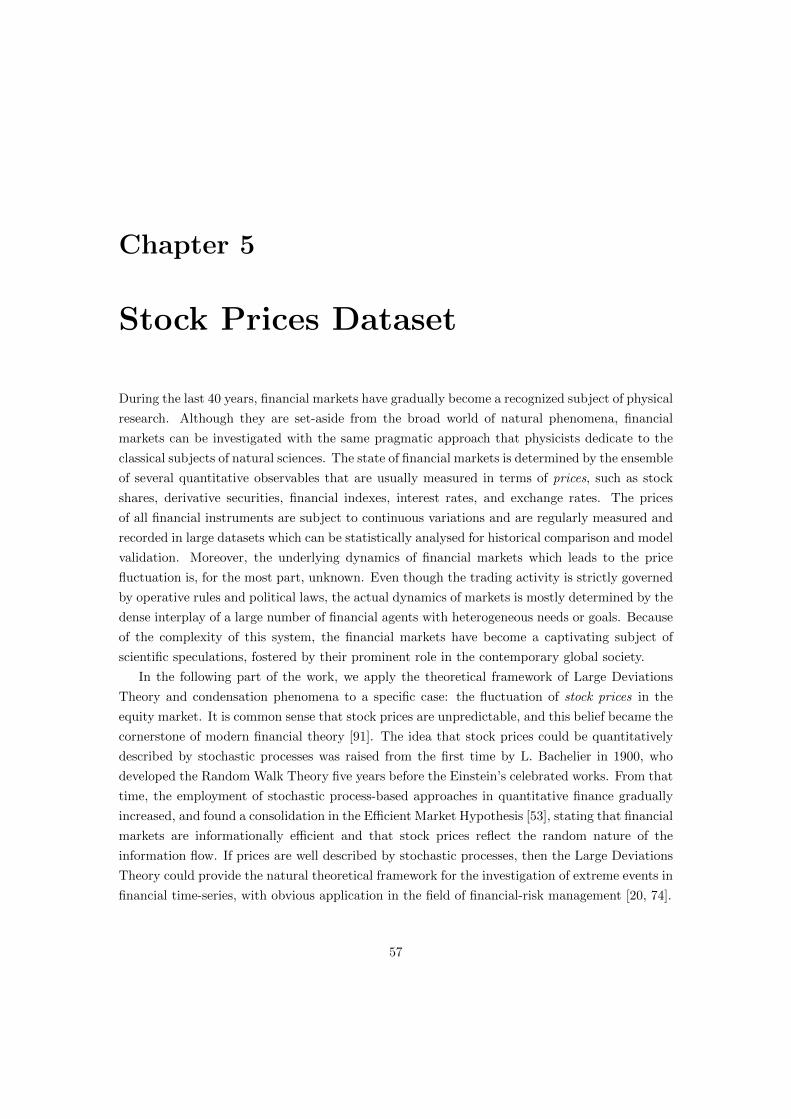
Chapter 5
Stock Prices Dataset
During the last 40 years, financial markets have gradually become a recognized subject of physical
research. Although they are set-aside from the broad world of natural phenomena, financial
markets can be investigated with the same pragmatic approach that physicists dedicate to the
classical subjects of natural sciences. The state of financial markets is determined by the ensemble
of several quantitative observables that are usually measured in terms of prices, such as stock
shares, derivative securities, financial indexes, interest rates, and exchange rates. The prices
of all financial instruments are subject to continuous variations and are regularly measured and
recorded in large datasets which can be statistically analysed for historical comparison and model
validation. Moreover, the underlying dynamics of financial markets which leads to the price
fluctuation is, for the most part, unknown. Even though the trading activity is strictly governed
by operative rules and political laws, the actual dynamics of markets is mostly determined by the
dense interplay of a large number of financial agents with heterogeneous needs or goals. Because
of the complexity of this system, the financial markets have become a captivating subject of
scientific speculations, fostered by their prominent role in the contemporary global society.
In the following part of the work, we apply the theoretical framework of Large Deviations
Theory and condensation phenomena to a specific case: the fluctuation of stock prices in the
equity market. It is common sense that stock prices are unpredictable, and this belief became the
cornerstone of modern financial theory [91]. The idea that stock prices could be quantitatively
described by stochastic processes was raised from the first time by L. Bachelier in 1900, who
developed the Random Walk Theory five years before the Einstein’s celebrated works. From that
time, the employment of stochastic process-based approaches in quantitative finance gradually
increased, and found a consolidation in the Efficient Market Hypothesis [53], stating that financial
markets are informationally efficient and that stock prices reflect the random nature of the
information flow. If prices are well described by stochastic processes, then the Large Deviations
Theory could provide the natural theoretical framework for the investigation of extreme events in
financial time-series, with obvious application in the field of financial-risk management [20, 74].
57

In the present work we perform an empirical analysis of real financial time-series, which refer
to the most important stocks from the Italian equity market over the last two years. In this
chapter, we introduce the trading rules of the financial market by presenting the order book, i.e.
the financial system that matches supply and demand and fixes the ultimate value of prices [23].
Then, we describe the available dataset by presenting the raw structure of data and the selected
procedures for the measurements of stock prices.
5.1 The Order Book
Before moving to the statistical analysis of stock prices, it could be useful to review the funda-
mental mechanics that lead to the fluctuation of stock prices. Stock prices are defined by trades
or, more specifically, by financial transactions. A transaction is an agreement between two agents
where some shares of a stock are transferred from one agent (the seller) to another agent (the
buyer) in exchange for money. The amount of exchanged money per share defines the price of
the stock. Strictly speaking, a stock has no a-priori value, and its price is defined time-by-time
at the occurrence of a new transaction.
In modern financial markets, trades are usually executed by means of a continuous double
auction [23]. The term “auction” indicates that the buyer, the seller, and the price of each
transaction are defined through a highest-priority mechanism that selects the best bids. The
adjective “double” refers to the existence of two separate auctions where shares can be either
bought or sold. Finally, the term “continuous” specifies that the bids can be made, accepted, or
revoked at any time between the opening and closure of markets.
In financial jargon, bids are called quotes or orders. They are identified by several variables,
such as the owner, the type (either “buy” or “sell”), the number of exchanged shares, the price
per share, the placing time, and the expiry time. For practical purposes, the orders are recorded
and managed in a register called the order book, which has been schematically illustrated in Fig.
5.1. The order book is defined by the collection of all available quotes up to the current time.
At any instant, an agent can place a new quote with a certain number of shares on any allowed
price level. The price levels denote the price of each share and are fixed by market’s regulators to
multiples of the tick-size, which defines the smallest possible increment for the stock price. The
typical structure of the order book divides the price levels in two separate regions: the ask-side,
containing sell-orders, and the bid-side, containing buy-orders. The smallest non-empty price
level in the ask-side is called the best-ask price; conversely, the highest non-empty price level in
the bid-side is called the best-bid price. The difference between the best-ask and the best-bid
prices is defined as the bid-ask spread, and denotes the width of the empty region between the
two sides of the order book. The dynamics of the order book prevents the mixing of ask and bid
quotes and keeps this double-sided structure unaltered in time, although the best-ask and best-
bid prices may move across different price levels. Quite interestingly, the characteristic shape of
the order book does not allow to define a unique value for the price of the stock, but the actual
58

Figure 5.1 – Schematic representation of the order book, with the fundamental types of
orders and the definitions of price.
price is somehow determined by the whole structure of quotes recorded in the order book at a
specific time. In some sense, the best definition of the stock price is related to the best-ask and
best-bid prices, because they are the actual prices at which transactions are executed.
During the trading activity, financial agents can send orders to the order book to add new
quotes, modify their previous quotes, and execute trades with other agents. In each financial
market, agents are able to perform several kinds of operations which depends on the details of
the market’s regulations. Yet, all possible operations can be ultimately reduced to three different
types of order or, at most, to a combination of them. The possible orders are the following:
• Limit-Order. It simply denotes the placement of a new quote in the order book. A
limit-order does not generate an actual transaction, but it is recorded in the order book
until it is executed by a market-order or deleted by a cancellation (see later). The term
“limit” indicates that the owner of a limit-order fixes a limit price for the transaction,
which cannot be executed at a worse price than the selected one. Since transactions are
always executed at the best prices, this implies that limit-orders are exactly executed at
the limit price. A limit-order can be a buy-order or a sell-order, and must be placed on the
respective side of the order-book (any limit-order placed on the opposite side is executed as
an effective market-order). Limit-orders of both kinds could also be placed on the empty
region between the two sides of the order book and, in that case, they generate a variation
of either the best-ask or the best-bid prices, depending on the type of order.
• Market Order. This is the only kind of order that generates a real transaction. In limit-
orders, the owner can fix the transaction price, but has no control on the execution time. In
market-orders, instead, the two kinds of control are reverted: the owner decides the exact
59

time in which the transaction is executed (i.e. the instant in which the market-order is send
to the order book) but it is forced to trade at the best available price. Market orders can
be buy-orders or sell-orders, and are directed to the opposite side of the order-book. Every
market-order is matched with a limit-order at either the best-ask or the best-bid prices,
depending on the direction of the order. The limit-order is selected according to its arrival
time (oldest orders are chosen first). After the matching, the market-order generates a
transaction between the owners of the two orders and removes the corresponding quotes
from the order book. If the number of shares of the two orders do not match, then the
market-order is split into several orders with smaller amounts of quotes, which can be
matched with multiple limit-orders. It may happen that a market-order is larger than the
quantity of quotes placed on the best price; in that case, the market-order consumes all
available quotes and moves to the next non-empty price level, causing a variation of the
best price. This effect is one of the generating mechanisms of price-fluctuations, and is
often denoted as the mechanical impact of trades on stock prices.
• Cancellation. The limit-orders that are not executed by market-orders are eventually
deleted from the order book by means of cancellations. A limit-order can be revoked for
various reasons, for instance, because the owner wants to change its limit price, or simply
because it reached its expiry time. A cancellation may generate a price change as well as
other kinds of orders but, in order to do so, it should delete the last quotes placed on the
best-ask and best-bid prices.
The continuous arrival of these kinds of orders from all financial agents modifies the shape of
the order book during time and leads to the ultimate fluctuations of prices. According to the
mechanics presented above, the price of the stock is not a single continuous stochastic process,
but it is rather a doubled step-wise process with finite increments at discrete times. Indeed, the
price of each stock is defined by two separate values, i.e. the best-ask and the best bid prices,
whose changes are always multiple of the tick-size and simultaneous to some specific order acting
on the best quotes. In spite of this, whenever a stock price is observed over sufficiently large
time-scales (for instance, over few days or more), the bid-ask spread and the tick-size become
much smaller than the typical price-fluctuations, and the actual movements of prices can be
well-approximated by a single continuous stochastic process. The most common features of such
process are presented in the next section.
5.2 Description of the Dataset
In the following work, we perform the statistical analysis of a real financial dataset, which have
been made available by List S.p.A. The dataset contains historical information about prices,
trades, and quotes of some stocks from the Italian equity market. The time series cover a period
of two years, from July 2, 2012 to June 27, 2014. The available stocks belong to the FTSE MIB
60

n. ISIN Company Sector
01 IT0000062072 Assicurazioni Generali Financials02 IT0000062957 Mediobanca Financials03 IT0000064482 Banca Popolare di Milano Financials04 IT0000068525 Saipem Oil & Gas05 IT0000072618 Intesa Sanpaolo Financials06 IT0001063210 Mediaset Consumer Services07 IT0001479374 Luxottica Consumer Goods08 IT0003128367 Enel Utilities09 IT0003132476 Eni Oil & Gas10 IT0003153415 Snam Utilities11 IT0003242622 Terna Utilities12 IT0003487029 UBI Banca Financials13 IT0003497168 Telecom Italia Telecommunications14 IT0003506190 Atlantia Industrials15 IT0003856405 Finmeccanica Industrials16 IT0004176001 Prysmian Industrials17 IT0004623051 Pirelli & C. Consumer Goods18 IT0004781412 UniCredit Financials19 LU0156801721 Tenaris Basic Materials20 NL0000226223 STMicroelectronics Technology
Table 5.1 – The constituents of the dataset, with the International Securities Identifi-
cation Number (ISIN) and the economic sectors. The numbering of constituents will be
preserved for the entire work.
index, which is a common benchmark for the Italian stock exchange and is constructed as the
weighted sum of the 40 most traded stocks in the national market. We do not examine all 40
stocks in the index for many reasons: (a) the 40 stocks are heterogeneous, and the least traded
stocks exhibit a different behaviour from the most traded stocks (lower frequency of trades, larger
bid-ask spread, etc.); (b) the components of the FTSE MIB index are not constant in time and
the least valuable stocks may be excluded from the index in favour of other eligible stocks; and
(c) the information about some stocks may be partially unavailable, due to some changes in the
data recording procedure. As a consequence, we restrict our analysis to only 20 stocks among
the 40 constituents of the FTSE MIB index, selecting them by means of the following criteria:
• The financial time series of the stock is fully available.
• The stock has been a constituent of the FTSE MIB index during the whole period of
observations.
• The weight of the stock as a FTSE MIB constituent is relatively large.
• The stock belongs to a company with high market capitalization.
• The financial activity of the stock is relatively intense.
61

The 20 selected stocks are listed in Table 5.1, together with their International Securities Iden-
tification Number (ISIN) and their economic sectors.
From a practical point of view, our dataset is composed of 20 files (one for each stock)
containing tick-by-tick information. This means that any change in the state of the market is
recorded as a new event. In our case, the dataset contains the information from any market-order,
limit-order, or cancellation occurring at the best quotes. A single file appears like this:
...
TS=[2012/10/12 13:32:25:000]Date=[20121012]Time=[133225430]...
TS=[2012/10/12 13:32:25:000]Date=[20121012]Time=[133225650]...
TS=[2012/10/12 13:32:29:000]Date=[20121012]Time=[133229680]...
TS=[2012/10/12 13:32:30:000]Date=[20121012]Time=[133230290]...
TS=[2012/10/12 13:32:30:000]Date=[20121012]Time=[133230290]...
TS=[2012/10/12 13:32:30:000]Date=[20121012]Time=[133230290]...
...
Each line represents an event and is composed of the following fields:
• TS: it is the time-stamp at which the event has been received by the recording system from
the market. It has a resolution of one second.
• Date and Time: they denotes the date and time at which the event occurred according
to the market itself. With respect to TS, they are recorded with a different format and
a higher resolution (0.01 s). The two time-stamps exhibit a small lag, probably due to
different reference times or to rounding errors.
• Type: this field can have two possible values, namely, [Best] or [Last]. If Type=[Best],
then the event is generated by a limit-order or a cancellation at either the best-ask or the
best-bid, and is characterized by a change in the prices and the volumes of the best quotes.
If Type=[Last], instead, the event is generated by a market-order and it denotes an actual
trade of some shares of the stock (the term [Last] comes from “last execution”, which
commonly denotes the most recent trade).
• Last.Price and Last.Qty: this fields are informative only for market-orders (i.e. when
Type=[Last]). In this case, they respectively denote the price at which the trade has been
made and the corresponding amount of exchanged shares.
• BestBid.Price and BestBid.Qty: they denote the current price and volume of the best-
bid and they are updated at any limit-order or cancellation occurred at the best quotes
(i.e. when Type=[Best]).
• BestAsk.Price and BestAsk.Qty: they work exactly as BestBid.Price and BestBid.Qty,
but they refer to the best-ask instead of the best-bid.
62

Time Stamp Time Stamp Last Last Bid Bid Ask Ask(date) (time) Date Time Type Price Qty. Price Qty. Price Qty.
20121012 48743.00 20121012 48743.06 0 0.000 00000 4.304 05742 4.312 0513220121012 48743.00 20121012 48743.86 0 0.000 00000 4.304 07210 4.312 0513220121012 48745.00 20121012 48745.43 0 0.000 00000 4.304 07210 4.312 0100020121012 48745.00 20121012 48745.65 0 0.000 00000 4.304 08539 4.312 0100020121012 48749.00 20121012 48749.68 0 0.000 00000 4.306 05606 4.314 1064520121012 48750.00 20121012 48750.29 1 4.306 01606 4.306 05606 4.314 1064520121012 48750.00 20121012 48750.29 1 4.306 00394 4.306 05606 4.314 1064520121012 48750.00 20121012 48750.29 0 0.000 00000 4.306 03606 4.314 1064520121012 48750.00 20121012 48750.33 0 0.000 00000 4.304 07071 4.312 0211020121012 48750.00 20121012 48750.55 0 0.000 00000 4.304 05329 4.312 02110
Table 5.2 – An excerpt from one datafile after the first cleaning procedure.
The dataset is very large (more than 20 Gbyte) and contains nearly all information about the
trades and state of the market with respect to the best quotes. Generally, each recorded event
denotes a single order (market-order, limit-order, or cancellation), but this is not always true
since the recording system may both aggregate and divide single orders. If many limit-orders
and cancellation occur in a very short time (of the order of few hundredths of second), then
the multiple orders may be aggregated and recorded as a single event. On the contrary, if the
volume of a market-order does not match with the volumes of the existing limit-orders, it may
be split into smaller orders in order to find a matching. Therefore, even if the state of the
market is recorded with high precision, it is not always possible to extract from the dataset the
information about every single order. However, for our purposes, this is not a big issue: we are
more interested in price fluctuations than in order arrivals, and the presented dataset provides
all information we need for the analysis of prices.
The dataset presented above cannot be directly handled and needs some cleaning. First of
all, the dataset should be converted in a numeric format. For each file, we removed all field
names, we brought all dates and times in the same format, and we converted Type in a boolean
variable. The dates have been expressed in the format YYYYMMDD, as for the Date field, and have
been treated as labels (this format preserves the natural ordering of dates). On the contrary,
the times have been expressed in a more physical-like form and have been measured in seconds
starting from the midnight of each trading day. The final output is shown in Table 5.2.
The main problem about the dataset concerns its size. Even after this cleaning procedure,
the whole dataset is larger than 20 Gbyte. Performing whatever computation or measurement
over the entire dataset is a very slow operation, which can be carried out only by low-level
programming. Yet, for what concerns the analysis of price fluctuations, the dataset contains
much more information than necessary. For instance, if we want to know only the price of the best
quotes and not their volumes, then any event denoting a change in the volumes may be ignored.
In order to lighten the dataset, we have to figure out what observables must be investigated and
what data is required for their measurements. After that, all useless information can be thrown
away.
63

5.3 Measuring Times and Prices
Stock prices can be considered as stochastic processes over time. Therefore, in order to carry on
the empirical analysis of prices, we need to define and measure both times and prices. In the
present work, the time and the price of each financial event are defined as the physical time and
the mid-price, respectively. The reasons that led to this choice are explained below.
In finance, the concept of “time” has a non-trivial meaning. It does not only denote the
physical passing of time, but also the typical duration of financial activities. There are many
ways of defining time [91]. The most common definitions are the following:
• Physical Time. It denotes the true passing of time and is somehow the fundamental
definition of time in physics as well as in finance. Any other definition of time can be
considered as a local rescaling of the physical time, which can be dilated or shrunk according
to the trading activity. The physical time has many advantages with respect to the other
definitions of time: it is unambiguous, it can be directly measured, and it is at the basis of
market regulations. For instance, markets open and close at the same hour every day, and
the physical duration of a trading day is fixed (in the Italian market, for example, a trading
day lasts 8:30 hours, from 09:00 AM to 05:30 PM). The physical time is important also at
micro-structural level, since orders must be physically processed and are registered with
a fixed time resolution. Despite of this, the financial activities may be quite uncorrelated
with the physical time. The fluctuations of prices are mainly driven by the arrival of news
and orders on the market, and their incoming rate is quite heterogeneous in time. The
trading activity is often characterized by periods of over-excitement, spaced out by period
of relaxation, and prices react in accordance to this. Therefore, the physical definition of
time is not always the best choice for the analysis of price fluctuations.
• Volume Time. It is defined as the cumulative number of exchanged shares of a given
stock, and it is usually measured from the beginning of each trading day. If the shares are
exchanged at a constant rate, than it coincides with the physical time. On the contrary,
when the exchange rate is heterogeneous, the volume time becomes a direct measure of the
financial activity. In contrast with the physical time, the volume time can be considered a
“subjective time”: it slows down during the periods of high trading activity and accelerates
during the relaxation times. It is reasonable to assume that price movements become much
more regular when measured in volume time. As for the physical time, the volume time can
be directly measured, but has one great disadvantage: it depend on each stocks and each
day, and its fundamental unit is not defined. Let us be more specific. The duration of a
trading day in volume time is equal to the total exchanged volume, and varies from day to
day as well as from stock to stock. There could be “long days” and “short days”, according
to the intensity of trades, and some stocks may be more active then others even on the
same day. Moreover, the typical amount of shares exchanged in a single transaction is not
constant, but it strongly depends on each stock and, above all, on their prices. Therefore,
64

stocks and days can be characterized by very different trading activities even when their
volume times increase at the same rates.
• Tick Time. It is a variant of the volume time and is defined as the cumulative number of
market-orders over a given stock. The number of orders could be a more stable quantity
with respect to the volume of exchanged shares, yet, it is usually not measurable with
direct observations. In our case, for instance, single orders are often aggregated or split
into multiple orders, then their effective number actually depends on their arrival rate and
on their sizes. Beyond this differences, the tick time has about the same advantages and
disadvantages of the volume time.
As well as time, also prices can have multiple definitions. Whenever a stock price is observed
at high-frequency, the micro-structural features of the market become relevant [1]. In this case,
prices cannot be considered as continuous stochastic processes, but rather as random processes
occurring at discrete levels and at discrete times. Moreover, the concept of a unique price for each
stock is contradicted by the presence of multiple quotes in the order book that are simultaneously
placed at different prices. According to these considerations, the simplest definitions of prices
are listed below:
• Executed Price. It is in some sense the “actual price”. It is defined as the price at which
market-orders are sent to the order book and so it denotes the price at which the shares
of a stock are actually exchanged. This definition of the price is quite unambiguous and
can be directly measured from financial time series, yet, it has two main defects. First,
the executed price is subject to the so-called bid-ask bounces: market-orders, indeed, can
be send as either sell-orders or buy-orders, so they can hit either the best-ask or the best-
bid quotes. As a result, the executed price usually exhibits sudden jumps, whose size
is determined by the bid-ask spread. Thus, at high frequencies, the executed price has
much larger fluctuations than what could be inferred from the analysis of prices at low-
frequencies. As a second disadvantage, we stress that the executed price is well-defined
only during transactions. According to this definition, if the trading activity is relaxed
and the transactions are spaced out by long periods of time then, during those periods,
the behaviour of the price is completely unknown. In particular, the prices of the best
quotes could be very different from the executed price of the most recent transaction. This
disadvantage makes the executed price particularly unsuited for the analysis of prices at
high frequencies.
• Ask and Bid Prices. While the executed price is the one at which transactions occur,
the ask and bid prices are the ones at which transactions could occur. They are simply
defined as the prices of the best-ask and best-bid quotes, respectively. In contrast with
the executed price, the ask and bid prices are continuously updated and are always well-
defined. This fixes the main disadvantage of the executed price. While the historical series
65

Physical VolumeDate Time Time Mid-Price
20121012 48739.67 2223779 4.31020121012 48739.86 2223779 4.30820121012 48740.82 2223779 4.30720121012 48742.87 2223779 4.30820121012 48749.68 2223779 4.31020121012 48750.33 2225779 4.30820121012 48757.47 2226279 4.31020121012 48757.50 2226279 4.30920121012 48762.08 2226279 4.31020121012 48768.90 2226279 4.309
Table 5.3 – An excerpt from one datafile after the reduction procedure.
of transactions are easily available, the historical series of the quotes requires much more
information and are less common. However, when this kind of data is available (as in our
case) the ask and bid prices become much more reliable than the executed price. The
main issue concerning the ask and bid prices is that we are considering two different prices
instead of one, and so, in this case, the price of the stock is not unambiguously defined.
• Mid-Price. The simplest way to combine the ask and bid price in just one quantity is to
compute their average, namely, the mid-price. In the step from the ask/bid prices to the
mid-price we loose all information about the bid-ask spread. Yet, the mid-price is uniquely
defined, is not subject to bid-ask bounces, and is constantly updated, so it is one of the
best choices to define prices. Quite oddly, transaction never occurs at the mid-price: the
bid-ask spread is always grater then zero and the ask and bid prices never coincide with
the mid-price.
In this work, we opt for the following choices. We measure times according to the physical
time, which is an objective quantity and allows a more precise analysis of price fluctuations; and
we measure prices according to the mid-price, which yields continuous and stable measurements.
In spite of this, we decided to record also the volume time, which could provide additional
information about the intensity of the trading activity.
With respect to these choices, our dataset turns out to be over-informative. We do not need
to know the volumes of the best quotes (BestAsk.Qty and BestBid.Qty) but only their prices
(BestAsk.Price and BestBid.Price) which can be combined in a single observable through their
average. As well, we do not need to record every transaction but we only need to keep track of the
exchanged volumes (Last.Qty) in order to measure the volume time. The information about the
physical time is redundant too: we need just one of the two available time-stamps and we decided
to measure dates and times from the fields Date and Time, which have a higher resolution. As
a consequence, we performed a general reduction of our dataset, keeping the desired observables
and discarding all the exceeding information. Each file in the resulting dataset is defined by
only four fields, namely, the date, the physical time, the volume time, and the mid-price. Files
66

have been lightened not only over columns (observables) but also over rows (events). Indeed, we
require to record a new event only when the mid-price is changing. The resulting dataset is much
smaller and manageable then the original one: it is smaller than 1 Gbyte and has been reduced
to less than 4% of its original size. This operation preserved the basic information contained in
the dataset and allows us to perform a wide variety of measurement in short computation times.
En excerpt of the final dataset has been shown in Table 5.3.
67

Chapter 6
Stylized Facts about Stock Prices
In financial literature, the statistical properties of stock prices are usually described by means of
stylized facts [33]. A stylized fact is an empirical feature of stock prices that is observed in a large
variety of circumstances, across different markets, time periods, and financial assets. There is
no reasons to suppose that different financial instruments, such as stock prices, derivative prices,
exchange rates, from different economic and industrial sectors, should follow the same stochastic
dynamics. Yet, form an empirical point of view, all financial instruments are characterized by a
common statistical behaviour and share many non-trivial properties [33].
In this chapter, we introduce some stylized facts about stock prices. The following description
is in general agreement with the observations reported in literature [44, 33, 91, 20, 17], yet, instead
of presenting a simple review of the consolidated facts, we prefer to recover the most important
stylized facts from a direct observation of the available dataset. The advantage of this approach
is twofold: (a) we provide a further evidence of the universality of some stylized facts; and (b) we
ensure that the examined stocks follows the same statistical behaviour described in literature.
This guarantees that the results of the present work are not due to exceptional features related
to the observed dataset, but are rather the effects of the intrinsic dynamics of stock prices and
could be extended to more general cases. The following description is not comprehensive of all
stylized facts reported in literature, but it reports only the most relevant facts with respect to our
main topic, namely, the statistical characterization of extreme returns in financial time-series.
6.1 The Geometric Brownian Motion
Before investigating the stylized facts about stock prices, it could be useful to review the funda-
mental concepts about the stochastic dynamics of price fluctuations. This would be the chance
to define some basic quantities such as price returns and volatility in a precise way. In this sec-
tion, we refer to a specific model for price fluctuations, namely, the Geometric Brownian Motion
(GBM), which is a direct descendant of the Bachelier’s random walk introduced in 1900 [91]. As
68

we are going to see in the next few sections, the GBM does not provide a faithful description
of stock prices, but it can be considered as a good first-order approximation of the real price
dynamics. Indeed, it can be recognized at the basis of several more accurate models, which can
be arguably considered as corrections of the GBM to specific cases (see Chapter 8 for a short
review). The popularity of the GBM in quantitative finance is probably due to the celebrated
Black & Scholes formula (1973), which employed the model in the evaluation of option prices
and became a milestone of the modern financial research [14].
Let us denote by S(t) the price of a specific stock at the instant t. According to the GBM,
the infinitesimal increments dS(t) are non-stationary and are proportional to the price itself. In
formulas, the dynamics of the stock price S(t) can be expressed through the following stochastic
differential equation:
dS(t) = µ′ S(t) dt+ σ S(t) dW (t) , (6.1)
where dW (t) is the infinitesimal increment of a Wiener process (i.e. a standard Brownian Motion)
and scales as the square root of dt. The parameters µ′ and σ are the drift rate and the volatility
of the stock, respectively. The drift rate µ′ measures the exponential growth of the stock price in
absence of stochastic fluctuations, whereas the volatility σ denotes typical scale of fluctuations.
According to the above equation, the logarithmic price X(t) = logS(t) behaves as a classical
Brownian Motion, namely:
dX(t) = µdt+ σ dW (t) , (6.2)
where, by Ito’s lemma, µ = µ′ − σ2/2. This simple result suggests that logarithmic prices X(t)
represent more fundamental quantities than linear prices S(t), and settles the formers at the
basis of most statistical model. The stochastic differential equations (6.1) and (6.2) admit a
solution in a closed analytical form, which can be expressed through the probability distribution
functions:
PS(t)(s) =1√
2πs2σ2texp
{−[
log ss0−(µ′ − 1
2σ2)t]2
2σ2t
},
and:
PX(t)(x) =1√
2πσ2texp
{− [x− x0 − µt]2
2σ2t
},
where we assumed that S(0) = s0 and X(0) = x0. As a consequence, the ratio S(t)/S(0) and
the difference X(t)−X(0) are log-normal and normal random variables, respectively, with mean
µ t and variance σ2 t.
The stochastic dynamics of stock prices can be investigated by means of the statistical analysis
of price changes or price returns, which measure the variation of prices at fixed time-scales. These
quantities may be defined in different ways [91], and the most common choices are the following:
• Price changes:
∆τS(t) = S(t+ τ)− S(t) .
69

• Linear returns:∆τS(t)
S(t)=S(t+ τ)
S(t)− 1 .
• Logarithmic returns:
∆τ logS(t) = logS(t+ τ)
S(t).
Unlike linear returns, price changes and logarithmic returns are cumulative quantities, in the
sense that:
∆NτF (t) =
N−1∑n=0
∆τF (t+ nτ) ,
where F (t) can be chosen as either S(t) or X(t) = logS(t). This scaling law facilitates the
statistical analysis of these quantities on multiple time-scales, and makes them more appropriate
then linear returns. The general advantage of price returns with respect to price changes is
that returns are non-dimensional quantities and, for these reasons, their statistical features are
expected to be more stationary. According to these criteria, the logarithmic returns are the best
choice for the analysis of stock prices, and will be employed for the rest of the present work. In
order to simplify the notations, from now on we will drop the adjective “logarithmic” and we
will denote price returns simply as:
xτ (t) = logS(t+ τ)
S(t). (6.3)
The above definition is also supported by the theoretical framework of the Geometric Brownian
Motion. Indeed, by assuming the validity of eq. (6.1), one finds that the returns xτ (t) are
independent normally distributed random variables with mean µτ and variance σ2τ , described
by the pdf:
Pxτ (x) =1√
2πσ2τexp
{− (x− µτ)2
2σ2τ
}.
For future convenience, it could be useful to define the realized absolute moment of order q.
Given a time interval [t, t+Nτ ], this can be defined as:
Mqτ (t, t+Nτ) =
1
N
N−1∑n=0
∣∣xτ (t+ nτ)∣∣q , (6.4)
Being an averaged quantity, the absolute moment Mqτ (t, t + Nτ) is defined up to two different
time-scales: a finer time-scale τ for the price sampling, and a coarser time-scale Nτ for the
averaging. The specific case q = 2 leads to the definition of the realized volatility, namely:
στ (t, t+Nτ) =√M2τ (t, t+Nτ) , (6.5)
According to eqs. (6.1) and (6.2), if the drift parameter µ is small (compared to the charac-
70

0.5 1.0 5.0 10.0 50.0 100.0
105
106
107
108
109
20
19
18
17
16
15
14
13
1211
10
9
8
7
6
5
4
3
21
Svwap
Vtot
Figure 6.1 – Global overview of the dataset showing the characteristic volumes and prices
of each stock. Each point is determined by the volume weighted average price Svwap and
by the total exchanged volume Vtot for each trading day in the dataset. Different colors
refer to different stocks. The white labels denotes the identification number of the stock
and are placed at the average value of the observation (evaluated on a logarithmic scale).
These values have been shown in Table 6.1. The dashed line denotes a least-squares fit
with the inverse proportionality law Vtot = A/Svwap, where A = 3.878× 10⁷.
teristic frequency σ/√τ), then the realized volatility στ (t, t + Nτ) can be used as an empirical
approximation for the exact volatility σ. Indeed, thanks to the law of large numbers, it is easy
to show that:
limT→∞
στ (t, t+ T )√τ
= σ +O
(µ2τ
σ
),
where the normalization factor√τ explicitly accounts for the diffusivity of the process.
6.2 Global Properties of Stocks
In order to investigate the empirical properties of price returns in details, it is worth to get
an overview of the whole dataset over the included stocks and trading days. Stocks could be
very heterogeneous, so it could be important to identify their main features. In this section we
measure and compare the prices and volumes of all dataset components on a global level. For
each date and each stock, we measure the total exchanged volume Vtot, and the volume weighted
71

n. Company Vtot (106) Svwap Vtot · Svwap (106)
01 Assicurazioni Generali 5.624 14.15 79.59 ∗02 Mediobanca 4.857 5.213 25.3203 Banca Popolare di Milano 49.08 0.468 22.9504 Saipem 2.027 21.81 44.20 ∗05 Intesa Sanpaolo 133.8 1.549 207.3 ∗06 Mediaset 10.98 2.439 26.8007 Luxottica 0.503 36.10 18.1708 Enel 32.88 3.037 99.85 ∗09 Eni 10.00 17.66 176.6 ∗10 Snam 6.807 3.712 25.2711 Terna 5.652 3.309 18.7012 UBI Banca 5.770 3.907 22.5413 Telecom Italia 81.07 0.696 56.46 ∗14 Atlantia 1.493 14.40 21.4915 Finmeccanica 4.656 4.627 21.5516 Prysmian 0.960 16.19 15.5417 Pirelli & C. 2.033 9.723 19.7718 UniCredit 72.99 4.413 322.1 ∗19 Tenaris 1.404 16.06 22.5520 STMicroelectronics 4.438 5.900 26.18
Table 6.1 – Global overview of the dataset showing the characteristic volumes and prices
of each stock. The fields denote the average daily values of the volume weighted average
price Svwap and of the total exchanged volume Vtot of each stock, together with their
product. The reported values correspond to the white labels of Fig. 6.1, and their statis-
tical errors can be estimated from the same figure. The symbol (*) denotes a significant
deviation from the inverse proportionality law observed in the figure.
average price Svwap. The latter is defined as the average price in volume time, namely:
Svwap =1
Vtot
∫ Vtot
0
S(t) dv(t) ,
where v(t) denotes the volume time as a function of the physical time. The results are shown in
Fig. 6.1 and in Table 6.1, where we recorded the average prices and volumes of each stock. Both
Vtot and Svwap turn out to be very different from stock to stock, yet, Fig. 6.1 shows that Vtot
and Svwap are strongly correlated and, in a zero-th order approximation, they obeys the inverse
proportionality law:
Vtot × Svwap = constant .
We recall that the product Vtot × Svwap is exactly equal to the total amount of money invested
in a given stock every day, so it somehow defines the importance of the stock in the financial
market. The above formula asserts that the total amount of money invested by traders is about
72

-0.02 -0.01 0.00 0.01 0.02
0.1
1
10
100
1000
xτ
pro
babilit
yden
sity
-4 -2 0 2 4
0.001
0.005
0.010
0.050
0.100
0.500
1.000
xτ/στ
pro
babilit
yden
sity
Figure 6.2 – The empirical probability density function of price returns at 30 minutes,
evaluated for natural returns xτ (t) (left) and rescaled returns xτ (t)/στ (right). Plots show
the superposition of all distributions evaluated from the time-series of individual stocks,
highlighting their relative behaviour. Different colors refer to different stocks. In the
rescaled case, the functions almost fall on the same curve, showing cross-stock invariance.
the same for all stocks and, the smaller the price, the larger the volume of exchanged shares.
However, this naive rule is far from being exact. For some stocks, the product Vtot × Svwap
is considerably higher then the ones of the other stocks. These stocks are related to the most
important companies listed in the Italian equity market, and have been denoted in Table 6.1
with the symbol (∗).
6.3 Probability Distribution of Price Returns
In this section we investigate the time-series of stock prices in more details by examining the
price returns xτ (t) for each stock. Our aim is the characterization of the probability distribution
function Pxτ (x) of the price returns. For the sake of simplicity, we sample returns at a fixed time-
scale, namely, τ = 30 minutes. The distribution of the returns for all 20 stocks are simultaneously
plotted in Fig. 6.2 (left). The distributions are roughly symmetric and centred around zero, but
they have different dispersions. In Table 6.2 (left) we show the mean and the standard deviation of
each distribution. The means are about two orders of magnitude smaller than the corresponding
standard deviations, so they can be approximated to zero. The standard deviations, instead,
vary from stock to stock. If we try to rescale the returns of each stock by its realized volatility,
namely:
xresτ (t) =
xτ (t)
στ,
then we obtain the distributions plotted in Fig. 6.2 (right). As we can see, all distribution almost
fall on the same curve. As a result, we can assert the following stylized fact:
73

Normal Distribution Student’s t-Distribution
n. µ (10−6) σ (10−3) p-value µ (10−6) σ (10−3) α p-value
01 +8.131 3.355 0% +19.23 2.284 3.514 15.18%02 −3.828 4.975 0% +70.29 3.425 3.555 14.80%03 −56.27 5.642 0% −103.7 3.686 3.131 11.85%04 −55.15 3.585 0% −62.29 2.157 2.910 16.51%05 −28.23 4.496 0% +8.761 2.976 3.338 5.069%06 −65.94 5.381 0% −102.9 3.570 3.331 21.21%07 +50.47 2.626 0% +59.97 1.937 4.176 29.48%08 +30.51 3.223 0% +61.60 2.346 4.243 8.222%09 +17.21 2.350 0% +27.24 1.692 4.236 0.006%10 −4.632 2.196 0% +32.89 1.606 4.192 0.979%11 +2.696 2.213 0% +20.60 1.609 4.047 1.655%12 −35.61 5.023 0% +29.42 3.612 3.862 19.64%13 +27.01 4.316 0% −48.45 2.918 3.382 5.211%14 −11.77 2.967 0% +24.98 2.050 3.615 4.323%15 −19.85 4.694 0% +9.116 3.234 3.583 9.909%16 +47.78 3.518 0% +36.38 2.525 4.002 18.12%17 +11.29 3.663 0% +28.17 2.615 4.000 11.34%18 −24.86 4.817 0% −12.30 3.237 3.544 12.16%19 +12.22 3.058 0% +33.90 2.120 3.648 6.974%20 +6.633 3.983 0% −31.73 2.805 3.817 10.93%
Table 6.2 – Most likely parameters for the empirical distribution of returns at 30 minutes
according to a Normal Distribution (left) and to a Student t-Distribution (right) obtained
through a maximum likelihood estimation. The estimated parameters are the location
µ, the dispersion σ, and the tail index α. In the normal case, the parameters µ and σ
correspond to the mean and the standard deviation of the returns, respectively. For each
estimation, the table also shows the p-value of an Anderson-Darling test. A value of 0%
denotes a p-value below 10−6 (the hypothesis of normal returns is always rejected).
Stylized Fact no.1: at a fixed time-scale τ , each stock is characterized by a specific
volatility στ , but the rescaled returns xresτ (t) = xτ (t)/στ of all stocks are approximately
described by the same probability distribution.
Thanks to this stylized fact, we can reasonably rescale the returns of each stock and merge them
in a unique sample with a large number of observations. The empirical distribution of all rescaled
returns has been plotted in Fig. 6.3.
It is often assumed that stock returns are distributed according to a power-law distribution
[91, 20]. The figures presented above clearly show that returns have much heavier tails than nor-
mal variables, and so our dataset could validate this assumption. In order to better characterize
the tails of the distribution we compared the pdfs of Fig. 6.2 to a Student’s t-distribution. For
each stock, we approximated the empirical distribution of returns with a student’s t-distribution
74

-5 0 5
10-5
10-4
0.001
0.01
0.1
1
xτ/στ
pro
bab
ilit
yd
ensi
ty
Figure 6.3 – The empirical distribution of price returns at 30 minutes evaluated from
the whole available dataset. The distribution has been evaluated by merging the rescaled
returns of each stock in a unique sample. A comparison is shown with a standard normal
distribution (dotted line) and a Student’s t-distribution with 4 degrees of freedom and
unitary variance (continuous line).
0 5 10 15 20
0
1
2
3
4
5
6
stock (id. number)
tail
index
Negative Tail
0 5 10 15 20
0
1
2
3
4
5
6
stock (id. number)
tail
index
Positive Tail
Figure 6.4 – The tail indexes of the empirical distribution of price returns, evaluated
through the Hill estimator and related to each stock in the dataset. Two cases are shown,
in relation to the two tails of the distributions. The measurements fluctuates around 3
and fit with a unique tail index for all distribution and both tails.
75

-0.03 -0.02 -0.01 0.00 0.01 0.02 0.03
0.1
1
10
100
1000
104
xτ
pro
babilit
yden
sity
-0.0006 -0.0004 -0.0002 0.0000 0.0002 0.0004 0.0006
1
10
100
1000
104
105
xτ/√τ
pro
babilit
yden
sity
Figure 6.5 – The empirical probability density function of price returns for the 18-th
stock (“UniCredit”) at several time-scales, evaluated for natural returns xτ (t) (left) and
time-rescaled returns xτ (t)/√τ (right). Plots show the superposition of all distributions
evaluated from different time-scales, namely, τ = 1, 1.5, 2, 3, 5, 7.5, 10, 15, 20, 30, 40, 60,
90, and 120 minutes, and the relative colors shade from red (1 minute) to blue (2 hours).
In the rescaled case, the functions almost fall on the same curve, showing the diffusive
scale-invariance of the distribution.
with α degrees of freedom and location-dispersion parameters µ and σ, then we evaluated the
most likely values of the parameters by a maximum likelihood estimation. The results are shown
in table 6.2 (right). The tail index α turns out to be about the same for all stocks and is very
close to 3 ÷ 4. In order to test if the resulting Student’s t-distribution is a good approximation
of the empirical distribution, we performed an Anderson-Darling test for each estimated distri-
bution. The p-values obtained from the tests are quite high and, for most stocks, the hypothesis
of Student’s t-distributed returns cannot be rejected. The tail index of the empirical distribution
has been also evaluated by means of the Hill estimator. The result are represented in Fig. 6.4.
The obtained values for the Hill estimators are compatible with the degrees of freedom of the
most-likely Student’s t-distribution and, above all, it is about the same for all stocks and both
tails of the distribution. As a result, we can finally assert the following:
Stylized Fact no.2: At the observed time-scales (1 min ÷ 1 hour), the probability dis-
tribution of returns is a power-law distribution with a tail index of about 3 ÷ 4. The tail
index is the same for all stocks [20].
The above stylized facts have been verified also over different time-scales, ranging form 30 seconds
to one trading day (8h 30m).
6.4 Diffusivity of Prices
At this stage, we investigate how the probability distribution of price returns xτ (t) depends on
the sampling time-scale τ . In the previous section we observed the returns of different stocks
76

50 100 500 1000 5000 1´104
0.0010
0.0100
0.0050
0.0020
0.0200
0.0030
0.0015
0.0150
0.0070
τ (seconds)
στ
Figure 6.6 – The realized volatility στ as a function of the time-scale τ for the 18-th
stock (“UniCredit”). The dashed line denotes a least-squares linear fit with the diffusive
law στ = σ√τ .
n. Company σ (10−4 sec−1/2) T%
1 Assicurazioni Generali 0.853 3h 49m2 Mediobanca 1.229 1h 50m3 Banca Popolare di Milano 1.426 1h 22m4 Saipem 0.911 3h 21m5 Intesa Sanpaolo 1.104 2h 17m6 Mediaset 1.350 1h 31m7 Luxottica 0.672 6h 09m8 Enel 0.806 4h 17m9 Eni 0.583 8h 11m10 Snam 0.560 8h 51m11 Terna 0.563 8h 45m12 UBI Banca 1.274 1h 43m13 Telecom Italia 1.124 2h 12m14 Atlantia 0.740 5h 04m15 Finmeccanica 1.174 2h 01m16 Prysmian 0.868 3h 41m17 Pirelli & C. 0.916 3h 19m18 UniCredit 1.177 2h 00m19 Tenaris 0.769 4h 42m20 STMicroelectronics 1.007 2h 44m
Table 6.3 – Estimates of the diffusive parameters σ for each stock in the dataset evaluated
from the diffusivity law στ = σ√τ as in Fig. 6.6. The measurements are also expressed
in terms of the characteristic times T% = (0.01/σ)2 i.e. the average times in which prices
diffuses over 1% of their original values.
77

-10 -5 0 5 10
10-5
10-4
0.001
0.01
0.1
1
10
xτ/(σ√τ)
pro
bab
ilit
yd
ensi
ty
Figure 6.7 – Scale-invariance of the empirical distribution of price returns at several time-
scales, evaluated from the whole available dataset. For each time-scale τ , the probability
distribution has been evaluated by merging the rescaled returns xτ/(σ√τ) of each stock
in a unique sample. The diffusivity parameters σ are listed in Table 6.3. The evaluated
distributions have been superposed in a unique plot, and refer to several scales form 1
minute (red curve) to 2 hours (blue curve). Micro-structural effects at small time-scales
are visible, as well as small deviations from the pure diffusive law in the tails of the
distributions. A comparison is shown with the Student’s t-distribution at 4 degrees of
freedom (black curve).
at a fixed time-scale; now we do the reverse, and we observe the returns of a unique stock for
different sampling times. In Fig. 6.5 (left) we plot the p.d.f. of the returns xτ (t) for the 18-th
stock of the dataset (“UniCredit”). We selected the time-scale τ = 1, 1.5, 2, 3, 5, 7.5, 10, 15, 20,
30, 40, 60, 90, and 120 minutes. The typical dispersion of the returns becomes larger and larger
as τ increases, and this behaviour could prove that log-prices are diffusive. In Fig. 6.5 (right) we
plot the p.d.f. of the time-rescaled returns:
xτ (t) =xτ (t)√τ
,
and we found that all distributions fall about on the same curve. In order to be more quantitative,
we measured the realized volatility στ at each time-scale and we observed its dependence on time.
The result is plotted in Fig. 6.6 and is in good agreement with the diffusive law:
στ = σ√τ .
78

We notice that this result is not restricted to the chosen stock, but holds for all 20 stocks of our
dataset. In conclusion, we can state the following:
Stylized Fact no.3: The logarithm of price is a diffusive process, i.e. the dispersion of
returns over the time-scale τ grows as the square root of τ .
This fact proves that, at a first approximation, the Geometric Brownian Motion (GBM) is
indeed a good description for the price fluctuations, and the ratio στ/√τ provides an empirical
estimate for the diffusion parameter σ defined by the GBM. In Table 6.3, for each stock, we
show the estimated value for σ obtained through a linear fit of log στ vs. log τ (as illustrated
in Fig. 6.6). The specific value of σ is a characteristic quantity of each stock. Once that
all diffusion parameters σ have been evaluated, we are able to rescale price returns both over
different stocks and over different time-scale. In Fig. 6.7, as a conclusive result, we show the
probability distribution of all price returns after a rescaling with the diffusive term σ√τ . The
distribution has been evaluated by merging the time-series of all stocks, in order to increase the
statistical sample, and has been measured at several time-scales, from 1 minutes to 2 hours. The
figure shows a clear scale-invariance over different times, but this invariance is not perfect and
small deviations can be recognized in the tails of the distribution.
6.5 Auto-Correlation of Price Returns
During the analysis of the probability distribution of price returns and its scaling properties, we
handled price returns as independent random variables. Yet, the returns are not guaranteed to
be really independent variables, and the classical results in financial literature suggest that this is
not the case [20]. In Fig. 6.8 we show the scatter-plots of subsequent price returns at the selected
time-lag. The price returns have been evaluated at a time-scale of 30 min for all 20 stocks in the
dataset and have been rescaled by the stock volatility. Two different plots are shown: one for
the real sequence of price returns, and one for a reshuffled sequence. The reshuffling preserves
the statistical properties of individual returns, but destroys their mutual dependence over time,
therefore, the difference between the two scatter-plots is entirely due to the auto-correlation of
price-returns. The figure shows a clear sign of time-dependence: according to the symmetry of
the scatter-plots, price returns should be linearly uncorrelated, but they could have some other
form of time-dependence which modifies the typical range of price fluctuations.
These results have also been highlighted in Fig. 6.9, where we show the auto-correlation
function of price returns at one minute in two different cases: for linear returns xτ (t) (left)
and for absolute returns |xτ (t)| (right). The linear auto-correlation is not measurable and is
effectively zero for all time-lags. This allows us to state the following result:
Stylized Fact no.4: Price returns are not linearly auto-correlated [20].
This fact is in agreement with the so-called “weak form” of the Efficient Market Hypothesis
[53] which, loosely speaking, asserts that historical prices are determined by the information
79

xτ (t)/στ
xτ(t
+τ)/στ
Raw Dataset
xτ (t)/στxτ(t
+τ)/στ
Reshuffled Dataset
Figure 6.8 – Scatter plot of consecutive rescaled returns, i.e. xτ (t+ τ)/στ vs. xτ (t)/στ ,
for τ = 30 min. The two plots refer to time-ordered data (left) and reshuffled data (right).
The blue curves denote the iso-probability contours of the resulting probability distribu-
tion, evaluated through a smooth-kernel density estimation. The difference between the
two plots is entirely due to auto-correlation effects. Both plots are symmetric under
axis-inversion, and this suggests the absence of liner auto-correlation in price returns.
The different shapes of the probability distributions are related to higher-order forms of
correlation.
flow and cannot be used to predict future prices. Indeed, the lack of auto-correlation does
not allow to recognize specific patterns in price fluctuations and, as a consequence, it prevents
any kind of speculation over price trends. The above fact proves that, at least at the leading
order, stock prices can be effectively described by random processes and, more specifically, by
martingales, which means that the best estimation of future prices is defined by current prices,
notwithstanding their history [91].
Even if price returns are linearly uncorrelated, this does not mean that they are fully in-
dependent random variables. In order to convince about this, let us take a look to the right
graph of Fig. 6.9, showing that the absolute values of price returns are sensibly correlated across
several time-lags. This phenomenon is often invoked in financial literature as volatility auto-
correlation, or volatility clustering [33], because absolute returns are indirect measures of price
volatilities. The term “clustering” indicates that price returns with similar magnitudes tends to
cluster in time because of their positive correlation. This new observation can be summarized in
the following fact:
80

0 20 40 60 80 100 120
0.0
0.2
0.4
0.6
0.8
1.0
time-lag (minutes)
auto
-corr
elati
on
0 20 40 60 80 100 120
0.0
0.2
0.4
0.6
0.8
1.0
time-lag (minutes)
auto
-corr
elati
on
0 20 40 60 80 100 120
0.10
0.20
0.15
time-lag (minutes)
auto
-corr
elati
on
Figure 6.9 – The auto-correlation functions of linear returns (top-left) and absolute
returns (top-right), for returns at 1 min, up to 2 hours. The lower plot is an alternative
representation of the right plot in logarithmic scale. The measurements are fitted with
the decaying function f(x) = c x−p e−x, after an opportune time-rescaling with some
characteristic time T . A logarithmic least-squares fit returns the following estimates:
c = 0.06885, p = 0.2041, and T = 299.1 minutes.
Stylized Fact no.5: The volatility of stock prices is strongly positively correlated across
several time-scales [20].
The above phenomenon represents one of the most evident effects of the mutual dependence
of price returns over time, and contradicts the simple hypotheses of the Geometric Brownian
Motion. According to both results of Fig. 6.9, one cannot forecast whether a stock price will
increase or decrease, yet, in spite of the direction of its movement, one can arguably predict the
typical size of the next fluctuations. This feature acquires great importance in the context of
financial risk evaluation, where one is more interested in the estimation of large price-losses or
price-gains, rather than in price trends.
81
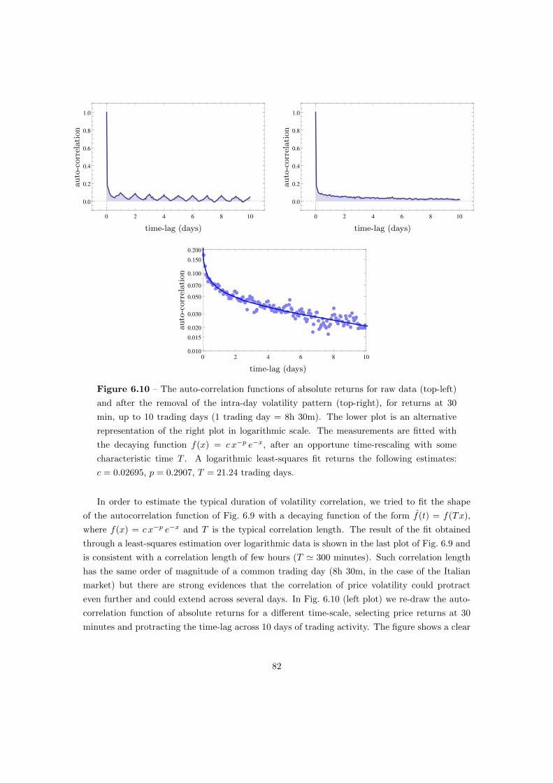
0 2 4 6 8 10
0.0
0.2
0.4
0.6
0.8
1.0
time-lag (days)
auto
-corr
elati
on
0 2 4 6 8 10
0.0
0.2
0.4
0.6
0.8
1.0
time-lag (days)
auto
-corr
elati
on
0 2 4 6 8 10
0.010
0.100
0.050
0.020
0.200
0.030
0.015
0.150
0.070
time-lag (days)
auto
-corr
elati
on
Figure 6.10 – The auto-correlation functions of absolute returns for raw data (top-left)
and after the removal of the intra-day volatility pattern (top-right), for returns at 30
min, up to 10 trading days (1 trading day = 8h 30m). The lower plot is an alternative
representation of the right plot in logarithmic scale. The measurements are fitted with
the decaying function f(x) = c x−p e−x, after an opportune time-rescaling with some
characteristic time T . A logarithmic least-squares fit returns the following estimates:
c = 0.02695, p = 0.2907, T = 21.24 trading days.
In order to estimate the typical duration of volatility correlation, we tried to fit the shape
of the autocorrelation function of Fig. 6.9 with a decaying function of the form f(t) = f(Tx),
where f(x) = c x−p e−x and T is the typical correlation length. The result of the fit obtained
through a least-squares estimation over logarithmic data is shown in the last plot of Fig. 6.9 and
is consistent with a correlation length of few hours (T ' 300 minutes). Such correlation length
has the same order of magnitude of a common trading day (8h 30m, in the case of the Italian
market) but there are strong evidences that the correlation of price volatility could protract
even further and could extend across several days. In Fig. 6.10 (left plot) we re-draw the auto-
correlation function of absolute returns for a different time-scale, selecting price returns at 30
minutes and protracting the time-lag across 10 days of trading activity. The figure shows a clear
82

oscillatory behaviour, whose period corresponds exactly to the typical duration of a trading day.
Such oscillations are due to the intra-day volatility pattern, namely, the typical pattern of the
volatility during the different hours of the day, which recurs almost unaltered day after day. Yet,
in spite of the oscillations, the auto-correlation function remains strictly positive over several
days, showing a significant correlation that is independent on the intra-day volatility pattern.
This observation suggest that the correlation length of stock volatility should be much larger than
few hours, and could extend over days, weeks, or even months. In order to estimate the duration
of the correlation, we tried to remove the effects of the intra-day volatility pattern in the following
way. For each day, we measured the price returns of each stock at specific time-steps, then we
performed two consecutive rescaling: (a) we normalized the returns with respect to the stock
volatility; and (b) we normalized the obtained returns with respect to their standard deviation
at each specific hour of the day. The result has been represented in Fig. 6.10 (right plot), which
shows a slowly decaying auto-correlation function without oscillations. The correlation length T
obtained by fitting the new auto-correlation function with the function f(t) = f(Tx) is T ' 20
trading days (i.e. about 1 month of trading activity), and is about 30 times larger than the one
obtained from infra-day measurements. This result has been presented again in Fig. 6.10.
83

Chapter 7
Large Deviations in Price Returns
In current days, financial risk management has become one of the most fecund activities in finan-
cial industry. The importance of a proper evaluation of financial risks has gradually increased
during the last 40 years because of a variety of factors, such as the technological progress of
financial markets and the consequent intensification of trading activities, the increased volatility
of prices and exchanged rates, the intensification of local and global financial crises, and the
spread of several kinds of derivative instruments which can be used to hedge and speculate on
risk [74].
Financial activities are intrinsically risky, and the most obvious source of financial risk is
due to the stochastic nature of prices and to their high volatility. As a result, the evaluation
of anomalous price returns in different assets and their auto-correlation and cross-correlation
properties are one of the most important subjects of financial risk management.
In this chapter we investigate the occurrence of large deviations and the emergence of conden-
sation phenomena in the financial time series of stock prices, within the theoretical framework of
the Large Deviation Theory described in the first part of this work. In Section 7.4 we present one
of the main results of this thesis, by reporting some original measurements on financial time-series
and by showing an interesting phenomenon: the inhibition of condensation phenomena in stock
prices due to auto-correlation effects. The auto-correlation of stock prices and the occurrence of
extreme events have been already investigated in a wide portion of financial literature (see, for
instance, [81, 80, 121]). Yet, to the best of our knowledge, this is the first time that condensation
phenomena in stock price are explicitly examined and measured on real financial time-series.
7.1 Large Deviations in Price Returns
The fundamental problem in financial risk management is the forecasting of future possible
losses. In the context of stock prices, this problem is translated in the estimation of the proba-
bility density function of price returns, which determines the probability of price-changes and,
84

consequently, of investment losses. Let us consider the following problem: imagine to know the
historical time-series of a stock price at some sampling time τ ; are we able to estimate the future
price of the stock at some time-horizon T = Nτ? If we assume that stock prices are stationary
processes, than we can use the historical information to evaluate the probability distribution
of the returns xτ (t) and propagate this distribution over different time-scales, from τ to Nτ .
According to the cumulative property of price return, we can write:
xNτ (t) =
N−1∑n=0
xτ (t+ nτ) . (7.1)
Therefore, the large-scale return xNτ (t) have the same statistical properties of the sum of N
small-scale returns xτ (t). For the sake of simplicity, in this section we neglect auto-correlation
effects and assume that price returns are i.i.d. random variables, in order to apply the theoretical
results described in the first part of the work. The auto-correlation effects will be recovered in
Section X, and will be presented as a correction to the present model.
According to the decomposition (7.1) and to the assumption of uncorrelated returns, the
quantity xNτ (t) is the sum of N i.i.d. random variables. In agreement with the empirical ob-
servations of Chapter 6, the small-scale returns xτ (t) should be characterized by finite mean µτ
and variance στ . Therefore, we are in the validity regime of the Central Limit Theorem and we
can conclude that, in the limit N →∞, the returns xNτ (t) are normally distributed with mean
and variance determined by the diffusive laws:
µNτ = N · µτ σNτ =√N · στ .
Yet, the Central Limit Theorem provides a good description of the probability distribution
of price returns only for their typical fluctuations, i.e. for xNτ (t) = O(√N), and does not
explain the occurrence of large price changes such as “jumps” or “crashes”, which are the real
sources of financial risk. In order to describe such rare events, we should move form the Central
Limit Theorem to the Large Deviation Theory, and apply the theoretical framework described
in Chapter 2.
Let us define the probability distribution of the returns xτ (t) and xNτ (t) as Pτ (x) and PNτ (x),
respectively. The results prescribed by the LDT depend on the nature of the distribution Pτ (x)
and, specifically, on whether it is a light-tailed or a heavy-tailed distribution.
• Light-Tailed Distribution. If Pτ (x) is a light-tailed distribution then, with a simple
rescaling, we can apply the results prescribed by the Cremer’s theorem and describe the
large deviations of price returns xNτ (t) by means of a rate function. Indeed, we find:
PNτ (x) ∼ e−NIτ (x/N) ,
where Iτ (x) is the Legendre-Fenchel transform of the cumulant generating function related
85

to the distribution Pτ (x). This results has two main consequences: (a) large deviations of
price returns xNτ (t) are exponentially suppressed in N ; and (b) they are generated by a
continuous price drift. Indeed, as described in Section 4.1, the marginal distribution of the
random variables xτ (t) in presence of a deviating mean (or sum) shifts from the original
distribution Pτ (x) to an effective distribution P ∗τ (x), whose mean is equal to the average
deviation xNτ (t)/N . As a result, all small-scale returns xτ (t + nτ) appearing in eq. (7.1)
deviate and fluctuate around the same value, and the stock prices behaves as a regular
diffusive process with an anomalous drift.
• Heavy-Tailed Distribution. If Pτ (x) is a light-tailed distribution then the Cremer’s
theorem cannot be applied and the Large Deviation Principle does not hold any more. As
discussed in Chapter 3, this case gives rise to condensation phenomena, characterized by the
spontaneous breaking of the system’s symmetry and by the emergence of anomalous scaling-
laws in the system’s variables. In the case represented by eq. (7.1), this means that there is
a specific time t+n∗τ between t and t+Nτ such that the return xτ (t+n∗τ) is anomalously
large and is the unique responsible of the final deviation of the large-scale return xNτ (t).
In agreement with the result of Section 4.2, the condensed return xτ (t+n∗τ) scales exactly
as xNτ (t), while all other returns behave as in absence of deviations. In conclusion, large
deviations of heavy-tailed random returns are not continuous, but appear as abrupt price
jumps or crashes, occurring at isolated points and uncorrelated to the surrounding price
fluctuations.
The empirical observations reported in financial literature and in the present work prove
that the probability distribution of price returns is a heavy-tailed distribution, and thus suggest
that large deviations in stock prices should be characterized by condensation phenomena. The
consequence of this claim is that the price-fluctuation process should be characterized by irregular
movements and discontinuities, which generates large and “unpredictable” price-changes. Indeed,
according to the assumption of independent price returns, such discontinuities are completely
unrelated to local price fluctuations and can be described only by a global statistical analysis of
price returns, resulting in the heavy-tailed shape of their probability distribution.
The considerations presented in this section describe how large deviation in stochastic pro-
cesses propagates from small to large times-scales. In light-tailed processes, on average, a large
return xτ (t) does not cause a large final return xNτ (t) because it is too small compared with
the typical size of the diffusive fluctuations. On the contrary, in heavy-tailed processes, a large
return xτ (t) could be extremely large and could propagate unaltered from the fine time-scale τ
to the the coarse time-scale Nτ . Loosely speaking, the larger xτ (t), the larger xNτ (t). This sim-
ple argument allows us to estimate the typical size of large deviations in heavy-tailed stochastic
process. According to the decomposition (7.1) and assuming that only one return xτ (t+ n∗τ) is
responsible for the total return xNτ (t), then the latter should scale as [52]:
|xNτ (t)| ∼ max{|xτ (t)|, |xτ (t+ τ)|, . . . , |xτ (t+ (N − 1)τ)|
}.
86

In the following section, in order to describe the propagation of large deviations in financial
time-series over different time-scales, we review the statistical properties of the maximum of N
i.i.d. random variables with heavy-tailed distributions, focusing to the empirically relevant case
of power-law distributions. In the successive sections, instead, we consider the effect of the auto-
correlation of price returns and we present our original measurements about the emergence of
condensation phenomena in stock prices.
7.2 Extreme Events in Power-Law Distributions
The most obvious difference between light-tailed and heavy-tailed distributions is about the
frequency and the magnitude of the extreme events [123]. Large deviations in heavy-tailed
distributions are much more likely: according to the empirical distribution of price returns (as
measured in Chapter 6), the probability of a 4-deviations return is about 100 times larger than in
the case of Gaussian returns, while the probability of a 6-deviations return is about 100,000 times
larger! In a world where the statistical analysis is often based on the assumption of Gaussian
fluctuations, such events could not be ignored and must be taken into account when evaluating
the financial risk related to large gain/loss in stock prices.
The magnitude of extreme events in stochastic processes with power-law returns can be
estimated with a simple scaling argument. Suppose that large returns of magnitude x1 or greater
are observed with probability p1. According to the power-law decay of the c.d.f. Fx(x) ≈ Ax−α,
the probability to observe an extreme event of magnitude at least equal to x2 = kx1 is about
p2 = p1/kα. Loosely speaking, if a return x ≥ x1 occurs once over T seconds, in average, one
must wait kαT seconds in order to observe a return x ≥ x2. This argument also shows that the
extreme returns in power-law stochastic processes diffuse as the α-th root of time, and obey a
different scaling-law with respect to the typical returns, which diffuse as the square root of time.
In order to express this concept in a more rigorous way, we can invoke the so-called Ex-
treme Value Theorem. Its formulation is equivalent to the CLT, but it applies to the maxi-
mum/minimum of i.i.d. random variables instead of their sum. It was developed by R. A. Fisher
and L. H. C. Tippett in 1928 [57], and then refined by B. V. Gnedenko in 1948 [64].
Extreme Value Theorem: Consider the maximum z ofN i.i.d. random variables {x1, . . . ,xN}and its c.d.f. Fz(z). Now consider two sequences of coefficients aN and bN and the limit:
Fev(z) = limN→∞
Fz(aN z + bN ) .
If the limit exists and is not degenerate, then Fev(z) belongs to one of the following distri-
bution families:
87

Frechet Distribution: Fev(z) =
0 if x < 0 ,
exp(−z−α) if x > 0 .
Gumbel Distribution: Fev(z) = exp(−e−z) .
Weibull Distribution: Fev(z) =
exp(−(−z)−α) if x < 0 ,
1 if x > 0 .
The basins of attraction of the three families depend on the right tail of the distribution Px(x).
If the outcomes of x are bounded above, then z tends to a Weibull variable. If x is not bounded
but Px(x) is thin-tailed, then z tends to a Gumbel variable. Finally, if Px(x) has a power-law
tail, then z tends to a Frechet variable, and the parameter α is equal to the tail-index of Px(x).
In the case of power-law distributions with Fx(x) ≈ Ax−α, the coefficients aN and bN can be
chosen as aN = (AN)1/α and bN = 0. Once that the coefficients are known, we can exploit the
Extreme Value Theorem to find an approximation for Fz(z) and Pz(z) for large values of N . For
all z > 0 we find:
Fz(z) ≈ exp
(− NA
zα
), Pz(z) ≈ αNA
zα+1exp
(− NA
zα
), (7.2)
while Fz(z) = 0 and Pz(z) = 0 for all z < 0. When α > 2, we can use the above formulas to
estimate the expected values 〈z〉 and 〈z2〉 and to find the asymptotic behaviour of z. The result
is:
〈z〉 ≈ Γ(α−1α
)(AN)
1α , 〈z2〉 ≈ Γ
(α−2α
)(AN)
2α ,
which yield 〈z〉 ∼ N1/α and√〈z2〉 − 〈z〉2 ∼ N1/α. Therefore, the maximum of N i.i.d. random
variables with power-law distribution scales as N1/α, but its fluctuations around the typical
values do not decrease, and scale as N1/α as well. This behaviour has been illustrated in Fig.
7.1 in the case of a Student’s t-distribution.
7.3 Preliminary Remarks
In the following section we are going to explicitly investigate the presence of condensation phe-
nomena in financial time-series, yet, before doing so, it is worth to consider the effect of the
auto-correlation of price returns in the frequency and magnitude of large deviations. Indeed,
although returns are not linearly auto-correlated, the strong auto-correlation of the volatility
proves that the assumption of independent returns should be rejected. Can we still claim that
large deviations in stock price obeys the same statistical properties of large deviations in i.i.d.
power-law random variables?
88

0 5 10 15 20
0.0
0.1
0.2
0.3
0.4
0.5
0.6
z
Pz(z)
Figure 7.1 – PDF of the maximum of N i.i.d. random variables drawn from a Student’s
t-distribution with 4 degrees of freedom (with null mean and unitary variance). Three
cases are shown, corresponding to N = 100 (red curves), N = 1000 (purple curves), and
N = 10000 (blue curves). For each case, we show the theoretical estimation (7.2) obtained
through the Extreme Value Theorem (dashed curve), and an empirical estimation obtained
through 100,000 independent draws (continuous curve).
In order to answer this question, we performed a simple test: we compared the real time-
propagation of price returns with the expected propagation in the case of independent returns.
We used the following recipe. We measured the price returns of every stock over the time-scale
of 1 minute, then we divided the whole time-series in time-intervals of 30 minutes (i.e. 30 time-
steps) and we computed the total returns of each interval. This aggregation procedure has been
performed twice: once preserving the natural order of returns, and once after an overall reshuffling
of the time-series. The first output is exactly the time-series of price returns at 30 minutes, while
the second output is an equivalent time-series obtained through independent returns. In Fig.
7.2 we compare the p.d.f.s of the two series. In order to obtain larger statistics, we superposed
the outputs obtained from each stock (after an opportune rescaling with respect to the stock
volatility). As one can see, the two distributions are different, and the expected distribution
is much more Gaussian-like than the real distribution. This difference is also reflected in the
occurrence of large deviations, and it turns out that price returns in real time-series could be
larger then expected.
This simple experiment shows that the time-correlation of price returns strongly affects the
diffusivity of prices and, above all, the magnitude of large deviations. The difference between
dependent and independent returns has been highlighted in Fig. 7.3, where we repeated the
above comparison over different time-scales, from 1 minute to 2 hours. It is worth to stress that
the two distributions of price returns have been obtained starting from the same time-series (i.e.
the time-series of returns at 1 minute), so they are based on the same occurrences of rare events.
The difference between the dependent and the independent cases then suggests that the actual
89

-60 -40 -20 0 20 40 60
10-6
10-5
10-4
0.001
0.01
0.1
1
x30min/σ1min
pro
babilit
yden
sity
-40 -20 0 20 40
0.00
0.02
0.04
0.06
0.08
0.10
0.12
0.14
x30min/σ1min
Minimum Maximum
pro
babilit
yden
sity
Figure 7.2 – Left: the empirical p.d.f. of price returns at 30 minutes (blue) compared with
the expected p.d.f. in the case of independent returns (red). Right: empirical distributions
of minimum and maximum returns over 200 hours drawn from both p.d.f.s (the color
scheme is the same). The expected p.d.f. of returns at 30 minutes has been inferred from
the empirical distribution of returns at 1 minute (see text).
behaviour of large deviation in financial time-series may be non-consistent with the condensation
phenomena observed in i.i.d. random variables.
7.4 Condensation Phenomena in Stock Prices
In this section we present our original measurements about the occurrence of condensation phe-
nomena in the financial time-series of stock prices and the role of auto-correlation effects in the
generation and propagation of large-deviations.
Consider a price return xNτ (t) over a coarse time-scale Nτ . In order to analyse its realization
over time, we need to decompose the total return xNτ (t) over smaller returns xτ (t + nτ) at a
finer time-scale, in accordance with the decomposition (7.1). If xNτ (t) is exceptionally large (in
absolute value), then the partial returns xτ (t+nτ) can exhibit a condensed configuration, when
one return xτ (t + n∗τ) at a specific time-step n∗ is much larger than the others. In order to
quantify the degree of condensation in the time-realization of xNτ (t), we can evaluate the IPR
of all returns xτ (t+ nτ) form n = 0 to n = N − 1. According to the definitions in Sec. 3.5, the
generalized IPR of order k can be written as:
YNτ→τ (t) =
[N−1∑n=0
(xτ (t+ nτ)
)2k] 1k−1
[N−1∑n=0
(xτ (t+ nτ)
)2] −kk−1
,
where we have used the statistical weights (3.9) with η = 2 and x0 = 0. The values attained by
YNτ→τ (t) span from 1/N to 1, which respectively denote perfect homogeneous and condensed
90

0.0 0.5 1.0 1.5 2.0
-50
0
50
time (hours)
pri
ce(c
onfiden
cein
terv
als
)
0.0 0.5 1.0 1.5 2.0
-50
0
50
time (hours)
pri
ce(c
onfiden
cein
terv
als
)
Figure 7.3 – The confidence intervals of price returns as a function of time (over a period
of 2 hours) for actual prices (left) and simulated prices with independent returns (right).
Each line represents a specific quantile in the distribution of returns. The probability
levels are (from the bottom to the top): 0.0001, 0.001, 0.01, 0.1, 0.9, 0.99, 0.999, and
0.9999. The dotted lines are empirical measurements, while the continuous coloured lines
are their best fit obtained through power-law functions. The simulated prices are based
on the distribution of price returns at 1 minute.
realizations of the return xNτ (t). Speaking in terms of the log-price X(t), a perfect homogeneous
realization of the return xNτ (t) appears as a constant drift from X(t) to X(t + Nτ), while a
perfect condensed realization appears as an abrupt price jump at some instant between t and
t+Nτ in a regime of constant prices. More in general, the IPR YNτ→τ (t) quantifies the amount
of regularity in price fluctuations: low values of the IPR denote a regular price diffusion, whereas
high values denote irregular movements with heterogeneous returns and discontinuities. If price
returns were i.i.d. random variables, because of condensation phenomena, large returns xNτ (t)
should be characterized by an IPR YNτ→τ (t) very close to one. Yet, since price returns are not
independent, we may find consistent deviations from this expectation.
In the scatter-plots of Fig. 7.4 we show our definitive results about the presence of condensa-
tion phenomena in financial time-series of stock prices and about the role of auto-correlation of
price returns in the generations of extreme events. In this figure we show the relative behaviour
of the IPR YNτ→τ (t) versus the total returns xNτ(t), measured at different sampling times t. We
selected k = 2 and N = 60, with time-scales τ = 30 sec and Nτ = 30 min. All returns have
been rescaled by the stock volatility στ , in order to perform a superposition of all measurements
obtained from the different stocks in the dataset. The left plot refers to real prices, while the
right plot has been obtained after a general reshuffling of price returns over time: the reshuf-
fling destroys any form of auto-correlation in the sequence of price returns, but preserves their
empirical probability distribution. Furthermore, we evaluated the joint probability distribution
of xNτ (t) and YNτ→τ (t) by means of a smooth kernel estimation with a Gaussian kernel, and
91

xNτ/στ
YNτ→τ(t
)
Raw Dataset
xNτ/στYNτ→τ(t
)
Reshuffled Dataset
Figure 7.4 – Scatter plot of the IPR YNτ→τ (t) versus the total rescaled returns
xNτ (t)/σNτ , denoting the occurrence of condensation phenomena in financial time-series
of stock prices, for τ = 30 sec. and Nτ = 30 min. (N = 60). The two plots refer to time-
ordered data (left) and time-reshuffled data (right), showing 150,000 points per plot. The
blue curves denote the iso-probability contours of the resulting probability distribution,
evaluated through a smooth-kernel density estimation. The difference between the two
plots is entirely due to auto-correlation effects. Condensed realization of large deviations
are characterized by high IPR and large absolute returns, and fall on the top corners
of the scatter plots. The time-ordered dataset shows a clear inhibition of condensation
phenomena.
we added the iso-probability contours of this distribution to the scatter-plots. This procedure
allows us to obtain a more precise evaluation of the results, even where the density of points is
too high or too small for a direct graphical estimation.
As one can see, the two scatter-plots exhibit two different shapes. In the reshuffled dataset,
the points with large absolute returns |xNτ (t)| spread over the whole range of YNτ→τ (t) and
are often characterized by an IPR very close to one. This is in agreement with the theoretical
prediction and confirms that, under the assumption of independent returns, large price-gains
and price-losses tend to be realized through abrupt price changes. Yet, the scatter-plot obtained
from the ordered dataset is significantly different: the shape of the iso-probability contours is
more triangle-like, and the upper corners of the plot are almost empty, denoting a substantial
inhibition of condensation phenomena. Compared to the reshuffled case, the real case shows at
least three important features:
• the absolute returns |xNτ (t)| extend over a wider range of values;
92

• large absolute returns are characterized by lower values of the IPR;
• high values of the IPR are characterized by smaller absolute returns;
The first feature has been already noted in previous section and can be identified as the anomalous
diffusion of extreme events in stock prices. The novelty in the above result is related to the
measurements on the IPR and is expressed by the second feature, which links large returns to
low IPRs. Indeed, the measurements performed on our dataset clearly show that large price
returns are more likely realized through diffusive price fluctuations rather than abrupt price
jumps. According to this result, the correlated and uncorrelated cases are not only quantitatively
different, but also qualitatively reversed, since they tend to generate extreme events with two
opposite mechanisms: “homogeneous diffusion” for correlated prices, and “condensed jumps” for
uncorrelated prices.
The third an last feature, which links high IPRs to small returns, could appear even more
striking. In accordance with stochastic processes driven by fat-tailed noise, one expects that an
extreme price return xτ (t+n∗τ) at some time-step between t and t+Nτ would generate a large
final return xNτ (t). Yet, this seems not true since high-IPR events generate much smaller returns
than low-IPR events. The measurements presented in Fig. 7.4 denote a complex dynamics in
the time-propagation of extreme events which can be stylized by two opposite mechanisms: a
reduction feedback, which reduces the final returns generated by irregular price movements; and
an amplification feedback, which amplifies the regular diffusion of prices.
How can we explain the above results? The inhibition of condensation phenomena in financial
time-series implies that large price jumps are not isolated, but are surrounded by correlated price
fluctuations that either: (a) decrease the final value of the total return xNτ (t); or (b) decrease
the final value of the IPR YNτ→τ (t). In our opinion, the latter phenomenon is more plausible: a
reduction of the total return is contradicted by the absence of linear correlation in price returns;
inversely, a reduction of the IPR could be explained by the positive correlation of volatilities.
The main idea is that an extreme price jump xτ (t+ n∗τ) does not always generate an high IPR
YNτ→τ (t), but the final value of the IPR depends on the noise background, i.e. on the other price
returns xτ (t+ nτ) that occur in the same time-window. Because of the volatility clustering, an
extreme return is likely preceded or followed by other returns with similar magnitude, therefore,
the final return xNτ (t) could be very large even if the IPR YNτ→τ (t) remains close to the
minimum value. This effect could explain both the reduction and amplification feedbacks at the
same time, and is validated by further observations presented in [55] and in Section 8.2.
The result of our measurements must not be confused. One could conclude that large returns
xNτ (t) at coarse time-scales are not caused by large returns xτ (t) at fine time-scales because
their IPR YNτ→τ (t) remains low, but this would not be true. According to our explanation,
large excursions of stock prices are still generated by extreme events at smaller time-scales, but
the key point is that such events are not perceived as jumps. The above results suggest that the
notion of “jump” is scale-dependent: a price jump xNτ (t) measured at some coarse time-scale Nτ
does not imply the occurrence of real price-discontinuity at some instant between t and t+Nτ ;
93

on the contrary, such return has more likely been realized through a price-diffusion process with
high volatility, and is perceived as a jump only when it is observed at the specific time-scale
Nτ . This phenomenon could be addressed as an effect of the so-called volatility intermittency,
which denotes the typical behaviour of volatility characterized by irregular outburst with mixed
magnitudes and self-similar scaling properties [4, 17].
According to the observation presented in this section, we can stylize the behaviour of stock
prices through the following statement. Stock prices are stochastic processes driven by correlated
random returns with hybrid statistical properties that derive from both thin-tailed and fat-tailed
random variables: the empirical distribution of individual returns is a fat-tailed distribution, but
the price-diffusion process is generated by a thin-tailed dynamics that enhances the regular fluc-
tuations of prices and inhibits the discontinuities. The present phenomenon could be arguably
caused by a self-exciting nature of price fluctuations, but the underlying dynamics is not com-
pletely clear and is currently a matter of debate (see [120, 75]). Notwithstanding the causes of
this phenomenon, the observations presented in this work highlight a non-trivial feature of stock
prices with strong implications in the estimation of extreme price returns and in the evaluation
of the financial risk related to large gains and losses of stock prices.
Before concluding this section, let us make some additional remarks. The result presented
in Fig. 7.4 is restricted to the specific time-scales τ = 30 sec and Nτ = 30 min, but the above
observation can be repeated on different time-scales and seems to be scale-independent. The
specific choices of the time-scales is not constrained to physical requirements, but rather to
statistical ones. The number of samples N should be large enough to have statistical relevance,
but should not be too large, otherwise the frequency of extreme events could be too small.
Moreover, the time-step τ should be as small as possible, in order to maximize the number
of measurements over a finite observation time, but should remain large enough to observe
significant fluctuations of the returns xτ (t). According to the characteristic of the available
dataset, the most evident results have been achieved with the presented time-scales, namely, τ
= 30 sec and Nτ = 30 min. However, the phenomenon highlighted in Fig. 7.4 has been observed
on different time-scales, ranging from few seconds to one trading day, and has been observed also
in different markets and different periods, acquiring the solidity of a stylized fact. Additional
information and measurements about this topic can be found in [55].
94

Chapter 8
Modelling Extreme Price Returns
The observations presented in Chapters 6 and 7 highlighted how the simple hypotheses of the
Geometric Brownian Motion (GBM) provide a good description of stock prices only at a first
order approximation. The GBM accounts for both the diffusivity of log-prices and the lack of
linear correlation in price returns; yet, it completely fails in capturing the fat-tailed nature of
returns and, above all, the complex effects of the auto-correlation of the volatility. For these
reasons, the GBM is a good description of stock prices in regimes with small and regular price-
diffusion, but is completely unsuited to characterize the frequency and generation of extreme
price returns. Unfortunately, given the statistical properties of stock prices (large volatility and
small drifts, fat-tailed noise, high frequency of extreme events), the estimation of extreme returns
is a cornerstone of quantitative finance, and has become one of the most important issues in the
evaluation of financial risk.
8.1 Beyond the Geometric Brownian Motion
The theoretical framework defined by the GBM for the fluctuations of stock prices found its
popularity with the formulation of the Black-Scholes-Merton model in 1973, one of the great
milestones of financial research. During the last 40 years, the simple hypotheses of the GBM
have been widely extended and corrected through a large variety of statistical models [91]. In this
section, we present a short review of the most important models from a historical and conceptual
point of view. The following list is far from being complete, and has no further presumption
than presenting some of the most common solutions that could overcome the limitation of the
Geometric Brownian Motion and that found a practical application in financial activities such
as the derivative pricing and the financial-risk management.
95

8.1.1 The Jump-Diffusion Model
This model was first proposed by Merton in 1976 [96], in order to describe the non-Gaussianity of
price returns. As the name suggests, the model is defined as the sum of two different stochastic
process: a GBM, which accounts for the regular fluctuation of price (diffusion); and a compound
Poisson process, which accounts for anomalous price returns (jumps). The model is defined
through the following stochastic differential equation:
dS(t) = µS(t) dt+ σ S(t) dW (t) + S(t) dY (t) ,
where Y (t) denotes the jump-component of the stochastic process and is defined as:
Y (t) =
N(t)∑n=1
yn .
In the above formula, N(t) is a Poisson process with intensity λ and denotes the number of jumps
up to the instant t, whereas {yn} are i.i.d. random variables drawn from a specific probability
distribution and denote the price returns generated by each jump. The three random processes
W (t), N(t), and {yn} are assumed to be mutually independent. The jump-component Y (t) can
be finely tuned in order to obtain a faithful representation of the empirical distribution of returns,
yet, even in that case, the jump-diffusion model retains a substantial weakness: assuming the
independence of the underlying processes, this model does not capture the auto-correlation of
price returns. As discussed in Section 7.4, the auto-correlation of returns is a core aspect in the
statistical analysis of stock prices. Even if price returns are distributed according to a fat-tailed
distribution, the genesis and propagation of extreme returns do not satisfy the expectation based
on independent random variables and exhibit a much more complex dynamics with a different
phenomenology. The lack of auto-correlations in the jump-diffusion process could compromise
the focal point of the model itself, namely, the statistical description of extreme events.
8.1.2 Stochastic-volatility Models
A much more realistic category of models for the description of stock prices goes under the name
of stochastic-volatility models. This kind of models are obtained by substituting the volatility
parameter σ in the GBM with a new stochastic process. In a quite general formulation, a
stochastic-volatility model can be defined by the following set of stochastic differential equation:
dS(t) = µS(t) dt+√V (t)S(t) dW1(t) ,
dV (t) = α(S, V, t) dt+ β(S, V, t) dW2(t) ,
where the process V (t) denotes the variance of the log-prices S(t), and the generic functions
α(S, V, t) and β(S, V, t) are some drift-like and volatility-like parameters, respectively, which de-
96
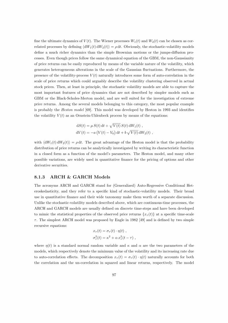
fine the ultimate dynamics of V (t). The Wiener processes W1(t) and W2(t) can be chosen as cor-
related processes by defining 〈dW1(t) dW2(t)〉 = ρdt. Obviously, the stochastic-volatility models
define a much richer dynamics than the simple Brownian motions or the jumps-diffusion pro-
cesses. Even though prices follow the same dynamical equation of the GBM, the non-Gaussianity
of price returns can be easily reproduced by means of the variable nature of the volatility, which
generates heterogeneous alterations in the scale of the Gaussian fluctuations. Furthermore, the
presence of the volatility-process V (t) naturally introduces some form of auto-correlation in the
scale of price returns which could arguably describe the volatility clustering observed in actual
stock prices. Then, at least in principle, the stochastic volatility models are able to capture the
most important features of price dynamics that are not described by simpler models such as
GBM or the Black-Scholes-Merton model, and are well suited for the investigation of extreme
price returns. Among the several models belonging to this category, the most popular example
is probably the Heston model [69]. This model was developed by Heston in 1993 and identifies
the volatility V (t) as an Ornstein-Uhlenbeck process by means of the equations:
dS(t) = µS(t) dt+√V (t)S(t) dW1(t) ,
dV (t) = −a(V (t)− V0
)dt+ b
√V (t) dW2(t) ,
with 〈dW1(t) dW2(t)〉 = ρ dt. The great advantage of the Heston model is that the probability
distribution of price returns can be analytically investigated by writing its characteristic function
in a closed form as a function of the model’s parameters. The Heston model, and many other
possible variations, are widely used in quantitative finance for the pricing of options and other
derivative securities.
8.1.3 ARCH & GARCH Models
The acronyms ARCH and GARCH stand for (Generalized) Auto-Regressive Conditional Het-
eroskedasticity, and they refer to a specific kind of stochastic-volatility models. Their broad
use in quantitative finance and their wide taxonomy make them worth of a separate discussion.
Unlike the stochastic-volatility models described above, which are continuous-time processes, the
ARCH and GARCH models are usually defined on discrete time-steps and have been developed
to mimic the statistical properties of the observed price returns {xτ (t)} at a specific time-scale
τ . The simplest ARCH model was proposed by Engle in 1982 [49] and is defined by two simple
recursive equations:
xτ (t) = στ (t) · η(t) ,
σ2τ (t) = κ2 + αx2
τ (t− τ) ,
where η(t) is a standard normal random variable and κ and α are the two parameters of the
models, which respectively denote the minimum value of the volatility and its increasing rate due
to auto-correlation effects. The decomposition xτ (t) = στ (t) · η(t) naturally accounts for both
the correlation and the un-correlation in squared and linear returns, respectively. The model
97

has been developed in order to describe a non-linear feedback in price volatilities which leads
to the self-excitation of price fluctuations. Quite interestingly, the volatility στ (t) is defined as
a deterministic function of the past returns, and its stochastic nature depend only on the noise
components η(t). The Engle’s model defines stock prices as Markov processes, and is usually
denoted as ARCH(1) because its recursive relations are protracted to just one time-step. From
its formulation to current days, the original ARCH(1) model has been widely enriched with the
addition of new terms and further corrections, in order to extend its range of applications and
reproduce more faithful time-series of price returns. The ARCH(p) model, for instance, is a long-
memory extension of the ARCH(1) model whose dynamics protract over additional time-steps,
namely:
σ2τ (t) = κ2 + α1 x
2τ (t− τ) + · · ·+ αp x
2τ (t− p τ) .
In 1986, in order to improve the validity of the ARCH(p) model without the addition of a large
number of parameters, Bollerslev proposed a diversification of the time-dependent terms with
the introduction of a direct volatility auto-correlation [15]. This improvement led to the so-called
GARCH(p, q) model, defined as:
σ2τ (t) = κ2 + α1 x
2τ (t− τ) + · · ·+ αp x
2τ (t− p τ) +
+ β1 σ2τ (t− τ) + · · ·+ βq σ
2τ (t− q τ) .
There is no precise prescription about the most appropriate number of parameters to be included
in the definition of the ARCH(p) and GARCH(p, q) processes. In recent days, the models have
been further modified in order to overcome this problem and to achieve even more generality.
The long-memory dynamics of the ARCH(p) model can be extended over the entire historical
series by substituting the infinite sequence of parameters {αp} with some time-dependent kernel
K(t). This lead to a formal ARCH(∞) model defined by:
σ2τ (t) = κ2 +
∞∑n=1
K(nτ)x2τ (t− nτ) .
Among all further extensions, we mention the HARCH model (Heterogeneous ARCH, [100]),
which includes heterogeneous returns over mixed time-scales:
σ2τ (t) = κ2 +
∞∑n=1
∞∑m=n
K(nτ,mτ)x2nτ (t−mτ) ,
98

and the QARCH model (Quadratic ARCH, [118]), which express the volatility στ (t) as the most
general quadratic function of the historical returns {xτ (t)}, namely:
σ2τ (t) = κ2 +
∞∑n=1
K1(nτ)xτ (t− nτ) +
+1
2
∞∑n=1
∞∑m=1
K2(nτ,mτ)xτ (t− nτ)xτ (t−mτ) .
The literature about ARCH and GARCH models and their possible variations is huge (see, for
instance, [91, 17, 30]). The application of ARCH-like models in quantitative finance is extremely
wide, and ranges from the description of stock prices, interest rates, and foreign exchange rates,
to the pricing of derivative securities. Yet, the variety of models and the elevate number of
parameters do not always simplify the statistical analysis of financial time-series, and it is often
necessary to perform complex procedures of model-fitting and parameter estimation.
8.1.4 The Multi-Fractal Random Walk
This specific kind of stochastic process has been introduced by Bacry, Delour, and Muzy in 2001
[4] to describe the complex self-similar nature of price fluctuations across different time-scales.
In order to introduce this model, let us define the difference between “mono-fractal” and “multi-
fractal” stochastic processes. In a scale-invariant process, the realized moments Mqτ defined in
eq. (6.4) obey the scaling-law:
Mqτ ∼ τ ζq ,
where ζq is some scaling-exponent depending on the parameter q. When ζq is a linear function of
q, i.e. ζq = Hq, then the process is said to be mono-fractal, otherwise it is said to be multi-fractal.
According to the diffusivity law στ = σ√τ , which is theoretically predicted by the GBM and
empirically observed in financial time-series (see Section 6.4), one could expect H = 1/2. Yet, in
recent works [4], it has been argued that the scaling exponent ζq is a strictly convex function of q,
and so that stock prices are multi-fractal stochastic processes with non-trivial scaling exponents.
As the name suggests, the Multi-Fractal Random Walk is a theoretical example of a stochastic
process with a multi-fractal scaling law. With a slightly abuse of notation, the model can be
defined by the stochastic differential equation:
dX(t) = σeω(t)dW (t) ,
where ω(t) is a specific stochastic process that determines the range of price returns and mimic
the effects of the volatility clustering. The process ω(t) is defined as a stationary Gaussian
process with a logarithmic correlation function, namely:
〈ω(t)〉 = −λ2C(0) , 〈ω`(t)ω`(t′)〉 = λ2C(t− t′) ,
99

where:
C(t) '
− log |t|Tint
if |t| < Tint
0 if |t| > Tint
Since C(0) diverges, the process ω(t) is mathematically undefined; yet, the entire process X(t)
can be rigorously determined by introducing a high-frequency cut-off in the correlation function
C(t) and letting the cut-off tend to zero [101]. The logarithmic divergence of C(0) is a necessary
ingredient and is the very responsible of the multi-fractal behaviour of the process X(t).
The Multi-Fractal Random Walk is defined by only two parameters, namely, the intermittency
coefficient λ2 and the integral scale Tint. They respectively define the strength and the maximum
time-scale of the volatility auto-correlation. For all time-scales τ < Tint, the realized moments
of the Multi-Fractal Random Walk obey the scaling law Mqτ ∼ τ ζq with a scaling-exponent:
ζq =q
2
[1− λ2(q − 2)
],
and this results proves the multi-fractal nature of the process for all λ2 > 0 [4]. For q = 2, the
scaling-exponent reduces to ζ2 = 12 and reproduces the classical diffusivity of prices. In spite of
the relative simplicity of the process and its mathematical beauty, the Multi-Fractal Random
Walk is able to capture many empirical features of stock prices, such as: (a) the un-correlation
of linear returns; (b) the volatility clustering; (c) the power-law distribution of returns; (d) the
diffusivity of price; and (e) the anomalous scaling-laws of the realized moments. Arguably, the
only stylized facts that are not included in the this list are those related to the asymmetry of the
price-fluctuation process, such as the time-reversal asymmetry and the “leverage effect” [27].
8.2 Condensation Phenomena and Volatility Clustering
In order to conclude this part of the work about condensation phenomena in stock prices, we
try to reproduce the empirical observations reported in Section 7.4 with theoretical simulations.
As we argued above, the inhibition of condensation phenomena in the time-series of stock prices
could be an effect of the volatility clustering, and most of the models presented in this chapter
have been explicitly developed to describe this feature. In our opinion, the most interesting
model among the presented ones is the Multi-Fractal Random Walk. Indeed, this model is able
to reproduce many stylized facts about stock prices with very few assumptions and just two free
parameters. Therefore, we employed the Multi-Fractal Random Walk to generate a simulated
time-series of price returns with the same statistical properties of the one examined in Section
7.4, and we repeated the previous analysis on the new series.
The Multi-Fractal Random Walk is determined by the intermittent coefficient λ2 and the
integral scale Tint. The empirical value of λ2 could be determined either from the scaling laws
of the empirical moments Mqτ or from the decay of the auto-correlation function of the log-
volatility, which is a rough estimate of the covariance function 〈ω(t)ω(t′)〉. In any case, the
100

- 4 - 2 0 2 4
0.005
0.010
0.050
0.100
0.500
1.000
xτ/στ
pro
bab
ilit
yd
ensi
ty
Figure 8.1 – Comparison of the empirical probability distributions of price returns at
τ = 30 minutes obtained from real time-series (blue curve) and simulated time-series
(red curve). The simulations have been generated with a Multi-Fractal Random Walk
with intermittency coefficient λ2 = 0.03 and integral scale Tint = 1000 τ , as for the
measurements in Fig. 8.2.
multi-fractality is not a manifest feature of stock prices, and the parameter λ2 turns out to be
very small. According to the results presented in [17], the intermittency coefficient is about
λ2 ≈ 0.03. Although weak, the multi-fractal behaviour of stock prices could be observed on a
wide range of time-scales, from few minutes to several days. This suggest that the integral scale
Tint should be very large compared to the typical observation scales. For our simulations, we
selected an integral scale of 1000 returns (i.e. Tint = 1000 ·Nτ), which, according to our empirical
time-scales (N = 60, τ = 30 seconds), corresponds to a period of several trading days.
In Fig. 8.1, we show a comparison between the empirical distributions of price returns obtained
form the real and the simulated time series, over a time-scale of 30 minutes. As one can see,
the agreement between the two distributions is very good, and the Multi-Fractal Random Walk
is perfectly able to reproduce the heavy-tailed nature of price returns over the observed sizes
of the statistical sample. In Fig. 8.2, instead, we show our conclusive result, by repeating the
same measurements performed in Fig. 7.4 in the case of simulated returns. The new figure is
able to replicate the old findings very faithfully. As in the previous case, the time-ordered case is
different from the reshuffled case and shows both an inhibition of condensation phenomena and
an amplification of diffusive returns. There is no manifest difference between Figs. 7.4 and 8.2,
except for the presence of few separate points in Fig. 7.4 with vanishing returns and IPR very
close to 1. Those points are generated by micro-structural effects and are due to the presence of
the tick-grid, which prevents all price-fluctuations that are smaller than the tick-size. Besides this
negligible effects, the Multi-Fractal Random Walk reproduces exactly the observation presented
in Chapter 7, and explains our empirical findings as the result of the volatility clustering.
101

xNτ/στ
YNτ→τ(t
)
Raw Dataset
xNτ/στ
YNτ→τ(t
)
Reshuffled Dataset
Figure 8.2 – Scatter plot of the IPR YNτ→τ (t) versus the total rescaled returns
xNτ (t)/σNτ , denoting the occurrence of condensation phenomena in simulated time-series
of price returns. The simulation has been generated with a Multi-Fractal Random Walk
with intermittency coefficient λ2 = 0.03 and integral scale Tint = 1000 ·Nτ , with N = 60.
The two plots refer to time-ordered data (left) and time-reshuffled data (right), show-
ing 150,000 points per plot. The blue curves denote the iso-probability contours of the
resulting probability distribution, evaluated through a smooth-kernel density estimation.
The difference between the two plots is entirely due to auto-correlation effects. The fig-
ure reproduces the same empirical observations reported in figure 7.4 and related to real
financial time-series.
102

Part III
Statistical Inference of the
Market Structure
103

Chapter 9
The Financial Network
In the previous part of the work, we measured the fundamental statistical properties of stock
prices, focusing in the generation and propagation of extreme price returns. In some sense, we
tried to find an answer to the general question: How do stock prices change? Now, instead, we
change our perspective and focus to another fundamental question: Why do stock prices change?
In the classical financial explanation supported by the Efficient Market Hypothesis, price
changes are generated by the release of news. Indeed, the diffusion of new pieces of information
forces the financial agents to reconsider their previous expectation, leading to a new sequence of
trades and eventually to a new equilibrium in stock prices. There are no doubts that financial
market may really react to economical and political announcements, yet, the real question is
whether all variations in stock prices are determined by this kind of mechanism or not [119, 75].
The question becomes even more important when it is applied to extreme price returns:
are large price gains/losses induced by information shocks? The literature usually separates
exceptional events in financial time-series as either endogenous or exogenous events, depending
on whether they have been generated by the internal dynamics of financial markets or by some
external event such as political announcements, economical news, environmental disasters, or
other occurrences in non-financial sectors of the society. Many analytical studies on stock prices
suggest that a large part of price jumps or crashes are not related to external causes and cannot
be classified as exogenous events [75].
In last years, the idea that price changes are always generated by the information flow has
raised many doubts. There are strong evidences that the volatility of stock prices is too high to
be entirely explained by the release of objective news or by the changes in the underlying values
[119].. In addition to this, the observed features of stock prices concerning the auto-correlation
of volatility (see Section 6.5, for instance) may be the sign of a complex non-linear dynamics that
enhances the endogenous fluctuations of stock prices. Loosely speaking, financial markets could
be characterized by feedback mechanisms that cause trades to induce other trades, giving raise
to an avalanche-like dynamics that generates excess volatility and eventually leads to financial
104

crashes, as it happens in many non-linear physical systems [75].
Understanding this kind of dynamics is an extremely important goal in order to explain
and forecast the emergence of exceptional events in financial markets. Yet, in our opinion, the
investigation of non-linear feedbacks in market dynamics cannot be focused to the analysis of
individual stock prices, but it must be extended to financial markets as a whole. Indeed, it is a
well established fact that the prices of different financial instruments are highly correlated, and
that large price-gains and price-losses are likely to occur in several assets at the same time [18]. In
order to convince about this, one could recall the notorious Flash Crash in the Dow Jones index in
May 6, 2010, when, within few minutes, an unexpected price-loss in the E-mini S&P 500 contracts
propagated towards different stocks, financial indices, and derivative instruments, escalating in
one of the largest price-drops in the history of the U.S. market [131]. As a consequence, one
could arguably affirm that the self-exciting dynamics of the trading activity is not restricted
to single assets, and is rather determined by some form of interaction between several financial
instruments in the same market.
In the following chapters, we develop the concept of interacting assets by introducing a specific
model for the propagation of price changes between different stocks in the market. The presented
model is based on the assumption of an interaction network between the several components of
the financial market, supported by the observation of cross-correlations in stock prices. The large
amount of data at our disposal should allow us to check the validity of the model and to infer the
interaction network at the basis of the financial market, comparing the relevance of endogenous
price fluctuations with respect to exogenous ones. The inference of the financial network will be
achieved by invoking the probabilistic framework of the Bayesian inference process [62], which
allows the estimation of the unknown parameters of the model (i.e. the interaction couplings
between different stocks) from the observation of the empirical data.
9.1 Cross-Stock Correlations in Financial Markets
In Chapter 6, we presented some stylized facts about stock prices by analysing the financial time-
series of individual stocks, neglecting any possible form of correlation in the returns of different
stocks. At this stage, in order to investigate the underlying mechanism at the basis of price
fluctuations, it is worth to analyse the cross-stock correlation properties of price returns over the
whole financial market. The following observations fit with the idea of a self-exciting feedback
in trading dynamics and will be at the basis of the market model described in Chapter 10.
The cross-correlation properties of stock prices are a well-established fact [20, 77]. Here, we
recover the most important result about this issue by analysing the financial dataset presented
in Chapter 5. The following results have been obtained from the time-series of the price returns
xτ (t) for all 20 stocks in the dataset and for the whole period of observation (500 days). We
selected a time-scale τ = 30 minutes (15 returns per day) and we measured the returns xτ (t)
at the same sampling times for all stocks, in order to obtain homogeneous time-series. The
105

1 5 10 15 20
1
5
10
15
20
j
i
Cij (ordered series)
-1.0
- 0.5
0.0
0.5
1.0
1 5 10 15 20
1
5
10
15
20
j
i
Cij (reshuffled series)
Figure 9.1 – The cross-stock correlation matrix Cij evaluated from the time-series of price
returns at 30 minutes over the whole dataset. Two cases are shown, obtained from the
time-ordered dataset (left) and a time-reshuffled dataset (right). The reshuffling destroys
any form of cross-stock correlation, reducing Cij to an identity matrix with statistical
fluctuations.
resulting sample is composed of M = 7500 observations for N = 20 assets, yielding a quality
factor M/N = 375.
At the first order, the correlation properties of stock prices can be analysed by means of the
empirical correlation matrix:
Cij =1
M
M∑m=1
x(i)τ (tm)
σ(i)τ
x(j)τ (tm)
σ(j)τ
,
where the superscripts (i) and (j) refer to different stocks, and {tm} is the sequence of the
sampling times. By definition, the diagonal elements of the matrix are normalized to one. The
empirical correlation matrix Cij obtained from the examined dataset is shown in Fig. 9.1. By
comparison, we also show the case of a totally uncorrelated dataset with the same statistical
properties of the examined one. The uncorrelated dataset has been obtained from the real
financial time-series by reshuffling the whole sequences of price returns stock-by-stock. As one
can see, the two matrices are very different: in the reshuffled case, the off-diagonal elements
fluctuate between −0.03 and +0.03, whereas, in the time-ordered case, they are always positive
and far above the typical scale of statistical fluctuations, spanning from 0.3 to 0.8. This result
clearly shows that stock prices are not statistically independent, but are characterized by an
overall positive correlation over the whole financial market. Moreover, the patterns observed
in the correlation matrix are too regular to be explained as statistical noise, and should be the
result of a deeper correlation structure between some specific groups of stocks.
106

1 2 3 4
0.2
0.5
1.0
2.0
5.0
10.0
20.0
0.2
0.5
1.0
2.0
5.0
10.0
20.0
algorithm step
λn λn
Figure 9.2 – The eigenvalues λn of the cross-stock correlation matrix during different
step of the “information extraction” algorithm described in text. The magnitude of the
eigenvalues is reported on the y-axis. The first column (step 1), refers to the real cor-
relation matrix Cij reported in Fig. 9.1 and shows the presence of a highly deviating
eigenvalue. The other columns refer, in the order, to the matrices C ′ij , C′′ij , C
′′′ij (see text).
The gray stripe centred at 1 denotes the typical range of the statistical fluctuations for
the eigenvalues, and has been estimated from the reshuffled correlation matrix reported
in Fig. 9.1.
In order to investigate the structure of the financial market in more details, we can analyse
eigenvalues and eigenvectors of the correlation matrix. Indeed, by assuming that Cij has been
obtained from multivariate normal random variables, we can statistically decompose the price
returns xτ (tm) as:
x(i)τ (tm) ' σ(i)
τ
N∑n=1
√λn v
(i)n ηn(tm)
where λn and vn are the n-th eigenvalue and eigenvector of Cij , respectively, and {ηn(tm)} is a
set of N ×M independent random variables with a standard normal distribution. The empirical
spectrum of the correlation matrix Cij is shown in Fig. 9.2 (left spectrum), in comparison to the
typical range of their statistical fluctuations. The highest eigenvalue is widely separated from the
bulk of the spectrum and is about 10 time larger than its expected value in the case of uncorrelated
prices. Such a large eigenvalue cannot be explained in terms of statistical noise and should be
related to some real correlation in the financial market. The corresponding eigenvector is shown
in Fig. 9.3 (top) and can be roughly identified as the homogeneous vector. This fluctuation mode
can be recognized as the “market” itself (namely, the market mode [20, 55]) and proves that, at
a first-order approximation, the rescaled price returns xτ (t)/στ are about the same for all stocks
in the market. The relative contribution of the market mode to the total volatility of each stock
107

0 5 10 15 20- 0.4
- 0.2
0.0
0.2
0.4
0.6
Cij
i
v(i)1
0 5 10 15 20- 0.4
- 0.2
0.0
0.2
0.4
0.6
C′ij
i
v(i)1
0 5 10 15 20- 0.4
- 0.2
0.0
0.2
0.4
0.6
C′′ij
i
v(i)1
Figure 9.3 – The principal eigenvector of the cross-stock correlation matrix (the one
related to the highest eigenvalue). Three cases are shown, corresponding to different steps
of the “information extraction” algorithm described in text and related to the matrices
Cij , C′ij , C
′′ij . The first case (top) refers to the real correlation matrix reported in Fig.
9.1. Blue components denote the stocks from the “financial“ economic sector, whereas
red components denote the ones from the “utility” sector.
can be estimated through the ratio λmax/N , and turns out to be about the 45% of the total
volatility observed in the dataset.
Beyond the global correlation generated by the market mode, the correlation matrix Cij may
hide a more interesting structure. In order to verify this, we employed the following method: we
evaluated the empirical realization of the market mode over the whole time-series, we rescaled
it for the volatility of each stock, and we subtracted it from the original series of price returns
xτ (t). The result is a de-trended time-series x′τ (t), which has been employed to evaluate a new
correlation matrix C ′ij . At each time-step, the empirical realization of the market mode has been
evaluated as the arithmetic mean of the rescaled price returns xτ (t)/στ of all stocks. In this
way, the new correlation matrix C ′ij has exactly one null eigenvalue corresponding to the new
market mode. The spectrum of the matrix C ′ij is shown in Fig. 9.2. Compared to the original
one, the new spectrum diffuses in a narrower range of values and shrinks towards the typical
range of the statistical fluctuations. Yet, the dispersion of the eigenvalues is still too high to
be explained by pure noise, and the highest ones could be determined by some real correlation
effect. The eigenvector corresponding to the highest eigenvalue of C ′ij is shown in Fig. 9.3 and
108
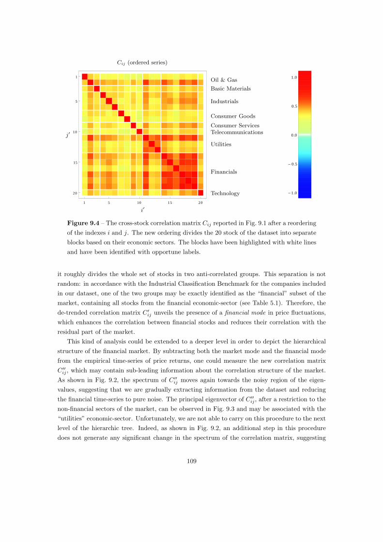
1 5 10 15 20
1
5
10
15
20
i′
j′
Cij (ordered series)
Oil & Gas
Basic Materials
Industrials
Consumer Goods
Consumer ServicesTelecommunications
Utilities
Financials
Technology -1.0
- 0.5
0.0
0.5
1.0
Figure 9.4 – The cross-stock correlation matrix Cij reported in Fig. 9.1 after a reordering
of the indexes i and j. The new ordering divides the 20 stock of the dataset into separate
blocks based on their economic sectors. The blocks have been highlighted with white lines
and have been identified with opportune labels.
it roughly divides the whole set of stocks in two anti-correlated groups. This separation is not
random: in accordance with the Industrial Classification Benchmark for the companies included
in our dataset, one of the two groups may be exactly identified as the “financial” subset of the
market, containing all stocks from the financial economic-sector (see Table 5.1). Therefore, the
de-trended correlation matrix C ′ij unveils the presence of a financial mode in price fluctuations,
which enhances the correlation between financial stocks and reduces their correlation with the
residual part of the market.
This kind of analysis could be extended to a deeper level in order to depict the hierarchical
structure of the financial market. By subtracting both the market mode and the financial mode
from the empirical time-series of price returns, one could measure the new correlation matrix
C ′′ij , which may contain sub-leading information about the correlation structure of the market.
As shown in Fig. 9.2, the spectrum of C ′′ij moves again towards the noisy region of the eigen-
values, suggesting that we are gradually extracting information from the dataset and reducing
the financial time-series to pure noise. The principal eigenvector of C ′′ij , after a restriction to the
non-financial sectors of the market, can be observed in Fig. 9.3 and may be associated with the
“utilities” economic-sector. Unfortunately, we are not able to carry on this procedure to the next
level of the hierarchic tree. Indeed, as shown in Fig. 9.2, an additional step in this procedure
does not generate any significant change in the spectrum of the correlation matrix, suggesting
109

that we cannot extract reliable information any more. Each de-trending procedure adds artificial
noise to the time-series and slowly corrupts the datasets. Moreover, the number of stocks in our
dataset is too small to identify new important sectors and, at this stage, the heterogeneity of the
individual stocks in the same sectors becomes too relevant.
In spite of its simplicity, the presented procedure highlights the presence of a clear structure
in the financial market and supports the idea of an interaction network between different stock
prices. At a first approximation, the market structure is related to the economic sectors of the
several companies listed in the dataset and, at least in principle, it could be directly inferred from
the dataset constituents. In order to convince about this, we re-draw the correlation matrix Cij
of Fig. 9.1 after an opportune permutation of the stocks indexes, regrouping the different stocks
into separate sectors. The result is presented in Fig. 9.4 and shows how the heterogeneities in the
correlation matrix tend to be uniformed into visible blocks, corresponding to the several sectors
of the financial market [20].
The market structure highlighted by the empirical shape of the correlation matrix could be
the result of an interacting dynamics between all stocks in the financial market. Yet, the analysis
of the correlation matrix does not provide any information about the underlying dynamics that
generates the correlations. In the following chapter, in order to investigate this dynamics in more
details, we will present an original model for the financial market based on interacting stock
prices. Then, using a statistical-inference procedure, we will estimate the model’s parameters
directly from the empirical data and we will obtain precise information about the interacting
structure of the market.
110

Chapter 10
A Model for Interactive Stock
Prices
In this chapter we present our model for the financial market based on interacting stock prices.
The model is developed on very basic assumptions, and is obtained by means of several mathe-
matical simplifications. Our purpose is not to describe the financial market in a hyper-realistic
approach, but rather to describe a clear and simple interacting mechanism between stock prices
that can be later recognized in real markets from their financial time-series. Basically, the fol-
lowing model is based on two separate components: a deterministic term, which describes the
desired interactions between stock prices, and a stochastic term, which describes all other forms
of price dynamics that are not captured by the former term. In this perspective, the two terms
describe the endogenous and exogenous factors at the basis of the price fluctuation model, re-
spectively. By comparing the model with the empirical data we can in principle evaluate the
relative contributions of each term to the real price dynamics. If the contribution of the stochas-
tic term is relatively small, then the deterministic term explains a significant amount of the price
dynamics and is a faithful description of the real financial interactions.
According to the above considerations, the ultimate purpose of this work is the statistical
inference of the model parameters from the empirical data at our disposal, in order to estimate
the relevance of all components of the model. The dynamics described by the following model is
based on the existence of an interaction network between all stock prices in the financial market.
A statistical-inference procedure, then, could be able to recognize the relative strengths of the
interactions between the different stocks and could outline the definitive structure of the financial
market. In order to move beyond the simple correlation properties of stock prices and capture
their real interaction mechanisms, the presented model should describe the price dynamics at
very high frequency, detecting the time-heterogeneities in the price-fluctuation process that could
establish a cause-effect relationship between the movements of different stock prices.
111

10.1 Micro-Structural Noise
Stock prices are usually perceived as unique continuous stochastic processes, yet, when they
are observed at very high frequencies, they appear very differently. First of all, prices are not
unique and may have different definitions (e.g. the executed price and the mid-price). At low
frequency, the discrepancies between the different definitions are much smaller than the typical
price-fluctuation and can be neglected, but, at high frequency, this is not true any more. In
addition, the natural price-fluctuation process is altered by the regulations. The most obvious
example is due to the tick-rule, which sticks prices to discrete values. Finally, price-changes
are not continuous and are determined by the arrival of orders to the market. For instance,
the executed price is defined by market-orders, while the mid-price is defined by limit-orders
and cancellations. As a result, stock prices at high frequencies are not continuous processes,
but they rather appears as multiple step-wise discontinuous processes. All theses features of
price dynamics can be recollected under the name of micro-structural noise [1]. With this term
we denote the ensemble of all high-frequency effects due to the complex dynamics of financial
markets, that alter the continuous price-fluctuation process observed at low-frequency.
These consideration allows us to introduce two different concept of prices, namely, the ob-
served price and the effective price. The observed price coincides with some market observable.
It can be the executed price, the mid-price, or any other price-like observable that is directly
measurable from the financial time-series. Once defined, the observed price is unambiguous and
is visible by all traders, but is naturally subject to the micro-structural noise as any other market
observable. On the contrary, the effective price is not measurable and does not have a precise
definition: in some sense, it could be defined as the “fair price” of a stock according to the col-
lective feelings of all financial agents. In the following, we assume that the effective price is the
continuous stochastic process that underlies the price fluctuations in absence of micro-structural
noise. At low frequencies, the discrepancy between the observed price and the effective price
vanishes because the micro-structural effects are negligible, yet, at high-frequency, the two kind
of prices can be considerably different [1, 115].
10.2 The Dynamics of Effective Prices
After the introduction of the observed and effective prices, we are ready to introduce our model
for interactive stocks. As we already pointed out, the dynamics of the effective price at low
frequencies coincides with the dynamics of measurable prices. Therefore, at a zero-th order ap-
proximation, the effective price can be described by a Geometric Brownian Motion, as explained
in Section 6.1 . In the following, we disregard the natural scale of prices and we focus on loga-
rithmic prices, instead, which can be described by a Standard Brownian Motion (from now on,
the term “price” will be used to denote the logarithm of prices, instead of natural prices). We
denote by Xi(t) the effective price of the i-th stock, then, in agreement with the eq. (6.1), we
112

can write:
dXi(t) = µidt+ σidWi(t) , (10.1)
where µi and σi are the characteristic drift and volatility of the i-th stock and Wi(t) is a Wiener
process. The model (10.1) does not define any explicit interaction between the different stocks
so, if the Wiener processes Wi(t) are uncorrelated, the stock prices are completely independent.
In order to describe the whole market as an assembly of interacting stocks, we need to extend
or correct the present model. We can follow two main recipes: (a) to establish some correlation
between the Wiener processes Wi(t); or (b) to add an explicit interaction term to eq. (10.1). To
our purpose, the latter approach is more advisable. Indeed, our aim is to separate the endogenous
and exogenous contributes to price dynamics in order to compare the two components and
quantify the relevance of stocks’ interactions within the financial market. The exogenous factors
are classically described by stochastic processes, because they are independent on the dynamics
of the market and their contribute is unpredictable. Therefore, we can argue that the exogenous
factors have been already included in the model (10.1) under the form of the Wiener processes
Wi(t), and that the endogenous factors should be introduced by means of additional terms. This
approach will allow us to specify the form of the interactions and to explicitly investigate the
structure of the financial market.
In order to extend the model (10.1), then, we assumes that Wi(t) are uncorrelated Wiener
processes and we add a new interaction term. Our final model can be expressed by the following
equation:
dXi(t) =∑j
Jij Fj(t) dt+ µi dt+ σi dWi(t) , (10.2)
where Fj(t) is some “signal” emitted by the j-th stock and Jij is the “strength” that links the
i-th to the j-th stocks (we assume Jii = 0 by definition). The presented model is quite general:
we are assuming that the price movements of each stock produces some kind of information (i.e.
the signal Fj(t)) that is transferred to all other stocks, is processed, and is converted into a
deviation of their effective prices. According to the eq. (10.2), the total deviation is proportional
both to the intensity of the signal Fj(t), and to the coupling Jij , which links the signal-emitter
(the j-th stock) to the signal-receiver (the i-th stock). In order to contain real information, the
signal Fj(t) should be defined over some measurable observable of the j-th stock, therefore, it
should depend on the observed price rather than on the effective price.
Let us denote by Qj(t) the observed price of the j-th stock. Because of micro-structural
effects, Qj(t) is a step-wise stochastic process and its price-changes are defined by discrete events.
We denote these events as the couple:
∆j,k = {tj,k, qj,k} , (10.3)
where tj,k is the instant in which Qj(t) changes for the k-th time, and qj,k is the corresponding
price change. Given the sequence {∆j,k} for each time-index k, we can easily recover the observed
113

price Qj(t) as:
Qj(t) = Qj(0) +∑k
qj,k θ(t− tj,k) , (10.4)
where θ(t) is the Heaviside step function. In this work, we assume that each price-change ∆j,k is
a source of information and contributes to the signal Fj(t) emitted by the j-th stock. We define
the signal Fj(t) as:
Fj(t) =∑k
V (qj,k)K(t− tj,k) . (10.5)
The function V (qj,k) defines the strength of the signal for a price return qj,k, while the kernel
K(t−tj,k) describes the time-propagation of the signal for an event occurred at tj,k. For the sake
of simplicity, we assume that the shapes of the functions V (qj,k) and K(t− tj,k) are the same for
all stocks. The kernel K(t− tj,k) has been defined as being time-stationary, indeed, it does not
depend on the instants t and tj,k individually, but only on their time-separation t− tj,k. In order
to preserve causality, we assume that K(t) = 0 for all t < 0. We also assume no long-memory
effects, therefore K(t)→ 0 for t→∞.
In the following, we make some simple assumption for the shape of the functions V (qj,k)
and K(t − tj,k). First of all, the function V (qj,k) should preserve the sign of qj,k because we
expect that opposite returns qj,k have opposite contributes to the signal Fj(t) (we notice that
anti-correlation effects in price dynamics can be described by negative values of the couplings
Jij). It is also reasonable to suppose that larger price-returns are more informative than smaller
ones, so V (qj,k) should be an increasing function of qj,k. In this work, we simply assume that
V (qj,k) = qj,k. For what concerns the kernel K(t − tj,k), instead, we analyse the system in
the approximation of instantaneous propagation of the information, which means that emitted
signals are instantaneously received and digested by stock prices. This approximation is not so
unlikely if we consider the relevance of high-frequency trading and algorithmic trading in modern
financial markets. In formula, this means that:
Fj(t) =∑k
qj,k δ(t− tj,k) . (10.6)
With these choices, our model can be simplified further. Comparing the equations (10.4) and
(10.6) it is clear that the signal Fj(t) is exactly the time-derivative of the observed price Qj(t).
This allows us to simplify the model (10.2) and to write:
dXi(t) =∑j
Jij dQj(t) + µi dt+ σi dWi(t) . (10.7)
The above formula explicitly links the dynamics of the i-th effective price to the dynamics of all
other observed price in the market. Yet, in order to complete our model, we need to close this
cycle and to define how the observed price Qi(t) depends on the effective price Xi(t).
114

10.3 The Dynamics of Observed Prices
The observed price is constrained by regulations to the tick-grid and, as a consequence, it appears
as a step-wise stochastic process with abrupt price-changes (see eq. (10.4)). The presence of a
tick-grid, therefore, is a fundamental feature in the modelling of the observed prices [114, 115].
In this work, we assume that the observed price Qi(t) can attain only the discrete values:
Qi(t) = n δ + constant , (10.8)
where n is some variable integer number and δ is the tick-size. This is only an approximation
and does not reflect the reality of facts. At a first sight, the tick-grid is built over equally spaced
ticks as in (10.8), but it applies to natural prices and not to logarithmic prices (we recall that
Qi(t) is indeed the logarithm of the observed price). In addition, the tick-grid is not exactly
uniform and is defined over price-bands: each band is characterized by a constant tick-size, but
the tick-size varies from band to band and depends on the order of magnitude of prices. The
band structure of the tick-grid is based on logarithmic prices rather than on natural prices and
so, at the end of the day, neither natural prices nor logarithmic prices are fixed to an equally
spaced grid. In any case, if prices are observed at a high-frequency scale and their fluctuations
are not large, then the discrepancy between a linear grid and a logarithmic grid is small and
can be neglected. Let us be more rigorous. Suppose that the observed price Qi(t) obeys a more
likely tick-rule:
Qi(t) = log(n δnat) ,
where δnat is the tick-size in natural scale. Let us denote by n0 the starting tick of the price at
the beginning of the observations and let us assume that n remains in the proximity of n0 during
the whole period of the observations. We can write:
Qi(t) = log(n0 δnat) + log(1 + n−n0
n0
),
and then:
Qi(t) = log(n0 δnat) + n−n0
n0+O
((n−n0
n0
)2).
By imposing δ = 1/n0 and by neglecting higher-order corrections, we recover exactly the tick-
rule (10.8). It turns out that the tick-size δ is not fixed and depends on the observation scale
of prices, yet, as long as price fluctuations remain small with respect to this observation scale
(namely, (n−n0)2 � n20), then the empirical rule (10.8) can be considered a good approximation
of the real tick-rule imposed by regulations.
As explained in Section 10.1, the observed price Qi(t) denotes the real price at which the
shares of the stock are traded, while the effective price Xi(t) somehow denotes what this price
should be according to the market sense. Unlike Qi(t), which is constrained to fixed levels,
the effective price Xi(t) can freely fluctuate in agreement with the Eq. (10.7). If the market is
115

Figure 10.1 – An example of the price dynamics linking the optimal price (black) to the
effective price (red), according to the threshold dynamics presented in Section 10.3. The
light-blue stripes denote the width of the certainty zones around each price-tick in the
tick-grid. The example is repeated three times, using the same pattern for the effective
price but different widths of the certainty zones, namely, ε = 0.2 (top), ε = 0.5 (centre),
and ε = 0.8 (bottom). The actual volatility of the observed price depends on the specific
choice for the parameter ε.
efficient and the trading prices reflects the “fair prices”, then it is reasonable to assume that the
prices Xi(t) and Qi(t) remain close together. When Xi(t) moves enough far from Qi(t), than
Qi(t) should follow Xi(t) and should jumps from its current tick n to a new tick n′ in order to
remain close to Xi(t). If this happens, a new event ∆i,k is recorded in the time-series of the i-th
stock and all other effective prices in the market react in agreement with the interaction term of
Eq. (10.7).
In the following, we assume that the observed price and the effective price are related by a
threshold-passing dynamics, which means that the observed price is instantly updated to a new
value every time that the effective price moves across some thresholds. In agreement with [115],
we divide the tick-grid into certainty and uncertainty zones. Let us consider a parameter ε such
that 0 ≤ ε ≤ 1 and let us define the price levels:
U+n =
(n+ ε
2
)δ + constant ,
U−n =(n− ε
2
)δ + constant ,
116

in accordance with the tick-rule (10.8). If U−n < Xi(t) < U+n , then we say that Xi(t) is in the
certainty zone of the n-th tick. On the contrary, if U+n < Xi(t) < U−n+1, then we say that Xi(t)
is in the uncertainty zone between the ticks n and n+ 1. The parameter ε defines the size of the
certainty zone in units of the tick-size δ. As in [114], we assume that Qi(t) is instantly updated
every time that Xi(t) leaves an uncertainty zone and enter into a new certainty zone, and the
new value of Qi(t) coincides with the tick of the new certainty zone. The dynamics of Qi(t) as a
function of Xi(t) has been illustrated in Fig. 10.1. As one can see, the parameter ε can be used
to tune the amount of micro-structural noise in the observed price Qi(t) (see [114, 115]).
The threshold mechanism presented here fully characterizes how the observed price Qi(t)
depends on the effective price Xi(t). By joining this threshold mechanism with the stochastic
differential equation (10.7), we achieve a complete model of the market that connects the dynam-
ics of every stock price. In the following chapters, this model will become the basic assumption
for the statistical inference of the market structure. Indeed, we will assume the validity of the
model and we will try to infer the inter-stock interactions starting from the empirical time-series
of the observed price-changes.
10.4 Analogy with Neural Networks
The model presented in the previous sections describes the formation of the events ∆i,k related
to the fluctuation of the observed price Qi(t) (see also Eqs. (10.3) and (10.4)). In principle, these
events should be visible and measurable by all operators in the financial market. Suppose that
we know the whole sequence of price-changes {∆i,k} for each stock in the market. In this case,
we can re-define our model as follows. For each stock i and each time-interval k between two
consecutive events ∆i,k−1 and ∆i,k, we can define the renormalized stochastic process:
Vi,k(t) =Xi(t)−Xi(ti,k−1)
Xi(ti,k)−Xi(ti,k−1),
which fluctuates from Vi,k(ti,k−1) = 0 to Vi,k(ti,k) = 1. The dynamics of Vi,k(t) is related to that
of Xi(t) and is expressed by:
dVi,k(t) =∑j
Jijxi,k
Fj(t) dt+µixi,k
dt+σixi,k
dWi(t) ,
where xi,k = Xi(ti,k) − Xi(ti,k−1). Therefore, after an opportune rescaling of the parameters
Jij , µi, and σi by the factor xi,k, the dynamics of Vi,k(t) becomes identical to that of Xi(t). The
main difference between the two processes depends on their threshold levels: while Xi(t) has
moving thresholds at the edges of the certainty zones of the tick-grid, the normalized process
Vi,k(t) as one fixed threshold at 1 for each stock i and each time-interval k.
The renormalized model for Vi,k(t) is well known in biological field. Indeed, up to an op-
portune re-definition of the parameters, the process Vi,k(t) behaves exactly as the membrane
117

potential of neural cells according to the so-called Integrate & Fire Model [99]. This model
assumes that the membrane potential of the i-th neuron varies as:
Ci dVi(t) = Isyni (t) dt+ Ii dt+ σi dWi(t) ,
where Ci is the membrane capacitance, Ii is an external current flow, and Isyni (t) is the current
flow received by other neurons by means of synaptic interactions. The latter can be expressed
in terms of a time-propagation kernel K(t) as:
Isynj (t) =
∑j
Jij∑k
K(t− tj,k) .
where ti,k denotes the instant in which the j-th neuron fires its k-th spike and Jij denotes
the synaptic strength between the j-th and the i-th cell. Whenever the potential Vi(t) reach
some threshold level V thi , the corresponding neuron emits a spike and transmits the signal to all
connected cells. After that, the potential Vi(t) is instantly reset to its resting value Vi(t) = 0. The
Wiener processes Wi(t) driven by the variances σi describe the unknown current flows received
by each neuron from the environment and from all other cells that are not explicitly included in
the system.
The above formulas prove that the Integrate & Fire model is mathematically equivalent to our
market-model for interactive stock prices, and that there is a one-to-one correspondence between
the neurons in a neural network and the stock prices in a financial market. According to our
model, each stock plays the role of a cell. The effective price can be charged and discharged
as a membrane potential, and the jumps of the observed price are comparable to neural spikes.
In the financial market, the information is spread from stock to stock as in a synaptic network,
and the interaction between two different stocks is defined by their “synaptic strength”. This
equivalence is a precious result: it allows us to re-interpret all financial observables as biological
observables and to borrow all mathematical and statistical tools developed for neural networks
for the analysis of financial markets [99, 107].
118

Chapter 11
Bayesian Inference of the
Financial Network
In its broadest definition, an inference process is a mathematical procedure that allows to estimate
the value of some non-measurable variable from a set of empirical observations. Given the
wide generality of this problem, the inference processes can be recognized at the very basis of
the physical approach for the investigation natural and social phenomena. In this chapter, we
focus our attention to a specific theoretical framework for the inference processes, namely, the
Bayesian statistical inference [62, 13]. By assuming the validity of a theoretical model and
its a-priori statistical properties, the Bayesian inference process defines in a rigorous way the
probability distribution of the model’s parameters in accordance with a statistical sample of
empirical measurements.
The employment of the Bayesian statistical inference in modern sciences is very broad, finding
its most important applications in Linear and Non-Linear Regression [62], Machine Learning [13],
Control Theory [9], and Statistical Mechanics [98]. In this section, we introduce the theoretical
framework of the Bayesian inference, and we apply it to the model presented in the previous
section. Doing so, we develop an inferring algorithm which is able to determine the most likely
interaction network in the financial market from the empirical time-series of stock prices.
11.1 Bayesian Inference
The Bayesian inference process is based on the so-called Bayes’ Theorem, which is a naive but
fundamental rule of probability theory. Its formulation can be traced back to the 18th century
and is based on the definition of conditional probability. To our purpose, the Bayes’ Theorem
can be stated as follows:
119

Bayes’ Theorem: Consider two (sets of) statistically dependent random variables a and
b. Then:
Pa|b(a|b) =Pb|a(b|a) · Pa(a)
Pb(b).
Loosely speaking, the Bayes’ Theorem allows us to rewrite the conditional probability distri-
bution Pa|b(a|b) in terms of the reversed probability distribution Pb|a(b|a). This may seem a
poor mathematical result, but this statement is indeed permeated by a profound philosophical
meaning. In order to show this, let us apply the Bayes’ Theorem to a specific case.
Consider a set of empirical observations ξ performed over some physical phenomenon, and
suppose that the observations are described by some theoretical model through a set of param-
eters θ. Both the observations ξ and the parameters θ are characterized by some amount of
uncertainty. Indeed, empirical measurements are naturally subjects to statistical errors, while
theoretical parameters are intrinsically unknown and must be tested by experiments. As a con-
sequence, both ξ and θ should be handled as random variables. Once that the parameters θ
have been chosen, the theoretical model provides a full description of the empirical observa-
tions ξ. This allows us, at least in principle, to evaluate the conditional probability distribution
Pobs|par(ξ|θ). Yet, in most cases, the scientific method forces us to deal with the inverse prob-
lem: given a set of measurements ξ and a theoretical model, we would like to know what is the
best set of parameters θ that describes the observations. Mathematically speaking, this means
that we want to investigate the inverse conditional probability distribution Ppar|obs(θ|ξ). Such
distribution is not defined by the theoretical model itself, but can be evaluated by means of the
Bayes’ rule:
Ppar|obs(θ|ξ) =Pobs|par(ξ|θ) · Ppar(θ)
Pobs(ξ). (11.1)
This approach is commonly denoted as Bayesian Inference [62, 13]. The Bayes’ rule, then, is not
only a mathematical tool, but defines a formal method to extract informations from observations.
Each term appearing in Eq. (11.1) is characterized by a specific meaning and is described here
in details.
• The term Ppar(θ) is called the prior distribution. It can be considered as the “input”
of the Bayesian inference process and denotes the preconceived beliefs about the values
of the parameters θ irrespective of the empirical observations ξ. The prior distribution is
arbitrary and must be defined at the beginning of the inference process. Usually, no strong
assumption is done about θ and Ppar(θ) is chosen as flat as possible. If the likelihood
is sufficiently peaked (see below), then the prior distribution can be even chosen as a
degenerate constant distribution.
• The term Ppar|obs(θ|ξ) is called the posterior distribution. It is the “output” of the
Bayesian inference process and can be considered as the correction of the prior distribution
Ppar(θ) which takes into account all information obtained from the empirical observations.
120

• The term Pobs|par(ξ|θ) is called the likelihood. It is the core term of the Bayes’ rule
since it defines the relationship between the observations ξ and the parameters θ. The
likelihood is formally a probability distribution on ξ but, in the Bayesian inference process,
it is handled as a function of θ instead. If the likelihood Pobs|par(ξ|θ) is much more peaked
than the prior Ppar(θ), as it is usually the case, then final shape of the posterior distribution
is determined by the likelihood itself. In the limit where the prior is a degenerate constant
distribution, it turns out that Ppar|obs(θ|ξ) is exactly proportional to Pobs|par(ξ|θ).
• The term Pobs(ξ) is called the empirical evidence. This is the only term that does not
explicitly depend on θ and plays the role of a mere normalization constant. It can be
expressed as:
Pobs(ξ) =
∫dθ Pobs|par(ξ|θ)Ppar(θ) ,
so it depends on the whole probability distribution Ppar(θ) rather than on a single occur-
rence of θ.
According to the above definitions, the Bayes’ rule (11.1) can be summarized in the following
simple form:
Posterior ∝ Likelihood × Prior .
Therefore, the likelihood maps the prior into the posterior by a mere multiplication, and the
final result of the inference process (the posterior) is the trade-off between our preconceived
beliefs (the prior) and the empirical facts (the likelihood). A pure inference process should be
exclusively based on empirical observations and should involve no a-priori hypotheses. Yet, the
inclusion of a prior distribution in the Bayesian inference avoids the risk of data over-fitting and
allows to obtain more stable results. There is no general recipe about the choice of the best prior
distribution, and this issue must be addressed case-by-case.
At this stage, we are able to answer the following question: given a theoretical model with
some unknown parameters θ, what are the best parameters θ∗ that describe the empirical obser-
vations ξ? In literature, the most frequent answers are the maximum likelihood estimators θ∗ML
and the maximum posterior estimators θ∗MP, which are defined as:
θ∗ML = arg maxθ
{Pobs|par(ξ|θ)
},
θ∗MP = arg maxθ
{Pobs|par(ξ|θ)Ppar(θ)
}.
(11.2)
Both estimators can be recovered from Bayesian principles. Indeed, they are defined as the mode
of the probability distribution Ppar|obs(θ|ξ), in accordance to some prior distribution Ppar(θ).
The maximum posterior estimators are exactly the most likely parameters θ according to Bayes’
rule (11.1). The maximum likelihood estimators, instead, can be considered as a special case
of the former estimators in the limit of a degenerate constant prior. The definitions (11.2) also
allows us to estimate the statistical error on the inferred parameters. Indeed, the uncertainty
121

over θ∗ML and θ∗MP is related to the typical width of the probability distribution Ppar|obs(θ|ξ)around its peak.
Before the application of the Bayesian inference to the case of the market-model with in-
teractive stock prices, it is convenient to introduce some additional definitions. Thanks to the
application of the logarithms, the Bayes’ rule (11.1) can be simplified in:
Lreg(θ) = L(θ) +R(θ) , (11.3)
where, up to some additive constants:
Lreg(θ) = − logPpar|obs(θ|ξ) + constant ,
L(θ) = − logPobs|par(ξ|θ) + constant ,
R(θ) = − logPpar(θ) + constant .
(11.4)
The function L(θ) is the (opposite) log-likelihood function, and has been defined here in accor-
dance with the cost-function or loss-function in machine learning and optimal control theory
[13, 9]. The function R(θ) is called the regularization function, and it is used to construct the
regularized log-likelihood function Lreg(θ). The functions L(θ) and Lreg(θ) are energy-like func-
tions and their minimization leads to the Bayesian estimators θ∗ML and θ∗MP. For the following
work, we define the optimal parameters θ∗ simply as:
θ∗ = arg minθLreg(θ) .
The values θ∗ correspond to the maximum posterior estimators θ∗MP, but can be led back to the
maximum likelihood estimators θ∗ML under the limit R(θ) → 0. Furthermore, the expansion of
the log-likelihood function around its minimum allows us to define the statistical errors related
to θ∗. We can write:
Lreg(θ) = Lreg(θ∗) +1
2(θ − θ∗) · L′′reg(θ∗) (θ − θ∗) +O
(|θ − θ∗|3
),
where L′′reg(θ∗) denotes the Hessian matrix of Lreg(θ) at the point θ∗. Then, according to the
definition (11.4), the probability distribution Ppar|obs(θ|ξ) can be approximated by a multivariate
normal distribution with mean θ∗ and variance matrix [L′′reg(θ∗)]−1.
11.2 Evaluation of the Likelihood Function
The main purpose of this work is to infer the price-interactions between different stocks in the
financial market, starting from the empirical observation of price fluctuations. According to the
model described in Chapter 10, price fluctuations are defined by the time-series of price-changes
{∆i,k}, while the interactive structure of stock prices is described by the couplings {Jij} that
122

relate the effective price of each stock to the observed price of all other stocks. Therefore, from a
mathematical point of view, the purpose of this work consists in the evaluation of the regularized
log-likelihood function:
Lreg
({Jij}
)= − logPpar|obs
({Jij}
∣∣{∆i,k})
+ constant ,
which describes the probability that the set of observations {∆ij} has been generated by the set
of parameters {Jij}. The function Lreg({Jij}) cannot be computed from the theoretical model
directly, but, according to the Bayes’ rule (11.1) and its logarithmic formulation (11.3), it can
be evaluated from the log-likelihood function:
L({Jij}
)= − logPobs|par
({∆i,k}
∣∣{Jij})+ constant ,
with the addition of an arbitrary regularization function R({Jij}). In this section, following the
inference process described in [99], we derive an algorithm for the evaluation of the log-likelihood
function L({Jij}), in agreement with the dynamics defined in Chapter 10.
As a preliminary task, let us try to answer the following question. Given the time-series
of the observed price Qi(t), what can we infer about the corresponding effective price Xi(t)?
Effective prices and observed prices are related through the threshold mechanism described in
Section 10.3, therefore, not all possible paths of Xi(t) match with the realized path of Qi(t). For
the sake of simplicity, let us consider a specific stock i and a specific time-interval k between two
consecutive price-changes ∆i,k−1 and ∆i,k. In the selected interval, according to the threshold
mechanism, the observed price Qi(t) is stuck to a specific price-tick, while the effective price
Xi(t) fluctuates between two separate threshold prices at the edges of the certainty zones of the
tick-grid. We know that, at the end of the time-interval, the effective price crosses one of the
two thresholds and forces the observed price to jump one tick upward or downward. Let us
denote the crossed threshold as Ai,k, and the avoided threshold as Bi,k. These threshold prices
are determined by the tick-grid, by the fluctuations of the effective price, and by the width ε of
the certainty zones. Yet, they can be directly inferred from the time-series of the observed price
Qi(t) without involving the tick-grid and without knowing the actual movements of the effective
price. Indeed, it is easy to prove that:
Ai,k =(ε2
)Qi(t
−i,k) +
(1− ε
2
)Qi(t
+i,k) ,
Bi,k =(2− ε
2
)Qi(t
−i,k)−
(1− ε
2
)Qi(t
+i,k) ,
(11.5)
where the superscripts “−” and “+” specify that the observed price is measured just before and
after the price-change ∆i,k, respectively. Once that the threshold levels Ai,k and Bi,k are known,
we can easily check if an hypothetical price Xi(t) matches with the realized price Qi(t). Given
the time-series of the observed price Qi(t), for each time-interval [ti,k, ti,k+1], an effective price
123

Xi(t) should obey the following constraint:
initial price: Xi(ti,k−1) = Ai,k−1 ,
final price: Xi(ti,k) = Ai,k ,
lower threshold: Xi(t) > min{Ai,k, Bi,k
},
upper threshold: Xi(t) < max{Ai,k, Bi,k
}.
(11.6)
For the sake of simplicity, we will group the four constraints (11.6) in the unique notation
Xi(t) ∈ X(i, k), where X(i, k) denotes the set of all possible effective prices Xi(t) that match
with the observed price Qi(t) over the time-interval between ∆i,k−1 and ∆i,k.
At this stage, we have a specific criterion to compare effective prices with observed prices,
and we can finally write an expression for the log-likelihood function L({Jij}). The conditions
(11.6) show that the state of the effective price Xi(t) collapses to Ai,k at each occurrence of the
price-change ∆i,k. As a consequence, stock prices have no memory of their state before their
latest price-change, and the probability to observe a specific sequence of events {∆i,k} can be
factorized over each stock i and each time-step k. Indeed, we find:
Pobs|par({∆i,k}
∣∣{Jij}) =∏i,k
W (∆i,k|∆i,k−1) , (11.7)
where the shortened notation W (∆i,k|∆i,k−1) denotes the probability to observe the event ∆i,k
given the preceding event ∆i,k−1 and all external events {∆j,h} occurred between ∆i,k−1 and
∆i,k. Obviously, the factorization (11.7) does not imply that the events {∆i,k} are mutually
independent. The conditional probability W (∆i,k|∆i,k−1) can be easily expressed in terms of
the effective price Xi(t) by means of the path-integral formalism [99, 107], namely:
W (∆i,k−1|∆i,k) ∝∫X(i,k)
DXi(t) e−Si,k[Xi(t)] , (11.8)
where the action Si,k[Xi(t)] defines the probability exp{−Si,k[Xi(t)]} to observe a specific path
Xi(t) over the time-interval [ti,k−1, ti,k], regardless of the threshold mechanism that link Xi(t)
to Qi(t). The functional Si,k[Xi(t)] is determined by the stochastic differential equation (10.7)
and is related to the probability to observe a specific Wiener process Wi(t). Starting from Eq.
(10.7), with a little abuse of notations, we can write:
dWi(t)
dt=
1
σi
{dXi(t)
dt− µi −
∑j
JijdQj(t)
dt
},
where the formal derivative dWi(t)/dt denotes the white-noise process at the basis of the Wiener
process Wi(t). The process Wi(t) can be recovered, in the continuous-time limit, as the sum
of many small increments dWi(t)/dt independently drawn from a normal distribution. As a
124

consequence, the probability exp{−Si,k[Xi(t)]} can be written as a normal distribution over the
infinitesimal increments dWi(t)/dt, and we get:
Si,k[Xi(t)] =1
2σ2i
∫ ti,k
ti,k−1
dt
[dXi(t)
dt− µi −
∑j
JijdQj(t)
dt
]2
. (11.9)
The above formula closes the evaluation of the log-likelihood function L({Jij}). Indeed, putting
together the equations (11.7), (11.8), and (11.9), we can finally write the conditional probability
Pobs|par({∆i,k}|{Jij}) as a function of the couplings {Jij}. The next step in the inference
procedure should be the evaluation of the most likely couplings {J∗ij} from the minimization of
the loss-function L({Jij}). Yet, for practical purposes, the above equations are too complicated
for a direct optimization procedure and require some kind of simplification [99, 107].
Before addressing this issue, let us make an important remark. We point out that the i-th
functional Si,k[Xi(t)] depends only on the couplings Ji1, . . . , JiN having i as the first index. This
result is due to the assumption that the Wiener processes Wi(t) related to different stocks are
mutually independent. Therefore, in agreement with the factorization (11.7), the log-likelihood
L({Jij}) can be decomposed as:
L({Jij}
)=∑i
Li(Ji1, . . . , JiN ) , (11.10)
where Li(Ji1, . . . , JiN ) is the single-stock contribute to L({Jij}) obtained from the i-stock and
implicitly defined by:
e−Li(Ji1,...,JiN ) ∝∏k
{∫X(i,k)
DXi(t) e−Si,k[Xi(t)]
}. (11.11)
From a practical point of view, the decomposition (11.10) is a precious result. First, it proves
that the minimization procedure over the loss-function L({Jij}) can be split into N separate
sub-procedures over the simpler functions Li(Ji1, . . . , JiN ). Second, it shows that the inferred
couplings J∗ij and J∗i′j′ are always independent unless i = i′. Basically, the decomposition (11.10)
reduces the dimensionality of the problem from a N × (N − 1)-dimensional space to a (N − 1)-
dimensional space, and enhances the stability of the results obtained from the Bayesian inference
process.
11.3 Weak-Noise Approximation
In this section, we consider an approximation for the log-likelihood functions Li(Ji1, . . . , JiN ) in
order to define an algorithm for the inference of the most likely couplings J∗i1, . . . , J∗iN . As in
[99], we focus on the weak-noise approximation. The main idea beyond this approximation is to
estimate the path integral (11.8) through the saddle-point method. Indeed, the characteristic
125

scale of the action (11.9) is defined by the variance σ2i and, in the weak-noise limit σi → 0, the
only path Xi(t) that contributes to the probability W (∆i,k|∆i,k−1) is the optimal path:
Xopti,k (t) = arg min
Xi(t)∈X(i,k)
Si,k[Xi(t)
]. (11.12)
Then, according to the saddle point method, Eq. (11.8) can be rewritten as:
W (∆i,k|∆i,k−1) ∝ e−Si,k[Xopti,k (t)] ,
which leads to the final results:
Li(Ji1, . . . , JiN ) =∑k
Si,k[Xopti,k (t)
]. (11.13)
Last formula shows that, in the weak-noise approximation, the evaluation of the likelihood func-
tions Li(Ji1, . . . , JiN ) reduces to the evaluation to the optimal prices (11.12). The optimal prices
Xopti,k (t) have been defined with respect to the inter-events intervals [ti,k−1, ti,k], but they can
be joined in a unique continuous path Xopti (t) defined over the whole observation time [tA, tB ].
Then, Eq. (11.13) can be expanded in:
Li(Ji1, . . . , JiN ) =1
2σ2i
∫ tB
tA
dt
[dXopt
i (t)
dt− µi −
∑j
JijdQj(t)
dt
]2
.
We point out that the above formula explicitly depends on the variance σ2i . In the limit σi → 0,
the log-likelihood function Li(Ji1, . . . , JiN ) degenerates and becomes an infinitely narrow function
of the couplings Ji1, . . . , JiN centred in its minimum point. In this case, the inferred couplings
J∗i1, . . . , J∗iN do not fluctuate and are not subject to statistical errors. In order to avoid this
problem, we assume that σi attains a small but strictly positive value.
In the following, we try to evaluate the optimal price Xopti,k (t) starting from the definition
(11.12). If we neglect the constraint Xi(t) ∈ X(i, k), then the functional derivative of Si,k[Xi(t)]
for Xi(t) = Xopti,k (t) should vanish. According to the definition (11.9), we have:
δSi,kδXi(t)
= − 1
σ2i
d
dt
[dXi(t)
dt− µi −
∑j
JijdQj(t)
dt
],
therefore, the optimal price Xopti,k (t) is identified by the condition:
dXopti,k (t)
dt− µi −
∑j
JijdQj(t)
dt= constant .
For each stock i and each time-interval k, we denote the arbitrary constant by ηi,k, then, we can
126

Xopti,k (t)
ηi,k
Figure 11.1 – An example of the optimal price Xopti,k (t) (top) and of the relative constants
ηi,k (bottom), according to the differential equation (11.14). The gray lines denotes the
thresholds Ai,k and Bi,k around the observed price Qi(t) (dotted line), while the black
points denote the value of the effective price at the beginning/end of each time-interval.
The vertical jumps of the optimal price are simultaneous to the external events ∆j,h and
their length is equal to Jij qj,h. The black paths are correct, while the red path trespass
the threshold prices and require an opportune correction (see Fig. 11.2). The constants
ηi,k denote the slope of the optimal price (assuming µi = 0) and are represented as a
function of the time, as well as the optimal noise Eq. (11.15).
finally express the dynamics of the optimal price Xopti,k (t) through the differential equation:
dXopti,k (t) =
∑j
Jij dQj(t) + µi dt+ ηi,k dt . (11.14)
This formula has the same form of Eq. (10.7), but the stochastic term σi dWi(t) has been replaced
with the deterministic term ηi,k dt. According to Eq. (11.14), the shape of the optimal price
Xopti,k (t) between the events ∆i,k−1 and ∆i,k is a straight line with a constant slope, interrupted
by some discontinuous jumps in correspondence to the external events {∆j,h} (see Fig. 11.1). The
correct value of the constant ηi,k can be determined by imposing the restriction Xopti,k (t) ∈ X(i, k).
Let us recall the four constraints listed in Eq. (11.6). The first two constraints about the initial
and final prices X(ti,k−1) and X(ti,k) can fix the constant ηi,k to a unique value, but then it
is not ensured that the last two constraints are satisfied. If the optimal price Xopti,k (t) obtained
through the first two constraints is always enclosed between the threshold prices Ai,k and Bi,k,
then we have found the correct path of the optimal price. In this case, we can compute the
action Si,k[Xopti,k (t)] as a function of the couplings Ji1, . . . , JiN and we can use the result for the
evaluation of the log-likelihood function (11.13). However, this method does not work for all
127

Xopti,k (t)
ηi,k(t)
Figure 11.2 – An example of the optimal price Xopti,k (t) (top) and of the optimal noise
ηi,k(t) (bottom), according to the differential equation (11.16). This picture represents
the corrected solution of the case presented in Fig. 11.1. The red points denote the contact
points of the optimal price with the threshold prices.
intervals [ti,k−1, ti,k] and for all couplings Jij (see again Fig. 11.1) so we need a correction to the
solution (11.14) which takes into account all effects of the constraint Xopti,k (t) ∈ X(i, k).
According to [99] and [107], the correct solution for the optimization problem (11.12) under
the constraint Xi(t) ∈ X(i, k) can be recovered by substituting the constant ηi,k with an op-
portune step-wise function ηi,k(t). Following the differential equation (11.14), indeed, it could
happen that the optimal price Xopti,k (t) reaches one of the thresholds prices Ai,k and Bi,k before
the final instant ti,k, but then, in order to remain in the allowed range of values, it should instantly
change its drift through a new value of the constant ηi,k. For each time-interval [ti,k−1, ti,k], we
denote by t`i,k the `-th instants in which the optimal price reaches a threshold price. Then, the
step-wise function ηi,k(t) can be defined as:
ηi,k(t) =∑`
η`i,k 1`i,k(t) , (11.15)
where 1`i,k(t) is the indicator function of the sub-interval [t`−1i,k , t
`i,k] and η`i,k is the constant
value of ηi,k(t) during that interval. Loosely speaking, in order to find the correct solution to
the minimization problem (11.12), we need to replace the unique constant ηi,k with a set of
constants {η`i,k}. Given the new step-wise function ηi,k(t), the differential equation (11.14) can
be rewritten in its correct form:
dXopti,k (t) =
∑j
Jij dQj(t) + µi dt+ ηi,k(t) dt . (11.16)
128

In the following, we refer to the quantity ηi,k(t) as to the optimal noise (in relation with the
stochastic term in Eq. (10.7)) and we refer to the instants t`i,k as to the contact points between
the optimal price and the threshold prices. The contact points can be classified into upper and
lower contacts, depending on which threshold has been reached. It can be demonstrated [99]
that ηi,k(t) can change its value only when Xopti,k (t) becomes discontinuous, and that the contact
points between the optimal price and the threshold prices occur just before or after the jumps
of the optimal price. As a consequence, in each time-interval [ti,k−1, ti,k] there is only a finite
number of contact points {t`i,k}, and they always coincide with some instants {tj,h} related to
the external events {∆j,h}. The typical shapes of the optimal price Xopti,k (t) and of the optimal
noise ηi,k(t) derived from Eqs. (11.15) and (11.16) are shown in Fig. 11.2.
Given a set of contact points {t`i,k} within the time-interval [ti,k−1, ti,k], the optimal noise
(11.15) is uniquely fixed by the constraints on the initial and final values of the optimal price at
each contact point. Indeed, it is easy to show that:
η`i,k =X`i,k −X
`−1i,k
t`i,k − t`−1i,k
− µi −∑j,h
Jij qj,h
t`i,k − t`−1i,k
1`i,k(tj,h) , (11.17)
where X`i,k denotes the value of the optimal price Xopt
i,k (t) at the contact point t`i,k. Including
the initial and final times ti,k−1 and ti,k in the definition of the contact points t`i,k, we get:
X`i,k =
Ai,k−1 if t`i,k is the initial time ti,k−1,
Ai,k if t`i,k is the final time ti,k,
min{Ai,k, Bi,k} if t`i,k is a lower contact,
max{Ai,k, Bi,k} if t`i,k is an upper contact.
The indicator function 1`i,k(tj,h) appearing in Eq. (11.17) checks whether the event ∆j,h occurred
between the contact points t`−1i,k and t`i,k or not. It frequently happens that an event ∆j,h occurs
exactly at a contact point t`i,k and should be included either in [t`−1i,k , t
`i,k] or in [t`i,k, t
`+1i,k ]. The
correct choice depends on the type of contact and on the sign of the discontinuity in Xopti,k
(t`i,k).
The expression (11.17) explicitly links the constants {η`i,k} to the couplings {Jij} and can be
used to write a definitive formula for the evaluation of the log-likelihood function Li(Ji1, . . . , JiN ).
According to Eqs. (11.9) and (11.13), and to the definitions of the optimal price and the optimal
noise, we can finally write:
Li(Ji1, . . . , JiN ) =1
2σ2i
∑k,`
(η`i,k)2 (
t`i,k − t`−1i,k
). (11.18)
This formula can be easily differentiated in order to evaluate the derivatives of Li(Ji1, . . . , JiN )
with respect to each coupling. Since the quantities {η`i,k} are linear functions of the couplings
129

{Jij}, the only non-vanishing derivatives are:
∂ Li(Ji1, . . . , JiN )
∂Jij=
1
σ2i
∑k,`
η`i,k∂ η`i,k∂Jij
(t`i,k − t`−1
i,k
),
∂2 Li(Ji1, . . . , JiN )
∂Jij ∂Jij′=
1
σ2i
∑k,`
∂ η`i,k∂Jij
∂ η`i,k∂Jij′
(t`i,k − t`−1
i,k
),
(11.19)
where:∂ η`i,k∂Jij
= −∑h
qj,h
t`i,k − t`−1i,k
1`i,k(tj,h) .
The log-likelihood function Li(Ji1, . . . , JiN ) turns out to be non-analytic function of the couplings
Ji1, . . . , JiN . Indeed, a variation of the couplings may create new contact points or destroy the
existing ones, altering the structure of the noise-constants {η`i,k} and reshaping the entire formula
(11.18). However, this effect is quite regular and emerges only at the second-order, resulting in
a discontinuity of the second derivatives [99]. Except for these non-analytical points, the log-
likelihood behaves as a quadratic function of the couplings, and turns out to be a continuous
and convex function for all Ji1, . . . , JiN . This feature ensures that Li(Ji1, . . . , JiN ) has a unique
global minimum corresponding to the most likely couplings J∗i1, . . . , J∗iN , and suggest that the
Bayesian inference of the couplings could be achieved with simple optimization algorithms.
The results presented in this section, inspired by the inference of the synaptic interactions in
neural networks [99], prove that the evaluation of the log-likelihood function Li(Ji1, . . . , JiN ) can
be reduced to the search for the contact points {t`i,k}. Once that the contact points have been
determined, we can compute both the log-likelihood function and its derivatives by means of Eqs.
(11.17), (11.18), and (11.19). The contact points {t`i,k} must be selected among all instants {tj,h}corresponding to the observed events {∆j,h}. Since the number of events in the time-interval
[ti,k−1, ti,k] is finite, the optimal price Xopti,k (t) can be chosen among a finite number of possible
paths. Let us be more precise. An instant tj,h may be an upper-contact point, a lower-contact
point, or neither. Therefore, each instants tj,h between ti,k−1 and ti,k has 3 possible states, and
the optimal price Xopti,k (t) can be chosen among 3N possible paths, where N is the number of
events occurred in the selected interval. In order to find the correct path among all the possible
choices, we just need to exclude all optimal prices that overcome the threshold prices, and then
select the one that minimizes the action Si,k[Xopti,k (t)]. This concept has been illustrated in Fig.
11.3. However, even if we reduced the number of possible paths for the optimal price to a finite
number of elements, we did not simplify the evaluation of the log-likelihood function. Indeed,
each time-interval requires to solve an optimization problem over a large number of elements,
and this number grows exponentially with the frequency of the events and, consequently, with
the size of the system. In conclusion, even in the weak-noise approximation, the evaluation
of the log-likelihood function could be a very expensive task in term of computational time,
and may requires some additional simplification or optimization. For our analysis, we use the
130

Figure 11.3 – The selection of the contact points in the sample case of a time-interval with
two external events. The graphs shows all possible paths of the optimal price Xopti,k
(t`i,k)
obtained from all possible combinations of the contact points. The gray box represents
the allowed region for the optimal price, which is delimited by the initial and starting
times ti,k−1 and ti,k, and by the two threshold prices Ai,k and Bi,k. The initial and
starting prices are fixed and are denoted by black points. The red points, instead, denote
the contact points of the optimal price with the thresholds. In this example, the allowed
paths are placed at the four corner of the grid, and the correct path, which minimizes
the action Si,k[Xopti,k (t)], is placed at the bottom-right corner (assuming µi = 0). In some
sense, the correct path is the closest path to the central one, which would be the correct
solution in the absence of the threshold prices.
fast-inference procedure described in [99]. This choice forces us to drop the constraint on the non-
passed threshold Bi,k and focus on the unique constraint determined by the passed threshold Ai,k.
Since the optimal price tends to leave Bi,k and move towards Ai,k in each interval [ti,k−1, ti,k],
this do not results in a drastic alteration of the inferring procedure. The performance of the final
inferring algorithm developed from the above procedure will be presented in the next chapter.
131

Chapter 12
Testing and Results
In the previous chapter we developed an inferring procedure based on the Bayesian statistical
inference for the evaluation of the most likely couplings Jij between different stock prices. In
this way, we developed an inferring algorithm that extracts the most-likely interaction network
in the financial market from the empirical time-series of price-changes related to the examined
stocks. The aim of the present chapter is twofold: (a) we evaluate the reliability of the algorithm
on simulated time series; and (b) we apply the inferring algorithm to the real time-series of stock
prices, in order to evaluate the interaction network of the financial market. As we are going
to see, the algorithm’s performances are quite good, but it does not detect a clear interactive
structure for the whole financial market. In spite of this, the algorithm identifies the presence of
significant interactions within a small subset of stocks, which are related to the most important
financial companies in the observed dataset. These results are presented in Section 12.3.
12.1 Statistical Errors
Before the application of the inferring algorithm to real and simulated time-series, it is worth
to discuss the validity of the inferring procedure on a more theoretical level. The stochastic
component of the price dynamics (10.7) is defined by the parameters µi and σi. According to the
empirical measurements on stock prices, the ratio µ2i /σ
2i is very small compared to the typical
observation times and does not exceed the 10−6 seconds−1. This means that we can neglect the
drift term µi dt by imposing µ = 0 and focus on the diffusive term σi dWi(t). Unlike µi, the
volatility parameter σi plays a fundamental role in the following discussion, since it defines the
reference scale of price fluctuations.
The log-likelihood function Li(Ji1, . . . , JiN ) can be computed by means of the formula (11.18)
which explicitly depends on the normalization factor σ2i . Since the parameter σ2
i is unknown, in
practice, we cannot measure the function Li(Ji1, . . . , JiN ) directly from empirical data but we
132

must turn our attention to some rescaled function:
Li(Ji1, . . . , JiN ) = σ2i τ0 · Li(Ji1, . . . , JiN ) ,
where τ0 is an arbitrary time-scale, which must be introduced in order to deal with non-
dimensional quantities. Then, as argued in Section 11.1, the couplings Ji1, . . . , JiN can be
considered as multivariate normal random variables with mean:
{J∗i1, . . . , J∗iN} = arg minJi1,...,JiN
Li(Ji1, . . . , JiN )
and covariance matrix:
⟨(Jia − J∗ia)(Jib − J∗ib)〉 ' σ2
i τ0
[∂2Li(Ji1, . . . , JiN )
∂Jia ∂Jib
]−1
Being a simple multiplicative constant, the variance σ2i does not alter the values of the most
likely couplings {J∗ij}, but only the value of the likelihood function measured at that point. As
a result, the whole optimization algorithm can be run without knowing the exact magnitude of
the noise process. Yet, the scaling factor σ2i is not irrelevant and defines the convexity of the
likelihood function around the optimal point. Even though the most likely couplings {J∗ij} do not
depend on the magnitude of the noise process, their statistical errors do and are proportional to
σ2i . In conclusion, the lack of information about the parameters σ2
i destroys any form of control
on the statistical significance of the inferred couplings {J∗ij}. In order to overcome this problem
and evaluate the statistical errors on {J∗ij}, we should estimate ex-post the real value of the
parameters σ2i from the results of the statistical inference process.
Once that the deterministic component of the process has been evaluated through the com-
putation of the optimal price Xopti,k (t), we can estimate the contribution of the stochastic term
by measuring the optimal noise ηi,k(t). Indeed, the drift process ηi,k(t) dt is the deterministic
equivalent of the stochastic process σi dWi(t), as expressed by eqs. (10.7) and (11.16). Recalling
that ηi,k(t) can be written in terms of the constants {η`i,k} for each time-interval between two
contact points, we can estimate the magnitude of the noise-process with the average:
〈η2i 〉 =
1
N({η`i,k}
) ∑k,`
(η`i,k)2 (
t`i,k − t`−1i,k
), (12.1)
where N({η`i,k}
)is the total number of constants {η`i,k}, i.e. the total number of intervals between
two consecutive contact points. As well as η`i,k, also 〈η2i 〉 is a function of the couplings Ji1, . . . , JiN .
By comparing eqs. (11.18) and (12.1), it becomes clear that:
Li(Ji1, . . . , JiN ) =N({η`i,k}
)2σ2
i
〈η2i 〉 .
133

Therefore, once that the contact points have been determined, the minimization of the likelihood
function Li(Ji1, . . . , JiN ) is equivalent to the minimization of the average noise 〈η2i 〉. This is an
intuitive result: as long as the couplings Ji1, . . . , JiN move towards the most likely couplings
J∗i1, . . . , J∗iN , we are increasingly capturing the real dynamics of stock prices, reducing the amount
of external noise required to explain the observations. According to this idea, the reliability of
the algorithm can be evaluated by means of the following quantities:
〈η2i 〉free = 〈η2
i 〉∣∣J=0
, 〈η2i 〉best = 〈η2
i 〉∣∣J=J∗
,
which denote the estimated magnitude of the noise-process in the two limiting cases: in absence
of interaction (“free”) and in presence of the most likely interaction (“best”). As a rule of thumb,
the ratio:
Ri =〈η2i 〉best
〈η2i 〉free
denotes the relative contribution of the stochastic term σi dWi(t) to the dynamics of the effective
price, while the complementary quantity 1 − Ri denotes the contribution of the deterministic
term. If the inference process returns a small value for Ri, then we can arguably assert that the
model is capturing a real interaction between stock prices. In the following, we denote Ri as the
noise-fraction. We notice that the evaluation of 〈η2i 〉best requires a complete inference process,
whereas 〈η2i 〉free can be directly evaluated from the time-series of the events {∆i,k}. Indeed, it is
easy to see that:
〈η2i 〉free =
1
Ki − 1
Ki−1∑k=1
[(1− ε
2
)qi,k +
(ε2
)qi,k−1
]2ti,k − ti,k−1
,
where Ki is the total number of price-changes in the i-th stock price. It is worth to recall that
this is only an approximation: the above formulas are based on the weak noise approximation
σi → 0, and they provide a good description of price dynamics only when the contribution of the
stochastic term is small compared to that of the deterministic term. Loosely speaking, we know
that the algorithm is reliable only after that the noise-fraction Ri has been evaluated and that
its value turns out to be small.
In the following, we will estimate the variance of the noise-process as σ2i ≈ 〈η2
i 〉best, and we
will measure times with the characteristic time-scale τ0 = 1/〈η2i 〉free. With these choices, the
rescaled likelihood becomes:
Li(Ji1, . . . , JiN ) =1
2 〈η2i 〉free
∑k,`
(η`i,k)2 (
t`i,k − t`−1i,k
),
and the covariance matrix of the most-likely couplings can be estimated as:
⟨(Jia − J∗ia)(Jib − J∗ib)
⟩≈ Ri
[∂2Li(Ji1, . . . , JiN )
∂Jia ∂Jib
]−1
.
134

Obviously, good algorithm’s performances will result in small values of Ri, leading to small
statistical uncertainty for the values of the couplings. In addition, even if the reference scale
σ2i τ0 for the statistical fluctuation has not been correctly evaluated, the structure of the above
covariance matrix can be exploited to recover the relative significance of the inferred couplings
with respect to each other.
12.2 Testing the Algorithm
In order to test the reliability of the inferring algorithm on financial time-series, we tested the
algorithm on simulated data. The tests are executed according to the following procedure. We
prepare a fictitious financial network by defining a set of couplings {Jexij } between N virtual
stocks. Then, we simulate the price fluctuations of each stock according to the dynamics pre-
sented in Chapter 10 and we record the time-series of the events {∆i,k} in a specific dataset.
Such dataset is used as input for the inferring algorithm, which returns the most likely couplings
{J infij } obtained from the minimization of the log-likelihood functions Li(Ji1, . . . , JiN ), according
to the formulas (11.18) and (11.19). Finally, the “inferred” couplings {J infij } are compared to the
“exact” couplings {Jexij }, in order to check if the algorithm returns stable and plausible results.
In the following, we present the tests executed on four different simulated dataset, based on
separate financial networks with different interaction mechanisms. All simulated datasets have
been generated in order to mimic the real financial time-series: the selected number of stocks is
N = 20, as in the available dataset, and the time-series of price-changes {∆i,k} contains 40.000
events, which is about the number of effective price-changes observed in a single trading day.
12.2.1 First Test – Homogeneous Network
For the first test, we assume that all stocks in the financial network receive the same type of signal
from all other stocks. Indeed, we impose that the coupling Jexij transferring the signal from the
j-th stock to the i-th stocks is independent on the receiver (i) and depends only on the emitter
(j). Moreover, we divide the whole assembly of stocks in several groups, and we assume that Jexij
is the same for all indexes j in a specific group. In the presented case, we divided the 20 stocks in
5 groups composed of 4 elements, and we assigned to each group the couplings −0.2, −0.1, 0.0,
+0.1, and +0.2. The results of the inference process are illustrated in Fig. 12.1, where we show
the full matrices Jexij and J inf
ij , and the scatter-plot of J infij vs Jex
ij . As one can see, the output
of the algorithm is good, and the inferring procedure returns a quite faithful representation of
the real interaction-network in the financial market. Although the inferred couplings exhibit
quite large statistical fluctuations, the algorithm is able to recognize the correct topology of the
network and to identify the five original groups of the financial market. Yet, the real concern
with the presented results is about the estimation of the statistical errors. Indeed, the estimated
errors ∆J infij on the inferred couplings J inf
ij are in the range of 10−3 ÷ 10−4, with a relative error
of about 0.1%, and are too small compared with the statistical fluctuations of the couplings J infij
135
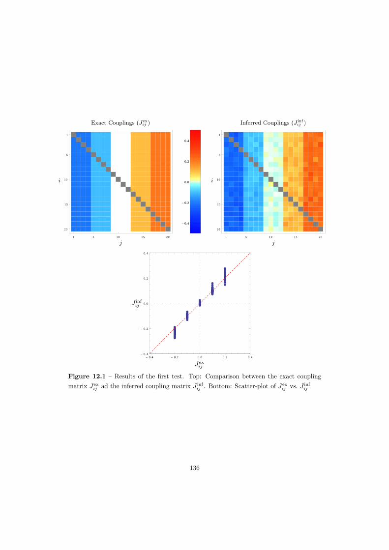
1 5 10 15 20
1
5
10
15
20
j
i
Exact Couplings (Jexij )
- 0.4
- 0.2
0.0
0.2
0.4
1 5 10 15 20
1
5
10
15
20
j
i
Inferred Couplings (J infij )
- 0.4 - 0.2 0.0 0.2 0.4
- 0.4
- 0.2
0.0
0.2
0.4
Jexij
J infij
Figure 12.1 – Results of the first test. Top: Comparison between the exact coupling
matrix Jexij ad the inferred coupling matrix J inf
ij . Bottom: Scatter-plot of Jexij vs. J inf
ij
136
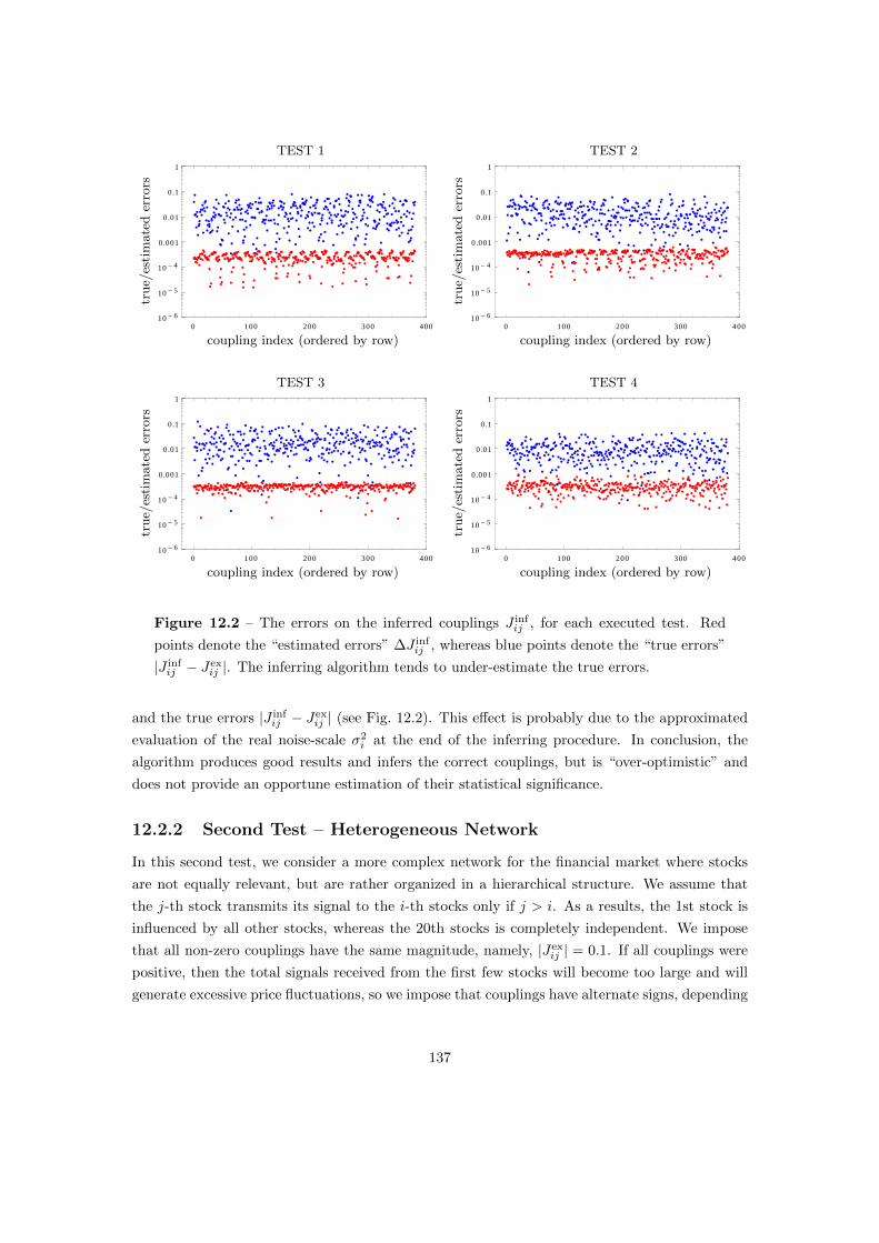
0 100 200 300 400
10-6
10-5
10-4
0.001
0.01
0.1
1
coupling index (ordered by row)
true/
esti
mate
der
rors
TEST 1
0 100 200 300 400
10-6
10-5
10-4
0.001
0.01
0.1
1
coupling index (ordered by row)
true/
esti
mate
der
rors
TEST 2
0 100 200 300 400
10-6
10-5
10-4
0.001
0.01
0.1
1
coupling index (ordered by row)
true/
esti
mate
der
rors
TEST 3
0 100 200 300 400
10-6
10-5
10-4
0.001
0.01
0.1
1
coupling index (ordered by row)
true/
esti
mate
der
rors
TEST 4
Figure 12.2 – The errors on the inferred couplings J infij , for each executed test. Red
points denote the “estimated errors” ∆J infij , whereas blue points denote the “true errors”
|J infij − Jex
ij |. The inferring algorithm tends to under-estimate the true errors.
and the true errors |J infij − Jex
ij | (see Fig. 12.2). This effect is probably due to the approximated
evaluation of the real noise-scale σ2i at the end of the inferring procedure. In conclusion, the
algorithm produces good results and infers the correct couplings, but is “over-optimistic” and
does not provide an opportune estimation of their statistical significance.
12.2.2 Second Test – Heterogeneous Network
In this second test, we consider a more complex network for the financial market where stocks
are not equally relevant, but are rather organized in a hierarchical structure. We assume that
the j-th stock transmits its signal to the i-th stocks only if j > i. As a results, the 1st stock is
influenced by all other stocks, whereas the 20th stocks is completely independent. We impose
that all non-zero couplings have the same magnitude, namely, |Jexij | = 0.1. If all couplings were
positive, then the total signals received from the first few stocks will become too large and will
generate excessive price fluctuations, so we impose that couplings have alternate signs, depending
137

1 5 10 15 20
1
5
10
15
20
j
i
Exact Couplings (Jexij )
- 0.4
- 0.2
0.0
0.2
0.4
1 5 10 15 20
1
5
10
15
20
j
i
Inferred Couplings (J infij )
- 0.3 - 0.2 - 0.1 0.0 0.1 0.2 0.3
- 0.3
- 0.2
- 0.1
0.0
0.1
0.2
0.3
Jexij
J infij
Figure 12.3 – Results of the second test. Top: Comparison between the exact coupling
matrix Jexij ad the inferred coupling matrix J inf
ij . Bottom: Scatter-plot of Jexij vs. J inf
ij
138

ææ
ææ æ æ æ æ
æ æ æ æ æ æ æ ææ
æ ææ
à à à àà
à à à àà à
à àà à
àà à
àà
ì ì
ìì
ì
ìì
ìì
ì ìì ì ì
ìì ì
ì ì
ì
ò ò ò ò òò
ò òò ò
ò ò ò òò ò ò ò ò ò
0 5 10 15 200.0
0.2
0.4
0.6
0.8
1.0
stock index
Ri
Figure 12.4 – The values of the noise-fraction Ri for each execution of the inferring
algorithm on simulated time-series. The inferring procedure is divided into N separate
sub-procedures (one for each stock), characterized by a specific value of the noise-fraction
Ri. Different markers correspond to different tests: blue points for the homogeneous
network (Test 1); purple squares for the heterogeneous network (Test 2); gold diamonds
for the random network (Test 3); and green triangles for no interaction (Test 4).
on the specific source of the signals. The structure of the matrix Jexij is illustrated in Fig. 12.3,
together with the result of the inference process. Once again the reliability of the algorithm is
quite good, and seems to be not influenced by the heterogeneity of the interactions. Yet, as
in the previous case, the inferred errors ∆J infij are very small (usually from 0.1% to 10%) and
they erroneously suggest that all inferred couplings are significant, even when they are related
to non-existent interactions. For instance, for the independent case i = 20 the algorithm detects
fluctuating couplings −0.03 < J infij < +0.03 with statistical errors ∆J inf
ij < 20%, indicating
the presence of significant interactions. When all detected couplings are effectively random and
the statistical errors are not properly evaluated, it is not easy to distinguish real interactions
from random fluctuations. In order to overcome this problem, we can turn our attention to the
noise-fraction Ri, which denotes the relevance of the stochastic component in price dynamics
and could be used as a goodness indicator for the inferring algorithm. The obtained values for
Ri has been reported in Figure 12.4, for all tests performed in the present section. Unlike the
previous test, where all ratios fluctuate around the same value, this case shows a clear trend, in
agreement with the stocks’ hierarchy in the financial network. In the independent case i = 20,
the noise-fraction Ri remains close to 1, suggesting that the deterministic component of the
price dynamics is too weak to extract real information from the empirical observations. At
variance, in the fully interacting case i = 1, the noise-fraction Ri is quite low (below 60%) and
139

indicates that the algorithm is capturing some real interacting structure of the financial network.
In the first test, where stock interactions were stronger and broader, the ratio Ri attains even
smaller values (below 50%). In conclusion, the parameter Ri turns out to be a better indicator
than the the statistical errors ∆J infij , which are generally under-estimated, and could be actually
employed as a goodness indicator to validate the result of the inference procedure. However,
this picture is highly qualitative, and the specific results of the algorithm must be accurately
evaluated case-by-case.
12.2.3 Third Test – Random Network
For this new test, we do not define a specific structure for the financial network, but we evaluate
the reliability of the algorithm in a random scenario. We define the coupling matrix Jexij by
drawing N(N − 1) random couplings from a normal distribution with mean 0.0 and standard
deviation 0.1. The results of the inferring algorithm are shown in Fig. 12.5, using the same
representative scheme of the previous tests. The two matrices Jexij and J inf
ij are quite similar,
although the absence of a specific structure in the financial network hinders a visual comparison
of the results. The scatter-plot J infij vs Jex
ij , instead, shows a clear agreement between the real
and inferred couplings, with small statistical errors. In this plot the points show a slightly
deviating trend, probably due to some approximation in the inferring procedure, but it tends to
sharpen the most significant couplings and should not affect the inference of the correct financial
network. The noise-fraction Ri exhibits larger fluctuation with respect to the other examined
cases, and this is probably due to the intrinsic randomness of the interaction network. However,
the obtained values for Ri are quite small, and typically fluctuate between the 40% and the 60%.
We can conclude that the inferring algorithm generates good results also in absence of clear
structures in the interactive dynamics of stock prices.
12.2.4 Fourth Test – No Network
As a final case, we examine the output of the algorithm in the most naive case, namely, in the
complete absence of interactions between the stock prices. This is probably the most important
case among the examined ones, because it defines the typical range of statistical errors and
provides the “benchmark” for the analysis of real time-series. The results of the algorithm
are reported in Fig. 12.6. This time, we are not able to distinguish any more between “good
results” and “bad results”, since we have no reference scale in the coupling matrix Jexij . The
inferred couplings J infij are non-zero and are much greater than their estimated errors ∆J inf
ij
(see Fig. 12.2). This proves again that the estimated errors are not good measurements for the
identification of significant couplings. On the contrary, the noise-fraction Ri remains close to 1
and fluctuates beyond 90%. This is considerably higher than all other other examined cases and
legitimates the usage of Ri as a goodness indicator of the algorithm’s reliability. According to the
measurements presented in this section, a noise-fraction Ri ≈ 90% does not confirm the presence
140

1 5 10 15 20
1
5
10
15
20
j
i
Exact Couplings (Jexij )
- 0.4
- 0.2
0.0
0.2
0.4
1 5 10 15 20
1
5
10
15
20
j
i
Inferred Couplings (J infij )
- 0.4 - 0.2 0.0 0.2 0.4
- 0.4
- 0.2
0.0
0.2
0.4
Jexij
J infij
Figure 12.5 – Results of the third test. Top: Comparison between the exact coupling
matrix Jexij ad the inferred coupling matrix J inf
ij . Bottom: Scatter-plot of Jexij vs. J inf
ij
141
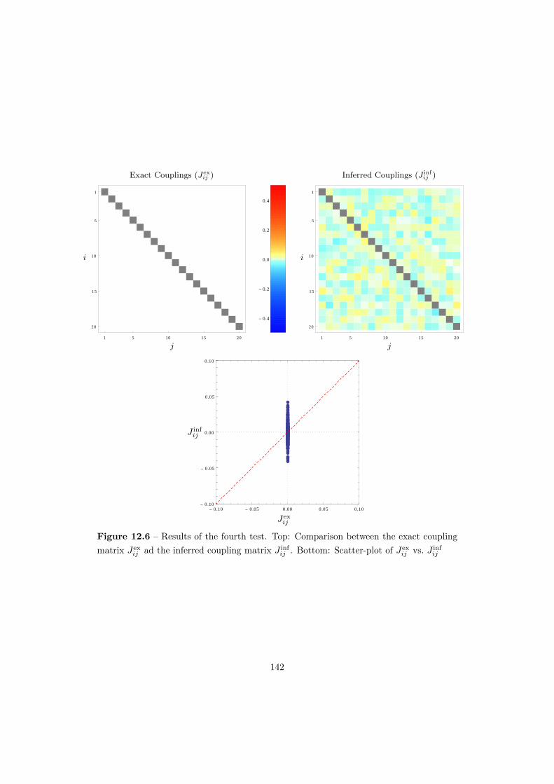
1 5 10 15 20
1
5
10
15
20
j
i
Exact Couplings (Jexij )
- 0.4
- 0.2
0.0
0.2
0.4
1 5 10 15 20
1
5
10
15
20
j
i
Inferred Couplings (J infij )
- 0.10 - 0.05 0.00 0.05 0.10
- 0.10
- 0.05
0.00
0.05
0.10
Jexij
J infij
Figure 12.6 – Results of the fourth test. Top: Comparison between the exact coupling
matrix Jexij ad the inferred coupling matrix J inf
ij . Bottom: Scatter-plot of Jexij vs. J inf
ij
142

of any deterministic component in price dynamics, whereas values of the order Ri ≈ 70% could
be determined by a real interaction network, as it happens in the previous three tests.
12.3 Inferring the Real Financial Structure
After the testing on simulated time-series, we are now ready to apply the inferring algorithm on
real financial data in order to infer the financial network of the real market. The application to
the real dataset requires some preliminary operations of data managing. Indeed, financial time-
series are recorded stock-by-stock, and should be merged and sorted in order to run the inferring
algorithm. For the following analysis, we unpacked the whole time-series in 500 sub-series, one
for each trading day. As shown in the previous section, daily time-series should be long enough
to estimate the market structure with good accuracy. In addition, the availability of multiple
datasets allows us to repeat the measurements and check the stability of the result. Finally, this
fragmentation excludes from the observed time series all price fluctuations occurring between
different days, which may have anomalous behaviour.
According to the considerations of the previous section, before the analysis of the inferred
couplings, we examine the general goodness of the algorithm by measuring the noise-fraction Ri,
for each stock and each trading day. The results are shown in Fig. 12.7. As one can see, most
of the values are in the range between 60% and 80%. The average values of Ri are not very
small, but are lower than the pure-random threshold of 90% detected in the previous section
and may be the results of real interactions in price dynamics. After all, we do not expect the
same goodness of results obtained in the testing stage: the simulated time series have been
generated by using the model itself and are optimal for the inferring algorithm; moreover, we
often assumed strong interactions in the financial network, which led to even sharper results. In
our opinion, the occurrence of several values of the noise-fraction below 70% (and even smaller)
can be interpreted as the sign of real price-interactions like the ones described by our model.
Now, we turn our attention to the inferred values of the couplings J infij . Since the financial
network has been evaluated on daily time-series, we end up with 500 measurements of each
coupling, one for each trading day. In Fig. 12.8 we present an overview of the results by showing
the confidence range of each coupling, by evaluating their mean mij and standard deviation sij
over the whole set of measurements. Different colors refer to different row-indexes i and separate
inferring procedures. The picture does not highlight the details of the financial network, but
only its general properties. As one can see, the couplings are clearly shifted towards positive
values, denoting a positive correlation of stock prices across the whole financial market. This
results is in agreement with the emergence of the market-mode in the cross-correlation matrix of
stock prices (see Section 9.1). Yet, the statistical fluctuations of J infij over different trading days
are quite large, and very often they exceed the average value of the couplings, suggesting that
they could be not statistically significant. In Fig. 12.9 we show the matrices of mij and sij for
the mean and the standard deviation of each coupling J infij . Both matrices exhibit recognizable
143

0 5 10 15 200.0
0.2
0.4
0.6
0.8
1.0
stock index
Ri
Figure 12.7 – The values of the noise-fraction Ri for each execution of the inferring
algorithm on financial time-series. The inferring procedure is spilt into N separate sub-
procedures (one for each stock), and is repeated 500 times (one for each trading day).
Each sub-procedure is characterized by a specific value of the noise-fraction Ri. Different
colors refer to different stock, following the same color scheme of Fig. 12.8.
0 100 200 300 400- 0.10
- 0.05
0.00
0.05
0.10
0.15
0.20
coupling index (ordered by row)
J infij
Figure 12.8 – The values of the inferred couplings J infij , with their statistical errors,
for each couple (i, j) (ordered by row). Values and errors have been estimated as the
mean and the standard deviation of all measurements performed on different trading
days. Couplings with different colors have been evaluated through uncorrelated inferring
procedures, following the same color scheme of Fig. 12.7.
144
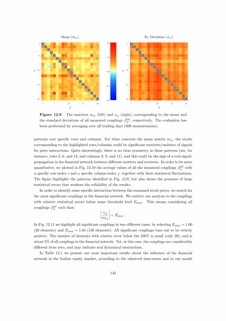
1 5 10 15 20
1
5
10
15
20
j
i
Mean (mij)
- 0.2
- 0.1
0.0
0.1
0.2
1 5 10 15 20
1
5
10
15
20
j
i
St. Deviation (sij)
Figure 12.9 – The matrices mij (left) and sij (right), corresponding to the mean and
the standard deviations of all measured couplings J infij , respectively. The evaluation has
been performed by averaging over all trading days (500 measurements).
patterns over specific rows and columns. For what concerns the mean matrix mij , the stocks
corresponding to the highlighted rows/columns could be significant receivers/emitters of signals
for price interactions. Quite interestingly, there is no clear symmetry in these patterns (see, for
instance, rows 2, 6, and 12, and columns 8, 9, and 11), and this could be the sign of a real signal-
propagation in the financial network between different emitters and receivers. In order to be more
quantitative, we plotted in Fig. 12.10 the average values of all the measured couplings J infij with
a specific row-index i and a specific column-index j, together with their statistical fluctuations.
The figure highlights the patterns identified in Fig. 12.9, but also shows the presence of large
statistical errors that weakens the reliability of the results.
In order to identify some specific interaction between the examined stock prices, we search for
the most significant couplings in the financial network. We restrict our analysis to the couplings
with relative statistical errors below some threshold level Emax. This means considering all
couplings J infij such that: ∣∣∣∣ sijmij
∣∣∣∣ < Emax .
In Fig. 12.11 we highlight all significant couplings in two different cases, by selecting Emax = 1.00
(20 elements) and Emax = 1.65 (120 elements). All significant couplings turn out to be strictly
positive. The number of elements with relative error below the 100% is small (only 20), and is
about 5% of all couplings in the financial network. Yet, in this case, the couplings are considerably
different from zero, and may indicate real dynamical interactions.
In Table 12.1 we present our most important results about the inference of the financial
network in the Italian equity market, according to the observed time-series and to our model
145

0 5 10 15 20- 0.10
- 0.05
0.00
0.05
0.10
0.15
0.20
J infij
j
Signal Emission
0 5 10 15 20- 0.10
- 0.05
0.00
0.05
0.10
0.15
0.20
J infij
i
Signal Reception
Figure 12.10 – Means and standard deviations of all measured couplings J infij with fixed
indexes j (left) and i (right), denoting the relevance of each stock as either a “signal
emitter” (left) or a “signal receiver” (right). The evaluation has been performed by
averaging over all trading days and all possible receivers/emitters (500×20 measurements).
1 5 10 15 20
1
5
10
15
20
j
i
Emax = 100%
- 0.2
- 0.1
0.0
0.1
0.2
1 5 10 15 20
1
5
10
15
20
j
i
Emax = 165%
Figure 12.11 – The mean-matrix mij (as in Fig. 12.9) restricted to the most significant
couplings with maximum relative error Emax = 1.00 (left – 20 elements) and Emax = 1.65
(right – 120 elements).
146

i j Emitter Receiver Jij
18 5 Int. Sanpaolo UniCredit 0.128 (56%)18 8 Enel UniCredit 0.111 (70%)18 9 Eni UniCredit 0.108 (87%)12 5 Int. Sanpaolo UBI Banca 0.107 (64%)12 8 Enel UBI Banca 0.102 (76%)12 18 UniCredit UBI Banca 0.100 (70%)5 18 UniCredit Int. Sanpaolo 0.098 (85%)5 8 Enel Int. Sanpaolo 0.095 (90%)1 8 Enel Ass. Generali 0.094 (89%)12 1 Ass. Generali UBI Banca 0.093 (87%)18 1 Ass. Generali UniCredit 0.092 (95%)2 8 Enel Mediobanca 0.085 (92%)2 18 UniCredit Mediobanca 0.080 (87%)2 12 UBI Banca Mediobanca 0.076 (96%)1 5 Int. Sanpaolo Ass. Generali 0.075 (80%)12 2 Mediobanca UBI Banca 0.074 (93%)2 5 Int. Sanpaolo Mediobanca 0.074 (91%)9 8 Enel Eni 0.071 (95%)6 8 Enel Mediaset 0.070 (95%)9 5 Int. Sanpaolo Eni 0.052 (96%)
Table 12.1 – Details about the most significant couplings shown in Fig. 12.11 (left).
for interacting prices. In this table we show the values of all 20 couplings that can be reliably
considered as strictly positive. The table also shows their relative errors and the company names
of the related stocks. Each coupling J infij is related to a specific direction in the signal propagation,
namely, from stock j to stock i, and denotes some hierarchical relationship between the signal
emitter (stock j) and the signal receiver (stock i). As one can see, emitters and receivers are
generally different. The most active emitters (i.e. the ones that are listed more often) are “Enel”
and “Intesa Sanpaolo” (stocks 8 and 5, respectively), whereas the most susceptible receivers are
“UBI Banca” and “Mediobanca” (stocks 12 and 2). “UniCredit” (stock 18), is both a strong
emitter and receiver. Interestingly, the sub-network composed of these interactions does not
spread over the whole financial market, but is restricted to a small group of stocks. The whole
set of couplings is defined over a subset of only 8 stocks, and each coupling involves one of the
mentioned stocks as either an emitter or a receiver. This structure is also visible in Fig. 12.11.
Most of the stocks listed in Table 12.1 are from the financial economic sector, the only exception
being “Enel” (Utilities), “Eni” (Oil & Gas), and “Mediaset” (Consumer Services). Some of
the listed stocks (namely, “Unicredit”, “Intesa Sanpaolo”, “Eni”, “Enel”, and “Assicurazioni
Generali”) have been already recognized as important elements of the Italian equity market by
means of the general analysis of the financial time-series performed in Section 6.2.
The measurements presented in this final section are in general agreement with the cross-
correlation properties of stock prices, as reported in Section 9.1. The overall positiveness of
147

0.0 0.2 0.4 0.6 0.8 1.0
- 0.1
0.0
0.1
0.2
Cij
Jexij
Figure 12.12 – Scatter plot of the inferred couplings J infij (and their statistical errors)
versus the correlation coefficients Cij . The dashed line denotes the direct proportionality
law J infij ≈ 0.090Cij , evaluated as a least-squares fit on the plotted data.
the coupling matrix J infij could capture the underlying mechanisms of cross-stock interactions
that give rise to correlation effects in financial time series. As a last result, we report in Fig.
12.12 the scatter plot of each coupling J infij versus the corresponding elements of the correlation
matrix Cij , evaluated from price returns at 30 minutes (the same matrix examined in Section
9.1). In spite of the large statistical fluctuations, the inferred couplings turn out to be roughly
proportional to the elements of the correlation matrix, suggesting that they could explain the
emergence of correlations in the financial market. In principle, the asymmetry of the couplings
J infij with respect to the symmetric coefficients Cij could be also exploited to distinguish the
stocks that are most responsible for the correlation effects. Yet this kind of analysis is prevented
by the large statistical errors on the couplings J infij , which do not guarantee the reliability of
the results. In our opinion, the inferring algorithm presented in this work is detecting a real
interaction network between stock prices (as confirmed by the values of the noise-fraction Ri
reported in Fig. 12.7), but this network is not enough stable to generate evident results, and it
is not possible to capture the fine structure of the financial market beyond the over-all positive
interaction, with the exception of the couplings listed in Table 12.1. The stability of the financial
network is not only related to the empirical properties of the financial market, but also to the
theoretical model used to describe the dynamics of prices, which is an intrinsic part of the
inferring algorithm. It is plausible that small changes in our model could lead to a more stable
definition of the cross-stock interactions and could improve the results presented above. This
will provide a better description of the underlying dynamics of financial markets by exploiting
the same inference procedure described in this work.
148

Chapter 13
Conclusions
The topics discussed in the present thesis are manifold, but they all refer to a common issue,
namely, the statistical characterization of stock prices and of rare events in financial time-series.
In the most naive description, stock prices are stochastic processes driven by independent normal
returns, yet, according to the empirical measurements, actual stock prices are characterized by
at least two non-trivial features: (a) price returns are heavy-tailed distributed; and (b) price
returns are not statistically independent. The lack of linear auto-correlation in price returns and
the time-diffusivity of prices are in perfect agreement with the naive description, which could
explain the typical fluctuations of stock prices in absence of rare events. Yet, when rare events
are taken into account, the two mentioned features become extremely important since: (a) the
heavy-tailed nature of price returns enhances the frequency and magnitude of large returns; and
(b) the auto-correlation of volatility modifies their generation and propagation over time. A
theoretical characterization of large deviations in heavy-tailed distributed random variables is a
mandatory step for the analysis of rare events in stock prices (Part I). However, their empirical
observation in real financial time-series could highlight significant discrepancies with respect to
the theoretical expectations, and this stresses the importance of a more pragmatic analysis of
large price returns (Part II). Finally, the self-exciting dynamics between different stock prices in
the financial market could define the underlying mechanism of the volatility clustering, which
eventually leads to the generation of rare events; therefore, the inference of the price dynamics
from empirical data could provide interesting information about the actual generation of price
fluctuations (Part III).
13.1 Part I
In the first part of the work we analysed the emergence of condensation phenomena in heavy-
tailed distributions within the theoretical framework of the Large Deviations Theory. Conden-
sation phenomena in statistical samples of heavy-tailed random variables are generated by large
149

deviations of some global observable, and are due to a simple conceptual mechanism: if the
random variables are heavy-tailed, then macroscopic individual deviations are more likely than
microscopic collective ones. In a statistical-mechanical interpretation, collective and individual
deviations denote separate phases of the statistical sample, and condensation phenomena arise
as phase transitions with spontaneous symmetry breaking, destroying the intrinsic equivalence
of the random variables. The condensed phase of the system is characterized by anomalous
scaling-laws in all moments of the statistical sample, and this has been highlighted in the phase
diagrams of Fig. 4.2. It is worth to notice that the “critical point” of the examined system falls
exactly on the “typical point”, which characterizes the state of the system in absence of large
deviations. As a consequence, the statistical samples of power-law random variables provide a
rigorous example of complex system with self-organized criticality, stating a precise relationship
between power-law distributions and critical phenomena [55].
Quite interestingly, the condensation phenomena considered in this work are generated by
pure statistical mechanisms, and do not rely on any specific interaction between the underlying
random variables. When condensation phenomena are empirically observed in real systems with
power-law behaviours, such as in the geographical distribution of the economic wealth or in the
size of cities, one could be tempted to explain the observations as the results of some dynamical
interaction. Yet, as we argued above, condensation phenomena naturally arise in power-law
distributions, and the observations could be rather explained in terms of large deviations of some
global observable. For instance, concentrations in wealth distribution or in city sizes could be
explained, in principle, by an excess of global wealth or global population, respectively, without
any other assumption. This idea has been exploited in [55], for instance, to explain the emergence
of the market-mode in financial correlation matrices (see 9.1) as an effect of the excess covariance,
without assuming any specific interaction between the financial instruments.
The results presented in Part I have been obtained for independent random variables, yet,
condensation phenomena can arise also in presence of statistical correlation. This depends on
the specific form of the interaction between the considered random variables: “attractive inter-
actions” may reduce or eliminate condensation phenomena, while “repulsive interaction” may
increase their effects. In a statistical sample of random variables described by a joint elliptical
distribution, for instance, condensation phenomena are prohibited even though the random vari-
ables have a power-law marginal distribution [55]. A similar effect also occurs in the empirical
distribution of price returns, as shown in Part II. On the contrary, condensation phenomena can
be detected in the eigenvalues of random matrices, which are characterized by the same repulsive
interaction of 2-dimensional Coulomb charges [105, 55]. Beyond this examples, the condensation
of large deviations has been observed in several physical systems, such as in complex networks
[11], in bipartite quantum systems [105], in out-of equilibrium mass-transport models [83], and
in disordered systems [42].
Most of the results developed in Part I, like the phase diagrams of Fig. 4.2, have been obtained
(or recovered) by means of the theoretical framework of the Density Functional Method. The
150

method is extremely neat and flexible, and provides interesting results also in more complex
contexts, as in the Random Matrix Theory [39, 134]. Yet, it has a strong limitation: it is
defined only in the thermodynamic limit N → ∞ and does not provide any information about
the finite-size scaling of the observed variables. Some results about this issue can be already
found in literature [83] and have been also reviewed in this work. Yet, it could be interesting to
develop a more comprehensive knowledge about condensation phenomena in finite samples, for
both independent and interactive variables, and to extend the known results to different kinds
of statistical observables. In this context, a deeper analysis of the finite-size behaviour for the
IPR and other possible order parameters could be an interesting topic for future works.
13.2 Part II
In the second part of this work we performed a thorough analysis of stock prices under an
empirical point of view. The analysis pointed out the most important stylized facts about the
probability distribution of price returns, such as the power-law behaviour, the price-diffusivity
and the volatility clustering. Above all, we showed that the probability distribution of price
returns is stable and has about the same shape for all financial stocks, and time-scales, at
least within one trading-day. It is known that the probability distribution of price returns is
aggregationally Gaussian, in the sense that, moving towards large time-scales, it becomes more
and more similar to a Gaussian distribution [33]. This indicates that the normal diffusivity of
price becomes increasingly relevant with respect to the auto-correlation effects, altering the scale-
invariance of price-returns (this effect is visible also in the Multi-Fractal Random Walk, while
approaching the integral-scale Tint). In our analysis, this effect is not clearly evident, probably
because we are not observing sufficiently large time-scales. In this analysis we neither observe
the distribution asymmetries that are frequently addressed to in the literature. It is indeed often
claimed that large negative returns are more frequent than large positive returns [33]. In our
dataset this is not clearly observable: the mean of the distribution is always comparable to zero,
and the two tails have very similar behaviour. According to our observations, the asymmetries
are not related to the bulk of the distributions, but rather to the rare events: further analyses
on extreme price returns could denote the presence of small asymmetries in the occurrence of
rare events that enhance the probability of extreme negative returns. This could be also related
to the so-called leverage effect [33, 27], a stylized fact denoting a negative correlation between
returns and volatilities (i.e. negative price fluctuations are more volatile than positive ones).
Our analysis confirmed the widespread idea that the price-fluctuation process is characterized
by a highly non-trivial behaviour. The combination of scale-invariant and diffusive properties
in a stochastic process is often associated to the Central Limit Theorem, and should be re-
lated to normal and independent increments. Neither of the two features are observed in real
price time-series but, somehow, the complex interplay of non-normality and non-independence in
price returns results in the same scaling behaviour observed in the simplest stochastic processes.
151

This is, in some sense, the main observation performed in [90], which is considered as the first
popular contribution of econophysics to financial research. The observations performed in Part
II with respect to the inhibition of condensation phenomena extend our knowledge about this
topic. Indeed, the amplification and reduction feedbacks observed in the analysis of Fig. 7.4,
with the consequent reduction of price discontinuities and amplification of diffusive fluctuations,
could highlight the underlying mechanism that yields the scale-invariant properties of the price-
fluctuation process. The observations emphasizes the effects of this dynamics on large returns,
showing that: (a) extreme price returns are quantitatively larger than in the case of indepen-
dent returns; and (b) they are qualitatively realized through drastically different mechanisms,
favouring regular diffusion in spite of abrupt jumps or falls. This suggests that the anomalous
diffusivity of prices should be carefully taken into account in order to obtain a correct estimation
of the financial risk related to large deviations of stock prices.
13.3 Part III
In the third part of this work, we developed an original model for the financial market based on
interacting stock prices, and we tried to infer the interaction network of the market from the his-
torical time-series of stock prices. The inferring algorithm is able to detect a quasi-homogeneous
interaction between the whole financial market, and identifies some selected stronger interactions
between a small subset of stocks related to the most important companies listed in the available
dataset. In spite of this, the inferred couplings for the cross-stock interactions are characterized
by high statistical fluctuations, and do not allow to investigate the structure of the financial
market in deeper details.
There could be several reasons for this. The inferred couplings are generally small and spread
over the whole financial market, then it could be difficult to distinguish the presence of non-
zero couplings from the background of statistical fluctuations. Another explanation is that the
the interaction network of the market exists and has a clearly recognizable structure, but is not
stable in time and is not detectable from a global analysis over the whole time-series. In addition,
the market could be over-sensitive to exogenous events, such as political and economical news,
or price-changes in other financial instruments that are not included in the available dataset;
in this case the statistical fluctuations can be anomalously large and could sensibly affect the
results of the inferring algorithm. In the worst possible case, we simply over-estimated the
reliability of the algorithm, since we used too rough approximations in the definition of the
inferring procedures, and the statistical fluctuations of stock prices are too large to extract
actual information from the empirical time-series. In our opinion, the issue is not about the
reliability of the algorithm, but rather about the reliability of the results. Indeed, the validity
of the algorithm has been successfully validated in the testing phase on the simulated datasets,
but we do not have enough control on the statistical significance of the inferred couplings and
on the effective amount information extracted from the empirical time-series.
152

Is it possible to improve the inferring algorithm? In literature, especially in the context of
Machine Learning and Optimal Control Theory, it is possible to find a large variety of techniques
intended to improve the performances of statistical inference procedures on complex systems with
high dimensionality [13]. One of the most used methods in this context is the introduction of a
regularization, namely, some specific prior distribution for the inferred parameters intended to
increase the stability of the results and to prevent over-fitting (this concept has been introduced
in Section 11.1). A prior distribution may alter the final value of the inferred couplings, but could
improve the identification of the significant ones. The most common choices of regularizations
are based on normal and double-exponential distributions for the inferred parameters, and give
rise to the L2-norm and L1-norm regularizations, respectively [2]. The L1 norm is specifically
intended to set the least significant couplings to zero and focus the inferring procedure on the most
significant ones, searching for the correct topology of the financial network. Another interesting
technique for the inference of the network topology is the decimation procedure, which recursively
removes the most unlikely couplings from the inferring procedure up to some optimal point
[41]. The inference of the correct topology of the financial networks has a double advantage:
it highlights the real structure of the financial market and it reduces the dimensionality of
the problem by removing the least significant couplings from the inferring procedure, with a
consequent improvement of the algorithm reliability.
Notwithstanding the specific technique used to increase the stability of the results, the infer-
ring algorithm could be modified also at its very basis. The model presented in this work is based
on a specific form of interaction between stock prices, based on a signal-transmission mechanism
that is triggered by price-changes. Yet, it is not ensured that financial markets actually follow
this kind of dynamics. It could be interesting to investigate different dynamics by changing the
definition of the triggering events from price-changes to some other kind of measurable events.
This could allow us to analyse different dynamics for the financial markets while keeping the
whole algorithmic structure unaltered. Financial time-series are characterized by natural events,
namely, the trading executions, which occur at specific time and and have a specific intensity
(the traded volume). It is well known that trades induce price movements: this effect is known
as market impact and is a core topic in the analysis of the market micro-structure [23]. The
market impact is usually explained as a mechanical impact due to the arrival of market-orders to
the order book, and, for this reason, it should affect only the traded stock. In spite of this, it is
possible to imagine the presence of an informative impact, that affects all stocks in the financial
markets with variable intensity, through the same signal-transmission mechanism developed for
our model. It has been already argued that traded volumes may give rise to actual inferable
interactions [137], so this alternative model could provide new insights for the identification of
the dynamical structure of the financial markets.
153

Bibliography
[1] F. Abergel, J. Bouchaud, T. Foucault, C. Lehalle, and M. Rosenbaum. Market Microstruc-
ture: Confronting Many Viewpoints. The Wiley Finance Series. Wiley, 2012.
[2] E. Alpaydin. Introduction to Machine Learning. Adaptive Computation and Machine
Learning Series. MIT Press, 2014.
[3] L. Bachelier. Theorie de la speculation. Gauthier-Villars, 1900.
[4] E. Bacry, J. Delour, and J.-F. Muzy. Multifractal random walk. Physical Review E,
64(2):026103, 2001.
[5] E. Bacry, A. Kozhemyak, and J. Muzy. Log-Normal continuous cascades: aggregation prop-
erties and estimation. Application to financial time-series. arXiv preprint arXiv:0804.0185,
2008.
[6] E. Bacry and J. F. Muzy. Log-infinitely divisible multifractal processes. Communications
in Mathematical Physics, 236(3):449–475, 2003.
[7] C. Barbieri, S. Cocco, and R. Monasson. Inferring interactions in assemblies of stochastic
integrate-and-fire neurons from spike recordings: method, applications and software. BMC
Neuroscience, 12(Suppl 1):P40, 2011.
[8] O. E. Barndorff-Nielsen and N. Shephard. Power and bipower variation with stochastic
volatility and jumps. Journal of financial econometrics, 2(1):1–37, 2004.
[9] D. Bertsekas. Dynamic Programming and Optimal Control. Number v. 1 in Athena Scien-
tific optimization and computation series. Athena Scientific, 2005.
[10] P. Bialas, Z. Burda, and D. Johnston. Phase diagram of the mean field model of simplicial
gravity. Nuclear Physics B, 542(12):413 – 424, 1999.
[11] G. Bianconi and A.-L. Barabasi. Bose-einstein condensation in complex networks. Physical
Review Letters, 86(24):5632, 2001.
[12] G. Biroli, J.-P. Bouchaud, and M. Potters. On the top eigenvalue of heavy-tailed random
matrices. EPL (Europhysics Letters), 78(1):10001, 2007.
154

[13] C. M. Bishop et al. Pattern recognition and machine learning. Springer New York, 2006.
[14] F. Black and M. Scholes. The pricing of options and corporate liabilities. The journal of
political economy, pages 637–654, 1973.
[15] T. Bollerslev. Generalized autoregressive conditional heteroskedasticity. Journal of econo-
metrics, 31(3):307–327, 1986.
[16] C. Borghesi, M. Marsili, and S. Micciche. Emergence of time-horizon invariant correlation
structure in financial returns by subtraction of the market mode. Physical Review E,
76(2):026104, 2007.
[17] L. Borland, J.-P. Bouchaud, J.-F. Muzy, and G. Zumbach. The Dynamics of Financial
Markets - Mandelbrot’s Cascades and Beyond. Wilmott Magazine, pages 86–96, 2005.
[18] G. Bormetti, L. M. Calcagnile, M. Treccani, F. Corsi, S. Marmi, and F. Lillo. Modelling
systemic price cojumps with hawkes factor models. arXiv preprint arXiv:1301.6141, 2013.
[19] G. Bormetti, V. Cazzola, G. Livan, G. Montagna, and O. Nicrosini. A generalized fourier
transform approach to risk measures. Journal of Statistical Mechanics: Theory and Exper-
iment, 2010(01):P01005, 2010.
[20] J. Bouchaud and M. Potters. Theory of Financial Risks: From Statistical Physics to Risk
Management. Alea Saclay collection. Cambridge University Press, 2000.
[21] J.-P. Bouchaud. An introduction to statistical finance. Physica A: Statistical Mechanics
and its Applications, 313(1):238–251, 2002.
[22] J.-P. Bouchaud. Economics needs a scientific revolution. Nature, 455(7217):1181–1181,
2008.
[23] J.-P. Bouchaud, J. D. Farmer, and F. Lillo. How markets slowly digest changes in supply
and demand. Handbook of financial markets: dynamics and evolution, 1:57, 2009.
[24] J.-P. Bouchaud, Y. Gefen, M. Potters, and M. Wyart. Fluctuations and response in finan-
cial markets: the subtle nature of randomprice changes. Quantitative Finance, 4(2):176–
190, 2004.
[25] J.-P. Bouchaud and M. Mezard. Universality classes for extreme-value statistics. Journal
of Physics A: Mathematical and General, 30(23):7997, 1997.
[26] J.-P. Bouchaud and M. Mezard. Wealth condensation in a simple model of economy.
Physica A: Statistical Mechanics and its Applications, 282(34):536 – 545, 2000.
[27] J.-P. Bouchaud and M. Potters. More stylized facts of financial markets: leverage effect and
downside correlations. Physica A: Statistical Mechanics and its Applications, 299(1):60–70,
2001.
155

[28] Z. Burda, A. Grlich, A. Jarosz, and J. Jurkiewicz. Signal and noise in correlation matrix.
Physica A: Statistical Mechanics and its Applications, 343(0):295 – 310, 2004.
[29] J. L. Cabrera and J. G. Milton. On-off intermittency in a human balancing task. Physical
Review Letters, 89(15):158702, 2002.
[30] R. Chicheportiche and J.-P. Bouchaud. The fine-structure of volatility feedback I: multi-
scale self-reflexivity. Physica A: Statistical Mechanics and its Applications, 410:174–195,
2014.
[31] S. Cocco, S. Leibler, and R. Monasson. Neuronal couplings between retinal ganglion cells in-
ferred by efficient inverse statistical physics methods. Proceedings of the National Academy
of Sciences, 106(33):14058–14062, 2009.
[32] S. Cocco and R. Monasson. Adaptive cluster algorithm to infer boltzmann machines from
multi-electrode recording data. BMC Neuroscience, 12(Suppl 1):P224, 2011.
[33] R. Cont. Empirical properties of asset returns: stylized facts and statistical issues. Quan-
titative Finance, 1(2):223–236, 2001.
[34] F. Corsi. Measuring and modelling realized volatility: from tick-by-tick to long memory.
PhD thesis, University of Lugano Prof. T. Bollerlsev, Duke University, 2005.
[35] T. Cover and J. Thomas. Elements of Information Theory. A Wiley-Interscience publica-
tion. Wiley, 2006.
[36] P. F. Craigmile. Simulating a class of stationary gaussian processes using the davies–harte
algorithm, with application to long memory processes. Journal of Time Series Analysis,
24(5):505–511, 2003.
[37] H. Cramer. Sur un nouveau theoreme limite de la probabilities. Actualites Sci. Indust,
736, 1938.
[38] K. Dayri and M. Rosenbaum. Large tick assets: implicit spread and optimal tick size.
arXiv preprint arXiv:1207.6325, 2012.
[39] D. S. Dean and S. N. Majumdar. Large deviations of extreme eigenvalues of random
matrices. Physical review letters, 97(16):160201, 2006.
[40] D. S. Dean and S. N. Majumdar. Extreme value statistics of eigenvalues of gaussian random
matrices. Phys. Rev. E, 77:041108, Apr 2008.
[41] A. Decelle and F. Ricci-Tersenghi. Pseudolikelihood decimation algorithm improving the
inference of the interaction network in a general class of ising models. Physical review
letters, 112(7):070603, 2014.
156

[42] B. Derrida. Random-energy model: An exactly solvable model of disordered systems. Phys.
Rev. B, 24:2613–2626, Sep 1981.
[43] B. Derrida. Non-self-averaging effects in sums of random variables, spin glasses, random
maps and random walks. In On Three Levels, pages 125–137. Springer, 1994.
[44] Z. Ding, C. W. Granger, and R. F. Engle. A long memory property of stock market returns
and a new model. Journal of Empirical Finance, 1(1):83 – 106, 1993.
[45] J. Doyne Farmer 5, L. Gillemot, F. Lillo, S. Mike, and A. Sen. What really causes large
price changes? Quantitative finance, 4(4):383–397, 2004.
[46] R. Ellis. Entropy, Large Deviations, and Statistical Mechanics. Classics in Mathematics.
Springer, 2005.
[47] R. S. Ellis. Large deviations for a general class of random vectors. The Annals of Probability,
pages 1–12, 1984.
[48] P. Embrechts, C. Kluppelberg, and T. Mikosch. Modelling extremal events: for insurance
and finance. Springer, 1997.
[49] R. F. Engle. Autoregressive conditional heteroscedasticity with estimates of the variance
of united kingdom inflation. Econometrica: Journal of the Econometric Society, pages
987–1007, 1982.
[50] M. Evans, S. Majumdar, and R. Zia. Canonical analysis of condensation in factorised
steady states. Journal of Statistical Physics, 123(2):357–390, 2006.
[51] M. R. Evans and T. Hanney. Nonequilibrium statistical mechanics of the zero-range process
and related models. Journal of Physics A: Mathematical and General, 38(19):R195, 2005.
[52] M. R. Evans and S. N. Majumdar. Condensation and extreme value statistics. Journal of
Statistical Mechanics: Theory and Experiment, 2008(05):P05004, 2008.
[53] E. F. Fama. Efficient capital markets: A review of theory and empirical work*. The journal
of Finance, 25(2):383–417, 1970.
[54] E. F. Fama and K. R. French. The capital asset pricing model: Theory and evidence.
Journal of Economic Perspectives, 18(3):25–46, 2004.
[55] M. Filiasi, G. Livan, M. Marsili, M. Peressi, E. Vesselli, and E. Zarinelli. On the concen-
tration of large deviations for fat tailed distributions, with application to financial data.
Journal of Statistical Mechanics: Theory and Experiment, 9:30, Sept. 2014.
[56] M. Filiasi, E. Zarinelli, E. Vesselli, and M. Marsili. Condensation phenomena in fat-tailed
distributions. arXiv preprint arXiv:1309.7795, 2013.
157

[57] R. A. Fisher and L. H. C. Tippett. Limiting forms of the frequency distribution of the
largest or smallest member of a sample. In Mathematical Proceedings of the Cambridge
Philosophical Society, volume 24, pages 180–190. Cambridge Univ Press, 1928.
[58] U. Frisch and D. Sornette. Extreme deviations and applications. Journal de Physique I,
7(9):1155–1171, 1997.
[59] K. Gangopadhyay. Interview with eugene h. stanley. IIM Kozhikode Society & Management
Review, 2(2):73–78, 2013.
[60] J. Gartner. On large deviations from the invariant measure. Theory of Probability & Its
Applications, 22(1):24–39, 1977.
[61] J. Gatheral. No-dynamic-arbitrage and market impact. Quantitative Finance, 10(7):749–
759, 2010.
[62] A. Gelman, J. Carlin, H. Stern, D. Dunson, A. Vehtari, and D. Rubin. Bayesian Data
Analysis, Third Edition. Chapman & Hall/CRC Texts in Statistical Science. Taylor &
Francis, 2013.
[63] M. Gilli and E. Kellezi. An application of extreme value theory for measuring financial
risk. Computational Economics, 27(2-3):207–228, 2006.
[64] B. Gnedenko. Sur La Distribution Limite Du Terme Maximum D’Une Serie Aleatoire. The
Annals of Mathematics, 44(3):423+, July 1943.
[65] B. Gnedenko. Theory of Probability. CRC Press, 1998.
[66] B. V. Gnedenko and A. Kolmogorov. Limit distributions for sums of independent random
variables, volume 233. Addison-Wesley Reading, Massachusetts, 1968.
[67] P. Gopikrishnan, M. Meyer, L. Amaral, and H. Stanley. Inverse cubic law for the distribu-
tion of stock price variations. The European Physical Journal B - Condensed Matter and
Complex Systems, 3(2):139–140, 1998.
[68] S. J. Hardiman, N. Bercot, and J.-P. Bouchaud. Critical reflexivity in financial markets: a
hawkes process analysis. arXiv preprint arXiv:1302.1405, 2013.
[69] S. L. Heston. A closed-form solution for options with stochastic volatility with applications
to bond and currency options. Review of financial studies, 6(2):327–343, 1993.
[70] K. Huang. Statistical mechanics. Wiley, 1987.
[71] J. Hull. Options, futures and other derivatives. Pearson education, 2009.
[72] A. Johansen and D. Sornette. Endogenous versus exogenous crashes in financial markets,
in press in contemporary issues in international finance, 2004.
158

[73] I. M. Johnstone. On the distribution of the largest eigenvalue in principal components
analysis. Ann. Statist., 29(2):295–327, 04 2001.
[74] P. Jorion. Value at risk: the new benchmark for managing financial risk, volume 2.
McGraw-Hill New York, 2007.
[75] A. Joulin, A. Lefevre, D. Grunberg, and J.-P. Bouchaud. Stock price jumps: News and
volume play a minor role. Wilmott Magazine, Sep/Oct:1–7, 2008.
[76] L. Laloux, P. Cizeau, J.-P. Bouchaud, and M. Potters. Noise dressing of financial correlation
matrices. Physical Review Letters, 83(7):1467, 1999.
[77] L. Laloux, P. Cizeau, M. Potters, and J.-P. Bouchaud. Random matrix theory and financial
correlations. International Journal of Theoretical and Applied Finance, 3(03):391–397,
2000.
[78] F. Lillo and R. N. Mantegna. Power-law relaxation in a complex system: Omori law after
a financial market crash. Physical Review E, 68(1):016119, 2003.
[79] Y. Liu, P. Cizeau, M. Meyer, C.-K. Peng, and H. Eugene Stanley. Correlations in economic
time series. Physica A: Statistical Mechanics and its Applications, 245(3):437–440, 1997.
[80] F. M. Longin. The asymptotic distribution of extreme stock market returns. Journal of
business, pages 383–408, 1996.
[81] T. Lux. Turbulence in financial markets: the surprising explanatory power of simple
cascade models. Quantitative finance, 1(6):632–640, 2001.
[82] T. Lux and M. Marchesi. Scaling and criticality in a stochastic multi-agent model of a
financial market. Nature, 397(6719):498–500, 1999.
[83] S. N. Majumdar, M. Evans, and R. Zia. Nature of the condensate in mass transport models.
Physical review letters, 94(18):180601, 2005.
[84] S. N. Majumdar and G. Schehr. Top eigenvalue of a random matrix: large deviations and
third order phase transition. Journal of Statistical Mechanics: Theory and Experiment,
2014(1):P01012, 2014.
[85] S. N. Majumdar and M. Vergassola. Large deviations of the maximum eigenvalue for
wishart and gaussian random matrices. Physical review letters, 102(6):060601, 2009.
[86] S. N. Majumdar and P. Vivo. Number of relevant directions in principal component analysis
and wishart random matrices. Physical review letters, 108(20):200601, 2012.
[87] B. D. Malamud, G. Morein, and D. L. Turcotte. Forest fires: an example of self-organized
critical behavior. Science, 281(5384):1840–1842, 1998.
159

[88] B. Mandelbrot. The variation of certain speculative prices. The Journal of Business,
36(4):394–419, 1963.
[89] B. B. Mandelbrot. A multifractal walk down wall street. Scientific American, 280:70–73,
1999.
[90] R. N. Mantegna and H. E. Stanley. Scaling behaviour in the dynamics of an economic
index. Nature, 376(6535):46–49, 1995.
[91] R. N. Mantegna, H. E. Stanley, et al. An introduction to econophysics: correlations and
complexity in finance, volume 9. Cambridge university press Cambridge, 2000.
[92] M. Marsili, I. Mastromatteo, and Y. Roudi. On sampling and modeling complex systems.
Journal of Statistical Mechanics: Theory and Experiment, 2013(09):P09003, 2013.
[93] M. Marsili, G. Raffaelli, and B. Ponsot. Dynamic instability in generic model of multi-
assets markets. Journal of Economic Dynamics and Control, 33(5):1170 – 1181, 2009.
Complexity in Economics and Finance.
[94] I. Mastromatteo and M. Marsili. On the criticality of inferred models. Journal of Statistical
Mechanics: Theory and Experiment, 2011(10):P10012, 2011.
[95] R. C. Merton. Theory of rational option pricing. The Bell Journal of economics and
management science, pages 141–183, 1973.
[96] R. C. Merton. Option pricing when underlying stock returns are discontinuous. Journal
of financial economics, 3(1):125–144, 1976.
[97] A. Meucci. Risk and Asset Allocation. Springer Finance. Springer, 2009.
[98] M. Mezard and A. Montanari. Information, Physics, and Computation. Oxford Graduate
Texts. OUP Oxford, 2009.
[99] R. Monasson and S. Cocco. Fast inference of interactions in assemblies of stochastic
integrate-and-fire neurons from spike recordings. Journal of computational neuroscience,
31(2):199–227, 2011.
[100] U. A. Muller, M. M. Dacorogna, R. D. Dave, R. B. Olsen, O. V. Pictet, and J. E. von
Weizsacker. Volatilities of different time resolutionsanalyzing the dynamics of market com-
ponents. Journal of Empirical Finance, 4(2):213–239, 1997.
[101] J.-F. Muzy and E. Bacry. Multifractal stationary random measures and multifractal ran-
dom walks with log infinitely divisible scaling laws. Physical Review E, 66(5):056121, 2002.
[102] J.-F. Muzy, J. Delour, and E. Bacry. Modelling fluctuations of financial time series: from
cascade process to stochastic volatility model. The European Physical Journal B-Condensed
Matter and Complex Systems, 17(3):537–548, 2000.
160

[103] C. Nadal, S. Majumdar, and M. Vergassola. Statistical distribution of quantum entangle-
ment forarandom bipartite state. Journal of Statistical Physics, 142(2):403–438, 2011.
[104] C. Nadal and S. N. Majumdar. Nonintersecting brownian interfaces and wishart random
matrices. Physical Review E, 79(6):061117, 2009.
[105] C. Nadal, S. N. Majumdar, and M. Vergassola. Phase transitions in the distribution of
bipartite entanglement of a random pure state. Physical review letters, 104(11):110501,
2010.
[106] M. E. Newman. Power laws, pareto distributions and zipf’s law. Contemporary physics,
46(5):323–351, 2005.
[107] L. Paninski. The most likely voltage path and large deviations approximations for integrate-
and-fire neurons. Journal of computational neuroscience, 21(1):71–87, 2006.
[108] V. Pareto. Cours d’Economie politique. Librairie Droz, 1964.
[109] O. Peters and K. Christensen. Rain: Relaxations in the sky. Physical Review E,
66(3):036120, 2002.
[110] L. Pitaevskii and S. Stringari. Bose-Einstein Condensation. International Series of Mono-
graphs on Physics. Clarendon Press, 2003.
[111] V. Plerou, P. Gopikrishnan, B. Rosenow, L. A. N. Amaral, T. Guhr, and H. E. Stan-
ley. Random matrix approach to cross correlations in financial data. Physical Review E,
65(6):066126, 2002.
[112] V. Plerou, P. Gopikrishnan, B. Rosenow, L. A. N. Amaral, and H. E. Stanley. Universal
and nonuniversal properties of cross correlations in financial time series. Physical Review
Letters, 83(7):1471, 1999.
[113] A. Renyi. On measures of entropy and information. In Fourth Berkeley Symposium on
Mathematical Statistics and Probability, pages 547–561, 1961.
[114] C. Y. Robert and M. Rosenbaum. A new approach for the dynamics of ultra-high-frequency
data: The model with uncertainty zones. Journal of Financial Econometrics, 9(2):344–366,
2011.
[115] C. Y. Robert and M. Rosenbaum. Volatility and covariation estimation when microstruc-
ture noise and trading times are endogenous. Mathematical Finance, 22(1):133–164, 2012.
[116] Y. Roudi and J. Hertz. Mean field theory for nonequilibrium network reconstruction.
Physical review letters, 106(4):048702, 2011.
[117] A. Saichev and D. Sornette. universal distribution of interearthquake times explained.
Physical review letters, 97(7):078501, 2006.
161

[118] E. Sentana. Quadratic arch models. The Review of Economic Studies, 62(4):639–661, 1995.
[119] R. J. Shiller. Do stock prices move too much to be justified by subsequent changes in
dividends? Working Paper 456, National Bureau of Economic Research, February 1980.
[120] R. J. Shiller. Do stock prices move too much to be justified by subsequent changes in
dividends? American Economic Review, 71(3):421–36, 1981.
[121] D. Sornette. Critical market crashes. Physics Reports, 378(1):1–98, 2003.
[122] D. Sornette. Critical Phenomena in Natural Sciences: Chaos, Fractals, Selforganization
and Disorder: Concepts and Tools. Physics and astronomy online library. Springer, 2004.
[123] D. Sornette. Dragon-kings, black swans and the prediction of crises. arXiv preprint
arXiv:0907.4290, 2009.
[124] D. Sornette. Probability distributions in complex systems. In R. A. Meyers, editor, Ency-
clopedia of Complexity and Systems Science, pages 7009–7024. Springer New York, 2009.
[125] H. E. Stanley and P. Meakin. Multifractal phenomena in physics and chemistry. Nature,
335(6189):405–409, 1988.
[126] J. Szavits-Nossan, M. R. Evans, and S. N. Majumdar. Constraint-driven condensation in
large fluctuations of linear statistics. Physical review letters, 112(2):020602, 2014.
[127] N. Taleb. The Black Swan: The Impact of the Highly Improbable. Penguin Books Limited,
2008.
[128] H. Touchette. The large deviation approach to statistical mechanics. Physics Reports,
478(13):1 – 69, 2009.
[129] C. Tsallis. Possible generalization of boltzmann-gibbs statistics. Journal of statistical
physics, 52(1-2):479–487, 1988.
[130] J. Tyrcha, Y. Roudi, M. Marsili, and J. Hertz. The effect of nonstationarity on mod-
els inferred from neural data. Journal of Statistical Mechanics: Theory and Experiment,
2013(03):P03005, 2013.
[131] US Securities & Exchange Commission and US Commodity Futures Trading Commis-
sion. Findings regarding the market events of May 6, 2010: report of the staffs of
the CFTC and SEC to the joint advisory committee on emerging regulatory issues.
http://www.sec.gov/news/studies/2010/marketevents-report.pdf, 2010.
[132] S. R. S. Varadhan. Large deviations. Ann. Probab., 36(2):397–419, 03 2008.
[133] S. S. Varadhan. Asymptotic probabilities and differential equations. Communications on
Pure and Applied Mathematics, 19(3):261–286, 1966.
162
[134] P. Vivo, S. N. Majumdar, and O. Bohigas. Large deviations of the maximum eigen-
value in wishart random matrices. Journal of Physics A: Mathematical and Theoretical,
40(16):4317, 2007.
[135] M. Wyart, J.-P. Bouchaud, J. Kockelkoren, M. Potters, and M. Vettorazzo. Relation be-
tween bid–ask spread, impact and volatility in order-driven markets. Quantitative Finance,
8(1):41–57, 2008.
[136] I. Zaliapin, Y. Kagan, and F. Schoenberg. Approximating the distribution of pareto sums.
Pure and applied geophysics, 162(6-7):1187–1228, 2005.
[137] H. Zeng, R. Lemoy, and M. Alava. Financial interaction networks inferred from traded
volumes. arXiv preprint arXiv:1311.3871, 2013.
[138] G. K. Zipf. Human behavior and the principle of least effort. 1949.
[139] G. Zumbach and P. Lynch. Heterogeneous volatility cascade in financial markets. Physica
A: Statistical Mechanics and its Applications, 298(3):521–529, 2001.
163