university of nottingham netherlands aerospace centre · 3.7 transfer impedance model ... in...
TRANSCRIPT
University of Nottingham
Netherlands Aerospace Centre
THEORY MANUALSACAMOS: State of the Art CAble MOdels for Spice
Open Souce Cable Models for EMI Simulations
AUTHORSChristopher Smartt1, David Thomas1, Steve Greedy1,
Jaco Verpoorte2, Jesper Lansink Rotgerink2 and Harmen Schippers2
This document is subject to the GNU Free Documentation License (version 2.0).
CONTRACT: ESA 40000112765/14/NL/HKDATE: April 16, 2018DOCUMENT VERSION: 1.1
1University of Nottingham, contact: [email protected] Aerospace Centre, contact: [email protected]

Contents
1 Introduction 41.1 Overview . . . . . . . . . . . . . . . . . . . . . . . . . . . . . . . . 4
2 Multi-Conductor Transmission line theory 62.1 Multi-Conductor Transmission line equations . . . . . . . . . . . . . 62.2 Per-Unit-Length Parameters . . . . . . . . . . . . . . . . . . . . . . 9
2.2.1 The per-unit-length inductance matrix . . . . . . . . . . . . . 92.2.2 The per-unit-length capacitance matrix . . . . . . . . . . . . 92.2.3 The per-unit-length resistance matrix . . . . . . . . . . . . . 102.2.4 The per-unit-length conductance matrix . . . . . . . . . . . . 102.2.5 Exact analytic formulae for per-unit-length parameters . . . . 112.2.6 Approximate analytic formulae for per-unit-length parameters 12
2.3 Solution to the Multi-Conductor Transmission line equations . . . . . 152.3.1 Solution of the transmission line equations by modal decom-
position . . . . . . . . . . . . . . . . . . . . . . . . . . . . . 152.3.2 Incorporating terminal conditions . . . . . . . . . . . . . . . 182.3.3 Time domain solution of the transmission line equations . . . 19
2.4 Incident Field Excitation Model . . . . . . . . . . . . . . . . . . . . 20
3 The Spice Cable Model 243.1 Spice cable bundle model structure . . . . . . . . . . . . . . . . . . . 26
3.1.1 Terminology . . . . . . . . . . . . . . . . . . . . . . . . . . 283.2 Domain decomposition . . . . . . . . . . . . . . . . . . . . . . . . . 293.3 Twisted Pair Model . . . . . . . . . . . . . . . . . . . . . . . . . . . 33
3.3.1 Per-unit-length parameters for the twisted pair model . . . . . 343.3.2 Per-unit-length parameters for the shielded twisted pair model 34
3.4 Modal decomposition . . . . . . . . . . . . . . . . . . . . . . . . . . 363.5 Method of characteristics . . . . . . . . . . . . . . . . . . . . . . . . 413.6 Approximate model for frequency dependent transmission lines . . . 43
3.6.1 Frequency dependent dielectric models . . . . . . . . . . . . 433.6.2 Frequency dependent finite conductivity loss models . . . . . 433.6.3 Single mode propagation correction . . . . . . . . . . . . . . 453.6.4 Multi-mode propagation correction . . . . . . . . . . . . . . 47
3.7 Transfer Impedance Model . . . . . . . . . . . . . . . . . . . . . . . 51
1
3.7.1 Multiple mode propagation . . . . . . . . . . . . . . . . . . . 553.7.2 Spice circuit for Transfer Impedance model . . . . . . . . . . 57
3.8 Spice Incident Field Excitation Model . . . . . . . . . . . . . . . . . 613.8.1 Spice circuit for Incident field excitation . . . . . . . . . . . . 683.8.2 Incident field excitation with a ground plane . . . . . . . . . . 69
3.9 Spice Incident Field Excitation Model for shielded cables . . . . . . . 723.9.1 Incident field excitation with a ground plane . . . . . . . . . . 763.9.2 Multiple mode propagation . . . . . . . . . . . . . . . . . . . 763.9.3 Spice circuit for direct transfer impedance incident field cou-
pling model . . . . . . . . . . . . . . . . . . . . . . . . . . . 77
4 Numerical computation of the per-unit-length MTL parameters using aFEM solver 804.1 Solving the capacitance matrix based on energy . . . . . . . . . . . . 824.2 Procedure capacitance matrix computation based on energy analysis . 83
4.2.1 FEM Solver for the Open Boundary Electrostatic Field Problem 844.2.2 Asymptotic Boundary Conditions . . . . . . . . . . . . . . . 844.2.3 Computing the conductance matrix . . . . . . . . . . . . . . 85
5 Frequency dependent transfer functions 875.1 Introduction . . . . . . . . . . . . . . . . . . . . . . . . . . . . . . . 875.2 Filter fitting process for s-domain transfer functions . . . . . . . . . . 87
6 Cable models available 916.1 Frequency Dependent Cylindrical conductor with dielectric . . . . . . 926.2 Frequency Dependent Coaxial cable with transfer impedance and shield
surface impedance loss . . . . . . . . . . . . . . . . . . . . . . . . . 936.3 Frequency Dependent Twinax cable with transfer impedance and shield
surface impedance loss . . . . . . . . . . . . . . . . . . . . . . . . . 956.4 Frequency Dependent Twisted pair cable . . . . . . . . . . . . . . . . 966.5 Frequency Dependent Shielded twisted pair with transfer impedance
and shield surface impedance loss . . . . . . . . . . . . . . . . . . . 976.6 Frequency dependent spacewire with transfer impedance - high fre-
quency model including shield surface impedance loss . . . . . . . . 986.7 Frequency Dependent Overshield with transfer impedance and surface
impedance loss . . . . . . . . . . . . . . . . . . . . . . . . . . . . . 1006.8 Flex cable . . . . . . . . . . . . . . . . . . . . . . . . . . . . . . . . 1016.9 D connector . . . . . . . . . . . . . . . . . . . . . . . . . . . . . . . 102
7 Network synthesis for specified frequency dependent transfer functions 1037.1 Overview . . . . . . . . . . . . . . . . . . . . . . . . . . . . . . . . 1037.2 One port impedance models for positive-real transfer functions . . . . 104
7.2.1 Algorithm for impedance synthesis . . . . . . . . . . . . . . 1077.2.2 Identification of series impedance branches . . . . . . . . . . 1077.2.3 Identification of admittance branches . . . . . . . . . . . . . 1127.2.4 Brune Synthesis . . . . . . . . . . . . . . . . . . . . . . . . 118
2

SACAMOS: State of the Art CAble MOdels for Spice
7.3 Synthesis of non-positive real transfer functions . . . . . . . . . . . . 1197.4 Application of the network syntheis in Spice cable bundle models . . 121
ESA 40000112765/14/NL/HK 3 Theory Manual, V1.1
Chapter 1
Introduction
1.1 OverviewThis manual describes the theory which underlies the Spice cable bundle modellingsoftware SACAMOS. The SACAMOS software generates a Spice subcircuit whichmodels the propagation of signals on multi-conductor transmission lines i.e. cables andbundles of cables. The models include the effects of crosstalk, transfer impedance cou-pling and incident field excitation as required by the user. The frequency dependenceof the transmission line parameters is taken into account in the model. The resultingmodels take the form of Spice sub-circuits which may be linked to arbitrary termina-tion circuits. The use of the SACAMOS software and the resulting cable models isdescribed in the accompanying user guide [1].
The document is structured as follows:Chapter 2 describes the multiconductor transmission line equations which form
the basis for the Spice cable bundle model. The chapter includes a discussion of theper-unit-length paramters which characterise a multi-conductor transmission line, thesolution of the transmission line equations and the inclusion of termination conditionsinto the solution. The method for including the effect of a plane wave incident fieldilluminating a transmission line into the multi-conductor transmission line equations isalso described.
Following this review of the theory of multi-conductor transmission lines, the Spicemulti-conductor transmission line model is derived in chapter 3. The chapter providesan overview of the Spice model structure before describing the different aspects of theSpice cable bundle model; the domain decomposition approach to deal with shieldedcables , the model for twisted pairs, the implementation of modal decomposition andthe propagation model using method of characteristics (the technique used to incorpo-rate the frequency dependent propagation model) and finally the transfer impedancecoupling and incident field excitation models.
The ways in which the per-unit-length parameters of multi-conductor cables arecalculated using a Finite Element method are described in chapter 4. The ’filter fitting’process which is used to create s-domain transfer functions for frequency dependent
4

SACAMOS: State of the Art CAble MOdels for Spice
aspects of the model is described in chapter 5. Finally the types of cable implementedin the software are described and the approximations made for each cable type aredescribed in chapter 6.
ESA 40000112765/14/NL/HK 5 Theory Manual, V1.1
Chapter 2
Multi-Conductor Transmissionline theory
In this chapter we present the multi-conductor transmission line equations which un-derly the models which are used in the SACAMOS project. The fundamental approx-imations applied throughout this document are that the models produced will obtainquasi TEM propagation on cables and that the cables are uniform along their length[2]. The only non-uniformity along the length of the transmission lines that will beconsidered involves twisting of wire pairs.
2.1 Multi-Conductor Transmission line equationsThe electrical state of a multi-conductor cable bundle is described by the voltage andcurrent on each of the conductors. We assume that a multi-conductor cable bundle(including the ground plane) carries no common mode current, i.e. at any cross sectionof the cable normal to the propagation direction, z and at any time, t:
nconductors∑n=1
In (z, t) = 0. (2.1)
We note that this assumption does not preclude the use of the current distribution onthe conductors in 3D space from being used to provide an estimate of radiation froma cable bundle. The currents induced by external fields may be common mode on thecables but differential with respect to ground. Finally it is assumed that there is no fieldinteraction between the circuit subsystems (i.e. the interconnect can be broken downinto separate elements).
The differential mode voltage, V , and current, I , on the conductors of a z directedmulti-conductor cable bundle in the absence of sources may be described in the time
6
SACAMOS: State of the Art CAble MOdels for Spice
z
x
y
0
2
1
V1
I1
I2
I1+I2
V2
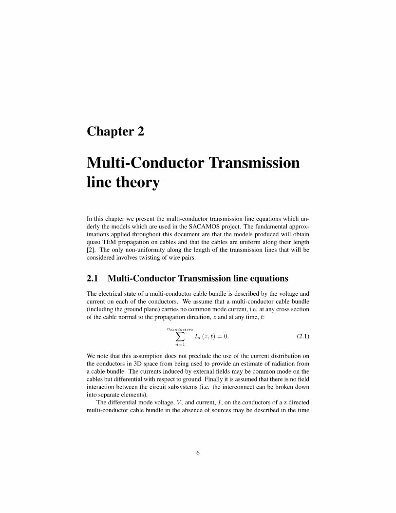
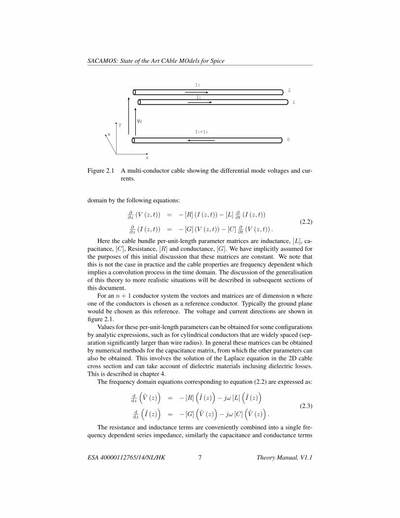
Figure 2.1 A multi-conductor cable showing the differential mode voltages and cur-rents.
domain by the following equations:
∂∂z (V (z, t)) = − [R] (I (z, t))− [L] ∂∂t (I (z, t))
∂∂z (I (z, t)) = − [G] (V (z, t))− [C] ∂∂t (V (z, t)) .
(2.2)
Here the cable bundle per-unit-length parameter matrices are inductance, [L], ca-pacitance, [C], Resistance, [R] and conductance, [G]. We have implicitly assumed forthe purposes of this initial discussion that these matrices are constant. We note thatthis is not the case in practice and the cable properties are frequency dependent whichimplies a convolution process in the time domain. The discussion of the generalisationof this theory to more realistic situations will be described in subsequent sections ofthis document.
For an n + 1 conductor system the vectors and matrices are of dimension n whereone of the conductors is chosen as a reference conductor. Typically the ground planewould be chosen as this reference. The voltage and current directions are shown infigure 2.1.
Values for these per-unit-length parameters can be obtained for some configurationsby analytic expressions, such as for cylindrical conductors that are widely spaced (sep-aration significantly larger than wire radius). In general these matrices can be obtainedby numerical methods for the capacitance matrix, from which the other parameters canalso be obtained. This involves the solution of the Laplace equation in the 2D cablecross section and can take account of dielectric materials inclusing dielectric losses.This is described in chapter 4.
The frequency domain equations corresponding to equation (2.2) are expressed as:
ddz
(V (z)
)= − [R]
(I (z)
)− jω [L]
(I (z)
)ddz
(I (z)
)= − [G]
(V (z)
)− jω [C]
(V (z)
).
(2.3)
The resistance and inductance terms are conveniently combined into a single fre-quency dependent series impedance, similarly the capacitance and conductance terms
ESA 40000112765/14/NL/HK 7 Theory Manual, V1.1

SACAMOS: State of the Art CAble MOdels for Spice
are combined into a single frequency dependent admittance term, this yields:
ddz
(V (z)
)= −
[Z] (I (z)
)ddz
(I (z)
)= −
[Y] (V (z)
),
(2.4)
where [Z]
= [R] + jω [L][Y]
= [G] + jω [C] .
(2.5)
This matrix formulation of the multi-conductor transmission line equations in fre-quency domain will be used in the next chapters to solve for currents and voltages oneach conductor. It is also used for generating the models with frequency dependentcable parameters.
ESA 40000112765/14/NL/HK 8 Theory Manual, V1.1

SACAMOS: State of the Art CAble MOdels for Spice
2.2 Per-Unit-Length ParametersThe multi-conductor transmission line equations express the transmission line voltagesand currents in terms of the inductance, capacitance, resistance and conductance ma-trices.
This chapter describes the per-unit-length parameters of the transmission lines andgives some formulae which may be used for their evaluation. A detailed discussion ofthe per-unit-length parameters may be found in [2]
2.2.1 The per-unit-length inductance matrixThe inductance matrix relates the total magnetic flux, Φ linking the ith circuit to thecurrents which produce it
Φ1
Φ2
...Φn
=
L1,1 L1,2 . . . L1,n
L2,1 L2,2 . . . L2,n
......
. . ....
Ln,1 Ln,2 . . . Ln,n
I1I2...In
(2.6)
An element of the inductance matrix Lij may be calculated by putting a current onconductor j and zero current on all other conductors then
Li,j =ΦiIj
∣∣∣∣Ik 6=j=0
(2.7)
2.2.2 The per-unit-length capacitance matrixThe capacitance matrix relates the charge , q, on conductors to the conductor voltages,V.
q1
q2
...qn
=
C1,1 C1,2 . . . C1,n
C2,1 C2,2 . . . C2,n
......
. . ....
Cn,1 Cn,2 . . . Cn,n
V1
V2
...Vn
(2.8)
The capacitance matrix is commonly calculated from its inverse, the elements ofthe inverse capacitance matrix [P ] = [C]−1 are determined by placing a charge onconductor j and zero change on all other conductors then
Pi,j =Viqj
∣∣∣∣Ik 6=j=0
(2.9)
then the capacitance matrix is found as
[C] = [P ]−1 (2.10)
In a homogeneous medium the capacitance matrix may be found from the induc-tance matrix using
[C] = µ0ε0εr [L]−1 (2.11)
ESA 40000112765/14/NL/HK 9 Theory Manual, V1.1
SACAMOS: State of the Art CAble MOdels for Spice
2.2.3 The per-unit-length resistance matrixThe per-unit-length resistance matrix, [R] incorporates the effects of conductor lossesin the model i.e. the effects of the finite conductivity of the conductors. It relatesthe voltage drop along the transmission line to the currents on the conductors. Theconductor resistance is a function of frequency due to the ’skin effect’. The calculationof the resitance of conductors, and the associated ’internal inductance’ is discussed insection 3.6.2. The resistance matrix relates the conductor voltages and currents at zerofrequency by
∂
∂z
V1
V2
...Vn
=
R1,1 R1,2 . . . R1,n
R2,1 R2,2 . . . R2,n
......
. . ....
Rn,1 Rn,2 . . . Rn,n
I1I2...In
(2.12)
If a conductor i, i = 1 . . . n has a resistance Ri and the reference conductor hasresistance R0 then the resistance matrix is given by
[R] =
R1 +R0 R0 . . . R0
R0 R2 +R0 . . . R0
......
. . ....
R0 R0 . . . Rn +R0
(2.13)
2.2.4 The per-unit-length conductance matrixThe per-unit-length conductance matrix , [G] incorporates the effects of losses due toconductance of the medium in which the conductors are situated and also due to polar-isation losses in dielectrics. The conductance loss will be assumed to be zero thereforethe only contributions to the conductance matrix are due to lossy dielectrics. In thiswork the conductance matrix is calculated by generalising the capacitance matrix cal-culation to complex permittivities.
The admittance matrix is written as
[Y ] = [G] + jω [C] = jω
[C − j
ωG
]= jω [C ′] (2.14)
Thus if we determine the complex capacitance matrix [[C ′] then we can calculatethe capacitance matrix and admittance matrices as
[C] = <[C ′] (2.15)
and[G] = −ω=[C ′] (2.16)
The calculation of the capacitance and conductance matrices for configurationswith lossy inhomogeneous dielectrics is discussed in section 4.
ESA 40000112765/14/NL/HK 10 Theory Manual, V1.1

SACAMOS: State of the Art CAble MOdels for Spice
2.2.5 Exact analytic formulae for per-unit-length parametersExact analytical formulae are available for the inductance and capacitance of someconductor configurations. There are also approximations which may be made whichallow the derivation of approximate analytic formulae. Where possible these formulaeare used in the SACAMOS software. The derivation of the formulae presented in thefollowing sections may be found in [2].
Figure 2.2 shows a coaxial cable
rw
rs
εr
Figure 2.2 Coaxial cable
In SACAMOS, the inductance and capacitance of the coaxial cable is always cal-culated using the analytic formulae
L =µ0
2πln
(rsrw
)(2.17)
C =2πε0εr (jω))
ln(rsrw
) (2.18)
Figure 2.3 shows a two wire transmission line.
rw
s
rw
Figure 2.3 Two wire cable
The analytic formulae used to calculate the inductance and capacitance of the twowire transmission line are
C =πε0
ln(
s2rw
+√
s2rw
2 − 1) (2.19)
ESA 40000112765/14/NL/HK 11 Theory Manual, V1.1
SACAMOS: State of the Art CAble MOdels for Spice
L =µ0ε0C
(2.20)
These formulae are used for the calculation of the differential mode inductance andcapacitance for twisted pairs.
2.2.6 Approximate analytic formulae for per-unit-length parame-ters
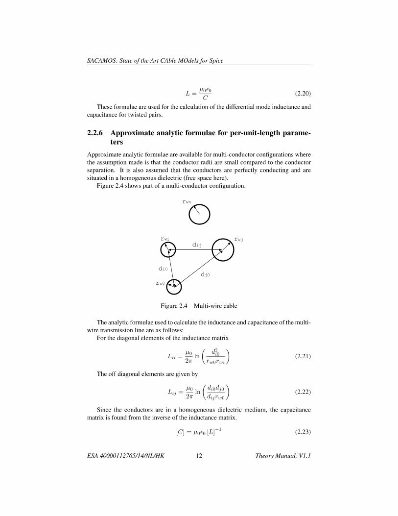
Approximate analytic formulae are available for multi-conductor configurations wherethe assumption made is that the conductor radii are small compared to the conductorseparation. It is also assumed that the conductors are perfectly conducting and aresituated in a homogeneous dielectric (free space here).
Figure 2.4 shows part of a multi-conductor configuration.
rwidij
rwj
rw0
rwn
dj0di0
Figure 2.4 Multi-wire cable
The analytic formulae used to calculate the inductance and capacitance of the multi-wire transmission line are as follows:
For the diagonal elements of the inductance matrix
Lii =µ0
2πln
(d2i0
rw0rwi
)(2.21)
The off diagonal elements are given by
Lij =µ0
2πln
(di0dj0dijrw0
)(2.22)
Since the conductors are in a homogeneous dielectric medium, the capacitancematrix is found from the inverse of the inductance matrix.
[C] = µ0ε0 [L]−1 (2.23)
ESA 40000112765/14/NL/HK 12 Theory Manual, V1.1

SACAMOS: State of the Art CAble MOdels for Spice
rwi
dij
rwj
hj
hi
ground plane
(reference, conductor 0)
Figure 2.5 Multi-wire cable over a ground plane
Figure 2.5 shows part of a multi-conductor configuration above a ground plane.Here the ground plane is the reference conductor
For the diagonal elements of the inductance matrix
Lii =µ0
2πln
(2hirwi
)(2.24)
The off diagonal elements are given by
Lij =µ0
4πln
(1 +
4hihjd2ij
)(2.25)
Since the conductors are in a homogeneous dielectric medium, the capacitancematrix may be found from the inverse of the inductance matrix.
[C] = µ0ε0 [L]−1 (2.26)
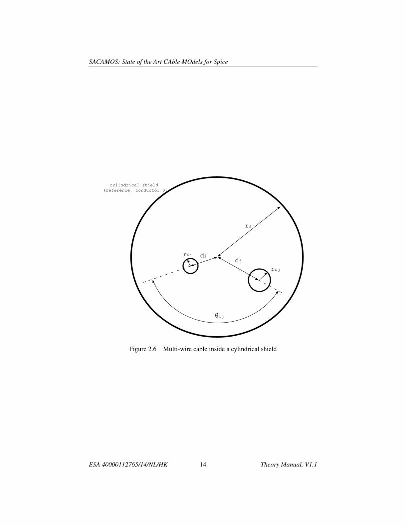
Figure 2.6 shows part of a multi-conductor configuration within a cylindrical shield.Here the shield is the reference conductor
For the diagonal elements of the inductance matrix
Lii =µ0
2πln
(r2s − d2
i
rsrwi
)(2.27)
The off diagonal elements are given by
Lij =µ0
2πln
djrs
√√√√(d2i d
2j + r4
s − 2didjr2s cos(θij)
d2i d
2j + d4
j − 2did3j cos(θij)
) (2.28)
Since the conductors are in a homogeneous dielectric medium, the capacitancematrix is found from the inverse of the inductance matrix.
[C] = µ0ε0 [L]−1 (2.29)
ESA 40000112765/14/NL/HK 13 Theory Manual, V1.1
SACAMOS: State of the Art CAble MOdels for Spice
rwi di
rwj
cylindrical shield
(reference, conductor 0)
dj
rs
θij
Figure 2.6 Multi-wire cable inside a cylindrical shield
ESA 40000112765/14/NL/HK 14 Theory Manual, V1.1
SACAMOS: State of the Art CAble MOdels for Spice
2.3 Solution to the Multi-Conductor Transmission lineequations
The SACAMOS software includes the ability to set up a validation test for the Spicetransmission line models. In the validation test a resistive termination circuit with se-ries voltage sources is specified and the solution for conductor voltages calculated withthe Spice transmission line model can be compared with the solution obtained usingthe frequency domain analytic solution. The frequency domain analytic solution is cal-culated on the basis of the full dimension multi-conductor transmission line equations(i.e. no domain decomposition) and therefore includes the self consistent model oftransfer impedance coupling. All the parameters in the analytic solution implementedare frequency dependent. The comparison between the Spice solution and the analyticsolution therfore allows the effect of the approximations made in the derivation of theSpice model to be tested.
This section outlines the solution of the transmission line equations defined in sec-tion 2.1. A more complete discussion of the multi-conductor transmission line equa-tions may be found in [2].
2.3.1 Solution of the transmission line equations by modal decom-position
The impedance and admittance matrices are given by:[Z]
= [R] + jω [L][Y]
= [G] + jω [C] .
(2.30)
We can derive a frequency domain solution to the transmission line equations using amodal analysis. Equation 2.4 can be re-written as an uncoupled second order equationin the following ways:
d2
dz2
(V (z)
)=
[Z] [Y] (V (z)
)d2
dz2
(I (z)
)=
[Y] [Z] (I (z)
).
(2.31)
A change of variables to modal quantities via a similarity transformation allows thedecoupling (diagonalisation) of the matrix system. The conductor voltages and currentsare related to their corresponding modal quantities by:
V (z) =[TV
] (Vm (z)
)I (z) =
[TI
] (Im (z)
).
(2.32)
ESA 40000112765/14/NL/HK 15 Theory Manual, V1.1
SACAMOS: State of the Art CAble MOdels for Spice
The voltage modal transformation matrix, [TV ] diagonalises the first equation given in(2.31):
d2
dz2
(Vm (z)
)=
[TV
]−1 [Z] [Y] [TV
] (Vm (z)
)=
[γ2] (Vm (z)
),
(2.33)
where[γ2]
is a diagonal matrix with elements whose values are the squares of themode propagation constants. The elements of the diagonal matrix
[γ2]
are found as
the eigenvalues of the [Z][Y ] product and the columns of the matrix[TV
]are the
corresponding eigenvectors. (We note that when there are repeated eigenvalues whichmay originate from the symmetry of the cable cross section, then the diagonalisation isnot unique. The eigenvectors corresponding to these eiganvalues are only required tospan a certain subspace of the original matrix. In this situation the eigenvector solverfor general complex matrices in Eispack ([11]) may on rare occasions return the sameeigenvector for more than one eigenvalue. In order to avoid this in practice we perturbthe matrix by a very small amount in a manner which prevents this degeneracy).
In the lossless case the impedance matrices and admittance matrices are imaginaryand symmetric, and the [Z] [Y ] product is real and symmetric. The modal transforma-tion matrices are real and are independent of frequency and the diagonal
[γ2]
matrixhas negative, real values of the form −ω
2
v2 , where v is the mode velocity. Modal de-composition for a lossless transmission line will be important in the derivation of theSpice multi-conductor transmission line model derived in section 3.
The solution for the modal voltages at any point z on the multi-conductor transmis-sion line may be written in terms of modes travelling in the +z and −z directions as:
Vm (z) =[e−γz
] (V +m
)+[e+γz
] (V −m
). (2.34)
The general solution for the actual conductor voltages is then:
V (z) =[TV
] ([e−γz
] (V +m
)+[e+γz
] (V −m
)). (2.35)
Similarly, the current modal transformation matrix [TI] diagonalises the secondequation in (2.31):
d2
dz2
(Im (z)
)=
[TI
]−1 [Y] [Z] [TI
] (Im (z)
)=
[γ2] (Im (z)
).
(2.36)
It can be shown [2] that the voltage and current modal transformation matrices canbe related by: [
TI
]T=[TV
]−1
. (2.37)
The solution for the modal currents at any point z on the multi-conductor transmissionline may be written in terms of modes travelling in the +z and −z directions as:
Im (z) =[e−γz
] (I+m
)−[e+γz
] (I−m
). (2.38)
ESA 40000112765/14/NL/HK 16 Theory Manual, V1.1
SACAMOS: State of the Art CAble MOdels for Spice
The general solution for the actual conductor currents is then:
I (z) =[TI
] ([e−γz
] (I+m
)−[e+γz
] (I−m
)). (2.39)
The conductor voltage vector may be written in terms of the modal current vectors as:
V (z) =[ZC
] [TI
] ([e−γz
] (I+m
)+[e+γz
] (I−m
)), (2.40)
where [ZC ] is the characteristic impedance matrix defined as:[ZC
]=[Y]−1 [
TI
][γ][TI
]−1
=[Z] [TI
][γ]−1[TI
]−1
. (2.41)
ESA 40000112765/14/NL/HK 17 Theory Manual, V1.1
SACAMOS: State of the Art CAble MOdels for Spice
2.3.2 Incorporating terminal conditionsThe solution in terms of voltages and currents of the MTL equations are given by (2.39)and (2.40). These expressions allow computing the state, i.e. current and voltage, ofeach conductor at any point of the transmission line, after determining the constantsI+m and I−m. Therefore the terminal conditions have to be incorporated, which can be
done via the generalised Thevenin equivalent:[V (0)
]=
[VS
]−[ZS
] (I (0)
)[V (L)
]=
[VL
]+[ZL
] (I (L)
),
(2.42)
where[ZS
]and
[ZL
]are the matrices with termination impedances on respectively
the source and load side of the multi conductor transmission line, i.e. respectivelyat z = 0 and z = L. VS and VL are the vectors containing the voltage sources onrespectively source and load side of the transmission line.
By evaluating equations (2.39) and (2.40) at z = 0 and z = L and substituting thisinto the Thevenin equivalent given by equation 2.42, we obtain:
([ZC
]+[ZS
]) [TI
] ([ZC
]−[ZS
]) [TI
]([ZC
]−[ZL
]) [TI
]e−γL
([ZC
]+[ZL
]) [TI
]eγL
I+
m
I−m
=
VS
VL
(2.43)
This matrix equation is readily solverd for the current waves, I+m and I−m and then equa-
tions (2.39) and (2.40) lead to a final solution for the conductor voltages and currents.The detail of the solution as it is implemented in the SACAMOS software is de-
scribed here. In order to keep the solution clear, these equations are rewritten as[M11
] [M12
][M21
] [M22
] I+
m
I−m
=
VS
VL
(2.44)
These equations are solved for I+m and I−m first by eliminating I−m to give
[[M11
]−[M12
] [M22
]−1 [M21
]] (I+m
)=(VS
)−[M12
] [M22
]−1 (VL
)(2.45)
Thus
(I+m
)=
[[M11
]−[M12
] [M22
]−1 [M21
]]−1((VS
)−[M12
] [M22
]−1 (VL
))(2.46)
I−m may then be found as(I−m
)=[M22
]−1 ((VL
))−[M21
] (I+m
)(2.47)
ESA 40000112765/14/NL/HK 18 Theory Manual, V1.1
SACAMOS: State of the Art CAble MOdels for Spice
substituting these expressions in equations (2.39) and (2.40) leads to a final solutionfor the conductor voltages and currents along the entire length of the multi conductortransmission line.
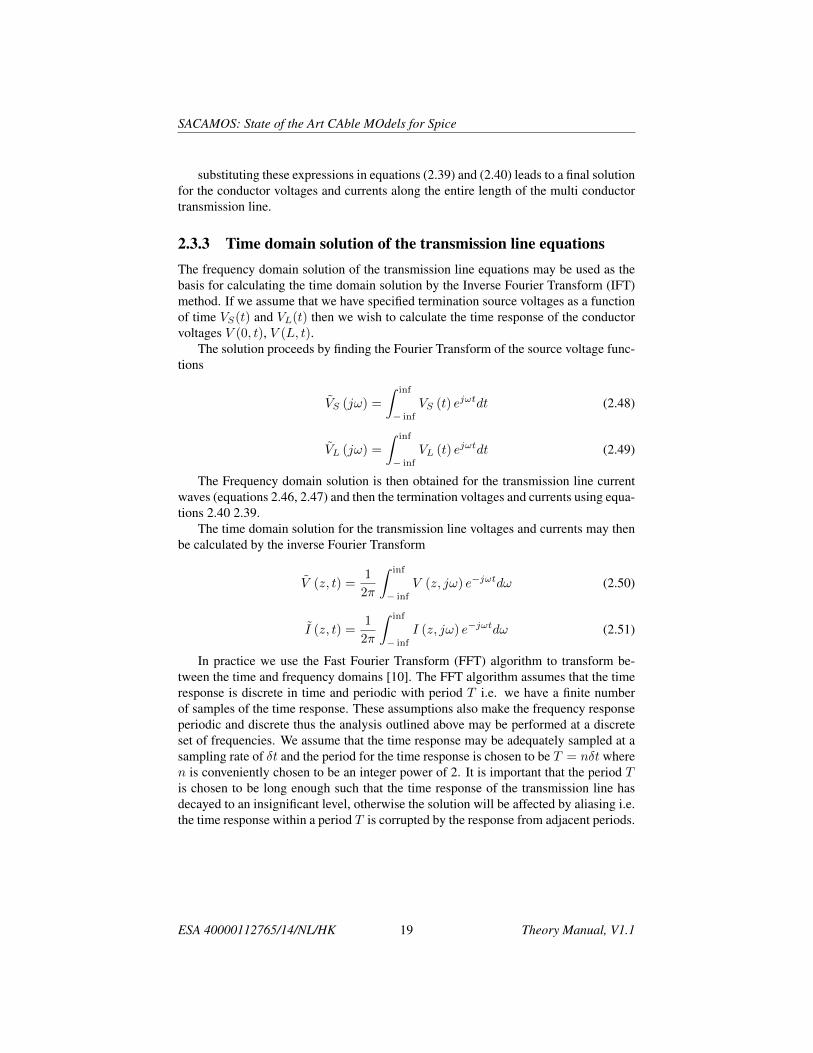
2.3.3 Time domain solution of the transmission line equationsThe frequency domain solution of the transmission line equations may be used as thebasis for calculating the time domain solution by the Inverse Fourier Transform (IFT)method. If we assume that we have specified termination source voltages as a functionof time VS(t) and VL(t) then we wish to calculate the time response of the conductorvoltages V (0, t), V (L, t).
The solution proceeds by finding the Fourier Transform of the source voltage func-tions
VS (jω) =
∫ inf
− inf
VS (t) ejωtdt (2.48)
VL (jω) =
∫ inf
− inf
VL (t) ejωtdt (2.49)
The Frequency domain solution is then obtained for the transmission line currentwaves (equations 2.46, 2.47) and then the termination voltages and currents using equa-tions 2.40 2.39.
The time domain solution for the transmission line voltages and currents may thenbe calculated by the inverse Fourier Transform
V (z, t) =1
2π
∫ inf
− inf
V (z, jω) e−jωtdω (2.50)
I (z, t) =1
2π
∫ inf
− inf
I (z, jω) e−jωtdω (2.51)
In practice we use the Fast Fourier Transform (FFT) algorithm to transform be-tween the time and frequency domains [10]. The FFT algorithm assumes that the timeresponse is discrete in time and periodic with period T i.e. we have a finite numberof samples of the time response. These assumptions also make the frequency responseperiodic and discrete thus the analysis outlined above may be performed at a discreteset of frequencies. We assume that the time response may be adequately sampled at asampling rate of δt and the period for the time response is chosen to be T = nδt wheren is conveniently chosen to be an integer power of 2. It is important that the period Tis chosen to be long enough such that the time response of the transmission line hasdecayed to an insignificant level, otherwise the solution will be affected by aliasing i.e.the time response within a period T is corrupted by the response from adjacent periods.
ESA 40000112765/14/NL/HK 19 Theory Manual, V1.1

SACAMOS: State of the Art CAble MOdels for Spice
2.4 Incident Field Excitation ModelAn electromagnetic field illuminating a transmission line can couple energy onto theline and therefore be a cause of interferance. The effect of an incident field excitationmay be included in the transmission line equations by distributed forcing functions IFand VF in the transmssion line equations as described in references [3], [2] thus thetransmission line equations with incident field excitation are written as
∂∂z (V (z, t)) = − [R] (I (z, t))− [L] ∂∂t (I (z, t)) + VF (z, t)
∂∂z (I (z, t)) = − [G] (V (z, t))− [C] ∂∂t (V (z, t)) + IF (z, t) .
(2.52)
Assuming that the conductors are widely separated, the time domain forcing functionsmay be written in terms of the incident electric field as
VF (z, t) = − ∂
∂zET (z, t) + EL (z, t) (2.53)
where for the i=th conductor
EL (z, t)i = Eincz (ith conductor, z, t)− Eincz (reference conductor, z, t) (2.54)
and
ET (z, t)i =
∫ conductori
ref
Einc (z, t) · dl (2.55)
andIF (z, t) = .− [G] (ET (z, t))− [C]
∂
∂t(ET (z, t)) (2.56)
Reference [3] notes the following assumptions made in the derivation of this modelfor incident field excitation:
1. The propagation is transverse magnetic
2. The sum of the induced currents in any cross section, including the referenceconductor is zero
3. ∂Esz
∂z is small compared with∇tEt
4. The conductivity of the medium surrounding the conductors is homogeneous.
A solution may be obtained in the frequency domain by the use of chain parametermatrices [2] which relate the voltages and currents at one end of the transmission lineto the volages and currents at the other. In the absence of distributed forcing functionswe can write
V (L) = Φ11 (L)V (0) + Φ12 (L) I (0)
I (L) = Φ21 (L)V (0) + Φ22 (L) I (0)(2.57)
ESA 40000112765/14/NL/HK 20 Theory Manual, V1.1
SACAMOS: State of the Art CAble MOdels for Spice
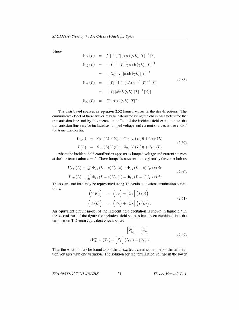
whereΦ11 (L) = [Y ]
−1[T ] [cosh (γL)] [T ]
−1[Y ]
Φ12 (L) = − [Y ]−1
[T ] [γ sinh (γL)] [T ]−1
= − [ZC ] [T ] [sinh (γL)] [T ]−1
Φ21 (L) = − [T ][sinh (γL) γ−1
][T ]−1
[Y ]
= − [T ] [sinh (γL)] [T ]−1
[YC ]
Φ22 (L) = [T ] [cosh (γL)] [T ]−1
(2.58)
The distributed sources in equation 2.52 launch waves in the ±z directions. Thecumuulative effect of these waves may be calculated using the chain parameters for thetransmission line and by this means, the effect of the incident field excitation on thetransmission line may be included as lumped voltage and current sources at one end ofthe transmission line
V (L) = Φ11 (L)V (0) + Φ12 (L) I (0) + VFT (L)
I (L) = Φ21 (L)V (0) + Φ22 (L) I (0) + IFT (L)(2.59)
where the incident field contribution appears as lumped voltage and current sourcesat the line termination z = L. These lumped source terms are given by the convolutions
VFT (L) =∫ L
0Φ11 (L− z)VF (z) + Φ12 (L− z) IF (z) dz
IFT (L) =∫ L
0Φ21 (L− z)VF (z) + Φ22 (L− z) IF (z) dz
(2.60)
The source and load may be represented using Thevenin equivalent termination condi-tions: (
V (0))
=(VS
)−[ZS
] (I (0)
)(V (L)
)=
(VL
)+[ZL
] (I (L)
),
(2.61)
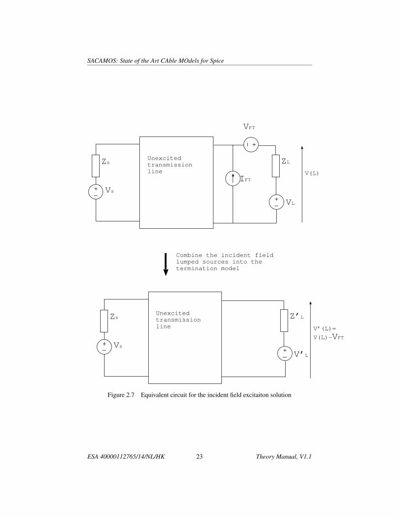
An equivalent circuit model of the incident field excitation is shown in figure 2.7 Inthe second part of the figure the includent field sources have been combined into thetermination Thevenin equivalent circuit where [
Z ′L
]=[ZL
](V ′S) = (VS) +
[ZL
](IFT )− (VFT )
(2.62)
Thus the solution may be found as for the unexcited transmission line for the termina-tion voltages with one variation. The solution for the termination voltage in the lower
ESA 40000112765/14/NL/HK 21 Theory Manual, V1.1

SACAMOS: State of the Art CAble MOdels for Spice
part of figure 2.7 includes VFT so to determine the actual transmission line voltageswe have
(V (L)) = (V ′ (L))− (VFT ) (2.63)
ESA 40000112765/14/NL/HK 22 Theory Manual, V1.1
SACAMOS: State of the Art CAble MOdels for Spice
Vs
Zs
VL
ZL
VFT
IFT
Unexcited
transmission
line
Vs
Zs
V’L
Z’LUnexcited
transmission
line
Combine the incident field
lumped sources into the
termination model
V(L)
V’(L)=
V(L)-VFT
Figure 2.7 Equivalent circuit for the incident field excitaiton solution
ESA 40000112765/14/NL/HK 23 Theory Manual, V1.1
Chapter 3
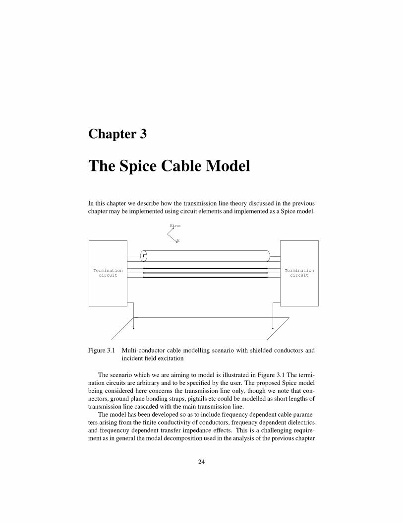
The Spice Cable Model
In this chapter we describe how the transmission line theory discussed in the previouschapter may be implemented using circuit elements and implemented as a Spice model.
Termination
circuit
Termination
circuit
Einc
k
Figure 3.1 Multi-conductor cable modelling scenario with shielded conductors andincident field excitation
The scenario which we are aiming to model is illustrated in Figure 3.1 The termi-nation circuits are arbitrary and to be specified by the user. The proposed Spice modelbeing considered here concerns the transmission line only, though we note that con-nectors, ground plane bonding straps, pigtails etc could be modelled as short lengths oftransmission line cascaded with the main transmission line.
The model has been developed so as to include frequency dependent cable parame-ters arising from the finite conductivity of conductors, frequency dependent dielectricsand frequencuy dependent transfer impedance effects. This is a challenging require-ment as in general the modal decomposition used in the analysis of the previous chapter
24

SACAMOS: State of the Art CAble MOdels for Spice
is a function of frequency. It is shown in section 3.6 that if the d.c. resistance of theconductors is lumped at the cable terminations then the modal decomposition becomesa weak function of frequency. Simulations show that the frequency dependence of themodal decomposition can be neglected and the decomposition based on lossless highfrequency inductance and capacitance matrices can be used provided that the propaga-tion of the individual modes is corrected for the propagation loss.
The spice model of the scenario depicted is based on a number of different partsthese are:
• Domain decomposition: we model shielded conductor systems as separate do-mains, in which the electrical quantities are referenced the shielding conductor,plus the external domain consisting of the ground plane, unshielded conductorsand the exterior surface of shields.
• Modal decomposition: Signal propagation on the multi-conductor system withineach domain is analysed by a modal decomposition method i.e. we diagonalisethe transmission line equations within each domain and propagate the modes on’modal transmission lines’
• Method of characteristics. The propagation of each mode is treated using themethod of characteristics [2] i.e. modes are propagated in the +z and -z direc-tions and the state of the transmission line is the combination of these +z and -zpropagating modes.
• Frequency dependent propagation characteristics are dealt with using an approx-imate model in which the d.c. resistance is extracted and lumped at the ends ofeach transmission line and the frequency dependence of the propagation is dealtwith by applying a frequency dependent propagation correction to the +z and -zpropagating modes at the ends of the transmission lines.
• Incident field excitation is assumed to be a plane wave, in this model appropriatecontrolled source terms lumped at the cable terminations take account of theincident field excitation.
• Coupling through imperfect shields is modelled with transfer impedance termsand implemented in a weak form i.e. source and victim conductors are identifiedand one way coupling is implemented using appropriate controlled source terms
• The twisted pair model is derived on the assumption that there is no couplingbetween the differential mode and the other conductors within the bundle (orthe shield for a shielded twisted pair) although coupling to the common mode isincluded. This model does however allow coupling from the common mode tothe differential mode and vice versa, through unbalanced terminations.
In the subsequent sections each of these stages is treated in turn and theoreticalmodel derivations and associated circuit diagrams will be presented.
ESA 40000112765/14/NL/HK 25 Theory Manual, V1.1

SACAMOS: State of the Art CAble MOdels for Spice
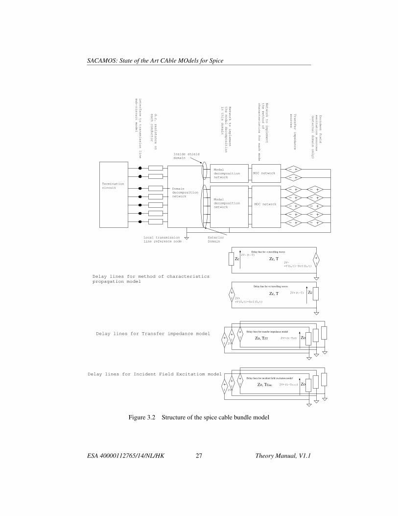
3.1 Spice cable bundle model structureFigure 3.2 shows the structure of the spice cable bundle model with a terminationnetwork. The termination network is an arbitrary network to be constructed by theuser and does not concern us here. The spice cable bundle model consists of a numberof cascaded elements. The major elements are (in order from the model terminalsinwards)
1. d.c. conductor resistance
2. Domain decomposition network
3. Modal decomposition network
4. Souces to include transfer impedance and incident field excitation
5. Method of characteristics delay lines
6. Transfer impedance delay lines
7. Incident field delay lines
ESA 40000112765/14/NL/HK 26 Theory Manual, V1.1
SACAMOS: State of the Art CAble MOdels for Spice
Transfer impedance
sources
Exterior
Domaind.c. resistance on
each conductor
Incident field
excitation sources
(external domain only)
Network to implement
the modal decomposition
in this domain
Network to implement
the method of
characteristics for each mode
interface to transmission line
sub-circuit model
Termination
circuit
Inside shield
domain
Modal
decomposition
network
Modal
decomposition
network
MOC network
MOC network
Domain
decomposition
network
Local transmission
line reference node
Zc, T Zc
Zc, TZc
2V+
=V(0,t)+ZcI(0,t)
2V-
=V(L,t)-ZcI(L,t)
Delay line for -z travelling waves
Delay line for +z travelling waves
2V+(t-T)
2V-(t-T)
Zo, TZT Zo
2V+
Delay lines for transfer impedance model
2V+(t-TZT)
Zo, TEinc Zo
2V+
Delay lines for incident field excitation model
2V+(t-TEinc)
Delay lines for method of characteristics
propagation model
Delay lines for Transfer impedance model
Delay lines for Incident Field Excitatiom model
Figure 3.2 Structure of the spice cable bundle model
ESA 40000112765/14/NL/HK 27 Theory Manual, V1.1

SACAMOS: State of the Art CAble MOdels for Spice
3.1.1 TerminologyIn discussing the spice cable bundle model we require a clear terminology so as toallow unambiguous reference to particuar sections of the model.
Cable numbering always relates to the numbering of the cables within a bundle andis specified by the order in which they are included in the cable spec file.
Within a cable there is a local numbering system for cables and domains within acable e.g for a coaxial cable the inner wire is local conductor 1 and the shield is localconductor 2. Similarly the inner coaxial domain is domain 1 and the external domainis domain 2.
Once a cable bundle is built a global numbering is introduced.We adopt the terminology in table 3.1 both in this document and in the software
itself:
Name parameters Descriptionglobal terminal conductor conductor number The global conductor number in the
cable bundleglobal domain conductor domain number, con-
ductor numberThe global conductor number in aparticular domain
local cable conductor cable number The local conductor number in aparticular cable. This is fixed foreach cable type
global cable conductor cable number, con-ductor number
The global conductor number in aparticular cable
local cable domain cable number The local domain number in a par-ticular cable. This is fixed for eachcable type
global cable domain cable number, con-ductor number
The global domain number in a par-ticular cable
Table 3.1 Spice cable bundle model terminology
ESA 40000112765/14/NL/HK 28 Theory Manual, V1.1
SACAMOS: State of the Art CAble MOdels for Spice
3.2 Domain decompositionThe basis for computation of the systems being addressed in this work is the multi-conductor cable bundle. A bundle consists of multiple individual cables. These cablesmay consist of shielded and/ or un-shielded conductors perhaps with the addition ofover-shielding and a ground plane (satellite panel).
The spice cable bundle model decomposes the transmission line system into do-mains. The domains consist of an external domain whose conductors are exposed tothe external EM environment and internal domains in which conductors are shieldedfrom the external environment. These domains are assumed to be only weakly coupledthrough transfer impedance terms.
The domain decomposition method along with the weak coupling assumption leadsto a smaller system of coupled equations and has the advantage of removing one of thestrong frequency dependent effects, that of transfer impedance coupling, from the mainpropagation model.
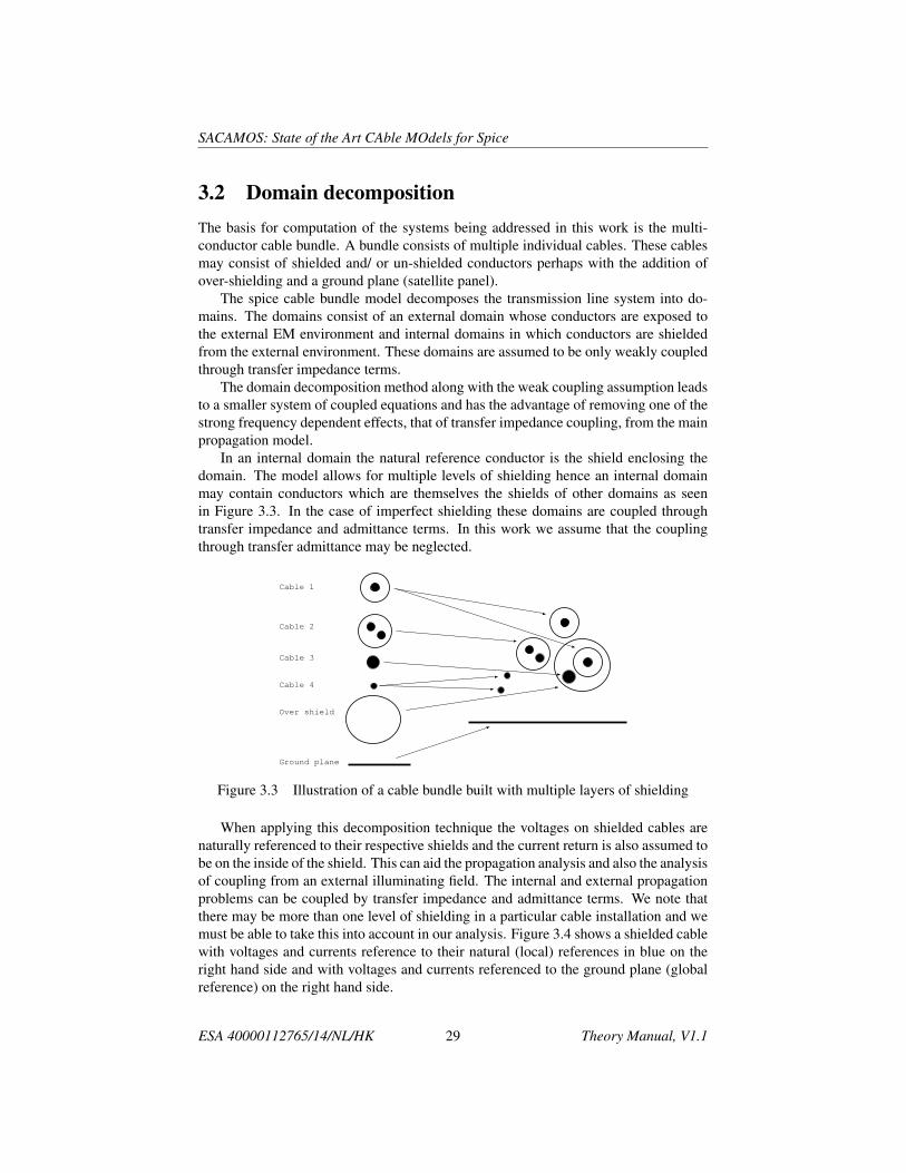
In an internal domain the natural reference conductor is the shield enclosing thedomain. The model allows for multiple levels of shielding hence an internal domainmay contain conductors which are themselves the shields of other domains as seenin Figure 3.3. In the case of imperfect shielding these domains are coupled throughtransfer impedance and admittance terms. In this work we assume that the couplingthrough transfer admittance may be neglected.
Cable 1
Cable 2
Cable 3
Cable 4
Over shield
Ground plane
Figure 3.3 Illustration of a cable bundle built with multiple layers of shielding
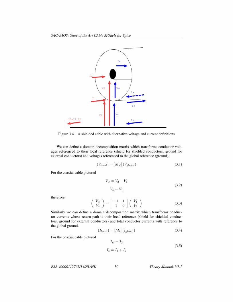
When applying this decomposition technique the voltages on shielded cables arenaturally referenced to their respective shields and the current return is also assumed tobe on the inside of the shield. This can aid the propagation analysis and also the analysisof coupling from an external illuminating field. The internal and external propagationproblems can be coupled by transfer impedance and admittance terms. We note thatthere may be more than one level of shielding in a particular cable installation and wemust be able to take this into account in our analysis. Figure 3.4 shows a shielded cablewith voltages and currents reference to their natural (local) references in blue on theright hand side and with voltages and currents referenced to the ground plane (globalreference) on the right hand side.
ESA 40000112765/14/NL/HK 29 Theory Manual, V1.1
SACAMOS: State of the Art CAble MOdels for Spice
V1
V2 Vw
Vs
I0=I1+I2
I1
I2
Iw
Iw
Is
Is
Figure 3.4 A shielded cable with alternative voltage and current definitions
We can define a domain decomposition matrix which transforms conductor volt-ages referenced to their local reference (shield for shielded conductors, ground forexternal conductors) and voltages referenced to the global reference (ground).
(Vlocal) = [MV ] (Vglobal) (3.1)
For the coaxial cable pictured
Vw = V2 − V1
Vs = V1
(3.2)
therefore (VwVs
)=
[−1 11 0
](V1
V2
)(3.3)
Similarly we can define a domain decomposition matrix which transforms conduc-tor currents whose return path is their local reference (shield for shielded conduc-tors, ground for external conductors) and total conductor currents with reference tothe global ground.
(Ilocal) = [MI ] (Iglobal) (3.4)
For the coaxial cable picturedIw = I2
Is = I1 + I2(3.5)
ESA 40000112765/14/NL/HK 30 Theory Manual, V1.1

SACAMOS: State of the Art CAble MOdels for Spice
therefore (IwIs
)=
[0 11 1
](I1I2
)(3.6)
Figure 3.3 shows a complex cable bundle with multiple levels of shielding. In thiscase there are multiple local voltage references. The transformation matrices for thesecomplex situations can be defined in a similar manner as for the coaxial cable.
The domain decomposition process is achieved by a matrix multiplication. Thismay be implemented in a Spice model using controlled voltage and current sources. Inthe example of the coaxial cable above a ground plane there are three conductors. Wedefine the global voltage variables with respect to the ground plane as
V1 = Vshield
V2 = Wwire
(3.7)
The model is divided into two domains, the inner domain consisting of the inner wireand the shield (domain 1) and the external domain consisting of the outer shield andthe ground (domain 2). Each of the domains has a single conductor in addition to itsreference. The domain based voltage variables are
Vd1 c1 = Vwire − Vshield = V2 − V1
Vd2 c1 = Wshield = V1
(3.8)
The equation relating the global voltage variables and domain voltage variables is Vd1 c1
Vd2 c1
=
−1 1
1 0
V1
V2
= [MV ]
V1
V2
(3.9)
Inverting this equation gives V1
V2
=
1 1
1 0
Vd1 c1
Vd2 c1
= [MV ]−1
Vd1 c1
Vd2 c1
(3.10)
Similarly the equation relating the global current variables and domain current vari-ables is Id1 c1
Id2 c1
=
0 1
1 1
I1
I2
= [MI ]
I1
I2
(3.11)
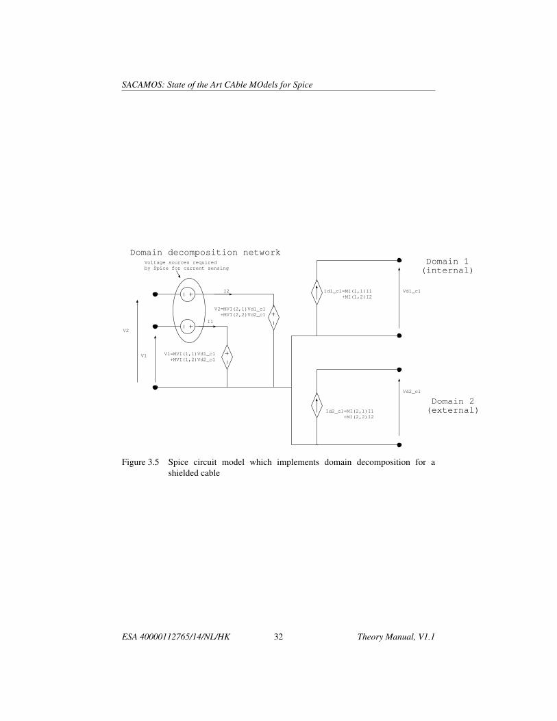
Figure 3.5 shows a Spice circuit model which implememnts equations 3.10 and 3.11.Note that the voltage sources on the left hand side of the figure have a value of zerovolts, they are only required as Spice uses such voltage sources as current sensingelements for the current controlled voltage sources.
ESA 40000112765/14/NL/HK 31 Theory Manual, V1.1
SACAMOS: State of the Art CAble MOdels for Spice
Domain decomposition network Domain 1(internal)
Domain 2(external)
Voltage sources required
by Spice for current sensing
V1
V2
Vd1_c1
Vd2_c1
Id1_c1=MI(1,1)I1
+MI(1,2)I2
I2
I1
Id2_c1=MI(2,1)I1
+MI(2,2)I2
V1=MVI(1,1)Vd1_c1
+MVI(1,2)Vd2_c1
V2=MVI(2,1)Vd1_c1
+MVI(2,2)Vd2_c1
Figure 3.5 Spice circuit model which implements domain decomposition for ashielded cable
ESA 40000112765/14/NL/HK 32 Theory Manual, V1.1
SACAMOS: State of the Art CAble MOdels for Spice
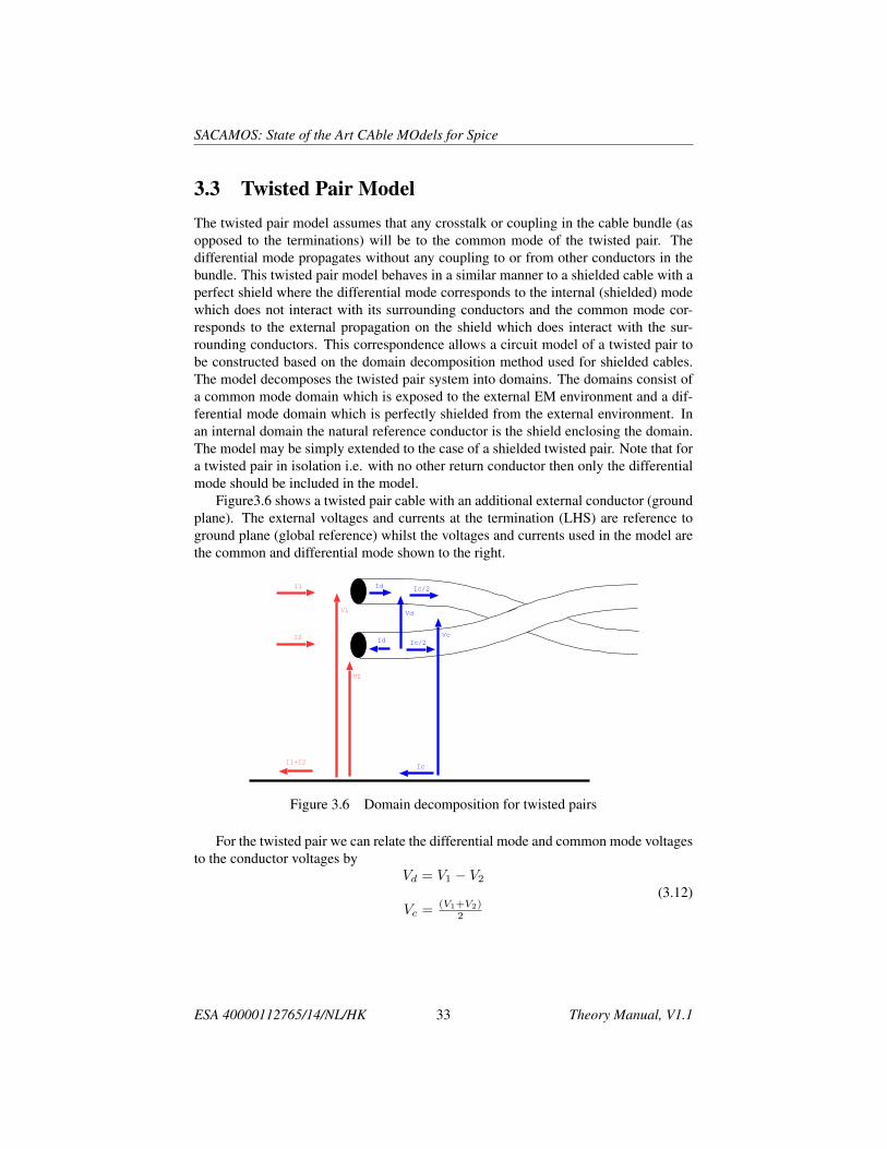
3.3 Twisted Pair ModelThe twisted pair model assumes that any crosstalk or coupling in the cable bundle (asopposed to the terminations) will be to the common mode of the twisted pair. Thedifferential mode propagates without any coupling to or from other conductors in thebundle. This twisted pair model behaves in a similar manner to a shielded cable with aperfect shield where the differential mode corresponds to the internal (shielded) modewhich does not interact with its surrounding conductors and the common mode cor-responds to the external propagation on the shield which does interact with the sur-rounding conductors. This correspondence allows a circuit model of a twisted pair tobe constructed based on the domain decomposition method used for shielded cables.The model decomposes the twisted pair system into domains. The domains consist ofa common mode domain which is exposed to the external EM environment and a dif-ferential mode domain which is perfectly shielded from the external environment. Inan internal domain the natural reference conductor is the shield enclosing the domain.The model may be simply extended to the case of a shielded twisted pair. Note that fora twisted pair in isolation i.e. with no other return conductor then only the differentialmode should be included in the model.
Figure3.6 shows a twisted pair cable with an additional external conductor (groundplane). The external voltages and currents at the termination (LHS) are reference toground plane (global reference) whilst the voltages and currents used in the model arethe common and differential mode shown to the right.
V1
V2
Vd
Vc
I1+I2
I1
I2
Id
Ic
Id
Ic/2
Ic/2
Figure 3.6 Domain decomposition for twisted pairs
For the twisted pair we can relate the differential mode and common mode voltagesto the conductor voltages by
Vd = V1 − V2
Vc = (V1+V2)2
(3.12)
ESA 40000112765/14/NL/HK 33 Theory Manual, V1.1
SACAMOS: State of the Art CAble MOdels for Spice
therefore the domain decomposition matrix MV is given by Vd
Vc
= [MV ]
V1
V2
=
1 −1
12
12
V1
V2
(3.13)
Similarly we can relate the differential mode and common mode currents to the con-ductor current by
Id = (I1−I2)2
Ic = I1 + I2
(3.14)
therefore the domain decomposition matrix MI is given by Id
Ic
= [MI ]
I1
I2
=
12 − 1
2
1 1
I1
I2
(3.15)
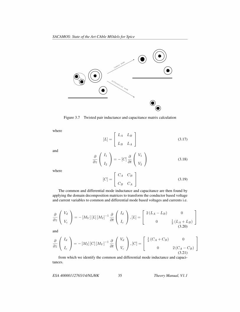
3.3.1 Per-unit-length parameters for the twisted pair modelThe decomposition into the differential mode and the common mode for the twistedpair model requires the per-unit-length inductance and capacitance to be determinedfor these modes. The differentail mode of a twisted pair in a bundle with other con-ductors and/ or a ground plane is assumed not to interact with the other conductorsin the bundle, the differential mode inductance and capacitance are calculated for thetwo conductors in isolation i.e. with all other conductors removed. The differentialmode inductance and capcitance are then independent of the orientation of the conduc-tors in the analysis. The common mode inductance and capacitance are calculated byassuming that the common mode current is carried by an equivalent cylindrical conduc-tor placed on the axis of the twisted pair. This equivalent conductor is then used in theanalysis of the bundle cross section in the calculation of the twisted pair common modecontribution to the inductance and capacitance matrices. This process is illustrated infigure 3.7
3.3.2 Per-unit-length parameters for the shielded twisted pair modelThe per-unit-length parameters for a shielded twisted pair are determined in a slightlydifferent manner than for a twisted pair in a bundle with other conductors. In the caseof a shielded twisted pair the orientation of the conductors is not of any significancedue to the symmetry of the shield conductor. The inductance and capacitance of thethree conductor system formed by the twisted pair and the shield can be calculatedusing the Laplace solver with the shield chosen as the reference conductor. This givesthe conductor based transmission line equations of the following form
∂
∂z
V1
V2
= − [L]∂
∂t
I1
I2
(3.16)
ESA 40000112765/14/NL/HK 34 Theory Manual, V1.1
SACAMOS: State of the Art CAble MOdels for Spice
Common mode
differential mode
Figure 3.7 Twisted pair inductance and capacitance matrix calculation
where
[L] =
LA LB
LB LA
(3.17)
and∂
∂z
I1
I2
= − [C]∂
∂t
V1
V2
(3.18)
where
[C] =
CA CB
CB CA
(3.19)
The common and differential mode inductance and capacitance are then found byapplying the domain decomposition matrices to transform the conductor based voltageand current variables to common and differential mode based voltages and currents i.e.
∂
∂z
Vd
Vc
= − [MV ] [L] [MI ]−1 ∂
∂t
Id
Ic
, [L] =
2 (LA − LB) 0
0 12 (LA + LB)
(3.20)
and
∂
∂z
Id
Ic
= − [MI ] [C] [MV ]−1 ∂
∂t
Vd
Vc
, [C] =
12 (CA + CB) 0
0 2 (CA − CB)
(3.21)
from which we identify the common and differential mode inductance and capaci-tances.
ESA 40000112765/14/NL/HK 35 Theory Manual, V1.1

SACAMOS: State of the Art CAble MOdels for Spice
3.4 Modal decompositionThe multi-conductor frequency domain transmission line equations are given by
ddz
(V (z)
)= −
[Z] (I (z)
)ddz
(I (z)
)= −
[Y] (V (z)
),
(3.22)
where [Z]
= [R] + jω [L][Y]
= [G] + jω [C] .
(3.23)
The frequency domain solution of these equations relied on a modal decompositionmethod as described in section 2 in which the [Z][Y ] product was diagonalised i.e. wemust diagonalise the matrix[
Z] [Y]
= [[R] + jω [L]] [[G] + jω [C] .] (3.24)
Even if we assume that the parameters of the cable are independent of frequencythen the problems with the diagonalisation process can be seen by looking at the limitsas jω → 0 and jω → inf . In the first case we have (if we assume that [G] = 0[
Z] [Y]
= [R] [jω [C]] (3.25)
whereas at high frequency we can neglect [R] and [G] in comparison to to jω[L]and jω[C] and we have [
Z] [Y]
= −ω2 [L] [C] (3.26)
In the first case the [Z][Y ] matrix product is dominated by [R] and [C] whereas athigh frequency it is dominated by [L] and [L]. In the general case, we must thereforediagonalise the [Z][Y ] matrix product at every frequency.
A model which eliminates this problem may be found by lumping the d.c. resis-tances of the conductors at the conductor ends i.e. place a lumped resistance withvalue Rdc/2 at either end of the transmission line. Once this is done, the [Z][Y ] matrixproduct is again given by equation 3.26.
A justification for this is that the transmission line resistance may be attributed tothe finite conductivity of the conductors. The resistance resulting from this is freqencydependent and increases as 1√
(f). Subtracting the d.c. resistance will result in a model
which is still correct at d.c. and reasonably accurate provided the transmission line isshort compared with the wavelength. The modal decomposition will be a weak func-tion of frequency and the losses associated with the propagation of a mode on a lossytransmission line may be corrected by a frequency dependent loss term as describedbelow.
ESA 40000112765/14/NL/HK 36 Theory Manual, V1.1
SACAMOS: State of the Art CAble MOdels for Spice
It is interesting to observe that (if we consider a single mode transmission line), ifthere is a d.c. resistance present then the characteristic impedance of the lossy line isgiven by
Z0 =
√R+ jωL
jωC(3.27)
at low frequency
Z0 →
√R
jωC(3.28)
i.e. the characteristic impedance varies as 1√(jω)
i.e. Z0 → inf as ω → 0.
The individual conductor currents and voltages within a domain are transformedinto the modal currents and voltages. The conductor voltages and currents are solutionsof the coupled first order equations
ddz
(V (z)
)= − [L] d
dt
(I (z)
)ddz
(I (z)
)= − [C] d
dt
(V (z)
) (3.29)
Two uncoupled second order equations may be written:
d2
dz2
(V (z)
)=
[L] [C]
d2
dt2
(V (z)
)d2
dz2
(I (z)
)=
[C] [L]
d2
dt2
(I (z)
).
(3.30)
A change of variables via a similarity transformation to modal quantities allows the de-coupling (diagonalisation) of the matrix system. The conductor voltages and currentsare related to their corresponding modal quantities by voltage and current transforma-tion matrices (
V (z))
=[TV
] (Vm (z)
)(I (z)
)=
[TI
] (Im (z)
) (3.31)
Thus the coupled first order equations 3.29 become
ddz
(Vm (z)
)= − [TV ]
−1[L] [TI ]
ddt
(Im (z)
)ddz
(Im (z)
)= − [TI ]
−1[C] [TV ] d
dt
(Vm (z)
) (3.32)
and the uncoupled second order equations 3.30 become
d2
dz2
(Vm (z)
)= [TV ]
−1[L] [C]
[TV ] d2
dt2
(Vm (z)
)d2
dz2
(Im (z)
)= [TI ]
−1[C] [L]
[TI ]d2
dt2
(Im (z)
).
(3.33)
ESA 40000112765/14/NL/HK 37 Theory Manual, V1.1
SACAMOS: State of the Art CAble MOdels for Spice
In the case of a lossless inhomogeneous transmission line it is possible to find matrices[TV ] and [TI ] which simultaneoously diagonalise both [L] and [C] i.e.
[TV ]−1
[L] [TI ] = [Lm]
[TI ]−1
[C] [TV ] = [Cm](3.34)
where [Lm] and [Cm] are diagonal matrices. Thus we have an uncoupled system formodal propagation where the mode characteristic impedance of the ith mode is
Zcmi =
√lmicmi
(3.35)
and the mode velocity is
Vmi =1√
lmicmi(3.36)
The matrices [L] and [C] are real, symmetric and positive definite and we may obtainthe diagonalisation of these matrices as follows:
First diagonalise the real,symmetric matrix, [C] with the orthogonal transformationmatrix [U ]
[U ]t[C] [U ] =
[θ2]
(3.37)
where[U ]
t= [U ]
−1 (3.38)
The capacitance matrix, [C] is positive definite so the square root of the diagonal eigen-value matrix, [θ] is real.
Second form the product
[M ] = [θ] [U ]t[L] [U ] [θ] (3.39)
[M ] is a real symmetric matrix which may again be diagonalised with an orthogonalmatrix.
[S]t[M ] [S] =
[Γ2]
(3.40)
where[S]
t= [S]
−1 (3.41)
Define the normalised matrix [Tnorm] as
[Tnorm] = [U ] [θ] [S] [α] (3.42)
where the diagonal matrix [α] normalises the columns of [Tnorm] to length 1.The matrices which diagonalise [L] and [C] are then
[TV ]−1
= [Tnorm]t (3.43)
and[TI ]
−1= [Tnorm]
−1 (3.44)
ESA 40000112765/14/NL/HK 38 Theory Manual, V1.1

SACAMOS: State of the Art CAble MOdels for Spice
Thus the voltage and current modal transformation matrices are related by[TI
]T=[TV
]−1
(3.45)
The mode impedance and velocity for a mode i are
Zcmi =
√lmicmi
= α2iiΓi (3.46)
Vmi =1√
lmicmi=
1
Γi(3.47)
Mode propagation will underly the method of characteristics based propogation algo-rithm in the Spice model.
This leads to an efficient algorithm for both a.c. and transient models of multi-conductor propagation provided that the modal decomposition matrices are indepen-dent of frequency. Discussion of the incorporation of loss and frequency dependentproperties will be discussed in sections 7.4 and 7.5.
For the example of a lossless 3 conductor cable the conductor currents are relatedto the modal currents by matrices of dimension 2: I1
I2
=[TI
] Im1
Im2
(3.48)
Hence the modal currents are related to the conductor currents by Im1
Im2
=[TI
]−1
I1
I2
(3.49)
And the conductor voltages are related to the modal voltages by V1
V2
=[TV
] Vm1
Vm2
(3.50)
A modal decomposition for a three conductor (two mode) transmission line is im-plemented by the network model in Figure 3.8. The model implements equations 3.49and 3.50. As for the domain decomposition matrix implementation, the voltage sourceson the left hand side of the figure have a value of zero volts, they are only required asSpice uses such voltage sources as current sensing elements for the current controlledvoltage sources.
This model may be implemented in any of the Spice versions considered in thisstudy and is suitable for a.c. and transient analysis. It may be extended to an arbitrarynumber of conductors under the assumption that the multi-conductor is lossless andnon-dispersive.
ESA 40000112765/14/NL/HK 39 Theory Manual, V1.1

SACAMOS: State of the Art CAble MOdels for Spice
Modal decomposition network Mode 1
mode 2
Voltage sources required
by Spice for current sensing
V1
V2
Vm1
Vm2
Im1=TII(1,1)I1
+TII(1,2)I2
I2
I1
Im2=TII(2,1)I1
+TII(2,2)I2
V1=TV(1,1)Vm1
+TV(1,2)Vm2
V2=TV(2,1)Vm1
+TV(2,2)Vm2
Figure 3.8 Spice circuit model which implements modal decomposition for a threeconductor system
ESA 40000112765/14/NL/HK 40 Theory Manual, V1.1
SACAMOS: State of the Art CAble MOdels for Spice
3.5 Method of characteristicsThe propagation of modes is implemented using the method of characteristics [2] i.e.we identify modes propagating in the +z and -z directions at the terminations and prop-agate these separately. This has advantages for incorporating incident field excitationand transfer impedance coupling processes. In the derivation of the method of charac-teristics model we consider a lossless, dispersionless single mode transmission line oflength L. This analysis generalizes to multi-mode transmission lines where each modeis treated separately and so is sufficient for the derivation of the proposed model. If weconsider the propagation of a mode with modal current, I, modal voltage, V, and modalcharacteristic impedance Zc then the voltage and current may be written as the sum ofwaves propagating in the +z and -z directions as
V = V + + V −
I = I+ − V −(3.51)
The voltage and current for the +z and -z waves are related by
I+ = V +
Zc
I− = −V−
Zc
(3.52)
We can work out the decomposition into +z and -z travelling modes from the voltageand current at any point, z, along the transmission line
2V + = V + ZcI
2V − = V − ZcI(3.53)
Evaluating equation 3.53 at z=0 gives
V (0, t) = ZcI (0, t) + 2V − (0, t) (3.54)
Similarly, at z=L we have
V (L, t) = −ZcI (L, t) + 2V + (0, t) (3.55)
The -z travelling mode quantities at z=0 are the -z travelling mode quantities launchedfrom the z=L termination at time t-T where T is the transmission line delay thus sub-stituting equation 3.53 evaluated at time t-T, and z=L gives
V (0, t) = ZcI (0, t) + V (L, t− T )− ZcI (L, t− T ) (3.56)
A similar process leads to an equation for the z=L end of the transmission line
V (L, t) = −ZcI (0, t) + V (0, t− T ) + ZcI (0, t− T ) (3.57)
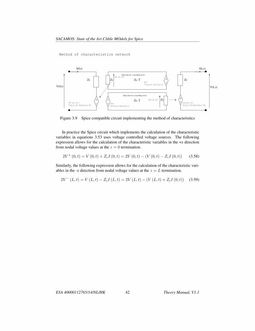
Equations 3.54, 3.55 and 3.56, 3.57 are implemented in the spice compatible circuitshown in Figure 3.9 where the time delay is incorporated into the model by a perfectlymatched ideal transmission line.
ESA 40000112765/14/NL/HK 41 Theory Manual, V1.1
SACAMOS: State of the Art CAble MOdels for Spice
Method of characteristics network
V(0,t)
2V-(t-T)=
V(L,t-T)-ZcI(L,t-T)
Zc, T Zc
Zc
I(0,t)
Zc, TZc
V(L,t)
I(L,t)
2V+(t-T)=
V(0,t-T)+ZcI(0,t-T)2V+
=V(0,t)+ZcI(0,t)
2V-
=V(L,t)-ZcI(L,t)
Delay line for -z travelling waves
Delay line for +z travelling waves
Zc
2V+(t-T)
2V-(t-T)
Figure 3.9 Spice compatible circuit implementing the method of characteristics
In practice the Spice circuit which implements the calculation of the characteristicvariables in equations 3.53 uses voltage controlled voltage sources. The followingexpression allows for the calculation of the characteristic variables in the +z directionfrom nodal voltage values at the z = 0 termination.
2V + (0, t) = V (0, t) + ZcI (0, t) = 2V (0, t)− (V (0, t)− ZcI (0, t)) (3.58)
Similarly, the following expression allows for the calculation of the characteristic vari-ables in the -z direction from nodal voltage values at the z = L termination.
2V − (L, t) = V (L, t)− ZcI (L, t) = 2V (L, t)− (V (L, t) + ZcI (0, t)) (3.59)
ESA 40000112765/14/NL/HK 42 Theory Manual, V1.1

SACAMOS: State of the Art CAble MOdels for Spice
3.6 Approximate model for frequency dependent trans-mission lines
The derivation of the model for frequency dependent transmission lines will be de-scribed in two stages. Firstly the model is described for single mode propagation. Thismodel is subsequently generalised to multi-mode propagation. The frequency depen-dent properties in the models derived here arise from two mechanisms:
1. frequency dependent permittivity of dielectrics
2. finite conductivity of conductors.
3.6.1 Frequency dependent dielectric modelsFrequency dependent cable properties (dielectric relative permittivity or transfer impedance)may be included in the model using the rational function form for the relative permit-tivity i.e.
εr (jω) =a0 + a1
(jωω0
)+ a2
(jωω0
)2
+ . . .
b0 + b1
(jωω0
)+ b2
(jωω0
)2
+ . . .(3.60)
For example the frequency dependent cable dielectric constant could be approximatedby a Debye model [4] which has a relative permittivity (although in practice debyedielectrics would be too lossy to be used in transmission lines) described by
εr = ε∞ +εs − ε∞1 + jωτ
(3.61)
where ε∞ is the relative permittivity at the high frequency limit, εs is the relative per-mittivity at the low frequency limit and τ is the relaxation time of the material.
A frequency dependent dielectric model will then give rise to a frequency depen-dent admittance in the transmission line equations. We note however that the frequencydependent relative permittivity function in equation 3.60 will give rise to no admittanceat d.c. The only mechanism which would give rise to a d.c. admittance would be a non-zero electrical conductivity in the dielectric.
3.6.2 Frequency dependent finite conductivity loss modelsCable losses arising from the finite conductivity of a conductor are incorporated intosome of the cable models available. In these models the conductivity of the conductorsare specified as parameters of the cable model. The cylindrical conductor loss modelsare based on reference [5] and the model for rectangular conductors is derived in [2]The models of finite conductivity of conductors include both a resistance and internalinductance (due to the magnetic field penetrating the conductor). These are frequencydependent and thus a complex internal impedance contributes to the impedance matrixof the idealised cable.
ESA 40000112765/14/NL/HK 43 Theory Manual, V1.1

SACAMOS: State of the Art CAble MOdels for Spice
It is seen that the internal resistance due to finite conductivity increases as√
(f)and the internal inductance decreases as 1√
f. This is important to note for the derivation
of the propagation correction.
Cylindrical Conductor
For a cylindrical conductor of radius, r, and conductivity, σ, the internal impedancedue to the magnetic field penetrating the conductor at frequency f is given by [5], [2]
Zint =1√
2πrσδ
(ber(q) + jbei(q)
bei′(q)− jber′(q)
)(3.62)
where ber and bei are Kelvin functions, δ is the skin depth given by
δ =1√πfµσ
(3.63)
and q is
q =√
2r
δ(3.64)
Cylindrical Shell
For a cylindrical shell i.e. a cable shield of radius, r, thickness, t, and conductivity, σ,the surface impedance (neglecting small terms related to the curvature of the conductor)may be evaluated as follows [5]
The d.c. resistance of a shell of radius, r, and thickness, t, is
Rdc =1√
2πσrt(3.65)
The complex propagation constant in the conductor is
γ =(1 + j)
δ(3.66)
Then the surface impedance of the cylindrical shell is
Zint shell = Rdcγtcosech (γt) (3.67)
It is important to note that at low frequency the surface impedance is equal to thed.c. resistance of the shield. and that the transfer impedance also takes this same value.
Rectangular Conductor
The loss model for rectangular conductors assumes that the internal impedance of theconductor takes the form [2]
Zint rectangular = Rdc +B√jω (3.68)
ESA 40000112765/14/NL/HK 44 Theory Manual, V1.1

SACAMOS: State of the Art CAble MOdels for Spice
where Rdc is the d.c. resistance of a rectangular wire of width w, and height, t, is givenby
Rdc =1
σwt(3.69)
and B is given by
B =1
2 (w + t)
õ
σ(3.70)
3.6.3 Single mode propagation correctionAssume that the frequency dependence of the transmission line parameters takes theform
L (jω) = L0 + Lint (jω)
R (jω) = Rdc +Rint (jω)
C (jω) = C0 + Cfreq (jω)
(3.71)
In the light of the models of the frequency dependence of the cable parameters dis-cussed above, we emphasise the following points:
1. The internal inductance, Lint (jω), decreases with frequency as 1√f
.
2. The internal resistance, Rint (jω), is equal to 0Ω at d.c.
3. The internal resistance, Rint (jω), increases with frequency as√f
4. The capacitance, C (jω)→ C0 as ω → inf
thus as ω → inf , we can assume that the inductance of the transmission line is L0
and the capacitance of the transmission line is C0. The characteristic impedance of thetransmission line is
Zc (jω) =
√R (jω) + jωL (jω)
jωC (jω)(3.72)
The propagation factor of the transmission line is ejγL where
γ (jω) =√
(R (jω) + jωL (jω)) (jωC (jω)) (3.73)
The method of characteristics outlined in section3.5 above may be generalised for fre-quency dependent properties, including losses. Initially frequency domain expressionsare obtained for the termination voltages as
V (0, jω) = Zc (jω) I (0, jω) + e−γL (V (L, jω)− Zc (jω) I (L, jω)) (3.74)
A similar process leads to an equation for the z=L end of the transmission line
V (L, jω) = Zc (jω) I (L, jω) + e−γL (V (0, jω) + Zc (jω) I (0, jω)) (3.75)
ESA 40000112765/14/NL/HK 45 Theory Manual, V1.1

SACAMOS: State of the Art CAble MOdels for Spice
Multiplication in the frequency domain implies a convolution in the time domain there-fore the frequency dependent propagation and the frequency dependent impedancefunctions require convolution processes for time domain calculations. It has been foundthat a sufficiently accurate model across a wide frequency band down to d.c. and upinto the GHz frequency range may be derived by a suitable extraction of the loss anddispersion effects to the terminations of the transmission line model. The first com-plication in equations 3.74 and 3.75 is the frequency dependent impedance. This issimplified firstly by assuming that the d.c. resistance of the transmission line, Rdc ,can be lumped into two resistances Rdc
2 at either end of the line. The impedance of thetransmission line with the d.c. resistance removed in this way is now
Zc (jω) =
√Rint (jω) + jωL0 + jωLint (jω)
jωC0 + jωCfreq (jω)(3.76)
Rint is 0 at d.c. and significantly less than the inductive impedance jωL0+jωLint(jω)at high frequency, we also observe that the internal inductance due to the skin effectdecreases with frequency as
√f therefore it appears to be an acceptable approxima-
tion that as far as the transmission line characteristic impedance is concerned we maycalculate it using the high frequency inductance
Z0 =
√L0
C0(3.77)
Therefore we can write
V ′ (0, jω) = Z0I (0, jω) + eγ′(jω)L (V ′ (L, jω)− Z0I (L, jω)) (3.78)
V ′ (L, jω) = −Z0I (L, jω) + eγ′(jω)L (V ′ (0, jω) + Z0I (0, jω)) (3.79)
where V’ is the voltage across the modified (d.c. resistance removed) transmission linetermination and the revised propagation factor γ′ also takes account of the extractionof the d.c. resistance and is
γ′ (jω) =√
(Rint (jω) + jωL (jω)) (jωC (jω)) (3.80)
The second complication is the frequency dependence of the propagation factor. Thisis treated as follows: We define γ0 using the high frequency inductance value as
Then equations 3.78 and 3.79 may be written
V ′ (0, jω) = Z0I (0, jω) + eγ0Le(γ′(jω)−γ0)L (V ′ (L, jω)− Z0I (L, jω)) (3.81)
V ′ (L, jω) = −Z0I (L, jω) + eγ0Le(γ′(jω)−γ0)L (V ′ (0, jω) + Z0I (0, jω)) (3.82)
The ejγ0l propagation term is a simple delay of T seconds where
T =√L0C0 (3.83)
ESA 40000112765/14/NL/HK 46 Theory Manual, V1.1

SACAMOS: State of the Art CAble MOdels for Spice
The propagation factor ejγ0Lej(γ′(jω)−γ0)L can be thought of as a delay with a subse-
quent frequency dependent propagation correction applied.The propagation of the characteristic variables can thus be implemented as a sim-
ple delay line in Spice followed by a frequency dependent correction factor H(jω) =
ej(γ′(jω)−γ0)L which may be implemented in Spice using the s-domain transfer func-
tion element. The corresponding time domain model equations are now
V ′ (0, t) = Z0I (0, t) +H(jω)∗ (V ′ (L, t− T )− Z0I (L, t− T )) (3.84)
V ′ (L, t) = −Z0I (L, t) +H(jω)∗ (V ′ (0, t− T ) + Z0I (L, t− T )) (3.85)
whereH(jω) = ej(γ
′(jω)−γ0)L (3.86)
The Spice model for the method of characteristics propagation model with the propa-gation correction included is shown in Figure 3.10 The transmission line model may be
Method of characteristics network
VL
VsL=H*(V-(t-T))
Zc, T Zc
Zc
IL
Zc, TZc
VR
IR
VsL=H*(V+(t-T))
V+=VL(t)+ZcIL(t)
V-=VR(t)-ZcIR(t)
Delay line for -z travelling waves
Delay line for +z travelling waves
Zc
Figure 3.10 Method of characteristics Spice model with propagation correction
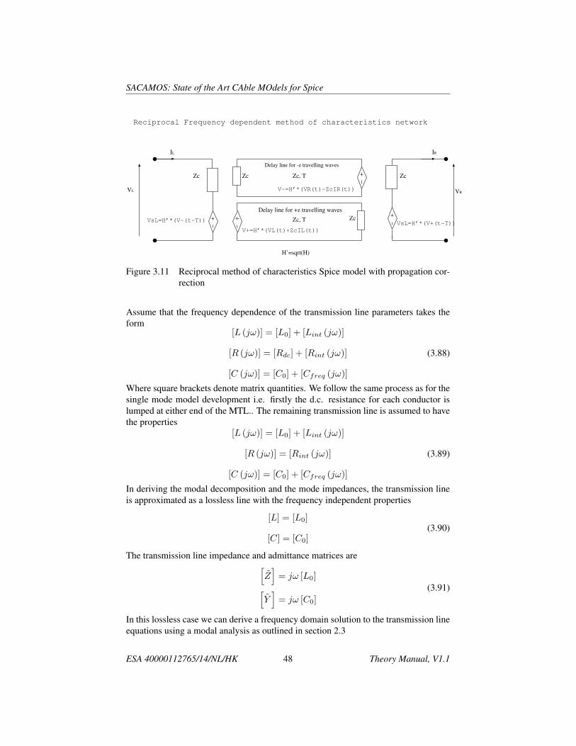
thought of as a lossless transmission line with a network at either end which models theeffect of the frequency dependent line losses. It is found that the individual terminationmodels implemented as shown in figure 3.10 is not reciprocal i.e. at the terminationof the lossless line the propagation correction is applied to the wave in only one direc-tion. The model can be made reciprocal by a termination network which applies half ofthe propagation correction
(√H(jω)
)at each end of the lossless transmission line as
shown in Figure 3.11. Each part of the propagation correction corrects for propagationalong half the length of the transmission line i.e. the propagation correction applied ateach end of the method of characteristics delay line is
H ′(jω) = ej(γ′(jω)−γ0)L
2 (3.87)
3.6.4 Multi-mode propagation correctionWe follow the analysis of the frequency dependent single mode transmission line inour development of a frequency dependent multi-conductor transmission line model.
ESA 40000112765/14/NL/HK 47 Theory Manual, V1.1
SACAMOS: State of the Art CAble MOdels for Spice
Reciprocal Frequency dependent method of characteristics network
VL
VsL=H’*(V-(t-T)) Zc, T Zc
Zc
IL
Zc, TZc
VR
IR
VsL=H’*(V+(t-T))
V+=H’*(VL(t)+ZcIL(t))
V-=H’*(VR(t)-ZcIR(t))
Delay line for -z travelling waves
Delay line for +z travelling waves
Zc
H’=sqrt(H)
Figure 3.11 Reciprocal method of characteristics Spice model with propagation cor-rection
Assume that the frequency dependence of the transmission line parameters takes theform
[L (jω)] = [L0] + [Lint (jω)]
[R (jω)] = [Rdc] + [Rint (jω)]
[C (jω)] = [C0] + [Cfreq (jω)]
(3.88)
Where square brackets denote matrix quantities. We follow the same process as for thesingle mode model development i.e. firstly the d.c. resistance for each conductor islumped at either end of the MTL.. The remaining transmission line is assumed to havethe properties
[L (jω)] = [L0] + [Lint (jω)]
[R (jω)] = [Rint (jω)]
[C (jω)] = [C0] + [Cfreq (jω)]
(3.89)
In deriving the modal decomposition and the mode impedances, the transmission lineis approximated as a lossless line with the frequency independent properties
[L] = [L0]
[C] = [C0](3.90)
The transmission line impedance and admittance matrices are[Z]
= jω [L0][Y]
= jω [C0]
(3.91)
In this lossless case we can derive a frequency domain solution to the transmission lineequations using a modal analysis as outlined in section 2.3
ESA 40000112765/14/NL/HK 48 Theory Manual, V1.1
SACAMOS: State of the Art CAble MOdels for Spice
The diagonal modal inductance and capacitance matrices on the lossless line aregiven by [2]
[Lm] = [TV ]−1
[L0] [TI ]
[Cm] = [TI ]−1
[C0] [TV ](3.92)
The impedance of the ith mode is then
Zm,i =
√Lm,iCm,i
(3.93)
The modal transformation matrices and the modal impedances derived from the losslessline parameters are independent of frequency. It now remains to calculate the propaga-tion correction which takes into account the frequency dependence of the transmissionline losses. Taking into account the loss terms but excluding the d.c. resistance whichhas already been removed, the impedance and admittance matrices are[
Z ′]
= [Rint (jω)] + jω [[L0] + [Lint (jω)]][Y ′]
= jω [[C0] + [Cfreq (jω)]]
(3.94)
Having subtracted the d.c. resistance we know that Rint(jω) = 0 when ω = 0. Alsothe contribution to the impedance due to the internal inductance (which is due to thefield penetrating the conductors) becomes negligible compared to the inductance L0
as ω → inf . The impedance matrix is assumed to be weakly varying with frequencywhich provides justification for the approximation that the modal decomposition andmode impedances are independent of frequency. In order to determine a propagationcorrection which incorporates the effects of loss we perform the modal decompositionon the product of the frequency dependent impedance and admittance i.e. diagonalisethe matrix system [
Z ′] [Y ′]
=[TV
] [γ2] [TV
]−1
(3.95)
As for the single mode transmission line the propagation correction for mode i is givenby
Hi (jω) = e− (γ′i (jω)− γ0,i)L (3.96)
Again, the propagation correction can be applied at both ends of the transmission lineto give a reciprocal and symmetrical model. The propagation correction in this case isthe square root of H ′(jω) i.e.
H ′i (jω) = e− (γ′i (jω)− γ0,i)L
2(3.97)
The implementation of the propagation correction for each mode is identical tothat described in the previous section. The derivation of the correction factor as de-scribed above relies on being able to uniquely identify each mode of the frequencydependent transmission line with a corresponding mode of the frequency independent
ESA 40000112765/14/NL/HK 49 Theory Manual, V1.1
SACAMOS: State of the Art CAble MOdels for Spice
transmission line. The voltage transformation matrix [Tv] which diagonalises the fre-quency dependent system in equation (7.57) has been found to be a weak function offrequency and hence the mode identification has been straightforward. We note thatidentifying the corresponding modes of the lossy transmission line and the losslesstransmission line may require some care. In the implementation of this process weidentify the modes on the lossy transmission line by identifying the closest mode ofthe lossless transmission line (using the vector norm as a distance measure). The prop-agation correction for the twisted pair model must take proper account of the domaindecomposition. The propagation correction is developed as follows:
In the first stage the d.c. resistance of the conductors is lumped at the ends of thecable bundle model before the domain decomposition.
As derived in section 3.6 the propagation of the differential mode can be imple-mented as a simple delay line followed by a frequency dependent correction factorH(jω) = ej(γ
′(jω)−γ0)L where γ′ takes account of the extraction of the d.c. resistancefor the differential mode. The differential mode current sees the twice the impedancecontribution of a single wire i.e. (2Rdc), twice the resistance of a single wires is sub-tracted.
γ′ (jω) =√
(Zint (jω) + jωLDM (jω)) (jωCDM (jω)) (3.98)
The common mode is slightly different in that the common mode current is dis-tributed between the two twisted pair conductors in parallel so the contribution to theloss of the common mode is
(12Rdc
), i.e half the resistance of a single wires is sub-
tracted (note that any resistance in the common mode return must be subtracted too).
ESA 40000112765/14/NL/HK 50 Theory Manual, V1.1

SACAMOS: State of the Art CAble MOdels for Spice
3.7 Transfer Impedance ModelThe spice model for trasfer impedance coupling through cable shields uses a weak formof transfer impedance coupling i.e. the coupling is assumed to be in one direction onlyfrom source to victim domains. This requires identification of the source and victimdomains by the user in each scenario. Transfer admittance is not included in the shieldcoupling model.
In this work the transfer impedance is assumed to take the form of a rational func-tion in jω i.e.
ZT (jω) =a0 + a1
(jωω0
)+ a2
(jωω0
)2
+ . . .
b0 + b1
(jωω0
)+ b2
(jωω0
)2
+ . . .(3.99)
where ω0 is a normalisation constant to and the expansion can be taken up to any orderrequired. Note that this model includes the common ZT = RT + jωLT model asa particular case. The transfer impedance of a shield is reciprocal thus the couplingthrough the shield is determined by the same transfer impedance for both couplingdirections.
The model will be derived initially for a single mode in the source and victimdomain before generalising to the multi-mode situation. In the derivation losses areassumed to be zero as we are using the ’propagation correction’ model in which theeffect of losses are lumped into the terminations as a lumped d.c. resistance and apropagation correction applied to the forward and backward modes on the transmissionline.
The transfer impedance model derivation starts from the frequency domain equa-tions for propagation in the victim domain.
∂∂z
(Vv (z)
)+ jω [L]
(Iv (z)
)= VZT,v (z)
∂∂z
(Iv (z)
)+ jω [C]
(Vv (z)
)= 0
(3.100)
in which the voltage source on the right hand side is due to transfer impedance couplingfrom source to victim domain and is given by the product of the frequency dependenttransfer impedance and the shield current in the source domain.
VZT,v (z) = Z ′T (z) Is (z) (3.101)
We note here that for the transfer impedance in equation 3.101, Z ′T the d.c. part of thetransfer impedance has been subtracted. This is a consequence of the extraction of thed.c. resistance of conducors being lumped at the transmission line terminations wherewe note that the transfer impedance of a shield is equal to the d.c. resistance of theshield and lumping this at the terminations of the transmission line means that the d.c.transfer impedance coupling is already included in the model (we also observe that thed.c. transfer impedance coupling will always be present in the model and is includedin a self consistent manner in the model) thus
Z ′T (ω) = ZT (ω)− ZT (ω = 0) (3.102)
ESA 40000112765/14/NL/HK 51 Theory Manual, V1.1
SACAMOS: State of the Art CAble MOdels for Spice
It has been found that this approximation can lead to errors at high frequency forshielded cables whose shields are terminated with very low (comparable with the shieldresistance at d.c. or less). In this situation, improved results are obtained by exclud-ing the Rdc value from the process of lumping the d.c. resistances at the terminationsand keeping it in the transfer impedance model. A flag is available when running thesoftware to use this alternative model. The price to be paid for this is accuracy of themodel at low frequency. It is recommended that a suitable validation test be run to testwhich model is most appropriate in any given circumstance.
The voltage and current in the source domain are expressed using the sum and dif-ference of forward and backward voltage waves (characteristic variables) as in equation3.51 i.e.
Vs (z) = 12
(V +s (0) e−jβsz + V −s (L) ejβs(z−L)
)Is (z) = 1
2Zs
(V +s (0) e−jβsz − V −s (L) ejβs(z−L)
) (3.103)
where the forward and backward voltage waves are
V +s (0) = H ′s
(Vs (0) + ZsIs (0)
)V −s (L) = H ′s
(Vs (L)− ZsIs (L)
) (3.104)
where the propagation correction, H ′s has been applied in the source domain to deter-mine the characteristics in the source domain.
In the victim domain the characteristics incident at the terminations, and subse-quently corrected for the victim domain propagation by H ′v , are given by the sum oftwo contributions. The first comes from waves launched from the terminations in thevictim domain and the second from the transfer impedance distributed sources i.e.
V +v (L) = Vv (L) + Zv Iv (L) = H ′vV
+v (0) e−jβvL +H ′vV
+L,ZT,v
V −v (0) = Vv (0)− Zv Iv (0) = H ′vV−v (L) e−jβvL +H ′vV
−0,ZT,v
(3.105)
where the waves launched from the terminations are found as
V +v (0) = H ′v
(Vv (0) + Zv Iv (0)
)V −v (L) = H ′v
(Vv (L)− Zv Iv (L)
) (3.106)
and where V +L,ZT,v is the voltage wave in the +z direction resulting from the transfer
impedance coupling, received at the z = L termination. Similarly, V −0,ZT,v is the volt-age wave in the −z direction resulting from the transfer impedance coupling, receivedat the z = 0 termination. The current in the source domain transmission line is givenby equation 3.103. The distributed voltage source on the victim transmission line istherefore given by
VZT,v (z) = Z ′T (z) Is (z) =Z ′T (ω)
2Zs
(V +s (0) e−jβsz − V −s (L) ejβs(z−L)
)(3.107)
ESA 40000112765/14/NL/HK 52 Theory Manual, V1.1

SACAMOS: State of the Art CAble MOdels for Spice
At a point z on the victim transmission line, a voltage source VZT,v dz launches wavesin both the -z and +z directions. The waves in the -z direction has amplitude
V −dz = − VZT,vdz2
(3.108)
and the wave in the +z direction has amplitude
V +dz = +VZT,vdz
2(3.109)
The currents associated with the waves are
I−dz =VZT,vdz
2Zv(3.110)
and
I+dz =VZT,vdz
2Zv(3.111)
Therefore the characteristic variables (section 3.5) for the -z travelling wave is
2V −dz = V − Zv I = −VZT,vdz (3.112)
and for the +z travelling wave it is
2V +dz = V + Zv I = VZT,vdz (3.113)
Thus the contribution to the -z travelling wave arriving at the z=0 termination of thevictim transmission line is found by integrating the distributed contributions to the -ztravelling wave from 0 to L i.e.
V −0,ZT,v =∫ L
02V − (z) dz
=∫ L
0−VZT,v (z) dz
= −∫ L
0Z′T (ω)
2Zs
(V +s (0) e−jβsz − V −s (L) ejβs(z−L)
)e−jβvzdz
= −Z′T (ω)2Zs
∫ L0
(V +s (0) e−j(βs+βv)z − V −s (L) e−jβsLej(βs−βv)z
)dz
(3.114)The contribution to the +z tranvelling wave at the z=L termination is found by integrat-ing the distributed contributions from z=0 to z=L
V +L,ZT,v =
∫ L0
2V + (z) dz
=∫ L
0VZT,v (z) dz
=∫ L
0Z′T (ω)
2Zs
(V +s (0) e−jβsz − V −s (L) ejβs(z−L)
)e−jβv(L−z)dz
=Z′T (ω)
2Zs
∫ L0
(V +s (0) e−jβvLe−j(βs−βv)z − V −s (L) e−j(βs+βv)(L−z)
)dz
(3.115)
ESA 40000112765/14/NL/HK 53 Theory Manual, V1.1

SACAMOS: State of the Art CAble MOdels for Spice
In the time domain these equations become
V −v (0) = Vv (0, t)− ZvIv (0, t)
= H ′v (t) ∗ V −v (L, t− TV ) +H ′v (t) ∗ V −0,ZT,v (t)(3.116)
where Tv is the time delay of the victim transmission line.The first term in these equations are the method of characteristics propagation
model already described in section 3.5.The time domain source terms due to the transfer impedance coupling is described
term by term as follows. Firstly the two terms contributing to the -z travelling wavearriving at the z=0 termination of the victim transmission line, V −0,ZT,v in equation3.114
-z propagation, term1: contribution to V −0,ZT,v from the +z wave in the sourcetransmission line:
− Z ′T (ω)
2Zs
∫ L
0
V +s (0) e−j(βs+βv)zdz =
− 1
2Zs
(−Z
′T (ω)
jω
(L
Tz + Tv
)(1− e−j(βs+βv)L
)V +s (0)
)(3.117)
Transforming to the time domain gives
1
2Zs
Z ′T (ω)
jω
(L
Tz + Tv
)(1− e−j(βs+βv)L
)V +s (0)↔
1
2Zs
(L
Ts + Tv
)H ′ZT ∗
(V +s (0, t)− V +
s (0, t− Ts − Tv))
(3.118)
where the z-domain transfer function H ′ZT (jω) = Z′T (jω)jω and H ′ZT (t) is the impulse
response of this transfer function.-z propagation, Term2: contribution to V −0,ZT,v from the -z wave in the source
transmission line:
Z ′T (ω)
2Zs
∫ L
0
V −s (L) e−j(βsL)ej(βs−βv)zdz ↔
1
2Zs
(L
Ts − Tv
)H ′ZT ∗
(V −s (L, t− Tv)− V −s (L, t− Ts)
)(3.119)
In a similar manner, the characteristic variables incident at the +z termination are ex-pressed in the time domain as
V +v (L) = Vv (L, t) + ZvIv (L, t)
= H ′v (t) ∗ V +v (0, t− TV ) +H ′v (t) ∗ V +
L,ZT,v (t)(3.120)
Secondly the two terms contributing to the +z travelling wave arriving at the z=Ltermination of the victim transmission line, V +
L,ZT,v in equation 3.115.
ESA 40000112765/14/NL/HK 54 Theory Manual, V1.1

SACAMOS: State of the Art CAble MOdels for Spice
+z propagation, term1: contribution to V +L,ZT,v from the +z wave in the source
transmission line:
Z ′T (ω)
2Zs
∫ L
0
V +s (0) e−j(βvL)e−j(βs−βv)zdz ↔
1
2Zs
(L
Ts − Tv
)H ′ZT ∗
(V +s (0, t− Tv)− V +
s (0, t− Ts))
(3.121)
+z propagation, term2: contribution to V +L,ZT,v from the -z wave in the source trans-
mission line:
− Z ′T (ω)
2Zs
∫ L
0
V −s (L) e−j(βs+βv)(L−z)dz ↔
− 1
2Zs
(L
Ts + Tv
)H ′ZT ∗
(V −s (L, t)− V −s (L, t− Ts − Tv)
)(3.122)
3.7.1 Multiple mode propagationThe above theory is readily extended to the case of multi-mode systems, both in thesource and victim domains. First we will discuss how to manage a multi-mode sourcedomain before going on to derive the model for multi-mode victim domain.
multiple modes in the source domain
If there is more than one mode in the source domain then we must take into accountthat multiple modes can contribute to the shield current. There are two scenarios inwhich the shield is or is not the reference conductor for the source domain. These twoscenarios must be treated separately.
If the shield is not the reference conductor in the source domain then the conductorcurrents are related to the mode currents by(
I)
=[TI
] (Im
)(3.123)
thus the shield current can be expressed in terms of the individual mode currents as
˜Ishield =
Nm∑i=1
˜TI,shield,i ˜Im,i (3.124)
If the shield is the reference conductor then the reference conductor current is foundas minus the sum of the currents on all the other conductors in the domain i.e.
˜Ishield = −∑Nm
j=1 Ij
= −∑Nm
j=1
(∑Nm
i=1˜TI,j,i ˜Im,i
)=
∑Nm
i=1
(−∑Nm
j=1˜TI,j,i
)˜Im,i
(3.125)
ESA 40000112765/14/NL/HK 55 Theory Manual, V1.1
SACAMOS: State of the Art CAble MOdels for Spice
In either case the shield current is expressed as a linear combination of the individ-ual mode currents in the source domain i.e.
˜Ishield =
Nm∑i=1
Ps,i ˜Im,i (3.126)
where Ps,i is the coefficient of the ith mode contribution.
multiple modes in the victim domain
The voltage source in the victim domain appears only on the shield conductor thereforeeach victim domain mode vmmay recieve a contribution from this source term . sourceand victim domains.
If there are multiple modes in the victim domain there are again two situationswhich need to be treated separately dependent on whether the shield is or is not thereference conductor of the domain. In the victim domain the weak transfer impedancecoupling model gives a voltage source on the shield conductor Vs,ZT = ZT Ishield.
If the shield is not the reference conductor then the modal voltage can be related tothe individual conductor voltages by(
Vm
)=[
˜T−1V
] (V)
(3.127)
thus the modal voltage source for mode i is found as(˜Vm,i
)= ˜T−1
V,i,shield
(˜Vs,ZT
)(3.128)
If the shield is the reference conductor in the victim domain then all the otherconductors have a source voltages -Vs,ZT on them. The modal voltage source for modei is found as (
˜Vm,i
)= −
Nm∑j=1
˜T−1V,i,j
(˜Vs,ZT
)(3.129)
Again, in either case, the contribution to mode i has a weighting factor Pv,i(˜Vm,i
)= Pv,i ˜Vs,ZT (3.130)
multiple modes in the source domain and victim domains
In order to generalise the transfer impedance coupling model to multiple source andvictim domains, equations 3.116 and 3.120 must be generalised. This is done by recog-nising that if there are ns source domain modes and nv victim domain modes then thereare ns×nv contributions to the transfer impedance coupling i.e. there is a contributionrelating to every combination of source and victim modes.
The contribution from source mode, si, to victim mode, vj , is readiliy found usingthe weighted values in equations 3.126 and 3.130.
ESA 40000112765/14/NL/HK 56 Theory Manual, V1.1

SACAMOS: State of the Art CAble MOdels for Spice
In this case equations 3.116 and 3.120 become:
V +vj (L, t) = Vvj (L, t) + ZvjIvj (L, t)
= H ′vj (t) ∗ V +vj (0, t− TV j) +
Ps,iPv,j
2ZsiHZT ∗H ′vj (t) ∗((
LTsi−Tvj
) (V +si (0, t− Tv)− V +
si (0, t− Tsi))
−(
LTsi+Tvj
) (V −si (L, t)− V −si (L, t− Tsi − Tvj)
)) (3.131)
and
V −vj (0, t) = Vvj (0, t)− ZvjIvj (0, t)
= H ′vj (t) ∗ V −vj (L, t− TV )− Ps,iPv,j
2ZsiHZT ∗H ′vj (t) ∗((
LTsi+Tvj
) (V +si (0, t)− V +
si (0, t− Tsi − Tvj))
−(
LTsi−Tvj
) (V −si (L, t− Tvj)− V −si (L, t− Tsi)
)) (3.132)
3.7.2 Spice circuit for Transfer Impedance modelThe transfer impedance model equations may be implemented in spice using controlledsources, delay lines plus s-domain transfer functions to implement the frequency de-pendent transfer functions/ time domain convolutions. The Spice model for the mainmethod of characteristics propagation model for souce domain mode smi, and victimdomain model, vmi are seen in figure 3.12
The following delay lines are also required in addition to the delay lines requiredto implement the method of characteristics in the source and victim domains:
1. Delay line for V +si (0, t− Tsi − Tvi)
2. Delay line for V +si (0, t− Tvi)
3. Delay line for V −si (0, t− Tsi − Tvi)
4. Delay line for V −si (0, t− Tvi)
The Spice model for these elements is shown in figure 3.13When Ts = Tv there is a problem implementing equations 3.119 and 3.121 in
Spice. in this case it can be shown that as Ts → Tv equation 3.119 becomes
1
2Zs
(L
Ts − Tv
)HZT ∗
(V −s (L, t− Tv)− V −s (L, t− Ts)
)→
L
2ZsHZT ∗
dV −s (0, t− Tv)dt
(3.133)
The time derivative may be implemented in Spice using a 1H inductor in parallel witha current source of value V +
s (0, t− Tv) whose voltage will provide the time derivativeas shown in figure 3.14 Similarly, equation 3.121 becomes
ESA 40000112765/14/NL/HK 57 Theory Manual, V1.1

SACAMOS: State of the Art CAble MOdels for Spice
1
2Zs
(L
Ts − Tv
)HZT ∗
(V +s (0, t− Tv)− V +
s (0, t− Ts))→
L
2Zs
dV +s (0, t− Tv)
dt(3.134)
and the Spice circuit takes a similar form to that shown in figure 3.14Controlled sources with s-domain transfer functions implement the convolutions in
equations 3.118, 3.119, 3.121 and 3.122.
ESA 40000112765/14/NL/HK 58 Theory Manual, V1.1
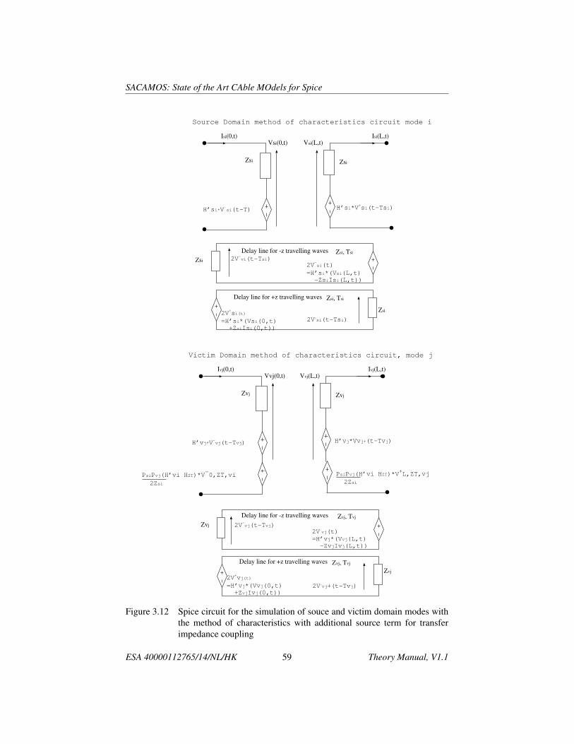
SACAMOS: State of the Art CAble MOdels for Spice
Vsi(0,t)
H’si*V-si(t-T)
Zsi
Isi(0,t)
Zsi, Tsi
Vsi(L,t)Isi(L,t)
H’si*V+si(t-Tsi)
2V+si(t)
=H’si*(Vsi(0,t)
+ZsiIsi(0,t))
2V-si(t)
=H’si*(Vsi(L,t)
-ZsiIsi(L,t))
Delay line for -z travelling waves
Delay line for +z travelling waves
2V+si(t-Tsi)
2V-vi(t-Tsi)
Zsi, Tsi
Zsi
Zsi
Zsi
Source Domain method of characteristics circuit mode i
Vvj(0,t)
H’vj*V-vj(t-Tvj)
Zvj
Ivj(0,t)
Zvj, Tvj
Vvj(L,t)Ivj(L,t)
H’vj*Vvj+(t-Tvj)
2V+vj(t)
=H’vj*(Vvj(0,t)
+ZvjIvj(0,t))
2V-vj(t)
=H’vj*(Vvj(L,t)
-ZvjIvj(L,t))
Delay line for -z travelling waves
Delay line for +z travelling waves
2V+vj+(t-Tvj)
2V-vj(t-Tvj)
Zvj, Tvj
Zvj
Zvj
Zvj
Victim Domain method of characteristics circuit, mode j
PsiPvj(H’vi HZT)*V-0,ZT,vi
2Zsi
PsiPvj(H’vi HZT)*V+L,ZT,vj
2Zsi
Figure 3.12 Spice circuit for the simulation of souce and victim domain modes withthe method of characteristics with additional source term for transferimpedance coupling
ESA 40000112765/14/NL/HK 59 Theory Manual, V1.1
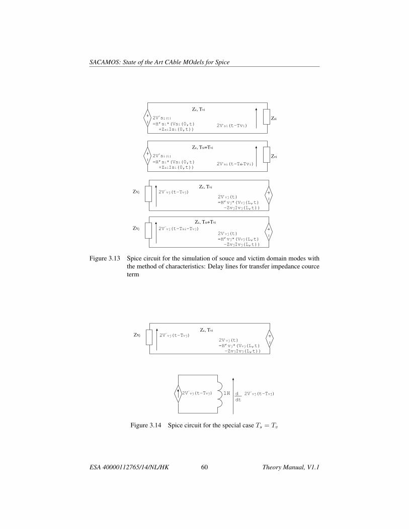
SACAMOS: State of the Art CAble MOdels for Spice
2V+si(t)
=H’si*(Vsi(0,t)
+ZsiIsi(0,t))2V+
si(t-Tvi)
Zc, Tvi
Zsi
2V-vj(t)
=H’vj*(Vvj(L,t)
-ZvjIvj(L,t))
2V-vj(t-Tvj)Zvj
2V+si(t)
=H’si*(Vsi(0,t)
+ZsiIsi(0,t))2V+
si(t-Tsi-Tvi)
Zc, Tsi+Tvi
Zvi
Zc, Tvi
2V-vj(t)
=H’vj*(Vvj(L,t)
-ZvjIvj(L,t))
2V-vj(t-Tsi-Tvj)Zvj
Zc, Tsi+Tvi
Figure 3.13 Spice circuit for the simulation of souce and victim domain modes withthe method of characteristics: Delay lines for transfer impedance courceterm
1H d 2V-vj(t-Tvj)
dt
2V-vj(t)
=H’vj*(Vvj(L,t)
-ZvjIvj(L,t))
2V-vj(t-Tvj)Zvj
Zc, Tvi
2V-vj(t-Tvj)
Figure 3.14 Spice circuit for the special case Ts = Tv
ESA 40000112765/14/NL/HK 60 Theory Manual, V1.1
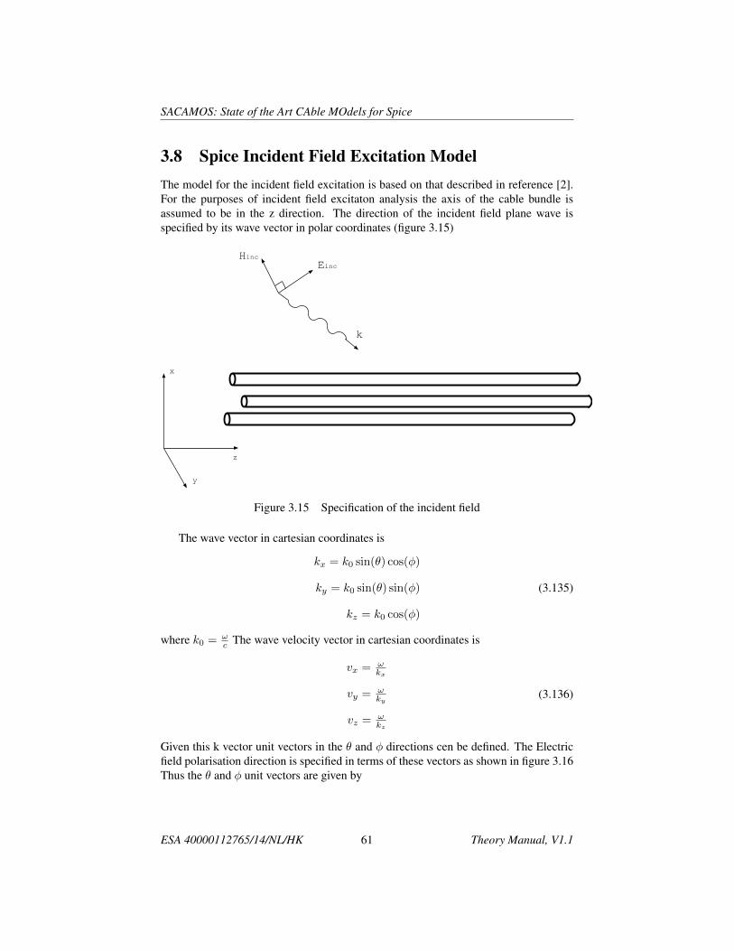
SACAMOS: State of the Art CAble MOdels for Spice
3.8 Spice Incident Field Excitation ModelThe model for the incident field excitation is based on that described in reference [2].For the purposes of incident field excitaton analysis the axis of the cable bundle isassumed to be in the z direction. The direction of the incident field plane wave isspecified by its wave vector in polar coordinates (figure 3.15)
z
x
y
EincHinc
k
Figure 3.15 Specification of the incident field
The wave vector in cartesian coordinates is
kx = k0 sin(θ) cos(φ)
ky = k0 sin(θ) sin(φ)
kz = k0 cos(φ)
(3.135)
where k0 = ωc The wave velocity vector in cartesian coordinates is
vx = ωkx
vy = ωky
vz = ωkz
(3.136)
Given this k vector unit vectors in the θ and φ directions cen be defined. The Electricfield polarisation direction is specified in terms of these vectors as shown in figure 3.16Thus the θ and φ unit vectors are given by
ESA 40000112765/14/NL/HK 61 Theory Manual, V1.1

SACAMOS: State of the Art CAble MOdels for Spice
y
z
x
kθ
kφ
k
E
Eθ
Eφ
Figure 3.16 Specification of the incident field polarisation
θx = cos(θ) cos(φ)
θy = cos(θ) sin(φ)
θz = sin(φ)
(3.137)
φx = sin(φ)
φy = cos(φ)
φz = 0
(3.138)
and thus the polarisation vector is
ex = Eθθx + Eφφx
ey = Eθθy + Eφφy
ez = Eθθz + Eφφz
(3.139)
The frequency domain electric field is given by
Ex = E0(ω)e−j(kxx+kyy+kzz)ex
Ey = E0(ω)e−j(kxx+kyy+kzz)ey
Ez = E0(ω)e−j(kxx+kyy+kzz)ez
(3.140)
ESA 40000112765/14/NL/HK 62 Theory Manual, V1.1
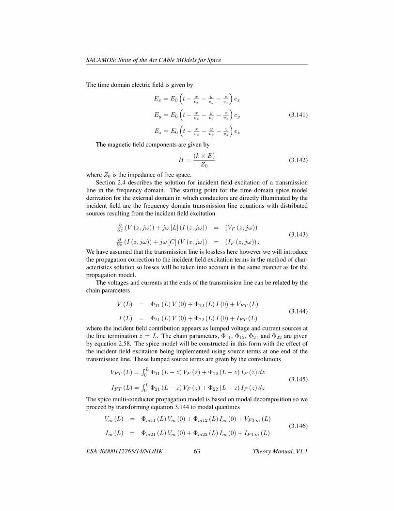
SACAMOS: State of the Art CAble MOdels for Spice
The time domain electric field is given by
Ex = E0
(t− x
vx− y
vy− z
vz
)ex
Ey = E0
(t− x
vx− y
vy− z
vz
)ey
Ez = E0
(t− x
vx− y
vy− z
vz
)ez
(3.141)
The magnetic field components are given by
H =(k × E)
Z0(3.142)
where Z0 is the impedance of free space.Section 2.4 describes the solution for incident field excitation of a transmission
line in the frequency domain. The starting point for the time domain spice modelderivation for the external domain in which conductors are directly illuminated by theincident field are the frequency domain transmission line equations with distributedsources resulting from the incident field excitation
∂∂z (V (z, jω)) + jω [L] (I (z, jω)) = (VF (z, jω))
∂∂z (I (z, jω)) + jω [C] (V (z, jω)) = (IF (z, jω)) .
(3.143)
We have assumed that the transmission line is lossless here however we will introducethe propagation correction to the incident field excitation terms in the method of char-acteristics solution so losses will be taken into account in the same manner as for thepropagation model.
The voltages and currents at the ends of the transmission line can be related by thechain parameters
V (L) = Φ11 (L)V (0) + Φ12 (L) I (0) + VFT (L)
I (L) = Φ21 (L)V (0) + Φ22 (L) I (0) + IFT (L)(3.144)
where the incident field contribution appears as lumped voltage and current sources atthe line termination z = L. The chain parameters, Φ11, Φ12, Φ21 and Φ22 are givenby equation 2.58. The spice model will be constructed in this form with the effect ofthe incident field excitaiton being implemented using source terms at one end of thetransmission line. These lumped source terms are given by the convolutions
VFT (L) =∫ L
0Φ11 (L− z)VF (z) + Φ12 (L− z) IF (z) dz
IFT (L) =∫ L
0Φ21 (L− z)VF (z) + Φ22 (L− z) IF (z) dz
(3.145)
The spice multi-conductor propagation model is based on modal decomposition so weproceed by transforming equation 3.144 to modal quantities
Vm (L) = Φm11 (L)Vm (0) + Φm12 (L) Im (0) + VFTm (L)
Im (L) = Φm21 (L)Vm (0) + Φm22 (L) Im (0) + IFTm (L)(3.146)
ESA 40000112765/14/NL/HK 63 Theory Manual, V1.1

SACAMOS: State of the Art CAble MOdels for Spice
where the (diagonal) modal chain parameter matrices are given by
Φm11 (L) = [TV ]−1
Φ11 (L) [TV ]
= cosh (γmL)
Φm12 (L) = [TV ]−1
Φ12 (L) [TI ]
= − [Zm] sinh (γmL)
Φm21 (L) = [TI ]−1
Φ21 (L) [TV ]
= − sinh (γmL) [Zm]−1
Φm22 (L) = [TI ]−1
Φ22 (L) [TI ]
= cosh (γmL)
(3.147)
and the modal forcing functions (using the properties of the modal decomposition ma-trices in equations 3.34) may be expressed as
VFTm (L) = [TV ]−1VFT (L)
=∫ L
0cosh (γmL− z)VFm (z)
− sinh (γmL− z) [Zcm] IFm (z) dz
(3.148)
IFTm (L) = [TI ]−1IFT (L)
=∫ L
0− sinh (γmL− z) [Zcm]
−1VFm (z)
+ cosh (γmL− z) IFm (z) dz
(3.149)
where γm is the diagonal matrix of mode propagation constants and Zcm is the diago-nal matrix of mode impedances, VFm = [TV ]−1VF and IFm = [TI ]
−1IF .The modal characteristic varibles at z = 0 and z = L are found by first substituting
the modal chain parameters (equation 3.147) into the expressions for the modal voltageand current expressions (equation 3.146)
Vm (L) = cosh (γmL)Vm (0)− sinh (γm (z)) [Zm] Im (0) + VFTm (L)
[Zm] Im (L) = − sinh (γmz)Vm (0) + cosh (γmz) [Zm] Im (0) + [Zm] IFTm (L)(3.150)
The characteristic variables are found by adding and subtracting these equations to give
V −m,0 = Vm (0)− [Zm] Im (0) = e−γmL [Vm (L)− [Zm] Im (L)] + Einc0 (L)
V +m,L = Vm (L) + [Zm] Im (L) = e−γmL [Vm (0) + [Zm] Im (0)] + EincL (L)
(3.151)
ESA 40000112765/14/NL/HK 64 Theory Manual, V1.1
SACAMOS: State of the Art CAble MOdels for Spice
The incident field source terms are
Einc0 (L) = −e−γmL [VFTm (L)− [Zm] IFTm (L)]
EincL (L) = [VFTm (L) + [Zm] IFTm (L)](3.152)
The exponential in equations 3.151 and 3.152 may be recognised as a time delay there-fore equation 3.151 may be expressed in the time domain for mode i as
V −m,0(t) = Vmi (0, t)− [Zmi] Imi (0, t)
= [Vmi (L, t− Tmi)− [Zmi] Imi (L, t− Tmi)] + Einc0,i (L, t)
V +m,0(t) = Vmi (L, t) + [Zmi] Imi (L, t)
= [Vmi (0, t− Tmi) + [Zmi] Imi (0, t− Tmi)] + EincL,i (L, t)(3.153)
Tmi is the delay in mode i, propagating a distance L.
Tmi =L
vmi=γmiL
jω(3.154)
Equations 3.151 express the method of characteristics based model as described insection 3.5 with the addition of sources which model the effect of the incident fieldcoupling. In order to develop a viable Spice model for incident field coupling, weneed to develop a circuit model for the time domain source terms Einc0,i (L, t) andEincL,i (L, t)
If the incident field takes the form of a plane wave then the source termsEinc0,i (L, t)and EincL,i (L, t) may be derived analytically to give a complete time domainspicemodel for incident field excitation of multi-conductor transmission lines which may beimplemented using delay lines and controlled sources.
Substituting the expressions for the distributed incident field sources 2.53 and 2.56,transformed to the frequency domain, with the Electric field expressions for a planewave (3.140) allows the evaluation of the modal forcing functions in equations 3.148and 3.149. The modal incident field transmission line source functions may be writ-ten in terms of the transverse and longitudinal electric field contributions ET (z) andEL (z) respectively
Einc0 (L) = −e−γmL [VFTm (L)− [Zm] IFTm (L)]
= −∫ L
0e−γmz [TI ]
tEL (z) dz
−e−γmL [TI ]tET (L)− [TI ]
tET (0)
EincL (L) = [VFTm (L) + [Zm] IFTm (L)]
=∫ L
0e−γm(L−z) [TI ]
tEL (z) dz
− [TI ]tET (L) + e−γmL [TI ]
tET (0)
(3.155)
ESA 40000112765/14/NL/HK 65 Theory Manual, V1.1

SACAMOS: State of the Art CAble MOdels for Spice
where the transverse electric field contribution for the incident field expression givenin equation 3.140 for conductor k is
ET (z)k =
∫ conductori
ref
Einc(ω) · dl
=
∫ dk
0
Einc(ω)
(exxk − x0
di+ ey
yk − y0
dk
)e−jkzze
−j(kx
xs−x0dk
+kyys−x0
dk
)dl
= Einc(ω)
(exxk − x0
dk+ ey
yk − y0
dk
)e−jkzze
j(kx
x0dk
+kyx0dk
) ∫ dk
0
e−j
(kx
xdk
+kyydk
)sdl
= Einc(ω) (ex (xk − x0) + ey (yk − y0)) e−jkzzej(kx
x0dk
+kyx0dk
)e−jψk
sin(ψk)
ψk(3.156)
where (xk, yk) is the position of the kth conductor in the x-y plane, (x0, y0) is theposition of the reference conductor in the x-y plane and dk is the distance betweenthese conductors and
ψk =kxxk + kyyk
2(3.157)
If we assume that the origin in the x-y plane is at the position of the reference conductorthen we can write
ET (z)k = Einc(ω) (exxk + eyyk) e−jkzze−jψk sin(ψk)ψk
(3.158)
The contribution from the longitudinal field is
EL (z)i = E0(ω)(e−j(kxxk+kyyk+kzz) − e−j(kzz)
)= E0(ω)e−jkzz
(e−j(kxxk+kyyk) − 1
)= −j (kxxk + kyyk)E0(ω)e−jψk sin(ψk)
ψke−jkzz
(3.159)
The shift of the origin of the cross section coordinate system will only have the effectof adding a timeshift to the incident field function.
The cross section time delay is defined for conductor k as
Txyk =xk − x0
vx+yk − y0
vy(3.160)
The time delay for the incident field to travel the length of the transmission line isdenoted Tz and the delay for mode i is denoted Ti where
Tz =L
vz(3.161)
ESA 40000112765/14/NL/HK 66 Theory Manual, V1.1
SACAMOS: State of the Art CAble MOdels for Spice
andTi =
L
vi=γiL
jω(3.162)
Following [2] equations 3.152 can be expressed for each mode i as
Einc0 (L)i = E0(ω)
n∑k=1
[sin(ψk)
ψk
][TI ]
ti,k
[ezTxykL+ (exxk + eyyk) (Ti − Tz)][e−jω(Txyk/2) − e−jω(Ti+Tz+Txyk/2)
(Ti + Tz)
]
(3.163)
EincL (L)i = E0(ω)sumnk=1
[sin(ψk)
ψk
][TI ]
ti,k
[ezTxykL+ (exxk + eyyk) (Ti − Tz)][e−jω(Ti+Txyk/2) − e−jω(Tz+Txyk/2)
(Ti − Tz)
](3.164)
The transformation to the time domain is again acheived by recognising the e−jωT
terms as time delays to give
Einc0 (t)i =
n∑k=1
[ezTxykL− (exxk + eyyk) (Ti + Tz)] [TI ]
ti,k
pk(t) ∗ E0 (t− Txyk/2)− E0 (t− Ti − Tz − Txyk/2)
(Ti + Tz)
EincL (t)i =
n∑k=1
[ezTxykL+ (exxk + eyyk) (Ti − Tz)] [TI ]
ti,k
pk(t) ∗ E0 (t− Ti − Txyk/2)− E0 (t− Tz − Txyk/2)
(Ti − Tz)
(3.165)
Where pk(t) is a pulse function for the kth conductor which is convolved with the de-layed incident field functions. Provided that the transmission line cross section is smallit may be assumes that the pulse function is approximately an impulse function, we
ESA 40000112765/14/NL/HK 67 Theory Manual, V1.1
SACAMOS: State of the Art CAble MOdels for Spice
may also assmue that the cross section delay time is negligable. Under this assumptionthe convolution is eliminated and the source terms are for mode i,
Einc0 (t)i = α0
[E0(t)−E0(t−Ti−Tz)
(Ti+Tz)
]EincL (t)i = αL
[E0(t−Ti)−E0(t−Tz)
(Ti−Tz)
] (3.166)
where the vectors α0 and αL are for mode i
α0,i =∑nk=1
[ezTxykL− (exxk + eyyk) (Ti + Tz)] [TI ]
ti,k
αL,i =
∑nk=1
[ezTxykL+ (exxk + eyyk) (Ti − Tz)] [TI ]
ti,k
(3.167)
The characteristic based expression for the incident field model in equation 3.151 maybe written as
V −m,0(t) = Vmi (0, t)− [Zmi] Imi (0, t)
= [Vmi (L, t− Tmi)− [Zmi] Imi (L, t− Tmi)] + α0,i
[E0(t)−E0(t−Ti−Tz)
(Ti+Tz)
]V +m,0(t) = Vmi (L, t) + [Zmi] Imi (L, t)
= [Vmi (0, t− Tmi) + [Zmi] Imi (0, t− Tmi)] + αL,i
[E0(t−Ti)−E0(t−Tz)
(Ti−Tz)
](3.168)
These incident field source terms in this model are seen to consist of the time do-main incident field function, E0 (t) and delayed versions of this, each scaled by appro-priate constants which are found in terms of the angle of incidence and polarisation ofthe incident plane wave (equations 3.167).
3.8.1 Spice circuit for Incident field excitationThe equations 3.168 may be implemented in Spice using controlled sources and delaylines. Two delay lines are required for each transmission line mode for the propagationmodel (delay Ti). In addition, for each mode, two delay lines with delays Ti and Ti+Tzare required for the incident field and a final delay line with delay Tz is required. Thestructure of the Spice circuit model is shown in figure 3.17.
If Ti = Tz for any mode, the second term in equation 3.168 has a zero in thedenominator in this case the last term in square brackets may be rewritten as[
E0 (t− Ti)− E0 (t− Tz)(Ti − Tz)
]Ti⇒Tz
=d
dtE0 (t− Ti) (3.169)
The time derivative may be implemented by an inductor of 1H driven by a currentsource as shown in figure 3.18
ESA 40000112765/14/NL/HK 68 Theory Manual, V1.1

SACAMOS: State of the Art CAble MOdels for Spice
A second practical issue is for the case when Tz < 0 i.e. if kz < 0 in this case themodel would require negative time delays. This case is simply dealt with by reversingthe transmission line terminations and kz .
The Spice model for incident field excitation provides the incident field equivalentsource in the form of the characteristic variables incident on the terminations of thetransmission line i.e. Vm (0) − ZmIm (0) and Vm (L) − ZmIm (L). These wavesrequire correction for the propagation losses in the transmission line. In order to includethe propagation correction into the model these characteristic variables are multipliedby (convolved with) the appropriate mode propagation correction H ′(jω) giving thesource terms on the transmission line terminations for mode i as
V −Einc(0, t) = H ′i(t) ∗ (Vmi (0, t)− [Zmi] Imi (0, t))
V +Einc(L, t) = H ′i(t) ∗ (Vmi (L, t) + [Zmi] Imi (L, t))
(3.170)
3.8.2 Incident field excitation with a ground planeIf there is a ground plane present then the incident field may be expressed as the super-position of a direct wave and the wave reflected from the ground. Working through theanalysis above in this case shows [2] that the effect of a ground plane can be taken intoaccount by simply doubling the α terms in equations 3.167.
ESA 40000112765/14/NL/HK 69 Theory Manual, V1.1
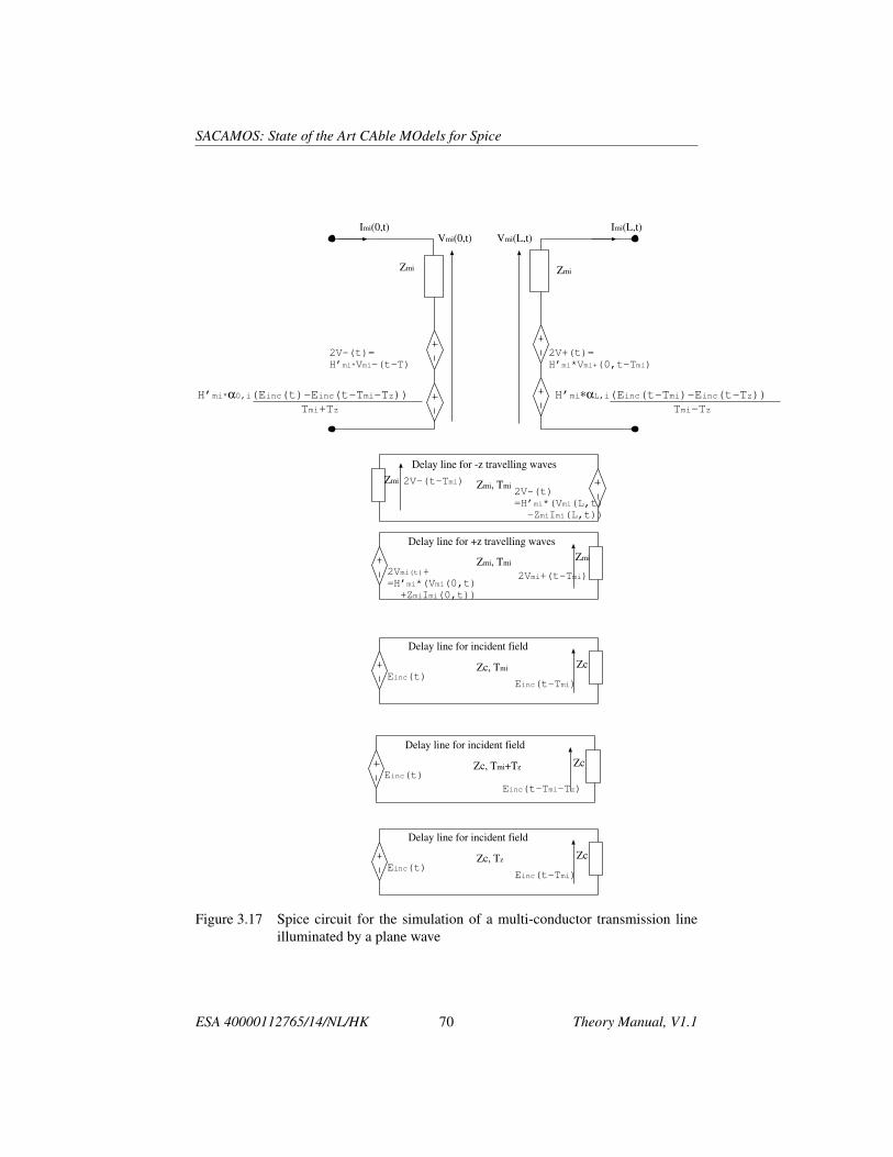
SACAMOS: State of the Art CAble MOdels for Spice
Vmi(0,t)
2V-(t)=
H’mi*Vmi-(t-T)
Zmi
Imi(0,t)
Zmi, Tmi
Vmi(L,t)Imi(L,t)
2V+(t)=
H’mi*Vmi+(0,t-Tmi)
2Vmi(t)+
=H’mi*(Vmi(0,t)
+ZmiImi(0,t))
2V-(t)
=H’mi*(Vmi(L,t)
-ZmiImi(L,t))
Delay line for -z travelling waves
Delay line for +z travelling waves
2Vmi+(t-Tmi)
2V-(t-Tmi)
Zc, Tmi ZcEinc(t)
Delay line for incident field
Einc(t-Tmi)
Zmi, Tmi
Zmi
Zmi
Zmi
Zc, Tmi+Tz ZcEinc(t)
Delay line for incident field
Einc(t-Tmi-Tz)
Zc, Tz ZcEinc(t)
Delay line for incident field
Einc(t-Tmi)
H’mi*α0,i(Einc(t)-Einc(t-Tmi-Tz))
Tmi+Tz
H’mi∗αL,i(Einc(t-Tmi)-Einc(t-Tz))
Tmi-Tz
Figure 3.17 Spice circuit for the simulation of a multi-conductor transmission lineilluminated by a plane wave
ESA 40000112765/14/NL/HK 70 Theory Manual, V1.1
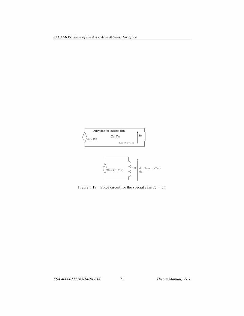
SACAMOS: State of the Art CAble MOdels for Spice
Zc, Tmi ZcEinc(t)
Delay line for incident field
Einc(t-Tmi)
Einc(t-Tmi)1H d Einc(t-Tmi)
dt
Figure 3.18 Spice circuit for the special case Ti = Tz
ESA 40000112765/14/NL/HK 71 Theory Manual, V1.1
SACAMOS: State of the Art CAble MOdels for Spice
3.9 Spice Incident Field Excitation Model for shieldedcables
The development of Spice models for incident field excitation and also for transferimpedance coupling have been described in sections 3.8 and 3.7. It has been shown inreference [7] that a rigorous model of incident field excitation of shielded cables canbe derived. This section provides an outline of the analysis presented in reference [7]and gives the main results as implemented in the SACAMOS software.
The solution for the conductor voltage and current for a single mode, sm, in theexternal (source) domain may be expressed using the method of characteristics
Vsm (z) = 12
(V +sm (0) e−jβsmz + V −sm (L) e+jβsmz + V +
Eim (z) + V −Eim (z))
(3.171)
Ism (z) = 12Zsm
(V +sm (0) e−jβsmz − V −sm (L) e+jβsmz + V +
Eim (z)− V −Eim (z))
(3.172)where:V +sm is the forward mode in the source domain launched from the z = 0 terminationV −sm is the backward mode in the source domain launched from the z = L termi-
nationV +Eim (z) is the contribution to the +z travelling wave due to the incident field
excitationV −Eim (z) is the contribution to the −z travelling wave due to the incident field
excitationand Zsm and βsm are the characteristic impedance and propagation constant of the
mode on the lossless transmission line.The forward mode launched from the termaination at z=0, with the propagation
correction for the mode applied is given by
V +sm (0) = H ′sm (Vsm (0) + ZsmIsm (0)) (3.173)
the backward (-z) propagating mode launched from the termination at z=L with thepropagation correction for the mode applied is
V −sm (L) = H ′sm (Vsm (L)− ZsmIsm (L)) (3.174)
The +z propagating voltage wave due to the distributed incident field sources (VFand IF in equation 3.143) is found by integrating the contributions to this wave from 0to z i.e.
V +Eim (z) =
∫ z0
(VF (τ) + ZsmIF (τ)) e−jβsm(z−τ)dτ (3.175)
Similarly the -z propagating voltage wave due to the distributed incident field sourcesis found as
V −Eim (z) =∫ zL
(VF (τ)− ZsmIF (τ)) e+jβsm(z−τ)dτ (3.176)
ESA 40000112765/14/NL/HK 72 Theory Manual, V1.1
SACAMOS: State of the Art CAble MOdels for Spice
The response on the inner (victim) domain is again written in terms of the characteristicvariables launched from the terminations plus an additional term related to the transferimpedance coupling from the external domain current thus the characteristic variablesincident at the terminations (and with the propagation correction for the victim domainapplied) are expressed as
V +vm (L) = Vvm (L) + ZvmIvm (L)
= H ′vm (Vvm (0)− ZvmIvm (0)) e−jβvmL +H ′vmV+L,Einc,ZT
= H ′vm
(V +vm (0)
)e−jβvmL +H ′vmV
+L,Einc,ZT (3.177)
V −vm (0) = Vvm (0)− ZvmIvm (0)
= H ′vm (Vvm (L)− ZvmIvm (L)) e−jβvmL +H ′vmV−0,Einc,ZT
= H ′vm
(V −vm (L)
)e−jβvmL +H ′vmV
−0,Einc,ZT (3.178)
In the time domain, these equations become
V +vm (L, t) = H ′vm ∗
(V +vm (0, t− Tvm)
)+H ′vm ∗ V +
L,Einc,ZT (3.179)
V −vm (0, t) = H ′vm ∗(V −vm (0, t− Tvm)
)+H ′vm ∗ V −0,Einc,ZT (3.180)
Where the transfer impedance coupling sources may be expressed as
V −0,ZT =HZT
2Zsm(jω)
[−V +
0,ext + V −0,ext]
(3.181)
V +L,ZT =
HZT
2Zsm(jω)
[V +L,ext − V
−L,ext
](3.182)
Transforming equations 3.181 and 3.181 into the time domain gives
V −0,ZT =1
2ZsmHZT (t) ∗
[−V +
0,ext(t) + V −0,ext(t)]
(3.183)
V +L,ZT =
1
2ZsmHZT (t) ∗
[V +L,ext(t)− V
−L,ext(t)
](3.184)
where V +0,ext and V −0,ext are the contributions to the source term at z=0 due to the
+z and -z propagating characteristics on the external conductor and V +L,ext and V −L,ext
ESA 40000112765/14/NL/HK 73 Theory Manual, V1.1

SACAMOS: State of the Art CAble MOdels for Spice
are the contributions to the source term at z=L due to the +z and -z propagating char-acteristics on the external conductor
V +0,ext =
∫ L
0
V +sm (0) e−j(βsm+βvm)zdz +
∫ L
0
V +Eim (z) e−j(βvm)zdz (3.185)
V −0,ext =
∫ L
0
V −sm (L) e−jβsmLej(βsm−βvm)zdz+
∫ L
0
V −Eim (z) e−j(βvm)zdz (3.186)
V +L,ext =
∫ L
0
V +sm (0) e−jβvmLej(βvm−βsm)zdz +
∫ L
0
V +Eim (z) e−jβvmLejβvmzdz
(3.187)
V −L,ext =
∫ L
0
V −sm (L) e−jβvm+smLej(βsm+βvm)zdz +
∫ L
0
V −Eim (z) ejβvm(L−z)dz
(3.188)Each of these terms has a contribution from the characteristic variables scattered
from the terminations ( Vsm terms ) and from characteristic variables directly launchedby the incident field source terms ( VEim terms ) i.e. the source terms (including thepropagation correction for the victim domain propagation in equations 3.177 and 3.178may be expressed as
H ′vm ∗ V −0,ZT =1
2ZsmH ′vmHZT
[V −0,ZT,vm + V −0,Einc,ZT,sm,vm
](3.189)
H ′vm ∗ V +L,ZT =
1
2ZsmH ′vmHZT
[V +L,ZT,vm + V +
L,Einc,ZT,sm,vm
](3.190)
The contributions from the characteristic variables scattered from the terminationsV −0,ZT,v and V +
L,ZT,v have already been described in section 3.7. Here we will describehow the additional terms related to the ( VEim terms in equations 3.185 to 3.188 ) i.e.the direct coupling of the incident field through the shield before any interation with theterminations, may be included in the Spice cable bundel model. It is worth noting herethat the influence of the incident field will be allowed to couple through the shield viathe transfer impedance once it has scattered from the terminations when it is becomesa part of the V +
sm and V −sm terms. The additional terms discussed here are a refinementof the incident field coupling model and caould be considered to be a ’direct transferimpedance incident field coupling’ model.
The contributions due to the direct transfer impedance incident field coupling modelare
H ′vm ∗ V −0,Einc,ZT = 12Zsm
H ′vmHZTV−0,Einc,ZT,sm,vm
= 12Zsm
H ′vmHZT
[−E+
0 Eim + E−0 Eim] (3.191)
ESA 40000112765/14/NL/HK 74 Theory Manual, V1.1
SACAMOS: State of the Art CAble MOdels for Spice
where
V +0 Eim =
∫ L0V +Eim (z) e−jβvmzdz
V −0 Eim =∫ L
0V −Eim (z) e−jβvmzdz
(3.192)
and
H ′vm ∗ V +L,Einc,ZT = 1
2ZsmH ′vmHZTV
+L,Einc,ZT,sm,vm
= 12Zsm
H ′vmHZT
[V +L Eim − V
−L Eim
] (3.193)
where
V +L Eim =
∫ L0V +Eim (z) e−jβvmLej(βvm)zdz
V −L Eim =∫ L
0V −Eim (z) e−jβvmLej(βvm)zdz
(3.194)
If we assume a plane wave excitation as defined in equation 3.140 in the timedomain and 3.141 for the frequency domain and identify the distributed source termsin the external domain as in equation 2.53 and 2.56 then we can substitute 2.53 and2.56 into 3.175 and 3.176.
Using the resulting expressions for V +Eim (z) and V −Eim (z) in equations 3.192 and
3.194 and evaluating the resulting double integrals leads to a frequency domain so-lution. Recognising the ejβz terms as representing time delays then leads to a timedomain solution for the contributions to the terminations at z=0 and z=l as
H ′vm ∗ V −0,Einc,ZT =1
2ZsmH ′ZTvm ∗
[−V +
0 Eim (t) + V −0 Eim (t)]
(3.195)
H ′vm ∗ V +L,Einc,ZT =
1
2ZsmH ′ZTvm ∗
[V +L Eim (t)− V −L Eim (t)
](3.196)
where H ′ZTvis the impulse response of the transfer function H′vmHZT
jω and
V +0 Eim (t) = 2dL
et (Tz − Tsm)− ezTxTz − Tsm
E0 (t)− E0 (t− (Tsm + Tvm))
Tsm + Tvm
−E0 (t)− E0 (t− (Tz + Tvm))
Tz + Tvm
(3.197)
V −0 Eim (t) = 2dLet (Tz + Tsm)− ezTx
Tz + Tsm
−E0 (t)− E0 (t− (Tz + Tvm))
Tz + Tvm
−E0 (t− (Tz + Tvm))− E0 (t− (Tz + Tsm))
Tvm − Tsm
(3.198)
ESA 40000112765/14/NL/HK 75 Theory Manual, V1.1

SACAMOS: State of the Art CAble MOdels for Spice
V +L Eim (t) = 2dL
et (Tz − Tsm)− ezTxTz − Tsm
E0 (t− Tz)− E0 (t− Tvm)
Tz − Tvm
−E0 (t− Tvm)− E0 (t− Tsm)
Tvm − Tsm
(3.199)
V −L Eim (t) = 2dLet (Tz + Tsm)− ezTx
Tz + Tsm
E0 (t− Tz)− E0 (t− Tvm)
Tz − Tvm
+E0 (t− Tz)− E0 (t− (Tz + Tvm + Tsm))
Tvm + Tsm
(3.200)
where et and ez are the components of the Electric field in the plane of the cablefrom reference to the conductor in question and the z directions respectively, d is thedistance from the reference conductor to the conductor in question, Tz = L
vzand Tx =
Lvx
and vz and vx are the velocities of propagation of the incident field in the x and zdirections.
3.9.1 Incident field excitation with a ground planeIf there is a ground plane present then the incident field may be expressed as the super-position of a direct wave and the wave reflected from the ground and the source termsare found as described in section 3.8.2.
3.9.2 Multiple mode propagationAs for the transfer impedance coupling model, the above theory is readily extended tothe case of multi-mode systems, both in the external (source) domain and the shielded(victim) domain. The calculation of the contribution from each mode to the shield cur-rent is discussed in section 3.7.1, similarly the distribution of a voltage source (due totransfer impedance coupling) to the modes in the victim (sheilded) domain is discussedin section 3.7.1. We can summarise these discissions by noting that:
1. The shield current is expressed as a linear combination of the individual modecurrents in the source domain i.e.
˜Ishield
Nm∑i=1
Ps,i ˜Im,i (3.201)
2. the voltage source contribution to victim mode i has a weighting factor Pv,i(˜Vm,i
)= Pv,i ˜Vs,ZT (3.202)
ESA 40000112765/14/NL/HK 76 Theory Manual, V1.1

SACAMOS: State of the Art CAble MOdels for Spice
multiple modes in the source domain and victim domains
In order to generalise the direct transfer impedance incident field coupling model tomultiple source and victim domains, equations 3.195 and 3.196 must be generalised.This is done by recognising that if there are ns source domain modes and nv victimdomain modes then there are ns×nv contributions to the transfer impedance couplingi.e. there is a contribution relating to every combination of source and victim modes.
The contribution from source mode, smi, to victim mode, vmj, is readily foundusing the weighted values in equations 3.201 and 3.202.
In this case equations 3.195 and 3.196 become:
H ′vmj∗V −0,Einc,ZT,smi,vmj =1
2ZsmiPs,iPv,jH
′ZTvmj∗
[−E+
0 Eim,smi,vmj (t) + E−0 Eim,smi,vmj (t)]
(3.203)
H ′vmj∗V +L,Einc,ZT,smi,vmj =
1
2ZsmiPs,iPv,jH
′ZTvmj∗
[E+L Eim,smi,vmj (t)− E−L Eim,smi,vmj (t)
](3.204)
where the expressions forE+0 Eim,smi,vmj (t),E−0 Eim,smi,vmj (t),E+
L Eim,smi,vmj (t)
andE−L Eim,smi,vmj (t) are evaluated using equations 3.197 to 3.200 with delays Tvm =Tvmi and Tsm = Tsmi
3.9.3 Spice circuit for direct transfer impedance incident field cou-pling model
The Spice circuit for the direct transfer impedance incident field coupling model is avariation on the circuit for transfer impedance coupling seen in figures 3.12 and 3.13.The only change to the main circuit in figure 3.12 is that there is an addional sourceterm in series with the ususal transfer impedance csource term at the z = 0 and z = Lterminations of the victim transmission line as shown in figure 3.19.
The following delay lines are also required in addition to the delay lines requiredto implement the method of characteristics in the source and victim domains:
1. Delay line for E0 (t− Tz − Tsi − Tvi)
2. Delay line for E0 (t− Tsi − Tvi)
3. Delay line for E0 (t− Tz − Tvi)
4. Delay line for E0 (t− Tz − Tsi)
5. Delay line for E0 (t− Tvi)
6. Delay line for E0 (t− Tsi)
7. Delay line for E0 (t− Tz)
ESA 40000112765/14/NL/HK 77 Theory Manual, V1.1
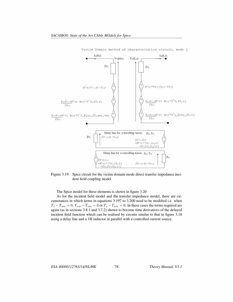
SACAMOS: State of the Art CAble MOdels for Spice
Vvj(0,t)
H’vj*V-vj(t-Tvj)
Zvj
Ivj(0,t)
Zvj, Tvj
Vvj(L,t)Ivj(L,t)
H’vj*Vvj+(0,t-Tvj)
2V+vj(t)
=H’vj*(Vvj(0,t)
+ZvjIvj(0,t))
2V-vj(t)
=H’vj*(Vvj(L,t)
-ZvjIvj(L,t))
Delay line for -z travelling waves
Delay line for +z travelling waves
2V+vj+(t-Tvj)
2V-vj(t-Tvj)
Zvj, Tvj
Zvj
Zvj
Zvj
Victim Domain method of characteristics circuit, mode j
PsiPvj(H’vi HZT)*V-0,ZT,vi
2Zsi
PsiPvj(H’vi HZT)*V+0,ZT,vj
2Zsi
PsiPvj(H’vi HZT)*V-0_Einc_ZT,smi,vmi
2Zsi
PsiPvj(H’vi HZT)*V+L_Einc_ZT,vj
2Zsi
Figure 3.19 Spice circuit for the victim domain mode direct transfer impedance inci-dent field coupling model
The Spice model for these elements is shown in figure 3.20As for the incident field model and the transfer impedance model, there are cir-
cumstances in which terms in equations 3.197 to 3.200 need to be modified i.e. whenTz−Tsm = 0, Tvm−Tsm = 0 or Tz−Tvm = 0. In these cases the terms required areagain (as in sections 3.8.1 and 3.7.2) shown to become time derivatives of the delayedincident field function which can be realised by circuits similar to that in figure 3.18using a delay line and a 1H inductor in parallel with a controlled current source.
ESA 40000112765/14/NL/HK 78 Theory Manual, V1.1
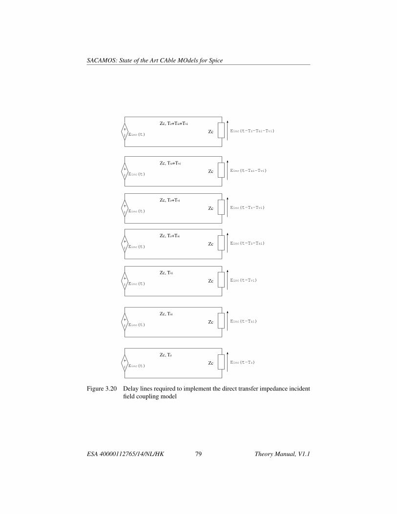
SACAMOS: State of the Art CAble MOdels for Spice
Zc, Tz+Tsi+Tvi
ZcEinc(t)
Einc(t-Tz-Tsi-Tvi)
Zc, Tsi+Tvi
ZcEinc(t)
Einc(t-Tsi-Tvi)
Zc, Tz+Tvi
ZcEinc(t)
Einc(t-Tz-Tvi)
Zc, Tz+Tsi
ZcEinc(t)
Einc(t-Tz-Tsi)
Zc, Tvi
ZcEinc(t)
Einc(t-Tvi)
Zc, Tsi
ZcEinc(t)
Einc(t-Tsi)
Zc, Tz
ZcEinc(t)
Einc(t-Tz)
Figure 3.20 Delay lines required to implement the direct transfer impedance incidentfield coupling model
ESA 40000112765/14/NL/HK 79 Theory Manual, V1.1
Chapter 4
Numerical computation of theper-unit-length MTLparameters using a FEM solver
Multiconductor Transmission Line (MTL) modelling is based on a set of coupled firstorder phasor MTL equations as discussed in chapter 2. In the set of coupled first-order MTL equations the impedance matrix
[Z (ω)
]and admittance matrix
[Y (ω)
]are given by
[Z (ω)
]=[R (ω)
]+ jω
[L (ω)
](4.1)
[Y (ω)
]=[G (ω)
]+ jω
[C (ω)
](4.2)
with[R (ω)
]the per unit length resistance matrix,
[L (ω)
]the per unit length induc-
tance matrix,[G (ω)
]the per unit length conductance matrix and
[C (ω)
]the per unit
length capacitance matrix. In order to be able to perform a propagation or crosstalkanalysis using MTL modelling it is important to determine good approximations ofthese per-unit length parameter matrices.
It is assumed in the initial discussion that the inductance and capacitance matrix areindependent of frequency and that dielectrics are loss-less and frequency independent.In section 4.2.3 frequency dependent capacitance is introduced by means of a complexrelative permittivity. In this case the capacitance and conductance matrix may be eval-uated at specific frequencies.In the book by Paul,[2], chapter 5, a definition of the [L], [G] and [C] matrices is givenand it is explained that these matrices can be determined from static field solutions in
80

SACAMOS: State of the Art CAble MOdels for Spice
the transverse plane for perfect line conductors. Closed-form solutions for these staticfield problems however only exist for a small set of configurations and several approx-imate solutions have limited applicability. As a consequence approximate numericalmethods must be used for the computation of the entries in the per-unit-length matrices.In the same book by Paul, chapter 5, it is also shown that in order to numerically de-termine the entries of the [L], [G] and [C] matrices we only need a capacitance solver,that is, we only need a numerical solver that is able to compute a capacitance matrix[C]. The inductance matrix [L] can be derived from the capacitance matrix solution[C0] for the static field problem in which we have replaced all dielectrics in the cross-section with free space, the per-unit-length inductance matrix can be obtained from
[L] = µ0ε0 [C0]−1 (4.3)
with µ0 and ε0 the permeability and permittivity of free space. The conductance matrix[G] can be obtained by introducing a complex permittivity and solving for a complexvalued capacitance matrix [C].
Two dimensional electrostatic field problems are governed by the two-dimensionalPoisson equation
− ∂
∂x
(εr,x
∂φ
∂x
)− ∂
∂y
(εr,y
∂φ
∂y
)=ρc
ε0(4.4)
with φ the potential, ρc the charge density, ε0 the permittivity of free space, εr,x andεr,y the diagonal components of the relative permittivity tensor (we have assumed alloff-diagonal terms are zero) of the materials in the configuration.
We can solve the capacitance matrix, [C], by discretising the cross-section of the cable(MTL) and solving the Laplace equation for this cross section numerically.
The two-dimensional Poisson equation follows from Gauss’s law,
∂
∂xDx +
∂
∂yDy = ρc (4.5)
the constitutive relation between the electric flux density and the electric field intensityfor a linear axial medium
Dx
Dy
= ε0
εr,x 0
0 εr,y
Ex
Ey
(4.6)
ESA 40000112765/14/NL/HK 81 Theory Manual, V1.1

SACAMOS: State of the Art CAble MOdels for Spice
and the definition of the scalar electric potential:
Ex
Ey
= −
∂φ∂x
∂φ∂y
(4.7)
In the static field problems that need to be solved in order to determine the entries ofthe capacitance matrix of a MTL, there is no free charge in the region between the con-ductors and the potential is prescribed on the conductors. As a result we have to solvethe two dimensional field problem:
− ∂
∂x
(εr∂φ
∂x
)− ∂
∂y
(εr∂φ
∂y
)= 0 (4.8)
with Dirichlet boundary condition
φ = p (4.9)
In the SACAMOS project the capacitance (and conductance) matrices are calculatednumerically using a Finite Element Method [8] as outlined in the rest of this chapter.Details of the implementation are not discussed here however the software closely fol-lows the process described in chapter 4 of [8].
4.1 Solving the capacitance matrix based on energyThe capacitance matrix can be solved based on energy or based on charges. We willuse the method based on energy.The total electrostatic energy stored in the multi-conductor configuration can be com-puted from the static field solution as
W =1
2
∫∫S
DEdA (4.10)
For this method we set the pth and qth conductor to 1V, that is, Vp = Vq = 1and connect all other conductors to reference, that is, all other conductors are set to0V which impliesVi = 0 for all i 6= q or p, the electrostatic energy Wpqstored in thesystem equals
ESA 40000112765/14/NL/HK 82 Theory Manual, V1.1
SACAMOS: State of the Art CAble MOdels for Spice
Wpq = Wp +Wq − cpq (4.11)
where cpq is the coupling capacitance. As a result, in case we have determined Wp forall p = 1, · · · , n and Wpq for all combinations of p = 1, · · · , n and q = 1, · · · , n forwhich p 6= q we can first compute all coupling capacitances cpq, namely
cpq = Wp +Wq −Wpq (4.12)
Then we may compute the coupling capacitances cp0
cp0 = 2Wp −n∑j=1j 6=p
cpj (4.13)
We can also immediately compute the coefficients of capacitance Cpq for all combina-tions of p = 1, · · · , n and q = 1, · · · , n as we note that:
Cpq = −cpq = Wpq −Wp −Wq (4.14)
Cpp =
n∑j=0j 6=p
cpj = 2Wp (4.15)
So, with a static field solver available we are able to compute the entries in the capaci-tance matrix.
4.2 Procedure capacitance matrix computation basedon energy analysis
The procedure for determining the capacitance matrix via computation of the energystorage is:
1. First select all n non-reference conductors one after another and each time com-pute the static field solution with the voltage of the conductor under considerationset to 1V and all other conductors set to the reference 0V. With the pth conductorset to 1V (Vp = 1V) and all other conductors to reference (0V), compute the
ESA 40000112765/14/NL/HK 83 Theory Manual, V1.1
SACAMOS: State of the Art CAble MOdels for Spice
electrostatic energy Epstored in the configuration by using the surface integral(4.10). This requires that the static field problem and energy integral has to bedetermined a total of n times.
2. Second select all combinations of two different conductors from the n non-reference conductors one after another and each time compute the static fieldsolution with the voltage of the two conductors under consideration set to 1Vand all other conductors set to the reference 0V. With the pth and qth conductorset to 1V (Vp = Vq = 1) and all other conductors set to reference (0V), computethe electrostatic energy Epqstored in the configuration by using the surface inte-gral (4.10). This requires that the static field solution and energy integral has tobe determined a total of n (n− 1) /2 times.
3. Determine the entries of the capacitance matrix from the computed stored ener-gies Epand Epq using expressions (4.14) and (4.15).
The reference conductor can be either a ground plane, a shield or a circular or rectan-gular conductor.
4.2.1 FEM Solver for the Open Boundary Electrostatic Field Prob-lem
Without an outer shield the electrostatic field is no longer confined to a bounded do-main while the FEM can only be used on a finite computational domain. In the courseof time a number of techniques have been developed to circumvent this problem. A re-view of the most important finite element open boundary techniques is given by Chenand Konrad [9]. Of all available techniques we have chosen to truncate the domainby introducing a fictitious contour that encloses the domain of primary interest andprescribe on it an asymptotic boundary condition which mimics the behaviour of theelectrostatic potential in the region outside the contour. Not only has it been shown thatasymptotic boundaries give good results, the technique is relatively easy to implementand preserves the sparsity of the finite element coefficient matrix which makes it a veryefficient method as-well.
4.2.2 Asymptotic Boundary ConditionsFor electrostatic problems, the potential in a point r, can be written as
φ (r) =
∫∫Ω
ρ (r′)G (r, r′) dr′ (4.16)
ESA 40000112765/14/NL/HK 84 Theory Manual, V1.1

SACAMOS: State of the Art CAble MOdels for Spice
Where Ω is the charged region, ρ (r′) is the charge distribution and G (r, r′) is the freespace Greens function:
G (r, r′) =1
2πε0ln |r− r′| (4.17)
In the expression for the potential , the effect of dielectrics is taken into account byincorporating the polarization charge density in the charge distribution. Using polarcoordinates (r, θ) the position vectors may be written as r = (r cos θ, r sin θ) andr′ = (r′ cos θ′, r′ sin θ′) and the free space Green function equals
G (r, θ, r′, θ′) =1
4πε0ln(r2 + r′2 − 2rr′ cos (θ − θ′)
)(4.18)
and hence
∂
∂rG (r, θ, r′, θ′) =
1
2πε0
r − r′ cos (θ − θ′)r2 + r′2 − 2rr′ cos (θ − θ′)
(4.19)
Expression immediately implies that the potential for r r′, with r′ the distancesfrom the origin of the charges in the charged region, satisfies
∂
∂rφ (r, θ) =
1
r ln (r)φ (r, θ) (4.20)
4.2.3 Computing the conductance matrixThe conductance matrix [G] can be obtained by introducing a complex permittivity andsolving for a complex valued capacitance matrix [C]. ( reference [2] equation 3.6.1)
If the surrounding medium is homogeneous, G can be obtained from C or L by
G =σ
εC = µσLe
−1 (4.21)
Le is the external inductance matrix assuming perfect conductors.Next we want to obtain G for inhomogeneous media. This can be the case for a con-ductor or shield that has a dielectric jacket (insulator). Actually, this is a simple mod-ification of the calculation of the per-unit-length capacitance matrix C (also computedassuming perfect conductors). Losses in the medium are due to:
ESA 40000112765/14/NL/HK 85 Theory Manual, V1.1

SACAMOS: State of the Art CAble MOdels for Spice
• Conductive losses (due to the conductance parameter σ).
• Polarization losses
Both of the losses can be represented by a complex permittivity.
ε = ε′ − jε′′ (4.22)
ε′ = ε (4.23)
ε′′ = εb +σ
ω= ε′ tan(δ) (4.24)
where tan(δ) is the loss tangent and εb are the polarization losses due to bound charges.σ represents the conduction current losses.We can include losses in the medium by solving for the capacitance matrix for amedium having a complex permittivity
ε = ε′ (1− j tan (δ)) (4.25)
and from that result directly obtain C and G.
Y = G+ jωC (4.26)
Y = jω
(C − j
ωG
)= jωC (4.27)
From that we can obtain the capacitance matrix C
C = Re(C) (4.28)
And the conductance matrix G
G = −$Im(C) (4.29)
ESA 40000112765/14/NL/HK 86 Theory Manual, V1.1

Chapter 5
Frequency dependent transferfunctions
5.1 IntroductionFrequency dependent transfer functions are implemented in the Spice models using s-domain transfer functions, this includes the propagation corrections and transfer impedanceterms. The coefficients of the s-domain transfer functions are required to provide the’best fit’ to a frequency dependent transfer function evaluated at a discrete set of fre-quencies. The software includes a process whereby the coefficients of an s-domaintransfer function (taking the form of a rational function in s), which provides an ap-proximation to a function, are determined.
5.2 Filter fitting process for s-domain transfer functionsThe process implemented is based on that described in [12].
The starting point for the process is a set of complex transfer function valuesH ′ (jωi) at a set of discrete frequencies i = 1..n and the aim is to find a rationalfunction H(jω) which best fits the available data points.
The transfer function takes the form:
H (jω) =a0 + a1
(jωω0
)+ a2
(jωω0
)2
+ · · ·+ ann
(jωω0
)nn1 + b1
(jωω0
)+ b2
(jωω0
)2
+ · · ·+ bnd
(jωω0
)nd =A(jω)
1 +B(jω)(5.1)
where the order of the numerator and the denominator are to be specified and the coeffi-cients aj and bj are to be determined. If we assume that the numerator and denominatororder are specified as nn and nd then we have unknown coefficients aj , j = 0..nn andbj , j = 1..nd.
87
SACAMOS: State of the Art CAble MOdels for Spice
At a frequency wi the error between the filter fit model and the transfer functionvalue is
err(jωi) = fracA(jωi)1 +B(jωi)−H ′ (jωi) (5.2)
multiplying equation 5.2 by 1 +B(jωi) gives
(1 +B(jωi)) err(jωi) = err′(jωi) = A(jωi)− (1 +B(jωi))H′ (jωi) (5.3)
The left hand side can be thought of as a weighted error function, err′.Evaluating equation 5.3 for each frequency ωi gives a set of n equations
err′(jω1)err′(jω2)
...err′(jωn)
=
−H ′(jω1)−H ′(jω2)
...−H ′(jωn)
+
− (jω1)H ′(jω1) . . . − (jω1)
ndH ′(jω1) 1 (jω1) . . . (jω1)
nn
− (jω2)H ′(jω2) . . . − (jω2)ndH ′(jω2) 1 (jω2) . . . (jω2)
nn
......
......
......
......
− (jωn)H ′(jωn) . . . − (jωn)ndH ′(jωn) 1 (jωn) . . . (jωn)
nn
b1...bnda0
a1
...ann
(5.4)
The coefficients of the transfer function are required to be real. This can be enforcedby augmenting the set of equations with an equal number of equations evaluated atnegative frequency where we impose the condition H(−jω) = H∗(jω).
err′(−jω1)err′(−jω2)
...err′(−jωn)
=
−H ′∗(jω1)−H ′∗(jω2)
...−H ′∗(jωn)
+
− (−jω1)H ′∗(jω1) . . . − (−jω1)
ndH ′∗(jω1) 1 (−jω1) . . . (−jω1)
nn
− (−jω2)H ′∗(jω2) . . . − (−jω2)ndH ′∗(jω2) 1 (−jω2) . . . (−jω2)
nn
......
......
......
......
− (−jωn)H ′∗(jωn) . . . − (−jωn)ndH ′∗(jωn) 1 (−jωn) . . . (−jωn)
nn
b1...bnda0
a1
...ann
(5.5)
ESA 40000112765/14/NL/HK 88 Theory Manual, V1.1
SACAMOS: State of the Art CAble MOdels for Spice
This combined set of equations is of the form
(err′) (D)− [X] (W ) (5.6)
The mean square error is found as
‖err‖2 = 1n<
(err′)∗
(err′)
= 1n<
(D)∗
(D) + (W )T
[X]∗
[X] (W )− 2 (D) [X]∗
(W ) (5.7)
where ∗ denotes the conjugate transpose and < denotes the real partIf we define
[R] = <
[X]∗
[X]
(5.8)
and
(P ) = [X]∗
(D) (5.9)
then
‖err‖2 =1
n<
(D)∗
(D) + (W )T
[R] (W )− 2 (P )T
(W )
(5.10)
This expression is minimised with respect to the vector (W ) of unknown coeffi-cients by differentiating with respect to (W ) and equating the result to zero i.e.
∂ ‖err‖2
∂ (W )=
1
n<
2 [R] (W )− 2 (P )T
= 0 (5.11)
This system of equations may be solved directly to give the unknown coefficientvector
(W ) = [R]−1
(P ) (5.12)
An alternative approach to reaching equation 5.12 is to start from the set of equa-tions 5.4 and 5.5. If we set the error on the left hand side to zero then we have theoverdetermined set of equations
(D) = [X] (W ) (5.13)
A solution to this set of equations may be found by solving the ’normal equations’which are found by pre-multiplying equation 5.13 by [X]
∗
[X]∗
(D) = [X]∗
[X] (W ) (5.14)
The matrix [X]∗
[X] is a square matrix which may be inverted to give the solution
(W ) =[[X]∗
[X]]−1
[X]∗
(D) (5.15)
The matrix[[X]∗
[X]]−1
[X]∗ is the Moore Penrose pseudo inverse and solves the
original overdetermined system of equation in a least squares sense.
ESA 40000112765/14/NL/HK 89 Theory Manual, V1.1

SACAMOS: State of the Art CAble MOdels for Spice
Stability of the transfer function
The spice models are required to operate in the time domain which implies that alltransfer functions in the model should be causal and that their impulse response shouldnot diverge as t→∞. This implies that all poles of the transfer function H(s) shouldlie in the left hand side of the s-plane. This condition is not naturally enforced by themethod described above however experience has shown that if the function to be fittedis a physically reasonable then the filter fit process will produce a stable model.
Enforcing constraints on the transfer function
It may be the case that the transfer function is subject to constraints. If this is thecase then the process may be adapted such that the constraints are naturally enforced.The filter fitting process is applied in a number of different aspects of the model. thefilter fit required for the propagation correction function is subject to the constraint thatH (ω = 0) = 1. In this case we calculate a model fit to H ′ (ω) = H (ω) − 1 whereH ′ (ω = 0) = 0 thus a′0 = 0 for the initial model. Once we have the coefficients forthe initial model we can easily calculate the filter coefficients for H (ω) = 1 +H ′ (ω).
ESA 40000112765/14/NL/HK 90 Theory Manual, V1.1
Chapter 6
Cable models available
In this section each of the cable types available will be described and any assumptionsregarding the specific cable models will be described.
The cable models available are
1. Frequency Dependent Cylindrical conductor with dielectric
2. Frequency Dependent Coaxial cable with transfer impedance and shield surfaceimpedance loss
3. Frequency Dependent Twinax cable with transfer impedance and shield surfaceimpedance loss
4. Frequency Dependent Twisted pair
5. Frequency Dependent Shielded twisted pair with transfer impedance and shieldsurface impedance loss
6. Frequency Dependent Spacewire with transfer impedance and shield surfaceimpedance loss
7. Frequency Dependent Overshield with transfer impedance and surface impedanceloss
8. Frequency Dependent flex cable
9. D connector
For each cable type the method of calculation for the inductance and capacitancematrices for any internal domains will be outlined. The domain decomposition matri-ces which relate local domain based voltages and currents to global condcutor basedvoltages and currents will be shown. These domain decomposition matrices for cableswill be augmented to include an external (reference) conductor which allows the cableto carry a common mode current.
91
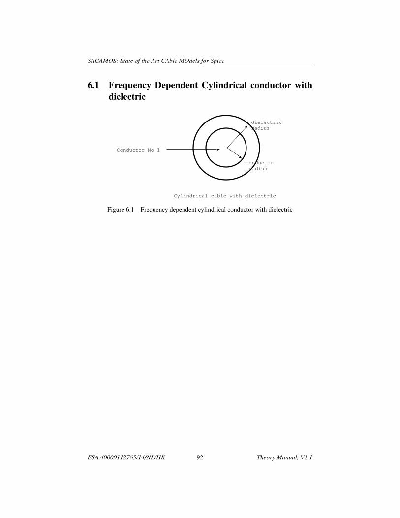
SACAMOS: State of the Art CAble MOdels for Spice
6.1 Frequency Dependent Cylindrical conductor withdielectric
Cylindrical cable with dielectric
conductor
radius
dielectric
radius
Conductor No 1
Figure 6.1 Frequency dependent cylindrical conductor with dielectric
ESA 40000112765/14/NL/HK 92 Theory Manual, V1.1

SACAMOS: State of the Art CAble MOdels for Spice
The cylindrical conductor has no shielded conductors so no inductance/ capacitancematrix calculation has to be performed for internal domains.
The domain decomposition voltage matrix, MV for the single conductor is givenby (
Vd1 c1
Vref
)=
[1 −10 1
](V1
V0
)(6.1)
The domain decomposition current matrix, MI for the single conductor is given by(Id1 c1
Iref
)=
[1 01 1
](I1I0
)(6.2)
6.2 Frequency Dependent Coaxial cable with transferimpedance and shield surface impedance loss
Coaxial cable with surface impedance loss
Inner
conductor
radius
Outer
dielectric
radius
Shield radius
Outer dielectric
relative permittivity
Inner dielectric
relative permittivity
Conductor No 1
Conductor No 2
Shield thickness
Figure 6.2 Frequency Dependent Coaxial cable - high frequency model includingshield surface impedance loss
The coaxial cable has a single internal domain in which a single mode propagates.The inductance and capacitance of the coaxial mode are calculated as
L =µ0
2πln
(rsrw
)H/m (6.3)
ESA 40000112765/14/NL/HK 93 Theory Manual, V1.1

SACAMOS: State of the Art CAble MOdels for Spice
C (jω)) =2πε (jω)
ln(rsrw
)F/m (6.4)
where rs is the shield radius, rw is the inner wire radius and eps (jω)) is the permit-tivity of the dielectric filling the space between the shield and the inner wire. Thisdielectric may be frequency dependent and in this case the capacitance will also befrequency dependent.
The domain decomposition voltage matrix, MV for the coaxial cable is given by Vd1 c1
Vd2 c1
Vref
=
1 −1 00 1 −10 0 1
V1
V2
V0
(6.5)
The domain decomposition current matrix, MI for the coaxial cable is given by Id1 c1
Id2 c1
Iref
=
1 0 01 1 01 1 1
I1I2I0
(6.6)
ESA 40000112765/14/NL/HK 94 Theory Manual, V1.1
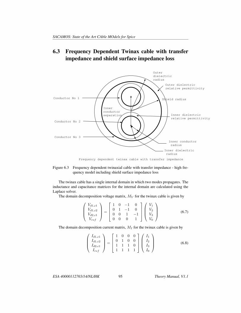
SACAMOS: State of the Art CAble MOdels for Spice
6.3 Frequency Dependent Twinax cable with transferimpedance and shield surface impedance loss
Frequency dependent twinax cable with transfer impedance
Inner conductor
radius
Outer
dielectric
radius
Shield radius
Outer dielectric
relative permittivity
Inner dielectric
relative permittivity
Inner
conductor
separation
Conductor No 1
Conductor No 2
Conductor No 3
Inner dielectric
radius
Figure 6.3 Frequency dependent twinaxial cable with transfer impedance - high fre-quency model including shield surface impedance loss
The twinax cable has a single internal domain in which two modes propagates. Theinductance and capacitance matrices for the internal domain are calculated using theLaplace solver.
The domain decomposition voltage matrix, MV for the twinax cable is given byVd1 c1
Vd1 c2
Vd2 c1
Vref
=
1 0 −1 00 1 −1 00 0 1 −10 0 0 1
V1
V2
V3
V0
(6.7)
The domain decomposition current matrix, MI for the twinax cable is given byId1 c1
Id1 c2
Id2 c1
Iref
=
1 0 0 00 1 0 01 1 1 01 1 1 1
I1I2I3I0
(6.8)
ESA 40000112765/14/NL/HK 95 Theory Manual, V1.1
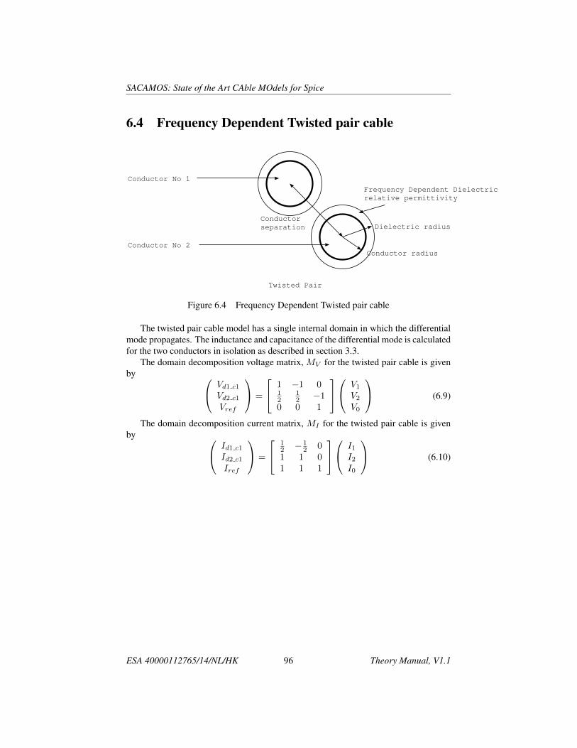
SACAMOS: State of the Art CAble MOdels for Spice
6.4 Frequency Dependent Twisted pair cable
Twisted Pair
Conductor radius
Frequency Dependent Dielectric
relative permittivity
Conductor
separation
Conductor No 1
Conductor No 2
Dielectric radius
Figure 6.4 Frequency Dependent Twisted pair cable
The twisted pair cable model has a single internal domain in which the differentialmode propagates. The inductance and capacitance of the differential mode is calculatedfor the two conductors in isolation as described in section 3.3.
The domain decomposition voltage matrix, MV for the twisted pair cable is givenby Vd1 c1
Vd2 c1
Vref
=
1 −1 012
12 −1
0 0 1
V1
V2
V0
(6.9)
The domain decomposition current matrix, MI for the twisted pair cable is givenby Id1 c1
Id2 c1
Iref
=
12 − 1
2 01 1 01 1 1
I1I2I0
(6.10)
ESA 40000112765/14/NL/HK 96 Theory Manual, V1.1

SACAMOS: State of the Art CAble MOdels for Spice
6.5 Frequency Dependent Shielded twisted pair withtransfer impedance and shield surface impedanceloss
Frequency dependent shielded Twisted Pair with transfer impedance
Inner conductor
radius
Outer
dielectric
radius
Shield radius
Outer dielectric
relative permittivity
Inner dielectric
relative permittivity
Inner conductor
separation
Conductor No 1
Conductor No 2
Conductor No 3
Inner dielectric
radius
Figure 6.5 Frequency dependent shielded twisted pair cable with transfer impedance- high frequency model including shield surface impedance loss
The shielded twisted pair cable model has two internal domains, one for the differ-ential mode of the twisted pair and one for the common mode of the twisted pair withthe shield as return conductor. The inductance and capacitance matrices for the internaldomains are calculated using the Laplace solver as described in section 3.3.
The domain decomposition voltage matrix, MV for the shielded twisted pair cableis given by
Vd1 c1
Vd2 c1
Vd3 c1
Vref
=
1 −1 0 012
12 −1 00 1 −1
0 0 0 1
V1
V2
V3
V0
(6.11)
The domain decomposition current matrix, MI for the shielded twisted pair cableis given by
Id1 c1
Id2 c1
Id3 c1
Iref
=
12 − 1
2 0 01 1 0 01 1 1 01 1 1 1
I1I2I3I0
(6.12)
ESA 40000112765/14/NL/HK 97 Theory Manual, V1.1
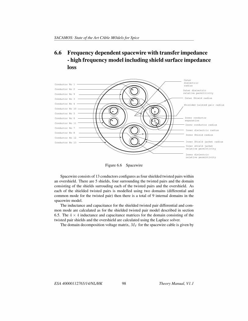
SACAMOS: State of the Art CAble MOdels for Spice
6.6 Frequency dependent spacewire with transfer impedance- high frequency model including shield surface impedanceloss
Inner conductor radius
Outer
dielectric
radius
Outer Shield radius
Outer dielectric
relative permittivity
Inner dielectric
relative permittivity
Inner conductor
separation
Conductor No 1
Conductor No 2
Conductor No 9
Conductor No 3
Conductor No 4
Conductor No 10
Conductor No 5
Conductor No 6
Conductor No 11
Conductor No 7
Conductor No 8
Conductor No 12
Conductor No 13
Inner Shield radius
Inner Shield jacket radius
Inner shield jacket
relative permittivity
Shielded twisted pair radius
Inner dielectric radius
Figure 6.6 Spacewire
Spacewire consists of 13 conductors configures as four shielded twisted pairs withinan overshield. There are 5 shields, four surrounding the twisted pairs and the domainconsisting of the shields surrouding each of the twisted pairs and the overshield. Aseach of the shielded twisted pairs is modelled using two domains (differential andcommon mode for the twisted pair) then there is a total of 9 internal domains in thespacewire model.
The inductance and capacitance for the shielded twisted pair differential and com-mon mode are calculated as for the shielded twisted pair model described in section6.5. The 4 × 4 inductance and capacitance matrices for the domain consisting of thetwisted pair shields and the overshield are calculated using the Laplace solver.
The domain decomposition voltage matrix, MV for the spacewire cable is given by
ESA 40000112765/14/NL/HK 98 Theory Manual, V1.1

SACAMOS: State of the Art CAble MOdels for Spice
Vd1 c1
Vd2 c1
Vd3 c1
Vd4 c1
Vd5 c1
Vd6 c1
Vd7 c1
Vd8 c1
Vd9 c1
Vd9 c2
Vd9 c3
Vd9 c4
Vd10 c1
Vref
=
1 −1 0 0 0 0 0 0 0 0 0 0 0 012
12 0 0 0 0 0 0 −1 0 0 0 0 0
0 0 1 −1 0 0 0 0 0 0 0 0 0 00 0 1
212 0 0 0 0 0 −1 0 0 0 0
0 0 0 0 1 −1 0 0 0 0 0 0 0 00 0 0 0 1
212 0 0 0 0 −1 0 0 0
0 0 0 0 0 0 1 −1 0 0 0 0 0 00 0 0 0 0 0 1
212 0 0 0 −1 0 0
0 0 0 0 0 0 0 0 1 0 0 0 −1 00 0 0 0 0 0 0 0 0 1 0 0 −1 00 0 0 0 0 0 0 0 0 0 1 0 −1 00 0 0 0 0 0 0 0 0 0 0 1 −1 00 0 0 0 0 0 0 0 0 0 0 0 1 −10 0 0 0 0 0 0 0 0 0 0 0 0 1
V1
V2
V3
V4
V5
V6
V7
V8
V9
V10V11V12V13V0
(6.13)
The domain decomposition voltage matrix, MI for the spacewire cable is given by
Id1 c1
Id2 c1
Id3 c1
Id4 c1
Id5 c1
Id6 c1
Id7 c1
Id8 c1
Id9 c1
Id9 c2
Id9 c3
Id9 c4
Id10 c1
Iref
=
12 − 1
2 0 0 0 0 0 0 0 0 0 0 0 01 1 0 0 0 0 0 0 0 0 0 0 0 00 0 1
2 − 12 0 0 0 0 0 0 0 0 0 0
0 0 1 1 0 0 0 0 0 0 0 0 0 00 0 0 0 1
2 − 12 0 0 0 0 0 0 0 0
0 0 0 0 1 1 0 0 0 0 0 0 0 00 0 0 0 0 0 1
2 − 12 0 0 0 0 0 0
0 0 0 0 0 0 1 1 0 0 0 0 0 01 1 0 0 0 0 0 0 1 0 0 0 0 00 0 1 1 0 0 0 0 0 1 0 0 0 00 0 0 0 0 0 0 0 0 0 1 0 0 00 0 0 0 0 0 0 0 0 0 0 1 0 01 1 1 1 1 1 1 1 1 1 1 1 1 01 1 1 1 1 1 1 1 1 1 1 1 1 1
I1I2I3I4I5I6I7I8I9I10I11I12I13I0
(6.14)
ESA 40000112765/14/NL/HK 99 Theory Manual, V1.1
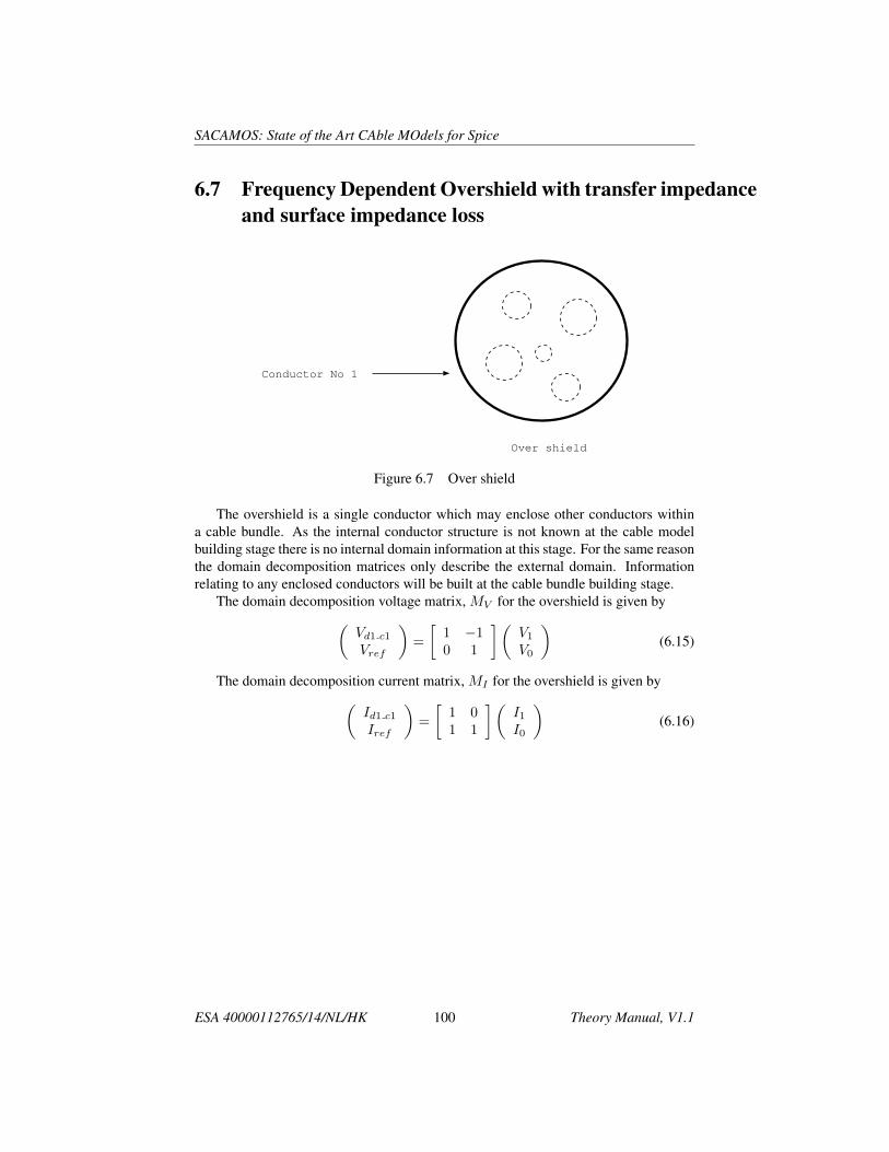
SACAMOS: State of the Art CAble MOdels for Spice
6.7 Frequency Dependent Overshield with transfer impedanceand surface impedance loss
Over shield
Conductor No 1
Figure 6.7 Over shield
The overshield is a single conductor which may enclose other conductors withina cable bundle. As the internal conductor structure is not known at the cable modelbuilding stage there is no internal domain information at this stage. For the same reasonthe domain decomposition matrices only describe the external domain. Informationrelating to any enclosed conductors will be built at the cable bundle building stage.
The domain decomposition voltage matrix, MV for the overshield is given by(Vd1 c1
Vref
)=
[1 −10 1
](V1
V0
)(6.15)
The domain decomposition current matrix, MI for the overshield is given by(Id1 c1
Iref
)=
[1 01 1
](I1I0
)(6.16)
ESA 40000112765/14/NL/HK 100 Theory Manual, V1.1

SACAMOS: State of the Art CAble MOdels for Spice
6.8 Flex cable
n conductor Flex cable
width
Conductor No 1
height
separation
Conductor No 2 Conductor No n
dielectric
x offset
dielectric y offset
Figure 6.8 flex cable
A flex cable may have an arbirary number of conductors, Nc. The dimension of thedomain decomposition matrices is Nc + 1. The domain decomposition voltage matrix,MV for a flex cable is given by
Vd1 c1
Vd1 c2
...Vd1 cNc
Vref
=
1 0 · · · 0 −10 1 · · · 0 −1...
.... . .
......
0 0 · · · 1 −10 0 · · · 0 1
V1
V2
...VNcV0
(6.17)
The domain decomposition current matrix, MI for a flex cable is given byId1 c1
Id1 c2
...Id1 cNc
Iref
=
1 0 · · · 0 00 1 · · · 0 0...
.... . .
......
0 0 · · · 1 01 1 · · · 1 1
I1I2...
INcI0
(6.18)
ESA 40000112765/14/NL/HK 101 Theory Manual, V1.1

SACAMOS: State of the Art CAble MOdels for Spice
6.9 D connector
D connector
Conductor radius
Conductor x separation
Conductor No 1
Conductor No 2
Conductor
y separation
Conductor No N-1Conductor No N (reference)
Shield offset
Figure 6.9 D connector
A D connector may have an arbirary number of conductors,Nc consisting ofNc−1internal conductor pins and the outer shell.
The internal conductor pins are all shielded by the connector shell therefore thereis a single internal domain. The inductance and capacitance matrices for the internaldomain are calculated using the Laplace solver.
The dimension of the domain decomposition matrices is Nc + 1 The domain de-composition voltage matrix, MV for a flex cable is given by
Vd1 c1
Vd1 c2
...Vd1 cNc−1
Vd2 c1
Vref
=
1 0 · · · 0 −100 1 · · · 0 −10...
.... . .
.........
0 0 · · · 1 −100 0 · · · 0 1− 10 0 · · · 0 01
V1
V2
...VNc−1
VNcV0
(6.19)
The domain decomposition voltage matrix, MI for a flex cable is given by
Id1 c1
Id1 c2
...Id1 cNc−1
Id2 c1
Iref
=
1 0 · · · 0 0 00 1 · · · 0 0 0...
.... . .
.........
0 0 · · · 1 0 00 0 · · · 0 1 01 1 · · · 1 1 1
I1I2...
INc−1
INcI0
(6.20)
ESA 40000112765/14/NL/HK 102 Theory Manual, V1.1
Chapter 7
Network synthesis for specifiedfrequency dependent transferfunctions
7.1 OverviewIt has been found from experience that Spice models making use of s-domain transferfunctions to simulate frequency dependent transfer functions in Spice were susceptibleto fail due to convergence problems, especially for transient analysis in Ngspice. Aninitial investigation of this issue showed that when the s-domain transfer functions werereplaced by equivalent passive circuits which implemented the same transfer function,the convergence problems could be eliminated. This initial investigation was limitedto first and second order rational functions only, however this observation has lead tothe development of a general implementation of s-domain transfer functions as passivecircuits so that the convergence issues can be mitigated for the general case.
This chapter describes the theory which underlies the modelling of frequency de-pendent transfer functions as passive circuits in Spice. Frequency dependent transferfunctions in this work are represented as rational functions in tha laplace variable, s. Itis assumed that the rational functions represent stable systems i.e. that their impulseresponse does not diverge as t→∞. This implies that the poles of the transfer functionmust lie in the left hand side of the s plane.
We consider two types of transfer functions according to their properties
1. Positive-real transfer functions which may be represented as a one port network(simple impedance)
2. non-positive-real transfer functions which may be represented as two port net-works
The first type of transfer function arises in this work in the propagation correctionfunctions. The second type may arise in transfer impedance models where the transfer
103

SACAMOS: State of the Art CAble MOdels for Spice
resistance and/or inductance may be negative at some frequencies.The form of the transfer functions that we wish to implement as a passive circuit
are rational functions as in equation7.1
H (s) =a0 + a1
(sω0
)+ a2
(sω0
)2
+ . . .
b0 + b1
(sω0
)+ b2
(sω0
)2
+ . . .(7.1)
where ω0 is a frequency normalisation factor. The methods applied make use of thework of Foster Cauer[13], [14],and Brune [15]. The underlying theory and examplesof the techniques outlined here are described in reference [16].
7.2 One port impedance models for positive-real trans-fer functions
A passive impedance function must be ’positive-real’ to constitute a physical impedancewhich can be synthesised from a network of inductors, capacitors, resistors and trans-formers. A positive-real rational function is defined by the following conditions:
1. The real part of the function Z(s) must be positive for all s = α+ jω, α > 0
2. The imaginary part of the functionZ(s) must be zero for all s = α+ jω, ω = 0
Positive real rational functions have the following properties:
1. The number of poles and zeros differ by at most 1
2. The coefficients of the rational function are all real and positive
3. The poles and zeros of the function must lie in the left hand side of the s-planeor on the s = jω axis
4. If a function Z(s) is positive-real then so is Y (s) = 1Z(s)
In this section we describe how an impedance represented as a rational function ins may be synthesised by a passive one port circuit consisting of resistors, inductors,capacitors and transformers i.e. Spice R, L, C and K elements.
Figure 7.1 shows a one port network driven by a current source I (jω) whose portvoltage is given by V (jω) = Z (jω) I (jω). The impedance can be synthesised as aladder network as shown in figure 7.2 The impedance of the ladder network may beexpressed as the sum of the first series impedance, Z1(s) and a remainder, Zr1(s) i.e.
Z (s) = Z1(s) + Zr1(s) (7.2)
The circuit is shown in figure 7.3 where Z1(s) is the impedance of a combinationof R, L, C, K elements and Zr1(s) is a stable positive real function. The remainder
ESA 40000112765/14/NL/HK 104 Theory Manual, V1.1

SACAMOS: State of the Art CAble MOdels for Spice
V(jω) Z(jω)I(jω)
Figure 7.1 One port network model of a positive-real transfer function
V(jω)
Z3(jω)
I(jω) Y2(jω)
Z5(jω)
Y4(jω) Yn(jω)
Z1(jω)
Figure 7.2 Ladder network synthesis of an impedance
impedance, Zr1(s), is then synthesised as the parallel combination of the admittancefunction Y2(s) and a remainder, Yr2(s) as seen in figure 7.4
Zr1(s) =1
Y2(s) + Yr2(s)(7.3)
thusZ (s) = Z1(s) +
1
Y2(s) + Yr2(s)(7.4)
The admittance Yr2(s) is then synthesised as the sum of two series impedances i.e.
Z (s) = Z1(s) +1
Y2(s) +1
Z3(s) + Zr3(s)
(7.5)
It is seen from this that the impedance function of the ladder network is expressed in acontinued fraction form with alternating impedance and admittance terms. The circuitat this third stage is shown in figure 7.5. This synthesis procedure in which admittanceand impedance elements of the ladder network are identified in turn continues until theremainder term is reduced to zero. This leads to a relatively straightforward synthesisprocess for impedance functions.
ESA 40000112765/14/NL/HK 105 Theory Manual, V1.1

SACAMOS: State of the Art CAble MOdels for Spice
V(jω)I(jω) Zr(jω)
Z1(jω)
Figure 7.3 Initial stage of ladder network synthesis
V(jω)I(jω) Y2(jω) Yr2(jω)
Z1(jω)
Figure 7.4 Second stage of ladder network synthesis
V(jω)I(jω) Y2(jω) Zr3(jω)
Z1(jω) Z3(jω)
Figure 7.5 Third stage of ladder network synthesis
ESA 40000112765/14/NL/HK 106 Theory Manual, V1.1

SACAMOS: State of the Art CAble MOdels for Spice
7.2.1 Algorithm for impedance synthesisThe starting point for the algorithm for impedance synthesis is a rational function ins which must be stable and positive-real. The impedance is synthesised by extractingseries impedances and parallel admittances in turn until the remainder is zero. Theimpedance/ admittance extraction makes use of a pole-residue representation of thetransfer function in order to identify branches which are combinations of R, L and Celements. This method can get stuck in that a viable branch cannot be identified whileleaving a stable positive-real remainder function. In this case a technique developed byBrune [15] is used to continue the synthesis. Brune’s method makes use of transformers(K elements in Spice).
An outline of the algorithm is as follows:
1. Attempt to identifiy a viable series impedance branch i.e. a branch which maybe synthesised with R, L, and C elements and which leaves a remainder Zr(s)which is stable and posistive-real. If a viable branch is found then this processcan be repeated until no further viable series impedance branches can be found.
2. Once no futher viable series impedance contributions can be found, calculate theadmittance Yr(s) = 1/Zr(s) and attempt to identifiy a viable parallel admittancebranch i.e. a branch which may be synthesised with R, L, and C K elements andwhich leaves a remainder Yr(s) which is stable and posistive-real. If a viablebranch is found then this process can be repeated until no further viable paralleladmittance brances can be found.
3. If no viable series impedance branches or parallel admittance branches can befound then use the Brune synthesis method and implement the resulting circuitwith R, L, C and K elements
4. Return to step 1 and repeat until the remainder impedance/ admittance is zero.
7.2.2 Identification of series impedance branchesA vaiable series impedance branch can be one of the following:
1. RLC branch
2. LC branch
3. RC branch
4. RL branch
5. C branch
6. L branch
7. R branch (which may be identified in two different ways)
ESA 40000112765/14/NL/HK 107 Theory Manual, V1.1
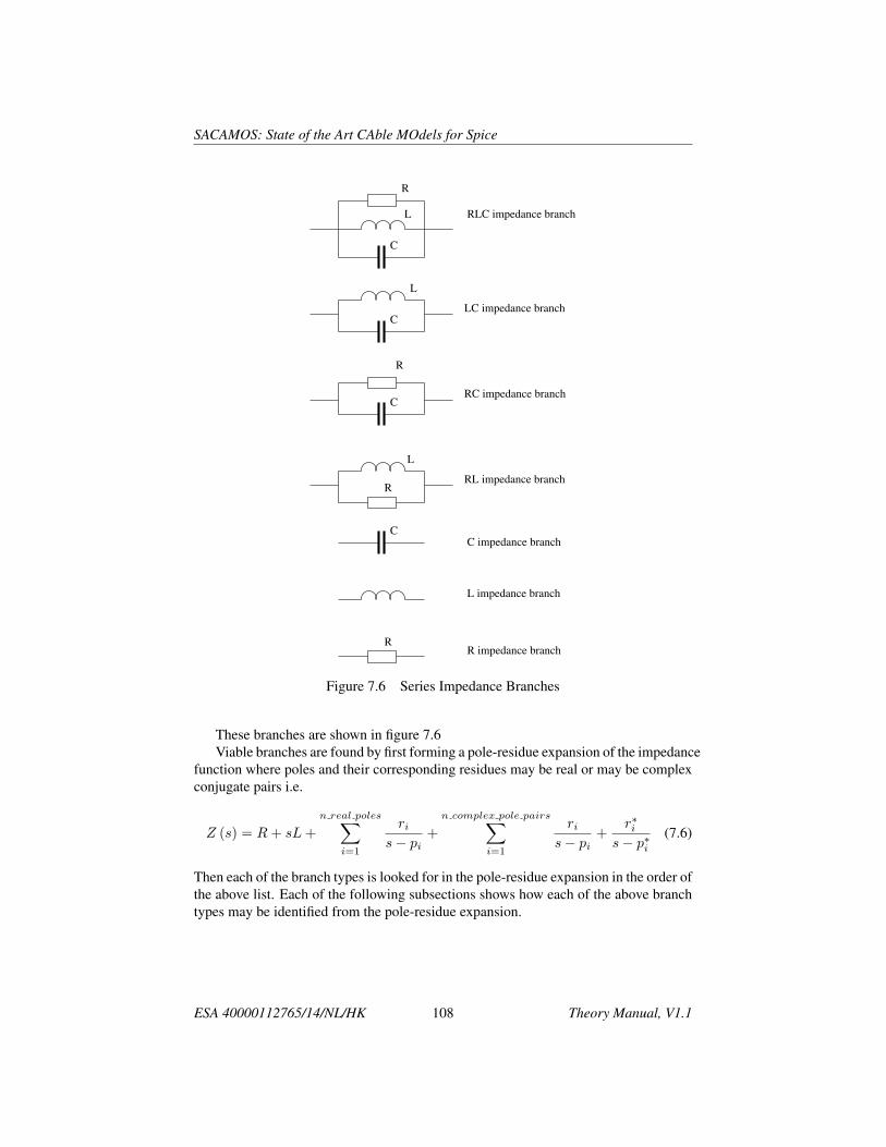
SACAMOS: State of the Art CAble MOdels for Spice
L
C
R
RLC impedance branch
L
CLC impedance branch
CRC impedance branch
R
L
RRL impedance branch
C
R
C impedance branch
L impedance branch
R impedance branch
Figure 7.6 Series Impedance Branches
These branches are shown in figure 7.6Viable branches are found by first forming a pole-residue expansion of the impedance
function where poles and their corresponding residues may be real or may be complexconjugate pairs i.e.
Z (s) = R+ sL+
n real poles∑i=1
ris− pi
+
n complex pole pairs∑i=1
ris− pi
+r∗i
s− p∗i(7.6)
Then each of the branch types is looked for in the pole-residue expansion in the order ofthe above list. Each of the following subsections shows how each of the above branchtypes may be identified from the pole-residue expansion.
ESA 40000112765/14/NL/HK 108 Theory Manual, V1.1

SACAMOS: State of the Art CAble MOdels for Spice
RLC impedance branch
The RLC impedance branch has an impedance function which can be expressed inrational function as
Z (s) =sC
1LC + s
CR + s2(7.7)
This may be expressed in pole-residue form as the complex pole-residue pair
Z (s) =r
s− p+
r∗
s− p∗=
(rp∗ − r∗p) + (r + r∗) s
pp∗ − (p+ p∗) s+ s2(7.8)
Where the poles are complex (and not purely imaginary). Equating coefficients of therational functions a requirement for a viable RLC branch can be established i.e. thenumerator constant term is zero:
rp∗ − r∗p = 0 (7.9)
In addition we require that all the component values of the RLC circuit be positive i.e.
C =1
r + r∗> 0 (7.10)
L =r + r∗
pp∗> 0 (7.11)
R =r + r∗
p+ p∗> 0 (7.12)
The final requirement is that the remainder function be positive real i.e. the remainingterms of the impedance function describe a physical impedance. If these requirementsare satisfied then a RLC branch can be extracted from the impedance function andimplemented as an impedance branch in the ladder network.
LC impedance branch
The LC impedance branch has an impedance function which can be expressed in ratio-nal function as
Z (s) =sC
1LC + s2
(7.13)
This is a special case of the RLC branch in which R → ∞ may be expressed in pole-residue form as the complex pole-residue pair
Z (s) =r
s− p+
r∗
s− p∗=
(rp∗ − r∗p) + (r + r∗) s
pp∗ − (p+ p∗) s+ s2(7.14)
Where the poles are purely imaginary. Equating coefficients of the rational functionsa requirement for a viable LC impedance branch can be established i.e. the poles areimaginary:
p∗ + p = 0 (7.15)
ESA 40000112765/14/NL/HK 109 Theory Manual, V1.1

SACAMOS: State of the Art CAble MOdels for Spice
The numerator constant term is zero:
rp∗ − r∗p = 0 (7.16)
In addition we require that all the component values of the LC circuit be positive i.e.
C =1
r + r∗> 0 (7.17)
L =r + r∗
pp∗> 0 (7.18)
The final requirement is that the remainder function be positive real i.e. the remainingterms of the impedance function describe a physical impedance. If these requirementsare satisfied then an LC branch can be extracted from the impedance function andimplemented as an impedance branch in the ladder network.
RC impedance branch
The RC impedance branch has an impedance function which can be expressed in ratio-nal function as
Z (s) =1C
1RC + s
(7.19)
This may be expressed in pole-residue form as
Z (s) =r
s− p(7.20)
Where the pole and residue are both real. By equating coefficients of the functions,values of R and C can be identified We require that all the component values of the RCcircuit be positive i.e.
C =1
r> 0 (7.21)
R =−rp> 0 (7.22)
The final requirement is that the remainder function be positive real i.e. the remainingterms of the impedance function describe a physical impedance. If these requirementsare satisfied then an RC branch can be extracted from the impedance function andimplemented as an impedance branch in the ladder network.
RL impedance branch
The RL impedance branch has an impedance function which can be expressed in ratio-nal function as
Z (s) =sR
RL + s
= R−R2
L
s+ RL
(7.23)
ESA 40000112765/14/NL/HK 110 Theory Manual, V1.1
SACAMOS: State of the Art CAble MOdels for Spice
This may be expressed in pole-residue form, including a constant term as
Z (s) = K +r
s− p(7.24)
Where the pole and residue are both real. By equating coefficients of the functions,values of R and L can be identified We require that all the component values of the RLcircuit be positive i.e.
R =r
p> 0 (7.25)
L =−rp2
> 0 (7.26)
The final requirement is that the remainder function be positive real i.e. the remainingterms of the impedance function describe a physical impedance. If these requirementsare satisfied then an RL branch can be extracted from the impedance function andimplemented as an impedance branch in the ladder network.
Capacitance branch
The capacitance branch has an impedance function which consists of a pole at zero i.e.
Z (s) =1
sC(7.27)
Thus in the pole-residue expansion we require a pole at zero. In addition we requirethat capacitance be positive i.e.
C =1
r> 0 (7.28)
The final requirement is that the remainder function be positive real i.e. the remainingterms of the impedance function describe a physical impedance. If these requirementsare satisfied then a capacitance branch can be extracted from the impedance functionand implemented as an impedance in the ladder network.
Inductance branch
The inductance branch has an impedance given by
Z (s) = sL (7.29)
Thus in the pole-residue expansion we require a sL term (pole at infinity in the impedancefunction) with positive inductance, L. The final requirement is that the remainder func-tion be positive real i.e. the remaining terms of the impedance function describe aphysical impedance. If these requirements are satisfied then an inductance branch canbe extracted from the impedance function and implemented as an impedance in theladder network.
ESA 40000112765/14/NL/HK 111 Theory Manual, V1.1

SACAMOS: State of the Art CAble MOdels for Spice
Resistance branch, type 1
The resistance branch of type 1 is identified by a positive constant term, R, in thepole-residue expansion of the impedance. If the remainder function is positive real i.e.the remaining terms of the impedance function describe a physical impedance then aresistance branch can be extracted from the impedance function and implemented asan impedance in the ladder network.
Resistance branch, type 2
The resistance branch of type 2 may be found from the rational function form of theimpedance i.e. if
Z (s) =a0 + a1
(sω0
)+ a2
(sω0
)2
+ . . .
b0 + b1
(sω0
)+ b2
(sω0
)2
+ . . .(7.30)
then we can calculate the resistance, R as
R =a0
b0(7.31)
as opposed to the pole-residue form whose constant (resistance) term is found as the ra-tio of the numerator and denominator coefficients of the highest power of s subtractingthe resistance as defined in 7.31 results in a remainder impedance function with a poleat infinity. As for all the othetr branch identification methods, this resistance branch canonly be extracted if the remainder impedance is a stable physical impedance function.
7.2.3 Identification of admittance branchesA vaiable admittance branch can be one of the following combinations:
1. GLC branch
2. LC branch
3. GC branch
4. GL branch
5. C branch
6. L branch
7. G branch (which may be identified in two different ways)
ESA 40000112765/14/NL/HK 112 Theory Manual, V1.1
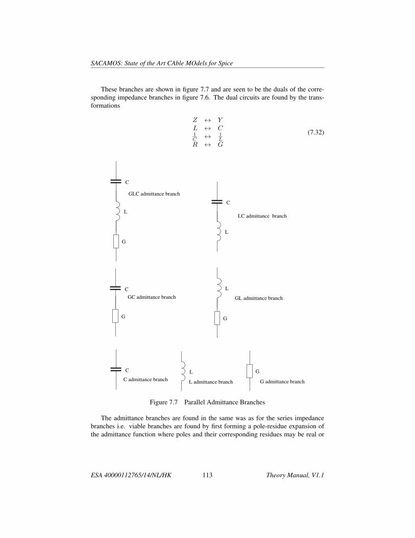
SACAMOS: State of the Art CAble MOdels for Spice
These branches are shown in figure 7.7 and are seen to be the duals of the corre-sponding impedance branches in figure 7.6. The dual circuits are found by the trans-formations
Z ↔ YL ↔ C1C ↔ 1
LR ↔ G
(7.32)
GLC admittance branch
LC admittance branch
GC admittance branch GL admittance branch
C admittance branch L admittance branch G admittance branch
L GC
L
G
C
L
C
G
C L
G
Figure 7.7 Parallel Admittance Branches
The admittance branches are found in the same was as for the series impedancebranches i.e. viable branches are found by first forming a pole-residue expansion ofthe admittance function where poles and their corresponding residues may be real or
ESA 40000112765/14/NL/HK 113 Theory Manual, V1.1
SACAMOS: State of the Art CAble MOdels for Spice
may be complex conjugate pairs i.e.
Y (s) = G+ sC +
n real poles∑i=1
ris− pi
+
n complex pole pairs∑i=1
ris− pi
+r∗i
s− p∗i(7.33)
For completeness a brief summary of the admittance branch identification processes isgiven here. The admittances may have inductance, capacitance or conductance thougha non-zero conductance is implemented as a resistance R = 1
G in Spice.
GCL admittance branch
The GCL admittance branch has an admittance function which can be expressed inrational function as
Y (s) =sL
1CL + s
LG + s2(7.34)
This may be expressed in pole-residue form as the complex pole-residue pair
Y (s) =r
s− p+
r∗
s− p∗=
(rp∗ − r∗p) + (r + r∗) s
pp∗ − (p+ p∗) s+ s2(7.35)
The poles are complex (and not purely imaginary). Equating coefficients of the rationalfunctions a requirement for a viable GCL admittance branch can be established i.e. thenumerator constant term is zero:
rp∗ − r∗p = 0 (7.36)
In addition we require that all the component values of the GCL circuit be positive i.e.
L =1
r + r∗> 0 (7.37)
C =r + r∗
pp∗> 0 (7.38)
G =r + r∗
p+ p∗> 0 (7.39)
The final requirement is that the remainder function be positive real i.e. the remainingterms of the admittance function describe a physical admittance. If these requirementsare satisfied then a GCL branch can be extracted from the admittance function andimplemented as an admittance branch in the ladder network.
LC admittance branch
The LC admittance branch has an admittance function which can be expressed in ra-tional function as
Y (s) =sL
1CL + s2
(7.40)
ESA 40000112765/14/NL/HK 114 Theory Manual, V1.1

SACAMOS: State of the Art CAble MOdels for Spice
This is a special case of the GCL branch in which G→∞ (R→ 0) may be expressedin pole-residue form as the complex pole-residue pair
Y (s) =r
s− p+
r∗
s− p∗=
(rp∗ − r∗p) + (r + r∗) s
pp∗ − (p+ p∗) s+ s2(7.41)
Where the poles are purely imaginary. Equating coefficients of the rational functionsa requirement for a viable LC admittance branch can be established i.e. the poles areimaginary:
p∗ + p = 0 (7.42)
The numerator constant term is zero:
rp∗ − r∗p = 0 (7.43)
In addition we require that all the component values of the LC circuit be positive i.e.
L =1
r + r∗> 0 (7.44)
C =r + r∗
pp∗> 0 (7.45)
The final requirement is that the remainder function be positive real i.e. the remainingterms of the admittance function describe a physical admittance. If these requirementsare satisfied then an LC branch can be extracted from the admittance function andimplemented as an admittance branch in the ladder network.
GL admittance branch
The GL admittance branch has an admittance function which can be expressed in ra-tional function as
Y (s) =1L
1GL + s
(7.46)
This may be expressed in pole-residue form as
Y (s) =r
s− p(7.47)
Where the pole and residue are both real. By equating coefficients of the functions,values of G and L can be identified We require that the component values of the GLcircuit be positive i.e.
L =1
r> 0 (7.48)
G =−rp> 0 (7.49)
The final requirement is that the remainder function be positive real i.e. the remainingterms of the admittance function describe a physical admittance. If these requirementsare satisfied then a GL branch can be extracted from the admittance function and im-plemented as an admittance branch in the ladder network.
ESA 40000112765/14/NL/HK 115 Theory Manual, V1.1

SACAMOS: State of the Art CAble MOdels for Spice
GC admittance branch
The GC admittance branch has an admittance function which can be expressed in ra-tional function as
Y (s) =sG
GC + s
= G−G2
C
s+ GC
(7.50)
This may be expressed in pole-residue form, including a constant term as
Y (s) = K +r
s− p(7.51)
Where the pole and residue are both real. By equating coefficients of the functions,values of G and C can be identified We require that all the component values of theseries GC circuit be positive i.e.
G =r
p> 0 (7.52)
C =−rp2
> 0 (7.53)
The final requirement is that the remainder function be positive real i.e. the remainingterms of the admittance function describe a physical admittance. If these requirementsare satisfied then a GC branch can be extracted from the admittance function and im-plemented as an admittance branch in the ladder network.
Inductance branch
The inductance branch has an admittance function which consists of a pole at zero i.e.
Y (s) =1
sL(7.54)
Thus in the pole-residue expansion we require a pole at zero. In addition we requirethat inductance be positive i.e.
L =1
r> 0 (7.55)
The final requirement is that the remainder function be positive real i.e. the remainingterms of the admittance function describe a physical admittance. If these requirementsare satisfied then a inductance branch can be extracted from the admittance functionand implemented as an admittance in the ladder network.
Capacitance branch
The capacitance branch has an admittance given by
Y (s) = sC (7.56)
Thus in the pole-residue expansion we require a sC term (pole at infinity in the admit-tance function) with positive capacitance, C. The final requirement is that the remainder
ESA 40000112765/14/NL/HK 116 Theory Manual, V1.1

SACAMOS: State of the Art CAble MOdels for Spice
function be positive real i.e. the remaining terms of the admittance function describe aphysical admittance. If these requirements are satisfied then a capacitance branch canbe extracted from the admittance function and implemented as an admittance in theladder network.
Conductance (Resistance) branch, type 1
The conductance branch of type 1 is identified by a positive constant term, G, in thepole-residue expansion of the admittance. If the remainder function is positive real i.e.the remaining terms of the admittance function describe a physical admittance then aresistance branch can be extracted from the admittance function and implemented asan admittance in the ladder network.
Conductance (Resistance) branch, type 2
The conductance branch of type 2 may be found from the rational function form of theadmittance i.e. if
Y (s) =a0 + a1
(sω0
)+ a2
(sω0
)2
+ . . .
b0 + b1
(sω0
)+ b2
(sω0
)2
+ . . .(7.57)
then we can calculate the conductance, G as
G =a0
b0(7.58)
ESA 40000112765/14/NL/HK 117 Theory Manual, V1.1
SACAMOS: State of the Art CAble MOdels for Spice
7.2.4 Brune SynthesisThere are circumstances when the ladder network synthesis procedure described abovefails i.e. a physical impedance/ admittance function results for which no viable se-ries impedance or parallel admittance branch can be found. In this case the methoddescribed by Brune [15] may be applied to allow the process to proceeed. Brune’smethod involves the use of a transformer which can be included in Spice simulationsusing the K element. The basic process is described here however the associated proofsof the properties of the functions at each stage will not be given. For further details seereferences [15] and [16].
The ladder network synthesis procedure ensures that poles at zero, poles at infinity,zeros at infinity, zeros at zero, poles on the s = ±jω axis and zeros on the s = ±jωaxis have been removed from the impedance function. Brune’s method then operateson this remainer function, Zr(s), as follows:
Stage 1. Find ω0 such that the real part of the impedance Zr(s = jω0) is a mini-mum. The minimum resistance value at this frequency is Rmin.
Stage 2. Subtract Rmin from Zr(s) to give the minimum resistance impedancefunction
Z1 (s) = Zr (s)−Rmin (7.59)
i.e. Rmin is extracted as a series resistance.The function Z1 (s) is now purely reactive at w0 i.e. Z1 (ω0) = jX . This reactance
is set to be the reactance of an inductor, LA where LA = Xω0
. Note that this inducatancemay be negative.
This series inductance is subtracted from Z1(s) to give
Z2 (s) = Z1 (s)− sLA (7.60)
Z2 (s) has a zero of order 2 at s = jω0 and we can write the admittance Y2(s) =1
Z2(s) as
Y2 (s) =1
Z1 (s)− sLA=
α
s2 + ω20
+ Y3 (s) (7.61)
From this we can identify a LC admittance branch where LB = 1α andCB = 1
ω20LB
The remainder impedance Z3 (s) = 1Y3(s) after subtraction of the LC admittance
branch has a first order pole at infinity and therefore a series inductance can be extractedi.e.
Zr (s) = Z3 (s)− sLC (7.62)
where LC is negative if LA is positive and vice versa. In addition to this it can beshown that the remainder impedance, Zr(s) is positive-real.
This series of component identification leads to the circuit shown in figure 7.8 how-ever this is not a physical circuit in that one of the series inductorsLA orLB is negative.
ESA 40000112765/14/NL/HK 118 Theory Manual, V1.1

SACAMOS: State of the Art CAble MOdels for Spice
The three inductances may be combined into two positive inductors with a mutual in-ductance term as seen in figure 7.9. In this circuit the component values can be shownto be
L1 = LA + LBL2 = LC + LBK = 1
(7.63)
The inductances in the final Brune synthesis circuit are all positive and may there-fore be simulated in Spice using L, C R and K elements. Since the remainder impedanceis positive-real, the ladder network synthesis procedure can proceed.
LB
CB
Zr
Rmin LA LC
Figure 7.8 Initial Brune Synthesis Circuit
L1
C
L2
K
Rmin
Zr
Figure 7.9 Final Brune Synthesis Circuit
7.3 Synthesis of non-positive real transfer functionsThe process for one port synthesis requires that the impedance transfer function is apositive-real function. It may be the case that we need to synthesise a transfer function
ESA 40000112765/14/NL/HK 119 Theory Manual, V1.1
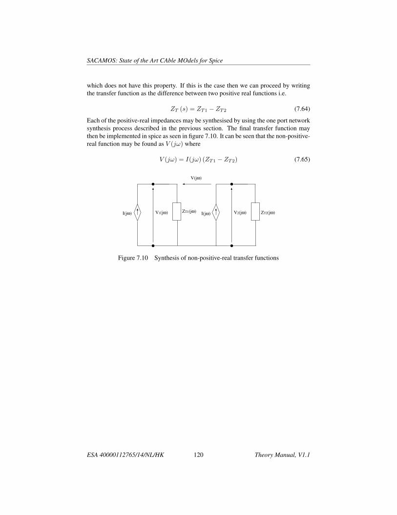
SACAMOS: State of the Art CAble MOdels for Spice
which does not have this property. If this is the case then we can proceed by writingthe transfer function as the difference between two positive real functions i.e.
ZT (s) = ZT1 − ZT2 (7.64)
Each of the positive-real impedances may be synthesised by using the one port networksynthesis process described in the previous section. The final transfer function maythen be implemented in spice as seen in figure 7.10. It can be seen that the non-positive-real function may be found as V (jω) where
V (jω) = I(jω) (ZT1 − ZT2) (7.65)
V1(jω)I(jω) ZT1(jω) V2(jω)I(jω) ZT2(jω)
V(jω)
Figure 7.10 Synthesis of non-positive-real transfer functions
ESA 40000112765/14/NL/HK 120 Theory Manual, V1.1
SACAMOS: State of the Art CAble MOdels for Spice
7.4 Application of the network syntheis in Spice cablebundle models
The Spice cable bundle models require the use of frequency domain transfer functionsfor the implementation of the propagation correction and for the transfer impedancecoupling model. The propagation correction is expected to be a positive-real functionas it represents the loss and dispersion in the modal propagation thus it will be im-plemented using a single port impedance. The transfer impedance functions howevermay have negative transfer resistance and/or inductance at certain frequencies and willtherefore require a two port model for its implementation.
ESA 40000112765/14/NL/HK 121 Theory Manual, V1.1

Bibliography
[1] C. Smartt, D.W.P. Thomas, S. Greedy, J. Verpoorte, J. Lansink RotgerinkSACAMOS User Guide
[2] C.R. Paul, Analysis of Multi-conductor Transmission Lines, Second edition, JohnWiley & Sons, 2008, ISBN 978-0-470-13154-1.
[3] A.K. Agrawal, H.J. Price, S.H. Gurbaxani, Transient Response of MulticonductorTransmission Lines Excited by a Nonuniform Electromagnetic Field, IEEE TransEMC, Vol 22, No 2, pp 119-129, 1980.
[4] B.K.P. Scaife, Principles of Dielectrics, Oxford University Press, 1998
[5] S.A. Schelkunoff, The Electromagnetic Theory of Coaxial Transmission Lines andCylindrical Shields, Bell System Technical Journal,Vol 13, No 4, pp 532-579,1934.
[6] C.R. Paul, A SPICE Model for Multiconductor Transmission Lines Excited by anIncident Electromagnetic Field, IEEE Trans EMC, Vol 36, No 4, pp 342-354, 1994.
[7] H. Xie, J. Wang, R. Fan, Y. Liu, SPICE Models to Analyze Radiated and Con-ducted Susceptibilities of Shielded Coaxial Cables, IEEE Trans EMC, Vol 52, No1, pp 215-222, 2010.
[8] J-M Jin, The Finite Element Method in Electromagnetics 3rd Edition, John Wiley& sons 2014.
[9] Q. Chen, A. Konrad, A Review of Finite Element Open Boundary Techniquesfor Static and Quasi-Static Electromagnetic Field Problems, IEEE Transactions onMagnetics, Vol.33, No 1, January 1997
[10] E.O. Brigham, The Fast Fourier Transform and its Applications, Prentice Hall,1988.
[11] http://www.netlib.org/eispack/
[12] J.F. Dawson, J.A. Cole, S.J. Porter, Modelling of transmission and reflection ofthin layers for EMC applications in TLM. 10th international conference on EMC,1997, pp65-70.
122

SACAMOS: State of the Art CAble MOdels for Spice
[13] W. Cauer Synthesis of Linear Communication Networks vols 1 and 2, 2nd ed.McGraw-Hill New York, 1958.
[14] R. M. Foster A reactance Theorem Bell System Tech. J, vol 3 1924, pp 259-267
[15] O. Brune, Synthesis of a finite two-terminal network whose driving-pointimpedance is a prescribed function of frequency J. of Math. Phys., Vol 10, 1931,pp 191-236.
[16] D. C. Youla Theory and Synthesis of Linear Time-Invariant Networks CambridgeUniversity Press, 2015.
ESA 40000112765/14/NL/HK 123 Theory Manual, V1.1