university of nairobi · 2019-11-10 · by application of the root locus,nyquist plot, bode plot...

UNIVERSITY OF NAIROBI

DEPARTMENT OF ELECTRICAL AND ELECTRONICS

ENGINEERING

AUTHOR : SEBASTIAN M. MUTHUSI

PROJECT CODE : J103

SUPERVISOR : DR. MANG’OLI

SUBMISSION DATE : 20TH MAY 2009

PROJECT TITLE : MODELING WARD LEONARD

SPEED CONTROL SYSTEM

SUBJECT:

TO TAKE THE NECESSARY MEASUREMENT AND TO

DESIGN AND CONSTRUCT A THREE KILOWART SET.

THIS PROJECT IS SUBMITTED IN PARTIAL

FULFILMENT FOR THE AWARD OF THE DEGREE OF

BSc. ELECTRICAL & ELECTRONIC ENGINEERING,

UNIVERSITY OF NAIROBI.

ii Sebastian M. Muthusi

ACKNOWLEGEMENT

I acknowledge with gratitude the help of;

1. Dr. Mang’oli, my supervisor, Chairman in the Institute of Research and a Senior

lecturer in the Department of Electrical and Electronics Engineering in University of

Nairobi; for is un-tiring efforts at his supervision and for providing the back ground

without which this work could not have been possible.

2. John Githaiga, Kenya Airports Authority Engineer and the Manager in charge of the

Engineering Department; for instructing me and giving the authority to operate their

systems during their days of maintenance. Also for his cooperation to make sure that the

data collected was correct and for is signing and approving it.

3. Mr. Jeremiah, a Senior Electrical Auto Card Teacher at Zetech College; for his kind

supervision during the circuit design.

4. The University of Nairobi workshop staff and stores staff; for their cooperation.

5. My sisters Anthea and Sylvia; for their hearty support during the financial challenges.

iii Sebastian M. Muthusi

ABSTRACT

A D.C. Generator is connected in series opposed to the polarity of a D.C. power source

supplying a dc. Drive motor. The back ground of the ward Leonard speed control system

is explained in chapter two. It was explained by use of different theories for instance the

use of proportional integral controller and why it was preferred to proportional integral

derivatives (PID) and the proportional derivative (PD). The integral and the derivative

part are also explained in this chapter. Different constants involved have also been

considered including the motor constants, generator constant and torque constant among

others. To obtain these constants data is collected from an industry and different graphs

are plotted and their gradients calculated which are considered to be the required

constants. By use of these constants the modeled equations in chapter three are solved.

stability of the DC motor is determined by solving the Routh’s Hauwtz criterion. Also for

stability the open loop and closed loop transfer functions are simulated using matlab and

the nyquist, bode plot, root locus and the Nichols chart are plotted. The system appears to

be very stable and having considerable steady state error and therefore concluded that the

objectives were realized

The aim of the project was to design and construct an electronic speed control unit

capable of operating the closed loop ward Leonard speed control system in the machines

laboratory.

Unfortunately the ward Leonard speed control system in the machines lab was faulty ;that

is the load had short circuited since it has been rained on. Efforts to change the load did

not succeed because its resistor bank had very unique ratings from any other load in the

machines lab. This work hence was carried out at the Kenya airports authority for the

determination of the relevant constants in the main substation and substation no 4.

iv Sebastian M. Muthusi

TABLE OF CONTENTS

CHAPTER ONE ....................................................................................................... 1 INTRODUCTION ..................................................................................................... 1

CHAPTER TWO ...................................................................................................... 3 2.0 DC GENERATORS ........................................................................................... 3 2.1 HOW IT WORKS................................................................................................ 4 2.1 PID CONTROLLER .......................................................................................... 6

2.1.1 General schematic diagram ............................................................................ 6 2.2 CONTROL LOOP BASICS ................................................................................ 7 2.3 PID CONTROLLER THEORY......................................................................... 9

2.3.1 Proportional term ............................................................................................ 9 2.3.2 Integral term ................................................................................................. 10 2.3.3 Derivative term ............................................................................................. 12

2.4 SUMMARY........................................................................................................ 13 2.5 MANUAL TUNING .......................................................................................... 13 2.6 ZIEGLER–NICHOLS METHOD .................................................................... 15 2.7 MODIFICATIONS TO THE PID ALGORITHM ........................................... 15 2.8 LIMITATIONS OF PID CONTROL ............................................................... 17 2.9 PHYSICAL IMPLEMENTATION OF PID CONTROL ................................ 18

2.9.1 Ideal versus standard PID form ..................................................................... 19 2.9.2 Laplace form of the PID controller ................................................................ 20

2.10 P I CONTROLLER ..................................................................................... 20 2.10.1 Advantages of a Proportional Plus Integral Controller .............................. 20

2.11 PI CONTROLLER MODEL........................................................................... 21 2.11.1 Finding a value for G .................................................................................. 21 2.11.2 Finding a value for τ.................................................................................... 21

2.12 DISADVANTAGES OF A PROPORTIONAL PLUS INTEGRAL CONTROLLER ...................................................................................................... 22 2.13 TYPES OF MOTOR CONTROLLERS ......................................................... 22

2.13.1 Motor starters .............................................................................................. 22 2.13.2 Adjustable-speed drives .............................................................................. 23

2.14 CALCULATING STEADY-STATE ERRORS .............................................. 23 2.15 SYSTEM TYPE AND STEADY-STATE ERROR......................................... 25

CHAPTER THREE ............................................................................................... 28 3.0 OBJECTIVES .................................................................................................... 28 3.1 ANALYSIS OF THE GENERAL CLOSED LOOP WARD LEONARD SPEED CONTROL SYSTEM ................................................................................ 28 3.2CONSIDER SECTION 1 .................................................................................... 30 3.3NOW CONSIDER SECTION II ........................................................................ 30 3.4 ASSUMPTION .................................................................................................. 31 3.5CONSIDER THE FEED-BACK LOOP ............................................................ 31 3.6THE AMPLIFIERS ............................................................................................ 32 3.7THE TRANSFER FUNCTION BLOCK DIAGRAM ....................................... 32 3.8THE CLOSED LOOP TRANSFER FUNCTION AND THE CHARACTERISTICS EQUATION....................................................................... 32

v Sebastian M. Muthusi

3.9EXAMINATION FOR STABILITY BY THE ROUTH HURWITZ CRITERION ............................................................................................................ 33 3.10THE SYSTEM LOOP GAIN ........................................................................... 33 3.11THE POSITIONAL CONSTANT KP .............................................................. 34

3.11.1 Velocity Constant KV .................................................................................. 34 3.12ACCELERATION CONSTANT OF THE SYSTEM ..................................... 34 3.13STEADY STATE ERROR ............................................................................... 35 3.14 EXAMINATION FOR THE NATURAL FREQUENCY WN OF THE SYSTEM .................................................................................................................. 36 3.15DETERMINATION OF THE TIME DOMAIN RESPONSE OF THE SYSTEM AND THE RISE TIME EQUATION ..................................................... 36 3.16 EFFECTS OF LOAD TORQUE ON THE SYSTEM ................................... 38

3.16.1 Consider Fig. 3 ............................................................................................ 38 3.17 INDEX OF CONTROL .................................................................................. 41 3.18 MEASUREMENT AND DESIGN OF CONTROL SYSTEM ...................... 41

3.18.1 Determination of Kg ................................................................................... 41 3.18.2 Determination of Km .................................................................................. 42 3.18.3 Determination of Kt .................................................................................... 42 3.18.4 Determination of the field resistance ........................................................... 42 3.18.5 Determination of Tg and Tm ....................................................................... 42

CHAPTER FOUR .................................................................................................. 47 4.0 SUMMARY OF RESULTS ............................................................................... 47 4.1 DESIGN OF THE PROJECT SYSTEM ......................................................... 47 4.2 CHOICE OF THE DAMPING FACTOR ....................................................... 47 4.3 CHOICE OF LOOP GAIN AND CONSEQUENTLY THE SETTLING ERROR .................................................................................................................... 47 4.4 CHOICE OF Kt AND HENCE THE VOLTAGE DIVIDING RATIO OF THE TACHOGENERATOR VOLTAGE. ............................................................. 48 4.5 CHOICE OF AMPLIFIER GAIN KA........................................................... 49 4.6 THE TRANSFER FUNCTION OF THE PROJECT SYSTEM ..................... 49 4.7 CONFIRMATION OF ABSOLUTE STABILITY BY ROOT LOCUS .......... 50 4.8 TIME DOMAIN SOLUTION OF SYSTEM RESPONSE TO A UNIT STEP FUNCTION ............................................................................................................. 50

CHAPTER FIVE ......................................................................................................... 57 5.0 CONCLUSION ................................................................................................ 57 5.1 RECOMMENDATION .................................................................................... 58

REFERENCES ............................................................................................................ 59

1 Sebastian M. Muthusi

CHAPTER ONE

INTRODUCTION

In many industrial applications it is important to be able to make accurately crawling

speed as well as high speed.

The ward –Leonard speed control system is well suited for this. Invented by American

investor whose name is bears, this system consists essentially of prime-movers, a variable

voltage de generator and a dc work –motor

The prime move may consists of a steam turbine, a water turbine or as is usually the case

of a three phase induction motor

Although an adjustable voltage installation of this type is rather expensive, involving as it

does three machines to control a motor it does nevertheless find wide application

wherever low and high speeds must be accurately made and where the service is severe

and exacting such as in mill areas, and where do motors are still preferred to as motors

due to the requirement of the superior performance characteristics of the machines

In addition the word Leonard speed control system offers the following advantages:-

• The motor is started, accelerated; speed adjusted and stopped by the more

adjustment of a single potential meter which is turn adjusts the ward Leonard

generator voltage.

• Many generators having special characteristics can be employed to match specific

motor load requirements. This is particularly desirable in certain machine told for

such heavy equipment as excavators

• .magnetic and rotating amplifiers with their outstanding and astonishing

performance characteristics can be readily adapted to this system of control.

• Where this is done control power can be greatly reduced and regulation is

considerably improved.


Chapter two is a clear explanation of theories used, diagrams tables advantages and

disadvantages of choosing one criterion to the other. This is also the general overview of

the whole project report.

To be able to design such a control unit one has to be familiar with the system as well as

know the relevant constants involved. To satisfy the former requirement an analysis of

the general closed loop system is carried out in chapter three. Here is also the modeling

control equation and assumptions are made to approximate the system with a second

order system and the stability of the general system is examined. In chapter 3 also the

second demand is satisfied by making measurements on a particular system . The

general system is linked with the particular system for which the speed control unit is to

be designed.

The measurements are further employed in predicting the system dynamic and in stability

studies. By application of the root locus,nyquist plot, bode plot and the Nichols chart

techniques we confirm what had been predicted by the Routh Hurwitz criterion in this

chapter.

Chapter 4 is overview look at the preliminary results summarize and try to solve them.

The equations modeled in chapter three are solved using the constants determined from

the graphs in that chapter.

Chapter five is the conclusion of the including the comparison of practical values with

theoretical values.


CHAPTER TWO

2.0 DC GENERATORS When used as a power amplifier a DC generator would have a power rating to match that

of the load and would be driven at nominally Constant speed. Usually by a three phase

induction motor of comparable power rating as shown in fig 1

Typically the power gain might be in the order of 1000 where as the voltage gain would

be in the range of 1 to 10 the advantage of draining a good current wave form from the

AC main must be offset against the capital cost of two machines to match the load in

terms of two machines to match the load in terms of power rating, together with the

reliability and maintainability limitations of commentator machine where the generator

output drives the armature of a comparably rated DC drive motor, the system becomes a “

ward –Leonard set” the generator field sometimes may be center tapped or split, to suit

the requirements of the transistor power amplifier . Regenerative breaking is inherent,

where by the motor can be accelerated by returning energy via the other two machines,

back into the AC machines The Ward Leonard motor control system was Mr. Leonard’s

best known and most lasting invention.


2.1 HOW IT WORKS Leonard had patents for more than 100 inventions during his lifetime, but is best known

for the Ward Leonard motor control system. The Ward Leonard system was devised in

1891. It involves a prime mover (usually an AC or alternating current motor) which

operates a direct current or DC generator at a consistent speed .the framework of the

generator is connected to a direct current or DC motor. The motor in turn, is responsible

for adjusting the speed of the equipment and does so by altering the output voltage with

the generator with the help of a rheostat. The flow of motor field typically stays unaltered

and can be reduced at times to increase the speed of the base. Ward Leonard systems

typically include an exciter generator that is operated by the prime mover in order to field

power supply from the DC exciter.

The Ward Leonard motor control system was Mr. Leonard’s best known and most lasting

invention. In ward Leonard system, a prime mover drives a direct current (DC) generator

at a constant speed. The armature of the DC generator is connected directly to tharmature

of a DC motor, the DC motor drives the load equipment at an adjustable speed the motor

speed is adjusted by adjusting the output voltage of the generator using a rheostat to

adjust the excitation current in the field winding. The motor field current is usually not

adjusted but the motor field is sometimes reduced to increase the speed above the base

speed. The prime mover is usually an alternating current (AC) motor, but a DC motor or

an engine might be used instead. To provide the DC field excitation power supply, Ward

Leonard systems usually include an exciter generator that is driven by the prime mover.


2.1 PID CONTROLLER

A proportional–integral–derivative controller (PID controller) is a generic control

loop feedback mechanism (controller) widely used in industrial control systems. A PID

controller attempts to correct the error between a measured process variable and a desired

set point by calculating and then outputting a corrective action that can adjust the process

accordingly and rapidly, to keep the error minimal.

2.1.1 General schematic diagram

Fig 2.1

A block diagram of a PID controller

The PID controller calculation involves three separate parameters; the proportional, the

integral and derivative values. The proportional value determines the reaction to the

current error, the integral value determines the reaction based on the sum of recent errors,

and the derivative value determines the reaction based on the rate at which the error has

been changing. The weighted sum of these three actions is used to adjust the process via a

control element such as the position of a control valve or the power supply of a heating

element.

By tuning the three constants in the PID controller algorithm, the controller can provide

control action designed for specific process requirements. The response of the controller

can be described in terms of the responsiveness of the controller to an error, the degree to

which the controller overshoots the set point and the degree of system oscillation. Note


that the use of the PID algorithm for control does not guarantee optimal control of the

system or system stability.

Some applications may require using only one or two modes to provide the appropriate

system control. This is achieved by setting the gain of undesired control outputs to zero.

A PID controller will be called a PI, PD, P or I controller in the absence of the respective

control actions. PI controllers are particularly common, since derivative action is very

sensitive to measurement noise, and the absence of an integral value may prevent the

system from reaching its target value due to the control action.

Note: Due to the diversity of the field of control theory and application, many naming

conventions for the relevant variables are in common use.

2.2 CONTROL LOOP BASICS

A familiar example of a control loop is the action taken to keep one's shower water at the

ideal temperature, which typically involves the mixing of two process streams, cold and

hot water. The person feels the water to estimate its temperature. Based on this

measurement they perform a control action: use the cold water tap to adjust the process.

The person would repeat this input-output control loop, adjusting the hot water flow until

the process temperature stabilized at the desired value.

Feeling the water temperature is taking a measurement of the process value or process

variable (PV). The desired temperature is called the set point (SP). The output from the

controller and input to the process (the tap position) is called the manipulated variable

(MV). The difference between the measurement and the set point is the error (e), too hot

or too cold and by how much.

As a controller, one decides roughly how much to change the tap position (MV) after one

determines the temperature (PV), and therefore the error. This first estimate is the

equivalent of the proportional action of a PID controller. The integral action of a PID

controller can be thought of as gradually adjusting the temperature when it is almost

right. Derivative action can be thought of as noticing the water temperature is getting


hotter or colder, and how fast, anticipating further change and tempering adjustments for

a soft landing at the desired temperature (SP).

Making a change that is too large when the error is small is equivalent to a high gain

controller and will lead to overshoot. If the controller were to repeatedly make changes

that were too large and repeatedly overshoot the target, this control loop would be termed

unstable and the output would oscillate around the set point in either a constant, growing,

or decaying sinusoid. A human would not do this because we are adaptive controllers,

learning from the process history, but PID controllers do not have the ability to learn and

must be set up correctly. Selecting the correct gains for effective control is known as

tuning the controller.

If a controller starts from a stable state at zero error (PV = SP), then further changes by

the controller will be in response to changes in other measured or unmeasured inputs to

the process that impact on the process, and hence on the PV. Variables that impact on the

process other than the MV are known as disturbances. Generally controllers are used to

reject disturbances and/or implement set point changes. Changes in feed water

temperature constitute a disturbance to the shower process.

In theory, a controller can be used to control any process which has a measurable output

(PV), a known ideal value for that output (SP) and an input to the process (MV) that will

affect the relevant PV. Controllers are used in industry to regulate temperature, pressure,

flow rate, chemical composition, speed and practically every other variable for which a

measurement exists. Automobile cruise control is an example of a process which utilizes

automated control.

Due to their long history, simplicity, well grounded theory and simple setup and

maintenance requirements, PID controllers are the controllers of choice for many of these

applications.


2.3 PID CONTROLLER THEORY

This section describes the parallel or non-interacting form of the PID controller. For other

forms please see the Section "Alternative notation and PID forms".

The PID control scheme is named after its three correcting terms, whose sum constitutes

the manipulated variable (MV). Hence:

………………………...........................2.1

where Pout, Iout, and Dout are the contributions to the output from the PID controller from

each of the three terms, as defined below.

2.3.1 Proportional term

Fig 2.2

Plot of PV vs time, for three values of Kp (Ki and Kd held constant)

The proportional term (sometimes called gain) makes a change to the output that is

proportional to the current error value. The proportional response can be adjusted by

multiplying the error by a constant Kp, called the proportional gain.

The proportional term is given by:

…………………………………………………….2.2


Where

• Pout: Proportional term of output

• Kp: Proportional gain, a tuning parameter

• e: Error = SP − PV

• t: Time or instantaneous time (the present)

A high proportional gain results in a large change in the output for a given change in the

error. If the proportional gain is too high, the system can become unstable (See the

section on loop tuning). In contrast, a small gain results in a small output response to a

large input error, and a less responsive (or sensitive) controller. If the proportional gain is

too low, the control action may be too small when responding to system disturbances.

In the absence of disturbances, pure proportional control will not settle at its target value,

but will retain a steady state error that is a function of the proportional gain and the

process gain. Despite the steady-state offset, both tuning theory and industrial practice

indicate that it is the proportional term that should contribute the bulk of the output

change.

2.3.2 Integral term

Fig 2.3

Plot of PV vs time, for three values of Ki (Kp and Kd held constant)


The contribution from the integral term (sometimes called reset) is proportional to both

the magnitude of the error and the duration of the error. Summing the instantaneous error

over time (integrating the error) gives the accumulated offset that should have been

corrected previously. The accumulated error is then multiplied by the integral gain and

added to the controller output. The magnitude of the contribution of the integral term to

the overall control action is determined by the integral gain, Ki.

The integral term is given by:

………………………………………………………..2.3

Where

• Iout: Integral term of output

• Ki: Integral gain, a tuning parameter



• τ: A dummy integration variable

The integral term (when added to the proportional term) accelerates the movement of the

process towards set point and eliminates the residual steady-state error that occurs with a

proportional only controller. However, since the integral term is responding to

accumulated errors from the past, it can cause the present value to overshoot the set point

value (cross over the set point and then create a deviation in the other direction). For

further notes regarding integral gain tuning and controller stability, see the section on

loop tuning.


2.3.3 Derivative term

Fig 2.4

Plot of PV vs time, for three values of Kd (Kp and Ki held constant)

The rate of change of the process error is calculated by determining the slope of the error

over time (i.e., its first derivative with respect to time) and multiplying this rate of change

by the derivative gain Kd. The magnitude of the contribution of the derivative term

(sometimes called rate) to the overall control action is termed the derivative gain, Kd.

The derivative term is given by:

……………………………………………………..2.4

Where

• Dout: Derivative term of output

• Kd: Derivative gain, a tuning parameter



The derivative term slows the rate of change of the controller output and this effect is

most noticeable close to the controller set point. Hence, derivative control is used to


reduce the magnitude of the overshoot produced by the integral component and improve

the combined controller-process stability. However, differentiation of a signal amplifies

noise and thus this term in the controller is highly sensitive to noise in the error term, and

can cause a process to become unstable if the noise and the derivative gain are

sufficiently large.

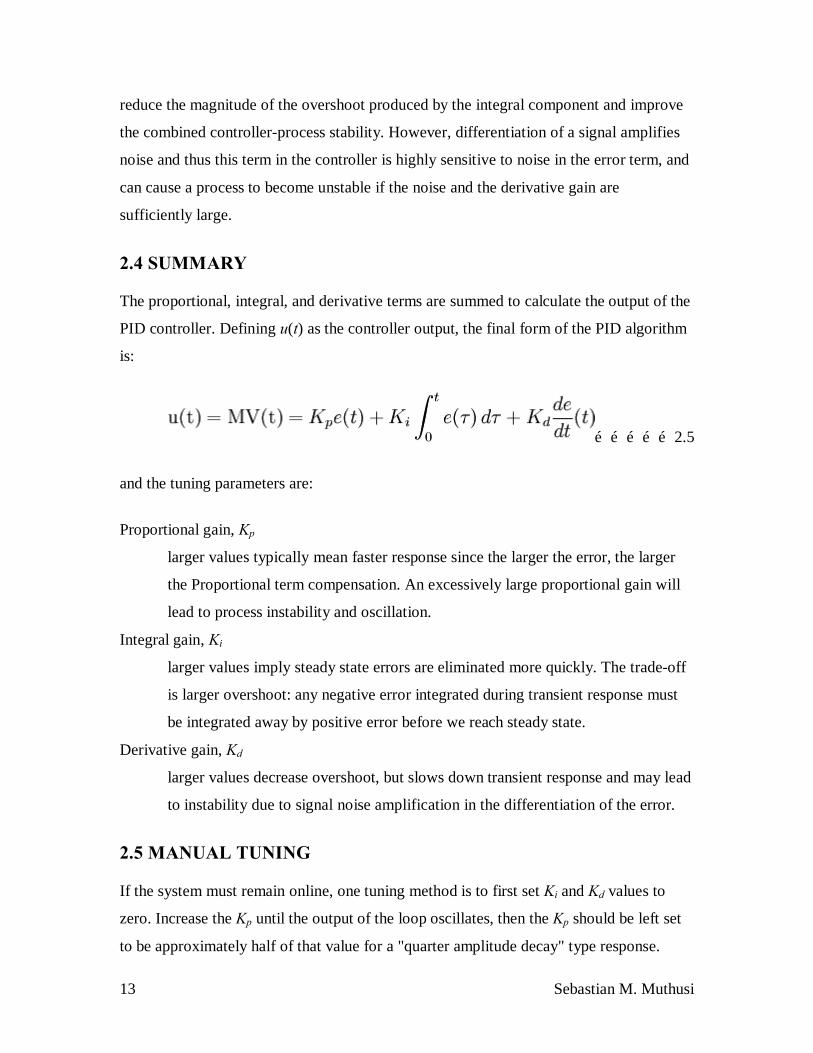
2.4 SUMMARY

The proportional, integral, and derivative terms are summed to calculate the output of the

PID controller. Defining u(t) as the controller output, the final form of the PID algorithm

is:

……………2.5

and the tuning parameters are:

Proportional gain, Kp

larger values typically mean faster response since the larger the error, the larger

the Proportional term compensation. An excessively large proportional gain will

lead to process instability and oscillation.

Integral gain, Ki

larger values imply steady state errors are eliminated more quickly. The trade-off

is larger overshoot: any negative error integrated during transient response must

be integrated away by positive error before we reach steady state.

Derivative gain, Kd

larger values decrease overshoot, but slows down transient response and may lead

to instability due to signal noise amplification in the differentiation of the error.

2.5 MANUAL TUNING

If the system must remain online, one tuning method is to first set Ki and Kd values to

zero. Increase the Kp until the output of the loop oscillates, then the Kp should be left set

to be approximately half of that value for a "quarter amplitude decay" type response.


Then increase Ki until any offset is correct in sufficient time for the process. However,

too much Ki will cause instability. Finally, increase Kd, if required, until the loop is

acceptably quick to reach its reference after a load disturbance. However, too much Kd

will cause excessive response and overshoot. A fast PID loop tuning usually overshoots

slightly to reach the set point more quickly; however, some systems cannot accept

overshoot, in which case an "over-damped" closed-loop system is required, which will

require a Kp setting significantly less than half that of the Kp setting causing oscillation

Effects of increasing parameters

Parameter Rise time Overshoot Settling

time

Error at

equilibrium

Kp Decrease Increase Small

change Decrease

Ki Decrease Increase Increase Eliminate

Kd Indefinite (small decrease or

increase) Decrease Decrease None

Table 2.1


2.6 ZIEGLER–NICHOLS METHOD

Another tuning method is formally known as the Ziegler–Nichols method, introduced by

John G. Ziegler and Nathaniel B. Nichols. As in the method above, the Ki and Kd gains

are first set to zero. The P gain is increased until it reaches the critical gain, Kc, at which

the output of the loop starts to oscillate. Kc and the oscillation period Pc are used to set

the gains as shown:

Ziegler–Nichols method

Control Type Kp Ki Kd

P 0.50Kc - -

PI 0.45Kc 1.2Kp / Pc -

PID 0.60Kc 2Kp / Pc KpPc / 8

Table 2.2

2.7 MODIFICATIONS TO THE PID ALGORITHM

The basic PID algorithm presents some challenges in control applications that have been

addressed by minor modifications to the PID form.


One common problem resulting from the ideal PID implementations is integral windup.

This problem can be addressed by:

• Initializing the controller integral to a desired value

• Increasing the set point in a suitable ramp

• Disabling the integral function until the PV has entered the controllable region

• Limiting the time period over which the integral error is calculated

• Preventing the integral term from accumulating above or below pre-determined

bounds

Many PID loops control a mechanical device (for example, a valve). Mechanical

maintenance can be a major cost and wear leads to control degradation in the form of

either stiction or a deadband in the mechanical response to an input signal. The rate of

mechanical wear is mainly a function of how often a device is activated to make a

change. Where wear is a significant concern, the PID loop may have an output deadband

to reduce the frequency of activation of the output (valve). This is accomplished by

modifying the controller to hold its output steady if the change would be small (within

the defined deadband range). The calculated output must leave the deadband before the

actual output will change.

The proportional and derivative terms can produce excessive movement in the output

when a system is subjected to an instantaneous step increase in the error, such as a large

set point change. In the case of the derivative term, this is due to taking the derivative of

the error, which is very large in the case of an instantaneous step change. As a result,

some PID algorithms incorporate the following modifications:

Derivative of output

In this case the PID controller measures the derivative of the output quantity,

rather than the derivative of the error. The output is always continuous (i.e., never

has a step change). For this to be effective, the derivative of the output must have

the same sign as the derivative of the error.

Set point ramping


In this modification, the set point is gradually moved from its old value to a newly

specified value using a linear or first order differential ramp function. This avoids

the discontinuity present in a simple step change.

Set point weighting

Set point weighting uses different multipliers for the error depending on which

element of the controller it is used in. The error in the integral term must be the

true control error to avoid steady-state control errors. This affects the controller's

set point response. These parameters do not affect the response to load

disturbances and measurement noise.

2.8 LIMITATIONS OF PID CONTROL

While PID controllers are applicable to many control problems, they can perform poorly

in some applications.

PID controllers, when used alone, can give poor performance when the PID loop gains

must be reduced so that the control system does not overshoot, oscillate or hunt about the

control set point value. The control system performance can be improved by combining

the feedback (or closed-loop) control of a PID controller with feed-forward (or open-

loop) control. Knowledge about the system (such as the desired acceleration and inertia)

can be fed forward and combined with the PID output to improve the overall system

performance. The feed-forward value alone can often provide the major portion of the

controller output. The PID controller can then be used primarily to respond to whatever

difference or error remains between the set point (SP) and the actual value of the process

variable (PV). Since the feed-forward output is not affected by the process feedback, it

can never cause the control system to oscillate, thus improving the system response and

stability.

For example, in most motion control systems, in order to accelerate a mechanical load

under control, more force or torque is required from the prime mover, motor, or actuator.

If a velocity loop PID controller is being used to control the speed of the load and

command the force or torque being applied by the prime mover, then it is beneficial to

take the instantaneous acceleration desired for the load, scale that value appropriately and


add it to the output of the PID velocity loop controller. This means that whenever the

load is being accelerated or decelerated, a proportional amount of force is commanded

from the prime mover regardless of the feedback value. The PID loop in this situation

uses the feedback information to effect any increase or decrease of the combined output

in order to reduce the remaining difference between the process set point and the

feedback value. Working together, the combined open-loop feed-forward controller and

closed-loop PID controller can provide a more responsive, stable and reliable control

system.

Another problem faced with PID controllers is that they are linear. Thus, performance of

PID controllers in non-linear systems (such as HVAC systems) is variable. Often PID

controllers are enhanced through methods such as PID gain scheduling or fuzzy logic.

Further practical application issues can arise from instrumentation connected to the

controller. A high enough sampling rate, measurement precision, and measurement

accuracy are required to achieve adequate control performance.

A problem with the Derivative term is that small amounts of measurement or process

noise can cause large amounts of change in the output. It is often helpful to filter the

measurements with a low-pass filter in order to remove higher-frequency noise

components. However, low-pass filtering and derivative control can cancel each other

out, so reducing noise by instrumentation means is a much better choice. Alternatively,

the differential band can be turned off in many systems with little loss of control. This is

equivalent to using the PID controller as a PI controller.

]

2.9 PHYSICAL IMPLEMENTATION OF PID CONTROL

In the early history of automatic process control the PID controller was implemented as a

mechanical device. These mechanical controllers used a lever, spring and a mass and

were often energized by compressed air. These pneumatic controllers were once the

industry standard.


Electronic analog controllers can be made from a solid-state or tube amplifier, a capacitor

and a resistance. Electronic analog PID control loops were often found within more

complex electronic systems, for example, the head positioning of a disk drive, the power

conditioning of a power supply, or even the movement-detection circuit of a modern

seismometer. Nowadays, electronic controllers have largely been replaced by digital

controllers implemented with microcontrollers or FPGAs.

Most modern PID controllers in industry are implemented in programmable logic

controllers (PLCs) or as a panel-mounted digital controller. Software implementations

have the advantages that they are relatively cheap and are flexible with respect to the

implementation of the PID algorithm.

2.9.1 Ideal versus standard PID form

The form of the PID controller most often encountered in industry, and the one most

relevant to tuning algorithms is the standard form. In this form the Kp gain is applied to

the Iout, and Dout terms, yielding:

…………………2.6

where

Ti is the integral time

Td is the derivative time

In the ideal parallel form, shown in the controller theory section

…………………2.7

the gain parameters are related to the parameters of the standard form through

and . This parallel form, where the parameters are treated as


simple gains, is the most general and flexible form. However, it is also the form where

the parameters have the least physical interpretation and is generally reserved for

theoretical treatment of the PID controller. The standard form, despite being slightly

more complex mathematically, is more common in industry.

2.9.2 Laplace form of the PID controller

Sometimes it is useful to write the PID regulator in Laplace transform form:

……………………2.8

Having the PID controller written in Laplace form and having the transfer function of the

controlled system, makes it easy to determine the closed-loop transfer function of the

system.

2.10 P I CONTROLLER

In control engineering, a PI Controller (proportional-integral controller) is a feedback

controller which drives the plant to be controlled with a weighted sum of the error

(difference between the output and desired set-point) and the integral of that value. It is a

special case of the common PID controller in which the derivative (D) of the error is not

used.

The controller output is given by

………………………………………………….2.9

where Δ is the set-point error.

2.10.1 Advantages of a Proportional Plus Integral Controller

The integral term in a PI controller causes the steady-state error to be zero for a step

input.


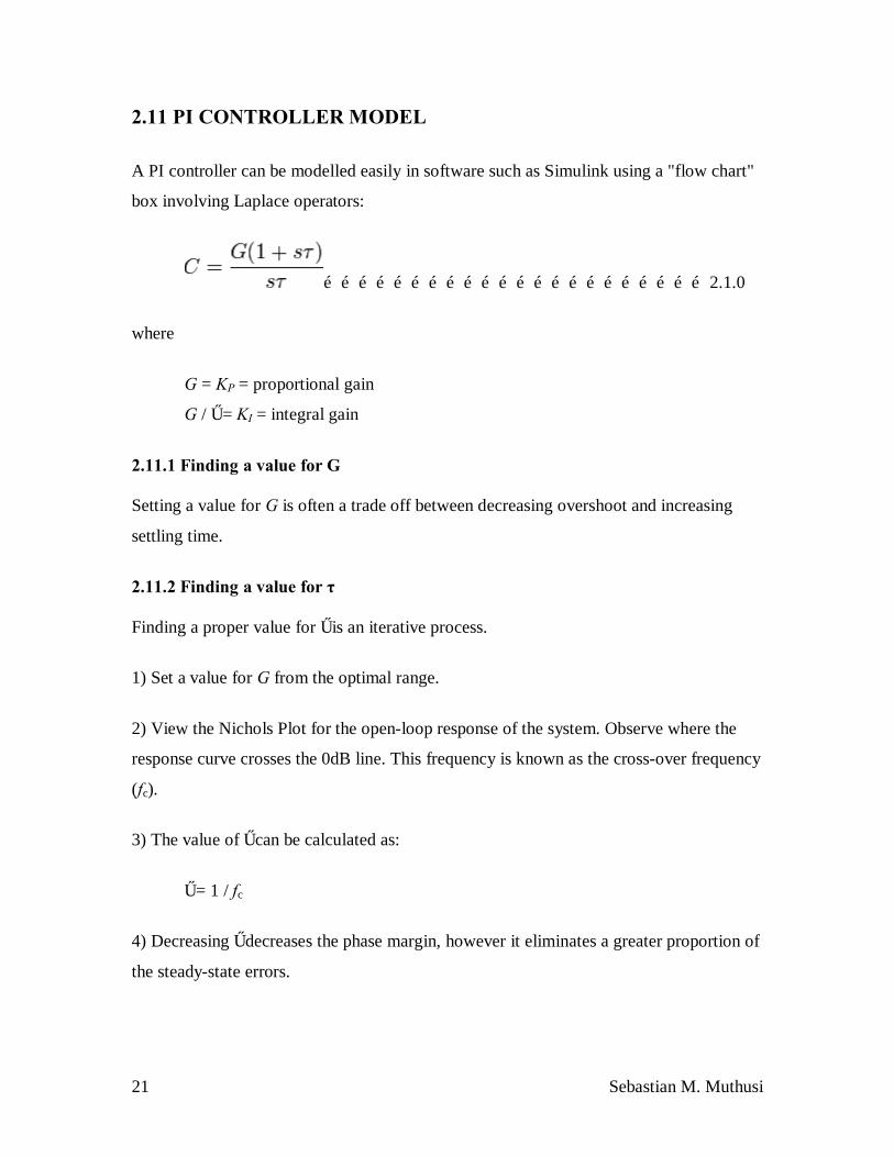
2.11 PI CONTROLLER MODEL

A PI controller can be modelled easily in software such as Simulink using a "flow chart"

box involving Laplace operators:

…………………………………………………………2.1.0

where

G = KP = proportional gain

G / τ = KI = integral gain

2.11.1 Finding a value for G

Setting a value for G is often a trade off between decreasing overshoot and increasing

settling time.

2.11.2 Finding a value for τ

Finding a proper value for τ is an iterative process.

1) Set a value for G from the optimal range.

2) View the Nichols Plot for the open-loop response of the system. Observe where the

response curve crosses the 0dB line. This frequency is known as the cross-over frequency

(fc).

3) The value of τ can be calculated as:

τ = 1 / fc

4) Decreasing τ decreases the phase margin, however it eliminates a greater proportion of

the steady-state errors.


2.12 DISADVANTAGES OF A PROPORTIONAL PLUS INTEGRAL CONTROLLER

The problem with using a PI controller is that it introduces a phase-lag. This means that

on a Nichols Plot, the stability margin (the phase margin) decreases. So careful design

considerations with respect to the gain must be considered.

2.13 TYPES OF MOTOR CONTROLLERS

Motor controllers can be manually, remotely or automatically operated. They may

include only the means for starting and stopping the motor or they may include other

functions.

An electric motor controller can be classified by the type of motor it is to drive such as

permanent magnet, servo, series, separately excited, and alternating current.

A motor controller is connected to a power source such as a battery pack or power

supply, and control circuitry in the form of analog or digital input signals.

2.13.1 Motor starters

Main article: Direct on line starter

Main article: Motor soft starter

A small motor can be started by simply plugging it into an electrical receptacle or by

using a switch or circuit breaker. A larger motor requires a specialized switching unit

called a motor starter or motor contactor. When energized, a direct on line (DOL) starter

immediately connects the motor terminals directly to the power supply. A motor soft

starter connects the motor to the power supply through a voltage reduction device and

increases the applied voltage gradually or in steps.


2.13.2 Adjustable-speed drives

Main article: Adjustable-speed drive.

An adjustable-speed drive (ASD) or variable-speed drive (VSD) is an interconnected

combination of equipment that provides a means of driving and adjusting the operating

speed of a mechanical load. An electrical adjustable-speed drive consists of an electric

motor and a speed controller or power converter plus auxiliary devices and equipment. In

common usage, the term “drive” is often applied to just the controller.[4][5]

2.14 CALCULATING STEADY-STATE ERRORS

. Steady-state error can be calculated from the open or closed-loop transfer function for

unity feedback systems. For example, let's say that we have the following system:

Fig 2.5

which is equivalent to the following system:

Fig2.6

We can calculate the steady state error for this system from either the open or closed-loop

transfer function using the final value theorem (remember that this theorem can only be

applied if the denominator has no poles in the right-half plane):

………………………………………………..2.1.1

…………………………………………2.1.2

http://en.wikipedia.org/wiki/Motor_controller

http://en.wikipedia.org/wiki/Motor_controller


Now, let's plug in the Laplace transforms for different inputs and find equations to

calculate steady-state errors from open-loop transfer functions given different inputs:

• Step Input (R(s) = 1/s):

………………2.1.3

• Ramp Input (R(s) = 1/s^2):

……………….2.1.4

• Parabolic Input (R(s) = 1/s^3):

………2.1.5

When we design a controller, we usually want to compensate for disturbances to a

system. Let's say that we have the following system with a disturbance:

Fig 2.7

we can find the steady-state error for a step disturbance input with the following

equation:

………………………………………2.1.6


Lastly, we can calculate steady-state error for non-unity feedback systems:

Fig 2.8

By manipulating the blocks, we can model the system as follows:

Fig 2.9

Now, simply apply the equations we talked about above.

2.15 SYSTEM TYPE AND STEADY-STATE ERROR

If you refer back to the equations for calculating steady-state errors for unity feedback

systems, you will find that we have defined certain constants ( known as the static error

constants). These constants are the position constant (Kp), the velocity constant (Kv), and

the acceleration constant (Ka). Knowing the value of these constants as well as the

system type, we can predict if our system is going to have a finite steady-state error.

First, let's talk about system type. The system type is defined as the number of pure

integrators in a system. That is, the system type is equal to the value of n when the system

is represented as in the following figure:


Fig 2.1.0

Therefore, a system can be type 0, type 1, etc. Now, let's see how steady state error

relates to system types:

Type 0 systems Step Input Ramp Input Parabolic Input

Steady State Error Formula 1/(1+Kp) 1/Kv 1/Ka

Static Error Constant Kp = constant Kv = 0 Ka = 0

Error 1/(1+Kp) infinity infinity

Table 2.3



Static Error Constant Kp = infinity Kv = constant Ka = 0

Error 0 1/Kv infinity

Table 2.




Static Error Constant Kp = infinity Kv = infinity Ka = constant

Error 0 0 1/Ka

Fig 2.5


CHAPTER THREE

3.0 OBJECTIVES To use a proportional action that will reduce steady state error and increase the

step response overshoot as the proportional band Kp is reduced.

Adjustment of compensator parameters equivalent to the tuning of general

purpose process controllers.

Use of regenerative braking which requires that the directional sense of the motor

torque be controlled in a manner causing a return of energy to the AC supply

when this is required

A negative armature current feedback path in cooperating a dead space element

may be provided to affect automatic armature current limiting so as to protect the

motor against possible overload.

Integral action that will eliminate steady state error arising from most causes and

as the integral action time T1 is reduced ,increase the step response overshoot .

Negative armature current feed back that can be used to change the converter into

to a current source as opposed to voltage source.

A derivative action that will reduce the step response overshoot as the derivative

action Td is increased.

The primary (negative) speed feed back to be obligatory and normally derived

from a DC tachogenerator.

3.1 ANALYSIS OF THE GENERAL CLOSED LOOP WARD

LEONARD SPEED CONTROL SYSTEM The schematic diagram of a closed Ward Leonard Speed Control System is shown in Fig.

2. Although the title of this project is Ward Leonard speed control system and an open

loop Ward Leonard System do exist, the project is strictly concerned with the closed loop

Ward Leonard system as has already been quietly implied in the introduction.

As shown in Fig. 2 the system can be divided into two sections for purposes of analysts.


3.2 CONSIDER SECTION 1 The following equations can be written down

ffff eiR

dtdi

Lf =+ …………………………………………………………1

ffa ike =

Where

Lf = Field winding inductance

if = field current

Rf = field winding resistance

ef = voltage across the field winding.

EA = voltage output of the W.L. generator.

Combining equations 1 and 2, and through Laplace transformation, we have.

)1()()(

STk

SeSe

g

g

f

a

+= ……………………………………………………………3

Where Kg = Rfkf

= W.L. Generator gain constant.

RfLfTg = = W.L. generator excitation time constant.

3.3 NOW CONSIDER SECTION II The following equation can be written down.

eb=ea -

+

dtLadiaiR aa ………………………………………………….4

eb = kbW0(t)……………………………………………………………..5

T = KTia = FW0(t)+Jddt

tW )(0 ……………………………………………..6

Where in the above equations,

eb = work Motor Back emf

ea = W.L. Generator output voltage


Ra = Armature resistance of Work motor

La = Armature inductance of Work motor

ia = Armature current

Kb = Back constant

KT = Torque constant

F = Friction

J = Inertia of Work motor

W0(t) = output speed

By combining equations (4), (5), (6) and taking L aplace transforms, we arrive at

++

++

=

T

ba

T

aa

T

aa

KKFR

KFLJRS

KJLsse

sW)(

1)()(

2

0 ………………………….7

3.4 ASSUMPTION For all practical purpose we can neglect La. Firstly because it is small in comparison with

KT even when the motor is on load. Secondly because the frequency of operation in dc

control systems is of the order of a few radians per sec

Hence

( ) )1()()(0

STK

KKFRJSRK

sesW

m

m

Tbaa

T

a +=

++= ………………………………….8

Km = bTa

T

KKFRK+

= Work motor gain constant

Tm = bTa

a

KKFrJR

+= Work motor mechanical time constant

3.5 CONSIDER THE FEED-BACK LOOP The following is true:

e0 = KtW0(t)…………………………………………………………………..9

e0 = output voltage from tachogenerator


Kt = tachogenerator constant

e = ( )0l−ine ……………………………………………………………......10

e = error voltage

ein = reference voltage

e0 = output voltage from tachogenerator

3.6 THE AMPLIFIERS Assuming that the time constants of the amplifiers are small in comparison with the time

constants of the motor and generator, we can write

ef = KAef…………………………………………………………………………………………………………11

Where KA = gain of the amplifiers.

3.7 THE TRANSFER FUNCTION BLOCK DIAGRAM We are now in a position to make a transfer function block diagram. By combining

equations 3, 8, 9 and 11 we obtain the transfer function Block diagram shown in fig 2.

3.8 THE CLOSED LOOP TRANSFER FUNCTION AND THE

CHARACTERISTICS EQUATION From Fig. 3 the open loop transfer-function

G(s) = )1)(1( STST

KKK

mg

mgA

++……………………………………………12

It can be shown that the closed loop transfer function is given by

)()(1

)()()(0

SHsGsG

sesW

in += ………………………………………………13

Where H (S) is the feedback loop transfer function.

In our case

H(s) = kt

Hence


)1)(1(1

)1)(1()()(0

STSTKtKKK

STSTKKK

sesW

mg

mgA

mg

mgA

a

++

+++

=

= tgmAgmgm

mgA

KKKKSTTSTTKKK

++++ 1)(2 ………………………….14

Thus the characteristic equation is given by:-

01)(2 =

++

++

gm

tgkA

gm

gm

TTkKKK

TTSTT

S ………………………………15

3.9 EXAMINATION FOR STABILITY BY THE ROUTH HURWITZ

CRITERION From equation 15, we can assemble the Routh Hurwitz Array:

S2 1 gm

tmgA

TTKKKK+1

S1 gm

gm

TTTT +

0

S0 ( )2

))(1(

gm

gmtmgA

TT

TTKKKK ++

For stability

( )2

))(1(

gm

gmtmgA

TT

TTKKKK ++> 0……………………………………………..16

1+ KAKgKmKt >0

KAKgKmKt > -1

tmg

A KKKK 1−

> …………………………………………………………….17

This means that absolute stability is guaranteed for all values of the amplifier gain KA.

3.10 THE SYSTEM LOOP GAIN


By definitaion Loop gain is

)()(0

sHsGK LimS→

= ……………………………………………………..18

Where

G(s) = Open loop transfer function

H(s) = Feed back loop transfer function

In case of the Ward Leonard speed control system this becomes

K = KAKgKmKt……………………………………………………………………………………………19

3.11 THE POSITIONAL CONSTANT KP By definition

)()(0

sHsGK LimS

P→

=

= KAKgKmKt…………………………………………………………………………………………20

= K (for the system under consideration)

3.11.1 Velocity Constant KV

By definition

KV = )()(0

sHsSGLimS→

……………………………………………………21

= )1)(1(

)(

0 STSTKKKKS

mg

tmgA

SLim ++→

= 0

3.12 ACCELERATION CONSTANT OF THE SYSTEM

Kac = )()(2

0sHsGSLim

S→

= )1)(1(

2

0 STSTKKKK

Smg

tmgA

SLim ++→

………………………………………..22


= 0

3.13 STEADY STATE ERROR

Ss(t) = )()(1

)(0 sHsG

sSRLimS +→

……………………………………………….....23

Where R(s) is the input constant

Thus for a unit step input,

ss (t) = ( ))()(10 sHsGSSLim

S +→

= tmgA KKKK+1

1 ………………………………………………………….24

= PK+1

1

While for a unit ramp

ess(t) = ( ))()(120 sHsGS

SLimS +→

…………………………………………25

= ∞


3.14 EXAMINATION FOR THE NATURAL FREQUENCY WN

OF THE SYSTEM

From Equation

( )gm

tmgA

gm

gm

gm

mgA

in

TTKKKK

TTsTT

S

TTKKK

sesW

++

++

=1)()(

)(

2

0

= 220

2 nn wSwSK

++ ε………………………………………………26

where ε – damping factor

wn – natural frequency of the system

( )gm

gmA

TTKKK

K =0

From the above we have

gm

tmgAn TT

KKKKW

+=

12

Wn = ( ) 2

1

1

+

gm

tmgA

TTKKKK

………………………………………27

3.15 DETERMINATION OF THE TIME DOMAIN RESPONSE OF

THE SYSTEM AND THE RISE TIME EQUATION From equation 26

))(()( 0

0 γα ++=

sSK

sW ……………………………………………..28

Where


K0 = gm

mgA

TTKKK

-s1 = jwjww nn +=−+ δε 21 ……………………………………..29

-s2 = jwjww nn −=−− δε 21 ……………………………………...30

Hence

W= 21 ε−nW ………………………………………………………31

Let us assume a unit step input subjected into the system

))(()()( 00

γα ++=

sSK

sesW

in

s

sein1)( =

Hence

))((

)( 00 γα ++

=ssS

KsW …………………………………………………..32

))(())((

)( 000 αγαα

αγαγγαγ +−

++−

+=ss

KKsW

( )

−

+−

+= −−+− tjwtjw eea

KtW )()(0

0 (1)( δδ

αγα

γγ

αγ

+−= − wtSin

wwtCose

KtW t δ

αδ1)( 0

0 …………………………………33

To determine where W0(t) is a maximum we differentiate equation 33 with respect to

time and equate the derivative to zero.

0)sin()(0 =

+−−+ −− CoswtwtweSinwt

wSoswte

K dtdt δαγ

012

2

=

+ Sinwt

wδ


Since in general 012

2

≠

+

wδ

Sinwtm = 0

i.e. wtm = π

Using the conventional definition of rise time in control tm i.e. the time it takes a system

to get to the 1st overshoot we have

Wtr = π

tr = 21 ε

ππ−

=nWW

……………………………………………….34

3.16 EFFECTS OF LOAD TORQUE ON THE SYSTEM The effect of load torque on the Work-motor is to reduce the speed of the said motor.

This reduction should be transmitted to the Ward Leonard generator and consequently to

the driving prime mover. Unless the prime-mover is such a machine as a synchronous

motor the net effect will be a reduction in the speed of the prime-mover. In the Ward-

Leonard system this is a high undesirable state. In fact the foregoing analysis has

assumed a constant speed implicitly. A variable speed in the prime mover would mean a

varying Kg. This is obviously a non linearity in the system. Nevertheless, induction

motors are used as prime movers in the system almost invariably. This is achieved as we

shall show below by providing high gain in the amplifiers and the use of Proportional

Integral Controllers.

3.16.1 Consider Fig. 3

The load torque could be considered as a disturbance into the system. Considering now

that the dotted line s full and Z0(s) the disturbance transfer function forms part of the

system we see that:

The open loop transfer function as seen at the point from which the disturbance enters

into the system is given by


)()(

00 sZT

sW

OLL

=

……………………………………………………35

The closed loop transfer function as seen from the same point is given by

)1)(1()(

1

)()(0

00

STsTsZKKKK

sZT

sW

gm

tgmAFBL

+++

=

……………………………………36


3.17 INDEX OF CONTROL The index of control is defined as

)1)(1()(

1

1)(

)(

00

0

STSTsZKKKK

TsW

TsW

gm

tgmA

OLL

FBL

+++

=

……………………………………37

The index of control represents a measure of disturbance reduction by the use of

feedback.

It is self evident that by increasing KA, the gain of the amplifiers, we increase

considerably the disturbance reduction. It is also evident that no matter how large KA is,

the effect of disturbances into will never be eliminated. To eliminate the residual effects

of disturbances completely we use integration in the system. Hence the importance of

Proportional Integral controllers.

3.18 MEASUREMENT AND DESIGN OF CONTROL SYSTEM With the foregoing analysis of the closed loop ward Leonard speed control

system fairly complete,we are know in a position to decide on what measurement to

make on the project system to help us design a speed control unit.

The constants relevant to design are Kg,Km,Kt,Tm,Tg and Rf.field winding

resistance of the ward Leonard generator.By determining Kg,Km,Kt and by choice of

suitable K-loop gain we shall be in a position to choose a suitable KA such that it is

consonant with the demand for good disturbance reduction. The knowledge of Tg and Tm

will help us decide of suitable location of a PI controller in the frequency domain

whereas knowing RF we are able to decide on the supply voltage necessary to achieve a

required current in the ward Leonard generator fields.

3.18.1 Determination of Kg

This constant constant was determined by taking some voltage measurement

across the field winding of the generator and at the same time taking the measurement of

the corresponding generated voltage from the W.L Generator.


These measurements of the field winding voltage were plotted against the generator

output voltage. The slope gives Kg. see graph NO 1:

3.18.2 Determination of Km

For various voltages inputs to the work motor the corresponding speeds were

taken. A plot of input voltage versus output speed gives Km.See graph NO 2

3.18.3 Determination of Kt

For various speed of the work motor the output voltage at the tachogenerator

terminals was measured and the speed was plotted against the output voltage. The slope

gives Kt. See graph NO.3;

3.18.4 Determination of the field resistance

The field resistance was determined firstly by the use of an avometer. This gave a value

of about 150 ohms per half field. This was not realistic. Consequently determination of

the same Rf by the dc drop test gave a half field resistance of about 30 ohms .the plot of

the voltage versus current is shown in graph NO.4:

3.18.5 Determination of Tg and Tm

Theoretically this values where to be obtained by the use of a cathode ray oscilloscope,

their trace photographed and a tangent drawn from the origin and where it intersects the

horizontal line indicating the magnitude of the unit step. At the ward Leonard speed

control in the Kenya airport authority this values were obtained direct from the machine.


-100

-50

0

50

100

150

0 5 10 15 20 25 30 35 40Ge

ne

rato

r V

olt

ag

e

Field Voltage

DETERMINATION OF KG

y

Graph no. 1


Series1Linear (Series1)

Graph no. 2


DERTERMINATION OF KT

020406080

100120140160

0 500 1000 1500

SPEED IN RPM

VOLT

AGE

IN V

OLTS

YLinear (Y)

Graph no. 3


Graph no 4

DETERMINATIION OF RF

0

5

10

15

20

25

30

35

40

45

0 0.5 1 1.5

CURRENT IN AMPS

VO

LT

AG

E IN

VO

LT

S

YLinear (Y)


CHAPTER FOUR

4.0 SUMMARY OF RESULTS Kg = 6.67

Km = 1.35 radians/volt/sec. Tm = 70msecs

Kt = 1.05volts/radian/sec Tg = 700msecs

Rf = 29.5 ohms

4.1 DESIGN OF THE PROJECT SYSTEM In this section we want to determine the minimum value of KA – the amplifier gain which

makes the system have a fairly good response when the system is on non-load. Obviously

we shall have to provide a much large KA than this in order to absorb damping associated

with loading in the design of amplifiers. We shall also confirm the result on stability

reached earlier on in equation 17 by using the Routh Harwitz criterion. This time we shall

use the Root locus for confirmation.

4.2 CHOICE OF THE DAMPING FACTOR The damping factor of 0.425 was chosen because it gives an overshoot of approximately

22.88% and a good rise time of about 0.347 secs. In fact past experience has shown that

this damping factor is within the optimum range of sampling factors for second order

system.

4.3 CHOICE OF LOOP GAIN AND CONSEQUENTLY THE

SETTLING ERROR From equation 26 we have

21

1

122

+

+==

gm

gm

gm

ngm

gm

TTk

xTTTT

WTTTT

ε …………………………………………..37

Putting = 0.425

Tm = 70 msec


Tg = 700 msec

In equation 37 we obtain

K = 15.85 ≅ 16

From Equation 24

Setting error = K+1

1 =0.595 <6%

4.4 CHOICE OF Kt AND HENCE THE VOLTAGE DIVIDING

RATIO OF THE TACHOGENERATOR VOLTAGE.

The value we obtained for Kt was 1.05 volts/radian/se/

At 1500 rpm the output from the tachogenerator is given by

Output volts = 60

2150005.1 πxx

= 165V

It is quite evident that it is unpalatable to work with such voltages closely. It would also

mean that one would have to provide a reference voltage of +165V to be able to operate

at 1500rpm. It was therefore decided to reduce the output voltage from the tachogenerator

to 161 of it value so that a reference voltage of approximately +10V could be used.

Hence

Kt’ = 0657.01605.12

16==

Kt

Output from tachogenerator at 1500rpm

= volts3.1016165

=

This reduction in the output voltage from tachogenerator is to be effect by means of a

voltage divider.


4.5 CHOICE OF AMPLIFIER GAIN KA Form equation 19

K=KAKgKmKt = 16

Since we cannot alter Km, Kg if we want the loop sign to remain at 16 after we have

altered the tachogenerator constant we must alter KA.

The altered KA we designate as KA.

So we have

16 = KAKgKmKt = KA’KgKmKt’

KA’ = 65.067.635.1

16xx

= 27

4.6 THE TRANSFER FUNCTION OF THE PROJECT SYSTEM From equation 14

tmgAgmgm

mgA

KKKKSTTSTTKKK

sinsW

1)()()(

20

+++=

= ''1)(2

tmgAgmgm

mgA

KKKKSTTSTTKKK

++++………………………….38

Feeding in the values of KA’, Km, Kg, Kt’ Kg and Tm in the above equation and re-

arranging we arrive at

3477.15

975)()(

2 ++=

SSsesW

in

o ………………………………………………..39

= )875.1685.7)(875.1685.7(

975jsjS −+++

……………………….40


4.7 CONFIRMATION OF ABSOLUTE STABILITY BY ROOT

LOCUS From equation 38 the characteristics equation can be written as

S2+15.7S+20.4(1+K) = 0

S = 4

)1(6.812982

7.15 K+−±

− ………………………………………….41

Quite clearly for K<-1 we have a pole in the right half plane confirming instability as

predicted by Routh Harwitz in equation 17. The complete Root Locus is shown in Graph

No. 5A.

4.8 TIME DOMAIN SOLUTION OF SYSTEM RESPONSE TO A

UNIT STEP FUNCTION From Equation 33

+−= − wt

wwteKfW t

O sin(cos1)( 0 δαγ

δ

Rearranging this equation, we arrive at

+

+−= − )sin(1)(

220 φδ

αγδ wt

wweKtW t

O ………………………………………….42

Where δ

φ w1tan−= ………………………………………………………….43

a) 975==mg

mgAO TT

KKKK ……………………………………………….44

b) ( )

gm

tmmgA

TTKKKKK ''1+

= ………………………………………………45

c) ( )

sec/65.18'1 2

1

radTT

KKKKKW

gm

tmmgAn =

+= …………………………46

d) 21 ε−= nww

= 18.65x0.82 = 16.8rad/sec…………………………………………..47


e) nwεδ =

= 0.425x18.65=7.9……………………………………………………48

Putting the above values in equation 42 and simplifying, we obtain

[ ])18.08.16(2sin11.118.2)( 85.7 +−= − tetW tO π ……………………………..49

A plot of 8.2

)(tWO is shown in Graph No.5 C

num = [144.07];

>> den = [49000 770 10.36];

>> G = tf(num,den)

Transfer function:

144.1

-------------------------

49000 s^2 + 770 s + 10.36

>> rlocus(G)


-0.015 -0.01 -0.005 0 0.005 0.01-0.04

-0.03

-0.02

-0.01

0

0.01

0.02

0.03

0.04Root Locus

Real Axis

Imag

inary

Axis

Graph no; 5A


>>num = [144.07];

>> den = [49000 770 1];

>> H = tf(num,den)

Transfer function:

144.1

---------------------

49000 s^2 + 770 s + 1

>> bode(H) GRAPH NO 5B

-50

-40

-30

-20

-10

0

10

20

30

40

50

Magn

itude

(dB)

Bode Diagram

Frequency (rad/sec)10

-410

-310

-210

-110

0-180

-135

-90

-45

0

System: HPhase Margin (deg): 16.5Delay Margin (sec): 5.42

At frequency (rad/sec): 0.0533Closed Loop Stable? Yes

Phas

e (de

g)


Step Response

Time (sec)

Ampl

itude

0 100 200 300 400 500 600 700 8000

2

4

6

8

10

12

14

16

System: GFinal Value: 13.9

System: GSettling Time (sec): 399

System: GPeak amplitude: 15.8Overshoot (%): 13.3At time (sec): 260

System: GRise Time (sec): 118

nyquist(H) GRAPH NO 5C


Nyquist Diagram

Real Axis

Imag

inary

Axis

-20 0 20 40 60 80 100 120 140 160-80

-60

-40

-20

0

20

40

60

800 dB

System: HPeak gain (dB): 43.2

Frequency (rad/sec): 2.86e-012

System: HPhase Margin (deg): 16.5Delay Margin (sec): 5.42At frequency (rad/sec): 0.0533Closed Loop Stable? Yes

GRAPH NO; 5D


>>nichols(G)

G

Nichols Chart

Open-Loop Phase (deg)

Ope

n-Lo

op G

ain

(dB)

-360 -315 -270 -225 -180 -135 -90 -45 0-40

-30

-20

-10

0

10

20

30

40

6 dB

3 dB

1 dB

0.5 dB

0.25 dB

0 dB

-1 dB

-3 dB

-6 dB

-12 dB

-20 dB

-40 dB

System: GPeak gain (dB): 23.7

Frequency (rad/sec): 0.00853

System: GPhase Margin (deg): 17.1Delay Margin (sec): 5.42At frequency (rad/sec): 0.055Closed Loop Stable? Yes

GRAPH NO 5E


CHAPTER FIVE

5.0 CONCLUSION For this project design there was no any instant did the system show signs of instability

even with the PI controlled added on into the system. This means that although the Ward

Leonard system is certainly of orders higher than two. Approximation as shown in the

modeling equations in chapter three with a second order system is extremely good.

By use of the PI controller it improved the damping and reduced the maximum

overshoot.

This also increased the risetime as shown in the unit step, that is graph No 5B… that is

the Bode Plot, there was improved gain margin and phase margin and hence giving

Avery stable system. Due to the problem in working with the Polar coordinates at the

nyquist of G(jw) that the curve no longer retains its original shape when a simple

modification such as the change of loop gain is made to the system; the nicholes chart

was plotted in graph no 5E… and this gave a peak gain (DB) 23.7w and phase margin

(deg) 17.1 and delay margin (sec) 5.42 at frequency 0.055 and thus the close loop system

was very stable.

For design work involving resonant Peak Mr and Bandwidth (Bw) as specification. It was

more convenient to work with the magnitude – phase plot at G(jw) since when the loop

gain is altered the entire G(jw) curve is shifted up or down vertically without distortion.

Graphs No, 1,2,3,4 gave very good characteristics to determine the gradient and hence

the relevant constants.

The necessary and sufficient condition that all roots of the characteristics equation as

shown in chapter four lie in the left half of the s-plane is that the equations Hurwitz

determination.

There was no any sign change in the first column in the Routh’s Hurwitz tabulation and

this shows there is an absolute stability.

The gain of 1500 rpm should have been capable of reducing drop considerably even with

a load of 3kw, remembering that only a gain of 28 was required in the system on no load

to give the response shown on no graph No 5C, that is the unit step response. This leaves


us with the PI controller as the sole victim, may be there was no integration at all, the

system could be affected by disturbance and noise as in the case of an aircraft.

5.1 RECOMMENDATION In this work, voltage control was done using the energy wasting rheostat to provide a

variable voltage. This instead could be done by the use of voltage choppers which uses

chopper circuit to provide variable dc voltage from affixed dc supply. this dc supply is to

be switched on off at high frequency using electronic switching devices such as

MOSFETs,IGBTs,or GTOs to provide a pulsed DC wave form.

In position control of the motors potentiometers were used to provide position of the

feedback in closed loop systems but shaft encoders could be used to provide more precise

travel feedback by counting pulses.


REFERENCES

1. Automatic control systems

Benjamin C. Kuo

2. Control Engineering

N.M. Morris

3. Electrical control systems in industry

Charles S. Sis kind

4. Transistor manual

Generic Electric.

5. Control system design.

Savant.

6. Control Systems 4th year class notes

Dr Mbuthia.

7. Control Systems 5th year class notes,

Dr M.K Mang’oli’s

university of nairobi · 2019-11-10 · by application of the root locus,nyquist plot, bode plot...

Documents