Inchworm Monte Carlo method for open quantum systems

Zhenning Cai1, Jianfeng Lu2, Siyao Yang1

Abstract

We investigate in this work a recently proposed diagrammatic quantumMonte Carlo method— the inchwormMonte Carlo method — for open quantum systems. We establish its validity rigorously based on resumma-tion of Dyson series. Moreover, we introduce an integro-differential equation formulation for open quantumsystems, which illuminates the mathematical structure of the inchworm algorithm. This new formulationleads to an improvement of the inchworm algorithm by introducing classical deterministic time-integrationschemes. The numerical method is validated by applications to the spin-boson model.

Keywords: quantum Monte Carlo, open quantum system, diagrammatic methods, spin-boson model

1. Introduction

For realistic quantum systems, the system we are interested in is often coupled with an uninterestingenvironment to a non-negligible extent, which requires us to study the open quantum system, including theeffects such as quantum decoherence [33] and quantum dissipation [10]. The application of open quantumsystem ranges in a wide variety of quantum fields, including quantum optical systems [1], nonlinear statisticalmechanics [17], quantum computation [26], etc. Due to the existence of the quantum bath/environment, theevolution of the projected density matrix of the system is a non-Markovian process. One classical approachis to apply the Nakajima-Zwanzig projection operator technique to obtain an integro-differential masterequation [25, 36]. By taking the weak-coupling limit, a Markovian approximation can be obtained [5, 6],which is easier for numerical simulations. The Markovian approximation however breaks down for opensystems with stronger coupling. Approaches that directly simulate the non-Markovian processes include thepath-integral approaches such as the QuAPI (quasi-adiabatic propagator path integral) methods [19, 24]and the HEOM (hierarchical equations of motion) technique [32]. These methods yield accurate numericalresults, while the computational cost is huge, often unaffordable. To reduce the computational cost, onestrategy is to replace the exact summation or numerical integration in these methods by the stochasticMonte Carlo methods. In this paper, we are going to study a specific type of path-integral methods calledthe diagrammatic quantum Monte Carlo method [35] to solve the time-dependent open quantum systems.In particular, our study is largely motivated by the inchworm Monte Carlo method recently proposed in[4, 2] to reduce the variance in quantum Monte Carlo by diagrammatic resummation.

The basis of the diagrammatic quantum Monte Carlo method has been established as early as 1960s[13]. However, as other quantum Monte Carlo methods, this type of methods also suffer from the notoriousdynamical sign problem, meaning that the number of Monte Carlo samples is required to grow at leastexponentially in time in order to keep the accuracy of the simulation. To relieve the dynamical sign problem,Stockburger and Grabert introduced stochastic unraveling of influence functionals in [31], and Makri [18, 21]proposed to assume a finite memory time of the bath-correlation function and apply an iterative procedure toefficiently implement the summation. The inchworm Monte Carlo method applies the idea of diagrammatic

1Department of Mathematics, National University of Singapore, Level 4, Block S17, 10 Lower Kent Ridge Road, Singapore119076.

2Department of Mathematics, Department of Physics, Department of Chemistry, Duke University, Box 90320, Durham NC27708, USA.

resummation as in the bold diagrammatic Monte Carlo method [27] to the real-time evolution of the quantumsystems. Similar to the bold-line diagrammatic Monte Carlo method proposed in [11, 12] (see also a moremathematical presentation [16]), the inchworm Monte Carlo method tackles the dynamical sign problemby lumping a large number of diagrams into a “bold line”, which effectively reduces the number of totaldiagrams to be summed to reach desired numerical accuracy. The inchworm method makes maximum useof the previous calculations, at the expense of higher memory cost for storing all Green’s functions. Despiteits success in the application of spin-boson model [3] and the Anderson impurity model [7, 28], it requiresbetter understanding to reveal the intrinsic mathematical structure of the inchworm method, and to furtherimprove the method. In particular, it would be interesting to see how the bold lines are built on the basisof shorter bold lines, and how the bold lines propagate when the iterative procedure is precise. While theanswers to these questions are not detailed in the original derivation of the inchworm method [4, 2], in thispaper, we will show the validity of the inchworm method with mathematical rigor. The rigorous proof notonly justifies the original algorithm, but also leads us to a new formulation of the open quantum system asan integro-differential equation, based on which more accurate and efficient numerical approaches can bedeveloped.

The inchworm Monte Carlo method and the new integro-differential equation formulation will be provedto be applicable for the Ohmic spin-boson model, which is a simple open quantum system widely usedas benchmark problems [34, 15, 8]. Based on the integro-differential equation, part of the Monte Carlointegration can be replaced by classical time-integration methods to achieve higher accuracy. The resultingnew algorithm will be applied to the spin-boson model to show the numerical efficiency.

The rest of this paper is organized as follows. In Section 2, we introduce the basic formulation of theopen qunatum system and its Dyson series expansion. Section 3 gives a complete review of the inchwormMonte Carlo method and proves its validity. The integro-differential equation associate with the inchwormalgorithm is derived in Section 4. As an application, we analyze the spin-boson model in Section 5. Ournew numerical method is introduced in Section 6 and some numerical examples are given in Section 7. Asimple summary is given in Section 8 as the end of the paper.

2. Dyson series expansion for open quantum systems

Before considering open quantum system, let us first recall the time-dependent perturbation theory andthe associated Dyson series. Consider the von Neumann equation for quantum evolution (of a closed system)

idρ

dt= [H, ρ], (1)

where ρ(t) is the density matrix at time t, and H is the Schrodinger picture Hamiltonian with the form

H = H0 +W.

Here H0 is the unperturbed Hamiltonian and W is viewed as a perturbation. Following the convention, forany Hermitian operator A, we define 〈A〉 = tr(ρ(0)A). We are interested in the evolution of the expectationfor a given observable O, defined by

〈O(t)〉 = tr(Oρ(t)) = tr(Oe−itHρ(0)eitH

)= 〈eitHOe−itH〉. (2)

Using standard time dependent perturbation theory, the unitary group e−itH generated by H can be repre-sented using a Dyson series expansion [9]

e−itH =

+∞∑

n=0

∫

t>tn>···>t1>0

(−i)ne−i(t−tn)H0W e−i(tn−tn−1)H0W · · ·W e−i(t2−t1)H0W e−it1H0 dt1 · · · dtn, (3)

where the integral should be interpreted as

∫

t>tn>···>t1>0

dt1 · · · dtn =

∫ t

0

∫ tn

0

· · ·

∫ t2

0

dt1 · · · dtn−1 dtn. (4)

2

Inserting the Dyson series (3) into (2), one obtains

〈O(t)〉 =+∞∑

n=0

+∞∑

n′=0

∫

t>tn>···>t1>0

∫

t>t′n′>···>t′1>0

(−i)nin′

〈eit′1H0W ei(t

′2−t′1)H0W · · ·W ei(t

′n′−t′

n′−1)H0W ei(t−t′

n′)H0O ×

e−i(t−tn)H0W e−i(tn−tn−1)H0W · · ·W e−i(t2−t1)H0W e−it1H0〉dt′1 · · · dt′n dt1 · · · dtn.

(5)

Since the unperturbed Hamiltonian H0 is usually easier to solve, the above expansion provides the basis ofa feasible approach to find 〈O(t)〉 using Monte Carlo method.

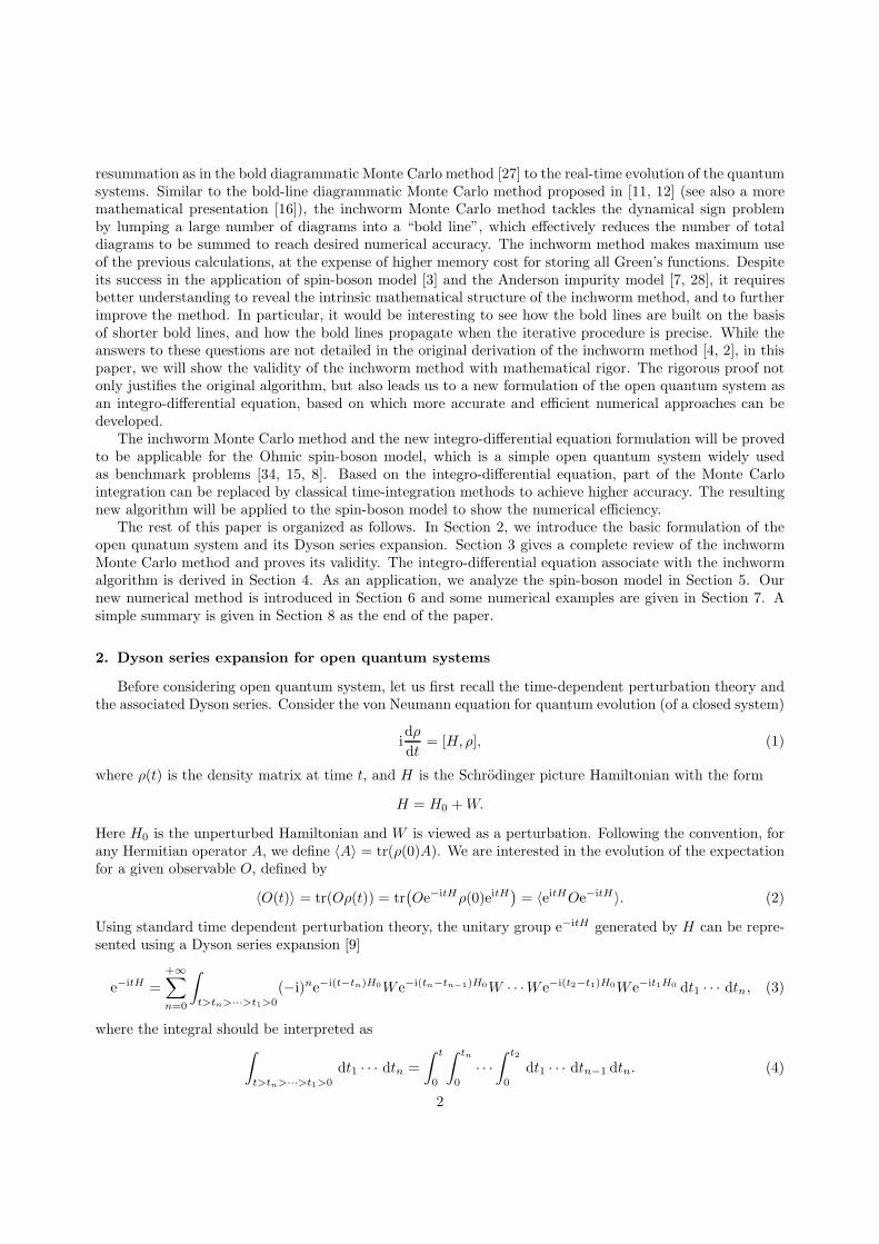
For notational simplicity, the above integral is often denoted by the Keldysh contour plotted in Figure1. The Keldysh contour should be read following the arrows in the diagram, and therefore has a forward(upper) branch and a backward (lower) branch. The symbols are interpreted as follows:

• Each line segment connecting two adjacent time points labeled by ts and tf means a propagatore−i(tf−ts)H0 . On the forward branch, tf > ts, while on the backward branch, tf < ts.

• Each black dot introduces a perturbation operator ±iW , where we take the minus sign on the forwardbranch, and the plus sign on the backward branch. At the same time, every black dot also representsan integral with respect to the label, whose range is from 0 to the adjacent label to its right.

• The cross sign at time t means the observable in the Schrodinger picture.

Note that according to the above interpretation, two Keldysh contours differ only when at least one of thevalues of n, n′ and t is different, while the positions of the labels on each branch do not matter. Thus,by taking the expectation 〈·〉 of this “contour”, we obtain the summand in (5). Therefore 〈O(t)〉 can beunderstood as the sum of the expectations of all possible Keldysh contours.

t

0t1 t2

· · · tn

0

t′

1t′

2 · · ·t′

n′

Figure 1: Keldysh contour

Such an interpretation also shows that we do not need to distinguish the forward and backward brancheswhen writing down the integrals. In fact, when the series (5) is absolutely convergent in the sense that

+∞∑

n=0

+∞∑

n′=0

∫

t>tn>···>t1>0

∫

t>t′n′>···>t′1>0

∣∣∣∣〈eit′1H0W ei(t

′2−t′1)H0W · · ·W ei(t

′n′−t′

n′−1)H0W ei(t−t′

n′)H0O ×

× e−i(t−tn)H0W e−i(tn−tn−1)H0W · · ·W e−i(t2−t1)H0W e−it1H0〉

∣∣∣∣dt′1 · · · dt

′n dt1 · · · dtn < +∞,

we can reformulate (5) as

〈O(t)〉 =+∞∑

m=0

∫

2t>sm>···>s1>0

(−1)#{s<t}im ×

×⟨G(0)(2t, sm)WG(0)(sm, sm−1)W · · ·WG(0)(s2, s1)WG(0)(s1, 0)

⟩ds1 · · · dsm,

(6)

where we use s as a short-hand for the decreasing sequence (sm, · · · , s1) and #{s < t} is the number ofelements in s which are less than t, i.e., the number of sk on the forward branch of the Keldysh contour.

3

For a given t, the propagator G(0) is defined as

G(0)(sf , si) =

e−i(sf−si)H0 , if si 6 sf < t,

ei(sf−si)H0 , if t 6 si 6 sf ,ei(sf−t)H0Oe−i(t−si)H0 , if si < t 6 sf .

(7)

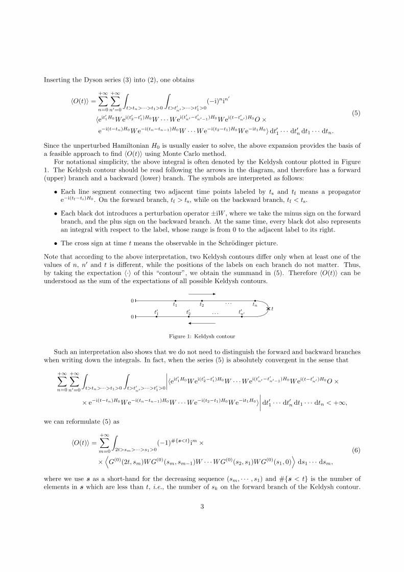
The integral (6) can also be understood graphically as the “unfolded Keldysh contour” plotted in Figure 2.In order to use only a single integral in (6), we set the range of the unfolded Keldysh contour to be [0, 2t],and the mapping of time points from the unfolded Keldysh contour to the original Keldysh contour hasbeen implied in the definition of G(0)(·, ·). By comparing (6) with Figure 2, one can see that G(0)(·, ·) canbe considered as the unperturbed propagator on the unfolded Keldysh contour, with an action of observableO at time t.

0 2ts1 s2 · · · sn smsm−1· · ·t sn+1

Figure 2: Unfolded Keldysh contour

To proceed, we now assume that the von Neumann equation (1) describes an open quantum systemcoupled with a bath, which means that both ρ and H are Hermitian operators on the Hilbert space H =Hs ⊗Hb, with Hs and Hb representing respectively the Hilbert spaces associated with the system and thebath. We consider the interaction picture and take H0 to be the Hamiltonian without coupling:

H0 = Hs ⊗ Idb + Ids ⊗Hb,

where Hs and Hb are respectively the uncoupled Hamiltonians for the system and the bath, and Ids and Idbare respectively the identity operators for the system and the bath. Then the perturbation W describes thecoupling, and here we assume W takes the form without loss of generality

W =Ws ⊗Wb.

Furthermore, we assume the initial density matrix has the separable form ρ(0) = ρs ⊗ ρb, and we areconcerned with observables acting only on the system O = Os ⊗ Idb (recall that physically the system is theinteresting part). With these assumptions, (6) becomes

〈O(t)〉 =+∞∑

m=0

im∫

2t>sm>···>s1>0

(−1)#{s<t} trs(ρsU(0)(2t, s, 0))Lb(s) ds1 · · · dsm, (8)

where the integrand is separated into U (0) and Lb for the system and bath parts:

U (0)(sf , s, si) = U (0)(sf , sm, · · · , s1, si)

= G(0)s (sf , sm)WsG

(0)s (sm, sm−1)Ws · · ·WsG

(0)s (s2, s1)WsG

(0)s (s1, si),

(9)

Lb(s) = trb(ρbG(0)b (2t, sm)WbG

(0)b (sm, sm−1)Wb · · ·WbG

(0)b (s2, s1)WbG

(0)b (s1, 0)), (10)

where trs and trb take traces of the system and bath respectively. The propagators G(0)s and G

(0)b are defined

similarly to (7):

G(0)s (sf , si) =

e−i(sf−si)Hs , if si 6 sf < t,

e−i(si−sf )Hs , if t 6 si 6 sf ,

e−i(t−sf )HsOse−i(t−si)Hs , if si < t 6 sf ,

(11)

4

and

G(0)b (sf , si) =

e−i(sf−si)Hb , if si 6 sf < t,

e−i(si−sf )Hb , if t 6 si 6 sf ,

e−i(2t−si−sf )Hb , if si < t 6 sf .

(12)

Note that the observable Os is inserted into the propagator G(0)s to keep the expression in (9) concise.

3. Inchworm algorithm

In this section, we are going to study the inchworm algorithm introduced in [2], where the method wasproposed for the spin-Boson model from a purely diagrammatic point of view. By matching the mathematicalinterpretation and the diagrammatic interpretation of the algorithm, we will establish rigorously the validityof the algorithm in a more general sense. The central idea of the algorithm is to consider the problem as anevolution problem and reuse as much previous information as possible, and we will start the introduction ofthe algorithm by introducing the “full propagators”, which are exactly the carriers of the information to berecycled.

3.1. Full propagator and its Dyson series expansion

The inchworm algorithm proposed in [2] considers the following “full propagators”:

G(sf , si) =

trb(ρbG(0)b (2t, sf)e

−i(sf−si)HG(0)b (si, 0)), if si 6 sf < t,

trb(ρbG(0)b (2t, sf)e

−i(si−sf )HG(0)b (si, 0)), if t 6 si 6 sf ,

trb(ρbG(0)b (2t, sf)e

i(sf−t)HOe−i(t−si)HG(0)b (si, 0)), if si < t 6 sf .

(13)

Here the trace is taken only on the space of the bath Hb, and hence G(sf , si) is an operator on Hs. Followingthe same method from (3) to (7), we get the following Dyson series expansion for G(sf , si):

G(sf , si) =

+∞∑

m=0

∫

sf>sm>···>s1>si

(−1)#{s<t}im trb

(ρbG

(0)b (2t, sf)G

(0)(sf , sm)WG(0)(sm, sm−1)W

· · ·WG(0)(s2, s1)WG(0)(s1, si)G(0)b (si, 0)

)ds1 · · · dsm.

(14)

To apply the inchworm algorithm, we need the following two hypotheses, which are abstracted from thespin-Boson model studied in [2]:

(H1) The initial density matrix for the bath ρb commutes with the HamiltonianHb. Physically, this conditionholds when the bath is initially at the thermal equilibrium associated with the Hamiltonian Hb.

(H2) There exists a function B(·, ·) such that the following Wick’s theorem holds:

Lb(sm, · · · , s1) =

0, if m is odd,∑

q∈Q(sm,··· ,s1)

L(q), if m is even, (15)

where the right hand side is given by all possible ordered pairings of the time points:

L(q) =∏

(τ1,τ2)∈q

B(τ1, τ2),

Q(sm, · · · , s1) ={{(sj1 , sk1), · · · , (sjm/2

, skm/2)}∣∣∣ {j1, · · · , jm/2, k1, · · · , km/2} = {1, · · · ,m},

sjl 6 sklfor any l = 1, · · · ,m/2

},

When m = 0, the value of L(∅) is defined as 1.

5

In hypothesis (H2), Q(sm, · · · , s1) is the set of all possible ordered pairings of {sm, · · · , s1}. For example,

Q(s2, s1) ={{(s1, s2)}

},

Q(s4, s3, s2, s1) ={{(s1, s2), (s3, s4)}, {(s1, s3), (s2, s4)}, {(s1, s4), (s2, s3)}

}.

We can also represent these sets by diagrams:

Q(s2, s1) ={

s1 s2

},

Q(s4, s3, s2, s1) =

{s1 s2 s3 s4

,s1 s2 s3 s4

,s1 s2 s3 s4

}.

Manifestly, each arc stands for a pair formed by the labels on the two end points, and each diagram denotesa set of pairs.

As in the quantum field theory, Wick’s theorem (hypothesis (H2)) turns integrals into diagrams, whichallows us to use diagrammatic quantum Monte Carlo methods in the simulation. The first hypothesis (H1)allows us to associate the full propagators with observables. Precisely, when si < t < sf and si + sf = 2t,

trs(ρsG(sf , si)) = tr(ρse

i(sf−t)HOe−i(t−si)H)= 〈O(t− si)〉,

which shows that the evolution of the observable from time 0 to t can be fully obtained once the propagatorG(sf , si) is solved for every pair of sf and si. By splitting system and bath parts and applying Wick’stheorem (15), we get from (14) that

G(sf , si) =

+∞∑

m=0m is even

∫

sf>sm>···>s1>si

∑

q∈Q(s)

(−1)#{s<t}imU (0)(sf , s, si)L(q) ds1 · · · dsm. (16)

Here the integral of (−1)#{s<t}imU (0)(sf , s, si)L(q) can also be represented by a diagram like Figure 3, whichis interpreted by

• Each line segment connecting two adjacent time points labeled by ts and tf means a propagator

G(0)s (tf , ti).

• Each black dot introduces a perturbation operator ±iWs, and we take the minus sign on the forwardbranch, and the plus sign on the backward branch. Here the label for time t, which separates the twobranches of the Keldysh contour, is omitted. Additionally, each black dot also represents the integralwith respect to the label over the interval from si to its next label.

• The arc connecting two time points ts and tf stands for B(ts, tf).

sis1 s2 s3 s4 s5 s6 sf

Figure 3: Diagrammatic representation for the integral of (−1)#{s<t}imU(0)(sf , s, si)L(q) when m = 6 and q ={(s1, s6), (s2, s4), (s3, s5)}.

Such a diagrammatic representation allows us to rewrite (16) as

si sf

=si sf

+si sf

s1 s2+

si sfs1 s2 s3 s4

+ +si sf

s1 s2 s3 s4+ +

si sfs1 s2 s3 s4

+ + · · ·

(17)

6

where the bold line on the left side represents the full propagator G(sf , si). The Monte Carlo method basedon (17) is referred to as “bare diagrammatic quantum Monte Carlo” method in [2], which is essentiallyidentical to the Monte Carlo method based on the Dyson series expansion (3), except that the bath functionLb(s) is also evaluated by the Monte Carlo method.

3.2. Description of the inchworm algorithm

The inchworm algorithm uses another series expansion of G(sf , si) that leads to efficient use of resultsof previous time steps for future computations on the contour. Before introducing the inchworm series, weneed the following definitions:

Definition 1 (Linked pairs and linked set of pairs). Two pairs of real numbers (s1, s2) and (τ1, τ2) satisfyings1 6 s2 and τ1 6 τ2 are linked if either of the following two statements holds:

1. s1 6 τ1 6 s2 and τ1 6 s2 6 τ2.

2. τ1 6 s1 6 τ2 and s1 6 τ2 6 s2.

For two sets of pairs q1 and q2, we say the two sets q1 and q2 are linked if there exists (s1, s2) ∈ q1 and

(τ1, τ2) ∈ q2 such that (s1, s2) and (τ1, τ2) are linked.

Given a set of pairs q, we say q is a linked set of pairs if it cannot be decomposed into the union of two

sets of pairs that are not linked. We define

Qc(sm, · · · , s1) = {q ∈ Q(sm, · · · , s1) | q is linked}.

For example, according to the above definition, when s1 < s2 < s3 < s4, the pairs (s1, s3) and (s2, s4)are linked, while (s1, s4) and (s2, s3) are not, which can be also clearly seen from the diagrams:

s1 s2 s3 s4 s1 s2 s3 s4

It is also clear that the set of pairs in the left diagram is a linked set, while the other one is not.

Definition 2 (Linked component decomposition). For any q ∈ Q(sm, · · · , s1), there exists a collection of

its disjoint subsets q1, q2, · · · , qn such that

1. q1, q2, · · · , qn are all linked sets of pairs;

2. q = q1 ∪ q2 ∪ · · · ∪ qn;

3. qn1 and qn2 are not linked if n1 6= n2.

We call q = q1 ∪ q2 ∪ · · · ∪ qn the linked component decomposition of q.

An simple example of the linked component decomposition is given below by digrammatic representations:

s1 s2 s3 s4 s5 s6

=

s1 s6

⋃s2 s3 s4 s5

Definition 3 (Inchworm properness). Given a decreasing sequence of real numbers sm, · · · , s1 and a real

number s↑, a set of integer pairs q ∈ Q(sm, · · · , s1) is called inchworm proper, if in its linked component

decomposition q = q1 ∪ q2 ∪ · · · ∪ qn, each qk contains at least one point greater than or equal to s↑. Below

we use Qs↑(sm, · · · , s1) to denote the collection of all inchworm proper pair sets.

The structure of the set Qs↑(sm, · · · , s1) is determined by the relative position of s↑ in the decreasingsequence sm, · · · , s1. For example, if m = 4 and s↑ ∈ (s2, s3], then

Qs↑(s4, s3, s2, s1) ={{(s1, s3), (s2, s4)}, {(s1, s4), (s2, s3)}

}=

{s1 s2 s↑ s3 s4

, s1 s2 s↑ s3 s4

};

if s↑ ∈ (s3, s4], then Qs↑(s4, s3, s2, s1) contains only one element:

Qs↑(s4, s3, s2, s1) ={{(s1, s3), (s2, s4)}

}={

s1 s2 s3 s↑ s4

}.

7

In fact, if s↑ ∈ (sm−1, sm], the number of sets of pairs in the linked component decomposition of an inchwormproper set q must be 1, which means q is linked. Therefore we have

Qs↑(sm, · · · , s1) = Qc(sm, · · · , s1), if sm−1 < s↑ 6 sm. (18)

Based on the definition of inchworm proper set of pairs, we have the following theorem:

Theorem 1. Suppose the Dyson series (16) is absolutely convergent in the sense that

+∞∑

m=0m is even

∫

sf>sm>···>s1>si

‖U(sf , s, si)‖s

∣∣∣∣∣∣

∑

q∈Q(s)

L(q)

∣∣∣∣∣∣ds1 · · · dsm < +∞, ∀si, sf ∈ [0, 2t], (19)

where ‖ · ‖s is the operator norm in the Hilbert space Hs. For any s↑ ∈ (si, sf), we have

G(sf , si) = Gs↑(sf , si) +

+∞∑

m=2m is even

∫

sf>sm>···>s1>si

(−1)#{s<t}im

∑

q∈Qs↑(s)

L(q)

×

Gs↑(sf , sm)WsGs↑(sm, sm−1)Ws · · ·WsGs↑(s2, s1)WsGs↑(s1, si) ds1 · · · dsm,

(20)

where

Gs↑(sf , si) =

G(sf , si), if si 6 sf 6 s↑,

G(0)s (sf , si), if s↑ < si 6 sf ,

G(0)s (sf , s↑)G(s↑, si), if si 6 s↑ < sf .

Note that the right-hand side of (20) has a very similar structure to (16), except that the bare Green’s

function G(0)s is replaced by Gs↑ and the sum consists only of “inchworm proper diagrams”, which will be

further discussed below. This theorem shows that G(sf , si) can be evaluated by the Monte Carlo simulationof the right-hand side of (20) based on the knowledge of G(τ2, τ1) for all si < τ1 < τ2 < s↑. Therefore thealgorithm can be designed as follows:

Choose a time step ∆t = t/Nfor sf from 0 to 2t with step ∆t

for si from sf to 0 with step −∆tUse (20) to evaluate G(sf , si) by the Monte Carlo method

end forend for

This algorithm computes all G(sf , si) when si and sf are multiples of ∆t. When evaluating the right-handside of (20), interpolation might be needed to get G(τ2, τ1) when τ1 or τ2 is not an integer multiple of ∆t.Details about the interpolation will be given in Section 6.

A rigorous proof of Theorem 1 will be given in the next section. Here we would like to provide thediagrammatic understanding of this algorithm, following [2, 3]. As already mentioned, on the right-handside of (20), only “inchworm proper diagrams” appear, for example,

si s↑sf

,si s↑

sfs1 s2

,si s↑

sfs1

s2,

si s↑sfs1 s2 s3

s4,

si s↑sfs1 s2

s3 s4, · · ·

(21)

These diagrams are interpreted as follows:

8

• Each bold line segment connecting two adjacent time points labeled by ti and tf means a full propagatorG(tf , ti).

• Each thin line segment connecting two adjacent time points labeled by ti and tf means a propagator

G(0)s (tf , ti).

• Each black dot introduces a perturbation operator ±iWs, which takes the minus sign on the forwardbranch and the plus sign on the backward branch. It also introduces an integral with respect to thelabel from s↑ to the next label.

• Each white vertical line introduces a perturbation operator ±iWs, which takes the minus sign on theforward branch and the plus sign on the backward branch. It also introduces an integral with respectto the label from si to the next label.

• The arc connecting two time points ti and tf stands for B(ti, tf).

By (17), we can see that each bold line in the above diagrams is a sum consisting of infinite “thin diagrams”.Therefore it can be expected that (20) converges faster than (16). It is also worth mentioning that thefollowing diagrams are not included in the inchworm series (20):

si s↑sfs1 s2

,si s↑

sfs1 s2 s3s4

,si s↑

sfs1 s2 s3s4

, · · ·

since the terms presented by these diagrams have actually appeared in other diagrams, which are respectively

si s↑sf

,si s↑

sfs1

s2,

si s↑sfs1

s2, · · ·

Below we use a diagrammatic equation to summarize the idea of the inchworm algorithm:

si sf

=si s↑

sf⊃

si s↑sfs1 s2

+si s↑

sfs1 s2

+si s↑

sfs1s2

⊃si s↑

sfs1 s2 s3s4

+si s↑

sfs1 s2 s3s4

+si s↑

sfs1 s2s3 s4

⊃si s↑

sfs1 s2 s3 s4 s5 s6s7 s8

+ · · ·

(22)The proof of Theorem 1 follows such understanding of the inchworm series. However, to make sure nodiagrams are missed or double-counted in this equation, we need to interpret these diagrammatic equationsprecisely using mathematical equations, which will be detailed in the following section.

3.3. Proof of Theorem 1

This section is devoted to the proof of (20), which is to equate the right-hand side of (20) and the series(16). To see this, we will first introduce s↑ to the expansion of G(sf , si) by the following lemma:

Lemma 1. When the Dyson series (16) is absolutely convergent in the sense of (19), for any s↑ ∈ (si, sf),it holds that

G(sf , si) = G(0)s (sf , s↑)G(s↑, si) +

+∞∑

m=2m is even

m−1∑

p=0

∫

sf>sm>···>sp+1>s↑

∫

s↑>sp>···>s1>si

∑

q∈Q(s)

(−1)#{s<t}imU (0)(sf , s, si)L(q) ds1 · · · dsp dsp+1 · · · dsm.

(23)

9

Proof. For any positive integer m, it holds that

∫

sf>sm>···>s1>si

ϕ(s) ds1 · · · dsm =m∑

p=0

∫

sf>sm>···>sp+1>s↑

∫

s↑>sp>···>s1>si

ϕ(s) ds1 · · · dsp dsp+1 · · · dsm

(24)for any function ϕ. This can be proven by mathematical induction since when the above equation holds forsome m, we have

∫

sf>sm+1>···>s1>si

ϕ(s) ds1 · · · dsm+1 =

∫ sf

si

(∫

sm+1>sm>···>s1>si

ϕ(s) ds1 · · · dsm

)dsm+1

=

∫ s↑

si

(∫

sm+1>sm>···>s1>si

ϕ(s) ds1 · · · dsm

)dsm+1 +

∫ sf

s↑

(∫

sm+1>sm>···>s1>si

ϕ(s) ds1 · · · dsm

)dsm+1

=

∫

s↑>sm+1>···>s1>si

ϕ(s) ds1 · · · dsm+1

+

∫ sf

s↑

(m∑

p=0

∫

sm+1>sm>···>sp+1>s↑

∫

s↑>sp>···>s1>si

ϕ(s) ds1 · · · dsp dsp+1 · · · dsm

)dsm+1

=

∫

s↑>sm+1>···>s1>si

ϕ(s) ds1 · · · dsm+1

+m∑

p=0

∫

sf>sm+1>···>sp+1>s↑

∫

s↑>sp>···>s1>si

ϕ(s) ds1 · · · dsp dsp+1 · · · dsm+1

=

m+1∑

p=0

∫

sf>sm+1>···>sp+1>s↑

∫

s↑>sp>···>s1>si

ϕ(s) ds1 · · · dsp dsp+1 · · · dsm+1,

and it is obvious that (24) holds for m = 1. By (24), we can rewrite (16) as

G(sf , si) =

+∞∑

m=0m is even

m∑

p=0

∫

sf>sm>···>sp+1>s↑

∫

s↑>sp>···>s1>si

∑

q∈Q(s)

(−1)#{s<t}imU (0)(sf , s, si)L(q) ds1 · · · dsp dsp+1 · · · dsm

=+∞∑

m=0m is even

∫

s↑>sm>···>s1>si

∑

q∈Q(s)

(−1)#{s<t}imU (0)(sf , s, si)L(q) ds1 · · · dsm

+

+∞∑

m=2m is even

m−1∑

p=0

∫

sf>sm>···>sp+1>s↑

∫

s↑>sp>···>s1>si

∑

q∈Q(s)

(−1)#{s<t}imU (0)(sf , s, si)L(q) ds1 · · · dsp dsp+1 · · · dsm,

(25)

where we have used the absolute convergence (19) to ensure the validity of the second equality. When

sm < s↑, we have U (0)(sf , s, si) = G(0)s (sf , s↑)U (0)(s↑, s, si). Hence

+∞∑

m=0m is even

∫

s↑>sm>···>s1>si

∑

q∈Q(s)

(−1)#{s<t}imU (0)(sf , s, si)L(q) ds1 · · · dsm

= G(0)s (sf , s↑)

+∞∑

m=0m is even

∫

s↑>sm>···>s1>si

∑

q∈Q(s)

(−1)#{s<t}imU (0)(s↑, s, si)L(q) ds1 · · · dsm = G(0)s (sf , s↑)G(s↑, si).

10

Inserting this equation into (25) yields our conclusion (23).

By the above lemma, we have extracted the first diagram in (22) from the definition of the bold line(17). Our next step is to introduce the inchworm proper pairings to the series expansion. The basic ideais to decompose every set of pairs into the union of one inchworm proper subset and several other unlinkedsubsets. The result reads

Lemma 2. When the Dyson series (16) is absolutely convergent in the sense of (19), for any s↑ ∈ (si, sf),it holds that

G(sf , si) = G(0)s (sf , s↑)G(s↑, si) +

+∞∑

m=2m is even

m−1∑

p=0

∫

sf>sm>···>sp+1>s↑

∫

s↑>sp>···>s1>si

p∑

p=0p−p is even

p−p∑

np=0np is even

p−p−np∑

np−1=0np−1 is even

· · ·

p−p−np−···−n2∑

n1=0n1 is even

∑

q∈Qs↑(s)

∑

qp∈Q(s(p))

· · ·∑

q0∈Q(s(0))

(−1)#{s<t}imU (0)(sf , s, si)L(q) ds1 · · · dsp dsp+1 · · · dsm,

(26)

where the notations are

• s = (sm, · · · , s1);

• q = q ∪ qp ∪ · · · ∪ q0;

• s, s(p), · · · , s(0) are all subsequences of s, defined by

s = (sm, · · · , sp+1, s(p), sp, s

(p−1), sp−1, · · · , s(1), s1, s

(0)),

where m = m+ p− p and s = (sm, · · · , s1).

Proof. By comparing (26) with (23), we construct the following map for given m, p and a decreasing sequences:

P → Q(s)(p, np, · · · , n1, q, qp, · · · , q0) 7→ q ∪ qp ∪ · · · ∪ q0

(27)

where

P = {(p, np, · · · , n1, q, qp, · · · , q0) | p ∈ {p, p− 2, · · · , p− 2⌊p/2⌋}; n1 + · · ·+ np 6 p− p;

np, · · · , n1 are even; q ∈ Qs↑(s); qp ∈ Q(s(p)); · · · ; q0 ∈ Q(s(0))}.

The subsequences s, s(p), · · · , s(0) are defined as in the lemma. If (27) is a bijection, then (26) is a re-arrangement of the series (23). The equality (26) then follows by the absolute convergence of the Dysonseries.

Now it remains only to show that (27) is one-to-one. The definition of P shows that in a map(p, np, · · · , n1, q, qp, · · · , q0) 7→ q, if q and q are given, other parameters are automatically determined by

p = 2|q| − (m− p), q0 = {(τ1, τ2) ∈ q | τ1 < τ2 < s1},

qk = {(τ1, τ2) ∈ q | sk < τ1 < τ2 < sk+1}, k = 1, · · · , p,

nk = 2|qk|, k = 1, · · · , p.

(28)

Here 2|q| (2|qk|) is actually the number of time points in q (qk). Meanwhile, the set of pairs q satisfies

1. q is not linked to any other pair in q;

2. q ∈ Qs↑(s) and therefore contains sp+1, · · · , sm.

11

Now we consider an arbitrary set of pairs q ∈ Q(s) with its linked component decomposition being q =q1 ∪ · · · ∪ qn. The only subset of q satisfying the above two conditions is

q =⋃

{qk | qk contains a pair (τ1, τ2) with τ2 > sp}.

Taking such a q and applying (28) to find other parameters, we obtain an inverse image of q. This inverseimage is unique due to the uniqueness of q, which yields that (27) is a bijection.

Lemma 3. When the Dyson series (16) is absolutely convergent in the sense of (19), for any s↑ ∈ (si, sf),it holds that

G(sf , si) = G(0)(sf , s↑)G(s↑, si) +

+∞∑

m=2m is even

m−1∑

p=0

+∞∑

np=0np is even

· · ·+∞∑

n0=0n0 is even

∫

sf>sm>···>sp+1>s↑

∫

s↑>sp>···>s1>si

∑

q∈Qs↑(s)

∑

qp∈Q(s(p))

· · ·∑

q0∈Q(s(0))

(−1)#{s<t}imU (0)(sf , s, si)L(q) ds1 · · · dsp dsp+1 · · · dsm,

(29)

where m = m+ n0 + · · ·+ np, and other parameters are defined in the same way as in Lemma 2.

Proof. It is not difficult to see that the map

P → P(m, p, np, · · · , n0) 7→ (m, p, p, np, · · · , n1)

with m = m+ np + · · ·+ n0 and p = p+ np + · · ·+ n0 is a bijection. Here

P ={(m, p, np, · · · , n0)

∣∣∣m,np, · · · , n0 are positive and even; p ∈ {0, · · · ,m− 1}},

P ={(m, p, p, np, · · · , n1)

∣∣∣ m, np, · · · , n1 are positive and even;

p ∈ {0, · · · , m− 1}; p ∈ {0, 2, · · · , 2⌊p/2⌋}; p+ np + · · ·+ n1 6 p}.

(30)

Hence (29) is a rearrangement of the series (26), and therefore (29) follows by the absolute convergence ofthe Dyson series.

Now we are ready to carry out the proof of the inchworm series (20):

Proof of Theorem 1. Following the notations in Lemma 2 and 3, we have the following identities:

U (0)(s) = U (0)(sf , sm, · · · , sp+1, s↑)U(0)(s↑, s

(p), sp)WsU(0)(sp, s

(p−1), sp−1)Ws · · ·WsU(0)(s1, s

(0), si),

#{s < t} = #{s < t}+#{s(p) < t}+ · · ·+#{s(0) < t}, L(q) = L(q)L(qp) · · · L(q0).

Substituting these equalities to (29) yields

G(sf , si) = G(0)s (sf , s↑)G(s↑, si) +

+∞∑

m=2m is even

m−1∑

p=0

+∞∑

np=0

np is even

· · ·+∞∑

n0=0n0 is even

∫ sf

s↑

∫ sm

s↑

· · ·

∫ sp+2

s↑

∫ s↑

si

∫ sp

si

· · ·

∫ s2

si

∫

s(p)⊂(sp,s↑)

∫

s(p−1)⊂(sp−1,sp)

· · ·

∫

s(1)⊂(s1,s2)

∫

s(0)⊂(si,s1)∑

q∈Qs↑(s)

∑

qp∈Q(s(p))

· · ·∑

q0∈Q(s(0))

(−1)#{s<t}+#{s(p)<t}+···+#{s(0)<t}im+np+···+n0 ×

U (0)(sf , sm, · · · , sp+1, s↑)U(0)(s↑, s

(p), sp)WsU(0)(sp, s

(p−1), sp−1)Ws · · ·WsU(0)(s1, s

(0), si)×

L(q)L(qp) · · · L(q0) ds(0) ds(1) · · · ds(p−1) ds(p) ds1 · · · dsp−1 dsp dsp+1 · · · dsm−1 dsm,

(31)

12

where the integrals with respect to s(k) are interpreted by

∫

s(k)⊂(a,b)

ds(k) =

∫

b>s(k)nk

>···>s(k)1 >a

ds(k)1 · · · ds(k)nk

. (32)

Hence the integrals in the second line of (31) is actually the same as the integrals in (29). Due to the absoluteconvergence, we are allowed to safely interchange sums and integrals, which can give us the following factors:

+∞∑

np=0

∫

s(p)⊂(sp,s↑)

∑

qp∈Q(s(p))

(−1)#{s(p)<t}inkU (0)(s↑, s(p), sp)L(qp) ds

(p),

+∞∑

nk=0

∫

s(k)⊂(sk,sk+1)

∑

qk∈Q(s(k))

(−1)#{s(k)<t}inkU (0)(sk+1, s(k), sk)L(qk) ds

(k), k = 0, · · · , p− 1.

(33)

This quantity can be replaced, respectively, by G(sp, s↑) and G(sk+1, sk), k = 0, · · · , p−1 according to (16).Such replacement turns (31) into

G(sf , si) = G(0)s (sf , s↑)G(s↑, si) +

+∞∑

m=2m is even

m−1∑

p=0

∫

sf>sm>···>sp+1>s↑

∫

s↑>sp>···>s1>si

∑

q∈Qs↑(s)

(−1)#{s<t}im ×

U (0)(sf , sm, · · · , sp+1, s↑)G(s↑, sp)WsG(sp, sp−1)Ws · · ·WsG(s2, s1)WsG(s1, si)L(q) ds1 · · · dsp dsp+1 · · · dsm.

(34)

Noting that

U (0)(sf , sm, · · · , sp+1, s↑)G(s↑, sp)WsG(sp, sp−1)Ws · · ·WsG(s2, s1)WsG(s1, si)

= Gs↑(sf , sm)WsGs↑(sm, sm−1)Ws · · ·WsGs↑(s2, s1)WsGs↑(s1, si),

we see that the integrand in (34) is actually the same as the integrand in (20). Furthermore, the sum overp in (34) can be replaced by

∑mp=0, because when p = m, the set Qs↑(s) is empty. By doing this, we can

apply the identity (24) and obtain the equality (20), which completes the proof of Theorem 1.

4. Integro-differential equations

To better understand the algorithm, we are going to derive the limiting equation of the inchwormalgorithm by considering the case in which sf − s↑ is infinitesimal. Suppose ∆t = sf − s↑ and sf and s↑ areboth on the forward branch of the Keldysh contour, i.e. s↑ < sf < t. By (7) and (9), we can find that

G(0)s (sf , s↑) = e−i∆tHs = I − i∆tHs +O(∆t2),

U (0)(sf , sm, s↑) = G(0)s (sf , sm)WsG

(0)s (sm, s↑) =Ws +O(∆t).

(35)

In the inchworm method (34), the domain of the integral

∫

sf>sm>···>sp+1>s↑

(integrand) dsp+1 · · · dsm−1 dsm

13

has volume 1(m−p)!∆t

m−p. Therefore all the terms with p < m− 1 are higher order in ∆t, and (34) can berewritten as

G(sf , si) = G(0)s (sf , s↑)G(s↑, si) +

+∞∑

m=2m is even

im∫ sf

s↑

∫

s↑>sm−1>···>s1>si

∑

q∈Qs↑(s)

(−1)#{s<t}L(q)×

U (0)(sf , sm, s↑)U(s↑, sm−1, · · · , s1, si) ds1 · · · dsm−1 dsm +O(∆t2)

= (I − i∆tHs)G(s↑, si) ++∞∑

m=2m is even

im∫ sf

s↑

∫

s↑>sm−1>···>s1>si

∑

q∈Qs↑(s)

(−1)#{s<t}L(q)×

WsU(s↑, sm−1, · · · , s1, si) ds1 · · · dsm−1 dsm +O(∆t2),

(36)

where we have used the short hand

U(s↑, sm−1, · · · , s1, si) = G(s↑, sm−1)WsG(sm−1, sm−2)Ws · · ·WsG(s2, s1)WsG(s1, si).

Our assumption that s↑ < sf < t shows that #{s < t} = m. Also, by (10) and (18), one sees that∑

q∈Qs↑(s)

L(q) =∑

q∈Qs↑(s↑,sm−1,··· ,s1)

L(q) +O(∆t) =∑

q∈Qc(s↑,sm−1,··· ,s1)

L(q) +O(∆t).

Thus on the right-hand side of (36), the first order term of the integrand is actually independent of sm,which can then be integrated out. We write the result by moving G(s↑, si) to the left-hand side and divideboth sides by ∆t:

G(sf , si)−G(s↑, si)

∆t= −iHsG(s↑, si)−

+∞∑

m=2m is even

im∫

s↑>sm−1>···>s1>si

∑

q∈Qc(s↑,sm−1,··· ,s1)

(−1)m−1L(q)WsU(s↑, sm−1, · · · , s1, si) ds1 · · · dsm−1 +O(∆t).

(37)

Taking the limit as ∆t → 0 and renaming m to m + 1, we obtain the integro-differential equations for thepropagator G(·, ·):

∂G(s↑, si)

∂s↑= −iHsG(s↑, si)

−+∞∑

m=1m is odd

im+1

∫

s↑>sm>···>s1>si

∑

q∈Qc(s↑,s)

(−1)#{s<t}L(q)WsU(s↑, s, si) ds1 · · · dsm.(38)

Here we have again used the fact that all the components of s are less than t. The equation (38) gives anintegro-differential equation for the full propagator G(s↑, si) when s↑ < t. If s↑ > t, we can use the samemethod to derive a similar integro-differential equation:

∂G(s↑, si)

∂s↑= iHsG(s↑, si)

++∞∑

m=1m is odd

im+1

∫

s↑>sm>···>s1>si

∑

q∈Qc(s↑,s)

(−1)#{s<t}L(q)WsU(s↑, s, si) ds1 · · · dsm.(39)

When s↑ = t, one can see from (13) that G(·, si) is discontinuous, and it satisfies

lims↑→t+

G(s↑, si) = Os lims↑→t−

G(s↑, si). (40)

Combing (38) and (39), we get the following theorem:

14

Theorem 2. When the Dyson series (16) is absolutely convergent in the sense of (19), the full propagator

G(·, ·) satisfies the integro-differential equation

sgn(s↑ − t)∂G(s↑, si)

∂s↑= iHsG(s↑, si) +

+∞∑

m=1m is odd

im+1

∫

s↑>sm>···>s1>si

∑

q∈Qc(s↑,s)

(−1)#{s<t}L(q)WsU(s↑, s, si) ds1 · · · dsm, ∀si ∈ [0, 2t]\{t}, s↑ ∈ [si, 2t]\{t},

(41)

with the jump condition (40) and the “initial condition” G(s↑, s↑) = Id.

Although the integro-differential equation (41) has been derived from the inchworm method, the infinites-imal terms O(∆t) or O(∆t2) have not been rigorously verified. Below we are going to provide a rigorousproof of Theorem 2 starting from the definition of G(·, ·).

Proof of Theorem 2. We will start the proof by deriving the dynamics of the propagator with a more straight-forward method, and then show that the result is equivalent to (41). Again we consider the case s↑ < t, andtake derivative of the definition of G (13) to get

∂G(s↑, si)

∂s↑= trb(ρbG

(0)b (2t, s↑)(iHb − iH)e−i(s↑−si)HG

(0)b (si, 0))

= −i trb(ρbG(0)b (2t, sf)(Hs +W )e−i(s↑−si)HG

(0)b (si, 0))

= −iHsG(s↑, si)− iWs trb(ρbG(0)b (2t, s↑)Wbe

−i(s↑−si)HG(0)b (si, 0)).

(42)

The propagator e−i(s↑−si)H can be expanded into Dyson series as (3), which turns (42) into

∂G(s↑, si)

∂s↑= −iHsG(s↑, si)−

+∞∑

m=0

im+1

∫

s↑>sm>···>s1>si

(−1)mWsG(0)s (s↑, sm)WsG

(0)s (sm, sm−1)Ws · · ·WsG

(0)s (s2, s1)WsG

(0)s (s1, si)×

trb(ρbG(0)b (2t, s↑)WbG

(0)b (s↑, sm)WbG

(0)b (sm, sm−1)Wb · · ·WbG

(0)b (s2, s1)WbG

(0)b (s1, si)G

(0)b (si, 0))

ds1 · · · dsm.

(43)

Since G(0)b (s1, si)G

(0)b (si, 0) = G

(0)b (s1, 0), we can use the definitions (10) and (9) to simplify the above

equation:

∂G(s↑, si)

∂s↑= −iHsG(s↑, si)−

+∞∑

m=0

im+1

∫

s↑>sm>···>s1>si

(−1)mWsU(0)(s↑, s, si)L(s↑, s) ds1 · · · dsm

= −iHsG(s↑, si)−+∞∑

m=1m is odd

im+1

∫

s↑>sm>···>s1>si

∑

q∈Qc(s)

(−1)#{s<t}WsU(0)(s↑, s, si)L(q) ds1 · · · dsm.

(44)

To see that the above equation is identical to the “inchworm equation” (38), we can mimic (31) and replacethe propagators G(·, ·) in the integral of (38) by its Dyson series expansion. Following the same way as inthe previous section, we obtain a result similar to (26):

∂G(s↑, si)

∂s↑= −iHsG(s↑, si)−

+∞∑

m=1m is odd

+∞∑

nm=0nm is even

· · ·+∞∑

n0=0n0 is even

im+1

∫

s↑>sm>···>s1>si

∑

q∈Qc(s↑,s)

∑

qm∈Q(s(m))

· · ·∑

q0∈Q(s(0))

(−1)#{s<t}WsU(0)(s↑, s, si)L(q) ds1 · · · dsm,

(45)

15

whereq = q ∪ qm ∪ · · · ∪ q0, m = m+ nm + · · ·+ n0, s = (sm, · · · , s1),

and s, s(m), · · · , s(0) can be determined by

s = (s(m), sm, s(m−1), sm−1, · · · , s

(1), s1, s(0)), s = (sm, · · · , s1).

Now we need to use the following equivalence of sums:

+∞∑

m=1m is odd

+∞∑

nm=0nm is even

· · ·+∞∑

n0=0n0 is even

=

+∞∑

m=1m is odd

m∑

m=0m−m is even

m−m∑

nm=0nm is even

· · ·m−m−nm∑

nm−1=0

nm−1 is even

· · ·m−m−nm−···−n2∑

n1=0n1 is even

.

Due to the absolute convergence of the Dyson series, the equation (45) becomes

∂G(s↑, si)

∂s↑= −iHsG(s↑, si)−

+∞∑

m=1m is odd

im+1

∫

s↑>sm>···>s1>si

m∑

m=1m−m is even

m−m∑

nm=0nm is even

m−m−nm∑

nm−1=0

nm−1 is even

· · ·m−m−nm−···−n2∑

n1=0n1 is even

∑

q∈Qc(s↑,s)

∑

qm∈Q(s(m))

· · ·∑

q0∈Q(s(0))

(−1)#{s<t}WsU (0)(s↑, s, si)L(q) ds1 · · · dsm.

(46)

The last step is to verify that the right-hand side of the above equation equals the right-hand side of (44). Bycomparison, we just need to show that for any given positive odd integer m and a sequence s = (sm, · · · , s1)satisfying s↑ > sm > · · · > s1 > si, the following map is a bijection:

P → Qs↑(s)(m,nm, · · · , n0, q, qp, · · · , q0) 7→ q ∪ qp ∪ · · · ∪ q0

(47)

where

P = {(m,nm, · · · , n0, q, qp, · · · , q0) | p ∈ {m, m− 2, · · · , 1}; n0 + · · ·+ nm = m−m; nm, · · · , n0 are even;

q ∈ Qc(s↑, s); qm ∈ Q(s(p)); · · · ; q0 ∈ Q(s(0))}.

This map can actually be considered as a special case of (27) when p = m − 1, and hence is one-to-one.Till now, the inchworm equation (41) is confirmed to be identical to (42) when s↑ < t, which describes thecorrect dynamics of the full propagator. The case s↑ > t can be dealt with following the same procedure,which is omitted for conciseness.

Since the equation in the above theorem is firstly derived by setting sf − s↑ to be infinitesimal in theinchworm algorithm, the algorithm can actually be considered as an iterative scheme for the equation. Fromthis point of view, we can improve the numerical method by solving (41) with a higher-order scheme. Beforeintroducing the details of the method, we will first present the spin-boson model, and show that it satisfiesall the conditions needed for the inchworm method.

5. Spin-boson model

To demonstrate the algorithm in a specific model, we consider the spin-boson model in which the systemis a single spin and the bath is given by a large number of harmonic oscillators. In detail, we have

Hs = span{|1〉 , |2〉}, Hb =

L⊗

l=1

(L2(R3)

),

16

where L is the number of harmonic oscillators. The corresponding Hamiltonians are

Hs = ǫσz +∆σx, Hb =L∑

l=1

1

2(p2l + ω2

l q2l ).

The notations are described as follows:

• ǫ: energy difference between two spin states.

• ∆: frequency of the spin flipping.

• σx, σz : Pauli matrices satisfying σx |1〉 = |2〉, σx |2〉 = |1〉, σz |1〉 = |1〉, σz |2〉 = − |2〉.

• ωl: frequency of the lth harmonic oscillator.

• ql: position operator for the lth harmonic oscillator defined by ψ(q1, · · · , qL) 7→ qlψ(q1, · · · , qL).

• pl: momentum operator for the lth harmonic oscillator defined by ψ(q1, · · · , qL) 7→ −i∇qlψ(q1, · · · , qL).

The coupling between system and bath is assumed to be linear:

W =Ws ⊗Wb, Ws = σz , Wb =L∑

l=1

clql,

where cl is the coupling intensity between the lth harmonic oscillator and the spin. Suppose the initial stateof the bath is in the thermal equilibrium with inverse temperature β, i.e. ρb = Z−1 exp(−βHb), and Z ischosen such that tr(ρb) = 1. Thus the hypothesis (H1) is fulfilled, and Wick’s theorem (15) holds for

B(τ1, τ2) =

L∑

l=1

c2l2ωl

[coth

(βωl

2

)cosωl(τ2 − τ1)− i sinωl(τ2 − τ1)

]. (48)

In order to apply the inchworm algorithm to the spin-boson model, we need to show the absoluteconvergence (19). By the definition of U (9), we immediately have

‖U(sf , s, si)‖s 6 ‖Ws‖ms max{‖Os‖s, 1} = ‖σz‖

ms max{‖Os‖s, 1} = max{‖Os‖s, 1}.

And from (48), we see that

|B(τ1, τ2)| 6L∑

l=1

c2l2ωl

√

coth2(βωl

2

)cos2 ωl(τ2 − τ1) + sin2 ωl(τ2 − τ1) 6

L∑

l=1

c2l2ωl

coth

(βωl

2

). (49)

Let Cb be the right-hand side of the above inequality. Then when m is even,

|L(q)| 6 Cm/2b , ∀q ∈ Q(sm, · · · , s1).

Since the number of pair sets in Q(sm, · · · , s1) is (m− 1)!!, we have

+∞∑

m=0m is even

∫

sf>sm>···>s1>si

‖U (0)(sf , s, si)‖s

∣∣∣∣∣∣

∑

q∈Q(s)

L(q)

∣∣∣∣∣∣ds1 · · · dsm

6

+∞∑

m=0m is even

∫

sf>sm>···>s1>si

max{‖Os‖s, 1} · (m− 1)!!Cm/2b ds1 · · · dsm

= max{‖Os‖s, 1}+∞∑

m=0m is even

(sf − si)m

m!!C

m/2b = max{‖Os‖s, 1} exp

(Cb(sf − si)

2

2

).

(50)

17

Since Hs is a finite-dimensional space, the observable Os is always a bounded operator. Therefore the right-hand side of the above equation is finite, which shows the absolute convergence. In the spin-boson model,people are usually interested in the population of the spin on each of the two spin states, meaning that wecan take Os = σz .

When the Dyson series expansion (16) is directly used in the Monte Carlo simulation, the fast growthof the variance as sf − si increases causes great numerical difficulties. Similar to (50), the expectation of‖U (0)(sf , s, si)L(q)‖2s can be estimated by

+∞∑

m=0m is even

∫

sf>sm>···>s1>si

∑

q∈Q(s)

‖U (0)(sf , s, si)‖2s|L(q)|

2 ds1 · · · dsm

6

+∞∑

m=0m is even

∫

sf>sm>···>s1>si

(m− 1)!!(max{‖Os‖s, 1})2Cm

b ds1 · · · dsm

= (max{‖Os‖s, 1})2 exp

(C2

b (sf − si)2

2

).

(51)

Since ‖G(sf , si)‖s 6 max{‖Os‖s, 1}, the growth of the variance is characterized by

exp

(C2

b (sf − si)2

2

)− 1.

This is the well-known “dynamical sign problem” in the quantum Monte Carlo simulations. The inchwormmethod relieves the dynamical sign problem by lumping a number of samples based on the simulation resultsof shorter bold lines, which pushes the simulation time significantly longer.

Different from the inchworm methods presented in [2], which directly applies the Monte Carlo methodto (20), we will design our numerical method based on the integro-differential equation (41), and apply theidea of classical Runge-Kutta methods for temporal discretization to solve the full propagators. As will bepresented, this can both enhance the numerical efficiency and simplify the implementation. The algorithmwill be detailed in the following section.

6. Numerical method

In order to find the full propagator G(sf , si) numerically for all si ∈ [0, 2t] and sf ∈ [si, 2t]. Below weare going to develop a second-order method in analogous to Heun’s method for general ordinary differentialequations. For the general initial value problem

u′(t) = f(t, u(t)), t > 0

with initial condition u(0) = u0, Heun’s method reads

U∗k = Uk−1 +∆tf(tk−1, Uk−1),

Uk =1

2(Uk−1 + U∗

k ) +1

2∆tf(tk, U

∗k ),

where ∆t is the time step, tk = tk−1 +∆t, and Uk is the numerical approximation of u(tk). The method issecond-order if the solution is third-order continuously differentiable. In our case, the full propagator G(·, ·)is known to be discontinuous on the line segments [0, t] × {t} and {t} × [0, t] due to the presence of theobservable Os. Therefore in order to keep the second-order convergence rate, special care needs to be takenfor these discontinuities.

In our implementation, we take a uniform time step ∆t = t/N , and compute the numerical solutionsG(sf , si) only when sf and si are multiples of ∆t. This corresponds to a two-dimensional triangular mesh

18

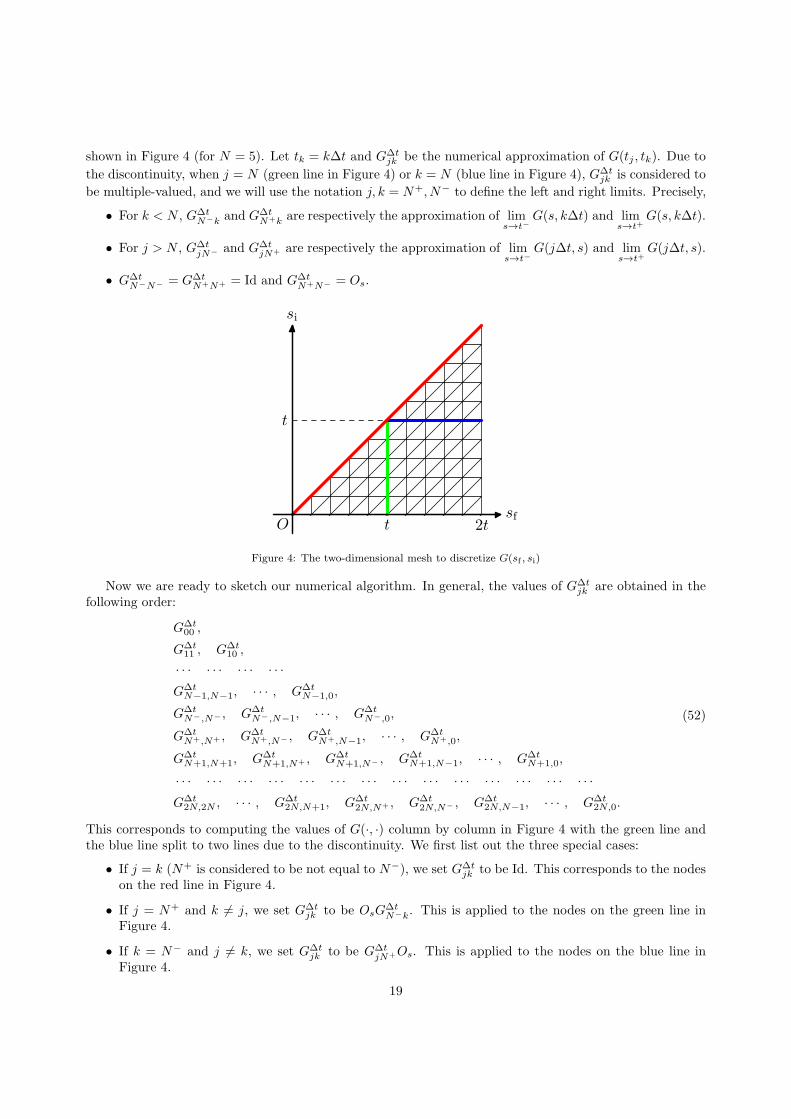
shown in Figure 4 (for N = 5). Let tk = k∆t and G∆tjk be the numerical approximation of G(tj , tk). Due to

the discontinuity, when j = N (green line in Figure 4) or k = N (blue line in Figure 4), G∆tjk is considered to

be multiple-valued, and we will use the notation j, k = N+, N− to define the left and right limits. Precisely,

• For k < N , G∆tN−k and G∆t

N+k are respectively the approximation of lims→t−

G(s, k∆t) and lims→t+

G(s, k∆t).

• For j > N , G∆tjN− and G∆t

jN+ are respectively the approximation of lims→t−

G(j∆t, s) and lims→t+

G(j∆t, s).

• G∆tN−N− = G∆t

N+N+ = Id and G∆tN+N− = Os.

O t 2t

t

sf

si

Figure 4: The two-dimensional mesh to discretize G(sf , si)

Now we are ready to sketch our numerical algorithm. In general, the values of G∆tjk are obtained in the

following order:

G∆t00 ,

G∆t11 , G∆t

10 ,

· · · · · · · · · · · ·

G∆tN−1,N−1, · · · , G∆t

N−1,0,

G∆tN−,N− , G∆t

N−,N−1, · · · , G∆tN−,0,

G∆tN+,N+ , G∆t

N+,N− , G∆tN+,N−1, · · · , G∆t

N+,0,

G∆tN+1,N+1, G∆t

N+1,N+ , G∆tN+1,N− , G∆t

N+1,N−1, · · · , G∆tN+1,0,

· · · · · · · · · · · · · · · · · · · · · · · · · · · · · · · · · · · · · · · · · ·

G∆t2N,2N , · · · , G∆t

2N,N+1, G∆t2N,N+ , G∆t

2N,N− , G∆t2N,N−1, · · · , G∆t

2N,0.

(52)

This corresponds to computing the values of G(·, ·) column by column in Figure 4 with the green line andthe blue line split to two lines due to the discontinuity. We first list out the three special cases:

• If j = k (N+ is considered to be not equal to N−), we set G∆tjk to be Id. This corresponds to the nodes

on the red line in Figure 4.

• If j = N+ and k 6= j, we set G∆tjk to be OsG

∆tN−k. This is applied to the nodes on the green line in

Figure 4.

• If k = N− and j 6= k, we set G∆tjk to be G∆t

jN+Os. This is applied to the nodes on the blue line inFigure 4.

19

For all other cases, we follow Heun’s method and find the values of G∆tjk as follows:

1. Let

G∗jk = G∆t

j−1,k + sgn(tj − t)∆t

[iHsG

∆tj−1,k +

+∞∑

m=1m is odd

im+1

∫

tj−1>sm>···>s1>tk

∑

q∈Qc(tj−1,s)

(−1)#{s<t}

× L(q)WsGI(tj−1, sm)WsGI(sm, sm−1)Ws · · ·WsGI(s2, s1)WsGI(s1, tk) ds1 · · · dsm

],

(53)

where GI(·, ·) is the interpolated function satisfying

GI(tj′ , tk′) = G∆tj′k′ , for all integers j′, k′ satisfying k 6 k′ 6 j′ 6 j − 1. (54)

In our implementation, piecewise linear interpolation is adopted, and the function GI(·, ·) is linear oneach triangle in Figure 4.

2. Set G∆tjk to be

1

2G∆t

j−1,k +1

2G∗

jk +1

2sgn(tj − t)∆t

[iHsG

∗jk +

+∞∑

m=1m is odd

im+1

∫

tj>sm>···>s1>tk

∑

q∈Qc(tj ,s)

(−1)#{s<t}L(q)WsG∗I(tj , sm)WsG

∗I(sm, sm−1)Ws · · ·WsG

∗I(s2, s1)WsG

∗I(s1, tk) ds1 · · · dsm

],

(55)

where G∗I(·, ·) is the interpolated function satisfying G∗

I(tj , tk) = G∗jk and

G∗I(tj′ , tk′) = G∆t

j′k′ , for all integers j′, k′ satisfying k 6 k′ 6 j′ 6 j and (j′, k′) 6= (j, k). (56)

Again, the same piecewise linear interpolation is adopted.

When applying (53) and (55), we follow the rules as below:

• When j = N−, j − 1 is interpreted as N − 1; when j = N + 1, j − 1 is interpreted as N+.

• sgn(tN− − t) = −1.

• The interpolation of GI and G∗I should respect such discontinuities. Therefore when k = N or l = N ,

the equation (54) should be interpreted by

lims→t±

GI(tk, s) = G∆tkN± , lim

s→t±GI(s, tl) = G∆t

N±l,

lims→t+

lims→t+

GI(s, s) = lims→t−

lims→t−

GI(s, s) = Id, lims→t+

lims→t−

GI(s, s) = Os.

The equation (56) should be similarly interpreted. Especially, when j = N+, the term GI(tN+ , sm) inthe integral should be interpreted as OsGI(tN− , sm).

The order of computation (52) ensures that all information needed in the two stages has been obtainedbeforehand.

Now we consider the numerical computation of the infinite sums in (53) and (55). The numerical resultsin [3] show that in the original inchworm method (20), we can truncate the series at m = M for some

20

positive even integer M , and obtain results with sufficient quality. In our method, the integer M needs tobe odd and we perform the similar truncation by replacing the infinite sums in (53) and (55) with

M∑

m=1m is odd

im+1

∫

tf>sm>···>s1>tk

∑

q∈Qc(tf ,s)

S(q, s) ds1 · · · dsm, (57)

where S(q, s) is the summand in (53) or (55), and tf is the corresponding tj or tj+1. For every m, thehigh-dimensional integral over s and the sum over q are evaluated using the Monte Carlo method. Thesampling of s can be done by sampling a uniform distribution in [tk, tf ]

m, and then sort the time points. Asfor q, we first list out all the elements in Qc(tf , s), and then pick a random one for each sample. Obviouslythe number of pair sets in Qc(tf , s) depends only on the value of m, and it has been given in [29] that thisnumber can be evaluated by

N1 = 1, Nm =m− 1

2

m−2∑

j=1j is odd

NjNm−1−j.

In [30], it is proven that Nm grows asymptotically as m!!. In our numerical experiments, we are onlyconcerned about a small m, and therefore such a strategy is feasible.

As the end of this section, we will discuss briefly the difference between this numerical method andthe original inchworm method based on the Monte Carlo simulation of (20). Both numerical methods aretime-stepping methods which can be regarded as a numerical approximation of

G(sf , si) = G(s↑, si) +

∫ sf

s↑

RHS(s) ds, (58)

where RHS(s) is the right-hand side of (38) or (39), with s↑ replaced by s. From the diagrammatic equation(22), one can see that the original inchworm algorithm in principle allows to put an arbitrary number ofpoints between s↑ and sf to evaluate the integral in (58), and all these points are stochastic, which impliesthat in the time-stepping process, the integral between two time steps is approximated using a Monte Carlosimulation; while in our method, this is replaced by a numerical integration of second-order convergence,which can be expected to be more efficient. One possible benefit of the Monte Carlo integration from s↑to sf is that when a sufficient number of samples are used, this integral can be evaluated up to arbitraryprecision; while in the Runge-Kutta integration, an error of O((sf − s↑)

α), where α depends on the order ofthe method, is always there. However, this does not mean that the numerical error will vanish as the numberof samples increases in the original inchworm algorithm, since another part of numerical error comes fromthe approximation of RHS(s), where the interpolation on the lattice shown in Figure 4 is inevitable in bothmethods. Such error will only vanish as the grid size tends to zero, but will not vanish as the number ofsamples tends to infinity. Usually, it is sufficient to match the order of accuracy for evaluating the integral in(58) and the interpolation. This can be achieved easier and cheaper by using the Runge-Kutta integrationstrategy. Another benefit of this new method is that we can draw the samples for q more easily. Considera diagram with four points. The set Qc(s1, s2, s3, s4) contains only one set of pairs {(s1, s3), (s2, s4)}, whilethe inchworm proper set of pairs has 9 possibilities:

• Qs↑(s1, s2, s3, s4) = {{(s1, s3), (s2, s4)}} if s3 < s↑ 6 s4;

• Qs↑(s1, s2, s3, s4) = {{(s1, s3), (s2, s4)}, {(s1, s4), (s2, s3)}} if s2 < s↑ 6 s3;

• Qs↑(s1, s2, s3, s4) = {{(s1, s3), (s2, s4)}, {(s1, s4), (s2, s3)}, {(s1, s2), (s3, s4)}} if s1 < s↑ 6 s2;

• Qs↑(s1, s2, s3, s4) = {{(s1, s3), (s2, s4)}, {(s1, s4), (s2, s3)}, {(s1, s2), (s3, s4)}} if s↑ 6 s1.

For the more time points, finding out all the inchworm proper pair sets is even harder than just finding outQc(s). This indicates that the implementation of the new method is easier.

21

7. Numerical experiments

In our numerical experiments, we consider the spin-Boson model with a bath with Ohmic spectral density,for which the frequency ωl are distributed in [0, ωmax] as introduced in [20]:

ωl = ωc ln

(1−

l

L[1− exp(ωmax/ωc)]

), l = 1, · · · , L,

where ωc is the primary frequency to be specified later. The coupling intensity cl is

cl = ωl

√ξωc

L[1− exp(ωmax/ωc)], l = 1, · · · , L,

with ξ being the Kondo parameter. To compare our results with reference solutions, we adopt the param-eters provided in [14] where L = 200 and β = 5∆−1. Different settings of bias, coupling intensity andnonadiabaticity will be considered in our experiments. In all the numerical tests, the maximum frequencyωmax is set to be 4ωc, and the time step is chosen to be ∆t = 0.1 if not otherwise specified. Numericalresults obtained by the QuAPI method [22, 23] will be used as reference solutions.

7.1. Experiments with changing bias

We first choose ωc = 2.5∆ and ξ = 0.2, for which the amplitude of the bath correlation function B(·, ·) isplotted in Figure 5. In our implementation, we precompute the values of B(·, ·) up to a very high precision ona very fine grid, and in the inchworm algorithm, we retrieve its value by linear interpolation when necessary.The numerical results for ǫ = 0,∆ and 2∆ are given in Figure 6. It turns out thatM = 3 in (57) can alreadyprovide satisfying numerical results up to time t = 5∆−1, and the general behavior of the observable hasbeen well captured by the results of M = 1.

0 1 2 3 4 50

0.1

0.2

0.3

0.4

0.5

0.6

Figure 5: The amplitude of the bath correlation function B(·, ·)

The order of convergence of our numerical method is also verified using the test case with ǫ = 0. Ingeneral, the stochastic error and the “deterministic error” caused by Runge-Kutta and interpolation cannotbe separated. In order to cast off the stochastic error, we only consider the truncation M = 1, for which thesum (57) contains only a one-dimensional integral, and thus can be evaluated by the composite mid-pointrule. As a result, the whole scheme is deterministic and the order of convergence is still expected to beO(∆t2). The reference solution is obtained by choosing ∆t = 1/320∆−1, and the numerical error of 〈σz(t)〉is tabulated in Table 1, which clearly shows the numerical error is second order of ∆t.

7.2. Experiments with changing coupling intensity

Now we fix the values of ωc and ǫ to be 2.5∆ and ∆ respectively, and consider the coupling intensityξ = 0.1 and ξ = 0.2. It can be expected that the convergence of the inchworm series gets slower when ξincreases, as is confirmed in our numerical tests shown in Figure 7. In spite of this, very good matchingwith the QuAPI results can still be obtained using M = 1 for both parameters, and further improvement isindeed achieved by using M = 3.

22

0 0.5 1 1.5 2 2.5 3 3.5 4 4.5 5

t∆

-0.8

-0.6

-0.4

-0.2

0

0.2

0.4

0.6

0.8

1

〈 σ

z(t

) 〉

QUAPI

M=1 (one pair)

M=2 (two pairs)

0 0.5 1 1.5 2 2.5 3 3.5 4 4.5 5

t∆

-0.6

-0.4

-0.2

0

0.2

0.4

0.6

0.8

1

〈 σ

z(t

) 〉

QUAPI

M=1 (one pair)

M=2 (two pairs)

0 0.5 1 1.5 2 2.5 3 3.5 4 4.5 5

t∆

-0.2

0

0.2

0.4

0.6

0.8

1

〈 σ

z(t

) 〉

QUAPI

M=1 (one pair)

M=2 (two pairs)

Figure 6: Evolution of 〈σz(t)〉 under different settings of the electronic bias (from left to right: ǫ = 0, ǫ = ∆ and ǫ = 2∆), withother parameters ωc = 2.5∆ and ξ = 0.2. QuAPI results are plotted as a reference.

h error (t = 0.5) order error (t = 1) order error (t = 1.5) order error (t = 2) order

1/10 0.0014 – 0.0022 – 0.0014 – 0.0067 –1/20 0.0004 1.9740 0.0005 2.0537 0.0004 1.8855 0.0017 1.99101/30 0.1620 × 10−3 1.9961 0.2343 × 10−3 2.0307 0.1722 × 10−3 1.9632 0.7490 × 10−3 2.00641/40 0.0909 × 10−3 2.0087 0.1305 × 10−3 2.0344 0.0970 × 10−3 1.9941 0.4189 × 10−3 2.02041/50 0.0578 × 10−3 2.0299 0.0826 × 10−3 2.0470 0.0618 × 10−3 2.0188 0.2658 × 10−3 2.03761/60 0.0398 × 10−3 2.0505 0.0567 × 10−3 2.0657 0.0426 × 10−3 2.0422 0.1826 × 10−3 2.0587

Table 1: Numerical error of 〈σz(t)〉 and the order of accuracy

As a reference, the numerical results for a direct summation of the truncated Dyson series

G(sf , si) ≈M∑

m=0m is even

∫

sf>sm>···>s1>si

∑

q∈Q(s)

(−1)#{s<t}imU (0)(sf , s, si)L(q) ds1 · · · dsm,

are also provided in Figure 7 with label “bare dQMC”. The results show that the convergence of the Dysonseries (16) is much slower than the inchworm series, and therefore require a much larger M to get the samequality of the solutions for large t.

0 0.5 1 1.5 2 2.5 3 3.5 4 4.5 5

t∆

-0.4

-0.2

0

0.2

0.4

0.6

0.8

1

〈σz(t)〉

QUAPI

bare dQMC,M=2 (one pair)

bare dQMC, M=4 (two pairs)

M=1 (one pair)

M=3 (two pairs)

0 0.5 1 1.5 2 2.5 3 3.5 4 4.5 5

t∆

-0.8

-0.6

-0.4

-0.2

0

0.2

0.4

0.6

0.8

1

〈σz(t)〉

QUAPI

bare dQMC,M=2 (one pair)

bare dQMC, M=4 (two pairs)

M=1 (one pair)

M=3 (two pairs)

Figure 7: Evolution of 〈σz(t)〉 under different settings of the coupling intensity (left: ξ = 0.1, right: ξ = 0.2), with otherparameters ωc = 2.5∆ and ǫ = ∆. QuAPI results are plotted as a reference.

7.3. Experiments with changing nonadiabaticity

To show the role of the parameter ωc, we fix ξ to be 0.4 and ǫ to be ∆, and consider the cases ωc = 0.25∆and ωc = 2.5∆. Since the upper bound of |B(τ1, τ2)| in (49) gets larger when ωc increases, we can expectslower convergence in terms ofM for larger ωc. The evolution of the observable is plotted in Figure 8. In theright figure, due to the large value of both ξ and ωc, even when M = 3 is used, some discrepancy betweenour results and QuAPI can still be observed.

23

0 0.5 1 1.5 2 2.5 3 3.5 4 4.5 5

t∆

0

0.1

0.2

0.3

0.4

0.5

0.6

0.7

0.8

0.9

1

〈 σ

z(t

) 〉

QUAPI

M=1 (one pair)

M=2 (two pairs)

0 0.5 1 1.5 2 2.5 3 3.5 4 4.5 5

t∆

-0.8

-0.6

-0.4

-0.2

0

0.2

0.4

0.6

0.8

1

〈 σ

z(t

) 〉

QUAPI

M=1 (one pair)

M=2 (two pairs)

Figure 8: Evolution of 〈σz(t)〉 under different settings of the nonadiabaticity (left: ωc = 0.25∆, right: ωc = 2.5∆), with otherparameters ξ = 0.4 and ǫ = ∆. QuAPI results are plotted as a reference.

8. Summary

We have studied the inchworm Monte Carlo method introduced in [4, 2], and proven rigorously that themethod converges to the solution of the open quantum system whose bath configuration satisfies Wick’stheorem. By assuming the iterative step length to be infinitesimal, we have derived a new continuous modelfor the open quantum system, and have proposed an improvement of the inchworm method to achievebetter numerical efficiency and simpler implementation. In this new method, the stochastic error andthe deterministic error are coupled together, and one needs to apply numerical analysis to find optimalcombinations of parameters. This will be left for future works.

Acknowledgements

The work of Zhenning Cai is supported by National University of Singapore Startup Fund under GrantNo. R-146-000-241-133. The work of Jianfeng Lu is supported in part by National Science Foundationunder grant DMS-1454939. This collaboration is also supported by National Science Foundation undergrant RNMS-1107444 (KI-Net).

References

[1] H. Breuer and F. Petruccione. Applications to Quantum Optical Systems, pages 391–438. Oxford University Press, 2007.[2] H.-T. Chen, G. Cohen, and D. R. Reichman. Inchworm Monte Carlo for exact non-adiabatic dynamics. I. Theory and

algorithms. J. Chem. Phys., 146:054105, 2017.[3] H.-T. Chen, G. Cohen, and D. R. Reichman. Inchworm Monte Carlo for exact non-adiabatic dynamics. II. Benchmarks

and comparison with established methods. J. Chem. Phys., 146:054106, 2017.[4] G. Cohen, E. Gull, D. R. Reichman, and A. J. Millis. Taming the dynamical sign problem in real-time evolution of

quantum many-body problems. Phys. Rev. Lett., 115(26):266802, 2015.[5] E. B. Davies. Markovian master equations. Commun. Math. Phys., 39(2):91–110, 1974.[6] E. B. Davies. Markovian master equations. II. Math. Ann., 219(2):147–158, 1976.[7] Q. Dong, I. Krivenko, J. Kleinhenz, A. E. Antipov, G. Cohen, and E. Gull. Quantum monte carlo solution of the dynamical

mean field equations in real time. Phys. Rev. B, 96:155126, 2017.[8] C. Duan, Z. Tang, J. Cao, and J. Wu. Zero-temperature localization in a sub-ohmic spin-boson model investigated by an

extended hierarchy equation of motion. Phys. Rev. B, 95(21):214308, 2017.[9] F. J. Dyson. The radiation theories of Tomonaga, Schwinger, and Feynman. Phys. Rev., 75(3):486–502, 1949.

[10] M. Esposito, K. Lindenberg, and C. Van den Broeck. Entropy production as correlation between system and reservoir.New J. Phys., 12(1):013013, 2010.

[11] E. Gull, D. R. Reichman, and A. J. Millis. Bold-line diagrammatic Monte Carlo method: General formulation andapplication to expansion around the noncrossing approximation. Phys. Rev. B, 82(7):075109, 2010.

[12] E. Gull, D. R. Reichman, and A. J. Millis. Numerically exact long-time behavior of nonequilibrium quantum impuritymodels. Phys. Rev. B, 84(8):085134, 2011.

[13] L. V. Keldysh. Diagram technique for nonequilibrium processes. Sov. Phys. JETP, 20(4):1018–1026, 1965.[14] A. Kelly and T. E. Markland. Efficient and accurate surface hopping for long time nonadiabatic quantum dynamics. J.

Chem. Phys., 139(1):014104, 2013.

24

[15] D. Mac Kernan, G. Ciccotti, and R. Kapral. Surface-hopping dynamics of a spin-boson system. J. Chem. Phys.,116(6):2346–2353, 2002.

[16] Y. Li and J. Lu. Bold diagrammatic Monte Carlo in the lens of stochastic iterative methods, 2017. preprint,arXiv:1710.00966.

[17] K. Lindenberg and B. J. West. The Nonequilibrium Statistical Mechanics of Open and Closed Systems. Wiley, 1990.[18] D. E. Makarov and N. Makri. Path integrals for dissipative systems by tensor multiplication. Condensed phase quantum

dynamics for arbitrarily long time. Chem. Phys. Lett., 221(5–6):482–491, 1994.[19] N. Makri. Numerical path integral techniques for long time dynamics of quantum dissipative systems. J. Math. Phys.,

36(5):2430–2457, 1995.[20] N. Makri. The linear response approximation and its lowest order corrections: An influence functional approach. J. Phys.

Chem. B, 103(15):2823–2829, 1999.[21] N. Makri. Iterative blip-summed path integral for quantum dynamics in strongly dissipative environments. J. Chem.

Phys., 146(13):134101, 2017.[22] N. Makri and D. E. Makarov. Tensor propagator for iterative quantum time evolution of reduced density matrices. I.

theory. J. Chem. Phys., 102(11):4600–4610, 1995.[23] N. Makri and D. E. Makarov. Tensor propagator for iterative quantum time evolution of reduced density matrices. II.

numerical methodology. J. Chem. Phys., 102(11):4611–4618, 1995.[24] N. Makri, E. Sim, D. E. Makarov, and M. Topaler. Long-time quantum simulation of the primary charge separation in

bacterial photosynthesis. Proc. Natl. Acad. Sci., 93(9):3926–3931, 1996.[25] S. Nakajima. On quantum theory of transport phenomena. Prog. Theo. Phys., 20(6):948–959, 1958.[26] M. A. Nielsen and I. L. Chuang. Quantum Computation and Quantum Information: 10th Anniversary Edition. Cambridge

University Press, 2010.[27] N. Prokof’ev and B. Svistunov. Bold diagrammatic Monte Carlo technique: When the sign problem is welcome. Phys.

Rev. Lett., 99(25):250201, 2007.[28] M. Ridley, V. N. Singh, E. Gull, and G. Cohen. Numerically exact full counting statistics of the nonequilibrium Anderson

impurity model. Phys. Rev. B, 97(11):115109, 2018.[29] P. R. Stein. On a class of linked diagrams, I. Enumeration. J. Comb. Theory Ser. A, 24:357–366, 1978.[30] P. R. Stein. On a class of linked diagrams, II. Asymptotics. Discrete Math., 21:309–318, 1978.[31] J. T. Stockburger and H. Grabert. Exact c-number representation of non-Markovian quantum dissipation. Phys. Rev.

Lett., 88(17):170407, 2002.[32] J. Strumpfer and K. Schulten. Open quantum dynamics calculations with the hierarchy equations of motion on parallel

computers. J. Chem. Theory Comput., 8(8):2808–2816, 2012.[33] K.-A. Suominen. Open Quantum Systems and Decoherence, pages 247–282. Springer International Publishing, 2014.[34] H. Wang. Basis set approach to the quantum dissipative dynamics: Application of the multiconfiguration time-dependent

Hartree method to the spin-boson problem. J. Chem. Phys., 113(22):9948–9956, 2000.[35] P. Werner, T. Oka, and A. J. Millis. Diagrammatic Monte Carlo simulation of nonequilibrium systems. Phys. Rev.,

79(3):035320, 2009.[36] E. Zwanzig. Ensemble method in the theory of irreversibility. J. Chem. Phys., 33(5):1338–1341, 1960.

25