university of manchester...incompressible sph (isph) • solves incompressible navier-stokes...
TRANSCRIPT

SPH now and in the future
Peter Stansby
University of Manchester
Manchester Vigo Parma Lisbon Gent Barcelona

Why SPH ?
• We have commercial fluids and solids codes – STAR CCM, ANSYS Fluent, Mechanical, Structural, ABAQUS, NASTRAN, Delft3D, etc
• Open source codes – Code_SATURNE, Code_ASTER, OpenFOAM, Telemac, SWAN (coastal) etc
• So successful that more is wanted ! • So what are blockages – highly distorted free
surfaces/interfaces, multi-phase, phase change, multi-physics, complex boundaries/meshing, computational times and cost
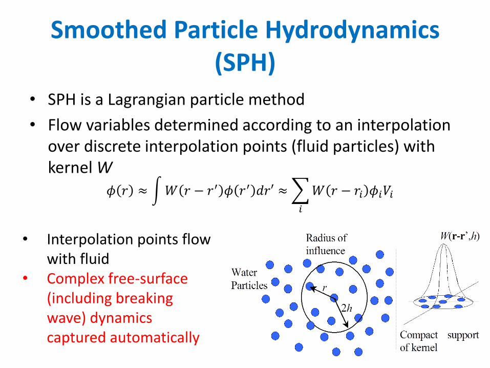
Smoothed Particle Hydrodynamics (SPH)
• SPH is a Lagrangian particle method
• Flow variables determined according to an interpolation over discrete interpolation points (fluid particles) with kernel W
• Interpolation points flow with fluid
• Complex free-surface (including breaking wave) dynamics captured automatically
𝜙 𝑟 ≈ 𝑊 𝑟 − 𝑟′ 𝜙 𝑟′ 𝑑𝑟′ ≈ 𝑊 𝑟 − 𝑟𝑖 𝜙𝑖𝑉𝑖𝑖
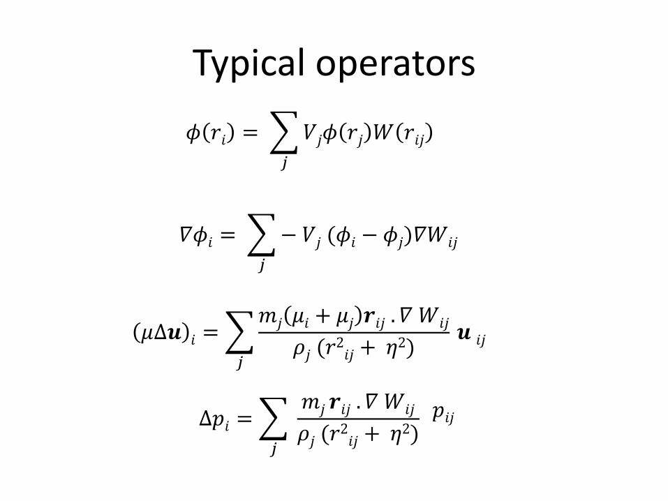
Typical operators
𝜙 𝑟𝑖 = 𝑉𝑗𝜙 𝑟𝑗 𝑊 𝑟𝑖𝑗𝑗
𝛻𝜙𝑖 = − 𝑉𝑗 (𝜙𝑖 − 𝜙𝑗)𝛻𝑊𝑖𝑗𝑗
𝜇∆𝒖 𝑖 = 𝑚𝑗 𝜇𝑖 + 𝜇𝑗 𝒓𝑖𝑗 . 𝛻 𝑊𝑖𝑗𝜌𝑗 (𝑟
2𝑖𝑗 + 𝜂
2)𝑗
𝒖 𝑖𝑗
∆𝑝𝑖 = 𝑚𝑗 𝒓𝑖𝑗 . 𝛻 𝑊𝑖𝑗𝜌𝑗 (𝑟
2𝑖𝑗 + 𝜂
2)𝑗
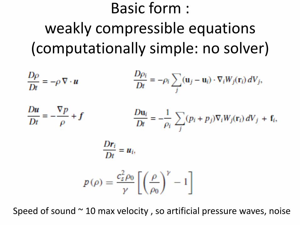
Basic form : weakly compressible equations
(computationally simple: no solver)
Speed of sound ~ 10 max velocity , so artificial pressure waves, noise
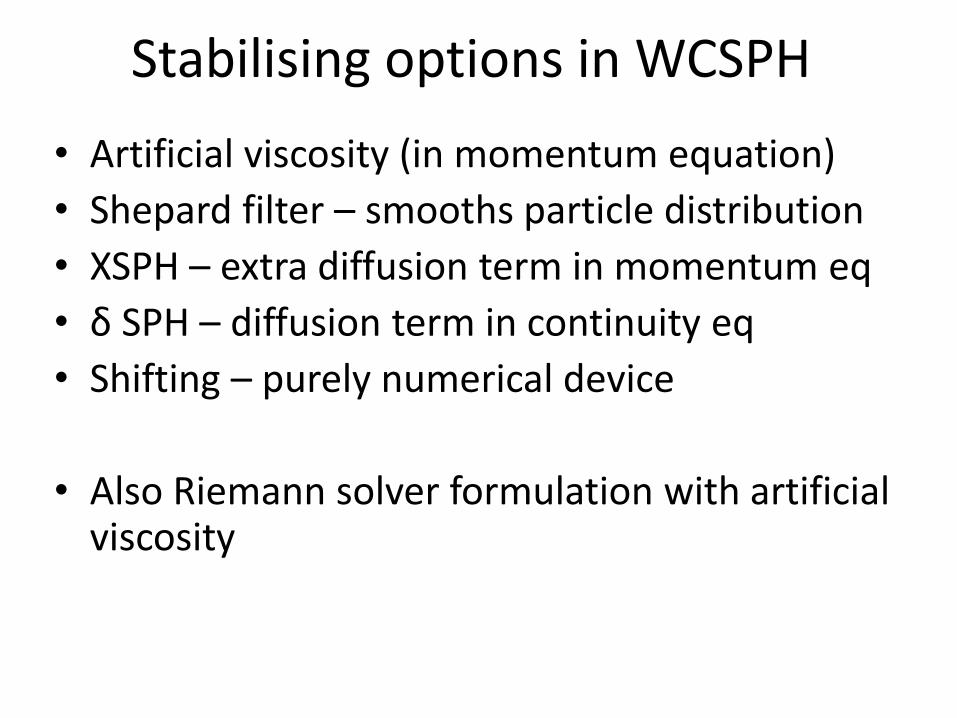
Stabilising options in WCSPH
• Artificial viscosity (in momentum equation)
• Shepard filter – smooths particle distribution
• XSPH – extra diffusion term in momentum eq
• δ SPH – diffusion term in continuity eq
• Shifting – purely numerical device
• Also Riemann solver formulation with artificial viscosity
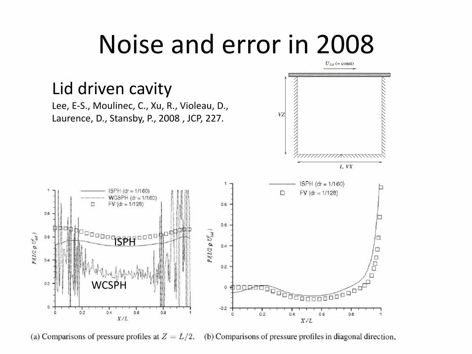
Noise and error in 2008
Lid driven cavity Lee, E-S., Moulinec, C., Xu, R., Violeau, D., Laurence, D., Stansby, P., 2008 , JCP, 227.
WCSPH
ISPH

Incompressible SPH now
• Noise free with numerical stabilisation (without contriving physics)
• Greater accuracy
• But requires Poisson solver for pressure so less ideal for GPUs but progress made there
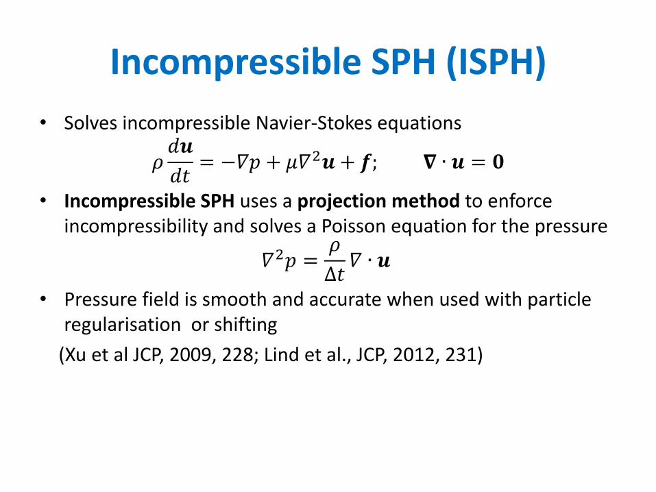
Incompressible SPH (ISPH)
• Solves incompressible Navier-Stokes equations
𝜌𝑑𝒖
𝑑𝑡= −𝛻𝑝 + 𝜇𝛻2𝒖 + 𝒇; 𝛁 ∙ 𝒖 = 𝟎
• Incompressible SPH uses a projection method to enforce incompressibility and solves a Poisson equation for the pressure
𝛻2𝑝 =𝜌
∆𝑡𝛻 ∙ 𝒖
• Pressure field is smooth and accurate when used with particle regularisation or shifting
(Xu et al JCP, 2009, 228; Lind et al., JCP, 2012, 231)
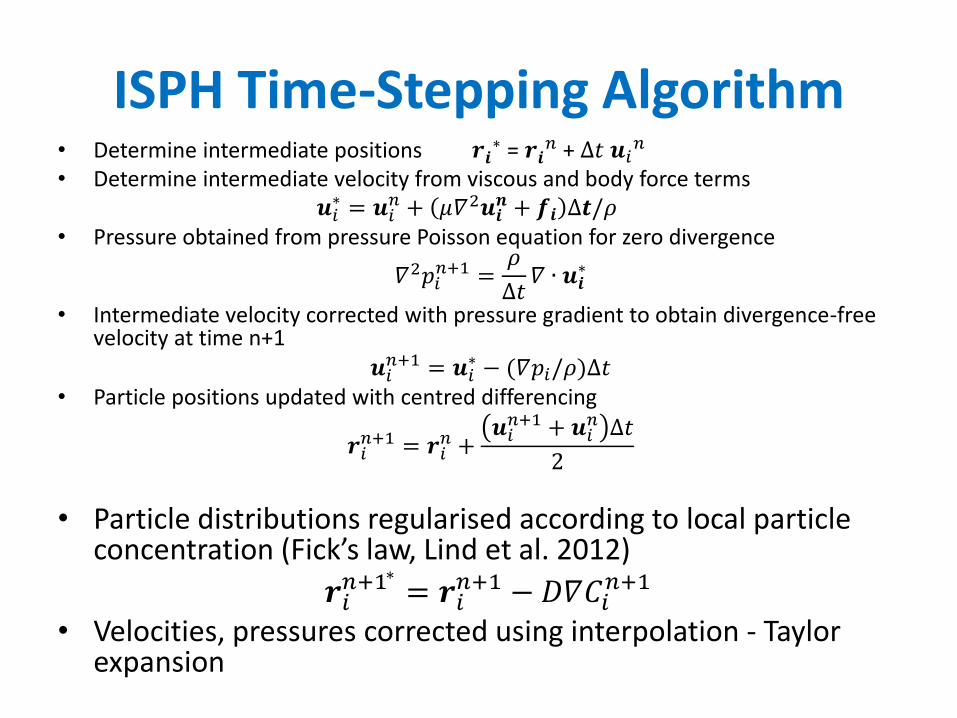
ISPH Time-Stepping Algorithm • Determine intermediate positions 𝒓𝒊
∗ = 𝒓𝒊𝑛 + ∆𝑡 𝒖𝑖
𝑛 • Determine intermediate velocity from viscous and body force terms
𝒖𝑖∗ = 𝒖𝑖
𝑛 + 𝜇𝛻2𝒖𝒊𝒏 + 𝒇𝒊 ∆𝒕/𝜌
• Pressure obtained from pressure Poisson equation for zero divergence
𝛻2𝑝𝑖𝑛+1 =
𝜌
∆𝑡𝛻 ∙ 𝒖𝒊
∗
• Intermediate velocity corrected with pressure gradient to obtain divergence-free velocity at time n+1
𝒖𝑖𝑛+1 = 𝒖𝑖
∗ − (𝛻𝑝𝑖/𝜌)∆𝑡 • Particle positions updated with centred differencing
𝒓𝑖𝑛+1 = 𝒓𝑖
𝑛 +𝒖𝑖𝑛+1 + 𝒖𝑖
𝑛 ∆𝑡
2
• Particle distributions regularised according to local particle concentration (Fick’s law, Lind et al. 2012)
𝒓𝑖𝑛+1∗ = 𝒓𝑖
𝑛+1 − 𝐷𝛻𝐶𝑖𝑛+1
• Velocities, pressures corrected using interpolation - Taylor expansion
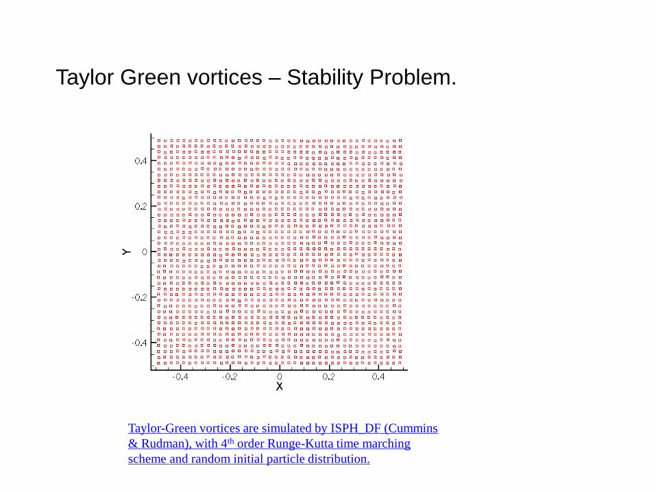
Taylor Green vortices – Stability Problem.
Taylor-Green vortices are simulated by ISPH_DF (Cummins
& Rudman), with 4th order Runge-Kutta time marching
scheme and random initial particle distribution.
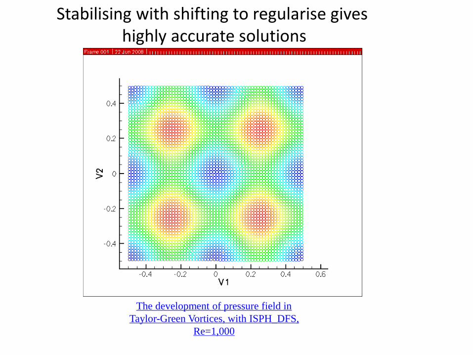
The development of pressure field in
Taylor-Green Vortices, with ISPH_DFS,
Re=1,000
Stabilising with shifting to regularise gives highly accurate solutions

Accuracy and stability tests
• Taylor Green vortices – 2D periodic array,
• lid driven cavity,
• dam breaks,
• impulsive plate,
• wave propagation
Above with analytical or high accuracy solutions
complex SPHERIC test cases
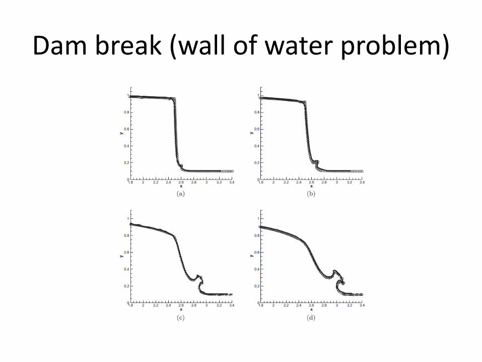
Dam break (wall of water problem)
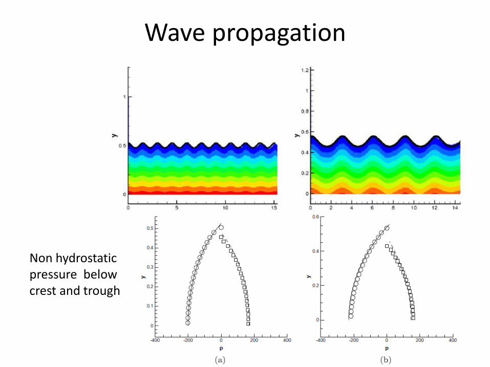
Wave propagation
Non hydrostatic pressure below crest and trough
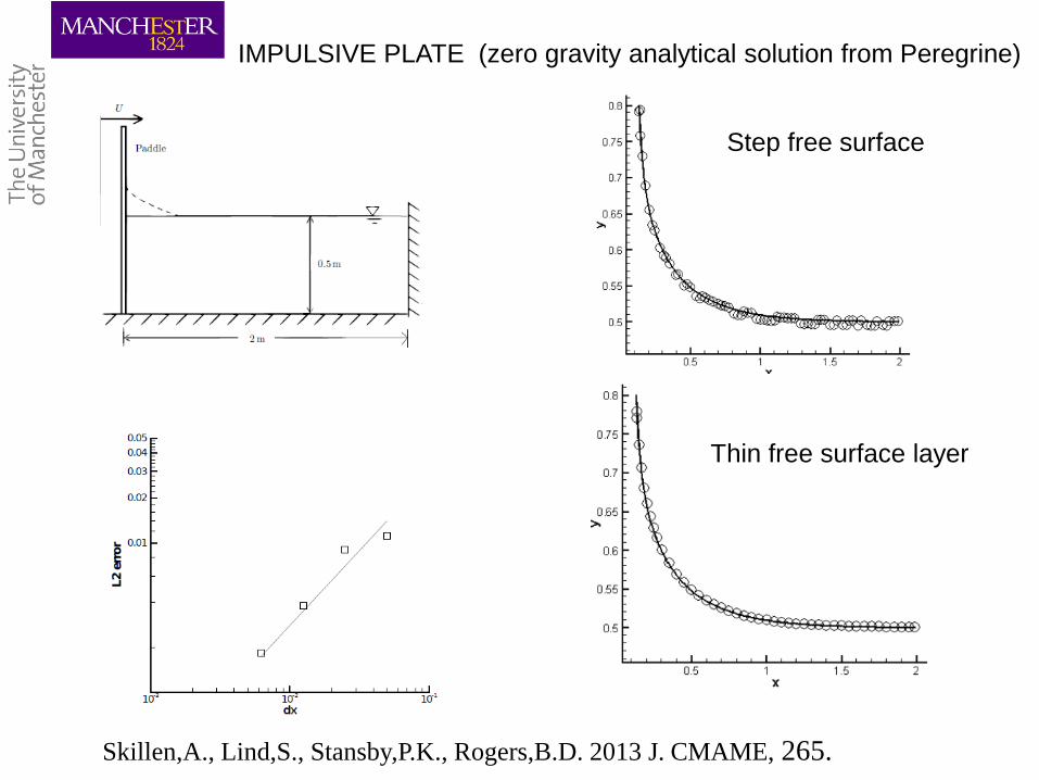
IMPULSIVE PLATE (zero gravity analytical solution from Peregrine)
Step free surface
Thin free surface layer
Skillen,A., Lind,S., Stansby,P.K., Rogers,B.D. 2013 J. CMAME, 265.
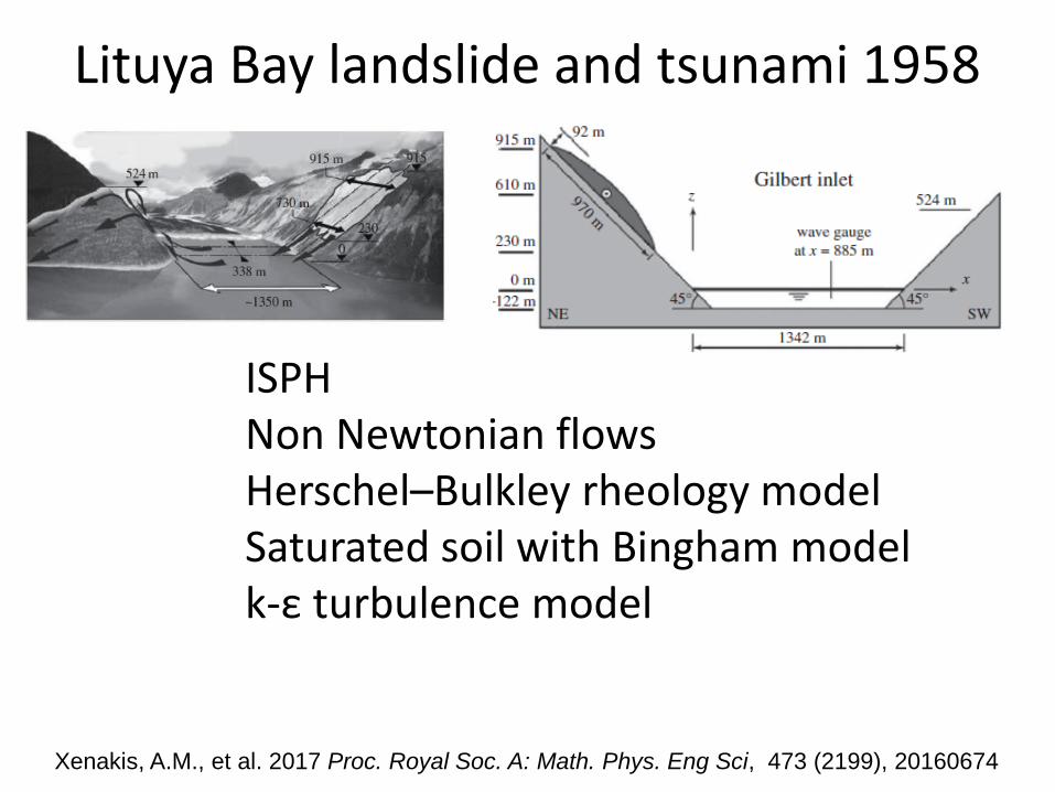
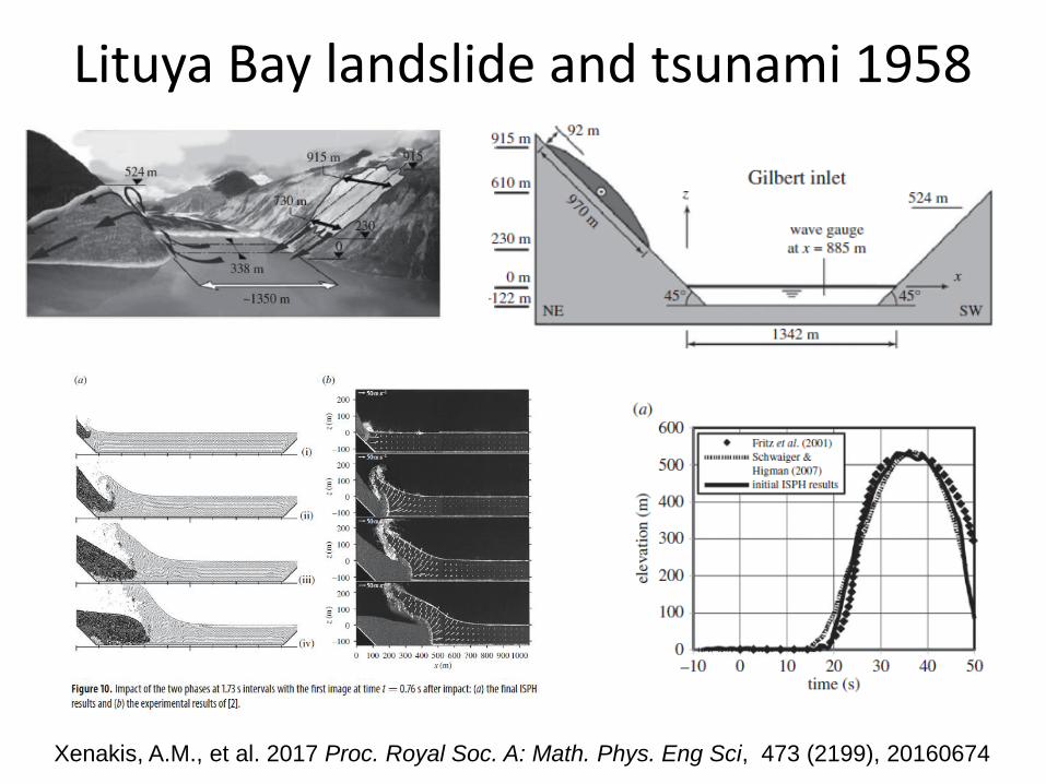
Lituya Bay landslide and tsunami 1958
ISPH Non Newtonian flows Herschel–Bulkley rheology model Saturated soil with Bingham model k-ε turbulence model
Xenakis, A.M., et al. 2017 Proc. Royal Soc. A: Math. Phys. Eng Sci, 473 (2199), 20160674
Lituya Bay landslide and tsunami 1958
Xenakis, A.M., et al. 2017 Proc. Royal Soc. A: Math. Phys. Eng Sci, 473 (2199), 20160674
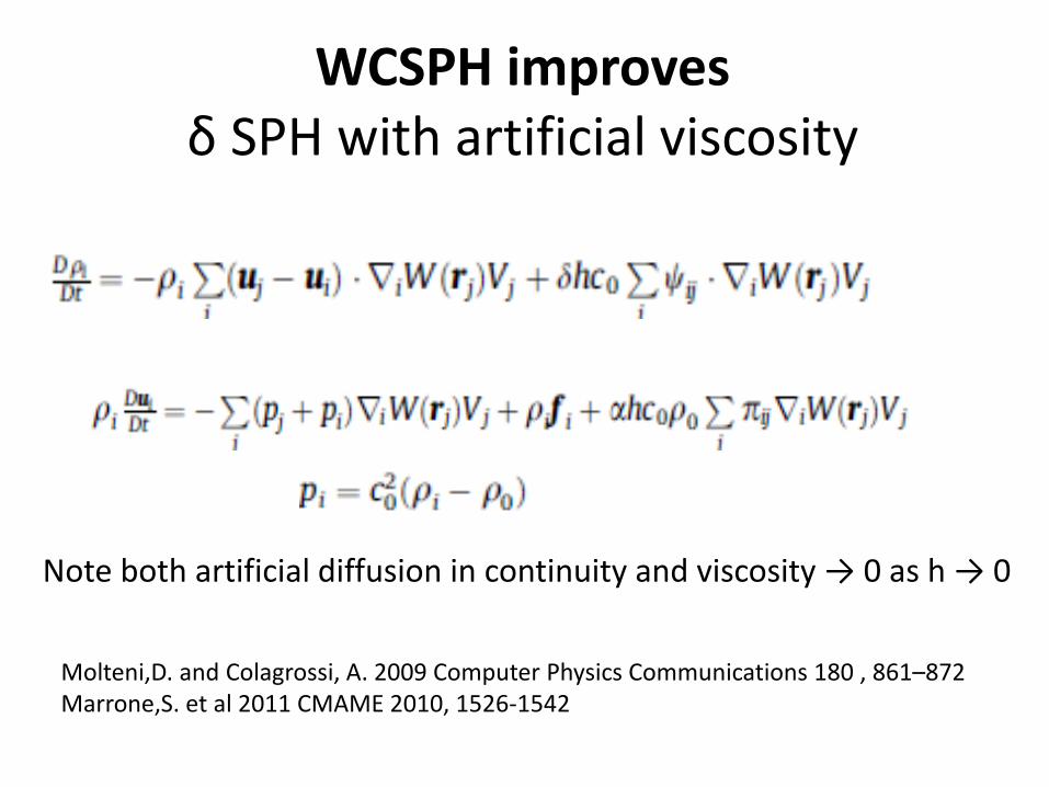
WCSPH improves δ SPH with artificial viscosity
Molteni,D. and Colagrossi, A. 2009 Computer Physics Communications 180 , 861–872 Marrone,S. et al 2011 CMAME 2010, 1526-1542
Note both artificial diffusion in continuity and viscosity → 0 as h → 0
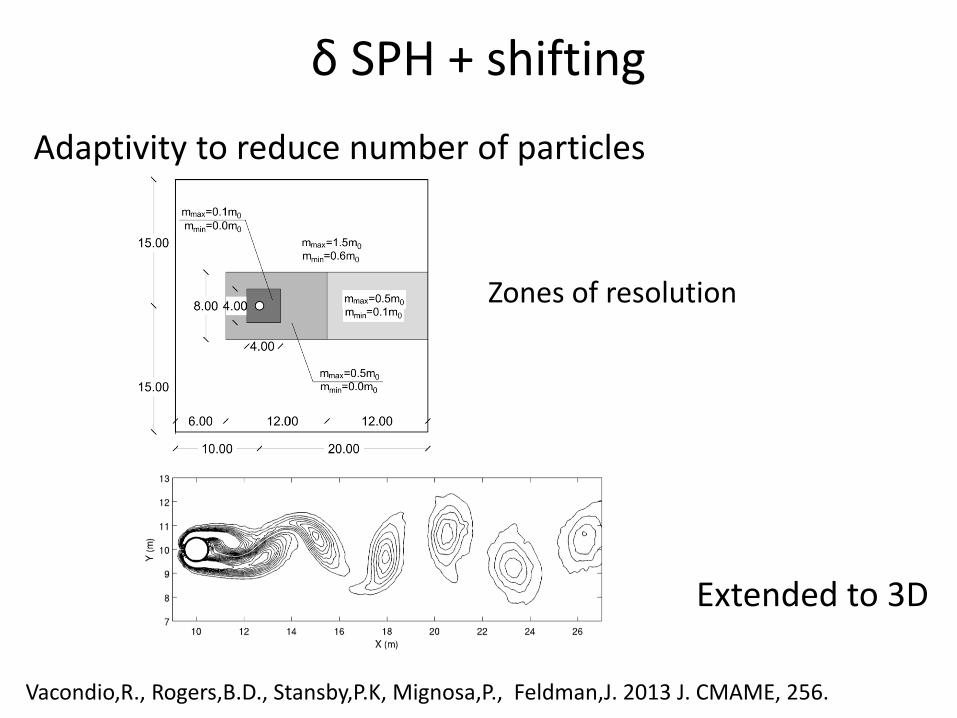
δ SPH + shifting
Adaptivity to reduce number of particles
Vacondio,R., Rogers,B.D., Stansby,P.K, Mignosa,P., Feldman,J. 2013 J. CMAME, 256.
Extended to 3D
Zones of resolution

CD and CL Re=100
Little noise
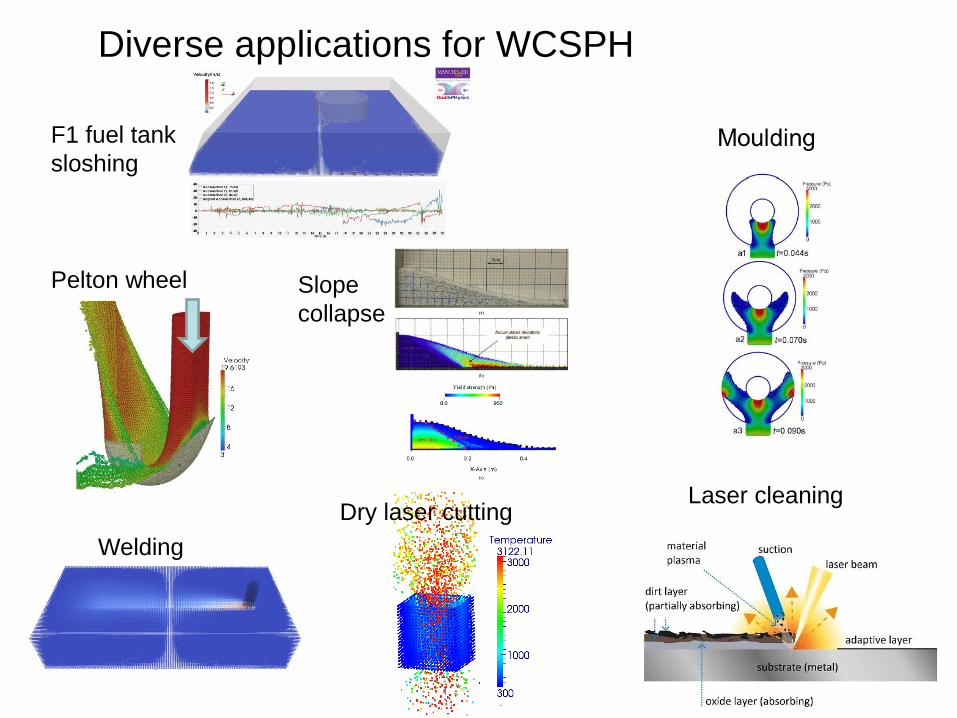
Pelton wheel Slope
collapse
Laser cleaning
Welding
Dry laser cutting
Diverse applications for WCSPH
F1 fuel tank
sloshing
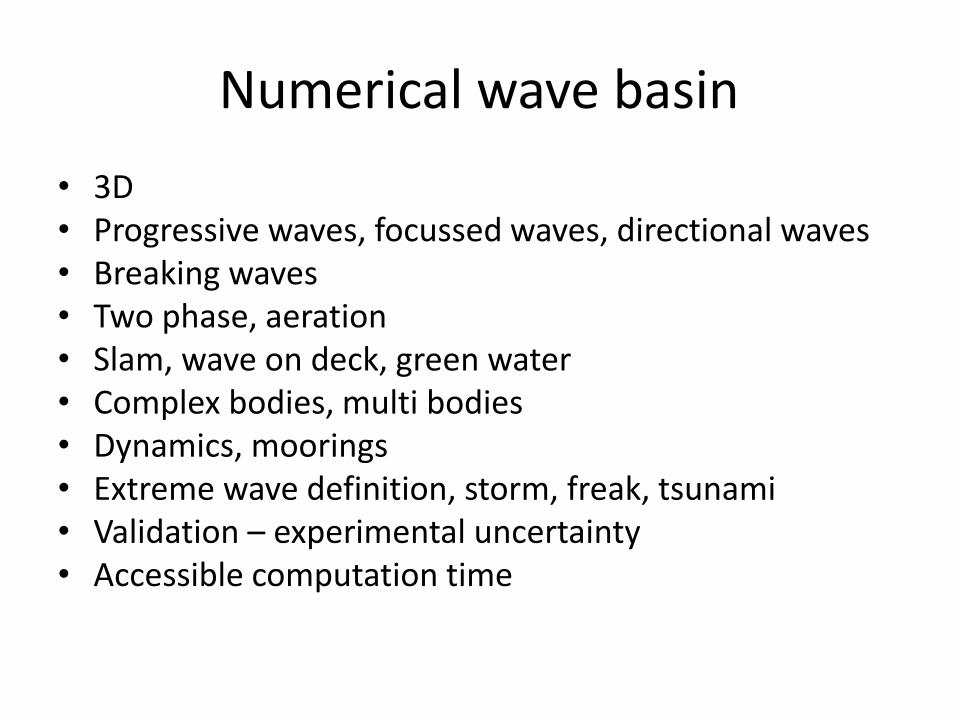
Numerical wave basin
• 3D • Progressive waves, focussed waves, directional waves • Breaking waves • Two phase, aeration • Slam, wave on deck, green water • Complex bodies, multi bodies • Dynamics, moorings • Extreme wave definition, storm, freak, tsunami • Validation – experimental uncertainty • Accessible computation time
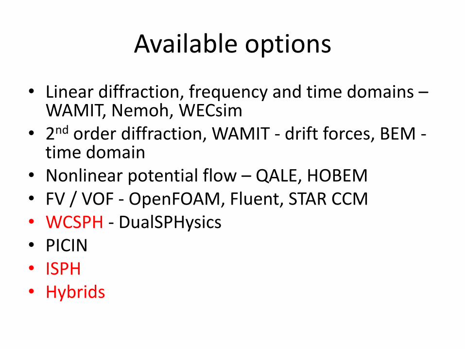
Available options
• Linear diffraction, frequency and time domains – WAMIT, Nemoh, WECsim
• 2nd order diffraction, WAMIT - drift forces, BEM - time domain
• Nonlinear potential flow – QALE, HOBEM • FV / VOF - OpenFOAM, Fluent, STAR CCM • WCSPH - DualSPHysics • PICIN • ISPH • Hybrids
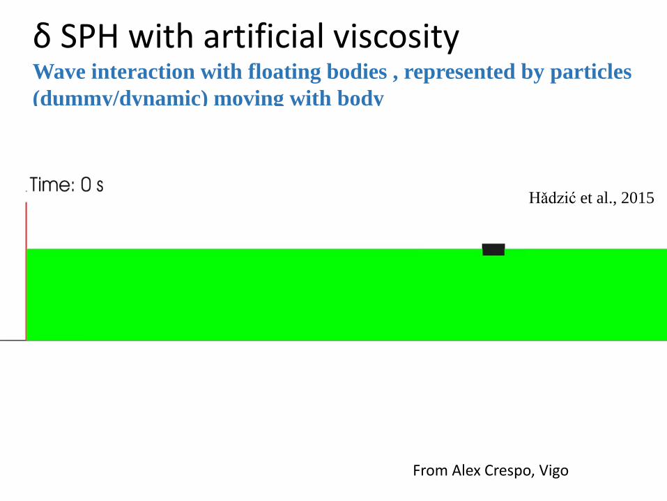
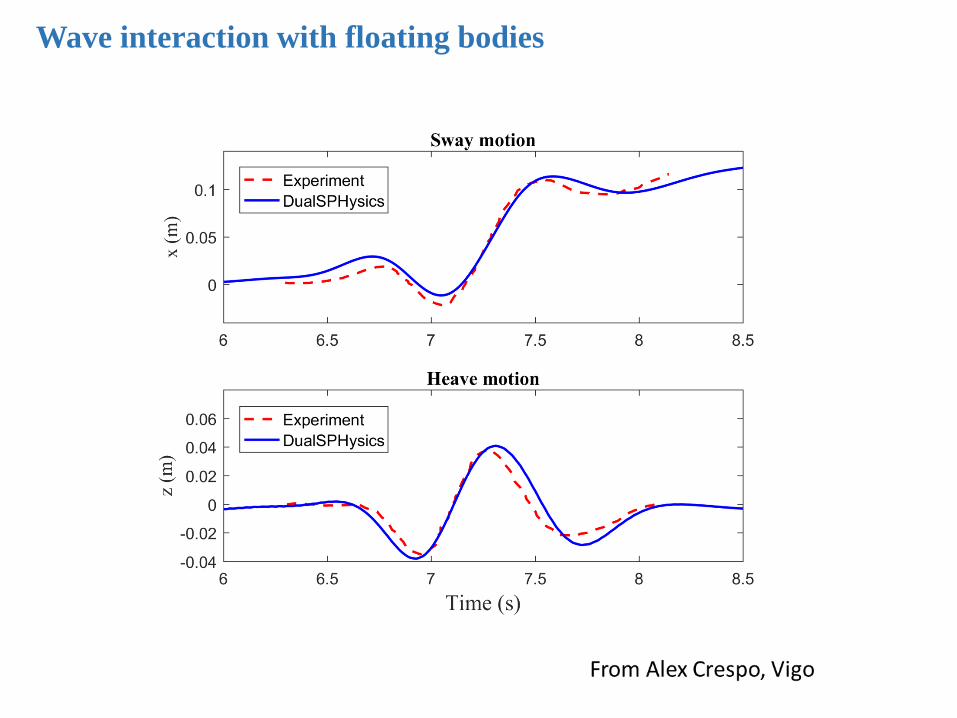
δ SPH with artificial viscosity Wave interaction with floating bodies , represented by particles
(dummy/dynamic) moving with body
Floating body subjected to a wave packet is validated with experimental data
Hadzić et al., 2015
From Alex Crespo, Vigo
Wave interaction with floating bodies
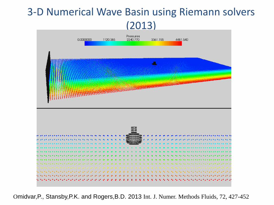
3-D Numerical Wave Basin using Riemann solvers (2013)
Omidvar,P., Stansby,P.K. and Rogers,B.D. 2013 Int. J. Numer. Methods Fluids, 72, 427-452
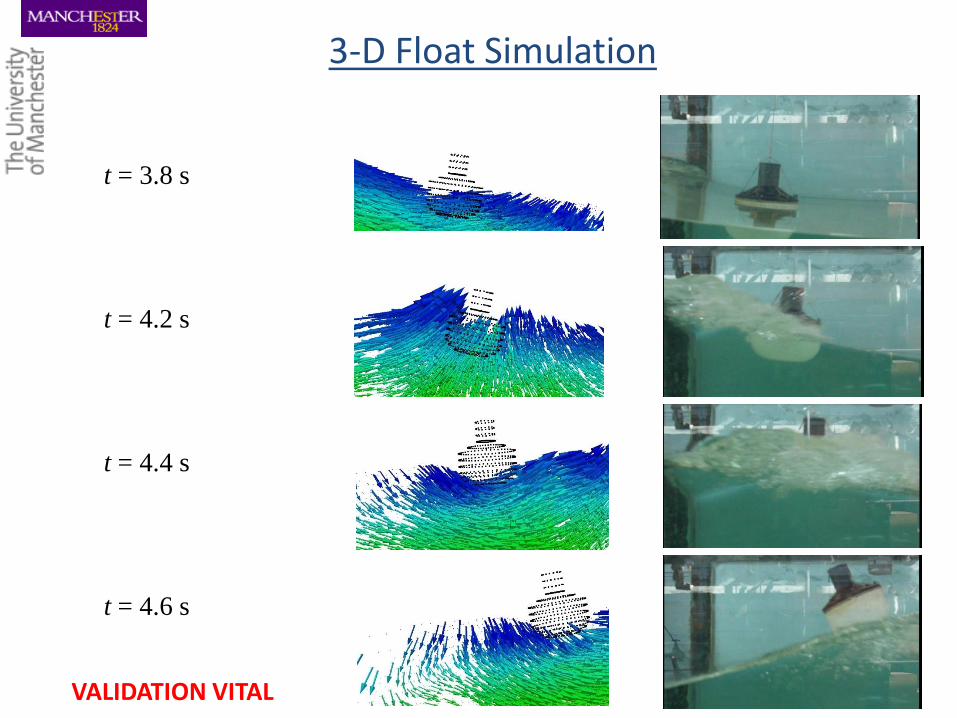
3-D Float Simulation
t = 3.8 s
t = 4.2 s
t = 4.4 s
t = 4.6 s
VALIDATION VITAL
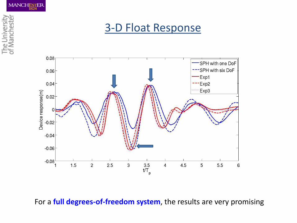
3-D Float Response
For a full degrees-of-freedom system, the results are very promising
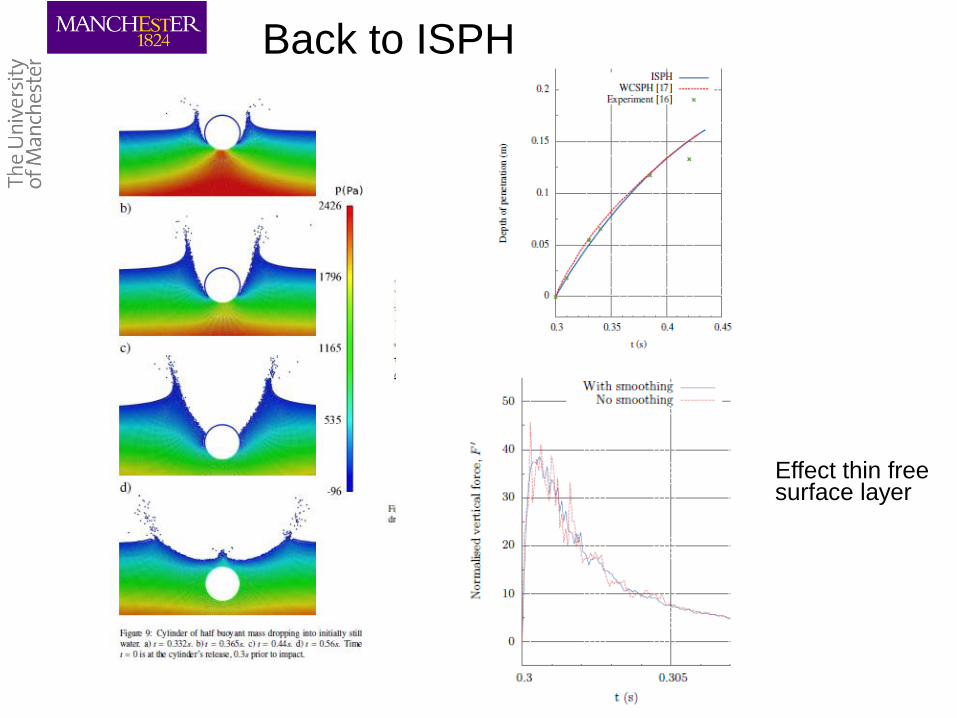
Back to ISPH
Effect thin free surface layer
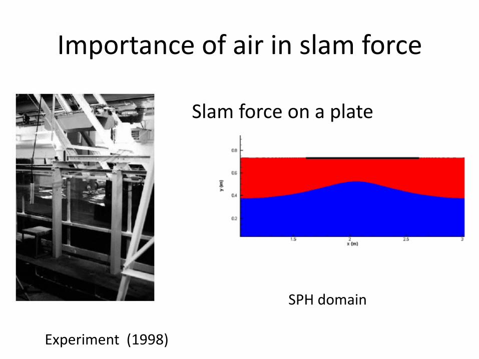
Importance of air in slam force
Experiment (1998)
SPH domain
Slam force on a plate
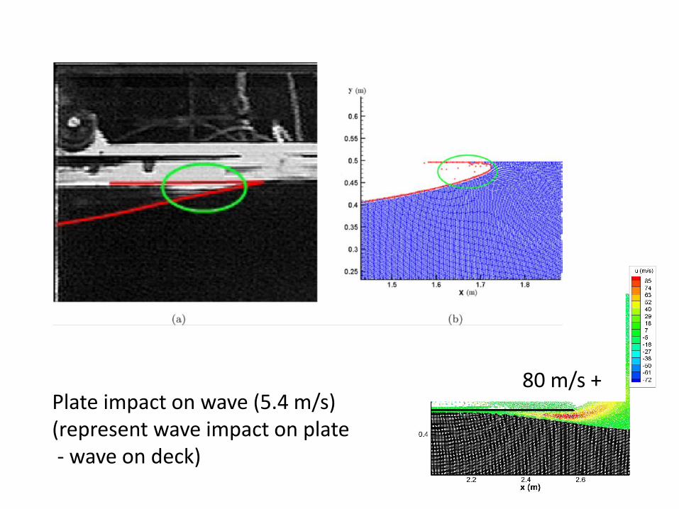
Plate impact on wave (5.4 m/s) (represent wave impact on plate - wave on deck)
80 m/s +

Air – water coupling (ICSPH)
velocity pressure
Lind,S.J., Stansby,P.K., Rogers,B.D., Lloyd, P.M. 2015, Applied Ocean Research, 49, 57-71.
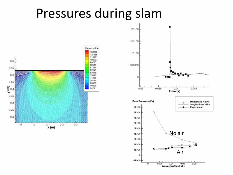
Pressures during slam
No air
Air
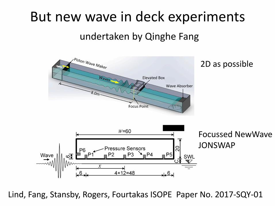
But new wave in deck experiments undertaken by Qinghe Fang
Lind, Fang, Stansby, Rogers, Fourtakas ISOPE Paper No. 2017-SQY-01
2D as possible
Focussed NewWave JONSWAP
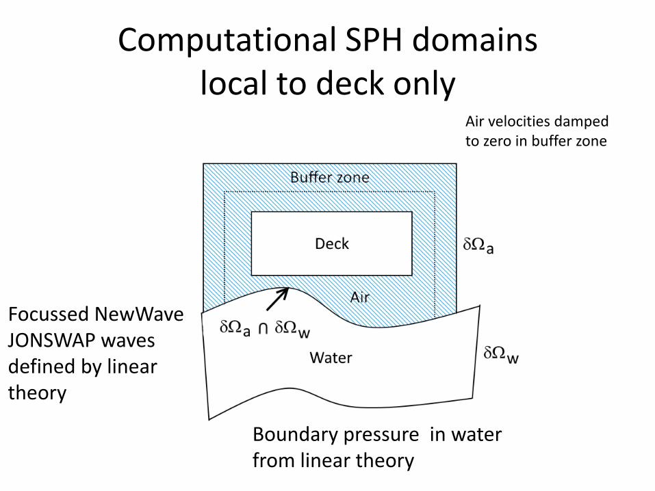
Computational SPH domains local to deck only
Boundary pressure in water from linear theory
Air velocities damped to zero in buffer zone
Focussed NewWave JONSWAP waves defined by linear theory
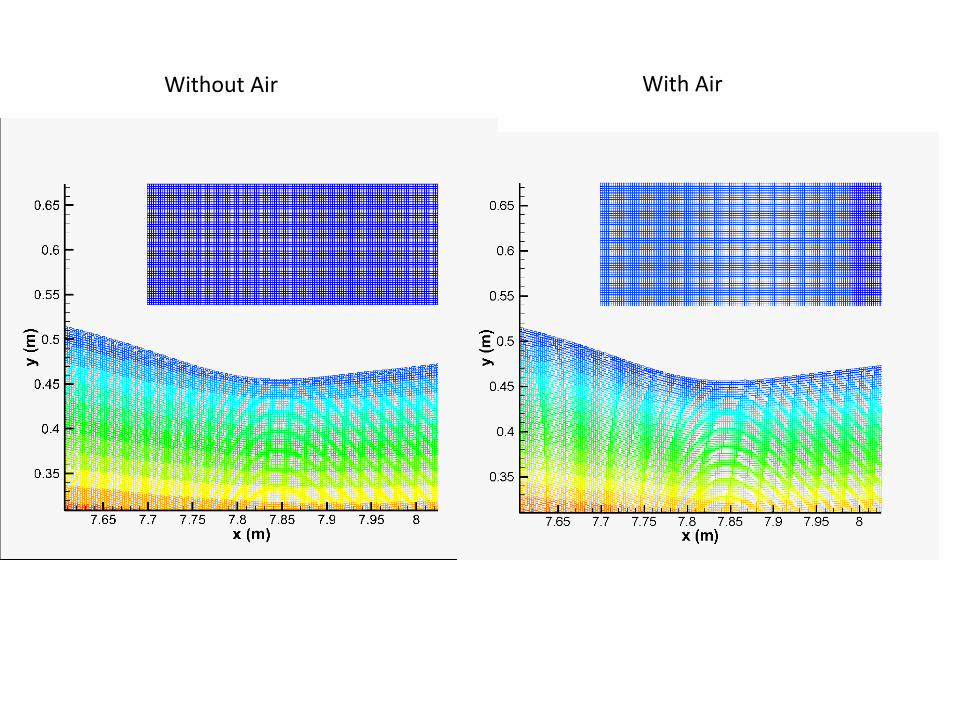
Without Air With Air
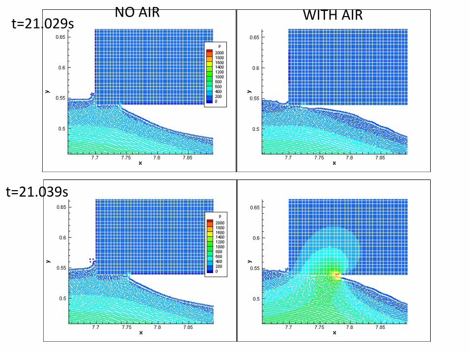
NO AIR WITH AIR t=21.029s
t=21.039s

Preliminary SPH results
dx = 0.00125m dx = 0.025m
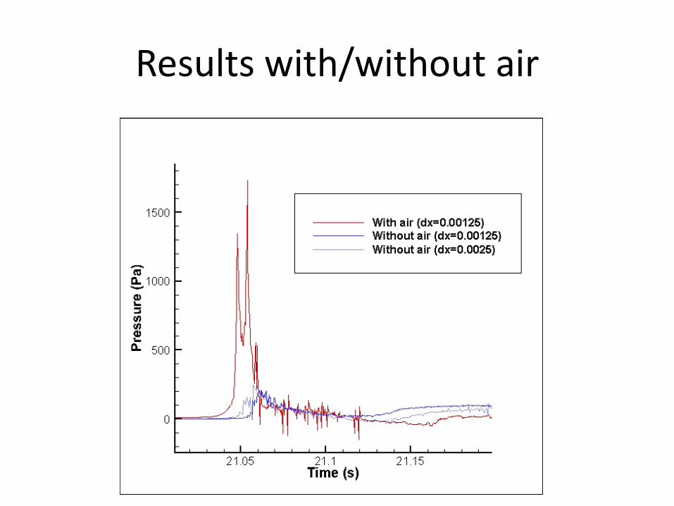
Results with/without air
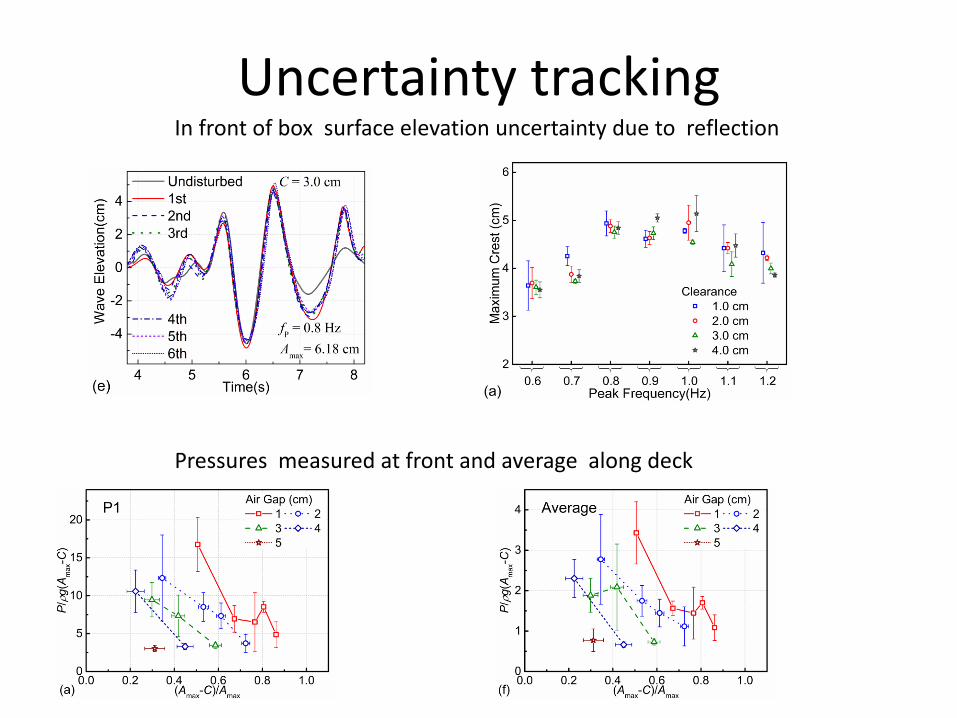
Uncertainty tracking In front of box surface elevation uncertainty due to reflection
Pressures measured at front and average along deck
Froude Krylov approximate method for extreme
inertia loading : useful fast solution
• Froude Krylov force may be accurately modelled , including breaking waves
• Added mass approximated from potential flow
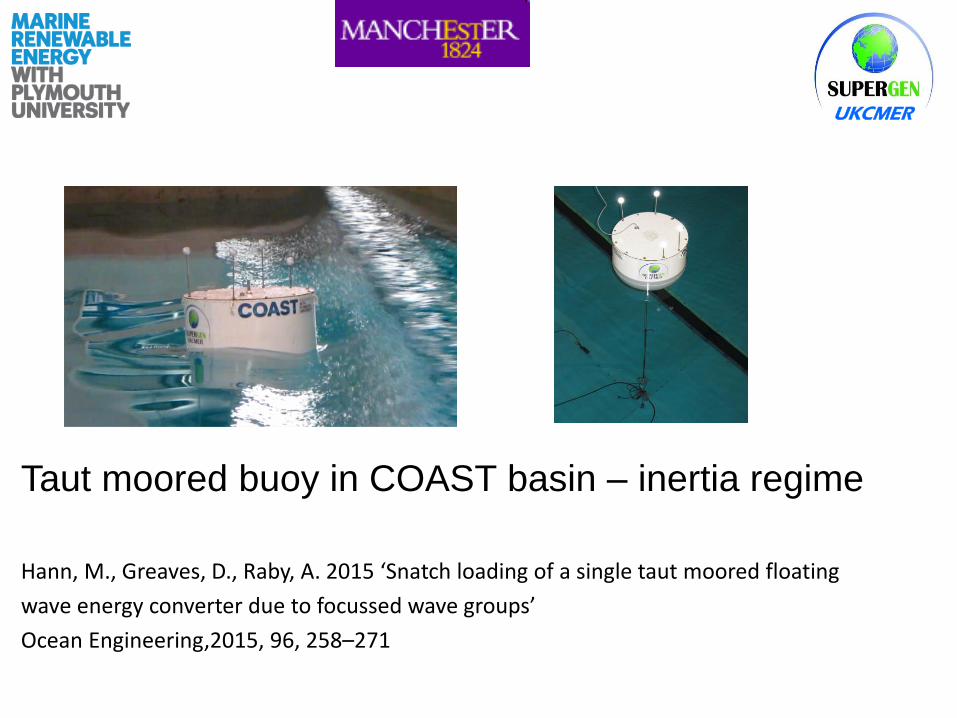
Taut moored buoy in COAST basin – inertia regime
Hann, M., Greaves, D., Raby, A. 2015 ‘Snatch loading of a single taut moored floating
wave energy converter due to focussed wave groups’
Ocean Engineering,2015, 96, 258–271
UKCMER
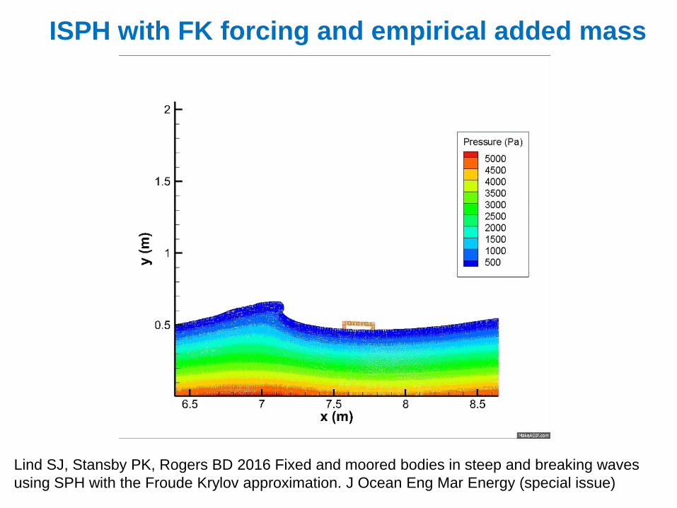
ISPH with FK forcing and empirical added mass
Lind SJ, Stansby PK, Rogers BD 2016 Fixed and moored bodies in steep and breaking waves
using SPH with the Froude Krylov approximation. J Ocean Eng Mar Energy (special issue)
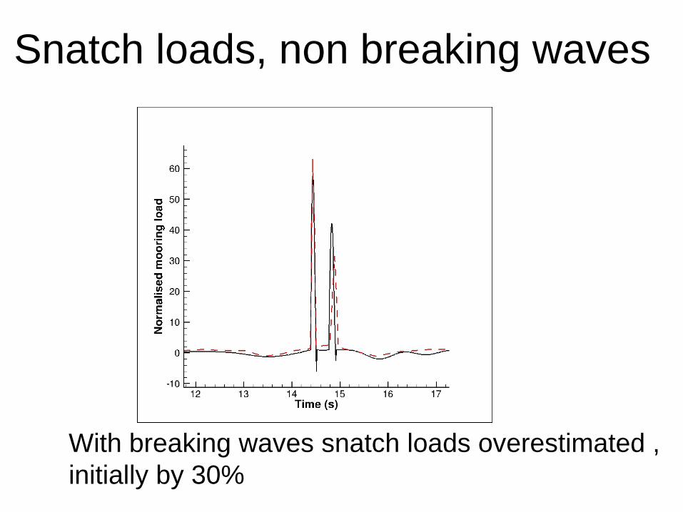
Snatch loads, non breaking waves
With breaking waves snatch loads overestimated ,
initially by 30%
Hybrid coupled schemes to reduce computation time
• Adaptivity (Parma, UoM)
• FV – SPH (Nantes/Rome)
• Eulerian – Lagrangian SPH (UoM)
• Boussinesq – SPH (UoM, Paris)
• QALE-SPH (UoM, City)
ISOPE-2017 San Francisco Conference The 27th International Ocean and Polar Engineering Conference
San Francisco, California, June 25−30, 2017: www.isope.org
On the coupling of Incompressible SPH with
a Finite Element potential flow solver for
nonlinear free surface flows
G. Fourtakas*, B. D. Rogers, P. Stansby
and S. Lind
School of Mechanical, Aerospace and Civil
Engineering,
University of Manchester
Manchester, UK
S. Yan, Q.W. Ma
School of Engineering and Mathematical
Sciences
City University of London
London, UK
ISOPE-2017
San Francisco
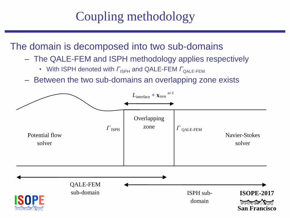
Coupling methodology
The domain is decomposed into two sub-domains
– The QALE-FEM and ISPH methodology applies respectively
• With ISPH denoted with ΓISPH and QALE-FEM ΓQALE-FEM
– Between the two sub-domains an overlapping zone exists
Γ QALE-FEM Γ ISPH
Potential flow
solver
Navier-Stokes
solver
QALE-FEM
sub-domain ISPH sub-
domain
Overlapping
zone
Linterface + xISPH n+1
ISOPE-2017
San Francisco
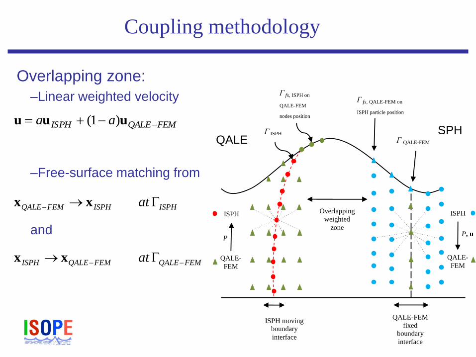
Coupling methodology
Overlapping zone: –Linear weighted velocity
–Free-surface matching from
and
FEMQALEISPH aa uuu )1(
ISPHISPHFEMQALE at xx
FEMQALEFEMQALEISPH at xx
ISPH
QALE-
FEM
P, u
Γ ISPH
Γ QALE-FEM
ISPH
QALE-FEM
fixed boundary
interface
Overlapping
weighted
zone
Γ fs, ISPH on
QALE-FEM
nodes position
Γ fs, QALE-FEM on
ISPH particle position
ISPH moving boundary
interface
QALE-
FEM
P
QALE SPH
ISOPE-2017
San Francisco
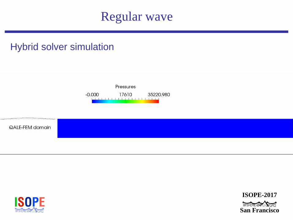
Regular wave
Hybrid solver simulation
ISOPE-2017
San Francisco
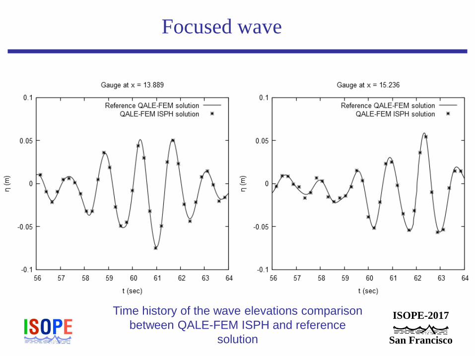
Focused wave
Time history of the wave elevations comparison
between QALE-FEM ISPH and reference
solution
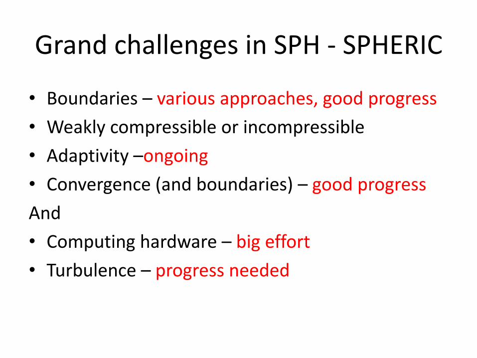
Grand challenges in SPH - SPHERIC
• Boundaries – various approaches, good progress
• Weakly compressible or incompressible
• Adaptivity –ongoing
• Convergence (and boundaries) – good progress
And
• Computing hardware – big effort
• Turbulence – progress needed
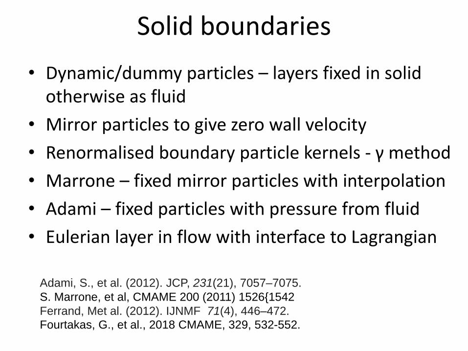
Solid boundaries
• Dynamic/dummy particles – layers fixed in solid otherwise as fluid
• Mirror particles to give zero wall velocity
• Renormalised boundary particle kernels - γ method
• Marrone – fixed mirror particles with interpolation
• Adami – fixed particles with pressure from fluid
• Eulerian layer in flow with interface to Lagrangian
Adami, S., et al. (2012). JCP, 231(21), 7057–7075.
S. Marrone, et al, CMAME 200 (2011) 1526{1542
Ferrand, Met al. (2012). IJNMF 71(4), 446–472.
Fourtakas, G., et al., 2018 CMAME, 329, 532-552.

Accuracy for general SPH solver
Is higher order possible? Presently ~ 1.5
Affected by
• Interpolation error (kernel)
• Discretisation error (particle spacing)
• Particle distribution (uniform is best)
• Boundary condition (requires zero velocity)
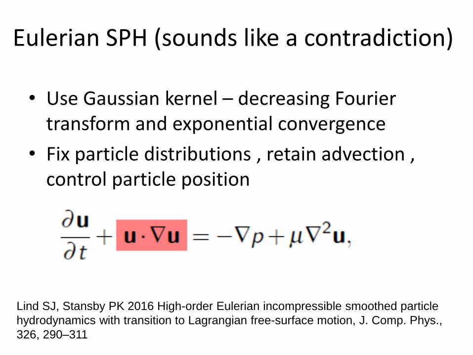
• Use Gaussian kernel – decreasing Fourier transform and exponential convergence
• Fix particle distributions , retain advection , control particle position
Eulerian SPH (sounds like a contradiction)
Lind SJ, Stansby PK 2016 High-order Eulerian incompressible smoothed particle
hydrodynamics with transition to Lagrangian free-surface motion, J. Comp. Phys.,
326, 290–311
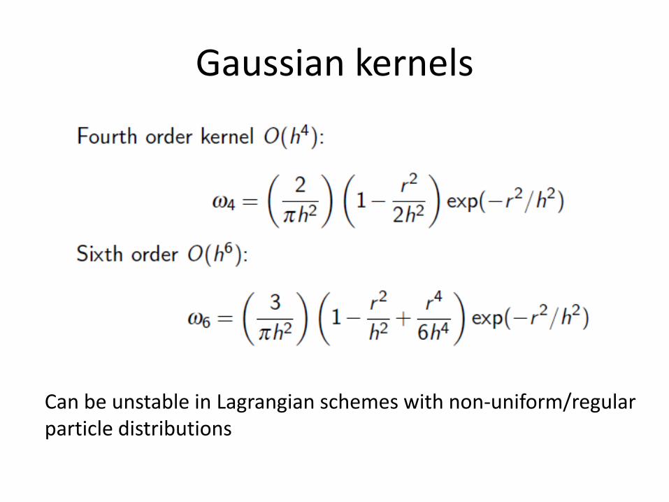
Can be unstable in Lagrangian schemes with non-uniform/regular particle distributions
Gaussian kernels
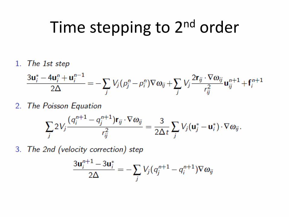
Time stepping to 2nd order
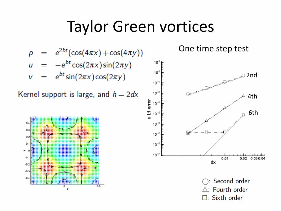
Taylor Green vortices One time step test
2nd
4th
6th

Errors at t=0.1
Ideal convergence recovered with small time steps and solver convergence Compares well with high order finite difference
2nd
4th
6th

Accuracy with small number particles Lid driven cavity example
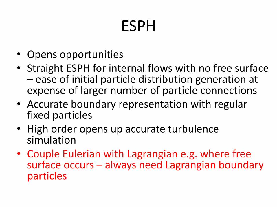
ESPH
• Opens opportunities • Straight ESPH for internal flows with no free surface
– ease of initial particle distribution generation at expense of larger number of particle connections
• Accurate boundary representation with regular fixed particles
• High order opens up accurate turbulence simulation
• Couple Eulerian with Lagrangian e.g. where free surface occurs – always need Lagrangian boundary particles
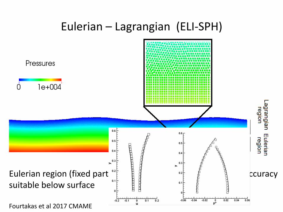
Eulerian – Lagrangian (ELI-SPH)
Eulerian region (fixed particles) efficient and of arbitrary high accuracy suitable below surface Fourtakas et al 2017 CMAME
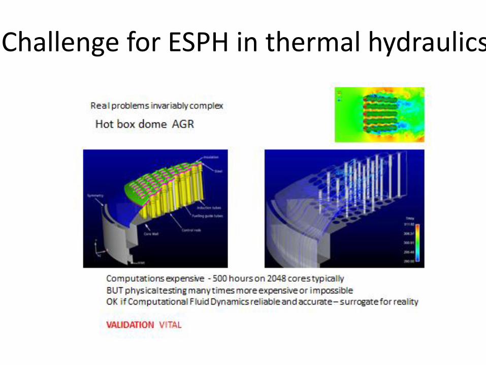
Challenge for ESPH in thermal hydraulics
ISPH speedup
• Particle adaptivity – coalescing/splitting (Renato Vacondio
Parma, UoM)
• MPC – 108 particles , PetSC Poisson solver, Zoltan library,
Hilbert space filling curve, 12000 partitions with MPI,
typically 40% efficient, petascale computing
(Xiaohu Guo STFC, UoM)
• GPU – DualSPHysics+ViennaCL for PPE (Alex Chow UoM)
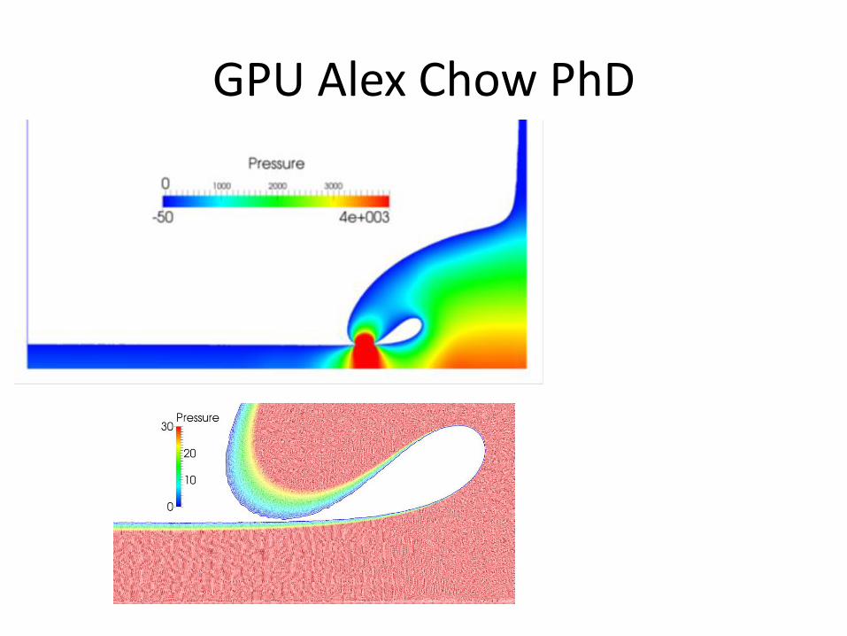
GPU Alex Chow PhD
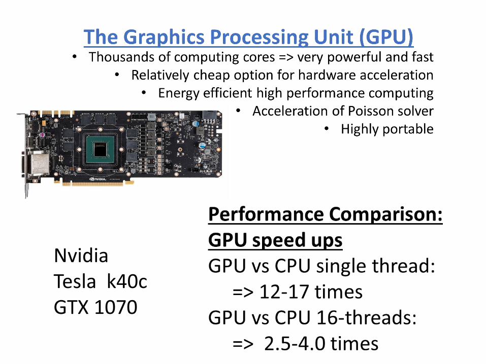
Nvidia Tesla k40c GTX 1070
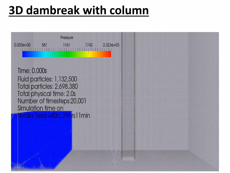
3D dambreak with column
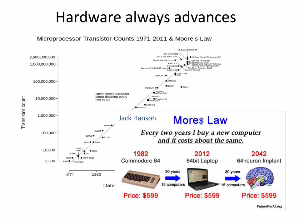
Hardware always advances
Jack Hanson

How is hardware accelerating?
• Today GPUs – multi-GPUs, MPC - petascale
• Tomorrow - exascale , Tensor Processing Units
• FPGAs – ‘field programmable gate array’
• With quantum computing, graphene, nanotubes etc speed massive exoscale +++
• But occasional faults possible – need fault tolerant algorithms – SPH with multiple particle connections potentially suited
• Need to plan algorithms for hardware
What are we doing tomorrow ?
• 3D hybrid QALE – ISPH
• Include two phase formulation
• ESPH to high order for thermal hydraulics

Thanks for your attention
and questions