University of Groningen

The Simulation of Violent Free-Surface Dynamics at Sea and in SpaceVeldman, Arthur E.P.

Published in:EPRINTS-BOOK-TITLE

IMPORTANT NOTE: You are advised to consult the publisher's version (publisher's PDF) if you wish to cite fromit. Please check the document version below.

Document VersionPublisher's PDF, also known as Version of record

Publication date:2006

Link to publication in University of Groningen/UMCG research database

Citation for published version (APA):Veldman, A. E. P. (2006). The Simulation of Violent Free-Surface Dynamics at Sea and in Space. InEPRINTS-BOOK-TITLE University of Groningen, Johann Bernoulli Institute for Mathematics and ComputerScience.

CopyrightOther than for strictly personal use, it is not permitted to download or to forward/distribute the text or part of it without the consent of theauthor(s) and/or copyright holder(s), unless the work is under an open content license (like Creative Commons).

The publication may also be distributed here under the terms of Article 25fa of the Dutch Copyright Act, indicated by the “Taverne” license.More information can be found on the University of Groningen website: https://www.rug.nl/library/open-access/self-archiving-pure/taverne-amendment.

Take-down policyIf you believe that this document breaches copyright please contact us providing details, and we will remove access to the work immediatelyand investigate your claim.

Downloaded from the University of Groningen/UMCG research database (Pure): http://www.rug.nl/research/portal. For technical reasons thenumber of authors shown on this cover page is limited to 10 maximum.

Download date: 23-03-2022

European Conference on Computational Fluid DynamicsECCOMAS CFD 2006

P. Wesseling, E. Onate and J. Periaux (Eds)c© TU Delft, The Netherlands, 2006

THE SIMULATION OF VIOLENT FREE-SURFACEDYNAMICS AT SEA AND IN SPACE

Arthur E.P. Veldman∗

∗Institute of Mathematics and Computing Science, University of GroningenP.O. Box 800, 9700AV Groningen, The Netherlands

e-mail: veldman@math.rug.nlweb page: http://www.math.rug.nl/∼veldman/

Key words: Free-surface flow, Nonlinear waves, Green water, Dambreak flow, Sloshing,Spacecraft dynamics

Abstract. Non-linear free-surface phenomena, such as extreme waves and violent slosh-ing, and their impact on the dynamics response of the containing vessels have long beensubjects that could only be studied with experimental methods. Nowadays, computationalCFD tools can make a significant contribution to these flow problems. The paper startswith a short overview of the most popular numerical methods to simulate highly non-linearfree-surface phenomena, with emphasis on Navier–Stokes methods. Thereafter, it describesthe development efforts made in the maritime SAFE-FLOW project and the micro-gravitySloshSat FLEVO project. In particular, the improved Volume-of-Fluid (iVOF) free-surfacesimulation method ComFlo is presented. Examples of violent fluid dynamics in both ap-plication areas are presented. In all cases experimental data are available to validate theoutcome of the calculations.

1 INTRODUCTION

Every-day life shows many examples of free-surface flow: the glass of wine you like tosip or the beautiful surf along the shore in a light sea breeze, to name but a few. However,these flows can also be less romantic, e.g. when the light breeze has strengthened to aheavy storm. In such weather conditions waves can become quite extreme and dangerous.For example, large quantities of ‘green’ water can come onto the deck of floating andmoored structures, presenting a real hazard for both the well-being of the crew and theintegrity of the structure1.

Over the years, several incidents with serious damage have been reported. For instance,in January 2000 the living quarters on the bow of the Varg FPSO were hit by green water,resulting in the damage of a window at the second floor, and flooding the area behind it(Fig. 1). The vessel was out of operation for a number of days. Another example is waveimpact damage to the bow of the Schiehallion FPSO in 1998, resulting in an evacuationof the personnel and expensive hull repairs including redesign2.

1

Arthur E.P. Veldman

Figure 1: Left: Damage and first repair of a window on the Varg FPSO. Right: Artist impression of theNEAR spacecraft.

But also away from our ‘blue planet’ liquid motion can seriously endanger operations.Everyone over 40 years old will remember the first lunar landing of the Apollo 11 mission.Less well known (but good visible in the video footage) is that shortly before the actuallanding, sloshing of the remaining fuel caused an oscillatory motion of the Lunar Module(of about 2-3 degrees), which seriously hampered a safe landing manoeuvre3. Anotherwell-documented example is the NEAR (Near Earth Asteroid Rendezvous) mission, wherea spacecraft was sent to closely fly-by the Eros asteroid. During the final course correctionthe spacecraft experienced unexpected motion and went into a safety mode. Groundcontrol was ultimately able to recover the mission, although at the cost of a 13-monthdelay of the intended rendezvous. Again fuel slosh was named as the probable cause4.

Thus far, existing analysis methods for free-surface motion largely depend on the ap-plication of linear potential flow theory. The physical phenomena accompanying extremeevents are highly nonlinear, however, and require new methods as a basis for predictionof the behavior of the water flow. Thus, the desire for simulating complex free-surfaceproblems like slamming, sloshing and the green water phenomenon has been present fora long time5–7.

The author’s research group is involved in a number of projects where the above flowphenomena are studied. Since the late 1970s, together with the National AerospaceLaboratory NLR, theoretical studies are carried out to investigate liquid sloshing on boardspacecraft8–12. This research has culminated in the design, construction and actual flightof Sloshsat FLEVO, a facility for liquid experimentation in orbit13. The project was ledby NLR and sponsored by national and international agencies. In the maritime area,the cooperation with MARIN has to be mentioned, leading to the SAFE-FLOW andComFLOW-2 joint-industry projects. In the present paper we will describe some issuesrelated to the computational modelling of violent free-surface motion in the projectsmentioned.

The mathematical model for complex water flow dates from the first half of the 19thcentury already, known as the Navier–Stokes equations. However, it is only for a decadethat these field equations can be solved for large scale complex free-surface flow problems,thanks to novel numerical algorithms and the increase in computer power. This is an

2

Arthur E.P. Veldman

important development; in the near future it should provide, besides model testing, anadditional tool for design problems involving these types of flows. This numerical tool isrelatively cheap (in comparison with the costs of experimental facilities), therefore it canbe used in an early stage of the design process.

The paper will give an impression of the state-of-the art of hydrodynamical methodsfor describing extremely nonlinear flow. It begins with a short overview of the existingbasic methods for complex free-surface flows. Thereafter, the potential is demonstratedof the ComFlo simulation method, which was developed during the above-mentionedcooperations. It is based on the Volume-of-Fluid (VOF) technique, developed by Hirtand Nichols14. A number of improvements were found necessary to overcome the weakpoints of the VOF approach; these are discussed further on in the paper. Originally themethod was developed to simulate sloshing liquid on board spacecraft11,12,15–17; in thisenvironment capillary forces and contact line dynamics can be quite influential. Later themethod was extended to cover applications in maritime engineering18–20 and biomedicalapplications21,22. Several types of simulations are presented. In the maritime area we showa dambreak flow and a ‘green water’ event; as an ‘extra-terrestrial’ example one of theSloshsat FLEVO manoeuvres is presented. In all examples comparison with experimentaldata is included.

2 METHODS FOR FREE-SURFACE FLOW

To treat dynamically changing, arbitrary liquid configurations a large amount of flex-ibility has to be present in the numerical approach. It is no longer sufficient to apply aboundary-element philosophy23,24, but instead a field method has to be used, includinga ‘bookkeeping’ system for tracking the position of the liquid and its free surface25. Inthe literature a number of approaches can be found, of which a short assessment will begiven next. A subdivision into three types of methods will be made: fixed-grid methods,moving-grid methods and gridless methods.

2.1 Fixed-grid methods

A fixed (or Eulerian) grid to discretise the mathematical model greatly reduces thegrid generation effort. However, because the grid is not adapted to the boundaries andfree surface, special attention must be paid to capture the position of the free surfaceand to the implementation of boundary conditions. When an appropriate free-surfacetracking/capturing method is used, like Marker-and-Cell (MAC), Volume of Fluid (VOF)or level set, large free-surface deformations can be handled, including fluid splitting andfluid merging.

MAC and VOF The Marker-and-Cell (MAC) method is the ‘father’ of all free-surfaceflow methods26, and makes use of massless particles to keep track of the liquid region.Accuracy requires a considerable amount of particles per grid cell, making the method

3

Arthur E.P. Veldman

computationally expensive, especially in 3D. A cheaper way is to apply only surfacemarkers27, but now splitting and merging of the surface are difficult to handle. The MACfollow up is the Volume-of-Fluid (VOF)14. Here a discrete indicator (or color) functionis used that corresponds to the cell volume occupied by fluid. Although the originalversion of the reconstruction and displacement algorithm leads to considerable ‘flotsam’and ‘jetsam’, i.e. artificial drops that numerically pinch off, variants can be designed thatcan track an arbitrarily moving free surface with high reliability28,29. A powerful variantis the piecewise linear reconstruction method (PLIC) introduced by Youngs30. Anothersuccessful member of this family is the CIP method31. An important property of VOF-type methods, resulting from its finite-volume philosophy, is the exact conservation of theamount of liquid present. Various maritime applications of VOF can be mentioned32–34.

Level set An alternative to the indicator-function methods is the level set method35,which makes use of a function representing the distance to the liquid surface. Reconstruc-tion of the free surface is conceptually simpler than with the VOF method. However, forviolently moving free surfaces the level set function requires to be redefined regularly,and conservation of the amount of liquid cannot be guaranteed36. Therefore, level setapplications mainly focus on relative calm flows, like the steady wave field around shiphulls37–39. To reduce mass loss, the level set method is sometimes combined with the VOFmethod40,41.

2.2 Moving-grid methods

In moving-grid methods, also known as ALE (Arbitrary Lagrangian Eulerian) meth-ods42, each time step the grid is fitted to the moving free surface in a Lagrangian manner.Their advantage is that the boundaries are well defined, making it easy to apply bound-ary conditions43. However, when the free surface undergoes large deformation, splits ormerges, these methods suffer great problems. This makes them less suitable for applica-tions involving complex free-surface flows.

2.3 Gridless methods

Gridless methods represent the fluid by a large number of particles. In principle thismakes them good methods for problems with large free surface deformations, fluid splittingand fluid merging. The smoothed particle hydrodynamics (SPH) method is an exampleof such a gridless method. Introduced by Monaghan in an astrophysical context, laterapplications include the splashing of breaking waves44, the dam breaking problem45–47,and the response of floating structures48. The application of SPH to fluid dynamicsis very young and the method is quite different from other methods, therefore little isknown about appropriate numerical boundary conditions (e.g. non-reflecting conditions)and required computational effort (which is still quite large because many particles andsmall time steps should be used).

4

Arthur E.P. Veldman

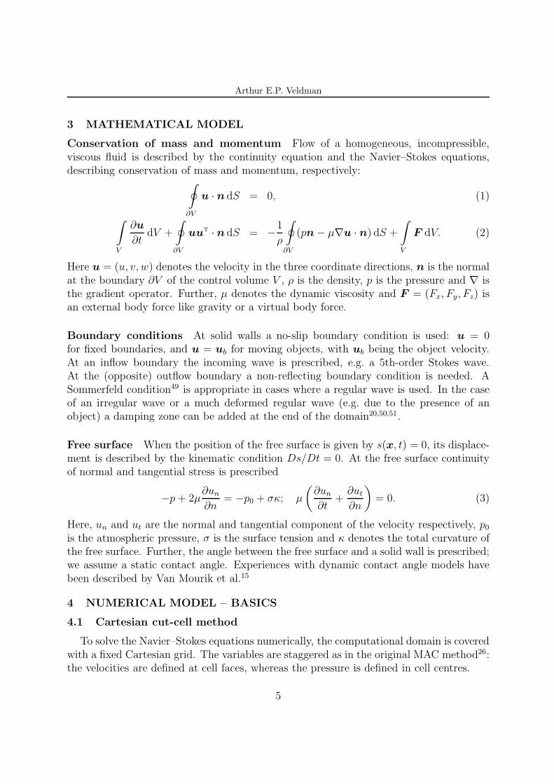
3 MATHEMATICAL MODEL

Conservation of mass and momentum Flow of a homogeneous, incompressible,viscous fluid is described by the continuity equation and the Navier–Stokes equations,describing conservation of mass and momentum, respectively:

∮

∂V

u · n dS = 0, (1)

∫

V

∂u

∂tdV +

∮

∂V

uuT · n dS = −1

ρ

∮

∂V

(pn − µ∇u · n) dS +

∫

V

F dV. (2)

Here u = (u, v, w) denotes the velocity in the three coordinate directions, n is the normalat the boundary ∂V of the control volume V , ρ is the density, p is the pressure and ∇ isthe gradient operator. Further, µ denotes the dynamic viscosity and F = (Fx, Fy, Fz) isan external body force like gravity or a virtual body force.

Boundary conditions At solid walls a no-slip boundary condition is used: u = 0for fixed boundaries, and u = ub for moving objects, with ub being the object velocity.At an inflow boundary the incoming wave is prescribed, e.g. a 5th-order Stokes wave.At the (opposite) outflow boundary a non-reflecting boundary condition is needed. ASommerfeld condition49 is appropriate in cases where a regular wave is used. In the caseof an irregular wave or a much deformed regular wave (e.g. due to the presence of anobject) a damping zone can be added at the end of the domain20,50,51.

Free surface When the position of the free surface is given by s(x, t) = 0, its displace-ment is described by the kinematic condition Ds/Dt = 0. At the free surface continuityof normal and tangential stress is prescribed

−p + 2µ∂un

∂n= −p0 + σκ; µ

(

∂un

∂t+

∂ut

∂n

)

= 0. (3)

Here, un and ut are the normal and tangential component of the velocity respectively, p0

is the atmospheric pressure, σ is the surface tension and κ denotes the total curvature ofthe free surface. Further, the angle between the free surface and a solid wall is prescribed;we assume a static contact angle. Experiences with dynamic contact angle models havebeen described by Van Mourik et al.15

4 NUMERICAL MODEL – BASICS

4.1 Cartesian cut-cell method

To solve the Navier–Stokes equations numerically, the computational domain is coveredwith a fixed Cartesian grid. The variables are staggered as in the original MAC method26:the velocities are defined at cell faces, whereas the pressure is defined in cell centres.

5

Arthur E.P. Veldman

The body geometry is piecewise linear and cuts through the fixed rectangular grid: acut-cell method52,53. Volume apertures (F b) and edge apertures (Ax, Ay and Az) are usedto indicate for every cell which part of the cell and cell face, respectively, is open for fluid.When moving bodies are present, these apertures are time dependent.

To track the free surface the Volume-of-Fluid function F s is used, which takes valuesbetween 0 and 1, depending on which fraction of the cell is filled with fluid. Cell labellingis introduced to distinguish between cells of different characters (Fig. 2). First the cellsthat are completely blocked by geometry are called B(oundary) cells. These cells havevolume aperture F b = 0. Then the cells that are empty but have the possibility of lettingfluid flow in are labelled E(mpty). The adjacent cells containing fluid are S(urface) cells.The remaining cells are labelled as F(luid) cells.

F F F F F

F F F F F

S S F F B

E E S B B

E E E E E

Figure 2: Cell labelling: dark grey denotes solid body, light grey is liquid.

4.2 Discretisation of the continuity equation

The continuity and momentum equations are discretised using the finite-volume methodstarting from the conservative formulation as given in Eqs. (1) and (2). In this paper thediscretisation is explained in two dimensions; it can be extended to three dimensions ina straightforward manner. In Fig. 3 a computational F-cell is shown, which is cut by thebody geometry. When applying conservation of mass in this cell, the discretisation resultsin

ueAxeδy + vnAy

nδx − uwAxwδy − vsA

ysδx + l(ub · nb) = 0, (4)

where the notation is explained in Fig. 3 and ub = (ub, vb).

F bδxδyAx

eδy

Aynδx

Axwδy

Aysδx

lue

vn

uw

vs

ub

vb

Figure 3: Conservation cell for the continuity equation.

6

Arthur E.P. Veldman

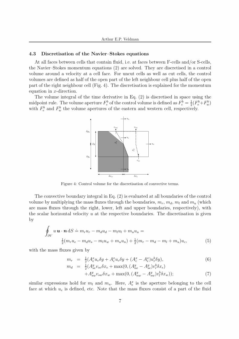
4.3 Discretisation of the Navier–Stokes equations

At all faces between cells that contain fluid, i.e. at faces between F-cells and/or S-cells,the Navier–Stokes momentum equations (2) are solved. They are discretised in a controlvolume around a velocity at a cell face. For uncut cells as well as cut cells, the controlvolumes are defined as half of the open part of the left neighbour cell plus half of the openpart of the right neighbour cell (Fig. 4). The discretisation is explained for the momentumequation in x-direction.

The volume integral of the time derivative in Eq. (2) is discretised in space using themidpoint rule. The volume aperture F b

c of the control volume is defined as F bc = 1

2(F b

e +F bw)

with F be and F b

w the volume apertures of the eastern and western cell, respectively.

uc

un

ue

us

vnw vne

vse

ubl

ubr

δxw δxe

δy

δys

δyn

Figure 4: Control volume for the discretisation of convective terms.

The convective boundary integral in Eq. (2) is evaluated at all boundaries of the controlvolume by multiplying the mass fluxes through the boundaries, mr, md, ml and mu (whichare mass fluxes through the right, lower, left and upper boundaries, respectively), withthe scalar horizontal velocity u at the respective boundaries. The discretisation is givenby

∮

∂V

u u · n dS.= mrur − mdud − mlul + muuu =

12(mrue − mdus − mluw + muun) + 1

2(mr − md − ml + mu)uc, (5)

with the mass fluxes given by

mr = 12(Ax

eueδy + Axcucδy + (Ax

c − Axe)u

brδy), (6)

md = 12(Ay

sevseδxe + max(0, (Ayne − Ay

se)vbrδxe)

+Ayswvswδxw + max(0, (Ay

nw − Aysw)vb

l δxw)); (7)

similar expressions hold for ml and mu. Here, Axe is the aperture belonging to the cell

face at which ue is defined, etc. Note that the mass fluxes consist of a part of the fluid

7

Arthur E.P. Veldman

flow through the open boundaries and a part of the moving body. Inspection learnsthat the coefficient of the central velocity uc in Eq. (5) vanishes, making the convectivecontribution to the coefficient matrix skew symmetric (like the continuous operator),which is a favourable property54. Further, artificial diffusion is added such that it transfersthe above central discretisation of the convective term into a (more stable) first-orderupwind discretisation.

For the diffusive term a discretisation is adopted in which the geometry is handled ina staircase way, so the cut cells are treated as if they are uncut. This has been doneto prevent stability problems in small cut cells. In this way, the diffusive discretisationbecomes first order, but in the convection-dominated simulations studied here diffusion isnot really important19,20.

The pressure gradient in the x-momentum equation is discretised as a boundary integral

∮

∂V

pnxdS.= (pe − pw)Ax

c δy. (8)

Here, pe and pw are the pressure in the eastern and western cells, respectively (Fig. 4),and Ax

c is the edge aperture of the cell face where the central velocity is defined. Thusthe discrete gradient is the negative transpose of the discrete divergence operator Eq. (4),which is also an analytic property54. The external force is written as Fg = −∇gz, and itis discretised similar to the pressure gradient. In this way, it exactly cancels the discretehydrodynamic pressure.

The equations of motion are discretised in time using the forward Euler method. Thisfirst order method is accurate enough, because the order of the overall accuracy is alreadydetermined by the first order accuracy of the free-surface displacement algorithm. Thepressure is solved from a Poisson equation55. It does not require boundary conditionsat solid walls; at the free surface the boundary conditions follow from the normal-stresscondition in Eq. (3)26. Numerical stability of the above time integration puts the usualconvective and diffusive requirements on the maximum allowable time step, such as aCFL-condition16,18–20.

5 NUMERICAL MODEL – FREE-SURFACE ISSUES

This section describes some numerical issues concerning the treatment of the free sur-face: the displacement algorithm and the boundary conditions for the velocity. In partic-ular with respect to these two issues adaptations to the original VOF method have beenmade.

5.1 Free-surface displacement

The free surface is displaced using an improved (iVOF) version of the Volume-of-Fluidmethod14. A piecewise constant reconstruction of the free surface is used, where the freesurface is displaced by changing the VOF value in a cell using calculated fluxes through

8

Arthur E.P. Veldman

cell faces. Near the free surface these fluxes are constrained, based on available liquidand/or void space; the original flux expressions14 are used.

h

x

z

Figure 5: The VOF function in cells near surface cells is updated using a local height function.

The original VOF method has two main drawbacks. The first is that flotsam andjetsam can appear28,58, which are small droplets disconnecting from the free surface. Theother drawback is the gain or loss of water due to rounding the VOF function when F s > 1or F s < 0. By combining the VOF method with a local height function16, these problemsdo not appear any more. For every surface cell locally a function is defined that givesthe height of the fluid in a column of three cells (Fig. 5). The direction in which thefunction is defined is the direction of the coordinate axis that is most normal to the freesurface (the positive z-direction in Fig. 5). Then, after calculating the fluxes across thecell boundaries of all three cells (the dashed-line region in Fig. 5) as in classical VOF, notthe individual VOF values of the three column cells are updated, but the height functionis updated. The individual VOF values of the three cells are then calculated from theheight of the fluid in the column. In this way, the method is strictly mass conserving andalmost no flotsam and jetsam appear19. The local height function can also be used toaccurately compute the curvature of the free surface16 (essential for capillary-dominatedapplications), which has recently led to increasing attention for this approach56,57.

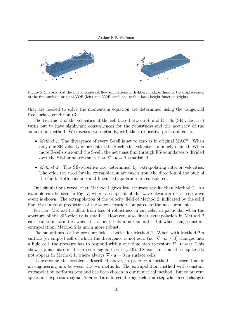
Both methods, the original VOF method and the iVOF method with local heightfunction, have been compared in a dambreak simulation. In the left Fig. 6 the result isshown of the free surface configuration of a calculation with the original VOF displacementmethod. The created flotsam and jetsam, small droplets disconnecting from the freesurface, are clearly visible. With a local height function, the amount of flotsam andjetsam has decreased considerably as can be seen in the right Fig. 6. Further, the lossof water using original VOF is considerable: about 7% after 6 seconds. In the adaptediVOF method, the loss of water is only 0.02%, so mass is much better conserved.

5.2 Velocities near the free surface

Velocities in the neighbourhood of the free surface can be grouped in different classes(see Fig. 2): i) the velocities between two F- and/or S-cells are determined from themomentum equation; ii) the velocities between an S- and an E-cell are determined usingboundary conditions that will be described below; iii) the velocities between two E-cells

9

Arthur E.P. Veldman

Figure 6: Snapshots at the end of dambreak flow simulations with different algorithms for the displacementof the free surface: original VOF (left) and VOF combined with a local height function (right).

that are needed to solve the momentum equation are determined using the tangentialfree-surface condition (3).

The treatment of the velocities at the cell faces between S- and E-cells (SE-velocities)turns out to have significant consequences for the robustness and the accuracy of thesimulation method. We discuss two methods, with their respective pro’s and con’s.

• Method 1: The divergence of every S-cell is set to zero as in original MAC26. Whenonly one SE-velocity is present in the S-cell, this velocity is uniquely defined. Whenmore E-cells surround the S-cell, the net mass flux through FS-boundaries is dividedover the SE-boundaries such that ∇ · u = 0 is satisfied.

• Method 2: The SE-velocities are determined by extrapolating interior velocities.The velocities used for the extrapolation are taken from the direction of the bulk ofthe fluid. Both constant and linear extrapolation are considered.

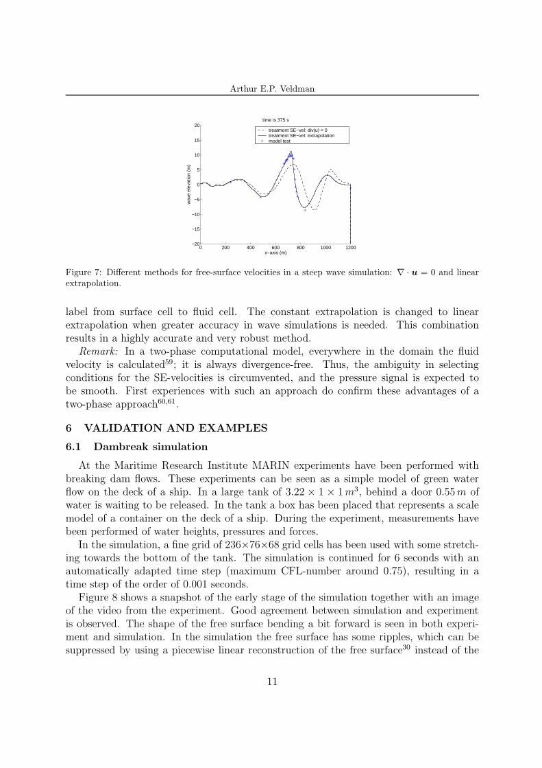
Our simulations reveal that Method 1 gives less accurate results than Method 2. Anexample can be seen in Fig. 7, where a snapshot of the wave elevation in a steep waveevent is shown. The extrapolation of the velocity field of Method 2, indicated by the solidline, gives a good prediction of the wave elevation compared to the measurements.

Further, Method 1 suffers from loss of robustness in cut cells, in particular when theaperture of the SE-velocity is small19. However, also linear extrapolation in Method 2can lead to instabilities when the velocity field is not smooth. But when using constantextrapolation, Method 2 is much more robust.

The smoothness of the pressure field is better for Method 1. When with Method 2 asurface (or empty) cell of which the divergence is not zero (i.e. ∇ · u 6= 0) changes intoa fluid cell, the pressure has to respond within one time step to restore ∇ · u = 0. Thisshows up as spikes in the pressure signal (see Fig. 10). By construction, these spikes donot appear in Method 1, where always ∇ · u = 0 in surface cells.

To overcome the problems described above, in practice a method is chosen that isan engineering mix between the two methods. The extrapolation method with constantextrapolation performs best and has been chosen in our numerical method. But to preventspikes in the pressure signal, ∇·u = 0 is enforced during each time step when a cell changes

10

Arthur E.P. Veldman

0 200 400 600 800 1000 1200−20

−15

−10

−5

0

5

10

15

20time is 375 s

x−axis (m)

wav

e el

evat

ion

(m)

treatment SE−vel: div(u) = 0treatment SE−vel: extrapolationmodel test

Figure 7: Different methods for free-surface velocities in a steep wave simulation: ∇ · u = 0 and linearextrapolation.

label from surface cell to fluid cell. The constant extrapolation is changed to linearextrapolation when greater accuracy in wave simulations is needed. This combinationresults in a highly accurate and very robust method.

Remark: In a two-phase computational model, everywhere in the domain the fluidvelocity is calculated59; it is always divergence-free. Thus, the ambiguity in selectingconditions for the SE-velocities is circumvented, and the pressure signal is expected tobe smooth. First experiences with such an approach do confirm these advantages of atwo-phase approach60,61.

6 VALIDATION AND EXAMPLES

6.1 Dambreak simulation

At the Maritime Research Institute MARIN experiments have been performed withbreaking dam flows. These experiments can be seen as a simple model of green waterflow on the deck of a ship. In a large tank of 3.22 × 1 × 1 m3, behind a door 0.55 m ofwater is waiting to be released. In the tank a box has been placed that represents a scalemodel of a container on the deck of a ship. During the experiment, measurements havebeen performed of water heights, pressures and forces.

In the simulation, a fine grid of 236×76×68 grid cells has been used with some stretch-ing towards the bottom of the tank. The simulation is continued for 6 seconds with anautomatically adapted time step (maximum CFL-number around 0.75), resulting in atime step of the order of 0.001 seconds.

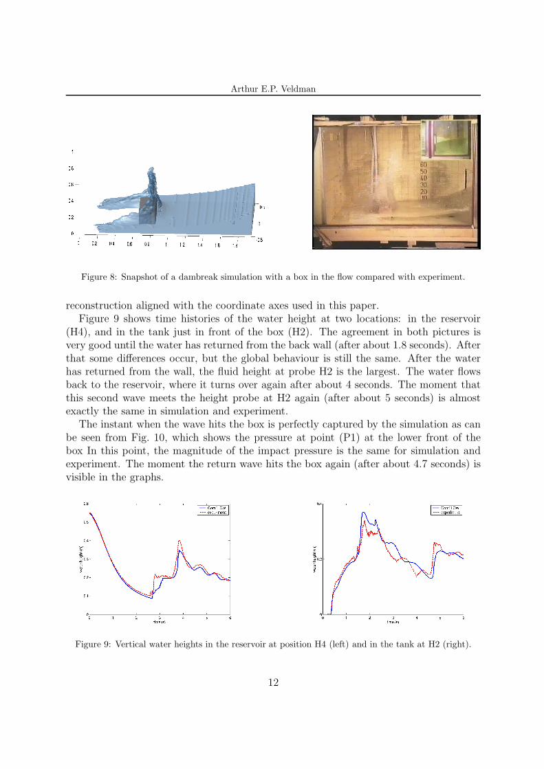
Figure 8 shows a snapshot of the early stage of the simulation together with an imageof the video from the experiment. Good agreement between simulation and experimentis observed. The shape of the free surface bending a bit forward is seen in both experi-ment and simulation. In the simulation the free surface has some ripples, which can besuppressed by using a piecewise linear reconstruction of the free surface30 instead of the

11

Arthur E.P. Veldman

Figure 8: Snapshot of a dambreak simulation with a box in the flow compared with experiment.

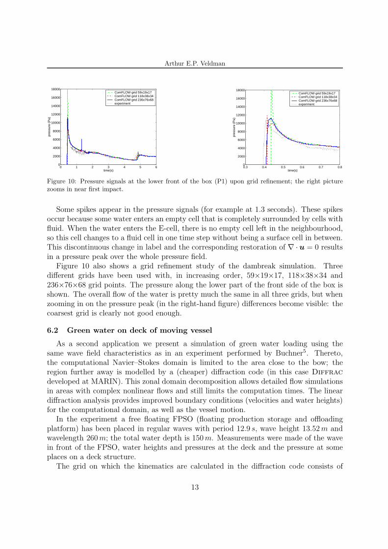
reconstruction aligned with the coordinate axes used in this paper.Figure 9 shows time histories of the water height at two locations: in the reservoir

(H4), and in the tank just in front of the box (H2). The agreement in both pictures isvery good until the water has returned from the back wall (after about 1.8 seconds). Afterthat some differences occur, but the global behaviour is still the same. After the waterhas returned from the wall, the fluid height at probe H2 is the largest. The water flowsback to the reservoir, where it turns over again after about 4 seconds. The moment thatthis second wave meets the height probe at H2 again (after about 5 seconds) is almostexactly the same in simulation and experiment.

The instant when the wave hits the box is perfectly captured by the simulation as canbe seen from Fig. 10, which shows the pressure at point (P1) at the lower front of thebox In this point, the magnitude of the impact pressure is the same for simulation andexperiment. The moment the return wave hits the box again (after about 4.7 seconds) isvisible in the graphs.

Figure 9: Vertical water heights in the reservoir at position H4 (left) and in the tank at H2 (right).

12

Arthur E.P. Veldman

0 1 2 3 4 5 60

2000

4000

6000

8000

10000

12000

14000

16000

18000

time(s)

pres

sure

(P

a)

ComFLOW grid 59x19x17ComFLOW grid 118x38x34ComFLOW grid 236x76x68experiment

0.3 0.4 0.5 0.6 0.7 0.80

2000

4000

6000

8000

10000

12000

14000

16000

18000

time(s)

pres

sure

(P

a)

ComFLOW grid 59x19x17ComFLOW grid 118x38x34ComFLOW grid 236x76x68experiment

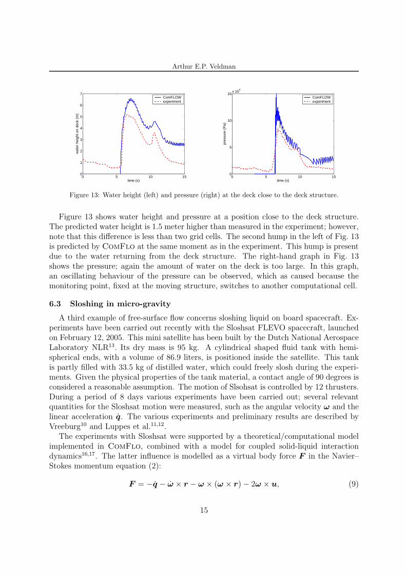
Figure 10: Pressure signals at the lower front of the box (P1) upon grid refinement; the right picturezooms in near first impact.

Some spikes appear in the pressure signals (for example at 1.3 seconds). These spikesoccur because some water enters an empty cell that is completely surrounded by cells withfluid. When the water enters the E-cell, there is no empty cell left in the neighbourhood,so this cell changes to a fluid cell in one time step without being a surface cell in between.This discontinuous change in label and the corresponding restoration of ∇ ·u = 0 resultsin a pressure peak over the whole pressure field.

Figure 10 also shows a grid refinement study of the dambreak simulation. Threedifferent grids have been used with, in increasing order, 59×19×17, 118×38×34 and236×76×68 grid points. The pressure along the lower part of the front side of the box isshown. The overall flow of the water is pretty much the same in all three grids, but whenzooming in on the pressure peak (in the right-hand figure) differences become visible: thecoarsest grid is clearly not good enough.

6.2 Green water on deck of moving vessel

As a second application we present a simulation of green water loading using thesame wave field characteristics as in an experiment performed by Buchner5. Thereto,the computational Navier–Stokes domain is limited to the area close to the bow; theregion further away is modelled by a (cheaper) diffraction code (in this case Diffrac

developed at MARIN). This zonal domain decomposition allows detailed flow simulationsin areas with complex nonlinear flows and still limits the computation times. The lineardiffraction analysis provides improved boundary conditions (velocities and water heights)for the computational domain, as well as the vessel motion.

In the experiment a free floating FPSO (floating production storage and offloadingplatform) has been placed in regular waves with period 12.9 s, wave height 13.52 m andwavelength 260 m; the total water depth is 150 m. Measurements were made of the wavein front of the FPSO, water heights and pressures at the deck and the pressure at someplaces on a deck structure.

The grid on which the kinematics are calculated in the diffraction code consists of

13

Arthur E.P. Veldman

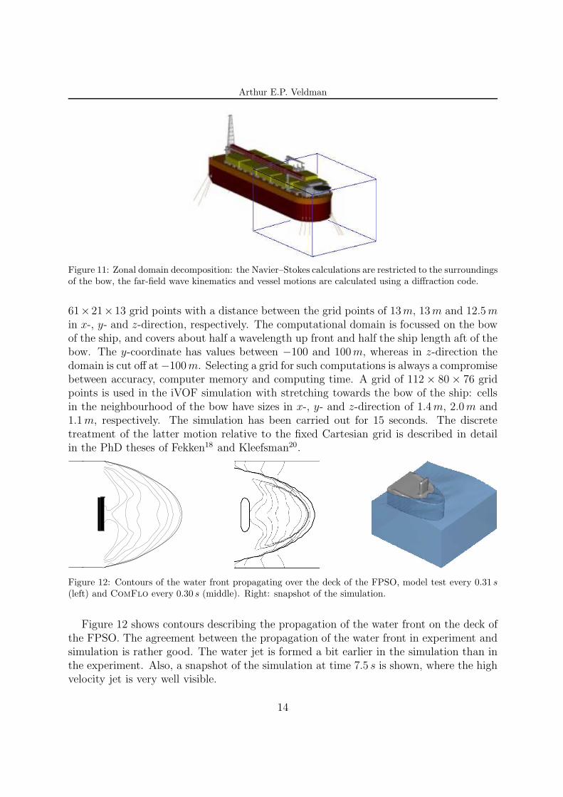
Figure 11: Zonal domain decomposition: the Navier–Stokes calculations are restricted to the surroundingsof the bow, the far-field wave kinematics and vessel motions are calculated using a diffraction code.

61×21×13 grid points with a distance between the grid points of 13 m, 13 m and 12.5 min x-, y- and z-direction, respectively. The computational domain is focussed on the bowof the ship, and covers about half a wavelength up front and half the ship length aft of thebow. The y-coordinate has values between −100 and 100 m, whereas in z-direction thedomain is cut off at −100 m. Selecting a grid for such computations is always a compromisebetween accuracy, computer memory and computing time. A grid of 112 × 80 × 76 gridpoints is used in the iVOF simulation with stretching towards the bow of the ship: cellsin the neighbourhood of the bow have sizes in x-, y- and z-direction of 1.4 m, 2.0 m and1.1 m, respectively. The simulation has been carried out for 15 seconds. The discretetreatment of the latter motion relative to the fixed Cartesian grid is described in detailin the PhD theses of Fekken18 and Kleefsman20.

� �� �� �� �� �� �� �� �� �� �� �� �� �� �� �

� �� �� �� �� �� �� �� �� �� �� �� �� �� �� �

Figure 12: Contours of the water front propagating over the deck of the FPSO, model test every 0.31 s

(left) and ComFlo every 0.30 s (middle). Right: snapshot of the simulation.

Figure 12 shows contours describing the propagation of the water front on the deck ofthe FPSO. The agreement between the propagation of the water front in experiment andsimulation is rather good. The water jet is formed a bit earlier in the simulation than inthe experiment. Also, a snapshot of the simulation at time 7.5 s is shown, where the highvelocity jet is very well visible.

14

Arthur E.P. Veldman

0 5 10 150

1

2

3

4

5

6

7

time (s)

wat

er h

eigh

t on

deck

(m

)

ComFLOWexperiment

0 5 10 150

5

10

15x 10

4

time (s)

pres

sure

(P

a)

ComFLOWexperiment

Figure 13: Water height (left) and pressure (right) at the deck close to the deck structure.

Figure 13 shows water height and pressure at a position close to the deck structure.The predicted water height is 1.5 meter higher than measured in the experiment; however,note that this difference is less than two grid cells. The second hump in the left of Fig. 13is predicted by ComFlo at the same moment as in the experiment. This hump is presentdue to the water returning from the deck structure. The right-hand graph in Fig. 13shows the pressure; again the amount of water on the deck is too large. In this graph,an oscillating behaviour of the pressure can be observed, which as caused because themonitoring point, fixed at the moving structure, switches to another computational cell.

6.3 Sloshing in micro-gravity

A third example of free-surface flow concerns sloshing liquid on board spacecraft. Ex-periments have been carried out recently with the Sloshsat FLEVO spacecraft, launchedon February 12, 2005. This mini satellite has been built by the Dutch National AerospaceLaboratory NLR13. Its dry mass is 95 kg. A cylindrical shaped fluid tank with hemi-spherical ends, with a volume of 86.9 liters, is positioned inside the satellite. This tankis partly filled with 33.5 kg of distilled water, which could freely slosh during the experi-ments. Given the physical properties of the tank material, a contact angle of 90 degrees isconsidered a reasonable assumption. The motion of Slsohsat is controlled by 12 thrusters.During a period of 8 days various experiments have been carried out; several relevantquantities for the Sloshsat motion were measured, such as the angular velocity ω and thelinear acceleration q. The various experiments and preliminary results are described byVreeburg10 and Luppes et al.11,12.

The experiments with Sloshsat were supported by a theoretical/computational modelimplemented in ComFlo, combined with a model for coupled solid-liquid interactiondynamics16,17. The latter influence is modelled as a virtual body force F in the Navier–Stokes momentum equation (2):

F = −q − ω × r − ω × (ω × r) − 2ω × u, (9)

15

Arthur E.P. Veldman

Figure 14: The Sloshsat FLEVO satellite: left the exterior; right a schematic internal view.

where q denotes the linear acceleration of the moving coordinate frame fixed to the solidbody, and ω and ω denote the angular velocity and acceleration of the solid body.

In this paper we will present some results for a so-called flat-spin manoeuvre. Here,Sloshsat is initially forced to rotate around the axis of intermediate MOI (moment ofinertia), during which the fluid configuration settles in equilibrium. After some time,the thruster action is canceled and a free tumble of Sloshsat commences. During thisfree tumble, the rotational direction of Sloshsat (slowly) moves towards the maximumMOI, with a significant amount of nutation and large-scale fluid action. Hence, such amanoeuvre is very suitable for the validation of our numerical model.

-5.0E-01-4.0E-01-3.0E-01-2.0E-01-1.0E-010.0E+001.0E-012.0E-013.0E-014.0E-015.0E-016.0E-01

100 200

Wx (

rad/s

)

time (s)

-5.8E-01-5.6E-01-5.4E-01-5.2E-01-5.0E-01-4.8E-01-4.6E-01-4.4E-01

100 200

Wy (

rad/s

)

time (s)

-5.0E-01-4.0E-01-3.0E-01-2.0E-01-1.0E-010.0E+001.0E-012.0E-013.0E-014.0E-015.0E-01

100 200

Wz (

rad/s

)

time (s)

experiment simulation

Figure 15: Simulation versus measurements for the flat-spin experiment.

The comparison for the flat-spin manoeuvre is given in Fig. 15. Controlled by thrusteraction, in the first 33 seconds Sloshsat is approximately rotating around the axis of in-

16

Arthur E.P. Veldman

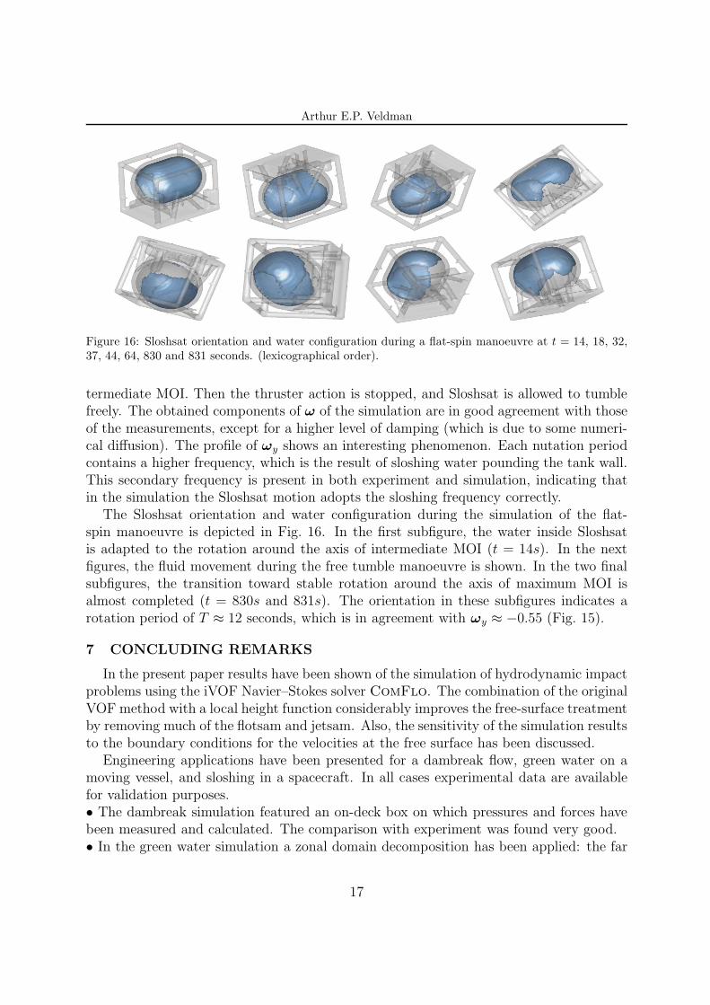
Figure 16: Sloshsat orientation and water configuration during a flat-spin manoeuvre at t = 14, 18, 32,37, 44, 64, 830 and 831 seconds. (lexicographical order).

termediate MOI. Then the thruster action is stopped, and Sloshsat is allowed to tumblefreely. The obtained components of ω of the simulation are in good agreement with thoseof the measurements, except for a higher level of damping (which is due to some numeri-cal diffusion). The profile of ωy shows an interesting phenomenon. Each nutation periodcontains a higher frequency, which is the result of sloshing water pounding the tank wall.This secondary frequency is present in both experiment and simulation, indicating thatin the simulation the Sloshsat motion adopts the sloshing frequency correctly.

The Sloshsat orientation and water configuration during the simulation of the flat-spin manoeuvre is depicted in Fig. 16. In the first subfigure, the water inside Sloshsatis adapted to the rotation around the axis of intermediate MOI (t = 14s). In the nextfigures, the fluid movement during the free tumble manoeuvre is shown. In the two finalsubfigures, the transition toward stable rotation around the axis of maximum MOI isalmost completed (t = 830s and 831s). The orientation in these subfigures indicates arotation period of T ≈ 12 seconds, which is in agreement with ωy ≈ −0.55 (Fig. 15).

7 CONCLUDING REMARKS

In the present paper results have been shown of the simulation of hydrodynamic impactproblems using the iVOF Navier–Stokes solver ComFlo. The combination of the originalVOF method with a local height function considerably improves the free-surface treatmentby removing much of the flotsam and jetsam. Also, the sensitivity of the simulation resultsto the boundary conditions for the velocities at the free surface has been discussed.

Engineering applications have been presented for a dambreak flow, green water on amoving vessel, and sloshing in a spacecraft. In all cases experimental data are availablefor validation purposes.• The dambreak simulation featured an on-deck box on which pressures and forces havebeen measured and calculated. The comparison with experiment was found very good.• In the green water simulation a zonal domain decomposition has been applied: the far

17

Arthur E.P. Veldman

field has been described by a (cheaper) diffraction method, and only the close vicinity ismodelled with the (more expensive) nonlinear Navier–Stokes equations. Pressure loadson the deck structure compare quite well with experiment, although the amount of wateron deck is somewhat overpredicted.• The flat-spin example includes capillary physics as well as liquid–spacecraft interaction.It shows that the sloshing frequency of the water inside the tank is adopted correctly bythe satellite motion, although the damping is somewhat overpredicted.

The results of the simulations give much confidence in the performance of the method.It will be developed further in the coming years by extending it towards compressible two-phase flows (in the ComFLOW-2 project61). A major advantage of a two-phase modelis that the boundary conditions for the velocities at the free surface, which have a largeinfluence on the robustness and accuracy of the method, are not needed anymore. Also,in this way pockets of entrapped air in the wave impact region can be modelled; thesecan have a substantial influence on the impact pressures62,63.

ACKNOWLEDGEMENTS

The paper describes the efforts of the ComFlo development team at the University of Groningen,which operates in close cooperation with the Maritime Research Institute MARIN, FORCE Technology(Norway), Delft University of Technology, and the National Aerospace Laboratory NLR. In particular,the author would like to acknowledge the contributions of (in alphabetical order) Geert Fekken, JeroenGerrits, Joop Helder, Theresa Helmholt-Kleefsman, Erwin Loots, Roel Luppes and Rik Wemmenhove atthe University of Groningen; Bas Buchner, Tim Bunnik and Arjan Voogt at MARIN; Erik Falkenbergand Bogdan Iwanowski at FORCE Technology; Jo Pinkster and Peter Wellens at TU Delft; and, last butnot least, Koos Prins and Jan Vreeburg at NLR.

The maritime part of the presented research has been carried out in the SAFE-FLOW project (SAFE-FLOating offshore structures under impact loading of shipped green water and Waves), funded by theEuropean Community under the ’Competitive and Sustainable Growth’ Programme (EU Project No.:GRD1-2000-25656) and a group of 26 industrial participants. The author is solely responsible for thepresent paper and it does not represent the opinion of the European Community. The ComFLOW-2 jointindustry project is co-funded by the Dutch Technology Foundation STW.The micro-gravity part of the presented research has been supported by the National Institute for SpaceResearch in the Netherlands (SRON; project MG-065). The Sloshsat FLEVO project is a harmonisedprogramme between the European Space Agency (ESA) and the Netherlands Agency for AerospacePrograms (NIVR) with NLR as main contractor.

REFERENCES

[1] W.D.M. Morris, J. Millar and B. Buchner. Green water susceptibility of North Sea FPSO/FSUs. In:Proc. 15th Conf. on Floating Production Systems (FPS), London (2000).

[2] P. Gorf, N. Barltrop, B. Okan, T. Hodson and R. Rainey. FPSO bow damage in steep waves. In:Proc. Rogue Waves, Brest (2000).

[3] Apollo 11 Lunar Surface Journal. The first lunar landing. See 102:38:20 mission time. Available athttp://www.hq.nasa.gov/office/pao/History/alsj/a11/a11.landing.html

[4] NEAR Anomaly Review Board. The NEAR Rendezvous burn anomaly of December 1998. JohnsHopkins University, Applied Physics Laboratory (November 1999).

18

Arthur E.P. Veldman

[5] B. Buchner. Green water on ship-type offshore structures. PhD thesis, Department of MaritimeTechnology, Delft University of Technology (2002).

[6] O.M. Faltinsen. Sea Loads on Ships and Offshore Structures. Cambridge University Press (1999).

[7] B. Molin and J. Ferziger. Hydrodynamique des structures offshore. Appl. Mech. Rev., 56, B29 (2003).

[8] A.E.P. Veldman and M.E.S. Vogels. Axisymmetric liquid sloshing under low gravity conditions. ActaAstronautica 11, 641–649 (1984).

[9] J.P.B. Vreeburg and A.E.P. Veldman. Transient and sloshing motions in an unsupported container.In: R. Monti (ed.) Physics of Fluids in Microgravity. Taylor and Francis Publishers, pp. 293–321(2002).

[10] J.P.B. Vreeburg. Measured states of SLoshsat FLEVO. In: Proc. 56th Int. Astronaut. Congr.,Fukuoka, Japan, Paper IAF-05-C1.2.09 (2005).

[11] R. Luppes, J.A. Helder and A.E.P. Veldman. Liquid sloshing in microgravity. In: Proc. 56th Int.Astronaut. Congr., Fukuoka, Japan, Paper IAF-05-A2.2.07 (2005).

[12] R. Luppes, J.A. Helder and A.E.P. Veldman. The numerical simulation of liquid sloshing in micro-gravity. In: Proc. ECCOMAS CFD 2006, Egmond aan Zee, Netherlands (2006).

[13] J.J.M. Prins. Sloshsat flevo: Facility for liquid experimentation and verification in orbit. In: Proc.51st Int. Astronaut. Congr., Paper IAF-00-J.2.05 (2000).

[14] C.W. Hirt and B.D. Nichols. Volume of fluid (vof) method for the dynamics of free boundaries.J. Comp. Phys., 39, 201–225 (1981).

[15] S. van Mourik, A.E.P. Veldman and M. Dreyer. Simulation of capillary flow with a dynamic contactangle. Microgravity Sci. Technol., 17(3), 87–94 (2005).

[16] J. Gerrits. Dynamics of liquid-filled spacecraft. PhD thesis, University of Groningen (2001).

[17] J. Gerrits and A.E.P. Veldman. Dynamics of liquid-filled spacecraft. J. Eng. Math., 45, 21–38 (2003).

[18] G. Fekken. Numerical simulation of free-surface flow with moving rigid bodies. PhD thesis, Universityof Groningen (2004).

[19] K.M.T. Kleefsman, G. Fekken, A.E.P. Veldman, B. Iwanowski and B. Buchner. A Volume-of-Fluidbased simulation methods for wave impact problems. J. Comp. Phys., 206, 363–393 (2005).

[20] K.M.T. Kleefsman. Water impact loading on offshore structures - a numerical study. PhD thesis,University of Groningen (2005).

[21] E. Loots, B. Hillen and A.E.P. Veldman. The role of hemodynamics in the development of theoutflow tract of the heart. J. Eng. Math., 45, 91–104 (2003).

[22] N.M. Maurits, G.E. Loots and A.E.P. Veldman. The influence of vessel wall elasticity and peripheralresistance on the flow wave form: a CFD model compared to in-vivo ultrasound meaurements. J.Biomech., available online February 2006.

[23] R.W. Yeung. Numerical methods in free-surface flows. Ann. Rev. Fluid Mech., 12, 395–442 (1982).

[24] W. Tsai and D.K.P. Yue. Computation of nonlinear free-surface flows. Ann. Rev. Fluid Mech., 28,249–278 (1996).

[25] R. Scardovelli, S. Zaleski. Direct numerical simulation of free-surface and interfacial flow, Ann. Rev.Fluid Mech., 31, 567–603 (1999).

19

Arthur E.P. Veldman

[26] F.H. Harlow and J.E. Welch. Numerical calculation of time-dependent viscous incompressible flowof fluid with free surface. Phys. Fluids, 8, 2182–2189 (1965).

[27] D. Juric and G. Tryggvason. A front tracking method for dendritic solidification, J. Comp. Phys.,123, 127–148 (1996).

[28] W.J. Rider and D.B. Kothe. Reconstructing volume tracking. J. Comp. Phys., 141, 112–152 (1998).

[29] M. Rudman. Volume-tracking methods for interfacial flow calculations, Int. J. Numer. Meth. Fluids,24, 671–691 (1997).

[30] D.L. Youngs. An interface tracking method for a 3D Eulerian hydrodynamics code, Technical ReportAWRE/44/92/35, Atomic Weapons Research Establishment, 1987.

[31] T. Yabe, F. Xiao and T. Utsumi. The constrained interpolation profile method for multiphaseanalysis. J. Comp. Phys., 169, 556–593 (2001).

[32] M. Greco, O.M. Faltinsen and M. Landrini. Numerical simulation of heavy water shipping. In: Proc.17th Workshop on Water Waves and Floating Bodies, Cambridge UK, 14-16 April 2002.

[33] Y. Kim. Numerical simulation of sloshing flows with impact load. Appl. Ocean Res., 23, 53–62 (2001).

[34] S. Muzaferija, M. Peric, P. Sames and T. Schellin. A two-fluid Navier–Stokes solver to simulate waterentry. In: Proc. 22nd Symp. Naval Hydrodynamics, pp. 638-649 (2001).

[35] J.A. Sethian. Level Set Methods: Evolving Interfaces in Geometry, Fluid Mechanics, ComputerVision and Materials Science. Cambridge University Press (1996).

[36] W.J. Rider and D.B. Kothe. Stretching and tearing interface tracking methods. AIAA paper 95-1717(1995).

[37] F. Bet, D. Hanel, and S. Sharma. Numerical simulation of ship flow by a method of artificialcompressibility. In: Proc. 22th Symp. Naval Hydrodynamics, page 173 (1998).

[38] M. Sussman and D. Dommermuth. The numerical simulation of ship waves using cartesian gridmethods. In: Proc. 23th Symp. Naval Hydrodynamics, pp. 762–779 (2001).

[39] A. Iafrati, A. Di Mascio, E.F. Campana. A level set technique applied to unsteady free surface flows.Int. J. Numer. Methods Fluids, 35, 281–297 (2001).

[40] M. Sussman and E.G. Puckett. A coupled level set and volume-of-fluid method for computing 3dand axisymmetric incompressible two-phase flows. J. Comp. Phys., 162, 301–337 (2000).

[41] S. van der Pijl. Computation of bubbly flows with a mass-conserving level-set method. PhD thesis,TU Delft (2005).

[42] C.W. Hirt, A.A. Amsden and J.L. Cook. An arbitrary Lagrangian-Eulerian method for all flowspeeds. J. Comp. Phys., 14, 227–253 (1974).

[43] B. Alessandrini and G. Delhommeau. A fully coupled Navier–Stokes solver for calculation of tur-bulent incompressible free surface flow past a ship hull. Int. J. Num. Meth. Fluids, 29, 125–142(1999).

[44] M.P. Tulin and M. Landrini. Breaking waves in the ocean and around ships. In: Proc. 23th Symp.Naval Hydrodynamics, pp. 713–745 (2001).

[45] J.J. Monaghan. Simulating Free Surface Flows with SPH. J. Comp. Phys., 110, 399–406 (1994).

[46] Y. Andrillon, M. Doring, B. Alessandrini, and P. Ferrant. Comparison between sph and vof freesurface flow simulation. In: Proc. 5th Numerical Towing Tank Symposium (2002).

20

Arthur E.P. Veldman

[47] A. Colagrossi and M. Landrini. Numerical simulations of 2-phase flows by smoothed particle hydro-dynamics. In: Proc. 5th Numerical Towing Tank Symposium (2002).

[48] H. Maeda, K. Nishimoto, K. Masuda, T. Asanuma, M.M. Tsukamoto and T. Ikoma. Numericalanalysis for hydrodynamic motions of floating structure using MPS method. In: Proc. 23rd Int.Conf. Offshore Mech. Arctic Eng., Vancouver, June 20-25 (2004).

[49] I. Orlanski. A simple boundary condition for unbounded hyperbolic flows. J. Comp. Phys., 21,251–269 (1976).

[50] A. Clement. Coupling of two absorbing boundary conditions for 2D time-domain simulations of freesurface gravity waves. J. Comp. Phys., 126, 139–151 (1996).

[51] M. Israeli, S.A. Orszag. Approximation of radiation boundary conditions. J. Comp. Phys., 41, 115–135 (1981).

[52] G. Yang, D.M. Causon and D.M. Ingram. Calculation of compressible flows about complex movinggeometries using a Cartesian cut cell method. Int. J. Num. Meth. Fluids, 33, 1121–1151 (2000).

[53] M. Droge and R. Verstappen. A new symmetry-preserving Cartesian-grid method for computingflow past arbitrarily shaped objects. Int. J. Num. Meth. Fluids, 47, 979–985 (2005).

[54] R.W.C.P. Verstappen and A.E.P. Veldman, Symmetry-preserving discretisation of turbulent flow.J. Comp. Phys., 187, 343–368 (2003).

[55] E.F.F. Botta and M.H.M. Ellenbroek. A modified SOR method for the Poisson equation in unsteadyfree-surface flow calculations. J. Comp. Phys., 60 119-134 (1985).

[56] S.J. Cummins, M.M. Francois and D.B. Kothe. Estimating curvature from volume fractions. Comput.Struct., 83, 425–434 (2005).

[57] M.M. Francois, S.J. Cummins, E.D. Dendy, D.B. Kothe, J.M. Sicilian and M.W. Williams, Abalanced-force algorithm for continuous and sharp interfacial surface tension models within a volumetracking framework. J. Comp. Phys., 213, 141–173 (2006).

[58] D.J.E. Harvie and D.F. Fletcher. A new volume of fluid advection algorithm: the stream scheme. J.Comp. Phys., 162, 1–32 (2000).

[59] S.J. Osher and G. Tryggvason (eds.) Special issue on ‘Computational methods for multiphase flows’.J. Comp. Phys. 169, 249–759 (2001).

[60] R. Wemmenhove, E. Loots, R. Luppes and A.E.P. Veldman. Modelling two-phase flow with off-shore applications. In: Proc. 24th Int. Conf. Offshore Mech. Arctic Eng., Halkidiki, Greece, paperOMAE2005-67460 (2005).

[61] R. Wemmenhove, E. Loots and A.E.P. Veldman. Numerical simulation of hydrodynamic wave loadingby a compressible two-phase model. In: Proc. ECCOMAS CFD 2006. Egmond aan Zee, Netherlands(2006).

[62] D.H. Peregrine and L. Thais. The effect of entrained air in violent water wave impacts. J. FluidMech., 325, 377–397 (1996).

[63] J.H. Duncan. Spilling breakers. Ann. Rev. Fluid Mech., 33, 519–547 (2001).

21