university of albertachintha/pdf/thesis/msc_maolin.pdfdr. majid khabbazian, for their time reviewing...

University of Alberta

Gauss-Chebyshev Quadratures for Wireless Performance Analysis

by

Maolin Wang

A thesis submitted to the Faculty of Graduate Studies and Research

in partial fulfillment of the requirements for the degree of

Master of Science

in

Communications

Department of Electrical and Computer Engineering

©Maolin Wang

Spring 2014

Edmonton, Alberta

Permission is hereby granted to the University of Alberta Libraries to reproduce single copies of this thesis

and to lend or sell such copies for private, scholarly or scientific research purposes only. Where the thesis is

converted to, or otherwise made available in digital form, the University of Alberta will advise potential

users of the thesis of these terms.

The author reserves all other publication and other rights in association with the copyright in the thesis and,

except as herein before provided, neither the thesis nor any substantial portion thereof may be printed or

otherwise reproduced in any material form whatsoever without the author's prior written permission.

Dedicated to my beloved parents...

Abstract

Bit/symbol error rate and outage probability are common performance metrics used

to quantify the reliability of wireless communication systems. Error rates for a

broad class of digital modulation schemes and outage probability are expressed as

integrals, which often do not have closed-form solutions. Therefore, accurate and

simple approximations to develop insight are desirable. Toachieve this goal, clas-

sical Gaussian Chebyshev quadrature and rational GaussianChebyshev quadrature

rules are studied in this thesis. These rules are used to compute symbol error rates

over multipath fading channels and outage caused by co-channel interference. The

accuracy and convergence rate of these rules are investigated.

∼

Acknowledgement

I would never have been able to finish my dissertation withoutthe guidance of my

supervisor and help from friends.

I would like to express my sincere gratitude and respect to mysupervisor, Dr.

Chintha Tellambura, for his excellent guidance, support and supervision. He has

led me into in this promising field and offered much of his insight to a beginner as

me. His advice and encouragement have been instrumental in making this work a

success.

My thanks also go to the members of examining committee, Dr. Hai Jiang and

Dr. Majid Khabbazian, for their time reviewing my thesis andfor their valuable

suggestions for improvement. I am also grateful to the faculty and the administra-

tive staff of the ECE for their support and for creating an environment conducive to

research excellence.

I would also like to thank my fellow lab-mates. It has been a pleasure to work

with them, and the intellectually challenging environmentthey created enhanced

my learning experience.

A great gratitude goes to Yamuna Dhungana, who was my co-researcher in most

of the works and offered me much help. I would also like to thank Prasanna Herath

and Hao Fang, who provided valuable comments on my thesis.

Finally, I would like to express my deepest gratitude and respect to my family,

who gives me faithful support and great encouragement.

∼

Table of Contents

1 Introduction 1

1.1 Wireless Communication . . . . . . . . . . . . . . . . . . . . . . . 1

1.2 Problem Statement . . . . . . . . . . . . . . . . . . . . . . . . . . 3

1.3 Contributions and Outline . . . . . . . . . . . . . . . . . . . . . . . 5

2 Background 7

2.1 Digital Modulation . . . . . . . . . . . . . . . . . . . . . . . . . . 7

2.1.1 ASK . . . . . . . . . . . . . . . . . . . . . . . . . . . . . 8

2.1.2 PSK . . . . . . . . . . . . . . . . . . . . . . . . . . . . . . 10

2.1.3 QAM . . . . . . . . . . . . . . . . . . . . . . . . . . . . . 11

2.1.4 FSK . . . . . . . . . . . . . . . . . . . . . . . . . . . . . . 13

2.2 Performance Integrals . . . . . . . . . . . . . . . . . . . . . . . . . 15

2.3 GaussianQ-Function . . . . . . . . . . . . . . . . . . . . . . . . . 15

2.4 Gaussian Quadrature . . . . . . . . . . . . . . . . . . . . . . . . . 16

2.4.1 Classical GCQ . . . . . . . . . . . . . . . . . . . . . . . . 17

2.4.2 Convergence of classical GCQ . . . . . . . . . . . . . . . . 17

2.4.3 Rational GCQ . . . . . . . . . . . . . . . . . . . . . . . . 19

2.5 Conclusion . . . . . . . . . . . . . . . . . . . . . . . . . . . . . . 23

3 GCQ rules for SER 24

3.1 Introduction . . . . . . . . . . . . . . . . . . . . . . . . . . . . . . 24

3.2 System Model . . . . . . . . . . . . . . . . . . . . . . . . . . . . . 25

3.2.1 Non-fading Channels . . . . . . . . . . . . . . . . . . . . . 25

3.2.2 Rayleigh Fading . . . . . . . . . . . . . . . . . . . . . . . 26

3.2.3 Rician Fading . . . . . . . . . . . . . . . . . . . . . . . . . 26

3.2.4 Nakagami-m Fading . . . . . . . . . . . . . . . . . . . . . 26

3.3 Error Probability . . . . . . . . . . . . . . . . . . . . . . . . . . . 27

3.3.1 Coherent Detection of ASK . . . . . . . . . . . . . . . . . 27

3.3.2 Coherent Detection of PSK . . . . . . . . . . . . . . . . . . 29

3.3.3 Coherent Detection of squared QAM . . . . . . . . . . . . 33

3.3.4 Coherent Detection of FSK . . . . . . . . . . . . . . . . . . 34

3.3.5 Noncoherent Detection ofM-ary Differential PSK . . . . . 35

3.4 Application of GCQ rules . . . . . . . . . . . . . . . . . . . . . . . 37

3.4.1 Error Performance of Coherent ASK . . . . . . . . . . . . . 37

3.4.2 Error Performance of Coherent PSK . . . . . . . . . . . . . 38

3.4.3 Error Performance of Coherent QAM . . . . . . . . . . . . 39

3.4.4 Error Performance of Coherent FSK . . . . . . . . . . . . . 40

3.4.5 Error Performance of Nocoherent modulation . . . . . . . .40

3.5 Numerical and Simulation Results . . . . . . . . . . . . . . . . . . 43

3.5.1 Error Performance of Single Channel Reception . . . . . .. 43

3.5.2 Error Performance of Diversity Reception . . . . . . . . . .50

3.6 Conclusion . . . . . . . . . . . . . . . . . . . . . . . . . . . . . . 60

4 GCQ for Co-Channel Interference Outage 61

4.1 Introduction . . . . . . . . . . . . . . . . . . . . . . . . . . . . . . 61

4.2 Outage Probability . . . . . . . . . . . . . . . . . . . . . . . . . . 61

4.2.1 Rician Fading with Multiple Rayleigh Interferers . . .. . . 63

4.2.2 Multiple Rician Interferers . . . . . . . . . . . . . . . . . . 64

4.2.3 Mixed Rayleigh and Rician Interferers . . . . . . . . . . . . 64

4.3 Numerical Results . . . . . . . . . . . . . . . . . . . . . . . . . . . 65

4.3.1 Rician Fading with Multiple Rayleigh Interferers . . .. . . 65

4.3.2 Rician Fading with Multiple Rician Interferers . . . . .. . 66

4.3.3 Rician Fading with Mixed Rayleigh and Rician Interferers . 66

4.4 Conclusion . . . . . . . . . . . . . . . . . . . . . . . . . . . . . . 70

5 Conclusions 71

5.1 Future Research Directions . . . . . . . . . . . . . . . . . . . . . . 72

Bibliography 73

List of Tables

1.1 Typical wireless telecommunication standards . . . . . . .. . . . . 2

2.1 Common performance measures . . . . . . . . . . . . . . . . . . . 15

3.1 Common Digital Modulation Scheme using Gauss ChebyshevQuadra-

ture . . . . . . . . . . . . . . . . . . . . . . . . . . . . . . . . . . 42

3.2 Relative errors:L = 1, 2, 3, MRC, Rayleigh fading . . . . . . . . . . 53

3.3 Relative errors:L = 1, 2, 3, MRC, Rician fading and Rician factor

K = 3 . . . . . . . . . . . . . . . . . . . . . . . . . . . . . . . . . 56

3.4 Relative errors:L = 1, 2, 3, MRC, Nakagami-2 fading . . . . . . . . 59

List of Figures

2.1 Digital modulator . . . . . . . . . . . . . . . . . . . . . . . . . . . 7

2.2 ASK Constellation [1] . . . . . . . . . . . . . . . . . . . . . . . . 9

2.3 PSK Constellation [1] . . . . . . . . . . . . . . . . . . . . . . . . . 11

2.4 QAM Constellation [1] . . . . . . . . . . . . . . . . . . . . . . . . 12

2.5 3-FSK Constellations [1] . . . . . . . . . . . . . . . . . . . . . . . 14

2.6 Contour plots of the error|φ(z)−rm(z)| for the GCQ formulas with

m = 8 and16. . . . . . . . . . . . . . . . . . . . . . . . . . . . . . 20

2.7 GCQ error bound for the BER of BPSK over Rayleigh fading [2] . . 21

3.1 Channel Model . . . . . . . . . . . . . . . . . . . . . . . . . . . . 25

3.2 Optimum Receiver of Amplitude Shift Keying [1] . . . . . . . .. . 27

3.3 Binary equiprobable signals’ decision regions . . . . . . .. . . . . 28

3.4 The ASK constellation [1] . . . . . . . . . . . . . . . . . . . . . . 29

3.5 Optimum Receiver of Phase Shift Keying [1] . . . . . . . . . . . .30

3.6 PSK signalling constellation . . . . . . . . . . . . . . . . . . . . . 30

3.7 Signalling constellation of MPSK system [1] . . . . . . . . . .. . 32

3.8 Polar coordinates system for MPSK constellation . . . . . .. . . . 32

3.9 Optimum Receiver of Quadrature Amplitude Modulation [1] . . . . 34

3.10 Optimum Receiver of Frequency Shift Keying [1] . . . . . . .. . . 35

3.11 Optimum Receiver of Differential Phase Shift Keying Modulation [1] 36

3.12 Coherent Detection ofM-ary ASK (M = 2, 4, 8) in Rayleigh fading 44

3.13 Coherent Detection ofM-ary PSK (M = 2, 4, 8) in Rayleigh fading 44

3.14 Coherent Detection ofM-ary QAM (M = 4, 16, 64) in Rayleigh

fading . . . . . . . . . . . . . . . . . . . . . . . . . . . . . . . . . 44

3.15 Coherent Detection of BFSK in Rayleigh fading . . . . . . . .. . . 45

3.16 Non Coherent Detection of4-ary DPSK andπ/4-DQPSK modula-

tion in Rayleigh fading . . . . . . . . . . . . . . . . . . . . . . . . 45

3.17 Coherent Detection ofM-ary ASK (M = 2, 4, 8) in Rician fading

(K = 3). . . . . . . . . . . . . . . . . . . . . . . . . . . . . . . . . 46

3.18 Coherent Detection ofM-ary PSK (M = 2, 4, 8) in Rician fading

(K = 3). . . . . . . . . . . . . . . . . . . . . . . . . . . . . . . . . 46

3.19 Coherent Detection ofM-ary QAM (M = 4, 16, 64) in Rician fad-

ing (K = 3). . . . . . . . . . . . . . . . . . . . . . . . . . . . . . . 47

3.20 Coherent Detection of BFSK in Rician fading (K = 3). . . . . . . . 47

3.21 Non Coherent Detection of4-ary DPSK andπ/4-DQPSK in Rician

fading (K = 3). . . . . . . . . . . . . . . . . . . . . . . . . . . . . 47

3.22 Coherent Detection ofM-ary ASK (M = 2, 4, 8) in Nakagami-2

fading . . . . . . . . . . . . . . . . . . . . . . . . . . . . . . . . . 48

3.23 Coherent Detection ofM-ary PSK (M = 2, 4, 8) in Nakagami-2

fading . . . . . . . . . . . . . . . . . . . . . . . . . . . . . . . . . 48

3.24 Coherent Detection ofM-ary QAM (M = 4, 16, 64) in Nakagami-

2 fading . . . . . . . . . . . . . . . . . . . . . . . . . . . . . . . . 49

3.25 Coherent Detection of BFSK in Nakagami-2 fading . . . . . .. . . 49

3.26 Non Coherent Detection ofM-ary DPSK andπ/4-DQPSK in Nakagami-

2 fading . . . . . . . . . . . . . . . . . . . . . . . . . . . . . . . . 49

3.27 Error performance for 8PSK with diversity reception inRayleigh

fading (nodes = 8). . . . . . . . . . . . . . . . . . . . . . . . . . . 51

3.28 Error performance for 8PSK with MRC (L = 1) in Rayleigh fading. 52



3.31 Error performance for 8PSK with diversity reception inRician fad-

ing (K = 3) and (nodes = 8). . . . . . . . . . . . . . . . . . . . . 54

3.32 Error performance for 8PSK with MRC (L = 1) in Rician fading

(K = 3). . . . . . . . . . . . . . . . . . . . . . . . . . . . . . . . . 55


(K = 3). . . . . . . . . . . . . . . . . . . . . . . . . . . . . . . . . 55


(K = 3). . . . . . . . . . . . . . . . . . . . . . . . . . . . . . . . . 56

3.35 Error performance for 8PSK with diversity reception inNakagami-

2 fading (nodes = 8). . . . . . . . . . . . . . . . . . . . . . . . . . 57

3.36 Error performance for 8PSK with MRC (L = 1) in Nakagami-2

fading. . . . . . . . . . . . . . . . . . . . . . . . . . . . . . . . . . 58


fading (m = 2). . . . . . . . . . . . . . . . . . . . . . . . . . . . . 58


fading (m = 2). . . . . . . . . . . . . . . . . . . . . . . . . . . . . 59

4.1 Outage performance of a Rician fading with multiple Rayleigh in-

terferers . . . . . . . . . . . . . . . . . . . . . . . . . . . . . . . . 67

4.2 Outage performance of a Rician fading with multiple Rician inter-

ferers . . . . . . . . . . . . . . . . . . . . . . . . . . . . . . . . . 68

4.3 Outage performance of a Rician fading with multiple Rayleigh and

Rician interferers . . . . . . . . . . . . . . . . . . . . . . . . . . . 69

List of Acronyms

GCQ Gauss-Chebyshev Quadrature

GSM Global System for Mobile communications

CDMA Code Division Multiple Access

IMT International Mobile Telecommunications

ITU International Telecommunication Union

IEEE Institute of Electrical and Electronics Engineers

WCDMA Wideband CDMA

TD-SCDMA Time Division Synchronous Coded Division Multiple Access

FOMA Freedom of Mobile Multimedia Access

LTE Long-Term Evolution

WLAN Wireless Local Area Network

WPAN Wireless Personal Area Networks

WMAN Wireless Metropolitan Area Networks

BER Bit Error Rate

SER Symbol Error Rate

CCI Co-Channel Interference

CEP Conditional Error Probability

ASK Amplitude Shift Keying

PSK Phase Shift Keying

FSK Frequency Shift Keying

QAM Quadrature Amplitude Modulation

GMSK Gaussian Minimum Shift Keying

CDF Cumulative Distribution Function

PDF Probability Density Function

AWGN Additive White Gaussian Noise

MRC Maximum Ratio Combining

MGF Moment Generating Function

MAP Maximal A Posteriori Probability

SNR Signal to Noise Ratio

List of Symbols

Q(x) GaussianQ function

ξ Signal energy

ξb Average energy per bit

s(t) Transmitted signal

n(t) Additive white Gaussian noise

r(t) Received signal

wk Quadrature weights

J(x) Joukowski transformation

pX(x) Probability density function of random variableX

E(X) Statistical average of random variableX

P(x) Probability

ϕ(x) Moment generating function

d Euclidean distance

Re(X) Real parts of random variableX

ǫ Error probability

γ Signal to noise ratio

Ω Signal to interference ratio

Chapter 1

Introduction

1.1 Wireless Communication

Due to the phenomenal growth of wireless communications in recent decades, sev-

eral wireless network standards have been developed. The common ones are listed

as follows [3]:

1. Global System for Mobile Communications (GSM)

GSM, the most popular second-generation (2G) cellular standard, has dom-

inated over80% of the mobile phone standards by 2012 [4]. The GSM’s

extensions include GSM-900, GSM-1800, and GSM-1900. Data transport

has been added via General Packet Radio Services (GPRS) and Enhanced

Data rates for GSM Evolution (EDGE) [5].

2. Code Division Multiple Access (CDMA)

The rival standard of GSM is CDMA, which is also referred as Interim Stan-

dard 95 (IS-95). CDMA standard has achieved a considerable subscribers

base in the U.S.A. and South Korea. The CDMA family includes CDMAone,

CDMA2000, and CDMA2000 1xEV.

3. International Mobile Telecommunications 2000 (IMT-2000)

IMT-2000 refers mainly to a family of 3G standards, which have been ap-

proved by the International Telecommunication Union (ITU). The leading 3G

standards include CDMA2000 and Wideband CDMA (WCDMA). The vari-

ous customizations of IMT-2000 include Time Division Synchronous Coded

1

Division Multiple Access (TD-SCDMA) [6] and Freedom of Mobile Mul-

timedia Access (FOMA) WCDMA [7] used China and Japan, respectively.

Moreover, due to the high growth of wireless data services, Long-Term Evo-

lution (LTE) has been developed.

4. Institute of Electrical and Electronics Engineers (IEEE) standards

These standards provide interoperability and thus have built a consensus in

the communications industry. IEEE 802.11 on Wireless LocalArea Network

(WLAN) [8], IEEE 802.15 on Wireless Personal Area Networks (WPAN) [9],

and IEEE 802.16 on Wireless Metropolitan Area Networks(WMAN) [3] are

some of the most popular IEEE standards.

These wireless standards have gained widespread adaption,more than 6.8 bil-

lion mobile phone subscribers by 2013, about 96% of the world’s population [10].

This strong growth is facilitated and governed by the abovementioned wireless stan-

dards. Bit error rate (BER) targets and modulation schemes for these standards are

listed in Table 1.1.

Table 1.1: Typical wireless telecommunication standards

Group Standard ModulationMaximum

Allowed BER

GSMGSM900/GSM1800/GSM1900

Gaussian Minimum Shift Keying (GMSK)/Quadrature Amplitude Modulation (QAM)

10−5 [11]

EDGE 8 Phase Shift Keying (8PSK)

CDMA/IMT-2000

CDMAone Quadrature Phase Shift Keying (QPSK)

CDMA2000 QPSK/8PSK/16QAM 10−4 [12]

TD-SCDMA QPSK/8PSK/16QAM

IEEE

802.11 (WLAN) PSK/QAM 8× 10−8 [13]

802.15 (WPAN)Amplitude Shift Keying (ASK)/Frequency

Shift Keying (FSK)/PSK10−7 [9]

802.16 (WMAN) PSK/QAM 10−6 [14]

The BER is the ratio of the number of error bits to the total number of trans-

mitted bits during a certain time interval, and is perhaps the most important quality

of service (QoS) measure. It provides a useful method to quantify the reliability of

wireless channels for different wireless standards and modulation schemes. For ex-

ample, for QAM in GSM900/GSM1800/GSM1900 and IEEE802.11 (WLAN), the

2

maximal allowed BER differs. As a result, for each standard to maintain a reliable

transmission, the BER due to the difference between the received and transmitted

signals influenced by noise, interference, and fading through the channels is speci-

fied.

BER is closely related to symbol error rate (SER), which is the ratio between

the number of erroneously decoded symbols and the total number of transmitted

symbols. For binary modulations, the BER is simply equal to the SER. ForM-ary

modulation, however, since one symbol representslog2M bits, BER and SER may

be roughly related as

BER ≃ 1

log2MSER. (1.1)

Due to this relationship, SER serves as a simple proxy for BER. This the-

sis therefore investigates accurate SER evaluations of several digital modulation

schemes used in the aforementioned wireless standards (Table 1.1). Since these

wireless systems operate over multipath fading channels, which are the fundamen-

tal cause of harmful signal-strength fluctuations and result in increasing the SER,

accurate evaluation of SER reveals the BER degradation due to fading.

Wireless performance also degrades due to co-channel interference (CCI), which

arises when multiple users access the same time-frequency slots. The impact of CCI

can be measured in terms of the outage probability. Thus, this thesis also studies

the outage probability of wireless systems due to CCI.

1.2 Problem Statement

As mentioned in Section 1.1, BER/SER, outage and capacity are used to quantify

wireless system performance. These metrics can be expressed in the following

generalized format as [15,16]

E[h(x)] =

∫ ∞

0

h(ηγ)pγ(γ) dγ, (1.2)

whereh(.) represents outage, BER/SER, or capacity;η is a parameter dependent on

different types of measures; andγ is the instantaneous signal to noise ratio (SNR)

or signal to interference ratio (SIR). The average is performed over the probability

3

density function (PDF) ofγ, pγ(γ). Further details of (1.2) can be found in Table

2.1.

However, obtaining the exact closed-form for (1.2) either may not always be

possible or may have a high computation complexity and may not give the direct

insight about the core parameters that dominate the performance. Therefore, accu-

rate and simple approximations to develop insight are desirable.

Specifically, two Gaussian Chebyshev quadrature (GCQ) rules are studied in

this thesis to tackle these problems.

• Gaussian quadrature allows approximate evaluation of integrals (1.2) as a

simple weighted sum. GCQ rules are special cases of Gaussianquadrature,

which have been widely used in numerical analysis for approximation calcu-

lations.

• Specifically, GCQ rules for SER and outage analysis have beenstudied exten-

sively. While classical GCQ rule is commonly used for wireless analysis, the

accuracy of this rule has not been investigated in detail. However, it is known

that in the high SNR region, the classical GCQ rule is highly accurate. What

is not known widely is that the GCQ rule requires a large number of terms

for the low SNR region. Thus, the convergence rate of this rule depends on

the operating SNR. In this thesis, the convergence rates in both low and high

SNR regions are investigated.

• Moreover, rational GCQ, which has not yet been widely used, is also stud-

ied in this thesis. Rational GCQ rule for SER of several digital modulations

and outage probability is comprehensively described. Furthermore, SER ex-

pressions of digital modulations amenable to GCQ rules are tabulated. Also,

rational GCQ rule for outage computation is developed.

• The comparisons of the convergence rates of classical GCQ and rational GCQ

rules have been paid little attention. Thus, the convergence rate, measured by

the minimum required numbers of nodes for each GCQ rule, for SER and

outage probability is investigated in this thesis.

4

1.3 Contributions and Outline

The main contributions of the thesis are assessment and comparison of the accuracy

of classical and rational GCQ rules for SER of several digital modulation schemes

and for wireless outage. These contributions are listed below:

• SER expressions for coherent and noncoherent digital modulations that can

use the GCQ rules are presented.

• Both classical and rational GCQ rules to approximate SER of wireless trans-

missions over multipath fading channels, Rayleigh, Ricianand Nakagami-m,

are presented. Their convergence rates are compared by evaluating the num-

ber of nodes needed to achieve a given level of accuracy.

• A Gaussian integral model for arbitrary upper limits forM-ary PSK mod-

ulation is developed by using the rational GCQ rule. Expression of error

probability ofM-PSK modulation, using the rational GCQ rule, is analyzed

instead of using the former analysis with GaussianQ-function in the format

of Craig’s transformation with limit[0, π/2].

• Rational GCQ rule is adopted for outage analysis of several cases, which are

a desired Rician faded signal and aggregate CCI under Rayleigh or Rician or

the combination of these two fading scenarios. Convergencerate is studied

through the number of nodes required for a given accuracy level.

The thesis has the following organization:

Chapter 2

In Chapter 2, basic background concepts and models of digital modulation schemes

are presented. Mathematical tools of the classical and rational GCQ rules and node

and weight computation are also described.

Chapter 3

Chapter 3 reviews error performance of coherent and noncoherent digital modula-

tions. Multipath fading models are presented, and the conditional error probability

5

(CEP) of each modulation is obtained. Subsequently, classical and rational GCQ

rules for calculating SER are evaluated. Numerical performance results for digital

modulation and diversity schemes are presented.

Chapter 4

Chapter 4 investigates classical and rational GCQ rules forCCI outage. The ex-

act closed-form outage expressions in the generalized fading scenario are derived.

Numerical results of the desired signal under the Rician fading in the presence of

multiple CCI is presented.

Chapter 5

Finally, Chapter 5 concludes the thesis and provides directions for further research.

∼

6

Chapter 2

Background

This chapter describes several digital modulation schemesand mathematical tools

and methods that are used for their performance analyses. Specifically, Gaussian

Q-function and GCQ rules are discussed.

2.1 Digital Modulation

Figure 2.1: Digital modulator

A typical digital modulator (Figure 2.1) maps input digitalbits to a sequence of

real or complex symbols,qm, wherem = 1, 2, ...,∞. Modulated symbolqm may

be expressed as

qm =

am amplitude modulation

ejθm phase modulation

ej2πfmt frequency modulation

(2.1)

wherej =√−1, andam, θm, andfm are amplitude, phase, and frequency terms,

respectively. These terms are functions of input data bits.How inputs are mapped

to am, θm, andfm is determined by the given modulation scheme. The stream of

qm (m = 1, 2, ...,∞) drives a transmit filter whose output iss(t).

7

The modulated signal may then be expressed as

s(t) =

+∞∑

m=−∞amg(t−mTs), (2.2)

wheream is the information amplitude in themth symbol interval, andg(t) is the

pulse shape of the transmit filter with durationTs seconds.

The baseband modulated signals(t) is transmitted over a wireless channel by

using a suitable carrier. For our purposes, the transmit signal energy anddmin, the

minimum Euclidean distance between any two constellation points, are the critical

parameters. These parameters for several modulations willbe presented next.

2.1.1 ASK

Since ASK simply maps input digital data to the amplitude of the carrier signal, its

mapper output thus takes on symmetric real values from

am = 2m− 1−M, m = 1, 2, . . . ,M. (2.3)

Hence, the amplitudes are±1,±3, . . . ,±(M − 1) in each symbol durationTs.

Sincelog2M is the number of bits per symbol, the bit duration is given byTb =

Ts/log2M .

If ξg is the energy ofg(t), the transmit signal energy is given by [1]

ξavg =ξg2M

M∑

m=1

a2m

=2ξg2M

(12 + 32 + . . .+ (M − 1)2)

=(M2 − 1)ξg

6.

Since energy consumption for data transmission is a critical factor, the energy

per bitξb,avg = ξavg/log2M is important. The energy per bit is given by [1]

ξb,avg =(M2 − 1)ξg6 · log2M

. (2.4)

For notational simplicity,ξb,avg is represented asξb.

Three ASK signal constellations are shown in Figure 2.2.

8

(a) BASK (M = 2)

(b) 4-ASK (M = 4)

(c) 8-ASK (M = 8)

0 1

00 01 11 10

000 001 011 010 110 111 101 100

Figure 2.2: ASK Constellation [1]

The minimum distance of two constellation points is thus given by [1]

dmin =√

2ξg. (2.5)

The minimum ASK distance can be expressed in terms ofξb by substituting

(2.4) into (2.5). Thus, in terms of the constellation size and energy per bit, the

minimum distance becomes [1]

dmin =

√

12log2M

M2 − 1ξb. (2.6)

The minimum distance is critical to the operation of the detector, which searches

among all possible transmitted signal points to find the one that is closest to the

received signal in terms of the Euclidean distance. In Chapter 3, error probability

of ASK will be described in terms ofdmin.

ASK is commonly used to transmit data in optical fibres and hasthe advantage

of simple implementation. But it is an inefficient modulation technique since it is

highly susceptible to noise interference, such as atmospheric and impulse noises,

9

which tend to cause rapid fluctuations in amplitude [17]. These drawbacks are

eliminated in PSK and QAM, which will be discussed next.

2.1.2 PSK

In PSK, information bits drive the phase of the carrier signal. The phase signalθ(t)

thus takes values from the discrete set

θm =2π(m− 1)

M, m = 1, 2, . . . ,M (2.7)

in each symbol durationTs.

Since phase change does not affect the signal energy, the relationship between

energy per bit and signal energy is

ξb =ξg

2log2M. (2.8)

Transmitted PSK signal can be represented as [1]

s(t) = Re[ejθm · g(t) · ej2πfct]

= Re[ej2π(m−1)

M · g(t) · ej2πfct]

= g(t) cos(2π(m− 1)

M) cos(2πfct)− g(t) sin(

2π(m− 1)

M) sin(2πfct). (2.9)

wherem = 1, 2, ...,M is theM possible phases of the carrier that convey the

transmitted information, andfc is the carrier frequency.

Binary PSK (BPSK,M = 2), quaternary PSK (QPSK,M = 4), and 8-PSK

signal constellations are shown in Figure 2.3. Note that constellation points are

uniformly spaced by2π/M radians on a unit circle.

The Euclidean distance between two signal points is [1]

dmn =√

||sm − sn||2

=

√

ξg[1− cos(2π

M(m− n))]. (2.10)

Therefore, the minimum distance of the constellation can befound to|m− n| = 1

is [1]

dmin =

√

ξg(1− cos2π

M) =

√

2ξg(sin2 2π

M). (2.11)

10

(a) BPSK (M = 2) (b) QPSK (M = 4) (c) Octal PSK (M = 8)

0 1

01

00

10

11 000

001011

010

110

111101

100

Figure 2.3: PSK Constellation [1]

With simple modification and by substituting (2.8) into (2.11), dmin in terms ofξb

can be expressed as [1]

dmin = 2

√

(sin2 π

M× log2M)ξb. (2.12)

As described previously, the key factor for the detector reliability is dmin, which

will be discussed for PSK error probabilities in Chapter 3.

PSK is used for high-speed data transfer applications [17].The outstanding

feature of PSK is that it is more robust against the interference than ASK. However,

PSK modulation requires more complex signal detection and recovery processes.

2.1.3 QAM

QAM can be viewed as a combination of amplitude/phase modulation. The two sep-

arate in-phase and quadrature carriers are in the form ofcos(2πfct) andsin(2πfct),

which are separated by a phase shift ofπ/2 radians. The QAM signal may be

expressed as [1]

s(t) = Re[(ami + jamq)g(t)ej(2πfct)]

= amig(t) cos(2πfc)− amqg(t) sin(2πfc), (2.13)

where the in-phase and quadrature-phase carriers are modulated by the information

bearing amplitudesami andamq. These are usually independently distributed over

the set of equiprobable values

ami, amq ∈ 2i− 1−√M |i = 1, 2, . . . ,

√M.

11

The transmit signal energy is the sum of in-phase and quadrature-phase terms:

ξm =a2mi

2· ξg +

a2mq

2· ξg. (2.14)

In Figure 2.4,M-ary QAM signal constellations whereM is a power of two are

presented; i.e.,M = 2k, such asM = 4, 16, 64, and with amplitudes±1, ±3, . . . ,

±(√M − 1) on both horizontal and vertical directions. An immediate observation

is that whenk is the integral power of2, the constellations are rectangular.

M = 64

M = 16

M = 4

Figure 2.4: QAM Constellation [1]

The Euclidean distance between a pair of QAM points is [1]

dmn =√

||sm − sn||2

=

√

(

a2mi − a2ni2

+a2mq − a2nq

2

)

ξg. (2.15)

Since the constellation map is a rectangular gird with points uniformly spaced along

each axis by 2 units, the minimum distance is

dmin =√

2ξg. (2.16)

12

For the squared QAM modulation, the average signal energy and energy per bit

are [1]

ξ =ξg

2 ·M

√M∑

m=1

√M∑

n=1

(a2m + a2n)

=ξg

2 ·M × 2M(M − 1)

3=

(M − 1)ξg3

, (2.17)

ξb =ξ

log2M=

(M − 1)ξg3log2M

, respectively. (2.18)

The minimum distance in terms ofξb is then given by [1]

dmin =

√

6log2M

M − 1ξb, (2.19)

wheredmin once again is the critical parameter when the detector searches among

all possible transmitted signals to find the one that is closest to the received signal.

The QAM error probability will be discussed in Chapter 3.

QAM modulation is widely used in cable TV, Wireless Fidelity(Wi-Fi), and

WLAN to achieve high data rates over bandwidth-limited channels. For example,

the most generally used64-QAM can reach up to54 Mbit/s in the WLAN of 2.4

GHz frequency band [17]. The advantage of QAM modulation is the enormous

efficiency of spectrum usage since it contains two independent carrier signals. For

example, the theoretical spectrum efficiency of64-QAM can reach up to6 bits/s/Hz.

However, demodulation, especially in the presence of noise, can be challenging.

2.1.4 FSK

FSK encodes the input information bits in the frequency of the carrier. The frequen-

cies thus take values from

fm =(2m− 1)π

M, m = 1, 2, . . . ,M (2.20)

in each symbol intervalTs. Therefore,f(t) can be modelled in the form of

f(t) =+∞∑

m=−∞fmg(t−mTs), (2.21)

wherefm is the information frequency for themth symbol, andg(t) is a unit am-

plitude rectangular pulse of durationTs.

13

In contrast to ASK and PSK, FSK is multidimensional signalling due to the mul-

tiple carrier frequencies. In fact, FSK is a special case oforthogonal modulation,

in which the signal set is mutually orthogonal and has equal energy, such that [1]∫ ∞

−∞sm(t)sn(t) dt =

ξ m = n0 m 6= n

ForM = 3, these symbols are represented in Figure 2.5.

)0,0,(1 εs

2s

3s

1φ

3φ

2φ

d

d

d

Figure 2.5: 3-FSK Constellations [1]

The minimum Euclidean distance is

dmin =√

2ξ. (2.22)

The relationship between average energy per symbol and energy per bit is given by

ξb =ξ

log2M. (2.23)

The minimum distance can be expressed as [1]

dmin =√

2log2M · ξb. (2.24)

Error Probability of FSK will be discussed in detail in Chapter 3.

14

2.2 Performance Integrals

As stated in Section 1.2, typical wireless performance metrics, such as BER/SER,

capacity, and outage can be expressed as integrals. For convenience, we repeat (1.2)

here again as

E[h(x)] =

∫ ∞

0

h(ηγ)pγ(γ) dγ. (2.25)

Several cases chosen forh(x) are listed in Table 2.1.

Table 2.1: Common performance measures

Expression type h(γ)SER Q(

√αγ)

Outage P[γ < γth]Capacity log2(1 + γ)

For SER, only the case of BPSK is listed, whereα = 2, γ is the instantaneous

SNR, andQ(.) is GaussianQ-function described in the next section. The SER of

most coherent modulations can be represented byQ(.) or linear combination of

weightedQ(.)’s or powers ofQ(.). For outage,γth is the power protection ratio

or minimum receiver SIR requirement, usuallyγth = 9.5 dB [18]. The capacity is

given by the classical Shannon formula.

The performance measures given in Table 2.1 and (2.25) can beeasily com-

puted by using the Gaussian quadrature rules. In this thesis, two specific numerical

estimations achieved by using the Gaussian quadrature, classical and rational GCQ

rules, are considered. Those methods will be further adopted for error and outage

performance analysis in the following chapter.

Next, GaussianQ-function is introduced. Classical and rational GCQ rules are

discussed later.

2.3 Gaussian Q-Function

GaussianQ-function or equivalently the complementary error function erfc(·) is of-

ten used for performance analysis. This is due to the fact that conditional BER/SER

of a broad class of coherent and differentially encoded digital modulation schemes

15

can be expressed in terms ofQ-function [1, 19]. A detailed list of conditional

BER/SER expressions involvingQ-function is given in Table 3.1. The Gaussian

Q-function is defined as the complement of the cumulative distribution function

(CDF) of a zero mean and unit variance Gaussian random variable. The canonical

representation of GaussianQ-function can be expressed as

Q(x) =1

2erfc(

x√2) =

∫ ∞

x

1√2π

exp(−y2

2) dy, x ≥ 0. (2.26)

This form presents analytical difficulties for numerical integral evaluation since

the lower limit ofQ(x) containsx, and the upper limit is infinity. This is due to

the fact that in order to calculate the average error rate, (2.26) needs to be averaged

over the PDF of random variablex. For such cases, variablex present in the lower

integration limit is a drawback. Therefore, various approximations, bounds and

expressions have been derived for solving this issue [20–30]. Craig [31] generates

one such closed-expression for the GaussianQ-function, which can be written as

Q(x) =1

π

∫ π/2

0

exp

(

− x2

2 sin2 θ

)

dθ, (2.27)

Q2(x) =1

π

∫ π/4

0

exp

(

− x2

2 sin2 θ

)

dθ. (2.28)

Expressions (2.27) and (2.28) have finite integration limits independent of the

argumentx. These forms are particularly useful in the analysis of the error rates

of coherent and noncoherent modulation schemes in the presence of fading, which

will be presented in Chapter 3. Moreover, to evaluate error probability efficiently

and precisely, Gaussian quadrature is described next.

2.4 Gaussian Quadrature

Gaussian quadrature has been widely used in numerical analysis for approximation

calculation of definite integrals. For a definite integralf(x), [32]

I(f) =

∫ b

a

f(x)u(x) dx. (2.29)

16

anm-point Gaussian quadrature rule may be expressed as

Im(f) =m∑

k=1

wkf(xk) +Rm, (2.30)

wherexk are the quadrature points which depend on the number of nodesm but

not onf(x), wk are the quadrature weights, andu(x) is a weight function on[a, b],

wherea andb are normally set to−1 and1, respectively. TheRm is the remainder or

error term. Its key idea is to use the interpolation nodes in range[a, b] to maximize

the exactness and accuracy. The use of Gaussian quadrature has been found to be

convenient for wireless analysis.

2.4.1 Classical GCQ

The classical GCQ was first introduced by Bigilier, Caire, Taricco and Ventura-

Travest in [33] and [34]. This method was further developed for error performance

analysis of coded system in [35,36], diversity combing systems with binary modu-

lations in [37], andM-ary quadrature amplitude modulation (M-ary QAM) in [38].

The classical GCQ technique is simple and useful, but it requires a higher number

of nodes for accurate results in low SNR.

The classical GCQ rule can be expressed as the special case of(2.29) when

a = −1, b = 1, andu(x) = 1/√1− x2. For this case, nodes and weights are

explicitly given. This rule can be given as [39]

∫ +1

−1

f(x)√1− x2

dx =

m∑

k=1

ωkf(xk) +Rm, (2.31)

whereωk = π/m andxk = cos(2k − 1)π/2m are the corresponding weights and

nodes. In (2.31), the integral is approximated by the summation of the weighted

values off(x) evaluated at the abscissasxk, wherek = 1, 2, . . . , m. It can be

shown that the errorRm = 0 if f(x) is a polynomial of a degree less than or equal

to 2m− 1 [40].

2.4.2 Convergence of classical GCQ

Convergence refers to how fast|Rm| → 0 asm increases. To explore classical GCQ

rule’s convergence rate, Cauchy integral in the complex plane is advocated [41]. If

17

functionf(x) is analytic in a domain containing[−1, 1], Cauchy’s integral formula

for I(f) can be expressed as

I(f) =

∫ +1

−1

f(x)√1− x2

dx

=

∫ +1

−1

1

2πi

∫

Γ

f(z)√1− x2(z − x)

dz dx

=1

2πi

∫

Γ

f(z)φ(z) dz, (2.32)

whereΓ is a contour contained in the domain of analyticity off that encloses[−1, 1]

once in the counter-clockwise direction, andφ(z) is given by

φ(z) =

∫ +1

−1

1√1− x2(z − x)

dx =π

z√

1− 1z2

. (2.33)

With the same procedure, using complex residue calculus, the approximation

Im(f) can be expressed as a contour integral overΓ as

Im(f) =

m∑

k=1

wkf(xk) +Rm =1

2πi

∫

Γ

f(z)rm(z) dz +Rm, (2.34)

where by substitutingwk = π/m andxk = cos(2k − 1)π/2m into rm, hencerm is

defined by

rm(z) =m∑

k=1

wk

z − xk=

π

n

m∑

k=1

1

z − cos( (2k−1)π2m

). (2.35)

ThenRm is given by

Rm = I(f)− Im(f) =1

2πi

∫

Γ

f(z)(φ(z)− rm(z)) dz, (2.36)

whereφ(z), rm(z) are defined by (2.33) and (2.35). However, this expression for

Rm can not be exactly evaluated, but tight upper bounds may reveal the convergence

behaviour.

Also, from (2.36), it follows that [42, Theorem 2.48]

|Rm| ≤l(Γ)

2πmaxz∈Γ

|φ(z)− rm(z)| ·maxz∈Γ

|f(z)|, (2.37)

wherel(Γ) is the length of contourΓ.

Figure 2.6 shows errors|φ(z) − rm(z)| as contour plots in the complex plane

with m = 8 andm = 16. In each case, the contours correspond to the levels

18

1, 10−2, 10−4, ..., 10−14 from inner to outer circle. Thus,|φ(z) − rm(z)| decreases

as the contours move away from[−1, 1]. For a given value ofm, (2.37) gives a

upper boundary ofRm for a contour far from[−1, 1], where the contour is limited

to wheref is analytic. From another point, the desired accuracy can beachieved

only by increasingm, since for an analytic functionf with a small neighbourhood

of [−1, 1], the bound ofRm will not be small due to the closer contour chosen.

One example of the relationship between the GCQ error bound for BER of

BPSK and the number of nodes is shown in Figure 2.7. The analytic function is

f(x) = 12π

x+1x+1+2γ

, which has a pole at−(1 + 2γ). Thus, the radiusr of the circular

contourΓ chosen should be1 < r < (1 + 2γ) such thatf is analytic in|z| ≤ r.

For γ in the region from−10 dB to 10 dB, the region of analyticity is|z| < 1.2,

|z| < 3, |z| < 21, |z| < 201, respectively. The bound derived in [43],

|Rm| ≤1.05

r2m−2(2m)1/2

(

1

r4 − 1

)1/2

||f ||, (2.38)

is used for the plot where||f ||2 =∫ 2π

0|f(reiφ)|2 dφ.

Figure 2.7 reveals that at low SNR values, the classical GCQ has a slow conver-

gence rate; i.e., for theRm = 10−15, it requiresm = 92 for γ = −10 dB, m = 15

for γ = 0dB, m = 6 for γ = 10 dB, andm = 3 for γ = 20 dB to converge.

Thus, the convergence rate of classical GCQ rule improves dramatically for large

SNR values. However, the low convergence rate in low SNR suggests the usage of

rational GCQ rule.

2.4.3 Rational GCQ

The adopted rational GCQ rule was derived by Deun, Bultheel,and Gonzalez-Vera

in [40] and is briefly described in Dhungana’s paper [2]. The appearance of classical

and rational GCQ has the same format, except for the computation of weightswk

and nodesxk. In the following sections, preliminaries of Chebyshev orthogonal

rational functions are illustrated first, and then rationalGCQ approximation rule for

the weights and nodes calculation is presented.

19

1e−14

1e−14

1e−14

1e−1

4

1e−141e−14

1e−14

1e−12

1e−12

1e−12

1e−12

1e−12

1e−10

1e−10

1e−10

1e−10

1e−08

1e−08

1e−08

1e−06

1e−0

61e−06

0.00010.0001

0.01

0.0111

−5 0 5−5

−4

−3

−2

−1

0

1

2

3

4

5

m=8

1e−1

4

1e−14 1e−141e

−14

1e−141e−14

1e−14

1e−12

1e−12

1e−12

1e−12

1e−12

1e−12

1e−10

1e−10

1e−10

1e−101e−10

1e−08

1e−08

1e−08

1e−08

1e−08

1e−061e−06

1e−06

1e−06

0.0001 0.0001

0.00010.0001

0.01 0.01

0.010.01

111

1

−2 −1.5 −1 −0.5 0 0.5 1 1.5 2−2

−1.5

−1

−0.5

0

0.5

1

1.5

2

m=16

Figure 2.6: Contour plots of the error|φ(z) − rm(z)| for the GCQ formulas withm = 8and16.

20

5 10 15 20 25 30 35 4010

−20

10−15

10−10

10−5

100

number of nodes (m)

Err

or B

ound

Rm

γ=−10 dB

γ=0 dB

γ=10 dB

γ=20 dB

Figure 2.7: GCQ error bound for the BER of BPSK over Rayleigh fading [2]

Chebyshev orthogonal rational functions

The Chebyshev orthogonal rational function is defined as

Zk(x) =bkx

k + bk−1xk−1 + ...+ b0x

0

(1− x/αk)(1− x/αk−1)...(1− x/α1)), k = 1, 2, ... (2.39)

whereα1, α2, ... is a sequence of real poles outside[−1, 1]. All Zk must be or-

thogonal overW (x) = 1/√1− x2 on [−1, 1], andZk are calledChebyshev or-

thogonal rational functions. In the special case of allαk = ∞, then (2.39) reduces

to Chebyshev polynomials of degreek.

Rational GCQ rule

Through the Joukowski transformationx = 12(z + z−1), denoted asx = J(z), the

unit circle is mapped onto the interval[−1, 1] and points outside the interval[−1, 1]

are mapped onto the range|z| < 1. With the sequence of real polesα1, α2, ...

21

outside this interval, we associated a sequence ofβ1, β2, ... whereβk = J−1(αk)

should lie in the range of|βk| < 1.

The nodesxknk=1 in then nodes rational GCQ rule (2.31) can be computed

asxk = cos(θk) whereθk is the only zero on (0,π) of a real-valued functionfn(θk)

that strictly increases over the interval (0,π):

fn(θk) =2

n−1∑

j=1

arctansin θk

cos θk − βj+ arctan

sin θkcos θk − βn

− (n− 1)θk − π/2 (2k − 1). (2.40)

The corresponding weight equationswk in (2.31) can be derived as

wk = 2π (1 + gn(xk))−1, k = 1, 2, . . . , n, (2.41)

where

gn(xk) = 2

n−1∑

j=1

√

1− 1/α2j

1− x/αj+

√

1− 1/α2n

1− x/αn. (2.42)

Theorem: The above functionfn is strictly increasing for0 ≤ θ ≤ π, then

we have0 ≤ θ1 < θ2 < . . . < θn ≤ π. Furthermore, the functionfn is concave

on (0,π) if all the poles are positive, and convex if all the poles arenegative. If

there are both positive and negative poles,fn(θk) has only one inflection point in

the interval of (0,π).

Newton’s method is introduced into this monotonic functionfor finding the ze-

ros θk of fn(θk). In our computation of interest, there are two possible choices

of poles, which are all poles are either all positive or all negative. For the case

where all poles are positive, as a strictly increasing concave function, the iterations

of Newton’s method can rapidly converge towards to the actual result if the initial

guess value is less from the exact solution. With the initialguess ofθ0 = θ1 = 0

and the linear extrapolation ofθk+1 = θk + (θk − θk−1), the zeros offn can be

easily obtained. For the case where all poles are negative, the procedure is sim-

ilar, but with the initial guess ofθn = θn+1 = π and the linear extrapolation of

θk−1 = θk + (θk − θk+1), then the zeros offn can be obtained.

22

2.5 Conclusion

This chapter provided background material for digital modulation schemes and

GCQ rules. ASK, PSK, QAM and FSK modulation schemes were described. Gen-

eralized integral for performance metrics analysis, such as outage, BER/SER, and

capacity, was presented. Mathematical tools, such as classical and rational GCQ

rules, and convergence rate, were described.

∼

23

Chapter 3

GCQ rules for SER

Chapter 2 introduced several digital modulation schemes. This chapter develops

an exact analysis and two Gaussian quadrature rules, named classical and rational

GCQ, for the approximation analysis of digital modulation schemes.

3.1 Introduction

In this chapter, classical and rational GCQ rules are adopted for SER of several

modulation schemes. Widely used multipath fading models ofRayleigh, Rician and

Nakagami-m fading are considered. Numerical examples are provided to demon-

strate the high accuracy of using the GCQ rules for SER.

The error performance of digital modulations over many fading channels has

been extensively analyzed in the literature. Different approaches include analyt-

ically simple and tight closed-form bounds and approximations for Gaussian in-

tegral function [20–28], characteristic function method [44], asymptotic analysis

approach [45], and alternative Craig’s exponential integral representations for the

Q-function and its corresponding Gaussian integral function [19]. Nevertheless,

simple GCQ approximations are highly desirable.

The rest of this chapter is organized as follows. Rayleigh, Rician and Nakagami-

m fading models are described in Section 3.2. The CEP of selected digital modula-

tion schemes is presented in Section 3.3. The rational GCQ rule and classical GCQ

rule for error probability of each digital modulation are illustrated in Section 3.4.

Numerical and simulation examples are presented in Section3.5. Finally, Section

24

3.6 concludes the chapter.

3.2 System Model

The basic model of wireless transmission is shown in Figure 3.1. The received

signalr(t) through the channel can be represented as

r(t) = α · s(t) + n(t), (3.1)

wheres(t) is transmitted signal,n(t) is zero-mean additive white Gaussian noise

(AWGN) with power spectral densityN0/2, andα is the channel gain. In a non-

fading channel,α is set equal to unity. In a fading channel, the distribution of α

depends on the type of fading models.

Figure 3.1: Channel Model

3.2.1 Non-fading Channels

Here, the received signal is simply given by

r(t) = s(t) + n(t), (3.2)

wherer(t) is the received signal,s(t) is the transmitted digitally modulated signal,

i.e., ASK, PSK, QAM, and FSK explained in Chapter 2, andn(t) is a zero-mean

AWGN parameter with the power spectral density ofN0/2. The probability density

function (PDF) ofn is given by [1]

p(n) = (1√πN0

)e− n2

N20 . (3.3)

25

3.2.2 Rayleigh Fading

Rayleigh fading is one of the commonly used multipath fadingmodels, which de-

scribes radio links with no direct line-of-sight (LOS) [1].When radio links are

subject to Rayleigh fading, SNR per symbolγ = ξs/N0 follows exponential distri-

bution as

pγ(γ) =1

γexp(−γ

γ), 0 ≤ γ < ∞, (3.4)

whereγ is the average SNR.

The moment generating function (MGF) ofγ, ϕγ(s) = E[e−sγ ], can be written

as [1]

ϕγ(s) =

∫ ∞

0

e−sγpγ(γ) dγ =1

1 + sγ. (3.5)

The MGF is necessary in order to use the GCQ rules.

3.2.3 Rician Fading

Rician fading characterizes channels consisting of a dominant direct LOS compo-

nent and multiple random components. Thus, with Rician fading, the PDF of the

instantaneous SNR per symbol is given by [1]

pγ(γ) =(1 +K)e−K

γexp[−(1 +K)γ

γ]I0(2

√

K(1 +K)γ

γ), γ ≥ 0, (3.6)

where0 ≤ K < ∞ is the Rician factor, andI0(.) is the zeroth-order modified

Bessel function of the first kind [1, 39]. Rayleigh fading is aspecial case of Rician

fading model whenK = 0.

The MGF of SNRγ can be written as

ϕγ(s) =1 +K

1 +K + sγexp

(

Ksγ

1 +K + sγ

)

. (3.7)

3.2.4 Nakagami-m Fading

This is a versatile statistical model which can represent a variety of fading environ-

ments. When radio links are subject to Nakagami-m fading, SNRγ has the PDF,

pγ(γ) =mmγm−1

γmΓ(m)exp

(

−mγ

γ

)

, γ ≥ 0 (3.8)

26

wherem is the Nakagami-m fading parameter, which ranges from12

to ∞. This

model reduces to Rayleigh fading whenm = 1.

The MGF ofγ can be written as

ϕγ(s) =(

1 +sγ

m

)−m

. (3.9)

3.3 Error Probability

The transmitter side of various digital modulation schemeshas already been dis-

cussed in Chapter 2. In this section, the receiver of coherent detection and non-

coherent detection of selected digital modulations is presented. In particular, the

conditional BER/SER expressions are derived.

3.3.1 Coherent Detection of ASK

In coherent detection, the receiver reconstructs the carrier with perfect knowledge

of the phase and frequency. The received signalr(t) reconstructs the transmitted

signals(t) with perfect knowledge of the transmitter. A matched filter and decision

device provide output symbols in Figure 3.2.

Matched filter

MMMM----1111

----((((MMMM----1111))))

Data

Amplitude

Decision

ma)(~ tr )(ty

sTt=

Figure 3.2: Optimum Receiver of Amplitude Shift Keying [1]

Details of acquiring minimum Euclidean distance for signalling detection have

already been discussed in Chapter 2. According to geometricimplementation, the

Euclidean distance region of bisector for two signal pointsis illustrated in Figure

3.3. An error occurs ifr is inD2 for transmitted signals1 sending. This error means

the distance between the projection ofr − s1 on s2 − s1, i.e., point A, froms1 is

larger thand122

, whered12 = ||s2 − s1||. For the transmitted signals1 in AWGN

27

channel, the noise isn = r − s1, zero-mean Gaussian noise with variance ofd212N0

2,

and the projection ofr− s1 on s2 − s1 is equal ton·(s2−s1)d12

. The error probability in

terms of Euclidean distance is given by [1]

Pe = P[n · (s2 − s1)

d12>

d122]

= P[n · (s2 − s1) >d2122]

= Q

d2122

d12

√

N0

2

= Q

(

d12√2N0

)

. (3.10)

1D

2D

1s

2s

r~

n

A

Figure 3.3: Binary equiprobable signals’ decision regions

Specific coherent detection of ASK modulation is presented below.

M-ary ASK

As we assuming all the signals are equiprobable, the error probability for M-ary

ASK follows the procedure of bisector for two signal points.The constellation for

M-ary ASK is shown in Figure 3.4 in terms the minimum distance,dmin, which is

given (2.6) as

dmin =

√

12log2M

M2 − 1ξb. (3.11)

The constellation points are located at±12dmin,±3

2dmin, . . . ,±M−1

2dmin.

The two types of points in theM-ary ASK constellation are theM − 2 inner

points and the2 outer points in the constellation. Each inner point has two detection

28

Figure 3.4: The ASK constellation [1]

regions, and the outer points have only one detection region. According to (3.10),

the error probabilities for the inner points and outer points are given as [1]

Pei = P[|n| > 1

2dmin] = 2Q

(

dmin√2N0

)

, (3.12)

Peo = P[n >1

2dmin] = Q

(

dmin√2N0

)

. (3.13)

The total symbol error probabilities are given as [1]

Pe =1

M

M∑

m=1

P[error|am sent]

=1

M[2(M − 2)Pei + 2 · Peo]

=2(M − 1)

MQ

(

dmin√2N0

)

. (3.14)

Substituting the right-hand side of (3.11) fordmin and using the instantaneous

SNR per bitγb = ξb/N0 yields [1]

Pe =2(M − 1)

MQ

(

√

6

M2 − 1γblog2M

)

. (3.15)

One example of ASK modulation is BASK (M = 2, γ = γb). Therefore, the

probability of error is given as

Pe = Q(√

2γ). (3.16)

3.3.2 Coherent Detection of PSK

With the same assumption of coherent detection, the received signal at receiver side

is r(t) = s(t)+n(t). In the PSK modulation,s refers toejθmg(t), wherem is in the

range of1 ≤ m ≤ M andg(t) is same for each signal which can be omitted. One

29

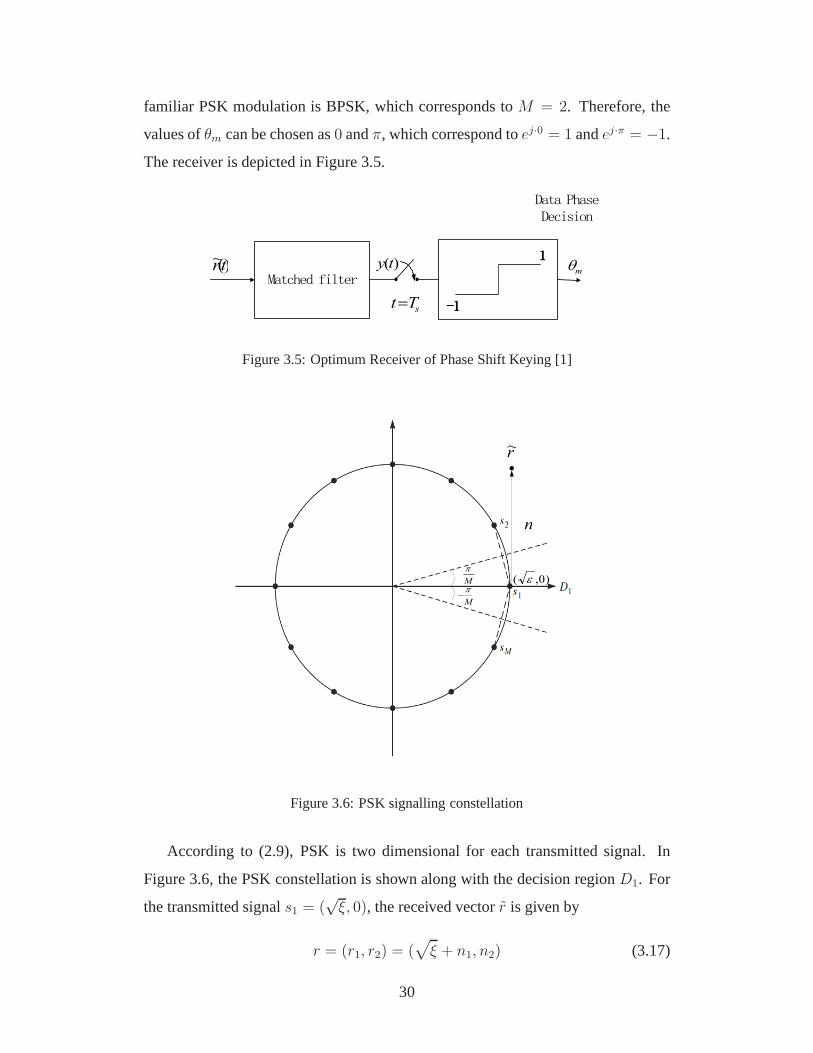
familiar PSK modulation is BPSK, which corresponds toM = 2. Therefore, the

values ofθm can be chosen as0 andπ, which correspond toej·0 = 1 andej·π = −1.

The receiver is depicted in Figure 3.5.

Data Phase

Decision

mθ1111

----1111

Matched filter

)(~tr )(ty

sTt=

Figure 3.5: Optimum Receiver of Phase Shift Keying [1]

M

π−

M

π

)0,( ε

r~

n

Figure 3.6: PSK signalling constellation

According to (2.9), PSK is two dimensional for each transmitted signal. In

Figure 3.6, the PSK constellation is shown along with the decision regionD1. For

the transmitted signals1 = (√ξ, 0), the received vectorr is given by

r = (r1, r2) = (√

ξ + n1, n2) (3.17)

30

wheren1, n2 are noise of independent Gaussian random variables with variance

δ2 = 12N0, and means are both0. The joint PDF of(n1, n2) is given by [1]

p(n1, n2) =1

πN0e−n2

1+n22

N0 . (3.18)

By using the transformation of polar coordinates, the new variables are given

by V =√

n21 + n2

2 andΘ = arctan n2

n1. Then, the joint PDF ofV andΘ is given

as [1]

pV,Θ(v, θ) =v

πN0e− v2

N0 . (3.19)

The decision region is partitioned intoM regions denoted byD1, D2, ..., DM such

that if r ∈ Dm, thenθm = θm. The regionDm, 1 ≤ m ≤ M , is called the decision

region for transmitted signalam. In Figure 3.6, the decision regionD1 is described

asD1 = θ : −π/M < θ < π/M.

Specific coherent detection of PSK modulation is presented below.

M-ary PSK

As we discussed above, we have the transformation of the PSK signalling constella-

tions in the polar coordinates system. TheM-ary PSK follows the same procedure.

The constellation forM-ary PSK is shown in Figure 3.7. Only points1 and its de-

cision region are shown here. The shaded area, which can extend to infinity, shows

the error region whens1 is transmitted.

One conventional transformation is to let the new polar coordinates system’s

origin be at√ξ, which is shown in Figure 3.8. Therefore, the error probability is

P [(n1, n2) ∈ shaded area]. The new polar coordinates system is given as [1]

r =√

n21 + n2

2, (3.20)

ς = arctann2

n1, (3.21)

wheren1 andn2 are independent Gaussian random variables with zero means and

varianceδ2 = 12N0. The length ofR is a function in terms ofθ and is given as [1]

R(θ) =√

ξ sinπ

M· 1

sin θ. (3.22)

31

Figure 3.7: Signalling constellation of MPSK system [1]

),(~ 21 nnr

)0,0()0,( ε−

φ

Figure 3.8: Polar coordinates system for MPSK constellation

32

Therefore, the error probability is given as [1]

Pe =

∫ 2π− πM

πM

dς

∫ ∞

R

r

πN0exp

(

− r

N0

)

dr

= 2

∫ π

πM

dς

∫ ∞

R

exp

(

− ξ sinπM

N0 sin2(φ− π/M)

)

dr

=1

π

∫(M−1)π

M

0

exp

(

− ξ

N0

sin2 πM

sin2 θ

)

dθ. (3.23)

Substituting instantaneous SNR per bitγb = ξb/N0 and using the relationship

between instantaneous SNR per bit and SNR per symbolγ = γblog2M yields

Pe =1

π

∫(M−1)π

M

0

exp(−gpsklog2Mγbsin2 θ

) dθ, where gpsk = sin2 π

M. (3.24)

The most commonly used PSK modulation scheme is BPSK, whereM = 2.

Therefore, the probability of error is given as

Pe =1

π

∫ π2

0

exp(

− γ

sin2 θ

)

dθ = 2Q(√

2γ), (3.25)

where in the case of BPSK,γ andγb are equivalent.

3.3.3 Coherent Detection of squared QAM

Coherent detection of QAM follows the same procedure as thatfor ASK. The re-

ceived signalr(t) = s(t) + n(t), wheres(t) refers toRe[(ami + jamq)g(t)ej2πfct],

whereg(t)ej2πfct is same and is omitted here. The receiver is depicted in Figure

3.9.

Squared M-ary QAM

For the squaredM-ary QAM, the signal constellation is shown as Figure 2.4. Since

the in-phase termami and quadrature-phase termamq both take the equiprobable

values of their information amplitudes,M-ary QAM can be considered as two√M -

ary ASK constellations in the in-phase and quadrature directions. By using the same

procedure of bisector for two signal points, the constellation can be considered in

terms ofdmin as well asM-ary ASK modulation, wheredmin is given (2.19) as

dmin =

√

6log2M

M − 1ξb. (3.26)

33

mia

Decision

mqa

2/M

2/M−

2/M

2/M−

Matched filter

)(~ tr )(ty

sTt =

Decision

Figure 3.9: Optimum Receiver of Quadrature Amplitude Modulation [1]

The probability of the correct detection forM-ary QAM is the product of correct

decision probabilities for constituent ASK modulation; i.e., [1]

Pc,M−QAM = P 2c,√M−ASK

= (1− Pe,√M−ASK)

2. (3.27)

Therefore, the error probability is given by [1]

Pe,M−QAM = 1− Pc,M−QAM = 2Pe,√M−ASK − P 2

e,√M−ASK

. (3.28)

According to (3.14) and (3.26), the probability of error is simplified to [1]

Pe,M−QAM = 4(

√M − 1√M

)Q

(

√

3

M − 1γblog2M

)

− 4(

√M − 1√M

)2Q2

(

√

3

M − 1γblog2M

)

. (3.29)

The most commonly used QAM modulation is 4-QAM, which isM = 4. For

4-QAM,

Pe = 2Q(√

2γ)−Q2(√

2γ). (3.30)

3.3.4 Coherent Detection of FSK

The received signal for coherent FSK isr(t) = s(t) + n(t). The decision about

the transmitted signal is based on the largest frequency. The receiver is depicted in

Figure 3.10.

34

Max ReMax ReMax ReMax Re[[[[ssss((((tttt)])])])]

Decision

mfMatched filter

)(~tr )(ty

sTt=

Figure 3.10: Optimum Receiver of Frequency Shift Keying [1]

In FSK, s(t) refers toRe[ej2πfmt√

2ξg/Tej2πfct], wherem is in the rage of

1 ≤ m ≤ M , and√

2ξg/Tej2πfct is same for each signal and is omitted here for

simplification.

BFSK

One common version of FSK is BFSK, which corresponds toM = 2. Therefore,

the frequencies offm are equal tof1 andf2, respectively. Since we assume all

transmitted signals are equiprobale, the error probability for BFSK follows the pro-

cedure of bisector for two signal points. The error probability of BFSK can be

expressed in terms ofdmin, which is given (2.24) as

dmin =√

2log2M · ξb. (3.31)

Therefore, the error probability of BFSK can be obtained by substitutingdmin

from (3.31) into the bisector determination described in (3.10) in the form of

Pe = Q(

√2ξb√2N0

) = Q(√γ). (3.32)

3.3.5 Noncoherent Detection of M-ary Differential PSK

The noncoherent receiver is not perfectly synchronized with the transmitter. Thus,

the received signal at receiver side isr(t) = s(t− td) + n(t), wheretd represents a

timing error. In such a case, differential PSK may be used.

Differential PSK (DPSK) is also one kind of phase modulationthat conveys or

modifies the phase of the signal waves. Compared to the ordinary PSK modulation

explained in Section 2.1.2, the DPSK modulation does not need a constant reference

35

carrier and can operate with respect to itself; i.e., if∆θm is the information phase to

be transmitted in themth transmission interval, the transmitter would first modulate

θm = θm−1 +∆θm, modulo 2π, (3.33)

and then modulateθm on the carrier. At the receiver side, successive decisions on

θm andθm−1 will be made depending on∆θm. In Figure 3.11, the receiver side of

two adjacent phase decisions for a differentially encoded Quadrature PSK system

is illustrated.

DecisionDecisionDecisionDecision

mθ

DecisionDecisionDecisionDecision

1+mθDelayDelayDelayDelay

TsTsTsTs////2222

∫+

s

s

Tn

nT

dt)1(

(.)

∫+

+

s

s

Tn

Tn

dt)2

3(

)2

1(

(.)DelayDelayDelayDelay

TsTsTsTs////2222

1

-1

-1

1

)(~ tr

Figure 3.11: Optimum Receiver of Differential Phase Shift Keying Modulation [1]

In this modulation technique, the demodulation part determines the changes

in the phase of the received signal rather than the phase of a reference carrier

signal. DPSK is a simpler modulation technique than ordinary PSK modulation

since DPSK does not require a coherent reference at the receiver (this technique

is referred to asnoncoherent detection) and thus it can be noncoherently demodu-

lated. However, DPSK will produce more erroneous demodulation than the ordi-

nary PSK’s demodulation.

The error probability ofM-ary DPSK is given by [46]

Pe =sin π

M

π

∫ π2

0

exp[−log2Mγ(1− cos( πM

cos θ))]

1− cos πM

cos θdθ (3.34)

36

π/4-Differential QPSK

The modulation technique ofπ/4-DQPSK is based on the QPSK modulation. The

ordinary QPSK modulation is a special case ofM-ary PSK; i.e.,M = 4, and the

phase set,θm, is chosen from0, π/2, π, 3π/2 to represent the information phases.

By converting with the initial transmitted phaseπ/4, the ordinary QPSK is con-

verted to the conventional form of Differential QPSK (DQPSK) modulation, in

which theθm is range over the setπ/4, 3π/4, 5π/4, 7π/4.

In the noncoherent detection ofπ/4-DQPSK, the receiver side’s phase decisions

∆θm are based on

∆θm =(2k − 1)π

4, k = 1, 2, 3, 4; (3.35)

i.e., the phase angles areπ/4, 3π/4, 5π/4, 7π/4, in each symbol durationTs. The

error probability ofπ/4-DQPSK is given by [47]

Pe =1

2π

∫ π

0

exp

(

γ(b2 − a2)2

2(a2 + b2)− 4ab cos θ

)

dθ, (3.36)

wherea =√

(1−√

1− |ρ|2/2), b =√

(1 +√

1− |ρ|2/2), and0 ≤ |ρ| ≤ 1 is

the magnitude of the cross-correlation coefficient betweenthe two signals.

3.4 Application of GCQ rules

In Section 3.3, SER expressions for selected digital modulation schemes were given.

These must be averaged over the distribution of the SNR in fading channel. For our

purpose, GCQ rules are introduced for calculating the CEP.

3.4.1 Error Performance of Coherent ASK

The conditional symbol error probability for coherentM-ary ASK can be expressed

in the form of

Ps(ǫ|γb) =2(M − 1)

MQ

(

√

6

M2 − 1γblog2M

)

. (3.37)

By using the transformation of Craig’s formula in (2.27), the CEP is given as

Ps(ǫ|γb) =2(M − 1)

Mπ

∫ π/2

0

exp

(

− 3γblog2M

(M2 − 1) sin2 θ

)

dθ. (3.38)

37

By changing the variablescos(2θ) = x, the CEP of (3.38) can be transformed into

the desired form of GCQ rule as

Ps(ǫ|γb) =M − 1

Mπ

∫ +1

−1

exp

(

6M2

−1log2Mγb

x−1

)

√1− x2

dx. (3.39)

For BASK, 4-ASK, 8-ASK, which isM = 2, M = 4,M = 8 respectively, the CEP

in the desired form of GCQ rule is given as

Pb(ǫ|γb) =1

2π

∫ +1

−1

exp(

2γbx−1

)

√1− x2

dx, BASK, (3.40)

Ps(ǫ|γb) =3

4π

∫ +1

−1

exp(

45γb

x−1

)

√1− x2

dx, 4− ASK, (3.41)

Ps(ǫ|γb) =7

8π

∫ +1

−1

exp(

27γb

x−1

)

√1− x2

dx, 8− ASK. (3.42)

where in BASK, there is only conditional bit error probability instead of the condi-

tional symbol error probability.

3.4.2 Error Performance of Coherent PSK

The conditional symbol error probability for coherentM-ary PSK can be expressed

in the form of

Ps(ǫ|γb) =1

π

∫(M−1)π

M

0

exp(−gpsklog2Mγbsin2 θ

) dθ, where gpsk = sin2 π

M. (3.43)

Through the variable substitution ofx = cos(Mθ/(M − 1)), the desired form of

GCQ rule can be expressed as

Ps(ǫ|γb) =M − 1

Mπ

∫ +1

−1

exp(

gpsklog2Mγbsin2(M−1

Mcos−1(x))

)

√1− x2

dx, where gpsk = sin2 π

M.

(3.44)

One immediate observation can be found is that the upper limit of (3.43) is

(M − 1)π/M , i.e., an arbitrary number. Through the variable substitution of x =

cos(Mθ/(M − 1)), any integration with an arbitrary upper limit can be expressed

in the form of GCQ rule.

38

For BPSK, 4-PSK, 8-PSK, which isM = 2, M = 4, andM = 8 respectively,

the CEP in desired form of GCQ rule is given as

Pb(ǫ|γb) =1

2π

∫ +1

−1

exp(

2γbx−1

)

√1− x2

dx, BPSK, (3.45)

Ps(ǫ|γb) =3

4π

∫ +1

−1

exp(

γbsin2( 3

4cos−1(x))

)

√1− x2

dx, 4− PSK, (3.46)

Ps(ǫ|γb) =7

8π

∫ +1

−1

exp(

3 sin2 π8γb

sin2( 78cos−1(x))

)

√1− x2

dx, 8− PSK, (3.47)

where in BPSK, there is only conditional bit error probability instead of the condi-

tional symbol error probability.

3.4.3 Error Performance of Coherent QAM

The conditional symbol error probability for coherent squaredM-ary QAM can be

expressed in the form of

Ps(ǫ|γb) = 4

(√M − 1√M

)

Q

(

√

3

M − 1γblog2M

)

− 4

(√M − 1√M

)2

Q2

(

√

3

M − 1γblog2M

)

. (3.48)

Following the same procedure as that in the ASK modulation, by using the trans-

formation of Craig’s formula in (2.27) and (2.28), the CEP isgiven as

Ps(ǫ|γb) =4

π

(√M − 1√M

)

∫ π2

0

exp

(

−3

M−1log2Mγb

2 sin2 θ

)

dθ

− 4

π

(√M − 1√M

)2∫ π

4

0

exp

(

−3

M−1log2Mγb

2 sin2 θ

)

dθ (3.49)

where the first term in (3.49) can be achieved as the desired form of GCQ rule

following the ASK’s substitution. By using the variable substitutioncos(4θ) = x

for the second term, the desired form of GCQ rule for the CEP isthus given as

Ps(ǫ|γb) =2

π

(√M − 1√M

)

∫ +1

−1

exp(

3log2Mγb(M−1)(x−1)

)

√1− x2

dx

− 1

π

(√M − 1√M

)2∫ +1

−1

exp(

3log2Mγb2(M−1) sin2( 1

4cos−1 x)

)

√1− x2

dx. (3.50)

39

For 4-QAM, 16-QAM, and 64-QAM, which isM = 4, M = 16, andM = 64,

respectively, the desired form of CEP is given as

Ps(ǫ|γb) =1

2π

∫ +1

−1

exp(

2γbx−1

)

√1− x2

dx

− 1

4π

∫ +1

−1

exp

(

γbsin2( 1

4cos−1 x)

)

√1− x2

dx, 4−QAM, (3.51)

Ps(ǫ|γb) =3

2π

∫ +1

−1

exp(

4γb5(x−1)

)

√1− x2

dx

− 9

16π

∫ +1

−1

exp

(

2γb5 sin2( 1

4cos−1 x)

)

√1− x2

dx, 16−QAM, (3.52)

Ps(ǫ|γb) =7

4π

∫ +1

−1

exp(

2γb7(x−1)

)

√1− x2

dx

− 49

64π

∫ +1

−1

exp

(

γb7 sin2( 1

4cos−1 x)

)

√1− x2

dx, 64−QAM. (3.53)

3.4.4 Error Performance of Coherent FSK

The CEP for coherent BFSK can be expressed in the form of

Pb(ǫ|γb) = Q(√γb). (3.54)

By following the same procedures as that for ASK, and using the variable substitu-

tion of cos(2θ) = x, the desired form of CEP can be expressed as

Pb(ǫ|γb) =1

2π

∫ +1

−1

exp(

γbx−1

)

√1− x2

dx. (3.55)

3.4.5 Error Performance of Nocoherent modulation

The CEP for noncoherent M-ary DPSK is given by [46]

Ps(ǫ|γb) =sin π

M

π

∫ π2

0

exp[−log2Mγ(1 − cos( πM) cos θ)]

1− cos πM

cos θdθ. (3.56)

By changing of the variable,x = cos(2θ), the desired form of CEP is acquired as

Ps(ǫ|γb) =sin π

M

2π

∫ +1

−1

exp[−γblog2M(1−cos πM

cos( 12cos−1 x))]

1−cos πM

(cos( 12cos−1 x))√

1− x2dx. (3.57)

40

For noncoherent QDPSK, which isM = 4, the CEP in the desired form of GCQ

rule is given as

Ps(ǫ|γb) =sin π

4

2π

∫ +1

−1

exp[−2γb(1−cos π4cos( 1

2cos−1 x))]

1−cos π4(cos( 1

2cos−1 x))√

1− x2dx. (3.58)

The CEP for noncoherent detection of equal energy,π/4 DQPSK, is given by

[47]

Ps(ǫ|γb) =1

2π

∫ π

0

exp

(

− 2γb

2 −√2 cos θ

)

dθ. (3.59)

By using the variable substitution ofcos θ = x, the desired form of GCQ rule can

be expressed as

Ps(ǫ|γb) =1

2π

∫ +1

−1

exp(

−2γb2−

√2x

)

√1− x2

dx. (3.60)

The conditional BERs/SERs of several digital modulation schemes are given

in Table 3.1. To author’s best knowledge, Table 3.1 has tabulated every digital

modulation scheme which can adopt the GCQ rule.

Furthermore, one recognition can be acquired immediately from Table 3.1, that

these expressions can be classified into two general forms

1. the simple-angle limits GaussianQ-function, i.e.,Q(·), which has the Craig’s

transformation with limits[0, π2], and

2. the multi-angle limits Gaussian integral function, i.e., the CEP ofM-ary PSK,

which has the limits[0, (M−1)πM

] .

Moreover, the simple-angle limits GaussianQ-function can be considered as a spe-

cial case of the multi-angle limits Gaussian integral function, which can be obtained

through modifying the upper limits to the corresponding single angle.

The average BER/SER over the fading channels can be derived by integrating

the CEP over the PDF of SNR, which can be expressed as

P =

∫ ∞

0

P (ǫ|γ)pγdγ =

∫ +1

−1

ζγ(x)√1− x2

dx, (3.61)

whereζγ(x) is selected and calculated with respect to the corresponding digital

modulation scheme in Table 3.1.

41

Table 3.1: Common Digital Modulation Scheme using Gauss Chebyshev Quadrature

Coherent ModulationModulation Modulation Conditional Error Probability Gauss Chebyshev Quadrature Format

Type Name P (ǫ|γb) P (ǫ|γb)

ASK

BASK Pb = Q(√2γb) Pb = 1

2π

∫+1−1

exp(2γbx−1

)√1−x2

dx

MASKPs = 2(M−1

M) Ps = M−1

Mπ

·Q(√

6M2

−1γblog (M))

·∫+1−1

exp

6M2

−1log(M)γb

x−1

√1−x2

dx

PSK

BPSK Pb = Q(√2γb) Pb = 1

2π

∫+1−1

exp(2γbx−1

)√1−x2

dx

MPSK

Ps = 1π

Ps = M−1Mπ

·∫

(M−1)πM

0 exp(− gpsklog(M)γbsin2(θ)

) dθ ·∫+1−1

exp(−gpsklog(M)γb

sin2( M−1M

cos−1(x)))

√1−x2

dx

wheregpsk = sin2 πM

wheregpsk = sin2 πM

QAM

4-QAMPs = 2Q(

√2γb) Ps = 1

π

∫+1−1

exp(2γbx−1

)√1−x2

dx

−Q2(√2γb) − 1

4π

∫+1−1

exp(2γb

2 sin2( 14

cos−1(x)))

√1−x2

dx

SqraredPs = 4(

√

M−1√

M) Ps = 2

π(√

M−1√

M)

·Q(√

3M−1

γblog (M)) ·∫+1−1

exp(3γblog(M)

(M−1)(x−1))√

1−x2dx

M-QAM−4(

√

M−1√

M)2 − 1

π(√

M−1√

M)2

·Q2(√

3M−1

γblog (M)) ·∫+1−1

exp(3γblog(M)

2(M−1) sin2(cos−1(x)))

√1−x2

dx

FSK BFSK Pb = Q(√γb) Pb = 1

2π

∫+1−1

exp(γb

x−1)√

1−x2dx

Non-Coherent ModulationMDPSK Ps =

sin πM

πPs =

sin πM

2π

∫

π2

0

exp[−log(M)γb(1−cos( πM

cos θ))]

1−cos πM

cos θdθ ∫+1

−1

exp[−log(M)(1−cos πM

cos( 12

cos−1 x))γb]

1−cos πM

(cos( 12

cos−1 x))√1−x2

dx

π/4-DQPSK Ps = 12π

∫ π0 exp

(

− 2γb2−

√

2 cos θ

)

dθ Ps = 12π

∫+1−1

exp(

−2γb

2−√

2x

)

√1−x2

42

3.5 Numerical and Simulation Results

In this section, classical and rational GCQ rules are used for evaluating SER in both

single and diversity receptions over the Rayleigh, Rician and Nakagami-m fading

channels. The MGF approach of calculating the average errorrate is adopted.

3.5.1 Error Performance of Single Channel Reception

Numerical results for several digital modulation schemes are provided to investigate

the efficiency of both classical and rational GCQ rules. An excellent agreement

between the analytical and numerical integration simulation results is observed.

Rayleigh Fading

Figures 3.12-3.16 show the performance of different digital modulation schemes

described in Section 3.4 in the single channel reception over Rayleigh fading sce-

nario. The average BERs/SERs are quantified by both classical and rational GCQ

rules. For comparison, the exact average BERs/SERs are generated through numer-

ical integrations.

Subfigures 3.12-3.16 (a) show the exact BERs/SERs of severaldigital modula-

tion schemes and the quantified BERs/SERs by adopting the classical and rational

GCQ rules with2 nodes. These subfigures show that the rational GCQ outperforms

the classical GCQ rule in the low SNR region.

Subfigures 3.12-3.16 (b) show the number ofnodes required for each method

to converge. The convergence rate is defined by

limm→∞

υm − υm−1

υm≤ 10−5, (3.62)

wherem refers to the number ofnodes, andυ refers to the relative error, which

is determined by the number ofnodes. By comparing the relative error obtained

through the number ofnodes and its adjacent number of (nodes − 1) at the same

SNR in the region of less or equal than10−5, the minimal requiredm can be ob-

tained. It is clear that rational GCQ rule converges faster than the classical GCQ

rule in the lower SNR region.

43

−30 −20 −10 0 10 2010

−3

10−2

10−1

100

SNR

Sym

bol E

rror

Rat

e

peexact

pegcq

percq

4−ASK

BASK

8−ASK

(a) Error performance with 2 nodes

−30 −20 −10 0 10 200

10

20

30

40

50

60

70

80

90

100

SNR

Num

ber

of n

odes

nodes

gcq

nodesrcq

8−ASK

4−ASK

BASK

(b) Convergence rate of GCQ

Figure 3.12: Coherent Detection ofM -ary ASK (M = 2, 4, 8) in Rayleigh fading

−30 −20 −10 0 10 2010

−3

10−2

10−1

100

SNR

Sym

bol E

rror

Rat

e

peexact

pegcq

percq

BPSK

4−PSK

8−PSK


−30 −20 −10 0 10 200

10

20

30

40

50

60

70

80

90

100

SNR

Num

ber

of n

odes

nodes

gcq

nodesrcq

8−PSK 4−PSK

BPSK


Figure 3.13: Coherent Detection ofM -ary PSK (M = 2, 4, 8) in Rayleigh fading

−30 −20 −10 0 10 2010

−3

10−2

10−1

100

101

SNR

Sym

bol E

rror

Rat

e

peexact

pegcq

percq

4−QAM

16−QAM

64−QAM


−30 −20 −10 0 10 200

10

20

30

40

50

60

70

80

90

100

SNR

Num

ber

of n

odes

nodes

gcq

nodesrcq

64−QAM

16−QAM

4−QAM


Figure 3.14: Coherent Detection ofM -ary QAM (M = 4, 16, 64) in Rayleigh fading

44

−30 −20 −10 0 10 2010

−3

10−2

10−1

100

SNR

Sym

bol E

rror

Rat

e

pe

exact

pegcq

percq


−30 −20 −10 0 10 200

10

20

30

40

50

60

70

80

SNR

Num

ber

of n

odes

nodes

gcq

nodesrcq


Figure 3.15: Coherent Detection of BFSK in Rayleigh fading

−30 −20 −10 0 10 20

10−2

10−1

100

101

SNR

Sym

bol E

rror

Rat

e

pe

exact

pegcq

percq

4−DPSK

π/4−DQPSK


−30 −20 −10 0 10 200

5

10

15

20

25

SNR

Num

ber

of n

odes

nodes

gcq

nodesrcq

4−DPSK

π/4 QDPSK


Figure 3.16: Non Coherent Detection of4-ary DPSK andπ/4-DQPSK modulation in Ray-leigh fading

45

Rician Fading

Figures 3.17-3.21 show the SER of several digital modulations in Rician fading

(K = 3). It can be seen that in each different digital modulation scheme, the

rational GCQ performs better than the classical GCQ rule, especially, in the low

SNR region. These figures also show that the rational GCQ ruleconverges faster

than classical GCQ rule; i.e., rational GCQ requires fewernodes than the classical

one, where the convergence rate is defined as the same as it is in the numerical

analysis shown in Rayleigh fading.

−30 −20 −10 0 10 2010

−4

10−3

10−2

10−1

100

SNR

Sym

bol E

rror

Rat

e

peexact

pegcq

percq

BASK

4−ASK

8−ASK


−30 −20 −10 0 10 200

10

20

30

40

50

60

70

80

SNR

Num

ber

of n

odes

nodes

gcq

nodesrcq

8−ASK

4−ASK

BASK


Figure 3.17: Coherent Detection ofM -ary ASK (M = 2, 4, 8) in Rician fading (K = 3).

−30 −20 −10 0 10 2010

−4

10−3

10−2

10−1

100

SNR

Sym

bol E

rror

Rat

e

peexact

pegcq

percq

BPSK

4−PSK

8−PSK


−30 −20 −10 0 10 200

10

20

30

40

50

60

70

80

SNR

Num

ber

of n

odes

nodes

gcq

nodesrcq

8−PSK

4−PSK

BPSK


Figure 3.18: Coherent Detection ofM -ary PSK (M = 2, 4, 8) in Rician fading (K = 3).

46

−30 −20 −10 0 10 2010

−4

10−3

10−2

10−1

100

101

SNR

Sym

bol E

rror

Rat

e

peexact

pegcq

percq

4−QAM

16−QAM

64−QAM


−30 −20 −10 0 10 2010

20

30

40

50

60

70

80

SNR

Num

ber

of n

odes

nodes

gcq

nodesrcq

64−QAM

16−QAM

4−QAM


Figure 3.19: Coherent Detection ofM -ary QAM (M = 4, 16, 64) in Rician fading (K = 3).

−30 −20 −10 0 10 2010

−3

10−2

10−1

100

SNR

Sym

bol E

rror

Rat

e

pe

exact

pegcq

percq


−30 −20 −10 0 10 200

10

20

30

40

50

60

70

SNR

Num

ber

of n

odes

nodes

gcq

nodesrcq


Figure 3.20: Coherent Detection of BFSK in Rician fading (K = 3).

−30 −20 −10 0 10 20

10−2

10−1

100

101

SNR

Sym

bol E

rror

Rat

e

pe

exact

pegcq

percq

4−DPSK π/4 DQPSK


−30 −20 −10 0 10 200

5

10

15

20

25

SNR

Num

ber

of n

odes

nodes

gcq

nodesrcq

4−DPSK

π/4−DQPSK


Figure 3.21: Non Coherent Detection of4-ary DPSK andπ/4-DQPSK in Rician fading(K = 3).

47

Nakagami-2 Fading

The error performance of different digital modulations in Nakagami-2 fading is

presented in Figures 3.22-3.26. The rational GCQ rule has a relatively lower error

in the low SNR region, and its convergence rate is better thanthat of the classical

GCQ rule.

−30 −20 −10 0 10 2010

−5

10−4

10−3

10−2

10−1

100

SNR

Sym

bol E

rror

Rat

e

peexact

pegcq

percq

BASK

4−ASK

8−ASK


−30 −20 −10 0 10 200

10

20

30

40

50

60

SNR

Num

ber

of n

odes

nodes

gcq

nodesrcq

8−ASK

4−ASK

BASK


Figure 3.22: Coherent Detection ofM -ary ASK (M = 2, 4, 8) in Nakagami-2 fading

−30 −20 −10 0 10 2010

−5

10−4

10−3

10−2

10−1

100

SNR

Sym

bol E

rror

Rat

e

peexact

pegcq

percq

BPSK

4−PSK

8−PSK


−30 −20 −10 0 10 200

10

20

30

40

50

60

SNR

Num

ber

of n

odes

nodes

gcq

nodesrcq

8−PSK

4−PSK

BPSK


Figure 3.23: Coherent Detection ofM -ary PSK (M = 2, 4, 8) in Nakagami-2 fading

48

−30 −20 −10 0 10 2010

−4

10−3

10−2

10−1

100

101

SNR

Sym

bol E

rror

Rat

e

peexact

pegcq

percq

4−QAM

16−QAM

64−QAM


−30 −20 −10 0 10 200

10

20

30

40

50

60

70

80

SNR

Num

ber

of n

odes

nodes

gcq

nodesrcq

64−QAM

16−QAM

4−QAM


Figure 3.24: Coherent Detection ofM -ary QAM (M = 4, 16, 64) in Nakagami-2 fading

−30 −20 −10 0 10 2010

−4

10−3

10−2

10−1

100

SNR

Sym

bol E

rror

Rat

e

pe

exact

pegcq

percq


−30 −20 −10 0 10 200

10

20

30

40

50

60

70

SNR

Num

ber

of n

odes

nodes

gcq

nodesrcq


Figure 3.25: Coherent Detection of BFSK in Nakagami-2 fading

−30 −20 −10 0 10 20

10−3

10−2

10−1

100

101

SNR

Sym

bol E

rror

Rat

e

peexact

pegcq

percq

4−DPSK

π/4−DQPSK


−30 −20 −10 0 10 200

5

10

15

20

25

SNR

Num

ber

of n

odes

nodes

gcq

nodesrcq

4−DPSKπ/4 DQPSK


Figure 3.26: Non Coherent Detection ofM -ary DPSK andπ/4-DQPSK in Nakagami-2fading

49

3.5.2 Error Performance of Diversity Reception

The three commonly used diversity combining techniques aremaximal ratio com-

bining (MRC), equal gain combining (EGC), and selection combining (SC). Here,

we will focus on only MRC. MRC is an optimal diversity combining technique for

the independent AWGN channels since MRC provides the highest average output

SNR regardless of the fading statistics [48]. The MGF of the SNR in MRC can be

expressed as

ϕγ(s) = E[exp[−s(γ1 + γ2 + . . .+ γL)]]

=L∏

l=1

ϕγl(s) (3.63)

whereL is the number of diversity branches. Thus, the MRC case for digital mod-

ulation schemes can be obtained by combining Table 3.1 and the MGF of the SNR

over different fading scenarios.

Recognizing that the CEP ofM-ary PSK in Table 3.1 has a common format, we

can intuitively derive every single angle from it. Thus, we will useM-ary PSK as

a proxy for general digital modulation schemes to investigate the rational GCQ in

different common fadings.

Rayleigh Fading

Figure 3.27 shows the SERs of 8-PSK with the assumption that all the MRC space

diversity branches undergo identical Rayleigh fading. Theexact performance curve

of MRC is generated by using the numerical integration simulation. Figure 3.27

reveals that the difference between rational GCQ and classical GCQ rules is quite

small .

Figures 3.28, 3.29, and 3.30 compare the convergence rate as(nodes → ∞) of

the classical and rational GCQ rules for Rayleigh fading channels. These figures

show that as the diversity orderL increases the absolute error,|Pexact − Pgcq| , is

decreasing. In other words, MRC provides the best combination of SER of any of

the modulation schemes. This result is to be expected because diversity reception

implements an effective technique for suppressing the channel fading effects. As

50

the nodes increase, both classical GCQ and rational GCQ turn to be equivalent.

Another observation is that by using a small number ofnodes for both classical

and rational GCQ rules for evaluation, rational GCQ rule hasa lower value of the

absolute error, so that the rational GCQ rule has a better convergence rate.

Table 3.2 shows the required number ofnodes for classical and rational GCQ

rules and their relative error. One recognition is that in the low SNR region, the

rational GCQ requires fewernodes to converge, and the relative error is smaller

than that of the classical GCQ rule. In the high SNR region, the rational GCQ and

the classical GCQ require almost an equal number ofnodes to converge, and the

relative error for each is almost the same. However, when thenumber ofnodes is

smaller, the rational GCQ performs better than the classical GCQ.

−30 −20 −10 0 10 2010

−6

10−5

10−4

10−3

10−2

10−1

100

SNR

Sym

bol E

rror

Rat

e

peexact

pegcq

percq

L=1

L=2

L=3

Figure 3.27: Error performance for 8PSK with diversity reception in Rayleigh fading(nodes = 8).

51

0 10 20 30 40 5010

−14

10−12

10−10

10−8

10−6

10−4

10−2

100

number of nodes

|Pex

act−

Pgc

q|

−10 dB cGCQ−10 dB rGCQ0 dB cGCQ0 dB rGCQ10 dB cGCQ10 dB rGCQ20 dB cGCQ20 dB rGCQ

Figure 3.28: Error performance for 8PSK with MRC (L = 1) in Rayleigh fading.

0 10 20 30 40 5010

−20

10−15

10−10

10−5

100

number of nodes

|Pex

act−

Pgc

q|



52

0 10 20 30 40 5010

−30

10−25

10−20

10−15

10−10

10−5

100

number of nodes

|Pex

act−

Pgc

q|



Table 3.2: Relative errors:L = 1, 2, 3, MRC, Rayleigh fading

Average SNR L number of nodes Relative Errorγb nodesgcq nodesrcq relative errorgcq relative errorrcq

−20 dB

1 54 22 2.78e-05 3.56e-05

2 56 28 5.52e-05 4.75e-05

3 44 32 1.41e-04 5.69e-05

−10 dB

1 38 38 7.97e-05 8.35e-05

2 46 48 1.03e-04 1.02e-04

3 50 52 1.09e-04 1.12e-04

0 dB

1 46 46 9.85e-05 1.01e-04

2 40 42 8.41e-05 8.20e-05

3 30 32 5.96e-05 6.05e-05

10 dB

1 42 42 8.92e-05 9.05e-05

2 10 10 5.77e-05 6.14e-05

3 10 12 2.31e-06 2.36e-06

20 dB

1 40 40 9.07e-05 9.11e-05

2 10 10 2.17e-05 2.22e-05

3 10 10 5.06e-07 5.02e-07

53

Rician Fading

Figure 3.31 compares the SER of 8-PSK with MRC reception in identical Rician

fading, where the Rician fading factorK = 3. One recognition is that SER evalua-

tion using rational and classical GCQ rules is quite close tothe exact performance.

Figure 3.32, 3.33, and 3.34 compare the convergence rate as (nodes → ∞) of the

classical GCQ and rational GCQ rules for Rician fading (K = 3) channel. It can

be seen that as the diversity orderL increases, the evaluation of the absolute errors

between classical and rational rules is decreasing. This result verifies that MRC is

an effective diversity combining technique.

In Table 3.3, selected data of the required number ofnodes and relative error

between the classical GCQ and rational GCQ rules are presented. This table reveals

that in the low SNR region, the required number ofnodes and the relative errors

of rational GCQ are smaller than those of the classical GCQ rule. In the high

SNR region, the number ofnodes required to converge and the relative errors are

similar, except whenγb = −10 dB, L = 1 andγb = 20 dB, L = 3. These two

exceptions are caused by the convergence rate. The classical GCQ rule converges

faster than the rational GCQ in these two exceptional points. However, compared

to the results of the relative error, the rational GCQ rule has a high accuracy at these

two exceptions.

−30 −20 −10 0 10 2010

−10

10−8

10−6

10−4

10−2

100

SNR

Sym

bol E

rror

Rat

e

peexact

pegcq

percq

L=1

L=2

L=3

Figure 3.31: Error performance for 8PSK with diversity reception in Rician fading (K = 3)and (nodes = 8).

54

0 10 20 30 40 5010

−14

10−12

10−10

10−8

10−6

10−4

10−2

100

number of nodes

|Pex

act−

Pgc

q|


Figure 3.32: Error performance for 8PSK with MRC (L = 1) in Rician fading (K = 3).

0 10 20 30 40 5010

−25

10−20

10−15

10−10

10−5

100

number of nodes

|Pex

act−

Pgc

q|



55

0 10 20 30 40 5010

−30

10−25

10−20

10−15

10−10

10−5

100

number of nodes

|Pex

act−

Pgc

q|



Table 3.3: Relative errors:L = 1, 2, 3, MRC, Rician fading and Rician factorK = 3


−20 dB

1 38 48 4.56e-04 2.71e-05

2 54 38 5.94e-05 4.11e-05

3 44 36 1.48e-04 5.10e-05

−10 dB

1 26 40 1.78e-04 8.56e-05

2 46 48 1.04e-04 1.04e-04

3 50 52 1.10e-04 1.14e-04

0 dB

1 46 48 1.07e-04 1.02e-04

2 40 40 8.05e-05 8.75e-05

3 30 32 5.65e-05 5.82e-05

10 dB

1 38 38 7.52e-05 7.73e-05

2 22 24 4.92e-05 4.53e-05

3 10 12 2.41e-05 2.29e-05

20 dB

1 40 40 8.32e-05 8.41e-05

2 28 28 5.74e-05 5.91e-05

3 8 18 1.03e-04 3.18e-05

56

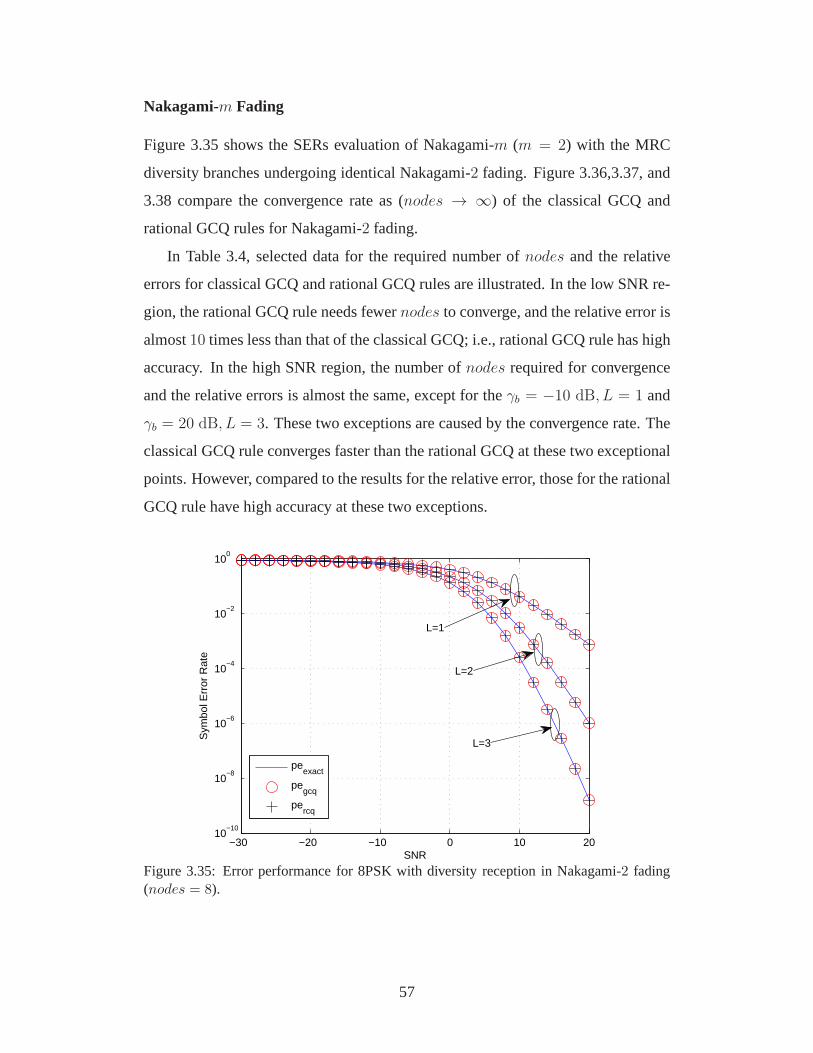
Nakagami-m Fading

Figure 3.35 shows the SERs evaluation of Nakagami-m (m = 2) with the MRC

diversity branches undergoing identical Nakagami-2 fading. Figure 3.36,3.37, and

3.38 compare the convergence rate as (nodes → ∞) of the classical GCQ and

rational GCQ rules for Nakagami-2 fading.

In Table 3.4, selected data for the required number ofnodes and the relative

errors for classical GCQ and rational GCQ rules are illustrated. In the low SNR re-

gion, the rational GCQ rule needs fewernodes to converge, and the relative error is

almost10 times less than that of the classical GCQ; i.e., rational GCQrule has high

accuracy. In the high SNR region, the number ofnodes required for convergence

and the relative errors is almost the same, except for theγb = −10 dB, L = 1 and

γb = 20 dB, L = 3. These two exceptions are caused by the convergence rate. The

classical GCQ rule converges faster than the rational GCQ atthese two exceptional

points. However, compared to the results for the relative error, those for the rational

GCQ rule have high accuracy at these two exceptions.

−30 −20 −10 0 10 2010

−10

10−8

10−6

10−4

10−2

100

SNR

Sym

bol E

rror

Rat

e

peexact

pegcq

percq

L=1

L=2

L=3

Figure 3.35: Error performance for 8PSK with diversity reception in Nakagami-2 fading(nodes = 8).

57

0 10 20 30 40 5010

−16

10−14

10−12

10−10

10−8

10−6

10−4

10−2

100

number of nodes

|Pex

act−

Pgc

q|


Figure 3.36: Error performance for 8PSK with MRC (L = 1) in Nakagami-2 fading.

0 10 20 30 40 5010

−25

10−20

10−15

10−10

10−5

100

number of nodes

|Pex

act−

Pgc

q|


Figure 3.37: Error performance for 8PSK with MRC (L = 2) in Nakagami-2 fading (m =2).

58

0 10 20 30 40 5010

−35

10−30

10−25

10−20

10−15

10−10

10−5

100

number of nodes

|Pex

act−

Pgc

q|


Figure 3.38: Error performance for 8PSK with MRC (L = 3) in Nakagami-2 fading (m =2).

Table 3.4: Relative errors:L = 1, 2, 3, MRC, Nakagami-2 fading


−20 dB

1 40 22 4.56e-04 3.63e-05

2 58 28 2.62e-05 4.67e-05

3 48 32 3.75e-05 5.59e-05

−10 dB

1 30 40 1.15e-04 8.45e-05

2 44 46 1.02e-04 1.01e-04

3 48 52 1.09e-04 1.03e-04

0 dB

1 48 48 1.02e-04 1.05e-04

2 44 44 9.25e-05 9.83e-05

3 38 40 7.58e-05 7.57e-05

10 dB

1 34 34 7.41e-05 7.59e-05

2 32 34 6.34e-05 6.54e-05

3 22 22 4.36e-05 4.73e-05

20 dB

1 30 30 6.47e-05 6.53e-05

2 30 30 6.29e-05 6.38e-05

3 20 8 3.61e-05 1.62e-04

59

3.6 Conclusion

This chapter reviewed the performance of coherent and noncoherent digital mod-

ulation schemes over typical multipath fading channels. Analytical expressions of

BER/SER were tabulated for the cases where the classical andrational GCQ rules

can be adopted. One new generalized integral model for adopting rational GCQ

rule, i.e., SER ofM-PSK, with arbitrary upper limits was investigated. Numer-

ical results showed that in the low SNR region, the rational GCQ rule provided

a rapid convergence rate and better accuracy than the classical GCQ rule. In the

high SNR region, the classical and rational GCQ rules had almost the same perfor-

mance. However, when the number of nodes was smaller, i.e., less than the number

required for each rule to converge, the rational GCQ performed better than the clas-

sical GCQ.

∼

60

Chapter 4

GCQ for Co-Channel InterferenceOutage

In Chapter 3, performance metrics of SER over multipath fading channels were

described. This chapter will use GCQ rules for computing theoutage.

4.1 Introduction

In this chapter, the use of classical and rational GCQ rules for outage probability

analysis in the presence of CCI is investigated. Numerical examples of unequal

Rice factors and transmit powers over the Rayleigh and Rician fading distributions

demonstrate the high accuracy of these methods.

In the remainder of this chapter, outage computation and thedesired form of

GCQ rule for calculating outage probability of each different fading case is illus-

trated in Section 4.2. Numerical and simulation examples are presented in Section

4.3. Finally, Section 4.4 concludes the chapter.

4.2 Outage Probability

The outage probability,Pout , is defined as the probability that the instantaneous

SIR falls below a certain threshold value. The outage probability of an interference-

limited network can be expressed as

Pout = PΩ0 < γth(Ω1 + . . .+ ΩL), (4.1)

61

whereΩ0 andΩ1, . . . ,ΩL are the instantaneous signal powers of the desired signal

and interfering signals, respectively, with average power, Ωl, l = 0, 1, . . . , L. The

power protection ratio,γth, is fixed by the type of modulation and transmission

technique employed and the quality of service desired.

The instantaneous SIR is given by

Γ =Ω0

Ω1 + . . .+ ΩL=

Ω0∑L

l=1Ωl

, (4.2)

where the instantaneous SIR falls below a pre-defined threshold γth. It is easy to

show that the outage probability in terms ofΓ andγth is presented as

Pout = P(Γ < γth). (4.3)

Let us define a new variableγSIR:

γSIR = Γ− γth

=Ω0

γth−

L∑

l=1

Ωl. (4.4)

The MGF ofγSIR is given by

ϕγSIR= ϕ0(

s

γth)

L∏

l=1

ϕl(−s), (4.5)

whereϕl is the MGF ofpl and can be any one of the MGFs in Section 3.2. It follows

that the outage probability is given by

Pout = P(γSIR < 0). (4.6)

Pout can also be written as [49]

Pout =1

2π

∫ ∞

−∞

ϕγSIR(c+ jw)

c+ jwdw

=1

π

∫ ∞

0

Re[(c− jw)(ϕγSIR(c+ jw))]

c2 + w2dw, (4.7)

wherej2 = −1, 0 < c < smin = minsi|1 ≤ i ≤ L with si being thei-th pole of

ϕγSIR(s) in the right-half plane. Although the value ofc can be selected anywhere

between0 andsmin, it is better to choose it such thatϕγSIRdecays very rapidly as

w → ∞. In practice, it is sufficient to usec = smin/2 [18,49].

62

By substitutingw = c tan(θ/2) into (4.7), we get [18]

Pout =1

2π

∫ π

0

Re[(1− j tan(θ

2))(ϕγSIR

(c+ jc tan(θ

2)))] dθ. (4.8)

Further, by using variable substitutionx = cos θ in (4.8), we get [2]

Pout =1

2π

∫ +1

−1

Re(

1− j√1−x2

1+x

)

ϕγSIR

(

c+ jc√1−x2

1+x

)

√1− x2

dx, (4.9)

which is the desired form for applying the rational GCQ and classical GCQ rules.

By using the MGF of the corresponding fading scenario, the desired GCQ for-

mat of outage probability of each different fading case can be obtained. However,

the available models for using both classical and rational GCQ rules are limited to

Rayleigh and Rician fading only, since for other fading scenarios, the use of the

rational GCQ rule for the nodes computation always involvescomplex numbers,

which do not satisfy the initial assumption that all the nodes are real values.

4.2.1 Rician Fading with Multiple Rayleigh Interferers

In this case, the desired signal experiences Rician fading whileL interfering signals

are subject to Rayleigh fading. By using the results from (3.5) and (3.7) for Ray-

leigh and Rician distributions and substituting them into equation (4.5), the desired

signal,ϕ0(s/γth), and the interfering signals,ϕl(−s), are obtained as

ϕ0(s

γth) =

exp

(

−KΩ0s

(K+1)γth

1+Ω0

(K+1)γth

)

1 + Ω0s(K+1)γth

, (4.10)

ϕl(−s) =1

(1− Ωls). (4.11)

Therefore, the MGF ofγSIR is

ϕγSIR(s) = ϕ0(

s

γth)

L∏

l=1

ϕl(−s)

=

exp

(

−KΩ0s

(K+1)γth

1+Ω0

(K+1)γth

)

(

1 + Ω0s(K+1)γth

∏Ll=1(1− Ωls)

) . (4.12)

The outage can be computed by substituting (4.12) into (4.9). For the rational

GCQ rule, the pole of the functionf(x) needs to be found first. One observation can

63

be found is thatf(x) has a pole of infinite multiplicity at−(

1 +2Ω2

0c2/(γ2

th(K+1)2)

1+2Ω0c/(γth(K+1))

)

andL simple poles at−(

1 +2Ω2

lc2

1−2Ωlc

)

.

4.2.2 Multiple Rician Interferers

In the case of the desired signal and theL interfering signals both experiencing

Rician fading, by applying the MGF expression from (3.7), the desired signal,

ϕ0(s/γth) , and the interfering signals,ϕl(−s) are obtained as

ϕ0(s

γth) =

exp

(

−K0Ω0s

(1+K0)γth

1+Ω0s

(1+K0)γth

)

1 + Ω0s(1+K0)γth

, (4.13)

ϕl(−s) =

exp

(

KlΩls

1+Kl

1− Ωls

1+Kl

)

1− Ωls1+Kl

. (4.14)

The MGF ofγSIR is

ϕγSIR(s) =

exp

(

−K0Ω0s

(1+K0)γth

1+Ω0s

(1+K0)γth

)

1 + Ω0s(1+K0)γth

·L∏

l=1

exp

(

KlΩls

1+Kl

1− Ωls

1+Kl

)

1− Ωls1+Kl

. (4.15)

To compute the outage, we just need to substitute (4.15) into(4.9). By using

the rational GCQ rule, the poles off(x) can be found at one pole of multiplicity at

−(

1 +2Ω2

0c2/(γth(K0+1))2

1+2Ω0c/(γth(K0+1))

)

andL simple poles at−(

1 +2Ω2

lc2/((1+Kl)

2)

1+2Ωlc/(1+Kl)

)

.

4.2.3 Mixed Rayleigh and Rician Interferers

In this case, the desired signal is subject to Rician fading,and the total number

of L interfering signals are composed of both Rayleigh and Rician faded signals;

i.e., there areM Rayleigh interferers andL − M Rician interferers. By applying

the MGF from (3.5) and (3.7), the corresponding desired signal, ϕ0(s/γth), the

interfering signals of Rayleigh fading,ϕm(−s), and the interfering signals of Rician

64

fading,ϕn(−s) can be written as

ϕ0(s

γth) =

exp

(

−K0Ω0s

(1+K0)γth

1+Ω0s

(1+K0)γth

)

1 + Ω0s(1+K0)γth

, (4.16)

ϕm(−s) =1

Ωms, (4.17)

ϕn(−s) =

exp

(

KnΩns1+Kn

1− Ωns1+Kn

)

1− Ωns1+Kn

. (4.18)

Therefore, the MGF ofγSIR is given by

ϕγSIR(s) =

exp

(

−K0Ω0s

(1+K0)γth

1+Ω0s

(1+K0)γth

)

1 + Ω0s(1+K0)γth

· 1∏M

m=1(1− Ωms)·

L∏

n=M+1

exp

(

KnΩns1+Kn

1− Ωns1+Kn

)

1− Ωns1+Kn

.

(4.19)

The outage can be computed by substituting (4.19) into (4.9). By adopting the

rational GCQ approximation, the poles off(x) can be found. There is one pole

located at−(

1 +2Ω2

0c2/(γth(K0+1))2

1+2Ω0c/(γth(K0+1))

)

,M simple poles located at−(

1 + 2Ω2mc2

1−2Ωmc

)

,

andL−M simple poles located at−(

1 + 2Ω2nc

2/((1+Kn)2)1+2Ωnc/(1+Kn)

)

.

4.3 Numerical Results

In this section, a set of numerical results and simulation examples are provided

under the asumption that Rayleigh and Rician fading channels are present. Since

the desired format of (4.9) for rational GCQ and classical GCQ rules is straightfor-

ward, the main aim is to verify their accuracy, relative error, and convergence rate.

In addition, we use the value ofc = smin/2 as a rule of thumb for the outage com-

putations. For comparison purposes, the exactPout is computed by evaluating (4.8)

by using Matlab’squad8 function with an absolute tolerance of10−15 [49]. All the

investigated cases show excellent agreement between the analytical and simulation

results.

4.3.1 Rician Fading with Multiple Rayleigh Interferers

Figure 4.1 shows the outage performance when the desired signal is subject to

Rician fading while the interfering signals are Rayleigh faded. The Rician fad-

65

ing factor of the desired signalK = 3, and the number of interferersL = 2.

The interfering signals’ powers areΩl = [1, 1.8] , and the power protection ra-

tio is γth = 9.5 dB [18]. The instantaneous SIR over the power protection ratio

Λ = Ω0/(γth∑L

l=1 Ωl). In Figure 4.1 (a), the outage probability values obtained

by using the classical GCQ and rational GCQ rules are compared with the exact

results. For both GCQ rules,3 nodes are used. It is apparent from Figure 4.1 (a)

that both rules yield highly accurate results. Figure 4.1(b) shows the relative er-

ror of each rule. It is clear that rational GCQ rule outperforms the classical GCQ

rule with a relatively small number of nodes. In other words,for a given number

of nodes, the rational GCQ achieves relatively fewer errorsthan the classical GCQ

rule.

4.3.2 Rician Fading with Multiple Rician Interferers

Figure 4.2 shows the outage performance when both the desired signal and interfer-

ing signals are subject to Rician fading. The Rician fading factor of the desired sig-

nalK = 2 and the interference signal statistics are given byL = 2, Kl = [1.8, 1.5],

andΩl = [1, 1.6]. The power protection ratioγth = 9.5 dB, and the instantaneous

SIR over the power protection ratioΛ = Ω0/(γth∑L

l=1 Ωl). Figure 4.2 (a) shows

that both rules yield highly accurate results. Figure 4.2 (b) shows the relative error

of each rule. Clearly, rational GCQ rule has better accuracythan the classical GCQ

rule, especially in low SIR region. As SIR increases, both methods converge to

roughly same levels of relative error.

4.3.3 Rician Fading with Mixed Rayleigh and Rician Interferers

Figure 4.3 illustrates the outage performance when the desired signal is subject

to Rician fading and the interfering signals are composed ofboth Rayleigh and

Rician faded signals. The statistics of the given example are K = 2.8, M = 1,

L = 2, Kn = 1.5, Ωl = [1.1, 0.6], the power protection ratio isγth = 9.5 dB,

and the instantaneous SIR over the power protection ratioΛ = Ω0/(γth∑L

l=1 Ωl).

It is apparent from Figure 4.3 that the rational GCQ approximation yields a better

performance in the low SIR region.

66

−20 −15 −10 −5 0 5 10 15 2010

−3

10−2

10−1

100

101

SIR/γth

Pou

t

outage

exact

outagegcq

outagercq

(a) Outage performance versus SIR in a Rician (desired) /Rayleigh (interferer)fading channel with 3 nodes

−20 −15 −10 −5 0 5 10 15 200

0.005

0.01

0.015

0.02

0.025

0.03

0.035

SIR/γth

Rel

ativ

e er

ror

relative error

gcq

relative errorrcq

(b) Relative error versus SIR in a Rician (desired) /Rayleigh (interferer) fadingchannel with 3 nodes

Figure 4.1: Outage performance of a Rician fading with multiple Rayleigh interferers

67

−20 −15 −10 −5 0 5 10 15 2010

−3

10−2

10−1

100

101

SIR/γth

Pou

t

outage

exact

outagegcq

outagercq

(a) Outage performance versus SIR in a Rician (desired) /Rician (interferer)fading channel with 6 nodes

−20 −15 −10 −5 0 5 10 15 200

0.005

0.01

0.015

0.02

0.025

0.03

0.035

0.04

0.045

SIR/γth

Rel

ativ

e er

ror

relative error

gcq

relative errorrcq

(b) Relative error versus SIR in a Rician (desired) /Rician (interferer) fadingchannel with 6 nodes

Figure 4.2: Outage performance of a Rician fading with multiple Rician interferers

68

−20 −15 −10 −5 0 5 10 15 2010

−3

10−2

10−1

100

101

SIR/γth

Pou

t

outage

exact

outagegcq

outagercq

(a) Outage performance versus SIR in a Rician (desired) /Rayleigh and Rician(interferer) fading channel with 4 nodes

−20 −15 −10 −5 0 5 10 15 200

0.02

0.04

0.06

0.08

0.1

0.12

SIR/γth

Rel

ativ

e er

ror

relative error

gcq

relative errorrcq

(b) Relative error versus SIR in a Rician (desired) /Rayleigh and Rician (in-terferer) fading channel with 4 nodes

Figure 4.3: Outage performance of a Rician fading with multiple Rayleigh and Ricianinterferers

69

4.4 Conclusion

This chapter presented an exact closed-form expression forthe probability of outage

in a generalized fading environment. In order to calculate the outage performance,

classical GCQ and rational GCQ rules were applied. Since theavailable modes for

using both classical and rational GCQ rules are restricted,all the available cases

were listed, i.e., the desired Rician faded signal and aggregate CCIs under Rayleigh

or Rician fading or the mix of these two fading scenarios. Thesimulations results

showed that both rules yielded high accuracy. However, whenthe number of nodes

was relatively small, rational GCQ rule always performed better than the classical

GCQ rule; i.e., the relative error of rational GCQ was lower than that of classical

GCQ rule.

∼

70

Chapter 5

Conclusions

This thesis focused on the relative accuracy of the classical and rational GCQ rules

for error performance of digital modulation in the fading and outage performance

due to the CCI. These two rules were thus compared in terms of accuracy and

complexity. Both rules were shown to provide highly accurate results, and their

convergence rate was found to depend on the SNR.

In Chapter 2, several digital modulation techniques and classical and rational

GCQ rules were described.

In Chapter 3, classical and rational GCQ rules for SER analysis of coherent and

noncoherent detection of different digital modulations incommon fading channels

were studied. The most significant utilization of those techniques occurred with

models for which the closed-form expressions for the error probability were not

known. Therefore, in many cases, numerical integration wasrequired to obtain the

error probability. Based on these techniques, the closed-form approximations for

each modulation were derived. We evaluated the performanceof the new technique,

rational GCQ, and the conventional technique, classical GCQ, for different digital

modulations in multipath fading scenarios. The comparisonshowed that the rational

GCQ had a much more rapid convergence rate and a lower relative error in the

low SNR region. Although in the high SNR region, the number ofnodes required

for convergence was similar, when the number of nodes was less than the number

required for convergence, the rational GCQ had a faster rateof convergence.

In Chapter 4, the GCQ formulas were adopted for the outage analysis. The

exact closed-form expression for the probability of outagein generalized fading

71

environment was presented. When the desired signal was Rician fading and the

interfering signals were Rayleigh or Rician or the combination of those two, the

outage expressions were derived.

5.1 Future Research Directions

This thesis work provides a foundation for further researchbased on the classical

and rational GCQ rules. Since the error and outage performance evaluated in this

thesis are based on the MGF approach, other fading models anddiversity reception

methods, where MGF is available, can be evaluated by using GCQ rules [50].

Also, further application of the rational GCQ rule to modelswith capacity prob-

lems may also prove to be useful. In [51, 52], the classical GCQ is successfully

applied to analyze of the capacity problem. The rational GCQcan also be used for

capacity analysis since the GCQ format is always the same except for the calcula-

tion of nodes and weight.

Furthermore, the adopted rational GCQ rule is applicable only when the poles

of f(x) are real. In [53], the researchers suggest an algorithm thatcan be used to

calculate the rational GCQ rule when the poles forf(x) are complex. Therefore,

the rational GCQ rule can be further extended to more fading environments.

Finally, investigating how to find the poles of the rational functions used in the

GCQ rule would possibly increase the accuracy of the calculations.

∼

72

Bibliography

[1] J. G. Proakis and M. Salehi,Digital Communications. McGraw-Hill Educa-

tion, 2007.

[2] Y. Dhungana and C. Tellambura, “Rational Gauss-Chebyshev quadratures for

wireless performance analysis,”IEEE Wireless Commun. Lett., vol. 2, no. 2,

pp. 215–218, 2013.

[3] A. Molisch, Wireless Communications. Wiley, 2010.

[4] Mobile Communications - Data transmission in industry. Phoneix

Contact, 2012. [Online]. Available: https://www.phoenixcontact.com/assets/

downloadsed/global/webdwl technicalinfo/52000746EN DE LR-1.pdf

[5] T. Halonen, R. Romero, J. Romero, and J. Melero,GSM, GPRS and EDGE

Performance: Evolution Towards 3G/UMTS. Wiley, 2003.

[6] B. Li, D. Xie, S. Cheng, J. Chen, P. Zhang, W. Zhu, and B. Li,“Recent ad-

vances on TD-SCDMA in China,”IEEE Commun. Mag., vol. 43, no. 1, pp.

30–37, 2005.

[7] T. Okada, “Mobile terminal RF circuit technology for increasing capac-

ity/coverage and international roaming,” online, NTT DOCOMO, Tech. Rep.,

2009. [Online]. Available: http://www.nttdocomo.co.jp/english/binary/pdf/

corporate/technology/rd/technicaljournal/bn/vol102/vol10 2 047en.pdf

[8] “IEEE standard for information technology–telecommunications and informa-

tion exchange between systems local and metropolitan area networks–specific

73

https://www.phoenixcontact.com/assets/downloads_ed/global/web_dwl_technical_info/52000746_EN_DE_LR-1.pdf

https://www.phoenixcontact.com/assets/downloads_ed/global/web_dwl_technical_info/52000746_EN_DE_LR-1.pdf

http://www.nttdocomo.co.jp/english/binary/pdf/corporate/technology/rd/technical_journal/bn/vol10_2/vol10_2_047en.pdf

http://www.nttdocomo.co.jp/english/binary/pdf/corporate/technology/rd/technical_journal/bn/vol10_2/vol10_2_047en.pdf

requirements part 11: Wireless lan medium access control (MAC) and physi-

cal layer (PHY) specifications,”IEEE Std 802.11-2012 (Revision of IEEE Std

802.11-2007), pp. 1–2793, 2012.

[9] “IEEE standard for information technology - telecommunications and infor-

mation exchange between systems - local and metropolitan area networks -

specific requirements. - part 15.1: Wireless medium access control (MAC)

and physical layer (PHY) specifications for wireless personal area networks

(WPANs),” IEEE Std 802.15.1-2005 (Revision of IEEE Std 802.15.1-2002),

pp. 1–580, 2005.

[10] “The world in 2013: ICT facts and figures,” online, ITU, Tech. Rep., 2013.

[Online]. Available: http://www.itu.int/en/ITU-D/Statistics/Documents/facts/

ICTFactsFigures2013.pdf

[11] “Digtial cellular telecommunications system (Phase 2+); radio transmission

and reception,” online, GSM 05.05, Tech. Rep., Mar. 1996. [Online].

Available: http://www.etsi.org/deliver/etsigts/05/0505/05.00.0060/gsmts

0505v050000p.pdf

[12] J. Liberti and T. Rappaport, “Accurate techniques to evaluate CDMA bit er-

ror rates in multipath channels with imperfect power control,” in Proc. IEEE

Global Telecommun. Conf., 1995, pp. 33–37.

[13] “IEEE standard for local and metropolitan area networks: Overview and archi-

tecture. amendment 2: Registration of object identifiers,”IEEE Std 802-2001

(Revision of IEEE Std 802-1990), pp. 1–, 2002.

[14] “IEEE standard for local and metropolitan area networks part 16: Air interface

for broadband wireless access systems,”IEEE Std 802.16-2009 (Revision of

IEEE Std 802.16-2004), pp. 1–2080, 2009.

[15] C. Tellambura, Y. Dhungana, and M. Soysa, “Uniform approximations for

wireless performance in fading, noise and interference,” in Proc. IEEE Int.

Conf. Commun., 2012, pp. 2410–2415.

74

http://www.itu.int/en/ITU-D/Statistics/Documents/facts/ICTFactsFigures2013.pdf

http://www.itu.int/en/ITU-D/Statistics/Documents/facts/ICTFactsFigures2013.pdf

http://www.etsi.org/deliver/etsi_gts/05/0505/05.00.00_60/gsmts_0505v050000p.pdf

http://www.etsi.org/deliver/etsi_gts/05/0505/05.00.00_60/gsmts_0505v050000p.pdf

[16] Y. Dhungana and C. Tellambura, “Uniform approximations for wireless per-

formance in fading channels,”IEEE Trans. Commun., vol. PP, no. 99, pp.

1–12, 2013.

[17] F. Xiong,Digital Modulation Techniques. Artech House, Incorporated, 2000.

[18] A. Annamalai and C. Tellambura, “A general approach forevaluating the out-

age probability in microcellular mobile radio systems,” inProc. Int. Conf.

Commun., vol. 3, 1999, pp. 1836–1840.

[19] M. K. Simon,Digital Communication over Fading Channels. Wiley, 2005.

[20] P. Borjesson and C. Sundberg, “Simple approximations of the error function

Q(x) for communications applications,”IEEE Trans. Commun., vol. 27, no. 3,

pp. 639–643, 1979.

[21] N. Beaulieu, “A simple series for personal computer computation of the error

functionQ(·),” IEEE Trans. Commun., vol. 37, no. 9, pp. 989–991, 1989.

[22] M. Chiani and D. Dardari, “Improved exponential boundsand approximation

for theQ-function with application to average error probability computation,”

in Proc. IEEE Global Telecommun. Conf., vol. 2, 2002, pp. 1399–1402.

[23] M. Chiani, D. Dardari, and M. K. Simon, “New exponentialbounds and ap-

proximations for the computation of error probability in fading channels,”

IEEE Trans. Wireless Commun., vol. 2, no. 4, pp. 840–845, 2003.

[24] G. Karagiannidis and A. Lioumpas, “An improved approximation for the

GaussianQ-function,” IEEE Commun. Lett., vol. 11, no. 8, pp. 644–646,

2007.

[25] Y. Isukapalli and B. Rao, “An analytically tractable approximation for the

GaussianQ-function,” IEEE Commun. Lett., vol. 12, no. 9, pp. 669–671,

2008.

[26] W. M. Jang, “A simple upper bound of the GaussianQ-function with closed-

form error bound,”IEEE Commun. Lett., vol. 15, no. 2, pp. 157–159, 2011.

75

[27] Q. Shi and Y. Karasawa, “An accurate and efficient approximation to the Gaus-

sianQ-function and its applications in performance analysis in Nakagami-m

fading,” IEEE Commun. Lett., vol. 15, no. 5, pp. 479–481, 2011.

[28] O. Olabiyi and A. Annamalai, “Invertible exponential-type approximations

for the Gaussian probability integralQ(x) with applications,”IEEE Wireless

Commun. Lett., vol. 1, no. 5, pp. 544–547, 2012.

[29] ——, “New exponential-type approximations for theerfc(.) and erfcp(.)

functions with applications,” inProc. Wireless Commun. and Mobile Comput-

ing Conf., 2012, pp. 1221–1226.

[30] G. T. F. De Abreu, “Arbitrarily tight upper and lower bounds on the Gaussian

Q-function and related functions,” inProc. Int. Conf. Commun., 2009, pp.

1–6.

[31] C. Tellambura and A. Annamalai, “Derivation of Craig’sformula for Gaussian

probability function,”Electron. Lett., vol. 35, no. 17, pp. 1424–1425, 1999.

[32] J. Stoer and R. Bulirsch,Introduction to Numerical Analysis. Springer-

Verlag, 1980.

[33] E. Biglieri, G. Caire, G. Taricco, and J. Ventura-Traveset, “Simple method

for evaluating error probabilities,”Electron. Lett., vol. 32, no. 3, pp. 191–192,

1996.

[34] ——, “Computing error probabilities over fading channels: A unified ap-

proach,”European Trans. Telecommun., vol. 9, no. 1, pp. 15–25, 1998.

[35] C. Tellambura, “Evaluation of the exact union bound fortrellis-coded mod-

ulations over fading channels,”IEEE Trans. Commun., vol. 44, no. 12, pp.

1693–1699, 1996.

[36] E. Biglieri and G. Taricco, “Exact pairwise error probability of space-time

codes,” inProc. Int. Conf. Commun., vol. 3, 2002, pp. 1373–1376 vol.3.

76

[37] A. Annamalai, C. Tellambura, and V. Bhargava, “Efficient computation of

MRC diversity performance in Nakagami fading channel with arbitrary pa-

rameters,”Electron. Lett., vol. 34, no. 12, pp. 1189–1190, 1998.

[38] ——, “Exact evaluation of maximal-ratio and equal-gaindiversity receivers

for M-ary QAM on Nakagami fading channels,”IEEE Trans. Commun.,

vol. 47, no. 9, pp. 1335–1344, 1999.

[39] M. Abramowitz and I. Stegun,Handbook of Mathematical Functions: With

Formulars, Graphs, and Mathematical Tables. Dover Publications, Incorpo-

rated, 1964.

[40] J. V. Deun, A. Bultheel, and P. Gonzalez-Vera, “On computing rational Gauss-

Chebyshev quadrature formulas,”Math. Comput., vol. 75, no. 253, pp. 307–

326, Oct. 2006.

[41] L. N. Trefethen, “Is Gauss quadrature better than clenshaw-curtis?” SIAM

Rev., vol. 50, no. 1, pp. 67–87, Feb. 2008.

[42] W. Gautschi,Orthogonal Polynomials: Computation and Approximation.

Oxford University Press, 2004.

[43] F. Stetter, “Error bounds for Gauss-Chebyshev quadrature,” Mathematics of

Computation, vol. 22, no. 103, pp. 657–659, 1968.

[44] A. Annamalai, C. Tellambura, and V. Bhargava, “A general method for cal-

culating error probabilities over fading channels,”IEEE Trans. Commun.,

vol. 53, no. 5, pp. 841–852, 2005.

[45] Z. Wang and G. Giannakis, “A simple and general parameterization quantify-

ing performance in fading channels,”IEEE Trans. Commun., vol. 51, no. 8,

pp. 1389–1398, 2003.

[46] A. Annamalai, C. Tellambura, and V. Bhargava, “Unified analysis of MPSK

and MDPSK with diversity reception in different fading environments,”Elec-

tron. Lett., vol. 34, no. 16, pp. 1564–1565, Aug. 1998.

77

[47] A. Annamalai and C. Tellambura, “Error rates for Nakagami-m fading mul-

tichannel reception of binary and M-ary signals,”IEEE Trans. Commun.,

vol. 49, no. 1, pp. 58–68, 2001.

[48] P. Herath, U. Gunawardana, R. Liyanapathirana, and N. Rajatheva, “Outage

probability analysis of multiple antenna dual-hop networks with interference-

limited relay,” IEICE Trans. Commun., vol. E96-B, no. 2, pp. 577–584, 2013.

[49] C. Tellambura and A. Annamalai, “An unified numerical approach for com-

puting the outage probability for mobile radio systems,”IEEE Commun. Lett.,

vol. 3, no. 4, pp. 97–99, 1999.

[50] M. J. Radermacher, “Probability of error analysis using a Gauss-Chebyshev

quadrature rule,” Master’s thesis, Univ. of Colorado at Colorado Springs,

1999.

[51] M. Di Renzo, F. Graziosi, and F. Santucci, “Ei-transform: A useful and general

framework for channel capacity analysis over fading channels,” in Proc. IEEE

Sarnoff Symp., 2009, pp. 1–6.

[52] F. Yilmaz, O. Kucur, and M.-S. Alouini, “Exact capacityanalysis of multihop

transmission over amplify-and-forward relay fading channels,” in Proc. Int.

Symp., 2010, pp. 2293–2298.

[53] K. Deckers, J. V. Deun, and A. Bultheel, “Rational Gauss-Chebyshev quadra-

ture formulas for complex poles outside[−1, 1].” Math. Comput., vol. 77, no.

262, pp. 967–983, 2008.

∼

78