UNIVERSITY OF CALIFORNIA

Los Angeles

Acoustic typology of vowel inventories and Dispersion Theory:

Insights from a large cross-linguistic corpus

A dissertation submitted in partial satisfaction of the

requirements for the degree Doctor of Philosophy

in Linguistics

by

Roy Becker-Kristal

2010

ii

The dissertation of Roy Becker-Kristal is approved

_____________________________ Sandra Ferrari-Disner

_____________________________ Patricia Keating

_____________________________ Jaye Padgett

_____________________________ Megha Sundara, Committee Co-chair

_____________________________ Bruce Hayes, Committee Co-chair

University of California, Los Angeles

2010

iii

This dissertation is dedicated to Erika and Armand, with love.

iv

TABLE OF CONTENTS

TABLE OF CONTENTS .............................................................................................. iv

LIST OF TABLES .......................................................................................................vii

LIST OF FIGURES ....................................................................................................... x

VITA ........................................................................................................................... xvi

PUBLICATIONS AND PRESENTATIONS ............................................................xvii

ABSTRACT OF THE DISSERTATION ................................................................ xviii

PREFACE ...................................................................................................................... 1

1. Introduction ............................................................................................................. 3

1.1 The goals of this dissertation ............................................................................ 3

1.2 Structural typology of vowel inventories ......................................................... 6

1.3 Dispersion Theory .......................................................................................... 10

1.3.1 Dispersion and Structural typology of inventories ......................................... 10

1.3.2 Principles of Dispersion Theory and their implications ................................. 11

1.3.3 Formal dispersion models ................................................................................ 17

1.3.4 Other theories .................................................................................................... 19

1.4 The need for an acoustic typology of vowel inventories ............................... 23

2. Compilation of the corpus .................................................................................... 27

2.1 Assumptions and scope .................................................................................. 27

2.1.1 Vowel inventory as a set of phonemes with specified phonetic targets ........ 27

2.1.2 Place-specified plain oral modal monophthongs ............................................ 28

2.1.3 Quantity contrasts as orthogonal to timbre contrasts ...................................... 29

2.1.4 Adult male data ................................................................................................. 31

2.1.5 Structural configuration .................................................................................... 32

2.1.6 Acoustic geometry ............................................................................................ 34

2.2 Data collection................................................................................................ 35

2.2.1 Sources and review ........................................................................................... 35

2.2.2 Language coverage ........................................................................................... 40

2.2.3 Processing and modifying source data ............................................................ 42

2.3 Structural Classification ................................................................................. 45

2.3.1 Splitting inventories into quantity-contrastive constituents ........................... 45

v

2.3.2 Discerning structural configurations ................................................................ 47

2.3.3 Multiple classifications of the same inventory ............................................... 53

2.4 Data registration ............................................................................................. 54

3. Data normalization and transformation ................................................................ 56

3.1 Centroids and the Universal Centroid ............................................................ 57

3.1.1 Linear vs. logarithmic centroid ........................................................................ 57

3.1.2 Universal centroid ............................................................................................. 60

3.1.3 Universal centroid approximation ................................................................... 61

3.2 Vocal tract normalization ............................................................................... 64

3.2.1 Background and rationale ................................................................................. 64

3.2.2 Devising the normalization procedure ............................................................. 65

3.2.3 Implementation and validation ........................................................................ 67

3.3 Elicitation method normalization ................................................................... 71

3.3.1 Background and rationale ................................................................................. 71

3.3.2 Devising the normalization procedure ............................................................. 73

3.3.3 Implementation and validation ........................................................................ 80

3.4 Estimating F3 and F2’ for fronter vowels after normalization....................... 83

3.4.1 Background and rationale ................................................................................. 83

3.4.2 F3 estimation models ........................................................................................ 85

3.4.3 F2’ estimation model ........................................................................................ 88

3.5 Correcting for language, dialect and speaker distribution.............................. 91

3.5.1 Background and rationale ................................................................................. 91

3.5.2 Devising the weighting factor .......................................................................... 92

3.6 Acoustic geometries and inventory typology ................................................. 95

3.6.1 Distribution of the corpus vowels in the acoustic space ................................. 96

3.6.2 Coverage of inventory typology ...................................................................... 99

3.6.3 Merger of structures split elsewhere .............................................................. 100

3.6.4 Split of structures merged elsewhere ............................................................. 106

3.6.5 Cross-structure distribution of inventories with robust vowel harmony ..... 110

4. Analyses .............................................................................................................. 112

4.1 Dispersion Theory and its predictions .......................................................... 112

4.2 Entire vowel space effects ............................................................................ 114

4.2.1 Structure and space size – descriptive statistics ............................................ 115

4.2.2 Structure and space size – analyses ............................................................... 117

vi

4.2.3 Asymptotic behavior of formant spans ......................................................... 121

4.3 Vowel-specific effects I: point vowels ......................................................... 122

4.3.1 Point vowels and structural complexity ........................................................ 122

4.3.2 F2 of the low vowel as a function of peripheral configuration .................... 123

4.3.3 F1 difference between high vowels as a function of peripheral configuration .......................................................................................................................... 128

4.4 Vowel-specific effects II: peripheral mid vowels ........................................ 131

4.4.1 F1 of peripheral mid vowels as a function of peripheral configuration ...... 131

4.4.2 F2 of peripheral mid vowels as a function of non-peripheral configuration .......................................................................................................................... 139

4.5 Vowel-specific effects III: non-peripheral vowels ....................................... 145

4.5.1 F1 of non-peripheral vowels as a function of non-peripheral configuration .......................................................................................................................... 145

4.5.2 F2 of non-peripheral vowels as a function of peripheral configuration ...... 153

4.6 Even spacing ................................................................................................ 155

4.6.1 F1 of peripheral vowels and even spacing .................................................... 156

4.6.2 F2’ of non-peripheral vowels and even spacing ........................................... 160

4.7 Summary ...................................................................................................... 168

4.7.1 Summary of the analyses ................................................................................ 168

4.7.2 Dispersion Theory and structural typology ................................................... 169

4.7.3 Towards a better formal model of Dispersion Theory ................................. 171

4.7.4 Future research ................................................................................................ 176

APPENDIX A ............................................................................................................ 179

APPENDIX B ............................................................................................................ 189

REFERENCES .......................................................................................................... 198

vii

LIST OF TABLES

Table 2-1: Geographical (continent-based) distribution of languages and inventories in the corpus. .................................................................................................................... 40

Table 2-2: Interpretation of vowels into vowel-space regions as a function of IPA symbol and formant frequencies (the word ‘inventory’ refers to quantity-specific inventory constituent whenever relevant). ................................................................................ 50

Table 2-3: Generalized inventory structures that occurred in five or more different languages in the survey, with the number of languages and the number of inventories in which each structure is represented. ........................................................................................... 52

Table 2-4: A registered entry in the survey, based on Teodorescu’s (1985) study of the vowels of Standard Romanian. ............................................................................................ 55

Table 3-1: Averages and standard deviations of frequencies and relative positions in formant spans for F1 and F2 of linear centroids in the survey, as a function of elicitation method. ............. 60

Table 3-2: Centroids and UCA indices in all studies of Korean inventories in the survey. .... 63

Table 3-3: Matched-pair t-tests results for the differences in indices of distance from centroid between wordlist elicitation and each of the other elicitation methods, and average between-method ratios for each index. “*” denotes near-significance at p<0.05 and “**” denotes significance at the Bonferroni-adjusted threshold of p<0.0033. ...................... 76

Table 3-4: Average ratios of vowel distance from centroid between each of the four elicitation methods listed and wordlist elicitation, pooled from all indices. .................................. 79

Table 3-5: Numbers of fronter vowels with specified F3 frequencies as a function of vowel type and elicitation method, and their utilization in the construction and validation of the F3 estimation models. .............................................................................................. 86

Table 3-6: F3 estimation models derived by regression analyses and their r² and residual standard errors for the modeling sample, validation sample and the additional (optional) validation sample. ................................................................................................... 87

Table 3-7: F2’ frequencies calculated by the ad-hoc function for selected vowels, from F1,F2 and F3 frequencies that are close to the averages of all raw data vowels transcribed by the particular IPA symbol. .............................................................................................. 90

Table 3-8: Distribution of vowels between the four regions of the vowel space (front, low, back and non-peripheral) in the corpus and in UPSID according to Schwartz et al. (1997a). .................................................................................................................. 96

Table 3-9: Structural configurations appearing in five or more language-specific, structure-specific entries in the corpus, and their corresponding number of instances in UPSID according to Roark (2001) and Schwartz et al. (1997a). ............................................. 99

Table 4-1: Averages and standard deviations of space size indices – area (in 10000Hz²), F1SPAN (in Hz) and F2SPAN (in Hz) – as a function of number of vowels (V), peripheral vowels (P) and

viii

non-peripheral vowels (NP). The structural index values on the left are grouped on the right. For V,P = 9~10, where vowel harmony inventories form at least a significant minority, parenthesized space size indices are based only on inventories without vowel harmony. ... 116

Table 4-2: r² values for the correlation between structural indices and space size indices of all the inventories in the survey. The structural indices appear both in regular and asymptotic form, where the asymptote is always 1. In parentheses: r² values for correlations based only on inventories without vowel harmony. ................................ 118

Table 4-3: Summary of 21 unpaired t-tests (degrees of freedom, t-score and probability) comparing space size indices (area, F1SPAN and F2SPAN) for grouped values of structural indices (V – total number of vowels, P – number of peripheral vowels, NP – number of non-peripheral vowels). In the df columns, “u” denotes that the number of degrees of freedom is appropriate for unequal-variance unpaired t-test, as determined by a preliminary F-test for variance (with p<0.05 as significance threshold). “*” denotes near-significance at p<0.05 and “**” denotes significance at the Bonferroni-adjusted threshold of p<0.0024. In parentheses are the details of t-tests for P=7-8 vs. P=9-10 where the latter sample consists only of inventories without vowel harmony. ............ 120

Table 4-4: Number of inventories, and average and standards deviations for F1U-F1I as a function of peripheral configuration (left-crowded, symmetrical, right-crowded), according to different criteria for excluding inventories whose peripheral configuration is suspected to have been improperly assigned. ........................................................... 130

Table 4-5: Summary of unpaired t-tests for mean difference of F1U-F1I between different peripheral configurations (“S” = symmetrical, “L” = left-crowded, “R” = right-crowded) according to different criteria for excluding inventories whose peripheral configuration is suspected to have been improperly assigned. In the df columns, “u” denotes that the number of degrees of freedom is appropriate for unequal-variance unpaired t-test, as determined by a preliminary F-test for variance (with p<0.05 as significance threshold). “*” and “**” respectively indicate near-significant (p<0.05) and significant (p<0.0033) results. ............ 130

Table 4-6: The individual peripheral mid vowels in peripheral configurations appearing in eight or more inventories in the survey, each with the number of inventories, and the average and standard deviation of the F1 frequency. In some cases, the number of inventories is not the same for vowels belonging to the same peripheral configuration, because of inventories where the data for a particular peripheral mid vowel is missing. Data for peripheral mid vowels in 9S inventories without vowel harmony are in parentheses. .......................................................................................................... 134

Table 4-7: Summary of unpaired t-tests for difference of average F1 frequencies between corresponding peripheral mid vowel categories in different peripheral configurations. In the df columns, “u” denotes that the number of degrees of freedom is appropriate for unequal-variance unpaired t-test, as determined by a preliminary F-test for variance (with p<0.05 as significance threshold). “*” denotes near-significance at p<0.05 and “**” denotes significance at the Bonferroni-adjusted threshold of p<0.0007. “����” denotes that the difference (always non-significant) is in a direction opposite to the prediction of Dispersion Theory. ................................................................................................ 136

Table 4-8: Averages and standard deviations of ‘horizontal deviation indices’ for front and back mid vowels as a function of configuration of the non-peripheral vowels in the inventory. ............................................................................................................. 141

ix

Table 4-9: Summary of unpaired t-tests comparing average ‘horizontal deviation indices’ for peripheral mid vowels between different non-peripheral configurations. In the df columns, “u” denotes that the number of degrees of freedom is appropriate for unequal-variance unpaired t-test, as determined by a preliminary F-test for variance (with p<0.05 as significance threshold). “*” denotes near-significance at p<0.05 and “**” denotes significance at the Bonferroni-adjusted threshold of p<0.0036.................................... 141

Table 4-10: regression models of F2 as a function of F1 for peripheral mid vowels in inventories with different non-peripheral configurations........................................... 142

Table 4-11: averages and standard deviations of F1 frequencies of non-peripheral vowels as a function of non-peripheral configuration. For NP=1, parenthesized values represent only inventories without robust ATR vowel harmony. For NP≥2 in a vertical series (NP≥2VER), F1 data are provided for each vowel for each value of NP. Superscript letters serve as indices for the individual average frequencies and are referred to in the text. ............. 146

Table 4-12: average, standard deviation and quartiles of indices of F1 difference between the highest non-peripheral vowel and the highest vowel in the inventory, as a function of non-peripheral configuration........................................................................................... 148

Table 4-13: Regression models of F2 as a function of F1 for peripheral non-low vowels according to different non-peripheral configurations. ............................................... 154

Table 4-14: F1 spacing indices and t-tests comparing them for inventories with three-level peripheries, four-level peripheries and four+five level peripheries (with the second and third height levels pooled), calculated in the linear Hz scale and in four perceptual scales: ln(Hz), Bark, ERB and Mel. “*” denotes near-significance at p<0.05 and “**” denotes significance at the Bonferroni-adjusted threshold of p<0.0014. ...................................................... 158

Table 4-15: averages and standard deviations of relative F2’ position indices of non-peripheral vowels (averaged from all four perceptual scales) in inventories of European vs. non-European languages, as a function of non-peripheral configuration. .............. 162

x

LIST OF FIGURES

Figure 3-1: Raw (grey) and vocal-tract normalized (black) vowels of the /i a u/ inventory of Amis (Maddieson & Wright 1995), plotted both linearly (a) and logarithmically (b). ... 66

Figure 3-2: Raw (a) and vocal-tract normalized (b) F1xF2 data for Shanghai Wu (raw data based on Chen 2008, black) and Muhu Estonian (raw data based on Niit 2007, grey). The large ‘+’ sign marks the universal centroid, the small ‘+’ signs mark the UCA indices in the raw data, and the ‘C’ signs mark the centroids. ........................................................................... 69

Figure 3-3: Raw (a), centroid-anchored normalized (b) and vocal-tract normalized (c) F1xF2 data for Wari’ (raw data based on MacEachern et al. 1996, black) and Chakhar Inner Mongolian (raw data based on Svantesson 1995, grey). The large ‘+’ sign marks the universal centroid, the small ‘+’ signs mark the UCA indices in the raw data, and the ‘C’ signs mark the centroids. .......................................................................................... 71

Figure 3-4: Raw (a), vocal-tract normalized (b) and vocal-tract+method normalized (c) F1xF2 data pooled from the 11 /i e ɛ a ɔ o u/ entries of varieties of Italian in the survey. ....... 82

Figure 3-5: Merger of the twelve 5S0 entries of Spanish in the corpus into one using weighted average. The individual entries are represented by grey circles. Circle sizes roughly represent entry weights (1+ln(N), where N is the number of speakers). The merged Spanish entry is represented by ‘+’ signs. .................................................................. 94

Figure 3-6: F1xF2 plot of the 2065 vowels with fully calculated formant frequencies in all the language-specific, structure-specific entries in the corpus (squares: front vowels; triangles: low vowels; circles: back vowels; ‘x’ marks: non-peripheral vowels. The thin grey line demarcates the area assumed to represent the characteristic range of vowels pronounced without excessive effort in wordlist elicitation. The thick grey curve and lines divide the space to the front, low, back and non-peripheral regions. ................................. 97

Figure 3-7: F1xF2 plot of representative formant frequencies of the 28 standard IPA vowels, used in narrow transcriptions of vowels throughout the rest of the dissertation. ............ 98

Figure 3-8: F1xF2 plots of the acoustic geometries of the structures (a) 3S0, (b) 3S1, (c) 4L0 and (d) 4L1, repeated from Appendix B. Each vowel category is represented by its one standard deviation ranges for F1 and F2. The back vowel in all structures and the non-peripheral vowel in 3S1 and 4L1 are in black, all other vowels are in grey. ............... 102

Figure 3-9: F1xF2 plot of the acoustic geometries of 4L0 (black) and 5S0 (grey) together. ....... 104

Figure 3-10: F1xF2 plot of the acoustic geometry of structure 5S1, repeated from Appendix B. The non-peripheral vowel appears in black, all other vowels are in grey. .............. 105

Figure 3-11: F1xF2 plots of the acoustic geometries of the structures (a) 6L0 and (b) 6L1, repeated from Appendix B. The lower front vowel in 6L0 and non-peripheral vowel in 6L1, with their wide F1 ranges, are in black, all other vowels are in grey. ................. 106

xi

Figure 3-12: F1xF2 plot of means and standard deviations of the vowels in the global 5S0 geometry based on 42 languages (panel a) and its three sub-geometries (panel b): the major sub-geometry (black, 23 languages), the ‘lax’ minor sub-geometry (dark grey, 11 languages) and the ‘tense’ minor sub-geometry (light grey, 8 languages)................... 107

Figure 3-13: F1xF2 plot of means and standard deviations of the vowels in the global 7S0 geometry (thin black lines, 34 languages) and its two sub-geometries, major (dark grey, 21 languages), and minor (light grey, 11 languages)................................................. 110

Figure 3-14: F1xF2 plots of the acoustic geometries of the structures (a) 9S0 and (b) 9S1, repeated from Appendix B. The second- and third-highest vowels, which overlap in both the front and back regions in both structures, are in black, all other vowels are in grey. ......................... 111

Figure 4-1: Averages and standard deviations of area (a), F1SPAN (b) and F2SPAN (c) as a function of grouped indices of total number of vowels (V, darker grey), number of peripheral vowels (P, lighter grey) and number of non-peripheral vowels (NP, white). The indices for P=9-10 are based only on inventories without vowel harmony. .......... 117

Figure 4-2: Average and standard deviation of the F2 frequency of the low vowel in inventories with the following peripheral configurations: symmetrical (“S”, solid line, 198 inventories), strictly left-crowded (“L”, dashed line, 34 inventories), strictly right-crowded (“R”, dashed-dotted line, 26 inventories), left-crowded but suspected as symmetrical with two low vowels (“L?S2”, dotted line, 26 inventories) and right-crowded but suspected as symmetrical with twi low vowels (“R?S2”, dotted line, 18 inventories). ...................... 127

Figure 4-3: Illustration of the peripheral mid vowel nomenclature in 5S (left), 6L (center) and 8R (right) periphery configurations. Mid vowels (labeled) are in black, point vowels (unlabeled) are in grey. ........................................................................................... 133

Figure 4-4: Averages and standard deviations of the F1 frequencies for the peripheral mid vowels in each of the peripheral configurations appearing in eight or more inventories in the survey. Peripheral configurations with the same number of mid vowels in a given region are juxtaposed in the order for which Dispersion theory predicts decrements in F1 frequencies from left to right. Data for the peripheral configuration 9S from inventories without vowel harmony are in grey. ........................................................................ 135

Figure 4-5: regression models of F2 as a function of F1 for peripheral mid vowels in inventories with different non-peripheral configurations........................................... 142

Figure 4-6: Averages and standard deviations of F1 frequencies of non-peripheral vowels. On the left, data points represent all vowel categories in single vertical series configuration of different lengths. On the right, data points represent F1 minima and maxima for different non-peripheral configurations. Superscript letters serve as indices for the individual average frequencies and are referred to in the text. ................................... 146

Figure 4-7: F1xF2 plot of the highest non-peripheral (triangles), highest front (squares) and highest back (circles) vowels in all the inventories with non-peripheral vowels in the survey. Black, grey and white mark fillings respectively refer to inventories with one non-peripheral vowel, with multiple non-peripheral vowels in one vertical series and with multiple non-peripheral vowels with horizontal contrasts. ................................. 149

xii

Figure 4-8: A simplified two-dimensional space with an inventory comprising five peripheral vowels (grey dots) and one non-peripheral vowel (black dot), which is maximally high (a) or lowered (b). Also displayed are the distances, in arbitrary distance units, of the non-peripheral vowel from all the peripheral vowels in the inventory. ....................... 152

Figure 4-9: Averages and standard deviations of characteristic F1 frequencies of vowel height levels in peripheries with 5-6 vowels (three heights) and with 7-8 vowels (four heights), on the Hz scale (a) and the ln(Hz) scale (b). Hz equivalents of the ln(Hz) values are shown on the right edge of the right panel. .............................................................. 159

Figure 4-10: Distribution of non-peripheral vowels from inventories of European (dark circumference, light interior) and non-European languages (light circumference, dark interior) on the F1xF2’ plane in ln(Hz) units, with Hz equivalents on the secondary axes. The curves on the left and right are respectively 0.1 ln(Hz) unit below and above the representative curves of F2’ as a function of F1 for front and back vowels, and the curve in the middle represents the F2’ midline. ................................................................. 163

xiii

ACKNOWLEDGEMENTS

This dissertation could not have been written without the help of the following

people, to whom I would like to express my utmost gratitude.

I had the pleasure to work with two co-chairs whose scholarship epitomizes their two

very different approaches to the study of sound in language. Thank you, Megha Sundara,

for accompanying me as the main advisor through most of this journey, for your attention

to details and insistence on explicitness and concreteness, and for undertaking the

impossible task of improving the clarity of my writing. Even though maternity leave

prevented you from being the primary supervisor of the final text, you were the reader I

had in my mind. Thank you, Bruce Hayes, for inciting my interest in vowel inventories

and helping me to turn vague ideas into testable questions at the very beginning, for

stepping in as a fully committed co-chair and at the very end, and for your insistence on

the broader context, your ability to immediately conceptualize the essence of every

dilemma I ever presented to you in gory details, and for your sheer enthusiasm and

positive and encouraging attitude along the way.

The three other members of my advisory committee were also very helpful. Thank

you, Patricia Keating, for always knowing what I was talking about even when everyone

else (myself included) did not, for always giving the useful advice, and for last-minute

editing. Thank you, Jaye Padgett and Sandra Ferrari-Disner, for your passionate

involvement and discussions, for your germane commentaries and for your support.

The corpus of acoustic vowel studies that serves as the basis of this dissertation could

not have reached its scope and size without the responsiveness and generosity of many

scholars and students who brought studies to my attention, sent papers to me, answered

my questions, and even shared their raw data with me. These are (alphabetically ordered):

xiv

Patti Adank, Kofi Adu Manyah, Coleen Anderson-Starwalt, Rima Bacevičiūtė, Neil

Bardhan, Ocke-Schwen Bohn, Mike Cahill, Rod Casali, Yiya Chen, Caleb Everett, Janet

Fletcher, Hudu Fusheini, Bryan Gick, Juris Grigorjevs, Susan Guíon, Gwendolyn Hyslop,

Shinji Ido, Antti Iivonen, Vladimir Ivanov, Eric Jackson, Allard Jongman, Brian Joseph,

Peter Jurgec, Phil King, James Kirby, Yerraguntla Krishna, Susan Kung, Theraphan

Luangthongkum, Robert Mayr, Abebayehu Messele, Sylvia Moosmüller, Daniela Müller,

Mary Pearce, Bert Remijsen, Carlo Schirru, Patrycja Strycharczuk, Laura Tejada,

Christina Thornell, Peter Trudgill, Jarek Weckwerth and Erik Willis. Thank you all.

Thanks also to Tomoko Ishizuka, Sun Ah Jun, Jianjing Kuang, Grace Kuo, Craig

Melchert and Henry Tehrany for making some foreign-language sources intelligible.

Thank you, Kristine Yu, for the odd reference, the other analysis, the fruitful

corridor discussion and the relevant question, and thanks to everyone else at the

phonetics lab for never tiring (I hope) from hearing me talking about vowels.

Many thanks to Xiao Chen from the UCLA Statistical Consulting Center, who

spent many hours with me (and even some without me), helping me with data mining

and gearing me up with the statistical analyses.

Thank you, Melanie Levin, the UCLA linguistics student affairs officer, for

always being so helpful (and so cheerful), and a source of peace of mind whenever

administrative matters arose (and there were plenty).

Special thanks to Paola Escudero, for being my only close friend who can actually

respond when I talk about research, and my only colleague who doesn’t just nod when I

talk about the things that really matter in life. You are one in a million.

Erika, my wife, my love, my best friend, thank you so much. Thank you for

coming after me to Los Angeles, for making our apartment into a cozy retreat, for

xv

enduring 1700 days with endless patience, too often seeing only my profile during the

day, going to sleep by yourself at night, only to find me sitting in the same position

the next morning. Thank you for tolerating my grumpiness and lifelessness, and for

supporting me in every possible way. This dissertation is yours as much as it is mine.

Let me just cite what one wise man once said in Jerusalem some 2600 years ago:

)'ב' ב, ירמיהו." (לא זרועה ארץב, במדבר לכתך אחריי, אהבת כלולותייך, זכרתי לך חסד נעורייך “

Last but not least, my son Armand. You were born during this dissertation year, so

fortunately you will not remember anything from these stressful times, and the one rare

privilege I had was to witness every moment in your early life and to always be there for

you. Thank you, my little Mandulau, for helping Aba in your little ways: crawling with

you on the floor, singing to you, taking you for a walk, making you smile and giggle,

hearing you coo and babble, all these reminded me that there is tomorrow.

xvi

VITA

June 24, 1976 Born, Haifa, Israel

1995-1998 Military service, Israel Defense Forces

1998-2001 B.A., Linguistics Tel-Aviv University Summa cum Laude

2001-2003 M.Litt., Linguistics University College Dublin Recommended with Distinction

2001-2002 Teaching Assistant, Department of Linguistics University College Dublin

2005 Teaching Fellow, Department of English University of Haifa

2005 Phonetic and linguistic analyst, Eric Cohen Books (Burlington Books) / DigiSpeech

2006-2010 Phonetic and linguistic occasional consultant Eric Cohen Books (Burlington Books) / DigiSpeech

2006-2007 Department Fellowship, Department of Linguistics University of California, Los Angeles

2007 Teaching Assistant, Department of Linguistics University of California, Los Angeles

2008 Teaching Fellow, Department of Linguistics University of California, Los Angeles

2008-2009 Betty and S.L. Huang Graduate Student Support Award, University of California, Los Angeles

2009-2010 Dissertation Year Fellowship, University of California, Los Angeles

xvii

PUBLICATIONS AND PRESENTATIONS

2002. The blurring effect of sonorants – a study in experimental phonology. Talk

presented at the 6th Conference on Gaelic Linguistics, University College Dublin.

2006. Predicting vowel inventories: the Dispersion-Focalization Theory revisited.

Poster presented at the 4th Joint Meeting of the Acoustical Society of America and the Acoustical Society of Japan, Honolulu, November 29, 2006.

2007. Focalization within dispersion predicts vowel inventories better’. UCLA

Working Papers in Phonetics 105:138-146. 2010. Acoustic structures of vowel inventories and Dispersion Theory: insights from

a large cross-linguistic survey. Talk presented at the UCLA Linguistics Colloquium.

xviii

ABSTRACT OF THE DISSERTATION

Acoustic typology of vowel inventories and Dispersion Theory:

Insights from a large cross-linguistic corpus

by

Roy Becker-Kristal

Doctor of Philosophy in Linguistics

University of California, Los Angeles, 2010

Professor Megha Sundara, Co-chair

Professor Bruce Hayes, Co-chair

This dissertation examines the relationship between the structural, phonemic

properties of vowel inventories and their acoustic phonetic realization, with particular

focus on the adequacy of Dispersion Theory, which maintains that inventories are

structured so as to maximize perceptual contrast between their component vowels.

In order to assess this relationship between structure and realization of vowel

inventories, formant frequency data were collected from 320 studies describing the

acoustic properties of 555 inventories of a wide variety of structures from 230

different languages (many represented by multiple dialects). The formant data of the

different inventories in the corpus were normalized with respect to vocal tract and

xix

elicitation method differences, and data from multiple instantiations of the same

inventory structure in the same language were pooled. The result of this process is a

corpus of normalized formant data from 304 inventories representing unique

language-structure combinations. The distribution of structures in this corpus is

similar to the distribution attested in studies of structural typology of inventories.

By averaging data from same-structure inventories of different languages,

prototypical acoustic realizations of many of the more universally common inventory

structures are established, in terms of well-defined ranges of formant frequencies for

the component vowels in each structure. In some cases, the emerging acoustic patterns

challenge certain previous typological findings. For example, it is shown that instead

of the two six-vowel structures [i e a o u ɨ] and [i e a o u ə], which were assumed to

be distinct, with the non-peripheral vowel sharing the same height as either the high

or the mid peripheral vowels, there is in fact only one structure, which can be broadly

transcribed as [i e a o u ɘ]. Its non-peripheral vowel [ɘ] has a distinct height, and is

not more variable than the other vowels in the structure.

Rigorous statistical analyses of the corpus data are used to test various principles

of Dispersion Theory, and in most cases these principle are shown to operate

consistently. Thus, there is clear correlation between the number of vowels and

acoustic space sizes of inventories, with the number of peripheral vowels more

correlated with the F1 frequency spans of inventories and the number of non-

peripheral vowels with the F2 frequency spans. In addition, instantiations of specific

vowel categories shift acoustically as a function of structure so as to escape from

crowded regions and fill less crowded ones. For example, low vowels vary

horizontally between back, central and front when inventory peripheries are

xx

respectively front-crowded asymmetrical, symmetrical and back-crowded

asymmetrical. This behavior of low vowels is one aspect of a more general push chain

shift process, which is initiated by increased local pressure upon the addition of a

peripheral vowel, and propagates with gradual decay through the entire inventory

periphery. Moreover, vowel height levels in the inventory periphery are evenly spaced

perceptually (only when the log(Hz) scale is used).

In order to accommodate non-peripheral vowels in the inventory, the periphery

expands horizontally. However, this effect is sensitive to perceptual needs: when there

is only one non-peripheral vowel, this vowel tends to occupy a distinct vowel height

and thus contrast with peripheral vowels both horizontally and vertically, requiring

only limited horizontal expansion of the periphery. Once a second non-peripheral

vowel is added, the non-peripheral vowels are forced into the same height levels as

peripheral vowels. Consequently, this contrast becomes predominantly horizontal, and

peripheral vowels become substantially more extreme. However, in the lower-mid

region, where non-peripheral vowels rarely appear, such horizontal expansion is not

necessary, and is indeed avoided.

Unlike vertical spacing, horizontal spacing is not even, and non-peripheral

vowels tend to be acoustically and perceptually fronter than the midline between front

and back vowels. This tendency to be fronter is significantly stronger in higher non-

peripheral vowels, where it results in close proximity of F2 and F3, thus providing

support for the Dispersion-Focalization Theory, a particular model that combines

dispersion with preference of vowels with proximate formants.

All these behaviors are consistent, but at the same time they are too gradient and

subtle to surface in typological studies based on phonological, contrast-oriented

xxi

descriptions. While the corpus data strongly support the concepts and principles

underlying Dispersion Theory in general and Dispersion-Focalization Theory in

particular, they also point to severe limitations of previous attempts to formalize these

concepts in simulations of computational models, implying that accurate prediction of

acoustic patterns of inventory structures would require a drastically revised

Dispersion-Focalization Theory model. Possible modifications and additional

components necessary for such an improved model are discussed.

1

PREFACE

This dissertation is the result of a one-year project that started as a secondary

component in a larger research enterprise, which was the focus of my work during

most of my term as a doctoral student at UCLA, and whose goal had been to improve

upon previous formal models of Dispersion Theory as studied in computational

simulations. The original purpose of the project described in this dissertation was to

collect a corpus of a few dozen formant studies of vowel inventories, and use it to

create a reference for evaluating the predictions of Dispersion Theory models, by

averaging formant data from structurally-similar inventories of different languages.

About two months after I began to work on this project I realized that there were

many more formant studies available than I initially expected to find, and that the

resulting corpus would thus allow more rigorous analyses of the acoustic typology of

vowel inventories, beyond the limited scope of serving as a reference for simulation

studies. Moreover, preliminary analyses of the data indicated that the acoustic patterns

found in real inventories differ from those predicted by Dispersion Theory models (both

mine and others’) in certain fundamental ways, but at the same time seem to follow from

Dispersion Theory principles that may have not been formalized in such models. As the

whole idea behind Dispersion Theory is to derive a model based on phonetic substance in

real languages, expanding the analysis of the corpus data became my top priority, as I

realized that it would contribute to our understanding of the structure of vowel inventories

much more than any revision of a formal model. As more data accumulated and the

analyses became more comprehensive, it turned out that including simulation and

modeling as part of the dissertation would have actually masked what I consider to be

2

the important output of my work, and so I decided to turn the corpus and its analyses

into the sole topic of this dissertation.

During my work on this project I made every effort to ensure the accuracy of the

corpus data (as I registered them based on my own interpretation of their sources) and

their analyses. However, in particular due to the limited time and to my own

misapprehensions and inefficiencies, it is possible that I failed to find some acoustic

studies worth of including in the corpus,1 or that I inaccurately interpreted the data in

certain studies, or that I made typos and/or other errors while registering the source data

in my own files. Errors may have also occurred during the various transformations

applied on the corpus data, and possibly also in the analyses themselves. I take full

responsibility for all errors, discrepancies and inconsistencies readers may notice, in the

dissertation text or in the corpus, and I apologize to the authors of studies included in

the corpus in case they believe that I misinterpreted their studies in any way. Most

apparent discrepancies are a result of the need to review and interpret each study in the

context of all other studies, and all remaining discrepancies or errors are incidental.

Nevertheless, readers are strongly advised not to cite language-specific formant data

directly from the corpus collected as part of this dissertation, and to always consult the

original studies. Authors and readers alike are welcome to contact me with any question

concerning the corpus data, their sources and the analyses.

1 Studies made available after January 2010 could not be included in the corpus, as I began the final analyses of the corpus in early February 2010.

3

1. Introduction

1.1 The goals of this dissertation

This dissertation examines the relationship between the structural, phonemic

properties of vowel inventories and the acoustic phonetic realization of their vowels,

with particular focus on manifestations of this relationship as predicted by the

principles of Lindblom’s Dispersion Theory (Liljencrants & Lindblom 1972,

Lindblom 1986). The relationship between structural properties and acoustic

realization of vowel inventories has been central to research of the interface between

phonology and phonetics for decades, and has been addressed in many theoretical,

computational and empirical studies. This dissertation adrdresses this relationship on

the basis of analyzing a corpus of acoustic descriptions of inventories from 230

different languages (many represented by multiple dialects), collected and constructed

specifically for this purpose. At this size, this corpus is comparable to the phoneme

inventory corpora in the typological studies of Crothers (1978), covering 209

languages, and Maddieson’s (1984) UPSID, covering 317 languages. Just as these two

corpora served as data references for various studies dedicated to the structural

patterns in inventories (Ferrari-Disner 1984, Lindblom 1986, Schwartz et al. 1997a,

1997b, de Boer 2000, Roark 2001, Carré 2009, among others), the corpus constructed

as part of this dissertation is intended to serve as a data reference for studying the

acoustic properties associated with these structural patterns.

Using this corpus, this dissertation has two principal goals. First, it establishes

prototypical acoustic realizations for many common inventory structures, which

together account for the inventories of the overwhelming majority of the world’s

4

languages (at least according to Crothers 1978 and Maddieson 1984). This acoustic

typology of inventories may serve primarily for evaluating formal models that try to

explain and predict vowel inventories and their properties. It might also prove relevant

for addressing other major research questions. For example, if the acoustic

manifestation (established here) of structural differences between inventory types is

found to be correlated with other between-language phonetic differences (established

elsewhere) in the vocalic system, e.g. in duration and/or rhythm patterns, we may gain

further insights about the behavior of the vocalic-phonetic system as a whole.

Implications may reach beyond phonetic and phonological theory. For example,

knowing the prototypical phonetic realizations of the most common inventory types,

and the differences between them, may prove useful in devising generic pedagogical

strategies for improving pronunciation of vowels in foreign languages.

This dissertation also applies standard statistical analyses on the corpus data,

from inventories of both common and rare structures, to test various aspects of cross-

linguistic acoustic realization of inventories as predicted by principles of Dispersion

Theory. Most of these predictions are borne out when the large corpus is properly

analyzed. As such, this dissertation provides strong support for Dispersion Theory,

and at times provides a basis for refuting previous studies that rejected dispersion

principles based on comparative acoustic data from very few languages (often only

two). To give a concrete example, Dispersion Theory predicts that inventories with

more vowels should cover larger acoustic spaces. Livijn (2000), based on acoustic

data from 28 languages, one of the largest acoustic corpora collected prior to this

dissertation, concluded that there is little or no correlation between the number of

vowels in inventories and the size of the acoustic space they use. The analysis of the

5

much larger corpus in this dissertation suggests that number of vowels and acoustic

space size are clearly correlated, but also that the variability of space size is large

enough to mask this correlation in small data corpora.

The dissertation also proposes methods necessary in order to render formant data,

which were gathered in many different studies, more comparable and more suitable for

the analyses. These methods include a normalization procedure for vocal tract

differences inherent in acoustic data from different languages, and a model for

estimating the F3 frequency of a given vowel based on its F1 and F2 frequencies. These

methods have very few predecessors in the literature, as the practical need for them

hardly ever arose, and the data that served as the basis for their predecessors were very

limited. These methods and their contribution are tentative because, in this dissertation,

they are only a tool, not a goal, and as such, the improvements they make are rather

modest in most cases, suggesting that there is much room for further improvement.

One other contribution of this dissertation is the availability of its raw data and

their source references. It is hoped that researchers will use the corpus data to study

theoretical questions related to the acoustic realization of vowel inventories not

covered here. The list of references may facilitate future work on the vowel

inventories and/or the entire phonetic systems of many languages, including poorly

studied ones. It is also hoped that this list of references will encourage researchers to

expand it with acoustic studies of many more inventories.

The rest of this introductory chapter is dedicated to a review of the two core areas

that constitute both the basis and the goal for this dissertation: Vowel inventory

typology literature is reviewed in Section 1.2, and Dispersion Theory and its influence

on the study of vowel inventories are reviewed in Section 1.3. Section 1.4 elaborates

6

on the need for a cross-linguistic acoustic corpus. Chapter 2 of this dissertation

describes the compilation process of the corpus. Chapter 3 describes the data

transformation process, which takes as its input the raw corpus data, and yields as its

output formant data that are more suitable for analyses, as wells as a coherent acoustic

typology of common inventory structures. Chapter 4 is dedicated to analyses of the

corpus data in the context of Dispersion Theory and its predictions. Section 4.7, which

concludes Chapter 4, summarizes the insights obtained through the analyses and

suggests several ways to enhance existing formal dispersion models so they would

better describe and predict the newly available acoustic typology of inventories.

1.2 Structural typology of vowel inventories

Consistent trends in the structure of vowel inventories across languages have

been known for many decades. Systematic typological studies of vowel inventories

emerged as part of a general enterprise in the mid-twentieth century to establish a

representative typology of consistent cross-linguistic facts, as the basis for research

within universalistic linguistic theories. The Stanford Phonology Archiving Project,

part of the Stanford Project on Language Universals, yielded two publications on

vowel inventory universals, based on phonemic transcriptions of inventories from a

representative sample of the world’s languages. Seldak (1969) mostly reaffirmed

some tentatively held universals, based on 150 inventories. Crothers (1978), based on

inventories from a genetically and areally balanced sample of 209 languages, was

more comprehensive and laid the foundation for our present understanding of the

structural typology of vowel inventories.

7

Crothers (1978) divided the vowel inventory of a given language into sub-

systems based on length (normal/long) and oral/nasal quality, and identified the basic

sub-system as ‘the arrangement of qualities of normal-length oral vowels’ (Crothers

1978:100). His analyses were based on the 209 language-specific basic sub-systems,

whose structures were classified according to (a) the number of vowels, (b) the

number of peripheral vowels (front unrounded, low and back rounded) vs. non-

peripheral or interior vowels (all others), and (c) the arrangement of the peripheral

vowels (symmetrical vs. asymmetrical, where symmetrical means the same number of

front and back vowels). The analyses showed that, with few exceptions, the basic sub-

systems of vowel inventories have between three and nine vowels, and that each

inventory size is associated with one or two common arrangements. For example, five

vowel inventories are dominated (90%) by the structure /i ɛ a ɔ u/ (two front

unrounded vowels, one low vowel, two back rounded vowels), and seven vowel

inventories appear mostly either in the form /i e ɛ a ɔ o u/ (three front, one low, three

back) or /i ɛ a ɔ u ɨ-y ə-œ/ (two front, one low, two back, two non-peripheral). The

ten most common structures accounted for 173 (82%) of the corpus inventories.

Crothers (1978) used his corpus to establish twelve universal generalizations on

vowel inventory structure, each violated by very few (or none) of the corpus

inventories. Among the more important universals we find: “All languages have /i a

u/”, “All languages with four or more vowels have /ɨ/ or /ɛ/”, “Languages with two or

more interior vowels always have a high one” and “The number of height distinctions

in front vowels is equal to or greater than the number in back vowels”. However,

some of these universals, in particular those referring to specific vowel qualities, need

to be interpreted with caution. For example, /u/ (which is said to be present in every

8

inventory) may be phonetically [ɯ] or [o], similarly, /ɨ/ may be phonetically [ə] if it is

the only non-peripheral vowel in the inventory.

Maddieson’s (1984) UPSID (UCLA Phonological Segment Inventory Database)

was based on inventory descriptions similar to those used for the Stanford Phonology

Archiving Project, but covered many more languages (317 in its original version).

UPSID was later expanded to cover 451 languages (Maddieson & Precoda 1990), but

all the studies that analyzed its vowel inventory data are based on its original version.

When discussing the vowel inventories in UPSID and the typological patterns they

fall into, it is desirable to consider not only Maddieson’s (1984) own analyses and

interpretations, but also those done by others (Ferrari-Disner 1984, Schwartz et al.

1997a, Roark 2001). For example, while Maddieson’s (1984) analysis included fine

phonetic distinctions and did not attempt to generalize structural patterns in

inventories, Schwartz et al. (1997a) and Roark (2001) do so. Schwartz et al.’s (1997a)

analyses retain some of the phonetic detail and their UPSID-based typology of

inventory structures is finer (and more diverse) than Crothers’ (1978), but Roark

(2001) abstracts away from phonetic detail and his inventory typology is expressed in

terms almost identical to Crothers’ (1978). While Maddieson’s (1984) analysis tends

not to split inventories into sub-systems according to vowel quantity, and

consequently recognizes inventories with as many as 17 vowels and more, Schwartz

et al. (1997a) treat vowels sharing the same quality but differing in quantity as parts of

different sub-systems.

Overall, the typology of inventory structures emerging from UPSID, in particular

as analyzed by Roark (2001), resembles Crothers’ (1978) typology to a great extent.

For example, the ten most common inventory structures in Crothers (1978) account

9

for 245 (77%) of the inventories in UPSID, and are all among the 13 most common

structures in UPSID. As such, the larger language sample in UPSID makes it a more

reliable source for determining the typology of inventory structures. Moreover, the

coarse analysis of UPSID inventory structures in Roark (2001) is complemented by

the finer sensitivity to details of the other UPSID-based analyses (Maddieson 1984,

Ferrari-Disner 1984, Schwartz et al. 1997a). For example, both Crothers (1978) and

Roark (2001) do not distinguish between [u] and [o] in three-vowel inventories or

between [ɨ] and [ə] as single non-peripheral vowels. However, Maddieson (1984,

Chapter 8), Ferrari-Disner (1984) and Schwartz et al. (1997a) are sensitive to these

distinctions. In fact, sensitivity to such distinctions led Ferrari-Disner (1984) to reject

Crothers’ (1978) universal that all languages have /i a u/.

For the purpose of this dissertation, the most important outcome of these

typological studies is that they establish a core of inventory structures that account for the

overwhelming majority (above 80%) of the inventories in the world’s languages, and that,

within this set of inventory structures, different inventory sizes are represented by very

few (typically two) structural patterns. Throughout the dissertation, structural typology of

inventories will usually be referenced through the newer studies of Schwartz et al.

(1997a) and Roark (2001), rather than through the original typological surveys (Crothers

1978, Maddieson 1984), because the newer studies use the larger and more reliable

dataset (Maddieson’s UPSID) while applying classificational nomenclatures and

summaries of inventory structures resembling Crothers (1978).

10

1.3 Dispersion Theory

1.3.1 Dispersion and Structural typology of inventories

The idea that vowel inventories are structured in a manner that enhances contrast,

by maximally dispersing vowels in the auditory-perceptual space, is as old as the

intuition that vowel inventories follow universal structural patterns. As soon as

linguists noticed that inventories always have the vowels /i a u/, and that front vowels

are usually unrounded while back vowels are rounded, they also noticed that

inventories tend to spread their vowels along the periphery of the acoustic and

perceptual space. Further support came from the fact that a phonological front-back

contrast is usually absent in low vowels, i.e. precisely where the acoustic correlate of

this contrast (F2 difference) is smallest, and that non-peripheral vowels, with

intermediate F2 frequencies, tend to appear between front unrounded (high F2) and

back rounded vowels (low F2) in the higher regions of the acoustic space, where the

range of F2 frequencies is greatest.

Maximization of dispersion evolved into a formal model intended to predict the

structure of vowel inventories more or less in synchrony with the development of

rigorous structural typologies of vowel inventories, and the two parallel enterprises

maintained a ‘scientific dialogue’ during the course of their development. Thus,

Liljencrants & Lindblom (1972) used Seldak (1969) and other sources as the reference

for evaluating the predictions of their model, and Crothers (1978), as part of his analysis

of his own typological study, referred extensively to Liljencrants & Lindblom (1972)

and indeed proposed some refinements for their model. Crothers (1978) was later used

as the typological reference in Lindblom’s (1986) study of his revised dispersion model,

whose earlier version was among the theoretical references in Ferrari-Disner’s (1984)

11

analyses of vowel spacing as emerging from the inventories in Maddieson’s (1984)

UPSID. The UPSID-based typology in Schwartz et al. (1997a) was the typological

reference for Schwartz et al.’s (1997b) Dispersion-Focalization Theory.

1.3.2 Principles of Dispersion Theory and their implications

Dispersion Theory may be used as the generic term for the theoretical approach

underlying various formal modeling studies since Liljencrants & Lindblom (1972). It

relies on certain principles and makes explicit, but qualitative, predictions. As such it is

important to distinguish Dispersion Theory both from the rather vague notions of

contrast enhancement that preceded it and from its quantitative formulations in specific

models. While most dispersion-related research focused on formal modeling and

computer simulations, several attempts have been made to test dispersion principles

experimentally or otherwise relate empirical findings to dispersion principles. Following

is a description of the principles of Dispersion Theory and of relevant empirical findings

in the literature. Formal dispersion models are described in Section 1.3.3.

The first principle of Dispersion Theory is that vowels should be maximally

perceptually dispersed from one another (Liljencrants & Lindblom 1972). This means

that, articulatory and other considerations set aside, more extreme vowel qualities

should be preferred over less extreme ones, because the more extreme the vowel is,

the farther it is (and more perceptually distinct) from other vowels. Although

limited,direct empirical support for this principle is found in Johnson et al.’s (1993)

and Johnson’s (2000) studies of the ‘Hyperspace Effect’. In these studies, listeners

rated vowel stimuli with extreme formant frequencies as more prototypical exemplars

of the point vowel phonemes of the inventory than stimuli with more natural formant

frequencies, that is, given the choice, listeners preferred a maximally dispersed

12

version of the inventory. However, the hyperspace effect has been demonstrated only

with speakers of English, and thus provides only tentative support for the principle of

maximization of dispersion. Additional, cross-linguistic, but indirect evidence may be

found in findings regarding the vowel space in infant-directed speech. For example,

Kuhl et al. (1997) showed that, when speaking to infants, speakers of English,

Swedish and Russian pronounce the point vowels with significantly more extreme

qualities that when speaking to adults. Regardless of whether or not this tendency to

maximize vowel inventory dispersion indeed enhances perception of vowels and

vowel contrasts by infants, the fact that speakers choose this strategy while speaking

to infants implies that the speakers themselves (subconsciously) associate

maximization of dispersion with enhancement of perceptual clarity.

Another principle of Dispersion Theory is that the value of individual vowel

qualities and their contribution to the virtue of inventories are relational. Vowels are

good candidates for inventories only to the extent that they are perceptually distant from

other vowels in that inventory. Thus, no particular vowel quality is favored, and given

two different arrangements of all other vowels in the inventory, the same vowel may be

optimal for one arrangement and unacceptable for the other. Consequently, vowel

qualities are adaptive, that is, minimal structural changes in the inventory may cause the

arrangement of vowels in the inventory to be less dispersed, and so vowels have to shift

and assume new positions in order to maximize dispersion (Liljencrants & Lindblom

1972). Direct empirical evidence for the relational nature of inventories and the

adaptive behavior of their vowels is found in Recasens & Espinosa’s (2006, 2009)

acoustic studies of inventories of major (regional) and minor (local) Catalan dialects.

Contrasts between higher-mid and lower-mid peripheral vowels (/e/ and /ɛ/, /o/ and /ɔ/),

13

which are preserved in the major dialects (Recasens & Espinosa’s 2006), are at a stage

of near-merger in some local dialects (Recasens & Espinosa’s 2009). Whenever a local

dialect preserves the contrast, the acoustic qualities of the higher and lower mid vowels

are very similar to the same vowels in the major regional dialect. However, if the

contrast is being merged (whether it is the front pair, the back pair, or both), this merger

takes place somewhere in the middle of the acoustic range between the two vowels,

rendering the merged vowel roughly halfway between the high and low vowel, thus

maximizing its contrast between the high, mid and low vowels. Recasens & Espinosa

(2006) also show that the presence of a mid-central /ə/ as a phoneme in one of the

dialects is correlated with more extreme F2 frequencies of the higher-mid and lower-

mid vowels in this dialect than in the other dialects, which suggests that the peripheral

mid vowels in this dialect are adjusted in order to accommodate the additional vowel.

A third principle is that maximization of dispersion is achieved via even spacing

between vowels (Ferrari-Disner 1984). Even spacing essentially refers to a requirement

that different pairs of adjacent vowels maintain a particular minimal distance between

them. This has been interpreted both as a universal criterion for sufficient contrast

between vowels observed in different inventories (Lindblom 1986), and as a language-

specific criterion observed by the same language under different circumstances, in

particular in the sense that compression of the acoustic space size in unstressed syllables

is accompanied by reduction in the number of vowels and vowel contrasts (Flemming

2004, 2005).

The first, cross-linguistic, interpretation of the minimal distance principle makes

three predictions. First, there should be an upper limit on the number of vowels in

inventories, above which the minimal distance can no longer be maintained because the

14

acoustic space is finite. Empirical support for this prediction is found in the typological

finding that nine vowels is the upper limit of viable inventories, above which

inventories become extremely rare (Crothers 1978, Schwartz et al. 1997a). Second, in

order to maintain minimal distance between vowels, the phonetic realization of the

vowels should be rather precise in more crowded inventories, whereas inventories

with fewer vowels may allow greater variability in phonetic realization without

violating the sufficient contrast criterion. Unfortunately, according to the review and

discussion (and novel data) in Recasens & Espinosa (2009), evidence for the

correlation between the number of vowels and phonetic precision has usually not been

found. Third, inventories with more vowels should cover a larger acoustic space than

inventories with fewer vowels. This prediction, which at the same time manifests the

principle of vowel adaptiveness in the case of point vowels (they have to shift if the

acoustic space size differs as a function of inventory complexity), has been addressed in

a variety of studies comparing acoustic data of vowel inventories differing in the

number of their respective vowels. Some of these studies support this hypothesis

(Ferrari-Disner 1983, Jongman et al. 1989, Guíon 2003, Altamimi & Ferragne 2005,

Recasens & Espinosa 2006), but others show null results (Bradlow 1995, Meunier et al.

2003, Recasens & Espinosa 2009). Among the studies with more positive results,

Guíon’s (2003) study of Quichua (three vowels) vs. Ecuadorian Spanish (five vowels)

seems most conclusive, especially as part of the acoustic data is drawn from speakers

that are simultaneously bilingual in the two languages. For these speakers all

parameters other than language are controlled, and still their acoustic vowel space is

greater in Spanish than in Quichua.

15

It should be noticed that the predicted correlation between the number of vowels

and used space size may follow also from the principle of maximization of contrast

alone, without the requirement for sufficient contrast, provided that it is combined

with an articulatory principle of effort minimization (ten Bosch 1991a,b). According

to this view, the more extreme a vowel is acoustically, the more costly its articulation,

and acoustic space size is the result of compromise between perceptual pressure to

expand the space and articulatory pressure to compress it. Due to the substantially

stronger perceptual pressure in more crowded inventories, compromise is reached at a

larger acoustic space size. This view is reinforced by the fact that, in all the studies

that showed correlation between the number of vowels and space size, the difference

in space size was rather small and the inventories did not seem to adhere to the same

constraint on minimal between-vowel distance, the inventory with more vowels

appearing more spatially crowded. Finally, Livijn (2000), which is the only study that

compares data from a large number of languages (28 languages based on a multi-

language recording database), reports very weak correlation (r² = 0.075) between the

number of vowels and acoustic space size. While Livijn (2000) does not rule out that

this weak correlation is genuine and manifests a tendency to accommodate more

complex structure by expansion of the acoustic space, his data imply that variability in

space size as a function of structural complexity is too great to manifest any criterion of

sufficient dispersion and minimal between-vowel distance.

In the second, within-language interpretation, minimal distance and even spacing

principle explains the phenomenon of reduction in the number of vowels and vowel

contrasts (phonological vowel reduction) in unstressed syllables attested in many

languages (Flemming 2005). In unstressed syllables vowels are shorter and

16

consequently the vowel space is significantly compressed due to undershoot and/or

coarticulation. Consequently, maintaining a minimal distance between vowels in a

compressed space can be achieved only by reducing the number of vowels. Many

acoustic studies have demonstrated the compression of the acoustic space in unstressed

syllables, in inventories with or without phonological vowel reduction. However, very

few studies directly addressed the issue of maintaining the same minimal distance

between vowels in stressed syllables and unstressed syllables with phonological vowel

reduction. According to Flemming (2004), such a criterion appears to be operative in

Italian, at least in the F1 dimension, according to formant data in stressed vs. unstressed

syllables in Leoni et al. (1995). However, in acoustic studies of phonological vowel

reduction in Russian (Padgett & Tabain 2005) and Catalan (Herrick 2005) no evidence

was found for a consistent between-vowel distance threshold maintained either in

different stress conditions or between different vowel pairs.

In summary, Dispersion Theory maintains that inventories are (a) structured so as

to maximize dispersion, which is achieved by (b) adaptive behavior of vowel qualities,

which tend to be (c) evenly spaced and adhere to (d) constraints on the minimal

perceptual distance between them. Some empirical support is found for the first two

principles, but not for the other two. However, it should be kept in mind that proponents

of Dispersion Theory have so far focused more on attempts to predict the typology of

vowel inventories by formal models than on finding anecdotal evidence for its

principles in individual languages, because Dispersion Theory is meant to work more at

the global, cross-linguistic level. It is plausible that, just as any generalization (in

linguistics and elsewhere) is often violated by many individuals and yet holds at the

population level, the true test for Dispersion Theory and its principles is only against

17

large amounts of cross-linguistic data. As will be shown throughout Chapter 4, when

acoustic data from many inventories are analyzed together, most principles of

Dispersion Theory are strongly supported.

1.3.3 Formal dispersion models

Various formal models of Dispersion Theory have been proposed in the literature

(Liljencrants & Lindblom, Lindblom 1986, ten Bosch 1991a, Schwartz et al. 1997b,

de Boer 2000, Roark 2001, Diehl et al. 2003, Becker-Kristal 2007, Sanders & Padgett

2008b). It is beyond the scope of the current work to elaborate on these models and

evaluate them, but as the development of Dispersion Theory as a conceptual

framework was always translated into formal models tested in computer simulations,

the shared properties of these formal models and some of the differences between

them provide a more concrete view of the mechanisms of Dispersion Theory.

All dispersion models share the assumption that possible inventories can be

evaluated as better or worse candidates as a function of the spatial arrangement of

their vowels. Thus, these models formalize a space of possible vowels, and a vowel

inventory is represented as a set of coordinates in this space. They also formalize a

distance metric between vowels, as well as a function from these between-vowel

distances in the inventory to a global score, or energy function, by which the

inventory is evaluated against other possible inventories. A computer simulation

searches through possible inventories, and inventories with the lowest energy function

(or otherwise best score) are identified as the inventories predicted by the model.

There are many parameters by which individual models may differ, including the

dimensions and shape of the space, the acoustic and perceptual representation of

vowels, the perceptual distance unit and distance metric, the precise calculation of the

18

energy function, and the incorporation of factors other than dispersion as part of the

model, like effort minimization or biases towards certain perceptual representations.

It is nevertheless possible to outline a representative formal dispersion model based

on attributes that are shared by most models, bearing in mind that each of these

attributes may be represented differently in the individual models.

In one such generic model, vowels have acoustic representations that include the

frequencies of the first four formants in Hz units, and a two dimensional perceptual

representation (F1xF2’, where F2’ is based on F2 but may be corrected for F3 and F4

when F2 is high), on an auditory frequency scale (typically the Bark scale). The

perceptual distance between two vowels is the two-dimensional Euclidean distance

between their coordinates on the F1xF2’ plane. This Euclidean distance is often weighted

such that the contribution of F1 is greater. The inventory energy function is based on the

distances between all the vowel pairs in the inventory, in a formulation that substantially

enhances penalty (increases the energy level) for smaller distances, thus militating against

vowel pairs that are very close together. The formulation of the energy function is:

(1.1) ∑∑−

= +=

=1

1 12

,

1n

i

n

ij jidE

(n = the number of vowels; di,j = distance between the two vowels i and j)

Certain settings of Schwartz et al.’s (1997b) Dispersion-Focalization Theory model

(settings where the optional ‘focalization’ component of their model is neutralized and

F2’ is weighted relative to F1 by a factor of about 0.3) may be regarded as the model

most similar to the generic model just outlined (see Schwartz et al.’s 1997b for more

detail). Examples of alternative model architectures include representation of vowels

based on entire spectra rather than only formants (Lindblom 1986, Diehl et al. 2003),

19

frequency representation in Mel units (Liljencrants & Lindblom 1972) or log(Hz) units

(ten Bosch 1991a, Roark 2001) and calculation if the inventory energy function based on

the least dispersed pair only (ten Bosch 1991a, Becker-Kristal 2007).

The differences between any pair of models and their implementations usually

involve two or more components, which makes it difficult to directly compare the

contribution of specific components to the differences in models’ predictions. While it

is nevertheless possible to compare between the typological predictions themselves,

and prefer one model over the other strictly based on predictive accuracy, such

comparison is intentionally avoided here. As will be explained at length in Section

1.4, such a comparison is meaningless until the known structural typology of vowel

inventories is assigned acoustic values on which predictions of dispersion based

models can be tested, which is one of the goals of this dissertation.

It is interesting to note that, although virtually all proponents of dispersion

models adopt even vowel spacing as a principle of Dispersion Theory, this principle

has never been explicitly formulated as part of the energy function in any formal

model, e.g. by favoring a narrow distribution of the set of shortest between-vowel

distances in the inventory (one for each vowel). It has not been explicitly shown that

even spacing (in numerical terms) is indeed achieved by the existing energy functions

either. Nevertheless, impressionistic observation of the inventories predicted by

various dispersion models suggests that, more often than not, these inventories are

characterized by even spacing.

1.3.4 Other theories

Dispersion Theory is the only theory that was fully formalized to predict vowel

inventories and explain their typology (see Section 1.3.3). While no other theory has

20

ever been developed to this level with respect to vowel inventories, it is worth

recognizing the fundamental aspects of major rival theories and how they differ from

Dispersion Theory.

According to Distinctive Feature Theory (Jakobson et al. 1952, Chomsky & Halle

1968), inventory structures are determined by the combinations of features with

discrete values: each feature combination forms a sound, and all the sounds form the

inventory. Feature values can be unmarked (default) or marked, and inventories tend

to maximize the use of unmarked values, hence certain vowels are expected to be

more common than others. For example, since [-round] is unmarked while [+round] is

marked, unrounded vowels should be more common in inventories, which is

expressed by the fact that low vowels and central vowels are seldom rounded, and that

while there are some inventories with no rounded vowels (e.g. /i a ɯ/ in Nunggubuyu

and Jaqaru according to Crothers 1978, /i a ɨ/ in a dialect of Hakka according to Zee

& Lee 2007), all inventories have unrounded vowels. Distinctive Feature Theory thus

treats certain inherent properties of vowels as preferred over others, and differs from

Dispersion Theory, which recognizes only relations between vowels. Another, related,

difference between the two theories has to do with phonetic implementation and

vowel quality. Dispersion Theory maintains that vowel quality is adaptive and is

regulated by perceptual distances from other vowels. Conversely, Distinctive Feature

Theory maintains either that the phonetic implementation of vowel features like

[+high], [-back] etc. should be rather precise (hence not variable as a function of the

nature of other vowels in the inventory) or that it is language-specific and not part of

the core linguistic system. Dispersion Theory and Distinctive Feature Theory are thus

21

rather incompatible with one another (but see Boersma 1998 for criticism of both

theories and a preliminary attempt to reconcile them).

According to Stevens’ (1972, 1989) Quantal Theory, some speech sounds are

also preferred because of their inherent, absolute properties and not by their relations

to other speech sounds. However, unlike Distinctive Feature Theory, the preferred

inherent properties are not discrete feature values but concrete phonetic qualities that

render the sounds in question stable and impervious to contextual effects. In fact,

Quantal Theory maintains that these stable phonetic qualities are the basis for discrete

feature values, because they quantize the phonetic continuum, i.e. impose a quasi-

discrete partition on it. With respect to vowels, Quantal Theory views within-vowel

formant proximity as a quantal property, because those vowels are characterized by

minimal acoustic sensitivity to articulatory variability. According to Quantal Theory,

this property explains the cross-linguistic popularity of the three point vowels [i ɑ u],

as [i] is preferred because of F2-F3-F4 proximity, and [ɑ] and [u] are preferred

because of F1-F2 proximity (at different frequency ranges). These vowels are

predicted to be preferred, and to the same extent, regardless of other vowels in their

vicinity, and are not expected to shift around in response to structural changes.

One major development within Quantal Theory with respect to vowel inventory

structure was the view that formant proximity within a certain distance range has a

quantal effect at the perceptual level. Based predominantly on experimental findings

by Chistovich & Lublinskaya (1979), proponents of Quantal Theory maintained that

formants that are less than 3-3.5Bark apart are integrated into one perceptual

component, and that this component is relatively stable across different distances

between formants as the 3-3.5Bark distance threshold is maintained. However, most

22

work within this approach did not try to explain vowel inventory structures and

predict their typology, and focused on providing phonetic basis for phonological,

feature-based distinctions in inventories, by applying the 3-3.5Bark distance threshold

on formant pairs as determining the threshold between feature values: F1-f0 for

[±high], F2-F1 for [±back] and F3-F2 for [±front] (e.g. Fant 1983, Syrdal & Gopal

1986, Stevens 1998).

Dispersion Theory and Quantal Theory are not entirely incompatible with one

another because Quantal Theory is not designed to predict entire inventories but only

specific sounds or sound contrasts, and it does not preclude that dispersion may

explain the organization elsewhere in the inventory. Such a combined approach is

manifested in Roark’s (2001) model, which practically fixes the phonetic qualities of

the three point vowels and lets dispersion determine the rest of the inventory structure.

Another such approach is Schwartz et al.’s (1997b) Dispersion Focalization Theory,

which views the preference of maximal perceptual distances between vowels and of

formant proximity within vowels as two independent factors.

According to Carré’s Distinctive Region Model (Mrayati et al. 1988, Carré 2009),

vowel inventories are organized such that minimal articulatory differences between

vowels yield maximal acoustic and perceptual differences. While this theory recognizes

the role of perceptual dispersion, its emphasis is on economy and efficiency during

connected speech. Since vowels occur in the dynamic context of connected speech,

there is always transition from one vowel to another. These transitions are more

efficient if their articulatory trajectories are short while the acoustic and perceptual

distances between their endpoints are large. Most efficient are the three trajectories

between the three point vowels [i a u], and as such they are the most suitable

23

trajectories to be further divided to intervals and form series ([i e ɛ a], [a ɔ o u], [u ɯ ɨ

i]). Although this theory has not been fully formalized, from its descriptions it

particularly disfavors individual vowels that require new trajectories just for

themselves. For example, assuming a six-vowel inventory [i e a o u ɨ], with three

trajectories each with two intervals – two endpoints and one midpoint (front [i e a],

back [a o u] and high [u ɨ i]), accommodation of a seventh vowel should be achieved

by adding a vowel to one of the three trajectories (e.g. [ɛ], [ɔ] or [ɯ]), not by adding a

vowel requiring a new trajectory (e.g. [ø]). The Distinctive Region Model also much

prefers acoustic-perceptual series involving monotonous articulatory transitions like [i y

ʉ u] (with increasing lip rounding as the tongue goes back) over series with very

similar acoustic-perceptual values but involving ‘articulatory zigzag’ like [i y ɯ u].

Conversely, Dispersion Theory is indifferent to such considerations, and prefers vowel

combinations solely based on maximization of perceptual dispersion, regardless of the

articulatory trajectories between them.

Since none of the theories described in this section has ever been fully formalized

to make falsifiable predictions of the typology of vowel inventory structures, there is

very little sense in using typological corpora to make a comparative evaluation between

each of them and Dispersion Theory (or between themselves). Therefore, only sporadic

reference will be made to these theories through the rest of this dissertation.

1.4 The need for an acoustic typology of vowel inventories

Our present understanding of the relationship between the structural properties of

vowel inventories and their acoustic realization is rather limited. On one hand, the

established typological facts suggest that perceptual contrast enhancement plays an

24

important role in inventory structure. On the other, support for Dispersion Theory,

which translates the notion of contrast enhancement into more concrete principles, is

rather inconclusive. In this regard, it is important to highlight a long term paradox in

the development of Dispersion Theory. Since the inception of this theory, its

proponents put emphasis on formal models of dispersion, and on computational

simulations that served for testing these models, as described in Section 1.3.3. These

formal models rely heavily on numerical representations, as they evaluate and predict

inventories based on the formant frequencies of vowels, which are translated to

numerical scores. However, when inventories predicted by these models are compared

against typological data, their component vowels are not considered based on their

acoustic qualities but on phonetic transcriptions assigned to them, because the

typological reference consists only of transcribed inventories.

For example, both Lindblom (1986) and Schwartz et al. (1997b) commonly

predict inventories with a high-back vowel labeled [u], with F1 frequency at around

300Hz and a F2 frequency close to 600Hz, the lowest F2 frequency possible in those

simulations. In both simulations, a vowel with the same F1 frequency but F2

frequency at around 875Hz ([ɯ] in Lindblom 1986, ‘V1’ in Schwartz et al. 1997b) is

never predicted. Clearly, the extremely low F2 frequency contributed to the

preference for [u] over the vowel with the slightly higher F2 frequency in these

simulation studies. Both studies treat the overwhelming preference for inventories

containing a vowel labeled as /u/ in their respective typological references as

evidence for successful modeling. However, suppose that the F2 frequency of a vowel

labeled as /u/, though often lowest in the inventory, tends in fact to be around 875Hz

across different languages, and hardly ever reaches below 750Hz. Should those model

25

predictions still be regarded as just as successful because a vowel labeled [u] with a

relatively low F2 frequency was predicted? Or should they be regarded as inadequate,

because a vowel with the appropriate F2 frequency was never predicted? Thus,

although coarsely defined inventory typologies are crucial for establishing general

structures the models should aspire at predicting, they are inadequate for testing

gradient phonetic models if they are not assigned more precise, numerical qualities of

the same type as the predictions of these models.

In her evaluation of a pre-publication version of Lindblom (1986), Ferrari-Disner

(1983:4-5) expresses criticism along the same lines. In reference to Lindblom’s claim

that Crothers’ (1978) data support his model, she asserts that “such proof [of aspects

of Lindblom’s model] would require more phonetically detailed data, preferably a

large sample of acoustic data drawn from multiple speakers of a wide range of

languages”. Lindblom (1986:30) is clearly aware of this type of criticism, and

comments: “Regretably, we are unable to present a comparison between predictions

and facts in terms of acoustic measurements”.

Substantial advancement in our understanding of the relationship between

structure and realization of vowel inventories can be achieved only through the

collection and analysis of a large corpus of acoustic data from many languages. It is

worth mentioning that Ferrari-Disner (1983), who was the first to express this view,

undertook the initiative and presented acoustic vowel data from 11 different

languages, with many speakers for each, based on both existing sources and novel

recordings she made herself. Unfortunately, too few scholars followed Ferrari-

Disner’s initiative, and although acoustic data for dozens of languages had already

been available at the time, no attempt was made to translate the newly established

26

structural inventory typologies of Crothers (1978) or Maddieson (1984) into an

acoustic typology. Two initial attempts to accumulate larger corpora of cross-

linguistic acoustic data and use them to analyze the relationship between structure and

phonetic realization of vowel inventories have been reported in the literature. One is

Livijn’s (2000) brief analysis of distances between point vowels based on formant

data from 28 languages, and the other is a bibliography of existing formant studies of

55 languages reported in Sonderegger (2005) but with no analyses and no follow up.

Accordingly, this dissertation constitutes the first major attempt to construct and

analyze a sufficiently large corpus of acoustic studies, covering at present 320 studies

and 230 different languages. Since Ferrari-Disner’s (1983) work, hundreds of new

acoustic studies have become available, not merely due to the 27 years of research

that naturally would have yielded new studies. More importantly, the development of

user-friendly acoustic analysis software has made the task of performing a descriptive

acoustic study of the vowel inventory of a given language very easy. In recent years,

such a study no longer requires advanced expertise in phonetics, and many fieldwork

linguists today accompany their description of the vowel inventory of a language with

reliable formant frequency data. The exponential growth in the volume of such studies

is represented by the fact that, although formant measurements can be traced to the

middle of the previous century, more than 80% of the studies included in the corpus

collected for this dissertation had not been written at the time of Ferrari-Disner’s

dissertation in 1983.

27

2. Compilation of the corpus

This chapter describes the compilation of the corpus. Section 2.1 defines the

scope of inventories and their representation levels. Section 2.2 describes the

collection of studies and the review process. Section 2.3 discusses the classification of

structural properties of inventories, which are the basis for the independent variables

in dispersion-related analyses. Section 2.4 describes and illustrates how the corpus

data were tabulated.

2.1 Assumptions and scope

2.1.1 Vowel inventory as a set of phonemes with specified phonetic targets

Virtually all dispersion-oriented models share the assumption that a language’s

vowel inventory is a set of phonemes with prototypical phonetic qualities, or targets.

Given the default realization context and the ideal between-speaker normalization

procedure, vowel phoneme targets should be realized, by all speakers sharing the

same language variety, with the same phonetic quality at least at some level (probably

perceptual). This assumption was standard among phoneticians, phonologists and

linguistic typologists at the time when Dispersion Theory evolved. Thus, in inventory

typology studies, vowel phonemes were represented by their ‘major realizations’

(Crothers 1978:103) or ‘most representative allophones’ (Maddieson 1984:162). The

idea that vowel phonemes have precise prototypical percepts received empirical

support in studies like Kuhl (1991) and Iverson & Kuhl (2000). In these studies,

vowel exemplars subjectively ranked as more prototypical in a rating task also

invoked more phonemic (categorical), rather than auditory (gradient), mode of

perception in a discrimination task, implying that the phoneme as a category is

28

associated with certain phonetic qualities more than with others within its acceptable

range of realizations.

The phoneme and prototype assumption is adopted here, with the following

consequences. First, the survey is limited to acoustic descriptions of prototypical

realizations of vowel phonemes, as defined or implied by the study authors. Vowels

identified in a given study as non-prototypical allophones, like vowels in a specific

segmental context (e.g. adjacent to nasal or pharyngeal consonants) or weak prosodic

context (e.g. in unstressed syllables), were excluded from the inventory and their data

were ignored. Second, the acoustic realization of the prototypical allophone is

assumed to be represented by average formant frequencies (or median, if reported

instead). When data were reported only as formant ranges, range midpoints were

used. Standard deviations and other distribution statistics were ignored.

2.1.2 Place-specified plain oral modal monophthongs

In the dispersion-oriented model tradition, vowel inventories are restricted to sets

of monophthongs (no diphthongs), which are modal (no creaky, breathy or otherwise

non-modal phonation), oral (no nasalization) and plain (no secondary articulation in

the form of apicalization, rhoticization or pharyngealization). For example, in their

typological analysis of vowel inventories appearing in Maddieson’s (1984) UPSID,

Schwartz et al. (1997a) treat all plain oral modal monophthongs in a given inventory

as the primary system, and all other monophthongs as the secondary (and sometimes

also tertiary) system, but only the primary systems are the object of their modeling

attempt in Schwartz et al. (1997b). The same practice will be followed here, and only

plain oral modal monophthong data were included in the survey.

29

Vowels not inherently specified for place, i.e. the features front/back and

rounded/unrounded, likewise stay outside the scope of most dispersion-oriented

models. Such vowels often occur both under contextual neutralization of phonemic

contrast, typically in unstressed syllables as in English and Dutch, and in ‘vertical’

vowel systems as in Marshallese and Kabardian, where according to standard analyses

vowel place features are determined by the secondary articulation of the adjacent

consonants. While these vowels are commonly transcribed phonemically as central

unrounded, their realizations are too variable to suggest a specific phonetic target (see

e.g. acoustic phonetic data of American English unstressed /ɨ/ in Flemming &

Johnson 2007 and of Marshallese /ɨ/, /ə/, /ɐ/ in Choi 1992). Therefore, vertical vowel

systems are excluded from this corpus, as are vowels emerging from contextual

contrast neutralization. Of course, central unrounded vowels with fully contrastive

phonemic status are treated as place-specified phonemes and are included (e.g. /ə/ and

/ɨ/ in Romanian).

2.1.3 Quantity contrasts as orthogonal to timbre contrasts

Treatment of vowel quantity contrasts, typically between short and long vowels,

has been somewhat complicated in the dispersion literature. No dispersion-oriented

model has so far incorporated quantity considerations and/or dealt with quantity

contrasts. At least implicitly, this means that quantity should be treated as orthogonal

to timbre, and that dispersion is expected to explain only timbre contrasts within a

system of vowels sharing the same quantity, so short and long vowels of the same

inventory should be treated as separate systems. This approach was exercised by

Crothers’ (1978) analysis of his corpus. However, Schwartz et al. (1997a,b) consider

30

the set of all independent vowel timbres in a language’s inventory, regardless of

whether they belong to a short or a long vowel, as timbre-contrastive. For example,

the inventory of Arabic, with three short vowels /ɪ a ʊ/ and five long vowels /iː eː æː

oː uː/, was analyzed in Schwartz et al. (1997a) as an eight-vowel primary system /i ɪ e

æ a o ʊ u/, and as such did not contribute to the evaluation of three- and five-vowel

inventory predictions in Schwartz et al. (1997b).2

Schwartz et al.’s (1997a) approach cannot be applied to the current corpus, where

vowel timbres are represented by formant frequencies. For example, while Schwartz

et al. (1997a) distinguish the eight-timbre /ɪ a ʊ iː eː æː oː uː/ inventory of Arabic

from the five-timbre /i a u iː e̞ː aː o̞ː uː/ inventory of Dagomba, it is impossible to set

a priori formant frequency criteria that would treat Dagomba /iː/ and /i/ as sharing the

same timbre, but Arabic /iː/ and /ɪ/ as different. The only possibilities here are either

to treat all vowel timbres, regardless of quantity, as one inventory, or to split the

inventory to two parallel inventories.

Formant studies of inventories manifesting quantity contrasts far more often

follow the second practice, reporting formant data separately for short and long

vowels, while seldom expressing the formant difference between related short and

long vowels in transcription. For example, in both Norlin’s (1984) and Altamimi et

al.’s (2004) studies, respectively of Egyptian and Jordanian Arabic, the short vowels

are transcribed as /i a u/ and the long vowels as /iː eː aː oː uː/, even though the

formant data suggest that the high short vowels /i u/ are significantly lower than their

long correspondents /iː uː/ and could have been duly transcribed as [ɪ ʊ]. As this

2 Schwartz et al. (1997b) do not present inventory predictions for eight-vowel inventories.

31

common practice in formant studies is also consistent with the view of timbre and

quantity as orthogonal, this approach was adopted here. Thus, whenever inventory

data are provided separately for short vs. long vowels, the two subsets are treated as

separate inventories. Quantity interpretation of inventories is explained in more detail

in Section 2.3.1.

2.1.4 Adult male data

To date, all dispersion-oriented modeling studies used an acoustic vowel space of

a typical adult male speaker, characterized, for example, by an F1 frequency range

between 250Hz and 800Hz and an F2 frequency range between 600Hz and 2400Hz.

This practice was probably adapted from the better understanding of the acoustic

properties of the adult male vocal tract, on which Fant’s (1960) Acoustic Theory of

Speech Production has been based. Accordingly, the corpus consists exclusively of

data drawn from native adult male speakers. Acoustic descriptions of vowels elicited

from female speakers, children and non-native speakers are excluded.

It is worth mentioning that including acoustic data from women and children

studies would have contributed very little novel typological data, because, with very

few exceptions, if an acoustic description exists for a given language’s inventory, then

it is based on vowels pronounced by adult males (with women and children data

possibly found in the same studies or elsewhere). At the same time, inclusion of data

drawn from women and children would have severely complicated the corpus, due to

inherent differences in the shape and proportions of the vocal tract between adult

males and other populations (Fant 1975, Fitch & Giedd 1999). In addition, adult male

data are often more reliable, because the lower fundamental frequency provides a

greater number of harmonics, and thus a finer resolution of the harmonic spectral

32

pattern, essentially ensuring that formant bandwidths always span at least one

harmonic. In women and children’s spectra, formant peaks (and at times entire

formant bandwidths) might fall between the more widely spaced harmonics, which

often results in miscalculations of formant frequencies by automatic algorithms.

Nevertheless, future research should extend the current work to cover at least female

data as well, in particular given the important role of adult female speech in language

acquisition. Not less importantly, adult males are the ‘marked’ human population, in

terms of vowel spectra, due to the male-specific vocal tract transformation at puberty.

In children, anatomical differences between female and male speakers are limited, and

consequently their formant patterns are similar and resemble adult female patterns

(see e.g. Bennett 1981 for English child vowel data and discussion and comparative

Hebrew vowel data for girls, boys, women and men in Most et al. 2000).

2.1.5 Structural configuration

The term ‘structural configuration’ refers to the general arrangement of the vowel

phonemes in the inventory, possibly shared with other inventories. Two or more

inventories that share the same structural configuration may differ in the actual

phonetic symbols used to transcribe their component vowels, yet it is possible to

intuitively map the inventories onto each other such that each vowel in one has its

own matching vowel in the other. Thus, by definition, to be matched, the two

inventories must have the same number of vowels, and these vowels should be

organized in the same fashion. For example, two four-vowel inventories respectively

transcribed as /i e a o/ and /i ɛ ɑ u/ follow the same configuration and allow one-to-

33

one mapping of their respective vowels (/i/⇔/i/, /e/⇔/ɛ/, /a/⇔/ɑ/, /o/⇔/u/), even

though only one pair of corresponding vowels share the same phonetic symbol.

The question of what counts as similar or different organizational configurations

is a matter of subjective interpretation and its resolution. However, as mentioned in

Section 1.2, a coarse division of the phonological vowel space into four regions –

front, low, back and non-peripheral – is a common denominator in structure-oriented

typological sources (Crothers 1978, Ferrari-Disner 1984, Schwartz et al. 1997a, Roark

2001). Inventories with the same number of vowels in each of these four regions can

be treated as sharing the same structure, and it is usually possible to map each vowel

in each of these inventories to its corresponding vowel in any of the other inventories.

The classification of inventories into structures is described in detail in Section 2.3.2.

The importance of structural configurations is that they allow us to efficiently

establish the properties of vowel inventories in the world’s languages. As mentioned

in Section 1.2, the ten most common structures account for 75%-80% of the

inventories in both Crothers (1978) and Maddieson’s (1984) UPSID. Expanding this

set with the next 10-15 structures, which are not as common but still surface

consistently in unrelated languages, creates a core of 20-25 structures that cover 85%-

90% of attested inventories.

It is very likely that, among the 7000 languages of the world, and their many

more dialects, there are hundreds of unique structures, most of which are extremely

rare (at least 20 such rare structures surface once or twice in any survey of a few

hundred inventories). As in the case of many other typological patterns in languages,

it stands to reason to distinguish between the core of relatively few common patterns

that account for the vast majority of languages, and the periphery of many rare

34

patterns. Accounting for the entire set of patterns (inventory structures in this case) is

not feasible, and universalist theories, like Dispersion Theory and its formal models,

should be expected to account for the core patterns only, with the hope that this core

be extended as the theory improves. It is therefore a primary goal of the current work

is to establish the acoustic properties of as many structures as possible, thus creating

the proper reference for evaluating present and future dispersion models.

2.1.6 Acoustic geometry

The term ‘acoustic geometry’ refers to absolute and relational numerical

properties of the formant pattern of the inventory. Such properties may be systemic,

like the span of F1 and F2 frequencies for the entire inventory, or involve one vowel

or two, like the absolute F2 frequency (or its relative position within the F2 span) of

the lowest vowel, or F1 difference between corresponding front unrounded and back

rounded vowels.

Establishing prototypical acoustic geometries for common inventory

configurations will be achieved by averaging acoustic geometries of same-structure

inventories of different languages. This is analogous to the prototypical acoustic

geometry of the inventory of a particular language, which is established by averaging

formant data from different speakers. Pursuing this analogy further, the acoustic

geometries of structural configurations may be regarded as coherent to the extent they

mimic the distribution of formant data in acoustic inventory studies of acceptable

standards, in terms of the number of speakers participating in the study and the

standard deviations of formant frequencies.

In studies published in peer-reviewed phonetics journals in recent years, the

number of speakers varies greatly, and although at least a dozen speakers are required

35

for high reliability, 4-6 speakers appears to be sufficiently representative of a speech

community (Bradlow 1995, Deterding 1997, Fourakis et al. 1998, Fulop et al. 1998,

Johnson & Martin 2001, Guíon et al. 2004, Hawkins & Midgley 2005, Nishi et al.

2008, Recasens & Espinosa 2006, 2009). Standard deviations, if reported in such

studies, also vary, but as a rule of thumb they are at about 10% of the formant

frequencies. For example, Escudero et al.’s (2009) study of Portuguese vowels

describes a novel method that substantially reduces formant estimation errors, in order

to reduce standard deviations in multiple-speaker data to about 8% of the frequencies.

Thus, applying the same criteria to structural configurations, acoustic geometries

based on five different languages or more, and with average formant standard

deviations of around 10% (typically 50Hz for F1, 150Hz for F2), may be regarded as

sufficiently coherent.

It is important to note that the corpus is not confined to inventories manifesting

common structural configurations, and covers many additional inventories, which

share their structures with very few other inventories or none at all. Such inventories

are included and participate in various dispersion-oriented analyses that target general

structural properties, like the effects of the number of vowels or front-back

asymmetries on properties of acoustic geometries.

2.2 Data collection

2.2.1 Sources and review

As mentioned in Section 1.4, there are studies of formant data available for

hundreds of languages, written by scholars of varying degrees of phonetic expertise

and experience, and available in many types of publication venues. However, for the

36

corpus to be as comprehensive as desired, it has to include as many studies as

possible, as long as their formant data appear reliable. Screening studies based on

other criteria (e.g. studies with five speakers or more, published in an international

peer-reviewed journal etc.) would result in a corpus too small to allow either the

establishment of reliable cross-linguistic geometries or meaningful statistical

analyses.

In an attempt to accumulate the largest possible corpus of studies, a systematic

keyword-based search was carried out for relevant papers, monographs, theses, squibs

etc., covering (a) all international phonetic journals, (b) working-paper periodicals of

phonetic labs, (c) proceedings of phonetics conferences, (d) all journals of general

linguistics, areal linguistics and working-paper periodicals listed on the LinguistList,

(e) the Linguistic and Language Behavior Abstract database, (f) dissertation and thesis

databases, (g) the Melvyl inter-library catalog of the University of California3, and (h)

the World Wide Web. Additional search initiatives included (a) following relevant

references in studies already collected, (b) a LinguistList query asking readers to send

papers or references, (c) contacting scholars who had written papers or books that

seemed relevant but were inaccessible, and (d) sporadic yet intensive search through

grammar books and dialectology or philology journals available at the UCLA library.4

3 The University of California Melvyl inter-library search system was used for systematic searching books on languages for which no acoustic study had been found. One Melvyl query looked for titles listed under the subject 'phonetics'. Another set of hundreds of queries looked for titles listed under 'subject: X', where X is a language belonging to a language family for which little data had been found. Among the thousands of items returned by these queries, any item whose title indicated that it was dedicated to the phonetics of a specific language (or languages), and which was available, either from the UCLA library or via a successful inter-library loan request, was individually inspected in search for formant data. 4 The various searches and queries were tried not only in English but in many other languages as well, and titles found were inspected regardless of the languages in which they were written. In this regard it

37

Although the goal was to use as many studies as possible, some studies were

excluded. One reason for exclusion was that it was impossible to obtain formant data

for adult males, either because the study did not use adult male speakers at all, or

because the reported data from males and females (or adults and children) were

pooled together. Another reason was if formant data were available only for some

vowels, but not the entire inventory (e.g. studies describing only the behavior of the

point vowels /i a u/ in various contexts). However, coverage of only one quantity

constituent of a quantity-contrastive inventory (e.g. a study of only the long vowel

phonemes) was acceptable. Absence of data for one vowel phoneme in the inventory

was also accepted, and the missing vowel was still recognized as part of the structure

of the inventory, only without acoustic data (this never happened with inventories

with less than five vowels). Yet another reason for exclusion was if the study

described only non-prototypical vowels, like unstressed vowels, nasalized vowels,

pharyngealized vowels, breathy vowels etc.

Probably the most important and most robust criterion for exclusion was the

reported formant data. Although great leniency was exercised and somewhat atypical

formant frequencies were generally tolerated, highly implausible data were rejected.

Examples of excluded inventory descriptions are (a) an inventory whose entire F1

span was only 100Hz, (b) inventories with front vowels whose F2 frequencies are

below 1300Hz, or back vowels whose F2 frequencies exceed 2000Hz and so on, (c)

inventories where the F1 frequency of /i/ is higher (or the F2 frequency of /i/ is lower)

than that of /a/, (d) inventories whose formant data are reported only in frequency

is worth noting that, thanks to the rather consistent structure and technical nature of formant study reports, and to the availability of online dictionaries for many languages, it was relatively easy to inspect, understand and retrieve the relevant details from reports written in almost any language.

38

ranges, and these ranges cover most of the vowel space (e.g. F1 of /i/ between 200Hz

and 700Hz, F2 of /e/ between 1000Hz and 2700Hz), (e) inventories whose F1 data

seemed appropriate for typical adult males (200Hz<F1<900Hz) but their F2 data often

reached child-like frequencies (F2>3000Hz). If data seemed flawed for only one

vowel, the study was accepted and this particular vowel was ignored (treated like a

vowel whose data were missing). Also, in principle, if a study with apparently flawed

formant data explicitly addressed those peculiarities, it would have been included, but

this never happened. Independent corroboration of apparently peculiar data was also

sufficient. One concrete example is the existing formant data for Kazakh. In two

independent studies of Kazakh (Kenesbaev et al. 1969 and Dzhunisbekov 1972), /i/

was at the same height (same F1 frequency) and more retracted (significantly lower

F2 frequency) than /e/. The formant frequencies of /i/ in these studies suggest that this

vowel is a higher-mid central vowel, and that there is in fact no [i]-like vowel in

Kazakh at all, a feature never otherwise attested in inventories with more than three

vowels (Kazakh has nine). Nevertheless, once the two independent studies were found

to corroborate each other, both were included.

Special attention was given to understanding the elicitation method, or the

procedure by which speakers were prompted to pronounce vowels in each study. Five

different elicitation methods were identified: sustained isolated vowels (isolation),

vowels embedded in isolated words (wordlist), vowels embedded in words placed in a

constant sentential framework (carrier sentence), vowels embedded in words placed

in a variable, and meaningful, sentential framework (meaningful sentence) and vowels

pronounced as part of speech flow, which may be a read passage or spontaneous

conversation (running speech).

39

Elicitation methods differ in the speech rate they impose on the utterances and on

the test vowels embedded in them, in the segmental and prosodic contexts in which

the test vowels are placed and in speakers’ awareness of the purpose of the study. All

of these aspects affect the pronunciation of vowels and, consequently, their acoustic

qualities. As a result, inventories studied using different elicitation methods cannot be

compared without minimizing the inherent acoustic effects of elicitation methods. In

order to devise a procedure for minimizing elicitation method effects, multiple studies

of the same inventory in different elicitation conditions were very valuable, and even

more valuable were certain studies where multiple methods were used for eliciting the

same inventory with the same speakers. For this reason, formant datasets from

different elicitation methods in such studies were included separately in the survey.

Section 3.3 describes elicitation method normalization in detail.

Of course, the segmental material surrounding the target vowels is not less

important than elicitation method. F2 frequencies are particularly sensitive to co-

articulatory effects of adjacent consonants. However, as the vast majority of studies

elicit vowels in naturally occurring words, perfect control of segmental context is

seldom possible and is often not taken into account in the first place, as in studies of

running speech or studies based on words elicited as part of language documentation

fieldwork. Moreover, even those studies where such segmental material is fully

controlled do not agree on the identity of the segmental context. For example, while

nearly all studies of the vowels of English use a /h_d/ immediate context, and the

virtually identical /h_t/ context was used in Pols et al.’s (1972) study of Dutch,

Ferrari-Disner (1983) used a /d_d/ context for her Norwegian data (and other contexts

for other languages), Fourakis et al. (1999) chose a /p_s/~/p_ts/ context for Greek

40

vowels, Most et al. (2000) elicited Hebrew vowels in a /p_p/ context, and Adank et al.

(2004, 2006) and Escudero et al. (2009) preferred vowels flanked by coronal sibilants

in their studies of Dutch and Portuguese vowels. Thus, given the unlimited variability

of segmental context across studies, this aspect was neither taken into account in the

review process nor in the data normalization procedures.

After the review process, 320 studies remained, covering 447 inventory instances

of 230 languages (with independent ISO 639-3 codes).

2.2.2 Language coverage

Since a primary goal of the survey was to accumulate as many formant studies as

possible, no selection was made according to genetic or geographical basis. Thus,

unlike the typological studies of Crothers (1978) and Maddieson (1984), language

coverage in the corpus is not typologically representative. Table 2-1 summarizes the

geographical distribution of languages and inventories covered in the corpus, in

absolute numbers and proportions, as well as the proportional geographical

distribution of the world’s languages according to Ethnologue (2010).

Continent languages inventories Ethnologue (2010)

Languages of Africa (including Maltese, excluding Afrikaans and colonial languages)

70 (30%) 84 (19%) 30%

Indigenous languages of the Americas 35 (15%) 38 (9%) 15%

Languages of Asia (including Caucasian languages and non-Indo-European languages of Russia, excluding Turkish, languages of Indonesia and indigenous languages of Taiwan)

53 (23%) 104 (23%) 23%

Languages of Europe (including Afrikaans, Turkish, Yiddish and European languages in other continents, excluding Maltese and non-Indo-European languages of Russia)

52 (23%) 199 (44%) 3%

Indigenous languages of Oceania (including languages of Indonesia and indigenous languages of Taiwan)

20 (9%) 22 (5%) 29%

World 230 447

Table 2-1: Geographical (continent-based) distribution of languages and inventories in the corpus.

41

Clearly, the geographical distribution of languages covered is skewed. While

African, American and Asian languages are represented proportionally to their

respective share of the world’s languages, European and Oceanic languages are

respectively over- and under-represented. This typological skew is probably less

extreme as suggested by language coverage, because vowel inventory is often more a

function of dialect rather than language, and European languages tend to have many

dialects, whereas most languages of Oceania are limited to very small speech

communities with one or very few dialects. Nevertheless, for a more typologically

representative distribution, the numbers of European and Oceanic languages included

in the survey should have been reversed.

The skew towards European languages, which is even more pronounced in the

distribution of inventories, is only of minor concern. First, multiple studies of better

studied languages are of great importance, because, as will be seen in Sections 3.1-

3.3, they are crucial for the normalization procedures devised and applied on the

survey data as part of its preparation for analysis. At the same time, multiple studies

for the same language affect the analyses very little because, as will be explained in

detail in Section 3.5, all inventories pertaining to the same language and sharing the

same structure are collapsed into one data entry prior to the analyses. Third, it has to

be kept in mind that the purpose of this survey is not to establish a typology of

inventory structures, but to take such structures as given and establish their

prototypical acoustical geometries. As such, the relative structural diversity of

European inventories results in a contribution well distributed between the various

structural configurations, while very few structures are dominated by European

42

languages. In the cross-structure analyses that might be sensitive to the European bias,

this bias will be taken into account (Section 4.6.2).

The skewed distribution of languages and inventories is nevertheless lamentable

because certain structures that are rare in Europe but common elsewhere are poorly

represented. For example, the four-vowel structure with one front, one low, one back

and one non-peripheral vowel (e.g. /i a u ə/), which is common in e.g. indigenous

languages of Australia, Papua and Canada, is represented in the survey by only seven

languages. It is hoped that, as many more formant studies of presently less-studied

languages are accumulated, future versions of this survey or its like would represent

such structures more comprehensively.

2.2.3 Processing and modifying source data

For the majority of studies, formant data and additional information about an

inventory were registered into the survey unchanged. However, many studies required

corrections, described in this section. As such, the survey data should be viewed as

‘based upon’ the studies covered, rather than as entirely faithful to their original data.

The primary source for corrections and modifications of original data was the

study authors themselves.5 An attempt was made to contact the author(s) of every

study published since 1990, whose data appeared to be limited, inconsistent or

otherwise unsatisfactory for the purposes of the survey. Authors were contacted in

order to obtain clarifications (about the language, methodology, peculiar results,

5 I would like to again express my gratitude to each of the following authors: Patti Adank, Kofi Adu Manyah, Coleen Anderson-Starwalt, Rima Bacevičiūtė, Ocke-Schwen Bohn, Mike Cahill, Janet Fletcher, Bryan Gick, Juris Grigorjevs, Susan Guíon, Gwendolyn Hyslop, Shinji Ido, Antti Iivonen, Vladimir Ivanov, Eric Jackson, Peter Jurgec, Phil King, James Kirby, Yerraguntla Krishna, Robert Mayr, Sylvia Moosmüller, Daniela Müller, Mary Pearce, Bert Remijsen, Carlo Schirru, Patrycja Strycharczuk and Peter Trudgill.

43

possible typos, verification of crucial contents of a study written in a foreign language

etc.), additional formant data (partitioning of male and female speakers, F1 and F2

frequencies in numerical form when the text had only charts, formants above F2,

formant frequencies for additional speakers etc.), and even the raw data (original

numerical measurements and/or original recordings). Whenever data were modified as

a consequence of correspondence with the authors, this fact was noted by adding

“personal communication” to the source reference registered for these data.

In some studies, the original data were modified without correspondence with the

authors, as the data in the study were perfectly satisfactory except for their form of

presentation. Some studies reported formant data individually for different

participants, for different phonetic contexts, or for individual recordings, with no

general summary. For such studies, it was necessary to calculate the average formant

frequencies, and if the data of a participant, a particular phonetic context or even one

token had to be excluded due to implausible formant frequencies, the calculated

averages are no longer transparently derived from the original data. Some studies

reported individual participant data as well as average data pooled from both male and

female participants, or specific segmental context data as well as average data pooled

from stressed and unstressed syllables together. In such cases, average formant

frequencies had to be re-calculated only for male participants or stressed syllables,

yielding values that differ from those appearing in the original summary. Certain

studies reported formant data in scales other than Hz (Bark, Mel etc.), and/or in terms

other than absolute values (e.g. F2-F1, F3-F2), making it necessary to perform certain

arithmetical conversions in order to obtain absolute formant frequencies in Hz. A few

studies reported formant frequency ranges, rather than average frequencies. Range

44

midpoints were interpreted as average frequencies in such cases. In various studies,

the entire formant report was satisfactory except for local oddities that were most

likely the result of a superfluous formant, e.g. F3 frequencies lower than 1800Hz for

back vowels, or a missing formant, e.g. F2 frequency of /i/ close to 3000Hz (when F2

for /e/ is below 2000Hz and all other formant frequencies are typical for adult males).

Superfluous formants were ignored, while in the case of missing formants, existing

formants were interpreted as formants of higher order (so F2 at 3000Hz was

interpreted as F3), leaving a blank placeholder for the missing formant.

Many studies do not provide formant data in numerical form, but only as

coordinates on charts. In most of these studies, it was impossible to obtain the original

numerical data from the author(s), and formant frequencies had to be graphically

estimated from the charts. This process, which was performed carefully either by

graphical software or by ruler and pencil, involved magnifying the charts, adding finer

notches to the scales along the axes, determining the precise position of the vowel on

the chart (e.g. the center of the symbol or of the ellipse), and obtaining coordinates of

points relative to the axes. Coarsely marked data points (e.g. standard-deviation

ellipses or arbitrary-size shapes), coarse, non-linear and/or irregular scaling of the

axes, overlapping data markers and other graphical obstacles may have occasionally

degraded the accuracy of the estimates, and it can never be known with certainty that

the charts were faithful to the original numerical data in the first place.

45

2.3 Structural Classification

2.3.1 Splitting inventories into quantity-contrastive constituents

As mentioned in Section 2.1.3, the corpus should be constructed so as to

represent spectral contrast in inventories, which is viewed as orthogonal to quantity

contrast. It was therefore necessary to split entire inventory data into quantity-

contrastive constituents whenever relevant. In the vast majority of inventories, such

division is either non-existent, in which case the inventory has only one constituent of

uniform quantity, or explicit, that is, the inventory consists of long vs. short vowels.6

In the latter case, most studies provide separate reports for either constituent of the

inventory (or only report one and ignore the other), but in certain inventories, where

the two constituents are structurally identical, some studies report the data in a

combined form, with long and short variants pooled together. Such combined-

constituent inventories were registered in the survey unsplit.

There were also a few inventories where between-vowel contrasts are based on a

combination of quantity and quality. Though a small minority, some of these

inventories, in particular those of American English and Dutch, are represented by

many studies. Such inventories were interpreted as split between long and short

constituents if the study explicitly suggested this split, and as a single constituent of

mixed quantities otherwise. Explicit indication of short-long split could be (a)

contrastive length marks in the transcription of the vowels, (b) anywhere in the text,

6 Three languages covered in the survey, Estonian, Võru and Southwestern Dinka, have inventories with tertiary quantity contrast – short, long and overlong. In Estonian, Southwestern Dinka and one dialect of Võru it was possible to merge long and overlong subsets, because they had the same structures and nearly identical formant frequencies. Only in Navi Võru the long and overlong had to remain split.

46

or (c) dichotomously-split vowel duration data. If duration data were controlled and

reported, and suggested a clear split between phonetically long vs. phonetically short

vowels, such a split was preferred over a different, phonologically motivated split.

This approach is best explained by the specific example of North Midwestern

American English vowels, as described in Hillenbrand et al. (1995). According to

their data, the vowels /ɛ/ and /æ/ have near identical acoustic qualities (/ɛ/:

F1=580Hz, F2=1799Hz, F3=2605Hz, F4=3677Hz; /æ/: F1=588Hz, F2=1952Hz,

F3=2601Hz, F4=3624Hz). Phonologically, the two vowels are considered short, as

neither can appear word-finally in English. Phonetically, however, /ɛ/ is the second

shortest vowel (189ms) and belongs to a set of four short vowels /ɪ ɛ ʌ ʊ/, whose

average durations are virtually identical (188-192ms). Conversely, /æ/ is the second

longest (278ms), and belongs to the set of long vowels /i e æ ɑ ɔ o u ɝ/, which

occupies a range of durations between 237ms and 283ms. Such data leave little room

for doubt that /ɛ/ and /æ/ are distinguished primarily by duration, which also explains

how the fractional spectral contrast between these two vowels is tolerated. This

perhaps ‘unorthodox’, yet well motivated, duration-based division of American

English into long vs. short constituents, is balanced by other studies of American

English (e.g. Peterson & Barney 1952), where there are neither duration data nor any

other reference to quantity differences, and so the inventory was interpreted as a

single quantity constituent.

Out of the original 447 inventories in the corpus, 108 were split into two

quantity-contrastive inventories, making the total number of listed inventories 555.

47

2.3.2 Discerning structural configurations

The 555 inventory constituents had to be classified to structural configurations.

As already mentioned in Section 2.1.5, structural configuration refers to the

distribution of the vowels in the inventory along the division of the vowel space into

four coarse regions: front, low, back and non-peripheral.

This particular division of the vowel space is motivated not only by its use in

previous studies of vowel inventory typology (Crothers 1978, Roark 2001), but also by

the basic tendencies of vowel inventory structures. With few exceptions, most of which

involve vertical systems where vowel phoneme targets are only partially defined, all the

vowel inventories in the world’s languages have at least one front (unrounded) vowel, at

least one (and typically at most one) low vowel and at least one back (rounded) vowel.

With very few exceptions among these inventories, the number of front vowels and the

number of back vowels in any given inventory are balanced: they are equal, or differ by at

most one. Both sets of vowels are organized as vertical series, with F1 frequency as the

major acoustic correlate of contrast in the series.

Although non-peripheral vowels come in many forms, it is sensible to group them

together for two reasons. First, they are relatively rare, such that further dividing them

would not yield sufficiently frequent patterns across languages. Second, in inventories

with seven or more vowels, where the co-occurrence of two or more non-peripheral

vowels is common, the non-peripheral vowels often form a third vertical series

between the front-unrounded and back-rounded vowels. The non-peripheral vowels

usually agree in frontness and rounding and differ in height (significant F1 frequency

difference), and even when they differ in frontness and/or rounding, height is still the

major dimension of contrast between them.

48

As far as low vowels are concerned, it was decided that each inventory, without

exception, would be interpreted as having exactly one low vowel, the vowel with the

highest F1 frequency. In inventories with two low vowels, the low vowel with the

lower F1 frequency was forced into either the front or back region, according to its F2

frequency relative to the lowermost vowel. In many cases, this forced an classification

as asymmetrical upon inventories whose front and back regions are in fact

symmetrical. For example, in studies of the Finnish inventory /i e æ ɑ o u y ø/, low

front /æ/ is forced into the front region, and the entire inventory is forced into a

structure with three front vowels and two back vowels, essentially the same as the

structure of the German long vowel inventory /i e ɛ a o u y ø/.

This approach might do injustice to inventories with two low vowels (like

Finnish), but unfortunately no objective criterion or threshold could be established for

distinguishing inventories with two low vowels from inventories with one low vowel,

either according to transcription symbols or according to F1 frequencies or frequency

differences. For example, in Kaukeniene’s (2004) study of the inventory of Standard

Lithuanian, the difference between the lowest vowel /a/ and second lowest /æ/ is

100Hz for sustained isolated vowels, which is sufficient for treating /a/ as a single low

vowel, but in wordlist elicitation with the same speakers the difference shrinks to

merely 20Hz. While a vowel transcribed as /a/ nearly always has an F1 frequency

much higher than a vowel transcribed as /e/, in Pharris’ (2006) study of Molalla, long

/e/ has a higher F1 frequency than long /a/.

Moreover, both peripherally-symmetrical inventories with two low vowels and

peripherally-asymmetrical inventories with one low vowel are relatively infrequent. In

most of the structural configurations in question, distinguishing between these very

49

similar structure types would result in the different structures being represented by less

than the required minimum of five languages. The decision to merge such structures may

be understood as similar, in both nature and purpose, to the decision to group all non-

peripheral vowels as one region. Nevertheless, in certain cross-structural analyses

sensitive to the status of peripheral symmetry (Sections 4.3.2 and 4.3.3), the possible

symmetrical interpretation of inventories with two low vowels will be taken into account.

Assigning a given inventory’s vowels to the four regions was done using IPA

transcription symbols. In studies where a different annotation system was used (e.g.

orthography or a language-specific scholarly convention), annotations were converted

to IPA symbols first, based on other descriptive sources on the language. However,

the IPA symbols, regardless of whether they appeared in the study or were applied as

interpretation based on other sources, were inspected for their acoustic qualities. If the

two were incompatible, they were re-interpreted with a different IPA symbol. For

example, in the many dialects of English where the vowel transcribed as /u/ had too

high F2 frequencies for a high back rounded vowel (e.g. F2>1250Hz, often more than

400Hz above lowest F2 frequency in the inventory), it was re-interpreted as /ʉ/, or

even /y/ when necessary. Table 2-2 describes the coarse-region interpretations of

vowels as a function of transcription symbols and formant information.7

7It should be noted that, at the time of writing, a careful scrutiny of the corpus revealed about 20 odd cases, out of 3755 vowels in the entire corpus, where vowel interpretation was inconsistent with the criteria described above. These inconsistencies involve interpretation of front-unrounded or back vowels as non-peripheral and vice versa, and they occurred almost exclusively either with vowels properly transcribed as /ɪ/ or /ʊ/, whose peripheral status is ambiguous to begin with, or vowels in the half-back region transcribed as /u/ or /ʌ/ (in particular in some studies of varieties of English). Such inconsistencies have resulted in inappropriate structural interpretation of their respective inventories, because every incorrectly interpreted vowel changes the distribution of vowels between the four regions of the vowel space. Since it was too late to perform all structure-based analyses using corrected interpretations, the analyses reported in this paper are affected by these inconsistencies, but these effects should be very slight and random.

50

IPA Region Exceptions

i ɪ e Front Non-peripheral, if clearly indicated by absolute and relative formant frequencies, as in the case of Kazakh /i/ described in Section 2.2.1.

ɛ æ Front Low, if the vowel had the maximal F1 frequency in the inventory.

a Low Back, if there was /æ/ with higher F1 frequency, in which case /a/ had to be interpreted as /ɑ/ or /ɒ/ in the first place, due to too low F1 frequency and/or too small F2-F1 difference.

ɑ ɒ Back Low, if the vowel had the maximal F1 frequency in the inventory.

ɔ o ʊ u Back Non-peripheral, if clearly indicated by absolute and relative formant frequencies, as in the case of English /u/ in many studies.

y ʏ ø œ ɶ ʉ ɵ ʚ ɨ ɘ

Non-peripheral None.

ə ɜ ɐ Non-peripheral Low, if the vowel had the maximal F1 frequency in the inventory.

ɯ ɤ Non-peripheral Back, if F2 was very low in absolute value (e.g. F2<1100Hz) and relative value (within 150Hz from the minimal F2 frequency), and the vowel did not contrast with a back-rounded vowel of the same height.

ʌ Non-peripheral Low, if the vowel had the maximal F1 frequency in the inventory. Back, if F2 was sufficiently low (<1250Hz) and the vowel did not contrast with a back-rounded vowel of the same height.

Table 2-2: Interpretation of vowels into vowel-space regions as a function of IPA symbol and formant frequencies (the word ‘inventory’ refers to quantity-specific inventory constituent whenever relevant).

With all their vowels attributed to the four regions, inventories were assigned

structure labels, based on the following nomenclature:

• The number of peripheral vowels.

• The balance between the front and back regions:

o “S” = symmetrical, the same number of front and back vowels.

o “L” = left-crowded, more front vowels than back vowels.

o “R” = right-crowded, more back than front vowels.

• The number of non-peripheral vowels.

For example, 5S0 stands for an inventory with a symmetrical periphery of five

vowels with no non-peripheral vowels, e.g. Spanish /ie-a-ou/, 6L2 stands for an

inventory with a left-crowded six-vowel periphery and two non-peripheral vowels,

e.g. German /ieɛ-a-ou-yø/, and 10R4 stands for an inventory with a right-crowded

51

ten-vowel periphery and four non-peripheral vowels, e.g. Northern Khmer /iɪeɛ-a-

ɒɔoʊu-ɯɤəʌ/. Since there is always one low vowel, peripherally-symmetrical

inventories can only have odd-numbered peripheral vowels. Even-numbered

peripheries are always asymmetrical, with their more crowded side outnumbering the

other side by one vowel. In the very few inventories with odd-numbered asymmetrical

peripheries, the more crowded side outnumbers the other by two vowels.

In a few odd cases it was necessary to denote fundamentally distinct

configurations of multiple vowels in the non-peripheral region, and therefore a letter

index was added. There are many hypothetical arrangements for three or more non-

peripheral vowels, but in practice, only a distinction between a vertical series and one

other configuration was ever necessary, represented respectively by the indices ‘a’

and ‘b’. For example, 7S3a denotes a structure with a non-peripheral vertical series, as

the Standard French /ieɛ-a-ɔou–yøœ/, while 7S3b denotes a structure with a non-

peripheral triangle, like the (Old) Seoul Korean /ieɛ-a-ʌou–yøɨ/.8

Table 2-3 lists the inventory structures occurring in five languages or more in the

survey. For the individual languages for these and other structures see Appendix B.

8 In this regard, it is worth noting that inventories were also interpreted according to the number of sonority (height) and chromaticity (frontness and rounding) degrees. There have been various inconsistencies during this process, which tries to artificially tabularize a non-square structure, and so this interpretation is not described here further and is not used in the analyses. Nevertheless, information registered as part of this process was helpful, when it was necessary to distinguish certain structures that would otherwise be labeled the same, as in the case of Standard French (three chromaticity degrees) vs. Old Seoul Korean (four chromaticity degrees).

52

structure languages inventories structure languages inventories structure languages inventories

3S0 20 29 5S2a 14 38 7S1 6 9 3S1 7 12 6L0 8 16 7S2 12 22 4L0 7 12 6L1 8 14 7S3a 5 11 4L1 7 20 6L2 9 23 9S0 12 15 5S0 42 92 6R0 12 22 9S1 8 10 5S1 26 32 7S0 34 64

Table 2-3: Generalized inventory structures that occurred in five or more different languages in the survey, with the number of languages and the number of inventories in which each structure is represented.

Finally, inventories that participate in robust vowel harmony patterns, in

particular ATR, pharyngealization or register harmony, received special attention.

Such inventories are split into two subdivisions, and their most characteristic

phonological behavior is that, in the same word, all vowels belong to the same

subdivision. Phonetically, one subdivision is typically shifted down and/or back

relative to the other. Transcription conventions for such inventories often manifest

neither the split nature of such inventories nor the systematic positional relationship

between the two subdivisions, and label all the vowels as if they belong to a single-

division inventory. The systemic properties of such split inventories are too language-

specific, and are further complicated when the split is incomplete (e.g. when the two

subdivisions share one vowel) or when one subdivision has more vowels than the

other. Therefore, it was impossible to devise a unique procedure of structural

classification for such inventories. It was nevertheless important to mark these

inventories as inherently different even though they were classified in the same

manner as others. This was done by a binary indication, for each inventory, whether

or not its vowels participated in robust vowel harmony patterns, as indicated by the

study itself or by other descriptive sources about the language.

53

2.3.3 Multiple classifications of the same inventory

At times, interpreting multiple studies of the same inventory (same language,

same dialect) yielded different structures. One study may have explicitly

distinguished long from short vowels in a mixed-quantity inventory, leading to

interpretation as two smaller inventory constituents (e.g. American English in

Hillendbrand et al. 1995), while another ignored it altogether, and the inventory was

consequently interpreted as one large constituent (e.g. American English in Peterson

& Barney 1952). Vowels that were treated as monophthongs in one study may have

been treated as diphthongs in another (e.g. /e/ vs. /eɪ/ in American English). Vowels

that were treated as distinct in one study may have been treated as merged in another

(e.g. /ɑ/ vs. /ɔ/ in American English). A vowel with unclear phonemic status (e.g. /ɨ/

in Russian) may have been included as a phoneme in one study but treated as an

allophone in another.

The approach chosen here is simple and straightforward: If an inventory can be

interpreted and classified in more than one way, then all clasifications are valid, and

the same language thus may participate in different structural configurations. In the

case of near-merger of two vowels, which, in some studies, was the motivation for

research in the first place, the decision regarding the interpretation of the vowels as

merged or split (and hence of the number of vowels in the inventory and its structure)

depended on the conclusions of the authors.

54

2.4 Data registration

The corpus data were registered in an Excel file as ‘entries’, where each entry is a

single description of a quantity constituent of an inventory (often the only constituent)

in a given study.9 Following are the details registered for each entry:

a) Language information: ISO 639-3 code; language name; dialect name (if

available); genetic lineage of the language as appearing in Ethnologue (2010).

b) Source information: Reference; number of speakers and elicitation method

(isolation, wordlist, carrier sentence, meaningful sentence or running speech).

c) Structure information: Quantity constituent (uniform, long, short, combined

or mixed); number of vowels; structure label; number of sonority degrees;

number of chromaticity degrees; a binary indication of robust vowel harmony

in the language.

d) Vowel information: original vowel symbol; IPA interpretation of the vowel

symbol; F1 frequency; F2 frequency; F3 frequency; F4 frequency (means

across all speakers).

Appendix A lists the 555 survey entries, grouped by language. Each entry

appears with the dialect name, source reference, elicitation method, quantity

constituent, structure label and elicitation method. Table 2-4 illustrates one of the 555

entries, based on Teodorescu’s (1985) study of the vowels of Standard Romanian.

9 The registered corpus data are available at the following URL: http://www.linguistics.ucla.edu/faciliti/facilities/databases/databases.html In several entries, unpublished or corrected formant data received from authors via personal communication were omitted from this publicly available file per authors' request.

55

Language info: ISO 639-3: ron Language: Romanian Dialect: Standard

Genetic affiliation: Indo-European > Italic > Romance > East Romance

Source info: Reference: Teodorescu, M. (1985). Descrierea acustica a vocalelor din limba

romana literara. Studii şi Cercetari Lingvistice 36:463-477.

No. speakers: 3 Elicitation method: wordlist

Structure info: Quantity: uniform No. vowels: 7 Structure: 5S2a

Robust vowel harmony: no No. sonority degrees: 3 No. chromaticity degrees: 3

Vowel info: Original symbols: i e a o u î ă

IPA interpretations: i e ɐ o u ɨ ə F1: 232 443 657 465 260 260 495

F2: 2123 1823 1217 805 695 1533 1388

F3: 2768 2547 2333 2250 2035 2208 2390

F4: --- --- --- --- --- --- ---

Table 2-4: A registered entry in the survey, based on Teodorescu’s (1985) study of the vowels of Standard Romanian.

56

3. Data normalization and transformation

For the purpose of meaningful analyses, the raw formant data of the 555 registered

inventories had to be normalized and brought to the same frequency ranges. In

particular, statistical noise introduced by variable vocal tract size of speakers and by

variable elicitation methods had to be reduced. Such formant frequency manipulations

rely on spatial reference points, typically at the center of the vowel space. Section 3.1

describes the universal centroid, a reference point devised for the purpose of vocal tract

normalization across inventories, which is described in Section 3.2. Elicitation method

normalization is discussed and described in Section 3.3. During the normalization

process, whose ultimate goal was to reduce variance of F1 and F2 frequencies within

cross-linguistic structures, higher formant data (F3 and F4) were lost (if present in the

first place). For certain vowel types these formants (F3 in particular) are important

perceptually and combine with F2 to create F2’ (the effective second formant), a key

concept in the vowel perception and inventory dispersion literature. Section 3.4

describes two models derived statistically from the raw data, one estimating F3

frequencies based on F1, F2 and vowel type (Section 3.4.2), and the other estimating

F2’ based on F1, F2 and F3 (Section 3.4.3). These models are applied to the normalized

vowel data, making them more suitable for dispersion-oriented analysis. Section 3.5

describes a procedure that merges different entries belonging to the same language, and

sharing the same structure, into one data point for statistical analyses, thus reducing the

bias towards better studied languages. The result of the entire process is a set of 304

language-specific, structure-specific, normalized acoustic geometries, most of which

are further grouped into cross-linguistic, structure-specific average acoustic geometries.

57

Section 3.6 highlights certain properties of the cross-linguistic acoustic geometries in

the context of inventory structure typology established in the literature in the past.

3.1 Centroids and the Universal Centroid

3.1.1 Linear vs. logarithmic centroid

The centroid is the set of average frequencies in Hz for each formant, calculated

from all the vowels in the inventory, and is a key concept in normalization procedures,

as it is supposed to represent a point of constancy in the inventory. Not only does the

centroid result from a balance between all vowels, but it is also close to the center of the

acoustic space, which is characterized by lower articulatory effort (ten Bosch 1991a,b),

and in particular it is often close to the uniform-tube schwa, which is commonly

regarded as a neutral and effortless vowel (see e.g. Ladefoged 1996:116, Johnson

2005:103). The correlation between articulatory effort and acoustic peripheralization (or

articulatory laxness and centralization) implies that vowels in the center of the acoustic

space, and the centroid among them, should be more stable than peripheral vowels

across circumstances imposing different constraints on articulatory effort, in particular

elicitation methods (de Graaf & Koopmans-van Beinum 1984).

The association of centroid with articulatory and acoustic stability has also led to

its use as an anchor in standard vocal tract normalization algorithms. Both Lobanov’s

(1971) and Nearey’s (1978) between-speaker normalization methods use speakers’

centroids as anchor points. The major difference between the two methods is the

scale: linear centroid in Lobanov (1971) vs. logarithmic centroid in Nearey (1978).

However, the centroid is very sensitive to the details of the inventory’s acoustic

geometry, and can therefore serve for normalization only if geometry constancy can

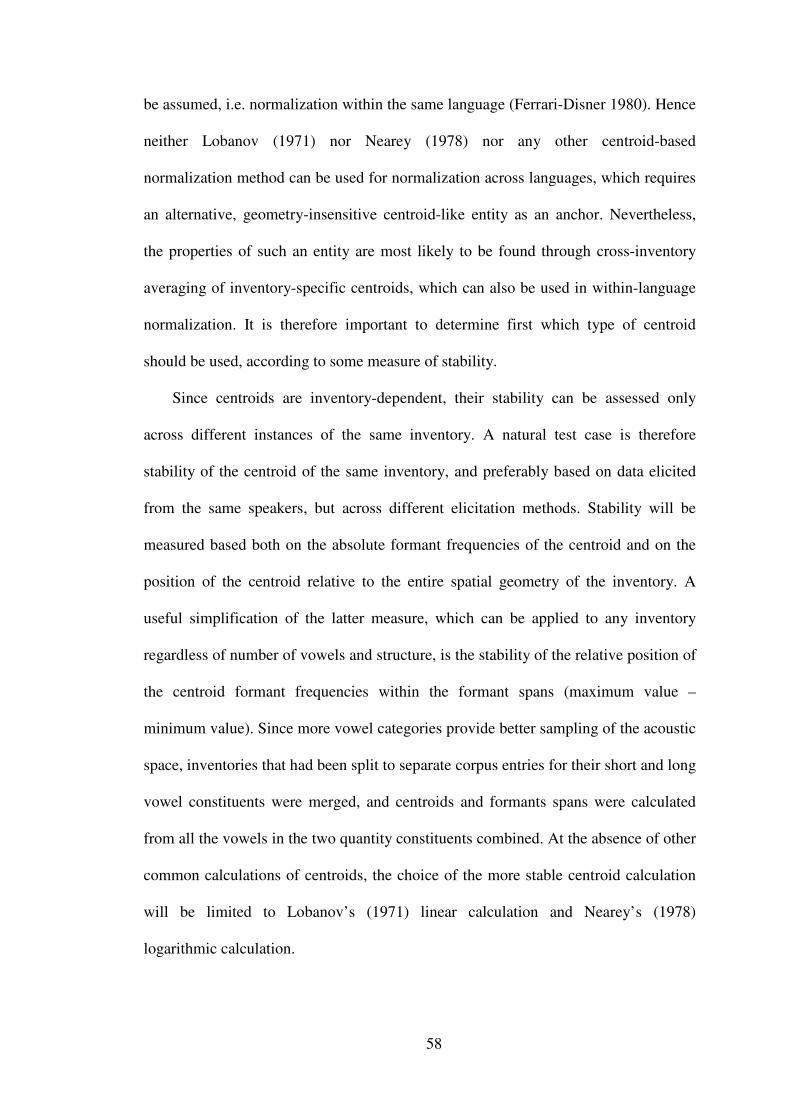
58

be assumed, i.e. normalization within the same language (Ferrari-Disner 1980). Hence

neither Lobanov (1971) nor Nearey (1978) nor any other centroid-based

normalization method can be used for normalization across languages, which requires

an alternative, geometry-insensitive centroid-like entity as an anchor. Nevertheless,

the properties of such an entity are most likely to be found through cross-inventory

averaging of inventory-specific centroids, which can also be used in within-language

normalization. It is therefore important to determine first which type of centroid

should be used, according to some measure of stability.

Since centroids are inventory-dependent, their stability can be assessed only

across different instances of the same inventory. A natural test case is therefore

stability of the centroid of the same inventory, and preferably based on data elicited

from the same speakers, but across different elicitation methods. Stability will be

measured based both on the absolute formant frequencies of the centroid and on the

position of the centroid relative to the entire spatial geometry of the inventory. A

useful simplification of the latter measure, which can be applied to any inventory

regardless of number of vowels and structure, is the stability of the relative position of

the centroid formant frequencies within the formant spans (maximum value –

minimum value). Since more vowel categories provide better sampling of the acoustic

space, inventories that had been split to separate corpus entries for their short and long

vowel constituents were merged, and centroids and formants spans were calculated

from all the vowels in the two quantity constituents combined. At the absence of other

common calculations of centroids, the choice of the more stable centroid calculation

will be limited to Lobanov’s (1971) linear calculation and Nearey’s (1978)

logarithmic calculation.

59

In order to compare centroid behavior across elicitation methods under the tightest

control, matched-paired t-tests were performed, using pairs of entries belonging to the

same language and sharing the same structure but differing in elicitation method (the

independent variable). Entry pairs based on studies comparing formant data for the

same speakers across elicitation methods were preferred and chosen whenever possible.

The dependent variables were the following linear and logarithmic centroid indices: F1

frequency, relative position within F1 span, F2 frequency and relative position within

F2 span. Relative position within span was calculated as follows:

(3.1) FC-REL = (FC-FMIN)/(FMAX-FMIN).

Notice that, in these t-tests, significant difference implied centroid instability. There

were five pairs of elicitation methods with enough same-language pairs to allow

meaningful t-tests: isolation vs. wordlist (15 pairs), isolation vs. carrier sentence (8 pairs),

wordlist vs. carrier sentence (18 pairs), wordlist vs. meaningful sentence (14 pairs) and

wordlist vs. running speech (15 pairs). Thus the total number of t-tests was 40 (5

elicitation method pairs x 4 centroid indices x 2 scale types). Following Bonferroni

correction, the significance threshold was set at p<0.00125 (=0.05/40). At this low

threshold, none of the 40 t-tests yielded a significant centroid difference as a function of

elicitation method difference, but the linear centroids were slightly more consistent, in

that only three out of the 20 tests were near-significant (0.02<p<0.05), whereas six of the

20 tests for logarithmic centroids were near-significant (p<0.05), including two at p<0.01.

In order to confirm the apparent superiority of the linear centroid, unpaired t-tests

were performed, comparing all four centroid indices for all possible ten pairs of

elicitation methods, using the centroids of all the inventories in the survey as

observations. Comparing centroids grouped from different geometries involves some

60

statistical noise, but the immense variety of structures for each method ensures that

the effect of such noise would be random. None of the 80 tests (10 method pairs x 4

indices x 2 scales) reached significance at the Bonferroni-corrected threshold of

p<0.000625 (=0.05/80), but only three out of the 40 linear centroid tests were near-

significant (p<0.05), compared to eleven of the 40 logarithmic centroid tests.

Although these results are still inconclusive, it was decided to use the linear centroid

in the normalization process on the basis of the near significant results.

3.1.2 Universal centroid

One important outcome of the analysis of centroids across elicitation methods is

the near-constant nature of the ‘centroid of linear centroids’, or the average of all the

linear centroids from all inventories in the survey. Table 3-1 provides the absolute

frequencies and relative positions of centroid averages and standard deviations across

elicitation methods, as well as the grand averages for the entire survey.10

F1 F2

elicitation method observations frequency relative

position

frequency relative

position

Isolation 41 452.2±50.9 0.395±0.069 1450.8±98.7 0.460±0.057

Wordlist 234 468.3±52.7 0.395±0.065 1474.2±89.6 0.471±0.047

Carrier sentence 91 452.8±46.9 0.374±0.056 1483.3±101.5 0.463±0.044

Meaningful sentence 41 465.9±43.1 0.404±0.064 1471.4±62.4 0.458±0.039

Running speech 38 457.8±48.9 0.388±0.049 1471.9±84.2 0.455±0.058

All 445 462.5±50.5 0.391±0.063 1473.3±90.3 0.466±0.048

Table 3-1: Averages and standard deviations of frequencies and relative positions in formant spans for F1 and F2 of linear centroids in the survey, as a function of elicitation method.

The centroid of linear centroids, from all inventories and acoustic geometries, is

probably the best approximation of the ‘dead center’ of the vowel space. Assuming a

10 The number of observations is 445 and not 447 because, in two inventories, crucial data for calculating F1 and F2 spans are missing.

61

uniform-tube schwa (F2=3xF1) with F1 at 485-490Hz and F2 at 1455-1470Hz, this

vowel is a slightly raised schwa, which is in good agreement with an effortless vowel,

with neutral tongue and lip position and loose and slightly open yet relatively high

jaw position (for a true uniform tube the jaw has to be lowered somewhat). This

vowel will be referred to as the universal centroid (UC) hereafter.

3.1.3 Universal centroid approximation

The absolute formant frequencies of the UC (F1=463Hz, F2=1473Hz) mean very

little with regard to individual inventory data. Although these formant frequency

coordinates are located in the interior region of the acoustic space for virtually every

adult male speaker, they may characterize a raised and rounded schwa ([ɵ]) for a

speaker with a small vocal tract and a vowel between [ɜ] and [ɛ] (lowered and advanced

schwa) for a speaker with a very large vocal tract. More important are the relative

positions of the UC within the F1 and F2 frequency spans, because they enable us to

approximate the inventory-specific reflection of the UC, with reasonable accuracy,

based solely on formant minima and maxima. The point located at the 391 thousandth

of the F1 span and the 466 thousandth of the F2 span should be very close to the same

‘slightly raised schwa’ in any inventory, regardless of the language, the number of

vowels, phonological structure and elicitation method. The formant frequencies of an

inventory’s universal centroid approximation index (UCA) are:

(3.2) F1UCA=F1MIN+0.391(F1MAX-F1MIN)

(3.3) F2UCA=F2MIN+0.466(F2MAX-F2MIN)

The cross-inventory stability of UCA vs. centroid was tested using all 442

inventories, for which both F1 and F2 frequencies of the centroid and UCA could be

62

reliably calculated. For centroids, average F2/F1 ratio was 3.220 and standard

deviation was 0.360. For UCAs, average F2/F1 was 3.200 and standard deviation was

0.305. While the difference in average ratios was not statistically significant (paired

t(441)=1.600, p>0.11 two-tailed), the variance of UCA ratios was found to be

significantly smaller than the variance of centroid ratios (F(441,441)=1.398,

p<0.0003), implying that UCAs have more consistent acoustic qualities across

languages and inventory geometries than centroids do, as expected.

The effectiveness of this UC approximation is easily illustrated by data from

studies of Korean. Korean is very diverse in terms of vowel inventory structure across

dialects, owing in part to changes in the standard (Seoul) dialect that took place in

recent generations. Owing to the rather homogeneous ethnic background of Koreans,

substantial differences in average speaker vocal tract size between multiple-speaker

studies are unlikely, so the acoustic quality of ‘slightly raised schwa’ should be

relatively consistent across Korean dialects. Table 3-2 summarizes centroid and UCA

indices from all seven studies of Korean included in the survey. Although the average

centroid is incidentally identical to the UC while the average UCA is slightly

different, variance is significantly smaller for the UCAs than for the centroids.

63

Dialect, source, # speakers

and structure

elicitation

method

formant

spans centroid UCA

F1 F2 F1 F2 F1 F2

Seoul old, Han (1975), 1, /i e ɛ a ɔ(ʌ) o u y ø ɨ(ɯ)/

wordlist 302 830

988 2229

440 1561 508 1566

Seoul old, Yang (1996), 10 /i e ɛ a ʌ o u y ø ɨ(ɯ)/

wordlist 338 738

945 2219

479 1587 494 1538

Seoul new, Lee (2000), 8 /i e ɛ a ə(ʌ) o u ɯ/

carrier sentence

320 770

890 2245

499 1460 496 1521

Seoul new, Kim (2001), 1 /i ɛ a ʌ o u ɯ/

isolation 330 710

950 1980

473 1424 479 1430

Pyongyang, Kang (1996), 1 /i e ɛ a o u/

carrier sentence

260 765

1007 2090

410 1570 457 1511

Chungnam, Seong (2005), 5 /i ɛ a ʌ o u ɯ/

carrier sentence

341 740

764 2209

493 1319 497 1437

Hamkyong, Kang (1997), 2 /i e ɛ a o u ɨ(ɯ) ʌ(ɤ)/

carrier sentence

307 735

822 2117

448 1406 474 1425

Average (sd): 464.7

(31.3)

1475.3

(100.6)

486.6

(17.3)

1489.8

(58.0)

Table 3-2: Centroids and UCA indices in all studies of Korean inventories in the survey.

The only problematic inventories for universal centroid approximation are those

that lack a particular peripheral region altogether, like the inventory of Southern

California English, with no true back-rounded vowels (see Hagiwara 1994 for formant

frequencies). For such inventories, the UCA is removed quite far from the ‘slightly

raised schwa’, but such inventories are very rare. Much more common are inventories

with structural asymmetries and/or crowded acoustic regions (e.g. the high-front

region in the inventories of most Germanic, Uralic, Altaic and Chinese languages).

Centroids, being calculated from all vowels, gravitate towards crowded acoustic

regions. Conversely, UCA indices, which are calculated only from F1 and F2 spans,

are impervious to crowded regions or asymmetries.

In summary, to the extent that it is possible to define a point of relative constancy

across languages, inventory structures and elicitation methods, this point should be

the inventory’s universal centroid approximation index (UCA), as defined in relative

64

positions within the inventory’s F1 and F2 spans on the linear Hz scale. UCA indices

were calculated for all the inventories in the survey, and whenever an inventory was

formed by the merger of two entries (short and long vowels), the same UCA index

was assigned to both entries.

3.2 Vocal tract normalization

3.2.1 Background and rationale

Vocal tract normalization of survey data was necessary for two reasons. First, most

studies provided formant data from very few speakers, making language-specific effects

and between-language variance strongly confounded with speaker-specific effects, vocal

tract size being an important source for such effects. Second, even studies whose data are

taken from many speakers might not be comparable with one another if their respective

speakers come from very distinct ethnic backgrounds, with characteristic differences in

stature, which inevitably lead to differences in vocal tract size (Fitch & Giedd 1999).

Many vocal tract normalization procedures for vowel inventories have been

proposed and used in the literature, and it is beyond the scope of the current work to

evaluate them, both because this has been done in the past (Ferrari-Disner 1980, Syrdal

1984, Adank et al. 2004), and because none of them is appropriate for the survey data.

The reason is that these methods are dedicated to the problem of normalizing data

between speakers of the same language, where underlying (linguistic) geometry of the

inventory is assumed to be consistent across speakers. As explained in Section 3.1.1,

centroid-based vocal tract normalization methods like Lobanov (1971) and Nearey (1978)

are inappropriate for cross-linguistic and cross-structural data, due to the sensitivity of the

centroid to inventory-specific geometry. Methods like Gerstman’s (1968), which anchor

65

inventories at their formant minima and maxima, are even less appealing. Not only do

they distort genuine differences between languages, for example by practically reducing

cross-linguistic variance of /i/ to zero (/i/ being simultaneously F1 minimum and F2

maximum in nearly all languages), but also immediately annul one of the key dispersion-

related analyses, of formant span as a function of phonological structure. Methods that

rely on frequency data of F3 and higher formants, which are more consistent across

vowels and thus potentially better correlated with speakers’ vocal tracts regardless of

inventory acoustic geometry, would have been more suitable (e.g. Fant 1959, Halberstam

& Raphael 2004). Unfortunately, too many studies included in the survey provide only F1

and F2 data, and in many others F3 frequencies seem inaccurate. Methods using formant

ratios or formant differences in perceptual scales (Mel, Bark, ERB) suffer from the same

problem, because they rely on the availability of data beyond F1 and F2 (at least f0 or

F3). Morrison & Nearey (2006) is probably the only attempt to specifically address the

problem of between-language normalization, but their model is applicable only for pairs

of languages. It was therefore necessary to devise a novel vocal tract normalization

procedure, which is based only on F1 and F2 and yet minimally sensitive to the inventory

acoustic geometry so it can be applied to all inventories.

3.2.2 Devising the normalization procedure

The normalization procedure devised here is based on the following principle: the set

of universal centroid approximation indices (UCAs) from all inventories presumably

represent the same vowel quality, a slightly raised schwa. Most of the variation in UCA

frequencies is due to differences in vocal tract size, which is roughly inversely related to

formant frequencies. Formant frequency ratios between the universal centroid (UC) and

the inventory’s UCA can serve as multiplication constants by which the formant

frequencies of all the inventory

UCA index at the UC, while retaining the acoustic geometry of the inventory intact. Since

rescaling by constants is a logarithmic transposition, it retains the acoustic geometry intact

in logarithmic scales. As such, it also re

extent, because perceptual scales (Bark, ERB, Mel) are quasi

F1 and F2 were treated independently. F1 and F2 frequencies of all the vowels in

a given inventory were respectively multiplied by the

F2UC/F2UCA. This is equivalent to transposing the entire inventory geometry on a

logarithmic F1xF2 plane.

linear (a) and logarithmic (b) scales, the raw (grey) and vocal

vowels of the /i a u/ inventory of Amis, based on formant data

speakers in Maddieson & Wright (1995).

= 517Hz (F1UC/F1UCA

normalization lowers the formant frequencies of all vowels, implying that the average

vocal tract of the two speakers recorded was relatively short.

Figure 3-1: Raw (grey) and vocal(Maddieson & Wright 1995)

11 All figures were prepared using Microsoft Excel and finalized using Microsoft Paint.

66

frequencies of all the inventory’s vowels can be rescaled. This will anchor the inventory

UCA index at the UC, while retaining the acoustic geometry of the inventory intact. Since

rescaling by constants is a logarithmic transposition, it retains the acoustic geometry intact

in logarithmic scales. As such, it also retains the perceptual geometry intact to a great

extent, because perceptual scales (Bark, ERB, Mel) are quasi-logarithmic.

F1 and F2 were treated independently. F1 and F2 frequencies of all the vowels in

a given inventory were respectively multiplied by the ratios F1

. This is equivalent to transposing the entire inventory geometry on a

logarithmic F1xF2 plane. Figure 3-1 illustrates this procedure by plotting, using both

linear (a) and logarithmic (b) scales, the raw (grey) and vocal-tract normalized (black)

a u/ inventory of Amis, based on formant data

Maddieson & Wright (1995).11 The UCA index for this

= 0.894), F2UCA = 1622Hz (F2UC/F2UCA = 0.908).

normalization lowers the formant frequencies of all vowels, implying that the average

vocal tract of the two speakers recorded was relatively short.

Raw (grey) and vocal-tract normalized (black) vowels of the /i a u/ inventory of AmisMaddieson & Wright 1995), plotted both linearly (a) and logarithmically (b).

All figures were prepared using Microsoft Excel and finalized using Microsoft Paint.

will anchor the inventory’s

UCA index at the UC, while retaining the acoustic geometry of the inventory intact. Since

rescaling by constants is a logarithmic transposition, it retains the acoustic geometry intact

tains the perceptual geometry intact to a great

logarithmic.

F1 and F2 were treated independently. F1 and F2 frequencies of all the vowels in

ratios F1UC/F1UCA and

. This is equivalent to transposing the entire inventory geometry on a

e by plotting, using both

tract normalized (black)

a u/ inventory of Amis, based on formant data drawn from two

The UCA index for this inventory is: F1UCA

= 0.908). Notice that

normalization lowers the formant frequencies of all vowels, implying that the average

a u/ inventory of Amis

All figures were prepared using Microsoft Excel and finalized using Microsoft Paint.

67

This implementation of vocal-tract normalization accepts any UCA as a ‘slightly

raised schwa’, even when the UCA is obviously removed from this vowel quality (i.e.

F2UCA/F1UCA ratio very different from 3.2), and has the potential drawbacks of

distorting F2/F1 ratios within vowels. A somewhat more complicated alternative

would have been to change UCA indices minimally such that all the UCAs would

have F2/F1 ratios identical to F2UC/F1UC (=3.2), and then apply the same FUC/FUCA ratio

as a rescaling factor for both F1 and F2 frequencies, thus retaining the original within-

vowel F2/F1 ratios. However, changing the UCA index to a UC-like F2/F1 ratio has

disadvantages of its own: Whenever the non-corrected F1UCA is below F1UC while non-

corrected F2UCA is above F2UC or vice-versa, any constant shift that would yield, for all

the inventory's vowels, reasonable frequencies for one formant, would yield

disturbingly high/low frequencies for the other.

3.2.3 Implementation and validation

Vocal tract normalization was thus performed for all the inventories in the

survey, excluding those for which spans could not be calculated (due to absent

formant data for a point vowel), by multiplying all F1 frequencies by F1UC/F1UCA and

all F2 frequencies by F2UC/F2UCA. It was hoped that this normalization procedure

would increase the geometrical match between inventories belonging to the same

structural configuration. In more statistically meaningful words, reduction of variance

was expected in the distribution of F1 and F2 frequencies for individual vowel

categories within those structures for which there are enough different entries.

Recall from Section 2.3.2 that in the entire survey there are 17 structural

configurations occurring in five languages or more. There were 7 other structures

occurring in four languages and/or in seven or more entries. Together, these 24

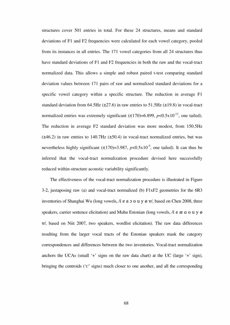
68

structures cover 501 entries in total. For these 24 structures, means and standard

deviations of F1 and F2 frequencies were calculated for each vowel category, pooled

from its instances in all entries. The 171 vowel categories from all 24 structures thus

have standard deviations of F1 and F2 frequencies in both the raw and the vocal-tract

normalized data. This allows a simple and robust paired t-test comparing standard

deviation values between 171 pairs of raw and normalized standard deviations for a

specific vowel category within a specific structure. The reduction in average F1

standard deviation from 64.5Hz (±27.6) in raw entries to 51.5Hz (±19.8) in vocal-tract

normalized entries was extremely significant (t(170)=6.899, p<0.5x10-11, one tailed).

The reduction in average F2 standard deviation was more modest, from 150.5Hz

(±46.2) in raw entries to 140.7Hz (±50.4) in vocal-tract normalized entries, but was

nevertheless highly significant (t(170)=3.987, p<0.5x10-5, one tailed). It can thus be

inferred that the vocal-tract normalization procedure devised here successfully

reduced within-structure acoustic variability significantly.

The effectiveness of the vocal-tract normalization procedure is illustrated in Figure

3-2, juxtaposing raw (a) and vocal-tract normalized (b) F1xF2 geometries for the 6R3

inventories of Shanghai Wu (long vowels, /i e a ɔ o u y ø ɤ/, based on Chen 2008, three

speakers, carrier sentence elicitation) and Muhu Estonian (long vowels, /i e æ ɑ o u y ø

ɤ/, based on Niit 2007, two speakers, wordlist elicitation). The raw data differences

resulting from the larger vocal tracts of the Estonian speakers mask the category

correspondences and differences between the two inventories. Vocal-tract normalization

anchors the UCAs (small ‘+’ signs on the raw data chart) at the UC (large ‘+’ sign),

bringing the centroids (‘C’ signs) much closer to one another, and all the corresponding

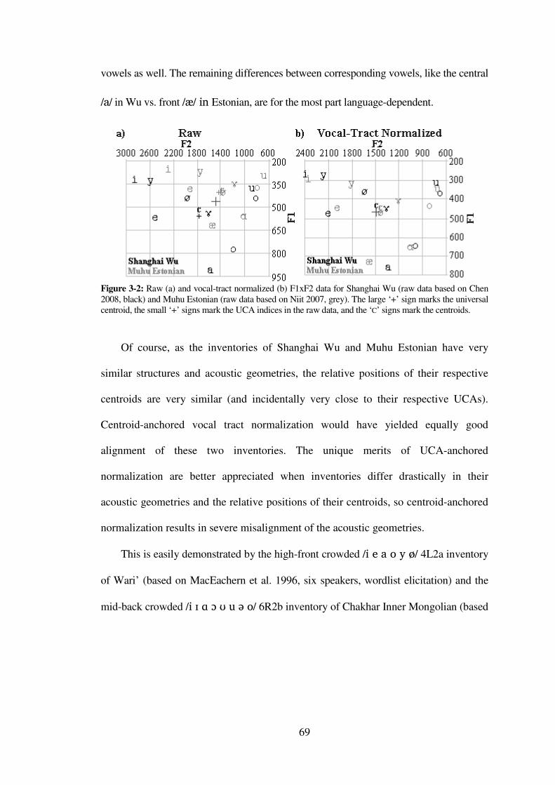
69

vowels as well. The remaining differences between corresponding vowels, like the central

/a/ in Wu vs. front /æ/ in Estonian, are for the most part language-dependent.

Figure 3-2: Raw (a) and vocal-tract normalized (b) F1xF2 data for Shanghai Wu (raw data based on Chen 2008, black) and Muhu Estonian (raw data based on Niit 2007, grey). The large ‘+’ sign marks the universal centroid, the small ‘+’ signs mark the UCA indices in the raw data, and the ‘C’ signs mark the centroids.

Of course, as the inventories of Shanghai Wu and Muhu Estonian have very

similar structures and acoustic geometries, the relative positions of their respective

centroids are very similar (and incidentally very close to their respective UCAs).

Centroid-anchored vocal tract normalization would have yielded equally good

alignment of these two inventories. The unique merits of UCA-anchored

normalization are better appreciated when inventories differ drastically in their

acoustic geometries and the relative positions of their centroids, so centroid-anchored

normalization results in severe misalignment of the acoustic geometries.

This is easily demonstrated by the high-front crowded /i e a o y ø/ 4L2a inventory

of Wari’ (based on MacEachern et al. 1996, six speakers, wordlist elicitation) and the

mid-back crowded /i ɪ ɑ ɔ ʊ u ə o/ 6R2b inventory of Chakhar Inner Mongolian (based

70

on Svantesson 1995, one speaker, wordlist elicitation).12 The difference in raw formant

spans of the two inventories is not as pronounced as in the case of Shanghai Wu and

Muhu Estonian, but nonetheless suggests that the Chakhar Inner Mongolian speaker has

a slightly smaller vocal tract than the average Wari’ speaker, an impression further

corroborated by F3 data, which are available for both inventories. For example, the F1-

F3 frequencies of Chakhar Inner Mongolian /i/ (356Hz, 2347Hz, 3016Hz) and /ɑ/

(825Hz, 1329Hz, 2851Hz) seem slightly elevated relative to Wari’ /i/ (325Hz, 2170Hz,

2920Hz) and /a/ (745Hz, 1545Hz, 2550Hz). Figure 3-3 shows F1xF2 plots of the

inventories. On the raw data plot (a), it is noticeable that the inventories’ UCAs (small

‘+’ signs) differ only slightly from each other and from the UC (large ‘+’ sign), while

their respective centroids (‘C’ signs), which are gravitated towards the crowded regions,

are far apart. Centroid-anchored normalization (b) has a colossal misalignment effect,

retracting the Wari’ vowels while advancing and raising the Chakhar Inner Mongolian

vowels too much (notice the vowels /i/ and /a~ɑ/ in particular). Conversely, UCA-

anchored normalization (c) improves the acoustic compatibility between the two

12 The structure of this inventory of Chakhar Inner Mongolian was interpreted as 6R2b, with /ə/ and /o/ as non-peripheral vowels contrasting horizontally with the peripheral /ɪ/ and /ʊ/ and with each other. The interpretation of /o/ as a non-peripheral vowel on the basis of its acoustic contrast with /ʊ/, which seemed to be based more on F2 than on F1, was later found to among the few cases where the structural interpretation had been inconsistent with the criteria described in Section 2.3.2, because the F2 frequency of this /o/ is too low to count as non-peripheral. The inventory of Chakhar Inner Mongolian participates in a robust pharyngealization/ATR vowel harmony system, where /ɪ ɑ ɔ ʊ/ are the [-ATR] counterparts of the [+ATR] /i ə o u/. Similar acoustic patterning of /ʊ/ and /o/ was found in a number of inventories in the corpus, all characterized by robust ATR harmony (and /ɔ ʊ/ correspondence to /o u/). In all these other inventories /o/ was properly interpreted as a back vowel. Such interpretation of this Chakhar Inner Mongolian inventory would have assigned it the structure 7R1. Since both 6R2b and 7R1 are extremely rare, the cross-linguistic acoustic typology is largely unaffected by the erroneous interpretation as 6R2b. However, the interpretation of this inventory as consisting of a 6R periphery and two non-peripheral vowels contrasting horizontally must have had some effect on analyses of the corpus that are sensitive to the configuration of the periphery and of the non-peripheral region, in particular the analyses of peripheral mid vowels reported in Section 4.4.

71

inventories relative to the raw data, for example by equating the heights of the three

unrounded peripheral vowels (Wari’ /i e a/, Chakhar Inner Mongolian /i ɪ ɑ/).

Figure 3-3: Raw (a), centroid-anchored normalized (b) and vocal-tract normalized (c) F1xF2 data for Wari’ (raw data based on MacEachern et al. 1996, black) and Chakhar Inner Mongolian (raw data based on Svantesson 1995, grey). The large ‘+’ sign marks the universal centroid, the small ‘+’ signs mark the UCA indices in the raw data, and the ‘C’ signs mark the centroids.

3.3 Elicitation method normalization

3.3.1 Background and rationale

Vocal-tract differences are not the only non-linguistic source for within-structure

acoustic variance. No less influential is the elicitation method. Different elicitation

methods position the elicited vowels in different segmental, prosodic and speech rate

contexts, and also involve different levels of speaker’s awareness and consciousness

of pronunciation. Longer duration, higher prosodic prominence and greater awareness

all contribute to greater articulatory displacement whenever the articulatory target of

the vowel is distant from the effortless position. Conversely, shorter duration, lower

prominence and casual speech all contribute to vowel undershoot and contextual

coarticulation, which are manifested systemically as acoustic centralization, because

the position of least effort is at the center of the acoustic space (Lindblom 1963, de

72

Graaf & Koopmans-van Beinum 1984, van Bergem 1993, Fourakis et al. 1998,

Johnson & Martin 2001, Parker 2001, Calamai & Sorianello 2003, among others).13

There is no empirical a priori preferred reference point for between-method

normalization. However, the well established effects of elicitation method on formant

frequencies and inventory space size suggest that this confound should not remain

untreated. The safest approach is to choose the most common elicitation method as the

target of normalization, thus leaving as much data as possible untouched. The target of

method normalization will therefore be wordlist elicitation, which covers more than one

half of the entries in the survey. It should be kept in mind that, to the extent that such

normalization can be accurate, the normalized data should still suffer from distortions of

acoustic vowel targets characteristic of wordlist elicitation, like coarticulatory effects of

adjacent consonants, which do not exist in isolation elicitation.14

Formal models of acoustic vowel reduction as a function of speech rate have been

proposed in the past (e.g. Lindblom 1963, van Bergem 1993). Unfortunately, as vowel

duration and speech rate are usually unavailable in the studies in the survey, such

models are of little relevance here. Although the discrete reduction and centralization

effect of speech condition, style or utterance type has been addressed in many studies,

none of them have proposed a formal acoustic model for this phenomenon. De Graaf

& Koopmans-van Beinum (1984) is probably the only study that goes a certain way in

this direction. In their study, the effect of three elicitation methods on vowel formants

13 Notice that this is not obvious. One could easily imagine a hypothetical language where all consonants are somewhat pharyngealized and a default tongue position with constricted pharynx, but vowel targets are not pharyngealized. In such a language, the acoustic vowel space would still compress under prominence and temporal reduction and casual speech style, but clearly wouldn't centralize, because F1 would rise and F2 would fall for all vowels. 14 Isolation elicitation has its own shortcomings, like the unnatural nature of the task, and hyperarticulation.

73

was demonstrated using data from six different languages. Vowel space size was

expressed as a function of distances of vowels from a global center point, the

logarithmic average of all vowels in all speech conditions. Comparing average

distance indices between vowels in isolation, in words and in running speech yielded

roughly consistent ratios of space size reduction. The choice of the logarithmic

average from all speech conditions implicitly suggests that this spatial point is

relatively stable across elicitation methods, and could serve as an anchor for

interpolation or extrapolation of formant frequencies as part of normalization. This

choice seems rather peculiar given de Graaf & Koopmans-van Beinum’s (1984) own

data. Their logarithmic vowel charts clearly show stronger centralization for high than

for low vowels and for back than for front vowels, that is, the logarithmic shift is

greater for lower F1 and F2 frequencies, which is expected if the shifts are of equal

magnitude on a linear scale.15 The findings in Section 3.1.1 also suggest that the linear

centroid is more stable across elicitation methods, hence more suitable as a

normalization anchor. In the absence of an adequate between-method normalization

procedure, such a procedure had to be devised here.

3.3.2 Devising the normalization procedure

The simplest normalization approach is to find, for each method pair comprising

wordlist elicitation and another method, the most representative between-method ratios

for F1 and F2 distances between vowels and the linear centroid. Notice that the universal

15 In de Graaf & van Beinum's (1984) logarithmic formant charts, the forward shift of back vowels and the downward shift of high vowels look substantially greater than the backward shift of front vowels and upward shift of low vowels. Linear representation would have yielded much more symmetrical inwards shifts, of about 200-250Hz for F2 and 75-100Hz for F1, from isolated vowels to running speech vowels.

74

centroid approximation (UCA) could in principle be used instead of the centroid, in

particular as the UCA seemed to be even more stable than the centroid across elicitation

methods. However, the centroid was preferred here because it is a familiar concept

established and used elsewhere for within-language inventory normalization.

The normalized frequencies for a given vowel are achieved by extrapolation,

from the centroid, of the F1 and F2 distances of the non-normalized vowel, multiplied

by the appropriate method-specific ratios, which are yet to be found. Let RM1 and RM2

be the representative ratios of F1 and F2 distance from centroid for wordlist elicitation

vs. method M, then the method-normalized formant frequencies for vowel V in an

inventory whose centroid is C elicited by method M are:

(3.4) F1V-MethodNormalized = F1C + (F1C – F1V) x RM1

(3.5) F2V-MethodNormalized = F2C + (F2C – F2V) x RM2

Notice that, since both the vocal-tract normalization procedure and this between-

method normalization scheme keep intact all the distance ratios in the inventory (within

the same formant), the combined result of both procedures is the same no matter which

procedure is applied first. However, the specific between-method ratio constants and

the analyses meant to establish them need to be performed using the linear Hz scale.

Therefore, the less variable the data are on this scale, the more reliable the analyses. In

Section 3.2.3 it was shown that vocal-tract normalization significantly reduced variance

on the Hz scale. Thus, vocal-tract normalized data, rather than raw formant data, was

used in the between-method normalization analyses.

As the relative position of the centroid in the inventory frequency spans is stable

across elicitation methods, formant span ratios between elicitation methods are

appropriate candidates for the extrapolation ratios necessary for between-method

75

normalization. However, formant spans and span ratios represent only the behavior of

the inventory point vowels, while the centroid is a function of all the vowels in the

inventory. It is possible that the behavior of point vowels as a function of elicitation

method differences differs from the behavior of other vowels, and it is important that

other vowels would also be represented in the calculation of the extrapolation ratios. It

was therefore decided to devise an additional index of distance from the centroid,

derived from all the vowels in the inventory and representing their distribution – the

more all the vowels are distributed, the more expanded the inventory. If a given

formant’s frequencies from all the inventory’s vowels are considered a sample and the

centroid’s frequency for this formant is the sample mean, then the sample standard

deviation essentially represents the desired index. Thus, for each inventory, four

dispersion indices were calculated: F1SPAN, F1SD, F2SPAN and F2SD.

The next step was to determine, for each of the four method pairs (wordlist

elicitation vs. each of the other four), whether the indices are indeed significantly

different. A series of 16 matched-pair t-tests was performed, with all four indices

(F1SPAN, F1SD, F2SPAN and F2SD) as dependent variables for each of the four method

pairs, using the same sets of entries as in the centroid analyses reported in Section

3.1.1. The one-tailed significance threshold was Bonferroni-corrected to 0.0033

(=0.05/16). Table 3-3 summarizes the results. Notice the similarity between average

ratios between corresponding span and standard deviation indices, implying that the

behavior of point vowels and other vowels as a function of elicitation method

differences is rather similar.

76

Isolation carrier sentence meaningful sentence running speech

df 15 17 13 14

F1SPAN t 4.878** 1.767 2.904* 5.538**

average ratio 0.884 1.055 1.171 1.340

F1 SD t 5.663** 1.492 3.762* 5.280**

average ratio 0.873 1.047 1.210 1.380

F2 SPAN t 4.580** 2.159* 5.028** 11.443**

average ratio 0.903 1.058 1.183 1.258

F2 SD t 5.261** 2.534* 6.261** 10.367**

average ratio 0.875 1.079 1.188 1.290 Table 3-3: Matched-pair t-tests results for the differences in indices of distance from centroid between wordlist elicitation and each of the other elicitation methods, and average between-method ratios for each index. “*” denotes near-significance at p<0.05 and “**” denotes significance at the Bonferroni-adjusted threshold of p<0.0033.

Virtually all the differences between wordlist elicitation and each of isolation,

meaningful sentence and running speech elicitations were highly significant. The

expanded indices in isolation elicitation are consistent with the longer duration, the

absence of coarticulatory effects and the higher phonetic awareness associated with

this task, relative to wordlist elicitation. Similarly, the reduced indices in meaningful

sentence and running speech elicitations are also consistent with these parameters,

because vowels are expected to be shorter, prosodically-weaker and more

coarticulated in entire sentences than in isolated words. Although no direct

comparison between the latter two elicitation methods was performed, their respective

results compared to wordlist elicitation suggest that running speech elicitation

involves more centralization than meaningful sentence elicitation. This is expected

given that speech rate and segmental context are typically partially controlled in

meaningful sentence elicitation but not in running speech elicitation.16

16The consistency of vowel space contraction and expansion as a function of elicitation method, combined with the consistent position of centroids across elicitation methods as well, imply that the effects of vowel undershoot (and/or overshoot) manifest overall centralization. This effect might be different from vowel space reduction in unstressed syllables, which has been claimed to manifest upward contraction due to constrained jaw movement, leading to substantial raising of the vowel space

77

In light of these highly significant results, the stronger centralization attested in

carrier sentence elicitation relative to wordlist elicitation seems genuine, and it would

be unwise to dismiss it solely due to statistical non-significance, given the very

restrictive significance threshold. If the differences between wordlist elicitation and

each of isolation, meaningful sentence and running speech elicitation had not been put

to test based on clear past evidence (e.g. de Graaf & Koopmans-van Beinum 1984),

the Bonferroni correction would have been less conservative, and some of the

wordlist vs. carrier sentence differences would have become significant. At the same

time, expanding carrier sentence-elicited vowel spaces by ratios around 1.06 without

clear-cut support seems equally unwise, because, in such studies, segmental context is

often controlled and subject awareness might be enhanced due to the unnatural

repetitions of the same sentential framework. This may lead to pronunciation of the

target word with special, contrastive focus, which is not the case in the more natural,

lexicon-oriented task of wordlist elicitation.17

It was therefore decided to look into the distribution of these four dispersion

indices as a function of elicitation method based on all inventories, without control for

language, assuming, as in the case of centroid comparisons, that the great variety

within each elicitation method exerts only a random effect on the average indices.

The average index ratios across elicitation methods appeared more conservative

than under within-language control. Isolation vs. wordlist elicitation ratios increased

floor (Flemming 2005, Padgett & Tabain 2005, Herrick 2005). This type of vowel reduction should yield a significant drop in centroid F1 frequencies, which is clearly not attested in the corpus data, as seen in Table 3-2 in Section 3.1.3. It is plausible that vowel undershoot in unstressed vowels is different from undershoot in stressed vowels in faster or more casual speech circumstances. However, much more cross-linguistic acoustic data on phonetic vowel reduction in unstressed syllables are necessary to establish the case for jaw movement constraints and acoustic raising as the source. 17Notice that wordlist elicitation using near-minimal sets is common in studies of English vowels (heed, hid, head etc.) but is rare elsewhere.

78

slightly (F1SPAN: 0.923, F1SD: 0.891, F2SPAN:0.899, F2SD: 0.898), and meaningful

sentence vs. wordlist ratios decreased substantially (F1SPAN: 1.123, F1SD: 1.109, F2SPAN:

1.089, F2SD:1.097), as did running speech vs. wordlist ratios (F1SPAN: 1.254, F1SD:

1.233, F2SPAN: 1.170, F2SD:1.195). These more conservative ratios remained significant

in unpaired t-tests (p<0.0033 for all except for one comparison with p=0.0045).

However, the picture changed dramatically for carrier sentence vs. wordlist elicitation

ratios: carrier sentence elicitations turned out to have greater F1 dispersion than

wordlist elicitations (F1SPAN ratio: 0.966, F1SD ratio: 0.968), and the two methods fared

virtually equally in their F2 dispersion indices (F2SPAN ratio: 1.011, F2SD ratio: 0.997).

None of these ratios was the result of even a near-significant difference.

Overall, the analyses of elicitation method effects suggested a complicated state

of affairs. The more tightly-controlled but less comprehensive comparisons suggested

rather drastic distance-from-centroid ratios, implying major arithmetical

transformations. Conversely, the more loosely-controlled but more comprehensive

comparisons suggested more conservative ratios and transformations. It was decided

to average them, as well as the span and standard deviation ratios. Thus the final

distance-from-centroid ratios, for each formant, for each method pair, was the average

of four values (span ratio and standard deviation ratio from both the language-

controlled and uncontrolled comparisons), rounded to the nearest 0.01, except for the

case of F1 for carrier sentence, where the average of 1.0089 was rounded to 1 (i.e. no

transformation), due to the non-significant and somewhat contradictory nature of the

comparison results. The final ratios are listed in Table 3-4. The consistency between

F1 and F2 ratios in both isolation and meaningful sentence elicitations is intriguing,

but is assumed to be coincidental.

79

Isolation carrier sentence meaningful sentence running speech

F1 0.89 1 1.15 1.30

F2 0.89 1.04 1.14 1.23

Table 3-4: Average ratios of vowel distance from centroid between each of the four elicitation methods listed and wordlist elicitation, pooled from all indices.

Before applying these ratios and normalizing the inventories for elicitation

method, it was necessary to ensure that expanded inventory geometries (from

meaningful sentence and running speech elicitations) would never reach formant

spans that are highly improbable in wordlist elicitation. The rationale is as follows: it

is quite plausible that a particular running speech study would yield an inventory with

large formant spans (for example, if all vowels analyzed were preselected according

to a criterion of minimal duration). If such formant spans are scaled by large factors,

they might reach unnatural magnitudes. While examining the F1 and F2 spans of the

234 word-list elicited, vocal-tract normalized inventories in the survey, two

inventories stood out for their extremely large F1 spans and one inventory stood out

for its large F2 span. Given the large corpus, it is plausible that these three extreme

formant spans are due to errors. Thresholds were set below these three extreme spans,

in the nearest 0.05 unit of the ln(Hz) representation (ln(FMAX) – ln(FMIN)) immediately

above the next largest formant spans. Logarithmic representation of span threshold

was used so that they could be applied without change if elicitation method

normalization is applied prior to vocal tract normalization and/or if the estimate of the

universal centroid changes (due to addition of many more studies). The span

thresholds are as follows:

(3.6) F1SPAN=605Hz (F1MIN=226Hz, F1MAX=831Hz, ln(F1MAX)=ln(F1MIN)+1.3)

(3.7) F2SPAN=1806Hz (F2MIN=632Hz, F2MAX=2438Hz, ln(F2MAX)=ln(F2MIN)+1.35).

80

Any inventory whose extrapolated formant span(s) exceeded these thresholds by

the elicitation method normalization was corrected by applying the extrapolation

constant(s) that reach these thresholds instead. Such corrections were needed (for

either formant span) in eight inventories: four with meaningful sentence elicitation

and four with running speech elicitation.

3.3.3 Implementation and validation

The elicitation method normalization procedure was also evaluated by paired t-

test comparison of formant standard deviations for all vowel categories in all common

structures. First, comparison between vocal-tract normalized formant standard

deviations to vocal-tract-and-elicitation-method formant standard deviations was

performed, using the same 171 standard deviation pairs as in the evaluation of vocal-

tract normalization in Section 3.2.3. This comparison yielded only fractional,

questionably statistically significant reduction of 0.44Hz on average, in F1 standard

deviations (t(170)=1.719, p=0.044, one-tailed), and a non-significant reduction of

0.04Hz in F2 standard deviations (t(170)=0.053, p=0.48, one-tailed). This was

somewhat expected, because three quarters of the formant data from which the

standard deviations were calculated were essentially the same – wordlist elicitation

data and carrier sentence F1 data remained unchanged while carrier sentence F2 data

were changed only marginally.

Excluding entries based on wordlist elicitation reduced the number of sufficiently

populated structures from 24 to 18 (covering 233 entries, rather than 501), with 123

vowel categories in total. This time standard deviation reduction for F1, from 51.2Hz

to 49.6Hz on average, was clearly significant (t(122)=2.471, p<0.008, one-tailed). F2

81

standard deviations also decreased, from 139.0Hz to 136.7Hz on average, but this

reduction was not significant (t(122)=1.323, p=0.093, one-tailed).

In order to see to what extent the elicitation method normalization procedure was

effective at the within language level, the following procedure was performed.

Multiple entries sharing the same language and the same inventory structure but

differing in elicitation method were grouped, and those entry groups containing

wordlist elicitation entries were excluded, leaving only 11 entry groups, which, at the

absence of wordlist entry among them, could not have been used when the

normalization procedure was devised. These 11 language-specific, structure-specific

entry groups comprised 97 vowel categories together. For every pair of entries in each

group, formant differences were calculated for each vowel category, and the absolute

values of all differences were summed, yielding a variability index for every

language-structure-vowel-formant combination (97 indices for each of F1 and F2).

These scores were calculated on the vocal-tract normalized data, both before and after

elicitation method normalization. Paired t-tests were performed, comparing

corresponding variability indices before and after normalization. The elicitation

method normalization procedure reduced F1 variability indices by 13% on average,

which was significant (t(96)=2.554, p<0.007, one tailed), while the 1% reduction in

F2 variability indices was not (t(96)=0.209, p>0.41, one tailed).

The between-method normalization procedure thus successfully reduced variance

in F1 data, and F2 variance did not increase. It was therefore decided to apply this

normalization procedure, keeping in mind that a much better procedure might be

82

found, in particular for F2, for example, by allowing different normalization

calculations for vowels from different acoustic and/or articulatory regions.18

The entire normalization process (vocal tract and method normalization) is

illustrated in Figure 3-4, showing data pooled together from the 11 different entries of

the /i e ɛ a ɔ o u/ inventory of Italian in the survey, based on formant data from

Ferrero (1972), Trumper et al. (1989), Esposito & Stevens (1995), Calamai (2001,

2002a, 2002b) and Calamai & Sorianello (2003), with all five elicitation methods

included (in some of these sources, vowels were elicited in more than one method).

Some of the variance within vowel categories is due to dialectal differences. Notice

the gradual within-category consolidation as normalization proceeds.

Figure 3-4: Raw (a), vocal-tract normalized (b) and vocal-tract+method normalized (c) F1xF2 data pooled from the 11 /i e ɛ a ɔ o u/ entries of varieties of Italian in the survey.

18 One reasonable explanation for the failure to significantly reduce F2 variance is the variability of the segmental context adjacent to vowels in all the studies, across all elicitation methods other than isolation. Consonantal coarticulation predominantly affects the F2 frequency of vowels, and when such effects are not controlled for, they introduce statistical noise that the between-method normalization is unable (and not meant) to reduce.

83

3.4 Estimating F3 and F2’ for fronter vowels after normalization

3.4.1 Background and rationale

In most vowel inventories, the phonemic role of F3 is very limited, which is why

F3 data are often not reported (or not measured in the first place) in acoustic

descriptions of inventories. Out of the 447 inventories in the survey, F3 data are

reported only for 275, many of which lack F3 data for some vowels and/or have

apparently unreliable F3 data for others.19 The existing F3 data in the survey are thus

partial and noisy, and were discarded during the normalization process.

Absence or loss of F3 data is problematic for the estimation of perceptual

dispersion. F3 contributes to the perception of frontness in fronter vowels (front

unrounded, front rounded and high to mid central unrounded vowels), and enhances

perceptual dispersion. For example, for speakers of languages that distinguish /i/ from

/y/, a vowel with F2 frequency characteristic of [i], but with F3 only slightly above it

(a property of [y]) is often perceived as /y/ and not as /i/ (see e.g. Schwartz &

Escudier 1989). This means that chromaticity of fronter vowels is an integrated

percept of F2 and F3. This integrated percept is best manifested in experimental

studies where listeners adjust the frequency of the second formant in two-formant

synthesized vowels so that they match targets, which are either multi-formant stimuli

or the listeners’ internal notion of the prototypical auditory qualities of vowel

phonemes in their language. The frequency of this formant, known as F2’ or the

19Given the general stability of F3 across the acoustic space, it was clear during the review process that, in many studies, F3 data were far less accurate and reliable, and probably more prone to analysis errors, than F1 and F2. In some studies, although F3 data were in acceptable ranges and behaved in an expected fashion across vowels, they also seemed systematically too high or too low (which is often the case if parameters of automatic formant analysis are not properly adjusted), which would have created serious inadequacies had F3 data been used for vocal-tract normalization.

84

effective second formant, matches the F2 frequency of the target if the target is a back

vowel. If the vowel is fronter, typically with F2 frequency above 1400Hz for adult

males, then F2’ is consistently higher (Delattre et al. 1952, Bladon & Fant 1978,

among others). Regardless of whether F2’ is a real psychoacoustic phenomenon or an

artifact of a forced attempt to approximate a complex spectral topography by a simple

one, using F2’ is probably the only means to keep calculations of perceptual vowel

distance sufficiently faithful and yet two-dimensional. Therefore, F2’ appears

consistently in the vowel perception and inventory dispersion literature, especially in

simulation studies (Liljencrants & Lindblom 1972, Schwartz et al. 1997b, de Boer

2000). From a perceptual dispersion point of view, a typology of acoustic geometries

of inventory structures without F2’ data is incomplete.

For vowel qualities outside the high front region, the systematic effect of F3 on

F2’ is limited and F2’ is within the lower third of the interval between F2 and F3. This

means that F2’ can be reasonably estimated based on F2 even if F3 is only coarsely

approximated. An error of 150Hz in F3 is translated to an error smaller than 50Hz in

F2’ for most fronter vowels. Such an error in F2’ estimation is about the just

noticeable difference for formants in these frequencies (Flanagan 1955, Mermelstein

1978). Estimating F3 based on F1 and F2 is possible, at least for some vowel types,

and Nearey (1989) gives a simple model of this sort for front unrounded vowels.

Nearey’s (1989) model was tested against F3 data in the survey, but its performance

for vowels other than front unrounded was far from satisfactory, and even its

reasonable performance for front unrounded vowels (r² = 0.541, residual standard

error: 172Hz) suggested that there was much room for improvement. It was therefore

decided to devise a new model for F3 estimation based on F1 and F2, using the F3

85

data available in the survey. Notice that, while the existing F3 data in the survey

might not always be accurate and cannot be used for within-inventory processing, it is

most likely that F3 inaccuracies across inventories go in both directions, so the

average behavior of F3 as a function of F1 and F2 across all inventories should be

rather typical, even if its distribution is greater than desired.

3.4.2 F3 estimation models

In the 275 survey inventories whose raw data include F3 frequencies, there are

about 1200 individual vowels for which F3 might participate in F2’ (F2>1350). The

models are derived using regression analysis of F3 as a function not only of F1 and

F2, but also an extrinsic index of vocal-tract size, in the form of UCA index of the

inventory, and last but not least, information about the state of the lips as implied by

the transcription symbol of the vowel. In order to ensure the validity of the model, a

certain amount of data is kept out of the sample used for modeling, and serves as a

sample for independent validation. Thus, the model is justified not because it is

elegant and/or theoretically sound, but because it works well, in the sense that it can

be generalized to a sample that did not participate in its construction. Once the model

has been independently validated, it can be applied to the normalized data.

The vowels in which F3 plays a role in determining F2’ are primarily divided into

front (unrounded) vs. non-peripheral vowels. In front vowels, F3 behaves differently

from other vowel types, and increases, rather than decreases, with decrements in F1.

Also, in these vowels, the effect of F3 on F2’ is greatest, so F3 estimation should be

as accurate as possible. Fortunately, in front unrounded vowels, chances for accurate

estimation are high, because there is very little freedom for the state of the lips, and

more importantly, these vowels are very common, allowing large samples for both

86

modeling and validation. In the case of non-peripheral vowels, a further division into

rounded (front to central) vs. unrounded (central to back) vowels is needed, because

these two vowel types overlap in F1xF2 but differ in F3, with the rounded (and

fronter) vowels having significantly lower F3 than the unrounded (and backer)

vowels. Coarse observation of raw vowel data accumulated according to transcription

symbols from all survey entries, showed overlap in F1 and F2 frequencies but

systematic differences in F3 frequencies in each of the pairs /ʏ ɨ/, /ø ɘ/, /œ ə/ and /ʉ

ɯ/, implying that the two vowel types should be modeled separately.

Finally, all three data sets (front unrounded, non-peripheral rounded, non-

peripheral unrounded) had to be further downsized, because the ultimate goal of the

models was to estimate F3 frequencies for vowels that are method-normalized

towards wordlist elicitation. Variation in elicitation method might exert its own

effects on F3, which is an unnecessary confound if the models are to be used on

method-normalized data. It was therefore decided to use, for both modeling and

validation, only wordlist and carrier sentence elicitation data (we have seen in Section

3.3.2 that these two methods are nearly equivalent), and treat the data elicited by all

other methods as an additional, optional validation sample. Dividing wordlist and

carrier sentence data between modeling and validation sample was done at random.

Table 3-5 summarizes the distribution of data used in modeling.

Front

unrounded

rounded

non-peripheral

unrounded

non-peripheral

valid for use (F3 available, UCA calculated, F2>1350) 860 207 85

wordlist or carrier sentence elicitation only 620 138 62

used in modeling sample 400 96 40

used in validation sample 220 42 22

other elicitation methods (additional validation) 240 69 23

Table 3-5: Numbers of fronter vowels with specified F3 frequencies as a function of vowel type and elicitation method, and their utilization in the construction and validation of the F3 estimation models.

87

For each of the three modeling samples, regression analyses were performed

using F3 as the dependent variable and F1, F2, F1UCA and F2UCA and some functions

derived from them (e.g. F1²) and interactions (e.g. F2UCAxF2) as the independent

variables. The exhaustive list of variables and the trial-and-error process of arriving at

the best models are of little interest. The best models were those with the highest r²

values among models based only on variables with statistically significant

contribution (p<0.05). While it is possible that even better models can be found, it is

unlikely that further improvements would be more than marginal without significantly

expanding the modeling samples. The models and their respective r² values and

residual standard errors are presented in Table 3-6. Notice that, since the

normalization process anchors the UCA index of every inventory at the UC

(F1UC=462.5Hz, F2UC =1473.3Hz), the inventory-specific contribution of F1UCA and

F2UCA are translated into constants in the normalized versions of the models.

Model

modeling

sample

validation

sample

additional

sample

r² RSE r² RSE r² RSE

front unrounded: F3 = 3699 + 0.6013 x F1UCA – 1.86 x F1 – 1.391 x F2 + … (15.95 x F1² + 4.911 x F2²) x 10-4 normalized: F3 = 3977 – 1.86 x F1 – 1.391 x F2 + … (15.95 x F1² + 4.911 x F2²) x 10-4

.630

135.4

.603

144.3

.644

138.8

rounded non-peripheral: F3 = 625.6 + 0.5677 x F2UCA + … (17.74 x F1UCA x F1 + 2.489 x F2UCA x F2) x 10-4 normalized: F3 = 1456 + 0.8205 x F1 + 0.3642 x F2

.558

107.0

.497

112.7

.450

138.4

unrounded non-peripheral: F3 = 1496 + (11 x F1UCA x F1 + 3.086 x F2UCA x F2) x 10-4 normalized: F3 = 1496 + 0.5088 x F1 + 0.4516 x F2

.403

120.1

.447

144.1

.116

171.6

Table 3-6: F3 estimation models derived by regression analyses and their r² and residual standard errors for the modeling sample, validation sample and the additional (optional) validation sample.

88

The F3 predictions of all models are significantly more accurate than Nearey’s

(1989) model, and are well within the 150Hz range of residual standard error, for both

the modeling sample and the independent validation sample. In terms of r², the model

for front unrounded vowels is particularly stable, and the residual standard error is at

about 5% of the formant frequency (average F3 = 2707Hz, sd = 227Hz). Its very high

r² value for the data elicited in the ‘other’ methods is particularly encouraging. This

model can therefore be generalized with confidence. In terms of raw standard error,

the model for rounded non-peripheral vowels performed even better, but this can be

attributed to the lower frequency range (average F3 = 2336Hz) and the much

narrower overall distribution of F3 frequencies for such vowels (sd = 166Hz). Its r²

values clearly decrease from the model sample to the validation sample and further to

the additional validation sample, but remain sufficiently high nevertheless. Least

impressive was the model for unrounded non-peripheral vowels (average F3 =

2477Hz, sd = 169Hz), whose standard error increased substantially from the modeling

sample to the validation sample. Its performance in the additional validation condition

was particularly poor. However, its performance in the more relevant validation

sample was sufficient, especially since the contribution of F3 to F2’ in these vowels is

marginal. It was therefore decided to apply all three models and estimate F3 for all

normalized vowels with F2 frequency higher than 1350Hz.

3.4.3 F2’ estimation model

With F3 frequencies for fronter vowels now estimated, F2’ can be estimated as

well. Although there are many models of F2’ to choose from (Fant 1959, Carlson et

al. 1975, Bladon & Fant 1978, Paliwal et al. 1983, Mantakas et al. 1986), none of

them is appropriate here, either because they require F4 data (Bladon & Fant 1978,

89

Mantakas et al. 1986), or because they are highly inaccurate (Fant 1959, Paliwal et al.

1983, see criticism respectively in Carlson et al. 1970, Bladon 1983), or both (Carlson

et al. 1975, see criticism in Bladon & Fant 1978).

One problem of these models is that they are each based on a different empirical

study, and there are contradictory behaviors of listeners in different studies. For example,

in Carlson et al.’s (1970) study of F2’ for Swedish vowels, the absolute F2’-F2 shift and

the relative (F2’-F2)/(F3-F2) shift are greater for [e] (310Hz, 62%) than for [y] (80Hz,

16%), whereas in Bladon & Fant’s (1978) study of F2’ for cardinal vowels the opposite

is true ([e]:181Hz, 33%, [y]: 211Hz, 58%). Another problem is that the F2’ frequency

modeled for [i] is often extremely high, between F3 and F4 (Carlson et al. 1975, Bladon

& Fant 1978, Mantakas et al. 1986). The empirical motivation for this F2’ modeling for

[i], supported independently also by Bladon & Lindblom (1981) and Eek & Meister

(1994), is usually confounded by the presence of an /i y/ contrast in the inventories of the

languages spoken by the participants in these studies (Swedish, French and Estonian,

although Bladon & Lindblom’s 1981 data are based on judgments of Swedish-like

vowels by English speakers). In most F2’ studies of English (Miller 1953, Paliwal et al.

1983, Blamey et al. 1996) and in Grigorjevs’ (2008) F2’ study of Latvian, F2’ for [i] is

below F3. Finally, if experienced phoneticians are the listeners most likely to transcend

native language top-down effects of contrast enhancement, then Delattre et al.’s (1952)

data of two-formant approximations of cardinal vowels are probably the most reliable

source for a ‘baseline’ F2’ frequency for [i] and other front vowels. In their study, the

F2’ frequency for [i] was found at 2900Hz (slightly below F3 for very close [i]). It is

desirable that F2’ frequencies above F3 would be a possible output of the model, but at

the same time their scope should be more limited than suggested by existing models,

90

restricted to a small region of extreme [i] qualities (e.g. F1<275, F2>2300, F3>3100 for

normalized [i] in the survey data). Delattre et al.’s (1952) F2’ data for [e] (2400Hz) and

[y] (1900Hz) also suggest greater absolute and relative shifts for the former vowel.

Observing F2’ data from various sources and keeping in mind their paucity and

sometimes contradictory results, the following, tentative hierarchy of relative upward

F2’ shift ((F2’-F2)/(F3-F2)) seems appropriate:

(3.8) [i]>[i]̽>[e ɪ]>[y ɛ]>[ɨ ø æ]>[ʉ ɘ œ a].

F2’ is thus closer to F3 in correlation with frontness, height and F2-F3 proximity.

For the purpose of the survey, an ad-hoc F2’ formula manifesting these tendencies

was devised using F1, F2 and F3 only, as follows:

(3.9) ( )

+−

−−+−+=

82

3F2Fx81

18901F2Fx

245030001F3F2Fx2F3F2F2F .'

Table 3-7 lists F2’ frequencies calculated by this function, for selected vowels

with formant frequencies close to the averages of raw data in the survey. The shifts of

F2’ relative to the F2-F3 interval (the “%” columns) are in agreement with the

tentative hierarchy suggested above.

F1 F2 F3 F2’ % F1 F2 F3 F2’ % F1 F2 F3 F2’ %

i 250 2300 3200 3239 104 y 290 1820 2330 1998 35 ɨ 360 1650 2430 1759 14

i ̽ 310 2180 2880 2669 70 ʏ 370 1620 2360 1716 13 ɘ 420 1590 2440 1672 10

e,ɪ 390 2030 2690 2324 45 ø 420 1590 2320 1672 11 ə 490 1470 2450 1515 5

e ̞ 470 1910 2600 2110 29 œ 480 1500 2310 1554 7 ɜ 540 1450 2460 1488 4

ɛ 540 1850 2580 2009 22 ɶ 540 1470 2350 1513 5 ɐ ̞ 700 1380 2500 1400 2

æ 650 1660 2490 1737 9 ʉ 330 1350 2350 1384 3 ɯ 390 1310 2420 1335 2

a ̟ 740 1530 2510 1570 4

Table 3-7: F2’ frequencies calculated by the ad-hoc function for selected vowels, from F1,F2 and F3 frequencies that are close to the averages of all raw data vowels transcribed by the particular IPA symbol.

91

Notice that the estimated F2’ for vowels with the same F1 and F2 and different

F3, e.g. [ø] and [ɘ], are similar. Since the available sources provide no empirical F2’

data for such pairs, it was decided to tune the function such that, within typical

formant ranges, larger relative F2’ shifts within smaller absolute F3-F2 ranges (as in

[ø]) and smaller relative F2’ shifts within larger absolute F3-F2 ranges (as in [ɘ]),

would be translated onto similar absolute F2’ shifts.

The behavior of the formula was not tested on vowels with F2 frequencies below

1200Hz, but at F2 frequencies between 1200Hz and 1400Hz the difference between

the calculated F2’ and F2 is below 20Hz. In the survey, the formula is applied only on

normalized vowels. Since normalized vowels with F2 frequency lower than 1350Hz

are not assigned F3 frequencies, the behavior of the formula for lower F2 frequencies

is of no concern. In vowels with F2 frequency lower than 1350Hz, F2’ is assigned the

frequency of F2.

3.5 Correcting for language, dialect and speaker distribution

3.5.1 Background and rationale

The last major shortcoming of the corpus data in their raw form is the abundance

of data from certain languages compared to others. While the vast majority of

languages covered in the survey are represented by one entry (or two entries, if their

inventory has a quantity contrast) based on a single study, some languages (mostly

European) are represented by multiple entries based on many different studies. Such

languages played a key role in devising the normalization procedures, but their

multiple entries might dominate the set of entries belonging to a specific structural

configuration. Unless such entries are grouped into one, the cross-linguistic acoustic

92

geometry for the structure would be strongly biased towards very few languages and

not typologically representative, especially if these languages are related or in contact.

Pooling data from different entries is not trivial, because the different entries are

not equally reliable. Reliability is a function of many variables, including but not

limited to the number of speakers, number of tokens recorded, methodology,

researcher’s experience and expertise etc. It is impossible to weight all of these

factors, and it is impossible to weight any of them objectively, except for the number

of speakers. In order to keep weighting objective and simple, it was decided to use the

number of speakers as the only weighting factor.

3.5.2 Devising the weighting factor

In meta-analysis, if different studies of the same question are weighted according

to the number of subjects, weighting is often linear. This would make sense here too,

whenever different studies describe the same language variety, e.g. the vowels of RP

British English. However, in most cases where a language is represented by multiple

entries in the survey, it is also represented by multiple dialects. Dialects sharing the

same inventory structure are nevertheless likely to differ in their precise realizations,

so the average of studies of different dialects cannot be merely the average of

speakers in these studies. To take a concrete example, there are 12 corpus entries for

different varieties of Spanish, with a total of 141 speakers, of which 91 are from

Martinez-Melgar’s (1994) study of Eastern Andalusian. If linear weights were used,

the averaged formant data for Spanish would be extremely biased towards Eastern

Andalusian. While the entry based on Martinez-Melgar’s (1994) study should weight

much more than any of the other entries, it should not wipe them out, especially when

cross-dialectal data from 50 speakers in eleven studies would otherwise be regarded

93

as highly reliable and representative, when most languages are represented by one

study and one or two speakers only.

It is thus clear that the weight of the number of speakers should be balanced

against sufficient weighting of the availability of multiple studies, with preference for

the latter. A log-based weighting therefore seems most appropriate. In the absence of

any other established standard for weighting pooled data, it was decided to devise a

log-based weighting function, as follows: the weight of a given entry equals the

natural log of the number of speakers plus one (W=1+ln(N)). Thus all entries based

on only one speaker (or unknown number of speakers), have the default weight of 1,

whereas an entry based on four speakers has the weight of 2.386, and the entry based

on Martinez-Melgar’s (1994) 91 speakers has the maximal weight of 5.511.

Within-language weighted averaging was performed over all entries representing

the same language (same ISO 639-3 code) and the same phonological structure, for raw,

vocal-tract normalized and vocal-tract+method normalized data. Separate entries

representing short vs. long constituents of the same phonological structure within the

same language were nevertheless pooled together, even in cases where there are large

acoustic differences between corresponding vowels (as in e.g. seven-vowel

representation of Standard Hungarian, where long /a/ corresponds to short /ɒ/), because

there is no objective a priori threshold for small vs. large acoustic difference. For

simplicity, different entries based on the same study, with the same speakers but

different elicitation methods, contributed to the pooled average as independent entries

with equal weights.20 Whenever the value of a particular formant of a given vowel was

20 This independent treatment unnecessarily boosts the contribution of certain individual speakers, but it stands to reason that such studies are more comprehensive in their coverage of the acoustic patterns

94

missing, the weight of the entry was properly subtracted from the denominator of the

weighted average for that formant of that vowel. As a result of the weighted averaging

procedure, the number of entries decreased from 555 to 304, and for each structure, a

given language had only one entry, with the number of speakers being the sum of

speakers in all the original entries together. The F1xF2 plot in Figure 3-5 shows the

merged 5S0 entry for Spanish (black ‘+’ signs) resulting from weighted averaging of the

twelve Spanish entries in the corpus (grey circles), based on data from Godinez (1978),

Alvarez –Gonzalez (1981), Morimoto (1988), Almeida (1990), Martinez-Melgar (1994),

Bradlow (1995), Sanders (1998), Iribar & Turrez (2001) and Guíon (2003 and p.c.).

Figure 3-5: Merger of the twelve 5S0 entries of Spanish in the corpus into one using weighted average. The individual entries are represented by grey circles. Circle sizes roughly represent entry weights (1+ln(N), where N is the number of speakers). The merged Spanish entry is represented by ‘+’ signs.

In theory, it is possible and even desirable, to use this weighting procedure between

languages as well, and obtain weighted average acoustic geometries for each structure.

For example, when coming to establish the cross-linguistically representative acoustic

geometry for the 7S0 structure (/i e ɛ a ɔ o u/), it makes very little sense to assign

of the inventory. While it might have been useful to take only wordlist elicitation data from such studies and ignore data of other elicitation methods, this solution would be inappropriate if wordlist elicitation was not among the methods used in the study.

95

Eastern Dinka, whose inventory was described in one study with one speaker, the same

weight as Italian, for which the survey contains 11 entries, from multiple dialects and

more than 40 speakers. In practice, however, this would have enhanced the already strong

European bias resulting from over-representation of European languages discussed in

Section 2.2.2. In addition, assigning weights to different entries within the same structure

would have complicated between-structure analysis, because in standard statistical

analyses individual observations in a sample are not weighted. It was therefore decided

not to apply weighting beyond within-language entry merger.

3.6 Acoustic geometries and inventory typology

The output of the entire data transformation process described in Sections 3- 3.5 is

a corpus of 304 vocal-tract normalized, elicitation-method normalized, language-

specific and structure-specific inventory entries. All these entries participate in the

analyses in Chapter 4. Before turning to the analyses, it is worthwhile to highlight

some of the typological characteristics of corpus data. Section 3.6.1 discusses the

distribution of the corpus vowels in the acoustic space and suggests characteristic

formant frequencies for standard IPA vowel symbols. Section 3.6.2 is dedicated to the

distribution of common inventory structures in the corpus. Section 3.6.3 examines the

acoustic geometries of several structural configurations that were split to two or more

structures in Schwartz et al. (1997a), and Section 3.6.4 suggests possible splits of

certain well-represented structural configurations into separate acoustic geometries.

Section 3.6.5 discusses the distribution of inventories with robust vowel harmony in

the corpus and highlights unique characteristics of those structural configurations

where vowel harmony inventories are dominant.

96

3.6.1 Distribution of the corpus vowels in the acoustic space

The corpus of 304 vocal-tract normalized, elicitation-method normalized,

language-specific and structure-specific inventory entries comprises 2086 vowels in

total. In two entries F2 frequencies could not be normalized due to absent data for a

point vowel, and in four other entries formant data were missing for one vowel, leaving

a total of 2065 vowels with normalized F1 and F2 frequencies (and also F3 and F2’

frequencies in fronter vowels). Table 3-8 shows the proportional distribution of these

vowels between the four coarse regions of the vowel space (front, low, back and non-

peripheral), together with the corresponding proportions of the 1928 vowels in the 317

inventories in UPSID according to Schwartz et al. (1997a). The proportions are similar,

except for the slightly higher proportion of non-peripheral vowels in the current corpus.

Corpus UPSID

vowels % vowels %

front 743 36 715 37

low 302 15 327 17

back 730 35 681 35

non-peripheral 290 14 205 11

All 2065 100 1928 100

Table 3-8: Distribution of vowels between the four regions of the vowel space (front, low, back and non-peripheral) in the corpus and in UPSID according to Schwartz et al. (1997a).

F1 and F2 frequencies for the 2065 corpus vowels are plotted in Figure 3-6. A thin

grey line demarcates an area contiguously populated by about 2000 vowels (~97%), and

is assumed to represent the characteristic range of vowels pronounced without excessive

effort in wordlist elicitation. Also plotted, in thick grey, are one quadratic function (curve)

and two linear functions (straight lines). The curve distinguishes low from non-low

vowels and the straight lines distinguish non-peripheral vowels from front and back

vowels. These functions, which form a compromise between maximal discrimination and

97

arithmetical simplicity, divide the acoustic spacesuch that 91.5% of each of the front, low

and back vowels and 88.5% of the non-peripheral vowels are contained within their

respective regions. These functions are as follows:

(3.10) Low vs. non-low: F1 = (17 / 18000) x F2² - (187 / 72) x F2 + (343525 / 144)

(3.11) Front vs. non-peripheral: F1 = 1650 – (2 / 3) x F2

(3.12) Back vs. non-peripheral: F1 = 3 x F2 - 2835

Figure 3-6: F1xF2 plot of the 2065 vowels with fully calculated formant frequencies in all the language-specific, structure-specific entries in the corpus (squares: front vowels; triangles: low vowels; circles: back vowels; ‘x’ marks: non-peripheral vowels. The thin grey line demarcates the area assumed to represent the characteristic range of vowels pronounced without excessive effort in wordlist elicitation. The thick grey curve and lines divide the space to the front, low, back and non-peripheral regions.

The most noticeable trends in the distribution of the vowels in the acoustic space

are as follows: The front and back regions are densely populated from the high to the

lower-mid levels (260Hz<F1<580Hz). The low region is densely populated in the

ranges 640Hz<F1<760Hz, 1200Hz<F2<1550Hz. Despite the apparent concentration

of the corpus vowels along the periphery, the periphery is not a narrow strap along the

edges of the space, but rather a thick ‘belt’, about 350Hz wide in the front and back

regions and 100Hz high in the low region. Various analyses in Chapter 4 examine

whether the positions of peripheral vowels within this thick belt are regulated by

98

Dispersion Theory principles. The fronter two thirds of the non-peripheral region

(F2>1325Hz) are moderately populated, while the backer third of the non-peripheral

region (F2<1325Hz) and the near-low part front and back regions

(600Hz<F1<700Hz) are somewhat more sparsely populated. A large region around

maximally high [ʉ] (F1<320Hz, 1100Hz<F2<1500Hz) is unpopulated altogether,

although there is no articulatory obstacle for producing a vowel with F1 frequency

similar to [y] and [u] and F2 frequency between them. The distributional patterns of

non-peripheral vowels are also analyzed in Chapter 4.

Figure 3-7 tentatively suggests characteristic F1 and F2 frequencies for the 28

vowel symbols on the standard IPA vowel chart, within the range of vowels

pronounced without excessive effort in wordlist elicitation. . The IPA symbols in

Figure 3-7 are used, often with diacritics, in narrow transcriptions of vowel qualities

throughout the rest of Section 3.6, Chapter 4 and Appendix B.

Figure 3-7: F1xF2 plot of representative formant frequencies of the 28 standard IPA vowels, used in narrow transcriptions of vowels throughout the rest of the dissertation.

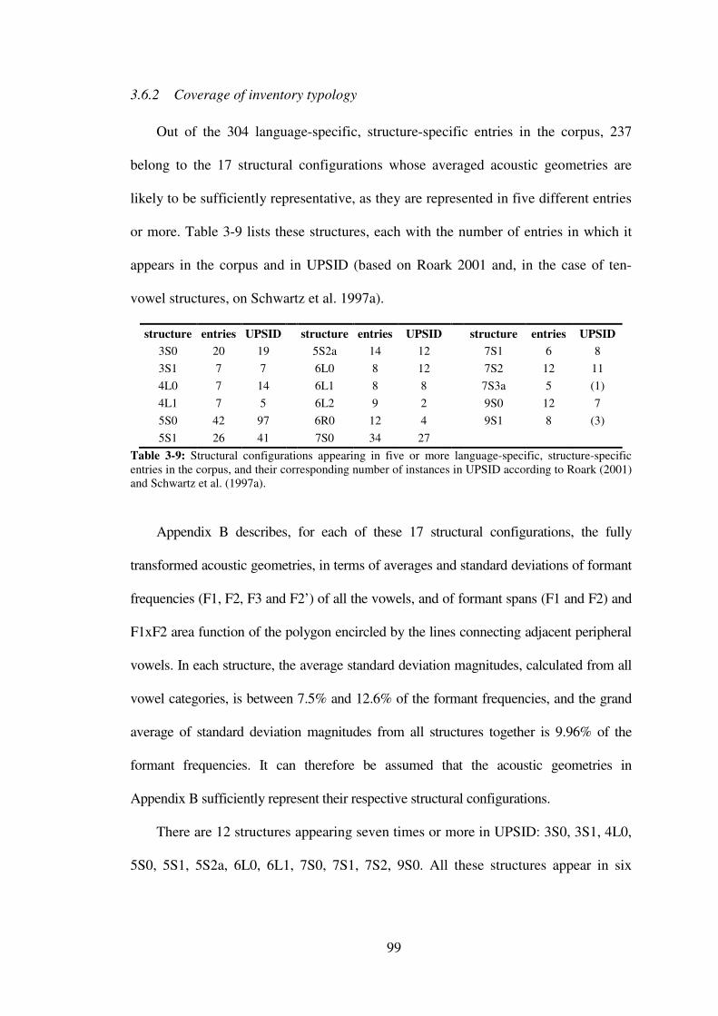
99

3.6.2 Coverage of inventory typology

Out of the 304 language-specific, structure-specific entries in the corpus, 237

belong to the 17 structural configurations whose averaged acoustic geometries are

likely to be sufficiently representative, as they are represented in five different entries

or more. Table 3-9 lists these structures, each with the number of entries in which it

appears in the corpus and in UPSID (based on Roark 2001 and, in the case of ten-

vowel structures, on Schwartz et al. 1997a).

structure entries UPSID structure entries UPSID structure entries UPSID

3S0 20 19 5S2a 14 12 7S1 6 8

3S1 7 7 6L0 8 12 7S2 12 11

4L0 7 14 6L1 8 8 7S3a 5 (1)

4L1 7 5 6L2 9 2 9S0 12 7

5S0 42 97 6R0 12 4 9S1 8 (3)

5S1 26 41 7S0 34 27

Table 3-9: Structural configurations appearing in five or more language-specific, structure-specific entries in the corpus, and their corresponding number of instances in UPSID according to Roark (2001) and Schwartz et al. (1997a).

Appendix B describes, for each of these 17 structural configurations, the fully

transformed acoustic geometries, in terms of averages and standard deviations of formant

frequencies (F1, F2, F3 and F2’) of all the vowels, and of formant spans (F1 and F2) and

F1xF2 area function of the polygon encircled by the lines connecting adjacent peripheral

vowels. In each structure, the average standard deviation magnitudes, calculated from all

vowel categories, is between 7.5% and 12.6% of the formant frequencies, and the grand

average of standard deviation magnitudes from all structures together is 9.96% of the

formant frequencies. It can therefore be assumed that the acoustic geometries in

Appendix B sufficiently represent their respective structural configurations.

There are 12 structures appearing seven times or more in UPSID: 3S0, 3S1, 4L0,

5S0, 5S1, 5S2a, 6L0, 6L1, 7S0, 7S1, 7S2, 9S0. All these structures appear in six

100

entries or more in the corpus, and their acoustic geometries appear in Appendix B.

Among the remaining structures whose acoustic geometries are established, two (4L1,

6R0) appear in UPSID four or five times. These 14 common structures cover 84% of

UPSID (and 70% of the entries in the current corpus). Owing to the rigorous language

sampling applied towards the construction of UPSID, it is likely that the same 14

structures together account for a similar proportion of the world’s languages. Together

with the remaining structures that are rare in UPSID but well represented here (6L2,

7S3a, 9S1), it is likely that the corpus provides representative acoustic geometries for

structures covering more than 85% of the world’s languages. There are only three

other structures appearing in UPSID four or five times (4R0, 4R1, 5S3), which are

rare in the corpus. At the end of Appendix B, five other structural configurations,

appearing in four languages each, are listed with their average formant frequencies,

and all other structures are listed only with the languages in which they appear.

3.6.3 Merger of structures split elsewhere

Schwartz et al. (1997a) is the only typological study of inventories that combines

rigorous classification of inventories into structural configurations with attention to

phonetic detail (as much as can be learned from inventory transcriptions without

acoustic data). It is therefore worthwhile to review the properties of acoustic

geometries of certain structural configurations where there seems to be a difference

between their treatments in Schwartz et al. (1997a) and in the current corpus,

specifically where Schwartz et al. (1997a) list more than one structure where the

current corpus (and also Crothers 1978 and Roark 2001) recognize only one. The

following discussion is by no means systematic and comprehensive, and is intended

only to highlight the potential typological insights from the current corpus.

101

For small structures with one back vowel (3S0, 3S1, 4L0, 4L1), Schwartz et al.’s

(1997a) typology suggests vertical high-to-mid variability in the back vowel,

corresponding to a consistently high front vowel. For example, 3S0 varies between /i a

u/ and /i a o/, and 4L0 similarly varies between /i e ̞ a u/ and /i e ̞ a o̞/. Similar

variability is presumably attested in the non-peripheral vowel in 3S1 and 4L1. Due to

these two variable categories, one finds 3S1 inventories labeled as /i a u ə/, /i a u ɨ/ and

/i a o ɨ/. Such variability should be manifested in greater variance of F1 frequencies for

the back and non-peripheral vowels in these structures, both in comparison with the

corresponding front vowel and with most vowels in all other structures.

The acoustic data in the current survey suggest otherwise. Figure 3-8 shows F1xF2

plots for these four structures (repeated from Appendix B) with vowel categories

represented by averages and one standard deviation ranges of their formant frequencies

(back and non-peripheral vowels are in black, other vowels in grey). F1 standard

deviations of the back and non-peripheral vowels in these structures are not always greater

than those of the (higher) front vowel. Given that the cross-structure, cross-category

average standard deviation of F1 frequencies is 51Hz, only the back vowel in 3S1 has an

exceptionally large F1 standard deviation of 86Hz, which is nevertheless mirrored by a

large F1 standard deviation of 68Hz in the front vowel in the same structure.

102

Figure 3-8: F1xF2 plots of the acoustic geometries of the structures (a) 3S0, (b) 3S1, (c) 4L0 and (d) 4L1, repeated from Appendix B. Each vowel category is represented by its one standard deviation ranges for F1 and F2. The back vowel in all structures and the non-peripheral vowel in 3S1 and 4L1 are in black, all other vowels are in grey.

There is no evidence for a split between structures with a high vowel and structures

with a mid vowel in the back and non-peripheral regions. Instead, there is a continuum of

vertical (F1) differences between the front vowel and the back and/or non-peripheral

vowel, with the front vowel being anywhere between negligibly lower (F1 higher by up

to 25Hz) to markedly higher (F1 lower by up to 140Hz) than the other vowels. However,

given the rather similar F1 standard deviations, F1 variability of the front vowel is just as

accountable for these differences as F1 variability of the back and/or non-peripheral

vowel. Moreover, there seems to be no correlation between an explicit transcription of

height contrast between the front vowel and the back/non-peripheral vowel and F1

difference. For example, among the twenty 3S0 entries, in the three entries with the

103

largest F1 difference between the front and the back vowel (a difference larger than 95Hz

in the normalized data), these vowels are transcribed as having the same height (/i u/ in

Amis, Maddieson & Wright 1995; /ɪ ʊ/ in Quichua, Guíon 2003, and in Punjabi, Singh

2005). Conversely, in Chickasaw (Gordon et al. 1997) these two vowels are transcribed

as /i o/ although the F1 difference between them is as small as 45Hz. At least in the case

of the back vowel, the high-mid split in the back vowel attested in typological studies

seems to be an artifact of inconsistent transcriptions, which probably result from the fact

that the characteristic (normalized) F1 frequency range for this vowel is 400-425Hz,

which is ambiguous between high and mid. The F1 frequency of the front vowel, on the

other hand, is typically 50Hz lower and seldom reaches 400Hz, which makes it far more

likely to be consistently transcribed as a high vowel.

The alleged variability of the back vowel in 4L0 between high and mid led some

scholars to interpret this structure as a ‘defective’ form of 5S0, where the back vowel

corresponds to one of the front vowels, and the other front vowel has no back counterpart.

In her commentary on vowel inventories in UPSID, Ferrari-Disner (1984) distinguishes

such structures (/i e ̞a u/ and /i e ̞a o̞/) from a small minority of 4L0 structures that repair

the imbalance by shifting the vowels to cover the vowel space more evenly, creating the

structure /i ɛ ɑ ʊ/. The acoustic geometry of 4L0 established here suggests that the latter

structure (or its somewhat centralized version) is the rule. The independence of this

structure from 5S0 is apparent in Figure 3-9, where the two geometries are plotted

together (4L0 in black, 5S0 in grey). Each of the 4L0 vowels is distinct from the 5S0

vowel(s) closest to it, a fact manifested in the narrow transcriptions of the prototypical

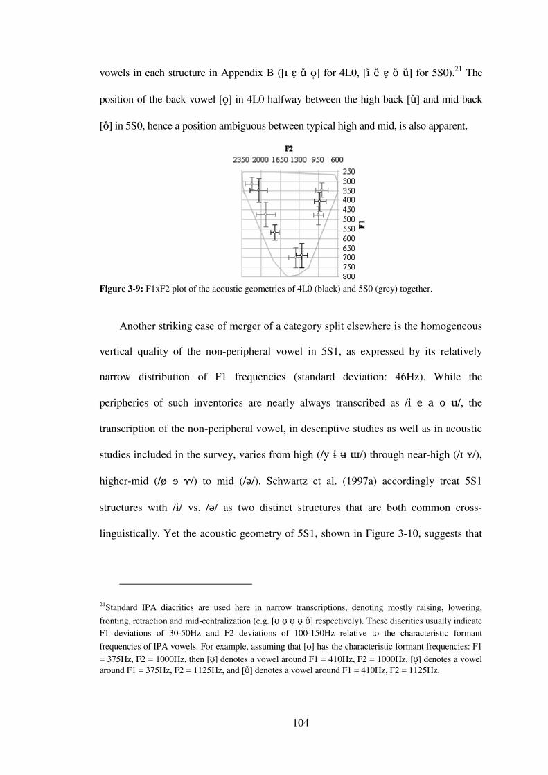
104

vowels in each structure in Appendix B ([ɪ ɛ ̞ɑ̽ o̟] for 4L0, [i ̽e ̽ ɐ̞ o̽ u̽] for 5S0).21 The

position of the back vowel [o̟] in 4L0 halfway between the high back [u̽] and mid back

[o̽] in 5S0, hence a position ambiguous between typical high and mid, is also apparent.

Figure 3-9: F1xF2 plot of the acoustic geometries of 4L0 (black) and 5S0 (grey) together.

Another striking case of merger of a category split elsewhere is the homogeneous

vertical quality of the non-peripheral vowel in 5S1, as expressed by its relatively

narrow distribution of F1 frequencies (standard deviation: 46Hz). While the

peripheries of such inventories are nearly always transcribed as /i e a o u/, the

transcription of the non-peripheral vowel, in descriptive studies as well as in acoustic

studies included in the survey, varies from high (/y ɨ ʉ ɯ/) through near-high (/ɪ ʏ/),

higher-mid (/ø ɘ ɤ/) to mid (/ə/). Schwartz et al. (1997a) accordingly treat 5S1

structures with /ɨ/ vs. /ə/ as two distinct structures that are both common cross-

linguistically. Yet the acoustic geometry of 5S1, shown in Figure 3-10, suggests that

21Standard IPA diacritics are used here in narrow transcriptions, denoting mostly raising, lowering,

fronting, retraction and mid-centralization (e.g. [ʊ̝ ʊ̞ ʊ̟ ʊ̠ ʊ̽] respectively). These diacritics usually indicate F1 deviations of 30-50Hz and F2 deviations of 100-150Hz relative to the characteristic formant

frequencies of IPA vowels. For example, assuming that [ʊ] has the characteristic formant frequencies: F1

= 375Hz, F2 = 1000Hz, then [ʊ̞] denotes a vowel around F1 = 410Hz, F2 = 1000Hz, [ʊ̟] denotes a vowel around F1 = 375Hz, F2 = 1125Hz, and [ʊ̽] denotes a vowel around F1 = 410Hz, F2 = 1125Hz.

105

the F1 frequency of the non-peripheral vowel category (in black) is more tightly

grouped than some of the peripheral vowels (in grey) in the structure.

Figure 3-10: F1xF2 plot of the acoustic geometry of structure 5S1, repeated from Appendix B. The non-peripheral vowel appears in black, all other vowels are in grey.

The average F1 frequency of the 5S1 non-peripheral vowel at 394Hz suggests a

distinct height level, which is slightly closer to the high vowels (combined F1

average: 326Hz) than to the mid vowels (combined F1 average: 481Hz). However,

logarithmic-like perceptual scales (log(Hz), ERB) would render this vowel even

closer to the position halfway between high and mid, as the Hz formant ratios are

virtually identical (326/394=0.827; 394/481=0.819).

There have been a few cases where a vertical split (two structures distinguished

by a higher vs. lower vowel) in Schwartz et al. (1997a) are merged into one in the

current survey, but the merged vowel category is indeed characterized by an

exceptionally wide F1 frequency distribution. Such is the case in the lower front

vowel in 6L0 (F1 standard deviation: 86Hz), where Schwartz et al. (1997a)

distinguish between an asymmetrical (left-crowded) structure with one low vowel and

a symmetrical structure with two low vowels. The non-peripheral vowel in 6L1 also

has a wide vertical distribution (F1 standard deviation: 106Hz), corresponding to a

distinction between two 6L1 structures, with high vs. mid non-peripheral vowels, in

106

Schwartz et al. (1997a). The acoustic geometries of both structures are plotted in

Figure 3-11, with the widely distributed vowel categories in black and all others in

grey. In both cases, the merged structure is represented in the survey by eight

languages only and cannot be split into two structures with coherent acoustic

geometries, for which at least five languages are required.

Figure 3-11: F1xF2 plots of the acoustic geometries of the structures (a) 6L0 and (b) 6L1, repeated from Appendix B. The lower front vowel in 6L0 and non-peripheral vowel in 6L1, with their wide F1 ranges, are in black, all other vowels are in grey.

3.6.4 Split of structures merged elsewhere

The structures 5S0, 5S1 and 7S0 are all very frequent in the survey (respectively 42,

26 and 34 languages), making it possible to search for sub-geometries, using the vowel

categories with the widest data distribution as natural candidates for geometry splits.

In 5S0, the mid front vowel had the widest distribution. The data distribution of

this vowel category suggested three distinct trends: a major variant resembling the

global average of the category, a high and tense minor variant and a low and lax

minor variant. The former co-occurred with a fronted low vowel and overall tenseness

(peripheralization and raising) in the non-low vowels, and the latter with a raised low

vowel and overall laxness (centralization and lowering) in non-low vowels. The entire

107

5S0 dataset was partitioned manually, in a manner that maximizes these tendencies,

into three sub-geometries: a major sub-geometry [i ̽ e ̽ ɐ ̞ o̽ u̽] (23 languages) almost

identical to the global 5S0 geometry, a ‘lax’ minor sub-geometry [ɪ ̝ ɛ ̠ ɐ ɔ ̟ ʊ] (11

languages) and a ‘tense’ minor sub-geometry [i ̞e ̞a ̝ o̞ u̞] (8 languages). Figure 3-12

plots F1 and F2 averages and standard deviations for the 5S0 geometries (global

geometry in (a) and the sub-geometries in (b): major in black; ‘lax’ minor in dark

grey; ‘tense’ minor in light grey).

Figure 3-12: F1xF2 plot of means and standard deviations of the vowels in the global 5S0 geometry based on 42 languages (panel a) and its three sub-geometries (panel b): the major sub-geometry (black, 23 languages), the ‘lax’ minor sub-geometry (dark grey, 11 languages) and the ‘tense’ minor sub-geometry (light grey, 8 languages).

As seen in Figure 3-12, this partition results in complete separation (no overlap)

between the one standard deviation ranges of the corresponding categories in the two

minor strategies, and in overall reduction of standard deviations of F1 and F2. Among

the new 30 standard deviations (2 formants x 5 vowels x 3 sub-geometries), 26 are

smaller than their correspondents in the global 5S0 geometry.

There is no apparent principle that explains the differences between the three sub-

geometries, but they are not an artifact of the normalization process. A split between a

108

peripheralized sub-geometry and a centralized sub-geometry could have been an

artifact of the concentric anchoring of inventories as part of vocal-tract normalization.

However, there is no reason why such a split should be correlated with vertical

separation in mid vowels, where the only relevant dimension for peripheralization vs.

centralization is horizontal, and with horizontal separation in the low vowel, where

only the vertical dimension is relevant. Elicitation method normalization cannot be

held accountable either because the distribution of methods is similar across the three

datasets. Finally, the datasets did not differ in the distribution of quantity constituents

(long, short, uniform etc.) either.

In 5S1, the most widely distributed vowel is the non-peripheral, due to its wide

range of F2 frequencies (2032≥F2≥1105). Gaps in the distribution of this category’s

formant data suggested a three-way split between fronted (F2≥1540Hz, 14 languages),

higher-central (F1≤412Hz, 1422≤F2≤1471Hz, 6 languages) and lower-retracted

(F1≥419Hz, F2≤1380Hz, 6 languages). This partition resulted in rather distinct sub-

geometries. The first sub-geometry, with the fronted non-peripheral vowel, had a

periphery almost identical to the global 5S1 geometry ([i ̞e ̽ɐ ̞o̽ u̽ ɪ-̠ʏ]̟).22 The second,

with the higher-central non-peripheral vowel, was tenser overall ([i e ̞a ̠o̽ u ɘ-̝ʏ]̠), its

mid-front vowel being higher and tenser (average F1: 453Hz, average F2: 1994Hz)

and its low vowel fronter (average F2: 1411Hz). The third, with the lower-retracted

non-peripheral vowel, was more centralized overall ([i ̽ ɛ ̽ ɑ̽ o̽ u̽ ɤ-ɵ̞]), its mid-front

vowel was lower (average F1: 514Hz, average F2: 1752) and its low vowel was

22Non-peripheral vowels in the acoustic geometries are usually ambiguous between a more advanced rounded vowel and more retracted unrounded vowel. In the narrow transcriptions here, these ambiguities are reflected by a hyphenated pair of symbols, the first denoting the unrounded option and the second denoting the rounded option, e.g. [ɪ-̠ʏ]̟.

109

retracted (average F2: 1252Hz). However, these splits failed to reduce formant

standard deviations except in the non-peripheral vowel category, and for each pair of

sub-geometries, all corresponding peripheral categories remained partly overlapping.

These splits are therefore considered tentative and are not discussed further.

In 7S0, the most widely distributed category was the lower-mid front vowel.

With the exception of two languages where this vowel was extremely high ([e],

F1<425Hz), its data suggested a dichotomous split between mid to lower-mid

realization ([e-̽ɛ] 460Hz<F1<580Hz, 23 languages) and near-low realization ([æ],

F1>615Hz, 9 languages). The latter, minor sub-geometry ([i e æ ɑ ɒ̝ o u]) had a

distinctly retracted low vowel and more peripheralized realization overall, while the

former, major sub-geometry ([i ̠ e ɛ ̝ a ̠ ɔ ̟ o̟ u̟]) had a slightly fronted low vowel and

negligible centralization elsewhere relative to the global 7S0 geometry. In order to

maximize the geometry split, two languages were moved from the majority to the

minority sub-geometry due to their general F1xF2 shapes.23 Though this split failed to

reduce within-category distribution and there is overlap between the realizations of

most categories, it is probably genuine. It is clearly attested in UPSID (Madison

1984), where three 7S0 languages (out of 23) are transcribed with /æ/ rather than /ɛ/,

and is also known as an isogloss in Tuscan Italian dialectology (Calamai 2001, 2002a,

2002b).24 Figure 3-13 plots F1 and F2 averages and standard deviations for the 7S0

geometries (global: thin black, major: dark grey, minor: light grey).

23 The inventory of Bengali, one of these two languages, is consistently transcribed as containing /æ/ rather than /ɛ/, both in the two studies included in the survey and in UPSID and many other sources. 24 In the survey, the /ɛ/ vs. /æ/ split in the Italian data was removed due to within-language data merger. It can nonetheless be seen in the cross-entry Italian data plotted in Figure 3-4 in Section 3.3.3, where one token of /ɛ/ appears consistently with distinctively high F1 frequency.

110

Figure 3-13: F1xF2 plot of means and standard deviations of the vowels in the global 7S0 geometry (thin black lines, 34 languages) and its two sub-geometries, major (dark grey, 21 languages), and minor (light grey, 11 languages).

In the analyses in Chapter 4, the sub-geometries of structures 5S0, 5S1 and 7S0

suggested here will be ignored. However, it is worthwhile to recognize them, as they

might be useful if acoustic geometries established here are to serve in the future in the

evaluation of simulated formal models predicting vowel inventories.

3.6.5 Cross-structure distribution of inventories with robust vowel harmony

Out of the 304 inventory entries, 27 are specified as participating in robust vowel

harmony patterns, i.e. inventories that comprise two sub-systems. The harmonizing

feature may be frontness, pharyngealization, register or ATR, respectively exemplified

by Võru, Khalkha, Somali and Degema. The sets of entries of most structural

configurations include very few inventories with vowel harmony, if any, so whatever

effect vowel harmony may have on the acoustic geometry of a particular entry becomes

negligible at the cross-linguistic level. However, in the structures 9S0 and 9S1 vowel

harmony inventories are the majority. All these inventories manifest ATR harmony and

belong to the Niger-Congo or Nilo-Saharan families. This generalization holds for all of

the instances of these structures in UPSID as well. One distinctive property

111

immediately observable in the acoustic geometries of these structures is the close

proximity and the overlap between certain vowels, in particular the second and third

highest vowels in both the front and the back region. This is shown in Figure 3-14, with

the overlapping vowels in black and all other vowels in grey.

Figure 3-14: F1xF2 plots of the acoustic geometries of the structures (a) 9S0 and (b) 9S1, repeated from Appendix B. The second- and third-highest vowels, which overlap in both the front and back regions in both structures, are in black, all other vowels are in grey.

Such proximity between vowels is not attested in any of the other acoustic

geometries established here. This and several other properties of the acoustic geometries

of 9S0 and 9S1 (and also 10L0 and 10R0) set these structures apart from others, and will

be discussed in greater detail in the context of various analyses in Chapter 4. From a

typological point of view it is important to notice that these generalized phonogical

structures appear very rarely in languages without vowel harmony, and their viability

seems to depend on the presence of vowel harmony in the language.

112

4. Analyses

In this chapter, the corpus data are used to test various predictions of Dispersion

Theory. General predictions are set forth in Section 4. Section 4.2 analyzes the

relationship between entire inventory complexity and acoustic space size. Sections

4.3- 4.5 are dedicated to the effects of local structural differences on individual

vowels: point vowels in Section 4.3, peripheral mid vowels in Section 4.4 and non-

peripheral vowels in Section 4.5. Section 4.6 is dedicated to even spacing between

vowels. Section 4.7 summarizes the insights gathered from all the analyses, proposes

modifications necessary for improving existing formal dispersion models, and

outlines directions for future research.

4.1 Dispersion Theory and its predictions

In order to test the validity of Dispersion Theory, it is necessary to set forth its

predictions explicitly. As mentioned in Section 1.3.2 the term ‘Dispersion Theory’

does not refer specifically to any one formal model, but to the general concept of

dispersion as a common denominator in studies of different kinds: theoretical,

computational, experimental or descriptive.

As can be seen from the acoustic geometries appearing in Appendix B, vowels

seldom reach the edges of the acoustic space, which implies that the classical

approach of maximization of dispersion as a single factor cannot be assumed. Instead,

the approach assumed here is that of ‘sufficient dispersion’ (Lindblom 1986), or

alternatively, a balance between maximization of dispersion and minimization of

articulatory effort (ten Bosch 1991a,b). Such an approach has been assumed in most

studies that test Dispersion Theory empirically, in particular studies comparing

113

acoustic space size and vowel variability as a function of the number of vowels in the

inventory (Ferrari-Disner 1983, Jongman et al. 1989, Bradlow 1995, Guion 2003,

Recasens & Espinosa 2006, 2009).

The first and most basic prediction of Dispersion Theory according to this

approach is that acoustic space area and structural complexity should be correlated.

This prediction holds both for entire inventories and for inventory components, like

series (e.g. the front unrounded vowels) or any set of adjacent vowels (e.g. the set of

peripheral, non-high, non-back vowels). Dispersion Theory predicts that the acoustic

area and/or formant frequency spans that such inventory components cover should be

correlated with the number of vowels comprising them. Any structural change in such

components should be reflected in a change in the acoustic area they cover, which

should further affect the acoustic geometry of the entire inventory. For example,

adding a new vowel between two existing vowels significantly shortens the perceptual

distances associated with these two vowels and should lead to their repulsion away

from the new vowel. Consequently, they might fall closer to other vowels, which are

repelled further, albeit by a smaller magnitude, and this process propagates as a push

chain shift with gradual decay through other vowels until the entire system finds a

new balance.

In order to simplify the testing and discussion of the adaptive behavior of vowels,

predictions will be made along one acoustic dimension at a time (F1 or F2/F2’).

Furthermore, in order to simplify the statistical analyses and make them more robust,

structural components not directly related to the hypothesis tested are assumed to be

constant even when they are not. For example, in tests of the effect of the presence or

absence of one peripheral vowel on the quality of another, the entire non-peripheral

114

region is assumed to exert no effect regardless of the number of non-peripheral

vowels. Similarly, in tests of the behavior of a certain vowel as a function of

peripheral symmetry or skewedness, inventories may be grouped into categories like

symmetrical, left-crowded or right-crowded regardless of the number of vowels in the

entire periphery or elsewhere (so, for example, 5S0, 5S2, 7S1 and 9S3 all count as

‘symmetrical’).

The predictions of Dispersion Theory are assumed to be as follows:

a) Inventories with more vowels should have wider formant frequency spans

and cover larger space sizes than inventories with fewer vowels.

b) Similarly, more crowded regions should cover greater formant spans than

less crowded regions. For example, the F1 span from highest to lowest

front vowel should be greater than the span for back vowels in a left-

crowded periphery.

c) A crowded region repels other vowels. For example, in left-crowded

periphery inventories, the low vowel should be relatively more retracted.

d) Vowels should be evenly spaced. Given the correct representation of the

perceptual space, distances between adjacent vowels should be similar

across vowel pairs.

In each of the following analysis sections, the general predictive principles

described here will be translated into more explicit and concrete predictions.

4.2 Entire vowel space effects

According to the view of Dispersion Theory assumed here, inventories with more

vowels should cover larger proportions of the available acoustic space. This

115

prediction is strongly supported by the survey data, as described in Section 4.2.1 and

analyzed in Section 4.2.2. As the available acoustic space is finite, the correlations

between structural complexity and formant spans are modeled as asymptotic curves,

which are described and discussed in Section 4.2.3.

4.2.1 Structure and space size – descriptive statistics

In the survey, entries have three structural indices: the total number of vowels

(V), the number of peripheral vowels (P) and the number of non-peripheral vowels

(NP). Entries also have three space size indices: area of the peripheral polygon25 (in

10000Hz² units), F1SPAN and F2SPAN. Table 4-1 summarizes the averages and standard

deviations of the space size indices as a function of the structural indices.26

Parenthesized indices represent only inventories without vowel harmony, whenever

inventories with vowel harmony constitute a significant proportion of the sample.

25 The area of the peripheral polygon was calculated as the sum of areas of triangles between whose corners are adjacent peripheral vowels and the inventory centroid. Polygons were extended to include high non-peripheral vowels if they were outside the polygon (above the line connecting the high back rounded and high front unrounded vowels), which was often the case in 4L1 inventories but rarely elsewhere. 26 On the right, the structural indices are grouped in a manner that emphasizes trends in the data and is also structurally meaningful. Grouping of V is based on the likelihood of non-peripheral vowels (3-4: rare; 5-6: possible, but rarely more than one, i.e. not as a series; 7-9: likely, including as a series; 10-14: rarely absent, and in addition, such 'extra-large' inventories are typologically very rare, see Schwartz et al. 1997a). Grouping of P is based on the number of members in the shortest peripheral vertical series (3-4: one vowel; 5-6: two vowels; 7-8: three vowels; 9-10: four vowels). Grouping of NP is based on the likelihood of non-peripheral vowel series (0-1: impossible, 2-6: rarely absent).

116

V entries area F1SPAN F2SPAN V entries area F1SPAN F2SPAN

3 20 13.52±5.52 275±64 1075±234 }3-4 35 15.88±7.16 296±85 1109±239

4 15 19.03±8.04 323±103 1154±245 5 55 27.83±10.00 389±80 1318±223

}5-6 105 28.26±9.14 395±77 1330±209 6 50 28.73±8.16 401±74 1343±194 7 62 34.11±9.95 434±71 1395±213

}7-9

126 34.46±9.39 431±72 1408±204 8 28 34.62±7.55 418±64 1449±174

9 36

(25) 34.92±9.92

(36.49±9.72) 435±81

(434±85) 1397±213

(1443±209)

10 24

(16) 34.60±8.60

(35.96±9.50) 450±71

(452±78) 1385±168

(1425±151) }10-14

38 36.28±9.62 446±67 1429±189 11 7 34.47±8.74 414±59 1431±226

12-14 7 43.65±11.36 464±57 1573±174

P entries area F1SPAN F2SPAN P entries area F1SPAN F2SPAN

3 31 16.55±8.25 305±89 1159±278 }3-4 52 19.63±9.96 326±86 1196±253

4 21 24.16±10.73 357±74 1251±205 5 87 28.82±9.53 398±81 1328±212

}5-6 144 30.26±9.30 401±79 1358±221 6 57 32.46±8.55 406±78 1404±228 7 61 35.63±9.26 446±65 1420±185

}7-8 79 36.18±9.14 443±65 1432±187 8 18 38.00±8.74 435±63 1472±193

9 23 (8)

34.76±10.48 (41.47±10.79)

460±75 (503±65)

1366±172 (1448±136) }9-10

29 (11)

34.78±10.24 (41.02±11.48)

458±68 (490±60)

1353±190 (1450±157)

10 6

(3) 34.90±10.21

(39.82) 451±39 (458)

1302±262 (1456)

NP entries area F1SPAN F2SPAN NP entries area F1SPAN F2SPAN

0 144 28.23±11.42 394±97 1288±246 }0-1 216 28.61±10.92 396±90 1307±227

1 72 29.36±9.87 401±76 1346±180 2 53 33.97±9.07 428±72 1443±184

}2-6

88 34.73±9.69 425±73 1450±198 3 27 35.04±8.78 421±68 1454±212 4-6 8 38.73±15.59 420±103 1486±267

Table 4-1: Averages and standard deviations of space size indices – area (in 10000Hz²), F1SPAN (in Hz) and F2SPAN (in Hz) – as a function of number of vowels (V), peripheral vowels (P) and non-peripheral vowels (NP). The structural index values on the left are grouped on the right. For V,P = 9~10, where vowel harmony inventories form at least a significant minority, parenthesized space size indices are based only on inventories without vowel harmony.

Local inconsistencies aside, space size indices clearly expand with increments in

structural indices, as predicted. The most convincing cases are: area as a function of V

and NP, F1SPAN as a function of V and P, and F2SPAN as a function of NP. These trends

are more consistent when adjacent values of the structural indices are grouped. The

only major deviants are the behaviors of the F2SPAN and area indices as a function of P,

which expand up to P=8, and then shrink back. However, the parenthesized F2SPAN and

area indices for P>8 are larger and consistent with predictions, indicating that these

117

deviations are due to the narrower F2 span in inventories with vowel harmony, which

comprise two smaller sub-systems. Figure 4-1 displays the averages and standard

deviations of (a) the area, (b) F1SPAN and (c) F2SPAN indices as a function of grouped

values of V (darker grey bars), P (lighter grey bars) and NP (white bars). The indices

for P=9-10 are based on data of inventories without vowel harmony.

Figure 4-1: Averages and standard deviations of area (a), F1SPAN (b) and F2SPAN (c) as a function of grouped indices of total number of vowels (V, darker grey), number of peripheral vowels (P, lighter grey) and number of non-peripheral vowels (NP, white). The indices for P=9-10 are based only on inventories without vowel harmony.

4.2.2 Structure and space size – analyses

Pearson coefficients were calculated between structural indices and space size

indices based on all 304 inventory entries. As the acoustic space is limited, dependency

of space size on structural complexity is expected to be asymptotic rather than linear,

i.e. the greater the structural index, the smaller the increment in space size should be for

118

further increment of the structural index. Accordingly the structural indices were

converted into asymptotic indices: 1/(1+1/V), 1/(1+1/P) and 1/(1+1/(NP+1)), and

Pearson coefficients were calculated between these asymptotic structural indices and

the space size indices as well. Notice that, for each of these indices, the asymptote

equals 1, and that the index for non-peripheral vowels is adjusted to allow the value

NP=0. Table 4-2 summarizes the r² values for the various correlations. Correlations

based only on the 277 entries of inventories without vowel harmony are in parentheses.

V P NP 1/(1+1/V) 1/(1+1/P) 1/(1+1/(NP+1))

area 0.257

(0.306) 0.232

(0.306)

0.068 (0.091)

0.313 (0.356)

0.285 (0.325)

0.057 (0.072)

F1SPAN 0.180

(0.202) 0.201

(0.243)

0.020 (0.035)

0.246 (0.269)

0.240 (0.260)

0.020 (0.033)

F2SPAN 0.135

(0.181) 0.075

(0.132)

0.090 (0.100)

0.171 (0.214)

0.107 (0.148)

0.087 (0.090)

Table 4-2: r² values for the correlation between structural indices and space size indices of all the inventories in the survey. The structural indices appear both in regular and asymptotic form, where the asymptote is always 1. In parentheses: r² values for correlations based only on inventories without vowel harmony.

Each of the space size indices is clearly correlated with V and P, and these

correlations are stronger with the asymptotic representations of V and P. Also, all

correlations are stronger once inventories with robust vowel harmony are excluded.

Notice that while the correlation between F2SPAN and P (and its asymptotic

representation) are weak, as a result of the behavior of F2SPAN for P>8, the correlation

between F2SPAN and V is stronger. Since V is the sum of P and NP, this must be the

result of the contribution of the genuine, albeit weak correlation of F2SPAN with NP.

The overall weak correlations of NP with space size indices are primarily the result of

the distribution of NP values. While all other indices are roughly normally distributed,

NP is distributed exponentially, with many tokens at the bottom of the scale (NP=0)

and very few at the top.

119

The fact that P is mostly correlated with F1SPAN while NP is mostly correlated

with F2SPAN is in agreement with Dispersion Theory principles. Within the periphery,

where F1 is the dominant acoustic correlate of contrast, accommodating an additional

vowel requires expansion of the F1 span in order to allow sufficient F1 differences.

The F1 span is less important in the accommodation of non-peripheral vowels,

because, across inventory structures, the number of vowels in any non-peripheral

vertical series is never greater than in the peripheral vertical series (a universal

generalization mentioned in Crothers 1978). Hence very little vertical adjustment is

needed to accommodate a non-peripheral vowel series. Conversely, non-peripheral

vowels are stuck between the front and back peripheries, so adding non-peripheral

vowels results in horizontal pressure, leading to F2 span increase. It is worth noticing

that the F2 span increase from one non-peripheral vowel to two is greater than the

increase from zero to one. Accommodating the first non-peripheral vowel requires

relatively little horizontal adjustment because this vowel is vertically free and tends to

form its own height degree, as seen in the inventory geometries in Appendix B (see

also Section 3.6.3). The contrast between this vowel and neighboring peripheral

vowels is partly vertical, alleviating some of the horizontal pressure. Once the second

non-peripheral vowel appears there is less vertical freedom, and non-peripheral

vowels are forced into F1 frequency ranges similar to those of peripheral vowels,

leaving the acoustic contrast between a non-peripheral vowel and its closest

peripheral neighbors entirely to F2, and the F2 span expands substantially as a result.

In addition to correlation analyses, space size indices of adjacent structural index

groups were directly compared in 21 unpaired t-tests (3 space size indices x 7 pairs of

adjacent groups: three for V and P, one for NP). Significance threshold was

120

Bonferroni-adjusted to 0.0024 (0.05/21). The results are listed in Table 4-3. Details of

tests involving inventories with P=9-10 and no vowel harmony are in parentheses.

Area F1SPAN F2SPAN

df t df t df t

V

3-4 vs. 5-6 138 -7.298** 138 -6.420** 138 -5.234**

5-6 vs. 7-9 228 -5.044** 229 -3.665** 228 -2.854**

7-9 vs. 10-14 160 -1.034 162 -1.145 160 -0.575

P

3-4 vs. 5-6 194 -6.935** 194 -5.731** 194 -4.353**

5-6 vs. 7-8 219 -4.538** 190u -4.300** 219 -2.484*

7-8 vs. 9-10 104 (86) 0.680 (-1.609) 106 (88) -1.027 (-2.285*) 104 (86) 1.926* (-0.306)

NP 0-1 vs. 2-6 300 -4.553** 198 u -2.919** 300 -5.123**

Table 4-3: Summary of 21 unpaired t-tests (degrees of freedom, t-score and probability) comparing space size indices (area, F1SPAN and F2SPAN) for grouped values of structural indices (V – total number of vowels, P – number of peripheral vowels, NP – number of non-peripheral vowels). In the df columns, “u” denotes that the number of degrees of freedom is appropriate for unequal-variance unpaired t-test, as determined by a preliminary F-test for variance (with p<0.05 as significance threshold). “*” denotes near-significance at p<0.05 and “**” denotes significance at the Bonferroni-adjusted threshold of p<0.0024. In parentheses are the details of t-tests for P=7-8 vs. P=9-10 where the latter sample consists only of inventories without vowel harmony.

All 15 tests other than the tests comparing indices of the ‘extra-large’ inventories

(V=10-14 or P=9-10) were significant (14 tests) or almost significant (one test) in the

direction predicted by Dispersion Theory. Conversely, all the six tests comparing

extra-large inventories to the ‘large’ group below them were non-significant: four in

the direction predicted by Dispersion Theory and two in the reverse direction (which

nevertheless get corrected once the set of inventories with 9-10 peripheral vowels is

limited to inventories without vowel harmony). The fact that extra-large inventories

do not occupy significantly larger spaces than large inventories implies that the large

inventories already tend to reach close to the maximal size. This space size might be

too small for the extra-large inventories, which are typologically rare. In this regard,

we are reminded that in the more typologically representative survey of UPSID

(Maddieson 1984), inventories with 10 vowels or more are rare (less than 6%), and

that Schwartz et al. (1997a:242) consequently suggest that “… the highest limit [of

121

number of vowels] for a viable primary system [= inventory of plain oral

monophthongs] is 9”. This fact, together with the tendency of extra-large inventories

without vowel harmony to nevertheless span the largest acoustic dimensions, imply

that the non-significant results cannot be interpreted as counter-evidence to

Dispersion Theory. In summary, Dispersion Theory accounts for the relationship

between structural complexity and acoustic space size in a satisfactory manner.

4.2.3 Asymptotic behavior of formant spans

Recall that in Table 4-2 in Section 4.2.2, the highest r² values for F1 and F2 spans

were achieved when these indices were correlated with 1/(1+1/V), the asymptotic

representation of V, and vowel harmony inventories were ignored. Regression

analyses of F1 and F2 spans as the dependent variables and 1/(1+1/V) as the

independent variable yielded the following models:

(4.1) F1SPAN = 1080.9 / (1 + 1 / V) – 524.23

(4.2) F2 SPAN = 2543.7 / (1 + 1 / V) – 831.8

These models represent the average formant spans as a function of (1+1/V), and

they respectively reach the asymptotes 567Hz and 1712Hz when V is infinite. If

average formant spans represent the point of equilibrium between maximization of

dispersion and minimization of articulatory effort for a given value of V, then any

span beyond these asymptotes is on the more effortful side of the equilibrium for any

value of V, in wordlist elicitation.

Recall that, in Table 3-4 in Section 3.3.2, the most representative formant span

interpolation ratio from isolation to word-list elicitation was found to be 0.89 for both F1

and F2, implying that the reverse (extrapolation) ratio is 1.124. Multiplying the F1 and F2

span asymptotes by this ratio gives respectively 637Hz and 1924Hz as the span

122

asymptotes for isolation elicitation (213Hz≤F1≤850Hz, 576Hz≤F2≤2500Hz). Since

isolation elicitation posits no articulatory constraints and all humanly possible vowels are

reachable, it stands to reason under Dispersion Theory that these span asymptotes and

formant extrema represent the absolute edges of the vowel space for the average male

speaker in the studies included in the corpus. This implies that, under vocal-tract

normalization only, no inventory in the corpus should exceed these span asymptotes. In the

entire corpus of 447 inventories normalized only for vocal tract, there are two inventories

with F1 span greater than 637Hz and one inventory with F2 span greater than 1924Hz.

99% of the inventories have formant spans smaller than 600Hz for F1 and 1800Hz for F2.

It is thus plausible that these three odd cases are due to errors, and that the isolation

elicitation asymptotes are indeed reasonable estimates of the possible vowel space.

4.3 Vowel-specific effects I: point vowels

Every inventory in the survey has at least one front vowel, a low vowel and at

least one back vowel. The highest front vowel, the low vowel and the highest back

vowel constitute the three point vowels, which will be referred to as I, A and U

henceforth. Section 4.3.1 briefly discusses the behavior of point vowels as a function

of structural complexity. Sections 4.3.2 and 4.3.3 discuss the effect of peripheral

configuration respectively on the behavior of A along the F2 dimension and on the

behavior of I and U relative to each other along the F1 dimension.

4.3.1 Point vowels and structural complexity

With very few exceptions, I is always at both the F1 minimum and F2 maximum

of the inventory, while A is always at the F1 maximum by definition, and U shows an

overwhelming tendency, albeit not as universal as those of I and A, to be at the F2

123

minimum and close to the F1 minimum. Dispersion Theory therefore predicts that F1

of I and U and F2 of U should decrease, while F2 of I and F1 of A should increase, as

a function of any increase in structural complexity. Unfortunately, the combination of

concentric inventory anchoring as part of vocal-tract normalization described in

Section 3.2 and the consistent correlations between structural complexity and formant

spans shown in Section 4.2 render these predictions trivially valid. Any correlation

between structural indices and inventory formant spans is paralleled by a correlation

between the same structural indices and formant extrema. Suffice it to say that such

significant correlations, albeit much weaker, are present already in the raw data. For

example, in the raw data, the correlations between the total number of vowels and F1

frequencies of A and I have the respective r² values 0.088 and 0.079 (p<10-6 for both).

The normalization process greatly improves these correlations, but it is impossible to

disentangle the complementary contributions of vowel-specific behavior and of the

methodological artifact due to the normalization procedure.

4.3.2 F2 of the low vowel as a function of peripheral configuration

While the F1 frequency of A is directly correlated with the inventory F1 span and

hence with structural complexity, its F2 frequency, which is always somewhere in the

middle of the F2 span, cannot be apriori assumed to correlate with any structural

property. However, Dispersion Theory makes clear predictions regarding the F2 of A

as a function of peripheral configuration. As the prominence of the front periphery

increases from right-crowded inventories through symmetrical to left-crowded

inventories, the front periphery should extend up and down. As a consequence, A

should be pushed back, i.e. its F2 should decrease.

124

In order to examine the effect of peripheral arrangement on the F2 frequency of

A, the set of 302 entries (two entries, for which normalized F2 frequencies could not

be calculated, were excluded) was divided into the three groups according to

periphery configuration: Symmetrical (S, 198 inventories), Left-crowded (L, 60

inventories) and Right-crowded (R, 44 inventories). For simplicity and robustness, the

specific number of vowels in any region was ignored. Descriptive statistics of F2

frequencies of the A show tendencies consistent with Dispersion Theory predictions,

with average values rising from F2=1274Hz (sd = 126Hz) in L inventories, through

F2=1372Hz (sd = 128Hz) in S inventories, to F2=1489Hz (sd = 141Hz) in R

inventories. Preliminary F-tests showed that the variances of the three groups were

not significantly different, and consequently equal-variance unpaired t-tests were used

for comparing the three groups. The effect of periphery configuration was highly

significant in all cases (S vs. L: t(256) = 5.224, p<1x10-6; S vs. R: t(240) = 5.398,

p<1x10-7; L vs. R: t(102) = 8.173, p<1x10-12).

These results imply that the F2 frequency of A is regulated by dispersion principles,

but it was suspected that a major confound was involved, the insistence on only one low

vowel per inventory. In inventories that are better described as having symmetrical

peripheries with two low vowels, this interpretation forced the classification of the

inventory as asymmetrical, with a single low vowel closer to the less crowded periphery.

It was suspected that a distinctly front or back quality of the lowest vowel appeared

almost exclusively in such inventories, and that, if there was truly only one low vowel,

this vowel would be central even if the inventory is left-crowded or right-crowded.

In order to eliminate this confound, a very restrictive criterion was imposed on

inventories previously analyzed as asymmetrical: only those inventories, where A had

125

F1 frequency more than 100Hz above the lowest among the vowels of the more

crowded periphery, were treated as ‘truly left-/right-crowded’. This reduced the number

of left-crowded inventories from 60 to 34, excluding 26 inventories where the lowest

vowel (typically rather back) contrasted with a very low front vowel. The number of

right-crowded inventories also decreased from 44 to 26, excluding 18 inventories where

the lowest vowel (typically rather front) contrasted with a very low back vowel. In the

two restricted asymmetrical groups pooled together (60 inventories), the average F1

frequencies of A and the second lowest vowel were respectively 720Hz (sd = 44Hz) and

534Hz (sd = 64Hz). As a result of the removal of inventories suspected as having two

low vowels, the average F2 frequency of A rose to 1302Hz (sd=99Hz) in the restricted

L inventory group, and dropped to 1448Hz (sd=149Hz) in the restricted R inventory

group, implying that the low vowels indeed got somewhat centralized.

Variances were significantly different for the L and R inventories (F(33,25) =

0.436, p<0.02) and for the S and L inventories (F(197,33) = 1.677, p<0.04), but not

for S and R inventories (F(197,25) = 0.732, p>0.12). Subsequent unpaired t-tests

show a reduced, yet still highly significant, effect of periphery configuration on the F2

frequency of A (S vs. L: t(54) = 3.646, p<0.0003; S vs. R: t(222) = 2.795, p<0.003; L

vs. R: t(41) = 4.317, p<0.00005). Thus, even when there is clearly only one low

vowel, the geometry is sensitive to dispersion pressures. It compensates for a slightly

shorter vertical contrast and/or greater vertical crowdedness by slightly increasing

horizontal contrast and attracting A to the less crowded periphery.

The relatively small acoustic magnitude of this effect, typically well within 100Hz

from ‘perfect central’, is probably why this effect often goes unnoticed in

impressionistic descriptions of vowel inventories with asymmetrical peripheries, as A is

126

overwhelmingly transcribed as (central) /a/. More often than not, A is within the

(normalized) range of 1275Hz<F2<1475Hz, i.e. an acceptable central low vowel. Given

speaker and context variability, it makes little sense to indicate its deviation from

central in summaries that aim at language properties other than phonetic precision. It is

only by examining data from hundreds of languages that the subtle effects of dispersion

become apparent. Along the same line, it is worth noticing that, when the inventory

seems to contain two low vowels, impressionistic descriptions are often sensitive to the

horizontal quality of the vowels, transcribing them as e.g. /æ/ vs. /ɑ/. According to the

survey data, this is far from surprising. Recall that restricting front-crowded and back-

crowded inventories only to those inventories, where the F1 frequency of A is at least

more than 100Hz above that of second lowest vowel, yielded reduced sensitivity of the

low vowel to peripheral asymmetries. The 44 inventories that were excluded by this

criterion (26 left-crowded, 18 right-crowded) may be suspected of having two low

vowels. These inventories are characterized by a lowest vowel with average F1

frequency of 693Hz (sd = 47Hz), compared to average F1 frequency of 652Hz (sd =

52Hz) of the lower vowel in the more crowded periphery, a marginal F1 contrast. In

these inventories, the lowest vowel is clearly back (average F2 = 1238Hz, sd = 149Hz)

or clearly front (average F2 = 1549Hz, sd = 106Hz) if the inventory is respectively left-

crowded or right-crowded. Regardless of whether or not these inventories have two low

vowels, it is clear that the marginal F1 contrast between the two vowels is compensated

for by a significantly greater F2 contrast, as Dispersion Theory predicts.

In summary, the behavior of A along the F2 dimension strongly supports Dispersion

Theory: it is in the middle when the periphery is symmetrical, but in case of asymmetry,

the more crowded side pushes A away towards the less crowded side, and the lower the

127

more crowded side gets, the farther A is pushed to the other side. Figure 4-2 displays the

one standard deviation distribution ranges of A on the F1xF2 plane as a function of

peripheral configuration (S = symmetrical, L = strictly left-crowded, R = strictly right-

crowded, L?S2 = left-crowded but suspected as symmetrical with low vowels, R?S2 =

right-crowded but suspected as symmetrical with two low vowels).

Figure 4-2: Average and standard deviation of the F2 frequency of the low vowel in inventories with the following peripheral configurations: symmetrical (“S”, solid line, 198 inventories), strictly left-crowded (“L”, dashed line, 34 inventories), strictly right-crowded (“R”, dashed-dotted line, 26 inventories), left-crowded but suspected as symmetrical with two low vowels (“L?S2”, dotted line, 26 inventories) and right-crowded but suspected as symmetrical with twi low vowels (“R?S2”, dotted line, 18 inventories).

In addition to supporting Dispersion Theory, the F2 behavior of A constitutes

strong evidence against Quantal Theory (Stevens 1972, 1989). According to Quantal

Theory, the cross-linguistic omnipresence of a low vowel in inventories is not a result

of relative distance from other vowels, but of an absolute property of this vowel:

acoustic stability and proximity of F1 and F2 at a point where F2 is at its lowest (and

F1 allegedly at its highest frequency). Thus, A should be fixed as a back [ɑ] regardless

of inventory structure. In addition, certain versions of Quantal Theory predict the

dominance of [ɑ] not only on the basis of articulatory-to-acoustic stability, but also of

acoustic-to-perceptual stability, because [ɑ] is the only low vowel where F1 and F2

are closer than the Center of Gravity Effect threshold of 3-3.5Bark (Chistovich &

128

Lublinskaya 1979). The horizontal variability of A itself, and the rather limited

presence of back [ɑ] quality in inventories, are contradictory to the predictions of

Quantal Theory, as is the fact that the preferred quality of A is low central [ɐ]̞, which

is characterized neither by a stable distance between F1 and F2 nor by F1-F2 distance

smaller than 3.5Bark (for the most typical A, with F1=700Hz and F2=1375Hz, this

distance is 3.9Bark). Finally, Figure 4-2 shows that A is not lowest at the back region,

as Quantal Theory suggests, nor is it at the central region. The lowest qualities

(highest F1 frequencies) are decidedly at the half-front region around F2=1450Hz,

although this might be due the fact that the fronter-than-central region is used more

frequently in inventories with more vowels (and consequently larger F1 spans).

4.3.3 F1 difference between high vowels as a function of peripheral configuration

While the behavior of I and U along the F1 frequency dimension is correlated

with the F1 span and hence with structural complexity, the difference between their

respective F1 frequencies, henceforth F1U – F1I, is not. It is well known that F1 tends

to be slightly lower in I than in U in inventories. Indeed, in 256 of the 304 inventories

in the corpus, the F1U –F1I index is positive, whereas it is negative in 36 inventories

and equals 0 in twelve. This tendency is valid across all structures. Even so, it is

interesting to see whether the peripheral configuration has correlates in the behavior

of F1U-F1I. Assuming that the F1U-F1I is positive, Dispersion Theory predicts that,

relatively to F1U-F1I in inventories with a symmetrical periphery, a front-crowded

periphery should push I up more, lowering its F1 frequency and increasing F1U-F1I,

whereas a back-crowded periphery should push U up more, thus reducing F1U-F1I.

129

Before testing these predictions using the survey data, some complications and

pitfalls should be considered. First, in some inventories, the identities of I and U are the

consequences of subjective interpretation. For example, the Standard Japanese /i e a o

ɯ/ inventory is classified as a 4L1 inventory (left-crowded four vowel periphery and

one non-peripheral vowel). This disputable interpretation both forces the inventory into

the left-crowded group and assigns the U status to /o/, whose F1 frequency is obviously

much higher than that of /i/, thus biasing the data in the direction of Dispersion Theory

predictions. Second, some of the smaller inventories whose peripheral structures are not

disputable, nevertheless have a pronounced height asymmetry between I and U, which

is manifested already in the transcription, as in the 3S0 inventory of Creek (/i a o/) or

the 4L0 inventory of Navajo (/i ɛ a o/), but there are no reverse cases where I is /e/ and

U is /u/ (such structures do not appear in UPSID either, see Ferrari-Disner 1984 for

discussion). Recall that, as mentioned in Section 3.6.3, such instances of /o/-labeled U

are not necessarily lower than instances of /u/-labeled U in other inventories. It is

nevertheless plausible that, in some inventories, the decision to label a vowel as /o/

rather than /u/ is based on phonological considerations (e.g. participating in regular

patterns together with the lower front vowel but not with the higher front vowel in 4L0).

It can therefore be argued that the true test for Dispersion Theory here is when such

height asymmetries are neutralized, that is, when the test is based only on those

inventories whose I and U denote vowels transcribed as sharing the same height.

Finally, again as a result of subjective interpretation, symmetrical inventories with two

low vowels may have been artificially treated as left- or right-crowded, as seen already

in the analysis of F2 of the low vowel in Section 4.3.2.

130

Having taken these possible confounds into account, separate analyses were

performed according to looser and stricter criteria. Table 4-4 lists the various exclusion

criteria, the number of inventories observed in each case and average and standard

deviation of F1U-F1I. Qualitative observation suggests that F1U-F1I averages behave

exactly according to the predictions of Dispersion Theory, i.e. the difference is always

greatest for left-crowded periphery inventories and always smallest for right-crowded

periphery inventories. However, standard deviations indicate that the behavior of F1U-

F1I substantially overlaps between all three types. Table 4-5 summarizes the results of

15 unpaired t-tests (3 periphery type pairs x 5 exclusion criteria). The one-tailed

significance threshold was Bonferroni-corrected to 0.0033 (=0.05/15).

Exclusion criteria left-crowded symmetrical right-crowded

obs. Av. F1u-F1ɪ obs. Av. F1u-F1ɪ obs. Av. F1u-F1ɪ

none 60 52.0 (±48.8) 199 30.8 (±34.8) 45 23.4 (±23.5)

disputable interpretation of I/U 55 45.3 (±45.0) 197 30.2 (±34.2) 45 23.4 (±23.5)

pronounced height asymmetry 48 33.2 (±31.1) 194 29.5 (±34.0) 45 23.4 (±23.5)

disputable interpretation of periphery asymmetry

29 59.9 (±52.9) 197 30.2 (±34.2) 27 23.0 (±22.6)

pronounced height asym. And disputable interpretation of periphery asymmetry

22 38.1 (±35.5) 194 29.5 (±34.0) 27 23.0 (±22.6)

Table 4-4: Number of inventories, and average and standards deviations for F1U-F1I as a function of peripheral configuration (left-crowded, symmetrical, right-crowded), according to different criteria for excluding inventories whose peripheral configuration is suspected to have been improperly assigned.

Exclusion criteria L vs. R S vs. L S vs. R

df t df t df t

none 90u 3.964** 78 u 3.126** 94 u 1.731*

I/U interpretation 84 u 3.122** 72 u 2.306* 92 u 1.591

pronounced height asymmetry 87 u 1.711* 240 0.669 92 u 1.435

peripheral asymmetry interpretation 38 u 3.440** 32 u 2.935** 44 u 1.452

height asymmetry + peripheral asymmetry interpretation 34 u 1.732* 214 1.111 44 u 1.319

Table 4-5: Summary of unpaired t-tests for mean difference of F1U-F1I between different peripheral configurations (“S” = symmetrical, “L” = left-crowded, “R” = right-crowded) according to different criteria for excluding inventories whose peripheral configuration is suspected to have been improperly assigned. In the df columns, “u” denotes that the number of degrees of freedom is appropriate for unequal-variance unpaired t-test, as determined by a preliminary F-test for variance (with p<0.05 as significance threshold). “*” and “**” respectively indicate near-significant (p<0.05) and significant (p<0.0033) results.

131

Evidently, not all differences are significant, in particular between the symmetrical

and each of the asymmetrical types. Significance is least attested in the strictest

exclusion criteria condition, which compares only inventories whose I and U are

transcribed as having the same height. However, in the case of left- vs. right-crowded

peripheries, the average F1U-F1I indices are always significantly or near-significantly

different, implying that the vertical positions of I and U are genuinely sensitive to the

configuration of the inventory periphery as predicted by Dispersion Theory, even if this

sensitivity is subtle. In addition, in the comparisons between inventories with

symmetrical vs. right-crowded peripheries, where results were least conclusive, the

differences were in the direction predicted by Dispersion Theory (p<0.10 in all five

conditions), which adds to the apparent consistency of this subtle sensitivity.

4.4 Vowel-specific effects II: peripheral mid vowels

Peripheral mid vowels are never at the F1 extrema of inventories, and with very

few exceptions, they are never at the F2 extrema either. As such, their formant

frequencies are not necessarily correlated with formant spans, and constitute an

independent test-case for Dispersion Theory. Section 4.4.1 examines the behavior of

individual peripheral mid vowels along the F1 dimension as a function of peripheral

configuration, and Section 4.4.2 looks at F2 of peripheral mid vowels as a function of

the number of non-peripheral vowels.

4.4.1 F1 of peripheral mid vowels as a function of peripheral configuration

In each entry in the corpus, all peripheral vowels other than the three point

vowels are mid vowels. As all entries have the three point vowels, any structural

132

difference between the peripheral configurations of any two entries is a difference in

the distribution of mid vowels. The principal prediction of Dispersion Theory is that

any such difference should be manifested in acoustic rearrangement of the entire

periphery and consequently in systematic F1 differences between corresponding

vowels in the different configurations. The effect of structural differences on the F1

frequency will be tested for each peripheral mid vowel separately.

The corpus contains sufficient data (at least 8 entries) for each of the following

peripheral structures: 4L, 5S, 6L, 6R, 7S, 8L, 8R, 9S. For simplicity and robustness,

data are pooled together from similar peripheries, across all non-peripheral

configurations accompanying them.27 In the analyses, peripheral mid vowels will be

labeled as follows: the peripheral structure, followed by F/B for ‘front/back’, followed

by H/M/L (higher mid – the highest among more than one mid vowels in the

periphery; mid – the only mid vowel in the periphery or the middle one among three

mid vowels; lower mid – the lowest among more than one mid vowels). For example,

6L:F:L refers to the lower-mid front vowel in a left-crowded six-vowel periphery.

Figure 4-3 illustrates this nomenclature with the peripheral mid vowels in 5S, 6L and

8R peripheral configurations.

27This is a simplification, because the number of non-peripheral vowels has been shown in Section 4.2.2 to exert some effect (albeit small) on the F1 span of the inventory, which would be most pronounced in the F1 frequencies of the point vowels, but might carry onto mid vowels as well. Not less importantly, it follows from Dispersion Theory itself that any change in the number of vowels would be reflected in reorganization of the entire inventory, differences in the number of non-peripheral vowels included. However, due to the great spatial variability of non-peripheral vowels and the small number of inventories pertaining to many of the specific (peripheral + non-peripheral) structures, this simplification is worthwhile, because it not only bases each of the analyses on many more inventories, but also allows us to extend the analysis into peripheral structures that are rather rare (e.g. 8 peripheral vowels).

133

Figure 4-3: Illustration of the peripheral mid vowel nomenclature in 5S (left), 6L (center) and 8R (right) periphery configurations. Mid vowels (labeled) are in black, point vowels (unlabeled) are in grey.

Since the number of mid vowels in a given region (front or back) varies between

one, two and three, correspondence between vowels belonging to the same region in

different structures is not always one-to-one. For example, when the mid front vowels

of a five-vowel periphery and of a left-crowded six-vowel periphery are compared,

5S:F:M (the only mid front vowel in 5S) corresponds to both 6L:F:H and 6L:F:L (the

higher and lower mid front vowels in 6L). On the other hand, correspondence is not

all-to-all either: H and L vowels do not correspond to each other across structures. In

fact, as the average F1 frequencies of the H vowel sets are all outside the single

standard-deviation range of the L vowel sets and vice-versa, it can be safely assumed

that H vowels are always higher (having lower F1 frequencies) than L vowels.

Three distinct effects of peripheral configuration on the F1 frequency of

peripheral mid vowels will be tested, defined as extension of a smaller peripheral

component to a larger one:

(a) Adding a vowel to the examined side (6R:F:M vs. 7S:F:H, 6R:F:M vs. 7S:F:L etc.).

(b) Adding one/two vowel(s) to the opposite side (4L:F:M vs. 5S:F:M/6R:F:M etc.).

(c) Adding one vowel to each side (5S:F:M vs. 7S:F:H, 5S:F:M vs. 7S:F:L etc.).

According to Dispersion Theory, expansion of the examined periphery, which is

the case in both (a) and (c), should result in vowels in the larger structure with F1

frequencies extrapolated above and below the vowel(s) in the smaller structure.

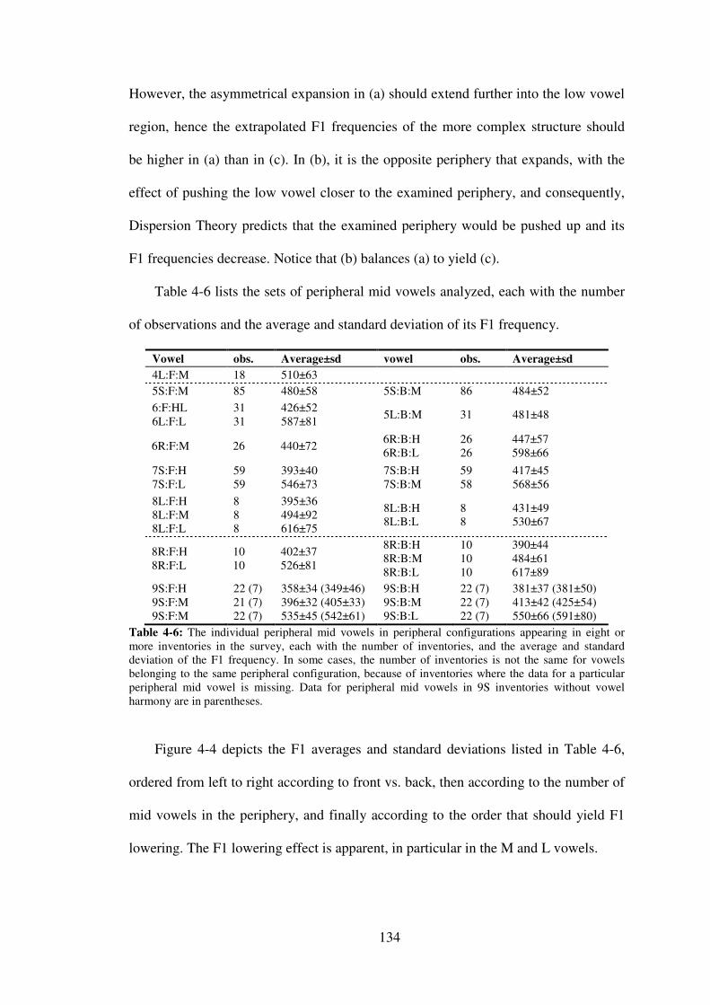
134

However, the asymmetrical expansion in (a) should extend further into the low vowel

region, hence the extrapolated F1 frequencies of the more complex structure should

be higher in (a) than in (c). In (b), it is the opposite periphery that expands, with the

effect of pushing the low vowel closer to the examined periphery, and consequently,

Dispersion Theory predicts that the examined periphery would be pushed up and its

F1 frequencies decrease. Notice that (b) balances (a) to yield (c).

Table 4-6 lists the sets of peripheral mid vowels analyzed, each with the number

of observations and the average and standard deviation of its F1 frequency.

Vowel obs. Average±sd vowel obs. Average±sd

4L:F:M 18 510±63 5S:F:M 85 480±58 5S:B:M 86 484±52

6:F:HL 6L:F:L

31 31

426±52 587±81

5L:B:M 31 481±48

6R:F:M 26 440±72 6R:B:H 6R:B:L

26 26

447±57 598±66

7S:F:H 7S:F:L

59 59

393±40 546±73

7S:B:H 7S:B:M

59 58

417±45 568±56

8L:F:H 8L:F:M 8L:F:L

8 8 8

395±36 494±92 616±75

8L:B:H 8L:B:L

8 8

431±49 530±67

8R:F:H 8R:F:L

10 10

402±37 526±81

8R:B:H 8R:B:M 8R:B:L

10 10 10

390±44 484±61 617±89

9S:F:H 9S:F:M 9S:F:M

22 (7) 21 (7) 22 (7)

358±34 (349±46) 396±32 (405±33) 535±45 (542±61)

9S:B:H 9S:B:M 9S:B:L

22 (7) 22 (7) 22 (7)

381±37 (381±50) 413±42 (425±54) 550±66 (591±80)

Table 4-6: The individual peripheral mid vowels in peripheral configurations appearing in eight or more inventories in the survey, each with the number of inventories, and the average and standard deviation of the F1 frequency. In some cases, the number of inventories is not the same for vowels belonging to the same peripheral configuration, because of inventories where the data for a particular peripheral mid vowel is missing. Data for peripheral mid vowels in 9S inventories without vowel harmony are in parentheses.

Figure 4-4 depicts the F1 averages and standard deviations listed in Table 4-6,

ordered from left to right according to front vs. back, then according to the number of

mid vowels in the periphery, and finally according to the order that should yield F1

lowering. The F1 lowering effect is apparent, in particular in the M and L vowels.

135

Figure 4-4: Averages and standard deviations of the F1 frequencies for the peripheral mid vowels in each of the peripheral configurations appearing in eight or more inventories in the survey. Peripheral configurations with the same number of mid vowels in a given region are juxtaposed in the order for which Dispersion theory predicts decrements in F1 frequencies from left to right. Data for the peripheral configuration 9S from inventories without vowel harmony are in grey.

Given the 29 sets of peripheral mid vowels listed in Table 4-6 and the three types

of configurational differences, 72 comparisons of F1 frequencies of two

corresponding sets were performed. In each comparison, depending on a preliminary

F-test for variance, equal- or unequal-variance unpaired t-test was performed (one

tailed, given the directional prediction of Dispersion Theory). The Bonferroni-

corrected significance threshold was set at p=0.0007 (=0.05/72). Table 4-7

summarizes the t-tests for all 72 comparisons.

136

Adding one vowel

to the examined side

adding one/two vowel(s)

to the opposite side

adding one vowel

to each side

comparison df t comparison df t comparison df t 5S:F:M, 6L:F:H 114 4.580** 4L:F:M, 5S:F:M 101 2.017* 4LF:M, 6L:F:H 47 5.075** 5S:F:M, 6L:F:L 42u -6.759** 5S:F:M, 6R:F:M 109 2.898* 4L:F:M, 6L:F:L 47 -3.435** 6R:F:M, 7S:F:H 32u 3.141* 4L:F:M, 6R:F:M 42 3.358* 5S:F:M, 7S:F:H 142u 10.660** 6R:F:M, 7S:F:L 83 -6.212** 6L:F:H, 7S:F:H 49u 3.387* 5S:F:M, 7S:F:L 106u -5.825** 7S:F:H, 8L:F:H 65 -0.183� 7S:F:H, 8R:F:H 67 -0.652� 6R:F:M, 8R:F:H 31u 2.100* 7S:F:H, 8L:F:M 7u -3.083* 6L:F:H, 8R:F:H 39 1.354 6R:F:M, 8R:F:L 34 -3.120* 7S:F:L, 8L:F:M 65 1.823* 6L:F:L, 7S:F:L 88 2.461* 6L:F:H, 8L:F:H 37 1.542 7S:F:L, 8L:F:L 65 -2.572* 7S:F:L, 8R:F:L 67 0.773 6L:F:H, 8L:F:M 8u -2.029* 8R:F:H, 9S:F:H 30 3.343* 6L:F:L, 8R:F:L 39 2.058* 6L:F:L, 8L:F:M 37 2.806* 8R:F:H, 9S:F:M 29 0.445� 8L:F:H, 9S:F:H 28 2.681* 6L:F:L, 8L:F:L 37 -0.921 8R:F:L, 9S:F:M 10u 4.885** 8L:F:M, 9S:F:M 8u 2.959* 7S:F:H, 9S:F:H 79 3.659** 8R:F:L, 9S:F:L 12u -0.308 8L:F:L, 9S:F:L 9u 2.895* 7S:F:H, 9S:F:M 78 -0.320 5S:B:M, 6R:B:H 110 3.080* 5S:B:M, 6L:B:M 115 0.225 7S:F:L, 9S:F:M 74u 12.729** 5S:B:M, 6R:B:L 110 -9.240** 6R:B:H, 7S:B:H 83 2.585* 7S:F:L, 9S:F:L 60u 0.819� 6L:B:M, 7S:B:H 88 6.241** 7S:B:H, 8L:B:H 65 -0.809� 5S:B:M, 7S:B:H 143 7.988** 6L:B:M, 7S:B:L 87 -7.499** 6R:B:H, 8L:B:H 32 0.712 5S:B:M, 7S:B:L 142 -9.472** 7S:B:H, 8R:B:H 67 1.731* 6R:B:L, 7S:B:L 82 2.212* 6L:B:M, 8L:B:H 37 2.615* 7S:B:H, 8R:B:M 67 -4.135** 7S:B:L, 8L:B:L 64 1.821* 6L:B:M, 8L:B:L 37 -2.371* 7S:B:L, 8R:B:M 66 4.440** 6R:B:L, 8L:B:L 32 2.531* 6R:B:H, 8R:B:H 34 2.814* 7S:B:L, 8R:B:L 10u -1.655 8R:B:H, 9S:B:H 30 0.573 6R:B:H, 8R:B:M 34 -1.731* 8L:B:H, 9S:B:H 28 3.030* 8R:B:M, 9S:B:M 30 3.914** 6R:B:L, 8R:B:M 34 4.724** 8L:B:H, 9S:B:M 28 0.989� 8R:B:L, 9S:B:L 30 2.395* 6R:B:L, 8R:B:L 34 -0.692 8L:B:L, 9S:B:M 9u 4.642** 7S:B:H, 9S:B:H 79 3.369** 8L:B:L, 9S:B:L 28 -0.706 7S:B:H, 9S:B:M 79 0.362� 7S:B:L, 9S:B:M 78 12.069** 7S:B:L, 9S:B:L 78 1.327�

Table 4-7: Summary of unpaired t-tests for difference of average F1 frequencies between corresponding peripheral mid vowel categories in different peripheral configurations. In the df columns, “u” denotes that the number of degrees of freedom is appropriate for unequal-variance unpaired t-test, as determined by a preliminary F-test for variance (with p<0.05 as significance threshold). “*” denotes near-significance at p<0.05 and “**” denotes significance at the Bonferroni-adjusted threshold of p<0.0007. “�” denotes that the difference (always non-significant) is in a direction opposite to the prediction of Dispersion Theory.

Out of the 72 comparisons, 22 resulted in significant difference in the direction

predicted by Dispersion Theory, and 30 more comparisons resulted in near-significant

difference (p<0.05, one-tailed) in the predicted direction, and twelve other comparisons

resulted in non-significant differences in the predicted direction. Only eight comparisons

resulted in differences in the opposite direction, all non-significant. These results can only

be interpreted as strongly corroborating Dispersion Theory. In fact, in the smaller and

137

more common peripheral structures (4L, 5S, 6L, 6R, 7S), mid vowels follow Dispersion

Theory predictions with extreme consistency. All 22 comparisons involving these

structures had results in the predicted direction, 12 significant and nine more near-

significant. If these were the only comparisons performed and the Bonferroni-corrected

significance threshold was accordingly set at p=0.0023 (=0.05/22), then four of the nine

near-significant results would have become significant as well.

Patterns are not as consistent in the mid vowels of 8L and 8R peripheries. Only

three out of the 28 comparisons between mid vowels in any of these peripheries and

any of 6L, 6R or 7S turned out significant. However, this is most likely a result of the

very low significance threshold, combined with the scarcity of 8L and 8R peripheries

(respectively in 8 and 10 inventories in total, none belonging to a structure with more

than four inventories). The consequent greater standard deviations and fewer degrees

of freedom in t-tests make it very hard to reach significance, especially given the

stringent probability threshold. Yet the fact that out of the 25 non-significant results,

15 were near-significant, while only three were non-significant in direction opposite

to Dispersion Theory predictions, suggests that 8L and 8R peripheries do adhere to

dispersion constraints, and that the major obstacle for showing this is paucity of data.

The results for the peripheral mid vowels of 9S are least consistent with Dispersion

Theory predictions. Only 13 out of the 22 comparisons were significant (seven) or near-

significant (six), while five were in the opposite direction (all non-significant). As shown

in Table 4-6 and Figure 8, the H and M vowels in these inventories are very close

together (less than 40Hz apart). This is explained in part by the fact that 15 of the 22

inventories have robust ATR vowel harmony. In these inventories, the H and M vowels

in each periphery are virtually indistinguishable by F1 (or by F2), as one of them is the

138

high [–ATR] vowel (/ɪ/ or /ʊ/) and the other is the mid [+ATR] vowel (/e/ or /o/), with no

systematic cross-linguistic pattern of which vowel is higher than which (in the corpus, the

H vowel is always the vowel with the lower F1 frequency, disregarding its ATR value). It

appears that ATR-harmony is the only guarantee for the retention of phonemic contrast

between these two height degrees, because inventories of related languages that lost the

harmony system very often lose one of these two height degrees and have seven-vowel

peripheries. One of the two height degrees is retained, and thus one finds a majority of

Niger-Congo and Nilo-Saharan /i e ɛ a ɔ o u/ inventories, a minority of /i ɪ ɛ a ɔ ʊ u/

inventories, but /ɪ e ɛ a ɔ o ʊ/ or /i ɪ e a o ʊ u/ inventories are never attested (Casali

1995, Anderson-Starwalt 2008). ATR-harmony inventories thus look as if they have a 7S

periphery, with no true M vowels, but locally split H vowels instead. The H-like nature of

the M vowels implies that further lowering of L vowels is not necessary. This explains

why so many comparisons yielded non-significant results, including five in the direction

opposite to predictions. In addition, the consistently significant results in the comparisons

between L vowels in 7S, 8L or 8R and M vowels in 9S are rather trivial if the latter

vowels are in fact variants of H. Once again, vowel harmony inventories appear to

challenge Dispersion Theory, but they are also the exception that proves the rule.

As seen in Table 4-6 and Figure 4-4, when 9S data are limited to the seven

inventories without vowel harmony, the vertical gaps between H and M vowels

increase slightly, and the L vowels are further lowered, enough to reverse three of the

five comparisons that contradicted Dispersion Theory predictions, but not enough to

increase significance in the other comparisons. In a parallel set of 22 comparisons

using only 9S data from these seven inventories, only three returned significant and

nine more near-significant. This is largely due to lack of power, but also due to the

139

fact that the M vowels in these seven inventories are still too high, which is correlated

with ambiguities in the phonological interpretation of some of these inventories.28

Finally, it is noticeable that dispersion-related effects are much more pronounced

at the immediate vicinity of structural changes, and more subtle in more remote

regions. Ten out of the 24 t-tests were significant at p<0.0007 (and eight more near-

significant at p<0.05) upon adding a vowel to the current periphery, whereas adding a

vowel to the opposite periphery yielded only one significant result (and 14 near-

significant) in 22 tests. This is in accordance with the gradual decay of repulsion

mechanisms predicted by Dispersion Theory, as explained in Section 4.

4.4.2 F2 of peripheral mid vowels as a function of non-peripheral configuration

According to Table 4-1 in Section 4.2.1, the F2 span and total area index of

inventories tend to increase with increments in the number of non-peripheral vowels,

although these tendencies turned out to be correlated more with the total number of

vowels, as shown in Table 4-2 in Section 4.2.2. Since the peripheral mid vowels are

very rarely at the extrema of the F2 span, those weak correlations imply very little

about the F2 frequencies of such vowels. Nevertheless, Dispersion Theory predicts

that increments in the number of non-peripheral vowels should increase the horizontal

pressure on the peripheral vowels, causing the F2 frequencies of mid front and mid

back vowels to increase and decrease respectively.

28It is worth noting that four of these seven inventories belong to Niger-Congo or Nilo-Saharan languages that probably had robust ATR harmony and still bear some of its relics (e.g. Sotho). Moreover, two others belong to Dutch and American English and represent those studies that do not make quantity distinctions and also treat secondary diphthongs as monophthongs, which results, for both languages, in mixed-quantity inventories containing nine peripheral vowels (American English /i ɪ eᶦ ɛ æ ɑ oᶷ ʊ u/, Dutch /i ɪ eᶦ ɛ a ɑ ɔ oᶷ u/). HM and M vowels are covered by the pairs /eᶦ ɪ/, /oᶷ ʊ/ in English and /eᶦ ɪ/, /oᶷ ɔ/ in Dutch. In both languages, both pairs are characterized by a small F1 frequency difference, which is complemented by duration and diphthogization contrast.

140

The F2 frequency of both front and back vowels is strongly correlated with their

F1 frequency, which means that when the behavior along the F2 frequency dimension

is examined for either vowel type as a group, the contribution of F1 to F2 has to be

controlled. For this purpose, simple regression models for F2 as a function of F1 were

calculated separately for mid front and mid back vowels, using all the peripheral mid

vowels in the corpus. These models are:

(4.3) F2FRONT = 2581.1 – 1.347 x F1 (r² = 0.474)

(4.4) F2BACK = 581.8 + 0.778 x F1 (r² = 0.292)

In order to determine the effect of non-peripheral configuration on F2 of the

peripheral mid vowels, each peripheral mid vowel in the corpus was assigned a ‘horizontal

deviation index’ (HDI) relative to the model by subtracting, from the F2 frequency of the

vowel, the F2 prediction of the model given the F1 frequency of the vowel.

(4.5) HDIV-FRONT = F2v – 2581.1 + 1.347 x F1v

(4.6) HDIV-BACK = F2v – 581.8 – 0.778 x F1v

Rather than treating non-peripheral configuration simply as the number of non-

peripheral vowels, it was decided to take into account the geometry within the non-

peripheral region: in case there were multiple non-peripheral vowels, arrangement in

one vertical series was distinguished from arrangements with horizontal contrasts

within the set of non-peripheral vowels. This was mostly relevant for inventories with

three non-peripheral vowels or more, but even among the inventories with only two

non-peripheral vowels, there was a small minority (five inventories out of 53) where

the two vowels differed clearly in F2 but not in F1. Each peripheral mid vowel was

assigned a structural index according to four possible non-peripheral configurations:

no vowels (NP=0), one vowel (NP=1), multiple vowels in one vertical series

141

(NP≥2VER), and multiple vowels with horizontal contrasts (NP≥2HOR). Table 4-8

summarizes the averages and standard deviations of HDIs of peripheral mid vowels as

a function of the non-peripheral configuration.

Non-peripheral configuration front back

obs. Average HDI obs. Average HDI

NP=0 200 -21.9 ± 130.7 199 +18.3 ± 103.6

NP=1 100 -23.1 ± 128.9 91 -4.8 ± 106.0

NP≥2VER 96 +38.0 ± 110.7 93 -14.4 ± 96.5

NP≥2HOR 45 +67.4 ± 134.3 45 -41.4 ± 117.1

NP≤1 300 -22.3 ± 129.9 290 11.0 ± 104.7

NP≥2 141 +47.4 ± 119.1 138 -23.2 ± 104.0

Table 4-8: Averages and standard deviations of ‘horizontal deviation indices’ for front and back mid vowels as a function of configuration of the non-peripheral vowels in the inventory.

It is apparent that mid front vowels get more advanced (HDI increases) and mid

back vowels get more retracted (HDI decreases) as a function of complexity in the

non-peripheral region, but the HDI indices greatly overlap between all configuration

types. Unpaired t-tests were performed comparing all 14 possible pairs of non-

peripheral configuration types (including comparisons between the joined types). The

significance threshold was set at p<0.0036 (=0.05/14) according to Bonferroni

correction. Table 4-9 summarizes the results.

Pairs of non-peripheral configuration front back

df t df t

NP=0 vs. NP=1 298 0.077 288 1.745*(p=0.041)

NP=0 vs. NP≥2VER 218u -4.096** 290 2.568*(p<0.006)

NP=0 vs. NP≥2HOR 243 -4.120** 242 3.402**

NP=1 vs. NP≥2VER 194 -3.549** 182 0.647

NP=1 vs. NP≥2HOR 143 -3.862** 134 1.829* (p=0.035)

NP≥2VER vs. NP≥2HOR 139 -1.375 136 1.431

NP≤1 vs. NP≥2 439 -5.388** 426 3.170**

Table 4-9: Summary of unpaired t-tests comparing average ‘horizontal deviation indices’ for peripheral mid vowels between different non-peripheral configurations. In the df columns, “u” denotes that the number of degrees of freedom is appropriate for unequal-variance unpaired t-test, as determined by a preliminary F-test for variance (with p<0.05 as significance threshold). “*” denotes near-significance at p<0.05 and “**” denotes significance at the Bonferroni-adjusted threshold of p<0.0036.

142

The results for the front vowels are straightforward: there is a categorical split

between configurations with zero or one non-peripheral vowel and configurations

with more than one non-peripheral vowel. All comparisons between configurations

across these two categories are significant, whereas all comparisons between

configurations within these categories are not. For the back vowels, the results suggest

a more gradual effect, as the only significant comparisons are between the two

extreme configurations (zero non-peripheral vowels vs. multiple non-peripheral

vowels with horizontal contrasts) and between the two major categories (up to one

non-peripheral vowels vs. multiple non-peripheral vowels). The effect is nevertheless

reinforced by a few other near-significant results. In order to examine the effect

further, regression models of F2 of front and back vowels as a function of F1 were

calculated separately for each of the four inventory types. Table 4-10 lists the models

and their r² values, and the models are plotted in Figure 4-5.

Non-peripheral configuration model (F2=…) r²

NP=0 front 2526 – 1.276 x F1 0.443

back 656 + 0.661 x F1 0.219

NP=1 front 2483 – 1.190 x F1 0.410

back 614 + 0.702 x F1 0.217

NP≥2VER front 2723 – 1.565 x F1 0.628

back 471 + 0.968 x F1 0.456

NP≥2HOR front 2771 – 1.602 x F1 0.577

back 364 + 1.132 x F1 0.496

Table 4-10: regression models of F2 as a function of F1 for peripheral mid vowels in inventories with different non-peripheral configurations.

Figure 4-5: regression models of F2 as a function of F1 for peripheral mid vowels in inventories with different non-peripheral configurations.

143

Figure 4-5 demonstrates the categorical nature of the effect in front vowels as

opposed to its gradual nature in back vowels. As already explained in Section 4.2.2,

the partly categorical shift from a configuration with one non-peripheral vowel to a

configuration with a vertical non-peripheral series seems to relate to the nature of the

contrasts with peripheral vowels. As long as a non-peripheral vowel is on its own, it is

free to assume its own distinct height and contrast with peripheral vowels both

horizontally and vertically, thus requiring very little horizontal adjustment from the

peripheral vowels. Once there are two or more non-peripheral vowels, they are no

longer free in the F1 dimension, and are more likely to share the same F1 frequencies

with peripheral vowels and base the contrast with them only on F2 (or F2’), which

pushes the peripheral vowels horizontally into more extreme qualities.

Another interesting fact apparent in Figure 4-5 is the tendency of the

peripheralization effect of non-peripheral configuration to correlate, or interact, with

vowel height. The effect is greatest in the highest mid vowels (higher-mid to lower

high, 350Hz<F1<400Hz), and it decreases gradually until it fades away in the lowest

mid vowels (lower-mid to higher-low, 550Hz<F1<600Hz). This apparent interaction

was tested using multiple regression analysis of F2 as a function of F1, non-peripheral

configuration (simplified to a NP≤1 vs. NP≥2, each represented by a dummy number)

and the interaction between the two variables. In front vowels, the analysis suggested

effects of F1 and non-peripheral configuration (respectively p<10-5 and p<0.001) and

of the interaction between them (p=0.02). In back vowels, effects were found for non-

peripheral configuration (p<0.001) and for the interaction (p<0.003), but the effect of

F1 alone is questionable (p=0.09). In either case, this analysis both reinforces the

144

effect of non-peripheral configuration on F2 of peripheral mid vowels and suggests

that the magnitude of this effect is indeed correlated with vowel height.

This correlation between vowel height and further peripheralization of peripheral

mid vowels as a function of more complex non-peripheral configuration is not

surprising, and lends further support to Dispersion Theory principles. In Section 4.5.1,

which discusses F1 frequency of non-peripheral vowels, it is shown that non-

peripheral vowels are concentrated in the higher half of the vowel space, and rarely

reach the lower part of the interior region (F1>550Hz, see in particular Figure 4-6,

Figure 4-7 and Figure 4-10). Therefore, peripheral lower-mid/higher-low vowels

([ɛ~æ], [ɔ~ɒ]) hardly ever contrast horizontally with a non-peripheral vowel at the

same height degree, and require little or no adjustment even if the inventory as a

whole has the most complex non-peripheral configuration. This is a local

manifestation of the same situation as in inventories with only one non-peripheral

vowel with a distinct height degree, where only limited horizontal adjustment of

peripheral vowels is necessary to accommodate the non-peripheral vowel.

The horizontal relationship between peripheral mid vowels and non-peripheral

vowels is thus regulated by dispersion constraints in three different ways. First,

peripheral mid vowels are sensitive to pressure exerted by non-peripheral vowels and

get further peripheralized to accommodate them, in particular when horizontal

pressure is strong in the presence of non-peripheral vowels at the same height.

Second, non-peripheral vowels are avoided in the lowest part of the interior region of

the vowel space, because, at these height levels, the entire space is too narrow to

allow a three-way horizontal contrast. Third, in the absence of a three-way horizontal

contrast in these height levels, the non-peripheral vowels are rather insensitive to

145

peripheral configuration higher in the vowel space. Thus, taken together, the behavior

of F2 frequencies of peripheral mid vowels as a function of non-peripheral

configuration lends strong support to Dispersion Theory.

4.5 Vowel-specific effects III: non-peripheral vowels

Non-peripheral vowels are the least frequent vowel type in the corpus and at the

same time cover the largest acoustic region. As such, they are the least acoustically

uniform, allowing fewer and less robust generalizations. Nevertheless, several

analyses were performed to test Dispersion Theory predictions. Section 4.5.1

examines the F1 frequency of some non-peripheral vowels as a function of non-

peripheral configuration, and Section 4.5.2 examines the effect of peripheral

configuration on the relative F2 position of non-peripheral vowels.

4.5.1 F1 of non-peripheral vowels as a function of non-peripheral configuration

Dispersion Theory makes the following predictions regarding the F1 frequencies

of non-peripheral vowels. First, in configurations with multiple non-peripheral

vowels, the highest and lowest vowels should be respectively above and below the

non-peripheral vowel in configurations with one non-peripheral vowel. Second,

multiple non-peripheral vowels organized in one vertical series (NP≥2VER) should

cover a larger F1 span than multiple non-peripheral vowels with horizontal contrasts

(NP≥2HOR). Third, in multiple non-peripheral vowels organized in one vertical series,

as in the case of peripheral vertical series, the addition of a vowel to the series should

result in both vertical expansion and vertical rearrangement of the series, that is, not

only should the vertical span be wider, but the individual vowels should shift up and

down to accommodate the added vowel.

146

Averages and standard deviations of F1 frequencies of non-peripheral vowels are

presented in Table 4-11 and Figure 4-6. The F1MIN and F1MAX indices respectively refer

to the highest and lowest non-peripheral vowel in each configuration (merged for

NP=1). F1 frequencies of other non-peripheral vowels are provided only for vertical

series configurations with three and four vowels. In the latter configuration, which

appears in only three inventories, only averages are reported. For NP=1, the values in

parentheses are the result of the exclusion of five 9S1 inventories with robust ATR

harmony, where the non-peripheral vowel serves as the low vowel of the [+ATR]

subsystem. The superscript letter indices serve as references in the text below.

Observations F1MIN F1MAX higher mid lower mid

NP=1 76

(71) 445a±98

(431a±85)

NP≥2VER

NP=2 48 328b±43 465c±66

NP=3 9 319d±35 483e±66 403f±64

NP=4 3 298g 598h 394i 481j

all 60 325k±42 474l±71

NP≥2HOR

28 330m±54 471n±61

Table 4-11: averages and standard deviations of F1 frequencies of non-peripheral vowels as a function of non-peripheral configuration. For NP=1, parenthesized values represent only inventories without robust ATR vowel harmony. For NP≥2 in a vertical series (NP≥2VER), F1 data are provided for each vowel for each value of NP. Superscript letters serve as indices for the individual average frequencies and are referred to in the text.

Figure 4-6: Averages and standard deviations of F1 frequencies of non-peripheral vowels. On the left, data points represent all vowel categories in single vertical series configuration of different lengths. On the right, data points represent F1 minima and maxima for different non-peripheral configurations. Superscript letters serve as indices for the individual average frequencies and are referred to in the text.

147

If standard deviations are ignored, the average F1 frequencies are consistent with

predictions of Dispersion Theory. The general predictions of Dispersion Theory can

be translated into 18 qualitative predictions regarding pairs of averages in Table 4-11,

which, using the superscript letter indices attached to the average values, are: a>k,

a<l, a>m, a<n, k<m, l>n, a>b, a<c, b>d, b<f, c>f, c<e, d>g, d<i, f>i, f<j, e>j, e<h. All

18 predictions are borne out without exception, which has a random probability

smaller than 4x10-6 (or even smaller given that all predictions concerning the average

F1 frequency of a single non-peripheral vowel were borne out regardless whether or

not inventories with ATR harmony were included).29

However, as most of the predicted qualitative differences are manifested in

quantitative frequency differences smaller than 20Hz, while most standard deviations

are larger than 40Hz, it is clear that very few individual comparisons would come out

significant in unpaired t-tests. Indeed, only the predictions a>k, a<l, a>m, a<n, a>b,

a<c and b<f were significant at p<0.00278 (=0.05/18), and the comparisons c>f, d<i,

f<j and e<h were near-significant at p<0.05 (in some of these, the comparison lacks

power because the indices i, j and h represent sets with only three tokens).

Disregarding the difference between predictions that are evidently true from those

that are likely to be due to mere chance, a tentative conclusion can be made that F1

frequencies of non-peripheral vowels behave according to the predictions of Dispersion

Theory, but more data are needed in order to fully establish these conclusions.

Another aspect of the vertical behavior of non-peripheral vowels is whether or

not they share the same F1 frequency range with peripheral vowels, in particular in

29 Notice that, with the exception of the predictions a>k and a<l, which are inevitably true if a>b>d>g and a<c<e<h are true, any pair of predictions are independent from one another, at least in case one of them is true.

148

the case of the highest non-peripheral vowel and the point vowels I and U. It has been

claimed in Sections 4.2.2 and 4.4.2 that a single non-peripheral vowel tends to have a

unique F1 level distinct from the rest of the inventory, but two or more non-peripheral

vowels are not as vertically free, and are forced into F1 levels similar to those of

peripheral vowels. Since the F2 and F2’ spans are widest at the lowest F1 frequencies,

it stands to reason, according to Dispersion Theory, that the highest non-peripheral

vowel would be at the F1 frequency range of I and U, thus allowing more vertical

variability in lower non-peripheral vowels, where the F2 and F2’ spans are narrower.

In order to test this, each of the 159 inventories with non-peripheral vowels was

assigned an index of vertical displacement of its highest non-peripheral vowel relative

to the highest vowel in the inventory F1minNP-F1min. Table 4-12 describes the

distribution of these indices for the different non-peripheral configurations. Since the

distributions are skewed due to the lower limit of 0Hz, medians and quartile rages are

more representative than averages and standard deviations. Again, in the case of non-

peripheral vowel inventories, indices were also calculated for the subset of inventories

without ATR vowel harmony (in parentheses in the table).

Non-peripheral configuration F1minNP-F1min (in Hz)

obs. Average ± sd median first quartile third quartile

NP=1 (NP=1, no vowel harmony)

71 (65)

137.4±110.1 (120.1±96.8)

105.4 (100.0)

51.6 (48.2)

216.4 (164.2)

NP≥2VER 57 29.4±34.1 20.3 5.4 43.4

NP≥2HOR 31 31.7±41.8 14.83 0 50.7

Table 4-12: average, standard deviation and quartiles of indices of F1 difference between the highest non-peripheral vowel and the highest vowel in the inventory, as a function of non-peripheral configuration.

It is immediately apparent that inventories with single and multiple non-

peripheral vowels follow distinct trends. Single non-peripheral vowels tend to be

vertically distinct from the highest vowel in the inventory, with F1 difference larger

149

than 50Hz in 75% of the cases. Conversely, the highest among multiple non-

peripheral vowels indeed tends to share the F1 level of the highest vowels in the

inventory, with F1 difference smaller than 50Hz in 75% of the cases. These data thus

validate Crothers’ (1978:121) well phrased generalization that “languages with two or

more interior vowels always have a high one”.

Figure 4-7 plots the highest front, back and non-peripheral vowels in the three

inventory types (from all 158 inventories with non-peripheral vowels in the survey for

which normalized frequencies of both F1 and F2 are available). Notice the vertical

spread of the single non-peripheral vowels (black triangles) and the concentration at

the top of the space of the highest among multiple non-peripheral vowels (white- and

grey-filled triangles).

Figure 4-7: F1xF2 plot of the highest non-peripheral (triangles), highest front (squares) and highest back (circles) vowels in all the inventories with non-peripheral vowels in the survey. Black, grey and white mark fillings respectively refer to inventories with one non-peripheral vowel, with multiple non-peripheral vowels in one vertical series and with multiple non-peripheral vowels with horizontal contrasts.

The different trends in single and multiple non-peripheral vowel inventories were

highly significant in unpaired t-tests (NP=1 vs. NP≥2VER: t(86)=7.809, p<1x10-11 (no

vowel harmony: t(82)=7.070, p<1x10-9); NP=1 vs. NP≥2HOR: t(99)=7.028, p<1x10-9

(no vowel harmony: t(93)=6.259, p<1x10-8), all tests assume unequal variance). There

150

was no significant difference between the two different configurations with multiple

non-peripheral vowels (t(86)= 0.245, p>0.40, equal variance assumed).

These results constitute evidence against Carré’s Distinctive Region Model

(DRM, Mrayati et al. 1988, Carré 2009). As described in Section 1.3.4 this theory

maintains that vowel inventories are arranged along very few articulatory trajectories

(e.g. low to high-front-unrounded, low to high-back-rounded). Carré (2009) uses

Crothers’ (1978) generalization that [ɨ] is the first non-peripheral vowel to appear in

inventories as evidence for a trajectory along the ceiling of the vowel space, from

high-front-spread [i] through high-mid-neutral [ɨ] to high-back-rounded [u]. If the

non-peripheral vowel that appears first in inventories is not high, then it is not on the

[i]-[u] trajectory. Moreover, as this vowel has its own distinct height, it is not on any

horizontal trajectory between a front and a back vowel.

Although the results do support Dispersion Theory, they form strong evidence

against its common formulation in simulation studies. Most models formalize

systemic dispersion as a penalty score based on all between-vowel distances in the n-

vowel inventory, as follows:

(4.7) ∑∑−

= +=

1

1 12

1n

i

n

ij j,id

This ‘aggregate approach’ favors vowels along the edges of the acoustic and

perceptual space, including its ceiling (minimal F1 frequency), so that the distances

between each vowel and all non-adjacent vowels would span as much as the vowel

space allows. Consequently, in model simulations, the first non-peripheral vowel to

emerge in the predicted inventories always, inconsistent with the survey data, has

minimal F1 frequency at the very top of the vowel space (Liljencrants & Lindblom

151

1972, Lindblom 1986, Schwartz et al. 1997b, de Boer 2000, Sanders & Padgett

2008a,b). Sanders & Padgett’s (2008b) model is able to predict inventories with a

lower single non-peripheral vowel, essentially schwa, using an effort minimization

component. This is unlikely to be the source of the non-high nature of single non-

peripheral vowels, for two reasons. First, a high non-peripheral vowel is clearly

favored once there is another non-peripheral vowel in the inventory. If the bias against

a high non-peripheral vowel were articulatory, it should have had some manifestation

in inventories with multiple non-peripheral vowels as well. Second, and more

importantly, as seen in the acoustic geometries in Appendix B, the single non-

peripheral vowel tends to be near-high or higher-mid, at a level distinctly lower than

the highest vowel but higher than any other level, hence this non-perheral vowel

involves some articulatory effort.

Since effort minimization is necessary anyway in order to explain the correlation

between the number of vowels and acoustic space size (Section 4.2), it might be

possible to explain the higher-mid level of a single non-peripheral vowel by some

compromise between aggregate dispersion and effort minimization. However, a more

reasonable explanation based entirely on dispersion is that the single non-peripheral

vowel settles at a distinct height level also in order to maximize horizontal distances

from the nearest vowels. As long as it keeps away from the height levels of other

vowels, it strives to be as high as possible in the acoustic space, where horizontal

distances are largest.

Such an explanation is more consistent with formalizations of dispersion based

on the ‘bottleneck approach’, where only the shortest between-vowel distance(s)

count and should be maximized, and distances from vowels farther away are ignored

(ten Bosch 1991b, Flemming 2005

difference between the two approaches, using a simp

with arbitrary distance units and a fixed five

non-peripheral vowel (black dot) is maximally high in the inventory in (a) but is one

unit lower in the inventory in (b).

Figure 4-8: A simplified two(grey dots) and one non-peripheral vowel (black dot), which is maximally high (a) or lowered (b). Also displayed are the distances, in arbitrary distance units, of the nonperipheral vowels in the inventory.

As the periphery is fixed, the penalty scores of both inventories differ only as a

function of the position of the non

approach, the penalty scores contributed by the distances associated with the non

peripheral vowels are:

(4.8) maximally high:

(4.9) lowered: 17

The aggregate approach favors the maximally high

its lower penalty score. Conversely, the bottleneck approach would favor the lower

non-peripheral vowel, because the minimal distance from other vowels, which is in

both cases associated with the peripheral high vowels, is longe

152

(ten Bosch 1991b, Flemming 2005, Becker-Kristal 2007). Figure

difference between the two approaches, using a simplified two-

with arbitrary distance units and a fixed five-vowel periphery (grey dots). The single

peripheral vowel (black dot) is maximally high in the inventory in (a) but is one

unit lower in the inventory in (b).

A simplified two-dimensional space with an inventory comprising five peripheral vowels peripheral vowel (black dot), which is maximally high (a) or lowered (b). Also

distances, in arbitrary distance units, of the non-peripheral vowel from all the peripheral vowels in the inventory.

As the periphery is fixed, the penalty scores of both inventories differ only as a

function of the position of the non-peripheral vowel. According to the aggregate

approach, the penalty scores contributed by the distances associated with the non

maximally high: 2254.049

1

25

1

25

1

16

1

16

1=++++

2565.036

1

18

1

18

1

17

1

17

1=++++

The aggregate approach favors the maximally high non-peripheral vowel due to

its lower penalty score. Conversely, the bottleneck approach would favor the lower

peripheral vowel, because the minimal distance from other vowels, which is in

both cases associated with the peripheral high vowels, is longer for the lower non

Figure 4-8 illustrates the

-dimensional space

vowel periphery (grey dots). The single

peripheral vowel (black dot) is maximally high in the inventory in (a) but is one

dimensional space with an inventory comprising five peripheral vowels

peripheral vowel (black dot), which is maximally high (a) or lowered (b). Also peripheral vowel from all the

As the periphery is fixed, the penalty scores of both inventories differ only as a

ccording to the aggregate

approach, the penalty scores contributed by the distances associated with the non-

peripheral vowel due to

its lower penalty score. Conversely, the bottleneck approach would favor the lower

peripheral vowel, because the minimal distance from other vowels, which is in

r for the lower non-

153

peripheral vowel than for the maximally high non-peripheral vowel due to the

contribution of the vertical dimension.

4.5.2 F2 of non-peripheral vowels as a function of peripheral configuration

According to Dispersion Theory, the same principles that were shown in Section

4.3.2 to govern the horizontal position of the low vowel apply in the case of non-

peripheral vowels. Non-peripheral vowels should be more retracted in inventories

with left-crowded periphery, more advanced in inventories with right-crowded

periphery and between the two in inventories with symmetrical periphery. However,

unlike the analysis of low vowels, the analysis of non-peripheral vowels cannot use

absolute F2 frequencies, because, due to the correlation between F1 and F2 in non-

low vowels (as discussed in Section 4.4.2), which differs across back and front

vowels, the same F2 frequency signals different relative horizontal position at

different F1 frequencies. The analysis therefore has to use proportional F2 frequencies

relative to the characteristic F2 spans for given F1 frequencies.

In order to enable a coherent analysis, models of characteristic F2 frequency span

as a function of F1 were devised, following the system used in Section 4.4.2, as

follows. First, simple regression models of F2 as a function of F1 were calculated,

using all peripheral non-low vowels in inventories containing non-peripheral vowels.

Separate models were calculated for each non-peripheral configuration, because it

was shown in Section 4.4.2 that different non-peripheral configurations yield different

characteristic F2 frequencies of peripheral non-low vowels. These models, which are

shown in Table 4-13 are very similar to the ones appearing in Table 4-10 in Section

4.4.2, but differ slightly as they cover peripheral high vowels as well.

154

Non-peripheral configuration observations model (F2=…) r²

NP=1 front 172 2608.4 – 1.419 x F1 0.636

back 163 689.2 + 0.550 x F1 0.185

NP≥2VER front 156 2706.5 – 1.532 x F1 0.749

back 153 538.0 + 0.846 x F1 0.436

NP≥2HOR front 72 2742.2 – 1.552 x F1 0.683

back 72 444.5 + 0.999 x F1 0.474

Table 4-13: Regression models of F2 as a function of F1 for peripheral non-low vowels according to different non-peripheral configurations.

Next, every non-peripheral vowel in the corpus was assigned a relative F2 index

based on the proportional position of its F2 frequency in the span between the

characteristic F2 frequencies of the front and back vowels sharing its F1 frequency.

Characteristic F2 frequencies for the front and back vowels were calculated using the

appropriate model from Table 4-13, given the known non-peripheral configuration in

which the specific non-peripheral vowel appears. For example, a non-peripheral

vowel with F1=400Hz, F2=1500Hz as part of a vertical series is assigned the relative

F2 index 0.512 (according to (F2-F2back)/(F2front-F2back), translated into: [1500-

(538.0+0.846x400)]/[(2706.5-1.532x400)-(538.0+0.846x400)] = 0.512).

Finally, all non-peripheral vowels, with their relative F2 indices assigned, were

grouped according to peripheral configuration. The total average index was 0.562

(±0.186), and the average indices were 0.556 (sd = ±0.201) for left-crowded periphery

inventories (72 vowels in total), 0.582 (sd = ±0.173) for symmetrical periphery

inventories (150 vowels) and 0.522 (sd = ±0.190) for right-crowded periphery

inventories (67 vowels). While non-peripheral vowels in left-crowded periphery

inventories indeed seem slightly more retracted than in symmetrical periphery

inventories, as Dispersion Theory predicts, the non-peripheral vowels in right-

crowded periphery inventories, which are supposed to be the most advanced, are in

155

fact the most retracted. However, in the three unpaired t-tests comparing the three

sets, only the comparison between non-peripheral vowels in right-crowded vs.

symmetrical periphery inventories turned out to be barely significant (t(215)=2.312,

p=0.022, two tailed).

Whether or not the F2 frequencies of non-peripheral vowels are sensitive to

peripheral configuration remains an open question, but in either case, the predictions

of Dispersion Theory as proposed at the beginning of this section are not borne out

this time. It is possible that the horizontal position of the low vowel, which leans

towards the less crowded side of the periphery, balances the repelling pressure on

vowels in the non-peripheral region, so there is in fact little or no difference between

the different peripheral configurations in this regard.

4.6 Even spacing

In formal models, dispersion is formalized as numerical penalties for short

perceptual distances between vowels, and maximization of dispersion is typically

achieved when vowels are evenly spaced, that is, when the shortest between-vowel

distance in the inventory is repeated in many vowel pairs. Between-vowel distance

and even spacing depend heavily on model-specific representations, like the

perceptual scale(s), the perceptual dimensions, the distance metric and weighting

factors. However, a first crude approximation of even spacing is the single-dimension

simple (non-weighted) distances within vertical and horizontal series. More

specifically, the scale on which such within-series distances are closest in magnitude

is the scale most likely for successful dispersion-oriented modeling of acoustic

geometries. The purpose of this section is to test whether such simple even spacing is

156

possible at all, and if it is, on which scale. Section 4.6.1 analyzes F1 distances in

peripheral vertical series, and Section 4.6.2 analyzes F2’ distances between non-

peripheral vowels and the front and back peripheries.

4.6.1 F1 of peripheral vowels and even spacing

In Sections 4.2- 4.4 it was shown that the vertical behavior of peripheral vowels

adheres to dispersion principles, and it is therefore likely that the different height

levels in the periphery are evenly spaced. In the analyses, only inventories with five or

more vowels in the periphery, i.e. inventories with at least three distinct height levels,

will be considered. In order to simplify the analyses and reduce statistical noise

caused by ‘vertically misbehaving’ individual vowels, height levels will be

represented as F1 averages of corresponding front and back vowels, so, for example,

in a 7S periphery, the F1 frequencies of /i/ and /u/ will be averaged, as will /e/ and /o/

and so on. In odd-numbered peripheries, the very few inventories with asymmetrical

peripheries will be ignored, and in all other inventories the low vowel will be treated

as a single-vowel height level. In even-numbered peripheries, which are by definition

asymmetrical, the lowest vowel and the lowermost vowel of the more crowded side

(the second lowest vowel) will be treated as sharing the same height, because (a) in

some inventories the second lowest vowel is indeed a low vowel, and (b) even in the

other inventories with only one low vowel, even spacing within each side should yield

even spacing between height levels when both sides are averaged.

With regard to peripheries with five height levels (22 inventories with 9S

periphery, three with 10L and three with 10R), it has been shown in Section 4.4.1 that

in 9S peripheries are too often characterized by extreme proximity of the second and

third height levels, and thus defy the notion of even spacing. Similar proximity of

157

these two heights was attested also in some of the ten-vowel periphery inventories,

and it was clear that these peripheral structures are not evenly spaced.30 This is of

little concern if it is acknowledged that the viability of 9S0, 10L0 and 10R0

inventories depends on vowel harmony (Section 3.6.5), and that inventories with ten

vowels or more are extremely rare and probably not viable to begin with (Schwartz et

al. 1997a). It was nevertheless decided to include the five height level peripheries in

the analyses by pooling the second and third heights together and treating these

peripheries as four height levels instead of five. The analyses for four height levels

were performed both with and without the five height peripheries.

Averaged F1 frequencies for distinct height levels were calculated for 249

inventories with peripheries containing five vowels or more, including 143

inventories with 5S, 6L or 6R peripheries and three height levels: high, mid and low

(H, M, L) and 106 inventories with 7S, 8R, 8L, 9S, 10R or 10L peripheries and four

height levels (of these 78 inventories with 7S, 8R, 8L peripheries): high, higher-mid,

lower-mid and low (H, HM, LM, L). For each two adjacent height levels, a spacing

index was calculated by subtracting the F1 frequency of the higher level from that of

the lower level, giving two spacing indices for three-level inventories (M-H, L-M)

and three spacing indices for four-level inventories (HM-H, LM-HM, L-LM). Then,

each pair of spacing indices was tested for significant difference by a paired t-test,

giving four t-tests, one for the three-level space indices (M-H vs. L-M) and three for

the four-level space indices (HM-H vs. LM-HM; HM-H vs. L-LM; LM-HM vs. L-

30Even when only the ten inventories with nine- and ten-vowel peripheries and no vowel harmony were considered, the average F1 distance between these two heights increased only to 67Hz, which is too small compared to 92Hz between the first and second heights and 144Hz between the third and the fourth height.

158

LM). The F1 frequency data were converted to four different perceptual scales:

ln(Hz), ERB, Bark and Mel. All indices and t-tests were calculated using the linear Hz

scale and each of the four perceptual scales. As a result, there were five t-tests for

three height level peripheries (1 spacing index pair x 5 scales) and 30 t-tests for four

height level peripheries (2 datasets x 3 index pairs x 5 scales). Thus, the total number

of t-tests was 35, and the two-tailed significance threshold was accordingly

Bonferroni-corrected to 0.0014 (=0.05/35). Table 4-14 summarizes the average

spacing indices and index comparisons as a function of number of height levels and

scale. Notice that indices and results for four level peripheries change very little when

the five level peripheries (with the pooled height levels) are added.

Hz ln(Hz) Bark ERB Mel

three

levels

indices M–H 144±49 0.366±0.118 1.32±0.43 2.14±0.69 147±48

L–M 215±67 0.379±0.123 1.73±0.54 2.50±0.79 190±60

t-tests M-H vs. L-M t(142)= 9.522** 0.883 n.s. 6.568** 3.825** 6.150**

four

levels

indices

HM – H 101±35 0.285±0.103 0.95±0.35 1.60±0.58 107±39

LM – HM 141±51 0.295±0.096 1.21±0.42 1.84±0.62 134±46

L – LM 170±62 0.276±0.107 1.32±0.49 1.86±0.71 145±54

t-tests

HM-H vs. LM-HM t(77)= 6.194** 0.637 n.s. 4.637** 2.687* 4.208**

HM-H vs. L-LM t(77)= 7.325** 0.495 n.s. 4.675** 2.169* 4.278**

LM-HM vs. L-LM t(77)= 2.799* 1.065 n.s. 1.270 n.s. 0.443 n.s. 1.175 n.s.

four

levels

+

five

levels

(levels

2 and 3

pooled)

indices

HM – H 100±36 0.284±0.100 0.94±0.34 1.59±0.56 106±38

LM – HM 145±49 0.304±0.094 1.25±0.41 1.90±0.60 138±45

L – LM 172±64 0.278±0.108 1.33±0.50 1.88±0.72 146±55

t-tests

HM-H vs. LM-HM t(105)= 8.622** 1.688 n.s. 6.700** 4.267** 6.165**

HM-H vs. L-LM t(105)= 8.775** 0.362 n.s. 5.723** 2.792* 5.259**

LM-HM vs. L-LM t(105)= 3.057* 1.725 n.s. 1.183 n.s. 0.216 n.s. 1.062 n.s.

Table 4-14: F1 spacing indices and t-tests comparing them for inventories with three-level peripheries, four-level peripheries and four+five level peripheries (with the second and third height levels pooled), calculated in the linear Hz scale and in four perceptual scales: ln(Hz), Bark, ERB and Mel. “*” denotes near-significance at p<0.05 and “**” denotes significance at the Bonferroni-adjusted threshold of p<0.0014.

In the linear Hz scale, spacing indices increase as the F1 frequencies involved

increase (i.e. between lower height levels), which is in line with quasi-logarithmic

perceptual scaling. However, while all perceptual scales succeed in equalizing the

middle and lower spacing indices in the four

similar index levels and the non

equalized on any scale except the ln(Hz) scale, where

4-9 displays the F1 averages and standard deviations of the various height

both configurations in the Hz scale on the left and ln(Hz) scale on the right (the four

level statistics are based only seven

effect of the ln(Hz) scale is apparent.

Figure 4-9: Averages and standard deviations of characteristic F1 frequencies of vowel height levels in peripheries with 5-6 vowels (three heights) and with 7the ln(Hz) scale (b). Hz equi

Two important conclusions can be derived from this analysis. First, that there is

at least one commonly used perceptual scale where vertical spacing is

constitutes yet another piece of evidence in favor of Dispersion Theory. Second, that

this scale is the logarithmic Hz scale, rather than any of the more sophisticated,

auditory-based scales. Unfortunately, the only simulation studies that used the

logarithmic Hz scale are ten Bosch et al. (1987) and Roark (2001), neither of which

159

perceptual scaling. However, while all perceptual scales succeed in equalizing the

middle and lower spacing indices in the four-level peripheries, as evident from the

similar index levels and the non-significant t-test results, none of the other indices go

equalized on any scale except the ln(Hz) scale, where all indices got equalized.

displays the F1 averages and standard deviations of the various height

both configurations in the Hz scale on the left and ln(Hz) scale on the right (the four

level statistics are based only seven- and eight-vowel peripheries). The equalizing

effect of the ln(Hz) scale is apparent.

Averages and standard deviations of characteristic F1 frequencies of vowel height levels in 6 vowels (three heights) and with 7-8 vowels (four heights), on the Hz scale (a) and

the ln(Hz) scale (b). Hz equivalents of the ln(Hz) values are shown on the right edge of the right panel.

Two important conclusions can be derived from this analysis. First, that there is

at least one commonly used perceptual scale where vertical spacing is

et another piece of evidence in favor of Dispersion Theory. Second, that

this scale is the logarithmic Hz scale, rather than any of the more sophisticated,

based scales. Unfortunately, the only simulation studies that used the

are ten Bosch et al. (1987) and Roark (2001), neither of which

perceptual scaling. However, while all perceptual scales succeed in equalizing the

level peripheries, as evident from the

test results, none of the other indices got

indices got equalized. Figure

displays the F1 averages and standard deviations of the various height levels in

both configurations in the Hz scale on the left and ln(Hz) scale on the right (the four-

vowel peripheries). The equalizing

Averages and standard deviations of characteristic F1 frequencies of vowel height levels in

8 vowels (four heights), on the Hz scale (a) and valents of the ln(Hz) values are shown on the right edge of the right panel.

Two important conclusions can be derived from this analysis. First, that there is

at least one commonly used perceptual scale where vertical spacing is even, which

et another piece of evidence in favor of Dispersion Theory. Second, that

this scale is the logarithmic Hz scale, rather than any of the more sophisticated,

based scales. Unfortunately, the only simulation studies that used the

are ten Bosch et al. (1987) and Roark (2001), neither of which

160

provides fully explicit predictions of inventories in terms of IPA-labeled vowels.

Liljencrants & Lindblom (1972) used the Mel scale and Lindblom (1986), Schwartz et

al. (1997b), de Boer (2000), Becker-Kristal (2007) and Sanders & Padgett (2008a,b)

all used the Bark scale. It is possible that at least some improvements in the predictive

adequacy of these models would have been achieved if they had used the logarithmic

Hz scale instead.

4.6.2 F2’ of non-peripheral vowels and even spacing

Recall that, in Section 4.5.2, the relative position of non-peripheral vowels on the

F2 span was examined as a function of peripheral configuration, and that they turned

out to be slightly more advanced than the midpoint of the F2 span in Hz, with an

average relative position of 0.562. These findings are meaningless as far as Dispersion

Theory is concerned, because perceptual spans and distances are based on F2’ on

quasi-logarithmic scales, rather than F2 on the linear Hz scale.

In order to estimate the relative perceptual horizontal position of non-peripheral

vowels, the procedure performed in Section 4.5.2 was repeated, but this time using the

F2’ estimates described in Section 3.4.3. First, regression models of F2’ of front

vowels were calculated as a function of F1 for the various non-peripheral

configurations (for back vowels, where F2’ is assumed to be the same as F2, the F2

regression models from Section 4.5.2 were used). All models had r² values above

0.700.31 Then, for each non-peripheral vowel, the F1-specific F2’ frequency span was

determined by using its F1 frequency in the appropriate model according to the non-

peripheral configuration type of its inventory. The F2’ estimate of the non-peripheral

31 These high correlations are not surprising given that F1 contributes both to the estimate of F3, which participates in determining F2', and to the estimate of F2' itself.

161

vowel, together with the F2’ estimates of the span extrema, were converted to the

same four perceptual scales used also in Section 4.6.1, ln(F2’), Bark, ERB and Mel.

The relative position index of the non-peripheral vowel on the span was calculated on

each scale separately.

The average relative position index was 0.592 (sd = 0.180) on the ln(F2’) scale,

0.575 (sd = 0.182) on the Bark scale, 0.578 (sd = 0.181) on the ERB scale and 0.559

(sd = 0.182) on the Mel scale, with a cross-scale average of 0.576 (sd = 0.181).

Regardless of scale, non-peripheral vowels tend to be more advanced and closer to

front than to back vowels. Anywhere between 65% (on the Mel scale) and 73% (on

the ln(Hz) scale) of the vowels had indices above 0.5, implying that horizontal

dispersion is not simply even spacing along the F2’ span, as most formal dispersion

models suggest. It is interesting to note that relative F2’ position indices were very

similar to their corresponding relative F2 position indices on the Hz scale, and the

correlation between the two index types was extremely high (r²=0.992). This implies

that the relative position of non-peripheral vowels on the F2 span in Hz is a highly

reliable measure for their relative perceptual position.

It was suspected that the advanced positions of non-peripheral vowels could be

explained by fact that front-rounded vowels are common in inventories of European

languages, which are are overrepresented in the survey (see Section 2.2.2). For this

purpose, the relative F2’ position indices of the 290 non-peripheral vowels, averaged

from all four scales, were divided according to whether or not they were contributed

by inventories belonging to European languages. Table 4-15 describes the distribution

of non-peripheral vowels according to inventory structure and European vs. non-

162

European affiliation. The tendency towards more advanced non-peripheral vowels in

European languages is evident for each inventory structure.

Non-peripheral configuration European non-European total

obs. F2’ position obs. F2’ position obs. F2’ position

NP=1 22 0.555 ± 0.201 49 0.516 ± 0.188 71 0.528 ± 0.191

NP≥2VER

74 0.627 ± 0.122 64 0.571 ± 0.179 138 0.601 ± 0.153

NP≥2HOR

37 0.612 ± 0.168 44 0.544 ± 0.235 81 0.575 ± 0.201

Total 133 0.611 ± 0.151 157 0.546 ± 0.199 290 0.576 ± 0.181

Table 4-15: averages and standard deviations of relative F2’ position indices of non-peripheral vowels (averaged from all four perceptual scales) in inventories of European vs. non-European languages, as a function of non-peripheral configuration.

Figure 4-10 plots all the non-peripheral vowels on the F1xF2’ ln(Hz) plane,

distinguishing between vowels from inventories of European (dark circumference,

light interior) and non-European languages (light circumference, dark interior). Also

plotted are three curves: the curve on the left is 0.1 ln(Hz) unit below the ln(Hz)

equivalent of characteristic F2’ frequencies of front vowels as a function of F1 in

inventories with non-peripheral vowels (averaged from the three configurations), the

curve on the right is its back vowel equivalent (0.1 ln(Hz) unit above the equivalent of

the average of the three models), and the curve in the middle is the F2’ midline. 97%

of the non-peripheral vowels are found in the area between the front and back curves.

The paucity of non-peripheral vowels from European inventories right of the midline

is apparent, as are the sparseness of the region F2’<1200Hz and the absence of truly

high retracted non-peripheral vowels (F1<330Hz).

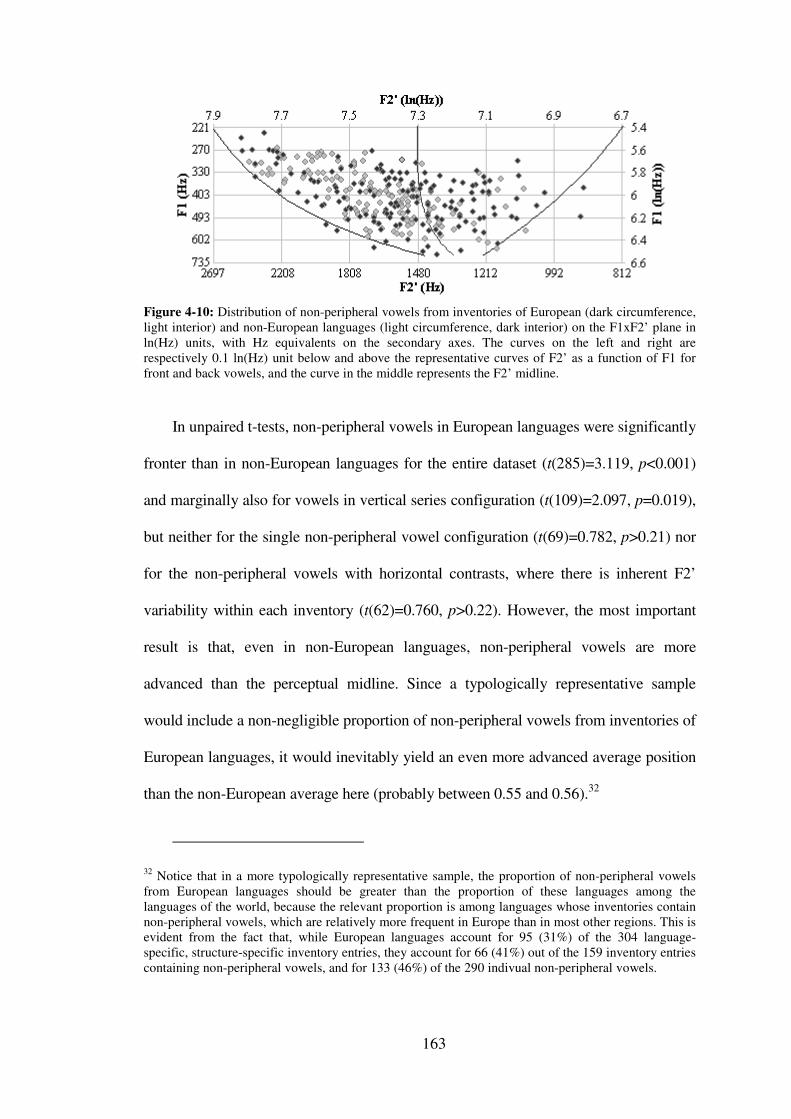
163

Figure 4-10: Distribution of non-peripheral vowels from inventories of European (dark circumference, light interior) and non-European languages (light circumference, dark interior) on the F1xF2’ plane in ln(Hz) units, with Hz equivalents on the secondary axes. The curves on the left and right are respectively 0.1 ln(Hz) unit below and above the representative curves of F2’ as a function of F1 for front and back vowels, and the curve in the middle represents the F2’ midline.

In unpaired t-tests, non-peripheral vowels in European languages were significantly

fronter than in non-European languages for the entire dataset (t(285)=3.119, p<0.001)

and marginally also for vowels in vertical series configuration (t(109)=2.097, p=0.019),

but neither for the single non-peripheral vowel configuration (t(69)=0.782, p>0.21) nor

for the non-peripheral vowels with horizontal contrasts, where there is inherent F2’

variability within each inventory (t(62)=0.760, p>0.22). However, the most important

result is that, even in non-European languages, non-peripheral vowels are more

advanced than the perceptual midline. Since a typologically representative sample

would include a non-negligible proportion of non-peripheral vowels from inventories of

European languages, it would inevitably yield an even more advanced average position

than the non-European average here (probably between 0.55 and 0.56).32

32 Notice that in a more typologically representative sample, the proportion of non-peripheral vowels from European languages should be greater than the proportion of these languages among the languages of the world, because the relevant proportion is among languages whose inventories contain non-peripheral vowels, which are relatively more frequent in Europe than in most other regions. This is evident from the fact that, while European languages account for 95 (31%) of the 304 language-specific, structure-specific inventory entries, they account for 66 (41%) out of the 159 inventory entries containing non-peripheral vowels, and for 133 (46%) of the 290 indivual non-peripheral vowels.

164

It is worth noting that the advanced position of non-peripheral vowels is not an

artifact of the choice of wordlist elicitation, rather than the more canonical isolation

elicitation, as the target for between-method normalization. If vowels were

normalized towards isolation elicitation, the F2 of front vowels would have shifted

forward slightly more than the backward shift in back vowels (because the

extrapolation anchor is at 0.466 of the F2 span, i.e. slightly behind the midline), and

F2’ of front vowels would have shifted forward even more. However, on quasi-

logarithmic perceptual scales, the backward shift of back vowels would have been

greater. At the same time, most non-peripheral vowels would have shifted slightly to

the front. Consequently, the relative position of non-peripheral vowels would have

been even more advanced.

In summary, the relative position of non-peripheral vowels on the F2’ span is not

equidistant from front and back vowels as Dispersion Theory predicts, but tends to be

more advanced and closer to front vowels. This lends support to the concepts underlying

Dispersion Focalization Theory (DFT, Schwartz et al. 1997b). According to this theory,

non-peripheral vowels should be halfway between the front and back vowels if only

dispersion is operating, but fronter non-peripheral vowels can emerge instead, whenever

the model activates the optional parameter of focalization, or preference of vowels with

formant proximity, which is characteristic of F2 and F3 in front rounded vowels. In

either case, more retracted non-peripheral vowels should be the rarest and the last to

emerge in inventories, in agreement with the trends established here.

Additional support for DFT and the role of focalization is found in the fact that

the tendency of non-peripheral vowels to be relatively fronter increases with vowel

height, as apparent in Figure 4-10. Although non-peripheral vowels of all heights tend

165

to be fronter than the F2’ midline, lower non-peripheral vowels are concentrated

much closer to it, and many more of them are found to its right. Higher non-peripheral

vowels on the other hand are almost exclusively to the left of the midline and farther

away from it. The only apparent reason why high non-peripheral vowels should be

very advanced while mid non-peripheral vowels are closer to the midline and more

variable overall is that only in high non-peripheral vowels can F2 reach close to F3

and maximize focalization. Conversely, in mid non-peripheral vowels, the F2

frequency cannot reach high, and hence F2-F3 focalization is modest at most, and its

fronting effect is only marginal as a result.

Interestingly, this apparent manifestation of focalization lends further support for

the preference of the logarithmic Hz scale over the more commonly used Bark scale.

DFT views focalization as proximity between any pair of formants, not only F2 and

F3, and therefore should favor vowels characterized by proximity of F1 and F2 as

well. However, it has been shown in Section 4.3.2 that, in low vowels, there is no

evidence for preference of [ɑ], the only low vowel with F1~F2 proximity. The

question is, of course, what distance counts as proximity, and on which scale. If the

vowel [œ], with characteristic F2 frequency of 1500Hz and F3 frequency of 2350Hz,

can be considered as representative of the threshold of effective focalization, i.e.

vowels with smaller F2-F3 distance are focal while vowels with greater F2-F3

distance are not, then this threshold is about 3Bark (1500Hz ≈ 11Bark, 2350Hz ≈

14Bark). If the same threshold is applied on the F1-F2 distance in low vowels with

characteristic F1 frequency of 720Hz (≈ 6.7Bark), then vowels with F2 frequency

below 1225Hz (≈ 9.7Bark) should be regarded as focal. However, if the threshold is

166

set based on the logarithmic Hz scale, i.e. a Hz-frequency ratio of 1.567 (2350/1500 =

1.567), then applying the same threshold on the F2/F1 ratio in low vowels would

assess as focal only vowels with F1 frequency below 1130Hz (1130/720 ≈ 1.567).

Such vowels are hard to produce without pharyngealization, and would still be

considered only as modestly focal. Substantial focalization as in [y] (F3/F2 ratio of

1.35 and below) cannot be achieved in low vowels unless F2 is brought below

1000Hz, which requires extreme pharyngealization. Thus, while Bark-based

focalization might favor low back vowels (and also mid back rounded vowels) just as

much as it would favor front rounded vowels, focalization based on the logarithmic

Hz scale would maintain the uniqueness of front rounded vowels. It should

nevertheless be acknowledged that an ERB-based focalization threshold would have

yielded very similar assessments as the log(Hz) threshold, so the possible role of

focalization may be taken as evidence against the Bark scale but not necessarily in

favor of the logarithmic Hz scale alone.

Finally, the data on average relative F2’ positions of non-peripheral vowels in

Table 4-15 indicate that single non-peripheral vowels are both more variable and

closer to the F2’ midline than multiple non-peripheral vowels in one vertical series.

This difference in relative position was significant for the entire dataset (t(117) =

2.786, p<0.007, unpaired, two tailed, unequal variance assumed), but did not reach

significance in either dataset (European and non-European) on its own (European:

t(26) = 1.598, p>0.12, unpaired, two tailed, unequal variance assumed; non-European:

t(111) = 1.589, p>0.11, unpaired, two tailed, equal variance assumed).

In Section 4.5.1 it was shown that a single non-peripheral vowel occupies a

distinct height level and relies on both F1 and F2’ for contrast with peripheral vowels,

167

whereas multiple non-peripheal vowels in a vertical series rely mostly on F2’ for this

contrast. If a vertical series of multiple non-peripheral vowels is indeed significantly

fronter than a single non-peripheral vowel, then F2’ even spacing is sacrificed for

stronger focalization precisely when F2’ distance (and presumably even spacing) is

needed the most. While this may appear contradictory to Dispersion Theory, it is

consistent with the view that the perceptual role of focalization is to enhance formant

percepts, and more particularly, that F2-F3 focalization enhances the percept of F2’.

Schwartz et al. (1997b:259) conjecture that focalization “could result in an increased

‘perceptual value’ because of acoustic salience”. Interestingly, while Schwartz et al.

(1997b) translate acoustic salience into assigning a higher weight to F1 than to F2’ in

the between-vowel distance metric, they do not formalize focalization in the same

manner (weight increments), but as a separate component independent from

dispersion in the inventory energy score. An alternative formalization proposed in

Becker-Kristal (2007) translates focalization into increments of formant weights,

which affect dispersion directly by enhancing between-vowel distances. This

approach is more consistent in its treatment of acoustic salience, regardless of whether

salience is an inherent property (of F1) or due to focalization. It is also more

consistent with the observation that non-peripheral vowels are fronter, hence more

focalized (with higher weight of F2’), when F2’ distances are more crucial, i.e. when

there are multiple non-peripheral vowels.33

33 According to the ‘focalization within dispersion’ approach, focalization (weight increment) of non-peripheral vowels compensates for the shortening of the acoustic distance between them and front unrounded vowels (which are also focal), while it enhances the distance of non-peripheral vowels from back rounded vowels (which are non-focal, especially if the perceptual scale is the logarithmic Hz or ERB scales, which render F1-F2 distances in back-rounded vowels too large for effective focalization).

168

4.7 Summary

4.7.1 Summary of the analyses

Sections 4.2- 4.6 used the corpus data to examine various aspects of the

relationship between structural (phonological) and acoustic-perceptual (phonetic)

properties of vowel inventories in the context of Dispersion Theory and its

predictions. With very few exceptions, the predictions of Dispersion Theory were

validated, and many subtle dispersion-based effects turned out to be statistically

significant in this large corpus. In Section 4.2, entire inventory formant spans and area

sizes were found to be positively correlated with the number of vowels in the

inventory, with the number of peripheral vowels affecting the F1 dimension more, and

the number of non-peripheral vowels affecting the F2 dimension. Sections 4.3 and 4.4

showed that, within the dispersion-affected acoustic area covered by the inventory,

dispersion is manifested in subtle shifts of peripheral vowels (front, low and back) in

response to structural differences. When a vowel is added along the inventory

periphery, it pushes vowels above and below it up and down (Section 4.4.1), the low

vowel gets pushed to the other side (Section 4.3.2), where vowels are pushed further

up (Section 4.4.1). During this chain process of pushing and transferring pressure,

some pressure is absorbed and the magnitude of shifts becomes smaller and smaller,

and typically fades out before reaching the high point vowel on the other side. As a

result, the high vowel closer to the added vowel is raised but the high vowel on the

other side is not (Section 4.3.3). The addition of non-peripheral vowels pushes

peripheral mid vowels sideways towards more cardinal qualities (Section 4.4.2). This

effect is more pronounced when the non-peripheral vowels are forced into the same

height levels as peripheral vowels, and yet even more as the non-peripheral region

169

itself gets horizontally crowded. Single non-peripheral vowels settle at distinct height

levels in order to use F1 as part of their contrast with peripheral vowels, but as soon as

another non-peripheral vowel is added, one of the two vowels becomes level with the

high vowels while the other is pushed down. Upon the addition of more non-

peripheral vowels to form a longer vertical series, the series seems to extend further

up and down, in a manner similar to the front and back series (Section 4.5.1). The

different height levels tend to be evenly spaced along the logarithmic Hz scale

(Section 4.6.1). The horizontal behavior of non-peripheral vowels does not

necessarily follow Dispersion Theory, as they are not repelled away from a more

crowded peripheral region (Section 4.5.2) and tend to be more advanced than the

midline between front and back on perceptual scales (Section 4.6.2). However, the

latter finding is consistent with the Dispersion-Focalization Theory, which favors

advanced non-peripheral vowels owing to their focal quality due to proximity of F2

and F3, and Section 4.6.2 shows that the distribution of non-peripheral vowels is

skewed towards focal vowels precisely where focalization is strongest. Across all

analyses, inventories with robust ATR harmony often violate the principles of

dispersion, in formant spans, in even vowel spacing and in phonetic adjustments in

response to structural changes. These deviations are understandable if such

inventories are not treated as one large system but as two parallel smaller subsystems.

4.7.2 Dispersion Theory and structural typology

Taken together, the analyses suggest that dispersion plays a central role in the

phonetic realization of vowel inventories. The typical realizations of vowel categories

are adaptive, rather than fixed, and follow dispersion principles. For example, while

the low vowel may share similar phonological functions across different languages

170

(e.g. attract stress) and as such forms a coherent cross-linguistic category, the cross-

linguistic phonetic realization of this vowel category would seem to vary in a manner

regulated by dispersion: higher in smaller inventories, more advanced in right-

crowded inventories and so on.

These dispersion-oriented realizations are subtle and would often escape the

attention of the descriptive linguist interested only in the contrastive phonemic role of

vowels and their behavior in the phonological system. This is why typological sources

that use impressionistic, contrast-based inventory descriptions fail to capture the

adaptive nature of cross-linguistic categories. For example, even though UPSID

(Maddieson 1984) employs a relatively fine grid of vowel transcription symbols for

low vowels [a ̟a ɐ ɑ], the symbols other than [a] are rarely used, and consequently the

typological tendency of 3S and 4L inventories to have respectively [ɐ] and [ɑ] rather

than [a] remains unnoticed. Similarly, the failure of descriptive sources to transcribe

the single non-peripheral vowel in 5S1 inventories as occupying a distinct height level

between high and mid, results in an artificial split in UPSID between inventories with

[ɨ] and inventories with [ə]. Such limitations are marginal as far as the goals of

UPSID are concerned, i.e. the discovery of the most general structural patterns of

sound inventories. However, they become acute once UPSID or other typological

sources are used as reference for phonetic theory, be it when artificially consistent

transcriptions of point vowels are interpreted as indicative of acoustic stability by

Quantal Theory (Stevens 1972), or when the role of dispersion is marginalized to

explain only local gaps in inventories (Boersma 1998), or when the successful

prediction of 5S1 inventory with [ɨ] is taken to be criterial (Liljencrants & Lindblom

1972, Schwartz et al. 1997b), when [ɘ] should have been predicted instead.

171

The robustness of dispersion and its manifestation in the adaptive behavior of

vowels, and the fact that the most universally common inventory structures (e.g. 3S0,

5S0, 5S1, 7S0) usually follow its principles, corroborate the hypothesis that dispersion

plays a major role also at the structural, phonological level. Dispersion not only

determines how a given structure is phonetically realized, but also which structures

are better to begin with. For example, both 7S2 (e.g. /i e ɛ a ɔ o u y ø/) and 5S4 (e.g.

/i e a o u y ø ɯ ɤ/) structures may manifest various dispersion principles in their

acoustic realization, like expansion of the F2 span relative to 7S0 and 5S0

respectively. However, the fact that 7S2 is a common structure, while 5S4 is

extremely rare, suggests that 7S2 is better than 5S4 regardless of the phonetic

realizations of its constituent vowels. The preference of 7S2 over 5S4 cannot be due

to feature-based organization, because 5S4 is more elegantly organized, with its eight

non-low vowels exhaustively exploiting all the 2x2x2 combinations of [±high ±back

±round], while 7S2 has a gap in its non-peripheral series (two vowels instead of

three). Articulatory constraints cannot explain the preference of 7S2 either. However,

the overcrowded interior region in 5S4 probably renders acoustic and perceptual

distances between vowels too short to distinguish all vowels reliably, regardless of

how the vowels are realized. Dispersion thus disprefers 5S4 as a matter of principle,

even though it may still determine its realization if it does occur.

4.7.3 Towards a better formal model of Dispersion Theory

The role of dispersion at the phonological level, and the preference for certain

structures over others, is precisely what formal dispersion models try to explain.

172

Unfortunately, the acoustic geometries established as part of the current work suggest

that the predictions of such models have so far been inadequate.

The primary limitation of these models is that the balance between maximization

of dispersion and minimization of articulatory effort was typically ignored altogether

(Liljencrants & Lindblom 1972, Lindblom 1986, Schwartz et al. 1997b among

others), and when implemented, it proved very difficult to control (ten Bosch 1991b).

The ultimate model would have to find a way to balance these two factors, and it is

hoped that, now that the targets are well defined (the acoustic geometries in Appendix

B) finding the proper balance would be easier.

Another limitation is that the formalization of dispersion based on all between-

vowel pairs in the inventory (the ‘aggregate approach’) leads to the arrangement of

vowels along the edges of the acoustic space, including its ‘ceiling’, i.e. the high

vowel region. This approach is responsible not only for predicting a maximally high

single non-peripheral vowel, which is a minor structural inadequacy, but also for the

more severe inadequacy of predicting the second non-peripheral vowel as maximally

high as well (Liljencrants & Lindblom 1972, Lindblom 1986, Schwartz et al. 1997b),

creating a four-way horizontal contrast among the high vowels, a structure rarely

attested in real inventories with only two non-peripheral vowels. In this regard, it is

worth noting that Becker-Kristal’s (2007) preliminary report of a revised Dispersion-

Focalization model based on the ‘bottleneck approach’ (the only such model for

which explicit predictions were reported), consistently predicts a mid vowel as the

second non-peripheral vowel in inventories (although a single non-peripheral vowel is

still always maximally high).

173

The use of perceptual scales like Mel and Bark, which, though motivated by

empirically demonstrated properties of the auditory system, fail to capture even

between-vowel spacing, is yet another limitation of previous models. In this regard it

is worth noticing that Schwartz et al. (1997b), while commenting about the limitations

of their Bark-scaled model, conjectured that the ERB scale, which magnifies the

contribution of F1 relative to F2 much more than the Bark scale, should have been

used instead. Although they were concerned only with the contribution of the vertical

dimension relative to the horizontal dimension, the more logarithmic-like ERB scale

may have yielded more adequate predictions also within the vertical dimension itself,

compared to the Bark scale, whose behavior is near-linear along most of the F1

frequency range. Along the same line, Roark (2001) argued that the logarithmic Hz

scale enhances the contribution of the vertical dimension most effectively, and the

current analysis suggests that this scale captures even between-vowel spacing best.

One other factor, which has not been discussed in this study, is the

complementary role of symmetry, or the organization of non-low vowels in equally

populated series. The idea that inventory structure manifests both dispersion and

symmetry has been raised in the past (Crothers 1978, Ferrari-Disner 1984, Boersma

1998). While careful examination of structural typology suggests that the role of

symmetry has been overestimated (Schwartz et al. 1997a), which is also suggested by

the many asymmetrical structures and/or geometries in the current corpus, symmetry

is too frequent to result from chance. For example, in both UPSID and the current

corpus, about 80% of seven-vowel inventories belong to either the 7S0 structure,

whose non-low vowels are arranged in two columns of three vowels, or the 5S2a

structure, whose non-low vowels form three columns of two vowels (or two rows of

174

three vowels). The high frequency of both structures is somewhat surprising, given

that the dominance of fully peripheral structures seems to be limited to inventories

with five vowels or less, and the dominance of structures with two non-peripheral

vowels is characteristic of nine-vowel inventories (see Crothers 1978, Schwartz et al.

1997a and the current corpus). Moreover, considering that six-vowel inventories have

zero or one non-peripheral vowel (0.7 on average), while most eight-vowel

inventories tend to have one or two (1.4 on average), it seems that, for seven-vowel

inventories, one non-peripheral vowel would have been the optimal balance. Yet 6L1

and 6R1 inventories, though not extremely rare, account together only for 20% of

seven vowel inventories – a ‘typological notch’ rather than a ‘typological peak’.

The reason seems to be that, from a purely organizational point of view, the

structures 6L1 and 6R1 are an asymmetrical disaster: unlike the elegant 3x2 (or 2x3)

organization of the non-low vowels in 7S0 and 5S2a, these structures require three

series of three different lengths (3, 2 and 1) both horizontally and vertically. It is

likely that the optimal dispersion solution is in 6L1 (and/or 6R1) inventories, which is

why they nevertheless form a non-negligible minority, but at the same time dispersion

is often sacrificed slightly in favor of a geometry that naturally lends itself to elegant

symmetrical arrangement.

Along the same line, it is very likely that the typological dominance of the

structure 5S0, which, according to both Crothers (1978) and UPSID, accounts for

90% of all five-vowel inventories and 30% of vowel inventories of all sizes, should be

attributed to this structure simultaneously constituting a dispersion optimum and

organization optimum. Nevertheless, the odd occurrence of 4L1 structures in

unrelated languages, with remarkably similar acoustic geometries, suggests that the

175

five-vowel dispersion optimum is somewhere between the two structures, and that

5S0 is overwhelmingly preferred again because of the amorphic organization in the

case of the 4L1 alternative. This is further corroborated by the six-vowel inventory

typology, where 5S1 seems to be the ‘first among equals’, slightly more common than

6L0 and 6R0.

In summary, the inventory structure for any given number of vowels seems to be

the result of four factors. The two major factors are maximization of dispersion and

minimization of articulatory effort, with focalization and symmetry playing a minor

role. Following is a sketch of how these factors could be combined into one model.

This sketch is highly speculative, and might be unfeasible altogether. It nevertheless

combines the insights gained from the current work.

Maximization of dispersion should be formalized based on the least dispersed

vowel pair in the inventory (the ‘bottleneck approach’), using the logarithmic Hz

scale or the sufficiently similar ERB scale, in order to predict evenly spaced

inventories. Some weighting of perceptual dimensions (most likely F1 vs. F2’) is

necessary in order to achieve the desired balance between peripheral and non-

peripheral vowels. The general geometrical shapes of 4L0 (four vowels), 6L1 (seven

vowels) and 7S2 (nine vowels) seem like the most appropriate targets for modeling,

and if this proves feasible, it is likely that shapes between 6L0 and 5S1 (six vowels)

and between 7S1 and 6L2 (eight vowels) would be accurately predicted by the same

model. Minimization of effort should adjust these shapes so they would cover the

appropriate space size. Focalization is necessary in order to accurately predict non-

peripheral vowels more advanced than the front-back midline, owing to F2-F3

proximity (in particular in high non-peripheral vowels). Finally, a symmetry

176

component should be able to often convert the seven-vowel structure 6L1 into either

5S2 or 7S0. With such abilities, this component should easily be able to convert an

inaccurate five-vowel structure between 5S0 and 4L1 (e.g. 5S0 with an excessively

front /u/) into the universally dominant 5S0.

4.7.4 Future research

The corpus and its analyses described here demonstrate the importance of

accumulating masses of comparable cross-linguistic numerical data for the purpose of

testing phonetic theories, identifying their merits and limitations, and refining them.

Many predictions of Dispersion Theory are manifested in patterns too subtle to be

found in comparisons between individual languages, and it is only through the

analyses of data from hundreds of languages that these patterns emerge as consistent.

As such, probably the most important aspect of future research is to further expand

this corpus. Too many inventory structures with intermediate cross-linguistic

frequency are currently represented by fewer than ten entries – enough for giving a

sense of the prototypical acoustic geometry and validating general dispersion-related

trends, but too few to ensure uniformity necessary for quantitative modeling, in

particular in the case of structures like 4L0 and 6L1, which might be the key for an

accurate model of dispersion. This is also true in reference to structures where it is

known, based on other typological sources or on very large standard deviations of

formant frequencies of some vowel categories, that they should be split, as in the case

of 6L0, where the lower front vowel can be either lower-mid or low. Moreover, some

sufficiently frequent structures, like 6L3 or 4R0, have too few representative

inventories in the survey to allow any generalization at all. Of course, it is important

that, as the survey is expanded, the strong bias towards European languages be

177

reduced. This should happen naturally as formant analysis becomes more and more

commonplace as part of descriptions and elementary analyses of languages spoken in

developing countries.

Another direction of research is to repeat some of the less conclusive analyses

once the corpus is expanded, and also to extend the analyses to involve additional

variables, like the effects of vowel quantity. It is quite plausible that acoustic

geometries would have distinct variants as a function of short vs. long vowels. A

related question is whether space-size reduction in short vowels is uniform, or

whether there are spatial regions that are affected more than others.

The current study has important implications on computer simulations intended

to evaluate dispersion models. First, the contiguous F1xF2xF3 range of the

normalized vowels in the corpus forms a more representative search space for

possible vowels than in previous simulations. Second, the distribution of the vowels in

the space provides reliable criteria for labeling vowels in a simulation as front, low,

back or non-peripheral (Section 3.6.1). This would allow the simulation to objectively

determine the structural configuration of predicted inventories even if the search

space used in the simulation is continuous, a problem avoided in some simulation

studies by representing the search space by a finite set of vowel prototypes. Third, the

acoustic typologies in Appendix B can be implemented as reference for automatic

evaluation of model prediction. Fourth, once a better simulation is constructed and

used to evaluate existing dispersion models, these models themselves may be

improved, by adjusting their existing parameters to better approximate the predictions

of inventories resembling the acoustic geometries in Appendix B, and perhaps also by

principles outlined in Section 4.7.3.

178

Another important direction of research, which emerges from the current study, is

the need for more empirical data on perceptual representations of vowels, and F2’ data

in particular. The concept of F2’ has been central in the development of Dispersion

Theory, but it is based on a remarkably small number of empirical studies. Much can be

learned about dispersion from the preferred F1xF2’ patterns of native speakers in two-

formant studies, for example, to what extent is the role of higher formants in F2’ of

front vowels a function of bottom-up auditory processing or of a top-down search for

contrast enhancement from non-peripheral vowels. Ideally, a language-independent

paradigm for F2’-matching experiments should be developed and used to obtain F1xF2’

data representative of many languages and inventory structures.

Last but not least, the raw survey data, even in their current form, allow the

development of more accurate normalization algorithms than the crude procedures

devised here. Improvements may come from methods for correcting unlikely

universal centroid approximation indices (UCAs) in oddly shaped inventories and/or

sensitivity to the behavior of vowels in specific acoustic regions in the elicitation

method normalization. Utilizing the partly available F3 data (and perhaps even the

limited amount of F4 data) may also contribute to the entire normalization procedure

and reduce within-geometry acoustic variance further, rendering analyses and

modeling significantly more reliable and informative.

179

APPENDIX A

Following are the identification details of the 555 entries in the survey, grouped

according to language and ordered according to structure. For each entry, the

following details are specified: serial number within the language-specific entry group

(SN), dialect (if known), source, inventory quantity constituent (QC: U = uniform, S =

short, L = long, O = overlong, M = mixed, C = combined), structural configuration

(Str) and elicitation method (EM). The full bibliographical details of the sources are

on the reference list.

Code Language SN Dialect Source QC Str EM

aeb Tunisian Arabic 1 Kairouan Badeddrime (1980) L 3S0 W 2 Tunis Metoui (1989) L 4L0 W 3 Tunis Metoui (1989) S 4L0 W

afn Defaka 1 Shyrock et al. (1995) C 7S0 W afr Afrikaans 1 Taylor & Uys (1988) S 5S3 W

2 Botha (1996) M 6L3b I aii Assyrian Neo-Aramaic 1 Koine Odisho (1988) C 5S1 C ajp Palestinian Arabic 1 Jordan Altamimi et al. (2004) S 3S0 I

2 Jordan Altamimi et al. (2004) S 3S0 W 3 Jordan Altamimi et al. (2004) L 5S0 I 4 Jordan Altamimi et al. (2004) L 5S0 W 5 Ramallah Shahin (2000) L 5S0 W

aka Akan 1 Kwawu Hess (1987) U 9S0 C ale Aleut 1 Cho et al. (1997) L 3S0 W

2 Cho et al. (1997) S 3S0 W aln Gheg Albanian 1 Halimi (1980) L 5S1 W

2 Halimi (1980) S 5S1 W amh Amharic 1 Standard Messele (2007) U 5S2a W ami Amis 1 Maddieson & Wright (1995) U 3S0 W amu Amuzgo 1 Guerrero Herrera Zendejas (2009) U 7S0 W apw Apache 1 Western Potter et al. (2000) L 4L0 W

2 Western Potter et al. (2000) S 4L0 W arg Aragonese 1 Chistabino Mott (2007) U 5S0 W ary Moroccan Arabic 1 Altamimi et al. (2004) L 3S0 I

2 Altamimi et al. (2004) L 3S0 W arz Egyptian Arabic 1 Cairo Norlin (1984, 1987) S 3S0 C

2 Elgendy (1982) S 3S0 I 3 Cairo Norlin (1984, 1987) L 5S0 C 4 Elgendy (1982) L 5S0 I

bar Bavarian 1 Traunmüller (1982) L 9S4 C bbc Toba Batak 1 Podesva (1999) U 5S0 C bcr Babine 1 Witsuwit’en Hargus (2007) U 6L1 W bdu Oroko 1 Mbonge Anderson-Starwalt (2008 and p.c.) U 7S0 W ben Bengali 1 Calcutta Basu-Ghosh (1986), Barman (1986) U 7S0 W

2 Bangladesh Alam et al. (2008) U 7S0 C bjv Bedjond 1 Beda Djarangar (1991) L 6R0 C

2 Bediondo Djarangar (1991, 1992) L 6R0 C

180

Code Language SN Dialect Source QC Str EM

bnh Banawa 1 Ladefoged et al. (1997) U 4L0 W boa Bora 1 Parker (2001) L 4L2b I

2 Parker (2001) L 4L2b W bov Tuwuli 1 Anderson-Starwalt (2008 and p.c.) U 7S0 W bre Breton 1 Argol Bothorel (1982) U 7S2 M bru Brou 1 Eastern Miller (1967) L 8R2 C

2 Eastern Miller (1967) S 8R2 C brx Bodo 1 Talukdar et al. (2004) U 5S1 I bul Bulgarian 1 Tilkov (1970) U 5S1 W

2 Standard Lehiste & Popov (1970) U 5S1 M bvi Viri 1 Hombert & Point (1987) U 6R0 I bvr Burarra 1 Trefry (1983) U 5S0 W bvx Dibole 1 Dzeke Anderson-Starwalt (2008 and p.c.) U 7S0 W cat Catalan 1 Sitgeta Recasens & Espinosa (2009) U 5S0 M

2 Rossellones Recasens & Espinosa (2009) U 5S0 M 3 Gironi Recasens & Espinosa (2009) U 6L0 M 4 Felanitxer Recasens & Espinosa (2009) U 6R1 M 5 Eastern Recasens i Vives (1986) U 7S0 I 6 Eastern Recasens i Vives (1986) U 7S0 C 7 Valencian Recasens & Espinosa (2006) U 7S0 M 8 Western Recasens & Espinosa (2006) U 7S0 M 9 Eastern Recasens & Espinosa (2006) U 7S0 M 10 Majorcan Recasens & Espinosa (2006) U 7S1 M

chf Chontal 1 Oaxaca Maddieson et al. (2009) U 5S0 W chr Cherokee 1 Western Poell (2004) L 4L2a W

2 Western Poell (2004) S 4L2a W chv Chuvash 1 Northern Kotlejev (1980) U 6L3b W cic Chickasaw 1 Gordon et al. (1997) L 3S0 W

2 Gordon et al. (1997) S 3S0 W cmn Mandarin 1 Taiwan Chang (1998) U 3S2 W

2 Standard Lu (1982) U 3S2 I 3 Standard Svantesson (1984) U 3S2 C

cng Northern Qiang 1 Hongyan Evans (2006) S 3S1 W cnt Tepetotutla Chinantec 1 Herrera Zendejas (2009) U 5S2a W cog Chong 1 Luangthongkum (1991) L 7S2 W

2 Luangthongkum (1991) S 7S2 W cym Welsh 1 North Eastern Mayr & Davies (2009 and p.c.) L 5S1 W

2 North Eastern Mayr & Davies (2009 and p.c.) S 5S2a W 3 Oftedal (1969) L 5S2a I 4 Oftedal (1969) S 5S2a I

dan Danish 1 Standard Frøkjær-Jensen (1966) L 7S3a W 2 Standard Fischer-Jorgensen (1972) L 7S3a W 3 Standard Fischer-Jorgensen (1972) S 7S3a W 4 Standard Fischer-Jorgensen (1972) L 7S3a I

ddo Tsez 1 Asax Maddieson et al. (1996) U 5S0 W deg Degema 1 Fulop et al. (1998) U 9S1 W deu German 1 Standard Northern Sendlmeier & Seebode (2006) S 5S2a W

2 Standard Central Iivonen (1987a, 1989) S 5S2a W 3 Standard Swiss Iivonen (1983) S 5S2a W 4 Vienna Iivonen (1987b) S 5S2a W 5 Standard Northern Jorgensen (1969) S 5S2a W 6 Standard Northern Patzold & Simpson (1997) L 5S2a M 7 Standard Northern Patzold & Simpson (1997) S 5S2a M 8 Vienna Moosmüller (2007) L 5S2a C 9 Vienna Moosmüller (2007) S 5S2a C 10 Vienna Moosmüller (2007) L 5S2a M 11 Vienna Moosmüller (2007) S 5S2a M 12 Vienna Moosmüller (2007) L 5S2a R

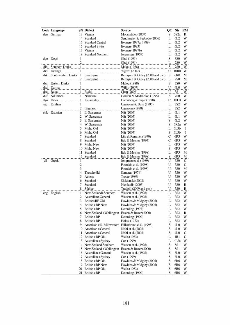
181

Code Language SN Dialect Source QC Str EM

deu German 13 Vienna Moosmüller (2007) S 5S2a R 14 Standard Sendlmeier & Seebode (2006) L 6L2 W 15 Standard Central Iivonen (1987a, 1989) L 6L2 W 16 Standard Swiss Iivonen (1983) L 6L2 W 17 Vienna Iivonen (1987b) L 6L2 W 18 Standard Northern Jorgensen (1969) L 6L2 W

dgo Dogri 1 Ghai (1991) S 3S0 W 2 Ghai (1991) L 7S0 W

dib Southern Dinka 1 Malou (1988) S 7S0 W did Didinga 1 Yigezu (2002) C 10R0 W dik Southwestern Dinka 1 Luanyjang Remijsen & Gilley (2008 and p.c.) S 6R0 M

2 Luanyjang Remijsen & Gilley (2008 and p.c.) L 7S0 M dks Eastern Dinka 1 Malou (1988) S 7S0 W drd Darma 1 Willis (2007) U 6L0 W dru Rukai 1 Budai Chen (2006) U 3S1 W duf Ndumbea 1 Naniouni Gordon & Maddieson (1995) S 7S0 W dyo Diola 1 Kujamutay Greenberg & Sapir (1978) C 10L0 W egl Emilian 1 Uguzzoni & Busa (1995) L 7S2 W

2 Frignano Uguzzoni (1988) L 7S2 W ekk Estonian 1 E. Saaremaa Niit (2005) L 6L1 W

2 W. Saaremaa Niit (2005) L 6L1 W 3 E. Saaremaa Niit (2005) S 6L2 W 4 W. Saaremaa Niit (2005) S 6R2a W 5 Muhu Old Niit (2007) L 6L3b I 6 Muhu Old Niit (2007) S 6L3b I 7 Standard Liiv & Remmel (1970) C 6R3 W 8 Standard Eek & Meister (1994) C 6R3 W 9 Muhu New Niit (2007) L 6R3 W 10 Muhu New Niit (2007) S 6R3 W 11 Standard Eek & Meister (1998) L 6R3 M 12 Standard Eek & Meister (1998) S 6R3 M

ell Greek 1 Jongman et al. (1989) U 5S0 C 2 Fourakis et al. (1998) U 5S0 C 3 Fourakis et al. (1998) U 5S0 M 4 Thesaloniki Samaras (1974) U 5S0 W 5 Athens Tseva (1989) U 5S0 W 6 Standard Sfakianaki (2002) U 5S0 W 7 Standard Nicolaidis (2003) U 5S0 R 8 Sfakian Trudgill (2009 and p.c.) U 5S0 R

eng English 1 New Zealand>Southern Watson et al. (1998) L 3S2 W 2 Australian>General Watson et al. (1998) L 3S2 W 3 British>RP Old Hawkins & Midgley (2005) L 3S2 W 4 British >RP New Hawkins & Midgley (2005) L 3S2 W 5 British >RP Deterding (1997) L 3S2 W 6 New Zealand >Wellington Easton & Bauer (2000) L 3S2 R 7 British >RP Deterding (1990) L 3S2 W 8 British >RP Holtse (1972) L 3S2 W 9 American >N. Midwestern Hillenbrand et al. (1995) S 4L0 W 10 American >General Nishi at al. (2008) S 4L0 W 11 American >General Nishi at al. (2008) S 4L0 C 12 British >RP Old Wells (1963) L 4R1 C 13 Australian >Sydney Cox (1999) L 4L2a W 14 New Zealand Southern Watson et al. (1998) S 5S1 W 15 New Zealand >Wellington Easton & Bauer (2000) S 5S1 W 16 Australian >General Watson et al. (1998) S 6L0 W 17 Australian >Sydney Cox (1999) S 6L0 W 18 British >RP Old Hawkins & Midgley (2005) S 6R0 W 19 British >RP New Hawkins & Midgley (2005) S 6R0 W 20 British >RP Old Wells (1963) S 6R0 W 21 British >RP Deterding (1990) S 6R0 W

182

Code Language SN Dialect Source QC Str EM

eng English 22 British >RP Deterding (1997) S 6R0 W 23 British >RP Holtse (1972) S 6R0 R 24 American >North Midwestern Hillenbrand et al. (1995) L 7S0 W 25 American >General Nishi at al. (2008) L 7S0 W 26 American >General Nishi at al. (2008) L 7S0 C 27 Australian >General Burgess (1968) M 8L0 C 28 Australian >Broad Burgess (1968) M 8L0 C 29 American >New England Bradlow (1995) M 8L1 W 30 American >General Old Peterson & Barney (1952) M 8L1 W 31 British >Somerset Nevalainen & Aulanko (1996) M 9R1 W 32 Canadian>Winnipeg Hagiwara (2006) M 9S1 R 33 American >South Californian Hagiwara (1994) M 9S1 C 34 American>Southwestern Yang (1996) M 10L1 C

eto Eton 1 van de Velde (2008) C 7S1 R eus Basque 1 Salaburu Etxeberria (1984) U 5S0 W

2 Bilbao Iribar & Turrez (2001) U 5S0 W 3 Bilbao Iribar & Turrez (2001) U 5S0 R 4 Viscaino Urrutia et al. (1995) U 5S0 M 5 Guipuzcoano Urrutia et al. (1995) U 5S0 M 6 Alto Navarro Septentrional Urrutia et al. (1995) U 5S0 M 7 Bajo Navarro Occidental Urrutia et al. (1995) U 5S0 M 8 Bajo Navarro Oriental Urrutia et al. (1995) U 5S0 M 9 Labortano Urrutia et al. (1995) U 5S0 M 10 Suletino Urrutia et al. (1995) U 5S1 M

evn Solon 1 Yaohe Svantesson (1985) L 8L2 W fin Finnish 1 Standard Wiik (1965) L 6L2 W

2 Standard Wiik (1965) S 6L2 W 3 Tampere Kuronen (2000) L 6L2 M 4 Tampere Kuronen (2000) S 6L2 M 5 Standard Savela (1999) ? 6L2 M 6 Helsinki Iivonen & Harnud (2005) L 6L2 W 7 Helsinki Iivonen & Harnud (2005) S 6R2a W

fla Montana Salish 1 Flemming et al. (1994) U 5S0 W fmp Fe’fe’ 1 Hombert (1979) U 6R2a W fod Foodo 1 Anderson-Starwalt (2008 and p.c.) U 9S0 C fra French 1 Standard New Kim & Lee (2001) U 7S3a I

2 Standard New Tubach (1989) U 7S3a W 3 Standard New Gendrot & Adda-Decker (2005) U 7S3a R 4 Standard Old Guth (1969) U 8R3a I 5 Standard Old Debrock & Forrez (1976) U 8R3a W 6 Quebec Martin (2002) U 8R3a W 7 Quebec>Chic.-Jonq. Paradis (1985) U 8R3a R

frr North Frisian 1 Fering Bohn. (2004 and p.c.) S 5S2a W 2 Fering Bohn. (2004 and p.c.) L 6L2 W

fry Frisian 1 West Ferrari-Disner (1983) L 7S2 W ggu Gban 1 N’da Le Saout (1976) U 7S0 M gla Scottish Gaelic 1 Bernera Ladefoged et al.(1998) L 7S2 W glg Galician 1 Gonzalez & Regueira (1994) U 7S0 C gug Paraguayan Guarani 1 Miotti (2008) U 5S1 W guj Gujarati 1 Dave (1968) U 6L1 W

2 Dave (1977) U 6L1 I guk Gumuz 1 Pearce (2008) U 5S1 R gup Kunwinjku 1 Fletcher et al. (2007 and p.c.) U 5S0 C

2 Fletcher & Butcher (2002) U 5S0 R gwj Gswi 1 Nakagawa (2006) U 5S0 W hak Hakka 1 Meixian Cheung (2007) U 5S0 C hau Hausa 1 Kano Lindau-Webb (1985) S 3S0 C

2 Kano Lindau-Webb (1985) L 5S0 C hbs Serbo-Croatian 1 Belgrad Kostic & Rhea (1969) C 5S0 W

183

Code Language SN Dialect Source QC Str EM

heb Hebrew 1 Standard Most et al. (2000) U 5S0 C 2 Standard Aronson et al. (1996) U 5S0 I 3 Standard Maimon (2002) U 5S0 R 4 Standard Schwarzwald (1972) U 5S0 W 5 Standard Becker-Kristal (in preparation) U 5S0 M

hts Hadza 1 Sands et al. (1993) U 5S0 W hun Hungarian 1 Standard Magdics (1963) L 5S2a M

2 Standard Magdics (1963) S 5S2a M 3 Standard Tarnoczy (1965) M 7S2 W

hup Hupa 1 Gordon (1996) S 3S0 W 2 Gordon (1996) L 3S0 W

iai Iaai 1 Maddieson & Anderson (1994) L 7R3 W ibo Igbo 1 Ladefoged (1964) U 8R0 W ife Ife 1 Tchetti Anderson-Starwalt (2008 and p.c.) U 7S0 W ind Indonesian 1 van Zanten (1989) U 5S1 I

2 van Zanten (1989) U 5S1 C isl Icelandic 1 Standard Garnes (1973, 1974) L 6L2 W 2 Standard Garnes (1973, 1974) S 6L2 W 3 Standard Petursson (1975) L 6L2 W 4 Standard Petursson (1975) S 6L2 W

ita Italian 1 Tuscany Trumper et al. (1989) U 7S0 W 2 Roma Calamai & Sorianello (2003) U 7S0 R 3 Roma Calamai & Sorianello (2003) U 7S0 M 4 Roma Calamai & Sorianello (2003) U 7S0 W 5 Pisa Calamai (2002b) U 7S0 W 6 Pisa Calamai (2002b) U 7S0 R 7 Florence Calamai (2002a) U 7S0 W 8 Tuscany Calamai (2001) U 7S0 W 9 Tuscany Calamai (2001) U 7S0 M 10 Standard Esposito & Stevens (1995) U 7S0 C 11 Florence Ferrero (1972) U 7S0 I

jpn Japanese 1 Tokyo Nishi at al. (2008) L 4L1 W 2 Tokyo Nishi at al. (2008) S 4L1 W 3 Tokyo Nishi at al. (2008) L 4L1 C 4 Tokyo Nishi at al. (2008) S 4L1 C 5 Standard de Graaf & Koopmans-van Beinum (1983) C 4L1 I 6 Standard de Graaf & Koopmans-van Beinum (1983) C 4L1 W 7 Standard de Graaf & Koopmans-van Beinum (1983) C 4L1 R 8 Standard Morimoto (1988) ? 4L1 W 9 Tokyo Keating & Huffman (1984) S 4L1 R 10 Tokyo Keating & Huffman (1984) S 4L1 W 11 Tosu Inozuka et al. (1993) S 4L1 W 12 Karatsu Inozuka et al. (1993) S 5S0 W 13 Saga Inozuka et al. (1993) S 5S0 W

kal Greenlandic 1 Holsteinborg Wood (1971) U 3S0 W 2 Holsteinborg Wood (1971) U 3S0 R

kan Kannada 1 Mysore Venkatesh (1995) L 5S0 C 2 Mysore Venkatesh (1995) S 5S0 C 3 Shimoga Maheshwaraiah (1986) C 5S0 W

kat Georgian 1 Standard Shosted & Chikovani (2006) U 5S0 W kaz Kazakh 1 Dzhunisbekov (1972) U 5S4 I

2 Kenesbaev et al. (1969) U 5S4 W kca Khanty 1 Ob’ Kurkina (2000) L 3S1 W

2 Ob’ Kurkina (2000) S 3S1 W kdt Kuy 1 Luangthongkum (1986) L 8R3a W

2 Luangthongkum (1986) S 8L3a W ker Kera 1 Pearce (2008) U 5S1 R khk Khalkha 1 Bajanhongor Svantesson (1985) L 6R2b W khk Khalkha 2 Standard Svantesson (1985) L 7R0 W

184

Code Language SN Dialect Source QC Str EM

khm Khmer 1 Battambang Wayland (1998) L 6R2a W 2 Battambang Wayland (1998) S 7S2 W

kiy Kirikiri 1 Clouse & Clouse (1993) U 7S0 W kma Konni 1 Cahill (2007) U 9S0 W koe Baale 1 Yigezu (2002) C 9S0 W kor Korean 1 Chungnam Seong (2005) S 5S2b C

2 Pyongyang Kang (1996) C 6L0 C 3 Hamkyong Kang (1997) C 6L2 C 4 Standard New Kim & Lee (2001) L 6R1 I 5 Seoul Lee (2000) L 7S1 C 6 Seoul Lee (2000) S 7S1 C 7 Seoul Yang (1996) U 7S3b W 8 Standard Old Han (1975) U 7S3b W

kpo Ikposo 1 Uwi Anderson-Starwalt (2008 and p.c.) U 9S1 W kpv Komi 1 Zyrian Savela (1999) U 5S2a M ktn Karitiana 1 Everett (2008) C 4L1 C kwv Nar 1 Doro Djarangar (1991,1992) L 6R0 C kxm Northern Khmer 1 Surin Thomas & Wanna (1988) L 10R4 W

2 Surin Thomas & Wanna (1988) S 10R4 W kyr Kuruaya 1 da Silva (2008) U 5S1 W laj Lango 1 Noonan (1992) U 9S1 W lav Latvian 1 Standard Grigorjevs (2001) L 6R0 I

2 Standard Grigorjevs (2001) S 6R0 I 3 Standard Kaukeniene (2004) L 6R0 I 4 Standard Kaukeniene (2004) S 6R0 I

lit Lithuanian 1 Standard Kaukeniene (2002) S 5S0 W 2 Standard Kaukeniene (2004) S 5S0 I 3 Bacevičiūtė (2004) S 5S0 I 4 Bacevičiūtė (2004) S 5S0 M 5 Standard Kaukeniene (2002) L 6L0 W 6 Standard Kaukeniene (2004) L 6L0 I 7 Šakiu Bacevičiūtė (2004) L 6L0 I 8 Šakiu Bacevičiūtė (2004) L 6L0 M 9 Standard Kudirka (2005) L 6L0 W

liv Livonian 1 Eastern Pajupuu & Viisto (1986) C 6L2 I lln Lele 1 Pearce (2008) U 5S0 R luo Dholuo 1 Jacobson (1977) U 9S0 W

2 Jacobson (1978) U 9S0 I mad Madurese 1 Standard Cohn & Lockwood (1994) U 6R2b C mai Maithili 1 Yadav (1984) U 7S1 I

2 Yadav (1984) U 7S1 W 3 Jha (2001) U 7S1 C

maj Jalapa Mazatec 1 Jalapa de Diaz Silverman et al. (1994) U 5S0 W mas Maa 1 Guion et al. (2004 and p.c.) U 9S0 W mbe Molalla 1 Pharris (2006) S 3S0 W

2 Pharris (2006) L 4R0 W mcw Mawa 1 Pearce (2008) U 5S1 R mcx Mpiemo 1 Nola Thornell & Nagano-Madsen (2004) U 7S0 W mdj Mangbetu 1 Demolin (1989) U 9S0 W

mdm Mayogo 1 McCord (1989) U 9S1 W mdw Mbosi Olee 1 Anderson-Starwalt (2008 and p.c.) U 7S0 W mir Isthmus Mixe 1 Dieterman (2002) U 5S1 R mlt Maltese 1 Gozo Puech (1987) S 4L0 I mnh Mono 1 Bili Olson (2001) U 6R2a W mos Moore 1 Calamai & Bertinetto (2005) S 8L0 W moz Moukoulu 1 Pearce (2008) U 5S1 R mpe Majang 1 Pearce (2008) C 9S0 R

2 Yigezu (2002) C 9S1 W

185

Code Language SN Dialect Source QC Str EM

mri Maori 1 North Maclagan et al. (2004) L 4L1 R 2 North Maclagan et al. (2004) S 4L1 R

mse Musey 1 Djodo Schirru (2003a) C 5S0 W mus Creek 1 Muskogee Johnson & Martin (2001) L 3S0 W

2 Muskogee Johnson & Martin (2001) S 3S0 W mvf Inner Mongolian 1 Chakhar Svantesson (1985) L 6R2b W

1 Chakhar Iivonen & Harnud (2005) S 8R2 W 2 Chakhar Iivonen & Harnud (2005) L 8R3b W 3 Baarin Svantesson (1985) L 8L3b W 4 Shiliingol Svantesson (1985) L 8L3b W

mwm Sar 1 Douyou Djarangar (1991) L 6R0 C mxp Ayutla Mixe 1 Romero-Mendez (2008) U 6R1 C mya Burmese 1 Standard Zlatoverkhova (1966) U 7S0 W myb Mbay 1 Moissala Djarangar (1991,1992) L 6R0 C myf Bambassi 1 Pearce (2008) U 5S0 R myu Munduruku 1 Picanco (2005) U 4L1 W nab Nambikwara 1 Kroeker (1976) U 5S0 W nan Min 1 Nan (Southern) Zee (1980) U 5S0 C nap Neapolitan 1 Naples Trumper et al. (1989) U 7S0 W

2 N. Calabrian>Rocca Imperiale Trumper et al. (1989) U 7S0 W 3 N. Calabrian>Trebisacce Trumper et al. (1989) U 7S0 W

nav Navajo 1 James (1974) L 4L0 W 2 James (1974) S 4L0 W

naw Nawuri 1 Casali (2002) L 9S0 W nde Ndebele 1 Manuel (1987) U 5S0 C nds Low German 1 Eastphalian Goschel (1967) L 7S0 R ndv Ndut 1 Gueye (1986) S 8L1 M

2 Gueye (1986) L 8L1 M nep Nepali 1 Eastern Khatiwada (2009) U 6R0 I new Ngwe 1 Ladefoged (1964) U 8R5 W ngk Dalabon 1 Fletcher & Butcher (2002) U 5S1 R nia Nias 1 Catford (1988) U 5S1 W njm Angami 1 Blankenship et al. (1993) U 5S1 C njo Ao 1 Mongsen Coupe (2003) U 3S2 W nld Dutch 1 Southern>Limburg Adank et al. (2007 and p.c.) L 3S1 C

2 Southern>Limburg Verhoeven & van Bael (2002) L 3S1 C 3 Southern>East Flanders Adank et al. (2007 and p.c.) L 3S2 C 4 Southern>West Flanders Adank et al. (2007 and p.c.) L 3S2 C 5 Southern>East Flanders Verhoeven & van Bael (2002) L 3S2 C 6 Southern>Brabant Adank et al. (2004,2007 and p.c.) S 4L1 C 7 Southern>Antwerp Verhoeven & van Bael (2002) S 4L1 C 8 Southern>Brabant Adank et al. (2004,2007 and p.c.) L 5S2a C 9 Southern>Antwerp Verhoeven & van Bael (2002) L 5S2a C 10 Southern>East Flanders Adank et al. (2007 and p.c.) S 6L1 C 11 Southern>West Flanders Adank et al. (2007 and p.c.) S 6L1 C 12 Southern>East Flanders Verhoeven & van Bael (2002) S 6L1 C 13 Southern>Limburg Adank et al. (2007 and p.c.) S 6L2 C 14 Southern>Limburg Verhoeven & van Bael (2002) S 6L2 C 15 Northern>Randstad Adank et al. (2004,2007 and p.c.) M 7S2 C 16 Northern>South Gelderland Adank et al. (2007 and p.c.) M 7S2 C 17 Northern>Limburg Adank et al. (2007 and p.c.) M 7S2 C 18 Northern>Groningen Adank et al. (2007 and p.c.) M 7S2 C 19 Standard Northern Pols et al. (1973) M 9S3 W 20 de Graaf & Koopmans-van Beinum (1983) M 9S3 I 21 de Graaf & Koopmans-van Beinum (1983) M 9S3 W 22 de Graaf & Koopmans-van Beinum (1983) M 9S3 R

nmn !Xoo 1 Lone Tree Traill (1985) U 5S0 W nnb Kinande 1 Gick et al. (2006 and p.c.) U 9S1 W

2 Yira Anderson-Starwalt (2008 and p.c.) U 9S1 W

186

Code Language SN Dialect Source QC Str EM

nor Norwegian 1 Standard Gamnes (1965), Ferrari-Disner (1983) L 6R3 W nun Anong 1 Mugujia Thurgood (2007) U 5S1 W oci Occitan 1 Roergue Lengadocian Müller (in preparation) U 6L1 C

2 Vivarolpenc Müller & Martin Mota (forthcoming and p.c.) U 6L1 C ogo Khana 1 Nagano & Burch (1988) U 7S0 W ood O’odham 1 Pima Jackson (2008 and p.c.) L 4R1 R

2 Pima Jackson (2008 and p.c.) S 4R1 R ori Oriya 1 Standard Panda (1986) U 6R0 I

2 Standard Panda (1986) U 6R0 W pan Punjabi 1 Doabi Singh (2005) S 3S0 W

2 Doabi Singh (2005) L 7S0 W pav Wari’ 1 MacEachern et al. (1996) U 4L2a W pbu Pashto 1 Northern Invanov (2001) L 3S0 W

2 Northern Invanov (2001) S 5S1 W pei Chichimeca 1 Herrera Zendejas (2009) U 6L1 W pes Persian 1 Salehi et al. (2008) M 6R0 I pms Piedmontese 1 Turin Schirru (2003b and p.c.) U 5S0 M pol Polish 1 Standard Strycharczuk & Jurgec (2008 and p.c.) U 5S1 W

2 Standard Krzysko et al. (1999) U 5S1 W por Portuguese 1 Brazilian>Sao Paulo Escudero et al. (2009) U 7S0 W

2 Brazilian>Sao Paulo Escudero et al. (2009) U 7S0 C 3 European>Lisbon Escudero et al. (2009) U 7S0 W 4 European>Lisbon Escudero et al. (2009) U 7S0 C 5 Blumenau Brazilian Pagel (1986) U 7S0 W 6 Brazilian Godinez (1978) U 7S0 C 7 European>Lisbon Delgado Martins (1973) U 7S1 W

pri Paici 1 Gordon & Maddieson (1996) U 7S3a W prk Wa 1 Kunming Svantesson (1993) U 7S2 W

2 Standard Watkins (2002) U 7S2 C prs Dari 1 Ivanov (1996 M 8R0 W

pwn Paiwan 1 Chen (2006) U 3S1 W que Quichua 1 Otavalo Guion (2003 and p.c.) U 3S0 C quz Quechua 1 Cusco Parker (2007) U 5S0 C roa Norman 1 Liesville-sur-Douve Maury (1976) C 10R4 R ron Romanian 1 Stadard Teodorescu (1985) U 5S2a W

2 Transylvania Mardarescu-Teodorescu (1992) U 7S2 W ruq Megleno-Romanian 1 Cohut & Mardarescu (1968) S 7S3a W rus Russian 1 Kuznetsov & Ott (1987) U 5S1 C

2 Lobanov (1971) U 5S1 W sbz Kaba 1 Paoua Djarangar (1991,1992) L 6R0 C scn Sicilian 1 Sallentinian>Lecce Costagliola (2004) U 5S0 M

2 Sallentinian>Parabita Romano (1999) U 5S0 W 3 South Calabrian>Cosenza Trumper et al. (1989) U 5S0 W 4 South Calabrian>Catanzaro Trumper et al. (1989) U 5S0 W

sgz Sursurunga 1 King (2007 and p.c.) U 5S1 W shi Tachelhit 1 Oukarim (1995) U 3S0 C shq Albanian 1 Kosovo Standard Moosmüller & Granser (2006) U 5S2a M

2 Northern Standard Moosmüller & Granser (2006) U 5S2a M 3 Central Standard Moosmüller & Granser (2006) U 5S2a M 4 Northern Standard Moosmüller & Granser (2006 and p.c.) U 5S2a W 5 Central Standard Moosmüller & Granser (2006 and p.c.) U 5S2a W 6 Kosovo Standard Moosmüller & Granser (2006 and p.c.) U 5S2a W 7 Southern Standard Moosmüller & Granser (2006) U 6L1 M 8 Southern Standard Moosmüller & Granser (2006 and p.c.) U 6L1 W

skf Sakurabiat 1 Alves & Galucio (2007) L 4L1 C 2 Alves & Galucio (2007) S 4L1 C

slk Slovak 1 Isacenko (1968) L 5S0 W 2 Romportl (1974) L 5S0 W

187

Code Language SN Dialect Source QC Str EM

slk Slovak 3 Isacenko (1968) S 6L0 W 4 Romportl (1974) S 6L0 W

slv Slovenian 1 Standard Jurgec (2005) S 5S0 W 2 Standard Jurgec (2005) L 7S1 W

sna Shona 1 Karanga Pongweni (1983) U 5S0 I 2 Manuel (1987) U 5S0 C

snw Sele 1 Maddieson & Gordon (1996) U 7S0 W som Somali 1 Standard Edmondson et al. (2004) L 10L0 W

2 Standard Edmondson et al. (2004) S 10L0 W sot Sotho 1 Southern Khabanyane (1991) U 9S0 C spa Spanish 1 Mexican>Tijuana Godinez (1978) U 5S0 C

2 Rioplatense>Buenos Aires Godinez (1978) U 5S0 C 3 Peninsular>Standard Godinez (1978) U 5S0 C 4 Peninsular >Madrid Bradlow (1995) U 5S0 C 5 Peninsular Standard Morimoto (1988) U 5S0 W 6 Eastern Andalusian Martinez-Melgar (1994) U 5S0 M 7 Eastern Andalusian Sanders (1998) U 5S0 C 8 Ecuador>Otavalo Guion (2003 and p.c.) U 5S0 C 9 Peninsular Standard Alvarez Gonzalez (1981) U 5S0 C 10 Canaria Almeida (1990) U 5S0 R 11 Peninsular>Bilbao Iribar & Turrez (2001) U 5S0 W 12 Peninsular>Bilbao Iribar & Turrez (2001) U 5S0 R

sro Sardinian 1 Campadinese Contini & Boe (1972) U 7S0 W ssw Siswati 1 Kockaert & Godwin (1997) U 5S0 W sun Sundenese 1 Yusuf (1993) U 5S2a W swe Swedish 1 Standard Lindblom (1963) S 5S3 C

2 Stockholm Kuronen (2000) S 5S3 M 3 Helsinki Kuronen (2000) L 5S3 M 4 Helsinki Kuronen (2000) S 5S3 M 5 Standard Fant (1959) S 5S3 I 6 Standard Fant (1959), Fant et al. (1969) L 6L3a I 7 Standard Ferrari-Disner (1983) L 6L3a W 8 Stockholm Kuronen (2000) L 6R3 M

tca Ticuna 1 Soares (1984) U 6R1 W tcx Toda 1 Shalev et al. (1993) M 6R3 W tee Huehuetla Tepehua 1 Smythe Kung (2007) C 5S0 W tel Telugu 1 Dutta Majumder et al. (1978) L 5S0 W 2 Rayalaseema Krishna (2009 and p.c.) L 5S0 C 3 Rayalaseema Krishna (2009 and p.c.) S 5S0 C 4 Telengana Krishna (2009 and p.c.) L 5S0 C 5 Telengana Krishna (2009 and p.c.) S 5S0 C 6 Dutta Majumder et al. (1978) S 6L0 W 7 Coastal Krishna (2009 and p.c.) L 6L0 C 8 Coastal Krishna (2009 and p.c.) S 6L0 C

tgk Tajik 1 Bukhara Ido (forthcoming and p.c.) U 5S1 I tha Thai 1 Standard Abramson (1962) L 7S2 I

2 Standard Abramson (1962) S 7S2 I 3 Standard Kelz & Kummer (1989) L 7S2 W 4 Standard Kelz & Kummer (1989) S 7S2 W 5 Standard Apiluck (1996) C 7S2 I

tlj Lubwisi 1 Anderson-Starwalt (2008 and p.c.) U 9S1 W top Totonac 1 Papantla Herrera Zendejas (2009) C 3S0 W

2 Papantla Alarcon Montero (2008) C 3S0 W trv Truku 1 Hualian Chiang & Chiang (2005) U 5S1 W tsg Tausug 1 Sulu Ferrari-Disner (1983) L 3S0 M tsn Setswana 1 Sengwato Tlale (2005) U 7S0 C

2 le Roux (2004) U 7S0 W tsu Tsou 1 Tfuea Wright & Ladefoged (1994) U 5S1 W

188

Code Language SN Dialect Source QC Str EM

tur Turkish 1 Istanbul Fukumori (1999) U 5S3 C 2 Istanbul Fukumori (1998) U 5S3 R 3 Istanbul Türk et al. (2004) U 5S3 I

twi Twi 1 Adu Manyah (2003 and p.c.) L 9S0 C 2 Adu Manyah (2003 and p.c.) S 9S0 C

udm Udmurt 1 Izhevsk Iivonen & Harnud (2005) U 5S2a W uig Uyghur 1 Tungchun (1992) U 6L2 W ukr Ukrainian 1 Standard Ishchenko (2008) U 6L0 W urd Urdu 1 Hussain (1997) S 3S0 C

2 Nakhat & Rabea (2003) S 4L0 W 3 Hussain (1997) L 7S0 C 4 Nakhat & Rabea (2003) L 7S0 W

vec Venetian 1 Padua Trumper et al. (1989) U 7S0 W vie Vietnamese 1 Hanoi Nguyen & Srihari (2004) M 8R3a W

2 Hanoi Kirby (in prep. And p.c.) M 8R3a W 3 Hanoi Han (1966) M 8R3a W

vro Voru 1 Vastseliina Parve (2000) S 6L4 R 2 Navi Teras (2000) L 6R3 R 3 Navi Teras (2000) O 8L3b R 4 Navi Teras (2000) C 8R6 I

wol Wolof 1 Baol Calvet (1966) S 6L1 R 2 Baol Calvet (1966) L 7S0 R

wuu Wu 1 Shanghai Chen (2008) S 3S1 C 2 Shanghai Chen (2008) L 6R3 C 3 Ningbo Hu (2005) U 7S2 C 4 Ningbo Hu (2005) U 7S3a C 5 Shanghai Svantesson (1989) U 7S3b C

xal Oriat 1 Kalmyk Svantesson (1995) L 6L2 W xkz Kurtoep 1 Educated Hyslop Lowes (2006 and p.c.) U 5S2a W yas Gunu 1 Quilis et al. (1990) L 7S0 W

2 Quilis et al. (1990) S 7S0 W yid Yiddish 1 Kleine (2008) U 5S0 R yor Yoruba 1 Ferrari-Disner (1983) U 7S0 I

2 Standard Przezdzietski (2005) U 7S0 C 3 Moba Przezdzietski (2005) U 7S0 C 4 Akure Przezdzietski (2005) U 9S0 C 5 Ekiti Anderson-Starwalt (2008 and p.c.) U 9S0 W

yue Cantonese 1 Hong Kong Zee (1983) S 3S1 C 2 Guangzhou Lee (1983) S 3S1 W 3 Hong Kong Lee (1983) S 3S1 W 4 Hong Kong So & Wang (1996) S 3S1 C 5 Hong Kong Zee (1983) L 5S2a C 6 Guangzhou Lee (1983) L 5S2a W 7 Hong Kong Lee (1983) L 5S2a W 8 Hong Kong So & Wang (1996) L 5S2a C

zai Juchitan Zapotec 1 Herrera (2000) U 5S0 W ??? Akuntsu 1 Aragon & de Carvalho (2007) U 4L1 R

189

APPENDIX B

Below are the acoustic geometries for the 17 structural configurations that appear in five

or more languages in the corpus. For each configuration, its component vowel categories

are listed, with averages and standard deviations of their normalized formant frequencies,

including F3 and F2’ estimates. For each category, narrow IPA transcription is proposed,

based on the average formant frequencies of the category and the proposed F1 and F2

frequencies of IPA transcription symbols in Figure 3-7 in Section 3.6.1. Vowel data are

followed by F1 and F2 spans and of the F1xF2 area (in 10000Hz² units) of the polygon

whose angles are all the peripheral vowels. Also listed are all the languages (each

followed by its unique ISO 639-3 three-letter code) where the particular structure appears.

In case the language appears under other structures, its three-letter code is followed by the

serial numbers (from Appendix A) of the entries listed with the current structure. The

formant charts display average F1xF2 qualities with one standard deviation ranges.

Structures appearing in less than five languages in the survey are listed at the end.

3S0:

IPA F1 F2 F3 F2’

ɪ 365 (±42) 2034 (±156) 2727 (±101) 2363 (±264)

ɐ ̝ 637 (±42) 1385 (±123) 2463 (±18) 1405 (±147)

ʊ̞ 410 (±42) 959 (±121) 959 (±121)

F1SPAN: 275 (±64) F2SPAN: 1075 (±234) Area: 13.52 (±5.52)

Languages: Tunisian Arabic (aeb:1), Palestinian Arabic (ajp:1-2), Aleut (ale), Amis (ami), Moroccan Arabic (ary), Egyptian Arabic (arz:1-2), Chickasaw (cic), Dogri (dgo:1), Hausa (hau:1), Hupa (hup), Greenlandic (kal), Molalla (mbe:1), Creek (mus), Punjabi (pan:1), Pashto (pbu:1), Quichua (que), Tachelhit (shi), Totonac (top), Tausug (tsg), Urdu (urd:1)

190

3S1:

IPA F1 F2 F3 F2’

ɪ 376 (±68) 2084 (±130) 2751 (±73) 2432(±205)

ɐ 686 (±55) 1395 (±113) 2479 (±31) 1416 (±132)

o̟ 417 (±86) 925 (±128) 925 (±128)

ə,̝œ̽ 454 (±58) 1472 (±189) 2421 (±54) 1526 (±229)

F1SPAN: 313 (±97) F2SPAN: 1158 (±255) Area: 16.03 (±5.58)

Languages: Northern Qiang (cng), Rukai (dru), Khanty (kca), Dutch (nld:1-2), Paiwan (pwn), Wu (wuu:1), Cantonese (yue:1-4)

4L0:

IPA F1 F2 F3 F2’

ɪ 348 (±61) 2041 (±156) 2745 (±134) 2396 (±298)

ɛ ̞ 570 (±40) 1744 (±76) 2507 (±25) 1857 (±99)

ɑ̽ 689 (±63) 1259 (±109) 1259 (±109)

o̟ 407 (±50) 922 (±103) 922 (±103)

F1SPAN: 341 (±120) F2SPAN: 1119 (±258) Area: 21.42 (±9.98)

Languages: Tunisian Arabic (aeb:2-3), Apache (apw), Banawa (bnh), English (eng:9-121), Maltese (mlt), Navajo (nav), Urdu (urd:2)

4L1:

IPA F1 F2 F3 F2’

i ̽ 320 (±19) 2145 (±115) 2826 (±86) 2583 (±211)

ɛ ̝ 492 (±41) 1926 (±136) 2601 (±70) 2131 (±199)

ɑ̝ 681 (±21) 1221 (±91) 1221 (±91)

o̞ 450 (±22) 849 (±38) 849 (±38)

ɘ,̠ɵ̟ 379 (±48) 1405 (±223) 2377 (±84) 1450 (±282)

F1SPAN: 360 (±38) F2SPAN: 1296 (±139) Area: 27.24 (±15.56)

Languages: Japanese (jpn:1-11), Karitiana (ktn), Maori (mri), Munduruku (myu), Dutch (nld:6-7), Sakurabiat (skf), Akuntsu (???)

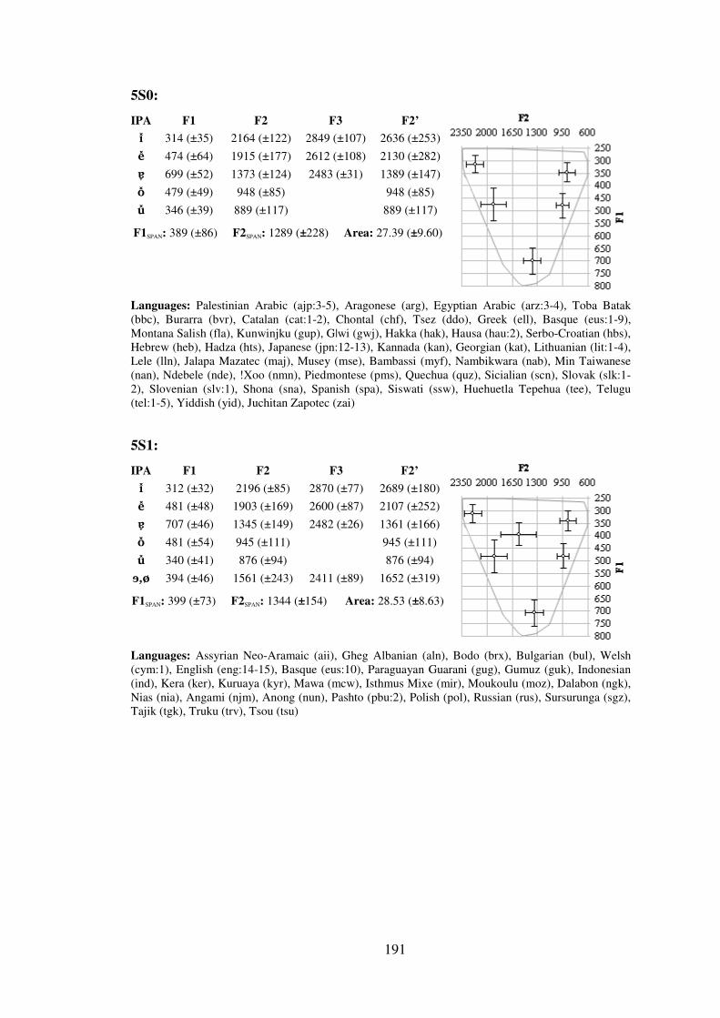
191

5S0:

IPA F1 F2 F3 F2’

i ̽ 314 (±35) 2164 (±122) 2849 (±107) 2636 (±253)

e ̽ 474 (±64) 1915 (±177) 2612 (±108) 2130 (±282)

ɐ ̞ 699 (±52) 1373 (±124) 2483 (±31) 1389 (±147)

o̽ 479 (±49) 948 (±85) 948 (±85)

u̽ 346 (±39) 889 (±117) 889 (±117)

F1SPAN: 389 (±86) F2SPAN: 1289 (±228) Area: 27.39 (±9.60)

Languages: Palestinian Arabic (ajp:3-5), Aragonese (arg), Egyptian Arabic (arz:3-4), Toba Batak (bbc), Burarra (bvr), Catalan (cat:1-2), Chontal (chf), Tsez (ddo), Greek (ell), Basque (eus:1-9), Montana Salish (fla), Kunwinjku (gup), G|wi (gwj), Hakka (hak), Hausa (hau:2), Serbo-Croatian (hbs), Hebrew (heb), Hadza (hts), Japanese (jpn:12-13), Kannada (kan), Georgian (kat), Lithuanian (lit:1-4), Lele (lln), Jalapa Mazatec (maj), Musey (mse), Bambassi (myf), Nambikwara (nab), Min Taiwanese (nan), Ndebele (nde), !Xoo (nmn), Piedmontese (pms), Quechua (quz), Sicialian (scn), Slovak (slk:1-2), Slovenian (slv:1), Shona (sna), Spanish (spa), Siswati (ssw), Huehuetla Tepehua (tee), Telugu (tel:1-5), Yiddish (yid), Juchitan Zapotec (zai)

5S1:

IPA F1 F2 F3 F2’

i ̽ 312 (±32) 2196 (±85) 2870 (±77) 2689 (±180)

e ̽ 481 (±48) 1903 (±169) 2600 (±87) 2107 (±252)

ɐ ̞ 707 (±46) 1345 (±149) 2482 (±26) 1361 (±166)

o̽ 481 (±54) 945 (±111) 945 (±111)

u̽ 340 (±41) 876 (±94) 876 (±94)

ɘ,ø 394 (±46) 1561 (±243) 2411 (±89) 1652 (±319)

F1SPAN: 399 (±73) F2SPAN: 1344 (±154) Area: 28.53 (±8.63)

Languages: Assyrian Neo-Aramaic (aii), Gheg Albanian (aln), Bodo (brx), Bulgarian (bul), Welsh (cym:1), English (eng:14-15), Basque (eus:10), Paraguayan Guarani (gug), Gumuz (guk), Indonesian (ind), Kera (ker), Kuruaya (kyr), Mawa (mcw), Isthmus Mixe (mir), Moukoulu (moz), Dalabon (ngk), Nias (nia), Angami (njm), Anong (nun), Pashto (pbu:2), Polish (pol), Russian (rus), Sursurunga (sgz), Tajik (tgk), Truku (trv), Tsou (tsu)

192

5S2a:

IPA F1 F2 F3 F2’

i ̞ 309 (±36) 2228 (±125) 2902 (±124) 2769 (±289) e ̞ 477 (±48) 2004 (±138) 2650 (±94) 2257 (±224) a ̠ 730 (±49) 1361 (±146) 2521 (±51) 1375 (±172) o̽ 490 (±57) 925 (±64) 925 (±64) u̞ 328 (±54) 829 (±125) 829 (±125) ɨ,y ̽ 327 (±35) 1672 (±208) 2381 (±66) 1800 (±277) ə,̟œ̝ 481 (±52) 1517 (±131) 2413 (±63) 1576 (±164)

F1SPAN: 432 (±77) F2SPAN: 1409 (±239) Area: 33.95 (±10.59)

Languages: Amharic (amh), Tepetotutla Chinantec (cnt), Welsh (cym:2-4), German (deu:1-13), North Frisian (frr:1), Hungarian (hun:1-2), Komi (kpv), Dutch (nld:8-9), Romanian (ron:1), Albanian (shq:1-6), Sundenese (sun), Udmurt (udm), Kurtoep (xkz), Cantonese (yue:5-8)

6L0:

IPA F1 F2 F3 F2’

i ̽ 304 (±33) 2188 (±134) 2876 (±116) 2693 (±286) e 409 (±45) 1993 (±125) 2671 (±97) 2268 (±221) ɛ ̞ 573 (±86) 1726 (±80) 2510 (±40) 1836 (±122) ɑ̟ 708 (±46) 1296 (±27) 1296 (±27) o̽ 479 (±49) 942 (±71) 942 (±71) u̽ 343 (±41) 855 (±127) 855 (±127)

F1SPAN: 403 (±79) F2SPAN: 1344 (±242) Area: 29.28 (±7.78)

Languages: Catalan (cat:3), Darma (drd), English (eng:16-17), Korean (kor:2), Lithuanian (lit:5-9), Slovak (slk:3-4), Telugu (tel:6-8), Ukranian (ukr)

6L1:

IPA F1 F2 F3 F2’

i ̠ 292 (±36) 2197 (±94) 2890 (±78) 2717 (±188) e ̽ 447 (±48) 1948 (±69) 2624 (±33) 2175 (±96) æ̝ 603 (±76) 1742 (±138) 2519 (±54) 1854 (±190) ɑ̟ 723 (±55) 1301 (±143) 1311 (±156) o̽ 492 (±41) 930 (±65) 930 (±65) u̟ 318 (±42) 872 (±146) 872 (±146)

ɘ,̟ø 421 (±106) 1585 (±261) 2387 (±64) 1678 (±348)

F1SPAN: 442 (±71) F2SPAN: 1365 (±163) Area: 34.15 (±7.51)

Languages: Babine (bcr), Estonian (ekk:1-2), Gujarati (guj), Dutch (nld:10-12), Occitan (oci), Chichimeca (pei), Albanian (shq:7-8), Wolof (wol:1)

193

6L2:

IPA F1 F2 F3 F2’

i ̞ 309 (±34) 2270 (±58) 2931 (±52) 2835 (±120) e 409 (±54) 2102 (±134) 2741 (±98) 2444 (±232) ɛ ̞ 590 (±68) 1769 (±114) 2523 (±44) 1892 (±163) ɑ̽ 696 (±47) 1279 (±158) 1287 (±179) o̞ 478 (±59) 893 (±92) 893 (±92) u̞ 343 (±39) 816 (±79) 816 (±79) ɨ,y ̽ 336 (±40) 1631 (±305) 2368 (±47) 1755 (±387)

ɘ,̞ø ̽ 444 (±56) 1547 (±195) 2401 (±74) 1621 (±245)

F1SPAN: 391 (±68) F2SPAN: 1478 (±108) Area: 33.34 (±6.51)

Languages: German (deu:14-18), Finnish (fin), North Frisian (frr:2), Icelandic (isl), Korean (kor:3), Livonian (liv), Dutch (nld:13-14), Uyghur (uig), Oriat (xal)

6R0:

IPA F1 F2 F3 F2’

i ̽ 310 (±43) 2196 (±153) 2881 (±121) 2705 (±299) e ̞ 430 (±70) 2003 (±187) 2679 (±130) 2283 (±314) a ̝ 715 (±59) 1512 (±143) 2503 (±29) 1556 (±176)

ʌ,̞ɒ̟ 594 (±56) 1122 (±52) 1122 (±52) o 432 (±58) 877 (±91) 877 (±91) u̞ 328 (±36) 861 (±151) 861 (±151)

F1SPAN: 408 (±92) F2SPAN: 1366 (±265) Area: 31.36 (±7.51)

Languages: Bedjond (bjv), Viri (bvi), Southwestern Dinka (dik:1), English (eng:18-23), Nar (kwv:1), Latvian (lav), Sar (mwm), Mbay (myb), Nepali (nep), Oriya (ori), Persian (pes), Kaba (sbz)

194

7S0:

IPA F1 F2 F3 F2’

i 289 (±29) 2222 (±115) 2915 (±106) 2780 (±266) e 393 (±41) 2040 (±117) 2709 (±80) 2349 (±197) ɛ 546 (±75) 1852 (±135) 2563 (±64) 2015 (±196) a ̠ 733 (±40) 1354 (±136) 2499 (±19) 1371 (±148) ɔ ̟ 560 (±46) 1023 (±86) 1023 (±86) o 410 (±43) 895 (±89) 895 (±89) u 316 (±33) 843 (±118) 843 (±118)

F1SPAN: 446 (±68) F2SPAN: 1398 (±213) Area: 35.41 (±10.50)

Languages: Defaka (afn), Amuzgo (amu), Oroko (bdu), Bengali (ben), Tuwuli (bov), Dibole (bvx), Catalan (cat:5-9), Dogri (dgo:2), Southern Dinka (dib), Southwestern Dinka (dik:2), Eastern Dinka (dks), Ndumbea (duf), English (eng:24-26), Gban (ggu), Galician (glg), Ife (ife), Italian (ita), Kirikiri (kiy), Mpiemo (mcx), Mbosi Olee (mdw), Burmese (mya), Neapolitan (nap), Low German (nds), Khana (ogo), Punjabi (pan:2), Portuguese (por:1-6), Sele (snw), Sardinian (sro), Setswana (tsn), Urdu (urd:3-4), Venetian (vec), Wolof (wol:2), Gunu (yas), Yoruba (yor:1-3)

7S1:

IPA F1 F2 F3 F2’

i 299 (±15) 2264 (±70) 2934 (±55) 2836 (±137) e 414 (±38) 2017 (±101) 2679 (±71) 2298 (±168) ɛ ̞ 593 (±74) 1802 (±81) 2533 (±24) 1935 (±118) ɐ ̞ 716 (±20) 1342 (±87) 2495 (±17) 1351 (±100) ɔ ̞ 581 (±61) 1003 (±94) 1003 (±94) o̞ 455 (±37) 851 (±69) 851 (±69) u̞ 338 (±13) 847 (±121) 847 (±121) ə 502 (±92) 1393 (±191) 2424 (±63) 1430 (±229)

F1SPAN: 418 (±35) F2SPAN: 1471 (±149) Area: 34.59 (±5.24)

Languages: Catalan (cat:10), Eton (eto), Korean (kor:5-6), Maithili (mai:1-3), Portuguese (por:7), Slovenian (slv:2)

195

7S2:

IPA F1 F2 F3 F2’

i 292 (±31) 2263 (±73) 2940 (±75) 2849 (±172) e 396 (±37) 2078 (±124) 2730 (±88) 2409 (±210) ɛ 552 (±66) 1864 (±141) 2565 (±66) 2031 (±208) a ̠ 735 (±38) 1404 (±92) 2502 (±22) 1423 (±109) ɒ̝ 596 (±78) 1007 (±116) 1007 (±116) o 434 (±51) 882 (±83) 882 (±83) u̞ 327 (±41) 881 (±237) 881 (±237) ɨ,y ̽ 330 (±63) 1682 (±213) 2382 (±68) 1813 (±283) ə,̟œ 465 (±85) 1527 (±141) 2404 (±81) 1591 (±182)

F1SPAN: 451 (±64) F2SPAN: 1461 (±127) Area: 36.76 (±7.01)

Languages: Breton (bre), Chong (cog), Emilian (egl), Frisian (fry), Scotish Gaelic (gla), Hungarian (hun:3), Khmer (khm:2), Dutch (nld:15-18), Wa (prk), Romanian (ron:2), Thai (tha), Wu (wuu:3)

7S3a:

IPA F1 F2 F3 F2’

i 282 (±20) 2247 (±62) 2935 (±65) 2828 (±150) ɪ ̟ 366 (±30) 2142 (±121) 2791 (±103) 2541 (±233) e ̞ 495 (±39) 1985 (±127) 2629 (±80) 2219 (±200) a 738 (±31) 1529 (±180) 2513 (±35) 1576 (±222)

ʌ,ɔ ̟ 551 (±23) 1085 (±123) 1085 (±123) o 397 (±21) 878 (±75) 878 (±75) u 315 (±25) 823 (±63) 823 (±63) ɨ,̟y 301 (±23) 1783 (±243) 2384 (±42) 1950 (±329) ɪ,̠ʏ ̟ 367 (±55) 1674 (±205) 2388 (±36) 1794 (±282) ə,̟œ̝ 463 (±71) 1592 (±145) 2423 (±42) 1675 (±196)

F1SPAN: 456 (±49) F2SPAN: 1432 (±111) Area: 36.54 (±8.15)

Languages: Danish (dan), French (fra:1-3), Megleno-Romanian (ruq), Wu (wuu:4), Paici (pri)

9S0:

IPA F1 F2 F3 F2’

i ̠ 288 (±29) 2160 (±104) 2866 (±86) 2652 (±210)

ɪ 355 (±37) 2066 (±155) 2753 (±118) 2426 (±288)

e 400 (±38) 2014 (±148) 2691 (±95) 2306 (±243)

ɛ 536 (±43) 1842 (±134) 2553 (±62) 2002 (±193)

a ̠ 743 (±57) 1409 (±100) 2493 (±25) 1431 (±115)

ɔ ̟ 542 (±60) 1030 (±82) 1030 (±82)

o ̟ 403 (±39) 982 (±171) 982 (±171)

ʊ 376 (±36) 966 (±134) 966 (±134)

u ̟ 304 (±46) 915 (±106) 915 (±106)

F1SPAN: 459 (±92) F2SPAN: 1313 (±195) Area: 33.95 (±12.55)

Languages: Akan (aka), Foodo (fod), Konni (kma), Baale (koe), Dholuo (luo), Maa (mas), Mangbetu (mdj), Majang (mpe:1), Nawuri (naw), Sotho (sot), Twi (twi), Yoruba (yor:4-5)

196

9S1:

IPA F1 F2 F3 F2’

i 288 (±23) 2204 (±66) 2896 (±61) 2732 (±142) ɪ,̟e ̝ 359 (±33) 2122 (±99) 2781 (±80) 2508 (±182) e,ɪ ̞ 386 (±26) 1995 (±168) 2689 (±103) 2284 (±275) ɛ 524 (±53) 1872 (±182) 2575 (±88) 2051 (±266) a 738 (±36) 1430 (±122) 2509 (±17) 1457 (±135) ɔ ̟ 540 (±73) 1013 (±74) 1013 (±74)

o̟,ʊ̞ 409 (±37) 1000 (±115) 1000 (±115) ʊ̠,o̝ 379 (±35) 865 (±83) 865 (±83) u̟ 309 (±28) 909 (±153) 909 (±153) ɜ ̞ 580 (±102) 1385 (±115) 2461 (±51) 1408 (±136)

F1SPAN: 452 (±59) F2SPAN: 1386 (±122) Area: 33.90 (±8.30)

Languages: Degema (deg), English (eng:32-33), Ikposo (kpo), Lango (laj), Mayogo (mdm), Majang (mpe:2), Kinande (nnb), Lubwisi (tlj),

Structures occurring in four languages in the survey:

3S2: 6R1: 6R2a:

IPA F1 F2 F3 F2’ IPA F1 F2 F3 F2’ IPA F1 F2 F3 F2’

i ̞ 308 2313 2969 2934 i ̞ 318 2219 2889 2737 i 287 2213 2914 2782 ɑ̟ 725 1310 2514 1320 e ̽ 489 1921 2596 2125 e 420 2080 2749 2452 ʊ̠ 366 731 731 a ̽ 682 1470 2479 1504 a 746 1573 2517 1624 y 299 1799 2357 1970 ʌ,ɒ̽ 579 1163 1163 ɒ 610 1068 1068

ə,̟œ̝ 460 1532 2429 1595 o̽ 454 910 910 o̽ 490 975 975 u̽ 354 894 894 u 310 817 817 ɘ ̠ 413 1471 2371 1526 ɨ,y ̽ 313 1616 2338 1723 ə,̝œ̽ 447 1492 2396 1547 Languages: Mandarin (cmn), English (eng:1-8), Ao (njo), Dutch (nld:3-5)

Languages: Catalan (cat:4), Korean (kor:4), Ayutla Mixe (mxp), Ticuna (tca)

Languages: Estonian (ekk:6), Fe’fe’ (fmp), Khmer (khm:1), Mono (mnh)

6L3b: 6R3:

IPA F1 F2 F3 F2’ IPA F1 F2 F3 F2’

i ̞ 324 2271 2923 2828 i ̞ 305 2226 2911 2785 e ̞ 445 2045 2685 2334 e ̞ 453 2019 2662 2283 æ̝ 590 1742 2544 1874 a ̝ 717 1516 2505 1558 ɑ̽ 693 1273 1273 ɑ̝,ɒ̟ 660 1118 2439 1124 o̞ 478 849 849 o̞ 456 906 906 ʊ̠ 358 806 806 u̞ 333 825 825 y ̞ 332 1979 2449 2212 y ̞ 307 1984 2431 2214 œ 515 1479 2444 1531 ø̞ 432 1570 2383 1646 ə 456 1406 2373 1438 ɘ,̠ɵ̟ 403 1449 2351 1492

Languages: Afrikaans (afr:2), Chuvash (chv), Estonian (ekk:4-5), Voru (vro:1)

Languages: Estonian (ekk:7-12), Norwegian (nor),Toda (tcx), Wu (wuu:2)

197

Other structures:

str. Languages str. Languages str. Languages

4L2a Cherokee (chr) English (eng:12) Wari’ (pav)

7R0 Khalkha (khk:2) 8R3a French (fra:4-7) Kuy (kdt:2) Vietnamese (vie)

7R3 Iaai (iai)

7S3b Korean (kor:7-8) Wu (wuu:5)

8R3b Inner Mongolian (mvf:5)

4L2b Bora (boa) 8R4 Inner Mongolian (mvf:6)

4R0 Molalla (mbe) 8L0 Moore (mos) English (eng:29-30)

8R5 Ngwe (new)

4R1 English (eng:13) O’odham (ood)

8R6 Voru (vro:4)

8L1 English (eng:27-28) Ndut (ndv)

9R1 English (eng:31)

5S2b Korean (kor:1) 9S3 Dutch (nld:19-22)

5S3 Afrikaans (afr:1) Turkish (tur) Swedish (swe:1-5)

8L2 Solon (evn) 9S4 Bavarian (bar)

8L3a Kuy (kdt:1) 10L0 Diola (dyo) Somali (som)

8L3b Inner Mongolian (mvf:2-3) Voru (vro:3)

5S4 Kazakh (kaz) 10L1 English (eng:34)

6L3a Swedish (swe:6-7) 8R0 Igbo (ibo) Dari (prs)

10R0 Didinga (did)

6L4 Voru (vro:1) 10R4 Northern Khmer (kxm) Norman (roa)

6R2b Khalkha (khk:1) Inner Mongolian (mvf:1) Madurese (mad)

8R2 Brou (bru) Inner Mongolian (mvf:4)

198

REFERENCES

Abramson, A.S. 1962. The vowels and tones of Standard Thai: acoustical measurements and experiments. Int. J. Am. Linguist. 28.

Adank, P., van Hout, R., Smits, R. 2004. An acoustic description of the vowels of Northern and Southern Standard Dutch. J. Acoust. Soc. Am. 116:1729-1738

Adank, P., van Hout, R., van de Velde, H. 2007. An acoustic description of the vowels of Northern and Southern Standard Dutch II: regional varieties. J. Acoust. Soc. Am. 121:1130-1141.

Adu Manyah, K. 2003. Duree et qualite des contrastes vocalique en twi. Travaux de l’institut de phonetique de Strasbourg 33:1-24

Alam, F., Murtoza Habib, S.M., Khan, M. 2008. Acoustic analysis of Bangla vowel inventory. BRAC University CRBLP Technical report.

Alarcon Montero, R. 2008. Indicios acusticos de las vocales rechinadas del totonaco. In Herrera, E., Butrageno, P.M. (eds.) Fonologia instrumental: patrones fonicos y variacion. Ciudad de Mexico: El Colegio de Mexico, 89-106

Albano Leoni, F., Caputo, M.R., Cerrato, L., Cutugno, F., Maturi, P., Savy, R. 1995. Il vocalismo dell’Italiano. Analisi di un campione televisivo. Studi Italiani di Linguistica Teorica e Applicata 24:405-411.

Almeida, M. 1990. El timbre vocalic en el espanol actual. Filologia Romanica 7:75-85.

Altamimi, J., Carre, R., Marsico, E. 2004. The status of vowels in Jordanian and Moroccan Arabic: insights from production and perception. Proc. Of 48th meeting of the Acoustical Society of America 2629-2629. http://www.ddl.ish-lyon.cnrs.fr/fulltext/Al-Tamimi/Al-Tamimi_2004_Poster_ASA.pdf

Altamimi, J.E., Ferragne, E. 2005. Does vowel system size depend on language vowel inventories? Evidence from two Arabic dialects and French. Proc. 6th Interspeech, Lisbon, 2453-2456.

Alvarez Gonzalez, J.A. 1981. Influencias de los sonidos contiguos en el timbre de las vocales (studio acustico). Revista Espanola de Linguistica 11:427-446.

Alves, A.C., Galucio, A.V. 2007. Analise fonetica acustica das vogais orais da lingua Sakurabiat. Letras de Hoje 42:27-42.

Anderson-Starwalt, C.G. 2008. The acoustic correlates of ATR harmony in seven- and nine-vowel African languages: a phonetic inquiry into phonological structure. Unpublished PhD Dissertation, University of Texas at Arlington

Apiluck, T. 1996. The mid central vowel in Thai. Mon-Khmer Studies 26:65-77.

Aragon, C.C., de Carvalho, F.O. 2007. Analise acustica das vogais orais da lingua Akuntsu. Revista da Abralin 6:41-55.

Aronson, L., Rosenhouse, J., Rosenhouse, G., Podoshin, L. 1996. An acoustic analysis of modern Hebrew vowels and voiced consonants. J. Phonetics 24:283-293

Bacevičiūtė, R. 2004. Šakių šnektos prozodija ir vokalizmas. Vilnius: Lietuvu kalbos instituto leidykla.

Badeddrime, B. 1980. Pour une etude phonetique et linguistique de l’emphase. Travaux de l’institut d’etudes linguistiques et phonetiques, universite de la Sorbonne nouvelle, Paris 3, 267-290.

Barman, S,N. 1986. Vowel quality in Bengali. In Rajapurohit (ed.), Acoustic studies in Indian languages. Central institute of Indian languages, Mysore, 12-20

Basu-Ghosh, S. 1986. A spectrographic study of Bengali vowels. In Rajapurohit (ed.), Acoustic studies in Indian languages. Central institute of Indian languages, Mysore, 7-11

199

Becker-Kristal, R. 2007. Focalization within dispersion predicts vowel inventories better. UCLA WPP 105:138-146.

Becker-Kristal, R. (in preparation). Hebrew stressed vowel in meaningful sentences. Unpublished manuscript.

Bennett, S. 1981. Vowel formant frequency characteristics of preadolescent males and females. J. Acoust. Soc. Am. 69:231-238

Bladon, A. 1983. Two-formant models of vowel perception: shortcomings and enhancements. Sp. Comm. 2:305-313

Bladon, A., Fant, G. 1978. A two-formant model and the cardinal vowels. STL-QPSR 19:1-8

Bladon, A., Lindblom, B. 1981. Modeling the judgment of vowel quality differences. J. Acoust. Soc. Am. 69:1414-1422.

Blamey, P.J., Parisi, E.S., Dooley, G.J. 1996. Perception of two-formant vowels by normal listeners and people using a hearing aid and a cochlear implant in opposite ears. In McCormack, P., Russell, A. (eds.) Proceedings of the Sixth Australian International Conference on Speech Science and Technology. Canberra, Australian Speech Science and Technology Association. 281–286.

Blankenship, B., Ladefoged, P., Bashkararao, P., Nichumeno, C. 1993. Phonetic structures of Khonoma Angami. UCLA WPP 84:127-142

Boersma, P. 1998. Functional Phonology. The Hague: Holland Academic Graphics.

Bohn, O.S. 2004. How to organize a fairly large vowel inventory: the vowels of Fering (North Frisian), J. Internat. Phonetic Assoc. 34:161-173

Botha, L. 1996. Towards modeling acoustic differences between L1 and L2 speech: the short vowels of Afrikaans and South-African English. Proceedings of IPS University of Amsterdam 20:65-80.

Bothorel, A. 1982. Etude phonetique et phonologique du breton parle a Argol (Finistere sud). Lille: Atelier national.

Bradlow, A. 1995. Comparative study of English and Spanish vowels. J. Acoust. Soc. Am. 97:1916-1924

Burgess, O.N. 1968. A spectrographic investigation of some Australian vowel sounds. Language and Speech 11:129-138.

Cahill, M. 2007. Aspects of the Morphology and Phonology of Konni. Dallas: SIL International.

Calamai, S. 2001. Aspetti qualitativi e quantitativi del vocalismo tonico pisano e livornese. Rivista Italiana di Dialettologia 25:153-207.

Calamai, S. 2002a. Vocali fiorentine e vocali pisane a confronto. Quaderni del Laboratorio di Linguistica 3:40-71

Calamai, S. 2002b. The Pisan vowel system of read and semispontaneous speech – an exploratory contribution. Quaderni del Laboratorio di Linguistica 3:72-98.

Calamai, S., Bertinetto, P.M. 2005. Indagine preliminare sul vocalismo orale della lingua moore (Gur, Niger Congo). Quaderni del Laboratorio di Linguistica, Pisa, 5.

Calamai, S., Sorianello, P. 2003. Aspetti stilistici del vocalismo romano. Quaderni del Laboratorio di Linguistica 4:27-42.

Calvet, M. 1966. Etude phonetique des voyelles du Wolof. Phonetica 14:138-168

Carré, R. 2009. Dynamic properties of an acoustic tube: predictions of vowel systems. Speech Comm. 51:26-41.

Carlson, R., Fant, G., Granstrom, B. 1975. Two-formant models, pitch and vowel perception. In Fant, G., Tatham, M.A.A. (eds.) Auditory analysis and perception of speech. London: Academic Press, 55-82.

200

Carlson, R., Granstrom, B., Fant, G. 1970. Some studies concerning perception of isolated vowels. STL-QPSR 11:19-35

Casali, R. 1995. On the reduction of vowel systems in Volta-Congo. Journal of African Cultural Studies 8:109-121.

Casali, R. 2002. Nawuri ATR harmony in typological perspective. Journal of West African Languages 39:3-43.

Catford, J.C. 1988. Notes on the phonetics of Nias. In McGinn, R. (ed.), Studies in Austronesian Linguistics. Ohio University, 151-172.

Chang, Y.C. 1998. Taiwanese Mandarin vowels: an acoustic investigation. Tsing Hua Journal of Chinese Linguistics 28:255-274.

Chen, C.M. 2006. A comparative study on Formosan phonology: Paiwan and Budai Rukai. Unpublished PhD dissertation, University of Texas at Austin.

Chen, Y. 2008. The acoustic realization of vowels of Shanghai Chinese. J. Phonetics. 36:629-648.

Cheung, Y.M. 2007. An acoustical analysis of the vowels, diphthongs and triphthongs in Hakka Chinese. Proc. 16th ICPhS, Saarbruecken, 841-844.

Chiang, W.Y., Chiang F.M. 2005. Vowel dispersion in Truku. Studies in Linguistics 31:21-45.

Chistovich, L.A., Lublinskaya, V.V. 1979. The ‘center of gravity’ effect in vowel spectra and critical distance between the formants: psychoacoustical study of the perception of vowel-like stimuli. Hearing Research 1:185-195.

Cho, T., Taff, A., Dirks, M., Ladefoged, P. 1997. Some phonetic structures of Aleut. UCLA WPP 95:68-90.

Choi, J.D. 1992. Phonetic underspecification and target interpolation: an acoustic study of Marshallese vowel allophony (UCLA WPP 82). PhD dissertation, University of California, Los Angeles.

Chomsky, N., Halle, M. 1968. The sound pattern of English. New York: Harper and Row.

Clouse, H., Clouse, D. 1993. Kirikiri and the Western Lakes Plains languages: selected phonological phenomena. Language and Linguistics in Melanesia 24:1-18.

Cohn, A.C., Lockwood, K. 1994. A phonetic description of Madurese and its phonological implications. Working Papers of the Cornell Phonetics Laboratory 9:67-92.

Cohut, C., Mardarescu, M. 1968. Analiza acustica a vocalelor meglenoromane. Studii şi Cercetari Lingvistice 19:11-28.

Contini, M., Boe, L.J. 1972. Oral and nasal vowels in Campidanian Sardic. An acoustico –phonological study. Phonetica 25:165-191.

Costagliola, A. 2004. Vocalismo tonico del dialetto di Lecce: analisi acustica di un campione di parlanti differenziato per sesso ed eta. Proc. AISV 1:567-596.

Coupe, A.R. 2003. A phonetic and phonological description of Ao: a Tibeto-Burman language of Nagaland, north-east India. Canbera: The Australian National University.

Cox, F. 1999. Vowel change in Australian English. Phonetica 56:1-27.

Crothers, J. 1978. Typology and universals of vowel systems. In Greenberg, J.H., Ferguson, C.A., Moravcsik, E.A. (eds.) Universals of human language, Vol. 2, Phonology. 93-152. Stanford: Stanford University Press.

Da Silva, E. B. 2008. Fonologia da lingua Kuruaya: distribuicao e dispersao das vogais orais. Anais do SETA 2:469-476.

Dave, R. 1968. A formant analysis of the clear, nasalized and murmured vowels in Gujarati. ARIPUC 2:119-132.

Dave, R. 1977. Studies in Gujarati phonology and phonetics. Unpublished PhD dissertation, Cornell University.

201

De Boer, B. 2000. Self organization in vowel systems. J. Phonetics 28(4), 441-465.

De Graaf, T., Koopmans-van Beinum, F.J. 1983. Vowel contrast reduction in Japanese compared to Dutch. Proceedings of IPS University of Amsterdam 7:27-38.

De Graaf, T., Koopmans-van Beinum, F.J. 1984. Vowel contrast reduction in terms of acoustic system contrast in various languages. Proceedings of IPS University of Amsterdam 8:41-53.

Debrock, M., Forrez, G. 1976. Analyse mathematique des voyelles orales du neerlandes et du francais: methodes et resultats201. Revue de Phonetique Appliquee 37:27-73.

Delgado Martins, 1973. Analise acustica das vogais orais tonicas em portugues. Boletim de Filologia (Lisboa) 24:1-11.

Delattre, P., Liberman, A.M., Cooper, F.S., Gerstman, L.G. 1952. An experimental study of the acoustic determinants of vowel color: observations on one- and two-formant vowels synthesized from spectrographic patterns. Word 8:195-210.

Demolin, D. 1989. Production et perception des voyelles en Mangbetu. Pholia 4:45-71.

Deterding, D. 1990. Speaker normalization for automatic speech recognition. PhD Thesis, Cambridge University.

Deterding, D. 1997. The formants of monophthong vowels in Standard Southern British English pronunciation. J. Internat. Phonetic Assoc. 27:47-55.

Diehl, R.L., Lindblom, B., Creeger, C.P. 2003. Increasing realism of auditory representations yields further insights into vowel phonetics. Proc 15th ICPhS, Barcelona, 1381-1384

Dieterman, J.I. 2002. Secondary palatalization in Isthmus Mixe: a phonetic and phonological account. Unpublished PhD dissertation, University of Texas at Arlington.

Djarangar, D.I. 1991. Some Sara vowel inventories and vowel system predictions. Proc. 12th ICPhS, Aix-En-Provence: Universite de Provence Service des Publications, 4:378-381.

Djarangar, D.I. 1992. De la dispersion des voyelles dans l’espace linguistique Sara. ICP Grenoble Bulletin de la communication parlee 2:89-104.

Dutta Majumder, D., Datta A.K., Ganguli, N.R. 1978. Some studies on acoustic-phonetic features of Telugu vowels. Acustica 41:55-64.

Dzhunisbekov, A. 1972. Glasnye kaazakhskogo iazyka (experimentalno-foneticheskoe issledovanie). Alma Ata: Nauka.

Easton, A., Bauer, L. 2000. An acoustic study of the vowels of New Zealand English. Aust. J. Linguist. 20:93-117.

Edmondson. J.A., Esling, J.H., Harris, J.G. 2004. Supraglottal cavity shape, linguistic register, and other phonetic features of Somali. Http://ling.uta.edu/~jerry/somali.pdf

Eek, A., Meister, E. 1994. Acoustics and perception of Estonan vowel types. PERILUS 18:55-90.

Eek, A., Meister, E. 1998. Quality of Standard Estonian vowels in stressed and unstressed syllables of the feet in three distinctive quantity degrees. Linguistica Uralica 34:226-233.

Elgendy, A.M. 1982. Acoustic data on the consonants and vowels in Egyptian Arabic. Paper from the Institute of Linguistics, Stockholm University.

Escudero, P., Boersma, P., Schurt Rauber, A., Bion, R.A.H. 2009. A cross-dialect description of vowels: Brazilian and European Portuguese. J. Acoust. Soc. Am. 126:1379-1393.

Esposito, A., Stevens, K.N. 1995. Notes on Italian vowels: an acoustical study (part I). MIT Speech Communication Group Working Papers 10:1-41.

202

Ethnologue. 2010. www.ethnologue.com.

Evans, J. 2006. Vowel quality in Hongyan Qiang. Language and Linguistics 7:731-754.

Everett, C. 2008. Aspects of Tupi-Karitiana vowels. Anthropological Linguistics 50:266-291

Fant, G. 1959. Acoustic analysis and synthesis of speech with application to Swedish. Ericsson Technics 15:3-108.

Fant, G. 1960. Acoustic Theory of Speech Production. The hague: Mouton.

Fant, G. 1975. Non-uniform vowel normalization. STL-QPSR 16:1-19

Fant, G. 1983. Feature analysis of Swedish vowels – a revisit. STL-QPSR 2-3/1983:1-19

Fant, G., Henningsson, G., Stalhammar, U. 1969. Formant frequencies of Swedish vowels. STL-QPSR 10:94-99

Ferrari-Disner, S. 1980. Evaluation of vowel normalization procedures. J. Acoust. Soc. Am. 67:253-261

Ferrari-Disner, S. 1983. Vowel quality, the relation between universal and language-specific factors. UCLA WPP 58.

Ferrari-Disner, S. 1984. Insights on Vowel Spacing. In Maddieson, I. Patterns of sounds. Cambridge: Cambridge University Press, 136-155.

Ferrero, F.E. 1972. Caratteristiche acustiche dei fonemi vocalici italiani. Parole e Metodi 3:9-31

Fischer-Jorgensen, E. 1972. Formant frequencies of long and short Danish vowels. In Firchow, E.S. et al. (eds.) Studies for Einar Haugen 189-213. The Hague: Mouton.

Fitch, W.T., Giedd, J. Morphology and development of the human vocal tract: a stuy using magnetic resonance imaging. J. Acoust. Soc. Am. 106:1511-1522.

Flanagan, J.L. 1955. A difference limen for vowel formant frequency. J. Acoust. Soc. Am. 27:613-617

Flemming, E. 2002. Auditory representations in phonology. New York: Routledge.

Flemming, E. 2004. Contrast and perceptual distinctiveness. In Hayes, B., Kirchner, R., Steriade, D. (eds.) Phonetically-based phonology. Cambridge: Cambridge University Press, 232-276.

Flemming, E. 2005. A phonetically-based model of vowel reduction. Retrieved from: http://web.mit.edu/~flemming/www/paper/vowelred.pdf

Flemming, E., Johnson, S. 2007. Rosa’s roses: reduced vowels in American English. . Internat. Phonetic Assoc. 37:83-96.

Flemming, E., Ladefoged, P., Thomason, S. 1994. Phonetic structures of Montana Salish. UCLA WPP 87:1-34.

Fletcher, J., Butcher, E. 2002. Vowel dispersion in two Northern Australian languages: Dalabon and Bininj Gun-Wok. Proc. 9th Australian International Conference on Speech Science & Technology, Melbourne, 343-348

Fletcher, J., Stoakes, H., Loakes, D., Butcher, A. 2007. Spectral and durational properties of vowels in Kunwinjku. Proc. 16th ICPhS, Saarbruecken, 937-940

Fourakis, M., Botinis, A., Katsiati, M. 1998. Acoustic characteristics of Greek vowels. Phonetica 56:28-43.

Frøkjær-Jensen, B. 1966. The Danish long vowels. ARIPUC 1:34-46.

Fukumori, T. 1998. An acoustic analysis of Turkish vowels with special reference to range variation in vowels. Ippan Gengogaku Ronso (Journal of General Linguistics) 1:73-93.

Fukumori, T. 1999. The intrinsic properties of Turkish vowels. Ippan Gengogaku Ronso (Journal of General Linguistics) 2:41-59.

Fulop, S.A., Kari, E., Ladefoged, P. 1998. An acoustic study of tongue root contrast in Degema vowels.

203

Phonetica 55:80-98.

Gamnes, H. 1965. En akustisk undersokelse og maling av formantfrekvenser i ost-norske vokaler. Unpublished thesis, University of Oslo

Garnes, S. 1973. Phonetic evidence supporting phonological analysis. J. Phonetics 1:273-283

Garnes, S. 1974. Suprasegmental aspects of Icelandic vowel quality. OSU WPL 17:144-159

Gendrot, C., Adda-Decker, M. 2005. Impact of duration of F1/F2 formant values of oral vowels: an automatic analysis of large broadcast news corpora in French and German. Proc. 9th Eurospeech – Lisbon, September 2005, 2453-2456.

Gertsman, L.H. 1968. Classification of self-normalized vowels. IEEE Trans. Audio Electoacoust. AU-16, 78-80.

Ghai, V.K. 1991. Studies in phonetics and phonology with special reference to Dogri. New Delhi: Ariana Publishing House.

Gick, B., Pulleyblank, D., Campbell, F., Mutaka, N. 2006. Low vowels and transparency in Kinande vowel harmony. Phonology 23:1-20

Godinez, M. 1978. A comparative study of some Romance vowels. UCLA WPP 41:3-19

Gonzalez, M., Regueira, X.L. 1994. Estudio acusticco das vocais galegas en posicion fonetica normal. Actas do XIX Congreso Internacional de Linguistica e Filoloxia Romanicas VI, 141-181.

Gordon, M. 1996. The phonetic structures of Hupa. UCLA WPP 93:164-187.

Gordon, M., Maddieson, I. 1995. The phonetics of Ndumbea. UCLA WPP 91:25-44.

Gordon, M., Maddieson, I. 1996. The phonetics of Paici vowels. UCLA WPP 93:111-124.

Gordon, M., Munro, P., Ladefoged, P. 1997. Some phonetic structures of Chickasaw. Anthropological linguistics 42:366-400.

Goschel, J. 1967. Phonetische Untersuchungen zu den Landvokalen der Mundart von Buntenbock im Oberharz. Mit einem Exkurs. ORBIS 16:368-406.

Greenberg, S., Sapir, J.S. 1978. Acoustic correlates of “big” and “thin” in Kujamutay. Proc. 4th Annual meeting of the Berkeley Linguistic Society, 293-310.

Grigorjevs 2008. Latviešu valodas patskaņu sistēmas akustisks un auditīvs raksturojums. Rīga: LU Latviešu valodas institūts

Grigorjevs, J. 2001. Latviesu valodas patskanu systemas akustisks raksturojmus. Acta Baltica 2001:15-40.

Gueye, G. 1986. Les correlats articulatoures et acoustique de la distinction ±ATR en ndut. Travaux de l’institut de phonetique de Strasbourg 18:137-249.

Guion, S. 2003. The vowel systems of Quichua-Spanish bilinguals. Phonetica 60:98-128

Guion, S., Post, M.W., Payne, D.L. 2004. Phonetic correlates of tongue root vowel contrasts in Maa. J. Phonetics 32:517-542

Guth, G. 1969. Contribution a l’etude de la structure acoustique des voyelles du francais. Travaux de l’institut de phonetique de Strasbourg 1:93-110.

Hagiwara, R. 1994. Sex, syllabic /r/, and the American English vowel space. UCLA WPP 88:63-91

Hagiwara, R. 2006. Vowel production in Winnipeg. Can. J. Ling. 51:127-141.

Halberstam, B., Raphael, L.J. 2004. Vowel normalization: the role of fundamental frequency and upper formants. J. Phonetics 32, 423-434.

204

Halimi, H. 1980. Problemes de la nasalite phonetique et phonologique en albanais (dialecte guegue). Travaux de l’institut d’etudes linguistiques et phonetiques, universite de la sorbonne nouvelle, Paris 3, 92-120.

Han, M.H. 1975. Breve contribution al’etude spectrografique des vouelles simple du coreen. BULAG (Universite de Besancon) 3:137-159.

Han, M.S. 1966. Studies in the Phonology of Asian Languages IV, Vietnamese Vowels. Acoustic Phonetics Research Laboratory, University of Southern California.

Hargus, S. 2007. Witsuwit’en grammar: phonetics, grammar, morphology. Vancouver: UBCPress.

Hawkins, S., Midgley, J. 2005. Formant frequencies of RP monophthongs in four age groups of speakers. J. Internat. Phonetic Assoc. 35:183-199

Herrera Zendejas, E. 2009. Formas sonoras: mapa fonico de las lenguas mexicanas. Ciudad de Mexico: El Colegio de Mexico.

Herrera, H. 2000. Amuzgo and Zapotec: two more cases of laryngeally complex languages. Anthropological Linguistics 42:545-563.

Herrick, D. 2005. Catalan vowel reduction and dispersion theory. Phonological Studies (Journal of the Phonological Society of Japan) 8:131-138.

Hess, S. 1987. Acoustic characteristics of the vowel harmony feature and vowel raising in Akan. UCLA WPP 68:58-82

Hillenbrand, J., Getty, L.A., Clark, M.J., Wheeler, K. 1995. Acoustic characteristics of American English vowels. J. Acoust. Soc. Am. 97:3099-3111.

Holtse, P. 1972. Spectrographic Analysis of English vowels. ARIPUC 6:1-48.

Hombert, J.M. 1979. Universals of vowel systems: the case of centralized vowels. Proc. 9th ICPhS, Copenhagen, 27-32

Hombert, J.M., Point, R. 1987. Contribution a l’etude des systems vocaliques: le cas du viri (Sud-Soudan). Universite Lumiere Pholia 2:75-84.

Hu, F. 2005. A phonetic study of the vowels in Ningbo Chinese. Unpublished PhD Dissertation, City University of Hong Kong.

Hussain, S. 1997. Phonetic correlates of lexical stress in Urdu. Unpublished PhD dissertation, Northwestern University.

Hyslop Lowes, G.M. 2006), Kurteop Phonetics and Phonology. Unpublished MA thesis, University of Oregon

Ido, S. 2009. An analysis of the formation of the Tajik vowel system. Studia Linguistica Upsaliensis 8:65-74.

Iivonen, A. 1983. Die Hochdeutschen und Shweizerhochdeutschen Betonten Monophthonge. Proc. 10th ICPhS, Dordrecht: Foris Publications, 2B:191-196

Iivonen, A. 1987a. Regional differences in the realization of Standard German vowels. Proc. 11th ICPhS Tallinn: Academy of Sciences of the Estonian SSR, 4:161-164

Iivonen, A. 1987b. Monophthonge des gehobenen Wienerdeutch. Folia Linguistica 21:293-336.

Iivonen, A. 1989. Regional German Vowel Studies. Helsingin yliopiston fonetiikan laitoksen monisteita 15.

Iivonen, A. Harnud, H. 2005. Acoustical comparison of the monophthong systems in Finnish, Mongolian and Udmurt. J. Internat. Phonetic Assoc. 35:59-71.

Inozuka,H.,Iguchi, A., Inozuka,E. 1993. The vowels in Karatsu, Saga and Tosu, Sage, Japan. Sophia Linguistica 33:333-344.

Iribar, A. Turrez, I. 2001. Algunos factores de variacion vocalica. Letras de Deusto 31:229-241.

205

Isacenko, A.V. 1968. Spektrograficka analyza slovenskych hlasok. Bratislava: Vydavatel’stvo Slovenskej akademie vied.

Ishchenko, O. 2008. Akustychni kharakterystyky golosnykh zvukiv suchanoi ukrainskoi literaturnoi movy. Ukrainska Mova 29:102-111.

Ivanov, V. 1996. Vokalizm i prozodika v persidskom iazyke i dari. Moscow: institut iazykoznaniya RAN.

Ivanov, V. 2001. Prosodic reduction of vowels in Pashto. In Issledovia po Iranskoy Philologii, Vypusk III. Moscow: ISAA MGU, 5-17

Iverson, P., Kuhl, P.K. 2000. Perceptual magnet and phoneme boundary effects in speech perception: Do they arise from a common mechanism? Percept. Psychophys. 62:874-886

Jackson, E. 2008. Dispersion in the vowel system of Pima. UCLA WPP 107:31-55

Jacobson, L.C. 1977. Phonetic aspects of Dholuo vowels. Studies in African Linguistics, Suppl. 7:127-135

Jacobson, L.C. 1978. DhoLuo vowel harmony – a phonetic investigation. UCLA WPP 43.

Jakobson, R., Fant, G., Halle, M., 1952. Preliminaries of speech analysis: the distinctive features and their correlates. Cambridge, MA: MIT Press.

James, J.R. 1974. An analysis of vowel quality in Navaho. Linguistics 132:33-42.

Jha, S.K. 2001. Maithili, some aspects of its phonetics and phonology. Delhi: Motilal Banarsidass Publishers.

Johnson, K. Adaptive dispersion in vowel perception. Phonetica 57:181-188

Johnson, K. 2005. Acoustic & Auditory Phonetics. Malden: Blackwell Publishing.

Johnson, K., Martin, J. 2001. Acoustic vowel reduction in Creek: effects of distinctive length and position in the word. J. Phonetics. 58:81-102.

Johnson, K., Flemming, E., Wright, R.: 1993. The hyperspace effect: Phonetic targets are hyperarticulated. Language 69: 505-528.

Jongman, A., Fourakis, M., Sereno, J. 1989. The acoustic vowel space of modern Greek and German. Language and Speech 32:321-348.

Jorgensen, H.P. 1969. Die gespannten und ungespannten Vokale in der norddeutschen Hochsprache, mit einer spezifischen Untersuchung der Struktur ihrer Formantfrequenzen. Phonetica 19:217-245.

Jurgec, P. 2005. Formant frequencies of standard Slovene vowels. Govor 22:127-144.

Kang, S.K. 1996. Acoustic analysis of South and North Korean vowels. Ohak Yongu 32:1-18.

Kang, S.K. 1997. The vowel systems of the Hamkyong dialect. Ohak Yongu 33:117-135.

Kaukeniene, L. 2002. Lietuvu bedrines kalbos nekirciuotu balsiu spektrai. Kalbotyra 51:41-59.

Kaukeniene, L. 2004. Dabartiniu baltu bendriniu kalbu balsiu spektrai. Baltistica 39:199-211.

Keating, P., Huffman, M. 1984. Vowel variation in Japanese. Phonetica 41:191-207.

Kelz, H.P., Kummer, M. 1989. Beitrage zur Phonetik des Thailandischen. Hamburg: Helmut Buske Verlag .

Kenesbaev, C.K., Blokhina, L.P., Potopova, R.K. 1969. Klasifikatsiya kazakhskikh glasnykh po dannym akusticheskogo analiza. Fonetika Kazakhskogo Yazyka. Alma Ata: Nauka., 43-60

Khabanyane, K.E. 1991. The five phonemic vowel heights of Southern Sotho: an acoustic and phonological analysis. Working Papers of the Cornell Phonetics Laboratory 5:1-36.

Khatiwada, R. 2009. Nepali. J. Internat. Phonetic Assoc. 39:373-380.

206

Kim, S.J., Lee, E.Y. 2001. A comparative study of Korean and French vowel systems. Speech sciences 8:53-66.

King, P. 2007. An acoustic description of central vowels in three Austronesian languages of New Ireland. SIL Electronic Working Papers 2007-005

Kirby, J. (in preparation). Vietnamese (Hanoi Vietnamese). To appear in J. Internat. Phonetic Assoc.

Kleine, A. 2008. Phonetik des Jiddischen (Jidische Schtudies 15). Hamburg: Helmut Buske Verlag.

Kockaert, H., Godwin, D. 1997. Contrastive vowel formant analysis of Siswati and French. Tydskrif vir Taalonderrig 31:140-153.

Kostic, D., Rhea, S.D. 1969. An analytical description of interrelationships among Serbo-Croatian vowels. Phonetica 20:193-204.

Kotlejev, V.I. 1980. A csuvas es az orosz maganhangzok akusztikus jegyeinek egybevetese. Hungarian papers in phonetics 5:130-137.

Krishna, Y. 2009. Acoustic characteristics of vowels in Telugu. Unpulished PhD dissertation, Manipal University, Karnataka, India

Kroeker, M.H. 1976. Condicionamento multiplo de vogais na lingua Nambikuara. Serie Linguistica 5:107-130.

Krzysko, M., Jassem, W., Czajka, S. 1999. The formants of Polish vowels: a multivariate analysis of variance with two factors. Speech and Language Technology (Polish Phonetics Association) 3:173-190.

Kudirka, R. 2005. Lietuviu bendrines kalbos monoftongu priegaidziu akustiniai pozymiai. Acta Linguistica Lithuanica 52:1-21.

Kuhl, P. 1991. Human adults and human infants show a “perceptual magnet effect” for the prototypes of speech categories, monkeys do not. Percept. Psychophys. 50:93-107.

Kuhl, P., Andurski, J., Chistovich, I., Chistovich, L., Kozhevnikova, E., Ryskina, V., Stolyarova, E., Sundberg, U., Lacerda, F. 1997, Cross –language analysis of phonetic units in language addressed to infants. Science 277:684-686.

Kurkina, G.G. 2000. Vokalizm khantyiskogo iazyka: experimentalnoe issledovanie. Novosibirsk: Sibirskiy Khronograf.

Kuronen, M. 2000. Vokaluttalets akustik i sverigesvenska, finlandssvenska och finska. Studia Philologica Jyvaskylaensia 49, University of Juvaskyla.

Kuznetsov, V., Ott, A. 1987. Spectral properties of Russian stressed vowels in the context of palatalized and nonpalatalized consonants. Proc. 11th ICPhS, Tallinn: Academy of sciences of the Estonian SSR, 3:117-120.

Ladefoged, P. 1964. A Phonetic Study of West African Languages. Cambridge: Cambridge University Press.

Ladefoged, P. 1996. Elements of Acoustic Phonetics. Chicago: University of Chicago Press.

Ladefoged, P., Ladefoged, J., Everett, D. 1997. Phonetic structures of Banawa, an endangered language. Phonetica 54:94-111

Ladefoged, P., Ladefoged, J., Turk, A., Hind, K., Skilton, J. 1998. Phonetic structures of Scottish Gaelic. J. Internat. Phonetic Assoc. 28:1-41.

Le Roux, M. 2004. An acoustic phonetic study of the vowels of Setswana. Unpublished MA thesis, University of South Africa.

Le Saout, J. 1976. Etude descriptive du Gban (Cote-d’Ivoire) phonetique et phonologie. Paris: SELAF

Lee, J.K. 2000. A study on the vowel length of Korean monophthongs. Onohak 26:251-271.

Lee, T. 1983. The vowel system in two varieties of Cantonese. UCLA WPP 57:97-114.

207

Lehiste, I., Popov, K. 1970. An acoustic analysis of Bulgarian syllable nuclei. Phonetica 21:40-48.

Liiv, G., Remmel, M. 1970. On acoustic distinctions in the Estonian vowel system. Soviet Fenno-Ugric Studies 1:7-23.

Liljencrants, J., Lindblom, B. 1972. Numerical simulation of vowel quality systems: the role of perceptual contrast. Language 48, 839-862.

Lindau-Webb, M. 1985. Hausa vowels and diphthongs. WCLA WPP 60:40-54

Lindblom, B. 1963. Spectrographic study of vowel reduction. J. Acoust. Soc. Am. 35:1773-1781.

Lindblom, B. 1986. Phonetic universals in vowel systems. In: Ohala, J., Jaeger, J. (eds.) Experimental Phonology. Orlando: Academic Press, 13-44.

Livijn, P. 2000. Acoustic distribution of vowels in differently sized inventories – hot spots or adaptive dispersion? PERILUS 23:93-96.

Lobanov, B.M. 1971. Classification of Russian vowels spoken by different speakers. J. Acoust. Soc. Am. 49:606-608.

Lu, S.N. 1982. Analyse der Fromanted chinesischer Vokale. IPKoln Berichte 12:127-168.

Luangthongkum, T. 1986. An acoustic study of the register complex in Kui (Suai). Mon-Khmer Studies Journal 15:1-20.

Luangthongkum, T. 1991. An instrumental study of Chong registers. In Davidson, J.H.C.S (ed.), Austroasiatic languages – essays in honour of H.L. Shorto. School of Oriental and African Studies, University of London, 141-160.

MacEachern, M.R., Kern, B., Ladefoged, P. 1996. Wari’ phonetic structures. UCLA WPP 93:65-93

Maclagan, M., Harlow, R., King, J., Keegan, P., Watson, K. 2004. Acoustic analysis of Maori: historical data. Proc. Conference of the Australian Linguistic Society 2004 http://hdl.handle.net/2123/104.

Maddieson, I. 1984. Patterns of sounds. Cambridge: Cambridge University Press.

Maddieson, I., Anderson, V. 1994. Phonetic structures of Iaai. UCLA WPP 87:163-182.

Maddieson, I. Avelino, H., O’connor, L. 2009. The phonetic structures of Oaxaca Chontal. Int. J. Am. Linguist. 75:69-101.

Maddieson, I., Gordon, M. 1996. Notes on the phonetics of Sele, with particular attention to vowels. UCLA WPP 93:149-163.

Maddieson, I., Precoda, K. 1990. Updating UPSID. UCLA WPP 74:104.111.

Maddieson, I., Rajabov, R., Sonnenschein, A. 1996. The main features of Tsez phonetics. UCLA WPP 93:94-110

Maddieson, I., Wright, R. 1995. The vowels and consonants of Amis – a preliminary phonetic report. UCLA WPP 91:45-66.

Magdics, K. 1963. Formant frequencies of Hungarian vowels. UCLA Phonetics Laboratory Progress Report 7-9.

Maheshwaraiah, H.M. 1986. Spectrographic analysis of liquids in Kannada. In Rajapurohit (ed.), Acoustic studies in Indian languages. Central institute of Indian languages, Mysore, 55-60.

Maimon, Y. 2002. Hashpaot svivatiyot al hatnuot beivrit – bxina akustit. MA Thesis, Ben Gurion University.

Malou, J. 1988. Dinka vowel system. Summer Institute of Linguistics.

Mantakas, M., Schwartz, J.L., Escudier, P. 1986. Modèle de prédiction du “deuxiéme formant effectif” F2’ –

208

application à l’étude de la labialité des voyelles avant du français. Proc. 15th Journées d’Étude sur la Parole, Société Française d’Acoustique, Paris, 157-161

Manuel, S.Y. 1987. Acoustic and perceptual correlates of vowel-to-vowel coarticulation in three Bantu languages. Unpublished PhD dissertation, Yale University.

Mardarescu-Teodorescu, M. 1992. Descriere acustica a vocalelor din unele graiuri transilvanene. Fonetică şi Dialectologie 11:155-160.

Martin, P. 2002. Le systeme vocalique du franais du Quebec. De l’acoustique a la phonologie. La Linguistique 38:71-88.

Martinez-Melgar, A. 1994. El vocalismo del andaluz oriental. Estudios de Fonetica Experimental 6:11-64.

Maury, N.G. 1976. Systeme vocalique d’un parler normand (Studia Phonetica 11). Montreal: Didier.

Mayr, R., Davies, H. 2009. The monophthongs and diphthongs of North-eastern Welsh: an acoustic study. Proc. 10th Interspeech 2315-2318

McCord, M.S. 1989. Acoustical and autosegmental analyses of the Mayogo vowel system. Unpublished MA thesis, University of Texas at Arlington.

Mermelstein, P. 1978. Difference limens for formant frequencies of steady-state and consonant-boundvowels. J. Acoust. Soc. Am. 63:572-580.

Messele, A. 2007. An acoustic analysis of a pathological speech: the case of an Amharic speaking person with flaccid dysarthria. Unpublished MA Thesis, Adis Ababa University

Metoui, M.M. 1989. Contribution a la phonetique et phonologie arabe: etude acoustique et articulatoire des voyelles du parler de Tunis. Idstein: Schultz-Kirchner Verlag.

Meunier, C., Frenck-Mestre, C., Lelekov-Boissard, T., Le Besnerais, M. 2003. Production and perception of vowels: does the density of the system play a role? In: Solé, M.J., Recasens, D., Romero, J. (eds.) Proc. 15th ICPhS, Barcelona, 723-726

Miller, J.D. 1967. An acoustical study of Brou vowels. Phonetica 17:149-177.

Miller, R.L. 1953. Auditory tests with synthetic vowels. J. Acoust. Soc. Am. 25:114-121.

Miotti, R. 2008. Analisi acustico-uditiva del vocalismo orale del guarani. Aspetti temporale e timbrico. Quaderni di lingue e letterature straniere 33:119-136.

Moosmüller, S. 2007. Vowels in Standard Austrian German. Unpublished PhD Dissertation, University of Vienna.

Moosmüller, S., Granser, T. 2006. The spread of Standard Albanian: an illustration based on an analysis of vowels. Language Variation and Change 18:121-140.

Morimoto, Y. 1988. The five vowels of Castilian and Japanese: a spectrographic analysis. Sophia Linguistica 23/24:181-192.

Morrison, J.S., Nearey, T.M. 2006. A cross-language vowel normalization procedure. Canadian Acoustics 34:94-95.

Most, T., Amir, O., Tobin, Y. 2000. The Hebrew vowel system: raw and normalized acoustic data. Language and Speech 43:295-308

Mott, B. 2007. Chistabino (Pyrenean Aragonese). J. Internat. Phonetic Assoc. 37:103-114.

Mrayati, M., Carre, R., Guerin, B. 1988. Distinctive regions and modes: a new theory of speech production. Sp. Comm. 7:257-286.

Müller, D., Martin Mota, S. (forthcoming). A preliminary acoustic study of the Occitan vowel system. In Actes du Colloque GalRom07 – Diachronie du gallo-roman, Nica, 15-16.01.2007

209

Müller, D.,(in preparation). The vowel system of Roergue Lenadocian Occitan. Unpublished research.

Nagano, K., Burch, K. 1988. Vowel variation by consonantal context in Kana. UCLA WPP 69:92-109.

Nakagawa, H. 2006. The vowel system of G|wi. Journal of the Institute of Language Research 11:67-87.

Nakhat, F., Rabea, A. 2003. Vowel structure of Urdu. CRULP Annual Student Report published in Akhbar-e-Urdu, April-May, National Language Authority, Islamabad, Pakistan.

Nearey, T.M. 1978. Phonetic feature systems for vowels. PhD thesis, Indiana University Linguistics Club.

Nearey, T.M. 1989. Static, dynamic and relational properties in vowel perception. J. Acoust. Soc. Am. 85:2088-2113.

Nevalainen, T., Aulanko, R. 1996. Stressed vowels in East Somerset: an acoustic-phonetic case study. In Klemola, J., Kyto, M., Rissanen, M. (eds.) Speech Past and Present – studies in English dialectology in memory of Ossi Ihalainen (University of Bamberg Studies in English Linguistics 38. Frankfurt am Main: Peter Lang, 236-264.

Nguyen, B., Srihari, R. 2004. A preliminary quantitative study of the characteristics of Vietnamese vowels and English vowels. Unpublished manuscript. http://www.cs.jhu.edu/~nguyen/data/phonetics_prjrpt.pdf

Nicolaidis, K. 2003. Acoustic variability of vowels in Greek spontaneous speech. Proc. 15th ICPhS, Barcelona, 3221-3224.

Niit, E. 2005. Vowels in initial syllables in Saaremaa. Linguistica Uralica 41:113-122.

Niit, E. 2007. Vowels in word-initial syllables in Muhu Estonian. Linguistica Uralica 43:241-249.

Nishi, K., Strange, W., Akahane-Yamada, R., Kubo, R., Trent-Brown, S.A. 2008. Acoustic and perceptual similarity of Japanese and American English vowels. J. Acoust. Soc. Am. 124:576-588.

Noonan, M. 1992. A Grammar of Lango. Berlin: Mouton de Gruyter.

Norlin, K. 1984. Acoustic analysis of vowels and diphthongs in Cairo Arabic. Lund WPL 27:185-209

Norlin, K. 1987. A phonetic study of emphasis and vowels in Egyptian Arabic. Lund WPL 30.

Odisho, E.Y. 1988. The Sound System of Modern Assyrian (Neo-Aramaic). Wiesbaden: Otto Harrassowitz.

Oftedal, M. 1969. A new approach to North Welsh vowels. Lochlann 4:243-269.

Olson, K.S. 2001. The phonology and morphology of Mono. Unpublished PhD dissertation, University of Chicago.

Oukarim, O. 1995. Fonetica y fonologia del bereber. Barcelona: Universitat Autonoma de Barcelona Servei de Publicacions.

Padgett, J. Tabain, M. 2005. Adaptive Dispersion Theory and Phonological Vowel Reduction in Russian. Phonetica 62:14-54.

Pagel, D.F. 1986. Les voyelles orales du portugais en milieu bilingue. Travaux de l’Institut de Phonétique de Strasbourg 18:77-105.

Pajupuu, H., Viisto, T.R. 1986. Livonian polyphthongs. Estonian Papers in Phonetics 1984-1985:96-130.

Paliwal, K.K., Ainsworth, W.A., Lindsay, D. 1983. A study of two-formant models for vowel identification. Sp. Comm. 2:295-303

Panda, D. 1986. A spectrographic study of Oriya vowels. In Rajapurohit (ed.), Acoustic studies in Indian languages. Central institute of Indian languages, Mysore, 26-31.

Paradis, C.C. 1985. An acoustic study of variation and change in the vowel system of Chicoutimi and Jonquire (Quebec). Unpublished PhD Dissertation, University of Pennsylvania.

210

Parker, S.G. 2001. The acoustic qualities of Bora vowels. Phonetica 58:179-195.

Parker, S.G. 2007. Un analisis acustico del Quechua del Cusco. GIALens: Electronic Notes Series 1(3).

Parve,M. 2000. On the acoustics of short monophthongs in Vastseliina (South Estonian). Linguistica Uralica 36:241-260.

Patzold, M., Simpson, A.P. 1997. Acoustic analysis of German vowels in the Kiel Corpus of Read Speech. AIPUK 32:215-247.

Pearce, M. 2008. Vowel harmony domains and vowel undershoot. UCL WPL 20:115-140.

Peterson, G., Barney, H. 1952. Control methods used in a study of the vowels. J. Acoust. Soc. Am. 24:175-184

Petursson, M. 1975. Le systeme vocalique de l’islandais faits phonetiques et interpretation phonologique. Lingua 35:35-59.

Pharris, N.J. 2006. Winiinsi Tm Talapaas: A Grammar of the Molalla Language. Unpublished PhD dissertation, University of Michigan.

Picanco, G.L. 2005. Munduruku: phonetics, phonology, synchrony, diachrony. Unpublished PhD Dissertation, University of British Columbia.

Podesva, R.J., Adisasmito-Smith, N. 1999. Acoustic investigation of the vowel systems of Buginese and Toba Batak. Proc. 14th ICPhS 535-538.

Poell, N.D. 2004. A phonetic study of the vowels and tones of Western Cherokee. Unpublished MA Thesis, University of Kansas.

Pols, L.C.W., Tromp, H.R.C., Plomp, R. 1973. Frequency analysis of Dutch vowels from 50 male speakers. J. Acoust. Soc. Am. 53:1093-1101.

Pongweni, A.J.C. 1983. An acoustic study of the qualitative and pitch effect of breathy voice on Shona vowels. J. Phonetics 11:129-138.

Potter, B., Gordon, M., Dawson, J., de Reuse, W., Ladefoged, P. 2000. Phonetic structures of Western Apache. UCLA WPP 98:10-38.

Przezdzietski, M. 2005. Vowel harmony and coarticulation in three dialects of Yoruba: phonetics determining phonology. Unpublished PhD Dissertation, Cornell University.

Puech, G. 1987. Production et perception des voyelles breve du maltais gozitian. Universite Lumiere Pholia 2:125-138.

Quilis, A., Ambadiang, T., Marrero, V. 1990. Phonologie et phonetique du gunu (langue bantu du Cameroun). Travaux de linguistique et de Philology 28:343-377.

Recasens i Vives, D. 1986. Estudis de fonetica experimental del Catala Oriental Central. Montserrat: Publicacions de l’Abadia de Montserrat.

Recasens, D., Espinosa, A. 2006. Dispersion and variability of Catalan vowels. Sp. Comm. 48:645-666

Recasens, D., Espinosa, A. 2009. Dispersion and variability in Catalan five and six peripheral vowel systems. Sp. Comm. 51:240-258

Remijsen, B, Gilley, L. 2008. Why are three-level vowel length systems rare? Insights from Dinka (Luanyjang dialect). J. Phonetics 36:318-344

Roark, B. 2001. Explaining vowel inventory tendencies via simulation: finding a role for quantal locations and formant normalization. In Proc. 31st Conference of the North East Linguistics Society.

Romano, A. 1999. A phonetic study of a Sallentinian variety (Southern Italy). Proc 14th ICPhS, San Francisco, 1051-1054

211

Romero-Mendez, R. 2008. A reference grammar of Ayutla Mixe (Tukyo’m Ayuujk). Unpublished PhD dissertation, State University of New York at Buffalo.

Romportl, M. 1974. K akustice slovenských vokálů a diftongů. Jazykovedné Štúdie 12:43-47.

Salaburu Etxeberria, P. 1984. Hizkuntz teoria eta Baztango euskalkia: fonetika eta fonologia. Servicio editorial, Universidad del pais vasco.

Salehi, F., Bahrami, A., Nuri, F., Qanbari, H., Baranzahi, T. 2008. Formant frequency of Persian vowels in 18-24 years old university students. Pazhuhesh dar ulume tavanbakhshi 4:35-44.

Samaras, M. 1974. Etude de l’influence de l’accent sur la structure formantique des voyelles du grec moderne. Bulletine de l’institut de phonetique de Grenoble 3:129-138.

Sanders, B.P. 1998. The Eastern Andalusian vowel system: form and structure. Rivista di Linguistica 10:109-135.

Sanders, N., Padgett, J. 2008a. Predicting vowel inventories from a Dispersion-Focalization model: new results. To appear in Proc 44th CLS.

Sanders, N., Padgett, J. 2008b. Exploring the role of production in predicting vowel inventories. Paper presented at the 82nd meeting of the Linguistic Society of America.

Savela, J. 1999. Tutkimus komisyrjaanin ja suomen vokaalifoneemien rakenteesta. Sananjalka 41:167-176.

Schirru, C. 2003a. Preliminari sperimentali sulla lingua musey. Annali della Facoltà di Lingue e Letterature Straniere, 3:17-48

Schirru, C. 2003b. Caratteristiche vocalo-formantiche dell’italiano in pirmonte. Bollettino dell’Atlante Linguistico Italiano, III serie, 26:27-56

Schwartz, J., Escudier, P. 1989. A strong evidence for the existence of a large-scale integrated spectral representation in vowel perception. Sp. Comm. 8:235-259

Schwartz, J.L., Boë, L.J., Vallée, N., Abry, C. 1997a. Major trends in vowel system inventories. J. Phonetics 25: 233-253

Schwartz, J.L., Boë, L.J., Vallée, N., Abry, C. 1997b. The Dispersion-Focalization Theory of vowel systems. J. Phonetics 25:255-286

Schwarzwald, O. 1972. Vowels in Hebrew and English: a spectrographic study. Hebrew Computational Linguistics 6:1-12.

Seldak, P. 1969. Typological considerations of vowel quality systems. Stanford University Working Papers on Language Universals 1:1-40.

Sendlmeier, W.F., Seebode, J. 2006. Formantkarten des deutschen Vokalsystems. TU Berlin, http://www.kgw.tu-berlin.de/forschung/Formantkarten.

Seong, C.J. 2005. A formant analysis of the Korean monophthongs of the college students speaking Chungnam. Onohak 43:189-213.

Sfakianaki, A. 2002. The acoustic characteristics of Greek vowels produced by adults and children. In Makri-Tsilipakou, M. (ed.) Selected Papers on Theoretical and Applied Linguistics. From the 14th International Symposium on Theoretical and Applied Linguistics, Aristotle University of Thessaloniki 20-22 April 2000, 383-394.

Shahin, K. 2000. Vowel innovation in Arabic: inductive grounding and pattern symmetry. In Lecarme, J. (ed.) Research in Afroasiatic Grammar II. Amsterdam: John Benjamins, 429-447.

Shalev, M., Ladefoged, P., Bashkararao, P. 1993. Phonetics of Toda. UCLA WPP 84:89-126.

Shosted, R.K., Chikovani, V. 2006. Standard Georgian. J. Internat. Phonetic Assoc. 36:255-264.

212

Shyrock, A., Ladefoged, P., Williamson, K. 1995. The phonetic structures of Defaka. UCLA WPP 91:89-109

Silverman, D. Blankenship, B., Kirk, P., Ladefoged, P. 1994. Phonetic structures in Jalapa Mazatec. UCLA WPP 87:113-130.

Singh, C.S. 2005. Experimental study of Punjabi vowels. Indian Linguistics 66:125-132.

Smythe Kung, S. 2007. A descriptive grammar of Huehuetla Tepehua. Unpublished PhD dissertation, University of Texas at Austin.

So, L.K.H, Wang, J. 1996. Acoustic distinction between Cantonese long and short vowels. Proc. 6th Australian Intenational Conference on Speech Science and Technology (Adelaide) 379-384.

Soares, M.F. 1984. Tracos acusticos das vogais em Tukuna. Cadernos de Estudos Linguisticos 7:137-175.

Sonderegger, M. 2005. Vowel formant database bibliography and methods. Unpublished manuscript.

Stevens, K.N. 1972. The quantal nature of speech: evidence from articulatory-acoustic data. In David, E.E., Denes, P.B. (eds.) Human communication: a unified view. 51-66. New York: McGraw-Hill.

Stevens, K.N. 1989. On the quantal nature of speech. J. Phonetics 17, 3-45.

Stevens, K.N. 1998. Acoustic Phonetics. Cambridge, MA: MIT Press

Strycharczuk, P., Jurgec, P. 2008. Prosodic influences on formant frequencies of Polish vowels. Proc. 3rd Newcastle Postgraduate Conference in Theoretical and Applied Linguistics

Svantesson, J.O. 1984. Vowels and diphthongs in Standard Chinese. Lund WPL 27:209-236.

Svantesson, J.O. 1985. Vowel harmony shift in Mongolian. Lingua 67:283-327.

Svantesson, J.O. 1989. Shanghai vowels. Lund WPL 35:191-202.

Svantesson, J.O. 1993. Phonetic correlates of register in Paraok. RUUL 23:102-106.

Svantesson, J.O. 1995. Phonetic evidence for the Great Mongolian Vowel Shift. Proc. 13th ICPhS, Stockholm, 416-419

Syrdal, A.K. 1984. Aspects of a model of the auditory representation of American English vowels. Sp. Comm. 4:121-135.

Syrdal, A.K., Gopal, H.S. 1986. A perceptual model of vowel recognition based on auditory representation of American English vowels. J. Acoust. Soc. Am. 79(4), 1086-1100

Talukdar, P.H., Bhattacharjee, U., Goswami, C.K., Barman, J. 2004. Cepstral measure of Bodo vowels through LPC analysis. Journal of the Computer Society of India 34:56-67.

Tarnoczy, T. 1965. Acoustic analysis of Hungarian vowels. STL-QPSR 5:8-12.

Taylor, J.R., Uys, J.Z. 1988. Notes on the Afrikaans vowel system. Leuvense Bijdragen 77:129-149.

Ten Bosch, L.F.M. 1991a. On the structure of vowel systems: an extended dispersion model. Unpublished PhD Dissertation, University of Amsterdam.

Ten Bosch, L.F.M. 1991b. Modeling vowel systems by effort and contrast. Proc. 12th ICPhS Aix-en-Provence, 406-409.

Ten Bosch, L.F.M., Bonder, L.J., Pols, L.C.W. 1987. Static and dynamic structure of vowel systems. Proc 11th ICPhS Tallinn, 235-238

Teodorescu, M. 1985. Descrierea acustica a vocalelor din limba romana literara. Studii şi Cercetari Lingvistice 36:463-477.

Teras, P. 2000. About the acoustics of long and overlong Voru monophthongs. Voru Vokaalid I. University of

213

Tartu., 39-74.

Terbeek, D. 1977. Some constraints on the principle of maximum perceptual contrast between vowels. Proc. 13th Regional Meeting of the Chicago Linguistic Society 640-650.

Thomas, D., Wanna, T. 1988. An acoustic study of Northern Khmer vowels. Mon-Khmer Studies 17:99-108.

Thornell, C., Nagano-Madsen, Y. 2004. Preliminaries of the phonetic structure of the Bantu language Mpiemo. Africa and Asia (Goteborg University) 4:163-180.

Thurgood, E. 2007. Phonetic variation in Anong vowels. Proc. 16th ICPhS Saarbrucken 609-612

Tilkov, D. 1970. Le vocalisme bulgare, les mouvements articulatoires et leur effet acoustique dans la formation des voyelles bulgares. Collection Linguistique publie par la Societe de Linguistique de Paris 65. Paris: Librairie C. Klincksieck.

Tlale, O. 2005. The phonetics and phonology of Sengwato, a dialect of Setswana. Unpublished PhD Dissertation, Georgetown University.

Traill, A. 1985. Phonetic and phonological studies of !Xoo Bushman. Hamburg: Helmut Buske Verlag.

Traunmuller, H. 1982. Vokalismus in der westniederosterreichischen Mundart. Zeitschrift fur Dialektologie und Linguistik 2:289-333.

Trefry, D. 1983. Discerning the back vowels /u/ and /o/ in Burarra, a language of the Australian Northern Territory. Macquarie SLRC Working Papers 3.6:19-51.

Trudgill, P. 2009. Greek dialect vowel systems, vowel dispersion theory, and sociolinguistic typology. Journal of Greek Linguistics 9:165-182

Trumper, J., Romito, L., Maddalon, M. 1989. Vowel systems and areas compared: definitional problems. In Magno Caldognetto, E., Beninca, P. (eds), L'Interfaccia tra fonologia e fonetica: atti del convegno di Padova, 43-72. Padova: Unipress.

Tseva, A. 1989. Structure acoustique des voyelles du grec moderne: ou en sont les connaissances? Bulletin de l'Institute de Phonetique de Grenoble 17/18:87-107.

Tubach, J.P. 1989. La parole et son traitement automatique. Paris: Masson.

Tungchun, J. 1992. Hazirqi zaman Uighur adabii tili tavushlirining akustikiliq tatqiqati. Xinjiang: Khelq Neshriyati.

Turk, O., Sayli, O., Ozsoy, A.S., Arslan, L.M. 2004. Ünlülerin Formant Frekans İncelemesi”, 18. Ulusal Dilbilim Kurultayi 2004, Ankara, Turkey.

Uguzzoni, A. 1988. Verso una analisi parametrica del vocalismo di un dialetto frignanese. L'Italia Dialettale 51:87-110

Uguzzoni, A., Busa, M.G. 1995. Acoustic correlates of vowel quantity contrasts in an Italian dialect. Proc. 13th ICPhS 3:390-393.

Urrutia, H., Etxeberria, M., Turrez, I., Iribar, A. 1995. Las vocales en euskera. Universidad de Deusto, Bilbao

van Bergem, D.R. 1993. Acoustic vowel reduction as a function of sentence accent, word stress and word class. Sp. Comm. 12:1-23.

van de Velde, M.L.O. 2008. A Grammar of Eton. Berlin: Mouton de Gruyter.

van Zanten, E. 1989. Vokal-vokal bahasa indonesia, penelitian akustik dan perseptual. Jakarta: Balai Pustaka.

Venkatesh, C.S. 1995. Acoustic analysis of Kannada speech sounds (vowels). PhD dissertation, Dept. of Speech Sciences, All India Institute of Speech and Hearing, Mysore.

Verhoeven,J., van Bael, C. 2002. Akoestische kenmerken van de Nederlandse klinkers in drie Vlaamse regio's.

214

Taal en Tongval 54:1-23.

Watkins, J. 2002. The phonetics of Wa: experimental phonetics, phonology, orthography and sociolinguistics. Canberra: The Australian National University.

Watson, C.I., Harrington, J., Evans, Z. 1998. An acoustic comparison between New Zealand and Australian English vowels. Aust. J. Lignuist. 18:185-207.

Wayland, R. 1998. An acoustic study of Battambang Khmer vowels. Mon-Khmer Studies 28:43-62.

Wells, J.C. 1963. A study of the formants of the pure vowels of British English. UCL Phonetics Laboratory Progress Report 1-6.

Wiik, K. 1965. Finnish and English vowels. Turun yliopiston julkaisuya B:94. Turun yliopisto.

Willis, C.M. 2007. A descriptive grammar of Darma: an endangered Tibeto-Burman language. Unpublished PhD dissertation, University of Texas at Austin.

Wood, S. 1971. A spectrographic study of allophonic variation and vowel reduction in West Greenlandic Eskimo. Lund WPL 4:58-94.

Wright, R., Ladefoged, P. 1994. A phonetic study of Tsou. UCLA WPP 87:67-92.

Yadav, R. 1984. Maithili phonetics and phonology. Mainz: Selden & Tamm.

Yang, B. 1996. A comparative study of American English and Korean vowels produced by male and female speakers. J. Phonetics 24:245-261.

Yigezu, M. 2002. A comparative study of the phonetics and phonology of Surmic languages. Unpublished PhD dissertation, Universite Libre de Bruxelles.

Yusuf, S. 1993. Sundenese vowel sounds: a spectrographic study. Unpublished MA Thesis, Ohio University.

Zee, E. 1980. Tone and vowel quality. J. Phonetics 8:247-258

Zee, E. 1983. Frequency analysis of the vowels in Cantonese. Proc. NACCL 10:90-97.

Zee, E., Lee, W. 2007. Vowel typology in Chinese. Proc 16th ICPhS, Saarbruecken, 1429-1432.

Zlatoverkhova, V.G. 1966. Fonetika birmanskogo literaturnogo iazyka. Moscow: Nauka.