UNIVERSITY OF CALIFORNIA

Los Angeles

On Low Power Self Organizing SensorNetworks

A dissertation submitted in partial satisfaction of the

requirements for the degree Doctor of Philosophy

in Electrical Engineering

by

Katayoun Sohrabi

2000

c Copyright by

Katayoun Sohrabi

2000

The dissertation of Katayoun Sohrabi is approved.

Mario Gerla

William J. Kaiser

Kung Yao

Gregory J. Pottie, Committee Chair

University of California, Los Angeles

2000

ii

DEDICATION

This dissertation is dedicated to my loving parents.

iii

Contents

Dedication . . . . . . . . . . . . . . . . . . . . . . . . . . . . . . . . . . iii

List of Figures . . . . . . . . . . . . . . . . . . . . . . . . . . . . . . . . x

Acknowledgements . . . . . . . . . . . . . . . . . . . . . . . . . . . . . xii

Vita . . . . . . . . . . . . . . . . . . . . . . . . . . . . . . . . . . . . . xiii

Abstract . . . . . . . . . . . . . . . . . . . . . . . . . . . . . . . . . . . xiv

1 Sensor Networks 1

1.1 State of the ART . . . . . . . . . . . . . . . . . . . . . . . . . . . 3

1.2 Design Challenges for Sensor Networks . . . . . . . . . . . . . . . 5

1.3 Original Accomplishments . . . . . . . . . . . . . . . . . . . . . . 7

2 Channel Propagation Measurements 10

2.1 Radio Propagation Phenomena . . . . . . . . . . . . . . . . . . . 11

2.2 Measurement Methods . . . . . . . . . . . . . . . . . . . . . . . . 12

2.3 Our Measurement Setup . . . . . . . . . . . . . . . . . . . . . . . 13

2.3.1 Description of Sites . . . . . . . . . . . . . . . . . . . . . . 15

2.4 Results . . . . . . . . . . . . . . . . . . . . . . . . . . . . . . . . . 17

2.5 Conclusion . . . . . . . . . . . . . . . . . . . . . . . . . . . . . . . 22

iv

3 Frequency Hopping and Code Synchronization for Sensor Net-

works 24

3.1 Introduction . . . . . . . . . . . . . . . . . . . . . . . . . . . . . . 24

3.1.1 Code Acquisition Problem . . . . . . . . . . . . . . . . . . 25

3.1.2 Spread Spectrum for Multiple Access . . . . . . . . . . . . 29

3.2 Transmitter Aided Code Acquisition . . . . . . . . . . . . . . . . 33

3.3 Hopping Code Generation . . . . . . . . . . . . . . . . . . . . . . 36

3.3.1 The Blum-Blum-Shub Generator . . . . . . . . . . . . . . 37

3.3.2 Discrete Chaotic Maps . . . . . . . . . . . . . . . . . . . . 38

3.3.3 Feedback Shift Registers . . . . . . . . . . . . . . . . . . . 39

3.3.4 Comparison of Sequence Generators . . . . . . . . . . . . . 40

3.4 Description of TACA . . . . . . . . . . . . . . . . . . . . . . . . . 41

3.5 Analysis of TACA . . . . . . . . . . . . . . . . . . . . . . . . . . . 43

3.5.1 Packet Capture Mechanism . . . . . . . . . . . . . . . . . 44

3.5.2 Marker Word Error and Erasure Events . . . . . . . . . . . 45

3.5.3 Lock Loss Event . . . . . . . . . . . . . . . . . . . . . . . 49

3.5.4 Partial-band Jamming Performance . . . . . . . . . . . . . 53

3.6 Simulation of TACA . . . . . . . . . . . . . . . . . . . . . . . . . 57

3.6.1 Calculation of Pc . . . . . . . . . . . . . . . . . . . . . . . 57

3.6.2 Calculation of Pwt . . . . . . . . . . . . . . . . . . . . . . . 59

3.7 Conclusion and Future Work . . . . . . . . . . . . . . . . . . . . . 62

4 Self Organization Background 66

4.1 Fundamentals of Medium Access Control . . . . . . . . . . . . . . 66

4.1.1 Random Access Schemes . . . . . . . . . . . . . . . . . . . 66

v

4.1.2 Organized Access Schemes . . . . . . . . . . . . . . . . . . 68

4.2 Ad-Hoc Networks and Self-Organization . . . . . . . . . . . . . . 70

4.2.1 Related Work . . . . . . . . . . . . . . . . . . . . . . . . . 71

4.2.2 Ad-hoc Wireless Networking Standards . . . . . . . . . . . 73

4.3 MAC Organization for Sensor Networks . . . . . . . . . . . . . . . 74

4.3.1 Related Work . . . . . . . . . . . . . . . . . . . . . . . . . 75

4.4 Summary . . . . . . . . . . . . . . . . . . . . . . . . . . . . . . . 77

5 SMACS Protocol 78

5.1 Motivation . . . . . . . . . . . . . . . . . . . . . . . . . . . . . . . 79

5.1.1 Distributed Control . . . . . . . . . . . . . . . . . . . . . . 79

5.1.2 Medium Access Scheme . . . . . . . . . . . . . . . . . . . 79

5.2 SMACS Protocol Details . . . . . . . . . . . . . . . . . . . . . . . 80

5.2.1 TDMA FRAME . . . . . . . . . . . . . . . . . . . . . . . 83

5.2.2 Un-assigned Bandwidth . . . . . . . . . . . . . . . . . . . 83

5.2.3 BOOTUP FRAME . . . . . . . . . . . . . . . . . . . . . . 84

5.3 Master Slave Bootup . . . . . . . . . . . . . . . . . . . . . . . . . 91

5.3.1 Power Control . . . . . . . . . . . . . . . . . . . . . . . . . 93

5.4 Time Management of Protocols . . . . . . . . . . . . . . . . . . . 95

5.5 Simulation Model . . . . . . . . . . . . . . . . . . . . . . . . . . . 97

5.5.1 The Propagation Model and Packet Capture . . . . . . . 98

5.6 Simulation Results . . . . . . . . . . . . . . . . . . . . . . . . . . 99

5.6.1 SMACS vs. MSB . . . . . . . . . . . . . . . . . . . . . . . 100

5.6.2 Network Lifetime . . . . . . . . . . . . . . . . . . . . . . 101

5.6.3 Variable Transmit Power levels . . . . . . . . . . . . . . . 105

vi

5.6.4 E�ect of Number of Channels on Performance . . . . . . . 109

5.7 Conclusion and Future Work . . . . . . . . . . . . . . . . . . . . . 110

6 Conclusion 114

Appendices 116

A Some Number Theoretic De�nitions 117

B Marker Tone Locations Are Almost Independent 120

vii

List of Figures

2.1 Two port model of the channel. . . . . . . . . . . . . . . . . . . . 14

2.2 Channel Measurement setup. . . . . . . . . . . . . . . . . . . . . . 15

2.3 Amplitude of frequency response at 10 m separation. . . . . . . . 16

2.4 Variation of coherence bandwidth with distance. . . . . . . . . . 22

3.1 A sliding correlator mechanism for FH spread spectrum. . . . . . 27

3.2 Matched �lter code acquisition method. . . . . . . . . . . . . . . . 27

3.3 SUPER FRAME structure for the FH code synchronization. . . . 33

3.4 Shift register structure with feedback. . . . . . . . . . . . . . . . . 39

3.5 Linear complexity pro�le of three di�erent pseudo-random bit gen-

erators. . . . . . . . . . . . . . . . . . . . . . . . . . . . . . . . . . 41

3.6 Packet structure. . . . . . . . . . . . . . . . . . . . . . . . . . . . 44

3.7 Detection process for a single marker tone. . . . . . . . . . . . . . 46

3.8 Search-Lock strategy for TACA. . . . . . . . . . . . . . . . . . . . 49

3.9 Markov chain model of TACA. . . . . . . . . . . . . . . . . . . . . 51

3.10 Comparison of TACA and non-TACA mean time to lose lock . . . 52

3.11 Dependence of packet capture probability on jamming parameters. 54

3.12 Interference region of the simulation model. . . . . . . . . . . . . 58

3.13 Packet capture probability as function of tra�c and node density. 59

viii

3.14 Marker word error probability as alphabet size and node density

changes. . . . . . . . . . . . . . . . . . . . . . . . . . . . . . . . . 62

3.15 Mean time to lose lock under TACA. . . . . . . . . . . . . . . . . 63

4.1 Medium Access problem. . . . . . . . . . . . . . . . . . . . . . . . 67

4.2 Hidden terminal problem . . . . . . . . . . . . . . . . . . . . . . . 68

4.3 Multiple Access Methods . . . . . . . . . . . . . . . . . . . . . . . 69

5.1 SUPER FRAME structure. . . . . . . . . . . . . . . . . . . . . . 83

5.2 State transition diagaram while in BOOTUP mode. . . . . . . . . 88

5.3 Message exchange sequence for sub-net to sub-net attachment . . . 89

5.4 An example of slot alignment for a linear network topology. . . . . 94

5.5 Feasible region for direct communications, for fourth power path

loss. . . . . . . . . . . . . . . . . . . . . . . . . . . . . . . . . . . 96

5.6 Feasible region for direct communications, for second power path

loss. . . . . . . . . . . . . . . . . . . . . . . . . . . . . . . . . . . 97

5.7 Simmulation Model of Self-organizing algorithms. . . . . . . . . . 98

5.8 Elapsed time until network is connected. . . . . . . . . . . . . . . 101

5.9 Duration of time radios are powered up. . . . . . . . . . . . . . . 102

5.10 Energy consumed to connect the network. . . . . . . . . . . . . . 103

5.11 Energy Consumption in 500 Super Frames . . . . . . . . . . . . . 104

5.12 Message exchange behavior in Scenario 1. . . . . . . . . . . . . . . 104

5.13 Energy consumption as transmit power level changes. . . . . . . . 106

5.14 Time until the network becomes connected. . . . . . . . . . . . . 108

5.15 Average length of time radio is turned on, until network is connected.109

5.16 Energy Consumption of SMACS and LCA until network becomes

connected. . . . . . . . . . . . . . . . . . . . . . . . . . . . . . . . 110

ix

5.17 Energy consumed in 500 SUPER FRAMES. . . . . . . . . . . . . 111

x

ACKNOWLEDGEMENTS

It takes a village to raise a child, and it certainly took the in uence of numer-

ous individuals to bring me to this point of life. Too many to name here. So I

will only mention the �rst and latest in uences.

Foremost in the list are my parents, Azar and Mansour Sohrabi, who taught

me all that matters, and my aunt and uncle, Nancy and Nasser Sohrabi, who

took the role of surrogate parents when I �rst arrived in the US. My father's own

engineering background, and attention to detail, pointed me in the direction of

sciences early on. The are for creativity, and building things, came from my

mother.

At UCLA, I had the very good fortune of working with Greg Pottie, who

let me have perfect freedom in pursuing ideas. And for that I am very grateful.

That is how I learned to further develop and trust my instincts and intuitions as

a researcher.

As for how I got involved with self-organizing problems, well it goes back

a long ways. My father �rst introduced me to the idea of cybernetics. And

although at the age of 10 or 11, I did not really grasp the idea, the notion that

it is something very exciting stayed with me during the years. And that is why

xi

when the possibility of working with self-organizing wireless networks presented

itself, something just clicked inside and I saw the light, so to speak.

I'd like to thank Loren Clare and Jon Agre, formerly of Rockwell Science

Center and now of JPL. It was during my brief association with their group,

that I began to really grasp the problems of MANETS, and from there went on

to understand how sensor networks are di�erent. Loren's priceless collection of

references dealing with all aspects of ad-hoc wireless networks which he generously

shared with me, in addition to his time and insight, are greatly appreciated.

I'd also like to thank Bill Kaiser of UCLA for being a truely inspiring indi-

vidual, and a model to follow. If it were not for the teamwork and day to day

interactions of my fellow group members, Vishal Ailawadhi and Jay Gao, this

thesis would still be un�nished. So, many thanks.

xii

VITA

November 11, 1967 Born, Tehran, Iran

1991 B.S. Electrical Engineeringsumma cum laudeUniversity of Missouri, RollaRolla, MO

1993 M.S. Electrical EngineeringUniversity of Missouri, RollaRolla, MO

PUBLICATIONS AND PRESENTATIONS

K. Sohrabi J. Gao, V. Ailawadhi, G. Pottie, \ A Protocol for Self-Organization of aWireless Sensor Network" IEEE Personal Communications Magazine, Oc-tober 2000

K. Sohrabi J. Gao, V. Ailawadhi, G. Pottie, \A Self Organizing Wireless Sensor Net-work" 37th Allerton Conference on Communication, Control, and Comput-ing, September 1999

K. Sohrabi G. Pottie, \Performance of a Self-Organizing Algorithm for Wireless Ad-Hoc Sensor Networks" Proceedings of IEEE Vehicular Technology Confer-ence, September 1999.

K. Sohrabi B. Amriquez, G. Pottie, \Near Ground Wideband Channel Measurementin 800 MHz-1 GHz" Proceeding of IEEE Vehicular Technology Conference,May 1999.

K. Sohrabi \Protocols for Self Organization of a Wireless Sensor Network" A talk pre-sented at ISI, September 20, 2000

xiii

ABSTRACT OF THE DISSERTATION

On Low Power Self Organizing Sensor Networks

by

Katayoun Sohrabi

Doctor of Philosophy in Electrical Engineering

University of California, Los Angeles, 2000

Professor Gregory J. Pottie, Chair

This dissertation presents the problem of building a wireless sensor network. Low

radio range, potentially high node density, and limited energy reservoirs at each

sensor node, in addition to the need for small size, impose stringent requirements

for low energy and low complexity on algorithmic and hardware design.

Designg e�cient wireless communications for sensor networks requires under-

standing of the propagation medium. In a sensor network, antenna heights are

typically low, since sensor nodes are most likely deployed near surfaces, i.e. on

the ground or oor. We present the �rst characterization of near ground RF

channel at the 800 MHz-1GHz band. Our experiment indicates that a fourth

power law is a suitable model for characterizing the path loss.

Then we propose a method for network link layer self-organization. The Self-

organizing Medium Access Control for Sensor-nets (SMACS) enables a wireless

nodes to form a connected multi-hop network. To reduce energy consumption,

xiv

radio communication between the nodes must be scheduled, and not contention

based. However, traditional methods of scheduling node activities, such as the

various well known \ link activation" and \node activation" algorithms require

some form of network-wide time synchronization. They also require nodes to

have information about radio topology of the network in order to avoid packet

collisions. The key innovative mechanism of SMACS is that, by use of a hybrid

TDMA/FH method which we call non-synchronous scheduled communication, it

enables links to be formed and scheduled concurrently throughout the network

without the need for costly exchange of global connectivity information or time

synchronization.

We also introduce a mechanism for code synchronization on point to point

links in wireless sensor networks. The Transmitter Aided Code Acquisition

(TACA) method, enables frequency hopping for a packet network, where packet

lengths are short. It uses randomly assigned long codes, speci�c to transmit-

ters, to control frequency hopping on links. The transmitter inserts a sequence

of tones between packets, conveying in coded form, the value of the hopping

pattern's phase. Only the intended receiver(s) will be able to decode this in-

formation. Simulation and analysis results for presformance of TACA will be

given.

xv

Chapter 1

Sensor Networks

Now that the nervous system of the cyberspace has been put in place, in the

form of the Internet, the next step is to form an electronic skin around the earth.

This will be realized by means of instrumenting our world [1] , and possibly

other worlds in our solar system [2], with many wireless sensor nodes, and then

connecting them to the Internet [3].

One of the building blocks of this electronic skin is the Wireless Integrated

Network Sensor or WINS [4]. A single WINS node combines microsensor tech-

nology, low power signal processing, low power computation, and low power, low

cost wireless networking capability in a compact system. These components are

needed to support the basic capabilities of the sensor node which are:

1. Sensing or/and actuation

2. On board signal processing

3. Communications capability ( RF,IR, Optical)

The node is responsible for the sensing task and processing the data collected

1

by its local sensor(s). The nodes must also perform collaborative signal processing

tasks on the pool of data gathered by some local neighborhood of nodes. The

sensor data may also need to be transported across the sensor network to reach

a certain information sink in the sensing arena.

Wireless sensor networks will be able to replace or enhance traditional wired

sensor technology as stand alone systems in disaster recovery, inventory control,

home security, manufacturing, and a myriad of other applications. They may

also be used in novel ways which we are just beginning to grasp today. For

example sensor networks may be used to monitor vital signs on patients and

soldiers. A variety of temperature, moisture, blood pressure, heart rate monitor

sensors, and GPS locators may be worn or placed on the body of a person which

will form a personal area network. A local central processing node may track

the data collected by the sensors, and send information to remote monitoring

posts. Another very exciting application for sensor networks is the role they

can play as the enabling technology for smart spaces [5] [6] [7] [8]. Individual

items in the speci�c space may be instrumented by means of tags or sensors to

form a local area network. The higher layer of the network stack will then be

designed to make possible interaction between the instrumented components in

an autonomous manner.

Imagine an environment such as a grocery store. A context for this environ-

ment can be the example of a person shopping in the store. The customer picks

up items from grocery racks and puts them in her basket. When �nished, she

walks out of the store passing a sensing portal on her way without the need for

explicit checkout. The tags on grocery items are able to detect being picked up

by the customer. The shopping basket is out�tted with wireless sensors which

2

are networked to the store's central inventory control system. The items sold

by weiged are measured in the basket and priced. The total cost of the items is

deducted from customers's bank account when she leaves the store.

This model illustrates the interaction of a variety of data/information/sensor

networks together.

� The Body Area Network, BAN, of the customer, comprising of her local

life sign sensors and her personal identi�er which upon entering the store

identiti�es her and signals the beginning of a potential transaction period.

This is a possible application for wearable computers [9, 10].

� Sensor network instrumentation of the store itself and tagging of products

in the store and the shopping cart. This enables pricing and automatic

inventory control.

� The secure data network which facilitates the �nancial transaction between

the customer's bank account and the store.

1.1 State of the ART

The following list includes representatives of various wireless sensor concepts, or

ideas related to them up to date:

� UCLA's LWIM program [11] addressed the sensor integration and basic

wireless networking issues for sensor networks. The AWAIRS [12] project

addressed some higher layer problems such as array signal processing, beam-

forming, collaborative signal processing, and sophisticated self-assembly

3

and routing issues for the wireless network and data collection method-

ologies.

� Piconet [13] which was developed at Olivetti and Oracle Research Lab-

oratory ( now AT&T Research Laboratories UK ), is an ad-hoc wireless

network which uses low-level radio and networking protocols. Its goal is

to use very simple FM modulation, and short datagrams to relay data be-

tween every day objects. Unlike LWIM and AWAIRS networks which are

multihop, the early version of Piconet is a single hop network.

� The Active Badge system [14] was also developed at AT&T Research Lab-

oratories UK. It is designed to locate individuals indoors. A person wears

an active badge which can be located by the system. The badge transmits

a unique infra-red signal every 10 seconds. Each o�ce within a building

is equipped with one or more networked sensors which detect these trans-

missions. The location of the badge (and hence its wearer) can thus be

determined on the basis of information provided by these sensors.

� The sensor dust concept [15] proposes to use corner cubed re ectors to

enable directed optical communications between very small MEMS sensor

motes. Individual nodes are millimeter scale sensing and communication

platforms. These networks can consist of hundreds to thousands of dust

motes and a few interrogating transceivers. Each mote consists of sensors, a

power supply, analog and digital circuits, and a communication transceiver.

The motes are built from integrated circuit and micromachining processes

for low cost, low power consumption, and small size.

4

� The Factoid system [16] is a collection of hand held systems similar to

key-less entry objects. They exchange information with their environement

as they come in contact with other factoids. The only I/O device on the

factoid is a 900MHz radio with a range of 30 feet. There is no power switch,

as the Factoid is always turned on. The device �ts on a keyring using not

much more space than a key. The interesting challenge is the ordering

and extraction of information from the data depository generated by an

individual's factoid.

In addition to these systems DARPA's SensIT program [17] and MURI 2000

[18] projects support ongoing research e�orts related to various layers of sensor

networks.

1.2 Design Challenges for Sensor Networks

The di�erent form factor, operating environment, tra�c type, energy source,

delay, throughput, and robustness requirements, and the potential for a very

large number of nodes make sensor networks inherently di�erent from exisitng

data networks. For this reason the sensor network must be engineered from the

ground up in many aspects. The challenges may be grouped under three major

categories:

� Hardware: this category includes the entire range of design activities re-

lated to the hardware platforms which comprise sensor networks. MEMS

sensor technology is an important aspect of this category [19]. Digital cir-

cuit design and system integration for low power consumption is also in

5

this category [4] . Design of a low power sophisticated RF front end and

associated control circuitry is also an important issue here.

� Wireless networking: engineering of physical, MAC, and networking layers

of the system falls in this category. The signalling, modulation, source

and channel coding must be designed to �t to the uniques requirements of

sensor networks. Channel access methods must be devised to be able to

support hundreds to tens of thousands of terminals in the network. Due

to small form factor and sensing tasks, new antenna designs which are

suitable to near surface and other types of new propagation media must

be found. Network self-organization and energy saving routing algorithms

must also be designed for wireless sensor networks. The problems which

are investigated in this work all fall in this category.

� Inforamtion Technology: The information technology design aspect for sen-

sor networks aims to create e�ective and new capabilities for e�cient ex-

traction, manipulation, transport and representation of information derived

from sensor data. This category deals with design issues for layers above

the lower three ISO stack layers. At the time of writing of this document,

most of the solutions in this category are related to the routing problem.

USC/ISI's SCADDS project [20] aims to use scalable coordination archi-

tectures along with directed di�usion techniques and adaptive �delity al-

gorithms to manage and extract information. In this approach the data is

addressed, and not a the node which generated it. MIT's SPIN protocol

[21] uses data negotiation and resource-adaptive algorithms. Nodes running

SPIN assign a high-level name to their data, called meta-data, and perform

6

meta-data negotiations before any data is transmitted. This assures that

these is no redundant data sent throughout the network. In addition, SPIN

has access to the current energy level of the node and adapts the protocol

it is running based on how much energy is remaining.

The underlying challenge of engineering wireless sensor networks is that, in

order to really save energy a good solution must consider the entire protocol stack

and the hardware.

1.3 Original Accomplishments

The work which will be presented here is concerned with wireless networking

issues for sensor networks. In this presentation we start with the physical layer

and work our way up to the link layer. At the physical layer, we introduce

novel results for channel propagation measurements for ground-lying antennas.

This is a situation which is encountered in sensor networks, where the nodes

must be placed near surfaces. After that we focus on two distinct but related

questions: how to maintain the individual links in the network and how to start

up a network. The �rst problem approaches the code acquisition for a bursty

slow frequency hopping point to point link in a wireless sensor network. To solve

the last problem we explore mechanisms for self-organization at the link layer

which is directly tied to Medium Access Control design.

Near Ground Channel Propagation Measurement

Prior to publication of our channel measurements, no models were reported in

the literature which dealt with characterizing propagation phenomena where the

7

antennna heights are below one meter. This situation, is however, precisely the

condition for radio propagation in sensor networks. Frequency domain chan-

nel propagation measurements in the 800 MHz-1GHz band were performed with

ground-lying antennas. The range of path-loss exponent and shadowing variance

for indoor and outdoor environments were determined. It was found that the

range of these values roughly agree with those measured for higher elevation an-

tennas. However, the coherence bandwidth was found to vary signi�cantly with

distance and in various settings. The details of channel measurement results are

given in Chapter 2.

Transmitter Aided Code Acquisition for slow frequency hopping

In the second part of this dissertation the problem of code synchronization for

bursty, slow frequency hopping communications is described. The limitations

of exisiting solutions with regard to this issue will be given, and our solution

will be dicussed in detail. The main thrust of the proposed solution is that the

transmitter must aid the receiver in acquring the code. To do this the transmitter

inserts certain extra signals in its transmission stream which will act as hooks to

align the receiver's code phase with the transmitter phase.

The problem of code generation and acquisition for the wireless sensor network

is unique, because of low energy and low complexity requirements. Fortunately

with the advent of highly sophisticated, low energy radios, it is possible to do

wideband, slow frequency hopping. The question is how to enable robust code

synchronization . We propose to do do this by having the transmitter embed

markers in its stream which lead to the location of the code phase. The details

of the TACA method, and its ability to maintain code synchronization under

8

various network topologies, and tra�c conditions will be given in Chapter 3.

Self-organizing Medium Access Control for Sensor Networks (SMACS)

The SMACS procedure enables the formation of an infrastructure, on the y, for

sensor networks. The unique aspect of the protocol is its ability to form a con-

nected network, without the need to establish global synchronization throughout

the collection of participating nodes. The SMACS procedure is able to build a

at and mulithop topology for large network sizes.

The innovative approach of our solution is the Non-synchronous Scheduled

Communication (NSC) mechanism, which enables the links to be formed concur-

rently thoughout the network, without the need for complete radio connectivity

information. In Chapter 4 detailed background about the self-organization prob-

lem for wireless ad-hoc neworks will be given. The details of the SMACS proce-

dure and its performance will be given in Chapter 5. The cinclusing remarks will

be given Chapter 6.

9

Chapter 2

Channel Propagation

Measurements

RF propagation conditions for ground-lying antennas are important in wireless

sensor networks. The radio environment for this kind of wireless RF transmission

consists of small range propagation with very low elevation antennas ( less than

one meter height). The 900 MHZ ISM band is one possible operating frequency

band for the wireless sensor network.

The propagation environment impacts the performance of a wireless com-

munication system to a great extent. Prior to this work, no channel models had

been introduced in the literature that focused on low antenna heights and limited

range. In this chapter, the results of a set of channel measurement experiments

aimed at characterizing this type of channel are given. The chapter is organized

as follows: �rst a short description of the channel models and measurement meth-

ods for characterizing them will be given. Next the details of our measurement

technique are discussed. Finally the channel measurement results for path loss

10

and channel frequency selectivity are given. The chapter ends with concluding

remarks.

2.1 Radio Propagation Phenomena

The radio channel degrades the transmitted signal in many ways. These may be

categorized under large-scale and small-scale e�ects. The large-scale phenomena

deal with variations of the mean signal level over large distances (compared to

the signal wavelength) or large time intervals. The small-scale e�ects are due to

signal variations about the signal mean and are modeled as caused by changes

in the local neighborhood of the receiver. The local neighborhood in this case is

comparable to the signal wavelength, or time intervals needed to cover comparable

distances, in the case of mobile communications.

The major parameter that characterizes large-scale e�ects is path loss. Path

loss refers to the di�erence between the transmitted power and received power in

(dB) [22] . This power loss is due to loss of energy density due to spreading of

the electromagnetic wave-front reaching the receiver as well as interactions of the

signal with the propagation medium. The path loss directly controls the power

drain in a transmitter, since it determines radio coverage of the transmitter for

various transmit power levels.

The small-scale channel variations may be grouped together under the "fad-

ing" heading. Before a digital pulse is transmitted over the channel its energy

is con�ned to a certain time and frequency interval. After passing through the

channel, depending on the pulse parameters, and characteristics of the channel

the pulse may be dispersed in time or frequency or both.

11

Frequency dispersion is due to relative motion of transmitter and receiver

and appears as Doppler spreading of the transmitted signal. Time dispersion

manifests itself in \ at" or \frequency selective" fading. In at fading, the channel

frequency response is at in amplitude and linear in phase over the bandwidth

occupied by the signal of interest. In frequency selective fading, the frequency

response of the channel varies over the signal bandwidth. In this case, the channel

coherence bandwidth corresponds to the average frequency band over which the

frequency response stays constant. A concise treatment of the channel models

can be found in [22]. More detailed information about the channel models may

be found in [23] and [24].

2.2 Measurement Methods

The radio-channel can be modeled as a randomly time-varying linear �lter [25] .

In order to characterize the channel, it is su�cient to determine its time-variant

impulse or frequency response. There are a number of di�erent identi�cation

methods used to determine, or estimate, channel response function over wide

frequency bands. These include the following [26]:

1. Swept frequency technique: In this method the channel frequency response

is measured directly in the frequency domain. A network analyzer is used

to make narrow-band measurements of the channel gain and phase response

at discrete frequency points in the bandwidth of interest. For this method

to be accurate, the channel must not change over the entire duration of a

frequency sweep.

12

2. Pulse technique: The channel impulse response is measured directly in the

time domain. A sequence of extremely wide-band pulses, with inter pulse

times larger than the channel's largest path delay is transmitted. The

echoes are recorded. From the arrivals and signal strengths of the received

echoes the channel impulse response is determined. This method requires

wide-band RF �lters at the receiver. This means high energy pulses must be

used to overcome the large amount of input noise. Also extremely accurate

synchronization between the transmitter and receiver is needed.

3. Sliding Correlator technique: In this method a narrow-band pulse is mod-

ulated by a direct sequence PN code. The receiver uses the same code,

running at a slightly lower rate. This enables the receiver to resolve and

lock onto all the echoes of the single transmitted pulse, up to the resolution

power of the receiver, which is one-half of the chip interval. However, since

the processed signal at the receiver, after despreading, is a narrow-band sig-

nal, better noise rejection and lower transmit powers are possible. Also, less

stringent synchronization between the transmitter and receiver is required.

2.3 Our Measurement Setup

Since the sensor nodes do not move and we are interested in characterizing the

e�ect of local geometry on the channel, it is reasonable to assume the channel

of interest is slowly time varying. For time-invariant channels frequency do-

main measurements using the swept frequency method is ideal. In this method

the complex frequency responses for the channels are measured directly. From

this response, path loss, shadowing parameters, and coherence bandwidth of the

13

channel for various indoor and outdoor environments will be calculated. Precise

de�nitions of the shadowing parameters and coherence bandwidth will be given

shortly.

If we model the channel as a two port linear system, then the S21 parameter

of this system measured over the frequency band of interest, 800MHz-1GHz for

instance, will correspond to the channel frequency response. For a two port

device S21 is the forward transmission coe�cient of the output, and represents

the ratio of the output signal to the input signal in complex format. The diagram

of Figure 2.1 depicts the concept.

S21

Channel

S = c / a21

Transmitteda

b

c

Incident

Reflected

Figure 2.1: Two port model of the channel.

The equipment setup and measurement approach used is very similar to the

one used in [27]. Figure 2.2 gives a description of the measurement system. In

this setup the laptop is used to remotely control the network analyzer and to

provide data storage. At various sites, both indoors and outdoors, the frequency

response of the channel was measured at regular intervals of transmitter receiver

separation. In each site one or more �xed locations for the transmitter antenna

were chosen. A long track starting at the transmitter location was determined

along which the receiver antenna would be placed. The receiver antenna was

14

AnalyzerNetwork Laptop

Receiver

COAX Cable

26 dBCOAX Cable

30 m

2 m

1 m

Transmitter

Figure 2.2: Channel Measurement setup.

then placed at regularly increasing distances from the transmitter, and for each

such distance m local snapshots of the complex frequency response of the channel

were made along a local track. These local snapshots would then be averaged in

amplitude to give an average frequency response for the speci�c separation. The

measurements were done in a 200MHz band centered at 900MHz. Each snapshot

was a collection of 801 points of received signal amplitude and phase in complex

format. Frequency separation was 250KHz. The discone antenna [27] used was

designed to operate in the band of interest to us and had height of approximately

15 cm. Antennas were placed directly on the surface in each location, i.e. either

on the ground or on the oor at each site. Figure 2.3 gives the amplitude of a

sample snapshot.

2.3.1 Description of Sites

We were interested in measuring channel behavior in a variety of locations where

our communications nodes would be placed. This fact and ease of access and

15

frequency (MHz)am

plitu

de (

dB)

Figure 2.3: Amplitude of frequency response at 10 m separation.

possibility of transporting our measurement equipment to the sites were impor-

tant factors in determining the sites. The following list gives short descriptions

of the sites for which data are presented in this chapter:

1. Engineering I: multi leveled building. This is an old brick structure, with

wide hallways, and large lab-like rooms on either side of hallways. Heavy

equipment and machinery are present in some labs.

2. Apartment Hallway: commercial apartment complex. This is a building

with wood-frame and narrow hallways. A �rst oor long hallway was our

measurement site.

3. Parking Structure: concrete and steel parking structure on UCLA campus.

It has 6 levels and open sides.

16

4. One-sided corridor: a corridor on the side of a modern multi- oored, steel

and concrete building. On one side it is open (similar to a long balcony).

5. One-sided patio: very large patio without roof and having only one wall on

the 2nd oor of modern steel and concrete building.

6. Concrete canyon: wide alley between large metal frame 7-8 storied struc-

tures which comprise the engineering complex on UCLA campus.

7. Plant fence: a thick growth of leafy plants about 1 m high, used as a fence

in a garden.

8. Small boulders: a wall of crushed limestone, similar to a surf-break. An-

tennas were placed on top of the wall.

9. Sandy at beach: Santa Monica Beach.

10. Bamboo: small bamboo jungle located in the UCLA Botanical Garden.

Used as a model for tropical forests.

11. Dry tall under-brush: tall grassy �elds, with few tall bushes.

2.4 Results

As mentioned earlier, each channel snapshot is a collection of 801 complex data

points. Each complex number is the S21 parameter of the channel at a �xed

frequency in the frequency band of interest. After correcting for the e�ect of the

ampli�er inserted in the signal path, the resulting signal is the channel frequency

response over the range 800-1000 MHz. Standard data analysis was performed

17

on the raw data collected at each location to determine power loss laws of the

wireless channel and to characterize channel frequency selectivity.

The model used for power loss is described in [22] and [28] where the path

loss at distance d between transmitter and receiver, PL(d), is given as:

PL(d) = PL(d0) + 10nlog10(d=d0) +Xs (2.1)

This formula deals with average path loss at a given separation between trans-

mitter and receiver at a �xed frequency. The reference distance d0 = 1 m and Xs

is a Gaussian random variable, when the relationships are taken to be in (dB).

The goal of the experiment is to estimate values for n and variance of Xs.

Linear regression is used to �t our raw data to this model for each frequency

point in the bandwidth of interest. The values of parameters of interest, namely

the path loss exponent, n, path loss at the reference distance, PL(d0), and shad-

owing variance, �2, were found for the entire measurement bandwidth. Over the

200MHz band there are some variations in these parameters. The data given

in Table 2.1 and Table 2.2 give the dynamic range of these parameters over the

measurement bandwidth. In Table 2.3 the mean of each parameter over the entire

bandwidth is given. For example, the power loss exponent for Parking Structure

at some frequency fx will have a value between 2.7 and 3.4 depending on the value

of the frequency, and a mean of 3.0. Generally, the path loss exponent agrees

with results obtained for other types of channels. The interesting part however,

is the fact that the onset of channel behavior is at much closer ranges compared

to other channels. The results for 1m path loss values indicate this point.

The relatively small value for the shadowing parameter is mostly due to the

fact that our measurements were done in Line of Sight (LOS) conditions. The

18

Table 2.1: Ranges for power loss exponent and shadowing variance over the

measurement band

Location Path Loss Exponent Shadowing Variance (dB)

Engineering I 1:4 < n < 2:2 5:7 < �2< 13:0

Apartment Hallway 1:9 < n < 2:2 3:0 < �2< 11:0

Parking Structure 2:7 < n < 3:4 2:4 < �2< 17:0

One-sided Corridor 1:4 < n < 2:4 4:0 < �2< 16:0

One-sided Patio 2:8 < n < 3:8 1:0 < �2< 9:2

Concrete Canyon 2:1 < n < 3:0 4:8 < �2< 20:0

Plant Fence 4:6 < n < 5:1 2:8 < �2< 5:0

Small Boulders 3:3 < n < 3:7 8:8 < �2< 18:2

Sandy Flat Beach 3:8 < n < 4:6 2:2 < �2< 10:0

Dense Bamboo 4:5 < n < 5:4 0:4 < �2< 46:0

Dry Tall Underbrush 3:0 < n < 3:9 4:2 < �2< 16:0

exception is the dense bamboo growth area, where indeed extreme signal ab-

sorption and scattering occurs. The unexpected high shadowing in the concrete

canyon is probably due to high levels of re ected energy o� the walls. Relatively

little shadowing is observed in wide-open areas. The power loss exponent, that

has a maximum of 5.4, is comparable with power loss exponents in channels with

higher antenna heights.

Channel coherence bandwidth (CBW) was also determined for each snapshot.

We de�ne the CBW as the -3dB bandwidth of the magnitude of the complex auto-

correlation function of the frequency response of the channel. Our de�nition of the

19

Table 2.2: Range of path loss at reference distance over the measurement band

Location Path Loss at 1 m(dB)

Engineering I �50:5 < PL(d0) < �39:0Apartment Hallway �38:2 < PL(d0) < �35:0Parking Structure �36:0 < PL(d0) < �32:7One-sided Corridor �44:2 < PL(d0) < �33:5One-sided Patio �39:0 < PL(d0) < �34:2Concrete Canyon �48:7 < PL(d0) < �44:0Plant Fence �38:2 < PL(d0) < �34:5Small Boulders �41:5 < PL(d0) < �37:2Sandy Flat Beach �40:8 < PL(d0) < �37:5Dense Bamboo �38:2 < PL(d0) < �35:2Dry Tall Underbrush �36:4 < PL(d0) < �33:2

complex auto-correlation function follows that of [29]. For each site, the CBW was

calculated for all the snapshots at a speci�c distance, and averaged. The average

CBW was then plotted as a function of distance. Based on our observations,

it was found that in general, the average CBW tends to decrease with distance

between transmitter and receiver. An intuitive explanation for this phenomenon

is that, as the separation is increased, a larger portion of the transmitted energy

that arrives at the receiver will have been re ected or scattered on its way, and

therefore there is higher possibility of destructive interference at some frequencies.

This destructive interference results in appearance of nulls in the amplitude of the

20

Table 2.3: Mean power loss and shadowing variance

Location Mean Path Loss Exponent Mean �2 (dB)

Engineering I 1.9 5.7

Apartment Hallway 2.0 8.0

Parking Structure 3.0 7.9

One-sided Corridor 1.9 8.0

One-sided Patio 3.2 3.7

Concrete Canyon 2.7 10.2

Plant Fence 4.9 9.4

Small Boulders 3.5 12.8

Sandy Flat Beach 4.2 4.0

Dense Bamboo 5.0 11.6

Dry Tall Underbrush 3.6 8.4

channel frequency response, which then contributes to smaller CBW calculated

for each snapshot. Needless to say, the speci�c behavior of channel selectivity is

closely related to the geometry of the measurement environment and the physical

properties of the re ecting surfaces in the vicinity of the transmitter and receiver

antennas. Figure 2.4 shows these results.

Note that CBW does not follow the same trend in hallways. Unlike open areas,

in hallways we see a roughly oscillating relationship with increasing distance for

average CBW. Hallways provided another interesting phenomenon also. It was

found that the power loss exponent in long, enclosed spaces is smaller than those

21

distance (m)

coherence bandwidth (MHz)

Figu

re2.4:

Variation

ofcoh

erence

bandwidth

with

distan

ce.

observed

inopen

spaces.

Thiscan

bedescrib

edas

aresu

ltof

awave-gu

idelike

e�ect.

Thesam

eprin

ciplemay

alsoberesp

onsib

lefor

theCBW

behavior.

2.5

Conclusio

n

Thechannelmeasu

rementexperim

ents

indicate

that

thepath

lossexponentfor

ground-ly

inganten

nas,

inthe800-1000

MHzband,on

averageran

gesbetw

een2.2

and5.

Thelow

erran

gebelon

gsto

hallw

aysin

indoor

environ

ments.

Outdoors,

thepath

lossexponentis

usually

closerto

4.Theshadow

ingvarian

cevalu

es

observed

inourexperim

ents

aregen

erallylow

erthan

those

observed

elsewhere

[22].Thisismostly

dueto

thefact

that

theobservation

swere

madeunder

LOS.

Ingen

eralitwas

observed

that

thechannelCBW

drop

swith

distan

ce,with

the

excep

tionof

hallw

ays.

Itwas

observed

that

inhallw

ays,som

etypeof

perio

dical

22

dependency with distance exists.

23

Chapter 3

Frequency Hopping and Code

Synchronization for Sensor

Networks

3.1 Introduction

In this chapter the problem of code synchronization for a very slow frequency

hopping multiple access system, such as the one encountered in a wireless sensor

network, will be investigated. Unlike other low power and small range radio

networks such as Bluetooth, here we have a peer to peer network. There are no

local or global master nodes, therefore, each individual point to point link must

assign its own code and maintain code synchronization.

First we will give a brief overview of various code synchronization methods

in conventional spread spectrum systems. Then issues related to modeling the

multiple access interference in a wireless network which uses spread spectrum

24

signaling will be discussed. In the remainder of the chapter the mechanism of

transmitter aided code acquisition (TACA) will be described and its performance

investigated.

3.1.1 Code Acquisition Problem

Code synchronization issues are investigated in depth in part 4 of [30]. The

material in this section is a brief summary of some of the topics covered in

[30]. For both the DS and FH spread spectrum signals, the code synchronization

problem consists of determination of the proper phase of the spreading sequence

which spreads the incoming signal.

To synchronize the local code phase with that of the incoming signal, the

receiver must search some area of phase uncertainty, which is usually divided

into cells, cell by cell. Based on the outcome of the search process, the receiver

will then decide whether the correct cell, and hence code phase synchronization,

is reached or not. Therefore, the two components needed for code synchronization

are the following:

� Search Strategy: a method of progression for moving amongst the cells in

the ambiguity region

� Detector Structure: A mechanism for inspection of a single cell to decide

whether it corresponds to the correct phase

The various parameters which determine the type of the detector structure are

outlined in [30]. The various search strategies may be categorized under parallel,

serial, and sequential estimation search classes. Under the parallel search, all

the cells in the region of ambiguity are inspected simultaneously. The cell which

25

has the highest detection decision variable will be chosen as the correct phase

cell. This approach is in reality, for the case of moderate to large code lengths,

impractical. Therefore the cells must be inspected in a serial fashion.

It is also possible to estimate the internal state of the code generator of the

hopping pattern, based on a short period observation of the incoming signal.

This method is useful when highly predictable m-sequences are used to generate

the code. Once the current state of the code generator mechanism is known, it

is possible to generate the exact replica of the code locally, and hence the code

synchronization problem is solved [31]. The family of RASE and RARASE [32]

code synchronization methods, which use sequential estimation techniques, are

examples of this approach.

The most popular and simplest synchronization mechanism which can be

designed is a non-coherent, single dwell time, active detector, which uses the

serial search strategy. The simple sliding correlator search method [33] is the most

popular implementation. A variation of this scheme is given in Figure 3.1 for a

frequency hopping system. In this method, the local frequency generator runs at

a rate slightly faster or slower than that of the incoming signal. Oftentimes, in

order to aid the synchronization task, the transmitter includes a known pattern

at the beginning of the transmission. Or, the receiver attempts to determine the

synchronized state when a speci�c segment of the code has been observed. In this

case, rather than searching the code phase space actively, the receiver attempts to

determine when a speci�c code segment has been observed, and hence a speci�c

code phase is reached. The matched �lter structure is used as a trap to catch the

speci�c pattern when it arrives. The details of a matched �lter synchronization

scheme having four stages are shown in Figure 3.2.

26

Interval =

fTx

fRx

τ

Timing Circuitry

EnvelopeBPFDetector

ThresholdComparison

Integrate

Search

(phase stepper)

ControlCode

Generator(FSM)

Frequency

Synthesizer Decision

From

Figure 3.1: A sliding correlator mechanism for FH spread spectrum.

f3

BPF

f4

BPF

f2

BPF

f1

Envelope

detector

Envelope

detector

Envelope

detector

Envelope

detector

delay

t1

delay

2 t1

delay

13 t

BPF

Output

SUM

Figure 3.2: Matched �lter code acquisition method.

27

Finally there exist hybrid code acquisition methods, which combine the se-

rial and matched �lter search schemes. For example, banks of parallel matched

�lters may be used to search for a speci�c preamble which is transmitted at the

beginning of the transmission, or are dispersed throughout the data portion of

the transmission. Once a preamble is acquired, a serial search mechanism will

kick in to verify and further synchronize the code. Examples are the multi-level

search methods of [34] and [35]. At the beginning of each communications burst,

the receiver must acquire a short pattern, by means of a matched �lter. When

this occurs, the receiver will switch to serial search, by using one of the available

C correlators, to verify that code acquisition has indeed occurred.

The two-level acquisition method has the drawback that its acquisition pre-

amble is readily observable by eaves-droppers and is thus not secure. It is possible

to get around this problem by means of introduction of yet another level of

synchronization as described by [35]. In this method, there are two codes. One

is the short PN code (SPNC) which acts as a preamble. The actual data is

transmitted using a long PN code (LPNC). Information about the phase of the

long PN code is transmitted over the short PN code. A bank of matched �lters

are used to detect acquisition of the preamble. Once this is done, the received

signal is demodulated to receive information about the actual phase of the LPNC.

This information is then fed to one of the active correlators on-board to verify

that indeed code synchronization is achieved with the LPNC.

In summary, serial search methods, are less complex, but are slower. Matched

�lter methods, are partially parallel search methods, which are able to achieve

faster code synchronization, but their cost, particularly for long codes, could be

28

prohibitive, in terms of required hardware. Finally, there are hybrid synchroniza-

tion methods which are able to provide relatively fast performance, without the

very high cost of long matched �ltering.

None of these methods alone are quite suitable for our sensor nodes, since

they are either too complex, or require long transmission lengths to acquire.

3.1.2 Spread Spectrum for Multiple Access

Spread Spectrum techniques were �rst used as physical layer signaling techniques.

Because of their anti-jam capabilities, they can be used as means of multiple

access for wireless networks. As described in chapter 5 of [30], there are two

distinct types of multiple access wireless networks which use spread spectrum.

They are:

� Point-To-Point (PTP): Many independent pairs of spread-spectrum radios

which are spatially separated communicate simultaneously.

� Multipoint-To-Point (MTP): Many single spread spectrum radios that are

distributed in space attempt to communicate with a single and �xed radio.

Examples of the former are many tactical land-mobile radio networks such

as [36]. The systems belonging to the latter type are encountered in CDMA

systems such as described by [37] and the IS-95 CDMA system. In all cases

we would like to take advantage of the anti-jam capability of spread-spectrum

techniques to support as many simultaneous transmissions as possible in the

limited space/bandwidth available to network.

For these systems, characterizing the self interference generated by the multi-

ple access tra�c is of signi�cant importance, since in general, it is the interference

29

which is the limiting factor in terms of system performance. For the wireless sen-

sor network under consideration here, the multiple access interference has direct

impact on the performance of the code synchronization maintenance, as will be

described in later sections in this chapter.

A large body of work is dedicated to characterizing multiple access interference

for both the MTP and PTP systems. Interference modeling has been studied

for packet radio systems, in order to determine probability of packet capture

at a given receiver. The packet capture phenomenon in these systems refers to

the ability of the receiver to lock onto and successfully receive one of the many

simultaneous packets arriving at the receiver.

The focus of our survey is frequency hopping systems which use RS codes

either as hopping patterns, or as channel codes. Also systems which use indepen-

dent i.i.d. hopping patterns are of interest. In order to model the interference

accurately, a number of key assumptions about the system to be modeled must

be made. To do this the following questions must be answered:

1. Are the packets synchronized?

2. Are the codes hop synchronized?

3. Are the received powers at the receiver(s) �xed or variable?

4. What is the spatial distribution of the nodes?

5. What sort of hopping pattern is used?

6. How is a hit event de�ned?

7. How are individual symbol hits in a packet de�ned?

30

8. Do we tolerate symbol erasures?

9. How do we determine whether a symbol is erased?

10. How is a packet collision de�ned?

The use of RS codes as hopping patterns for frequency hopping systems was

�rst proposed in [38]. Each node is assigned a transmission hopping pattern,

which is one of the codewords of an (n; k) RS code. Each packet is therefore

transmitted over n hopes. The hopping frequencies are chosen from a set of q

alphabet symbols (or frequencies), with n = q � 1.

In most cases error-and erasure decoding is used at the receiver to decode the

received packet. Given that there are s erased symbols and t symbols in error,

the codeword will be decoded if s + 2t � d1, where d1 � dmin is the bounded

distance [39] and dmin is the minimum distance of the code. If s + 2t > d1 the

received word is declared undecodable (or erased).

We de�ne Pwt, Pwe, and Pwc, to be the probability of a RS codeword decoding

error, erasure, and correct decoding, respectively. We also de�ne pt and pe to be

the code symbol error and erasure probabilities. The objective is to determine

Pwt and Pwe given the detector structure and interference model in the network.

If the code symbol error and erasure events in a codeword are independent and

remain �xed over all symbols, then good tight bounds for Pwt and Pwe are known

[39].

However in many models of FH systems, the symbol error and erasure events

are not independent [40]. The reason is that the multiple access interference and

other channel degradations , which cause symbol hits and thus lead to errors and

erasures, may extend over multiple contiguous symbols. This phenomenon occurs

31

under fading conditions and in networks with non-synchronous hopping. This

e�ect is pronounced for the packet structures with short lengths and limited or no

interleaving. In [40] a procedure for calculation of symbol error probability for a

FH system with �xed mean received power and fading and shadowing is proposed.

This probability is calculated for deterministic and i.i.d hopping patterns with

binary FSK signaling for non-synchronous hopping epochs and packet arrivals.

In [41] total packet error probability is found for the case of non- synchronous

packet arrival and hopping. Power levels are �xed, and any time overlap is as-

sumed su�cient to constitute a hit. Time domain analysis is done by enumerating

all possible overlap conditions and averaging hit probabilities.

The ideas are extended further in [42]. Here again the packets and the hopping

on each packet is non-synchronous with other packets. The level of interference a

symbol experiences is di�erent from symbol to symbol in a packet. Time overlap

alone is not enough to declare a symbol hit, instead the total received energy

will be used to determine whether a hit occurs or not. The hits on code-word

symbols are not independent, therefore joint probability distributions for hits

on the entire packet must be determined. Here a moment generating function

approach is used.

In all these schemes, the unifying approach is that, combinatorial arguments

are used to enumerate all the possible hits conditions. Once this is done, the

average symbol and word error and erasure probabilities are found by averaging

over all hit variations.

32

Packet Transmission

SUPER FRAME

Marker Tones

Packet Reception

Figure 3.3: SUPER FRAME structure for the FH code synchronization.

3.2 Transmitter Aided Code Acquisition

In our sensor network nodes are distributed randomly and uniformly in the plane

with density �. The network connection topology is at; that is, it is a true peer

to peer network, with all nodes behaving similarly. The multiple access network

is a point to point network, i.e. it is a collection of independently operating links.

Each node transmits and receives packets from neighbors according to its

local schedule. A node's time horizon is broken into contiguous, uniform length

periods. Each period is called a SUPER FRAME. The length of a SUPER

FRAME is �xed to Tframe for all nodes, and is �xed throughout the network. A

typical frame structure appears in Figure 3.3. This SUPER FRAME belongs to

a node which has �ve established links, each with a transmit and receiver slot.

The SUPER FRAME repeats in time.

We assume the channel assignment for each node is a random process which

33

leads to random location of transmission and reception slots in the node's SUPER

FRAME. We assume that all nodes have Nj neighbors, therefore 2Nj slots are

assigned in the SUPER FRAME. We also assume the slot assignment process

is identically and independently operating on each node. Di�erent nodes have

di�erent SUPER FRAME epochs. A single packet takes up a single slot duration.

Packet length, Tp is �xed. There are Ns slots in a SUPER FRAME and therefore

Tframe = NsTp.

In the sensor network, each link uses very slow frequency hopping. In this

mode, a single packet is sent over a �xed frequency. The hopping pattern in e�ect

controls the carrier frequencies of packets. The hopping pattern on each link is

controlled by the transmitter. Each new packet is transmitted on a di�erent

carrier frequency.

Each pair of nodes exchange information about the speci�c pattern and the

starting phase they will use during transmissions, when they �rst �nd each other

and establish a link. The goal of each receiver is then to stay synchronized, for

each incoming link, to the hopping pattern of the transmitter for that link. This

is also the objective of the TACA scheme. So in a sense, TACA is a phase tracking

scheme, rather than an initial code acquisition mechanism.

The traditional code synch mechanisms which were described at the beginning

of this chapter are all unsuitable to be used in the sensor network paradigm. The

di�culty with them is that packet sizes are too small, and hopping rate is too

slow. The short packet length, and the fact that single hops per packet are used,

make it impossible to perform code synchronization on a packet by packet basis,

as is done in many mobile packet radio systems. It is also not possible to do serial

searches on a sequence of packets directly, because that means many packets will

34

be lost before code synch �nishes. Parallel searches are also not possible due to

their need for extra hardware, and high levels of complexity.

Unlike the traditional methods where the entire burden of code acquisition and

synchronization is carried by the receiver, in the TACA scheme the transmitter

aids the receiver in maintaining code synchronization. This is done by inserting a

series of special signals in between the sequence of packets, which we call marker

words. Included in the marker word is information about the code phase at the

time the marker word is received.

Since the phase information is transmitted over the air, it has to be conveyed

in a fashion that only the intended users understand it. We want the hopping

pattern itself to appear as random as possible, such that an unauthorized receiver,

which may have very capable equipment, is unable to predict the phase from the

sequence itself. For example, a RARASE type receiver won't work. This means

that the code sequence should be as unpredictable as possible. Truly random

sequences have the property that a very long segment of them is needed in order

to be able to predict future values based on the history of the sequence. Therefore

such random sequences will be good candidates for our hopping patterns.

The remainder of this chapter is organized as follows. First a description of

some methods of code generation will be given. Then a detailed description of the

TACA will be followed by sections on the performance of TACA. The ability of

TACA to maintain code synch in a network environment and also for a single link

under partial band jamming will be investigated. The salient points of TACA and

insights into the performance of it will be summarized in the conclusion section.

35

3.3 Hopping Code Generation

In many cases a pseudo-random sequence is used as a hopping pattern. A pseudo-

random-sequence generator is a deterministic function that takes a randomly

generated seed number of length k, and produces a sequence of bits of length l,

where this new sequence "looks" random [43].

De�nition: Let k and l be positive integers such that l � k + 1. Then a

(k; l)-pseudo-random bit generator is a function:

f : (Z2)k ! (Z2)

l (3.1)

where (Z2)k is the space of all binary k-tuples. It is di�cult to give an exact

de�nition of the "randomness" of a sequence. According to the situation where a

random sequence is used, various indicators or properties that are consequences of

randomness may be speci�ed. Then one would like to generate a pseudo-random-

sequence that exhibits a speci�c set of those properties. For example, in the case

of our spread spectrum system, we would like to have a pseudo-random-sequence

which is unpredictable. That is, it mimics the predictability property of true

random sequences.

One measure that is a good indicator of the unpredictably of a sequence is

the linear complexity of that sequence [44]. The linear complexity of a binary

sequence fsng of length N is the length of the shortest linear feedback shift

register (LFSR) that can generate the sequence using its �rst � digits. The

linear complexity pro�le of a sequence generator is the graph of the sequence's

linear complexity as a function of its length. Massey [45] has given an e�cient

algorithm for synthesis of such a LFSR. It is a fact that for truly random binary

sequences of length l the linear complexity is a random variable which stays close

36

to l=2 [46].

Although there are clearly non-random sequences that have good linear com-

plexity for a speci�c length, in general families of sequences that have good linear

complexity pro�les (i.e. have good linear complexity for all lengths) and induce

uniform distribution on their alphabet space are considered unpredictable [44].

Three di�erent categories of pseudo-random-sequence generators have been

considered. In the following sections the degree of unpredictability, and also the

computational cost of running these generators are compared to �nd a suitable

sequence generator for our system.

3.3.1 The Blum-Blum-Shub Generator

This is a method of generating random-bits that is based on the problem of

distinguishing quadratic residues and non-residues in a �nite �eld. A brief listing

of de�nitions and facts is given in Appendix A. The method of random bit

generation is as follows:

Let N be a Blum integer with prime factors p and q. Let QR(N) be the set

of quadratic residues modulo N . A seed s0 is chosen from QR(N). For i � 1,

de�ne

si+1 = si2 mod N (3.2)

Then at each iteration the least signi�cant bit of si will be a random bit. The

sequence of these bits will be a pseudo-random sequence. Note that there are

(p� 1)(q � 1)=4 distinct quadratic residues. Therefore this sequence will have a

period of at most (p� 1)(q � 1)=4.

For very large values of N and unknown factors p and q, given the sequence

37

up to state i, it is impossible to predict the next bit in polynomial time, with

probability of correctness greater that 0.5 [43]. As long as the factorization is

unknown, the generated bit sequence will be unpredictable. For this reason, large

values of N must be chosen. This will then result in the generators performing a

large number of calculations per iteration to generate a single bit. However it is

possible to take more than one bit at each iteration. It has been shown that if the

number N is represented by n bits, then at each iteration log(n) least signi�cant

bits will be random.

In this method at each iteration a large number must be squared. Then the

modulo operation must be performed to obtain the log(n) bits. We need at

least a 64 bit operation to get modest sequence lengths. Another disadvantage

is the problem of �nding and storage of enough of seed values to accommodate

generation of large numbers of distinct sequences.

3.3.2 Discrete Chaotic Maps

A discrete map is the mathematical model that describes the state space of a

dynamical system as a function of time. The following is the general form of a

discrete map:

�n+1 = �(�n); �n 2 I; n = 0; 1; 2; ::: (3.3)

where �n = �n(�0) and I is an interval for one dimentional maps. There are a

number of di�erent families of these maps that exhibit chaotic behavior in certain

regions of their parameters. One such map which is of interest here is the Logistic

map, with �(x) = rx(1�x) and x 2 I = [0; 1]. For r 2 [3:57; 4] this map exhibits

chaos [47].

38

An orbit is de�ned as the sequence f�ngn=1n=0 . Note that this orbit is a sequence

of real valued numbers. Although this sequence is generated by means of a

deterministic rule, it will behave in a random manner in the chaotic regions [48].

A fairly straightforward method has been proposed for generating pseudo-random

bit sequences from these real valued orbits [49]. It works as follows: take �0 2 [0; 1]

at random. Using the Logistic map, with the given r value, generate an orbit. At

each iteration the corresponding random bit zn is obtained as follows:

zn =

8>>><>>>:1; �n � 0:5

0; �n < 0:5

(3.4)

Analysis done in [49] indicates that the sequence of bits generated in this manner

possesses very good random properties. To generate a bit sequence of period N ,

one only needs to generate the orbit up to its N th iteration.

3.3.3 Feedback Shift Registers

A shift register structure with feedback is depicted in Figure 3.4.

xn-1

x1

x0

x

0x

1x

n-1xf( , , ...

n-2

, )

Figure 3.4: Shift register structure with feedback.

39

Each stage xi is a storage element containing an M � ary value. At each

iteration the function f generates a new output. When the elements are binary

values and the function f can be described as

f(x0; x1; � � � ; xn�1) = c0x0 � c1x1 � � � � � cn�1xn�1 (3.5)

where each ci is a binary value and summation is modulo 2, then the structure

is called a binary Linear Feedback Shift Register (LFSR). The theory governing

the behavior of these structures is well known [50]. Although these structures

are simple to implement, as random bit generators they possess poor linear com-

plexity. That is, they generate highly predictable bit sequences. Introduction

of non-linear functions, or combination of more than one shift register are some

known methods for increasing the linear complexity without increasing the length

of the registers. However in most cases, the hardware cost is not acceptable. Also,

sequences with long periods may not result.

3.3.4 Comparison of Sequence Generators

The three generators we have considered so far may be categorized from complex

to simple, in terms of their implementation, and unpredictable to predictable.

The linear complexity pro�le of these three schemes is provided in Figure 3.5.

The BBS generator is provably the most unpredictable of the three. Note that for

the chaotic sequence we have only the evidence of statistical tests. The LFSR and

the various versions of it are the most predictable methods. On the other hand,

when implementation is of concern, both BBS and chaotic bit generators require

arithmetic processing for each iteration, while the LFSR can be implemented

directly in hardware. The discrete chaotic map is able to provide random behavior

40

0 500 1000 1500 2000 2500 3000 3500 4000 4500 50000

500

1000

1500

2000

2500

Sequence Length

Line

ar C

ompl

exity

"m" Sequence Logistic Map, 32 bit operationsBBS Generator, 64 bit operation

Figure 3.5: Linear complexity pro�le of three di�erent pseudo-random bit gener-

ators.

using 32 bit operations, while the BBS needs at least double precision. The given

sequence for BBS has only length 950. To obtain sequences with longer period

numbers which need more than 64 bits must be used. Therefore it appears that

the chaotic map would be an acceptable choice, because it has relative ease of

implementation and good random behavior.

3.4 Description of TACA

Ideally we would like to have a distinct code for each transmission link. That is

if node ni maintains links with Nn di�erent immediate neighbors, then it would

have that many di�erent hopping patterns. In the case of using a chaotic map as a

pattern generator, this would mean using Nn di�erent seeds. In this manner, each

receiver node which receives packets from ni may only depend on its dedicated

41

stream of packets for code synchronization. The transmitter must also then

provide Nn di�erent marker words. This can quickly lead to congestion, especially

as the number of nodes in the network increases.

So instead, we assume each transmitter uses one hopping pattern for all its

transmissions. Once the receiver nodes of ni know the total number of trans-

missions of ni in a SUPER FRAME, then a single marker word transmission

per SUPER FRAME will be su�cient to convey the same level of phase timing

information as before. Then it is up to it to inform its recipients of any changes

in the number of transmissions per frame, in a timely manner. If each receiver

is also informed of all the time epochs when ni transmits, then it will be able

to perform faster serial searches on the hopping pattern, i.e. use transmissions

intended for other nodes to search for the correct phase. Note that this extra

exchange of information is cost free, since it must be done to establish the link

in the �rst place. This also will reduce energy consumption at the transmitter.

We model the process of phase generation as a �nite state machine (FSM).

There is a one-to-one relationship between the states of the FSM and code phase.

So when the hopping pattern is in phase location Sn the corresponding FSM state

is Sn. For a long code, the total number of states of the FSM is large.

When a node ni forms a link with another node for the �rst time, it will

initiate its FSM to some randomly chosen state. It will also inform the other

node of this initial phase. Then each time this node transmits a packet, it will

change its internal state from current Sm to Sm+1 with Sm+1 = Sm + a, and a

some positive integer. When other nodes form links with ni at later times, they

are informed of the internal state of ni's FSM at that time and of the method

which governs state transitions for it, i.e. the value of a. The objective of the

42

code maintenance scheme is to enable the receiver nodes to estimate correctly

the internal state of ni's FSM at the time when they are due to receive a packet

from ni.

Given that node ni is currently in its kth SUPER FRAME, it will encode the

value of Sm it will have at the time it transmits its �rst packet in the k+1st SUPER

FRAME. It will use an (n; k) Reed Solomon code to encode this information. It

will then send this codeword as the marker word during the current SUPER

FRAME.

There are NT tones set aside throughout the entire network for marker word

coding, with NT � q, where q = n + 1 is the RS code alphabet size. When a

reduced alphabet size is used, then the single marker word will be extended to

have a length L = !n, where ! = dlog2(q)=log2(NT )e. The transmitter sends eachof the L tones, or channel symbols, of the marker word at randomly chosen time

tl, l = 1; 2; � � � ; L during its frame. The only restriction made on marker symbol

times is that they are chosen to not collide with transmission and reception slots

of interested nodes. The diagram of Figure 3.3 illustrates this concept.

3.5 Analysis of TACA

The goal of the TACA method is to maintain code synchronization. So the metric

of interest is the length of time it takes to lose code synchronism. However, to

determine this, the conditions of loss of code phase lock must be de�ned explicitly.

Once this is in place, then we may proceed to characterize time to lose lock.

Before de�ning the lock loss event, however, we will give background informa-

tion about the general detection structures for our system. Namely the packet

43

capture mechanism, and marker symbol detection mechanisms.

3.5.1 Packet Capture Mechanism

The code synchronization mechanism is concerned only with the ability to de-

termine the correct carrier frequency of the packets. Although it is possible for

a packet whose carrier frequency is estimated correctly be dropped, due to colli-

sions with other packets and/or jamming, the code synchronization system views

that packet as correctly captured. In our context, we de�ne a captured packet as

a packet whose carrier frequency is estimated correctly at the receiver, regardless

of the reliability of its contents.

Each packet is comprised of two sections, a preamble and a body, as shown

in Figure 3.6. The receiver uses the preamble to perform frequency and symbol

synchronization. Given that the receiving node is tuned to the proper frequency,

its ability to actually capture the frequency of the incoming packet depends on

the signal to interference ratio seen during the reception of the preamble.

��������������

��������������

Packet

����������������������������������������������������

����������������������������������������������������

Marker Tone Preamble

Figure 3.6: Packet structure.

The di�culty in determining this ratio is the non-stationary nature of the

44

interference in the PTP network. In our model, packet transmission times are

not synchronized with each other. Therefore the actual interference levels may

vary with time. The capture model we use here is based on the total received

interfering energy. We de�ne a packet's frequency to be captured when the total

received interfering energy incident on the receiver's input (EI) is less than a

fraction � of the desired packet's preamble energy Es. Interference includes the

sum of additive noise, jamming, and multiple access interference elements.

Throughout the remainder of this chapter, we assume that the probability of

packet capture events are i.i.d. for all packets and denote it by Pc. The packet

length is Tp and �xed and preamble length is �p.

3.5.2 Marker Word Error and Erasure Events

The receiver has a single energy detector, which has a tunable carrier frequency.

To determine the actual tone which was sent during one channel symbol interval of

length �m, the receiver will tune its frequency to allNT tones serially and measure

the received energy for duration of dwell interval �d. Figure 3.7.b illustrates this

idea. During each dwell interval the receiver acts as an independent energy

detecting branch. The output of the ith interval is mi. Using Viterbi's ratio

threshold test (RTT) [51] on the set of mi's the receiver decides on the condition

of the given marker tone, i.e. whether the tone is detected or erased. The

mechanisms which may lead to making a decision error on a single tone are

shown in Figure 3.7.a.

For an (n; k) linear q�ary code, with independent error and erasures on code

symbols and with errors-and-erasures decoding [39], the probability of codeword

decoding error, Pwt, codeword erasure, Pwe, and correct decoding, Pwc are derived

45

1

Interfering Tone f2

Interfering Tone f3

τm

τd

iπ

Tagged Marker Tone f

-j 2 f

b) Branch metric calculation for a single marker symbol

e

miτdIntegration interval:

Energy DetectorNormalize

Branch energyInput

a) Marker tone interference

Figure 3.7: Detection process for a single marker tone.

46

in [52]. They are given below for the case of a RS code with q = n + 1:

Pwc =

bd12cX

j=0

d1�2jXi=0

aijPji (3.6)

Pwe =nXj=0

n�jXi=0

FjiPji (3.7)

Pwt = 1� Pwc � Pwe (3.8)

with:

Tji =

n

j

! n� j

i

!(n)j (3.9)

and

Fji = Tji � aji (3.10)

If code symbol errors are i.i.d as well as erasure events, and given that code symbol

error and erasure probabilities are Pst and Pse respectively, then the expression

for [52]'s Pji becomes:

Pji = (Pstn)j(Pse)

i(1� Pst � Pst)n�j�i (3.11)

The value of aji = Tji for 2j + i � d1, and zero for i > d1. For the case where

2j + i > d1 and i � d1 we have:

aji =

bd1�i

2cX

m=�bd1�i

2c

iXi1=0

bbd1�i2

c�ji1�mj

2cX

i2=0

bd1�i

2c�ji1�mj�2i2Xi3=0

Aj+m

n� j �m

i� i1

!

j +m

i1

! n� j �m� (i� i1)

i2 + (i1 �m)+

! j +m� i1

i2 + (m� i1)+

! j +m� i1 � i2 � (m� i1)

+

i3

!ni2+(i1�m)+(n� 1)i3

(3.12)

47

where d1 is an integer with d1 < dmin, and (x)+ = max(0; x).

From a practical point of view, it is desirable to have a marker alphabet size

that is as small as possible, because this reduces the burden of marker symbol

detection at the receiving node. After all, given a received signal and limited

observation time, it is easier to decide between two possible hypotheses than four

hypotheses, for example. On the other hand, to generate an (n,k) codeword,

using an alphabet size which is smaller than q = n + 1 requires more channel

uses.

For a reduced alphabet size which requires ! channel symbols to represent a

single code symbol, the code symbol error and erasure probabilities, given that

code symbol error and erasure events are independent from symbol to symbol,

are related to the channel symbol error and erasure probabilities as given below:

Pse =!Xi=1

!�iXj=0

!

i

! ! � i

j

!pe

iptjpc

!�i�j (3.13)

Psc = pc! (3.14)

Pst = 1� Pse � Psc (3.15)

Where pc, pt, and pe are raw channel symbol event probabilities.

The raw channel symbol event probabilities, are functions of the detector

structure, the value of RTT ratio, , and the interference levels, which in turn are

functions of node density, transmit powers, and the channel access mechanism.

These are factors which are not easily quanti�ed in a single frame-work. For

example, no exact closed from expressions for error and erasure rates for systems

using more than two tones and multiple interfering packets under FSK exist.

48

Therefore we will use simulation to empirically estimate values of pc, pt, and pe.

Then using the expressions given above marker word error, erasure, and correct

decoding probabilities may be found.

3.5.3 Lock Loss Event

A search lock strategy is the collection of logical steps that control the operation

of the code synchronizer. Particularly the de�nition of the conditions, which

lead to declaration of a loss of code phase lock, is very important in the overall

performance of the code maintenance procedure. For the TACA the diagram of

Figure 3.8 give the details of our Loss of Lock (LL) condition.

c Pc

1 - Pc

Pc

Pc

Marker Word erased

Frame K+2

Marker Word

Frame K+2

decoded correctlyMarker Word

Frame K+2

decoded in error

Pc

1 -

Pwe

1 - P - Pwt weP

wt

P

P

Loss of Lock

c1 - P

c1 -

Frame KFrequencyCaptured

Packet not capturedalthough phase estimateis correct. Frame K+1

Declare

Figure 3.8: Search-Lock strategy for TACA.

49

Let the transmitting node be nt and receiver nr. During the kth frame nr was

able to determine correctly the carrier frequency of the incoming packet from nt.

The packet's frequency will not be captured during frame k + 1 with probability

1�Pc. When this happens, node nr will listen, during frame k+2 for nt's marker

tones. At the end of frame k + 2 one of the following cases will be true:

� nr was able to capture the packet from nt based on previous estimate of

hopping pattern's phase. In this case the marker information is disregarded.

� nr was not able to capture the packet from nt, and received a marker word

which was erased, with probability Pwe. Node nr will wait until frame k+3

when it will attempt to capture nt's packet based on the old phase estimate.

If not successful, then nr will declare a LL condition.

� Node nr was not able to capture packet, and the marker word was not

erased.

{ This word is decoded to a wrong code word with probability Pwt.

In frame k + 3, when nr attempts to receive a packet based on the

erroneous marker information, it will fail. At this point nr will declare

a LL condition.

{ The marker word is decoded to a correct code word with probability 1�Pwt�Pwe. Then during frame k+3 the receiver node will have a correctestimate of the phase. This correct phase will lead to a successful

packet capture with probability Pc. Otherwise, the packet frequency

will not be captured, and an LL will be declared with probability

1� Pc.

50

The TACA search lock strategy may be modeled as a discrete markov chain

as shown in Figure 3.9. The absorbing state is the LL state. The transition

probabilities on each branch are taken from Figure 3.8 and each transition takes

one frame duration. Pmarkov is the transition matrix of this chain, given below:2666664

1 0 0 0 0 0

0 Pc 1� Pc 0 0 0

0 Pc 0 (1 � Pc)Pwe (1 � Pc)Pwt (1 � Pc)(1� Pwt � Pwe)

1� Pc Pc 0 0 0 0

1 0 0 0 0 0

1� Pc Pc 0 0 0 0

3777775 (3.16)

c

P ( 1 - P )cwe

Pc

1 -

Pc

1 -

Pc

Pc

Pc

Pc

1 - P ( 1 - P )cwt

P

1

S 1 2 3 4 LL1

Figure 3.9: Markov chain model of TACA.

We de�ne time to lose lock (TLL) as the time it takes to move from state S

to L in our markov chain. Following the analysis method of [53] we are able to

determine the mean of TLL as follows:

TLL =1

�Pc3 + PwtPc3 � 2PwtPc

2 + 3Pc2 � 3Pc + PwtPc + 1

� 1

�Pc2 + PwtPc2 + 2Pc � PwtPc � 1

+1

�Pc + PwtPc + 1

(3.17)

The mean time to lose lock is depicted in Figure 3.10. This curve gives the

mean number of SUPER FRAMES it takes to lose lock after a link is established.

51

0.2 0.4 0.6 0.8 100.05

0.10.15

0

1

2

3

4

5

6

7

Pwt

Pc

log(

Tm

ean/T

fram

e)

No TACA

TACA

Figure 3.10: Comparison of TACA and non-TACA mean time to lose lock

For purposes of comparison the mean time to lose lock for another search lock

scenario which we call non-TACA is also shown in this �gure. In the non-TACA

scheme, no attempt to maintain code-synch is made. That is if a node is unable

to capture the frequency of an incoming packet for two consecutive frames, a lock

loss is declared. Using similar analysis methods, the mean time to lose lock for

non-TACA is found to be

T 0LL =

1

1� 2Pc + Pc2 +

1

1� Pc(3.18)

We would like to know, in practical terms, at what regions of this surface will a

typical sensor network operate? That is what are some typical values for Pc and

Pwt.

52

3.5.4 Partial-band Jamming Performance

In this mode, we investigate the ability of a single link to withstand hostile and

intentional jamming in the form of partial band jamming. We assume the network

is comprised of a single transmitter and a single receiver. The entire hopping

band, W , is jammed by a white noise source having power spectral density J0.

Under partial band jamming, the jammer will only cover a portion � of the

entire bandwidth. The jammed frequencies will then see a noise power density

of Jn = J0=� with probability �. We assume jamming power is the only type of

noise present. The aim is to determine the probabilities of packet capture Pc and

marker word error Pwt in this environment.

Packet Capture

As before, a packet's preamble is deemed captured, when the interfering energy

input to the receiver over the preamble interval, �p is less than a fraction � of

the received signal's energy. The probability of this occurring conditioned on the

values of r0 and f0 is

Ppp = Prob(Jn�pB <Pt�C(f0)�p

r04) (3.19)

where B is the detection bandwidth, C(f0) = ( c4�f0

)2 the propagation factor

at frequency f0, and r0 the distance between transmitter and receiver.

Given that r0 has distribution density fr0(x) =2x

Rmax2 for x 2 (0Rmax], after

averaging over r0, and conditioned on the value of f0, and assuming that the

53

frequency and distances are independent, we have:

Ppp =Z 4

qPt�C(f0)

BJn

0

2x

Rmax2 dx

=1

Rmax2 (

c

4�)1

f0

sPt�

BJn

(3.20)

Assuming all carrier frequencies in the band are uniformly distributed and equally

likely to be chosen, then if Q such frequencies exist, we will have:

Ppp =1

Rmax2 (

c

4�)

sPt�

BJn

1

Q

QXi=1

1

fi

!(3.21)

The probability of packet capture is then given by Pc = (1 � �) + �Ppp. This

probability as a function of � and J0 is given in Figure 3.11.

0 0.1 0.2 0.3 0.4 0.5 0.6 0.7 0.8 0.9 1

100

0

0.1

0.2

0.3

0.4

0.5

0.6

0.7

0.8

0.9

1

J0 (mW / Hz)

Partial Band Jamming

ρ

Pac

ket c

aptu

re p

roba

bilit

y, P

c

Figure 3.11: Dependence of packet capture probability on jamming parameters.

It can be seen from Figure 3.11 that the e�ect of the second term on Pc is

negligible, and Pc � 1� �.

54

Marker Tone Interference

Although from the diagram of Figure 3.10 it is clear that Pwt does not a�ect the

mean time to lose lock signi�cantly, we will outline a method for determining Pwt

for purposes of completeness.

The received signal energy is Es at a distance of r0 between the transmitter

and receiver. We can write Es =PtC(f0)�d

r04. But for now we will leave it as Es.

Also each branch output is the normalized metric

mi =branch energy

4Es=Jn(3.22)

If a tone and jamming noise are both present at the input to a branch, the

output is distributed as a non-central chi-square random variable, and when there

is only noise, the output is centralized chi-square distributed [30]. If a branch is

not jammed, its output is zero, in absence of signal tone. The only noise present

is the jamming noise, with characteristics as described above. Viterbi's threshold

ratio test is used to determine whether a tone is correctly detected, in error, or

erased, as before. The threshold is represented by . Without loss of generality,

we assume the tone with index one is transmitted. Wanted are the tone error,

pt, and erasure, pe, probabilities.

When both branches i and 1 are jammed, we de�ne Ps( ) as:

Ps( ) =Prob.(mi > m1)

=1� Prob.(mi � m1)

=Z 1

0(Z y

0e�x dx)e��e�yI0(2

py�) dy

=1

1 + e��

+1

(3.23)

55

With � = Es�

J0. We de�ne Pn( ) as:

Pn( ) =Prob.(mi � m1) i 6= 1

=Z 1

Es4 Es=Jn

e�x dx

=e�J04 �

(3.24)

The condition for Pn( ) occurs when the transmitted tone is not jammed, but

the ith branch which does not contain the tone is jammed.

To fully determine pt and pc all the possible combinations of tone jamming

and not jamming, for NT tones must be enumerated, and then total probabilities

may be found. For the case of NT = 4, the channel symbol error rate, pt may be

written as:

pt =3�4Ps(

1

)(

+ 1)2 + 6�3(1� �)Ps(

1

)(

+ 1)

+3�2(1� �)2Ps(1

) + 3�3(1� �)Pn(

1

)(

+ 1)2

+6�2(1� �)2Pn(1

)(

+ 1) + 3�(1� �)3Pn(

1

)

(3.25)

Probability of correct channel symbol detection is:

pc =�4(1� Ps( ))

3 + 3�3(1� �)(1� Ps( ))2 + 3�2(1� �)2(1� Ps( ))

+�(1� �)3 + �3(1� �)(1� Pn( ))3 + 3�2(1� �)2(1� Pn( ))

2

+�(1� �)3(1� Pn( )) + (1� �)4 (3.26)

Once these values are known, marker symbol error, erasure, and correct deci-

sion probabilities are found, and then marker word error probability is found

using 3.6, 3.7, and 3.8 . The marker word error probability thus found will have

a form such as Pwt(�; Jo=r0; f0) and will be a function of � and J0 after the values

of Pt and are �xed. This probability is however, still conditioned on the values

of marker tone frequency f0, which we assume are uniformly distributed over NT

56

tones. It will also be conditioned on transmitter-receiver distance r0. To remove

these conditional dependence we must perform the following:

Pwt =Z Rmax

0(i=NTXi=1

1

NT

Pwt(�; J0=x; fi))2x

R2max

dx (3.27)

3.6 Simulation of TACA

In order to determine TACA's performance under self-interference, the behavior

of the network must be simulated in order to determine packet capture probabil-

ities, Pc, and marker word error probability Pwt.

3.6.1 Calculation of Pc

The location of a single transmit or receive slot in a node's SUPER FRAME is

highly dependent on that of other slots. We have Nj packets assigned for a single

node in a frame. We have the restriction that packets may not overlap in time

with each other, and that they must be separated from each other according to

some minimum interval which we call a guard interval �. Then given that the

�rst slot's location is chosen uniformly in the frame, the locations of consequent

slots will be dependent on the location of slots which came before.

For this reason, to model the assigned slots of a single node, we must model

the entire frame for that node. Our simulation model follows a topology setup

according to that given in Figure 3.12.

In each simulation run, for a tagged receiver node, the total number of poten-

tial interfering nodes, J , which may lie in the disk of radius Rinter centered at the

location of the tagged node is determined. For each interfering node, a sequence

of transmitting slots ( i.e. a transmission schedule) is determined independently.

57

max

Rinter

r0

R

Transmitter

Interferer

Receiver

Figure 3.12: Interference region of the simulation model.

For the tagged node, using the same mechanism, a sequence of packet preambles

is generated. These are the preambles of the packets which are expected to arrive

at the tagged node from its established neighbors which reside inside the disk of

radius Rmax around the receiver. We call these preambles the tagged preambles,

since they belong to the good packets. Once the timing of interfering and tagged

packets are known, each packet will be assigned a random frequency chosen uni-

formly from the pool ofQ carriers. For each tagged preamble, the total interfering

energy incident at the receiver, plus additive white gaussian noise is measured

for the duration of the preamble. If the interference is larger than a fraction �

of the energy of the tagged preamble, the packet is declared lost. Otherwise,

it is captured. Figure 3.13 gives the simulated packet capture probabilities for

two values of node density. For these curves we have Pt = 1mW, Rmax = 10m,

Rinter = 20m, Tframe=Tp = 160, �p = Tp=14, � = 0:1. It is clear that as the tra�c

58

8 10 12 14 16 18 200.91

0.92

0.93

0.94

0.95

0.96

0.97

0.98

0.99

1

Pac

ket C

aptu

re P

roba

bilit

y, P

c

Number of assigned transmit slots, Nj

λ=0.04λ=0.25

Figure 3.13: Packet capture probability as function of tra�c and node density.

or node density is increased, packet capture probability declines. For � = 0:04,

the slight increase in packet capture probability is anomalous, and is related to

an implementation detail of the simulator.

3.6.2 Calculation of Pwt

The simulation setup for calculation of marker word error probabilities is slightly

di�erent from that of t packet capture model. Because the marker tones are

very narrow, we may model them as being independently located in the SUPER

FRAME, for a single node. See Appendix B for details. If we represent a marker

tone's starting time location in a frame by bl with l = 1; 2; � � � ; L, and L = !n,

then the joint distribution function of bls is

'(b1; b2; � � � ; bL) � (f(b1))L (3.28)

59

where f(b1) =1

Tframe. Each node chooses its marker tone locations independently

of other nodes, and at random. We de�ne a time hit to occur when another node's

marker tone has a non-zero time overlap with a marker at a tagged node. So it is

possible to simulate the time and frequency hit events of a single tone, as opposed

to the entire frame, as was done with the packets. This leads to signi�cant savings

in simulation time and complexity. We assume the marker tone frequency is

chosen uniformly from the NT possible choices. It is also assumed that tone

frequencies of a single word are chosen independently. This assumption may not

be true, but since for RS codes, alphabet repetition statistics are not known (

only code weight distribution is known [39]), then this assumption is as good as

any other assumption at this point.

Therefore it su�ces to simulate the time and frequency hits for a single tone,

and generate error and erasure statistics based on those events. The diagram of

Figure 3.12 describes the simulation model. The tagged receiver and transmitter

pair are a distance r0 from each other. This distance is a random variable which

is distributed according to fr0(x) = 2xRmax

2 , for x 2 (0 ; Rmax]. The tagged

tone frequency, f0 is chosen at random from the set ff1; � � � ; fNTg. The number

of interferers within Rinter radius of a tagged receiver node is found as K =

b��Rinter2 � 2c, where � is the node density, and the tagged transmitter and

receiver are not counted as interfering nodes.

Since the duty cycle of marker tones in the frame is L�m=Tframe, then the

probability that an interfering node has a time overlap with the single tagged tone

interval is �c = 2L�m=Tframe. The probability of having a time and frequency

collision is then �cc = �c=NT . The total number of nodes which will hit the

tagged tone, J, are chosen according to PJ =�K

J

��cc

J(1� �cc)K�J .

60

Once the value of J is known, random node distances (and therefore random

received power levels) are determined. The channel is modeled as a 4th power

lossy channel.

The node density, �, marker word length, L, transmit power level Pt and the

propagation model, are the factors which a�ect the tone symbol error, erasure,

and correct decoding probabilities.

We have seen that the marker word error probability, Pwt a�ects the over

all time until lock is lost. Values of Pwt for di�erent conditions are given in

Figure 3.14. As can be seen, as the node density, �, increases the marker word

error probability is generally increased. Also, at the lower node density, the

alphabet size has a more pronounced e�ect on the overall marker word error

probability. At lower levels of node density we are able to observe the e�ect

of reducing the dwell interval duration on the marker word performance. As

the number of tones is increased, and while a symbol duration is kept constant,

probability of error for a single symbol is increased, and that is why codeword

error probability is increased as tone count is increased. At higher node densities,

the marker symbol errors rise as a result of higher interference levels, and for that

reason, alphabet size does not a�ect the marker word error rates as much.

Using the simulated values of Pc and Pwt, we are able to determine estimates

of the mean time to lose lock, TLL, for the TACA scheme. Results are presented

for � = 0:04 and 0:025, and alphabet sizes of NT = 2; 4; 16. In each condition,

the value of TLL is determined for various tra�c loads. This is modeled as the

number of assigned slots in each SUPER FRAME for the nodes. For simplicity

we have kept the number of slots �xed for all nodes. Figure 3.15 gives these

results for TACA case.

61

2 4 6 8 10 12 14 1610

−4

10−3

10−2

10−1

Alphabet Size, Tcount

Mar

ker

wor

d er

ror

prob

abili

ty, P

wt

λ = 0.04λ = 0.25λ = 0.64

Figure 3.14: Marker word error probability as alphabet size and node density

changes.

We see that as the interference levels increase TLL is decreased. This may

occur either as the node density is increased, i.e. � becomes larger, or as the

tra�c level is increased, i.e. Nj increases. This suggests that the network must

be kept as sparse as possible, i.e. power control on links must be used.

3.7 Conclusion and Future Work

We have seen that, although the scheme is able to handle a network environment

well, it is susceptible to intentional partial band jamming. This is expected

because the scheme is designed to enable a very large network of nodes to work

together, and it was not optimized for operation under jamming.

The packet capture probability is the important factor in the robustness of

62

8 10 12 14 16 18 2010

3

104

105

106

107

Assigend slots per FRAME, Nj

TLL

/ T fr

ame

Tcount

= 2 T

count = 4

Tcount

= 16

λ = 0.25

λ = 0.04

Figure 3.15: Mean time to lose lock under TACA.

TACA. To make it impervious to hostile jamming, better packet capture mecha-

nisms must be used. One obvious, but non-trivial approach is the move to higher

hopping rates. The higher rate will a�ord better diversity bene�ts to the packet

capture mechanism. For example, the entire packet preamble may be repeated

over two distinct frequencies. Or perhaps the preamble may be transmitted with

higher power levels. However faster hopping rates require higher energy and more

sophisticated radios and will take us into a higher energy scale.

The key design issue here is that, because we have a very slow hopping fre-

quency hopping system, and because our data rates are low, there is usually a lot

of time to search a given cell (candidate hopping pattern phase, which is really

a single carrier frequency). By the same token, search rates are very slow, and

instead of losing multiple symbols while searching, we are prone to losing multiple

packets while searching. Therefore, our search strategy must re ect this. As a

63

result, our philosophy is to avoid search situations as much as possible, which

leads to spending e�ort in keeping synch, rather than aqcuiring it when it is lost.

If we were to employ a number of parallel receiver front ends (frequency

synthesizers and mulitpliers), then instead of using TACA, one would use the

following scheme. Each time a lock loss event is declared, where the lock loss

is de�ned according to some criterion, for example when two consecutive packet

are lost due to their fequency not being captured, then all the parallel receivers

would tune their frequencies to one of the frequencies within the region of ambi-

guity which is created, due to the lock loss event. Then a maximum likelihood

criterion could be used to choose the decision of one of the branches as the proper

frequency. Compared to TACA, this multiple receiver approach has the high cost

of redundant hardware, and possibly higher energy consumption. The advantage

is the ability to reacquire the hopping code phase quickly, and possibly over the

course of a single packet preamble, and no marker word would be needed. In this

method, rather than maintaining the code phase, we reacquire when code synch

is lost. Using multiple receivers could prove useful, in combatting intentional

jamming as well. Performing a maximum likelihood estimation on the frequency

of the incoming packet everytime a packet is expected to arrive, could improve

the probability of packet capturei, in situations with low signal to interference

levels.

Similarly, if we were to use a straightforward serial search to reacquire the

lost hopping phase, we could increase the length of the preamble on all packets,

proportional to the average time needed to search the region of ambiguity re-

sulting from the phase loss. In this manner, each transmitting node would have

to augment all its packet lengths by some amount, which could lead to higher

64

energy costs. However, in a noise environemnt, where there is a high proba-

bility of packet loss at all times, this may also prove useful. As future work,

this method may be compared to TACA, in detailed simulation or analysis, to

determine energy consumption tradeo� and robustness under di�erent types of

interference.

It is also possible to incorporate time hopping into TACA as follows. We

may group the marker tones together, to build a monolithic marker word. The

transmitter node may then move the transmission epoch of this marker word

around, in di�erent SUPER FRAMES, to avoid interference.

Future work in this direction may also include determination of the robustness

of all the above mentioned schemes when using imperfect clocks and oscillators.

Also the extent of energy savings of the schemes must be measured under realistic

conditions. These studies will be highly dependent on the hardware implemen-

tation.

65

Chapter 4

Self Organization Background

4.1 Fundamentals of Medium Access Control

The Medium Access probelm arises when many users need to share a single trans-

mission medium concurrently, as shown in Figure 4.1. Two major approaches may

be adopted. In one method the nodes will use the medium at random, without

any explicit coordination with others. In the second approach the nodes decide to

establish a form of organization amongst themselves, and then follow a schedule,

in time or frequency or both, to access the channel.

4.1.1 Random Access Schemes

In random access schemes there is no order imposed on the times nodes attempt

to use the channel. When a node has a packet to send, it will send it. This

packet may collide with another packet at the intended receiver. This idea is the

basis of the ALOHA [54] scheme. There are re�nements possible to this scheme.

The transmitting node may �rst listen to the channel, and send a packet only if

66

Wireless Node

��������������������������������������������������������������������������������������������������������������������������������������������������������������������������������������������������������������������������������������������������������������������������������������������������������������������������������������������������������������������������������

��������������������������������������������������������������������������������������������������������������������������������������������������������������������������������������������������������������������������������������������������������������������������������������������������������������������������������������������������������������������������������

Shared Medium

Figure 4.1: Medium Access problem.

it is not being used. This leads to the Carrier Sense Multiple Access (CSMA)

scheme. This will greately reduce the probability of collisions between packets.

In wired media, all the nodes which are attached to the chanel are able to detect

channel activity, regardless of their physical location. In wireless systems, due to

limited range of radios, and other transmission methods, some nodes may become

hidden from others. In order to have a successful packet transmission collisions

must be avoided at the intended receiver. The CSMA method the other hand, is

only able to determine channel activity at the vicinity of the transmitter. This

leads to the Hidden Terminal problem, illustrated in Figure 4.2. For example, if

node A intends to transmit to node B, it will not be able to detremine activities

67

of node C, which will have an e�ect on node B's receptions. To get around this,

C

A

B

B hears both C and A

Range of A

C is hidden from A

Range of C

A is hidden from C

Figure 4.2: Hidden terminal problem

the intended receiver, in this case node B, must transmit a busy tone to indicate

existence of activity in its vicinity. The MACAW algorithm which uses four

messages for each packet transmission addresses this problem [55]. The protocol

uses a Request To Send, RTS, message to initiate transmission. If the receiver is

free, it will send a Clear To Send, CTS, message. The transmitter will transmit

its DATA, along with a short Data Sending, DS, packet. The receiver then will

send an Acknowldgement, ACK, packet to complete the transaction.

4.1.2 Organized Access Schemes

In organized access schemes the channel is sectioned o� into separate sub-channels.

The separation may be in time which leads to TDMA schemes. Nodes transmit

68

������

����������

���������

��������� �

���

������

������

Frequency

Node "i"

Time

Energy

C) Code Division Multiple Access

Frequency Hopping

Time

������������������������

������������

������������

Time

Energy

Node "k" Node "i"Frequency

D) Code Divison Multiple Access:

Direct Sequence

����������������

����������������

��������������������

�������������������� �����

���������������

��������������������

���������

���������

B) Frequency Division Multiple Access

Energy

Node "i"Node "k"Time

Energy

Node "i"Frequency Frequency

A) Time Division Multiple Access

Figure 4.3: Multiple Access Methods

over the entire bandwidth, but in bursts. Another approach is to partition the

bandwidth into smaller sub-chanel, and each node will operate on the sub-band

at all times. This leads to FDMA method. It also possible to separate transmis-

sions in the "Code Space". Each code, is a unique assignment of transmission

energy in the time and frequency domain, such that many nodes will be able to

access the entire bandwidth concurrently. Spread Spectrum techniques are exam-

ples of Code Division Multiple Access schemes. Spread Spectrum techniques will

be described in more detail in subsequent chapters. Figure 4.3 illustrate these

concepts.

69

4.2 Ad-Hoc Networks and Self-Organization

An ad-hoc network is one which has no �xed infrastructure. In such a network the

nodes themselves must detremine connectivity and form links and schedule trans-

missions. In the early studies focused on multi-hop ad-hoc networks in late 1970's

and early 1980's two main approaches to the link layer protocols were dominant.

One was based on \random access" schemes such as ALOHA [54] or CSMA and

their variants [56, 57]. This approach is very simple algorithmically but could

not in any form guarantee any quality of service. The second approach has a

more structured view of the link layer. It determines connectivity of the network

and based on it establishes a form of schedule in the network; i.e. separate chan-

nel uses in an organized manner to provide con ict free transmission for all the

nodes involved. We call this approach the Self Organization method. The early

classical solutions for self-organization of wireless ad-hoc networks are described

in detail in the survey paper by Robertazzi and Sarachick in [58]. The paper by

Cidon and Sidi [59] also contains a comprehensive overview of the variations of

the channel assignment problem for self-organizing networks.

The problem of self-organization for ad-hoc networks is challenging [60]. The

di�culty lies in the fact that the network connectivity is not precisely known ( be-

cause of movement of nodes for example ). And also, even when the connectivity

is completely known, the problem of assigning con ict free AND e�cient sched-

ules to the network is very hard [61] . Therefore the major obstacles which must

be overcome to solve the self-organization problem in mobile ad-hoc networks are

� connectivity ( topology) discovery

� channel assignment ( separation of link or node activities in time, frequency,

70

or code domain) to avoid con icts, subject to some e�ciency criterion.

� maintenance of connectivity

The problem of routing is also an important issue which has received consid-

erable attention. However since it lies out of the scope of this work we will direct

the reader to other sources for further information.

4.2.1 Related Work

The self organization problem for ad-hoc wireless networks was �rst studied in the

context of military tactical communication networks such as the HF ITF network

and others [62, 63]. Here nodes are mobile, complex radio transceivers which

possess relatively high transmit powers, practically unlimited energy reserves,

and the objective is to be able to form and maintain network connectivity in the

face of node mobility without interruption of service. The total number of nodes

or at least its upper bound is assumed to be known. It is also assumed that a

nework wide slot synchronization is already in place.

The Linked Clustering Algorithm (LCA) proposed by Baker, Ephremides, and

Wieselthier [64, 65] solves this problem by forming a hierarchical network topol-

ogy consisiting of a backbone network among local masters (clusterheads) and a

local area network, among nodes in the vicinity of the local master (a cluster),

and relays or gateway nodes which connect clusters together. The algorithm has

two phases: �rst exchange of messages over an existing TDMA frame to deter-

mine connectivity. After the connectivity, cluster heads, gateways, and ordinary

nodes are detremined, the known topology will be used to assign a schedule of

transmission/reception slots to links using the Link Activation Algorithm (LAA),

71

which is only capable of avoiding primary con icts. The membership in the clus-

ters and choices of cluster heads and gateways change as network connectivity

changes. Therefore LCA and LAA algorithms are run periodically to track these

changes.

Many ad-on modi�cations of this basic approach are proposed to make it more

distributed. For example, in the Distributed Evolutionary Algorithm (DEA) [66],

the idea is that once the nodes possess the same connectivity information, they

will be able to run the same algorithm and come up with the same assignment

result. Thus the problem of link or node activation is transformed to the problem

of disseminating the network connectivity information to all the nodes in the

network. This link assignment method is able to avoid secondary con icts as

well.

Other self-organizing network algorithms include DARPA's PR-NET [36],

LayerNet [67], Self-Organizing Wireless Adaptive Network (SWAN) [68], and

MultiCluster Mobile Multimedia Radio Networks (MMMRN) [69].

The MMMRN is based on LCA. It also has mechanisms for providing quality

of service which LCA does not. The SWAN protocol uses the data portion of

network to change the link assignments gradually, as opposed to breaking down

the schedule each time a link goes down, i.e. it is an elastic protocol which changes

the schedule gradually. LayerNet is very similar to the DEA, and PR-NET does

not use any form of network-wide synchronization. Except for PR-NET all these

networks assume some form of slotted TDMA synchronization to be in place and

are designed to handle topology variations due to mobility.

72

4.2.2 Ad-hoc Wireless Networking Standards

The contention based access methods related to ALOHA have been implemented

in commercial standards mainly due to their low levels of complexity and ease of

implementation. The IEEE 802.11 [70] and the family of HiperLAN [71] standards

are examples of this category. Here the mobile nodes are usually portable com-

puting devices out�tted with fairly sophisticated wireless transceivers. Example:

a PDA or laprtop computer with an IR or RF transceiver, which is used indoors

mostly. In the ad-hoc mode of operation, a collection of nodes wish to form a

network "on the y". The 802.11 supports ad-hoc and infrastucutre topologies.

A Carier Sense Multiple Access with Collision Avoidance ( CSMA/CA) combined

with variation of MACAW with four message exchange is used. HiperLAN is a

European standard (ETSI) which supports ad-hoc and infrastructure topologies.

Uses CSMA/CD and CSMA/CA. HiperLAN2 supports ad-hoc networking.

Industry standards are moving to smaller and less complex wireless paradigms.

Standards such as Bluetooth [72] and HomeRF [73] aim to replace the wire in

home and o�ce devices. In this fashion they have need to support ad-hoc net-

works which need to self-organize. HomeRF uses a stripped down version of

802.11 for its physical layer. At the MAC layer it uses Share Wireless Access

Protocol standard (SWAP). SWAP uses a hybrid TDMA/CSMA approach with

frequency hopping.

The Bluetooth MAC layer is a star network topology, were a Master node

is able to have up to seven Slave nodes attached to it to form a Piconet. The

Piconet uses a centrally assigned TDMA schedule for channel access. In a Pi-

conet all nodes are synchronized to the Master. However there are provisions for

internetworking of Piconets to form Scatternets. The �nal topology is somewhat

73

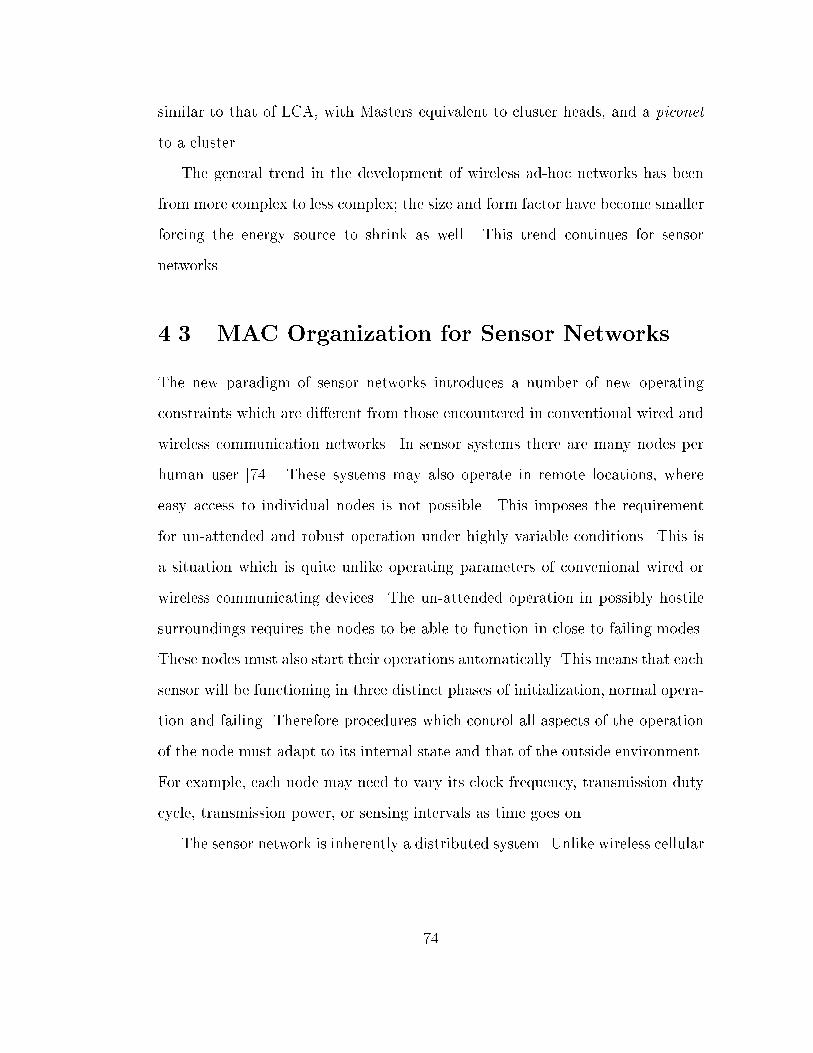
similar to that of LCA, with Masters equivalent to cluster heads, and a piconet

to a cluster.

The general trend in the development of wireless ad-hoc networks has been

from more complex to less complex; the size and form factor have become smaller

forcing the energy source to shrink as well. This trend continues for sensor

networks.

4.3 MAC Organization for Sensor Networks

The new paradigm of sensor networks introduces a number of new operating

constraints which are di�erent from those encountered in conventional wired and

wireless communication networks. In sensor systems there are many nodes per

human user [74]. These systems may also operate in remote locations, where

easy access to individual nodes is not possible. This imposes the requirement

for un-attended and robust operation under highly variable conditions. This is

a situation which is quite unlike operating parameters of convenional wired or

wireless communicating devices. The un-attended operation in possibly hostile

surroundings requires the nodes to be able to function in close to failing modes.

These nodes must also start their operations automatically. This means that each

sensor will be functioning in three distinct phases of initialization, normal opera-

tion and failing. Therefore procedures which control all aspects of the operation

of the node must adapt to its internal state and that of the outside environment.

For example, each node may need to vary its clock frequency, transmission duty

cycle, transmission power, or sensing intervals as time goes on.

The sensor network is inherently a distributed system. Unlike wireless cellular

74

systems where a base-station controls the behavior of the users in its associated

cell, in a sensor network it is not desirable or even possible to have a single point

of control, command, and coordination. However it is still an open question

how at the network topology must be. It is conceivable that at di�erent stack

layers, di�erent degrees of topological atness may exist. For exmaple, at the

link layer, the network may be completely at, with nodes allocating resources

and organizing themselves in a totally distributed fashion, based on strictly local

information. And yet at the networking layer clusters and cluster-heads may be

formed to aid the routing. It may also be more advantagous to have a hierarchical

topology, even at the link level, when heterogenous nodes are deployed side-

by-side in the same sensing arena. For example when some of the nodes have

more advanced equipment on board, such as a GPS transceiver, or more capable

signal processing boards and hence more powerful batteries, the network topology

could have a more hierarchical avor, with the more capable node commanding

more functions. It can be hypothesized that at higher levels, a more hierarchical

architecture must be used to �lter data, to manage high volumes of raw data and

to perform data fusion functions.

4.3.1 Related Work

There have not been many research e�orts concentrated on the problem of MAC

design for sensor networks. The work described in [75, 76] describes MAC for

large, scalable packet radio networks and [77] investigates a number of channel

access schemes for Radio Frequency Tags (RF-Tags).

Shepard [75] has studied the problem of management of the radio channel for a

packet radio network with a very large number of nodes. Although that problem

75

is concerned with nodes which will cover a metropolitan area and is not focused

on a low energy or low complexity solution, the ideas propose to achieve scalable

and decetralized operation. These are attributes which are of great importance

in a sensor network and are related to this work. Network-wide coordination and

synchronization are given up in favor of strictly local scheduling. In adition two

di�erent methods for mitigating interference generated by local and the aggregate

of faraway nodes are used. Local transmissions take place in time in a pseudo-

random fashion. That is, a variation of time-hopping is used to separate local

transmissions from each other. At the same time each tranmission is carried

out by spread-spectrum (Direct Sequence) to mitigate background interference

generated by farway nodes. Because of time-hopping no �xed transmission times

are scheduled to carry tra�c between �xed pairs of nodes and therefore, receivers

must always be turned on in order to receive all intended packets. For this reason

the described method is not an energy e�cient scheme.

The system under consideration for RF-Tags [77] is a single cell topology with

a single powerful basestation which controls the RF-Tags in a single hop (star

network) con�guration. The tra�c is highly assymetric (with the infomration

woing from the base station to the RF-Tags). The single base station usually

controls many RF-Tags and therefore issues of e�cient channel access and fairness

are important. Since RF-Tags use batteries which may not be changed the power

conservation is also an issue here. The three protocols discussed are

1. Grouped tag-TDMA (similar to POCSAG [78] paging scheme)

2. Directory protocol: at the beginning of each transmission interval a list

of tags which will receive messages are advertised. In this manner after

76

reading the directory, the tags which are not going to receive data in this

interval can go to sleep until next interval.

3. Pseurandom protocol: a time-hopping approach (each tag has its own

unique wake up times which are generated abased on a pseudo random

sequence which is controlled by the base station)

4.4 Summary

Self-organizing radio networks have been �rst studied in the context of military

tactical communications networks. That work has lead to a great body of work

dealing with issues of channel management for e�cient ( i.e. high throuhgpout,

low delay) communications for ad-hoc, multihop networks. The two major ap-

proaches taken have been to use contention-based random-access methods such

as ALOHA [54] and its variants. The other methods, have used organized channel

acces schemes which lead to variations of TDMA/FDMA/CDMA access. For the

scheduled channel access methods the problem of channel management becomes

a big issue. The commercial market has had its own approach with the use of

ALOHA like access schemes for Manets ( Mobile Ad-hoc NETworks ). However

these solutions are not appropriate for sensor networks.. The MAC protocol for

the sensor netowkrs must be self-organizing, robust, and low energy. This leads

to requirements for decentralized, scalable, and scheduled communications. In

Chapter 5 we describe and investigate the Self-organizing MAC for Sensornets

(SMACS) protocol which �ts the above requirements.

77

Chapter 5

SMACS Protocol

The objective of the self-organization protocol at the link layer is to form a

connected multi-hop network for a collection of randomly placed wireless sensor

nodes. The algorithm must start the network cold. No information is available

locally at the time each node starts. The node must �nd its radio neighbors, and

participate in a group e�ort to form an ordered method of channel access. The

single most important constraint is energy, and therefore, the self-organization

methods described in previous chapters are not suitable for our purposes. Also

in most systems described in chapter 4 it is assumed that a type of network

wide sysnchornization is already in place. In this work we are concerned with a

problem that occurs in an even earlier stage of network formation, and that is

the problem of formation of an early skeletal time frame. In this chapter details

of a self-organization protocol which achieves these goals will be given.

78

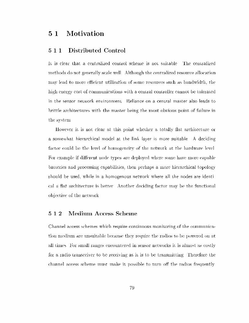
5.1 Motivation

5.1.1 Distributed Control

It is clear that a centralized control scheme is not suitable. The centralized

methods do not generally scale well. Although the centralized resource allocation

may lead to more e�cient utilization of some resources such as bandwidth, the

high energy cost of communications with a central controller cannot be tolerated

in the sensor network environment. Reliance on a central master also leads to

brittle architectures with the master being the most obvious point of failure in

the system.

However it is not clear at this point whether a totally at architecture or

a somewhat hierarchical model at the link layer is more suitable. A deciding

factor could be the level of homogeneity of the network at the hardware level.

For example if di�erent node types are deployed where some have more capable

batteries and processing capabilities, then perhaps a more hierarchical topology

should be used, while in a homogenous network where all the nodes are identi-

cal a at architecture is better. Another deciding factor may be the functional

objective of the network.

5.1.2 Medium Access Scheme

Channel access schemes which require continuous monitoring of the communica-

tion medium are unsuitable because they require the radios to be powered on at

all times. For small ranges encountered in sensor networks it is almost as costly

for a radio transceiver to be receiving as it is to be transmitting. Therefore the

channel access scheme must make it possible to turn o� the radios frequently.

79

Consequently CSMA methods are not suitable. This leads to a need for a time

schedule i.e. a TDMA like channel access scheme. However conventional TDMA

has a centralized element since a single TDMA schedule must be calculated. Also

all the terminals participating in the schedule must be synchronized at the slot

level. In conventional TDMA systems, such as satellite communications, this

tight slot synchronization is needed for purposes of bandwidth e�ciency.

In sensor networks it is possible to relax this network-wide slot synchronization

requirement and as a result do away with the need for a single master. We contend

that it will still be possible to maintain a scheduled mode of channel access. In

this vein we introduce the concept of Nonsynchronous Scheduled Communications

(NSC). Nonsynchronous refers to the notion that slot boundaries in the entire

network need not be aligned and scheduled refers to the idea that every node is

aware of the times it needs to turn its radio on and o� in order to communicate

with neighbors. The concept of NSC will be further explored in the following

sections.

5.2 SMACS Protocol Details

Let R be the set of all orthogonal channels available to our network. A channel

could be a combination of time, frequency, or code division. Consider a network

of N nodes, with connectivity matrix C = [cij]. A link lij exists from i to j, if j

is able to receive signal from i and cij = 2. If the received signal is not strong

enough to be detected properly, but strong enough to interfere with other good

signals, cij = 1. Otherwise cij = 0. Let this network have a total of L links,

numbered from 1 to L. Two links l1, from node i to node j, and l2, from node

80

k to node m , are de�ned to be interfering if at least one of the members of the

set fckj; cimg is greater than zero. Now an interference free organization of the

network will be a mapping, such that in the entire network no two interfering

links have the same channel r 2 R assigned to them. The size of this organization

is the total number of distinct channels assigned. It is a well known fact that

�nding a mapping where the total number of assigned channels is minimum is an

NP complete problem for general topologies.

In the sensor-networks we relax the requirement for optimal organization.

After all we are not concerned with pumping a lot of information through the

network as fast as possible. We only require an interference-free mapping, re-

gardless of its size. The important constraint is that this mapping must be found

using minimal energy.

For self-organizing ad-hoc networks the connectivity matrix must �rst be de-

termined. Afterwards a centralized or distributed mapping algorithm is run to

map each link to a speci�c channel. For the distributed case, a third phase exists

to resolve any potential con icting channel assignments that may arise due to

having only partial connectivity information at each node.

For energy constrained systems, this general approach requires too much mes-

sage passing and is therefore too costly. A node does not know the number of its

neighbors ahead of time. Therefore it does not know when to stop the neighbor

discovery phase. Also, this stopping time is di�erent for each node, because the

nodes have di�erent numbers of neighbors and also they start the discovery phase

at di�erent times. If we impose an arbitrary stopping time, then there will be

some nodes which have not had a chance to �nd any information yet. An intuitive

solution is to mix the discovery phase and link assignment phases together. In

81

the simplest case this means that a node will assign a channel to a link, as soon

as it is discovered. The node will then continue to �nd other neighbors and so

on.

This procedure relieves the system from establishing network-wide synchro-

nization as well. This means that di�erent nodes may have di�erent time-

references, and that slot boundaries need not be aligned throughout the network,

and hence the idea of NSC is born. A simple example demonstrates this point.

Take a linear multihop network, as shown in Figure 5.4.

In this network each node is able to hear its immediate neighbors only. Each

node i communicates with its right and left neighbors only. It must therefore be

aware of the timing of these two nodes: i.e. there must be agreement between

each pair as to the times each transmits and the other receives. Node i and i+2

may not transmit simultanously while i+ 1 is listening. Beyond this, node i and

k, k � i� 2 or k � i+ 2, need not coordinate in any form.

For general topologies each node synchronizes its transmission times with the

immediate neighbor it has just discovered without adjusting the timing of its

other allocated links, if they exist. As more nodes are discovered and attached to

each other a frame structure emerges. In this structure, time is segmented into

Super Frames. The length of a Super Frame is �xed. The Super Frame is broken

into smaller frames. Each frame is used for a diferent purpose. Note that the size

of each frame is not �xed, and may vary in time, for a single node. It may also

vary from node to node. Figure 5.1 illustrates the concept of the Super Frame.

82

BWassigned

on demand

on demand

assignedBW BW

on demand

assigned

BOOTUPnode i

node j

SUPER FRAME

TDMA TDMA

TDMA TDMABOOTUP BOOTUP

BW

assigned

on demand

BOOTUP

Figure 5.1: SUPER FRAME structure.

5.2.1 TDMA FRAME

The TDMA portion of the Super Frame is used for scheduled communication

between nodes. The startup algorithms which will be described in subsequent

sections are responsible for assignment of channels in the T�DMA frame. In this

mode a node transmits and receives mostly control and housekeeping packets to

and from neighbors which have already been discovered. The TDMA slots, which

are permanently assigned (until they fail), may be used as signalling channels to

establish new links on the y between neighbours when there is need for local,

cooperative activities.

5.2.2 Un-assigned Bandwidth

The un-assigned bandwidth is used for formation of local networks on the y to

deal with speci�c tasks of sensing or colaborative activities. For example, when

the existence of a target at some locality inside the hull of the network is detected,

83

a subset of nodes may need to form a local network to exchange sensor data and

perform beam-forming [79]. Not all nodes need to be involved in this operation.

Also the set of nodes which must group together to do the task may not be the

same for di�erent instances of target detection.

5.2.3 BOOTUP FRAME

The entire set of activities reposnsible for neighbor discovery and channel assign-

ment occur in this period. When a node is in BOOTUP mode, it is in one of

four possible states. A node passes from state to state upon reception of a valid

expected message from another node over the air, or upon time-outs when certain

messages are not received. The four states are SCAN, SCAN-RESPONSE, IN-

VITATION, and INVITATION-RESPONSE. During this period, nodes exchange

only four types of messages. These messages are:

� TYPE1: short invitation containing node's id. The node which sends it, is

the inviter during the search and hand-shaking transactions.

� TYPE2: response to TYPE1. The node which sends it, will be an invitee.

There may be more than one invitee for each inviter node. This message

gives the inviter and invitee's addresses, and invitee's attached state.

� TYPE3: response to TYPE2. Indicates which invitee was chosen. The se-

lection process is based on received signal levels and order in which TYPE2

messages are received. It contains the following additional information de-

pending on the node's attached state:

i) Inviter not attached: none.

84

ii) Invitee, inviter attached: inviter's schedule and frame epoch.

iii) Invitee not attached, inviter attached: proposed channel for the link,

calculated by inviter.

� TYPE4: response to TYPE3.

i) Invitee not attached, inviter not attached: channel determined by the

invitee.

ii) Invitee not attached, inviter attached: none.

iii) Invitee attached, inviter not attached: channel determined by the in-

vitee.

iv) Invitee attached, inviter attached: channel determined from own and

inviter's schedule information.

The messages are exchanged based on the state of the nodes as follows:

� SCAN: in this state the node scans the radio channel continuously on a

given �xed frequency. The node's receiver is on and it is waiting to hear a

TYPE1 or invitation message from another node.

{ If a TYPE1 message is received in a window of duration of �SCAN , the

time the message is received is saved at the receiving node, as TTY PE1.

A TYPE2 message is prepared and a number is chosen at random

between 1 and K. The TYPE2 message is broadcast on the Kth sub-

slot after TTY PE1. The node will then go to SCAN-RESPONSE state.

{ If a TYPE1 message is not received in �SCAN , the node itself will pre-

pare a TYPE1 message and broadcast it, and go to an INVITATION

state and wait for arrival of TYPE2 message(s).

85

� SCAN-RESPONSE: once in this state the node is in receive mode. It is

scanning the channel for a TYPE3 message from the same node which

prompted the node to go to this state. When such a message arrives within

�SCAN�RESPONSE of entering the state, and based on its contents, the re-

ceiving node determines that the two nodes are able to form a new TDMA

link, the node prepares a TYPE4 message and sends it. At this point the

node adds the new proposed link as a pending one int its schedule. The

node will then turn itself o� until the beginning of the next TDMA period.

During the next TDMA period the new pending link is tested by means of

exchange of very short NOM packets. If no valid message arrives the node

will go back to SCAN mode and start a new search.

� INVITATION: In this state the node is waiting for arrival of TYPE2 mes-

sages in response to the TYPE1 message it just sent out. The node will stay

in this state for K sub-slots. If no valid TYPE2 messages are received then

the node will go back to SCAN mode and start its search anew. Otherwise

it will choose one of the arrived messages according to some criterion. At

this time this criterion is the �rst arriving message. However, combinations

of criteria such as received signal strength, time of arrival, and number

of nodes attached to the sender may be used. At the end of the K sub-

slots the node prepares and sends out a TYPE3 message addressed to the

proper node and goes to INVITATION-RESPONSE to wait for the arrival

of TYPE4 message.

� INVITATION-RESPONSE: The node awaits arrival of TYPE4 message.

Upon reception of the message within �INV ITATION�RESPONSE of entering

86

the state the node will mark the new proposed link as a pending one, turn

itself o�, and wait until the next TDMA period to test the new link.

The state transitions are depicted in Figure 5.2. A node engages in a node attach-

ment operation with only one other node at a time. During the handshake that

takes place at discovery time the two nodes exchange their schedule information.

Based on this information they attempt to �nd a time period in their respective

schedules which is un-assigned and free for both. If there is such an interval then

the time interval is assigned to the new link and a frequency band (or a hopping

pattern) is also assigned at random (to protect against collisions with unknown

con icting links in the vicinity).

Node Attachment Scenarios

De�nition: a sub-net is a collection of nodes which form a connected graph and

all have coinciding Super Frame epochs.

The BOOTUP algorithm must be able to handle three scenarios of node

attachment:

� node$ node attachment: when both nodes are unattached.

� node $ sub � net attachment: when a node attaches to another which is

already attached.

� sub � net $ sub � net attachment: when two nodes which are already

attached to other nodes discover each other.

The case when the two nodes belong to di�erent sub-nets is the most challeng-

ing and is depicted in Figure 5.3. This case is most challenging because each of

87

- wait for TYPE4- send TYPE3

RESPONSE

SCAN

INVITATION

RESPONSE

INVITATION

SCAN

Tim

e-o

ut

Tim

e-o

ut

inviter actions

Tim

e-o

ut

Tim

e-o

ut

invitee actions

- send TYPE4

- turn off radio

- wait for TYPE3

- send TYPE2

- wait for TYPE2

- send TYPE1

TDMA

Figure 5.2: State transition diagaram while in BOOTUP mode.

the two nodes already has its own time reference (a Super Frame structure), and

this frame may already be �lled to some degree with assigned slots. However, be-

cuase of the NSC concept, there is no need to resynch the two exsiting schedules.

All that is required is information about the o�sets of the time references of the

two schedule (i.e. how far apart are the Super Frame epochs), and the location

of assigned slots in the two schedules. Because we are not going to re-shu�e the

assigned slots, it may not be possible for the two nodes to connect. For exam-

ple if there is no overlap between the respective TDMA Frames or none of the

un-assigned slots in the TDMA Frames coincide. In this case the two nodes will

88

disengage from each other and continue to search for other nodes.

j Pending Link Slots

iT

�� ��������

��������

����

����

������������

������������

������

������

������ ��

T

TY

PE

3������

������

����������

����������

������

������

�����

�����

����������

BOOTUP TDMA

TDMABOOTUP

node j

wake-up time

TY

PE

4

TY

PE

2

A Bnode i

TY

PE

1

Figure 5.3: Message exchange sequence for sub-net to sub-net attachment

In Figure 5.3 nodei wakes up, and listens on BOOTFREQ. It does not receive

any invitations and therefore it broadcasts a TYPE1 at time TT1. It will wait and

listen to the channel for a �xed period of duration K sub-slots after transmission

of TYPE1. All the nodes which hear nodei and wish to respond to it will transmit

a TYPE2message at random during one of theseK subslots. Nodej is one of these

nodes. The inviter node, nodei in this case, chooses nodej. In TYPE3 message

nodei announces its choice. In TYPE3 message is also included the beginning

time of nodei's next Super Frame, FRAMEBEGINi, and its schedule. When

nodej receives this information, it will �rst determine if it is possible for the

two nodes to establish a link by menas of determining whether the two nodes

have enough overlap between their respective TDMA Frames. If so then nodej

will pick two slot locations as the time intervals for the new pending link. The

location of the pending slots along with nodej's FRAMEBEGINj is transmitted

89

in TYPE4. Nodej will go to sleep after this. It will wake up at the beginning of

its next TDMA frame.

If the new proposed slot locations are agreeable to nodei, it will mark the new

link as a pending, go to sleep, and wake up at the beginning of its next TDMA

frame. If not it will start the whole search all over again. This continues until

either a new node is found and attached or the BOOTUP period ends.

Note that if the number of available slots in the TDMA period is large there is

higher likelihood of success in attaching nodes at the �rst attempt. The smaller

the number of attachment attempts the lower the amount of energy used. There-

fore a trade-o� between energy usage and available bandwidth exists.

BOOTUP and Frequency Hopping

The BOOTUP operation may be extended to operate on a very-slow frequency

hopping channel where an entire packet is transmitted over one or very few hop-

ping frequencies. The main task of capturingTYPE1 messages can be done as

follows.

An outgoing TYPE1 message will be repeatedly transmitted over a sequence

of frequencies. This sequence will be a hopping sequence with short period say 16

hops. The nodes scanning the channel will listen on all 16 hops according to their

own hopping pattern phase until a hit occurs. At this point the receiving node

will be in coarse synchronization with the transmitter. Once the TYPE1 message

is captured the rest of the hand-shake transaction and channel assignments will

be the same as before. The drawback of this method is that extra time and

extra energy are needed to connect the network. The extra amount of energy is

required to transmit multiple copies of the TYPE1 message at the inviter node.

90

5.3 Master Slave Bootup

The SMACS startup algorithm builds a totally at topology at the link layer.

However, we would like to compare this with the performance of a link layer

startup algorithm which builds a more hierarchical topology. The network for-

mation methodology which is used in the Bluetooth standard [72] provided a

good starting point for the hierarchical approach.

A standard Bluetooth network is comprised of a single MASTER node. The

�rst node awake is usually the MASTER. This node will then search for and

attach up to seven other nodes to itself as Slaves in a star topology. The Slaves

follow the timing reference of the Master. This single star network is a piconet.

To extend multihop capability to this network di�erent piconets are connected

together to form scatternets. The mechanism is as follows: a Slave of a particular

Master may itself become a new Master, or the Slave of another master. In this

manner some Slave may act as gateways between adjacent piconets and connect

them. Each piconet is distinguished by the timing reference of its Master. When

a Slave is attached to two di�erent Masters it must then follow two di�erent

timing references.

The Master Slave Bootup (MSB) algorithm which we have developed parallels

the Bluetooth concepts, except that practical issues such as content of messages,

timing of messages, assumed signalling rates, and consequently message lengths,

etc. are changed to be comparable to the BOOTUP algorithm.

There are three message types in MSB: INVITE, INVITE-RESPONSE, VER-

DICT. Also there are two logical types of nodes: MASTER and SLAVE. Only

a MASTER node sends an INVITE, but all nodes may choose to respond to an

91

INVITE. A MASTER sends out an INVITE message to �nd and attach new

neighbors. Another node which hears this INVITE, and decides to respond to it,

will transmit an INVITE-RESPONSE message at some random time somewhere

within the window �response after reception of the INVITE. The response is sent

over a frequency band centered at HANDSHAKEFREQ. The values of �response

and HANDSHAKEFREQ are chosen by the MASTER , usually at random, and

are included in the INVITE message. The INVITE-RESPONSE includes the

respondent's id, its connectivity information, and link assignment schedule if it

is already attached. Once the MASTER has received all the responses, it will

calculate a con ict free schedule for all the participating nodes, and form a lo-

cal star network, with itself at the center. The new schedule is broadcast over

HANDSHAKEFREQ in the body of a VERDICT message at the end of �response

window.

At startup there are a number of MASTER nodes which will form a number

of local star networks. In order to connect the entire collection of nodes these

local start networks must all become connected. At some point in time some of

the SLAVE members of the star networks may declare themselves as MASTERs

and start searching for other neighbors. In this fashion it is possible to connect

the entire network as an interconnection of many local star formations. Note

that unlike the Bluetooth standard, where all the SLAVEs are time synchronized

with their local MASTER, we use the NSC concept. This is to ease the process

of connection of two di�erent local star networks.

Details such as which nodes are chosen as MASTERs, and under what crite-

rion SLAVEs become MASTERs will a�ect the behavior of the algorithm. Here

92

we choose MASTERs at random, i.e. a node is a MASTER with probability pm,

0 < pm < 1. A node becomes a MASTER if it is already attached, but to less

than Nn other nodes. As the number Nn becomes smaller, the MSB moves closer

to building a at topology. If a very long time has passed and a SLAVE has not

heard from any other nodes, it will become a MASTER. In this algorithm, it is

possible to assign slots throughout the entire frame therefore distinct BOOTUP

and TDMA periods do not exist.

5.3.1 Power Control

We claim that it is more energy e�cient to transport bits in the network along

many short range hops than via a single longer range hop. The key reason for

this is the fourth power drop-o� of path-loss for near surface propagation as a

function of distance [80]. This phenomenon makes long distance communications

much more costly in terms of energy usage compared to an environments such as

those considered in [81] with 2nd order power drop-o�.

To further illustrate this point, we investigate a simple example of a linear

topology network, and follow the same line of analysis used in [81]. The network

diagram is given in Figure 5.4. There are n+1 nodes, with separation r between

adjacent nodes, all placed along a straight line. A single information symbol is

to be sent from node 0 to node n. Two scenarios are considered. In the �rst

scenario, node 0 transmits the single bit directly to node n in one large hop. This

requires the node to use a relatively large transmit power to reach the destination

node particularly if the values of r or n or both are large. In this case a single

transmission and a single reception takes place. The radios on the nodes consume

E J=bit when turned on, in either transmit or receive mode, and the radio front

93

node

������������

������������

������������

������������

������������

������������

Tx RxTime

0 i+2i+1ii-1 N-1

i

i-1

i+1

i+2

node

node

node

Figure 5.4: An example of slot alignment for a linear network topology.

end consumes � J=(bit � m4) to amplify the signal, to arrive at a receiver 1m

away, having a desired signal to noise ratio of s1. The total energy consumed is

Edirect = E + �n4r4 (5.1)

In the second scenario, the single bit is transported to the destination, via n small

hops. In this case there will be n� 1 receptions, and n transmissions, each over

a distance of r. The total consumed energy will be

Emult = nE + n�r4 + (n� 1)E (5.2)

= (2n� 1)E + �nr4 (5.3)

Wanted are values of r and n for which direct method consumes less total energy

per bit than the multiple method. That is

Edirect � Emult (5.4)

E + �n4r4 � (2n� 1)E + �nr4 (5.5)

r4(n3 + n2 + n) � E=� (5.6)

To understand the implications of this result, we use the following example.

For state of the art low power radios, operating at 2:5V and 30mA, with power

94

e�ciency of approximately 5 percent, the values of E = 7:9 � 10�7J=bit and

� = 7:3 � 10�9 J=(bit �m4) are typical. These values are valid for 2FSK non-

coherent reception, with noise power of Np = �67 dBm, at a symbol rate of

1=Tb = 10 Kb=s and BER = 10�3.

De�ning F (n; r) = E=��r4(n3+n2+n), the graph of Figure 5.5 gives the region

in the r�N plane where direct communications is better than multiple hops. It

can be seen that, the feasible number of steps of length r per hop quickly drops

down to unity, as the range between adjacent nodes increases or number of nodes

increases. For comparison, we include the same region for the case where path

loss drops o� with second power of distance, in Figure 5.6. It is clear that, for

second power loss, in many cases, direct communications is more feasible. But as

power loss becomes more severe, multiple hops become more feasible. Therefore,

at least for linear topologies, it can be concluded that connecting the network

by means of forming links which require the lowest transmit powers will result

in lower energy consumption for long-haul transport of bits, and thus extend the

lifetime of the network. We adopt the same strategy for spatial con�gurations

other than straight lines.

5.4 Time Management of Protocols

As the network becomes more connected, that is, each node �nd and attaches

more neighbors, the need for �nding new neighbors is reduced. It also becomes

harder to �nd new neighbors. So it is reasonable to reduce the duty cycle of the

time each node spends in BOOTUP. A number of di�erent methods may be used

95

0 2 4 6 8 10 12 14 160

5

10

15

20

25

30

35

40

Feasibility Region for Fourth Power Pathloss

r(m)

num

ber

of h

ops

Dark region indicates area where direct transmission uses least energy

Figure 5.5: Feasible region for direct communications, for fourth power path loss.

to achieve this limitting e�ect.

� Each node will be actively participating in BOOTUP with probability

pa(k) = 1=(Nn + 1), where Nn is the number of neighbors the node has

at the beginning of a SUPER FRAME k.

� Reduce the length of BOOTUP period in each SUPER FRAME, inversely

proportional to the number of a node's neighbors, or the length of time it

has been active. After a maximum number of neighbors are attached to a

node, it will stop participating in BOOTUP. It will start searching for new

nodes, if and when some of its neighbors are lost.

96

0 5 10 150

5

10

15

20

25

30

35

40Feasibility Region for Second Power Pathloss

r(m)

num

ber

of h

ops

Dark region indicates area where direct transmission uses less energy

Figure 5.6: Feasible region for direct communications, for second power path loss.

5.5 Simulation Model

Our protocols are implemented in a simuation environment written in PARSEC

[82]. In this model, each sensor node is modelled as a PARSEC entity. The

functionality of each networking layer, i.e. PHY, MAC, Networking, and etc. are

implemented as methods, or functions, within the body of the entity.

The sensor network is modelled as a collection of nodes, which transmit and

receive packets over a radio channel. The channel is also modelled as a speci�c

entity, which receives messages from nodes, implements radio propagation e�ects

such as path loss and shadowing, on each packet, and delivers it to all nodes

within radio earshot of the transmitting node. The channel entity simulates a

broadcast channel. The entire simulation is controlled by a driver entity which

is responsible for reading all the input �les, setting up each entity, informing the

channel of the number and location of nodes, and collecting simulation statistics,

when the run is �nished.

97

Inter layer communications within a single node, and PHY-PHY communica-

tion between di�erent nodes, are accomplished by means of passing of messages.

When a packet is generated at a node, it is passed down from layer to layer, until

it reaches the radio layer of the sending node. The radio layer generates an over

the air packet, and sends it to the channel entity. The channel entity will then

simulate the conditions of a radio broadcast channel, and deliver the packet to

all nodes which are close enough to receive it. The simulation model is depicted

in Figure 5.7.

BroadcastRadio Over The Air Packet

Channel

NETWORK

LINK/MAC

PHY/RADIO PHY/RADIO

NETWORK

LINK/MAC

NODE NODE

Inter Layer Message

Figure 5.7: Simmulation Model of Self-organizing algorithms.

5.5.1 The Propagation Model and Packet Capture

The radio channel model simulates Log-normal shadowing with � = 8dB. In ad-

dition, additive white gaussian is added to transmitted signals. For each transmit

power level, two ranges R1 and R2, with R1 < R2 are considered. The smaller

radius corresponds to the range of good communication for the transmitter, and

R2 is the range over which the node is capable of producing interfering signal

98

levels. The value of R1 depends on the transmit power level, propagation loss

model, and additive background noise levels. Here we set R1 to the distance

which corresponds to received SNR of s1. The value of s1 is chosen to yield a

raw symbol error rate of 10�3 for the given modulation method in additive noise.

The value of R2 depends on the sensitivity level of the radio receivers. Here we

set the value of R2 to the distance which yields SNR ratios of s1� 11dB . A good

packet is one which has received SNR above s1. Note that due to shadowing, the

goodness of a packet may not be determined solely based on distance between

transmitter/receiver pair. Only good packets which have no overlap with other

packets are captured. All other packets are dropped.

5.6 Simulation Results

A number of di�erent simulation experiments were conducted to investigate the

performance of our self-organization algorithms. We are interested in determin-

ing:

� Scalability : the ability to connect networks of many nodes, where the

protocol overhead stays essentially constant, regardless of network size

� Ability to conserve energy when connecting the network

� Ability to conserve energy both in short term and in the long run

The following set of experiments test one or more of the above attributes for

the network formation algorithms described previously.

99

5.6.1 SMACS vs. MSB

We are interested in determining whether performance tradeo�s exists when we

form a totally at network by means of the SMACS protocol, compared to a

more hierarchical topology, as is done in the MSB scheme. Particularly we are

interested in determining the time and energy it takes to build the network un-

der each of the algorithms. To generate the following results, the BOOTUP and

MSB procedures were run each for 1000 di�erent random con�gurations of collec-

tions containing 18, 45, 150 and 400 nodes respectively. Each network topology

has spatial node density of � = 0:04 nodes=m2. The nodes are distributed ran-

domly and uniformly in a square shaped plane. The Super Frame is set to 40

slots. There are 100 di�erent frequencies to choose from, apart from the BOOT-

FREQUENCY. For the BOOTUP algorithm, the TDMA frame contains 20 slots.

That is, only half of the bandwidth is set aside for scheduled communications. In

all simulations a �xed transmit power of 3.0 mW is used. Two scenarios are con-

sidered: BOOTUP with �xed transmit power, and MSB with �xed power. For

all cases, the initial invite is sent over the common BOOTFREQUENCY band.

However, the rest of the handshaking procedure for all cases is carried out over

the speci�c hand-shaking frequency of the transaction. The simulation stopping

time is the �rst instance when the network becomes connected.

Figure 5.8 gives the time, in SUPER FRAMES, until the network becomes

connected for the �rst time. We see that the MSB is able to connect the network

faster, for this experiment. This ability to connect the network faster is due

to the fact that a single master node is able to connect many nodes within a

single handshake transaction, while the BOOTUP (or SMACS) method, adds

at most one neighbor at a time, for each handshake transaction. However, as

100

we see in Figure 5.9, the MSB, requires nodes to be, on average, turned on for

longer durations, to achieve the faster connection times. This is again due to

the fact that, the MASTER nodes in MSB, must stay awake for a much longer

time, in order to hear all the responses to each of their INVITE messages.

0 50 100 150 200 250 300 350 4003.5

4

4.5

5

5.5

6

6.5

7

7.5

8

network size

Fra

mes

BOOTUPMSB

Figure 5.8: Elapsed time until network is connected.

The consequence of longer duty cycles for the radios is evident in Figure 5.10,

where we see the average used energy until connection time for MSB is larger

than BOOTUP �xed power. The conclusion to be made here, is that by adding

neighbors one at a time, as is done on the SMACS procedure, we will be able to

save energy, at the cost of prolonging the time it takes to connect the network.

5.6.2 Network Lifetime

The average consumed energy per node in 500 Super Frames was measured under

the following scenarios:

101

0 50 100 150 200 250 300 350 4000.6

0.7

0.8

0.9

1

1.1

1.2

1.3

1.4

1.5

1.6

network size

Fra

mes

BOOTUPMSB

Figure 5.9: Duration of time radios are powered up.

1. Scenario 1: Each node continues to search for more neighbors in each Super

Frame with probability pn = 1=(Nn + 1) where Nn is a node's number of

neighbors.

2. Scenario 2: In adition to the constraint in the above scenario, a node stops

searching for nodes, after it has found Nmax neighbors.

Both Scenarios were run for a single network of 18 nodes, and the second one

for a network of 150 nodes, with �xed values of link transmit power, for node

density of � = 0:04. In Figure 5.11 we see that, as expected, the consumed energy

increases with increased link transmit power. However after inspection of the

sources of energy consumption, it was found that most of the energy consumption

is due to transmissions of TYPE1 messages, which are never acknowledged. This

idea is supported based on the data given in Figure 5.12. The top curve gives

the total number of transmitted BOOTUP messages in 150 SUPER FRAMES.

102

0 50 100 150 200 250 300 350 4000.5

0.6

0.7

0.8

0.9

1

1.1

1.2

1.3

network size

Ene

rgy(

J)

BOOTUPMSB

Figure 5.10: Energy consumed to connect the network.

The middle curve gives the total number of TYPE1 messages sent. The lower

curve gives the number of TYPE1 messages which were sent and never received

by another node. So we see that a very large portion of the messages which are

sent over the air are in e�ect wasted, and do in fact waste energy. So, if we are

able to limit the number of transmitted TYPE1 messages, and still manage to

connect the network in a reasonable time, we may be able to save considerable

amounts of energy.

As it turns out, the BOOTUP portion of SMACS protocol, is able to connect

the majority of a node's neighbors very quickly, and after that, there is no point in

using the entire un-used bandwidth of the node to search for more nodes. For this

reason, we will allow a node to participate in BOOTUP only until it has found

Nmax = 5 neighbors. The improvements in energy consumption for Scenario 2

are evident from Figure 5.11. An alternative approach which will limit the time

spent in BOOTUP, is to make the duration spent searching for new neighbors

103

0 2 4 6 8 10 12 14 16 18 200

5

10

15

20

25

30

35

40

45

Link Transmit Power (mW)

Ene

rgy

(J)

Energy consumed in 500 FRAMES

FRAME=40 slots, TDMA=20 slots, 100 freq channels

150 nodes, Scenario 2 18 nodes, Scenario 2 18 nodes, Scenario 1

Figure 5.11: Energy Consumption in 500 Super Frames

.

0 1 2 3 4 5 6 7 8 9 10 11300

400

500

600

700

800

900

1000

1100

Link Transmit Power (mW)

Num

ber

of M

essa

ges

Stopping Time = 150 Super Frameis

Messages Not Acknowledged in BOOTUP

18 NodesScenario 1

missed TYPE1 sent TYPE1 total sent

Figure 5.12: Message exchange behavior in Scenario 1.

104

inversely proportional to the number of neighbors as well. In this manner, even

after Nn neighbors are attached, a node may still spend some time in BOOTUP.

This will enable the attachment of newly activated nodes possible well into the

lifetime of the network. This approach is a re�nement to the SMACS, and its

performance will not be discussed further here.

The increase in the lower region of the curves in Figure 5.13, which is a closeup

of Figure 5.11 indicates that link transmit power cannot be reduced arbitrarily.

Apart from the fact that with a �xed and low power level, the network may not

become connected, the data indicates that before this hard limit is reached, as

transmit power is reduced, it becomes harder to have successful handshakes in

the network, as shown in Figure 5.12. We see that for a given network, for both

Scenarios, there is an optimum transmit power level, which will achieve the lowest

possible consumed energy levels. However this value is a function of node density

and channel parameters, and may not be known prior to network deployment.

5.6.3 Variable Transmit Power levels

It is clear that we need power control on individual links in the network. There

are two possible approaches here. One is to connect the network at some �xed

transmit level, and then after links are established, use closed loop schemes to

lower the transmit levels on individual links, or use distributed power control

schemes similar to those used in cellular systems. The second aproach is to use

a very simple open loop method of assignment of power levels to links, during

the operation of SMACS protocol. A rudimentary scheme which was used in our

networks is as follows: Each node, upon wakeup, starts to engage in BOOTUP

at some lowest transmit level. If after certain number of Super Frames it has

105

0 2 4 6 8 10 12 14 16 18 207

8

9

10

11

12

13

14

15

Link Transmit Power (mW)

Ene

rgy

(J)

Energy consumed in 500 FRAMES

FRAME=40 slots, TDMA=20 slots, 100 freq channels

150 nodes,boot on18 nodes, boot on

Figure 5.13: Energy consumption as transmit power level changes.

not found any neighbors, it will use the next higher transmit level, and so on.

If the nodes has found some neighbors, and it is after POWER � CY CLE

Super Frames, then the node will also start cycling through its power levels to

�nd far away nodes. On the other hand if a node receives a TYPE1 message

from an unattached node, the receiver will adjust its power level to that of the

transmitter (the transmit power level is included in the body of the incoming

TYPE1 message).

The average short term and long term behavior of the SMACS algorithm was

measured for networks of 18, 45, 150, and 400 nodes under �xed and variable

power levels. In these experiments, the radio consumes 98 mW whenever it

is turned on. This number is comparable to a typical Bluetooth radio power

consumption. In addition, it will use an additional incremental level �p. The

value of �p is a function of the output transmit power. The �p represent the

106

Table 5.1: Values of �p for various transmit power levels.

Ptransmit (mW) �p (mW)

1 6.7

3 30.0

10 66.7

power consumption at the RF front end. The values used for �p are given in

Table 5.1. The power consumption for transmission is then (98 + �p) mW. The

network statistics were gathered at two points in time for each network: �rst at

the time the network becomes connected, and then after 500 SUPER FRAMES

are elapsed. We measure the average length of time a node is turned on , the

average transmit power level for the variable power case, the length of time it

takes to connect the network, and average energy used per node. These values

are depicted in the following �gures. Figure 5.14 gives the average time it takes

until the network is connected. In Figure 5.15, the average duration of radio

on time, in lengths of SUPER FRAMES, is given for �xed and variable power

scenarios. Figure 5.16 gives the average consumed energy until network becomes

connected. On this plot, the amount of energy which would be consumed, if

we used the classical Linked Clustering Algorithm (LCA), to self-organize the

network is also given. The energy consumtopn of LCA is calculated, assuming

the packet lengths for LCA are the same as a TYPE3 message, and that a single

round of LCA is su�cient to form the network. Radios are always in receive mode

for LCA, unless they transmit a message. It can be seen the level of energy savings

107

0 50 100 150 200 250 300 350 4003

3.5

4

4.5

5

5.5

6

Network size (number of nodes)

Tim

e (F

ram

es)

1mW3mW10mWVAR

Figure 5.14: Time until the network becomes connected.

.

SMACS will a�ord, compared to LCA. Furthermore, the SMACS algorithm has

the added bene�t that it does not require a global time reference to be established

before the algorithm is run, unlike the LCA. Also, we do not need to have any

information about the network size for SMACS.

We also see that there is clearly an optimum average transmit power level,

which brings down the consumed energy required to connect the network. Fur-

ther, the variable power level scheme is able to bring down the actual consumed

energy. So, for the short term, it makes sense to use variable powers. The penalty

for using variable levels, is increased time until the network becomes connected,

as is shown in Figure 5.14, a penalty which is most likely tolerable in sensor

networking environments.

The e�ect of having variable power levels on the long run energy consumption,

is given in Figure 5.17. In this scheme, each node stops searching for new nodes,

108

0 50 100 150 200 250 300 350 4000.26

0.28

0.3

0.32

0.34

0.36

0.38

0.4

0.42

0.44

Network size (number of nodes)

Tim

e (F

ram

es)

1mW3mW10mWVAR

Figure 5.15: Average length of time radio is turned on, until network is connected.

once it has found 5 neighbors. We see that, in the long run, the variable power

scheme builds a network which consumes the least amount of energy. This is due

to the fact that the variable power scheme builds a network with links which use

the smallest transmit power levels. Over repeated link usage, the power savings

will add up. Therefore, although it may take longer to build the network, if we

use variable power levels, in the long run, it is worth the e�ort, to do so. Another

important factor is that, for a randomly deplyed network, the node density, and

therefore the optimal link transmit power levels are not known, and in this case,

the only intelligent solution is to use a variable power scheme.

5.6.4 E�ect of Number of Channels on Performance

Networks of 150 nodes were investigated for the e�ect of the number of available

channels on the performance of the system. All the performance indicators were

measured for 5000 di�erent runs of the SMACS. The average of results of the

109

50 100 150 200 250 300 350 4000.1

0.15

0.2

0.25

0.3

0.35

0.4

0.45

0.5

Network size (number of nodes)

Ene

rgy

(J)

1 mW3 mW10 mWVARLCA, 3mW

Figure 5.16: Energy Consumption of SMACS and LCA until network becomes

connected.

simulation are given the Table 5.2. All measures of performance improve with

increasing number of channels. The most pronounced improvement is with the

time it takes to connect the network.

5.7 Conclusion and Future Work

Both the SMACS and MSB procedures are scalable schemes, which enable build-

ing of a network infrastructure for our sensor nodes. The MSB algorithm may be

described qualitatively as follows. The protocol attempts to build a more hirar-

chical topology, by means of assigning, at random, to some nodes the reponsibility

of being a MASTER node. These nodes then will search and �nd neighbors, and

attech them to form a local star network. The star networks are then attached

together, when a SLAVE of a MASTER declares itself to be a MASTER and

110

0 50 100 150 200 250 300 350 40010

12

14

16

18

20

22

24

Network size (number of nodes)

Ene

rgy

(J)

1mW3mW10mWVAR

Figure 5.17: Energy consumed in 500 SUPER FRAMES.

attaches two distinct star networks of which it is a member.

The SMACS protocol, on the other hand, builds a at topology. In this

scheme, a node �nds neighbors one at a time, and once a neighbor is found, it

is attached immediately. This method may take longer to build (connect all the

nodes in the network), compared to MSB, but it uses less energy to do so.

The self-organizing schemes were implemented in a simulation environment

written in PARSEC. It was determined that a variable transmit power scheme

is neccesary in order to reduce short term and long term energy consumption.

The SMACS scheme is able to form a network in a scalable fashion, as compared

to the LCA. In order to conserve energy, the self-organization mechanism must

employ some form of limiting behavior, to reduce its duty cycle as the network

ages, or as enough neighbors are found for each node.

We have demonstrated in simulation, that it is possible to form an ad-hoc

111

Table 5.2: Performance as number of channels changes

Frequency Count (Number of Chan-

nels)

50 5

Stop Time (FRAMES) 13.12 16.92

Time Radio On(FRAMES) 2.07 2.54

Consumed Energy (J) 0.82 1.00

Link Transmit Power (mW) 1.27 1.33

Number of Neighbors 3.02 3.03

Percent of Nets Connecting 75.5 74.1

infrastructure for sensor networks, without the need for prior time synchroniza-

tion, information about the network size, and network topology. The variable

power SMACS presents the most number of advantages as a suitable choice for

self-organization at the link layer.

Future work on this topic includes investigation of the e�ect of a particular link

layer self-organization scheme on the overall performance of the sensor network,

by simulating the joint performance of the system with an appropriate routing

mechanism. This measurement may be done under di�erent tra�c scenarios.

This requires development of suitable physical target and event models, which

will then translate into network tra�c models.

It is also of great value if we are to develop a method for determining a link

topology and its associated link transmit power levels, which will minimize the

average energy consumed per node. This \minimum energy" method may use

112

global information, and could be either a centralized or distributed algorithm,

and its output will be used as a performance benchmark for, say, comparing

various energy concious infrastructure building algorithms.

113

Chapter 6

Conclusion

The fact that path loss varies with the fourth power of the inverse transmitter-

receiver distances for low lying antennas has many signi�cant impacts on the

design choices one will make for wireless sensor networks.

Based on our measurements we found that the fourth power path loss, is

prevalent mostly in outdoor situations, and that the onset of the this phenomenon

is at very small distances. The path loss characteristics, indicate that many small

hops, in general, are more energy e�cient in moving bits around the network,

compared to having fewer but longer distance hops. This in turn had implications

as to the need for power control on the links themselves. In other words, it would

be best to use the lowest possible transmit power level of the radio to search

for neighbors and build an infrastructure. However, in order to make sure the

network actually becomes connected, higher transmit levels must also be used.

We found that using a very simple power control scheme, which involved cycling

through all possible transmit poer levels periodically, resulted in good energy

savings, particularly in the long run.

114

We also found out that building a at topology, may be more energy e�cient

compared to a hierarchical one. However, further studies, which will combine

the joint energy consumption of routing algorithms with link layer design must

be made, to determine the best solution. It is highly likely that, when routing

issues are also considered, the impact of the tra�c type, and nature of observed

phenomena, will also have an impact on the overall energy consumption charac-

teristics.

Finaly, in studying the frequency hopping issues, we found out that it is

possible, in principle to maintain code synchronism, for fairly long periods ( tens

of thousands of frames), if we are able to keep the multiple access interference

levels low in the network. The e�ective node density in the network has a great

bearing in this repect. It was again concluded that, by reducing the transmit

power levels, and hence, reducing the e�ective node density in the network, better

maintenance of code phase is possible.

In short, we have seen that it is possible to build an ad-hoc wireless sensor

network, without having any prior information about number of nodes involved,

their time references, and their locations. The self-organizing schemes which were

developed were highly scalable and able to form the network in a distributed

manner.

115

Appendices

116

Appendix A

Some Number Theoretic

De�nitions

The following is a short list of some required de�nitions and facts. They may be

found in any text dealing with cryptography, such as [43]

List of de�nitions

1. If n is an integer, then Z�n = fx 2 f0; 1; 2; � � � ; n� 1g 3 GCD(x; n) = 1g

2. a 2 Z�n is a quadratic residue modulo n when 9x 3 x2 � amodn. If a 2 Z�

n

and a is not a quadratic residue, then it is called a quadratic non-residue

modulo n.

3. For p prime and 0 < a < p the Legendre symbol is de�ned as:

L(a; p) =

8>>><>>>:�1; a not a quadratic residue

1; a a quadratic residue

(A.1)

117

4. For N � pq, where p and q are primes, the Jacobi symbol is de�ned as

J(a;N) =

8>>><>>>:0; a devides either p or q

L(a; p)L(a; q); otherwise

(A.2)

5. Let N � pq, and p and q primes, and both congruent to 3 modulo 4. Then

N is a Blum integer.

6. A one-way function is de�ned as a function f such that for every x in the

domain of f , f(x) is easy to compute; but for virtually all y in the range of

f , it is computationally infeasible to �nd an x such that y = f(x).

7. A trapdoor one-way function is de�ned as a one-way function, fz, such that

given z it is easy to �nd algorithms Ez and Dz that compute fx(x) and

f�z 1(y). In this case the algorithm Dz is the trapdoor function, which is

kept secret, and is known only by the agent authorized to invert fx(x).

Note that it is still infeasible to calculate f�z 1(y), even with knowledge of

Ez.

List of some relevant facts

1. ForN � pq, p and q prime, and z 2 Z�n, de�ne zp = zmodp and zq = zmodq,

then z is a quadratic residue mod N i� L(zp; p) = 1 and L(zq; q) = 1.

2. For N � pq, p and q prime, jZ�nj = (p� 1)(q � 1). OF all the members of

Z�n, only one-half have Jacobi symbol equal to one. Of these, only one-half

are quadratic residues mod N .

3. If the factorization of N is unknown, and for z 2 Z�n we know J(z;N) = 1.

Then it is not possible to determine whether z is a quadratic residue or not

118

in polynomial time. This is called the Quadratic Residuancy Determination

problem.

4. If N is a Blum integer and z0 is a quadratic residue mod N , then 8i >0; zi = z2i�1 mod N .

119

Appendix B

Marker Tone Locations Are

Almost Independent

The distribution of marker tones in a SUPER FRAME, once it is determined,

remains �xed for a node. We represent the SUPER FRAME by a line interval

I1 of length TFRAME. Marker tones are represented as intervals of length �m.

The ith marker tone starts at bi, i = 1; 2; � � � ; Li. Distinct marker tones may not

overlap in time.

Each marker tone's start time, bi, is a random variable. We would like to

determine the join distribution of marker tone locations for a single node. The

distribution is represented by '(b1; b2; � � � ; bL).We de�ne Bi to be the collection of points in the SUPER FRAME which are

blocked as choices for bi , and Ii as Tframe � Bi. The set Ii will be the union of

a �nite number of disjoint line intervals all inside I1. We de�ne �i = length(Ii).

The sequence of �i is a decreasing sequence.

Tone locations are determined according to the folowing procedure:

120

� The location of the �rst tone, b1 is chosen randomly in the interval I1.

� Given fb1; b2; � � � ; bi�1g, bi is chosen uniformly from the points in Ii.

� Stop after bL is determined.

For i > 1 we have the following:

�1 � (i� 1)(2�m � �) � �i � �1 � i�m + � (B.1)

The upper limit corresponds to the case when all the previous tones are placed

next to each other contigously, and the lower limit corresponds to the case when

all previou tones were place with exactly (�m � �) separation between them,

where � is an positive and arbitrarily small real number. Then we may write the

distribution of bi conditioned on the past marker locations as:

'(bi=bi�1; � � � ; b1) = 1

�i

(B.2)

Then we have

'(bi; � � � ; b2; b1) = '(bi=bi�1; � � � ; b1)'(bi�1=bi�2; � � � ; b1) � � �'(b2=b1)'(b1)

=1

�i

� 1

�i�1

� � � 1�2

� 1

�1 (B.3)

Using the upper and lower bounds of B.1, we may bound the joint distribution

as

1

Tframe

LYi=2

1

Tframe � i�m + �� '(bi; � � � ; b2; b1) � 1

Tframe

LYi=2

1

Tframe � (i� 1)(2�m � �)(B.4)

If we have

2(L� 1)�m << Tframe (B.5)

121

and let � = 0 then the upper and lower bounds of B.4 may both be approximated

by 1TLframe

and we will have:

'(bi; � � � ; b2; b1) � 1

TLframe

(B.6)

This indicates that we may model the process of assignment of marker tones

in the SUPER FRAME as a sequence of L independent marker tone assignments,

where the location of each tone is indepedently and uniformly chosen over the

entire SUPER FRAME. Note that the condition of B.5 implies that total interval

covered by all the marker tones must occupy a very small fraction of the SUPER

FRAME length in order for the independence arrguments of this Appendix to

hold. This requires the marker tone duration to be short and the length of the

marker word, L, small.

122

Bibliography

[1] Unknown, \21 ideas for 21st century", Business Week, September 1999.

[2] http://www.ipnsig.org/reports/insitu/index.htm.

[3] http://www.wcom.com/about the company/cerfs up/interplanetary

internet/index.phtml.

[4] G. Asada, M. Dong, T. S. Lin, F. Newberg, G. Pottie, W. J. Kaiser, and

H. O. Marcy, \Wireless integrated network sensors: Low power syste,s on a

chip", in Proceedings of the 1998 European Solid State Circuits Conference,

1998.

[5] http://www.fxpal.xerox.com/smartspaces.

[6] http://www-white.media.mit.edu/vismod/demos/smartspaces.

[7] http://www.research.ibm.com/journal/sj38-4.html.

[8] J. Heideman, R. Govindan, and D. Estrin, \Con�guration challenges for

smart spaces", in Proceedigns of the DARAP/NIST Smart Spaces Workshop,

Gaithersburg, Maryland, July 1998.

[9] http://lcs.www.media.mit.edu/projects/wearables.

123

[10] http://wearables.stanford.edu.

[11] http://www.janet.ucla.edu/WINS.

[12] http://www.janet/ucla.edu/awairs.

[13] F. Bennet, D. Clark, J. Evans, A. Hopper, A. Jones, and D. Leask, \Piconet:

Embedded mobile networking", IEEE Communications Magazine, pp. 7-15,

October 1997.

[14] http://www.cam-orl.co.uk/ab.html.

[15] J. M. Kahn, R. H. Katz, and K. S. J. Pister, \Mobile networking for smart

dust", in MobiCom. ACM/IEEE International Conference on Mobile Com-

puting and Networking, Seattle, Washington, USA, August 1999, pp. 17-19.

[16] http://www.research.digital.com/wrl/projects/Factoid/index.html.

[17] http://www.arap.mil/ito/Solicitations/CBD 000-25.html.

[18] http://www.onr.navy.mil/sci tech/special/muri2k/topics.htm.

[19] K. Bult et al., \Wireless integrated microsensors", in Technical Digest

of SolidState Sensor and Actuator Workshop, Hilton Head Island, South

Carolina, June 1996, pp. 205{210.

[20] http://netweb.usc.edu/SCADDS.

[21] W. Heinselman, J. Kulik, and H. Balakrishnan, \Adaptive protocols

for information dissemination in wireless sensor networks", in MobiCom.

ACM/IEEE International Conference on Mobile Computing and Network-

ing, Seattle, Washington, USA, August 1999.

124

[22] http://www.mprg.ee.vt.edu/research/glomo/prev2.html.

[23] J. G. Proakis, Digital Communications, McGraw-Hill, New York, 3 edition,

1995.

[24] D. Parsons, The Mobile Radio Propagation Channel, Wiley, New York, 1994.

[25] P. Bello, \Characterization of randomly time-variant linear channels", IEEE

Transactions on Communications Systems, december 1963.

[26] T. S. Rappaport, Wireless Communications: Principles and Practice, Pren-

tice Hall, Upper Saddle River, New Jersey, 1996.

[27] H. Zaghloul, G. Morrison, D. Tholl, M. G. Fry, and M. Fattouche, \Mea-

surement of the frequency response of the indoor channel", in Proceedings of

the Symposium on Antenna Technology and Applied Electromagnetics, 1991,

pp. 405-407.

[28] T. S. Rappaport and S. Sndhu, \Radio-wave propagation for emerging wire-

less personal-communication systems", IEEE Antennas and Propagation

Magazine, vol. 36, no. 5, October 1994.

[29] S. J. Howard and K. Pahlavan, \Autoregressive modeling of wideband indoor

radio propagation", IEEE Transactions on Communications, vol. 40, no. 9,

pp. 1540-1552, September 1992.

[30] M. K. Simon, J. K. Omura, R. A. Scholtz, and B. K. Levitt, Spread Spectrum

Communications Handbook, McGrawHill, New York, 1994.

125

[31] R. B. Ward, \Acquisition of pseudonoise signals by sequential estimation",

IEEE Transactions on Communications, vol. COM-13, pp. 475-483, Decem-

ber 1965.

[32] R. B. Ward and K. P Yiu, \Acquisition of pseudonoise signals by recursion

aided sequential estimation", IEEE Transactions on Communications, vol.

COM25, pp. 784-794, August 1977.

[33] G. F. Sage, \Serial synchronization of pseudonoise systems", IEEE Trans-

actions on Communications, vol. COM12, pp. 123-127, December 1964.

[34] S. S. Rappaport and D. L. Schiling, \A two-level coarse code acquisition

scheme for spread spectrum radio", IEEE Transactions on Communications,

vol. COM28, no. 9, pp. 1734-1742, September 1980.

[35] B. M. Todorovic, \Code acquisition scheme for frequency hopping radio in

channels with fading", Electronic Letters, vol. 33, no. 3, pp. 178-179, January

1997.

[36] J. Jubin and J. Tornow, \The DARPS packet radio network protocols",

Proceedings of the IEEE, pp. 21-32, January 1987.

[37] G. R. Cooper and R. W. Nettleton, \A spread spectrum technique for

high capacity mobile communications", IEEE Transactions on Vehicular

Technology, vol. VT-27, pp. 264-275, November 1978.

[38] G. Einarsson, \Address assignment for time-frequency-coded spread spec-

trum systems", Bell Systems Technical Journal, vol. 59, no. 7, pp. 1241-1255,

September 1980.

126

[39] G. D. Forney, Concatenated Codes, chapter 3, p. 42, The MIT Press, Cam-

bridge, Massachusetts, 1966.

[40] E. Geraniotis and M. Pursley, \Error probabilities for slow-frequency-

hoppes spread-spectrum multiple-access communications over fading chan-

nels", IEEE Transactions on Communications, vol. COM-30, no. 5, pp.

996-1009, May 1982.

[41] J. Tarr, J. E. Wieselthier, and A. Ephremides, \Packet-error probabilitie

analysis for unslotted fh-cdma systems with error-control coding", IEEE

Transactions on Communications, vol. 38, no. 11, pp. 1987-1993, November

1990.

[42] K. A. Mohamed and L. Pap, \Analysis of frequency-hopped packet radio

networks with random signal levels. part i: Error-only decoding", IEEE

Journal on Selected Areas in Communications, vol. 12, no. 4, pp. 723-732,

May 1994.

[43] D. Stinson, Cryptography: Theory and Practice, chapter 12, CRC Press,

1995.

[44] R. Rueppel, Analysis and Design of Stream Ciphers, SpringerVerlag, New

York, 1986.

[45] J. Massey, \Shift-register synthesis and BCH decoding", IEEE Transactions

on Information Theory, vol. 15, no. 1, pp. 122, January 1969.

[46] G. Simmons, Contemporary Cryptology, chapter 2, IEEE Press, 1992.

127

[47] T. Parker and L. Chua, \Chaos: A tutorial for engineers", Proceedings of

the IEEE, vol. 75, no. 8, pp. 982-1008, August 1987.

[48] A. Lasota and M. Mackey, Chaos, Fractals, and Noise: Stochastic Aspects

of Synamics, SpringerVerlag, New York, 1994.

[49] T. Kohda and A. Tsuneda, \Statistics of chaotic binary sequences", IEEE

Transactions od Information Theory, vol. 43, no. 1, pp. 104-12, January

1997.

[50] S. Golomb, Shift Register Sequences, HoldenDay, 1967.

[51] A. J. Viterbi, \A robust ratio-threshold technique to mitigate tone and

partial band jamming in coded mfsk systems", in IEEE Military Communi-

cation Conference, October 1982, pp. 22.4.1-22.4.5.

[52] A. A. Daraiseh and C. W. Baum, \Decoder error and failure probabilities

for reed-solomon codes: Decodable vectors method", IEEE Transactions on

Communications, vol. 46, no. 7, pp. 857-859, July 1998, Gives the formula

for error and failure probabilities for decoded words.

[53] P. M. Hopkins, \A uni�ed analysis of pseudonoise synchronization by enve-

lope correlation", IEEE Transactions on Communications, vol. COM25, no.

8, pp. 770-777, August 1977.

[54] N. Abramson, \The ALOHA system", in Computer Communication Net-

works, N. Abramson and F. Kuo, Eds., Engelwood Cli�s, New Jersey, USA,

1973, pp. 501-518, Prentice-Hall.

128

[55] V. Bharghavan, A. Demers, S. Shenker, and L. Zhang, \Macaw: A medi ac-

cess protocol for wireles lan's", in ACM SIGCOMM Conference on Commu-

nications Architectures, Protocols and Applications, London, UK, September

1994.

[56] A. S. Tenenbaum, Computer Networks, Prentice Hall, Engelwood Cli�s,

New Jersey, USA, 1981.

[57] J. A. Silvester and L. Kleinrock, \On the capacity of multihop slotted

ALOHA networks with regular structure", IEEE Transactions on Com-

munications, vol. COM31, August 1983.

[58] T. G. Robertazzi and P. E. Sarachik, \Selforganizing communication net-

works", IEEE Communication Magazine, vol. 24, no. 1, pp. 28-33, January

1986.

[59] I. Cidon and M. Sidi, \Distributed assignment algorithms for multihop

packet radio networks", IEEE Transactions on Computers, vol. 38, no. 10,

pp. 1353-1361, October 1989.

[60] N. Bambos, \Toward power-sensitive network architectures in wireless com-

munications: Concepts, issues, and design aspects", IEEE Personal Com-

munications Magazine, vol. 5, no. 3, pp. 50-59, June 1998.

[61] E. Arikan, \Some complexity resutls about radio networks", IEEE Trans-

actions on Information Theory, vol. IT30, pp. 681-685, July 1984.

129

[62] J. E. Wieselthier, D. J. Baker, and A. Ephremides, \Survey of problems

in the design of an HFIntraTaskForce communication network", Tech. Rep.

8501, Naval Research Lab (NRL), Washington DC, USA, 1981.

[63] A. Hauptshein and M. Kajor, \Recognition and self-organization of nodes

into DTDMA nets", IEEE Transactions on Aeronautics, vol. AES17, no. 4,

pp. 531-541, July 1981.

[64] D. J. Baker and A. Ephremides, \The architectural organization of a mobile

radio network via a distributed algorithm", IEEE Transactions on Commu-

nications, , no. 11, pp. 1694-1701, November 1981.

[65] D. J. Baker, J. Wieslethier, and A. Ephremides, \A distributed algorithm for

scheduling the activation of links in a self-organizing, mobile, radio network",

in ICC. IEEE International Conference on Communications, Philadelphia,

Pensylvania, USA, 1982.

[66] M. J. Post, P. E. Sarachik, and A. S. Kershenbaum, \A distributed evo-

lutionary algorithms for reorganizing network communications", in IEEE

Military Communications Conference (MILCOM), Boston, Massachussets,

USA, 1985.

[67] A. Bhatnagar and T. G. Tobertazzi, \LayerNet: a new self-organizing net-

work protocol", in MILCOM. IEEE Military Communications Conference,

1990.

[68] K. Scott and N. Bambos, \The self-organizing wireless adaptive network

(swan) protocol for communication among mobile users", in Globecom. IEEE

Global Communications Conference, 1995, pp. 355-359.

130

[69] M. Gerla and J. Tsai, \Multicluster, mobile, multimedia radio network",

Wireless Networks, vol. 1, no. 3, pp. 255-265, 1995.

[70] IEEE Computer Society LAN MAN Standards Committee, New York, New

York, USA, Wireless LAN Medium Access Control (MAC) and Physical

Layer (PHY) Speci�cation, IEEE std. 802.11 edition, 1997.

[71] Source: ETSI TC-RES and Reference: DE/RES-10-01, Radio Equipment

and Systems (RES); High Performance Radio Local Area Network (HIPER-

LAN) Type 1; Functional Speci�cation, European Telecommunications Stan-

dards Institute, Sophi Antipolis - Valbonne - France, October 1996.

[72] http://www.bluetooth.com/link/spec/bluetooth k1.pdf.

[73] http://www/homerf.org/tech/index.html.

[74] D. Estrin, R. Govindan, J. Heideman, and S. Kumar, \Next century chal-

lenges: Scalable coordination in sensor networks", MobiCom. ACM/IEEE

International Conference on Mobile Computing and Networking, August

1999.

[75] T. J. Shepard, Decentralized Channel Management in Scalable Multihop

Spread-Spectrum Packet Radio Networks, PhD thesis, MIT, Department of

Electrical Engineering and Computer Science, July 1995.

[76] T. J. Shepard, \A channel access scheme for large dense packet radio net-

works", in ACM SIGCOMM'96 COnference. Applications, Technologies,

Architectures, and Protocols for Computer Communications, Standford, Cal-

ifornia, USA, August 1996, pp. 219-230.

131

[77] I. Chlamtac, I. Petrioli, and C. Redi, \Energy-conserving access protocols

for identi�cation networks", IEEE/ACM Transactions on Networking, vol.

7, no. 1, pp. 51-59, February 1999.

[78] British Telecom., \A standard code for radio paging", Rep. Post O�ce Code

(POCSAG) Standardization Advisory Group, June 1987 and November 1980.

[79] K. Yao, R. Hudson, C. Reed, D. Chen, and F. Lorenzelli, \Blind beamform-

ing on a randomly distributed sensor array system", in Proceedings of SiPS,

October 1998.

[80] K. Sohrabi, B. Manriquez, and G. Pottie, \Near ground wideband channel

measurement in 800 mhz1 ghz", in IEEE Vehicular Tehcnology Conference,

Houston, Texas, USA, May 1999.

[81] W. R. Heinzelman, A. Chandrakasan, and H. Balakrishnan, \Energy-

e�cient communication protocol for wireless microsensor networks", in Pro-

ceedings of the Hawaii International Conference on System Sciences, January

2000.

[82] http://pcl.cs.ucla.edu/projects/parsec/.

132