university of calgary extended distillation and ... phd thesis...iii executive summary the...
TRANSCRIPT

UNIVERSITY OF CALGARY
Extended Distillation and Property Correlations for Heavy Oil
by
Maria Catalina Sanchez Lemus
A THESIS
SUBMITTED TO THE FACULTY OF GRADUATE STUDIES
IN PARTIAL FULFILMENT OF THE REQUIREMENTS FOR THE
DEGREE OF DOCTOR OF PHILOSOPHY
GRADUATE PROGRAM IN CHEMICAL AND PETROLEUM ENGINEERING
CALGARY, ALBERTA
DECEMBER, 2015
© Maria Catalina Sanchez Lemus 2015

ii
Abstract
A previously developed Deep Vacuum Fractionation Apparatus (DVFA) was modified and
improved to provide reproducible and consistent distillation data and samples of cuts with
reproducible physical properties. The apparatus can distill up to 50 wt% of a bitumen compared to
the 25% typically obtained with a conventional vacuum distillation. An interconversion method
was implemented to obtain the Normal Boiling Points (NBP) of the distillation fractions. The
physical properties of the distillation cuts collected were measured and used to improve and
develop correlations to predict the normal boiling point (NBP), specific gravity (SG), molecular
weight (MW), heat capacity, heat of vaporization, and heat of combustion of heavy distillation
cuts. In addition, two methods were developed to generate property distributions from only bulk
properties and distillation data. The extensive property measurements for the heavy distillation
cuts provide a unique property database. The correlations developed in this thesis form the basis
of an improved characterization procedure that requires only conventional distillation data and
bulk specific gravity.

iii
Executive Summary
The simulation of refining and recovery processes requires models to describe petroleum fluid
phase behavior and the associated physical properties. The input to these models is a fluid
characterization based on pseudo-components representing the distribution of properties within
the fluid. The characterization is typically based on distillation or GC data and well established
methodologies exist for conventional oils for which the distillable fraction represents the majority
of the fluid. However, these techniques are not necessarily accurate for heavy crude oils because
less than 30% of the whole heavy oil can be distilled and property extrapolation over the residue
introduces considerable uncertainty. To improve the characterization, an extended distillation
curve is required for heavy oils as well as physical property measurements of distillation cuts from
the extended distillation region.
A Deep Vacuum Fractionation Apparatus (DVFA), originally designed to measure vapor pressure
and previously shown capable of fractionating heavy oils and bitumen (Castellanos, 2012), was
modified and improved to provide reproducible and consistent distillation data and samples of cuts
with reproducible physical properties. After modifications, the DVFA apparatus was able to distill
a set of seven bitumen and heavy oil samples, sourced from Europe, North, Central, and South
America, up to 50 wt% without generating cracked samples. The repeatability for all tested oils
was less than 1.8% for the distillation curve, 0.2% for the density of the cuts, and 3% for the
molecular weight of the cuts.
The interconversion of the boiling temperatures measured in the DVFA to True Boiling Point
(TBP) was required for use in oil characterization procedures. An interconversion method based
on the simultaneous fitting of vapor pressure and heat capacity with the Cox vapor pressure
equation was successfully applied to the DVFA data. During this process, it was confirmed that
maltene distillation cuts follow a Gaussian distribution, which validates the characterization
methodology for heavy oils proposed by Castellanos et al. (2011). Additionally, a simplified
interconversion method was developed to predict distillation curves of heavy oils from bulk
properties.
Correlations to predict normal boiling point (NBP), specific gravity (SG) and molecular weight
(MW) of heavy distillation cuts were developed. A modified version of Soreide’s correlation was

iv
implemented to better estimate NBP and MW. The average relative deviations before and after
modification are as follows:
NBP %ARD* MW %ARD*
Original Modified Original Modified
Development Dataset (DDS) 3.0 2.0 7.8 5.3
Test Dataset (TDS) 2.5 2.3 5.4 5.1 *ARD average Relative Deviation
A new correlation was proposed to predict SG from the H/C ratio and MW. The average relative
deviations were less than 0.8% for the DDS and 1.4% for the TDS, compared with 1.7% and 3.1%,
respectively, for the best performing correlation in the literature. A simple correlation between
refractive index and SG was proposed that fitted the development dataset with an error less than
1.2%.
A new vapor pressure correlation was developed based on the trends found between the Cox vapor
pressure constants and molecular weight. The new equation improved the vapor pressure
predictions for the heavier oils and bitumen with an AARD within 50% for the DDS. The Maxwell-
Bonnell equations performed better for the light cuts with a deviation of 41% compared with 44%
from the correlation developed in this study. For the TDS, the deviations were decreased from
200% to 50%.
The Tsonopoulos (1986) heat capacity correlation was modified to better fit the data collected in
this thesis: first, with the Watson Factor and the SG of the cuts as input; second, with the H/C ratio
and SG of the cuts as input. Both versions improved the heat capacity prediction compared to the
original correlation, reducing the AARD from 4.5 to 1.0% for the DDS and from 6.0 to 1.1% for
the TDS.
Using the direct relationship between vapor pressure and enthalpy of vaporization from the
Clapeyron equation, the previously obtained Cox constants were used to estimate enthalpy of
vaporization values. Although the data cannot be regarded as experimental results, these calculated
values are the only estimate available for heats of vaporization of heavy distillation cuts. A new
correlation to calculate the enthalpy of vaporization at the normal boiling point was constructed
based on the calculated “data”. The overall AARD for the DDS was 7.5% compared with 9.5%
from the best literature correlation. In this case, the TDS was the development dataset used for the
v
best performing correlation (Fang, 2011); therefore, the proposed method had a slightly higher
error of 0.3% compared with Fang’s correlation.
The heats of combustion of some cuts were measured and the data was used to test the accuracy
of current correlations based on the elemental analysis. The Tsonopoulos (1986) and Yan et al.
(1988) correlations predicted the heats of combustion (HHV) for heavy distillation cuts to within
1%.
In practice, often only a distillation curve and bulk properties are available to construct an oil
characterization. Two methods were developed to generate property distributions from only bulk
properties and TBP data. The first method was a modified version of the Katz-Firoozabadi
correlation that included a new generalization of a correction proposed by Satyro and coworkers
(2011). The second method was an equation developed specifically for heavy oils and bitumen
samples, excluding pure components. Both methods showed an improvement from literature
correlations, decreasing the deviations from 2.8% to 1.3% for the modified K-F method and to
0.8% for the new correlation.
The final contribution of this study was in simulated distillation, which has proven to be faster and
more economical than physical distillation. Beyond 30 wt% distilled, simulated distillation from
ASTM D7169 diverged from the boiling point distribution obtained from the DVFA apparatus and
corroborated with a Gaussian extrapolation of the Spinning Band Distillation (SBD) data. A
preliminary correction factor based on the bulk molar volume was recommended for simulated
distillation data above 30 wt% distilled.
The correlations developed in this thesis form the basis of an improved characterization procedure
that requires only conventional distillation data and bulk specific gravity. It is recommended to
use a Gaussian extrapolation to obtain a complete distillation curve for the deasphalted fraction of
the oil. Then, the specific gravity distribution is determined using the correlations developed in
this work and the molecular weight distribution is determined using the modified version of
Soreide correlation. Additionally, vapor pressure and thermal properties can be determined from
the known and calculated physical properties. Note, a separate characterization for the asphaltenes
is recommended; since asphaltene self-associate, they are not expected to follow the same trends
as the non-associated maltenes. An asphaltene molecular weight distribution is calculated from a
Gamma distribution function and existing correlations are used for their specific gravity and

vi
boiling point. Common correlations to predict critical properties (such as the Lee-Kesler
correlations) are used to complete the characterization. This characterization procedure can
provide more accurate property predictions for heavy oils and their fractions than the currently
used methods.

vii
Acknowledgements
First of all, I am thankful to God for always lining up my path in the best possible way and never
leaving me wishing for something better.
To my supervisor, Dr. Harvey Yarranton, saying thank you wouldn’t be enough to express the
immense gratitude I have for his guidance and support. All the time he put in meetings, practice
presentations, discussions, answering emails, rewording convoluted Spanish-like sentences, a
difficult task I must say, and many other time-consuming but invaluable efforts, not only made
this thesis possible, but also made me a much better person. A great teacher is one who teaches
with love, patience, dedication, inspires and brings the best out of their students. As part of my
gratitude, I want to say that Harvey did a great job in making me realize how incomplete my
definition of a great teacher was.
A fruitful work is always the result of contributions by many people. A part of my awesome team
was my co-supervisor, Dr. Shawn Taylor. Once again, saying thanks seems a bit shorthanded. It
is highly appreciated all the time he gave to my project in useful discussions that left me wondering
if I knew what I was doing. Also very valued is the professional advice he was always ready to
provide and the times he had to fly to Calgary to check on my ‘great’ progress (and all the other
students) on the not so great 5 am flight.
To Elaine and Florian I offer my apologies for breaking so much stuff in the lab and complaining
about leaks that were technically inexistent, but terribly annoying for my experiments. I would like
to thank them for the lab support and insightful discussions about my project and also about life.
They made possible the construction of all the tables and figures in this thesis by teaching me how
to use a huge number of lab equipment.
I also want to extend my gratitude to Dr. Marco Satyro and Dr. Orlando Castellanos. They were
also big contributors to this work and part of my awesome team. I thank them for always giving
me valuable advice and answering the questions I was shy to ask to my supervisor (because I
thought I was supposed to know that). Thanks to them, there was a big idea and an apparatus I
used to complete this work.

viii
Thank you also to the NSERC Industrial Research Chair in Heavy Oil Properties and Processing,
Shell Canada, Schlumberger, Suncor Energy, Petrobras, Nexen Energy ULC, and Virtual
Materials Group for providing the funding and make this project possible.
I cannot finish this section before thanking the most important people in my life: my future hubby,
my mom, my daddy, and my brother. To my parents, I owe them everything I have learnt and I
will be forever in debt with them for giving me the best they had to make me the person I am today.
To my brother, I want to say that life acts in very strange ways, but the results are always rewarding
if you put your heart and mind in what you do. Last, but by no means least, I want to thank my
best friend and love of my life, Anthony, for supporting me through this path, for wiping my tears
when the VPO didn’t work and for being so caring and loving when I most needed it.

ix
Dedication
This thesis is dedicated to God and the parents, brother and husband He gave me to give purpose
to my life.

x
Table of Contents
Abstract ............................................................................................................................... ii
Executive Summary ........................................................................................................... iii
Acknowledgements ........................................................................................................... vii
Dedication .......................................................................................................................... ix
Table of Contents .................................................................................................................x
List of Tables ................................................................................................................... xiv
List of Figures and Illustrations ...................................................................................... xxii
List of Symbols, Abbreviations and Nomenclature .........................................................xxx
CHAPTER ONE: INTRODUCTION ..................................................................................1
1.1 Background ................................................................................................................1
1.2 Objectives ..................................................................................................................4
1.3 Outline .......................................................................................................................5
CHAPTER TWO: LITERATURE REVIEW ......................................................................8
2.1 Petroleum Definition ..................................................................................................8
2.2 Heavy Oil and Bitumen Chemistry ..........................................................................12
2.3 Petroleum Characterization ......................................................................................16
2.3.1 Characterization Assays ..................................................................................17
2.3.2 Inter-conversion Methods to Obtain AET and TBP ........................................24
2.3.3 Generation of Crude Oil Pseudo-Components: Splitting and Lumping ..........26
2.4 Physical and Thermal Property Correlation .............................................................27
2.4.1 Physical Properties ..........................................................................................29
2.4.2 Vapor Pressure and Thermal Properties ..........................................................37
CHAPTER THREE: EXPERIMENTAL METHODS ......................................................45
3.1 Materials ..................................................................................................................45
3.2 Sample Preparation: Water Content Determination and Dewatering ......................47
3.3 Sample Preparation: Deasphalting ...........................................................................48

xi
3.4 Spinning Band Distillation .......................................................................................49
3.5 Property Measurement of Crude Oil Fractions ........................................................50
3.5.1 Molecular Weight ............................................................................................51
3.5.2 Density .............................................................................................................52
3.5.3 Refractive Index ..............................................................................................54
3.5.4 Elemental Analysis ..........................................................................................55
3.5.5 Vapor Pressure .................................................................................................55
3.5.6 Liquid Heat Capacity .......................................................................................57
3.5.7 Heat of Combustion .........................................................................................58
CHAPTER FOUR: MODIFIED DEEP VACUUM FRACTIONATION APPARATUS AND
STANDARDIZED PROCEDURE ...........................................................................60
4.1 Proof of Concept for Extended Distillation .............................................................60
4.2 Modification of Original Deep Vacuum Apparatus ................................................65
4.3 Standardization of Fractionation Using DVFA-II ...................................................68
4.3.1 Sources of Error ...............................................................................................70
4.3.2 Distillation Procedure using DVFA-II ............................................................73
4.3.3 Cut Property Measurements ............................................................................75
CHAPTER FIVE: INTERCONVERSION METHOD DEVELOPED FOR THE DEEP
VACUUM FRACTIONATION APPARATUS .......................................................76
5.1 Interconversion Methodology ..................................................................................76
5.1.1 General Concept ..............................................................................................76
5.1.2 Ideal Gas Heat Capacity ..................................................................................79
5.1.3 Vapor Pressure Equation .................................................................................81
5.1.4 Regression Method ..........................................................................................82
5.2 Vapor Pressure and Heat Capacity Data for DVFA Cuts ........................................84
5.3 Application of Interconversion Method to WC-B-B1 Sample ................................88
5.3.1 Optimized Fit of Cox Equations to Vapor Pressure and Heat Capacity Data .88
5.3.2 Interconverted Boiling Points Using Vapor Pressure and Heat Capacity Data90
5.4 Correlation of Liquid Heat Capacity .......................................................................92
5.5 Interconversion Results for Seven Heavy Oil and Bitumen Samples .....................94

xii
5.6 Gaussian Extrapolation Validation ........................................................................103
5.7 Simplified Interconversion Method for DVFA .....................................................105
5.8 Prediction of Complete Distillation Curves ...........................................................107
CHAPTER SIX: PHYSICAL PROPERTY DISTRIBUTIONS AND THEIR
CORRELATION ....................................................................................................111
6.1 Normal Boiling Point .............................................................................................111
6.2 Molecular Weight ..................................................................................................125
6.3 Specific Gravity .....................................................................................................132
6.4 Specific Gravity and H/C Ratio .............................................................................141
CHAPTER SEVEN: CORRELATION FOR VAPOR PRESSURE AND THERMAL
PROPERTIES FOR HEAVY OILS AND BITUMEN ..........................................152
7.1 Vapor Pressure Correlations ..................................................................................153
7.2 Liquid Heat Capacity .............................................................................................164
7.3 Heat of Vaporization ..............................................................................................173
7.4 Heat of Combustion ...............................................................................................184
CHAPTER EIGHT: IMPROVED CHARACTERIZATION OF HEAVY OILS AND
BITUMEN SAMPLES ...........................................................................................188
8.1 Specific Gravity Distribution Correlations ............................................................188
CHAPTER NINE: CONCLUSIONS AND RECOMMENDATIONS ...........................201
9.1 Dissertation Contributions and Conclusions ..........................................................201
9.1.1 Deep Vacuum Fractionation Apparatus (DVFA) ..........................................201
9.1.2 Interconversion Method to TBP Data for DVFA ..........................................202
9.1.3 Physical Property Distributions and Correlation ...........................................202
9.1.4 Vapor Pressure and Thermal Property Distributions and Correlation ...........203
9.1.5 Characterization of Heavy Oils and Bitumen Samples .................................204
9.2 Recommendations ..................................................................................................205
REFERENCES ................................................................................................................207
APPENDIX A: TREATMENT OF DISTILLATION DATA TO OBTAIN TBP FOR
HEAVY OILS .........................................................................................................217
A.1. Is SBD Data Equivalent to a TBP Curve? ...........................................................217
xiii
A.2. Correction of Simulated Distillation for Heavy Oils and Bitumen Samples .......219
A.3. Deasphalted Specific Gravity Prediction .............................................................222
APPENDIX B: DISTILLATION DATA FROM DVFA ................................................224
APPENDIX C: . IDEAL GAS HEAT CAPACITY ........................................................227
APPENDIX D: LIQUID HEAT CAPACITY .................................................................234
APPENDIX E: EXPERIMENTAL VAPOR PRESSURE DATA ..................................242
APPENDIX F: SPINNING BAND DISTILLATION DATA AND CORRESPONDING
GAUSSIAN EXTRAPOLATION. .........................................................................248
F.1. Experimental SBD ................................................................................................248
F.2. Results obtained from the interconverted data using the simplified interconversion
method (Equation 5.18) .......................................................................................255
APPENDIX G: PHYSICAL PROPERTIES ....................................................................257
G.1. Normal boiling point ............................................................................................257
G.2. Molecular weight .................................................................................................258
G.3. Specific Gravity ...................................................................................................261
G.4. Elemental analysis ...............................................................................................263
APPENDIX H: VAPOR PRESSURE CORRELATION AND THERMAL DATA ......266
H.1. Vapor Pressure Correlation ..................................................................................266
H.2. Heat of Vaporization Data ...................................................................................272
H.3. Experimental Heat of Combustion for Distillation Cuts ......................................274

xiv
List of Tables
Table 2.1 Standard compositional ranges for CHSN and O for heavy oil and bitumen. .. 13
Table 2.2. SARA compositional analysis for bitumen samples and heavy oils (Akbarzadeh, et
al., 2005). .................................................................................................................. 16
Table 2.3. Summary of correlations to estimate normal boiling point. ............................ 29
Table 2.4. Summary of correlations to estimate molecular weight. ................................. 32
Table 2.5. Summary of correlations to estimate specific gravity. .................................... 34
Table 2.6. Summary of correlations to estimate refractive index. .................................... 36
Table 2.7. Summary of correlations to estimate vapor pressure. ...................................... 39
Table 2.8. Summary of correlations to estimate specific liquid heat capacity ................. 40
Table 2.9. Summary of correlations to estimate heats of vaporization at the normal boiling
point. ......................................................................................................................... 42
Table 2.10. Summary of correlations to estimate heats of combustion from elemental
analysis. ..................................................................................................................... 43
Table 3.1. Bitumen and heavy oils used in this thesis ...................................................... 46
Table 4.1. WC-B-B1 maltene cuts obtained using the DVFA-I. ...................................... 62
Table 4.2. Spinning Band Distillation (SBD) assay of WC-B-B1. ................................... 63
Table 4.3. Distillation time and wt% distilled of bitumen for each sample used in this work
................................................................................................................................... 67
Table 4.4. Distillation data using DVFA-II for WC-B-B1 ............................................... 69
Table 4.5. Repeatability obtained for density molecular weight and boiling point of seven
oils following the standardized procedure for DVFA-II ........................................... 75
Table 5.1 Parameters for predictive ideal gas heat capacity correlations ......................... 80
Table 5.2 Vapor pressure of eicosane measured in DVFA-I. ........................................... 83
Table 5.3. Measured vapor pressure of WC-B-B1 boiling cuts ........................................ 84
Table 5.4. Measured liquid heat capacity of WC-B-B1boiling cuts. ................................ 85

xv
Table 5.5. Calculated ideal gas heat capacity of WC-B-B1boiling cuts. .......................... 86
Table 5.6. ∆C’exp of WC-B-B1boiling cuts. ..................................................................... 87
Table 5.7. Parameters for Cox equations used to fit vapor pressure and ∆C’exp with P0 set to
101325 Pa. ................................................................................................................. 89
Table 5.8. Error analysis of the optimized correlation using the Cox equation................ 90
Table 5.9. Sensitivity analysis results after simultaneous correlation of vapor pressure and
heat capacity data for the WC-B-B1 sample. ............................................................ 91
Table 5.10. Constants for liquid heat capacity correlation (Equation 5.15). .................... 93
Table 5.11. Measured and calculated (Equation 5.15) liquid heat capacities of the distillation
cuts of the oils used in this study .............................................................................. 94
Table 5.12. Error analysis of the optimized correlation using the Cox equation.............. 98
Table 5.13 ARD and maximum ARD obtained for the comparison between Gaussian
extrapolation of SBD data and AET using Cox equation ....................................... 105
Table 5.14. ARD and maximum ARD obtained for the proposed simplified interconversion
method ..................................................................................................................... 106
Table 5.15. ARD and MARD for the proposed correlation to obtain complete distillation
curves for the seven oils in this study. .................................................................... 108
Table 5.16. Deviation between experimental TBP and calculated TBP using Equations 5.19
through 5.22. ........................................................................................................... 110
Table 6.1 Average absolute and relative deviations, maximum absolute and relative
deviations, and bias for NBP obtained using correlations from literature for the
development dataset. ............................................................................................... 114
Table 6.2. Average absolute and relative deviations and bias from the original and modified
Soreide correlation for NBP for the development dataset. ..................................... 119
Table 6.3. Maximum absolute and relative deviations from the original and modified Soreide
correlation for NBP of the development dataset. .................................................... 119
Table 6.4. Molecular weight, specific gravity, H/C atomic ratio, and normal boiling point of
ANS oil with bulk SG=0.89 and H/C=1.7 (Sturm and Shay, 2000). ...................... 120
Table 6.5. Molecular weight, specific gravity, H/C atomic ratio, and normal boiling point of
ALT oil with bulk SG=0.81and H/C=1.9 (Sturm and Shay, 2000). ....................... 121
Table 6.6. Molecular weight, specific gravity, H/C atomic ratio, and normal boiling point of
SJV oil with bulk SG=0.91and H/C=1.5 (Sturm and Shay, 2000). ....................... 121

xvi
Table 6.7. Molecular weight, specific gravity, H/C atomic ratio, and normal boiling point of
HVGO with bulk SG=1.02 and H/C= 1.47(Smith, 2007)....................................... 122
Table 6.8. Molecular weight, specific gravity, and normal boiling point of Iran, Russia, China
oils (Fang et al, 2003). ............................................................................................ 122
Table 6.9. Average absolute and relative deviations and bias from the original and modified
Soreide correlations for the NBP of the test dataset. .............................................. 124
Table 6.10. Maximum absolute and relative deviations from the original and modified
Soreide correlations for the NBP of the test dataset. .............................................. 125
Table 6.11 Average absolute and relative deviations, maximum absolute and relative
deviations, and bias for NBP obtained using correlations from literature for the
development dataset. ............................................................................................... 128
Table 6.12. Average absolute and relative deviations and bias from the original and modified
Soreide correlation for MW for the development dataset. ...................................... 130
Table 6.13. Maximum absolute and relative deviations from the original and modified
Soreide correlation for MW of the development dataset. ....................................... 130
Table 6.14. Average absolute and relative deviations and bias from the original and modified
Soreide correlations for the MW of the test dataset. ............................................... 132
Table 6.15. Maximum absolute and relative deviations from the original and modified
Soreide correlations for the MW of the test dataset. ............................................... 132
Table 6.16 Absolute and relative deviations for SG obtained using correlations from
literature. ................................................................................................................. 135
Table 6.17. Average absolute and relative deviations and bias from the Jacoby correlation
and the proposed correlation to H/C ratio (Eq. 6.2) for the SG of the development
dataset. .................................................................................................................... 138
Table 6.18 Maximum absolute and relative deviations from the Jacoby correlation and the
proposed correlation to H/C ratio (Eq. 6.2) for the SG of the development dataset.138
Table 6.19. Average absolute and relative deviations and bias from the Jacoby correlation
and the proposed correlation to H/C ratio (Eq. 7.2) for the SG of the test dataset. 140
Table 6.20. Maximum absolute and relative deviations from the Jacoby correlation and the
proposed correlation to H/C ratio (Eq. 6.2) for the SG of the test dataset. ............. 141
Table 6.21. Average and maximum absolute and relative deviations and bias from the
proposed correlation (Eq. 6.3) for the H/C ratio of the development dataset. ........ 144

xvii
Table 6.22. Average and maximum absolute and relative deviations and bias from the
proposed correlation (Eq. 6.3) for the H/C ratio of the test dataset. ....................... 145
Table 6.23. Average relative and absolute deviations obtained using 1/3 Rule, Vargas and
Chapman (VC) correlation, Equation 6.4 and 6.5 for the prediction of refractive index.
................................................................................................................................. 150
Table 6.24. Bias obtained using 1/3 Rule, Vargas and Chapman (VC) correlation, Equation
6.4 and 6.5 for the prediction refractive index. ....................................................... 150
Table 6.25. Maximum average relative and absolute deviations obtained using 1/3 Rule,
Vargas and Chapman (VC) correlation, Equation 6.4 and 6.5 for the prediction of
refractive index. ...................................................................................................... 151
Table 7.1. Constants of Equations 7.1 to 7.3. ................................................................. 156
Table 7.2. Average absolute and relative deviations obtained per cut from three different
vapor pressure correlations. .................................................................................... 159
Table 7.3. Average absolute and relative deviations obtained per cut from three different
vapor pressure correlations. .................................................................................... 159
Table 7.4. Average absolute and relative deviations obtained for first group in the test dataset
from three different vapor pressure correlations. .................................................... 162
Table 7.5. Average absolute and relative deviations obtained for the second group in the test
dataset from three different vapor pressure correlations. ........................................ 162
Table 7.6. Average absolute and relative deviations obtained for the third group in the test
dataset from three different vapor pressure correlations. ........................................ 163
Table 7.7. Average absolute and relative deviations obtained for the fourth group in the test
dataset from three different vapor pressure correlations. ........................................ 163
Table 7.8. Average absolute and relative deviations, maximum absolute and relative
deviations, and bias for Cpliq obtained using correlations from literature for the
development dataset. ............................................................................................... 167
Table 7.9. Constants for original (Equation 7.6), refitted Tsonopoulos, and modified
(Equation 5.15) Tsonopoulos correlations for specific liquid heat capacity........... 168
Table 7.10 Average absolute and relative deviations and bias from the retuned Tsonopoulos
using Watson factor and modified Tsonopoulos using H/C ratio correlations for Cpliq for
the development dataset. ......................................................................................... 170
Table 7.11. Maximum average absolute and relative deviations and bias from the retuned
Tsonopoulos using Watson factor and modified Tsonopoulos using H/C ratio
correlations for Cpliq for the development dataset. .................................................. 170

xviii
Table 7.12. Average relative deviation obtained for original, retuned and modified versions
of Tsonopoulos correlations for the test dataset...................................................... 173
Table 7.13. Maximum average relative deviation obtained for original, retuned and modified
versions of Tsonopoulos correlations for the test dataset. ...................................... 173
Table 7.14. Development dataset for ∆Hnbpvap of pure components and distillation cuts176
Table 7.15. Average absolute and relative deviations, maximum absolute and relative
deviations, and bias for heat of vaporization obtained using correlations from literature
for the development dataset. ................................................................................... 179
Table 7.16. Average absolute and relative deviations, maximum absolute and relative
deviations, and bias for heat of vaporization obtained using the proposed correlation for
the development dataset. ......................................................................................... 182
Table 7.17. Relative and absolute average deviations obtained for the test data set from
literature correlations and proposed method in this study. ..................................... 183
Table 7.18. Data set used to test the Tsonopoulos and Yan correlations........................ 186
Table 7.19. Average absolute and relative deviations obtained for the test data set. ..... 187
Table 7.20. Maximum average absolute and relative deviations obtained for the test data set.
................................................................................................................................. 187
Table 8.1. Development dataset used to test literature correlations ............................... 190
Table 8.2. Average absolute and relative deviations, maximum absolute and relative
deviations, and bias for SG distributions obtained using correlations from literature for
the development dataset. ......................................................................................... 192
Table 8.3. Average absolute and relative deviations and bias from the Constant Watson factor
method and Equation 8.5 for SG for the development dataset. .............................. 194
Table 8.4. Maximum absolute and relative deviations from the Constant Watson factor
method and Equation 8.5 for SG for the development dataset. .............................. 195
Table 8.5. Average absolute and relative deviations and bias using Equation 8.6 for SG for
the development dataset. ......................................................................................... 197
Table 8.6. Maximum absolute and relative deviations using Equation 8.6 for SG for the
development dataset. ............................................................................................... 197
Table 8.7. Average absolute and relative deviations for the SG predicted with Equations 8.5
and 8.6 for an HVGO sample. ................................................................................ 200
Table B.1. Distillation data of CO-B-A1 ........................................................................ 224

xix
Table B.2. Distillation data of MX-HO-A1 .................................................................... 224
Table B.3. Distillation data of CO-B-B1 ........................................................................ 225
Table B.4. Distillation data of US-OH-A1 ..................................................................... 225
Table B.5. Distillation data of WC-B-D1 ....................................................................... 226
Table B.6. Distillation data of RO-HO-A1 ..................................................................... 226
Table C.1. Calculated ideal molar heat capacity of WC-B-B1 ....................................... 227
Table C.2. Calculated ideal molar heat capacity of CO-B-A1 ....................................... 228
Table C.3. Calculated ideal molar heat capacity of MX-HO-A1 ................................... 229
Table C.4. Calculated ideal molar heat capacity of CO-B-B1 ........................................ 230
Table C.5. Calculated ideal molar heat capacity of US-OH-A1 ..................................... 231
Table C.6. Calculated ideal molar heat capacity of WC-B-D1 ....................................... 232
Table C.7. Calculated ideal molar heat capacity of RO-HO-A1 .................................... 233
Table D.1. Measured liquid molar heat capacity of WC-B-B1 ...................................... 234
Table D.2. Measured liquid molar heat capacity of CO-B-A1 ....................................... 235
Table D.3. Measured liquid molar heat capacity of MX-HO-A1 ................................... 236
Table D.4. Measured and calculated liquid molar heat capacity of CO-B-B1 ............... 237
Table D.5. Calculated liquid molar heat capacity of US-OH-A1 ................................... 238
Table D.6. Calculated liquid molar heat capacity of WC-B-D1 ..................................... 239
Table D.7. Calculated liquid molar heat capacity of RO-HO-A1................................... 240
Table E.1. Measured vapor pressure for distillation fractions of WC-B-B1 .................. 242
Table E.2. Measured vapor pressure for distillation fractions of CO-B-A1 ................... 243
Table E.3. Measured vapor pressure for distillation fractions of MX-HO-A1 ............... 243
Table E.4. Measured vapor pressure for distillation fractions of CO-B-B1 ................... 244
Table E.5. Measured vapor pressure for distillation fractions of US-OH-A1 ................ 244
Table E.6. Measured vapor pressure for distillation fractions of WC-B-D1 .................. 245
xx
Table E.7. Measured vapor pressure for distillation fractions of RO-HO-A1 ................ 245
Table E.8. Parameters for Cox equations used to fit vapor pressure and ΔC’exp with P0 set to
101325 Pa for the eight oils characterized in this work .......................................... 246
Table F.1. Experimental and extrapolated SBD data for WC-B-B1............................... 248
Table F.2. Experimental and extrapolated SBD data for CO-B-A1 ............................... 248
Table F.3. Experimental and extrapolated SBD data for MX-HO-A1 ........................... 249
Table F.4. Experimental and extrapolated SBD data for CO-B-B1 ............................... 250
Table F.5. Experimental and extrapolated SBD data for US-HO-A1............................. 251
Table F.6. Experimental and extrapolated SBD data for WC-B-D1 .............................. 252
Table F.7. Experimental and extrapolated SBD data for RO-HO-A1 ............................ 253
Table G.1 ARD and AAD obtained for the NBP of each bitumen and heavy oil distillation
fractions using literature correlations ...................................................................... 257
Table G.2 Maximum absolute and relative deviations for NBP obtained using correlations
from literature. ........................................................................................................ 258
Table. G.3 Absolute and relative deviations for MW obtained using correlations from
literature. ................................................................................................................. 259
Table. G.4 Absolute and relative deviations for MW obtained using correlations from
literature. ................................................................................................................. 259
Table. G.5. Maximum absolute and relative deviations for MW obtained using correlations
from literature. ........................................................................................................ 260
Table. G.6. Maximum absolute and relative deviations for MW obtained using correlations
from literature. ........................................................................................................ 260
Table. G.7 Absolute and relative deviations for SG obtained using correlations from
literature. ................................................................................................................. 261
Table. G.8. Maximum absolute and relative deviations for SG obtained using correlations
from literature. ........................................................................................................ 262
Table G.9. Measured elemental analysis for the distillation cuts ................................... 263
Table H.1. Bias obtained for the first test data set from three different vapor pressure
correlations. ............................................................................................................. 268
xxi
Table H.2. Bias obtained for the second test data set from three different vapor pressure
correlations. ............................................................................................................. 269
Table H.3. Bias obtained for the third test data set from three different vapor pressure
correlations. ............................................................................................................. 269
Table H.4. Bias obtained for the fourth test data set from three different vapor pressure
correlations. ............................................................................................................. 269
Table H.5. Maximum average absolute and relative deviations obtained for the first test
dataset from three different vapor pressure correlations. ........................................ 270
Table H.6. Maximum average absolute and relative deviations obtained for the second test
dataset from three different vapor pressure correlations. ........................................ 270
Table H.7. Maximum average absolute and relative deviations obtained for the third test
dataset from three different vapor pressure correlations. ........................................ 271
Table H.8. Maximum average absolute and relative deviations obtained for the fourth test
dataset from three different vapor pressure correlations. ........................................ 271
Table H.9. Heat of vaporization for the distillation cuts................................................. 272
Table H.10. Heat of combustion for CO-B-A1 distillation cuts and deasphalted oil ..... 274
Table H.11. Heat of combustion for MX-HO-A1 distillation cuts and deasphalted oil . 275
Table H.12. Heat of combustion for CO-B-B1 distillation cuts and deasphalted oil ..... 275

xxii
List of Figures and Illustrations
Figure 1.1 World oil reserves in billions of barrels (Reproduced from BP, 2015). ............ 1
Figure 1.2. Viscosity transition from light oil to oil sands. Adapted from source BP-Heavy
Oil, (2011). .................................................................................................................. 2
Figure 2.1. Property variation of crude oil with API (modified from Banerjee, 2012). ..... 9
Figure 2.2. Effect of carbon number and structure in boiling point. (Modified from Altgelt
and Boduszynski, 1994). ........................................................................................... 10
Figure 2.3 Fractionation scheme for crude oil samples based on solubility. (Modified from
Speight, 2001). .......................................................................................................... 11
Figure 2.4. Distribution of main compound classes within the different types of crude oil.
(Modified from Speight, 2001). ................................................................................ 12
Figure 2.5. Distillation fractions and their distribution of molecular weights and chemical
families. (Altgelt and Boduszynski, 1994)................................................................ 19
Figure 2.6 Summary of the boiling ranges of physical and simulated distillation techniques.
(Modified from Villalanti et al., 2000). Bottom four blue bars are standard physical
distillation methods, two middle red bars are standard simulated distillation methods,
and two upper green bars are alternative non-standard physical distillation methods.22
Figure 2.7 Flow chart for petroleum characterization. ..................................................... 23
Figure 2.8. Approach to split a TBP curve into pseudo-components. .............................. 27
Figure 2.9. Molar refractivity versus molecular weight for pure components and petroleum
saturate and aromatic cuts. SARA fractions from Powers (2014) and pure components
from NIST. ................................................................................................................ 36
Figure 3.1. Layout of the spinning band distillation apparatus (adapted from the BR
Instruments manual). ................................................................................................. 50
Figure 3.2. Vapor Pressure Osmometer Diagram (adapted from Jupiter VPO manual). . 51
Figure 3.3. Measured and predicted density at 20ºC for the initial four distillation fractions of
four bitumen samples. ............................................................................................... 53
Figure 3.4. Measured and predicted refractive index at 293 K for the initial four distillation
fractions of two bitumen samples ............................................................................. 55

xxiii
Figure 3.5. Simplified schematic of the deep vacuum apparatus (DVFA-I) in configuration to
measure vapor pressure ............................................................................................. 56
Figure 4.1. Simplified schematics of the deep vacuum apparatus (DVFA-I). .................. 61
Figure 4.2. Photograph of five different cuts and residue of WC-B-B1 maltenes from
Fractionation 1 (DVFA-I) proof-of-concept test. ..................................................... 63
Figure 4.3. Boiling point profiles for WC-B-B1 bitumen at DVFA-I apparatus pressure;
symbols are data and line is cubic spline fit to Fractionation 1 data. ....................... 64
Figure 4.4. Simplified schematics of the modified deep vacuum apparatus (DVFA-II). . 66
Figure 4.5. Effect of the modified sample vessel design on distillation time for the 443 to 463
K cut. ......................................................................................................................... 67
Figure 4.6. Boiling point profiles for WC-B-B1 bitumen in DVFA-II at apparatus pressure
(Fractionations 3 and 4) compared with profiles from DVFA-I (Fractionations 1 and 2).
Symbols are data; line is cubic spline fit to Fractionation 3 data. ............................ 69
Figure 4.7. Photograph of the seven different cuts of WC-B-B1 maltenes from Fractionation
4 (DVFA-II). ............................................................................................................. 71
Figure 4.8. Carbon number distribution for the first two boiling cuts from Fractionation 4 and
whole WC-B-B1 bitumen (free of C30+ compounds). ............................................. 71
Figure 5.1. Proposed Interconversion Methodology for Deep Vacuum Distillation using
DVFA-II .................................................................................................................... 77
Figure 5.2. Simultaneous fitting of experimental vapor pressure (left) and heat capacity
(right) of WC-B-B1 cuts using a three parameter Cox equation. ............................. 90
Figure 5.3. Interconverted boiling point from the simultaneous correlation of vapor pressure
and heat capacity. The vertical error bars correspond to the maximum and minimum
deviation obtained during the error analysis, and the horizontal error bars correspond to
the experimental error estimated based on the repeatability of the distillation procedure.
................................................................................................................................... 91
Figure 5.4. Dispersion (left) and relative error (right) plot for the liquid heat capacity of WC-
B-B1 using Equation 5.15. ........................................................................................ 93
Figure 5.5. Simultaneous fitting of experimental vapor pressure (left) and heat capacity
(right) of CO-B-A1using a three parameter Cox equation. ...................................... 95
Figure 5.6. Simultaneous fitting of experimental vapor pressure and heat capacity using a
three parameter Cox equation for MX-HO-A1. ........................................................ 95

xxiv
Figure 5.7. Simultaneous fitting of experimental vapor pressure and heat capacity using a
three parameter Cox equation for CO-B-B1. ............................................................ 96
Figure 5.8. Simultaneous fitting of experimental vapor pressure and heat capacity using a
three parameter Cox equation for US-HO-A1. ......................................................... 96
Figure 5.9. Simultaneous fitting of experimental vapor pressure and heat capacity using a
three parameter Cox equation for WC-B-D1. ........................................................... 97
Figure 5.10. Simultaneous fitting of experimental vapor pressure and heat capacity using a
three parameter Cox equation for RO-HO-A1. ......................................................... 97
Figure 5.11. Comparison of the boiling temperatures obtained from the Cox equation with
the experimental and extrapolated SBD data for the WC-B-B1, CO-B-A1, MX-HO-A1,
and CO-B-B1 oils. .................................................................................................. 101
Figure 5.12. Comparison of the boiling temperatures obtained from the Cox equation with
the experimental and extrapolated SBD data for the US-HO-A1, WC-B-D1, and RO-
HO-A1 oils. ............................................................................................................. 102
Figure 5.13. left) Relative deviation of the boiling temperature (distillable portion of the oil
using SBD) obtained with SBD and Cox fitting and right) dispersion plot of the same
data. ......................................................................................................................... 103
Figure 5.14. Deviation of the boiling points from the Gaussian extrapolation of SBD data
versus the interconverted DVFA data: left) relative error versus boiling point; right)
dispersion plot. ........................................................................................................ 104
Figure 5.15. Deviation of the DFVA boiling points from simplified interconversion method
versus the rigorous method: left) relative error versus boiling point; right) dispersion
plot. ......................................................................................................................... 107
Figure 5.16. Deviation of the correlated versus the measured boiling points for the oils in this
study: left) relative error versus boiling point; right) dispersion plot. .................... 109
Figure 5.17. Deviation of the correlated versus the measured boiling points for the oils in the
test dataset: left) relative error versus boiling point; right) dispersion plot. ........... 110
Figure 6.1. Relationship between MW and NBP for different compound classes. ........ 112
Figure 6.2. Measured and correlated NBP versus MW for the WC-B-B1 distillation cuts: left)
Soreide, Riazi Daubert (RD), API, and Nji et al. correlations; right) Twu, Rao Bardon
(RB), Lee Kesler (LK), and original Riazi Daubert (oldRD) correlations. ............ 113
Figure 6.3. Relative error obtained for predicted NBP using experimental density and
molecular weight values: left) Riazi Daubert (RD), API, Soreide, and Nji et al.

xxv
correlations; right) Twu, Rao Bardon (RB), original Riazi Daubert (oldRD), Lee Kesler
(LK). ........................................................................................................................ 113
Figure 6.4. NBP predictions obtained from Soreide’s correlation using experimental SG and
MW values. ............................................................................................................. 115
Figure 6.5. NBP curves obtained using left) the Lee-Kesler and right) Soreide correlations.
................................................................................................................................. 116
Figure 6.6. Dispersion plots for the NBP of the development dataset distillation cuts
determined from: left) the original Soreide correlation; right) the modified Soreide
correlation. .............................................................................................................. 118
Figure 6.7. Dispersion plots for the NBP of the development dataset pure hydrocarbons
determined from: left) the original Soreide correlation; right) the modified Soreide
correlation. .............................................................................................................. 118
Figure 6.8. Dispersion plots for the NBP of the test dataset determined from: left) the original
Soreide correlation; right) the modified Soreide correlation. ................................. 124
Figure 6.9. Measured and correlated MW versus NBP for the WC-B-B1 distillation cuts. left)
Twu, Goosens, Hauri and Sage (H-S), Katz Firoozabadi (KF), Lee Kesler (LK),
correlations; right) Soreide, Winn Mobil (WM), original Raizi Daubert (oldRD), new
Riazi Daubert (newRD), and Rao Bardon (RB) correlations.................................. 126
Figure 6.10. Relative error obtained for predicted MW using experimental SG and NBP
values: left) Goosens, Katz Firoozabadi (KF), Twu, Lee Kesler (LK), and Hauri and
Sage (H-S) correlations; right) original Raizi Daubert (oldRD), Winn Mobil (WM), Rao
Bardon (RB) and new Riazi Daubert (newRD). The errors for the Soreide correlation are
shown in Figure 6.11. .............................................................................................. 127
Figure 6.11. Dispersion plots for the MW of the development dataset distillation cuts
determined from: left) the original Soreide correlation; right) the modified Soreide
correlation. .............................................................................................................. 129
Figure 6.12. Dispersion plots for the MW of the development dataset pure hydrocarbons
determined from: a) the original Soreide correlation; b) the modified Soreide
correlation. .............................................................................................................. 129
Figure 6.13. Dispersion plots for the MW of the test dataset determined from: right) the
original Soreide correlation; left) the modified Soreide correlation. ...................... 131
Figure 6.14. Measured and correlated SG versus MW for the WC-B-B1 distillation cuts.
Left) Soreide, Jacoby, Whitson; right) Katz Firoozabadi (K-F), Riazi and Daubert using
boiling point and refractive index as inputs (RD Tb, I), and Gray. ........................ 134
xxvi
Figure 6.15. Relative error obtained for predicted SG using correlations with characterization
factors (left: Soreide, Jacoby, Whitson) and correlations with physical properties (right:
Katz Firoozabadi (K-F), Riazi and Daubert using boiling point and refractive index as
inputs (RD Tb, I), and Gray) as input parameters. .................................................. 134
Figure 6.16. Specific gravity versus molecular weight for Whitson correlation (solid lines for
Watson factors of 10, 11, 12, and 13), Soreide correlation (dashed line for Cf of 0.27,
0.29, 0.31 and 0.33), and the Jacoby correlation (dotted line for Ja of 0.0, 0.25, 0.5, 0.75,
and 1.0). .................................................................................................................. 136
Figure 6.17. Dispersion plots for the SG of the development dataset determined from: left)
the Jacoby correlation; right) the proposed correlation to H/C ratio (Eq. 6.2). ...... 137
Figure 6.18. Error plot obtained between the calculated and experimental bulk specific
gravity of seven different heavy oil and bitumen samples using Equation 6.2 ...... 139
Figure 6.19. Dispersion plot for the SG of the test dataset determined from Jacoby (left) and
the Eq. 6.2 (right). ................................................................................................... 140
Figure 6.20. H/C ratio of the DVFA distillation cuts versus cumulative weight percent
distilled. ................................................................................................................... 142
Figure 6.21. H/C ratio of the DVFA distillation cuts versus the specific gravity. .......... 143
Figure 6.22. Dispersion plot for the H/C ratio of the development dataset determined from
the proposed correlation (Eq. 6.3). .......................................................................... 143
Figure 6.23. Dispersion plot for the H/C ratio of the test dataset determined from the
proposed correlation (Eq. 6.3)................................................................................. 145
Figure 6.24. H/C ratio for the test dataset distillation cuts versus the specific gravity. . 146
Figure 6.25. FRI as a function of the density for the distillation cuts. ............................. 147
Figure 6.26. FRI as a function of the density for pure components, SARA fractions and
distillation cuts ........................................................................................................ 148
Figure 6.27. Relative error for the predicted FRI of the development dataset using (left) the
1/3 rule, Vargas and Chapman (VC), and Angle et al. correlations, and (right) Equation
6.4, and 6.5 proposed in this work. ......................................................................... 149
Figure 7.1. Measured and correlated vapor pressure using Riazi (left) and Maxwell and
Bonnell (right) correlations for the oil sample CO-B-B1. ...................................... 154
Figure 7.2. Relative (left) and absolute (right) deviations obtained for vapor pressure
prediction using Riazi and M-B correlations for the 63 distillation cuts collected in this
work. ....................................................................................................................... 154
xxvii
Figure 7.3. Trends obtained between molecular weight and Cox constants obtained in
constrained extrapolation of vapor pressure and heat capacity a) constant A0 b) constant
A1 and c) constant A2 .............................................................................................. 155
Figure 7.4. Dispersion plot for vapor pressures of the development dataset determined from
the M-B (top left), Riazi (top right), and new correlation (bottom). Possible outliers are
circled in the right hand plot. .................................................................................. 158
Figure 7.5. Dispersion plot for vapor pressures from the test dataset determined from the M-
B (top left), Riazi (top right), and the new correlation (bottom). The secondary axis in
top plots was required to observe errors for the fourth group in the test dataset. ... 161
Figure 7.6. Measured and correlated Cpliq versus Temperature for the WC-B-B1 distillation
cuts using Lee-Kesler (top left), Tsonopoulos (top right) and Dagostar (bottom)
correlations. ............................................................................................................. 165
Figure 7.7. Relative error obtained for predicted Cpliq using Lee-Kesler (left), Tsonopoulos
(centre) and Dagostar (right) correlations. .............................................................. 166
Figure 7.8. Relative error obtained for predicted Cpliq of the development dataset using
original Tsonopoulos using Watson factor (top left), retuned Tsonopoulos (top right),
and modified Tsonopoulos using H/C ratio (bottom) correlations. ........................ 169
Figure 7.9. Dispersion plots for the Cpliq of the test dataset determined from: original
Tsonopoulos using Watson factor (top left), retuned Tsonopoulos (top right), and
modified Tsonopoulos using H/C ratio (bottom) correlations. ............................... 172
Figure 7.10. Heat of vaporization of three distillation cuts from WC-B-B1 versus
temperature. ............................................................................................................ 175
Figure 7.11. Heat of vaporization at the normal boiling point versus molecular weight for
pure hydrocarbons and the DVFA distillation cuts. ................................................ 176
Figure 7.12. Relative error for the predicted heat of vaporization for the development dataset
from the Riazi (a), Vetere (b), Gopinathan (c), Fang (d), and proposed (e) correlations.
................................................................................................................................. 178
Figure 7.13. Dispersion plots for the calculated and predicted heat of vaporization at the
normal boiling point for the distillation cuts (left) and pure components (right) using
Equations 7.9, 7.4 to 7.6 ......................................................................................... 180
Figure 7.14. Dispersion plots for the calculated and predicted heat of vaporization at the
normal boiling point using the proposed correlations for the pure components and
distillation cuts. ....................................................................................................... 181
Figure 7.15. Dispersion plot for the test dataset using several correlations to predict heat of
vaporization at the normal boiling point. ................................................................ 183
xxviii
Figure 7.16. Variation of heat of combustion with specific gravity for pure components and
distillation cuts (left) and data for three oil samples (right) .................................... 185
Figure 7.17. Comparison between the calculated and experimental heat of combustion from
Yan and Tsonopoulos correlations. ......................................................................... 186
Figure 8.1. Measured and correlated SG versus NBP for the CO-B-A1 distillation cuts (left)
and SJV distillation cuts (right) using Bergman, constant Watson factor (Cte. Kw), Katz
Firoozabadi (K-F) and Satyro correlations. ............................................................ 191
Figure 8.2. Relative error obtained for SG distribution predicted from the experimental NBP
values using the Bergman, constant Watson factor (Cte. Kw) and Satyro correlations.
................................................................................................................................. 191
Figure 8.3. Dispersion plots for the SG distributions of the development dataset distillation
cuts from this study (left) and literature (right) determined from the Constant Watson
factor method and Equation 8.5. ............................................................................. 194
Figure 8.4. Dispersion plots for the SG distributions of the development dataset distillation
cuts from this study (left) and literature (right) determined from Equation 8.6. .... 196
Figure 8.5. Dispersion plot comparing the calculated and experimental bulk specific gravity
of seven different heavy oil and bitumen samples using Equations 8.5 and 8.6. ... 198
Figure 8.6. Predicted (from Equations 8.5 and 8.6) versus measured specific gravity for an
Athabasca HVGO. .................................................................................................. 200
Figure A.1. Comparison between experimental SBD and ASTM 7169 data for a the WC-B-
D1 sample. .............................................................................................................. 218
Figure A.2. Comparison between experimental SBD and ASTM 7169 data for a bitumen
sample ..................................................................................................................... 219
Figure A.3. Relative deviation obtained for the left) development data set and right) test data
set. ........................................................................................................................... 221
Figure A.4. Results obtained for the fitted boiling temperature of the development data set.
................................................................................................................................. 222
Figure F.1. Fitting obtained for the experimental NBP using simplified interconversion
method for four oils. ............................................................................................... 255
Figure F.2. Fitting obtained for the experimental NBP using simplified interconversion
method for three oils. .............................................................................................. 256
Figure H.1. Fitting obtained for a) WC-B-B1 and b) CO-B-A1 using Equation 7.2 and 7.4 to
7.6 to develop a new vapor pressure correlation for heavy petroleum fractions .... 266

xxix
Figure H.2. Fitting obtained for a) MX-HO-A1and b) CO-B-B1using Equation 7.2 and 7.4 to
7.6 to develop a new vapor pressure correlation for heavy petroleum fractions .... 267
Figure H.3. Fitting obtained for a) US-OH-A1and b) WC-B-D1using Equation 7.2 and 7.4 to
7.6 to develop a new vapor pressure correlation for heavy petroleum fractions .... 267
Figure H.4. Fitting obtained for RO-HO-A1 using Equation 7.2 and 7.4 to 7.6 to develop a
new vapor pressure correlation for heavy petroleum fractions ............................... 268

xxx
List of Symbols, Abbreviations and Nomenclature
Symbols Definition Units
∆C’ Change in Heat Capacity Defines as (𝑑∆𝐻𝑣𝑎𝑝/𝑑𝑇)𝑆𝑎𝑡
∆H’ Ratio defined as
∆𝐻𝑣𝑎𝑝
∆𝑧
∆Hvap Heat of Vaporization kJ/mol
∆U0 Heat of Combustion kJ/g
∆V Difference of Voltage Volts
∆z Compressibility Factor Difference in Vapor and Liquid
Phase
A Integrated Value of the Differential Heat Flow (Eq. 3.5)
Coefficient in VPO Calibration Equation (Eq. 3.1)
Ideal Gas Heat Capacity Constant (Eq. 5.6)
A0 First Adjustable Parameter in Cox Vapor Pressure
Equation
A1 Second Adjustable Parameter in Cox Vapor Pressure
Equation
K-1
A2 Third Adjustable Parameter in Cox Vapor Pressure
Equation
K-2
B Second Virial Coefficient
Ideal Gas Heat Capacity Constant (Eq. 5.6)
C Concentration (Eq. 3.1)
Ideal Gas Heat Capacity Constant (Eq. 5.6)
kg/m3, NA
Cf Soreide Characterization Factor
CN Carbon Number
Cp Specific Heat Capacity kJ/g K
d Standard Deviation
dr Relative Standard Deviation

xxxi
e Heat Of Combustion Correction Factor kJ/g
FRI Function of Refractive Index defined as 𝑛2−1
𝑛2+2
Ja Jacoby Characterization Factor
K VPO Calibration Constant
Kc Weighting Factor
Kw Watson Factor
MW Molecular Weight g/mol
n Refractive Index
NA Avogadro’s Number
NBP Normal Boiling Point K
P Pressure Pa
P0 Reference Pressure in cox Equation Pa
Pb Atmospheric Pressure Pa
Pvap Vapor Pressure Pa
R Universal Gas Constant kJ m3/mol K
Rm Molar Refraction m3/mol
SG Specific Gravity
T Temperature K
Tb Boiling Temperature K
v Molar Volume m3/mol
w Mass fraction
w% Weight Percent
Wc Calorimeter Heat Capacity kJ/K
z Mole fraction
Z Standard Normal Distribution Parameter
Subscripts Definition
mix Mixture Property
ss Heat Capacity Reference Substance

xxxii
vap Vapor Phase
liq Liquid Phase
sat Saturated Conditions
bulk Bulk Property of the Oil
i Pseudocomponent i
Superscripts Definition
0 Ideal Gas
l Saturated Liquid
calc Calculated Value
exp Experimental Value
Greek Symbols Definition Units
ρ Density kg/m3
τ Polarizability
α Similarity Variable
∆ Difference
Abbreviations Definition Units
AAAD Overall Average Absolute Deviation
AAD Average Absolute Deviation
AARD Overall Average Absolute Relative Deviation
AET Atmospheric Equivalent Temperature K
ARD Average Relative Deviation
ASTM American Society for Testing Materials

xxxiii
CEOS Cubic Equation of State
CF Correction Factor
DFVA Deep Vacuum Fractionation Apparatus
GC Gas Chromatography
HHV High Heating Value kJ/g
LHV Low Heating Value kJ/g
MAAD Maximum Average Absolute Deviation
MARD Maximum Average Relative Deviation
OF Optimization Function
PHAs Polyaromatic Hydrocarbons
PID Proportional-Integral-Derivative Controller
SBD Spinning Band Distillation
SimDist Simulated Distillation
TBP True Boiling Point
VPO Vapor Pressure Osmometry

1
CHAPTER ONE: INTRODUCTION
1.1 Background
The steady increase in global demand for oil and the depletion of conventional oil reserves has
created a transition from conventional to non-conventional oil. In this environment, heavy oil and
oil sands are expected to become a major source of energy and could potentially extend the world’s
energy reserves by 15 years (SER, 2010) if they can be recovered and transformed into final
products at a rate and price competitive with other energy sources (Chopra et al., 2010). Heavy oil
and oil sands have been found in countries such as Russia, United States, Mexico, China and some
regions in the Middle East. The largest deposits are located in Venezuela and Canada with an oil-
in-place equaling the world’s reserves of conventional oil. In Canada, unconventional oil is mainly
located in three areas: Peace River, Athabasca, and Cold Lake (Chopra et al., 2010). Alberta has
heavy oil and mineable oil sands reserves of 27 billion cubic meters (168 billion barrels) and
approximately 202 billion cubic meters (1.7 trillion barrels) of heavy oil-in-place. A general
overview of the global oil reserves is presented in Figure 1.1 (BP statistical Review of World
energy, 2015).
Figure 1.1 World oil reserves in billions of barrels (Reproduced from BP, 2015).
0
50
100
150
200
250
300
Ven
ezu
ela
Sau
di A
rab
ia
Ca
na
da
Iran
Iraq
Ku
wa
it
Ru
ss
ia
UA
E
Lib
ya
Nig
eri
a
Un
ited
Sta
tes
Ka
zak
hs
tan
Co
lom
bia
Billi
on
s o
f B
arr
els

2
Heavy oil and bitumen have significantly higher viscosity, density, and concentrations of nitrogen,
sulfur, oxygen, and heavy metals compared to conventional oil (BP-Heavy Oil, 2011), Figure 1.2.
These differences pose technological, economic, and environmental challenges in both
downstream and upstream processes. Over the past few decades, the industry has been seeking and
applying innovative extraction techniques and technological breakthroughs to recover heavy oil
with less energy usage while maintaining cost effectiveness, product quality, and minimizing
environmental impacts.
Figure 1.2. Viscosity transition from light oil to oil sands. Adapted from source BP-Heavy
Oil, (2011).
The main issue is the reduction of viscosity for the purposes of improving mobility for recovery,
transportation, and processing, which is most commonly facilitated by heating or dilution. For
heavy oil recovery processes, a solvent (usually an n-alkane) can be used directly, as in the VAPEX
process (Butler and Mokrys, 1989), or together with steam as in the ES-SAGD (Nars and Ayodele,
2006), N-SOL (Nenniger, 2005), SAP (Gupta et al, 202), LASER (Leaute, 202) and SAS (Zhao,
2004) processes. However, mixtures of solvent and heavy oil are challenging from a fluid modeling
perspective because they can form more than one liquid phase (Mehrotra et al, 1985) and may
experience asphaltene precipitation (Alboudwarej et al, 2005). In order to design and optimize
Light Oil
Heavy Oil
Extra Heavy
Oil
Tar, Bitumen
Viscosity (cP) at
reservoir temperature

3
these methods, an accurate phase behavior model is required that is based on a more rigorous
characterization of heavy oil than is usually required for thermal processes.
For phase behavior and property prediction, cubic equations of state (CEOS) and property
correlations are used in the majority of commercial simulators. The fluid must first be
characterized for input into the CEOS. The fluid is represented as a mixture of pseudo-components,
each with an assigned mass fraction and measured or calculated specific gravity, molecular weight,
and boiling point. The mass fractions as well as physical and critical properties of the pseudo-
components are the required inputs for the phase behavior calculation. Critical properties are
calculated since they cannot be measured for heavy petroleum fractions. Mixing rules are applied
to predict the properties of the phases formed from the crude oil/solvent systems at any given
pressure, temperature, and compositional conditions (Riazi, 2005).
This characterization methodology is commonly based on a distillation curve, which can be
obtained from either chromatographic techniques or direct distillation. Chromatographic
techniques are simple, fast, reproducible, and more economical than a laboratory-scale physical
distillation. However, the calibration is based on the retention time of normal paraffins and their
respective boiling points. The results for a heavy oil or bitumen must be interpreted with caution
as these samples are known to have large amounts of aromatic compounds. Direct distillations
techniques are abundant for crude oils (Riazi, 2005; Speight, 2001) and can be classified as
atmospheric and vacuum distillations. The maximum distillation temperature is limited by the
temperature (300ºC) at which the sigma bonds between carbons start to break and the chemical
composition of the crude oil is modified. The choice of distillation method is usually dictated by
the volatility of the oil; for example, an atmospheric distillation is sufficient for a light oil or
condensate liquid while a vacuum distillation is required for conventional and heavier oils. The
vacuum allows more liquid to be distilled below the 300°C limit.
The use of distillation curves together with cubic equations of state have proven sufficient to
predict conventional oil phase behavior in most petroleum related applications (Riazi, 2005).
However, there are several challenges when attempting to apply this established characterization
approach to bitumen/solvent mixtures.
1. Their phase behavior is often complex and requires a more rigorous characterization.

4
2. Only a small fraction of the fluid is distillable, limiting the ability to characterize it.
Although there is a wide range of distillation methods, most can only fractionate up to 30
wt % of the bitumen sample before reaching 300ºC even at vacuum conditions. Hence,
there is considerable uncertainty in extrapolating the distillation curve over the whole oil.
3. There is a lack of data for heavy petroleum fractions limiting the ability to correlate
properties. Since no heavy cuts can be collected with conventional distillation, there are
few physical and thermal property data available for heavy fractions. Currently, the only
option is to use the correlations developed for lighter oils which do not account for the
higher aromaticity and heteroatom content of the heavier cuts.
These challenges not only require adjustments in the models used to predict the behavior of the
mixtures, but also necessitate the development of alternative distillation techniques for
characterization of bitumen and heavy oils and collection of data in heavier regions not explored
before. A recently developed deep vacuum apparatus (DVA), originally designed to measure vapor
pressure of compounds with low volatility (Castellanos, 2012), provided an opportunity to
overcome the lack of data and incomplete characterization of heavy oils. The apparatus has the
potential to fractionate heavy oils at pressures lower than the current vacuum techniques (1x10⁻⁹
kPa) and to provide physical samples of heavy distillation fractions for property measurements.
1.2 Objectives
The goal of this work is to improve the characterization of bitumen and heavy oils samples by: 1)
developing a reproducible deep vacuum batch fractionation technique to generate distillation
curves beyond current commercial assays, and; 2) producing light and heavy fractions that can be
physically characterized and compared with the results of current physical correlations.
The specific objectives of this study are as follows:
a) Modify the deep vacuum apparatus to fractionate heavy oils and bitumen samples. Develop
and standardize the procedure to generate reproducible distillation data.
b) Develop an inter-conversion method to estimate the normal boiling point of the fractions
collected in the deep vacuum apparatus.

5
c) Propose a simplified inter-conversion method that is based on readily measurable physical
properties of the fractions.
d) Test the accuracy of a Gaussian extrapolation of conventional distillation curves (spinning
band method) towards non-distillable regions based on the inter-converted data collected
in this work for the heavy ends.
e) Fractionate heavy oils and bitumen samples from different geographic regions. The
diversity of origins creates a broader spectrum of data that can be generalized for heavy
oils and bitumens and is not limited to a specific region or extraction technique.
f) Measure the properties, including density, molecular weight, refractive index, vapor
pressure, heat capacity, heat of combustion, and elemental analysis of the fractions
obtained from the different oils. Use this data to tune and modify existing correlations (or
propose new correlations) to improve their predictive behavior for samples with high
content of aromatic and heteroatoms compounds. Determine the enthalpy of vaporization
from the heat capacity data.
g) Propose a characterization technique that requires a minimum amount of physical bulk or
fractional information for bitumen and heavy oils.
h) Compare the simulated distillation (ASTM D-7169) results with the distillation assay
obtained using the deep vacuum fractionation. Simulated distillation is a chromatographic
method commonly used to characterize crude oils. Incorporate adjustments to the
calibration techniques used in simulated distillation assays to better characterize bitumen
and heavy oil samples.
Seven bitumen and heavy oil samples from different geographic locations were used to develop
the fractionation method and their distillation cuts were used for physical and thermal property
measurements.
1.3 Outline
The thesis is divided into nine chapters each of which is described below.
Chapter Two reviews the basics of petroleum chemistry including their chemical compositions
and properties. It also reviews of the most common distillation techniques and presents a summary

6
of the characterization methods for heavy components. A summary of the correlations currently
available in the literature to predict physical and thermal properties is presented.
Chapter Three describes the experimental procedures related to the collection of physical
properties such as density, molecular weight, liquid heat capacity, vapor pressure, elemental
analysis, and refractive index. A description of the original version of the deep vacuum apparatus
is also presented and the steps prior to fractionation are explained.
Chapter Four presents the modifications made on the deep vacuum apparatus including a detailed
description of the advantages of the new apparatus and the reason for the modifications. The
chapter finishes with a description of the standard procedure developed in this study and the
statistics corresponding to repeatability of the distillation procedure.
Chapter Five presents the inter-conversion techniques developed to obtain normal boiling points
based on the measured boiling temperature at low pressure, measured vapor pressure, and liquid
heat capacity. The inter-conversion technique is constrained by the use of a vapor pressure
equation to fit vapor pressure and heat capacity data simultaneously. A simplified, less data
intensive inter-conversion method is also developed. Finally, a correlation for the normal boiling
point of heavy oil and bitumen cuts is proposed based only on specific gravity of the maltenes and
specific gravity of the fractions.
Chapter Six summarizes all the property data collected for the seven oils and their fractions. Here
the most common physical property correlations are assessed and modifications are proposed to
improve predictions of physical properties for heavy oils and bitumens. Also, additional properties
such as refractive index and elemental analysis are discussed and their correlation with other
physical properties is determined for heavy fractions.
Chapter Seven introduces the thermal property correlations available in the literature and their
deviations from measured values. Proposed correlations are introduced to improve predictions of
vapor pressure and liquid heat capacity. The enthalpy of vaporization is estimated from vapor
pressure data and recommendations to predict this value from correlations available in the
literature are presented.

7
Chapter Eight presents a new characterization methodology for heavy oils and bitumen samples
that uses only a distillation curve and bulk properties. This methodology is compared with other
techniques such as the constant Watson factor and Katz Firoozabadi tuning method.
Chapter Nine summarizes the major conclusions of this study and presents recommendations for
future research.
8
CHAPTER TWO: LITERATURE REVIEW
This chapter presents a review of petroleum chemistry, petroleum characterization methods and
the associated correlations. In particular, different approaches to classify crude oils and to measure
their property distributions are discussed. The methods used to represent their property
distributions for input into phase behavior models are presented including pseudo-component
generation and property correlations.
2.1 Petroleum Definition
Petroleum is a naturally occurring mixture of gas, liquid and solid hydrocarbons, which contains
varying amounts of oxygen, nitrogen, sulfur and metals such as vanadium and nickel (Speight,
2001; Altgelt and Boduszynski, 1994; McKenna et al., 2011). Petroleum, along with coal and shale
oils, consists of millions (perhaps many millions) of chemical compounds (Tsonopoulos et al.,
1986; Strausz and Lown, 2003; McKenna et al., 2011). Its composition mainly varies with the
source (Speight, 2001) and these differences are a result of processes such as biodegradation, water
washing, oxidation, deasphalting/evaporation and preferential migration of lighter components
(Deroo et al., 1977) that occurs during the migration of the oil and its subsequent accumulation in
the reservoir. All of these factors can have a significant effect on the final composition of the fluid.
The oil ultimately discovered in the reservoir rock may have mainly low boiling point components,
as is the case of light oils, or high concentrations of high boiling point components as occurs in
heavy oil and bitumen.
Crude oils can be classified according to recovery method. When conventional techniques (vertical
or horizontal wells under primary or waterflood recovery) are used to recover the crude oil from
the subsurface, the oil is categorized as conventional oil. However, if significant technical effort
and cost is required to recover the oil (such as thermal methods and multi-frac technology), then
the oil is categorized as an unconventional oil.
Crude oils can also be classified according to their fluid properties as depicted in Figure 2.1. On
the basis of API gravity, crude oil can be classified into the following categories: light (API> 31.1),

9
medium (22.3<API<31.1), heavy (API<22.3), and extra heavy or bitumen (API<10). The viscosity
at the reservoir conditions of light or medium crude oil ranges from 10 to 1,000 cP, heavy oils
from 1,000 to 10,000 cP, and bitumen from 10,000 cP to 1,000,000+ cP. The quality of the crude
oils are also classified based on sulfur content (Speight, 2001; Banerjee, 2012) as “sweet” (sulfur
content less than 1 wt%) or “sour” (sulfur content more than 1 wt%).
Figure 2.1. Property variation of crude oil with API (modified from Banerjee, 2012).
Figure 2.1 also shows the trends in composition through the oil classes. The asphaltene, sulfur,
nitrogen, and metals content increases from lighter to heavier crude oils. The variation in properties
indicated above is a consequence of differences in the chemical constituents in different types of
crude oils. For example, heavy oils and bitumens are deficient in hydrogen content (high
aromaticity) and have high contents of carbon, sulfur, nitrogen, and metal compounds. Density
and viscosity tend to increase with aromaticity. Bitumen is an oil that has been microbiologically
degraded (Larter and Head, 2014) and therefore is strongly depleted in straight chain paraffinic
components and relatively abundant in the naphthenic and aromatic classes. As a result, it is an
extremely viscous material.
Light Oil Medium Oil
Bitumen Heavy Oil

10
A relation between carbon number and boiling point was presented by Altgelt and Boduszynski,
(1994), Figure 2.2. Denser components tend to have higher boiling points (lower volatility). Hence,
heavier oils contain less volatile and distillable components. Also, as the molecular weight
increases, the number of species that fall into the same carbon number or boiling interval increases
dramatically. Hence, heavier oils are not only less volatile but are more complex mixtures than
light oils, and therefore are more challenging to characterize.
Figure 2.2. Effect of carbon number and structure in boiling point. (Modified from Altgelt
and Boduszynski, 1994).
Crude oils can also be considered as a mixture of chemical families which include paraffins, iso-
paraffins, oleofins, naphthenes, and aromatics. These families each encompass a very broad range
of molecular weights and heteroatomic sub-families. From a solubility point of view, the paraffins
and naphthenes are commonly lumped as saturates. The aromatics are divided into simple
aromatics (e.g. mono-, di-, and tri-ring), resins, and asphaltenes. Insoluble material (carbenes and
n-alkanes
naphthenes
polyaromatic hydrocarbons
petroporphyrines
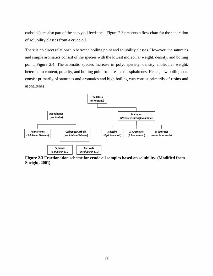
11
carboids) are also part of the heavy oil feedstock. Figure 2.3 presents a flow chart for the separation
of solubility classes from a crude oil.
There is no direct relationship between boiling point and solubility classes. However, the saturates
and simple aromatics consist of the species with the lowest molecular weight, density, and boiling
point, Figure 2.4. The aromatic species increase in polydispersity, density, molecular weight,
heteroatom content, polarity, and boiling point from resins to asphaltenes. Hence, low boiling cuts
consist primarily of saturates and aromatics and high boiling cuts consist primarily of resins and
asphaltenes.
Figure 2.3 Fractionation scheme for crude oil samples based on solubility. (Modified from
Speight, 2001).
Feedstock (n-Heptane)
Asphaltenes (Insolubles)
Maltenes(Percolate through alumina)
Asphaltenes (Soluble in Toluene)
Carbenes/Carboid(Insoluble in Toluene)
Carbenes(Soluble in CS2)
Carboids(Insoluble in CS2)
3: Resins(Pyridine wash)
2: Aromatics(Toluene wash)
1: Saturates(n-Heptane wash)

12
Figure 2.4. Distribution of main compound classes within the different types of crude oil.
(Modified from Speight, 2001).
2.2 Heavy Oil and Bitumen Chemistry
Elemental and Heteroatomic Composition
Typical elemental analysis for heavy oil and bitumen is provided in Table 2.1. Their H/C ratio
ranges from 1.4 to 1.6 consistent with low paraffin and high naphthene and aromatic content. For
context, the H/C ratio of benzene, n-heptane, and a typical light conventional oil are 1, 2.3 and 1.9,
respectively. Heavy oil and bitumen have a narrow range for their elemental composition (Altgelt
and Boduszynski, 1994; Speight, 2001; Strausz and Lown, 2003; Read and Whiteoak, 2003).
Recall that these fluids are defined by their relatively high density and viscosity. Higher H/C ratios
are only observed in less dense oils. Bitumen is approaching the lower limit of aromaticity that is
observed in naturally occurring liquid hydrocarbons; and, therefore, the lower range of the H/C
ratios is also limited.
Boiling Point – Carbon Number
Co
mp
osi
tio
n, w
t%
Paraffins
Naphthenes
Heteroatomiccompounds
Naphtheno-aromatics
Aromatics

13
Table 2.1 Standard compositional ranges for CHSN and O for heavy oil and bitumen.
Element Range Atomic Ratio Average Value
Carbon 83.1 ± 3 - -
Hydrogen 10.3 ± 0.5 H/C 1.48
Nitrogen 0.5 ± 0.2 N/C 0.005
Oxygen 1.1 ± 0.3 O/C 0.009
Sulfur 0.05 to 14 S/C 0.02
Metals (Ni and V) >1000 ppm - -
Sulfur compounds are distributed in the whole range of boiling fractions with a content varying
from 0.05 to about 14%. Sulfur content tends to increase monotonically from the low boiling to
the high and non-distillable fractions. The distillable fraction of sulfur is found in the form of
sulfoxides. In the heavier fractions, where more than half of the total sulfur is present, the sulfur
is in the form of thiophene derivatives. Small amounts of sulfides and sulfoxides are also present
in the heavier petroleum fractions (Boduszynski, 1987; Strausz and Lown, 2003; Speight, 2001).
Oxygen is the second most abundant heteroatom in bitumen and heavy oils, with a concentration
usually less than 2%. However, the concentration may vary if the oil is exposed to air. The most
common compounds are phenols, carboxylic acids, esters, ketones, ethers, amides (with nitrogen),
and sulfoxides (with sulfur). The oxygen compounds are concentrated in the most polar fractions
of the resins and their concentrations can be as high at 10% (Strausz and Lown, 2003).
Nitrogen is the least abundant heteroatom in heavy oil and bitumen, ranging from 0.1 to 0.7 wt%
and its concentration increases as molecular weight increases. The types of nitrogen in petroleum
are classified as neutral (mostly indoles, acridines and hydroxypyridines), basic (pyridine
derivaties, quinolones, indolines) and acid (pyrrole, carbazoles, benzocarbazoles). Identification
of nitrogen components provides crucial information in refinery operations, even in low
concentrations, since they may poison cracking catalysts and their elimination requires severe
hydrogenation conditions (Strauz and Lown, 2003; Gray, 1994; Speight, 2001).
Other non-hydrocarbon compounds include metals such as iron, nickel and vanadium and occur
primarily in the asphaltene fraction of the oil. Studies of different oils have shown that the most

14
predominant metal is vanadium, followed by nickel and in a minor concentration iron (Abu-Elgheit
et al., 1981; Altgelt and Boduszynski, 1994; Hodgson and Baker, 1957). The forms in which the
metals occur in the oils are called petroporphyrins, although some authors (Dunning et al., 1960;
Dickson et al., 1972; Reynolds and Biggs, 1985) believe that they are also present as metallo-
nonporphyrins. The petroporphyrins consist of four pyrrole units bonded by methine carbons with
a chelated metal. Their presence in petroleum fluids provided a definitive proof for their biological
nature (Treibs, 1934). The presense of metalloporphyrins has negative effects during upgrading
and refining processes since they cause reduction of performance and durability of catalysts used
in catalytic cracking and hydrodesulfurization due to deposition of the metals when porphyrins
thermally decompose (Speight, 2001; Dunning et al., 1960).
Hydrocarbon Composition
In heavy oil and bitumen, the aliphatic hydrocarbons or saturate region can be divided into two
groups: the low boiling saturates and the high boiling saturates. Several studies of different heavy
oil and bitumen samples from Canada and Venezuela have shown that the low boiling point
saturates are mainly paraffins with some mono- and di-naphthenes (Boduszynsky, 1987; Payzant
et al., 1985; Setti et al., 1992) followed by tri- and tetracyclic compounds depending on the level
of biodegradation that the precursor oil experienced (Strausz and Lown, 2003; Johns, 1986).
Interestingly, a comparison made between the cyclic compounds found and the cyclic terpenoid
hydrocarbon biological marker molecules showed that the low boiling point saturate region
contained the rearranged and partly degraded original biomarker. On the other hand, the high
boiling point saturates were comprised of the same base structures as low boiling point saturates,
but with a significantly higher amount of side-chains (Altgelt and Boduszynsky, 1994; Strausz and
Lown, 2003). This increase in side chains increases the paraffinic nature of the naphthenic
structures.
By definition, aromatic hydrocarbons have at least one aromatic ring attached to their molecular
structure. In general, the aromatic compounds in heavy oils and bitumens range from
alkylbenzenes to large condensed polyaromatic and heteroatomic molecules. Several studies have
revealed that the aromatic structures are mixtures of mono- to tetra-aromatics and some penta-
aromatic hydrocarbons (Payzant et al., 1985; Mojelshy et al., 1986; Poirier and Bas, 1984;

15
Boduszynski, 1987). Most importantly, aromatics contain substantial amounts of hetero-
compounds such as nitrogen (carbazoles), nitrogen (thiophenes) and oxygen (carboxylic acids).
The majority of the aromatic rings are fused to a minimum of one naphthenic ring and contain
considerable amounts of carbon as alkyl chains.
Resins are mainly a mixture of molecules that can be acidic, basic, or amphoteric (Strausz and
Lown, 2003). This fraction, along with the aromatic fraction, also contains a significant amount of
heteroatoms and have low H/C ratios. Since resins are a very poly-dispersed system, their
characterization requires combinations of efficient fractionation techniques and high resolution
analytical methods (Rodgers and McKenna, 2011; Merdrignac and Espinat, 2007; Payzant et al.,
1985). Some possible structures found in the resins are described later in this section.
Asphaltenes are defined as the fraction of the bitumen that is insoluble in n-alkanes, but is soluble
in more polar solvents such as toluene or benzene. In terms of volatility, they are part of the non-
distillable fraction of the crude oil. They are comprised of a large amount of hetero-compounds
that may contain more than one heteroatom per molecule and contain most of the metals in the
crude oil (Speight, 2001; Strausz and Lown, 2003; Altget and Boduszynski, 1994). The amount
and composition of asphaltenes vary based on the origin of the crude oil. Due to all the operational
problems this fraction causes during extraction transportation and refining processes, myriads of
studies have been devoted to understand their behavior (Shaw, 2002; Zou and Shaw, 2004, Kokal
et al., 1992; Mansoori, 1997; Maham et al., 2005; Anderson and Speight, 1999), molecular
composition and structure (Mullins, 2008; Mullins and Sheu, 1998), and physical properties
(Escobedo and Mansoori, 1998; Barrera et al., 2013; Parkash et al., 1979). It is important to note
that because asphaltenes are a solubility class, their yield and composition depend on the method
and conditions used to remove them from the oil including the amount and type of solvent,
temperature, pressure, time, and washing procedure (Alboudwarej et al., 2003, ASTM D2007M).
The structure of asphaltenes is widely debated and difficult to determine due to their
polydispersity. Two main structures have been postulated: the archipelago structure (polyaromatic
nuclei interconnected with aliphatic chains) and the continent structure (flat disk shape with
dominant aromatic core). Given their polydispersity, it is likely that both structures are present.

16
Asphaltene molecular weight has been of particular interest due to the tendency of asphaltenes to
self-aggregate. The molecular weight of the monomers has been reported to be in the order of 1000
g/mol, while aggregate molecular weight can be as high as 30,000 g/mol (Barrera et al., 2013).
Asphaltene molecules appear to be structures with active sites through which they interact with
similar molecules to form nano-aggregates (Mullins et al., 2007; Yarranton et al., 2007, Barrera
et al., 2013, McKenna et al., 2013).
A common method to obtain the fractions is SARA fractionation. Through this method the oil is
separated based on the solubility and polarity of these fractions in different solvents and media.
Table 2.2 shows the SARA analysis of some heavy oils and bitumen.
Table 2.2. SARA compositional analysis for bitumen samples and heavy oils (Akbarzadeh,
et al., 2005).
Fraction
(wt%)
Athabasca
Bitumen
Peace River
Bitumen
Venezuelan
Heavy Oil
Saturates 16.3 18.2 15.4
Aromatics 39.8 42.7 44.4
Resins 28.5 21.5 25
Asphaltenes 14.7 17.6 15
2.3 Petroleum Characterization
The phase behavior and physical properties of heavy oils and bitumen during extraction,
production and refining are essential inputs for the adaptation and development of new
technologies. However, their prediction for multicomponent mixtures is complex and poses
significant experimental and modelling challenges. Prediction of phase behavior and physical
properties is typically accomplished with Equations of State (EoS) or generalized correlations. The
required inputs to perform phase behavior calculations with an EoS are the critical temperature
and pressure and acentric factors of each component, as well as binary interaction parameters for
each pair of components in the mixture.
The critical properties of most petroleum components are pseudo-critical properties that cannot be
measured (Aladwani and Riazi, 2005). Instead, their critical properties are estimated from
17
correlations of their measurable properties, usually boiling point, density, and molecular weight.
It is impractical, if not impossible, to estimate these EoS parameters for each single component in
a heavy crude oil. Therefore, to study and characterize the physical and chemical behavior of heavy
oil and bitumen, a preliminary step of matrix simplification is recommended. In other words, the
mixture is divided into a set of pseudo-components that represent the distribution of properties in
the mixture. Oil characterization is the process of dividing the fluid into components and pseudo-
components and assigning properties to each of these components.
2.3.1 Characterization Assays
There are three main approaches to divide a petroleum fluid into pseudo-components: solubility
assays, chromatography, and distillation. Mass spectrometric techniques have been proposed as a
characterization technique (Espinat and Mendrignac, 2007); however, practical use of these data
is still under development.
Solubility Assays
Solubility assays include fractionation of the oil into:
paraffins, iso-paraffins, olefins, naphthenes, and aromatics (PIONA), or
paraffins, olefins, naphthenes, and aromatics (PONA), or
paraffins, naphthenes, and aromatics (PNA), or
saturates, aromatics, resins, and asphaltenes (SARA).
Solubility separation is particularly useful since asphaltenes can be separated from the oil to
facilitate the characterization of the maltene fraction. Removing the asphaltenes lowers the oil
viscosity and facilitates distillation. Several standard methods are used to precipitate the
asphaltenes and fractionate the deasphalted heavy oil (ASTM D-2006; ASTM D-2007; ASTM D-
4124; IP-143). For heavy oils and bitumen, the most common fractionation technique is SARA
fractionation. To obtain the SARA fractions, techniques such as high-performance liquid
chromatography or thin-layer chromatography with flame ionization detector have been
implemented (Vela et al, 1998). Although, the chemical information provided by this type of
fractionation provides some information for characterization of heavy oils and bitumen, the boiling
point, a critical property for characterization cannot be obtained this way.

18
Gas Chromatography Assays
Gas chromatography is used to separate individual hydrocarbon components by their retention
time which correlates to their carbon number or boiling point. A distillation curve produced by GC
is called a simulated distillation curve. This method is simple, fast, reproducible and more
economical than a laboratory-scale physical distillation. Currently, there are four commonly used
ASTM methods for characterization of heavy fractions: D2887, D5307, D6352, and D7169.
ASTM D7169 extends the applicability of simulated distillation to petroleum samples that do not
elute completely from the system, normally referred to as the residue. This method covers a wide
temperature boiling range, up to 993 K, which represents the elution of n-C100 (Vickers, 2002)
Although GC analysis provides fast and economical results, this technique requires calibration in
order to identify the components and the equivalent boiling points. Calibration is based on the
retention time of the normal paraffins and their respective boiling points. The interpretation of the
results for a heavy oil or bitumen must be done with caution as these samples are known to have
large amounts of aromatic compounds. Therefore, the boiling point of a given paraffin may not
correspond to that of the aromatic fraction that elutes at the same time.
Distillation Assays
Distillation is the most common approach to characterizing oils. It provides the boiling point
distribution of the sample and generates fractions that have a reduced molecular weight range and
a variety of chemical groups (Aladwani and Riazi, 2005). Distillation separates the oil components
by the differences in their vapor pressure, which decreases with increasing molecular weight. Note,
intermolecular forces also play an important role in the heat of vaporization, causing molecules of
similar molecular weight but different structure or atomic make-up to boil at a higher or lower
temperature. These forces are particularly important for compounds with high polarity.
Based on the continuum concept proposed by Boduszynsky (1987) distillation will provide
fractions of increasing average molecular weight, aromaticity, and heteroatom content. Figure 2.5
depicts how distillation fractionates the compositional matrix. Note how, although the average
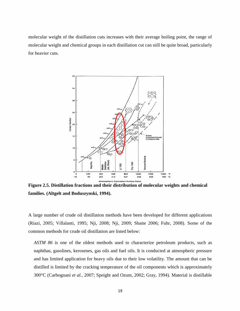
19
molecular weight of the distillation cuts increases with their average boiling point, the range of
molecular weight and chemical groups in each distillation cut can still be quite broad, particularly
for heavier cuts.
Figure 2.5. Distillation fractions and their distribution of molecular weights and chemical
families. (Altgelt and Boduszynski, 1994).
A large number of crude oil distillation methods have been developed for different applications
(Riazi, 2005; Villalanti, 1995; Nji, 2008; Nji, 2009; Sbaite 2006; Fuhr, 2008). Some of the
common methods for crude oil distillation are listed below:
ASTM 86 is one of the oldest methods used to characterize petroleum products, such as
naphthas, gasolines, kerosenes, gas oils and fuel oils. It is conducted at atmospheric pressure
and has limited application for heavy oils due to their low volatility. The amount that can be
distilled is limited by the cracking temperature of the oil components which is approximately
300°C (Carbognani et al., 2007; Speight and Ozum, 2002; Gray, 1994). Material is distillable

20
up to approximately 250ºC with this atmospheric pressure method. Since this method does not
represent actual boiling point of components in a petroleum fraction interconversion to true
boiling point data (TBP) is required using the correlation proposed by Riazi (2005), Equation
2.1.
ASTM D1160 was developed to extend the applicability of ASTM D86 to heavier petroleum
products. The distillation is carried out at 0.133 kPa with a separation equivalent to one
theoretical plate. Material is distillable up to approximately 400ºC Atmospheric Equivalent
Temperature (AET). When this technique is used for heavy oils and bitumen only 20 to 25% of
the original volume can be distilled before reaching the cracking temperature; hence far more
than half of the sample is left uncharacterized. Since this method is performed at sub-
atmospheric pressures, Maxwell and Bonnell correlation (1957) is used to convert the actual
distillation temperature to AET. To convert the AET distillation curves to TBP a two-step
procedure needs to be carried out to first get TBP at 10 mmHg and then TBP at 760 mmHg
(Edmister and Okamoto, 1959; Riazi, 2005).
ASTM D2892 is also called the TBP method or 15/5. The distillation is carried out at
atmospheric pressure first and then pressure is dropped to 0.25 kPa with a separation equivalent
of 14 to 18 theoretical plates (nominally 15). A reflux ratio of 5:1 is used. Material is distillable
up to about 400ºC AET. The actual distillation temperature is kept below the cracking
temperature but is equivalent to a higher temperature at atmospheric pressure. When vacuum is
used the vapor temperatures are converted to AET using Maxwell and Bonnell (1957)
correlations. The AET obtained in this method correspond to TBP data.
ASTM 5236 is an extension of ASTM D2892 and operates at pressures as low as 0.0133 kPa.
This method can be applied to heavy hydrocarbons with an initial boiling point higher than
150ºC and distills material up to approximately 565ºC AET. If the sample has low boiling
material, it is required to first run ASTM D2892 and then ASTM D5236. Hence, a large volume
sample (4 L) is required to run the distillation. The Maxwell and Bonnell correlation (1957) is
used to convert the actual distillation temperature to AET. The calculated AET temperature are
reported as TBP data because the measured temperatures correspond to a true thermodynamic
state point (Satyro and Yarranton, 2009). The drawback is that this method does not have the
21
same fractionation capabilities as ASTM D2892; therefore, the TBP temperatures are higher
than they would be if a more efficient fractionation was performed (Golden, 2012).
Spinning Band Distillation (SBD) operates with a spiral Teflon or metal band that increases the
liquid-vapor contact and can achieve efficiency of 50 theoretical plates in a 100 cm length
column. The reflux ratio can be adjusted to the desired value, but is normally operated at 5:1 if
distillation is performed to simulate ASTM D2892. The distillation pressure can also be
adjusted with a minimum value of 0.13kPa (1 mmHg). The system is equipped with four
receivers that allow collection of the distilled fractions. Heavy oils and bitumen can be distilled
using this technique to remove the light distillable fraction; however, approximately 35% of the
initial volume can be distilled leaving 65% of the oil uncharacterized. As in any other
distillation procedure, at atmospheric or vacuum condition, the pot temperature should not
exceed 300 ºC to avoid thermal decomposition of the sample. The AET reaches values up to
450ºC. The vapor temperatures are converted to AET using the correlations developed by
Maxwell and Bonnell (1957). A discussion about the validity of this method as TBP data will
be presented in Appendix A.
Short path distillation (HV-SPD) is a proposed ASTM method for molecular distillation. The
separation is carried out at 0.0001 kPa to approximately 650ºC AET. In this method, the sample
flows at constant rate over a hot surface at high vacuum, where temperature and pressure are
fixed. The system is equipped with rollers that assure a thin film on the wall and the collector
device is closely place so the evaporated molecules condense in the cold finger. For every run
only one fraction and a residue are obtained. Simulated distillation is performed to determine
the TBP temperatures of the obtained fractions.

22
A summary of the boiling ranges covered by the most commonly used GC and physical distillation
techniques is compared in Figure 2.6.
Figure 2.6 Summary of the boiling ranges of physical and simulated distillation techniques.
(Modified from Villalanti et al., 2000). Bottom four blue bars are standard physical
distillation methods, two middle red bars are standard simulated distillation methods, and
two upper green bars are alternative non-standard physical distillation methods.
The distillation curve obtained from any of these methods (GC or physical distillation) is then
extrapolated over the residue (the fraction of the oil that was not distilled) using a Gaussian
extrapolation (Castellanos et al., 2011). The completed curve is divided into pseudo-components
and each of them has an assigned set of physical properties that can be measured if fractions are
available. If fractions are not available, the physical properties can be estimated from correlations
and property distributions. Finally, critical properties and acentric factors of the pseudo-
components are estimated from correlations. Figure 2.7 present a summary of the characterization
procedure based on a distillation assay.
The approach depicted in Figure 2.7 has been extensively used for conventional oils and has been
extended to characterize heavy oils (Castellanos, 2012). For both conventional and unconventional
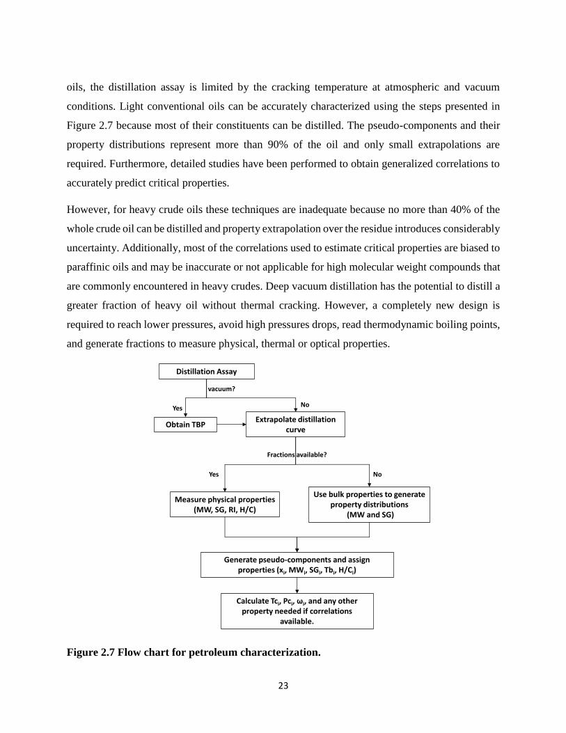
23
oils, the distillation assay is limited by the cracking temperature at atmospheric and vacuum
conditions. Light conventional oils can be accurately characterized using the steps presented in
Figure 2.7 because most of their constituents can be distilled. The pseudo-components and their
property distributions represent more than 90% of the oil and only small extrapolations are
required. Furthermore, detailed studies have been performed to obtain generalized correlations to
accurately predict critical properties.
However, for heavy crude oils these techniques are inadequate because no more than 40% of the
whole crude oil can be distilled and property extrapolation over the residue introduces considerably
uncertainty. Additionally, most of the correlations used to estimate critical properties are biased to
paraffinic oils and may be inaccurate or not applicable for high molecular weight compounds that
are commonly encountered in heavy crudes. Deep vacuum distillation has the potential to distill a
greater fraction of heavy oil without thermal cracking. However, a completely new design is
required to reach lower pressures, avoid high pressures drops, read thermodynamic boiling points,
and generate fractions to measure physical, thermal or optical properties.
Figure 2.7 Flow chart for petroleum characterization.
Distillation Assay
Obtain TBP Extrapolate distillation
curve
Measure physical properties (MW, SG, RI, H/C)
Use bulk properties to generate property distributions
(MW and SG)
vacuum?
NoYes
Fractions available?
NoYes
Generate pseudo-components and assign properties (xi, MWi, SGi, Tbi, H/Ci)
Calculate Tci, Pci, ωi, and any other property needed if correlations
available.

24
New Method: Deep Vacuum Fractionation Apparatus (DVFA). Castellanos et al. (2012) designed
and constructed an apparatus to measure vapor pressure using a static technique in which the
sample is placed under vacuum conditions at constant temperature in a closed vessel and the
pressure exerted by the vapor is directly measured. The DVFA apparatus consists on a liquid-trap
section, a turbo molecular pump and two thermocouples connected to a temperature controller.
The turbo molecular pump can reach pressures as low as 1·10-9 kPa at clean conditions; therefore,
the implementation of this system as a distillation technique could allow distillation data for heavy
oil and bitumen to be extended to an uncharted region. Castellanos et al. (2012) proved that
distillation of up to approximately 50 wt% of a bitumen can be performed using the newly
developed apparatus. An important feature of the DVFA is the liquid-trap section, which if
maintained at low temperatures can condense the vapor produced in the sample vessel allowing
for distillation cuts to be captured.
However, the implementation of this technique as a distillation assay required modifications to the
apparatus and in the fractionation procedure. Also, since the temperature range of pressure gauges
did not allow the collection of pressure readings during distillation, the DVFA required an
alternative inter-conversion method to that of Maxwell and Bonnell to obtain TBP data.
2.3.2 Inter-conversion Methods to Obtain AET and TBP
True boiling points are required for the correlations used to predict other physical and
thermodynamic properties. Since actual TBP data is very difficult to measure in terms of time and
cost, alternative distillation procedures have been developed to replace the TBP experimental
approach. For atmospheric distillation, such as ASTM D86, the measured boiling points are
converted to TBP using empirical correlations. If the distillation is undertaken at sub-atmospheric
pressures, it is also necessary to convert low pressure temperatures to atmospheric equivalent
temperatures (AET) and then determine if they correspond to TBP data. Note, AET are equivalent
to TBP if the measured temperatures correspond to an actual thermodynamic state.

25
Most of the ASTM distillation techniques have their own inter-conversion method which uses the
available distillation temperature and specific gravity of the fraction as inputs to estimate the TBP
data.
𝑇𝑖(𝑑𝑒𝑠𝑖𝑟𝑒𝑑) = 𝑎(𝑇𝑖(𝑎𝑣𝑎𝑖𝑙𝑎𝑏𝑙𝑒))𝑏𝑆𝐺𝑐 (2.1)
The coefficients a, b, and c for each ASTM method were determined by Riazi and Daubert and
can be found elsewhere (Riazi, 2005). This equation can be applied for a distillation performed at
atmospheric conditions.
To interconvert boiling points at reduced pressures to atmospheric equivalent boiling points
(AET), a vapor pressure correlation is required. The vapor pressure correlation developed for
petroleum fractions by Maxwell and Bonnell (1957) is the accepted industry standard. Other vapor
pressure correlations proposed by Myers and Fenske (1955) and Van Kranen and Van Nes (1951)
are less commonly used for inter-conversion.
When vapor pressure data are available, there are two other alternatives for inter-conversion. The
first option is to model the experimental vapor pressure of the cut with an equation of state and
then predict the normal boiling point with the tuned model. Using an equation of state and mixing
rules can be a very accurate way to estimate boiling points from vapor pressure. However, critical
properties and interaction parameters are also required and these values are rarely, if ever, available
for heavy fractions.
The second option involves the extrapolation of sub-atmospheric vapor pressures towards higher
pressures. Ruzicka (1993; 1994) developed a simultaneous treatment of vapor pressure and related
heat capacity data between the triple and normal boiling temperature for n-alkanes. Heat capacity
is related to vapor pressure through the Clausius-Clapeyron equation and can be used to constrain
the extrapolation of low temperature range vapor pressure measurements with heat capacity
measured over a broader temperature range. Different vapor pressure equations were tested by
Ruzicka (1996) and the best performance in the fitting and extrapolation of vapor pressure and
heat capacity data was obtained with the Cox equation (Ruzicka and Majer, 1986; 1994; 1996).

26
2.3.3 Generation of Crude Oil Pseudo-Components: Splitting and Lumping
For modelling purposes, the crude oil can be lumped or split into pseudo-components. Pseudo-
components are a way to simplify the characterization of crude oils, as they represent narrow
boiling range cuts with a known composition and physical properties. The number of pseudo-
components is normally defined between five and twenty depending on the process being
simulated (Whitson and Brule, 2000). Lumping is usually only used for chromatographic
characterizations. Some of the light components such as i-butane, n-butane, i-pentane, n-pentane,
are typically lumped into carbon number ranges such as C4-C6, C7-C10. The uncharacterized part
of the assay (e.g. C30+) can be split into a number of pseudo-components.
Splitting is always used for distillation based characterizations. The distillation curve is divided
into pseudo-components with an assigned set of average properties such as density, molecular
weight, normal boiling point, elemental composition, thermal properties, and critical properties.
The TBP curve can be split using temperature intervals or mass fraction intervals, Figure 2.8. The
assigned average boiling point for a mass fraction interval is given as:
𝑇𝑏𝑖 =1
𝑤𝑖 − 𝑤𝑖−1∫ 𝑇𝑇𝐵𝑃(𝑤)𝑑𝑤
𝑤𝑖
𝑤𝑖−1
(2.2)
where the terms w and T stand for the mass fraction and temperature respectively.
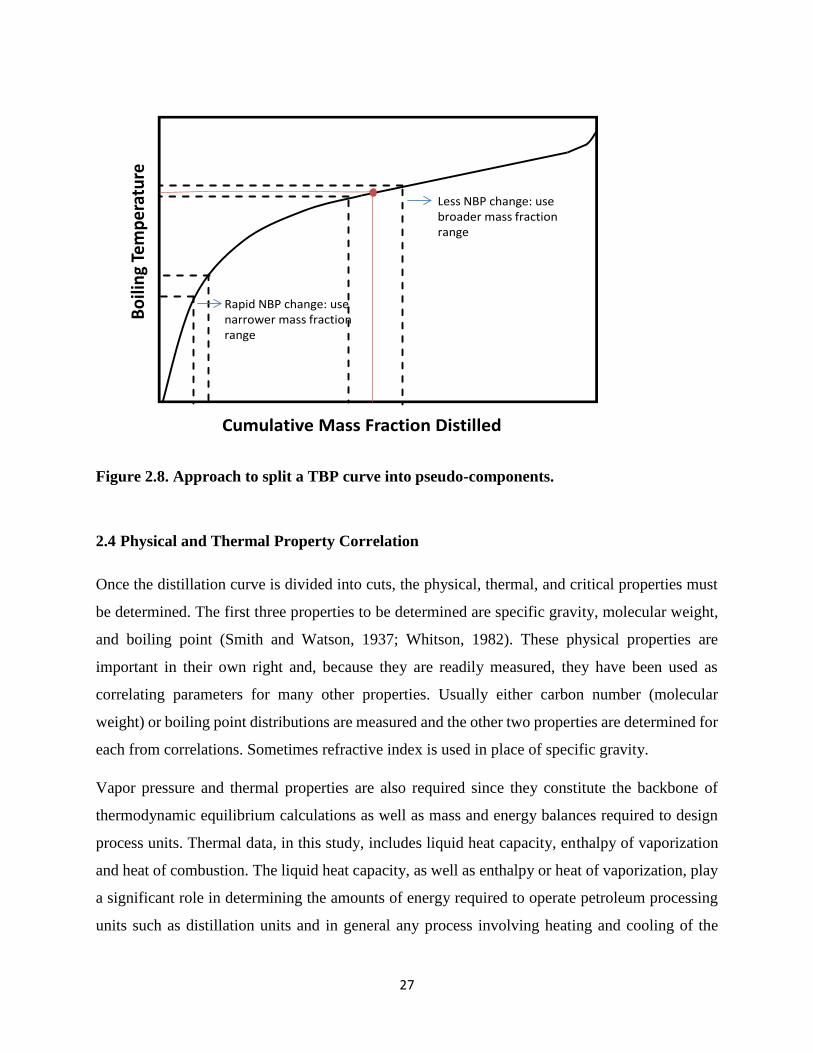
27
Figure 2.8. Approach to split a TBP curve into pseudo-components.
2.4 Physical and Thermal Property Correlation
Once the distillation curve is divided into cuts, the physical, thermal, and critical properties must
be determined. The first three properties to be determined are specific gravity, molecular weight,
and boiling point (Smith and Watson, 1937; Whitson, 1982). These physical properties are
important in their own right and, because they are readily measured, they have been used as
correlating parameters for many other properties. Usually either carbon number (molecular
weight) or boiling point distributions are measured and the other two properties are determined for
each from correlations. Sometimes refractive index is used in place of specific gravity.
Vapor pressure and thermal properties are also required since they constitute the backbone of
thermodynamic equilibrium calculations as well as mass and energy balances required to design
process units. Thermal data, in this study, includes liquid heat capacity, enthalpy of vaporization
and heat of combustion. The liquid heat capacity, as well as enthalpy or heat of vaporization, play
a significant role in determining the amounts of energy required to operate petroleum processing
units such as distillation units and in general any process involving heating and cooling of the
Bo
ilin
g Te
mp
erat
ure
Cumulative Mass Fraction Distilled
Less NBP change: use broader mass fraction range
Rapid NBP change: use narrower mass fraction range

28
crude oil (Parhizgar et al., 2013; Kikic and Vetere, 2011). Heat of combustion constitutes a crucial
property for hydrocarbons because its value helps to identify the quality of the hydrocarbon as a
fuel source and it is also used to derive the heat of formation for reaction enthalpy calculations
(Tsonopoulos, 1986; Strausz and Low, 2003). Several correlations are available in the literature to
predict these properties; usually, the inputs for these correlations are the specific gravity, molecular
weight and normal boiling point.
Critical properties are required for equation of state models. Since it is particularly difficult to
measure the critical state of complex mixtures, several methods and correlations to predict critical
properties of hydrocarbon mixtures have been developed (Anselme and Teja, 1990; Gambill, 1959;
King, 1957; Lixiong and Kiran, 1990; Zais, 1972; Whitson and Brule, 2000; Riazi, 2005). Most of
the correlations are polynomial or exponential equations based on one or more properties that can
be measured directly. The best option to determine the critical properties for pseudo-components
is to tune them to match phase behavior or vapor pressure data using equations of state.
Since pseudo-component critical properties cannot be measured, correlations cannot be validated
and are not considered in this thesis. The correlations for physical, thermal properties and vapor
pressure are summarized below.
Note, most of the correlations presented below apply only to compounds with molecular weight
less than 700 g/mol or normal boiling points less than 800 K. Furthermore, the majority of the
correlations are biased toward paraffins and light to medium oils due to availability of
experimental data used to build the generalized correlations.
Also note that whatever correlations are selected, the characterization procedure is subject to the
constraint that the appropriately weighted average of the pseudo-component properties should
result in the known bulk property of the crude oil as described in the following equations:
1 = ∑ 𝑧𝑖
𝑁
𝑖=1 (2.3)
and
𝑆𝐺𝐵𝑢𝑙𝑘 = ( ∑𝑤𝑖
𝑆𝐺𝑖
𝑁𝑖=1 )
−1
, 𝑀𝑊𝐵𝑢𝑙𝑘 = ∑ 𝑧𝑖𝑀𝑊𝑖𝑁𝑖=1 (2.4)

29
where z is the moles of pseudo-component i, N is the total number of pseudo-components, and the
subscript Bulk indicates the properties of the whole oil sample.
2.4.1 Physical Properties
Normal Boiling Point, Tb
The prediction of Tb is required when performing characterizations based on calculated molar
distributions, solubility class separations (SARA, PIONA), or when density and molecular weight
of the fractions are available. A common factor in the majority of the correlations to predict this
property is the use of MW and SG as input parameters. This is because the MW is a good parameter
to characterize compounds within the same hydrocarbon family, whereas SG is a property that
makes a distinction between hydrocarbon families. Their combinations provide a suitable pair of
input parameters that, combined in different forms, can be used to predict the normal boiling point
of a wide range of structures.
These correlations are very useful when expensive and time consuming distillations assays are not
available. However, all the correlations that have been developed to predict the normal boiling
point are mainly based on data for light to medium oils and pure components. Therefore, their
application for heavy oils and bitumen may be accurate for low boiling cuts, but may be biased
towards paraffinic properties for the heavier and more aromatic fractions. Table 2.3 presents the
most common correlations to estimate Tb from molecular weight, MW, and specific gravity, SG.
Note that some of the correlations were designed to predict MW from Tb and are implicit in Tb.
Table 2.3. Summary of correlations to estimate normal boiling point.
Source Correlation Range of
Applicability Eq.
Soreide
(1989)
𝑇𝑏 = [1928.3 − 169500 ∗ 𝑀𝑊−0.03522 ∗ 𝑆𝐺3.266𝐷] 1.8⁄
361< Tb<830 (2.5)

30
D = exp(−0.004922 ∗ 𝑀𝑊 − 4.7685 ∗ 𝑆𝐺 + 0.003462∗ 𝑀𝑊 ∗ 𝑆𝐺)
Kesler
and Lee
(1976)
Implicit
in Tb
𝑀𝑊 = [𝐷] +[𝐴]
𝑇𝑏+
[𝐵]
𝑇𝑏3
𝐷 = −12272.6 + 9486.4 ∗ 𝑆𝐺+ (4.6523 − 3.3287 ∗ 𝑆𝐺) ∗ 𝑇𝑏
𝐴 = (1 − 0.77084 ∗ 𝑆𝐺 − 0.02058 ∗ 𝑆𝐺2)
∗ (1.3437 −720.79
𝑇𝑏) ∗ 107
𝐵 = (1 − 0.80882 ∗ 𝑆𝐺 + 0.02226 ∗ 𝑆𝐺2)
∗ (1.8828 −181.92
𝑇𝑏) ∗ 1012
Tb<750 (2.6)
Riazi
and
Daubert
(1980)
Implicit
in Tb
𝑀𝑊 = 0.000045673 ∗ 𝑇𝑏2.1962 ∗ 𝑆𝐺−1.0164 300< Tb<610 (2.7)
Riazi
and
Daubert
(1986)
For MW<300
𝑇𝑏 = 3.76587 ∗ 𝐷 ∗ 𝑀𝑊0.40167 ∗ 𝑆𝐺−1.58262
𝐷 = exp(0.0037741𝑀𝑊 + 2.98404𝑆𝐺− 0.00425288𝑀𝑊𝑆𝐺)
For MW>300
𝑇𝑏 = 9.3369 ∗ 𝐷 ∗ 𝑀𝑊0.5369 ∗ 𝑆𝐺−0.7276
D = exp(0.00016414𝑀𝑊 + 1.4103𝑆𝐺− 0.00075152𝑀𝑊𝑆𝐺)
200< Tb<610 (2.8)
API
(1977)
𝑀𝑊 = 204.38 ∗ 𝑇𝑏0.118 ∗ 𝑆𝐺1.88 ∗ exp (0.00218
∗ 𝑇𝑏 − 3.07 ∗ 𝑆𝐺)
309< Tb<900 (2.9)
Rao and
Bardon
(1985) 𝑙𝑛 𝑀𝑊 = (1.27 + 0.071𝐾𝑤)𝑙𝑛 (
1.8𝑇𝑏
22.31 + 1.68𝐾𝑤) 361< Tb<830 (2.10)

31
Twu et
al.
(1984)
𝑇𝑏 = 𝑒𝑥𝑝 (5.1264 + 2.71579𝛽 − 0.28659𝛽2
−29.8544
𝛽−
0.122488
𝛽2)
− 13.7512𝛽 + 19.6197𝛽2
𝛽 = ln (𝑀°)
𝑀°
=𝑇𝑏
5.8 − 0.0052𝑇𝑏 𝑎𝑠 𝑎 𝑠𝑡𝑎𝑟𝑡𝑖𝑛𝑔 𝑖𝑡𝑒𝑟𝑎𝑡𝑖𝑛𝑔 𝑝𝑜𝑖𝑛𝑡
MW<600 (2.11)
Nji et al.
(2010)
𝑇𝑏 = (477.63 ∗ ln (𝑤 + 88.51
𝑤 + 1007) + 1214.4)
∗ (1 + 2 ∗ 𝑥
1 − 2 ∗ 𝑥)
2
𝑤 = −0.07412 ∗ Δ𝑆𝐺2 − 0.0075041 ∗ Δ𝑆𝐺− 2.6031 ∗ Δ𝑀𝑊2 + 0.090188∗ Δ𝑀𝑊 − 1.0482 ∗ Δ𝑆𝐺 ∗ Δ𝑀𝑊
Δ𝑆𝐺 = ln [0.83 +
89.9513𝑤 −
139.6612(𝑤 + 3.2033)1.0564
𝑆𝐺]
Δ𝑀𝑊 = ln (𝑤
𝑀𝑊)
𝑤 = 14 ∗ 𝐶𝑁 + 2
200< Tb<900 (2.12)
Molecular Weight
Molecular weight is a very useful property that can be used not only for critical property prediction,
but to convert from mole to mass units for equipment design. Additionally, molecular weight
values have impact on chemical equilibrium, vapor density calculations and hydrocarbon
processing systems (Schneider, 1998; Goossens, 1996). However, the measurement of molecular
weight is not simple and depending on the method used, either vapor pressure osmometry or
freezing point depression, some discrepancies may arise (Altgelt and Boduszynski, 1994). These

32
differences can be attributed to the assumptions that have to be made in the experimental
techniques and the association effects that solvents and temperature may have on the molecular
weight of complex mixtures. This property has the highest measurement uncertainty of the three
main physical properties.
Most of the correlations presented in Table 2.3 were developed for light to medium oils; therefore,
their application for heavy oils and bitumen may be accurate for low boiling cuts but may be biased
towards paraffinic properties for the heavier more aromatic fractions. Note that the application of
correlations in Table 2.4 is limited to deasphalted fractions. Asphaltenes self-associate and their
associated molecular weight is higher than the trend extrapolated from the non-associating
maltenes.
Table 2.4. Summary of correlations to estimate molecular weight.
Source Correlation Range of
Applicability Eq.
Soreide
(1989) See Equation 2.5 361< Tb<830 (2.5)
Kesler and
Lee (1976) See Equation 2.6 Tb<750 (2.6)
Riazi and
Daubert
(1980)
See Equation 2.7 300< Tb<610 (2.7)
Riazi and
Daubert
(1986)
See Equation 2.8 300< Tb<610 (2.8)
Rao and
Bardon
(1985)
See Equation 2.10 361< Tb<830 (2.10)
Twu (1984)
ln(𝑀) = 𝑙𝑛𝑀°[(1 + 2𝑓𝑀)/(1 − 2𝑓𝑀)]2
𝑓𝑀 = ∆𝑆𝐺𝑀 [𝜒 + (−0.0175691
+ 0.143979 𝑇𝑏
12⁄
⁄ )∆𝑆𝐺𝑀]
𝜒 = |0.012342 − 0.2445541/𝑇𝑏
12⁄
|
∆𝑆𝐺𝑀 = 𝑒𝑥𝑝[5(𝑆𝐺° − 𝑆𝐺)] − 1
𝑆𝐺° = 0.843593 − 0.128624𝛼 − 3.36159𝛼3
− 13749.5𝛼12
𝛼 = 1 − 𝑇𝑏/𝑇𝑐°
MW<600 (2.13)

33
𝑇𝑐° = 𝑇𝑏(0.533273 + 0.34383𝑥10−3𝑇𝑏
+ 2.52617𝑥10−7𝑇𝑏2
− 1.658481𝑥10−10𝑇𝑏3
+ 4.60776𝑥1024𝑇𝑏−13)−1
Goosens
(1996)
𝑀𝑊 =0.01077 ∗ 𝑇𝑏
𝑥
𝜌
𝑥 = 1.52869 + 0.06486 ∗ 𝑙𝑛(𝑇𝑏
1087 − 𝑇𝑏)
300< Tb<900 (2.14)
Hariu and
Sage (1969)
𝑀𝑊= 0.6670202 + 0.1552531𝐾𝑤− 0.005378496𝐾𝑤2
∗ 0.004583705𝑇𝑏𝐾𝑤+ 0.00002500584𝑇𝑏𝐾𝑤2
+ 0.000002698693𝑇𝑏2
+ 0.0000387595𝑇𝑏2𝐾𝑤
− 0.00000001566228𝑇𝑏2 ∗ 𝐾𝑤2
30< Tb<800 (2.15)
Katz and
Firoozabadi
(1978)
𝑀𝑊 = −0.000005763156 ∗ (𝐶𝑁 − 5)5
+ 0.0007293105∗ (𝐶𝑁 − 5)4
− 0.03341596∗ (𝐶𝑁 − 5)3
+ 0.5740517∗ (𝐶𝑁 − 5)2
+ 10.24725∗ (𝐶𝑁 − 5) + 72.53757
CN<45 (2.16)
Specific Gravity
As discussed previously, specific gravity is used to classify crude oils. It is also used to convert
from mass to volume for process calculations. Density seems to correlate to many different
properties including sulfur content, viscosity, nitrogen content, H/C ratio, and refractive index.
Several correlations for SG are based on MW and a characterization factor which is tuned to fit
the correlation to the bulk density (Jacoby, 1952; Soreide, 1989; Whitson, 1983). Other
correlations relate SG to carbon number alone (Katz and Firoozabadi, 1978) or to refractive index

34
and either MW or NBP (Riazi and Daubert, 2005). For these correlations, there is no tuning to
assure that the predicted bulk density matches the measured value. Gray’s correlation (Gray, 2002)
relates product quality with elemental composition and was developed mainly to predict the
product quality of upgrading processes. The described SG correlations are presented in Table 2.5.
Note that most of these correlations were developed from the properties of pure hydrocarbons and
light to medium petroleum cuts and therefore may not apply to heavy oils.
Table 2.5. Summary of correlations to estimate specific gravity.
Source Correlation Range of
Applicability Eq.
Soreide
(1989)
𝑆𝐺 = 0.28554 + 𝐶𝑓∗ (𝑀𝑊 − 65.94185)0.129969
300<MW<600 (2.17)
Whitson
(1983) 𝑆𝐺 = 6.0108 ∗ 𝑀𝑊0.17947 ∗ 𝐾𝑊
−1.18241 MW<250 (2.18)
Jacoby
(1952)
𝑆𝐺 = 0.8468 −15.8
𝑀𝑊+ 𝐽𝑎
∗ (0.2456 −1.77
𝑀𝑊)
(2.19)
Katz and
Firoozabadi
(1978)
𝑆𝐺 = 0.6839638(𝐶𝑁 − 5)0.08661026 C6<CN<C45 (2.20)
Riazi and
Daubert
(2005)
𝑆𝐺 = 24381000 ∗ 𝐷 ∗ 𝑇𝑏−0.3418 ∗ 𝑅𝐼6.9195
𝐷 = exp(−0.0004194𝑇𝑏 − 23.5535𝑛
+ 0.0039874𝑇𝑏𝑛)
300<MW<700 (2.21)
Riazi and
Daubert
(2005)
𝑆𝐺 = 1128400 ∗ 𝐷 ∗ 𝑀𝑊−0.0771 ∗ 𝑅𝐼6.3028
D = exp(−0.001588 ∗ 𝑀𝑊 − 20.594 ∗ 𝑛
+ 0.007344 ∗ 𝑀𝑊 ∗ 𝑛)
70<MW<700 (2.22)
Gray
(2002)
𝑆𝐺 = (1033 − 13.69 ∗ 𝐻 + 13.85 ∗ 𝑆
+ 115.7 ∗ 𝑁)/(1000
∗ 0.998207)
Only for
petroleum
fractions
(2.23)

35
Refractive Index
The refractive index (n) is a property that, like density, gives information about the intermolecular
interactions in a system. Since hydrocarbons do not have a significant amount of polar compounds,
the major molecular interactions can be attributed to the London dispersion forces which can be
described through polarizability by the following equation:
𝜏 = (3
4𝜋𝑁𝐴) (
𝑛2−1
𝑛2+2) (
𝑀𝑊
𝜌) (2.24)
where, τ is the polarizability, NA is the Avogadro’s number, n is the refractive index, MW is the
molecular weight and ρ is the density. The last two terms in Equation 2.22 are defined as the molar
refraction, Rm, as follows:
𝑅𝑚 = 𝐹𝑅𝐼 (𝑀𝑊
𝜌) (2.25)
where FRI is a function of the refractive index, FRI = (n² - 1)/(n² + 2). From Equations 2.24 and
2.25, it is evident there is a relationship between polarizability and molar refraction. These
relationships indicate that refractive index can describe the intermolecular forces of nonpolar
hydrocarbons, as density does. As with density, the refractive index could be correlated to an
additional energy parameter such as boiling point temperature and hence can be used as a
correlating parameter for the characterization of fossil fuels.
It has been noted by several authors that there is strong correlation between density and the
refractive index or FRI, and that refractive index can be used as a substitute for density in equation
of state modelling (Riazi and Yousef, 2001). Others have found a direct relation between FRI and
solubility parameter and have used this relationship to develop a method to predict the onset of
asphaltene precipitation from the refractive index of the mixture (Vargas and Chapman, 2010;
Taylor et al., 2001). In this thesis, the focus is on the relationship between refractive index and
density.
Vargas and Chapman (2010) used the relation presented in Equation 2.24 to propose a simple
relation between FRI and density. They plotted the molar refraction as a function of the molecular
weight and found that the slope of the curve approximated a constant value of 1/3 for all pure
components. This relationship is shown for pure hydrocarbons and petroleum solubility cuts in

36
Figure 2.9. It follows from this proportionality and from Eq. 2.24 that the FRI can be determined
simply by dividing the density by 3. This method is known as the one-third rule.
Figure 2.9. Molar refractivity versus molecular weight for pure components and petroleum
saturate and aromatic cuts. SARA fractions from Powers (2014) and pure components
from NIST.
Although Rm and MW have nearly the same ratio for all components, the density predictions using
the one-third rule are not accurate for the lightest and heaviest petroleum components. Angle et al.
(2006) proposed a linear correlation between density and refractive index. Vargas and Chapman
(2010) proposed a cubic equation to account for the deviations observed from the one-third rule.
The above correlations related to the refractive index are summarized in Table 2.6.
Table 2.6. Summary of correlations to estimate refractive index.
Source Correlation Range of
Applicability Eq.
One Third
Rule
𝐹𝑅𝐼
𝜌= 1/3 (2.26)
0
50
100
150
200
250
300
350
0 500 1000 1500
Rm
[c
m3
/mo
l]
Molecular Weight [g/mol]
Paraffins
Naphthenes
Aromatics
Saturates (SARA)
Aromatics (SARA)
1/3 Rule

37
Vargas and
Chapman
(2010)
𝐹𝑅𝐼
𝜌= 0.5054 − 0.3951𝜌 + 0.2314𝜌2
Pure
Components (2.27)
Angle et al.
(2006) 𝐹𝑅𝐼 = (
𝜌 + 0.0647
3.24)
Petroleum
fractions (2.28)
2.4.2 Vapor Pressure and Thermal Properties
Several correlations to estimate vapor pressure, liquid heat capacity, enthalpy of vaporization and
heats of combustion have been developed using either critical values or easily obtainable
parameters such as the normal boiling point and molecular weight. Since critical values for
petroleum fractions are unknown, correlations using physical properties have been reported as
more accurate and practical for thermal property estimation (Riazi, 2005; Vetere, 1979, 1995).
The most well-known correlations for vapor pressure and thermal properties are discussed below.
Vapor Pressure
Vapor pressure constitutes the backbone of thermodynamic equilibrium calculations. It is used to
check the consistency of phase equilibrium calculations and is frequently used together with liquid
density to determine equation of state parameters. The equilibrium provided by vapor pressure is
a requirement for design and operation of several refinery units such as atmospheric and vacuum
distillation columns.
One approach to determining the vapor pressure is through equations of state. However, a major
disadvantage of CEOS in predicting vapor pressure is that the main inputs for equations of state
are the critical temperature, critical pressure, and acentric factor. These values are not available
for complex mixtures and cannot be measured for heavy components. Therefore, values for critical
temperature, critical pressure, and acentric factor, must be estimated from correlations, introducing
additional uncertainty in the model predictions.
Other options to predict vapor pressure are generalized correlations. A plethora of vapor pressure
correlations have been developed to both fit and predict vapor pressure data of pure fluids. The
basis of most predictive methods follows from corresponding states theory and the Clapeyron
equation. These equations normally have a high degree of accuracy over a moderate range of
38
temperatures, but their reliability decreases significantly in the very low temperature range
(Velasco et al., 2008; Vetere, 1991).
The most commonly used predictive correlations used for pure hydrocarbons and narrow
petroleum fractions are the equations developed by Korsten (2000), Lee-Kesler (1975), and
Ambrose and Walton (1989). These equations are recommended when reliable critical properties
are available. Since these equations were developed using the principle of corresponding states,
the quality of the prediction is markedly affected by the quality of the critical properties.
Consequently, the major application of these equations is for light hydrocarbons, while their
application to complex systems such as hetero-atomic and highly aromatic petroleum fractions is
questionable.
A more general set of correlations were developed by Maxwell and Bonnell (1957) and Riazi
(2005). These equations have the advantage over the above correlations in that they were
developed using petroleum fraction vapor pressures and their inputs are measurable physical
properties. The Maxwell and Bonnell (M-B) is the most common method used to estimate vapor
pressures of petroleum fractions and to interconvert boiling temperatures at vacuum conditions.
This correlation is also known to perform well at subatmospheric pressures (P < 1atm). The M-B
correlation was developed using n-hexane as a reference compound; a temperature correction
factor is required for more aromatic fractions where the Watson Factor is less than 12. Tsonopoulos
and coworkers (1986) determined that the linear temperature dependence proposed by M-B for the
temperature correction factor is not accurate for more complex systems such as coal liquids. They
proposed a quadratic temperature dependence for the temperature correction factor based on a
dataset with Kw between 8.3 and 11.1. The new temperature correction factor improved the vapor
pressure predictions for the subatmospheric and super-atmospheric pressure ranges.
Riazi (2005) proposed one of the simplest equations for vapor pressures using only the normal
boiling point. The accuracy of this correlation for pure components is around 1% and is
recommended when data near the boiling temperature are available. All of the vapor pressure
correlations tested in this project are summarized in Table 2.7.

39
Table 2.7. Summary of correlations to estimate vapor pressure.
Source Correlation Range of
Applicability Eq.
Maxwell
and
Bonnell
(1957)
log10 𝑃𝑣𝑎𝑝 =3000.538𝑄 − 6.761560
43𝑄 − 0.987672
𝑄 =
𝑇𝑏′
𝑇 − 0.00051606𝑇𝑏′
748.1 − 0.3861𝑇𝑏′
𝑇𝑏′ = 𝑇𝑏 − 1.3889𝐹(𝐾𝑤 − 12) log10
𝑃𝑣𝑎𝑝
760
𝐹 = −3.2985 + 0.009𝑇𝑏
12<Kw<13
and
Pvap<1 atm
(2.29)
Riazi and
Daubert
(2005)
log10 𝑃𝑣𝑎𝑝 = 3.2041 (1
− 0.998𝑇𝑏 − 41
𝑇 − 41
1393 − 𝑇
1393 − 𝑇𝑏)
For T close to
Tb
(2.30)
Liquid Heat Capacity
Accurate correlation of the liquid heat capacity is required to determine the net heat fluxes for any
process where heating and cooling take place. For heavy oil in particular, the liquid heat capacity
is used to estimate the amount of heat required to preheat a heavy oil or bitumen during recovery.
For petroleum fractions, liquid heat capacity is normally estimated from physical using the Lee-
Kesler (1976) and Tsonopoulos (1986) correlations. The Lee-Kesler correlation was specifically
developed for petroleum fractions and is recommended for the range shown in Table 2.8.
Tsonopoulos developed a correlation to predict liquid heat capacity of coal liquids and aromatic
compounds, and Riazi (2005) showed that the Tsonopoulos correlation is also able to predict the
liquid heat capacity of hydrocarbons with good accuracy (4%).
Dagostar (2013) developed a correlation based on the principle that the energy requirements of
fundamental structures are due to the internal energy of the molecule (vibrational, rotational, and
translational modes). He demonstrated that for the types of molecules found in petroleum, these
energy modes depended mainly on the atomic composition and were less sensitive to the molecular

40
structure. He then developed a correlation for the liquid heat capacity based on elemental analysis.
The correlation retained the quadratic form of the Lee-Kesler correlation but the parameters were
redefined as a function of the similarity variable (α) which is function of elemental analysis. All
of the liquid heat capacity correlations presented above are summarized in Table 2.8.
Table 2.8. Summary of correlations to estimate specific liquid heat capacity
Source Correlation Range of
Applicability Eq.
Dagostar
(2013)
𝐶𝑝𝑙𝑖𝑞 = 𝐴1 + 𝐴2𝑇 + 𝐴3𝑇2
𝐴1 = 24.5(−0.3416𝛼 + 2.2671𝛼2)
𝐴2 = 0.1064𝛼 − 0.3874𝛼2
𝐴3 = 𝛼 + 2.2671𝛼2
Tr<0.95 (2.31)
Tsonopoulos
(1986)
𝐶𝑝𝑙𝑖𝑞 = 𝐵 ∗ [0.645 − 0.05959𝑆𝐺 + 𝐷]
𝐵 = (0.28299 + 0.23605𝐾𝑤)
𝐷 = (2.32056 − 0.94752𝑆𝐺) (𝑇
1000
− 0.25537)
Coal liquids
and aromatics (2.32)
Lee-Kesler
(1976)
𝐶𝑝𝑙𝑖𝑞 = 𝐴 + 𝐵 × 10−4𝑇 + 𝐶 × 10−7𝑇2
𝐴
= −4.90383
+ (. 099319 + 0.104281𝑆𝐺)𝐾𝑤
+ (4.81407 − 0.194833𝐾𝑤
𝑆𝐺)
𝐵 = (7.53624 + 6.214610𝐾𝑤) (1.12172
−0.27634
𝑆𝐺)
𝐶 = −(1.35652
+ 1.11863𝐾𝑤) (2.9027
−0.70958
𝑆𝐺)
Tr<0.85 (2.33)

41
Heat of Vaporization
Along with heat capacity, the heat of vaporization plays an important role in determining the
amounts of energy required to operate petroleum processing units such as distillation columns. For
petroleum fractions, the enthalpy of vaporization decreases with increasing temperature and at the
critical temperature, where HV and HL become the same, its value is zero. To determine the
enthalpy of vaporization at a given temperature, the enthalpy at a defined temperature, usually the
normal boiling temperature (∆𝐻𝑛𝑏𝑝𝑣𝑎𝑝) is first calculated. Then, the value at the desired temperature
is calculated from the change in sensible heat (i.e. from the liquid and vapor heat capacities).
Hence, most correlations are for the heat of vaporization at the normal boiling point.
Several correlations have been proposed to predict the ∆𝐻𝑛𝑏𝑝𝑣𝑎𝑝
for petroleum fractions (Parhizgar
et al., 2013; Kikic and Vetere, 2011). In general, there are two groups of equations. One group
uses the critical properties and normal boiling point as inputs. The second group uses empirical
correlations that try to relate ∆𝐻𝑛𝑏𝑝𝑣𝑎𝑝
with easily obtainable parameters such as specific gravity,
molecular weight, and normal boiling point. Since critical properties are not available for the
petroleum cuts used in this study, the second group of correlations was tested.
The simplest of these correlations is Trouton’s rule where it is assumed that, for any pure
component, the ratio ∆𝐻𝑛𝑏𝑝𝑣𝑎𝑝 𝑇𝑏⁄ is a constant. This ratio has been modified for the correlations for
petroleum cuts with expressions based on MW, SG, and/or Tb. Riazi (2005) proposed a correlation
based on the normal boiling point and the specific gravity, but it was developed using only pure
hydrocarbons and its application is limited to low molecular weight components. Vetere (1979 and
1995) also developed correlations based only on pure components. Gopinathan and Saraf (2001)
and Fang et al. (2003) published similar correlations, but these correlations were developed with
data from petroleum cuts. The above correlations for the heat of vaporization are summarized in
Table 2.9.

42
Table 2.9. Summary of correlations to estimate heats of vaporization at the normal boiling
point.
Source Correlation Range of
Applicability Eq.
Riazi and
Daubert
(2005)
∆𝐻𝑛𝑏𝑝𝑣𝑎𝑝 = 37.32315 𝑇𝑏
1.14086 𝑆𝐺0.00977089 70<MW<300 (2.34)
Vetere
(1979)
∆𝐻𝑛𝑏𝑝𝑣𝑎𝑝 =
𝑇𝑏
𝑀𝑊 (58.20 + 5.94𝑙𝑛𝑀𝑊
− (6.485[𝑇𝑏
− 263𝑀𝑊0.581]1.037))
Pure
compounds (2.35)
Vetere
(1995)
∆𝐻𝑛𝑏𝑝𝑣𝑎𝑝 = 4.1868𝑇𝑏 (9.08 + 4.36 𝑙𝑛𝑇𝑏
+ 0.0068𝑇𝑏
𝑀𝑊
+ 0.0009𝑇𝑏
2
𝑀𝑊)
Pure
compounds (2.36)
Gopinathan
and Saraf
(2001)
∆𝐻𝑛𝑏𝑝𝑣𝑎𝑝 = 1081 + (𝑆𝐺−0.01418𝑇𝑏) ∗ 𝐹
𝐹 = 31.98 𝑙𝑛𝑇𝑏 +22.12𝑇𝑏
−1.573
𝑀𝑊
245<Tb<1321 (2.37)
Fang
(2003)
∆𝐻𝑛𝑏𝑝𝑣𝑎𝑝 = 𝑇𝑏(9.549 + 14.811 𝑙𝑛𝑇𝑏
+ 19.334 𝑙𝑛𝑆𝐺 + 𝐹)
𝐹 = 12.346𝑇𝑏
𝑀𝑊− 0.06662
𝑇𝑏2
𝑀𝑊+ 7.833
× 10−5𝑇𝑏
3
𝑀𝑊
350<Tb<650 (2.38)
Heat of Combustion
The heat of combustion is determined as the amount of heat evolved by the combustion of a
quantity of fuel in the presence of oxygen under standard conditions. It represents an important
property for hydrocarbons because it helps to identify the quality of the hydrocarbon as a fuel
source. Heat of combustion is also used to derive the heat of formation for reaction enthalpy
calculations (Tsonopoulos, 1986; Strausz and Low, 2003). For a simple hydrocarbon the
combustion reaction can be expressed as:

43
𝐶𝑎𝐻𝑏 + (𝑎 + 𝑏/4)𝑂2(𝑔) → 𝑎𝐶𝑂2(𝑔) + (𝑏/2)𝐻2𝑂 (𝑙 𝑜𝑟 𝑔) (2.37)
For a precise definition for the heat of combustion, it is important to specify whether the value is
obtained at constant volume (∆U˚) or at constant pressure (∆H˚) and whether the water is in a
liquid (l) or gas phase (g). If the water is in a liquid phase, the measurement corresponds to the
gross or high heating value (HHV). If the water is in the gas phase the value represents the low or
net heating value (LHV) (Bruno and Smith, 2006). Since the amount of water produced depends
on the hydrogen content of the fuel, the relation between LHV and HHV is given as (Riazi, 2004):
𝐿𝐻𝑉 = 𝐻𝐻𝑉 − 0.22𝐻% (2.38)
where H% is the hydrogen content weight percent.
In this work, the values reported correspond to the heat released at constant volume (∆U˚) and
water is in the liquid phase (HHV).
There are two types of correlations for predicting the heat of combustion of fossil fuels. The first
type are correlations to SG or the Watson Factor. These correlations are infrequently used because
they are empirical and do not account for the presence of heteroatoms in the molecules. The second
type are correlations based on modifications of the model proposed by Dulong (Tsonoupolos,
1986) where the heat of combustion is calculated based upon elemental composition.
Improvements in the original model attempt to account for the presence of S, N and O in the
mixture (Ringen et al., 1979; Lloyd and Davenport, 1980; Jain and Sundararajan, 1981). More
recent correlations are those developed by Tsonoupolos and coworkers (1986) and Yan et al.
(1988). The above correlations for the heat of combustion are summarized in Table 2.10.
Table 2.10. Summary of correlations to estimate heats of combustion from elemental
analysis.
Source Correlation Range of
Applicability Eq.
Yan
(1987)
∆𝑈° = −0.347(%𝐶) − 1.1696(%𝐻)
− 0.1507(%𝑆)
+ 0.1927(%𝑂 + %𝑁)
Heavy
Oil/Bitumen (2.39)

44
Tsonopoulos
(1986)
∆𝑈° = 0.3506(%𝐶) + 1.1453(%𝐻)
+ 0.2054(%𝑆)
+ 0.0617(%𝑂)
− 0.0873(%𝑁)
Coal Liquids (2.40)

45
CHAPTER THREE: EXPERIMENTAL METHODS
This chapter describes the samples used in this project, sample preparation, and the experimental
methods used to characterize the distillation fractions. Sample preparation includes dewatering (if
required), deasphalting (asphaltene precipitation), and distillation of the de-asphalted bitumen. The
characterization measurements include molecular weight, density, refractive index, vapor
pressure, liquid heat capacity, enthalpies of combustion, and elemental analysis for all collected
fractions. All measurements were performed by the author except for the liquid heat capacity and
enthalpies of combustion (measured at the Institute of Chemical Technology, Prague) and the
elemental analysis (carried out by the University of Alberta Analytical & Instrumentation
Laboratory). All procedures except for the elemental analysis (a standard method) are described
below. Details of the apparatus and procedures for the deep vacuum fractionation method
developed in this thesis are described in Chapter 4
3.1 Materials
Seven different heavy oils and bitumen samples from five geographical regions were distilled and
characterized. The native samples were provided by Shell Canada Ltd. and Schlumberger Ltd.
Table 3.1 lists the samples used in this project. The nomenclature for the samples is as follows:
the first term indicates the country of origin (WC = Western Canada, CO = Colombia, MX =
Mexico, US = United States, RO = Romania); the second term indicates the type of oil (B =
bitumen, HO = heavy oil), and the third term indicates the reservoir and sample number. The
samples provided by Shell Canada Ltd. were obtained using VAPEX extraction. The samples
provided by Schlumberger Ltd. were obtained through a one-zone, one-well cold production
method. Once received in the laboratory, the samples were refrigerated and were stored in sealed
containers with nitrogen caps.
Prior to distillation the samples were checked for water content. Once the water was removed, the
crude oils were deasphalted. The asphaltenes were washed to remove solids and the deasphalted
and water-free crude oil was distilled using both spinning band distillation and deep vacuum

46
fractionation. The fractions obtained from the deep vacuum fractionation apparatus were
characterized by measuring density, molecular weight, refractive index, elemental analysis, vapor
pressure and liquid heat capacity. All the experimental methods related to this workflow are
described in the following sections.
Table 3.1. Bitumen and heavy oils used in this thesis
Sample Name API Gravity nC5 Asphaltene
Content wt%
Elemental
Analysis wt% Source
WC-B-B1 9.7 17.4
C:82.3
H:10.1
N:0.47
S:6.01
O:0.85
Shell
CO-B-A1 9.2 25.8
C:85.1
H:10.21
N:0.71
S:3.21
O:0.60
Schlumberger
MX-HO-A1 13.2 21.2
C:83.4
H:10.5
N:0.55
S:5.32
O:0.48
Schlumberger
CO-B-B1 10.9 22.7
C:86.1
H:10.57
N:0.59
S:2.59
O:0.57
Schlumberger
US-HO-A1 15.5 12.7 C:84.1
H:11.12 Schlumberger

47
N:0.81
S:2.37
O:1.61
WC-B-D1 10.4 16.2
C:84.6
H:10.8
N:0.36
S:3.26
O:0.35
Schlumberger
RO-HO-A1 15.4 6.5
C:86.8
H:11.6
N:0.77
S:0.19
O:0.56
Schlumberger
3.2 Sample Preparation: Water Content Determination and Dewatering
In any case where the water content of the oil sample was greater than 1%, the sample was
dewatered. Removing the water was necessary to obtain a correct distribution of boiling points for
the heavy oil and bitumen samples. The water content was initially determined by Karl Fisher
titration (Metrohm 787KF Titrino). The Karl Fisher procedure involved first filling the titration
vessel with a solvent mixture of 26 vol% 2-propanol and 74 vol% toluene, both ACS grade and
dried using molecular sieves. A pre-titration was carried out using Aqualine Complete 5 by EMD
supplied from VWR International. The crude oil was diluted with the same solvent mixture and
sonicated. Then a syringe with diluted sample was weighed before and after injection into the
titration vessel. The water content of the sample was then calculated from a calibration curve of
titrant volume versus water. Most of the samples had low water content except CO-B-A1, US-HO-
A1, and US-HO-A1 which had a water content higher than 3 wt%.

48
To remove water, the sample was placed in a separatory funnel and wrapped with heating tape to
warm the sample to 50 ºC. The temperature of the heating tape was controlled with a thermostat.
Upon heating, the water would coalesce and sediment at the bottom of the funnel where it could
be removed. The sample was heated until no more water was observed at the bottom of the funnel.
To determine the final water content, the sample was tested again by Karl Fischer titration. All the
samples had less than 1 wt% water after the dewatering process.
3.3 Sample Preparation: Deasphalting
Maltenes are required for the deep vacuum fractionation method and they were obtained by de-
asphalting the bitumen sample using n-pentane. The asphaltene precipitation was a modified
version of ASTM D2007. A known amount of bitumen was mixed with n-pentane at a ratio of 40
mL of solvent per 1 g of bitumen. The mixture was sonicated for 60 minutes and left to settle for
a total contact time of 24 hours. Then, the supernatant was decanted and filtered through a 24 cm
Whatman #2 filter. n-Pentane was then added to the sediment at an amount equivalent to 10 vol%
of the initial n-pentane added. The mixture was sonicated for 45 minutes and left to settle. After
16 hours of settling, the solution was filtered through the same filter used previously.
The filter cake was washed with n-pentane until the filtrate was colorless and then it was dried for
8 days at 333 K. The filter cake includes asphaltenes and any co-precipitated material and is termed
asphaltene/solids. Finally, all of the filtrate was rotoevaporated at 323 K and atmospheric pressure
to remove solvent to recover the maltenes.
To remove solids from the asphaltene/solids, mixtures of toluene and asphaltenes/solids were
prepared. The solution was sonicated for 45 min and left to settle for 60 minutes. Then, the solution
was centrifuged for 5 min at 4000 rpm (1780 RCF). The centrifuged solution was decanted into a
beaker and left to dry in a fume hood. A mass balance was performed to determine the amount of
solids. Negligible amounts of solids were observed in the asphaltenes/solids from all of the oils
used in this study.
49
3.4 Spinning Band Distillation
Distillations were performed using a BR Instruments model number 18-100-M-250 spinning band
distillation apparatus (SBD). This apparatus consists of a 200 cm³ round bottom flask, a heating
mantle, a spinning band equivalent to 200 theoretical plates, an automatically controlled reflux
valve, two thermocouples, a vacuum pump, a condenser bath and four receivers, Figure 3.1. The
temperature of the flask is controlled with the heating mantle. The thermocouples read the
temperatures of the vapor and liquid during the distillation. The receivers collect the fractions at
the desired temperature intervals set for the distillation. If distillation is undertaken at vacuum
conditions pressure is set to a desired value and controlled with a VAC-1000 vacuum system that
integrates a pressure sensor, control valve, cold trap and vacuum pump.
To start a distillation, 0.1 kg of dewatered bitumen was placed in the round bottom flask and
continuously heated until both liquid and vapor flows were observed, as indicated by one drop per
second of liquid exiting the condenser. The temperature of the condenser was set at 278 K. A
period of 40 minutes was required to equilibrate the liquid and vapor flows within the system.
Then the reflux valve was opened to a reflux ratio of 5:1. To increase the temperature of the system
the heating rate was set initially at 10% and after equilibration time it was increased to maintain
the liquid and vapor temperature curves parallel to each other throughout the distillation until the
cracking temperature (573 K) was reached. The operating pressure was maintained at 390 Pa (3
mmHg).
Four cuts were collected in the receivers for each distillation and the upper temperatures for each
cut were set to obtain a separation indicating a color change in the cuts collected. Once 573 K was
reached in the boiling flask, the distillation was stopped. The temperatures of the vapor and boiling
liquid sample were recorded before and after each cut was recovered. The Atmospheric Equivalent
Temperature (AET) of the vapor was calculated using the Maxwell-Bonnell inter-conversion
method for reduced distillations. Mass balances were performed to determine the amount of
bitumen distilled.

50
Figure 3.1. Layout of the spinning band distillation apparatus (adapted from the BR
Instruments manual).
3.5 Property Measurement of Crude Oil Fractions
The most commonly used properties used to supplement distillation-based characterizations are
molecular weight and density. Additional properties such as refractive index, elemental analysis
and thermal properties were measured to aid the inter-conversion methodology developed in
Chapter 5. The experimental methods used for each property are presented in the following thesis
section.
Condenser
Spinning Band
Boiling Flask
Heating Mantle
Vacuum System
Fraction Collector
Condenser Bath

51
3.5.1 Molecular Weight
Molecular weights of the bitumen and its distillation cuts were measured in toluene at 323 K using
a Jupiter Model 833 vapor pressure osmometer calibrated with sucrose octaacetate. Briefly, the
osmometer measures the voltage difference between a thermistor contacted with solvent and a
thermistor contacted with a solution of the same solvent and the solute of interest. Figure 3.2 shows
a schematic representation of the apparatus.
Figure 3.2. Vapor Pressure Osmometer Diagram (adapted from Jupiter VPO manual).
The difference in voltage is the result of differences in vapor pressure between the two thermistors.
The relation between voltage difference and molecular weight is given by:
𝛥𝑉
𝐶2= 𝐾 (
1
𝑀𝑊2+ 𝐴1𝐶2 + 𝐴2𝐶2
2 + ⋯ ) (3.1)
where ΔV is the voltage difference, C2 is the solute concentration in g/L, K is a calibration constant
and A1, A2 are constants to account for non-ideal behavior of the solution. At low concentrations,
the higher order terms (A2 plus) are negligible and the equation reduces to:
𝛥𝑉
𝐶2= 𝐾 (
1
𝑀𝑊2+ 𝐴1𝐶2) (3.2)
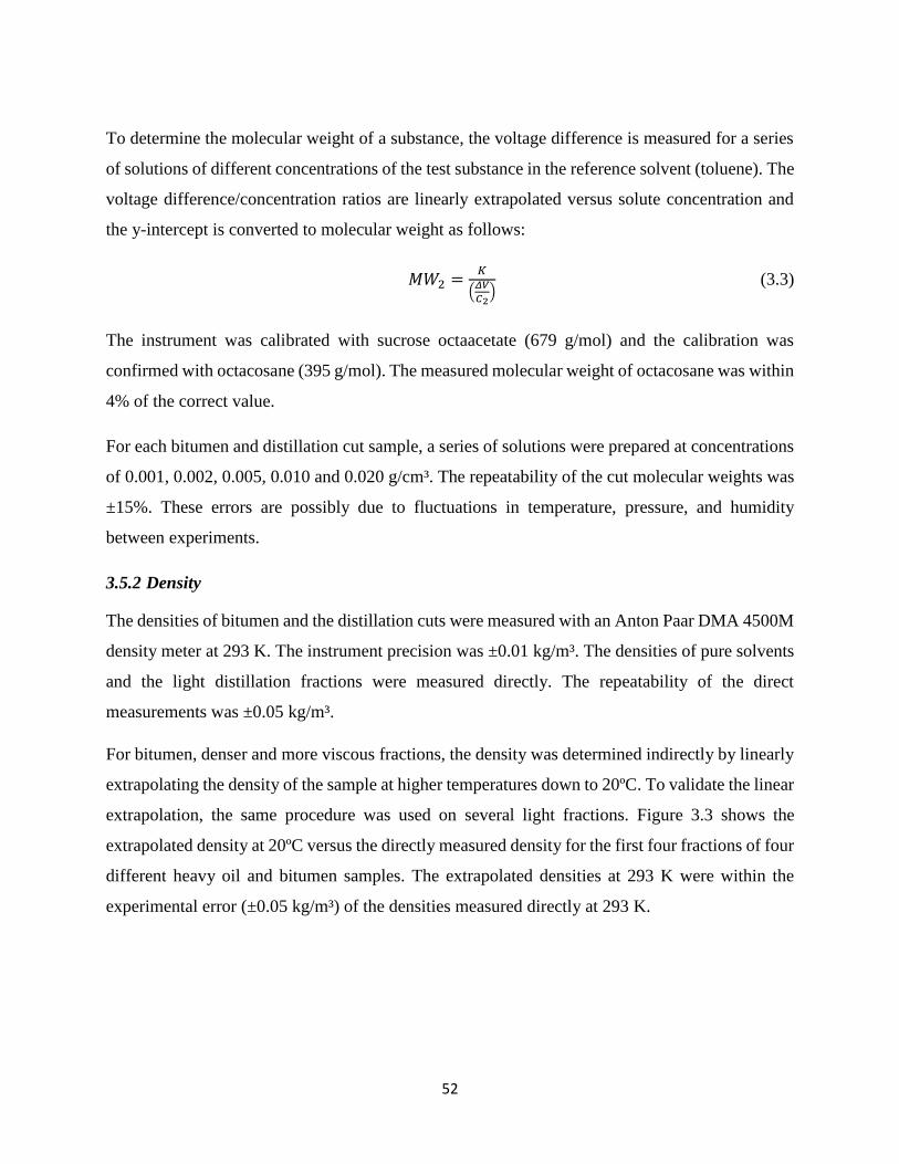
52
To determine the molecular weight of a substance, the voltage difference is measured for a series
of solutions of different concentrations of the test substance in the reference solvent (toluene). The
voltage difference/concentration ratios are linearly extrapolated versus solute concentration and
the y-intercept is converted to molecular weight as follows:
𝑀𝑊2 =𝐾
(𝛥𝑉
𝐶2) (3.3)
The instrument was calibrated with sucrose octaacetate (679 g/mol) and the calibration was
confirmed with octacosane (395 g/mol). The measured molecular weight of octacosane was within
4% of the correct value.
For each bitumen and distillation cut sample, a series of solutions were prepared at concentrations
of 0.001, 0.002, 0.005, 0.010 and 0.020 g/cm³. The repeatability of the cut molecular weights was
±15%. These errors are possibly due to fluctuations in temperature, pressure, and humidity
between experiments.
3.5.2 Density
The densities of bitumen and the distillation cuts were measured with an Anton Paar DMA 4500M
density meter at 293 K. The instrument precision was ±0.01 kg/m³. The densities of pure solvents
and the light distillation fractions were measured directly. The repeatability of the direct
measurements was ±0.05 kg/m³.
For bitumen, denser and more viscous fractions, the density was determined indirectly by linearly
extrapolating the density of the sample at higher temperatures down to 20ºC. To validate the linear
extrapolation, the same procedure was used on several light fractions. Figure 3.3 shows the
extrapolated density at 20ºC versus the directly measured density for the first four fractions of four
different heavy oil and bitumen samples. The extrapolated densities at 293 K were within the
experimental error (±0.05 kg/m³) of the densities measured directly at 293 K.

53
Figure 3.3. Measured and predicted density at 20ºC for the initial four distillation fractions
of four bitumen samples.
In the case of the distillation residue, the viscosity did not decrease enough to allow density
measurement at higher temperatures. Instead, solutions of the sample in toluene at concentrations
from 0.001 to 0.02 kg/L were prepared. The density of the residue was calculated using a mixing
rule (Powers, 2014)
Since the residue contains highly aromatic structures it is expected that a mixtures of residue and
toluene form nearly ideal solutions (Powers, 2014). Therefore, the density of the mixture is given
by:
𝜌𝑀𝑖𝑥 = [𝑤1
𝜌1+
𝑤2
𝜌2]
−1
(3.4)
where w is the mass fraction, ρ is the density, and subscripts Mix, 1, and 2 denote the mixture and
Components 1 and 2, respectively. Equation 3.4 was least squares fitted to the density data of the
mixtures of residue and toluene to obtain the residue density.
850
870
890
910
930
950
850 870 890 910 930 950
Ca
lcu
late
d D
en
sit
y [
kg
/m3]
Measured Density [kg/m3]
Cut 0
Cut 1
Cut 2
Cut 3

54
3.5.3 Refractive Index
Refractive index was measured with an Anton Paar Abbemat-WR refractometer. The apparatus
includes a measuring prism made of an isotropic crystal of a high refractive index (YAG -Yttrium-
Aluminum-Garnet). The refractometer is designed to be used with samples with a lower refractive
index than the prism. A liquid sample in contact with the prism is illuminated by an LED and the
critical angle of the total reflection at 589.3 nm sodium D wavelength is measured with a high-
resolution sensor array. The refractive index (nD) is calculated from this value. The instrument has
a precision of ±0.00002.
To measure the refractive index, the sample was placed on the measuring prism and after allowing
stabilization of the reading and temperature (30 to 60 seconds) the value was recorded. The
measurements were performed at 293 K and room pressure for samples with low viscosity. The
repeatability of the refractive index from direct measurements was ±0.0002.
Very viscous samples were warmed to 333 K in an oven prior to measurements to facilitate sample
placement and measurements at higher temperatures were linearly extrapolated to the refractive
index at a desired temperature. As with density, the extrapolated values at 293 K were compared
with the measured values for light fractions, thus testing the accuracy of the extrapolation. Figure
3.4 shows the measured and predicted value for four different fractions of two bitumen samples.
The extrapolated refractive indices at 293 K were within the experimental error (±0.0002) of the
indices measured directly at 293 K.

55
Figure 3.4. Measured and predicted refractive index at 293 K for the initial four distillation
fractions of two bitumen samples
3.5.4 Elemental Analysis
The elemental composition of the boiling fractions was determined via combustion using a Carlo
Erba EA 1108 elemental analyzer that simultaneously determines the total carbon, nitrogen,
hydrogen and sulfur based on the composition of the sample’s combustion products. Oxygen is
measured separately based on its conversion to carbon monoxide over a nickel carbon phase.
Standards fall within 0.3% of the theoretical values. These measurements were performed by the
Department of Chemistry at the University of Alberta (Moffat, 2012)
3.5.5 Vapor Pressure
The vapor pressure of the fractions was measured using a static method developed by Castellanos
et al. (2012) that was designed to achieve pressures below 0.1 Pa. The principle is simple: a liquid
sample is allowed to equilibrate with its vapor at a fixed volume and temperature. Note, since the
heavy oils are multi-component mixtures, the saturation pressure measured is not technically a
vapor pressure. However, the term vapor pressure is often used in the literature in this situation
and we have continued with this convention.
1.45
1.47
1.49
1.51
1.53
1.55
1.45 1.47 1.49 1.51 1.53 1.55
Ca
lcu
late
d R
efr
ac
tive
In
de
x
Measured Refractive Index
Cut 0
Cut 1
Cut 2
Cut 3

56
DVFA-I Apparatus. The apparatus consists of a sample vessel, two valves used to control the
operating cycles, a diaphragm gauge, a liquid trap and a turbomolecular pump, Figure 3.5. The
pressure readings were measured with an Inficon diaphragm gauge capable to measure pressures
in the 0.1-133 Pa range. Readouts of pressure gauge are recorded in a digital file using LabView
8.6 (2008). The desired temperature is attained using electric heating tapes which are uniformly
wrapped on the apparatus. J-type thermocouples are attached to the pipes to read the temperature
and PID temperature controllers maintain the temperature within ±0.1 K.
Figure 3.5. Simplified schematic of the deep vacuum apparatus (DVFA-I) in configuration
to measure vapor pressure
Measurement. Baking out of the empty apparatus and degassing of the samples are required to
eliminate contaminants that invalidate vapor pressure readings. The degassing process was carried
out at 313 K to minimize possible fractionation of the cuts. Note the fractions were stored in sealed

57
vials under nitrogen at 273 K in order to minimize any potential contamination prior to the vapor
pressure measurement.
After degassing, the vapor pressure was measured using the following procedure. The liquid
sample was placed in the sample vessel and the apparatus was heated up to the desired temperature.
The pump was switched on and once the apparatus reached the minimum pressure given by the
turbo-molecular pump (or baseline), the vapor pressure was measured at the test section between
Valves 1 and 2 in cycles. First, the test section was opened to the pump (open Valve 2 keeping
Valve 1 closed) for two minutes. Then the test section was isolated from the pump and opened to
the sample (close Valve 2 and open Valve 1) until the pressure reached a constant value. Finally,
Valve 1 was closed to isolate the sample and Valve 2 was opened to begin a new cycle. The cycles
were repeated until the peak pressures of at least three consecutive cycles were constant. To
account for the leak rate, the pressure readings for each cycle were corrected by extrapolating the
pressure back to the time when the cycle started.
The repeatability of the measurements was within 3%. The measured vapor pressures for
naphthalene and n-hexadecane were within 13% and 4%, respectively, of the literature values
(Castellanos-Diaz, 2012). The error in the vapor pressure measurements for the boiling fractions
is expected to have a maximum uncertainty of 13%.
3.5.6 Liquid Heat Capacity
The liquid heat capacities of the boiling fractions were measured at the Institute of Chemical
Technology in Prague (Ruzicka, 2015), with a Tian-Calvet calorimeter (Setaram DSC IIIa) in the
range from 258 to 355 K using an incremental temperature scanning mode with 5 K steps and a
heating rate of 0.3 K/min followed by isothermal delays of 2600 seconds. A synthetic sapphire,
NIST Standard Reference Material No.720, was used as the reference material. The typical mass
of samples was 0.4 to 1 g. The combined uncertainty (0.95 level of confidence) of heat capacity
measurements was estimated to be 1%. Details of the calorimeter, measurement procedure and its
calibration can be found elsewhere (Straka et al., 2007; Fulem et al., 2008).

58
The measurement of heat capacity for the boiling fractions was carried out after three successive
runs: 1) empty measuring cell; 2) cell filled with the reference material; 3) cell was filled with the
boiling fraction. The second vessel, the reference vessel, was empty during all three runs. Heat
capacity was calculated as follows.
𝐶𝑝,𝑓 =𝑚𝑠𝑠𝐶𝑝,𝑠𝑠(𝐴𝑓−𝐴𝑒)
𝑚𝑓(𝐴𝑠𝑠−𝐴𝑒) (3.5)
where Cp,f is the specific heat capacity of the boiling fraction; Cp,ss is the specific heat capacity of
the reference substance (synthetic sapphire); mf is the mass of the boiling fraction; mss is the mass
of the reference substance; Af is the integrated value of the differential heat flow when the
measuring vessel contains the sample; Ass is the integrated value of the differential heat flow when
the measuring vessel contains the reference substance; and Ae is the integrated value of the
differential heat flow when the measuring vessel is empty.
3.5.7 Heat of Combustion
The heat of combustion of the boiling fractions was measured at the Institute of Chemical
Technology, Prague, with a Parr 1356 Isoperibol Bomb Calorimeter at constant volume. In
“isoperibol” operation, the temperature of the jacket is held constant through the measurement
while the temperature of the bucket rises. To compensate for the heat flow within the calorimeter,
an automated correction is applied using a microprocessor controller. The energy equivalent of the
calorimeter was determined using 1.0 g pellets of benzoic acid. The precision of the standard
measurement was below 0.3%. A run with benzoic acid was performed before each measurement
to improve precision of the measurements. Since the amount of the distillation cut used for the
measurement was less than 0.5 g, a spiking material (benzoic acid) was used to drive the
combustion process to completion. Details for this method are provided elsewhere (Mahnel, 2015).
The results obtained from the bomb calorimeter represent the gross or high heat of combustion of
the cuts, which includes the heat of vaporization of the condensed water. The heat of combustion
was calculated as follows.
𝐻𝐻𝑉 =𝑊𝑐∆𝑇 − 𝑒𝑁 − 𝑒𝑆 − 𝑒𝐹
𝑚 (3.9)
59
where HHV is the gross heat of combustion of the distillation fraction in kJ/g, Wc is the heat
capacity of the calorimeter being used in kJ/˚C, ∆T is the temperature rise in ˚C, m is the mass of
the sample in grams, eN is a correction factor for the heat produced by burning nitrogen to form
nitric acid, eS is a correction factor for the heat produced by burning sulfur to form sulfuric acid,
and eF is a correction factor for the heat produced by the burning fuse.
60
CHAPTER FOUR: MODIFIED DEEP VACUUM FRACTIONATION APPARATUS
AND STANDARDIZED PROCEDURE
The original deep vacuum fractionation apparatus (DVFA-I) was designed to measure vapor
pressure. Its capability to distill heavy oil was evaluated in a proof of concept test and the results
of this test are presented in this chapter. Then, a modified version (DFVA-II) of the DFVA-I is
introduced along with the reasoning for the modifications. A new procedure to operate DVFA-II
to consistently distill deasphalted bitumen and heavy oil samples is presented and evaluated. The
WC-B-B1 bitumen is used to demonstrate the differences and improvements between DVFA-I and
DVFA-II. A summary of repeatability of the fractionations for the other six oils is presented at the
end of the chapter. The apparatus was also designed so that physical cuts could be collected for
property measurements. The properties measured in this thesis are summarized at the end of the
chapter but are discussed in detail in subsequent chapters.
4.1 Proof of Concept for Extended Distillation
The proof of concept test was performed with the static deep vacuum apparatus (DVFA-I)
developed by Castellanos-Diaz (2012) for the measurement of vapor pressure of heavy oils and
bitumen. In this case, the apparatus was operated as a batch distillation with no reflux and one
theoretical plate. The apparatus was described in Chapter 3 and its configuration is shown again
in Figure 4.1, for the reader’s convenience.
To fractionate a bitumen sample using the DVFA-I, the sample temperature was raised to the initial
condition at T1. The initial temperature of fractionation was the temperature at which a detectable
amount of condensate was visually observed in the cold finger after gradual heating. At this point,
the sample was left open to pump suction by leaving all the connecting valves open. The upper
DVFA-I section, above the sample vessel, was left at a temperature 20 K higher than T1 to facilitate
vapor transportation and avoid condensation in the inner pipe.

61
Figure 4.1. Simplified schematics of the deep vacuum apparatus (DVFA-I).
Each cut was collected by condensation in the cold finger which was replaced when the
fractionation process at T1 stops. To determine when the fractionation at a given temperature was
complete, the volume of the accumulating cut was measured over time. If the volume of the cut
did not change during 72 hours, the cut was considered to be complete. Then, the sample vessel
was isolated and the temperature is raised to a value T2, higher than T1. Once the temperature was
constant to within ± 0.1 K, the fractionation process was repeated. A set of cuts was collected at
temperatures between 413 and 563 K. Note, the pressure during fractionations was lower than the
minimum operational range of the Pirani gauge placed on top of the pump; therefore, the
distillation pressure could not be measured. Even if a wider-pressure-range gauge were available,
at pressures below 10-5 kPa, leaks and absorption/desorption phenomena will affect the pressure
readouts. Since pressure could not be measured during the experiments, an interconversion method
for the temperature, independent of the pressure, was required.
Deep vacuum fractionations were performed on maltenes instead of the whole bitumen.
Asphaltenes are non-distillable and contribute significantly to the high viscosity of the oil.
Removing the asphaltenes reduced the sample viscosity and thereby enhanced mass transfer which
Sample
Vessel
Valve 1
Turbomolecular
Pump
Cold Finger
Pirani Gauge Valve 2

62
is expected to decrease the distillation time, improve the separation, and possibly increase the
amount of oil that can be distilled.
Two fractionations were performed on WC-B-B1 maltenes in the proof-of-concept test. The results
are listed in Table 4.1 and Figure 4.2 shows a photo of the five cuts collected for Fractionation 1.
Note that as the boiling point of the cut increased, the color of the cut changed from light,
transparent amber to dark greenish brown, ending in an opaque black for the residue. In addition,
as expected the measured density (Table 4.1) of the cuts increased from the first to the last cut.
Slower flow was also observed as the separation proceeded, suggesting that the viscosity increased
from the first to last cut. These changes in physical properties indicate that a qualitatively
successful fractionation was achieved.
Table 4.1. WC-B-B1 maltene cuts obtained using the DVFA-I.
Trial Cut Temperature
[K]
Cumulative wt%
Bitumen Distilled
Density at
293 K
[kg/m³]
Fractionation 1
1 423 10.4 933.9
2 463 22.8 952.0
3 493 29.7 982.3
4 533 46.4 998.6
5 563 56.9 1018.5
Residue >563 1055.1
Fractionation 2
1 423 5.51 918.1
2 443 17.72 958.1
3 463 27.79 959.1
4 483 34.53 999.1
5 503 41.29 1001.5
6 523 45.43 1005.0
7 543 50.00 1016.3
8 573 56.08 1013.1
Residue >573 1050
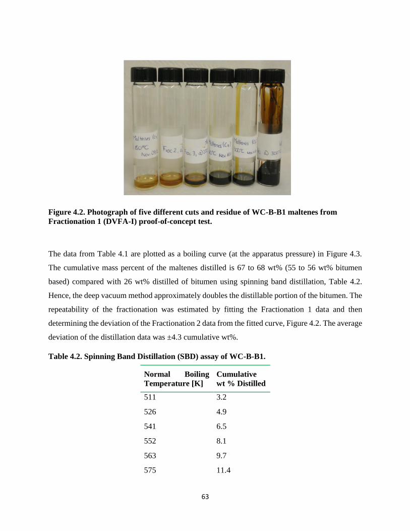
63
Figure 4.2. Photograph of five different cuts and residue of WC-B-B1 maltenes from
Fractionation 1 (DVFA-I) proof-of-concept test.
The data from Table 4.1 are plotted as a boiling curve (at the apparatus pressure) in Figure 4.3.
The cumulative mass percent of the maltenes distilled is 67 to 68 wt% (55 to 56 wt% bitumen
based) compared with 26 wt% distilled of bitumen using spinning band distillation, Table 4.2.
Hence, the deep vacuum method approximately doubles the distillable portion of the bitumen. The
repeatability of the fractionation was estimated by fitting the Fractionation 1 data and then
determining the deviation of the Fractionation 2 data from the fitted curve, Figure 4.2. The average
deviation of the distillation data was ±4.3 cumulative wt%.
Table 4.2. Spinning Band Distillation (SBD) assay of WC-B-B1.
Normal Boiling
Temperature [K]
Cumulative
wt % Distilled
511 3.2
526 4.9
541 6.5
552 8.1
563 9.7
575 11.4

64
587 13
597 14.6
613 17.9
623 19.5
631 21.1
640 22.7
648 24.3
653 26
Figure 4.3. Boiling point profiles for WC-B-B1 bitumen at DVFA-I apparatus pressure;
symbols are data and line is cubic spline fit to Fractionation 1 data.
The results from the proof-of-concept using DVFA-I were encouraging. However, the DVFA-I
posed several significant challenges: a very long experimental time per cut, potential sample
entrainment, and insufficient amounts of cut sample collected for further analysis. To overcome
these challenges and standardize the DVFA, a second apparatus (DVFA-II) was developed
utilizing the same basis of design of the DVFA-I.

65
4.2 Modification of Original Deep Vacuum Apparatus
The original DVFA-I had a capacity for a sample volume of 20 cm³ with a 5 cm³ volume capacity
for condensate collection. Given that 8 cuts were desired for the oil characterization and at least 7
cm³ of each cut was required for property measurements, the volume of the initial configuration
was insufficient. In addition, due to the small diameter of the sample vessel and high viscosity of
the fluid, many days were required for each cut to diffuse through the de-asphalted heavy oil,
making the complete procedure very time consuming (2 months per fractionation). Simply
increasing the length of the cylindrical sample vessel to obtain larger cuts would increase the height
of the fluid and the corresponding mass transfer resistance, leading to an increase in the distillation
time per cut.
Another issue was the proximity of the sample vessel to the collector device and the absence of a
physical barrier to avoid entrainment. Coloring of the light cuts was observed, indicating
overlapping and splashing of the sample, Figure 4.2. An important constraint is that additional
fittings and seals would increase the apparatus leak rate, which increased the pressure of the system
and therefore decreased the ability of the DVFA to extend the distillation of heavy oils.
To solve these issues without adding significantly more fittings, the original cylindrical sample
vessel was replaced with a tee-shaped fitting and two additional concentric reducers. The new
configuration used Swagelok fittings and the same metal gasket seals to minimize leaks. It
provided a larger sample volume (110 cm³) to obtain the desired cut volumes as well as a larger
sample surface area in order to reduce mass transfer resistance and therefore produce a
corresponding increase in mass transfer rate. Reducers above the tee-shaped sample vessel were
required to couple the tee diameter with the diameter of Valve 1. Due to their conical shape, the
reducers also act as a barrier for the entrained liquid when vapor is produced during the distillation,
Figure 4.4. When assembled and in the absence of fluid, the system is able to achieve pressures as
low as 1x10⁻⁷ Pa.
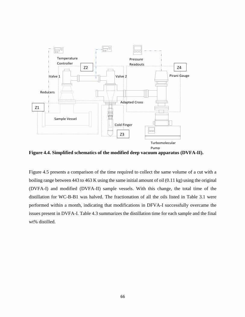
66
Figure 4.4. Simplified schematics of the modified deep vacuum apparatus (DVFA-II).
Figure 4.5 presents a comparison of the time required to collect the same volume of a cut with a
boiling range between 443 to 463 K using the same initial amount of oil (0.11 kg) using the original
(DVFA-I) and modified (DVFA-II) sample vessels. With this change, the total time of the
distillation for WC-B-B1 was halved. The fractionation of all the oils listed in Table 3.1 were
performed within a month, indicating that modifications in DFVA-I successfully overcame the
issues present in DVFA-I. Table 4.3 summarizes the distillation time for each sample and the final
wt% distilled.
16 cm
4.6 cm
Sample Vessel
Temperature
Controller Pressure
Readouts
Valve 1 Valve 2
Pirani Gauge
Turbomolecular
Pump
Cold Finger
Adapted Cross
Reducers
Z1
Z2
Z3
Z4

67
The completed DVFA-II has four different temperature zones. The first zone (Z1) corresponds to
the temperature at which each distillation cut is obtained; the second zone (Z2) is always 20 K
higher than Z1 to avoid condensation of vapor in the pipes; the third zone (Z3) is maintained at
253 K to assure condensation; and the fourth zone (Z4) is left at room temperature to avoid
overheating of the bearings of the pump. Note the temperatures of Z1 and Z2 are controlled during
the distillation procedure.
Figure 4.5. Effect of the modified sample vessel design on distillation time for the 443 to 463
K cut.
Table 4.3. Distillation time and wt% distilled of bitumen for each sample used in this work
Sample Distillation
Time (days)
Cumulative wt%
Bitumen Distilled*
WC-B-B1 30 51.7
CO-B-A1 31 42.8
MX-HO-A1 28 41.4
CO-B-B1 30 46.0

68
US-HO-A1 27 53.4
WC-B-D1 30 41.8
RO-HO-A1 25 62.2
*Mass balance normalized based on the losses
4.3 Standardization of Fractionation Using DVFA-II
The next step was to define an initial sample volume, cut point temperature, and number of cuts
as part of a standard procedure. To finalize the standardization of the distillation process, two
fractionations using DVFA-II were performed for a Western Canadian Bitumen (WC-B-B1).
Table 4.4 presents the distillation data collected for the maltenes as well as the density and
molecular weight of each cut. The repeatability of the DVFA-II fractionations was within an
average deviation of ±1.5 wt%, Figure 4.6. The distillations curves were fitted using cubic splines
to avoid discontinuities for the sole purpose of providing an exact as possible comparison between
curves where data points do not fall on the same X or Y coordinate. Note, the 0 wt% to 20 wt%
distilled seemed to have a discontinuity; however, this is an artifact introduced due to the fitting
process and scatter of the data but does not represent the nature of the data. The spinning band
distillation of this sample and the DVFA fractionations of other samples did not show this
discontinuity. Potential sources of error are considered below.
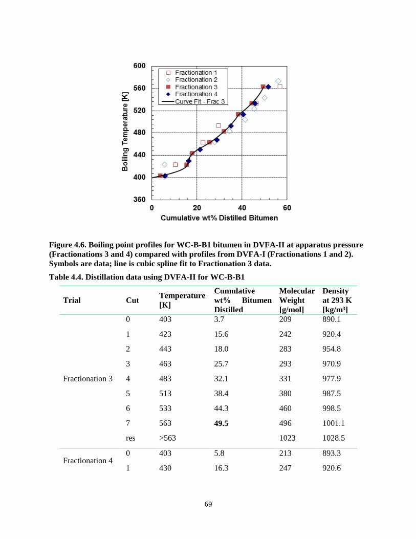
69
Figure 4.6. Boiling point profiles for WC-B-B1 bitumen in DVFA-II at apparatus pressure
(Fractionations 3 and 4) compared with profiles from DVFA-I (Fractionations 1 and 2).
Symbols are data; line is cubic spline fit to Fractionation 3 data.
Table 4.4. Distillation data using DVFA-II for WC-B-B1
Trial Cut Temperature
[K]
Cumulative
wt% Bitumen
Distilled
Molecular
Weight
[g/mol]
Density
at 293 K
[kg/m³]
Fractionation 3
0 403 3.7 209 890.1
1 423 15.6 242 920.4
2 443 18.0 283 954.8
3 463 25.7 293 970.9
4 483 32.1 331 977.9
5 513 38.4 380 987.5
6 533 44.3 460 998.5
7 563 49.5 496 1001.1
res >563 1023 1028.5
Fractionation 4 0 403 5.8 213 893.3
1 430 16.3 247 920.6

70
2 450 21.4 272 961.9
3 468 28.8 327 973.2
4 493 35.0 352 982.2
5 513 40.5 362 992.0
6 533 45.9 480 999.6
7 563 51.7 490 1016.8
res >563 1010 1035.0
4.3.1 Sources of Error
Some of the possible sources of error during the distillation are discussed below. The final
standardized procedure was design to minimize overlapping between cuts and light end losses as
well as to increase repeatability of the distillation curve and the properties of each cut.
Entrainment: One of the major issues with the initial apparatus was significant entrainment of
liquid droplets in the boiling vapor. To assess the impact of the modified apparatus on entrainment,
the distillation curves from the standardized fractionations are compared with the proof-of-concept
fractionations in Figure 4.6. Note, the amount of bitumen distilled using DVFA-II is 7 wt% less
than that obtained with DVFA-I apparatus. While a lower distillation of the sample does not sound
like an improvement, it is in fact evidence of a cleaner separation and reduction in entrainment.
Consider the early stage of the distillation: comparing Figures 4.1 and 4.7, a lighter color is
observed for the first cuts, Figure 4.7, when the modified DFVA-II was used. Also, the difference
between the wt% distilled for the first cut in Fractionations 1 and 2 in the proof-of-concept tests
was 4.9 wt%, whereas the difference for the first cut in Fractionations 3 and 4 in the standardized
procedure was only 2.1 wt%.
Figure 4.7 is a photo of the maltene cuts of the WC-B-B1 from Fractionation 4. The progressive
changes in color and viscosity were similar to the initial fractionations, but there are clearly sharper
distinctions in color between the cuts confirming that entrainment has been reduced or eliminated.
Finally, the gas chromatography (GC) assays of the initial cuts from Fractionation 4 are shown in
Figure 4.8. The carbon number in Figure 4.8 is an ‘equivalent carbon number’ corresponding to
the carbon number of a paraffin that elutes at the same retention time. The cuts show a near

71
Gaussian distribution of carbon numbers with no suggestion of entrainment of heavy components.
The distribution of density and molecular weights will be discussed later, although it is worth
noting that both values show smooth trends and no evidence of entrainment effects. Hence,
entrainment has been reduced to negligible levels.
Figure 4.7. Photograph of the seven different cuts of WC-B-B1 maltenes from
Fractionation 4 (DVFA-II).
Figure 4.8. Carbon number distribution for the first two boiling cuts from Fractionation 4
and whole WC-B-B1 bitumen (free of C30+ compounds).

72
Residual Pentane from De-asphalting of Maltenes: The GC assays for the first cuts (Cut 0 and Cut
1) from Fractionation 4 show no traces of pentane, Figure 4.8. The chromatographic results also
show the expected overlapping of compounds as a consequence of the compositional complexity
of the oil and the absence of reflux in the batch distillation. Finally, when compared to the assay
for the whole bitumen, it appears that the small amount of material in the C10 to C11 range may
have been partially stripped off during the asphaltene precipitation procedure. However, these
losses are negligible and correspond to approximately 0.006% of the total bitumen sample. This
mass fraction was calculated as the difference between the amounts of lightest components (from
C9 to C11) reported in the GC assay of the whole bitumen and the corresponding components in
the GC of the initial two cuts.
Losses: During fractionation there were two sources of losses during sample distillation: 1) the
escape of light components through the pump during the initial stages of the fractionation; 2) the
condensation of heavy boiling cuts in the lines during the final stages of the fractionation. The
latter losses were determined from the mass change of the DVFA-II fittings. The former were
determined from the difference between the initial mass sample and the sum of the masses of
residue, cuts, and condensed material on the fittings. On average, the total losses for all the 14
distillations were less than 3.2% of the initial sample mass.
Leak Rate: In all vacuum systems, air enters the apparatus through imperfect seals and limits the
ultimate vacuum pressure achievable. However, pressure cannot be monitored during the
fractionation due to temperature limitations in the pressure gauges and may be a source of
systematic error. Since the leak rate will vary from run to run (tightness of seals will vary), the
distillation pressure will also vary and therefore the amount distilled will be different. Any
differences in the leak rates will only be detectable at the higher temperatures where the leak rate
is largest. Despite the leak rate error, the average repeatability of the procedure was only 2% of
the cumulative weight percent collected for a given boiling point range, which is in within the
repeatability range of standard atmospheric and vacuum distillation methods.

73
4.3.2 Distillation Procedure using DVFA-II
Based on the previous results, the finalized distillation procedure can be divided into three general
steps: preparation of the apparatus, degassing and fractionation. Each step is discussed below.
Preparation of the Apparatus
Before starting the fractionation, all the fittings are washed with toluene and left in a vacuum oven
for 24 hours at 373 K and 8000 Pa. After cleaning, all parts are weighed and then assembled
together and connected to the pump as shown in Figure 4.1. The empty DVFA-II is baked-out at
573 K for one day to avoid contamination of the sample and cuts collected; contaminants are
collected in the cold finger. The main purpose is to clean the surface of the pipes by removing the
remaining contaminants and water vapor by desorption.
Degassing
Degassing of the sample begins by disconnecting the sample vessel, weighing it once more to
check for any major change in mass due to desorption of contaminants, and then 0.11 kg of de-
asphalted bitumen are added into the sample vessel. It is then reconnected to DVFA-II and two
thermocouples are placed on the outside wall of the sample vessel. Next, the cold finger that was
used to collect the contaminants is removed and replaced by a new, pre-weighed cold finger.
Heating and insulation tape are then uniformly wrapped over the entire DVFA-II apparatus except
for the cold finger. The heating tape provides temperature control for all of the non-cold finger
parts of DVFA-II. A bath of oil and dry ice is placed around the cold finger section to maintain its
temperature at 253 K. All the fittings after Valve 1 are heated to 30 K higher than the sample
temperature in order to avoid condensation in the pipes and to enhance the mobility of the produced
vapor as it travels toward the collector device. Once the DVFA-II apparatus is reassembled, both
Valves 1 and 2 are opened and the turbomolecular pump is switched on.
Degassing of n-pentane from the oil sample is achieved by holding the sample vessel at 323 K for
6 hours. After this time, the cold finger is replaced once again with a new, pre-weighed cold finger.
The sample vessel is disconnected and weighed to determine the remaining mass. A temperature
of 323 K is used to avoid losses of light ends from the oil.

74
Note, this temperature was found to be sufficient to remove the residual n-pentane from the de-
asphalting procedure used to prepare the maltenes. At the end of the degassing process,
approximately 0.01 to 0.22 wt% of the initial maltenes were collected in the cold finger. Gas
chromatography (GC) assays confirmed that this distilled material was almost entirely n-pentane.
GC assays of the subsequent lightest cuts confirmed that all of the pentane had been removed.
Potential losses of light ends will be discussed later.
Fractionation
Following degassing of the sample, the sample vessel is reconnected and fractionation initiated by
increasing the temperature at a rate of 10 K/h until the desired cut temperature is achieved. The
temperature is then held constant until the volume in the cold finger does not change for 24 hours.
Cuts are collected at temperature intervals of 20 K. The 20 K interval was selected because it
balanced the required sample volume for each cut with a reasonable number of cuts to use in the
oil characterization. Also, two to three of the lightest cuts had to overlap the distillable region of
the SBD in order to validate the method. For heavy oils, the first cut occurred at approximately
403 K and the fractionation produced 8 cuts plus a residue.
The following three steps are repeated for every cut collected:
i. Set the cut temperature
ii. Run distillation for the cut until volume in the cold finger does not change for 24 hours
iii. Close valves, turn off pump, disconnect cold finger, weight it, and replace it with a new,
pre-weighed cold finger
The maximum cut temperature is 563 K in order to avoid thermal cracking of the sample. At the
end of the distillation, the pump is switched off, all fittings are disassembled, and the mass of every
fitting is recorded. Any change in the mass of fitting is likely caused by condensation of the heavier
cuts and is used in the determination of losses during the procedure, as will be discussed later. The
collected cuts are stored in glass vials with nitrogen caps and then refrigerated until needed for
property analysis. The cleaning procedure is then repeated to prepare the apparatus for the next
sample.

75
The remaining six deasphalted oils were distilled by this procedure. Two fractionations were
performed for each sample and the density and molecular weight measured for all of the cuts.
Table 4.5 summarizes the average deviation of the distillation curves for a given sample following
the cubic spline approach. The deviations of the measured density and molecular weight of each
cut are also summarized.
The final test was to compare the results from the standardized fractionation with results from a
conventional vacuum distillation such as spinning band distillation. This comparison will be
detailed in Chapter Five after the low pressure boiling points are converted to atmospheric
equivalent boiling points.
Table 4.5. Repeatability obtained for density molecular weight and boiling point of seven
oils following the standardized procedure for DVFA-II
Sample Distillation Curve
ARD %
Density
ARD %
Molecular Weight
ARD %
WC-B-B1 2.3 0.18 4.0
CO-B-A1 0.8 0.10 1.2
MX-HO-A1 1.5 0.21 2.8
CO-B-B1 2.6 0.25 3.4
US-HO-A1 2.5 0.17 4.1
WC-B-D1 0.9 0.12 2.6
RO-HO-A1 2.5 0.27 3.6
4.3.3 Cut Property Measurements
A significant contribution from the deep fractionation apparatus is the ability to collect cuts,
including heavy fractions, for property measurements. In addition to the properties measured to
test the repeatability of the fractionation (density and molecular weight), the following properties
were measured for the distillation cuts: refractive index, elemental analysis, liquid heat capacity,
vapor pressure, and heat of combustion. The physical properties are presented and discussed in
Chapter 6.Vapor pressure and the thermal properties are presented and discussed in Chapter 7.

76
CHAPTER FIVE: INTERCONVERSION METHOD DEVELOPED FOR THE DEEP
VACUUM FRACTIONATION APPARATUS
In this chapter, a methodology to obtain an equivalent atmospheric temperature (AET) for each
boiling fraction from the deep vacuum apparatus is developed. The proposed methodology requires
vapor pressure and heat capacity data which were collected in this study and are presented here. A
new correlation for liquid heat capacity (presented in Chapter 7) is used for cases where data are
unavailable. The interconversion results for all seven oil samples considered in this thesis are
presented. The AET values are compared with the TBP data obtained from spinning band
distillations, and the use of the Gaussian distribution to extrapolate these distillation curves is
assessed. A simpler interconversion method to TBP data using only the bulk specific gravity and
actual distillation temperature for inputs is proposed. Finally a correlation of TBP to cumulative
wt% distilled is introduced to determine the whole distillation curve for heavy oils and bitumen up
to the asphaltene fraction with only bulk specific gravity as an input.
5.1 Interconversion Methodology
5.1.1 General Concept
The proposed interconversion approach is illustrated in Figure 5.1. The left plot demonstrates how
the measured vapor pressure in the low pressure region of a single cut is extrapolated to the boiling
point at 1atm. The extrapolation is made with a correlation constrained to fit both thermal and
vapor pressure data as a function of temperature. The AET from the extrapolations of all of the
cuts are then assembled to create the desired boiling point curve, as demonstrated on the right plot
of Figure 5.1.

77
Figure 5.1. Proposed Interconversion Methodology for Deep Vacuum Distillation using
DVFA-II
The key to the method is the relationship between vapor pressure, enthalpy of vaporization and
heat capacity. This relationship has been extensively studied, not only as an extrapolation
technique, but also as a methodology to assess the quality of the available experimental data for
pure compounds (Ruzicka and Majer, 1993). The thermodynamic relationship between vapor
pressure and caloric properties is given by the Clapeyron equation:
Hz
H
dT
PdRT
vap
vap
sat
ln2 (5.1)
where R is the gas constant, T is the absolute temperature, P is vapor pressure, ΔHvap is the enthalpy
of vaporization, and Δzvap stands for the difference between the compressibility factors of the
saturated vapor and the saturated liquid. ΔH’ represents the ratio of the enthalpy of vaporization to
the difference in compressibility factors. Given an expression for vapor pressure as a function of
temperature, Equation 5.1 allows the simultaneous correlation of enthalpy of vaporization and
vapor pressure as a function of temperature using only one set of constraints.
In this case, the available thermal data are heat capacities and a relationship between vapor pressure
and heat capacity is required. First, the change in heat capacity, ΔC’, is defined as follows:

78
satsat dT
PdRT
dT
d
dT
HdC
ln2 (5.2)
where the second equality comes from Equation 1. Equation 5.1 is introduced into Eq. 5,2 and the
compressibility factor is expressed in terms of a volume explicit virial expansion truncated after
the second virial coefficient to obtain the following expression (Ruzicka and Majer, 1993):
sat
l
sat
l
satvapdT
PdvBT
dT
dP
dT
vBdT
dT
BdTPCC
2
2
2
20 )(
)(2 (5.3)
where ΔC0 vap is the difference in the heat capacities of the saturated phases, B is the second virial
coefficient, and vl is the molar volume of the liquid phase. However, the last three terms of
Equation 5.3 are only significant at higher vapor pressure values (P >5000 Pa). At low pressures,
the enthalpy of vaporization and the change in heat capacity expressions reduce to:
vapHH (5.4)
l
ppvap CCCC 00 (5.5)
where 0
pC is the heat capacity of the ideal gas and l
pC is the heat capacity of the saturated liquid.
This approach has been mainly used to extrapolate vapor pressure in the middle pressure range
(between 1000 and 200000 Pa) towards the triple point; hence, the accuracy of the extrapolation
towards the boiling point is unknown.
The required elements for this method are then: a correlation of vapor pressure to temperature,
vapor pressure data, enthalpy of vaporization and/or liquid heat capacity data, and the ideal gas
heat capacity. Therefore, before developing the method it was required to collect experimental
data for each cut including vapor pressure, liquid heat capacity, elemental analysis, and molecular
weight. The following steps are required to complete the interconversion method:
1) Calculate the ideal gas heat capacity for each cut using Laštovka’s equation and the
elemental analysis of the cut
2) Select a vapor pressure equation

79
3) Regress the vapor pressure and heat capacity data with an appropriate optimization
function and initial guesses.
4) Validate the calculated AET versus the data obtained from a spinning band distillation.
Data collection was described in Chapter Three. The remaining steps are described below using
the WC-B-B1 bitumen as an example.
5.1.2 Ideal Gas Heat Capacity
The ideal gas heat capacity is the amount of heat required to increase one mole of sample by 1 K
assuming that there are no intermolecular forces that may increase or decrease the internal energy
of the molecules in the mixture. Laštovka et al. (2013) studied available correlations for predicting
ideal gas heat capacity and proposed a correlation for ill-defined hydrocarbons that had better
predictive capabilities. Laštovka et al.’s correlation for specific ideal gas heat capacity is a function
of temperature and elemental analysis. It was developed based on the principle that the effect of
fundamental vibrations of the atoms in a molecule (which determine heat capacity) are not
significantly altered by relatively small difference in the structure of the molecule. They developed
two correlations:
1. for aromatic hydrocarbons,
TCC
TCC
T
CCBB
TCC
TCC
T
CCBB
AA
AAACP
2221
22212
22212221
1211
12112
12111211
4
3
212
0
1
exp1
exp
exp1
exp
)(exp1
)(
(5.6)
2. for aliphatic hydrocarbons,

80
TCC
TCC
T
CCBB
TCC
TCC
T
CCBBAACP
2221
22212
22212221
1211
12112
1211121121
0
2
exp1
exp
exp1
exp
(5.7)
where A, B and C are constants and α is the similarity variable, which is given by:
(5.8)
where wi and Mi are the mass fraction and molecular mass of hydrogen, oxygen, nitrogen, sulfur
and carbon (i = 1-5), respectively. The values of the constants are provided in Table 5.1. The
reported relative deviations were 2.9% for aromatic and acyclic aliphatic hydrocarbons and 2.5%
cyclic aliphatic hydrocarbons.
Table 5.1 Parameters for predictive ideal gas heat capacity correlations
Parameter Eq 5.6 Eq 5.7
A1 0.58 -0.17935
A2 1.25 3.869444
A3 0.17338 -
A4 0.014 -
B11 0.739174 -0.08053
B12 8.883089 9.699713
C11 1188.281 686.4342
C12 1813.046 1820.466

81
B21 0.048302 -0.99964
B22 4.356567 17.26243
C21 2897.019 1532.256
C22 5987.804 5974.871
The ideal gas heat capacity of each cut was determined from a weighted average of 0
pC obtained
from Equations 5.6 and 5.7:
o
iP
o
iP
o
Pi CwCwC 2211 (5.9)
where, if (H/C)i <1.5, w1 = [(H/C)i – 1] and w2 = 1 - w1 and, if (H/C)i>1.5, w2 = [2 - (H/C)i]
and w1 = 1 - w2. This weighting is based on a maximum H/C ratio of 2 for 100% paraffinic
compounds and minimum H/C atomic ratio of 1 for highly aromatic petroleum compounds
(Strausz and Lown, 2003). The accuracy of the predicted ideal heat capacity for the cuts is
unknown, but it is expected to be within the accuracy reported by Laštovka (within 3%). The liquid
and ideal gas specific heat capacities were then converted to molar heat capacities using the
measured molecular weights of each cut.
5.1.3 Vapor Pressure Equation
Five different vapor pressure equations were tested for the extrapolation of the vapor pressure data:
the Antoine, the Quasi-Polynomial with two and three adjustable parameters, the Cox and the
Korsten equations. The criteria to select an appropriate equation were a low number of fitting
parameters and an accurate fit of the trends for experimental vapor pressure and heat capacity with
temperature. The best result was obtained for the three-parameter Cox equation, Equation 5.10:
(5.10)

82
where Pcalc is the calculated saturation pressure, T is the absolute temperature at the saturation
pressure, Pb is the atmospheric pressure. Tb is the absolute boiling temperature at atmospheric
conditions or AET and A0, A1 and A2 are the adjustable parameters in the Cox equation.
Ruzicka and Majer (1996) previously studied the performance of the Cox equation and concluded
that this mathematical relation between pressure and temperature had the best performance for
extrapolation purposes. Their findings were corroborated in this work. Additional advantages of
the Cox equation are that it does not depend on critical properties and the reference states can be
modified based on the need of the extrapolation.
The corresponding equation obtained from the relationship of heat capacity to vapor pressure from
Equation 5.2 is given in Equation 5.11:
∆𝐶′ 𝑐𝑎𝑙𝑐 = 𝑅𝑇𝑒𝑥𝑝(𝐴0 + 𝐴1𝑇 + 𝐴2𝑇2)[2𝐴1 + 4𝐴2𝑇 + (𝑇 − 𝑇0)
∗ (2𝐴2 + (𝐴1 + 2𝐴2𝑇)2] (5.11)
where superscript calc indicates a calculated value. The Cox equation has 4 fitting parameters: A0,
A1, A2 and Tb which are the same parameters as in Equation 5.10.
5.1.4 Regression Method
The regression is a least squares minimization of the following objective function by adjusting the
constants in the Cox equation:
m
i i
calc
ii
c
n
i i
calc
ii
C
CCK
P
PPOF
1
2
exp
exp
1
2
exp
exp
ln
lnln (5.12)
where n and m are the number of experimental values for vapor pressure and ΔC’ respectively, OF
stands for optimization function, the subscripts calc and exp correspond to the calculated and
experimental values of the corresponding variables and Kc is a weighting factor. The experimental
vapor pressures were measured directly and the experimental ΔC’ was determined using Equation
5.5. A Kc of unity was found to provide the best match to the spinning band distillation data and
was used for all cuts while minimizing OF. The optimization is sensitive to the initial guess and a
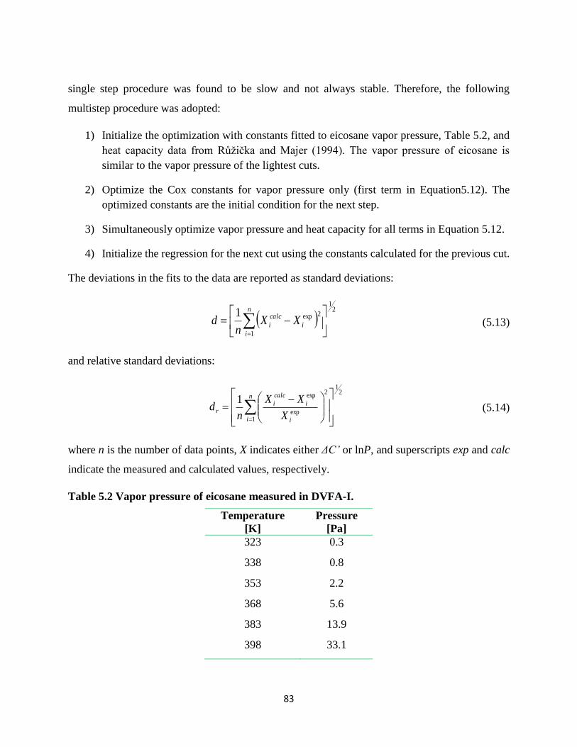
83
single step procedure was found to be slow and not always stable. Therefore, the following
multistep procedure was adopted:
1) Initialize the optimization with constants fitted to eicosane vapor pressure, Table 5.2, and
heat capacity data from Růžička and Majer (1994). The vapor pressure of eicosane is
similar to the vapor pressure of the lightest cuts.
2) Optimize the Cox constants for vapor pressure only (first term in Equation5.12). The
optimized constants are the initial condition for the next step.
3) Simultaneously optimize vapor pressure and heat capacity for all terms in Equation 5.12.
4) Initialize the regression for the next cut using the constants calculated for the previous cut.
The deviations in the fits to the data are reported as standard deviations:
2
1
1
2exp1
n
i
i
calc
i XXn
d (5.13)
and relative standard deviations:
21
1
2
exp
exp1
n
i i
i
calc
ir
X
XX
nd (5.14)
where n is the number of data points, X indicates either ΔC’ or lnP, and superscripts exp and calc
indicate the measured and calculated values, respectively.
Table 5.2 Vapor pressure of eicosane measured in DVFA-I.
Temperature
[K]
Pressure
[Pa]
323 0.3
338 0.8
353 2.2
368 5.6
383 13.9
398 33.1
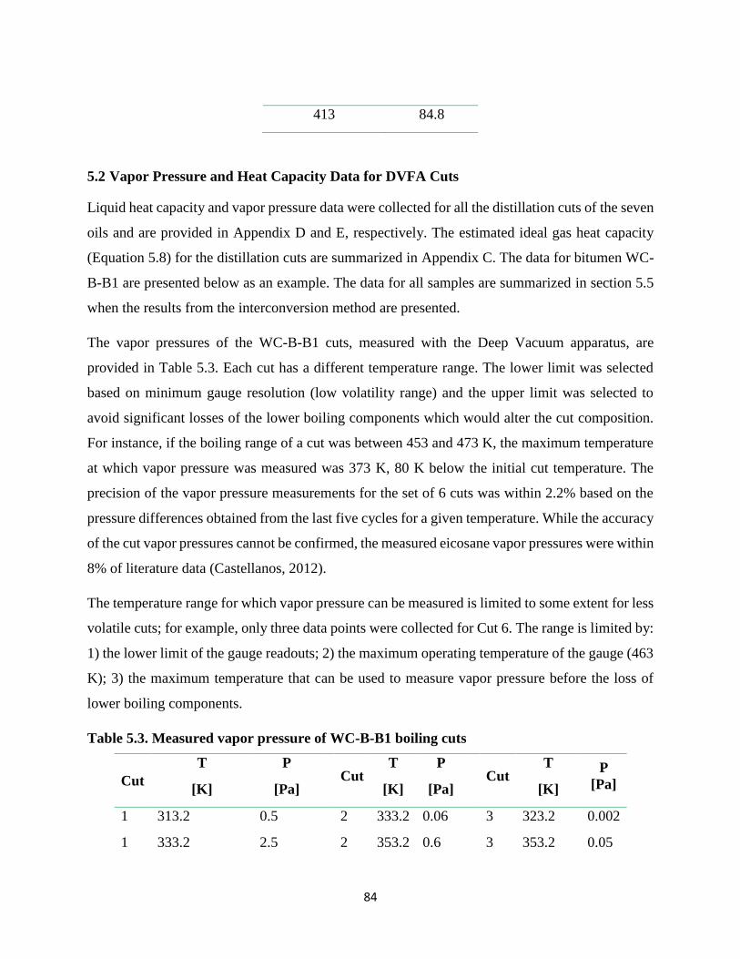
84
413 84.8
5.2 Vapor Pressure and Heat Capacity Data for DVFA Cuts
Liquid heat capacity and vapor pressure data were collected for all the distillation cuts of the seven
oils and are provided in Appendix D and E, respectively. The estimated ideal gas heat capacity
(Equation 5.8) for the distillation cuts are summarized in Appendix C. The data for bitumen WC-
B-B1 are presented below as an example. The data for all samples are summarized in section 5.5
when the results from the interconversion method are presented.
The vapor pressures of the WC-B-B1 cuts, measured with the Deep Vacuum apparatus, are
provided in Table 5.3. Each cut has a different temperature range. The lower limit was selected
based on minimum gauge resolution (low volatility range) and the upper limit was selected to
avoid significant losses of the lower boiling components which would alter the cut composition.
For instance, if the boiling range of a cut was between 453 and 473 K, the maximum temperature
at which vapor pressure was measured was 373 K, 80 K below the initial cut temperature. The
precision of the vapor pressure measurements for the set of 6 cuts was within 2.2% based on the
pressure differences obtained from the last five cycles for a given temperature. While the accuracy
of the cut vapor pressures cannot be confirmed, the measured eicosane vapor pressures were within
8% of literature data (Castellanos, 2012).
The temperature range for which vapor pressure can be measured is limited to some extent for less
volatile cuts; for example, only three data points were collected for Cut 6. The range is limited by:
1) the lower limit of the gauge readouts; 2) the maximum operating temperature of the gauge (463
K); 3) the maximum temperature that can be used to measure vapor pressure before the loss of
lower boiling components.
Table 5.3. Measured vapor pressure of WC-B-B1 boiling cuts
Cut
T
[K]
P
[Pa] Cut
T
[K]
P
[Pa] Cut
T
[K]
P
[Pa]
1 313.2 0.5 2 333.2 0.06 3 323.2 0.002
1 333.2 2.5 2 353.2 0.6 3 353.2 0.05

85
1 343.2 5.3 2 373.2 2.3 3 393.2 2.2
1 353.2 11.7 2 393.2 8.6 3 413.2 7.2
1 363.2 25.5 2 413.2 33.8 3 433.2 23.0
4 403.2 0.7 5 423.2 2.2 6 433.2 1.3
4 413.2 1.3 5 433.2 3.6 6 443.2 2.1
4 423.2 2.2 5 443.2 6.0 6 453.2 3.5
4 433.2 3.8 5 458.2 12.1
4 443.2 6.4
The liquid and ideal gas heat capacities of each cut are provided in Tables 5.4 and 5.5. Table 5.6
shows the ∆𝐶′𝑒𝑥𝑝 values obtained from experimental liquid heat capacity and the calculated ideal
gas heat capacity (Eq. 5.8). The values for ∆C’exp have four main sources of error (here shown for
the mass based ∆C’exp): 1) the error in the measured liquid heat capacity, estimated to be 1%; 2)
the error in the elemental analysis, estimated to be 0.3 wt%; 3) the error in the measured molecular
weight, estimated to be 3.2%, and; 4) the error in the ideal gas heat capacity calculated using
Laštovka correlation, reported to have a maximum deviation of 2.8% for ill-defined hydrocarbons.
The overall error for ∆C’exp was determined using a Monte Carlo sampling of the error distributions
and was found to be 3.9% for the mass based ∆C’exp and 2.1% for the molar ∆C’exp.
Table 5.4. Measured liquid heat capacity of WC-B-B1boiling cuts.
Temperature
[K]
Cpl [J mol-1 K-1]
Cut 1 Cut 2 Cut 3 Cut 4 Cut 5 Cut 6
258.1 420.9 459.8 536.7 612.4 692.3 775.7
263.2 425.5 464.7 542.4 619.0 698.6 782.7
268.3 430.0 469.6 548.1 625.5 705.4 790.4
273.4 434.6 474.5 553.8 632.0 711.7 797.4
278.5 439.1 479.4 559.5 638.5 718.6 805.1
283.6 443.7 484.3 565.3 645.1 725.5 812.9

86
288.7 448.2 489.2 571.0 651.6 732.4 820.6
293.8 452.8 494.1 576.7 658.1 739.8 828.9
298.9 457.3 499.0 582.4 664.6 746.0 835.9
304.0 461.8 503.9 588.1 671.2 752.7 843.4
309.1 466.4 508.8 593.8 677.7 759.7 851.2
314.3 470.9 513.6 599.6 684.2 766.7 859.1
319.4 475.5 518.5 605.3 690.8 773.9 867.1
324.5 480.0 523.4 611.0 697.3 781.3 875.4
329.6 484.6 528.3 616.7 703.8 788.4 883.4
334.7 489.1 533.2 622.4 710.3 795.7 891.5
339.8 493.7 538.1 628.1 716.9 803.2 899.9
344.9 498.2 543.0 633.9 723.4 810.5 908.1
350.0 502.8 547.9 639.6 729.9 817.9 916.5
355.1 507.3 552.8 645.3 736.5 825.0 924.4
Table 5.5. Calculated ideal gas heat capacity of WC-B-B1boiling cuts.
Temperature
[K]
Cpig [J mol-1 K-1]
Cut 1 Cut 2 Cut 3 Cut 4 Cut 5 Cut 6
258.1 281.7 302.6 349.4 398.5 452.6 493.9
263.2 287.5 308.8 356.6 406.7 461.6 504.0
268.3 293.2 314.9 363.6 414.7 470.6 514.0
273.4 298.9 321.1 370.7 422.8 479.6 524.1
278.5 304.6 327.2 377.8 430.9 488.6 534.1
283.6 310.3 333.4 384.9 438.9 497.6 544.1
288.7 315.9 339.5 392.0 447.0 506.5 554.1
293.8 321.6 345.6 399.0 455.0 515.5 564.1
298.9 327.3 351.7 406.1 463.0 524.4 574.1
304.0 332.9 357.8 413.1 471.1 533.3 584.1
309.1 338.5 363.9 420.1 479.0 542.2 594.0

87
314.2 344.2 369.9 427.1 487.0 551.1 604.0
319.4 349.7 376.0 434.1 495.0 559.9 613.8
324.5 355.3 382.0 441.0 502.9 568.7 623.7
329.6 360.9 388.0 448.0 510.8 577.5 633.5
334.7 366.4 393.9 454.9 518.6 586.2 643.3
339.8 371.9 399.9 461.7 526.5 594.9 653.1
344.9 377.4 405.8 468.6 534.3 603.6 662.8
350.0 382.8 411.7 475.4 542.0 612.3 672.4
355.1 388.3 417.6 482.2 549.8 0.0 682.1
Table 5.6. ∆C’exp of WC-B-B1boiling cuts.
Temperature
[K]
∆C’exp [J mol-1 K-1]
Cut 1 Cut 2 Cut 3 Cut 4 Cut 5 Cut 6
258.1 -139.3 -157.2 -187.3 -213.9 -248.8 -281.9
263.2 -138.0 -155.9 -185.8 -212.3 -245.9 -278.7
268.3 -136.9 -154.6 -184.5 -210.8 -243.8 -276.4
273.4 -135.7 -153.4 -183.1 -209.2 -241.1 -273.4
278.5 -134.5 -152.1 -181.7 -207.7 -239.0 -271.1
283.6 -133.4 -150.9 -180.4 -206.2 -236.9 -268.8
288.7 -132.3 -149.7 -179.0 -204.6 -234.8 -266.4
293.8 -131.1 -148.4 -177.7 -203.1 -233.2 -264.7
298.9 -130.0 -147.2 -176.3 -201.6 -230.6 -261.8
304.0 -128.9 -146.0 -175.0 -200.1 -228.3 -259.3
309.1 -127.8 -144.9 -173.7 -198.7 -226.3 -257.2
314.3 -126.8 -143.7 -172.5 -197.2 -224.5 -255.1
319.4 -125.8 -142.6 -171.2 -195.8 -222.8 -253.3
324.5 -124.7 -141.5 -170.0 -194.4 -221.3 -251.7
329.6 -123.7 -140.4 -168.8 -193.0 -219.7 -249.9
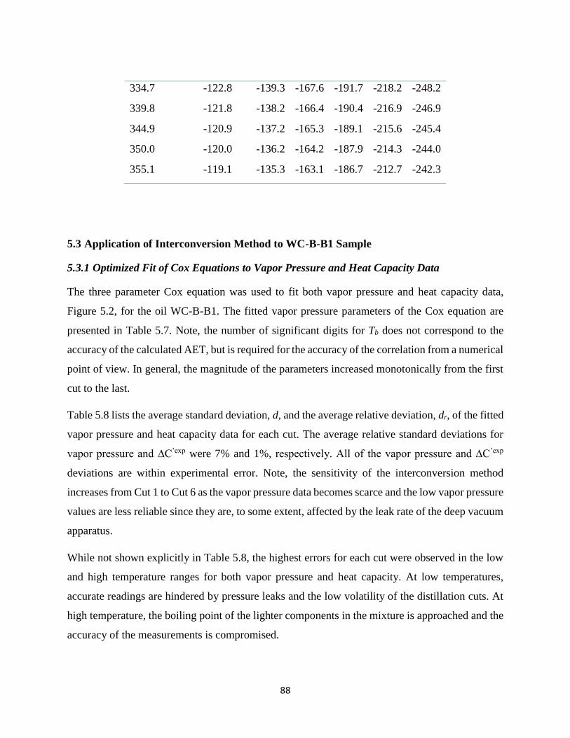
88
334.7 -122.8 -139.3 -167.6 -191.7 -218.2 -248.2
339.8 -121.8 -138.2 -166.4 -190.4 -216.9 -246.9
344.9 -120.9 -137.2 -165.3 -189.1 -215.6 -245.4
350.0 -120.0 -136.2 -164.2 -187.9 -214.3 -244.0
355.1 -119.1 -135.3 -163.1 -186.7 -212.7 -242.3
5.3 Application of Interconversion Method to WC-B-B1 Sample
5.3.1 Optimized Fit of Cox Equations to Vapor Pressure and Heat Capacity Data
The three parameter Cox equation was used to fit both vapor pressure and heat capacity data,
Figure 5.2, for the oil WC-B-B1. The fitted vapor pressure parameters of the Cox equation are
presented in Table 5.7. Note, the number of significant digits for Tb does not correspond to the
accuracy of the calculated AET, but is required for the accuracy of the correlation from a numerical
point of view. In general, the magnitude of the parameters increased monotonically from the first
cut to the last.
Table 5.8 lists the average standard deviation, d, and the average relative deviation, dr, of the fitted
vapor pressure and heat capacity data for each cut. The average relative standard deviations for
vapor pressure and ∆C’exp were 7% and 1%, respectively. All of the vapor pressure and ∆C’exp
deviations are within experimental error. Note, the sensitivity of the interconversion method
increases from Cut 1 to Cut 6 as the vapor pressure data becomes scarce and the low vapor pressure
values are less reliable since they are, to some extent, affected by the leak rate of the deep vacuum
apparatus.
While not shown explicitly in Table 5.8, the highest errors for each cut were observed in the low
and high temperature ranges for both vapor pressure and heat capacity. At low temperatures,
accurate readings are hindered by pressure leaks and the low volatility of the distillation cuts. At
high temperature, the boiling point of the lighter components in the mixture is approached and the
accuracy of the measurements is compromised.
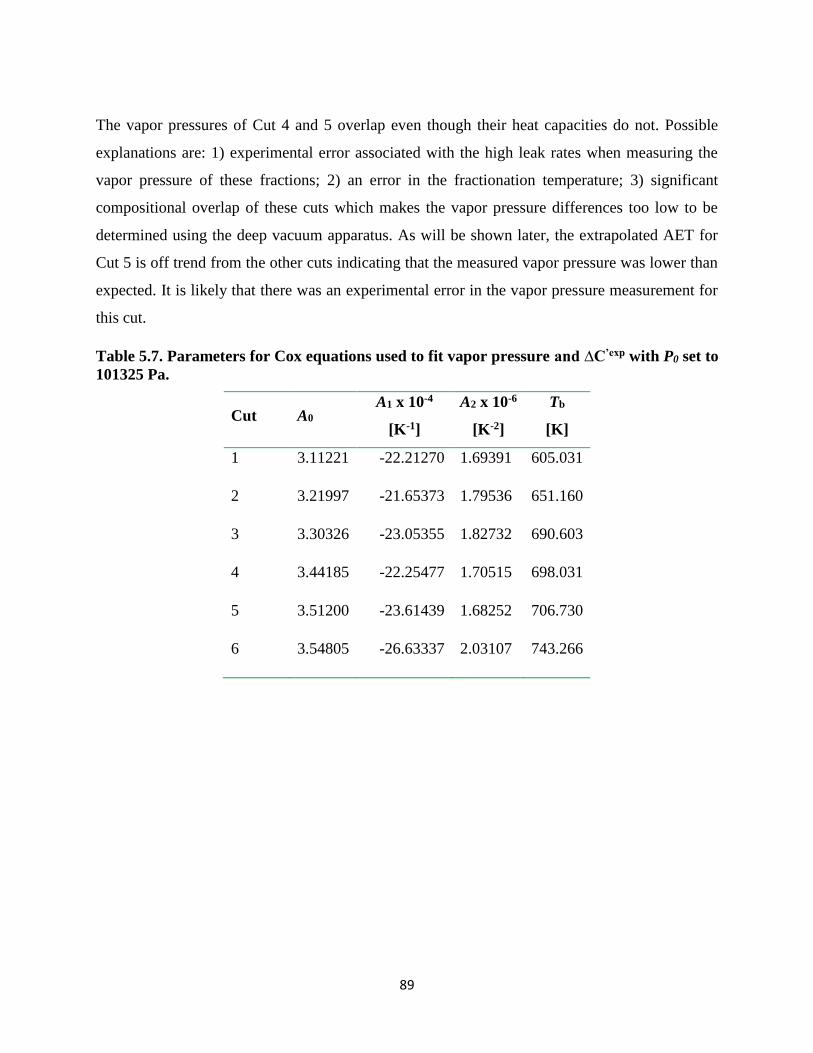
89
The vapor pressures of Cut 4 and 5 overlap even though their heat capacities do not. Possible
explanations are: 1) experimental error associated with the high leak rates when measuring the
vapor pressure of these fractions; 2) an error in the fractionation temperature; 3) significant
compositional overlap of these cuts which makes the vapor pressure differences too low to be
determined using the deep vacuum apparatus. As will be shown later, the extrapolated AET for
Cut 5 is off trend from the other cuts indicating that the measured vapor pressure was lower than
expected. It is likely that there was an experimental error in the vapor pressure measurement for
this cut.
Table 5.7. Parameters for Cox equations used to fit vapor pressure and ∆C’exp with P0 set to
101325 Pa.
Cut A0 A1 x 10-4
[K-1]
A2 x 10-6
[K-2]
Tb
[K]
1 3.11221 -22.21270 1.69391 605.031
2 3.21997 -21.65373 1.79536 651.160
3 3.30326 -23.05355 1.82732 690.603
4 3.44185 -22.25477 1.70515 698.031
5 3.51200 -23.61439 1.68252 706.730
6 3.54805 -26.63337 2.03107 743.266

90
Figure 5.2. Simultaneous fitting of experimental vapor pressure (left) and heat capacity
(right) of WC-B-B1 cuts using a three parameter Cox equation.
Table 5.8. Error analysis of the optimized correlation using the Cox equation.
Cut Vapor Pressure ∆C’exp
d [Pa] dr % d [J mol-1 K-1] dr %
1 1.1 5.2 0.92 1.0
2 0.5 8.7 1.17 1.0
3 0.2 3.0 1.27 0.8
4 0.1 7.8 1.26 0.6
5 0.3 9.0 3.05 1.3
6 0.1 10.5 2.41 1.0
5.3.2 Interconverted Boiling Points Using Vapor Pressure and Heat Capacity Data
Figure 5.3 presents the measured boiling points at the apparatus pressure and the interconverted
AET for WC_Bit_B1. The calculated final values for the optimization functions (OF) are
presented in Table 5.9. The interconverted boiling points are within experimental error of the

91
spinning band distillation (SBD) data. The error analysis is presented below and the Gaussian
extrapolation is discussed later.
Figure 5.3. Interconverted boiling point from the simultaneous correlation of vapor
pressure and heat capacity. The vertical error bars correspond to the maximum and
minimum deviation obtained during the error analysis, and the horizontal error bars
correspond to the experimental error estimated based on the repeatability of the distillation
procedure.
Table 5.9. Sensitivity analysis results after simultaneous correlation of vapor pressure and
heat capacity data for the WC-B-B1 sample.
Cut Calculated TBP
[K] OF
Maximum
ARD %
Minimum ARD
%
1 606 0.003 3.7 4.7
2 651 0.004 4.4 3.6
3 690 0.044 3.6 3.2
4 698 0.009 0.09 0.01
5 707 0.013 0.06 0.00
WC-B-B1

92
6 743 0.004 1.1 3.3
A sensitivity analysis was performed to determine how the errors of each property involved in the
interconversion method affect the predicted boiling point. The properties involved in the
interconversion include vapor pressure, molecular weight, elemental analysis, liquid heat capacity,
and gas ideal heat capacity. The value of each property was set to its highest or lowest value within
its range of error and the interconverted boiling points were recalculated for all combinations of
these values. The error bars in the inter-converted boiling point data, Figure 5.3, represent the
maximum and minimum deviation found during the sensitivity analysis. Table 5.9 presents the
absolute relative deviations for all the cuts of oil WC-B-B1. The maximum and minimum relative
deviations in the AET were 2.2% and -2.5% (corresponding to +8 K and -9 K), respectively.
5.4 Correlation of Liquid Heat Capacity
Liquid heat capacity data were not available for all of the distillation cuts. Therefore, a correlation
was required for the liquid heat capacity of heavy oil cuts before the interconversion method could
be applied to all seven samples. The proposed correlation is developed in Chapter 7 and has the
form:
𝐶𝑝𝑙𝑖𝑞 = (𝐵1 + 𝐴2𝐶𝑆) ∗ [𝐴3 − 𝐴4𝑆𝐺 + (𝐴5 − 𝐴6𝑆𝐺) (
𝑇
1000− 𝐴7)] (5.15)
where Cpliq is in J g-1 K-1, T is in K and Cs is defined in equation 5.16.
𝐶𝑆 = exp (−2.124
𝐻/𝐶) (5.16)
The constants are provided in Table 5.10. Figure 5.4 illustrates the errors obtained for the fitted
liquid heat capacity data of the WC-B-B1 oil. Overall the average error for all the WC-B-B1
distillation cuts was less than 1.5% with a maximum deviation of 2.5%. Note, here the specific
liquid heat capacity was fitted to the experimental data. However, for the interconversion method
the molar liquid heat capacity was used. Therefore, the values obtained using Equation 5.15 were
multiplied by the molecular weight.

93
Using Equation 5.15, the remaining liquid heat capacities of the other distillation cuts (where data
was not available) were calculated. Measured and calculated liquid heat capacity data for all the
distillation cuts are presented in Appendix D.
Table 5.10. Constants for liquid heat capacity correlation (Equation 5.15).
B1 1.621
A2 0.007
A3 0.733
A4 0.076
A5 4.401
A6 2.341
A7 0.092
Figure 5.4. Dispersion (left) and relative error (right) plot for the liquid heat capacity of
WC-B-B1 using Equation 5.15.
1.5
1.6
1.7
1.8
1.9
2
2.1
2.2
2.3
1.5 1.7 1.9 2.1 2.3
Ca
lcu
late
d C
p [
J g
-1K
-1
Experimental Cp [J g-1 K-1]
-15
-10
-5
0
5
10
15
1.5 1.7 1.9 2.1
(Cp
exp-C
pca
lc)/
Cp
exp*
10
0
Cpexp [J g-1 K-1]

94
5.5 Interconversion Results for Seven Heavy Oil and Bitumen Samples
The results of the fitting of both vapor pressure and heat capacity for WC-B-B1 were presented in
Figure 5.2 and are presented for the other oils in Figures 5.5 to 5.10. The Cox equation constants
obtained for each cut along with the boiling temperature are presented in Appendix E. A summary
of the average and relative absolute deviations obtained for the distillation cuts of the seven
samples is provided in Table 5.12. As mentioned previously in Section 5.4, not all the distillation
cuts had experimental liquid heat capacity and Equation 5.15 had to be used to estimate these
values. Table 5.11 shows what data were measured and what data were predicted for each of the
oils.
Table 5.11. Measured and calculated (Equation 5.15) liquid heat capacities of the distillation
cuts of the oils used in this study
Sample Measured Calculated
WC-B-B1 1 to 6
CO-B-A1 0 to 6
MX-HO-A1 0 to 4 5 to 7
CO-B-B1 0 to 3 4 to 6
US-HO-A1 0 to 7
WC-B-D1 0 to7
RO-HO-A1 0 to 7

95
Figure 5.5. Simultaneous fitting of experimental vapor pressure (left) and heat capacity
(right) of CO-B-A1using a three parameter Cox equation.
Figure 5.6. Simultaneous fitting of experimental vapor pressure and heat capacity using a
three parameter Cox equation for MX-HO-A1.
0.1
1
10
100
0.002 0.0025 0.003 0.0035
Va
por
Pre
ssu
re [
Pa]
1/T [K-1]
Cut 0 Cut 1Cut 2 Cut 3Cut 4 Cut 5Cut 6 Cox model
-280
-230
-180
-130
-80
-30
250 275 300 325 350 375
ΔC
' [J
/mol-1
K-1
]Temperature [K]
Cut 0 Cut 1Cut 2 Cut 3Cut 4 Cut 5Cut 6 Cox model
0.1
1
10
100
0.002 0.0025 0.003 0.0035
Va
po
ur
Pre
ssu
re [
Pa
]
1/T [K-1]
Cut 0 Cut 1Cut 2 Cut 3Cut 4 Cut 5Cut 6 Cox model
-280
-230
-180
-130
-80
-30
290 315 340 365 390
ΔC
' [J
/mo
l-1K
-1]
Temperature [K]
Cut 0 Cut 1Cut 2 Cut 3Cut 4 Cut 5Cut 6 Cox model

96
Figure 5.7. Simultaneous fitting of experimental vapor pressure and heat capacity using a
three parameter Cox equation for CO-B-B1.
Figure 5.8. Simultaneous fitting of experimental vapor pressure and heat capacity using a
three parameter Cox equation for US-HO-A1.
0.1
1
10
100
1000
0.002 0.0025 0.003 0.0035
Vap
or
Pre
ssu
re [
Pa]
1/T [K-1]
Cut 0 Cut 1Cut 2 Cut 3Cut 4 Cut 5Cut 6 Cox model
-280
-230
-180
-130
-80
-30
290 315 340 365 390
ΔC
' [J
/mol-1
K-1
]Temperature [K]
Cut 0 Cut 1Cut 2 Cut 3Cut 4 Cut 5Cut 6 Cox model
0.1
1
10
100
1000
0.002 0.0025 0.003 0.0035
Vap
or
Pre
ssu
re [
Pa]
1/T [K-1]
Cut 0 Cut 1Cut 2 Cut 3Cut 4 Cut 5Cut 6 Cox model
-300
-250
-200
-150
-100
-50
290 315 340 365 390
ΔC
' [J
/mo
l-1K
-1]
Temperature [K]
Cut 0 Cut 2Cut 3 Cut 4Cut 5 Cut 6Cox model
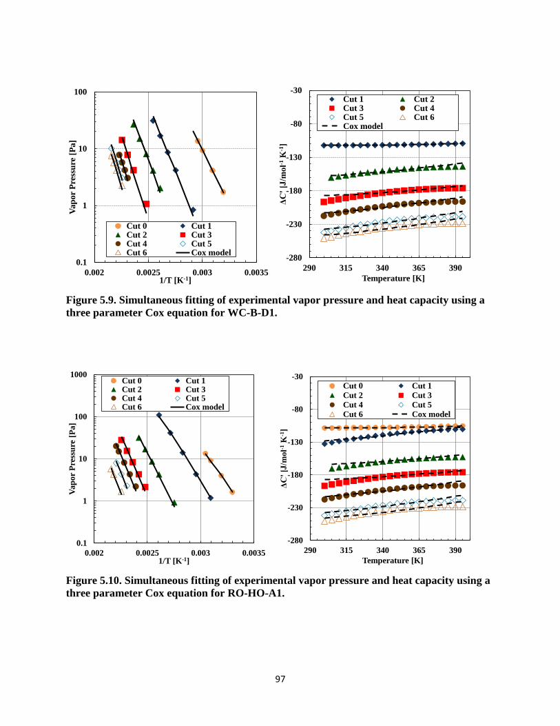
97
Figure 5.9. Simultaneous fitting of experimental vapor pressure and heat capacity using a
three parameter Cox equation for WC-B-D1.
Figure 5.10. Simultaneous fitting of experimental vapor pressure and heat capacity using a
three parameter Cox equation for RO-HO-A1.
0.1
1
10
100
0.002 0.0025 0.003 0.0035
Vap
or
Pre
ssu
re [
Pa
]
1/T [K-1]
Cut 0 Cut 1Cut 2 Cut 3Cut 4 Cut 5Cut 6 Cox model
-280
-230
-180
-130
-80
-30
290 315 340 365 390
ΔC
' [J
/mol-1
K-1
]Temperature [K]
Cut 1 Cut 2Cut 3 Cut 4Cut 5 Cut 6Cox model
0.1
1
10
100
1000
0.002 0.0025 0.003 0.0035
Va
po
r P
ress
ure
[P
a]
1/T [K-1]
Cut 0 Cut 1Cut 2 Cut 3Cut 4 Cut 5Cut 6 Cox model
-280
-230
-180
-130
-80
-30
290 315 340 365 390
ΔC
' [J
/mo
l-1K
-1]
Temperature [K]
Cut 0 Cut 1
Cut 2 Cut 3
Cut 4 Cut 5
Cut 6 Cox model

98
Table 5.12. Error analysis of the optimized correlation using the Cox equation
Sample Cut Vapor Pressure ΔC’exp
dr [%] d [Pa] dr [%] d [J mol-1 K-1]
WC-B-B1
1 5.2 1.1 1.0 0.9
2 8.7 0.5 1.0 1.2
3 3.0 0.2 0.8 1.3
4 7.8 0.1 0.6 1.3
5 9.0 0.3 1.3 3.0
6 10.5 0.1 1.0 2.4
CO-B-A1
0 6.0 0.5 9.8 1.4
1 1.3 0.1 9.5 1.7
2 9.9 0.9 10.1 2.9
3 12.4 1.2 12.8 5.3
4 8.4 0.4 12.6 3.5
5 12.3 0.5 9.4 2.9
6 7.1 0.2 7.9 2.5
MX-HO-A1
0 5.8 0.1 10.6 1.6
1 14.0 1.9 9.9 1.7
2 15.4 0.9 6.0 0.8
3 14.8 1.4 5.2 0.7
4 10.8 0.3 9.5 2.1
5 12.4 0.3 9.4 2.4
6 8.5 0.2 8.9 2.3
7 16.4 0.4 8.7 2.5
CO-B-B1
0 0.8 0.0 10.2 1.6
1 3.2 0.2 9.7 1.8
2 9.8 0.4 6.1 0.9
3 12.0 0.8 5.4 0.8

99
4 11.6 0.7 9.4 2.3
5 9.0 0.5 9.3 2.6
6 8.1 0.2 9.1 2.6
US-HO-A1
0 1.6 0.1 10.4 1.6
1 4.1 0.1 4.4 0.3
2 8.3 0.6 6.5 1.0
3 10.5 0.7 5.6 0.8
4 9.6 0.3 9.7 2.4
5 4.9 0.5 9.8 3.0
6 9.9 1.1 9.2 2.8
7 6.4 0.3 9.1 2.8
WC-B-D1
0 2.7 0.3 11.3 1.9
1 14.2 2.8 3.5 0.2
2 12.3 2.4 10.7 2.2
3 15.6 0.7 10.3 2.4
4 6.0 0.3 9.4 2.2
5 9.7 0.8 9.3 2.6
6 9.4 0.3 9.9 3.0
7 8.2 0.4 9.3 2.9
RO-HO-A1
0 0.2 0.0 11.5 2.0
1 6.4 1.2 5.1 0.3
2 10.6 2.1 10.9 2.2
3 11.7 1.9 5.6 3.8
4 8.3 0.5 11.0 2.9
5 3.7 0.3 10.6 2.8
6 5.0 0.3 10.3 3.0
7 5.0 0.3 10.1 3.3

100
The interconverted boiling points were compared with spinning band distillation (SBD) data in
Figure 5.3 for WC-B-B1 and for the other oils in Figures 5.11 to 5.12. In all cases, the inter-
converted data for the light cuts which overlapped the SBD measurement range were in good
agreement with the SBD data. Figure 5.13 shows the relative deviations (left) and the dispersion
plots (right) of the boiling temperature from the Cox fitting versus the SBD measurement. The
error bars on the dispersion plot in figures 5.13 to 5.16 correspond to the maximum deviation
expected based on the sensitivity analysis performed on the simultaneous fitting of vapor pressure
and heat capacity (Cox equation). The ARD was less than 1.3% which is lower than the expected
error in the interconverted boiling temperatures. The maximum deviation was less than 3.6%. The
dispersion plot shows that there is no systematic error in the inter-converted data. The spinning
band distillation data are summarized in Appendix F.
101
Figure 5.11. Comparison of the boiling temperatures obtained from the Cox equation with
the experimental and extrapolated SBD data for the WC-B-B1, CO-B-A1, MX-HO-A1, and
CO-B-B1 oils.
400
500
600
700
800
900
1000
1100
0 20 40 60 80 100
Tem
per
atu
re [
K]
Cumulative wt% Distilled Bitumen
SBD WC-B-B1
Interconverted using Cox
DVFA Boiling Point
SBD Gaussian Extrap.
400
500
600
700
800
900
1000
1100
0 20 40 60 80
Tem
per
atu
re [
K]
Cumulative wt% Distilled Bitumen
SBD CO-B-A1
Interconverted using Cox
DVFA Boiling Point
SBD Gaussian Extrap.
400
500
600
700
800
900
1000
1100
0 20 40 60 80 100
Tem
per
atu
re [
K]
Cumulative wt% Distilled Bitumen
MX-HO-A1
Interconverted using Cox
DVFA Boiling Point
SBD Gaussian Extrap.
400
500
600
700
800
900
1000
1100
0 20 40 60 80 100
Tem
per
atu
re [
K]
Cumulative wt% Distilled Bitumen
SBD CO-B-B1
Interconverted using Cox
DVFA Boiling Point
SBD Gaussian Extrap.

102
Figure 5.12. Comparison of the boiling temperatures obtained from the Cox equation with
the experimental and extrapolated SBD data for the US-HO-A1, WC-B-D1, and RO-HO-
A1 oils.
400
500
600
700
800
900
1000
1100
0 20 40 60 80 100
Tem
per
atu
re [
K]
Cumulative wt% Distilled Bitumen
SBD US-HO-A1
Interconverted using Cox
DVFA Boiling Point
SBD Gaussian Extrap.
400
500
600
700
800
900
1000
1100
0 20 40 60 80 100
Tem
per
atu
re [
K]
Cumulative wt% Distilled Bitumen
SBD WC-B-D1
Interconverted using Cox
DVFA Boiling Point
SBD Gaussian Extrap.
400
500
600
700
800
900
1000
1100
0 20 40 60 80 100
Tem
per
atu
re [
K]
Cumulative wt% Distilled Bitumen
SBD RO-HO-A1
Interconverted using Cox
DVFA Boiling Point
SBD Gaussian Extrap.
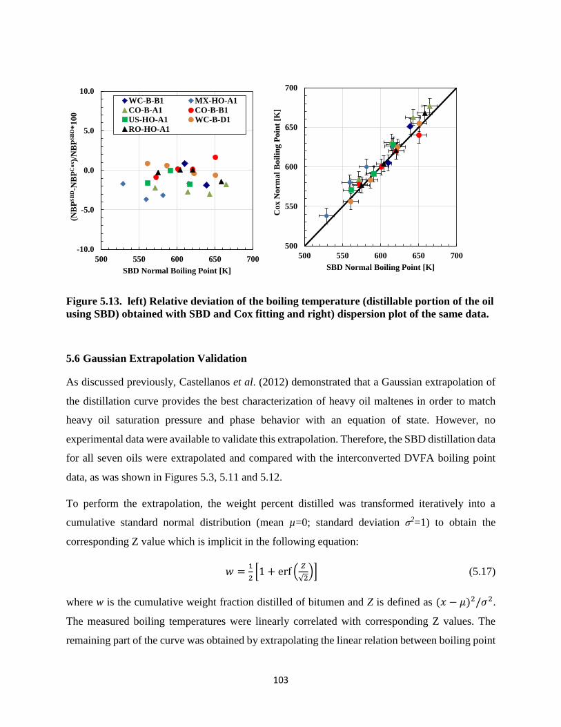
103
Figure 5.13. left) Relative deviation of the boiling temperature (distillable portion of the oil
using SBD) obtained with SBD and Cox fitting and right) dispersion plot of the same data.
5.6 Gaussian Extrapolation Validation
As discussed previously, Castellanos et al. (2012) demonstrated that a Gaussian extrapolation of
the distillation curve provides the best characterization of heavy oil maltenes in order to match
heavy oil saturation pressure and phase behavior with an equation of state. However, no
experimental data were available to validate this extrapolation. Therefore, the SBD distillation data
for all seven oils were extrapolated and compared with the interconverted DVFA boiling point
data, as was shown in Figures 5.3, 5.11 and 5.12.
To perform the extrapolation, the weight percent distilled was transformed iteratively into a
cumulative standard normal distribution (mean µ=0; standard deviation σ2=1) to obtain the
corresponding Z value which is implicit in the following equation:
𝑤 =1
2[1 + erf (
𝑍
√2)] (5.17)
where w is the cumulative weight fraction distilled of bitumen and Z is defined as (𝑥 − 𝜇)2/𝜎2.
The measured boiling temperatures were linearly correlated with corresponding Z values. The
remaining part of the curve was obtained by extrapolating the linear relation between boiling point
-10.0
-5.0
0.0
5.0
10.0
500 550 600 650 700
(NB
PS
BD-N
BP
Co
x)/
NB
PS
BD*
10
0
SBD Normal Boiling Point [K]
WC-B-B1 MX-HO-A1
CO-B-A1 CO-B-B1
US-HO-A1 WC-B-D1
RO-HO-A1
500
550
600
650
700
500 550 600 650 700
Co
x N
orm
al
Bo
ilin
g P
oin
t [K
]
SBD Normal Boiling Point [K]
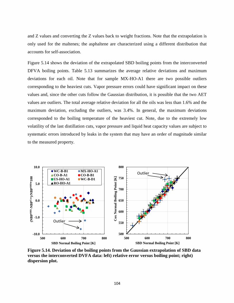
104
and Z values and converting the Z values back to weight fractions. Note that the extrapolation is
only used for the maltenes; the asphaltene are characterized using a different distribution that
accounts for self-association.
Figure 5.14 shows the deviation of the extrapolated SBD boiling points from the interconverted
DFVA boiling points. Table 5.13 summarizes the average relative deviations and maximum
deviations for each oil. Note that for sample MX-HO-A1 there are two possible outliers
corresponding to the heaviest cuts. Vapor pressure errors could have significant impact on these
values and, since the other cuts follow the Gaussian distribution, it is possible that the two AET
values are outliers. The total average relative deviation for all the oils was less than 1.6% and the
maximum deviation, excluding the outliers, was 3.4%. In general, the maximum deviations
corresponded to the boiling temperature of the heaviest cut. Note, due to the extremely low
volatility of the last distillation cuts, vapor pressure and liquid heat capacity values are subject to
systematic errors introduced by leaks in the system that may have an order of magnitude similar
to the measured property.
Figure 5.14. Deviation of the boiling points from the Gaussian extrapolation of SBD data
versus the interconverted DVFA data: left) relative error versus boiling point; right)
dispersion plot.
-10.0
-5.0
0.0
5.0
10.0
500 600 700 800
(NB
PS
BD-N
BP
Co
x)/
NB
PS
BD*100
SBD Normal Boiling Point [K]
WC-B-B1 MX-HO-A1
CO-B-A1 CO-B-B1
US-HO-A1 WC-B-D1
RO-HO-A1
500
550
600
650
700
750
800
500 600 700 800
Cox N
orm
al
Boil
ing P
oin
t [K
]
SBD Normal Boiling Point [K]
Outlier
s
Outlier
s

105
Table 5.13 ARD and maximum ARD obtained for the comparison between Gaussian
extrapolation of SBD data and AET using Cox equation
Sample ARD
[%]
MARD
[%]
WC-B-B1 1.3 2.4
CO-B-A1 2.0 3.3
MX-HO-A1 3.4 8.5
CO-B-B1 1.1 3.0
US-HO-A1 2.0 3.6
WC-B-D1 0.5 0.9
RO-HO-A1 0.4 1.5
5.7 Simplified Interconversion Method for DVFA
The data requirements for the above interconversion method are numerous and it is useful to
develop a simpler interconversion method. Most of the interconversion methods available in the
literature require the pressure at which distillation is performed because the correlations are based
on vapor pressure (Maxwell and Bonnell, 1955; Myers and Fenske, 1955; Riazi, 1979; Van Nes
and Van Western, 1951). Due to temperature constraints and vacuum detection limits, the DVFA
does not have a pressure gauge that allows data recording. Therefore, a different approach was
required with the following two main criteria: 1) minimum amount of measurements from
distillation cuts, and; 2) no pressure dependent equation.
The first input parameter is the measured boiling point data; that is, the end cut temperature of
each cut at the apparatus pressure. A second parameter is required and density was selected because
it is one of the most reliable and easy to measure properties that can be obtained for each distillation
cut. Finally, the bulk density of the sample distilled (in this case the maltenes) was used to account
for differences between different oils. The following interconversion equation, Equation 5.15, was
found to match the interconversion method based on vapor pressure and heat capacity data
(rigorous method):
𝐴𝐸𝑇 =𝑆𝐺𝑖
1.6068(𝑇𝑏𝑖∙𝑆𝐺𝐵𝑢𝑙𝑘)0.09661+260.77
0.9559 𝑆𝐺𝐵𝑢𝑙𝑘0.379
(5.18)
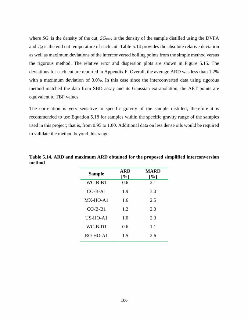
106
where SGi is the density of the cut, SGBulk is the density of the sample distilled using the DVFA
and Tbi is the end cut temperature of each cut. Table 5.14 provides the absolute relative deviation
as well as maximum deviations of the interconverted boiling points from the simple method versus
the rigorous method. The relative error and dispersion plots are shown in Figure 5.15. The
deviations for each cut are reported in Appendix F. Overall, the average ARD was less than 1.2%
with a maximum deviation of 3.0%. In this case since the interconverted data using rigorous
method matched the data from SBD assay and its Gaussian extrapolation, the AET points are
equivalent to TBP values.
The correlation is very sensitive to specific gravity of the sample distilled, therefore it is
recommended to use Equation 5.18 for samples within the specific gravity range of the samples
used in this project; that is, from 0.95 to 1.00. Additional data on less dense oils would be required
to validate the method beyond this range.
Table 5.14. ARD and maximum ARD obtained for the proposed simplified interconversion
method
Sample ARD
[%]
MARD
[%]
WC-B-B1 0.6 2.1
CO-B-A1 1.9 3.0
MX-HO-A1 1.6 2.5
CO-B-B1 1.2 2.3
US-HO-A1 1.0 2.3
WC-B-D1 0.6 1.1
RO-HO-A1 1.5 2.6
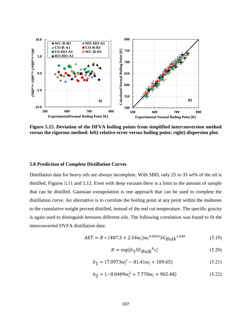
107
Figure 5.15. Deviation of the DFVA boiling points from simplified interconversion method
versus the rigorous method: left) relative error versus boiling point; right) dispersion plot.
5.8 Prediction of Complete Distillation Curves
Distillation data for heavy oils are always incomplete. With SBD, only 25 to 35 wt% of the oil is
distilled, Figures 5.11 and 5.12. Even with deep vacuum there is a limit to the amount of sample
that can be distilled. Gaussian extrapolation is one approach that can be used to complete the
distillation curve. An alternative is to correlate the boiling point at any point within the maltenes
to the cumulative weight percent distilled, instead of the end cut temperature. The specific gravity
is again used to distinguish between different oils. The following correlation was found to fit the
interconverted DVFA distillation data:
𝐴𝐸𝑇 = 𝐵 ∗ (487.3 + 2.54𝑤𝑖)𝑤𝑖0.0503𝑆𝐺𝐵𝑢𝑙𝑘
1.028 (5.19)
𝐵 = exp[𝑏1𝑆𝐺𝐵𝑢𝑙𝑘𝑏2] (5.20)
𝑏1 = (7.0973𝑤𝑖2 − 81.41𝑤𝑖 + 109.65) (5.21)
𝑏2 = (−0.0409𝑤𝑖2 + 7.770𝑤𝑖 + 902.48) (5.22)
-10.0
-5.0
0.0
5.0
10.0
500 600 700 800
(NB
PE
xp
. -N
BP
Ca
lc. )
/NB
PE
xp
. *100
ExperimentalNormal Boiling Point [K]
WC-B-B1 MX-HO-A1
CO-B-A1 CO-B-B1
US-HO-A1 WC-B-D1
500
550
600
650
700
750
800
500 600 700 800
Calc
ula
ted
Norm
al
Boil
ing P
oin
t [K
]Experimental Normal Boiling Point [K]
a) b)
-10.0
-5.0
0.0
5.0
10.0
500 600 700 800
(NB
PS
BD-N
BP
Co
x)/
NB
PS
BD*100
SBD Normal Boiling Point [K]
WC-B-B1 MX-HO-A1
CO-B-A1 CO-B-B1
US-HO-A1 WC-B-D1
RO-HO-A1
500
550
600
650
700
750
800
500 600 700 800
Co
x N
orm
al
Bo
ilin
g P
oin
t [K
]
SBD Normal Boiling Point [K]

108
where wi is the bitumen cumulative weight percent and SGBulk is the density of the sample distilled
(deasphalted oil).
Figure 5.16 presents the relative error and dispersion plot for the correlated versus the measured
boiling points for the seven oils from this study. Table 5.15 summarizes the deviation for each oil.
The average deviation for all the oils was within 1.2% and the maximum deviation was 4.0%.
Note, the residue is included in the error analysis since its weight percent is known. Its
‘experimental’ TBP was obtained from the Gaussian extrapolation of the SBD data.
Note that sample MX-HO-A1 has the highest deviation. It is possible that, due to its highly
paraffinic character, the slope of the curve was distinctly steeper compared with the rest of the oils
and possibly an additional variable is required to account for this effect. However, since the fitting
gave an error below the experimental error, the correlation was not further modified.
Table 5.15. ARD and MARD for the proposed correlation to obtain complete distillation
curves for the seven oils in this study.
Sample ARD
[%]
MARD
[%]
WC-B-B1 0.6 1.1
CO-B-A1 0.4 1.7
MX-HO-A1 1.6 7.0
CO-B-B1 0.8 1.8
US-HO-A1 0.7 1.3
WC-B-D1 1.2 2.1
RO-HO-A1 0.5 0.8

109
Figure 5.16. Deviation of the correlated versus the measured boiling points for the oils in this
study: left) relative error versus boiling point; right) dispersion plot.
The proposed correlation was then tested on an independent dataset extracted from an API
technical report (Sturm and Shay, 2000). The dataset included the following three oils which
covered a significant specific gravity and aromaticity range: Alaska North Slope (ANS) crude
(SG=0.8911), Utah Altamont (ALT) crude (very paraffinic; SG=0.8179), and San Joaquin Valley
(SJV) crude (very aromatic; SG=0.9772). Table 5.16 summarizes the deviations of the correlated
boiling points for test data set. The test data set had a total average deviation of less than 5.5% and
maximum deviation of 14.3%.
It is evident that for the most aromatic oils (Figure 5.17), the correlation was able to predict the
TBP with good accuracy. However, for the paraffinic sample, the performance was not as good.
This is attributed to the slightly different slope that distillation curves of light oils have compared
with those of heavy, aromatic oils. Therefore, the correlation is recommended for samples with
SG higher than 0.85; for lighter samples, alternative methods like Riazi method (Riazi, 2005) can
be used.
-10.0
-5.0
0.0
5.0
10.0
500 600 700 800 900 1000
(NB
PE
xp
. -N
BP
Ca
lc. )/N
BP
Exp
. *1
00
ExperimentalNormal Boiling Point [K]
WC-B-B1 MX-HO-A1CO-B-A1 CO-B-B1US-HO-A1 WC-B-D1RO-HO-A1
500
550
600
650
700
750
800
850
900
950
1000
500 600 700 800 900 1000
Ca
lcu
late
d N
orm
al
Bo
ilin
g P
oin
t [K
]
Experimental Normal Boiling Point [K]
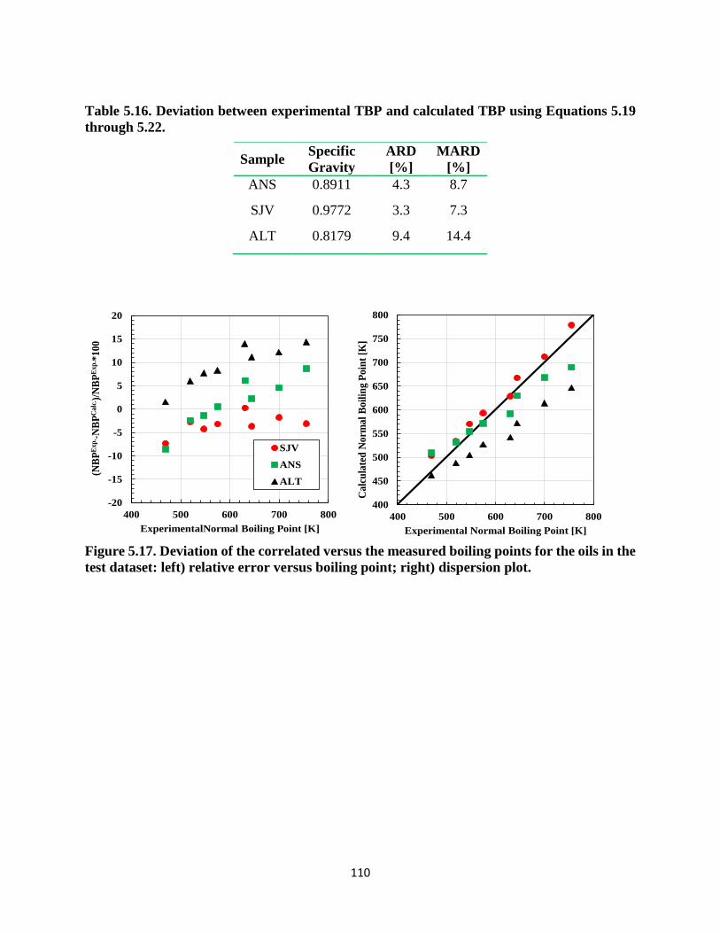
110
Table 5.16. Deviation between experimental TBP and calculated TBP using Equations 5.19
through 5.22.
Sample Specific
Gravity
ARD
[%]
MARD
[%]
ANS 0.8911 4.3 8.7
SJV 0.9772 3.3 7.3
ALT 0.8179 9.4 14.4
Figure 5.17. Deviation of the correlated versus the measured boiling points for the oils in the
test dataset: left) relative error versus boiling point; right) dispersion plot.
-20
-15
-10
-5
0
5
10
15
20
400 500 600 700 800
(NB
PE
xp
. -N
BP
Ca
lc. )
/NB
PE
xp
. *1
00
ExperimentalNormal Boiling Point [K]
SJV
ANS
ALT
400
450
500
550
600
650
700
750
800
400 500 600 700 800
Ca
lcu
late
d N
orm
al
Bo
ilin
g P
oin
t [K
]
Experimental Normal Boiling Point [K]

111
CHAPTER SIX: PHYSICAL PROPERTY DISTRIBUTIONS AND THEIR
CORRELATION
In this chapter, the physical properties collected for 63 cuts from different oil samples are
presented. It is shown that most of the correlations existing in the literature cannot correctly predict
the properties of the heavy cuts. New correlations are proposed that can be used when experimental
data are not available and predictions must be made. The most commonly employed correlating
properties are normal boiling point (NBP), molecular weight (MW), and specific gravity (SG), and
their correlations to each other are examined in first three sections of this chapter. Finally, the
correlations between specific gravity to the atomic H/C ratio and between specific gravity and the
refractive index are provided.
6.1 Normal Boiling Point
As was discussed in Chapter 2, the normal boiling point is usually correlated to MW and SG. For
pure paraffins, NBP increases monotonically with MW, Figure 6.1. Naphthenes follow the same
trend and aromatics and complex polyaromatic hydrocarbons (PAH) deviate to a higher NBP.
Riazi proposed a set of generalized correlations for the NBP (and other properties) of different
chemical families using only MW values as an input (Riazi, 2005). However, to correlate NBP
when all compound classes are present in a mixture (as is the case for petroleum cuts), a second
parameter is required. Typically, this additional correlating variable is SG since it captures the
changes that arise when different homologous series are present in a mixture.

112
Figure 6.1. Relationship between MW and NBP for different compound classes.
The correlations available in the literature for NBP were given in Table 2.2 and include the: Riazi
Daubert (RD), API, Soreide, Nji et al., Twu, Rao Bardon (RB), original Riazi Daubert (oldRD),
and Lee Kesler (LK) correlations. The correlations were compared to the experimental NBP of the
heavy oil cuts using their measured specific gravity and molecular weight as inputs. Measured data
are reported in Appendix B. As an example, Figure 6.2 shows the measured and correlated NBP
versus MW for the WC-B-B1 distillation cuts as an example. Figure 6.3 presents the deviations
for all of the above correlations from the measured TBP for all the oils. The average and maximum
absolute and relative deviations and the bias obtained for each correlation are reported in Table
6.1. Detailed results for each sample are summarized in Appendix G.
100
200
300
400
500
600
700
800
900
0 200 400 600
AE
T [
K]
Molecular Weight [g/mol]
Paraffins
Naphthenes
Aromatics
Iso-Paraffins
PAH

113
Figure 6.2. Measured and correlated NBP versus MW for the WC-B-B1 distillation cuts: left)
Soreide, Riazi Daubert (RD), API, and Nji et al. correlations; right) Twu, Rao Bardon (RB),
Lee Kesler (LK), and original Riazi Daubert (oldRD) correlations.
Figure 6.3. Relative error obtained for predicted NBP using experimental density and
molecular weight values: left) Riazi Daubert (RD), API, Soreide, and Nji et al. correlations;
right) Twu, Rao Bardon (RB), original Riazi Daubert (oldRD), Lee Kesler (LK).
500
600
700
800
900
1000
1100
1200
1300
100 300 500 700 900 1100
NB
P [
K]
Molecular Weight [g/mol]
SoreideRDAPINjiWC-B-B1
500
600
700
800
900
1000
1100
1200
1300
100 300 500 700 900 1100
NB
P [
K]
Molecular Weight [g/mol]
TwuRBLKoldRDWC-B-B1
-50
-40
-30
-20
-10
0
10
20
30
40
50
400 600 800 1000
(NB
PC
alc
-NB
PE
xp)/
NB
PE
xp
X1
00
Experimental NBP
RD
API
Soreide
Nji
-50
-40
-30
-20
-10
0
10
20
30
40
50
400 600 800 1000
(NB
PC
alc
-NB
PE
xp)/
NB
PE
xp
X1
00
Experimental NBP
Twu
RB
oldRD
LK
Residues

114
Table 6.1 Average absolute and relative deviations, maximum absolute and relative
deviations, and bias for NBP obtained using correlations from literature for the development
dataset.
Correlation AAD
[K]
ARD
[%]
MAAD
[K]
MARD
[%]
Bias
[%]
Soreide 25 3.7 110 14 3.3
LK 116 8.5 586 39 8.1
RD 43 6.2 98 14 5.4
API 68 5.3 264 19 5.2
oldRD 202 15.4 690 47 15.4
RB 57 7.8 243 31 7.6
Twu 76 10.9 198 25 10.9
Nji 30 4.4 92 11 1.6
The lowest relative deviation, 3.7%, was observed for the Soreide (1989) correlation. The
correlation with highest deviation, 15.4%, was the oldRD, the initial version of the correlation
proposed by Riazi (2005). This large deviation is not surprising since the oldRD correlation was
expected to fail since the heaviest hydrocarbon used to develop the correlation corresponded to
carbon numbers up to C25. Interestingly, the Lee-Kesler (1976) correlation, which is one of the
most commonly used correlations in simulation software, failed to predict the NBP of high
molecular weight distillation cuts and reports an average deviation of 8.5%.
All of the correlations, except for one oil (WC-B-B1) using the Nji et al. (2010) equation, have a
positive bias of the same magnitude as the relative deviation indicating that the majority of the
deviations over-predict the NBP. Also, all of the correlations have an increasing deviation from
the low to the high boiling cuts (excluding the residue). These trends are illustrated in the
dispersion plot for the best performing correlation (Soreide) in Figure 6.4. These correlations were
developed from datasets that included light to medium oils and pure paraffinic components. For
example, the development dataset for the Soreide correlation contained mostly North Sea Oils and
gas condensates (Soreide, 1989) with API values no lower than 25. These correlations do not
account for the higher aromaticity with heteroatom content of the heavier cuts. Since the

115
correlations are being used outside the range where they accurately predict the NBP, the higher
deviations for heavy cuts and residue are to be expected. Therefore, it is proposed to develop a
new correlation to address the consistent deviation observed for the higher boiling cuts.
Figure 6.4. NBP predictions obtained from Soreide’s correlation using experimental SG and
MW values.
Before proposing a new correlation, the best performing (Soreide) and most commonly used (Lee-
Kesler) correlations were evaluated to determine what features made one correlation better than
the other. Figure 6.5 shows the family of NBP curves that are obtained for several values of specific
gravity and molecular weight. The Lee-Kesler correlation does not have an asymptotic NBP at
infinite MW causing the observed over-prediction in NBP values for higher MW cuts, Figure 6.3B.
The effect of specific gravity in this correlation is smaller than the effect of the MW, and it is used
mainly to produce a family of curves with similar shape that converge to the specific gravity and
molecular weight of a low boiling point paraffin.
400
500
600
700
800
900
1000
400 600 800 1000
Calc
ula
ted
NB
P [
K]
Experimental NBP [K]
WC-B-B1
CO-B-A1
MX-HO-A1
CO-B-B1
US-HO-A1
WC-B-D1
RO-HO-A1

116
On the other hand, Soreide’s correlation produces a family of curves that have a maximum
asymptotic NBP for an infinite MW and SG, Equation 2.5 and Figure 6.3 (right). Here the effect
of density is again smaller than the effect of MW. However, at MW values lower than 280 g/mol,
the predicted NBP increases with increasing density while above 280 g/mol, the trend reverses.
This reversal likely reflects the change in aromaticity from lower MW to higher MW cuts but, of
more relevance here, it mathematically forces the predicted NBP values to approach an asymptote,
avoiding unrealistic NBP predictions for heavy cuts.
Figure 6.5. NBP curves obtained using left) the Lee-Kesler and right) Soreide correlations.
It was proposed to keep the structure of the Soreide correlation and retune it for heavy components
using the experimental data collected in this study. To make the modified Soreide correlation
applicable to a wide range of distillation cuts, the proposed correlation was fitted to a development
dataset which included the NBP of 300 pure components as well as the 63 heavy distillation cuts.
The pure components included paraffins, isoparaffins, naphthenes, aromatics and polycondensed
aromatic structures. The final correlation is given by:
𝑇𝑏 = 1805 − 1131 ∗ 𝑀𝑊−0.049 ∗ 𝑆𝐺1.5258 ∗ 𝐷 1.8 ⁄
𝐷 = exp(−0.005 ∗ 𝑀𝑊 − 2.675 ∗ 𝑆𝐺 + 0.003 ∗ 𝑀𝑊 ∗ 𝑆𝐺) (6.1)
300
400
500
600
700
800
900
1000
1100
0 200 400 600 800 1000
NB
P [
K]
MW
0.7
0.75
0.8
0.85
0.9
0.95
1
300
400
500
600
700
800
900
1000
1100
1200
0 200 400 600 800 1000
NB
P [
K]
MW
0.7
0.75
0.8
0.85
0.9
0.95
1
Density
Density
Density

117
where Tb is the normal boiling temperature in K. Equation 6.1 was based on boiling point data in
the temperature range from 300 to 900 K. The shape of the equation allows prediction of NBP
values not higher than 1300 K for high molecular weight and specific gravity values outside the
established range.
Figure 6.6 presents the dispersion plots of the NBP predictions for the distillation cuts from the
original and modified versions of the Soreide correlation. The NBP error bars were calculated from
the propagation of the experimental errors for SG and MW. MW errors were the major contributor
to the errors in the predictions. Figure 6.7 is a dispersion plot for the NBP of pure components
ranging from paraffins to polycondensed aromatic structures. The average absolute and relative
deviations and bias for the original and modified Soreide correlations are summarized in Table 6.2
and the maximum deviations in Table 6.3. The new correlation improved the average and
maximum deviations for both pure hydrocarbons and the heavy distillation cuts, and significantly
reduced the bias (from 3.1 to 1.6%).
The original version of the Soreide correlation is an excellent generally applicable predictive
correlation for the NBP of distillation cuts. However, as was discussed in Chapter 2, small errors
in the predicted NBP can produce significant errors in phase behavior predictions. Therefore, the
improvements in the NBP predictions using the new correlation are expected to help provide more
accurate phase behavior predictions for heavy oil and bitumen samples.

118
Figure 6.6. Dispersion plots for the NBP of the development dataset distillation cuts
determined from: left) the original Soreide correlation; right) the modified Soreide
correlation.
Figure 6.7. Dispersion plots for the NBP of the development dataset pure hydrocarbons
determined from: left) the original Soreide correlation; right) the modified Soreide
correlation.
400
500
600
700
800
900
1000
400 600 800 1000
Calc
ula
ted
NB
P [
K]
Experimental NBP [K]
WC-B-B1CO-B-A1MX-HO-A1CO-B-B1US-HO-A1WC-B-D1RO-HO-A1
400
500
600
700
800
900
1000
400 600 800 1000
Calc
ula
ted
NB
P [
K]
Experimental NBP [K]
WC-B-B1CO-B-A1MX-HO-A1CO-B-B1US-HO-A1WC-B-D1RO-HO-A1
50
150
250
350
450
550
650
750
50 200 350 500 650 800
Calc
ula
ted
NB
P [
K]
Experimetal NBP [K]
50
150
250
350
450
550
650
750
50 200 350 500 650 800
Calc
ula
ted
NB
P [
K]
Experimetal NBP [K]

119
Table 6.2. Average absolute and relative deviations and bias from the original and modified
Soreide correlation for NBP for the development dataset.
Oil Sample
Original Soreide Modified Soreide
AAD
[K]
ARD
[%]
Bias
[%]
AAD
[K]
ARD
[%]
Bias
[%]
WC-B-B1 23 3.2 2.1 19 2.8 0.8
CO-B-A1 7.2 1.0 -0.02 14 1.9 -1.2
MX-HO-A1 29 4.4 4.4 22 3.3 3.5
CO-B-B1 43 3.6 3.3 20 2.7 1.7
US-HO-A1 30 4.3 3.9 22 2.9 2.2
WC-B-D1 30 4.5 4.5 20 2.6 3.0
RO-HO-A1 6.6 4.2 3.7 21 2.9 2.4
Pure Components 13 2.9 2.0 8.9 1.9 0.02
Overall 15 3.0 2.2 11 2.0 0.4
Table 6.3. Maximum absolute and relative deviations from the original and modified Soreide
correlation for NBP of the development dataset.
Oil Sample
Original Soreide Modified Soreide
MAAD
[K]
MARD
[%]
MAAD
[K]
MARD
[%]
WC-B-B1 56 7.5 40 5.4
CO-B-A1 14 2.1 40 4.3
MX-HO-A1 43 6.4 33 5.3
CO-B-B1 61 9.0 49 7.3
US-HO-A1 58 8.3 46 6.6
WC-B-D1 63 8.7 49 6.8
RO-HO-A1 14 1.6 21 2.9
Pure Components 82 28 47 16
Overall 82 28 49 16

120
The original and modified Soreide correlations were evaluated against an independent test dataset
obtained from the literature (Sturm and Shay, 2000; Smith, 2007; Fang et al., 2003) and provided
in Tables 6.5 to 6.9. The dataset included 100 cuts encompassing a wide range of aromaticity and
paraffinicity dictated by the bulk H/C ratios values. Note, no experimental error was presented by
the authors. Fang et al. (2003) provided data for three oils but combined the data into a single table
without distinguishing between the oils, hence the specific gravity of each bulk sample is not
reported for these oils.
Table 6.4. Molecular weight, specific gravity, H/C atomic ratio, and normal boiling point of
ANS oil with bulk SG=0.89 and H/C=1.7 (Sturm and Shay, 2000).
Molecular
Weight
[g/mol]
Specific
Gravity
H/C
Ratio
Normal
Boiling
Point
[K]
152 0.8095 1.90 469.2
245 0.8456 1.84 519.2
248 0.8633 1.79 547.0
263 0.8696 1.81 574.8
271 0.8867 1.77 630.3
434 0.9021 1.75 644.2
442 0.9296 1.72 699.8
518 0.9437 1.66 755.3
573 0.9628 1.61 810.9
683 0.9678 1.58 866.4
850 0.9830 1.55 922.0

121
Table 6.5. Molecular weight, specific gravity, H/C atomic ratio, and normal boiling point of
ALT oil with bulk SG=0.81and H/C=1.9 (Sturm and Shay, 2000).
Molecular
Weight
[g/mol]
Specific
Gravity
H/C
Ratio
Normal
Boiling
Point
[K]
148 0.7649 2.00 469.3
225 0.7853 2.08 519.3
231 0.7945 2.07 547.0
264 0.8003 2.08 574.8
289 0.8044 2.06 630.4
338 0.8203 1.95 644.3
401 0.8338 2.05 699.8
457 0.8413 2.07 755.4
551 0.8577 2.01 810.9
750 0.8741 2.03 866.5
1018 0.8848 922.0
Table 6.6. Molecular weight, specific gravity, H/C atomic ratio, and normal boiling point of
SJV oil with bulk SG=0.91and H/C=1.5 (Sturm and Shay, 2000).
Molecular
Weight
[g/mol]
Specific
Gravity
H/C
Ratio
Normal
Boiling
Point
[K]
171 0.8532 1.86 469.2
207 0.8745 1.80 519.2
228 0.8914 1.76 547.0
244 0.9124 1.70 574.8
272 0.9317 1.64 630.3
283 0.9483 1.58 644.2
335 0.9604 1.58 699.8
432 0.9872 1.50 755.3

122
540 1.0034 1.47 810.9
640 1.015 1.45 866.4
718 1.0274 1.44 922.0
Table 6.7. Molecular weight, specific gravity, H/C atomic ratio, and normal boiling point of
HVGO with bulk SG=1.02 and H/C= 1.47(Smith, 2007).
Molecular
Weight
[g/mol]
Specific
Gravity
Normal
Boiling
Point
[K]
288 0.9232 616.15
287 0.9456 632.15
304 0.9592 660.65
328 0.9672 685.65
359 0.9714 710.65
402 0.9770 735.65
451 0.9796 760.65
578 0.9948 785.65
Table 6.8. Molecular weight, specific gravity, and normal boiling point of Iran, Russia, China
oils (Fang et al, 2003).
Molecular
Weight
[g/mol]
Specific
Gravity
Normal
Boiling
Point
[K]
Molecular
Weight
[g/mol]
Specific
Gravity
Normal
Boiling
Point
[K]
95 0.7066 355.5 171 0.8114 467.7
95 0.7255 357.2 162 0.8004 477.7
108 0.7370 377.2 163 0.8069 478.3
108 0.7374 377.5 162 0.8178 481.5
107 0.7303 380.5 171 0.8135 490.7
107 0.7466 381.1 201 0.8568 502.4
120 0.7585 385.4 180 0.8192 503.7

123
120 0.7573 402.7 180 0.8199 506.8
120 0.7639 406.6 187 0.8305 509.2
119 0.7545 407.7 199 0.8336 526.6
134 0.7764 411.0 199 0.8312 530.1
133 0.7742 427.4 205 0.8430 530.9
130 0.7756 429.1 199 0.8362 531.7
131 0.7769 431.0 210 0.8408 542.4
133 0.7824 431.3 221 0.8441 556.7
131 0.7650 433.3 226 0.8522 556.8
132 0.7786 433.6 220 0.8457 557.4
133 0.7797 434.9 232 0.8524 559.3
139 0.7808 437.1 243 0.8681 577.7
134 0.7810 437.4 249 0.8597 582.1
136 0.7823 439.8 244 0.8554 583.3
137 0.7837 443.0 256 0.8644 595.0
139 0.7851 445.7 267 0.8789 601.2
147 0.7894 446.2 272 0.8737 607.0
147 0.7879 452.0 268 0.8740 610.5
155 0.7972 455.4 295 0.8854 624.4
146 0.7866 457.2 299 0.8837 629.6
147 0.7990 457.3 296 0.8827 634.3
159 0.8187 461.1 325 0.8973 646.8
Figure 6.8 presents the dispersion plots of the NBP predictions for the test dataset from the original
and modified versions of the Soreide correlation. The average absolute and relative deviations and
bias for the original and modified Soreide correlations are summarized in Table 6.9 and the
maximum deviations in Table 6.10. Overall the improvement is slight but nonetheless the
maximum deviations are decreased for the majority of the cuts. The improvement is a more
significant success than appears at first glance. The modified correlation was optimized for heavy
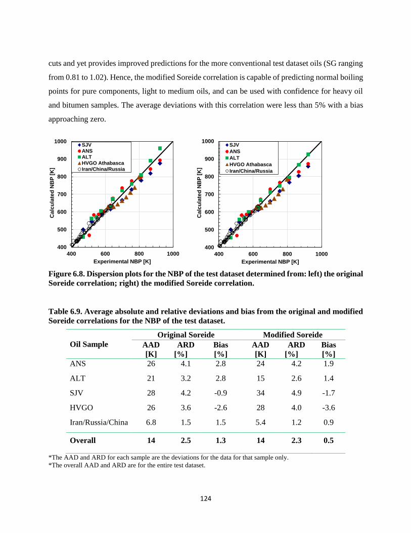
124
cuts and yet provides improved predictions for the more conventional test dataset oils (SG ranging
from 0.81 to 1.02). Hence, the modified Soreide correlation is capable of predicting normal boiling
points for pure components, light to medium oils, and can be used with confidence for heavy oil
and bitumen samples. The average deviations with this correlation were less than 5% with a bias
approaching zero.
Figure 6.8. Dispersion plots for the NBP of the test dataset determined from: left) the original
Soreide correlation; right) the modified Soreide correlation.
Table 6.9. Average absolute and relative deviations and bias from the original and modified
Soreide correlations for the NBP of the test dataset.
Oil Sample
Original Soreide Modified Soreide
AAD
[K]
ARD
[%]
Bias
[%]
AAD
[K]
ARD
[%]
Bias
[%]
ANS 26 4.1 2.8 24 4.2 1.9
ALT 21 3.2 2.8 15 2.6 1.4
SJV 28 4.2 -0.9 34 4.9 -1.7
HVGO 26 3.6 -2.6 28 4.0 -3.6
Iran/Russia/China 6.8 1.5 1.5 5.4 1.2 0.9
Overall 14 2.5 1.3 14 2.3 0.5
*The AAD and ARD for each sample are the deviations for the data for that sample only.
*The overall AAD and ARD are for the entire test dataset.
400
500
600
700
800
900
1000
400 600 800 1000
Ca
lcu
late
d N
BP
[K
]
Experimental NBP [K]
SJV
ANS
ALT
HVGO Athabasca
Iran/China/Russia
400
500
600
700
800
900
1000
400 600 800 1000
Ca
lcu
late
d N
BP
[K
]
Experimental NBP [K]
SJV
ANS
ALT
HVGO Athabasca
Iran/China/Russia
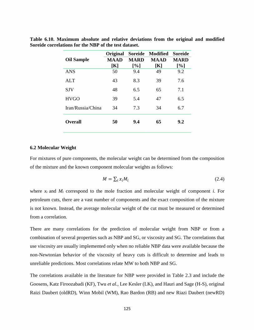
125
Table 6.10. Maximum absolute and relative deviations from the original and modified
Soreide correlations for the NBP of the test dataset.
Oil Sample
Original Soreide Modified Soreide
MAAD
[K]
MARD
[%]
MAAD
[K]
MARD
[%]
ANS 50 9.4 49 9.2
ALT 43 8.3 39 7.6
SJV 48 6.5 65 7.1
HVGO 39 5.4 47 6.5
Iran/Russia/China 34 7.3 34 6.7
Overall 50 9.4 65 9.2
6.2 Molecular Weight
For mixtures of pure components, the molecular weight can be determined from the composition
of the mixture and the known component molecular weights as follows:
𝑀 = ∑ 𝑥𝑖𝑀𝑖𝑖 (2.4)
where xi and Mi correspond to the mole fraction and molecular weight of component i. For
petroleum cuts, there are a vast number of components and the exact composition of the mixture
is not known. Instead, the average molecular weight of the cut must be measured or determined
from a correlation.
There are many correlations for the prediction of molecular weight from NBP or from a
combination of several properties such as NBP and SG, or viscosity and SG. The correlations that
use viscosity are usually implemented only when no reliable NBP data were available because the
non-Newtonian behavior of the viscosity of heavy cuts is difficult to determine and leads to
unreliable predictions. Most correlations relate MW to both NBP and SG.
The correlations available in the literature for NBP were provided in Table 2.3 and include the
Goosens, Katz Firoozabadi (KF), Twu et al., Lee Kesler (LK), and Hauri and Sage (H-S), original
Raizi Daubert (oldRD), Winn Mobil (WM), Rao Bardon (RB) and new Riazi Daubert (newRD)
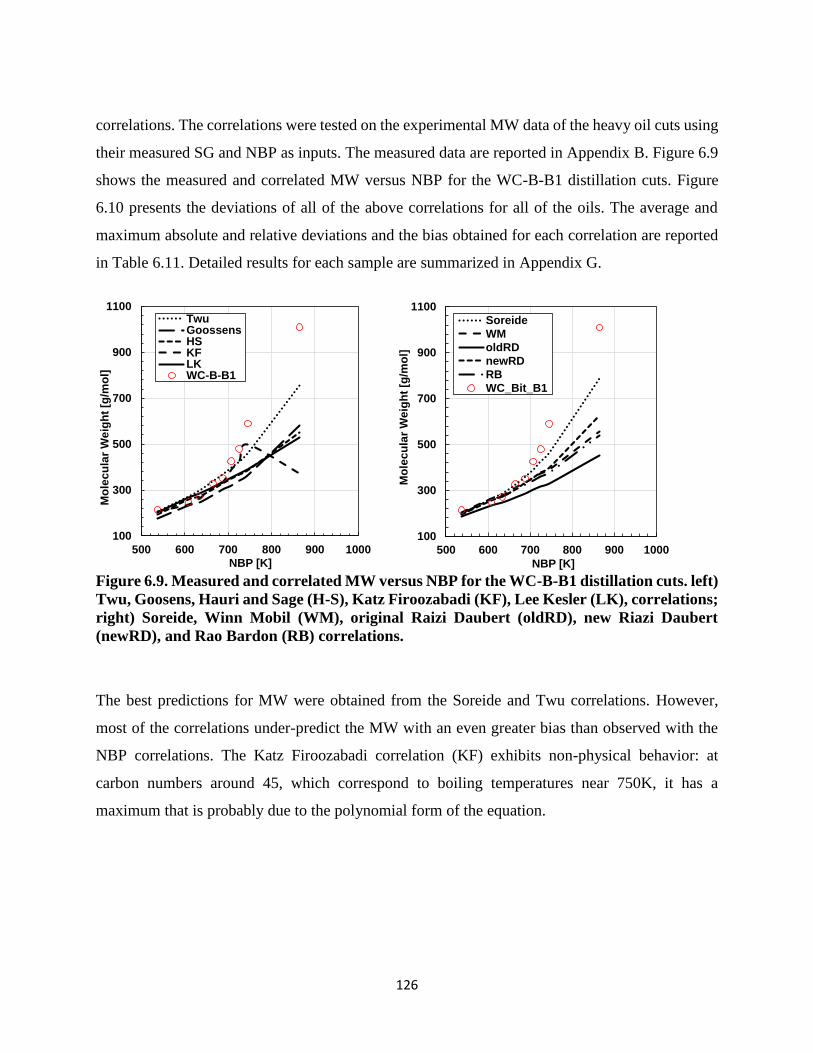
126
correlations. The correlations were tested on the experimental MW data of the heavy oil cuts using
their measured SG and NBP as inputs. The measured data are reported in Appendix B. Figure 6.9
shows the measured and correlated MW versus NBP for the WC-B-B1 distillation cuts. Figure
6.10 presents the deviations of all of the above correlations for all of the oils. The average and
maximum absolute and relative deviations and the bias obtained for each correlation are reported
in Table 6.11. Detailed results for each sample are summarized in Appendix G.
Figure 6.9. Measured and correlated MW versus NBP for the WC-B-B1 distillation cuts. left)
Twu, Goosens, Hauri and Sage (H-S), Katz Firoozabadi (KF), Lee Kesler (LK), correlations;
right) Soreide, Winn Mobil (WM), original Raizi Daubert (oldRD), new Riazi Daubert
(newRD), and Rao Bardon (RB) correlations.
The best predictions for MW were obtained from the Soreide and Twu correlations. However,
most of the correlations under-predict the MW with an even greater bias than observed with the
NBP correlations. The Katz Firoozabadi correlation (KF) exhibits non-physical behavior: at
carbon numbers around 45, which correspond to boiling temperatures near 750K, it has a
maximum that is probably due to the polynomial form of the equation.
100
300
500
700
900
1100
500 600 700 800 900 1000
Mo
lec
ula
r W
eig
ht
[g/m
ol]
NBP [K]
TwuGoossensHSKFLKWC-B-B1
100
300
500
700
900
1100
500 600 700 800 900 1000
Mo
lec
ula
r W
eig
ht
[g/m
ol]
NBP [K]
Soreide
WM
oldRD
newRD
RB
WC_Bit_B1

127
All the correlations were developed from datasets that included only light to medium petroleum
cuts and here are being used outside their range of applicability. As observed for the NBP, all of
the correlations have an increasing deviation from the low to the high boiling cuts. Part of the
increased bias can be attributed to differences in MW measurements. MW was measured by vapor
pressure osmometry (VPO) in this thesis but freezing point depression methods are often used in
the literature. MW from freezing point depression are often lower than VPO measurements
(Altgelt and Boduszynski, 1994). Nonetheless, most of the deviation is attributed to extrapolating
the correlations beyond their range of applicability. This issue will be addressed when the test
dataset is examined later.
Figure 6.10. Relative error obtained for predicted MW using experimental SG and NBP
values: left) Goosens, Katz Firoozabadi (KF), Twu, Lee Kesler (LK), and Hauri and Sage
(H-S) correlations; right) original Raizi Daubert (oldRD), Winn Mobil (WM), Rao Bardon
(RB) and new Riazi Daubert (newRD). The errors for the Soreide correlation are shown in
Figure 6.11.
-80
-70
-60
-50
-40
-30
-20
-10
0
10
20
100 600 1100
(MW
Calc
-MW
Ex
p)/
MW
Ex
pX
10
0
Experimental MW
oldRDnewRDWMRBSoreide
-80
-70
-60
-50
-40
-30
-20
-10
0
10
20
100 600 1100
(MW
Calc
-MW
Exp)/
MW
Exp
X1
00
Experimental MW
GoossensKFTwuLKHS
Heavy
distillation cuts
and Residues

128
Table 6.11 Average absolute and relative deviations, maximum absolute and relative
deviations, and bias for NBP obtained using correlations from literature for the development
dataset.
Correlation AAD
[K]
ARD
[%]
MAAD
[K]
MARD
[%]
Bias
[%
Soreide 49 9.8 347 38 -8.6
LK 90 15.5 480 52 -14.7
old RD 134 25.8 564 59 -25.8
new RD 78 14.7 439 48 -14.5
Goossens 108 22.3 483 53 -22.3
HS 91 16.5 471 51 -16.4
KF 85 11.2 971 93 -11.2
WM 86 15.1 464 51 -14.2
RB 93 16.7 480 52 -16.3
Twu 48 9.4 364 40 -7.3
Figure 6.11 presents the dispersion plots of the MW predictions for the development dataset
distillation cuts from the original and modified versions of the Soreide correlation. The MW error
bars were calculated from the propagation of the experimental errors for SG and NBP. Figure 6.12
is a dispersion plot for the MW of pure components ranging from paraffins to polycondensed
aromatic structures. The average absolute and relative deviations and bias for the original and
modified Soreide correlations are summarized in Table 6.12 and the maximum deviations in Table
6.13. The new correlation improved the average and maximum deviations for both pure
hydrocarbons and the heavy distillation cuts, and significantly reduced the bias (from -5.5 to -
0.4%).

129
Figure 6.11. Dispersion plots for the MW of the development dataset distillation cuts
determined from: left) the original Soreide correlation; right) the modified Soreide
correlation.
Figure 6.12. Dispersion plots for the MW of the development dataset pure hydrocarbons
determined from: a) the original Soreide correlation; b) the modified Soreide correlation.
100
300
500
700
900
1100
100 300 500 700 900 1100
Ca
lcu
late
d M
W
Experimental MW
WC-B-B1CO-B-A1MX-HO-A1CO-B-B1US-HO-A1WC-B-D1RO-HO-A1
100
300
500
700
900
1100
100 300 500 700 900 1100
Ca
lcu
late
d M
WExperimental MW
WC-B-B1CO-B-A1MX-HO-A1CO-B-B1US-HO-A1WC-B-D1RO-HO-A1
50
100
150
200
250
300
350
400
450
50 150 250 350 450
Ca
lcu
late
d M
W
Experimetal MW
50
100
150
200
250
300
350
400
450
50 150 250 350 450
Ca
lcu
late
d M
W
Experimetal MW

130
Table 6.12. Average absolute and relative deviations and bias from the original and modified
Soreide correlation for MW for the development dataset.
Oil Sample
Original
Soreide
Modified
Soreide
AAD
[g/mol]
ARD
[%]
Bias
[%]
AAD
[g/mol]
ARD
[%]
Bias
[%]
WC-B-B1 55 9.5 -6.3 45 8.7 -2.8
CO-B-A1 15 3.2 0.4 39 6.3 5.0
MX-HO-A1 46 11.4 -11.4 38 9.7 -8.6
CO-B-B1 96 16.6 -16.6 86 14.5 -14.5
US-HO-A1 52 11.4 -11.4 39 9.1 -9.1
WC-B-D1 64 11.7 -11.7 47 9.0 -9.0
RO-HO-A1 15 2.8 -1.3 17 3.2 2.3
Pure Components 12 7.5 -4.9 8 4.6 0.6
Overall 19 7.8 -5.5 14 5.3 -0.4
Table 6.13. Maximum absolute and relative deviations from the original and modified
Soreide correlation for MW of the development dataset.
Oil Sample
Original Soreide Modified Soreide
MAAD
[g/mol]
MARD
[%]
MAAD
[g/mol]
MARD
[%]
WC-B-B1 127 21.4 103 17.4
CO-B-A1 21 5.3 37 9.2
MX-HO-A1 66 16.1 57 13.9
CO-B-B1 109 22.9 96 20.0
US-HO-A1 101 20.8 89 18.4
WC-B-D1 122 22.3 106 19.5
RO-HO-A1 24 4.7 31 7.7
Pure Components 194 95.9 57 35.4
The original and modified Soreide correlations were evaluated against the same independent test
dataset obtained from the literature for the NBP correlations, Tables 6.4 to 6.8. The MW were
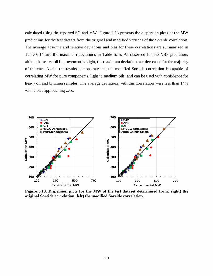
131
calculated using the reported SG and MW. Figure 6.13 presents the dispersion plots of the MW
predictions for the test dataset from the original and modified versions of the Soreide correlation.
The average absolute and relative deviations and bias for these correlations are summarized in
Table 6.14 and the maximum deviations in Table 6.15. As observed for the NBP prediction,
although the overall improvement is slight, the maximum deviations are decreased for the majority
of the cuts. Again, the results demonstrate that the modified Soreide correlation is capable of
correlating MW for pure components, light to medium oils, and can be used with confidence for
heavy oil and bitumen samples. The average deviations with this correlation were less than 14%
with a bias approaching zero.
Figure 6.13. Dispersion plots for the MW of the test dataset determined from: right) the
original Soreide correlation; left) the modified Soreide correlation.
100
200
300
400
500
600
700
100 300 500 700
Ca
lcu
late
d M
W
Experimental MW
SJVANSALTHVGO AthabascaIran/China/Russia
100
200
300
400
500
600
700
100 300 500 700
Ca
lcu
late
d M
W
Experimental MW
SJVANSALTHVGO AthabascaIran/China/Russia

132
Table 6.14. Average absolute and relative deviations and bias from the original and modified
Soreide correlations for the MW of the test dataset.
Oil Sample
Original
Soreide
Modified
Soreide
AAD
[g/mol]
ARD
[%]
Bias
[%]
AAD
[g/mol]
ARD
[%]
Bias
[%]
ANS 46 13.4 -11.2 43 12.7 -10.2
ALT 19 7.0 -5.9 19 6.9 -3.9
SJV 28 10.3 -0.1 34 11.7 1.8
HVGO 29 7.6 3.4 35 9.5 8.6
Iran/Russia/China 5 3.1 -2.9 4 2.3 -1.8
Overall 14 5.4 -3.2 14 5.1 -1.5
Table 6.15. Maximum absolute and relative deviations from the original and modified
Soreide correlations for the MW of the test dataset.
Oil Sample
Original
Soreide
Modified
Soreide
MAAD
[g/mol]
MARD
[%]
MAAD
[g/mol]
MARD
[%]
ANS 1245 28.8 121 27.8
ALT 34 15.2 32 14.4
SJV 53 14.7 74 18.3
HVGO 44 12.0 65 15.8
Iran, Russia, China 29 14.1 29 14.3
6.3 Specific Gravity
As shown in Chapter 2, there are several correlations to predict SG that use different input
variables. These variables range from simply MW and characterization factors (Jacoby, 1952;
Soreide, 1989; Whitson, 1983) to refractive index combined with either MW or boiling point

133
(Riazi and Daubert, 2005). Elemental analysis was also used as correlating variable to predict SG
(Gray, 2002; Katz and Firoozabadi, 1978).
The correlations were tested on the experimental MW of the heavy oil cuts using their measured
properties as inputs. Measured data are reported in Appendix B. Figure 6.14 shows the measured
and correlated SG versus MW for the WC-B-B1 distillation cuts. Figure 6.15a and Figure 6.15b,
respectively, show the errors for the methods that require a characterization factor and the methods
that do not use characterization factors and instead use other physical properties. The average and
maximum average and relative deviations and bias are presented in Table 6.16. The deviations and
bias for each sample are summarized in Appendix G.
The SG predictions are much more accurate than the NBP and MW predictions. However,
excluding the residue fraction, all of the correlations (except for RD MW, RI and K-F) exhibit a
trend in the error with the maximum over-prediction occurring for the light cuts and the maximum
under-prediction occurring for the heavy cuts. Note, since the K-F correlation preserves the same
shape as the distillation cuts experimental density, it will be used in Chapter 8 to develop an
improved specific gravity distribution. Interestingly, the Gray correlation performed similarly to
the other correlations although it only used elemental analysis as an input.
Not surprisingly, the correlations with the characterization factor had lower deviations and bias on
average than the other methods. The smallest deviations and bias were found with the Jacoby
(1982) correlation because it provided better predictions for the residues. The maximum deviation
with this correlation was only 6% but the systematic trend in the errors suggest that the correlation
can be improved upon.

134
Figure 6.14. Measured and correlated SG versus MW for the WC-B-B1 distillation cuts.
Left) Soreide, Jacoby, Whitson; right) Katz Firoozabadi (K-F), Riazi and Daubert using
boiling point and refractive index as inputs (RD Tb, I), and Gray.
Figure 6.15. Relative error obtained for predicted SG using correlations with
characterization factors (left: Soreide, Jacoby, Whitson) and correlations with physical
properties (right: Katz Firoozabadi (K-F), Riazi and Daubert using boiling point and
refractive index as inputs (RD Tb, I), and Gray) as input parameters.
0.8
0.9
1.0
1.1
1.2
100 300 500 700 900 1100
SG
Molecular Weight [g/mol]
Soreide
Jacoby
Whitson
WC-B-B1
0.8
0.9
1.0
1.1
1.2
100 300 500 700 900 1100
SG
Molecular Weight [g/mol]
K-F
RD Tb, I
Gray
WC-B-B1
-20
-15
-10
-5
0
5
10
15
20
0.80 0.90 1.00 1.10
(SG
Calc
-SG
Exp)/
SG
exp
X1
00
Experimental SG
RD Tb, RI
RD MW, RI
K-F
Gray
-20
-15
-10
-5
0
5
10
15
20
0.80 0.90 1.00 1.10
(SG
Calc
-SG
Exp)/
SG
exp
X1
00
Experimental SG
Jacoby
Soreide
Whitson

135
Table 6.16 Absolute and relative deviations for SG obtained using correlations from
literature.
Correlation AAD ARD
[%] MAAD
MARD
[%]
Bias
[%]
Soreide 0.02 2.0 0.04 4.3 1.5
Whitson 0.05 4.9 0.09 8.5 3.4
Jacoby 0.02 1.8 0.06 6.8 -0.5
RD Tb, RI 0.03 2.8 0.06 5.8 2.2
RD MW, RI 0.09 8.8 0.64 63.3 -7.6
K-F 0.06 6.1 0.10 10.8 6.1
Gray 0.03 3.1 0.11 11.2 -0.3
Since the best results were obtained with characterization factors, this approach is tested first. To
facilitate the discussion, the correlations are provided in Equations 2.16 to 2.18:
Soreide: 𝑆𝐺 = 0.28554 + 𝐶𝑓 ∗ (𝑀𝑊 − 65.94185) 0.129969
(2.16)
Whitson: 𝑆𝐺 = 6.0108 ∗ 𝑀𝑊0.17947 ∗ 𝐾𝑤−1.18241 (2.17)
Jacoby: 𝑆𝐺 = 0.8468 −15.8
𝑀𝑊+ 𝐽𝑎 ∗ (0.2456 −
1.77
𝑀𝑊) (2.18)
In Equations 2.16 to 2.18 to obtain the SG of the pseudocomponents, the inputs are the MW of the
pseudocompnents and the characterization factors Ja, Cf, and Kw which are tuned to fit the
correlation to the bulk density. For the Jacoby correlation Ja varies between 0 and 1 for petroleum
fractions; the 0 value indicates a 100% paraffinic compound and 1 represents a 100% aromatic
compound. Soreide developed a similar characterization factor that ranges between 0.27 and 0.33
depending on the oil; the lower end corresponds to paraffinic structures and the higher end to
aromatic ones. Similarly, the Whitson correlation requires the commonly used Kw (Watson Factor)
which can range from 10 to 13 for distillation cuts.
The characterization factors are not only used to match bulk properties but also, to some extent
account for the relative aromaticity of the oil. Figure 6.16 shows the relationship between SG and
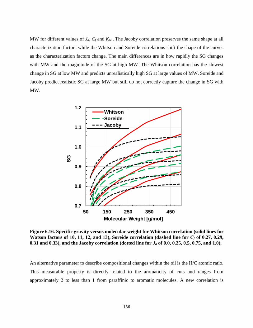
136
MW for different values of Ja, Cf and Kw., The Jacoby correlation preserves the same shape at all
characterization factors while the Whitson and Soreide correlations shift the shape of the curves
as the characterization factors change. The main differences are in how rapidly the SG changes
with MW and the magnitude of the SG at high MW. The Whitson correlation has the slowest
change in SG at low MW and predicts unrealistically high SG at large values of MW. Soreide and
Jacoby predict realistic SG at large MW but still do not correctly capture the change in SG with
MW.
Figure 6.16. Specific gravity versus molecular weight for Whitson correlation (solid lines for
Watson factors of 10, 11, 12, and 13), Soreide correlation (dashed line for Cf of 0.27, 0.29,
0.31 and 0.33), and the Jacoby correlation (dotted line for Ja of 0.0, 0.25, 0.5, 0.75, and 1.0).
An alternative parameter to describe compositional changes within the oil is the H/C atomic ratio.
This measurable property is directly related to the aromaticity of cuts and ranges from
approximately 2 to less than 1 from paraffinic to aromatic molecules. A new correlation is
0.7
0.8
0.9
1.0
1.1
1.2
50 150 250 350 450
SG
Molecular Weight [g/mol]
Whitson
Soreide
Jacoby
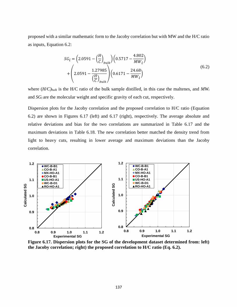
137
proposed with a similar mathematic form to the Jacoby correlation but with MW and the H/C ratio
as inputs, Equation 6.2:
(6.2)
where (H/C)bulk is the H/C ratio of the bulk sample distilled, in this case the maltenes, and MWi
and SGi are the molecular weight and specific gravity of each cut, respectively.
Dispersion plots for the Jacoby correlation and the proposed correlation to H/C ratio (Equation
6.2) are shown in Figures 6.17 (left) and 6.17 (right), respectively. The average absolute and
relative deviations and bias for the two correlations are summarized in Table 6.17 and the
maximum deviations in Table 6.18. The new correlation better matched the density trend from
light to heavy cuts, resulting in lower average and maximum deviations than the Jacoby
correlation.
Figure 6.17. Dispersion plots for the SG of the development dataset determined from: left)
the Jacoby correlation; right) the proposed correlation to H/C ratio (Eq. 6.2).
0.8
0.9
1.0
1.1
1.2
0.8 0.9 1.0 1.1 1.2
Calc
ula
ted
SG
Experimental SG
WC-B-B1CO-B-A1MX-HO-A1CO-B-B1US-HO-A1WC-B-D1RO-HO-A1
0.8
0.9
1.0
1.1
1.2
0.8 0.9 1.0 1.1 1.2
Ca
lcu
late
d S
G
Experimental SG
WC-B-B1CO-B-A1MX-HO-A1CO-B-B1US-HO-A1WC-B-D1RO-HO-A1
𝑆𝐺𝑖 = (2.0591 − (𝐻
𝐶)
𝑏𝑢𝑙𝑘) (0.5717 −
4.802
𝑀𝑊𝑖)
+ (2.0591 −1.27985
(𝐻𝐶
)𝑏𝑢𝑙𝑘
) (0.6171 −24.68
𝑀𝑊𝑖)

138
Table 6.17. Average absolute and relative deviations and bias from the Jacoby correlation
and the proposed correlation to H/C ratio (Eq. 6.2) for the SG of the development dataset.
Oil Sample
Jacoby Equation 6.2
AAD ARD
[%]
Bias
[%] AAD
ARD
[%]
Bias
[%]
WC-B-B1 0.02 1.8 -0.5 0.01 1.4 1.0
CO-B-A1 0.02 1.9 0.9 0.01 0.7 0.2
MX-HO-A1 0.02 2.1 -1.5 0.01 0.6 -0.3
CO-B-B1 0.02 1.7 0.0 0.01 0.7 -0.5
US-HO-A1 0.02 2.0 -1.0 0.01 0.6 -0.1
WC-B-D1 0.01 1.5 -1.0 0.01 0.6 -0.1
RO-HO-A1 0.01 1.0 0.0 0.01 1.3 1.2
Overall 0.02 1.7 -0.4 0.01 0.8 0.2
Table 6.18 Maximum absolute and relative deviations from the Jacoby correlation and the
proposed correlation to H/C ratio (Eq. 6.2) for the SG of the development dataset.
Oil Sample
Jacoby Equation 6.2
MAAD MARD
[%] MAAD
MARD
[%]
WC-B-B1 0.05 6.0 0.02 2.5
CO-B-A1 0.03 3.1 0.01 1.3
MX-HO-A1 0.06 6.8 0.01 1.8
CO-B-B1 0.04 4.6 0.02 2.3
US-HO-A1 0.05 5.6 0.01 1.5
WC-B-D1 0.04 4.7 0.01 1.3
RO-HO-A1 0.03 3.2 0.02 2.5
An important check for the proposed correlation is that predicted SG of the cuts are consistent with
the bulk SG of the whole sample (the deasphalted oil). The SG of the bulk oil was calculated from
the correlated SG of the cuts assuming ideal mixing (zero excess volume) as follows:

139
𝑆𝐺𝐵𝑢𝑙𝑘 = ( ∑𝑤𝑖
𝑆𝐺𝑖
𝑁𝑖=1 )
−1
(2.4)
The measured and calculated bulk SG for each oil are compared in Figure 6.18. The overall
absolute average and relative deviations were 0.003 and 0.31%, respectively. For the majority of
the oils, the error of calculated bulk density is within the experimental error (±0.5%) of the
measurements. Note, the H/C ratios of the cuts can be tuned with a constant multiplier so that the
calculated bulk SG matches the measured value.
Figure 6.18. Error plot obtained between the calculated and experimental bulk specific
gravity of seven different heavy oil and bitumen samples using Equation 6.2
The Jacoby equation and the proposed correlation (without tuning) were evaluated against the
same independent test dataset obtained from the literature for the NBP correlations, Tables 6.4 to
6.7. Figure 6.19 is a dispersion plot of the correlated versus measured SG and the relative
deviations and bias and the maximum deviations are summarized in Tables 6.19 to 6.20. Overall,
the proposed correlation predicted SG with an average absolute relative deviation less than 1.4%;
compared with Jacoby correlation the new equation was able to predict the SG with an
improvement of almost 50%. The average maximum absolute deviations using Equation 6.2 were
lower (3.1 %) than the ones obtained with Jacoby correlation (6.0 %). The deviations obtained
-2.0
-1.5
-1.0
-0.5
0.0
0.5
1.0
1.5
2.0
0.94 0.96 0.98 1.00
(SG
exp-S
Gcalc
)/S
Gexp
X1
00
Experimental SG
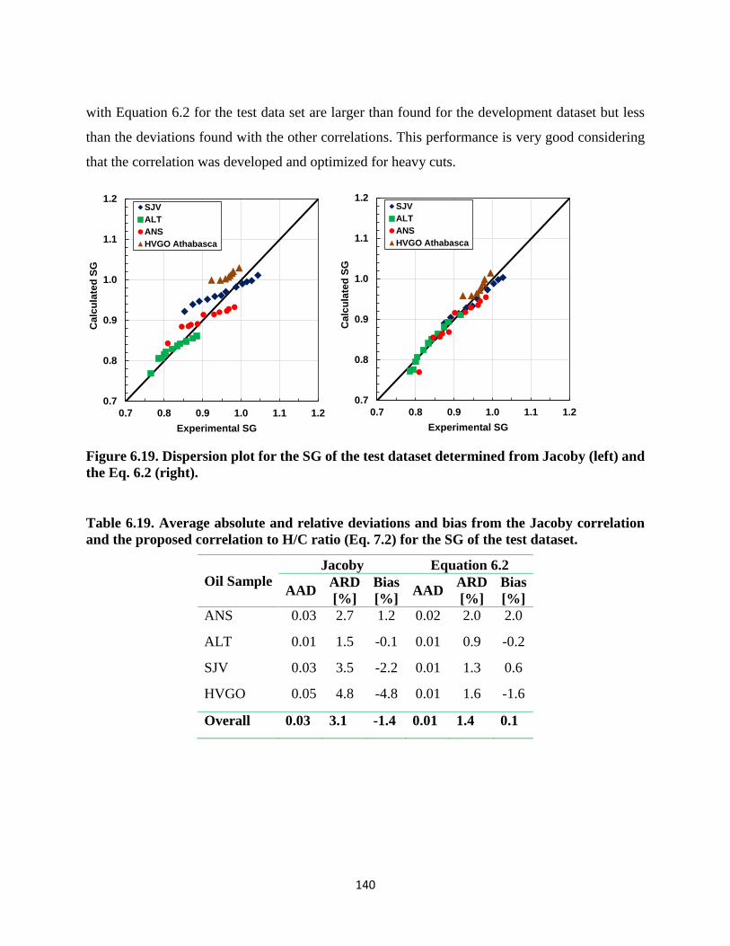
140
with Equation 6.2 for the test data set are larger than found for the development dataset but less
than the deviations found with the other correlations. This performance is very good considering
that the correlation was developed and optimized for heavy cuts.
Figure 6.19. Dispersion plot for the SG of the test dataset determined from Jacoby (left) and
the Eq. 6.2 (right).
Table 6.19. Average absolute and relative deviations and bias from the Jacoby correlation
and the proposed correlation to H/C ratio (Eq. 7.2) for the SG of the test dataset.
Oil Sample
Jacoby Equation 6.2
AAD ARD
[%]
Bias
[%] AAD
ARD
[%]
Bias
[%]
ANS 0.03 2.7 1.2 0.02 2.0 2.0
ALT 0.01 1.5 -0.1 0.01 0.9 -0.2
SJV 0.03 3.5 -2.2 0.01 1.3 0.6
HVGO 0.05 4.8 -4.8 0.01 1.6 -1.6
Overall 0.03 3.1 -1.4 0.01 1.4 0.1
0.7
0.8
0.9
1.0
1.1
1.2
0.7 0.8 0.9 1.0 1.1 1.2
Calc
ula
ted
SG
Experimental SG
SJV
ALT
ANS
HVGO Athabasca
0.7
0.8
0.9
1.0
1.1
1.2
0.7 0.8 0.9 1.0 1.1 1.2
Calc
ula
ted
SG
Experimental SG
SJV
ALT
ANS
HVGO Athabasca

141
Table 6.20. Maximum absolute and relative deviations from the Jacoby correlation and the
proposed correlation to H/C ratio (Eq. 6.2) for the SG of the test dataset.
Oil Sample
Jacoby Equation 6.2
MAAD MARD
[%] MAAD
MARD
[%]
ANS 0.05 5.15 0.04 5.0
ALT 0.02 2.69 0.02 2.3
SJV 0.07 8.04 0.02 2.3
HVGO 0.08 8.25 0.04 3.8
6.4 Specific Gravity and H/C Ratio
The proposed correlation for the SG of distillation cuts requires the bulk H/C ratio as an input. H/C
ratio is a useful property in its own right for assessing the aromaticity and heating value of an oil.
It is also used as a parameter in upgrading models. However, the H/C ratio is not commonly
measured for crude oils and their cuts. Riazi (2005) presented a correlation to calculate the C/H
ratio as a function of boiling point and specific gravity. However, in this study it was found that a
simpler relation between specific gravity and H/C ratio exists for several distillation cuts. It is more
convenient to correlate H/C ratio to a single and more commonly measured property such as the
bulk specific gravity.
First consider the distribution of H/C ratios in different crude oils. The measured elemental
composition for all the petroleum cuts is provided in Appendix G. Figure 6.20 presents the H/C
ratio of the distillation cuts versus their cumulative weight percent distilled. The lightest oil (RO-
HO-A1) has the highest H/C ratios compared with the more aromatic oils such as WC-B-B1 and
CO-B-A1. As expected, the H/C ratio decreases for the higher boiling point cuts. As discussed in
Chapter 2, the lower boiling point cuts are less dense and richer in saturated hydrocarbons (high
H/C ratio), while the heavier cuts are denser and more aromatic (low H/C ratio). The H/C ratio is
inversely proportional to SG, Figure 6.21, and the properties were correlated as follows:
(𝐻𝐶⁄ )
𝑖=
1.7661−𝑆𝐺𝑖
0.50337 (6.3)
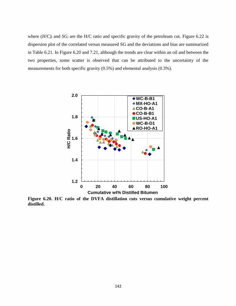
142
where (H/C)i and SGi are the H/C ratio and specific gravity of the petroleum cut. Figure 6.22 is
dispersion plot of the correlated versus measured SG and the deviations and bias are summarized
in Table 6.21. In Figure 6.20 and 7.21, although the trends are clear within an oil and between the
two properties, some scatter is observed that can be attributed to the uncertainty of the
measurements for both specific gravity (0.5%) and elemental analysis (0.3%).
Figure 6.20. H/C ratio of the DVFA distillation cuts versus cumulative weight percent
distilled.
1.2
1.4
1.6
1.8
2.0
0 20 40 60 80 100
H/C
Rati
o
Cumulative wt% Distilled Bitumen
WC-B-B1MX-HO-A1CO-B-A1CO-B-B1US-HO-A1WC-B-D1RO-HO-A1

143
Figure 6.21. H/C ratio of the DVFA distillation cuts versus the specific gravity.
Figure 6.22. Dispersion plot for the H/C ratio of the development dataset determined from
the proposed correlation (Eq. 6.3).
0.80
0.85
0.90
0.95
1.00
1.05
1.2 1.4 1.6 1.8 2.0
Sp
ec
ific
Gra
vit
y
H/C
WC-B-B1MX-HO-A1CO-B-A1CO-B-B1US-HO-A1WC-B-D1RO-HO-A1
1.40
1.50
1.60
1.70
1.80
1.40 1.50 1.60 1.70 1.80
Ca
lcu
late
d H
/C r
ati
o
Experimental H/C ratio
WC-B-B1
CO-B-A1
MX-HO-A1
CO-B-B1
US-HO-A1
WC-B-D1
RO-HO-A1

144
Table 6.21. Average and maximum absolute and relative deviations and bias from the
proposed correlation (Eq. 6.3) for the H/C ratio of the development dataset.
Oil Sample AAD ARD
[%] MAAD
MARD
[%]
Bias
[%]
WC-B-B1 0.02 1.1 0.03 2.3 0.2
CO-B-A1 0.01 0.9 0.04 2.5 0.7
MX-HO-A1 0.01 0.6 0.02 1.3 0.1
CO-B-B1 0.02 1.1 0.04 2.2 1.1
US-HO-A1 0.01 0.7 0.03 1.6 -0.5
WC-B-D1 0.01 0.8 0.04 2.5 -0.6
RO-HO-A1 0.03 1.5 0.05 3.0 -1.4
TOTAL 0.02 1.0 0.04 2.2 -0.04
The proposed correlation was evaluated against the oils from the independent test dataset for which
H/C ratios were available (ANS, ALT and SJV), Tables 6.4 to 6.7. Figure 6.23 is a dispersion plot
of the correlated versus measured H/C ratio and the deviations and bias are summarized in Table
6.22. Overall, for the test data set, the proposed correlation is within 4.6 % of the measured values.
The main contributor to this error is due to the drastic under-prediction of the H/C ratios for the
ALT oil, which was the least dense and most paraffinic of the three oils. For the other oils, SJV
and ANS, the relative deviations were considerably lower (less than 1.9 %) and comparable to the
absolute deviations obtained for the development dataset with a slight difference of 0.015.
To further investigate the issue with the ALT oil, the H/C ratio of each cut was plotted versus SG
to determine if the oil had the expected trend of decreasing H/C ratio from low to high boiling
cuts, Figure 6.24. Surprisingly and unlike the other two oils, the content/C ratio of the ALT oil
distillation cuts remained constant. It appears that this oil consists mainly of saturated
hydrocarbons and the higher boiling cuts contain larger saturated molecules but no additional
aromatic species; hence, the H/C ratio does not change.
The direct correlation of H/C ratio to SG (or vice versa) appears to apply to typical petroleum cuts
where both size and aromaticity increases in higher boiling cuts. For this type of mixture, the bulk
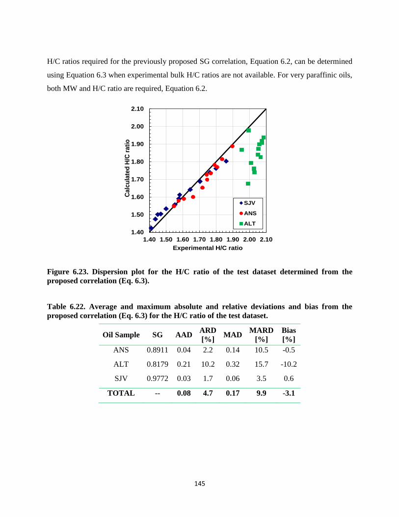
145
H/C ratios required for the previously proposed SG correlation, Equation 6.2, can be determined
using Equation 6.3 when experimental bulk H/C ratios are not available. For very paraffinic oils,
both MW and H/C ratio are required, Equation 6.2.
Figure 6.23. Dispersion plot for the H/C ratio of the test dataset determined from the
proposed correlation (Eq. 6.3).
Table 6.22. Average and maximum absolute and relative deviations and bias from the
proposed correlation (Eq. 6.3) for the H/C ratio of the test dataset.
Oil Sample SG AAD ARD
[%] MAD
MARD
[%]
Bias
[%]
ANS 0.8911 0.04 2.2 0.14 10.5 -0.5
ALT 0.8179 0.21 10.2 0.32 15.7 -10.2
SJV 0.9772 0.03 1.7 0.06 3.5 0.6
TOTAL -- 0.08 4.7 0.17 9.9 -3.1
1.40
1.50
1.60
1.70
1.80
1.90
2.00
2.10
1.40 1.50 1.60 1.70 1.80 1.90 2.00 2.10
Ca
lcu
late
d H
/C r
ati
o
Experimental H/C ratio
SJV
ANS
ALT
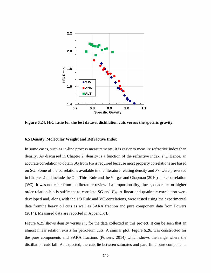
146
Figure 6.24. H/C ratio for the test dataset distillation cuts versus the specific gravity.
6.5 Density, Molecular Weight and Refractive Index
In some cases, such as in-line process measurements, it is easier to measure refractive index than
density. As discussed in Chapter 2, density is a function of the refractive index, FRI. Hence, an
accurate correlation to obtain SG from FRI is required because most property correlations are based
on SG. Some of the correlations available in the literature relating density and FRI were presented
in Chapter 2 and include the One Third Rule and the Vargas and Chapman (2010) cubic correlation
(VC). It was not clear from the literature review if a proportionality, linear, quadratic, or higher
order relationship is sufficient to correlate SG and FRI. A linear and quadratic correlation were
developed and, along with the 1/3 Rule and VC correlations, were tested using the experimental
data fromthe heavy oil cuts as well as SARA fraction and pure component data from Powers
(2014). Measured data are reported in Appendix B.
Figure 6.25 shows density versus FRI for the data collected in this project. It can be seen that an
almost linear relation exists for petroleum cuts. A similar plot, Figure 6.26, was constructed for
the pure components and SARA fractions (Powers, 2014) which shows the range where the
distillation cuts fall. As expected, the cuts lie between saturates and paraffinic pure components
1.4
1.6
1.8
2.0
2.2
0.7 0.8 0.9 1.0 1.1
H/C
Rati
o
Specific Gravity
SJV
ANS
ALT

147
on the low end, and on the high end they are aligned with the aromatics from SARA fractions and
pure components.
Figure 6.25. FRI as a function of the density for the distillation cuts.
850
890
930
970
1010
1050
0.27 0.29 0.31 0.33 0.35
De
ns
ity [
kg
/m3
]
FRI
WC-B-B1CO-B-A1MX-HO-A1CO-B-B1US-HO-A1WC-B-D1RO-HO-A1

148
Figure 6.26. FRI as a function of the density for pure components, SARA fractions and
distillation cuts
A quadratic polynomial relation can describe the relation between FRI and density. A quadratic
correlation first developed by Powers (2014) was modified using all the components presented in
Figure 6.23 to obtain the following:
𝐹𝑅𝐼−20°𝐶 = 3.384𝑥10−7𝜌20°𝐶2 − 2.835𝑥10−4𝜌20°𝐶 + 0.2737 (6.4)
A simpler relation can be constructed between the FRI and density, provided asphaltenes are not
considered in the correlation. As mentioned previously and as can be seen in Figure 6.23, there is
a linear relationship between the density and FRI up to the aromatic fraction. The data excluding
the asphaltenes was fitted to obtain the linear correlation shown in Equation 6.5:
𝐹𝑅𝐼−20°𝐶 =𝜌20°𝐶 /1000+ 0.1058
3.4033 (6.5)
Figure 6.27 compares the errors from one-third rule, Vargas and Chapman (2010, VC), and
Equations 6.4 and 6.5. The average absolute and relative deviations, bias, and maximum deviations
are presented in Table 6.23, 6.24 and 6.25 respectively. Compared with the one-third rule,
500
600
700
800
900
1000
1100
1200
1300
0.20 0.30 0.40 0.50
Den
sit
y [
kg
/m3
]
FRI
ParaffinsNaphthenesAromaticsSaturates (SARA)Aromatics (SARA)Asphaltenes (SARA)Distillation cuts
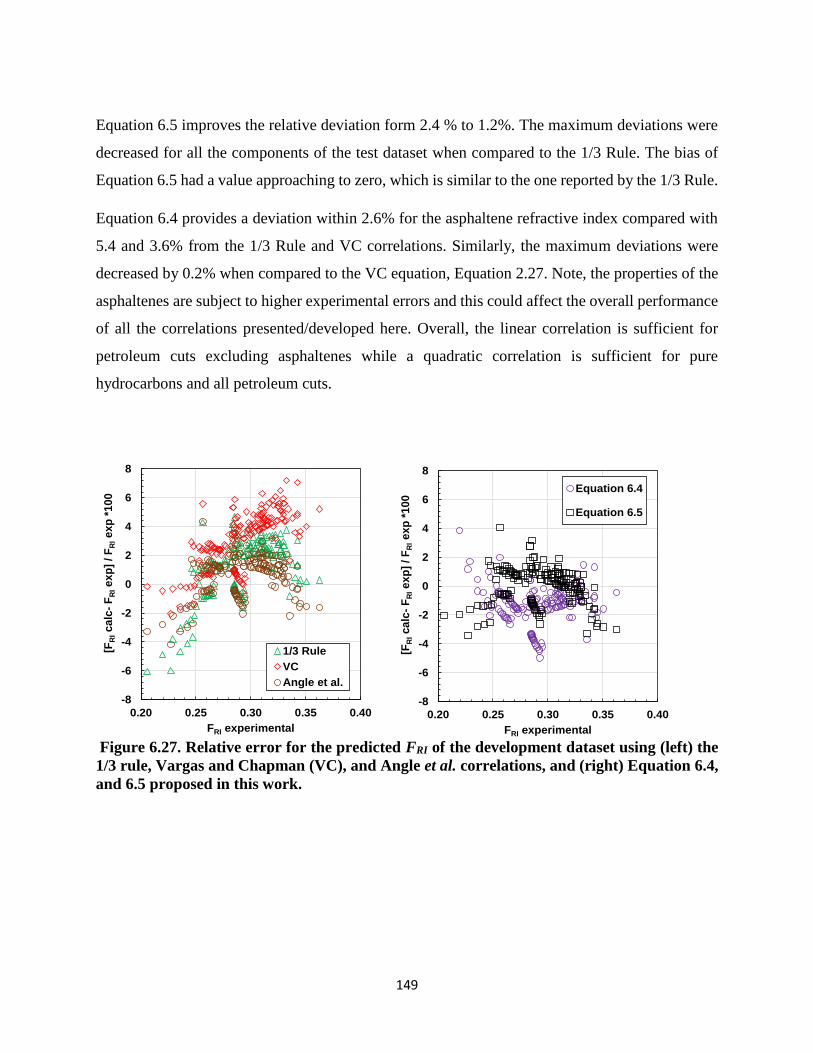
149
Equation 6.5 improves the relative deviation form 2.4 % to 1.2%. The maximum deviations were
decreased for all the components of the test dataset when compared to the 1/3 Rule. The bias of
Equation 6.5 had a value approaching to zero, which is similar to the one reported by the 1/3 Rule.
Equation 6.4 provides a deviation within 2.6% for the asphaltene refractive index compared with
5.4 and 3.6% from the 1/3 Rule and VC correlations. Similarly, the maximum deviations were
decreased by 0.2% when compared to the VC equation, Equation 2.27. Note, the properties of the
asphaltenes are subject to higher experimental errors and this could affect the overall performance
of all the correlations presented/developed here. Overall, the linear correlation is sufficient for
petroleum cuts excluding asphaltenes while a quadratic correlation is sufficient for pure
hydrocarbons and all petroleum cuts.
Figure 6.27. Relative error for the predicted FRI of the development dataset using (left) the
1/3 rule, Vargas and Chapman (VC), and Angle et al. correlations, and (right) Equation 6.4,
and 6.5 proposed in this work.
-8
-6
-4
-2
0
2
4
6
8
0.20 0.25 0.30 0.35 0.40
[FR
Ic
alc
-F
RIe
xp
] / F
RIe
xp
*1
00
FRI experimental
1/3 Rule
VC
Angle et al.
-8
-6
-4
-2
0
2
4
6
8
0.20 0.25 0.30 0.35 0.40
[FR
Ica
lc-
FR
Iex
p]
/ F
RIex
p *
100
FRI experimental
Equation 6.4
Equation 6.5

150
Table 6.23. Average relative and absolute deviations obtained using 1/3 Rule, Vargas and
Chapman (VC) correlation, Equation 6.4 and 6.5 for the prediction of refractive index.
Compound
1/3 Rule Angle et al. VC Eq. 6.4 Eq. 6.5
AAD ARD
[%] AAD
ARD
[%] AAD
ARD
[%] AAD
ARD
[%] AAD
ARD
[%]
Distillation cuts 0.008 2.6 0.005 1.52 0.014 4.4 0.003 1.0 0.002 0.7
Paraffins 0.005 2.3 0.003 1.45 0.002 0.8 0.005 2.0 0.003 1.3
Naphthenes 0.003 1.3 0.004 1.43 0.007 2.6 0.003 1.1 0.003 1.2
Aromatics 0.002 0.6 0.003 0.98 0.004 1.3 0.010 3.5 0.005 1.5
Saturates (SARA) 0.008 2.7 0.006 2.11 0.011 3.8 0.003 1.1 0.004 1.5
Aromatics (SARA) 0.006 1.8 0.003 0.85 0.016 4.7 0.003 0.9 0.003 0.9
Asph. (SARA) 0.024 5.4 0.033 7.71 0.015 3.6 0.011 2.6 - -
Overall 0.008 2.4 0.008 2.29 0.010 3.0 0.005 1.7 0.003 1.2
Table 6.24. Bias obtained using 1/3 Rule, Vargas and Chapman (VC) correlation, Equation
6.4 and 6.5 for the prediction refractive index.
Compound
1/3 Rule Angle et al. VC Eq. 6.4 Eq. 6.5
Bias
[%]
Bias
[%]
Bias
[%]
Bias
[%]
Bias
[%]
Distillation cuts 2.6 1.45 4.4 -0.9 0.5
Paraffins -2.3 -1.40 0.1 -0.6 -1.2
Naphthenes 1.3 1.43 2.6 -0.7 1.2
Aromatics -0.2 -0.86 1.2 -3.4 -1.5
Saturates (SARA) 2.7 2.11 3.8 -0. 9 1.5
Aromatics (SARA) 1.8 0.31 4.7 -0.9 -0.9
Asphaltenes (SARA) -5.4 -7.71 3.4 -2.4 -
Overall 0.06 -0.67 2.9 -1.4 -0.08

151
Table 6.25. Maximum average relative and absolute deviations obtained using 1/3 Rule, Vargas and Chapman (VC) correlation,
Equation 6.4 and 6.5 for the prediction of refractive index.
Compound
1/3 Rule Angle et al. VC Eq. 6.4 Eq. 6.5
MAAD MARD
[%] MAAD
MARD
[%] MAAD
MARD
[%] MAAD
MARD
[%] MAAD
MARD
[%]
Distillation cuts 0.013 4.2 0.009 3.0 0.024 7.2 0.012 3.7 0.011 3.3
Paraffins 0.014 6.1 0.009 4.2 0.005 2.1 0.017 8.2 0.008 3.4
Naphthenes 0.011 4.3 0.011 4.4 0.014 5.6 0.005 2.0 0.010 4.1
Aromatics 0.013 4.7 0.011 3.9 0.017 5.9 0.006 2.2 0.009 3.2
Saturates (SARA) 0.010 3.0 0.006 2.1 0.024 7.1 0.015 5.0 0.011 3.0
Aromatics (SARA) 0.013 4.7 0.011 3.9 0.017 5.9 0.006 2.2 0.009 3.2
Asphaltenes (SARA) 0.048 10.3 0.058 12.6 0.029 7.3 0.031 7.1
Overall 0.017 5.3 0.017 4.9 0.018 5.8 0.013 4.3 0.010 3.4

152
CHAPTER SEVEN: CORRELATION FOR VAPOR PRESSURE AND THERMAL
PROPERTIES FOR HEAVY OILS AND BITUMEN
Vapor pressure and thermal data (heat capacity, heat of vaporization, and heat of combustion) are
the backbone of the thermodynamic equilibrium calculations that, along with mass and energy
balances, are required to design and simulate process units. However, it is challenging to determine
the vapor pressure and thermal properties of heavy oils and bitumen because they contain high
boiling point and high molecular weight compounds. These compounds have a very low volatility
which is difficult to measure and challenging to extrapolate to typical operating pressures.
The vapor pressure and liquid heat capacity of the distillation cuts obtained using the DVFA-II
were measured and the data were presented in Chapter 5 as part of the development of an
interconversion method using constrained extrapolation of vapor pressure and heat capacity. In
this chapter, the aim is to test correlations available in the literature against these data and
recommend the best alternative for heavy oil and bitumen fractions. Since critical properties were
not available for the cuts, only the correlations based on physical properties are tested here.
The heat of vaporization cannot be measured directly because the samples thermally decompose
before reaching their normal boiling point. However, the heat of vaporization can be calculated
from Cox equation that was fitted to vapor pressure data; the version is based on the direct
relationship between vapor pressure and heat of vaporization through the Clapeyron equation.
Although these derived property data cannot be regarded as experimental results, the calculated
values are the best estimate available for heavy distillation cuts. The distillation cut data are
compared with data from pure components and other crude oil mixtures. The correlations available
in the literature are tested using this dataset and an alternative calculation linked with Clapeyron
equation is proposed.
Finally, the heat of combustion data collected in this study for some distillation cuts are presented
and the performance of correlations for the heat of combustion from elemental analysis is
evaluated.

153
7.1 Vapor Pressure Correlations
As noted in Chapter 2, there are several correlations to predict vapor pressure that require either
critical or physical properties as inputs. Only the correlations that use physical properties as input
variables (Riazi, 2005; Maxwell and Bonnell, 1957) are evaluated here. Note, these correlations
give the exact normal boiling point at 101325 Pa since it is an input to the equation. This constraint
makes the correlations consistent with the TBP based oil characterization but not always accurate
for vapor pressures below the normal boiling temperature.
Figure 7.1 compares the Riazi and M-B correlations versus the measured vapor pressure of the
cuts from CO-B-B1 oil. Figure 7.2 presents the relative and absolute errors for the predicted vapor
pressure values. Errors higher than 150% were observed for vapor pressures in the low and high
temperature ranges for the distillation cuts. The error decreases exponentially as the pressure
approaches atmospheric conditions. The high error at low pressures can be attributed to the use of
reference components, such low boiling point paraffins, to develop the correlations. The
extrapolation of these correlations outside their range of development is not recommended
particularly at very low vapor pressure ranges (below 50000 Pa).
Note, for pressures below 1000 Pa, small magnitude deviations give high relative deviations. That
is why in a relative deviation plot the errors appear to be excessively large. Since the literature
correlations gave deviations higher than 300% for heavy oils distillation cuts, a new methodology
to predict vapor pressure is proposed.

154
Figure 7.1. Measured and correlated vapor pressure using Riazi (left) and Maxwell and
Bonnell (right) correlations for the oil sample CO-B-B1.
Figure 7.2. Relative (left) and absolute (right) deviations obtained for vapor pressure
prediction using Riazi and M-B correlations for the 63 distillation cuts collected in this work.
Recall that the measured vapor pressure for the distillation cuts reported in Chapter 5 were
simultaneously fitted with heat capacity data using the three parameter Cox equation. Figure 7.3
shows that the average values of the fitted parameters, do follow consistent trends versus
1.E-01
1.E+00
1.E+01
1.E+02
1.E+03
1.E+04
1.E+05
1.E+06
300 500 700 900
Pre
ss
ure
[P
a]
Temperature [K]
Cut 0
Cut 1
Cut 2
Cut 3
Cut 4
Cut 5
Cut 6
1.E-01
1.E+00
1.E+01
1.E+02
1.E+03
1.E+04
1.E+05
1.E+06
300 500 700
Pre
ss
ure
[P
a]
Temperature [K]
Cut 0
Cut 1
Cut 2
Cut 3
Cut 4
Cut 5
Cut 6
-100
-50
0
50
100
150
200
250
300
0 25 50 75 100
[Pv c
alc
-P
v e
xp
]/P
v e
xp
x 1
00
Pressure x 103 [Pa]
M-B
Riazi
-15
-10
-5
0
5
10
15
20
25
0 25 50 75 100
Ab
s [
Pv c
alc
-P
v e
xp
] x
10
3
Pressure x 103 [Pa]
M-B
Riazi
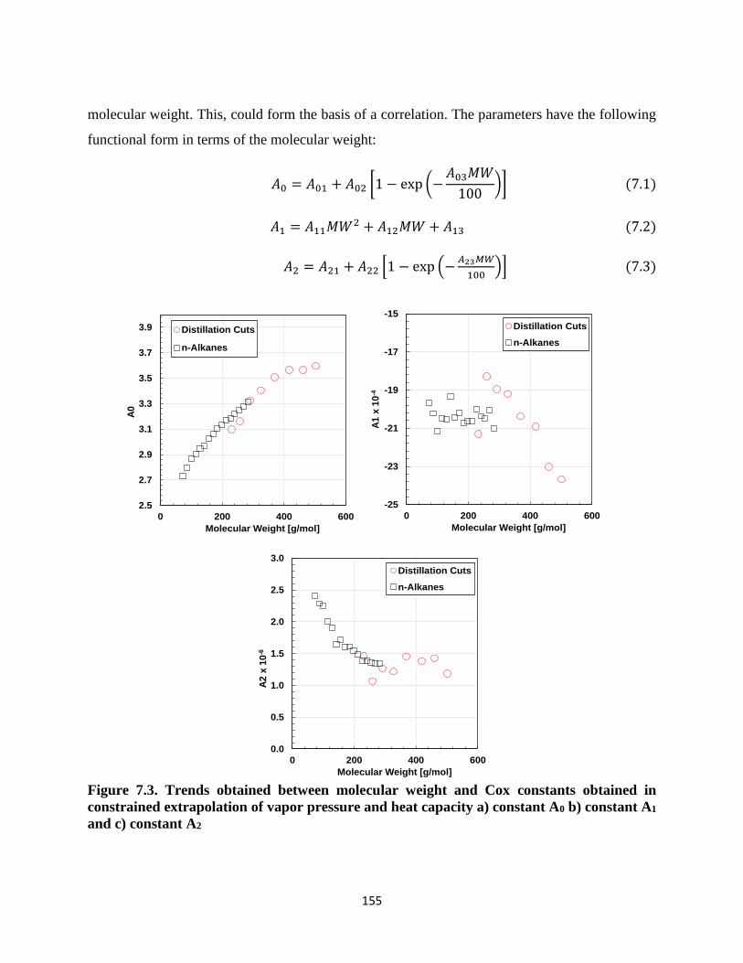
155
molecular weight. This, could form the basis of a correlation. The parameters have the following
functional form in terms of the molecular weight:
𝐴0 = 𝐴01 + 𝐴02 [1 − exp (−𝐴03𝑀𝑊
100)] (7.1)
𝐴1 = 𝐴11𝑀𝑊2 + 𝐴12𝑀𝑊 + 𝐴13 (7.2)
𝐴2 = 𝐴21 + 𝐴22 [1 − exp (−𝐴23𝑀𝑊
100)] (7.3)
Figure 7.3. Trends obtained between molecular weight and Cox constants obtained in
constrained extrapolation of vapor pressure and heat capacity a) constant A0 b) constant A1
and c) constant A2
2.5
2.7
2.9
3.1
3.3
3.5
3.7
3.9
0 200 400 600
A0
Molecular Weight [g/mol]
Distillation Cuts
n-Alkanes
-25
-23
-21
-19
-17
-15
0 200 400 600
A1
x 1
0-4
Molecular Weight [g/mol]
Distillation Cuts
n-Alkanes
0.0
0.5
1.0
1.5
2.0
2.5
3.0
0 200 400 600
A2
x 1
0-6
Molecular Weight [g/mol]
Distillation Cuts
n-Alkanes

156
However, the average parameters are not constrained to provide the correct normal boiling point
and do not fit the individual oil data. Therefore, the Cox correlation was constrained to match the
NBP from the oil characterization by setting the reference temperature equal to the NBP as follows:
𝑙𝑛 (𝑃𝑠𝑎𝑡
𝑃𝑏) = (1 −
𝑇𝑁𝐵𝑃
𝑇) exp(𝐴0 + 𝐴1𝑇 + 𝐴2𝑇2) (7.4)
where TNBP is the normal boiling point. Finally, in order to better constrain the data fitting to obtain
the correct shape of the vapor pressure curve, the following data were included:
1. measured vapor pressure (low pressure range)
2. experimental NBP obtained from oil characterization
3. synthetic data ‘generated’ from the Cox correlation using individually fitted Cox constants
for each cut
The constants were then adjusted to minimize the following optimization function (OF) for the
development dataset:
𝑂𝐹 = [1
𝑛∑(𝑃𝑣𝑖
𝑐𝑎𝑙𝑐 − 𝑃𝑣𝑖𝑒𝑥𝑝)
2𝑛
𝑖=1
] (7.5)
where Pvicalc and Pvi
exp are the calculated and the experimental vapor pressure respectively and n
is the number of experimental points. The optimized constants are summarized in Table 7.1.
Table 7.1. Constants of Equations 7.1 to 7.3.
Constant: A0 Constant: A1 [K-1] Constant: A2[K-2]
A01 -1.7348 A11 -0.00014 A21 4.4414
A02 5.3750 A12 0.08681 A22 -3.1774
A03 0.9799 A13 -33.3372 A23 1.3091
The deviations for the predicted vapor pressure for the distillation cuts from the proposed
correlation and for the RD and MB correlations are compared in Figure 7.4. Table 7.2 and Table
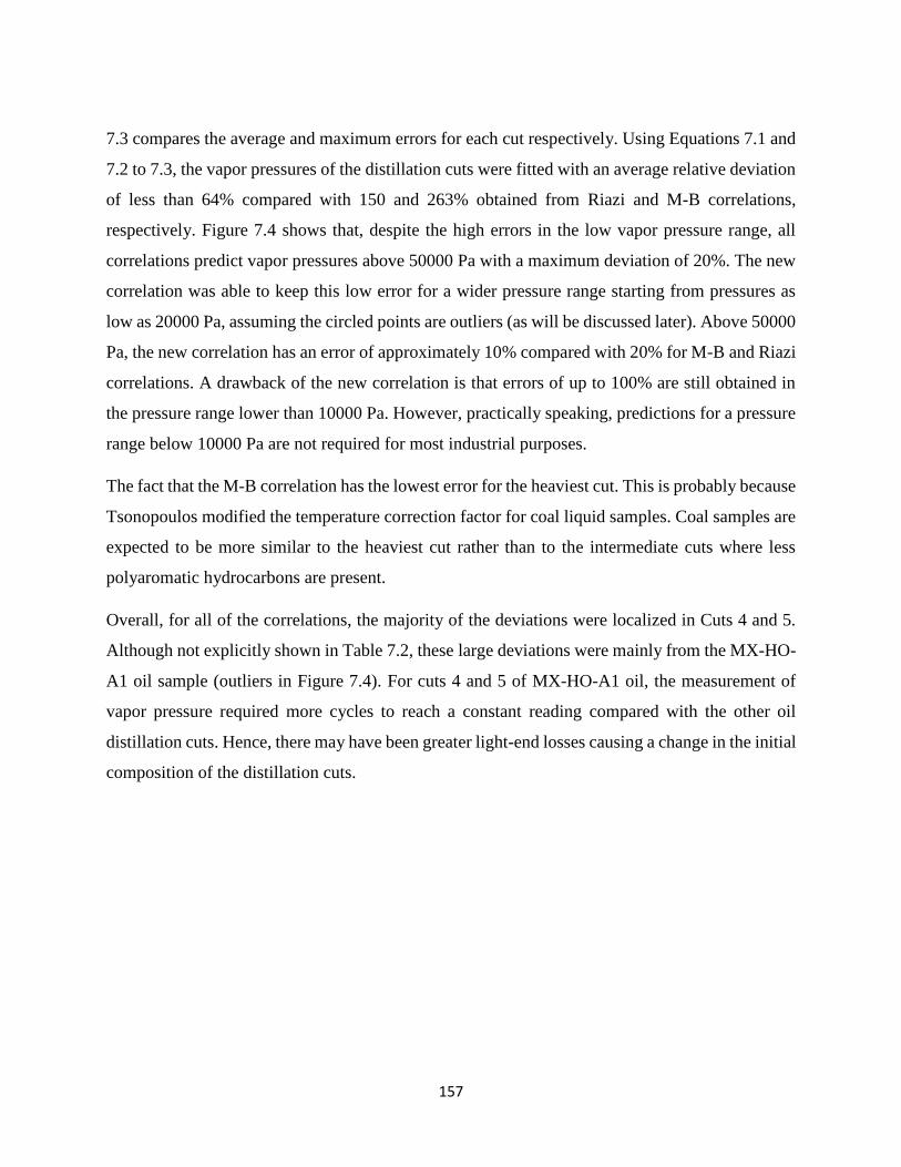
157
7.3 compares the average and maximum errors for each cut respectively. Using Equations 7.1 and
7.2 to 7.3, the vapor pressures of the distillation cuts were fitted with an average relative deviation
of less than 64% compared with 150 and 263% obtained from Riazi and M-B correlations,
respectively. Figure 7.4 shows that, despite the high errors in the low vapor pressure range, all
correlations predict vapor pressures above 50000 Pa with a maximum deviation of 20%. The new
correlation was able to keep this low error for a wider pressure range starting from pressures as
low as 20000 Pa, assuming the circled points are outliers (as will be discussed later). Above 50000
Pa, the new correlation has an error of approximately 10% compared with 20% for M-B and Riazi
correlations. A drawback of the new correlation is that errors of up to 100% are still obtained in
the pressure range lower than 10000 Pa. However, practically speaking, predictions for a pressure
range below 10000 Pa are not required for most industrial purposes.
The fact that the M-B correlation has the lowest error for the heaviest cut. This is probably because
Tsonopoulos modified the temperature correction factor for coal liquid samples. Coal samples are
expected to be more similar to the heaviest cut rather than to the intermediate cuts where less
polyaromatic hydrocarbons are present.
Overall, for all of the correlations, the majority of the deviations were localized in Cuts 4 and 5.
Although not explicitly shown in Table 7.2, these large deviations were mainly from the MX-HO-
A1 oil sample (outliers in Figure 7.4). For cuts 4 and 5 of MX-HO-A1 oil, the measurement of
vapor pressure required more cycles to reach a constant reading compared with the other oil
distillation cuts. Hence, there may have been greater light-end losses causing a change in the initial
composition of the distillation cuts.
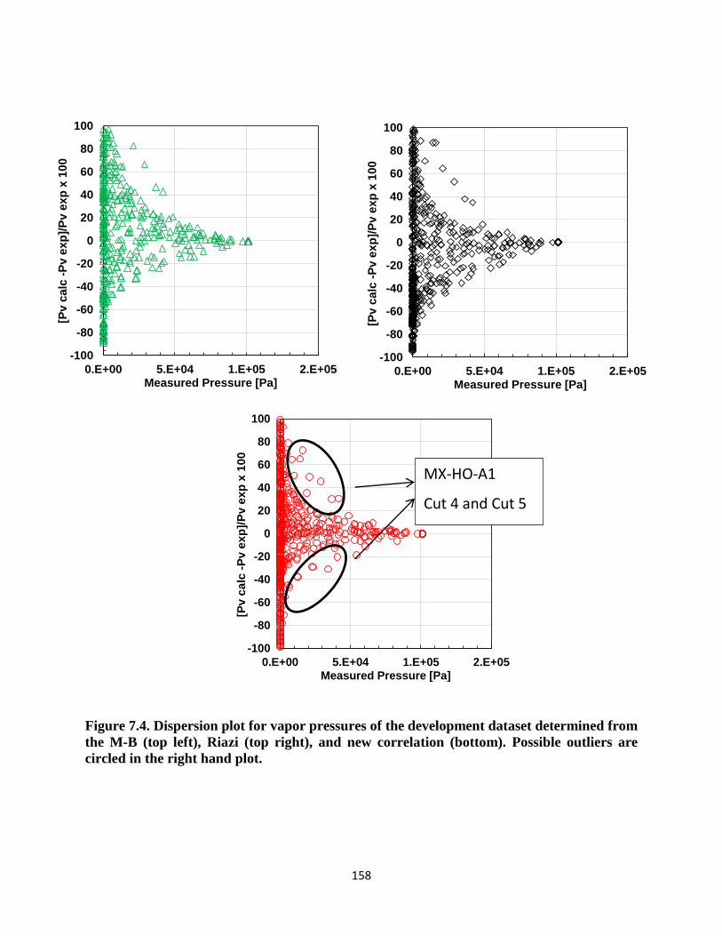
158
Figure 7.4. Dispersion plot for vapor pressures of the development dataset determined from
the M-B (top left), Riazi (top right), and new correlation (bottom). Possible outliers are
circled in the right hand plot.
-100
-80
-60
-40
-20
0
20
40
60
80
100
0.E+00 5.E+04 1.E+05 2.E+05
[Pv c
alc
-P
v e
xp
]/P
v e
xp
x 1
00
Measured Pressure [Pa]
-100
-80
-60
-40
-20
0
20
40
60
80
100
0.E+00 5.E+04 1.E+05 2.E+05
[Pv c
alc
-P
v e
xp
]/P
v e
xp
x 1
00
Measured Pressure [Pa]
-100
-80
-60
-40
-20
0
20
40
60
80
100
0.E+00 5.E+04 1.E+05 2.E+05
[Pv c
alc
-P
v e
xp
]/P
v e
xp
x 1
00
Measured Pressure [Pa]
MX-HO-A1
Cut 4 and Cut 5
-100
-80
-60
-40
-20
0
20
40
60
80
100
0.E+00 5.E+04 1.E+05 2.E+05
[Pv c
alc
-P
v e
xp
]/P
v e
xp
x 1
00
Measured Pressure [Pa]
-100
-80
-60
-40
-20
0
20
40
60
80
100
0.E+00 5.E+04 1.E+05 2.E+05
[Pv c
alc
-P
v e
xp
]/P
v e
xp
x 1
00
Measured Pressure [Pa]
-100
-80
-60
-40
-20
0
20
40
60
80
100
0.E+00 5.E+04 1.E+05 2.E+05[P
v c
alc
-P
v e
xp
]/P
v e
xp
x 1
00
Measured Pressure [Pa]
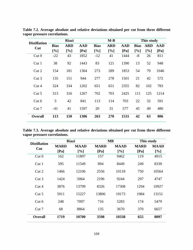
159
Table 7.2. Average absolute and relative deviations obtained per cut from three different
vapor pressure correlations.
Distillation
Cut
Riazi M-B This study
Bias
[%]
ARD
[%]
AAD
[Pa]
Bias
[%]
ARD
[%]
AAD
[Pa]
Bias
[%]
ARD
[%]
AAD
[Pa]
Cut 0 -22 43 1852 -12 41 1444 -8 26 811
Cut 1 38 92 1443 83 121 1390 13 52 948
Cut 2 154 181 1304 273 289 1853 54 79 1046
Cut 3 135 151 944 277 278 1501 21 42 572
Cut 4 324 334 1202 651 651 2355 82 102 783
Cut 5 313 316 1267 702 703 2425 111 125 1214
Cut 6 3 42 841 113 114 703 22 32 591
Cut 7 -41 41 1597 20 31 577 45 49 480
Overall 113 150 1306 263 278 1531 42 63 806
Table 7.3. Average absolute and relative deviations obtained per cut from three different
vapor pressure correlations.
Distillation
Cut
Riazi MB This study
MARD
[Pa]
MAAD
[%]
MARD
[Pa]
MAAD
[%]
MARD
[Pa]
MAAD
[%]
Cut 0 162 11897 157 9462 119 4915
Cut 1 595 11549 894 8449 249 8339
Cut 2 1466 12106 2556 10118 750 10564
Cut 3 1424 5064 2196 9244 297 4747
Cut 4 3876 13799 8326 17308 1294 10927
Cut 5 5911 15227 13806 19173 1984 13151
Cut 6 248 7097 716 5283 174 5479
Cut 7 68 8864 135 3670 370 6657
Overall 1719 10700 3598 10338 655 8097

160
The correlations were tested on a test dataset that was separated into the following four groups to
better determine the type of samples for which the correlations give the most accurate vapor
pressure predictions.
1) a paraffinic set of distillation cuts from the ALT oil (Sturm and Shay, 2000).
2) an intermediate set of distillation cuts from the ANS oil (Sturm and Shay, 2000).
3) an aromatic set of distillation cuts from the SJV oil (Sturm and Shay, 2000).
4) a Western Canadian Bitumen, its de-asphalted fraction, and eicosane (Castellanos et al.,
2012).
Figure 7.5 presents the dispersion plot that compares the fit obtained for the four test datasets using
Riazi, M-B, and the new correlation. Tables 7.4 to 7.7 report the absolute and average deviations
for each set individually. The maximum deviations are summarized in Appendix H. Overall, the
M-B and the new correlation perform better than the Riazi correlation. The Riazi correlation, as
indicated by the author, is a good correlation for vapor pressures near the normal boiling point. It
is not surprising that it performs poorly for datasets outside this range. The performance of the M-
B correlation is slightly better for the first three datasets but the new correlation provides
significantly better predictions for the heaviest cuts and for the fourth, most aromatic, dataset. As
intended, the new correlation is well suited to predict the vapor pressure of heavy petroleum
fractions. Note, the new correlation must be used with caution for samples with molecular weight
values less than 200 g/mol since this was the lowest MW in the set of distillation cuts used to
develop the new correlation.

161
Figure 7.5. Dispersion plot for vapor pressures from the test dataset determined from the M-
B (top left), Riazi (top right), and the new correlation (bottom). The secondary axis in top
plots was required to observe errors for the fourth group in the test dataset.
-1000
0
1000
2000
3000
4000
5000
6000
7000
8000
9000
10000
-100
-50
0
50
100
150
200
0.E+00 3.E+04 6.E+04 9.E+04 1.E+05
[Pv c
alc
-P
v e
xp
]/P
v e
xp
x 1
00
Measured Pressure [Pa]
ALT
ANS
SJV
Bit/DAO/C20
-100
-50
0
50
100
150
200
0.E+00 3.E+04 6.E+04 9.E+04 1.E+05
[Pv c
alc
-P
v e
xp
]/P
v e
xp
x 1
00
Measured Pressure [Pa]
ALT
ANS
SJV
Bit/DAO/C20
0
1000
2000
3000
4000
5000
6000
-100
-50
0
50
100
150
200
0.E+00 3.E+04 6.E+04 9.E+04 1.E+05
[Pv c
alc
-P
v e
xp
]/P
v e
xp
x 1
00
Measured Pressure [Pa]
ALT
ANS
SJV
Bit/DAO/C20
-1000
0
1000
2000
3000
4000
5000
6000
7000
8000
9000
10000
-100
-50
0
50
100
150
200
0.E+00 3.E+04 6.E+04 9.E+04 1.E+05
[Pv c
alc
-P
v e
xp
]/P
v e
xp
x 1
00
Measured Pressure [Pa]
ALT
ANS
SJV
Bit/DAO/C20
-100
-50
0
50
100
150
200
0.E+00 3.E+04 6.E+04 9.E+04 1.E+05
[Pv c
alc
-P
v e
xp
]/P
v e
xp
x 1
00
Measured Pressure [Pa]
ALT
ANS
SJV
Bit/DAO/C20
0
1000
2000
3000
4000
5000
6000
-100
-50
0
50
100
150
200
0.E+00 3.E+04 6.E+04 9.E+04 1.E+05[P
v c
alc
-P
v e
xp
]/P
v e
xp
x 1
00
Measured Pressure [Pa]
ALT
ANS
SJV
Bit/DAO/C20
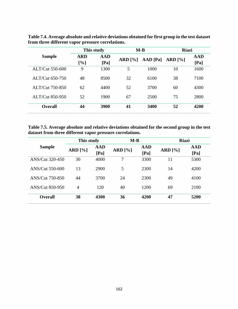
162
Table 7.4. Average absolute and relative deviations obtained for first group in the test dataset
from three different vapor pressure correlations.
Sample
This study M-B Riazi
ARD
[%]
AAD
[Pa] ARD [%] AAD [Pa] ARD [%]
AAD
[Pa]
ALT/Cut 550-600 9 1300 5 1000 10 1600
ALT/Cut 650-750 48 8500 32 6100 38 7100
ALT/Cut 750-850 62 4400 52 3700 60 4300
ALT/Cut 850-950 52 1900 67 2500 75 2800
Overall 44 3900 41 3400 52 4200
Table 7.5. Average absolute and relative deviations obtained for the second group in the test
dataset from three different vapor pressure correlations.
Sample
This study M-B Riazi
ARD [%] AAD
[Pa] ARD [%]
AAD
[Pa] ARD [%]
AAD
[Pa]
ANS/Cut 320-450 30 4000 7 3300 11 5300
ANS/Cut 550-600 13 2900 5 2300 14 4200
ANS/Cut 750-850 44 3700 24 2300 49 4100
ANS/Cut 850-950 4 120 40 1200 69 2100
Overall 38 4300 36 4200 47 5200

163
Table 7.6. Average absolute and relative deviations obtained for the third group in the test
dataset from three different vapor pressure correlations.
Sample
This study M-B Riazi
ARD [%] AAD
[Pa]
ARD
[%]
AAD
[Pa]
ARD
[%]
AAD
[Pa]
SJV/Cut 450-650 29 6300 41 8700 51 10100
SJV/Cut 500-550 7 3500 11 3000 18 6000
SJV/Cut 600-650 8 1600 20 3000 7 1100
SJV/Cut 650-750 72 14000 64 14000 75 15500
SJV/Cut 750-850 86 5600 81 5300 90 6000
SJV/Cut 850-950 35 1600 45 1300 76 2300
Overall 42 5600 44 5800 53 7000
Table 7.7. Average absolute and relative deviations obtained for the fourth group in the test
dataset from three different vapor pressure correlations.
Sample
This study M-B Riazi
ARD [%] AAD
[Pa]
ARD
[%]
AAD
[Pa]
ARD
[%]
AAD
[Pa]
Bitumen WC-B-B1 33 17 1500 600 800 200
Maltenes WC-B-B1 91 13 7000 600 4200 400
Eicosane 26 1 40 1 120 2
Overall 50 10 2900 400 1700 200
An attempt was made to correlate the Cox constants with NBP instead of MW; however, the
deviations were significantly higher compared with the correlations using MW for both the
development and test datasets. The correlation with MW also includes NBP through Eq. 7.4, while
a correlation to NBP only has the one input. It may be possible that two input variables are required
to accurately predict vapor pressure. Note, if molecular weight is not available as part of the
characterization data, it can be calculated from Equation 6.1 using NBP and SG as inputs.

164
7.2 Liquid Heat Capacity
As introduced in Chapter 2, the most commonly used correlations available in the literature to
determine the liquid heat capacity at constant pressure from physical properties are the Lee-Kesler
(1976), Dagostar (2013), and Tsonopoulos (1986) correlations. The correlations were tested on a
development dataset that included the following distillation cuts for which liquid heat capacity
were available:
WC-B-B1 Cut 0 to Cut 6
CO-B-A1 Cut 0 to Cut 6
MX-B-A1 Cut 0 to Cut 4
CO-B-B1 Cut 0 to Cut 3
Figure 7.6 shows the measured and correlated liquid heat capacities, Cpliq, versus temperature for
the WC-B-B1 distillation cuts as an example. Figure 7.7 presents the deviations for all of the above
correlations from the measured Cpliq of the distillation cuts. The average and maximum absolute
and relative deviations and the bias obtained for each correlation are reported in Table 7.8.
The lowest relative deviations and bias was observed for the Lee-Kesler (1976) correlation. The
lowest deviations obtained with the Lee-Kesler correlation were for the lightest fractions (Cut 0
and Cut 1); however, the deviations significantly increased from the low to high boiling fractions
reaching a maximum relative deviations of 12%. The Dagostar (2013) correlation, which uses
elemental analysis as input, had the highest deviation, 6.3%. The poor performance of the Dagostar
correlation can be attributed to the significant diversity in structures within a single distillation cut.
Recall that this correlation was developed with pure components and does not account for
molecular polydispersity. The Tsonopoulos (1986) correlation had a higher average deviation than
the Lee-Kesler correlation (4.5% versus 3.6%) but had the lowest maximum average and relative
deviations (0.14 J/mol K and 7.3% respectively).
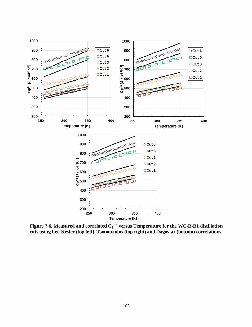
165
Figure 7.6. Measured and correlated Cpliq versus Temperature for the WC-B-B1 distillation
cuts using Lee-Kesler (top left), Tsonopoulos (top right) and Dagostar (bottom) correlations.
200
300
400
500
600
700
800
900
1000
250 300 350 400
Cp
liq
[J m
ol-
1K
-1]
Temperature [K]
Cut 6
Cut 5
Cut 3
Cut 2
Cut 1
200
300
400
500
600
700
800
900
1000
250 300 350 400C
pli
q[J
mo
l-1K
-1]
Temperature [K]
Cut 6
Cut 5
Cut 3
Cut 2
Cut 1
200
300
400
500
600
700
800
900
1000
250 300 350 400
Cp
liq
[J m
ol-
1K
-1]
Temperature [K]
Cut 6
Cut 5
Cut 3
Cut 2
Cut 1
200
300
400
500
600
700
800
900
1000
250 300 350 400
Cp
liq
[J m
ol-
1K
-1]
Temperature [K]
Cut 6
Cut 5
Cut 3
Cut 2
Cut 1
200
300
400
500
600
700
800
900
1000
250 300 350 400
Cp
liq
[J m
ol-
1K
-1]
Temperature [K]
Cut 6
Cut 5
Cut 3
Cut 2
Cut 1
200
300
400
500
600
700
800
900
1000
250 300 350 400
Cp
liq
[J m
ol-
1K
-1]
Temperature [K]
Cut 6
Cut 5
Cut 3
Cut 2
Cut 1

166
Figure 7.7. Relative error obtained for predicted Cpliq using Lee-Kesler (left), Tsonopoulos
(centre) and Dagostar (right) correlations.
-15
-10
-5
0
5
10
15
1.5 1.7 1.9 2.1
(Cp
calc
-Cp
exp)/
Cp
exp*1
00
Cpexp [J g-1 K-1]
-15
-10
-5
0
5
10
15
1.5 1.7 1.9 2.1
(Cp
calc
-Cp
exp)/
Cp
exp*1
00
Cpexp [J g-1 K-1]
-15
-10
-5
0
5
10
15
1.5 1.7 1.9 2.1(C
pc
alc
-Cp
exp)/
Cp
exp*1
00
Cpexp [J g-1 K-1]
-15
-10
-5
0
5
10
15
1.5 1.7 1.9 2.1
(Cp
calc
-Cp
exp)/
Cp
exp*1
00
Cpexp [J g-1 K-1]
-15
-10
-5
0
5
10
15
1.5 1.7 1.9 2.1
(Cp
calc
-Cp
exp)/
Cp
exp*1
00
Cpexp [J g-1 K-1]
-15
-10
-5
0
5
10
15
1.5 1.7 1.9 2.1
(Cp
ca
lc-C
pexp)/
Cp
exp*1
00
Cpexp [J g-1 K-1]
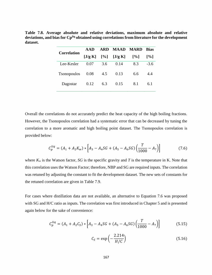
167
Table 7.8. Average absolute and relative deviations, maximum absolute and relative
deviations, and bias for Cpliq obtained using correlations from literature for the development
dataset.
Correlation AAD
[J/g K]
ARD
[%]
MAAD
[J/g K]
MARD
[%]
Bias
[%]
Lee-Kesler 0.07 3.6 0.14 8.3 -3.6
Tsonopoulos 0.08 4.5 0.13 6.6 4.4
Dagostar 0.12 6.3 0.15 8.1 6.1
Overall the correlations do not accurately predict the heat capacity of the high boiling fractions.
However, the Tsonopoulos correlation had a systematic error that can be decreased by tuning the
correlation to a more aromatic and high boiling point dataset. The Tsonopoulos correlation is
provided below:
𝐶𝑝𝑙𝑖𝑞 = (𝐴1 + 𝐴2𝐾𝑤) ∗ [𝐴3 − 𝐴4𝑆𝐺 + (𝐴5 − 𝐴6𝑆𝐺) (
𝑇
1000− 𝐴7)] (7.6)
where Kw is the Watson factor, SG is the specific gravity and T is the temperature in K. Note that
this correlation uses the Watson Factor; therefore, NBP and SG are required inputs. The correlation
was retuned by adjusting the constant to fit the development dataset. The new sets of constants for
the retuned correlation are given in Table 7.9.
For cases where distillation data are not available, an alternative to Equation 7.6 was proposed
with SG and H/C ratio as inputs. The correlation was first introduced in Chapter 5 and is presented
again below for the sake of convenience:
𝐶𝑝𝑙𝑖𝑞 = (𝐴1 + 𝐴2𝐶𝑆) ∗ [𝐴3 − 𝐴4𝑆𝐺 + (𝐴5 − 𝐴6𝑆𝐺) (
𝑇
1000− 𝐴7)] (5.15)
𝐶𝑆 = exp (−2.214
𝐻/𝐶) (5.16)
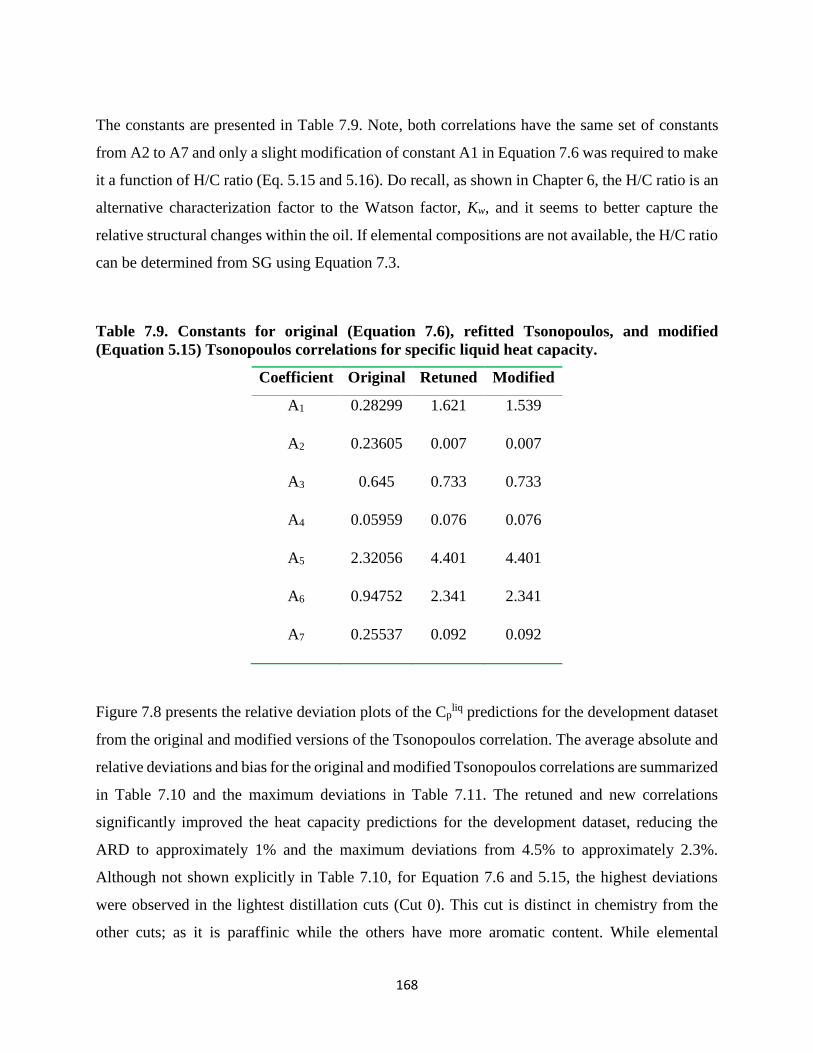
168
The constants are presented in Table 7.9. Note, both correlations have the same set of constants
from A2 to A7 and only a slight modification of constant A1 in Equation 7.6 was required to make
it a function of H/C ratio (Eq. 5.15 and 5.16). Do recall, as shown in Chapter 6, the H/C ratio is an
alternative characterization factor to the Watson factor, Kw, and it seems to better capture the
relative structural changes within the oil. If elemental compositions are not available, the H/C ratio
can be determined from SG using Equation 7.3.
Table 7.9. Constants for original (Equation 7.6), refitted Tsonopoulos, and modified
(Equation 5.15) Tsonopoulos correlations for specific liquid heat capacity.
Coefficient Original Retuned Modified
A1 0.28299 1.621 1.539
A2 0.23605 0.007 0.007
A3 0.645 0.733 0.733
A4 0.05959 0.076 0.076
A5 2.32056 4.401 4.401
A6 0.94752 2.341 2.341
A7 0.25537 0.092 0.092
Figure 7.8 presents the relative deviation plots of the Cpliq predictions for the development dataset
from the original and modified versions of the Tsonopoulos correlation. The average absolute and
relative deviations and bias for the original and modified Tsonopoulos correlations are summarized
in Table 7.10 and the maximum deviations in Table 7.11. The retuned and new correlations
significantly improved the heat capacity predictions for the development dataset, reducing the
ARD to approximately 1% and the maximum deviations from 4.5% to approximately 2.3%.
Although not shown explicitly in Table 7.10, for Equation 7.6 and 5.15, the highest deviations
were observed in the lightest distillation cuts (Cut 0). This cut is distinct in chemistry from the
other cuts; as it is paraffinic while the others have more aromatic content. While elemental
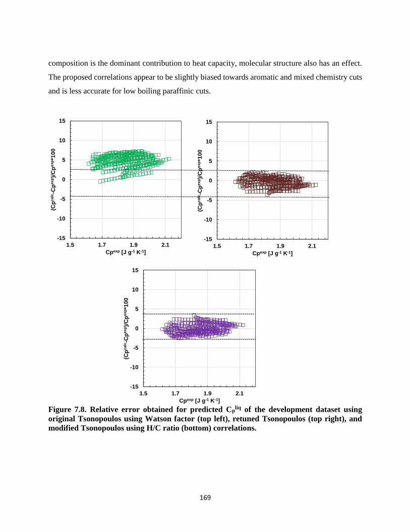
169
composition is the dominant contribution to heat capacity, molecular structure also has an effect.
The proposed correlations appear to be slightly biased towards aromatic and mixed chemistry cuts
and is less accurate for low boiling paraffinic cuts.
Figure 7.8. Relative error obtained for predicted Cpliq of the development dataset using
original Tsonopoulos using Watson factor (top left), retuned Tsonopoulos (top right), and
modified Tsonopoulos using H/C ratio (bottom) correlations.
-15
-10
-5
0
5
10
15
1.5 1.7 1.9 2.1
(Cp
calc
-Cp
exp)/
Cp
exp*1
00
Cpexp [J g-1 K-1]
-15
-10
-5
0
5
10
15
1.5 1.7 1.9 2.1
(Cp
calc
-Cp
exp)/
Cp
exp*1
00
Cpexp [J g-1 K-1]
-15
-10
-5
0
5
10
15
1.5 1.7 1.9 2.1
(Cp
calc
-Cp
exp)/
Cp
exp*1
00
Cpexp [J g-1 K-1]
-15
-10
-5
0
5
10
15
1.5 1.7 1.9 2.1
(Cp
calc
-Cp
exp)/
Cp
exp*1
00
Cpexp [J g-1 K-1]
-15
-10
-5
0
5
10
15
1.5 1.7 1.9 2.1
(Cp
calc
-Cp
exp)/
Cp
exp*1
00
Cpexp [J g-1 K-1]
-15
-10
-5
0
5
10
15
1.5 1.7 1.9 2.1
(Cp
calc
-Cp
exp)/
Cp
exp*1
00
Cpexp [J g-1 K-1]

170
Table 7.10 Average absolute and relative deviations and bias from the retuned Tsonopoulos
using Watson factor and modified Tsonopoulos using H/C ratio correlations for Cpliq for the
development dataset.
Oil Sample
Retuned
(Kw)
Modified
(H/C)
ARD
[%]
AAD
[J/g K]
Bias
[%]
ARD
[%]
AAD
[J/g K]
Bias
[%]
WC-B-B1 1.2 0.02 -1.1 1.0 0.02 0.6
CO-B-A1 1.1 0.02 0.5 1.3 0.02 -0.9
MX-HO-A1 1.5 0.03 -1.5 1.2 0.02 1.2
CO-B-B1 0.5 0.01 0.2 0.6 0.01 -0.6
Overall 1.1 0.02 -0.5 1.0 0.02 0.1
Table 7.11. Maximum average absolute and relative deviations and bias from the retuned
Tsonopoulos using Watson factor and modified Tsonopoulos using H/C ratio correlations for
Cpliq for the development dataset.
Oil Sample
Retuned (Kw) Modified (H/C)
MARD
[%]
MAAD
[J/g K]
MARD
[%]
MAAD
[J/g K]
WC-B-B1 2.9 0.05 2.4 0.04
CO-B-A1 2.3 0.05 2.5 0.04
MX-HO-A1 3.6 0.07 2.7 0.06
CO-B-B1 1.0 0.02 1.3 0.03
Overall 2.4 0.05 2.2 0.04
The original, retuned, and modified Tsonopoulos correlations were evaluated against an
independent test dataset that included distillation cuts for the following oils:
MX-B-A1 cut 5 to cut 7
CO-B-B1 cut 4 to cut 6
Mayan Oil (Fulem et al., 2008)

171
The test dataset was small because several physical properties were required to test both
correlations simultaneously and few datasets in the literature included Cpliq, NBP, SG, and H/C
ratio.
Figure 7.9 is a dispersion plot for the original, retuned, and modified Tsonopoulos correlations
applied to the test dataset. The deviations are summarized in Table 7.12 and 7.13. The proposed
correlations significantly improve the predictions of the liquid heat capacity (AARD of 1.5%
compared with 6% from the original Tsonopoulos correlation). The maximum deviations were
reduced to less than 2% compared with 7% from the original correlation. Both the retuned
(Equation 7.6) and modified (Equation 5.15) correlations predict the heat capacities to within the
experimental error of the measurements (≈1%). The modified correlation has a better performance
for a wider range of liquid heat capacities with the lowest average and maximum deviations and
lowest bias. Note for the distillation cuts, both correlations have a deviation of less than 0.2%. A
greater difference is observed for the Mayan crude oil where the modified correlation outperforms
the retuned correlation by 1.6%. The retuned and modified correlations appear to be well suited
for heavy oils but have not been tested on conventional oils.

172
Figure 7.9. Dispersion plots for the Cpliq of the test dataset determined from: original
Tsonopoulos using Watson factor (top left), retuned Tsonopoulos (top right), and modified
Tsonopoulos using H/C ratio (bottom) correlations.
1.5
1.7
1.9
2.1
2.3
2.5
2.7
2.9
1.5 1.7 1.9 2.1 2.3 2.5 2.7 2.9
Ca
lcu
late
d C
p [
J g
-1K
-1]
Experimental Cp [J g-1 K-1]
Maya (Fulem et al, 2008)
CO-B-B1
MX-HO-A1
1.5
1.7
1.9
2.1
2.3
2.5
2.7
2.9
1.5 1.7 1.9 2.1 2.3 2.5 2.7 2.9
Ca
lcu
late
d C
p [
J g
-1K
-1]
Experimental Cp [J g-1 K-1]
Maya (Fulem et al, 2008)
CO-B-B1
MX-HO-A1
1.5
1.7
1.9
2.1
2.3
2.5
2.7
2.9
1.5 1.7 1.9 2.1 2.3 2.5 2.7 2.9
Ca
lcu
late
d C
p [
J g
-1K
-1]
Experimental Cp [J g-1 K-1]
Maya (Fulem et al, 2008)
CO-B-B1
MX-HO-A1
1.5
1.7
1.9
2.1
2.3
2.5
2.7
2.9
1.5 1.7 1.9 2.1 2.3 2.5 2.7 2.9
Ca
lcu
late
d C
p [
J g
-1K
-1]
Experimental Cp [J g-1 K-1]
Maya (Fulem et al, 2008)
CO-B-B1
MX-HO-A1
1.5
1.7
1.9
2.1
2.3
2.5
2.7
2.9
1.5 1.7 1.9 2.1 2.3 2.5 2.7 2.9
Ca
lcu
late
d C
p [
J g
-1K
-1]
Experimental Cp [J g-1 K-1]
Maya (Fulem et al, 2008)
CO-B-B1
MX-HO-A1
1.5
1.7
1.9
2.1
2.3
2.5
2.7
2.9
1.5 1.7 1.9 2.1 2.3 2.5 2.7 2.9
Ca
lcu
late
d C
p [
J g
-1K
-1]
Experimental Cp [J g-1 K-1]
Maya (Fulem et al, 2008)
CO-B-B1
MX-HO-A1

173
Table 7.12. Average relative deviation obtained for original, retuned and modified versions
of Tsonopoulos correlations for the test dataset.
Oil Sample
Original
Tsonopoulos
Retuned
(Kw)
Modified
(H/C)
AAD
[J/g K]
AR
D
[%]
Bias
[%]
AAD
[J/g K]
ARD
[%]
Bias
[%]
AAD
[J/g K]
ARD
[%]
Bias
[%]
Maya (Fulem
et al, 2008) 0.18 7.5 -7.5 0.06 2.5 -2.5 0.02 0.9 -0.9
MX-HO-A1 0.10 5.1 5.1 0.03 1.6 -1.6 0.02 1.3 -1.3
CO-B-B1 0.10 5.4 5.4 0.01 0.4 -0.2 0.01 0.4 0.3
Overall 0.13 6.0 1.0 0.03 1.5 -1.4 0.02 0.9 -0.6
Table 7.13. Maximum average relative deviation obtained for original, retuned and modified
versions of Tsonopoulos correlations for the test dataset.
Oil Sample
Original Tsonopoulos Retuned
(Kw)
Modified
(H/C)
MAAD
[J/g K]
MARD
[%]
MAAD
[J/g K]
MARD
[%]
MAAD
[J/g K]
MARD
[%]
Maya (Fulem et al, 2008) 0.19 9.6 0.09 3.2 0.04 1.6
MX-HO-A1 0.11 5.9 0.04 1.8 0.03 1.5
CO-B-B1 0.11 5.7 0.02 0.9 0.02 0.9
Overall 0.14 7.1 0.05 2.0 0.03 1.3
7.3 Heat of Vaporization
In Chapter 2 several correlations were presented that could be used to determine the heat of
vaporization at the normal boiling point (Riazi, 2005; Vetere, 1995; Gopinathan, 2001; and Fang,
2005). To test the correlations, it was first necessary to generate heat of vaporization data.
Unfortunately, the enthalpy of vaporization of a heavy hydrocarbon cannot be measured directly
at its normal boiling point because heavy hydrocarbons decompose below this temperatures (at

174
atmospheric pressure). Instead, as noted in Chapter 5, it can be calculated from vapor pressure data
through the Clausius-Clapeyron equation,
−∆𝐻𝑣𝑎𝑝
𝑅=
𝑑𝑃𝑠𝑎𝑡
𝑑(1/𝑇) (5.1)
Since the parameters of the Cox equation were obtained from the fitting of both vapor pressure
and heat capacity, this same set of parameters can be used to determine ∆𝐻𝑣𝑎𝑝 using Equations
7.7 and 7.8, which are a derived form of the Cox equation for the heat of vaporization:
∆𝐻𝑣𝑎𝑝 = 𝑅[𝑇𝑏 + (𝑇 − 𝑇𝑏) ∗ (𝐴1𝑇 + 𝐴2𝑇2)]exp (𝐴0 + 𝐴1𝑇 + 𝐴2𝑇2) (7.7)
When T=Tb, this equation reduces to:
∆𝐻𝑛𝑏𝑝𝑣𝑎𝑝 = R 𝑇𝑏 exp(𝐴0 + 𝐴1𝑇𝑏 + 𝐴2𝑇𝑏
2) /1000 (7.8)
The heats of vaporization determined using Equation 7.8 are provided in Appendix H. The
‘experimental’ ∆𝐻𝑣𝑎𝑝 follows the expected trends with temperature and molecular weight, Figure
7.10, for Cuts 1, 3 and 6 from WC-B-B1. The values of ∆𝐻𝑣𝑎𝑝 decrease as the temperature
increases and approaches the normal boiling point. The higher the temperature of the fluid, the
higher the kinetic energy of the molecules relative to the intermolecular forces. Therefore to break
intermolecular forces at a higher temperature requires less energy than at a lower temperature. The
heat of vaporization trend increases from the lowest boiling to highest boiling cuts as their MW
increases. The attractive forces between the molecules tend to be greater for larger molecules and
therefore they have larger heats of vaporization.

175
.
Figure 7.10. Heat of vaporization of three distillation cuts from WC-B-B1 versus
temperature.
Note, the ‘experimental’ heats of vaporization may not correspond to the actual experimental
values due to the assumptions made during the development of Equation 5.1. To check the results,
the ∆𝐻𝑛𝑏𝑝𝑣𝑎𝑝
values for the distillation cuts are compared with the known heats of vaporization of
pure components versus molecular weight, Figure 7.11. Note, there are two trends for pure
components, one for the paraffinic compounds and another for aromatic and PAH compounds. The
PAHs follow a different trend because the intermolecular attraction between aromatic rings is
relatively strong. Hence, their heat of vaporization is greater than those of paraffinic and
naphthenic compounds of the same molecular weight. Although the data for the distillation cuts
are scattered, their calculated heats of vaporization fall between the two trends as is expected based
on their mixed chemistry. The distillation cuts shift from near paraffinic values to near aromatic
values from lighter to heavier cuts, consistent with the increasing aromaticity of the cuts. Since no
experimental data are available for the cuts, the deviation for ∆𝐻𝑛𝑏𝑝𝑣𝑎𝑝
from the actual value was
assumed to be within the reported values for n-alkanes from Ruzicka et al. (2004); that is, less than
6%.
40
60
80
100
120
140
160
180
200 400 600 800
∆H
va
p [
kJ
/mo
l]
Temperature [K]
Cut 1
Cut 3
Cut 6
Increasing MW
and NBP

176
Figure 7.11. Heat of vaporization at the normal boiling point versus molecular weight for
pure hydrocarbons and the DVFA distillation cuts.
The heats of vaporization from this study as well as for selected pure hydrocarbons, Table 7.14,
were used to test the correlations obtained from the literature and to develop a new correlation.
The deviations of the literature correlations developed by Riazi (2005), Vetere (1995), Gopinathan
(2001) and Fang (2005) are shown in Figure 7.12 and summarized in Table 7.15. Although not
shown explicitly in Table 7.15, the highest deviations for all the correlations were obtained for the
distillation cuts and the aromatic/PAHs. These high errors likely arise because there were no
aromatic compounds in the datasets used to develop these correlations. Also, as shown in Figure
7.11, if the PAHs are neglected as part of the dataset, the predicted heat of vaporization will
correspond to the lower trend observed for the paraffinic and naphthenic compounds and the heat
of vaporization of PAHs will be significantly under-predicted. Hence, there is potential to develop
an improved correlation for the heat of vaporization correlations of heavy cuts.
Table 7.14. Development dataset for ∆𝑯𝒏𝒃𝒑𝒗𝒂𝒑
of pure components and distillation cuts
10
30
50
70
90
110
130
0 200 400 600
∆H
va
p(N
BP
)[k
J/m
ol]
Molecular Weight [g/mol]
Paraffins/NaphthalenesAromatics/PAHsDistillation Cuts

177
Component Data
Points Reference
n-Alkanes/Naphthanes 35 Ruzicka and Majer, 1993, Yaws, 2003
Aromatics/PAHs 28 Fang et al., 2003, Yaws, 2003
Distillation cuts 63 this study

178
Figure 7.12. Relative error for the predicted heat of vaporization for the development dataset
from the Riazi (a), Vetere (b), Gopinathan (c), Fang (d), and proposed (e) correlations.
-40
-30
-20
-10
0
10
20
30
0.00 50.00 100.00 150.00
[∆H
va
p
calc
. -∆
Hvap
exp
.]/∆
Hvap
exp
. *1
00
'Experimental' ∆Hvap
-40
-30
-20
-10
0
10
20
30
0.00 50.00 100.00 150.00
[∆H
va
p
calc
. -∆
Hva
p e
xp
.]/∆
Hva
p e
xp
. *1
00
'Experimental' ∆Hvap
-40
-30
-20
-10
0
10
20
30
0.00 50.00 100.00 150.00
[∆H
vap
c
alc
. -∆
Hva
p e
xp
.]/∆
Hva
p e
xp
. *1
00
'Experimental' ∆Hvap
-40
-30
-20
-10
0
10
20
30
0.00 50.00 100.00 150.00
[∆H
va
p
calc
. -∆
Hva
p e
xp
.]/∆
Hvap
exp
. *1
00
'Experimental' ∆Hvap
-40
-30
-20
-10
0
10
20
30
0.00 50.00 100.00 150.00
[∆H
vap
calc
. -∆
Hva
p e
xp
.]/∆
Hva
p e
xp
. *1
00
'Experimental' ∆Hvap
-40
-30
-20
-10
0
10
20
30
0.00 50.00 100.00 150.00
[∆H
va
p
calc
. -∆
Hva
p e
xp
.]/∆
Hvap
exp
. *1
00
'Experimental' ∆Hvap
-40
-30
-20
-10
0
10
20
30
0.00 50.00 100.00 150.00
[∆H
va
p
ca
lc. -∆
Hva
p e
xp
.]/∆
Hva
p e
xp
. *1
00
'Experimental' ∆Hvap
-40
-30
-20
-10
0
10
20
30
0.00 50.00 100.00 150.00
[∆H
vap
calc
. -∆
Hva
p e
xp
.]/∆
Hvap
exp
. *1
00
'Experimental' ∆Hvap
-40
-30
-20
-10
0
10
20
30
0.00 50.00 100.00 150.00
[∆H
vap
c
alc
. -∆
Hvap
exp
.]/∆
Hvap
exp
. *1
00
'Experimental' ∆Hvap
-40
-30
-20
-10
0
10
20
30
0.00 50.00 100.00 150.00
[∆H
va
p
calc
. -∆
Hva
p e
xp
.]/∆
Hva
p e
xp
. *1
00
'Experimental' ∆Hvap
-40
-30
-20
-10
0
10
20
30
0.00 50.00 100.00 150.00
[∆H
vap
calc
. -∆
Hvap
exp
.]/∆
Hvap
exp
. *1
00
'Experimental' ∆Hvap
-40
-30
-20
-10
0
10
20
30
0.00 50.00 100.00 150.00
[∆H
vap
calc
. -∆
Hvap
exp
.]/∆
Hvap
exp
. *1
00
'Experimental' ∆Hvap
-40
-30
-20
-10
0
10
20
30
0.00 50.00 100.00 150.00
[∆H
vap
calc
. -∆
Hvap
exp
.]/∆
Hvap
exp
. *1
00
'Experimental' ∆Hvap
-40
-30
-20
-10
0
10
20
30
0.00 50.00 100.00 150.00
[∆H
vap
calc
. -∆
Hvap
exp
.]/∆
Hvap
exp
. *1
00
'Experimental' ∆Hvap
-40
-30
-20
-10
0
10
20
30
0.00 50.00 100.00 150.00
[∆H
vap
calc
. -∆
Hvap
exp
.]/∆
Hvap
exp
. *1
00
'Experimental' ∆Hvap
-40
-30
-20
-10
0
10
20
30
0.00 50.00 100.00 150.00
[∆H
va
p
calc
. -∆
Hva
p e
xp
.]/∆
Hva
p e
xp
. *1
00
'Experimental' ∆Hvap
-40
-30
-20
-10
0
10
20
30
0.00 50.00 100.00 150.00
[∆H
va
p
ca
lc. -∆
Hva
p e
xp
.]/∆
Hva
p e
xp
. *1
00
'Experimental' ∆Hvap
-40
-30
-20
-10
0
10
20
30
0.00 50.00 100.00 150.00
[∆H
va
p
calc
. -∆
Hva
p e
xp
.]/∆
Hva
p e
xp
. *1
00
'Experimental' ∆Hvap
-40
-30
-20
-10
0
10
20
30
0.00 50.00 100.00 150.00
[∆H
va
p
calc
. -∆
Hva
p e
xp
.]/∆
Hva
p e
xp
. *1
00
'Experimental' ∆Hvap
-40
-30
-20
-10
0
10
20
30
0.00 50.00 100.00 150.00
[∆H
va
p
calc
. -∆
Hva
p e
xp
.]/∆
Hva
p e
xp
. *1
00
'Experimental' ∆Hvap

179
Table 7.15. Average absolute and relative deviations, maximum absolute and relative
deviations, and bias for heat of vaporization obtained using correlations from literature for
the development dataset.
Correlation AAD ARD Bias MAAD MARD
[kJ/mol] [%] [%] [kJ/mol] [%]
Riazi 9.4 11.9 -9.9 23.6 24.5
Vetere 10.4 13.1 -12.0 26.3 27.3
Gopinathan 9.7 12.3 -10.7 24.4 25.2
Fang 6.2 9.0 -1.9 17.0 20.5
To develop a new correlation, the heats of vaporization for the dataset shown in Table 7.14 were
first recalculated using Equation 7.8 with the generalized equations for Cox constants (Eq. 7.1 to
7.3). Figure 7.13 shows that the heats of vaporization of the distillation cuts were predicted with
deviations of less than 7%. However, the paraffins and naphthenes were systematically under-
predicted for compounds with molecular weight lower than 350 g/mol, with deviations as high as
50%. The heats of vaporization of heavy PAHs were similarly under-predicted. Not surprisingly,
this approach predicted the heats of vaporization of the distillation cuts (from which the average
parameters were obtained) with reasonably accuracy. However, it does not perform well for pure
components.

180
Figure 7.13. Dispersion plots for the calculated and predicted heat of vaporization at the
normal boiling point for the distillation cuts (left) and pure components (right) using
Equations 7.9, 7.4 to 7.6
The deviations between the predicted and “experimental” heats of vaporization were found to
correlate to MW and SG, and the majority of the deviations were observed at molecular weights
lower than 300 g/mol. The main trend in the deviations correlated to MW and a MW based
correction factor was found to eliminate the paraffinic and naphthenic deviations. A secondary
correlation based on SG was required to correct the under-prediction of the heat of vaporization
for PAHs. The corrected version of Equation 7.8 for MW<300 g/mol is given by:
∆𝐻𝑛𝑏𝑝𝑣𝑎𝑝 = R 𝑇𝑏 exp(𝐴0 + 𝐴1𝑇𝑏 + 𝐴2𝑇𝑏
2)/1000 − 𝐶𝐹1 (7.9)
𝐶𝐹1 =−25.03
1 + exp[(𝑀𝑊 − 198.92)/𝐶𝐹2)] (7.10)
𝐶𝐹2 = 25.32 +2.02
1.996 + exp[𝑆𝐺 − 9.327] (7.11)
where R is 8.314 J/mol K, Tb is the normal boiling temperature in K, and A0, A1, and A2 are
generalized Cox constants given in Equations 7.1 to 7.3. For compounds with MW≥300, ∆𝐻𝑛𝑏𝑝𝑣𝑎𝑝
is
10
30
50
70
90
110
130
150
10 30 50 70 90 110 130 150
∆H
vap
(N
BP
)[k
J/m
ol]
Ca
lcu
late
d∆Hvap (NBP)[kJ/mol] Experimental
Paraffins/Naphthalenes
Aromatics/PAHs
10
30
50
70
90
110
130
150
10 30 50 70 90 110 130 150
∆H
vap
(N
BP
)[k
J/m
ol]
Ca
lcu
late
d
∆Hvap (NBP)[kJ/mol] Experimental

181
provided by Equation 7.8. Figure 7.14 shows the dispersion plot for the new correlation applied to
the development dataset and Table 7.16 summarizes the average and maximum deviations for each
development data set. Note, the low MW compounds are now accurately predicted as well as the
PAHs. The new correlation decreased the overall AARD to 7.5% compared with 9.0% for the best
prediction from the literature correlations (Fang et al., 2005). Also, a reduction in the maximum
deviations (less than 16 %) as well as the overall bias (-1.5 %) compared with results shown in
Table 7.15.
Figure 7.14. Dispersion plots for the calculated and predicted heat of vaporization at the
normal boiling point using the proposed correlations for the pure components and
distillation cuts.
10
30
50
70
90
110
130
150
10 30 50 70 90 110 130 150
∆H
vap
(N
BP
)[k
J/m
ol]
Ca
lcu
late
d
∆Hvap (NBP)[kJ/mol] Experimental
Paraffins/Naphthalenes
Aromatics/PAHs
Distillation Cuts

182
Table 7.16. Average absolute and relative deviations, maximum absolute and relative
deviations, and bias for heat of vaporization obtained using the proposed correlation for the
development dataset.
Component AAD ARD Bias MAAD MARD
[kJ/mol] [%] [%] [kJ/mol] [%]
Paraffins/Naphthalenes 1.8 4.4 3.9 6.0 11.6
Aromatics/PAHs 6.2 8.9 -3.9 18.7 15.9
Distillation fractions 6.8 9.2 -1.5 15.2 19.1
Overall 4.9 7.5 -1.5 13.3 15.9
The proposed correlations as well as the literature correlations were tested for a set of distillation
cuts from three different oils (Fang et al., 2005). No distinction between the cuts was made by the
author, therefore the combined results for all the 58 distillation cuts are presented. Figure 7.15
shows the dispersion plots obtained for all of the correlations and the deviations are summarized
in Table 7.17. The new correlation performs better than all of the literature correlations, except the
Fang correlation, with an average relative deviation less than 2.7%. The slightly better
performance from Fang’s correlation is not surprising because the test dataset used here is the same
dataset that was used to develop the Fang correlation. The improvement over the other three
correlations (Vetere, Riazi, and Gopinathan) is significant for heats of vaporization higher than 40
kJ/mol where these correlations under-predict the heat of vaporization by as much as 20%.
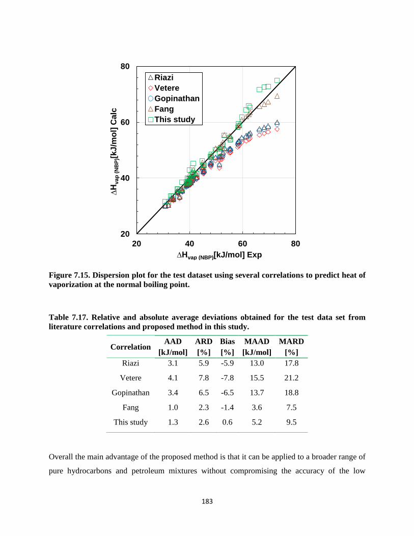
183
Figure 7.15. Dispersion plot for the test dataset using several correlations to predict heat of
vaporization at the normal boiling point.
Table 7.17. Relative and absolute average deviations obtained for the test data set from
literature correlations and proposed method in this study.
Correlation AAD ARD Bias MAAD MARD
[kJ/mol] [%] [%] [kJ/mol] [%]
Riazi 3.1 5.9 -5.9 13.0 17.8
Vetere 4.1 7.8 -7.8 15.5 21.2
Gopinathan 3.4 6.5 -6.5 13.7 18.8
Fang 1.0 2.3 -1.4 3.6 7.5
This study 1.3 2.6 0.6 5.2 9.5
Overall the main advantage of the proposed method is that it can be applied to a broader range of
pure hydrocarbons and petroleum mixtures without compromising the accuracy of the low
20
40
60
80
20 40 60 80
∆H
vap
(N
BP
)[k
J/m
ol]
Ca
lc
∆Hvap (NBP)[kJ/mol] Exp
Riazi
Vetere
Gopinathan
Fang
This study
184
molecular weight compounds. Although the predictions were improved by the new correlation, the
physics behind the heat of vaporization for different chemical families are not fully described by
only physical properties (see Figure 7.14). It is plausible that structural data showing the number
of rings and double bonds could more accurately capture the attractive intermolecular forces that
cause the heat of vaporization to have a different trends for the molecules with multiple aromatic
rings and hetero-atomic molecules. Several studies (Kolska et al., 2005, 2012; Marrero and Gani,
2001; Ma and Zhao, 1993; Drucos et al., 1980, 1981, 1982, 1984) have shown the advantage of
multilevel group contribution methods to predict heat values for wide ranges of chemical families.
However, this approach is beyond the scope of this thesis which is focussed on correlations to
physical properties. .
7.4 Heat of Combustion
As part of the project, the heats of combustion of some distillation cuts were measured at constant
volume. The values are reported in Appendix H. Figure 7.16 compares the heat of combustion
(high heating value-HHV) of the distillation cuts with pure components including paraffins,
naphthenes, aromatics, and PAHs hydrocarbons. Figure 7.16 also shows how heat of combustion
varies with the specific gravity for some of the oils used in this project. Overall, the data follows
an expected trend with the lower boiling cuts (low SG) having higher heats of combustion than the
higher boiling cuts (high specific gravity and higher heteroatom content).

185
Figure 7.16. Variation of heat of combustion with specific gravity for pure components and
distillation cuts (left) and data for three oil samples (right)
The correlations available in the literature for heat of combustion were provided in Table 2.8 and
include the Tsonopoulos and Yan correlations. The correlations were tested on the experimental
heats of combustion from the dataset listed in Table 7.18. Figure 7.17 presents the dispersion plot
for both correlations. The error bars correspond to the 0.3% uncertainty from elemental analysis.
Table 7.19 and 7.20 summarizes the average absolute and relative deviations, bias and maximum
deviations.
Both correlations were able to predict the heat of combustion with similar accuracy: average
deviations of 1.0% (0.4 kJ/g) for the Yan et al. (1988) correlation and 1.2% (0.5 kJ/g) for the
Tsonopoulos (1986) correlation. It was observed that the major deviations were present in the coal
liquid heat of combustion calculation. This higher error for coal liquids was also noted by the
authors and may be an effect of higher errors in elemental analysis measurements, particularly for
oxygen. Since the correlations have a sound fundamental basis and low error, a new correlation
was not considered.
30
35
40
45
50
55
0.0 0.5 1.0 1.5
Uc
om
b.-
HH
V [
kJ
/g]
Specific Gravity
Pure Components (NIST)
Distillation Cuts
40
41
42
43
44
45
46
0.85 0.90 0.95 1.00 1.05
Uc
om
b.-
HH
V [
kJ
/g]
Specific Gravity
MX-HO-A1
CO-B-A1
CO-B-B1

186
Table 7.18. Data set used to test the Tsonopoulos and Yan correlations.
Sample Data
Points Reference
Distillation cuts 20 This Study
Heavy oil/ Bitumen 6 Yan et al., 1988
Coal Liquids 17 Jain and Sundararajan, 1981
Figure 7.17. Comparison between the calculated and experimental heat of combustion from
Yan and Tsonopoulos correlations.
-50
-45
-40
-35
-30
-25
-50 -40 -30
Uc
om
b.,
ca
lcu
late
d [k
J/g
]
Ucomb, experimental [kJ/g]
Yan
Tsonopoulos

187
Table 7.19. Average absolute and relative deviations obtained for the test data set.
Oil Sample
Yan Tsonopoulos
Bias
[%]
ARD
[%]
AAD
[kJ/mol]
Bias
[%]
ARD
[%]
AAD
[kJ/mol]
Distillation Cuts 0.6 1.2 0.5 -0.2 1.0 0.4
Heavy Oil/Bitumen 0.1 0.3 0.1 -1.1 1.1 0.4
Coal Liquids -0.7 1.6 0.6 -0.3 1.5 0.6
Overall 0.0 1.0 0.4 -0.5 1.2 0.5
Table 7.20. Maximum average absolute and relative deviations obtained for the test data set.
Tsonopoulos Yan
Oil Sample MARD
[%]
MAAD
[kJ/mol]
MARD
[%]
MAAD
[kJ/mol]
Distillation Cuts 2.5 1.0 2.5 1.0
Heavy Oil/Bitumen 1.3 0.4 0.8 0.3
Coal Liquids 1.2 0.5 1.5 0.5

188
CHAPTER EIGHT: IMPROVED CHARACTERIZATION OF HEAVY OILS AND
BITUMEN SAMPLES
It is not always practical and economically viable to perform all the property measurements
required to fully and accurately characterize a complex mixture like heavy oil. In many cases, the
only information available for a heavy oil are its bulk properties (often only density) and a TBP
curve from a distillation assay or from a simulated TBP curve obtained through gas
chromatography analysis. The property correlations discussed in the previous chapters usually
require two properties. Therefore, to initiate a pseudo-component based characterization, two
property distributions are required: in this case, one for TBP and one for another property.
Typically, density is selected as the second property and the form of its distribution is assumed.
For instance, the exponential model is used for light reservoir fluids and the gamma model gives
reasonable predictions for gas condensate systems (Whitson, 2000; Riazi, 2005). In this chapter,
the existing methods to predict SG distributions are evaluated, a modification is proposed for one
of the methods, and a new method is developed.
8.1 Specific Gravity Distribution Correlations
Methods to obtain specific gravity distributions from only boiling point data and bulk properties
include the Bergman, constant Watson Factor, and Katz-Firoozabadi methods.
Bergman
Bergman used measured data for gas condensates with light plus fractions to relate specific gravity
to the normal boiling point as follows:
𝑆𝐺 =(0.4189 + 2.786𝑥10−3𝑇𝑏 − 8.685𝑥10−6𝑇𝑏
2 + 1.306𝑥10−8𝑇𝑏3 − 7.092𝑥10−12𝑇𝑏
4)
0.9991 (8.1)
Since this method was developed exclusively for light oils, it may not be suitable for heavy oils.

189
Constant Watson Factor (Cte Kw.)
The method proposed by Miquel and Castells (1993, 1994) is based on the assumption that the
Watson factor is constant for all the pseudo-components of a mixture. Therefore, the SG of each
pseudo-component is given by:
𝑆𝐺𝑖 =𝑇
𝑏𝑖
13⁄
𝐾𝑤 (8.2)
The Watson K factor, Kw, is calculated from the average boiling point and bulk specific gravity of
the oil using the same equation. As noted by the authors, this method gives a good estimate for
compounds with boiling point less than 500 K. Since for heavy oils and bitumens more than 30%
of the sample has a boiling point higher than 500 K, this method may not accurately predict the
SG distribution of a heavy petroleum sample. The Watson factor can also be adjusted to obtain the
correct bulk SG (VMGSim User’s Manual).
Katz-Firoozabadi (K-F)
Katz and Firoozabadi (1978) presented a set of properties for single carbon numbers up to C45.
Several authors correlated those values into polynomial functions of carbon number (Whitson,
1982; Naji, 2010). Whitson (1982) modified the set to improve the consistency of the predictions.
Later Naji (2010) developed a similar set of equations as a function of the carbon number. The
original K-F correlation is given by Equation 8.3:
𝑆𝐺𝑖 =(0.5516 + 1.208𝑥10−3𝑇𝑏𝑖 − 2.231𝑥10−6𝑇𝑏𝑖
2 + 2.265𝑥10−9𝑇𝑏𝑖3 − 8.614𝑥10−13𝑇𝑏𝑖
4 )
0.9991 (8.3)
However, the original version and its modifications could not be applied for components with
carbon number greater than C45 or a normal boiling point higher that 850 K because a maximum
occurred at these values.
Satyro and coworkers (2000) proposed a simpler expression by fitting data from 700 to 850 K
range with specific gravity approaching a value of 1.05. They used the same data as was used to
develop Equation 8.3, however, the form proposed by Satyro and coworkers eliminates the
maximum in Equation 8.3. The final equation has the following form, Equation 8.4:
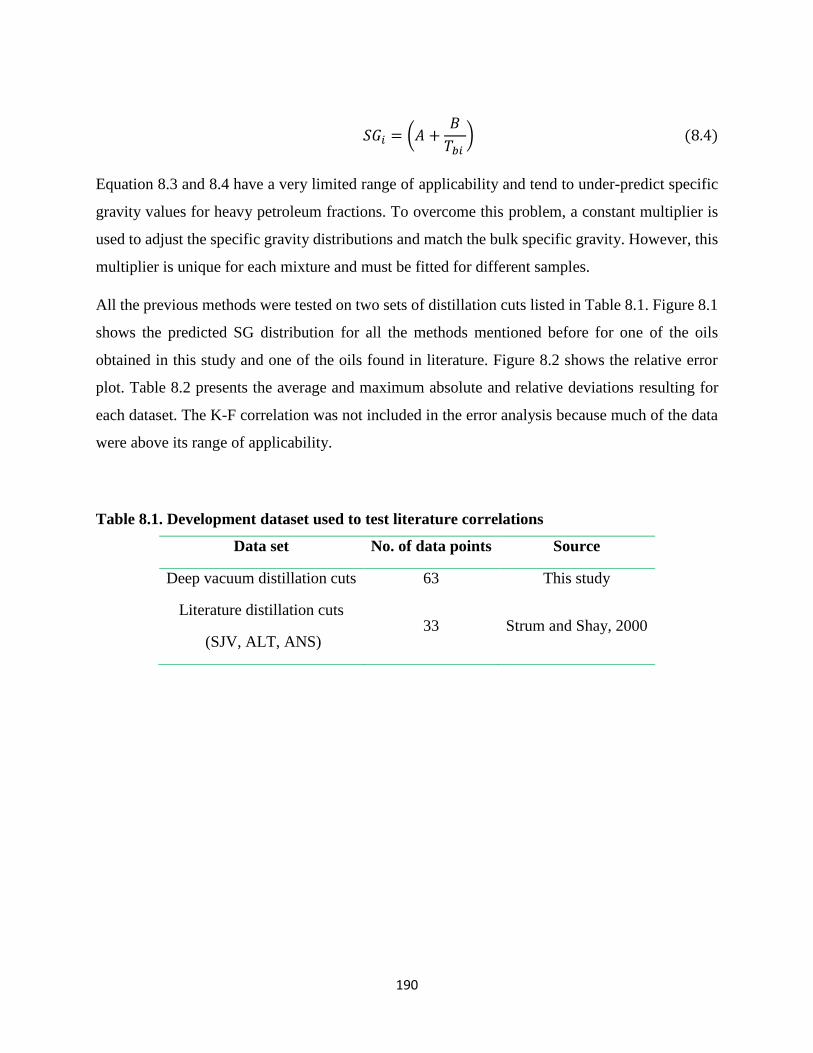
190
𝑆𝐺𝑖 = (𝐴 +𝐵
𝑇𝑏𝑖 ) (8.4)
Equation 8.3 and 8.4 have a very limited range of applicability and tend to under-predict specific
gravity values for heavy petroleum fractions. To overcome this problem, a constant multiplier is
used to adjust the specific gravity distributions and match the bulk specific gravity. However, this
multiplier is unique for each mixture and must be fitted for different samples.
All the previous methods were tested on two sets of distillation cuts listed in Table 8.1. Figure 8.1
shows the predicted SG distribution for all the methods mentioned before for one of the oils
obtained in this study and one of the oils found in literature. Figure 8.2 shows the relative error
plot. Table 8.2 presents the average and maximum absolute and relative deviations resulting for
each dataset. The K-F correlation was not included in the error analysis because much of the data
were above its range of applicability.
Table 8.1. Development dataset used to test literature correlations
Data set No. of data points Source
Deep vacuum distillation cuts 63 This study
Literature distillation cuts
(SJV, ALT, ANS) 33 Strum and Shay, 2000

191
Figure 8.1. Measured and correlated SG versus NBP for the CO-B-A1 distillation cuts (left)
and SJV distillation cuts (right) using Bergman, constant Watson factor (Cte. Kw), Katz
Firoozabadi (K-F) and Satyro correlations.
Figure 8.2. Relative error obtained for SG distribution predicted from the experimental
NBP values using the Bergman, constant Watson factor (Cte. Kw) and Satyro correlations.
0.80
0.85
0.90
0.95
1.00
1.05
1.10
500 600 700 800 900 1000
Sp
ec
ific
Gra
vit
y
NBP [K]
K-F
Bergman
Cte Kw
Satyro
CO-B-A1
0.70
0.75
0.80
0.85
0.90
0.95
1.00
1.05
1.10
1.15
400 500 600 700 800 900 1000
Sp
ec
ific
Gra
vit
yNBP [K]
Bergman
K-F
Cte Kw
Satyro
SJV
-30
-25
-20
-15
-10
-5
0
5
10
0.80 0.90 1.00 1.10
(SG
calc
-SG
exp)/
SG
exp
X1
00
Experimental SG
Bergman
Cte Kw
Satyro

192
Table 8.2. Average absolute and relative deviations, maximum absolute and relative
deviations, and bias for SG distributions obtained using correlations from literature for the
development dataset.
Correlation AAD ARD
[%]
Bias
[%] MAAD
MARD
[%]
Bergman 0.24 25.1 -23.9 2.04 202.4
Cte Kw 0.03 2.8 2.5 0.05 5.8
Satyro 0.07 7.8 -6.7 0.13 12.7
The Bergman method has a maximum at approximately 650 K causing the predicted specific
gravity to decrease as NBP increases, opposite to the correct trend. Not surprisingly, this
correlation has the highest deviations, 25.1%. It is evident that the light plus fractions used to
develop Bergman’s correlations provided insufficient range to extrapolate accurately to heavy oil
and bitumen samples. Note, this correlation was not designed to work for heavy oils and is only
shown here for comparison.
The constant Watson factor is the best performing correlation with an average deviation of less
than 2.8%. Note, in the middle range (near the average Kw of the oil), the predictions show the
smallest deviations and in the low and high boiling range the deviations grow as the difference of
this fractions from the whole sample are greater. The largest errors are generally for the residues.
The Satyro correlation under-predicts the SG and the deviations increase monotonically from the
lowest to the highest boiling fraction. The under-predictions were expected since the development
dataset of for this correlations consisted of pure components with a carbon number up to 45. Note,
the correction proposed by Satyro and coworkers, completely eliminate the maximum observed in
the original versions of this method. The average relative deviations were around 5% higher than
using constant Watson factor. However, since the error grows monotonically a simple correction
factor can be introduced for this correlation to improve its predictive capabilities.

193
Modified K-F/Satyro Method
The proposed correlation is based on the Satyro version of the K-F correlation and adds an
additional term that acts as a multiplier to match the bulk specific gravity of the oil. The modified
K-F correlation is given by Equation 8.5:
𝑆𝐺𝑖 = (1.0563 +−125.114
𝑇𝑏𝑖 ) ∗ (
0.4493 + 𝑆𝐺𝐵𝑢𝑙𝑘
1.3062) (8.5)
where Tbi is the normal boiling temperature of each pseudo-component in K and SGBulk is the
specific gravity of the whole sample.
Figure 8.3 presents the dispersion plots of the SG predictions for the distillation cuts from Equation
8.5 and the best performing literature correlation, the constant Watson factor method. The average
absolute and relative deviations and bias from the Constant Watson factor method and Equation
8.5 are summarized in Table 8.3 and the maximum deviations in Table 8.4. The new correlation
improved the average and maximum deviations for both sets of distillation cuts (from 2.8% to
1.3%), and significantly reduced the bias (from 2.5 to 0.1%). Despite the good approximations
obtained using Equation 8.5, most of the relative errors are higher than the experimental errors.
Ideally, the SG predictions should be maintained within the experimental measurement errors
(1%), in order to avoid significant propagation of errors during the characterization when
predicting molecular weights and other thermal properties from the SG of each pseudo component.
Therefore, a new correlation was proposed.

194
Figure 8.3. Dispersion plots for the SG distributions of the development dataset distillation
cuts from this study (left) and literature (right) determined from the Constant Watson
factor method and Equation 8.5.
Table 8.3. Average absolute and relative deviations and bias from the Constant Watson
factor method and Equation 8.5 for SG for the development dataset.
Oil Sample
Cte. Kw Equation 8.5
AAD ARD
[%]
Bias
[%] AAD
ARD
[%]
Bias
[%]
WC-B-B1 0.02 2.5 2.5 0.02 1.6 -0.3
CO-B-A1 0.02 2.3 2.3 0.01 1.3 1.3
MX-HO-A1 0.03 3.1 3.1 0.01 1.1 0.7
CO-B-B1 0.03 3.4 3.4 0.01 1.4 -0.3
US-HO-A1 0.03 3.5 3.5 0.01 1.2 0.1
WC-B-D1 0.03 3.0 3.0 0.01 1.0 1.0
RO-HO-A1 0.02 2.4 2.4 0.01 0.9 -0.6
ALT 0.02 2.3 0.5 0.01 1.6 1.6
ANS 0.01 1.0 -0.3 0.02 2.2 -2.2
SJV 0.04 4.7 4.7 0.01 1.2 -0.3
Overall 0.03 2.8 2.5 0.01 1.3 0.1
0.8
0.9
1.0
1.1
0.8 0.9 1.0 1.1
Ca
lcu
late
d S
G
Experimental SG
Cte Kw
Eq. 9.5
0.7
0.8
0.9
1.0
1.1
0.7 0.8 0.9 1.0 1.1
Ca
lcu
late
d S
G
Experimental SG
Cte Kw
Eq. 9.5

195
Table 8.4. Maximum absolute and relative deviations from the Constant Watson factor
method and Equation 8.5 for SG for the development dataset.
Oil Sample
Cte. Kw Equation 8.5
MAAD MARD
[%] MAAD
MARD
[%]
WC-B-B1 0.05 4.5 0.03 3.1
CO-B-A1 0.08 7.7 0.03 3.4
MX-HO-A1 0.08 7.6 0.04 4.8
CO-B-B1 0.05 6.0 0.03 3.7
US-HO-A1 0.05 5.7 0.03 3.9
WC-B-D1 0.06 6.1 0.03 3.5
RO-HO-A1 0.07 7.3 0.01 1.6
ALT 0.04 4.1 0.03 3.5
ANS 0.02 2.1 0.04 3.9
SJV 0.07 7.1 0.02 2.1
Overall 0.06 5.8 0.03 3.3
New Method
A correlation to improve the prediction of specific gravity for heavy distillation cuts was developed
using the dataset showed in Table 8.1, and is given by:
𝑆𝐺𝑖 = (0.6923 + 0.1962 ∗ {1 − exp [−3.5003 ∗ (𝑇𝑏𝑖
1000− 0.5209)]})
+ (𝑆𝐺𝐷𝐴𝑂−𝐵𝑢𝑙𝑘 − 0.7830)
(8.6)
where SGDAO-Bulk corresponds to the specific gravity of the maltene fraction of the oil and Tbi is the
normal boiling point of the pseudo-component in K.
The performance of Equation 8.6 is presented as a dispersion plot for the development datasets in
Figure 8.4. Table 8.5 and 8.6 summarize the average and maximum absolute and relative errors

196
and bias obtained with Equation 8.6. Note, the overall performance was shown separately for the
data from this study and from the literature to better observe where the improvement was obtained.
For all the deep vacuum distillation cuts, the average absolute and relative deviations were less
than 0.01 and 0.8%, respectively. The deviations were higher for the literature data with the highest
deviations observed for the lightest oil included in the development dataset (ALT). It is possible
that the higher dispersion in the low density range is due to experimental errors caused by high
volatility of the samples. However, since there is no evidence to prove that the deviation is due to
an experimental error, it is recommended to limit the application of Equation 8.6 to samples with
specific gravities greater than 0.8. To better characterize an oil with bulk SG less than 0.81, as is
the case of the oil ALT, it is recommended Equation 8.5 be used.
Figure 8.4. Dispersion plots for the SG distributions of the development dataset distillation
cuts from this study (left) and literature (right) determined from Equation 8.6.
0.8
0.9
1.0
1.1
0.8 0.9 1.0 1.1
Ca
lcu
late
d S
G
Experimental SG
0.7
0.8
0.9
1.0
1.1
0.7 0.8 0.9 1.0 1.1
Ca
lcu
late
d S
G
Experimental SG

197
Table 8.5. Average absolute and relative deviations and bias using Equation 8.6 for SG for
the development dataset.
Oil Sample
Equation 8.6
AAD ARD
[%]
Bias
[%]
WC-B-B1 0.01 0.8 0.2
CO-B-A1 0.01 0.9 -0.5
MX-HO-A1 0.01 0.7 0.2
CO-B-B1 0.01 0.9 0.5
US-HO-A1 0.01 0.7 -0.2
WC-B-D1 0.01 0.8 0.8
RO-HO-A1 0.01 0.7 -0.1
Overall 0.01 0.8 0.1
ALT 0.03 3.5 -3.5
ANS 0.02 2.0 -2.0
SJV 0.01 1.1 1.0
Overall 0.01 2.2 -1.5
Table 8.6. Maximum absolute and relative deviations using Equation 8.6 for SG for the
development dataset.
Oil Sample
Equation 8.6
MAAD MARD
[%]
WC-B-B1 0.03 2.9
CO-B-A1 0.01 1.4
MX-HO-A1 0.02 2.7
CO-B-B1 0.03 3.3
US-HO-A1 0.02 2.2
WC-B-D1 0.02 1.9
RO-HO-A1 0.02 1.8
Overall 0.02 2.3

198
ALT 0.08 10.0
ANS 0.03 3.6
SJV 0.02 1.9
Overall 0.03 5.1
Consistency Check for Equation 8.5 and 8.6
As mentioned before, the characterization methods should be consistent with the bulk properties.
Therefore, the specific gravities calculated using Equations 8.5 and 8.6 were used to determine the
bulk specific gravity of the oil as follows:
𝑆𝐺𝐵𝑢𝑙𝑘 = ( ∑𝑤𝑖
𝑆𝐺𝑖
𝑁𝑖=1 )
−1
(2.4)
The measured and calculated bulk specific gravities for each oil are compared in the dispersion
plot, Figure 8.5. For the majority of the oils, the error of calculated bulk density is within the
experimental error of the measurements (errors bars).
Figure 8.5. Dispersion plot comparing the calculated and experimental bulk specific gravity
of seven different heavy oil and bitumen samples using Equations 8.5 and 8.6.
0.92
0.94
0.96
0.98
1.00
1.02
0.92 0.94 0.96 0.98 1.00 1.02
Ca
lcu
late
d S
G
Experimental SG
Eq. 9.5
Eq. 9.6
8.5
8.6

199
Note that some of the correlations developed here use the specific gravity of the deasphalted
fraction of the bitumen as an input. This information is not always available since it requires prior
deasphalting of the samples and this is not a routine procedure. It is more common to have the
specific gravity of the whole mixture and the asphaltene content of that sample. Therefore, a simple
relation between these two variables was developed to predict the specific gravity of the
deasphalted oil, Equation 8.7:
𝑆𝐺𝐷𝐴𝑂−𝐵𝑢𝑙𝑘 =𝑆𝐺𝐵𝑖𝑡
0.9913 ∗ 𝑤𝑡%𝐴𝑠𝑝0.009133 (8.7)
where SGBit is the specific gravity of the heavy oil or bitumen sample and wt%Asp is the asphaltene
content. The correlation fitted the SG of the maltenes for the oils in Table 8.1 with average absolute
and relative deviation of 0.003 and 0.33% respectively. The previously developed methods,
Equation 8.5 and 8.6, were tested using the calculated SG of the deasphalted oil. The average
relative deviations for the development dataset was less than 1.3% and 1.4% for Equations 8.5 and
8.6, respectively, compared with 1.1 and 0.9% when the measured SG were used. Hence, Equation
8.7 can be used instead of the measured SG to estimate the SG distribution using Equation 8.5 or
8.6, without a significant loss in accuracy.
An Athabasca High Vacuum Gas oil (HVGO) was used to test Equations 8.5 and 8.6 (Smith,
2007). Note, the SG of the maltenes was not available and Equation 8.7 was used to estimate this
value, however due to the low content of asphaltenes in HVGO both bitumen and DAO specific
gravities were similar. The TBP curve and bulk properties were obtained from the literature
(Smith, 2007). Figure 8.6 presents a dispersion plot of the predicted and measured specific gravity
values from Equations 8.5 and 8.6. The average and maximum absolute and relative deviations
and bias obtained for the HVGO from all the equations are summarized in Table 8.7. Both
correlations predicted the data with a relative error near the experimental error. Equation 8.5
provided a slightly more accurate prediction probably because it was developed from a dataset that
included pure components. Hence, it is more consistent through a wider range of specific gravities
and boiling points.

200
Figure 8.6. Predicted (from Equations 8.5 and 8.6) versus measured specific gravity for an
Athabasca HVGO.
Table 8.7. Average absolute and relative deviations for the SG predicted with Equations 8.5
and 8.6 for an HVGO sample.
Method AAD ARD
[%]
Bias
[%] MAAD
MARD
[%]
Eq. 8.5 0.01 0.8 -0.8 0.01 1.4
Eq. 8.6 0.01 1.1 1.1 0.02 2.1
0.8
0.9
1.0
1.1
0.8 0.9 1.0 1.1
Calc
ula
ted
SG
Measured SG
Eq. 8.5
Eq. 8.6

201
CHAPTER NINE: CONCLUSIONS AND RECOMMENDATIONS
9.1 Dissertation Contributions and Conclusions
The major contributions of this thesis are: 1) the development of a reproducible deep vacuum batch
fractionation technique to generate distillation curves beyond the range of current commercial
assays; 2) the measurement of the physical and thermal properties of the cuts obtained from the
new apparatus - the heaviest cuts are a fraction of the fluid for which properties have not previously
been measured; 3) the evaluation and modification of existing property correlations and
development of new correlations, and; 4) a recommended correction to the ASTM D7169 method
for the cumulative wt% distilled above an AET of 600 K.
9.1.1 Deep Vacuum Fractionation Apparatus (DVFA)
The DVFA, originally designed to measure vapor pressure and previously shown capable of
fractionating heavy oils and bitumen (Castellanos, 2012), was modified and improved to produce
reproducible and consistent distillation data and cuts with reproducible properties. The
modifications introduced several challenges, the main one being the introduction of larger fittings
which increased the potential for leaks. These issues were successfully resolved by introducing a
T-shaped sample vessel with concentric adapters into the system. This simple rearrangement
improved the fractionation, reduced the time of the experiment, and produced consistent
distillation cuts. In addition, couplings using copper o-ring seals were used to minimize leaks in
the system.
After the modifications, the apparatus was able to distill bitumen and heavy oils to up to 50 wt%
without generating cracked samples. The repeatability for all the oils was on average less than
1.8% for the distillation curve, 0.2% for the density of the cuts, and 3% for the molecular weight
of the cuts. Although the DVFA method is not practical for routine assays due to time and cost
constraints, it was essential for the development of a methodology and correlations that can be
used to characterize heavy oils based on conventional distillation data. First, the Gaussian
extrapolation of conventional distillation data was validated. Second, a robust dataset of cut

202
properties was obtained and used to improve the property correlations for heavy oils. While the
results have made the DVFA method redundant for routine assays, it is still recommended if a
detailed and extensive analysis of the samples is required.
9.1.2 Interconversion Method to TBP Data for DVFA
The interconversion of the boiling temperatures measured in the DVFA to TBP was required for
use in existing oil characterization procedures. An interconversion method based on the
simultaneous fitting of vapor pressure and heat capacity with the Cox vapor pressure equation was
successfully applied to the DVFA data. The same approach can be used to inter-convert data from
any sub-atmospheric pressure distillation.
Other contributions that arose during the development of the inter-conversion method are:
1) the generation of experimental vapor pressure and liquid heat capacity data for heavy
distillation cuts.
2) the confirmation that maltene distillation cuts follow a Gaussian distribution, which
validates the characterization methodology for heavy oils proposed by Castellanos et al.
(2011).
3) the development of new correlations to predict distillation curves of heavy oils from bulk
properties.
9.1.3 Physical Property Distributions and Correlation
One of the major advantages of the deep vacuum fractionation apparatus was that real cuts could
be collected for further analysis. Experimental values of heavy distillation cuts proved to be a
valuable tool to improve, modify, or develop new correlations to obtain better property
descriptions for heavy oils and bitumen.
Correlations to predict boiling point (NBP), specific gravity (SG) and molecular weight (MW) of
heavy distillation cuts were developed. For the NBP and MW a modified version of Soreide’s

203
correlation was used to better estimate these two properties. The average relative deviations for
the development data set (DDS) were slightly decreased by 1% and 2.5% for the NBP and MW,
respectively, when compared to the original Soreide correlation. The predicted NBP and MW for
the test data set (TDS) was improved by 0.2% and 0.3%, respectively. In addition, a new
correlation was proposed to predict SG from the H/C ratio and MW. The AARD was considerably
improved from 1.7 to 0.8 for the DDS. The TDS confirmed the predictive capabilities of the new
correlation with an AARD of less than 1.4%. The importance of the H/C ratio as a new
characterization parameter was described and a correlation to predict it from SG was developed
for cases where the measured H/C ratio was not available. The data was fitted within a 1% error.
A simple correlation between refractive index and SG was proposed. The DDS was fitted with an
error of less than 1.2% compared with 2.3% for the best performing correlation from the literature.
A clear relationship between density and refractive index was shown, validating the use refractive
index as a substitute for density in equation of state modelling.
9.1.4 Vapor Pressure and Thermal Property Distributions and Correlation
The simultaneous fitting of vapor pressure and heat capacity to obtain NBP, provided a series of
Cox constants. The values of these constants for the cuts of seven different oils were plotted against
their MW and TBP. A trend was observed which was used to correlate Cox constants with MW
and TBP, providing a new vapor pressure correlation that provided more accurate predictions for
heavy cuts than the Maxwell-Bonnell and Riazi correlations. The new correlation improved the
vapor pressure predictions for the heavier oils and bitumen with and AARD within 50%. The
Maxwell-Bonnell equations performed better for the light cuts with a deviation of 41% compared
with 44% from the correlation developed in this study.
The Tsonopoulos (1986) correlation for liquid heat capacity was modified to better fit the data
collected as part of this thesis: first, with the Watson Factor and the SG of the cuts as input; second,
with the H/C ratio and SG of the cuts as input. Both versions successfully predicted the liquid heat
capacity by improving the AARD from 4.5 to around 1% for the DDS. Both retuned and modified
correlations were tested and the best performance was obtained with the modified version that uses
the H/C ratio as input parameter (0.8% compared with 1.5%). However, the second version is more

204
practical since it does not require boiling point data as an input parameter and, although it requires
the H/C ratio, the ratio can be correlated to SG making the liquid heat capacity a function of only
the SG.
Using the direct relationship between vapor pressure and enthalpy of vaporization through the
Clapeyron equation, the previously calculated Cox constants were used to estimate enthalpy of
vaporization. Although the data cannot be regarded as experimental, the calculated values gave the
best estimate available for heavy distillation cuts. A new correlation to calculate the enthalpy of
vaporization at the normal boiling point was developed. The overall AARD for the DDS was 7.5%
compared with 9.5% from the best literature correlation. The proposed method predicted the
enthalpy of vaporization over a wide range of MW and SG with deviations of less than 2.6% for
the TDS.
The heats of combustion of some cuts were measured and the data were used to test the accuracy
of current correlations using the elemental analysis. The Tsonopoulos (1986) and Yan et al. (1988)
correlations predicted the heats of combustion (HHV) for heavy distillation cuts within 1%.
9.1.5 Characterization of Heavy Oils and Bitumen Samples
In this project, the distribution of many properties was measured for each oil. In practice, often
only a distillation curve and bulk properties are available. The distribution of one other property
is required for most correlations and SG was selected as this second property. Two methods were
developed to generate property distributions from only bulk properties and TBP data. The first
method was a modified version of the Katz-Firoozabadi correlation that included a new
generalization of a correction factor proposed by Satyro and coworkers (2011). The second method
was an equation developed specifically for heavy oils and bitumen samples, excluding pure
components. Both methods showed an improvement from literature correlations by decreasing the
deviations from 2.8% to 1.3% for the modified K-F method and to 0.8% for the new correlation.
However, the application of this method is restricted to oils with SG higher than 0.8.
Once TBP and SG distributions are obtained, it is recommended to determine the MW using the
modified version of Soreide’s correlation (1989) and then the other physical and thermal properties

205
can be determined using the equations developed in this work. Hence, a complete oil
characterization can be generated from only TBP and bulk SG data.
The final contribution of this project was in the area of simulated distillation, which has proven to
be faster and more economical than physical distillation. First, the TBP from ASTM D7169
simulated distillation assays were shown to be in good agreement with spinning band distillation
(SBD) data for the distillable part of the oil (up to 30 wt% of the oil). Beyond 30 wt% distilled,
simulated distillation from ASTM D7169 diverged from the boiling point distribution obtained
from the DVFA apparatus and corroborated with a Gaussian extrapolation of the SBD data. Note,
30 wt% distilled is the point at which the simulated distillation experimental temperature exceeded
the estimated cracking temperature of heavy oils (~ 350 ˚C) and the cuts started to become more
aromatic and polydisperse, A preliminary correction factor based on the bulk molar volume was
recommended for simulated distillation data above 30 wt% distilled.
9.2 Recommendations
Recommendations for future project studies include the following:
1) Improve the insulation system for the deep vacuum fractionation apparatus to better control
the temperature gradients and subsequently the internal temperature of the sample being
distilled. This can be accomplished by either building an oven for the apparatus or making
a custom-made mantle for all parts or sections of the apparatus with inbuilt temperature
controllers.
2) Measure the liquid heat capacity of the remaining distillation cuts to fully test the predictive
capabilities of the correlations developed in this work for more of the high boiling cuts
3) For all the correlations developed in this work, include a larger and more extensive dataset
to increase the range of applicability for crude oils with different API values. Note, the aim
of this study was to make the correlations particularly accurate for heavy oils and bitumen
samples, however the accuracy for these fluids may be reduced if the range of the
correlations is extended.

206
4) Improve the enthalpy of vaporization predictions by using group contribution methods to
provide a better alternative to account for the aromatic ring and heteroatomic distribution
within the oil that cannot be fully described by using only physical properties.
5) Measure the viscosity of the cuts and develop a predictive model for the viscosity of the
whole sample. Note, this work is currently underway in a separate project.
6) Obtain ASTM D7169 and physical distillation data for additional heavy oils to test the
proposed correction to simulated distillation data for a wider range of oils.
7) Implement the correlations proposed in this work in a software simulator to test if these
correlation and the critical property predictions from existing correlations match available
phase behaviour data. A final solution for phase behaviour prediction is not expected since
there are other factors affecting the outcome of these models, such as the mixing rules for
the co-volume and energy parameter and the equations used to obtain the binary interaction
parameters for different crude oil/solvent systems. However, this work targeted one of the
sources of error when using these models: the distribution of thermo-physical properties of
heavy oil and bitumen samples.
8) Test the correlations for visbroken, thermocracked and hydrocracked samples to determine
their applicability for downstream models.
207
References
2010 Survey of Energy Resources, World Energy Council, London, www.worldenergy.org.
Abu-Elgheit, M. B.; Elkholy, I. S.; Barakat, B. O. Distribution of Trace Metals in Petroleum and
its Heavy Refinery Products. Journal of Chemical Technology and Biotechnology. 1981, 31, pp.
760-764.
Aladwani, H. S.; Riazi, M. R. Some Guidelines for Choosing a Characterization Method for
Petroleum Fractions in Process Simulators. Chemical Engineering Research and Design. 2005,
83(2), pp. 160-166.
Alboudwarej, H.; Akbarzadeh, K.; Svrcek, W. Y.; and Yarranton, H. W. A Generalized Regular
Solution Model for Aphalthene Precipitation from n-Alkane Diluted Heavy Oils and Bitumens.
Fluid Phase Equilibria, 232, 2005, pp. 159-170.
Altgelt, K. H.; Boduszynski, M. M. Composition and Analysis of Heavy Petroleum Fractions. Ed
Dekker. U.S.B. 1994.
Ambrose, D.; Counsell, J. F.; Davenport, B. J. The Use of Chebyshev Polynomials for the
Representation of Vapour Pressure between the Triple Point and the Critical Point. J. Chem. Eng.
Thermodyn. 1970, 2.
Ambrose, D.; Walton, J. Vapor pressures up to their critical temperatures of normal alkanes and
1-alkanols. Pure Appl. Chem. 1989, 61, pp. 1395-1403.
Anderson, S. I.; Speight, J. G. Thermodynamic models for asphaltene solubility and precipitation.
J. Can. Pet. Eng. 1999, 22, pp. 53-66.
Anselne, M. J.; Teja, B. S., Critical Properties of Dilute Multi-Component Mixtures. AIChE
Journal. 1990, 36 (6), pp. 897.
Avlonitis, G; Mourikas, G.; Stamataki, S.; Tassios, D. A generalized correlation for the interaction
coefficients of nitrogen hydrocarbon binary mixtures, Fluid Phase Equilibria, 1994, Vol. 68, pp.
47-102.
Banerjee, D. K. Oil sands, heavy oils & bitumen: from recovery to refinery. Penwell Corp. U.S.B.
2012, pp 32-33.
Barrera, D. M.; Ortiz, D. P. Yarranton, H. W. Molecular Weight and Densit Distributions of
Asphaltenes from Crude Oils. Energy and Fuels. 2013, 27, pp. 2474-2487.
Boduszynski, M. M. Composition of Heavy Petroleums 2- Molecular Characterization. Energy
Fuels. 1988, 2, pp. 597-613.

208
Boduszynski, M. M. Composition of Heavy Petroleums. .1. Molecular Weight, Hydrogen
Deficiency, and Heteroatom Concentration as a function of Atmospheric Equivalent Boiling Point
up to 1400 F. Energy and Fuels. 1987, 1, pp. 2-11
BP Statistical Review of World Energy 2015. London, UK, June, 2015
Bruno, T.; Smith, B. L. Enthalpy of Combustion of Fuels as a Function of Distillate Cut:
Application of an Advanced Distillation Curve Method. Energy and Fuels. 2006, 20, pp. 2109-
2116.
Butler, R.M.; Mokrys, I.J. Solvent Analog Model of Steam-Assisted Gravity Drainage. AOSTRA
J. Res, 1989, 5, 17.
Carbognani, L.; Lubkowitz, J.; Gonzalez, M. F.; Pereira-Almao, P. High Temperature Simulated
Distillation of Athabasca Vacuum Residue Fractions. Bimodal Distributions and Evidence for
Secondary “On-Column” Cracking of Heavy Hydrocarbons. Energy & Fuels, 21, 2007, pp. 2831-
2839.
Castellanos, Díaz, O.; Schoeggl, F.; Yarranton, H. W.; Satyro, M. B.; Lovestead, T. M.; Bruno, T.
J. Modeling the Vapour Pressure of Biodiesel Fuels. World Academy of Science, Engineering and
Technology. 2012, 65
Castellanos, O. Measurement and Modeling Methodology for Heavy Oil and Bitumen Vapor
Pressure, University of Calgary, June 2012.
Castellanos, O.; Modaresghazani, M.; Satyro, M. B.; Yarranton, H. W. Modelling the Phase
Behavior of Heavy Oil and Solvent Mixtures. Fluid Phase EquilibriB. 2011, 304 (1-2), pp.74- 85
Castellanos-Diaz, O.; Schoeggl, F.; Yarranton, H.; Satyro, M. Measurement of Heavy Oil and
Bitumen Vapour Pressure for Fluid Characterization, Industrial Engineering Chemistry Research
Journal. 2013, 52(8), pp. 3027-3035
Castellanos-Diaz, O.; Sanchez-Lemus, M.C.; Schoeggl, F.F.; Satyro, M.A.; Taylor, S.D.;
Yarranton, H.W. Deep-Vacuum Fractionation of Heavy Oil and Bitumen, Part I: Apparatus and
Standardized Procedure, Energy & Fuels, 28 (5), 2014, pp. 2857-2865.
Chirico, R.; Nguyen, B. Steele, W.; Strube, M. Vapor Pressure of n-Alkanes Revisited. New High
Precision Vapor Pressure Data on n-Decanbe, n-Eicosane, and n-Octacosane. J. Chem. Eng. DatB.
1989, 34, pp.149-156
Chopra, S.; Lines, L.; Schmitt, D. and Batzle, M. Heavy Oils: Reservoir Characterization and
Production Monitoring. Geophysical Developments No. 13. Society of Exploration Geophysicists.
U.S.B. , 2010; pp 1-7
Chueh, P. L.; Prausnitz, J. M. Vapor-liquid equilibria at high pressures: calculation of partial molar
volumes in non-polar liquid mixtures. AICHE J., Vol. 13, pp. 1099-1107.
209
Dagostar, N. Predicting Liquid phase Heat Capacity of Ill-defined Hydrocarbons. Doctoral
Dissertation, University of Alberta, Edmonton, Canada, 2013.
Deroo, G; Powell, B.; Tissot, B. The origin and migrations of petroleum in the Western Canadian
Sedimentary Basin, Alberta- Geochemical and thermal maturation study. Geological Survey of
Canada Bulletin. 1977.
Dickson, F. E.; Kunesh, C. J.; McGinnis, E. L.; Petrakis, L. Used of electromagnetic resonance to
characterize Vanadium-sulfur species in petroleum. Anal. Chem. 1972, 42, 978.
Ducros, M.; Gruson, J. F.; Sannier, H. Estimation of the Enthalpies of Vaporization of Liquid
Organic Compounds. Part 1. Alkanes, Cycloalkanes, Alkenes, Aromatic Hydrocarbons, Alcohols,
Thiols, Chloro and Bromoalkanes, Nitriles, Esters, Acides and Aldehydes. Thermochim. ActB.
1980, 36, 39.
Ducros, M.; Gruson, J. F.; Sannier, H. Estimation of the Enthalpies of Vaporization of Liquid
Organic Compounds. Part 2. Ethers, Thioalkanes, Ketones and Amines. Thermochim. ActB. 1981,
44, 131.
Ducros, M.; Sannier, H. Determination of vaporization enthalpies of liquid organic compounds.
Part 4. Application to organometallic compounds. Thermochim. ActB. 1984, 75 (3), 329.
Ducros, M.; Sannier, H. Estimation of the Enthalpies of Vaporization of Liquid Organic
Compounds. Part 3. Unsaturated Hydrocarbons. Thermochim. ActB. 1982, 54, 153.
Dunning, H. N.; Moore, J. W.; Bieber, H.; Williams, R. B. Porphyrin, Nickel, Vanadium and
Nitrogen in Petroleum. J. Chem. Eng. DatB. 1960, 5, 547.
Escobedo, J.; Mansoori, G. B. Viscometric principles of the onset of colloidal asphaltene
flocculation in paraffinic oils and asphaltene micellization in aromatics. SPE J. 1998, pp. 116-122.
Fang, W; Lei, Q; Lin, R. Enthalpies of vaporization of petroleum fractions from vapor pressure
measurements and their correlation along with pure hydrocarbons. Fluid Phase Equilibria, 2003,
Vol. 205, pp. 149-161.
Fuhr, B. Heavy Oil and Bitumen Analytical Methods: Understanding Their Capabilities and
Limitations. Canadian Crude Quality Technical Association. Alberta Research Counsil. 2008.
Fulem M.; Laštovka, V.; Straka M.; Růžička K.; Shaw J. Heat Capacities of Tetracene and
Pentacene. J. Chem. Eng. DatB. 2008, 53, pp. 2175-2181
Gambill, W. R. Predict Critical Temperature. Chem. Eng. 1959 66,181.
Gao, G; Daridon, J. L.; Saint-Guirons, H.; Xans, p.; Montel, F. A simple correlation to evaluate
binary interaction parameters of the Peng-Robinson equation of state: binary light hydrocarbon
systems, Fluid Phase Equilibria, 1992, Vol. 774, pp. 85-93.
Goossens, B. G. Prediction of Molecular Weight of Petroleum Fractions. Industrial and
Engineering Chemistry Research, 1996, Vol. 35, pp. 985-988.

210
Gopinathan, N; Saraf, D. N. Predict heat of vaporization of crudes and pure components Revised
II. Fluid Phase Equilibria, 2001, Vol. 179, pp. 277-284.
Graboski, M. S.; Daubert, T. E. A modified Soave equation of state for phase equilibrium
calculations. 2. Systems containing CO2, H2S, N2 and CO. Ind. Eng. Chem. Proc. Des. Dev.,
1978, 17, pp. 448-454.
Gray, M. R. New technique defines the limits of upgrading heavy oils, bitumens. Oil & Gas
Journal, 2002, pp. 50-54.
Gray, M. R. Upgrading Petroleum Residues and Heavy Oils. Marcel Dekker. New York. 1994.
Gupta, S.C.; Gittins, S.D.; Picherack, P. Field Implementation of Solvent Aided Process; CIPC
Paper 2002-299, Can. Int. Petr. Conf., Calgary, Alberta, June 2002.
Hariu, O. H.; Sage, R. C. Crude Split Figured by Computer. Hydrocarbon Processing, 1969, pp.
143-148.
Hepler, L. G. Thermochemical and Thermodynamic Properties. AOSTRA technical Handbook of
Oil Sands, Bitumens and Heavy Oils. Series No. 6, Edmonton, 1989.
Hodgson, G. W.; Baker, B. L. Vanadium, Nickel and Porphyrins in Thermal Geochemistry of
Petroleum. Am. Assoc. Petrol. Geol. Bull. 1957, 41.
HRES, BP- Heavy Oil; Heavy Oil vs. Light Oil; 2011.
Hsu, C. S.; Robinson, P. R. Practical advances in Petroleum Processing. Vol 1. Springer. U.S.B.
2006. Ref 1, pp. 438.
International Petroleum Reserves and Resources, U.S. Energy Information Administration,
http://www.eiB.gov/emeu/international/oilreserves.html
Jacoby, R. H.; Rzasa, M. J. Equlibrium Vaporization Ratios for Nitrogen, Methane, Carbon
Dioxide, Ethane, and Hydrogen Sulfide in Absorber Oil/Natural Gas and Crude Oil/Natural Gas
Systems. Trans., AIME, 1952, 195, 99.
Jain, S. R.; Sundararajan, R. New method of calculating calorific values from elemental
compositions of fossil fuels. Fuel. 1981, Vol 60, pp 1079-1082.
Johns, R. B. Biological Markers in the Sedimentary Record. Elsevier. Amsterdam. 1986.
Kato, K.; Nagahama, K.; Hirata, M. Generalized interaction parameters for the Peng-Robinson
equation of state: Carbon dioxide n-paraffin binary systems. Fluid Phase Equilibria, 1981, Vol. 7,
pp. 219-231.
Katz, D. L.; Firoozabadi, B. Predicting Phase Behavior of Condensate/Crude Oil Systems Using
Methane Interaction Coefficients. J. Pet. Tech., 1978, 228, pp. 1649-1655.
Kesler, M. G.; Lee, B. I. Improve Prediction of Enthalpy of Fractions, Hydrocarbon Processing,
1976. Vol. 55, pp. 153-158.

211
Kikic, I.; Vetere, B. Evaluation of several literature equations to predict vaporization enthalpies at
the normal boiling point. Fluid Phase EquilibriB. 2011, 309, pp. 151-154.
King, M. B. The Law of Corresponding States for Binary Gas and Liquid Mixtures. Trans.
Faraday So.1957, 53, 149.
King, M. B.; Al-Najar, H. A Method for Correlating and Extending Vapor Pressure Data to Lower
Temperatures Using Thermal Data: Vapor Pressure Equations for some n-Alkanes at Temperatures
below the Normal Boiling Point. Chemical Engineering Science. 1974, 29, pp. 1003-1011
Kokal, S. L.; Najman, J. Sayegh, S. G. George, B. E. Measurement and correlation of asphaltene
precipitation from heavy oils by gas injection. J. Can. Pet. Technol. 1992, 31, 24.
Kolska, Z.; Ruzicka, V.; Gani, R. Estimation of the Enthalpy of Vaporization and the Entropy of
Vaporization for Pure Organic Compounds at 298.15 K and at Normal Boiling Point Temperature
by a Group Contribution Method. Ind. Eng. Chem. Res. 2005, 44, pp. 8436-8454.
Kolska, Z; Zabransky, M.; Randova, B. Group Contribution Methods for Estimation of Selected
Physico-Chemical Properties of Organic Compounds. INTECH. Chapter 6, 2012.
Kordas, B.; Tsoutsouras, K.; Stamataki, S.; Tassios, D. A generalized correlation for the interaction
coefficients of CO2-hydrocarbon binary mixtures. Fluid Phase Equilibria, 1994, Vol. 93, pp. 141-
166.
Korsten, H. Internally Consistent Prediction of Vapor Pressure and Related Properties. Industrial
and Engineering Chemical Research. 2000, 39, pp. 813-820.
Larter, S. R.; Head, I. M. Oil Sands and Heavy Oil: Origin and Exploitation, Elements, 2014, Vol.
10, pp. 277-284.
Laštovka, V.; Shaw, J. M. Predictive correlations for ideal gas heat capacities of pure hydrocarbons
and petroleum fractions, Fluid Phase Equilibria 2013, 356, pp. 338-370
Leaute, R.P. Liquid Addition to Steam for Enhancing Recovery of Bitumen with CSS: Evolution
of Technology from Research Concept to a Field Pilot at Cold Lake; SPE Paper 79011-MS, SPE
Int. Thermal Operations and Heavy Oil Symp. And Int. Horizontal Well Technol. Conf., Calgary,
Alberta, November 2002.
Lee, B. I.; Kesler, M. G.; A Generalized Thermodynamic Correlation Based on the Three-
Parameter Corresponding States. American Institute of Chemical Engineering Journal. 1975, 21,
pp. 510-527.
Lixiong, L.; Kiran, E. Estimation of Critical Properties of Binary Mixtures Using Group
Contribution Methods. Chem. Eng. Comm 1990, 94, 131.
Lloyd, W. G.; Davenport, D. B. Applying Thermodynamics to Fossil Fuels: Heats of combustions
from elemental compositions. Journal of Chemical Education. 1980, Vol 57(1), pp. 56-60.

212
Ma, P.; Zhao, X. Modified Group Contribution Method for Predicting the Entropy of Vaporization
at the Normal Boiling Point. Ind. Eng. Chem. Res. 1993, 32, 3180.
Maham, Y.; Chodakowski, M. G.; Zhang, X.; Shaw, J. M. Asphaltene phase behavior; Prediction
at a crossroads. Fluid phase Equilib. 2005, 227, pp. 177-182.
Mansoori, G. B. Modeling of asphaltene and other heavy organic depositions. J. Can. Pet.
Eng.1997, 17, pp. 101-111.
Marrero, J.; Gani, R. Group-Contribution Based Estimation of Pure Substances. Fluid Phase
EquilibriB. 2001, pp. 183-184.
Maxwell, J. B.; Bonnell, L. S. Derivation and Precision of a New Vapor Pressure Correlation for
Petroleum Hydrocarbons. Ind. Eng. Chem. Res. 1957, 49(7), pp. 1187-1196.
McKenna, B. M.; Donald, L; Fitzsimmons, J.; Juyal, P.; Spicer, V.; Standing, G; Marshall, B.;
Rodgers, R. Heavy Petroleum Composition. 3. Asphaltene Aggregation. Energy and Fuels. 2013,
27, pp. 1246-1256.
Mehrotra, B. K.; Sarkar, M.; and Svrcek, W. Y., Bitumen Density and Gas Solubility Prediction
Using the Peng-Robinson Equation of State, AOSTRA Journal of Research, 1985, pp. 216-229.
Merdrignac, I.; Espinat, D. Physicochemical Characterization of Petroleum Fractions: the State of
Art. Oil and Gas Science and Technology. 2007, 62, pp. 7-32.
Moffat, W. Private Communication, Analytical and Instrumentation Laboratory, University of
Alberta, Edmonton, Canada, 2012.
Mojelsky, T. W.; Montgomery, D. S.; Strausz, O. P. The Side Chains Associated with the
Undistillable Aromatic and Resin Components of Athabasca Bitumen. AOSTRA J Res. 1986, Vol
2, 177.
Moysan, J. M.; Paradowski, H.; Vidal, J. Prediction of phase behavior of gas containing systems
with cubic equations of state. Chem. Eng. Sci., 1986, Vol. 41, pp. 2069-2074.
Mullins, O. C. Petroleomics and Structure-Function Relations of Crude Oils and Asphaltenes, in
Asphaltenes, Heavy Oils and Petroleomics. New York. 2007.
Mullins, O. C. Review of the Molecular Structure and Aggregation of Asphaltenes and
Petroleomics. SPE J. 2008, pp. 48-57.
Mullins, O. C.; Sheu, E. Y. Structures and Dynamics of Asphaltenes. Plenum Press. New York.
1998.
Mullins, O. C.; Sheu, E. Y.; Hsmmsmi, B.; Marshall, B. G. Asphaltenes, Heavy Oils and
Petroleomics. Springer Science + Business MediB. 2007. pp 489-507.
Myers, H. S.; Fenske, M. R. Measurement and Correlation of Vapor Pressure Data for High
Boiling Hydrocarbons. Ind. Eng. Chem. 1955, 47(8), pp. 1652-1658.

213
Nars, T.N.; Ayodele, O.R. New Hybrid Steam Solvent Processes for the Recovery of Heavy Oil
and Bitumen; SPE Paper 101717, 2006 Abu Dhabi Int. Petr. Exhibition and Conf., Abu Dhabi,
U.B.E., November 5-8, 2006.
National Instruments, LabView 8.6, User Manual, National Instruments Corporation, Texas, 2008.
Nenniger, J.B. Method and Apparatus for Stimulating Heavy Oil Production. Canadian Patent
#2299790. 2005.
Nishiumi, H.; Arai, T.; Takeuchi, K. Generalization of the binary interaction parameter of the
Peng-Robinson equation of state by component family. Fluid Phase Equilibria, 1988, Vol. 42, pp.
43-62.
Nji, G. N. Characterization of Heavy Oils and Bitumens. Doctoral Dissertation, University of
Calgary, Calgary, Canada, 2010.
Nji, G. N.; Svrcek, W. Y.; Yarranton, H. W.; Satyro, M. B. Characterization of Heavy Oils and
Bitumens . 1. Vapor Pressure and Critical Constant Prediction Method for Heavy Hydrocarbons.
Energy Fuels, 2008, 43(1), pp. 455-462.
Nji, G. N.; Svrcek, W. Y.; Yarranton, W. H.; Satyro, M. B. Characterization of Heavy Oils and
Bitumens 2. Improving the Prediction of Vapor Pressures for Heavy Hydrocarbons at Low
Reduced Temperatures Using the Peng−Robinson Equation of State. Energy & Fuels, 2009, 23(1),
pp. 366-373.
Parhizgar, H.; Dehghani, M. R.; Eftekhari, B. Modeling of vaporization enthalpies of petroleum
fractons and pure hydrocarbons using genetic programming. Journal of Petroleum Science and
Engineering. 2013, 112, pp. 97-104.
Parkash, S.; Moschopedis, S.; Speight, J. Physical properties and surface characteristics of
asphaltenes. Fuel. 1979, 58, pp. 877-882.
Payzant, J.D.; Hogg, B. M.; Montgomery, D.S.; Strausz, O.P. A Field Ionization Mass
Spectrometric Study of the Maltene Fraction of Athabasca Bitumen. Part I- The saturates.
AOSTRA J Res. 1985, 1, 175.
Payzant, J.D.; Hogg, B. M.; Montgomery, D.S.; Strausz, O.P. A Field Ionization Mass
Spectrometric Study of the Maltene Fraction of Athabasca Bitumen. Part II- The Aromatics.
AOSTRA J Res. 1985, 1, 183.
Poirier, M. B.; Bas, B. S. Characterization of Polynuclear Aromatic Hydrocarbons in Bitumen,
Heavy Oil Fractions Boiling Above 350 C by Gas Chromatography-Mass Spectrometry. Fuel.
1984, 63, 361.
Poling, B. E.; Prausnitz, J. M.; O’connell, J. P. Properties of gases and liquids, 5th edition,
McGraw-hill, New York, 1987.

214
Rao, V. K; Bardon, M. F. Estimating the molecular weight of petroleum fractions. Ind. Eng. Chem.
Proc. Des. Dev., 1985, 24, 498.
Read, J.; Whiteoak, D. Shell Bitumen Handbook (5th Edition). ICE Publishing. 2003.
Reynolds, J. G.; Biggs, W. R. Characterization of vanadium compounds in selected crudes II.
Electron paramagnetic resonance studies of the first coordination spheres in Porphyrin and non-
porphyrin fractions. Liq. Fuels Tech. 1985, 4, pp. 425-448.
Riazi, M. R. Characterization and Properties of Petroleum Fractions, 1st Edition, ASTM
international, U.S.B., 2005
Riazi, M. R.; Daubert, T. E. Analytical Correlations Interconvert Distillation-Curve Types. Oil &
gas J., 1986, 50.
Riazi, M. R.; Daubert, T. E. Simplify property predictions. Hydro. Pro. 115, 1980.
Ringen, S.; Lanum, J; Miknis, F. P. Calculating heating values from elemental compositions of
fossil fuels. Fuel. 1979, Vol 58, pp. 69-71.
Rodgers, R. P.; McKenna, B. M. Petroleum Analysis. Anal. Chem. 2011, 83, pp. 4665-4687.
Růžička, K.; Majer, V. Simple and Controlled Extrapolation of Vapor Pressures towards the Triple
Point. AIChE J. 1996, 42 (6), pp.1723-1740
Růžička, K.; Majer, V. Simultaneous Correlation of Vapor Pressures and Thermal Data:
Application to 1-Alkanols. Fluid Phase Equilibria. 1986, 28, pp. 253-264
Růžička, K.; Majer, V. Simultaneous Treatment of Vapor Pressures and Related Thermal Data
between the Triple and Normal Boiling Temperatures for n -Alkanes C5 – C20. J Phys. Chem.
1994, 23
Růžička, K; Fulem, M.; Private Communication, Institute of Chemical Technology, Prague, 2012.
Sanchez, M.C., Schoeggl, F.F., Taylor, S.D., Fulem, M., Yarranton, H.W. Deep Vacuum
Fractionation of Heavy Oil and Bitumen: Part 2 Interconversion Method, Energy & Fuels, 28,
2014, pp. 2866-2873.
Sbaite, P.; Batistella, C. B.; Winter, B.; Vasconcelos, C. J. G.; Maciel, M. R. W.; Filho, R. M.;
Gomes, B. True Boiling Point Extended Curve of Vacuum Residue Through Molecular
Distillation. Petroleum Science and Technology, 2006, 24(3-4), pp. 265-274.
Setti, L.; Lanzaniri, G.; Pifferi, P. G.; Spagna, G. Further Research into the Aerobic Degradation
of n-Alkanes in a Heavy Oil by a Pure Culture of a Pseudomonas SP. Chemosphere. 1993, 26, pp.
1151-1157.
Shaw, J. M. Towards common generalized phase diagrams for asphaltene containing hydrocarbon
fluids. ACS Pet. Chem. Div. Prepr. 2002, 47, pp. 338-342.
215
Smith, R. L.; Watson, K. M. Boiling Points and Critical Properties of Hydrocarbon Mixtures. Ind.
Eng. Chem. 1937, 29, 1408.
Smith, D. F. Petroleomics Applications of Fourier Transform Ion Cyclotron Resonance Mass
Spectrometry: Crude Oil and Bitumen Analysis, Florida State University, October 2007.
Soreide, I. Improved Phase Behavior Predictions of Petroleum Reservoir Fluids from a Cubic
Equation of State. Doctoral Dissertation, Norwegian Inst. Of Technology, Trondheim, Norway,
1989.
Speight, J. G. Handbook of Petroleum Analysis. John Wiley and Sons, Inc. U.S.B. 2001.
Speight, J. G. Oil Sand Production Processes. Elsevier Inc. U.S.B. 2013; pp 1-12.
Straka, M.; Růžička, K.; Růžička, V. Heat Capacities of Chloroanilines and Chloronitrobenzenes.
J. Chem. Eng. DatB., 2007, 52, pp. 1375-1380
Strausz, O. P.; Lown, E. M. The Chemistry of Alberta Oil Sands, Bitumen and Heavy Oils. Alberta
Energy Research Institute. Calgary, Alberta, 2003.
Sturm, G. P.; Shay, J. Y. Comprenhensive Report of API Crude Oils Characterization
Measurements – Downstream Segment; API Technical Report 997. 1st Ed., August, 2000.
Technical Data Book – Petroleum Refining, third edition, API, New York, 1977.
Treibs, B. Organic Mineral Substances. II. Ocurrence of Chlorophyl derivatives in an Oil Shale of
the Upper Triasic. Justus Liegbis Ann. Chem. 1934, 509, 103.
Tsonopoulos, C.; Heidman, J. L.; Thermodynamic and Transport Properties of Coal Liquids. John
Wiley & Sons, Inc., New York, 1986, pp. 99-113.
Twu, C. H. An Internally Consistent Correlation for Predicting the Critical Properties and
Molecular Weight of Petroleum and Coal-Tar Liquids. Fluid Phase Equilibria, 1984, 16,137.
Van Nes, K.; Van Western, H. B. Aspects of Constitution of Minerals Oils, Elsevier New York.
1951.
Velasco, B.; Roman, F. L.; White, J. B.; Mulero, B. A predictive vapor-pressure equation. J. Chem.
Thermodynamics. 2008, 40, pp. 789-797.
Vetere, B. Methods to predict the vaporization enthalpies at the normal boiling temperature of pure
compounds revisited. Fluid Phase Equilibria, 1995, Vol.106, No.1-2, pp. 1-10.
Vetere, B. The Riedel Equation. Ind. Eng. Chem. Res. 1991, 30, pp. 2487-2492.
Vickers, A. K. Higher-Temperature Simulated Distillation with DB-HT Sim Dis Columns.
Applications. Agilent Technologies Inc., Hydrocarbon Processing, October 2002, USA.
Villalanti, D. C.; Raia, J. C.; Maynard, J. B. High-temperature Simulated Distillation Applications
in Petroleum Characterization. Encyclopedia of Analytical Chemistry. 1995.
216
Whitson, C. H. Characterizing Hydrocarbon plus Fraction. SPEJ, Trans, AIME, 1983, 275, pp.
683-694.
Whitson, C.H. Effect of physical properties estimation on equation-of-state predictions. SPE 1120,
presented at the 57th Annual Fall Technical Conference and Exhibition of the Society of Petroleum
Engineers of AIME, New Orleans, LA, 1982.
Yan, H. K.; Zhou,y.; Hepler, L. G. Heats of Combustion of Light and Heavy Oils, Oilfield
Chemistry. 1998, 5, 208.
Yarranton, H. W.; Fox, W. B.; Svrcek, W. Y. Effect of Resins on Asphaltene Self-Association and
Solubility. The Canadian Journal of Chemical Engineering. 2007, 85, pp. 635-642.
Yaws, Carl L.Yaws' Handbook of Thermodynamic and Physical Properties of Chemical
Compounds. Knovel. 2003, online version available at:
http://app.knovel.com/hotlink/toc/id:kpYHTPPCC4/yaws-handbook-thermodynamic/yaws-
handbook-thermodynamic
Zais, E. J. An Improved Binary Interaction Model For The Prediction of Critical Pressures of
Multi-component Hydrocarbon Systems, The University of Texas at Austin, Austin, TX, (1972).
Zhao L. Steam Alternating Solvent Process. SPE Paper 86957, SPE Int. Thermal Operations and
Heavy Oil Symp., Bakersfield, California 2004.
Zou, X. Y.; Shaw, J. M. Dispersed phases and dispersed phase deposition issues arising in
asphaltene rich hydrocarbon fluids. J. Pet. Sci. Technol. 2004, 22, pp.759-771.

217
APPENDIX A: TREATMENT OF DISTILLATION DATA TO OBTAIN TBP FOR
HEAVY OILS
Two main points regarding physical (SBD), simulated (ASTM D7169), and TBP data are reviewed
in this chapter. First, a validation of SBD data as TBP data will be presented. Then a preliminary
correction factor as a function of the bulk specific gravity and molecular weight for simulated
distillation will be proposed to correct the predicted boiling point of the heavy ends of a sample.
A.1. Is SBD Data Equivalent to a TBP Curve?
A TBP is defined as the boiling temperature measured at distillation conditions that provide the
highest degree of separation possible for a petroleum fluid; that is, at high reflux ratios and a large
number of theoretical plates. The standard laboratory conditions for a TBP curve are a distillation
column with 15-100 theoretical plates and a 5:1 reflux ratio (Villalanti et al., 1997; Riazi, 2005;
ASTM D2882). For samples with wide boiling ranges, such as heavy oils, the only physical
distillations considered to provide TBP data are the ASTM D2892 and D5236 methods after inter-
conversion to AET. ASTM D2892 is an atmospheric distillation while D5236 is a vacuum
distillation.
One approach to verify that the SBD provides TBP data is then to compare an SBD boiling curve
with those obtained with ASTM D5236. Unfortunately, for the crude oils used in this study, ASTM
D2892 and D5236 were not measured due to the cost associated with the experiments. An
alternative approach is to compare the SDB distillations with high temperature simulated
distillations (ASTM D7169). ASTM D7169 is an extension of the ASTM D2887 method for
petroleum cuts and mixtures containing boiling range material above 811 K (538 ˚C). Villalanti
and coworkers (Villalanti et al., 1997, 2000; Golden et al., 1995) compared ASTM D7169 results
with physical distillations (ASTM D2892 and D5236) for 100 crudes ranging in API gravity from
light to heavy. Overall, they concluded that the difference was less than 2% mass between the
initial boiling point and a cut temperature of 650 K. However, for boiling temperatures above 650
K they observed a deviation between physical and simulated distillation. They attributed this
difference to the change between physical distillations from atmospheric (D2892) to vacuum
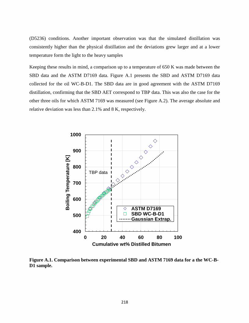
218
(D5236) conditions. Another important observation was that the simulated distillation was
consistently higher than the physical distillation and the deviations grew larger and at a lower
temperature form the light to the heavy samples
Keeping these results in mind, a comparison up to a temperature of 650 K was made between the
SBD data and the ASTM D7169 data. Figure A.1 presents the SBD and ASTM D7169 data
collected for the oil WC-B-D1. The SBD data are in good agreement with the ASTM D7169
distillation, confirming that the SBD AET correspond to TBP data. This was also the case for the
other three oils for which ASTM 7169 was measured (see Figure A.2). The average absolute and
relative deviation was less than 2.1% and 8 K, respectively.
Figure A.1. Comparison between experimental SBD and ASTM 7169 data for a the WC-B-
D1 sample.
400
500
600
700
800
900
1000
0 20 40 60 80 100
Bo
ilin
g T
em
pe
ratu
re [
K]
Cumulative wt% Distilled Bitumen
ASTM D7169SBD WC-B-D1Gaussian Extrap.
TBP data
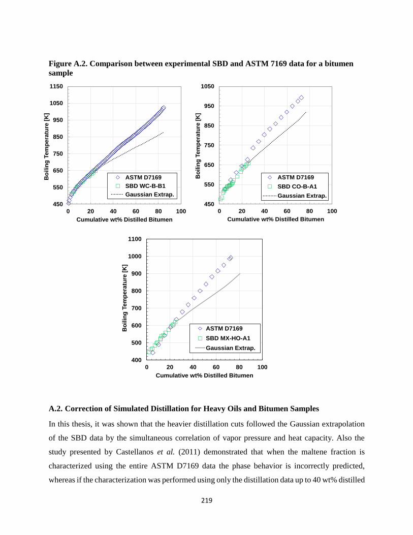
219
Figure A.2. Comparison between experimental SBD and ASTM 7169 data for a bitumen
sample
A.2. Correction of Simulated Distillation for Heavy Oils and Bitumen Samples
In this thesis, it was shown that the heavier distillation cuts followed the Gaussian extrapolation
of the SBD data by the simultaneous correlation of vapor pressure and heat capacity. Also the
study presented by Castellanos et al. (2011) demonstrated that when the maltene fraction is
characterized using the entire ASTM D7169 data the phase behavior is incorrectly predicted,
whereas if the characterization was performed using only the distillation data up to 40 wt% distilled
450
550
650
750
850
950
1050
1150
0 20 40 60 80 100
Bo
ilin
g T
em
pe
ratu
re [
K]
Cumulative wt% Distilled Bitumen
ASTM D7169
SBD WC-B-B1
Gaussian Extrap.
450
550
650
750
850
950
1050
0 20 40 60 80 100
Bo
ilin
g T
em
pe
ratu
re [
K]
Cumulative wt% Distilled Bitumen
ASTM D7169
SBD CO-B-A1
Gaussian Extrap.
400
500
600
700
800
900
1000
1100
0 20 40 60 80 100
Bo
ilin
g T
em
pe
ratu
re [
K]
Cumulative wt% Distilled Bitumen
ASTM D7169
SBD MX-HO-A1
Gaussian Extrap.

220
(~700 K) and a Gaussian extrapolation for the remainder of the maltenes, a better phase boundary
prediction was obtained.
Figure A.1 shows that the Gaussian extrapolation deviates from ASTM D7169 data above a boiling
temperature of 650 K, the same temperature Villalanti and coworkers observed higher
discrepancies between physical and simulated distillation. They attributed the deviation to a switch
from atmospheric and vacuum conditions. The most likely reason for the deviation is that the
calibration standards used to correlate retention times and boiling points do not extrapolate to
higher boiling cuts. Several authors (Boczkaj and Kaminski, 2013; Boczkaj and Przyjazny, 2011;
Roussis and Fitzgerald, 2000; Durand et al., 1999; Petroff et al., 1987) have shown that the basic
principle under which simulated distillation works does not apply to aromatic compounds
(linearity between retention time and boiling point). The choice of the stationary phase also has a
significant impact on whether or not there is agreement between the simulated and real distillation
curves (Durand et al., 1999).
Another possibility is that some cracking occurs at the high temperatures to which the samples are
subjected in a high temperature SimDist. On-column thermal cracking has been demonstated with
the appearance of a bimodal distribution of the chromatogram obtained using ASTM D7961
(Carbognani et al., 2007). Using this bimodal response, Carbognani and coworkers (2007) were
able to indicate the level of thermal maturity of the samples and to use the abundance of the second
peak as an index of crackability. Other authors (Speight, 2001; Altgelt and Boduszynski, 1994)
have also reported possible cracking of organic compounds due to the severe temperatures
employed for elution of the heavy fraction of the samples (~703 K, 430˚C).
Hence, above a boiling temperature of 600 K the simulated boiling points require a correction to
account for the incorrect boiling point predictions for the heavy ends. The following correction
was designed to match the Gaussian extrapolation of the physical distillation obtained with SBD
for three bitumen samples (WC-B-D1, CO-B-A1 and MX-HO-A1):
For TBP > 650 K:
𝑇𝐶𝐹 = 𝑇𝑆𝐷 − 𝑥 (𝐴. 1)

221
𝑥 = (−6.12𝑥10−6 𝑤𝑡%2 + 0.346 𝑤𝑡% − 5.6) (𝑀𝑊𝐵𝑢𝑙𝑘
100 ∗ 𝑆𝐺𝐵𝑢𝑙𝑘) (𝐴. 2)
where TCF (in K) is the corrected temperature that matches the boiling points corresponding to
extrapolated SBD data, TSD (in K) is the measured temperature using ASTM D7169, wt% is the
cumulative weight percent of the corresponding TSD, and MWBulk and SGBulk correspond to the
molecular weight an specific gravity of the whole sample. Figure 8.9a presents a relative deviation
plot for the fitted boiling points. The absolute and relative error of the fitted boiling temperatures
were less than 13 K and 1.7 %, respectively, with a bias of 0.1%.
A fourth oil (WC-B-B1) was used to test Equations A.1 and A.2. Figure A.3 presents a relative
deviation plot for the predicted boiling points. Note, the simulated distillation data collected for
this sample was obtained from a different laboratory. The absolute and relative error of the fitted
boiling temperatures were 5 K and 0.7 %, respectively, with a bias of 0.7%. Although the results
are promising they are only preliminary. More data are required in order to build a more robust
correction factor. Figure A.4 presents the plots of the corrected boiling temperature for the four oil
samples used in this study.
Figure A.3. Relative deviation obtained for the left) development data set and right) test
data set.
-5
-4
-3
-2
-1
0
1
2
3
4
5
600 700 800 900 1000
(Tb
-CF
-T
b-S
BD)/
Tb
-SB
Dx
10
0
Tb-SBD [K]
-5
-4
-3
-2
-1
0
1
2
3
4
5
600 700 800 900 1000
(Tb
-CF
-T
b-S
BD)/
Tb
-SB
Dx
10
0
Tb-SBD [K]
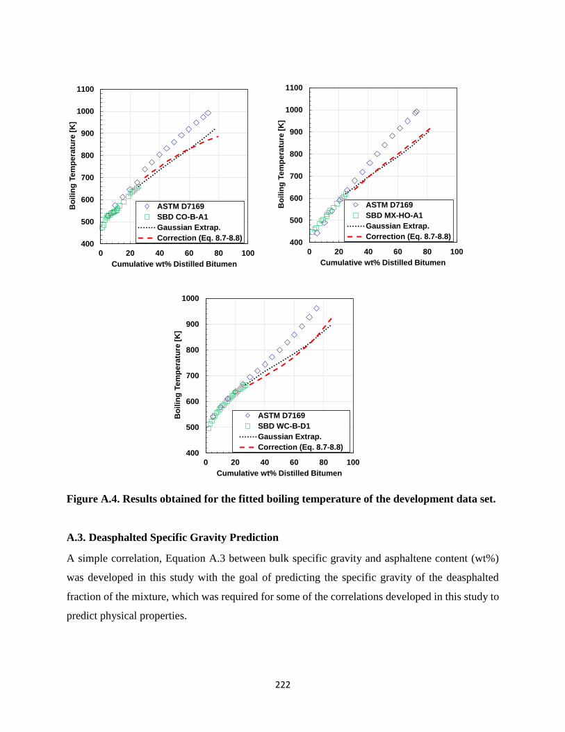
222
Figure A.4. Results obtained for the fitted boiling temperature of the development data set.
A.3. Deasphalted Specific Gravity Prediction
A simple correlation, Equation A.3 between bulk specific gravity and asphaltene content (wt%)
was developed in this study with the goal of predicting the specific gravity of the deasphalted
fraction of the mixture, which was required for some of the correlations developed in this study to
predict physical properties.
400
500
600
700
800
900
1000
0 20 40 60 80 100
Bo
ilin
g T
em
pe
ratu
re [
K]
Cumulative wt% Distilled Bitumen
ASTM D7169
SBD WC-B-D1
Gaussian Extrap.
Correction (Eq. 8.7-8.8)
400
500
600
700
800
900
1000
1100
0 20 40 60 80 100
Bo
ilin
g T
em
pe
ratu
re [
K]
Cumulative wt% Distilled Bitumen
ASTM D7169
SBD CO-B-A1
Gaussian Extrap.
Correction (Eq. 8.7-8.8)400
500
600
700
800
900
1000
1100
0 20 40 60 80 100
Bo
ilin
g T
em
pe
ratu
re [
K]
Cumulative wt% Distilled Bitumen
ASTM D7169
SBD MX-HO-A1
Gaussian Extrap.
Correction (Eq. 8.7-8.8)

223
𝑆𝐺𝐷𝐴𝑂 = (𝑆𝐺𝐵𝑢𝑙𝑘
0.9534 ∗ 𝑤𝑡% 𝑎𝑠𝑝 0.020266)
1/0.0684
(𝐴. 3)
The specific gravity average absolute and relative deviations obtained with Equation A.3 were less
than 0.006 and 0.6 % respectively.

224
APPENDIX B: DISTILLATION DATA FROM DVFA
Distillation data including density and molecular weight of each fraction is presented in Tables
B.1 to B.6
Table B.1. Distillation data of CO-B-A1
Cut Temperature
[K]
Cumulative
wt% Bitumen Distilled
Molecular Weight
[g/mol]
Density
[kg/m³]
0 413 10.9 235.9 898.0
1 423 15.7 257.7 921.0
2 443 19.7 301.4 941.7
3 463 23.0 328.7 956.8
4 483 26.9 380.2 966.1
5 513 33.0 398.3 976.8
6 533 37.6 475.3 988.9
7 563 42.8 515.6 993.7
res >563 971.0 1004.2
Table B.2. Distillation data of MX-HO-A1
Cut Temperature
[K]
Cumulative
wt% Bitumen Distilled
Molecular Weight
[g/mol]
Density
[kg/m³]
0 413 12.74 207.0 858.2
1 423 16.96 264.8 899.2
2 443 19.94 284.8 916.7
3 463 25.13 325.4 928.5
4 483 28.45 345.5 940.4
5 513 33.25 408.2 950.5
6 533 37.47 436.0 963.8
7 563 41.45 468.1 967.1
res >563 999.0 1023.5

225
Table B.3. Distillation data of CO-B-B1
Cut Temperature
[K]
Cumulative
wt% Bitumen Distilled
MolecularWeight
[g/mol]
Density
[kg/m³]
0 413 13.32 233.9 884.8
1 423 18.45 280.8 921.7
2 443 22.60 306.1 935.2
3 463 29.76 350.3 945.6
4 483 33.60 387.8 956.8
5 513 38.98 431.7 962.2
6 533 42.23 447.3 973.1
7 563 46.03 476.4 979.9
res >563 920.1 1017.8
Table B.4. Distillation data of US-OH-A1
Cut Temperature
[K]
Cumulative
wt% Bitumen Distilled
Molecular Weight
[g/mol]
Density
[kg/m³]
0 413 14.9 227.0 866.8
1 423 19.9 260.8 898.8
2 443 25.8 294.9 915.9
3 463 29.7 337.3 923.9
4 483 34.9 372.2 933.9
5 513 43.4 410.6 946.1
6 533 48.6 484.5 956.1
7 563 53.4 493.3 958.6
res >563 841.1 1010.0
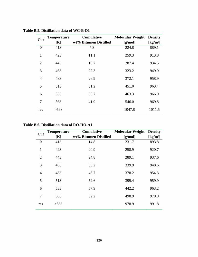
226
Table B.5. Distillation data of WC-B-D1
Cut Temperature
[K]
Cumulative
wt% Bitumen Distilled
Molecular Weight
[g/mol]
Density
[kg/m³]
0 413 7.3 224.8 889.1
1 423 11.1 259.3 913.8
2 443 16.7 287.4 934.5
3 463 22.3 323.2 949.9
4 483 26.9 372.1 958.9
5 513 31.2 451.0 963.4
6 533 35.7 463.3 966.0
7 563 41.9 546.0 969.8
res >563 1047.8 1011.5
Table B.6. Distillation data of RO-HO-A1
Cut Temperature
[K]
Cumulative
wt% Bitumen Distilled
Molecular Weight
[g/mol]
Density
[kg/m³]
0 413 14.8 231.7 893.8
1 423 20.9 258.9 920.7
2 443 24.8 289.1 937.6
3 463 35.2 339.9 948.6
4 483 45.7 378.2 954.3
5 513 52.6 399.4 959.9
6 533 57.9 442.2 963.2
7 563 62.2 498.9 970.0
res >563 978.9 991.8

227
APPENDIX C: . IDEAL GAS HEAT CAPACITY
Ideal gas heat capacity calculated for several fractions of seven different heavy oil and bitumen
samples is presented in Tables B1 to B7
Table C.1. Calculated ideal molar heat capacity of WC-B-B1
Temperature [K] Cp
ig [J mol-1 K-1]
Cut 1 Cut 2 Cut 3 Cut 4 Cut 5 Cut 6
258.1 281.7 302.6 349.4 398.5 452.6 493.9
263.2 287.5 308.8 356.6 406.7 461.6 504.0
268.3 293.2 314.9 363.6 414.7 470.6 514.0
273.4 298.9 321.1 370.7 422.8 479.6 524.1
278.5 304.6 327.2 377.8 430.9 488.6 534.1
283.6 310.3 333.4 384.9 438.9 497.6 544.1
288.7 315.9 339.5 392.0 447.0 506.5 554.1
293.8 321.6 345.6 399.0 455.0 515.5 564.1
298.9 327.3 351.7 406.1 463.0 524.4 574.1
304.0 332.9 357.8 413.1 471.1 533.3 584.1
309.1 338.5 363.9 420.1 479.0 542.2 594.0
314.2 344.2 369.9 427.1 487.0 551.1 604.0
319.4 349.7 376.0 434.1 495.0 559.9 613.8
324.5 355.3 382.0 441.0 502.9 568.7 623.7
329.6 360.9 388.0 448.0 510.8 577.5 633.5
334.7 366.4 393.9 454.9 518.6 586.2 643.3
339.8 371.9 399.9 461.7 526.5 594.9 653.1
344.9 377.4 405.8 468.6 534.3 603.6 662.8
350.0 382.8 411.7 475.4 542.0 612.3 672.4
355.1 388.3 417.6 482.2 549.8 0.0 682.1

228
Table C.2. Calculated ideal molar heat capacity of CO-B-A1
Temperature [K] Cp
ig [J mol-1 K-1]
Cut 0 Cut 1 Cut 2 Cut 3 Cut 4 Cut 5 Cut 6
261.5 272.6 295.6 339.0 367.5 426.2 444.3 526.0
265.0 276.4 299.8 344.1 372.7 430.8 449.7 533.2
270.0 281.8 305.6 350.7 379.8 439.0 458.3 543.4
275.0 287.2 311.4 357.3 387.0 447.3 466.9 553.6
280.0 292.6 317.2 363.9 394.1 455.6 475.6 563.9
285.0 298.0 323.0 370.5 401.3 463.8 484.2 574.1
290.0 303.3 328.8 377.1 408.4 472.1 492.8 584.3
295.0 308.7 334.5 383.7 415.5 480.3 501.4 594.5
300.0 314.0 340.3 390.2 422.6 488.5 509.9 604.6
305.0 319.3 346.0 396.8 429.7 496.7 518.5 614.8
310.0 324.6 351.7 403.3 436.8 504.9 527.0 624.9
315.0 329.9 357.4 409.8 443.8 513.0 535.5 635.0
320.0 335.1 363.0 416.3 450.8 521.1 544.0 645.0
325.0 340.4 368.7 422.7 457.8 529.2 552.4 655.1
330.0 345.6 374.3 429.2 464.8 537.3 560.8 665.1
335.0 350.8 379.9 435.6 471.8 545.3 569.2 675.0
340.0 355.9 385.5 442.0 478.7 553.3 577.6 684.9
345.0 361.1 391.0 448.3 485.6 561.3 585.9 694.8
350.0 366.2 396.6 454.7 492.4 569.2 594.2 704.6
354.8 371.1 402.1 460.3 498.9 577.0 602.2 713.8

229
Table C.3. Calculated ideal molar heat capacity of MX-HO-A1
Temperature [K] Cp
ig [J mol-1 K-1]
Cut 0 Cut 1 Cut 2 Cut 3 Cut 4 Cut 5 Cut 6 Cut 7
300.0 280.0 350.4 372.4 424.0 448.4 528.9 561.8 595.9
305.0 284.7 356.3 378.7 431.1 456.0 537.8 571.3 605.9
310.0 289.5 362.2 384.9 438.3 463.5 546.6 580.7 615.9
315.0 294.2 368.1 391.2 445.4 471.0 555.4 590.1 625.9
320.0 298.9 373.9 397.4 452.4 478.4 564.3 599.4 635.8
325.0 303.6 379.8 403.6 459.5 485.9 573.0 608.7 645.7
330.0 308.3 385.6 409.7 466.5 493.3 581.8 618.0 655.5
335.0 312.9 391.4 415.9 473.5 500.7 590.5 627.3 665.4
340.0 317.6 397.1 422.0 480.4 508.0 599.1 636.5 675.1
345.0 322.2 402.9 428.1 487.3 515.4 607.8 645.7 684.9
350.0 326.8 408.6 434.1 494.2 522.6 616.4 654.8 694.6
355.0 331.3 414.3 440.2 501.1 529.9 624.9 663.9 704.2
360.0 335.9 419.9 446.2 508.0 537.1 633.5 673.0 713.9
365.0 340.4 425.6 452.2 514.8 544.3 642.0 682.0 723.4
370.0 344.9 431.2 458.1 521.6 551.5 650.4 691.0 733.0
375.0 349.4 436.8 464.1 528.3 558.7 658.8 699.9 742.5
380.0 353.9 442.4 470.0 535.0 565.8 667.2 708.8 751.9
385.0 358.3 447.9 475.9 541.7 572.8 675.6 717.7 761.3
390.0 362.8 453.4 481.7 548.4 579.9 683.9 726.5 770.7
395.0 367.2 458.9 487.6 555.0 586.9 692.1 735.3 780.0
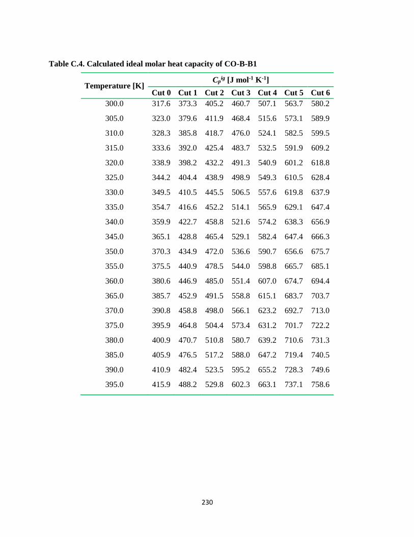
230
Table C.4. Calculated ideal molar heat capacity of CO-B-B1
Temperature [K] Cp
ig [J mol-1 K-1]
Cut 0 Cut 1 Cut 2 Cut 3 Cut 4 Cut 5 Cut 6
300.0 317.6 373.3 405.2 460.7 507.1 563.7 580.2
305.0 323.0 379.6 411.9 468.4 515.6 573.1 589.9
310.0 328.3 385.8 418.7 476.0 524.1 582.5 599.5
315.0 333.6 392.0 425.4 483.7 532.5 591.9 609.2
320.0 338.9 398.2 432.2 491.3 540.9 601.2 618.8
325.0 344.2 404.4 438.9 498.9 549.3 610.5 628.4
330.0 349.5 410.5 445.5 506.5 557.6 619.8 637.9
335.0 354.7 416.6 452.2 514.1 565.9 629.1 647.4
340.0 359.9 422.7 458.8 521.6 574.2 638.3 656.9
345.0 365.1 428.8 465.4 529.1 582.4 647.4 666.3
350.0 370.3 434.9 472.0 536.6 590.7 656.6 675.7
355.0 375.5 440.9 478.5 544.0 598.8 665.7 685.1
360.0 380.6 446.9 485.0 551.4 607.0 674.7 694.4
365.0 385.7 452.9 491.5 558.8 615.1 683.7 703.7
370.0 390.8 458.8 498.0 566.1 623.2 692.7 713.0
375.0 395.9 464.8 504.4 573.4 631.2 701.7 722.2
380.0 400.9 470.7 510.8 580.7 639.2 710.6 731.3
385.0 405.9 476.5 517.2 588.0 647.2 719.4 740.5
390.0 410.9 482.4 523.5 595.2 655.2 728.3 749.6
395.0 415.9 488.2 529.8 602.3 663.1 737.1 758.6

231
Table C.5. Calculated ideal molar heat capacity of US-OH-A1
Temperature [K] Cp
ig [J mol-1 K-1]
Cut 0 Cut 1 Cut 2 Cut 3 Cut 4 Cut 5 Cut 6 Cut 7
300.0 309.6 350.2 392.3 447.7 491.9 541.8 634.3 641.2
305.0 314.8 356.1 398.9 455.2 500.1 550.9 645.0 652.0
310.0 320.1 362.0 405.4 462.7 508.4 559.9 655.6 662.7
315.0 325.3 367.9 412.0 470.2 516.6 569.0 666.2 673.4
320.0 330.5 373.7 418.5 477.6 524.8 578.0 676.7 684.0
325.0 335.6 379.5 425.0 485.0 532.9 587.0 687.2 694.7
330.0 340.8 385.3 431.5 492.4 541.0 595.9 697.7 705.2
335.0 345.9 391.1 438.0 499.8 549.1 604.8 708.1 715.8
340.0 351.0 396.8 444.4 507.1 557.2 613.7 718.5 726.3
345.0 356.1 402.6 450.8 514.4 565.2 622.5 728.8 736.7
350.0 361.2 408.3 457.2 521.7 573.2 631.3 739.1 747.1
355.0 366.2 413.9 463.5 529.0 581.2 640.1 749.4 757.5
360.0 371.2 419.6 469.9 536.2 589.1 648.8 759.6 767.8
365.0 376.2 425.2 476.1 543.4 597.0 657.5 769.7 778.1
370.0 381.2 430.8 482.4 550.5 604.8 666.2 779.9 788.4
375.0 386.2 436.4 488.7 557.6 612.7 674.8 790.0 798.6
380.0 391.1 442.0 494.9 564.7 620.4 683.4 800.0 808.7
385.0 396.0 447.5 501.1 571.8 628.2 691.9 810.0 818.8
390.0 400.9 453.0 507.2 578.8 635.9 700.4 820.0 828.9
395.0 405.8 458.5 513.4 585.8 643.6 708.9 829.9 838.9

232
Table C.6. Calculated ideal molar heat capacity of WC-B-D1
Temperature [K] Cp
ig [J mol-1 K-1]
Cut 0 Cut 1 Cut 2 Cut 3 Cut 4 Cut 5 Cut 6 Cut 7
300.0 306.4 348.0 380.3 423.9 487.4 589.8 605.2 711.0
305.0 311.6 353.9 386.6 431.0 495.5 599.7 615.3 722.9
310.0 316.8 359.7 393.0 438.0 503.6 609.5 625.4 734.8
315.0 321.9 365.5 399.3 445.1 511.8 619.3 635.5 746.6
320.0 327.0 371.3 405.6 452.1 519.8 629.1 645.5 758.4
325.0 332.2 377.1 411.9 459.1 527.9 638.8 655.5 770.2
330.0 337.2 382.8 418.2 466.1 535.9 648.6 665.5 781.9
335.0 342.3 388.6 424.4 473.1 543.9 658.2 675.4 793.6
340.0 347.4 394.3 430.7 480.0 551.9 667.9 685.3 805.2
345.0 352.4 399.9 436.9 486.9 559.8 677.5 695.2 816.8
350.0 357.4 405.6 443.0 493.8 567.7 687.0 705.0 828.3
355.0 362.4 411.2 449.2 500.6 575.6 696.6 714.8 839.8
360.0 367.3 416.8 455.3 507.4 583.4 706.0 724.5 851.3
365.0 372.3 422.4 461.4 514.2 591.2 715.5 734.2 862.7
370.0 377.2 428.0 467.5 521.0 599.0 724.9 743.8 874.0
375.0 382.1 433.5 473.5 527.7 606.7 734.2 753.4 885.3
380.0 387.0 439.1 479.5 534.4 614.4 743.6 763.0 896.5
385.0 391.8 444.5 485.5 541.1 622.1 752.9 772.5 907.7
390.0 396.7 450.0 491.5 547.7 629.7 762.1 782.0 918.9
395.0 401.5 455.5 497.4 554.3 637.3 771.3 791.5 930.0
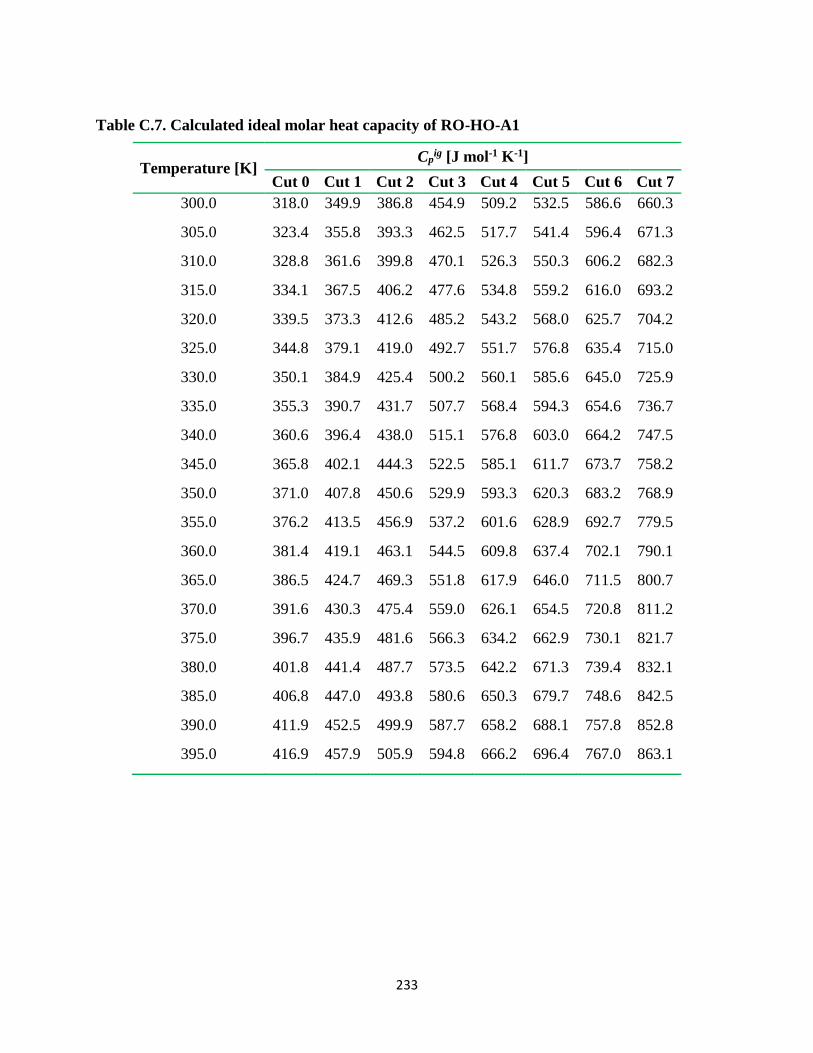
233
Table C.7. Calculated ideal molar heat capacity of RO-HO-A1
Temperature [K] Cp
ig [J mol-1 K-1]
Cut 0 Cut 1 Cut 2 Cut 3 Cut 4 Cut 5 Cut 6 Cut 7
300.0 318.0 349.9 386.8 454.9 509.2 532.5 586.6 660.3
305.0 323.4 355.8 393.3 462.5 517.7 541.4 596.4 671.3
310.0 328.8 361.6 399.8 470.1 526.3 550.3 606.2 682.3
315.0 334.1 367.5 406.2 477.6 534.8 559.2 616.0 693.2
320.0 339.5 373.3 412.6 485.2 543.2 568.0 625.7 704.2
325.0 344.8 379.1 419.0 492.7 551.7 576.8 635.4 715.0
330.0 350.1 384.9 425.4 500.2 560.1 585.6 645.0 725.9
335.0 355.3 390.7 431.7 507.7 568.4 594.3 654.6 736.7
340.0 360.6 396.4 438.0 515.1 576.8 603.0 664.2 747.5
345.0 365.8 402.1 444.3 522.5 585.1 611.7 673.7 758.2
350.0 371.0 407.8 450.6 529.9 593.3 620.3 683.2 768.9
355.0 376.2 413.5 456.9 537.2 601.6 628.9 692.7 779.5
360.0 381.4 419.1 463.1 544.5 609.8 637.4 702.1 790.1
365.0 386.5 424.7 469.3 551.8 617.9 646.0 711.5 800.7
370.0 391.6 430.3 475.4 559.0 626.1 654.5 720.8 811.2
375.0 396.7 435.9 481.6 566.3 634.2 662.9 730.1 821.7
380.0 401.8 441.4 487.7 573.5 642.2 671.3 739.4 832.1
385.0 406.8 447.0 493.8 580.6 650.3 679.7 748.6 842.5
390.0 411.9 452.5 499.9 587.7 658.2 688.1 757.8 852.8
395.0 416.9 457.9 505.9 594.8 666.2 696.4 767.0 863.1

234
APPENDIX D: LIQUID HEAT CAPACITY
Measured liquid heat capacity of the fractions is presented in Tables C1 to C4. Tables C5 to C7
contain the calculated liquid heat capacities using Eq. 5.15 introduced in Chapter 5.
Table D.1. Measured liquid molar heat capacity of WC-B-B1
Temperature [K] Cp
liq [J mol-1 K-1]
Cut 1 Cut 2 Cut 3 Cut 4 Cut 5 Cut 6
258.1 420.9 459.8 536.7 612.4 698.6 775.7
263.2 425.5 464.7 542.4 619.0 705.4 782.7
268.3 430.0 469.6 548.1 625.5 711.7 790.4
273.4 434.6 474.5 553.8 632.0 718.6 797.4
278.5 439.1 479.4 559.5 638.5 725.5 805.1
283.6 443.7 484.3 565.3 645.1 732.4 812.9
288.7 448.2 489.2 571.0 651.6 739.8 820.6
293.8 452.8 494.1 576.7 658.1 746.0 828.9
298.9 457.3 499.0 582.4 664.6 752.7 835.9
304.0 461.8 503.9 588.1 671.2 759.7 843.4
309.1 466.4 508.8 593.8 677.7 766.7 851.2
314.2 470.9 513.6 599.6 684.2 773.9 859.1
319.4 475.5 518.5 605.3 690.8 781.3 867.1
324.5 480.0 523.4 611.0 697.3 788.4 875.4
329.6 484.6 528.3 616.7 703.8 795.7 883.4
334.7 489.1 533.2 622.4 710.3 803.2 891.5
339.8 493.7 538.1 628.1 716.9 810.5 899.9
344.9 498.2 543.0 633.9 723.4 817.9 908.1
350.0 502.8 547.9 639.6 729.9 825.0 916.5
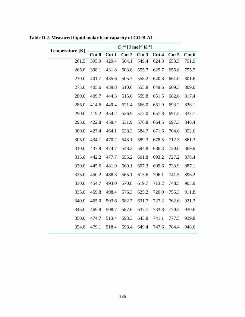
235
Table D.2. Measured liquid molar heat capacity of CO-B-A1
Temperature [K] Cp
liq [J mol-1 K-1]
Cut 0 Cut 1 Cut 2 Cut 3 Cut 4 Cut 5 Cut 6
261.5 395.9 429.4 504.1 549.4 624.3 653.5 791.9
265.0 398.1 431.8 503.8 555.7 629.7 655.8 795.5
270.0 401.7 435.6 505.7 558.2 640.8 661.0 801.6
275.0 405.6 439.8 510.6 555.8 649.6 669.3 809.0
280.0 409.7 444.3 515.6 559.8 651.5 682.6 817.4
285.0 414.6 449.4 521.4 566.0 651.9 693.2 826.1
290.0 419.2 454.2 526.9 572.0 657.8 691.5 837.1
295.0 422.8 458.4 531.9 576.8 664.5 697.3 846.4
300.0 427.4 464.1 538.3 584.7 671.6 704.6 852.6
305.0 434.1 470.2 543.1 589.3 678.5 712.3 861.3
310.0 437.9 474.7 548.2 594.8 686.3 720.0 869.9
315.0 442.2 477.7 555.2 601.8 693.2 727.2 878.4
320.0 445.6 481.9 560.1 607.3 699.6 733.9 887.1
325.0 450.2 488.3 565.1 613.6 706.1 741.5 896.2
330.0 454.7 493.0 570.8 619.7 713.2 748.5 903.9
335.0 459.8 498.4 576.3 625.2 720.0 755.3 911.8
340.0 465.0 503.6 582.7 631.7 727.2 762.6 921.3
345.0 469.8 508.7 587.6 637.7 733.8 770.5 930.6
350.0 474.7 513.4 593.3 643.8 741.1 777.5 939.8
354.8 479.1 518.4 598.4 649.4 747.6 784.4 948.6

236
Table D.3. Measured liquid molar heat capacity of MX-HO-A1
Cpliq [J mol-1 K-1]
Temp.
[K] Cut 0
Temp.
[K] Cut 1
Temp.
[K] Cut 2
Temp.
[K] Cut 3
Temp.
[K] Cut 4
265.0 376.0 281.4 485.3 291.3 522.7 299.0 602.9 300.9 631.8
270.0 378.4 285.0 488.1 295.0 525.5 300.4 603.9 305.0 636.0
275.0 381.3 290.0 492.5 300.0 529.9 305.0 608.2 310.0 641.4
280.0 384.4 295.0 495.2 305.0 534.3 310.0 613.4 315.0 646.9
285.0 388.2 300.0 501.4 310.0 538.9 315.0 618.8 320.0 652.4
290.0 392.5 305.0 504.7 315.0 543.6 320.0 624.1 325.0 658.3
295.0 394.4 310.0 508.1 320.0 548.4 325.0 629.9 330.0 665.1
300.0 398.9 315.0 513.6 325.0 553.4 330.0 636.4 335.0 671.3
305.0 402.5 320.0 518.1 330.0 559.2 335.0 642.4 340.0 676.7
310.0 405.1 325.0 522.9 335.0 564.3 340.0 647.6 345.0 682.5
315.0 409.6 330.0 527.2 340.0 568.8 345.0 652.8 350.0 688.9
320.0 413.5 335.0 531.5 345.0 573.5 350.0 658.4 355.0 695.3
325.0 417.1 340.0 535.7 350.0 578.4 355.0 664.4 358.0 699.5
330.0 420.7 345.0 540.1 355.0 583.5 357.9 667.9
335.0 424.5 350.0 544.6 357.9 586.8
340.0 428.0 355.0 548.5
345.0 431.6 358.1 550.6
350.0 435.6
355.0 439.2
357.7 441.8

237
Table D.4. Measured and calculated liquid molar heat capacity of CO-B-B1
Cpliq [J mol-1 K-1]
Temp
.
[K]
Cut
0
Temp
.
[K]
Cut
1
Temp
.
[K]
Cut
2
Temp
.
[K]
Cut
3
Temp
.
[K]
Cut
5*
Cut
6*
Cut
7*
262.4 400.
8 275.0
482.
6 289.0
545.
6 300.0
630.
5 300.0
759.
9
808.
4 860.6
265.0 402.
8 276.0
484.
2 290.3
546.
7 301.5
631.
5 305.0
766.
6
815.
6 868.5
270.0 406.
5 280.0
489.
4 295.0
551.
9 305.0
635.
4 310.0
773.
3
822.
9 876.4
275.0 410.
3 285.0
495.
1 300.0
557.
9 310.0
641.
4 315.0
780.
2
830.
3 884.5
280.0 414.
4 290.0
500.
3 305.0
562.
2 315.0
647.
6 320.0
787.
1
837.
7 892.6
285.0 419.
2 295.0
504.
4 310.0
568.
1 320.0
653.
8 325.0
794.
2
845.
3 900.8
290.0 423.
8 300.0
511.
4 315.0
574.
1 325.0
660.
3 330.0
801.
3
853.
0 909.1
295.0 427.
7 305.0
514.
7 320.0
579.
6 330.0
667.
7 335.0
808.
5
860.
7 917.5
300.0 431.
5 310.0
519.
0 325.0
585.
9 335.0
674.
4 340.0
815.
8
868.
5 926.0
305.0 437.
0 315.0
525.
2 330.0
591.
2 340.0
680.
5 345.0
823.
2
876.
5 934.5
310.0 439.
8 320.0
530.
9 335.0
596.
1 345.0
686.
6 350.0
830.
7
884.
5 943.2
315.0 443.
8 325.0
537.
0 340.0
601.
4 350.0
693.
1 355.0
838.
3
892.
6 951.9
320.0 450.
3 330.0
542.
0 345.0
606.
6 355.0
699.
6 360.0
845.
9
900.
8 960.8
325.0 454.
8 335.0
546.
4 350.0
612.
8 357.9
703.
8 365.0
853.
7
909.
1 969.7
330.0 458.
0 340.0
551.
8 355.0
618.
0 370.0
861.
5
917.
5 978.7

238
335.0 461.
5 345.0
556.
4 357.8
621.
3 375.0
869.
4
925.
9 987.9
340.0 467.
1 350.0
562.
1 380.0
877.
4
934.
5 997.1
345.0 471.
9 355.0
567.
3 385.0
885.
5
943.
2
1006.
4
350.0 476.
6 357.6
568.
9 390.0
893.
7
951.
9
1015.
7
355.0 481.
3 395.0
902.
0
960.
7
1025.
2
*Predicted values using Eq. 5.16
Table D.5. Calculated liquid molar heat capacity of US-OH-A1
Temperature [K] Cp
liq [J mol-1 K-1]
Cut 0 Cut 1 Cut 2 Cut 3 Cut 4 Cut 5 Cut 6 Cut 7
300.0 439.8 474.1 559.4 638.7 702.5 773.9 907.8 919.6
305.0 443.1 480.0 564.0 644.0 708.4 780.4 915.6 927.6
310.0 446.5 485.9 568.7 649.4 714.4 787.0 923.6 935.8
315.0 450.0 491.8 573.5 654.8 720.4 793.7 931.6 944.0
320.0 453.5 497.6 578.3 660.4 726.6 800.6 939.8 952.4
325.0 457.1 503.4 583.2 666.0 732.9 807.5 948.0 960.9
330.0 460.8 509.1 588.2 671.8 739.2 814.5 956.4 969.5
335.0 464.6 514.8 593.3 677.6 745.7 821.7 964.9 978.2
340.0 468.4 520.5 598.5 683.5 752.2 828.9 973.5 987.0
345.0 472.3 526.1 603.7 689.5 758.9 836.2 982.2 995.9
350.0 476.3 531.7 609.0 695.6 765.6 843.7 991.0 1004.9
355.0 480.3 537.3 614.4 701.7 772.4 851.2 1000.0 1014.0

239
360.0 484.4 542.8 619.8 708.0 779.3 858.8 1009.0 1023.3
365.0 488.6 548.2 625.4 714.3 786.3 866.6 1018.2 1032.6
370.0 492.8 553.7 631.0 720.7 793.4 874.4 1027.5 1042.1
375.0 497.2 559.1 636.7 727.3 800.6 882.4 1036.9 1051.7
380.0 501.6 564.4 642.4 733.8 807.9 890.4 1046.4 1061.4
385.0 506.1 569.8 648.3 740.5 815.3 898.5 1056.0 1071.2
390.0 510.6 575.0 654.2 747.3 822.8 906.8 1065.7 1081.1
395.0 515.2 580.3 660.2 754.2 830.3 915.1 1075.5 1091.1
Table D.6. Calculated liquid molar heat capacity of WC-B-D1
Temperature [K] Cp
liq [J mol-1 K-1]
Cut 0 Cut 1 Cut 2 Cut 3 Cut 4 Cut 5 Cut 6 Cut 7
300.0 435.0 460.3 542.4 605.7 696.6 843.3 865.8 1018.3
305.0 438.8 466.2 546.9 610.9 702.7 850.6 873.3 1027.2
310.0 442.2 472.0 551.5 616.2 708.8 858.0 880.9 1036.3
315.0 445.6 477.8 556.2 621.6 714.9 865.5 888.6 1045.4
320.0 449.1 483.5 561.0 627.0 721.2 873.2 896.5 1054.7
325.0 452.7 489.2 565.8 632.5 727.6 880.9 904.4 1064.0
330.0 456.3 494.8 570.7 638.1 734.0 888.7 912.4 1073.5
335.0 460.1 500.5 575.7 643.7 740.5 896.6 920.6 1083.2
340.0 463.8 506.0 580.8 649.5 747.1 904.6 928.8 1092.9
345.0 467.7 511.6 585.9 655.3 753.8 912.8 937.2 1102.8
350.0 471.6 517.1 591.1 661.2 760.6 921.0 945.6 1112.8
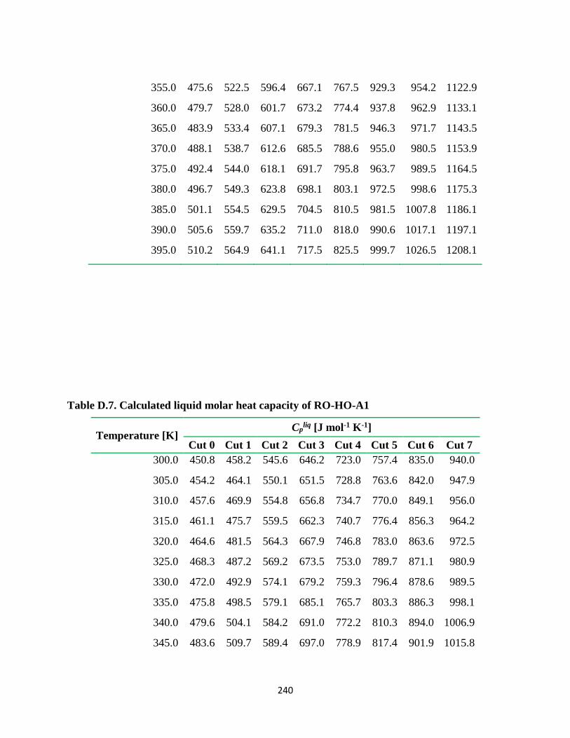
240
355.0 475.6 522.5 596.4 667.1 767.5 929.3 954.2 1122.9
360.0 479.7 528.0 601.7 673.2 774.4 937.8 962.9 1133.1
365.0 483.9 533.4 607.1 679.3 781.5 946.3 971.7 1143.5
370.0 488.1 538.7 612.6 685.5 788.6 955.0 980.5 1153.9
375.0 492.4 544.0 618.1 691.7 795.8 963.7 989.5 1164.5
380.0 496.7 549.3 623.8 698.1 803.1 972.5 998.6 1175.3
385.0 501.1 554.5 629.5 704.5 810.5 981.5 1007.8 1186.1
390.0 505.6 559.7 635.2 711.0 818.0 990.6 1017.1 1197.1
395.0 510.2 564.9 641.1 717.5 825.5 999.7 1026.5 1208.1
Table D.7. Calculated liquid molar heat capacity of RO-HO-A1
Temperature [K] Cp
liq [J mol-1 K-1]
Cut 0 Cut 1 Cut 2 Cut 3 Cut 4 Cut 5 Cut 6 Cut 7
300.0 450.8 458.2 545.6 646.2 723.0 757.4 835.0 940.0
305.0 454.2 464.1 550.1 651.5 728.8 763.6 842.0 947.9
310.0 457.6 469.9 554.8 656.8 734.7 770.0 849.1 956.0
315.0 461.1 475.7 559.5 662.3 740.7 776.4 856.3 964.2
320.0 464.6 481.5 564.3 667.9 746.8 783.0 863.6 972.5
325.0 468.3 487.2 569.2 673.5 753.0 789.7 871.1 980.9
330.0 472.0 492.9 574.1 679.2 759.3 796.4 878.6 989.5
335.0 475.8 498.5 579.1 685.1 765.7 803.3 886.3 998.1
340.0 479.6 504.1 584.2 691.0 772.2 810.3 894.0 1006.9
345.0 483.6 509.7 589.4 697.0 778.9 817.4 901.9 1015.8

241
350.0 487.6 515.2 594.6 703.1 785.6 824.5 909.9 1024.9
355.0 491.7 520.7 599.9 709.3 792.4 831.8 918.0 1034.0
360.0 495.9 526.1 605.2 715.5 799.4 839.2 926.2 1043.3
365.0 500.1 531.5 610.7 721.9 806.4 846.7 934.6 1052.7
370.0 504.5 536.9 616.2 728.4 813.6 854.3 943.0 1062.3
375.0 508.9 542.2 621.8 734.9 820.9 862.0 951.6 1071.9
380.0 513.3 547.5 627.5 741.6 828.3 869.8 960.2 1081.7
385.0 517.9 552.8 633.2 748.3 835.7 877.7 969.0 1091.6
390.0 522.5 558.0 639.0 755.1 843.3 885.8 977.9 1101.6
395.0 527.2 563.2 644.9 762.0 851.0 893.9 986.9 1111.7

242
APPENDIX E: EXPERIMENTAL VAPOR PRESSURE DATA
Measured vapor pressure of the fractions is presented in Tables D1 to D7. The constants obtained
from the constrained extrapolation are summarized in Table D8
Table E.1. Measured vapor pressure for distillation fractions of WC-B-B1
Cut T
[K]
P
[Pa] Cut
T
[K]
P
[Pa] Cut
T
[K]
P
[Pa]
1 313.2 0.5 2 333.2 0.06 3 323.2 0.002
1 333.2 2.5 2 353.2 0.6 3 353.2 0.05
1 343.2 5.3 2 373.2 2.3 3 393.2 2.2
1 353.2 11.7 2 393.2 8.6 3 413.2 7.2
1 363.2 25.5 2 413.2 33.8 3 433.2 23
4 403.2 0.7 5 423.2 2.2 6 433.2 1.3
4 413.2 1.3 5 433.2 3.6 6 443.2 2.1
4 423.2 2.2 5 443.2 6 6 453.2 3.5
4 433.2 3.8 5 458.2 12.1
4 443.2 6.4

243
Table E.2. Measured vapor pressure for distillation fractions of CO-B-A1
Cut T
[K]
P
[Pa] Cut
T
[K]
P
[Pa] Cut
T
[K]
P
[Pa] Cut
T
[K]
P
[Pa]
0 318 2.5 1 323 1.1 2 343 1.1 3 383 1.2
0 328 5.6 1 333 2.3 2 353 2.1 3 393 2.2
0 333 8.4 1 343 4.6 2 363 4.0 3 403 3.9
0 343 19.3 1 353 9.1 2 373 7.5 3 413 7.0
0 1 363 18.4 2 383 13.7 3 423 12.1
4 403 1.2 5 433 1.3 6 443 1.3
4 413 2.2 5 443 2.2 6 453 2.2
4 423 3.7 5 453 3.5 6 458 2.8
4 433 6.2 5 463 5.7 6 463 3.5
4 443 10.2
Table E.3. Measured vapor pressure for distillation fractions of MX-HO-A1
Cut T [K] P
[Pa] Cut
T
[K]
P
[Pa] Cut
T
[K]
P
[Pa] Cut
T
[K]
P
[Pa]
0 305.2 1.4 1 343.2 1.2 2 373.2 1.2 3 393.2 1.3
0 313.2 2.6 1 353.2 2.3 2 383.2 2.3 3 403.2 2.3
0 323.2 6.1 1 363.2 4.6 2 393.2 4.2 3 413.2 3.9
0 333.2 14.2 1 373.2 9.0 2 403.2 7.5 3 423.2 6.6
1 383.2 17.7 2 413.2 13.0 3 433.2 11.0
4 413.2 1.3 5 443.2 1.7 6 443.2 1.7 7 448.2 1.8
4 423.2 2.2 5 448.2 2.1 6 448.2 2.2 7 453.2 2.3
4 433.2 3.7 5 453.2 2.8 6 453.2 2.8 7 458.2 2.8
4 443.2 6.1 6 463.2 4.4 7 463.2 3.5

244
Table E.4. Measured vapor pressure for distillation fractions of CO-B-B1
Cut T
[K]
P
[Pa] Cut
T
[K]
P
[Pa] Cut
T
[K]
P
[Pa] Cut
T
[K]
P
[Pa]
0 303.2 1.6 1 323.2 1.2 2 363.2 0.9 3 403.2 2.1
0 313.2 4.0 1 338.2 4.3 2 383.2 4.3 3 413.2 4.3
0 323.2 9.1 1 353.2 14.0 2 393.2 8.7 3 423.2 8.2
0 328.2 13.3 1 368.2 41.1 2 403.2 16.9 3 433.2 15.4
0 333.2 19.1 1 383.2 109.3 2 413.2 31.8 3 443.2 27.8
4 418.2 2.2 5 433.2 2.3 6 443.2 1.7
4 428.2 4.3 5 443.2 4.3 6 458.2 4.3
4 438.2 8.1 5 453.2 8.0 6 463.2 5.8
4 448.2 14.9
4 453.2 20.0
Table E.5. Measured vapor pressure for distillation fractions of US-OH-A1
Cut T
[K]
P
[Pa] Cut
T
[K]
P
[Pa] Cut
T
[K]
P
[Pa] Cut
T
[K]
P
[Pa]
0 302.2 1.5 1 313.2 0.3 2 383.2 2 3 403.2 2.1
0 313.2 3.8 1 343.2 4.3 2 393.2 4.2 3 413.2 4.2
0 318.2 5.8 1 363.2 19.6 2 403.2 8.3 3 423.2 8.1
0 323.2 8.5 1 383.2 74.7 2 413.2 15.6 3 433.2 15
1 393.2 136.1
4 413.2 2.2 5 423.2 2.2 6 433.2 2.2 7 433.2 2.2
4 423.2 4.2 5 433.2 4.3 6 443.2 4.2 7 443.2 4.2
4 433.2 8 5 443.2 8 6 453.2 7.8 7 453.2 7.7
4 438.2 10.9 5 453.2 14.5 6 463.2 14.1

245
Table E.6. Measured vapor pressure for distillation fractions of WC-B-D1
Cut T
[K]
P
[Pa] Cut
T
[K]
P
[Pa] Cut
T
[K]
P
[Pa] Cut
T
[K]
P
[Pa]
0 313.2 1.7 1 343.2 0.8 2 383.2 2.0 3 403.2 1.1
0 323.2 4.2 1 363.2 4.2 2 393.2 4.2 3 423.2 4.2
0 333.2 9.3 1 373.2 8.6 2 403.2 8.1 3 433.2 7.8
0 338.2 13.6 1 383.2 16.8 2 413.2 15.1 3 443.2 14.2
343.2 19.6 1 393.2 31.0 423.2 26.9
4 433.2 3.0 5 443.2 3.1 6 443.2 2.2 7 443.2 2.2
4 438.2 4.2 5 448.2 4.2 6 453.2 4.2 7 453.2 4.2
4 443.2 5.7 5 453.2 5.6 6 458.2 5.7 7 463.2 7.6
4 448.2 7.8 5 463.2 10.1 6 463.2 7.6
Table E.7. Measured vapor pressure for distillation fractions of RO-HO-A1
Cut T
[K]
P
[Pa] Cut
T
[K]
P
[Pa] Cut
T
[K]
P
[Pa] Cut
T
[K]
P
[Pa]
0 313.2 1.7 1 343.2 0.8 2 383.2 2.1 3 413.2 2.2
0 323.2 4.1 1 363.2 4.2 2 393.2 4.2 3 423.2 4.2
0 333.2 9.2 1 373.2 8.7 2 403.2 8.4 3 433.2 8.0
0 338.2 13.4 1 383.2 17.3 2 413.2 15.9 3 443.2 14.6
343.2 19.1 1 393.2 32.4 423.2 28.8 453.2 26.0
4 433.2 2.2 5 443.2 2.3 6 443.2 2.3 7 443.2 2.3
4 443.2 4.3 5 453.2 4.3 6 453.2 4.3 7 453.2 4.2
4 453.2 7.9 5 458.2 5.8 6 463.2 7.8 7 463.2 7.7
4 463.2 14.2 5 463.2 7.8

246
Table E.8. Parameters for Cox equations used to fit vapor pressure and ΔC’exp with P0 set to
101325 Pa for the eight oils characterized in this work
Sample Cut A0 A1 x 10-4 A2 x 10-6 Tb [K]
WC-B-B1
1 3.11221 -22.21270 1.69391 605.03
2 3.21997 -21.65373 1.79536 651.16
3 3.30326 -23.05355 1.82732 690.60
4 3.44185 -22.25477 1.70515 698.03
5 3.51200 -23.61439 1.68252 706.73
6 3.54805 -26.63337 2.03107 743.27
CO-B-A1
0 3.03826 -20.90684 1.52903 583.90
1 3.03583 -21.41957 1.50693 630.96
2 3.13523 -22.96500 1.63447 662.54
3 3.28486 -20.99280 1.63595 676.86
4 3.34154 -24.06453 2.16413 710.32
5 3.43789 -20.96773 1.72373 724.04
6 3.54117 -23.65263 1.66748 748.31
MX-HO-
A1
0 3.15065 -18.77709 1.30126 537.97
1 3.33299 -18.45701 1.18662 580.00
2 3.43547 -15.76080 0.89250 600.00
3 3.38597 -18.70039 0.87783 626.10
4 3.62043 -16.42552 1.05355 630.00
5 3.72662 -17.27968 1.08588 650.67
6 3.52580 -21.60550 1.15697 743.91
7 3.57652 -21.25255 0.97102 748.37
CO-B-B1
0 3.06663 -23.22736 1.49441 577.52
1 3.18426 -22.41889 1.17258 600.00
2 3.36047 -18.67288 1.03968 620.00
3 3.49478 -17.82440 0.95283 640.00

247
4 3.55921 -19.86677 1.22121 660.38
5 3.62346 -20.55609 1.23245 675.60
6 3.59308 -21.16838 1.21716 717.43
US-HO-
A1
0 3.07951 -22.84177 1.56285 570.55
1 3.12333 -16.27584 0.58643 591.32
2 3.36762 -17.68206 1.05620 627.90
3 3.45084 -18.09667 1.01993 650.00
4 3.51787 -20.50515 1.35065 662.00
5 3.50544 -21.61711 1.24991 699.58
6 3.57981 -24.02399 1.27938 724.04
7 3.58040 -24.40041 1.25377 730.36
WC-B-D1
0 3.15140 -20.21226 1.37550 556.14
1 3.22183 -13.36731 0.64219 583.22
2 3.37584 -18.13824 1.20763 625.16
3 3.46817 -17.58520 1.12370 655.05
4 3.54972 -18.84684 1.19256 670.00
5 3.63159 -21.19822 1.24781 690.00
6 3.62578 -21.52190 1.21851 706.00
7 3.66026 -24.42117 1.13626 735.00
RO-HO-
A1
0 3.10731 -21.87253 1.49821 576.60
1 3.14183 -13.87169 0.66331 603.98
2 3.37906 -17.86694 1.23924 620.17
3 3.44240 -18.24768 1.09803 667.99
4 3.51507 -20.61720 1.49350 692.00
5 3.51059 -21.16420 1.43574 718.20
6 3.53713 -22.62613 1.40093 731.00
7 3.56891 -24.63554 1.36926 750.00

248
APPENDIX F: SPINNING BAND DISTILLATION DATA AND CORRESPONDING
GAUSSIAN EXTRAPOLATION.
F.1. Experimental SBD
This section presents the experimental TBP curves obtained using SBD as well as the Gaussian
extrapolation up to the asphaltene region. Both sets of data are included in the same table for the
oils. The data corresponding to Gaussian Extrapolation is marked with a start (*)
Table F.1. Experimental and extrapolated SBD data for WC-B-B1
Normal
Boiling
Temperature
[K]
wt %
Distilled
Normal
Boiling
Temperature
[K]
wt %
Distilled
510.6 3.1 622.8 18.9
525.6 4.7 631.2 20.5
541.1 6.3 640.5 22.0
551.8 7.9 648.4 23.6
562.6 9.4 661.9 28.0*
574.9 11.0 697.2 37.5*
586.7 12.6 730.3 47.2*
597.2 14.2 763.3 57.0*
613.0 17.3 864.8 82.6*
Table F.2. Experimental and extrapolated SBD data for CO-B-A1

249
Normal
Boiling
Temperature
[K]
wt %
Distilled
Normal
Boiling
Temperature
[K]
wt %
Distilled
474.7 1.1 554.4 9.8
484.1 1.9 561.4 10.2
509.1 2.8 571.9 11.2
516.9 3.7 590.7 13.7
525.5 3.8 593.6 14.7
528.4 4.7 610.5 15.7
530.7 5.6 618.2 16.6
538.8 6.0 625.7 17.6
540.0 6.5 633.0 18.6
541.6 7.3 675.2 25.0
543.4 7.4 744.2 37.5*
546.8 7.9 792.2 47.2*
547.9 8.4 840.0 57.0*
550.6 9.3 931.5 74.2*
Table F.3. Experimental and extrapolated SBD data for MX-HO-A1
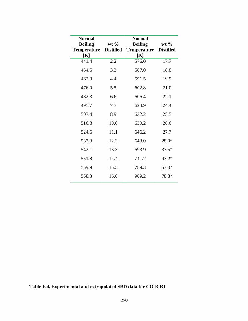
250
Normal
Boiling
Temperature
[K]
wt %
Distilled
Normal
Boiling
Temperature
[K]
wt %
Distilled
441.4 2.2 576.0 17.7
454.5 3.3 587.0 18.8
462.9 4.4 591.5 19.9
476.0 5.5 602.8 21.0
482.3 6.6 606.4 22.1
495.7 7.7 624.9 24.4
503.4 8.9 632.2 25.5
516.8 10.0 639.2 26.6
524.6 11.1 646.2 27.7
537.3 12.2 643.0 28.0*
542.1 13.3 693.9 37.5*
551.8 14.4 741.7 47.2*
559.9 15.5 789.3 57.0*
568.3 16.6 909.2 78.8*
Table F.4. Experimental and extrapolated SBD data for CO-B-B1

251
Normal
Boiling
Temperature
[K]
wt %
Distilled
Normal
Boiling
Temperature
[K]
wt %
Distilled
451.5 2.0 597.7 19.1
474.3 3.0 597.4 20.1
484.4 4.0 607.1 21.1
503.1 5.0 614.6 22.1
506.9 6.0 618.6 23.1
517.7 7.0 623.3 24.1
521.7 8.0 626.8 25.1
536.6 9.0 632.0 26.1
540.8 10.0 633.1 27.1
551.3 11.0 638.1 28.1
556.3 12.0 640.7 29.1
566.4 13.0 671.5 40.0*
571.7 14.0 701.9 50.0*
577.7 15.0 732.3 60.0*
582.3 16.0 764.9 70.0*
589.3 17.1 791.7 77.3*
591.5 18.1
Table F.5. Experimental and extrapolated SBD data for US-HO-A1
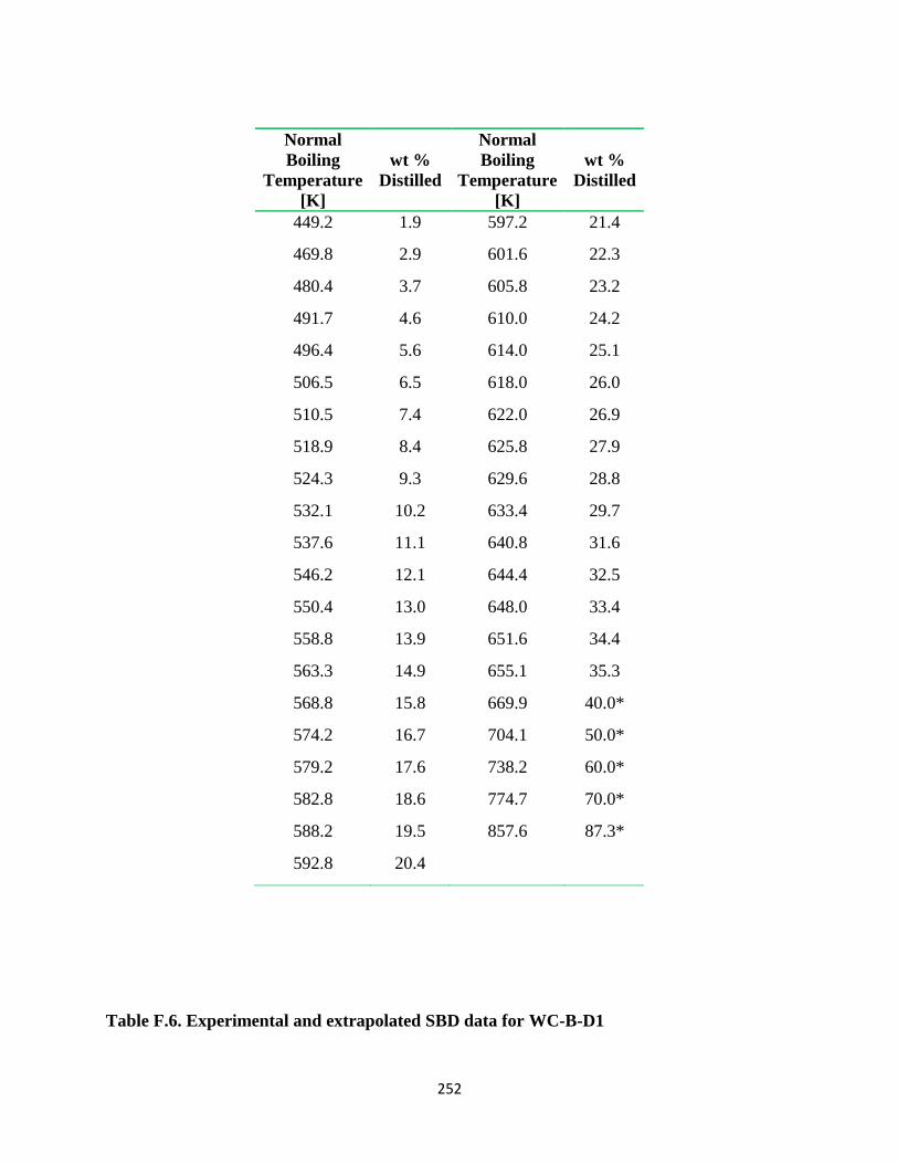
252
Normal
Boiling
Temperature
[K]
wt %
Distilled
Normal
Boiling
Temperature
[K]
wt %
Distilled
449.2 1.9 597.2 21.4
469.8 2.9 601.6 22.3
480.4 3.7 605.8 23.2
491.7 4.6 610.0 24.2
496.4 5.6 614.0 25.1
506.5 6.5 618.0 26.0
510.5 7.4 622.0 26.9
518.9 8.4 625.8 27.9
524.3 9.3 629.6 28.8
532.1 10.2 633.4 29.7
537.6 11.1 640.8 31.6
546.2 12.1 644.4 32.5
550.4 13.0 648.0 33.4
558.8 13.9 651.6 34.4
563.3 14.9 655.1 35.3
568.8 15.8 669.9 40.0*
574.2 16.7 704.1 50.0*
579.2 17.6 738.2 60.0*
582.8 18.6 774.7 70.0*
588.2 19.5 857.6 87.3*
592.8 20.4
Table F.6. Experimental and extrapolated SBD data for WC-B-D1

253
Normal
Boiling
Temperature
[K]
wt %
Distilled
Normal
Boiling
Temperature
[K]
wt %
Distilled
494.7 1.9 624.0 17.1
514.3 2.9 630.6 18.1
524.9 3.8 634.8 19.0
538.2 4.8 640.5 20.0
544.0 5.7 645.4 20.9
555.4 6.7 650.2 21.9
560.1 7.6 654.8 22.8
569.0 8.6 659.4 23.8
575.6 9.5 663.9 24.7
583.8 10.5 681.0 30.0*
588.1 11.4 717.2 40.0*
596.4 12.4 751.2 50.0*
601.1 13.3 785.1 60.0*
608.5 14.3 821.4 70.0*
613.0 15.2 883.3 83.8*
619.6 16.2
Table F.7. Experimental and extrapolated SBD data for RO-HO-A1

254
Normal
Boiling
Temperature
[K]
wt %
Distilled
Normal
Boiling
Temperature
[K]
wt %
Distilled
471.3 1.9 618.3 24.2
484.9 2.9 621.9 25.2
496.7 3.9 628.0 26.2
512.6 4.8 630.0 27.1
517.1 5.8 635.1 28.1
524.6 6.8 638.5 29.1
529.2 7.8 644.1 30.0
537.2 8.7 647.3 31.0
539.7 9.7 651.2 32.0
550.2 10.7 654.0 32.9
554.5 11.6 658.4 33.9
561.9 12.6 660.7 34.9
567.0 13.6 664.8 35.8
573.4 14.5 666.3 36.8
577.5 15.5 668.8 37.8
584.9 16.5 673.5 38.8
588.0 17.4 678.6 40.7
596.3 19.4 711.0 50.0*
603.0 20.3 744.2 60.0*
606.4 21.3 779.7 70.0*
611.0 22.3 909.4 93.5*
614.2 23.3
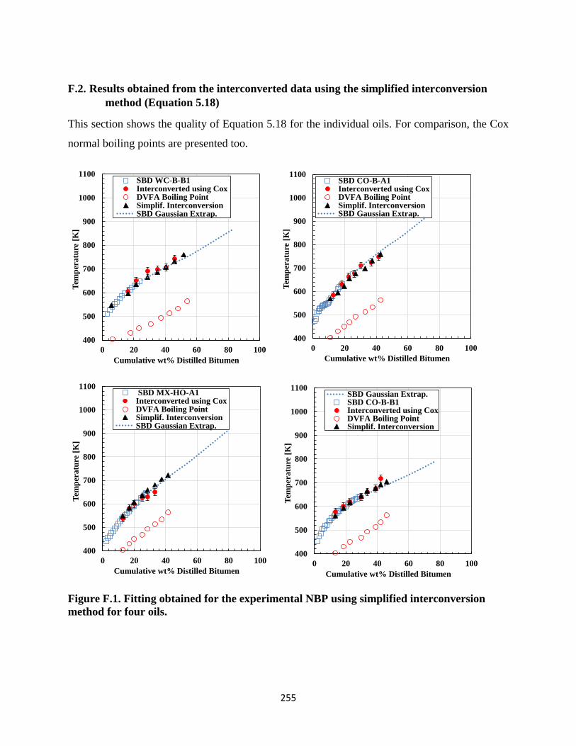
255
F.2. Results obtained from the interconverted data using the simplified interconversion
method (Equation 5.18)
This section shows the quality of Equation 5.18 for the individual oils. For comparison, the Cox
normal boiling points are presented too.
Figure F.1. Fitting obtained for the experimental NBP using simplified interconversion
method for four oils.
400
500
600
700
800
900
1000
1100
0 20 40 60 80 100
Tem
per
atu
re [
K]
Cumulative wt% Distilled Bitumen
SBD WC-B-B1Interconverted using CoxDVFA Boiling PointSimplif. InterconversionSBD Gaussian Extrap.
400
500
600
700
800
900
1000
1100
0 20 40 60 80 100
Tem
per
atu
re [
K]
Cumulative wt% Distilled Bitumen
SBD CO-B-A1Interconverted using CoxDVFA Boiling PointSimplif. InterconversionSBD Gaussian Extrap.
400
500
600
700
800
900
1000
1100
0 20 40 60 80 100
Tem
per
atu
re [
K]
Cumulative wt% Distilled Bitumen
SBD MX-HO-A1Interconverted using CoxDVFA Boiling PointSimplif. InterconversionSBD Gaussian Extrap.
400
500
600
700
800
900
1000
1100
0 20 40 60 80 100
Tem
per
atu
re [
K]
Cumulative wt% Distilled Bitumen
SBD Gaussian Extrap.SBD CO-B-B1Interconverted using CoxDVFA Boiling PointSimplif. Interconversion

256
Figure F.2. Fitting obtained for the experimental NBP using simplified interconversion
method for three oils.
400
500
600
700
800
900
1000
1100
0 20 40 60 80 100
Tem
per
atu
re [
K]
Cumulative wt% Distilled Bitumen
SBD US-HO-A1Interconverted using CoxDVFA Boiling PointSimplif. InterconversionSBD Gaussian Extrap.
400
500
600
700
800
900
1000
1100
0 20 40 60 80 100
Tem
per
atu
re [
K]
Cumulative wt% Distilled Bitumen
SBD WC-B-D1Interconverted using CoxDVFA Boiling PointSimplif. InterconversionSBD Gaussian Extrap.
400
500
600
700
800
900
1000
1100
0 20 40 60 80 100
Tem
per
atu
re [
K]
Cumulative wt% Distilled Bitumen
SBD RO-HO-A1Interconverted using CoxDVFA Boiling PointSimplif. InterconversionSBD Gaussian Extrap.

257
APPENDIX G: PHYSICAL PROPERTIES
G.1. Normal boiling point
The absolute and relative error obtained in the prediction of NBP using correlations available in
literature is reported per sample in Table G.1. The maximum deviations are summarized in Table
G.2.
Table G.1 ARD and AAD obtained for the NBP of each bitumen and heavy oil distillation
fractions using literature correlations
Oil
Sample
Soreide L-K RD API
AAD ARD AAD ARD AAD ARD AAD ARD
WC-B-B1 22.6 3.1 137.7 9.9 37.4 5.4 72.5 5.4
CO-B-A1 7.2 1.0 83.2 5.7 33.6 4.6 33.6 2.6
MX-HO-A1 29.0 4.4 120.3 9.1 48.7 7.3 76.0 6.3
CO-B-B1 50.4 7.4 136.6 10.6 68.7 10.3 97.7 7.8
US-HO-A1 30.1 4.4 115.8 8.8 43.7 6.5 76.7 6.1
WC-B-D1 30.4 4.3 138.2 10.0 44.0 6.4 84.4 6.6
RO-HO-A1 6.6 0.9 78.6 5.4 24.6 3.3 32.8 2.5
TOTAL 25.2 3.7 115.8 8.5 43.0 6.2 67.7 5.3
Oil
Sample
oldRD RB Twu Nji
AAD ARD AAD ARD AAD ARD AAD ARD
WC-B-B1 216.3 16.0 66.1 8.7 80.9 11.2 49.5 7.1
CO-B-A1 172.2 12.6 39.8 5.1 58.9 8.3 14.0 1.9
MX-HO-A1 204.8 16.0 59.6 8.4 78.0 11.6 16.5 2.3
CO-B-B1 221.9 17.7 72.0 10.2 92.9 13.7 52.0 7.8
US-HO-A1 202.7 15.9 59.0 8.2 78.4 11.4 31.5 4.8
WC-B-D1 229.7 17.5 68.3 9.2 85.6 12.2 23.9 3.5
RO-HO-A1 166.9 12.2 36.6 4.7 56.6 8.0 23.3 3.3
TOTAL 202.1 15.4 57.4 7.8 75.9 10.9 30.1 4.4

258
Table G.2 Maximum absolute and relative deviations for NBP obtained using correlations
from literature.
Oil
Sample
Soreide L-K RD API
MAAD MARD MAAD MARD MAAD MARD MAAD MARD
WC-B-B1 53.4 7.2 586.1 37.7 89.7 12.0 201.1 12.9
CO-B-A1 13.9 2.1 371.9 22.2 63.0 6.9 58.1 4.3
MX-HO-A1 42.8 6.4 432.6 26.4 74.6 11.1 102.9 8.5
CO-B-B1 110.2 13.9 548.0 38.5 98.0 14.2 263.8 18.5
US-HO-A1 58.2 8.3 370.2 24.0 86.5 12.4 131.5 10.4
WC-B-D1 62.7 8.7 552.7 34.8 88.9 12.6 171.1 11.3
RO-HO-A1 62.7 8.7 552.7 34.8 88.9 12.6 171.1 11.3
Oil
Sample
oldRD RB Twu Nji
MAAD MARD MAAD MARD MAAD MARD MAAD MARD
WC-B-B1 690.3 44.4 233.7 27.0 690.3 44.4 233.7 27.0
CO-B-A1 499.6 29.8 130.1 14.0 499.6 29.8 130.1 14.0
MX-HO-A1 562.0 34.3 159.3 17.5 562.0 34.3 159.3 17.5
CO-B-B1 673.1 47.2 242.8 30.7 673.1 47.2 242.8 30.7
US-HO-A1 500.5 32.4 153.2 17.9 500.5 32.4 153.2 17.9
WC-B-D1 62.7 8.7 552.7 34.8 88.9 12.6 171.1 11.3
RO-HO-A1 62.7 8.7 552.7 34.8 88.9 12.6 171.1 11.3
G.2. Molecular weight
The absolute and relative error obtained in the prediction of MW using correlations available in
literature is reported per sample in Tables G.3 to G.4. The maximum deviations are summarized
in Table G.5 to G.6.

259
Table. G.3 Absolute and relative deviations for MW obtained using correlations from
literature.
Oil Samle Soreide L-K RD old RD new Goossens
AAD ARD AAD ARD AAD ARD AAD ARD AAD ARD
WC-B-B1 83.8 13.7 102.7 16.1 143.2 25.0 90.4 14.7 118.6 21.6
CO-B-A1 47.9 9.0 64.9 10.5 114.1 21.8 41.5 8.0 70.6 15.9
MX-HO-A1 94.6 18.9 89.5 16.8 131.4 26.6 76.0 16.2 103.5 23.6
CO-B-B1 120.5 20.6 118.1 22.0 159.0 32.0 120.5 23.5 149.2 30.7
US-HO-A1 86.5 18.0 84.8 16.3 127.0 26.3 77.0 15.8 108.1 23.7
WC-B-D1 105.6 18.7 106.2 17.0 151.8 27.7 96.8 17.2 127.4 24.9
RO-HO-A1 55.2 9.6 63.0 9.8 111.8 21.2 43.7 7.6 75.8 16.1
Table. G.4 Absolute and relative deviations for MW obtained using correlations from
literature.
Oil Sample H-S K-F Winn-Mobil Rao-Bardon Twu
AAD ARD AAD ARD AAD ARD AAD ARD AAD ARD
WC-B-B1 103.4 16.5 97.9 13.3 99.5 15.8 106.7 17.0 61.2 10.6
CO-B-A1 61.9 10.9 82.3 10.7 58.1 9.7 65.9 11.5 15.4 3.3
MX-HO-A1 89.6 17.9 91.7 12.5 84.9 16.5 91.4 17.9 41.7 10.0
CO-B-B1 125.8 24.3 62.4 8.9 117.9 22.1 125.8 24.0 92.8 17.5
US-HO-A1 87.1 17.3 44.6 7.2 81.3 15.9 88.3 17.4 52.8 11.1
WC-B-D1 109.6 18.8 127.5 14.7 102.4 16.7 110.8 18.6 60.3 10.1
RO-HO-A1 59.9 10.0 91.3 10.9 56.7 9.0 63.3 10.4 14.4 3.0

260
Table. G.5. Maximum absolute and relative deviations for MW obtained using correlations from literature.
Oil Sample Soreide L-K RD old RD new Goossens
MAAD MARD MAAD MARD MAAD MARD MAAD MARD MAAD MARD
WC-B-B1 146.6 24.8 480.1 47.5 559.0 55.3 384.9 38.1 427.3 42.3
CO-B-A1 35.3 14.9 325.8 33.6 423.4 43.6 142.4 14.7 150.9 21.5
MX-HO-A1 84.6 20.7 381.7 38.2 476.6 47.7 231.4 23.2 259.7 28.6
CO-B-B1 118.5 25.0 474.2 51.5 542.2 58.9 439.3 47.7 482.9 52.5
US-HO-A1 114.7 23.6 304.7 36.2 387.2 46.0 215.6 25.9 262.4 33.3
WC-B-D1 140.4 25.7 477.0 45.5 564.1 53.8 359.6 34.3 400.6 38.2
RO-HO-A1 39.6 11.6 356.6 36.4 452.9 46.3 206.5 21.1 234.4 23.9
Table. G.6. Maximum absolute and relative deviations for MW obtained using correlations from literature.
Oil Sample H-S K-F Winn-Mobil Rao-Bardon Twu
MAAD MARD MAAD MARD MAAD MARD MAAD MARD MAAD MARD
WC-B-B1 461.1 45.7 640.1 63.4 452.9 44.8 472.5 46.8 256.6 25.4
CO-B-A1 266.3 27.4 587.0 60.5 276.0 28.4 288.0 29.7 54.1 6.7
MX-HO-A1 331.5 33.2 649.3 65.0 340.2 34.1 352.1 35.2 71.3 14.9
CO-B-B1 471.4 51.2 416.7 45.3 464.4 50.5 480.1 52.2 364.4 39.6
US-HO-A1 282.4 33.6 250.9 29.8 279.7 33.3 295.7 35.2 120.1 20.7
WC-B-D1 445.0 42.5 971.3 92.7 444.3 42.4 460.3 43.9 220.8 22.1
RO-HO-A1 302.8 30.9 711.4 72.7 314.8 32.2 325.1 33.2 50.7 5.2

261
G.3. Specific Gravity
The absolute and relative error obtained in the prediction of SGusing correlations available in
literature is reported per sample in Table G.7. The maximum deviations are summarized in Table
G.8.
Table. G.7 Absolute and relative deviations for SG obtained using correlations from
literature.
Oil Sample Soreide Withson Jacoby
AAD ARD AAD ARD AAD ARD
WC-B-B1 0.02 2.02 0.00 4.81 0.02 1.82
CO-B-A1 0.03 3.34 0.06 6.32 0.02 1.90
MX-HO-A1 0.02 1.74 0.05 5.00 0.02 2.13
CO-B-B1 0.02 1.70 0.04 4.28 0.02 1.68
US-HO-A1 0.01 0.63 0.03 2.76 0.02 2.00
WC-B-D1 0.02 2.30 0.06 6.04 0.01 1.50
RO-HO-A1 0.02 2.22 0.05 4.76 0.01 0.96
Oil Sample RD Tb, I RD MW, I K-F Gray
AAD ARD AAD ARD AAD ARD AAD ARD
WC-B-B1 0.03 3.56 0.10 9.91 0.08 8.59 0.02 1.66
CO-B-A1 0.03 2.75 0.09 8.68 0.07 6.86 0.02 1.99
MX-HO-A1 0.02 2.58 0.09 9.16 0.05 5.08 0.03 2.80
CO-B-B1 0.03 3.10 0.08 7.67 0.06 6.00 0.03 2.97
US-HO-A1 0.02 1.98 0.07 6.87 0.04 4.42 0.06 5.87
WC-B-D1 0.03 2.69 0.10 10.46 0.06 5.83 0.03 3.30
RO-HO-A1 0.03 2.76 0.08 7.79 0.00 0.05 5.71 0.02
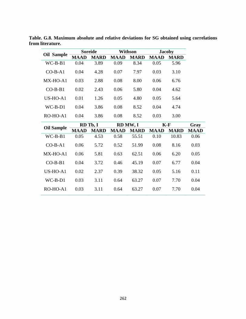
262
Table. G.8. Maximum absolute and relative deviations for SG obtained using correlations
from literature.
Oil Sample Soreide Withson Jacoby
MAAD MARD MAAD MARD MAAD MARD
WC-B-B1 0.04 3.89 0.09 8.34 0.05 5.96
CO-B-A1 0.04 4.28 0.07 7.97 0.03 3.10
MX-HO-A1 0.03 2.88 0.08 8.00 0.06 6.76
CO-B-B1 0.02 2.43 0.06 5.80 0.04 4.62
US-HO-A1 0.01 1.26 0.05 4.80 0.05 5.64
WC-B-D1 0.04 3.86 0.08 8.52 0.04 4.74
RO-HO-A1 0.04 3.86 0.08 8.52 0.03 3.00
Oil Sample RD Tb, I RD MW, I K-F Gray
MAAD MARD MAAD MARD MAAD MARD MAAD
WC-B-B1 0.05 4.53 0.58 55.51 0.10 10.83 0.06
CO-B-A1 0.06 5.72 0.52 51.99 0.08 8.16 0.03
MX-HO-A1 0.06 5.81 0.63 62.51 0.06 6.20 0.05
CO-B-B1 0.04 3.72 0.46 45.19 0.07 6.77 0.04
US-HO-A1 0.02 2.37 0.39 38.32 0.05 5.16 0.11
WC-B-D1 0.03 3.11 0.64 63.27 0.07 7.70 0.04
RO-HO-A1 0.03 3.11 0.64 63.27 0.07 7.70 0.04

263
G.4. Elemental analysis
The measured elemental composition of the petroleum fractions collected in this work are
presented in Table G.9.
Table G.9. Measured elemental analysis for the distillation cuts
Sample Cut N wt% C wt% H wt% S wt% O wt%
WC-B-B1
0 0.43 84.75 12.18 2.74 0.31
1 0.10 83.34 11.52 3.27 1.74
2 0.00 83.59 10.65 4.41 2.01
3 0.23 83.42 10.56 4.67 2.12
4 0.27 84.08 10.84 4.72 1.95
5 0.40 83.87 10.57 4.90 2.13
6 0.36 83.35 10.45 5.63 1.81
7 0.30 82.64 10.48 6.07 0.49
Residue 0.56 81.99 10.00 6.75 1.94
CO-B-A1
0 0.10 86.17 12.41 1.27 2.00
1 0.13 86.51 12.04 1.61 1.91
2 0.16 86.22 11.47 2.04 2.04
3 0.19 86.30 11.33 2.44 1.89
4 0.23 85.66 11.26 2.42 2.04
5 0.28 85.60 11.16 2.46 1.96
6 0.39 85.22 11.00 2.76 1.87
7 0.45 85.30 10.93 3.10 2.09
Residue 0.70 84.90 10.50 3.44 2.21
MX-HO-A1 0 0.11 83.61 12.60 2.86 0.14
1 0.13 83.18 11.95 3.86 0.33

264
2 0.19 83.54 11.65 4.19 0.25
3 0.24 83.79 11.57 4.16 0.30
4 0.28 84.49 11.52 4.10 0.29
5 0.24 84.51 11.46 4.14 0.29
6 0.24 84.27 11.31 4.40 0.23
7 0.28 83.75 11.02 4.82 0.34
Residue 0.41 83.42 10.45 5.51 0.45
CO-B-B1
0 0.02 86.44 12.50 0.65 0.24
1 0.04 86.29 11.79 1.27 0.24
2 0.10 85.98 11.67 1.55 0.20
3 0.12 85.94 11.51 1.72 0.27
4 0.18 85.97 11.36 1.83 0.26
5 0.20 85.88 11.31 1.82 0.29
6 0.25 85.87 11.17 2.08 0.30
7 0.29 85.39 11.00 2.42 0.31
Residue 0.58 85.01 10.43 2.85 0.49
US-HO-A1
0 0.25 86.67 12.87 0.92 0.30
1 0.29 86.35 12.34 1.52 0.34
2 0.43 86.03 12.07 1.88 0.44
3 0.54 85.94 11.98 1.88 0.39
4 0.98 85.57 11.86 1.80 0.48
5 1.17 85.86 11.83 1.59 0.50
6 1.09 85.61 11.63 2.02 0.56
7 1.36 85.26 11.46 2.33 0.46
Residue 1.12 84.92 10.68 3.09 0.69

265
WC-B-D1
0 0.02 86.12 12.66 0.91 0.07
1 0.02 85.92 12.12 1.42 0.09
2 0.03 85.74 11.74 2.07 0.14
3 0.07 85.34 11.45 2.27 0.20
4 0.09 85.33 11.40 2.24 0.21
5 0.13 85.37 11.36 2.24 0.18
6 0.17 85.79 11.43 2.45 0.16
7 0.20 85.48 11.37 2.71 0.21
Residue 0.40 84.50 10.81 3.64 0.41
RO-HO-A1
0 0.43 86.68 12.89 0.00 0.06
1 0.56 86.96 12.35 0.20 0.22
2 0.45 86.90 11.95 0.21 0.39
3 0.28 86.93 11.91 0.18 0.41
4 0.55 86.82 12.16 0.15 0.28
5 0.97 87.11 11.92 0.17 0.36
6 0.81 86.98 11.71 0.21 0.42
7 0.75 87.09 11.62 0.22 0.38
Residue 0.70 87.03 11.06 0.27 0.74

266
APPENDIX H: VAPOR PRESSURE CORRELATION AND THERMAL DATA
H.1. Vapor Pressure Correlation
This appendix illustrates the deviations obtained when Equation 7.2 and 7.4 to 7.6 were used to
fit the vapor pressure of the 63 distillation cuts from seven different heavy oil and bitumen
samples. Tables H.1 to H.4 presents the bias for the test data set. Tables H.5 to H.8 summarizes
the maximum average and relative deviations obtained for the tests data set.
Figure H.1. Fitting obtained for a) WC-B-B1 and b) CO-B-A1 using Equation 7.2 and 7.4
to 7.6 to develop a new vapor pressure correlation for heavy petroleum fractions
1.E-01
1.E+00
1.E+01
1.E+02
1.E+03
1.E+04
1.E+05
1.E+06
300 500 700 900
Pre
ss
ure
[P
a]
Temperature [K]
Cut 1
Cut 2
Cut 3
Cut 4
Cut 5
Cut 6
1.E-01
1.E+00
1.E+01
1.E+02
1.E+03
1.E+04
1.E+05
1.E+06
300 400 500 600 700 800
Pre
ss
ure
[P
a]
Temperature [K]
Cut 0
Cut 1
Cut 2
Cut 3
Cut 4
Cut 5
Cut 6
a) b)
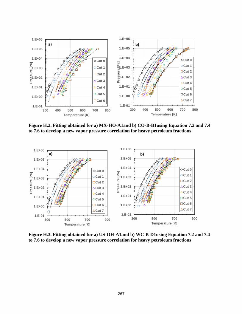
267
Figure H.2. Fitting obtained for a) MX-HO-A1and b) CO-B-B1using Equation 7.2 and 7.4
to 7.6 to develop a new vapor pressure correlation for heavy petroleum fractions
Figure H.3. Fitting obtained for a) US-OH-A1and b) WC-B-D1using Equation 7.2 and 7.4
to 7.6 to develop a new vapor pressure correlation for heavy petroleum fractions
1.E-01
1.E+00
1.E+01
1.E+02
1.E+03
1.E+04
1.E+05
1.E+06
300 400 500 600 700 800
Pre
ss
ure
[P
a]
Temperature [K]
Cut 0
Cut 1
Cut 2
Cut 3
Cut 4
Cut 5
Cut 6
Cut 7
1.E-01
1.E+00
1.E+01
1.E+02
1.E+03
1.E+04
1.E+05
1.E+06
300 400 500 600 700 800
Pre
ss
ure
[P
a]
Temperature [K]
Cut 0
Cut 1
Cut 2
Cut 3
Cut 4
Cut 5
Cut 6
1.E-01
1.E+00
1.E+01
1.E+02
1.E+03
1.E+04
1.E+05
1.E+06
300 500 700 900
Pre
ss
ure
[P
a]
Temperature [K]
Cut 0
Cut 1
Cut 2
Cut 3
Cut 4
Cut 5
Cut 6
Cut 71.E-01
1.E+00
1.E+01
1.E+02
1.E+03
1.E+04
1.E+05
1.E+06
300 500 700 900
Pre
ss
ure
[P
a]
Temperature [K]
Cut 0
Cut 1
Cut 2
Cut 3
Cut 4
Cut 5
Cut 6
Cut 7
a) b)
a) b)

268
Figure H.4. Fitting obtained for RO-HO-A1 using Equation 7.2 and 7.4 to 7.6 to develop a
new vapor pressure correlation for heavy petroleum fractions
Table H.1. Bias obtained for the first test data set from three different vapor pressure
correlations.
Sample This study MB Riazi
Bias Bias Bias
ALT/Cut 550-600 -9 -5 -10
ALT/Cut 650-750 -48 -32 -38
ALT/Cut 750-850 -62 -52 -60
ALT/Cut 850-950 -52 -67 -75
Overall -43 -39 -46
1.E-01
1.E+00
1.E+01
1.E+02
1.E+03
1.E+04
1.E+05
1.E+06
300 500 700 900
Pre
ss
ure
[k
Pa
]
Temperature [K]
Cut 0
Cut 1
Cut 2
Cut 3
Cut 4
Cut 5
Cut 6
Cut 7

269
Table H.2. Bias obtained for the second test data set from three different vapor pressure
correlations.
Sample This study MB Riazi
Bias Bias Bias
ANS/Cut 320-450 30 -5 -7
ANS/Cut 550-600 -13 -5 -13
ANS/Cut 750-850 -44 -24 -49
ANS/Cut 850-950 4 -40 -69
Overall -6 -19 -35
Table H.3. Bias obtained for the third test data set from three different vapor pressure
correlations.
Sample This study MB Riazi
Bias Bias Bias
SJV/Cut 450-650 -29 -41 -51
SJV/Cut 500-550 -7 -10 -16
SJV/Cut 600-650 1 20 -3
SJV/Cut 650-750 -72 -64 -75
SJV/Cut 750-850 -86 -81 -90
SJV/Cut 850-950 -53 -45 -76
Overall -41 -37 -52
Table H.4. Bias obtained for the fourth test data set from three different vapor pressure
correlations.
Sample This study MB Riazi
Bias Bias bias
Bitumen WC-B-B1 25 1513 804
Maltenes WC-B-B1 34 7036 3715
Eicosane -26 -37 105
Overall 11 2837 1541

270
Table H.5. Maximum average absolute and relative deviations obtained for the first test
dataset from three different vapor pressure correlations.
Sample
Riazi MB This study
MARD
[%]
MAAD
[Pa]
MARD
[%]
MAAD
[Pa]
MARD
[%]
MAAD
[Pa]
ALT/Cut 550-600 10 1628 5 1033 9 1262
ALT/Cut 650-750 38 7129 32 6091 48 8521
ALT/Cut 750-850 60 4294 52 3708 62 4393
ALT/Cut 850-950 75 2793 67 2519 52 1936
Overall 46 3961 39 3338 43 4028
Table H.6. Maximum average absolute and relative deviations obtained for the second test
dataset from three different vapor pressure correlations.
Sample Riazi MB This study
MARD
[%]
MAAD
[Pa]
MARD
[%]
MAAD
[Pa]
MARD
[%]
MAAD
[Pa]
ANS/Cut 320-450 11 5346 7 3343 30 4001
ANS/Cut 550-600 14 4155 5 2329 13 2947
ANS/Cut 750-850 49 4093 24 2260 44 3610
ANS/Cut 850-950 69 2056 40 1192 4 128
Overall 36 3912 19 2281 23 2671

271
Table H.7. Maximum average absolute and relative deviations obtained for the third test
dataset from three different vapor pressure correlations.
Sample Riazi MB This study
MARD
[%]
MAAD
[Pa]
MARD
[%]
MAAD
[Pa]
MARD
[%]
MAAD
[Pa]
SJV/Cut 450-650 51 10175 41 8719 29 6318
SJV/Cut 500-550 18 6024 11 3007 7 3492
SJV/Cut 600-650 7 1123 20 2997 8 1588
SJV/Cut 650-750 75 15503 64 13587 72 14708
SJV/Cut 750-850 90 5961 81 5296 86 5647
SJV/Cut 850-950 76 2268 45 1334 53 1569
Overall 53 6843 44 5823 42 5554
Table H.8. Maximum average absolute and relative deviations obtained for the fourth test
dataset from three different vapor pressure correlations.
Sample Riazi MB This study
MARD
[%]
MAAD
[Pa]
MARD
[%]
MAAD
[Pa]
MARD
[%]
MAAD
[Pa]
Bitumen WC-B-B1 804 189 1513 372 33 17
Maltenes WC-B-B1 3715 343 7036 608 91 13
Eicosane 105 22 42 1 23 1
Overall 1541 185 2864 327 49 10

272
H.2. Heat of Vaporization Data
The ‘experimental’ heats of vaporization for all the oils generated using the Cox constants
obtained from simultaneous fitting of vapor pressure and liquid heat capacity are presented in the
table below.
Table H.9. Heat of vaporization for the distillation cuts
Sample Cut ∆H vap NBP [kJ/mol]
WC-B-B1
1 54.8
2 70.8
3 76.0
4 88.0
5 86.0
6 91.1
CO-B-A1
0 50.3
1 54.6
2 73.7
3 76.8
4 90.0
5 101.3
6 93.0
MX-HO-A1
0 55.4
1 69.1
2 83.0
3 67.3
4 105.6
5 115.6
6 79.9
7 78.1
CO-B-B1 0 50.5

273
1 58.8
2 69.6
3 82.8
4 88.5
5 92.1
6 88.8
US-HO-A1
0 46.6
1 52.4
2 75.7
3 80.9
4 86.3
5 78.7
6 74.2
7 71.6
WC-B-D1
0 53.7
1 69.4
2 78.4
3 89.4
4 93.7
5 90.9
6 88.5
7 0.0
RO-HO-A1
0 50.0
1 64.1
2 80.5
3 83.8
4 94.9
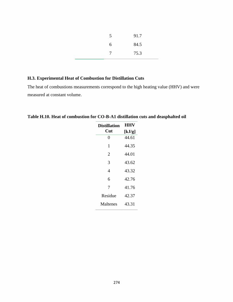
274
5 91.7
6 84.5
7 75.3
H.3. Experimental Heat of Combustion for Distillation Cuts
The heat of combustions measurements correspond to the high heating value (HHV) and were
measured at constant volume.
Table H.10. Heat of combustion for CO-B-A1 distillation cuts and deasphalted oil
Distillation
Cut
HHV
[kJ/g]
0 44.61
1 44.35
2 44.01
3 43.62
4 43.32
6 42.76
7 41.76
Residue 42.37
Maltenes 43.31
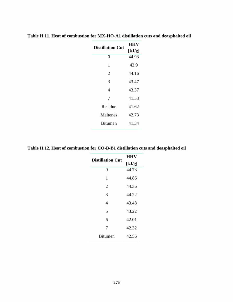
275
Table H.11. Heat of combustion for MX-HO-A1 distillation cuts and deasphalted oil
Distillation Cut HHV
[kJ/g]
0 44.93
1 43.9
2 44.16
3 43.47
4 43.37
7 41.53
Residue 41.62
Maltenes 42.73
Bitumen 41.34
Table H.12. Heat of combustion for CO-B-B1 distillation cuts and deasphalted oil
Distillation Cut HHV
[kJ/g]
0 44.73
1 44.86
2 44.36
3 44.22
4 43.48
5 43.22
6 42.01
7 42.32
Bitumen 42.56