university of bologna - unibo.it · university of bologna department of electrical engineering...
TRANSCRIPT

University of Bologna
DEPARTMENT OF ELECTRICAL ENGINEERING FACULTY OF ENGINEERING
Ph. D. in Electrical Engineering XXII year
POWER ELECTRONICS, MACHINES AND DRIVES (ING-IND/32)
Modulation Techniques for Multi-Phase Converters and
Control Strategies for Multi-Phase Electric Drives
Ph. D. Thesis of
Michele Mengoni
Tutor:
Prof. Giovanni Serra
Ph. D. Coordinator:
Prof. Francesco Negrini
Final Dissertation in 2010


CONTENTS……………………………………………………………………….. I PREFACE…………………………………………………………………………. 1 I THREE-PHASE ELECTRICAL DRIVES
Chapter 1 Mathematical Model of theThree-Phase Induction Motors………………… 7
1.1 A Historical Touch……………………………………………………... 7 1.2 Study Hypotheses……………………………………………………… 8 1.3 The Mathematical Model………………………………………………. 9 A. Determination of the Stator and Rotor Magnetic Field……………... 9 B. Space Vector Representation………………………………………... 11 C. Determination of the Magnetic Field in Air-Gap…………………… 12 D. Determination of the Linkage Fluxes……………………………….. 14 E. Determination of the Electromagnetic Torque……………………… 16 1.4 Machine Equations…………………………………………………… 18
1.5 From Machine Equations to the Vector Control of an Induction Machine………………………………………………………………… 19
1.6 Conclusions…………………………………………………………….. 20 1.7 References……………………………………………………………… 21
Chapter 2 Three-Phase Inverter 23
2.1 Introduction…………………………………………………………….. 23 2.2 Structure of a Three-Phase Inverter…………………………………….. 24 2.3 Modulation Strategies…………………………………………………... 24 A. Space Vector Modulations…………………………………………... 25 B. Duty Cycle Space Vector Modulation………………………………. 29 C. Continuous Modulation……………………………………………... 30 D. Discontinuous Modulations…………………………………………. 33 2.4 Conclusions…………………………………………………………….. 33 2.5 References……………………………………………………………… 34
able of contents

Table of Contents
II
Chapter 3 Stator Flux Vector Control of Induction Motor Drives in the Field-Weakening Region……………………………………………………… 37
3.1 Introduction…………………………………………………………….. 37 3.2 Machine equations and maximum torque capability…………………… 39 A. Control Algorithm ………………………………………………….. 42 B. Torque Control………………………………………………………. 43 C. Control of Stator and Rotor Fluxes………………………………….. 43 D. Maximum Torque Capability……………………………………….. 44 E. Field Weakening Algorithm………………………………………… 44 3.3 Flux and Torque Observers…………………………………………….. 46 A. Flux Observer……………………………………………………….. 46 B. Estimation of the Angular Frequency of the Rotor Flux Vector……. 47 C. Torque Estimation…………………………………………………... 47 3.4 Simulations and Experimental Results…………………………………. 47
3.5 Field-Weakening Control Schemes for High-Speed Drives Based on
Induction Motors: a Comparison……………………………………….. 51 3.6 Description of the control schemes…………………………………….. 51 A. Control Scheme (A)…………………………………………………. 52 B. Control Scheme (B)…………………………………………………. 53 C. Control Scheme (C)…………………………………………………. 53 3.7 Flux Observers…………………………………………………………. 54 3.8 Tuning of the Control Schemes………………………………………… 55 3.9 Experimental Results…………………………………………………… 55 A. Comparison of The Steady-State Behavior…………………………. 56 B. Tuning the Regulators and Robustness……………………………… 57 C. Stability of the Control System……………………………………… 58 D. Comparative Table…………………………………………………... 59
3.10. Extension of Stator Flux Vector Control to Non Conventional
Converter Structure…………………………………………………….. 61 3.11. Simulations and Experimental Results…………………………………. 62 3.12 Conclusions…………………………………………………………….. 66 3.13 References……………………………………………………………… 68
Chapter 4 Control Scheme With Energy Saving For Electric Vehicles……………….. 71
4.1 Introduction…………………………………………………………….. 71 4.2 Basic Ideas Behind the Control Strategy……………………………….. 73 A. Rotor Flux Oriented Control………………………………………… 73 B. Minimum Motor Losses…………………………………………….. 73 4.3 Maximum Torque Capability…………………………………………... 75 4.4 Graphic Representation of the Motor Behavior………………………... 77 4.5 Control Scheme………………………………………………………… 79 A. Torque and Flux Control Scheme…………………………………… 80 B. Robust Field Weakening…………………………………………….. 80 C. Fluctuation of DC-Link Voltage…………………………………….. 81 4.6 Tuning the Regulator and Dynamic Behavior………………………….. 82 A. Tuning of the Current Regulators…………………………………… 83
Table of Contents
III
B. Tuning of the Torque Regulator…………………………………….. 83 C. Tuning the Voltage Regulator………………………………………. 84 4.7 Power Measurement……………………………………………………. 85 4.8 Experimental Results…………………………………………………… 86 4.9 Conclusions…………………………………………………………….. 90 4.10 References……………………………………………………………… 92 II MULTI-PHASE ELECTRIC DRIVES
Chapter 5 Mathematical Model of the Multi-Phase Induction Motors…………… 95
5.1 Introduction………………………………………………………... 95 5.2 The Mathematical Model………………………………………….. 96 5.3 Multiple Space Vector Representation…………………………….. 98 5.4 Determination of the Magnetic Field in Air-Gap………………….. 99 5.5 Determination of the Linkage Fluxes……………………………… 101 5.6 Determination of the Electromagnetic Torque…………………….. 103 5.7 Machine Equations………………………………………………… 105
5.8 From Machine Equations to the Extended Vector Control of a
Multi-Phase Induction Machine…………………………………… 106 5.9 Conclusions………………………………………………………... 107 5.10 References…………………………………………………………. 108
Chapter 6 Multi-Phase Inverter……………………………………………………... 109
6.1 Introduction………………………………………………………... 109 6.2 Multiple Space Vector Representation…………………………….. 111 6.3 Duty Cycle Space Vector Approach………………………………. 112 6.4 Relationship between Pole and Load Voltages……………………. 114 6.5 Definition of Duty Cycle Space Vectors…………………………... 114 6.6 Generalized Modulation Strategies for M-Phase VSI……………... 115 6.7 Voltage Limits……………………………………………………... 115 6.8 Five-Phase Inverter………………………………………………... 117 A. Motor Drives without Third Spatial Harmonic………………… 117 B. Motor Drives with Third Spatial Harmonic……………………. 118 C. Multi-Motor Drives…………………………………………….. 119 D. Experimental Results…………………………………………… 120 6.9 Seven Phase Inverter………………………………………………. 123 6.10 General theory of Space Vector Modulation ……………………... 125 6.11 Identification of the Sector Number………………………………. 127 A. Identification of Sector for Three Phase VSI………………….. 127 B. Sectors in Multi-Phase Inverter………………………………… 128 6.12 Generation of Lookup Tables……………………………………… 129 A. Equivalence between Carrier-Based PWM and SVM…………. 129 B. Look-Up Table…………………………………………………. 131 C. Case Study: Five Phase Inverters………………………………. 131 6.13 Remarks on the Proposed SVM Algorithm……………………….. 133 6.14 Experimental Results for Look-Up Table Solution……………….. 135

Table of Contents
IV
6.15 Space Vector Modulation for a Multi-Phase Inverter: Solution
Based on Ranking Functions……………….……………………… 138 A. Lexicographic Ranking Function………………………………. 139 B. Steinhaus- Johnson-Trotter Ranking Function…………………. 139 6.16 Experimental Results for Algorithm Solution……………………... 141 6.17 Conclusions………………………………………………………... 142 6.18 References…………………………………………………………. 142
Chapter 7 Minimization of the Power Losses in IGBT Multiphase Inverters with Carrier-Based Pulse Width Modulation……………………………….. 145
7.1 Introduction………………………………………………………... 145 7.2 Assessment on Pulse Width Modulation for Multi-Phase Inverter... 146 7.3 Effect of the Zero Sequence Component on the Power Losses…… 147 7.4 Optimal Modulation Strategy……………………………………… 148 7.5 Evaluation of the Conduction Losses……………………………… 150 7.6 Validity Limits of the Theoretical Analysis……………………….. 151 7.7 Determination of the Switching Power Losses……………………. 152 A. Analytical Expression…………………………………………... 152 B. Comparison of the Efficiency of the Modulation Strategies…... 155 7.8 Simulation Results………………………………………………... 157 A. Power Losses…………………………………………………… 158 B. Current Quality…………………………………………………. 159 7.9 Experimental Results……………………………………………… 160 A. Feasibility of the Optimal Modulation Strategy…………………… 160 B. Assessment of the Theoretical Analysis of the Switching Losses… 161 7.10 Conclusions………………………………………………………... 163 7.11 References…………………………………………………………. 164
Chapter 8 Extended Stator Flux Vector Control of Multi-Phase Induction Motor Drives……………………………………………………………… 165
8.1 Introduction………………………………………………………... 165 8.2 Machine Equations of Seven-Phase Induction Motor……………... 166 8.3 Stator Flux Vector Control………………………………………… 168 A. Torque Control…………………………………………………. 169 B. Rotor Flux Control……………………………………………... 169 C. Stator Flux Regulator ………………………………………….. 169 D. Flux Observer…………………………………………………... 170 E. Torque Observer………………………………………………... 171 8.4 Experimental Results……………………………………………… 171 8.5 Conclusions…………………….………………………………….. 174 8.6 References…………………………………………………………. 174
Chapter 9 High Torque Density Applications……………………………………… 177
9.1 Introduction………………………………………………………... 177
a)

Table of Contents
V
9.2 Machine Equations of Seven-Phase Induction Motor……………... 178 9.3 Motor Control for High Torque Density…………………………... 179 9.4 Field Weakening Operation……………………………………….. 180 A. Voltage Limits………………………………………………….. 180 B. Current Limits………………………………………………….. 182 C. Maximum Torque Capability in Field Weakening Operation….. 182 9.5 Control Scheme……………………………………………………. 183 A. Current Loop…………………………………………………… 184 B. Torque Loop……………………………………………………. 184 C. Flux Loop………………………………………………………. 185
9.6 Calculation of the Amplitude of the Third Spatial Harmonic of the
Magnetic Field in the Air-Gap…………………………………….. 186
A. Approach of Maximization of the Fundamental Component of
the Air-Gap Field……………………………………………….. 186 B. Optimization of the Motor Torque……………………………... 187 9.7 Experimental Results……………………………………………… 189 9.8 Conclusions………………………………………………………... 190 9.9 References…………………………………………………………. 191
Chapter 10 Fault-Tolerant Control Strategy Under an Open Circuit Phase Fault Condition………………………………………………………………….. 193
10.1 Introduction………………………………………………………. 193 10.2 Analysis of the MMF in the Air-Gap………..…………………… 194 10.3 Operation in Healthy Conditions………………………………… 195 10.4 Current control Strategies in Fault Conditions…………………… 196 A. Optimal Disturbance-free Operations in Fault Conditions……. 197 B. Strategy (B)…………………………………………………… 199 C. Strategy (C)…………………………………………………… 200
10.5 Comparison of the Fault-Tolerant Strategies in Steady-State
Conditions…………………………………………………...…… 200 10.6 Experimental Results………………………………………..…… 206 10.7 Conclusions………………………………………………………. 208 10.8 References………………………………………………...……… 208
Chapter 11 Multi-Motor Applications 211
11.1 Introductions………………………………………………………. 211 11.2 Operating Principle………………………………………………... 213 11.3 Description of the Multi-Motor Drive……………………………... 216 11.4 Experimental Results……………………………………………… 218 11.5 Conclusions………………………………………………………... 219 11.6 References…………………………………………………………. 220 APPENDIX………………………………………………………………………… 225


The ever-increasing spread of automation in industry puts the electrical engineer in a
central role as a promoter of technological development in a sector such as the use of electricity, which is the basis of all the machinery and productive processes. Moreover the spread of drives for motor control and static converters with structures ever more complex, places the electrical engineer to face new challenges whose solution has as critical elements in the implementation of digital control techniques with the requirements of inexpensiveness and efficiency of the final product.
The successfully application of solutions using non-conventional static converters awake an increasing interest in science and industry due to the promising opportunities. However, in the same time, new problems emerge whose solution is still under study and debate in the scientific community
During the Ph.D. course several themes have been developed that, while obtaining the recent and growing interest of scientific community, have much space for the development of research activity and for industrial applications.
The first area of research is related to the control of three phase induction motors with high dynamic performance and the sensorless control in the high speed range. The management of the operation of induction machine without position or speed sensors awakes interest in the industrial world due to the increased reliability and robustness of this solution combined with a lower cost of production and purchase of this technology compared to the others available in the market.
During this dissertation control techniques will be proposed which are able to exploit the total dc link voltage and at the same time capable to exploit the maximum torque capability in whole speed range with good dynamic performance. The proposed solution preserves the simplicity of tuning of the regulators.
Furthermore, in order to validate the effectiveness of presented solution, it is assessed in terms of performance and complexity and compared to two other algorithm presented in literature. The feasibility of the proposed algorithm is also tested on induction motor drive fed by a matrix converter.
Another important research area is connected to the development of technology for vehicular applications. In this field the dynamic performances and the low power consumption is one of most important goals for an effective algorithm. Towards this direction, a control scheme for induction motor that integrates within a coherent solution
reface
Preface
2
some of the features that are commonly required to an electric vehicle drive is presented. The main features of the proposed control scheme are the capability to exploit the maximum torque in the whole speed range, a weak dependence on the motor parameters, a good robustness against the variations of the dc-link voltage and, whenever possible, the maximum efficiency.
The second part of this dissertation is dedicated to the multi-phase systems. This technology, in fact, is characterized by a number of issues worthy of investigation that make it competitive with other technologies already on the market.
Multiphase systems, allow to redistribute power at a higher number of phases, thus making possible the construction of electronic converters which otherwise would be very difficult to achieve due to the limits of present power electronics.
Multiphase drives have an intrinsic reliability given by the possibility that a fault of a phase, caused by the possible failure of a component of the converter, can be solved without inefficiency of the machine or application of a pulsating torque.
The control of the magnetic field spatial harmonics in the air-gap with order higher than one allows to reduce torque noise and to obtain high torque density motor and multi-motor applications.
In one of the next chapters a control scheme able to increase the motor torque by adding a third harmonic component to the air-gap magnetic field will be presented. Above the base speed the control system reduces the motor flux in such a way to ensure the maximum torque capability.
The presented analysis considers the drive constrains and shows how these limits modify the motor performance.
The multi-motor applications are described by a well-defined number of multiphase machines, having series connected stator windings, with an opportune permutation of the phases these machines can be independently controlled with a single multi-phase inverter. In this dissertation this solution will be presented and an electric drive consisting of two five-phase PM tubular actuators fed by a single five-phase inverter will be presented.
Finally the modulation strategies for a multi-phase inverter will be illustrated. The problem of the space vector modulation of multiphase inverters with an odd number of phases is solved in different way. An algorithmic approach and a look-up table solution will be proposed. The inverter output voltage capability will be investigated, showing that the proposed modulation strategy is able to fully exploit the dc input voltage either in sinusoidal or non-sinusoidal operating conditions.
All this aspects are considered in the next chapters. In particular, Chapter 1 summarizes the mathematical model of induction motor. The Chapter 2 is a brief state of art on three-phase inverter. Chapter 3 proposes a stator flux vector control for a three- phase induction machine and compares this solution with two other algorithms presented in literature. Furthermore, in the same chapter, a complete electric drive based on matrix converter is presented. In Chapter 4 a control strategy suitable for electric vehicles is illustrated.
Chapter 5 describes the mathematical model of multi-phase induction machines whereas chapter 6 analyzes the multi-phase inverter and its modulation strategies.

Preface
3
Chapter 7 discusses the minimization of the power losses in IGBT multi-phase inverters with carrier-based pulse width modulation.
In Chapter 8 an extended stator flux vector control for a seven-phase induction motor is presented. Chapter 9 concerns the high torque density applications and in Chapter 10 different fault tolerant control strategies are analyzed.
Finally, the last chapter presents a positioning multi-motor drive consisting of two PM tubular five-phase actuators fed by a single five-phase inverter.


THREE-PHASE ELECTRIC
DRIVES


Mathematical Model of the Three-Phase
Induction Machine Abstract Among all types of electrical machines, the induction machines, in particular the cage type, is the most widespread in industries. These machines are very economical, reliable and rugged and they are available in arrangements of fractional kW power to multi-Megawatt capacity. In other words the induction motor is the work horse of industry due to its quality and the possibility to use it in variable speed drive. In fact thanks to the diffusion of power electronics the induction motor can be used in transportations, machine tools, robotics, and hybrid or electric vehicle in addition to pumps, compressors, ventilators and other fluid transportation. This chapter presents a mathematical model of induction motor and the machine equations used in the implementations of induction motor electric drives.
1.1 A Historical Touch
Faraday discovered the electromagnetic induction law around 1831 and Maxwell formulated the laws of electricity (or Maxwell’s equations) around 1860. The knowledge was ripe for the invention of the induction machine which has two fathers: Galileo Ferraris (1885) and Nicola Tesla (1886).
In Ferrari’s patent the rotor was made of a copper cylinder, while in the Tesla’s patent the rotor was made of a ferromagnetic cylinder provided with a short-circuited winding.
Though the contemporary induction motors have more elaborated topologies (Figure 1.1) and their performance is much better, the principle has remained basically the same.
That is, a multiphase a.c. stator winding produces a rotanting field which induces voltages that produce currents in the short-circuited (or closed) windings of the rotor. The interaction between the stator produced field and the rotor induced currents produces torque and thus operates the induction motor. As the torque at zero rotor speed is nonzero, the induction motor is self-starting. The three-phase a.c. power grid capable of delivering
hapter 1

Chapter 1
8
energy at a distance to induction motors and other consumers has been put forward by Dolivo- Dobrovolsky around 1880. In 1889, Dolivo-Dobrovolsky invented the induction motor with the wound rotor and subsequently the cage rotor in a topology very similar to that used today. He also invented the double-cage rotor.
Thus, around 1900 the induction motor was ready for wide industrial use. No wonder that before 1910, in Europe, locomotives provided with induction motor propulsion, were capable of delivering 200 km/h. However, at least for transportation, the d.c. motor took over all markets until around 1985 when the IGBT PWM inverter was provided for efficient frequency changers. This promoted the induction motor spectacular comeback in variable speed drives with applications in all industries [1]-[3].
1.2 Study Hypotheses
A mathematical model is based on definite assumptions that determine the validity area and applicability limits of a study. To define the hypothesis of a problem is essential to understand if the mathematical model is suitable to describe the reality.
Maxwell equations are an instrument able to describe all electromagnetic phenomena from the wave theory used in telecommunication systems, to operating principle of a compass. The Maxwell equations are used in this dissertation to formulate the mathematical models of electrical machines under the electrodynamics quasi-stationary hypotheses.
The first hypothesis is connected to the magnetic field in air-gap, where the magnetic lines are assumed parallel each other and they are considered perpendicular to stator and rotor surfaces in other words air gap camber is neglected.
Moreover, in order to simplify the analysis, the magnetic coupling between phases caused by leakage flux is neglected.
The other used assumptions are connected to the problem geometry and material characterization. In this study the stator and the rotor slots are consider half-closed with a infinitesimal slot opening and all transversal sections are supposed equivalent. These geometry hypotheses consider a regular air gap and to neglect the extremity magnetic field effects.
Fig 1.1 A state-of-the-art three-phase induction motor

Mathematical Model of a Three-Phase Induction Motor
9
Furthermore, for simplicity, a concentrated winding machine is considered. if this hypothesis should not be checked, a winding coefficient that takes into account the winding typology can be introduced.
In summary the presented study of electrical machine is based on following assumption:
i) The first derivative of electric displacement vector in the time is considered equal
to zero
ii) Magnetic coupling between phases caused by leakage flux is neglected
iii) The air gab camber is neglected
iv) The air gap is regular
v) Extremity effects are neglected
vi) The permeability of iron is infinite
1.3 The Mathematical Model
A. Determination of the Stator and Rotor Magnetic Field Under the assumption discussed in the previous section it is possible to write the
equations used in modern induction motor drives. For this analysis a single pairs of pole machine with wound rotor is considered. This
hypothesis does not reduce the validity area of this study because it is easily extendable. The stator coordinate θs and the magnetic field coordinate generated by stator winding
k, ψsk in fig. 1.2 are defined. Fig. 1.3 shows the stator magnetic field distribution. The amplitude of the magnetic
Fig 1.2 Stator system coordinate description Fig 1.3 Stator magnetic field distribution

Chapter 1
10
field can be obtained due to Ampère's circuital law (1.1)
p
iNhiNhdlH kS
kkSkk
42 . (1.1)
In (1.1) Ns is the number of conductor in series per phase, p the poles pairs, and the air-gap width. During the application of (1.1) a infinite value of iron permeability is assumed.
The magnetic field distribution, as is showed in figure 1.3, is a periodic square wave, therefore it can be decomposed in Fourier series.
Equation (1.2) describe the relationship between the stator current flowed in the k
winding Ski and the stator magnetic field Skh .
.
211,
odd
jje
SkSSSk
SkS eep
iNth
. (1.2)
In (1.2) the symmetry relationships that exist for odd functions are used. In the same way the rotor system coordinate and rotor magnetic field distribution in
figures 1.4 and 1.5 are described.
The expression of magnetic field Rkh produced by the rotor windings can be obtained
in the following compact form, in terms of rotor current Rki .
.
211,
odd
jje
RkRRRk
RkR eep
iNth
. (1.3)
In (1.2) Nr is the number of rotor conductor in series per phase, R the coordinate
integral with the rotor and ψrk the magnetic field coordinate generated by rotor windings. The total magnetic field produced by the stator in the stator reference frame is the sum
of the contributions of the magnetic fields generated by each phase.
3
1
,,k
SSkSs thth (1.4)
Fig 1.4 Rotor system coordinate description Fig 1.5 Rotor magnetic field distribution

Mathematical Model of a Three-Phase Induction Motor
11
.3,2,13
21 kkSk
(1.5)
According to (1.2) ,(1.4) , and (1.5) the follow relationship can be written:
odd
j
S
j
SSjs
Ss eieiieep
Nth S
3
4
33
2
21
211, . (1.6)
The introduction of the symbol
3
2j
e and by means of simple calculations leads to (1.7).
oddSSS
jsSS iiiee
p
Nth S
23
12
01
21
3
21
2
3, . (1.7)
An analogous relationship can be deduced for magnetic field produced by the rotor winding:
odd
j
R
j
RRjs
RR eieiieep
Nth R
3
4
33
2
21
211, (1.8)
oddRRR
jsRR iiiee
p
Nth R
23
12
01
21
3
21
2
3, (1.9)
where ψRk is assumed as follows:
.3,2,13
21 kkRk
(1.10)
Equation (1.7) and (1.9) describe two important relationships that can be simplified due to the introduction of a new powerful mathematical tool, the space vector representation.
B. Space Vector Representation The study of three-phase systems, in steady-state and transient operating conditions,
takes advantage of the definition of a space vector and a zero sequence component. For a given set of 3 real variables (x1, x2, x3) a new complex variables ( x ) can be
obtained by means of the following symmetrical linear transformations:
3
1
1
3
2
k
kkh xx , (1.11)
where 3/2exp j .
Relationships (1.11) lead to a real variable 00 xx (zero sequence component) and to
complex variable 1x (space vector).
The inverse transformations are:

Chapter 1
12
2
0
1
2
1
h
khk xx , (k = 1, 2, 3), (1.12)
where the symbol “ ” represents the scalar product.
From (1.11) it can be recognized that the two space vectors are redundant, being
*12 xx (1.13)
where the symbol “*” specifies the complex conjugate. Owing to this property, only one space vector, besides the zero sequence component,
is necessary to represent the set of three real variables.
In this dissertation, only the space vectors 1x will be utilized.
As a consequence, the relationships (1.11) and (1.12) can be rewritten as:
M
k
kkxxx
1
11 3
2 (1.14)
102
1 kk xxx , (k = 1, 2, 3). (1.15)
The space vector can move arbitrarily in the corresponding d-q plane. Relation (1.14) can expanded to obtain (1.16)
23
12
013
2 xxxx . (1.16)
The equation (1.14) expresses the same relations that appear in (1.7) and (1.9), therefore the space vector representation isn’t just a simple mathematical tool, but it is strongly connected to physical reality by means of machine equations.
The reasons for the success of this tool are traceable to the importance it plays in mathematical description of electrical machines.
C. Determination of the Magnetic Field in Air-Gap As a consequence of the introduction of space vector representation, the equations
(1.8) and (1.9) can be rewritten as:
odd
Sjs
SS ieep
Nth S
211
2
3, (1.17)
odd
Rjs
RR ieep
Nth R
211
2
3, (1.18)
Furthermore, a new notation for the ρ-th harmonic of stator magnetic field produced by stator and rotor can be introduced.

Mathematical Model of a Three-Phase Induction Motor
13
SS
S ip
Nh
2
1
1
2
3
(1.19)
RR
R ip
Nh
2
1
1
2
3
(1.20)
Taking (1.17) and (1.18) into account (1.19) and (1.20) can be rewritten as:
odd
jSSS
Seheth
, (1.21)
odd
jRSR
Reheth
, (1.22)
The magnetic-field spatial harmonics of order ( = 3, 9, 15, 21,...,) are stationary
with variable amplitude. The magnetic-field spatial harmonic of order ( = 1, 7, 13,
19,...,) rotate with the same direction of Si but with a speed inversely proportional to the
order ρ (ωρ= ω/ρ). The magnetic-field spatial harmonic of order ( = 1, 5, 11, 17,...,)
rotate with the same direction of *Si (complex conjugate of Si ) with a speed inversely
proportional to the order ρ (ωρ= ω/ρ). A similar conclusion can be expressed for the rotor magnetic field, therefore in a three-
phase machine the first and the third magnetic-field spatial harmonic can be independently controlled. Otherwise the harmonics (ρ>3) have to consider disturbs. These harmonics can create torque pulsations and current distortions.
The magnetic field in the air-gap is the sum of stator and rotor contributions. It can be expressed in the stator reference frame as:
S
S
jjR
RS
Se
jjR
RS
SeST
eeip
Ni
p
N
eeip
Ni
p
Nth
3300 22
2
3
2
3,
(1.23)
j
RR
SSS
T eip
Ni
p
Nh
2
3
2
31 (1.24)
3
003 22j
RR
SSS
T eip
Ni
p
Nh (1.25)
and in rotor reference frame as:
R
R
jR
RjS
Se
jR
RjS
SeRT
eip
Nei
p
N
eip
Nei
p
Nth
30
30 22
2
3
2
3,
(1.26)
Chapter 1
14
RRj
SSR
T ip
Nei
p
Nh
2
3
2
31 (1.27)
03
03 22 RRj
SSR
T ip
Nei
p
Nh
. (1.28)
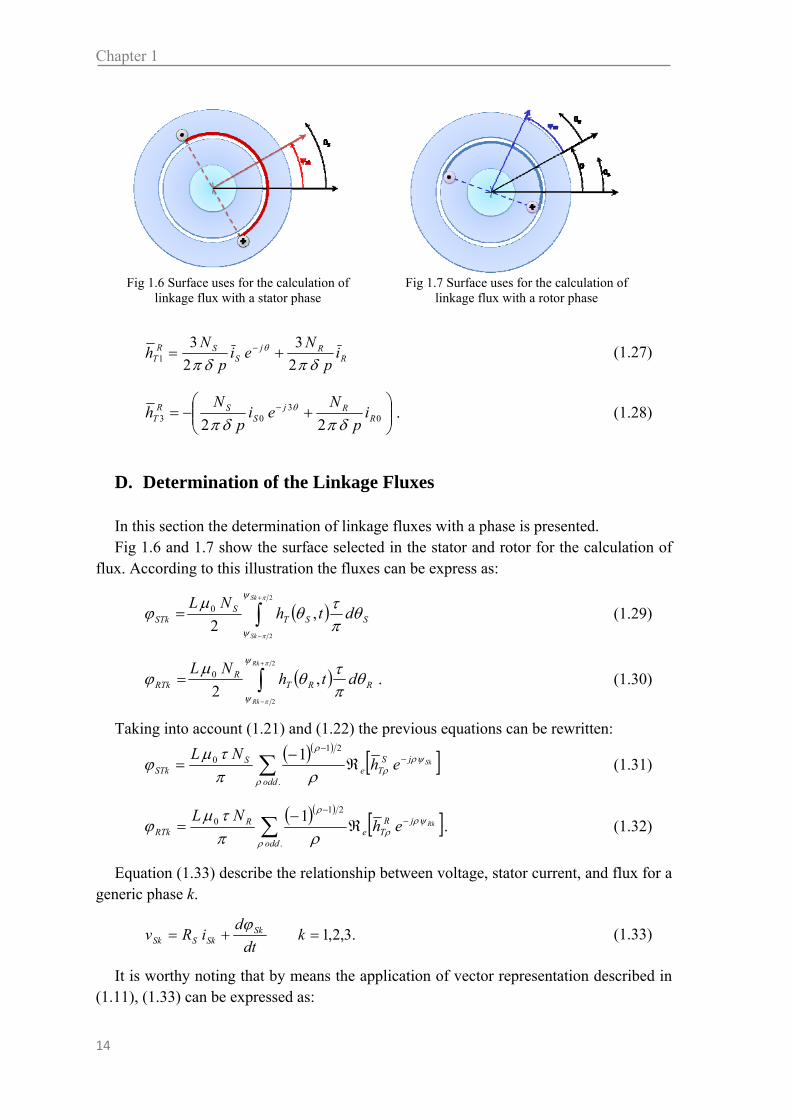
D. Determination of the Linkage Fluxes In this section the determination of linkage fluxes with a phase is presented. Fig 1.6 and 1.7 show the surface selected in the stator and rotor for the calculation of
flux. According to this illustration the fluxes can be express as:
2
2
,20
Sk
Sk
SSTS
STk dthNL
(1.29)
2
2
,20
Rk
Rk
RRTR
RTk dthNL
. (1.30)
Taking into account (1.21) and (1.22) the previous equations can be rewritten:
.
210 1
odd
jSTe
SSTk
SkehNL
(1.31)
.
210 1
odd
jRTe
RRTk
RkehNL
. (1.32)
Equation (1.33) describe the relationship between voltage, stator current, and flux for a generic phase k.
.3,2,1 kdt
diRv Sk
SkSSk
(1.33)
It is worthy noting that by means the application of vector representation described in (1.11), (1.33) can be expressed as:
Fig 1.6 Surface uses for the calculation of
linkage flux with a stator phase Fig 1.7 Surface uses for the calculation of
linkage flux with a rotor phase

Mathematical Model of a Three-Phase Induction Motor
15
dt
diRv S
SSS0
00
(1.34)
dt
diRv S
SSS
. (1.35)
In same way it is possible to write the rotor equations as follows:
.3,2,1 kdt
diRv Rk
RkRRk
(1.36)
dt
diRv R
RRR0
00
(1.37)
dt
diRv R
RRR
. (1.38)
The total linkage flux with a generic phase k is the sum of leakage flux and the air-gap linkage flux.
.3,2,1 kSTkSdkSk (1.39)
.3,2,1 kRTkRdkRk (1.40)
The application of the transformation (1.11) to the equations (1.39) and (1.40) permits to obtain the following relationships:
000 STSdS (1.41)
STSdS (1.42)
000 RTRdR (1.43)
RTRdR . (1.44)
The leakage coefficient Lsd describe the relationship between current and linkage flux with phase k.
.3,2,1 kiL SkSdSdk (1.45)
The introduction of the leakage coefficient Lsd permits to express the (1.41) - (1.45) as:
00 SSdSd iL (1.46)
SSdSd iL (1.47)
00 RRdRd iL (1.48)
RRdRd iL . (1.49)
Furthermore the application of transformation (1.11) to equations (1.31) and (1.32) determine the following relations:

Chapter 1
16
STe
SST h
NL3
00 3
2
(1.50)
ST
SST h
NL1
0
(1.51)
RTe
RRT h
NL3
00 3
2
(1.52)
RT
RRT h
NL1
0
. (1.53)
E. Determination of the Electromagnetic Torque The electromagnetic torque in electric machines can be determined by means of an
energy balance.
m
mkmem
iWT
, '
(1.54)
where emT is the torque, m is the mechanical angle, and 'mW is the magnetic co-energy.
When the motor is not in magnetic saturation the magnetic co-energy is equal to magnetic energy.
m
mkmem
iWT
, . (1.55)
The angle m is related to with a simple relationship:
mp (1.56)
, kmem
iWpT . (1.57)
The initial hypothesis permits to consider the magnetic energy connected to leakage fluxes invariant with angular position . Therefore to determine the torque is sufficient to consider the magnetic energy in the air-gap.
, kmTem
iWpT . (1.58)
Equation (1.23) describes the magnetic field in the air-gap as sum of the contribution of stator and rotor magnetic fields.
.
,odd
jjRSeST
Seehhth
. (1.59)
Therefore the torque can be expressed as:

Mathematical Model of a Three-Phase Induction Motor
17
SSTmT dthLpW
,2
1 20
2
0 (1.60)
.
*02
1
odd
ST
STmT hhLpW
(1.61)
.
2
02
1
odd
STmT hLpW
(1.62)
where
ST
jRS hehh
(1.63)
SR
jR heh
. (1.64)
The torque produced by an induction motor can be rewritten as:
odd
jRSem ehjhLpT
2
0 . (1.65)
Equation (1.65) describes the torque by means of the magnetic field produced by stator and rotor windings, but it can be also related to the currents present in machine.
33311
20 3 j
RSj
RSem ehjhehjhLpT . (1.66)
where
SS
S ip
Nh
2
31 (1.67)
RR
R ip
Nh
2
31 (1.68)
03 2 SS
S ip
Nh
(1.69)
03 2 RR
R ip
Nh
. (1.70)
If the machine winding are star connected the common mode current is equal to zero, and if the rotor is short-circuited, new relationships can be written.
The introduction of self-inductance coefficients and mutual inductance coefficient permits to express the relationships generally used in the control of electric drives.
2
2
20
2
3
S
SS
N
p
LL (1.71)
2
2
20
2
3
R
RR
N
p
LL (1.72)

Chapter 1
18
22
0
2
3
RS NN
p
LM (1.73)
11 SSSdS LLL (1.74)
11 RRRdR LLL . (1.74)
Finally the expression of torque can be found as follows.
jRSem eijiMpT 12
3. (1.75)
1.4 Machine Equations
In this section the machine equations of induction motor are summarized. The common mode equations are given by:
RTe
RRT
STe
SST
jST
RT
jR
RS
SST
RTRRdR
STSSdS
RRRR
SSSS
hNL
hNL
ehh
eip
Ni
p
Nh
iL
iLdt
diRv
dt
diRv
30
0
30
0
333
3003
000
000
000
000
3
2
3
2
22
(1.76)
whereas the machine equations in d-q plane can be expressed as:
jST
RT
jR
RS
SST
RTRRdR
STSSdS
RRRR
SSSS
ehh
eip
Ni
p
Nh
iL
iLdt
diRv
dt
diRv
11
1 2
3
2
3
(1.77)

Mathematical Model of a Three-Phase Induction Motor
19
RT
RRT
ST
SST
hNL
hNL
10
10
(1.77)
Finally (1.75) defines the torque delivered to the load.
1.5 From Machine Equations to the Vector Control of an Induction Machine
Taking (1.76) and (1.77) into account it is possible to show how the most important machine quantities are connected to the rotor flux.
The ρ-th rotor flux can be express as:
j
RR e (1.78)
and its derivative is given by:
j
RrjRR eje
dt
d
dt
d (1.79)
where
Rdt
d . (1.80)
The relationships among the machine quantities and the rotor flux are resumed in the following equations.
j
RRR
RR ej
dt
d
Ri
1 (1.81)
jjRR
R
RR
R
RRS ee
R
Lj
dt
d
R
L
Mi
11
1
1 (1.82)
j
RRR
RdR
R
RdR
SRT e
R
Lj
dt
d
R
L
Mp
Nh
2
3 (1.83)
R
RRem R
pT2
2
3 . (1.84)
Therefore the rotor and the stator current, the torque and the magnetic field in the air-gap are strongly connected to the rotor flux. This result suggests the operating principle of the vector control i.e. the control of the rotor flux.
By substituting (1.84) in (1.81) – (1.83) a new set of equations can be obtained.
Chapter 1
20
j
R
emR
RR e
T
pj
dt
d
Ri
3
21 (1.85)
jj
R
emR
R
R
RRS ee
TL
pj
dt
d
R
L
Mi
1
1
1 3
21 (1.86)
j
R
emRd
R
R
RdR
SRT e
TL
pj
dt
d
R
L
Mp
Nh
3
2
2
3
11 . (1.87)
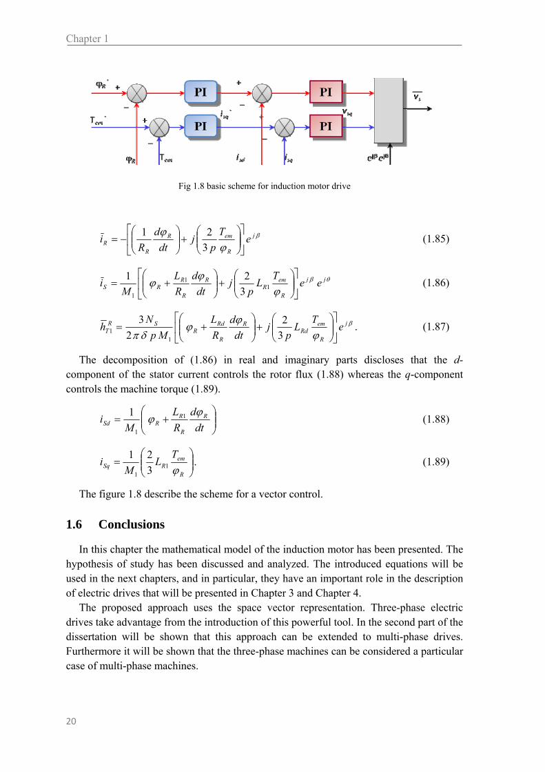
The decomposition of (1.86) in real and imaginary parts discloses that the d-component of the stator current controls the rotor flux (1.88) whereas the q-component controls the machine torque (1.89).
dt
d
R
L
Mi R
R
RRSd
1
1
1 (1.88)
R
emRSq
TL
Mi
11 3
21. (1.89)
The figure 1.8 describe the scheme for a vector control.
1.6 Conclusions
In this chapter the mathematical model of the induction motor has been presented. The hypothesis of study has been discussed and analyzed. The introduced equations will be used in the next chapters, and in particular, they have an important role in the description of electric drives that will be presented in Chapter 3 and Chapter 4.
The proposed approach uses the space vector representation. Three-phase electric drives take advantage from the introduction of this powerful tool. In the second part of the dissertation will be shown that this approach can be extended to multi-phase drives. Furthermore it will be shown that the three-phase machines can be considered a particular case of multi-phase machines.
Fig 1.8 basic scheme for induction motor drive

Mathematical Model of a Three-Phase Induction Motor
21
1.7 References
[1] Ion Boldea, Syed A. Nasar, “The Induction Machine Handbook”, CRC Press LLC, 2002
[2] Ned Mohan, “Power Electronics and Drives”, Minneapolis, MNPERE, 2003
[3] Bimal K. Bose, “Modern Power Electronics and AC Drives”, Upper Saddle River, PHPTR, 2002

Three-Phase Inverter Abstract This chapter is a brief state of the art on three phase inverter where the basic structure and technology of DC-AC converters are presented. An ample part is dedicated to the modulation strategies and to their degree of freedom, and prominence is given to the passage from Pulse Width Modulation to Space Vector Modulation.
2.1 Introduction
Power electronics converters are a family of electrical circuits which convert electrical energy from one level of voltage/current/frequency to another using semiconductors-based electronics switches [1]. The essential characteristic of these type of circuits is that this type of switch can operate only in two states. These states are called state ON and state OFF. When an electronic component is state ON, it can be ideally considered like short circuit whereas when the state is OFF the component behave likewise an open circuit.
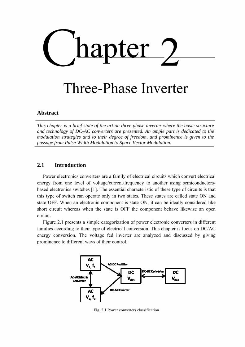
Figure 2.1 presents a simple categorization of power electronic converters in different families according to their type of electrical conversion. This chapter is focus on DC/AC energy conversion. The voltage fed inverter are analyzed and discussed by giving prominence to different ways of their control.
hapter 2
Fig. 2.1 Power converters classification

Chapter 2
24
Fig. 2.2 Three phase inverter scheme
2.2 Structure of a Three Phase Inverter
Voltage-fed converters, as the name indicate, receive DC voltage at one side and convert it to AC voltage to the other side [2]. The AC voltage and frequency are a degree of freedom of the system and they can be variable or constant depending on the applications. In fact the general name “converter” is given because it can operate in bidirectional way: the same circuit can work as an inverter as well as a rectifier.
An ideal inverter should have a stiff voltage source at the input, that is, its Thevenin impedance should be zero. A large capacitor is usually connected at the input to realize a stiff voltage source (Figure 2.2).
The voltage-fed inverters can be classified according to the number of legs in single-phase inverters, H-bridge inverters, three-phase inverters and multi-phase inverters. According to the structure of the converter is possible to distinguish belong multi-level inverters, Z-inverters and others non-traditional converters.
Multi-phase inverter is the natural extension of a three-phase inverter when the number of phases is higher than three. This type of converter has a great relevance in this dissertation and to its description will be dedicated the entire chapter 6. However to understand multi-phase drives and theirs numerous degrees of freedom is essential to clearly comprehend three-phase drive.
Basically a three phase inverter is composed by 6 electronic components, every component is composed by an electronic switch and a diode. There exist many technologies developed over time that can perform in an inverter. The most common technologies are IGBT (acronym of Insulated Gate Bipolar Transistor), MOSFET (Metal Oxide Semiconductor Field Effect Transistor) and SiC (Silicon Carbide). Particular attention should be given to this latest technology (SiC). Although it is very recent, it can profoundly change the performance of the new generation of inverter[19] and [20].
2.3 Modulation Strategies
The process of switching the electronics devices in a power electronic converters from one state to another is called modulation. There exists an infinite number of modulation strategies due to the degrees of freedom offered by the problem. Parameters such as
Three Phase Inverter
25
switching frequency, harmonic distortion, losses and speed of response are the typical issues which must be considered when a modulation strategy is developed.
In reference to the figure 2.2 the following relationships can be write:
0330
000220
0110
3,2,1
NN
kkNkNN
NN
vvv
kvvvvvv
vvv
(2.1)
If the equations in the set (2.1) are summed together a new relationship can be found:
nonnn vvvvvvv 3321302010 . (2.2)
For a general ohmic-inductive balanced load with a active back electromotive force created by an symmetric electrical machine the phase voltages can be expressed by (2.3) and (2.4).
kk
kkn edt
diLRiv (2.3)
3
1
3
1
3
1k k kkkkn ei
dt
dRv (2.4)
In a three phase load the sum of the line currents is identically zero likewise the sum of the voltages of a symmetric electrical machine.
003
1
3
1
3
1
k
kk
nkk
k evi (2.5)
3
302010 vvvvno
(2.6)
The common mode voltage of the inverter can be seen like the degree of freedom of the system. The infinite values of common mode voltage characterize different modulation strategies and according to their waveform the modulation strategies can be classified in continuous and discontinuous modulations.
A. Space Vector Modulations The study of three-phase Voltage Source Inverter (VSI) can take advantage of the
definition of space vectors and zero sequence component. The introduction of the vectorial notation is extremely useful to understand the operating principle of a three-phase inverter and it is deeply related to the model of a three-phase machine (as the previous chapter showed)
For three given pole voltages v10, v20, v30 a new set of variables v0 and v can be defined
by the following symmetrical linear transformations:
3
100 3
1
kkvv (2.7)
Chapter 2
26
3
103
2
kkkvv (2.8)
where
1
3
2
kj
k e
, (k=1,2,3). (2.9)
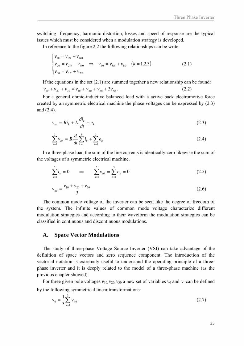
The real quantity v0 calculated by (2.7) is the zero-sequence component of the pole voltages, whereas the variables, usually called “space vectors”, are complex quantities that can be directly related to the load phase voltages (2.10).
20303
10202
00101
2
2
2
vv
vv
vv
vv
vv
vv
Load
Load
Load
(2.10)
The quantity Loadv0 is the zero-sequence voltage of the load and for any type of
symmetrical load it is equal to zero in any instant. So (2.10) concludes that the voltage space vector of the load is equal to the pole-voltage space vector of inverter (2.11).
kNLoad vv . (2.11)
The goal of the modulation process is to determine how to control the inverter switches, so that the mean values of the space vectors v over a switching period Tsw are
equal to the reference values refv .
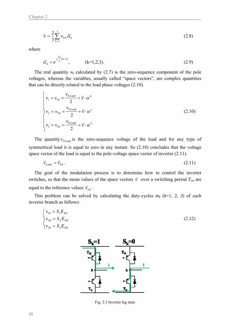
This problem can be solved by calculating the duty-cycles mk (k=1, 2, 3) of each inverter branch as follows:
DC
DC
DC
ESv
ESv
ESv
330
220
110
(2.12)
Fig. 2.3 Inverter leg state

Three Phase Inverter
27
where Sk (k=1,2,3) describes the inverter leg state (fig. 2.3). Its values are 0 and 1. The final relationships can be found by combining (2.12) and (2.11).
23
12
013
2 SSSEv DC (2.13)
Since the load common mode voltage is always zero, (2.13) implies that the load voltages are not dependent on the common mode component of the inverter voltages; in
other words each set of voltages 1v , 2v and 3v applied by the inverter has the same effect
on the load. Anyway, different sets of voltages may have different effects on the sources or on the converter components. The zero sequence voltage v0 is a degree of freedom that the designer can choose to improve the performance of the modulation strategy.
The equation (2.13) correlates the load phase voltage with the inverter leg state. There are eight (namely 23) possible configurations for a three-phase inverter,
depending on the states of the three switch commands S1, S2 and S3. Six configurations correspond to voltage vectors with non-null magnitudes. These vectors, usually referred to as active vectors, are represented in Fig. 2.4. Beside each vector there is also its configuration expressed in the form (s3,s2,s1). Two configurations, i.e. (s3,s2,s1)=(0,0,0) and (s3,s2,s1)=(1,1,1), lead to voltage vectors with null magnitudes, usually referred to as zero vectors.
The Space Vector Modulation (SVM) selects two active vectors and applies each of them to the load for a certain fraction of the switching period. Finally, the switching period is completed by applying the zero vectors.
The active vectors and their duty-cycles are determined so that the mean value of the output voltage vector in the switching period is equal to the desired voltage vector.
The best choice for the active vectors is given by the two vectors delimiting the sector in which the reference voltage vector lies. The concept of sector is one of the most important ideas that the space vector modulation introduced and differentiates this type of modulation from the Pulse Width Modulation (PWM). Since two consecutive vectors differ only in the state of one switch, this choice allows ordering the active and the zero vectors so as to minimize the number of switch commutations in a switching period.
For example, if the desired voltage vector lies in sector 1, as shown in Fig. 3, the two
1
2
3
4
5
6
2v3v
4 v
5v 6v
1v (0,0,1)
(0,1,0)
(1,0,0)
(0,1,1)
(1,1,0)
(1,0,1)
refv
d
q
Fig. 2.4 - Voltage vectors used in SVM technique, represented in d-q reference frame.

Chapter 2
28
adjacent voltage vectors are 1v and 2v , whose configurations (0,0,1) and (0,1,1) differ in
only one bit. After the active vectors have been chosen, the requested voltage can be expressed as a linear combination of them as follows:
2211 vvvref (2.14)
where δ1 and δ2 are the duty-cycles of 1v and 2v in the switching period.
The explicit expressions of δ 1 and δ 2 can be easily calculated evaluating the following dot products:
)1(1 wvref (2.15)
)2(2 wvref (2.16)
where
2121
2)1( 1
dcEvjv
vjw (2.17)
3212
1)2( 1
dcEvjv
vjw (2.18)
Once δ1 and δ2 have been calculated, the designer can still choose in which proportion the two zero vectors are used to fill the switching period.
It is worth noting that (2.15)-(2.18) have an interesting graphical meaning, which is shown in Fig. 2.5. The duty-cycles δ1 and δ2 can be interpreted as the projections of refv
on the new vectors )1(w and )2(w that form a non-orthogonal vector basis. This result is well-known in tensor analysis, where the duty-cycles δ1 and δ2 are usually referred to as
contra-variant components of refv , and )1(w and )2(w are referred to as reciprocal
vectors.[3].
1
2
refv
1v
2v
)1(w
)2(w
Fig. 2.5 - Decomposition of the reference vector on the reciprocal vectors and calculation of the duty-cycles(contra variant components) in the three-phase case.

Three Phase Inverter
29
B. Duty Cycle Space Vector Modulation The Duty Cycle Space Vector (DCSV) is based on the representation of the duty
cycles of the inverter legs with space vectors. In this case, likewise SVM, the goal is to feed the load with a voltage which have the same mean value in a switching period of the voltage reference vector.
Equation (2.13) suggests the possibility to introduce the concept of a new space vector as follows:
SEvSSSEv DCDC 2
31
20
13
2 (2.19)
2
31
20
13
2 SSSS (2.20)
where S can assume seven value. The voltage reference can be written as the mean value of the inverter voltage vector.
dtST
Evdtv
Tv
swsw T
sw
DCref
T
swref
00
1 (2.21)
mEv DCref . (2.22)
The quantity m is the duty cycle space vector and it can be related to the inverter state
with simple equations:
dtST
mswT
sw0
1 (2.23)
23
12
013
2 mmmm (2.24)
dtST
m
dtST
m
dtST
m
sw
sw
sw
T
sw
T
sw
T
sw
0
33
0
22
0
11
1
1
1
(2.25)
DC
refDCref E
vmmEv . (2.26)
The following equations are the direct and inverse transformation to determine the elements of the duty cycle Clarke’s transformation.
Chapter 2
30
203
102
001
DC
ref
DC
ref
DC
ref
E
vmm
E
vmm
E
vmm
(2.27)
203
102
001
mmm
mmm
mmm
(2.28)
Equations (2.28) show that a modification of 0m determines a “rigid translation” of the
modulating signals, but it does not change the application time of the active inverter
configurations. The quantity 0m is a real degree of freedom and its adjustment affect the
time division between the null-configurations. The degree of freedom of SVM, i.e. the possibility of dividing the duty cycle of the
zero vector arbitrarily between two null-configurations corresponds to the degree of freedom of the DCSV strategy, which allows to translate the modulating signals. Hence it is possible to conclude that SVM and DCSV are completely equivalent.
C. Continuous Modulation The DCSV modulation is a useful tool to analyze different type of modulation
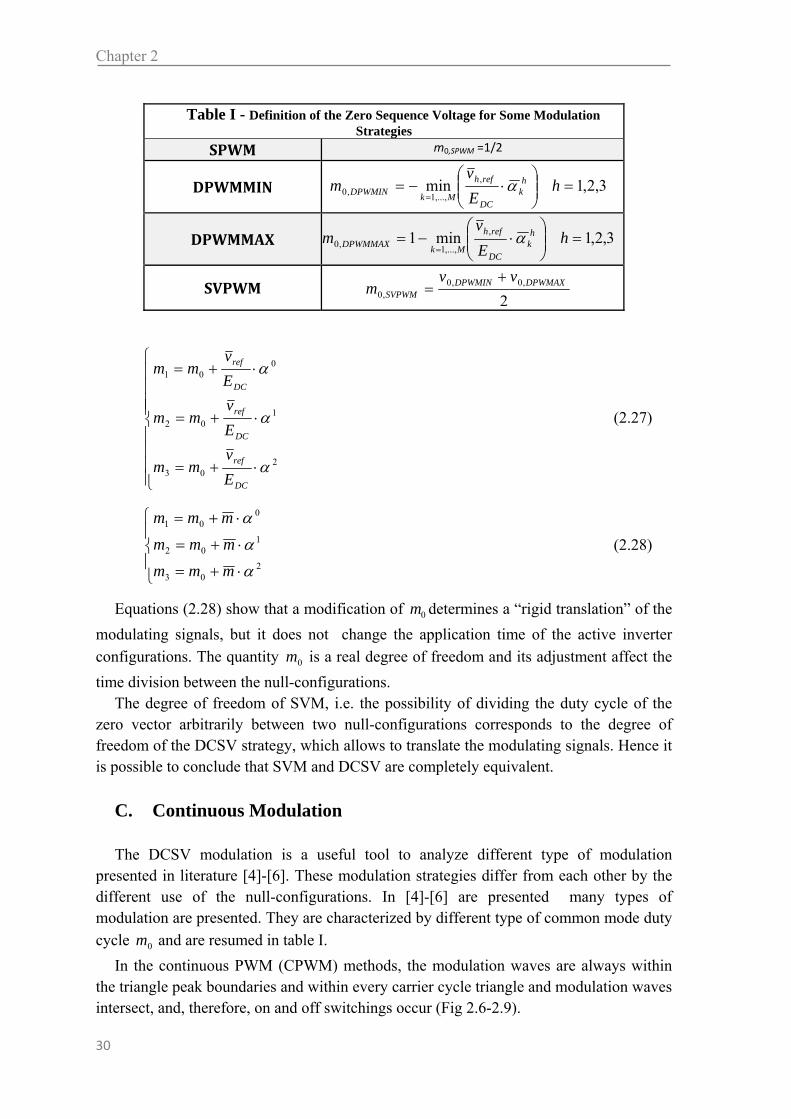
presented in literature [4]-[6]. These modulation strategies differ from each other by the different use of the null-configurations. In [4]-[6] are presented many types of modulation are presented. They are characterized by different type of common mode duty
cycle 0m and are resumed in table I.
In the continuous PWM (CPWM) methods, the modulation waves are always within the triangle peak boundaries and within every carrier cycle triangle and modulation waves intersect, and, therefore, on and off switchings occur (Fig 2.6-2.9).
Table I - Definition of the Zero Sequence Voltage for Some Modulation Strategies
SPWM m0,SPWM =1/2
DPWMMIN 3,2,1min ,
,...,1,0
h
E
vm h
kDC
refh
MkDPWMIN
DPWMMAX 3,2,1min1 ,
,...,1,0
h
E
vm h
kDC
refh
MkDPWMMAX
SVPWM 2
,0,0,0
DPWMAXDPWMINSVPWM
vvm

Three Phase Inverter
31
In the discontinuous PWM (DPWM) methods, the modulation wave of a phase has at least one segment which is clamped to the positive or negative dc rail for at most a total of 120: Therefore, within such intervals the corresponding inverter leg discontinues modulation. Since no modulation implies no switching losses, the switching loss characteristics of CPWM and DPWM methods are different. Detailed studies indicated the waveform quality and linearity characteristics are also significantly different. Therefore, this classification aids in distinguishing the differences.
The modulation strategy referred to as SPWM is the traditional sinusoidal PWM, and its zero sequence duty cycle is always ½ (Fig 2.6).
The SPWM method is the simplest modulation with limited voltage linearity range and poor waveform quality in the high-modulation range. [7]
The zero sequence voltage of DPWMMIN is selected so that the minimum duty-cycle among m1, m2, m3 is always zero, whereas the maximum duty-cycle of DPWMMAX is always 1. As a consequence, when these strategies are used, in every switching period there is an inverter branch that does not commutate (Fig 2.7, 2.8).
Note that the DPWMMAX and DPWMMIN methods have nonuniform thermal stress on the switching devices and in DPWMMAX the upper devices have higher conduction losses than the lower ones, while in DPWMMIN the opposite is true [7].
The use of these last two modulation techniques reduces the commutation losses of the inverter but they increase the ripple of load line current. These results further demonstrate the influence of common mode voltage on the inverter behavior.
The strategy SVPWM is often referred to as "symmetric modulation". In this case the
Fig 2.6 PWM modulating signal of phase 1 and zero‐sequence duty cycle
Fig 2.7- 2.8 DPWMMIN and DPWMMAX modulating signal of phase 1 and zero-sequence duty cycle

Chapter 2
32
signal m0 can be calculate on basis of to the average value of the values of m0 obtained for DPWMMAX and DPWMMIN.
SVPWM uses in any commutation period both the switching configurations (0, 0, 0) (1, 1, 1) to generate the zero vector. The name SVPWM is caused by symmetric
distribution of space vector in reference to the middle period 2swT .
Due to the simplicity of algebraically defining their zero-sequence signals, THIPWM (Fig 2.10, 2.11) modulators have been frequently discussed in the literature. The zero-
sequence signal is )3cos(41 tEVm DCMo for THIPWM1/6 [8], and
)3cos(41 tEVm DCMo for THIPWM1/4 [9].
In the past, both methods suffered from implementation complexity determined by the utilization of trigonometric identities. Nowadays this problem is outdated due to Digital Signal Processor (DSP) of new generation.
Although the THIPWM1/4 has theoretically minimum harmonic distortion, it is only slightly better than SVPWM and has narrower voltage linearity range [10], [11], [12]. With their performance being inferior to SVPWM and implementation complexity significantly higher, both THIPWM methods have academic and historical value, but little practical importance.
Fig 2.9 2.10 THIPWM1/6 and THIPWM1/4 modulating signal of phase 1 and zero-sequence duty cycle
Fig 2.11 SVPWM modulating signal of phase 1 and zero-sequence duty cycle

Three Phase Inverter
33
D. Discontinuous Modulations DPWM0 [13], [14], DPWM1 [15], [16], and DPWM2 [13], [17] are three special cases
of a generalized DPWM (GDPWM) method [19] (Fig 2.12-2.15). The discontinuous modulation strategies avoid the commutation in a inverter branch,
as the previous techniques DPWMMIN and DPWMMAX, but they change the null-configuration (0, 0, 0) or (1, 1, 1) according to the position of the vector voltage reference.
The positioning of reference vector in sector influence the modulation behavior. In Figure 2.16 - 2.28 are illustrated this concept for discontinuous modulation
technique present in literature.
2.4 Conclusions
In this chapter a brief state of the art of three phase inverter is presented. The most important modulation strategies are illustrated.
The choice of the modulation technique can influence the current ripple, inverter efficiency, maximum modulation index and the over-modulation behavior.
the choice of modulation technique is therefore very important, because it influence the converter design and so the entire drive.
Fig 2.12 DPWM0 modulating signal of phase 1 and zero-sequence duty cycle
Fig 2.13 DPWM1 modulating signal of phase 1 and zero-sequence duty cycle
Fig 2.14 DPWM2 modulating signal of phase 1 and zero-sequence duty cycle
Fig 2.15 DPWM3 modulating signal of phase 1 and zero-sequence duty cycle

Chapter 2
34
2.5 References
[1] D. G. Holmes and T. A. Lipo, Pulse Width Modulation for Power Converters. New York: Wiley, 2003.
[2] Bimal K. Bose, Modern Power Electronics and AC drives. Upper Saddle River, New Jersey :Prentice Hall PTR 2002
[3] K. F. Riley, M. P. Hobson, and S. J. Bence, Mathematical Methods for Physics and Engineering, 2nd ed. Cambridge, U.K.: Cambridge Univ. Press.
[4] D. Casadei, G. Serra, A. Tani, L. Zarri, “Matrix converter modulation strategies: a new general approach based on space-vector representation of the switch state,” IEEE Trans. on Ind. Electron., vol. 49, no. 2, pp. 370-381, April 2002.
Fig 2.14 Zero-state partitioning DPWMMIN Fig 2.15 Zero-state partitioning DPWMMIN
Fig 2.16 Zero-state partitioning DPWM0 Fig 2.16 Zero-state partitioning DPWM1
Fig 2.16 Zero-state partitioning DPWM2 Fig 2.16 Zero-state partitioning DPWM3

Three Phase Inverter
35
[5] C. Rossi, G. Serra, A. Tani, L. Zarri, “Cascaded multilevel inverter modulation strategies: a novel
solution based on Duty-Cycle Space Vector approach,” Proc. of ISIE, June 20-23, 2005, vol. II, pp. 733-738.
[6] D. Casadei, G. Serra, A. Tani, L. Zarri, “Multi-phase inverter modulation strategies based on Duty-Cycle Space Vector approach,” Ship Propulsion and Railway Traction Systems Conference, SPRTS, Bologna (Italy), 4-6
[7] H. M. Hava, R. J. Kerkman , T. A. Lipo, “Simple Analytical and Graphical Methods for Carrier-Based PWM-VSI Drives” IEEE Trans. on Power. Electron., vol 14 No 1 pp 40-61, January 1999.
[8] G. Buja and G. Indri, “Improvement of pulse width modulation techniques,” Archiv f¨ur Elektrotechnik, vol. 57, pp. 281–289, 1975.
[9] S. R. Bowes and A. Midoun, “Suboptimal switching strategies for microprocessor controlled PWM inverter drives,” Proc. Inst. Elect. Eng., vol. 132, pt. B, pp. 133–148, May 1985.
[10] J. Holtz, “Pulsewidth modulation for electronic power conversion,” Proc. IEEE, vol. 8, pp. 1194–1214, Aug. 1994
[11] K. W. Kolar, H. Ertl, and F. C. Zach, “Minimization of the harmonic rms content of the mains current of a PWM converter system based on the solution of an extreme value problem,” in ICHPC Conf. Rec., Budapest, Hungary, 1990, pp. 234–243.
[12] A. M. Hava, “Carrier based PWM-VSI drives in the overmodulation region,” Ph.D. dissertation, Univ. Wisconsin, Madison, 1998.
[13] J. W. Kolar, H. Ertl, and F. C. Zach, “Influence of the modulation method on the conduction and switching losses of a PWM converter system,” IEEE Trans. Ind. Applicat., vol. 27, pp. 1063–1075, Nov./Dec. 1991.
[14] T. Kenjo, Power Electronics for the Microprocessor Age. Oxford, U.K.: Oxford Univ. Press, 1990.
[15] J. Schr¨orner, “Bezugsspannung zur umrichtersteuerung,” in ETZ-b, Bd. 27, pp. 151–152, 1976.
[16] M. Depenbrock, “Pulse width control of a 3-phase inverter with non-sinusoidal phase voltages,” in IEEE-ISPC Conf. Rec., pp. 399–403, 1977.
[17] S. Ogasawara, H. Akagi, and A. Nabae, “A novel PWM scheme of voltage source inverter based on space vector theory,” in European Power Electron. Conf. Rec., Aachen, Germany, 1989, pp. 1197–1202.
[18] A. M. Hava, R. J. Kerkman, and T. A. Lipo, “A high performance generalized discontinuous PWM algorithm,” in IEEE-APEC Conf. Rec., Atlanta, GA, 1997, pp. 886–894.
[19] Ozpineci, B.; Tolbert, L.M.; Islam, S.K.; Hasanuzzaman, M.,” Effects of silicon carbide (SiC) power devices on HEV PWM inverter losses” in Industrial Electronics Society, 2001. IECON '01 Volume 2, 29 Nov.-2 Dec. 2001 Page(s):1061 - 1066 vol.2
[20] Rabkowski, J.; Barlik, R.;, “Extreme high efficiency PV-power converters” in EPE 09 8-10 Sept. 2009 Page(s):1 - 13


Stator Flux Vector Control of Induction Motor Drives
in the Field-Weakening Region
Abstract The control scheme of a speed-sensorless induction motor drive fed by a three phase inverter is presented. The proposed scheme allows the motor to exploit the maximum torque in the whole speed range, and shows a reduced dependence on the motor parameters. Furthermore, to validate the effectiveness of the presented algorithm it is assessed in terms of performance and complexity and compared with two other algorithm presented in literature. The flexibility and the effectiveness of the Stator Flux Vector Control is also tested an induction motor drive fed by a matrix converter. The experimental results confirm the feasibility of this solution.
3.1 Introduction
When the induction motors are used for applications at high speed, it is desirable to retain the maximum torque capability in the field weakening region. The torque capability of an induction motor is limited by the maximum current and the maximum voltage that the inverter can apply to the motor. Several papers were presented in order to achieve the maximum torque capability of the machine over the whole field weakening region [1]–[4]. According to these field weakening algorithms, the optimal flux value of the motor should be updated by means of look-up tables or explicit expressions containing the motor parameters and quantities such as the motor speed, the motor currents, the dc-link voltage and the requested torque. However, the performance of these algorithms is strictly related to the accuracy by which the parameters are known.
hapter 3

Chapter 3
38
A further problem is represented by the variable value of the leakage and magnetizing inductances, to which the rotor-flux-oriented scheme is particularly sensitive [5]. In addition, the drive performance in the high speed range may depend on the correct determination of the base speed, which is function of the actual dc-link voltage and the overload capability.
As a consequence, new methods to compensate the parameter variations and the uncertainties of the models have been investigated. Among these, some adaptive schemes have been proposed in order to provide a suitable estimation of the varying parameters [6]–[8]. These methods provide good drive performance to the detriment of the complexity of the control scheme and the tuning of the regulators.
For the reasons stated above, the stator-flux-oriented drive, more insensitive to parameter variations than the rotor-flux-oriented one, has received an increasing attention for field weakening applications [9]–[11]. In particular, [10] presents a robust method for field weakening operation of DTC induction motor drives where the flux reference is adjusted on the basis of the torque error behavior. In fact, a suitable method for robust field weakening is to determine the optimal flux level using closed-loop schemes that analyze the motor behavior, rather than look-up tables or explicit expressions containing the motor parameters.
From this point of view, interesting contributions towards robust field weakening strategies were proposed in [12], [13] for stator-flux-oriented induction motor drives and in [14]–[18] for rotor-flux-oriented induction motor drives. According to these papers, the flux is adjusted on the basis of the supply voltage requested by the regulators. If this voltage is greater than the available one, the field weakening algorithm reduces the flux. Furthermore, employing a suitable voltage control strategy allows the motor to exploit the maximum torque in the whole speed range.
The traditional field-oriented control utilizes the stator current components as control variables. The d-component of the stator current acts on the rotor flux, whereas the q-component is proportional to the motor torque. As the control of the motor flux is obtained indirectly by controlling the motor currents, the algorithm presented in [14] for achieving the maximum torque is rather complex, requiring the tuning of several PI regulators (two PI regulators are used for the current regulation, two PI regulators for the field weakening and another one for the speed regulation). The stator-flux field oriented control presented in [13], similarly, uses the same number of PI regulators. This makes difficult to obtain an optimal motor behavior, especially for drives with low inertia.
In this chapter, a novel field weakening scheme for induction motor drives is presented [19]. In the proposed rotor-flux-oriented control scheme the main control variables are the stator flux components instead of the stator current components. This basic choice simplifies the control scheme, exhibits a fast torque response and reduces the number of PI regulators. In addition, the proposed scheme allows the motor to exploit the maximum torque capability in the whole speed range.
In order to verified if the feasibility of the field weakening technique is confirmed, simulations and experimental tests are presented. Furthermore a comparison between the control schemes showed in [13], [14] and [19] offer the possibility to analyze three
SFVC of Induction Motor Drives in the Field-Weakening Region
39
control strategy in terms of number and type of regulators, complexity of implementation and transient behavior.
For the comparison, the three control schemes have been implemented on the same experimental platform, i.e. the same DSP, power inverter and induction motor, and use the same basic functions, such as the voltage modulator.
Finally the control scheme illustrated in [22] for a speed-sensorless induction motor drive fed by a matrix converter is presented. The experimental evidences permit to conclude that the control algorithm is totally general and it is applicable to different converter structures with the same effectiveness.
3.2 Machine Equations and Maximum Torque Capability
In the traditional Field Oriented Control for induction machines the main control variables are the stator current components. In a reference frame synchronous with the rotor flux vector, the d component of the stator current vector establishes the rotor flux level, whereas the motor torque is proportional to the q component.
The behavior of the induction machine can be described in terms of space vectors by the following equations written in a reference frame synchronous with the rotor flux. This approach is described in Chapter 1, where the mathematical machine model was presented.
dt
djiRv s
ssss
(3.1)
dt
djiR r
rmrr
0 (3.2)
rsss iMiL (3.3)
srrr iMiL (3.4)
rr jipT 2
3. (3.5)
where p is the pole pairs number, is the angular speed of the rotor flux vector, m is the rotor angular speed in electric radians, and “·” denotes the scalar product.
Solving (3.3) and (3.4) with respect to si and ri , and substituting in (3.2) and (3.5)
yields
dt
dj
L
R
LL
MR rrm
r
rs
rs
r
0 (3.6)
rsrs
jLL
MpT
2
3 (3.7)
where the parameter is defined as follows:

Chapter 3
40
rs LL
M 2
1 . (3.8)
The reference frame orientation is chosen so that the d-axis has the direction of the rotor flux vector. Hence (3.6) can be rewritten in terms of d and q components as follows:
sds
rr
r
r
L
M
dt
d
R
L
(3.9)
sqrs
rrm LL
MR
. (3.10)
Also (3.7) can be rewritten as follows
sqrrs LL
MpT 2
3 . (3.11)
As can be seen, these equations are quite similar to the corresponding equations of the traditional field oriented control based on d-q stator current components. In fact the rotor
flux depends only on sd , whereas the motor torque is proportional to sq .
In steady-state operation, (3.1), (3.3) and (3.9) become
ssss jIRV (3.12)
sdssd IL (3.13)
sqssq IL (3.14)
sds
r L
M . (3.15)
These steady-state equations will be utilized for the analysis of the maximum torque capability. In the high-speed range the motor performance is limited by the maximum inverter voltage, the inverter current rating and the machine thermal rating.
The maximum voltage magnitude Vs,max that the inverter can apply to the machine is related to the dc-link voltage EDC and the modulation strategy. Using Space Vector Modulation (SVM) the maximum magnitude of the stator voltage vector is
DCs,max EV3
1 . (3.16)
The voltage limit and the current limit can be represented by the following inequalities:
vs ≤ Vs,max (3.17)
is ≤ Is,max . (3.18)
Inequalities (3.17) and (3.18) sensibly influence the motor behavior, especially at high speed. It is known that the operation of an induction motor can be divided into three

SFVC of Induction Motor Drives in the Field-Weakening Region
41
speed ranges, namely the low speed range (region I), the constant-power speed range (region II) and the decreasing-power speed range (region III).
In region I, the current limit and the rated flux level determine the operating point corresponding to the maximum torque.
The beginning of region II is defined as the voltage required to inject the maximum current reaches Vs,max. In region II, it is necessary to reduce the stator flux magnitude to keep the back emf approximately constant. Therefore the operating point corresponding to the maximum torque requires a rotor flux magnitude lower than the rated one, and the magnitudes of the stator current vector and stator voltage vector are equal to the limit values Is,max and Vs,max respectively. As the torque is inversely proportional to the rotor speed, the power delivered to the load is nearly constant.
Finally, in region III the available dc-link voltage is not sufficient to inject the maximum current and the power delivered to the load decreases nearly proportionally with the rotor speed.
It is evident that the maximum torque capability is a consequence of the voltage and current limits.
In order to determine the operating point corresponding to the maximum torque, when the stator voltage is equal to Vs,max, it is opportune to introduce the angle α between the stator flux vector and the rotor flux vector, as follows:
φsd = φs cos α (3.19)
φsq = φs sin α. (3.20)
Combining (3.11), (3.15), (3.19) and (3.20), it is possible to express the motor torque as follows
2sin4
3 2
2
2
s
rs LL
MpT . (3.21)
At high speed, the voltage drop on the stator resistance is small and (3.12) can be approximated as
ss,maxV . (3.22)
Combining (3.22) and (3.21) leads to the following expression of the torque in the high speed region:
2sin4
32
max,
2
2
s
rs
V
LL
MpT . (3.23)
From (3.23) it is clear that, for any value of ω, the maximum torque is produced when the stator flux and the rotor flux vectors are delayed by an angle of 45°, i.e. sq is equal
to sd .
However, when the maximum torque is delivered to the load, the current could be greater than Is,max. In fact, according to (3.13) and (3.14), the stator current components are related to the corresponding stator flux components.

Chapter 3
42
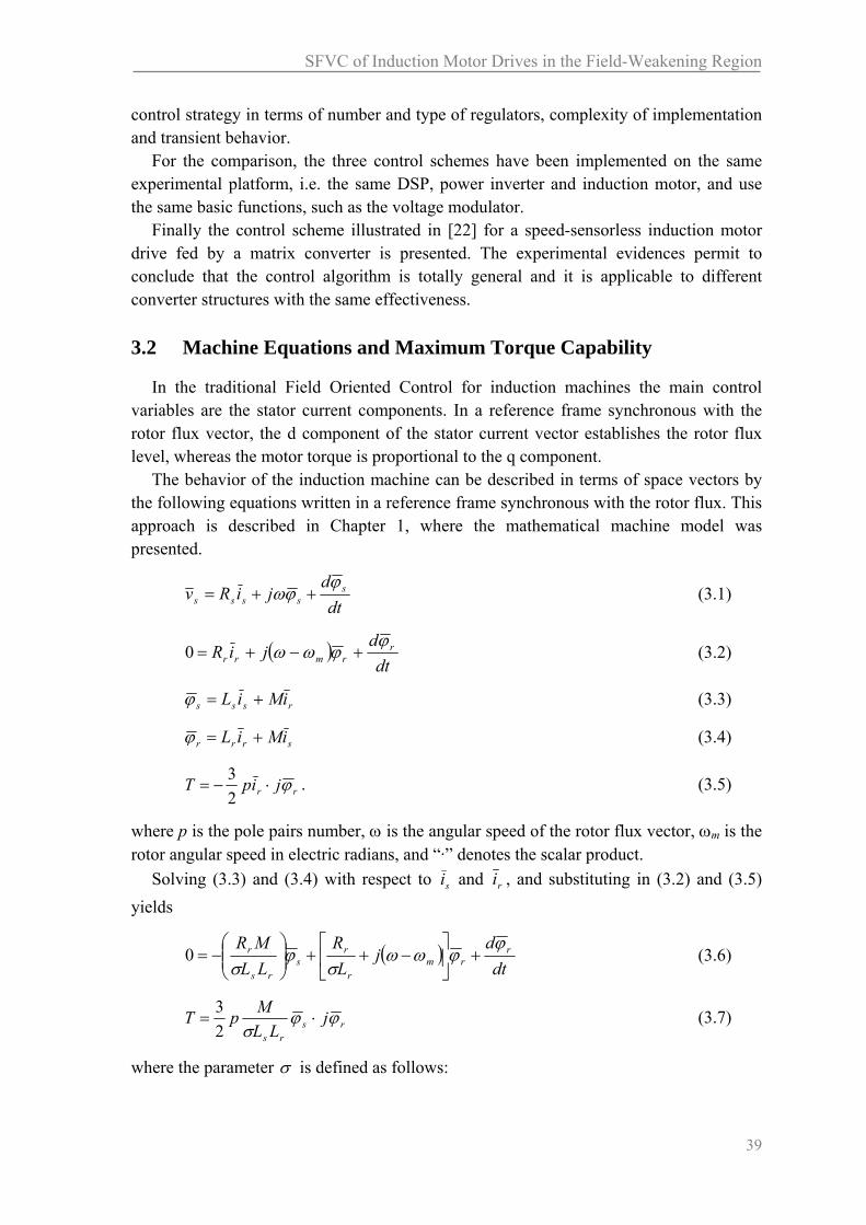
Since the magnitude of the stator current vector must not exceed the maximum current Is,max, a limitation strategy should be present to prevent the flux request φsq,req from reaching too high values.
If isd is the d-component of the current corresponding to the flux φsd, in order to guarantee that the current limit (3.18) is satisfied, the absolute value of isq cannot be greater than the following value:
22,, sdmaxsavailablesq iIi . (3.24)
As a consequence, due to (3.14), the flux component φsq cannot be greater than the following limit value:
φsq,available = σLs isq,available. (3.25)
In conclusion, the maximum torque compatible with the constraints (3.17) and (3.18) is given in any operating condition by the following value of φsq:
availablesqsdsq,max ,,min . (3.26)
This fundamental relationship will be used by the field weakening algorithm to achieve the maximum torque operation.
A. Control Algorithm The torque control block diagram, including the proposed field weakening strategy, is
shown in Fig. 3.1. It is worth noting that the subscript "req" in Fig. 3.1 is used for the output quantities of the regulators, whereas the subscript "ref" denotes the reference signals at the input of the regulation loops.
The control scheme is implemented in a reference frame synchronous with the rotor flux vector, as traditional field oriented controls. It is assumed that a suitable observer
estimates s , r , and the angular frequency of the rotor flux vector.
s
refs ,
s
Stator Flux Regulator
s,maxV
s,reqvje SVM
IM
dq abc
s
si
T
refT
refsd ,
refsq ,s,maxV
Limitation (d)
refsv ,
reqsq ,
srefsv ,
| · | ABS
Maximum voltage request
reqs,maxv
reqsd ,
T
maxsq ,
availablesqi ,
min
availablesq ,s
si jeLimitation (c)
sL isd
isq
maxsI ,
reqs,maxv
si
si
Limitation (b)
maxsq ,
PI (a)
PI (e)
Anti-windup
Anti-windup
ratedsd ,
Limitation (f)
22sds,max iI
Observer for stator and
rotor fluxes, and angular frequency .
Fig 3.1 Block diagram of the torque control scheme, including the field weakening strategy.

SFVC of Induction Motor Drives in the Field-Weakening Region
43
B. Torque Control The motor torque is controlled by comparing the torque reference Tref with the
estimated torque T. On the basis of the torque error, the PI regulator (a) produces a torque request by adjusting the q-component of the stator flux, according to (3.11). Therefore, if the reference torque is higher than the actual torque, the PI regulator (a) tends to increase
the q,req, otherwise it tends to decrease it.
C. Control of Stator and Rotor Fluxes The rotor flux is controlled by adjusting the d-component of the stator flux, according
to (3.9). In region I, the d-component of the stator flux is constant and has the rated value
ratedsd , . At higher speeds, instead, it is reduced by the field weakening algorithm, as
described in section 3.4. The stator flux regulator behaves as a proportional controller, with some additional
terms compensating the stator back-EMF and the voltage drop caused by the stator resistance. The stator flux regulator equation can be expressed as follows:
srefs
sssreqs jiRv
,
, (3.27)
where 1/ represents the gain of the controller.
Combining (3.27) and (3.1), i.e. reqss vv , , leads to the following equation, expressing
the dynamic behavior of the stator flux vector:
refsss
dt
d,
. (3.28)
According to (3.28), in order to obtain fast flux transients, and consequently a high
torque dynamic, it is necessary to adopt small values of . The limitation block (d) ensures that the voltage reference satisfies the voltage
constraint (3.17), namely the voltage reference vector lies inside a circle with radius Vs,max.
The behavior of the limitation block (d) is described by the following equation:
s,maxreqss,max
reqs
reqs
s,maxreqsreqs
refsVvifV
v
v
Vvifv
v,
,
,
,,
, (3.29)
According to (3.29), if the requested voltage is greater than Vs,max the limitation block (d) performs a proportional reduction of its magnitude, but preserves the angular phase.
Finally, the reference voltage vector in the stator reference frame is calculated by
means of the operator je , where is the phase angle of the rotor flux vector with respect to the stationary reference frame.

Chapter 3
44
D. Maximum Torque Capability In order to guarantee the maximum torque capability, the flux request has to be lower
than φsq,max given by (3.26). This task is performed by the limitation block (b), shown in details in Fig. 3.2. At low speed this block does not limit φsq for usual overload conditions.
It is interesting to note that, at high speed, the limitation block (b) prevents instability phenomena by limiting the torque reference (i.e. φsq,ref) to values lower than the maximum achievable torque, according to (3.26). In fact, without the limitation block (b), an excessive torque request causes an increase of the requested voltage, which in turn yields to a reduction of φsd and the produced torque. This behavior leads to a progressive reduction of the stator flux until the motor stops.
E. Field Weakening Algorithm Several field weakening strategies are possible for induction motor drives, as reported
in the introduction. However, the best results are obtained using closed-loop controllers based on the principle of reducing the flux reference as soon as the voltage request becomes greater than the available voltage. The algorithms presented in [13] and [14] are based on the same principle. They are described in section 3.6, where they are compared with the control strategy illustrated in [19].
This principle can be implemented according to the block diagram shown in Fig. 3.3. As can be seen, the stator flux regulator compares the flux reference with the
corresponding estimated value and establishes the voltage that has to be applied to the motor. When the motor operating point is very close to the field weakening region, the voltage request may become greater than the limit voltage Vs,max. A negative difference
maxsq,
reqsq,
refsq,
maxsq,
Fig. 3.2 Limitation block (b) for the q-component of the stator flux vector.
s
refs ,
s
Stator Flux Regulator
s,maxV
s,reqvSVM
s,maxV
Limitation (d)s
refsv ,
reqsd ,
Anti-windup
ratedsd ,
Limitation (f)
| · | ABSPI (e)
refsd ,
Fig 3.3 Block diagram of the field weakening controller based on the saturation of the voltage regulator.
SFVC of Induction Motor Drives in the Field-Weakening Region
45
between the limit voltage and the amplitude vs,req of the requested voltage means that the back-emf is too high and the flux level should be reduced. This task is performed by the PI regulator (e), that integrates the difference s,reqs,max vV . If this difference is negative,
the flux request decreases; otherwise, the flux level increases up to the rated value defined in the limitation block (f). Fig. 3.4 shows the behavior of the limitation block (f) in
details, where sd,rated and sd,min are the rated and the minimum admissible value of the d-component of the stator flux, respectively.
It is worth noting that in the field weakening region, owing to the integral part of the regulator (e), the amplitude of the voltage request tends to equal the limit voltage. From this point of view, the field weakening control scheme is very similar to an anti-windup scheme preventing a voltage request greater than the available voltage.
Although the scheme of Fig. 3.3 allows the motor to fully utilize the supply voltage, it has an inherent drawback related to the fact that fast variations of the torque demand in region II and III lead to undesired flux transients, that delay the torque response. In fact
this scheme is based on selecting sd,ref so that the voltage required to produce the demanded torque satisfies the voltage limit. For example, when a torque variation is required in region II or III, the control system, as a consequence of the corresponding
variation of the requested voltage, changes sd,ref, thus causing undesired transients. To avoid this problems, the scheme of Fig. 3.3 should be modified in order to change
the basic principle for the selection of the flux level. In particular, the flux level should be always set to the value required to generate the maximum achievable torque at any operating speed. In this way any demand of torque variations within the admissible values
is achieved without changing sd but only sq. This new field weakening strategy is implemented as shown in Fig. 3.1.
For a given value of the d-component of the stator flux, and consequently of the rotor
flux, the maximum torque is achieved when sq,ref = ±sq,max. Taking this equation into account, the voltage required to generate the maximum torque can be determined from (3.27) as follows:
sdrefsd
maxsqsqmaxsdsreqmaxsd iRv
,
,, sign . (3.30)
sqrefsq
sdmaxmaxsqsreqmaxsq iRv
,
,, . (3.31)
where isq,max is defined as follows:
ratedsd ,
ratedsd ,
reqsd ,
minsd ,
refsd ,
minsd ,
Fig. 3.4 Limitation block (f) for the d-component of the stator flux vector.

Chapter 3
46
s
maxsq
maxsq Li
,
, . (3.32)
and ωmax is the corresponding angular frequency of the rotor flux, expressed by
sd
sqmaxsq
r
rsqmax L
R
||sign ,
. (3.33)
It is worth noting that in practical applications it is possible to approximate ωmax with ω and therefore the knowledge of the rotor parameters are not necessary.
The main advantage of the proposed field weakening scheme is the independence of the base speed and a fast torque response in the field weakening region.
3.3 Flux and Torque Observers
A. Flux Observer The aim of the flux observer is the determination of stator flux and phase angle of the
rotor flux, which are necessary for the field oriented control of the induction machine. The flux observer operates in the stator reference frame. In the following the subscript “s” will be used to identify quantities expressed in the stator reference frame.
The stator flux is determined integrating the stator voltage:
dtiRv sss
ss
ss . (3.34)
The rotor flux can be estimated as follows
sss
ss
rsr iL
M
L . (3.35)
The phase angle of the rotor flux vector, necessary for the field oriented control, can be derived from (3.35) as follows
sss
ss
sr iL argarg . (3.36)
It is evident from (3.34) that the estimation of the stator flux vector can be affected by stator resistance mismatch, sensor offsets and the inverter non-linearity (inverter dead-times, voltage drop on the conducting switches, etc.). However, at high speed, and hence in the field weakening region, the estimation error is lower than that at low speed, because the input voltage becomes the most relevant term in the second member of (3.34).
The estimation error on the phase angle depends on the stator flux estimation error,
the mismatch on the leakage inductance Ls and the offset of the current sensors. The leakage inductance shows moderate variations with the stator currents and it will be assumed practically constant.
In conclusion, the stator flux observer depends only on two machine parameters,
namely Rs and Ls, but the effects of this dependence can be considered negligible in the

SFVC of Induction Motor Drives in the Field-Weakening Region
47
high speed range. On the contrary, in order to obtain good performance at low speed, it is preferable to adopt a closed-loop flux estimator, that could reduce the effect of parameter mismatch and sensor offsets [4], [20] and [21].
B. Estimation of the Angular Frequency of the Rotor Flux Vector The angular frequency ω needed in (3.27) and (3.33) is obtained by means of the
following equation:
r
r
r
r jdt
d
. (3.37)
The angular frequency ω is insensitive to disturbance and noise that usually affect the stator flux and the stator currents, owing to the filtering action applied to the rotor flux. When this action is not adequate, an additional low-pass filter can be applied to (3.37).
C. Torque Estimation The torque can be estimated from the measurements of the stator current and the
estimation of the stator flux, as follows:
ss jipT 2
3 (3.38)
As can be seen, the torque estimation does not require explicitly any motor parameters, excepts the pole pairs.
3.4 Simulations and Experimental Results
Preliminarily, some numerical simulations have been carried out to confirm the effectiveness of the field weakening strategy. The motor parameters are reported in Tab. I, and the load is supposed to be only inertial.
Fig. 3.5 shows the motor behavior in response to a 25 Nm step command of the motor
torque (the figure does not include the end of the transient). Vertical dash-dotted lines delimit the three regions of operation of the induction motor. Initially, the torque delivered to the load is zero, the motor is at standstill and the stator flux corresponds to the rated value. As the torque command is applied, the motor starts up. The q-component
TABLE I – MOTOR PARAMETERS
Prated = 4 kW Rs = 0.45 Is, rated = 16 Arms Rr = 0.44 Vs,rated = 110 Vrms Ls = 56 mH s = 250 rad/s Lr = 56 mH J = 0.03 Kg m2 M = 53 mH Jtot = 0.22 Kg m2 p = 2

Chapter 3
48
of the stator flux requested by the PI regulator (a) is limited by the value sq,max, corresponding to a stator current equal to Is,max.
As soon as vs,max req reaches the voltage limit, the field weakening algorithm decreases the d-component of the stator flux. As a consequence of the reduction of the magnetizing
current, the q-component of the stator current, proportional to sq,ref, increases, making it possible to keep the stator current equal to the limit current in region II. As soon as the
motor enters in region III, the current decreases and the maximum value of sq,ref is set
equal to sd,ref. Fig. 3.6 shows the motor behavior after a torque reduction from 25 Nm to 5 Nm in
region II. As can be seen, immediately after the torque decreases, the voltage delivered to
the loads is lower than Vs,max, but this voltage margin does not cause the increase of sd. In
fact, the motor continues accelerating and sd decreases without unwanted transients. This behavior could not be achieved without changing the basic scheme of the field weakening strategy of Fig.3.3 as proposed in Fig. 3.1.
A complete drive system has been realized to verify the feasibility of the proposed control scheme. The experimental set-up consists of an IGBT inverter and a 4 kW, 4-pole squirrel cage induction motor. The motor parameters are the same ones reported in Tab. I. The test motor is coupled to a separately excited DC machine, 18.4 kW, 3000 rpm. The control algorithm is implemented on a Digital Signal Processor (DSP) TMS320C28. The
cycle period of the control scheme, including the field weakening algorithm, is 100 s. Some tests have been carried out to investigate the drive performance in the field
weakening region. In order to limit the test bench speed to safe values, the motor has been fed with a reduced voltage, i.e. 50% of the rated voltage, so leading to a rated speed of about 700 rpm.
10
20
30
40
0
0.2
0.4
0
50
100
0.5 1 1.5 2 2.5 3 3.5 4-50
0
50
0.5 1 1.5 2 2.5 3 3.5 40
1000
2000
(2)
(3)
(4)
(5)
(7)
(8)
Nm
Wb
V
A
rpm
Region I Region II Region III
(1)
(6)
0.5 s/div
Fig. 3.5 Computer simulation. Starting transient from 0% up to 700% of the base speed after a torque step of 25 Nm. Main motor quantities. 1) Torque reference. 2) Estimated torque. 3) φsd,ref. 4) φsq,ref.. 5) Vs,max. 6) Vs, max req.

SFVC of Induction Motor Drives in the Field-Weakening Region
49
Fig. 3.7 shows the motor behavior during a transient from 0% up to 700% of the rated speed (the figure does not include the end of the transient) after a torque step of 20 Nm. As can be seen, the motor behaves as expected, namely the current is constant in region II and decreases in region III. The experimental results are in good agreement with the computer simulations shown in Fig. 3.5. In particular φsq,ref, constant in region I, slightly increases in region II, keeping the stator current equal to the limit value.
Some tests were carried out to assess the dynamic performance of the motor drive. In Fig. 3.8, the motor behavior in region I during a 20 Nm torque reversal is shown. As can be seen, the motor behavior is not affected by the field weakening algorithm and a torque dynamic is achieved.
Fig.3.9 shows the motor behavior in region II during a fast variation of the torque command form 20 Nm to 5 Nm during an acceleration transient. As can be seen, the
0 10
20
30
40
0
0.2
0.4
0
50
100
-50
0
50
0
1000
2000
(1)
(2)
(3)
(4)
(5)
(7)
(8)
0.5 s/div
Nm
Wb
V
A
rpm
Region I Region II
(6) (6´)
Fig. 3.6 Computer simulation. Torque reduction from 25 Nm to 5 Nm in region II during an acceleration transient. Main motor quantities. 1) Torque reference 2) Estimated torque. 3) φsd,ref. 4) φsq,ref.. 5) Vs,max. 6) vs,max req. 6’) vs. 7) Stator current. 8) Motor speed.
(2)
(4)
Region I Region II Region III
(1)
(3)
Fig. 3.7 Experimental test. Starting transient from 0% up to 700% of the base speed. Main motor quantities.1) Estimated torque (20 Nm/div). 2) φsd,ref (0.2 Wb/div). 3) φsq,ref. (0.2 Wb/div). (4) Stator current (20A/div).

Chapter 3
50
behavior of the motor is similar to that of Fig. 3.6, namely φsd,ref is not affected by the torque transient. In response to the torque variation only φsq,ref changes and consequently
(2)
(4)
(1)
(3)
Fig. 3.8 Experimental test. Torque reversal from 20 Nm to -20 Nm starting from 70% of the base speed. 1)Estimated torque (20 Nm/div). 2) Speed (700 rpm/div). 3) φsq,ref. (0.2 Wb/div). 4) Stator current (20A/div).
(2)
(4)
(1)
(3)
Region I Region II Region III
(1’)
Fig. 3.9 Experimental test. Torque variation in region II from 20 Nm to 5 Nm during an accelerationtransient. Main motor quantities. 1) Estimated torque (20 Nm/div). 1’) Torque command (20 Nm/div). 2)φsd,ref (0.2 Wb/div). 3) φsq,ref (0.20 Wb/div). 4) Stator current (20A/div).
(2)
(4)
Region III Region II Region I
(1)
(3)
Fig. 3.10 Experimental test. Deceleration transient from 600% to 80% of the base speed. Main motorquantities. 1) Estimated torque (20 Nm/div). 2) φsd,ref. (0.2 Wb/div). 3) φsq,ref.(0.2 Wb/div). 4) Stator current (20A/div).
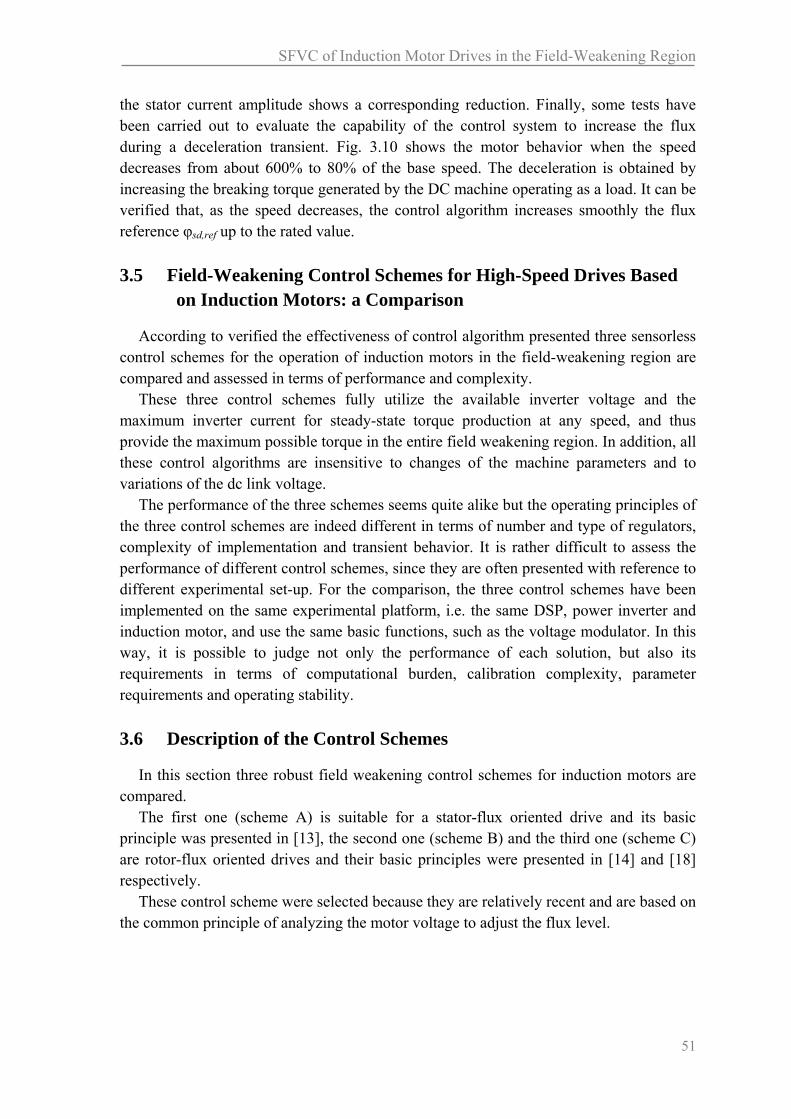
SFVC of Induction Motor Drives in the Field-Weakening Region
51
the stator current amplitude shows a corresponding reduction. Finally, some tests have been carried out to evaluate the capability of the control system to increase the flux during a deceleration transient. Fig. 3.10 shows the motor behavior when the speed decreases from about 600% to 80% of the base speed. The deceleration is obtained by increasing the breaking torque generated by the DC machine operating as a load. It can be verified that, as the speed decreases, the control algorithm increases smoothly the flux reference φsd,ref up to the rated value.
3.5 Field-Weakening Control Schemes for High-Speed Drives Based on Induction Motors: a Comparison
According to verified the effectiveness of control algorithm presented three sensorless control schemes for the operation of induction motors in the field-weakening region are compared and assessed in terms of performance and complexity.
These three control schemes fully utilize the available inverter voltage and the maximum inverter current for steady-state torque production at any speed, and thus provide the maximum possible torque in the entire field weakening region. In addition, all these control algorithms are insensitive to changes of the machine parameters and to variations of the dc link voltage.
The performance of the three schemes seems quite alike but the operating principles of the three control schemes are indeed different in terms of number and type of regulators, complexity of implementation and transient behavior. It is rather difficult to assess the performance of different control schemes, since they are often presented with reference to different experimental set-up. For the comparison, the three control schemes have been implemented on the same experimental platform, i.e. the same DSP, power inverter and induction motor, and use the same basic functions, such as the voltage modulator. In this way, it is possible to judge not only the performance of each solution, but also its requirements in terms of computational burden, calibration complexity, parameter requirements and operating stability.
3.6 Description of the Control Schemes
In this section three robust field weakening control schemes for induction motors are compared.
The first one (scheme A) is suitable for a stator-flux oriented drive and its basic principle was presented in [13], the second one (scheme B) and the third one (scheme C) are rotor-flux oriented drives and their basic principles were presented in [14] and [18] respectively.
These control scheme were selected because they are relatively recent and are based on the common principle of analyzing the motor voltage to adjust the flux level.

Chapter 3
52
A. Control Scheme (A) The block diagram of control scheme (A) is shown in Fig. 3.11. The control scheme is
implemented in a reference frame synchronous with the stator flux vector. The main control variables are the stator flux magnitude φs and the q component of the stator current isq.
The speed is adjusted by PI regulator (a), that generates the request of torque-producing current, isq,req. The current reference is tracked in its turn by the PI regulator (d). Due to the action of the saturation block (g), isq,ref is limited so that the stator current magnitude cannot exceed Is,max in region I and II. In this case, the maximum value for isq,ref depends on the current isd used for the generation of the flux. The greater is isd, the lower is isq,max. In region III PI regulator (e) further decreases isq,max until the angle between the stator and rotor flux vectors is 45°, i.e., the maximum torque condition is reached.
The stator flux command is generated by the PI regulator (b) on the basis of the voltage request. If this request is greater than the available voltage, the field weakening algorithm reduces the flux, otherwise the flux is increased, but not beyond its rated value.
Finally, the switch (s) can create a temporary voltage margin to enable a fast reaction of the current controller, in order to improve the transient behavior. If the requested voltage is greater than the available voltage, i.e., the flux is being decreased, the switch (s) is closed and the angle θs of the reference frame is modified by adding a small quantity Δθs proportional to the speed error. As a consequence, this small rotation of the reference frame is applied to the stator voltage and has the effect to improve the torque production to the detriment of the flux especially in the beginning of the speed transient
Although this last algorithm has the aim of improving the behavior of the motor during the speed transients in the field weakening speed range, actually it is not essential for the field weakening operation. Hence for the sake of simplicity the effects related to the switch (s) have not been considered in this analysis
PI (e)
s
SVM
IM
dq abc
s
ssi
Observer for stator and
rotor fluxes, angular
frequency and motor speed m
s,maxV
m
refm,
rateds ,
maxsqi ,
PI (a)
PI (b)
s
s
s
s+
reqsv ,
maxsqi ,
maxsqi ,
22 )(s,maxI
s,maxV
Limitation (i)
PI (c) refs ,
Limitation (f)
max=45°
refsqi ,
sqi
isd
Switch (s) < 0
ssje
sje
Limitation (h)
reqsqi ,PI (d)
| · | ABS
reqsv ,
Gains (m)
s
vsd,req
vsq,req
Limitation (g)
Anti-windup
Anti-windup
Anti-windup
Fig. 3.11 Block diagram of the control scheme (A).

SFVC of Induction Motor Drives in the Field-Weakening Region
53
B. Control Scheme (B) The block diagram of the control scheme (B) is shown in Fig. 3.12. The control
scheme is implemented in a reference frame synchronous with the rotor flux vector. The motor currents, which are the main control variables, are adjusted by PI regulators
(c) and (d). The d component of the stator current is used to regulate the rotor flux, whereas the q component is used to vary the motor torque.
To adjust the field level, the scheme uses the same method proposed in scheme (A), namely the reference value for isd is set by the PI regulator (b) on the basis of the voltage request. If the voltage request is greater than the available voltage, the flux level is reduced, otherwise it is increased to the rated value.
The speed is controlled by the regulator (a), that generates the reference value for isq. The limitation block (g) ensures that the constraint on the stator current is satisfied in region I and II, and also the exploitation of the maximum torque capability in region III.
In fact the output signal isq,max of the limitation block (g) is equal to 22sds,max iI in region I
and II, whereas in region III it is decreased until the absolute value of the vsd is equal to
2s,maxV
. As explained in section 3.2, this condition means that, under the assumption that
the maximum voltage is applied to the motor, the phase angle of the voltage vector in the
rotor-flux oriented reference frame is 90°45°.
C. Control Scheme (C) The block diagram of the control scheme (C) is shown in Fig. 3.13. In this rotor-flux-
oriented control scheme the main control variables are the stator flux components instead of the stator current components. The scheme (C) corresponds to the same control strategy described in sections 3.3 and 3.4 except for the fact that the input reference is a speed instead of a torque.
s
refs ,
s
Stator Flux Regulator
s,maxV
s,reqvje SVM
IM
dq abc
s
si
m
refm,
refsd ,
refsq ,s,maxV
Limitation (d)
refsv ,
reqsq ,
srefsv ,
| · | ABS
Maximum voltage request
reqs,maxv
reqsd ,
T
maxsq ,
availablesqi ,
min
availablesq ,s
si jeLimitation (c)
sL isd
isq
maxsI ,
reqs,maxv
si
si
Limitation (b)
maxsq ,
PI (a)
PI (e)
Anti-windup
Anti-windup
ratedsd ,
Limitation (f)
22sds,max iI
Observer for stator and
rotor fluxes, and angular frequency .
Fig 3.13 Block diagram of the torque control scheme, including the field weakening strategy.
PI (c)
PI (d)
refsqi ,
sqi
m
refm,maxsqi ,
PI (a)
maxsqi ,
SVM
IM
dq abc r
ssi
Observer for stator and
rotor fluxes, angular
frequency and motor speed m
s,maxV
Limitation (i)
s,maxV
| · | ABS
reqsv ,
PI (b)
Limitation (f)
22 )(s,maxI
PI (e)
Limitation (h)
2
s,maxV
|vsd,req| maxsqi ,
isd,refratedsdi ,
rje
rje sdi
sdi
vsd,req
vsq,req
Limitation (g)
availableqi ,
reqsqi ,
Back-emf compensation
availableqi ,
Anti-windup
Anti-windup
Anti-windup
Fig. 3.12 Block diagram of the control scheme (B).

Chapter 3
54
3.7 Flux Observers
The control schemes (B) and (C) are implemented in a reference frame synchronous with the rotor flux vector whereas scheme (A) is described in a reference frame synchronous with the stator flux. Hence, the same flux observer, described in section 3.3, is used for the schemes (B) and (C) whereas the scheme (A) uses a different solution.
to obtain good performance at low speed, all the schemes adopt a closed-loop flux estimators, that could reduce the effect of parameter mismatch and sensor offsets.
A closed-loop estimator is based on the principle that feeding back the difference between the measured output of the observed system and the estimated output, and continuously correcting the model by the error signal, the error should be minimized. In the case of a flux estimator, the motor flux cannot be directly measured, but the idea of realizing a closed-loop system is still applicable if the difference between a signal representing the steady-state value of the reference flux and the signal of the estimated flux vector is used as feedback signal.
Let us denote with θs and θr the phase angle of ss and s
r in the stator reference
frame. Hence, (3.34) is replaced for scheme (A) by the following equation:
ss
jrefss
sss
ss
ss seGiRv
dt
d
, (3.39)
and for schemes (B) and (C) by the following equation:
sr
srefrr
sss
ss
ss GiRv
dt
d
, . (3.40)
The quantities Gs and Gr in (3.39) and (3.40) are the gains of the flux observers. The reference flux vector can be calculated for scheme (B) as
rjrefsd
srefr eMi ,, (3.41)
PI (c)
PI (d)
refsqi ,
sqi
m
refm,maxsqi ,
PI (a)
maxsqi ,
SVM
IM
dq abc r
ssi
Observer for stator and
rotor fluxes, angular
frequency and motor speed m
s,maxV
Limitation (i)
s,maxV
| · | ABS
reqsv ,
PI (b)
Limitation (f)
22 )(s,maxI
PI (e)
Limitation (h)
2
s,maxV
|vsd,req| maxsqi ,
isd,refratedsdi ,
rje
rje sdi
sdi
vsd,req
vsq,req
Limitation (g)
availableqi ,
reqsqi ,
Back-emf compensation
availableqi ,
Anti-windup
Anti-windup
Anti-windup
Fig. 3.13 Block diagram of the control scheme (B).

SFVC of Induction Motor Drives in the Field-Weakening Region
55
and for scheme (C) as
rjrefsd
s
srefr e
L
M ,, (3.42)
The performance of these observers at low speed is not equal. Furthermore they require the knowledge of different motor parameters. Therefore it could seem unfair the use of different observers for the comparison of three different control schemes.
These solutions have been adopted mainly for the sake of simplicity. Nevertheless, it is opportune to recall that the purpose of this analysis is to compare the field-weakening algorithms of the three control schemes and it is sufficient that the observers present approximately the same behavior before entering the field weakening speed range. In fact, at high speed, the integration of the voltage back-emf provides an estimation of the stator flux vector that is sufficiently reliable for all the three observers, and the effect of the feedback signal is less important.
3.8 Tuning of the Control Schemes
The three schemes presents a different complexity in terms of tuning of the regulators. In total, scheme (A) requires 5 PI regulators (two PI regulators are used for the flux and current control, one for the speed control and the other two for the robust field-weakening algorithm), and if a fast torque response is needed, it is necessary to tune also the two constant gains shown in block (m).
Scheme (B) requires 5 PI regulators (two PI regulators are used for the current control, one for the speed control and the other two for the robust field-weakening algorithm).
Finally, scheme (C) requires two PI regulators (the first one for the speed control and the second one for the robust field-weakening control), and two gain constants for the flux regulator (7) and (8).
For the regulators of the inner loops, i.e., regulators (d) and (e) in scheme (A), regulators (c) and (d) in scheme (B) and the stator flux regulators in scheme (C), some simple design rules can be derived, generally based on zero-pole cancellations.
The tuning of the other regulators, instead, is more difficult, because the drive dynamics depends on the motor inertia and on the field-weakening algorithm. So the tuning of these regulators has been initially faced by means of numerical simulations, and then it has been refined during the experimental tests by using a trial-and-error procedure.
3.9 Experimental Results
A complete drive system has been realized to verify the performances of the control schemes. The experimental set-up is the same described in section 3.6. The sampling
period (coinciding with the switching period) is 100 s. The parameters of the electric drive are shown in Table I and the rated speed is about
700 rpm. It is important to note that the performance of each control scheme depends on many
factors that are not directly related to the field-weakening control scheme, such as the use
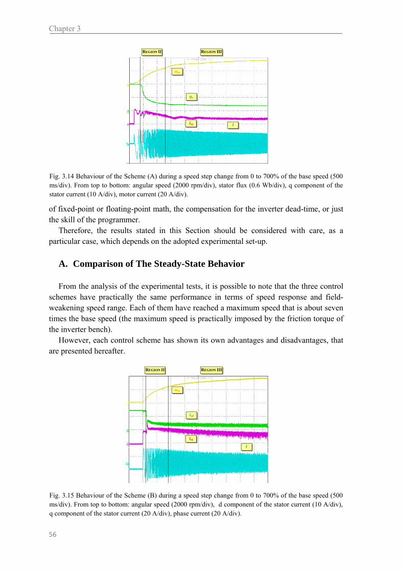
Chapter 3
56
of fixed-point or floating-point math, the compensation for the inverter dead-time, or just the skill of the programmer.
Therefore, the results stated in this Section should be considered with care, as a particular case, which depends on the adopted experimental set-up.
A. Comparison of The Steady-State Behavior From the analysis of the experimental tests, it is possible to note that the three control
schemes have practically the same performance in terms of speed response and field-weakening speed range. Each of them have reached a maximum speed that is about seven times the base speed (the maximum speed is practically imposed by the friction torque of the inverter bench).
However, each control scheme has shown its own advantages and disadvantages, that are presented hereafter.
REGION II REGION III
m
s
isq i
Fig. 3.14 Behaviour of the Scheme (A) during a speed step change from 0 to 700% of the base speed (500ms/div). From top to bottom: angular speed (2000 rpm/div), stator flux (0.6 Wb/div), q component of thestator current (10 A/div), motor current (20 A/div).
REGION II REGION III
m
isd
isq
i
Fig. 3.15 Behaviour of the Scheme (B) during a speed step change from 0 to 700% of the base speed (500ms/div). From top to bottom: angular speed (2000 rpm/div), d component of the stator current (10 A/div),q component of the stator current (20 A/div), phase current (20 A/div).

SFVC of Induction Motor Drives in the Field-Weakening Region
57
Figs. 3.14, 3.15 and 3.16 show the behavior of the three control schemes during a speed step command up to 700% of the base speed. Each figure shows the speed response (at the top) and the corresponding phase current waveform (at the bottom). The two intermediate traces of each figure show the waveforms of the main control variables of each control scheme, i.e., the stator flux and the current isq for scheme (A), the stator current components for scheme (B) and the stator flux components for scheme (C).
In Figs. 3.14, 3.15 and 3.16 the speed ranges of region II and region III are also represented.
The main comments that can be done are as follows:
i. The speed responses of schemes (B) and (C) are quite similar, whereas the one of scheme (A) shows some small oscillations in region III.
ii. The best quality of the motor current is obtained by scheme (B), since the stator current components are the main control variables. The current quality can be seen also during the transition from Region I to Region II and from Region II to Region III.
iii. The best flux quality is obtained by scheme (C), since the stator flux components
are the main control variables
B. Tuning the Regulators and Robustness As expected, the tuning of scheme (C) is simpler than that of other ones, whereas the
tuning of scheme (A) is more complex, especially for the flux regulators (b) and (c) of Fig. 3.12, in order to avoid flux and torque oscillations during the transition from Region II to Region III.
As far as the robustness against parameter uncertainties is concerned, the performance of the three control schemes is affected mainly by mismatching of the leakage inductance
REGION II REGION III
m
sd
sq
i
Fig. 3.16- Behaviour of the Scheme (C) during a speed step change from 0 to 700% of the base speed (500 ms/div). From top to bottom: angular speed (2000 rpm/div), d component of the stator flux (0.25 Wb/div),q component of the stator flux (0.25 Wb/div), phase current (20 A/div).
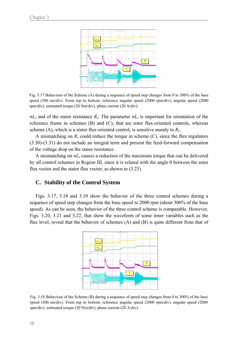
Chapter 3
58
σLs and of the stator resistance Rs. The parameter σLs is important for orientation of the reference frame in schemes (B) and (C), that are rotor flux-oriented controls, whereas scheme (A), which is a stator flux-oriented control, is sensitive mainly to Rs.
A mismatching on Rs could reduce the torque in scheme (C), since the flux regulators (3.30)-(3.31) do not include an integral term and present the feed-forward compensation of the voltage drop on the stator resistance.
A mismatching on σLs causes a reduction of the maximum torque that can be delivered by all control schemes in Region III, since it is related with the angle θ between the rotor flux vector and the stator flux vector, as shown in (3.23).
C. Stability of the Control System Figs. 3.17, 3.18 and 3.19 show the behavior of the three control schemes during a
sequence of speed step changes from the base speed to 2000 rpm (about 300% of the base speed). As can be seen, the behavior of the three control scheme is comparable. However, Figs. 3.20, 3.21 and 3.22, that show the waveform of some inner variables such as the flux level, reveal that the behavior of schemes (A) and (B) is quite different from that of
m,ref
m
T
i
Fig. 3.17 Behaviour of the Scheme (A) during a sequence of speed step changes from 0 to 300% of the basespeed (500 ms/div). From top to bottom: reference angular speed (2000 rpm/div), angular speed (2000rpm/div), estimated torque (20 Nm/div), phase current (20 A/div).
m,ref
m
T
i
Fig. 3.18 Behaviour of the Scheme (B) during a sequence of speed step changes from 0 to 300% of the basespeed (500 ms/div). From top to bottom: reference angular speed (2000 rpm/div), angular speed (2000rpm/div), estimated torque (20 Nm/div), phase current (20 A/div).

SFVC of Induction Motor Drives in the Field-Weakening Region
59
scheme (C). While the flux level of scheme (C) tends to decrease as expected, the flux level of scheme (A) and (B) presents a short undershot after each speed step. The reason is that these control schemes are based on different operating principle. In fact, as explained in section 3.8, the scheme (C) keeps the rotor flux almost constant during the torque transient, in order to achieve the fastest torque response, whereas the other control schemes adjust the flux level after any torque variation. These flux oscillations are undesired and could prevent the correct operation of the control scheme at high speed. To limit their effect, the designer is forced to tune carefully the speed regulators and to reduce the bandwidth of the whole control system.
D. Comparative Table Table II shows the main results of the comparison of the three control schemes. The properties that are compared in Table II are the easiness of tuning of the
regulators, the quality of the motor currents, the torque dynamic, the independence of the motor parameters and the stability of the control system at high speed.
A grade has been given for each of them based on the results obtained from the experimental tests. This grade is qualitative and varies from "+" (lowest performance) to
m,ref
m
T
i
Fig. 3.19 Behaviour of the Scheme (C) during a sequence of speed step changes from 0 to 300% of thebase speed (500 ms/div). From top to bottom: reference angular speed (2000 rpm/div), angular speed (2000rpm/div), estimated torque (20 Nm/div), phase current (20 A/div).
m
i
s
Fig. 3.20- Behaviour of the Scheme (A) during several step changes from 0 to 300% of the base speed (500ms/div). From top to bottom: reference and actual angular speed (2000 rpm/div), stator flux magnitude(0.25 Wb/div), motor current (20 A/div).

Chapter 3
60
"+++" (best performance). It is important to point out that this grade has not an absolute meaning but it refers only to the comparison of the selected control schemes, implemented on the same experimental platform, available in laboratory
The results cannot be generalized, since they depend on the specific DSP, inverter and motor used to carry out the experimental tests. Nevertheless, they suggest some practical rules that can be useful to select which control scheme is the most suitable for an application.
The control scheme (A) should be preferred when the robustness to variations of the motor parameters could be crucial for the drive performance. The control scheme (B) should be preferred for a specific application when the quality of the motor currents plays a key role. Finally the control scheme (C) is preferable when the application requires a fast torque response in the field-weakening region or the tuning of the regulators has to be as simple as possible
m
sd
i
sq
Fig. 3.22- Behaviour of the Scheme (C) during several step changes from 0 to 300% of the base speed (500ms/div). From top to bottom: angular speed (2000 rpm/div), d and q components of the stator flux (0.25 Wb/div), motor current (20 A/div).
m
sd
i
sq
Fig. 3.21- Behaviour of the Scheme (B) during several step changes from 0 to 300% of the base speed(500 ms/div). From top to bottom: angular speed (2000 rpm/div), d and q components of the stator flux(0.25 Wb/div), motor current (20 A/div).
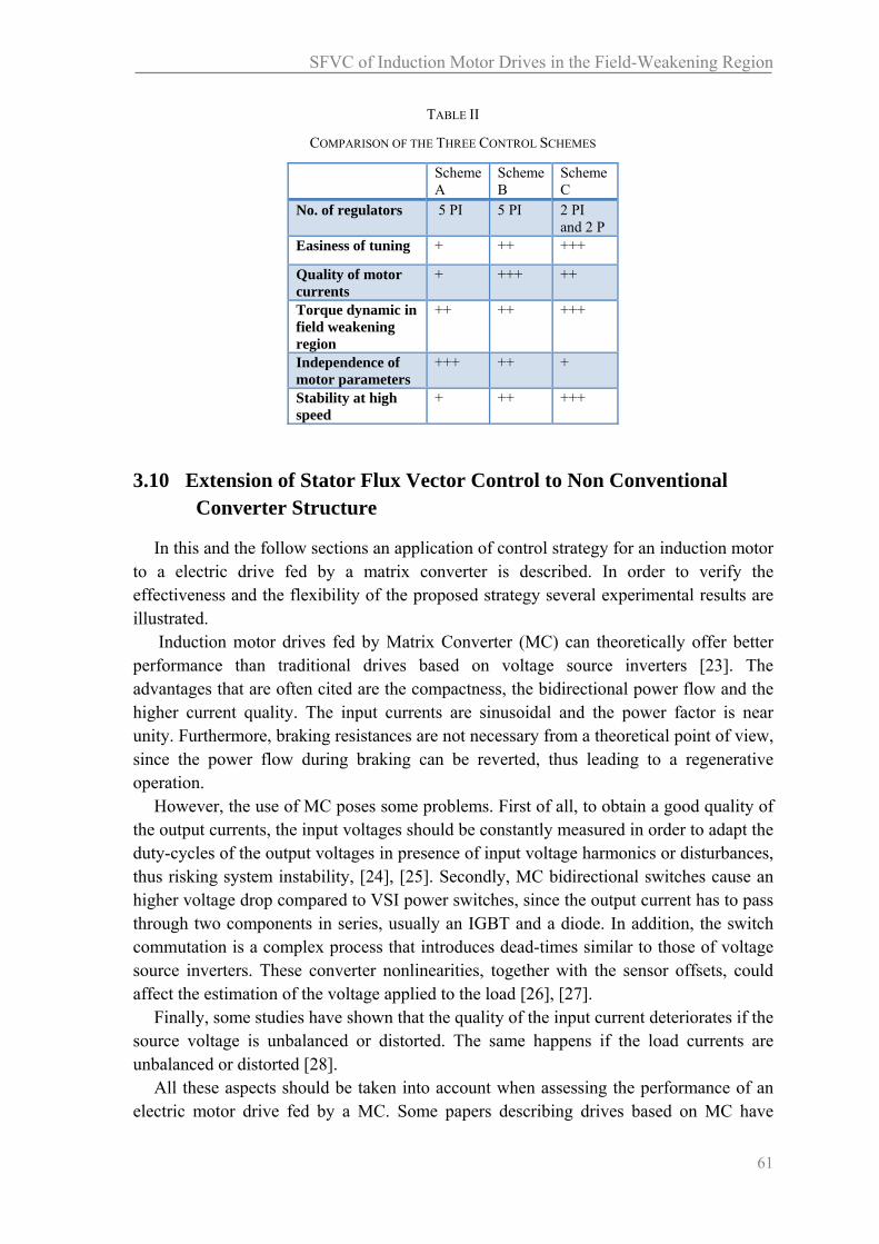
SFVC of Induction Motor Drives in the Field-Weakening Region
61
3.10 Extension of Stator Flux Vector Control to Non Conventional Converter Structure
In this and the follow sections an application of control strategy for an induction motor to a electric drive fed by a matrix converter is described. In order to verify the effectiveness and the flexibility of the proposed strategy several experimental results are illustrated.
Induction motor drives fed by Matrix Converter (MC) can theoretically offer better performance than traditional drives based on voltage source inverters [23]. The advantages that are often cited are the compactness, the bidirectional power flow and the higher current quality. The input currents are sinusoidal and the power factor is near unity. Furthermore, braking resistances are not necessary from a theoretical point of view, since the power flow during braking can be reverted, thus leading to a regenerative operation.
However, the use of MC poses some problems. First of all, to obtain a good quality of the output currents, the input voltages should be constantly measured in order to adapt the duty-cycles of the output voltages in presence of input voltage harmonics or disturbances, thus risking system instability, [24], [25]. Secondly, MC bidirectional switches cause an higher voltage drop compared to VSI power switches, since the output current has to pass through two components in series, usually an IGBT and a diode. In addition, the switch commutation is a complex process that introduces dead-times similar to those of voltage source inverters. These converter nonlinearities, together with the sensor offsets, could affect the estimation of the voltage applied to the load [26], [27].
Finally, some studies have shown that the quality of the input current deteriorates if the source voltage is unbalanced or distorted. The same happens if the load currents are unbalanced or distorted [28].
All these aspects should be taken into account when assessing the performance of an electric motor drive fed by a MC. Some papers describing drives based on MC have
TABLE II
COMPARISON OF THE THREE CONTROL SCHEMES
Scheme A
Scheme B
Scheme C
No. of regulators 5 PI 5 PI 2 PI and 2 P
Easiness of tuning + ++ +++
Quality of motor currents
+ +++ ++
Torque dynamic in field weakening region
++ ++ +++
Independence of motor parameters
+++ ++ +
Stability at high speed
+ ++ +++

Chapter 3
62
already been presented. Some studies have been made to transfer the existing control techniques for voltage source inverters to MCs, such as constant V/Hz, field-oriented control and direct torque control [29]-[34].
Electric drives are often requested to deliver constant power at speed higher than the rated one. However so far the performance of drives fed by MC and operating in the field-weakening region has not been examined in details.
When the induction motors are used for applications at high speed, it is desirable to retain the maximum torque capability in the field weakening region. Several papers about this issue were presented for drives fed by traditional VSI [35]-[40]. According to these field weakening algorithms, the optimal flux value of the motor should be updated by means of look-up tables or explicit expressions containing the motor parameters and quantities such as the motor speed, the motor currents, the dc-link voltage and the requested torque. However, the performance of these algorithms is strictly related to the accuracy by which the parameters are known. In addition, the drive performance in the high speed range may depend on the correct determination of the base speed, which is function of the actual dc-link voltage and the overload capability.
3.11 Simulations and Experimental Results
Preliminarily, some numerical simulations have been carried out to confirm the effectiveness of the field weakening strategy. The motor parameters are reported in Table. III, and the load is supposed to be only inertial.
Fig. 3.23 shows the motor behavior in response to a step command of the motor torque (the figure does not include the end of the transient). Vertical dash-dotted lines delimit the three regions of operation of the induction motor. Initially, the torque delivered to the load is zero, the motor is at standstill and the stator flux corresponds to the rated value. As the torque command is applied, the motor starts up.
The q-component of the stator flux requested by the PI regulator (a) is limited to the
0
0.5
1
0
0.4
0
0.4
0
1000
2000
-2
0
2
(2)
(3)
(4)
(5)
(7)
Nm
Wb
Wb
A
rpm
Region I Region II Region III
(1)
(6)
0.5 s/div
Fig. 3.23 – Computer simulation. Starting transient from 0% up to 600% of the base speed after the application of the rated torque. Main motor quantities. 1) Torque reference. 2) Estimated torque. 3) sd,ref. 4) φsq,ref.. 5) Rotor flux. 6) Motor speed. 7) Stator current.
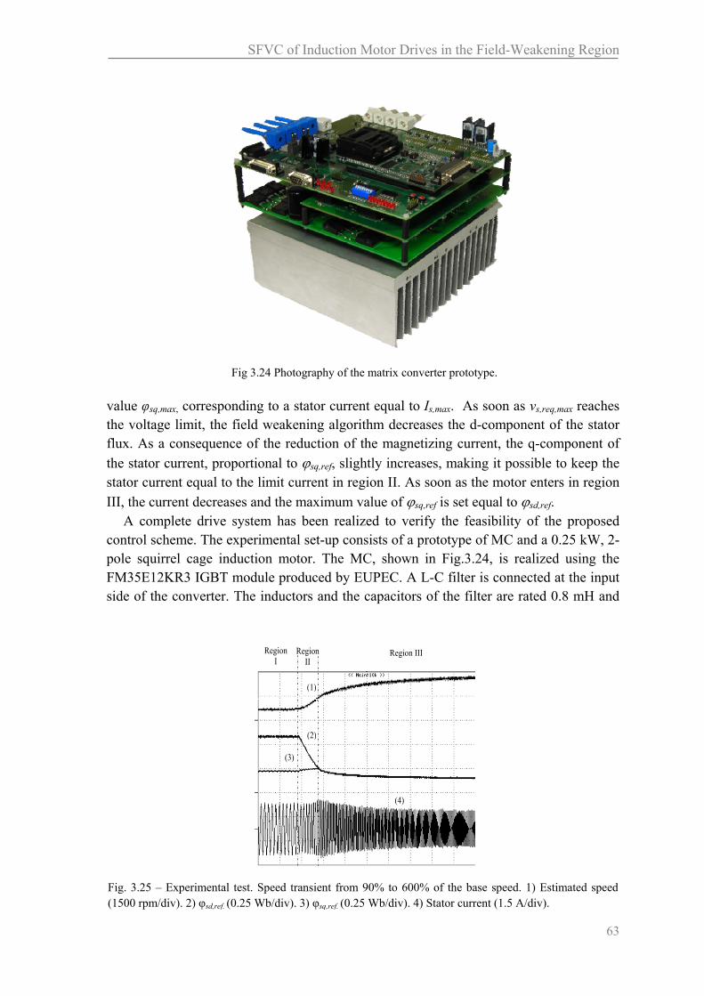
SFVC of Induction Motor Drives in the Field-Weakening Region
63
value φsq,max, corresponding to a stator current equal to Is,max. As soon as vs,req,max reaches the voltage limit, the field weakening algorithm decreases the d-component of the stator flux. As a consequence of the reduction of the magnetizing current, the q-component of
the stator current, proportional to sq,ref, slightly increases, making it possible to keep the stator current equal to the limit current in region II. As soon as the motor enters in region
III, the current decreases and the maximum value of sq,ref is set equal to sd,ref. A complete drive system has been realized to verify the feasibility of the proposed
control scheme. The experimental set-up consists of a prototype of MC and a 0.25 kW, 2-pole squirrel cage induction motor. The MC, shown in Fig.3.24, is realized using the FM35E12KR3 IGBT module produced by EUPEC. A L-C filter is connected at the input side of the converter. The inductors and the capacitors of the filter are rated 0.8 mH and
Fig 3.24 Photography of the matrix converter prototype.
(2)
(4)
(1)
(3)
Region I
Region II
Region III
Fig. 3.25 – Experimental test. Speed transient from 90% to 600% of the base speed. 1) Estimated speed(1500 rpm/div). 2) φsd,ref. (0.25 Wb/div). 3) φsq,ref. (0.25 Wb/div). 4) Stator current (1.5 A/div).

Chapter 3
64
20 F respectively. The motor parameters are the same ones reported in Table. III. The test motor is
coupled to a separately excited DC machine, which can operate up to 3000 rpm. The control algorithm is implemented on a Digital Signal Processor (DSP)
TMS320C28. The cycle period of the control scheme, including the field weakening algorithm, is 125 μs.
Some tests have been carried out to investigate the drive performance in the field weakening region and to assess the dynamic performance of the motor drive. In order to limit the test bench speed to safe values, the motor has been fed with a reduced voltage, i.e. 25% of the rated voltage, so leading to a rated speed of about 700 rpm.
Fig. 3.25 shows the motor behaviour during a transient from 90% up to 600% of the rated speed (the figure does not include the end of the transient). As can be seen, the
(2)
(4)
Region I
Region II
Region III
(1)
(3)
Fig. 3.26 – Experimental test. Starting transient from 0% up to 600% of the base speed. Main motorquantities. 1) Estimated speed (1500 rpm/div). 2) φsd,ref (0.25 Wb/div). 3) φsq,ref. (0.25 Wb/div). 4) Statorcurrent (1.5 A/div).
(2)
(4)
Region I
Region II
Region III
(1)
(3)
Fig. 3.27 – Experimental test. Starting transient from 0% up to 600% of the base speed. Main motorquantities. 1) Estimated speed (1500 rpm/div). 2) φsd,ref (0.25 Wb/div). 3)T Estimated torque (0.8 Nm/div). (4) Stator current (1.5 A/div).

SFVC of Induction Motor Drives in the Field-Weakening Region
65
motor behaves as expected, namely the current is constant in region II and decreases in region III
In Figs. 3.26 and 3.27 the behaviour during a transient after a torque step is shown. The experimental results are in good agreement with the computer simulations shown in Fig. 3.26 In particular φsq,ref, constant in region I, slightly increases in region II, keeping the stator current equal to the limit value.
Fig. 3.28 shows the motor behaviour when the speed decreases from about 500% to 90% of the base speed. The deceleration is obtained by increasing the braking torque generated by the DC machine operating as a load. It can be verified that, as the speed decreases, the control algorithm increases smoothly the flux reference φsd,ref up to the rated value.
Finally, the quality of the input and output currents has been assessed. Although the load current, whose typical waveform is shown in Fig. 3.29, is always sinusoidal and its harmonic content is negligible, the input current is particularly sensitive to the input voltage distortion and unbalance. Table IV reports the main harmonic magnitude of the input voltage vector, normalised with respect to the magnitude of the fundamental component. As can be seen, distortion harmonics of order -1,+2, +3, 5 , and +7, which
(2)
(4)
Region I
Region II Region III
(1)
(3)
Fig. 3.28– Experimental test. Braking transient from 500% down to 90% of the base speed. Main motorquantities. 1) Estimated speed (1500 rpm/div). 2) φsd,ref (0.25 Wb/div). 3) φsq,ref. (0.25 Wb/div). (4) Statorcurrent (1.5 A/div).
Tab. IV Normalised magnitude of the main harmonic components of the Input voltage vector
Harmonic Magnitude (%)
‐1 1,29
+2 0,72
+3 0,48
‐5 1,87
+7 0,58
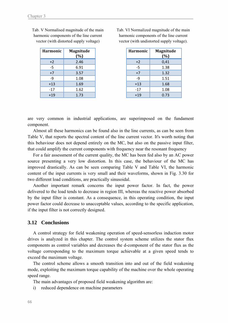
Chapter 3
66
are very common in industrial applications, are superimposed on the fundament component.
Almost all these harmonics can be found also in the line currents, as can be seen from Table V, that reports the spectral content of the line current vector. It's worth noting that this behaviour does not depend entirely on the MC, but also on the passive input filter, that could amplify the current components with frequency near the resonant frequency
For a fair assessment of the current quality, the MC has been fed also by an AC power source presenting a very low distortion. In this case, the behaviour of the MC has improved drastically. As can be seen comparing Table V and Table VI, the harmonic content of the input currents is very small and their waveforms, shown in Fig. 3.30 for two different load conditions, are practically sinusoidal.
Another important remark concerns the input power factor. In fact, the power delivered to the load tends to decrease in region III, whereas the reactive power absorbed by the input filter is constant. As a consequence, in this operating condition, the input power factor could decrease to unacceptable values, according to the specific application, if the input filter is not correctly designed.
3.12 Conclusions
A control strategy for field weakening operation of speed-sensorless induction motor drives is analyzed in this chapter. The control system scheme utilizes the stator flux components as control variables and decreases the d-component of the stator flux as the voltage corresponding to the maximum torque achievable at a given speed tends to exceed the maximum voltage.
The control scheme allows a smooth transition into and out of the field weakening mode, exploiting the maximum torque capability of the machine over the whole operating speed range.
The main advantages of proposed field weakening algorithm are: i) reduced dependence on machine parameters
Tab. V Normalised magnitude of the main harmonic components of the line current
vector (with distorted supply voltage)
Harmonic Magnitude (%)
+2 2.46
‐5 6.91
+7 3.57
‐9 1.08
+13 1.69
‐17 1.62
+19 1.73
Tab. VI Normalized magnitude of the main harmonic components of the line current vector (with undistorted supply voltage).
Harmonic Magnitude (%)
+2 0,41
‐5 1.38
+7 1.32
‐9 1.51
+13 1.68
‐17 1.08
+19 0.73
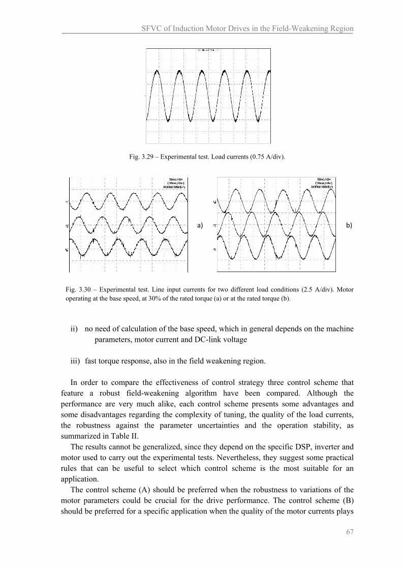
SFVC of Induction Motor Drives in the Field-Weakening Region
67
ii) no need of calculation of the base speed, which in general depends on the machine
parameters, motor current and DC-link voltage
iii) fast torque response, also in the field weakening region.
In order to compare the effectiveness of control strategy three control scheme that feature a robust field-weakening algorithm have been compared. Although the performance are very much alike, each control scheme presents some advantages and some disadvantages regarding the complexity of tuning, the quality of the load currents, the robustness against the parameter uncertainties and the operation stability, as summarized in Table II.
The results cannot be generalized, since they depend on the specific DSP, inverter and motor used to carry out the experimental tests. Nevertheless, they suggest some practical rules that can be useful to select which control scheme is the most suitable for an application.
The control scheme (A) should be preferred when the robustness to variations of the motor parameters could be crucial for the drive performance. The control scheme (B) should be preferred for a specific application when the quality of the motor currents plays
Fig. 3.29 – Experimental test. Load currents (0.75 A/div).
a)
b)
Fig. 3.30 – Experimental test. Line input currents for two different load conditions (2.5 A/div). Motor operating at the base speed, at 30% of the rated torque (a) or at the rated torque (b).

Chapter 3
68
a key role. Finally the control scheme (C) is preferable when the application requires a fast torque response in the field-weakening region or the tuning of the regulators has to be as simple as possible
Furthermore the algorithm is applied to speed-sensorless induction motor drives fed by matrix converter. The experimental results confirm the feasibility of the proposed solution.
3.13 References
[1] X. Xu and D. W. Novotny, “Selection of the flux reference for induction machine drives in the field
weakening region,” IEEE Trans. Ind. Appl., vol. 28, no. 6, pp. 1353–1358, Nov./Dec. 1992. [2] S. H. Kim and S. K. Sul, “Maximum torque control of an induction machine in the field weakening
region,” IEEE Trans. Ind. Appl., vol. 31, no. 4, pp. 787–794, Jul./Aug. 1995. [3] G. Griva, F. Profumo, M. Abrate, A. Tenconi, and D. Berruti, “Wide speed range DTC drive
performance with newflux weakening control,” in Proc. PESC’98 Conf., Fukuoka, Japan, May 17–22, 1998, vol. 2, pp. 1599–1604.
[4] D. Casadei, F. Profumo, G. Serra, A. Tani, and L. Zarri, “Performance analysis of a speed-sensorless
induction motor drive based on a constant-switching-frequency DTC scheme,” IEEE Trans. Ind. Appl., vol. 39, no. 2, pp. 476–484, Mar./Apr. 2003.
[5] H. Grotstollen and J. Wiesing, “Torque capability and control of a saturated induction motor over a
wide range of flux weakening,” IEEE Trans. Ind. Electron., vol. 42, no. 4, pp. 374–381, Aug. 1995. [6] R. J. Kerkman, T. M. Rowan, and D. Leggate, “Indirect field-oriented control of an induction motor in
the field-weakening region,” IEEE Trans. Ind. Appl., vol. 28, no. 4, pp. 850–857, Jul./Aug. 1992. [7] E. Levi and M.Wang, “A speed estimator for high performance sensorless control of induction motors
in the field weakening region,” IEEE Trans. Power Electron., vol. 17, no. 3, pp. 365–378, May 2002. [8] M. S. Huang, “Improved field-weakening control for IFO induction motor,” IEEE Trans. Aerosp.
Electron. Syst., vol. 39, no. 2, pp. 647–658, Apr. 2003. [9] M. H. Shin, D. S. Hyun, and S. B. Cho, “Maximum torque control of stator-flux-oriented induction
machine drive in the field-weakening region,” IEEE Trans. Ind. Appl., vol. 38, no. 1, pp. 117–121, Jan./Feb 2002.
[10] D. Casadei, G. Serra, A. Tani, and L. Zarri, “A Robust method for flux weakening operation of DTC
induction motor drive with on-line estimation of the break-down torque,” in Proc. EPE’05, Sep. 11–14, 2005, pp. 1–10.
[11] T. S. Kwon, M. H. Shin, and D. S. Hyun, “Speed sensorless stator fluxoriented control of induction
motor in the field weakening region using Luenberger observer,” IEEE Trans. Power Electron., vol. 20, no. 4, pp. 864–869, Jul. 2005.
[12] A. Biinte, H. Grotstollen, and P. Krafka, “Field weakening of induction motors in a very wide region
with regard to parameter uncertainties,” in Proc. PESC’96, Jun. 26–27, 96, vol. 1, pp. 944–950.

SFVC of Induction Motor Drives in the Field-Weakening Region
69
[13] H. Abu-Rub, H. Schmirgel, and J. Holtz, “Sensorless control of induction motors for maximum steady-state torque and fast dynamics at field weakening,” presented at the IAS’06, Tampa, FL, Oct. 8–12, 2006.
[14] S. H. Kim and S. K. Sul, “Voltage control strategy for maximum torque operation of an in-duction
machine in the field weakening region,” IEEE Trans. Ind. Electron., vol. 44, no. 4, pp. 512–518, Aug. 1997.
[15] L. Harnefors, K. Pietiläainen, and L. Gertmar, “Torque-maximizing field-weakening control: Design,
analysis, and parameter selection,” IEEE Trans. Ind. Electron., vol. 48, no. 1, pp. 117–122, Feb. 2001. [16] F. Briz, A. Diez, M. W. Degner, and R. D. Lorenz, “Current and flux regulation in field-weakening
operation,” IEEE Trans. Ind. Appl., vol. 37, no. 1, pp. 42–50, Jan./Feb. 2001. [17] D. Casadei, G. Serra, A. Tani, and L. Zarri, “Robust flux weakening operation of induction motor
drives based on stator flux vector control,” in Proc. Int. Conf. Elect. Machines (ICEM’06), Chania, Greece, Sep. 2–5, 2006, pp. 489/1–489/6.
[18] D. Casadei, G. Serra, A. Tani, and L. Zarri, “A robust method for field weakening operation of
induction motor drives with maximum torque capability,” in Proc. IAS’06, Tampa, FL, Oct. 8–12, 2006, vol. 1, pp. 111–117.
[19] M. Mengoni, L. Zarri, A. Tani, C. Rossi, G. Serra, D. Casadei, "Stator Flux Vector Control of
Induction Motor Drives in the Field-Weakening Region", Proc. of APEC 2007, Feb. 25- March 1, 2007, Anaheim, California, IEEE Cat. 07CH37843C, ISBN 1-4244-0714-1, Lib. of Cong. 90-643607, ISSN:1048-2334, pp.207-213
[20] C. Lascu, I. Boldea, and F. Blaabjerg, “Comparative study of adaptive and inherently sensorless
observers for variable-speed induction-motor drives,” IEEE Trans Ind. Electron., vol. 53, no. 1, pp. 57–65, Feb. 2006.
[21] C. Lascu, I. Boldea, and F. Blaabjerg, “Very-low-speed variable-structure control of sensorless
induction machine drives without signal injection,” IEEE Trans Ind. Appl., vol. 41, no. 2, pp. 591–598, Mar./Apr. 2005.
[22] D. Casadei, M. Mengoni, G. Serra, A. Tani, L. Zarri, "Assessment of an Induction Motor Drive for
High Speed Operation based on Matrix Converter," Proc. of EPE 2007, 2-5 Sept. 2007, Aalborg, Denmark, ISBN 9789075815108, IEEE Cat. No. 07EX1656C, Paper 598 on CD, pp1-10
[23] E. Watanabe, S. Ishii., E, Yamamoto, H. Hara, J. Kang, Ahmet M. Hava, “High performance motor
drive using matrix converter”, IEE Seminar on Advances in Induction Motor Control, 23 May 2000, pp.7/1-7/6.
[24] D. Casadei, G. Grandi, G. Serra, A. Tani, “Space vector control of matrix converters with unity input
power factor and sinusoidal input/output waveforms”, in Proc. EPE Conference, Brighton (UK), 13-16 September 1993, vol. 7, pp. 170-175.
[25] D.Casadei, G. Serra, A. Tani, A. Trentin, L. Zarri, “Theoretical and experimental investigation on the
stability of matrix converters”, IEEE Trans. on Industrial Electronics, Vol. 52, No. 5, April 2005, pp.1409-1419.

Chapter 3
70
[26] P.W. Wheeler, J. C. Clare, L. Empringham, "A vector controlled MCT matrix converter induction motor drive with minimized commutation times and enhanced waveform quality", Proc. of IEEE IAS 2002, Vol. 1, 13-18 Oct. 2002, pp. 466 - 472.
[27] Kyo-Beum Lee, F. Blaabjerg, “Improved sensorless vector control for induction motor drives fed by a
matrix converter using nonlinear modeling and disturbance observer”, IEEE Trans. on Energy Conversion, Vol. 21, No. 1, March 2006, pp. 52-58.
[28] D. Casadei, G. Serra, A. Tani, “A general approach for the analysis of the input power quality in
matrix converters”, IEEE Trans. on PE, vol. 13, n. 5, September 1998, pp. 882-891. [29] C. Klumpner, P. Nielsen, I. Boldea, F. Blaabjerg, “A new matrix converter motor (MCM) for industry
applications”, IEEE Trans. on Ind. Elect., Vol. 49, No. 2, April 2002, pp. 325-335. [30] Jun-ichi Itoh, I. Sato, A. Odaka, H. Ohguchi, H. Kodachi, N. Eguchi, “A novel approach to practical
matrix converter motor drive system with reverse blocking IGBT”, IEEE Transaction on Power Electronics, Vol. 20, No. 6, Nov. 2005, pp. 1356-1362.
[31] D. Casadei, G. Serra, A. Tani, “The use of matrix converters in direct torque control of induction
machines”, IEEE Transaction on Power Electronics, vol. 48, No.6, December 2001, pp.1057-1064. [32] Kyo-Beum Lee, F. Blaabjerg, “Reduced-order extended Luenberger observer based sensorless vector
control driven by matrix converter with nonlinearity compensation”, IEEE Transaction on Industrial Electronics, Vol.53, No.1, February 2006, pp. 66-74.
[33] K. Sun, L Huang, K. Matsuse, T. Ishida, “Combined control of matrix converter fed induction motor
drive system”, IAS 2003, 12-16 Oct. 2003, Vol. 3, pp. 1723-1729. [34] T. Podlesak, D. Katsis, P. Wheeler, J. Clare, L. Empringham, M. Bland, “A 150 kVA vector-controlled
matrix converter induction motor drive”, IEEE Trans. on Ind. App., Vol. 41, No. 3, May/June 2005, pp. 841-847.
[35] X. Xu, D. W. Novotny, “Selection of the flux reference for induction machine drives in the field
weakening region,” IEEE Trans. on Ind. App., Vol 28, No 6, Nov. – Dec. 1992, pp. 1353-1358. [36] S.H.Kim, S.K. Sul, “Maximum torque control of an induction machine in the field weakening region,”
IEEE Trans. on. Ind. Appl., Jul./Aug. 1995, vol.31, No.4, pp. 787-794. [37] G. Griva, F. Profumo, M. Abrate, A. Tenconi, D. Berruti, “Wide speed range DTC drive performance
with new flux weakening control,” Conf. Rec. PESC’98, 17-22 May 1998, Fukuoka, Japan, vol. 2, pp. 1599–1604.
[38] D. Casadei, F. Profumo, G. Serra, A. Tani, L. Zarri, “Performance analysis of a speed-sensorless
induction motor drive based on a constant-switching-frequency DTC scheme,” IEEE Trans. on Ind. App., Vol. 39, No. 2, March/April 2003, pp. 476-484.
[39] H. Grotstollen, J.Wiesing, “Torque capability and control of a saturated induction motor over a wide
range of flux weakening,” IEEE Trans. on Ind. Elec., vol. 42, No. 4, Aug. 1995, pp. 374-381. [40] R. J. Kerkman, T. M. Rowan, D. Leggate, “Indirect field-oriented control of an induction motor in the
field-weakening region,” IEEE Trans. on Ind. Applications, Vol. 28, No. 4, July / August 1992, pp. 850-857.

Control Scheme With Energy Saving For Electric Vehicles
Abstract A control scheme for induction motor that integrates within a coherent solution some of the features that are commonly required to an electric vehicle drive is presented. The main features of the proposed control scheme are the capability to exploit the maximum torque in the whole speed range, a weak dependence on the motor parameters, a good robustness against the variations of the dc-link voltage and, whenever possible, the maximum efficiency. The performance of the control scheme is verified by experimental tests.
4.1 Introduction
Electric vehicles (EVs) are seen as a possible step toward the solution of the pollution problem in urban environment. With the growing interest in EVs, much effort is demanded for the development of efficient, reliable and economical ac drives. Both induction motor (IM) drives and permanent magnet brushless motor drives have been applied to EVs. This chapter is focused on induction motors because, although they have generally lower efficiency and power density than synchronous motors, they can offer higher reliability, overload capacity, maximum speeds and - last but not least – a reasonable cost [1].
The control system of an induction motor for EV has to face several problems. First of all, the drive train of an EV has to deliver constant torque at low speed, whereas a torque decrease at constant power is requested at medium and high speed. Another problem of the control system is the complete exploitation of the battery voltage, that is indispensable to improve the range of the EV or to increase the motor performance. In addition, the dc-link voltage of EVs shows large variations as fast accelerations and decelerations are requested, that can trouble the control system. During the acceleration the available
hapter 4
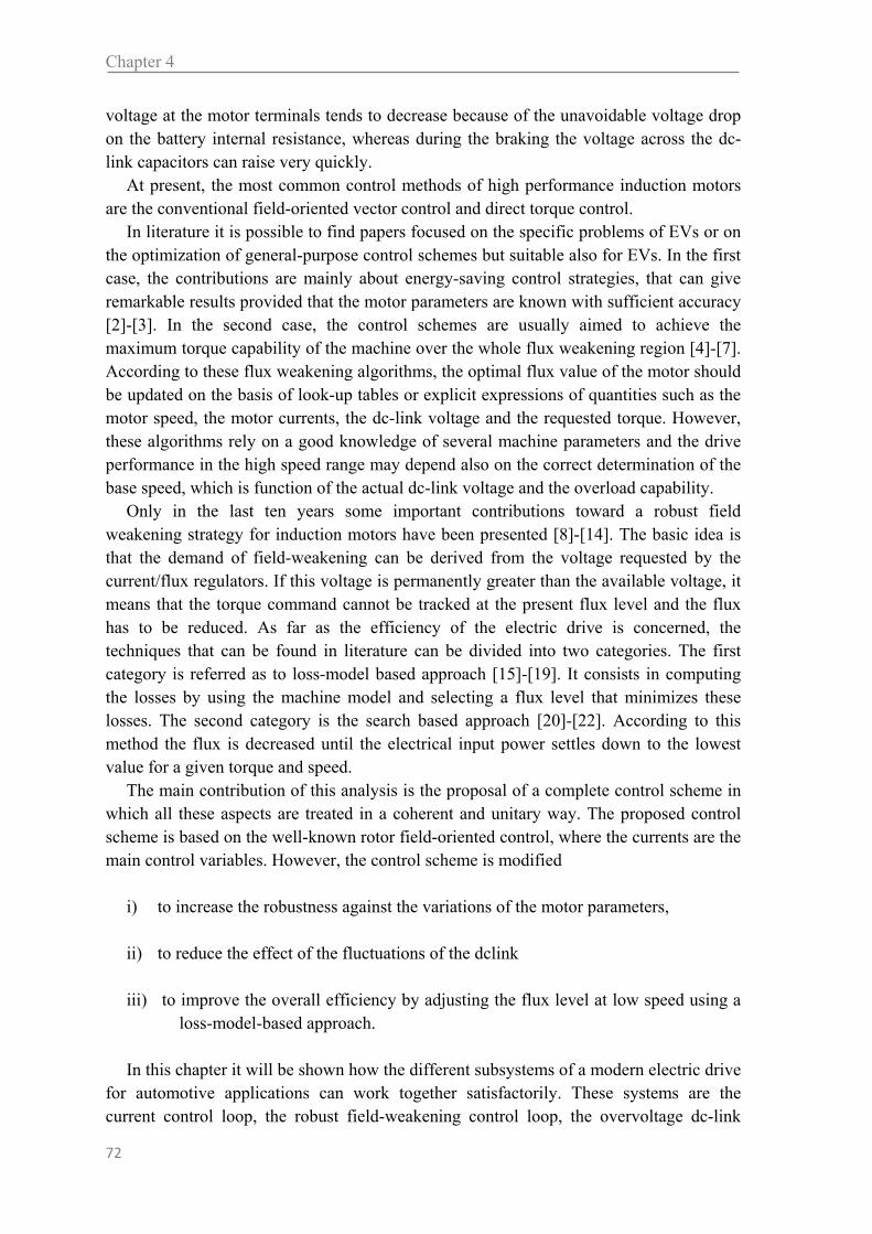
Chapter 4
72
voltage at the motor terminals tends to decrease because of the unavoidable voltage drop on the battery internal resistance, whereas during the braking the voltage across the dc-link capacitors can raise very quickly.
At present, the most common control methods of high performance induction motors are the conventional field-oriented vector control and direct torque control.
In literature it is possible to find papers focused on the specific problems of EVs or on the optimization of general-purpose control schemes but suitable also for EVs. In the first case, the contributions are mainly about energy-saving control strategies, that can give remarkable results provided that the motor parameters are known with sufficient accuracy [2]-[3]. In the second case, the control schemes are usually aimed to achieve the maximum torque capability of the machine over the whole flux weakening region [4]-[7]. According to these flux weakening algorithms, the optimal flux value of the motor should be updated on the basis of look-up tables or explicit expressions of quantities such as the motor speed, the motor currents, the dc-link voltage and the requested torque. However, these algorithms rely on a good knowledge of several machine parameters and the drive performance in the high speed range may depend also on the correct determination of the base speed, which is function of the actual dc-link voltage and the overload capability.
Only in the last ten years some important contributions toward a robust field weakening strategy for induction motors have been presented [8]-[14]. The basic idea is that the demand of field-weakening can be derived from the voltage requested by the current/flux regulators. If this voltage is permanently greater than the available voltage, it means that the torque command cannot be tracked at the present flux level and the flux has to be reduced. As far as the efficiency of the electric drive is concerned, the techniques that can be found in literature can be divided into two categories. The first category is referred as to loss-model based approach [15]-[19]. It consists in computing the losses by using the machine model and selecting a flux level that minimizes these losses. The second category is the search based approach [20]-[22]. According to this method the flux is decreased until the electrical input power settles down to the lowest value for a given torque and speed.
The main contribution of this analysis is the proposal of a complete control scheme in which all these aspects are treated in a coherent and unitary way. The proposed control scheme is based on the well-known rotor field-oriented control, where the currents are the main control variables. However, the control scheme is modified
i) to increase the robustness against the variations of the motor parameters,
ii) to reduce the effect of the fluctuations of the dclink
iii) to improve the overall efficiency by adjusting the flux level at low speed using a
loss-model-based approach.
In this chapter it will be shown how the different subsystems of a modern electric drive for automotive applications can work together satisfactorily. These systems are the current control loop, the robust field-weakening control loop, the overvoltage dc-link

Control Scheme With Energy Saving For Electric Vehicles
73
control loop and the minimization of the power losses. This chapter shows which signal saturations and PI anti-windup regulators should be taken into account, and proposes a solution for their tuning.
Experimental results demonstrate the effectiveness of the proposed approach.
4.2 Basic Ideas Behind the Control Strategy
A. Rotor Flux Oriented Control As known, the basic equations for the torque control of induction motors, written in a
rotor-flux oriented reference frame, are as follows:
sdrr
r
r Midt
d
R
L
(4.1)
sqrr
iL
MpT
2
3 (4.2)
where r is the rotor flux, sdi and sqi are the d-q components of the stator current, Ls, Lr
and M are the motor inductances and p is the pole pairs. Equation (4.1) states that the
rotor flux depends only on sdi , whereas (4.2) shows that the torque is proportional to the
product of the rotor flux and the current isq.
B. Minimum Motor Losses In order to optimize the power consumption of the motor, it is necessary to express the
motor torque as function of the stator currents in steady-state condition. Substituting in (4.2) the steady-state value of the rotor flux, which is obtainable from
(4.1), leads to the following expression of the motor torque:
sqsdr
IIL
MpT
2
2
3 . (4.3)
Equation (4.3) suggests that the motor can produce the same torque for different
combinations of sdI and sqI , and therefore it is opportune to find which couple of values
corresponds to the maximum efficiency. The Joule losses can be expressed as the sum of the contributions due to the rotor and
the stator windings, as follows:
2222
2
3rqrrdrsqssdsJouule IRIRIRIRP . (4.4)
whereas the iron losses due to magnetic hysteresis and eddy currents can be approximated with the following expression:

Chapter 4
74
222
2
3sdhystsdecIron IKIKP (4.5)
where Kec and Khyst are constants depending on the motor, and ω is the angular frequency of the input voltage.
The iron losses in (4.5) are supposed to depend only on the current sdi , i.e. on the flux-
producing component of the stator current. This is equivalent to assume that the iron losses are related to the rotor flux, whereas it should be more precise to assume that they depend on the air-gap flux. In addition, the iron losses due to the current ripple are not considered, since the control system is not able to control the current ripple, but evaluates only the mean value of the currents over a switching period.
Nevertheless, the expression (4.5) of the iron losses is acceptable for the calculation of the minimum power losses, which is an approximated process for its own nature. Furthermore, (4.5) has the advantage of being relatively simple, compared to other models that are more accurate but require an higher number of motor parameters [18].
If a rotor-flux oriented reference frame is used, it can be demonstrated that the rotor currents have a very simple form in steady-state condition:
0rdI (4.6)
sqr
rq IL
MI . (4.7)
Summing (4.4) and (4.5), together with (4.6) and (4.7), leads to the following expression of the total power losses of the motor, which can be written as a function of the stator current components only:
2
2
2
2
3)(
2
3sq
rrssdIronsIron I
L
MRRIKRP
(4.8)
where, for sake of compactness, the new coefficient Kiron has been introduced:
hystecIron KKK 2)( . (4.9)
The minimum of (4.8) subject to the constraint that the torque, expressed by (4.3), is assigned, can be found using the method of Lagrange multipliers. It is straightforward to
verify that the minimum of (4.8) occurs when the ratio of sdI to sqI is equal to a precise
quantity that depends on the motor parameters as well as on the input angular frequency.
The optimal value for sdI turns out to be as follows:
sqoptoptsd IKI , . (4.10)
where:
)(
)(
2
irons
rrs
opt KR
L
MRR
K
. (4.11)

Control Scheme With Energy Saving For Electric Vehicles
75
It is worth noting that, at low speed, Kiron is negligible and Kopt is little sensitive to temperature variations, since it is practically a ratio of resistances, and to the motor speed. At very high speed, instead, the term Kiron becomes dominant in the denominator of (4.11) and the coefficient Kopt tends to zero. This behavior is very important in the field-weakening speed range, since it can be the cause of an erroneous operation of the motor drive. This problem will be discussed further in section 4.3.
Finally, readers interested in the method used for the determination of the motor parameters can find further details in section 4.6.
4.3 Maximum Torque Capability
In the high-speed range, the motor operation is limited by the maximum inverter
voltage, the inverter current rating, and the machine thermal rating. The maximum voltage that the inverter can apply to the machine is defined by the dc-link voltage and by the PWM strategy. In any operating condition, the magnitude of the stator voltage vector must satisfy the following equation:
2max,
22ssqsd Vvv . (4.12)
Without overmodulation, if the output voltage vector is synthesized using Space Vector Modulation (SVM) or PWM with 3rd harmonics injection, the maximum magnitude of the phase voltage vector is:
3
max,dc
s
EV . (4.13)
It is opportune to find the maximum torque that the motor, subject to the constraint (4.12), can deliver to the load. For this purpose, it can be verified that the stator windings equations in steady-state operation are [6]:
sqssdssd ILIRV (4.14)
sdssqssq ILIRV (4.15)
where σis the leakage coefficient. Introducing (4.14) and (4.15) in (4.12), and taking into account that the voltage drop
caused by the stator resistance is negligible for high-speed operation, leads to the following equation:
s
ssqsd L
VII
max,222 . (4.16)
The maximum value of the torque subject to the constraint (4.12) can be found again with the method of the Lagrange multipliers, and occurs when (4.16) becomes an equality and sqI is equal to the quantity max,sqI defined as:
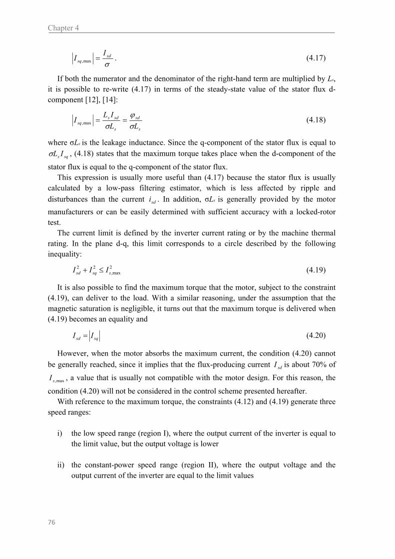
Chapter 4
76
sdsq
II max, . (4.17)
If both the numerator and the denominator of the right-hand term are multiplied by Ls, it is possible to re-write (4.17) in terms of the steady-state value of the stator flux d-component [12], [14]:
s
sd
s
sdssq LL
ILI
max, (4.18)
where σLs is the leakage inductance. Since the q-component of the stator flux is equal to
sqs IL , (4.18) states that the maximum torque takes place when the d-component of the
stator flux is equal to the q-component of the stator flux. This expression is usually more useful than (4.17) because the stator flux is usually
calculated by a low-pass filtering estimator, which is less affected by ripple and
disturbances than the current sdi . In addition, σLs is generally provided by the motor
manufacturers or can be easily determined with sufficient accuracy with a locked-rotor test.
The current limit is defined by the inverter current rating or by the machine thermal rating. In the plane d-q, this limit corresponds to a circle described by the following inequality:
2max,
22ssqsd III (4.19)
It is also possible to find the maximum torque that the motor, subject to the constraint (4.19), can deliver to the load. With a similar reasoning, under the assumption that the magnetic saturation is negligible, it turns out that the maximum torque is delivered when (4.19) becomes an equality and
sqsd II (4.20)
However, when the motor absorbs the maximum current, the condition (4.20) cannot
be generally reached, since it implies that the flux-producing current sdI is about 70% of
max,sI , a value that is usually not compatible with the motor design. For this reason, the
condition (4.20) will not be considered in the control scheme presented hereafter. With reference to the maximum torque, the constraints (4.12) and (4.19) generate three
speed ranges: i) the low speed range (region I), where the output current of the inverter is equal to
the limit value, but the output voltage is lower
ii) the constant-power speed range (region II), where the output voltage and the output current of the inverter are equal to the limit values
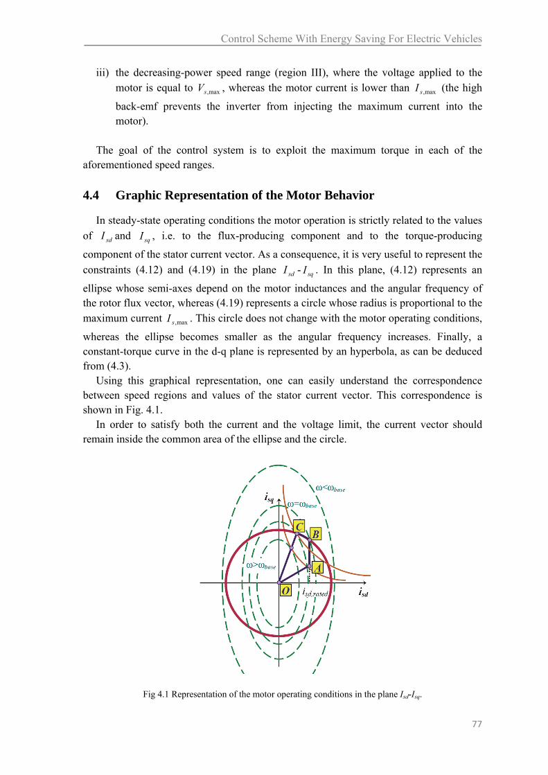
Control Scheme With Energy Saving For Electric Vehicles
77
iii) the decreasing-power speed range (region III), where the voltage applied to the motor is equal to max,sV , whereas the motor current is lower than max,sI (the high
back-emf prevents the inverter from injecting the maximum current into the motor).
The goal of the control system is to exploit the maximum torque in each of the
aforementioned speed ranges.
4.4 Graphic Representation of the Motor Behavior
In steady-state operating conditions the motor operation is strictly related to the values
of sdI and sqI , i.e. to the flux-producing component and to the torque-producing
component of the stator current vector. As a consequence, it is very useful to represent the
constraints (4.12) and (4.19) in the plane sdI - sqI . In this plane, (4.12) represents an
ellipse whose semi-axes depend on the motor inductances and the angular frequency of the rotor flux vector, whereas (4.19) represents a circle whose radius is proportional to the maximum current max,sI . This circle does not change with the motor operating conditions,
whereas the ellipse becomes smaller as the angular frequency increases. Finally, a constant-torque curve in the d-q plane is represented by an hyperbola, as can be deduced from (4.3).
Using this graphical representation, one can easily understand the correspondence between speed regions and values of the stator current vector. This correspondence is shown in Fig. 4.1.
In order to satisfy both the current and the voltage limit, the current vector should remain inside the common area of the ellipse and the circle.
Fig 4.1 Representation of the motor operating conditions in the plane Isd-Isq.

Chapter 4
78
When the motor operates in Region I, the speed is lower than the base speed and the limit ellipse is larger than the limit circle. The operating states of the motor are those represented in Fig. 4.1 by the points of the segment O-A, whose equation is given by (4.10). For the drawing of this segment, the speed has been assumed the same for all the
points. In the point A the current sdI has the rated value ratedsdI , ; hence a torque increase
can be obtained only by increasing sqI along the segment A-B until the magnitude of the
stator current vector is equal to max,sI , in the point B.
When the operating condition is that of the point B, the motor produces the maximum torque and the rotor flux has the value
ratedsdratedrd MI ,, (4.21)
However, this operating condition can be reached by the motor only if the actual speed is lower than the base speed, because the more the speed increases, the smaller the ellipse becomes. When the angular frequency is equal to the rated value, the ellipse passes through the point B.
At higher speeds, the reduction of the ellipse forces the operating point corresponding to the maximum achievable torque to move from B to C, while the magnitude of the stator current remains constant. The point C is the one corresponding to the maximum achievable speed without reducing the magnitude of the current injected in the motor, and it can be found imposing the condition that the ellipse is tangent to the constant-torque hyperbola. It is straightforward to recognize that the points of the arc B-C corresponds to Region II.
Finally, when the back-emf becomes too big and it is not possible to inject the maximum current in the motor, the motor enters into Region III. This operating condition is represented by the points of the segment C-O, whose equation is given by (4.18).
In the graphical representation of Fig. 4.1 the segment O-A is drawn supposing that the motor speed is lower than the base speed. The slope of the segment O-A has a behavior that is opposite of the coefficient Kopt, i.e. it tends to increase with the speed. This behavior can potentially interfere with the exploitation of the torque capability of the
Fig 4.2 –Representation of the motor operating conditions in the plane Isd-Isq. Maximum torque that can be obtained while minimizing the power losses.

Control Scheme With Energy Saving For Electric Vehicles
79
motor in the field weakening speed range, as explained hereafter. Let's consider Fig. 4.2, where the motor speed is supposed to be equal to the base
speed. The slope of the segment O-A has been exaggerated for the sake of clearness and is supposed greater than the slope of the segment O-B. In this case the maximum torque could be produced in both the operating points A' and B. The operating point A' is on the segment of the minimum losses but it is not practically achievable, because it is outside the current circle. The maximum torque that can be produced without violating the constraint of minimum losses is the one of the point A, but this torque value is lower than that of the point B.
In other words, when the motor operates in the field weakening speed range, the requirement of exploiting the torque capability is not compatible with that of minimizing the power losses.
It is useful to calculate the value of the coefficient Kopt that makes the slope of the segment O-A equal to that of the segment O-B. It is straightforward to verify that this value is:
2,
2max,
,min,
ratedsds
ratedsdopt
II
IK
(4.22)
This equation will be used in the control scheme to guarantee a correct operation of the motor in the field-weakening speed range.
4.5 Control Scheme
The block diagram of the control scheme based on the previous considerations is shown in Fig. 4.3.
As can be seen, the control scheme is composed by three different parts. The first one is the control loop of torque and flux, the second one manages the field weakening
Fig 4.3 Block diagram of the control scheme

Chapter 4
80
operation, whereas the third one minimizes the effect of fast fluctuations of the dc-link voltage.
A. Torque and Flux Control Scheme The motor torque is adjusted by the PI regulator (d) that compares the reference torque
with the actual torque. The output of this regulator is the torque-producing current reqsdi , ,
that tends to increase when the requested torque is greater than the estimated torque, and to decrease in the opposite case.
Two PI regulators, (a) and (b), are used to track the reference signals refsdi , and refsqi , .
As usual, the output signals of these regulators are compensated for the back electromotive forces. The reference voltages, synthesized by the inverter, are kept in the linear modulation range by the limitation block (c), whose explicit expression is as follows:
max,,max,
,
,
max,,,
,
sreqss
reqs
reqs
sreqsreqs
refsVvifV
v
v
Vvifv
v (4.23)
This block ensures that the magnitude of the reference voltage vector is not greater than the maximum voltage max,sV at disposal, that depends on the adopted modulation
strategy and on the dc-link voltage.
B. Robust Field Weakening The maximum torque that the motor can produce is limited by the maximum current
Is,max in region I and II, and by the available voltage Vs,max in region III. The limitation block (f) indirectly assures that the two aforementioned constraints are
satisfied in any speed region. In fact, the absolute value of the current isq is bounded by isq,max, which makes the stator current equal to Is,max or φsq equal to φsd, depending on which one is the most restrictive constraint at the present speed. The behavior of the limitation block (f) is shown in details in Fig. 4.4.
The rotor flux is indirectly controlled by the PI regulator (e), which adjusts the d component of the stator current isd,req, according to (4.1). When the motor operating point is very close to the flux weakening region, the stator current error can lead to a voltage
maxsqi ,
reqsqi ,
refsqi ,
maxsqi ,
Fig. 4.4 Limitation block (f) for the torque-producing component of the stator current.

Control Scheme With Energy Saving For Electric Vehicles
81
request greater than a limit voltage Vs,lim. For sake of simplicity, Vs,lim can be assumed equal to the maximum voltage Vs,max at present, but it will be shown in the next section that this equality is true only in steady-state operating conditions.
A positive difference between the amplitude of the requested voltage reqsv , , and the
limit voltage means that backemf is too high and the flux level should be reduced. This task is executed by the PI regulator (e), that integrates the difference reqss vV ,lim, . If this
difference is negative, the d-component of the stator current decreases; otherwise, it increases up to the threshold value max,sdi shown in the limitation block (g). This
threshold value is the minimum between the rated current ratedsdI , and the current optsdi , that
minimizes the motor losses. Fig. 4.5 shows the behavior of the limitation block (g) where
max,sdi and min,sdi are the maximum and the minimum admissible values of the d
component of the stator current, respectively. The value of optsdi , can be obtained by (4.10) but the gain Kopt has to be kept within the
lower bound Kopt,min, as shown in the limitation block (l). This expedient avoids that the motor behaves incorrectly at high speed as described in section 4.3.
The main advantage of the proposed field weakening scheme is that it is independent of the base speed and the motor parameters, except for the leakage inductance σLs, which is generally used in the state observer. In addition, it does not require any complex calculation of the flux level or look-up tables.
C. Fluctuation of DC-Link Voltage In the previous section the new quantity lim,sV
has been introduced. In steady-state
conditions lim,sV is equal to max,sV . However, as can be seen in Fig. 4.3, lim,sV can be lower
than max,sV during transient operation because of the low pass filter (m). This low pass
filter and the limitation block (i) have the aim to make the control system reactive to a fast reduction of the available voltage, but little sensitive to a fast increase. This increase, usually due to regenerative braking, could compromise the performance of the field-weakening algorithm when the vehicle slows down. In fact, although the rise in the dc-link voltage is transitory, the control system is deceived and untimely increases the flux level causing torque and current oscillations.
To avoid this behavior, when the actual dc-link voltage is greater than the rated value
rateddcE , , the limit voltage lim,sV is calculated using a filtered value, which is less sensitive
reqsdi ,
minsdi ,
refsdi ,
minsdi , maxsdi ,
maxsdi ,
Fig. 4.5 Limitation block (g) for the flux-producing component of the stator

Chapter 4
82
to fast variations. For simplicity, in the scheme of Fig. 4.3 it is supposed that the adopted modulation strategy is SVM, and hence the constant of proportionality between the dc-
link voltage and the limit voltage is 31
It is worth noting that, although the proposed scheme temporarily hides an increase of the dc-bus voltage to the control system, it immediately detects the reduction of the available voltage, and this selective behavior ensures robust performance of the field weakening operation.
4.6 Tuning the Regulator and Dynamic Behavior
It is opportune to recall some transfer functions that are particular important for the analysis of the motor drive. For sake of simplicity, in the following, the angular frequency of the rotor flux and motor speed are supposed to vary very slowly, i.e. their time constant is much greater than the duration of the other electrical transients.
These relationships are as follows:
)(1
)( sis
Ms sd
rr
(4.24)
)(1
1)( si
s
sLs sd
r
rssd
(4.25)
s
sqsd
srsr
rsd R
ssv
ss
ssi
)()(
1
1)(
2
(4.26)
s
sqsd
ssq R
ssv
ssi
)()(
1
1)(
. (4.27)
Equations (4.24) and (4.25) describes the behavior of the rotor flux and the d-
component of the stator flux vector as functions of the current sdi .
Equations (4.26) and (4.27) express stator currents as functions of the stator voltages. The poles of (4.26) are approximately placed at the following angular frequencies:
sr
p
1
1 (4.28)
rs
p
112 . (4.29)
In other words, the pole 1p depends on the time constant of the stator and the rotor
windings, whereas the pole 2p depends also on the leakage coefficient.

Control Scheme With Energy Saving For Electric Vehicles
83
A. Tuning of the Current Regulators The tuning of the regulators (a) and (b) is usually made with zero-pole cancellations.
The zero of the PI regulator (a) of the q-axis current is selected so that it cancels the pole of (4.27) at frequency -1/στs, due to the stator resistance and the leakage inductance. The
zero of the PI regulator (b) of the d-axis current is selected so that it cancels the pole 2p
of (4.26), since the effect of 1p is mitigated by the zero at angular frequency
r
z1
(4.30)
The integral gains of both regulators are selected in order to guarantee a sufficient phase margin (>75°), keeping in mind that there are certainly other poles at high frequency, due to the inverter and the limited band-width of the sensors.
As a conclusion, the closed-loop expressions of the current sdi and sqi can be
approximately expressed with first-order relationships:
)(1
)( , sis
Msi refsd
dsd
(4.31)
)(1
)( , sis
Msi refsq
qsq
(4.32)
where d and q are the crossover frequencies resulting from the choice of the regulator
integral gains.
B. Tuning of the Torque Regulator The relationships (4.31)-(4.32) can be used to tune the torque regulator (d), under the
assumption that the motor operates in Region I and that the current sdi is selected
according to the optimization law (4.11). The expression of the torque (4.3) is nonlinear. Therefore, it is opportune to linearize it around a steady-state operating point. One obtains:
rsqsqrr
iiL
MpT
2
3 (4.33)
where the operator Δ is used to distinguish small-signal variables from large-signal variables.
By using (4.10), (4.31) and (4.32), which are linear equations and hence are valid also for the small-signal analysis, it is possible to rewrite (4.33) as follows:
refsqrdq
optrr
isss
KL
MpT ,11
1
1
1
2
3
. (4.34)

Chapter 4
84
An immediate interpretation of the behavior of (4.34) is possible after expanding the second term inside the brackets in partial fractions, as follows:
refsqrdq
optrr
is
c
s
c
sK
L
MpT ,
21
111
1
2
3
. (4.35)
where:
rd
dc
1 (4.36)
dr
rc
2 . (4.37)
Since r is usually much greater than d and q , i.e. 01 c and 12 c , the torque
response is dominated by the time constant r and (4.35) can be approximated by a first-
order transfer function:
s
iK
L
MpT
r
refsqoptr
r
12
3 , . (4.38)
Therefore, the torque regulator can be tuned by cancelling the dominant pole of (4.38) and adjusting the integral gain to achieve a sufficient stability margin in the whole speed range.
C. Tuning the Voltage Regulator In this section some hints about the tuning of the voltage regulator (e) will be given. For sake of simplicity let's suppose that, when the motor operates in the field-
weakening speed range, the stator voltage magnitude can be approximated as:
sdv . (4.39)
Then, substituting (4.25) in (4.39) and using (4.31), the output voltage can be expressed as follows:
s
i
s
sLv
d
refsd
r
rs
11
1 , . (4.40)
The regulator (e) can be tuned by selecting the position of its zero so that it cancels the
low frequency pole r1 of (4.40).
The zero of (4.40) is related to the leakage inductances, whereas the second pole, at
higher frequency, is due to the control loop of the current sdi . It is worth noting that the
more the speed increases, the more the back-emf increases. This causes an increase of the open-loop gain, that is proportional to ω, as can be seen from (4.40).

Control Scheme With Energy Saving For Electric Vehicles
85
As a consequence the integral gain of the PI (e) has to be selected sufficiently small to ensure a good damping of the voltage response also at high speed and possibly a phase margin greater than 75 degrees.
4.7 Power Measurement
This section is dedicated to the methodology used to calculate and measure the mechanical and electric power and to the determination of machine parameters. This section is important to explain the way used to validate the proposed model.
Nowadays several manufactures commercialize instruments for electric power measurement with highly-distorted voltages. However, the determination of the electric power is still a complex problem when the motor is fed by an inverter.
The method that has been used for the measurement of the motor power is described hereafter.
It is worth noting that the motor currents are nearly sinusoidal, except for a little ripple due to the switching. On the contrary, the voltages are discontinuous signals.
The power measurement is based on the sampling of the motor currents and of the phase voltages [23]. The phase voltages can be measured directly, because the neutral point of the prototype is available.
The samples of the motor power are evaluated by multiplying the current samples and the voltage samples together, and then the products are numerically averaged to extract the bias component .
It is well-know that the overall accuracy achievable in electric drive measurements is mainly due to the transducers used to convert the current and voltage signals compatible with the input stage of the acquisition board. So, suitable transducers have been used, characterized by both large bandwidth and high accuracy.
The current transducers are three Hall-effect sensors LEM LAH50P, with a nominal current of 50 A(rms), an accuracy of 0.25%, a linearity uncertainty less than 0.1%, and a bandwidth of 200 kHz (-1dB).
The voltage transducers are three Hall-effect sensors LEM CV3 1000, with a nominal voltage of 700 V, an accuracy of 0.2 % and an offset voltage of 5 mV at 25°C, and a bandwidth of 500 kHz (-1 dB).
The load resistors of the current and voltage transducers have an accuracy of 0.25%. The acquisition board is the model NI PXI-5105 produced by TI, that features eight
12-bit channels with a sampling frequency up to 60 Ms/s. To avoid aliasing in the spectrum of the power (whose bandwidth is generally double
than that of current and voltage signals), the sampling frequency was 2 Ms/s, i.e. four times the voltage bandwidth. The use of 12-bit A/D converters allows to keep the quantization error within acceptable limits. The correct determination of the mean power requires that the averaging period is an integer multiple of the fundamental period. This condition can be strictly met only if the sampling rate is synchronized to the signal fundamental frequency (synchronous sampling condition). Since the sampling condition during the experimental tests was generally asynchronous, to reduce the leakage and the truncation errors, a very long averaging window was adopted.

Chapter 4
86
In conclusion, taking into account all the causes of error, it is possible to believe that the total uncertainty of the electric power measurement is lower than 4%.
The mechanical power has been measured by means of a suitable torque and speed sensor, model Buster 8651-100. The accuracy of the torque sensor is 0.15%, whereas the resolution of the encoder is 1 degree. Taking into account that these quantities are elaborated and displayed by a conditioning device, it is possible to suppose that the rated mechanical power can be measured with an uncertainty lower than 2%.
As a conclusion, the motor efficiency can be evaluated with an uncertainty of about 6%.
The calculation of the parameter Kopt requires the knowledge of several machine parameters.
By means of a locked-rotor test, it is possible to determine the leakage inductance and the sum of the stator and rotor resistances.
The stator resistance is usually determined directly by a dc measurement of the winding resistance, and hence it is possible to separate the contribution of the stator resistance from that of the rotor resistance in the result obtained in the locked-rotor test.
The mutual inductance M can be found by a no-load test when the motor is fed by the grid, under the assumption that the motor rotates at the synchronous speed. Generally, this can be achieved by dragging the motor with another speed-controlled electric drive.
For the determination of the core losses, several no-load tests at synchronous speed have been carried out by feeding the motor with an inverter at different frequencies and for different values of the current refsdI , . During each test the electric power, practically
consisting of the motor iron power losses given in (4.5), has been measured. The parameters Kec and Khyst have been found by means of the method of least squares. According to this method the values of Kec and Khyst in (4.5) have been adjusted to best fit the data set of the power measurements.
4.8 Experimental Results
A complete drive system has been realized to verify the feasibility of the proposed control scheme. The experimental set-up consists of an IGBT inverter and a 4 kW, 4-pole squirrel cage induction motor. The motor parameters are given in Table I.
Fig. 4.6 shows the behavior of the motor during a start-up transient when the torque reference is equal to the rated torque. Initially, the motor is at standstill and the stator current is nearly zero (in order to avoid useless waste of energy). After the application of
TABLE I – MOTOR PARAMETERS
Prated = 4 kW Rs = 0.4 Vs,rated = 110 Vrms Rr = 1 Is, max = 20 Apeak Ls = 32.6 mH sd,rated = 7.2 Apeak Lr = 32.6 mH
s = 250 rad/s M = 29.9 mH J = 0.03 Kg m2 Kec = 5·10-5 WA-2(rad/s)-2
Jtot = 0.22 Kg m2 Khyst = 6·10-4 WA-2(rad/s)-2

Control Scheme With Energy Saving For Electric Vehicles
87
the rated torque command, the motor starts up, and the current reaches its maximum value (regions I). In region II the flux weakening algorithm automatically modifies both the d-q components of the stator current with the aim to exploit the rated current (region II). As soon as the motor enters in region III, the current decreases and the refsq , becomes equal
to refsd , .
Figs. 4.6 and 4.8 show the behavior of the control system when the torque reference is very small, about 20% of the rated torque. The current refsdi , is selected on the basis of the
energy optimization strategy as far as this is possible, then the current injected in the motor tends to increase up to its maximum value for keeping the torque constant in region
II, and finally the current magnitude decreases in region III. In Fig. 4.7, the current sdi has
been normalized by dividing by Kopt. For this reason, in region I its trace follows exactly that of the current sqi .
Fig.4.6 Start-up transient with rated torque (500 ms/div). 1) Motor speed (2000 rpm/div), 2) stator flux φsd (0.25 Wb/div), 3) stator flux φsq (0.25 Wb/div), 4) phase current (20 A/div).
Fig.4.7 Start-up transient with 20% of the rated torque (500 ms/div). 1) Motor speed (2000 rpm/div), 2) current isd/Kopt (20 A/div), 3) stator current isq (20 A/div), 4) line current (20 A/div).

Chapter 4
88
Fig. 4.9 shows a torque reversal from -40% to +40% of the base speed, and the motor speed operates in the constant-power speed region. As can be seen, the current isq
reverses quickly and the current sdi changes accordingly, i.e. it is proportional to the
absolute value of sqi , so it firstly decreases nearly to zero, then it increases up to the rated
value ratedsdi , , that is greater than the value of the current at the beginning of the torque
reversal. Finally, when the motor speed exceeds the base speed, the current sdi decreases
again to allow the field weakening operation. As can be seen, although the torque reversal takes place in about 100 ms, the torque goes to zero much more quickly, and this could be important for a vehicle braking.
Fig. 4.10 shows the same situation of Fig. 4.9 but in this case the motor speed and dc-link voltage are shown instead of the motor torque and the line current. It can be noted that the dc-link voltage increases during the motor braking. This increment is transitory
Fig.4.9 Motor behavior during a torque reversal from -40% to +40% of the rated torque (200 ms/div). 1) Estimated torque (10 Nm/div), 2) line current (10 A/div), 3) stator current isd (20 A/div), 4) stator current isq (20 A/div).
Fig.4.8 Start-up transient with 20% of the rated torque (500 ms/div). 1) Motor speed (2000 rpm/div), 2) magnitude of the stator current (20 A/div), 3) estimated torque (5 Nm/div), 4) line current (20A/div).

Control Scheme With Energy Saving For Electric Vehicles
89
and lasts about 200 ms. However, this time interval is sufficient to deceive the field weakening algorithm, that could try to increase the flux level, hence triggering a sequence of voltage and current oscillations. The low pass filter (m) prevents this from happening and, as can be seen, the estimated torque remains unperturbed.
The behavior of the control scheme during a fast speed deceleration from 150% to 0% of the base speed is illustrated in Figs. 4.11 and 4.12. As can be seen in Fig. 4.11 the filtered dc-link voltage, which is used for the calculation of Vs,lim, is little sensitive to the fast rise of the dc-link. As a result, the waveforms of currents, fluxes and speed are smooth, without neither overshoot nor undershoot.
The results of Figs. 4.11 and 4.12 can be compared with those of Figs. 4.13 and 4.14, which show the behavior of the drive when the low-pass filter (m) is disabled. In this case, there is a counter-reaction in the current isd, that triggers some large oscillations in the current isq and, consequently, in the speed.
Fig.4.10 Motor behavior during a torque reversal from -40% to +40% of the rated torque (200 ms/div). 1) Motor speed (2000 rpm/div), 2) dc-link voltage (100 V/div), 3) stator current isd (20 A/div), 4) stator current isq (10 A/div).
(3)
(4)
(2)
(1)
Fig 4.11 Experimental test. Behaviour of the control scheme during a speed deceleration from 150% to 0% of the base speed (200 ms/div). 1) Motor speed (1000 rpm/div). 2) Dc-link voltage (200 V/div). 3) Filtered dc-link voltage (200 V/div). 4) Stator current (20 A/div).

Chapter 4
90
To assess the effectiveness of the power optimization, Figs. 4.15 and 4.16 show the motor efficiency as functions of the motor torque and speed. In Fig. 4.15 the power optimization is used, whereas in Fig. 4.16 it is not used, i.e. the saturation introduced by
optsdi , in the saturation block (g) has been removed.
For a better interpretation of these results, Fig. 4.17 shows the increment of efficiency due to the power optimization. As can be seen, the advantages are evident in particular at low speed and torque values (e.g. the vehicle is at a stand-still), where the improvement is about 20%. The optimization method does not offer any particular advantage when the motor torque is greater than 50% of the rated torque.
4.9 Conclusions
A control scheme for induction motor drives suitable for electric vehicles is analyzed in this chapter. The proposed scheme is based on a traditional rotor field-oriented control, improved in terms of robustness and efficiency.
The proposed control scheme allows a smooth transition into and out of the field weakening mode, exploiting the maximum torque capability of the machine over the whole operating speed range.
Whenever possible, the power losses are minimized by adjusting the flux level. The main advantages of proposed field weakening algorithm are:
i) reduced dependence on machine parameters and no need of calculation of the base speed, which in general depends on the machine parameters, motor current and DC-link voltage
ii) increase in the motor efficiency, useful specially when the motor operates at low speed
(3)
(4)
(2)
(1)
Fig 4.12 Experimental test. Behaviour of the control scheme during a speed deceleration from 150% to 0% of the base speed (200 ms/div). 1) Motor speed (1000 rpm/div). 2) Stator flux φsd (0.25 Wb/div). 3) Stator flux φsq (0.25 Wb/div). 4) Stator current (20 A/div).
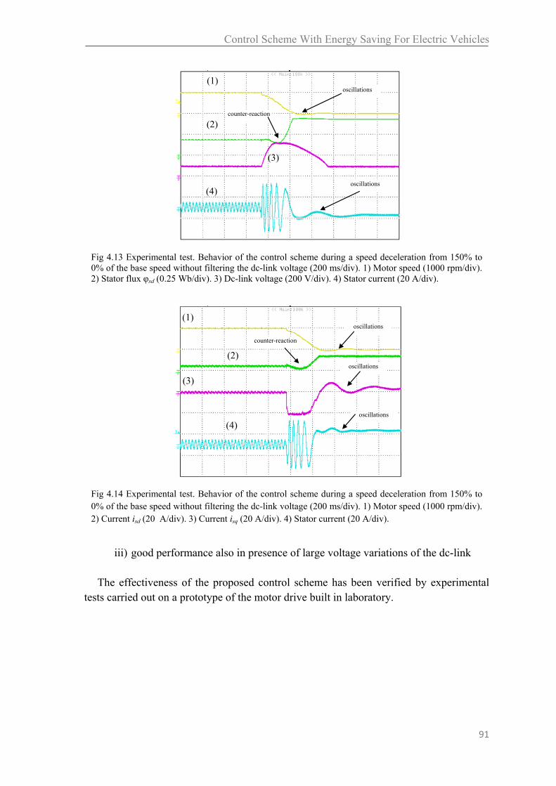
Control Scheme With Energy Saving For Electric Vehicles
91
iii) good performance also in presence of large voltage variations of the dc-link
The effectiveness of the proposed control scheme has been verified by experimental
tests carried out on a prototype of the motor drive built in laboratory.
(3)
(4)
(2)
(1)
counter-reaction
oscillations
oscillations
Fig 4.13 Experimental test. Behavior of the control scheme during a speed deceleration from 150% to 0% of the base speed without filtering the dc-link voltage (200 ms/div). 1) Motor speed (1000 rpm/div). 2) Stator flux φsd (0.25 Wb/div). 3) Dc-link voltage (200 V/div). 4) Stator current (20 A/div).
(3)
(4)
(2)
(1)
oscillations
oscillations
counter-reaction
oscillations
Fig 4.14 Experimental test. Behavior of the control scheme during a speed deceleration from 150% to 0% of the base speed without filtering the dc-link voltage (200 ms/div). 1) Motor speed (1000 rpm/div). 2) Current isd (20 A/div). 3) Current isq (20 A/div). 4) Stator current (20 A/div).
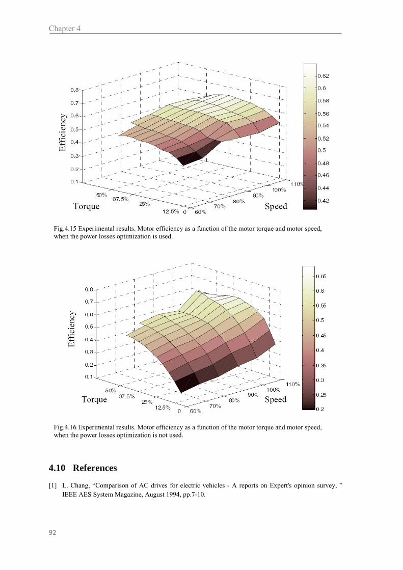
Chapter 4
92
4.10 References
[1] L. Chang, “Comparison of AC drives for electric vehicles - A reports on Expert's opinion survey, ” IEEE AES System Magazine, August 1994, pp.7-10.
Fig.4.15 Experimental results. Motor efficiency as a function of the motor torque and motor speed, when the power losses optimization is used.
Fig.4.16 Experimental results. Motor efficiency as a function of the motor torque and motor speed, when the power losses optimization is not used.

Control Scheme With Energy Saving For Electric Vehicles
93
[2] N. Mutoh, S. Kaneko, T. Miyazaki, R. Masaki, S. Obara, "A torque controller suitable for electric vehicles, ” IEEE Trans. on Industrial Electronics, vol. 44, No.1, February 1997, pp.54-63.
[3] J. Faiz, M. B. B. Sharifian, A. Keyhani, A. B. Proca, “Sensorless direct torque control of induction
motors used in electric vehicle, ” IEEE Trans. on Energy Conversion, vol. 18, No. 1, March 2003, pp. 1-10.
[4] X. Xu, D. W. Novotny, “Selection of the flux reference for induction machine drives in the field
weakening region,” IEEE Trans. on Industry Applications, Vol. 28, no. 6, pp. 1353-1358, Nov. – Dec. 1992.
[5] S. H. Kim, S. K. Sul, “Maximum torque control of an induction machine in the field weakening
region,” IEEE Trans. on. Industry Applications, vol.31, no. 4, pp. 787-794, Jul./Aug. 1995. [6] D. Casadei, F. Profumo, G. Serra, A. Tani, L. Zarri, “Performance analysis of a speed-sensorless
induction motor drive based on a constant switching frequency dtc scheme, ” IEEE Trans. on Industry Applications, vol. 39, no. 2, March/April 2003, pp. 476-484.
[7] M. Ho Shin, D. S. Hyun, S. B. Cho, “Maximum torque control of stator-flux oriented induction
machine drive in the field-weakening region,” IEEE Trans. on Industry Applications, vol. 38, no. 1, pp. 117-121, Jan./Feb. 2002.
[8] A. Biinte, H. Grotstollen, P. Krafka, “Field weakening of induction motors in a very wide region with
regard to parameter uncertainties,” PESC 96, vol. 1, 26- 27 June 96, Baveno, Italy, pp. 944-950. [9] S.H. Kim, S.K. Sul, “Voltage control strategy for maximum torque operation of an induction machine
in the field weakening region,” IEEE Trans. On Industrial Electronics, vol. 44, no.4, Aug. 1997, pp. 512-518.
Fig.4.17 Experimental results. Increment of efficiency due to the power optimization, as a function of the motor torque and speed.

Chapter 4
94
[10] H. Abu-Rub, Member, H. Schmirgel, J. Holtz, “Sensorless control of induction motors for maximum steady-state torque and fast dynamics at field weakening,” IAS 2006, 8-12 Oct. 2006, Tampa, Florida, Paper N.IAS03P3.
[11] L. Harnefors, K. Pietiläinen, L. Gertmar, “Torque-maximizing field-weakening control: design,
analysis, and parameter selection,” IEEE Trans. on Industrial Electronics, vol. 48, no. 1, Feb. 2001, pp. 117-122.
[12] D. Casadei, G. Serra, A. Tani, L. Zarri, “A robust method for field weakening operation of induction
motor drives with maximum torque capability, ” IAS 2006, 8-12 Oct. 2006, Tampa, Florida, Vol. 1, pp. 111-117.
[13] Z. Peroutka, K. Zeman, “New field weakening strategy for AC machine drives for light traction
vehicles, ” EPE 2007, 2-5 Sept. 2007, Aalborg, Denmark, pp.1-10. [14] M. Mengoni, L. Zarri, A. Tani, G. Serra, D. Casadei, “Stator flux vector control of induction motor
drive in the field weakening region, ” IEEE Trans. on Power Electronics, Vol. 23, No. 2, March 2008, pp. 941-948.
[15] H. G. Kim, S. K Sul, M. H. Park, “Optimal efficiency drive of a current source inverter fed induction
motor by flux control”, IEEE Trans. on Industry Applications, vol. IA-20, no. 6, November/December 1984, pp.1453-1459.
[16] I. Kioskeridis and N. Margaris, “Loss minimization in induction motor adjustable speed drives,” IEEE
Trans. Ind. Electron., vol. 43, pp. 226–231, Feb. 1996. [17] K. Matsuse, S. Taniguchi, T. Yoshizumi, K. Namiki, “A speed-sensorless vector control of induction
motor operating at high efficiency taking core loss into account, ” IEEE Trans. on Industry Applications, vol. 37, no. 2, March/April 2001, pp. 548-558.
[18] S. Lim and K. Nam, "Loss-minimising control scheme for induction motors, ” IEE Proc.-Electr. Power
Appl., Vol. 151, No. 4, July 2004, pp. 389-397 [19] G. Dong, O. Ojo, “Efficiency optimizing control of induction motor using natural variables, ” IEEE
Trans. on Industrial Electronics, vol. 53, no. 6, December 2006, pp.1791-1798. [20] D. S. Kirschen, D. W. Novotny, T. A. Lipo, “Optimal efficiency control of an induction motor drive, ”
IEEE Trans. on Energy Conversion, vol. EC-2, no. 1, March 1987, pp.70-76. [21] Cao-Minh Ta, Y. Hori, “Convergence improvement of efficiency-optimization control of induction
motor drives, ” IEEE Trans. on Industry Applications, vol. 37, no. 6, November/December 2001, pp.1764-1753.
[22] C. Chakraborty, Y. Hori, “Fast efficiency optimization techniques for the indirect vector-controlled
induction motor drives,” IEEE Trans. on Industry Applications, Vol. 39, No. 4, July/August 2003, pp. 1070-1076.
[23] C. De Capua, C. Landi, “Measurement station performance optimization for testing on high efficiency
variable speed drives,” IEEE Trans. on Instrumentation and Measurement, vol. 48, no. 6, December 1999, pp. 1149- 1154.

MULTI-PHASE ELECTRIC
DRIVES


Mathematical Model of the Multi-Phase
Induction Machine Abstract Nowadays variable speed ac drives are usually fed by power electronic converters. Although three-phase drives dominate the market, since the converter acts as an interface that decouples the three-phase voltage source from the motor, the number of phases may not be limited to three anymore. The advantages of multiphase drives over the traditional three-phase drives, such as improvement of the torque quality, reduction of the stator current per phase, improvement of torque density, and increase of the fault tolerance have drawn the attention towards this technology. The second part of this thesis is dedicated to the study of the multi-phase machine and multi-phase drives. This machine is characterized by a number of phases greater than three. In this chapter the mathematical model of a multi-phase induction machine is presented. The analysis is focused on machines with an odd number of phases.
5.1 Introduction
Multiphase motor drives offer a greater number of degrees of freedom compared to three-phase motor drives. In the following chapters it will be shown that the full exploitation can be used to improve the drive performance [1]. An interesting possibility, offered by multiphase machines, is the independent control of the low order spatial harmonic components of the magnetic field in the air gap of the machine. If the harmonic components of order greater than one are set to zero, the torque pulsation can be strongly reduced. On the other hand, if all the spatial harmonics are synchronized, the torque production capability of the machine can be increased [2], [3].
Another possibility is related to the so-called multi-motor drives. A well-defined number of multiphase machines, having series connected stator windings, with an
hapter 5

Chapter 5
96
opportune permutation of the phases, can be independently controlled with a single multiphase inverter [4], [5].
Finally, the multiphase drive offers better reliability against inverter faults, since it can operate even with a reduced number of active phases [6], [7].
It is worth noting that it is not possible to analyze the behavior of a multiphase motor drive using the space vector representation in a single d-q plane. In fact, to completely describe a multiphase electromagnetic system, it is necessary to adopt the space vector representation in multiple d-q planes (multiple space vectors) [8].
In order to introduce the multi-phase drives that use all the degrees of freedom of this technology, the mathematical model of a multi-phase induction motor is presented.
Furthermore this approach shows that three-phase machine can be considered a particular case of multi-phase machines.
5.2 The Mathematical Model
Under the same assumption discussed in the first chapter it is possible to describe the equations of a multi-phase induction machine.
In figure 5.1 the coordinate reference frame for a five-phase machine is illustrated. This model can be easily extended to a generic M-phase machine. In figure 5.2 and 5.3 the stator and the rotor magnetic field distribution produced by a generic phase k is showed.
The amplitude of the magnetic field can be obtained due to Ampère's circuital law (5.1):
.4
2p
iNhiNhdlH kS
kkSkk (5.1)
In (5.1) Ns is the number of conductors in series per phase, p the pairs of poles and the air-gap width. For the application of (5.1) a infinite value of iron permeability is
Fig 5.1 stator and rotor coordinate systems description

Mathematical Model of a Multi-Phase Induction Motor
97
assumed. Equation (5.1) can be expressed as a Fourier series. Equation (5.2) describes the
relationship between the stator current Ski flowing in the k-th winding Ski and the stator
magnetic field Skh , whereas (5.3) shows the expression of magnetic field Rkh produced
by the rotor windings in terms of rotor current Rki :
.
211,
odd
jje
SkSSSk
SkS eep
iNth
(5.2)
.
211,
odd
jje
RkRRRk
RkR eep
iNth
(5.3)
where Nr is the number of rotor conductor in series per phase, R the coordinate of the
rotor reference frame. The variables ψsk and ψrk are magnetic field coordinates generated by the rotor and the
stator windings. They can be expressed as:
.,...,2,12
1 MkM
kSk (5.4)
.,...,2,12
1 MkM
kRk (5.5)
The total magnetic field produced by the stator in the stator reference is the sum of the contributions of the magnetic field generated by each phase.
M
kSSkSs thth
1
,, . (5.6)
Taking (5.4) and (5.6) into account and by means of a substitution in (5.2), the stator magnetic field can be written as:
odd
M
kjM
ksk
jsSs eiee
p
Nth S
)1(2
1
211, . (5.7)
Fig 5.2 stator magnetic field distribution Fig 5.3 stator magnetic field distribution

Chapter 5
98
The introduction of the symbol
Mj
e2
leads to (5.8).
odd
kM
ksk
jsSs iee
p
Nth S
)1(
1
211, . (5.8)
An analogous relationships can be deduced for magnetic field produced by the rotor windings:
M
kRRkRR thth
1
,, (5.9)
odd
kM
kRk
jRRR iee
p
Nth R
)1(
1
211, . (5.10)
Equations (5.10) and (5.8) describe two important relationships, which can be simplified by means of the space vector representation.
5.3 Multiple Space Vector Representation
The space vector representation was introduced in 1918 by Fortescue with a paper “Method of Symmetrical Co-ordinates Applied to the Solution of Polyphase Networks” [9]. The Fortescue studies were connected to the analysis of power network and they represent the first important publication where the space vectors were introduced for a generic M-phase system. However only in the 1929, Park with the paper “Two-Reaction Theory of Synchronous Machines“ [10] applied this approach to the study of three phase electrical machine. Furthermore in 1943 and 1950 Edith Clarke published two-volume edition of “Circuit Analysis of A-C Power Systems” where the space vector approach was extended for the analysis of every three-phase electrical machines. In 1926 Edith Clarke became the first woman to deliver a paper at the American Institute of Electrical Engineers.
In this section the concept of multiple space vector representation is introduced. This powerful tool is strongly connected to the machine behavior.
For a given set of M real variables x1 ,..., xk ,..., xM a new set of complex variables
Mh xxxx ,...,,...,, 10 can be obtained by means of the following symmetrical linear
transformations:
M
k
khkh x
Mx
1
12 , (h = 0, 1, ..., M-1). (5.11)
The relationships (5.11) lead to a real variable 00 xx (zero sequence component) and
M-1 complex variables 11 ,...,,..., Mh xxx (multiple space vectors).
The inverse transformations are:
1
0
1
2
1 M
h
khhk xx , (k = 1, 2, ..., M), (5.12)

Mathematical Model of a Multi-Phase Induction Motor
99
where the symbol “ ” represents the scalar product.
From (5.11) it can be recognized that the M-1 space vectors are redundant, being
*hhM xx , (h = 1, 2, ..., M-1), (5.13)
where the symbol “*” specifies the complex conjugate Owing to this property, only (M-1)/2 space vectors, besides the zero sequence
component, are necessary to represent the set of M real variables. In this dissertation, only the space vectors having an odd subscript
( 2531 ,...,,...,,, Mh xxxxx ) will be utilized. The motivation of this particular choice is
connected to the strict correlation existing between spatial harmonics and space vectors of odd order.
As a consequence, the relationships (5.11) and (5.12) can be rewritten as:
M
k
khkh x
Mx
1
12 , (h = 0, 1, 3, 5, ..., M-2), (5.14)
2
,...5,3,1
102
1 M
h
khhk xxx , (k = 1, 2, ..., M). (5.15)
In general, each one of the (M-1)/2 space vectors can move arbitrarily in the corresponding d-q plane, independently of the others.
5.4 Determination of the Magnetic Field in Air-Gap
The introduction of multiple space vectors permits to rewrite (5.8) and (5.10) as follows:
odd
jS
sSS
Seiep
MNth
211
2, (1.17)
disp
jR
sRR
Reiep
MNth
211
2, . (1.18)
The stator magnetic field in air-gap can be expressed as:
odd
jSeSS
Sehth
, (1.19)
where
SS
S ip
NMh
2
1
1
2
. (1.20)
Furthermore the rotor magnetic field in air-gap is defined as:
.
,odd
jReRR
Rehth
(1.21)

Chapter 5
100
RR
R ip
Nh
2
1
1
2
5
. (1.22)
Note that the magnetic-field spatial harmonic of order ( = 1, 3, 5, ..., M-2) depends only on the corresponding current space vector Si . In particular, its amplitude is
proportional to the magnitude of Si and its angular speed (in electrical radians per
second) is h = / , where is the angular speed of Si .
The presence of these magnetic-field spatial harmonics can be utilized for improving the torque density of the machine. Of course, this result is of interest when achieved under the same rms value of the stator current and the maximum air-gap flux density.
In order to obtain this result it is necessary to synchronize, in terms of angular speed and position, the spatial harmonics on the basis of the following constraints [2]:
1 , (ρ = 1, 3, 5, ..., M-2). (5.23)
The spatial harmonics of order ( = M, 2M, 3M,…,kM) are stationary and their amplitude are proportional to the zero sequence component iS0 (usually null).
The spatial harmonics of order ( = 1, 2M+1, 4M+1, 6M+1,…, 2kM+1) rotate in the
same direction of 1Si with an angular speed
The spatial harmonics of order ( = 1, 2M-1, 4M-1, 6M-1,…, 2kM-1) rotate in the
same direction of *1Si (in other words they have a rotation verse opposite to 1Si ).
The spatial harmonics of order ( = 1, 2M+3, 4M+3, 6M+3,…, 2kM+3) rotate in the
same direction of 3Si .
The spatial harmonics of order ( = 1, 2M-3, 4M-3, 6M-3,…, 2kM-3) rotate in the
same direction of *3Si .
According to the number of phases several space vectors 5Si , 7Si , 9Si ,..., )2( MSi can
be introduced. In a M-phase machine with sinusoidally distributed windings only the stator current
space vector 1Si contributes to the air gap magnetic field, and then to the torque
production process. If the stator windings of (M-1)/2 machines are series connected, with an opportune permutation of the phases, each one of the (M-1)/2 current space vectors of the system can perform a high dynamic control of torque and flux in the corresponding machine, following the well-known Field Oriented Control (FOC) principle [11]. Note that the independent control of the (M-1)/2 M-phase machines can be obtained using only one M-phase VSI. To obtain the current space vectors required by this “Extended” FOC a very flexible modulation strategy must be adopted.
Otherwise to achieve the improvement of the machine torque density the principle of FOC can be applied separately to each field spatial harmonics, acting independently on the (M-1)/2 current space vectors, according to (5.23).
Once again, to obtain the current space vectors required by the “Extended” FOC a powerful VSI modulation strategy must be used. In the next chapter the multi-phase modulation strategies will be analyzed.
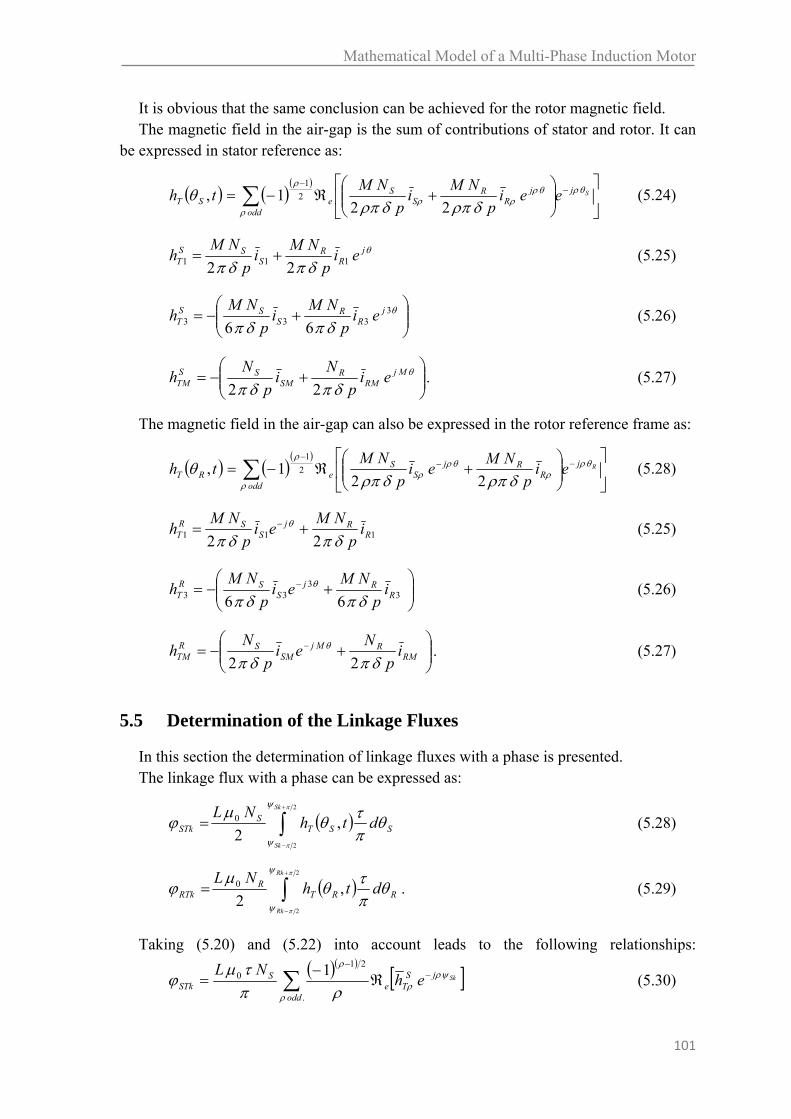
Mathematical Model of a Multi-Phase Induction Motor
101
It is obvious that the same conclusion can be achieved for the rotor magnetic field. The magnetic field in the air-gap is the sum of contributions of stator and rotor. It can
be expressed in stator reference as:
odd
jjR
RS
SeST
Seeip
NMi
p
NMth
221, 2
1
(5.24)
j
RR
SSS
T eip
NMi
p
NMh 111 22
(5.25)
3
333 66j
RR
SSS
T eip
NMi
p
NMh (5.26)
Mj
RMR
SMSS
TM eip
Ni
p
Nh
22. (5.27)
The magnetic field in the air-gap can also be expressed in the rotor reference frame as:
odd
jR
RjS
SeRT
Reip
NMei
p
NMth
221, 2
1
(5.28)
111 22 RRj
SSR
T ip
NMei
p
NMh
(5.25)
33
33 66 RRj
SSR
T ip
NMei
p
NMh
(5.26)
RMRMj
SMSR
TM ip
Nei
p
Nh
22. (5.27)
5.5 Determination of the Linkage Fluxes
In this section the determination of linkage fluxes with a phase is presented. The linkage flux with a phase can be expressed as:
2
2
,20
Sk
Sk
SSTS
STk dthNL
(5.28)
2
2
,20
Rk
Rk
RRTR
RTk dthNL
. (5.29)
Taking (5.20) and (5.22) into account leads to the following relationships:
.
210 1
odd
jSTe
SSTk
SkehNL
(5.30)

Chapter 5
102
.
210 1
odd
jRTe
RRTk
RkehNL
(5.31)
Equation (5.32) describes the relationships among voltage, stator current, and flux for a generic phase k.
.,...,2,1 Mkdt
diRv Sk
SkSSk
(5.32)
It is worthy noting that by means of the vector representation given in (5.11), (5.32) can be expressed as:
dt
diRv S
SSS0
00
(5.33)
)2,...,5,3,1( Mdt
diRv S
SSS
. (5.34)
In the same way it is possible to write the rotor equations
Mkdt
diRv Rk
RkRRk ,...,2,1
(5.35)
dt
diRv R
RRR0
00
(5.36)
)2,...,5,3,1( Mdt
diRv R
RRR
(5.37)
The total linkage flux with a generic phase k is the sum of the leakage flux and the air-gap linkage flux.
.,...,3,2,1 MkSTkSdkSk (5.38)
.,...,3,2,1 MkRTkRdkRk (5.39)
The application of the transformation (5.11) to (5.38) and (5.39) permits to obtain the following relationships:
)2,...,3,1,0( MSTSdS (5.40)
)2,...,3,1,0( MRTRdR . (5.41)
The leakage coefficients Lsd and Lrd describe the relationship between stator and rotor current and the linkage flux with phase k.
.,...,3,2,1 MkiL SkSdSdk (5.42)
.,...,3,2,1 MkiL RkRdRdk (5.42)
The introduction of the leakage coefficient Lsd and Lrd permits to express (5.40) - (5.41) as:

Mathematical Model of a Multi-Phase Induction Motor
103
)2,...3,1,0( MiL SSdSd (5.43)
)2,...3,1,0( MiL RRdRd . (5.44)
Furthermore the application of transformation (5.11) to equations (5.30) and (5.31) leads to the following relationships.
STMe
SST h
M
NL
00
2 (5.45)
)2,...,3,1(0 MhNL S
TS
ST
(5.46)
RTMe
RRT h
M
NL
00
2 (5.47)
)2,...,3,1(0 MhNL R
TR
RT
. (5.48)
5.6 Determination of the Electromagnetic Torque
The electromagnetic torque in electric machine can be determine by means of an energy balance.
m
mkmem
iWT
, '
(5.49)
where emT is the torque, m is the mechanical angle, and 'mW is the magnetic co-energy.
When the motor is not in magnetic saturation, the magnetic co-energy is equal to magnetic energy.
m
mkmem
iWT
, (5.50)
The angle m is related to by the following simple relationship:
mp (5.51)
, kmem
iWpT . (5.52)
The initial hypotheses permit to consider the magnetic energy of the leakage fluxes invariant with the angular position . Therefore to determine the torque is sufficient to consider the magnetic energy in the air-gap.
, kmTem
iWpT . (5.53)

Chapter 5
104
The equation (5.28) describe the magnetic field in the air-gap as sum of the contribution of stator and rotor magnetic field.
.
,odd
jjRSeST
Seehhth
(5.54)
Therefore the Torque can be expressed as:
SSTmT dthLpW
,2
1 20
2
0 (5.55)
.
*02
1
odd
ST
STmT hhLpW
(5.60)
.
2
02
1
odd
STmT hLpW
. (5.61)
where
ST
jRS hehh
(5.62)
SR
jR heh
. (5.63)
The torque produced by an induction motor can be rewritten as:
odd
jRSem ehjhLpT
2
0 . (5.64)
Equations (5.64) describes the torque by means the magnetic field produced by stator and rotor windings, but it can be related to the currents present in machine.
odd
jRSem ehjhLpT
2
0 . (5.65)
If the machine windings are star connected of the common mode currents are equal to zero, and if the rotor is short-circuited, new relationships can be written.
The introduction of self-inductance coefficients and mutual inductance coefficient permits to express relations generally used in the control of electric drives.
2
2
20
2
3
S
SS
N
p
LL (5.66)
2
2
20
2
3
R
RR
N
p
LL (5.67)
22
0
2
3
RS NN
p
LM (5.68)
)2,...,3,1( MLLL SSSdS (5.69)
)2,...,3,1( MLLL RRRdR . (5.70)

Mathematical Model of a Multi-Phase Induction Motor
105
Finally the expression of torque can be achieved.
odd
jRSem eijipM
MT
2. (5.71)
5.7 Machine Equations
In this section the machine equations of induction motor are resumed. The common mode equations are given by:
MhM
NL
hM
NL
ehh
eip
Ni
p
Nh
iL
iLdt
diRv
dt
diRv
RTe
RRT
STMe
SST
jMST
RTM
MjR
RS
SSTM
RTRRdR
STSSdS
RRRR
SSSS
30
0
00
3
002
1
000
000
000
000
2
2
221
(5.72)
Whereas the machine equation in dρ-qρ plane can be express as:
RT
RRT
ST
SST
jST
RT
jR
RS
SST
MTRRdR
STSSdS
RRRR
SSSS
hNL
hNL
ehh
eip
NMi
p
NMh
iL
iLdt
diRv
dt
diRv
0
0
22
(5.73)
The equation (5.71) define the electromagnetic torque produced.

Chapter 5
106
5.8 From Machine Equations to the Extended Vector Control of a Multi-Phase Induction Machine
By taking (5.72) and (5.73) into account it is possible to show that the most important machine quantities are connected to the rotor flux.
The rotor flux can be express as:
jRR e (5.74)
and its derivative is given by:
j
RrjRR eje
dt
d
dt
d (5.75)
where
Rdt
d . (5.76)
The relationships between the machine quantities and rotor flux are resumed in the following equations:
jRR
R
RR ej
dt
d
Ri
1 (5.77)
jjRR
R
RR
R
RRS ee
R
Lj
dt
d
R
L
Mi
1 (5.78)
j
RRR
RdR
R
RdR
SRT e
R
Lj
dt
d
R
L
Mp
NMh
21 (5.79)
odd R
RRem R
pM
T
2
2. (5.80)
Therefore the rotor and the stator current, the torque and the magnetic field in the air-gap are strongly connected to the rotor flux. This assumption suggests the operating principle of the vector controls, i.e. the control of the rotor flux.
Substituting (5.80) in (5.77) – (5.79) leads to a new set of equations.
j
R
emR
RR e
T
pMj
dt
d
Ri
21 (5.81)
jj
R
emR
R
R
RRS ee
TL
pj
dt
d
R
L
Mi
3
21 (5.82)
j
R
emRd
R
R
RdR
SRT e
TL
pMj
dt
d
R
L
Mp
MNh
2
2 1
. (5.83)

Mathematical Model of a Multi-Phase Induction Motor
107
The decomposition of (5.82) in real and imaginary part discloses that the d-component of the stator current controls the rotor flux (5.84) whereas the q-component controls the machine torque (5.85).
dt
d
R
L
Mi R
R
RRdS
1
(5.84)
R
emRqS
TL
MMi
21 (5.85)
Fig. 5.4 shows the scheme for the multi-phase vector control of an induction motor.
5.9 Conclusions
In this chapter the mathematical model of a multi-phase induction motor has been derived.
The equations presented have shown that the three-phase machine is a special case of a more general multi-phase machine, where only the fundamental harmonic is responsible for the production of torque. In a multi-phase machine, instead, there are several degrees of freedom that can be successfully used for various applications.
In this dissertation four different applications of a multi-phase machine will be analyzed. In Chapter 8 an extended stator flux vector control for seven-phase induction motor will be introduced. In this situation the spatial harmonics of order (ρ=3,5) will be set to zero to improve the torque quality.
Fig 5.4 Basic scheme for multi-phase induction motor drive.

Chapter 5
108
In Chapter 9 a high density torque application will be considered. In this case the spatial harmonic of order 3 will be successfully used in order to increase the torque of the motor in accordance with the constraints imposed from the drive.
In Chapter 10 different fault tolerant drives will be introduced and finally the chapter 11 the multi-motor application will be presented.
The multi-phase machines, due to their qualities, stand as a valid alternative to standard three-phase machine.
5.10 References
[1] E. Levi, R. Bojoi, F. Profumo, H. A. Toliyat, S. Williamson, "Multiphase induction motor driver - a technology status review," in IEE Electr. Power Appl., 2007, Vol. 4, No. 1, pp.489-516.
[2] L. Parsa, H.A. Toliyat, “Five-phase permanent-magnet motor drives,” IEEE Trans. on Industry Applicat., vol. 41, no. 1, pp. 30-37, January/February 2005.
[3] H. Xu, H.A. Toliyat, L.J.Petersen, “Five-phase induction motor drives with DSP-based control system,” IEEE Trans. on Power Electron., vol. 17, no. 4, pp. 524-533, July 2002.
[4] A. Iqbal, S.N. Vukosavic, E. Levi, M. Jones, H.A. Toliyat, “Dynamics of a series-connected two-motor five-phase drive system with a single-inverter supply,” in Proc. of IEEE Ind. Appl. Soc. Annual Meeting (IAS), 2005, pp. 1081-1088.
[5] A. Iqbal, E. Levi, M. Jones, S.N. Vukosavic, “A PWM scheme for a five-phase VSI supplying a five-phase two-motor drive,” in Proc. of Annual Conference of the IEEE Industrial Electronics Society (IECON), 2006, pp. 2575-2580.
[6] S. Dwari, L. Parsa, “An Optimal Control Technique for Multiphase PM Machines Under Open-Circuit Faults,” IEEE Trans. on Industrial Electronics, Vol. 55, No. 5, May 2008, pp. 1988-1995.
[7] F. Locment, E. Semail, X. Kestelyn, “Vectorial Approach-Based Control of a Seven-Phase Axial Flux Machine Designed for Fault Operation,” IEEE Trans. on Industrial Electronics, Vol. 55, No. 10, Oct. 2008, pp 3682 - 3691.
[8] D. Casadei, G. Serra, A.Tani, L. Zarri, “Multi-phase inverter modulation strategies based on duty-cycle space vector approach, ” in Proc. of SPRTS’2005, Bologna (Italy), 4-6 Sept. 2005, pp. 222-229.
[9] Fortescue, C. L., “Method of Symmetrical Co-Ordinates Applied to the Solution of Polyphase Networks” Transaction of AIEE , Volume: XXXVII , Issue: 2, 1918, page(s): 1027 - 1140
[10] Park, R. H. ,“Two-Reaction Theory of Synchronous Machines”, Transaction of AIEE, Volume: 48 , Issue: 3, 1929 , Page(s): 716 – 727
[11] E. Levi, M. Jones, S.N. Vukosavic, “Even-phase multi-motor vector controlled drive with single inverter supply and series connection of stator windings,” IEE Proc.-Electr. Power Appl., Vol. 150, No. 5, September 2003.

Multi-Phase Inverter Abstract Since late 1990s multiphase drives have become a serious alternative to three-phase drives in some particular applications such as electric ship propulsion, locomotive traction, electric vehicles and high power industrial applications. Nowadays the research activity is focused on the development of control strategies that can exploit the degrees of freedom that exist in multiphase machines. As known, a multiphase motor cannot be analyzed using the space vector representation in a single d-q plane, but it is necessary to introduce multiple d-q planes. In this chapter the structure of a multi-phase inverter is described and the degrees of employment of DC link is analyzed. The problem of the space vector modulation of multiphase inverters with an odd number of phases is solved in different way. An algorithmic approach and a look-up table solution are proposed. The validity of the analytical approach and the feasibility of the proposed solution are confirmed by several experimental tests.
6.1 Introduction
It is worth noting that it is not possible to analyze the behavior of a multiphase motor drive by using the space vector representation in a single d-q plane. In fact, to completely describe a multiphase electromagnetic system, it is necessary to adopt the space vector representation in multiple d-q planes (multiple space vectors).
In order to fully exploit the potential of M-phase motor drives, a suitable and flexible modulation strategy for M-phase voltage source inverters (VSIs) has to be defined.
Two different methods are usually adopted, i.e., space vector modulation (SVM) [2]–[6], and carrier-based pulsewidth modulation (PWM) [7]–[12]. For three-phase VSIs, the equivalence of the two methods has been proved, and they can be interchangeably implemented.
On the contrary, in the case of multiphase VSIs, the carrier-based PWM method seems the most feasible, due to its inherent simplicity. The reason is that PWM focuses the attention on the control of each inverter branch, and this task is relatively simple if

Chapter 6
110
compared with the aim of SVM, i.e., the determination of the switching pattern, which involves all the branches of the inverter.
For all these reasons, carrier-based PWM is considered more promising than SVM owing to its inherent simplicity in the case of multiphase VSIs.
The theory of carrier-based PWM for multiphase VSIs was presented in general terms in [8], but even before several remarkable contributions can be found in literature. The leading idea was usually to adapt the methods used for three-phase inverters to multiphase systems. Accordingly, modulation strategies with harmonic injection or discontinuous modulating signals were presented in [9]-[11]. Afterwards the research focused on the usage of carrier-based PWM for specific applications, such as multi-motor drives, five-phase or seven-phase motor drives [7], [16]
In this chapter the problem of the modulation strategy of M-phase inverters is completely solved using the Duty-Cycle Space Vector (DCSV) approach [17]–[18], which combines the multiple space vector representation, useful in modeling and controlling multi-phase machines, with traditional carrier-based PWM principle, suitable for multi-phase VSIs.
The DCSV approach, based on a space vector representation of the switch states, leads to the definition of a very flexible carrier-based PWM strategy that allows the full exploitation of the dc input voltage, and the independent control of fundamental and low order harmonics of the spatial field distribution. This modulation technique can be also employed for the control of multi-motor drives.
Furthermore, using the DCSV approach it is possible to predict the inverter voltage limit, which is very crucial for to the drive performance in the high-speed range [8].
Moreover SVM technique is also presented. The main reason of this choice is that SVM is well known for three-phase inverters, and it has been integrated in a number of logic devices that can manage the turn-on and turn-off of the inverter switches, such as field-programmable gate arrays (FPGAs) and complex programmable logic devices. For reasons related to the technical experience or just for economic convenience, a company could find preferable to update the available SVM algorithms for three-phase inverters rather than to completely renounce to its previous know-how. In addition, the definition of new methods for SVM could avoid potential patent violations.
To understand the basics of a M-phase system, the traditional space vector
representation in a single d–q plane is not sufficient, but it is necessary to use (M − 1)/2
d–q planes. The research activity for the definition of a general SVM in multiple d–q planes has
led to some remarkable results. Only recently some new approaches to SVM have led to general-purpose modulation
strategies based on iterative procedures, such as sorting or searching algorithms [15],[19]. These strategies are more flexible than the previous ones but have higher computational costs.
The first proposals [2]–[5],[20] have indeed the merit of demonstrating the feasibility of multiphase drives (in particular five-phase motor drives) but do not exploit all the available degrees of freedom. For example, the SVM techniques proposed in [13] and

Multi-Phase Inverter
111
[19] require the second voltage space vector to be always zero. The SVM technique defined in [3] and [7] considers the modulation of the first voltage space vector and allows also the modulation of the second voltage space vector with small magnitude. Finally, the SVM techniques presented in [17] and [18] can independently synthesize voltage vectors in more than one d–q plane, but they cannot ensure to fully utilize the dc input voltage.
Only recently some new approaches to SVM have led to general modulation strategies for multiphase inverters [14]–[15],[19].
Whereas the approaches proposed in [15] and [19] can be considered somehow a generalization of the traditional SVM for three-phase inverters, the approach presented in [14] adopts a different point of view. In that paper, the authors do not use the concept of space vector and the reference voltages are directly expressed in terms of phase voltages. In this way, they could obtain a very general solution, valid for M-phase electric systems, which is applicable also to multilevel inverter.
Nevertheless, the concept of space vector is particularly useful in motor control, and it is of interest to recover it, generalizing the traditional SVM theory of three-phase VSI. For this reason, in this chapter, it is proposed an alternative approach to space-vector modulation, derived from the method proposed in [15] for five-phase inverters, which is further developed and extended to multiphase inverters.
All proposed approaches lead to the definition of a very flexible modulation strategies that allows the full exploitation of the dc input voltage, and the simultaneous modulation of voltage space vectors in different d-q planes.
This last property allows one to synthesize the voltage vectors required by a multiphase system, either based on a multiphase motor with high torque density or on multi-motor drives. The proposed modulation theories are confirmed by several experimental tests
6.2 Multiple Space Vector Representation
The study of three-phase systems, in steady-state and transient operating conditions, takes advantage of the definition of a space vector and a zero sequence component. This powerful tool can be usefully extended, and then adopted, for the analysis of multi-phase systems [1].
For a given set of M real variables Mk xxx ,...,,...,1 a new set of complex variables
10 ,...,,..., Mh xxx can be obtained by means of the following symmetrical linear
transformations:
M
k
khkh x
Mx
1
12 , (h = 0, 1,..., M-1), (6.1)
where Mj /2exp .
Assuming M an odd number, the relationships (6.1) lead to a real variable 00 xx
(zero sequence component) and M-1 complex variables 11 ,...,,..., Mh xxx (multiple space
vectors).
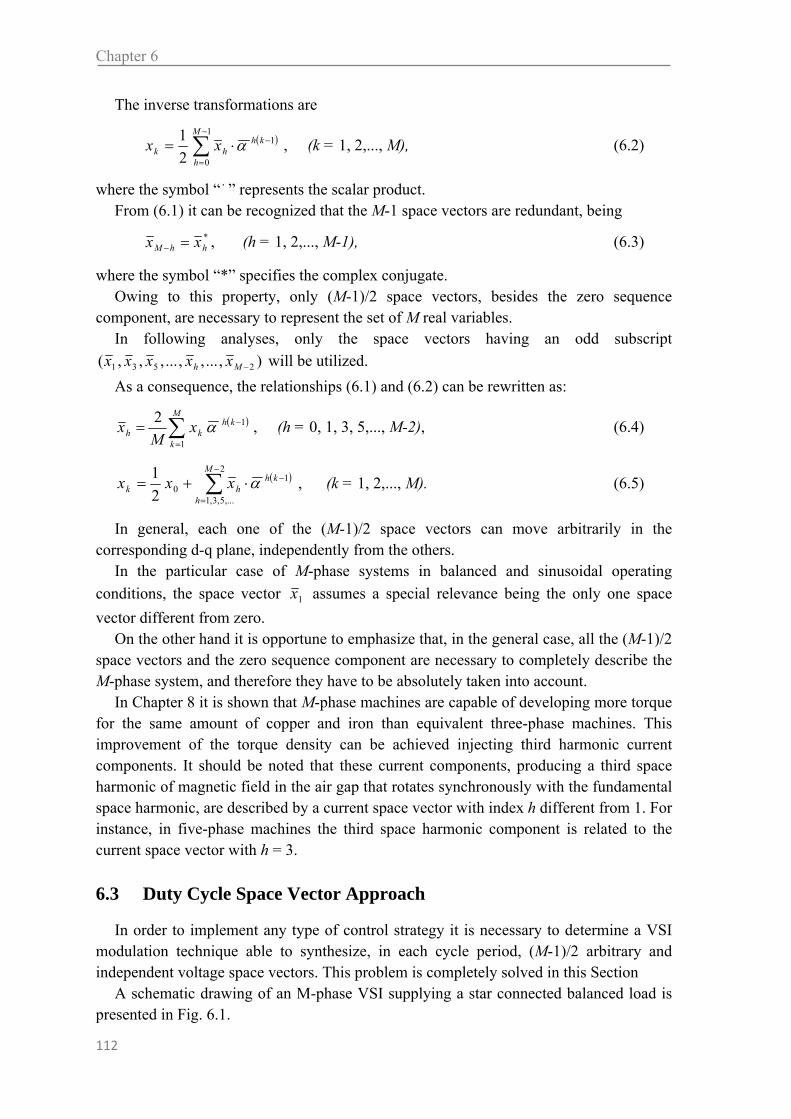
Chapter 6
112
The inverse transformations are
1
0
1
2
1 M
h
khhk xx , (k = 1, 2,..., M), (6.2)
where the symbol “ ” represents the scalar product. From (6.1) it can be recognized that the M-1 space vectors are redundant, being
*hhM xx , (h = 1, 2,..., M-1), (6.3)
where the symbol “*” specifies the complex conjugate. Owing to this property, only (M-1)/2 space vectors, besides the zero sequence
component, are necessary to represent the set of M real variables. In following analyses, only the space vectors having an odd subscript
),...,,...,,,( 2531 Mh xxxxx will be utilized.
As a consequence, the relationships (6.1) and (6.2) can be rewritten as:
M
k
khkh x
Mx
1
12 , (h = 0, 1, 3, 5,..., M-2), (6.4)
2
,...5,3,1
102
1 M
h
khhk xxx , (k = 1, 2,..., M). (6.5)
In general, each one of the (M-1)/2 space vectors can move arbitrarily in the corresponding d-q plane, independently from the others.
In the particular case of M-phase systems in balanced and sinusoidal operating
conditions, the space vector 1x assumes a special relevance being the only one space
vector different from zero. On the other hand it is opportune to emphasize that, in the general case, all the (M-1)/2
space vectors and the zero sequence component are necessary to completely describe the M-phase system, and therefore they have to be absolutely taken into account.
In Chapter 8 it is shown that M-phase machines are capable of developing more torque for the same amount of copper and iron than equivalent three-phase machines. This improvement of the torque density can be achieved injecting third harmonic current components. It should be noted that these current components, producing a third space harmonic of magnetic field in the air gap that rotates synchronously with the fundamental space harmonic, are described by a current space vector with index h different from 1. For instance, in five-phase machines the third space harmonic component is related to the current space vector with h = 3.
6.3 Duty Cycle Space Vector Approach
In order to implement any type of control strategy it is necessary to determine a VSI modulation technique able to synthesize, in each cycle period, (M-1)/2 arbitrary and independent voltage space vectors. This problem is completely solved in this Section
A schematic drawing of an M-phase VSI supplying a star connected balanced load is presented in Fig. 6.1.

Multi-Phase Inverter
113
The proposed approach is based on the direct determination of the switching signal kS
of each inverter leg (Fig. 6.1), according to the well known carrier-based PWM approach. The calculation of the switching signals is repeated in each cycle period Tc, allowing
any voltage waveform to be easily synthesized.
The switching signals kS (k = 1, 2, ..., M) are obtained comparing a triangular carrier
signal c, varying within the interval [0, +1], with M regular-sampled (i.e. assumed
constant in each cycle period) modulating signals km (k = 1, 2, ..., M), as shown in Figs.
6.2 and 6.3. It should be noted that the modulating signals represent also the duty-cycles of the
inverter legs, and they must satisfy the following constraints:
1,0km (k = 1, 2, ..., M). (6.6)
Assuming the input/output quantities of the inverter represented by their average values over the cycle period cT , the value of the modulating signals mk (k = 1, 2, ..., M), in
each cycle period, can be obtained by the following procedure, according to the DCSV approach.
Edc
1 0 k M
N
sk s1 sM
Fig. 6.1. Structure of a multiphase VSI.
Tc
+1
0 c
mk
m1
mM
t
Fig. 6.2. Carrier and modulating signals.
+
c
0 1 Sk
mk
Fig. 6.3. Switching signals generation.
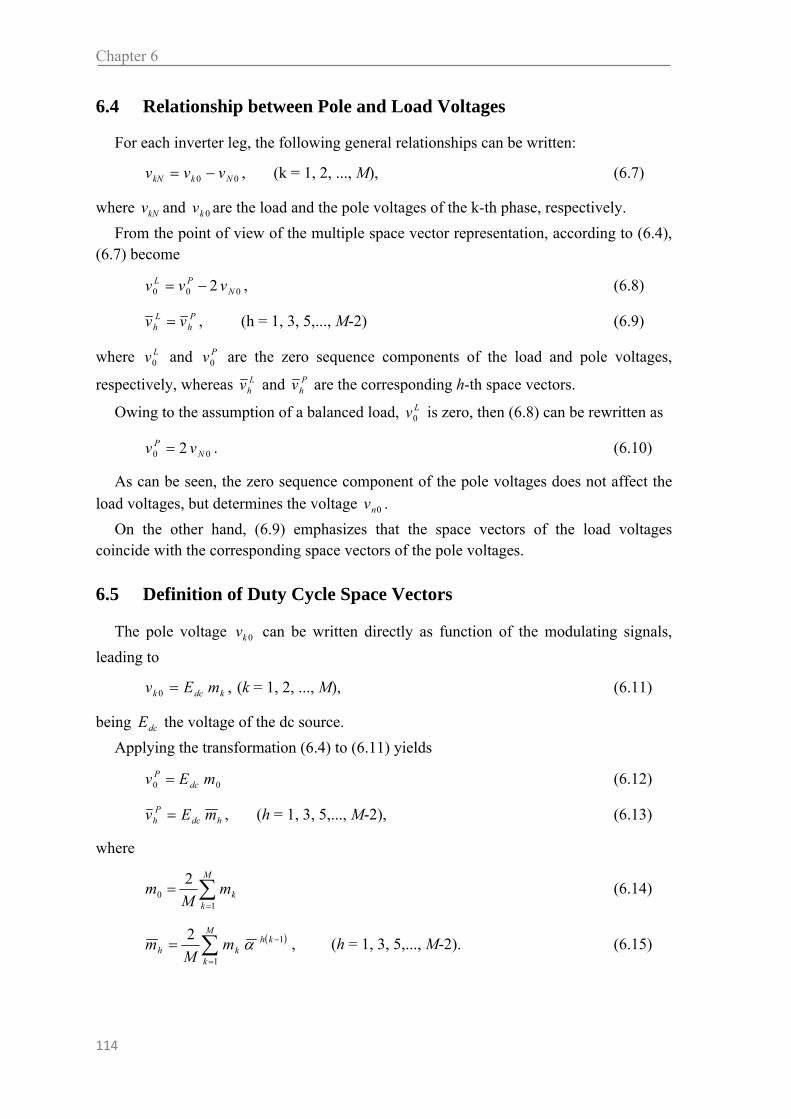
Chapter 6
114
6.4 Relationship between Pole and Load Voltages
For each inverter leg, the following general relationships can be written:
00 NkkN vvv , (k = 1, 2, ..., M), (6.7)
where kNv and 0kv are the load and the pole voltages of the k-th phase, respectively.
From the point of view of the multiple space vector representation, according to (6.4), (6.7) become
000 2 NPL vvv , (6.8)
Ph
Lh vv , (h = 1, 3, 5,..., M-2) (6.9)
where Lv0 and Pv0 are the zero sequence components of the load and pole voltages,
respectively, whereas Lhv and P
hv are the corresponding h-th space vectors.
Owing to the assumption of a balanced load, Lv0 is zero, then (6.8) can be rewritten as
00 2 NP vv . (6.10)
As can be seen, the zero sequence component of the pole voltages does not affect the
load voltages, but determines the voltage 0nv .
On the other hand, (6.9) emphasizes that the space vectors of the load voltages coincide with the corresponding space vectors of the pole voltages.
6.5 Definition of Duty Cycle Space Vectors
The pole voltage 0kv can be written directly as function of the modulating signals,
leading to
kdck mEv 0 , (k = 1, 2, ..., M), (6.11)
being dcE the voltage of the dc source.
Applying the transformation (6.4) to (6.11) yields
00 mEv dcP (6.12)
hdcP
h mEv , (h = 1, 3, 5,..., M-2), (6.13)
where
M
kkm
Mm
10
2 (6.14)
M
k
khkh m
Mm
1
12 , (h = 1, 3, 5,..., M-2). (6.15)

Multi-Phase Inverter
115
The quantity 0m is the zero-sequence component of the duty-cycles, whereas hm
represents the h-th DCSV of the M-phase VSI. Using (6.9) and (6.13) leads to:
hcL
h mVv , (h = 1, 3, 5,..., M-2). (6.16)
Note that the (M-1)/2 space vectors of the line-to-neutral load voltage are directly proportional to the corresponding DCSVs.
On the other hand, substituting (6.10) in (6.12) yields
2
00
mVv c
N . (6.17)
As can be seen from (6.16) and (6.17), the zero sequence component of the duty-cycles
does not affect the load voltages, but determines the voltage 0nv .
The duty-cycle zero sequence component 0m does not affect the load voltage and then
can be used to determine different modulation strategies and to optimize the input voltage utilization.
6.6 Generalized Modulation Strategies for M-Phase VSI
The general solution to the modulation problem of an M-phase inverter can be readily obtained by using the previous relationships.
Let us consider the load voltage space vectors refhv , (h = 1, 3, 5, ..., M-2) known as
reference quantities, i.e. generated by the control algorithm in each cycle period. Using (6.5) and (6.26) leads to the following fundamental equations:
2
,...5,3,1
1,0
1
2
1 M
h
khrefh
ck v
Vmm , (k = 1, 2, 3,..., M). (6.18)
Equations (6.18) allow the calculation of the modulating signals of all the inverter legs in each cycle period, following the procedure shown in Fig. 6.4. All the possible PWM techniques for M-phase VSIs can be derived from (6.18), with an opportune choice of the zero sequence component m0, which represents a degree of freedom. The selection of m0, in each cycle period, should be carried out in order to fully utilize the dc voltage and to optimize some characteristics of the modulation law, such as the switching frequency and the output voltage spectrum.
6.7 Voltage Limits
The duty-cycle constraints, given in (6.6), introduce complicated limitations on the possible values of refMrefrefrefref vvvvv ,2)1(,5,3,1 ,...,,, that can be properly synthesized,
in each switching period. In three-phase inverters, this problem involves only the space vector refv ,1 , and it has been already completely solved.
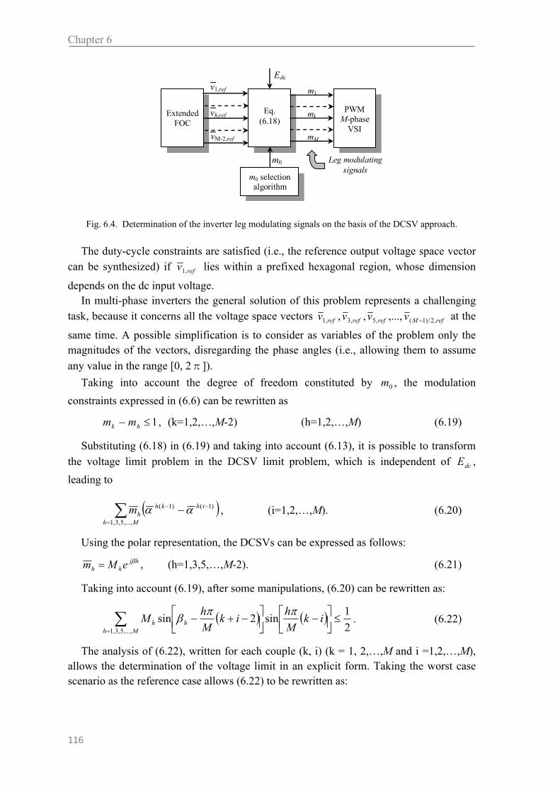
Chapter 6
116
The duty-cycle constraints are satisfied (i.e., the reference output voltage space vector can be synthesized) if refv ,1 lies within a prefixed hexagonal region, whose dimension
depends on the dc input voltage. In multi-phase inverters the general solution of this problem represents a challenging
task, because it concerns all the voltage space vectors refMrefrefref vvvv ,2)1(,5,3,1 ,...,,, at the
same time. A possible simplification is to consider as variables of the problem only the magnitudes of the vectors, disregarding the phase angles (i.e., allowing them to assume
any value in the range [0, 2π]).
Taking into account the degree of freedom constituted by 0m , the modulation
constraints expressed in (6.6) can be rewritten as
1 hk mm , (k=1,2,…,M-2) (h=1,2,…,M) (6.19)
Substituting (6.18) in (6.19) and taking into account (6.13), it is possible to transform
the voltage limit problem in the DCSV limit problem, which is independent of dcE ,
leading to
)1()1(
,...,5,3,1
ihkh
Mhhm , (i=1,2,…,M). (6.20)
Using the polar representation, the DCSVs can be expressed as follows:
hjhh eMm , (h=1,3,5,…,M-2). (6.21)
Taking into account (6.19), after some manipulations, (6.20) can be rewritten as:
2
1sin2sin
,...,5,3,1
ikM
hik
M
hM
Mhhh
. (6.22)
The analysis of (6.22), written for each couple (k, i) (k = 1, 2,…,M and i =1,2,…,M), allows the determination of the voltage limit in an explicit form. Taking the worst case scenario as the reference case allows (6.22) to be rewritten as:
m0
Edc
m1
mk
mM
Leg modulating signals
Eq. (6.18)
PWM M-phase
VSI
ExtendedFOC
vM-2,ref
v1,ref
vh,ref
m0 selection algorithm
Fig. 6.4. Determination of the inverter leg modulating signals on the basis of the DCSV approach.

Multi-Phase Inverter
117
2
1sin
,...,5,3,1
ikM
hM
Mhh
, (k,i=1,2,…,M). (6.23)
Due to the inherent symmetry, the constraint conditions (6.23) can be summarized in different forms according to number of phases.
The inequality (6.23) is a exhaustive relationship, it is able to describe the voltage limits of any type of multi-phase inverter with odd number of phases.
The following sections give prominence to the five and seven phase inverter. This choice is justified to the fact that five and seven phase systems are the first multi-phase system with odd number of phase over three. And they are the subject of numerous and most important study in this sector. Furthermore when the number of phase is very high the possibility of describing graphically the solution of voltage limits is lost.
6.8 Five-Phase Inverter
For a five phase inverter the modulation constraints expressed in (6.19)-(6.23) become:
1 ik mm , (k = 1, 2, ..., 5), (i = 1, 2,..., 5) (6.24)
131
11
,h
ihkhhm , (k = 1, 2,..., 5), (i = 1, 2,..., 5). (6.25)
hjhh emm , (h = 1, 3). (6.26)
Finally equation (6.22) can be write as:
2
1
5
3sin
5
32sin
5sin
52sin 3311
ikikmikikm
(6.27)
The analysis of (6.27), written for each couple (k, i) (k = 1, 2,..., 5 and i = 1, 2,..., 5), allows the determination of the voltage limit in each switching period.
In order to clarify the application of (6.27), the analysis will be focused on some relevant operating conditions.
A. Motor Drives without Third Spatial Harmonic In this case the third spatial harmonic of magnetic field in the air gap is not utilized
and the five-phase VSI has to generate balanced and sinusoidal output voltages. The corresponding DCSVs can be expressed as follows:
tjeMm 11 , (6.28)
03 m . (6.29)
Substituting (6.28) and (6.29) in (6.27) yields

Chapter 6
118
2
1
5sin
52sin1
ikiktM , (k = 1, 2,..., 5), (i=1, 2,..., 5).
(6.30)
Taking the worst condition into account leads to
526.052sin2
11
M . (6.31)
The relationship (6.31) represents the well-known voltage limit that can be achieved
provided that an opportune choice of the zero-sequence 0m in each switching period, is
taken. If 0m is simply fixed to 21 (sinusoidal PWM) the voltage limit becomes
5.01 M . (6.32)
B. Motor Drives with Third Spatial Harmonic When the third spatial harmonic of magnetic field in the air gap is considered, the VSI
has to generate balanced but non-sinusoidal output voltages. The corresponding DCSVs, which must ensure the synchronization of the first and
third spatial harmonics, can be described by the following general expressions:
tjeMm 11 , (6.33)
tjj eeMm 3
33 . (6.34)
Substituting (6.33) and (6.34) in (6.27) leads to
2
1
5
3
5
323
552 31
iksiniktsinMiksiniktsinM.
(6.35)
In this case, the analytical determination of the DCSV limit in explicit form, taking
0 0.1 0.2 0.3 0.4 0.5 0.6 0.70
0.1
0.2
0.3
0.4
0.5
0.6
0.7
M1
M3
= 0° = 30° = 60° = 90°
= 120°
= 150°
= 180°
Fig 6.5 Validity domains of M1 and M3 as function of the phase angle φ
A B
C

Multi-Phase Inverter
119
into account the parameter φ, is not so easy. The results obtained using a numerical procedure are summarized in Fig. 6.5. In this
figure the validity domains of M1 and M3 are shown, for different values of the phase angle φ. The range of variation of φ is [0°, 180°], because the behavior of M1 and M3 is the same for positive and negative values of φ.
Note that, when M3 = 0, the maximum value of M1 is equal to the value predicted by (6.32). This operating condition is represented by the point A in Fig. 6.5.
For small values of the phase angle φ, an increase in the value of M3 causes a reduction of the maximum achievable value of M1. On the other hand, if φ is close to 180°, it is possible to increase the maximum achievable value of M1 up to nearly 0.6 (point C). It is worth noting that in this operating condition a third harmonic component is present and cannot be avoided.
C. Multi-Motor Drives In this case, the DCSVs must be completely independent, with arbitrary behavior,
being related to the first spatial harmonics in the two different machines. In general, they can be described as follows:
111
jemm , (6.36)
333
jemm . (6.37)
It is very interesting to derive the validity domain of 1m and 3m regardless of the
values of the phase angles β1 and β3. Taking into account the worst condition for β1 and β3 allows (6.27) to be rewritten as
2
1
5
3sin
5sin 31
ikmikm , (k = 1, 2,..., 5), (i = 1, 2,...,5).
(6.38)
The five inequalities in (25) can be summarized by the two following simultaneous constraints:
2
1
5sin
5
2sin
2
1
5
2sin
5sin
31
31
mm
mm
(6.39)
The corresponding validity domain of 1m and 3m is represented by the shaded area
in Fig. 6.6. As can be seen, the validity domain of Fig. 6.6 is the intersection of all the validity
domains shown in Fig. 6.5, for different values of the phase angle φ. Note that the square region with dashed boundary represents the validity domain
obtained when using the SVM technique proposed in [7].

Chapter 6
120
This result shows that, using the carrier-based PWM technique together with DCSV approach makes it possible to extend significantly the voltage limit.
D. Experimental Results In order to verify the effectiveness of the proposed modulation strategy and to validate
the consistency of the voltage limit analysis some experimental tests have been performed.
The experimental setup consists of a custom-designed five-phase voltage source inverter feeding a five-phase symmetrical series-connected R-L passive load (R = 22 Ω, L = 1.15 mH). The IGBTs are rated at 30A and 630 V and the dc bus voltage is around 100 V. The control algorithm is implemented in a Digital Signal Processor (DSP) TMS320F2812. The switching period is 250 μs, corresponding to a switching frequency of 4 kHz.
The particular modulation strategy adopted for the experimental tests can be considered as a generalization of the well-known symmetric modulation used with three-
phase inverters. The zero sequence component 0m is selected in order to maintain the five
modulating signals centered within the interval [0,1], according to the following relationship:
1,...,min,...,max 5151 mmmm . (6.40)
The experimental tests have been carried out in four different operating conditions,
Case 1) Case 2) Case 3) Case 4)
tjeMm 111
M1 = 0.526
ω1 = 2π 50 rad/sM1 = 0.6
ω1 = 2π 50 rad/sM1 = 0.6
ω1 = 2π 50 rad/s M1 = 0.326
ω1 = 2π 50 rad/s
tjj eeMm 333
M3 = 0 M3 = 0 M3 = 0.15
ω3 = 2π 150 rad/sφ= π rad
M3 = 0.326 ω3 = 2π 20 rad/s
φ = 0 rad
TABLE I OPERATING CONDITIONS CONSIDERED IN THE EXPERIMENTAL TESTS
0
0.1
0.2
0.3
0.4
0.5
0.6
0.7
0 0.1 0.2 0.3 0.4 0.5 0.6 0.7
m 1
m 3 D
Fig 6.6 Validity domain of 1m and 3m

Multi-Phase Inverter
121
named Case 1), Case 2), Case 3) and Case 4), as defined in Table I Case 1) is referred to a five-phase drive without third spatial harmonic, and
corresponds to the point A in Fig. 6.5, which lies on the voltage limit. The results obtained in the experimental tests are shown in Figs. 6.7
As can be seen in Fig. 6.7 (a), the modulating signal m1 remains within its validity domain, whose boundaries are emphasized by the two horizontal dashed lines. Fig. 6.7 (b) illustrates the waveforms of the load currents i1, i3 and i5, having sinusoidal shape and the right displacement. The waveforms of the load currents have been filtered using a low pass filter with a cut-off frequency of 500 Hz in order to cancel the current ripple due to the switch commutations, and to emphasize the harmonic content in the low frequency range.
Case 2) corresponds to the point B in Fig. 6.5, which exceeds the voltage limit, as
predicted by the theoretical analysis. The results of the experimental tests are shown in Figs. 6.8
As expected, the modulating signal m1, shown in Fig. 6.8 (a), exceeds the validity
Fig 6.7 Experimental test a)Modulating signal m1 (5 ms/div), b)filtered load currents i1, i3 and i5 (2 ms/div 1 A/div).)
Fig 6.8 Experimental test a) Modulating signal m1 (5 ms/div), b)filtered load currents i1, i3 and i5 (2 ms/div 1 A/div).)

Chapter 6
122
domain and then, the inverter operates out of the linear modulation region. As can be seen in Fig. 6.8 (b), the filtered load currents are no longer sinusoidal, but clearly distorted.
Case 3) makes reference to a hypothetical five-phase drive with third spatial harmonic, and corresponds to the point C in Fig. 6.5, which lies on the voltage limit. The obtained results are shown in Figs. 6.9.
As can be seen in Fig. 6.9 (a), the modulating signal m1 remains within its validity domain. The filtered waveforms of the load currents i1, i3 and i5, which are shown in Fig. 6.9 (b), are not sinusoidal. This is due to the load voltage space vector 3v , required to
inject a 150 Hz system of balanced sinusoidal load currents of sequence 3, responsible for the third spatial harmonic of the magnetic field in the air gap.
Case 4) makes reference to five-phase multi-motor drives and corresponds to point D
in Fig. 6.6. Note that this point lies on the voltage limit.
As expected, the modulating signals 1m , 3m and 5m , represented in Fig. 6.10 (a),
remain within their validity domain. Fig. 6.10 (b) shows the filtered waveforms of the
Fig 6.9 Experimental test a) Modulating signal m1 (5 ms/div), b)filtered load currents i1, i3 and i5 (2 ms/div 1 A/div).)
Fig 6.10 Experimental test a) Modulating signal m1 (5 ms/div), b)filtered load currents i1, i3 and i5 (2 ms/div 1 A/div).)
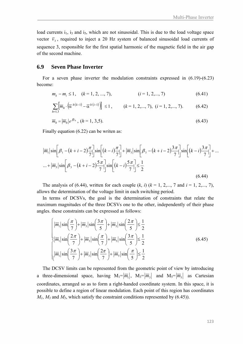
Multi-Phase Inverter
123
load currents i1, i3 and i5, which are not sinusoidal. This is due to the load voltage space
vector 3v , required to inject a 20 Hz system of balanced sinusoidal load currents of
sequence 3, responsible for the first spatial harmonic of the magnetic field in the air gap of the second machine.
6.9 Seven Phase Inverter
For a seven phase inverter the modulation constraints expressed in (6.19)-(6.23) become:
1 ik mm , (k = 1, 2, ..., 7), (i = 1, 2,..., 7) (6.41)
131
11
,h
ihkhhm , (k = 1, 2,..., 7), (i = 1, 2,..., 7). (6.42)
hjhh emm , (h = 1, 3,5). (6.43)
Finally equation (6.22) can be writen as:
2
1
7
5sin
7
52sin...
...7
3sin
7
32sin
7sin
72sin
35
3311
ikikm
ikikmikikm
(6.44)
The analysis of (6.44), written for each couple (k, i) (k = 1, 2,..., 7 and i = 1, 2,..., 7), allows the determination of the voltage limit in each switching period.
In terms of DCSVs, the goal is the determination of constraints that relate the maximum magnitudes of the three DCSVs one to the other, independently of their phase angles. these constraints can be expressed as follows:
2
1
5sin
7
2sin
7
3sin
2
1
5
3sin
7sin
7
2sin
2
1
5
2sin
5
3sin
7sin
531
531
531
mmm
mmm
mmm
(6.45)
The DCSV limits can be represented from the geometric point of view by introducing
a three-dimensional space, having M1= 1m , M3= 3m and M5= 5m as Cartesian
coordinates, arranged so as to form a right-handed coordinate system. In this space, it is possible to define a region of linear modulation. Each point of this region has coordinates M1, M3 and M5, which satisfy the constraint conditions represented by (6.45)).

Chapter 6
124
When, in a switching period, the three reference voltage space vectors refv ,1 , refv ,3 and
refv ,5 require three DCSVs ( 1m , 3m and 5m ) whose magnitudes M1, M3 and M5 define a
point within this region, then the seven modulating signals km (k = 1, 2, ..., 7) will
certainly satisfy the constraint conditions (6.6), provided that a suitable value for 0m is
chosen. This means that the three reference voltage space vectors can be properly synthesized. On the contrary, when the point associated to M1, M3 and M5 is out of the region of linear modulation, the modulating signals cannot satisfy (6.6) leading, in this case, to over-modulation conditions.
The inequalities (6.45) describe three portions of space that they are delimited by the equations (6.46).
2
1
5sin
7
2sin
7
3sin
2
1
5
3sin
7sin
7
2sin
2
1
5
2sin
5
3sin
7sin
531
531
531
MMM
MMM
MMM
(6.46)
Equation (6.47) set the framework within which (6.46) defines the voltage limits of a
Fig 6.11 Voltage limits of seven phase inverter, 3D representation
Table II COORDINATES OF SPECIFIC POINTS OF THE REGION OF LINEAR MODULATION
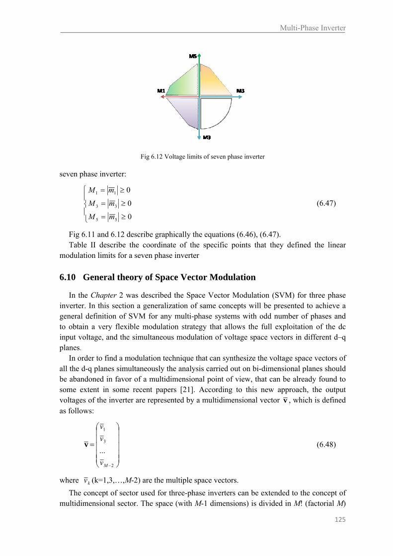
Multi-Phase Inverter
125
seven phase inverter:
0
0
0
55
33
11
mM
mM
mM
(6.47)
Fig 6.11 and 6.12 describe graphically the equations (6.46), (6.47). Table II describe the coordinate of the specific points that they defined the linear
modulation limits for a seven phase inverter
6.10 General theory of Space Vector Modulation
In the Chapter 2 was described the Space Vector Modulation (SVM) for three phase inverter. In this section a generalization of same concepts will be presented to achieve a general definition of SVM for any multi-phase systems with odd number of phases and to obtain a very flexible modulation strategy that allows the full exploitation of the dc input voltage, and the simultaneous modulation of voltage space vectors in different d–q planes.
In order to find a modulation technique that can synthesize the voltage space vectors of all the d-q planes simultaneously the analysis carried out on bi-dimensional planes should be abandoned in favor of a multidimensional point of view, that can be already found to some extent in some recent papers [21]. According to this new approach, the output voltages of the inverter are represented by a multidimensional vector v , which is defined as follows:
2
3
1
...
Mv
v
v
v (6.48)
where kv (k=1,3,…,M-2) are the multiple space vectors.
The concept of sector used for three-phase inverters can be extended to the concept of multidimensional sector. The space (with M-1 dimensions) is divided in M! (factorial M)
Fig 6.12 Voltage limits of seven phase inverter
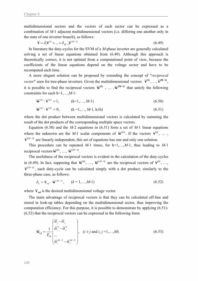
Chapter 6
126
multidimensional sectors and the vectors of each sector can be expressed as a combination of M-1 adjacent multidimensional vectors (i.e. differing one another only in the state of one inverter branch), as follows:
)1(1
)1(1 ...
MM vvv (6.49)
In literature the duty-cycles for the SVM of a M-phase inverter are generally calculated solving a set of linear equations obtained from (6.49). Although this approach is theoretically correct, it is not optimal from a computational point of view, because the coefficients of the linear equations depend on the voltage sector and have to be recomputed each time.
A more elegant solution can be proposed by extending the concept of "reciprocal
vector" seen for tree-phase inverters. Given the multidimensional vectors (1)v , …, 1)(Mv ,
it is possible to find the reciprocal vectors (1)w , … , 1)(Mw that satisfy the following constraints for each h=1,…,M-1:
1)()( kk vw , (k=1,…, M-1) (6.50)
0)()( hk vw , (k =1,…, M-1, k≠h) (6.51)
where the dot product between multidimensional vectors is calculated by summing the result of the dot products of the corresponding multiple space vectors.
Equation (6.50) and the M-2 equations in (6.51) form a set of M-1 linear equations
where the unknown are the M-1 scalar components of )(w k . If the vectors )(v 1 , … , )(v 1M are linearly-independent, this set of equations has one and only one solution.
This procedure can be repeated M-1 times, for h=1,…,M-1, thus leading to M-1
reciprocal vectors )(w 1 , …, )(w 1M . The usefulness of the reciprocal vectors is evident in the calculation of the duty-cycles
in (6.49). In fact, supposing that )(w 1 , …, )(w 1M are the reciprocal vectors of )(v 1 , …, )(v 1M , each duty-cycle can be calculated simply with a dot product, similarly to the
three-phase case, as follows:
)1( Mrefk wv , (k = 1,…,M-1) (6.52)
where refv is the desired multidimensional voltage vector.
The main advantage of reciprocal vectors is that they can be calculated off-line and stored in look-up tables depending on the multidimensional sector, thus improving the computation efficiency. For this purpose, it is possible to demonstrate by applying (6.51)-(6.52) that the reciprocal vectors can be expressed in the following form:
22
33
...
1
Mj
Mi
ji
ji
dcE
ji,w , (i ≠ j and i, j =1,…,M). (6.53)

Multi-Phase Inverter
127
From (6.53) it follows that there are M(M-1) different vectors ji,w , but it is sufficient
to store in look-up tables only half of them, because the vectors reverse if the subscripts are swapped, as follows:
ij,ji, ww . (6.54)
Likewise the active multidimensional vectors )(v 1 , …, )(v 1M , the reciprocal vectors depend on the sector in which the desired voltage vector is placed, and therefore can be stored in a look-up table depending on the sector number.
6.11 Identification of the Sector Number
In the traditional implementation of SVM some quantities, such as the switching configurations or the coefficients used for the calculation of the duty-cycles, are stored in lookup tables that are quickly accessed using the sector number as an index.
In this section, the identification of the sector number will be examined more in details.
A. Identification of Sector for Three Phase VSI The determination of the sector S of the reference vector, with modern floating-point
DSP or high-frequency fixed-point DSP, is very simple for three-phase inverters because
it is sufficient to calculate the argument θ of refv using inverse trigonometric functions.
Assuming θ in the range 0° ≤ θ < 360°, the sector number is given by:
60int
S (6.55)
where the function int(·) provides the integer part of the argument.
Another method to determine the sector of the reference vector is explained hereafter. This method can be used also for low-cost fixed point DSP, due to the fact that it does not require the evaluation of any inverse trigonometric function, but only the calculation of dot products.
The main idea is that each sector can be represented univocally as the intersection of three half-planes. For example, Fig. 6.13 shows that Sector 1 is the intersection of the three half-planes highlighted in gray.
To check if the reference voltage vector lies in a certain sector, it is sufficient to verify that it belongs to the three half-planes whose intersection is the given sector. This result is very powerful, since it is straightforward to check whether the reference voltage vector
=
Fig. 6.13 - Representation of Sector 1 as intersection of three half-planes.

Chapter 6
128
belongs to three half-planes or not by calculating the logic functions kL (k = 1, 2, 3)
defined as follows:
otherwise
uvifL kref
k0
01 (6.56)
where ku (k=1,2,3) are defined as follows:
)1(
3
2
kj
k jeu
(k=1, 2, 3). (6.57)
All vectors placed in the same sector lead to the same values of the logic functions kL ,
so it is possible to state that each sector is univocally identified by a sector code, i.e., a
tern of logic values ( 3L , 2L , 1L ).
This result is clearly shown in Fig. 6.14, where the correspondence between sector numbers and sector codes is shown.
Furthermore, Fig. 6.14 shows also the three vectors 1u , 2u , and 3u defined by (6.57).
It is worth noting that vectors 1u , 2u , and 3u represent a subset of the reciprocal vectors
that can be found by applying (6.53) in the case of three-phase inverters.
After the calculation of kL with (6.56), the sector of refv can be identified by using
Table III that relates the sector codes ( 3L , 2L , 1L ) to the sector numbers. The entries of
Table III have been ordered so that the sector code, interpreted as a binary number and converted to its decimal representation, can be used as the address for identifying the table entry of the sector number
B. Sectors in Multi-Phase Inverter The identification of the sector of a multidimensional voltage vector is not as
immediate as in the three-phase case, because the orientation of the multidimensional sectors in the space cannot be traced back to a simple principle.
The solution to this problem can be found by extending the method of space partitioning presented for three-phase VSI.
It can be demonstrated that a multidimensional sector of a M-phase inverter is the
intersection of M(M − 1)/2 half-spaces at most.
The logic functions that express the belonging of the reference multidimensional vector to an half-space can be written as follows:
TABLE III SECTOR NUMBER AS FUNCTION OF SECTOR BINARY CODE
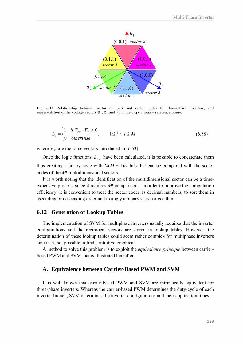
Multi-Phase Inverter
129
otherwise
wvifL
ijrefij
0
01, Mji 1 (6.58)
where ijw are the same vectors introduced in (6.53).
Once the logic functions khL , have been calculated, it is possible to concatenate them
thus creating a binary code with M(M − 1)/2 bits that can be compared with the sector
codes of the M! multidimensional sectors. It is worth noting that the identification of the multidimensional sector can be a time-
expensive process, since it requires M! comparisons. In order to improve the computation efficiency, it is convenient to treat the sector codes as decimal numbers, to sort them in ascending or descending order and to apply a binary search algorithm.
6.12 Generation of Lookup Tables
The implementation of SVM for multiphase inverters usually requires that the inverter configurations and the reciprocal vectors are stored in lookup tables. However, the determination of these lookup tables could seem rather complex for multiphase inverters since it is not possible to find a intuitive graphical
A method to solve this problem is to exploit the equivalence principle between carrier-based PWM and SVM that is illustrated hereafter.
A. Equivalence between Carrier-Based PWM and SVM It is well known that carrier-based PWM and SVM are intrinsically equivalent for
three-phase inverters. Whereas the carrier-based PWM determines the duty-cycle of each inverter branch, SVM determines the inverter configurations and their application times.
1u
(1,0,1)
(0,0,1)
(0,1,1)
(0,1,0)
(1,1,0)
(1,0,0)
sector 1
sector 2
sector 3
sector 5 sector 6
sector 4 2u 3u
Fig. 6.14 Relationship between sector numbers and sector codes for three-phase inverters, andrepresentation of the voltage vectors 1u , 2u and 3u in the d-q stationary reference frame.

Chapter 6
130
This equivalence is clearly shown in the example of Fig. 6.17. It is shown that the sequence of vectors obtained with SVM for the case of Fig. 6.17 can be deduced also with PWM when m1>m2>m3.
Initially, a zero vector is applied to the load, since all command signals sk (k = 1, 2, 3) are zero. Since m1>m2 and, consequently, s1 turns on before s2, the first active vector
applied to the load is 1v , whose configuration is (001). The second active vector is 2v ,
with configuration (011), followed by a zero vector with configuration (111). Finally, these same vectors complete the period, but they are applied in reverse order.
It is obvious that this result, now stated for vector lying in Sector 1, can be elevated to
a general principle, namely, each set of modulating signals 1m , 2m , and 3m can be related
to an equivalent sequence of space vectors, as if it were generated with SVM, and vice versa.
The equivalence between SVM and carrier-based PWM for three-phase inverters allows an interesting interpretation of the concept of sector used in SVM. It has just been shown that the vectors in Sector 1 leads to command signals satisfying the conditions
1m > 2m > 3m . Likewise, the vectors of Sector 2 are characterized by command signals
with 2m > 1m > 3m . In other words, it is possible to associate each sector to a specific
ordering of the duty-cycles 1m , 2m , and 3m , as illustrated in Table IV.
The equivalence between carrier-based PWM and SVM turns out to be true also for multiphase inverters. According to this point of view, the vectors of the multidimensional Sector 1 are those that satisfy the following constraints:
Mmmm ...21 (6.59)
whereas the other sectors are characterized by a different ordering of the duty-cycles of
the inverter branches. There are M! different ordering of 1m , 2m , . . . , Mm , hence there
are also M! different sectors.
TABLE IV RELATIONSHIP BETWEEN SECTORS AND ORDERING OF BRANCH DUTY CYCLES IN TRADITIONAL THREE PHASE INVERTER
Sector 1 ORDERING
1 321 mmm
2 312 mmm
3 132 mmm
4 123 mmm
5 213 mmm
6 231 mmm
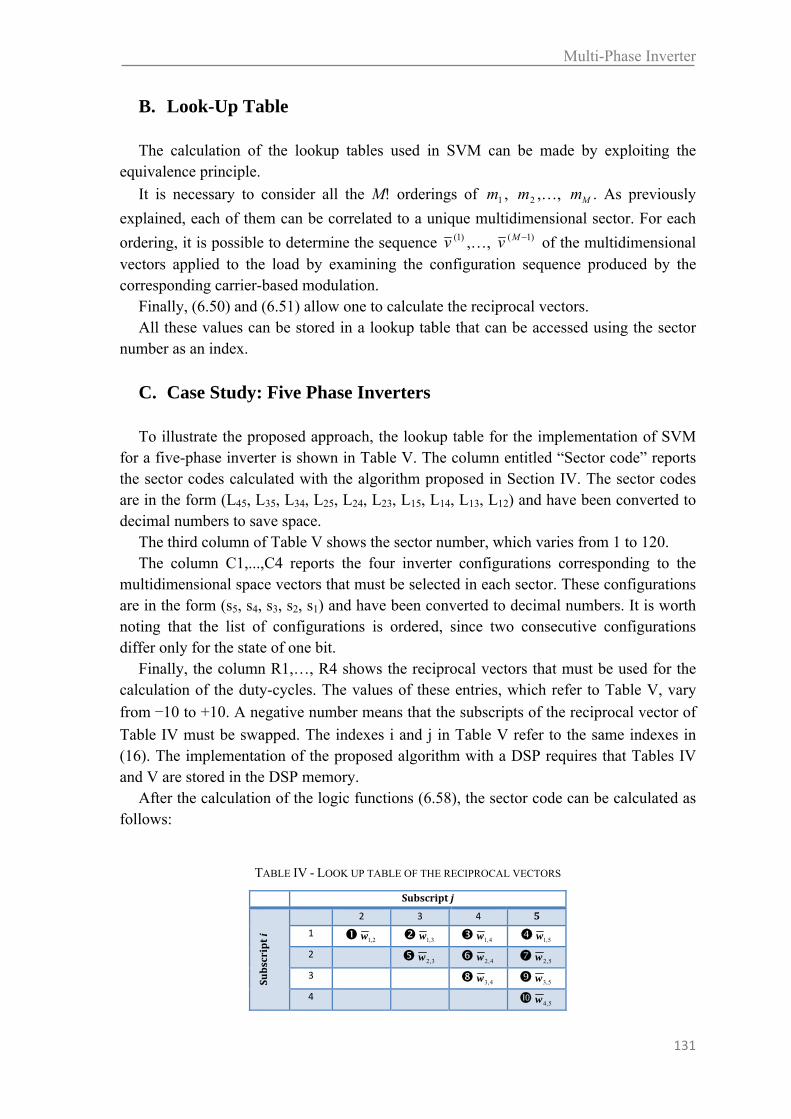
Multi-Phase Inverter
131
B. Look-Up Table The calculation of the lookup tables used in SVM can be made by exploiting the
equivalence principle.
It is necessary to consider all the M! orderings of 1m , 2m ,…, Mm . As previously
explained, each of them can be correlated to a unique multidimensional sector. For each
ordering, it is possible to determine the sequence )1(v ,…, )1( Mv of the multidimensional vectors applied to the load by examining the configuration sequence produced by the corresponding carrier-based modulation.
Finally, (6.50) and (6.51) allow one to calculate the reciprocal vectors. All these values can be stored in a lookup table that can be accessed using the sector
number as an index.
C. Case Study: Five Phase Inverters To illustrate the proposed approach, the lookup table for the implementation of SVM
for a five-phase inverter is shown in Table V. The column entitled “Sector code” reports the sector codes calculated with the algorithm proposed in Section IV. The sector codes are in the form (L45, L35, L34, L25, L24, L23, L15, L14, L13, L12) and have been converted to decimal numbers to save space.
The third column of Table V shows the sector number, which varies from 1 to 120. The column C1,...,C4 reports the four inverter configurations corresponding to the
multidimensional space vectors that must be selected in each sector. These configurations are in the form (s5, s4, s3, s2, s1) and have been converted to decimal numbers. It is worth noting that the list of configurations is ordered, since two consecutive configurations differ only for the state of one bit.
Finally, the column R1,…, R4 shows the reciprocal vectors that must be used for the calculation of the duty-cycles. The values of these entries, which refer to Table V, vary
from −10 to +10. A negative number means that the subscripts of the reciprocal vector of
Table IV must be swapped. The indexes i and j in Table V refer to the same indexes in (16). The implementation of the proposed algorithm with a DSP requires that Tables IV and V are stored in the DSP memory.
After the calculation of the logic functions (6.58), the sector code can be calculated as follows:
TABLE IV - LOOK UP TABLE OF THE RECIPROCAL VECTORS
Subscript j
Subscript i
2 3 4 5
1 2,1w 3,1w 4,1w 5,1w
2 3,2w 4,2w 5,2w
3 4,3w 5,3w
4 5,4w

Chapter 6
132
012
734
835
945 2...222 LLLLcodeSector (6.60)
It is worth noting that the calculation of (6.60) is usually very fast using binary numbers, since it can be done with left logical shift and bitwise operations.
To find the multidimensional sector, the sector code (6.60) has to be compared to the sector codes of Table V by using the binary search algorithm. In this way, it is possible to identify the reciprocal vectors needed for the calculation of the duty-cycles and the inverter configurations.
Id. Sector Code
Sector Number
C1,C2,C3,C4 R1,R2,R3,R4
1 0 65 16,24,28,30 -10,-8,-5,-1 2 1 56 16,24,28,29 -10,-8,-2,1 3 3 25 16,24,25,29 -10,-3,2,-5 4 7 26 16,17,25,29 -4,3,-8,-5 5 15 27 1,17,25,29 4,-10,-8,-5 6 16 96 16,24,26,30 -10,-6,5,-2 7 18 105 16,24,26,27 -10,-6,-1,2 8 19 16 16,24,25,27 -10,-3,1,5 9 23 15 16,17,25,27 -4,3,-6,5 10 31 14 1,17,25,27 4,-10,-6,5 11 48 95 16,18,26,30 -7,6,-8,-2 12 50 106 16,18,26,27 -7,6,-3,2 13 54 115 16,18,19,27 -7,-1,3,-8 14 55 6 16,17,19,27 -4,1,6,-8 15 63 7 1,17,19,27 4,-7,6,-8 16 112 94 2,18,26,30 7,-10,-8,-2 17 114 107 2,18,26,27 7,-10,-3,2 18 118 114 2,18,19,27 7,-4,3,-8 19 126 113 2,3,19,27 -1,4,-10,-8 20 127 8 1,3,19,27 1,7,-10,-8 21 128 66 16,20,28,30 -9,8,-6,-1 22 129 55 16,20,28,29 -9,8,-3,1 23 133 46 16,20,21,29 -9,-2,3,-6 24 135 35 16,17,21,29 -4,2,8,-6 25 143 34 1,17,21,29 4,-9,8,-6 26 160 75 16,20,22,30 -9,-5,6,-3 27 164 76 16,20,22,23 -9,-5,-1,3 28 165 45 16,20,21,23 -9,-2,1,6 29 167 36 16,17,21,23 -4,2,-5,6 30 175 37 1,17,21,23 4,-9,-5,6 31 176 86 16,18,22,30 -7,5,8,-3 32 180 85 16,18,22,23 -7,5,-2,3 33 182 116 16,18,19,23 -7,-1,2,8 34 183 5 16,17,19,23 -4,1,5,8 35 191 4 1,17,19,23 4,-7,5,8 36 240 87 2,18,22,30 7,-9,8,-3 37 244 84 2,18,22,23 7,-9,-2,3 38 246 117 2,18,19,23 7,-4,2,8 39 254 118 2,3,19,23 -1,4,-9,8 40 255 3 1,3,19,23 1,7,-9,8 41 384 67 4,20,28,30 9,-10,-6,-1 42 385 54 4,20,28,29 9,-10,-3,1 43 389 47 4,20,21,29 9,-4,3,-6 44 397 48 4,5,21,29 -2,4,-10,-6 45 399 33 1,5,21,29 2,9,-10,-6 46 416 74 4,20,22,30 9,-7,6,-3 47 420 77 4,20,22,23 9,-7,-1,3 48 421 44 4,20,21,23 9,-4,1,6 49 429 43 4,5,21,23 -2,4,-7,6 50 431 38 1,5,21,23 2,9,-7,6 51 480 73 4,6,22,30 -5,7,-10,-3 52 484 78 4,6,22,23 -5,7,-4,3 53 492 79 4,6,7,23 -5,-1,4,-10 54 493 42 4,5,7,23 -2,1,7,-10 55 495 39 1,5,7,23 2,-5,7,-10 56 496 88 2,6,22,30 5,9,-10,-3 57 500 83 2,6,22,23 5,9,-4,3 58 508 82 2,6,7,23 5,-2,4,-10 59 510 119 2,3,7,23 -1,2,9,-10 60 511 2 1,3,7,23 1,5,9,-10 61 512 64 8,24,28,30 10,-9,-5,-1 62 513 57 8,24,28,29 10,-9,-2,1 63 515 24 8,24,25,29 10,-4,2,-5 64 523 23 8,9,25,29 -3,4,-9,-5 65 527 28 1,9,25,29 3,10,-9,-5 66 528 97 8,24,26,30 10,-7,5,-2
TABLE V - LOOK UP TABLE FOR SVM OF 5-PHASE INVERTERS

Multi-Phase Inverter
133
67 530 104 8,24,26,27 10,-7,-1,2 68 531 17 8,24,25,27 10,-4,1,5 69 539 18 8,9,25,27 -3,4,-7,5 70 543 13 1,9,25,27 3,10,-7,5 71 592 98 8,10,26,30 -6,7,-9,-2 72 594 103 8,10,26,27 -6,7,-4,2 73 602 102 8,10,11,27 -6,-1,4,-9 74 603 19 8,9,11,27 -3,1,7,-9 75 607 12 1,9,11,27 3,-6,7,-9 76 624 93 2,10,26,30 6,10,-9,-2 77 626 108 2,10,26,27 6,10,-4,2 78 634 109 2,10,11,27 6,-3,4,-9 79 638 112 2,3,11,27 -1,3,10,-9 80 639 9 1,3,11,27 1,6,10,-9 81 768 63 8,12,28,30 -8,9,-7,1 82 769 58 8,12,28,29 -8,9,-4,1 83 777 59 8,12,13,29 -8,-2,4,-7 84 779 22 8,9,13,29 -3,2,9,-7 85 783 29 1,9,13,29 3,-8,9,-7 86 832 62 8,12,14,30 -8,-5,7,-4 87 840 61 8,12,14,15 -8,-5,-1,4 88 841 60 8,12,13,15 -8,-2,1,7 89 843 21 8,9,13,15 -3,2,-5,7 90 847 30 1,9,13,15 3,-8,-5,7 91 848 99 8,10,14,30 -6,5,9,-4 92 856 100 8,10,14,15 -6,5,-2,4 93 858 101 8,10,11,15 -6,-1,2,9 94 859 20 8,9,11,15 -3,1,5,9 95 863 11 1,9,11,15 3,-6,5,9 96 880 92 2,10,14,30 6,-8,9,-4 97 888 91 2,10,14,15 6,-8,-2,4 98 890 110 2,10,11,15 6,-3,2,9 99 894 111 2,3,11,15 -1,3,-8,9 100 895 10 1,3,11,15 1,6,-8,9 101 896 68 4,12,28,30 8,10,-7,-1 102 897 53 4,12,28,29 8,10,-4,1 103 905 52 4,12,13,29 8,-3,4,-7 104 909 49 4,5,13,29 -2,3,10,-7 105 911 32 1,5,13,29 2,8,10,-7 106 960 69 4,12,14,30 8,-6,7,-4 107 968 70 4,12,14,15 8,-6,-1,4 108 969 51 4,12,13,15 8,-3,1,7 109 973 50 4,5,13,15 -2,3,-6,7 110 975 31 1,5,13,15 2,8,-6,7 111 992 72 4,6,14,30 -5,6,10,-4 112 1000 71 4,6,14,15 -5,6,-3,4 113 1004 80 4,6,7,15 -5,-1,3,10 114 1005 41 4,5,7,15 -2,1,6,10 115 1007 40 1,5,7,15 2,-5,6,10 116 1008 89 2,6,14,30 5,8,10,-4 117 1016 90 2,6,14,15 5,8,-3,4 118 1020 81 2,6,7,15 5,-2,3,10 119 1022 120 2,3,7,15 -1,2,8,10 120 1023 1 1,3,7,15 1,5,8,10
6.13 Remarks on the Proposed SVM Algorithm
The main advantages of the proposed algorithm are: i) its generality, since it can be theoretically adopted for an M-phase inverter
(provided that M is an odd number);
ii) its capability to generate the whole set of the admissible output voltages and not only a reduced set; and
iii) its formal similarity with the three-phase SVM.
Several papers have been published on SVM of multiphase inverter, and some of them have obtained remarkable results, for example, showing the capability of the maximum voltage transfer ratio of about 0.6 for five-phase inverters. This result has been obtained

Chapter 6
134
by adding a small contribution of a third-harmonic component on the phase voltage [4], [5], synchronized with the fundamental component.
The wide majority of these papers is based on the idea that the selection of the inverter configurations can be made by correlating them to the positions (i.e., the sectors) of the multiple voltage vectors in the different d–q planes.
However, this concept could be somehow restrictive, as the following example demonstrates for five-phase inverters. Fig. 6.15 shows the admissible voltage vectors in the planes d1–q1 and d3–q3 of a five-phase inverter. If the desired output phase voltages
are nnnnn vvvvv 54321 , then the configurations selected by the proposed SVM
algorithm and by the carrier-based PWM algorithm are those inside the black rectangles. As shown, these configurations do not delimit any specific sector in the d–q planes and therefore it is not possible to derive a simple rule for their determination.
The algorithms based on the analysis carried out in separate d–q planes are not able to synthesize these voltages, although they work perfectly for the synthesis of sinusoidal or little distorted voltages. In other words, they give more priority to vectors in the plane d1–q1 over vectors in plane d3–q3.
More general results can be obtained with the methods proposed in [14] and [21] that can independently synthesize voltage vectors in more than one d–q plane, but needs more computational time, since both [14] and [21] require a sort algorithm.
It is worth noting that the most recent theories of SVM for multiphase inverter to some extent involve some CPU demanding tasks.
In the proposed modulation strategy, the most time consuming part is certainly the binary search algorithm, since (6.52) and (6.58) are mainly dot products that can be executed very quickly on modern DSP, optimized for multiply-and accumulate
operations. This binary search algorithm requires ceil ( )!(log2 M ) comparisons at most
for a M-phase inverter (the ceil function returns the smallest integer number that is greater or equal to the specified argument). For example, in the case of a five-phase inverter, the binary search requires seven comparisons. Instead, assuming that the sort algorithm used in [14] is a bubble sort (usually adopted for its efficiency when the number of elements is
Fig. 6.15. Multiple space vectors of a five-phase inverters, represented in planes d1-q1 and d3-q3.

Multi-Phase Inverter
135
very small), the sorting algorithm for a five-phase inverter involves ten comparisons and, at worst, also as many swaps of variables. Obviously, this result is far from proving that the proposed algorithm is faster or better than that of [14] that is suitable also for multilevel inverter, since the complexity should be related also to the available hardware, e.g., DSP or FPGA, its features and also on the capability of the programmer.
6.14 Experimental Results for Look-Up Table Solution
To verify the effectiveness of the proposed modulation strategy some experimental tests have been carried out.
The experimental setup consists of a five-phase voltage source inverter feeding a five-phase symmetrical series-connected R-L load. The load parameters in nominal condition are 11.5 Ω and around 11 mH. The dc bus voltage is around 100 V. The control algorithm is implemented in a DSP TMS320F2812 and an Altera FPGA Cyclone EP1C6. The switching period is 100 μs, corresponding to a switching frequency of 10 kHz.
The total computational time of the SVM algorithm is lower than 20μs. The calculation of the logic functions requires about 5 μs, the binary search algorithm about 12 μs and the calculation of the duty-cycles about 2 μs.
With reference to the demanded voltages, four cases will be considered, namely, A, B, C, and D. The corresponding values of refv ,1 and refv ,3 f are summarized in Table VI.
These cases have been selected to show that the proposed modulation technique is able to generate the reference multiple voltage vectors in the most critical operating conditions.
Fig 6.16 Experimental result. Waveform (top, 2 A/div) of the load currents and (bottom, 40 V/div) of the phase voltage in the condition A.
TABLE VI VALUES OF refv ,1 AND refv ,3 CONSIDERED IN EXPERIMENTAL TEST
A B C D
refv ,1 50 V, 50 Hz 0 30 V, 50 Hz 60 V, 50 Hz
refv ,3 0 50 V, 50 Hz 30 V, 150 Hz 15 V, 150 Hz

Chapter 6
136
Fig. 6.16 shows the waveforms of a load current and of the corresponding phase voltage in the condition A, when a voltage reference vector of 50 V is rotating at 2π50 rad/s in plane d1–q1, whereas the voltage reference vector in plane d3–q3 is zero. As shown, the waveforms are nearly sinusoidal, except for the current ripple due to the switching process, and the load phase voltage exhibits the typical nine-level waveform
(0,±1/5Edc,±2/5Edc, . . . ,±4/5Edc).
Fig. 6.17 shows the behavior of the five-phase inverter in the same operating condition. In particular, tracks 2, 3, and 4 show the sector number, the entry address in Table V, and the index R1 of the reciprocal vector used for the calculation of the first duty-cycle. It is evident that the sector number assumes ten different values in a period. Curiously, its waveform is not regular even in this simple case, because it often jumps from a value to another value that is not adjacent.
Finally, Fig. 6.18 shows the waveforms of the duty-cycles δ1, δ2, δ3, and δ4 for the same case of Figs. 6.17 and 6.16. It is interesting that the waveforms of δ1 and δ4 or δ2 and δ3 are nearly opposite.
Fig. 6.19 shows the behavior of the inverter in condition B, when only the voltage
Fig 6.17 Experimental result. Behavior of the inverter in the condition A. (From top to bottom) Load current (5 A/div), sector number (60/div), entry address of Table III (60/div), and index R1 of the first reciprocal vector (5/div).
Fig 6.18 Experimental result. Waveforms of the duty-cycles δ1, . . . , δ4 in condition A (2 ms/div).

Multi-Phase Inverter
137
vector in plane d3–q3 is not zero. As shown, the signals representing the sector number, the table entry and the reciprocal vector index are very different from those of Fig. 6.20, and this means that new voltage vectors are involved in the modulation process.
Afterward, some tests have been carried out to verify the capability of the proposed SVM to generate simultaneously multiple voltage vectors in the planes d1–q1 and d3–q3.
Fig. 6.20 shows the behavior of the inverter in the condition C, when a voltage reference vector of 30 V is rotating at 2π 50 rad/s in plane d1–q1 and a voltage reference vector of 30 V is rotating at 2π 150 rad/s in plane d3–q3.
The first trace of Fig. 6.20 shows the current waveform, which is evidently distorted by the presence of the third harmonic component. The other traces are the sector number, the entry address in Table V, and the index R1 of the first reciprocal vector. The waveforms of the duty-cycles corresponding to the operating condition of Fig. 6.20 are shown in Fig. 6.21 which highlights that δ2 and δ3 are now very similar.
Finally, Fig. 6.22 shows the behavior of the inverter in the condition D, that corresponds to the maximum phase voltages.
Fig 6.19 Experimental result. Behavior of the inverter in the condition B. (From top to bottom) Load current (3 A/div), sector number (60/div), entry address of Table III (60/div), and index R1 of the first reciprocal vector (5/div).
Fig 6.20 Experimental result. Behavior of the inverter in the condition C. (From top to bottom) Load current (3 A/div), sector number (60/div), entry address of Table III (60/div), and index R1 of the first reciprocal vector (5/div).

Chapter 6
138
As shown, the load current are remarkably distorted also in this case by the presence of a significant third harmonic component.
6.15 Space Vector Modulation for a Multi-Phase Inverter: Solution Based on Ranking Functions
The solution of SVM explained in the previous subsection requires the execution of a sorting algorithm, the calculation of the duty-cycles and the calculation of the switching configurations.
In the previous implementation of SVM some quantities, such as the switching configurations or the coefficients used for the calculation of the duty-cycles, are stored in look-up tables, that are quickly accessed using the sector number as an index.
Therefore, to adopt this methodology with multiphase inverters, it is necessary to identify the sector of the multidimensional vector with a unique number.
Fig 6.21 Experimental result. Waveform of the duty-cycles δ1, . . . , δ4 in the condition C.
Fig 6.22 Experimental result. Behavior of the inverter in the condition D. (From top to bottom) Load current (3 A/div), sector number (60/div), entry address of Table III (60/div), and index R1 of the first reciprocal vector (5/div).

Multi-Phase Inverter
139
This can be done by introducing the concept of ranking function R(p), i.e. a bijective algorithm that takes as input a permutation on the set 1, 2, …, M and produces a number in the range 0, …, M!-1.
The traditional approach to this problem is to first choose an ordering criterion for permutations. Then the rank of a permutation is simply defined as the number of permutations that precede it according to this ordering criterion.
The two most used ranking functions are the lexicographic ranking function Rlex and the Steinhaus- Johnson-Trotter (SJT) ranking function RSJT [23],[24].
When a ranking function is applied to the ordering permutation p(k) (k=1,2,…,M), the result is a unique number in the range [0,M!-1], that can be used to identify the corresponding multidimensional sector.
The algorithms for the ranking functions Rlex and RSJT are shown in Fig. 6.26 and Fig. 6.27, respectively.
The algorithm are written using MATLAB language. In both algorithms, p is the array of M elements that represents the permutation function. The variable r is the return variable containing the rank of p.
A detailed explanation of these ranking functions is beyond the scope of this treatment. A theoretical background can be found in [23]-[24].
A. Lexicographic Ranking Function The lexicographic order is based on the familiar idea as the ordering of words in
dictionaries, provided that letters are replaced by numbers. According to this ordering principle, for example, the permutation (1,2,3) comes
before the permutation (1,3,2), likewise the word "ABC" comes before the word "ACB" in a dictionary.
B. Steinhaus- Johnson-Trotter Ranking Function The SJT ordering is based on the idea that two consecutive permutations should differ
only by a transposition of two elements. For example, the six permutations of three objects 1, 2, 3, according to the SJT algorithm, could be listed in the following order:
(1,2,3), (2,1,3), (2,3,1), (3,2,1), (3,1,2), (1,3,2) This ordering is just one of the possibilities and it is characterized by the fact that the
number 1 “sweeps” from left to right, and then right to left, through each of the six
Fig 6.23 Matlab code for the lexicographic ranking function

Chapter 6
140
permutations. When the position of 1 becomes extreme (either at the right or left), then recursively an adjacent transposition is done between two of the remaining numbers.
As can be seen from Fig. 6.24, the SJT algorithm is more time-consuming than the lexicographic one and therefore it does not offer any advantage in this context. However, it is notable that applying the SJR algorithm to three-phase inverters leads to the traditional numeration of the sectors, shown in Table II (provided that the sector numbers are in the range 0,1,…,5 instead of 1,2,…,6).
Fig 6.24 Matlab code for the SJT ranking function
a)b)
c)
Fig 6.25 Experimental test. Behavior of the seven phase inverter when all the reference multiple vectors are zero except v1. (a) Waveform of currents i1, i3 and i5 (4A/div) and sector index (3000 sectors/div) calculated with lexicographic ranking function (5ms/div). (b) Waveform of currents i1, i3 and i5 (4A/div) and sector index (3000 sectors/div) calculated with STJ ranking function (5ms/div) (c) Waveforms of the duty-cycles δ1, δ2, δ3 and δ4 (2ms/div).

Multi-Phase Inverter
141
6.16 Experimental Results for Algorithm Solution
Some experimental tests have been carried out to verify the effectiveness of the proposed modulation strategy.
The experimental setup consists of a seven-phase voltage source inverter feeding a seven-phase symmetrical series-connected R-L load. The load parameters in nominal condition are 10.5 Ω and around 0.4 mH. The dc bus voltage is around 110 V. The control algorithm is implemented in a DSP TMS320F2812 and an Altera FPGA Cyclone EP1C6. The switching period is 100 μs, corresponding to a switching frequency of 10 kHz.
Fig. 6.25 shows behavior of the seven-phase inverter when a voltage reference vector of 50 V is rotating at 2π 50 rad/s in plane d1-q1, whereas the voltage reference vector in
the other planes is zero. Fig. 6.25(a) and 6.25(b) show the waveforms of the currents 1i ,
3i and 5i . The lower trace in both figures is the sector number, calculated with the
lexicographic ranking function and the SJT ranking function. As can be seen, the sector number assumes fourteen different values in a period. However its waveform is not regular even in this simple case, because it often jumps among non-contiguous values.
Fig.6.28 (c) shows the waveforms of the duty-cycles δ1, δ2, δ3 and δ4. It is interesting to note that in this case the duty-cycles appear to vary linearly during the fundamental period, and they form two groups, one with phase opposite to the other.
Fig. 6.26 shows the behavior of the inverter when a voltage reference vector of 30 V is rotating at 2π 50 rad/s in plane d1-q1, a voltage reference vector of 15 V is rotating at 2π
a) b)
Fig 6.26 Experimental test. Behavior of the seven phase inverter when v1 is 30 V, v3 is 15 V and v5 is 12 V. (a) Waveform of currents i1, i3 and i5 (4A/div) and sector index (3000 sectors/div) calculated with lexicographic ranking function (10ms/div). (b) Waveform of currents i1, i3 and i5 (4A/div) and sector index (3000 sectors/div) calculated with the STJ ranking function (10ms/div). (c) Waveforms of the duty-cycles δ1, δ2, δ3 and δ4 (2ms/div).
c)
Chapter 6
142
150 rad/s in plane d3-q3, and a voltage vector of 12 V is rotating at 2π 250 rad/s in plane d5-q5.
Fig. 6.26 (a) and 6.26 (b) show the waveforms of the currents, 1i 3i and 5i . The lower
trace in both figures is the sector number, calculated with the lexicographic ranking function and the SJT ranking function. Fig. 6.26 (c) shows the waveforms of the duty-cycles δ1, δ2, δ3 and δ4. It is interesting to note that the duty-cycles are now very different from the case of Fig. 6.25 (c) and each behaves differently from the others.
6.17 Conclusions
In this chapter a description of the multi-phase inverter with a odd number of phases has been presented.
A general theory of pulse width modulation and of space vector modulation has been proposed. Different solutions has been developed to solve the problem of generalization of SVM in the multi-phase systems.
The concepts of multidimensional space vector and reciprocal vector have been introduced. Using these concepts it is possible to consider the well-known three-phase space vector modulation as a particular case of the proposed approach. In particular it is possible to give a definition of "sector" that is coherent with the one used for three-phase inverters.
Finally different algorithm for the determination of the sector have been presented. The feasibility of the SVM algorithm has been confirmed with several experimental
tests on a five-phase inverter and a seven-phase inverter. In next chapter a new modulation technique will be presented. The main target of this
technique is the minimization of inverter losses
6.18 References
[1] G. Grandi, G. Serra, A. Tani, “General analysis of multi-phase systems based on space vector approach,” in Proc. of 12th Power Electronics and Motion Control Conference (EPE-PEMC), 2006, CD-ROM paper T2-409.
[2] ]J. K. Kelly, E.G. Strangas, J.M. Miller, “Multiphase space vector pulse width modulation,” IEEE
Trans. on Energy Conversion, vol. 18, no. 2, 2003, pp. 259-264. [3] ]P. S. N. De Silva, J. E. Fletcher, B. W. Williams, “Development of space vector modulation strategies
for five phase voltage source inverters,” in Proc. of IEE Power Electronics, Machines and Drives Conference, 2004, pp. 650-650.
[4] A. Iqbal, E. Levi, “Space vector modulation scheme for a five-phase voltage source inverter,” in Proc.
of 11th European Conf. on Power Electronics and Applications (EPE), 2005, CD-ROM paper 006. [5] H. M. Ryu, J. H. Kim, S. K. Sul, “Analysis of multiphase space vector pulse-width modulation based
on multiple d-q spaces concept,” IEEE Trans. on Power Electronics, vol. 20, no. 6, Nov. 2005, pp. 1364-1371.
Multi-Phase Inverter
143
[6] M. Duran, E. Levi, "Multi-dimensional approach to multi-phase space vector pulse width modulation," in Proc of IECON 2006, Paris, France, 7-10 November, 2006, pp.2103-2108.
[7] A. Iqbal, E. Levi, M. Jones, S.N. Vukosavic, “A PWM scheme for a five-phase VSI supplying a five-
phase two-motor drive,” in Proc. of Annual Conference of the IEEE Industrial Electronics Society (IECON), 2006, pp. 2575-2580
[8] D. Casadei, G. Serra, A.Tani, L. Zarri, “Multi-phase inverter modulation strategies based on duty-
cycle space vector approach, ” in Proc. of SPRTS’2005, Bologna (Italy), 4-6 Sept. 2005, pp. 222-229. [9] A. Iqbal, E. Levi, M. Jones, S.N. Vukosavic, “Generalised sinusoidal PWM with harmonic injection
for multi-phase VSIs,” in Proc. of IEEE Power Electronics Specialist Conference (PESC), 2006, pp. 2871 –2877.
[10] O. Ojo, G. Dong, “Generalized discontinuous carrier-based PWM modulation scheme for multi-phase
converter-machine systems,” in Proc. of IEEE Ind. Appl. Soc. Annual Meeting (IAS), 2005, pp. 1374-1381.
[11] O. Ojo, G. Dong, Z. Wu, “Pulse-width-modulation for five-phase converters based on device turn-on
times,” in Proc. of IAS 2006, 8-12 October, Tampa, Florida, USA, pp. 627-634. [12] D. Casadei, D. Dujic, E. Levi, G. Serra, A. Tani, L. Zarri, “General Modulation Strategy for Seven-
Phase Inverters with Independent Control of Multiple Voltage Space Vectors,” IEEE Trans. on Industrial Electronics, Vol. 23, No. 2, May 2008, pp.1921-1932.
[13] Ó. López, J. Álvarez, J. Doval-Gandoy, F. D. Freijedo, “Multilevel multiphase space vector PWM
algorithm," IEEE Trans. on Industrial Electronics, Vol. 55, No. 5, May 2008, pp. 1933-1942. [14] Ó. López, J. Álvarez, J. Doval-Gandoy, F. D. Freijedo, “Multilevel multiphase space vector PWM
algorithm with switching state redundancy," IEEE Trans. on Industrial Electronics, Vol. 56, No. 3, March 2009, pp. 792- 804.
[15] A. Lega, M. Mengoni, G. Serra, A. Tani, L. Zarri, “Space vector modulation for multiphase inverters
based on a space partitioning algorithm,” IEEE Trans. on Industrial Electronics, Vol. 56, No. 10, October 2009, pp.4119-4131
[16] D. Casadei, D. Dujic, E. Levi, G. Serra, A. Tani, L. Zarri, “General Modulation Strategy for Seven-
Phase Inverters with Independent Control of Multiple Voltage Space Vectors,” IEEE Trans. on Industrial Electronics, Vol. 23, No. 2, May 2008, pp.1921-1932
[17] Casadei, D.; Serra, G.; Tani, A.; Zarri, L.:”Matrix Converter Modulation Strategies: A New General
Approach Based on Space-Vector Representation of the Switch State” IEEE Trans. on Ind. Electron., vol. 49, no. 2, pp. 370-381, April 2002.
[18] Rossi, C.; Serra, G.; Tani, A.; Zarri, L.:”Cascaded Multilevel Inverter Modulation Strategies: a Novel
Solution Based on Duty-Cycle Space Vector Approach,”. Proc. of ISIE, vol. II, pp. 733-738, June 20-23, 2005.
[19] D. Casadei, F. Milanesi, G. Serra, A. Tani, L. Zarri, “Space Vector Modulation Based on a
Multidimensional Approach for Multiphase Inverters with an Odd Number of Phases,” PESC 2008, Rhodes, Greece, 15-19 June 2008, pp. 1351- 1357

Chapter 6
144
[20] A. Iqbal, E. Levi, “Space vector PWM for a five-phase VSI supplying two five-phase series-connected machines,” in Proc. of 12th International Power Electronics and Motion Control Conference (EPE-PEMC), 2006, CD-ROM paper T2-409.
[21] M. Duran, E. Levi, "Multi-Dimensional Approach to Multi-Phase Space Vector Pulse Width
Modulation," in Proc of IECON 2006, Paris, France, 7-10 November, 2006, pp. 2103-2108. [23] D.E. Knuth, "The Art of Computer Programming", Volume 4, Combinatorial Algorithm, 2005,
Addison Wesley, Upper Saddle River, N.J. [24] F. Ruskey, "Combinatorial Generation," Preliminary working draft, (2003), University of Victoria,
Victoria, B.C., Canada.

Minimization of the Power Losses in IGBT Multiphase
Inverters with Carrier-Based
Pulse Width Modulation Abstract Nowadays there is an increasing interest toward multiphase drives, especially for medium and high power applications. In this chapter some modulation strategies for multiphase voltage-source inverters are compared and the modulation strategy with the minimum switching losses is determined. If the switching devices of the inverter are IGBTs or BJTs, this modulation strategy turns out to be the one with the minimum total power losses. Simulation and experimental results confirm the validity of the analytical approach and the feasibility of the proposed modulation strategy.
7.1 Introduction
This chapter is focused on carrier-based PWM strategies and in particular on their comparison in terms of switching power losses.
Modulation strategies for three-phase inverters with minimum power losses have been analyzed [1]-[2], but so far very little research has been done on multiphase inverters [3]
In this chapter the modulation strategy that produces the minimum power losses for an M-phase inverter will be presented and assessed by computer simulations. Finally, experimental tests confirming the validity of this theoretical approach are presented and discussed.
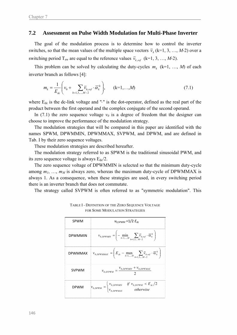
Chapter 7
146
7.2 Assessment on Pulse Width Modulation for Multi-Phase Inverter
The goal of the modulation process is to determine how to control the inverter
switches, so that the mean values of the multiple space vectors kv (k=1, 3, …, M-2) over a
switching period Tsw are equal to the reference values refkv , (k=1, 3, …, M-2).
This problem can be solved by calculating the duty-cycles km (k=1, …, M) of each
inverter branch as follows [4]:
2,...,3,1,0
1
Mh
hkrefh
dck vv
Em , (k=1,…,M) (7.1)
where Edc is the dc-link voltage and "" is the dot-operator, defined as the real part of the product between the first operand and the complex conjugate of the second operand.
In (7.1) the zero sequence voltage v0 is a degree of freedom that the designer can choose to improve the performance of the modulation strategy.
The modulation strategies that will be compared in this paper are identified with the names SPWM, DPWMMIN, DPWMMAX, SVPWM, and DPWM, and are defined in Tab. I by their zero sequence voltages.
These modulation strategies are described hereafter. The modulation strategy referred to as SPWM is the traditional sinusoidal PWM, and
its zero sequence voltage is always Edc/2. The zero sequence voltage of DPWMMIN is selected so that the minimum duty-cycle
among m1, …, mM is always zero, whereas the maximum duty-cycle of DPWMMAX is always 1. As a consequence, when these strategies are used, in every switching period there is an inverter branch that does not commutate.
The strategy called SVPWM is often referred to as "symmetric modulation". This
TABLE I - DEFINITION OF THE ZERO SEQUENCE VOLTAGE
FOR SOME MODULATION STRATEGIES
SPWM v0,SPWM =1/2 Edc
DPWMMIN
2,...3,1,
,...,1,0 min
Mh
hkrefh
MkDPWMIN vv
DPWMMAX
2,...3,1,
,...,1,0 max
Mh
hkrefh
MkdcDPWMMAX vEv
SVPWM 2
,0,0,0
DPWMAXDPWMINSVPWM
vvv
DPWM
otherwisev
Evifvv
DPWMAX
dcSVPWMDPWMINDPWM
,0
,0,0,0
2

Minimization of the Power Losses in IGBT Multiphase Inverters
147
strategy is the generalization for M-phase inverters of the traditional strategy that is commonly used for three-phase inverters.
Finally, DPWM is a discontinuous modulation, an intermediate strategy between DPWMMIN and DPWMMAX. It behaves like DPWMMAX if the zero sequence voltage of SVPWM is greater that Edc/2, otherwise it behaves like DPWMMIN.
This definition can be apply only for loads without reference voltage vectors in planes dk-qk (k 1).
The names adopted to identify these strategies, as mentioned before, are the same names that are traditionally used for three-phase inverters [5],[6]. In fact the strategies of Tab. I can be obtained by generalizing the corresponding techniques for three-phase inverters. It is worth noting that there are many other discontinuous modulation strategies for three-phase inverters, but they have not been included in this paper since their multiphase version is not able to synthesize voltage vectors in different d-q planes [7].
Once the duty-cycles have been determined, it is possible to generate the inverter switching signals sk (k = 1, 2, ... , M) by comparing a triangular carrier signal c(t), varying within the range [0, 1], with M regular-sampled (i.e. assumed constant in each switching period) modulating signals, obtained from mk (k = 1, 2, ... , M). Fig. 7.2 shows the triangular carrier, the modulating signals and the inverter command signals in the particular case m1>m2>…>mM.
7.3 Effect of the Zero Sequence Component on the Power Losses
As widely known, the power losses of an inverter consist of switching power losses and conduction power losses.
Since DPWMMAX and DPWMMIN prevent one branch of the inverter from commutating, their mean switching frequency is lower than that of SVPWM and SPWM, and consequently their switching power losses are expected to be lower.
If the inverter switches are IGBTs or BJTs, it turns out that the conduction power losses of multiphase inverters are approximately constant for all modulation strategies as
Tsw
+1
0
m1
t
triangular carrier, c(t)
mM
mk
s1
sM
sk
Fig. 7.1 - Carrier and modulating signals for a multiphase inverter, represented in the particular case when
m1>m2>…>mM.

Chapter 7
148
long as the operating conditions are similar, i.e. same dc-link voltage and output current waveforms. Consequently, one comes to the conclusion that the zero sequence voltage v0 does not affect the total conduction losses but only the switching losses. This remarkable result will be analytically justified in one of next sections.
As far as the switching power losses are concerned, let's consider the switching pattern shown in Fig. 7.1 and focus on the behavior of the first inverter branch. Under the assumption that the load current flows in the positive direction, i.e. towards the load, the calculation of the switching losses in a switching period Tsw is a straightforward task. Switching losses take place in the upper IGBT during turn-on and during turn-off, whereas reverse recovery losses take place in the lower diode during turn-off. If the load current reverses, it is possible to make a similar reasoning, but the switches that are involved in the commutation process are the lower IGBT and the upper diode.
In both cases, the total switching energy losses in a switching period can be written as follows [3]:
)(tiEE phasedcrroffonsw (7.2)
where τon and τoff are coefficients (with the dimension of time) related to the energy loss process in the IGBTs during turn-on and turn-off, τrr is a coefficient (with the dimension of time) related to the energy loss process in the diodes due to the reverse recovery currents during turn-off, and iphase(t) is the instantaneous value of the load current.
The switching power losses can be found by multiplying (7.2) by the switching frequency fsw:
)(tiEfP phasedcrroffonswsw . (7.3)
Equation (7.3) will be used in the next section for the determination of the optimal modulation strategy.
7.4 Optimal Modulation Strategy
Equation (7.3) shows that the switching power loss of an inverter branch is proportional to the load current flowing in that branch. Therefore the optimal strategy should try to avoid the state commutation of the branches that bear the highest currents.
Since there are only two basic strategies, DPWMMIN and DPWMMAX, that do not change the state of one branch of the inverter in each switching period, the optimal strategy consists in adopting DPWMMIN or DPWMMAX in each switching period depending on which one avoids the commutation of the highest load current.
To find an analytical formulation of this problem, it is necessary to split expression (7.2) of each duty-cycle mk in two terms. The first one, m0, is the zero-sequence component, which is constant for all the phases, whereas the second one, qk, depends on the multiple space vectors:
kk qmm 0 (7.4)

Minimization of the Power Losses in IGBT Multiphase Inverters
149
where
dcE
vm 0
0 (7.5)
2,...,3,1,
1
Mh
hkrefh
dck v
Eq . (7.6)
To understand which inverter branch can avoid a state commutation, it is sufficient to find the phase indexes kmax and kmin corresponding to the maximum and the minimum value of qk (k=1,…, M). In other words, kmax and kmin are such that
maxkq and minkq are
respectively the maximum and the minimum values in set q1, …, qM . The duty-cycle of the phase kmax can be easily driven to 1 by adding the following zero-sequence component:
maxkqm 10 . (7.7)
Similarly, the duty-cycle of phase kmin can be set to zero by adding the following zero-sequence component:
minkqm 0 . (7.8)
Once kmax and kmin are known, the zero-sequence component that minimizes the switching power losses turns out to be:
otherwiseq
iiifqm
min
minmaxmax
k
kphasekphasek ||||1 ,,
0 . (7.9)
The zero sequence component (7.9) may lead to discontinuities in the modulating signals, as can be seen in Fig. 7.2(a), which shows the waveform of the modulating signals of a five-phase inverter when the voltage transfer ratio is 0.5. This behavior should be compared to that of SVPWM whose modulating signals, more regular and symmetrical, are shown in Fig. 7.2(b) under the same operating conditions.
It must be noted that the modulation strategy derived from (7.9) is optimal, since it produces the minimum switching losses, whereas the conduction losses are independent of the modulation strategy. This strategy can be considered a generalization for
1
0 (a)
1
0(b)
Fig. 7.2 Waveforms of the modulating signals of a five-phase inverter when the voltage transfer ratio is0.5. (a) Optimal modulation. (b) SVPWM.

Chapter 7
150
multiphase inverters of the modulation strategy proposed in [1]- [3] for three-phase inverters. Furthermore, it can be applied to multiphase inverters whatever the number M of phases is (provided that M is odd). In addition it can synthesize voltage vectors in any d-q plane and is able to fully exploit the dc-link voltage.
7.5 Evaluation of the Conduction Losses
Let's consider an IGBT voltage source inverter. The simplest model of the conduction power losses of an inverter branch takes into account only the effect of the voltage drop on the IGBTs and the diodes.
Fig. 7.1 shows the waveform of the command signals of the branches of a multiphase inverter. Let's focus the attention on a single branch, and let's assume that the branch duty-cycle is m and that the current flows in the positive direction.
Let's suppose that the voltage drops of the IGBT and on the diode consist of two contributions, i.e. a constant term and a term varying with the current, as follows:
IGBTIGBTONIGBTIGBT irVv , (7.10)
DDONDD irVv , (7.11)
where VIGBT,ON is the IGBT saturation voltage, VD,ON is the diode forward voltage, rIGBT and rD are the differential resistances of the IGBT and of the diode, and iIGBT and iD are the currents flowing through the two components.
When the upper IGBT is on, there is a voltage drop equal to VIGBT across its terminals, and when the IGBT turns off, the current flows through the lower diode, thus causing a voltage drop VD. As a consequence, the mean value of the conduction losses over a switching period can be written as:
|)(|1 tivmvmP phaseDIGBTconduction , (iphase>0). (7.12)
With a similar reasoning, it is possible to find that, when the current flows in the opposite direction, the mean value of the conduction losses over a switching period is as follows:
|)(|1 tivmvmP phaseIGBTDconduction , (iphase<0). (7.13)
Equation (7.12) and (7.13) can be joined together as follows:
)()( tivvmtivP phaseDIGBTphaseONconduction (7.14)
where the new variable vON is defined as follows:
0)(
0)(
tiifv
tiifvv
phaseIGBT
phaseD
ON . (7.15)
The conduction power losses of the whole inverter can be obtained by summing the contributions of all the branches. It results:

Minimization of the Power Losses in IGBT Multiphase Inverters
151
totalconductionP , )(,1
, tivvmv kphase
M
kDIGBTkkON
. (7.16)
In (7.16) the contribution of the kth branch is identified by the subscript k. For sake of simplicity, let's now assume that the differential resistance rIGBT and rD in
(7.10) and (7.11) are so small that their effect can be neglected, namely vIGBT coincides with VIGBT,ON and vD with VD,ON.
As can be seen in (7.1), the duty-cycles of each branch can be written as a function of the zero-sequence voltage and of the reference voltage vectors. Substituting (7.1) in (7.16) leads to the following expression:
M
kkphasekON
Mh
hkrefh
dc
ONDONIGBTtotalconduction tivv
E
VVP
1,,
2,...,3,1,
,,, )(
M
kkphaseONDONIGBT
dc
tiVVE
v
1,,,
0 ).( (7.17)
Equation (7.17) can be further simplified by considering that Kirchhoff's law forces to zero the sum of the output currents:
0)(1
,
M
kkphase ti . (7.18)
In conclusion, the conduction losses are
M
kkkON
Mh
hkrefh
dc
ONDONIGBTtotalconduction tiVv
E
VVP
1,
2,...,3,1,
,,, )( . (7.19)
The zero-sequence component v0 does not appear in (A10) and hence it does not affect the total conduction losses of the converter, although it affects the conduction loss of each branch alone.
7.6 Validity Limits of the Theoretical Analysis
In the previous subsection (A10) has been determined under the assumption that the voltage drops on the IGBTs and on the diodes are independent of the currents. This assumption may seem too simplistic and it is necessary to investigate its validity interval.
If the differential resistances are not neglected, one comes to the following equation instead of (A10):
M
kkphasekON
Mh
hkrefh
dc
kDkIGBT
M
kkphasekphase
dcDIGBTtotalconduction
tiVvE
VV
iiE
vrrP
1,,
2,...,3,1,
,,
1,,
0,
)(. (7.20)
Unlike (7.19), in (7.20) there is a term depending on v0. The mean value of this term over a fundamental period is

Chapter 7
152
outT M
kkphasekphase
dcout
DIGBTcond dttiti
E
v
T
rrP
01
,,0
0, )()( . (7.21)
Two different modulation strategies, the first with a zero-sequence component v0' and the second with a zero-sequence component v0'', differ in the following amount of conduction losses:
outT M
kkphasekphase
dcout
DIGBTcond dtii
E
vv
T
rrP
0 1,,
000, . (7.22)
By inspecting (7.22) one comes to the conclusion that ΔPcond,0 is usually negligible in practical applications. In fact the difference between the differential resistances is usually very small. In addition, when the requested output voltage is near the maximum limit, the admissible interval for the zero sequence voltage is also very small, so the difference between v0' and v0'' is close to zero.
An upper bound for (7.22) can be easily found in the worst case. Applying the triangular inequality to (7.22), one finds the following result:
20, pkdIGBTcond IrrCP (7.23)
where Ipk is the maximum peak-value of the phase current and
dtI
titi
TC
outT M
k pk
kphasekphase
out
0
12
,, |)(|)(1 (7.24)
is a coefficient that depends only on the current waveforms, but not on their amplitude. If the load currents are sinusoidal, a numerical calculation shows that C is 0.078 for
five-phase inverters, 0.037 for seven-phase inverters, and 0.021 for nine-phase inverters. Applying the Cauchy-Schwarz integral inequality to (7.22) leads to the following
result:
20, 2
1pkdIGBTcond IrrP (7.25)
This inequality is valid under the assumption that the current space vectors move along circular trajectories in the corresponding d-q planes. Inequality (7.25) is much weaker than (7.24) but it has the advantage of being very simple, and it can be applied also for non-sinusoidal operating condition
7.7 Determination of the Switching Power Losses
A. Analytical Expression It is worth noting that, in the general case, the waveform of the modulating signals
produced by the optimal modulation strategy depends on the instantaneous values of the phase currents. However, if all the multiple space vectors of the currents are null except

Minimization of the Power Losses in IGBT Multiphase Inverters
153
one, the clamping instants depend only on the phase angle of the non-null current space vector, which happens independently of the current magnitude, as shown in Fig. 7.2(a).
If the load currents are assumed sinusoidal and with amplitude IM, it is straightforward to calculate the mean value of the total switching losses of the inverter. By integrating (7.9), this value turns out to have the following form:
Mdcrroffonswstrategytotalsw IEfMKP , (7.26)
where Kstrategy is a coefficient that depends on the modulation strategy, on the number of phases M and the load displacement angle φ.
If DPWMMIN or DPWMMAX are adopted, it is possible to demonstrate that the coefficient Kstrategy has the following expression:
otherwiseM
MifM
KMM
cos|)sin(|2
2||
sin)cos(2
. (7.27)
If SPWM or SVPWM are adopted, the coefficient Kstrategy has the constant value
2
SK . (7.28)
If the strategy DPWM is adopted, the coefficient Kstrategy is as follows:
Mif
MM
otherwiseMM
Mif
MM
KD
22cos
2cos|)sin(|1
2
)cos(2
sincos||sin2
22sinsin)cos(1
2
(7.29)
Finally, if the optimal modulation strategy is adopted, the coefficient Kstrategy is as follows:
otherwiseMM
MMif
M
Mif
M
Kopt
cos)sin(2
cos12
222
sinsin2
22sin1
2
. (7.30)

Chapter 7
154
It is worth noting that all these modulation strategies can be used to synthesize vectors in different d-q planes. However, the analytical calculation of the switching power losses has been developed here only in the case of sinusoidal operation, because this is the simplest case for which it is possible to present an explicit analytical solution.
To obtain (7.28) it is necessary to start from (7.3), which represents the switching losses of an inverter branch in a switching period Tsw. The total switching power losses of the converter in a fundamental period Tout of the output voltage is the sum of M equal contributions of the M phases; hence the mean total switching losses over a fundamental period can be written as:
2
2
, )(out
out
T
T phasedcrroffonsout
totalsw dttiEfT
MP . (7.31)
If the phase current is assumed sinusoidal,
)2
cos()( t
TIti
outMphase (7.32)
it turns out from the calculation of (7.31) that the total switching loss has the form (7.26) and that the coefficient KC is that shown in (7.28).
To obtain (7.30), equation (7.3) has to be modified to take into account the possibility that there are switching periods without state commutations. This can be done by introducing a multiplicative function ε that is 1 if the inverter branch commutates during the switching period and 0 otherwise. Equation (7.3) becomes:
)(tiEfP phasedcrroffonssw . (7.33)
In this case, the total switching loss in a period Tout can be expressed as follows:
2
2
, )()(out
out
T
T phasedcrroffonsout
totalsw dttiEftT
MP . (7.34)
0
1
Region where the inverter branch 1 could be forced not to commutate
Pha
se v
olta
ges
Loa
d cu
rren
ts
t1 t2 t3 t4
0
Fig. 7.3 Typical waveforms of the phase voltages, of the absolute values of the load currents and of thefunction ε for a five-phase inverter, under the assumption that the delay angle φ of the currents is lowerthan M2/ .

Minimization of the Power Losses in IGBT Multiphase Inverters
155
For the calculation of (7.34) it is necessary to know the waveform of ε(t). Fig. 7.3 shows the typical waveforms of the phase voltages, of the absolute values of the currents and of the function ε for a five-phase inverter as long as the optimal modulation strategy
is used, under the assumption that the load displacement angle φ is lower than M2
.
The waveform of the function ε has been drawn for the first branch of the inverter. As can be seen, it is zero when the voltage of phase 1 is the greatest or the lowest among all voltages and, simultaneously, the absolute value of corresponding current is the greatest one.
Since the function ε is non-zero only in the intervals [t1,t2] and [t3,t4] shown in Fig. 7.3, (7.34) becomes as follows:
4
3
2
1
)()(,
t
t phase
t
t phasedcrroffonsout
totalsw dttidttiEfT
MP (7.35)
where t1, t2, t3 and t4 are:
M
Tt out
221
(7.36)
M
Tt out
222
(7.37)
M
Tt out
223
(7.38)
M
Tt out
224
. (7.39)
It is now a straightforward task to prove by direct calculation of (7.35) that Kopt has the
expression given in (7.30) for M2
|| . In the case
M2||
, it is possible to make a
similar reasoning, thus obtaining the general result shown in (7.30).
B. Comparison of the Efficiency of the Modulation Strategies The coefficient Kstrategy allows the comparison of the modulation strategies. As long as
the values of the dc-link voltage, of the output current amplitude and of the switching frequency are the same, greater values of Kstrategy lead to greater switching losses.
Figs. 7.4(a) and 7.4(b) show the behavior of KMM, KS , KD and Kopt in the cases M=5 and M=7 respectively, whereas Figs. 7.5(a) and 7.5(b) show the switching loss reduction that can be obtained by adopting the optimal strategy instead of the other strategies. This reduction, expressed in percentage, is calculated by using the following relationship:
Energy saving percentage =
strategy
optstrategy
K
KK100 (7.40)

Chapter 7
156
where Kstrategy has to be set equal to KMM, KD or KS depending on which strategy is examined.
As can be seen, when the load power factor is close to one, the optimal modulation performs similarly to strategies DPWMMAX and DPWMMIN, but presents a conspicuous reduction compared to SPWM and SVPWM. The corresponding energy saving percentage, quantifiable by combining (7.27), (7.30) and (7.31), is
M2/sin100 .
The reduction of the switching losses can be up to 30% for a five-phase inverter and up to 22% for a seven-phase inverter.
When the optimal strategy is compared to DPWMMIN and DPWMMAX, the maximum reduction of the switching losses takes place when the load power factor is in
0
0
0
0
0
0
10
20
0.6 0.8 1 0.4
Power factor
Ene
rgy
savi
ng (
%)
0.2 0
DPWMMAX, DPWMMIN
SPWM, SVPWM
30
40
DPWM
(a)
0
10
20
0.60.81 0.4
Power factor
Ene
rgy
savi
ng (
%)
0.2 0
DPWMMAX, DPWMMIN
SPWM, SVPWM
30
40
DPWM
(b)
Fig. 7.5 Reduction of the switching losses as a function of the power factor for strategies SPWM, SVPWM, DPWMMIN, DPWMMAX, DPWM and the optimal modulation strategy. Five phase inverter (a). Seven phase inverter (b).
0.4
0.5
0.6
0.60.81 0.4Power factor
Coe
ffic
ient
Kst
rate
gy
0.2 0
Opt
DPWMMAX, DPWMMIN
SPWM, SVPWM
DPWM
(a)
0.4
0.5
0.6
0.60.81 0.4Power factor
Coe
ffic
ient
Kst
rate
gy
0.2 0
Opt
DPWMMAX, DPWMMIN
SPWM, SVPWM
DPWM
(b)
Fig. 7.4 Comparison of the coefficient Kstrategy for strategies SPWM, SVPWM, DPWMMIN, DPWMMAX, DPWM and the optimal modulation strategy. Five phase inverter (a). Seven phase inverter (b).

Minimization of the Power Losses in IGBT Multiphase Inverters
157
the range 0.4-0.6 and it can be up to 10% for a five phase inverter or 5% for a seven-phase inverter.
Since Kstrategy can be regarded as a quality index related to the exploitation of the silicon devices of an inverter branch, it can be useful also for the comparison of inverter topologies differing in the number M of phases.
Fig. 7.6 shows the behavior of Kopt for M=3, 5, 7, 11 and 15. As can be seen, an increase in M shows an increase in Kopt
This means that the best exploitation of the silicon devices of an inverter branch takes place in the three-phase case.
It is important to clarify that this result is valid only under the assumption of sinusoidal output currents, and it is not possible to infer any conclusion for different operating conditions.
7.8 Simulation Results
In order to verify the effectiveness of the proposed modulation strategy and to compare it to the traditional strategies, some computer simulations and experimental tests have been carried out. Both computer simulations and experimental tests refer to a five phase inverter feeding an R-L passive load.
Since the switch adopted for the experimental prototype is the IGBT SKW30N60 produced by Infineon, which comprises also a fast recovery anti-parallel diode, the simulations were carried out by modeling the behavior of this specific component by means of the circuit simulator PLECS 2.0.
Fig. 7.7 shows the output characteristic of the IGBT and the diode, whereas Fig. 7.8 shows the turn-on and turn-off energy losses when the voltage applied to the switches is 400 V and the junction temperature is 150°C. It is worth noting that, in this case, the manufacturer has included the reverse-recovery loss of the diode in the turn-on energy loss curve.
M=11M=15
0.3
0.4
0.5
0.6
0.60.81 0.4Power factor
Coe
ffic
ient
Kop
t
M=3
M=5
M=7
M=9
Fig. 7.6 Behavior of the coefficient Kopt for M=3, 5, 7, 9, 11 and 15.
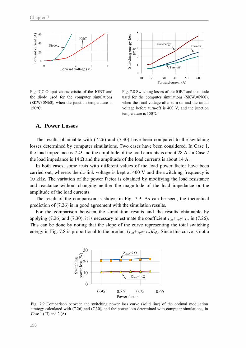
Chapter 7
158
A. Power Losses The results obtainable with (7.26) and (7.30) have been compared to the switching
losses determined by computer simulations. Two cases have been considered. In Case 1, the load impedance is 7 Ω and the amplitude of the load currents is about 28 A. In Case 2 the load impedance is 14 Ω and the amplitude of the load currents is about 14 A.
In both cases, some tests with different values of the load power factor have been carried out, whereas the dc-link voltage is kept at 400 V and the switching frequency is 10 kHz. The variation of the power factor is obtained by modifying the load resistance and reactance without changing neither the magnitude of the load impedance or the amplitude of the load currents.
The result of the comparison is shown in Fig. 7.9. As can be seen, the theoretical prediction of (7.26) is in good agreement with the simulation results.
For the comparison between the simulation results and the results obtainable by applying (7.26) and (7.30), it is necessary to estimate the coefficient τon+τoff+τrr in (7.26). This can be done by noting that the slope of the curve representing the total switching energy in Fig. 7.8 is proportional to the product (τon+τoff+τrr)Edc. Since this curve is not a
0
10
20
30
0.650.750.850.95Power factor
Sw
itch
ing
pow
er lo
ss (
W)
Zload=14
Zload=7
Fig. 7.9 Comparison between the switching power loss curve (solid line) of the optimal modulation strategy calculated with (7.26) and (7.30), and the power loss determined with computer simulations, in Case 1 () and 2 ().
0
20
40
60
0 1 2 3 4
For
war
d cu
rren
t (A
)
Forward voltage (V)
Diode
IGBT
0
1
2
3
4
5
10 20 30 40 50 60Forward current (A)
Sw
itchi
ng e
nerg
y lo
ss
(mJ)
Total energyTurn-on
Turn-off
Fig. 7.7 Output characteristic of the IGBT and the diode used for the computer simulations (SKW30N60), when the junction temperature is 150°C.
Fig. 7.8 Switching losses of the IGBT and the diode used for the computer simulations (SKW30N60), when the final voltage after turn-on and the initial voltage before turn-off is 400 V, and the junction temperature is 150°C.
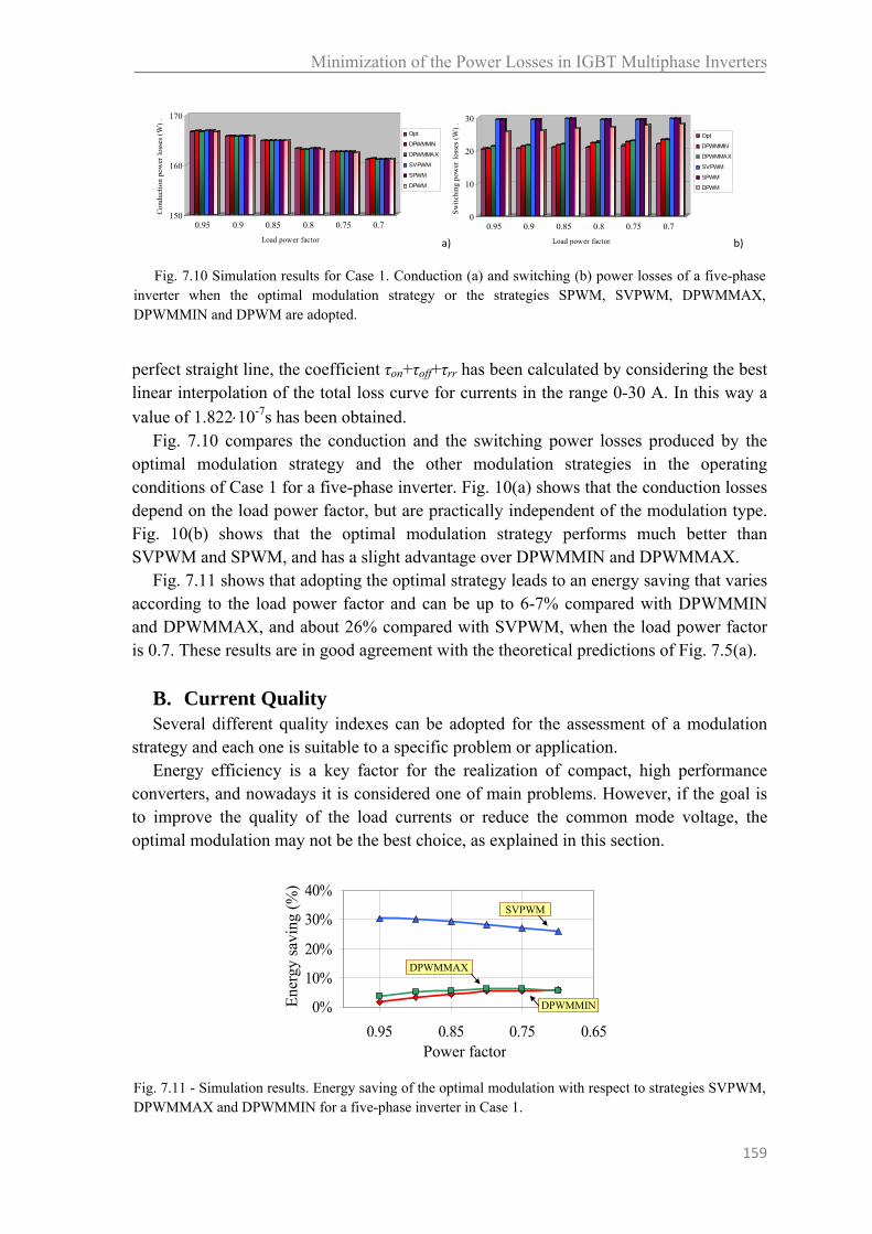
Minimization of the Power Losses in IGBT Multiphase Inverters
159
perfect straight line, the coefficient τon+τoff+τrr has been calculated by considering the best linear interpolation of the total loss curve for currents in the range 0-30 A. In this way a
value of 1.82210-7s has been obtained. Fig. 7.10 compares the conduction and the switching power losses produced by the
optimal modulation strategy and the other modulation strategies in the operating conditions of Case 1 for a five-phase inverter. Fig. 10(a) shows that the conduction losses depend on the load power factor, but are practically independent of the modulation type. Fig. 10(b) shows that the optimal modulation strategy performs much better than SVPWM and SPWM, and has a slight advantage over DPWMMIN and DPWMMAX.
Fig. 7.11 shows that adopting the optimal strategy leads to an energy saving that varies according to the load power factor and can be up to 6-7% compared with DPWMMIN and DPWMMAX, and about 26% compared with SVPWM, when the load power factor is 0.7. These results are in good agreement with the theoretical predictions of Fig. 7.5(a).
B. Current Quality Several different quality indexes can be adopted for the assessment of a modulation
strategy and each one is suitable to a specific problem or application. Energy efficiency is a key factor for the realization of compact, high performance
converters, and nowadays it is considered one of main problems. However, if the goal is to improve the quality of the load currents or reduce the common mode voltage, the optimal modulation may not be the best choice, as explained in this section.
150
160
170
Con
duct
ion
pow
er l
osse
s (W
) .
0.95 0.9 0.85 0.8 0.75 0.7
Load power factor
Opt
DPWMMIN
DPWMMAX
SVPWM
SPWM
DPWM
a)
0
10
20
30
Sw
itch
ing
pow
er l
osse
s (W
) .
0.95 0.9 0.85 0.8 0.75 0.7
Load power factor
Opt
DPWMMIN
DPWMMAX
SVPWM
SPWM
DPWM
b)
Fig. 7.10 Simulation results for Case 1. Conduction (a) and switching (b) power losses of a five-phaseinverter when the optimal modulation strategy or the strategies SPWM, SVPWM, DPWMMAX,DPWMMIN and DPWM are adopted.
0%
10%
20%
30%
40%
0.650.750.850.95Power factor
Ene
rgy
savi
ng (
%)
SVPWM
DPWMMAX
DPWMMIN
Fig. 7.11 - Simulation results. Energy saving of the optimal modulation with respect to strategies SVPWM,DPWMMAX and DPWMMIN for a five-phase inverter in Case 1.
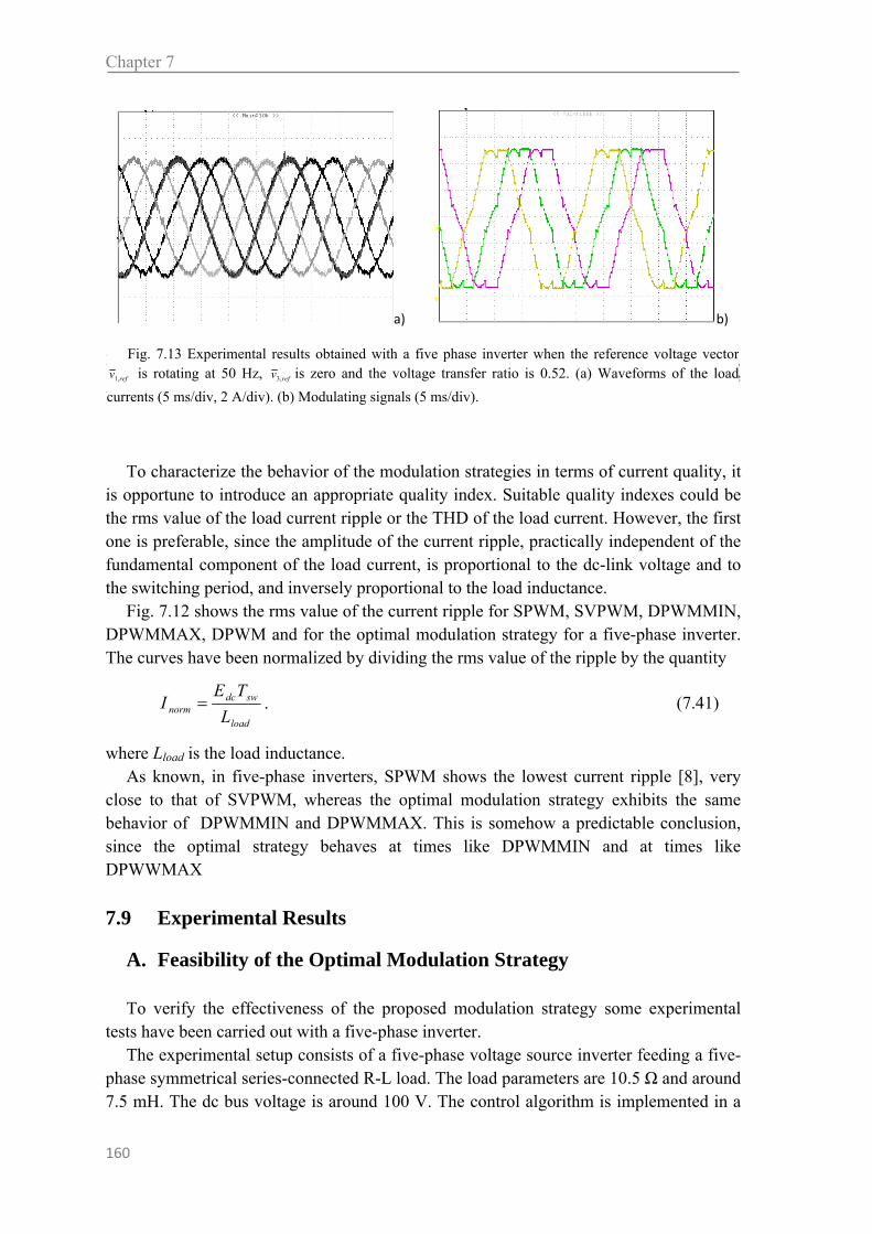
Chapter 7
160
To characterize the behavior of the modulation strategies in terms of current quality, it is opportune to introduce an appropriate quality index. Suitable quality indexes could be the rms value of the load current ripple or the THD of the load current. However, the first one is preferable, since the amplitude of the current ripple, practically independent of the fundamental component of the load current, is proportional to the dc-link voltage and to the switching period, and inversely proportional to the load inductance.
Fig. 7.12 shows the rms value of the current ripple for SPWM, SVPWM, DPWMMIN, DPWMMAX, DPWM and for the optimal modulation strategy for a five-phase inverter. The curves have been normalized by dividing the rms value of the ripple by the quantity
load
swdcnorm L
TEI . (7.41)
where Lload is the load inductance. As known, in five-phase inverters, SPWM shows the lowest current ripple [8], very
close to that of SVPWM, whereas the optimal modulation strategy exhibits the same behavior of DPWMMIN and DPWMMAX. This is somehow a predictable conclusion, since the optimal strategy behaves at times like DPWMMIN and at times like DPWWMAX
7.9 Experimental Results
A. Feasibility of the Optimal Modulation Strategy To verify the effectiveness of the proposed modulation strategy some experimental
tests have been carried out with a five-phase inverter. The experimental setup consists of a five-phase voltage source inverter feeding a five-
phase symmetrical series-connected R-L load. The load parameters are 10.5 Ω and around 7.5 mH. The dc bus voltage is around 100 V. The control algorithm is implemented in a
0.0
1.0
2.0
3.0
4.0
0.1 0.2 0.3 0.4 0.5Voltage transfer ratio
Nor
mal
ized
rm
s va
lue
of
the
curr
ent r
ippl
e (%
)
SVPWM
DPWM
Opt, DPWMMAX, DPWMMIN
SPWM
Fig. 12 - Normalized rms value of the load current ripple of a five-phase inverter for strategies SPWM,SVPWM, DPWMAX, DPWMMIN, DPWM and for the optimal strategy as a function of the voltagetransfer ratio.
a) b)
Fig. 7.13 Experimental results obtained with a five phase inverter when the reference voltage vector
refv ,1 is rotating at 50 Hz, refv ,3 is zero and the voltage transfer ratio is 0.52. (a) Waveforms of the load
currents (5 ms/div, 2 A/div). (b) Modulating signals (5 ms/div).
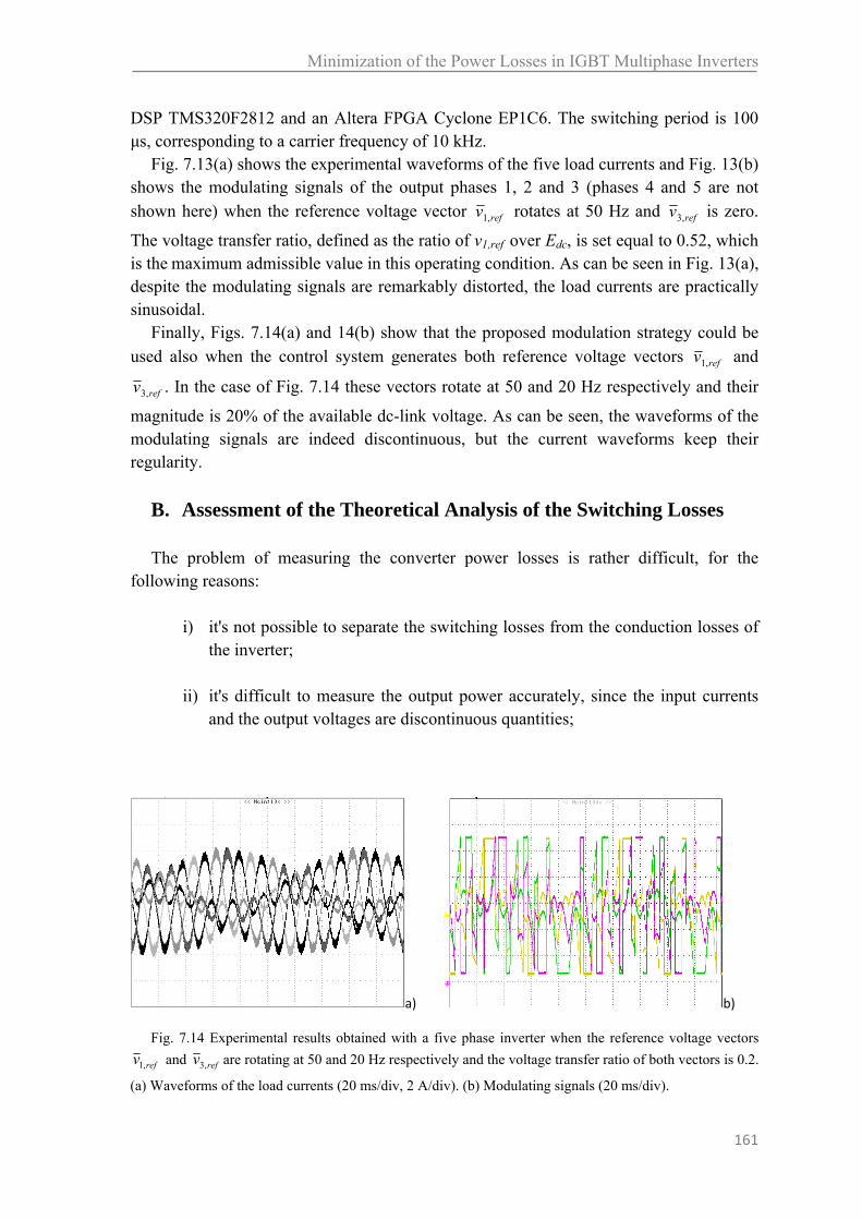
Minimization of the Power Losses in IGBT Multiphase Inverters
161
DSP TMS320F2812 and an Altera FPGA Cyclone EP1C6. The switching period is 100 μs, corresponding to a carrier frequency of 10 kHz.
Fig. 7.13(a) shows the experimental waveforms of the five load currents and Fig. 13(b) shows the modulating signals of the output phases 1, 2 and 3 (phases 4 and 5 are not shown here) when the reference voltage vector refv ,1 rotates at 50 Hz and refv ,3 is zero.
The voltage transfer ratio, defined as the ratio of v1,ref over Edc, is set equal to 0.52, which is the maximum admissible value in this operating condition. As can be seen in Fig. 13(a), despite the modulating signals are remarkably distorted, the load currents are practically sinusoidal.
Finally, Figs. 7.14(a) and 14(b) show that the proposed modulation strategy could be used also when the control system generates both reference voltage vectors refv ,1 and
refv ,3 . In the case of Fig. 7.14 these vectors rotate at 50 and 20 Hz respectively and their
magnitude is 20% of the available dc-link voltage. As can be seen, the waveforms of the modulating signals are indeed discontinuous, but the current waveforms keep their regularity.
B. Assessment of the Theoretical Analysis of the Switching Losses The problem of measuring the converter power losses is rather difficult, for the
following reasons:
i) it's not possible to separate the switching losses from the conduction losses of the inverter;
ii) it's difficult to measure the output power accurately, since the input currents and the output voltages are discontinuous quantities;
a) b)
Fig. 7.14 Experimental results obtained with a five phase inverter when the reference voltage vectors
refv ,1 and refv ,3 are rotating at 50 and 20 Hz respectively and the voltage transfer ratio of both vectors is 0.2.
(a) Waveforms of the load currents (20 ms/div, 2 A/div). (b) Modulating signals (20 ms/div).
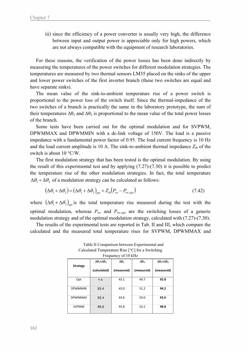
Chapter 7
162
iii) since the efficiency of a power converter is usually very high, the difference between input and output power is appreciable only for high powers, which are not always compatible with the equipment of research laboratories.
For these reasons, the verification of the power losses has been done indirectly by measuring the temperatures of the power switches for different modulation strategies. The temperatures are measured by two thermal sensors LM35 placed on the sinks of the upper and lower power switches of the first inverter branch (these two switches are equal and have separate sinks).
The mean value of the sink-to-ambient temperature rise of a power switch is proportional to the power loss of the switch itself. Since the thermal-impedance of the two switches of a branch is practically the same in the laboratory prototype, the sum of their temperatures Δθ1 and Δθ2 is proportional to the mean value of the total power losses of the branch.
Some tests have been carried out for the optimal modulation and for SVPWM, DPWMMAX and DPWMMIN with a dc-link voltage of 150V. The load is a passive impedance with a fundamental power factor of 0.95. The load current frequency is 10 Hz and the load current amplitude is 10 A. The sink-to-ambient thermal impedance Zth of the switch is about 10 °C/W.
The first modulation strategy that has been tested is the optimal modulation. By using the result of this experimental test and by applying (7.27)-(7.30) it is possible to predict the temperature rise of the other modulation strategies. In fact, the total temperature
21 of a modulation strategy can be calculated as follows:
optswswthopt PPZ ,2121 (7.42)
where opt21 is the total temperature rise measured during the test with the
optimal modulation, whereas Psw and Psw,opt are the switching losses of a generic modulation strategy and of the optimal modulation strategy, calculated with (7.27)-(7.30).
The results of the experimental tests are reported in Tab. II and III, which compare the calculated and the measured total temperature rises for SVPWM, DPWMMAX and
Table II Comparison between Experimental and Calculated Temperature Rise [°C] for a Switching
Frequency of 10 kHz
Strategy
1+2
(calculated)
1
(measured)
2
(measured)
1+2
(measured)
Opt n.a. 43.1 49.7 92.8
DPWMMIN 93.4 43.0 51.2 94.2
DPWMMAX 93.4 43.6 50.0 93.6
SVPWM 98.8 45.8 53.1 98.8

Minimization of the Power Losses in IGBT Multiphase Inverters
163
DPWMMIN when the switching frequency is 10 kHz and 16 kHz respectively. As can be seen, there is a good agreement between the temperatures experimentally
measured and the ones theoretically calculated.
7.10 Conclusions
In this chapter the carrier-based PWM modulation strategy with the minimum switching losses for multiphase VSIs with an odd number of phases has been presented. If the inverter is based on IGBTs or BJTs, this modulation strategy is also the best one in terms of total power losses, since the conduction losses are approximately constant for all the modulation strategies.
The proposed strategy has been compared to some traditional strategies and, in the case of 5-phase inverters, it has been shown to reduce the switching power losses by 6% to 26% when the load power factor is 0.7.
Experimental results confirm the validity and the effectiveness of the proposed modulation strategy
7.11 References
[1] A. Trzynadlowski, S. Legowski, “Minimum-loss vector PWM strategy for three-phase inverters”, IEEE Trans. on Power Electronics, vol. 9, no. 1, Jan. 1994, pp. 26-34.
[2] A. Trzynadlowski, S. Legowski, R. L. Kirlin, “Space vector PWM technique with minimum switching losses and a variable pulse rate, ” IEEE Trans. on Industrial Electronics, vol. 44, No. 2, April 1997
[3] A. Trzynadlowski, S. Legowski, R. L. Kirlin, “Space vector PWM technique with minimum switching losses and a variable pulse rate, ” IEEE Trans. on Industrial Electronics, vol. 44, No. 2, April 1997.
[4] M. C. Cavalcanti, E. R. Cabral da Silva, A. M. Nogueira Lima, C. B. Jacobina, R. N. Cunha Alves, “Reducing losses in three-phase PWM pulsed dc-link voltage-type inverter system, ” IEEE Trans. on Industry Applications, Vol. 38, No.4, July/August 2002.
Table III - Comparison between Experimental and Calculated Temperature Rise [°C] for a Switching
Frequency of 16 kHz
Strategy
1+2
(calculated)
1
(measured)
2
(measured)
1+2
(measured)
Opt n.a. 46.7 52.8 99.5
DPWMMIN 100.0 46.2 54.7 100.9
DPWMMAX 100.0 47.5 53.9 101.4
SVPWM 109.2 51.2 59.4 110.6

Chapter 7
164
[5] D. Casadei, G. Serra, A.Tani, L. Zarri, “Multi-phase inverter modulation strategies based on duty-cycle space vector approach, ” in Proc. of SPRTS’2005, Bologna (Italy), 4-6 Sept. 2005, pp. 222-229.
[6] D. G. Holmes and T. A. Lipo, Pulse Width Modulation for Power Converters. New York: Wiley, 2003.
[7] A. M. Hava, R. J. Kerkman, Thomas A. Lipo, “Simple analytical and graphical methods for carrier-based PWM-VSI drives, ” IEEE Trans. on Industrial Electronics, Vol. 14, No. 1, January 1999, pp. 49-60.
[8] O. Ojo, G. Dong, “Generalized discontinuous carrier-based PWM modulation scheme for multi-
phase converter-machine systems,” in Proc. of IEEE Ind. Appl. Soc. Annual Meeting (IAS), 2005, pp. 1374-1381.
[9] D. Dujic, M. Jones, E. Levi, “Analysis of output current ripple rms in multiphase drives using space
vector approach, ” IEEE Trans. on Power Electronics, Vol. 24, No. 8, August 2009, pp. 1926-1938.
[10] D. Casadei, M. Mengoni, G. Serra, A. Tani, L. Zarri, "Carrier-Based PWM with Minimum Power Losses for IGBT Multiphase Inverters," Proc. Of EPE 2009, Barcelona, Spain, 8-10 Sept. 2009, pp. 1-10.

Extended Stator Flux Vector Control of
Multi-Phase Induction Motor Drives
Abstract In this chapter, a rotor-flux-oriented control scheme for seven-phase induction motor drive, having the stator flux components instead of the stator current components as main control variables, is presented. As a consequence, a simple stator flux regulator can replace the conventional current regulators implemented in the synchronous reference frame. The proposed Stator Flux Vector Control (SFVC) scheme uses a flexible modulation strategy for seven-phase Voltage Source Inverters (VSIs) that allows the simultaneous modulation of voltage space vectors in different d-q planes. This problem is completely solved using the Duty-Cycle Space Vector (DCSV) representation, which describes the state of the switches by means of complex variables. Using the DCSV representation it is possible to combine the multiple space vector representation, useful in modeling multi-phase machines, with traditional carrier-based PWM principle, suitable for the modulation of multi-phase VSIs. The validity of the proposed control scheme is confirmed by several experimental tests.
8.1 Introduction
A variable-speed drive is usually composed by a three-phase inverter supplying a three-phase motor. However, since variable-speed drives are always supplied from power electronic converters, the number of phases can be considered as a design variable and does not have to be equal to three anymore. On the contrary, a three-phase drive should be regarded as a particular case.
Nowadays, there is an increasing interest towards multi-phase motor drives, especially for medium and high power applications in naval and railway propulsion systems.

Chapter 8
166
In fact, the use of multi-phase inverters together with multi-phase ac machines has been recognized as a viable approach to obtain high power ratings without increasing the stator current per phase, making it possible to use standard power switches based on a single device.
Furthermore, multi-phase motor drives have several advantages over the traditional three-phase motor drives such as reduction of the amplitude and increase of the frequency of torque pulsations, and increase of the fault tolerance. In addition, multi-phase motor drives offer a greater number of degrees of freedom compared with three-phase motor drives, which can be utilized for improving the drive performance [1]-[2].
It is worth noting that it is not possible to analyze multi-phase motor drives using the space vector representation in a single d-q plane. It is known that, to completely describe a multi-phase electromagnetic system, the space vector representation in multiple d-q planes (multiple space vectors) must be adopted [3]-[4].
Several control schemes for multi-phase induction machines, of symmetrical [5]-[8] and unsymmetrical [9]-[12] type, based on Field Oriented Control (FOC) principles, have been presented. All of them utilize the stator current components as main control variables.
In this chapter, a rotor-flux-oriented control scheme for seven-phase induction motor drive is presented. The main control variables are the stator flux components instead of the stator current components, thus a simple stator flux regulator can replace the conventional current regulators implemented in the rotor-flux-oriented reference frame. This basic choice simplifies the control scheme and exhibits a fast torque response [13].
The implementation of the proposed control scheme requires the utilization of a flexible modulation strategy for seven-phase VSIs, allowing the full exploitation of the dc input voltage, and the simultaneous modulation of voltage space vectors in different d-q planes.
In this chapter the problem of the modulation strategy of seven-phase inverters is completely solved using the Duty-Cycle Space Vector (DCSV) representation [14]-[15]. Basically, this representation describes the state of the switches by means of complex variables [16]-[17]. Using the DCSV representation it is possible to combine the multiple space vector representation, useful in modeling multi-phase machines, with traditional carrier-based PWM principle, suitable for the modulation of multi-phase VSIs.
The performance of the proposed control scheme is verified by experimental tests carried out on a seven-phase induction motor drive prototype.
8.2 Machine Equations of Seven-Phase Induction Motor
Let’s consider a seven-phase star-connected induction machine, with stator windings symmetrically distributed within the stator slots, and squirrel cage rotor.
The behavior of the machine can be described by means of an opportune mathematical model, described in chapter 5, which takes into account the spatial distribution of the magnetic field in the air gap up to the seventh harmonic.
The mathematical model is based on the following assumptions. Flux saturation, hysteresis losses and eddy current losses in the iron cores are neglected. Furthermore, iron

Extended Stator Flux Vector Control of Multi-Phase Induction Motor
167
cores with infinite permeability are considered and the slot effects are not taken into account.
The machine equations, written in terms of multiple space vectors in three reference frames synchronous with the corresponding rotor fluxes, are:
dt
djiRv S
SSSS1
1111
(8.1)
dt
djiR R
RmRR1
1110
(8.2)
11111 RSSS iMiL (8.3)
11111 RRSR iLiM (8.4)
dt
djiRv S
SSSS3
3333
(8.5)
dt
djiR R
RmRR3
333 30
(8.6)
33333 RSSS iMiL (8.7)
33333 RRSR iLiM (8.8)
dt
djiRv S
SSSS5
5555
(8.9)
dt
djiR R
RmRR5
555 50
(8.10)
55555 RSSS iMiL (8.11)
55555 RRSR iLiM (8.12)
555333111 532
7RSRSRS ijiMijiMijiMpT (8.13)
where p is the pole pairs number, ωk is the angular speed of the k-th rotor flux vector, and ωm is the rotor angular speed in electric radians.
Note that using the multiple space vector representation leads to decoupled equations of the electrical quantities. In fact, the three sub-systems of Eqs. (8.1)-(8.5), (8.6)-(8.9) and (8.10)-(8.13) are independent of each other.
As a consequence, a seven-phase induction machine can be considered as constituted by three independent three-phase induction machines (denoted by indexes 1, 3, and 5) acting on the same rotor shaft.
It is worth noting that the current space vectors 1Si and 1Ri are responsible for the
fundamental spatial component of the magnetic field in the air gap, whereas 3Si , 3Ri and
5Si , 5Ri generate the third and the fifth spatial harmonic, respectively.

Chapter 8
168
In this paper the third and the fifth spatial harmonic of the magnetic field in the air gap
are set to zero. This goal is reached by zeroing the voltage space vectors 3Sv and 5Sv .
This choice has been made for the sake of simplicity to describe the control algorithm of the seven-phase induction motor drives. The possibility to use the third and the fifth spatial harmonic components is out of the scope of the present chapter.
The seventh spatial harmonic is zero since it is generated by the zero-sequence component of the stator current, which is null in the case of star-connected stator windings.
8.3 Stator Flux Vector Control
Solving (8.3) and (8.4) with respect to 1Si and 1Ri , and substituting in (8.3) and (8.13)
yields
111
111
11
1S
RS
RRm
R
RR
LL
MRj
L
R
dt
d
(8.14)
11111
1
2
7RS
RS
jLL
MpT
, (8.15)
where the parameter σ1 is defined as follows:
11
21
1 1RS LL
M . (8.16)
The reference frame orientation is chosen so that the d-axis has the direction of the rotor flux vector. Hence (8.14) can be rewritten in terms of d and q components as follows:
dSS
RR
R
R
L
M
dt
d
R
L1
1
11
111
(8.17)
m0
VDC
m1
mk
m7
Eq. (42)
PWM 7-phase
VSI
m0 selection algorithm
dc bus
IM
Observer for stator and
rotor fluxes, and angular
frequency .
Motor currents
T
Tref +
-
PI
e j Stator flux regulator
Sref,Sv 1
03 Sref,Sv
05 Sref,Sv
ref,Sv 1ref,S1 ref,qS1
ref,dS1 + -
1S
Fig. 8.1.Block diagram of the proposed SFVC scheme.

Extended Stator Flux Vector Control of Multi-Phase Induction Motor
169
qSRS
RRm LL
MR1
111
111
. (8.18)
Also (8.16) can be rewritten as follows:
11111
1
2
7RqS
RS LL
MpT
. (8.19)
As can be seen, these equations are quite similar to the corresponding equations of the traditional FOC based on d-q stator current components. In fact the rotor flux depends only on dS1 , whereas the motor torque is proportional to qS1 .
A block diagram of the proposed SFVC scheme is shown in Fig. 8.1. The control scheme is implemented in a reference frame synchronous with the rotor
flux vector, like traditional field oriented controls. It is assumed that a suitable observer estimates 1s , 1r , and the angular frequency ω1 of the rotor flux vector.
A. Torque Control The motor torque is controlled by comparing the torque reference Tref with the
estimated torque T. On the basis of the torque error, the PI regulator produces a torque request by adjusting the q-component of the stator flux, according to (8.19). Therefore, if the reference torque is higher than the actual torque, the PI regulator tends to increase the φS1q,ref, otherwise it tends to decrease it.
B. Rotor Flux Control The rotor flux is controlled by adjusting the d-component of the stator flux, according
to (8.17). In the low speed range, the d-component of the stator flux is constant and has the rated
value rated,dS1 . At higher speeds, instead, it can be reduced by an opportune field
weakening algorithm.
C. Stator Flux Regulator The stator flux regulator behaves as a proportional controller, with some additional
terms compensating the stator back-EMF and the voltage drop caused by the stator resistance. The stator flux regulator equation can be expressed as follows:
1,1
111,1
SrefS
SSSrefS jiRv
(8.20)
where 1/τ represents the gain of the controller. Combining (8.20) and (8.1), i.e. refSS vv ,11 , leads to the following equation,
expressing the dynamic behavior of the stator flux vector:

Chapter 8
170
refSSS
dt
d,11
1
. (8.21)
According to (8.21), in order to obtain fast flux transients, and consequently a high torque dynamic, it is necessary to adopt small values of τ.
D. Flux Observer The aim of the flux observer is the determination of stator flux and phase angle of the
rotor flux, which are necessary for the field oriented control of the induction machine. The flux observer operates in the stator reference frame. In the following the superscript “s” will be used to identify quantities expressed in the stator reference frame.
The stator flux is determined by integrating the following stator voltage equation:
SSS
SS
SS iRv
dt
d11
1
. (8.22)
If the measure of the stator currents is available, the rotor flux can be estimated as follows
SSS
SS
RSR iL
M
L1111
1
11 . (8.23)
The phase angle θ1 of the rotor flux vector, necessary for the field oriented control, can be derived from (8.23) as follows
SSS
SS
SR iL 111111 argarg . (8.24)
It is evident from (8.22) that the estimation of the stator flux vector can be affected by stator resistance mismatch, sensors offsets and the inverter non-linearity (inverter dead-times, voltage drop on the conducting switches, etc.).
The estimation error on the phase angle depends on the stator flux estimation error,
the mismatch on the leakage inductance LS1 and the offset of the current sensors. The leakage inductance shows moderate variations with the stator currents and it will
be assumed practically constant.
However, the influence of the two machine parameters, namely RS1 and LS1, on the flux estimation can be considered negligible in the high speed range. Whereas, in the low speed range, the performance of the flux observer must be improved by a feedback loop [18]. A closed-loop estimator is based on the principle that feeding back the difference between the measured output of the observed system and the estimated output, and continuously correcting the model by the error signal, the error should be minimized.
In the case of a flux estimator, the motor flux cannot be directly measured, but the idea of realizing a closed-loop system is still applicable if the difference between a signal representing the steady-state value of the reference rotor flux and the signal of the estimated rotor flux vector is used as feedback signal.
Hence, (8.22) has to be replaced by the following equation:
Extended Stator Flux Vector Control of Multi-Phase Induction Motor
171
SR
SrefR
SSS
SS
SS GiRv
dt
d1,111
1
, (8.25)
where G is the gain of the flux observer and the reference flux vector is
1,1
1
1,1
jrefdS
RSrefR e
M
L . (8.26)
This observer is much more robust than an open loop estimator and reduces the sensitivity of the control scheme to stator parameter variations and to sensor offset, even at low speed. However, it requires the knowledge of a further machine parameter, namely the ratio LR1/M1, and the tuning of the gain G.
E. Torque Observer The torque can be estimated from the measurements of the stator current and the
estimation of the stator flux, as follows:
112
7SS jipT . (8.27)
As can be seen, the torque estimation does not require explicitly any motor parameters, except the pole pairs.
8.4 Experimental Results
In order to verify the effectiveness of the proposed control scheme some experimental tests have been performed on a seven-phase induction motor drive prototype.
The experimental setup consists of a custom-designed seven-phase voltage source inverter (Fig. 8.2 (a)) feeding a seven-phase squirrel cage induction motor (Fig. 8.2(b)), whose parameters are reported in Tab. I
(a) (b)
Fig. 8.2.Laboratory induction motor drive a)Custom-designed seven-phase voltage source inverter, b) Custom-designed seven-phase squirrel cage induction motor

Chapter 8
172
The IGBTs are rated 30A and 600 V. The dc bus voltage is about 130 V, obtained with
a three-phase diode rectifier and filtered by a capacitance of 3300 F. The test motor is coupled to a separately excited dc machine acting as load. The control algorithm is implemented in a Digital Signal Processor (DSP)
TMS320F2812. The switching period is 250 μs, corresponding to a switching frequency of 4 kHz.
The particular modulation strategy adopted for the experimental tests can be considered as a generalization of the well-known symmetric modulation used with three-phase inverters. The zero sequence component m0 is selected in order to maintain the seven modulating signals centered within the interval [0,1], according to the following relationship:
1,...,min,...,max 7171 mmmm . (8.28)
The behaviour of the proposed SFVC scheme has been analyzed in steady-state and transient conditions.
The experimental tests in steady-state conditions have been carried out with Tref = 10 Nm, φSd,ref = 0.52 Wb and a rotor speed of about 550 rpm. The results are presented in Figs. 8.4 and 8.5.
For display purposes, Fig. 8.3 shows the behaviour of only three of the stator currents. As expected, the stator currents exhibit sinusoidal waveforms having the same amplitude, and a displacement angle of 4π/7. The superimposed small ripple is due to the switching effects.
The trajectories of the stator current space vectors 1Si , 3Si and 5Si , in the
0 ‐
TABLE I MOTOR PARAMETERS
RATED POWER
RATED PHASE VOLTAGE
RATED SPEED
POLE NUMBER
SLOT NUMBER
3500 W
120VRMS, 50 HZ
1450 RPM
4
28
Fig. 8.3. Experimental test. Waveforms of stator currents in phase 1, 3, and 5, in steady-state conditions (20 ms/div, 4A/div).

Extended Stator Flux Vector Control of Multi-Phase Induction Motor
173
corresponding d-q planes, are presented in Fig. 8.4. As can be seen the space vector 1Si
rotates at constant speed along a circular trajectory, whereas the space vectors 3Si and 5Si
are null, according to the choice of 0,3 SrefSv and 0,5 S
refSv . This result confirms that the
stator currents are balanced and sinusoidal. The good behavior of the estimated torque and of the estimated rotor flux magnitude is
emphasized in Fig. 8.5 (a). In order to evaluate the dynamic response of the proposed control scheme, a square-
wave torque reference from 5 Nm to 10 Nm, having a frequency of 2 Hz, has been
applied to the drive system. The flux reference has been kept constant (Sd,ref = 0.52 Wb).
The waveforms of the estimated torque, of the estimated rotor flux and of the - components of stator current space vector 1Si are shown in Fig. 8.5 (b). As can be seen,
the system exhibits a fast torque response, whereas the rotor flux magnitude remains constant. This behavior shows that the proposed SFVC scheme is able to perform a decoupled control of torque and flux.
Fig. 8.4 Experimental test. a)Trajectory of the space vector 1Si in steady-
state conditions (4A/div). b)Trajectory of the space vector 3Si in steady-
state conditions (4A/div). c). Experimental test. Trajectory of the space vector 5Si in steady-state conditions (4A/div).

Chapter 8
174
8.5 Conclusions
It has been shown in this chapter that, by combining the multiple space vector representation with traditional carrier-based pulse width modulation, it is possible to define a rotor-flux-oriented control scheme for seven-phase induction motor drive.
The peculiarity of this control scheme is the adoption of the stator flux components instead of the stator current components as main control variables. This choice allows replacing the conventional current regulators, implemented in the rotor-flux-oriented reference frame, with a simple stator flux regulator.
The implementation of the proposed control scheme requires a flexible modulation strategy for seven-phase VSI, which is based on the DCSV representation of the inverter state. This carrier-based modulation strategy allows the full exploitation of the dc input voltage, and the simultaneous modulation of three voltage space vectors in different d-q planes.
Several experimental tests have been carried out showing that it is possible to obtain decoupled torque and flux control, with fast torque response.
8.6 References
[1] L. Parsa, “On advantages of multi-phase machines,” in Proc. Annual Conference of the IEEE Industrial Electronics Society IECON, 2005, pp. 1574-1579.
[2] E. Levi, R. Bojoi, F. Profumo, H.A. Toliyat, S. Williamson, “Multiphase induction motor drives – a technology status review,” IET Electr. Power Appl., vol. 1, no.4, pp. 489-516, July 2007.
[3] D.C. White, H.H. Woodson, “Electromechanical Energy Conversion,” John Wiley and Sons, New York, NY, 1959.
[4] G. Grandi, G. Serra, A. Tani, “General analysis of multi-phase systems based on space vector approach,” in Proc. of 12th Power Electronics and Motion Control Conference EPE-PEMC, 2006, CD-ROM paper T2-409.
Fig. 8.5. Experimental test.a) Estimated torque (top, 5 Nm/div) and estimated rotor flux (bottom, 0.25 Wb/div) in steady-state conditions (500 ms/div).b). Estimated torque (top, 5 Nm/div), estimated rotor flux (0.5 Wb/div) and is1 components of the stator current space vector 1Si (bottom, 10 A/div). Response to a
square-wave torque reference from 5 Nm to 10 Nm, having a frequency of 2 Hz (200 ms/div).

Extended Stator Flux Vector Control of Multi-Phase Induction Motor
175
[5] H. Xu, H.A. Toliyat, L.J.Petersen, “Rotor field oriented control of five-phase induction motor with
the combined fundamental and third harmonic currents,” in Proc. of IEEE Applied Power Electronics Conference, APEC, 2001, pp. 392-398.
[6] H. Xu, H.A. Toliyat, L.J.Petersen, “Five-phase induction motor drives with DSP-based control system,” IEEE Trans. on Power Electron., vol. 17, no. 4, 2002, pp. 524-533.
[7] L. Hou, Y. Su, L. Chen, “DSP-based indirect rotor flux oriented control for multiphase induction machines,” in Proc. of IEEE International Electric Machines and Drives Conference, IEMDC, 2003, pp. 976-980.
[8] E. Levi, M. Jones, S.N. Vukosavic, “Even-phase multi-motor vector controlled drive with single inverter supply and series connection of stator windings,” IEE Proc.-Electr. Power Appl., vol. 150, no. 5, 2003, pp. 580-590.
[9] R. Bojoi, M. Lazzari, F. Profumo, A. Tenconi, "Digital field oriented control for dual three-phase induction motor drives," IEEE Trans. on Ind. Applicat., Vol. 39, no. 3, 2003, pp. 752-760.
[10] [R. Bojoi, F. Profumo, A. Tenconi, "Digital synchronous frame current regulation for dual three-phase induction motor drives," in Proc. of IEEE Power Electronics Specialist Conference, PESC, 2003, pp. 1475-1480.
[11] G.K. Singh, K. Nam, S.K. Lim, "A simple indirect field-oriented control scheme for multiphase induction machine," IEEE Trans. on Industrial Electronics, vol. 52, no. 4, 2005, pp. 1177- 1184.
[12] K.K. Mohapatra, R.S. Kanchan, M.R. Baiju, P.N. Tekwani, K. Gopakumar, "Independent field-oriented control of two split-phase induction motors from a single six-phase inverter," IEEE Trans. on Industrial Electronics, vol. 52, no. 5, 2005, pp. 1372- 1382.
[13] D. Casadei, G. Serra, A. Tani, L. Zarri, “A robust method for field weakening operation of induction motor drives with maximum torque capability,” in Proc. of IEEE Ind. Appl. Soc. Annual Meeting IAS, 2006, pp. 111-117.
[14] D. Casadei, G. Serra, A. Tani, L. Zarri, “General Inverter Modulation Strategy for Multi-Phase Motor Drives,” in Proc. IEEE International Symposium on Industrial Electronics, ISIE, June 4-7, 2007, Vigo (Spain), CD-rom, pp.1131-1137.
[15] [D. Casadei, G. Serra, A. Tani, L. Zarri, “Multi-phase inverter modulation strategies based on duty-cycle space vector approach,” in Proc. of Ship Propulsion and Railway Traction Systems Conference, 2005, pp. 222-229.
[16] [D. Casadei, G. Serra, A. Tani, L. Zarri, “Matrix converter modulation strategies: a new general approach based on space-vector representation of the switch state,” IEEE Trans. on Ind. Electron., vol. 49, no. 2, 2002, pp. 370-381.
[17] C. Rossi, G. Serra, A. Tani, L. Zarri, “Cascaded multilevel inverter modulation strategies: a novel solution based on duty-cycle space vector approach,” in Proc. IEEE Int. Symp. on Industrial Electronics ISIE, 2005, pp. 733-738.
[18] D. Casadei, G. Serra, A. Tani, “Steady-state and transient performance evaluation of a DTC scheme in the low speed range,” IEEE Trans. on Power Electron., vol. 16, no. 6, 2001, pp. 846-851.


High Torque Density Applications
Abstract In this chapter, a rotor-flux-oriented control scheme for seven-phase induction motor drives is presented. At low speed the proposed control scheme is able to increase the motor torque by adding a third harmonic component to the air-gap magnetic field. Above the base speed the control system reduces the motor flux in such a way to ensure the maximum torque capability. The analysis consider the drive constrains and show how these limits modify the motor performances. The validity of the proposed control scheme is confirmed by experimental tests.
9.1 Introduction
The use of multi-phase inverters together with multi-phase ac machines has been recognized as a viable approach to obtain high power ratings without increasing the stator current per phase, making it possible to use standard power switches based on a single device.
Several control schemes, based on field oriented control, have been presented for multiphase drives. These control strategies have been applied to symmetrical, unsymmetrical and special multiphase machines as well as multi-motor drives [3]-[10]
Multiphase drives offer the opportunity to increase the torque density by adding a third spatial harmonic in the magnetic field. This feature has been exploited mainly in permanent magnet synchronous motors [11]-[12]. It is worth noting that the development of high torque density drives is dependent on successful implementation of proper modulation strategies which will enable the precise synthesis of non-sinusoidal variables [13]-[14].
High-torque density control scheme were presented for five-phase induction motor drives [15],[16].
So far, very little research has been done on the operation of multiphase electric drives in field weakening region and the realization of robust control scheme.
Chapter 9
178
In this context, the present paper proposes a solution to the control problem of seven-phase induction motors. The adopted control scheme exploits the maximum torque capability of the motor at any speed. In addition, the operation in field-weakening speed range requires the knowledge of very few motor.
The performance of the proposed control scheme is verified by experimental tests carried out on a seven-phase induction motor drive prototype.
9.2 Machine Equations of Seven-Phase Induction Motor
In the previous chapters the machine equations of multi-phase motor, and in particular of seven phase induction motor, are have been analyzed and described. In this section there is only a short resume.
The machine equations, written in terms of multiple space vectors in three reference frames synchronous with the corresponding rotor fluxes, are as follow:
dt
djiRv S
SSSS1
1111
(9.1)
dt
djiR R
RmRR1
1110
(9.2)
11111 RSSS iMiL (9.3)
11111 RRSR iLiM (9.4)
dt
djiRv S
SSSS3
3333
(9.5)
dt
djiR R
RmRR3
333 30
(9.6)
33333 RSSS iMiL (9.7)
33333 RRSR iLiM (9.8)
dt
djiRv S
SSSS5
5555
(9.9)
dt
djiR R
RmRR5
555 50
(9.10)
55555 RSSS iMiL (9.11)
55555 RRSR iLiM (9.12)
555333111 532
7RSRSRS ijiMijiMijiMpT . (9.13)
where p is the pole pairs number, ωk is the angular speed of the k-th rotor flux vector, and ωm is the rotor angular speed in electric radians.

High Torque Density Applications
179
It is worth noting that the current space vectors 1Si and 1Ri are responsible for the
fundamental spatial component of the magnetic field in the air gap, whereas 3Si , 3Ri and
5Si , 5Ri generate the third and the fifth spatial harmonics, respectively.
9.3 Motor Control for High Torque Density
If a multiphase motor with concentrated windings, i.e. with one slot per pole per phase, is considered, it is possible to increase the torque density of a multiphase motor by adding spatial harmonic components of order greater than one to the air-gap magnetic field.
Some authors have shown that, if a third spatial harmonic is added to the air-gap magnetic field and this harmonic moves synchronously with the fundamental component, the waveform of the magnetic field in the air-gap resulting from their superposition can have a peak value that is lower than that of the fundamental component. This result is illustrated in Fig. 9.1. In this way it is possible to increase the amplitude of the fundamental component up to 115% without overcoming the rated peak value of the flux density, i.e. the amplitude of the flux density when the distribution of magnetic field in the air-gap is sinusoidal.
The fifth spatial is generally not considered and is set to zero, since it cannot be used to increase the motor torque perceptibly and leads to an unjustified increment in the control scheme complexity. For this reason, in the following it is supposed that the motor is not excited by voltages in plane d5-q5 and consequently the corresponding current and flux vectors in this plane are null.
Let's suppose that the d-axes of reference frames d1-q1 and d3-q3 have the same
directions of flux vectors 1R and 3R . Consequently, the components φR1q and φR3q are
zeros. Combining (9.2) and (9.4), and considering only the q-component of the result, shows
that the slip frequency ω1-ωm is related to the current iS1q as follows: qSRmR iM 11111 . (9.14)
Third harmonic
Air-gap magnetic field
Nor
mal
ized
mag
neti
c fi
eld
0 0.52 1.05 1.57 2.09 2.62 3.140.5
0
0.5
11
0.15
)
)
) b ( )
Fundamental component
Fig. 9.1 Waveform of the air-gap magnetic field: fundamental component and third spatial harmonic.

Chapter 9
180
where τR1 is defined as the ratio of LR1 over RR. Similarly, combining (9.6) and (9.8), one obtains:
qSRmR iM 33333 3 . (9.15)
where τR3 is defined as the ratio of LR3 over RR. If the third spatial harmonic of the magnetic flux moves synchronously with the
fundamental component, its electric angular speed is triple of that of the fundamental wave, i.e.
ω3=3ω1. (9.16)
Substituting (9.16) in (9.15) and considering (9.14), one comes to the conclusion that the condition of synchronism (9.16) can be verified only if the following relationship is satisfied:
qS
qS
RR
RR
iM
iM
11
33
11
333
. (9.17)
In steady-state condition, the rotor fluxes are proportional to iS1d and iS3d respectively.
φR1 = M1 iS1d (9.18)
φR3 = M3 iS3d. (9.19)
Substituting (9.18) and (9.19) in (9.17) leads to the following result:
qS
qS
dSR
dSR
i
i
i
i
1
3
11
333
. (9.20)
This result is used in following sections, to calculate the correct value of the current iS3q, so that the magnetic field wave generated by the current vectors 3Si is synchronous
with that generated by 1Si and 1Ri .
9.4 Field Weakening Operation
In the high-speed range, the motor operation is limited by the available dc-link voltage, the inverter current rating, and the machine thermal rating.
A. Voltage Limits The degree of utilization of the dc-link voltage depends on the voltage modulation
strategy that has been adopted. Hereafter it is assumed that the modulation strategy of the drive is able to fully exploit the dc-link voltage and to generate all the admissible combinations of voltage vectors in the three d-q planes. For example, a modulation strategy with these features is the carrier-based pulse width modulation with a suitable choice of the zero-sequence voltage [17].

High Torque Density Applications
181
In chapter 6 the problem of the control of multi-phase inverter is discussed and solved. In this section are summarized only the equations useful to clarify the drive voltage constrains.
An explicit solution for the voltage limit of a seven-phase inverter has been determined in chapter 6, leading to a set of inequalities that link the magnitudes of the multiple voltage space vectors, independently of their phase angles.
This set of inequalities is as follows:
27
2sin
7
3sin
7sin ,5,3,1
dcrefrefref
Evvv
, (9.21)
27
3sin
7sin
7
2sin ,5,3,1
dcrefrefref
Evvv
(9.22)
27
sin7
2sin
7
3sin ,5,3,1
dcrefrefref
Evvv
. (9.23)
The variables in (9.21)-(9.23) are the magnitudes of the three reference voltage vectors that should be generated by the inverters.
The output voltage boundaries can be represented from a geometric point of view by introducing a three-dimensional space, having v1,ref, v3, ,ref and v5, ,ref normalized by Edc as Cartesian coordinates, arranged so as to form a right-handed coordinate system. In this space it is possible to define a region of linear modulation that is shown in Fig. 9.2. Each point of this region satisfy the three constraints (9.21)-(9.23).
If it is assumed that the currents in plane d5-q5 are not used, the reference voltage vector v5,ref is always zero and the admissible voltage vectors are represented by the base surface of the polyhedron of Fig. 9.2. For clarity, this region is shown in Fig. 9.3 and the constraints on the voltage vectors become as follows:
27
3sin
7sin ,3,1
dcrefref
Evv
, (9.24)
dc
ref
E
v ,1
dc
ref
E
v ,3
C
C
C
O
dc
ref
E
v ,5
Fig. 9.2 Validity domains of v1,ref, v3,ref, v5,ref, normalized dividing by the dc-link voltage.
0
0.2
0.4
0.6
0 0.2 0.4 0.6
dc
ref
E
v ,10.8 1.0
C
B
C
Fig. 9.3 Validity domains of v1,ref and v3,ref , normalized dividing by the dc-link voltage.

Chapter 9
182
dcrefref Evv
7
2sin
7
3sin ,3,1
. (9.25)
B. Current Limits The current limit is defined by the inverter current rating or by the machine thermal
rating. This limit can be approximately described by an inequality in the following form:
2max,
23
23
21
21 SqSdSqSdS IIIII . (9.26)
It is easy to recognize that the left-hand member of (9.26) is proportional to the sum of the squared rms value of the stator currents and is proportional to the Joule losses of the stator windings.
C. Maximum Torque Capability in Field Weakening Operation It is well-known that, when the rotor speed of a three-phase induction motor increases,
the inverter dc-link voltage may become insufficient to inject the requested currents into the motor. To allow the motor to operate at higher speeds, it is necessary to reduce the flux level, although this choice leads inevitably to a reduction of the maximum torque that the motor can deliver to the load.
The same principle may be used also for the field-weakening operation of high-torque density multiphase motors but in this case the problem of selecting the correct flux level is rather complex. In fact, the control scheme has to choose between decreasing the magnetizing currents iS1d or iS3d, and it is not simple to understand which law is the best one to maximize the torque capability because of the large number of parameters and constraints.
A numerical analysis can be very useful to solve this problem. Equations (9.1)-(9.13) have been used to find the best combination of currents iS1d and iS3d that maximize the torque capability of the motor at any operating speed without overcoming the current limit, the voltage limit and the peak value of the air-gap flux density. The result of this optimization procedure is shown in Fig. 9.4.
The motor parameters adopted for the numerical optimization are reported in Table I and correspond to the seven-phase induction motor used also for the experimental tests discussed in followings sections.
TABLE I – SEVEN-PHASE MOTOR PARAMETERS
Trated = 25 Nm LS1 = 180 mH Edc = 100 V LR1 = 180 mH Is,max = 7.5 A M1 = 175 mH ISd,rated = 3.13 A LS3 = 24 mH Edc = 100 V LR3 = 24 mH RS = 1.1 Ω M3 = 19 mH RR = 1.0 Ω p = 2
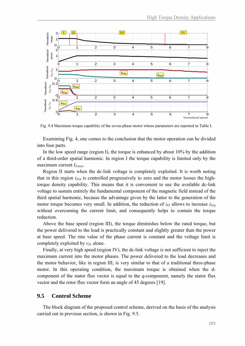
High Torque Density Applications
183
Examining Fig. 4, one comes to the conclusion that the motor operation can be divided into four parts.
In the low speed range (region I), the torque is enhanced by about 10% by the addition of a third-order spatial harmonic. In region I the torque capability is limited only by the maximum current IS,max.
Region II starts when the dc-link voltage is completely exploited. It is worth noting that in this region iS3d is controlled progressively to zero and the motor looses the high-torque density capability. This means that it is convenient to use the available dc-link voltage to sustain entirely the fundamental component of the magnetic field instead of the third spatial harmonic, because the advantage given by the latter to the generation of the motor torque becomes very small. In addition, the reduction of iS3 allows to increase iS1q without overcoming the current limit, and consequently helps to contain the torque reduction.
Above the base speed (region III), the torque diminishes below the rated torque, but the power delivered to the load is practically constant and slightly greater than the power at base speed. The rms value of the phase current is constant and the voltage limit is completely exploited by vS1 alone.
Finally, at very high speed (region IV), the dc-link voltage is not sufficient to inject the maximum current into the motor phases. The power delivered to the load decreases and the motor behavior, like in region III, is very similar to that of a traditional three-phase motor. In this operating condition, the maximum torque is obtained when the d-component of the stator flux vector is equal to the q-component, namely the stator flux vector and the rotor flux vector form an angle of 45 degrees [19].
9.5 Control Scheme
The block diagram of the proposed control scheme, derived on the basis of the analysis carried out in previous section, is shown in Fig. 9.5.
0 1 2 3 4 5 6 7 80
1
2
0 1 2 3 4 5 6 7 80
1
2
0 1 2 3 4 5 6 7 80
1
0 1 2 3 4 5 6 7 80
0.3
0 1 2 3 4 5 6 7 80
0.6
Nor
mal
ized
torq
ue
Nor
mal
ized
pow
er
Nor
mal
ized
i S1d
, iS1
q
Nor
mal
ized
i S3d
, iS3
q
Nor
mal
ized
v S1, v
S3
I II III IV
iS1qiS1d
iS3q
iS3d
vS1
vS3
Normalized speed
Fig. 9.4 Maximum torque capability of the seven-phase motor whose parameters are reported in Table I.

Chapter 9
184
In the control scheme, it is possible to identify three different parts. The first one is responsible for the tracking of the current references, the second one is the torque control loop, whereas the third one manages the field-weakening operation.
In Fig. 9.5, the controlled variables are expressed in two reference frames d1-q1 and d3-q3, synchronous and aligned with the corresponding rotor flux vectors. For the proper operation of the control scheme, it is assumed that estimations of the motor fluxes, torque and speed are available, although the problem of the observer is out of the scope of this analysis.
A. Current Loop Two PI regulators, (a) and (b), are used to track the reference signals iS1d,ref and iS1q,ref.
Two other PI regulators, (c) and (d), have the same task for the reference signals iS3d,ref and iS3q,ref.
As usual, the output signals of these regulators should be compensated for the back electromotive forces. If the dc-link voltage is not sufficient to synthesize the reference voltage vectors, their magnitudes are re-computed by multiplying for a reduction factor, lower than one, so that the rescaled reference voltages are kept inside the linear modulation area of Fig. 9.3. This task is accomplished by the limitation block (e).
B. Torque Loop The motor torque is adjusted by the PI regulator (f) that compares the reference torque
with the estimated actual torque. The output of this regulator is the torque-producing current iS1q,req, that tends to increase when the requested torque is greater than the estimated torque, and to decrease in the opposite case. It is worth noting that the reference
PI (j)
PI (f)
PI (h)
PWM
IM
d1q1
ab…fg
Sensorless or sensored
observer for stator flux,
phase angle of the rotor flux,
and torque.
d,maxSi 1
Limitation (k)
Limitation (g)
maxqSi ,1
11
1
SL
iS1d
iS1q
Back-emf
comp.
PI (a)
PI (b)
S1d
S1q
maxqSi ,1
iS1d
iS1q
dcEiS1q,ref
iSd1,ref
Anti-windup
Anti-windup
Treq
T
| | ABS
MIN
PI (c)
d,maxSi 3
Back-emf
comp.
PI (d)
d3q3
SSi 1
SSi 3
1S
23
23
21
2qSdSdSS,max iiiI iS1q,available
iS1d,req
iS1q,req
je 3
je3
reqSv ,1
reqSv ,3
iS3d,req
iS3q,ref
iS3d
iS3q
iS3d,ref
Edc
Calculation of the necessary dc-link
voltage
vS1,req
vS3,req vS1,req
Edc
iS3d
iS3q
T
SrefSv ,3
SrefSv ,1
| | ABS
SreqSv ,1
SreqSv ,3reqSv ,3
Anti-windup
Calculation of iS3q,ref
iS1q,ref vS3,req
Limitation (e)
Limitation (i)
cost. C
iS1d,ref
je
je
Fig. 9.5 Block diagram of the control scheme.

High Torque Density Applications
185
value iS3q,ref, necessary for ensuring the synchronism between the fundamental and the third-order spatial harmonics of the magnetic field, is calculated by (9.22) once iS1q,ref is known.
In region I, II, III the maximum deliverable torque is limited by the maximum current Is,max, whereas in region IV the maximum torque takes places when the d-component of the stator flux vector is equal to the q-component of the stator flux vector. In steady-state condition, this latter equality can be written as follows:
11
11
S
dSqS L
i
. (9.27)
The limitation block (g) assures that these constraints are satisfied in any speed region. In fact, the absolute value of the current iS1q is bounded by iS1q,max, which makes the stator current equal to Is,max or makes φS1q equal to φS1d, depending on which one is the most restrictive constraint in the present operating condition.
C. Flux Loop The rotor flux magnitude φR1 is indirectly controlled by PI regulator (j), which adjusts
the d-component iS1d,req of the stator current vector. In the same way, PI regulator (h) adjusts iS3d,req to control the rotor flux magnitude φR3.
When the motor speed is too high, the available dc-link voltage Edc is not sufficient to satisfy entirely the voltage request. The dc-link voltage that would be necessary for satisfying the voltage request can be calculated with the following equation:
7
2sin
7
3sin
7
3sin
7sin
max
,3,1
,3,1
,
reqSreqS
reqSreqS
reqdc
vv
vv
E (9.28)
If Edc,req is greater than the present dc-link voltage, it means that the motor is operating in region II, III or IV, and certainly the third spatial harmonic of the magnetic field has to be reduced. This task is accomplished by PI regulator (h), that integrates the difference Edc - Edc,req. If this difference is negative, iS3d is brought to zero. Otherwise it increases up to the threshold value iS3d,max shown in the limitation block (i).
It is worth noting that the decrease of iS3d causes a corresponding reduction of the
voltage request and, if vS1,req is lower than )73sin(21 Edc, i.e. 0.51 Edc, the freed
voltage resources can be used to keep φR1 unaltered as long as possible.
On the other hand, if the voltage request vS1,req is greater than )73sin(21 Edc, as
happens in region III and IV, it can never be satisfied, even if the third harmonic of the magnetic field is set to zero. In this case, PI regulator (j), which integrates a quantity proportional to the difference reqSdc vE ,1)73sin(2 , decreases φR1 by acting on the
current iS1d. The limitation block (k) forces this current to stay between an upper bound
Chapter 9
186
iS1d,max, and a lower bound iS1d,min. This is necessary to ensure the stable operation of the motor at high speed.
The main advantage of the proposed field weakening scheme is that it is independent of the base speed and the motor parameters, except for the leakage inductance σ1LS1, which is generally used in the state observer. In addition, it does not require any complex calculation of the flux level or look-up tables.
9.6 Calculation of the Amplitude of the Third Spatial Harmonic of the Magnetic Field in the Air-Gap
In previous sections the maximum values of the magnetizing currents maxdSi ,1 , maxdSi ,3
in the planes d1-q1 and d3-q have been introduced , but the meaning of these currents has not been clarified. In this section the problem of maximizing the torque capability in multiphase drives based on induction motors by adding a third spatial harmonic in the air-gap field is investigated.
The analysis shows that not considering the inverter and motor current rating may lead to suboptimal motor performance
It is worth noting that nearly all the papers that describe the control scheme of a multiphase motor with high torque density choose a value of the third spatial harmonic of the air-gap field that is deduced from a well-established method, namely the maximization of the amplitude of the fundamental component of the air-gap field. Although this choice could lead to an effective improvement of the motor torque in some cases, actually there are situations where it turns out to be useless or even detrimental.
The main reason is that the maximization of the fundamental component of the air-gap field coincides with the maximization of the motor torque only for the motor alone. When the motor is considered as a part of a complete electric drive, the solution for the maximum torque capability may be different. In fact, in the case of the whole drive, the motor is subject to constraints such as the inverter voltage limit, the inverter current rating or the machine thermal rating. These constraints remarkably affect the motor performance.
A. Approach of Maximization of the Fundamental Component of the Air-Gap Field
The corresponding values of the flux-producing components of the stator currents turn
out to be approximately as follows:
ratedSdmaxdS ii ,,13
2 (9.29)
ratedSdmaxdS ii ,,33
1 (9.30)

High Torque Density Applications
187
where iSd,rated is the rated magnetizing current of the motor operating without third spatial harmonic. Equations (9.29)-(9.30) are approximated in that the effect of the leakage flux has been neglected for their determination.
To obtain the relationships (9.29) and (9.30), it is necessary analyze the air-gap magnetic field present in a multi-phase electrical machine.
If no constraint on the motor currents is present, an increment of the fundamental component of air-gap field always leads to an increment of the motor torque. For this reason, (9.29) and (9.30) are usually adopted in the field-oriented control of high-torque density multiphase drives. The torque of a n-phase motor (the number n of phases is assumed odd) with only the contributions of the first and the third harmonics can be written as follows:
qSdS
RqSdS
R
iiL
Mii
L
MnT 33
3
23
111
21 3
2 (9.31)
where M1 and M3 are mutual inductances between stator and rotor windings in the plane d1-q1 and d3-q3, whereas LR1 and LR3 are rotor self inductances. As can be seen from (9.31), the torque depends on all the current components, but it can be demonstrated that the first term inside the brackets is usually the dominant one. This is the reason why the increment of iS1d in (9.29) has a positive repercussion on the motor torque.
B. Optimization of the Motor Torque In practical applications, the torque capability of a multiphase motor drive is mainly
limited by the inverter current rating and the motor current rating. The maximum value
that is admissible for the stator current is denoted with max,SI . This current limit can be
expressed by (9.26). Equation (9.26) is particularly important for the optimization of the torque in
multiphase drives. In fact, if the currents iS1d and iS3q are not set to zero and a third spatial harmonic is added to the air-gap field, (9.26) shows that there is a reduction of the current iS1q at disposal for torque generation.
Fig. 9.7 Example of behavior of the maximum torque for different values of the ratio of the magnetizing currents.

Chapter 9
188
Consequently the maximum torque capability corresponds to a precise combination of all the current components and results from a constrained optimization that has to consider not only the maximum admissible value of the air-gap field but also inequality (9.26).
Fig. 9.7 shows an example of the behavior of the maximum torque for different values of the ratio of the magnetizing currents, and refers to the motor parameters in Tab. I. As can be seen, the motor torque is maximum when the ratio iS3d/iS1d is about 0.32, and this result is very different from that given by (9.29)-(9.30), that lead to a ratio of 0.5.
It is possible to shown that the torque improvement that could be obtained for a given motor depends on the ratio between the magnetizing current ISd,rated and the maximum
current max,SI , as shown in Fig. 9.8. It is worth noting that the third harmonic is useless or
even detrimental if this ratio is 22 or greater.
Fig. 9.9 show the behavior of the currents iS1d and iS3d that correspond to the maximum torque enhancement. As can be seen, the optimal values are similar to (9.29) and (9.30)
Fig. 9.8 Maximum torque that can be obtained by adding a third spatial harmonic of the air-gap field as a function of the ratio between the magnetizing current and the maximum current.
Fig 9.9 Normalized values of the magnetizing currents iS1d and iS1q for different ratios ISd,rated/IM.

High Torque Density Applications
189
only when the magnetizing current of the motor is small compared to the maximum current, whereas they may be sensibly lower when the magnetizing current is at least 40% of the maximum current.
9.7 Experimental Results
Fig. 9.10 shows some experimental results obtained with a field-oriented drive based on a seven-phase induction motor. The figure compares the start-up transients in the cases that the third spatial harmonic of the air-gap field is generated either according (9.29)-(9.30) or according the proposed method. During the start-up transient the control system tries to produce the maximum torque. As can be seen, in the second case the motor is slightly faster, i.e. the motor produces a higher torque. In fact, after 0.4 s of acceleration, the motor speed is about 430 rpm in the first case and 510 rpm in the second case.
Figs. 9.11-9.13 show the behavior of the motor during a start-up transient when the torque reference is equal to the rated. Trace 9.11 of both Figs. 9.12 and 9.13 shows the waveform of a line current during the transient. In addition Fig 9.11 shows the waveforms of the estimated torque and of the currents iS1d and iS1q, whereas Fig. 9.12 shows the waveforms of the rotor speed and of the currents iS3d and iS3q. Initially, the motor is at standstill and absorbs only the magnetizing currents iS1d and iS3d.
After the rated torque command, the motor starts up and the line current reaches the maximum admissible amplitude (region I). In region II the control algorithm quickly reduces iS3d and, accordingly, iS3q. In region III the motor flux keeps decreasing, as can be recognized by examining the waveform of iS1d.
The control system, to entirely exploit the current limit (9.26) slightly increases iS1q, to take advantage of the progressive reduction of the other current components in region II and III.
Fig 9.10 Experimental results. Behavior of a 7-phase induction motor during a speed transient when thethird spatial harmonics is generated by maximizing the fundamental component of the air-gap field (a), orby maximizing the motor torque (b)

Chapter 9
190
Fig. 9.13 shows the behavior of the control system in the same operating condition of Fig. 9.11 and 9.12, but focuses the attention on region II. In this transition speed range, the waveform of the line current is initially distorted by the presence of a third harmonic component, but becomes more and more sinusoidal while iS3d decreases.
9.8 Conclusions
A rotor-flux-oriented control scheme for high-torque density seven-phase induction motor drives has been presented and experimentally assessed. The proposed control scheme is able to exploit the maximum torque capability of the motor at any speed. Its main advantage is that the flux control loop is independent of the base speed and the
motor parameters, except for the leakage inductance LS1. In addition, it does not require any complex calculation of the flux level or look-up tables
Furthermore the analyses of the problem of maximizing the torque capability of multiphase drives based on induction motors by adding a third spatial harmonic in the air-gap field is presented. The analysis takes into account the current limit of the motor and of the inverter and shows that the traditional solution of this problem, available in literature for induction motors without considering any current constraint, may lead to
(1)
(2)
(4)
(3)
II III
I
(1)
(2)
(4)
(3)
IIIII
I
Fig.9.11 - Start-up transient with rated torque (500 ms/div). 1) Motor torque (20 Nm/div), 2) iS1d (2 A/div), 3) iS1q (2 A/div), 4) Phase current (10 A/div).
Fig.9.12 - Start-up transient with rated torque (500 ms/div). 1) Motor speed (750 rpm/div), 2) iS3d (1 A/div), 3) iS3q (1 A/div), 4) Phase current (10 A/div).
(1)
(2)
(4)
(3)
(1)(2)
(3)(4)
Fig.9.13 - Start-up transient with rated torque. The time scale is 1 s/div for upper traces and 100 ms/div for lower traces. 1) Motor torque (20 Nm/div), 2) iS1d (4 A/div), 3) iS3d (2 A/div), 4) Phase current (10 A/div).

High Torque Density Applications
191
suboptimal motor performance. The main reason is that the traditional solution, based on the maximization of the fundamental component of the air-gap field, is valid only for the motor alone. When the motor is considered as a part of a complete electric drive, the solution corresponding to the maximum torque may be different.
The results described in this paper can be useful for the design of multiphase induction motors and drives, or for the tuning of the control systems.
The validity of the theoretical analysis is verified by numerical simulation and experimental results.
9.9 References
[1] L. Parsa, “On advantages of multi-phase machines,” in Proc. of IEEE IECON, 2005, pp. 1574-1579.
[2] E. Levi, R. Bojoi, F. Profumo, H.A. Toliyat, S. Williamson, “Multiphase induction motor drives – a technology status review,” IET Electr. Power Appl., vol. 1, no.4, pp. 489-516, July 2007.
[3] G.K. Singh, K. Nam, S.K. Lim, “A simple indirect field-oriented control scheme for multiphase induction machine,” IEEE Trans. on Industrial Electronics, vol. 52, no. 4, 2005, pp. 1177- 1184.
[4] E. Levi, M. Jones, S.N. Vukosavic, “Even-phase multi-motor vector controlled drive with single inverter supply and series connection of stator windings,” IEE Proc.-Electr. Power Appl., vol. 150, no. 5, 2003, pp. 580-590.
[5] A. Iqbal, S. Moinuddin, M.R. Khan, I.Ashraf, “Indirect rotor flux oriented control of a seven-phase induction motor drive,” Proc. of IEEE ICIT 2006, 15-17 Dec. 2006, pp. 440 - 445.
[6] D. Casadei, M. Mengoni, G. Serra, A. Tani and L. Zarri, “Seven-Phase Induction Motor Drive Based on Stator Flux Vector Control,” in Proc. of SPEEDAM 2008, 11-13 June 2008, Ischia, Italy, pp.113-119.
[7] F. Locment, E. Semail, X. Kestelyn, “Vectorial approach-based control of a seven-phase axial flux machine designed for fault operation,” IEEE Trans. on Industrial Electronics, Vol. 55, No. 10, Oct. 2008, pp. 3682 - 3691.
[8] R. Bojoi, M. Lazzari, F. Profumo, A. Tenconi, “Digital field oriented control for dual three-phase induction motor drives,” IEEE Trans. on Ind. Applicat., Vol. 39, no. 3, 2003, pp. 752-760.
[9] R. Bojoi, F. Profumo, A. Tenconi, “Digital synchronous frame current regulation for dual three-phase induction motor drives,” in Proc. of IEEE Power Electronics Specialist Conference, PESC, 2003, pp. 1475-1480.
[10] K.K. Mohapatra, R.S. Kanchan, M.R. Baiju, P.N. Tekwani, K. Gopakumar, “Independent field-oriented control of two split-phase induction motors from a single six-phase inverter,” IEEE Trans. on Industrial Electronics, vol. 52, no. 5, 2005, pp. 1372- 1382.
[11] L. Parsa, H. A. Toliyat, “Five-phase permanent-magnet motor drives,” IEEE Trans. on Industry Applications, Vol. 41, No. 1, Jan./Feb. 2005, pp.30-37.
[12] L. Parsa, N. Kim and H. Toliyat, “ Field Weakening Operation of a High Torque Density Five Phase Permanent Magnet Motor Drive,” IEEE IEMDC, May 15-18, 2005, pp. 1507 - 1512.
Chapter 9
192
[13] H Shan Xue, Xuhui Wen, Zhao Feng, “A novel multi-dimensional SVPWM strategy of multiphase motor drives,” in Proc. of EPE-PEMC 2006, Portoroz, Slovenia, pp. 931-935.
[14] S. Xue, X. Wen, Z. Feng, “Multiphase Permanent Magnet Motor Drive System Based on A Novel Multiphase SVPWM, ” in Proc. of IPEMC 2006, 14-16 Aug. 2006, Vol. 1, pp. 1-5.
[15] Xu, H.A. Toliyat, L.J.Petersen, “Rotor field oriented control of five-phase induction motor with the combined fundamental and third harmonic currents,” in Proc. of IEEE Applied Power Electronics Conference, APEC, 2001, pp. 392-398.
[16] H. Xu, H.A. Toliyat, L.J.Petersen, “Five-phase induction motor drives with DSP-based control system,” IEEE Trans. on Power Electron., Vol. 17, No. 4, 2002, pp. 524-533.
[17] D. Casadei, D. Dujic, E. Levi, G. Serra, A. Tani, L. Zarri, “General Modulation Strategy for Seven-Phase Inverters with Independent Control of Multiple Voltage Space Vectors,” IEEE Trans. on Industrial Electronics, Vol. 23, No. 2, May 2008, pp.1921-1932.
[18] M. Mengoni, L. Zarri, A. Tani, G. Serra, D. Casadei, "Stator Flux Vector Control of Induction Motor Drive in the Field Weakening Region," IEEE Trans. on Power Electronics, Vol. 23, No. 2, March 2008, pp. 941-948.
Fault-Tolerant Control Strategy Under an Open Circuit Phase Fault
Condition Abstract In this chapter some different control strategies, suitable for open-phase fault operation of multi-phase current regulated induction motor drives, are presented. These strategies, which are valid in steady-state as well as in transient operating conditions, are then compared in terms of stator and rotor copper losses and torque pulsations. The comparison is based on an opportune mathematical model of the machine that, exploiting the properties of the multiple space vector representation of multi-phase systems, takes into account the first five spatial harmonics of the air-gap magneto motive force. An optimal free-disturbance control strategy, for multi-phase current regulated motor drives, suitable for open-phase fault operation, is presented and tested. The proposed strategy, minimizes the stator and copper losses in transient and steady-state operating conditions. The effectiveness of the proposed fault tolerant control strategies is confirm by numerical simulations based on finite element analysis and by some experimental tests, carried out on a seven-phase asynchronous motor drive prototype.
10.1 Introduction
The development of modern power electronic devices and the improvement in the control techniques make it possible to consider the number of phases of variable-speed motor drives as one of the design variables. As a consequence, the conventional three-phase solution simply represents a particular case.
The increase of the phase number leads to a reduction of the stator current per phase with the same power, with evident advantages in terms of inverter power devices.

Chapter 10
194
Furthermore, the improved spatial distribution of the Magneto Motive Force (MMF) in the machine air gap reduces the rotor copper losses and the amplitude of the torque pulsation [1]-[2].
A further advantage of multi-phase drives, with respect to the three-phase ones, is the greater number of degrees of freedom that can be exploited in different ways.
One possibility consists in improving the fault-tolerant capability of the motor drive. This characteristic represents a crucial point for all applications requiring a high degree of reliability, such as aircraft or marine ones.
This chapter investigates a class of faults for multi-phase motor drives where one of the phases becomes open-circuited. This type of fault can be caused by mechanical failure of a machine terminal connector, an internal winding rupture, or by an electrical failure in one of the inverter phase leg.
Some control strategies, able to ensure disturbance-free operation of multi-phase motor drives under an open circuit phase fault condition, without any additional hardware connection, have been already presented in literature.
In [3] and [4] the problem has been solved using the usual phasor representation of each stator current in steady-state operating conditions. In [5] the proposed solution is based on the Fortescue’s symmetrical component representation of the stator currents. Also in this case reference is made to steady-state conditions.
A different approach, which is based on the multiple space vector representation of multi-phase quantities [6], [7], has been proposed in [8] for multi-phase motors with “sinusoidally” distributed stator windings, having an odd number of phases.
In this chapter, the multiple space vector representation is used in order to define different fault-tolerant control techniques for multi-phase current-regulated induction motor drives. The proposed approach allows the analytical determination in closed form of the waveform of the stator currents in the healthy phases, ensuring disturbance-free operation in transient and steady-state operating conditions.
Using an opportune mathematical model of the seven-phase induction machine, which takes into account the undesired effects of the third and fifth spatial harmonics of the MMF in the air gap, the properties of the proposed control strategies, in terms of stator and rotor copper losses and torque pulsations are analyzed and compared.
Some experimental tests have been carried out on a seven-phase asynchronous motor drive prototype available in laboratory. The results confirm the effectiveness and the properties of the proposed fault-tolerant control strategies.
10.2 Analysis of the MMF in the Air-Gap
The behavior of the MMF spatial distribution produced by the stator windings in the air gap of the machine directly affects the rotor quantities dynamics, and then the rotor copper losses and the electromagnetic torque.
Under the assumptions usually adopted and described in Chapter 5, the description of the spatial distribution of the MMF in the air gap produced by the symmetrical stator windings of a star connected multi-phase induction motor, can be written, in terms of stator current space vectors, in the following compact form:
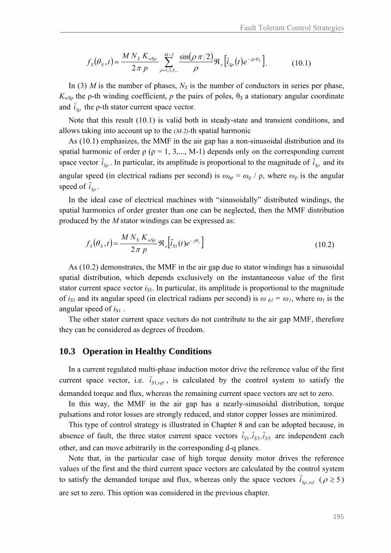
Fault Tolerant Control Strategies
195
2
,..5,3,1
2sin
2,
Mj
SewSS
SSSeti
p
KNMtf
. (10.1)
In (3) M is the number of phases, NS is the number of conductors in series per phase, KwSρ the ρ-th winding coefficient, p the pairs of poles, θS a stationary angular coordinate and Si the ρ-th stator current space vector.
Note that this result (10.1) is valid both in steady-state and transient conditions, and allows taking into account up to the (M-2)-th spatial harmonic
As (10.1) emphasizes, the MMF in the air gap has a non-sinusoidal distribution and its spatial harmonic of order ρ (ρ = 1, 3,..., M-1) depends only on the corresponding current space vector Si . In particular, its amplitude is proportional to the magnitude of Si and its
angular speed (in electrical radians per second) is ωhρ = ωρ / ρ, where ωρ is the angular speed of Si .
In the ideal case of electrical machines with “sinusoidally” distributed windings, the spatial harmonics of order greater than one can be neglected, then the MMF distribution produced by the M stator windings can be expressed as:
sjSe
wSSSS eti
p
KNMtf
)(
2, 1 (10.2)
As (10.2) demonstrates, the MMF in the air gap due to stator windings has a sinusoidal spatial distribution, which depends exclusively on the instantaneous value of the first stator current space vector iS1. In particular, its amplitude is proportional to the magnitude of iS1 and its angular speed (in electrical radians per second) is ω h1 = ω1, where ω1 is the angular speed of iS1 .
The other stator current space vectors do not contribute to the air gap MMF, therefore they can be considered as degrees of freedom.
10.3 Operation in Healthy Conditions
In a current regulated multi-phase induction motor drive the reference value of the first current space vector, i.e. ref,Si 1 , is calculated by the control system to satisfy the
demanded torque and flux, whereas the remaining current space vectors are set to zero. In this way, the MMF in the air gap has a nearly-sinusoidal distribution, torque
pulsations and rotor losses are strongly reduced, and stator copper losses are minimized. This type of control strategy is illustrated in Chapter 8 and can be adopted because, in
absence of fault, the three stator current space vectors 531 SSS i,i,i are independent each
other, and can move arbitrarily in the corresponding d-q planes. Note that, in the particular case of high torque density motor drives the reference
values of the first and the third current space vectors are calculated by the control system to satisfy the demanded torque and flux, whereas only the space vectors refSi , ( 5 )
are set to zero. This option was considered in the previous chapter.
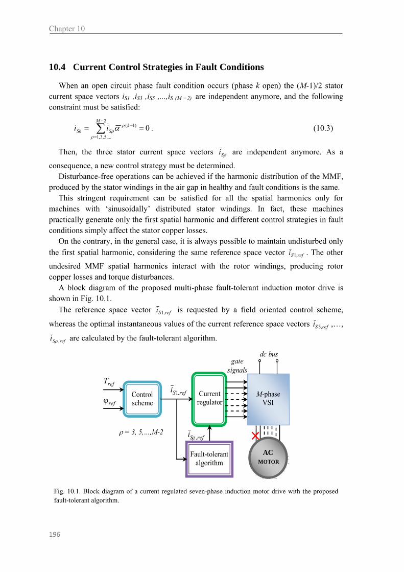
Chapter 10
196
10.4 Current Control Strategies in Fault Conditions
When an open circuit phase fault condition occurs (phase k open) the (M-1)/2 stator current space vectors iS1 ,iS3 ,iS5 ,...,iS (M −2) are independent anymore, and the following constraint must be satisfied:
02
,...5,3,1
)1(
M
kSSk ii
. (10.3)
Then, the three stator current space vectors Si are independent anymore. As a
consequence, a new control strategy must be determined. Disturbance-free operations can be achieved if the harmonic distribution of the MMF,
produced by the stator windings in the air gap in healthy and fault conditions is the same. This stringent requirement can be satisfied for all the spatial harmonics only for
machines with ‘sinusoidally’ distributed stator windings. In fact, these machines practically generate only the first spatial harmonic and different control strategies in fault conditions simply affect the stator copper losses.
On the contrary, in the general case, it is always possible to maintain undisturbed only the first spatial harmonic, considering the same reference space vector ref,Si 1 . The other
undesired MMF spatial harmonics interact with the rotor windings, producing rotor copper losses and torque disturbances.
A block diagram of the proposed multi-phase fault-tolerant induction motor drive is shown in Fig. 10.1.
The reference space vector ref,Si 1 is requested by a field oriented control scheme,
whereas the optimal instantaneous values of the current reference space vectors ref,Si 3 ,…,
refSi , are calculated by the fault-tolerant algorithm.
M-phase VSI
dc bus
Control scheme
ref,Si 1
ref,Si
refT
ref
AC MOTOR
gate signals
Current regulator
= 3, 5,…,M-2
Fault-tolerant algorithm
Fig. 10.1. Block diagram of a current regulated seven-phase induction motor drive with the proposed fault-tolerant algorithm.

Fault Tolerant Control Strategies
197
A. Optimal Disturbance-free Operations in Fault Conditions The first strategy (strategy (A)) is a disturbance free operation control algorithm,
which minimizes the instantaneous stator copper losses steady-state and transient conditions
The instantaneous stator copper losses can be calculated as:
M
kSksSJ iRP
...3,2,1
2 . (10.4)
Substituting the inverse Clarke transformation in (6), and considering a null value of the zero sequence component, owing to the winding star connection, leads to:
22
,..5,3,12
M
SsSJ iM
RP
. (10.5)
The reference space vector iS1,ref is requested by the control scheme, and the fault algorithm calculates the most opportune remaining reference current space vectors satisfying the optimization criterion and the constraint condition (10.3).
Equation (10.3) can be rewritten as
)1(,1
)1(2
,..5,3,
krefS
kM
refS ii
. (10.6)
As (10.6) suggests, each current space vector refSi , (ρ = 3, 5, M-2) can be
decomposed along two orthogonal directions (T and N), as expressed by the following relationship:
)1(,,
)1(,,,
kNrefS
kTrefSrefS jiii
. (10.7)
Note that (10.7) defines a constraint exclusively for the T-components, then, in order to minimize the stator copper losses, all the N-components are set to zero,
As a consequence (10.6) and (10.7) can be rewritten as:
)1(,1
)1(2
,..5,3,
krefS
kM
refTS ii
(10.8)
)1(,,,
kTrefSrefS ii
(ρ=3, 5, M-2) (10.9)
The last step consists in the determination of the T-components TrefSi ,, (ρ = 3, 5, M-
2). According to (10.9) the optimal solution coincides with (M-3)/2 equal T-components. As a consequence, the optimal instantaneous values of the current reference space
vectors, which guarantee the minimum stator copper losses, taking the constraint (5) into account, can be expressed in closed form, in a stator reference frame, as follows:
)1(,1
)1(
, 3
2
k
refS
k
refS iM
i
, (ρ=3, 5, M-2) (10.10)

Chapter 10
198
It can be demonstrated that, in the particular conditions characterized by a space vector iS1,ref rotating on a circular trajectory with constant angular speed, the proposed fault tolerant control scheme leads to a system of sinusoidal, but unbalanced, stator currents.
In the ideal case of ac motors with ‘sinusoidally’ distributed stator windings the current space vectors calculated by (10.10) do not contribute to the spatial distribution of the MMF. On the contrary, in the practical case, each current space vector iSρ,ref (ρ = 3, 5, M-2) produces two counter-rotating sinusoidal spatial harmonics of MMF of order ρ, having the same amplitude.
In following analyzes for simplicity it will be supposed that the phase 1 breaks. This hypothesis does not reduce the validity area of the theory but permits to simplify the equations.
Therefore when the hypothesis is applied, (10.3) can be expressed as:
2
,...5,3,11 1
M
SS ii
. (10.11)
In this situation for a five phase machine the current space vectors can be described by means of two constants, as follows:
refSrefS
refSrefS
iKi
iKi
,13,3
,13,3
(10.12)
where
refSrefSrefS
refSrefSrefS
ijii
ijii
,3,3,3
,1,1,1
(10.13)
Under this hypothesis strategy A for a five phase machine can be expressed as follows:
0,1 33 KK , α=2π/5. (10.14)
Furthermore for a seven phase machine the equations (10.12) and (10.13) can be defined as:
ref,Sref,S
ref,Sref,S
ref,Sref,S
ref,Sref,S
iKi
iKi
iKi
iKi
155
155
133
133
(10.15)
where
ref,Sref,Sref,S
ref,Sref,Sref,S
ref,Sref,Sref,S
ijii
ijii
ijii
555
333
111
(10.16)
Strategy (A) can be expressed for seven phase machine as follows:

Fault Tolerant Control Strategies
199
021021 5533 K,K,K,K . (10.17)
In steady-state operating conditions (i.e. refSi ,1 rotating with constant angular speed on
a circular trajectory), the current space vectors refSi ,3 and refSi ,5 move along an horizontal
segment (see Fig. 2a). As a consequence, the interactions between the stator direct components and the rotor
reaction inverse components (and vice versa) produce a pulsating torque, having frequency 2 f, where f is the stator current frequency.
B. Strategy (B) In order to improve the spatial distribution of stator copper losses in the stator
windings and to minimize the peak inverter current, a new fault control strategy, can be introduced.
Strategy (A) minimize the joule stator losses but it obtains different amplitude for line currents both in transient and in steady state conditions. This situations can determine a different temperature distribution for stator phases and a different exploitation of the machine iron.
In steady state operating condition strategy (B) allow to obtain the same amplitude for all remaining stator currents after the fault. This constrain saturate all degree of freedom only for a five phase machine whereas, when the number of phases is higher than five, for this problem there are infinite solutions.
Under this hypothesis strategy B for a five phase machine can be expressed:
)2
cos(43)2sin()sin(
)2sin()sin(,1 33
KK , α=2π/5 (10.18)
In [3] one of the possible solutions is proposed but only with reference to steady-state operating conditions, owing to the phasorial representation of the stator currents.
In this section the solution presented in [3] is introduced with vectorial representation, useful for the implementation of a multi-phase drive based on vector control system.
For a seven-phase machine the equations (10.18) can be rewrite as:
2560.0,5550.0,1882.0,4450.0 5533 KKKK (10.19)
In (10.19) 5533 , KKKK have not an analytic solution but only a numeric solution.
In steady-state operating conditions this leads to six sinusoidal stator currents of equal amplitude and the current space vectors refSi ,3 and refSi ,5 move along elliptical trajectories
(Fig. 10.2b)._Therefore, also in this case, both the third and the fifth spatial harmonics of the MMF are constituted by two counter-rotating components, leading to pulsating torque components.
For multi phase system with a number of phases higher than seven a solution can be always found but only in a numeric way.

Chapter 10
200
C. Strategy (C) Low frequency torque pulsation can represent a problem in some applications. In order
to eliminate this pulsating torque in fault conditions, counter-rotating stator MMF components have to be avoided.
This result can be obtained for a five phase induction machine by forcing the current space vectors refSi ,3 to move along circular trajectories, with constant angular speed.
The fault control strategy reaching this goal, with minimum stator and rotor copper losses, can be defined as:
1,1 33 KK (10.20)
This result can be obtained by forcing the current space vector refSi ,3 to move along
circular trajectories, with constant angular speed. For a seven phase machine the strategy (C) can be express as:
21,21,21,21 5533 KKKK (10.21)
In this case, the current space vectors refSi ,3 and refSi ,5 rotate in the same direction of
refSi ,1 , with the same angular speed, as can be seen in Fig. 10.2c.
For a generic M-phase machine with odd number of phases (10.20) and (10.21) can be generalized as:
,32,32 MKMK (ρ=3, 5, …, M-2) (10.22)
10.5 Comparison of the Fault-Tolerant Strategies in Steady-State Conditions
The three proposed fault-tolerant strategies (A), (B), and (C) have been compared, in steady-state operating conditions, in terms of stator and rotor copper losses, average torque and torque ripple.
ref,Si 3
ref,Si 5
ref,Si 1
ref,Si 3
ref,Si 5
ref,Si 1
ref,Si 3
ref,Si 5
ref,Si 1
Fig. 10.2. Trajectories of the stator current space vectors. a) Strategy A. b) Strategy B. c) Strategy C.

Fault Tolerant Control Strategies
201
In the case of ‘sinusoidally’ distributed stator windings, only the stator copper losses must be calculated, owing to the undisturbed behavior of the other quantities.
The instantaneous stator copper losses can be evaluated by (10.5): Taking (10.17), (10.19) and (10.21) into account for a five phase machine, it can be
demonstrated that:
healthyJSAfaultJS PP ,)(, 2
3 , (10.23)
healthyJSBfaultJS PP ,)(, 52786.1 , (10.24)
healthyJSCfaultJS PP ,)(, 2 . (10.25)
For a seven-phase machine:
healthyJSAfaultJS PP ,)(, 4
5 , (10.26)
healthy,JS)B(fault,JS P.P 3031, (10.27)
healthy,JS)C(fault,JS PP2
3
. (10.28)
For a M-phase machine the ratio between the stator joule power losses in healthy condition and fault conditions for strategies (A) and (C) can be expressed:
healthyJSAfaultJS PM
P ,)(, 3
11
, (10.29)
healthyJSCfaultJS PM
P ,)(, 3
21
. (10.25)
As can be seen, Strategy A is the best [8], whereas Strategy C is the worst. This conclusion is independent of the number of phases. The comparison in terms of rotor copper losses, average torque and torque ripple
depends on the operating conditions and is strongly affected by the stator winding distribution. In the following, reference is made to a seven-phase squirrel-cage induction machine, having stator winding with one slot per pole per phase. The machine parameters are shown in Tab. I.
The mathematical model of a current fed seven-phase induction machine can be written in terms of multiple space vectors as follows (stator reference frame):
TABLE I MOTOR PARAMETERS
RATED POWER
RATED PHASE VOLTAGE
RATED SPEED
POLE NUMBER
SLOT NUMBER
3500 W
120VRMS, 50 HZ
1450 RPM
4
28

Chapter 10
202
RR
RR jdt
diR 0 , (ρ = 1, 3, 5) (10.26)
RRSR iLiM, (ρ = 1, 3, 5) (10.27)
5,3,12
7
RS ijiMpT , (10.28)
where RR is the rotor resistance, LRρ and Mρ are, respectively, the rotor and mutual inductances concerning the ρ-th spatial harmonic, and ω is the rotor angular speed in electrical radians.
The behavior of the proposed fault-tolerant algorithms in steady-state conditions can be determined by solving. (10.26)-(10.28) by means of a numerical procedure, assuming the stator currents as input variables. Then, the rotor copper losses can be evaluated as follows:
5,3,1
2
2
7
RRJR iRp . (10.29)
Note that this model takes into account the first five spatial harmonics of the MMF in the air gap.
The results of the comparison as function of the rotor speed (in p.u. of the rated value), with rated value of the torque, are presented in Figs. 10.3-10.5.
0.8
0.85
0.9
0.95
1
1.05
1.1
1.15
1.2
-1 -0.8 -0.6 -0.4 -0.2 0 0.2 0.4 0.6 0.8 1
Rotor speed (p.u.)
Ave
rage
torq
ue (
p.u.
)
Strat. A
Strat. B
Strat. C
Fig. 10.4. Average torque as function of the rotor speed.
0.90.95
11.051.1
1.151.2
1.251.3
1.35
-1 -0.8 -0.6 -0.4 -0.2 0 0.2 0.4 0.6 0.8 1
Rotor speed (p.u.)
Rot
or c
oppe
r lo
sses
(p.
u.)
Strat. A
Strat. B
Strat. C
Fig. 10.3. Rotor copper losses as function of the rotor speed.

Fault Tolerant Control Strategies
203
Fig. 10.3 illustrates the rotor copper losses (in p.u. of the value in healthy condition). As can be seen, Strategy A is slightly better than Strategy B, whereas Strategy C is clearly the worst. Note that the rotor copper losses have a minimum for low rotor speed whereas are constant for high rotor speed.
The average value of the torque (in p.u. of the rated value) as a function of the rotor speed is shown in Fig. 10.4. Also in this case, Strategy C is the worst owing to the higher value of the torque disturbance, and Strategy A is better than Strategy B.
The results of the comparison in terms of peak-to-peak amplitude of the torque ripple are presented in Fig. 10.5. As expected, Strategy C generates no torque ripple in the whole speed range, whereas Strategy A and Strategy B lead to high values of the torque, especially at low speed. From this point of view, Strategy B is better than Strategy A.
Furthermore in order to emphasize the effectiveness of the fault tolerant control strategy (A), the simulation of a field-oriented drive based on a five-phase surface mounted permanent magnet synchronous motor has been implemented using FE analysis.
To better comprehend the undesired effects of the spatial harmonic components of the magnetic field in the air gap two different double-layer stator winding arrangements, having two slots per pole per phase, are considered.
Fig. 10.6. Cross-section of the permanent magnet motor, with a superimposed typical flux plot obtained by FE analysis.
0
0.02
0.04
0.06
0.08
0.1
0.12
0.14
-1 -0.8 -0.6 -0.4 -0.2 0 0.2 0.4 0.6 0.8 1
Rotor speed (p.u.)
Tor
que
ripp
le (
p.u.
)
Strat. A
Strat. B
Strat. C
Fig. 10.5.Torque ripple amplitude as function of the rotor speed.
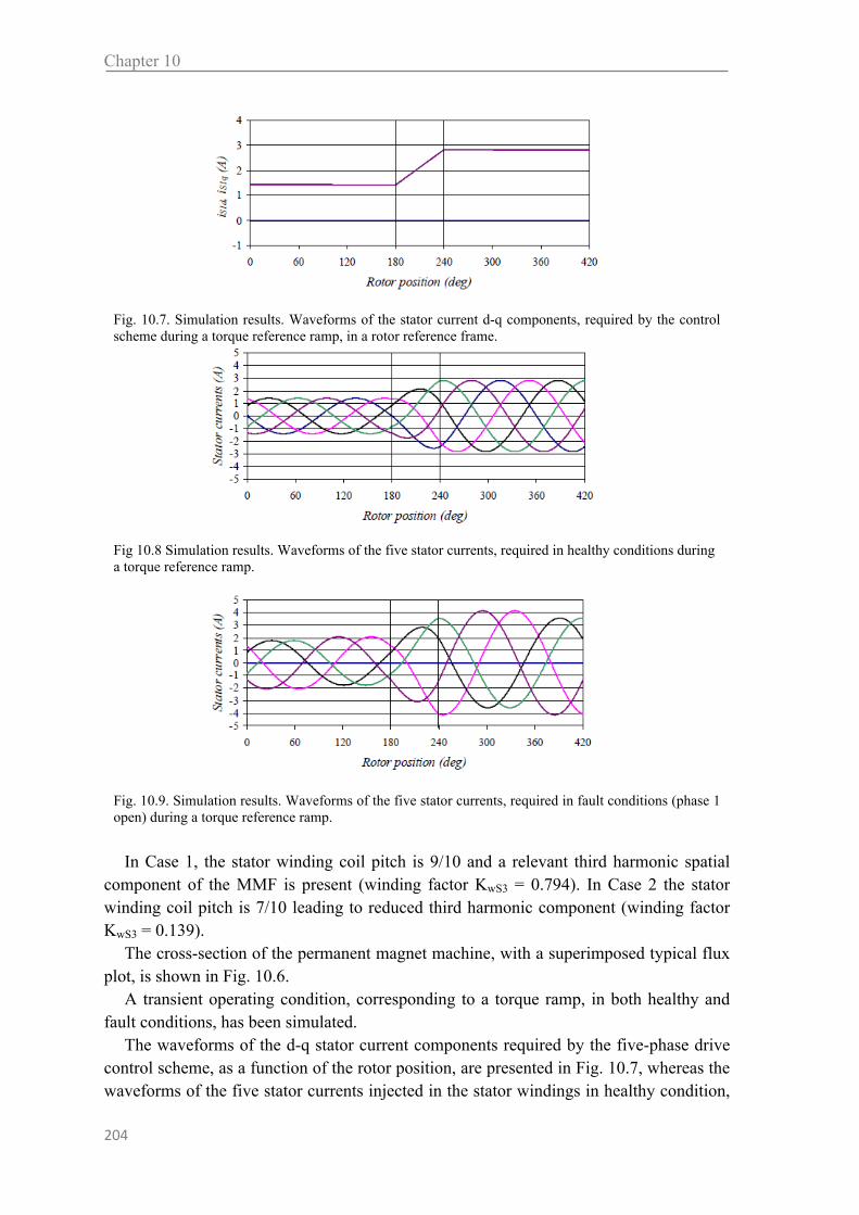
Chapter 10
204
In Case 1, the stator winding coil pitch is 9/10 and a relevant third harmonic spatial component of the MMF is present (winding factor KwS3 = 0.794). In Case 2 the stator winding coil pitch is 7/10 leading to reduced third harmonic component (winding factor KwS3 = 0.139).
The cross-section of the permanent magnet machine, with a superimposed typical flux plot, is shown in Fig. 10.6.
A transient operating condition, corresponding to a torque ramp, in both healthy and fault conditions, has been simulated.
The waveforms of the d-q stator current components required by the five-phase drive control scheme, as a function of the rotor position, are presented in Fig. 10.7, whereas the waveforms of the five stator currents injected in the stator windings in healthy condition,
Fig. 10.7. Simulation results. Waveforms of the stator current d-q components, required by the control scheme during a torque reference ramp, in a rotor reference frame.
Fig 10.8 Simulation results. Waveforms of the five stator currents, required in healthy conditions during a torque reference ramp.
Fig. 10.9. Simulation results. Waveforms of the five stator currents, required in fault conditions (phase 1 open) during a torque reference ramp.

Fault Tolerant Control Strategies
205
are illustrated in Fig. 10.8. As can be seen, during steady-state operating conditions, the stator current are balanced and sinusoidal.
In fault condition, the stator current calculated by the fault tolerant control strategy on the basis of (10.10) and injected in the stator winding are shown in Fig. 10.9. As expected, in steady-state conditions, with an open-circuited phase, the proposed control strategy requires a system of unbalanced sinusoidal stator currents.
The torque response obtained by FE analysis in Case 1 in healthy conditions is shown in Fig. 10.10. As can be seen, the torque matches the reference value very well, except for a small ripple due to the slot effects.
In Fig. 10.11 the corresponding torque response in fault condition is presented. Large oscillations at relatively low frequency are clearly recognizable. They are caused by the
Fig. 10.10 Simulation results. Torque response calculated by FE analysis, in healthy conditions (coil pitch = 9/10).
Fig 10.11 Simulation results. Torque response calculated by FE analysis, in fault conditions (phase 1 open, coil pitch = 9/10).
Fig. 10.12. Simulation results. Torque response calculated by FE analysis, in healthy conditions (coil pitch = 7/10).
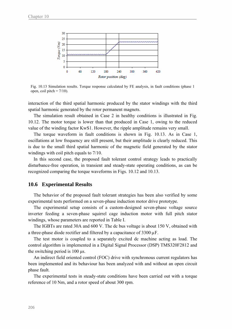
Chapter 10
206
interaction of the third spatial harmonic produced by the stator windings with the third spatial harmonic generated by the rotor permanent magnets.
The simulation result obtained in Case 2 in healthy conditions is illustrated in Fig. 10.12. The motor torque is lower than that produced in Case 1, owing to the reduced value of the winding factor KwS1. However, the ripple amplitude remains very small.
The torque waveform in fault conditions is shown in Fig. 10.13. As in Case 1, oscillations at low frequency are still present, but their amplitude is clearly reduced. This is due to the small third spatial harmonic of the magnetic field generated by the stator windings with coil pitch equals to 7/10.
In this second case, the proposed fault tolerant control strategy leads to practically disturbance-free operation, in transient and steady-state operating conditions, as can be recognized comparing the torque waveforms in Figs. 10.12 and 10.13.
10.6 Experimental Results
The behavior of the proposed fault tolerant strategies has been also verified by some experimental tests performed on a seven-phase induction motor drive prototype.
The experimental setup consists of a custom-designed seven-phase voltage source inverter feeding a seven-phase squirrel cage induction motor with full pitch stator windings, whose parameters are reported in Table I.
The IGBTs are rated 30A and 600 V. The dc bus voltage is about 150 V, obtained with
a three-phase diode rectifier and filtered by a capacitance of 3300 F. The test motor is coupled to a separately excited dc machine acting as load. The
control algorithm is implemented in a Digital Signal Processor (DSP) TMS320F2812 and the switching period is 100 μs.
An indirect field oriented control (FOC) drive with synchronous current regulators has been implemented and its behaviour has been analyzed with and without an open circuit phase fault.
The experimental tests in steady-state conditions have been carried out with a torque reference of 10 Nm, and a rotor speed of about 300 rpm.
Fig. 10.13 Simulation results. Torque response calculated by FE analysis, in fault conditions (phase 1 open, coil pitch = 7/10).

Fault Tolerant Control Strategies
207
The results obtained in healthy conditions are presented in Figs. 10.14-10.15. The stator currents in phase 1, 2, 3, and 4, are shown in Fig. 10.14. As expected, the stator currents are balanced and sinusoidal.
The behavior of the torque, which has been measured by a torque meter, is illustrated in Fig. 10.15. As can be seen, the torque is practically constant.
The results achieved in fault conditions (phase 1 open) are illustrated in Figs. 10.16-10.17 (Strategy A) and 10.18-10.19 (Strategy C), respectively.
As can be seen in Figs. 10.16 and 10.17, Strategy A allows sinusoidal and unbalanced stator currents to be obtained, and the corresponding torque behavior is characterized by a
Fig. 10.14 Experimental results. Waveforms of stator currents in phase 1, 2, 3, and 4, in healthy conditions (20 ms/div, 5 A/div).
Fig. 10.15 Experimental results. Measured torque in healthy conditions (100 ms/div, 5 Nm/div).
Fig. 10.16 Experimental results. Strategy A. Waveforms of stator currents in phase 1, 2, 3, and 4, in fault conditions (20 ms/div, 5 A/div).
Fig. 10.17 Experimental results. Strategy A. Measured torque in fault conditions (100 ms/div, 5 Nm/div).
Fig. 10.18 Experimental results. Strategy C. Waveforms of stator currents in phase 1, 2, 3, and 4, in fault conditions (20 ms/div, 5 A/div).
Fig. 10.19. Experimental results. Strategy C. Measured torque in fault conditions (100 ms/div, 5 Nm/div).
Chapter 10
208
torque ripple having frequency double with respect to the stator one. Also Strategy C leads to sinusoidal and unbalanced stator currents (Fig. 10.18), but
with amplitudes greater than those concerning Strategy A, according to the theoretical results. Furthermore, as can be seen in Fig. 10.19, in this case the torque ripple component at low frequency is practically absent.
10.7 Conclusions
In this chapter, three different control strategies for multi-phase machine, allowing disturbance-free operation in the case of open-phase fault condition, have been proposed and compared.
The determination of these fault-tolerant control strategies, which can be implemented in steady-state as well as in transient operating conditions, is based on the multiple space vector representation of the multi-phase quantities.
The comparison, in terms of stator and rotor copper losses, average torque and torque ripple, is based on an opportune mathematical model of the seven-phase induction machine that takes into account the first five spatial harmonics of the air-gap magneto motive force.
The results of the comparison can be summarized as follows. If the induction machine has ‘sinusoidally’ distributed stator windings, Strategy A is
optimal in terms of stator copper losses, whereas Strategy B is the best with reference to the minimum peak inverter current.
In the case of induction machine with concentrated windings, Strategy A has the best performance in terms of rotor copper losses and average torque, but Strategy C is the best with reference to the torque ripple.
A seven-phase asynchronous motor drive prototype has been built in the laboratory and some experimental tests have been carried out. The results have confirmed the effectiveness of the proposed fault-tolerant control strategies.
10.8 References
[1] L. Parsa, “On Advantages of Multi-Phase Machines,” in Proc. of Annual Conference of the IEEE Industrial Electronics Society IECON, pp. 1574-1579, November 6-10, 2005, Raleigh, North Carolina, USA.
[2] E. Levi, R. Bojoi, F. Profumo, H.A. Toliyat, S. Williamson, “Multiphase induction motor drives – a technology status review,” IET Electr. Power Appl., vol. 1, no.4, pp. 489-516, July 2007.
[3] J.R. Fu, T.A.Lipo, “Disturbance-Free Operation of a Multiphase Current-Regulated Motor Drive with an Opened Phase,” IEEE Trans. on Ind. Applicat., vol. 30, no.5, pp. 1267-1274, October 1994.
[4] L. Parsa, H.A. Toliyat, “Fault-Tolerant Five-Phase Permanent Magnet Motor Drives,” in Proc. of IAS, Vol. 2, pp. 1048-1054, Oct. 3-7, 2004, Seattle, USA.
Fault Tolerant Control Strategies
209
[5] L. Zheng, J.E. Fletcher, B.W. Williams, “Current Optimization for a Multi-Phase Machine under an Open Circuit Phase Fault Condition,” in Proc. of Power Electronics, Machines and Drives Conference, PEMD, pp. 414-419, April 4-6 , 2006, Dublin, Ireland.
[6] D.C. White, H.H. Woodson, “Electromechanical Energy Conversion,” John Wiley and Sons, New York, NY, 1959.
[7] G. Grandi, G. Serra, A. Tani, “General analysis of multi-phase systems based on space vector approach,” in Proc. of 12th Power Electronics and Motion Control Conference, EPE-PEMC, CD-ROM paper T2-409, August 30 – September 1, 2006, Portoroz, Slovenia.
[8] D. Casadei, M. Mengoni, G. Serra, A. Tani, L. Zarri, “Optimal Fault-Tolerant Control Strategy for Multi-Phase Motor Drives Under an Open Circuit Phase Fault Condition,” in Proc. of International Conference on Electrical Machines, ICEM, CD-ROM, 6-9 Semptember, 2008, Vilamoura, Portugal.

Multi-Motor Applications Abstract An interesting possibility, offered by multiphase machines is related to the so-called multi-motor drives. A well-defined number of multiphase machines, having series connected stator windings, with an opportune permutation of the phases, can be independently controlled with a single multi-phase inverter. In this chapter an electric drive consisting of two five-phase PM tubular actuators fed by a single five-phase inverter is described. The control scheme of the drive for position control is presented and the performance of the drive is evaluated by experimental results
11.1 Introduction
Several applications, such as in textile manufacturing, industrial manipulators, winders and electric vehicles, require more than one variable-speed electric drive.
The current solutions use a three-phase machine drive realized with a common dc link, while each ac machine has its own voltage source inverter (VSI) as the supply.
A vector control algorithm can be applied to each three-phase machine separately to obtain an independent control of every machine. In this way is possible to achieve completely independent control systems able to operate with different machine types (induction machine, brushless), with different speed and loading conditions.
The multi-phase drives permit to achieve the same results with a multi-motor application. According to this solution, a single multi-phase inverter can supply several multi-phase motors with different motor parameters and different load conditions. The particularity of multi-motor applications is the fact that the motors are connected in series even so every machine can be totally independent from each others [1]-[4].
On the contrary the existing attempts to utilize a single three-phase inverter for supply and the vector control of two or more three-phase machines connected in parallel are restricted to situations where speeds and loading of the machines are supposed to be the same [5]–[8].

Chapter 11
212
Probably the first proposal of a multiphase variable speed electric drive dates back to 1969 [9]. While [9] proposed a five-phase induction motor drive, a six-phase (double star) induction machine supplied from a six-phase inverter was examined in [10], [11]. The early interest in multiphase machines was caused by the possibility to apply this technology in high power applications where the reduction of the power per inverter leg can be an attractive goal.
Other advantages of multiphase machines over their three-phase counterparts include an improvement in the noise characteristics [12], in reliability (chapter 10) and in motor torque density (chapter 9) [19].
The numerous degrees of freedom of multi-phase drive permit the full exploitation of the different advantages of multi-machines for a single application. In other words when a multi-phase machine is applied in a multi-motor application it can conserve the intrinsic reliability.
Recent surveys of the state-of-the art in this area [12], [13] indicate an ever increasing interest in multiphase machines within the scientific community world-wide.
The purpose of this chapter is to analyze a concept for a multi-phase multi-motor vector controlled drive system in which stator windings of the machines are connected in series, with an appropriate phase transposition, and the supply is a single current-controlled VSI.
Two linear actuators with five phases are used for this applications. The use of linear actuators in positioning drives has received a growing interest in
industrial applications [14]-[17]. Linear actuators provide thrust force directly to the load, without mechanical transmissions of gear trains, thus leading to higher control bandwidth and dynamic performance.
Fig 11.1 Some applications of the linear actuators

Multi-Motor Applications
213
Fig 11.1 shows some useful industry applications for linear actuators. Among the various linear actuators, tubular topologies with permanent magnet
excitation are particularly attractive, since they do not show the typical assembly problems of linear open machines and show a compact structure and high force density [14]-[17].
PM tubular actuators can be constructed with surface-mounted radial magnetized magnets or with axially magnetized magnets. An interesting comparison between the two solutions is carried out in [18], where the axially magnetized machine turns out to have higher force density but to require more permanent magnet material. If the same volume of permanent magnet is used, the two topologies lead to the same force density. However, axially magnetized machine should be preferred because axially anisotropic rare-earth magnets are usually less expensive and widely available.
The conventional approach for an electric actuator is to supply it with a three-phase inverter. However, since variable-speed drives are invariably supplied from power electronic converters, the number of phases does not have to be equal to three anymore and it can be considered as a design variable.
The use of a multi-phase drive reduces the overall dimensions of the application and it can ensure a global reliability.
11.2 Operating Principle
According to what was described in previous chapters, the machine equations in a generic plane k can be resumed as follows:
dt
djiRv Sk
SkSkSSk
1 (11.1)
dt
djiR Rk
RkmRkR
10 (11.2)
RkkSkSkSk iMiL (11.3)
RkRkSkkRk iLiM (11.4)
The multi-phase machines can be analyzed as the sum of different three-phase machine connected in same shaft. The total torque produced is the weighted algebraic sum of the torques of the single motors (11.5).
2
,...5,3,12
M
kRkSkk ijiMkp
MT (11.5)
Since only one space vector is needed for the flux and torque control in one machine, there is a possibility of using the existing degrees of freedom for controlling of other machines that would be connected in series with the first machine.
However, if the control of the machines with series connected stator windings is to be decoupled one from the other, it is necessary that the flux/torque producing currents of one machine do not produce flux and torque in all the other machines in the group.

Chapter 11
214
In other words in a M-phase drive is possible to connect up to (M-1)/2 different machines. Therefore every space vector can be used to independently control a single machine.
In simple terms, and taking the five-phase machine case into account, it will become possible to independently realize vector control of two five phase machines using a single voltage source inverter, provided that the stator windings of the two machines are connected in series and that an appropriate phase transposition is introduced so that the set of five five-phase currents that produce rotating mmf in the first machine, does not produce rotating mmf in the second machine and vice versa.
A correct phase transposition is essential for the operation of multi-motor applications. This transposition is created on the basis of the general Park transformation presented in the previous chapters (11.6).
M
k
khkh x
Mx
1
12 , (h = 1,3,5,…,M-2), (11.6)
Equation (11.6) takes into account only the odd space vectors because the even vectors are the complex conjugates of the previous ones.
Based to (11.6) the first space vector can be expressed by (11.7)
145
34
2321
1
11 ...
22
MM
M
k
kk xxxxxx
Mx
Mx (11.7)
where
TAB I CONNECTION FOR FIVE-PHASE
MACHINES
M1 M3 1 1 2 4 3 2 4 5 5 3
TAB II CONNECTION FOR SEVEN-PHASE
MACHINES
M1 M3 M5 1 1 1 2 4 6 3 7 4 4 3 2 5 6 7 6 2 5 7 5 3
TAB III CONNECTION FOR NINE-PHASE MACHINES
M1 M3 M5 M7
1 1 1 1 2 4 6 8 3 7 2 6 4 1 7 4 5 4 3 2 6 7 8 9 7 1 4 7 8 4 9 5 9 7 5 3

Multi-Motor Applications
215
Mj
e
2
(11.8)
Furthermore also the second space vector can be expressed in a similar way.
13125
94
63
321
1
133 ...
22
MM
M
k
kk xxxxxx
Mx
Mx (11.9)
Eq. (11.9) can be also re-written as:
13125
94
63
321
1
133 ...
22
MM
M
k
kk xxxxxx
Mx
Mx (11.10)
On the basis of relationships (11.10) and (11.7) it is possible to conclude that the phase ’1’ of all the machines will be connected in series without transposition, indeed the phase
step among 1x and 3x relatively to x1 is zero.
The phase ‘2’ of second machine will be connected to the fourth phase of the first
motor because there is a displacement between 1x and 3x relatively to x2 is 2 .
In same way the Tables I, II, and III describe phase connections for five-phase machine, seven-phase machine and nine-phase machine. Figure 11.2, 11.3, and 11.4 illustrate the same connections.
Table III and figure 11.3 show how the number of phases influences the possibility of to connecting multi-phase machines in series. In fact, in Tab III, the machine described with symbol M3 cannot be a nine phase machine but only a three-phase machine. This means that it is possible to connect multi-phase motors in series even when the number of the phases is different. Therefore if a nine-phase system is adopt, a standard three phase machine can be connected to three others nine-phase machine and controlled independently.
Fig 11.2 Five-phase machines connection
Fig 11.3 Seven-phase machines connection
Fig 11.4 Nine-phase machines connection

Chapter 11
216
In general, it is possible to conclude that the number of phases of system determines both the number of machine that is possible connect, and the number of phases of the connected machines.
If M is the number of phases of the application, two possibilities may arise:
i) M is a prime number. In this situation the maximum number of machines that can be connected in series with phase transposition are equal to number of independent space vectors.
2
1
MNumberMachine (11.11)
ii) M isn’t a prime number and it can be decomposed with a prime factorization. By the fundamental theorem of arithmetic, every positive integer has a unique prime factorization, therefore M can be expressed as a product of k factors.
npppM ...21 (11.12)
In this situation it is not possible to connect (M-1)/2 machines with M phases because (p1-1)/2 machines must have p1 phases, (p2-1)/2 machines must have p2 phases etc. The maximum number of M-phases machines that can be connected is:
2
1...
2
1
2
1
2
1 21
npppM
NumberMachine
Based on previous statement, with a nine-phase system (9=32) it is possible to connect a single three-phase machine ((3-1)/2) and three nine-phase machines.
With a fifteen-phase system (15=5·3) it is possible to connect a single three-phase machine, two five-phase machine , and four fifteen-phase machines.
11.3 Description of the Multi-Motor Drive
In this section the analysis is focused on a multi-motor drive consisting of two tubular axially magnetized actuators fed by a single five-phase inverter. The basic scheme of a tubular PM actuator is shown in Fig. 11.5
The slider is composed by axially magnetized magnets and ferromagnetic pole pieces, assembled within a non-magnetic stainless tube, whereas the stator has five star-connected windings. The scheme of the connections of the two actuators is shown in Fig.
Fig 11.5 Basic scheme of a tubular permanent magnet motor with axial magnets.

Multi-Motor Applications
217
11.2. The control scheme of the multi-motor drive is shown in Fig. 11.6. As can be seen, it is
possible to identify two different parts. The first one is related to the control of the first actuator, whereas the second one is related to the control of the second actuator.
Each part is very similar to that of a traditional three-phase PM actuator. Positions x1 and x2 of the sliders are measured by Hall sensors and are transformed into electric angles θ1 and θ2. These angles are necessary for the implementation of the field-oriented control of each actuator that requires the representation of the motor currents in the synchronous reference frames d1-q1 and d2-q2.
The PI regulators a1, a2, b1 and b2 are used to adjust the actuator currents. The set-point for the d component of the stator current is zero for both actuators, whereas the q component of the stator current is proportional to the magnetic thrust force.
The PI regulators c1 and c2 adjust the currents iq1 and iq2 depending on the speed errors. Finally, the proportional regulators d1 and d2 are used for the position control.
To improve the bandwidth of the position loop, two signals, proportional to the derivative of the position set-points, are added to the speed errors (this feed-forward action is very common in position control schemes adopted for applications of industrial automation).
As can be seen, the control scheme of a single actuator does not present remarkable differences compared to that of a three-phase actuator. Hence it can be understood also by readers that are not familiar with multiphase technology.
However, the control scheme of the multi-motor has to combine the reference stator
voltage vectors refSv ,1 , and refSv ,2 , together to generate the five-phase voltages.
Although the actuators are independent, they share the same dc-link bus. Consequently, the exploitation of the potential of a multi-motor is possible only if the
Fig 11.6 Block diagram of the control scheme
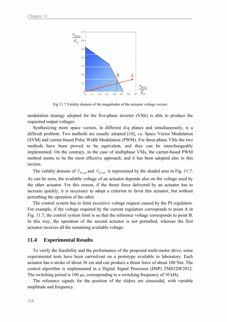
Chapter 11
218
modulation strategy adopted for the five-phase inverter (VSIs) is able to produce the requested output voltages.
Synthesizing more space vectors, in different d-q planes and simultaneously, is a difficult problem. Two methods are usually adopted [16], i.e. Space Vector Modulation (SVM) and carrier-based Pulse Width Modulation (PWM). For three-phase VSIs the two methods have been proved to be equivalent, and they can be interchangeably implemented. On the contrary, in the case of multiphase VSIs, the carrier-based PWM method seems to be the most effective approach, and it has been adopted also in this section.
The validity domain of refSv ,1 and refSv ,1 is represented by the shaded area in Fig. 11.7.
As can be seen, the available voltage of an actuator depends also on the voltage used by the other actuator. For this reason, if the thrust force delivered by an actuator has to increase quickly, it is necessary to adopt a criterion to favor this actuator, but without perturbing the operation of the other.
The control system has to limit excessive voltage request caused by the PI regulators. For example, if the voltage required by the current regulators corresponds to point A in Fig. 11.7, the control system limit is so that the reference voltage corresponds to point B. In this way, the operation of the second actuator is not perturbed, whereas the first actuator receives all the remaining available voltage.
11.4 Experimental Results
To verify the feasibility and the performance of the proposed multi-motor drive, some experimental tests have been carried-out on a prototype available in laboratory. Each actuator has a stroke of about 36 cm and can produce a thrust force of about 100 Nm. The control algorithm is implemented in a Digital Signal Processor (DSP) TMS320F2812. The switching period is 100 μs, corresponding to a switching frequency of 10 kHz.
The reference signals for the position of the sliders are sinusoidal, with variable amplitude and frequency.
Fig 11.7 Validity domain of the magnitudes of the actuator voltage vectors
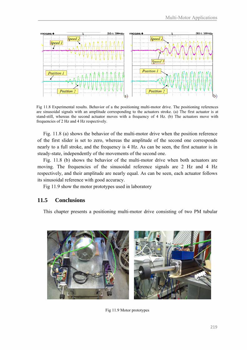
Multi-Motor Applications
219
Fig. 11.8 (a) shows the behavior of the multi-motor drive when the position reference of the first slider is set to zero, whereas the amplitude of the second one corresponds nearly to a full stroke, and the frequency is 4 Hz. As can be seen, the first actuator is in steady-state, independently of the movements of the second one.
Fig. 11.8 (b) shows the behavior of the multi-motor drive when both actuators are moving. The frequencies of the sinusoidal reference signals are 2 Hz and 4 Hz respectively, and their amplitude are nearly equal. As can be seen, each actuator follows its sinusoidal reference with good accuracy.
Fig 11.9 show the motor prototypes used in laboratory
11.5 Conclusions
This chapter presents a positioning multi-motor drive consisting of two PM tubular
Fig 11.8 Experimental results. Behavior of a the positioning multi-motor drive. The positioning references are sinusoidal signals with an amplitude corresponding to the actuators stroke. (a) The first actuator is at stand-still, whereas the second actuator moves with a frequency of 4 Hz. (b) The actuators move with frequencies of 2 Hz and 4 Hz respectively.
Fig 11.9 Motor prototypes

Chapter 11
220
five-phase actuators fed by a single five-phase inverters. This kind of solution leads to a more compact design and to a reduction in size and weight, and is seen with interest by automation industry, for example, for aerospace applications.
Up to now, very little research has been done on positioning multi-motor drives. This paper analyzes the control scheme of the drive and discusses the main problems that could reduce the performance, such as the parasitic coupling between the actuators, the limited available voltage, and the existence of cogging force.
These problems are analyzed in depth and the drive performance is evaluated by experimental results.
11.6 References
[1] E. Levi, R. Bojoi, F. Profumo, H.A. Toliyat, S. Williamson, “Multiphase induction motor drives – a technology status review,” IET Electr. Power Appl., vol. 1, no.4, pp. 489-516, July 2007.
[2] E. Levi, “Multiphase Electric Machines for Variable-Speed Applications,” IEEE Trans. on Industrial Electronics, Vol. 55, No.5, May 2008, pp. 1893-1909.
[3] E. Levi, M. Jones, S. N. Vukosavic, H. A. Toliyat, "Operating principles of a novel multiphase multimotor vector-controlled drive, IEEE Trans. on Energy Conversion, Vol. 19, No. 3, Sept. 2004, pp. 508-517.
[4] E. Levi, M. Jones, S. N. Vukosavic, H. A. Toliyat, "A Novel concept of a multiphase, multimotor vector controlled drive system supplied from a single voltage source inverter", IEEE Trans. on Power Electronics, Vol. 19, No. 2, March 2004, pp. 320-335.
[5] Y. Kuono, H. Kawai, S. Yokomizo, and K. Matsuse, “A speed sensorless vector control method of parallel connected dual induction motor fed by a single inverter,” in Proc. IEEE Ind. Applicat. Soc. Annu. Meeting IAS’01, Chicago, IL, 2001.
[6] Y. Matsumoto, S. Ozaki, and A. Kawamura, “A novel vector control of single-inverter multiple-induction motors drives for Shinkansen traction system,” in Proc. IEEE Appl. Power Elec. Conf. APEC’01, Anaheim, CA, 2001, pp. 608–614.
[7] R. P. Eguiluz, M. Pietrzak-David, and B. de Fornel, “Observation strategy in a mean control structure for parallel connected dual induction motors in a railway traction drive system,” in Proc. Eur. Conf. Power Elect. Appl. EPE, Graz, Austria, 2001.
[8] E. E. Ward and H. Härer, “Preliminary investigation of an invertor-fed5-phase induction motor,” Proc. Inst. Elect. Eng., vol. 116, no. 6, pp. 980–984, 1969.
[9] M. A. Abbas, R. Christen, and T. M. Jahns, “Six-phase voltage source inverter driven induction motor,” IEEE Trans. Ind. Applicat., vol. IA-20, pp. 1251–1259, Sept./Oct. 1984.
[10] K. Gopakamur, S. Sathiakumar, S. K. Biswas, and J. Vithayathil, “Modified current source inverter fed induction motor drive with reduced torque pulsations,” Proc. Inst. Elect. Eng. B, vol. 131, no. 4, pp. 159–164, 1984.
[11] A. N. Golubev and S. V. Ignatenko, “Influence of number of statorwinding phases on the noise
characteristics of an asynchronous motor,” Russian Elect. Eng., vol. 71, no. 6, pp. 41–46, 2000.

Multi-Motor Applications
221
[12] G. K. Singh, “multiphase induction machine drive research—a survey,” Elect. Power Syst. Res., vol. 61, pp. 139–147, 2002.
[
[13] M. Jones and E. Levi, “A literature survey of state-of-the-art in multiphase ac drives,” in Proc. 36th Univ. Power Eng. Conf. UPEC, Stafford, U.K., 2002, pp. 505–510.
[14] E. Masada, “Linear drives for industrial application in Japan – history, existing state and future
rospective,” Proceedings of LIDIA’95, Japan, pp. 9-12.
[15] I. Boldea, “Linear electromagnetic actuators and their control: a review,” EPE-PEMC 2002, Dubrovnik & Cavtat, Croatia, 9-11 Sept. 2002, P.1-P.13.
[16] J.F. Eastham, F. Profumo, A. Tenconi, G. Gianolio, “ Linear drive in industrial application: state of the art and open problems,” ICEM 2002, Bruge, Belgium, 25-28 August 2002.
[17] J.F. Eastham, R. Akmese, H. C. Lai, “Optimum design of brushless tubular linear machines”, IEEE Trans. On Magnetics, Vol. 26, No. 5, September 1990, pp. 2547-2549.
[18] J. Wang, G.W. Jewell, d. Howe, “Design optimisation and comparison of tubular permanent machine topologies,” IEE Proc. Electr. Power Appl. , Vol. 148, No. 5, Sept. 2001, pp. 456- 464.
[19] L. Parsa, “On advantages of multi-phase machines,” in Proc. of IEEE IECON, 2005, pp. 1574-1579.


List of papers by Michele Mengoni
[1] D. Casadei, M. Mengoni, G. Serra, A. Tani, L. Zarri, "Assessment of an Induction Motor Drive for High Speed Operation based on Matrix Converter," Proc. of EPE 2007, 2-5 Sept. 2007, Aalborg, Denmark, ISBN 9789075815108, IEEE Cat. No. 07EX1656C, Paper 598 on CD, pp1-10.
[2] D. Casadei, M. Mengoni, G. Serra, A. Tani, L .Zarri, "A robust control scheme for induction motor drives for applications in the field-weakening speed range", Proceedings of PCIM 2007, 22-24 May 2007, Nuremberg, Germany, CD-ROM, file "S3d-4", pp. 1 - 6.
[3] M. Mengoni, L. Zarri, A. Tani, C. Rossi, G. Serra, D. Casadei, "Stator Flux Vector Control of Induction Motor Drives in the Field-Weakening Region", Proc. of APEC 2007, Feb. 25- March 1, 2007, Anaheim, California, IEEE Cat. 07CH37843C, ISBN 1-4244-0714-1, Lib. of Cong. 90-643607, ISSN:1048-2334, pp.207-213
[4] M. Mengoni, L. Zarri, A. Tani, G. Serra, D. Casadei, "Stator Flux Vector Control of Induction Motor Drive in the Field Weakening Region ", IEEE Trans. on Power Electronics, VOL. 23, NO. 2, MARCH 2008, pp. 941-949.
[5] D. Casadei, M. Mengoni, G. Serra, A. Tani and L. Zarri, "Seven-Phase Induction Motor Drive Based on Stator Flux Vector Control," Proc. of SPEEDAM 2008, 11-13 June 2008, Ischia, Italy, pp.113-119, IEEE Catalog Number CFP0848A-CDR, ISBN 978-1-4244-1664-6, Library of Conference 2007936381, Conference CD-ROM (paper 283).
[6] D. Casadei, M. Mengoni, G. Serra, A. Tani, L. Zarri, "Field-Weakening Control Schemes for High-Speed Drives Based on Induction Motors: a Comparison", PESC 2008, 39th IEEE Annual Power Electronics Specialists Conference, Rhodes, Greece, 15-19 June 2008, Conference CD-ROM, IEEE Catalog Number: CFP08POE-CDR, ISBN: 978-1-4244-1668-4, Library of Congress: 80-646675, ISSN: 0275-9306, pp. 21591- 2166.
[7] Alberto Lega, Michele Mengoni, Giovanni Serra, Angelo Tani, Luca Zarri “General Theory of Space Vector Modulation for Five-Phase Inverters” Proc. of ISIE 2008, 30 June- 2 July 2008, Cambridge, England, pp.237-244, IEEE Catalog Number CFP08ISI-CDR, ISBN 978-1-4244-1666-0, Library of Conference 2007936380.
[8] Domenico Casadei, Michele Mengoni, Giovanni Serra, Angelo Tani, Luca Zarri, "Optimal Fault-Tolerant Control Strategy for Multi-Phase Motor Drives Under an Open Circuit Phase Fault
ppendix
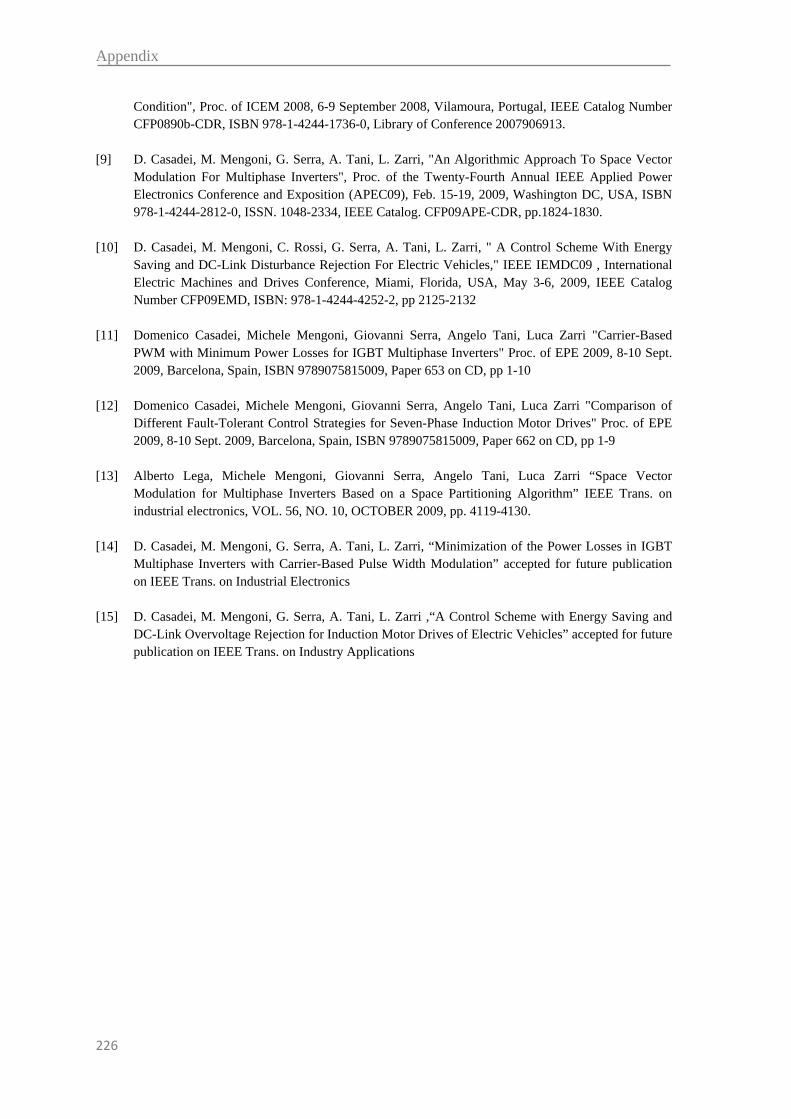
Appendix
226
Condition", Proc. of ICEM 2008, 6-9 September 2008, Vilamoura, Portugal, IEEE Catalog Number CFP0890b-CDR, ISBN 978-1-4244-1736-0, Library of Conference 2007906913.
[9] D. Casadei, M. Mengoni, G. Serra, A. Tani, L. Zarri, "An Algorithmic Approach To Space Vector Modulation For Multiphase Inverters", Proc. of the Twenty-Fourth Annual IEEE Applied Power Electronics Conference and Exposition (APEC09), Feb. 15-19, 2009, Washington DC, USA, ISBN 978-1-4244-2812-0, ISSN. 1048-2334, IEEE Catalog. CFP09APE-CDR, pp.1824-1830.
[10] D. Casadei, M. Mengoni, C. Rossi, G. Serra, A. Tani, L. Zarri, " A Control Scheme With Energy Saving and DC-Link Disturbance Rejection For Electric Vehicles," IEEE IEMDC09 , International Electric Machines and Drives Conference, Miami, Florida, USA, May 3-6, 2009, IEEE Catalog Number CFP09EMD, ISBN: 978-1-4244-4252-2, pp 2125-2132
[11] Domenico Casadei, Michele Mengoni, Giovanni Serra, Angelo Tani, Luca Zarri "Carrier-Based PWM with Minimum Power Losses for IGBT Multiphase Inverters" Proc. of EPE 2009, 8-10 Sept. 2009, Barcelona, Spain, ISBN 9789075815009, Paper 653 on CD, pp 1-10
[12] Domenico Casadei, Michele Mengoni, Giovanni Serra, Angelo Tani, Luca Zarri "Comparison of Different Fault-Tolerant Control Strategies for Seven-Phase Induction Motor Drives" Proc. of EPE 2009, 8-10 Sept. 2009, Barcelona, Spain, ISBN 9789075815009, Paper 662 on CD, pp 1-9
[13] Alberto Lega, Michele Mengoni, Giovanni Serra, Angelo Tani, Luca Zarri “Space Vector Modulation for Multiphase Inverters Based on a Space Partitioning Algorithm” IEEE Trans. on industrial electronics, VOL. 56, NO. 10, OCTOBER 2009, pp. 4119-4130.
[14] D. Casadei, M. Mengoni, G. Serra, A. Tani, L. Zarri, “Minimization of the Power Losses in IGBT Multiphase Inverters with Carrier-Based Pulse Width Modulation” accepted for future publication on IEEE Trans. on Industrial Electronics
[15] D. Casadei, M. Mengoni, G. Serra, A. Tani, L. Zarri ,“A Control Scheme with Energy Saving and DC-Link Overvoltage Rejection for Induction Motor Drives of Electric Vehicles” accepted for future publication on IEEE Trans. on Industry Applications

