university of alberta · 3d visualization developed using maxscript in 3d studio max for automation...
TRANSCRIPT

University of Alberta
Automated Post-Simulation Visualization of Modular Building Production Assembly Line
by
Sang Hyeok Han
A thesis submitted to the Faculty of Graduate Studies and Research in partial fulfillment of the requirements for the degree of
Master of Science in
Construction Engineering and Management
Department of Civil and Environmental Engineering
©Sang Hyeok Han Fall 2010
Edmonton, Alberta
Permission is hereby granted to the University of Alberta Libraries to reproduce single copies of this thesis and to lend or sell such copies for private, scholarly or scientific research purposes only. Where the thesis is
converted to, or otherwise made available in digital form, the University of Alberta will advise potential users of the thesis of these terms.
The author reserves all other publication and other rights in association with the copyright in the thesis and,
except as herein before provided, neither the thesis nor any substantial portion thereof may be printed or otherwise reproduced in any material form whatsoever without the author's prior written permission.

Examining Committee
Yasser Mohamed, Civil and Environmental
Mohamed Al-Hussein, Civil and Environmental
Evan Davies, Civil and Environmental
Ioanis Nikolaids, Computing Science
Saad Al-Jibouri, University of Twente, Netherlands
ABSTRACT
Simulation is often used to model production processes with the aim of
understanding and improving them. In many cases, however, information produced by
simulation is not detailed enough and can be misinterpreted. The use of visualization
in combination with simulation can provide project participants with a detailed-level
model to prevent misinterpretation of information and to understand the production
process. The purpose of this research is to automate the visualization process as a
post-simulation tool through sharing interactive information between simulation and
visualization. The proposed methodology has been applied to the production line of
modular buildings with the output of lean, simulation, and visualization in the form of
animation. Based on the new scheduling developed by applying lean principles, a
simulation model was built and its output was extracted to an ASCII file used to build
3D visualization developed using Maxscript in 3D Studio Max for automation of
visualization process.

Acknowledgements
I am deeply indebted to all individuals who have assisted and supported me in
this endeavor. The guidance and encouragement I received from them are deeply
appreciated.
Sincere thanks to my supervisor Dr. Mohamed Al-Hussein for being a constant
source of inspiration throughout this program. Thank you for believing I could
succeed and for giving me the opportunities to do so.
I would like to thank to my parents to continuously pursue graduate studies in
Canada and for supporting me through all the steps of the process, even though they
have difficult economy. I would like to say that I love and respect them in the world.
Special thanks are due to my wife, You Sun Kang, for encouraging me to finish
graduate studies in Canada. I strongly believe that I could not finish my studies
without her. I hope that she peacefully sleeps in heaven. I devote this thesis to her. I
would like to say to her that I love you forever.

TABLE OF CONTENTS
CHAPTER 1- INTRODUCTION ................................................................... 1
1.1 Overview ............................................................................................................... 1
1.2 Research Motivation .......................................................................................... 5
1.3 Research Objectives ........................................................................................... 6
1.4 Research Methodology ..................................................................................... 7
1.5 Thesis Organization ........................................................................................... 8
CHAPTER 2-LITERATURE REVIEW ..................................................... 9
2.1 Introduction........................................................................................................... 9
2.2 State of the Art Literature Review in Lean Production .......................... 9
2.3 State of the Art Literature Review in Construction Simulation ......... 13
2.3.1 Computer Simulation Methods ....................................................................... 13
2.3.2 Application of General Purpose Simulation Tools ......................................... 14
2.3.3 Application of Special Purpose Simulation Tools .......................................... 15
2.4 State of the Art Literature Review in 3D Visualization ........................ 16
2.5 Application of 3D Visualization with Simulation .................................. 18
CHAPTER 3-PROPOSED METHODOLOGY ................................... 21
3.1 Introduction......................................................................................................... 21
3.2 General Manufactured Production Process .............................................. 21
3.3 Problem Description ........................................................................................ 22
3.4 Proposed System Architecture ...................................................................... 25
3.5 Proposed Methodology ................................................................................... 26
3.6 Lean Production ................................................................................................ 30
3.6.1 Data Collection ................................................................................................. 30
3.6.2 Current Map ...................................................................................................... 32
3.6.3 Analysis of Current Map .................................................................................. 34
3.6.4 Future Map ....................................................................................................... 36
3.7 Simulation Approach ....................................................................................... 38
3.7.1 Simulation Template for Manufacturing Production Line ............................. 38
3.7.2 Development of Simulation Models ............................................................... 42
3.8 3D Visualization Approach ............................................................................ 46
3.9 Summary .............................................................................................................. 50

CHAPTER 4-PROPOSED METHODOLOGY IMPLEMENTA-
TATION ........................................................................................................................ 52
4.1 Introduction......................................................................................................... 52
4.2 Background of Case Study ............................................................................ 52
4.2.1 Station 1 ............................................................................................................ 53
4.2.2 Station 2 ............................................................................................................ 54
4.2.3 Station 3 ............................................................................................................ 55
4.2.4 Station 4 ............................................................................................................ 55
4.2.5 Station 5 ............................................................................................................ 56
4.2.6 Station 6 ............................................................................................................ 57
4.2.7 Station 7 ............................................................................................................ 58
4.2.8 Station 8 ............................................................................................................ 59
4.3 Implementation of Lean Production ........................................................... 59
4.3.1 Current VSM .................................................................................................... 62
4.3.2 Proposition of Improvement ............................................................................ 63
4.4 Simulation Model Experiment ..................................................................... 71
4.4.1 Simulation Model for the Original Production Line ...................................... 71
4.4.2 Simulation Model for the Proposed Production Line .................................... 79
4.4.3 Validation and Discussion................................................................................ 88
4.5 Developing the Virtual Reality Model ....................................................... 92
4.5.1 Station 1 ............................................................................................................ 95
4.5.2 Station 2 ............................................................................................................ 96
4.5.3 Station 3 ............................................................................................................ 98
4.5.4 Station 4 ............................................................................................................ 99
4.5.5 Station 5, Station 6, and Station 7 ................................................................. 100
4.6 Conclusion ........................................................................................................ 102
CHAPTER 5- CONCLUSION ..................................................................... 104
5.1 General Conclusion ........................................................................................ 104
5.2 Research Contribution ................................................................................... 106
5.3 Proposed Future Research............................................................................ 107
REFERENCES ...................................................................................................... 109
APPENDIX .............................................................................................................. 117

LIST OF TABLES
Table 3.1: Key Information in Each Station ................................................................... 32
Table 3.2: Common Template and Enhaced Element in Simphony .............................. 38
Table 3.3: Input Data Distribution for the Proposed Schedule ...................................... 43
Table 4.1: Production Line Data ...................................................................................... 60
Table 4.2: Input Data for the Original Schedule ............................................................. 72
Table 4.3: Input Data for the Proposed Schedule ........................................................... 80
Table 4.4: Compare with Outputs of the Original and Proposed Simulation Models .. 89

LIST OF FIGURES
Figure 1.1: Average Percentage of Gross Revenue Generated from Markets ................ 2
Figure 1.2: Revenue Growth in Commercial Modular Industry ..................................... 3
Figure 1.3: Compare Modular Timeline to Site-Buit Timeline(CMC report 2009) ....... 5
Figure 3.1: System Architecture ...................................................................................... 26
Figure 3.2: The Proposed Main Research Process ......................................................... 28
Figure 3.3: Maxscript Format .......................................................................................... 30
Figure 3.4: Current Map ................................................................................................... 34
Figure 3.5: The Proposed Schedule with Original Schedule ......................................... 37
Figure 3.6: A Simulation Model for A Production Line in Simphony .......................... 44
Figure 3.7: Detailed Process Model in Station 2 ............................................................ 45
Figure 3.8: Relationship between Simulation and Animation Time (Revised Mohammed
Al-Hussein et al 2005) ............................................................................................................ 47
Figure 3.9: A Framework for Animation of Interior Gypsum Board Task ................... 50
Figure 3.10: Animation Snapshots of Interior Gypsum Board related to 3D Scheduling
and Sequence .................................................................................................................... 50
Figure 4.1: Station 1 ......................................................................................................... 53
Figure 4.2: Station 2 ......................................................................................................... 54
Figure 4.3: Station 3 ......................................................................................................... 55
Figure 4.4: Station 4 ......................................................................................................... 56
Figure 4.5: Station 5 ......................................................................................................... 57
Figure 4.6: Station 6 ......................................................................................................... 58
Figure 4.7: Station 7 ......................................................................................................... 59
Figure 4.8: Current Map ................................................................................................... 63
Figure 4.9: Proposed Schedule with Original Schedule in Stations .............................. 70

Figure 4.10: Simulation Model for the Original Schedule ............................................ 74
Figure 4.11: Detailed Process Model of Each Station in the Original Schedule .......... 78
Figure 4.12: Cycle Time Distributin of the Simulation Model of the Original Schedule
........................................................................................................................................... 79
Figure 4.13: Simulation Model for the Proposed Schedule ........................................... 83
Figure 4.14: Detailed Process Model for the Proposed Schedule ................................. 87
Figure 4.15: Cycle Time Distribution of the Simulation Model of the Proposed
Schedule ............................................................................................................................ 88
Figure 4.16: Sensitivity Analysis of the Erection of the Prefabricated Panels ............. 90
Figure 4.17: Sensitivity Analysis of Exterior J-Channel................................................ 90
Figure 4.18: Sensitivity Analysis of Drywall Exterior ................................................... 91
Figure 4.19: Sensitivity Analysis of Paint Door Frame ................................................. 91
Figure 4.20: Sensitivity Analysis of Grounding Holes .................................................. 91
Figure 4.21: Sensitivity Analysis of Hang Doors ........................................................... 92
Figure 4.22: Sensitivity Analysis of Final Check and Ship Loose ................................ 92
Figure 4.23: S.A.C. ........................................................................................................... 94
Figure 4.24: Animation Snapshots of Station 1 with 3D Scheduling ............................ 96
Figure 4.25: Animation Snapshots of Station 2 with 3D Scheduling ............................ 97
Figure 4.26: Animation Snapshots of Station 3 with 3D Scheduling ............................ 98
Figure 4.27: Animation Snapshots of Station 4 with 3D Scheduling ............................ 99
Figure 4.28: Animation Snapshots of Station 5 with 3D Scheduling .......................... 100
Figure 4.29: Animation Snapshots of Station 6 with 3D Scheduling .......................... 101
Figure 4.30: Animation Snapshots of Station 7 with 3D Scheduling .......................... 101
Figure 5.1: Flow of the Proposed Methodology ........................................................... 106

1
Chapter 1
INTRODUCTION
1.1 Overview
Modular buildings are pre-fabricated buildings that started gaining popularity
early in the 20th
century. The end of World War II caused the modular market to truly
expand and evolve because the marketplace, which used traditional building processes,
could not handle customer demands from veterans that came back to America and
needed new homes. This led the industry to look for new solutions to increase
efficiency and lower the cost of new home construction. The modular building
process answered both of these needs. In the 1980s, cranes that had the capacity to lift
100 tons or more were a reason that the modular building industry grew sharply, since
large modules could be constructed and shipped cross-country.
The Modular Building Institute (MBI), founded in 1983, defines modular as a
construction method or process where individual modules, stand-alone or assembled
together, make up larger structures. The modular building industry comprises several
different markets including offices, education, government buildings, healthcare, retail
and commercial, and military. Figure 1.1 shows the average percentage of gross
revenue generated from markets in the modular building industry from MBI. The
Commercial Modular Construction (CMC) report, conducted by MBI, states that the
non-residential construction market strongly influences the commercial modular
market; there is evidence that the increase of non-residential project numbers will
generally have a positive impact on the commercial modular industry (CMC report
2009). According to the United States Department of Education, public school

2
enrollment in prekindergarten rose from 29.9 million in Fall 1990 to 34.2 million in
Fall 2003, and elementary enrollment is projected to continue to increase through
2016 (CMC report 2009). The U.S. Army Corps of Engineers (USACE) has been
tasked to find ways to streamline construction processes in order to reduce costs and
speed up overall delivery of projects, while at the same time provide quality facilities
(CMC report 2009). The Army also requires a minimum 15% reduction in cost and a
minimum 20% reduction in time to occupancy (CMC report 2009). In response to
these new requirements, USACE has focused on the modular building industry.
Figure 1.1: Average Percentage of Gross Revenue Generated from Markets
In addition, the CMC report describes the revenue growth of the modular
building industry and the average percentage of gross revenue generated from the
commercial modular industry. Manufacturers reported their revenue growth from the
2nd quarter of 2006 to the 1st quarter of 2009, illustrated in Figure 1.2. Revenue
growth was in the positive percentages between the 2nd quarter of 2006 and the 4th
quarter of 2007, except for the 1st quarter of 2007. But it decreased by 11% in the 1st
quarter of 2007 and by 23% in the 1st quarter of 2009 compared to the previous year.

3
The decrease of revenue growth and the number of floors produced are influenced by
the world’s weak economy. As the market predictors mentioned above state, however,
the modular building industry still remains a big market with increased benefits, even
though revenue growth and the number of floors have dropped from 2008.
Figure 1.2: Revenue Growth in Commercial Modular Industry
Production managers in the manufacturing industry have tried to apply concepts
from various disciplines including lean, simulation, and visualization, to the
production line to increase productivity and reduce cost. Lean production theory, as a
production management tool, can describe a system that delivers a finished product
with no defects to a customer in zero time and leaves nothing in inventory. This
management tool is widely used for improving productivity and cost reduction in the
manufacturing industry that produces multiple copies of the same product. In lean
production, waste that causes excess activity and increased cost must be eliminated or
reduced from the process. Implementing lean production theory follows three main
points: 1) eliminate or reduce all activities that do not add value to the final product,
2) pull material through the process, and 3) reduce variability by controlling
4
uncertainties within the process. After developing a proposed system based on lean
production, a project manager usually applies it to the real world, analyzes the
productivity, and then continuously redesigns the system if the productivity is not
increased. This is time-consuming and increases cost. For these reasons, computer
simulation is used as a validation tool for the proposed system before implementation
in the real world.
Computer simulation is defined by Pritsker (1986) as the process of designing a
mathematical-logical model of a real world system and experimenting with the model
on a computer. Simulation is a useful tool to evaluate project scenarios, establish
feasible work plans, and convert practical systems to models. There are many existing
simulation tools that have been developed and used in construction. Simphony (Hajjar
and AbouRizk, 1999) is an example of such tools and will be used in this research.
The tool was developed under the Natural Science and Engineering Research Council
(NSERC)/Alberta Construction Industry Research Chair Program in Construction
Engineering and Management, and can be used as both a general purpose and special
purpose simulation (SPS) tool. It was developed with the objective of providing a
standard, consistent, and intelligent environment for both the development and
utilization of construction SPS tools (Hajjar and AbouRizk, 1999). Hajjar and
AbouRizk (1999) stated that Simphony greatly simplified the SPS tool development
process, which can reuse code and common design models and standardized
simulation, modeling, and analysis.
Additionally, many researchers and planners have recently focused on using 3D
visualization together with simulation tools in the fields of construction management,
productivity and cost analysis, resource management, and assessment of site layout. It
has been found that 3D visualization provides more realistic and clear feedback with
5
simulation studies and dynamic graphical depictions such as the state of each task at a
specific time, the work space required for construction activities, and clear
communication about projects with participants. It can also help users fully
understand the construction processes of a project.
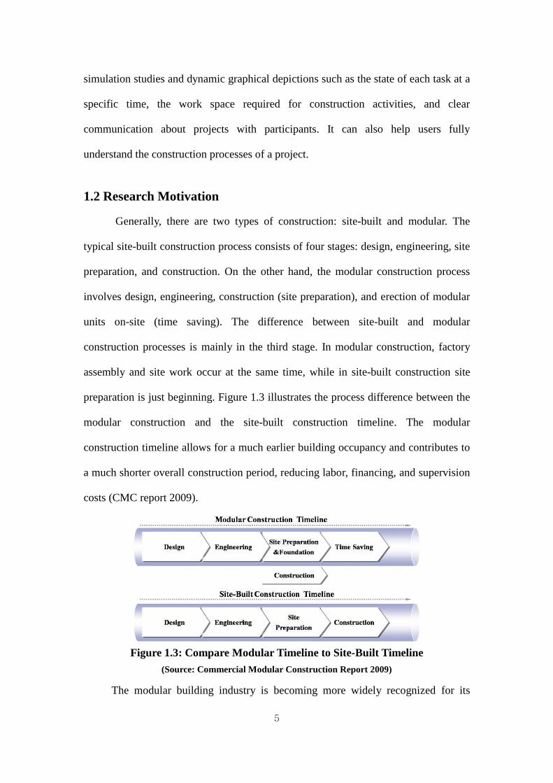
1.2 Research Motivation
Generally, there are two types of construction: site-built and modular. The
typical site-built construction process consists of four stages: design, engineering, site
preparation, and construction. On the other hand, the modular construction process
involves design, engineering, construction (site preparation), and erection of modular
units on-site (time saving). The difference between site-built and modular
construction processes is mainly in the third stage. In modular construction, factory
assembly and site work occur at the same time, while in site-built construction site
preparation is just beginning. Figure 1.3 illustrates the process difference between the
modular construction and the site-built construction timeline. The modular
construction timeline allows for a much earlier building occupancy and contributes to
a much shorter overall construction period, reducing labor, financing, and supervision
costs (CMC report 2009).
Figure 1.3: Compare Modular Timeline to Site-Built Timeline
(Source: Commercial Modular Construction Report 2009)
The modular building industry is becoming more widely recognized for its
6
environmentally-friendly construction process, speed of construction, and waste
reduction at cost competitive prices (CMC report 2008). Improvement of productivity
and potential cost reduction can be gained by redesigning the production process,
facility layout, and material handling in the modular construction method. Previous
research has shown that various disciplines including lean, simulation, or integrated
systems can be used to set stable and effective production flow (Haitao Yu et al, 2009,
Roberto J. Arbulu and Iris D. Tomelein, 2002). Simulation alone, integrated lean and
simulation (Ping Wang et al, 2009), or integrated simulation and visualization (Ayman
Abu Hammad et al, 2004, Ayman Abu Hammad, 2003, and Abhi Sabharwal, 2004)
can also be used in the process. However, these various efforts for improvement of
productivity and reduction of cost have not yet seen full scale success. For example,
lean has a limited validation tool before implementation of the proposed method.
Simulation is an abstraction from reality, and results are difficult to understand
because they provide only a numerical and logical computation. Visualization
provides a more detailed process model than simulation. Therefore, the development
of an effective and convenient tool through integration of the disciplines cannot be
ignored.
This research describes a methodology to share information between simulation
and visualization. The proposed methodology has been incorporated into a computer
system A case example is used in this research to demonstrate the effectiveness of the
proposed methodology.
1.3 Research Objectives
This research proposes to share project information between lean, simulation,
and visualization. The methodology used minimizes activities performed during the

7
visualization processes through a user interface. The 3D model uses the output
parameters from the simulation model to perform visualization and 3D animation. The
system reduces animation process time and adds flexibility to import simulated results
to visualization tools. This research builds on the research done by Haitao Yu (2008)
that improved the efficiency of the production line for modular building by applying
lean principles. The results of this research were as follows:
To build Value Stream Mapping (VSM) for the current state of the
modular building process.
To develop takt time1 based on analysis of current practice with VSM
model.
To develop framework for input parameters based on takt time to be
used in the simulation model.
Based on the previous research, the research objectives of this project are:
To automate the visualization processes based on a simulation model,
input parameters for visualization, and 3D animation.
To develop a strategy for the standard output of the simulation model
to be used for building visualization and animation.
1.4 Research Methodology
To achieve the research objectives described, two steps were followed: 1)
standardizing the input parameters so they are automatically generated from the
simulation model and imported to 3D visualization software, and 2) automating the
animation frame keys for 3D objects so they react to change in the input parameters
from simulation results. Microsoft Access and Excel were used to build a database to
1 The maximum time per unit allowed to produce a product to meet customer demand (Wikipedia).

8
share information between simulation and visualization. To accomplish this, a user
interface using Maxscript within 3D Studio Max was developed. The implementation
of the proposed methodology consisted of three main steps. First, VSM as a lean
implementation tool defined in Chapter 2 was used to improve better production
processes and employee scheduling. Second, a simulation model was built to validate
the result from the VSM. Finally, a visualization using Autodesk 3D Studio Max and
3D AutoCAD was performed based on the input parameters from the simulation.
1.5 Thesis Organization
This thesis is organized into five chapters. Chapter 2 (Literature review) is an
extensive study of the available research and evaluates the various approaches for the
manufacturing industry. The previous works on lean, simulation, and visualization are
explored. Chapter 3 (Proposed methodology) presents a problem description
regarding lean, simulation, and visualization, the proposed methodology used in this
research, and the characteristics of lean, simulation, and visualization. Chapter 4
(Proposed methodology implementation and case study) describes the step-wise detail
of the implementation process using a case study. The objective of this chapter is to
verify the proposed methodology process using an example. Chapter 5 (Conclusion)
summarizes a conclusion of this research. It also describes research contributions and
a list of proposed future research to enhance the integrated system proposed in this
thesis.
9
Chapter 2
LITERATURE REVIEW
2.1 Introduction
The purpose of this literature review is to identify the current state of
knowledge about the main tools used in this thesis. There are four topics to discuss in
this chapter. First, lean production theory, literature, and tools, especially VSM (Value
Stream Mapping), are discussed. Second, the current state of simulation knowledge is
reviewed. Third, previous works on visualizing construction processes by various
tools and techniques are identified. Finally, research in simulating and visualizing the
manufactured production process, supply chain, material flow, and facility layout are
investigated.
2.2 State of the Art Literature Review in Lean Production
Lean thinking has gained recognition as a new manufacturing paradigm. It is
based on principles of the Toyota Production System (TPS), developed by by Ohno, a
manager, and Shingo, an industrial engineer, for the Toyota Automotive Company on
the basis of the mass production system. Womack and Jones (1996) presented value
specification, value stream (waste elimination), flow, pull, and continuous pursuit of
perfection as the lean principles in order to emphasize the same principles across to
the whole company. Lauri Koskela (2000) proposed the following principles of lean
production theory:
1) Reduce the share of non-value adding activities (waste)

10
2) Reduce variability
3) Reduce the cycle time
4) Increase output flexibility
5) Increase process transparency
6) Simplify by minimizing the number of steps, parts, or linkages
7) Build continuous improvement into the process
8) Balance flow improvement with conversion improvement
9) Focus control on the complete process
10) Increase output value through systematic consideration of customer
requirement
11) Benchmark
A main concept of lean production theory is to eliminate or reduce waste. Waste
refers to all efforts that do not add value to the final product from the point of view of
the client. Womack et al. (1990) identified seven sources of waste: defects in products,
overproduction of goods, excess inventories, unnecessary processing, unnecessary
movement of people, unnecessary transport of goods, and waiting time. A tool for
waste elimination is VSM (Value Stream Mapping), described by Rother and Shook
(2000). Rother and Shook (2000) define VSM as describing all activity, both value-
added and non-value added, currently required to bring a product through the two
main flows essential to every product, the production flow from raw material to
customer and the design flow from concept to launch. VSM was created by
practitioners at Toyota and has commonly been used in lean planning. It graphically
presents every step that involves the flow of material through production and the flow
of information from the customer back to each production process. The most

11
important purpose of using VSM is to reveal time waste by displaying the cycle time
for each operation and the total lead time for a process.
Ikovenko (2004) defines lean production as “an approach to manufacturing the
right product in the right quantity through instant material supply while minimizing
wastes and maintaining flexibility to adapt to varying production requirements.”
There are three phases required to implement a lean production process: the first
phase is to have a strategic change in a production line; the second phase is to
introduce lean production principles and to transform the way of “thinking” and
“seeing” the company; and the third phase is to prepare the production line for
physical change (Fernanda Pasqualini and Paulo A. Zawislak, 2005). Lean production
aims to produce more quality and variety, quickly and with less costs. To achieve this,
eliminating waste based on the concepts of lean production is most important to
developing a new production process because waste raises costs, hides process
problems, and does not generate value. Therefore, value-added activity and non-value
added activity must be identified on the value flow of a production line before
implementing waste elimination. After value-added activity and non-value added
activity have been specified and a certain product’s value flow has been identifed, the
activites that produce waste are reduced and/or eliminated.
Roberto J. Arbulu and Iris D. Tomelein (2002) demonstrated that VSM is a
valuable tool when trying to improve supply chain performance. They illustrated how
processes flow throughout the design, procurement, and fabrication steps of pipe
supports used in power plants. To achieve their purposes, waste elimination was
considered in order to reduce the total delivery lead time of pipe supports and thereby
improve supply chain performance.
Haitao Yu et al. (2009) show data collection, value stream selection, and

12
current practice analysis to propose specific changes to the lean production model.
The objective of the research is to create a stable production flow rather than
eliminate individual waste for home construction. The authors use VSM to analyze a
current process and to formulate a lean production model for increasing process
reliability, reducing total lead time, and improving quality. To verify the model and
assist in the development of an interim implementation model, a simulation template
is used.
The lean production principles and flow production for shop fabrication are
described by Ping Wang et al. (2009). A simulation tool is used to verify and facilitate
the implementation of the system used in this research. The developed simulation-
based approach demonstrates a more powerful tool than VSM for modeling and for
quantitatively evaluating the performance of a complex and dynamic spool fabrication
shop (Ping Wang et al, 2009).
The use of VSM for make-to-order products in a job shop environment,
specifically the fabrication of Heating Ventilating and Air Conditioning (HVAC) sheet
metal ductwork, is investigated by Thais da C. L. Alves et al. (2005). VSM for the
fabrication of sheet metal ducts and the use of lean production concepts are described.
The authors recommend systematic data collection to reveal current practices and
opportunities for improvement.
Haitao Yu (2010) developed a lean production approach for the North American
homebuilding industry. His research provided a framework and a set of guidelines that
can help production homebuilders improve efficiency through lean strategies, such as
continuous flow, pull system, production levelling, and standardized work. That is,
production homebuilders can use his framework to build a roadmap for developing
their own lean production systems and lean implementation strategies.

13
2.3 State of the Art Literature Review in Construction Simulation
Construction engineers have tried to develop efficient construction methods and
processes to deal with repetitive construction projects such as highways, buildings,
tunnelling, and earth moving. Simulation is a powerful tool to evaluate project
scenarios, establish feasible work plans, and describe a practical system to model
using computer software. Thus, simulation assists project managers or researchers in
making decisions for a variety of scenarios, which can be added to or removed from
the system to achieve a desired purpose. It also validates how resources can be used in
work-task sequences and how the operation can be changed using scenarios for better
productivity measurement, risk analysis, resource planning, performance assessment,
and design and analysis of construction methods.
There are two kinds of simulation methods: continuous event and discrete
event. Simulation tools are generally divided into two categories: general purpose and
special purpose. The following sections describe these methods and tools.
2.3.1 Computer Simulation Methods
Time is the most independent variable in a simulation system. In continuous
event simulation, dependent variables, such as the trajectory of missiles and velocities
of spacecraft, continuously change over time. In discrete event simulation, the
dependent variables change at a specific time, referred to as event time. Researchers
and project managers generally use discrete event simulation for their projects when
analyzing the logic of a construction production system. One of the examples in
discrete simulation is loader-truck operations. In order to know the productivity of the
operation, researchers analyse when a loader finishes loading and when a truck can
start hauling the earth to the dump location at the event time.

14
2.3.2 Application of General Purpose Simulation Tools
General Purpose Simulation (GPS) can be used to model various construction
processes such as asphalt paving, high-rise building, and tunnelling. Users need to
learn the rules of general purpose simulation tools in order to design and build the
simulation model. Users can also modify the models for their specific needs.
Halpin (1973) developed the Cyclone (Cyclic Operation Network) modeling
simulation software. Cyclone helps simplify modeling methodology and is easy to
learn. It also facilitates visual communication because everything is contained in the
network. Cyclone became the basis for a number of construction simulation systems
because construction practitioners with a limited simulation background could use it
easily. Also in 1973, Halpin and Woodhead developed the Constructo project
management game at the University of Illinois to integrate the effects of weather and
labour productivity into the management of projects in a network format (Halpin and
Woodhead, 1973).
Insight (Interactive Simulation Using Graphics Techniques) is economic for
collecting production time data in the field using videotapes of field construction
operations (Paulson et al, 1987). Stroboscope (State and Resource Based Simulation
of Construction Processes) by Martinez and Ioannou (1994) considers uncertainty for
any aspect such as the quantities of resources produced or consumed. The most
important feature of Stroboscope is that users can access the simulation during
execution time and differentiate the properties of resources involved in an operation.
Huang et al. (1994) developed DISCO (Dynamic Interface for Simulation of
Construction Operations) in the Visual Basic environment. It extends the capabilities
of Cyclone so the user can set the stop clock and change the resource assignment rules
of the simulation. MicroCyclone is a core simulation engine to run simulations in
Disco. It provides graphical processing after the results generated by MicroCyclone

15
are sent back to DISCO.
2.3.3 Application of Special Purpose Simulation Tools
Special Purpose Simulation (SPS) tools focus on specific construction
processes. An example is a truck dispatcher simulation model for a mixer plant. Hajjar
et al. (1998) suggest SPS be tailored to specific requirements in a given industry field.
Several intuitive and user-friendly SPS tools have been developed for construction
engineers. COOPS (Construction Object-Oriented Process Simulation System),
developed by Liu (1991), is a similar simulation system to Cyclone, It includes a
control package such as queue, activity, and flag controls. One of the most successful
SPS simulation tools is Simphony, developed under the Natural Science and
Engineering Research Council (NSERC)/Alberta Construction Industry Research
Chair Program in Construction Engineering and Management at the University of
Alberta. Simphony is a Microsoft Windows Environment System. It was developed
with the objective of providing a standard, consistent, and intelligent environment for
both the development and utilization of construction SPS tools (Hajjar and AbouRizk,
1999). Hajjar and AbouRizk (1999) state that Simphony greatly simplified the SPS
tool development process, by reusing code and common design models, and
standardized simulation, modeling, and analysis. Lu (2003) developed HKCONSIM,
which is a simulation model for the Hong Kong one-plant-multsite Ready-Mixd
Concrete (RMC) production system. The system is adaptable for resource planning
and production planning of the RMC plant. The most important feature of this system
is in the interactions of multiple sites within the plant. The system advances the
supply service level and the utilization of plant resources. The user does not need to
be familiar with any simulation tools or modeling schematics. SPS is very attractive to

16
the construction industry because little or no simulation knowledge is required to use
them. SPS tools appear very frequently, so it is almost impossible to introduce them
all.
2.4 State of the Art Literature Review in 3D Visualization
In recent years, many researchers and planners have focused on using 3D
visualization for construction management, productivity and cost analysis, resource
management, and assessment of site layout. In particular, decision makers as well as
simulation developers can obtain more realistic and clear feedback from 3D
visualization than from simulation studies. 3D visualization of modeled construction
operations graphically illustrates the same logic and physical relationships contained
in the simulation models. 3D visualization can be used to experiment on a computer
screen to avoid potential costly on-site error before implementation in the real world.
The dynamic graphical depiction in 3D visualization with a 3D schedule provides
decision makers detailed information such as the state of each task at a specific time,
work space required for construction activities to be executed safely and productively,
and clear communication about the simulation model. It also clearly illustrates the
project sequence. Bonsang Koo and Martin Fischer (2000) developed a 4D model
including 3D objects, bar charts, and component lists in the graphical interface. The
results of 4D detected the incompleteness of the original schedule, found
inconsistencies in the level of detail among the schedule activities, and discovered any
impossible schedule sequences (Bonsang Koo and Martin Fischer, 2000). This 4D
model also allowed construction practitioners to identify potential time-space conflicts
and quickly understand a schedule in the design stages of a project.
Sheryl Staub-French et al. (2008) described two-way relationship between 3D
CAD software and a software implementation of linear planning that includes the
17
ability to define a project product model and associate it with the process model. The
two-way process described the consistency of product representation in CAD and
scheduling models. The benefits of the method are modifying construction sequences
and examining their consequences by 4D CAD so that the scheduling strategy can be
improved. The users are also able to validate the completeness of the product model
representations by connecting to 3D objects and activities. Beliveau et al. (1993)
developed a method for using CAD to control material handling on sites. Computer
Graphics and CAD are combined with a dynamic modeller that simulates material-
handling operations using tower cranes through computer animation. Vineet R.
Kanmat and C. Martinez (2001) attempted to build a dynamic visualization for
construction operations. This method is able to model a spatially and chronologically
accurate 3D visualization of construction operations. The general-purpose 3D
visualization system described in the paper is simulation and CAD software
independent. They also helped set up the reliability of the simulation model and
provide users more realistic and clear feedback from simulation analyses. Mohamed
Al-Hussein et al. (2005) described a practical methodology for integrating 3D
visualization with special purpose simulation to perform lifting and hoisting activities
using a tower crane. This integrating system indicated that 3D visualization is a very
useful tool to verify and validate simulation results and effectively communicate the
essence of a simulated operation, thus improving the accessibility of simulation as a
decision making aid. Juan D. Manrique et al. (2007) presented a way to integrate a
crane selection algorithm and optimization model utilizing 3D modeling and
animation for the selection, utilization, and location of cranes on a construction site of
a complex residential tilt-up panel structure. This integrating system was used to
avoid potential costly on-site errors, decrease traveling time and distance of the

18
selected crane to improve the crane lifting sequence, and reduce the use of panel
casting slabs.
2.5 Application of 3D Visualization with Simulation
This section explores previous research in simulation application in
manufacturing. Manufacturing is defined as the use of machines, tools, and labour in a
factory to make products for use or sale. That is, the purpose of manufacturing is to
reduce cost and skilled-labour shortages, and increase productivity, safety, and quality
control by automation in a factory. The manufacturing process is complex and
combines line-flow product movement with a complex precedence network and
physical constraints. Researchers focus on the production process, material
management, and supply chain and facility layout in a factory by using simulation
software and material management for their purposes. One of the focuses is
optimizing the production process in the modern manufacturing industry to increase
productivity. The production process usually consists of an arrangement of multiple
work stations. The material flows continuously or step-by-step through each station,
and the overall workflow follows a directed path or flow pattern.
Senghore (2001) explored the production process and material flow that take
place in a manufactured housing plant. The primary goal of his study was to show
how the production processes of manufactured housing could be improved and
resource utilization streamlined by what-if scenarios. He suggested a process flow
model for multi-section houses and developed a production and material flow model.
To demonstrate his concept, he selected a section of a production line with 3-4
stations and transformed the process in the EZStrobe simulation software (Martinez,
1998). Ayman Abu Hammad et al. (2004) developed a simulation model to improve
the productivity of the manufactured housing construction process by reducing the

19
cycle time and enhancing the quality of material. The production process was
simulated by ARENA, which mimics the behaviour of the real system components,
layout, and flow logic and produces data distributions and confidence intervals to
measure performance as well as display animation. His study also identified methods
of improving the productivity of the manufacturing process in a plant.
Abhi Sabharwal (2004) studied the effect of manufactured housing components
assembly redesign on the productivity of the production process. The material
handling cost of the facility layout was studied. The report showed the effects using
FactoryFlow facility layout software and ARENA simulation software. Ayman Abu
Hammad (2003) used simulation software to develop a decision support system for
manufactured housing production process planning and facility design. He found
some problems such as inefficient production process and layout limitations to the
production capacity. The objectives of his research were to solve the problems by
developing a streamlined manufactured housing process, optimizing models to
streamline activities, predicting relevant parameters, and advancing layout designs by
theories in manufacturing like lean production. He used ARENA simulation software
to experiment in his study. Mahdi Nasereddin et al. (2007) described automated
simulation models for the modular housing industry. A modular home is produced in a
factory and is transported to the construction site. The report discussed common
elements found in modular manufacturing and summarized an approach for
automating the model development process using ProModel and Visual Basic. This
approach reduces the model development time and improves modeling consistency
and quality. The supply chain greatly affects the performance of manufactured
housing. Jeong (2003) studied supply chain analysis and simulation modeling for the
manufactured housing industry to develop an efficient supply chain management

20
system. The report suggested an alternative to the current system through a simulation
that optimizes process time from order to installation. He also proposed design
alternatives from the factory to customers based on an optimized supply chain
simulation model.

21
Chapter 3
PROPOSED METHODOLOGY
3.1 Introduction
Researchers have applied a blend of various disciplines to the production
process, facility layout, material management, and supply chain in the modular
building industry to improve productivity and reduce cost. The purpose of this
research is to automate the visualization process as a post-simulation tool by sharing
interactive information between simulation and visualization. A method to reduce the
process time of the proposed methodology, especially between simulation and
visualization, is also required. In the following section, challenges of the discipline-
specific tools used in this thesis are defined.
3.2 General Manufactured Production Process
The manufactured modular buildings consist of various components and
subassemblies. It is essential to study and have a detailed understanding of the
production process, the components, and their functions to propose a new production
line. The production line can generally have up to eight stations and a varying number
of activities at each station depending on the complexity of the modular built. The
building modular production process and manufactured housing production process
have similar processes. Therefore, in this research, the building modular production
process can be identified from the manufactured housing production process.
Senghore (2001) divided a manufactured housing process into five areas: (1) floors,
(2) walls, (3) roofing, (4) exterior finishes, and (5) interior finishes.

22
Manufactured module is built on a steel base frame in floor process. The
process starts with the floor frame being constructed on top of the steel base. The
floor joists are put in place according to the plan and the specified spacing. The
process starts installing the floor, party wall, front, right, left, rear frames, and roof
using an overhead crane that runs on tracks attached to the ceiling of the plant
building at Station 1. After this work, the modular is moved to install interior gypsum
boards and the drywall exterior for wall processes. All the walls are built complete
with insulation. The roofing process consists of installing ceiling boards, lights, and
uni-strut, and insulation. After insulating the roof, a crew of workers deck the roof
with sheets of plywood nailed to the roof frame. In the exterior finish processes,
workers are simultaneously installing doors and exterior boards. Exterior and interior
finishes start after the walls are installed. The walls are covered with exterior boards
and windows openings are cut and then installed the cable pots, and louvers. Electrical
and mechanical tasks such as wireway, wires, plumbing, Air conditions, and conduits
are worked in exterior finish processes. The Electrical and mechanical testing and
inspection are performed at last Station including check for interior switches and their
installation to manufacturer’s specifications.
3.3 Problem Description
In a global economy, successful manufacturers are constantly changing the way
they do business in order to stay competitive. Production managers in the
manufacturing industry have tried to improve the productivity of the production
process by reducing the cycle time and enhancing the quality of both material and
level of technicality used. They have used several disciplines such as lean production
and simulation in order to achieve or assist their objectives. However,

23
misinterpretation of information by project participants often results in construction
errors on the manufacturing production line and rework, as well as the subsequent loss
of productivity and increase in costs. In this section, the characteristics of lean,
simulation, and visualization and their current limitations are described.
Lean production using Value Stream Mapping (VSM) is a powerful concept to
investigate and analyse the current real problems of a production process on a
manufacturing production line. It also provides an excellent tool to design a new
schedule for continuous material and production flow, workforce management, and
balance of subtasks on the production line. The implementation of VSM consists of
four steps which are lean assessment, current state map, future state design, and
implementation. When a new system obtained by applying lean production is
implemented on a real production line, the results of the plan and design phases of
lean production cannot be fully predicted because many unknowns and uncertainties
may exist in real world. Therefore, the proposed design is continuously changed until
the developer’s purposes are obtained. Hence, the proposed changes in the process
require validation before implementation. Otherwise, there is a risk of increased cost
and consumed time.
For many manufacturers, implementing changes in their production lines can be
risky because it is expensive and time-consuming. Simulation can be used to eliminate
unforeseen bottlenecks, to effectively use resources, and to optimize system
performance before an existing system is altered by the proposed design. However,
simulation is an abstraction of reality and difficult to understand on its own.
Visualization of simulated construction processes, on the other hand, can be a
substantial help in the analysis and communication of simulation results for decision
makers and others. Dynamic graphical depictions show the simulated operations as

24
they would be in real time. The following features of two methods, simulation and
visualization, are compared:
(1) Construction participants who have no simulation knowledge cannot fully
understand the simulation results and process flow because it’s provided in
numerical and logical computation. 3D visualization, on the other hand,
creates smooth and natural scenes for quick and easy understanding.
(2) In a simulation model, the workspace requirement and limitation in production
processes is not provided. However, in 3D visualization geometric information
such as coordination of all components is provided to identify workspace and
traffic line of operators.
(3) The simulation models focus only on a target object’s movement. On the other
hand, every level of detail of the construction activities is described in
visualization. For example, the only movement in a simulation model could be
modules on the manufactured production line, but in visualization, all
components such as employees, conduit, door, exterior board, and crane in the
production line are shown and animated.
(4) In a simulation model, users cannot identify errors in the logic of the schedule.
However, 3D visualization can provide scheduling animation while animation
of all components is running. So, the errors in the schedule can be identified.
In this research, a methodology is proposed to incorporate lean, simulation, and
visualization. It provides a more realistic model for understanding and validating the
proposed changes in the design of the production process to decrease time and cost.

25
3.4 Proposed System Architecture
A system database was developed to store all the informaton needed for
operating Value Stream Mapping (VSM), simulation, and visualization. Figure 3.1
shows the architecture of the proposed system. The central database consists of five
elements which are 3D object libraries designated for modular components,
scheduling, component specification, time data, and an ASCII file. The time data has
the following features: (1) list of activities, (2) transfer time beween each station, (3)
start time and finish time of activities, and (4) cycle time. The schedules are managed
based on number of employees required for operations at every subtask and
prioritized subtasks that must be performed within a set period of time in the
production line. There are two types of scheduling: one is based on the old production
process and the other is based on the new system of production line. The VSM,
simulation, and 3D visualization share the information stored in the system database
and their results. The proposed system has following features:
1) Convey efficiently the output of simulation to a 3D visualization tool. The
input data to build a 3D visualization model is extracted and saved from the
simulation model to the ASCII file. The ASCII file shares information
between simulation and visualization. It consists of the identification of tasks,
average start and finish times of tasks.
2) Develop a framework to smoothly animate the proposed production processes.
The framework explains in section 3.8.
3) Control easily the animation, import the output of simulation to the 3D
visualization tool, and reset the animation of the production line when the
output of simulation is changed. S.A.C (Simulation-Animation Controller) is
built using Maxscript which is a built-in language in 3D Studio Max. It

26
consists of an operation window that loads the ASCII file to a reality 3D
model, simply resets animation frame keys of 3D objects, and controls the
animation such as play, stop, and animation speed.
The proposed improvements of a manufactured production line are developed
using VSM. Simulation is used to validate and verify the proposed results generated
from lean production. Furthermore, a 3D visualization model is implemented to
generate a dynamic graphical depiction to assist decision makers in understanding
detailed information of the manufactured production line such as the limitation and
requirement of workspace and the current state of the production process. The
collaboration of lean, simulation, and visualization provides decision makers with a
better understanding of the proposed operation and predicts the performance resulting
from alternative decisions.
Figure 3.1: System Architecture
3.5 Proposed Methodology
The previous section described the main features of the proposed system and

27
the importance of incorporation and communication between lean, simulation, and
visualization for future use. The following sections will describe the proposed method
to develop a future production line: first the scheduling of an improved production
line is proposed using VSM; second, a simulation model based on the future
scheduling is developed; and third, a 3D visualization model is built with the required
input data from simulation. Figure 3.2 depicts the proposed methodology. The
following sections also describe what kinds of input parameters were required for lean,
simulation, and visualization. The research faced two challenges: 1) how to link
simulation and visualization for information sharing, whereby output data from
simulation is used as input parameters for visualization, and 2) how to reset the
animation key frames of the 3D objects and easily import the simulated input data to
the 3D visualization environment when the simulation model’s output data is changed.
Scheduling in the proposed methodology is based on both the current and future
scheduling system of a production line and workforce management at every station.
The workforce management shows how many employees are required for subtask
operations to achieve the proposed lean production schedule. The future workforce in
subtasks may be different from the current one to improve productivity and reduce
cycle time. The specification of all components used in the 3D visualization describes
width, length, and installation location. A designer can develop 3D objects using
AutoCAD with component specification.
This methodology is categorized by three distinct phases which are VSM,
simulation, and visualization. The input parameters for VSM as a lean production tool
are current scheduling, transfer time, subtask process time, and cycle time for stations.
Production managers interpret VSM to analyze a system view of the production
process, to find out real problems and wastes, and to suggest improvements. To

28
improve the production process, the propositions for improvement in the VSM are
continuous production flow and takt time, which is related to waste reduction. The
output of the VSM represents the proposed new scheduling for the production line.
The focus is developing a better future production process according to customer
demands of a manufacturing company called takt time and continuous flow of the
production process. The proposed production process developed by Haitao Yu (2008)
was used to implement the methodology.
Figure 3.2: The Proposed Main Research Process
The simulation models are generated based on both the original schedule and
the proposed schedule from VSM; both simulation models are built in Simphony with
the required data consisting of transfer time, subtask process time, and scheduling.
Before building the simulation models, the process times of subtasks are converted to
a probability distribution function. The cycle time statistic of the production line,
29
generated from the original and future state simulation models, can be used for
comparison in order to validate the proposed scheduling improvement of production
processes. The outputs involve the modular cycle time statistic and the ASCII file.
The ASCII file, which involves start time and finish time for subtasks and travel time
between stations, is a unique file that imports the simulation result into 3D Studio
Max. The data in the ASCII file is automatically extracted and stored in a Microsoft
Access 2007 database. The generation of the ASCII text file is the most important key
to automating the visualization process based on the simulation model.
A 3D visualization model is built with components specification, scheduling
fitted in the simulation model, transfer time, 3D components, 3D production modular,
and ASCII file. The proposed scheduling and the ASCII file are the criteria input data
for the 3D visualization. In particular, the ASCII file is used to simply set or reset
animation frame keys of the 3D objects and 3D scheduling chart between their
process time points for real movement of all components such as employees, interior
walls, exterior walls, roof, doors, and conduits without any reworks in the
visualization model. To animate the 3D objects in 3D Studio Max, the Maxscript
illustrated by example in Figure 3.3, is used. Maxscript is a built-in language tool to
automate repetitive tasks, to combine existing functionality in new ways, and to
develop user interfaces. Therefore, the setup of animation keys using Maxscript is
implemented only once. This eliminates the need to redesign the Maxscript code to
reset the animation frame keys when the data in the ASCII file is changed. The bars of
subtasks on the 3D scheduling chart are animated between specific times, while
components related to the subtasks are animated within the same times. The virtual
reality model in combination with the 3D scheduling chart is able to effectively
validate various assumptions such as the proposed scheduling and requirement and

30
limitation of work space. The output of the 3D visualization involves a virtual reality
model with a 3D scheduling chart.
Figure 3.3: Maxscript Format
3.6 Lean Production
A tool used for implementing lean production in this research is Value Stream
Mapping (VSM). Basically, the implementation of VSM consists of four steps: (1)
data collection, (2) current map, (3) analysis of current map, and (4) future map.
3.6.1 Data Collection
There are usually several stations on a manufactured production line. To make
the manufacturing processes more effective, production managers or researchers
consider whether two or more individual subtasks in each station can be joined and
integrated to the main task as one. These activities could also be moved to other

31
stations or switched with others to improve the production process. In this research,
redesigning the production process at every station focuses on how changing the tasks
affect cycle time of production processes. Therefore, it was essential to study an
actual production line and have a detailed understanding of the production processes
before proposing a new production schedule based on lean principles.
Once the processes of the production line have been studied, sufficient input
data needs to be collected to analyze the current production line and propose new
production processes. The data collection can be conducted using one or a
combination of the following:
The mapping team directly records process time by following a modular in an
existed production line through a series of questions, such as how many tasks
are worked and the process times of these tasks.
Process times of all activities in a production line can be collected from a
contractor, the estimation of shop management staff, or by interviewing
managers, superintendents, and foremen.
Before drawing a current VSM, time collection in lean production must be
conducted to measure job performance of the existed production line. That may help
to make the families of processes, which similar processes are collected in one family,
for the cycle time reduction of the production line. Then, production information and
customer demands, meaning the amount of products ordered during a certain period,
are required for calculating takt time. The production information consists of the cycle
time of each station, the number of employees required at each subtask, process time
of subtasks, transfer time, and scheduling. An example of key information is showed
in Table 3.1.

32
Table 3.1: Key Information in Each Station
No. Station Activities Process Time Number of Employee Cycle Time
Station 1 Erection 300min 2W
300
Interior gypsum board (Equipment room) 300min 2C
Interior gypsum board (Generator room) 240min 2C
Ceiling, lights & uni-strut (gen. room), 110min 2C
Insulation 200min 1C
Exterior J-channel for sheetrock 90min 2C
Drywall exterior (include tarp paper) 330min 2C
360
FRP and plywood 270min 2C
Ceiling, lights & uni-strut (equip. room) 260min 2C
Exterior J-channel for Stenni 90min 2C
Wireway 300min 1C
Containment Pan 165min 1C
360
Stenni 300min 3C
Rough Conduit and panel (equip. room) 300min 3E
Rough Conduit (Gen. room) 300min 1E
Start grounding 300min 2G
300
Roof termination 260min 2C
Paint door frame 120min 1P
Install A/C units 240min 2C
Install louvers, cable ports and trim/ finish carp 300min 2C
Pull wires (Equip. room) 300min 3E
Pull wires (Gen. room) 300min 1E
Plumbing 300min 1P
360
Cable tray 300min 1C
Electrical termination (Equip. room) 300min 3E
Electrical termination (Gen. room) 300min 1E
Grounding holes 140min 1G
330
VCT 220min 1C
Hang doors 300min 1C
Paint base frame 90min 1P
Paint Generator floor 90min 1P
Finish grounding 230min 1G
240
Final check and ship loose 330min 1C
Elelctrical testing 300min 1E
330
Total 43
Station 8
Station 2
Station 3
Station 4
Station 5
Station 6
Station 7
3.6.2 Current Map
After collecting the required data, a current map can be drawn with value
stream mapping icons such as a data box, control point, process box, external source,
inventory, and operator. An example of a current map is shown in Figure 3.4. Data

33
relating to customer demand are important because a lean production rhythm, i.e.
cycle time, must be synchronized with the sales rhythm related to takt time to improve
the productivity of the production line. If the cycle time is over takt time, overtime is
occurred and it leads to increase cost and time. If the cycle time is under takt time,
overproduction is occurred. That is, the production rate should match the customer
demand rate. Takt time (Tc) is calculated, according to Equation 3.1:
where: Nc = Net available time for identified time period
D = Customer demand for the same time period
The net available time is the time that the production processes are opened and
operating. However, one should subtract any time during which the processes are not
operating due to meetings, breaks, lunch, or other scheduled downtime. The customer
demand for the same time period means the amount of product that the customer
requires during that same time frame.
Time is a crucial element in VSM because it can help to transform the whole
value flow of a production line to respond to customers’ demands. There are two
kinds of standard data in VSM, total cycle time and total lead time. Total cycle time
(CT), shown at the top right of the current map, is the sum of all cycle time collected.
It determines the amount of time required for one unit of product to be processed
through all the steps of the value stream if it does so without interruption. Total lead
time (LT) is the actual time elapsed from the moment work is started to the time a
product is completed. Once calculated, then it can be compared to total cycle time.
For example, total cycle time in a company may be two minutes but the total lead time

34
is fourteen days. One must ask why it takes fourteen days for a product to flow from
start to finish if it only takes two minutes to actually process a unit of work through all
the steps. This comparison can identify non-value-added activities and lead to changes
of a production line in order to improve productivity.
Figure 3.4: Current Map
3.6.3 Analysis of Current Map
A current map is very useful for analyzing how production is currently
happening. The analysis of the map, based on lean thinking, identifies existing waste
35
in a production process and proposes improvement of the production process in order
to generate the shortest lead time, highest quality, and lowest cost. Rother and Shook
(1998) suggest some propositions to implement lean production as guidelines.
The first proposition is to develop production scheduling according to takt time
to reduce waste. Takt time can be defined as the maximum time per unit allowed to
produce a product to meet customer demand. It sets the pace for the manufacturing
production line. That is, the modules are assembled on a line and are moved on to the
next station after a certain time which is takt time. Therefore, the production rhythm
(cycle time of each station) should be balanced at takt time or slightly below to deliver
products to customers on time. Othterwise, when the production rhythm is below takt
time, there is overproduction. When the production rhythm is above takt time, it
means that the production process cannot readily respond to customers’ orders. For
example, a product has two stations in a manufacturing production line, and takt time
for each station is six hours. The cycle time of the first station is five hours and the
cycle time of second station is seven hours. There is overproduction at the first station
since it is one hour below takt time. The second station does not respond to customers’
orders because of being one hour above takt time. Thus, the cycle time of both
stations should be close to takt time by redistributing employees, hiring new
employees, and redesigning scheduling of subtasks to provide products to customers
on time and to reduce and/or eliminate waste on the production line.
The second proposition is to develop a continuous flow of production processes
which means no waiting time while the production line is operating. If continuous
flow is not possible, the third proposition is to use a “supermarket” in order to control
production processes and inventory. The supermarket is a controlled inventory that
supplies a process with the next unit of a product or with parts for the next unit of a
36
product. The fourth proposition is the process flows: pushing process and pulling
process. In the pushing process, resources are provided to each station of a production
line based on business forecasts or scheduling. However, the pulling process is a
method of controlling the flow of resources by replacing only the amount that has
been consumed. In this research, takt time and implementation of continuous flow of
the production process are the main factors considered in order to build a new
schedule of the production processes.
3.6.4 Future Map
The future map is the fourth and last phase of VSM. It is the result of analyzing
the current map guided by two factors, takt time and continuous flow of the
production processes. The proposed improvements aim to expose wastes and how
they can be reduced or eliminated from the production processes if possible. The
future map is a drawing of an ideal operation of the manfacturing production
processes. In this research, the scheduling of each station based on takt time and
continuous flow of production processes was designed by Haitao. Yu (2008). Figure
3.5 shows an example that compares the new scheduling with the old one.
After building the future map, the actual production processes can be
transformed and physically changed. The implementation of the proposed
improvements in a real production line may not be satisfied at first, but will ultimately
lead closer to the proposed improvement. Although VSM is easy to learn and may be
used to identify waste in a system, it has some shortcomings:
(1) In the real world, companies have many value streams that consist of tens or
hundreds of industrial parts and products. However, VSM cannot represent the
variability, dynamic nature, and high uncertainty of a complex system.
37
(2) VSM does not support a validation tool. The implementation of a future map
to a real production line without prior validation is time consuming and
increases cost because one has to continuously adjust the proposition before
reaching the ideal state of the manufacturing production process. These
problems are not in keeping with lean production concepts, which are to
produce more quality and variety, more quickly and with less cost, while
eliminating waste.
To solve these problems, we need a more powerful tool to model such a system,
to evaluate the changes of a production line in manufacturing, and to test more
scenarios. So, simulation is used to validate and develop the proposed improvement
based on lean production with less time and cost.
Task
FRP and plywood
Ceiling, lights & uni-
strut (equip. room)
Ceiling, lights & uni-
strut (Gen. room)
Wireway
Containment Pan
Task
FRP and plywood
Ceiling, lights & uni-
strut (equip. room)
Exterior J-channel
for Stenni
Wireway
Containment Pan 1C / 165 min
Hour 5 Hour 6
Crew 1 (2C) / 270 min
Crew 2 (2C) / 260 min
Crew 2 (2C) 90 min
Crew 3 (1C) / 300 min
Hour 1 Hour 2 Hour 3 Hour 4
Hour 3 Hour 4 Hour 5
Takt time 6 hr Takt time 8 hr
Crew 3 (1C) / 300 min
Crew2 (2C) / 100
Hour 6 Hour 7 Hour 8
Crew 1 (2C) / 270 min
Crew 2 (2C) / 260 min
Crew 2 (2C) / 110 min
Hour 1 Hour 2
Figure 3.5: The Proposed Schedule with Original Schedule

38
3.7 Simulation Approach
Simulation is widely used in industry. In construction, many studies have used
simulation to model and analyze production processes in repetitive production. 3D
visualization combined with simulation could potentially be a powerful tool in process
modeling. In this research, simulation is used to verify and validate a new schedule
based on lean production and to improve the performance of the manufacturing
production line of a modular building. The visualization model based on the simulated
result is built using 3D Studio Max to represent the performance of all objects based
on the new schedule.
3.7.1 Simulation Template for Manufacturing Production Line
In this research, simulation models for manufacturing production processes are
built in order to describe, experiment with, and compare two systems using the
enhanced common template in the Simphony environment. Simphony’s common
template is a general-purpose simulation (GPS) tool for discrete-event simulation.
Table 3.2 defines the functionality of several important modeling elements in the
Common Template and enhanced element (Simphony User’s Guide, 2009).
Table 3.2: Common Template and Enhanced Element in Simphony
Name Notation Description
Sub-Model
Element
It is used to build sub-models inside the main model.
The user can create other elements as children inside
a sub-model element and link them to high elements
through the InPort and OutPort elements.
InPort
It represents the link between the elements at one
hierarchical level and the element in a lower level
represented inside a submodel element.
OutPort
It represents the link between the elements in a
39
lower level represented by a sub-model inside a
SubModel element and the elements at the higher
hierarchical level.
Execute
Use it to enforce the execution of an expression
defined through the link property of the input
parameter of the element. Whenever an entity passes
through the element, the expression linked to the
element is executed.
Statistics
To collect statistics on certain parameter in the
model, a statistic should first be declared. The
declared statistic can then be used by “collect”
elements to add observations to it. It produces the
mean, standard deviation, minimum, and maximum
values for the collected observations.
Statistics
Collection
It adds observations to the declared statistic
elements. Each one can be assigned one statistic to
which it adds observations.
NewEntity
It creates new entities by the number and time
intervals specified by the user and transfer them out
through its output connection point.
Task
It represents a normal task that requires duration to
perform. Each entity transferred to the element is
transferred out after the delay time specified in the
input parameters of the task element.
Consolidate
It helps to manage the number of entities flowing
through it. The element has two output connection
points. The right hand side output connection point
transfer out the same entities that are transferred into
the element while the bottom output point transfer
out clones of these elements depending on the
setting of the element. The element waits until the
specified number of entities to consolidate is reached
then it produces the specified number of entities to
40
generate. The generated entities are clones of the last
entity passing the element when the number to
consolidate was reached.
Set Entity
Attributes
It assigns values for new or existing attributes of
entities passing through it.
Resource
Handing resources in the common template involves
a number of operations: declaring a waiting file,
declaring a resource, capturing a resource, releasing
it. To be able to use a resource in the capture and
release elements, the resource must first be declared
through the declare element. Once a resource is
declared, it can be captured or released by the
capture resource or release resource element. This
resource element defines one type of resources in the
model in addition to the total number of units of that
resource.
Capture
It is triggered by any entity that is transferred into it.
Upon the arrival of an entity, the element adds it to
the file defined in its input parameters. A check for
the entities in that file is then triggered at the file
element. More than one element can be captured in
the same capture element. Each capture element can
be assigned a capture priority number. This number
specifies how the entities should be ranked in the
waiting file. The higher the number, the higher the
priority of the entity in getting its requested
resources.
Release
It is triggered by any entity transferred into it. Upon
the arrival of an entity, more than one element can
be captured in by the same capture element. This
element uses Capture element together.
Delete
Entity
This element deletes any entities that are transferred
into it.
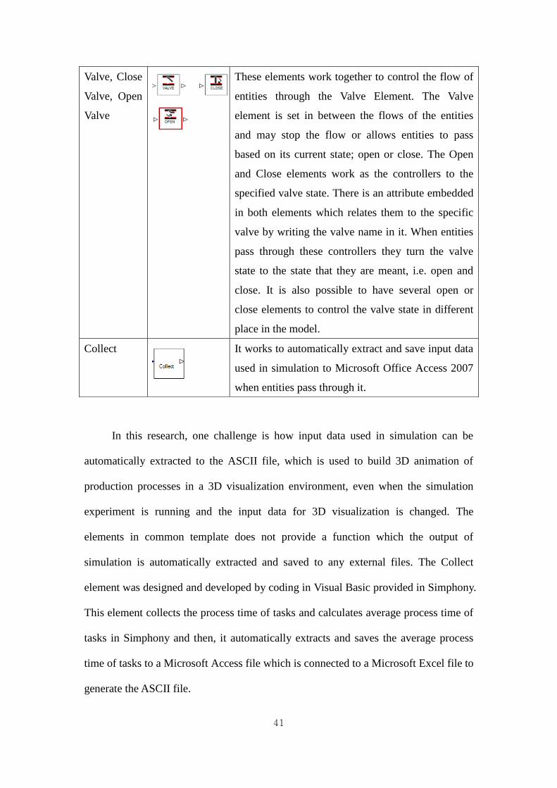
41
In this research, one challenge is how input data used in simulation can be
automatically extracted to the ASCII file, which is used to build 3D animation of
production processes in a 3D visualization environment, even when the simulation
experiment is running and the input data for 3D visualization is changed. The
elements in common template does not provide a function which the output of
simulation is automatically extracted and saved to any external files. The Collect
element was designed and developed by coding in Visual Basic provided in Simphony.
This element collects the process time of tasks and calculates average process time of
tasks in Simphony and then, it automatically extracts and saves the average process
time of tasks to a Microsoft Access file which is connected to a Microsoft Excel file to
generate the ASCII file.
Valve, Close
Valve, Open
Valve
These elements work together to control the flow of
entities through the Valve Element. The Valve
element is set in between the flows of the entities
and may stop the flow or allows entities to pass
based on its current state; open or close. The Open
and Close elements work as the controllers to the
specified valve state. There is an attribute embedded
in both elements which relates them to the specific
valve by writing the valve name in it. When entities
pass through these controllers they turn the valve
state to the state that they are meant, i.e. open and
close. It is also possible to have several open or
close elements to control the valve state in different
place in the model.
Collect
It works to automatically extract and save input data
used in simulation to Microsoft Office Access 2007
when entities pass through it.

42
3.7.2 Development of Simulation Models
Before building a simulation model, users must have proper input data in the
form of statistical models for work-task durations to get accurate simulation results.
The duration of each process, based on a collected sample of observations of
construction processes, is classically converted by fitting a statistical distribution such
as lognormal, triangular, normal, or beta. The analysis of input data was discussed by
Simaan M. AbouRizk and Daniel W. Halpin (1991, 1994). Table 3.3 shows an
example of input data by fitting a statistical distribution.
Based on the Common Template and Collect element, two simulation models,
old system and new system, are built in Simphony according to an old schedule and
new schedule developed by lean production. Figure 3.6 shows a whole model of the
production line. Figure 3.7 describes in detail one part of the whole model. After
finishing simulation, the simulator is required to validate and verify the two models.
The verification and validation is important to detect any errors in the simulation
model and the proposed new schedule. There are two methods to validate the output
of the simulation models. First, it can be checked by comparing the average cycle
time for a certain amount of units produced in simulation models. Second, it can be
checked by comparing the number of units produced for designated times in
simulation models. In this research, the first option, comparing the average cycle time
in the old system and the new system for a certain amount of units, was selected.
After the simulation runs, the Collect element created in Simphony
automatically exports and stores the required data for the virtual 3D model to
Microsoft Access 2007. The data in Microsoft Access 2007 is then converted to the
ASCII file using Microsoft Excel 2007. The ASCII file, identification numbers for
activities, start time and finish time of activities, are simply updated in Microsoft
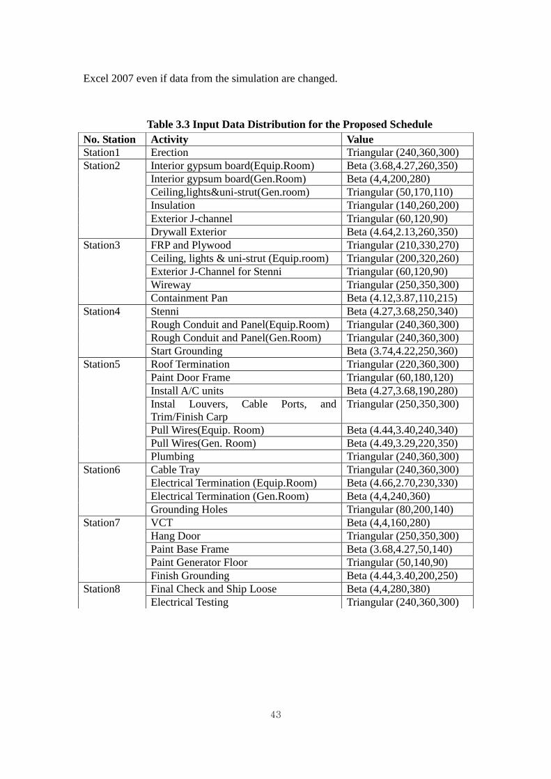
43
Excel 2007 even if data from the simulation are changed.
Table 3.3 Input Data Distribution for the Proposed Schedule
No. Station Activity Value
Station1 Erection Triangular (240,360,300)
Station2 Interior gypsum board(Equip.Room) Beta (3.68,4.27,260,350)
Interior gypsum board(Gen.Room) Beta (4,4,200,280)
Ceiling,lights&uni-strut(Gen.room) Triangular (50,170,110)
Insulation Triangular (140,260,200)
Exterior J-channel Triangular (60,120,90)
Drywall Exterior Beta (4.64,2.13,260,350)
Station3 FRP and Plywood Triangular (210,330,270)
Ceiling, lights & uni-strut (Equip.room) Triangular (200,320,260)
Exterior J-Channel for Stenni Triangular (60,120,90)
Wireway Triangular (250,350,300)
Containment Pan Beta (4.12,3.87,110,215)
Station4 Stenni Beta (4.27,3.68,250,340)
Rough Conduit and Panel(Equip.Room) Triangular (240,360,300)
Rough Conduit and Panel(Gen.Room) Triangular (240,360,300)
Start Grounding Beta (3.74,4.22,250,360)
Station5 Roof Termination Triangular (220,360,300)
Paint Door Frame Triangular (60,180,120)
Install A/C units Beta (4.27,3.68,190,280)
Instal Louvers, Cable Ports, and
Trim/Finish Carp
Triangular (250,350,300)
Pull Wires(Equip. Room) Beta (4.44,3.40,240,340)
Pull Wires(Gen. Room) Beta (4.49,3.29,220,350)
Plumbing Triangular (240,360,300)
Station6 Cable Tray Triangular (240,360,300)
Electrical Termination (Equip.Room) Beta (4.66,2.70,230,330)
Electrical Termination (Gen.Room) Beta (4,4,240,360)
Grounding Holes Triangular (80,200,140)
Station7 VCT Beta (4,4,160,280)
Hang Door Triangular (250,350,300)
Paint Base Frame Beta (3.68,4.27,50,140)
Paint Generator Floor Triangular (50,140,90)
Finish Grounding Beta (4.44,3.40,200,250)
Station8 Final Check and Ship Loose Beta (4,4,280,380)
Electrical Testing Triangular (240,360,300)
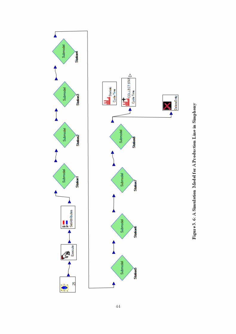
44

45

46
3.8 3D Visualization Approach
There are two main issues in this research to implementing 3D visualization.
First, the information gap between simulation and 3D visualization must be addressed,
so that the output of simulation is effectively conveyed in 3D visualization. This was
done through the generation of the ASCII file as explained above. Second, a time
distribution plan to smoothly animate 3D objects must be developed. This explains
next sections. The 3D objects were built using AutoCad, and 3D animation was
developed using 3D Studio Max (3DS).
Before creating 3D animation, users must understand the relationship between
simulation and visualization time to define key frames of sub-activities on desired
points on a timeline of 3DS. The simulation model has a lower level of detail than
does the visualization model. It only shows the high level activities such as start time
and end time of an operation. However, the visualization model provides a detailed
description based on specifications and other data. For example, in the visualization
model the process time is 300 minutes for installation of interior gypsum board in
equipment room in Station 2. The simulation model only shows that start time of
installation is 0 minute and end time is 300 minutes. The visualization model
describes all sub-activities to install interior gypsum boards, such as animation of
operators for delivery to destination location, installation, and movement to source
location. Figure 3.8 graphically explains the relationship between the simulation and
animation time based on installation of interior gypsum boards in Station 2.

47
Figure 3.8: Relationship between Simulation and Animation Time
(Revised Mohamed Al-Hussein et al 2005)
To build animation of 3D objects in 3DS, key frames are required because 3D
objects are animated between the key frames designated on the timeline in 3DS. For
example, key frames are 0, 2, 6, 60 seconds on the timeline of animation time in
Figure 3.8. When animation is built, there are many sub-activities of 3D objects to
describe detailed production processes. The sub-activities such as movement and
installation are animated between the key frames based on sub-activity frames. That is,
the sub-activities of each task except installation are animated between consistency
times which are sub-activity frames. A sub-activity frame for each task is calculated
using Eq. 3.2:
Where: M= End Time for the Task – Start Time for the Task
N=Number of Key Frames required for the Task

48
The simulation time unit is minute but animation time unit is second. To convert
a minute to seconds, the process time should be multiplied by 60 but deletes it for fast
animation. Usually, one second consists of 60 frames in animation time but defines 30
frames for fast animation. Therefore, 30 frames per minute are used to provide smooth
animation. Therefore, time scale factor used for sub-activities of tasks on the
production line is 1/30, making 1 minute of simulation time into 30 frames of
visualization. To convert simulation time to visualization time, the process time of
each task in the ASCII file is multiplied by 30. In this work, the number of key frames
required for sub-activities of the task is assumed first time because it will be
influenced by installation location of the material in each task. However, even if the
assumption is wrong, the number can simply be changed on the Maxscript in 3DS.
To create animation in 3DS, a series of key frames, defined by start and end
points of sub-activities for 3D objects, are basically created on timeline. These can
explain the state of subtasks at a designated point in time. To smoothly describe the
operation of a production line in 3DS, each task is divided into the following three
actions: 1) Operators deliver the source to destination location, 2) The operators
install boards, and 3) The operators move back to the source location. This cycle is
operated until the installation of material is finished on the production line. Each
action also has many sub-activities in animation. For example, there are two operators
required to install interior gypsum boards in the equipment room in Station 2.
Eighteen interior gypsum boards are installed in the equipment room. To calculate the
sub-activity frame, the process time and number of key frames are required. The
process time for interior gypsum boards was imported from the ASCII file. Users may
not be known exactly how many key frames which are sub-activities of each action
were needed for animation of delivery, installation, and movement before developing

49
the animation. These are influenced by the installation location because boards are
installed in different positions. Therefore, consistent key frames were designated,
where a key frame is defined as one sub-activity frame to animate a sub-activity of 3D
objects such as a step of the operator. When a sub-activity frame for interior gypsum
board task is 11.10 frames, the key frames to animate one step of an operator are
defined at 0 and 11.10 frames. Then, one step of the operator is animated between 0
and 11.10 frames on a timeline in 3DS and the second step of the operator is animated
between 11.10 and 22.20 frames. Figure 3.9 describes a framework of animation for
interior gypsum board task. Based on this work and the sequence of installation, the
animation of the interior gypsum board is built. Figure 3.10 shows the sequence and
animation snapshots of the interior gypsum board task and 3D chart.
The visualization can identify the requirement and limitation of workspace,
accessibility problems for employees, and inconsistencies in the level of detail among
tasks in the proposed schedule. The virtual reality model in combination with 3D
scheduling chart can help validate the completeness and consistency of the proposed
schedule. It can also help users fully understand the production processes of a
manufacturing production line.

50
Figure 3.9: A Framework for Animation of Interior Gypsum Board Task
Figure 3.10: Animation Snapshots of Interior Gypsum Board related to 3D
Scheduling and Sequence
3.9 Summary
This research designed and developed an integrated system using lean,
simulation, and visualization to increase productivity of a production line in the

51
manufacturing industry. Improvement for the production line was suggested by VSM,
and a simulation model based on the proposition was built to verify whether or not
productivity was improved. A 3D visualization based on the output of the simulation
model was then developed for validation of the proposition. The project manager can
use this system to get suggestions on efficiently improving the processes of the
production line before implementing the proposition in the real world. It also leads to
decrease rework, reduce cost, and save time.

52
Chapter 4
PROPOSED METHODOLOGY IMPLEMENTATION
4.1 Introduction
In this chapter, the proposed methodology is implemented in a real case. First, a
proposed schedule was developed using Value Stream Mapping (VSM) for a
manufactured production line. Then, two simulation models based on the original
schedule and the proposed schedule were built in Simphony to identify the total cycle
time of a set amount of product. Finally, a 3D virtual reality model was designed in
3D Studio Max according to the proposed schedule. Before implementing this
methodology, it was necessary to understand the manufactured production line,
analyze the main stations and subtasks to know their inter-relationships, and study the
modular flow in the production line.
4.2 Background of Case Study
This section describes the background information related to the case study. The
case study company, Kullman Building Company (KBC), is one of the leading
modular building manufacturers in the US. It has over 200 employees and has
expanded its market to produce a variety of building types, including equipment
shelters, schools, dormitories, multi-story residential buildings, correctional facilities,
healthcare facilities, and US embassies. Ninety-five percent of the production line
constructs 12×30 ft (350 914cm) or 12×20 ft (350 609 cm) standard modules with
similar configurations and then a module joins with other modules on site. According
to the type of the module, the sequence of the production process and process time of

53
subtasks are different. In this research, the focus was on the 12×30ft standard module
to implement the proposed methodology. KBC has limited clients in educational
institutions, and government, which are less cost constrained because modular
typically 10-20% more expensive than those built on-site. Therefore, the
manufactured production line at KBC required redesign to reduce the production
cycle time and average labour hours per module to ensure a competitive cost in the
manufacturing industry. There is a total of eight stations including several subtasks in
the KBC production line. The description of the case is based on the original schedule.
4.2.1 Station 1
The first station of the production line, shown in Figure 4.1, had only one
subtask that is erection. A crane lifted module frames, which were a base, front, right,
left, part, rear, and roof. Before installing them, wall assembly, roof preparation, and
base preparation were required. The task sequences were such that first, the base was
in position. Second, wheels were installed on the sides of the base using the crane for
movement between stations. Third, part wall, front, right, left, and rear studs were
installed one by one on the base, and finally the roof was installed. The required
workforce was two welders. The duration of the erection task was about 5 hours. The
module completed in Station 1 then waited until Station 2 was available.
Figure 4.1: Station 1

54
4.2.2 Station 2
Station 2, shown in Figure 4.2, had five subtasks: interior gypsum board in the
equipment room, interior gypsum board in the generator room, insulation, exterior J-
channel for sheetrook, and drywall exterior. A total of five carpenters were required in
Station 2. The interior gypsum board in the equipment room and generator room were
installed at the same time by two carpenters each when a module arrived from Station
1. The duration of the interior gypsum board task for the equipment room was five
hours, in comparison to only four hours for the generator room. The quality issue was
that joints between interior gypsum boards must be tight and straight and screws in
line. A fifth carpenter installed insulation for three and half hours, an hour after the
interior gypsum board tasks started. As soon as two carpenters completed the
installation of the interior gypsum board in the generator room, they started installing
the exterior J-channel for one and a half hours. The drywall exterior task was already
being worked on for half an hour by the two carpenters that installed the gypsum
board in the equipment room. The two carpenters helped with the drywall exterior
task as soon as they finished the exterior J-channel task. The total cycle time in
Station 2 was eight hours.
Figure 4.2: Station 2
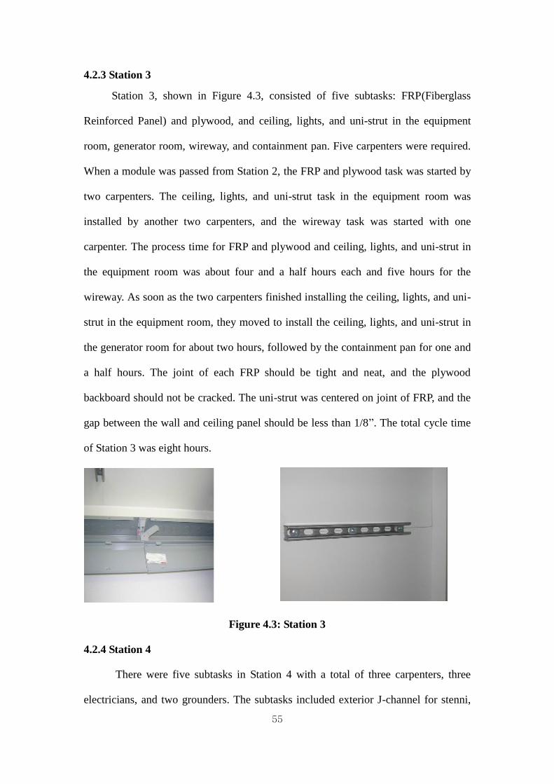
55
4.2.3 Station 3
Station 3, shown in Figure 4.3, consisted of five subtasks: FRP(Fiberglass
Reinforced Panel) and plywood, and ceiling, lights, and uni-strut in the equipment
room, generator room, wireway, and containment pan. Five carpenters were required.
When a module was passed from Station 2, the FRP and plywood task was started by
two carpenters. The ceiling, lights, and uni-strut task in the equipment room was
installed by another two carpenters, and the wireway task was started with one
carpenter. The process time for FRP and plywood and ceiling, lights, and uni-strut in
the equipment room was about four and a half hours each and five hours for the
wireway. As soon as the two carpenters finished installing the ceiling, lights, and uni-
strut in the equipment room, they moved to install the ceiling, lights, and uni-strut in
the generator room for about two hours, followed by the containment pan for one and
a half hours. The joint of each FRP should be tight and neat, and the plywood
backboard should not be cracked. The uni-strut was centered on joint of FRP, and the
gap between the wall and ceiling panel should be less than 1/8”. The total cycle time
of Station 3 was eight hours.
Figure 4.3: Station 3
4.2.4 Station 4
There were five subtasks in Station 4 with a total of three carpenters, three
electricians, and two grounders. The subtasks included exterior J-channel for stenni,

56
stenni, rough conduit and panel in equipment room, rough conduit in generator room,
and start grounding. The three carpenters installed the exterior J-channel for stenni on
the corners of the module and beside the door frames for one and a half hours, and
then installed the stenni for another five hours. The rough conduit and panel in the
equipment room and generator room and start grounding tasks were done at the same
time. The process time of rough conduit and panel in the equipment room was seven
and a half hours. The process time of start grounding and rough conduit and panel in
the generator room was five hours each. The quality control points of installation of
the stenni were that all screws must be in place and there is no apparent fall-off of
stones. All conduits and boxes must be measured using a level before they are fixed,
and the conduits must be bent in right offset and angle, so they can be firmly fixed
against the wall and ceiling. Figure 4.4 shows the installation of the conduit and stenni.
The total cycle time of Station 4 was seven and half hours.
Figure 4.4: Station 4
4.2.5 Station 5
Station 5, shown in Figure 4.5, was composed of roof termination, paint door
frame, install A/C units, louvers and cable ports, trim and finish carp entry, pull wires
in equipment room and generator room, and plumbing tasks. Six carpenters, a painter,
and three electricians were required. The roof termination with two carpenters, pull
wires in the equipment room with two electricians and the generator rooms with one

57
electrician, louvers and cable ports with two carpenters, and plumbing with a painter
tasks were begun together when a module arrived at Station 5. The process time of
pull wires in generator room and plumbing tasks were five hours each. The process
time of roof termination was four and a half hours. The process time of pull wires in
the equipment room was seven and a half hours, and the process time of louvers and
cable ports was two and a half hours. The start time of the paint door frame task was
six hours after the module arrived with a painter and lasted two hours. Two carpenters
installed the A/C units for five hours as soon as the installation of louvers and cable
ports task was finished. The quality control points for roof termination were that
corners of the roof were straight and neat, and bottom angles were tight against the
EPDM and stenni without bubble. Labels were attached at both ends of all wires in
the generator room for the pull wire task in the equipment room and generator room.
The total cycle time of Station 5 was eight hours
Figure 4.5: Station 5
4.2.6 Station 6
Station 6, shown in Figure 4.6, included four subtasks: cable tray, finish pull
wires and electrical termination in equipment room and generator room, and
grounding holes. One carpenter and three electricians were required. The cable tray

58
with one carpenter and finish pull wires and termination in the equipment room with
two electricians were the first tasks when the module arrived at Station 6. The cycle
time for each of them was five hours. The other electrician started the electrical
termination in the generator room two and a half hours after the module first arrived.
The working time of this task was five hours. The grounding holes were done for two
and half hours by the two carpenters that finished installation of the cable tray. The
quality control point of the cable tray was that hangers were vertical and cable trays
level. The grounding holes were drilled at 45˚ and the sleeve was flat with the wall
surface. The total cycle time of Station 6 was seven and half hours.
Figure 4.6: Station 6
4.2.7 Station 7
Station 7, pictured in Figure 4.7, had four subtasks: VCT, hang door, paint door
frame, and finish grounding. The VCT with one carpenter and hang doors with one
carpenter were started as soon as the module was arrived. The process time of the
VCT and hang door tasks was four hours and three hours, respectively. The start time
of the paint door frame task was one and a half hours after the module arrived and
lasted for one and a half hours with one painter. After the paint door frame task was
completed, the finish grounding task was started two hours later and lasted for two
and a half hours with two grounders. The quality control points of VCT were that the
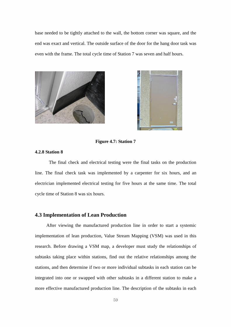
59
base needed to be tightly attached to the wall, the bottom corner was square, and the
end was exact and vertical. The outside surface of the door for the hang door task was
even with the frame. The total cycle time of Station 7 was seven and half hours.
Figure 4.7: Station 7
4.2.8 Station 8
The final check and electrical testing were the final tasks on the production
line. The final check task was implemented by a carpenter for six hours, and an
electrician implemented electrical testing for five hours at the same time. The total
cycle time of Station 8 was six hours.
4.3 Implementation of Lean Production
After viewing the manufactured production line in order to start a systemic
implementation of lean production, Value Stream Mapping (VSM) was used in this
research. Before drawing a VSM map, a developer must study the relationships of
subtasks taking place within stations, find out the relative relationships among the
stations, and then determine if two or more individual subtasks in each station can be
integrated into one or swapped with other subtasks in a different station to make a
more effective manufactured production line. The description of the subtasks in each

60
station of the case study was already explained in the previous section. Sufficient data
collection is important to view more detail in the production line, to identify real
problems and waste, and to propose improvement of the production process. There are
two ways to collect the required data from the manufactured production line. First, the
information can be obtained directly at the production line, following the production
process from beginning to end on the same day. Second, the developer can interview
people who work in each subtask or managers if he cannot see the production line
directly. In this research, the required data was obtained from Haitao Yu (2008). When
a few types of modules are produced in the manufactured production line, information
such as the task sequences and process time can be different. In this case study, the
focus was on the sequences of production process for the 12×30 ft module. The
required data, cycle time of each station, workforce requirement at each subtask,
process time of subtasks, transfer time, and a list of subtasks in each station are
summarized in Table 4.1 obtained from Haitao Yu (2008).
Table 4.1: Production Line Data
Station Activity Process Time Workforce Cycle Time
Station 1 Erection 300min 2W
300min
Station 2 Interior Gypsum Board
(Equip. Room)
300min 2C
Interior Gypsum Board
(Gen. Room)
240min 2C
Insulation 200min 1C
Station 2 Exterior J-chaneel
for sheetrock
90min 2C
Drywall exterior 330min 2C
480min
Station 3 FRP and Plywood 270min 2C
Ceiling, lights &
uni-strut (Equip.room)
260min 2C

61
Ceiling, lights &
uni-strut (Gen.room)
110min 2C
Wireway 300min 1C
Containment Pan 100min 2C
480min
Station 4 Exterior J-Channel for
Stenni
90 min 3C
Stenni 300 min 3C
Rough Conduit and panel
(Equip.room)
450 min 2E
Rough Conduit and panel
(Gen.room)
300 min 1E
Start Grounding 300 min 2G
450min
Station 5
Roof Termination 260min 2C
Paint Door Frame 120min 1P
Install louvers,
cable ports
150min 2C
Install A/C units 300min 2C
Trim/finish carp 180min 2C
Pull wires
(Equip.room)
450min 2E
Pull wires
(Gen.room)
300min 1E
Plumbing 300min 1P
480min
Station 6 Cable tray 300min 1C
Electrical Termination
(Equip.room)
300min 2E
Grounding Holes 140min 1G
450min
Station 7 VCT 220 min 1C
Hang Doors 180 min 1C
Paint Base Frame 90min 1P
Finish Grounding 150min 2G
450min
Station 8 Final check and ship loose 300min 1C

62
Electrical testing 300min 1E
300min
Total 56.5hr
Note:
C : Carpenter, P: Painter, G: Grounder, E: Electrician, W:Welder
The transfer time between stations is about ten minutes.
4.3.1 Current VSM
Based on the data collection and original schedule of the production line in the
case study, a current map was developed using VSM in Microsoft Visio 2007. The
goal of the current map is to create a clear existing production line and identify waste.
Figure 4.8 shows the current map using VSM icons. The information recorded in the
data table icon was estimated. The working time was defined as one work shift minus
breaks, equalling 27,000 seconds or 7.5 hours. Cycle time (CT) was calculated as the
time it takes to complete all tasks in all station. The total cycle time was 56.5 hours. It
was recorded in the data box of each station. Transfer time between each station was
about 10 minutes. As mention in Chapter 3, takt time can be obtained by taking the
net working time for an identified period divided by customer demand for the same
period. Takt time was 8 hours in this case. The map shows eight stations of the
production line, including thirty-three subtasks described under the map, and
workforce requirements in each station is represented by activity boxes. The process
can be thought of as one module passing through a line of stations.
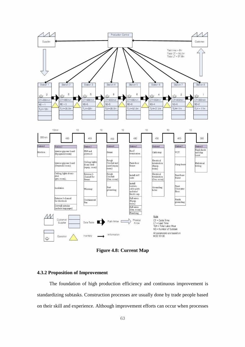
63
Figure 4.8: Current Map
4.3.2 Proposition of Improvement
The foundation of high production efficiency and continuous improvement is
standardizing subtasks. Construction processes are usually done by trade people based
on their skill and experience. Although improvement efforts can occur when processes

64
are shifted between tasks, they are mostly ignored by the workforce. Haitao Yu et al.
(2008) found problems in the production line of the case study. The production
process in this case study was highly unpredictable, and the line was disorganized all
the time because a line manager assigned workers to the subtasks on a daily, even
hourly, basis. The line was only moved when most of the subtasks in a station had
been done. This caused an increase in the process time and cycle time of each station
in the production line.
The first proposition for improvement of the production line was to standardize
the production line on the basis of takt time to reduce waste. The original takt time
was 8 hours. However, based on a time series analysis of the historical data of
customers’ orders in the past 12 months, the takt time was calculated as six hours
(Haitao Yu, 2008). This meant that the subtasks in every station should be done in six
hours. The second suggestion for improvement was to ensure continuous flow of the
production line. A module should continuously flow from one process to the next
without waiting time. To do this, the positions of some tasks in the schedule needed to
change to different stations or combined with other subtasks, and more workers were
required to reduce the process time. Based on takt time and continuous flow, the
production line was restructured by Haitao Yu (2008). Figure 4.9 describes the new
schedule with original scheduling of each station.
The ceiling, lights, and uni-strut in generator room moved from Station 3 to
Station 2. It is carried out by the same workers as the interior gypsum board task in
the generator room. The exterior J-channel for sheetrock task was begun when the
module arrived, and then the drywall exterior task was worked on for four and a half
hours. As a result, two extra workers were required in Station 2. As soon as the two
workers finished the installation of the interior gypsum board for the equipment room,

65
they moved to assist with the drywall exterior task for about an hour. The cycle time
of Station 2 was cut from eight hours to six hours.
Station 3, based on the new schedule, required one more worker than before
because the containment pan task needed to start right away after a module arrived.
The exterior J-channel for stenni task was moved from Station 4 to Station 3, so that
the production process in Station 3 flowed continuously. The process time of the
ceiling, lights and uni-strut task in the equipment room remained the same as before.
The wireway task started an hour after the module arrived at Station 3. As a result, the
cycle time of Station 3 was reduced from eight hours to six hours.
At Station 4, the start time of the stenni task was changed because the exterior
J-channel for stenni task was moved to Station 3. This meant that the start times of the
stenni, rough conduit and panel in the equipment room and generator room, and start
grounding were the same. In the original production line, the rough conduit in the
equipment room was installed for seven and half hours with two electricians, but only
one more electrician was required to reduce the process time to five hours in the new
schedule, so that cycle time in Station 4 was reduced by three hours.
At Station 5, the louver, cable port task, and trim/finish carpentry tasks were
combined into one task requiring two carpenters for five hours. The pull wire in
equipment room task was performed for seven and a half hours with two electricians
on the real production line, but when one more electrician was added, the process time
was decreased to five hours. The start time of the paint door frame task was moved up,
so that the task starts four hours rather than six hours after arrival of the module. The
process time of installation of the A/C units was reduced from five hours to four hours
by the concept in lean production of waste elimination. The total cycle time for
Station 5 was reduced from eight hours to six hours.

66
Based on the takt time, six hours, one more carpenter and electrician were
required at Station 6. The electrician was needed for the electrical termination in
equipment room task to reduce the process time from seven and a half hours to five
hours. An extra carpenter could make grounding holes in the walls of the module, so
that the start time of the task can be moved up two hours. The waiting time of the
electrical termination in generator room task was changed from two and a half hours
to zero after the module was arrived. The total cycle time of Station 6 was reduced
from eight hours to five and a half hours. Based on takt time and continuous flow of
the production line, finish grounding was begun when the module was in position at
Station 7. This movement of start time for the finish grounding task reduced the cycle
time of Station 7 from eight hours to four hours, and only one grounder was required
for the task.
According to the new schedule of the production process, the lean team and
production manager can predict and expect results that reduce the cycle time of each
station and improve productivity. In lean production, the proposed design is
continuously changed until the intention of the developer is achieved, because many
unknowns and uncertainties may be generated in the real world.

67
Task
Interior gypsum
board( equip. room)
Interior gypsum
board (gen. room)
Insulation
Exterior J-channel
for sheetrock
Drywall exterior
(include tarp paper)
Crew
1
Task
Interior gypsum
board( equip. room)
Interior gypsum
board (gen. room)
Ceiling, lights & uni-
strut (gen. room),
Insulation
Exterior J-channel
for sheetrock
Drywall exterior
(include tarp paper)
Station 2 Takt time 6 hr Takt time 8 hr
Crew 1 (2C) / 300 min
Crew 2 (2C) / 240 min
Crew 2 (2C) / 110 min
Crew3 (1C) / 200 min
Crew 4 (2C) 90 min
Crew 4 (2C) 330 Crew 1 & 4
Crew 2 (2C) / 90
min
Crew 1 & 2
Hour 1 Hour 2 Hour 3 Hour 4 Hour 5 Hour 6
Hour 6 Hour 7 Hour 8
Crew 1 (2C) / 300 min
Crew 2 (2C) / 240 min
Crew3 (1C) / 200 min
Hour 1 Hour 2 Hour 3 Hour 4 Hour 5

68
Task
FRP and plywood
Ceiling, lights & uni-
strut (equip. room)
Ceiling, lights & uni-
strut (Gen. room)
Wireway
Containment Pan
Task
FRP and plywood
Ceiling, lights & uni-
strut (equip. room)
Exterior J-channel
for Stenni
Wireway
Containment Pan
Station 3
1C / 165 min
Hour 5 Hour 6
Crew 1 (2C) / 270 min
Crew 2 (2C) / 260 min
Crew 2 (2C) 90 min
Crew 3 (1C) / 300 min
Hour 1 Hour 2 Hour 3 Hour 4
Hour 3 Hour 4 Hour 5
Takt time 6 hr Takt time 8 hr
Crew 3 (1C) / 300 min
Crew2 (2C) / 100
Hour 6 Hour 7 Hour 8
Crew 1 (2C) / 270 min
Crew 2 (2C) / 260 min
Crew 2 (2C) / 110 min
Hour 1 Hour 2
Task
Exterior J-channel
for Stenni
Stenni
Rough Conduit and
panel (equip. room)
Rough Conduit
(Gen. room)
Start grounding
Task
Stenni
Rough Conduit and
panel (equip. room)
Rough Conduit
(Gen. room)
Start grounding
Station 4 Takt time 6 hr Takt time 8 hr
Crew 1 (3C) / 300 min
Crew 2 (3E) / 300 min
Crew 3 (1E) 300 min
Crew 4 (2G) 300 min
Crew 4 (2G) 300 min
Hour 1 Hour 2 Hour 3 Hour 4 Hour 5 Hour 6
Hour 7 Hour 8
Crew 1 (3C) / 90
min
Crew 1 (3C) / 300 min
Crew 2 (2E) / 450 min
Crew 3 (1E) 300 min
Hour 1 Hour 2 Hour 3 Hour 4 Hour 5 Hour 6

69
Task
Roof termination
Paint door frame
Install A/C units
Louvers, cable ports
Trim/ finish carp
Pull wires (Equip.
room)
Start pull wires
(Gen. room)
Plumbing
Task
Roof termination
Paint door frame
Install A/C units
Install louvers, cable
ports and trim/ finish
carp
Pull wires (Equip.
room)
Pull wires (Gen.
room)
Plumbing
Takt time 6 hr Takt time 8 hr
Station 5
Crew 5 (1E) / 300 min
1Pl / 300 min
Hour 6
Crew 1 (2C) / 260 min
1P / 120 min
Crew2 (2C) / 240 min
Crew 3 (2C) / 300 min
Crew 4 (3E) 300 min
Crew 2 (2C) / 150 min
2C / 180 min
Crew 3 (2E) 450 min
1E / 300 min
Crew 6 (1Pl) / 300 min
Hour 1 Hour 2 Hour 3 Hour 4 Hour 5
Hour 6 Hour 7 Hour 8
Crew 1 (2C) / 260 min
1P / 120 min
Crew2 (2C) / 300 min
Hour 1 Hour 2 Hour 3 Hour 4 Hour 5
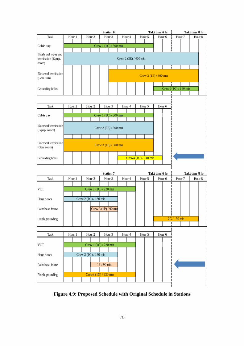
70
Task
Cable tray
Finish pull wires and
termination (Equip.
room)
Electrical termination
(Gen. Rm)
Grounding holes
Task
Cable tray
Electrical termination
(Equip. room)
Electrical termination
(Gen. room)
Grounding holes
Takt time 6 hrStation 6 Takt time 8 hr
Crew 1 (1C) / 300 min
Crew 2 (3E) / 300 min
Crew 3 (1E) / 300 min
Crew4 (1C) / 140 min
Hour 1 Hour 2 Hour 3 Hour 4 Hour 5 Hour 6
Hour 7 Hour 8
Crew 1 (1C) / 300 min
Crew 2 (2E) / 450 min
Crew 3 (1E) / 300 min
Crew 1(1C) / 140 min
Hour 1 Hour 2 Hour 3 Hour 4 Hour 5 Hour 6
Task
VCT
Hang doors
Paint base frame
Finish grounding
Task
VCT
Hang doors
Paint base frame
Finish grounding
Takt time 8 hrStation 7 Takt time 6 hr
Crew 1 (1C) / 220 min
Crew 2 (1C) / 180 min
1P / 90 min
Crew3 (1G) / 230 min
2G / 150 min
Hour 1 Hour 2 Hour 3 Hour 4 Hour 5 Hour 6
Hour 6 Hour 7 Hour 8
Crew 1 (1C) / 220 min
Crew 2 (1C) / 180 min
Crew 3 (1P) / 90 min
Hour 1 Hour 2 Hour 3 Hour 4 Hour 5
Figure 4.9: Proposed Schedule with Original Schedule in Stations
71
4.4 Simulation Model Experiment
Lean production focuses on studying and developing production processes in
order to improve productivity by reducing the cycle time of each station using takt
time and continuous flow concepts. However, the value stream map has some
limitations. First, it cannot represent the variability, dynamic nature, and high
uncertainty of a complex system. Second, it does not support a validation tool before
implementing the proposed improvements. According to the improvement principles
in lean production, the lean team usually implements the improvements in the real
world, and then adjusts them until obtaining an ideal state of the manufactured
production processes. This can be time-consuming and increases cost. As Halpin
(2002) remarks, “Lean thinking and simulation are very closely linked and even
synonymous.” Simulation is widely used in manufacturing industry. In the
construction process, many studies using simulation have been presented for decades.
Simulation is also a powerful tool to analyze and model the production process,
especially repetitive processes. Therefore, simulation can serve lean production as a
validation tool. This research used simulation to facilitate the application of
production flow to improve the performance of the manufactured production line.
Two simulation models of the production line, based on the old system and the
new lean system, were built in Simphony. After building the models, the results of
simulation were compared.
4.4.1 Simulation Model for the Original Production Line
For a simulation experiment, the simulation users must have proper input data
in the form of statistical models for work-task durations to get simulation results
before building the models. The process time for each task, based on a collected
sample of observation of the manufactured production processes, was classically

72
converted by fitting a statistical distribution such as lognormal, triangular, normal, or
beta. The collected distributions based on the original system are summarized in Table
4.2. The analysis of input data was discussed by Simaan M. AbouRizk and Daniel W.
Halpin (1991, 1994).
Table 4.2 Input Data for the Original Schedule
Station Activities Value
Station 1 Erection Triangular (240, 360, 300)
Station 2 Interior gypsum board (Equip. Room) Beta (260, 350, 3.68, 4.27)
Interior gypsum board (Gen. Room) Beta (200, 280 , 4, 4)
Insulation Triangular (140, 260, 200)
Exterior J-Channel for sheetrock Triangular (60, 120, 90)
Drywall Exterior Beta (130, 240, 3.74, 4.22)
Station 3 FRP and Plywood Triangular (210, 330, 270)
Ceiling,lights & uni-strut (Equip.Room) Triangular (200, 320, 260)
Ceiling,lights & uni-strut (Gen.Room) Triangular (50, 170, 110)
Wireway Triangular (250, 350, 300)
Containment Pan Beta (50, 150, 4, 4)
Station 4 Exterior J-channel for stenni Triangular (60, 120, 90)
Stenni Beta (250, 340, 4.27, 3.68)
Rough conduit & panel (Equip.Room) Triangular (390, 510, 450)
Rough conduit & panel (Gen.Room) Triangular (240,360,300)
Start Grounding Beta (250, 360, 3.74, 4.22)
Station 5 Roof Termination Triangular (220, 300, 260)
Paint Door Frame Triangular (60, 180, 120)
Install A/C units Beta (250, 350, 4, 4)
Install louvers and cable ports Triangular (100, 200, 150)
Trim/finish carp Triangular (140, 220, 180)
Pull wires (Equip. Room) Beta (390, 490, 4.44, 3.40)
Pull wires (Gen. Room) Beta (220, 350, 4.49, 3.29)
Plumbing Triangular (240, 360, 300)
Station 6 Cable Tray Triangular (240, 360, 300)
Electrical Termination (Equip.Room) Beta (230,330, 4.66, 2.70)
Electrical Termination (Gen.Room) Beta (240, 360, 4, 4)
Grounding Holes Triangular (80, 200, 140)
Station 7 VCT Beta (160, 280, 4, 4)

73
Hang Doors Triangular (130, 230, 180)
Paint Base Frame Beta (50, 140, 3.68, 4.27)
Finish Grounding Beta (120, 170, 4.44, 3.40)
Station 8 Final Check and ship loose Beta (260, 350, 3.68, 4.27)
Electrical testing Triangular (240, 360, 300)
Note:
The unit of measurement is in minutes.
Beta (Minimum, Maximum, Shape A, Shape B)
Triangular (Minimum, Maximum, Average)
To describe, compare, and experiment with the old and new systems, the
production line of the case study was built by using the enhanced Common Template
in Simphony. It is a general-purpose simulation (GPS) and also a special-purpose
simulation (SPS) tool. The functionality of elements in Simphony was described in
Chapter 3. Ninety-five percent of the KBC production line produces two kinds of
standard modules, 12×30 ft or 12×20 ft. The module type was the most important
factor in determining the process time and schedule of each activity in the stations. In
this thesis, simulation models based on the 12×30 ft module were developed.
Based on the original schedule of the production line and the elements in
Simphony, the simulation model of the old production line was built. Figure 4.10
shows the old production line with the model depicted at the top of the hierarchy. The
levels of hierarchy model the process flow. Each working station, shown at the second
level of hierarchy, is detailed by a process model simulating the activities and
resource interactions. Detailed process models for each station on the second level of
the hierarchy are demonstrated in Figure 4.11.

74

75

76
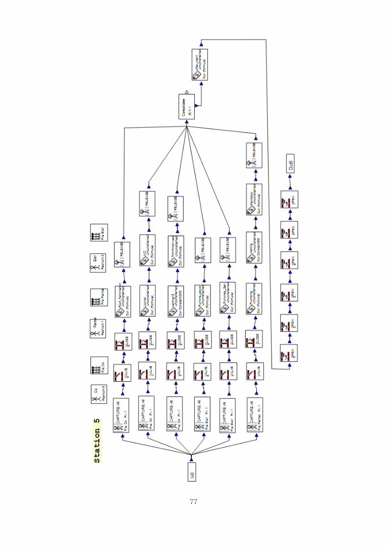
77
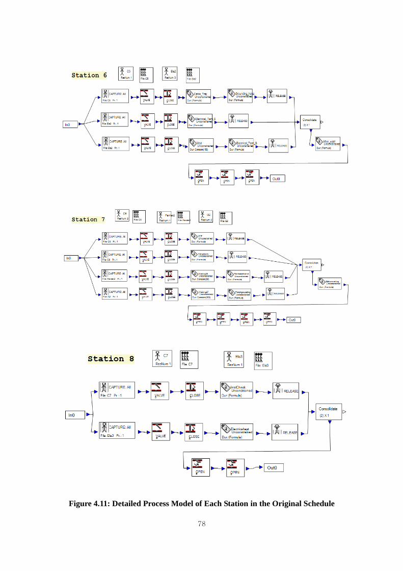
78
Figure 4.11: Detailed Process Model of Each Station in the Original Schedule

79
A sample job consisting of 50 modules was loaded into the entity element in the
simulation model. The model was run and the time required to produce all of the 50
modules was recorded in the simulation model. Based on eight working hours in a day,
the average cycle time in the simulation model of the old system was 33.8 days. The
maximum cycle time was 59.5 days. The recorded data were extracted from the
simulation database and analyzed using EasyFit. The cycle time distribution is given
in Figure 4.12.
Figure 4.12: Cycle Time Distribution of the Simulation Model of Original
Schedule
4.4.2 Simulation Model for the Proposed Production Line
The duration for each task, based on a collected sample of observation of the
production processes, was also classically converted by fitting a statistical distribution
such as lognormal, triangular, normal, or beta. The input data for each task was
summarized by Haitao Yu. The collected data in the new system are summarized in
Table 4.3. Based on a comparison of the input data in the old and new systems, the
lists of tasks and process times in each station were changed according to the output

80
of lean production. The installation of the ceiling, lights, and uni-strut in the generator
room task was moved to Station 2 from Station 3. The average process time of the
drywall exterior in Station 2 was also changed from 180 minutes to 330 minutes. The
installation of exterior J-channel for stenni was moved to Station 3. The average
process time of the containment pan task in Station 3 was increased as 165 minutes.
The average process time of the rough conduit and panel for equipment room task was
reduced to 300 minutes from 450 minutes. The installation of louvers and cable ports
task and the trim and finish carpentry task in Station 5 were combined into one task.
The average process time for these was controlled to 300 minutes. The paint generator
floor task was generated in Station 7. It was 90 minutes for the average process time.
The process time for final check and ship loose and electrical testing tasks were
changed from six hours to five and an half hours.
Table 4.3 Input Data for the Proposed Schedule
Station Activities Value
Station 1 Erection Triangular (240, 360, 300)
Station 2 Interior gypsum board (Equip. Room) Beta (260, 350, 3.68, 4.27)
Interior gypsum board (Gen. Room) Beta (200, 280 , 4, 4)
Ceiling, lights & unit-strut(Gen.Room) Triangular (50, 170, 110)
Insulation Triangular (140, 260, 200)
Exterior J-Channel for sheetrock Triangular (60, 120, 90)
Drywall Exterior Beta (260, 350, 4.64, 2.13)
Station 3 FRP and Plywood Triangular (210, 330, 270)
Ceiling,lights & uni-strut (Equip.Room) Triangular (200, 320, 260)
Exterior J-channel for stenni Triangular (60, 120, 90)
Wireway Triangular (250, 350, 300)
Containment Pan Beta (110, 215, 4.12, 3.87)
Station 4 Stenni Beta (250, 340, 4.27, 3.68)
Rough conduit & panel (Equip.Room) Triangular (240, 360, 300)
Rough conduit & panel (Gen.Room) Triangular (240,360,300)
Start Grounding Beta (250, 360, 3.74, 4.22)
Station 5 Roof Termination Triangular (220, 300, 260)

81
Paint Door Frame Triangular (60, 180, 120)
Install A/C units Beta (190, 280, 4.27, 3.68)
Install louvers, cable ports, and
Trim/finish carp
Triangular (250, 350, 300)
Pull wires (Equip. Room) Beta (240, 340, 4.44, 3.40)
Pull wires (Gen. Room) Beta (220, 350, 4.49, 3.29)
Plumbing Triangular (240, 360, 300)
Station 6 Cable Tray Triangular (240, 360, 300)
Electrical Termination (Equip.Room) Beta (230,330, 4.66, 2.70)
Electrical Termination (Gen.Room) Beta (240, 360, 4, 4)
Grounding Holes Triangular (80, 200, 140)
Station 7 VCT Beta (160, 280, 4, 4)
Hang Doors Triangular (250, 350, 300)
Paint Base Frame Beta (50, 140, 3.68, 4.27)
Paint generator Floor Triangular (50, 140, 90)
Finish Grounding Beta (200, 250, 4.44, 3.40)
Station 8 Final Check and ship loose Beta (260, 380, 4, 4)
Electrical testing Triangular (240, 360, 300)
Note:
The unit of measurement is in minutes.
Beta (Minimum, Maximum, Shape A, Shape B)
Triangular (Minimum, Maximum, Average)
Based on the output of lean production, a simulation model for the new system
was built in Simphony. Figure 4.13 shows the new production line with the model
depicted at the top of the hierarchy. This level of hierarchy also modeled the process
flow. The distributions of process time for tasks were set in the setattributes element
in Simphony. The Collect element at the top of the hierarchy in the simulation model
was the most important functionality. It collected the process time of tasks and
automatically saved them to Microsoft Access 2007 connected to Microsoft Excel
2007 for generating the ASCII file, which is the most critical factor to design a 3D
visualization. The ASCII file consists of identification numbers, start and finish time
of tasks. Each working station, shown at the second level of the hierarchy, was

82
detailed by a process model simulating the activities and resource interactions. The
detailed process model for each station is demonstrated in Figure 4.14 on the second
level of the hierarchy.
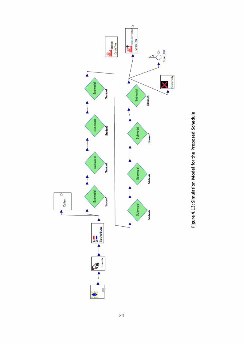
83

84

85

86

87
Figure 4.14: Detailed Process Model for the Proposed Schedule

88
The same sample job, consisting of 50 modules, was loaded into the entity
element in the simulation model. The model was run and the time required to produce
all of the 50 modules was recorded in the simulation model. Figure 4.12 describes the
simulation output which was cycle time. Based on the eight working hours in a day,
the average cycle time in the simulation model of new system was 31.5 days. The
maximum cycle time was 56.9 working days. The recorded data were extracted from
the simulation database and analyzed using EasyFit. The cycle time distribution is
given in Figure 4.15.
Figure 4.15: Cycle Time Distribution of the Simulation Model of the Proposed
Schedule
4.4.3 Validation and Discussion
To validate the output of the old and new simulation models, the cycle time of
the two systems at a certain amount of units produced were compared. The working
hour is 8 hours in a day. The average cycle time of the new system, 31.53 working
days, was shorter than the average cycle time of the old system, 33.85 working days.
The average productivity of the new system, 1.58 module per working day, was better

89
than the average productivity of the old system, 1.47 module per working day. Table
4.4 summarizes the output of the simulation models. There was a difference in the
average cycle time of up to 2.33 days between the two systems. The cycle time
distribution of the old system was slightly more scattered. The cycle time distribution
of the new system was more convergent. The likelihood of a cycle time of about 2
days was higher in the old system than in the new system. It was concluded that the
old system had higher variability in producing modules on the production line.
Therefore, the new schedule based on lean production was accepted as more effective
than the old system. However, the cycle time calculated by the two simulation models
may be smaller than that in real life. There are a few possible explanation for this,
such as the model did not include certain minor activities such as rework because of
insufficient information.
Old System New System
Maximum 59.59 56.92
Mean 33.8 31.53
Minimum 7.43 6.34
Std. Deviation 15.35 14.86
Productivity 1.47 1.58
Table 4.4: Compare with Outputs of the Original and Proposed Simulation
Models
The simulation approach is an effective quantitative tool for testing multiple
scenarios. There are thirty-four tasks in the production line. The researcher analyzed
which subtasks could reduce the cycle time for future strategies. The sensitivity
analysis was done based on the new model of the production line. The most sensitive
tasks of cycle time on the production process were the erection task in Station 1,
described in Figure 4.16, the grounding holes task in Station 5, described in Figure

90
4.20, the hang door task in Station 7, described in Figure 4.21, and the final check and
ship loose task in Station 8, described in Figure 4.22. These tasks strongly affected the
increase or decrease of cycle time of the production line. The exterior J-channel for
sheetrock task in Station 2 and paint door frame task in Station 5 should also be
improved for cycle time reduction. The results of the sensitivity analysis for these
tasks are shown in Figure 4.17 and Figure 4.19, respectively. The drywall exterior task
in Station 2, shown in Figure 4.18, also influenced the cycle time reduction.
Figure 4.16: Sensitivity Analysis of the Erection of the Prefabricated Panels
Figure 4.17: Sensitivity Analysis of Exterior J-Channel

91
Figure 4.18: Sensitivity Analysis of Drywall Exterior
Figure 4.19: Sensitivity Analysis of Paint Door Frame
Figure 4.20: Sensitivity Analysis of Grounding Holes

92
Figure 4.21: Sensitivity Analysis of Hang Doors
Figure 4.22: Sensitivity Analysis of Final Check and Ship Loose
4.5 Developing the Virtual Reality Model
As explained in Chapter 3, there are two issues in implementing the 3D
visualization in this research. First, there is data transformation between the
simulation and the visualization. The process time for each task in the stations was
generated in the simulation model and automatically stored in Microsoft Access 2007
using Collect element in Simphony. The Access file was linked to Microsoft Excel

93
2007 to generate the ASCII file consisted of identification number, start and finish
time of tasks. This file is to efficiently convey the information in simulation to
visualization because it is the only accepted form to import external data into 3D
Studio Max (3DS). The second issue was the time distribution plan to smoothly
animate 3D objects such as operators and material. To smoothly animate 3D objects,
three activities, delivery to destination location, installation, and movement to source
location, were required. Each activity also included sub-activities, where operators
walked between designated points, called sub-activity frames on the timeline in 3DS.
A S.A.C. (Simulation-Animation Controller), shown in Figure 4.30, was buit by
coding 3D Studio Max’s scripting language called Maxscript. It is a built-in language
tool to automate repetitive tasks, to combine existing functionality in new ways, and
to develop user interfaces in 3D Studio Max. The S.A.C. can help users to easily
control and automatically reset the animation key frames of 3D objects.
The “import input data” box is used to load an ASCII file into the 3D
visualization model. The “set” box defines the animation key frames of the 3D objects
based on the ASCII file. The animation key frames generally define on the timeline by
hand. However, the animation key frames in this research should be automatically
defined when the time data in the ASCII file is changed because problems may be
identified and then, the start and finish time of tasks in the proposed schedule may be
changed to remove the problems. Otherwise, time consuming is occurred to define the
animation key frames again. Therefore, based on the proposed schedule, the ASCII
file, and the time distribution plan of tasks described in section 3.8, the coding of
animation of 3D objects which defines animation key frames was implemented in
Maxscript so that the “set” box makes possible to automatically reset the animation
key frames of 3D objects when the time data in the ASCII file is changed. For
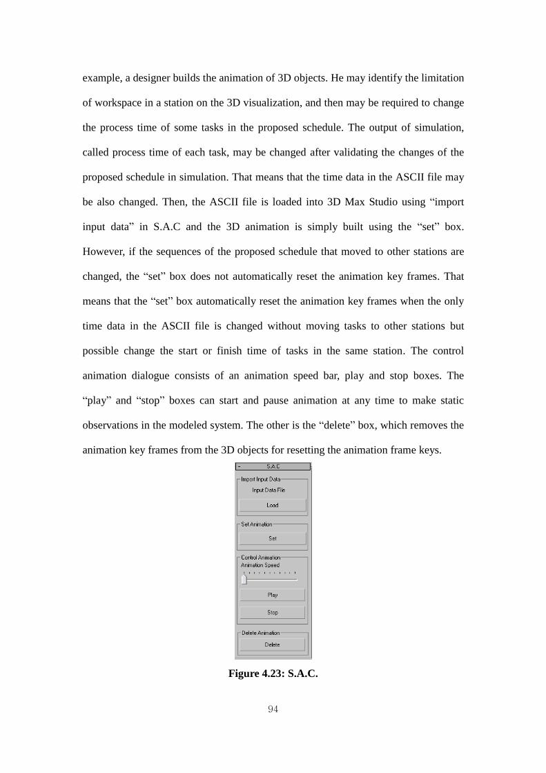
94
example, a designer builds the animation of 3D objects. He may identify the limitation
of workspace in a station on the 3D visualization, and then may be required to change
the process time of some tasks in the proposed schedule. The output of simulation,
called process time of each task, may be changed after validating the changes of the
proposed schedule in simulation. That means that the time data in the ASCII file may
be also changed. Then, the ASCII file is loaded into 3D Max Studio using “import
input data” in S.A.C and the 3D animation is simply built using the “set” box.
However, if the sequences of the proposed schedule that moved to other stations are
changed, the “set” box does not automatically reset the animation key frames. That
means that the “set” box automatically reset the animation key frames when the only
time data in the ASCII file is changed without moving tasks to other stations but
possible change the start or finish time of tasks in the same station. The control
animation dialogue consists of an animation speed bar, play and stop boxes. The
“play” and “stop” boxes can start and pause animation at any time to make static
observations in the modeled system. The other is the “delete” box, which removes the
animation key frames from the 3D objects for resetting the animation frame keys.
Figure 4.23: S.A.C.

95
4.5.1 Station 1
The equipment required to install a module in Station 1 was a crane to deliver
the material to destination location. The sequence of installation was base, wheel,
party wall, front, right, left, and rear studs and roof. Based on the three activities such
as delivery to destination location, installation, and movement back to source location,
some sub-activities were generated for smooth animation when the crane was
operated in Station 1. The sub-activities of the crane can explain that the crane was
moved to source location, lifted the stud up, moved to the destination location for
installation, placed the stud down in the final location, and move back to source. That
was one cycle to operate the crane. It was continuously animated until finishing the
installation of the stud. Each sub-activity was defined between sub-activity frames. To
calculate the sub-activity frame, the process time of each task and number of key
frames were required. An ASCII file including process time of tasks was imported in
3DS. The sub-activity frames can be easily calculated in the Maxscript of 3DS if users
know the number of key frames required for smooth animation. The number of key
frames required for erection was 322 frames and the process time was 305.05 minutes
from the ASCII file. Therefore, the sub-activity frame was 28.4. To build animation to
install the base using the crane, the crane was moving to source location between 0
and 28.4 frames, lifting between 28.4 and 56.8 frames, moving to the destination
location between 56.8 and 113.6 frames, and placing it between 113.6 and 227.2
frames, and moving back to source between 227.2 and 255.6 frames. Based on these
steps, the coding of animation for station 1 was implemented in Maxscript. Figure
4.23 describes 3D scheduling related and the animation snapshot of Station 1. 3D
scheduling helps users to easily understand the state of Station 1 which is percentage
of installation completed.
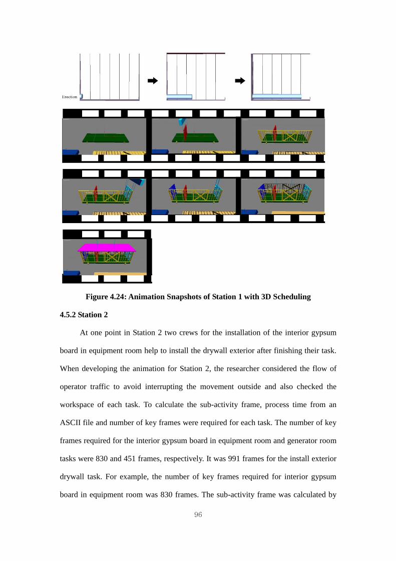
96
Figure 4.24: Animation Snapshots of Station 1 with 3D Scheduling
4.5.2 Station 2
At one point in Station 2 two crews for the installation of the interior gypsum
board in equipment room help to install the drywall exterior after finishing their task.
When developing the animation for Station 2, the researcher considered the flow of
operator traffic to avoid interrupting the movement outside and also checked the
workspace of each task. To calculate the sub-activity frame, process time from an
ASCII file and number of key frames were required for each task. The number of key
frames required for the interior gypsum board in equipment room and generator room
tasks were 830 and 451 frames, respectively. It was 991 frames for the install exterior
drywall task. For example, the number of key frames required for interior gypsum
board in equipment room was 830 frames. The sub-activity frame was calculated by

97
process time from the ASCII file multiplied by 30 and divided by 830 frames. The
sub-activity frame was 11.1 frame. One sub-activity for one step animation of a
operator was animated between 0 and 11.1 frames. Second step animation of the
operator was animated between 11.1 and 22.2 frames. Based on these steps, the
animation for interior gypsum boards in equipment room was built by coding in
Maxscript. The cooperation of operators and work space could not be identified in a
simulation model but possible in a visualization model. There were no problems
identified in this animation based on the work space, cooperation of operators, and
traffic line of operators. Therefore, the sequences of tasks in Station 2 were accepted.
Figure 4.24 shows animation snapshots of Station 2 with 3D scheduling.
Figure 4.25: Animation Snapshots of Station 2 with 3D Scheduling

98
4.5.3 Station 3
The construction sequence of the FRP and plywood task was right wall,
concurrently rear and front walls, and then party wall. After the FRP and plywood task
was completely installed on one of the walls, one operator using a ladder installed the
wireway over the FRP. Ceiling, light, and uni-strut were also installed concurrently if
work space was available. The number of key frames for FRP and plywood, ceiling,
light and uni-strut, and wireway tasks was 800 frames each. The sub-activity frame
was calculated by the process time from the ASCII file and the number of key frames.
The FRP and plywood, ceiling, lights and uni-strut, and wireway tasks were carried
out in the equipment room with five operators for similar time. The important things
were to identify traffic line of operators and work space of tasks in the animation but
impossible in a simulation model. The sequences of tasks in Station 3 were accepted
because there were no problems identified in animation based on the work space and
traffic line of operators. Figure 4.25 presents animation snapshots of Station 3.
Figure 4.26: Animation Snapshots of Station 3 with 3D scheduling

99
4.5.4 Station 4
The sequence of the stenni task was front, right, rear, and left wall. The process
time of tasks in Station 4 was from an ASCII file. The number of key frames for
stenni; rough conduit and panel in equipment room and generator room; and start
grounding tasks was 950, 500 for the equipment room, 250 for the generator room,
and 240 frames, respectively. Therefore, the sub-activity frame was calculated in
Maxscript. The four tasks at Station 4, stenni, rough conduit and panel in equipment
room and generator room, and start grounding were worked on concurrently.
Therefore, the work space of tasks and traffic line of operators should be identified
outside and inside of a module in the animation. As results, any problems, base on
limitation of work space and traffic line of operators, were not identified so, the
proposed processes of tasks were accepted. Figure 4.26 shows the animation of each
task with 3D scheduling. The 3D scheduling with 3D visualization can be substantial
help in communicating the simulation results to domain experts.
Figure 4.27: Animation Snapshots of Station 4 with 3D scheduling

100
4.5.5 Station 5, Station 6, and Station 7
At Station 5, two operators using a lift installed A/C units on the right wall of a
module. The number of key frames for the A/C units, louvers and cable ports, and
roof termination tasks in Station 5 was 205, 210, and 215 frames, respectively. Figure
4.27 shows the animation of the tasks in Station 5. The almost of tasks in Station 5
were worked on concurrently. The work space and traffic line of operators should be
identified outside and inside of a module in the animation. Based on them, any
problems in Station 5 were not identified in the animation. The cable tray task in
Station 6, shown in Figure 4.28, was installed by an operator using a ladder. The
number of key frames for this task was 253. The operation of the VCT, hang doors,
and finish grounding tasks in Station 7 is shown in Figure 4.29. The number of key
frames was 220 for the finish grounding task, 243 for installation of VCT, and 274 for
installation of doors. The transfer key frames between stations were 300 frames. The
work space and traffic line of operators in Station 7 were also identified. There were
no problems based on the work space and traffic line of operators in Station 7.
Therefore, the proposed processes of tasks in Station 5, Station 6, and Station 7 were
worked on well.
Figure 4.28: Animation Snapshots of Station 5 with 3D Scheduling

101
Figure 4.29: Animation Snapshots of Station 6 with 3D Scheduling
Figure 4.30: Animation Snapshots of Station 7 with 3D Scheduling
Based on the work space, traffic line of operators, logic of proposed schedule,
and cooperation of operators in the visualization model, any problems were not
identified in the whole stations of the proposed schedule. That means that the
proposed schedule is worked on well and can be adjusted to a real production line. If
102
problems are identified in the visualization, the proposed schedule should be
improved using lean production, validated in simulation, and visualization would be
built again to reduce rework, cost, and time before implementing the proposed
schedule in a real production line.
4.6 Conclusion
The KBC manufactured production line was used as a case study to validate
the effectiveness of the proposed methodology and to illustrate the essential features
of the developed models. Lean production was implemented for improvement of the
production process. Two disciplines of lean production, “continuous flow” and “takt
time,” were used. After developing the proposed production process, a simulation
approach was implemented to validate the output of lean production. It was used to
validate the improvement of cycle time and productivity by comparing the output of
the original system and the proposed system. Simulation can be used to establish
future strategies by experimenting with various scenarios. Based on the results of
simulation and lean production, a 3D visualization using Maxscript was implemented
in 3D Studio Max. This chapter described that the ASCII file makes possible to link
between simulation and visualization to share required information. Based on the
proposed schedule, the ASCII file, and the time distribution plan for animation, the
animation key frames was defined using coding in Maxscript so that animation could
be automatically rebuilt when the time data in the ASCII file is changed.
The research demonstrated that the combination of simulation and 3D
visualization can assist project managers understand a proposed production process.
The project manager can also use this system to experiment the proposed processes of
the production line to reduce rework, cost, and time before implementing the
103
proposition in the real world. Animation can be used to predict possible spatial
interference of crews and identify limited space, making it possible to decide whether
or not the sequences of tasks can work well. Thus, the visualization ensures the
validity of the simulation results. One of different points between the simulation and
visualization models is workspace. For example, the eight workers required in Station
5 work concurrently in the equipment room. Traffic problems may occur. Therefore,
users must identify the workspace and spatial interference of the workers in the room.
The visualization model clearly shows whether or not there is enough workspace to
work concurrently. The space components such as workspace and operators’
movement cannot be shown using the simulation model alone. For example, five
operators in Station 3 worked on in the same place for the similar time. It is possible
that there is limitation work space to work on together. This work space could not be
identified in a simulation model but it was identified in the animation and then, there
were no any problems about the work space, cooperation of operators, and the traffic
line of operators in the proposed process of a case study. Even though there was no
problems that the work space, cooperation of operators, traffic line of operators were
identified on the proposed production processes in the 3D visualization, it gives
project managers opportunities to improve the proposed production process if
problems are identified before implementing the proposed production process in a real
world. The dynamic graphical depiction in 3D visualization with a 3D schedule
provides decision makers detailed information such as the state of each task at a
specific time, and clearly communicates the results of the simulation model. It also
contributes to make easier understanding of the project sequence.

104
Chapter 5
CONCLUSION
5.1 General Conclusion
This thesis described a methodology to improve productivity and to reduce the
cycle time in the manufactured production line by using various disciplines, which
were lean, simulation, and visualization. This research has focused on the sequence of
a production process to improve productivity and reduce cycle time in a manufactured
production line. A case study of a manufactured production process was conducted
based on the proposed methodology. Value Stream Mapping (VSM), as a tool of lean
production, was used to develop the schedule in the manufactured production line.
Simulation models based on the original and proposed schedules were built using
Collect element and common template in Simphony. The Collect element was built to
automatically extract and save the output of the simulation into Microsoft Access
2007. The Access file was connected to Microsoft Excel 2007 and an ASCII file,
consisted of identification number and process time of tasks, was manually generated
from an excel file. Simulation has proven a useful tool for validation rather than
directly applying the result of lean production to a real production line. Therefore, the
cycle time statistic in two simulation models was compared to identify for
improvement of productivity and cycle time. If the cycle time and productivity are not
improved in simulation, the proposed schedule should be improved using lean
production again. In the case study, the improvement of productivity and reduction of
cycle time of the production line were identified. Based on the ASCII file and the
proposed schedule, a 3D visualization model in 3D Studio Max was experimented to

105
verify the proposed schedule based on the logic of the proposed schedule, work space,
cooperation of operators, and traffic line of operators before implementing the
proposed schedule to a real production line. If some problems such as work space and
traffic line of operators are identified in the visualization, the proposed schedule
should be developed again. If the proposed schedule is rebuilt, rework and time
consuming are occurred to develop the 3D visualization because the visualization
model are already built once. Therefore, the visualization model should be
automatically rebuilt when the process time of tasks are changed. The S.A.C
(Simulation-Animation Controller) developed using Maxscript helps to automatically
reset animation for the similar proposed schedule without rework and time consuming.
Figure 5.1 describes the flow of the proposed methodology. The 3D visualization has
shown that it can provide decision makers, managers, and workers with detailed
information and clear communication about the proposed schedule related to logic of
schedule, limitation of workspace, and consistency in level of detail of schedule
before implementing the proposed schedule to a real production line.

106
Figure 5.1: Flow of the Proposed Methodology
5.2 Research Contribution
The contributions of this research can be summarized as follows:
Efficiently convey the output of simulation into 3D visualization. An ASCII
file is only one accepted file which efficiently transfers external data to 3D
Studio Max as a 3D visualization tool. The Collect element in Simphony is
developed to automatically extracted and saved the output of simulation to a
Microsoft Access file connected to a Microsoft Excel file and then an ASCII
file is manually generated from the excel file.
Based on output of simulation, the visualization processes are automatically
implemented when the proposed schedule is developed again after problems
such as work space, logic of schedule, and traffic line of operators are
identified in the proposed schedule. S.A.C (Simulation-Animation

107
Controller) is developed using coding in Maxscript so that the visualization
model is automatically rebuilt when the output of simulation is changed. The
S.A.C also helps to easily import an ASCII file into 3DS, control the
animation such as animation speed, play, and stop.
A time distribution plan is developed for smooth animation. The animation of
a production line consists of three activities which are delivery, installation,
and movement back to material location. Each activity also has sub-activities.
The sub-activities except related installation activity are animated based on
the time distribution plan.
In addition, the 3D visualization assists decision makers and managers to better
understand the improvement propositions in their projects. The 3D visualization with
3D scheduling also allows them to identify a consistent level of detail for activities,
omission of activities in schedule, the limitation of workspace, and any problems
related to logic of schedule, traffic line of operators, and cooperation of operators. It
can be a support tool for decision makers to understand project sequences easier and
verify the proposed schedule before applying the proposed schedule to a real world.
The 3D visualization model can lead to reduce time consuming, cost and reduce.
5.3 Proposed Future Research
This research proposes a system that implements lean production to generate
propositions for improvement of a production line, simulates the result of lean
production, and designs a 3D visualization model based on results of simulation.
Further expansion of the proposed system includes modification of the methodology
to provide additional functionality. The following is a list of recommendations for

108
future developments:
1. Enhance the existing 3D visualization model to modify the sequences of the
production process. When problems such as work space and traffic line of
operators in a 3D visualization model are found in the proposed schedule and
some subtasks may be required to move to other stations to solve the problems,
the current 3D visualization model does not support to automatically update
the movement of tasks from a station to others but the 3D animation is
automatically modified without movement of tasks when start and finish time
of tasks in the same stations is changed.
2. A limitation of the 3D visualization used in this research is that alternate 3D
objects for different modules of other cases are not supported. The 3D objects
which are components and modules may need to be changed for other cases
because different product modules may be required. To solve this problem,
future researchers should improve the existing system described in this thesis
or develop a new system using different 3D tools.
3. This thesis has focused on the sequence of the production process to improve
productivity and to reduce cycle time. In the 3D visualization model, the
production layout is not described. To develop a more realistic virtual model,
production layout and rework rate should be collected and formalized to
describe more detailed level of 3D visualization.

109
References
AbouRizk S. M. and K. Mather (2000). “Simplifying simulation modeling through
integration with 3D CAD.” Journal of construction engineering and management,
ASCE, Vol. 126, No. 6, 475-483.
AbouRizk, S. M. and Daniel W. Halpin (1990). “Probabilistic Simulation Studies for
Repetitive Construction Processes” Journal of Construction Engineering and
Management, ASCE, Vol.116, 575-594.
AbouRizk, S. M. (1992). “A Stochastic Bidding Game for Construction
Management.” In Second Canadian Conference on Computing in Civil Engineering,
CSCE, Ottawa, Ontario, 576-587.
AbouRizk, S. M. and Daniel W. Halpin (1994). “Fitting Beta Distributions based on
Sample Data.” Journal of Construction Engineering and Management, ASCE, Vol.120,
288-305.
Akinci Burcu, Martin Fischer, and John Kunz (2002). “Automated Generation of
Work Spaces Required by Construction Activities.” Journal of Construction
Engineering and Management, ASCE, Vol. 128, No. 4, 3006-3015.
Al-Hussein Mohamed, Muhammad Athar Niaz, Haitao Yu, and Hyoungkwan Kim
(2005). “Integrating 3D visualization and simulation for tower crane operations on
construction site.” Automation in Construction 15, ELSEVIER ,pp 554-562.

110
Au, Y. Bostleman, R. and Parti, E. (1969). “Construction Management Game
Deterministic Model.” Journal of the Construction Division, ASCE, Vol. 95, 25-38.
Banks, Jerry (1998). “Handbook of simulation: principles, methodology, advances,
applications, and practice.” John Wiley & Sons, New York.
Borcherding, John D. (1977). “Cost Control Simulation and Decision Making.”
Journal of the Construction Division, ASCE, Vol. 103, No. 4, 577-591.
Beliveau, Y., Dal, T. and Dixit, S. (1993). “CAD applications for material handling in
the construction environment.” 5th
International Conference of Computing in Civil
Engineering, ASCE, 125-128.
Hajjar, D. and AbouRizk, S.M. (1996). “Building a Special Purpose Simulation Tool
for Earth Moving Operations.” Proceedings of the 1996 Winter Simulation
Conference, San Diego, CA, 1313-1320.
Hajjar, D. and AbouRizk, S.M. (1999). “Simphony: An Environment for Building
Special Purpose Construction Simulation Tools.” Proceedings of the 1999 Winter
Simulation Conference, Phoenix, AX, 998-1006.
Halpin, D. W. (1977). “CYCLONE: Method for modeling of Job Site Processes.”
Journal of the Construction Division, ASCE, Vol. 103, No3, 489-499.

111
Halpin, D. W. (1973). “An investigation of the use of simulation networks for
modeling construction operations.” PhD thesis, University of Illinois, USA.
Halpin, D. W., and Woodhead, R. W. (1973). “Constructo – A Heuristic Game for
Construction Management.” University of Illinois Press, Champaign, Illinois.
Halpin, D. W., and Kueckmann, M. (2002). “Lean Construction and Simulation.”
Proceedings of 2002 Winter Simulation Conference, ed. Enver Yucesan, Chun-Hung
Chen, Jane L. Snowdon, and John M. Charnes, SanDiego, California, Vol. 2, 1697-
1703.
Hammad Ayman Abu, O. Senghore, Makarand Hastak, and Matt Syal (2004).
“Simulation Model for Manufactured housing Processes.” Journal of computing in
civil engineering, ASCE, Vol. 22, No. 3, 286-297.
Hammad Ayman Abu (2003). “A Decision Support System for Manufactured Housing
Production Process Planning and Facility Layout.” PhD thesis, Dept of Civil and
Environmental Engineering, University of Cincinnati.
Howell, G. A. (1999). “What is the lean construction.” Proceedings seventh Annual
Conference of the International Group for Lean Construction, IGLC-7, Berkeley, CA,
1-10.

112
Huang, R, Grigoriadis, A.M., and Halpin, D.W. (1994). “Simulation of Cable-Stayed
Bridges Using DISCO.” Proceedings of the Winter Simulation Conference, Orlando,
FL, 1130-1136.
Ikovenko, S. (2004). “TRIZ as a lean thinking tool.” ETRIA TRIZ Future conference,
Florence, Italy, 157-164.
Jeong J. (2003). “Supply Chain Analysis and Simulation Modeling of the
Manufactured housing Industry.” MS thesis, Dept of Construction Management,
Purdue University.
Kamat Vineet R. and Julio C. Martinez (2001). “Visualizing simulated construction
operations in 3D.” Journal of computing in civil engineering, ASCE, Vol. 15, No. 4,
329-337.
Koo Bonsang and Martin Fischer (2000). “Feasibility Study of 4D CAD in
commercial construction.” Journal of construction engineering and management,
ASCE, Vol. 126, No. 4, 251-260.
Koskela, L. (2000). “An Exploration Towards a production theory and its Application
to Construction.” Technical Research Centre of Finland, Helsinki University of
Technology, Espoo, Finland.
113
Lian, Y-H. and Van L. H. (2002). “An Application of Simulation and Value Stream
Mapping in Lean Manufacturing.” Proceedings of the 14th
European Simulation
Symposium, ESS2002. Dresden, Germany, SCS.
Liu, L. Y. (1991). “COOPS Construction Object-Oriented Process Simulation
System.” Ph.D. Dissertation, Dept. of Civil & Environment Engineering, University
of Michigan.
Martinez. J. C. and Ioannou. P. G. (1994). “General Purpose Simulation with
Stroboscope.” Proceedings of the 1994 Winter Simulation Conference, Orlando, FL,
1159-1166.
Manrique Juan D., Mohamed Al-Hussein, Avi Telyas, and Geoff Funston (2007).
“Constructing a Completes Precast Tilt-up-Panel Structure Utilizing and Optimization
Model, 3D CAD, and Animation.” Journal of Construction Engineering and
Management, ASCE, Vol. 133, No.3, 199-207.
Modular Building Institute (2007). “Commercial Modular Construction Report.”
Modular Building Institute, Virginia, USA.
Modular Building Institute (2008). “Commercial Modular Construction Report.”
Modular Building Institute, Virginia, USA.

114
Modular Building Institute (2009). “Commercial Modular Construction Report.”
Modular Building Institute, Virginia, USA.
Nasereddin Mahdi, Michael A. Mullens, and Dayana Cope (2007). “Automated
simulator development: A strategy for modeling modular housing production.”
Automation in construction 16, ELSEVIER, 212-223.
Nash Mark A. and Sheila R. Poling (2008). “Mapping the Total Value Stream.” Taylor
& Francis Group, NY, USA.
NSERC/Alberta Construction Industry Research Chair (2000). “Simphony User’s
Guide.” Edmonton, Alberta, Canada.
Pasqualini Fernanda, and Paulo, A. Zawislak (2005). “Value Stream Mapping in
Construction: A Case study in a Brazilian Construction Company.” Proceedings
thirteenth Annual Conference of the International Group for Lean Construction,
IGLC-13, Sydney, Australia, 117-125.
Paulson, B.C. Jr., Chan, W.T., and Koo, C.C. (1987). “Construction Operation
Simulation by Microcomputer.” Journal of Construction Engineering and
Management, ASCE, Vol. 113, No. 2, 302-314.
Pritsker, A.A.B (1986), “Introduction to Simlation and SLAM II: Networks for
decision Support”, , Prentice Hall, Englewoods Cliffs, New Jersey.

115
Pritsker, A.A.B., O’Reilly, J.J, and LaVal, D.K. (1997). “Simulation with visual Slam
and Awesim.” John Wiley & Sons, New York, US.
Roberto J. Arbulu and Iris D. Tommelein (2002), “Value Stream Analysis of
Construction Supply Chains: Case Study on Pipe Supports used in Power Plants”,
Proceedings Tenth Annual Conference of the International Group for Lean
Construction, IGLC-10,Gramada, Brazil, 183-195.
Rother, M. and Shook, J. (1998). “Learning to see: value stream mapping to create
value and eliminate muda.” The Lean enterprise Institute, Brookline, Massachusetts,
USA,96.
Sabharwal Abhi (2004). “Manufactured Housing Components Assembly Redesign
Process and Its Impact on Production Process and Facility Layout.” MS thesis,
Construction Management Program, Michigan State University.
Stub-French Sheryl, Alan Russell, and Ngoc Tran (2008). “Linear Scheduling and 4D
Visualization.” Journal of computing in civil engineering, ASCE, Vol. 22, No. 3, 192-
205.
Senghore O. (2001). “Production and Material Flow Process Model for Manufactured
Housing.” MS Thesis, Construction Management Program, Michigan State University.

116
Wang Ping, Tasser Mohamed, Simaan M. Abourizk, and R. Tony Rawa (2009). “Flow
Production of Pipe Spool Fabrication: Simulation to Support Implementation of Lean
Technique.” Journal of Construction Engineering and Management, ASCE, Vol. 135,
No. 10, 1027-1038.
Yu Haitao, M. Al-Hussein and A. Telyas (2008). “Lean Implementation for Building
Modular Production.” CSCE 2008 Annual Conference, QC, Canada.
Yu Haitao, Tarry Tweed, Mohamed Al-Hussein, and Reza Nasseri (2009).
“Development of Lean Model for House Construction Using Value Stream Mapping.”
Journal of Construction Engineering and Management, ASCE, Vol. 135, No. 8, 782-
790.

117
APPENDIX
System Manual for automated Visualization Process for a Modular
Building Assembly Line
This system manual shows how to develop a visualization model using
Maxscript in 3D Sudio Max from the results of simulation. To build the visualization
model, the proposed schedule and process time of tasks used in a simulation model
are required. The proposed schedule is from lean production. The process time of
tasks is from simulation. Therefore, the process time of tasks should be automatically
extracted and saved to an external file. An ASCII file as an external file is only
accepted in Maxscript. In a simulation model, the Collect element was developed in
Simphony. It automatically extracts and saves the process time of tasks used in
simulation to an access file. The ASCII file is manually generated from an excel file
connected to the access file. Based on the proposed schedule and the process time of
tasks from the access file, the start time and finish time are calculated in the excel file.
The ASCII file consists of identification number, start time, and finish time of tasks.
The names of tasks should be defined as identification number because the Maxscript
cannot read texts.

118
3D objects are built in AutoCad based on the component’s specification. The
cad file is imported into 3DS. The names of 3D objects are separately defined for
smooth animation. To easily import the ASCII file as input parameters in 3DS, S.A.C
(Simulation-Animation Controller) is built using Maxscript before building animation.
The “load” makes possible to fine out the ASCII file wherever it is in a computer. The
“Set animation” helps to rebuilt animation when the time data from simulation is
changed. The codes for S.A.C in Maxscript describes below. The Maxscript reference
is located in 3DS if users would like to study more.
utility SimAniVisual "Simulation-Animation Controller"
( rollout Simanimation "S.A.C" width:162 height:400
(
button btn1 "Load" pos:[9,61] width:142 height:26 label lbl1 "Input Data File" pos:[37,35] width:84 height:16
groupBox grp3 "Control Animation" pos:[5,177] width:150 height:148
button btn2 "Play" pos:[11,250] width:138 height:26 enabled:true button btn3 "Stop" pos:[11,287] width:138 height:26
groupBox grp5 "Import Input Data" pos:[5,12] width:150 height:84
slider slider1 "Animation Speed" pos:[13,193] width:134 height:44 range:[0,4,0] groupBox grp6 "Delete Animation" pos:[6,336] width:150 height:54
button btn5 "Delete" pos:[11,355] width:138 height:26
groupBox grp28 "Set Animation" pos:[5,107] width:150 height:62 button btn35 "Set" pos:[9,131] width:142 height:26
on btn1 pressed do
(
filein "Getvalues.ms" )
on btn2 pressed do (
playanimation()
)
on btn3 pressed do
( stopanimation()
)
on slider1 changed val do
(
)
on slider1 buttondown do (
)
on slider1 buttonup do
(
)
on btn5 pressed do
(
filein "deletekeys for crane with station1.ms"

119
)
on btn35 pressed do (
filein "final station1_1.ms"
filein "final station2_Egypsumboard.ms"
filein "final station2_Ggypsumboard.ms"
filein "final station2_Gceiling.ms" filein "final station2_extboard.ms"
filein "set station2.ms"
filein "final station3 for FRP and plywood.ms"
filein "final station3 for wireway.ms"
filein "final station3 for ceiling.ms" filein "set station3.ms"
filein "final station4 for stenni.ms" filein "final station4 for Econduit.ms"
filein "final station4 for Gconduit.ms"
filein "final station4 for grounding.ms" filein "set station4.ms"
filein "final station5 for AC.ms" filein "final station5 for EPDM.ms"
filein "final station5 for louver.ms"
filein "set station5.ms"
filein "final station6 for cable.ms"
filein "set station6.ms"
filein "final station7 for VCT.ms"
filein "final station7 for finish grounding.ms" filein "final station7 for door.ms"
filein "set station7.ms"
filein "set station8.ms"
--second
filein "final station1_2.ms"
filein "final station2_Egypsumboard_1.ms"
filein "final station2_Ggypsumboard_1.ms"
filein "final station2_Gceiling_1.ms" filein "final station2_extboard_1.ms"
filein "set station2_1.ms"
filein "final station3 for FRP and plywood_1.ms"
filein "final station3 for wireway_1.ms"
filein "final station3 for ceiling_1.ms" filein "set station3_1.ms"
filein "final station4 for stenni_1.ms"
filein "final station4 for Econduit_1.ms"
filein "final station4 for Gconduit_1.ms" filein "final station4 for grounding_1.ms"
filein "set station4_1.ms"
filein "final station5 for AC_1.ms"
filein "final station5 for EPDM_1.ms"
filein "final station5 for louver_1.ms" filein "set station5_1.ms"
filein "final station6 for cable_1.ms" filein "set station6_1.ms"
filein "final station7 for VCT_1.ms" filein "final station7 for finish grounding_1.ms"
filein "final station7 for door_1.ms"
--third cycle
filein "final station1_3.ms"
filein "final station2_Egypsumboard_2.ms"

120
filein "final station2_Ggypsumboard_2.ms"
filein "final station2_Gceiling_2.ms" filein "final station2_extboard_2.ms"
filein "set station2_2.ms"
filein "final station3 for FRP and plywood_1_2.ms"
filein "final station3 for wireway_2.ms"
filein "final station3 for ceiling_2.ms" filein "set station3_2.ms"
filein "final station4 for stenni_2.ms" filein "final station4 for Econduit_2.ms"
filein "final station4 for Gconduit_2.ms"
filein "final station4 for grounding_2.ms" filein "set station4_2.ms"
filein "final station5 for AC_2.ms" filein "final station5 for EPDM_2.ms"
filein "final station5 for louver_2.ms"
filein "set station5_2.ms"
filein "final station6 for cable_2.ms"
--four cyle
filein "final station1_4.ms"
filein "final station2_Egypsumboard_3.ms"
filein "final station2_Ggypsumboard_3.ms"
filein "final station2_Gceiling_3.ms" filein "final station2_extboard_3.ms"
filein "set station2_3.ms"
filein "final station3 for FRP and plywood_3.ms"
filein "final station3 for wireway_3.ms"
filein "final station3 for ceiling_3.ms" filein "set station3_3.ms"
filein "final station4 for stenni_3.ms" filein "final station4 for Econduit_3.ms"
filein "final station4 for Gconduit_3.ms"
filein "final station4 for grounding_3.ms" filein "set station4_3.ms"
filein "final station5 for AC_3.ms" filein "final station5 for EPDM_3.ms"
filein "final station5 for louver_3.ms"
--five clcle
filein "final station1_5.ms"
filein "final station2_Egypsumboard_4.ms"
filein "final station2_Ggypsumboard_4.ms"
filein "final station2_Gceiling_4.ms" filein "final station2_extboard_4.ms"
filein "set station2_4.ms"
filein "final station3 for FRP and plywood_4.ms"
filein "final station3 for wireway_4.ms"
filein "final station3 for ceiling_4.ms" filein "set station3_4.ms"
filein "final station4 for stenni_4.ms" filein "final station4 for Econduit_4.ms"
filein "final station4 for Gconduit_4.ms"
filein "final station4 for grounding_4.ms"
-- six
filein "final station1_6.ms"
filein "final station2_Egypsumboard_5.ms"
filein "final station2_Ggypsumboard_5.ms" filein "final station2_Gceiling_5.ms"
filein "final station2_extboard_5.ms"
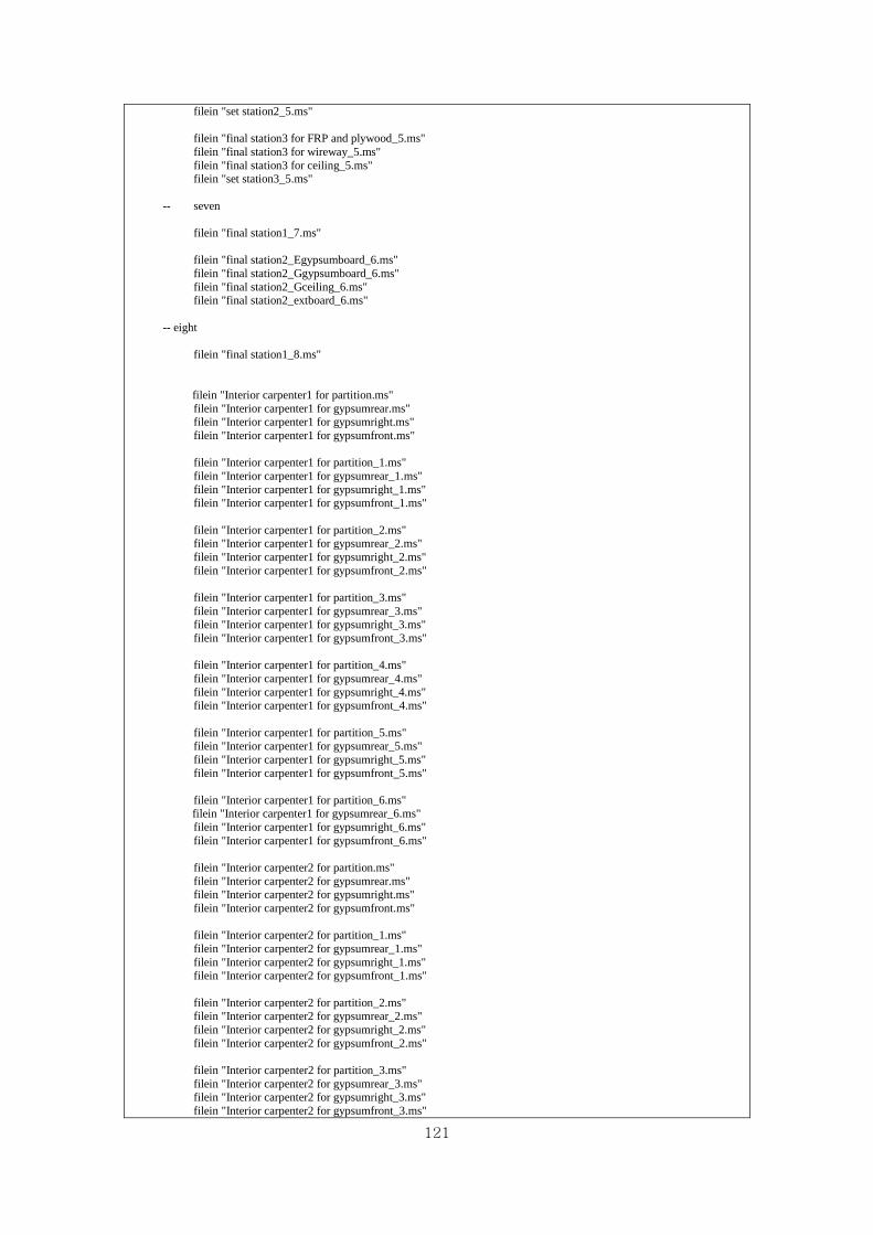
121
filein "set station2_5.ms"
filein "final station3 for FRP and plywood_5.ms"
filein "final station3 for wireway_5.ms"
filein "final station3 for ceiling_5.ms" filein "set station3_5.ms"
-- seven
filein "final station1_7.ms"
filein "final station2_Egypsumboard_6.ms"
filein "final station2_Ggypsumboard_6.ms"
filein "final station2_Gceiling_6.ms" filein "final station2_extboard_6.ms"
-- eight
filein "final station1_8.ms"
filein "Interior carpenter1 for partition.ms"
filein "Interior carpenter1 for gypsumrear.ms" filein "Interior carpenter1 for gypsumright.ms"
filein "Interior carpenter1 for gypsumfront.ms"
filein "Interior carpenter1 for partition_1.ms"
filein "Interior carpenter1 for gypsumrear_1.ms"
filein "Interior carpenter1 for gypsumright_1.ms" filein "Interior carpenter1 for gypsumfront_1.ms"
filein "Interior carpenter1 for partition_2.ms" filein "Interior carpenter1 for gypsumrear_2.ms"
filein "Interior carpenter1 for gypsumright_2.ms"
filein "Interior carpenter1 for gypsumfront_2.ms"
filein "Interior carpenter1 for partition_3.ms"
filein "Interior carpenter1 for gypsumrear_3.ms" filein "Interior carpenter1 for gypsumright_3.ms"
filein "Interior carpenter1 for gypsumfront_3.ms"
filein "Interior carpenter1 for partition_4.ms"
filein "Interior carpenter1 for gypsumrear_4.ms"
filein "Interior carpenter1 for gypsumright_4.ms" filein "Interior carpenter1 for gypsumfront_4.ms"
filein "Interior carpenter1 for partition_5.ms" filein "Interior carpenter1 for gypsumrear_5.ms"
filein "Interior carpenter1 for gypsumright_5.ms"
filein "Interior carpenter1 for gypsumfront_5.ms"
filein "Interior carpenter1 for partition_6.ms" filein "Interior carpenter1 for gypsumrear_6.ms"
filein "Interior carpenter1 for gypsumright_6.ms"
filein "Interior carpenter1 for gypsumfront_6.ms"
filein "Interior carpenter2 for partition.ms"
filein "Interior carpenter2 for gypsumrear.ms" filein "Interior carpenter2 for gypsumright.ms"
filein "Interior carpenter2 for gypsumfront.ms"
filein "Interior carpenter2 for partition_1.ms"
filein "Interior carpenter2 for gypsumrear_1.ms"
filein "Interior carpenter2 for gypsumright_1.ms" filein "Interior carpenter2 for gypsumfront_1.ms"
filein "Interior carpenter2 for partition_2.ms" filein "Interior carpenter2 for gypsumrear_2.ms"
filein "Interior carpenter2 for gypsumright_2.ms"
filein "Interior carpenter2 for gypsumfront_2.ms"
filein "Interior carpenter2 for partition_3.ms"
filein "Interior carpenter2 for gypsumrear_3.ms" filein "Interior carpenter2 for gypsumright_3.ms"
filein "Interior carpenter2 for gypsumfront_3.ms"

122
filein "Interior carpenter2 for partition_4.ms" filein "Interior carpenter2 for gypsumrear_4.ms"
filein "Interior carpenter2 for gypsumright_4.ms"
filein "Interior carpenter2 for gypsumfront_4.ms"
filein "Interior carpenter2 for partition_5.ms"
filein "Interior carpenter2 for gypsumrear_5.ms" filein "Interior carpenter2 for gypsumright_5.ms"
filein "Interior carpenter2 for gypsumfront_5.ms"
filein "Interior carpenter2 for partition_6.ms"
filein "Interior carpenter2 for gypsumrear_6.ms"
filein "Interior carpenter2 for gypsumright_6.ms" filein "Interior carpenter2 for gypsumfront_6.ms"
filein "Interior carpenter3 for partition.ms" filein "Interior carpenter3 for gypsumrear.ms"
filein "Interior carpenter3 for gypsumleft.ms"
filein "Interior carpenter3 for front.ms"
filein "Interior carpenter3 for partition_1.ms"
filein "Interior carpenter3 for gypsumrear_1.ms" filein "Interior carpenter3 for gypsumleft_1.ms"
filein "Interior carpenter3 for front_1.ms"
filein "Interior carpenter3 for partition_2.ms"
filein "Interior carpenter3 for gypsumrear_2.ms"
filein "Interior carpenter3 for gypsumleft_2.ms" filein "Interior carpenter3 for front_2.ms"
filein "Interior carpenter3 for partition_3.ms" filein "Interior carpenter3 for gypsumrear_3.ms"
filein "Interior carpenter3 for gypsumleft_3.ms"
filein "Interior carpenter3 for front_3.ms"
filein "Interior carpenter3 for partition_4.ms"
filein "Interior carpenter3 for gypsumrear_4.ms" filein "Interior carpenter3 for gypsumleft_4.ms"
filein "Interior carpenter3 for front_4.ms"
filein "Interior carpenter3 for partition_5.ms"
filein "Interior carpenter3 for gypsumrear_5.ms"
filein "Interior carpenter3 for gypsumleft_5.ms" filein "Interior carpenter3 for front_5.ms"
filein "Interior carpenter3 for partition_6.ms" filein "Interior carpenter3 for gypsumrear_6.ms"
filein "Interior carpenter3 for gypsumleft_6.ms"
filein "Interior carpenter3 for front_6.ms"
filein "Interior carpenter4 for partition.ms" filein "Interior carpenter4 for gypsumrear.ms"
filein "Interior carpenter4 for gypsumleft.ms"
filein "Interior carpenter4 for gypsumfront.ms"
filein "Interior carpenter4 for partition_1.ms"
filein "Interior carpenter4 for gypsumrear_1.ms" filein "Interior carpenter4 for gypsumleft_1.ms"
filein "Interior carpenter4 for gypsumfront_1.ms"
filein "Interior carpenter4 for partition_2.ms"
filein "Interior carpenter4 for gypsumrear_2.ms"
filein "Interior carpenter4 for gypsumleft_2.ms" filein "Interior carpenter4 for gypsumfront_2.ms"
filein "Interior carpenter4 for partition_3.ms" filein "Interior carpenter4 for gypsumrear_3.ms"
filein "Interior carpenter4 for gypsumleft_3.ms"
filein "Interior carpenter4 for gypsumfront_3.ms"
filein "Interior carpenter4 for partition_4.ms"
filein "Interior carpenter4 for gypsumrear_4.ms" filein "Interior carpenter4 for gypsumleft_4.ms"
filein "Interior carpenter4 for gypsumfront_4.ms"

123
filein "Interior carpenter4 for partition_5.ms" filein "Interior carpenter4 for gypsumrear_5.ms"
filein "Interior carpenter4 for gypsumleft_5.ms"
filein "Interior carpenter4 for gypsumfront_5.ms"
filein "Interior carpenter4 for partition_6.ms"
filein "Interior carpenter4 for gypsumrear_6.ms" filein "Interior carpenter4 for gypsumleft_6.ms"
filein "Interior carpenter4 for gypsumfront_6.ms"
filein "exterior C6.ms"
filein "exterior C7.ms"
filein "exterior C6_1.ms"
filein "exterior C7_1.ms"
filein "exterior C6_2.ms"
filein "exterior C7_2.ms"
filein "exterior C6_3.ms"
filein "exterior C7_3.ms"
filein "exterior C6_4.ms"
filein "exterior C7_4.ms"
filein "exterior C6_5.ms"
filein "exterior C7_5.ms"
filein "exterior C6_6.ms"
filein "exterior C7_6.ms"
filein "C5 for station3.ms"
filein "C5 for station3_1.ms"
filein "C5 for station3_2.ms" filein "C5 for station3_3.ms"
filein "C5 for station3_4.ms"
filein "C5 for station3_5.ms"
filein "C8 for station3.ms"
filein "C8 for station3_1.ms" filein "C8 for station3_2.ms"
filein "C8 for station3_3.ms"
filein "C8 for station3_4.ms" filein "C8 for station3_5.ms"
filein "C9 for station3.ms" filein "C9 for station3_1.ms"
filein "C9 for station3_2.ms"
filein "C9 for station3_3.ms" filein "C9 for station3_4.ms"
filein "C9 for station3_5.ms"
filein "C10 for station3.ms"
filein "C10 for station3_1.ms" filein "C10 for station3_2.ms"
filein "C10 for station3_3.ms"
filein "C10 for station3_4.ms" filein "C10 for station3_5.ms"
filein "C11 for station3.ms" filein "C11 for station3_1.ms"
filein "C11 for station3_2.ms"
filein "C11 for station3_3.ms" filein "C11 for station3_4.ms"
filein "C11 for station3_5.ms"
--station4
filein "C12 for station4.ms" filein "C12 for station4_1.ms"
filein "C12 for station4_2.ms"
filein "C12 for station4_3.ms" filein "C12 for station4_4.ms"

124
filein "C13 for station4.ms"
filein "C13 for station4_1.ms" filein "C13 for station4_2.ms"
filein "C13 for station4_3.ms"
filein "C13 for station4_4.ms"
filein "C14 for station4.ms"
filein "C14 for station4_1.ms" filein "C14 for station4_2.ms"
filein "C14 for station4_3.ms"
filein "C14 for station4_4.ms"
filein "C15 for station4.ms"
filein "C15 for station4_1.ms" filein "C15 for station4_2.ms"
filein "C15 for station4_3.ms"
filein "C15 for station4_4.ms"
filein "C16 for station4.ms"
filein "C16 for station4_1.ms" filein "C16 for station4_2.ms"
filein "C16 for station4_3.ms"
filein "C16 for station4_4.ms"
filein "C17 for station4.ms"
filein "C17 for station4_1.ms" filein "C17 for station4_2.ms"
filein "C17 for station4_3.ms"
filein "C17 for station4_4.ms"
filein "C18 for station4.ms"
filein "C18 for station4_1.ms" filein "C18 for station4_2.ms"
filein "C18 for station4_3.ms"
filein "C18 for station4_4.ms"
filein "C19 for station4.ms"
filein "C19 for station4_1.ms" filein "C19 for station4_2.ms"
filein "C19 for station4_3.ms"
filein "C19 for station4_4.ms"
filein "C20 for station4.ms"
filein "C20 for station4_1.ms" filein "C20 for station4_2.ms"
filein "C20 for station4_3.ms"
filein "C20 for station4_4.ms"
--station5 workers
filein "C21 for station5.ms"
filein "C21 for station5_1.ms" filein "C21 for station5_2.ms"
filein "C21 for station5_3.ms"
filein "C22 for station5.ms"
filein "C22 for station5_1.ms"
filein "C22 for station5_2.ms" filein "C22 for station5_3.ms"
filein "C23 for station5.ms" filein "C23 for station5_1.ms"
filein "C23 for station5_2.ms"
filein "C23 for station5_3.ms"
filein "C24 for station5.ms"
filein "C24 for station5_1.ms" filein "C24 for station5_2.ms"
filein "C24 for station5_3.ms"
filein "C25 for station5.ms"
filein "C25 for station5_1.ms"
filein "C25 for station5_2.ms" filein "C25 for station5_3.ms"
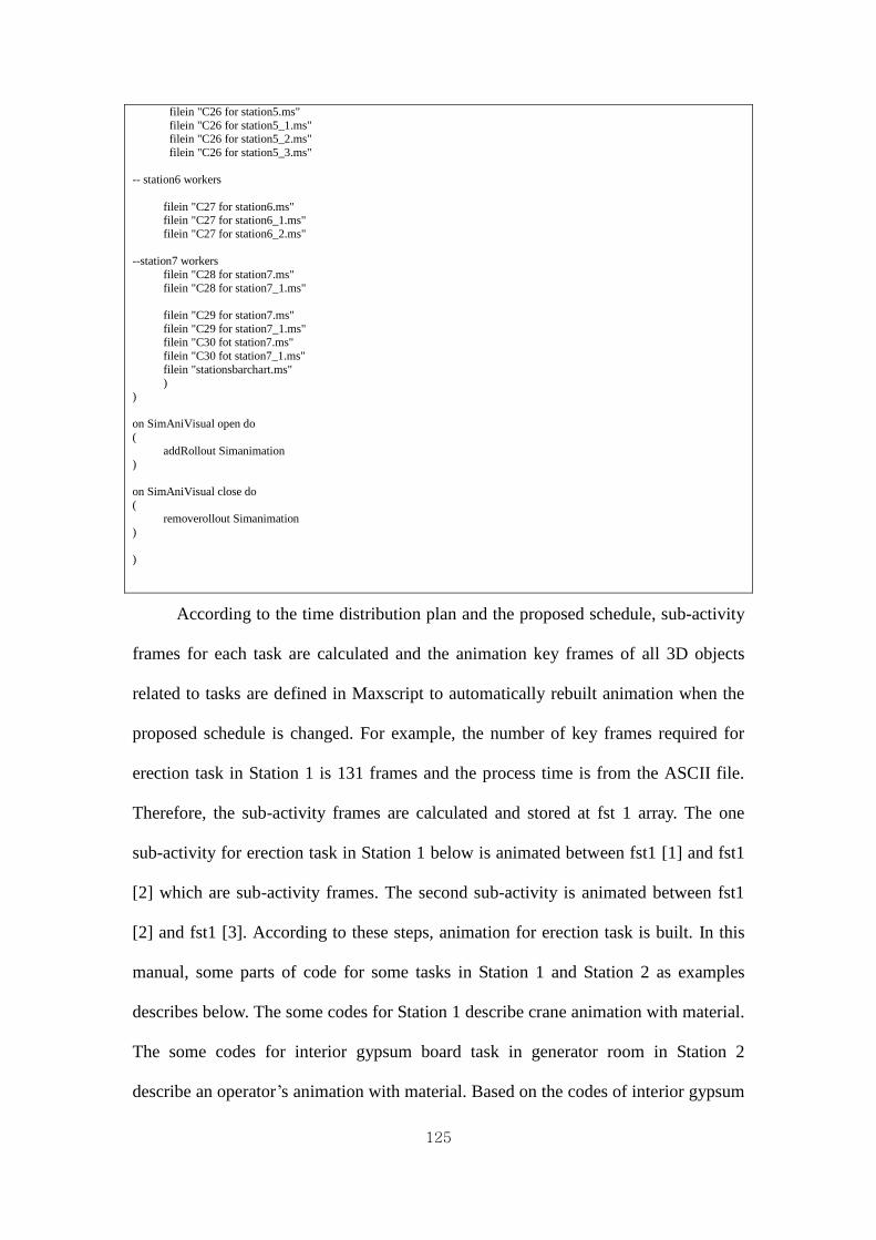
125
filein "C26 for station5.ms"
filein "C26 for station5_1.ms" filein "C26 for station5_2.ms"
filein "C26 for station5_3.ms"
-- station6 workers
filein "C27 for station6.ms" filein "C27 for station6_1.ms"
filein "C27 for station6_2.ms"
--station7 workers
filein "C28 for station7.ms"
filein "C28 for station7_1.ms"
filein "C29 for station7.ms"
filein "C29 for station7_1.ms" filein "C30 fot station7.ms"
filein "C30 fot station7_1.ms"
filein "stationsbarchart.ms" )
)
on SimAniVisual open do
(
addRollout Simanimation )
on SimAniVisual close do (
removerollout Simanimation
)
)
According to the time distribution plan and the proposed schedule, sub-activity
frames for each task are calculated and the animation key frames of all 3D objects
related to tasks are defined in Maxscript to automatically rebuilt animation when the
proposed schedule is changed. For example, the number of key frames required for
erection task in Station 1 is 131 frames and the process time is from the ASCII file.
Therefore, the sub-activity frames are calculated and stored at fst 1 array. The one
sub-activity for erection task in Station 1 below is animated between fst1 [1] and fst1
[2] which are sub-activity frames. The second sub-activity is animated between fst1
[2] and fst1 [3]. According to these steps, animation for erection task is built. In this
manual, some parts of code for some tasks in Station 1 and Station 2 as examples
describes below. The some codes for Station 1 describe crane animation with material.
The some codes for interior gypsum board task in generator room in Station 2
describe an operator’s animation with material. Based on the codes of interior gypsum

126
board in generator room in Station 2, animation for all tasks in stations can be built
using Maxscript. All tasks in stations are continuously working on when modules are
at stations even though they are finished on a modular because modules are
continuously moved between stations until installed all material required. Therefore,
the repetitive works for each station should be animated. The Maxscript helpts users
easily built repetitive animation after only changing the time.
Station 1
station1arr = #($BASE,$PANEL,$Front,$RIGHT,$LEFT,$REAR,$ROOF)
trailerarr = #($wheel,$center,$hookline1,$hookline2,$hook1,$hook) circle50 = #($cirlceframe15,$circle15)
t1_operation = (fi_type1-st_type1)*30 t1_tasktime = t1_operation/131
fst1 = #()
fst1[1] = t1_tasktime for c = 2 to 131 do
(
fst1[c] = fst1[c-1] + t1_tasktime )
movingtime6 = fst1[131] + 299
backtime6 = fst1[131] + 300 animate on
(
at time fst1[1] circle50[1].visibility.controller.value = 0 at time fst1[1] circle50[2].visibility.controller.value = 0
for c1 = 1 to 7 do (
at time fst1[1] station1arr[c1].visibility.controller.value = 0
) for c2 = 1 to 7 do
(
at time fst1[2] station1arr[c2].visibility.controller.value = 1 )
at time fst1[1] rotate stati on1arr[1] (quat 0 x_axis) at time fst1[1] rotate station1arr[1] (quat 0 y_axis)
at time fst1[1] rotate station1arr[1] (quat 0 z_axis)
at time fst1[1] move station1arr[1] [0,0,0]
at time fst1[1] rotate station1arr[2] (quat 0 x_axis)
at time fst1[1] rotate station1arr[2] (quat 0 y_axis) at time fst1[1] rotate station1arr[2] (quat 0 z_axis)
at time fst1[1] move station1arr[2] [0,0,0]
at time fst1[1] rotate station1arr[3] (quat 0 x_axis)
at time fst1[1] rotate station1arr[3] (quat 0 y_axis)
at time fst1[1] rotate station1arr[3] (quat 0 z_axis) at time fst1[1] move station1arr[3] [0,0,0]
at time fst1[1] rotate station1arr[4] (quat 0 x_axis) at time fst1[1] rotate station1arr[4] (quat 0 y_axis)
at time fst1[1] rotate station1arr[4] (quat 0 z_axis)
at time fst1[1] move station1arr[4] [0,0,0]
at time fst1[1] rotate station1arr[5] (quat 0 x_axis)
at time fst1[1] rotate station1arr[5] (quat 0 y_axis) at time fst1[1] rotate station1arr[5] (quat 0 z_axis)
at time fst1[1] move station1arr[5] [0,0,0]

127
at time fst1[1] rotate station1arr[6] (quat 0 x_axis) at time fst1[1] rotate station1arr[6] (quat 0 y_axis)
at time fst1[1] rotate station1arr[6] (quat 0 z_axis)
at time fst1[1] move station1arr[6] [0,0,0]
at time fst1[1] rotate station1arr[7] (quat 0 x_axis)
at time fst1[1] rotate station1arr[7] (quat 0 y_axis) at time fst1[1] rotate station1arr[7] (quat 0 z_axis)
at time fst1[1] move station1arr[7] [0,0,0]
at time fst1[2] rotate station1arr[1] (quat 0 x_axis)
at time fst1[2] rotate station1arr[1] (quat 0 y_axis)
at time fst1[2] rotate station1arr[1] (quat 0 z_axis) at time fst1[2] station1arr[1].pos = [-23.774,-7.64,0.043]
at time fst1[2] rotate station1arr[2] (quat 0 x_axis) at time fst1[2] rotate station1arr[2] (quat 90 y_axis)
at time fst1[2] rotate station1arr[2] (quat 0 z_axis)
at time fst1[2] station1arr[2].pos = [-33.691,-2.349,0.043]
at time fst1[2] rotate station1arr[3] (quat 90 x_axis)
at time fst1[2] rotate station1arr[3] (quat 0 y_axis)
at time fst1[2] rotate station1arr[3] (quat 0 z_axis) at time fst1[2] station1arr[3].pos = [-23.932,2.857,0.078]
at time fst1[2] rotate station1arr[4] (quat 0 x_axis) at time fst1[2] rotate station1arr[4] (quat 90 y_axis)
at time fst1[2] rotate station1arr[4] (quat 0 z_axis)
at time fst1[2] station1arr[4].pos = [-33.854,2.638,0.078]
at time fst1[2] rotate station1arr[5] (quat 0 x_axis)
at time fst1[2] rotate station1arr[5] (quat 90 y_axis) at time fst1[2] rotate station1arr[5] (quat 0 z_axis)
at time fst1[2] station1arr[5].pos = [-33.854,2.638,0.078]
at time fst1[2] rotate station1arr[6] (quat 90 x_axis)
at time fst1[2] rotate station1arr[6] (quat 0 y_axis)
at time fst1[2] rotate station1arr[6] (quat 0 z_axis) at time fst1[2] station1arr[6].pos = [-23.932,2.857,0.078]
at time fst1[2] rotate station1arr[7] (quat 0 x_axis) at time fst1[2] rotate station1arr[7] (quat 0 y_axis)
at time fst1[2] rotate station1arr[7] (quat 0 z_axis)
at time fst1[2] station1arr[7].pos = [-23.778,-2.039,0.075]
--install base
at time fst1[3] rotate trailerarr[1] (quat 0 x_axis)
at time fst1[3] rotate trailerarr[1] (quat 0 y_axis)
at time fst1[3] rotate trailerarr[1] (quat 0 z_axis) at time fst1[3] move trailerarr[1] [20,0,0]
at time fst1[3] rotate trailerarr[2] (quat 0 x_axis)
at time fst1[3] rotate trailerarr[2] (quat 0 y_axis)
at time fst1[3] rotate trailerarr[2] (quat 0 z_axis) at time fst1[3] move trailerarr[2] [20,0,0]
at time fst1[3] rotate trailerarr[3] (quat 0 x_axis) at time fst1[3] rotate trailerarr[3] (quat 0 y_axis)
at time fst1[3] rotate trailerarr[3] (quat 0 z_axis)
at time fst1[3] move trailerarr[3] [20,0,0]
at time fst1[3] rotate trailerarr[4] (quat 0 x_axis)
at time fst1[3] rotate trailerarr[4] (quat 0 y_axis) at time fst1[3] rotate trailerarr[4] (quat 0 z_axis)
at time fst1[3] move trailerarr[4] [20,0,0]
at time fst1[3] rotate trailerarr[5] (quat 0 x_axis)
at time fst1[3] rotate trailerarr[5] (quat 0 y_axis)
at time fst1[3] rotate trailerarr[5] (quat 0 z_axis) at time fst1[3] move trailerarr[5] [20,0,0]

128
at time fst1[3] rotate trailerarr[6] (quat 0 x_axis)
at time fst1[3] rotate trailerarr[6] (quat 0 y_axis) at time fst1[3] rotate trailerarr[6] (quat 0 z_axis)
at time fst1[3] move trailerarr[6] [20,0,0]
2. Station 2 2.1 Interior gypsum boards in Generator Room
2.1.1 3D objects
Gright = #($G_gypsumright1_1,$G_gypsumright1_2,$G_gypsumright1_3,$G_gypsumright1_4,$G_gypsumright1_5) Gright1 = #($G_gypsumright2_1,$G_gypsumright2_2,$G_gypsumright2_3,$G_gypsumright2_4,$G_gypsumright2_5)
Grear = #($G_gypsumrear1_1,$G_gypsumrear1_2,$G_gypsumrear1_3) Grear1 = #($G_gypsumrear2_1,$G_gypsumrear2_2,$G_gypsumrear2_3)
Gleft = #($G_gypsumleft1_1,$G_gypsumleft1_2,$G_gypsumleft1_3,$G_gypsumleft1_4) Gleft1 = #($G_gypsumleft2_1,$G_gypsumleft2_2,$G_gypsumleft2_3,$G_gypsumleft2_4)
Gfront = #($G_gypsumfront1_1,$G_gypsumfront1_2) Gfront1 = #($G_gypsumfront2_1,$G_gypsumfront2_2)
Jchannel = #($rearJchannel,$rightJchannel,$leftJchannel,$frontJchannel)
positiontime = backtime6-10 positiontime1 = backtime6-8
positiontime2 = backtime6-6
positiontime3 = backtime6-4 for UI = 1 to 4 do
(
Gleft[UI].pos.controller = bezier_position() Gleft1[UI].pos.controller = bezier_position()
Gleft[UI].rotation.controller = bezier_rotation() Gleft1[UI].rotation.controller = bezier_rotation()
)
Gright.visibility = bezier_float
Gright1.visibility = bezier_float
Grear.visibility = bezier_float
Grear1.visibility = bezier_float
Gleft.visibility = bezier_float
Gleft1.visibility = bezier_float
Gfront.visibility = bezier_float
Gfront1.visibility = bezier_float
Jchannel.visibility = bezier_float
intduration1 = (fi_type3-st_type3) * 30 -- install first layer gypsumboard
inttaskTime1 = intduration1/12
Ggypsumtime = #()
Ggypsumtime1 = #()
Ggypsumtime2 = #() Ggypsumtime3 = #()
Ggypsumtime4 = #()
Ggypsumtime5 = #() Ggypsumtime6 = #()
Ggypsumtime7 = #()
Ggypsumtime8 = #() Ggypsumtime9 = #()
Ggypsumtime10 = #()
Ggypsumtime11 = #() Ggypsumtime12 = #()

129
-- 1st gypsumboard
contG = inttaskTime1/34 Ggypsumtime[1] = contG + backtime6
for A1 = 2 to 34 do
(
Ggypsumtime[A1] = Ggypsumtime[A1-1] + contG
)
contG1 = inttaskTime1/28 Ggypsumtime1[1] = Ggypsumtime[34] + contG1
for A2 = 2 to 28 do
( Ggypsumtime1[A2]=Ggypsumtime1[A2-1] + contG1
)
contG2 = inttaskTime1/34
Ggypsumtime2[1] = Ggypsumtime1[28] + contG2
for A3 = 2 to 34 do (
Ggypsumtime2[A3]=Ggypsumtime2[A3-1] + contG2
)
contG3 = inttaskTime1/28
Ggypsumtime3[1] = Ggypsumtime2[34] + contG3 for A4 = 2 to 28 do
(
Ggypsumtime3[A4]=Ggypsumtime3[A4-1] + contG3 )
contG4 = inttaskTime1/38 Ggypsumtime4[1] = Ggypsumtime3[28] + contG4
for A5 = 2 to 38 do
( Ggypsumtime4[A5]=Ggypsumtime4[A5-1] + contG4
)
contG5 = inttaskTime1/38
Ggypsumtime5[1] = Ggypsumtime4[38] + contG5
for A6 = 2 to 38 do (
Ggypsumtime5[A6]=Ggypsumtime5[A6-1] + contG5
)
contG6 = inttaskTime1/38
Ggypsumtime6[1] = Ggypsumtime5[38] + contG6 for A7 = 2 to 38 do
(
Ggypsumtime6[A7]=Ggypsumtime6[A7-1] + contG6 )
contG7 = inttaskTime1/38
Ggypsumtime7[1] = Ggypsumtime6[38] + contG7
for A8 = 2 to 38 do (
Ggypsumtime7[A8]=Ggypsumtime7[A8-1] + contG7
)
contG8 = inttaskTime1/38
Ggypsumtime8[1] = Ggypsumtime7[38] + contG8 for A9 = 2 to 38 do
(
Ggypsumtime8[A9]=Ggypsumtime8[A9-1] + contG8 )
contG9 = inttaskTime1/38 Ggypsumtime9[1] = Ggypsumtime8[38] + contG9
for A10 = 2 to 38 do
( Ggypsumtime9[A10]=Ggypsumtime9[A10-1] + contG9
)
contG10 = inttaskTime1/38
Ggypsumtime10[1] = Ggypsumtime9[38] + contG10

130
for A11 = 2 to 38 do
( Ggypsumtime10[A11]=Ggypsumtime10[A11-1] + contG10
)
contG11 = inttaskTime1/38
Ggypsumtime11[1] = Ggypsumtime10[38] + contG11
for A12 = 2 to 38 do (
Ggypsumtime11[A12]=Ggypsumtime11[A12-1] + contG11
)
contG12 = inttaskTime1/23
Ggypsumtime12[1] = Ggypsumtime11[38] + contG12 for A13 = 2 to 23 do
(
Ggypsumtime12[A13]=Ggypsumtime12[A13-1] + contG12 )
--to get the jchaneel time to install
JchannelTime = (fi_type6 - st_type6)*30
JchannelTime1 = backtime6 + JchannelTime
unvisi_Jchannel = JchannelTime1 - 5
unvisi_Jchannel2 = JchannelTime1 - 4
unvisi_Jchannel3 = JchannelTime1 - 3 unvisi_Jchannel4 = JchannelTime1 - 2
unvisi_Jchannel5 = JchannelTime1 - 1
animate on
(
at time positiontime3 rotate Gright (quat 0 y_axis) at time positiontime3 rotate Gright1 (quat 0 y_axis)
at time positiontime3 rotate Grear (quat 0 y_axis)
at time positiontime3 rotate Grear1 (quat 0 y_axis) at time positiontime3 rotate Gleft (quat 0 y_axis)
at time positiontime3 rotate Gleft1 (quat 0 y_axis)
at time positiontime3 rotate Gfront (quat 0 y_axis) at time positiontime3 rotate Gfront1 (quat 0 y_axis)
at time positiontime3 rotate Gleft1 (quat 0 z_axis)
at time positiontime3 rotate Gleft (quat 0 z_axis)
at time positiontime3 rotate Grear (quat 0 z_axis) at time positiontime3 rotate Grear1 (quat 0 z_axis)
at time positiontime3 rotate Gright (quat 0 z_axis) at time positiontime3 rotate Gright1 (quat 0 z_axis)
at time positiontime3 rotate Gfront (quat 0 z_axis)
at time positiontime3 rotate Gfront1 (quat 0 z_axis)
at time positiontime3 rotate Gleft1 (quat 0 x_axis)
at time positiontime3 rotate Gleft (quat 0 x_axis) at time positiontime3 rotate Grear (quat 0 x_axis)
at time positiontime3 rotate Grear1 (quat 0 x_axis)
at time positiontime3 rotate Gright (quat 0 x_axis) at time positiontime3 rotate Gright1 (quat 0 x_axis)
at time positiontime3 rotate Gfront (quat 0 x_axis)
at time positiontime3 rotate Gfront1 (quat 0 x_axis)
at time positiontime3 move Gleft [0,0,0]
at time positiontime3 move Gleft1 [0,0,0] at time positiontime3 move Grear [0,0,0]
at time positiontime3 move Grear1 [0,0,0]
at time positiontime3 move Gright [0,0,0] at time positiontime3 move Gright1 [0,0,0]
at time positiontime3 move Gfront [0,0,0]
at time positiontime3 move Gfront1 [0,0,0]
for vis5 = 1 to 5 do

131
(
at time positiontime3 Gright[vis5].visibility.controller.value = 0 at time positiontime3 Gright1[vis5].visibility.controller.value = 0
)
for vis6 =1 to 4 do
( at time positiontime3 Gleft[vis6].visibility.controller.value = 0
at time positiontime3 Gleft1[vis6].visibility.controller.value = 0
)
for vis7 =1 to 3 do
( at time positiontime3 Grear[vis7].visibility.controller.value = 0
at time positiontime3 Grear1[vis7].visibility.controller.value = 0
)
for vis8 =1 to 2 do
( at time positiontime3 Gfront[vis8].visibility.controller.value = 0
at time positiontime3 Gfront1[vis8].visibility.controller.value = 0
)
for vs5 = 1 to 5 do (
at time backtime6 Gright[vs5].visibility.controller.value = 1
at time backtime6 Gright1[vs5].visibility.controller.value = 1
)
for vs6 =1 to 4 do
(
at time backtime6 Gleft[vs6].visibility.controller.value = 1 at time backtime6 Gleft1[vs6].visibility.controller.value = 1
)
for vs7 =1 to 3 do
(
at time backtime6 Grear[vs7].visibility.controller.value = 1 at time backtime6 Grear1[vs7].visibility.controller.value = 1
)
for vs8 =1 to 2 do
(
at time backtime6 Gfront[vs8].visibility.controller.value = 1 at time backtime6 Gfront1[vs8].visibility.controller.value = 1
)
--install Gright 1-2
at time Ggypsumtime[1] move Gright[2] [0,0,0] at time Ggypsumtime[1] rotate Gright[2] (quat 0 y_axis)
at time Ggypsumtime[1] rotate Gright[2] (quat 0 z_axis)
at time Ggypsumtime[1] rotate Gright[2] (quat 0 x_axis)
at time Ggypsumtime[2] rotate Gright[2] (quat 90 y_axis)
at time Ggypsumtime[2] rotate Gright[2] (quat 15 y_axis) at time Ggypsumtime[2] rotate Gright[2] (quat 0 x_axis)
at time Ggypsumtime[2] rotate Gright[2] (quat 0 z_axis)
at time Ggypsumtime[2] move Gright[2] [-0.5,0.9,1]
at time Ggypsumtime[3] move Gright[2] [0,0.6,0]
at time Ggypsumtime[3] rotate Gright[2] (quat 0 y_axis) at time Ggypsumtime[3] rotate Gright[2] (quat 0 z_axis)
at time Ggypsumtime[3] rotate Gright[2] (quat 0 x_axis)
at time Ggypsumtime[4] move Gright[2] [0,0.6,0]
at time Ggypsumtime[4] rotate Gright[2] (quat 0 y_axis)
at time Ggypsumtime[4] rotate Gright[2] (quat 0 z_axis) at time Ggypsumtime[4] rotate Gright[2] (quat 0 x_axis)
at time Ggypsumtime[5] move Gright[2] [0,0.6,0] at time Ggypsumtime[5] rotate Gright[2] (quat 0 y_axis)
at time Ggypsumtime[5] rotate Gright[2] (quat 0 z_axis)

132
at time Ggypsumtime[5] rotate Gright[2] (quat 0 x_axis)
at time Ggypsumtime[6] move Gright[2] [0,0.6,0]
at time Ggypsumtime[6] rotate Gright[2] (quat 0 y_axis)
at time Ggypsumtime[6] rotate Gright[2] (quat 0 z_axis) at time Ggypsumtime[6] rotate Gright[2] (quat 0 x_axis)
at time Ggypsumtime[7] move Gright[2] [0,0.6,0] at time Ggypsumtime[7] rotate Gright[2] (quat 0 y_axis)
at time Ggypsumtime[7] rotate Gright[2] (quat 0 z_axis)
at time Ggypsumtime[7] rotate Gright[2] (quat 0 x_axis)
at time Ggypsumtime[8] move Gright[2] [0,0.4,0.4]
at time Ggypsumtime[8] rotate Gright[2] (quat 0 y_axis) at time Ggypsumtime[8] rotate Gright[2] (quat 0 z_axis)
at time Ggypsumtime[8] rotate Gright[2] (quat 0 x_axis)
at time Ggypsumtime[9] move Gright[2] [0,0.5,0]
at time Ggypsumtime[9] rotate Gright[2] (quat 0 y_axis)
at time Ggypsumtime[9] rotate Gright[2] (quat 0 z_axis) at time Ggypsumtime[9] rotate Gright[2] (quat 0 x_axis)
at time Ggypsumtime[10] move Gright[2] [0,0.5,0] at time Ggypsumtime[10] rotate Gright[2] (quat 0 y_axis)
at time Ggypsumtime[10] rotate Gright[2] (quat 0 z_axis)
at time Ggypsumtime[10] rotate Gright[2] (quat 0 x_axis)
at time Ggypsumtime[11] move Gright[2] [0,0.5,0]
at time Ggypsumtime[11] rotate Gright[2] (quat 0 y_axis) at time Ggypsumtime[11] rotate Gright[2] (quat 0 z_axis)
at time Ggypsumtime[11] rotate Gright[2] (quat 0 x_axis)
at time Ggypsumtime[12] move Gright[2] [0,0.5,0]
at time Ggypsumtime[12] rotate Gright[2] (quat 0 y_axis)
at time Ggypsumtime[12] rotate Gright[2] (quat 0 z_axis) at time Ggypsumtime[12] rotate Gright[2] (quat 0 x_axis)
at time Ggypsumtime[13] move Gright[2] [0,0,0] at time Ggypsumtime[13] rotate Gright[2] (quat 0 y_axis)
at time Ggypsumtime[13] rotate Gright[2] (quat 0 z_axis)
at time Ggypsumtime[13] rotate Gright[2] (quat 0 x_axis)
at time Ggypsumtime[14] move Gright[2] [0,0,0]
at time Ggypsumtime[14] rotate Gright[2] (quat -15 y_axis) at time Ggypsumtime[14] rotate Gright[2] (quat 0 z_axis)
at time Ggypsumtime[14] rotate Gright[2] (quat 0 x_axis)
at time Ggypsumtime[15] rotate Gright[2] (quat 0 y_axis)
at time Ggypsumtime[15] rotate Gright[2] (quat 0 z_axis)
at time Ggypsumtime[15] rotate Gright[2] (quat -90 x_axis) at time Ggypsumtime[15] move Gright[2] [0.2,0.6,0]
at time Ggypsumtime[16] move Gright[2] [0.1,0,0]
at time Ggypsumtime[17] Gright[2].pos = [-13.291,11.189,1.515] at time Ggypsumtime[17] rotate Gright[2] (quat 0 y_axis)
at time Ggypsumtime[17] rotate Gright[2] (quat 0 z_axis)
at time Ggypsumtime[17] rotate Gright[2] (quat 0 x_axis)
2.1.2 An operator
C4 = #($'Bip_WorkManA_04',$'Bip_WorkManA_04 R Foot',$'Bip_WorkManA_04 L Foot',$'Bip_WorkManA_04
L Forearm',$'Bip_WorkManA_04 R Forearm')
contC4 = C4[1].transform.controller
contC4_1 = C4[2].transform.controller
contC4_2 = C4[3].transform.controller
contC4_3 = C4[4].transform.controller
contC4_4 = C4[5].transform.controller

133
St_C1 = backtime6
animate on
(
disablesceneredraw()
at time St_C1 biped.setplantedkey C4[2]
at time St_C1 biped.setplantedkey C4[3]
at time St_C1 biped.settransform C4[1] #pos [-14.219,3.26,0.508] true
at time St_C1 biped.settransform C4[4] #pos [-14.296,3.469,0.728] true
at time St_C1 biped.settransform C4[5] #pos [-14.251,2.887,0.746] true
--G_gysumboard1_3
at time Ggypsumtime[1] biped.settransform C4[1] #pos [-14.219,3.26,0.508] true at time Ggypsumtime[1] biped.settransform C4[2] #pos [-14.256,3.116,-0.316] true
at time Ggypsumtime[1] biped.settransform C4[3] #pos [-14.263,3.37,-0.318] true
at time Ggypsumtime[1] biped.settransform C4[4] #pos [-14.296,3.469,0.728] true at time Ggypsumtime[1] biped.settransform C4[5] #pos [-14.251,2.887,0.746] true
at time Ggypsumtime[3] biped.settransform C4[1] #pos [-14.219,3.26,0.508] true at time Ggypsumtime[3] biped.settransform C4[2] #pos [-14.256,3.116,-0.316] true
at time Ggypsumtime[3] biped.settransform C4[3] #pos [-14.263,3.37,-0.318] true
at time Ggypsumtime[3] biped.settransform C4[4] #pos [-14.296,3.469,0.728] true at time Ggypsumtime[3] biped.settransform C4[5] #pos [-14.251,2.887,0.746] true
at time Ggypsumtime[4] biped.settransform C4[1] #rotation (quat 0 z_axis) true
at time Ggypsumtime[4] biped.settransform C4[1] #pos [-14.219,3.26,0.508] true
at time Ggypsumtime[4] biped.settransform C4[2] #pos [-14.256,3.116,-0.316] true at time Ggypsumtime[4] biped.settransform C4[3] #pos [-14.263,3.37,-0.318] true
at time Ggypsumtime[4] biped.settransform C4[4] #pos [-14.01,3.469,0.8] true
at time Ggypsumtime[4] biped.settransform C4[5] #pos [-13.251,3.062,2.8] true at time Ggypsumtime[4] rotate c4[3] (quat 0 z_axis)
at time Ggypsumtime[4] rotate c4[2] (quat 0 z_axis)
at time Ggypsumtime[5] rotate c4[3] (quat 90 z_axis)
at time Ggypsumtime[5] rotate c4[2] (quat 90 z_axis)
at time Ggypsumtime[5] biped.settransform C4[1] #rotation (quat -50 z_axis) true at time Ggypsumtime[5] biped.settransform C4[1] #pos [-14.219,3.26,0.508] true
at time Ggypsumtime[5] biped.settransform C4[2] #pos [-14.256,3.116,-0.316] true
at time Ggypsumtime[5] biped.settransform C4[3] #pos [-14.263,3.37,-0.318] true at time Ggypsumtime[5] biped.settransform C4[4] #pos [-14.298,3.519,0.758] true
at time Ggypsumtime[5] biped.settransform C4[5] #pos [-13.95,3.225,1.246] true
at time Ggypsumtime[6] biped.settransform C4[1] #pos [-14.219,3.86,0.508] true
at time Ggypsumtime[6] biped.settransform C4[2] #pos [-14.256,3.916,-0.316] true
at time Ggypsumtime[6] biped.settransform C4[3] #pos [-14.263,3.37,-0.318] true at time Ggypsumtime[6] biped.settransform C4[4] #pos [-14.298,4.119,0.758] true
at time Ggypsumtime[6] biped.settransform C4[5] #pos [-13.95,3.825,1.246] true
at time Ggypsumtime[7] biped.settransform C4[1] #pos [-14.219,4.46,0.508] true
at time Ggypsumtime[7] biped.settransform C4[3] #pos [-14.263,4.57,-0.318] true
at time Ggypsumtime[7] biped.settransform C4[2] #pos [-14.256,3.916,-0.316] true at time Ggypsumtime[7] biped.settransform C4[4] #pos [-14.298,4.719,0.758] true
at time Ggypsumtime[7] biped.settransform C4[5] #pos [-13.95,4.425,1.246] true
at time Ggypsumtime[8] biped.settransform C4[1] #pos [-14.1,5,0.508] true
at time Ggypsumtime[8] biped.settransform C4[2] #pos [-14.034,5.2,-0.32] true
at time Ggypsumtime[8] biped.settransform C4[3] #pos [-14.24,4.626,-0.32] true at time Ggypsumtime[8] biped.settransform C4[4] #pos [-14.192,5.314,0.7] true
at time Ggypsumtime[8] biped.settransform C4[5] #pos [-13.849,4.988,1.3] true
at time Ggypsumtime[9] biped.settransform C4[1] #pos [-14.1,5.6,0.508] true
at time Ggypsumtime[9] biped.settransform C4[3] #pos [-14.24,5.826,-0.32] true
at time Ggypsumtime[9] biped.settransform C4[2]#pos [-14.034,5.2,-0.32] true at time Ggypsumtime[9] biped.settransform C4[4] #pos [-14.192,5.914,0.7] true
at time Ggypsumtime[9] biped.settransform C4[5] #pos [-13.849,5.588,1.3] true
at time Ggypsumtime[10] biped.settransform C4[1] #pos [-14.1,6.2,0.508] true
at time Ggypsumtime[10] biped.settransform C4[2] #pos [-14.034,6.4,-0.32] true
at time Ggypsumtime[10] biped.settransform C4[3] #pos [-14.24,5.826,-0.32] true at time Ggypsumtime[10] biped.settransform C4[4] #pos [-14.192,6.5,0.7] true
at time Ggypsumtime[10] biped.settransform C4[5] #pos [-13.849,6.2,1.3] true

134
at time Ggypsumtime[11] biped.settransform C4[1] #pos [-14.1,6.8,0.508] true at time Ggypsumtime[11] biped.settransform C4[3] #pos [-14.24,7.026,-0.32] true
at time Ggypsumtime[11] biped.settransform C4[2] #pos [-14.034,6.4,-0.32] true
at time Ggypsumtime[11] biped.settransform C4[4] #pos [-14.192,7.1,0.7] true at time Ggypsumtime[11] biped.settransform C4[5] #pos [-13.849,6.8,1.3] true
at time Ggypsumtime[12] biped.settransform C4[1] #pos [-14.1,7.3,0.508] true at time Ggypsumtime[12] biped.settransform C4[2] #pos [-14.034,7.5,-0.32] true
at time Ggypsumtime[12] biped.settransform C4[3] #pos [-14.24,7.026,-0.32] true
at time Ggypsumtime[12] biped.settransform C4[4] #pos [-14.192,7.6,0.7] true at time Ggypsumtime[12] biped.settransform C4[5] #pos [-13.849,7.3,1.3] true
at time Ggypsumtime[13] biped.settransform C4[1] #pos [-14.1,7.9,0.9] true at time Ggypsumtime[13] biped.settransform C4[3] #pos [-14.24,8.126,-0.1] true
at time Ggypsumtime[13] biped.settransform C4[2] #pos [-14.034,7.5,-0.1] true
at time Ggypsumtime[13] biped.settransform C4[4] #pos [-14.192,8.2,1.1] true at time Ggypsumtime[13] biped.settransform C4[5] #pos [-13.849,7.9,1.7] true
at time Ggypsumtime[14] biped.settransform C4[1] #pos [-14.1,8.5,0.9] true at time Ggypsumtime[14] biped.settransform C4[2] #pos [-14.034,8.7,-0.1] true
at time Ggypsumtime[14] biped.settransform C4[3] #pos [-14.24,8.126,-0.1] true
at time Ggypsumtime[14] biped.settransform C4[4] #pos [-14.192,8.8,1.1] true at time Ggypsumtime[14] biped.settransform C4[5] #pos [-13.849,8.5,1.7] true
at time Ggypsumtime[15] biped.settransform C4[1] #pos [-14.1,9.1,0.9] true at time Ggypsumtime[15] biped.settransform C4[3] #pos [-14.24,9.326,-0.1] true
at time Ggypsumtime[15] biped.settransform C4[2] #pos [-14.034,8.7,-0.1] true
at time Ggypsumtime[15] biped.settransform C4[4] #pos [-14.192,9.4,1.1] true at time Ggypsumtime[15] biped.settransform C4[5] #pos [-13.849,9.1,1.7] true
at time Ggypsumtime[16] biped.settransform C4[1] #pos [-14.1,9.7,0.9] true at time Ggypsumtime[16] biped.settransform C4[2] #pos [-14.034,9.9,-0.1] true
at time Ggypsumtime[16] biped.settransform C4[3] #pos [-14.24,9.326,-0.1] true
at time Ggypsumtime[16] biped.settransform C4[4] #pos [-14.192,10.0,1.1] true at time Ggypsumtime[16] biped.settransform C4[5] #pos [-13.849,9.7,1.7] true
at time Ggypsumtime[17] biped.settransform C4[1] #pos [-14.1,10.1,0.9] true at time Ggypsumtime[17] biped.settransform C4[3] #pos [-14.24,10.326,-0.1] true
at time Ggypsumtime[17] biped.settransform C4[2] #pos [-14.034,9.9,-0.1] true
at time Ggypsumtime[17] biped.settransform C4[4] #pos [-14.192,10.4,1.1] true at time Ggypsumtime[17] biped.settransform C4[5] #pos [-13.849,10.1,1.64] true
at time Ggypsumtime[17] rotate c4[3] (quat 0 z_axis)
at time Ggypsumtime[17] rotate c4[2] (quat 0 z_axis) at time Ggypsumtime[17] biped.settransform C4[1] #rotation (quat -50 z_axis) true
at time Ggypsumtime[18] rotate c4[3] (quat -90 z_axis) at time Ggypsumtime[18] rotate c4[2] (quat -90 z_axis)
at time Ggypsumtime[18] biped.settransform C4[1] #rotation (quat 0 z_axis) true
at time Ggypsumtime[18] biped.settransform C4[1] #pos [-14.1,10.2,0.9] true at time Ggypsumtime[18] biped.settransform C4[3] #pos [-14.24,10.326,-0.1] true
at time Ggypsumtime[18] biped.settransform C4[2] #pos [-14.034,10.1,-0.1] true at time Ggypsumtime[18] biped.settransform C4[4] #pos [-13.958,10.455,1.149] true
at time Ggypsumtime[18] biped.settransform C4[5] #pos [-13.954,10,1.64] true
at time Ggypsumtime[19] biped.settransform C4[1] #pos [-14.1,10.2,0.9] true
at time Ggypsumtime[19] biped.settransform C4[3] #pos [-14.24,10.326,-0.1] true
at time Ggypsumtime[19] biped.settransform C4[2] #pos [-14.034,10.1,-0.1] true at time Ggypsumtime[19] biped.settransform C4[4] #pos [-13.5,10.455,1.4] true
at time Ggypsumtime[19] biped.settransform C4[5] #pos [-13.5,10,1.3] true
at time Ggypsumtime[20] biped.settransform C4[1] #pos [-14,10.2,0.9] true
at time Ggypsumtime[20] biped.settransform C4[3] #pos [-13.94,10.326,-0.1] true
at time Ggypsumtime[20] biped.settransform C4[2] #pos [-14.034,10.1,-0.1] true at time Ggypsumtime[20] biped.settransform C4[4] #pos [-13.5,10.455,1.4] true
at time Ggypsumtime[20] biped.settransform C4[5] #pos [-13.5,10,1.3] true
at time Ggypsumtime[21] biped.settransform C4[1] #pos [-14,10.2,0.9] true
at time Ggypsumtime[21] biped.settransform C4[3] #pos [-13.94,10.326,-0.1] true
at time Ggypsumtime[21] biped.settransform C4[2] #pos [-14.034,10.1,-0.1] true at time Ggypsumtime[21] biped.settransform C4[4] #pos [-14.3,10.455,0.7] true
at time Ggypsumtime[21] biped.settransform C4[5] #pos [-14.2,10,0.7] true
at time Ggypsumtime[21] rotate c4[3] (quat 0 z_axis) at time Ggypsumtime[21] rotate c4[2] (quat 0 z_axis)
at time Ggypsumtime[21] biped.settransform C4[1] #rotation (quat 0 z_axis) true

135
at time Ggypsumtime[22] rotate c4[3] (quat -90 z_axis) at time Ggypsumtime[22] rotate c4[2] (quat -90 z_axis)
at time Ggypsumtime[22] biped.settransform C4[1] #rotation (quat 90 z_axis) true
at time Ggypsumtime[22] biped.settransform C4[1] #pos [-14,10.2,0.9] true at time Ggypsumtime[22] biped.settransform C4[3] #pos [-13.94,10.326,-0.1] true
at time Ggypsumtime[22] biped.settransform C4[2] #pos [-14.034,10.1,-0.1] true
at time Ggypsumtime[22] biped.settransform C4[4] #pos [-13.762,10.235,1.11] true at time Ggypsumtime[22] biped.settransform C4[5] #pos [-14.2,10.19,1.108] true
)