University Course Scheduling

Using a Genetic Algorithm

GRADUATE PROJECT TECHNICAL REPORT

Submitted to the Faculty of

the Department of Computing and Mathematical Sciences

Texas A&M University-Corpus Christi

Corpus Christi, Texas

in Partial Fulfillment of the Requirements for the Degree of

Master of Science in Computer Science

by

David D. Barth

Summer 2003

Committee Members

Dr. Michelle Moore

Committee Chairperson ______________________________

Dr. Dulal Kar

Committee Member ______________________________

Dr. David Thomas

Committee Member ______________________________

ii

ABSTRACT

Creating course schedules is a time consuming operation for both humans and computers.

When creating a schedule, the scheduler must allocate resources (i.e. rooms, instructors,

and meeting times) while ensuring that multiple constraints are satisfied. This paper

presents an automated scheduling algorithm that applies the concepts of genetic

algorithms to the course scheduling problem. For ease of use, a graphical user interface

has been incorporated into the system. The result is an easy to use scheduling algorithm

that produces good schedules in a short time frame.

iii

TABLE OF CONTENTS

Abstract ............................................................................................................................... ii

1. Introduction and Background ........................................................................................ 1

1.1 The Course Scheduling Problem .............................................................................. 1

1.2 Genetic Algorithms................................................................................................... 2

1.3 Terms of Genetic Algorithms ................................................................................... 4

1.4 Using Genetic Algorithms to Solve the Course Scheduling Problem ...................... 5

1.5 Background Research ............................................................................................... 5

2. Course Scheduling System ............................................................................................. 7

2.1 Data Entry ................................................................................................................. 7

2.2 Schedule Creation ................................................................................................... 14

2.3 Reports .................................................................................................................... 15

3. System Design .............................................................................................................. 17

3.1 The Database........................................................................................................... 17

3.2 The Graphical User Interface.................................................................................. 19

3.2.1 Database Access............................................................................................... 19

3.2.2 Constraint Classes ............................................................................................ 20

3.2.3 Other Data Entry Classes ................................................................................. 21

3.2.4 Integrity............................................................................................................ 22

3.2.5 Simplicity and Uniformity ............................................................................... 25

3.3 The Scheduling Algorithm...................................................................................... 25

3.3.1 Representation of Schedules ............................................................................ 26

3.3.2 Representation of Constraints .......................................................................... 27

iv

3.3.3 Calculating Fitness........................................................................................... 28

3.3.4 Selection........................................................................................................... 29

3.3.5 Recombination ................................................................................................. 32

3.3.6 Mutation........................................................................................................... 34

3.3.7 Structure ........................................................................................................... 35

3.3.8 Special Considerations..................................................................................... 37

3.3.9 Programming Language................................................................................... 41

4. Evaluation and Results.................................................................................................. 42

4.1 Testing .................................................................................................................... 42

4.2 Evaluation ............................................................................................................... 43

4.2.1 Running Time .................................................................................................. 43

4.2.2 Violation Free Schedules ................................................................................. 43

4.2.3 Comparison of Simple GA and Steady State GA ............................................ 44

5. Future Work .................................................................................................................. 48

5.1 Mechanism for Manual Changes ............................................................................ 48

5.2 Determination of Data Dependencies ..................................................................... 48

5.3 Testing On Larger Schedules.................................................................................. 48

5.4 Use of Clusters in Schedule Creation ..................................................................... 49

6. Conclusion .................................................................................................................... 50

Bibliography and References............................................................................................ 51

v

LIST OF FIGURES

Figure 2.1 Course Data Entry From.................................................................................... 9

Figure 2.2 Courses to Schedule Form............................................................................... 10

Figure 2.3 Course Constraints Form Conflicts ................................................................. 11

Figure 2.4 Course Constraints Form (Time)..................................................................... 12

Figure 2.5 Instructor Constraints Form............................................................................. 13

Figure 2.6 Constraint Penalties Form ............................................................................... 14

Figure 2.7 Scheduling Algorithm Message ...................................................................... 15

Figure 3.1 Entity Relationship Diagram ........................................................................... 17

Figure 3.2 Database Class................................................................................................. 19

Figure 3.3 Base Class........................................................................................................ 20

Figure 3.4 Constraint Classes ........................................................................................... 21

Figure 3.5 Other Data Entry Classes................................................................................. 22

Figure 3.6 Representation of a Schedule .......................................................................... 26

Figure 3.7 Representation of a Constraint ........................................................................ 28

Figure 3.8 Roulette Wheel Sized According to Fitness.................................................... 30

Figure 3.9 Chromosomes Before Swapping ..................................................................... 32

Figure 3.10: Chromosomes After Swapping .................................................................... 33

Figure 3.11 Structure Chart............................................................................................... 36

Figure 3.12 Bit String Representation of Days................................................................. 38

Figure 4.1 Comparison of sGA and ssGA Over 1000 Generations.................................. 45

Figure 4.2 Comparison of sGA and ssGA Over 10,000 Generations............................... 46

Figure 4.3 Comparison of sGA and ssGA Over 100,000 Generations............................. 47

vi

LIST OF TABLES

Table 3.1 Entity Data Dictionary...................................................................................... 18

Table 2 Schedule Fitness Values ...................................................................................... 30

1

1. INTRODUCTION AND BACKGROUND

1.1 The Course Scheduling Problem

Every semester members of a college’s faculty or staff must grapple with the

problem of scheduling the courses to be taught in the next semester. Creating these

semester schedules is a time consuming and error prone task that causes many

frustrations for the person in charge of their creation. When creating a schedule, the

scheduler must ensure that every course is assigned a classroom, instructor, and a

timeslot.

The difficulty of creating schedules is due mainly to the fact that the scheduler

must assign courses to a finite number of resources (e.g. classrooms, instructors, etc).

When assigning these resources to a course, the scheduler must be sure that no conflicts

are created, such as assigning two courses to the same room at the same time. Scheduling

conflicts often go undetected during the planning process and result in incorrect

schedules being delivered to students.

Typically, when creating a schedule, the scheduler must contend with a set of

constraints. Some colleges deal with the following types of constraints when creating

schedules:

1. Some courses may not be taught at the same time (to allow students to take

both courses in the same semester). This is the course conflicts constraint.

2. Some courses must be taught at specific times.

3. Some courses must be taught in particular classrooms.

4. A course may be assigned a specific instructor.

2

5. Instructors may only teach courses for which they are qualified.

6. Instructors have course load requirements (how many hours per week they are

willing to spend in the classroom).

7. Instructors have time preferences (instructors may not want to teach at certain

times).

8. Instructors cannot teach two courses at the same time.

9. A room cannot have two courses scheduled at the same time.

10. Class size should not exceed the capacity of the scheduled classroom.

11. Some parts of the day may be blacked out, so that courses may not be

scheduled during the blackout period.

When creating a schedule, the scheduler must ensure that none of these constraints have

been violated, or at least be aware of any violations that were unavoidable. Coping with

these constraints is a time consuming process that the scheduler would be more than

happy to turn over to a computer.

1.2 Genetic Algorithms

A genetic algorithm (GA) is a problem solving method that is based on the

process of natural selection. In nature, a species survives when two individuals of that

species reproduce to form an offspring. The process of natural selection chooses the

individuals, within a species, that are allowed to reproduce. This selection is made based

on the rule of “survival of the fittest”; strong individuals are more likely to reproduce

than weaker individuals, which results in stronger offspring.

3

When two individuals mate, their offspring is a combination of its parents' genetic

material. The offspring’s chromosomes are created when the chromosomes of its parents

interact with one another exchanging genetic information. This interaction is known as

recombination.

An individual’s genes can also be affected by the process of mutation. A

mutation is the permanent alteration of an individual’s genes. This change can improve

the individual, harm the individual or have no effect on the individual.

A GA operates by simulating the genetic operators of selection, recombination,

and mutation. A GA works by creating an initial population of solutions to the problem

at hand. Each individual within the population is a complete solution to the problem;

therefore a population is made up of multiple solutions. This initial population can be

created by some algorithm, or can be created at random.

Once the initial population has been created, those individuals that will be

allowed to reproduce are selected based on the individual’s fitness value. An individual’s

fitness is a measure of how well that individual solves the problem. An individual with a

higher fitness is more likely to be selected for reproduction than an individual with a

lower fitness.

In the recombination phase the individuals selected for mating are paired up and

exchange information between one another. The information exchanged between the

parents is chosen at random. This information exchange results in the creation of two

new individuals that may be a stronger solution then the parents.

The mutation phase involves the changing of information in single individual.

The information to be changed is chosen at random, with the hope that making the

4

change will result in a stronger individual. The individual may also be unaffected or

made weaker by performing mutation.

GAs solve problems by performing the following steps:

1. Initialization of the initial population.

2. Evaluation of the fitness of each individual in the population.

3. Selection of the most fit individuals.

4. Changing of the individuals through a process of recombination or mutation.

5. Repeating of steps 2 thru 4 until a desirable solution is found.

These steps are performed regardless of the type of problem being solved, which means

that GAs can be applied to a wide range of optimization problems (such as scheduling).

In order to apply a GA to a problem, we must be able to represent a problem solution

with some sort of data structure encoding and have a means of determining the fitness of

each individual. Section 3 of this report will discuss the encoded representation of

individual schedules and evaluation of a schedule’s fitness. It will also discuss the

manner in which the genetic operators (selection, recombination and mutation) are

applied.

1.3 Terms of Genetic Algorithms

The terms of a genetic algorithm are borrowed from the biological study of

genetics. An individual is a complete solution to the problem. An individual is made up

of chromosomes, where a chromosome is one part of the solution. For example, in a

course scheduling system an individual would contain schedules for each of the courses,

and a chromosome would be the schedule for a single course. Chromosomes are made up

5

of genes, which are individual properties of a chromosome such as the time at which a

course is scheduled to meet. When a gene takes on a particular value, that value is called

an allele.

As the genetic algorithm proceeds, the groups of individuals that make up the

search space for the GA change. The individuals that are a member of the search space at

any given time are known as a generation.

1.4 Using Genetic Algorithms to Solve the Course Scheduling Problem

The purpose of this project was to develop a system that will create a complete

semester schedule without user intervention. In order to create a schedule, the constraints

listed in section 1.1 are considered. Algorithms that would yield an optimal schedule are

very time consuming and fall into a class of problems known as “NP-complete”. A

scheduling algorithm that performs an exhaustive search is NP-complete because as the

number of items to schedule increases the execution time increases exponentially. This

project uses a genetic algorithm to produce an approximate solution to the course

scheduling problem that runs in polynomial time (see section 4.2.1).

1.5 Background Research

Two of the primary concerns of this project were how to represent a schedule of

courses and how to perform the genetic operations of crossover and mutation. Dave

Corne et al. [Corne 1995] describe a method of representing the individuals and

constraints using arrays. This is appealing because it allows for a simple means of

storing an individual schedule; it also simplifies the task of constraint checking. This

6

report will discuss how two-dimensional arrays were used to represent schedules and

constraints in a manner similar to the one suggested by Corne. The actual use of two

dimensional arrays will be discussed in section 3.

Lars Kragelund [Kragelund 1997] in discussing the solution for a system to

schedule doctors to shifts at an emergency room describes different types of GAs. What

makes each GA different is the method by which the individuals of a generation are

replaced. Kragelund calls the two methods for replacing the individuals of a generation

"steady state GA (ssGA)" and "simple GA (sGA)".

With sGA every individual in a population is replaced in the next generation. The

replacement occurs through the use of the crossover and mutation operators. ssGA

performs a partial replacement of the population between generations. In Kragelund’s

example individuals are selected for reproduction or replacement through the use of a

tournament. A tournament randomly selects a group of individuals. The tournament

group is then used to select the two most fit individuals for crossover and the two least fit

individuals for replacement. With ssGA, some individuals are able to live for multiple

generations, while an individual exist only for one generation with sGA. This project

implemented both ssGA and sGA and compared the performance of these methods. The

comparison of ssGA and sGA is discussed in section 4.

Kragelund also presents a structure for storing the representations of a schedule.

He uses a structure that contains a two dimensional array to contain a schedule and

variables to store the fitness value for that schedule.

7

2. COURSE SCHEDULING SYSTEM

The software created during the course of this project is designed to create

complete course schedules without intervention from the user. The scheduling algorithm

takes into account the constraints mentioned in section 1.1 and attempts to create a

schedule that does not violate any constraints. The scheduling algorithm is designed for

use by non-technical users. Because of this, an easy to use GUI is provided and is

discussed in this section. For this report, the user will be referred to as the scheduler, the

genetic algorithm will be refereed to as the scheduling algorithm and the graphical user

interface will be referred to as the GUI.

All interaction with the scheduling algorithm occurs through the GUI. The

functionality provided by the GUI is divided into three categories:

1. Data Entry

2. Schedule Creation

3. Reports

This section discusses the GUI as it appears to the scheduler. The design and internal

operation of the GUI is discussed in section 3.

2.1 Data Entry

The following data is required by the scheduling algorithm in order to create a

complete schedule:

1. Course Data.

2. Course Constraint Data

a. Conflicts – Some courses may not be taught at the same time.

8

b. Instructors – A course must be taught by a specific instructor.

c. Times – Some courses must be taught at specific times.

d. Classrooms – Some courses must be taught in a particular room.

e. Blackout times – Colleges may choose to set aside specific times in

which no courses will be taught.

3. Instructor Data.

4. Instructor Constraint Data.

a. Contact Hour Loads – Instructors can teach a minimum and maximum

number of hours per week.

b. Courses – Instructors are qualified to teach certain courses.

c. Time Preferences – Instructors prefer to teach at certain times.

5. Classroom Data.

6. Building Data – Allows user to specify in which building a classroom is

located.

The data entry screens allow the scheduler to enter course information, specify

which courses to schedule and apply constraints to those courses. When the program first

opens, the user is asked to specify the semester for which input is occurring. All data

entry is tied to the selected semester with the exception of:

1. Buildings/Rooms

2. Courses

3. Blackout times

4. Instructor qualifications

5. Constraint penalty values

9

Each of the data entry screens allows the scheduler to add, edit and delete data. The

methods for performing these actions are uniform across the system. This uniformity

reduces the learning time required of the scheduler.

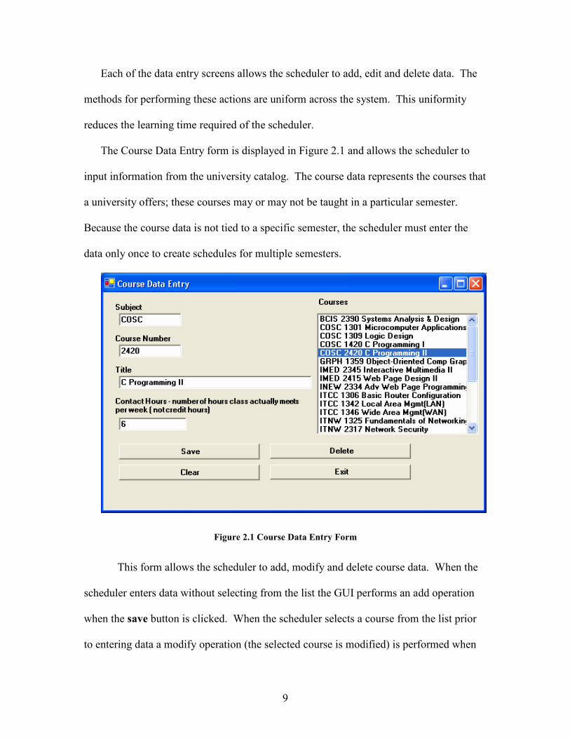
The Course Data Entry form is displayed in Figure 2.1 and allows the scheduler to

input information from the university catalog. The course data represents the courses that

a university offers; these courses may or may not be taught in a particular semester.

Because the course data is not tied to a specific semester, the scheduler must enter the

data only once to create schedules for multiple semesters.

Figure 2.1 Course Data Entry Form

This form allows the scheduler to add, modify and delete course data. When the

scheduler enters data without selecting from the list the GUI performs an add operation

when the save button is clicked. When the scheduler selects a course from the list prior

to entering data a modify operation (the selected course is modified) is performed when

10

the Save button is clicked. To delete a course the scheduler must first select a course

from the list, and then click the Delete button, the scheduler is then prompted to verify

the delete operation. The Clear button, when clicked, empties all of the fields and

deselects the selected course. This readies the form for an add operation to be performed.

All of the data entry forms in the GUI follow this same method for data entry.

Figure 2.2 displays the Courses to Schedule form which is used to specify which

courses are to be considered on the schedule.

Figure 2.2 Courses to Schedule Form

To add a course to the list of courses to schedule, the scheduler selects a course

from the courses list and clicks the right arrow button. To remove a course from the

schedule the scheduler selects the course from the courses to schedule list and clicks the

left arrow. Clicking the double right arrow moves all courses onto the schedule. The

capacity field allows the scheduler to specify the maximum capacity for a course and

11

defaults to 20 when a value is not specified. The capacity value is associated with an

individual course so each course can have a different capacity specified.

The form allows multiple sections of the same course to be specified by simply

adding the course the required number of times. When multiple sections are specified,

each section is seen as a separate course offering by the GUI and scheduling algorithm.

This means that any constraints applied to a particular section of a course are applied to

that section and all other sections are unaffected.

Since the courses to schedule are tied to a specific semester, the selected semester

is displayed in the title bar (the selected semester is always displayed in the title bar of

the main form). If the scheduler selects another semester while this form is open, the

form is automatically updated to the new semester. This operation is true for any form

that deals with data entry that is tied to a specific semester.

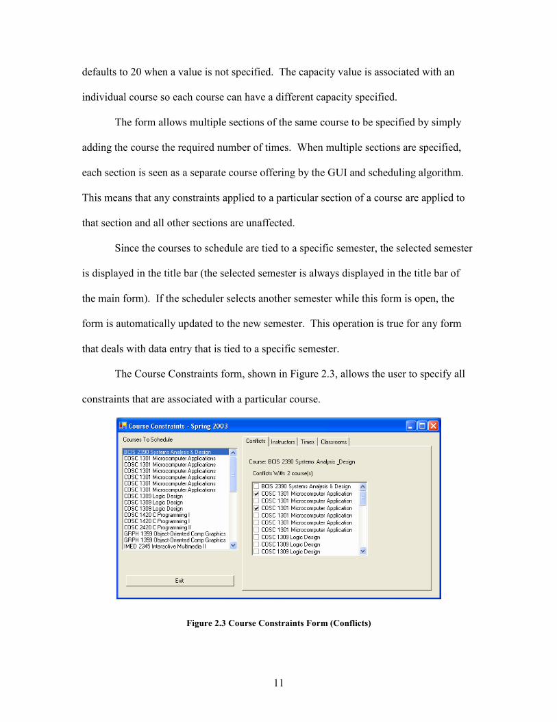
The Course Constraints form, shown in Figure 2.3, allows the user to specify all

constraints that are associated with a particular course.

Figure 2.3 Course Constraints Form (Conflicts)

12

All course constraints are attached to an individual course section. When multiple

sections of the same course exist, only the selected section is affected by course

constraints.

To operate this form, the scheduler first selects the desired course section from the

Courses to Schedule list and then applies constraints to the selected section. The four

types of course constraints can be accessed by clicking on the appropriate tab. In Figure

2.3 the course constraints form is shown with the Conflicts tab selected. To add a new

conflict the scheduler simply places a check mark next to the appropriate course. To

remove a conflict the scheduler simply removes the check mark. Any constraint data

entry that makes use of a checked list follows this method of data entry.

Figure 2.4 displays the Course Constraints form with the Times tab selected. This

demonstrates the manner in which days and times are entered by the scheduler. The

scheduler simply places a check mark next to each day desired and enters the time in the

appropriate box. All times must be entered using a 24-hour format. Any data entry that

requires the entry of days and times uses this method.

Figure 2.4 Course Constraints Form (Time)

13

A course section can have a single starting time associated with it. After entering

the days and times, the scheduler clicks the Save button to attribute the days and time to

the selected course. An existing day and time can be modified by making the appropriate

changes and clicking the Save button. The Delete button is used to remove the existing

days and time from the selected course. Once the days and time have been deleted, the

time constraint will not exist for the selected course.

The Instructor Constraints form is shown in Figure 2.5. The basic operations of

this form are the same as the Course Constraints form. Care has been taken during the

development of the GUI to make the data entry methods as uniform as possible. This

uniformity reduces the amount of time required to learn to use the GUI.

Figure 2.5 Instructor Constraints Form

The scheduling algorithm provides a means of implementing soft and hard

constraints. These will be discussed in section 3. The scheduler has the ability to adjust

the penalty values of each constraint, thereby determining which constraints are soft and

14

which constraints are hard. The Constraint Penalties form is displayed in Figure 2.6. It

allows the user to adjust the penalty value of each constraint by moving the slider up or

down. The user can also change the penalty value by typing the value in the associated

box. The constraint penalties can be set to a maximum of 20 and a minimum of 0.

Figure 2.6 Constraint Penalties Form

2.2 Schedule Creation

Once the scheduler has completed all of the required data entry the scheduling

algorithm can be invoked by clicking Create Schedule on the schedule menu. The

creation of a schedule is completely automated and does not require any user

intervention.

The scheduling algorithm runs until a schedule is found that has 5 or fewer

constraint violations or until 100,000 generations have elapsed. At that point the user has

the choice of accepting the schedule as is or of having the scheduling algorithm continue

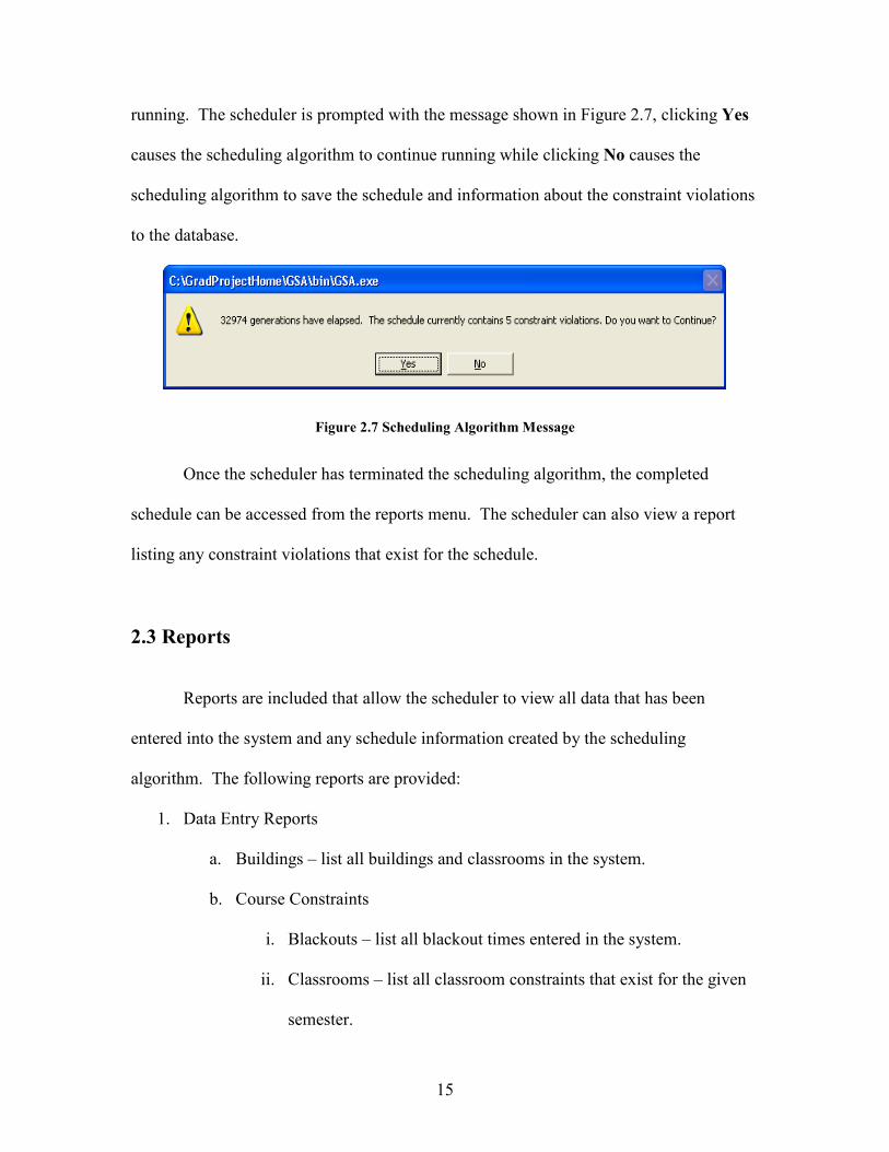
15

running. The scheduler is prompted with the message shown in Figure 2.7, clicking Yes

causes the scheduling algorithm to continue running while clicking No causes the

scheduling algorithm to save the schedule and information about the constraint violations

to the database.

Figure 2.7 Scheduling Algorithm Message

Once the scheduler has terminated the scheduling algorithm, the completed

schedule can be accessed from the reports menu. The scheduler can also view a report

listing any constraint violations that exist for the schedule.

2.3 Reports

Reports are included that allow the scheduler to view all data that has been

entered into the system and any schedule information created by the scheduling

algorithm. The following reports are provided:

1. Data Entry Reports

a. Buildings – list all buildings and classrooms in the system.

b. Course Constraints

i. Blackouts – list all blackout times entered in the system.

ii. Classrooms – list all classroom constraints that exist for the given

semester.

16

iii. Conflicts – list all conflicts that exist for the given semester.

iv. Instructors – list all courses that must be taught by a specific

instructor for the given semester.

v. Times – list all courses that must be taught at a specific time for

the given semester.

c. Instructor Constraints

i. Loads – list each instructor that has a minimum and maximum

course load specified.

ii. Preferences – list the time preferences entered for each instructor.

iii. Qualification – list each instructor along with the courses they are

qualified to teach.

d. Courses – list all courses entered into the system.

e. Instructors – list all instructors entered into the system.

2. Schedule Reports – based on data created by the scheduling algorithm.

a. Schedule – list each course along with the instructor, room and time that

has been assigned to the course. The report can be sorted by course,

instructor, classroom or time.

b. Constraint Violations – list all constraint violations that exist on the

selected schedule.

A sample of each of the reports listed is contained in Appendix A.

17

3. SYSTEM DESIGN

The Course Scheduling System consists of three parts: a GUI to allow user

interaction, the scheduling algorithm that creates the actual schedules, and a database.

Each of these components will be discussed separately in this section.

3.1 The Database

A Microsoft Access database was used to handle the data storage requirements of

course scheduling. These requirements include the storage of user input, such as course

and constraint information, as well as the storage of completed schedules.

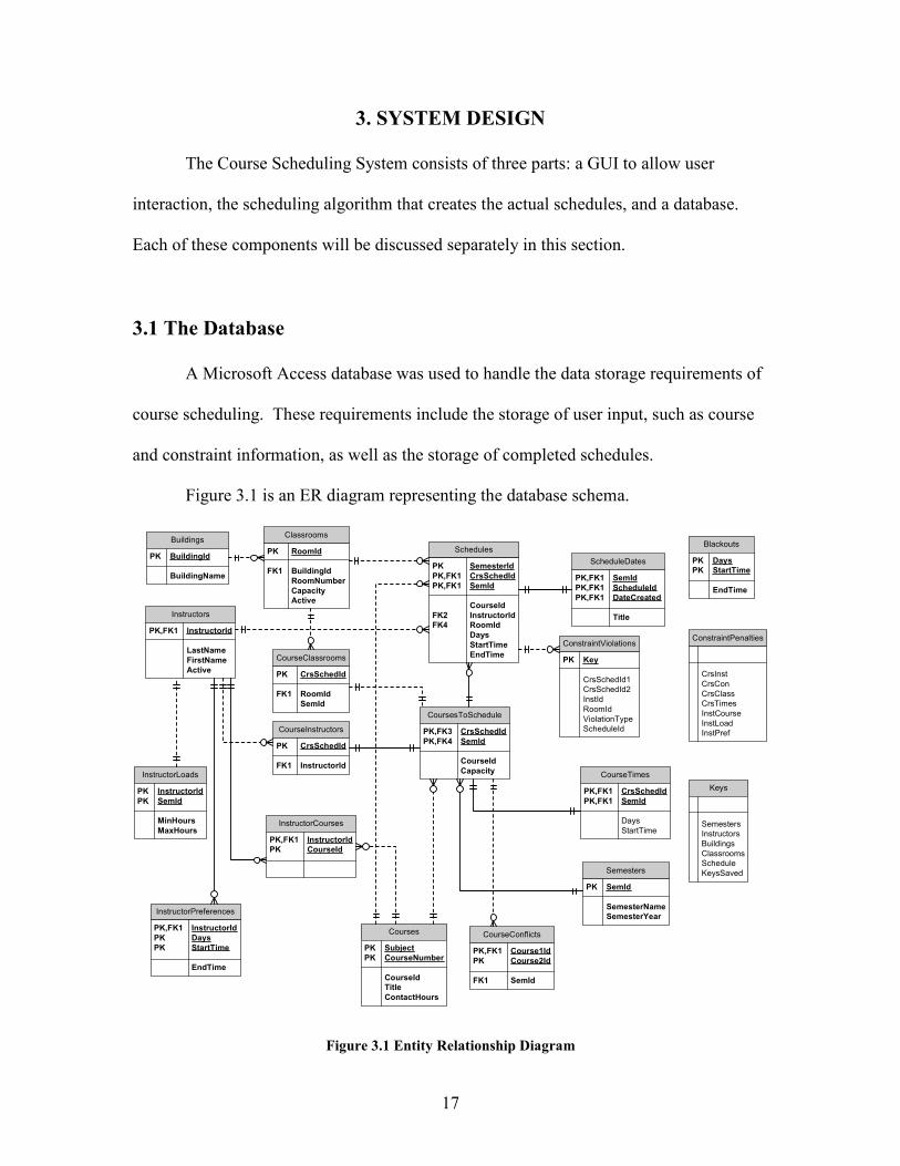
Figure 3.1 is an ER diagram representing the database schema.

Blackouts

PK Days

PK StartTime

EndTime

Buildings

PK BuildingId

BuildingName

Classrooms

PK RoomId

FK1 BuildingId

RoomNumber

Capacity

Active

ConstraintPenalties

CrsInst

CrsCon

CrsClass

CrsTimes

InstCourse

InstLoad

InstPref

ConstraintViolations

PK Key

CrsSchedId1

CrsSchedId2

InstId

RoomId

ViolationType

ScheduleId

CourseClassrooms

PK CrsSchedId

FK1 RoomId

SemId

CourseConflicts

PK,FK1 Course1Id

PK Course2Id

FK1 SemId

CourseInstructors

PK CrsSchedId

FK1 InstructorId

Courses

PK Subject

PK CourseNumber

CourseId

Title

ContactHours

CoursesToSchedule

PK,FK3 CrsSchedId

PK,FK4 SemId

CourseId

CapacityCourseTimes

PK,FK1 CrsSchedId

PK,FK1 SemId

Days

StartTimeInstructorCourses

PK,FK1 InstructorId

PK CourseId

InstructorLoads

PK InstructorId

PK SemId

MinHours

MaxHours

InstructorPreferences

PK,FK1 InstructorId

PK Days

PK StartTime

EndTime

Instructors

PK,FK1 InstructorId

LastName

FirstName

Active

Keys

Semesters

Instructors

Buildings

Classrooms

Schedule

KeysSaved

ScheduleDates

PK,FK1 SemId

PK,FK1 ScheduleId

PK,FK1 DateCreated

Title

Schedules

PK SemesterId

PK,FK1 CrsSchedId

PK,FK1 SemId

CourseId

FK2 InstructorId

FK4 RoomId

Days

StartTime

EndTime

Semesters

PK SemId

SemesterName

SemesterYear

Figure 3.1 Entity Relationship Diagram

18

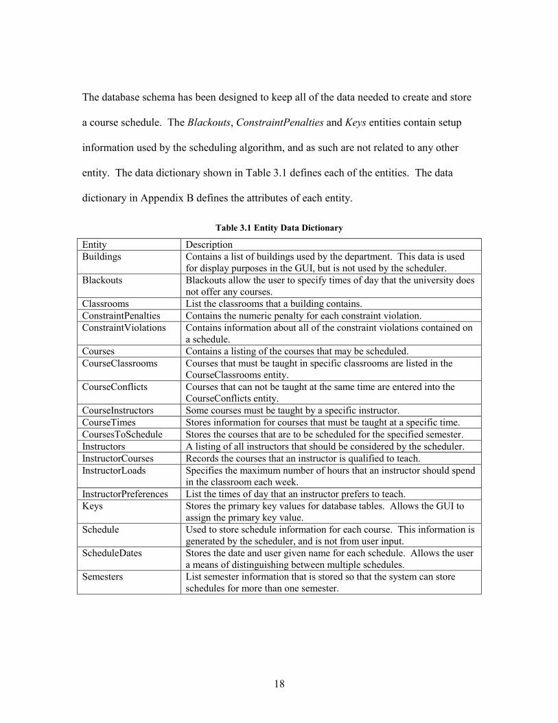
The database schema has been designed to keep all of the data needed to create and store

a course schedule. The Blackouts, ConstraintPenalties and Keys entities contain setup

information used by the scheduling algorithm, and as such are not related to any other

entity. The data dictionary shown in Table 3.1 defines each of the entities. The data

dictionary in Appendix B defines the attributes of each entity.

Table 3.1 Entity Data Dictionary

Entity Description

Buildings Contains a list of buildings used by the department. This data is used

for display purposes in the GUI, but is not used by the scheduler.

Blackouts Blackouts allow the user to specify times of day that the university does

not offer any courses.

Classrooms List the classrooms that a building contains.

ConstraintPenalties Contains the numeric penalty for each constraint violation.

ConstraintViolations Contains information about all of the constraint violations contained on

a schedule.

Courses Contains a listing of the courses that may be scheduled.

CourseClassrooms Courses that must be taught in specific classrooms are listed in the

CourseClassrooms entity.

CourseConflicts Courses that can not be taught at the same time are entered into the

CourseConflicts entity.

CourseInstructors Some courses must be taught by a specific instructor.

CourseTimes Stores information for courses that must be taught at a specific time.

CoursesToSchedule Stores the courses that are to be scheduled for the specified semester.

Instructors A listing of all instructors that should be considered by the scheduler.

InstructorCourses Records the courses that an instructor is qualified to teach.

InstructorLoads Specifies the maximum number of hours that an instructor should spend

in the classroom each week.

InstructorPreferences List the times of day that an instructor prefers to teach.

Keys Stores the primary key values for database tables. Allows the GUI to

assign the primary key value.

Schedule Used to store schedule information for each course. This information is

generated by the scheduler, and is not from user input.

ScheduleDates Stores the date and user given name for each schedule. Allows the user

a means of distinguishing between multiple schedules.

Semesters List semester information that is stored so that the system can store

schedules for more than one semester.

19

The Schedules and ConstraintViolations entities receive their information from the

scheduling algorithm and are read only for the scheduler.

3.2 The Graphical User Interface

The GUI is designed to give the scheduler an easy to use, uniform means of

interacting with the database and the scheduling algorithm. The GUI was implemented

using Microsoft Visual Basic .Net (VB .Net).

3.2.1 Database Access

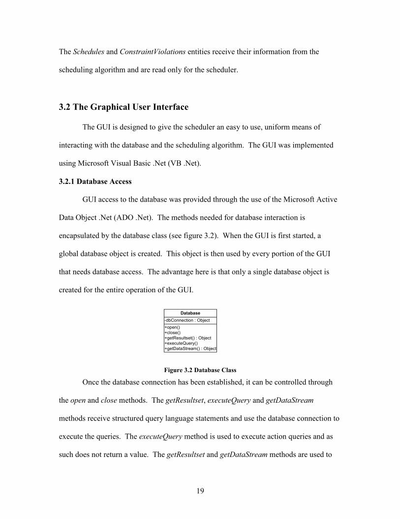
GUI access to the database was provided through the use of the Microsoft Active

Data Object .Net (ADO .Net). The methods needed for database interaction is

encapsulated by the database class (see figure 3.2). When the GUI is first started, a

global database object is created. This object is then used by every portion of the GUI

that needs database access. The advantage here is that only a single database object is

created for the entire operation of the GUI.

+open()

+close()

+getResultset() : Object

+executeQuery()

+getDataStream() : Object

-dbConnection : Object

Database

Figure 3.2 Database Class

Once the database connection has been established, it can be controlled through

the open and close methods. The getResultset, executeQuery and getDataStream

methods receive structured query language statements and use the database connection to

execute the queries. The executeQuery method is used to execute action queries and as

such does not return a value. The getResultset and getDataStream methods are used to

20

execute select queries, getResultset returns a data adapter object and getDataStream

returns a data reader object.

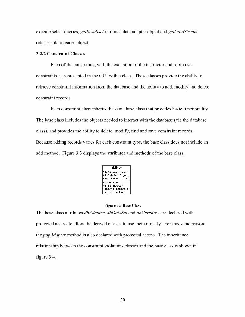
3.2.2 Constraint Classes

Each of the constraints, with the exception of the instructor and room use

constraints, is represented in the GUI with a class. These classes provide the ability to

retrieve constraint information from the database and the ability to add, modify and delete

constraint records.

Each constraint class inherits the same base class that provides basic functionality.

The base class includes the objects needed to interact with the database (via the database

class), and provides the ability to delete, modify, find and save constraint records.

Because adding records varies for each constraint type, the base class does not include an

add method. Figure 3.3 displays the attributes and methods of the base class.

Figure 3.3 Base Class

The base class attributes dbAdapter, dbDataSet and dbCurrRow are declared with

protected access to allow the derived classes to use them directly. For this same reason,

the popAdapter method is also declared with protected access. The inheritance

relationship between the constraint violations classes and the base class is shown in

figure 3.4.

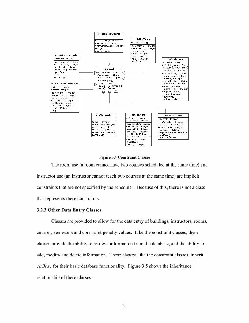
21

Figure 3.4 Constraint Classes

The room use (a room cannot have two courses scheduled at the same time) and

instructor use (an instructor cannot teach two courses at the same time) are implicit

constraints that are not specified by the scheduler. Because of this, there is not a class

that represents these constraints.

3.2.3 Other Data Entry Classes

Classes are provided to allow for the data entry of buildings, instructors, rooms,

courses, semesters and constraint penalty values. Like the constraint classes, these

classes provide the ability to retrieve information from the database, and the ability to

add, modify and delete information. These classes, like the constraint classes, inherit

clsBase for their basic database functionality. Figure 3.5 shows the inheritance

relationship of these classes.

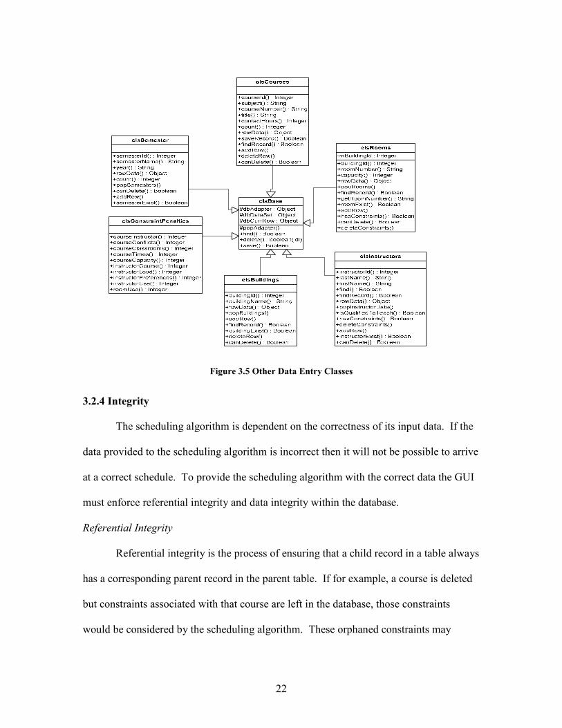
22

Figure 3.5 Other Data Entry Classes

3.2.4 Integrity

The scheduling algorithm is dependent on the correctness of its input data. If the

data provided to the scheduling algorithm is incorrect then it will not be possible to arrive

at a correct schedule. To provide the scheduling algorithm with the correct data the GUI

must enforce referential integrity and data integrity within the database.

Referential Integrity

Referential integrity is the process of ensuring that a child record in a table always

has a corresponding parent record in the parent table. If for example, a course is deleted

but constraints associated with that course are left in the database, those constraints

would be considered by the scheduling algorithm. These orphaned constraints may

23

prevent a good schedule from being reached. Because of this, referential integrity is very

important to the scheduling algorithm.

Referential integrity can be enforced by the database engine, however in this

project it was decided to enforce referential integrity within the GUI. This decision was

made because of the increased flexibility in providing error messages to the scheduler

and in program flow (error handling does not have to be implemented to handle

referential integrity).

When the scheduler attempts to delete a record, the GUI queries any related tables

looking for child records. If a child record is found in any related table, then the

scheduler is given the option of deleting all child records. If the scheduler declines to

delete the child records the parent record deletion is denied.

Data Integrity

The data integrity enforced by the GUI is based on the data requirements that are

defined by the scheduling algorithm. The GUI must ensure that the scheduler, when

performing data entry, does not input constraints that cannot be fulfilled. Data integrity is

crucial because the errors that can be made are subtle and may not be readily apparent to

the scheduler. For example, if the scheduler were to apply a constraint specifying the

instructor for a course and the instructor was not qualified to teach the course a data error

would exist. The scheduling algorithm would not be able to make an instructor

assignment that would not violate one of the two constraints.

Whenever a constraint is input, the GUI checks to see if it conflicts with any other

constraints already entered into the system. If a conflicting constraint exists then the

24

constraint being input is rejected. The GUI checks for the following conflicting

constraints:

1. A course cannot be set to conflict with itself.

2. Instructors cannot be specified for a course they are not qualified to teach.

3. A course time cannot be set during the school’s blackout times.

4. An instructor cannot be given a time preference that occurs during the school’s

blackout times.

5. A room cannot be specified for a course if the room’s capacity is less then the

course’s capacity.

By enforcing the above rules, the GUI can ensure that conflicting constraints cannot

be entered.

Class Days

When assigning meeting times to a course, the scheduling algorithm will only

assign days that are combinations of Monday, Wednesday and Friday or combinations of

Tuesday and Thursday. For example, a course could be assigned meeting days of

Monday, Monday, Wednesday or Monday, Wednesday and Friday. This is done to

prevent the assignment of meeting days that would not be desirable at many institutions.

When the scheduler specifies a meeting time for a course, the GUI must ensure

that the days entered for the course meet the requirement described above. Any meeting

time that does not meet the requirement is rejected by the GUI.

25

3.2.5 Simplicity and Uniformity

The course scheduling system was designed for non-technical users who may

have a very limited knowledge of computer operation. Because of this, every attempt has

been made to produce a GUI that is easy to use and that is uniform in operation. The

uniformity is extremely important, because as stated earlier uniformity shortens the

amount of time required to learn how to use the system.

The operation of the scheduling algorithm is completely hidden from the

scheduler’s view. This is an important feature that significantly contributes to the

simplicity of the system. The scheduler does not have to have any knowledge of how a

schedule is created to use this system, but must only understand which constraints can be

applied and how to perform the data entry.

3.3 The Scheduling Algorithm

In order to apply a genetic algorithm to the scheduling problem several factors

must be considered. These factors are:

1. How will a schedule be represented?

2. How will a constraint be represented?

3. How will a schedule’s fitness be determined?

4. How will the selection process be implemented?

5. How will recombination be implemented?

6. How will mutation be implemented?

This section will discuss each of these questions and will also discuss special

considerations that arose during the implementation of the scheduling algorithm.

26

3.3.1 Representation of Schedules

Schedules are represented with a two dimensional integer array. Each row of the

array represents a single course and each element of the row represents an assignment

that has been made to that course.

0 1 2 3 4 5 6 7 8

Course

Schedule

Id

Course

Id

Room

Id

Day

Assignment

Begin

Time

End

Time

Instructor

Id

Contact

Hours

Capacity

0 1 23 2 5 800 930 3 3 25

1 2 34 4 21 1030 1230 5 6 20

Figure 3.6 Representation of a Schedule

Figure 3.6 shows the manner in which a two dimensional array of integers is used to

represent a schedule. The heading in each column indicates the values stored in that

column, while the numbers on the far left represent the row index and the numbers across

the top represent the column index. The CourseScheduleId and CourseId are the primary

keys of the CoursesToSchedule and Courses tables respectively. They are included in the

schedule array for the purpose of comparing constraints to the schedule and saving the

completed schedule to the database. The contact hours and capacity are included for the

purpose of constraint checking. The room id, day assignment, beginning time, ending

time, and instructor id are the only values assigned by the scheduling algorithm.

27

The following structure was created to represent a schedule.

struct schedule

{

int (*sch)[9];

float fitnessValue;

int totalViolations;

};

The member sch is a pointer to the two dimensional array which must be dynamically

allocated since the number of courses to schedule is not known at design time. The

members fitnessValue and totalViolations allows each schedule to contain its own fitness

and number of constraint violations.

The scheduling algorithm creates 40 schedules assigning values to the room id,

instructor id, days, start time, and end time fields at random. These schedules are

contained in an array of schedule structures.

3.3.2 Representation of Constraints

Constraints, like schedules, are represented using a two dimensional array of

integers. The constraint arrays are also dynamically allocated since the number of

constraints is not known at design time. The number of columns in the array is

dependent upon the type of constraint being represented. Since the syntax of C++

requires the number of columns to be specified at design time, the columns are set to the

maximum number of columns needed (not all constraints require 4 columns). Constraint

arrays are created using the structure shown below:

struct constraint

{

int (*cons)[4];

int penalty;

};

The penalty field allows the scheduler to set the penalty value for each constraint

based on specific schedule preferences. When the scheduling algorithm creates the

28

constraint arrays, it queries the database for the penalty value for each constraint. Figure

3.7 illustrates the use of a two dimensional array to represent the course conflicts

constraint.

Course 1 Id Course 2 Id

1 2

1 3

3 4

Figure 3.7 Representation of a Constraint

It can be seen in this array that course 1 cannot be taught at the same time as course 2 and

3, and that course 3 cannot be taught at the same time as course 4.

3.3.3 Calculating Fitness

A schedule’s fitness is determined by comparing each course in the schedule to

each of the constraints. Whenever a constraint violation is found, the constraints penalty

value is added to the schedule's total fitness. Once all constraints have been compared,

the schedule’s fitness value is set equal to 1 / total fitness. The division is performed so

that the best schedule will have the highest fitness value.

int courseInstructorFitness(struct schedule &s)

{

int instructorFitness = 0;

int index;

int crsIndex = 0;

for(index = 0; index < totalCrsInstCons; index++)

{

while(s.sch[crsIndex][0] != crsInst.cons[index][0] &&

crsIndex < totalCourses)

crsIndex++;

if(crsIndex < totalCourses)

{

//if a course is not taught by the correct

//instructor

if(s.sch[crsIndex][6] != crsInst.cons[index][1])

{

//then a constraint violaion exist

instructorFitness += crsInst.penalty;

s.totalViolations++;

}

}

}

return instructorFitness;}

29

The function above is used to compare a schedule against the course instructor

constraint. The data type of s is the structure presented in subsection 3.3.1 and the data

type of crsInst is the structure presented in subsection 3.3.2. The outer for loop is used to

process each of the course instructor constraints. The inner while loop searches through

the schedule until the course specified by the current constraint is found. Once the course

has been found the assigned instructor is compared to the instructor specified by the

constraint. If these values do not match, then a constraint violation exists. When a

constraint violation has been determined the constraint’s penalty value is added to the

total and the schedule's count of violations is incremented. Each of the constraint

checking functions is implemented in a manner similar to that shown above.

3.3.4 Selection

Selection is the process of determining which individuals in a population will be

allowed to reproduce and create offspring in the next generation. When two individuals

reproduce, they are replaced in the next generation by their offspring. This project

implemented two versions of schedule replacement: simple GA (sGA) and steady state

GA (ssGA). In section 4 the performance of sGA and ssGA will be compared.

The type of replacement scheme used affects the type of selection scheme that can

be used. With sGA all of the members of the current generation are replaced by new

individuals in the succeeding generation, so the number of schedules selected must be

equal to the number of schedules in the generation.

For sGA, selection was implemented by using a method described by Goldberg

[Goldberg 1989]. This method uses a roulette wheel to determine which individuals will

be selected for reproduction. The wheel is biased in that each individual in the

30

population “has a roulette wheel slot sized in proportion to its fitness” [Goldberg 1989].

Consider this example, which is based on an example found in [Goldberg 1989].

Suppose that we have 4 complete schedules with fitness evaluations shown in Table 2.

Table 2 Schedule Fitness Values

Schedule Penalty Fitness % of Total

1 300 0.0033 25

2 170 0.0058 44

3 550 0.0018 13

4 400 0.0025 18

Total 0.0131 100

In this example, the penalty value corresponds to the total number of constraint violations

found in the schedule. This means that the best schedule has the lowest penalty value. In

order to assign the largest fitness value to the best schedule, the fitness value is defined as

1 / penalty.

Once the fitness values have been assigned, the roulette wheel is created by giving

each schedule a percentage of the wheel equal to its percentage of the total fitness value

(see Figure 2.13). Schedules are chosen for reproduction by spinning the wheel (4 times

in this case). Schedule 2 was given the largest percentage of the wheel since it has the

best fitness. This means that schedule 2 is more likely to be chosen for reproduction then

are the other schedules.

.

Figure 3.8 Roulette Wheel Sized According to Fitness

31

In this example we would choose 4 schedules for reproduction with the possibility of

choosing the same schedule more than once. Since the roulette wheel is based on the

fitness values of the schedule, the fitter schedules are favored.

The roulette wheel is represented as an array of integers with 100 elements. Each

element in the array stores the location (index) of the schedule (in the array of schedules)

assigned the slot. The number of array elements in a slot is determined by the schedule’s

percentage of the total fitness. For example, if a schedule’s fitness was 15% of the total

fitness (the sum of the fitness of all schedules) then the schedule would have 15 array

elements in its slot.

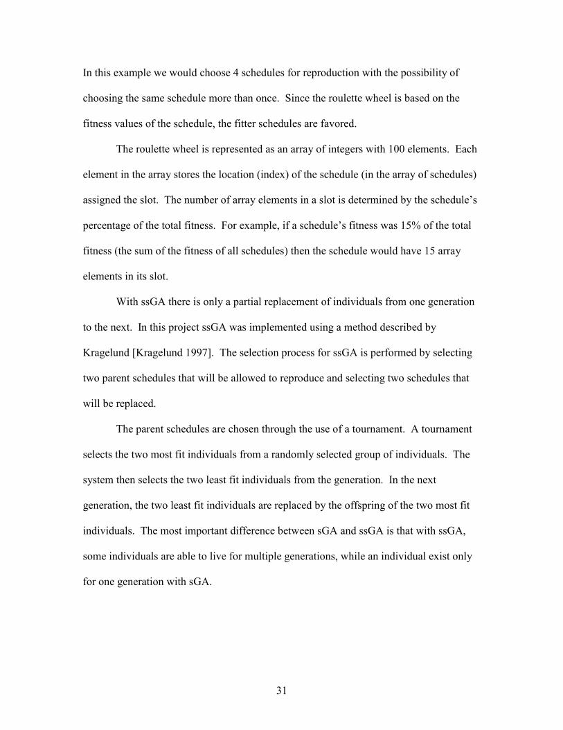
With ssGA there is only a partial replacement of individuals from one generation

to the next. In this project ssGA was implemented using a method described by

Kragelund [Kragelund 1997]. The selection process for ssGA is performed by selecting

two parent schedules that will be allowed to reproduce and selecting two schedules that

will be replaced.

The parent schedules are chosen through the use of a tournament. A tournament

selects the two most fit individuals from a randomly selected group of individuals. The

system then selects the two least fit individuals from the generation. In the next

generation, the two least fit individuals are replaced by the offspring of the two most fit

individuals. The most important difference between sGA and ssGA is that with ssGA,

some individuals are able to live for multiple generations, while an individual exist only

for one generation with sGA.

32

3.3.5 Recombination

The recombination operator, also known as crossover, creates the new individuals

in the next generation. The individuals that were selected by the reproduction operator

are used in crossover; these individuals make up the mating pool. Individuals in the

mating pool are paired with a mate at random.

Recall from section 1.2.1 that an individual is a complete solution to the problem,

in this case a complete schedule, and that an individual is made up of chromosomes. In

this case the chromosome represents the assignments (days, time, room, and instructor)

that have been made to a particular course. In a course schedule, the chromosomes are

represented by the rows of the two dimensional array (see section 3.3.1). Each individual

element of a row represents a gene, where a gene describes how the schedule looks. For

example, in a schedule a gene represents an instructor assignment . The value of this

gene, known as an allele, describes which instructor is teaching the course.

The crossover operator exchanges genes between the chromosomes of the mating

pair of individuals. For example, consider the chromosomes in Figure 3.9.

Figure 9 Chromosomes Before Swapping

Each pair of genes has a 50% probability of being swapped. If a pair of genes is chosen,

the crossover is achieved by exchanging values between the genes. If the first and last

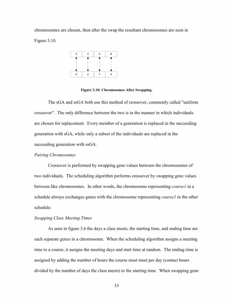
33

chromosomes are chosen, then after the swap the resultant chromosomes are seen in

Figure 3.10.

Figure 3.10: Chromosomes After Swapping.

The sGA and ssGA both use this method of crossover, commonly called "uniform

crossover". The only difference between the two is in the manner in which individuals

are chosen for replacement. Every member of a generation is replaced in the succeeding

generation with sGA, while only a subset of the individuals are replaced in the

succeeding generation with ssGA.

Pairing Chromosomes

Crossover is performed by swapping gene values between the chromosomes of

two individuals. The scheduling algorithm performs crossover by swapping gene values

between like chromosomes. In other words, the chromosome representing course1 in a

schedule always exchanges genes with the chromosome representing course1 in the other

schedule.

Swapping Class Meeting Times

As seen in figure 3.6 the days a class meets, the starting time, and ending time are

each separate genes in a chromosome. When the scheduling algorithm assigns a meeting

time to a course, it assigns the meeting days and start time at random. The ending time is

assigned by adding the number of hours the course must meet per day (contact hours

divided by the number of days the class meets) to the starting time. When swapping gene

34

values, these three genes must be swapped as a unit, otherwise the meeting times created

will not be valid.

3.3.6 Mutation

Based on the course and constraint data entered by the user, there are a finite

number of valid schedules that can be generated using that data. This set of possible

solutions is the problem’s search space.

Since the initial population of solutions is generated at random, it is possible that

the gene values generated will not allow the algorithm to move through the entire search

space. It is also possible that in the process of swapping gene values, that the

reproduction and crossover operators may lose the combination of gene values that are

needed to move throughout the search space.

The mutation operator attempts to insure that the individuals have gene values

that allow the entire search space to be explored. Mutation works by changing, at

random, the value of an individual gene within a chromosome. Mutation is used

sparingly, because too much mutation will reduce the effects of reproduction and

crossover and cause the individuals to become less fit. In this project mutation has a 5%

chance of occurring.

Mutation is implemented by giving each chromosome a 5% chance of being

mutated. When a chromosome is mutated, a single gene value (chosen at random) is

changed. If any of the genes that make up a course’s meeting time is chosen for

mutation, the entire meeting time (days, start time, and end time) are mutated. This is

done for the same reasons discussed in the section on crossover.

35

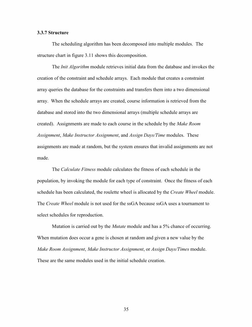
3.3.7 Structure

The scheduling algorithm has been decomposed into multiple modules. The

structure chart in figure 3.11 shows this decomposition.

The Init Algorithm module retrieves initial data from the database and invokes the

creation of the constraint and schedule arrays. Each module that creates a constraint

array queries the database for the constraints and transfers them into a two dimensional

array. When the schedule arrays are created, course information is retrieved from the

database and stored into the two dimensional arrays (multiple schedule arrays are

created). Assignments are made to each course in the schedule by the Make Room

Assignment, Make Instructor Assignment, and Assign Days/Time modules. These

assignments are made at random, but the system ensures that invalid assignments are not

made.

The Calculate Fitness module calculates the fitness of each schedule in the

population, by invoking the module for each type of constraint. Once the fitness of each

schedule has been calculated, the roulette wheel is allocated by the Create Wheel module.

The Create Wheel module is not used for the ssGA because ssGA uses a tournament to

select schedules for reproduction.

Mutation is carried out by the Mutate module and has a 5% chance of occurring.

When mutation does occur a gene is chosen at random and given a new value by the

Make Room Assignment, Make Instructor Assignment, or Assign Days/Times module.

These are the same modules used in the initial schedule creation.

36

Figure 3.11 Structure Chart

37

Crossover occurs every generation and operates by first invoking the Spin Wheel

module (a tournament is used in the case of ssGA) to select schedules for reproduction.

Once the schedules have been selected, they are copied into the next generation by the

Copy Schedule module. The Swap Values module exchanges gene values between the

schedules in the manner described in section 3.3.5.

When the genetic algorithm has completed running, the Save Schedule module is

invoked to save the created schedule. The operations of the scheduling algorithm

produce a single schedule that is saved to the database. This schedule is the best schedule

found across all generations of schedules.

The structure chart shown above does not include all modules that exist in the

scheduling algorithm. For clarity some auxiliary modules have not been included,

however the structure chart captures the main structure of the scheduling algorithm and

provides an accurate depiction of its inner workings.

3.3.8 Special Considerations

During the implementation of the scheduling algorithm several concerns became

evident and had to be addressed. These concerns are discussed in this section.

Population Size

The scheduling algorithm uses a small population of schedules in each generation.

A small population is used since the scheduling algorithm is designed to run on a desktop

computer which may have limited resources. The population size is currently set at 40

schedules. This number was determined through trial and error and seems to yield good

results.

38

Representation of Days and Times

In order for the scheduler to identify a specific time for a course, the days of the

week on which the course meets must be represented in some form. This is a problem

because a class can meet on any combination of days during a week. To address this

problem, courses are represented using a 5 digit binary string where the most significant

bit represents Friday and the least significant bit represents Monday.

Representing the days a course meets in this manner simplifies the comparison

between two courses when checking constraints such as “Some courses may not be

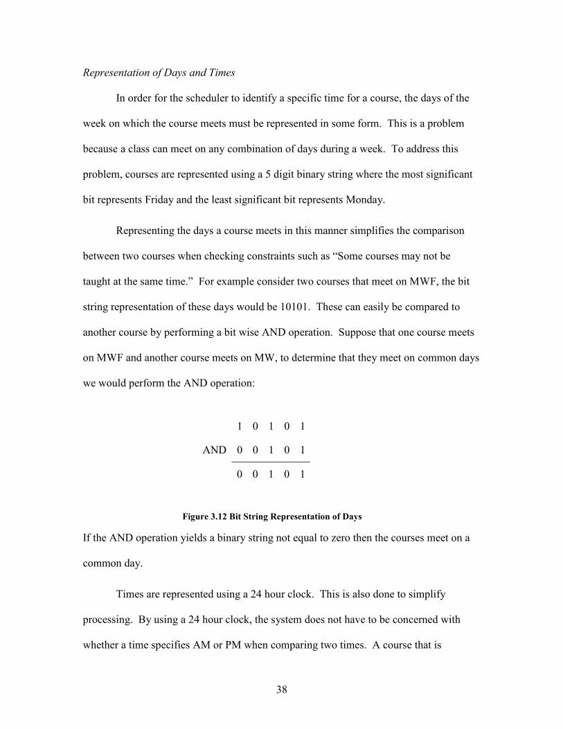
taught at the same time.” For example consider two courses that meet on MWF, the bit

string representation of these days would be 10101. These can easily be compared to

another course by performing a bit wise AND operation. Suppose that one course meets

on MWF and another course meets on MW, to determine that they meet on common days

we would perform the AND operation:

If the AND operation yields a binary string not equal to zero then the courses meet on a

common day.

Times are represented using a 24 hour clock. This is also done to simplify

processing. By using a 24 hour clock, the system does not have to be concerned with

whether a time specifies AM or PM when comparing two times. A course that is

1 0 1 0 1

AND 0 0 1 0 1

0 0 1 0 1

Figure 3.12 Bit String Representation of Days

39

scheduled to meet in room 100 on MWF from 09:00 to 10:00 would have a conflict if

another course had been scheduled to meet in room 100 on MWF from 08:00 to 10:00.

The 24 hour clock representation of times allows this conflict to be easily detected by the

test:

if(Course2.beginTime <= Course1.endTime &&

Course2.beginTime >= Course1.beginTime)

//A time conflict exist

Assigning Meeting Times

As discussed in section 2, the days a class meets is restricted to combinations of

Monday – Wednesday – Friday and Tuesday – Thursday. This was done to prevent the

assigning of non-traditional meeting days and to limit the possibility of courses

conflicting with one another.

The blackout constraint is enforced when times are assigned to the courses. The

system will not assign a time that violates a blackout constraint. This prevents invalid

data from entering the schedules and will allow the process of crossover to be more

effective.

Assigning of Instructors and Rooms

When assigning instructors to a schedule, the scheduling algorithm simply

generates at random an integer value that corresponds to the instructor id (primary key)

value in the database. Since these instructor id values are not sequential (since the user

can delete instructors all primary key values will not be present) the system must ensure

that all instructor ids assigned are valid. This same problem holds true for the assignment

of classrooms.

40

Soft and Hard Constraints

Since the scheduling algorithm is usually not able to arrive at schedules that are

completely free of constraint violations (discussed in section 4) soft and hard constraints

have been introduced. A soft constraint is a constraint whose violation is acceptable.

Said another way a soft constraint is a preference, we prefer for the constraint to be met,

but if it is violated the schedule will still be considered valid. A hard constraint is a

constraint that cannot be violated in a valid schedule. Any schedule that violates a hard

constraint would be considered invalid.

Soft and hard constraints are implemented by varying the amount of penalty

associated with each constraint. A hard constraint is given a higher penalty value then a

soft constraint. This results in a schedule that violates hard constraints having a poorer

fitness than a schedule that violates soft constraints. Since the scheduling algorithm

favors those schedules that have a better fitness, schedules that violate hard constraints

tend to die off while schedules that violate soft constraints tend to continue to be selected

for reproduction.

The course scheduling system does not arbitrarily decide which constraints to

enforce as hard constraints and which constraints to enforce as soft constraints, but rather

gives this control to the scheduler. The scheduler can set the penalty value for each

constraint, those that receive higher penalty values will be seen as hard constraints while

those that receive lower penalty values will be seen has soft constraints.

41

3.3.9 Programming Language

The scheduling algorithm was implemented using the Microsoft Visual C++

programming language. Database access was performed using the Microsoft Foundation

Classes Open Database Connectivity objects.

42

4. EVALUATION AND RESULTS

4.1 Testing

The modules within the scheduling algorithm and the GUI were tested as they

were developed. When a module was completed it was tested with test cases chosen to

exercise the paths through the module. If errors were found, they were corrected and the

module was re-tested.

Testing for the completed system was performed by creating multiple schedules

for a set of inputs and verifying the correctness of the schedules that were created. All

constraints were verified by hand to ensure that they had been eliminated by the

scheduling algorithm. In cases where a completed schedule contained constraint

violations, it was verified that all constraint violations were reported by the scheduling

algorithm. Non constraint issues such as verifying that day, time and room assignments

were correct were also verified by hand.

Since the system is designed for non-technical users, the GUI is an extremely

important feature. Because of this, the GUI’s usability was tested by non-technical users.

Each user was asked to work with the GUI and answer the following questions:

1. Were the forms/reports easy to use?

2. Were the required inputs easy to understand?

3. Were the operations uniform throughout the GUI?

4. How easy was it to learn to use the system? (scale of 1 (hard) to 5 (easy))

5. What is the best aspect of the GUI?

6. What is the poorest aspect of the GUI?

43

The responses to each of these questions have been considered and where appropriate

have been used to correct problems and improve the usability of the GUI.

4.2 Evaluation

4.2.1 Running Time

The time required to compare constraints has the largest effect on the running

time of the scheduling algorithm. The use of arrays to represent both schedules and

constraints necessitates the use of nested loops to compare a single schedule to a single

constraint. Each of the constraint comparing functions has two levels of nesting which

gives them an upper bound running time of O(n2). Since the scheduling algorithm

implements sGA, all schedules must have their fitness calculated in each generation. The

CalculateFitness module performs this operation by looping through each schedule and

invoking the various fitness functions. Using a loop to invoke functions that have two

levels of nesting causes CalculateFitness to have three levels of nesting which gives it an

upper bound running time of O(n3). The CreateSchedule module uses a loop to control

the number of generations, and for each generation invokes the CalculateFitness module,

which means that four levels of nested loops exist for CreateSchedule and gives an

overall upper bound of O(n4) for the scheduling algorithm.

4.2.2 Violation Free Schedules

The scheduling algorithm is not always able to create schedules that do not violate

any of the specified constraints. This is mainly due to the number of constraints that have

been specified in the test cases (fewer constraints make it easier to find schedules that do

not violate any constraints). However, the algorithm has been consistently able to

44

produce schedules that violate only a few constraints. Typically 2 to 5 constraint

violations exist in a completed schedule.

This small number of violations can easily be manually corrected by the

scheduler. To assist in this process the scheduling algorithm records all constraint

violations that exist in a completed schedule, and also provides for hard and soft

constraints as discussed in section 3.

4.2.3 Comparison of Simple GA and Steady State GA

This project implemented both sGA and ssGA for the purpose of determining

which method of selection and replacement was most suited to the creation of course

schedules. While the scheduler is interested in how long it takes to create a schedule,

using time as a measure for comparison may not be completely accurate. Times may

vary for reasons that do not involve the scheduling algorithm, such as the CPU’s

switching between multiple processes. A generation, as a unit of measure, provides a

more accurate basis for comparison because a generation is an equal amount of work in

both types of genetic algorithms. For these reasons generations will be used as the unit of

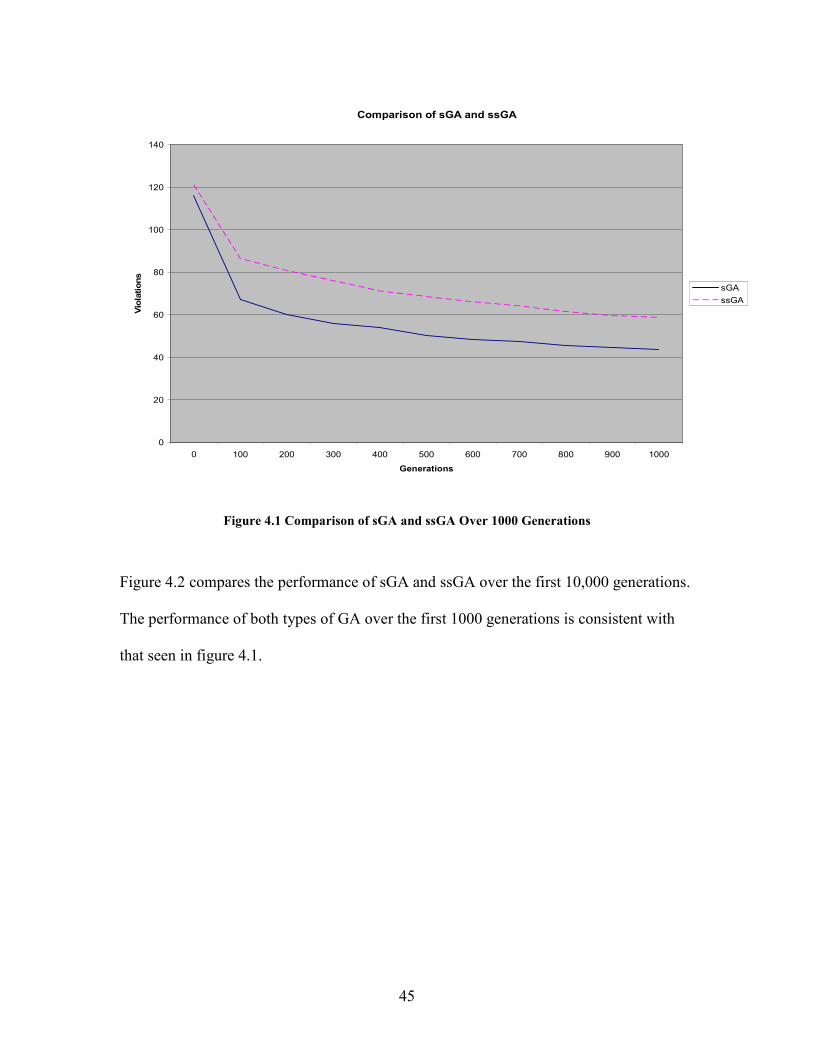
comparison. Figure 4.1 compares the performance of sGA and ssGA over the first 1000

generations. For all comparisons an average for the violations was taken based on 10

separate runs of each GA type. Each chart used a separate run of 10 for its data.

45

Comparison of sGA and ssGA

0

20

40

60

80

100

120

140

0 100 200 300 400 500 600 700 800 900 1000

Generations

Violations

sGA

ssGA

Figure 4.1 Comparison of sGA and ssGA Over 1000 Generations

Figure 4.2 compares the performance of sGA and ssGA over the first 10,000 generations.

The performance of both types of GA over the first 1000 generations is consistent with

that seen in figure 4.1.

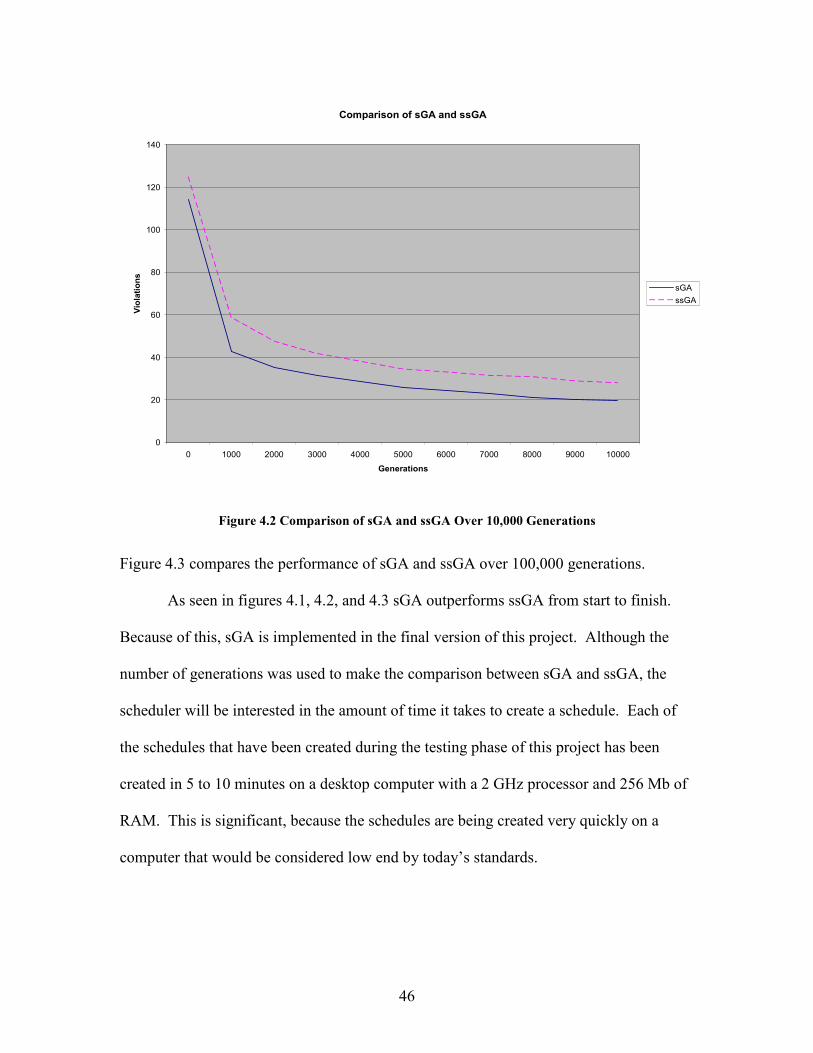
46

Comparison of sGA and ssGA

0

20

40

60

80

100

120

140

0 1000 2000 3000 4000 5000 6000 7000 8000 9000 10000

Generations

Violations

sGA

ssGA

Figure 4.2 Comparison of sGA and ssGA Over 10,000 Generations

Figure 4.3 compares the performance of sGA and ssGA over 100,000 generations.

As seen in figures 4.1, 4.2, and 4.3 sGA outperforms ssGA from start to finish.

Because of this, sGA is implemented in the final version of this project. Although the

number of generations was used to make the comparison between sGA and ssGA, the

scheduler will be interested in the amount of time it takes to create a schedule. Each of

the schedules that have been created during the testing phase of this project has been

created in 5 to 10 minutes on a desktop computer with a 2 GHz processor and 256 Mb of

RAM. This is significant, because the schedules are being created very quickly on a

computer that would be considered low end by today’s standards.

47

Comparison of sGA and ssGA

0

20

40

60

80

100

120

140

0 10000 20000 30000 40000 50000 60000 70000 80000 90000 100000

Generations

Violations

sGA

ssGA

Figure 4.3 Comparison of sGA and ssGA Over 100,000 Generations

48

5. FUTURE WORK

5.1 Mechanism for Manual Changes

Since the scheduling algorithm is not always able to create a schedule that is free

of constraint violations, a method could be made available to allow the scheduler to make

manual changes within the GUI to a schedule to correct the constraint violations that still

exist. As the scheduler makes a change to the schedule, the GUI could report any

constraint violations caused by the change. The GUI could track all constraints that exist

while the schedule is being altered and inform the scheduler when no constraint

violations exist.

5.2 Determination of Data Dependencies

As discussed in section 3.2.4, the data entry by the scheduler is critical since

conflicting constraint values can easily be entered. The relationships between each

constraint type could be re-examined to determine if any conflicts have been missed and

where possible add code that can prevent these conflicts from being input.

5.3 Testing On Larger Schedules

The scheduling algorithm has been shown to produce good schedules when the

number of course sections to schedule is small (38 course sections were used in most

tests). The scheduling algorithm could be tested using a larger number of course sections

to determine if it can produce schedules with few constraint violations and measure the

amount of time it takes to do so.

49

5.4 Use of Clusters in Schedule Creation

Originally proposed was the idea of creating a scheduling algorithm that would

run on a cluster of nodes. Because of the success of the algorithm running on a single

computer, it was determined that this step was not necessary. If in the future, it is

determined that the scheduling algorithm does not perform well with a large number of

course sections, then a clustered implementation can be pursued.

Each node in the cluster would run the same copy of the scheduling algorithm.

Since genetic algorithms work at random, each copy of the genetic algorithm would

arrive at different schedules. Each node would go through the process of creating new

generations which would result in each node having a unique generation of schedules. At

some regular interval, each node would choose the best schedules of the current

generation to distribute to all other nodes. Each node would then have the same

generation made up of the best schedules from each node. At this point, each node would

continue to work in isolation until the next exchange occurs. The idea here is to

determine if having the scheduling algorithm running on multiple nodes, with each node

reaching its own random conclusions (and sharing those conclusions with all other

nodes), will result in schedules that are better then those created on a single computer.

50

6. CONCLUSION

This paper presented a genetic algorithm that was designed and implemented to

solve the course scheduling problem. The algorithm, based on user input, creates a

semester course schedule by assigning each course a room, instructor, and meeting time.

The scheduling algorithm considers 10 different constraints and attempts to create a

schedule that does not violate any of these constraints.

The course scheduling system was designed to be used by non-technical users, so

a complete graphical user interface was provided. The implementation of the GUI

focused on creating a GUI that is easy to use and that is uniform in its operations.

Course schedules are created by applying the genetic operators (selection,

recombination, and mutation) to the course scheduling problem. Two types of genetic

algorithms (simple GA and steady state GA) were implemented and compared for

effectiveness. Based on this comparison, simple GA was found to be the most effective

method. For this reason the final product implements simple GA.

The scheduling algorithm implemented by this project has been found to be a very

good solution to the course scheduling problem. Although the scheduling algorithm does

not usually create violation free schedules, it does create schedules that have very few

constraint violations (usually 2 to 5). The scheduling algorithm produces usable

schedules that free the scheduler from the arduous task of manual schedule creation.

51

BIBLIOGRAPHY AND REFERENCES

[Cormen 1990] Cormen, T., Leiserson, C., Rivest, R. Introduction to Algorithms,

McGraw-Hill, New York, 1990.

[Corne 1995] Corne, D., Ross, P. and Fang, H. Evolving Timetables In

Practical Handbook of Genetic Algorithms, CRC Press, Boca Raton, 1995.

Edited by Chambers, L.

[Goldberg 1986] Goldberg, D. E. The Genetic Algorithm: Who, How, and What Next? In

Adaptive and Learning Systems, Plenum, New York, 1986. Edited By Narenda, K.

[Goldberg 1989] Goldberg, D. E. Genetic Algorithms in Search, Optimization, and

Machine Learning, Addison-Wesley, New York, 1989.

[Holland 1992] Holland, J. H., Genetic Algorithms, Scientific American 267(1) 1992,

66-72

[Kragelund 1997] Kragelund, L. V. Solving a Timetabling Problem using Hybrid

Genetic Algorithms. Software – Practice And Experience 27, (Oct. 1997), 1121-1134.

[Pacheco 1997] Pacheco, P. S. Parallel Programming With MPI¸ Morgan Kaufmann, San

Francisco, 1997.

[Pfister 1998] Pfister, G. In Search of Clusters. Second Edition, Prentice-Hall PTR,

UpperSaddle, NJ, 1998.

[Sullivan 1997] Sullivan, M. Genetic Algorithms: A Brief Introduction. Available from

http://www.cs.qub.ac.uk/~M.Sullivan/ga/ga_index.html (visited Sept. 1, 2002)

[Wayner 1991] Wayner, P. Genetic Algorithms: Programming takes a valuable tip from

nature, Byte, January, 1991, 361-368.

52

APPENDIX A – REPORTS

53

APPENDIX B – DATA DICTIONARY

Entity Field Data type Length Description

Buildings

BuildingId Integer System assigned unique value

Name String 20 Name of the building

Blackouts

Days Integer Integer value representing the days of the

week for which the record exist.

StartTime Integer Beginning time for the blackout –

entered as military time

EndTime Integer Ending time for the blackout – entered as

military time

Classrooms

RoomId Integer System assigned unique value

RoomNumber String 6 Room number as assigned by university

BuildingId Integer Unique value from the Buildings entity

Capacity Integer Max number of people that can be in the

room

Active Boolean Determines if the room can be included

on a schedule.

Courses

CourseId Integer System assigned unique value

Subject String 4 4 letter code representing the course

subject such as ‘ENGL’ for English

CourseNumber String 4 4 number code representing the course

such as ‘1301’

Title String 30 Name of the course

Schedule Boolean Indicates whether or not the course

should be placed on the schedule

ContactHours Integer Number of hours actually spent in the

classroom

CourseConflicts

Course1Id Integer Unique value from the Courses entity

Course2Id Integer Unique value from the Courses entity

SemId Integer Semester for which the constraint exist

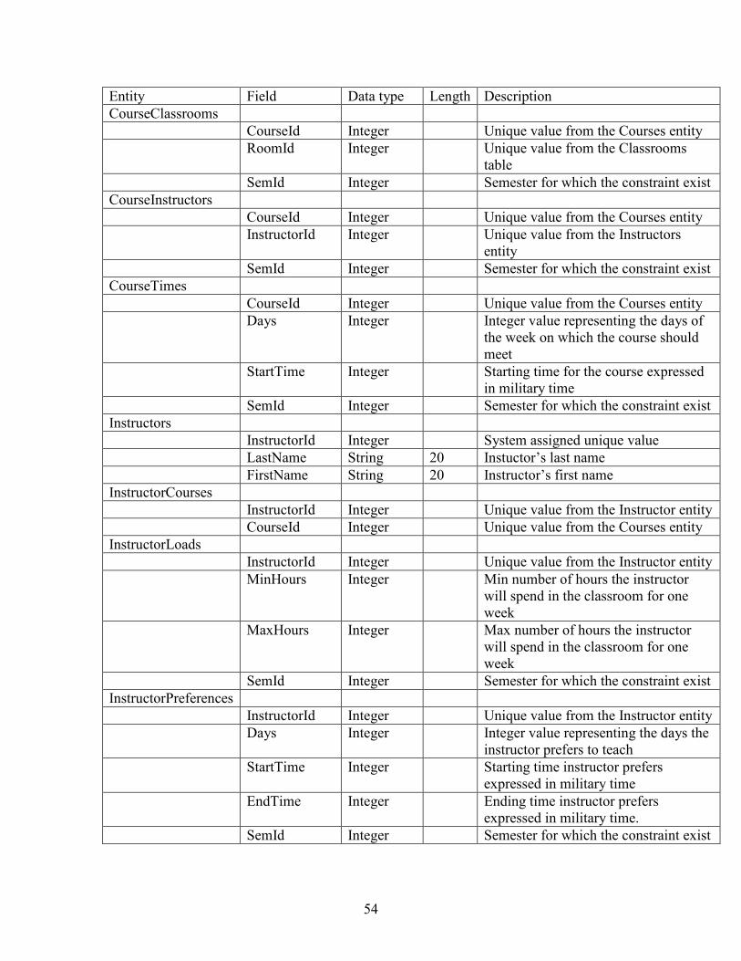
54

Entity Field Data type Length Description

CourseClassrooms

CourseId Integer Unique value from the Courses entity

RoomId Integer Unique value from the Classrooms

table

SemId Integer Semester for which the constraint exist

CourseInstructors

CourseId Integer Unique value from the Courses entity

InstructorId Integer Unique value from the Instructors

entity

SemId Integer Semester for which the constraint exist

CourseTimes

CourseId Integer Unique value from the Courses entity

Days Integer Integer value representing the days of

the week on which the course should

meet

StartTime Integer Starting time for the course expressed

in military time

SemId Integer Semester for which the constraint exist

Instructors

InstructorId Integer System assigned unique value

LastName String 20 Instuctor’s last name

FirstName String 20 Instructor’s first name

InstructorCourses

InstructorId Integer Unique value from the Instructor entity

CourseId Integer Unique value from the Courses entity

InstructorLoads

InstructorId Integer Unique value from the Instructor entity

MinHours Integer Min number of hours the instructor

will spend in the classroom for one

week

MaxHours Integer Max number of hours the instructor

will spend in the classroom for one

week

SemId Integer Semester for which the constraint exist

InstructorPreferences

InstructorId Integer Unique value from the Instructor entity

Days Integer Integer value representing the days the

instructor prefers to teach

StartTime Integer Starting time instructor prefers

expressed in military time

EndTime Integer Ending time instructor prefers

expressed in military time.

SemId Integer Semester for which the constraint exist

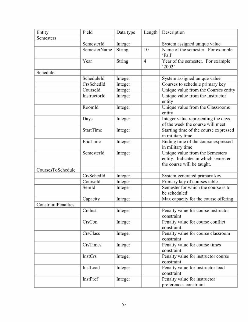
55

Entity Field Data type Length Description

Semesters

SemesterId Integer System assigned unique value

SemesterName String 10 Name of the semester. For example

‘Fall’

Year String 4 Year of the semester. For example

‘2002’

Schedule

ScheduleId Integer System assigned unique value

CrsSchedId Integer Courses to schedule primary key

CourseId Integer Unique value from the Courses entity

InstructorId Integer Unique value from the Instructor

entity

RoomId Integer Unique value from the Classrooms

entity

Days Integer Integer value representing the days

of the week the course will meet

StartTime Integer Starting time of the course expressed

in military time

EndTime Integer Ending time of the course expressed

in military time

SemesterId Integer Unique value from the Semesters

entity. Indicates in which semester

the course will be taught.

CoursesToSchedule

CrsSchedId Integer System generated primary key

CourseId Integer Primary key of courses table

SemId Integer Semester for which the course is to

be scheduled

Capacity Integer Max capacity for the course offering

ConstraintPenalties

CrsInst Integer Penalty value for course instructor

constraint

CrsCon Integer Penalty value for course conflict

constraint

CrsClass Integer Penalty value for course classroom

constraint

CrsTimes Integer Penalty value for course times

constraint

InstCrs Integer Penalty value for instructor course

constraint

InstLoad Integer Penalty value for instructor load

constraint

InstPref Integer Penalty value for instructor

preferences constraint

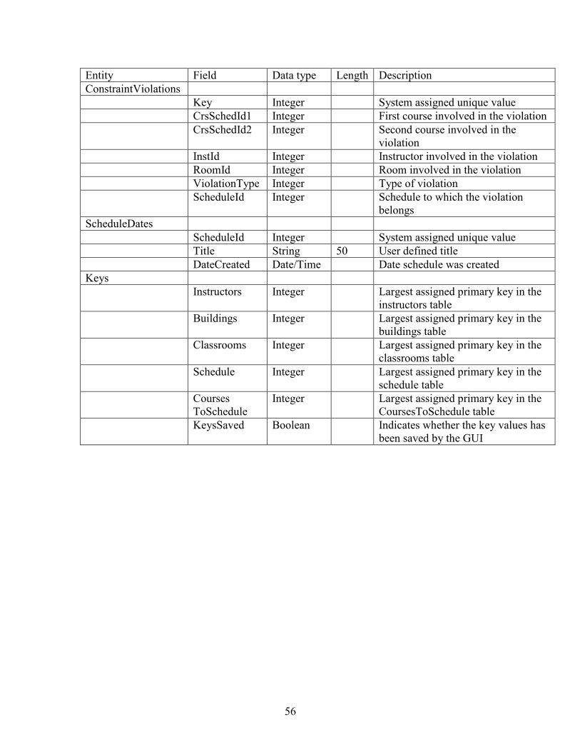
56

Entity Field Data type Length Description

ConstraintViolations

Key Integer System assigned unique value

CrsSchedId1 Integer First course involved in the violation

CrsSchedId2 Integer Second course involved in the

violation

InstId Integer Instructor involved in the violation

RoomId Integer Room involved in the violation

ViolationType Integer Type of violation

ScheduleId Integer Schedule to which the violation

belongs

ScheduleDates

ScheduleId Integer System assigned unique value

Title String 50 User defined title

DateCreated Date/Time Date schedule was created

Keys

Instructors Integer Largest assigned primary key in the

instructors table

Buildings Integer Largest assigned primary key in the

buildings table

Classrooms Integer Largest assigned primary key in the

classrooms table

Schedule Integer Largest assigned primary key in the

schedule table

Courses

ToSchedule

Integer Largest assigned primary key in the

CoursesToSchedule table

KeysSaved Boolean Indicates whether the key values has

been saved by the GUI