universitÀ degli studi di padova centro...
TRANSCRIPT
UNIVERSITÀ DEGLI STUDI DI PADOVA
CENTRO INTERDIPARTIMENTALE “Centro Ricerche Fusione”
UNIVERSIDADE TÉCNICA DE LISBOA
INSTITUTO SUPERIOR TÉCNICO
JOINT RESEARCH DOCTORATE IN FUSION SCIENCE AND ENGINEERING
CYCLE XXVII
Numerical studies of a negative ion beam and of a tomographic
beam diagnostic
Coordinator:
Prof. Paolo Bettini
Supervisors:
Prof. Piergiorgio Sonato
Dott. Roberto Pasqualotto
Dott. Gianluigi Serianni
Doctoral student: Nicola Fonnesu

iii
Abstract
ITER is the first reactor-scale scientific experiment that aims to demonstrate the scientific and the
technological feasibility of fusion energy. It is based on the tokamak concept of magnetic
confinement, in which the fuel, a mixture of deuterium and tritium heated to temperatures in excess of
150 million degrees Celsius, is contained in a toroidal vacuum chamber. Among the systems used to
reach such high temperature range, a fundamental role is played by the injection of intense beams of
neutral particles into the plasma, which is consequently heated by collisions. This process is realized
by means of two Neutral Beam Injectors (NBIs), capable of delivering to the plasma a power of 16.7
MW each. These devices are mainly composed of a negative deuterium ion source, an electrostatic
accelerator where a 40 A beam of negative deuterons will be accelerated to 1 MV and a neutralizer
which converts part of the beam into high energy neutrals able to penetrate the high magnetic field
confining the ITER plasma. The ITER requirements for these devices have never been simultaneously
achieved so far in a full scale, full performance device and therefore a neutral beam test facility is
being constructed at Consorzio RFX in Padova.
The research activity presented in this thesis work is in the framework of the development of the
negative ion source (SPIDER) and full injector (MITICA) prototypes for the ITER neutral beam. In
particular, it is focused on two main topics: particle transport studies inside the MITICA accelerator
and the development of a tomographic beam diagnostic.
A proper modeling of the particle transport inside the MITICA accelerator, considering the main
processes that generate secondary particles relevant for the evaluation of the heat loads on the
accelerator grids is essential for the thermo-mechanical analysis and the mechanical design of the
accelerator. For this reason an upgrade of the relativistic particle tracking code called EAMCC has
been undertaken and the simulations performed for evaluating the thermal power deposited on the
MITICA accelerator grids are presented in the first part of the present thesis work. For the first time,
an entire source called NIO1 installed at RFX and made of nine beamlets has been simulated in
EAMCC considering multi-beamlet effects which were neglected earlier and discarding the axis-
symmetry hypothesis of the electric fields imposed by the original version of the code. Results
obtained, also presented in the first part, will be used for benchmarking the modifications introduced
in the code.
The second part of the thesis is dedicated to beam tomography, an important diagnostic for the
assessment of the density profile of the beam. A tomography code based on algebraic reconstruction
techniques has been developed and numerically tested. Beam emissivity profiles considered for testing
the code are calculated by the upgraded version of EAMCC. The tomography code has been
developed with the aim of realizing a versatile instrument, applicable to linear accelerators as well as
to a tokamak and without adding any hypotheses about the beam characteristics or the emissivity in a
particular region of the tomography plane, not to limit the capability of the code of detecting
irregularities in the beam profiles. The effects of the instrumental noise on tomography reconstructions
have also been studied and, in order to reduce its impact, different filtering techniques have been
considered both in the frequency and in the spatial domain, demonstrating the feasibility to filter out
the effect of the noise by post-processing the reconstructed image of the beam.

iv
v
Riassunto
ITER (International Thermonuclear Experimental Reactor) è un reattore sperimentale a fusione
termonucleare basato sulla configurazione magnetica tokamak e volto a dimostrare la possibilità di
sfruttare l’energia da fusione per la generazione di elettricità. Il combustibile nucleare costituito da una
miscela di deuterio e trizio, portato a temperature eccedenti i 150 milioni di gradi centigradi, è
confinato in una camera di forma toroidale per mezzo di campi magnetici. Tra i sistemi usati per
riscaldare il combustibile nucleare, l’iniezione di neutri riveste un ruolo fondamentale. Essa consiste
nella iniezione di nuclei di deuterio ad alta energia (1 MeV) che scaldano il combustibile gassoso
altamente ionizzato (denominato plasma) a seguito delle collisioni con lo stesso. In ITER sono previsti
due iniettori di neutri (NBIs), ciascuno in grado di immettere nel plasma una potenza di 16,7 MW. Tali
iniettori sono essenzialmente costituiti da una sorgente di ioni negativi di deuterio, un acceleratore
elettrostatico dove un fascio di 40 A di tali ioni viene accelerato fino a raggiungere l’energia di 1 MeV
e un neutralizzatore nel quale una parte del fascio viene convertita in particelle neutre ad alta energia
che possono penetrare gli intensi campi magnetici usati per confinare il plasma: il sistema dovrà
operare continuativamente per un’ora. Le prestazioni richieste per tali iniettori di neutri non sono mai
state raggiunte fino ad ora simultaneamente in un unico esperimento e su tale scala. Si è reso pertanto
necessario lo studio e lo sviluppo di un prototipo di iniettore, affidato al Consorzio RFX di Padova. Il
progetto prevede lo studio e la realizzazione della sorgente di ioni dell’ITER NBI (SPIDER) e
successivamente la costruzione del prototipo dell’intero iniettore (MITICA).
La mia attività di ricerca, presentata in questa tesi, si inserisce in tale contesto e più in particolare è
incentrata sullo studio del trasporto di particelle all’interno di acceleratori lineari finalizzato al calcolo
della potenza termica depositata nelle griglie dell’acceleratore di MITICA e sullo sviluppo di una
diagnostica tomografica per fasci di particelle.
Un appropriato modello fisico, il più realistico possibile, dei fascetti di particelle che compongono il
fascio di MITICA è fondamentale per l’analisi termo-meccanica e per il progetto meccanico
dell’acceleratore. A tale scopo, sono state eseguite delle modifiche al codice di calcolo EAMCC usato
per simulare i processi di creazione di cariche secondarie che generano notevoli carichi termici sulle
griglie dell’acceleratore. La versione modificata del codice è stata utilizzata per lo studio del trasporto
di cariche nell’acceleratore di MITICA e per il calcolo dei carichi termici, come illustrato nella prima
parte della tesi. Inoltre, per la prima volta, l’intera sorgente chiamata NIO1 installata a RFX e
costituita da nove fascetti di ioni negativi di idrogeno è stata simulata con EAMCC, considerando
effetti fino ad ora non simulati, come l’interazione tra fascetti vicini, ed eliminando l’ipotesi
semplificativa di campi elettrici assial-simmetrici. I risultati delle simulazioni su NIO1 verranno usati
in futuro per la validazione sperimentale delle modifiche introdotte in EAMCC e sono sintetizzati
sempre nella prima parte del presente lavoro di tesi.
La seconda parte è invece dedicata alla tomografia del fascio che rappresenta una diagnostica
importante per la misura del profilo di densità delle particelle e consente di valutare il grado di
uniformità dello stesso, un requisito fondamentale per l’iniettore di neutri. In tale ambito è stato
sviluppato un codice tomografico basato su diverse tecniche di ricostruzione algebriche, più indicate
rispetto a tecniche basate sulla trasformata di Radon nel caso in cui il numero di rivelatori disponibile
sia molto inferiore rispetto al numero di pixel del profilo ricostruito. Tale codice è stato testato su
NIO1 e su MITICA con risultati promettenti. Non essendo disponibile alcuna misura sperimentale
dell’emissione dei fasci di particelle, grazie alle modifiche introdotte in EAMCC è stato possibile
calcolare il profilo di emissività di fotoni del fascio usato poi per il test del codice tomografico. E’
stato inoltre studiato il ruolo del rumore strumentale e il suo impatto sulle ricostruzioni tomograficche.
Sono state considerate tecniche di filtraggio sia nel dominio delle frequenze spaziali sia in quello
spaziale e in particolare, una tecnica usata per filtrare le immagini radar è stata adattata al caso
tomografico e implementata nel codice dimostrando la possibilità di limitare fortemente l’effetto
negativo del rumore sulla tomografia del fascio.

vi
vii
Contents
Abstract ................................................................................................................................................. iii
Riassunto ................................................................................................................................................ v
Introduction ........................................................................................................................................... 1
1 Neutral beam injectors for thermonuclear fusion .......................................................................... 5
1.1 Thermonuclear fusion ............................................................................................................... 5
1.2 ITER ........................................................................................................................................... 8
1.3 ITER NBI and the PRIMA test facility ....................................................................................... 10
1.3.1 SPIDER ............................................................................................................................. 11
1.3.2 MITICA ............................................................................................................................. 14
2 Simulation tools ............................................................................................................................... 17
2.1 SLACCAD ................................................................................................................................. 17
2.2 OPERA ..................................................................................................................................... 17
2.3 EAMCC .................................................................................................................................... 17
2.3.1 Negative ion stripping and ionization of the background gas ......................................... 18
2.3.2 Electron impact on the accelerator grids ........................................................................ 20
2.3.3 Heavy particle impact with accelerator grids .................................................................. 22
2.4 Modifications introduced in EAMCC ....................................................................................... 23
3 A multi-beamlet analysis of the MITICA accelerator.................................................................. 25
3.1 MITICA accelerator ................................................................................................................. 25
3.2 Reference conditions .............................................................................................................. 29
3.3 Comparison between EAMCC and EAMCC-mod .................................................................... 31
3.4 3D effects on a single-beamlet analysis.................................................................................. 32
3.5 Multi-beamlet analysis ........................................................................................................... 35
3.6 Conclusions and future works ................................................................................................ 39
4 Particle transport and heat loads in NIO1 .................................................................................... 41
4.1 The NIO1 experiment at RFX .................................................................................................. 41
4.2 Upgrade of the ion extractor and reference conditions for simulations................................ 43
4.3 Beam core and co-extracted electrons ................................................................................... 44
4.4 Beam halo ............................................................................................................................... 51
4.5 Conclusions and future works ................................................................................................ 55
5 A Multi-formula Iterative Reconstruction Tomography code for NIO1 ................................... 57
5.1 Beam emission tomography ................................................................................................... 57
5.2 Reconstruction algorithms implemented in the code ............................................................ 57
5.2.1 Algebraic Reconstruction Technique (ART) ..................................................................... 59
5.2.2 Simultaneous Algebraic Reconstruction Technique (SART) ............................................ 60
viii
5.2.3 Maximum-Likelihood Expectation-Maximization Algorithm (ML-EM) ........................... 61
5.3 The calculation of the emissivity profile for testing the tomography code ........................... 62
5.4 Geometry configurations and reconstructions....................................................................... 65
5.5 Instrumental noise and Butterworth filter ............................................................................. 71
5.6 Reconstruction of the MITICA emissivity profile .................................................................... 75
5.7 Instrumental noise in MITICA ................................................................................................. 79
5.8 Conclusions and future works ................................................................................................ 84
6 An Image Filtering Technique for SPIDER Visible Tomography .............................................. 85
6.1 Introduction ............................................................................................................................ 85
6.2 Emissivity profiles of the SPIDER beam .................................................................................. 85
6.3 Noise model and errors in the reconstructed beam profile ................................................... 87
6.4 Filtering in the frequency domain .......................................................................................... 90
6.4.1 Window function ............................................................................................................. 97
6.5 Filtering in the spatial domain by a local statistics method ................................................... 99
6.5.1 The implementation of the Lee’s algorithm .................................................................. 100
6.5.2 Results with a 3x3 and 5x5 local statistics ..................................................................... 101
6.6 Conclusions and future works .............................................................................................. 103
7 Conclusions .................................................................................................................................... 105
Bibliography ...................................................................................................................................... 107
Aknowledgements ............................................................................................................................. 112
1
Introduction
If a deuterium nucleus fuses with a tritium nucleus, an alpha particle is produced and a neutron
released. The nuclear rearrangement results in a reduction in total mass with the consequent release of
a significant amount of energy. In macroscopic terms, just 1 kg of this fuel would release 108 kWh of
energy and would provide the requirements of a 1 GW (electrical) power station for a day. The same
energy would be produced by burning more than 11600 tons of a good quality coal, or about 8700 tons
of fuel oil. Substantial advantages over other innovative forms of energy generation distinguish
nuclear fusion, in terms of environmental protection (no carbon emissions, neither transuranic nor
fission products), large fuel availability (deuterium can be extracted from water and tritium is
produced from lithium, which is found in the earth's crust) and intrinsic safety (the small amounts of
fuel used in fusion devices means that a large-scale nuclear accident is not possible).
Far from being commercially available, the production of energy from nuclear fusion could represent a
cleaner way to respond to our increasing energy demand, declining supplies of fossil fuel, responsible
for the negative effects of the greenhouse gases on the environment.
To build an operating controlled fusion reactor the most promising solution requires the particle
thermal energy to reach a sufficient threshold to overcome the Coulomb barrier between the reactants.
At these temperature values the fuel is in a state of ionized gas called plasma, where the electrostatic
charge of the nuclear ions is balanced by the presence of an equal number of electrons. Since such
high temperatures preclude confinement by material walls and plasma particles are subject to magnetic
fields, they can be confined in a toroidal region in which particles are forced to follow prescribed
gyrating orbits.
Presently the major efforts of the international community are focused on the controlled thermonuclear
fusion using magnetic fields to confine a plasma of tritium and deuterium in a vacuum chamber of
toroidal shape in the so called tokamak configuration. Great progress has been made in solving the
scientific problems and large efforts are currently devoted to tackle the technological challenges.
Many of the critical issues will be addressed in a new experiment known as ITER (the “path” towards
fusion energy), the world first reactor-scale burning plasma experiment under construction in France
(Cadarache).
In order to have a sufficient number of reactions to occur, the plasma temperature in ITER must be
raised up to 150 million degrees Celsius. The ohmic heating which is intrinsically produced by
externally induced and self-induced current flowing in the plasma is not sufficient to reach this
temperature and the use of auxiliary heating methods is necessary. Among the systems used to reach
such a high temperature range, a fundamental role is played by the injection of intense beams of
neutral particles into the plasma, which is consequently heated by collisions. This process will be
realized in ITER by means of two Neutral Beam Injectors (NBIs), capable of delivering to the plasma
a power of 16.7 MW each.
These devices are mainly composed of a negative deuterium ion source, an electrostatic accelerator
where a 40 A beam of negative deuterons will be accelerated to 1 MV and a neutralizer which
converts part of the beam into high energy neutrals, capable of penetrating the high magnetic field
confining the ITER plasma: the device should work continuously for one hour. The ITER
requirements for these devices have never been simultaneously achieved so far in a full scale, full
performance device and therefore a neutral beam test facility is being constructed at Consorzio RFX in
Padova. The facility will host two experimental devices: SPIDER, the full size prototype of the ITER
NBI ion source and MITICA the prototype of the full neutral beam. The purpose of this project is to
demonstrate the feasibility of a reliable and efficient prototype injector and to optimize its
performances.
My research activity is in the framework of the development of the negative ion source and full
injector prototypes for the ITER neutral beam. In particular it is focused on two main topics: particle
transport studies inside the MITICA accelerator and development of a tomographic beam diagnostic.
For what concerns the first topic, a proper modeling of the particle transport inside the MITICA
accelerator, considering all the secondary emission processes responsible for a relevant power
deposition on the accelerator grids, is essential for the thermo-mechanical analysis and the mechanical
2
design of the accelerator. This calculation is performed by EAMCC, a relativistic particle tracking
code based on the Monte-Carlo method for describing collisions inside the accelerator. EAMCC is
able to perform a single-beamlet analysis of the accelerator, which means that it simulates the
propagation of just one of the 1280 beamlets composing the MITICA beam, under the hypothesis of
axis-symmetric electric fields. An upgrade of EAMCC has been undertaken and a fully 3D version of
the code is now available for performing more realistic multi-beamlet simulations of the MITICA
accelerator. For the first time, an entire source called NIO1 installed at RFX and made of nine
beamlets has been simulated in EAMCC considering multi-beamlet effects before neglected and
discarding the axis-symmetry hypothesis of the electric fields imposed by the original version of the
code. Results obtained will be used for benchmarking the modifications introduced in the code.
As for tomography, its application to an ion beam can be useful for the assessment of the density
profile of the beam. It can go beyond the simple detection of the lack of uniformity of the beam,
giving information about its causes and suggesting possible solutions. A tomography code based on
algebraic reconstruction techniques has been developed and tested on the NIO1 emissivity profile
calculated by EAMCC. Algebraic techniques have been used since they are more suitable than
algorithms based on the Radon transform when the number of detectors is limited compared to the
number of pixels. The tomography code has been developed with the aim of realizing a versatile
instrument, applicable to different accelerators as well as to a tokamak and without adding any
hypotheses about the beam characteristics or imposing particular geometrical constraints to the
emissivity, in order not to limit the capability of the code of detecting irregularities in the beam
profiles.
The effects of the instrumental noise on tomography reconstructions have also been studied: a
particular case of interest regards the SPIDER tomographic diagnostic based on a pre-existing
reconstruction code. The main aim of this diagnostic in SPIDER will be measuring the uniformity of
the beam: in particular the ITER requirement for the beam is that the maximum acceptable deviation
from uniformity is ± 10%, thus the deviation of the tomographic reconstruction from the real
emissivity of the beam has to be sufficiently lower than this value. It was found that the noise has a
large influence on the maximum achievable resolution of the diagnostic and in order to reduce its
impact different filtering techniques have been considered both in the frequency and in the spatial
domain. In particular, a technique developed for radar imaging and based on a local statistics method
has been adapted and implemented in the SPIDER tomography code, demonstrating the feasibility to
filter out the effect of the noise by post-processing the reconstructed image of the beam.
The present thesis work synthesizes the mentioned activities and it is structured as follows:
Chapter 1 introduces the concept of thermonuclear fusion, the ITER project and the essentials
of a neutral beam injector, together with the description of the two experiments SPIDER and
MITICA.
Particle transport and heat load calculations
Chapter 2 is dedicated to the numerical simulation tools for the particle transport calculations
inside the accelerator. Codes used for the estimation of magnetic field and electric potential
maps inside the particle accelerator (required by EAMCC) are described, together with the
physics model and numerical approach in EAMCC.
Chapter 3 presents the simulation of the MITICA beam with EAMCC and the calculation of
heat loads on the accelerator grids: after the description of the MITICA accelerator, a
comparison between simulations performed with the original code and the modified version is
presented, as a validation of the modifications introduced in the latter. Subsequently, the main
results of a single-beamlet analysis performed with the two versions of the code are shown and
the differences between the 2D and the 3D simulations discussed. The last part of the chapter
is dedicated to the multi-beamlet simulation of the accelerator.
In Chapter 4 a 3D analysis of the NIO1 beam performed for the first time by EAMCC is
presented. The H- beam core, the co-extracted electrons and the beam halo fraction have been
simulated for determining the heat loads on grids and the power transmitted out of the

3
accelerator. The main results are reported after the description of the device, the proposed
upgrade and the reference conditions for the simulations.
Tomography and image filtering
Chapter 5 is focused on the tomography code developed for NIO1. In the the first part of this
chapter the algebraic method for tomography reconstructions and the iterative techniques
implemented in the code are described. Subsequently, the simulation of the transport of the 9
H- beamlets on the NIO1 tomography plane made by the modified version of EAMCC which
represents the ‘experimental’ emissivity profile to be reconstructed, the hypothesized
configurations of the tomography system and the reconstructions obtained in these cases are
presented. A concluding paragraph illustrates the reconstruction of the beam profile of
MITICA without including any constraint concerning the beam characteristics. In doing so, a
larger number of degrees of freedom are introduced in the tomography inversion problem and
consequently the reconstruction errors increase. However, the proposed technique allows the
correct reconstruction of the beam emissivity profile.
Chapter 6 is dedicated to a theoretical study of the instrumental noise in the SPIDER visible
tomography. It was found that the noise has a large influence on the maximum achievable
resolution of the diagnostic and in order to reduce its impact different filtering techniques have
been considered both in the frequency and in the spatial domain.
Chapter 7 summarizes the results of the previous chapters.

4
5
Chapter 1
Neutral beam injectors for thermonuclear fusion
Substantial advantages over other forms of innovative energy generation distinguish nuclear fusion, in
terms of environmental protection, fuel availability and intrinsic safety. Far from being commercially
available, the production of energy from nuclear fusion could represent a cleaner way to supply the
global increasing energy demand, declining supplies of fossil fuel, responsible for the negative effects
on the environment.
The major efforts of the international community are focused on the controlled thermonuclear fusion
by using magnetic fields to confine an ionized gas of tritium and deuterium in a vacuum chamber of
toroidal shape in the so called tokamak configuration. Great progress has been made in solving the
scientific problems and large efforts are currently underway to address the technological challenges
of a future fusion reactor. Many of the critical issues will be addressed in a new experiment known as
the International Thermonuclear Experimental Reactor (ITER) the world’s first reactor-scale burning
plasma experiment under construction in France (Cadarache.)
This introductory chapter gives a short overview on the basic issues of the controlled thermonuclear
fusion and the ITER project. In the context of the auxiliary systems required to heat the nuclear fuel up
to the temperature required to have a significant fusion reaction rate and consequently a positive
energy balance, the last part of the chapter is dedicated to the description of the neutral beam injector
system (NBI) and to the test facility under construction at RFX for the realization of the ITER NBI
prototype.
1.1 Thermonuclear fusion
Nuclear fusion is the reaction between two light nuclei that fuse into a heavier one, releasing energetic
reaction products. It was recognized as the power source of the Sun and other stars in 1938 [Bet38]
and since then, fusion research has been planned in many laboratories all over the world for
reproducing it on the Earth in a controlled manner.
Studies of the nuclear properties of light elements indicate that three such reactions may be
advantageous for the production of nuclear energy. These reactions involve the isotopes of the
hydrogen H2 and H
3, respectively called deuterium (D) and tritium (T), and helium-3 (He
3), an isotope
of helium.
The D-D reaction produces fusion energy by the nuclear interaction of two deuterium nuclei: this is
the most desirable reaction in the sense of a virtually unlimited supply of fuel, since the deuterium
could be extracted from the ocean water [Fre07]. This reaction has two branches, each occurring with
an approximately equal likelihood and can be written as follows (n is a neutron, p a proton):
)45.2()82.0(322 MeVnMeVHeHH , (1.1)
)03.3()01.1(322 MeVpMeVHHH . (1.2)
The second reaction of interest is the D-He3:
)67.14()67.3(432 MeVpMeVHeHeH . (1.3)
This reaction fuses a deuterium nucleus with a helium-3 nucleus. There are no natural supplies of
helium-3 on the Earth and this is the reason why current fusion research is not focused around this
reaction. Despite that, the reaction is worth discussing since the end products are all charged particles:
from an engineering point of view charged particles are more desirable than neutrons for extracting
energy as they greatly reduce the problems associated with materials activation and radiation damage.
6
They also offer the possibility of converting the nuclear energy directly into electricity without passing
through an inefficient steam cycle [Fre07].
The third reaction, the D–T, involves the fusion of a deuterium nucleus with a tritium nucleus:
)06.14()52.3(432 MeVnMeVHeHH . (1.4)
This reaction produces a high-energy neutron and a 3.5 MeV alpha particle. It requires a supply of
tritium in order to be capable of continuous operation. Tritium does not exist in nature and furthermore
it is radioactive (i.e. it is a low-energy beta emitter with a half-life of about 12 years). It can be
produced in the nuclear reactor from lithium, which exists in large quantities in the Earth’s crust (Li6
with isotopic abundance of ~7.5% and Li7 with ~ 92.5%), by bombarding it with neutrons produced by
the fusion reaction itself:
MeVHHenLi 8.4346 (1.5)
MeVnHHenLi 5.2347 (1.6)
The D–T reaction, nevertheless, produces a significant amount of nuclear energy, mostly as kinetic
energy of neutrons. In spite of the problems associated to high-energy neutrons (material activation
and radiation damage) and radioactivity associated with tritium, the D–T reaction is the central focus
of worldwide fusion research, a choice dominated by the fact that it is the easiest fusion reaction to
initiate. In fact, the reaction rate per unit volume is proportional to the density of reactants and to the
cross section of the considered fusion reaction, which mimics the probability of the same to occur
[Dua72, Per79].
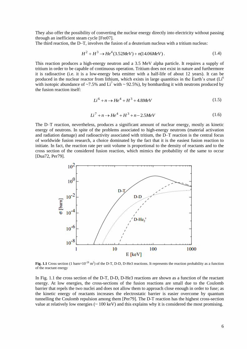
Fig. 1.1 Cross section (1 barn=10-28 m2) of the D-T, D-D, D-He3 reactions. It represents the reaction probability as a function
of the reactant energy
In Fig. 1.1 the cross section of the D-T, D-D, D-He3 reactions are shown as a function of the reactant
energy. At low energies, the cross-sections of the fusion reactions are small due to the Coulomb
barrier that repels the two nuclei and does not allow them to approach close enough in order to fuse; as
the kinetic energy of reactants increases the electrostatic barrier is easier overcome by quantum
tunnelling the Coulomb repulsion among them [Per79]. The D-T reaction has the highest cross-section
value at relatively low energies (~ 100 keV) and this explains why it is considered the most promising.
7
For a significant fraction of fusion reactions to occur, the nuclear fuel has thus to be brought to high
densities and temperatures for a sufficiently long time. In such conditions, matter is in the plasma
state, an ionized gas in globally neutral condition which exhibits collective properties [Gol95].
Since such high temperatures preclude confinement by material walls two methods emerged to be
rather promising for plasma confinement: magnetic confinement, which exploits the use of strong
magnetic fields [Wes04] and inertial confinement where small volumes of solid matter are brought to
sufficiently high temperatures and densities by firing high power lasers from many different directions
[Atz04].
Since the present thesis work is devoted to investigate some aspects of the neutral beam injector, an
important auxiliary system in fusion machines based on the magnetic confinement, henceforth just this
technology will be considered.
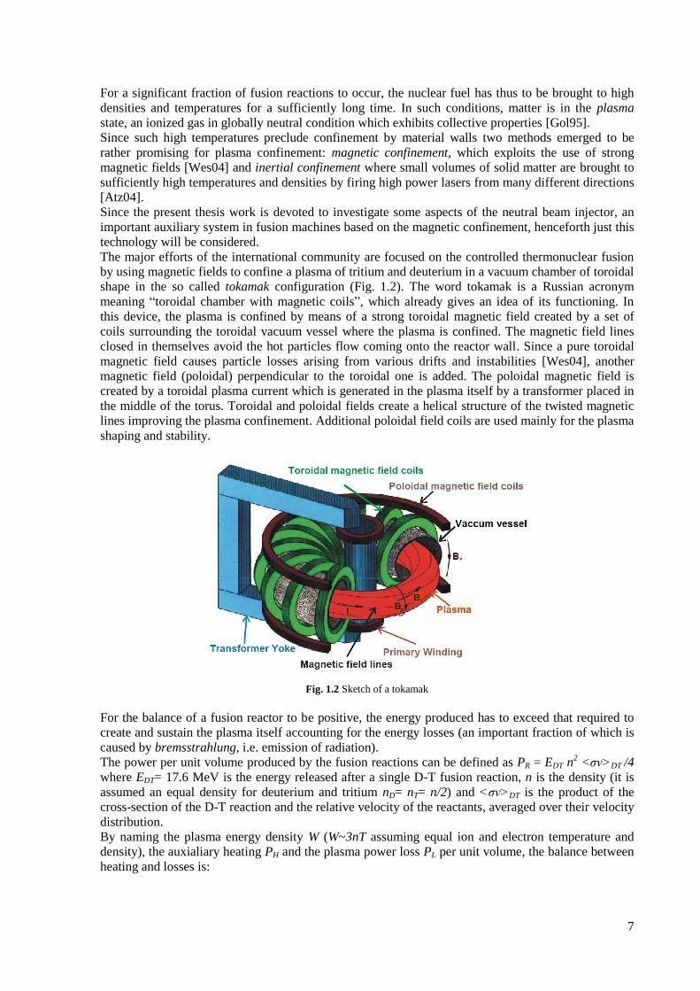
The major efforts of the international community are focused on the controlled thermonuclear fusion
by using magnetic fields to confine a plasma of tritium and deuterium in a vacuum chamber of toroidal
shape in the so called tokamak configuration (Fig. 1.2). The word tokamak is a Russian acronym
meaning “toroidal chamber with magnetic coils”, which already gives an idea of its functioning. In
this device, the plasma is confined by means of a strong toroidal magnetic field created by a set of
coils surrounding the toroidal vacuum vessel where the plasma is confined. The magnetic field lines
closed in themselves avoid the hot particles flow coming onto the reactor wall. Since a pure toroidal
magnetic field causes particle losses arising from various drifts and instabilities [Wes04], another
magnetic field (poloidal) perpendicular to the toroidal one is added. The poloidal magnetic field is
created by a toroidal plasma current which is generated in the plasma itself by a transformer placed in
the middle of the torus. Toroidal and poloidal fields create a helical structure of the twisted magnetic
lines improving the plasma confinement. Additional poloidal field coils are used mainly for the plasma
shaping and stability.
Fig. 1.2 Sketch of a tokamak
For the balance of a fusion reactor to be positive, the energy produced has to exceed that required to
create and sustain the plasma itself accounting for the energy losses (an important fraction of which is
caused by bremsstrahlung, i.e. emission of radiation).
The power per unit volume produced by the fusion reactions can be defined as PR = EDT n2 <σv>DT /4
where EDT= 17.6 MeV is the energy released after a single D-T fusion reaction, n is the density (it is
assumed an equal density for deuterium and tritium nD= nT= n/2) and <σv>DT is the product of the
cross-section of the D-T reaction and the relative velocity of the reactants, averaged over their velocity
distribution.
By naming the plasma energy density W (W~3nT assuming equal ion and electron temperature and
density), the auxialiary heating PH and the plasma power loss PL per unit volume, the balance between
heating and losses is:
8
LRH PPPt
W
. (1.7)
Without any heating, the energy decreases almost exponentially ∂W/∂t=-W/τE with a characteristic
energy confinement time τE. One of the most desirable reactor scenarios is one in which the alpha
particles produced by fusion reactions are confined and replace all the energy losses by transferring
their energy to the plasma, whereas neutrons escape the plasma volume and their energy is converted
to electric energy. By analogy with the burning of fossil fuels this event is called ignition: the auxiliary
heating can be removed since the plasma temperature is sustained solely by alpha particle heating. The
ignition condition can be calculated considering that it must be PR ≥ PL where PR= Pα =Eα n <σv>DT /4
and Eα=3.5 MeV is the kinetic energy of the alpha particle released after the D-T reaction.
Under these assumptions, the ignition condition, that is usually expressed in the following convenient
form, becomes:
][103 321 skeVmTn E (1.8)
Where the so called triple product (nτET) brings out clearly the requirements on density, temperature
and confinement time for the burning plasma.
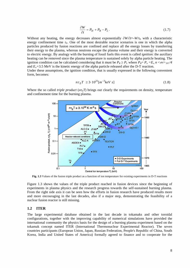
Fig. 1.3 Values of the fusion triple product as a function of ion temperature for existing experiments in D-T reactions
Figure 1.3 shows the values of the triple product reached in fusion devices since the beginning of
experiments in plasma physics and the research progress towards the self-sustained burning plasma.
From the right side axis it can be seen how the efforts in fusion research have produced results more
and more encouraging in the last decades, also if a major step, demonstrating the feasibility of a
nuclear fusion reactor is still missing.
1.2 ITER
The large experimental database obtained in the last decade in tokamaks and other toroidal
configurations, together with the improving capability of numerical simulations have provided the
international community the physics basis for the design of a burning plasma experiment based on the
tokamak concept named ITER (International Thermonuclear Experimental Reactor). The seven
countries participants (European Union, Japan, Russian Federation, People's Republic of China, South
Korea, India and United States of America) formally agreed to finance and to cooperate for the
9
realization of the project in November 2006. The site preparation (Cadarache, France) is in progress
and the first plasma operation is expected in 2020 [Ite14].
ITER would offer the possibility of studying several reactor relevant scientific and technological
issues, which are beyond the present experimental capabilities. New physical regimes and a variety of
technological issues will be explored with ITER, like the test of advanced materials facing very large
heat and particle fluxes, the test of concepts for a tritium breeding module, the superconducting
technology under high neutron flux and many others. All of these requirements are expected to solve
many of the scientific and engineering issues concerning a burning plasma and could allow to make a
straightforward step towards the demonstration of a nuclear fusion power plant.
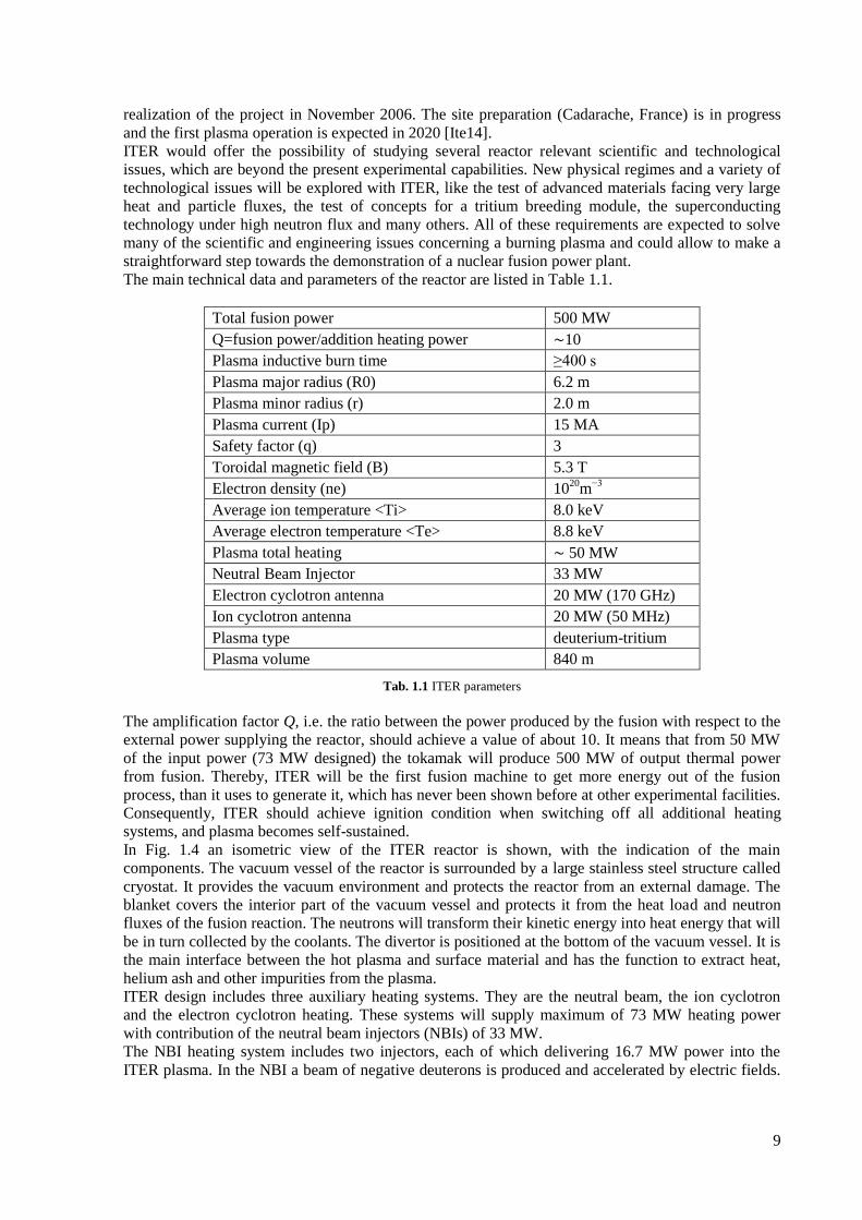
The main technical data and parameters of the reactor are listed in Table 1.1.
Total fusion power 500 MW
Q=fusion power/addition heating power ∼10
Plasma inductive burn time ≥400 s
Plasma major radius (R0) 6.2 m
Plasma minor radius (r) 2.0 m
Plasma current (Ip) 15 MA
Safety factor (q) 3
Toroidal magnetic field (B) 5.3 T
Electron density (ne) 1020
m−3
Average ion temperature <Ti> 8.0 keV
Average electron temperature <Te> 8.8 keV
Plasma total heating ∼ 50 MW
Neutral Beam Injector 33 MW
Electron cyclotron antenna 20 MW (170 GHz)
Ion cyclotron antenna 20 MW (50 MHz)
Plasma type deuterium-tritium
Plasma volume 840 m
Tab. 1.1 ITER parameters
The amplification factor Q, i.e. the ratio between the power produced by the fusion with respect to the
external power supplying the reactor, should achieve a value of about 10. It means that from 50 MW
of the input power (73 MW designed) the tokamak will produce 500 MW of output thermal power
from fusion. Thereby, ITER will be the first fusion machine to get more energy out of the fusion
process, than it uses to generate it, which has never been shown before at other experimental facilities.
Consequently, ITER should achieve ignition condition when switching off all additional heating
systems, and plasma becomes self-sustained.
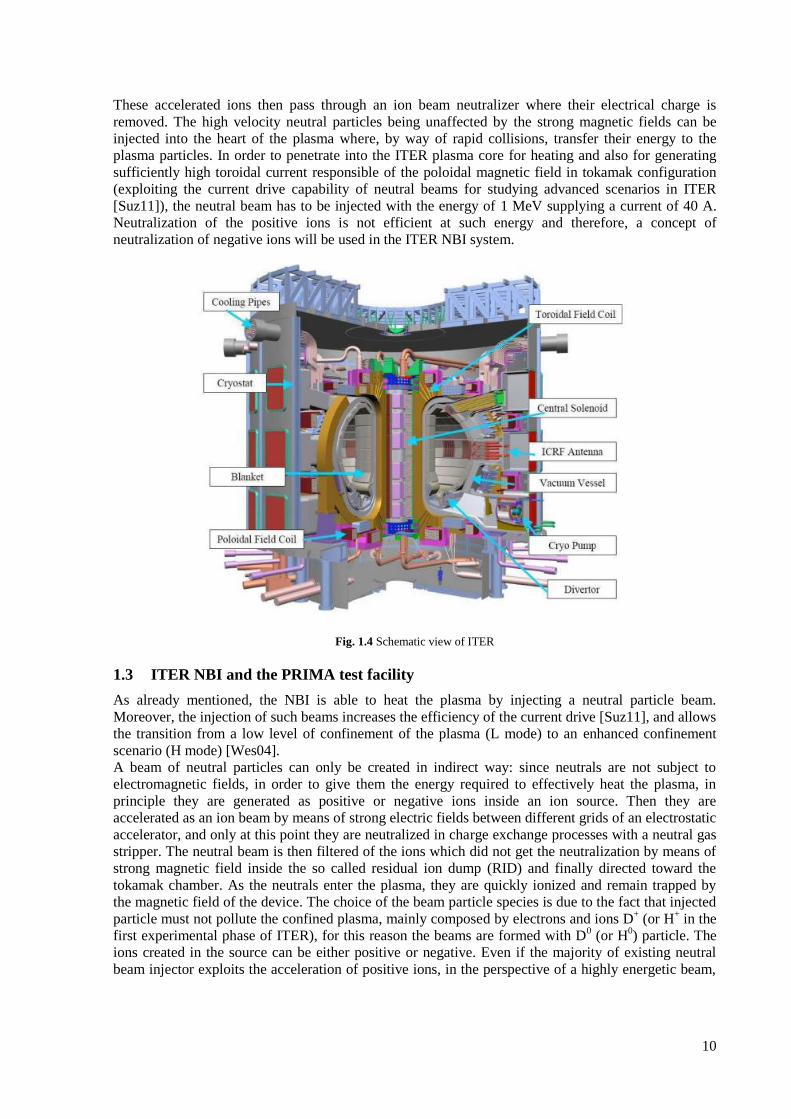
In Fig. 1.4 an isometric view of the ITER reactor is shown, with the indication of the main
components. The vacuum vessel of the reactor is surrounded by a large stainless steel structure called
cryostat. It provides the vacuum environment and protects the reactor from an external damage. The
blanket covers the interior part of the vacuum vessel and protects it from the heat load and neutron
fluxes of the fusion reaction. The neutrons will transform their kinetic energy into heat energy that will
be in turn collected by the coolants. The divertor is positioned at the bottom of the vacuum vessel. It is
the main interface between the hot plasma and surface material and has the function to extract heat,
helium ash and other impurities from the plasma.
ITER design includes three auxiliary heating systems. They are the neutral beam, the ion cyclotron
and the electron cyclotron heating. These systems will supply maximum of 73 MW heating power
with contribution of the neutral beam injectors (NBIs) of 33 MW.
The NBI heating system includes two injectors, each of which delivering 16.7 MW power into the
ITER plasma. In the NBI a beam of negative deuterons is produced and accelerated by electric fields.
10
These accelerated ions then pass through an ion beam neutralizer where their electrical charge is
removed. The high velocity neutral particles being unaffected by the strong magnetic fields can be
injected into the heart of the plasma where, by way of rapid collisions, transfer their energy to the
plasma particles. In order to penetrate into the ITER plasma core for heating and also for generating
sufficiently high toroidal current responsible of the poloidal magnetic field in tokamak configuration
(exploiting the current drive capability of neutral beams for studying advanced scenarios in ITER
[Suz11]), the neutral beam has to be injected with the energy of 1 MeV supplying a current of 40 A.
Neutralization of the positive ions is not efficient at such energy and therefore, a concept of
neutralization of negative ions will be used in the ITER NBI system.
Fig. 1.4 Schematic view of ITER
1.3 ITER NBI and the PRIMA test facility
As already mentioned, the NBI is able to heat the plasma by injecting a neutral particle beam.
Moreover, the injection of such beams increases the efficiency of the current drive [Suz11], and allows
the transition from a low level of confinement of the plasma (L mode) to an enhanced confinement
scenario (H mode) [Wes04].
A beam of neutral particles can only be created in indirect way: since neutrals are not subject to
electromagnetic fields, in order to give them the energy required to effectively heat the plasma, in
principle they are generated as positive or negative ions inside an ion source. Then they are
accelerated as an ion beam by means of strong electric fields between different grids of an electrostatic
accelerator, and only at this point they are neutralized in charge exchange processes with a neutral gas
stripper. The neutral beam is then filtered of the ions which did not get the neutralization by means of
strong magnetic field inside the so called residual ion dump (RID) and finally directed toward the
tokamak chamber. As the neutrals enter the plasma, they are quickly ionized and remain trapped by
the magnetic field of the device. The choice of the beam particle species is due to the fact that injected
particle must not pollute the confined plasma, mainly composed by electrons and ions D+ (or H
+ in the
first experimental phase of ITER), for this reason the beams are formed with D0 (or H
0) particle. The
ions created in the source can be either positive or negative. Even if the majority of existing neutral
beam injector exploits the acceleration of positive ions, in the perspective of a highly energetic beam,
11
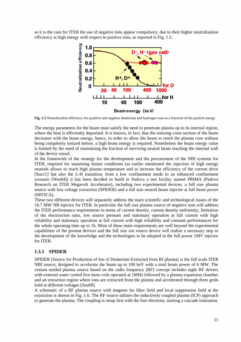
as it is the case for ITER the use of negative ions appear compulsory, due to their higher neutralization
efficiency at high energy with respect to positive ions, as reported in Fig. 1.5.
Fig. 1.5 Neutralization efficiency for positive and negative deuterium and hydrogen ions as a function of the particle energy
The energy parameters for the beam must satisfy the need to penetrate plasma up to its internal region,
where the heat is efficiently deposited. It is known, in fact, that the ionizing cross section of the beam
decreases with the beam energy, hence, in order to allow the beam to reach the plasma core without
being completely ionized before, a high beam energy is required. Nonetheless the beam energy value
is limited by the need of minimizing the fraction of surviving neutral beam reaching the internal wall
of the device vessel.
In the framework of the strategy for the development and the procurement of the NBI systems for
ITER, required for sustaining fusion conditions (as earlier mentioned the injection of high energy
neutrals allows to reach high plasma temperature and to increase the efficiency of the current drive
[Suz11] but also the L-H transition, from a low confinement mode to an enhanced confinement
scenario [Wes04]) it has been decided to build in Padova a test facility named PRIMA (Padova
Research on ITER Megavolt Accelerator), including two experimental devices: a full size plasma
source with low voltage extraction (SPIDER) and a full size neutral beam injector at full beam power
(MITICA).
These two different devices will separately address the main scientific and technological issues of the
16.7 MW NB injector for ITER. In particular the full size plasma source of negative ions will address
the ITER performance requirements in terms of current density, current density uniformity, limitation
of the electron/ion ratio, low source pressure and stationary operation at full current with high
reliability and stationary operation at full current with high reliability and constant performances for
the whole operating time up to 1h. Most of these main requirements are well beyond the experimental
capabilities of the present devices and the full size ion source device will realize a necessary step to
the development of the knowledge and the technologies to be adopted in the full power 1MV injector
for ITER.
1.3.1 SPIDER
SPIDER (Source for Production of Ion of Deuterium Extracted from Rf plasma) is the full scale ITER
NBI source, designed to accelerate the beam up to 100 keV with a total beam power of 6 MW. The
cesium seeded plasma source based on the radio frequency (RF) concept includes eight RF drivers
with external water cooled five turns coils operated at 1MHz followed by a plasma expansion chamber
and an extraction region where ions are extracted from the plasma and accelerated through three grids
hold at different voltages [Son09].
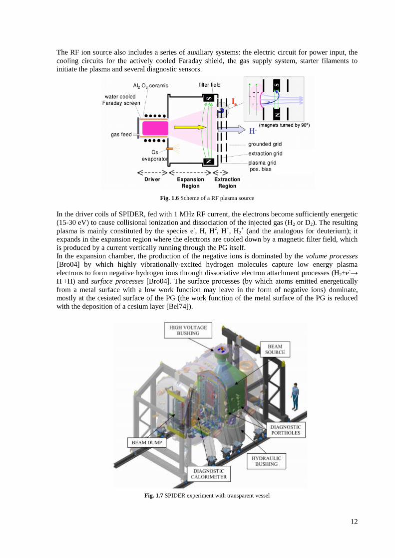
A schematic of a RF plasma source with magnets for filter field and local suppression field at the
extraction is shown in Fig. 1.6. The RF source utilizes the inductively coupled plasma (ICP) approach
to generate the plasma. The coupling is setup first with the free electrons, starting a cascade ionization.
12
The RF ion source also includes a series of auxiliary systems: the electric circuit for power input, the
cooling circuits for the actively cooled Faraday shield, the gas supply system, starter filaments to
initiate the plasma and several diagnostic sensors.
Fig. 1.6 Scheme of a RF plasma source
In the driver coils of SPIDER, fed with 1 MHz RF current, the electrons become sufficiently energetic
(15-30 eV) to cause collisional ionization and dissociation of the injected gas (H2 or D2). The resulting
plasma is mainly constituted by the species e-, H, H
2, H
+, H2
+ (and the analogous for deuterium); it
expands in the expansion region where the electrons are cooled down by a magnetic filter field, which
is produced by a current vertically running through the PG itself.
In the expansion chamber, the production of the negative ions is dominated by the volume processes
[Bro04] by which highly vibrationally-excited hydrogen molecules capture low energy plasma
electrons to form negative hydrogen ions through dissociative electron attachment processes (H2+e-→
H-+H) and surface processes [Bro04]. The surface processes (by which atoms emitted energetically
from a metal surface with a low work function may leave in the form of negative ions) dominate,
mostly at the cesiated surface of the PG (the work function of the metal surface of the PG is reduced
with the deposition of a cesium layer [Bel74]).
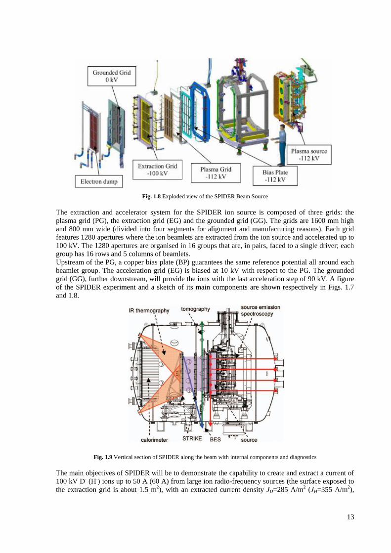
Fig. 1.7 SPIDER experiment with transparent vessel
13
Fig. 1.8 Exploded view of the SPIDER Beam Source
The extraction and accelerator system for the SPIDER ion source is composed of three grids: the
plasma grid (PG), the extraction grid (EG) and the grounded grid (GG). The grids are 1600 mm high
and 800 mm wide (divided into four segments for alignment and manufacturing reasons). Each grid
features 1280 apertures where the ion beamlets are extracted from the ion source and accelerated up to
100 kV. The 1280 apertures are organised in 16 groups that are, in pairs, faced to a single driver; each
group has 16 rows and 5 columns of beamlets.
Upstream of the PG, a copper bias plate (BP) guarantees the same reference potential all around each
beamlet group. The acceleration grid (EG) is biased at 10 kV with respect to the PG. The grounded
grid (GG), further downstream, will provide the ions with the last acceleration step of 90 kV. A figure
of the SPIDER experiment and a sketch of its main components are shown respectively in Figs. 1.7
and 1.8.
Fig. 1.9 Vertical section of SPIDER along the beam with internal components and diagnostics
The main objectives of SPIDER will be to demonstrate the capability to create and extract a current of
100 kV D- (H
-) ions up to 50 A (60 A) from large ion radio-frequency sources (the surface exposed to
the extraction grid is about 1.5 m2), with an extracted current density JD=285 A/m
2 (JH=355 A/m
2),
14
focusing on the uniformity (the admissible ion inhomogeneity should be better than 10 %) and in the
containment of electron leakages. In particular the ratio between the number of electrons with respect
to the number of ions extracted from the source should be limited to less than 1.
Most of these studies can be performed thanks to a dedicated set of diagnostics shown in Fig. 1.9. The
RF source will be monitored with thermocouples, electrostatic probes, optical emission spectroscopy,
cavity ring down, and laser absorption spectroscopy. The beam is analyzed by cooling water
calorimetry, a short pulse instrumented calorimeter, beam emission spectroscopy, visible tomography
and neutron imaging [Pas12]. In particular the visible tomography system devoted to the measurement
of the beam density profile and to the assessment of the beam uniformity will be the subject of the
chapter 6 of the present thesis work.
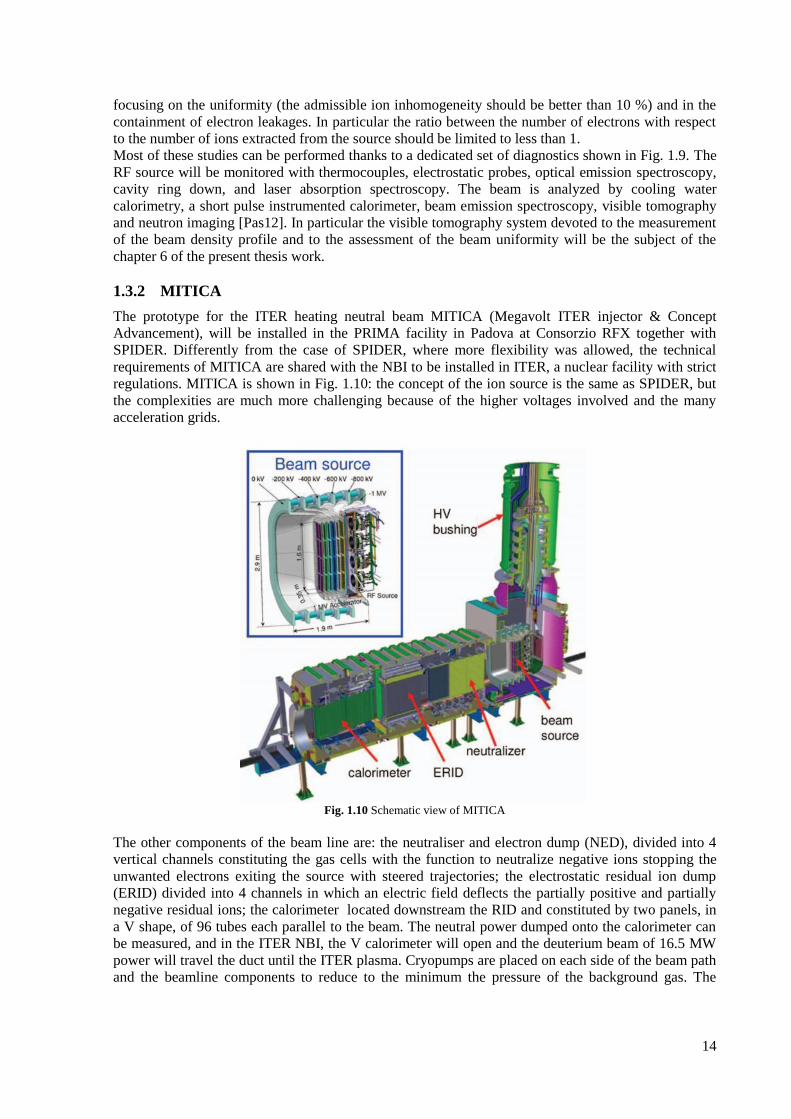
1.3.2 MITICA
The prototype for the ITER heating neutral beam MITICA (Megavolt ITER injector & Concept
Advancement), will be installed in the PRIMA facility in Padova at Consorzio RFX together with
SPIDER. Differently from the case of SPIDER, where more flexibility was allowed, the technical
requirements of MITICA are shared with the NBI to be installed in ITER, a nuclear facility with strict
regulations. MITICA is shown in Fig. 1.10: the concept of the ion source is the same as SPIDER, but
the complexities are much more challenging because of the higher voltages involved and the many
acceleration grids.
Fig. 1.10 Schematic view of MITICA
The other components of the beam line are: the neutraliser and electron dump (NED), divided into 4
vertical channels constituting the gas cells with the function to neutralize negative ions stopping the
unwanted electrons exiting the source with steered trajectories; the electrostatic residual ion dump
(ERID) divided into 4 channels in which an electric field deflects the partially positive and partially
negative residual ions; the calorimeter located downstream the RID and constituted by two panels, in
a V shape, of 96 tubes each parallel to the beam. The neutral power dumped onto the calorimeter can
be measured, and in the ITER NBI, the V calorimeter will open and the deuterium beam of 16.5 MW
power will travel the duct until the ITER plasma. Cryopumps are placed on each side of the beam path
and the beamline components to reduce to the minimum the pressure of the background gas. The

15
pressure downstream the accelerator must be low in order to minimize losses in the accelerator. The
pressure downstream of the neutralizer must be low in order to minimize re-ionization of the D0.
Two modes of operations are foreseen for the NBI, the plasma operation mode, and the
commissioning/conditioning mode in which the neutral beam is dumped on the calorimeter.
The MITICA accelerator will be described in chapter 3 where a particle transport study for the
calculation of the heat loads on the accelerator grids is presented.

16
17
Chapter 2
Simulation tools
This chapter is dedicated to the description of the numerical simulation tools that will be used for
performing particle transport calculations inside the electrostatic accelerator of MITICA. EAMCC is
a relativistic particle tracking code where the macro-particle trajectories of a single negative ion
beamlet (and related secondary particles), are calculated in prescribed electric and magnetic fields
inside the ion accelerator vessel. The magnetic field maps are produced by 3D codes, in particular by
OPERA-TOSCA, while for the calculation of the electric field, electric potential maps are calculated
by SLACCAD and OPERA-SCALA.
2.1 SLACCAD
The SLACCAD code estimates the electric potential inside an electrostatic accelerator by integrating
the Poisson's equation and using a Monte Carlo approach. It is a modified version of the SLAC code,
developed at the Stanford laboratories in the '70s and devoted to the simulation of the positive ions
based plasma source facility [Her79]. The implementation of the negative ions, including beam
attenuation and a free plasma boundary is due to J. Pamela [Pam91]. SLACCAD simulates the
acceleration of negative ions in a linear accelerator, considering a 2 dimensional (2D) axial symmetric
geometry, giving self consistent results on the potential distribution due to both accelerating electrodes
and space charge distribution of the beam.
In spite of the fact that it neglects many physical aspects such as the influence of magnetic fields on
the ion trajectories and the electrons space charge, and it does not perform any plasma physics
calculations, due to its long-time usage on different laboratories it is considered one of the most stable
and efficient codes for calculating the single beamlet optics of negative ion beams.
2.2 OPERA
Opera is a three dimensional (3D) commercial simulation software suite based on the finite element
method (FEM) for electromagnetic analysis [Ope14]. It includes eight analysis programs to deal with
different electromagnetic analysis and for what concerns the beam accelerator, SCALA and TOSCA
are the two modules of interest.
SCALA analyses electrostatic fields taking into account the effects of space charge created by beams
of charged particles. It uses the finite element method to solve the electrostatic Poisson’s equation, and
calculate the electric scalar potential (i.e. the electric potential map of the accelerator). The space
charge density, included in the Poisson’s equation solution, is found by calculating the trajectories of a
set of charged particles from the emitters under the influence of the electrostatic field and magnetic
fields. Secondary particles produced as a result of collisions are also included in the calculation. The
extraction of charged particle beams from the plasma source is also modelled.
The magnetic fields are provided by coupling SCALA with TOSCA, which solves nonlinear
magnetostatic field and current flow models in three dimensions. In particular, TOSCA is used for the
calculation of magnetostatic fields inside the accelerator due to current sources and permanent
magnets embedded in the accelerator grids.
OPERA incorporates state of the art algorithms for the calculation of electromagnetic fields, advanced
finite element and nonlinear equation numerical analysis procedures.
2.3 EAMCC
EAMCC is a relativistic particle tracking code where the macro-particle trajectories of a single
negative hydrogen (H-) or deuterium (D
-) beamlet and related secondary particles, are calculated in
18
prescribed electric and magnetic fields inside the ion accelerator vessel. In the code each macro-
particle represents an ensemble of rays, carrying a microcurrent of typically 50 nA.
The code has been developed by G. Fubiani [Fub08] with the purpose of modeling particle-particle
and particle-surface interactions in ITER NBI-like accelerators (i.e. multiaperture and multigrid
negative ion accelerators) for the calculation of the relevant thermal power deposition on the
accelerator grids.
For the calculation of the electric field inside the accelerator, EAMCC requires a 2D axy-symmetric
electric potential map. This map is made by SLACCAD code [Pam91] that solves Poisson’s equation
on a 2D cylindrically symmetric grid. SLACCAD does not perform any plasma physics calculations
and as a consequence the plasma meniscus (i.e. the boundary which separates the source plasma from
the accelerated negative ion beam, where the potential is ~ 0 V) is calculated rather simply by
imposing a vanishing electrostatic field inside the simulation domain dedicated to the ion source area,
i.e. the region where the potential drops below the plasma grid potential. The magnetic field maps are
produced by 3D codes.
The different kinds of particle-metallic surface and particle-particle interactions (electron and heavy
ion/neutral collisions with accelerator grids, negative ion single and double stripping reactions,
ionization of background gas) are modeled using a Monte-Carlo method [Vah95] and in the following
subsections, the details of the numerical approach are reported.
2.3.1 Negative ion stripping and ionization of the background gas
Negative ion (H-/D
-) stripping occurs due to collisions with the residual background gas (H2/D2) in the
accelerator, which either comes from the ion source or the neutralizer. Stripping of negative ions is the
main cause of high energy electron production in conventional electrostatic accelerators found on
fusion machines (typically of the order of 20-30%) [Fub08]. These electrons are assumed to be emitted
at the location of the collision with the same direction and velocity as the parent H- or D
-.�
Ionization of the background gas caused by negative ions and neutrals (H0/D
0) are also important
reactions leading to destruction of negative and neutral hydrogen (or deuterium) with the production of
secondary particles.
Stripping and ionization reactions considered in EAMCC for hydrogen are:
Single ion stripping eHHHH 20
2 (2.1)
Double ion stripping eHHHH 222 (2.2)
Ionization by negative ions eHHHH 22 (2.3)
Ionization by neutrals eHHHH 20
20 (2.4)
As earlier mentioned, the same reactions are implemented in the code also for deuterium.
These reactions are calculated using a Monte-Carlo method. For instance, the rate equation for
destruction of negative ions caused by stripping (reactions 2.1 and 2.2) may be written as follows:
Nzvdz
dN
i
i )(2
1
(2.5)
giving
z
tot dzzvNzN
0
0 )(exp)(
(2.6)
19
where N(z) is the number of negative ions at location z inside the accelerator, N0=N(z=0) is the number
at the ion extraction location (plasma grid location), and vtot is the total frequency associated with the
two considered stripping reactions:
)()()(2
1
zznzv
i
igtot
(2.7)
In Eq. 2.7 ng represents the background gas density and σi the cross section of the i-th considered
reaction. Consequently, for a macro-particle, a reaction occurs if within a small interval Δz we have:
zzvzN
zNr itot
i
i
)(exp1)(
)(1
(2.8)
where ΔN(zi)= N(zi)-N(zi+Δz) and r1 is a random number between 0 and 1. In order to determine
which type of reactions occurred (2.1 or 2.2), a second random number r2 is used. If r2≤ v1/vtot then
reaction 2.1 occured, otherwise reaction 2.2 would have happened [Fub08].
The same scheme is also applied to the ionization of the background gas by collisions with negative
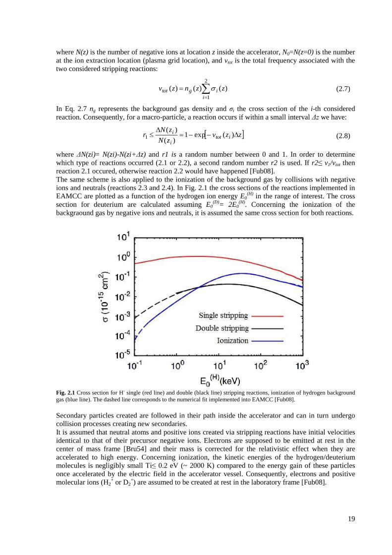
ions and neutrals (reactions 2.3 and 2.4). In Fig. 2.1 the cross sections of the reactions implemented in
EAMCC are plotted as a function of the hydrogen ion energy E0(H)
in the range of interest. The cross
section for deuterium are calculated assuming E0(D)
= 2E0(H)
. Concerning the ionization of the
backgraound gas by negative ions and neutrals, it is assumed the same cross section for both reactions.
Fig. 2.1 Cross section for H- single (red line) and double (black line) stripping reactions, ionization of hydrogen background
gas (blue line). The dashed line corresponds to the numerical fit implemented into EAMCC [Fub08].
Secondary particles created are followed in their path inside the accelerator and can in turn undergo
collision processes creating new secondaries.
It is assumed that neutral atoms and positive ions created via stripping reactions have initial velocities
identical to that of their precursor negative ions. Electrons are supposed to be emitted at rest in the
center of mass frame [Bru54] and their mass is corrected for the relativistic effect when they are
accelerated to high energy. Concerning ionization, the kinetic energies of the hydrogen/deuterium
molecules is negligibly small Ti≤ 0.2 eV (~ 2000 K) compared to the energy gain of these particles
once accelerated by the electric field in the accelerator vessel. Consequently, electrons and positive
molecular ions (H2+ or D2
+) are assumed to be created at rest in the laboratory frame [Fub08].
20
2.3.2 Electron impact on the accelerator grids
The greatest power deposition on the accelerator grids is usually from electrons, created by stripping
and ionization reactions illustrated in the previous subsection and co-extracted from the ion source
[Dud12, Kra12].
The knowledge of the energy and spatial distribution of seconday and reflected electrons, which
depend on the energy and angle of the incident electron [Mat74, Dar75], is essential for modeling the
consequences of the impacts of electrons on the accelerator grids.
The emission energy spectra of secondary electrons can be separated into three quasi-independent
phenomena [Fur02]: (i) elastically reflected electrons with Ekb=E0, where Ekb is the reflected electron
energy, i.e., electron reflection with almost no energy loss; (ii) backscattered electrons with an energy
range 0 to E0, where E0 is the energy of the incident electron; (iii) true secondary electron production
with a typically low-energy spectra extending from 0 to 50 eV.
The first effect is negligible for energies greater than ~ 500 eV and it is not included in EAMCC
[Fub08].
The modeling of backscattered electron processes is based on a semianalytical approach [Sta94]. The
kinetic energy of backscattered electrons (Ekb) normalized to the incident electron energy E0 is
calculated as:
/1
/10 )/(ln
11
PS
K
E
Ep
kb
(2.9)
where P is a random number between 0 and 1,
)exp(0p
b KS
(2.10)
where ηb0= η( ϑ1 =0) is the probability for a primary electron to be backscattered at normal incidence.
γ and K are:
2/3ln6exp1
B
(2.11)
4ln70 BK
(2.12)
Bϑ is calculated according to the formula:
2
0210 )cos1(exp),,(
i
iBEB (2.13)
where ϑ1, ϑ2 are the incidence and scattering angles.
In Eqs. 2.9-2.13, p, B0, α and τ are parameters used to fit experimental data taken from [Mat74, Ste54],
as reported in Tab.2.1. For intermediate energies, a linear interpolation is performed for obtaining their
value.
The probability ηb for a primary electron impacting the grid at an incidence angle ϑ1 to be
backscattered is calculated considering the backscattered probability at normal incidence ηb0 [Dar75]:
)cos1(exp)( 1001 bbb A
(2.14)
where the coefficient Ab0 is calculated by fitting experimental data [Sta94] as:
))/1ln(( 000 bb EkA
(2.15)
with
))(83.1exp(1 4/10 keVEk
(2.16)
21
E0 (keV) 2 10 20 370
p
0.320 0.270 0.270 0.270
B0
0.200 0.240 0.265 0.273
α
2.200 2.200 2.200 2.200
τ
0.510 0.412 0.365 0.350
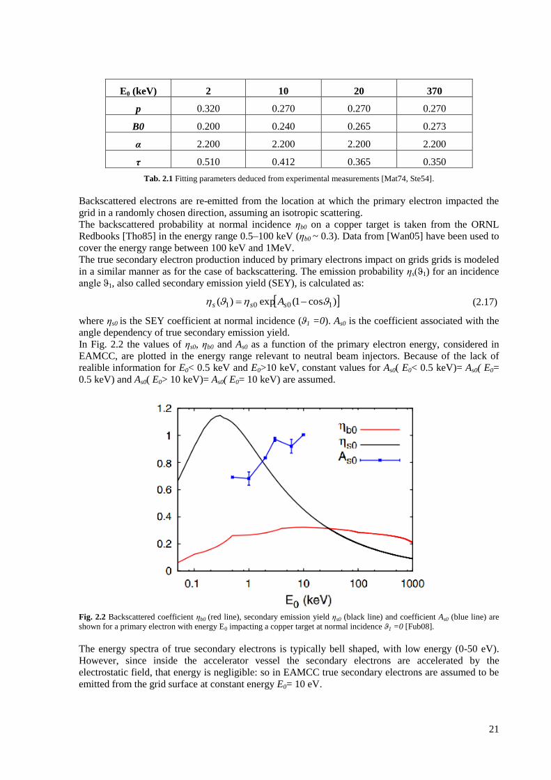
Tab. 2.1 Fitting parameters deduced from experimental measurements [Mat74, Ste54].
Backscattered electrons are re-emitted from the location at which the primary electron impacted the
grid in a randomly chosen direction, assuming an isotropic scattering.
The backscattered probability at normal incidence ηb0 on a copper target is taken from the ORNL
Redbooks [Tho85] in the energy range 0.5–100 keV (ηb0 ~ 0.3). Data from [Wan05] have been used to
cover the energy range between 100 keV and 1MeV.
The true secondary electron production induced by primary electrons impact on grids grids is modeled
in a similar manner as for the case of backscattering. The emission probability ηs(ϑ1) for an incidence
angle ϑ1, also called secondary emission yield (SEY), is calculated as:
)cos1(exp)( 1001 sss A
(2.17)
where ηs0 is the SEY coefficient at normal incidence (ϑ1 =0). As0 is the coefficient associated with the
angle dependency of true secondary emission yield.
In Fig. 2.2 the values of ηs0, ηb0 and As0 as a function of the primary electron energy, considered in
EAMCC, are plotted in the energy range relevant to neutral beam injectors. Because of the lack of
realible information for E0< 0.5 keV and E0>10 keV, constant values for As0( E0< 0.5 keV)= As0( E0=
0.5 keV) and As0( E0> 10 keV)= As0( E0= 10 keV) are assumed.
Fig. 2.2 Backscattered coefficient ηb0 (red line), secondary emission yield ηs0 (black line) and coefficient As0 (blue line) are
shown for a primary electron with energy E0 impacting a copper target at normal incidence ϑ1 =0 [Fub08].
The energy spectra of true secondary electrons is typically bell shaped, with low energy (0-50 eV).
However, since inside the accelerator vessel the secondary electrons are accelerated by the
electrostatic field, that energy is negligible: so in EAMCC true secondary electrons are assumed to be
emitted from the grid surface at constant energy E0= 10 eV.
22
2.3.3 Heavy particle impact with accelerator grids
Heavy ions and neutrals, produced by ion stripping and background gas ionization, may impact with
the accelerator grids. These impacts with the grids may in turn result in the creation of secondary
electrons together with the possibility of being backscattered. Because of their larger stopping power,
the secondary emission of electrons is significantly greater than the one induced by primary electron
impacts. The secondary emission yield for heavy particle impacts is calculated with the same
expression used for the primary electrons in the previous subsection (Eq. 2.17):
)cos1(exp)( 1)(
0)(
01)(
i
si
si
s A
(2.18)
where i is the index of the reaction: i=0 for neutrals (H0 or D
0), i=- for negative ions (H
- or D
-) and i=+
for positive ions (H2+ or D2
+) which are impacting on the grids. Identical SEY coefficients at normal
incidence (ϑ1= 0) are assumed for all heavy particles, that is ηs0(0)
(E0)~ ηs0(-)
(E0)~ ηs0(+)
(E0). The
behaviour of this coefficient as a function of the energy of the incident ion is plotted in Fig. 2.3.
The parameter As0(i)
was found to be close to 1.45, based on data taken from the ORNL Redbooks
[Tho85] for protons impacting Ni targets. Because of the lack of information on copper (i.e. the
material of which the accelerator grids are made) this value is considered in EAMCC for impacts on
the accelerator grids and for all heavy particle impacts (i.e. also for negative ions and neutrals).
Concerning secondary electron energy spectra, as explained in the previous subsection, it is assumed
that electrons are emitted at a fixed energy, E0= 10 eV.
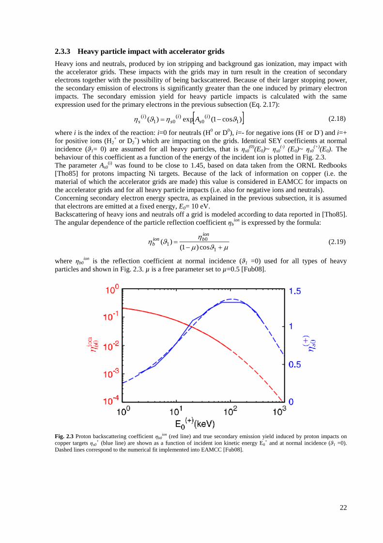
Backscattering of heavy ions and neutrals off a grid is modeled according to data reported in [Tho85].
The angular dependence of the particle reflection coefficient ηbion
is expressed by the formula:
1
01
cos)1()(
ionbion
b (2.19)
where ηb0ion
is the reflection coefficient at normal incidence (ϑ1 =0) used for all types of heavy
particles and shown in Fig. 2.3. µ is a free parameter set to µ=0.5 [Fub08].
Fig. 2.3 Proton backscattering coefficient ηb0
ion (red line) and true secondary emission yield induced by proton impacts on
copper targets ηs0+ (blue line) are shown as a function of incident ion kinetic energy E0
+ and at normal incidence (ϑ1 =0).
Dashed lines correspond to the numerical fit implemented into EAMCC [Fub08].
23
2.4 Modifications introduced in EAMCC
The size (in terms of memory) of the electric potential and the magnetic field maps of the accelerator
required by EAMCC, due to computer’s limits, does not allow to extend the simulated domain over a
single beamlet, considering a uniform mesh with an adequate pitch. In order to perform a multi-
beamlet analysis it is necessary to extend the size of the simulated domain limiting the increase of the
size of the maps. In other words it is necessary to use maps with a finer mesh just in the regions where
a more precise description of the electric and magnetic fields is required and to modify the code
making it able to deal with an uneven mesh map.
Different modifications have been introduced in the original version of EAMCC: first of all, the
possibility to deal with a 3D potential map with the same pitch of the magnetic map. Both maps had to
be with identical cubic mesh. The most recent modifications allowed to decouple the frame of
reference of the potential map from the magnetic field one by defining a pitch for the potential map
and another one for the magnetic field map. The grid of the two maps can be cubic or parallelepiped (a
pitch along x,y and z directions had been introduced for both the potential and the magnetic field
maps). Moreover, it has been added the possibility to simulate a larger region of the accelerator
making the code able to treat a multi-aperture domain.
The grid of the potential map is used by the code as a frame of reference for the calculation of the
nodes which defines the cell containing the generic particle for every time-step and the evaluation of
the potential and electric field in the same position.
The same grid is used for the evaluation of the dimensions and position of the accelerator grids and
their apertures (in the input file EAMCC requires to declare just the number and potential values of
every grid, but the position is found comparing the declared values with the potential map).
The introduction of a variable pitch along every direction led to several and scattered modifications of
the code in the main program and sub-routines.
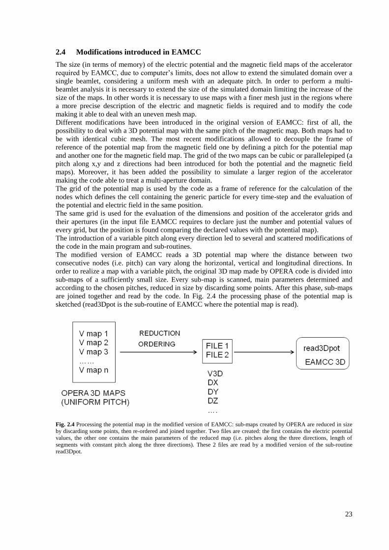
The modified version of EAMCC reads a 3D potential map where the distance between two
consecutive nodes (i.e. pitch) can vary along the horizontal, vertical and longitudinal directions. In
order to realize a map with a variable pitch, the original 3D map made by OPERA code is divided into
sub-maps of a sufficiently small size. Every sub-map is scanned, main parameters determined and
according to the chosen pitches, reduced in size by discarding some points. After this phase, sub-maps
are joined together and read by the code. In Fig. 2.4 the processing phase of the potential map is
sketched (read3Dpot is the sub-routine of EAMCC where the potential map is read).
Fig. 2.4 Processing the potential map in the modified version of EAMCC: sub-maps created by OPERA are reduced in size
by discarding some points, then re-ordered and joined together. Two files are created: the first contains the electric potential
values, the other one contains the main parameters of the reduced map (i.e. pitches along the three directions, length of
segments with constant pitch along the three directions). These 2 files are read by a modified version of the sub-routine
read3Dpot.

24
25
Chapter 3
A multi-beamlet analysis of the MITICA accelerator
The thermo-mechanical analysis and the mechanical design of the accelerator of MITICA (i.e. the full
size prototype of the ITER neutral beam injector under construction at RFX [Gri12,Ant14], are based
on the calculation of the power deposition induced by particle impacts. This calculation is performed
by EAMCC [Fub08], a relativistic particle tracking code based on the Monte-Carlo method for
describing collisions inside the accelerator, under prescribed electric and magnetic fields. The
magnetic field maps are produced by 3D codes, while the electric field maps come from the 2D axi-
symmetric code SLACCAD [Pam91].
So far, EAMCC has been used for performing single-beamlet analyses of the MITICA accelerator,
under the hypothesis of axi-symmetric electric field and the total power deposited on the accelerator
grids is obtained by scaling the results over the 1280 beamlets of the accelerator [Ago11, Zac12].
For a more realistic simulation, a 3D multi-beamlet analysis, which allows to take into account the
beamlet-beamlet repulsion and to consider other effects neglected under the hypothesis of axi-
symmetric beam (e.g. the influence of magnetic fields on the calculation of electric potential maps and
the effect of steering plates called kerbs on the particle trajectories) should be considered. The size of
3D potential maps in terms of computer’s memory, does not allow to consider a simulation domain
larger than a single-beamlet, considering maps with a uniform and sufficiently fine mesh.
For these reasons, a modified version of EAMCC, fully 3D, capable of modifying the mesh of the 3D
maps and of dealing with uneven meshes has been developed [Fon14] (see chapter 2): a finer mesh is
used just in the regions where a more detailed description of the fields is required.
This chapter is dedicated to the simulation of the MITICA beam with EAMCC and the calculation of
heat loads on the accelerator grids: after the description of the MITICA accelerator, a comparison
between simulations performed with the original code and the modified version is presented, as a
validation of the modifications introduced in the latter. Subsequently, the main results of a single-
beamlet analysis performed with the two versions of the code are shown and the differences between
the 2D and the 3D simulations discussed. The last part of the chapter is dedicated to the multi-beamlet
simulation of the accelerator.
3.1 MITICA accelerator
As described in chapter 1, a full scale prototype of the NBI ITER injector, called MITICA, is under
construction at Consorzio RFX (Padova) [Gri12, Ant14]. The device is mainly composed of a cesium
seeded negative deuterium/hydrogen ion source, an electrostatic accelerator where a 40 A beam of
negative deuterons will be accelerated to 1 MV (870 keV for H-), a neutralizer which converts part of
the beam into high energy neutrals, a residual ion dump devoted to electrostatically deflect the positive
and negative ions still present in the beam to suitably cooled plates and a calorimeter.
The MITICA accelerator (Fig. 3.1) consists of a plasma grid (PG) which separates the accelerator
from the ion source, an extraction grid (EG) for focusing the extracted beam, four acceleration grids
(AG1, AG2, AG3, AG4) and a grounded grid (GG). All the grids are 1600 mm high and 800 mm wide
(divided into four segments of about 400 mm x 800 mm for beam alignment and manufacturing
reasons). Each grid features 1280 apertures (320 per segment), arranged into 4x4 rectangular groups
(beamlet groups) of 16x5 apertures, where the ion beamlets are extracted from the ion source and
accelerated up to 1 MeV, forming an ion beam of the required 40 A at the exit of the grounded grid.
D- or H
- ions are extracted from the radio frequency plasma source (kept at -1 MV) by means of a
voltage difference of 10 kV applied between the PG and the EG.
The surface production of negative ions (i.e. one of the main ion production processes occurring in the
source by which an atom emitted energetically from a metal surface with a low work function may
leave in the form of negative ion [Bro04]) is increased by the reduction of the work function of the

26
metal surface and the most widely used method for doing it, is the deposition of a cesium layer on the
PG surface [Bel74]. In order to enhance the cesium effect for negative ion surface generation, the PG
is required to operate at a temperature of about 150 °C.
Fig. 3.1 MITICA’s Isometric views of a vertical section with the indication of the nominal electric potentials of the grids and
main dimensions (a), a horizontal section with the indication of the seven grids (b) and the grid aperture pattern (c) with the
indication of grid segments and beamlet groups (dimensions in mm).
The extracted negative ion beam is accelerated in five steps by the acceleration grids, which are biased
(starting from the AG1 and ending with the GG) at the electric potentials of -800, -600, -400, -200 and
0 kV. The gaps between these grids are kept as large as 88 mm, in order to hold the voltage with a
reasonable safety margin [Koj12]. The potentials of the grids can be varied in a certain range for
improving the beam collimation: in particular, varying the EG potential is an effective way to adjust
the optics of the beam and minimize the beam divergence at the exit, i.e. to obtain a beam that is
neither divergent nor convergent at the exit of the accelerator.
A current of about 4 kA flows through the PG in the vertical direction, to provide a horizontal
magnetic field, called filter field, that reduces the local electron density and so the number of co-
extracted electrons (a certain amount of electrons is extracted together with the negative ions from the
source, due to the fact that they have the same charge) and the local electron temperature (and so the
negative ion stripping rate). The same current also provides a magnetic field inside the accelerator,
called long-range magnetic field to distinguish it from the short range magnetic field produced by the
magnets embedded in the grids [Ago14].
The principal function of the permanent magnets embedded in the accelerator grids [Chi12, Chi14] is
the suppression of the co-extracted and stripped electrons (i.e. electrons created inside the accelerator
by means of stripping reactions that occur when a negative ion loses an electron by reacting with the
background gas inside the accelerator, see chapter 2).
Magnets embedded in the EG, named Co-extracted Electrons Suppression Magnets (CESM) are
located horizontally between the aperture rows and are shown in Fig. 3.2(a) where a vertical section of
the ion extraction region in correspondence of two grid apertures is depicted. CESM generate a
magnetic field mainly along the vertical direction and alternated from row to row: the blue line in Fig.
3.2(b) represents the typical symmetric double-swing profile of the vertical component (By) of this
field, which assures that most of the co-extracted electrons will be deflected and will impinge on the
upstream side of the EG. In the same figure it is shown the plasma meniscus position (i.e. the surface
boundary between the plasma and the beam, from which ions are emitted) along the beamlet path, at
the coordinate z=z0.
CESM also deflect the negative ions and a remaining alternate horizontal deflection is generally
measured at the accelerator exit, the so called Criss-Cross Deflection Effect (CCDE). In fact, as
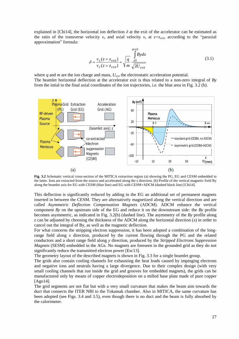
27
explained in [Chi14], the horizontal ion deflection δ at the exit of the accelerator can be estimated as
the ratio of the transverse velocity vx and axial velocity vz at z=zexit, according to the “paraxial
approximation” formula:
exit
zexit
z
exitz
exitx
U
Bydz
m
q
zzv
zzv
2)(
)( 0
(3.1)
where q and m are the ion charge and mass, Uexit the electrostatic acceleration potential.
The beamlet horizontal deflection at the accelerator exit is thus related to a non-zero integral of By
from the intial to the final axial coordinates of the ion trajectories, i.e. the blue area in Fig. 3.2 (b).
Fig. 3.2 Schematic vertical cross-section of the MITICA extraction region (a) showing the PG, EG and CESM embedded in
the latter. Ions are extracted from the source and accelerated along the z direction. (b) Profile of the vertical magnetic field By
along the beamlet axis for EG with CESM (blue line) and EG with CESM+ADCM (dashed black line) [Chi14].
This deflection is significantly reduced by adding in the EG an additional set of permanent magnets
inserted in between the CESM. They are alternatively magnetized along the vertical direction and are
called Asymmetric Deflection Compensation Magnets (ADCM). ADCM enhance the vertical
component By on the upstream side of the EG and reduce it on the downstream side: the By profile
becomes asymmetric, as indicated in Fig. 3.2(b) (dashed line). The asymmetry of the By profile along
z can be adjusted by choosing the thickness of the ADCM along the horizontal direction (x) in order to
cancel out the integral of By, as well as the magnetic deflection.
For what concerns the stripping electron suppression, it has been adopted a combination of the long-
range field along x direction, produced by the current flowing through the PG and the related
conductors and a short range field along y direction, produced by the Stripped Electrons Suppression
Magnets (SESM) embedded in the AGs. No magnets are foreseen in the grounded grid as they do not
significantly reduce the transmitted electron power [Esc13].
The geometry layout of the described magnets is shown in Fig. 3.3 for a single beamlet group.
The grids also contain cooling channels for exhausting the heat loads caused by impinging electrons
and negative ions and neutrals having a large divergence. Due to their complex design (with very
small cooling channels that run inside the grid and grooves for embedded magnets), the grids can be
manufactured only by means of copper electrodeposition on a milled base plate made of pure copper
[Ago14].
The grid segments are not flat but with a very small curvature that makes the beam aim towards the
duct that connects the ITER NBI to the Tokamak chamber. Also in MITICA, the same curvature has
been adopted (see Figs. 3.4 and 3.5), even though there is no duct and the beam is fully absorbed by
the calorimeter.
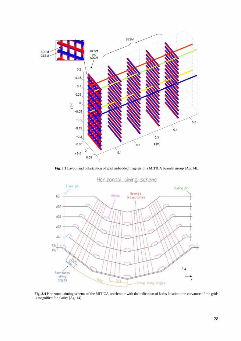
28
Fig. 3.3 Layout and polarization of grid embedded magnets of a MITICA beamlet group [Ago14].
Fig. 3.4 Horizontal aiming scheme of the MITICA accelerator with the indication of kerbs location; the curvature of the grids
is magnified for clarity [Ago14].
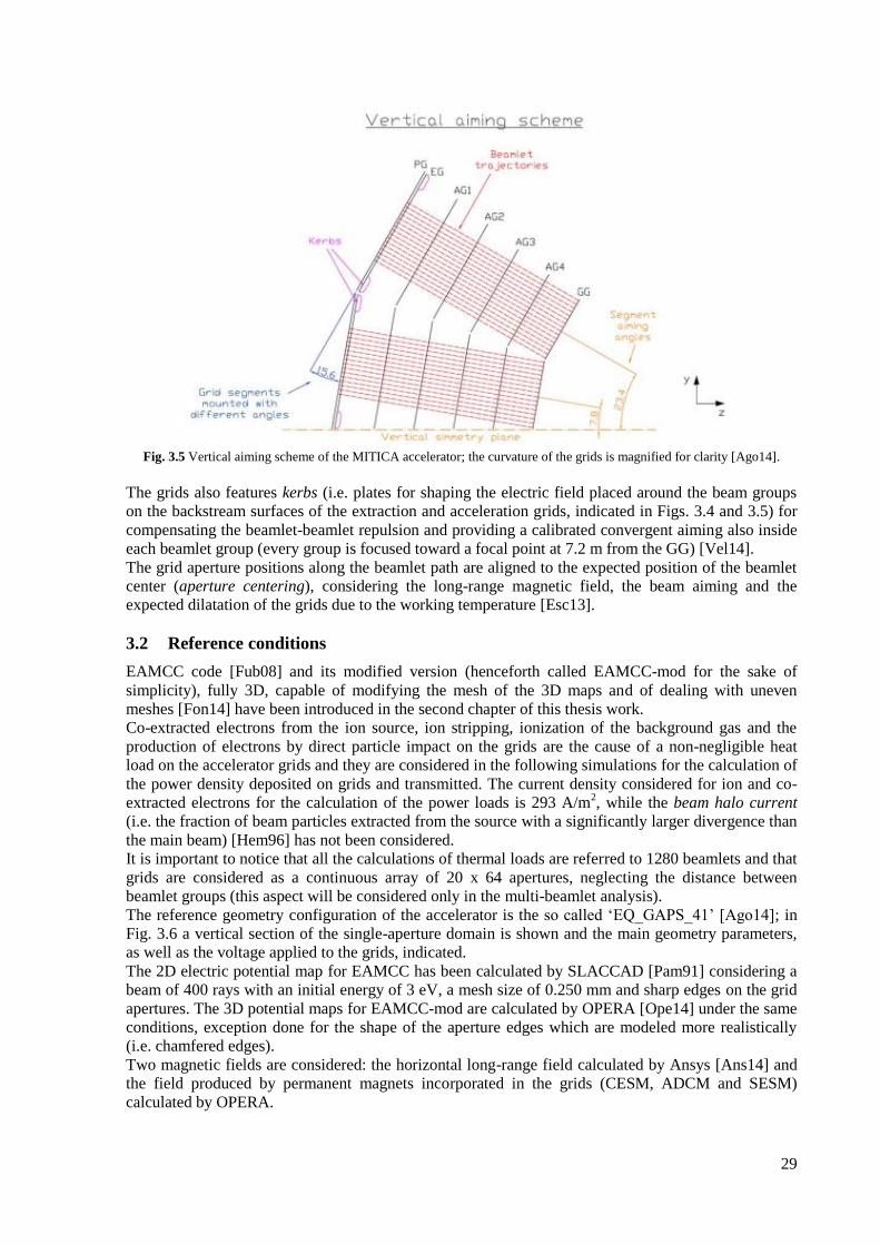
29
Fig. 3.5 Vertical aiming scheme of the MITICA accelerator; the curvature of the grids is magnified for clarity [Ago14].
The grids also features kerbs (i.e. plates for shaping the electric field placed around the beam groups
on the backstream surfaces of the extraction and acceleration grids, indicated in Figs. 3.4 and 3.5) for
compensating the beamlet-beamlet repulsion and providing a calibrated convergent aiming also inside
each beamlet group (every group is focused toward a focal point at 7.2 m from the GG) [Vel14].
The grid aperture positions along the beamlet path are aligned to the expected position of the beamlet
center (aperture centering), considering the long-range magnetic field, the beam aiming and the
expected dilatation of the grids due to the working temperature [Esc13].
3.2 Reference conditions
EAMCC code [Fub08] and its modified version (henceforth called EAMCC-mod for the sake of
simplicity), fully 3D, capable of modifying the mesh of the 3D maps and of dealing with uneven
meshes [Fon14] have been introduced in the second chapter of this thesis work.
Co-extracted electrons from the ion source, ion stripping, ionization of the background gas and the
production of electrons by direct particle impact on the grids are the cause of a non-negligible heat
load on the accelerator grids and they are considered in the following simulations for the calculation of
the power density deposited on grids and transmitted. The current density considered for ion and co-
extracted electrons for the calculation of the power loads is 293 A/m2, while the beam halo current
(i.e. the fraction of beam particles extracted from the source with a significantly larger divergence than
the main beam) [Hem96] has not been considered.
It is important to notice that all the calculations of thermal loads are referred to 1280 beamlets and that
grids are considered as a continuous array of 20 x 64 apertures, neglecting the distance between
beamlet groups (this aspect will be considered only in the multi-beamlet analysis).
The reference geometry configuration of the accelerator is the so called ‘EQ_GAPS_41’ [Ago14]; in
Fig. 3.6 a vertical section of the single-aperture domain is shown and the main geometry parameters,
as well as the voltage applied to the grids, indicated.
The 2D electric potential map for EAMCC has been calculated by SLACCAD [Pam91] considering a
beam of 400 rays with an initial energy of 3 eV, a mesh size of 0.250 mm and sharp edges on the grid
apertures. The 3D potential maps for EAMCC-mod are calculated by OPERA [Ope14] under the same
conditions, exception done for the shape of the aperture edges which are modeled more realistically
(i.e. chamfered edges).
Two magnetic fields are considered: the horizontal long-range field calculated by Ansys [Ans14] and
the field produced by permanent magnets incorporated in the grids (CESM, ADCM and SESM)
calculated by OPERA.
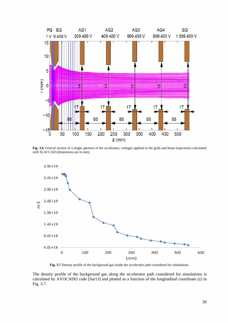
30
Fig. 3.6 Vertical section of a single aperture of the accelerator, voltages applied to the grids and beam trajectories calculated
with SLACCAD (dimensions are in mm).
Fig. 3.7 Density profile of the background gas inside the accelerator path considered for simulations.
The density profile of the background gas along the accelerator path considered for simulations is
calculated by AVOCADO code [Sar13] and plotted as a function of the longitudinal coordinate (z) in
Fig. 3.7.
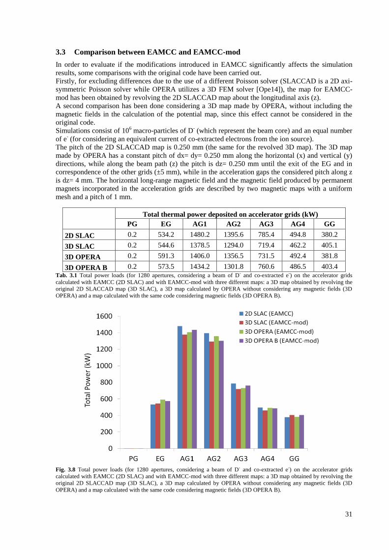
31
3.3 Comparison between EAMCC and EAMCC-mod
In order to evaluate if the modifications introduced in EAMCC significantly affects the simulation
results, some comparisons with the original code have been carried out.
Firstly, for excluding differences due to the use of a different Poisson solver (SLACCAD is a 2D axi-
symmetric Poisson solver while OPERA utilizes a 3D FEM solver [Ope14]), the map for EAMCC-
mod has been obtained by revolving the 2D SLACCAD map about the longitudinal axis (z).
A second comparison has been done considering a 3D map made by OPERA, without including the
magnetic fields in the calculation of the potential map, since this effect cannot be considered in the
original code.
Simulations consist of 106 macro-particles of D
- (which represent the beam core) and an equal number
of e- (for considering an equivalent current of co-extracted electrons from the ion source).
The pitch of the 2D SLACCAD map is 0.250 mm (the same for the revolved 3D map). The 3D map
made by OPERA has a constant pitch of dx= dy= 0.250 mm along the horizontal (x) and vertical (y)
directions, while along the beam path (z) the pitch is dz= 0.250 mm until the exit of the EG and in
correspondence of the other grids (±5 mm), while in the acceleration gaps the considered pitch along z
is dz= 4 mm. The horizontal long-range magnetic field and the magnetic field produced by permanent
magnets incorporated in the acceleration grids are described by two magnetic maps with a uniform
mesh and a pitch of 1 mm.
Total thermal power deposited on accelerator grids (kW)
PG EG AG1 AG2 AG3 AG4 GG
2D SLAC 0.2 534.2 1480.2 1395.6 785.4 494.8 380.2
3D SLAC 0.2 544.6 1378.5 1294.0 719.4 462.2 405.1
3D OPERA 0.2 591.3 1406.0 1356.5 731.5 492.4 381.8
3D OPERA B 0.2 573.5 1434.2 1301.8 760.6 486.5 403.4
Tab. 3.1 Total power loads (for 1280 apertures, considering a beam of D- and co-extracted e-) on the accelerator grids
calculated with EAMCC (2D SLAC) and with EAMCC-mod with three different maps: a 3D map obtained by revolving the
original 2D SLACCAD map (3D SLAC), a 3D map calculated by OPERA without considering any magnetic fields (3D
OPERA) and a map calculated with the same code considering magnetic fields (3D OPERA B).
Fig. 3.8 Total power loads (for 1280 apertures, considering a beam of D- and co-extracted e-) on the accelerator grids
calculated with EAMCC (2D SLAC) and with EAMCC-mod with three different maps: a 3D map obtained by revolving the
original 2D SLACCAD map (3D SLAC), a 3D map calculated by OPERA without considering any magnetic fields (3D
OPERA) and a map calculated with the same code considering magnetic fields (3D OPERA B).
32
The total power deposition calculated by EAMCC (labeled “2D SLAC”), by EAMCC-mod with the
revolved map (“3D SLAC”) and by EAMCC-mod with OPERA maps without and with including
(respectively labeled “3D OPERA” and “3D OPERA B”) the magnetic field in the calculation of the
potential map are reported in Tab. 3.1 and plotted in Fig. 3.8. The last case will be studied in detail in
the next paragraph and it has been considered in this comparison for completeness.
The calculations include the power deposition on grids due to secondary particles created by the beam
core inside the accelerator (stripped electrons, electrons emitted from grid surfaces, D0,D
+,D2
+) and to
co-extracted electrons. Loads on the plasma grid are negligible, and henceforth no longer considered.
Fig. 3.9 Normalized values (to the power calculated by EAMCC) of the loads resulting from the simulation with EAMCC-
mod for the three described cases.
The agreement between the 2D SLAC and 3D SLAC simulations seems encouraging: the maximum
variation is ~ 7%, mainly due to the fact that the two codes have non negligible differences (see
chapter 2), for instance in the calculation of collisions and in the determination of the geometry of
grids.
The comparison with the third simulation (3D OPERA) reports a maximum difference of 11% (Fig.
3.9) in the case of the extraction grid. The power deposition on this grid is strongly dependent on the
plasma meniscus (i.e. the boundary between the plasma and the beam, where the potential is ~ 0 V)
calculation, perfomed with the two different Poisson solvers and this could explain the difference. In
fact, the meniscus position, its shape and the deepness of its curvature (with respect to the PG plane)
play an important role for the ion beam formation and the beam optics as it defines the velocity
starting angle of the extracted particles [Moc14].
These results are useful for evaluating how much the modifications introduced in the code and the use
of a different Poisson solver can influence the calculation of the heat loads and also allow us to state
that modifying the pitch of the potential map in the regions where there are not steep potential
variations, does not affect significantly the results of the simulations.
3.4 3D effects on a single-beamlet analysis
Since a 3D Poisson solver is used by OPERA for the calculation of the electric potential inside the
accelerator, it is possible to consider in this calculation the influence of the magnetic fields on particle
trajectories and the subsequent modification of the electric charge distribution. As previously said, this
aspect is neglected under the hypothesis of axi-symmetric beam and so far, it has not been considered
in the simulations with EAMCC. An assessment of the importance of this effect on the results of the
simulations can be achieved by comparing in detail the two simulations performed by EAMCC-mod
33
and introduced in the previous paragraph where the potential maps are calculated without and with the
presence of the magnetic fields (respectively labeled “3D OPERA” and “3D OPERA B”).
Fig. 3.10 Power deposition (considering a beam of D- and co-extracted e-) on the upstream surface of the EG (a), AG1 (b),
AG2 (c), AG3 (d), AG4 (e), GG(f) and power transmitted at the exit of the GG (g) neglecting magnetic fields in the
calculation of the potential map (simulation 3D OPERA).
Fig. 3.11 Power deposition (considering a beam of D- and co-extracted e-) on the upstream surface of the EG (a), AG1 (b),
AG2 (c), AG3 (d), AG4 (e), GG(f) and power transmitted at the exit of the GG (g) considering magnetic fields in the
calculation of the potential map (simulation 3D OPERA B).
In Figs. 3.10 and 3.11 the density of the power deposited on the upstream surface of the grids is
plotted for EG (a), AG1 (b), AG2 (c), AG3 (d), AG4 (e), GG (f), respectively for the case without and
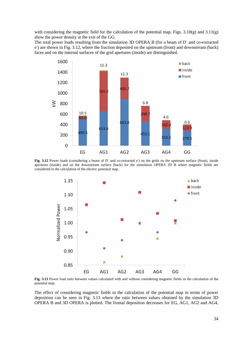
34
with considering the magnetic field for the calculation of the potential map. Figs. 3.10(g) and 3.11(g)
show the power density at the exit of the GG.
The total power loads resulting from the simulation 3D OPERA B (for a beam of D- and co-extracted
e-) are shown in Fig. 3.12, where the fraction deposited on the upstream (front) and downstream (back)
faces and on the internal surfaces of the grid apertures (inside) are distinguished.
Fig. 3.12 Power loads (considering a beam of D- and co-extracted e-) on the grids on the upstream surface (front), inside
apertures (inside) and on the downstream surface (back) for the simulation OPERA 3D B where magnetic fields are
considered in the calculation of the electric potential map.
Fig. 3.13 Power load ratio between values calculated with and without considering magnetic fields in the calculation of the
potential map.
The effect of considering magnetic fields in the calculation of the potential map in terms of power
deposition can be seen in Fig. 3.13 where the ratio between values obtained by the simulation 3D
OPERA B and 3D OPERA is plotted. The frontal deposition decreases for EG, AG1, AG2 and AG4,
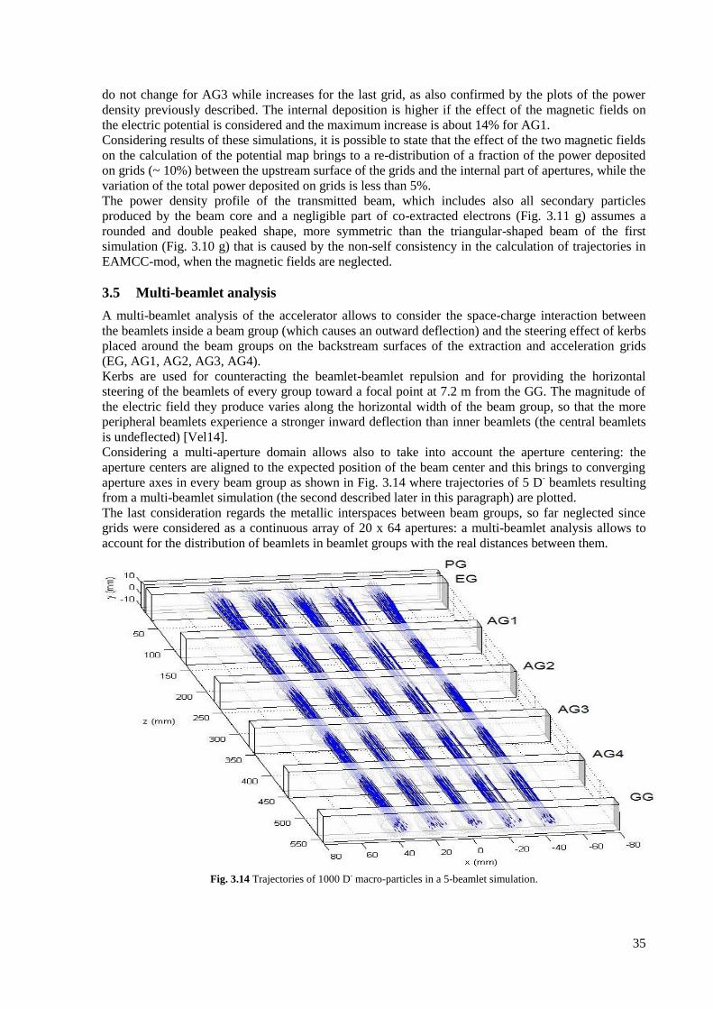
35
do not change for AG3 while increases for the last grid, as also confirmed by the plots of the power
density previously described. The internal deposition is higher if the effect of the magnetic fields on
the electric potential is considered and the maximum increase is about 14% for AG1.
Considering results of these simulations, it is possible to state that the effect of the two magnetic fields
on the calculation of the potential map brings to a re-distribution of a fraction of the power deposited
on grids (~ 10%) between the upstream surface of the grids and the internal part of apertures, while the
variation of the total power deposited on grids is less than 5%.
The power density profile of the transmitted beam, which includes also all secondary particles
produced by the beam core and a negligible part of co-extracted electrons (Fig. 3.11 g) assumes a
rounded and double peaked shape, more symmetric than the triangular-shaped beam of the first
simulation (Fig. 3.10 g) that is caused by the non-self consistency in the calculation of trajectories in
EAMCC-mod, when the magnetic fields are neglected.
3.5 Multi-beamlet analysis
A multi-beamlet analysis of the accelerator allows to consider the space-charge interaction between
the beamlets inside a beam group (which causes an outward deflection) and the steering effect of kerbs
placed around the beam groups on the backstream surfaces of the extraction and acceleration grids
(EG, AG1, AG2, AG3, AG4).
Kerbs are used for counteracting the beamlet-beamlet repulsion and for providing the horizontal
steering of the beamlets of every group toward a focal point at 7.2 m from the GG. The magnitude of
the electric field they produce varies along the horizontal width of the beam group, so that the more
peripheral beamlets experience a stronger inward deflection than inner beamlets (the central beamlets
is undeflected) [Vel14].
Considering a multi-aperture domain allows also to take into account the aperture centering: the
aperture centers are aligned to the expected position of the beam center and this brings to converging
aperture axes in every beam group as shown in Fig. 3.14 where trajectories of 5 D- beamlets resulting
from a multi-beamlet simulation (the second described later in this paragraph) are plotted.
The last consideration regards the metallic interspaces between beam groups, so far neglected since
grids were considered as a continuous array of 20 x 64 apertures: a multi-beamlet analysis allows to
account for the distribution of beamlets in beamlet groups with the real distances between them.
Fig. 3.14 Trajectories of 1000 D- macro-particles in a 5-beamlet simulation.
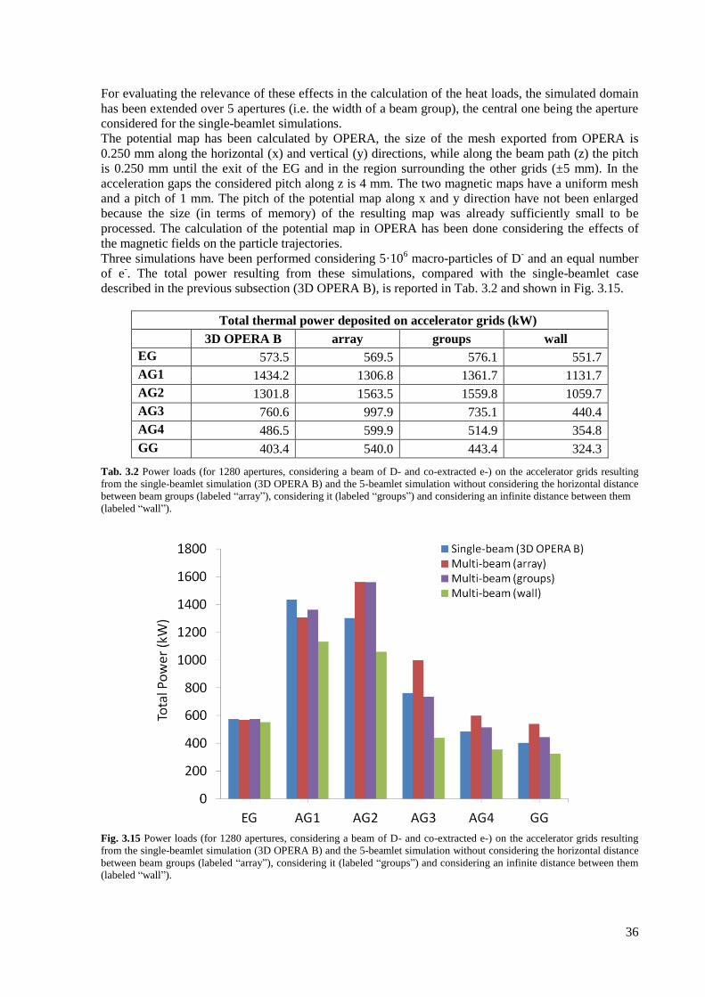
36
For evaluating the relevance of these effects in the calculation of the heat loads, the simulated domain
has been extended over 5 apertures (i.e. the width of a beam group), the central one being the aperture
considered for the single-beamlet simulations.
The potential map has been calculated by OPERA, the size of the mesh exported from OPERA is
0.250 mm along the horizontal (x) and vertical (y) directions, while along the beam path (z) the pitch
is 0.250 mm until the exit of the EG and in the region surrounding the other grids (±5 mm). In the
acceleration gaps the considered pitch along z is 4 mm. The two magnetic maps have a uniform mesh
and a pitch of 1 mm. The pitch of the potential map along x and y direction have not been enlarged
because the size (in terms of memory) of the resulting map was already sufficiently small to be
processed. The calculation of the potential map in OPERA has been done considering the effects of
the magnetic fields on the particle trajectories.
Three simulations have been performed considering 5·106 macro-particles of D
- and an equal number
of e-. The total power resulting from these simulations, compared with the single-beamlet case
described in the previous subsection (3D OPERA B), is reported in Tab. 3.2 and shown in Fig. 3.15.
Total thermal power deposited on accelerator grids (kW)
3D OPERA B array groups wall
EG 573.5 569.5 576.1 551.7
AG1 1434.2 1306.8 1361.7 1131.7
AG2 1301.8 1563.5 1559.8 1059.7
AG3 760.6 997.9 735.1 440.4
AG4 486.5 599.9 514.9 354.8
GG 403.4 540.0 443.4 324.3
Tab. 3.2 Power loads (for 1280 apertures, considering a beam of D- and co-extracted e-) on the accelerator grids resulting
from the single-beamlet simulation (3D OPERA B) and the 5-beamlet simulation without considering the horizontal distance
between beam groups (labeled “array”), considering it (labeled “groups”) and considering an infinite distance between them
(labeled “wall”).
Fig. 3.15 Power loads (for 1280 apertures, considering a beam of D- and co-extracted e-) on the accelerator grids resulting
from the single-beamlet simulation (3D OPERA B) and the 5-beamlet simulation without considering the horizontal distance
between beam groups (labeled “array”), considering it (labeled “groups”) and considering an infinite distance between them
(labeled “wall”).
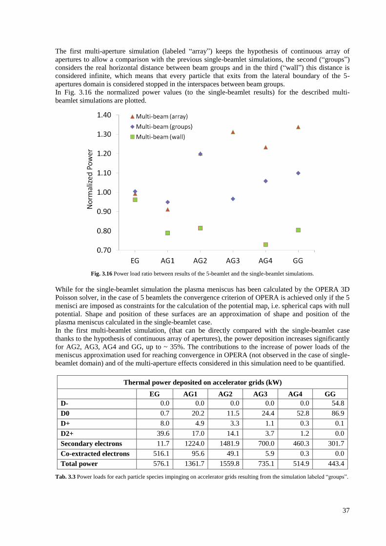
37
The first multi-aperture simulation (labeled “array”) keeps the hypothesis of continuous array of
apertures to allow a comparison with the previous single-beamlet simulations, the second (“groups”)
considers the real horizontal distance between beam groups and in the third (“wall”) this distance is
considered infinite, which means that every particle that exits from the lateral boundary of the 5-
apertures domain is considered stopped in the interspaces between beam groups.
In Fig. 3.16 the normalized power values (to the single-beamlet results) for the described multi-
beamlet simulations are plotted.
Fig. 3.16 Power load ratio between results of the 5-beamlet and the single-beamlet simulations.
While for the single-beamlet simulation the plasma meniscus has been calculated by the OPERA 3D
Poisson solver, in the case of 5 beamlets the convergence criterion of OPERA is achieved only if the 5
menisci are imposed as constraints for the calculation of the potential map, i.e. spherical caps with null
potential. Shape and position of these surfaces are an approximation of shape and position of the
plasma meniscus calculated in the single-beamlet case.
In the first multi-beamlet simulation, (that can be directly compared with the single-beamlet case
thanks to the hypothesis of continuous array of apertures), the power deposition increases significantly
for AG2, AG3, AG4 and GG, up to ~ 35%. The contributions to the increase of power loads of the
meniscus approximation used for reaching convergence in OPERA (not observed in the case of single-
beamlet domain) and of the multi-aperture effects considered in this simulation need to be quantified.
Thermal power deposited on accelerator grids (kW)
EG AG1 AG2 AG3 AG4 GG
D- 0.0 0.0 0.0 0.0 0.0 54.8
D0 0.7 20.2 11.5 24.4 52.8 86.9
D+ 8.0 4.9 3.3 1.1 0.3 0.1
D2+ 39.6 17.0 14.1 3.7 1.2 0.0
Secondary electrons 11.7 1224.0 1481.9 700.0 460.3 301.7
Co-extracted electrons 516.1 95.6 49.1 5.9 0.3 0.0
Total power 576.1 1361.7 1559.8 735.1 514.9 443.4
Tab. 3.3 Power loads for each particle species impinging on accelerator grids resulting from the simulation labeled “groups”.
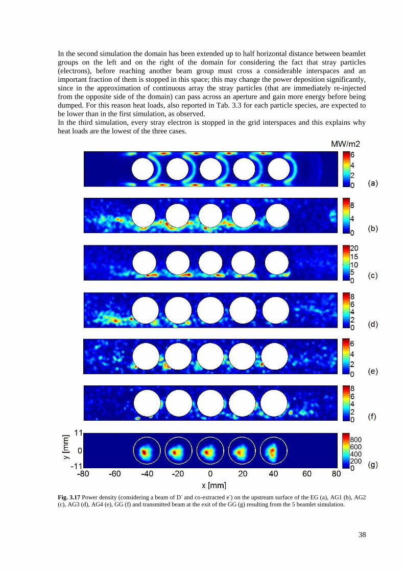
38
In the second simulation the domain has been extended up to half horizontal distance between beamlet
groups on the left and on the right of the domain for considering the fact that stray particles
(electrons), before reaching another beam group must cross a considerable interspaces and an
important fraction of them is stopped in this space; this may change the power deposition significantly,
since in the approximation of continuous array the stray particles (that are immediately re-injected
from the opposite side of the domain) can pass across an aperture and gain more energy before being
dumped. For this reason heat loads, also reported in Tab. 3.3 for each particle species, are expected to
be lower than in the first simulation, as observed.
In the third simulation, every stray electron is stopped in the grid interspaces and this explains why
heat loads are the lowest of the three cases.
Fig. 3.17 Power density (considering a beam of D- and co-extracted e-) on the upstream surface of the EG (a), AG1 (b), AG2
(c), AG3 (d), AG4 (e), GG (f) and transmitted beam at the exit of the GG (g) resulting from the 5 beamlet simulation.
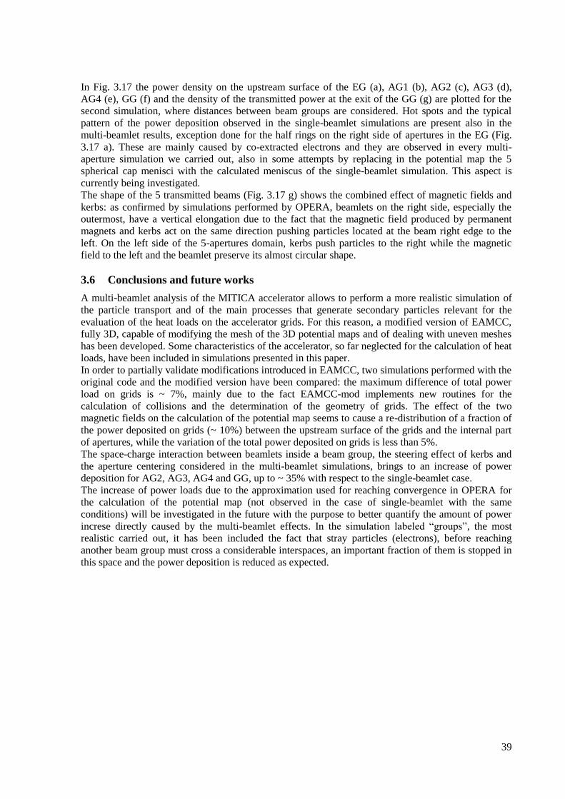
39
In Fig. 3.17 the power density on the upstream surface of the EG (a), AG1 (b), AG2 (c), AG3 (d),
AG4 (e), GG (f) and the density of the transmitted power at the exit of the GG (g) are plotted for the
second simulation, where distances between beam groups are considered. Hot spots and the typical
pattern of the power deposition observed in the single-beamlet simulations are present also in the
multi-beamlet results, exception done for the half rings on the right side of apertures in the EG (Fig.
3.17 a). These are mainly caused by co-extracted electrons and they are observed in every multi-
aperture simulation we carried out, also in some attempts by replacing in the potential map the 5
spherical cap menisci with the calculated meniscus of the single-beamlet simulation. This aspect is
currently being investigated.
The shape of the 5 transmitted beams (Fig. 3.17 g) shows the combined effect of magnetic fields and
kerbs: as confirmed by simulations performed by OPERA, beamlets on the right side, especially the
outermost, have a vertical elongation due to the fact that the magnetic field produced by permanent
magnets and kerbs act on the same direction pushing particles located at the beam right edge to the
left. On the left side of the 5-apertures domain, kerbs push particles to the right while the magnetic
field to the left and the beamlet preserve its almost circular shape.
3.6 Conclusions and future works
A multi-beamlet analysis of the MITICA accelerator allows to perform a more realistic simulation of
the particle transport and of the main processes that generate secondary particles relevant for the
evaluation of the heat loads on the accelerator grids. For this reason, a modified version of EAMCC,
fully 3D, capable of modifying the mesh of the 3D potential maps and of dealing with uneven meshes
has been developed. Some characteristics of the accelerator, so far neglected for the calculation of heat
loads, have been included in simulations presented in this paper.
In order to partially validate modifications introduced in EAMCC, two simulations performed with the
original code and the modified version have been compared: the maximum difference of total power
load on grids is ~ 7%, mainly due to the fact EAMCC-mod implements new routines for the
calculation of collisions and the determination of the geometry of grids. The effect of the two
magnetic fields on the calculation of the potential map seems to cause a re-distribution of a fraction of
the power deposited on grids (~ 10%) between the upstream surface of the grids and the internal part
of apertures, while the variation of the total power deposited on grids is less than 5%.
The space-charge interaction between beamlets inside a beam group, the steering effect of kerbs and
the aperture centering considered in the multi-beamlet simulations, brings to an increase of power
deposition for AG2, AG3, AG4 and GG, up to ~ 35% with respect to the single-beamlet case.
The increase of power loads due to the approximation used for reaching convergence in OPERA for
the calculation of the potential map (not observed in the case of single-beamlet with the same
conditions) will be investigated in the future with the purpose to better quantify the amount of power
increse directly caused by the multi-beamlet effects. In the simulation labeled “groups”, the most
realistic carried out, it has been included the fact that stray particles (electrons), before reaching
another beam group must cross a considerable interspaces, an important fraction of them is stopped in
this space and the power deposition is reduced as expected.

40
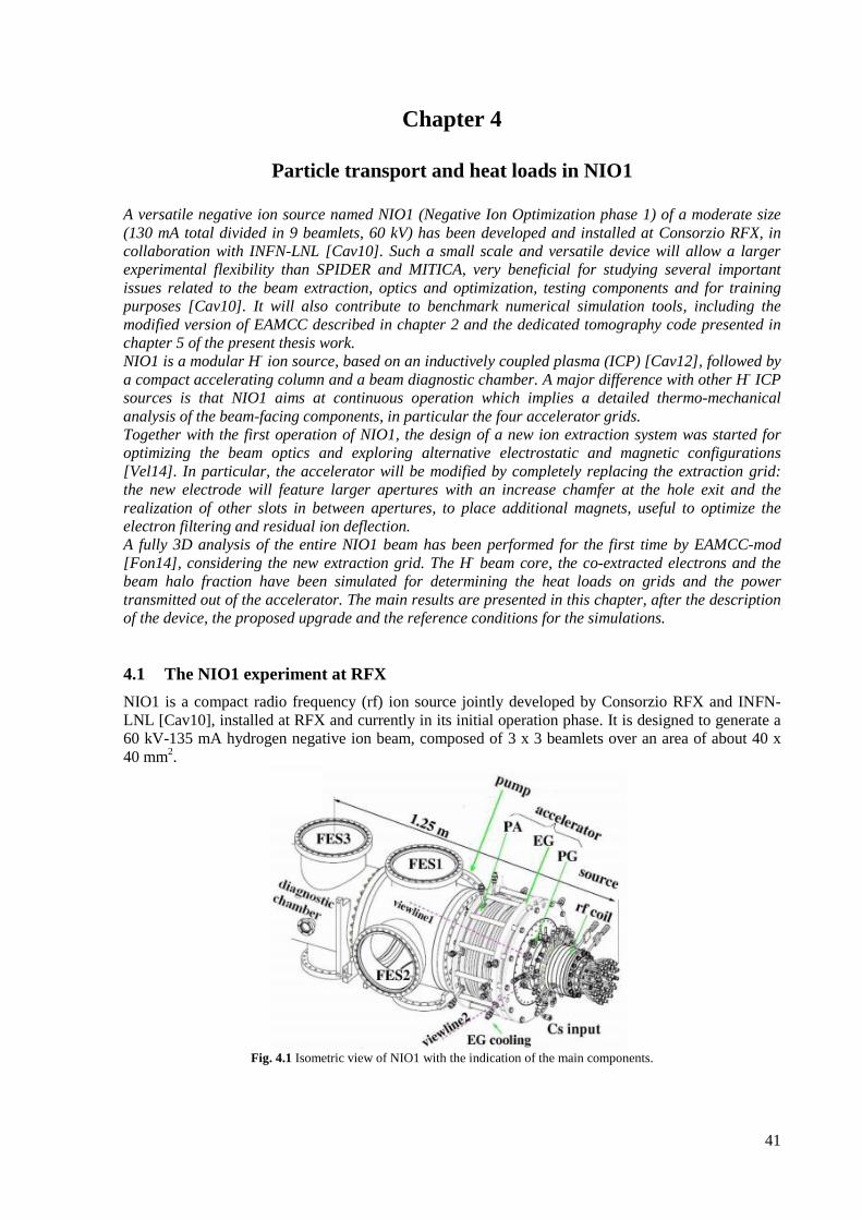
41
Chapter 4
Particle transport and heat loads in NIO1
A versatile negative ion source named NIO1 (Negative Ion Optimization phase 1) of a moderate size
(130 mA total divided in 9 beamlets, 60 kV) has been developed and installed at Consorzio RFX, in
collaboration with INFN-LNL [Cav10]. Such a small scale and versatile device will allow a larger
experimental flexibility than SPIDER and MITICA, very beneficial for studying several important
issues related to the beam extraction, optics and optimization, testing components and for training
purposes [Cav10]. It will also contribute to benchmark numerical simulation tools, including the
modified version of EAMCC described in chapter 2 and the dedicated tomography code presented in
chapter 5 of the present thesis work.
NIO1 is a modular H- ion source, based on an inductively coupled plasma (ICP) [Cav12], followed by
a compact accelerating column and a beam diagnostic chamber. A major difference with other H- ICP
sources is that NIO1 aims at continuous operation which implies a detailed thermo-mechanical
analysis of the beam-facing components, in particular the four accelerator grids.
Together with the first operation of NIO1, the design of a new ion extraction system was started for
optimizing the beam optics and exploring alternative electrostatic and magnetic configurations
[Vel14]. In particular, the accelerator will be modified by completely replacing the extraction grid:
the new electrode will feature larger apertures with an increase chamfer at the hole exit and the
realization of other slots in between apertures, to place additional magnets, useful to optimize the
electron filtering and residual ion deflection.
A fully 3D analysis of the entire NIO1 beam has been performed for the first time by EAMCC-mod
[Fon14], considering the new extraction grid. The H- beam core, the co-extracted electrons and the
beam halo fraction have been simulated for determining the heat loads on grids and the power
transmitted out of the accelerator. The main results are presented in this chapter, after the description
of the device, the proposed upgrade and the reference conditions for the simulations.
4.1 The NIO1 experiment at RFX
NIO1 is a compact radio frequency (rf) ion source jointly developed by Consorzio RFX and INFN-
LNL [Cav10], installed at RFX and currently in its initial operation phase. It is designed to generate a
60 kV-135 mA hydrogen negative ion beam, composed of 3 x 3 beamlets over an area of about 40 x
40 mm2.
Fig. 4.1 Isometric view of NIO1 with the indication of the main components.
42
In Fig. 4.1 an isometric view of the device is shown: it is mainly composed of a cesium seeded rf
source, an electrostatic accelerator where the 9 beamlets will be accelerated up to 60 keV, a 350 mm
diameter diagnostic chamber with several ports for diagnostics [Zan14] and pumping, and a
calorimetric beam dump [Cav12].
An external rf coil, placed approximately halfway between the source rear cover and the extraction
area, feeded by the 2 MHz/2500 W radiofrequency generator, creates the plasma in the cylindrical
chamber of 50 mm radius and 200 mm long shown in Fig. 4.2 (a). The chamber is surrounded by
magnets forming multipoles to improve the plasma confinement, where H- ions are created by volume
processes [Bac79, Bac06] and surface conversion of H+ or H
0 [Bro04] enhanced by cesium surface
coverage [Bel74], and extracted from the 9 apertures of the plasma grid (PG).
There are three acceleration grids (see Fig. 4.2 a), named plasma grid (PG) at -60 kV, extraction grid
(EG) at -52 kV and post acceleration grid (PA) at the ground voltage, followed by a repeller electrode
(REP) for a better control of the space charge compensation of the extracted beam [Cav10] and to
prevent the drain of positive ions from the drift region [Vel14]. The accelerator is about 58 mm long,
from the exit of the PG to the exit of the repeller.
PG apertures are arranged in a square lattice with a spacing Lx= Ly= 14 mm and an extraction radius
r= 3.8 mm. The gap distance g between the PG and EG can be adjusted in the range g= 5 ± 1 mm and
it is actually set to the middle position. EG has an entrance radius r1= 3.2 mm, exit radius r2= 4.1 mm
and a thickness of 10.3 mm (d1= 8.8 mm, d2= 1.5 mm in Fig. 4.2 b); PA has r1= 3.5 mm and r2= 4.4
mm, while repeller has a constant radius r1= r2= 4.4 mm.
Fig. 4.2 (a) Vertical section of the NIO1 ion source and accelerator assembly. (b) Zoom on the ion extraction region enclosed
by the red rectangle in (a) showing the shape of the plasma grid (PG) and extraction grid (EG) [Vel14].
All grids are realized by electro-deposition of copper and successive milling, and include empty
channels for water cooling (EG and PA) or water/air heating (PG temperature will be regulated around
400 K at which the cesium coverage needed for the H- surface production seems to be optimal).
In the EG four array of CESM magnets (Co-extracted Electron Suppression Magnets, see Fig. 4.2 b)
are embedded to prevent the acceleration of co-extracted electrons, with magnetization along z, as
usual in standard negative ion sources and in the original MITICA design. CESM produces a magnetic
field having the component Bx that is negligible compared to By and Bz at beamlet position. Since
beam velocity vz is much greater than vx and vy, beam deflection is mainly due to By and it is in x
direction. As respect to periodicity, each row of beamlets is deflected in opposite directions.
In the PA, magnets are incorporated to support the disposal of stripped electrons and partially recover
the primary beam alignment after the deflection induced by the EG magnets. Soft iron bars are placed
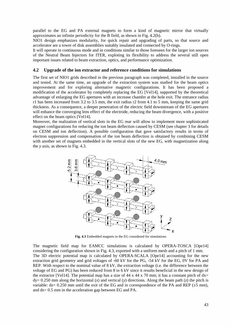
43
parallel to the EG and PA external magnets to form a kind of magnetic mirror that virtually
approximates an infinite periodicity for the B field, as shown in Fig. 4.2(b).
NIO1 design emphasizes modularity, for quick repair and upgrading of parts, so that source and
accelerator are a tower of disk assemblies suitably insulated and connected by O-rings.
It will operate in continuous mode and in conditions similar to those foreseen for the larger ion sources
of the Neutral Beam Injectors for ITER, exploting its flexibility to address the several still open
important issues related to beam extraction, optics, and performance optimization.
4.2 Upgrade of the ion extractor and reference conditions for simulations
The first set of NIO1 grids described in the previous paragraph was completed, installed in the source
and tested. At the same time, an upgrade of the extraction system was studied for the beam optics
improvement and for exploring alternative magnetic configurations. It has been proposed a
modification of the accelerator by completely replacing the EG [Vel14], supported by the theoretical
advantage of enlarging the EG apertures with an increase chamfer at the hole exit. The entrance radius
r1 has been increased from 3.2 to 3.5 mm, the exit radius r2 from 4.1 to 5 mm, keeping the same grid
thickness. As a consequence, a deeper penetration of the electric field downstream of the EG apertures
will enhance the converging lens effect of the electrode, reducing the beam divergence, with a positive
effect on the beam optics [Vel14].
Moreover, the realization of vertical slots in the EG rear will allow to implement more sophisticated
magnet configurations for reducing the ion beam deflection caused by CESM (see chapter 3 for details
on CESM and ion deflection). A possible configuration that gave satisfactory results in terms of
electron suppression and compensation of the ion beam deflection is obtained by combining CESM
with another set of magnets embedded in the vertical slots of the new EG, with magnetization along
the y axis, as shown in Fig. 4.3.
Fig. 4.3 Embedded magnets in the EG considered for simulations
The magnetic field map for EAMCC simulations is calculated by OPERA-TOSCA [Ope14]
considering the configuration shown in Fig. 4.3, exported with a uniform mesh and a pitch of 1 mm.
The 3D electric potential map is calculated by OPERA-SCALA [Ope14] accounting for the new
extraction grid geometry and grid voltages of -60 kV for the PG, -54 kV for the EG, 0V for PA and
REP. With respect to the nominal value of 8 kV, the extraction voltage (i.e. the difference between the
voltage of EG and PG) has been reduced from 8 to 6 kV since it results beneficial in the new design of
the extractor [Vel14]. The potential map has a size of 44 x 44 x 70 mm; it has a constant pitch of dx=
dy= 0.250 mm along the horizontal (x) and vertical (y) directions. Along the beam path (z) the pitch is
variable: dz= 0.250 mm until the exit of the EG and in correspondence of the PA and REP (±5 mm),
and dz= 0.5 mm in the acceleration gap between EG and PA.
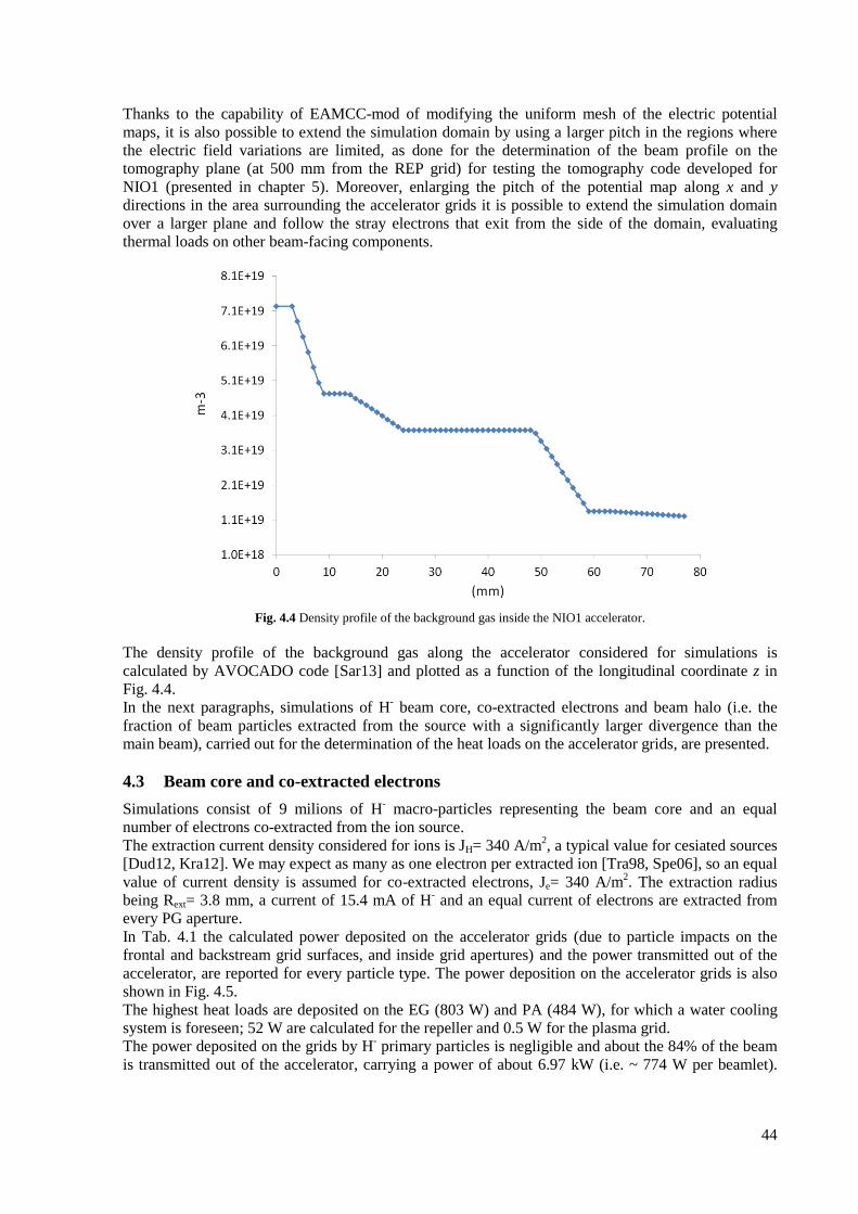
44
Thanks to the capability of EAMCC-mod of modifying the uniform mesh of the electric potential
maps, it is also possible to extend the simulation domain by using a larger pitch in the regions where
the electric field variations are limited, as done for the determination of the beam profile on the
tomography plane (at 500 mm from the REP grid) for testing the tomography code developed for
NIO1 (presented in chapter 5). Moreover, enlarging the pitch of the potential map along x and y
directions in the area surrounding the accelerator grids it is possible to extend the simulation domain
over a larger plane and follow the stray electrons that exit from the side of the domain, evaluating
thermal loads on other beam-facing components.
Fig. 4.4 Density profile of the background gas inside the NIO1 accelerator.
The density profile of the background gas along the accelerator considered for simulations is
calculated by AVOCADO code [Sar13] and plotted as a function of the longitudinal coordinate z in
Fig. 4.4.
In the next paragraphs, simulations of H- beam core, co-extracted electrons and beam halo (i.e. the
fraction of beam particles extracted from the source with a significantly larger divergence than the
main beam), carried out for the determination of the heat loads on the accelerator grids, are presented.
4.3 Beam core and co-extracted electrons
Simulations consist of 9 milions of H- macro-particles representing the beam core and an equal
number of electrons co-extracted from the ion source.
The extraction current density considered for ions is JH= 340 A/m2, a typical value for cesiated sources
[Dud12, Kra12]. We may expect as many as one electron per extracted ion [Tra98, Spe06], so an equal
value of current density is assumed for co-extracted electrons, Je= 340 A/m2. The extraction radius
being Rext= 3.8 mm, a current of 15.4 mA of H- and an equal current of electrons are extracted from
every PG aperture.
In Tab. 4.1 the calculated power deposited on the accelerator grids (due to particle impacts on the
frontal and backstream grid surfaces, and inside grid apertures) and the power transmitted out of the
accelerator, are reported for every particle type. The power deposition on the accelerator grids is also
shown in Fig. 4.5.
The highest heat loads are deposited on the EG (803 W) and PA (484 W), for which a water cooling
system is foreseen; 52 W are calculated for the repeller and 0.5 W for the plasma grid.
The power deposited on the grids by H- primary particles is negligible and about the 84% of the beam
is transmitted out of the accelerator, carrying a power of about 6.97 kW (i.e. ~ 774 W per beamlet).
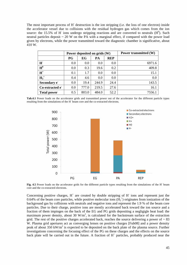
45
The most important process of H- destruction is the ion stripping (i.e. the loss of one electron) inside
the accelerator vessel due to collisions with the residual hydrogen gas which comes from the ion
source: the 15.5% of H- ions undergo stripping reactions and are converted to neutrals (H
0). Such
neutral particles deposit ~ 20 W on the PA with a marginal effect, if compared with the power load
given by electrons, while the power transmitted toward the diagnostic chamber is significative, about
410 W.
Power deposited on grids (W) Power transmitted (W)
PG EG PA REP
H- 0.0 0.0 0.0 0.0 6971.6
H0 0.0 0.3 19.6 0.2 409.8
H+ 0.1 1.7 0.0 0.0 15.1
H2+ 0.4 4.6 0.0 0.0 0.0
Secondary e- 0.0 19.4 244.9 24.4 143.5
Co-extracted e- 0.0 777.0 219.5 27.6 16.1
Total power 0.5 803.0 484.0 52.2 7556.1
Tab.4.1 Power loads on the accelerator grids and transmitted power out of the accelerator for the different particle types
resulting from the simulations of the H- beam core and the co-extracted electrons.
Fig. 4.5 Power loads on the accelerator grids for the different particle types resulting from the simulations of the H- beam
core and the co-extracted electrons.
Concerning positive charges, H+ are created by double stripping of H
- ions and represent just the
0.64% of the beam core particles, while positive molecular ions (H2+) originates from ionization of the
background gas by collisions with neutrals and negative ions and represent the 1.9 % of the beam core
particles. Due to their charge, positive ions are mostly accelerated back toward the ion source and a
fraction of them impinges on the back of the EG and PG grids depositing a negligigle heat load: the
maximum power density, about 30 W/m2, is calculated for the backstream surface of the extraction
grid. The rest of the positive charges accelerated back, reaches the source delivering a power of ~ 83
W. Plasma grid apertures act as converging lenses on positive charges [Fub08] and a power density
peak of about 350 kW/m2 is expected to be deposited on the back plate of the plasma source. Further
investigations concerning the focusing effect of the PG on these charges and the effects on the source
back plate will be carried out in the future. A fraction of H+ particles, probably produced near the
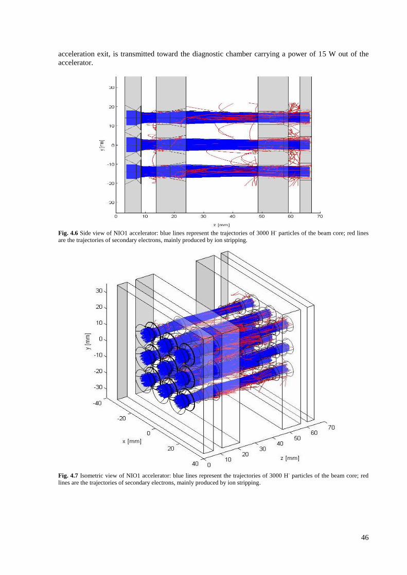
46
acceleration exit, is transmitted toward the diagnostic chamber carrying a power of 15 W out of the
accelerator.
Fig. 4.6 Side view of NIO1 accelerator: blue lines represent the trajectories of 3000 H- particles of the beam core; red lines
are the trajectories of secondary electrons, mainly produced by ion stripping.
Fig. 4.7 Isometric view of NIO1 accelerator: blue lines represent the trajectories of 3000 H- particles of the beam core; red
lines are the trajectories of secondary electrons, mainly produced by ion stripping.
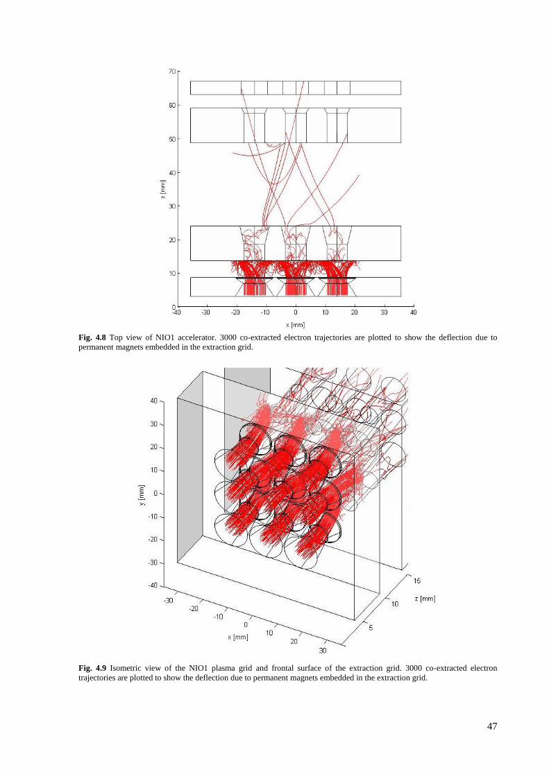
47
Fig. 4.8 Top view of NIO1 accelerator. 3000 co-extracted electron trajectories are plotted to show the deflection due to
permanent magnets embedded in the extraction grid.
Fig. 4.9 Isometric view of the NIO1 plasma grid and frontal surface of the extraction grid. 3000 co-extracted electron
trajectories are plotted to show the deflection due to permanent magnets embedded in the extraction grid.

48
In Figs. 4.6 and 4.7 the trajectories of 3000 H- particles are plotted (in blue), together with secondary
electrons (in red) generated by single and double ion stripping, ionization of the hydrogen gas and
direct impacts of primary and secondary particles on grids.
Electrons are responsible for the majority of the grid power loads (~ 98% of total power): the power
deposition due to co-extracted electrons is relatively important in the EG, representing the 97% of the
grid load, and in the PA where represents the 45%. The rest of the load on the PA grid is essentially
due to secondary electrons. Stripping of negative ions is the main cause of secondary electron
production in conventional electrostatic accelerators [Fub08]: created electrons are assumed to be
emitted at the location of the collision with H2 background gas with the same direction and velocity as
the parent H-. A fraction of secondary electrons is transmitted out of the accelerator, delivering a
power of 143 W to the diagnostic chamber.
As mentioned earlier, magnets embedded in the EG generate a field mainly along the vertical direction
and alternated from row to row which deflects nearly all the co-extracted electrons onto the EG itself,
while having little effect on the trajectories of the heavier H- ions; about the 98% of electrons is
collected in the EG, which corresponds to a relatively low power deposition (777 W) due to the
moderate potential difference between the plasma and extraction grid (i.e. 6 kV).
The effect of permanent magnets is clearly visible in Figs. 4.8 and 4.9, where the trajectories of 3000
electrons are plotted. Electrons extracted from the first and third aperture rows are deflected to the left
(By is positive, according to the magnetization scheme shown in Fig. 4.3) while the deflection in the
central row is toward the right side of the EG grid. The deflection of secondary electrons produced by
the H- beam core in the extraction gap (between PG and EG) causes the deposition of about 20 W on
the extraction grid. In Fig. 4.10 the power density due to the electron deflection on the frontal surface
of EG is shown for secondary (a) and co-extracted electrons (b): a relevant power density peak is
calculated for co-extracted electrons, about 4.5 MW/m2.
Fig. 4.10 Power density deposition on the frontal surface of EG due to secondary electrons (a) and co-extracted electrons (b).
The 2% of co-extracted electrons are transmitted through the EG downstream of the accelerator. These
electrons are accelerated in the main accelerator gap: 1.3% impact on the PA grid delivering a power
of 220 W and the remaining 0.3% is transmitted out of the accelerator, carrying a power of about 1.8
W per single beamlet. Around 1040 W of power is wasted for extracting and accelerating primary
electrons and approximately 430 W for accelerating secondary electrons.
Figs. 4.11, 4.12, 4.13 show the total power density deposited on the frontal surfaces of PG, EG and
REP. The most relevant power density region, ~ 4.5 MW/m2, is due to the co-extracted and secondary
electron deposition on the EG, as shown in Fig. 4.11 where the sum of the two contributions of Fig.
4.10 is considered (even if the secondary electron contribution is very limited). Other significative
power density peaks are observed in the PA (~ 1.6 MW/m2) and in the REP (500 kW/m
2) grids.
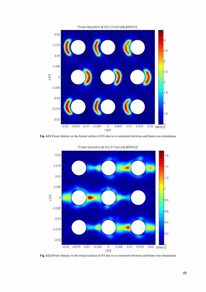
49
Fig. 4.11 Power density on the frontal surface of EG due to co-extracted electrons and beam core simulations
Fig. 4.12 Power density on the frontal surface of PA due to co-extracted electrons and beam core simulations
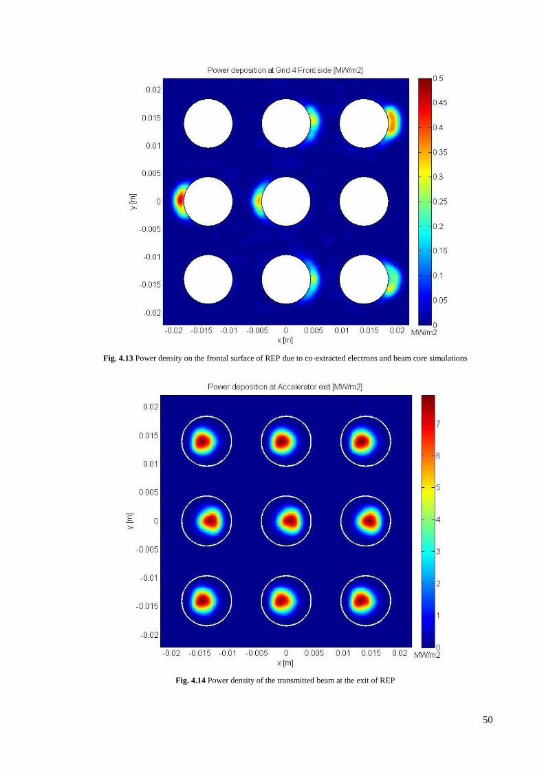
50
Fig. 4.13 Power density on the frontal surface of REP due to co-extracted electrons and beam core simulations
Fig. 4.14 Power density of the transmitted beam at the exit of REP
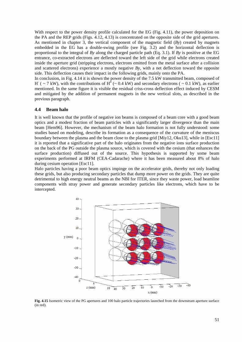
51
With respect to the power density profile calculated for the EG (Fig. 4.11), the power deposition on
the PA and the REP grids (Figs. 4.12, 4.13) is concentrated on the opposite side of the grid apertures.
As mentioned in chapter 3, the vertical component of the magnetic field (By) created by magnets
embedded in the EG has a double-swing profile (see Fig. 3.2) and the horizontal deflection is
proportional to the integral of By along the charged particle path (Eq. 3.1). If By is positive at the EG
entrance, co-extracted electrons are deflected toward the left side of the grid while electrons created
inside the aperture grid (stripping electrons, electrons emitted from the metal surface after a collision
and scattered electrons) experience a mostly negative By, with a net deflection toward the opposite
side. This deflection causes their impact in the following grids, mainly onto the PA.
In conclusion, in Fig. 4.14 it is shown the power density of the 7.5 kW transmitted beam, composed of
H- ( ~ 7 kW), with the contributions of H
0 (~ 0.4 kW) and secondary electrons ( ~ 0.1 kW), as earlier
mentioned. In the same figure it is visible the residual criss-cross deflection effect induced by CESM
and mitigated by the addition of permanent magnets in the new vertical slots, as described in the
previous paragraph.
4.4 Beam halo
It is well known that the profile of negative ion beams is composed of a beam core with a good beam
optics and a modest fraction of beam particles with a significantly larger divergence than the main
beam [Hem96]. However, the mechanism of the beam halo formation is not fully understood: some
studies based on modeling, describe its formation as a consequence of the curvature of the meniscus
boundary between the plasma and the beam close to the plasma grid [Miy12, Oku13], while in [Esc11]
it is reported that a significative part of the halo originates from the negative ions surface production
on the back of the PG outside the plasma source, which is covered with the cesium (that enhances the
surface production) diffused out of the source. This hypothesis is supported by some beam
experiments performed at IRFM (CEA-Cadarache) where it has been measured about 8% of halo
during cesium operation [Esc11].
Halo particles having a poor beam optics impinge on the accelerator grids, thereby not only loading
these grids, but also producing secondary particles that dump more power on the grids. They are quite
detrimental to high energy neutral beams as the NBI for ITER, since they waste power, load beamline
components with stray power and generate secondary particles like electrons, which have to be
intercepted.
Fig. 4.15 Isometric view of the PG apertures and 100 halo particle trajectories launched from the downstram aperture surface
(in red).

52
In order to evaluate the effect of these high-divergence particles on NIO1 grids, a beam halo current
equal to 8% of the beam core current (as measured at IRFM by de Esch et al. [Esc11]) is simulated by
launching 9.10
5 H
- macro-particles from the downstream side of the PG apertures. In Fig. 4.15 an
isometric view of the PG is shown and the halo emitting surface is highlighted in red.
The power deposition on the accelerator grids resulting from the simulation is due to primary (H-) and
secondary impinging particles. Secondaries are created by ionization of the background gas (H2+,e
-),
stripping (H0, e
-) and double stripping (H
+, 2 e
-) reactions, and direct impact on grids (e
-).
Simulation results are reported in Tab. 4.2 and shown in Fig. 4.16, where the power deposition for the
different particle species is indicated.
Thermal power deposited on accelerator grids (W)
PG EG PA REP
H- 0.0 18.1 0.1 0.0
H0 0.0 0.2 0.9 0.0
H+ 0.0 0.1 0.0 0.0
H2+ 0.0 0.1 0.0 0.0
Secondary electrons 0.0 1.3 13.9 1.3
Total power 0.0 19.8 14.9 1.3
Tab. 4.2 Power loads on accelerator grids due to beam halo and related secondary particles
Fig. 4.16 Power loads on accelerator grids due to beam halo and related secondary particles
About 12% of the primary H- macro-particles undergoes stripping reaction, double stripping is 0.5%
and H2+ created by ionizing the background gas correspond to 1.4% of the primary beam particles;
secondary electrons are mostly created by stripping reactions.
Compared to the heat loads caused by beam core and co-extracted electrons, the power deposition due
to the beam halo is very limited, the highest value being about 20 W for EG. Thermal power deposited
on the PA grid is less than 15 W, while loads on PG and REP grids are negligible.
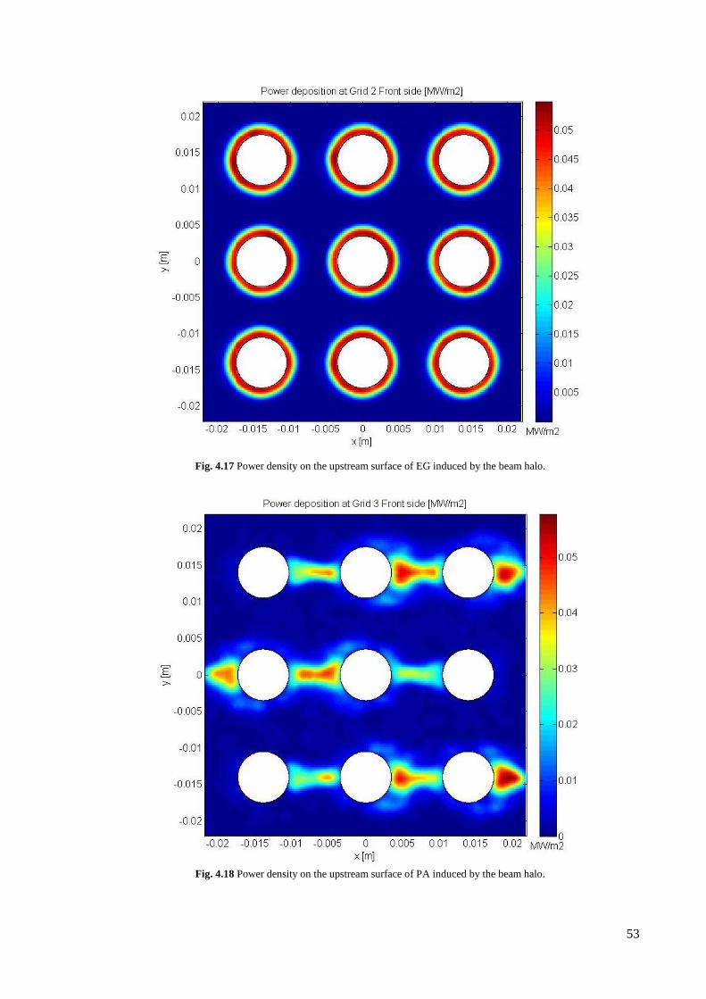
53
Fig. 4.17 Power density on the upstream surface of EG induced by the beam halo.
Fig. 4.18 Power density on the upstream surface of PA induced by the beam halo.
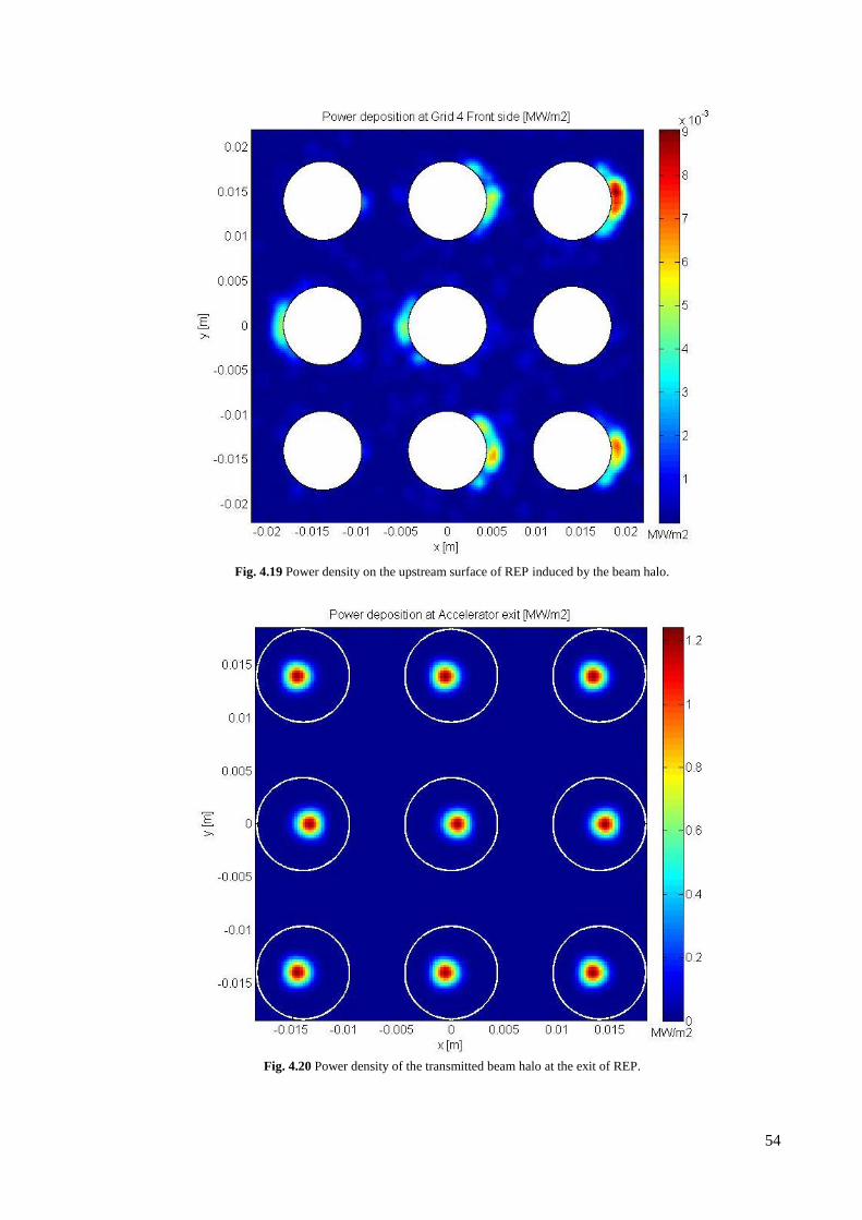
54
Fig. 4.19 Power density on the upstream surface of REP induced by the beam halo.
Fig. 4.20 Power density of the transmitted beam halo at the exit of REP.
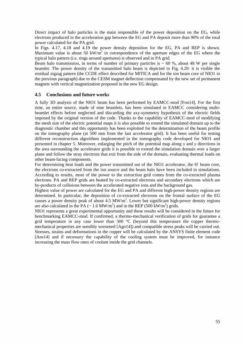
55
Direct impact of halo particles is the main responsible of the power deposition on the EG, while
electrons produced in the acceleration gap between the EG and PA deposit more than 90% of the total
power calculated for the PA grid.
In Figs. 4.17, 4.18 and 4.19 the power density deposition for the EG, PA and REP is shown.
Maximum value is about 50 kW/m2 in correspondence of the aperture edges of the EG where the
typical halo pattern (i.e. rings around apertures) is observed and in PA grid.
Beam halo transmission, in terms of number of primary particles is ~ 60 %, about 48 W per single
beamlet. The power density of the transmitted halo beam is depicted in Fig. 4.20: it is visible the
residual zigzag pattern (the CCDE effect described for MITICA and for the ion beam core of NIO1 in
the previous paragraph) due to the CESM magnet deflection compensated by the new set of permanent
magnets with vertical magnetization proposed in the new EG design.
4.5 Conclusions and future works
A fully 3D analysis of the NIO1 beam has been performed by EAMCC-mod [Fon14]. For the first
time, an entire source, made of nine beamlets, has been simulated in EAMCC considering multi-
beamlet effects before neglected and discarding the axy-symmetry hypothesis of the electric fields
imposed by the original version of the code. Thanks to the capability of EAMCC-mod of modifying
the mesh size of the electric potential maps it is also possible to extend the simulated domain up to the
diagnostic chamber and this opportunity has been exploited for the determination of the beam profile
on the tomography plane (at 500 mm from the last accelerator grid). It has been useful for testing
different reconstruction algorithms implemented in the tomography code developed for NIO1 and
presented in chapter 5. Moreover, enlarging the pitch of the potential map along x and y directions in
the area surrounding the accelerator grids it is possible to extend the simulation domain over a larger
plane and follow the stray electrons that exit from the side of the domain, evaluating thermal loads on
other beam-facing components.
For determining heat loads and the power transmitted out of the NIO1 accelerator, the H- beam core,
the electrons co-extracted from the ion source and the beam halo have been included in simulations.
According to results, most of the power to the extraction grid comes from the co-extracted plasma
electrons. PA and REP grids are heated by co-extracted electrons and secondary electrons which are
by-products of collisions between the accelerated negative ions and the background gas.
Highest value of power are calculated for the EG and PA and different high-power density regions are
determined. In particular, the deposition of co-extracted electrons on the frontal surface of the EG
causes a power density peak of about 4.5 MW/m2. Lower but significant high-power density regions
are also calculated in the PA (~ 1.6 MW/m2) and in the REP (500 kW/m
2) grids.
NIO1 represents a great experimental opportunity and these results will be considered in the future for
benchmarking EAMCC-mod. If confirmed, a thermo-mechanical verification of grids for guarantee a
grid temperature in any case lower than 300 °C (beyond this temperature the copper thermo-
mechanical properties are sensibly worsened [Ago14]) and compatible stress peaks will be carried out.
Stresses, strains and deformations in the copper will be calculated by the ANSYS finite element code
[Ans14] and if necessary the capability of the cooling system must be improved, for instance
increasing the mass flow rates of coolant inside the grid channels.

56
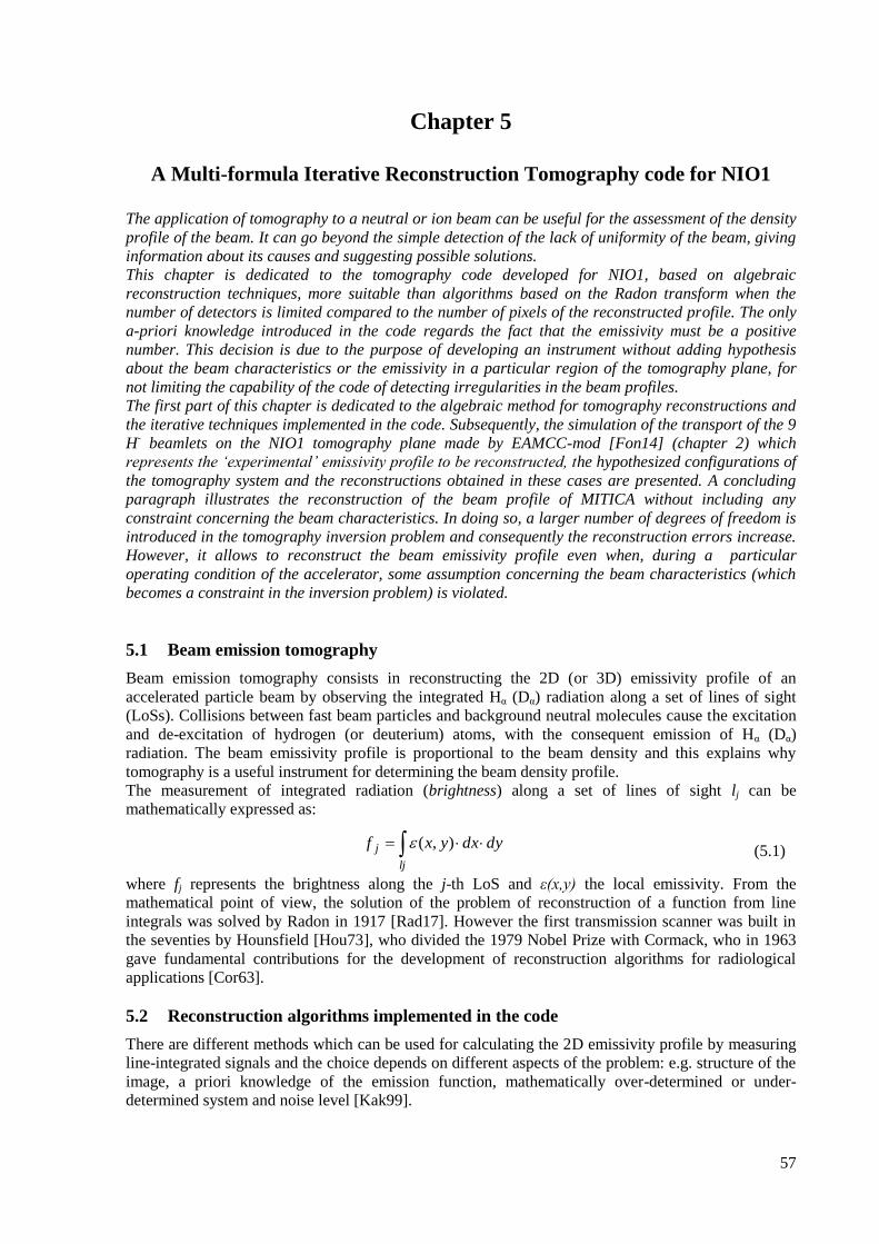
57
Chapter 5
A Multi-formula Iterative Reconstruction Tomography code for NIO1
The application of tomography to a neutral or ion beam can be useful for the assessment of the density
profile of the beam. It can go beyond the simple detection of the lack of uniformity of the beam, giving
information about its causes and suggesting possible solutions.
This chapter is dedicated to the tomography code developed for NIO1, based on algebraic
reconstruction techniques, more suitable than algorithms based on the Radon transform when the
number of detectors is limited compared to the number of pixels of the reconstructed profile. The only
a-priori knowledge introduced in the code regards the fact that the emissivity must be a positive
number. This decision is due to the purpose of developing an instrument without adding hypothesis
about the beam characteristics or the emissivity in a particular region of the tomography plane, for
not limiting the capability of the code of detecting irregularities in the beam profiles.
The first part of this chapter is dedicated to the algebraic method for tomography reconstructions and
the iterative techniques implemented in the code. Subsequently, the simulation of the transport of the 9
H- beamlets on the NIO1 tomography plane made by EAMCC-mod [Fon14] (chapter 2) which
represents the ‘experimental’ emissivity profile to be reconstructed, the hypothesized configurations of
the tomography system and the reconstructions obtained in these cases are presented. A concluding
paragraph illustrates the reconstruction of the beam profile of MITICA without including any
constraint concerning the beam characteristics. In doing so, a larger number of degrees of freedom is
introduced in the tomography inversion problem and consequently the reconstruction errors increase.
However, it allows to reconstruct the beam emissivity profile even when, during a particular
operating condition of the accelerator, some assumption concerning the beam characteristics (which
becomes a constraint in the inversion problem) is violated.
5.1 Beam emission tomography
Beam emission tomography consists in reconstructing the 2D (or 3D) emissivity profile of an
accelerated particle beam by observing the integrated Hα (Dα) radiation along a set of lines of sight
(LoSs). Collisions between fast beam particles and background neutral molecules cause the excitation
and de-excitation of hydrogen (or deuterium) atoms, with the consequent emission of Hα (Dα)
radiation. The beam emissivity profile is proportional to the beam density and this explains why
tomography is a useful instrument for determining the beam density profile.
The measurement of integrated radiation (brightness) along a set of lines of sight lj can be
mathematically expressed as:
lj
j dydxyxf ),( (5.1)
where fj represents the brightness along the j-th LoS and ε(x,y) the local emissivity. From the
mathematical point of view, the solution of the problem of reconstruction of a function from line
integrals was solved by Radon in 1917 [Rad17]. However the first transmission scanner was built in
the seventies by Hounsfield [Hou73], who divided the 1979 Nobel Prize with Cormack, who in 1963
gave fundamental contributions for the development of reconstruction algorithms for radiological
applications [Cor63].
5.2 Reconstruction algorithms implemented in the code
There are different methods which can be used for calculating the 2D emissivity profile by measuring
line-integrated signals and the choice depends on different aspects of the problem: e.g. structure of the
image, a priori knowledge of the emission function, mathematically over-determined or under-
determined system and noise level [Kak99].
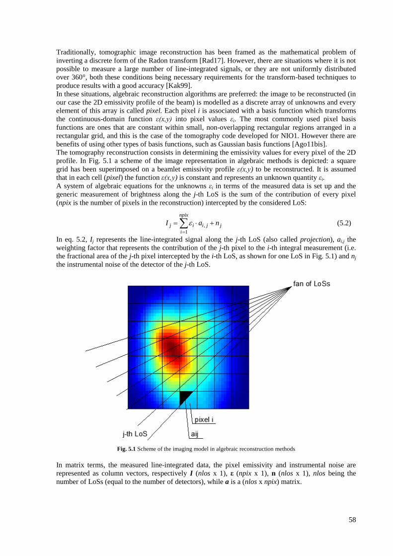
58
Traditionally, tomographic image reconstruction has been framed as the mathematical problem of
inverting a discrete form of the Radon transform [Rad17]. However, there are situations where it is not
possible to measure a large number of line-integrated signals, or they are not uniformly distributed
over 360°, both these conditions being necessary requirements for the transform-based techniques to
produce results with a good accuracy [Kak99].
In these situations, algebraic reconstruction algorithms are preferred: the image to be reconstructed (in
our case the 2D emissivity profile of the beam) is modelled as a discrete array of unknowns and every
element of this array is called pixel. Each pixel i is associated with a basis function which transforms
the continuous-domain function ε(x,y) into pixel values εi. The most commonly used pixel basis
functions are ones that are constant within small, non-overlapping rectangular regions arranged in a
rectangular grid, and this is the case of the tomography code developed for NIO1. However there are
benefits of using other types of basis functions, such as Gaussian basis functions [Ago11bis].
The tomography reconstruction consists in determining the emissivity values for every pixel of the 2D
profile. In Fig. 5.1 a scheme of the image representation in algebraic methods is depicted: a square
grid has been superimposed on a beamlet emissivity profile ε(x,y) to be reconstructed. It is assumed
that in each cell (pixel) the function ε(x,y) is constant and represents an unknown quantity εi.
A system of algebraic equations for the unknowns εi in terms of the measured data is set up and the
generic measurement of brightness along the j-th LoS is the sum of the contribution of every pixel
(npix is the number of pixels in the reconstruction) intercepted by the considered LoS:
j
npix
i
jiij naI 1
,
(5.2)
In eq. 5.2, Ij represents the line-integrated signal along the j-th LoS (also called projection), ai,j the
weighting factor that represents the contribution of the j-th pixel to the i-th integral measurement (i.e.
the fractional area of the j-th pixel intercepted by the i-th LoS, as shown for one LoS in Fig. 5.1) and nj
the instrumental noise of the detector of the j-th LoS.
Fig. 5.1 Scheme of the imaging model in algebraic reconstruction methods
In matrix terms, the measured line-integrated data, the pixel emissivity and instrumental noise are
represented as column vectors, respectively I (nlos x 1), ε (npix x 1), n (nlos x 1), nlos being the
number of LoSs (equal to the number of detectors), while a is a (nlos x npix) matrix.
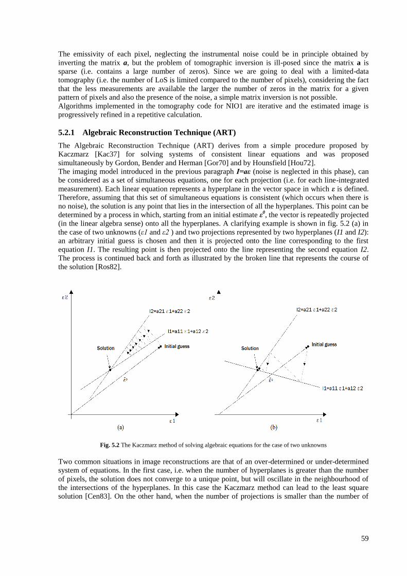
59
The emissivity of each pixel, neglecting the instrumental noise could be in principle obtained by
inverting the matrix a, but the problem of tomographic inversion is ill-posed since the matrix a is
sparse (i.e. contains a large number of zeros). Since we are going to deal with a limited-data
tomography (i.e. the number of LoS is limited compared to the number of pixels), considering the fact
that the less measurements are available the larger the number of zeros in the matrix for a given
pattern of pixels and also the presence of the noise, a simple matrix inversion is not possible.
Algorithms implemented in the tomography code for NIO1 are iterative and the estimated image is
progressively refined in a repetitive calculation.
5.2.1 Algebraic Reconstruction Technique (ART)
The Algebraic Reconstruction Technique (ART) derives from a simple procedure proposed by
Kaczmarz [Kac37] for solving systems of consistent linear equations and was proposed
simultaneously by Gordon, Bender and Herman [Gor70] and by Hounsfield [Hou72].
The imaging model introduced in the previous paragraph I=aε (noise is neglected in this phase), can
be considered as a set of simultaneous equations, one for each projection (i.e. for each line-integrated
measurement). Each linear equation represents a hyperplane in the vector space in which ε is defined.
Therefore, assuming that this set of simultaneous equations is consistent (which occurs when there is
no noise), the solution is any point that lies in the intersection of all the hyperplanes. This point can be
determined by a process in which, starting from an initial estimate ε0, the vector is repeatedly projected
(in the linear algebra sense) onto all the hyperplanes. A clarifying example is shown in fig. 5.2 (a) in
the case of two unknowns (ε1 and ε2 ) and two projections represented by two hyperplanes (I1 and I2):
an arbitrary initial guess is chosen and then it is projected onto the line corresponding to the first
equation I1. The resulting point is then projected onto the line representing the second equation I2.
The process is continued back and forth as illustrated by the broken line that represents the course of
the solution [Ros82].
Fig. 5.2 The Kaczmarz method of solving algebraic equations for the case of two unknowns
Two common situations in image reconstructions are that of an over-determined or under-determined
system of equations. In the first case, i.e. when the number of hyperplanes is greater than the number
of pixels, the solution does not converge to a unique point, but will oscillate in the neighbourhood of
the intersections of the hyperplanes. In this case the Kaczmarz method can lead to the least square
solution [Cen83]. On the other hand, when the number of projections is smaller than the number of
60
unknowns and an infinite number of solutions exists, Tanabe [Tan71] demonstrates that the Kaczmarz
method converges to the solution closest to the initial guess.
This iterative procedure can be written for a generic number of LoS (nlos), npix unknowns and
considering the j-th projection, as:
jinpix
i
ji
npix
i
jikij
ki
ki a
a
aI
,
1
2,
1
,
1
)(
(5.3)
Eq. 5.3 represents the ART iterative formula: the value of emissivity for the pixel i at the step k+1 is
calculated by summing to the previous estimation an error-correcting term, i.e. the weighted (by ai,j)
and normalized difference between the measured Ij and its estimation at the previous step k. ART is
sequential: the error-correcting term is calculated and applied for every projection, in a sequential way.
Its convergence rate may be dependent on the orthogonality of the successive projections and this can
be understood by comparing Fig. 5.2 (a) and (b): in the second case, the two projections being almost
orthogonal allow to reach the solution point in a few iterations.
Different approaches are suggested for improving the convergence rate of ART: treating the
projections in a random order in each cycle [Gor74] and considering successive projections at least
60° away [Her80]. For what concerns the code presented in this chapter the second option has been
adopted, with a reduction of the number of iterations required for reaching the convergence, that in
any case, considering the limited number of pixels and LoSs foreseen for NIO1 tomography, is small.
A more significant improvement in terms of reconstruction errors reduction, has been obtained by
normalizing the correction-term of Eq. 5.3 with the sum of ai,j ‘s elements instead of the sum of their
squared value. For this reason, also the following modified version of the ART formula has been
implemented in the code:
jinpix
i
ji
npix
i
jikij
ki
ki a
a
aI
,
1
,
1
,
1
(5.4)
Since emissivity is positive by definition, a non-negativity constraint has been introduced into the
algorithm and in each iteration, any pixel having a negative value is set to zero. It has been chosen not
to include in the algorithm any hypothesis concerning the characteristics of the beam (the so called a-
priori knowledge, e.g. Gaussian beamlets, pixels inside a particular region constrained to some known
values) in order not to preclude the emissivity reconstruction in any situation, in particular during
malfunctions when some a-priori knowledge could be not realistic.
5.2.2 Simultaneous Algebraic Reconstruction Technique (SART)
The Simultaneous Algebraic Reconstruction Technique (SART) was developed by Andersen and Kak
[And84] as a major refinement of ART. The sequential correction scheme of the ART requires a
considerably large number of iterations for convergence while SART is supposed to yield
reconstructions of good quality and numerical accuracy in only one iteration [Kak99]. This technique
is based on the simultaneous application of the error correcting term discussed for eq. 5.3 and the
average of the corrections generated by all the line-integrated measurements is simultaneously applied.
The iterative scheme of SART follows the following formula:
61
nlos
j
ji
nlos
jnpix
i
ji
npix
i
kijij
ji
ki
ki
a
a
aI
a
1
,
1
1
,
1
,
,
1
(5.5)
The emissivity of the i-th pixel is updated at the step k+1 considering simultaneously all the LoSs
intersecting it and the error-correcting term is averaged over the sum of contributions of the j-th pixel
to every line-integrated measurement.
A non-negativity constraint for pixel emissivity has been included in the SART routine implemented
in the tomography code. Moreover, in view of the application of this code for tomography
reconstructions with a larger number of pixel and LoSs (e.g. MITICA or SPIDER tomography), every
sum cycle has been optimized in order to make it computationally faster, which means that null
elements are not considered in the sum process. In doing so, only LoSs intercepting the i-th pixel are
considered for the sum over all the LoSs and only ai,j ’s not null are considered for the sum over the
image pixels.
5.2.3 Maximum-Likelihood Expectation-Maximization Algorithm (ML-EM)
The ML-EM algorithm has been for years the leading iterative reconstruction algorithm in medical
imaging for SPECT and PET [Wer04]. It was originally proposed in 1977 as the solution to
incomplete data problems in statistics [Dem77] and successively applied to tomography [She82],
[Lan84]. The iterative formula reads:
ji
nlos
jnpix
i
jiki
j
nlos
j
ji
kik
i a
a
I
a
,
1
1
,
1
,
1
(5.6)
It has a simple form, all pixels are updated simultaneously as in SART and errors and updates are
multiplicative. Despite its simple formula (it seems a sort of multiplicative simultaneous ART) the
derivation of the ML-EM algorithm is based on more complex statistics considerations: given a
limited knowledge of the image (i.e. the so called limited data represented by the set of line-integrated
measurements) we are interested in determining the complete data (the position of every emitted
photon). The task of the image reconstruction is, in a sense, to un-mix the photon counts finding the
most probable space distribution of photons (i.e. the emissivity of every pixel).
The ML-EM algorithm has two main shortcomings: the convergence of the algorithm is slow and it
yields noisy reconstructed images. ML-EM has been shown consistently to cause low spatial
frequencies to appear first during the iterative process and then gradually to develop higher spatial
frequencies: as the iterations proceed and the algorithm approaches the maximum-likelihood solution,
the variance of the image estimate, which is manifested as noise, increases [Wer04]. In practice the
ML-EM algorithm yields goods results if the iterative procedure is stopped prematurely, and the
results may, in addition, benefit from application of a post-reconstruction low-pass filter, which is a
common approach in clinical applications [Wer04].
For what concerns the non-negativity constraint, it is automatically imposed by the algorithm, since
the correcting-error term is multiplicative. Also in this case, the sum cycles are optimized for being
faster: sums are performed on sub-matrices which contain just the non-null elements (for instance in
the sum over the LoSs this is done considering just LoSs that intercept the i-th pixel), avoiding long
and time-consuming sums of null elements.
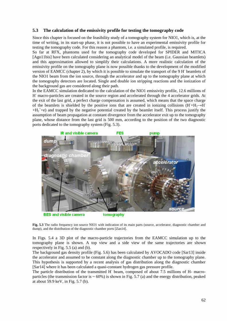
62
5.3 The calculation of the emissivity profile for testing the tomography code
Since this chapter is focused on the feasibility study of a tomography system for NIO1, which is, at the
time of writing, in its start-up phase, it is not possible to have an experimental emissivity profile for
testing the tomography code. For this reason a phantom, i.e. a simulated profile, is required.
So far at RFX, phantoms used for the tomography code developed for SPIDER and MITICA
[Ago11bis] have been calculated considering an analytical model of the beam (i.e. Gaussian beamlets)
and this approximation allowed to simplify their calculations. A more realistic calculation of the
emissivity profile on the tomography plane is now possible thanks to the development of the modified
version of EAMCC (chapter 2), by which it is possible to simulate the transport of the 9 H- beamlets of
the NIO1 beam from the ion source, through the accelerator and up to the tomography plane at which
the tomography detectors are located. Single and double ion stripping reactions and the ionization of
the background gas are considered along their path.
In the EAMCC simulation dedicated to the calculation of the NIO1 emissivity profile, 12.6 millions of
H- macro-particles are created in the source region and accelerated through the 4 accelerator grids. At
the exit of the last grid, a perfect charge compensation is assumed, which means that the space charge
of the beamlets is shielded by the positive ions that are created in ionizing collisions (H-+H2→H
-
+H2++e) and trapped by the negative potential created by the beamlet itself. This process justify the
assumption of beam propagation at constant divergence from the accelerator exit up to the tomography
plane, whose distance from the last grid is 500 mm, according to the position of the two diagnostic
ports dedicated to the tomography system (Fig. 5.3).
Fig. 5.3 The radio frequency ion source NIO1 with indication of its main parts (source, accelerator, diagnostic chamber and
dump), and the distribution of the diagnostic chamber ports [Zan14].
In Figs. 5.4 a 3D plot of the macro-particle trajectories from the EAMCC simulation up to the
tomography plane is shown. A top view and a side view of the same trajectories are shown
respectively in Fig. 5.5 (a) and (b).
The background gas density profile (Fig. 5.6) has been calculated by AVOCADO code [Sar13] inside
the accelerator and assumed to be constant along the diagnostic chamber up to the tomography plane.
This hypothesis is supported by a recent analysis of gas distribution along the diagnostic chamber
[Sar14] where it has been calculated a quasi-constant hydrogen gas pressure profile.
The particle distribution of the transmitted H- beam, composed of about 7.5 millions of H- macro-
particles (the transmission factor is ~ 60%) is shown in Fig. 5.7 (a) and the energy distribution, peaked
at about 59.9 keV, in Fig. 5.7 (b).
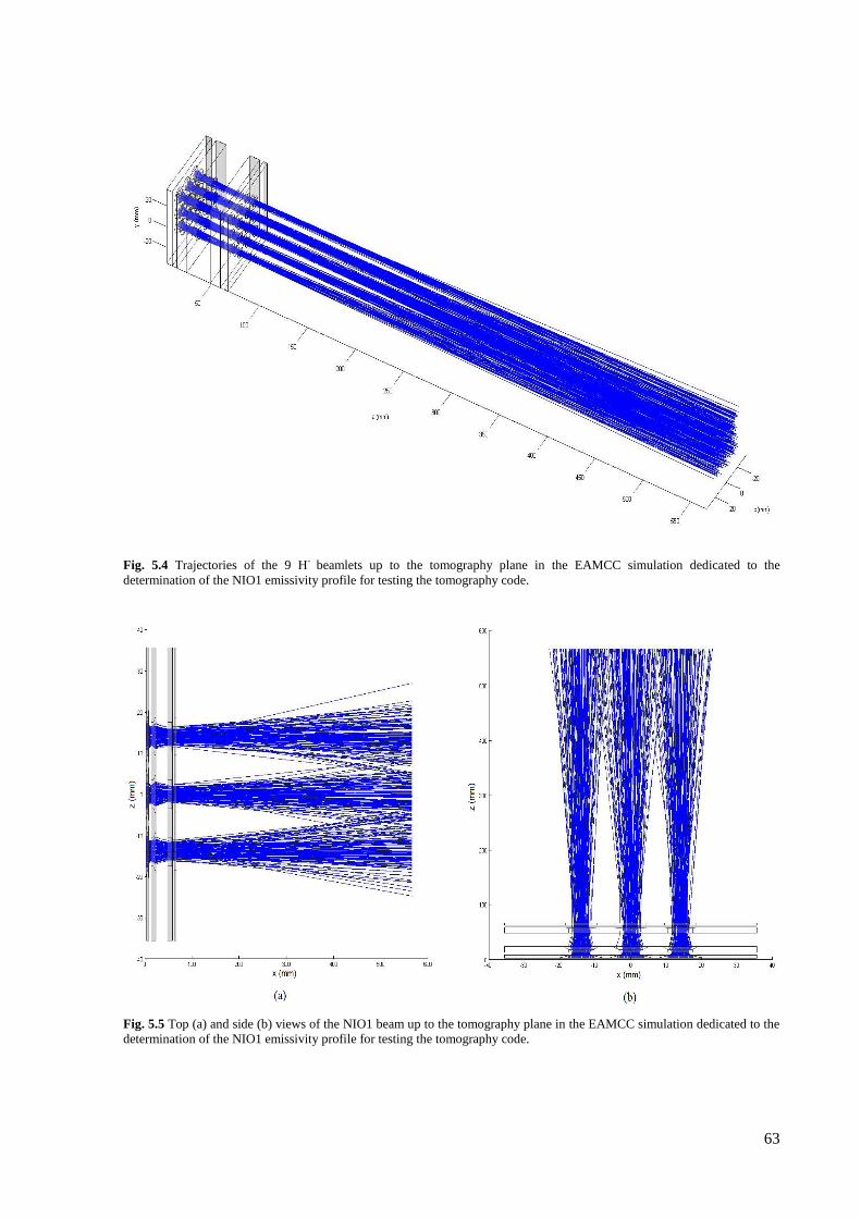
63
Fig. 5.4 Trajectories of the 9 H- beamlets up to the tomography plane in the EAMCC simulation dedicated to the
determination of the NIO1 emissivity profile for testing the tomography code.
Fig. 5.5 Top (a) and side (b) views of the NIO1 beam up to the tomography plane in the EAMCC simulation dedicated to the
determination of the NIO1 emissivity profile for testing the tomography code.
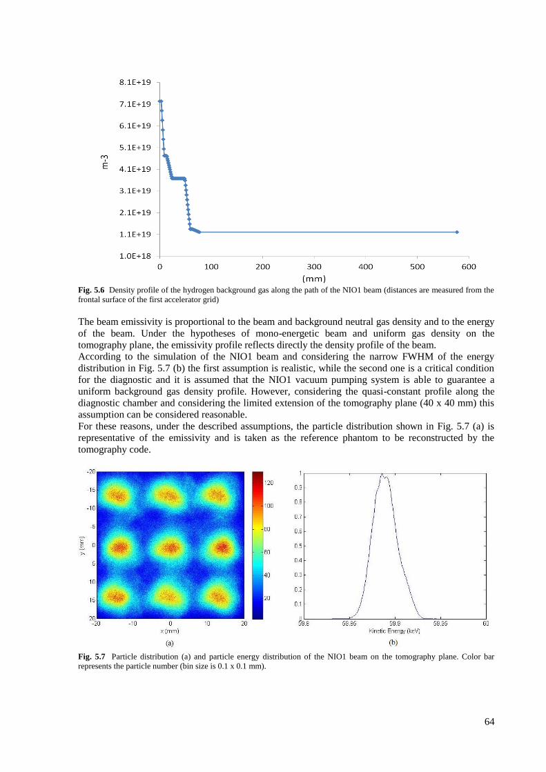
64
Fig. 5.6 Density profile of the hydrogen background gas along the path of the NIO1 beam (distances are measured from the
frontal surface of the first accelerator grid)
The beam emissivity is proportional to the beam and background neutral gas density and to the energy
of the beam. Under the hypotheses of mono-energetic beam and uniform gas density on the
tomography plane, the emissivity profile reflects directly the density profile of the beam.
According to the simulation of the NIO1 beam and considering the narrow FWHM of the energy
distribution in Fig. 5.7 (b) the first assumption is realistic, while the second one is a critical condition
for the diagnostic and it is assumed that the NIO1 vacuum pumping system is able to guarantee a
uniform background gas density profile. However, considering the quasi-constant profile along the
diagnostic chamber and considering the limited extension of the tomography plane (40 x 40 mm) this
assumption can be considered reasonable.
For these reasons, under the described assumptions, the particle distribution shown in Fig. 5.7 (a) is
representative of the emissivity and is taken as the reference phantom to be reconstructed by the
tomography code.
Fig. 5.7 Particle distribution (a) and particle energy distribution of the NIO1 beam on the tomography plane. Color bar
represents the particle number (bin size is 0.1 x 0.1 mm).
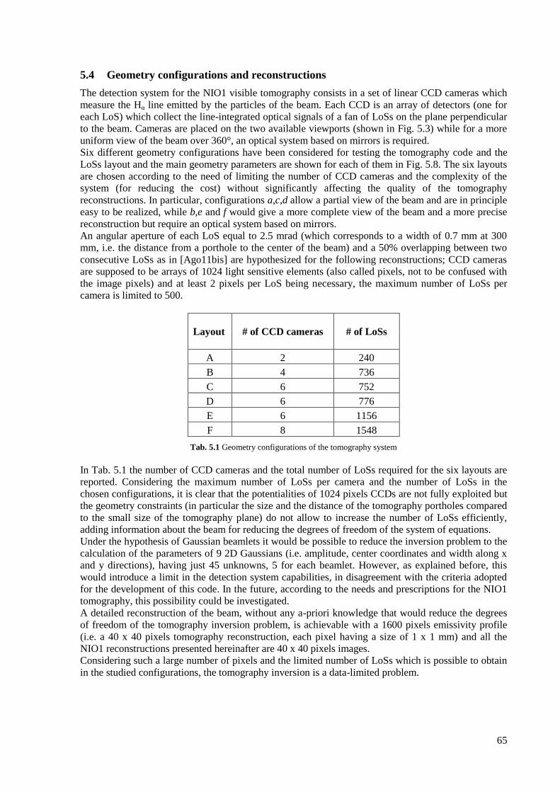
65
5.4 Geometry configurations and reconstructions
The detection system for the NIO1 visible tomography consists in a set of linear CCD cameras which
measure the Hα line emitted by the particles of the beam. Each CCD is an array of detectors (one for
each LoS) which collect the line-integrated optical signals of a fan of LoSs on the plane perpendicular
to the beam. Cameras are placed on the two available viewports (shown in Fig. 5.3) while for a more
uniform view of the beam over 360°, an optical system based on mirrors is required.
Six different geometry configurations have been considered for testing the tomography code and the
LoSs layout and the main geometry parameters are shown for each of them in Fig. 5.8. The six layouts
are chosen according to the need of limiting the number of CCD cameras and the complexity of the
system (for reducing the cost) without significantly affecting the quality of the tomography
reconstructions. In particular, configurations a,c,d allow a partial view of the beam and are in principle
easy to be realized, while b,e and f would give a more complete view of the beam and a more precise
reconstruction but require an optical system based on mirrors.
An angular aperture of each LoS equal to 2.5 mrad (which corresponds to a width of 0.7 mm at 300
mm, i.e. the distance from a porthole to the center of the beam) and a 50% overlapping between two
consecutive LoSs as in [Ago11bis] are hypothesized for the following reconstructions; CCD cameras
are supposed to be arrays of 1024 light sensitive elements (also called pixels, not to be confused with
the image pixels) and at least 2 pixels per LoS being necessary, the maximum number of LoSs per
camera is limited to 500.
Layout # of CCD cameras # of LoSs
A 2 240
B 4 736
C 6 752
D 6 776
E 6 1156
F 8 1548
Tab. 5.1 Geometry configurations of the tomography system
In Tab. 5.1 the number of CCD cameras and the total number of LoSs required for the six layouts are
reported. Considering the maximum number of LoSs per camera and the number of LoSs in the
chosen configurations, it is clear that the potentialities of 1024 pixels CCDs are not fully exploited but
the geometry constraints (in particular the size and the distance of the tomography portholes compared
to the small size of the tomography plane) do not allow to increase the number of LoSs efficiently,
adding information about the beam for reducing the degrees of freedom of the system of equations.
Under the hypothesis of Gaussian beamlets it would be possible to reduce the inversion problem to the
calculation of the parameters of 9 2D Gaussians (i.e. amplitude, center coordinates and width along x
and y directions), having just 45 unknowns, 5 for each beamlet. However, as explained before, this
would introduce a limit in the detection system capabilities, in disagreement with the criteria adopted
for the development of this code. In the future, according to the needs and prescriptions for the NIO1
tomography, this possibility could be investigated.
A detailed reconstruction of the beam, without any a-priori knowledge that would reduce the degrees
of freedom of the tomography inversion problem, is achievable with a 1600 pixels emissivity profile
(i.e. a 40 x 40 pixels tomography reconstruction, each pixel having a size of 1 x 1 mm) and all the
NIO1 reconstructions presented hereinafter are 40 x 40 pixels images.
Considering such a large number of pixels and the limited number of LoSs which is possible to obtain
in the studied configurations, the tomography inversion is a data-limited problem.
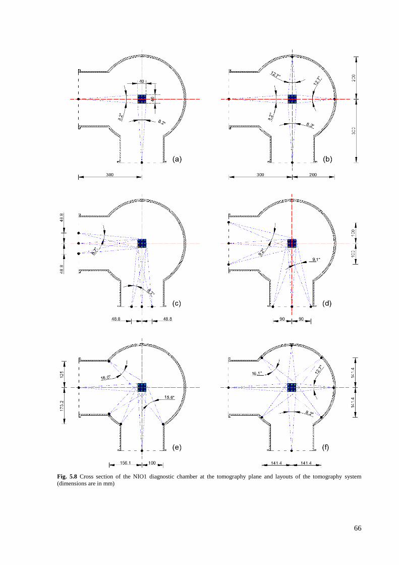
66
Fig. 5.8 Cross section of the NIO1 diagnostic chamber at the tomography plane and layouts of the tomography system
(dimensions are in mm)
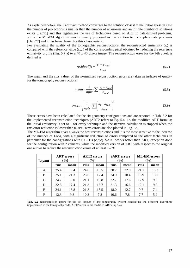
67
As explained before, the Kaczmarz method converges to the solution closest to the initial guess in case
the number of projections is smaller than the number of unknowns and an infinite number of solutions
exists [Tan71] and this legitimizes the use of techniques based on ART in data-limited problems,
while the ML-EM algorithm was originally proposed as the solution to incomplete data problems
[Dem77] and it has been chosen for this characteristic.
For evaluating the quality of the tomographic reconstructions, the reconstructed emissivity (εi) is
compared with the reference value (εreal) of the corresponding pixel obtained by reducing the reference
emissivity profile (Fig. 5.7 a) to a 40 x 40 pixels image. The reconstruction error for the i-th pixel, is
defined as:
real
realiiresidual
)(
(5.7)
The mean and the rms values of the normalized reconstruction errors are taken as indexes of quality
for the tomography reconstructions:
real
reali
npixmean
1
(5.8)
21
real
reali
npixrms
(5.9)
These errors have been calculated for the six geometry configurations and are reported in Tab. 5.2 for
the implemented reconstruction techniques (ART2 refers to Eq. 5.4, i.e. the modified ART formula;
the initial emissivity is set to 1 for every technique and the iterative calculation is stopped when the
rms error reduction is lower than 0.01%. Rms errors are also plotted in Fig. 5.9.
The ML-EM algorithm gives always the best reconstructions and it is the most sensitive to the increase
of the number of LoSs, with a significant reduction of errors compared to the other techniques in
particular for the configurations with 6 CCDs (c,d,e). SART works better than ART, exception done
for the configuration with 2 cameras, while the modified version of ART with respect to the original
one allows to reduce the reconstruction errors of at least 1-2 %.
Layout
ART errors
(%)
ART2 errors
(%)
SART errors
(%)
ML-EM errors
(%)
rms mean rms mean rms mean rms mean
A 25.4 19.4 24.0 18.5 30.7 22.0 21.1 15.3
B 25.1 21.3 23.6 17.4 24.9 18.4 16.9 13.0
C 24.2 18.0 21.1 16.8 22.7 17.6 12.9 9.9
D 22.8 17.4 21.3 16.7 21.3 16.6 12.1 9.2
E 24.1 16.8 21.3 15.5 18.0 12.7 9.7 7.4
F 12.3 9.8 10.3 7.8 10.6 7.8 7.7 5.9
Tab. 5.2 Reconstruction errors for the six layouts of the tomography system considering the different algorithms
implemented in the tomography code. ART2 refers to the modified ART (Eq. 5.4).
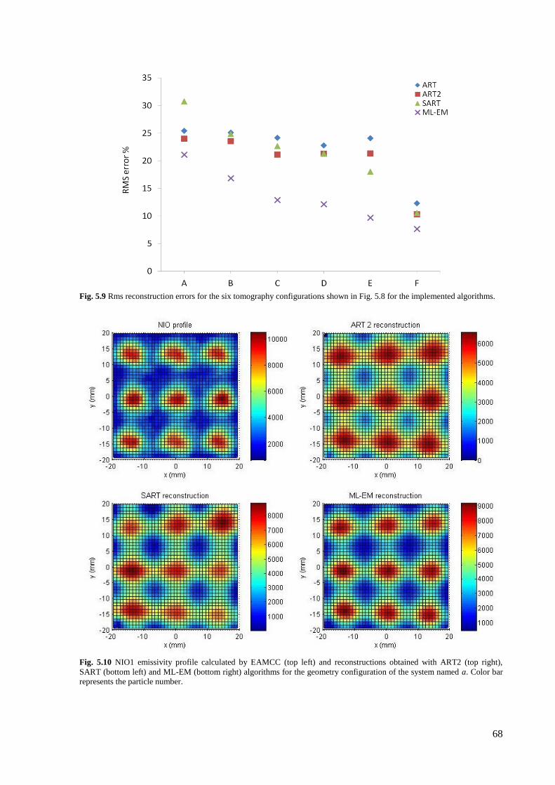
68
Fig. 5.9 Rms reconstruction errors for the six tomography configurations shown in Fig. 5.8 for the implemented algorithms.
Fig. 5.10 NIO1 emissivity profile calculated by EAMCC (top left) and reconstructions obtained with ART2 (top right),
SART (bottom left) and ML-EM (bottom right) algorithms for the geometry configuration of the system named a. Color bar
represents the particle number.
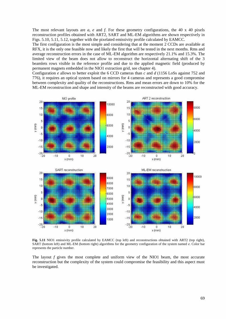
69
The most relevant layouts are a, e and f. For these geometry configurations, the 40 x 40 pixels
reconstruction profiles obtained with ART2, SART and ML-EM algorithms are shown respectively in
Figs. 5.10, 5.11, 5.12, together with the pixelated emissivity profile calculated by EAMCC.
The first configuration is the most simple and considering that at the moment 2 CCDs are available at
RFX, it is the only one feasible now and likely the first that will be tested in the next months. Rms and
average reconstruction errors in the case of ML-EM algorithm are respectively 21.1% and 15.3%. The
limited view of the beam does not allow to reconstruct the horizontal alternating shift of the 3
beamlets rows visible in the reference profile and due to the applied magnetic field (produced by
permanent magnets embedded in the NIO1 extraction grid, see chapter 4).
Configuration e allows to better exploit the 6 CCD cameras than c and d (1156 LoSs against 752 and
776), it requires an optical system based on mirrors for 4 cameras and represents a good compromise
between complexity and quality of the reconstructions. Rms and mean errors are down to 10% for the
ML-EM reconstruction and shape and intensity of the beams are reconstructed with good accuracy.
Fig. 5.11 NIO1 emissivity profile calculated by EAMCC (top left) and reconstructions obtained with ART2 (top right),
SART (bottom left) and ML-EM (bottom right) algorithms for the geometry configuration of the system named e. Color bar
represents the particle number.
The layout f gives the most complete and uniform view of the NIO1 beam, the most accurate
reconstruction but the complexity of the system could compromise the feasibility and this aspect must
be investigated.

70
Fig. 5.12 NIO1 emissivity profile calculated by EAMCC (top left) and reconstructions obtained with ART2 (top right),
SART (bottom left) and ML-EM (bottom right) algorithms for the geometry configuration of the system named f. Color bar
represents the particle number.
Fig. 5.13 Convergence of the iterative algorithms.
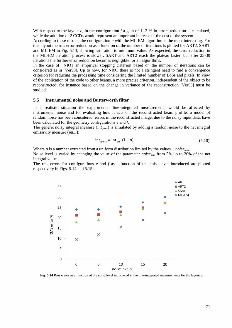
71
With respect to the layout e, in the configuration f a gain of 1- 2 % in errors reduction is calculated,
while the addition of 2 CCDs would represent an important increase of the cost of the system.
According to these results, the configuration e with the ML-EM algorithm is the most interesting. For
this layout the rms error reduction as a function of the number of iterations is plotted for ART2, SART
and ML-EM in Fig. 5.13, showing saturation to minimum value. As expected, the error reduction in
the ML-EM iteration process is slower. SART and ART2 reach the plateau faster, but after 25-30
iterations the further error reduction becomes negligible for all algorithms.
In the case of NIO1 an empirical stopping criterion based on the number of iterations can be
considered as in [Ver93]. Up to now, for NIO1 there is not a stringent need to find a convergence
criterion for reducing the processing time considering the limited number of LoSs and pixels. In view
of the application of the code to other beams, a more precise criterion, independent of the object to be
reconstructed, for instance based on the change in variance of the reconstruction [Ver93] must be
studied.
5.5 Instrumental noise and Butterworth filter
In a realistic situation the experimental line-integrated measurements would be affected by
instrumental noise and for evaluating how it acts on the reconstructed beam profile, a model of
random noise has been considered: errors in the reconstructed image, due to the noisy input data, have
been calculated for the geometry configurations e and f.
The generic noisy integral measure (intgross) is simulated by adding a random noise to the net integral
emissivity measure (intnet):
)1(intint pnetgross
(5.10)
Where p is a number extracted from a uniform distribution limited by the values ± noisemax.
Noise level is varied by changing the value of the parameter noisemax from 5% up to 20% of the net
integral value.
The rms errors for configurations e and f as a function of the noise level introduced are plotted
respectively in Figs. 5.14 and 5.15.
Fig. 5.14 Rms errors as a function of the noise level introduced in the line-integrated measurements for the layout e.
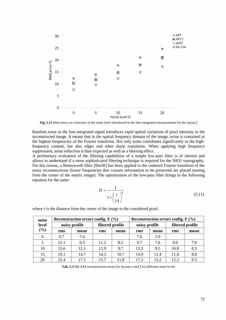
72
Fig. 5.15 Rms errors as a function of the noise level introduced in the line-integrated measurements for the layout f
Random noise in the line-integrated signal introduces rapid spatial variations of pixel intensity in the
reconstructed image. It means that in the spatial frequency domain of the image, noise is contained at
the highest frequencies of the Fourier transform. Not only noise contributes significantly to the high-
frequency content, but also edges and other sharp transitions. When applying high frequency
suppression, noise reduction is then expected as well as a blurring effect.
A preliminary evaluation of the filtering capabilities of a simple low-pass filter is of interest and
allows to understand if a more sophisticated filtering technique is required for the NIO1 tomography.
For this reason, a Butterworth filter [But30] has been applied to the centered Fourier transform of the
noisy reconstructions (lower frequencies that contain information to be preserved are placed starting
from the center of the matrix image). The optimization of the low-pass filter brings to the following
equation for the same:
4
141
1
r
H (5.11)
where r is the distance from the center of the image to the considered pixel.
noise
level
(%)
Reconstruction errors config. E (%) Reconstruction errors config. F (%)
noisy profile filtered profile noisy profile filtered profile
rms mean rms mean rms mean rms mean
0 9.7 7.4
7.6 5.9
5 12.1 9.3 11.2 8.5 9.7 7.6 9.0 7.0
10 15.6 12.1 12.9 9.7 12.3 9.5 10.8 8.3
15 19.1 14.7 14.2 10.7 14.9 11.4 11.4 8.8
20 22.4 17.1 15.7 11.8 17.3 13.2 12.2 9.5
Tab. 5.3 ML-EM reconstruction errors for layouts e and f for different noise levels
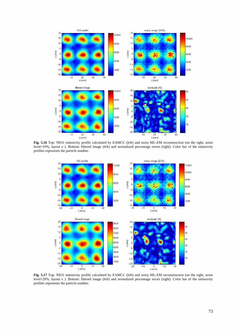
73
Fig. 5.16 Top: NIO1 emissivity profile calculated by EAMCC (left) and noisy ML-EM reconstruction (on the right, noise
level=10%, layout e ). Bottom: filtered image (left) and normalized percentage errors (right). Color bar of the emissivity
profiles represents the particle number.
Fig. 5.17 Top: NIO1 emissivity profile calculated by EAMCC (left) and noisy ML-EM reconstruction (on the right, noise
level=20%, layout e ). Bottom: filtered image (left) and normalized percentage errors (right). Color bar of the emissivity
profiles represents the particle number.
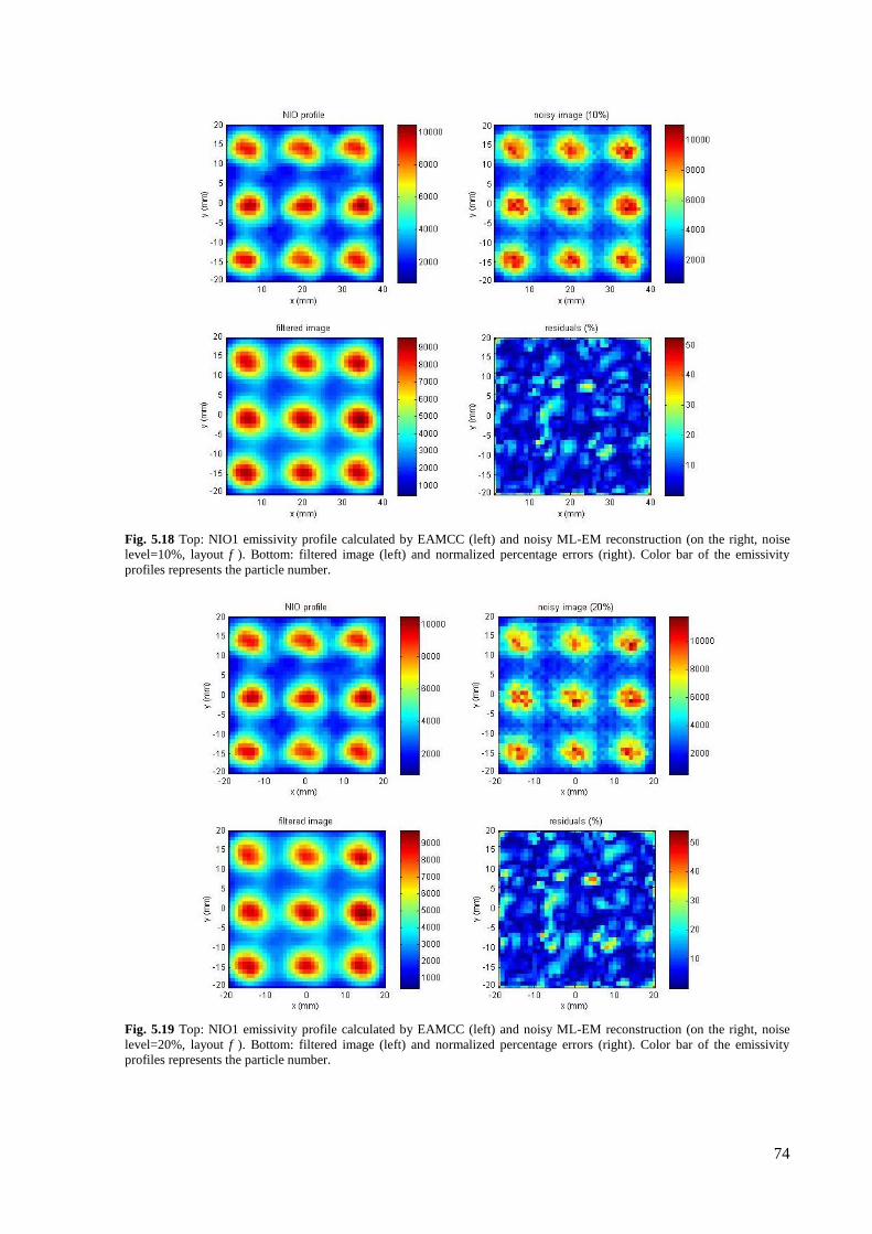
74
Fig. 5.18 Top: NIO1 emissivity profile calculated by EAMCC (left) and noisy ML-EM reconstruction (on the right, noise
level=10%, layout f ). Bottom: filtered image (left) and normalized percentage errors (right). Color bar of the emissivity
profiles represents the particle number.
Fig. 5.19 Top: NIO1 emissivity profile calculated by EAMCC (left) and noisy ML-EM reconstruction (on the right, noise
level=20%, layout f ). Bottom: filtered image (left) and normalized percentage errors (right). Color bar of the emissivity
profiles represents the particle number.
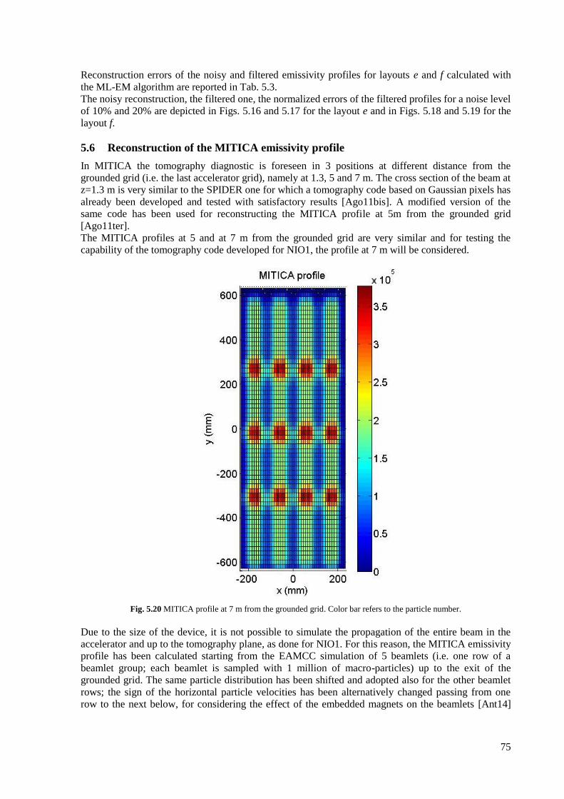
75
Reconstruction errors of the noisy and filtered emissivity profiles for layouts e and f calculated with
the ML-EM algorithm are reported in Tab. 5.3.
The noisy reconstruction, the filtered one, the normalized errors of the filtered profiles for a noise level
of 10% and 20% are depicted in Figs. 5.16 and 5.17 for the layout e and in Figs. 5.18 and 5.19 for the
layout f.
5.6 Reconstruction of the MITICA emissivity profile
In MITICA the tomography diagnostic is foreseen in 3 positions at different distance from the
grounded grid (i.e. the last accelerator grid), namely at 1.3, 5 and 7 m. The cross section of the beam at
z=1.3 m is very similar to the SPIDER one for which a tomography code based on Gaussian pixels has
already been developed and tested with satisfactory results [Ago11bis]. A modified version of the
same code has been used for reconstructing the MITICA profile at 5m from the grounded grid
[Ago11ter].
The MITICA profiles at 5 and at 7 m from the grounded grid are very similar and for testing the
capability of the tomography code developed for NIO1, the profile at 7 m will be considered.
Fig. 5.20 MITICA profile at 7 m from the grounded grid. Color bar refers to the particle number.
Due to the size of the device, it is not possible to simulate the propagation of the entire beam in the
accelerator and up to the tomography plane, as done for NIO1. For this reason, the MITICA emissivity
profile has been calculated starting from the EAMCC simulation of 5 beamlets (i.e. one row of a
beamlet group; each beamlet is sampled with 1 million of macro-particles) up to the exit of the
grounded grid. The same particle distribution has been shifted and adopted also for the other beamlet
rows; the sign of the horizontal particle velocities has been alternatively changed passing from one
row to the next below, for considering the effect of the embedded magnets on the beamlets [Ant14]
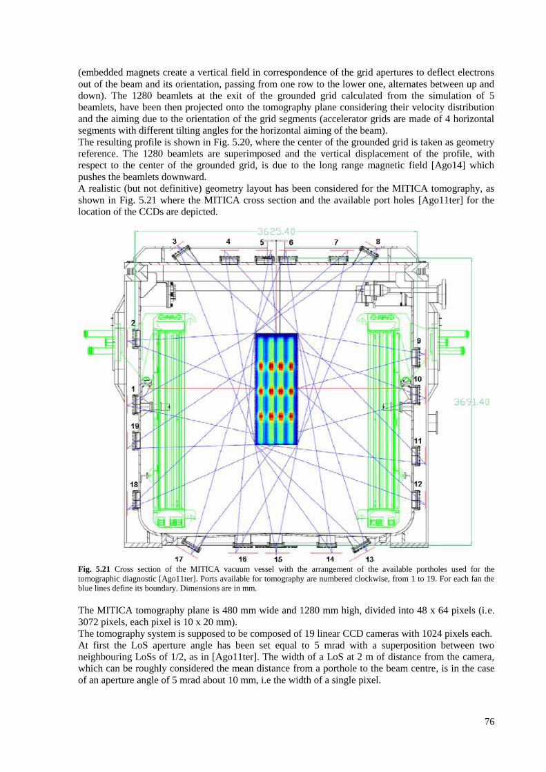
76
(embedded magnets create a vertical field in correspondence of the grid apertures to deflect electrons
out of the beam and its orientation, passing from one row to the lower one, alternates between up and
down). The 1280 beamlets at the exit of the grounded grid calculated from the simulation of 5
beamlets, have been then projected onto the tomography plane considering their velocity distribution
and the aiming due to the orientation of the grid segments (accelerator grids are made of 4 horizontal
segments with different tilting angles for the horizontal aiming of the beam).
The resulting profile is shown in Fig. 5.20, where the center of the grounded grid is taken as geometry
reference. The 1280 beamlets are superimposed and the vertical displacement of the profile, with
respect to the center of the grounded grid, is due to the long range magnetic field [Ago14] which
pushes the beamlets downward.
A realistic (but not definitive) geometry layout has been considered for the MITICA tomography, as
shown in Fig. 5.21 where the MITICA cross section and the available port holes [Ago11ter] for the
location of the CCDs are depicted.
Fig. 5.21 Cross section of the MITICA vacuum vessel with the arrangement of the available portholes used for the
tomographic diagnostic [Ago11ter]. Ports available for tomography are numbered clockwise, from 1 to 19. For each fan the
blue lines define its boundary. Dimensions are in mm.
The MITICA tomography plane is 480 mm wide and 1280 mm high, divided into 48 x 64 pixels (i.e.
3072 pixels, each pixel is 10 x 20 mm).
The tomography system is supposed to be composed of 19 linear CCD cameras with 1024 pixels each.
At first the LoS aperture angle has been set equal to 5 mrad with a superposition between two
neighbouring LoSs of 1/2, as in [Ago11ter]. The width of a LoS at 2 m of distance from the camera,
which can be roughly considered the mean distance from a porthole to the beam centre, is in the case
of an aperture angle of 5 mrad about 10 mm, i.e the width of a single pixel.
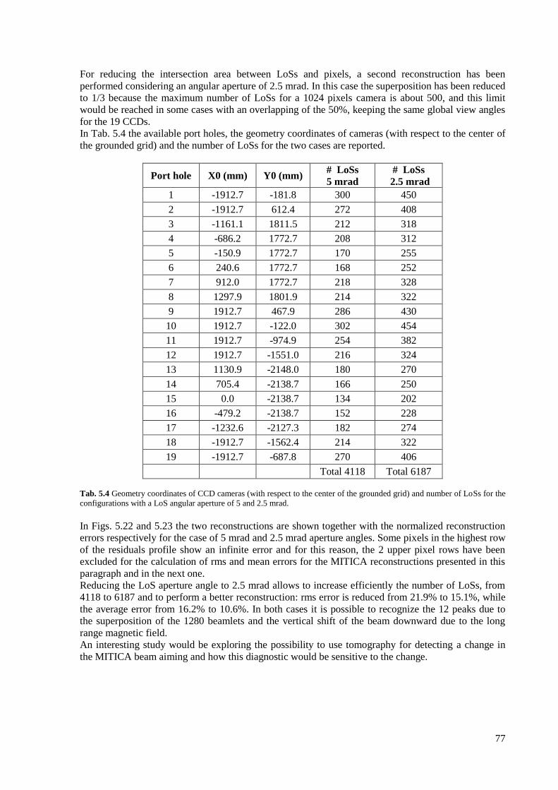
77
For reducing the intersection area between LoSs and pixels, a second reconstruction has been
performed considering an angular aperture of 2.5 mrad. In this case the superposition has been reduced
to 1/3 because the maximum number of LoSs for a 1024 pixels camera is about 500, and this limit
would be reached in some cases with an overlapping of the 50%, keeping the same global view angles
for the 19 CCDs.
In Tab. 5.4 the available port holes, the geometry coordinates of cameras (with respect to the center of
the grounded grid) and the number of LoSs for the two cases are reported.
Port hole X0 (mm) Y0 (mm) # LoSs
5 mrad
# LoSs
2.5 mrad
1 -1912.7 -181.8 300 450
2 -1912.7 612.4 272 408
3 -1161.1 1811.5 212 318
4 -686.2 1772.7 208 312
5 -150.9 1772.7 170 255
6 240.6 1772.7 168 252
7 912.0 1772.7 218 328
8 1297.9 1801.9 214 322
9 1912.7 467.9 286 430
10 1912.7 -122.0 302 454
11 1912.7 -974.9 254 382
12 1912.7 -1551.0 216 324
13 1130.9 -2148.0 180 270
14 705.4 -2138.7 166 250
15 0.0 -2138.7 134 202
16 -479.2 -2138.7 152 228
17 -1232.6 -2127.3 182 274
18 -1912.7 -1562.4 214 322
19 -1912.7 -687.8 270 406
Total 4118 Total 6187
Tab. 5.4 Geometry coordinates of CCD cameras (with respect to the center of the grounded grid) and number of LoSs for the
configurations with a LoS angular aperture of 5 and 2.5 mrad.
In Figs. 5.22 and 5.23 the two reconstructions are shown together with the normalized reconstruction
errors respectively for the case of 5 mrad and 2.5 mrad aperture angles. Some pixels in the highest row
of the residuals profile show an infinite error and for this reason, the 2 upper pixel rows have been
excluded for the calculation of rms and mean errors for the MITICA reconstructions presented in this
paragraph and in the next one.
Reducing the LoS aperture angle to 2.5 mrad allows to increase efficiently the number of LoSs, from
4118 to 6187 and to perform a better reconstruction: rms error is reduced from 21.9% to 15.1%, while
the average error from 16.2% to 10.6%. In both cases it is possible to recognize the 12 peaks due to
the superposition of the 1280 beamlets and the vertical shift of the beam downward due to the long
range magnetic field.
An interesting study would be exploring the possibility to use tomography for detecting a change in
the MITICA beam aiming and how this diagnostic would be sensitive to the change.
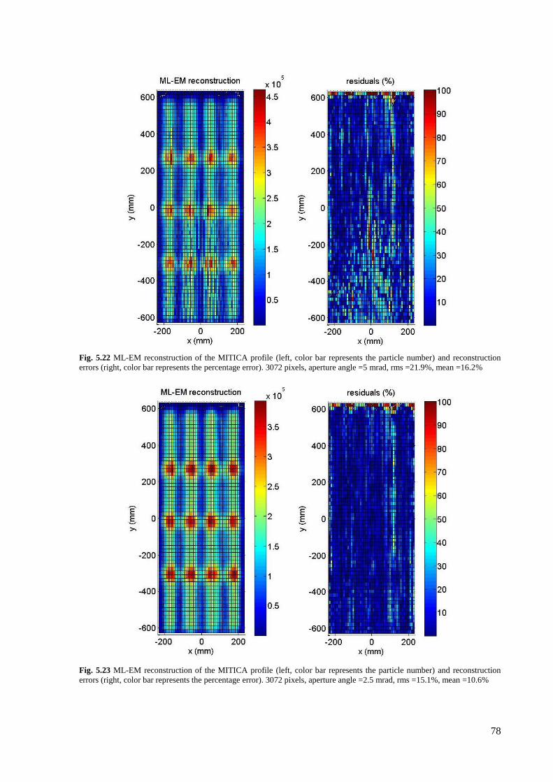
78
Fig. 5.22 ML-EM reconstruction of the MITICA profile (left, color bar represents the particle number) and reconstruction
errors (right, color bar represents the percentage error). 3072 pixels, aperture angle =5 mrad, rms =21.9%, mean =16.2%
Fig. 5.23 ML-EM reconstruction of the MITICA profile (left, color bar represents the particle number) and reconstruction
errors (right, color bar represents the percentage error). 3072 pixels, aperture angle =2.5 mrad, rms =15.1%, mean =10.6%
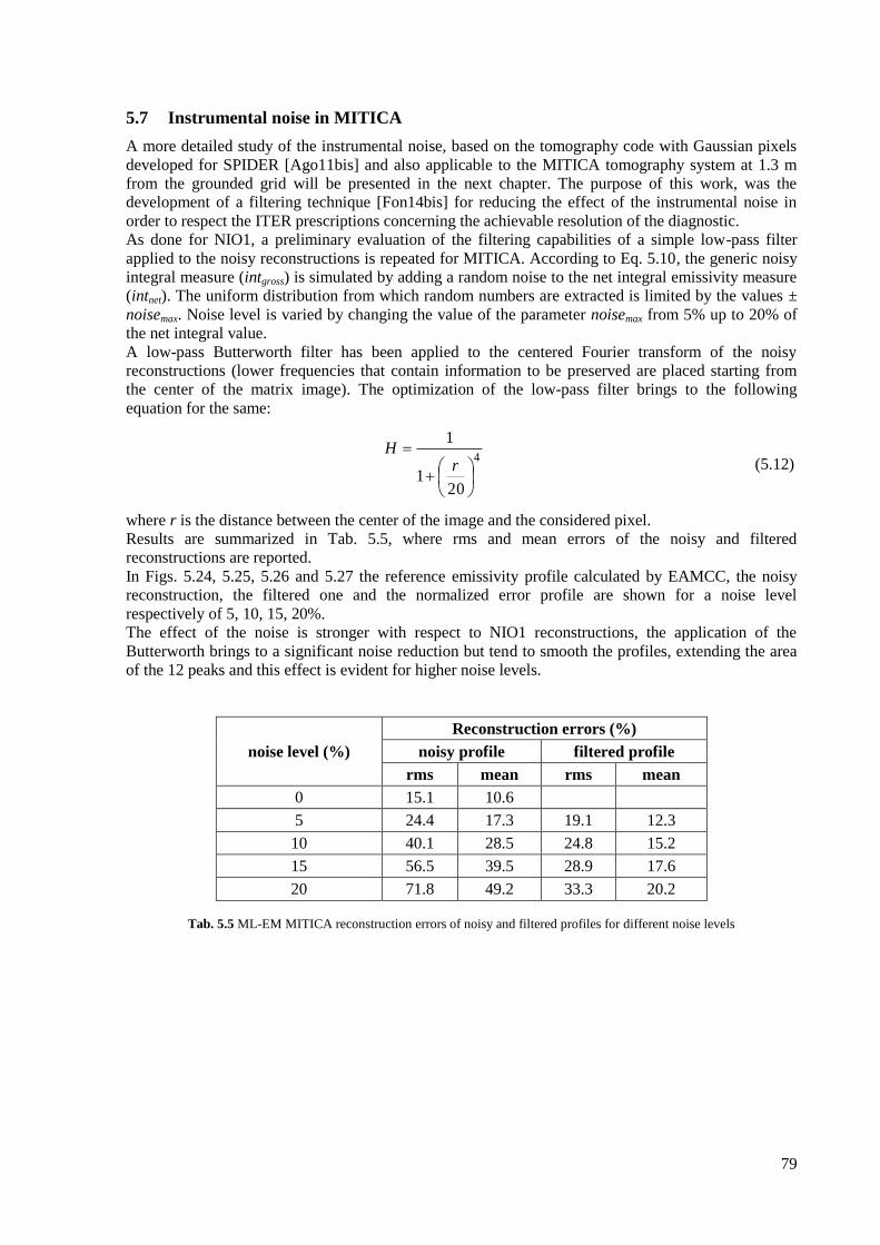
79
5.7 Instrumental noise in MITICA
A more detailed study of the instrumental noise, based on the tomography code with Gaussian pixels
developed for SPIDER [Ago11bis] and also applicable to the MITICA tomography system at 1.3 m
from the grounded grid will be presented in the next chapter. The purpose of this work, was the
development of a filtering technique [Fon14bis] for reducing the effect of the instrumental noise in
order to respect the ITER prescriptions concerning the achievable resolution of the diagnostic.
As done for NIO1, a preliminary evaluation of the filtering capabilities of a simple low-pass filter
applied to the noisy reconstructions is repeated for MITICA. According to Eq. 5.10, the generic noisy
integral measure (intgross) is simulated by adding a random noise to the net integral emissivity measure
(intnet). The uniform distribution from which random numbers are extracted is limited by the values ±
noisemax. Noise level is varied by changing the value of the parameter noisemax from 5% up to 20% of
the net integral value.
A low-pass Butterworth filter has been applied to the centered Fourier transform of the noisy
reconstructions (lower frequencies that contain information to be preserved are placed starting from
the center of the matrix image). The optimization of the low-pass filter brings to the following
equation for the same:
4
201
1
r
H (5.12)
where r is the distance between the center of the image and the considered pixel.
Results are summarized in Tab. 5.5, where rms and mean errors of the noisy and filtered
reconstructions are reported.
In Figs. 5.24, 5.25, 5.26 and 5.27 the reference emissivity profile calculated by EAMCC, the noisy
reconstruction, the filtered one and the normalized error profile are shown for a noise level
respectively of 5, 10, 15, 20%.
The effect of the noise is stronger with respect to NIO1 reconstructions, the application of the
Butterworth brings to a significant noise reduction but tend to smooth the profiles, extending the area
of the 12 peaks and this effect is evident for higher noise levels.
noise level (%)
Reconstruction errors (%)
noisy profile filtered profile
rms mean rms mean
0 15.1 10.6
5 24.4 17.3 19.1 12.3
10 40.1 28.5 24.8 15.2
15 56.5 39.5 28.9 17.6
20 71.8 49.2 33.3 20.2
Tab. 5.5 ML-EM MITICA reconstruction errors of noisy and filtered profiles for different noise levels
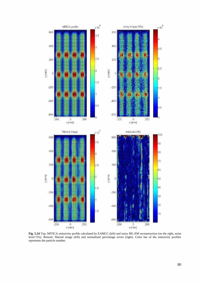
80
Fig. 5.24 Top: MITICA emissivity profile calculated by EAMCC (left) and noisy ML-EM reconstruction (on the right, noise
level=5%). Bottom: filtered image (left) and normalized percentage errors (right). Color bar of the emissivity profiles
represents the particle number.
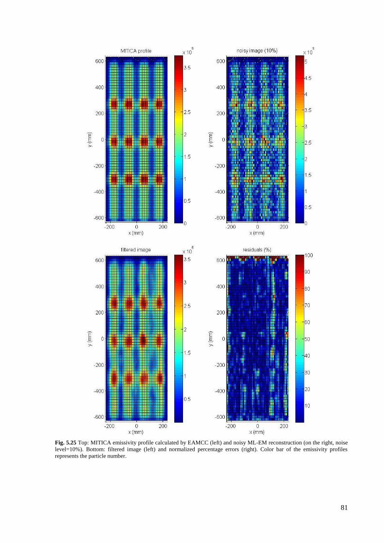
81
Fig. 5.25 Top: MITICA emissivity profile calculated by EAMCC (left) and noisy ML-EM reconstruction (on the right, noise
level=10%). Bottom: filtered image (left) and normalized percentage errors (right). Color bar of the emissivity profiles
represents the particle number.
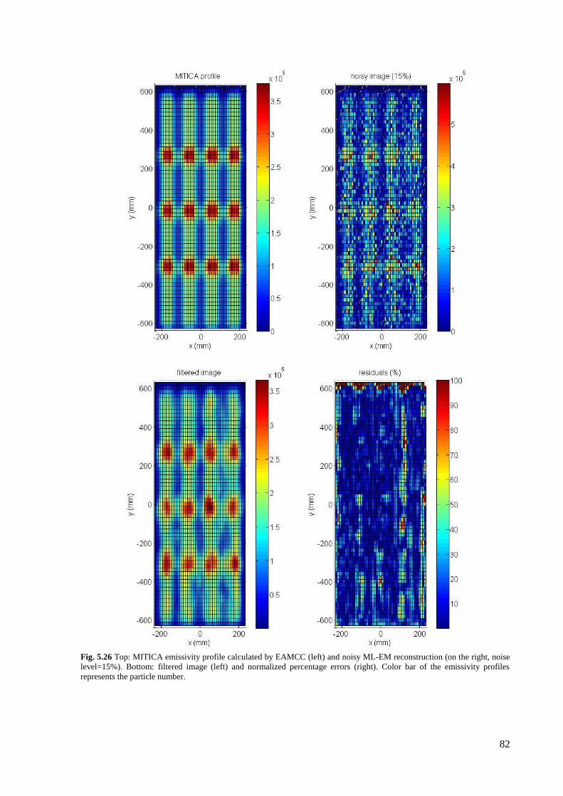
82
Fig. 5.26 Top: MITICA emissivity profile calculated by EAMCC (left) and noisy ML-EM reconstruction (on the right, noise
level=15%). Bottom: filtered image (left) and normalized percentage errors (right). Color bar of the emissivity profiles
represents the particle number.
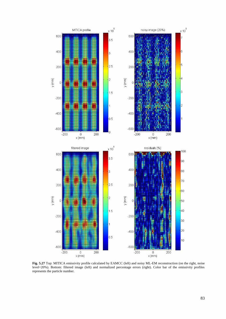
83
Fig. 5.27 Top: MITICA emissivity profile calculated by EAMCC (left) and noisy ML-EM reconstruction (on the right, noise
level=20%). Bottom: filtered image (left) and normalized percentage errors (right). Color bar of the emissivity profiles
represents the particle number.
84
5.8 Conclusions and future works
A multi-formula tomography code, based on iterative reconstruction algorithms has been developed
for NIO1 and the first results obtained are described in this chapter. Considering a reasonable
compromise between the cost of the tomography system for NIO1 (strongly influenced by the number
of cameras) and the quality of tomography reconstructions, the limited view of the beam due to the
available diagnostic ports, different geometry configurations have been analyzed.
According to the simulations, the most simple system made of 2 CCD cameras, allow to reconstruct a
1600 pixels emissivity profile with an rms error of 21.1% and a mean error of 15.3%. Considering the
number of pixels and the number of lines-of-sight (240), the inversion is a limited-data problem and
results obtained with the ML-EM technique are significant. A more complex system with 6 CCDs
allow to reduce the reconstruction errors down to 10% and represents a good compromise between
complexity and quality of reconstructions.
Some a-priori knowledge would allow to reduce the reconstruction errors and it will be considered in
the future, keeping in mind that also a limit in the detection capabilities would be introduced.
For what concerns the instrumental noise, a more detailed study is required, in particular the
experimental evaluation of the noise model and its intensity. If the experimental noise level is lower
than 10% a simple low-pass filter could be sufficient, otherwise a more sophisticated filtering
technique should be considered.
The tomography code has been also applied to the MITICA profiles, 3072 pixels reconstructions have
been obtained. Reducing the aperture angle from 5 to 2.5 mrad, a significant improvement in the
reconstruction quality is obtained. Reconstructions clearly show the right position of the 12 peaks due
to the superposition of the 1280 beamlets and also the vertical displacement downward due to the
applied magnetic field. The instrumental noise has, in the case of MITICA, a stronger effect, but
before considering a proper image filtering, an experimental measurement of the noise level is
necessary. The application of this code to the MITICA tomography system, despite a dedicated code
already exists, could be of interest and complementary, due to the peculiarity of not being based on
any hypothesis concerning the beam characteristics.
85
Chapter 6
An Image Filtering Technique for SPIDER Visible Tomography
The tomographic diagnostic developed for the beam generated in the SPIDER facility (100 keV, 50 A
prototype negative ion source of ITER neutral beam injector, described in Chapter 1) will
characterize the two-dimensional particle density distribution of the beam. The request for the beam is
that the maximum acceptable deviation from uniformity is ±10%, thus the deviation of the
tomographic reconstruction from the real emissivity of the beam has to be sufficiently lower than this
value.
In this chapter the role of the instrumental noise in the reconstruction capability of the tomography
code developed for SPIDER [Ago11bis] is studied. It was found that the noise has a large influence on
the maximum achievable resolution of the diagnostic and in order to reduce its impact different
filtering techniques have been considered both in the frequency and in the spatial domain. In
particular, a technique developed for radar imaging and based on a local statistics method [Lee86]
has been adapted and implemented in the SPIDER tomography code. It is able to reduce significantly
the reconstruction errors in different operating conditions of SPIDER and demonstrates the feasibility
to filter out the effect of the noise by post-processing the reconstructed image of the beam.
6.1 Introduction
SPIDER is a lower energy prototype negative ion source for the ITER neutral beam injector, aimed at
demonstrating the capability to create and extract a current of 100 kV D- (H
-) ions up to 50 A (60 A).
The ions are extracted over a wide surface (1.52 x 0.56 m2) with a prescribed uniformity of ± 10%.
The main aim of the SPIDER tomography diagnostic will be measuring the uniformity of the beam: in
particular the request for the beam is that the maximum acceptable deviation from uniformity is ±
10%, thus the deviation of the tomographic reconstruction from the real emissivity of the beam has to
be sufficiently lower than this value. Moreover, a complete reconstruction of the beam emissivity in
two dimensions obtained with the proposed tomography can go beyond the simple detection of the
lack of uniformity of the beam, giving information about its causes and suggesting possible solutions.
A tomographic algorithm based on the simultaneous algebraic reconstruction technique (SART,
described in the previous chapter) has already been developed and tested with satisfactory results
[Ago11bis].
In the real tomography system, the role of the instrumental noise introduced in the line integrated
signals must be taken into account. This is included in the simulations and it is shown to affect the
accuracy of the reconstructed profile, imposing a limit on the maximum acceptable noise level. In
order to reduce the effect of experimental noise and keep the deviation between the real and the
reconstructed beam profiles lower than the prescribed value, it is necessary to introduce a digital
filtering technique in the algorithm.
6.2 Emissivity profiles of the SPIDER beam
The SPIDER beam is simulated with 1280 beamlets whose emissivity has a Gaussian shape, arranged
into 16 rectangular shaped beamlet groups, as described in [Pas11] and in [Ago11bis]. In the same
references also the tomographic inversion technique is discussed.
The reconstructed beam profile is composed of Gaussian pixels of equal size. The 2D emissivity
profiles (phantoms) which reproduce different possible experimental beam configurations and have to
be reconstructed are described below and identified by a number.
The phantom 1, shown in Fig. 6.1, represents a realistic linear non uniformity, simulated by linearly
varying the amplitude of each beamlet both in horizontal (x) and vertical (y) directions.
In this phantom, the amplitude of the 1280 Gaussian beamlets (the beamlet width is σxg= σyg= 3mm)
is defined as:
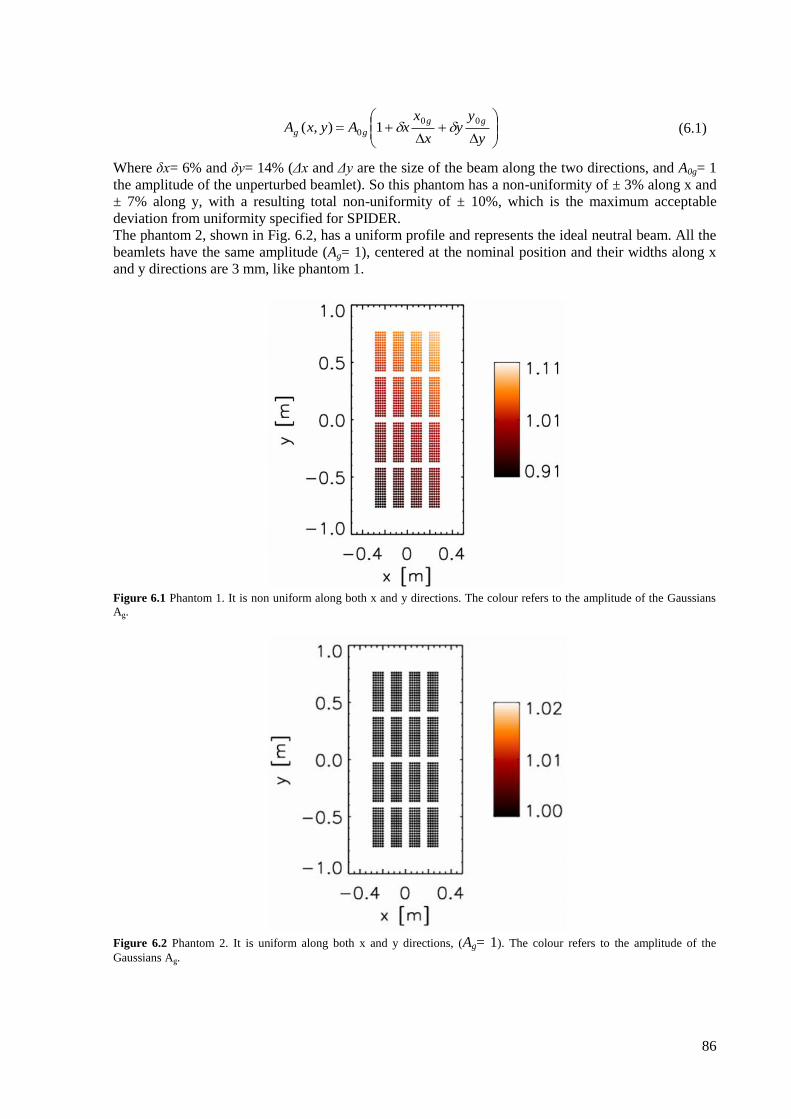
86
y
yy
x
xxAyxA
gg
gg
00
0 1),(
(6.1)
Where δx= 6% and δy= 14% (Δx and Δy are the size of the beam along the two directions, and A0g= 1
the amplitude of the unperturbed beamlet). So this phantom has a non-uniformity of ± 3% along x and
± 7% along y, with a resulting total non-uniformity of ± 10%, which is the maximum acceptable
deviation from uniformity specified for SPIDER.
The phantom 2, shown in Fig. 6.2, has a uniform profile and represents the ideal neutral beam. All the
beamlets have the same amplitude (Ag= 1), centered at the nominal position and their widths along x
and y directions are 3 mm, like phantom 1.
Figure 6.1 Phantom 1. It is non uniform along both x and y directions. The colour refers to the amplitude of the Gaussians
Ag.
Figure 6.2 Phantom 2. It is uniform along both x and y directions, (Ag= 1). The colour refers to the amplitude of the
Gaussians Ag.
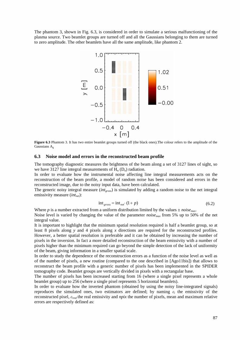
87
The phantom 3, shown in Fig. 6.3, is considered in order to simulate a serious malfunctioning of the
plasma source. Two beamlet groups are turned off and all the Gaussians belonging to them are turned
to zero amplitude. The other beamlets have all the same amplitude, like phantom 2.
Figure 6.3 Phantom 3. It has two entire beamlet groups turned off (the black ones).The colour refers to the amplitude of the
Gaussians Ag
6.3 Noise model and errors in the reconstructed beam profile
The tomography diagnostic measures the brightness of the beam along a set of 3127 lines of sight, so
we have 3127 line integral measurements of Hα (Dα) radiation.
In order to evaluate how the instrumental noise affecting line integral measurements acts on the
reconstruction of the beam profile, a model of random noise has been considered and errors in the
reconstructed image, due to the noisy input data, have been calculated.
The generic noisy integral measure (intgross) is simulated by adding a random noise to the net integral
emissivity measure (intnet):
)1(intint pnetgross
(6.2)
Where p is a number extracted from a uniform distribution limited by the values ± noisemax.
Noise level is varied by changing the value of the parameter noisemax from 5% up to 50% of the net
integral value.
It is important to highlight that the minimum spatial resolution required is half a beamlet group, so at
least 8 pixels along y and 4 pixels along x directions are required for the reconstructed profiles.
However, a better spatial resolution is preferable and it can be obtained by increasing the number of
pixels in the inversion. In fact a more detailed reconstruction of the beam emissivity with a number of
pixels higher than the minimum required can go beyond the simple detection of the lack of uniformity
of the beam, giving information in a smaller spatial scale.
In order to study the dependence of the reconstruction errors as a function of the noise level as well as
of the number of pixels, a new routine (compared to the one described in [Ago11bis]) that allows to
reconstruct the beam profile with a generic number of pixels has been implemented in the SPIDER
tomography code. Beamlet groups are vertically divided in pixels with a rectangular base.
The number of pixels has been increased starting from 16 (where a single pixel represents a whole
beamlet group) up to 256 (where a single pixel represents 5 horizontal beamlets).
In order to evaluate how the inverted phantom (obtained by using the noisy line-integrated signals)
reproduces the simulated ones, two estimators are defined; by naming εi the emissivity of the
reconstructed pixel, εreal the real emissivity and npix the number of pixels, mean and maximum relative
errors are respectively defined as:
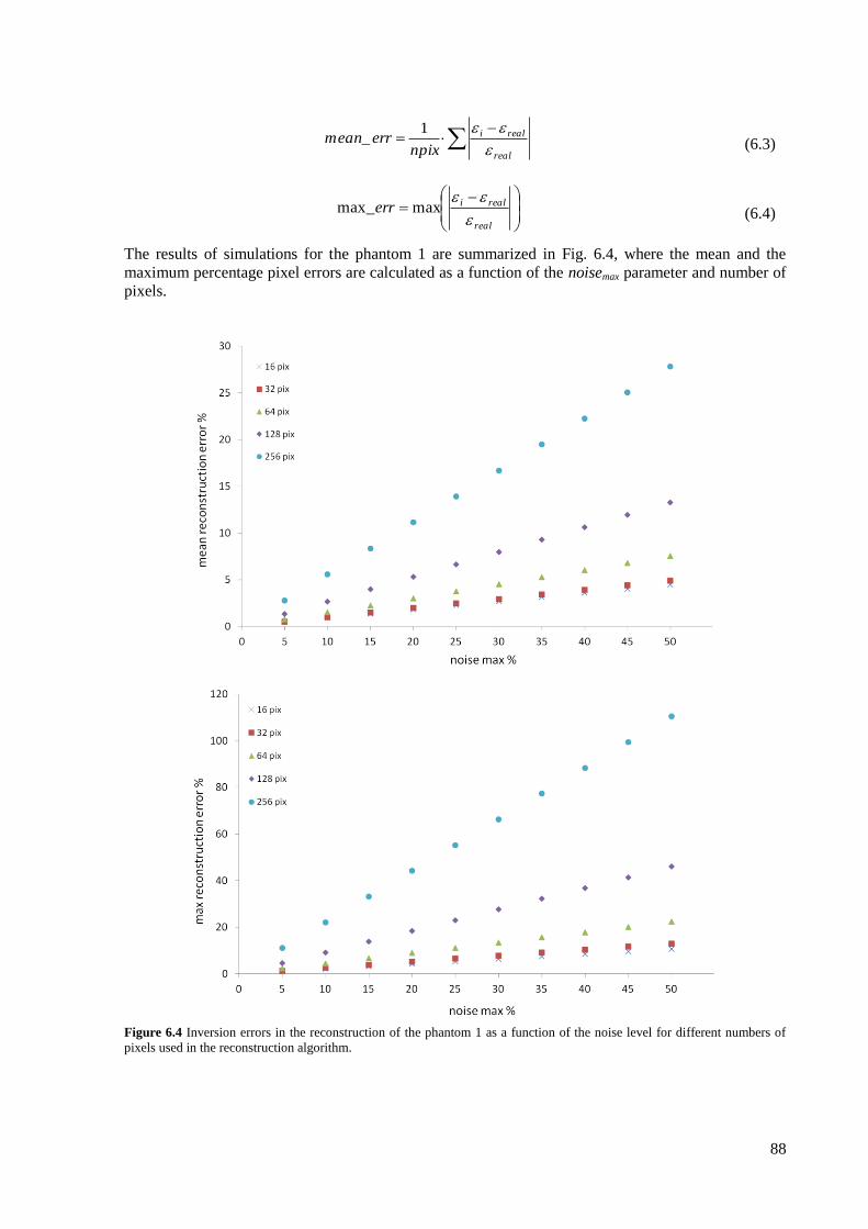
88
real
reali
npixerrmean
1_
(6.3)
real
realierr
maxmax_
(6.4)
The results of simulations for the phantom 1 are summarized in Fig. 6.4, where the mean and the
maximum percentage pixel errors are calculated as a function of the noisemax parameter and number of
pixels.
Figure 6.4 Inversion errors in the reconstruction of the phantom 1 as a function of the noise level for different numbers of
pixels used in the reconstruction algorithm.
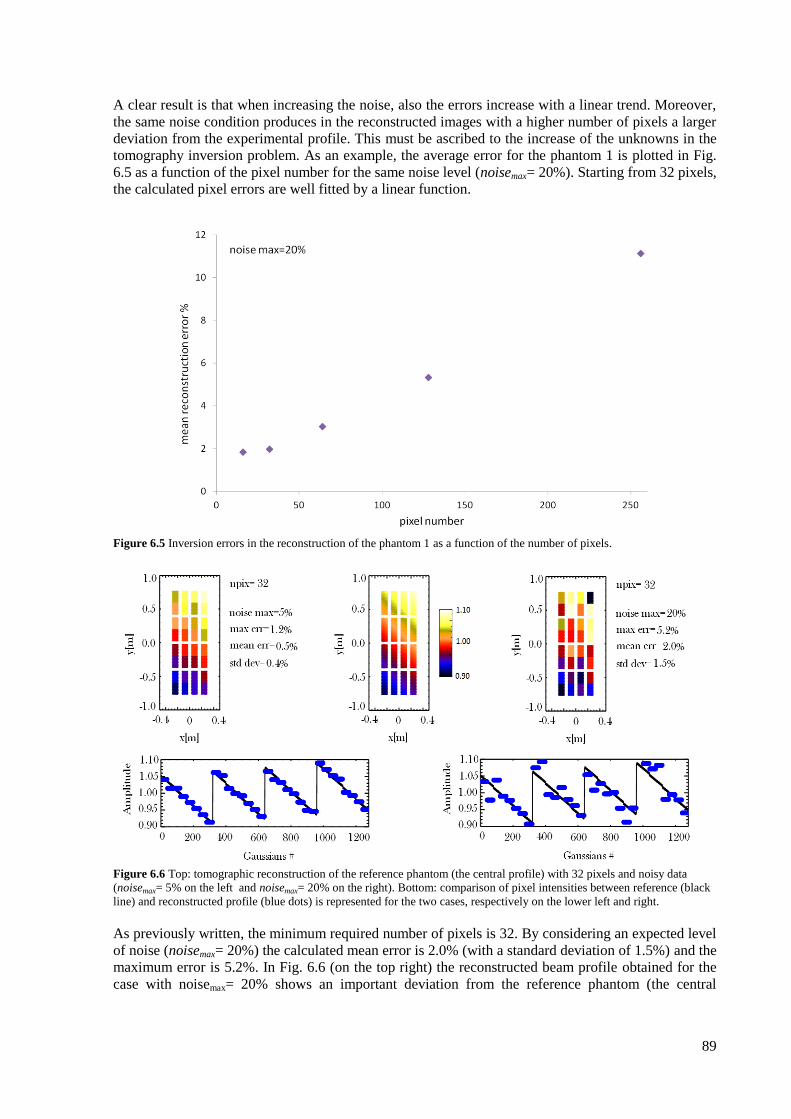
89
A clear result is that when increasing the noise, also the errors increase with a linear trend. Moreover,
the same noise condition produces in the reconstructed images with a higher number of pixels a larger
deviation from the experimental profile. This must be ascribed to the increase of the unknowns in the
tomography inversion problem. As an example, the average error for the phantom 1 is plotted in Fig.
6.5 as a function of the pixel number for the same noise level (noisemax= 20%). Starting from 32 pixels,
the calculated pixel errors are well fitted by a linear function.
Figure 6.5 Inversion errors in the reconstruction of the phantom 1 as a function of the number of pixels.
Figure 6.6 Top: tomographic reconstruction of the reference phantom (the central profile) with 32 pixels and noisy data
(noisemax= 5% on the left and noisemax= 20% on the right). Bottom: comparison of pixel intensities between reference (black
line) and reconstructed profile (blue dots) is represented for the two cases, respectively on the lower left and right.
As previously written, the minimum required number of pixels is 32. By considering an expected level
of noise (noisemax= 20%) the calculated mean error is 2.0% (with a standard deviation of 1.5%) and the
maximum error is 5.2%. In Fig. 6.6 (on the top right) the reconstructed beam profile obtained for the
case with noisemax= 20% shows an important deviation from the reference phantom (the central
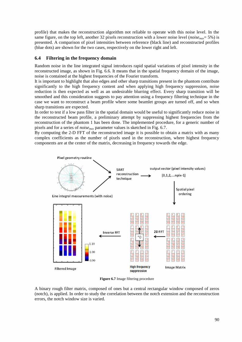
90
profile) that makes the reconstruction algorithm not reliable to operate with this noise level. In the
same figure, on the top left, another 32 pixels reconstruction with a lower noise level (noisemax= 5%) is
presented. A comparison of pixel intensities between reference (black line) and reconstructed profiles
(blue dots) are shown for the two cases, respectively on the lower right and left.
6.4 Filtering in the frequency domain
Random noise in the line integrated signal introduces rapid spatial variations of pixel intensity in the
reconstructed image, as shown in Fig. 6.6. It means that in the spatial frequency domain of the image,
noise is contained at the highest frequencies of the Fourier transform.
It is important to highlight that also edges and other sharp transitions present in the phantom contribute
significantly to the high frequency content and when applying high frequency suppression, noise
reduction is then expected as well as an undesirable blurring effect. Every sharp transition will be
smoothed and this consideration suggests to pay attention using a frequency filtering technique in the
case we want to reconstruct a beam profile where some beamlet groups are turned off, and so when
sharp transitions are expected.
In order to test if a low pass filter in the spatial domain would be useful to significantly reduce noise in
the reconstructed beam profile, a preliminary attempt by suppressing highest frequencies from the
reconstruction of the phantom 1 has been done. The implemented procedure, for a generic number of
pixels and for a series of noisemax parameter values is sketched in Fig. 6.7.
By computing the 2-D FFT of the reconstructed image it is possible to obtain a matrix with as many
complex coefficients as the number of pixels used in the reconstruction, where highest frequency
components are at the center of the matrix, decreasing in frequency towards the edge.
Figure 6.7 Image filtering procedure
A binary rough filter matrix, composed of ones but a central rectangular window composed of zeros
(notch), is applied. In order to study the correlation between the notch extension and the reconstruction
errors, the notch window size is varied.
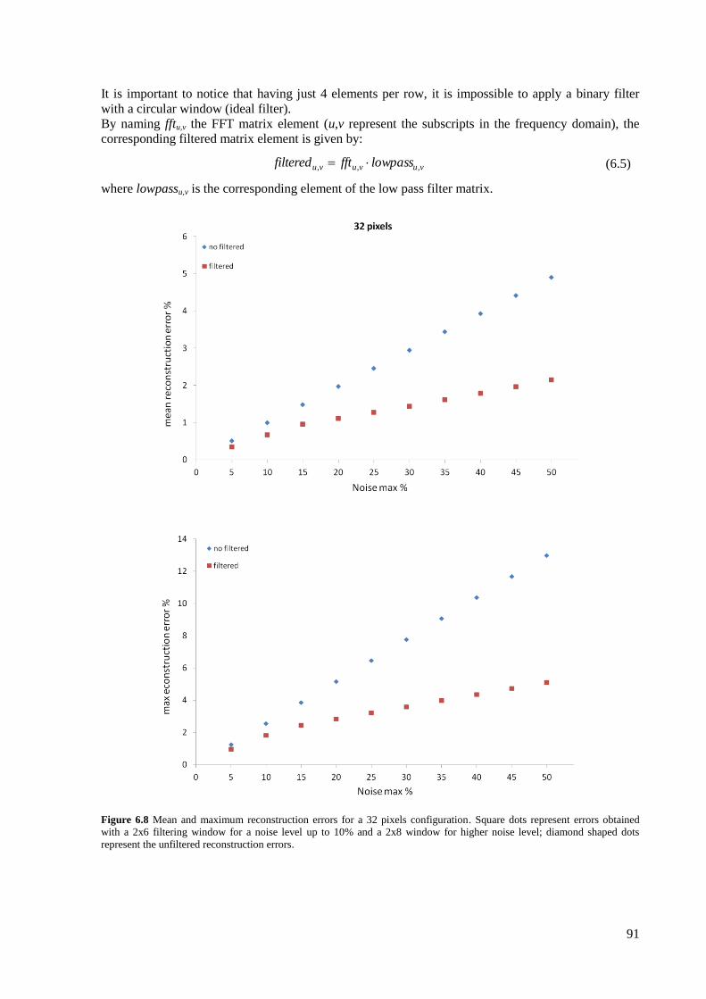
91
It is important to notice that having just 4 elements per row, it is impossible to apply a binary filter
with a circular window (ideal filter).
By naming fftu,v the FFT matrix element (u,v represent the subscripts in the frequency domain), the
corresponding filtered matrix element is given by:
vuvuvu lowpassfftfiltered ,,,
(6.5)
where lowpassu,v is the corresponding element of the low pass filter matrix.
Figure 6.8 Mean and maximum reconstruction errors for a 32 pixels configuration. Square dots represent errors obtained
with a 2x6 filtering window for a noise level up to 10% and a 2x8 window for higher noise level; diamond shaped dots
represent the unfiltered reconstruction errors.
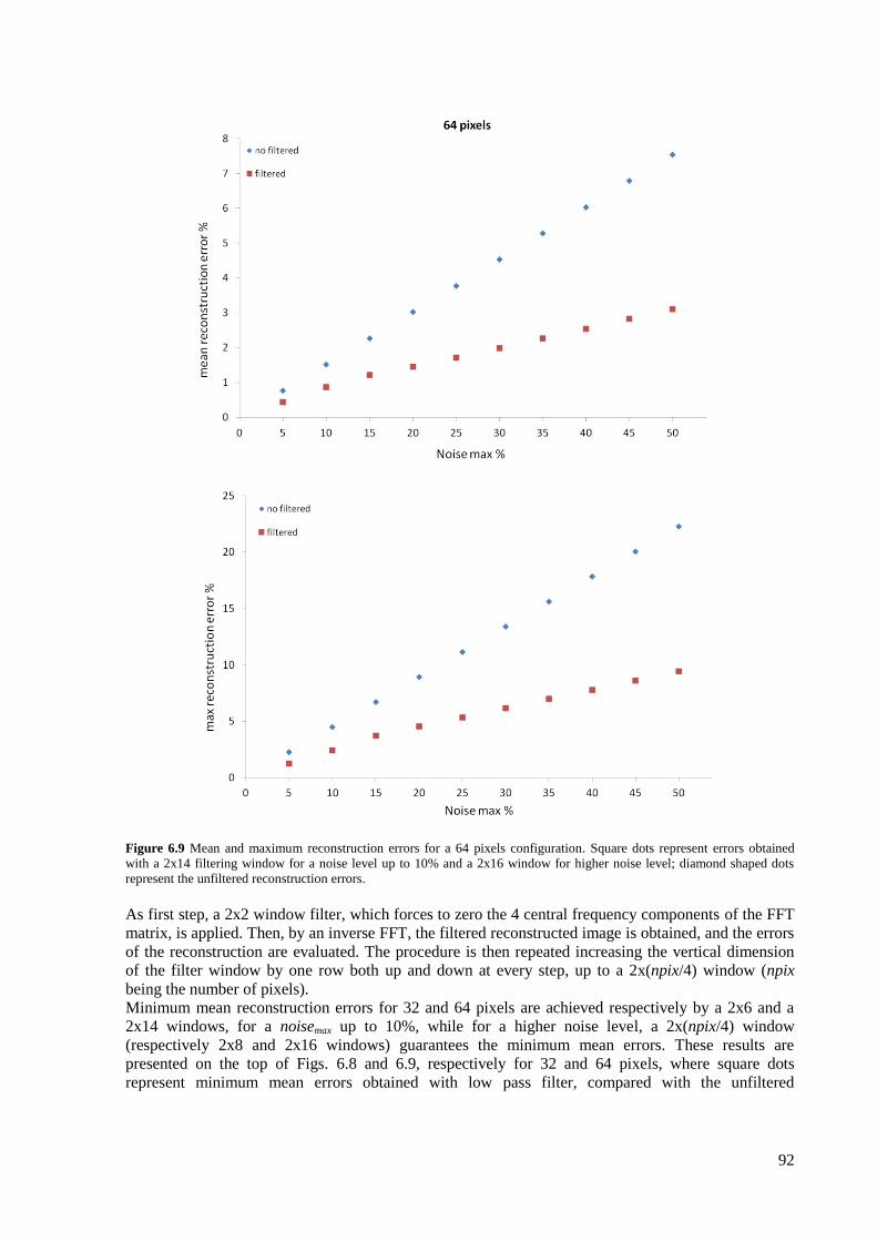
92
Figure 6.9 Mean and maximum reconstruction errors for a 64 pixels configuration. Square dots represent errors obtained
with a 2x14 filtering window for a noise level up to 10% and a 2x16 window for higher noise level; diamond shaped dots
represent the unfiltered reconstruction errors.
As first step, a 2x2 window filter, which forces to zero the 4 central frequency components of the FFT
matrix, is applied. Then, by an inverse FFT, the filtered reconstructed image is obtained, and the errors
of the reconstruction are evaluated. The procedure is then repeated increasing the vertical dimension
of the filter window by one row both up and down at every step, up to a 2x(npix/4) window (npix
being the number of pixels).
Minimum mean reconstruction errors for 32 and 64 pixels are achieved respectively by a 2x6 and a
2x14 windows, for a noisemax up to 10%, while for a higher noise level, a 2x(npix/4) window
(respectively 2x8 and 2x16 windows) guarantees the minimum mean errors. These results are
presented on the top of Figs. 6.8 and 6.9, respectively for 32 and 64 pixels, where square dots
represent minimum mean errors obtained with low pass filter, compared with the unfiltered
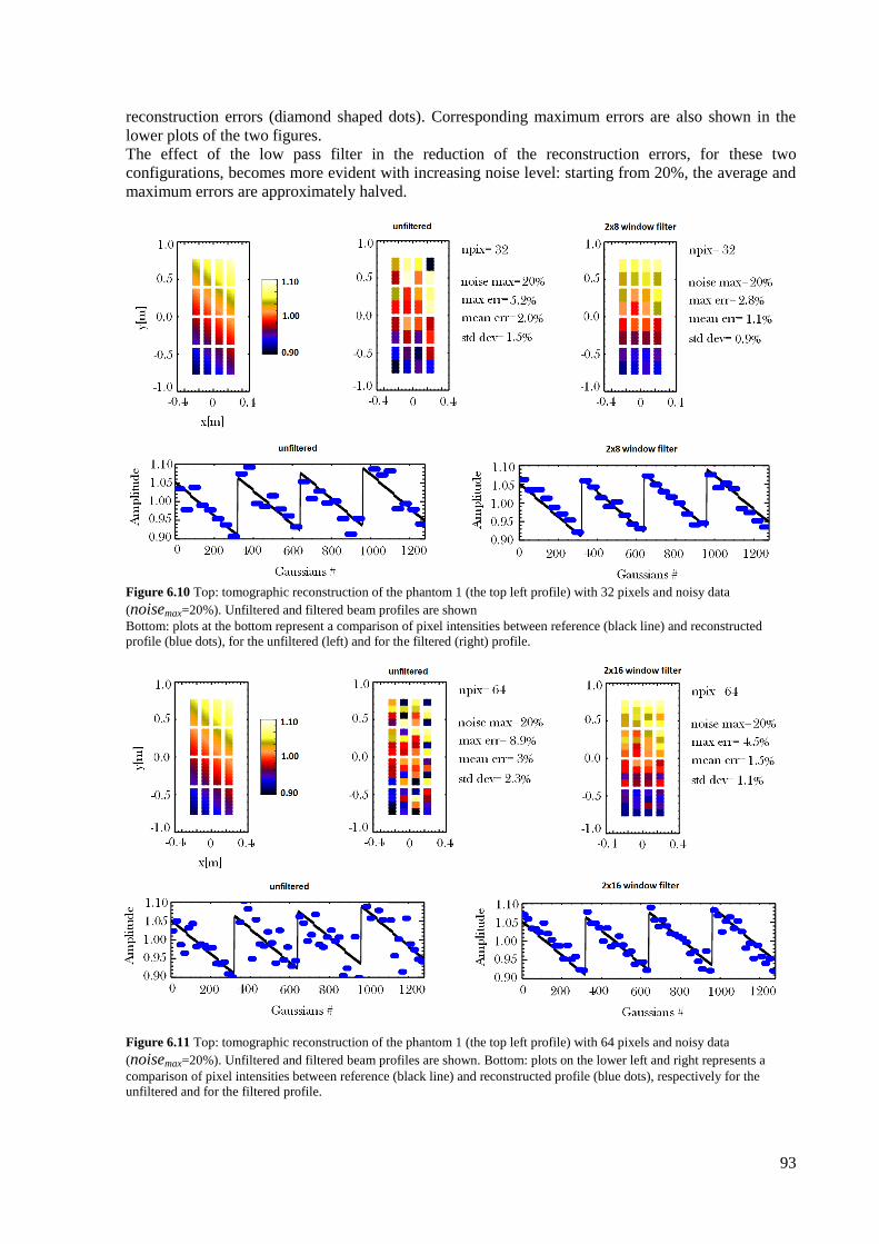
93
reconstruction errors (diamond shaped dots). Corresponding maximum errors are also shown in the
lower plots of the two figures.
The effect of the low pass filter in the reduction of the reconstruction errors, for these two
configurations, becomes more evident with increasing noise level: starting from 20%, the average and
maximum errors are approximately halved.
Figure 6.10 Top: tomographic reconstruction of the phantom 1 (the top left profile) with 32 pixels and noisy data
(noisemax=20%). Unfiltered and filtered beam profiles are shown
Bottom: plots at the bottom represent a comparison of pixel intensities between reference (black line) and reconstructed
profile (blue dots), for the unfiltered (left) and for the filtered (right) profile.
Figure 6.11 Top: tomographic reconstruction of the phantom 1 (the top left profile) with 64 pixels and noisy data
(noisemax=20%). Unfiltered and filtered beam profiles are shown. Bottom: plots on the lower left and right represents a
comparison of pixel intensities between reference (black line) and reconstructed profile (blue dots), respectively for the
unfiltered and for the filtered profile.
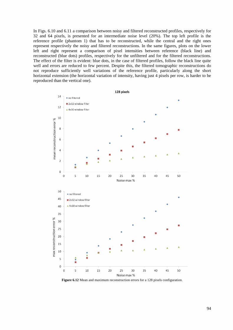
94
In Figs. 6.10 and 6.11 a comparison between noisy and filtered reconstructed profiles, respectively for
32 and 64 pixels, is presented for an intermediate noise level (20%). The top left profile is the
reference profile (phantom 1) that has to be reconstructed, while the central and the right ones
represent respectively the noisy and filtered reconstructions. In the same figures, plots on the lower
left and right represent a comparison of pixel intensities between reference (black line) and
reconstructed (blue dots) profiles, respectively for the unfiltered and for the filtered reconstructions.
The effect of the filter is evident: blue dots, in the case of filtered profiles, follow the black line quite
well and errors are reduced to few percent. Despite this, the filtered tomographic reconstructions do
not reproduce sufficiently well variations of the reference profile, particularly along the short
horizontal extension (the horizontal variation of intensity, having just 4 pixels per row, is harder to be
reproduced than the vertical one).
Figure 6.12 Mean and maximum reconstruction errors for a 128 pixels configuration.
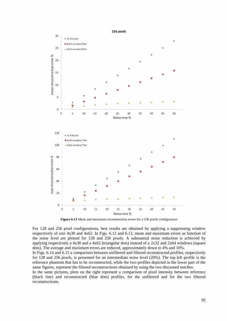
95
Figure 6.13 Mean and maximum reconstruction errors for a 256 pixels configuration
For 128 and 256 pixel configurations, best results are obtained by applying a suppressing window
respectively of size 4x30 and 4x62. In Figs. 6.12 and 6.13, mean and maximum errors as function of
the noise level are plotted for 128 and 256 pixels. A substantial noise reduction is achieved by
applying respectively a 4x30 and a 4x62 (triangular dots) instead of a 2x32 and 2x64 windows (square
dots). The average and maximum errors are reduced, approximately down to 4% and 10%.
In Figs. 6.14 and 6.15 a comparison between unfiltered and filtered reconstructed profiles, respectively
for 128 and 256 pixels, is presented for an intermediate noise level (20%). The top left profile is the
reference phantom that has to be reconstructed, while the two profiles depicted in the lower part of the
same figures, represent the filtered reconstructions obtained by using the two discussed notches.
In the same pictures, plots on the right represent a comparison of pixel intensity between reference
(black line) and reconstructed (blue dots) profiles, for the unfiltered and for the two filtered
reconstructions.
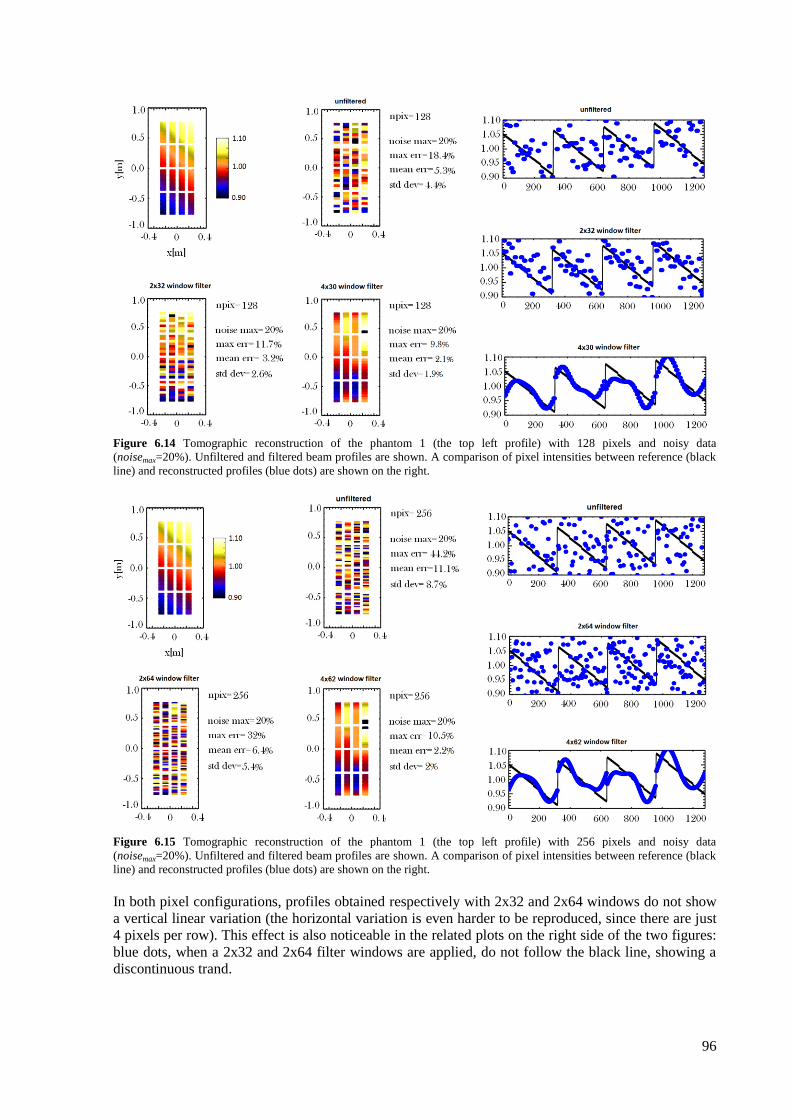
96
Figure 6.14 Tomographic reconstruction of the phantom 1 (the top left profile) with 128 pixels and noisy data
(noisemax=20%). Unfiltered and filtered beam profiles are shown. A comparison of pixel intensities between reference (black
line) and reconstructed profiles (blue dots) are shown on the right.
Figure 6.15 Tomographic reconstruction of the phantom 1 (the top left profile) with 256 pixels and noisy data
(noisemax=20%). Unfiltered and filtered beam profiles are shown. A comparison of pixel intensities between reference (black
line) and reconstructed profiles (blue dots) are shown on the right.
In both pixel configurations, profiles obtained respectively with 2x32 and 2x64 windows do not show
a vertical linear variation (the horizontal variation is even harder to be reproduced, since there are just
4 pixels per row). This effect is also noticeable in the related plots on the right side of the two figures:
blue dots, when a 2x32 and 2x64 filter windows are applied, do not follow the black line, showing a
discontinuous trand.
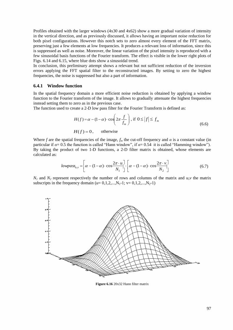
97
Profiles obtained with the larger windows (4x30 and 4x62) show a more gradual variation of intensity
in the vertical direction, and as previously discussed, it allows having an important noise reduction for
both pixel configurations. However this notch sets to zero almost every element of the FFT matrix,
preserving just a few elements at low frequencies. It produces a relevant loss of information, since this
is suppressed as well as noise. Moreover, the linear variation of the pixel intensity is reproduced with a
few sinusoidal basis functions of the Fourier transform. The effect is visible in the lower right plots of
Figs. 6.14 and 6.15, where blue dots show a sinusoidal trend.
In conclusion, this preliminary attempt shows a relevant but not sufficient reduction of the inversion
errors applying the FFT spatial filter to the reconstructed images. By setting to zero the highest
frequencies, the noise is suppressed but also a part of information.
6.4.1 Window function
In the spatial frequency domain a more efficient noise reduction is obtained by applying a window
function to the Fourier transform of the image. It allows to gradually attenuate the highest frequencies
instead setting them to zero as in the previous case.
The function used to create a 2-D low pass filter for the Fourier Transform is defined as:
mf
ffH 2cos)1()( , if mff 0
0)( fH , otherwise
(6.6)
Where f are the spatial frequencies of the image, fm the cut-off frequency and α is a constant value (in
particular if α= 0.5 the function is called “Hann window”, if α= 0.54 it is called “Hamming window”).
By taking the product of two 1-D functions, a 2-D filter matrix is obtained, whose elements are
calculated as:
21
,
2cos)1(
2cos)1(
N
v
N
ulowpass vu
(6.7)
N1 and N2 represent respectively the number of rows and columns of the matrix and u,v the matrix
subscripts in the frequency domain (u= 0,1,2,...,N1-1; v= 0,1,2,...,N2-1)
Figure 6.16 20x32 Hann filter matrix
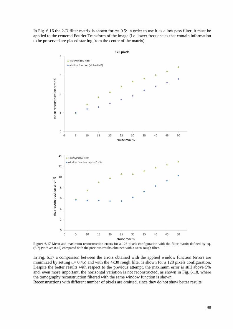
98
In Fig. 6.16 the 2-D filter matrix is shown for α= 0.5: in order to use it as a low pass filter, it must be
applied to the centered Fourier Transform of the image (i.e. lower frequencies that contain information
to be preserved are placed starting from the center of the matrix).
Figure 6.17 Mean and maximum reconstruction errors for a 128 pixels configuration with the filter matrix defined by eq.
(6.7) (with α= 0.45) compared with the previous results obtained with a 4x30 rough filter.
In Fig. 6.17 a comparison between the errors obtained with the applied window function (errors are
minimized by setting α= 0.45) and with the 4x30 rough filter is shown for a 128 pixels configuration.
Despite the better results with respect to the previous attempt, the maximum error is still above 5%
and, even more important, the horizontal variation is not reconstructed, as shown in Fig. 6.18, where
the tomography reconstruction filtered with the same window function is shown.
Reconstructions with different number of pixels are omitted, since they do not show better results.
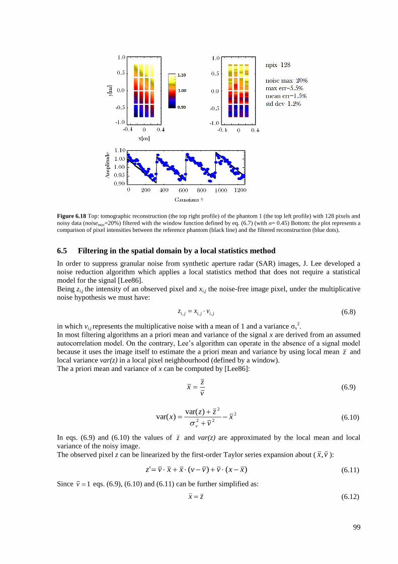
99
Figure 6.18 Top: tomographic reconstruction (the top right profile) of the phantom 1 (the top left profile) with 128 pixels and
noisy data (noisemax=20%) filtered with the window function defined by eq. (6.7) (with α= 0.45) Bottom: the plot represents a
comparison of pixel intensities between the reference phantom (black line) and the filtered reconstruction (blue dots).
6.5 Filtering in the spatial domain by a local statistics method
In order to suppress granular noise from synthetic aperture radar (SAR) images, J. Lee developed a
noise reduction algorithm which applies a local statistics method that does not require a statistical
model for the signal [Lee86].
Being zi,j the intensity of an observed pixel and xi,j the noise-free image pixel, under the multiplicative
noise hypothesis we must have:
jijiji vxz ,,,
(6.8)
in which vi,j represents the multiplicative noise with a mean of 1 and a variance σv2.
In most filtering algorithms an a priori mean and variance of the signal x are derived from an assumed
autocorrelation model. On the contrary, Lee’s algorithm can operate in the absence of a signal model
because it uses the image itself to estimate the a priori mean and variance by using local mean z and
local variance var(z) in a local pixel neighbourhood (defined by a window).
The a priori mean and variance of x can be computed by [Lee86]:
v
zx
(6.9)
2
22
2)var()var( x
v
zzx
v
(6.10)
In eqs. (6.9) and (6.10) the values of z and var(z) are approximated by the local mean and local
variance of the noisy image.
The observed pixel z can be linearized by the first-order Taylor series expansion about ( vx, ):
)()(' xxvvvxxvz
(6.11)
Since 1v eqs. (6.9), (6.10) and (6.11) can be further simplified as:
zx
(6.12)
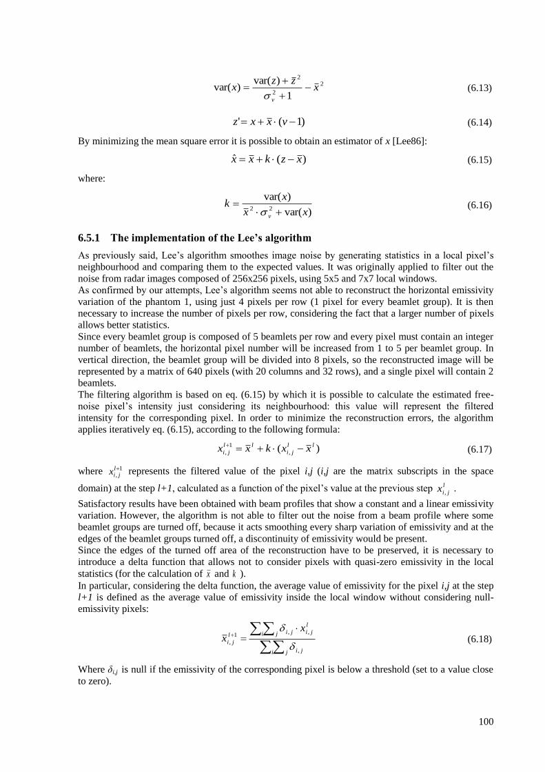
100
2
2
2
1
)var()var( x
zzx
v
(6.13)
)1(' vxxz
(6.14)
By minimizing the mean square error it is possible to obtain an estimator of x [Lee86]:
)(ˆ xzkxx
(6.15)
where:
)var(
)var(22 xx
xk
v
(6.16)
6.5.1 The implementation of the Lee’s algorithm
As previously said, Lee’s algorithm smoothes image noise by generating statistics in a local pixel’s
neighbourhood and comparing them to the expected values. It was originally applied to filter out the
noise from radar images composed of 256x256 pixels, using 5x5 and 7x7 local windows.
As confirmed by our attempts, Lee’s algorithm seems not able to reconstruct the horizontal emissivity
variation of the phantom 1, using just 4 pixels per row (1 pixel for every beamlet group). It is then
necessary to increase the number of pixels per row, considering the fact that a larger number of pixels
allows better statistics.
Since every beamlet group is composed of 5 beamlets per row and every pixel must contain an integer
number of beamlets, the horizontal pixel number will be increased from 1 to 5 per beamlet group. In
vertical direction, the beamlet group will be divided into 8 pixels, so the reconstructed image will be
represented by a matrix of 640 pixels (with 20 columns and 32 rows), and a single pixel will contain 2
beamlets.
The filtering algorithm is based on eq. (6.15) by which it is possible to calculate the estimated free-
noise pixel’s intensity just considering its neighbourhood: this value will represent the filtered
intensity for the corresponding pixel. In order to minimize the reconstruction errors, the algorithm
applies iteratively eq. (6.15), according to the following formula:
)( ,
1
,
ll
ji
ll
ji xxkxx
(6.17)
where 1,ljix represents the filtered value of the pixel i,j (i,j are the matrix subscripts in the space
domain) at the step l+1, calculated as a function of the pixel’s value at the previous step l
jix , .
Satisfactory results have been obtained with beam profiles that show a constant and a linear emissivity
variation. However, the algorithm is not able to filter out the noise from a beam profile where some
beamlet groups are turned off, because it acts smoothing every sharp variation of emissivity and at the
edges of the beamlet groups turned off, a discontinuity of emissivity would be present.
Since the edges of the turned off area of the reconstruction have to be preserved, it is necessary to
introduce a delta function that allows not to consider pixels with quasi-zero emissivity in the local
statistics (for the calculation of x and k ).
In particular, considering the delta function, the average value of emissivity for the pixel i,j at the step
l+1 is defined as the average value of emissivity inside the local window without considering null-
emissivity pixels:
i j ji
i j
l
jijil
ji
xx
,
,,1
,
(6.18)
Where δi,j is null if the emissivity of the corresponding pixel is below a threshold (set to a value close
to zero).
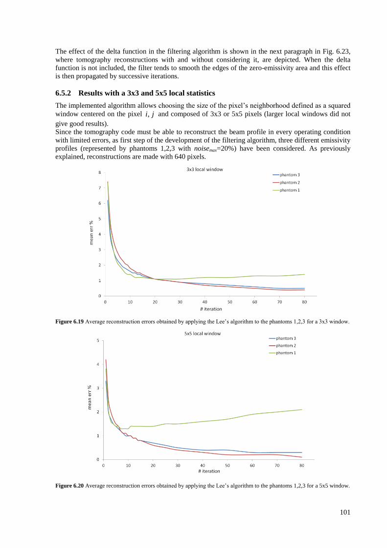
101
The effect of the delta function in the filtering algorithm is shown in the next paragraph in Fig. 6.23,
where tomography reconstructions with and without considering it, are depicted. When the delta
function is not included, the filter tends to smooth the edges of the zero-emissivity area and this effect
is then propagated by successive iterations.
6.5.2 Results with a 3x3 and 5x5 local statistics
The implemented algorithm allows choosing the size of the pixel’s neighborhood defined as a squared
window centered on the pixel ji, and composed of 3x3 or 5x5 pixels (larger local windows did not
give good results).
Since the tomography code must be able to reconstruct the beam profile in every operating condition
with limited errors, as first step of the development of the filtering algorithm, three different emissivity
profiles (represented by phantoms 1,2,3 with noisemax=20%) have been considered. As previously
explained, reconstructions are made with 640 pixels.
Figure 6.19 Average reconstruction errors obtained by applying the Lee’s algorithm to the phantoms 1,2,3 for a 3x3 window.
Figure 6.20 Average reconstruction errors obtained by applying the Lee’s algorithm to the phantoms 1,2,3 for a 5x5 window.
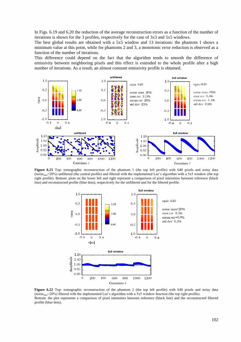
102
In Figs. 6.19 and 6.20 the reduction of the average reconstruction errors as a function of the number of
iterations is shown for the 3 profiles, respectively for the case of 3x3 and 5x5 windows.
The best global results are obtained with a 5x5 window and 13 iterations: the phantom 1 shows a
minimum value at this point, while for phantoms 2 and 3, a monotonic error reduction is observed as a
function of the number of iterations.
This difference could depend on the fact that the algorithm tends to smooth the difference of
emissivity between neighboring pixels and this effect is extended to the whole profile after a high
number of iterations. As a result, an almost constant emissivity profile is obtained.
Figure 6.21 Top: tomographic reconstruction of the phantom 1 (the top left profile) with 640 pixels and noisy data
(noisemax=20%) unfiltered (the central profile) and filtered with the implemented Lee’s algorithm with a 5x5 window (the top
right profile). Bottom: plots on the lower left and right represent a comparison of pixel intensities between reference (black
line) and reconstructed profile (blue dots), respectively for the unfiltered and for the filtered profile.
Figure 6.22 Top: tomographic reconstruction of the phantom 2 (the top left profile) with 640 pixels and noisy data
(noisemax=20%) filtered with the implemented Lee’s algorithm with a 5x5 window function (the top right profile).
Bottom: the plot represents a comparison of pixel intensities between reference (black line) and the reconstructed filtered
profile (blue dots).
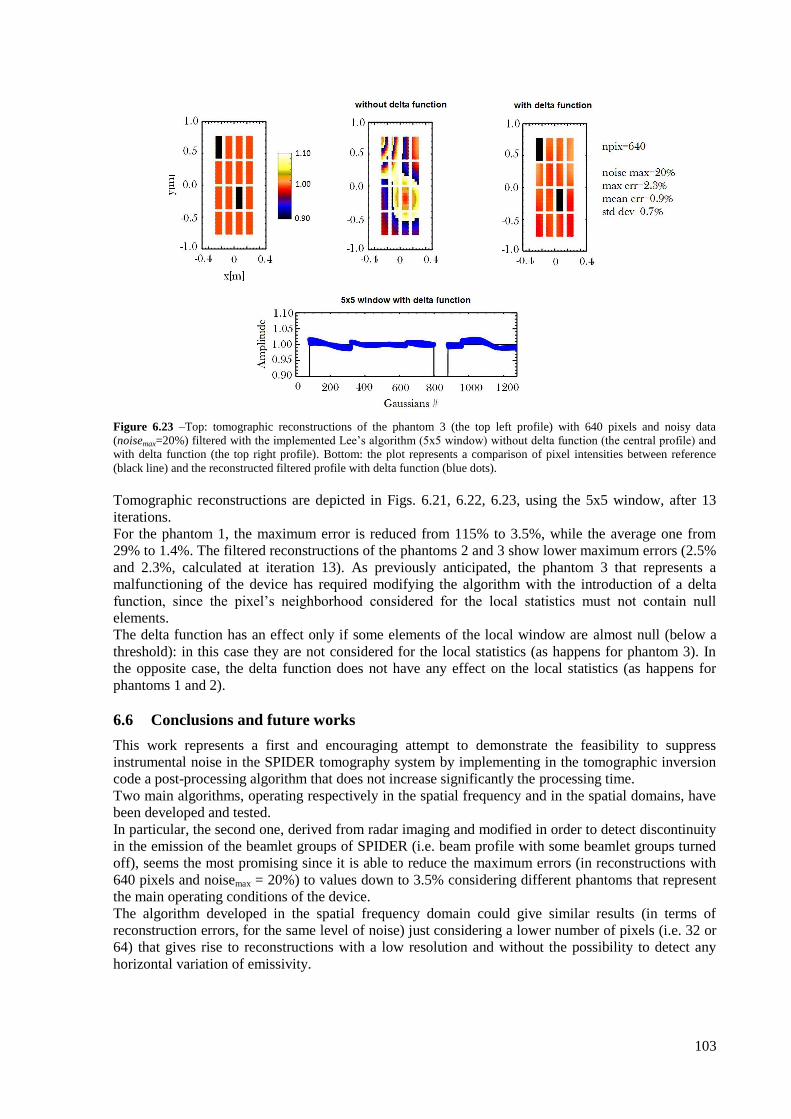
103
Figure 6.23 –Top: tomographic reconstructions of the phantom 3 (the top left profile) with 640 pixels and noisy data
(noisemax=20%) filtered with the implemented Lee’s algorithm (5x5 window) without delta function (the central profile) and
with delta function (the top right profile). Bottom: the plot represents a comparison of pixel intensities between reference
(black line) and the reconstructed filtered profile with delta function (blue dots).
Tomographic reconstructions are depicted in Figs. 6.21, 6.22, 6.23, using the 5x5 window, after 13
iterations.
For the phantom 1, the maximum error is reduced from 115% to 3.5%, while the average one from
29% to 1.4%. The filtered reconstructions of the phantoms 2 and 3 show lower maximum errors (2.5%
and 2.3%, calculated at iteration 13). As previously anticipated, the phantom 3 that represents a
malfunctioning of the device has required modifying the algorithm with the introduction of a delta
function, since the pixel’s neighborhood considered for the local statistics must not contain null
elements.
The delta function has an effect only if some elements of the local window are almost null (below a
threshold): in this case they are not considered for the local statistics (as happens for phantom 3). In
the opposite case, the delta function does not have any effect on the local statistics (as happens for
phantoms 1 and 2).
6.6 Conclusions and future works
This work represents a first and encouraging attempt to demonstrate the feasibility to suppress
instrumental noise in the SPIDER tomography system by implementing in the tomographic inversion
code a post-processing algorithm that does not increase significantly the processing time.
Two main algorithms, operating respectively in the spatial frequency and in the spatial domains, have
been developed and tested.
In particular, the second one, derived from radar imaging and modified in order to detect discontinuity
in the emission of the beamlet groups of SPIDER (i.e. beam profile with some beamlet groups turned
off), seems the most promising since it is able to reduce the maximum errors (in reconstructions with
640 pixels and noisemax = 20%) to values down to 3.5% considering different phantoms that represent
the main operating conditions of the device.
The algorithm developed in the spatial frequency domain could give similar results (in terms of
reconstruction errors, for the same level of noise) just considering a lower number of pixels (i.e. 32 or
64) that gives rise to reconstructions with a low resolution and without the possibility to detect any
horizontal variation of emissivity.

104
It is important to notice that a reconstruction of the beam emissivity with a higher number of pixels
can go beyond the simple detection of the lack of uniformity of the beam, giving information about its
causes and suggesting possible solutions.
Being this work based on a model that simulates the role of the instrumental noise introduced in the
line integrated signals, an important further step will be the experimental validation of this noise
model that would also allow to have a more precise idea about the expected noise level of the system.
A measure of the noise level is essential to decide which is the best filtering technique. Lee’s
algorithm, since it is able to strongly reduce the reconstruction errors, is more suitable for a high noise
level, but for a very low noise level (around a few percent) even without a digital filter it is possible to
respect the ITER prescriptions for reconstruction errors [Ago11bis].
An improvement of the Lee’s algorithm could be the addition of a routine for the optimization of the
number of iterations required to minimize the reconstruction errors (since it varies with the considered
phantom) and the validation with phantoms representing other operating conditions of SPIDER.
105
Chapter 7
Conclusions
The research activity presented in this thesis work is in the framework of the development of the
negative ion source (SPIDER) and of the full injector (MITICA) prototypes for the ITER neutral
beam. In particular, it is focused on two main topics: particle transport studies inside the MITICA
accelerator and the development of a tomographic beam diagnostic.
A proper modeling of the particle transport inside the MITICA accelerator, considering the main
processes that generate secondary particles relevant for the evaluation of the heat loads on the
accelerator grids is essential for the thermo-mechanical analysis and the mechanical design of the
accelerator. This calculation is performed by EAMCC, a relativistic particle tracking code based on
the Monte-Carlo method for describing collisions inside the accelerator under prescribed electric and
magnetic fields. In this thesis the code has been deeply modified in order to perform complete 3D
multi-beamlet analysis: this allows to take into account the beamlet-beamlet repulsion and to consider
other effects neglected under the hypothesis of axi-symmetric beamlet (e.g. the influence of magnetic
fields on the calculation of electric potential maps and the effect of steering plates called kerbs on the
particle trajectories. This modified version of EAMCC (called EAMCC-mod for the sake of
simplicity), is fully 3D and capable of modifying the mesh of the 3D maps and of dealing with uneven
meshes for extending the physical dimensions of the simulated domain: a finer mesh is used just in the
regions where a more detailed description of the fields is required. In order to validate modifications
introduced in EAMCC, two simulations performed with the original code and the modified version
have been compared: the maximum difference of total power load on grids is ~ 7%, mainly due to the
fact that EAMCC-mod implements new routines for the calculation of collisions and the determination
of the geometry of grids.
Hot spots and the typical pattern of the power deposition observed in the single-beamlet simulations
are present also in the multi-beamlet results, apart from some aspects that will be investigated in the
future. The most relevant difference is that in the multi-beamlet simulation half ring regions are
observed in the extraction grid with a power density of about 3 MW/m2 due to the impinging electrons
co-extracted from the ion source. Moreover, the total power deposition on the accelerator grids
calculated in the multi-beamlet simulation, with respect to the single-beamlet case, shows non-
negligible differences and for these reasons an experimental validation is necessary. An opportunity of
experimental validation is represented by NIO1, a versatile negative ion source installed at Consorzio
RFX currently in its initial operation phase.
A fully 3D analysis of the NIO1 beam has been performed using EAMCC-mod. For the first time, an
entire source, made of nine beamlets, has been simulated in EAMCC considering multi-beamlet
effects before neglected and discarding the axis-symmetry hypothesis of the electric fields imposed by
the original version of the code. For determining heat loads and the power transmitted out of the NIO1
accelerator, the H- beam core, the electrons co-extracted from the ion source and the beam halo have
been included in simulations. According to results, most of the power to the extraction grid comes
from the co-extracted plasma electrons. Post acceleration (PA) and repeller (REP) grids are heated by
co-extracted electrons and secondary electrons which are by-products of collisions between the
accelerated negative ions and the background gas. Highest value of power are calculated for the EG
and PA and other high-power density regions are determined. In particular, the deposition of co-
extracted electrons on the front surface of the extraction grid causes a power density peak of about 4.5
MW/m2. Lower but meaningful high-power density regions are also calculated in the PA (~ 1.6
MW/m2) and in the REP (500 kW/m
2) grids. NIO1 represents a great experimental opportunity and
these results will be considered in the future for benchmarking EAMCC-mod. If confirmed, a thermo-
mechanical verification of grids to guarantee a grid temperature in any case lower than 300 °C
(beyond this temperature the copper thermo-mechanical properties are sensibly worsened) and
compatible stress peaks will be carried out. Stresses, strains and deformations in the copper will be
calculated and if necessary the capability of the cooling system will be improved.
106
Concerning tomography, its application to an ion beam will be useful for the assessment of the density
profile of the beam. It can go beyond the simple detection of the lack of uniformity of the beam,
giving information about its causes and suggesting possible solutions. A tomography code based on
algebraic reconstruction techniques, more suitable than algorithms based on the Radon transform
when the number of detectors is limited compared to the number of pixels of the reconstructed profile,
has been developed and tested on the NIO1 emissivity profile. The tomography code has been
developed with the aim of realizing a versatile instrument, applicable to linear accelerators as well as
to a tokamak and without adding any hypotheses about the beam characteristics or the emissivity in a
particular region of the tomography plane, not to limit the capability of the code of detecting
irregularities in the beam profiles.
Since NIO1 is in its start-up phase, it is not possible to have an experimental emissivity profile for
testing the tomography code. For this reason a phantom (i.e. a simulated profile) was calculated with
EAMCC-mod, by which it was possible to simulate the transport of the 9 H- beamlets of the NIO1
beam from the ion source, through the accelerator and up to the tomography plane at which the
tomography detectors are located. Considering a reasonable compromise between the cost of the
tomography system for NIO1 (strongly influenced by the number of cameras) and the quality of
tomography reconstructions, the limited view of the beam due to the available diagnostic ports,
different geometry configurations have been analyzed. According to the simulations, the simplest
system made of 2 CCD cameras, allows to reconstruct a 1600 pixels emissivity profile with an rms
error of 21.1% and a mean error of 15.3%. Considering the number of pixels and the number of lines-
of-sight (240), the inversion is a limited-data problem and results obtained with the Maximum-
Likelihood Expectation-Maximization (ML-EM) algorithm are significant. A more complex system
with 6 CCDs would allow to reduce the reconstruction errors down to 10% and represents a good
compromise between complexity and quality of reconstructions.
Some a-priori knowledge would allow to reduce the reconstruction errors and it will be considered in
the future, keeping in mind that also a limit in the detection capabilities would be introduced.
For what concerns the instrumental noise, a more detailed study is required, in particular the
experimental evaluation of the noise model and of its intensity. If the experimental noise level is lower
than 10% a simple low-pass filter could be sufficient, otherwise a more sophisticated filtering
technique should be considered.
The tomography code has been also applied to the MITICA profiles (simulated by EAMCC code),
3072 pixels reconstructions have been obtained. Reducing the aperture angle from 5 to 2.5 mrad, a
significant improvement in the reconstruction quality is obtained. Reconstructions clearly show the
proper position of the 12 peaks due to the superposition of the 1280 beamlets and also the vertical
displacement downwards due to the applied magnetic field. The instrumental noise has, in the case of
MITICA, a stronger effect, but before considering a proper image filtering, an experimental
measurement of the noise level is necessary.
A more detailed study of the instrumental noise has been carried out for the SPIDER visible
tomography. The main aim of this diagnostic in SPIDER will be measuring the two-dimensional
particle density distribution of the beam: in particular the ITER requirement for the beam is that the
maximum acceptable deviation from uniformity is ± 10%, thus the deviation of the tomographic
reconstruction from the real emissivity of the beam has to be sufficiently lower than this value.
It was found that the noise has a large influence on the maximum achievable resolution of the
diagnostic, imposing a limit on the maximum acceptable noise level. In order to reduce its impact
different filtering techniques have been considered both in the frequency and in the spatial domain. In
particular, a technique developed for radar imaging has been adapted and implemented in the SPIDER
tomography code. It proved capable of reducing significantly the reconstruction errors in different
operating conditions of SPIDER and demonstrates the feasibility to filter out the effect of the noise by
post-processing the reconstructed image of the beam.
107
Bibliography
[Ago10] M. Agostini et al., Optical measurements for turbulence characterization in RFX-mod edge,
Rev. Sci. Instrum. 81, 10D715 (2010)
[Ago11] P. Agostinetti, et al., Physics and engineering studies on the MITICA accelerator:
comparison among possible design solutions, AIP Conf. Proc. 1390 (2011)
[Ago11bis] M.Agostini et al., Tomographic diagnostic of the hydrogen beam from a negative ion
source, Phys. Rev. ST Accel. Beams 14, 102801 (2011)
[Ago11ter] M.Agostini et al., MITICA Visible Tomography Feasibility study: optimisation of the
inversion algorithm, RFX Technical note RFX_MITICA_TN_115, 20/12/2011
[Ago14] P. Agostinetti et al., Single beamlet optics studies and functional optimization of the MITICA
accelerator, RFX Technical note RFX-MITICA-TN-270, 10/11/2014
[And84] A.H. Andersen and A.C. Kak, Simultaneous Algebraic Reconstruction Technique (SART): a
superior implementation of the ART algorithm, Ultrasonic Imaging 6, 81 (1984)
[Ans14] ANSYS Inc., http://www.ansys.com
[Ant14] V. Antoni et al., Physics design of the injector source for ITER neutral beam injector, Rev.
Sci. Instrum. 85, 02B128 (2014)
[Atz04] Stefano Atzeni and Jurgen Meyer-Ter-Vehn, The Physics of Inertial Fusion, Oxford Science
Publication (2004)
[Bac06] M. Bacal., Physics aspects of negative ion sources, Nucl. Fusion 46, S250 (2006)
[Bac79] M. Bacal and G.W. Hamilton, H- and D
- production in plasmas, Phys. Rev. Lett. 42, 1538
(1979)
[Bar79] R. A. Baragiola et al., Electron emission from clean metal surfaces induced by low-energy
light ions, Phys. Rev. B 19, 121 (1979)
[Bel74] Y.I. Belchenko et al. A powerful injector of neutrals with a surface-plasma source of negative
ions, Nuclear Fusion 14 (1974)
[Bet38] H.A. Bethe, Energy production in stars , Phys. Rev. 55, 434 (1938)
[Bro04] I.G. Brown, editor. The physics and thechnology of ion sources, Wiley-VCH Verlag GmbH &
Co., Weinheim (2004)
[Bru54] M. B. E. Bruining, Physics and applications of secondary electron emission, Pergamon Press,
New York (1954).
[But30] S. Butterworth, On the theory of filter amplifiers, Wireless Engineer 7, 536 (1930)
[Cav10] M. Cavenago et al., Design of a versatile multiaperture negative ion source, Rev. Sci.
Instrum. 81, 02A713 (2010)
[Cav12] M. Cavenago et al., Development of a versatile multiaperture negative ion source, Rev. Sci.
Instrum. 83, 02A707 (2012)
108
[Cav14] M. Cavenago et al., Development of versatile multiaperture negative ion sources, Proc. of
International Symposium on Negative Ions, Beams and Sources (NIBS), IPP Garching (Germany),
Oct. 6-10 2014 (to be published)
[Cen83] Y. Censor, Strong underrelaxation in Kaczmarz’s method for inconsistent systems, Numer.
Math. 41, 83 (1983)
[Chi12] G. Chitarin et. al., Concepts for the magnetic design of the MITICA neutral beam test facility
ion accelerator, Rev. Sci. Instrum. 83, 02B107 (2012)
[Chi14] G. Chitarin et al., Cancellation of the ion deflection due to electron-suppression magnetic
field in a negative-ion accelerator, Rev. Sci. Instrum. 85, 02B317 (2014)
[Cor63] A.M. Cormack, Representation of a function by its line integrals, with some radiological
applications, J. Appl. Physics 34, 2722 (1963)
[Dar75] E.H. Darlington, Backscattering of 10-100 keV electrons from thick targets, J. Phys. D: Appl.
Phys. 8, 85 (1975)
[Dem77] A.P. Dempster et al., Maximum likelihood from incomplete data via the EM algorithm, J.
Royal Stat. Soc. B39, 1 (1977)
[Dua72] B.H. Duane, Fusion cross-section theory, Annual Report on CTR Technology Rep. BNWL-
1685 (1972)
[Dud12] V. Dudnikov, Forty years of surface plasma source development, Rev. Sci. Instrum. 83,
02A708 (2012)
[Esc11] H.P.L. de Esch et al., Negative ion beam halo mitigation at the 1 MV testbed at IRFM, Fusion
Eng. Des. 86, 363 (2011)
[Esc13] H.P.L. de Esch et al., Status of physics design of the HNB accelerator for ITER, AIP
Conference Proceedings 1515, 512 (2013)
[Fon14] N. Fonnesu et al., A multi-beamlet analysis of the MITICA accelerator, Proc. of International
Symposium on Negative Ions, Beams and Sources (NIBS), IPP Garching (Germany), Oct. 6-10 2014
(to be published)
[Fon14bis] N. Fonnesu et al., An image filtering thechnique for SPIDER visible tomography, Rev. Sci.
Instrum. 85, 02A730 (2014)
[Fre07] J.P. Freidberg, Plasma Physics and Fusion Energy, Cambridge University Press, 2007
[Fub08] G. Fubiani at al., Modeling of secondary emission processes in the negative ion based
electrostatic accelerator of the International Thermonuclear Experimental Reactor, Phys. Rev. ST
Accel. Beams 11, 014202 (2008)
[Fub09] G. Fubiani et al., Analysis of the two accelerator concepts foreseen for the neutral beam
injector of the International Thermonuclear Experimental Reactor, Phys. Rev. ST Accel. Beams 12,
050102 (2009)
[Fur02] M. A. Furman and M.T.F. Pivi, Probabilistic model for the simulation of secondary electron
emission, Phys. Rev. ST Accel. Beams 5, 124404 (2002)
109
[Gol95] R.J. Goldston and P.H. Rutherford, Introduction to Plasma Physics, Institute of Physics
Publishing, 1995
[Gor70] R. Gordon et al, Algebraic Reconstruction Techniques (ART) for three-dimensional electron
microscopy and x-ray photography, J. Theor. Biol. 29, 471 (1970)
[Gor74] R. Gordon, A tutorial on ART, IEEE Trans. Nucl. Sci. NS-21, 78 (1974)
[Gri12] L. Grisham et al., Recent Improvements to the ITER Neutral Beam System Design, Fusion
Eng. Des. 87, 1805 (2012)
[Hem96] R. S. Hemsworth et al., Neutral beams for ITER, Rev. Sci. Instrum. 67, 1120 (1996)
[Her79] W.B Hermansfeld, Electron trajectory program, technical report, Stanford Linear Accelerator
Center (1979)
[Her80] G.T. Herman, Image reconstruction from projections, Academic, New York (1980)
[Hou72] G.N. Hounsfield, A method and apparatus for examination of a body by radiation such as X
or Gamma radiation, Patent Specification 1283915, London, England (1972)
[Hou73] G.N. Hounsfield, Computerized transverse axial scanning (tomography): Part 1. Description
of system, Brit. J. Radiol. 46, 1016 (1973)
[Ite14] ITER Organization, http://www.iter.org
[Jac05] J. Jacquinot et al, Steady-state operation of tokamaks: key experiments, integrated modelling
and technology developments on Tore Supra, Nucl. Fusion 45, S118 (2005)
[Kac37] S. Kaczmarz, Angenaherte auflosung von systemen lenearer gleichungen, Bull. Int. Acad.
Pol. Sci. Lett. A., 355 (1937)
[Kak99] A.C. Kak, M. Slaney, Principles of computerized tomographic imaging, IEEE Press., New
York (1999)
[Koj12] A. Kojima et al., Vacuum insulation of the high energy negative ion source for fusion
application, Rev. Sci. Instrum. 83, 02B117 (2012)
[Kra12] W. Kraus et al., The development of the radio frequency driven negative ion source for
neutral beam injectors, Rev. Sci. Instrum. 83, 02B104 (2012)
[Lan84] K. Lange and R. Carson, EM reconstruction algorithms for emission and transmission
tomography, J. Comput. Assist. Tomogr. 8, 306 (1984)
[Lee86] J.S. Lee, Speckle suppression and analysis for synthetic aperture radar image, Optical
Engineering 25 (5), 636 (1986)
[Mat74] T. Matsukawa et al., Measurements of the energy distribution of backscattered kilovolt
electrons with a spherical retarding-field energy analyser, J. Phys. D: Appl. Phys. 7, 695 (1974)
[Miy12] K. Miyamoto et al., Meniscus and beam halo formation in a tandem-type negative ion source
with surface production, Appl. Phys. Lett. 100, 233507 (2012)
110
[Moc14] S. Mochalskyy et al., On the meniscus formation and the negative hydrogen ion extraction
from ITER neutral beam injection relevant ion source, Plasma Phys. Control. Fusion 56, 105001
(2014)
[Oku13] S. Okuda et al., Study of plasma meniscus formation and beam halo in negative hydrogen ion
sources, AIP Conference Proceedings 1515, 107 (2013)
[Ope14] OPERA-3D software, Cobham plc. http://www.cobham.com
[Pam03] J. Pamela et al., Overview of JET results, Nucl. Fusion 43, 1540 (2003)
[Pam91] J. Pamela, A model for negative ion extraction and comparison on negative ion optics
calculations to experimental results, Rev. Sci. Instrum. 62, 1163 (1991)
[Pas11] R.Pasqualotto et al., SPIDER Visible Tomography System Description, RFX Technical note
RFX_SPIDER_TN_111, 18/04/2011
[Pas12] R.Pasqualotto et al., Diagnostics of the ITER neutral beam test facility, Rev. Sci. Instrum. 83,
02B103 (2012)
[Per79] A. Peres, Fusion cross sections and thermonuclear reaction rates, J. Appl. Phys. 50, 5569
(1979)
[Rad17] J.Radon, On the determination of functions from their integrals along certain manifolds, Ber.
Saechs. Akad. Wiss, Leipzig Math. Phyis. 69, 262 (1917)
[Ros82] A. Rosenfeld and A.C. Kak, Digital picture processing, NY Academic Press, New York
(1982)
[Sar13] E. Sartori and P. Veltri, Avocado: A numerical code to calculate gas pressure distribution,
Vacuum 90, 80 (2013)
[Sar14] E. Sartori and P. Veltri, Simulation of gas distribution in NIO1 in molecular flow regime, RFX
Technical note RFX_NIO_TN_6, 23/12/2014
[She82] L.A. Shepp, and Y. Vardi, Maximum likelihood estimation for emission tomography, IEEE
Trans. Med. Imaging 1,113 (1982)
[Son09] P. Sonato et al., The ITER full size plasma source device design, Fusion Eng. Des. 84, 269
(2009)
[Spe06] E. Speth et al., Overview of the RF source development programme at IPP Garching, Nucl.
Fusion 46, S220 (2006)
[Sta94] P.F. Staub, Bulk target backscattering coefficient and energy distribution of 0.5-100 keV
electrons: an empirical and synthetic study, J. Phys. D: Appl. Phys. 27, 1533 (1994)
[Ste54] E. J. Sternglass, Backscattering of kilovolt electrons from solids, Phys. Rev. 95, 345 (1954)
[Suz11] T. Suzuki et al., Experimental investigation and validation of neutral beam current drive for
ITER through ITPA Joint Experiments, Nucl. Fusion 51 083020 (2011)
[Sve82] B. Svensson and G. Holmén, Electron emission from aluminium and copper under molecular-
hydrogen-ion bombardment, Phys. Rev. B 25, 3056 (1982)
111
[Tan71] K.Tanabe, Projection method for solving a singular system of linear equations and its
applications, Numer. Math. 17, 203 (1971)
[Tho85] E. W. Thomas, Oak Ridge National Laboratory, Technical Report No. ORNL-6088, 1985
[Tra98] R. Trainham et al., Negative ion sources for neutral beam injection into fusion machines, Rev.
Sci. Instrum. 69, 926 (1998)
[Vah95] V. Vahedi and M. Surendra, A Monte-Carlo collision model for the particle-in-cell method:
applications to argon and oxygen discharges, Comput. Phys. Commun. 87, 179 (1995)
[Vel14] P. Veltri et al., Compensation of beamlet deflections and focusing methods in the electrostatic
accelerator of MITICA Neutral Beam Injector, IEEE Transactions on Plasma Science 42, 4 (2014)
[Ver93] D. Verhoeven, Limited-data computed tomography algorithms for the physical sciences,
Appl. Opt. 32, 3736 (1993)
[Wan05] L. Wang et al., Stripped electron collection at the Spallation Neutron Source, Phys. Rev. ST
Accel. Beams 8, 094201 (2005)
[Wer04] M.N. Wernick and J.N. Aarsvold, Emission Tomography: the fundamentals of PET and
SPECT, Elsevier Academic Press, London (2004)
[Wes04] J. Wesson, Tokamaks, Clarendon Press, Oxford (2004)
[Zac12] P. Zaccaria et al., Progress in the MITICA beam source design, Rev. Sci. Instrum. 83, 02B108
(2012)
[Zan14] B. Zaniol et al., NIO1 Diagnostics, proceedings of the NIBS 2014 (Garching, Munchen), to
be published
112
Aknowledgements
I gratefully acknowledge the scientific, the administrative and the technical staff of Consorzio RFX for
giving me the opportunity to work, during the last three years, in a friendly, professional and high-
level scientific environment.
In particular, I want to express my gratitude to Matteo Agostini, Roberto Pasqualotto, Gianluigi
Serianni and Pierluigi Veltri for their constant support, suggestions and encouragement.
I want also to thank the NBI team and the Plasma Engineering group, in particular Piero Agostinetti,
Simone Peruzzo and Samuele Dal Bello, for their time and availability.
Many thanks to my supervisor Piergiorgio Sonato, the doctorate director Paolo Bettini, Fiorella
Colautti, Prof. Buffa and Piero Martin.
Special thanks to my family and much gratitude to Elisa for her patience while this thesis work was
being written, and before ;)