universit`a degli studi di milano - optlab web pageoptlab.di.unimi.it/docs/tresoldi2.pdf ·...

Universita degli Studi di MilanoDipartimento di Tecnologie dell’Informazione

Corso di laurea in Scienze e Tecnologie dell’Informazione

Optimization Algorithms forData Transmission Planning and Scheduling Problems

in ESA’s Mars Express Space Mission

RELATOREProf. Giovanni Righini

CORRELATOREDott. Alessandro Donati

TESI DI LAUREA DIEmanuele Tresoldi

Matr. 684093

Anno Accademico 2006/2007

Contents

Mars Express 1

1 The Mars Express Uplink Problem 9

1.1 MEXUP Description . . . . . . . . . . . . . . . . . . . . . . . 10

1.2 MEXUP Formalization . . . . . . . . . . . . . . . . . . . . . . 11

1.2.1 Basic Entities . . . . . . . . . . . . . . . . . . . . . . . 11

1.2.2 Requirements and Constraints . . . . . . . . . . . . . . 13

1.3 MEXUP Solver . . . . . . . . . . . . . . . . . . . . . . . . . . 17

1.3.1 Reduced Confirmation Scheduling . . . . . . . . . . . . 17

1.3.2 Full Confirmation Scheduling . . . . . . . . . . . . . . 23

1.3.3 Secondary Windows Scheduling . . . . . . . . . . . . . 24

1.3.4 Solver Optimization . . . . . . . . . . . . . . . . . . . 24

1.3.5 Two Strategies of Scheduling . . . . . . . . . . . . . . . 26

1.4 MEXUP Graphical User Interface . . . . . . . . . . . . . . . . 26

1.4.1 The Input Form . . . . . . . . . . . . . . . . . . . . . . 27

1.4.2 The MDAF List Form . . . . . . . . . . . . . . . . . . 28

1.4.3 The charts . . . . . . . . . . . . . . . . . . . . . . . . . 30

1.5 MEXUP Evaluation . . . . . . . . . . . . . . . . . . . . . . . 30

1.5.1 RAXEM . . . . . . . . . . . . . . . . . . . . . . . . . . 32

1.5.2 Input and Output Formats . . . . . . . . . . . . . . . . 32

1.5.3 Experimental results . . . . . . . . . . . . . . . . . . . 35

1.6 Conclusions . . . . . . . . . . . . . . . . . . . . . . . . . . . . 46

2 The Mars Express Memory Dumping Problem 47

2.1 MEX-MDP Problem Description . . . . . . . . . . . . . . . . 48

I

2.2 MEX-MDP Formalization . . . . . . . . . . . . . . . . . . . . 49

2.3 MEX-MDP Model . . . . . . . . . . . . . . . . . . . . . . . . 53

2.4 An Optimal Algorithm for MEX-MDP . . . . . . . . . . . . . 56

2.4.1 Optimally Balanced Solutions . . . . . . . . . . . . . . 56

2.4.2 Keeping Solutions Balanced . . . . . . . . . . . . . . . 57

2.4.3 Balancing an Unbalanced Solution . . . . . . . . . . . 60

2.4.4 A Fast Heuristic . . . . . . . . . . . . . . . . . . . . . . 60

2.5 Computational Results . . . . . . . . . . . . . . . . . . . . . . 61

2.5.1 Implementation . . . . . . . . . . . . . . . . . . . . . . 61

2.5.2 Input . . . . . . . . . . . . . . . . . . . . . . . . . . . . 62

2.5.3 Results Analysis . . . . . . . . . . . . . . . . . . . . . 62

2.6 MEX-MDP Extensions . . . . . . . . . . . . . . . . . . . . . . 71

2.7 MEX-MDP extended problem evaluation . . . . . . . . . . . . 74

2.8 Conclusions . . . . . . . . . . . . . . . . . . . . . . . . . . . . 78

Bibliography 78

A MEX-MDP Linear Programming Model 80

B MEX-MDP EXTENDED Linear Programming Model 82

II

Mars Express

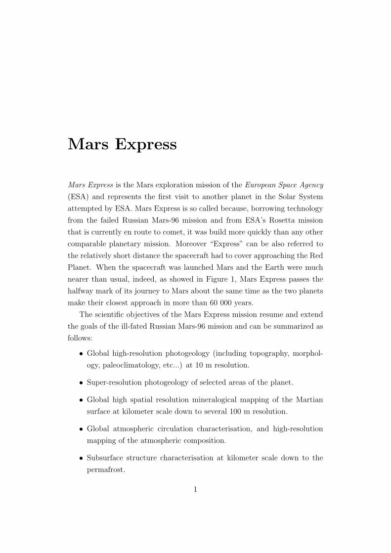
Mars Express is the Mars exploration mission of the European Space Agency

(ESA) and represents the first visit to another planet in the Solar System

attempted by ESA. Mars Express is so called because, borrowing technology

from the failed Russian Mars-96 mission and from ESA’s Rosetta mission

that is currently en route to comet, it was build more quickly than any other

comparable planetary mission. Moreover “Express” can be also referred to

the relatively short distance the spacecraft had to cover approaching the Red

Planet. When the spacecraft was launched Mars and the Earth were much

nearer than usual, indeed, as showed in Figure 1, Mars Express passes the

halfway mark of its journey to Mars about the same time as the two planets

make their closest approach in more than 60 000 years.

The scientific objectives of the Mars Express mission resume and extend

the goals of the ill-fated Russian Mars-96 mission and can be summarized as

follows:

• Global high-resolution photogeology (including topography, morphol-

ogy, paleoclimatology, etc...) at 10 m resolution.

• Super-resolution photogeology of selected areas of the planet.

• Global high spatial resolution mineralogical mapping of the Martian

surface at kilometer scale down to several 100 m resolution.

• Global atmospheric circulation characterisation, and high-resolution

mapping of the atmospheric composition.

• Subsurface structure characterisation at kilometer scale down to the

permafrost.

1

Figure 1: Mars Express’ trajectory - Credits: ESA

• Surface-atmosphere interaction; interaction of the atmosphere with the

interplanetary medium.

• Structure of the interior, atmosphere and environment via radio science

measurements.

• Surface geochemistry and exobiology.

The Mars Express spacecraft (figure 2) was made up of two parts, an

orbiter and a lander. It was designed to enter Martian orbit carring seven

scientific instruments and the lander. The scientific tools were provided by

academic institutions of different European countries, and were conceived

in order to investigate Martian atmosphere, surface and subsurface. On

the other hand, Beagle 2, the lander (Figure 3), was expected to perform

geochemistry research and measurement on the Martian ground searching

also for signs of past life.

Mars Express was launched on 2 June 2003 at 17.45 UT from Baikonur

Cosmodrome in Kazakhstan using a Soyuz-Fregat rocket (Figures 4 and 5).

After separation from Fregat and having escaped from Earth’s gravity the

spacecraft started its seven-months journey to Mars. Six days before its

2

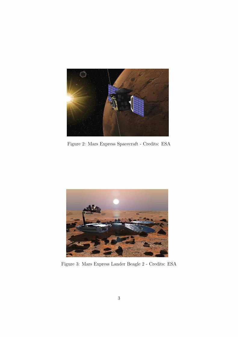
Figure 2: Mars Express Spacecraft - Credits: ESA

Figure 3: Mars Express Lander Beagle 2 - Credits: ESA

3

arrival, Mars Express ejected the Beagle 2 which entered Mars’ atmosphere

on the morning of 25 December. It was expected to reach Martian ground on

the same day but the confirmation of a successful landing was never received.

Attempts to contact Beagle 2 were made throughout January and February

2004 but they all failed and the lander was declared lost on 6 February 2004.

Figure 4: Mars Express Soyuz-Fregat - Credits: ESA

Mars Express spacecraft successfully entered the Martian orbit on 25

December 2004 and it manoeuvred into an highly elliptical capture orbit

from which it moved into its operational near polar orbit later in January

2004. After reached its final destination the spacecraft, step by step, deployed

its radars and antennas, started collecting data from scientific instruments

and transmitting them to the Earth.

The orbiter scientific payload is made up of seven instruments:

High Resolution Stereo Camera (HRSC) - Germany - The HRSC is imag-

ing the entire planet in full colour, 3D and with a resolution of about

10 meters. Selected areas will be imaged at 2-meters resolution.

Visible and Infrared Mineralogical Mapping Spectrometer (OMEGA)

- France - OMEGA determines mineral composition of the surface up

to 100 metres resolution. To achieve its purpose it analyzes the vis-

ible and infrared light reflected from the planet’s surface, moreover,

4

Figure 5: The Mars Express’ launch - Credits: ESA

as light reflected from the surface must pass through the atmosphere

before entering the instrument, OMEGA will also measure aspects of

atmospheric composition.

Sub-surface Sounding Radar Altimeter (MARSIS) - Italy -MARSIS is

aimed to investigate the composition of the sub-surface of Mars. This

instrument sends low frequency radio waves towards the planet which

are able to pierce the Martian crust to be reflected at sub-surface in-

terfaces between layers of different material, including water or ice.

Planetary Fourier Spectrometer (PFS) - Italy - The PFS is designed to

analyze the Martian atmospheric temperature and pressure. In partic-

ular, it measures the vertical pressure and temperature profile of carbon

dioxide which makes up 95% of the martian atmosphere, and looks for

minor constituents including water, carbon monoxide, methane and

formaldehyde.

5

Ultraviolet and Infrared Atmospheric Spectrometer (SPICAM) - France

- Assesses elemental composition of the atmosphere from the wave-

lengths of light absorbed by the constituent gases.

Energetic Neutral Atoms Analyzer (ASPERA) - Sweden - ASPERA

Investigates interactions between upper atmosphere and solar wind by

measuring ions, electrons and energetic neutral atoms in the outer at-

mosphere.

Mars Radio Science Experiment (MaRS) - Germany - Uses radio sig-

nals that convey data and instructions between the spacecraft and

Earth to investigate atmosphere, surface, subsurface, gravity and solar

corona density during solar conjunction.

The spacecraft is equipped with a directional high-gain antenna provid-

ing, when the spacecraft is far away from Earth, the communication between

the Mars Express and the ground station. On the other hand two low gain

antennas were used during launch and early operations to Mars. Mars Ex-

press Lander Communications (MELACOM) completes the communication

subsystem of the spacecraft, it was originally designed to allowing the data

transmission from the lander and the orbiter, and, at the moment, a test

phase is ongoing in order to determine whether and how MELACOM is us-

able in supporting NASA’s Phoenix lander scheduled to arrive at Mars on

25 May 2008.

Mars Express’ scientific instruments have collected data, analyzed by ESA

scientist, for more than 5000 orbits; during this period as a lot of scientific

experiments were achieved, many photos of the Martian surface and ground

were taken by HRSC (Figure 6). A large number of scientific discoveries

have been provided by the Mars Express instruments, in 2005 OMEGA has

pointed out the presence of hydrated sulphates, silicates and various rock-

forming minerals, PFS has detected methane in the atmosphere coming from

areas near the equator with subsurface ice, this indicates either some form

of active vulcanism or subsurface microorganisms and MARSIS has reported

the presence of deep underground water-ice (Figure 7).

6

Figure 6: Snapshot of Candor Chasma - Credits: ESA

Figure 7: Perspective view of residual water ice on the floor of VastitasBorealis Crater on Mars - Credits: ESA

7

After 687 days in orbit around the Red Planet Mars Express completed

its nominal mission. In 2005, the duration of the mission was extended until

31 October 2007, and currently, after a second extention, the mission end

date has been shifted to early-May 2009. Despite the failure of the Beagle 2,

Mars Express can be considered a very successful ESA mission which vastly

raised our knowledge of Mars answering fundamental questions about the

geology, atmosphere, surface environment, presence of water and potential

for life.

8

Chapter 1

The Mars Express Uplink

Problem

A sure, flexible and efficient communication management between ground

stations and the spacecraft is a critical factor for the success of a deep space

mission like Mars Express. In this scenario the MEX Flight Control Team

(located at ESOC in Darmstadt, Germany) plays a very importan role since

they are responsible for planning Mars Express uplink and downlink activ-

ities. In this chapter we are going to deal with the uplink problem shifting

the data dump problem to the next one.

The problem of generating usefull and robust plan for uplink activities for

Mars Express mission is usually referred to as Mars Express Uplink Problem

(MEXUP). Unfortunately, although ISTC-CNR (Institute of Cognitive Sci-

ence and Technology) made a tool (RAXEM) for supporting Mars Express

uplink activities they publish only a paper about MEXUP and RAXEM [1],

in this document they report, in addition to a complete description of the

tool, an analysis of the problem and an overwiev of the algorithm they use

to solve it. The ESA’s requirement for a tool to support the uplink planning

operations are detailed in [6]. In the next two section we are going to de-

scribe, following [6], the problem, before informally and than going more in

detail outlining the relevant entities and the constraints in MEXUP domain.

9

1.1 MEXUP Description

The spacecraft activities for each month are determined in accordance with

the Medium Term Plan (MTP) for the concerned period (usually 4 week).

Typical activities are scientific observations, technical tests, photoshoting of

the Martian ground, execution of maintenance routines, etc etc... Based on

the frozen MTP various operation requests (OR) are generated. During the

daily planning activities the operations requests are converted into MTL De-

tailed Agenda Files (MDAF) by the Mission Planning System. While ORs

detail the operations at Command Sequence (CSEQ) level, the MDAF ex-

pands the CSEQ into time-tagged telecommands (TC) which are transferred

to the spacecraft. Each TC usually represents an atohmic operation like the

switching on/off an orbiter instrument. On board the spacecraft the TC re-

side in the Master Timeline (MTL) buffer ordered by execution time. At the

specified time, each TC will be released and removed from the MTL.

MDAF are usually generated at least 3 or 4 days before the planned oper-

ations. They can contain operations for up to one week. The typical number

of TCs in a MDAF is between 100 and 600. The delivery of the MDAF to

the spacecraft is performed by means of satellite links, each period of time

assigned to Mars Express data upload is called Uplink Window (UW). All

given TCs should be on-board with enought time margin before execution

time to allow for contingencies, e.g. the loss of an UW, control system prob-

lems. It is the duty of the Spacecraft Operations Coordinator (SOC) to very

coherency, completeness and coordinate the transfer of the MDAFs to the

spacecraft.

Leaving the space context out, MEXUP can be reduced as follows: there

is a set of data to be transmitted from a point to another, the transmission

can be performed only during some prefixed periods of time and it is strongly

limited by many structural and logical constraints.

In this scenario, the purpose of a MEXUP solver is to generate a robust

delivery plan complaying with all given requirements.

10

1.2 MEXUP Formalization

In this section we are going to describe and define, in a more formal way

entities and constraints that are critical in MEXUP domain.

1.2.1 Basic Entities

There are three important entities relevant in solving MEXUP problem: The

MDAFs, the uplink windows and the MTL.

Master Timeline Detailed Agenda File (MDAF). An MDAF is a file contain-

ing operations requests which are made up of a set of telecommands

(TC) to be transferred to the spacecraft. Not all information contained

in a MDAF are necessary for our aim, in particular we take in to ac-

count the following ones:

• The generation time. Each MDAF is generated in a different time.

• The whole set of TC enclosed in a MDAF, each TC has two notable

records:

– The execution time: it is the instant of time in which the

operation associated to the TC takes place.

– The CESEQ name: it is a string of character and digits by

means of which it is possible to identify the type of an MDAF.

Usually the CESEQ names are referred to as type identifiers.

• The start time. It is equal to the execution time of the first TC

in the MDAF. The start time can be also seen as the expiration

date of a MDAF because it marks the deadline before which the

MDAF must be available onboard.

• The end time. It coincides with the execution time of the last TC

in the MDAF.

• The MDAF type. This type comes from processing the type iden-

tifiers contained in a MDAF. For each type a priority level is

defined. It is worth noting that the type priority is secondary

compared with the time priority.

11

Uplink Window (UW). An uplink windows represents the allocation of a

ground station to the MEXUP project. For our purpose it can be per-

ceived as a period of time during which it is possible to perform uplink

activities. An uplink window is usually characterize by the following

elements:

• Start time. The instant of time in which the uplink window starts

being available.

• End time. The instant of time in which the uplink window ends.

• Duration. The duration of an uplink windows is computed as the

difference, in seconds, from the end and the start time of an uplink

window.

• Station identifiers. It is the identifiers of the station providing the

uplink window.

• One-Way Light Time (OWLT). It is the elapsed time taken by the

signal to travel between the Earth and Mars.

Master Timeline (MTL). The MTL can bee perceived as a buffer in which

all uplinked TCs are stored and ordered by execution time. The MTL

is made up of two par:

• Solid State Mass Memory (SSMM). In this memory are stored the

telecommands that are not to be executed by short time. New

telecommands are usually stored in the SSMM.

• Cache. The cache is maintained in RAM and contains the first

300 TCs ordered by execution time and it is constantly updated,

when a TC is executed the next (in time order) TC is loaded. If a

MDAF containing one or more TCs having execution time which

falls within the execution time of the buffered TCs is uplinked

a cache operation is requested. Such a operation empties the

cache and then repopulates it with the 300 TCs having the nearest

expiration date. This operation takes 600 seconds.

12

1.2.2 Requirements and Constraints

In this section we detail the MEXUP requirements and constraints previously

mentioned in a more formal way.

A set of MDAF I to schedule is given. This set is made up of two subset,

one A contains the MDAFs that have been already uplinked and that, at

the start time of the planning, have at least one TC in MTL, the other B is

composed by the new MDAFs to be transferred. Thus I = A ∪ B. Given IA and B cannot be automatically determined and strictly depend on history

of past uplink activities. Anyhow the MDAFs having a start time earlier

than the beginning of the planning activities belong, beyond doubt, to the

already-uplinked set. The A set is crucial in order to provide the consistency

and coherency of the generated plan. In fact, the initial status of the MTL

must be exactly computed by means of it. Thus in our model at the beginning

of the computation the MTL contains all TCs in A having execution times

later than the start-planning time.

A MDAF is to be considered the smallest unit for transfer and cannot be

divided. All TCs to be uplinked are contained in MDAFs, for every MDAF

i ∈ I there is a set of TCs Ci, the number of TCs ni in Ci is usually refered

to as the size of an MDAF. This value is not fixed and is between 1 and a

maximum number defined by users (normally a MDAF contains between 100

and 600 TCs).

Usually all TCs into a MDAF are addressed to a specific scientific instru-

ment or operation. For this reason each MDAF can be associated with an

unique type having different priority. Whatever such a priority level is of

secondary importance in respect to time priority and have to be taken int

account if and only if the scheduling by time is not feasible.

The transmission of MDAFs can take place only during the uplink win-

dows, in this period Several MDAF may be considered for the transfer from

the Earth to Mars. The time needs to deliver a MDAF is directly proportional

to ni and, given the constant upload time per TC t, the total transfertime

13

can be formulated as follows:

tni + OWLT (1.1)

When a MDAF is uplinked all contained TCs are stored in a memory in

order to be preserved before execution. The number of TCs in the MTL must

never exceded the MTL size s. The overall memory capacity come from the

sum of the cache size and the SSMM size and it is usually 3000 TCs. The

size of the MTL can be changed by the user to simulate different situation

end to take into account a safety margin, for our purpose the memory size,

s, can be seen as a constant value, indeed, it cannot be changed during the

computation.

The addition of a single TC to the MTL takes a constant period of time,

p, usually referred to as onboard processing time. If TC having execution

time which falls within the execution time of the buffered TCs is added to

MTL a cache operation will be requested. This operation starts as soon as

this TC is received on-board and takes a constant period of time h of 600

seconds (h = 0 If no cache operation is requested). A cache operation can

be performed if and only if during this operation no TC from the MTL have

to be executed. The total onboard processing time is

pni + h (1.2)

The overall time in which a MDAF is available on board is:

(t + p)ni + h + OWLT (1.3)

At the end of the processing period the probe sends a reception acknowl-

edgement, the confirmation time c is equal to 1 ∗OWLT .

Usually the dispatch of the confirmation take place after the processing

time but, if not enought uplink time is available, the confirmation will be de-

livered at the end of the transfer time, these two situations are respectively

referred to as uplink with full confirmation and uplink with reduced confir-

mation (see figure 1.1). It is worth noting that the full confirmation provides

14

the generated plan with more robustness because, with reduced confirmation,

we do not know the outcome of the processing operation.

Several MDAF may be considered for the transfer in an uplink windows,

in particular more than one MDAF can be uplinked together, in this case

we referred to this set of MDAFs as packet. Anyway, since there are no

constraints which limit the number of uplink activities in a window we assume

that more than one packets can be uplinked in the same window. Transfer a

packet is less time consuming than transfer individually each MDAF, in fact

in the former case an OWLT is spent at the end of the transfer time and the

processing time of the whole packet, instead in the latter cased time is spent

for each uplinked MDAF (see Figure 1.2).

Figure 1.1: Full and Reduced Confirmation

In order to provide redundancy and robustness to the uplink scheme (e.g.

in case of a loss of a satellite track) each plan have to be scheduled with a

primary and a secondary uplink windows. The secondary window must be

allocated on a different ground station track. Usually a track is uniquely

identified by the station ID, in case that there are two subsequent windows

with The same ID a different track can be assumed if the start of one window

and the start of other are more than 12 hours apart.

MDAFs shall be uplinked by precedence of the execution time of the

contained TCs independent of the type, i.e. an MDAF containing TCs with

the closest execution time shall be scheduled firs. If the uplink plan is not

feasible by applying the execution time priority, the uplink schedule shall be

15

Figure 1.2: Single and Multiple MDAFs Uplink

based on MDAF type priority. The priorities for uplink planning are (from

the most to the less important):

• Uplink by execution time with secondary uplink window and full con-

firmation

• Uplink by execution time without secondary uplink window and full

confirmation

• Uplink by execution time without secondary uplink window and with-

out full confirmation

• Uplink by MDAF type

The purpose of the computation is to find an uplink plan that, respecting

all constraints previously presented, aims to keep the MTL as full as possible.

16

1.3 MEXUP Solver

In order to produce a solution to MEXUP we have developed a tool based

on a simple greedy algorithm reinforced with a lookahead window and some

backtracking abilities. This algorithm produces sub-optimal solutions and

does not provide any warranty on the quality of yielded planes. Basically,

given the set of MDAFs, the algorithm selects for each iteration the MDAF

with the earliest expiration date to be added to the solution, if this MDAF

can be transferred in the current uplink window it will be added to the plan.

This process is iterated until either every MDAF is added to the schedule

or there are not enought uplink windows to deliver all given data. The

algorithm needs three steps to generate a plan, each step correspond to a

robustness level. In the first step (Reduced Confirmation Scheduling) a basic

solution without full confirmation and without secondary uplink windows is

computed, if the algorithm can find a solution then the plan is make more

robust by means of the others two steps (pseudopod in Algorithm 1).

Data: MEXUP instanceResult: Uplink PlanInitialization;if Reduced Confirmation Scheduling then

Full Confirmation Scheduling ;Secondary Window Scheduling ;Generate Uplink Plan;

elseComputation Fails ;Uplink Plan Not Feasible;

Algorithm 1: MEXUP pseudocode - overview

1.3.1 Reduced Confirmation Scheduling

In this step (see Algorithm 2) a basic solution to MEXUP is computed. The

solver generate a plan without full confirmation and without backup windows,

if a solution is achieved it becomes the basis from which the optimization

process starts; else if the algorithm can not finds a solution the backtracking

17

process is loaded, if also the backtracking fails then the plan will be not

feasible and the total computation ends. At the beginning of this phase an

ordered by time MDAF list is generated from the MDAFs set. This list is

analyzed starting from the first MDAF, if this MDAF is uplinkable in the

current uplink window then it will be removed from the MDAFs list and

added to the present uplink packet. The algorithm always try to make the

packet as big as possible because a big packet requests less uplink time than

a set of small packet made up with the same MDAFs set. When a packet is

completed i.e. no other MDAFs are uplinkable in this packet, it is added to

the uplink plan; then the current uplink window is resized, i.e. all allocated

time, necessary to uplink the packet, is removed. If the window is still usefull

then it will take into account in the next iteration, else it will be removed

from the list of uplink windows(see Algorithm 3). In this way it is possible

to transmit more than one packet in the same uplink window. A packet is

considered uplinkable if the following four conditions hold:

• MTL Capacity. Enought free space have to be available into MTL to

contain the uplinked packet. The instant of time in which the measure-

ment of the MTL residual capacity is performed is the time in which

the packet starts being received on-board, it is equal to startuplink +

OWLT .

• UW duration. The duration of the uplink window have to be longer

than the time necessary to transfer the packet from the Earth to Mars

and to receive the confirmation. The exact amount of time depends on

what type of confirmation is requested.

• No Expiration. A packet is uplinkable if all contained MDAFs can

be make available on board before their expiration date.

• Chache Operation Feasibility. If a packet request an cache op-

eration we have to check that this operation can be performed. If it

can not be done the algorithm have to find another start point for the

uplink in order to fulfill all imposed constraints.

18

Data: A list of MDAFs and a list of Uplink WindowsResult: An Uplink Plan with the lowest robustness levelInitialization;if Generate Plan then

Full Confirmation Scheduling;Secondary Window Scheduling;

elseif backtracking then

Redo Reduced Confirmation Scheduling;else

Computation fails;

Algorithm 2: MEXUP pseudocode - Reduced Confirmation Scheduling

Data: A list of MDAFs I and a list of Uplink Windows JResult: A list of UplinksInitialization;while MDAFs’ list not empty and UWs’ list not empty do

foreach MDAF i ∈ I doif i uplinkable in j then

remove i from I;add i to P ;

elseif i < lookAhead window then

i = next MDAF;else

resize j;if j is useless then

remove j from J ;break;

Algorithm 3: MEXUP pseudocode - Generate Plan

19

Lookahead Window

During the process of making a packet of MDAFs to uplink, when the algo-

rithm meets a MDAF that can not be included in the uplink the packet is

closed and the uplink window is resized. Sometimes it is possible that one or

more MDAFs, which have expiration time later than the first not includable

MDAF, may be added to the packet e.g. they have smaller size than the

non includable MDAF. In this case the generated schedule does not respect

completely the time priority but is more efficient because it is able to keep

the MTL as full as possible and to wast less uplink time. Thus by using a

lookahead window the algorithm can analyze the next n MDAFs in order to

determine if or not they can be added to the present packet. The number

of MDAF which can be analyzed is usually referred to as size of the uplink

window. When the size is set to zero the algorithm generate an uplink plan

that strictly follows the time priority.

In order to give to the users the best flexibility on the optimization level of

the generated uplink plans we provide three different implementation of the

lookahead window. Each level raise the optimization by giving increasingly

up the compliance with the time and type priorities.

No optimization (Figure 1.3-A) The size of the lookAhead window is

reduced to zero, in this way no optimization are possible, all MDAFs

are uplinked following the priorities.

Type optimization (Figure 1.3-B) The size of the lookAhead window is

setted by the algorithm to the number of MDAF in to MDAF list and

then if the plan cannot be generated it is iteratively reduced. In this

level of optimization not all MDAFs following the first MDAF that

cannot be included in the packet may be taken into account. Indeed

only the MDAFs having type priority greater than the non includable

MDAF can be considered for the uplink. In this way the achieved

schedule complies with the type priority but not strictly with the time

priority, indeed none of the MDAFs is uplinked before another MDAF

having higher priority and earlier execution time. It is worth noting

20

that MDAFS having the same type priority are uplinked following the

time priority.

Global optimization (Figure 1.3-C) This represents the last level of op-

timization: all MDAF falling within the lookahead range are taken into

account to be added to the packet leaving out the type priority. The

produced plan does not respect the priorities but tries to keep the MTL

as full as possible.

Figure 1.3: Optimizations

Backtracking

The algorithm implements a backtracking strategy in order to try achieving

a solution when a plan, which respects the time priority, is not generable.

21

If, during the generation of the skimpiest plan (reduced confirmation and

without backup windows), the algorithm meets a MDAF that cannot be

added to the plan the backtracking process will start. The backtracking

phase tackes into account the type priority and moves the MDAFs in the

MDAF list according to they type. In this way MDAFs with highest type

priority will be scheduled before the others (see Figure 1.4). The moving of

a backtracked MDAF is performed according to the following two rules:

• The MDAF is moved, from its position to the head of the list, until it

overtakes a lower priority MDAF, if on its way to the new position it

meet MDAFs with equal or higher type priority these MDAFs will be

moved along with it.

• If either the MDAF is in the first position into the MDAFs list or all

MDAFs before it have higher type priority it will be removed from

the MDAFs list and added to the not-schedulable MDAF set and the

schedule will be reinitialized with the reduced MDAF list resorted by

time.

Figure 1.4: Backtracking

22

1.3.2 Full Confirmation Scheduling

If a plan with reduced confirmation can be achieved then the algorithms

will go to the next robustness step and try to generate an schedule with full

confirmation (Algorithm 4).

The simple plan outcome from the previous computation is the basis of

this iteration. Since every MDAF in a packet must have the same kind of

confirmation the confirmation is imposed at packet level. For each iteration

a packet is forced to be scheduled as if it would have full confirmation, if the

plan is feasible the next packet will be scheduled with full confirmation and

so on to the last packet. If a packet isn’t schedulable with full confirmation

the algorithm split the packet in two sub-packets in order to enforce the full

confirmation on the first part. This splitting process is iterated until the

packet cannot be scheduled with full confirmation. If a packet cannot be

further on divided, because it is made up of only one MDAF, this MDAF is

marked as to be scheduled with reduced confirmation. The Full Confirma-

tion step cannot fail, indeed, in the worst case none of the MDAFs will be

scheduled with full confirmation and the generated uplink plane will be equal

to the one generated in the previous step. The number of Full Confirmation

Scheduling iteration is between the number of packets and the number of

MDAFs, usually is very close or equal to the number of packets.

Data: The plan generated from the previous step and a list of UplinkWindows J

Result: A list of Uplinksforeach Packet p do

Impose full confirmation on p;if Plan not Generable then

if p size = 1 then /* p has only one MDAF */p scheduled with reduced confirmation;

elseSplit p;

Algorithm 4: MEXUP pseudocode - Full Confirmation Scheduling

23

1.3.3 Secondary Windows Scheduling

The Secondary Windows Scheduling is the last step on the way to improve

the robustness of the uplink plan. In this iteration the algorithm tries to find

a backup uplink chance for each MDAF in order to give a further possibility

to perform the uplink during critical situation like the loss of a ground station

track.

Given the uplink plan generated in the Full Confirmation Scheduling step,

for each iteration the algorithm puts in the MDAF list a “fake” MDAF equal

to the first MDAF, in priority order, which does not have a secondary uplink

window and try to achieve a valid uplink plan. If it is successful it will

proceed on the same way to the next MDAF, else the “fake” MDAF will be

removed and it will try with the next MDAF. Like the previous step, the

scheduling with secondary windows cannot fail, in the worst case no MDAF

will have a backup window. This process is iterated a number of time exactly

equal to the number of “real” MDAF in the MDAF list. The outcome of this

step is a plan with the best robustness which our algorithm can provide.

1.3.4 Solver Optimization

The last two steps are very time consuming procedure, since they emprove the

robustness iteratively packet by packet and MDAF by MDAF, this approach

is correct when not all MDAF can be scheduled with full confirmation or

with a secondary window, but experience shows the the whole set of MDAF

can usually be scheduled with the maximum robustness level. This is the

reason why, in the general structure of our algorithm, we take into account

this empiric verification as shown in Algorithm 5. We try to generate a plan

with full confirmation and secondary windows for all MDAFs if this is not

possible we try to achieve a plan with full confirmation for all MDAF and

then incrementally add secondary windows if also this step fails the complete

incremental procedure described above is loaded.

24

Data: A MEXUP instanceResult: A Uplink PlanImpose Full Confirmation and Secondary Uplink Window on I;if Plan not Generable then

Impose Only Full Confirmation on I;if Plan not Generable then start the incremental procedure

if Reduced Confirmation Scheduling thenFull Confirmation Scheduling ;Secondary Window Scheduling ;

elseComputation Fails ;Uplink Plan Not Feasible;

elseSecondary Window Scheduling ;

Generate Uplink Plan;Algorithm 5: MEXUP pseudocode - General scheme

Data: The plan generated from the previous step and a list of UplinkWindows J

Result: A list of Uplinksforeach MDAF i ∈ I do

Add a “fake” MDAF f to I;if Plan not Generable then

Remove f from I;

Algorithm 6: MEXUP pseudocode - Secondary Windows Scheduling

25

1.3.5 Two Strategies of Scheduling

Our algorithm is able to generate uplink plans following two different schedul-

ing ways.

As soon as possible. In this strategy the uplink activities take place as

soon as the communication channel are available, usually a packet is

delivered in the first part of an uplink window (see figure 1.5 A). The

start point of the uplink operation is fixed (usually the start time of the

uplink window) and the end point depends on the size of the packet.

As late as possible. In this case the uplink activities is usually performed

at the end of the window, the end point of the uplink process is fixed

(normally the end time of the uplink window) and the start point de-

pends on the packet size (see figure 1.5 B).

The first strategy is the most conservative and careful one in fact if we wait to

perform an uplink that could be already done we will have more possibilities

of losing the satellite track and failing the transmission of a packet. On the

other hand waiting, as the second strategy does, some TC will be executed

and so there will be more free space into MTC allowing us to uplink a bigger

packet. Our solver implements both the strategies in order to assure the best

flexibility, the choice of using one or the other strategy use is devolved upon

the user, anyway since “as soon as possible” is more safe it is the default

planning strategy.

1.4 MEXUP Graphical User Interface

We have developed a graphical user interface in order to make easier and more

flexible the input process and the result analysis. The graphical interface is

written in Java 1.5 using the JFreeChart version 1.09 and JCommon version

1.12 libraries to create and draw charts. The interface is, basically, made

up of three forms the firs and the second allow the user to configure and

manage the input, instead, the other one is the graphical representation of

26

Figure 1.5: Scheduling strategies

the output. In the remainder of this section we describe more extensively

these three forms.

1.4.1 The Input Form

The input form (see figure 1.6) is composed of five parts. From the top to

the bottom we can find:

• Three fields in which the users must indicate where the input files (the

MDAFs and the uplink windows lists) can be found and where the

solver have to store the output files.

• Three parameters that can be setted by the users: MTL size, uplink

and process time.

• A set of records to configure the initial time of the scheduling, it can

be easily set to the current time by pressing the “Now”” button.

• A table displaying the MDAF types and for each type the identifiers

and the priority associated with it.

• At the bottom there is place for the strategy and optimization buttons,

the user is able to chose which strategy the algorithm have to use

27

in computing the solution and what kind of optimization scheme the

algorithm have to follow in generating the uplink plan.

Figure 1.6: MDAF Input Form

There is also the possibility of loading previous saved configuration in

order to quickly replan old situation.

1.4.2 The MDAF List Form

This form (Figure 1.7) is a table displaying the whole input set of MDAF

sorted by execution time. For each MDAF the name, the type, the number

of TC, the execution of the firs and the last TC and the status are shown.

There are three possible status each one associated with a different color:

Expired (Red). All MDAFs that have already been completely executed

at the start time of the first useful uplink window, i.e. the expiration

time of their last TC is earlier than the first uplink window. The user

is able to add any other MDAF contained in the MDAF list to the set

of the expired MDAF in order to not uplink one or more MDAF.

28

On Board (Blue). MDAFs which are in the MTL at the beginning of the

planning process. This set comprends all MDAFs whose the first TC

has execution time earlier than the start time of the first useful window

and the last TC has not already been expired. The MDAFs in the

planned for uplink set can be added to this set if they have already

been uplinked.

Planned For Uplink (Green). This set contains all MDAFs whose the

execution time of the first TC is after the start time of the first usefull

uplink window. The user can remove some MDAFs from this set but

none can be added indeed it is strictly dependent on the start scheduling

time.

Figure 1.7: MDAF List Form

Below this table there are three buttons, from left to right:

New Scheduling. By clicking on this button the user is able to cancel the

current planning and to begin a new scheduling process.

Change Date. This button allow the users to change the initial time of the

scheduling.

29

Solve. This button starts the solver in order to generate a solution to the

present status.

1.4.3 The charts

The last form (Figure 1.8) is the outcome of the output elaboration and it is

made up two charts that have in common the same time axis. In both these

charts each MDAF type have a different color that is configurable by the user

through a configuration file, moreover each MDAF is marked with a label

reporting its name and, by clicking on a MDAF, a small window displaying

more information pops up . A red line in the top part of the chart and a

black line at the bottom represent respectively the total MTL and cache size

.

MTL status chart. In this chart by means of a blue line the MTL status for

each instant of time is displayed(A). The uplink activities are marked

by vertical line (B) and for each uplink are displayed the transferred

MDAFs(C). The width of the rectangles representing the MDAFs is

proportional to the number of TCs. Yellow stripes represent the uplink

windows.

On board chart. In this chart each MDAF is represented by a thick line

starting from the expiration date of its first TC and ending at execution

time of the last TC. All MDAF belonging to the same type are drown

on the same row with the same color.

It worth noting that when the mouse pointer is brought on a MDAF the

corresponding MDAFs on both chart change color (D) in order to make easy

to localize it, moreover, also a green line is displayed showing the start of the

secondary uplink window of the selected MDAF(E).

1.5 MEXUP Evaluation

Before starting to report the outcome of the test phase, it is important to

note that is not easy to establish when an uplink plan is better than another,

30

Figure 1.8: The Charts Form

indeed, there are a lot of factors which have to taken into account such as

the compliance with the priorities, the robustness of the plan, the number of

MDAFs delivered in each uplink windows, the size of the transmitted packet,

the MTL saturation level etc.. Each one of these parameters can be taken as

a quality index but none of them can be seen as the overall quality marker.

Usually there is a trade-off between two of these index e.g. reducing the

compliance with the priorities it is possible to increase the number of MDAF

transferred in each uplink window.

From the Mars Express planning team a solver for MEXUP is perceived as

a checker which says says whether a set of MDAFs is or not completely trans-

ferable in the available uplink windows. Since all MDAFs have to be strictly

uplinked following the priorities and with the maximum level of robustness

(full confirmation and secondary window), there is no place for optimization.

Anyway, our algorithm is much more than a simple way to automate the

drawing up process of uplink plans, indeed, it is able to optimize the gener-

ated plans finding solutions that maximize the MTL saturation, thus we can

not limit our analysis at the MEX Mission Planning point of view.

31

The solver, in order to optimize the scheduling, have to quits the planning

in strictly time order, thus the optimized plan are more risky than the not-

optimized ones i.e. if the uplink of a MDAF totally fails (both primary and

secondary windows cannot be use for some reason) so there is the possibility

that the MTL will be in a inconsistent status. In fact, it contains some TCs

which have to be execute after the not-uplinked MDAF and their execution

may depend on results of the execution of some never-delivered TCs. In

this case the status of the MTL is not easily fixed unless all stored TCs are

discharged; of course, this is a situation that we want to avoid.

1.5.1 RAXEM

RAXEM (see [1]) is a complete tool (solver and GUI) for continuous support

to data uplink activities for Mars Express. It is provided and maintained by

ISTC-CNR (Institute for Cognitive Science and Technology) and is currently

used by Mars Express mission planning team in order to make easier the

process of generating uplink plans. Thus, at the moment, RAXEM have to

be considered the state of the art in scheduling uplink activities for Mars

Express.

We had the chance to use the tool and in particular we utilized RAXEM

version 3.23(See Figure 1.9) in order to compare the plans generated by this

tool and those achieved by our algorithm. It is worth noticing that RAXEM is

constantly updated and patched to fix bugs and implement new features and

so new versions often become available, these may be significantly different

from the version we tested.

1.5.2 Input and Output Formats

The input basically consists of a set of MDAFs and a set of uplink windows

files. Both are implemented as sets of simple text files.

MDAF File. A MDAF is a text file (see Figure 1.10) in which every fields

is delimited with “|”. Every field contains a data but not all the infor-

mation are relevant for our purpose. It is worth noticing all times in

32

Figure 1.9: RAXEM – version 3.23

33

an MDAF file are in Julian second from 01/01/1970, e.g. 1174577246

corresponds to 22 March 2007 15:27:26 UTC. A typical MDAF file is

divided into two parts: the header and the body.

• In the header there is only one importan information in the third

fields: the generation time of the MDAF.

• The body contains the TCs, in particular each row starting with

“C|” identifies a TC. The fields 16 and 18 of this row are re-

spectively the execution time and the CSEQ name (called type

identifier in this paper). Lines without preceding “C|” contains

parameters linked to the TC above them.

The type of a MDAF depends on the whole set of type identifiers con-

tained in a MDAF file. If a file contains identifiers belonging to two

different types the MDAF is marked as “type unknown”, else if there

are no recognizable identifiers at all then, the MDAF is marked as

“manual” indicating that the MDAF is not the outcome of an auto-

mated process but it was manually drawn up.

Figure 1.10: A Sample of a MDAF File

34

Uplink Window File. This text file (see Figure 1.11) is a list of time win-

dows during which the data transferts can take place. For each row

there are five fields containing relevant information (from left to right):

• Start of the usable uplink window, it is given in Earth time (day

of years - year T hours : minutes : seconds . milliseconds).

• End of the usable uplink window, it is given in Earth time.

• Duration of the uplink window in seconds.

• Station ID, it is an unique number identifying a ground station.

• One-way light time in seconds.

Figure 1.11: A Sample of an Uplink Windows File

We remark that the algorithm does not provide any check on the co-

herency of the uplink windows (wrong duration, overlaps, etc...)

1.5.3 Experimental results

The algorithm has been written in standard POSIX C++ and all the ex-

perimental evaluations are been done by means of a Intel Core2 Duo T7300

(2.0GHz), 2 GB RAM machine on GNU/LINUX environment.

The experimental evaluation has been divided in two parts in the former

one we focus our attention on the comparison among the different strategies

of scheduling and optimization provided by our algorithm, in the latter one

we compare the plan generated by our tool with the RAXEM solution.

35

In order to compare the performances achieved by our algorithm with

different optimization and scheduling settings we use a test set made up

of 11 instances, all of them come from ESA’s data and exactly reflect the

real situations faced by the MEX Mission Planning team. In table 1.1 are

reported some statistics of our test set:

Number of MDAFs (N. MDAF) It is the total number of MDAF uplinked

during the planned period. In our case this value is between 25 and

114.

Number of Uplink Windows (N. UW) Is the total number of uplink win-

dows taken into account in the planned period, e.g. from the first to the

last used UW including the backup possibilities. There are three special

instances: 46-r, 305-r, 332-r; these instance have the same MDAF set

of instances 46, 305 and 332 but are characterized by a set of uplink

windows smaller than the original one. It has been simply obtained

leaving some uplink windows out.

Average number of TCs (AVG TC) It represents the average number of

TCs contained into the MDAFs. This value results always between 220

and 270.

Number of TC into MTL at Start Time (TC Start) It is the amount

of TCs stored into MTL at the beginning of the planned period and

represents the initial saturation level of the MTL. At the start time

in instances 46, 46-r and 287 the MTL is empty (this situation can

occurred either when there are very long eclipse periods or the MTL is

emptied because of some internal faults).

Each instance has been solved using every different combination of schedul-

ing strategies and optimization politics (see section 1.3.1), in particular we

obtained 6 different cases:

ASAP No Scheduling aimed at uplinking the MDAFs as soon as possible

without any kind of optimization. The generated plan complains with

all constraints and priorities. This planning and optimization politics

36

Instance N. MDAF N. UW AVG TC TC Start42 114 70 232.59 120446 98 60 229.12 0

46-r 98 54 229.12 049 83 52 229.80 205950 48 29 226.96 205963 26 14 235.38 1653287 25 17 266.64 0305 36 22 249.61 832

305-r 36 18 249.61 832332 34 25 238.85 1313

332-r 34 22 238.85 1313

Table 1.1: MEXUP instances

has been taken as touchstone in evaluating the quality of the plan

generated by the other ones.

ASAP Type Scheduling aimed at uplinking the MDAFs as soon as possible

with type optimization.

ASAP Global Scheduling aimed at uplinking the MDAFs as soon as pos-

sible with global optimization.

ALAP No Scheduling aimed at uplinking the MDAFs as late as possible

without any kind of optimization.

ALAP Type Scheduling aimed at uplinking the MDAFs as late as possible

with type optimization.

ALAP Global Scheduling aimed at uplinking the MDAFs as late as possi-

ble with global optimization.

The performances obtained are summarized in tables, one for each in-

stance, in which we use the following column headers:

Schedule Type The scheduling previously mentioned scheduling and opti-

mization settings used to solve the instance.

37

N Up The number of uplink activities performed during the planned period,

we remark that more than one uplink activities are possible in a single

uplink window.

TC in F The amount of TCs transferred in the first uplink.

TC post F The amount of TCs in the MTL after the first uplink.

AVG TC The average number of TCs in the MTL during the period taken

into account.

Median The median of the number of TCs delivered in each uplink. We

have chosen to utilize the median instead of the average because, in

this case, the average have not meaning. Since the overall amount of

uplinked TCs is always the same the average strictly depends on the

number of uplinks activities. The higher is the number of the uplink

the less is the average.

Max The maximum number of TCs transfered in a single uplink operation.

Min The minimum number of TCs transfered in a single uplink operation.

T The time used by our algorithm to solve the instance.

LAF The maximum lookahead size by which our algorithm was able to

achieve a solution (where applicable).

The rows labeled with “Diff%” represent the percentage difference be-

tween the results achieved by a planning strategy and the touchstone(ASAP

No). In the end, in Table 1.14 we report the average of the Diff% achieved

moreover, in the last three rows (AVG type, AVG Global, AVG ALAP) are

displayed the average Diff% obtained taking into account respectively both

ASAP and ALAP with Type optimization, both ASAP and ALAP with

Global optimization and all of the ALAP strategies.

Our analysis, comparing the results obtained by every strategy, tries to

figure out what are the pros and cons for each approach. The evaluation of

the quality of the generated plans is strictly linked to the goal of the planning,

38

indeed, as we have already pointed out at the beginning of this section, the

quality depends on the point of view in particular, we identify two index:

the efficiency and the robustness. The former one represents the ability of

an approach to keep the MTL as full as possible delivering for each uplink

window the maximum ammount of TCs, on the other hand the latter one

describes the ability of the achieved plans in tolerating unexpected events

like the loss of an uplink window.

Schedule Type N Up TC in F TC post F AVG TC Median Max Min T LAFASAP No 64 1350 2554 2519.14 327 1350 42 17.96 0

ASAP Type 68 1350 2554 2575.35 297 1350 54 62.38 22Diff% 6.25 0 0 2.23 -9.17 0 28.57 247.33 -

ASAP Global 71 1350 2554 2584.11 279 1350 36 51.33 19Diff% 10.94 0 0 2.58 -14.68 0 -14.24 185.8 -

ALAP NO 60 1625 2829 2493.11 357 1625 68 20.04 0Diff% -6.25 20.37 10.77 -1.03 9.17 20.37 61.9 11.58 -

ALAP Type 64 1693 2897 2563.27 300 1693 68 30.73 7Diff% 0 25.41 13.43 1.75 -8.26 25.41 61.90 71.10 -

ALAP Global 65 1693 2897 2566.70 300 1693 87 31.94 7Diff% 1.56 25.41 13.43 1.89 -8.26 25.41 107.14 77.844 -

Table 1.2: MEXUP instance 42

Schedule Type N Up TC in F TC post F AVG TC Median Max Min T LAFASAP No 52 2751 2751 2509.87 327 2751 42 0.33 -

ASAP Type 48 2790 2790 2509.87 336 2790 68 1.81 4Diff% -7.69 1.42 1.42 0.11 2.75 1.42 61.9 448.48 -

ASAP Global 52 2790 2790 2538.71 298 2790 87 1.58 4Diff% 0 1.42 1.42 1.15 -8.87 1.42 107.14 378.79 -

ALAP NO 48 2751 2751 2481.58 345 2751 68 0.35 -Diff% -7.69 0 0 - 1.13 5.5 0 61.9 6.06 -

ALAP Type 50 2790 2790 2501.12 314 2790 68 1.66 3Diff% -3.85 1.42 1.42 -0.35 -3.98 1.42 61.9 403.03 -

ALAP Global 51 2790 2790 2518.3 300 2790 87 1.63 4Diff% -1.92 1.42 1.42 0.34 -8.26 1.42 107.14 393.94 -



ASAP Type 51 2790 2790 2492.3 340 2790 53 19.74 6Diff% 4.08 1.42 1.42 0.86 -1.45 1.42 26.19 66.44 -

ASAP Global 49 2790 2790 2496.84 300 2790 169 15.48 4Diff% 0 1.42 1.42 1.04 - 13.04 1.42 302.38 30.52 -

ALAP NO 44 2751 2751 2442.55 453 2751 68 112.87 0Diff% -10.2 0 0 -1.15 31.3 0 61.9 851.69 -

ALAP Type 48 2790 2790 2477.25 364 2790 53 18.36 6Diff% -2.04 1.42 1.42 0.25 5.51 1.42 26.19 54.81 -

ALAP Global 47 2790 2790 2477.36 336 2790 141 16.37 4Diff% -4.08 1.42 1.42 0.26 -2.61 1.42 235.71 38.03 -

Table 1.4: MEXUP instance 46-r

Two index are quite relevant in order to evaluate the efficiency of a strat-

egy: The average number of TCs and the amount of TC delivered in the first

39


ASAP Type 44 909 2968 2498.33 373 956 68 2.65 4Diff% -8.33 6.19 1.82 0.11 14.07 -14.72 61.90 703.03 -

ASAP Global 48 909 2968 2526.11 298 1037 87 2.2 4Diff% 0 6.19 1.82 1.23 -8.87 -7.49 107.14 566.67 -

ALAP NO 44 856 2909 2614.4 357 1121 68 0.35 -Diff% -8.33 0 -0.21 4.76 9.17 0 61.9 6.06 -

ALAP Type 46 909 2962 2637.05 336 952 68 2.02 3Diff% -4.17 6.19 1.61 5.67 2.75 -15.08 61.9 512.12 -

ALAP Global 45 909 2962 2631.89 314 1335 87 2.06 4Diff% -6.25 6.19 1.61 5.46 -3.98 19.09 107.14 524.24 -


uplink. As the former one can be perceived as the ability of an approach to

keep the MTL as full as possible during the whole planned period, the latter

one points out the efficiency at filling the MTL as soon as possible. The other

index, although thy are not so relevant as the two previously mentioned, have

some effect on the efficiency.

The Global optimization approach has achieved, as we expected, the high-

est values in all primary indexes of efficiency. The Global optimization raises

the average number of TC into MTL by about 1.5%, in other words, using the

Global optimization, there are, on average, 30-40 TCs more into MTL than

without any optimization. The increase in the size of the firs uplinked packet

is by about 7%, but it greatly depends on the MTL status at the beginning

of the computation. Indeed, in some cases the amount of the TCs transmit-

ted with both Global Optimization and without optimization is equal, on

the other hand, sometimes the difference in the size of the first uplink is by

more than 200 TCs. The Type optimization approach does not make any

remarkable improvement in the average saturation level of the MTL. About

the ability at filling the MTL as soon as possible the increase in the amount

of TCs delivered during the first uplink is by about 6%.

Analyzing the differences between ASAP and ALAS we find out that the

latter one is the most efficient. It raises the amount of TC in the first up-

link and the MTL saturation level respectively by 7.60% and 1.29% whereas

ASAP-Type and ASAP-Global achieve, on average, an improvement on the

same indexes by 4.77% and 0.46%. This outcome is not unexpected, indeed,

it is quite easy to demonstrate that by waiting until the end of an uplink

window we have more chance to deliver a bigger packet.

40

It is worth noting that, although both the maximum and the minimum

size of the packets are increased, the Median value for Global optimization

is lowered. That means that there are few very big and very small packets

and a lot of medium size packet. This behavior can be explained as follow:

whereas both the No optimization and Type optimization strategies have to

wait until either the MTL is empty enought or the first MDAF they have to

transfer fits the current uplink window, the Global optimization every time

can choose any MDAF to uplink among the MDAFs set. In this way it makes

bigger the already big packets and brings in some new medium size packets

made up of MDAFs which are planned later by the other two strategies.


ASAP Type 25 856 2915 2359.95 298 1121 68 0.54 8Diff% 0.00 0.00 0.00 0.00 -8.87 0.00 0.00 0.00 -

ASAP Global 26 909 2968 2419.03 314 1207 68 0.88 12Diff% 4 6.19 1.82 2.5 -3.98 7.67 0.00 340 -

ALAP NO 25 856 2909 2576.54 345 1121 68 0.19 -Diff% 0.00 0.00 -0.21 9.18 5.50 0.00 0.00 -5.00 -

ALAP Type 25 856 2909 2576.54 298 1121 68 0.45 8Diff% 0.00 0.00 -0.21 9.18 -8.87 0.00 0.00 125.00 -

ALAP Global 27 909 2962 2665.22 297 1037 87 0.75 12Diff% 8.00 6.19 1.61 12.94 -9.17 -7.49 27.94 275.00 -



ASAP Type 12 1328 2981 2233.36 538 1328 207 0.13 26Diff% -7.69 0 0 0.66 15.2 0 16.95 18 -

ASAP Global 13 1328 2981 2234.34 468 1328 142 0.17 26Diff% 0 0 0 0.71 0.21 0 -19.77 54.55 -

ALAP NO 13 1328 2976 2223.35 430 1328 243 0.12 26Diff% 0 0 -0.17 0.21 -7.92 0 37.29 9.09 -

ALAP Type 12 1328 2976 2229.39 468 1328 207 0.14 26Diff% -7.69 0 -0.17 0.49 0.21 0 16.95 27.27 -

ALAP Global 12 1328 2976 2234.77 468 1328 142 0.16 26Diff% -7.69 0 -0.17 0.73 0.21 0 -19.77 45.45 -


We observed that the number of uplink activities is influenced by the

optimization and scheduling approaches. Usually the number of uplink ac-

tivities is lowered, because uplinked packets are, on average, bigger than

the ones generated by the No optimization schedule, therefore we need less

transmissions in order to transfer the whole MDAFs’ set. It is interesting the

Global optimization behaviour, although the amount of the uplink window

taken into account is still the same, the number of uplink activities is raised.

41

Often the the two other strategies skip some small uplink window because

the MDAF that they have to uplink does not fit into it, unlike the Global op-

timization is usually able to fill every uplink window putting a MDAF taken

from the following ones in the unused uplink window. Sometime the total

number of uplink activities overtake the number of the uplink windows, this

is possible because we can uplink more than one packet in an singe uplink

window. Indeed, during an uplink window some TCs are executed and it

happends that, next to the end of the window, there is enought place and

time to perform a further uplink.

About the robustness it is clear (as previously mentioned at the beginning

of this chapter) that, since the Global optimization can uplink the packets

leaving often the priorities out, it is not the best choice from the robustness

point of view, in the same way, the ALAP strategies have to be perceived

as not so safe because usually there are more probabilities of losing the last

part of an uplink windows than the first one. Moreover in instance 42 and

46-r, as showed in table 1.8 not all approach were able to schedule every

MDAF with secondary window. In these two instance only the ASAP without

any optimization managed to get the maximum robustness level for each

MDAF (note that in 46-r there is one MDAF that cannot be uplinked with a

backup window because its expiration date is earlier than the start time of the

second usefull uplink window). Since the ASAP without optimization totally

complies with time and type priorities and it provides the highest robustness

level, it is the best choice when the goal is the safety of the uplinks activities.

The consumption of computational time is quite variable and in our ex-

perience is it between 0.09 and 32 seconds. The time used by the algorithms

depends on two factor: the optimization strategy and the difficulty of the

instance. There is a trade-off between efficiency and time, indeed, the less a

strategy is efficient the less it is time consuming, e.g. the No optimization is

the faster one and the Global optimization is usually the slowest. Two factor

contribute to the difficulty of an instance: the amount of MDAFs to schedule

and the number of uplink activities indeed the product of these two quanti-

ties can be perceived as the size of the problem. At any rate, the algorithm

is petty fast when all given MDAF can be scheduled with the best possible

42

robustness level and become about 10 times slower when some MDAFs can

not be planned in the most safe way, the reason of this behaviour has been

explained in 1.3.4.

Schedule Type 42 46-rASAP No 110 97

ASAP Type 104 92ASAP Global 102 94ALAP NO 110 94

ALAP Type 110 92ALAP Global 108 94

Table 1.8: MEXUP Number of secondary windows


ASAP Type 8 2887 2887 2126.45 559 2887 305 0.10 25Diff% -11.11 0 0 -0.73 0 0 30.34 11.11 -

ASAP Global 9 2887 2887 2141.85 559 2887 234 0.10 25Diff% 0 0 0 -0.01 0 0 0 11.11 -

ALAP NO 8 2887 2887 2126.94 559 2887 309 0.08 -Diff% -11.11 0 0 -0.71 0 0 32.05 -11.11 -

ALAP Type 8 2887 2887 2126.94 559 2887 309 0.10 25Diff% -11.11 0 0 -0.71 0 0 32.05 11.11 -

ALAP Global 8 2887 2887 2126.94 559 2887 309 0.11 25Diff% -11.11 0 0 -0.71 0 0 32.05 22.22 -



ASAP Type 21 1328 2160 2221.97 389 1328 50 0.23 36Diff% 10.53 3.35 2.03 -1.94 -16.34 3.35 -78.63 43.75 -

ASAP Global 24 1328 2160 2294.60 277 1328 50 0.27 36Diff% 26.32 3.35 2.03 1.27 -40.43 3.35 -78.63 68.75 -

ALAP NO 19 1285 2117 2251.28 465 1285 234 0.11 -Diff% 0.00 0.00 0.00 -0.65 0.00 0.00 0.00 -31.25 -

ALAP Type 19 1378 2210 2233.42 507 1378 205 0.22 36Diff% 0.00 7.24 4.39 -1.43 9.03 7.24 -12.39 37.50 -

ALAP Global 21 1378 2210 2270.33 359 1378 162 0.28 0.28Diff% 10.53 7.24 4.39 0.19 -22.80 7.24 -30.77 75.00 -


Since RAXEM generates plan in which the MDAFs are uplinked as soon

as possible respecting both time and type priorities, the results provided by

this tool can be compared with the plans generated by our algorithm with

No optimization. Unfortunately RAXEM has not any optimization options

thus a comparison with the results of Global and Type optimization have no

43


ASAP Type 16 1328 2160 2173.46 548 1328 50 0.22 36Diff% 0 3.35 2.03 -1.38 3.01 3.35 -78.63 46.67 -

ASAP Global 18 1328 2160 2224.98 532 1328 50 0.25 36Diff% 12.5 3.35 2.03 0.96 0 3.35 -78.63 66.67 -

ALAP NO 16 1285 2117 2188.56 532 1285 234 0.17 -Diff% 0 0 0 -0.69 0 0 0 13.33 -

ALAP Type 15 1378 2210 2158.79 580 1378 205 0.22 36Diff% -6.25 7.24 4.39 -2.04 9.02 7.24 -12.39 46.67 -

ALAP Global 17 1378 2210 2217.56 538 1378 162 0.3 36Diff% 6.25 7.24 4.39 0.62 1.13 7.24 -30.77 100 -



ASAP Type 19 1619 2932 2329.78 318 1619 171 0.20 34Diff% -13.64 14.58 7.56 -1.36 6.71 14.58 0 42.86 -

ASAP Global 22 1682 2995 2374.42 302 1682 28 0.25 34Diff% 0 19.04 9.87 0.53 1.34 19.04 -83.63 78.57 -

ALAP NO 21 1711 3000 2344.22 302 1711 171 0.16 -Diff% -4.55 21.09 10.05 -0.75 1.34 21.09 0.00 14.29 -

ALAP Type 21 1711 3000 2354.12 318 1711 171 0.19 34Diff% -4.55 21.09 10.05 -0.33 6.71 21.09 0.00 35.71 -

ALAP Global 20 1711 3000 2365.17 318 1711 171 0.23 34Diff% -9.09 21.09 10.05 0.14 6.71 21.09 0 64.29 -



ASAP Type 18 1619 2932 2311.5 318 1619 171 0.22 34Diff% -5.26 14.58 7.56 -0.56 -17.19 14.58 0 37.5 -

ASAP Global 18 1682 2995 2330.43 370 1682 28 0.25 34Diff% -5.26 19.04 9.87 0.25 -3.65 19.04 -83.63 56.25 -

ALAP NO 18 1711 3000 2311.51 384 1711 171 0.16 -Diff% -5.26 21.09 10.05 -0.56 0 21.09 0 0 -

ALAP Type 19 1711 3000 2319.3 386 1711 66 0.19 34Diff% 0 21.09 10.05 -0.23 0.52 21.09 -61.4 18.75 -

ALAP Global 18 1711 3000 2343.56 428 1711 66 0.23 34Diff% -5.26 21.09 1 0.05 0.82 11.46 21.09 -61.4 43.75 -


Schedule Type N Up TC in F TC post F AVG TC Median Max Min TASAP Type -2.99 4.08 2.17 -0.18 -1.03 2.18 6.24 166.85ASAP Global 4.41 5.45 2.75 1.11 -8.36 4.34 14.37 167.06

ALAP No -4.85 5.69 2.75 0.68 4.92 5.69 28.81 1.96ALAP Type -3.60 8.28 4.22 1.11 1.15 6.35 15.88 122.10ALAP Global -1.73 8.84 4.38 2.06 -3.23 8.77 43.13 150.89AVG Type -3.30 6.18 3.19 0.47 0.06 4.26 11.06 144.47AVG Global 1.34 7.15 3.57 1.59 -5.80 6.56 28.75 158.97AVG ALAP -3.40 7.60 3.78 1.29 0.95 6.94 29.28 91.65

Table 1.14: MEXUP average Diff%

44

meaning. Both the algorithms are able to generate plans having the same

quality from both robustness and efficiency point of view. The MDAFs are

uplinked in the same order, usually in the same uplink windows and with the

same confirmation type, sometimes one tool prefers using an uplink window

as backup instead of primary window and vice versa, but these changes have

no consequences on the robustness of the plans. In table 1.15 we report the

average number of TCs in the MTL during the planned period; it easy to

see that the efficiency level achieved by both solvers is roughly the same.

The gap between the two values does not depends on the solution quality

and it can be imputed to different methods of sampling. In table 1.16 it is

displayed the time used RAXEM to solve the problem. Comparing it with

the time we obtained with our tool we figure out that our algorithm is quite

faster at solving easy instances but turns out to be slower on more difficult

instances. On the other hand although RAXEM is usually slower it has a

better scalability, indeed, the increase in time consumption on hard instance

is sensibly lower than that of our algorithm.

Instance ASAP Type RAXEM42 2519.14 2501.0646 2509.87 2498.89

46-r 2471.04 2465.9949 2495.53 2488.6750 2359.95 2359.2863 2218.62 2197.32287 2142.10 2123.47305 2265.93 2242.51

305-r 2203.85 2183.21332 2361.83 2333.51

332-r 2324.54 2302.44

Table 1.15: MEXUP RAXEM Average number of TC into MTL

45

Instance ASAP Type RAXEM42 17.96 12.0246 0.33 5.70

46-r 11.86 4.9149 0.33 7.5150 0.20 3.1463 0.11 2.10287 0.09 0.98305 0.16 1.28

305-r 0.15 1.47332 0.14 1.50

332-r 0.16 2.07

Table 1.16: MEXUP RAXEM Computational Time

1.6 Conclusions

In this thesis we have presented a complete tool for supporting the planning

and optimization of uplink activities for Mars Express. Although it results

not easy to determine the quality of the achieved plans we, analyzing and

comparing the plans generated by our algorithm with the ones provided by

RAXEM, can say that they are not worst than the plans generated by the

tool currently in use.

The introduction of two optimization ways shows that there are some

margins for improving the quality of the schedule, but, on the other hand,

outlines a clear tradeoff between the efficiency and the robustness of gen-

erated plans: the bigger the efficiency boost is the less robust the achieved

plans are. Generally speaking since our algorithm is not optimal, further

improvement on both quality and robustness sides are achievable and could

be interesting to find a provable way to improve the quality of a plan with

the least loss in robustness. Anyway, from MEX Mission Planning team

point of view this problem does not exist, indeed, they prefer to schedule

strictly following both time and type priorities, in this way no optimization

are operable.

46

Chapter 2

The Mars Express Memory

Dumping Problem

The Mars Express Memory Dumping Problem (MEX-MDP) was introduced

by Cesta et al. [3] and Oddi et al. [2] as a subproblem arising in the context

of planning and scheduling of the deep space mission Mars Express of the

European Space Agency.

The problem consists of scheduling transmission of data, which are ac-

quired by scientific observations and on board monitoring tasks, from Mars

to Earth. An algorithm to compute robust schedules was presented and

then refined by Oddi and Policella [3, 5]. The algorithm is heuristic and

iteratively improves the robustness of the schedule by solving a sequence of

max-flow problems with classical polynomial-time specialized mathematical

programming algorithms, such as the Ford and Fulkerson algorithm (see [7]).

We further elaborate on the formulation presented by Oddi and Policella

[3, 5] and we present a linear programming algorithm to compute schedules

of maximum robustness. The algorithm provides provably optimal solutions

in a very short time. We also give necessary and sufficient conditions to

characterize “easy” and “difficult” instances, such that the former ones can

be solved directly without any optimization algorithm. It is worth noticing

that the MEX-MDP, which we described and analyzed, is only a small piece

of the complete problem that MEX panning team have to face in planning

47

downlink activities. The MEX-MDP come from a simplification of the real

problem which includes further constraints due to limits of the space orbiter

and operational reasons. Hereafter we give a complete description of the

problem, a mathematical model, an algorithm to provide optimal solutions

and a fast sub-optimal heuristic. We present a comparison between the per-

formances of our approach and the results achieved by Oddi e Policella on

the same problem. Finally we describe the real problem, the differences from

the MEX-MDP and we analyze the applicability of our strategy to the real

problem.

2.1 MEX-MDP Problem Description

The space probe is equipped with a lot of tools, which are operated by

telecommands sent from Earth (see Chapter 1 ), to perform scientific obser-

vations and experiments in deep space. This instruments generate a very

big amount of data to transfer to the Earth (science data). Moreover, a

monitoring system, which is installed on board of the space probe, produces

information that have to be delivered to the Earth in order to ensure the

proper behavior of the spacecraft (housekeeping data). The monitoring sys-

tem makes the mission control team aware of faults, breakdowns and bad

status in general; it also gives significant information allowing the spotting

of the best way to operate in order to properly face dangerous situations

that can happen during a deep space mission. Both this type of data are

usually referred to as telemetry data. The space probe is not able to transfer

the acquired data to Earth in real time because it has got a single point-

ing system which can be aimed at Mars for scientific observations or at the

Earth to send data. As a consequence, before the transmission, data have

to be stored in a limited capacity solid state mass memory (SSMM) and

than they can be transferred to Earth. The SSMM is spitted in a set of

records named packet stores each one with a fixed and limited capacity. The

packet stores are cyclically managed so that previous pieces of information

will be overwritten, and then lost, if the amount of stored data overflows

the packet store capacity. For each scientific observation, performed by the

48

on board tools, the exact amount of data to store in every single packet

store is established (not all packet stores have to be used at the same time).

Since several observations can store data into the same packet stores and as

the data transmission is performed by communication channel, realized by

means of satellite links each one with limited transmission time and band,

the aim of the MEX planning team is to provide a downlink activities plan

able to deliver as soon as possible all stored data to the Earth avoiding data

overwriting.

A solution to an MEX-MDP instance is a set of telecommands by whom

a sequence of dump operations are performed; each dump operation remove

some data from a packet store and send them to the Earth. The goal of

the algorithms we present is to achieved the best solution according with the

following criteria: given two solution for MEX-MDP the best one is said to

be the solution having the lowest memory saturation level, indeed, in this

case we have more possibilities to manage an unexpected data flow.

2.2 MEX-MDP Formalization

Following Oddi and Policella [2, 5] we can more formally describe the MEX-

MDP.

The basic entities that are relevant in the MEX-MDP context can be

subdivided into resources and activities.

• Resources. Resources represent elements which are able to give ser-

vices. In MEX-MDP domain there are two crucial types of resources:

Solid State Mass Memory (SSMM). The SSMM can store both

science and housekeeping data, the former ones come from sci-

entific observations, instead the latter ones are produced by the

monitoring system. The SSMM is subdivided in a set of memory

devices named packet stores, PK = {pk1, pk2, . . . , pki}, each one

with a fixed capacity ci. Each packet store is cyclically managed

(if the store capacity is exceeded the data previously stored will

49

be overwritten). In particular, for each packet store pki we can de-

fine a time function usei(t), which represents the amount of data

memorized in the packet store pki at the instant t, such that for

each packet store pki the following constrain holds:

0 ≤ usei(t) ≤ ci (2.1)

Communication Channels(CC). These represent the connections

to Earth by means of which the data transmission is performed.

They are characterized by a a set of separated communication win-

dows CW = {cw1, cw2, . . . , cww} that identify intervals of time in

which a connection Mars-Earth can be set up. Each communi-

cation window cww is defined by a 3-tuple 〈rw, sw, ew〉 where rw

is the available data rate during the communication window wj,

sw and ew are, respectively, the start and the end time of this

window.

• Activities. They describe the operations to perform using available

resources. There are two basic types of activities in the MEX-MDP

domain:

Store Operation (ST). Each store operation sti = 〈pki, ei, qi〉 in-

stantaneously stores, an amount of data qi in a defined packet

store pki at its end-time ei.

Memory Dump (MD). A memory dump operation mdi = 〈pki, si, ew, qi〉moves an amount of data qi stored into the packet store pki to

Earth during the time interval [si, ei].

In the MEX-MDP there are two different kinds of data which can be

modeled by using store operations:

• Payload Operation Request (POR). A POR is a scientific observa-

tion generating a set of data to be distributed over the available packet

stores. Each POR can be seen as a set of store operations such that

pori = {stij}. All of those store operations have the same durations

50

and the same start time. Indeed a POR stores different data in different

packet stores at the same time.

• Continuous Data Stream (CDS). A CDS is an on board activity

working in background with respect to the scientific activities. These

processes generate a continuous flow of data to be stored into the

SSMM. Examples of such data streams are the housekeeping data gen-

erated by the on board monitoring system and periodically collected to

control the behavior of the on-board subsystems. Even though the two

sources of data have different characteristics they are both modelled as

a sequence of store operations: the constant-rate flow of data generated

by a CDS activity is modelled as a periodic sequence of store opera-

tions. In particular, given a CDS with a flat rate r we define a period

TCDS such that for each instant of time tj = jTCDS (j = 0, 1, 2, . . .) an

activity stij stores an amount of data equal to rTCDS. In the particular

case of t0 the amount of data stored is known.

A MEX-MDP instance is then made up of a set of scientific observations

POR = {por1, por2, . . . , pornp}, and a set of housekeeping productions CDS =

{cds1, cds2, . . . , cdsnc}, which are both modelled with a set of store opera-

tions, and a time horizon H = [0, H].

A solution to an MEX-MDP instance is a set of memory dump operations

S = {md1,md2, . . . , mdnd}.The following constraints hold:

• For each instant t ∈ H the amount of data stored in each packet store

pki must not exceded the packet store capacity ci. Indeed overwriting

is not allowed as modelled by the equation 2.1.

• The whole set of data must be delivered to Earth within the considered

temporal horizon H = [0, H], except a residual amount of data for each

packet store pki less or equal to the capacity ci at t = H, which cannot

be dumped within H.

• Each memory dump operation is executed within an assigned time win-

dow wj which has a constant data rate rj.

51

• Memory dump operations cannot mutually overlap.

We remark that the set of telecommands providing the right sequence of

dump activities can be easily got after setting up, for each packet store, the

exact amount of data to be transmitted from Mars to Earth for each time

windows.

The process of achieving a solution to a MEX-MDP instance can be

separated in two parts:

1. In the former part, according to the previously mentioned constraints,

the total amount of data to dump from each packet store pki for each

time window is assessed.

2. In the latter part the final dump commands are automatically generated

from the outcome of the previous step.

It is clear that only the former part of the process can be optimized, therefore

we focused the attention on this part.

The goal of an optimization algorithm is to find an high-quality solu-

tion satisfying all the imposed constraints. The quality of a plan is tightly

linked to the robustness of the achieved solution. Informally, an high-quality

plan delivers all the stored data and is able to absorb external modification

that might arise in a dynamic execution environment as a deep space mis-

sion. Since there may be a lot of flows of unexpected data, the solutions

to scheduling problem in such a uncertain environment are, by their nature,

fragile. We want to keep, by using optimization algorithms, the fragility rate

of a plan as low as possible.

In particular, in the case of the MEX-MDP, our aim is to control the level

of memory use in order to avoid possible loss of data due to overwriting. One

possibility for overwriting can occur when a greather than expected volume

of data has to be stored and there is not enought place in the packet store, so

new data overwrite the older ones causing a with no remedy data loss. For

this reason we define robust solutions as those preserving a specified amount

of space of each packet store in order to safeguard against overwriting. In

other worlds, the robustness of a solution is related to the concept of distance

52

to the overwriting state. Hence we consider the peaks of data in packet store

close to its maximum capacity as sources of schedule’s brittleness. A possible

way to increase the robustness of a solution is to flat there peaks by finding a

different distribution of the memory dumping operations within the horizon

[0, H] . Let use(max)i be the maximum value of usei(t) over the horizon [0, H].

We defile the packet store utilization αi =use

(max)i

cias the ratio between the

maximum level of data in the packet store pki and its capacity ci. The

robustness of a solution S is defined as the maximum saturation level among

packet stores, and it can be formalized as follows:

r(S) = maxi=1,...,n

{αi} = maxi=1,...,n

{use(max)i

ci

} (2.2)

A solution S is optimal when r(S) is minimal.

In the following section, we are going to show how a linear mathematical

model can be obtained by working all this information out.

2.3 MEX-MDP Model

The model is based on a partition of the temporal horizon. Following Oddi

and Policella [5] we split the temporal horizon H = [0, H] in a set J of

contiguous time windows J = {j1 = [t0, t1]|t0 = 0} ∪ {jn = (tn−1, tn]|n =

2, . . . , z, tn ∈ H} such that ∪zn=1jn = H. This partition is realized upon con-

sideration of significant events. Such events are assumed to be the start and

the end of the temporal horizon, the time instants where a memory reser-

vation on a packet store is performed and the time instants where a change

on the channel data rate is operated. It is assumed that such significant

events take place at the edges of the time windows. In this way, inside the

window wj it is possible only dump data and no store operations are exe-

cuted. At this point, we can express in a more formal way all data, variables

and constraints we need in order to yield a linear programming model for

MEX-MDP

• Data. We are given a set I of packet stores with a finite capacity ci for

53

each i ∈ I and a set J of time windows to transmit data from Mars to

Earth: the over all available capacity bj is known for each time window

j ∈ J . In each time period between two consecutive time windows

j − 1 and j scientific data are acquired; these data are stored into the

packet stores at the end of each time window j ∈ J , that is after the

transmission of old data to the Earth: the amount dij of data stored in

each packet store i ∈ I at the end of each time window j ∈ J is known.

We remark that the store operation takes place only at the end ot

the time window: hence the amount of data dij cannot be transmitted

during time window j ∈ J . We are also given an initial amount of data

di0 in each packet store i ∈ I.

• Variables. The decisions variables are the amounts of data to be

transferred from each packet store i ∈ I to the Earth in each time

window j ∈ J . We indicate these continuous non-negative variables by

xij. We also introduce auxiliary variables yij to indicate the amount of

data stored in each packet store i ∈ I after each time window j ∈ J

and zij to indicate the amount of data stored in each packet store i ∈ I

after the data transmission in the time window j ∈ J and before the

store operations occurring in the same time window. These are also

continuous and non-negative variables.

• Constraints. Three constraints come directly from the definition of

the variables:

xij ≥ 0 ∀i ∈ I, ∀j ∈ J (2.3)

yij ≥ 0 ∀i ∈ I, ∀j ∈ J (2.4)

zij ≥ 0 ∀i ∈ I, ∀j ∈ J (2.5)

The constraint 2.5 also forbid the overdumping: if there are no data

stored, dumping will not be allowed.

Flow conservations constraints represent the operations in each packet

54

store i ∈ I and in each time window j ∈ J , as follows:

yij−1 = xij + zij ∀i ∈ I, ∀j ∈ J (2.6)

zij + dij = yij ∀i ∈ I, ∀j ∈ J (2.7)

To forbid overwriting, an upper bound is imposed to the y variables:

yij ≤ ci ∀i ∈ I, ∀j ∈ J (2.8)

Finally the capacity constraints on transmission are imposed through

the following constraints:

∑i∈I

xij ≤ bj ∀j ∈ J (2.9)

• Objective function. The objective of the optimization is the robust-

ness of the schedule. This is measured by the maximum fraction of

capacity of a packet store which happens to be taken by stored data

at any point in the schedule. A schedule is robust when this fraction

is kept as low as possible, because this yields larger safety margins to

manage unexpected peaks of acquired data. Since the objective func-

tion is a ”min max”, we introduce an additional continuous variable α

to be minimized and we replace the constraints (2.8) with the following

ones:

yij ≤ αci ∀i ∈ I, ∀j ∈ J (2.10)

With the notation above the schedule robustness optimization problem

can be formulated as follows:

55

min α (2.11)

s.t. yij−1 = xij + zij ∀i ∈ I, ∀j ∈ J (2.12)

zij + dij = yij ∀i ∈ I, ∀j ∈ J (2.13)

zij ≥ 0 ∀i ∈ I, ∀j ∈ J (2.14)

yij ≤ αci ∀i ∈ I, ∀j ∈ J (2.15)∑i∈I

xij ≤ bj ∀j ∈ J (2.16)

xij ≥ 0 ∀i ∈ I, ∀j ∈ J (2.17)

yij ≥ 0 ∀i ∈ I, ∀j ∈ J (2.18)

zij ≥ 0 ∀i ∈ I, ∀j ∈ J (2.19)

The model yields a linear programming problem, easily solvable by the

very effective LP solvers available today.

2.4 An Optimal Algorithm for MEX-MDP

2.4.1 Optimally Balanced Solutions

Intuitively if in each time period the amount of new data to assigned to

each packet store is roughly proportional to its capacity, it is possible to

spread the memory occupation among all packet stores, so that their level of

occupation is uniform; in this way it is possible to devise a method that yields

the optimal solution to the maximum robustness scheduling problem for each

time period. Difficult instances of the problem occur when the amount of

new data are not uniformly distributed among all packet stores in each time

period. This intuitive concept can be express in a more formal way as follows.

Firs of all we define a solution to be optimally balanced after a given time

window j ∈ J if both these conditions hold:

Condition 1: the overall amount of data stored is minimum.

56

Condition 2: the amount of data stored in each packet store is directly

proportional to the capacity of the packet store.

The reason for Condition 1 is that we consider only schedules in which data

are transmitted to Earth as soon as possible, i.e., in other words, no trans-

mission capacity is left unused unless all packet stores are empty. It is easy

to prove that leaving more data than necessary in some packet stores cannot

improve the robustness of the schedule. Condition 2 is equivalent to asking

for a structure of the optimal solution which would be achieved if were possi-

ble to shift data from one packet store to another. In our problem this shift

is not possible and this is expressed by constraints 2.3. In the remainder of

this section we give necessary and sufficient conditions to characterize “easy”

and “difficult” instances; informally, easy instances are such that after each

time window it is possible achieve the same optimal solution as if constraints

2.3 were not present.

2.4.2 Keeping Solutions Balanced

Considering two consecutive windows j and j +1, we assume that after time

window j the overall amount of stored data is uniformly assigned to the

packet stores and we give necessity and sufficient conditions for the same

property to hold after time window j + 1.

We indicate the amount of data stored in the packet store i ∈ I after

the former time window with yi and the same quantity after the latter time

window by y′i. We assume that α = yi

ci∀i ∈ I i.e. the same fraction of

capacity is busy in all packet stores at the end of time window j. We wont

to obtain α′ =y′ici

∀i ∈ I i.e. the same property must hold after the end of

the time window j + 1. We indicate by di the amount of data sent to each

packet store i ∈ I at the end of time window j + 1 and by xi the amount of

data downloaded from each packet store i ∈ I in the time window j + 1. We

also use the following total quantities:

D =∑

i∈I di : the overall amount of new data stored at the end of time

window j + 1.

57

X =∑

i∈I xi : the overall amount of data downloaded during time window

j + 1.

C =∑

i∈I ci : the overall store capacity of the packet stores.

Y =∑

i∈I yi : the overall amount of data stored after time window j.

Y ′ =∑

i∈I y′i : the overall amount of data stored after time window j + 1.

B = bj+1: the overall available transmission capacity of time window j + 1

Note that, since all available transmission capacity must be used and over-

dumping is not allowed, X = min{B, Y }.We must distinguish two different cases: in Case 1 we have Y ≤ B and

X = Y , in Case 2 Y > B, and so X = B.

Case 1: If Y ≤ X in order to fulfill Condition 1 it is necessary to transmit

all the content of all packet stores, i.e. xi = yi∀i ∈ I and X = Y .

Therefore the new data are the only data stored at the end of time

window j + 1; hence an optimally balanced solution can be achieved if

and only if:

di =ci

CD ∀i ∈ I (2.20)

Case 2: If Y > X in order to fullfill the Condition1 we have X = B;

however in this case some residual data remain in the packet stores

and the values of the variables xi are not automatically determined,

indeed xi is between 0 and yi for each packet store i ∈ I.

The following relations hold:

α =Y

C(2.21)

α′ =Y ′

C(2.22)

y′i = yi − xi + di∀i ∈ I (2.23)

58

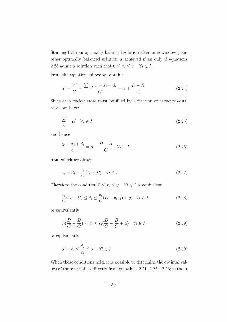
Starting from an optimally balanced solution after time window j an-

other optimally balanced solution is achieved if an only if equations

2.23 admit a solution such that 0 ≤ xi ≤ yi ∀i ∈ I.

From the equations above we obtain:

α′ =Y ′

C=

∑i∈I yi − xi + di

C= α +

D −B

C(2.24)

Since each packet store must be filled by a fraction of capacity equal

to α′, we have:

y′ici

= α′ ∀i ∈ I (2.25)

and hence

yi − xi + di

ci

= α +D −B

C∀i ∈ I (2.26)

from which we obtain

xi = di − ci

C(D −B) ∀i ∈ I (2.27)

Therefore the condition 0 ≤ xi ≤ yi ∀i ∈ I is equivalent

ci

C(D −B) ≤ di ≤ ci

C(D − bi+1) + yi ∀i ∈ I (2.28)

or equivalently

ci(D

C− B

C) ≤ di ≤ ci(

D

C− B

C+ α) ∀i ∈ I (2.29)

or equivalently

α′ − α ≤ di

ci

≤ α′ ∀i ∈ I (2.30)

When these conditions hold, it is possible to determine the optimal val-

ues of the x variables directly from equations 2.21, 2.22 e 2.23; without

59

having recourse to any optimization algorithm.

2.4.3 Balancing an Unbalanced Solution

Even if for some time window j it is impossible to achieve an optimally

balanced solution, as defined before, it is however of practical interest to

keep the solution as balanced as possible in the subsequent time window

j + 1. Following the method outlined before for Case 2, it easy to show that

an optimally balanced solution can be achieved after time window j +1 from

any solution after time window j if and only if the following conditions hold:

ci(D

C− B

C+

Y

C− yi

ci

) ≤ di ≤ ci(D

C− B

C+

Y

C) ∀i ∈ I (2.31)

The condition resembles condition 2.29 with the only difference that the

upper and the lower limit to di are now increased by a term ci(YC− yi

ci), which

can be positive or negative according to the load unbalance in packet store

i ∈ I with respect to the average load YC

. As a consequence in this case

each of the two bounds on di is more (or less) restrictive than in the case

analyzed in the previous subsection. In Case 1, i.e. when Y ≤ B, the analysis

presented in the previous subsection still holds.

2.4.4 A Fast Heuristic

The analysis presented here above directly suggests the implementation of an

very simple and fast heuristic, which iteratively considers the time windows

in chronological order, analyzes each of them in order to detect whether

the corresponding balancing subproblem is “easy” or “difficult” and solves

it, in the former case directly by using equations previously described, in

the latter case by linear programming by solving a problem like 2.11 - 2.19

without index j (because it concerns only one time window at a time). The

pseudocode of this Fast Heuristic for MEX-MDP (FH-MDP) is reported in

Algorithm 7. If all subproblem, one for each time window, happen to be

“easy”, then the overall problem is “easy” and the overall solution computed

by this algorithm is guarantied to be optimal; otherwise our algorithm achieve

60

the optimality in every single subproblem but not in the overall problem, so

there is no optimality guarantee. The advantage of such a heuristic algorithm

is to avoid solving a potentially large linear programming problem, in case

of very tight time restrictions (for instance when real-time re-planning is

needed).

Data: MEX-MDP instanceResult: Set of telecommandsInitialization;forall Time windows j ∈ J do

if B ≥ Y thenEasy iteration (Case 1);Dump all stored data ;

else if B = 0 thenEasy iteration (No optimizations are possible);Store all new data;

else if Condition 2.31 thenEasy iteration (Case 2);Solved by using equations 2.21, 2.22 e 2.23;

elseDifficult iteration;Solver (GLPK);

Automatic generation of telecommands;Algorithm 7: FH-MEX pseudocode

2.5 Computational Results

2.5.1 Implementation

We have developed a linear programming model and an heuristic algorithm.

Both, the model and the algorithm, have been designed to provide high-

quality solutions for MEX-MDP. The model has been written in GNU Math-

Prog language and solved by means of the free stand-alone LP/MIP solver

glpsol included in the GNU Linear Programming Kit (GLPK). A full tran-

scription of the model can be found in appendix A. The FH-MEX algorithm

has been implemented in C++ and it uses the linear programming API in-

61

cluded in GLPK to solve the difficult iterations, this API is a set of routines

written in ANSI C and organized in the form of a callable library for solving

linear and mixed integer programming problems. We have used the version

4.24 of GLPK (November 2007).

2.5.2 Input

Computational experiments have been done on one of the sets of the bench-

mark instances provided by Oddi and Policella [5], available on line. This set

has been referred to as “B5”, the instances contained in it come directly from

the test data provided by the ESA’s mission planning experts and have been

pushed through a randomization phase. All the instances of the set B5 are

made up of 13 packet stores (not all of them are used at the same time) and

of a set of POR. The number of POR is different from instance to instance

and it ranges from 15 to 96. The instances B5-8 and B5-9 are the easiest

ones to solve, indeed, they have only 15 POR and 4 useful packet stores.

We remark that such instances, although they have some simplifications, are

roughly as complex as the real instances.

2.5.3 Results Analysis

In the following section we present an analysis of computational results on

B5 instances. Our results are displayed by means of tables and charts. The

following abbreviations are employed:

OPT: the optimal results achieved by solving our linear model.

OP-MEX: the results of the algorithm for MEX-MDP described and im-

plemented by Oddi and Policella [3, 5]

FH-MEX: the results of our fast heuristic for MEX-MDP

The computational experiments have been done on a Intel Core2 Duo T7300

(2.0GHz), 2 GB RAM machine on GNU/LINUX operating system.

The best results obtained by the three approaches are summarized in

Table 2.1 and in Figure 2.1. These values indicate the maximum memory

62

Instance N OPT OP-MEX FH-MEX1 0.68 0.73 0.722 0.65 0.76 0.713 0.68 0.78 0.684 0.59 0.75 0.665 0.68 0.73 0.726 0.69 0.74 0.727 0.59 0.70 0.668 0.59 0.59 0.599 0.59 0.59 0.59

Media 0.64 0.71 0.67

Table 2.1: Maximum saturation level

Figure 2.1: Maximum saturation level

63

saturation level for each of the three algorithms. We recall that lower val-

ues indicate better performances because a lower utilization rate means a

higher robustness. The results obtained by FH-MEX are always in the mid-

dle between OP-MEX and OPT. Our heuristic comes to the optimal value

three-time. However the optimum is always achieved by all three algorithms

on the easiest instances in the benchmark set B5 (B5-8 and B5-9).

Instance OP-MEX FH-MEX Improvement%1 7.35 5.88 20.002 16.23 9.23 45.453 14.71 0 1004 27.12 11.86 56.255 7.35 5.88 20.006 7.25 4.35 40.007 18.64 11.87 36.368 0 0 09 0 0 0

Media 10.98 5.40 35.34

Table 2.2: GAP % relative to optimum

The table 2.2 and the Figure 2.2 present the percentage difference (gap%)

between the solutions obtained with each heuristic (OP-MEX and FH-MEX)

and the optimal value achieved by solving the linear programming model.

The results given by our heuristic are significantly better than those of the

Oddi and Policella’s algorithm: the average percentage gap from optimality

is 5.40% instead of 10.98%. The FH-MEX reduces the maximum gap% from

28.12% reached by OP-MEX to 11.87% improving the average robustness of

the generated solutions by 35.34%. In particular, leaving the easiest instances

(B5-8 and B5-9) out, FH-MEX always yields results which are at least 20%

better than OP-MEX.

In Table 2.3 and in the chart in Figure 2.3 it is displayed the average

memory saturation level obtained by the three algorithms. That is the math-

ematical average of the maximum saturation levels among all useful packet

stores. In order to compute this value we take into account only the really-

used packet stores, i.e. in some instances not all packet stores memorize any

64

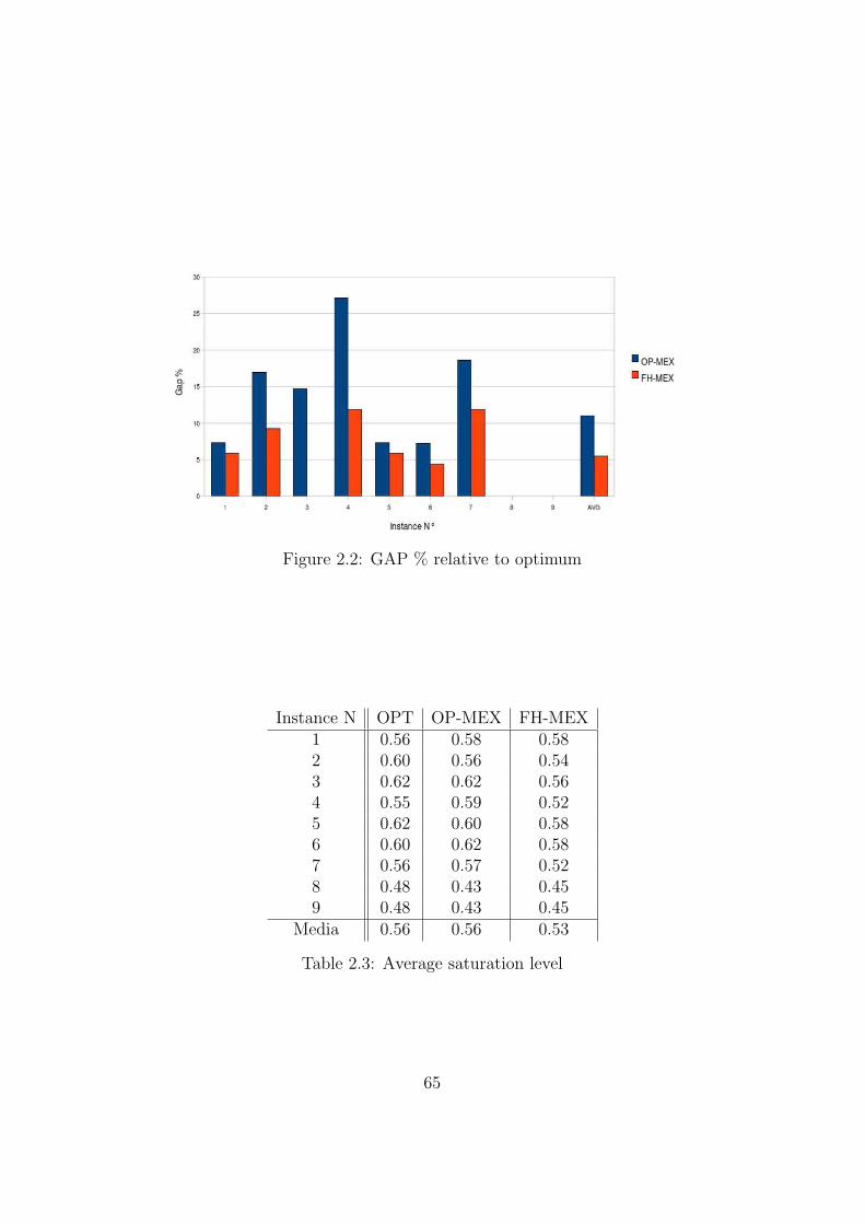
Figure 2.2: GAP % relative to optimum

Instance N OPT OP-MEX FH-MEX1 0.56 0.58 0.582 0.60 0.56 0.543 0.62 0.62 0.564 0.55 0.59 0.525 0.62 0.60 0.586 0.60 0.62 0.587 0.56 0.57 0.528 0.48 0.43 0.459 0.48 0.43 0.45

Media 0.56 0.56 0.53

Table 2.3: Average saturation level

65

Figure 2.3: Average saturation level

information, in this case the useless packet stores are not counted to compute

the average saturation level. We remark that a low value of average satura-

tion level does not directly mean an high-quality solution. Indeed OPT often

has a average saturation level higher than both OP-MEX and FH-MEX even

thought it achieves better solutions. In fact, it is possible that solutions in

which all packet stores nearly have the same saturation level, have a higher

average saturation level than solutions with high-variability saturation level.

Therefore we report in Table 2.4 and in Figure 2.4 the standard deviation

values of the average saturation level (SDev%). The SDev% indicates the

uniformity rate of the memory saturation among the packet stores. The

lower is this value the more uniform is the memory usage. High values mean

that there are some almost-full packet stores and some other which are nearly

empty.

At a superficial analysis the solutions seem to be quite similar. The

SDev% values achieved by OPT and FH-MEX are very near each other and

the values obtained by OP-MEX are not so far away. Moreover, OP-MEX

often yields solutions which have high variability in the memory usage and

FH-MEX seems to have the most uniform memory saturation even more

66

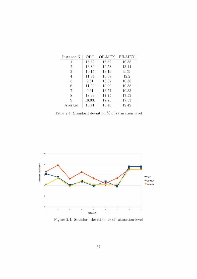
Instance N OPT OP-MEX FH-MEX1 15.52 16.52 10.382 13.89 19.58 13.443 10.15 13.19 9.594 11.94 16.38 12.25 9.81 13.37 10.386 11.90 10.99 10.387 9.61 13.57 10.338 18.93 17.75 17.539 18.93. 17.75 17.53

Average 13.41 15.46 12.42

Table 2.4: Standard deviation % of saturation level

Figure 2.4: Standard deviation % of saturation level

67

than the optimal algorithm. Going into more depth on our analysis we find

out that the solutions generated by the three algorithms have really different

structures.

In order to show what are the differences among the solutions we re-

port in Table 2.5 and in the chart in Figure 2.5 the maximum saturation

levels achieved by the three algorithms for each single packet store in the

instance B5-2. We chose this instance because in it the differences are more

pronounced. Anyway all instances show, approximately, the same behavior.

P/S N OPT OP-MEX FH-MEX1 0.65 0.73 0.572 0.65 0.75 0.543 0.65 0.64 0.534 0.65 0.66 0.675 0.59 0.73 0.7110 0.65 0.50 0.5211 0.65 0.35 0.5112 0.65 0.39 0.5613 0.23 0.23 0.23

Average 0.60 0.56 0.54Average 1-12 0.64 0.57 0.58

SDev% 13.89 19.58 13.44SDev% 1-12 2.12 16.33 7.37

Table 2.5: Saturation level Instance N◦ 2

The differences among the structures of the solutions computed by the

three algorithms are really clear. The solution generated by solving the linear

programming model have an uniform saturation level, equal to the optimal

value, for seven of the nine useful packet stores. Such a result assures a

very unifor memory saturation. Comparing the two heuristic algorithms we

notice that while the solution achieved by FH-MEX offers more uniformity

in the memory usage, instead, OP-MEX present perceptible variations in the

memory saturation among the packet stores i.e. in three packet stores the

saturation level is less than 0.4 and in other three is over 0.7.

68

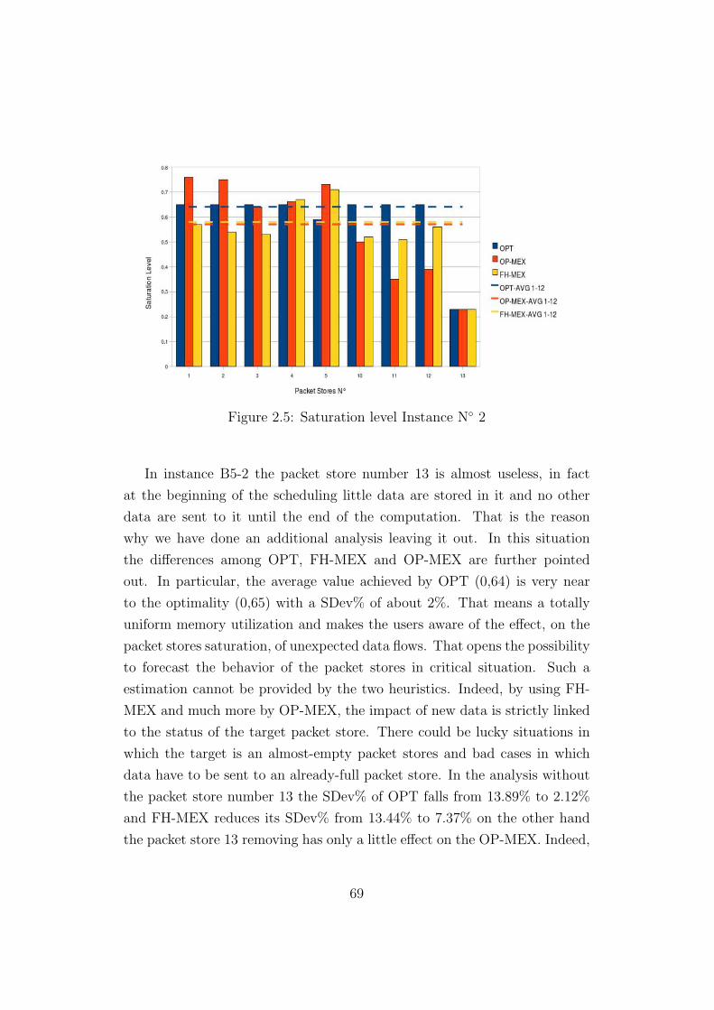
Figure 2.5: Saturation level Instance N◦ 2

In instance B5-2 the packet store number 13 is almost useless, in fact

at the beginning of the scheduling little data are stored in it and no other

data are sent to it until the end of the computation. That is the reason

why we have done an additional analysis leaving it out. In this situation

the differences among OPT, FH-MEX and OP-MEX are further pointed

out. In particular, the average value achieved by OPT (0,64) is very near

to the optimality (0,65) with a SDev% of about 2%. That means a totally

uniform memory utilization and makes the users aware of the effect, on the

packet stores saturation, of unexpected data flows. That opens the possibility

to forecast the behavior of the packet stores in critical situation. Such a

estimation cannot be provided by the two heuristics. Indeed, by using FH-

MEX and much more by OP-MEX, the impact of new data is strictly linked

to the status of the target packet store. There could be lucky situations in

which the target is an almost-empty packet stores and bad cases in which

data have to be sent to an already-full packet store. In the analysis without

the packet store number 13 the SDev% of OPT falls from 13.89% to 2.12%

and FH-MEX reduces its SDev% from 13.44% to 7.37% on the other hand

the packet store 13 removing has only a little effect on the OP-MEX. Indeed,

69

the Oddi And Policella’s algorithm still have a SDev% greater than 16% that

means a high variability in the memory saturation level.

Instance N. of packet stores OPT FH-MEXB5 13 0.01 <0.001

B5-28 28 0.7 0.10B5-54 54 2.32 0.11

Table 2.6: Average computing time (sec.)

Instance N. of packet stores OPT FH-MEXB5 13 3.7 0.2

B5-28 28 7.6 0.3B5-54 54 14.9 0.4

Table 2.7: Memory allocation (MB)

A direct comparison between our algorithms and the OP-MEX about the

computing time was not possible because the OP-MEX has been merged

in a very large tool providing complete support for the scheduling of Mars

Express downlink activities (MEXAR2) and so we were not able to reMEX-

MDP:tableTime-run the original Oddi and Policella’s algorithm for MEX-

MDP on our machine. For the sake of comparison with the state of the art,

the computing time reported in [5] for solving instance B5 in an approxi-

mate way is 21.8 seconds on a AMD Athlon 1.8 GHz processor. In table

2.6 are reported the computing times obtained by solving the model and by

our heuristic referred to three benchmark the first one, B5, is the same as

before; the other two are artificially made by combining together two or more

instances from B5, in order to have a larger number of packet stores. In par-

ticular the instances included in B5-28 and B5-54 have, respectively, 28 and

54 packet stores. The LP solver and our heuristic turns out, respectively, to

be three and four orders of magnitude faster than OP-MEX. FH-MEX is al-

ways faster than the LP solver and its computing time is growing, along with

the solved instances width, significantly more slowly than the time consumed

by the solver. The average number of MB of memory allocated by our two

70

algorithms are displayed in Table 2.7. It is clearly visible that the heuristic

utilization of memory is about twenty times lower than the LP solver usage.

Indeed, while the heuristic have to solve, for each iteration a problem which

have a dimension proportional to the number of packet stores on the other

hand the solver have to deal with a much larger problem i.e. proportional to

the product of the number of packet stores and the time windows.

Instance FH-MEX1 79.522 77.333 92.774 92.315 80.686 81.727 91.188 79.179 76.19

media 83.43

Table 2.8: % of “easy” iteration

None of the analyzed instances is “easy” (according to our definition in

section 2.4.4). For each instance there is at least a “difficult” iteration, the

percentage of “easy” iterations (those for which the heuristic does not call

the LP solver) is usually greater than 75% and that is one of the reasons why

the heuristic is so fast.

2.6 MEX-MDP Extensions

The model considered here is a simplified version of the real Mars Express

memory dumping problem. In this section we show how our approach can be

easily extended to cope with additional restrictions and objectives, described

hereafter.

Housekeeping data. Every day the housekeeping packet stores are to-

tally filled and have to be emptyed, as soon as possible, before a new data

71

injection. Moreover, due to the structure of the housekeeping packet stores

a dump operation performed on a housekeeping packet stores involves the

complete dump of the packet stores. For this reason a dump operation on

a housekeeping packet store cannot be splitted on two or mode parts. To

simulate this behaviour we do not use a mathematical model to allocate

housekeeping dump operation among the transmission window. We devel-

oped a preprocessing phase in which analyzing the time window between

two data injection on housekeeping packet stores we assign the dump of a

housekeeping packet store to the first available window having enought dump

capacity. The residual capacity will be used to dump science packet stores.

Residual data The firs goal of a dump plan is the minimization of the

residual amount of data in the packet stores at the end of the planned period.

To take this purpose into account we introduce a new objective in our model:

min :∑

i ∈ Iy[i, t] t = max(j ∈ J) (2.32)

This goal is the most important and is the first objective taken into account

by our model.

Constraints on the amount of dumped data. Scientific data cannot be

transmitted to the Earth in any amount, but only by integer multiples of bits.

Therefore all variables in our model are measured in bits and they can only

take on integer values. To achieve this, it is sufficient to impose integrality

constraints on the x variables, since the amounts d are guaranteed to be

integer and the equality constraints propagate this restriction also to y and

z variables.

Number of dump operations. Since the spacecraft is not able to manage

dump activities by itself, dump operations are driven by telecommands sent

from the Earth. The dispatch of a telecommands involves costs, uplink band

saturation and risk, for this reason the lower is the amount of dump operation

to perform the higher is the quality of a plan. To take this objective into

72

account we introduce binary variables wij for each packet store i ∈ I. If and

only if wij = 1, the content of packet store i ∈ I is transmitted to the Earth

during time window j ∈ J . Moreover, we introduce constraints

xij ≤ ciwij ∀i ∈ I ∀j ∈ J (2.33)

which ensure that only when wi,j = 1 a dump operation can take place. This

new objective is modelled as follow:

min :∑

i∈I,j∈J

w[i, j] (2.34)

The minimization of the total number of dump operations is more important

than the minimization of the saturation level (the objective function of the

reduced model) but less important than the minimization of the residual

data.

The real problem can be modelled as a multi objectives problem tak-

ing into account, following the relevance order, all objectives previously de-

scribed. In order to solve the multi-objective model we realized a 4-steps

algorithm:

1. Generation of a dump plan for housekeeping packet stores following the

criteria previously mentioned.

2. Generation of a dump plan for science packet stores in which the goal

is the minimization of the residual data in science packet stores at the

end of the planned period. In this step we use the same model used for

solving the reduced problem with 2.32 as objective function.

3. Optimization of the plan generated in the previous step minimizing

the number of dump operations. In this step we convert the objective

function of the previous step in a constraints:

∑i∈I

y[i, t] = objStep2 t = max(j ∈ J) (2.35)

We introduce, as described before, binary variables wi,j and the con-

73

straints 2.33, moreover we set the alpha value to 95% in order to achieve

a plan that do not totally saturate the packet store. The objective func-

tion of this step is 2.34.

4. Optimization of the plan generated in the previous step minimizing the

saturation level of the science packet stores. In this step, like in the pre-

vious one, we start from the outcome of the previous step introducing

the following constraint:

∑i ∈ I, j ∈ Jw[i, j] = objStep3 (2.36)

We reintroduce the alpha as used in the model for the reduced problem

and the objective function becomes 2.11 (the same objective function

we use in the reduced model).

The global model we use in the last three steps is reported in B.

2.7 MEX-MDP extended problem evaluation

To perform an experimental evaluation of our approach we use a set of 9

instance coming from real data. In table 2.9 are reported some information

about the input set:

• N Days: is the number of the days that are taken into account in the

instance.

• N CC: is the number of communication channels in the instance.

• N Store op: is the number of store operations in the instance.

The model has been solved using the commercial solver CPLEX 11 on a

Intel Core2 Duo E6850 (3GHz) 2 GB RAM machine. We tryed to achieve

a solution using non commercial solver like GLPK and lpsolve but we were

not able to generate right solution because of numerical problem due to the

size of the integer values in the model.

In order to compare our results with the state of the art we solve the

same set of instances with MEXAR2 using the following settings:

74

Instance N Days N CC N Store op70-71 2 9 3770-73 4 19 35770-83 14 64 63870-90 21 95 93570-100 31 141 131471-85 15 71 71580-81 2 10 11080-84 5 32 28780-100 21 98 876

Table 2.9: MEX-MDP-EXT instances

• No priority: the priority of the packet stores are not taken into account.

• No minimal duration: the dump operation do not have a minimal du-

ration.

• Max robustness: the robustness level of the plans generated by MEXAR2

is the maximum that can be achieved by this tool.

With these settings both tools taken into account the same set of constraints.

The results achieved by both tools are reported in table 2.10 in which we use

the following abbreviations:

• N dump: the overall number of dump operation.

• Saturation: the maxim level of saturation of the packet stores.

• Time: the computational time used to generate the plan. We impose

a 900 seconds limit to CPLEX.

In order to make easyer the comparison between the the solution gener-

ated by the model and by MEXAR we report in the table 2.11 the percentage

difference between the results achieved by the two tools taking RAXEM2 as

touchstone.

It is clear that, looking at the number of dump operation, the results

obtained by solving the model are significantly better than the ones achieved

75

MEX-MOD MEXAR2Instance n Dump Saturation Time n Dump Saturation Time70-71 21 47.28 0.02 24 47.28 3.8870-73 43 94.99 0.21 71 94.57 15.5370-83 156 94.99 0.99 280 94.57 243.5670-90 232 94.99 900 425 94.57 553.5770-100 291 94.99 900 577 94.57 1660.1971-85 173 94.99 900 319 94.57 338.1380-81 25 94.99 0.02 47 78.81 3.3880-84 68 94.99 0.48 111 94.57 24.3480-100 220 94.99 900 385 99.40 833.53

Table 2.10: MEX-MDP-EXT experimental results

Instance n Dump Saturation Time70-71 -37.50 0.00 -99.4870-73 -39.44 0.44 -98.6570-83 -44.29 0.44 -99.5970-90 -45.41 0.44 62.5870-100 -49.57 0.44 -45.7971-85 -45.77 0.44 166.1780-81 -46.81 20.53 -99.4180-84 -38.74 0.44 -98.0380-100 -45.94 -4.44 7.97average -40.94 2.08 -29.33

Table 2.11: MEX-MDP-EXT percentage difference

76

Figure 2.6: Saturation level on instance 70-71

by MEXAR2, on the other hand, since we are able to obtain optimal or

almost optimal solutions in the third step, the space for optimization in the

last step is very little. This is the reason why the final saturation level is very

near to the 95% threshold we imposed. It easy to demonstrate that relaxing

the constraints on the number of dump operations in the last step of our

algorithm it can achieves solution with a better saturation level. In chart 2.6

are reported the saturation levels on instance 70-71 using a number of dump

operation between 21 and 25. With the same number of dump operation

used by MEXAR2 our algorithm is able to generate a plan with maximum

saturation level equal to 38,52%, 33.33% better than the solution computed

by MEXAR2.

Our algorithm turns out to be usually faster on small instances and slower

on the biggest ones, indeed the algorithm used by MEXAR2 provides a better

scalability. Despite that imposing a 900 seconds time limit we are able to

generate better solution using roughly the same time used by MEXAR2.

77

2.8 Conclusions

The problem of computing a schedule of maximum robustness for the Mars

Express mission has been analyzed and solved via linear programming. Our

analysis also provides a characterization of “easy” and “difficult” instances.

In the former case the optimal solution can be computed directly by a simple

formula, without having recourse to any optimization algorithm; in the latter

case an optimal solution can be computed in fractions of seconds by a linear

programming solver.

Starting from the simplified model of Oddi and Policella [3, 5] we have

extended it to consider real constraints such as indivisibility of some data

files and different objective functions. The resulting integer linear program-

ming models have also been solved by general purpose solvers providing solu-

tions that turn out to be, as regards the number of dump operations, better

than the MEXAR2 solutions and mostly not worse than MEXAR2 from the

saturation level point of view. The ability to incorporate in these models

different and conflicting objective functions allowed to set-up an effective

decision support system for the decision-makers who manage the mission.

Future development plans for this approach concerns the finding of a better

trade-off between the minimization of the number of dump operation and

the saturation level and the implementation of a graphical user interface to

make the tool more user friendly.

78

Bibliography

[1] M. Denis A. Cesta, G. Cortellessa, A. Donati, S. Fratini, A. Oddi, N. Po-

licella, E. Rabenau, and J. Schulster. RAXEM - Supporting Command

Uplink in MARS EXPRESS . In Proceedings of the 9th International

Symposium in Artificial Intelligence, Robotics and Automation in Space,

iSAIRAS-08, 2008.

[2] A. Cesta A. Oddi, N. Policella and G. Cortellessa. Generating high quality

schedules for a spacecraft memory downlink problem. In CP-03, Kinsale,

Ireland, September 2003.

[3] A. Cesta, A. Oddi, G. Cortellessa, and N. Policella. Automating the

generation of spacecraft downlink operations in mars express: Analysis,

algorithms and an interactive solution aid. Technical Report MEXAR-

TR-02-10 (Project Final Report), ISTC-CNR [PST], Italian National Re-

search Council, July 2002.

[4] A. Makorin. Modeling Language GNU MathProg, May 2007. Language

Reference, Draft Edition for GLPK.

[5] Angelo Oddi and Nicola Policella. Improving robustness of spacecraft

downlink schedules. IEEE Transactions on Systems, Man, and Cyber-

netics – Part C: Applications and Reviews, 37(5), 2007.

[6] E. Rabenau. Uplink requirements tool specification (MEXUP). Technical

report, European Space Agency, March 2006.

[7] O.J. Orlin R.K. Ahuja, T.L. Magnanti. Network flows. Prentice Hall,

1993.

79

Appendix A

MEX-MDP LinearProgramming Model

The mathematical model here reported is written in GNU MathProg [4].

#MEX-MDP model

/* I: Packet Stores set*/

set I;

/* J: transmission windows set*/

set J;

/* c: capacity for each packet store*/

param c{i in I};

/* b: dump capacity for each window*/

param b{j in J};

/* f: amount of data stored in each packet stores i in I

at the start time (j=0)*/

param f{i in I};

/* d: amount of data stored in each packet stores i in I

at the end of each window j in J*/

param d{i in I, j in J};

/* x: amount of data to be transferred from each

80

packet stores i in I to the Earth in each window j in J*/

var x{i in I, j in J}>=0;

/* y: amount of data stored in each packet store i in I after each

time window j in J*/

var y{i in I, j in J}>=0;

/* z: amount of data stored in each packet store i in I after each

data transmission in window j in J*/

var z{i in I, j in J}>=0;

/* alpha: max fraction of capacity of a packet store (to minimize)*/

var alpha >=0 , <=1;

/*OBJ function*/

minimize fraction: alpha;

s.t. ini2{i in I,j in J: j=0}: 0 = x[i,j]

s.t. ini2{i in I,j in J: j=0}: f[i] = z[i,j];

s.t. con1{i in I,j in J: j>0}: y[i,j-1] = x[i,j] + z[i,j];

s.t. con2{i in I,j in J}: z[i,j] + d[i,j] = y[i,j];

s.t. con3{i in I,j in J}: y[i,j] <= alpha * c[i];

s.t. con4{j in J}: sum{i in I} x[i,j] <= b[j];

end;

81

Appendix B

MEX-MDP EXTENDEDLinear Programming Model

The mathematical model here reported is written in GNU MathProg [4].

#MEX-MDP model

/* I: Science Packet Stores set*/

set I;

/* J: transmission windows set*/

set J;

/* t: number of transmission windows is the max value in J*/

param t ;

/*r: overall amount of residual data in the last window (t)*/

param r ;

/*o: total number of TCs computed in the previous step*/

param o ;

/* c: capacity for each packet store*/

param c{i in I} ;

/* b: dump capacity for each window*/

param b{j in J} ;

/* f: amount of data stored in each packet stores i in I

82

at the start time (j = 0)*/

param f{i in I} ;

/* d: amount of data stored in each packet stores i in I

at the end of each window j in J*/

param d{i in I, j in J} integer, >=0;

/* x: amount of data to be transferred from each packet stores

i in I to the Earth in each window j in J*/

var x{i in I, j in J} integer, >=0;

/* y: amount of data stored in each packet store i in I after

each time window j in J*/

var y{i in I, j in J} integer, >=0;

/* z: amount of data stored in each packet store i in I after

each data transmission in window j in J*/

var z{i in I, j in J} integer, >=0;

/* w: dump or not dump packet store i in I

for each transmission window j in J*/

var w{i in I, j in J} binary;

/* alpha: max fraction of capacity of a packet store (to minimize)*/

var alpha >=0 , <=1;

/*OBJ function*/

minimize obj_0: sum{i in I} y[i,t];

minimize obj_1: sum{i in I, j in J} w[i,j];

minimize obj_2: alpha;

/*INITIALIZATION*/

/* at the beginning the amount of data transmitted +

the data stored after dumping but before the storing operation

is equal to the initial data*/

s.t. ini1{i in I, j in J: j=0}: f[i] = x[i,j] + z[i,j];

/*GLOBAL CONSTRAINTS*/

/* the amount of data stored at the end of each window

is equal to residual data after dump + new data */

83

s.t. con1g{i in I, j in J}: z[i,j] + d[i,j] = y[i,j];

/*the overall amount of data stored at the end of the j-1 window

is equal to the amount of data dumped in j + the residual data in j*/

s.t. con2g{i in I, j in J: j>0}: y[i,j-1] = x[i,j] + z[i,j];

/*the overall amount of data dumped during a window

cannot be greater than the dump capacity in this window*/

s.t. con3g{j in J}: sum{i in I} x[i,j] <= b[j];

/*w=0 dump not allowed*/

s.t. con4g{i in I, j in J}: x[i,j] <= w[i,j]*c[i];

/*The overall amount of residual data (window t) is equal to

the obj of the step 0*/

s.t. con5g: sum{i in I} y[i,t] <= r;

/*The number of TC is equal to the obj of the step 1*/

s.t. con6g: sum{i in I, j in J} w[i,j] <= o;

/*the overall amount of data stored at the end of the window j

is less or equal to the alpha fraction of the PS capacity*/

s.t. con7g{i in I, j in J}: y[i,j] <= alpha * c[i];

end;

84

universit`a degli studi di milano - optlab web pageoptlab.di.unimi.it/docs/tresoldi2.pdf ·...

Documents