· universidade de sao paulo˜ instituto de f´ısica aspectos de lac¸os de wilson...
TRANSCRIPT

Universidade de Sao Paulo
Instituto de Fısica
Aspectos de lacos de Wilson holograficos
Jose Renato Sanchez Romero
Orientador: Prof. Dr. Diego Trancanelli
Tese de doutorado apresentada ao Instituto de Fısica
da Universidade de Sao Paulo, como requisito parcial
para a obtencao do tıtulo de Doutor em Ciencias.
Banca Examinadora:
Prof. Dr. Diego Trancanelli - Orientador (IF-USP)
Prof. Dr. Victor Rivelles (IF-USP)
Prof. Dr. Horatiu Nastase (IFT-UNESP, Brasil)
Prof. Dr. Diego Correa (IF-UNLP, Argentina)
Prof. Dr. Alberto Faraggi (Ciencias Exactas/UNAB, Chile)
Sao Paulo
2019

FICHA CATALOGRÁFICAPreparada pelo Serviço de Biblioteca e Informaçãodo Instituto de Física da Universidade de São Paulo
Sánchez Romero, José Renato
Aspectos de laços de Wilson holográficos/Aspects of holographic Wilson loops. São Paulo, 2019.
Tese (Doutorado) – Universidade de São Paulo. Instituto de Física. Depto. de Física Matemática. Orientador: Prof. Dr. Diego Trancanelli Área de Concentração: Física Matemática Unitermos: 1. Supergravidade; 2. Teoria de campos; 3. Teoria de campos unificados; 4. Teoria quântica de campo; 5. Física teórica.
USP/IF/SBI-071/2019

University of Sao Paulo
Physics Institute
Aspects of holographic Wilson loops
Jose Renato Sanchez Romero
Supervisor: Prof. Dr. Diego Trancanelli
Thesis submitted to the Physics Institute of the Uni-
versity of Sao Paulo in partial fulfillment of the re-
quirements for the degree of Doctor of Science.
Examining Committee:
Prof. Dr. Diego Trancanelli - Orientador (IF-USP)
Prof. Dr. Victor Rivelles (IF-USP)
Prof. Dr. Horatiu Nastase (IFT-UNESP, Brazil)
Prof. Dr. Diego Correa (IF-UNLP, Argentina)
Prof. Dr. Alberto Faraggi (Ciencias Exactas/UNAB, Chile)
Sao Paulo
2019

A mis padres, por haber soportado esto.

Acknowledgments
O presente trabalho foi realizado com apoio da Coordenacao de Aperfeicoamento de Pes-
soal de Nl Superior -Brasil (CAPES) - Codigo de Financiamento 001.
I thank Prof. Diego Trancanelli for his advice and time.
I would like to thank the members of my defense committee: Prof. Victor Rivelles,
Prof. Horatiu Nastase, Prof. Diego Correa and Prof. Alberto Faraggi, for their comments
and suggestions on this work.
I also would like to specially thank Sara Bonansea for the discussions and for sharing
her notes. You saved my life. Grazie mille!
A Jona, Pedro y Pepe, quienes afortunadamente no son fısicos, por mantener a la
distancia mis pies en la tierra por tantos anos.
A Janett. A mis padres. A Laura.
i

ii
“In my opinion, one who intends to write a book ought to consider carefully the subject
about which he wishes to write. Nor would it be inappropriate for him to acquaint
himself as far as possible with what has already been written on the subject. If on his
way he should meet an individual who has dealt exhaustively and satisfactorily with one
or another aspect of that subject, he would do well to rejoice as does the bridegroom’s
friend who stands by and rejoices greatly as he hears the bridegroom’s voice. When he
has done this in complete silence and with the enthusiasm of a love that ever seeks
solitude, nothing more is needed; then he will carefully write his book as spontaneously
as a bird sings its song, and if someone derives benefit or joy from it, so much the better.”
VIGILIUS HAUFNIENSIS


Resumo
Nesta tese estudamos alguns aspectos da correspondencia AdS/CFT. Em particular aque-
les que involvem quantidades que podem ser calculadas exatamente, como os lacos de
Wilson. A correspondencia calibre/gravidade ou AdS/CFT nos permite interpretar duas
teorias diferentes com as mesmas simetrias globais como descricoes complementares da
”mesma fısica”. Os valores de expectacao dos lacos de Wilson em varias representacoes
podem ser calculados em ambos lados da dualidade usando modelos de matrizes na teoria
de calibre e cordas e branas no lado da gravidade. Do ponto de vista holografico, a re-
ceita geral nos diz que devemos minimizar a folhamundo das cordas ou volumemundo das
branas com limite no laco. Essas tecnicas, ja aplicadas aos casos das representacoes fun-
damental e (anti)simetrica do laco de Wilson, podem ser extendidas a representacoes mais
complicadas cujo dual sao branas coincidentes e geometrias ”bubbling”. Um fenomeno
interessante tambem e aquele que ocorre quando consideramos dois lacos, o que na teoria
de gravidade se traduz como a solucao conectada tipo catenoide. A existencia de super-
ficies conectadas entre dois lacos de Wilson depende do valor de varios parametros que
descrevem a geometria e posicao relativa dos lacos. Aqui, devido a esses parametros,
existe uma transicao de fase chamado de Gross-Ooguri, onde a solucao conectada nao e
“energeticamente favoravel” com respeito a solucao desconectada, i.e. dois lacos inde-
pendentes. Muito mais interessante e rico e o caso de lacos de Wilson na presenca de
defeitos, i.e. regioes de interfase devidas a presenca, no caso estudado aqui, de uma D5
brana. Estudamos tambem o correlador entre dois lacos neste caso.
Palavras chave Correspondencia AdS/CFT; lacos de Wilson; acao DBI naoabeliana;
transicao de Gross-Ooguri.
iii

Abstract
In this thesis we study some aspects of the AdS/CFT correspondence. In particular those
involving observables that can be computed exactly, as Wilson loops. The gauge/gravity
correspondence or AdS/CFT allows us to interpret two different theories with the same
global symmetries as complementary descriptions of the ”same physics”. The expectation
values of Wilson loops in several representations can be calculated on both sides of the
duality by using localization in the gauge theory and strings and branes on the gravity side.
From the holographic point of view, the general recipe tells us that we have to minimize
the string worldsheet or brane worldvolume with the loop as boundary. These techniques,
already applied to the fundamental and (anti)symmetric reprentations of the Wilson loops,
can be extended to more complicated reprentations whose duals are coincident branes and
bubbling geometries. An interesting phenomenom also is that in which we consider two
loops, that on the gravity side translate into the connected catenoid-like solution. The
existence of connected solutions between two loops depends on the values of several
parameters that describe the geometry and relative position between the loops. Here, due
to these parameters, exists a transition knows as Gross-Ooguri, in which the connceted
solution becomes energetically non-favorable with respect to the disconnected solution,
i.e. two independent loops. Much more interesting and rich is the case of two Wilson
loops in the presence of defects, i.e. interfase regions due to the presence of, in this case,
a D5 brane. We also study the correlator of two Wilson loops in this case.
Keywords AdS/CFT correspondence; Wilson loops; nonabelian DBI; Gross-Ooguri
phase transition.
iv


Contents
Acknowledgments i
Resumo iii
Abstract iv
Index iv
1 Introduction and Overview 1
2 Basics on the AdS/CFT correspondence 7
2.1 Superstring and supergravity: quick review . . . . . . . . . . . . . . . . 7
2.2 D3-branes in type IIB, the AdS5 × S5 geometry . . . . . . . . . . . . . . 9
2.3 D3-branes in type IIB, the N = 4 theory . . . . . . . . . . . . . . . . . . 11
2.3.1 A short pit stop on N = 4 D = 4 U(N) gauge theory. . . . . . . 14
2.3.2 The large N limit for any gauge theory . . . . . . . . . . . . . . 15
2.4 Motivating the AdS/CFT duality . . . . . . . . . . . . . . . . . . . . . . 17
2.4.1 Holographic duality . . . . . . . . . . . . . . . . . . . . . . . . 18
2.4.2 The dictionary . . . . . . . . . . . . . . . . . . . . . . . . . . . 19
3 Wilson loops, perturbative and exact results 21
3.1 (Supersymmetric) Wilson loops . . . . . . . . . . . . . . . . . . . . . . 21
3.1.1 Wilson loops in perturbation theory . . . . . . . . . . . . . . . . 24
3.1.2 Summing planar graphs . . . . . . . . . . . . . . . . . . . . . . 26
3.2 A brief introduction to matrix models and localization . . . . . . . . . . . 27
3.2.1 The saddle point method . . . . . . . . . . . . . . . . . . . . . . 30
v

vi
3.2.2 Orthogonal polynomials . . . . . . . . . . . . . . . . . . . . . . 31
3.2.3 Supersymmetric localization . . . . . . . . . . . . . . . . . . . . 33
4 Holographic Wilson loops 36
4.1 Boundary conditions . . . . . . . . . . . . . . . . . . . . . . . . . . . . 38
4.2 Legendre transform and the elimination of the divergence . . . . . . . . . 40
4.3 Three examples . . . . . . . . . . . . . . . . . . . . . . . . . . . . . . . 41
5 Branes as Wilson loops 46
5.1 Wilson loops in k-symmetric and k-antisymmetric representations . . . . 48
5.1.1 The large N ∼ k limit . . . . . . . . . . . . . . . . . . . . . . . 51
5.2 D-branes and holography . . . . . . . . . . . . . . . . . . . . . . . . . . 52
5.2.1 D5k-brane and the k-antisymmetric representation . . . . . . . . 53
5.2.2 D3k-brane and the k-symmetric representation . . . . . . . . . . 56
5.3 Beyond the leading order . . . . . . . . . . . . . . . . . . . . . . . . . . 59
5.4 Rectangular tableau and the need of a nonabelian DBI action . . . . . . . 60
5.4.1 Vertical rectangular tableau . . . . . . . . . . . . . . . . . . . . . 61
5.4.2 Horizontal rectangular tableau . . . . . . . . . . . . . . . . . . . 63
5.5 NADBI for two coincident D3 branes . . . . . . . . . . . . . . . . . . . 66
5.5.1 The U(2) case . . . . . . . . . . . . . . . . . . . . . . . . . . . . 70
6 Wilson loop correlators in holography 77
6.1 Two connected Wilson loops with ∆φ = 0 . . . . . . . . . . . . . . . . . 81
6.1.1 Evaluating the action . . . . . . . . . . . . . . . . . . . . . . . . 86
6.2 Two connected Wilson loops with ∆φ 6= 0 . . . . . . . . . . . . . . . . . 90
6.3 Disconnected case with the defect . . . . . . . . . . . . . . . . . . . . . 98
6.3.1 Evaluating the action . . . . . . . . . . . . . . . . . . . . . . . . 109
6.4 Phase transition in the presence of the defect . . . . . . . . . . . . . . . . 113
7 Results and outlook 121
A Symmetric/fundamental Wilson loop correlator 124
B Perturbative computation 132

vii
Bibliography 135

Chapter 1
Introduction and Overview
String theory [1,2] is one of its most fascinating attempts to formulate a consistent theory
of everything. One of the most captivating features of string theory is that it contains
gravity, having a graviton as an state of its spectrum. In order to be, mathematically, con-
sistent, string theory must be defined in ten-dimensional backgrounds making it necess-
sary to understand mechanisms to compactify the extra dimensions and making contact
with the real world. More than forty years after its discovery, there are still many people
trying to make progress in it. Not only theoretical physicists but also mathematicians and
even philosophers are working hard to understand the fundamentals of this theory and to
clarify some aspects of its formulation.
It was at the end of the nineties that a new avenue of research originated from string
theory appeared: the gauge/gravity (also known as gauge/string, in general, or simply
AdS/CFT) duality, that establishes that string theory in a certain background can be de-
scribed by (or as) a gauge theory [3–7]. The main point of this duality is that there must
exist one-to-one relations between observables on both sides. This is what we know as
the dictionary, or more precisely a bijection, of the duality. Both sides of the duality have
parameters such as coupling constant, central charge and radii of curvature which are re-
lated in simple ways. In particular, string theory is dual to a quantum field theory, but
depending on which regime of parameters one considers that either the stringy behavior
or the particle behavior of the theory is manifest. Also, string and quantum field theory
are complementary, i.e when it is hard to work with one of them then it is easier to work
with the other. This is called weak/strong coupling correspondence. In this sense we say
1

CHAPTER 1. INTRODUCTION AND OVERVIEW 2
that the correspondence ensures that we can look at a quantum field theory from a differ-
ent perspective, in which it looks like a string theory. We actually are not changing the
”nature” only its description. This means that, in the strong statement, all the physics of
one description can be mapped onto all the physics of the other. And, since string theory
contains gravity, this means that a theory of quantum gravity could be mapped to a quan-
tum field theory without it. It is also said that the duality is holographic: information of
the bulk is encoded at its boundary. In this case, information about strings is encoded at
the boundary of some space as a gauge theory [8, 9]. It was first studied the duality be-
tween Type IIB superstrings in AdS5 × S5 and N = 4 D = 4 SU(N) gauge theory [10],
being the simplest and best understood case until now since the gauge dual theory has the
largest supersymmetry in four dimensions and it is also a conformal field theory, i.e a the-
ory that does not depend on scales. In this case, it is assumed that the field theory “lives”
on the stack of D3 branes that source the ten-dimensional background. A lot of cases
were implemented thenceforth by trying to get evidence of the duality between string the-
ory in certain backgrounds and (supersymmetric) gauge theories. A particular example
is the duality between M theory/Type IIA string theory in AdS4 × S7/AdS4 × CP3 and
N = 6 D = 3 Chern-Simons theory, the most supersymmetric gauge theory in three
dimensions [11]. Another case that appeared almost at the same time that the first case
was the Klebanov-Witten background in which the S5 part was replaced by a singular
Calabi-Yau space T 11. The dual field theory of string in this background corresponds to
N = 1 SU(N)×SU(N) gauge theory [12] (see also [13,14]). Other cases include brane
intersections that, on the gauge side, generate new degrees of freedom, or defects that act
as boundaries in the field theory [15,16] (see also [17]). Also, results in a gauge (or string)
theory that inicially do not have their corresponding results in a string (or gauge) theory
serve as predictions and as a guide to pursue them, e.g non-commutative gauge theories
and deformed string backgrounds [18, 19] (see also [20] and references therein). Lots of
results have been obtained since the original statement of the conjecture, that allow us to
say that the duality is indeed true, so it appears as a new striking and useful theoretical
tool to make calculations and, principally, predictions. In particular, this could help to
explore quantum field theory in the non-perturbative regime.
There are now techniques to test the duality exactly, i.e. to have results that can be

CHAPTER 1. INTRODUCTION AND OVERVIEW 3
compared at the same regime, large N and large coupling constant: localization [21–24].
In particular, a largely studied observable in gauge theory is the Wilson operator [25,26]:
a non-local gauge invariant operator that describes the path of a heavy “quark”, an ob-
ject in the fundamental representation, in the (supersymmetric) field theory. It is known
as Wilson loop if the path is closed and circular Wilson loop if that closed path is a cir-
cle. Their expectation value in N = 4 gauge theory was computed perturbatively and
exactly [27–29]. In the gauge/gravity duality, the (fundamental) Wilson loop expecta-
tion value was first calculated by finding the area of the string worldsheet, given by the
string action, in the string background whose boundary is the loop itself [30–36]. Wil-
son loops in higher representations, which describe systems of “quarks” or a generalized
“quark”, were studied by generalizing the latter idea: by placing higher dimensional ob-
jects of string theory, branes, as probes in these backgrounds with the loop as a boundary,
and minimizing the action that describe them [37, 38]. As mentioned, there are meth-
ods in gauge theory that can produce exact results that include the regime in which the
gauge theory is more easily described by string theory. The calculation of the expected
value of Wilson loops in arbitrary representations was largely studied by using local-
ization techniques [39–42], because it was shown that when calculating the expectation
value of Wilson loops, Feynman diagrams involving loop corrections and vertices cancel
each other at each order in their expansion due to supersymmetry, resulting in a single
counting problem that can be expressed as a matrix model. This also worked for arbitrary
representations [43–45].
If instead of the expectation value of a single Wilson loop, one wanted to compute
the correlator between two loops, the relevant string worldsheet surface would be the
one connecting the two different contours [46–49]. This is similar to the Plateau’s prob-
lem (mentioned in [50]), in which one has to determine the shape of a thin soap film
stretched between two rings lying on parallel planes. Modifying the geometry of these
two rings introduces a phase structure: there are critical values for the parameters that
separate the ‘catenoid’ (connected or continuous) solution and the ‘Goldschmidt’ (dis-
connected or discontinuous) solution [51]. When the two rings are separated beyond a
certain critical value, the catenoid solution becomes unstable and breaks into the Gold-
schmidt one. Similarly, in the case of the Wilson loop, the string worldsheet describes a

CHAPTER 1. INTRODUCTION AND OVERVIEW 4
catenoid-like solution until, at certain values of the radii of the loops and the distance, it
becomes energetically unfavored with respect to the Goldschmidt-like solution. This is
called a Gross-Ooguri phase transition [48, 52, 53], and can be understood as transition
due to the string breaking that connects the two loops. This behavior is difficult to obtain
in the field theory but it can be studied in a certain limit of Feynman diagrams called lad-
der/rainbows [29, 54–59]. The discontinuous (broken) solution corresponds, in this case,
to two minimized surfaces in AdS, each attached to a different loop, i.e two separated
Wilson loops. These minimal surfaces are the usual onshell regularized actions with each
loop as boundary.
An interesting setup that has received recent attention in AdS/CFT is the one in which
a defect is introduced in the gauge theory and its corresponding string dual [15, 16, 60].
This defect is typically obtained by considering systems of intersecting branes (see also
[61,62]). In particular, intersecting D3 and D5 branes along three of the four worldvolume
directions allows to construct three-dimensional defects inside the N = 4 worldvolume
of the N D3 branes. The end result is that there are two different gauge groups on each
side of the defect brane. This is because n D3 branes now end on the D5 defect, so on
one side we have the usual SU(N) and on the other side we have SU(N − n). On the
string theory side, the solution corresponding to a single D5 wall inside AdS5 × S5 was
computed by considering that the D5 brane introduces a “magnetic” two-form flux that
couples with the four-form of the D3 branes [60]. The expectation value of a single Wilson
loop in this case was calculated in [63, 64]. In this work, the minimal worldsheet surface
is attached to the loop and ends on the defect. The presence of the defect introduces
then new boundary conditions for the string: the usual ones along the loop and the ones
that ensure that the worldsheet surface end on the defect. Here, we compute the Wilson
loop correlator in the presence of a D5 defect from holography. We, later, study the
Gross-Ooguri phase transition in this geometry, investigating in detail how this transition
depends on the (numerous) parameters of the setting. We compare this case with the
case without any defect and observe that the presence of the defect modifies the critical
values of the parameters for the transition. In this case we have to consider the radii and
separation of the loops, the relative distance to the defect and its inclination with respect
to the axis that connects the loops.

CHAPTER 1. INTRODUCTION AND OVERVIEW 5
Since the latter is studied by considering the connected solution of a single worldsheet
attached to two loops and its transition into two separated minimal worldsheet surfaces,
the gauge dual of this correlator will correspond to the expectation value of two Wilson
loops in the fundamental representations. As we mentioned above, the duality was tested
also for higher representations, which, on the string side, correspond to putting probe
branes in the string background. Thus, forN = 4 SYM theory, it was found that a Wilson
loop in the symmetric representations corresponds to a D3 probe in AdS5 × S5 [50] and
that the antisymmetric representation case to a D5 probe instead, both with the loop as
boundary [65]. It is still object of study to find corrections to the expectation value of
the corresponding matrix model for those cases [66–70]. In general, for an arbitrarily
high representation, the dual string description is in terms of bubbling geometries [71–
74]. Here, the string background is strongly deformed by a large number of branes in
it. Even the simplest case of two probe (non-backreacting) branes, which corresponds
to a rectangular representation, resulted to be very difficult to study in the gravitatinal
prescription because it requires an action for more than one probe branes [75–77]. This
case is going to be mentioned too.
The Wilson loop correlator in its string theory description was studied in the funda-
mental representation (only a string probe in the geometry). If we consider one of the
string attached to the loop as before but the other one attached now to a D3 brane, this is
the case of a Wilson loop correlator for mixed representations; in particular, the symmet-
ric/fundamental correlator. The antisymmetric/fundamental case, involving a D5 brane
as boundary of one end of the string was studied before [78, 79]. In general, on both the
string and gauge sides, the D5 (antisymmetric) case seems to be easier to deal with.
This work is organized as follows. In chapter 2 we review th basics of the AdS/CFT
correspondence. There we make brief stops about string theory and supergravity. Next,
we focus on the simplest, and firstly studied, but still rich case of supergravity in AdS5 ×
S5 and N = 4 SU(N) gauge theory in order to motivate the correspondence. There
we say some words about brane dynamics and what means to have a theory “living“ on
branes. Reader surely will find more complete details in the references we give. In chap-
ter 3, and continuing with the review, we start studying Wilson loops both perturbatively
and exactly by using localization methods. We give a very short mention about local-

CHAPTER 1. INTRODUCTION AND OVERVIEW 6
ization, a powerful technique that precisely allows to get exact results even for higher
representations. In chapter 4, we develop the idea of holographic Wilson loops, i.e. a
configuration in a string background that gives the same result as in the gauge theory. We
review how important are the boundary conditions we must impose and how a certain
Legendre transform eliminates the divergence when calculating the area of the corre-
sponding string worldsheet attached to the loop. In chapter 5, we continue in the gravity
(string) side but now for higher representations. There we explain our attempt to extend
some known results about Wilson loops in higher representations, in particular the case of
“rectangular” representations both symmetric and antisymmetric without going to the so-
called bubbling case. In the gravity dual these cases correspond to D-branes probing the
background but equally attached to a loop as in the fundamental case, which correspond
to a single string. In chapter 6, we study a very interesting phenomenom: the Gross-
Ooguri phase transition of two connected Wilson loops into two separated ones. At the
same time, we consider the case of those Wilson loops in the presence of a D5 defect. The
situation becomes interesting and rich in parameters, which include the distance between
loops and with respect to the defect, the ratio of the radii and inclination of the defect.

Chapter 2
Basics on the AdS/CFT correspondence
As usual in all works about/involving the AdS/CFT correspondence, in this first chapter,
we start with a quick, and not very self-contained, review. 1
In 1997, J. Maldecena conjectured that the large N limit of superconformal field theo-
ries with U(N) gauge symmetry inD dimensions is governed by supergravity (and, in the
strong case, string theory) on a high dimensional AdS space [8,10]. This correspondence
is “holographic” in the sense that “information” of the theory within some volume can be
described in terms of a different theory on its boundary (see [3]). This is the “holographic
principle”.
In his seminal paper [10] Maldacena focused on the case of N = 4 D = 4 SU(N)
gauge theory, which is conjecturally equivalent to type IIB superstring theory on AdS5 ×
S5. So, let us understand some details about this identification, making first some com-
ments about the constructions of each side, and later motivating the duality.
2.1 Superstring and supergravity: quick review
String theory was born out of attempts to understand the strong interactions (see the clas-
sic GSW textbook [1] for a short and understandable historical introduction). But soon it
became one of the most successful theoretical descriptions that include gravity in a nat-
1One of the most known reviews about AdS/CFT is [3]( the so-called MAGOO review). Some others
reviews are, for example, [2,4]; also textbooks [6,7] include the basics and recent applications. Even more,
philosophical (purely conceptual) works were written, for example, [80–83].
7

CHAPTER 2. BASICS ON THE AdS/CFT CORRESPONDENCE 8
ural way. String theory began as a theory involving one-dimensional extended bosonic
objects (closed and open) which move in a 26-dimensional spacetime. Later, bosonic
strings showed a number of drawbacks; principally, its spectrum contains tachyons and no
fermionic states. Supersymmetry can be implemented in three ways: the Ramond-Neveu-
Schwarz and the Green-Schwarz, which differ in where the supersymmetry is manifested,
either on the worldsheet or on the spacetime; and also the Pure Spinor formalism by
Berkovits, which mixed features of the last two descriptions. The critical dimension of
spacetime in the supersymmetric string theory, which can be obtained by canceling the
central charge for an anomaly-free theory (see the Polchinski textbooks, [84], for detailed
calculations), is 10.
In particular, the so-called type II superstring theory contains two Majorana-Weyl
spinors and combinations of the R (fermionic) and NS (bosonic) sectors: R-R (bosonic),
NS-NS (bosonic), R-NS (fermionic) and N-SR (fermionic). These sectors correspond to
two ways to impose periodicity on the two-component worldsheet spinor. Since we have
two fermionic degrees of freedom, our theory is N = 2 (type II). We can choose the
chirality of the spinor: for the same chirality, this is known as type II A, for opposite
chirality, this is known as type IIB.
For our purposes, type IIB superstring theory will be the central matter. In general,
spectra of states in string theory is go like M2 ∼ 1/α′, so when α′ → 0, massive states
become non-propagating leaving only the massless states as propagating. For type IIB we
have in the RR sector (bosonic) a scalar C0, a two-form gauge field, C2, and a four-form,
C4. In the NS-NS sector (bosonic): we have a dilaton, φ, an antisymmetric two-form,
B2; and the graviton, gMN (or the metric). And, in the fermionic sector we have the
dilatino and the gravitino. This is the field content of type IIB supergravity, the low
energy (massless) limit of type IIB superstring. In particular, as we will see below, the C4
RR (gauge) field is sourced by three-dimensional objects, D3 branes, where open strings
end. In the next section we will see that on those branes, due to the fact that the endpoints
of open strings describe gauge fields, we can define gauge theories.

CHAPTER 2. BASICS ON THE AdS/CFT CORRESPONDENCE 9
2.2 D3-branes in type IIB, the AdS5 × S5 geometry
It was pointed out by Polchinski [85] that D-branes are the same as p-branes, classical
(solitonic) solutions to supergravity with mass and Ramond-Ramond charge, by calculat-
ing the tension and charges of the D-branes from the string theory and matching with the
p-brane solutions of supergravity.
As we reviewed before, in type IIB theory there are massive charged objects which
act as sources for the RR gauge fields. Specializing to D3 branes, the action in the string
frame reads 2
S =1
(2π)7l8s
∫d10x√−G
(e−2φ
(R + 4(∂φ)2
)− 2
5!F 2
(5)
), (2.1)
where F(5) is the field strength of the four-form potential, C(4) (sourced by the D3 brane),
where F(5) = dC(4), with 3
N =
∫S5
F(5) (2.2)
units of RR charge. A general p-brane solution can be found in [3] (and references
therein), where the mass and charge, in the p = 3 case, are related by 4
M ≥ N
(2π)7gsl4s. (2.3)
The solution whose mass is at the lower bound of the last inequality is called an extremal
3-brane. The solution - metric, dilaton and five-form - in this case is
ds2 =1√H(r)
(−dt2 + d~x2
)+√H(r)
(dr2 + r2dΩ2
5
), H(r) = 1 +
R4
r4, (2.4)
eφ = gs, (2.5)
F = (1 + ∗)dt ∧ dx1 ∧ dx2 ∧ dx3 ∧ d(H−1
), (2.6)
where R4 = 4πgsNl4s .
5 In the near horizon region, when r → 0 (r R), we can
approximate
H(r) ∼ R4
r4. (2.7)
2Some constants could be different depending on which review or conventions one is using. As usual,
you can always “absorbe” them into the solution fields.3This is just a generalized form of electromagnetism.4This is a relation between mass and charge.5Some authors use L instead of R as the AdS radius.

CHAPTER 2. BASICS ON THE AdS/CFT CORRESPONDENCE 10
The geometry becomes
ds2 =r2
R2ηµνdx
µdxν +R2
r2dr2 +R2dΩ2
5, (2.8)
which is the metric of AdS5 × S5 (see [3, 5] for references about this space and its prop-
erties). When r is large (r R), the metric becomes Minkowski in ten dimensions. In
this description, branes are considered to be dissolved into the closed string sector. This
means that their effects remain and are taken into account in the geometry. Isometries of
this background are: SO(2, 4) ≡ SU(2, 2) of AdS5 and SO(6) ≡ SU(4) of S5. As we
will se later, these are going to be also symmetries of a gauge theory; in particular, the
first one due to conformal symmetry, and the second due to R-symmetry of N = 4 super
Yang-Mills in D = 4.
We are dealing with the low energy limit of string theory, when energies are smaller
than the string energy scale 1/ls, i.e
E Es =1√α′. (2.9)
So we can take α′ → 0 to take the string energy scale to infinity. An important property
of the metric (2.4) is its so-called non-constant redshift factor coming from the g00 term,
g00 =
(1 +
R4
r4
)−1/4
, (2.10)
which goes to 1 at large r, and to r/R when r → 0. The energy Ep of a particle measured
by an observer at constant position r differs from the energy, Ei, of the same particle as
measured by an observer at infinity as
Ei =
(1 +
R4
r4
)−1/4
Ep. (2.11)
When the particle approaches the throat of AdS5 × S5 at r → 0, it appears to have lower
and lower energy to the observer at infinity. This gives another notion of the low energy
regime.
Then, we have to distinguish two kinds of low energy excitations (as seen from infin-
ity):
• particles approaching the throat with any energy that will be at low-energy as
viewed from infinity, and

CHAPTER 2. BASICS ON THE AdS/CFT CORRESPONDENCE 11
• massless particles (gravitons) propagating in the bulk (away from r = 0).
These modes decouple since the bulk massless particles have large wavelengths that do
not “see” the throat, and excitations living in the throat cannot escape from it due to the
gravitational potential. So, we have free bulk closed string modes (free gravity) in flat
space and supergravity (and in general, superstrings) in the AdS5 × S5 region.
It is also important to mention that we can trust the supergravity solution when R4
l4s . This corresponds to say that α′ → 0, the supergravity limit of superstrings. On the
other hand, this requirement translates into
R4
l4s= 4πgsN 1 ⇒ gsN 1. (2.12)
2.3 D3-branes in type IIB, the N = 4 theory
Since there are lots of very good reviews and books about these introductory topics, we
will not enter into details, only giving some quick arguments. D-branes are objects where
open strings end. This is because the endpoints of these strings can satisfy two types of
boundary conditions: Dirichlet and Neumann. The first one means that the endpoints are
fixed, and the second one means that they are free, and moving at speed of light. So, if
we choose p+ 1 coordinates satisfying Neumann boundary conditions for p spatial coor-
dinates and time, the endpoints move freely on a p + 1 dimensional “wall” in spacetime:
the worldvolume of a D-brane, or more precisely, a Dp-brane (see [86] for an extensive
review about D-branes).
In [87] proved that Dp-branes are actually dynamical, so we can write an action for
them by minimizing their worldvolume just like we write the action for the particle by
minimizing its worldline. So, if we consider that the transverse coordinates are dynamical
scalars on the worldvolume, the action for a single brane will be
S[x] = −Tp∫dp+1ξ
√−dethµν where hµν = ∂µx
M∂νxNGMN(x), (2.13)
where Tp is the tension of the brane
TDp ∝1
gslp+1s
, (2.14)

CHAPTER 2. BASICS ON THE AdS/CFT CORRESPONDENCE 12
which has units of energy per length. Since in string theory the background metric GMN
appears together with the B-field and the dilaton at the massless level of closed strings,
the action must also contain these fields6
SDBI = −Tp∫dp+1ξe−φ
√−det [hµν + α′Bµν + α′Fµν ], Bµν = ∂µx
M∂νxNBMN(x),
(2.15)
where µ, ν are coordinates on the worldvolume, and M,N are coordinates of the tar-
get space, the spacetime. Notice that we have also included a gauge field Fµν , coming
from the fact that massless open string endpoints with Neumann boundary conditions
produce gauge fields living on the brane. The presence of the B-field is also required to
have charge conservation, since it carries the string charge that must go somewhere when
the string ends. This is the Dirac-Born-Infeld action, which at first order in α′ contains
Maxwell theory and the action for the scalar coordinate fields. The action for the brane
needs another terms, the so-called Wess-Zumino term that describes the coupling to the
corresponding antisymmetric tensor field, the Ramond-Ramond field C(p+1), that appears
in the superstring theory, and is sourced by the Dp-brane in the same way the electromag-
netic vector is sourced by the charged point particle. This terms is the generalization of
the electromagnetic case in which the electromagnetic field couples to the worldline of
the point particle,
SWZ = q
∫A (2.16)
to
SWZ = µp
∫P[C(p+1)
], (2.17)
where µp is the brane charge, P [· · · ] is the pullback on the worldvolume, and µp ∼ Tp.
Moreover, one can consider more than one brane, say N D-branes, and add labels to the
endpoints of the open string ending on the brane, |i〉, with i going from 1 to N , also
called Chan-Patton factors. For coincident branes the endpoints have N possible labels,
and then the gauge fields living on this stack of branes are U(N) gauge fields. This is
the origin of the U(N) theory “living” on N D3 branes. But here a problem arises: there
is no a well-defined action describing N coincident branes; this is because in the non-
abelian case the scalars in the adjoint representation of U(N) become matrices, so their
6Up to some conventions in front of the fields.

CHAPTER 2. BASICS ON THE AdS/CFT CORRESPONDENCE 13
interpretation as position of the branes will not be valid, or clear. Moreover, in order to
have gauge symmetry, we need to trace the square rooted expression of the action, and
produces more problems. There is until now no complete expression for the action of this
non-abelian DBI action7 but we expect that it should contain the non-abelian action for
U(N) (when α′ → 0) in the same way the U(1) theory8 appear from the DBI action for
one single brane,
SN D3 ∼∫d4ξ Tr
(− 1
4gsF aµνF
aµν + · · ·). (2.18)
In the superstring theory, the D-branes are supersymmetric, and live in ten dimensions,
so we expect that the gauge theory on them be also supersymmetric. One thing to notice
is that by comparing this action with the analogous term coming from the expansion of
the DBI action, one finds that
Tp ∼1
g2=
1
gs. (2.19)
The relation g2 = gs, where g2 is the YM coupling and gs is the string coupling, is
because we need two open strings with coupling g to be able to form one closed string with
coupling gs. This result also allows us to say that Dp-branes are indeed non-perturbative
objects, since they become heavy at weak coupling. Let us focus on the theory on D3
branes whose worldvolume is 3+1 dimensional, or simply inD = 4. The gauge theory on
them has gauge fields Aaµ, in general, where a = 1, · · · , N2 is the adjoint index of U(N);
with two on-shell degrees of freedom (polarizations), and six scalars ΦI corresponding
to the six transverse coordinates to the D3 brane, giving a total of eight bosonic on-shell
degrees of freedom. Since we are working with supersymmetric theories, we need the
fermionic partners of these eight bosonic fields. A minimal spinor in four dimensions
has two on-shell degrees of freedom, so we will need four of them, leading to a N = 4
gauge theory, with U(N) gauge group. Also, the field content we just found has a global
SU(4) symmetry, the R-symmetry, which rotates the supercharges in the theory. Under
this symmetry, the vector field is a singlet, it changes only by a phase, the spinors are in
the fundamental representation and the scalar rotates in the adjoint representation. This
SU(4) ≡ SO(6) symmetry coincides, as we will mention and expand later, with the
isometry of the S5 part of the background of AdS5 × S5.
7There is a well studied and detailed attempt for this by Myers [75–77].8This is the usual electromagnetism theory.

CHAPTER 2. BASICS ON THE AdS/CFT CORRESPONDENCE 14
2.3.1 A short pit stop on N = 4 D = 4 U(N) gauge theory.
We have just seen quickly how a nonabelian gauge theory emerges as the worldvolume
theory of the stack ofN D3 branes. But it was difficult to extract the dynamics by studying
the nonabelian DBI action of them. Luckily,N = 4 D = 4 super Yang-Mills was already
studied separately. In the context of AdS/CFT, we review [3,5], a pair of well known and
very good references.
Supersymmetric field theories are nice since they are more constrained than usual field
theories. In them bosonic and fermionic corrections cancel, as we will see, and lead to
finite results. Even if they are not realized in Nature, they serve as “toy models” from
which we can extract analytic results that could serve as a guide to guess the behavior
of more realistic theories. In supersymmetry, Poincare and internal (gauge) symmetries
are mixed in a nontrivial way by adding N fermionic generators resulting in a general
Lie algebra called superalgebra. The N = 4 D = 4 case is even more special. The
Poincare (bosonic) group of symmetry can be enlarged to include scale invariance; this,
in general, allows us to expand the Poincare group to the full conformal group (bosonic),
which includes scale invariance and Poincare. Thus, we can extend not only the Poncare
group but the full conformal group to a supergroup: the superconformal group. This is
the most symmetric (constrained) group we can have and this is precisely the symmetry
group of N = 4 D = 4 SYM: PSU (2, 2|4). The bosonic part of this superconformal
group is SO (2, 4) × SU(4). The U(N) gauge symmetry rotates each field and is going
to be present as a trace in front of the lagrangian and composite operators.
The action of N = 4 D = 4 U(N) gauge theory is [5]
SSYM =
∫d4x tr
− 1
g2F 2 +
θ
8π2FF − iλσDλ− (DΦ)2
+g Cλ[Φ, λ] + Cλ[Φ, λ] +g2
2[Φ,Φ]2
, (2.20)
where the trace is over gauge indices, and we have hidden the space indices. As known
in supersymmetry, the scalar potential must vanish in the supersymmetric ground state,
so [Φ,Φ] = 0. We have two options: Φ = 0, or at least one Φ 6= 0. The first one is
called the superconformal phase and the second one is called the spontaneously broken
or Coulomb phase. Explicitly, the field content is(Aµ, λ
aα,Φ
I), where µ = 0, · · · , 3,

CHAPTER 2. BASICS ON THE AdS/CFT CORRESPONDENCE 15
a = 1, · · · , 4, α = ± and I = 1, · · · , 6. In particular, notice the six scalars; they are
precisely those matrix “coordinates” of the stack of N D3 branes we mentioned above.
N = 4 SYM has another symmetry, most easily espressed by first combining g and θ as
τ :=θ
2π+
4πi
g2. (2.21)
The theory is invariant under SL(2,Z), i.e,
t→ aτ + b
cτ + d, ad− bc = 1 a, b, c, d ∈ Z. (2.22)
2.3.2 The large N limit for any gauge theory
One of the first hints that gauge theory could be described in terms of string theory comes
from the behavior of gauge theories at large N limit, where it was observed by ’t Hooft
that gauge theories simplify [88].
Before starting the analysis, it is important to mention that the U(N) group can be
written as
U(N) = SU(N)× U(1). (2.23)
Here the non-diagonal part, SU(N), correspond to excitations connecting the branes; and
the U(1) term is related to the center of mass motion of all the branes. Then, we can
consider that the stack of branes is located close the origin of space, this is the low energy
limit, and then the gauge theory is actually SU(N), not U(N).
Instead of focusing on the N = 4 SU(N) SYM theory, let us describe a general
SU(N) theory in four dimensions whose Lagrangian schematically looks like
L =1
g2Tr( (∂ΦI
)2+(ΦI)3
+(ΦI)4), (2.24)
where ΦI are fields in the adjoint representation of SU(N), so
ΦI =(ΦI a
)ij(T a)ji , witha = 1, · · · , N2−1 and i = 1, · · · , N , j = 1, · · · , N , (2.25)
and N and N represents fundamental and antifundmental indices, respectively. So, we
can work with(ΦI a
)ij
= ΦI (T a)ij , and the so-called double-line notation, in which the
adjoint field we wrote before is represented by a direct product of a fundamental and an
antifundmental field,(ΦI a
)ij. The “gluon” propagator can be written as
〈ΦijΦ
kl〉 ∝
(δilδ
jk −
1
Nδijδ
lk
). (2.26)

CHAPTER 2. BASICS ON THE AdS/CFT CORRESPONDENCE 16
At large N the second term can be neglected, so the propagator for the adjoint fields is the
same of the fundamental-antifundmental pair. Thus, Feynman diagrams involving Φ may
be viewed as a network of double lines involving fundamental/antifundmental fields.
Also, it is important to understand the behavior of the coupling g as we take N large
in the asymptotically pure SU(N) Yang-Mills theory. There, the beta function is
µdg
dµ= −11
3N
g3
16π2+O(g5), (2.27)
which is not well-behaved at largeN . Let us rescale the coupling constant as g → g/√N ,
then the las expression does not depend on N . More precisely, one can define the ’t Hooft
coupling as
λ := g2N. (2.28)
Back to our general lagrangian, this definition leads to
L =N
λTr(
(∂ΦA)2 + Φ3A + Φ4
A
). (2.29)
Then, in the Feynman diagrams: vertices (V) scale as N/λ, propagators (E) as λ/N , and
the loops (F) (sum over the indices in the trace) contributes with a factor of N . Hence, we
can write
diagram(V,E, F ) ∼ NV−E+FλE−V = NχλE−V , (2.30)
where χ = V−E+F is the Euler characteristic of the surface (plane graph) corresponding
to the diagram. For closed oriented surfaces, the Euler characteristic can be computed
from its genus, g, as
χ = 2− 2g. (2.31)
At large N , and fixed λ, diagrams will be dominated by the surfaces of maximal χ (or
minimal genus), which means that the dominant topology will be the sphere (or a plane).
We can conclude that these diagrams, called planar diagrams, will give a contribution of
order N2. This result will be valid, in particular, for the N = 4 SU(N) gauge theory,
and also important to motivate the AdS/CFT correspondence since it is related to the
expansion in gs, the closed string coupling in string theory.
Let us say some words about our new coupling. Since we have N D3 branes on top
of each other, the effective loop expansion parameter for the open strings ending on them
CHAPTER 2. BASICS ON THE AdS/CFT CORRESPONDENCE 17
is gsN rather than gs, since each open string comes with the Chan-Paton factor N . Thus,
expansions are valid when gsN 1. As we saw above, gs = g2, so we can conclude that
in the field theory “side“
λ = g2N 1. (2.32)
As we mentioned, these D3 branes were put on a flat ten-dimensional target where we
have open strings, that is why we have branes, and closed strings. At low energy, only the
massless states can be excited, so we can write the following schematic effective action
S = Sbulk + Sbrane + Sint. (2.33)
Here Sbulk describes the massless closed string modes, ten-dimensional supergravity, plus
corrections coming from the integration of the massive modes. The brane action Sbrane
when α′ → 0 is theN = 4 U(N) theory we saw above, plus higher derivative corrections.
Sint describes the interaction between the brane (open string) modes and the bulk (closed
string) modes. When α′ → 0, the bulk part reduces to free closed strings (free gravity)
and interactions are suppressed.
2.4 Motivating the AdS/CFT duality
In this section we will present the usual two heuristic arguments suggesting that there ex-
ists a correspondence (or duality or equivalence) between string theory and gauge theory:
the low energy descriptions and global symmetries.
As we said before, the dynamics of N D3 branes in the low energy regime, when
α′ → 0, can be described by the excitations of the open string endpoints on the D-branes:
gauge fields, parallel to the branes, and scalar fields, transversal to them. This gives
a field theory that lives on the four-dimensional worldvolume of the D3 branes: N = 4
SU(N) superconformal gauge theory in four dimensions with coupling λ = g2N 1 (or
gsN 1), plus decoupled massless closed string modes (supergravity) in the Minkowski
bulk spacetime. On the other hand, branes can in fact be also seen as solitonic solutions
of type IIB supergravity (the low energy, α′ → 0, limit of superstring theory) with mass
M and N units of RR gauge field. The solution metric, in this case is AdS5 × S5 where
we have type IIB supergravity modes plus decoupled supergravity in flat space. This

CHAPTER 2. BASICS ON THE AdS/CFT CORRESPONDENCE 18
description is valid when gsN 1, contrary to the condition for the open string (field
theory) side. These are the ”two faces” of the D-branes.
N = 4 D = 4 SU(N) gauge theory ≡ Type IIB superstring theory in AdS5 × S5
The complementarity of regimes where we can reliably perform calculations makes the
AdS/CFT correspondence useful, but also hard to prove. To close this heuristic “deriva-
tion“, let us notice some interesting facts coming from the symmetries of spacetime in the
gravity side and the symmetries in the field theory. As we mentioned, the isometries of
AdS5 and S5 are SO(2, 4) and SO(6) respectively; but SO(2, 4) is the conformal group
in four dimensions, the conformal symmetry of N = 4 SU(N) SYM. Moreover, the
SO(6) ≡ SU(4) correspond to the R-symmetry of our field theory. Besides of theses
symmetries, both sides have a SL(2,Z), called S-duality.
2.4.1 Holographic duality
The AdS5 metric is
ds2 = α′[U2
L2/α′ηµνdx
µdxν +L2
α′dU2
U2
], (2.34)
here the coordinates xµ may be thought of as the coordinates along the worldvolume of
the brane and can be identified with the gauge theory coordinates. The coordinate U ,
together with those of S5, describes the transverse directions to the brane. As U → ∞,
we approach to the so-called boundary of AdS5. Moreover, as we know, N = 4 SYM is
a CFT, so x→ Λx is a symmetry of the theory. At the same time, in the gravity side, this
transformation is also a symmetry, the rescalings U → U/Λ and U → Λx leave the metric
invariant. Now, when Λ 1, in the gauge theory, we get physics at large distances, i.e.,
at small energies (IR). In the gravity side, the U coordinate goes to zero, the near horizon
limit. Whereas, when Λ 1 we have physics at short distances in the gauge theory,
which means high energies (UV). In this case, U → ∞, the boundary of AdS5. Thus, U
can be identified with the renormalization group scale in the gauge theory
E ∼ U. (2.35)
This allows us to say that the field theory is not defined only on the boundary of AdS5,
where we have its UV limit (and thus, the IR limit in the gravity side); the field theory

CHAPTER 2. BASICS ON THE AdS/CFT CORRESPONDENCE 19
describes all the physics inside the AdS5 bulk. Because of the energy scale in the gravity
side is related directly to the radial coordinate of AdS5, we say that different regions
(slices of constant U ) correspond to different energy scales in the field theory.
2.4.2 The dictionary
Since it was conjectured, the equivalence between two different theories, we must mention
the statement in a more ”precise“ way by showing the explicit translation of objects of one
side into its dual side. This is known as ”dictionary”. 9
Let us explain some details about the correspondence between operators in the gauge
theory and fields in the gravity side. As a conformal theory, N = 4 SYM does not allow
us to define asymptotic states, since it does not make sense to construct states separated
by large distances. So, we will work instead with the collection of all local, and also the
non-local, gauge invariant, operatorsO(x) that are polynomials in the fields of the theory.
As we know, the physical quantities in a field theory are correlation functions of these
operators. This is the way we measure in theory,
〈O(x1)O(x2) · · · O(xn)〉 =δn
δJ1(x1)δJ2(x2) · · · δJn(xn)lnZCFT
∣∣∣∣J=0
, (2.36)
where
ZCFT [J ] :=⟨
exp
(−∫dxLJ
)⟩, LJ = L+
∑i
Ji(x)Oi(x). (2.37)
Gauge invariant operators are defined as the trace of polynomial functions of the scalar
fields of the gauge theory. The conformal dimension of the operators is ∆. In the gravity
side, the AdS5 space can be written in the following way
ds2 = R2dy2 + dx2
y2, (2.38)
where we set r = R2/y. In this metric, the boundary is located at y = 0. As we
mentioned before, the boundary of AdS5 corresponds to the UV limit of the gauge theory.
By solving the Klein-Gordon equation for a single scalar field, φ(x, y), we obtain the
following solution near the boundary
φ(x, y) ≈ 〈O∆(x)〉y∆ + J(x)y4−∆. (2.39)9Since we are dealing with a conjectured equivalence the word dictionary is also not exact.

CHAPTER 2. BASICS ON THE AdS/CFT CORRESPONDENCE 20
where
〈O∆(x)〉 ≡ limy→0
y−∆φ(x, y) , and J(x) ≡ limy→0
y∆−4φ(x, y). (2.40)
With this solution we can find an interesting relation for the mass of the scalar and ∆:
m2R2 = ∆(∆− 4). (2.41)
In order to see that the functions in front of each term in the solution for the scalar, φ(x, y),
correspond precisely to the expected value of the operator O∆(x) and to the source J(x)
on the boundary, we must establish the equivalence between partition functions in both
sides (see [8, 9] for details)
ZCFT [J(x)] =
⟨exp
(−∫d4xO∆(x)J(x)
)⟩≡ Zstrings
[y∆−4φ(x, y)
∣∣y→0
]. (2.42)
The complete correspondence between the representations of SU(2, 2|4) on both sides of
the duality is given in [5].
In the next chapter we will study one of the most important gauge invariant opera-
tors: Wilson loops, or in this case supersymmetric Wilson loops. These operators can
be calculated exactly for arbitrary values of gs and N , so it is possible to compare with
supergravity results, and test the correspondence.
Chapter 3
Wilson loops, perturbative and exact
results
In this chapter we study Wilson loops in the N = 4 SU(N) gauge theory, the supersym-
metric extension of the Wilson loops in gauge theory. These operators, since they can also
be calculated exactly, will provide a strong verification of the AdS/CFT correspondence.
Since Wilson loops are the central topic in this work, here we will give some important
and almost self-contained details about them. First, we start with the usual definitions in
quantum field theory and later, we move on to the supersymmetric case which we are
going to develop even more in the next chapter.
3.1 (Supersymmetric) Wilson loops
A Wilson loops is a non-local gauge invariant1 operator which is associated with the phase
acquired by a heavy particle in the fundamental representation of the gauge group around
a path C (see the textbook [25] for details). It is defined as
WC :=1
NTrP exp
(i
∮CdsAµ
dxµ
ds
), (3.1)
where C denotes a closed loop in spacetime parametrized as xµ = xµ(s), and the trace
is over the fundamental representation of the gauge group.2 We say that this operator
1We need to close the path and take the trace in order to have gauge invariance.2In general this trace is taken over some representation.
21

CHAPTER 3. WILSON LOOPS, PERTURBATIVE AND EXACT RESULTS 22
is non-local because it depends on a curve, not on some particular point of spacetime.
Moreover, formally the Wilson loop defined in this way is the trace of the holonomy of
the gauge connection A around the curve C. If we consider the loop contour is a rectangle
C = L×T , where T (euclidean “time”) is large, the expectation value of the Wilson loop
contains the potential between two charges (quark-antiquark) separated by a distance L
〈WC〉 = e−TV (L). (3.2)
If we assume that V (L) ∝ L (confining phase, i.e. an increasing force against separation),
the exponent in (3.2) describes the area of C: the area law. This result is usual in QCD,
which is known to be confining [26,89]. On the other hand, for QED 3, we have V (L) ∝
1/L, which is known as Coulomb phase (non-confining, i.e less force with separation).
Theories in this case are scale invariant and, in general, conformal. Hence, the Wilson
loop plays the role of order parameter.
In the supersymmetric case, and in particular, in the N = 4 U(N) case (instead of
SU(N)), as we saw before, the field content of N = 4 theory consists of the gauge field
Aµ, four Weyl fermions λaα, λαa (a = 1, · · · , 4 , α, α = 1, 2), which leads to have sixteen
supercharges, and six scalar fields ΦI (I = 1, · · · , 6) being all of them in the adjoint
representation of the gauge group U(N). But we do not have massive quarks (particles
in the fundamental representation) in N = 4, so we need to perform a setup in which
something with the same behavior appears. To do this, let us consider the breaking of
U(N + 1) to U(N) × U(1) by giving some expectation value to the scalar fields, which
will parametrize a point in S5 in the dual case as we will see in chapter 4. The phase factor
associated in this case to the trajectory of this “W-boson” (vector gauge field that become
massive by eating the scalar fields) gives to the (Maldacena-) Wilson loop operator the
following form in Euclidean space [27, 32–34] 4,
WC :=1
NTrP exp
[∮Cdτ(iAµ(τ)xµ + Φi(τ)yi
)], (3.3)
where xµ(τ) parametrizes the loop. Notice that this definition does not represent a pure
phase as the pure gauge case. It is in Minkowski space that the definition of Wilson loop
3There exists confining for QED in the strong coupling regime. See for example [90, 91].4The case of the pure gauge Wilson loop (with no scalar coupling), and its dual, was studied in [92–95].

CHAPTER 3. WILSON LOOPS, PERTURBATIVE AND EXACT RESULTS 23
is written as a pure phase, i.e with an i in front of the integral [30, 31]
WC :=1
NTrP exp
[i
∮Cdτ(Aµ(τ)xµ + Φi(τ)yi
)]. (3.4)
These two versions of the Wilson loops are related by a Wick rotation of the six “internal”
coordinates, yi → iyi [32].
The supersymmetry transformations in the ten-dimensional representation of the fields
[36] are
δεAµ = ΨΓµε , δεΦi = ΨΓiε, (3.5)
where ε is a ten-dimensional Majorana-Weyl spinor. By requiring invariance of the Eu-
clidean WC (3.3), the last transformations lead to the conditions:(iΓµx
µ + Γiyi)ε = 0. (3.6)
If the last condition results to be nilpotent, then(iΓµx
µ + Γiyi)2ε =
(x2 − y2
)ε = 0, (3.7)
so
x2 − y2 = 0 (3.8)
which is solved by making
yi(τ) = |x(τ)|θi(τ), (3.9)
where θi labels a point on the unit S5. From (3.9) we see that if we set x0 → ix0,
|x| = i√x2
0 − x21 − x2
2 − x23 , x2
0 − x21 − x2
2 − x23 > 0 (3.10)
i.e. a timelike Wilson loop in Minkowski space is a total phase. Back to Euclidean space,
nilpotency of the supersymmetry condition leads to x2 = y2 which breaks half of su-
persymmetries to eight, so the loop will be called 1/2 BPS [27, 32]. Now, in general
supersymmetry will be local, since (3.9) depends on τ . In order to have global supersym-
metry, we must fix a point over S5, i.e. θi = θi0 and also set |x| to be a constant, so the
path will be actually either a line or a circle.
Notice that, even though we wrote the supersymmetric extension of the Wilson loop
given in (3.1), there are no fermionic coordinates in (3.3). The reason of not having
fermionic fields in the supersymmetric Wilson loop is that they are descendants of the
operator above [3, 38] (see [96], a good textbook on conformal field theory).5
5See [35] for a complete definition of the supersymmetric Wilson loop.

CHAPTER 3. WILSON LOOPS, PERTURBATIVE AND EXACT RESULTS 24
In general, for arbitrary representations, the supersymmetric Wilson loop in N = 4 is
WC =1
dimRTrRP exp
∮Cdτ(iAµ(τ)xµ + Φi(τ)yi
), (3.11)
which reduces to (3.3) whenR = so dim = N .
3.1.1 Wilson loops in perturbation theory
Let us compute the expectation value of the Wilson loop in the fundamental representation
of SU(N) by expanding (3.3) as
〈WC〉 =∞∑n=0
Anλn =
∞∑n=0
Cn. (3.12)
Then,
〈WC〉 = 1 + C1
= 1 +1
N
∫dτ1
∫dτ2Tr
(−xµ1 xν2〈Aµ(x1)Aν(x2)〉+ |x1||x2|θi1θ
j2〈Φi(x1)Φj(x2)〉
)+ · · · . (3.13)
By remembering the fact that the fields are in the adjoint representation, Aµ = AaµTa and
Φi = Φi aT a, the second term can be written as
〈WC〉 = 1 +g2N
8π2
∫dτ1
∫dτ2|x1||x2| − x1 · x2
|x1 − x2|2+ · · ·
= 1 +λ
8π2
∫dτ1
∫dτ2|x1||x2| − x1 · x2
|x1 − x2|2+ · · · , (3.14)
where we have considered the propagators in Feynman gauge,6
〈Aµ(x)Aν(x)〉 =g2
4π2
ηµν|x− y|2
, 〈Φi(x)Φj(x)〉 =g2
4π2
δij|x− y|2
. (3.15)
Let us analyze the last term when x1 → x2. Notice that even though N = 4 is UV finite,
we can see that there exists a UV divergence when x1 = x2,7 so when 1/|x1−x2|2 = 1/ε2
(ε→ 0) we get [33]
λ
8π2
∫dτ1
∫dτ2|x1||x2| − x1 · x2
|x1 − x2|2x1→x2+ε︷︸︸︷
=λ
4π2ε
∫dτ1|x(τ1)|
(1− y2
x2
). (3.16)
6These propagator actually contain also a O (1/N) term that vanishes at large N .7Just like other composite operators in N = 4.

CHAPTER 3. WILSON LOOPS, PERTURBATIVE AND EXACT RESULTS 25
As we mentioned, supersymmetry imposes (3.8)
x2 − y2 = 0 (3.17)
which leads to the cancellation of the divergence. One important thing to notice is that
the cancellation does not occur between bosonic and fermionic contribution, but only
bosonic parts. Then we can say that supersymmetry imposed a constraint to cancel the
divergences.8 Does it happen with the other terms in the expansion? It was proven in
[27, 36] that UV divergences cancel each other also at order λ2. This is supposed to
happen at each order in the λ expansion because of conformal symmetry. It was argued
in [27] that part of the singular parts at order λ2 survive to compensate loop correction to
the propagators. In general, it was mentioned in [32] that at order λn, the linear divergence
has the following general form
λn
ε
∫dτ1|x(τ1)|Gn
(y2
x2
), (3.18)
where Gn(z) is a polynomial, and as we saw before, Gn(1) = 0. AdS/CFT will allow us
to see that there is no divergence in the expansion.
On the other hand, we can calculate the expected value of the Wilson loop, in the
1/2 BPS case for the line and the circle, which is related to the line by a conformal
transformation.
• The straight line, which can be parametrized by
x(τ) = (τ, 0, 0, 0) , −∞ < τ <∞, (3.19)
which leads to cancel the first contribution in λ. Then, the value of the Wilson line
is
〈Wline〉 = 1. (3.20)
This result is also valid at strong coupling. The symmetries preserved by the line
are SO(1, 2) × SO(3) (translations and inversion in one dimension plus rotations
in three spatial dimensions) in spacetime and SO(5) ⊂ SO(6) (the fixed point in
S5) because we fixed one θi = θ0.8This happens only for smooth loops, cusped loops does not show cancellation due to supersymmetry.

CHAPTER 3. WILSON LOOPS, PERTURBATIVE AND EXACT RESULTS 26
• The circle can be parametrized by
x(τ) = (cos τ, sin τ, 0, 0) , 0 ≤ τ ≤ 2π, (3.21)
which produces
〈Wcircle〉 = 1 +λ
16+ · · · (3.22)
It is worth to notice that the line and the circle are related by a conformal transformation
(inversion),
xµ → xµ
|x|. (3.23)
One could have thought that the results should be the same due to conformal symme-
try. The reason of this discrepancy is that the circular Wilson loop is determined by the
conformal anomaly that emerges when we perform this kind of transformations. Another
reason to expect different results is the fact that the (special) conformal transformation
line-circle, is not a symmetry of R4 but of S4, since it brings a point at infinity to a point
at a finite distance. It was shown in [34] the difference between the Wilson line and the
Wilson loop comes from the divergence in the gauge transformation that appears in the
gauge propagator under conformal transformation.
3.1.2 Summing planar graphs
As we have seen in (2.30), for large N and fixed λ, only planar diagrams are relevant.
This is a huge simplification, but actually these diagrams are composed by ladder (for the
case of the circular loop) or rainbow (for the case of the line) diagrams, which are those
who do not have any interaction, and also loop and vertex diagrams. It was proved in [27]
that the λ2 contributions of the one-loop correction and the internal three-vertex cancel
each other for the circle and the line and was conjectured that the same occurs at each
level in λ. In that paper it was then assumed that only ladder or rainbow diagrams are
involved in calculations. Let us consider the 2n-th order term in the Taylor expansion of
the loop in (3.12),
C2n =1
N
∫ 2π
0
dτ1
∫ τ1
0
dτ2 · · ·∫ 2n−1
0
dτ2n×
× Tr〈(iA1 · x1 + |x1|Φ1 · θ) · · · (iA2n · x2n + |x2n|Φ2n · θ)〉, (3.24)

CHAPTER 3. WILSON LOOPS, PERTURBATIVE AND EXACT RESULTS 27
where A1 = A(τ1) and Φ1 = Φ(τ1). The factor 1/(2n)! cancels with the (2n)! factor
coming from the particular ordering we choose. To construct the general term, let us
consider⟨(iAai · xi + |xi|Φa
i · θ) (iAbj · xj + |xj|Φb
j · θ)⟩
=g2
4π2
|x1||x2| − x1 · x2
|x1 − x2|2=
g2
4π2
1
2δab,
(3.25)
which is constant. Wick contractions in (2.30) lead to a product of n two-point functions,
and then
C2n =1
(2n)!
(λ
4
)nAn. (3.26)
Then, we can calculate the number of planar diagrams with n internal propagators, An,
An =(2n)!
(n+ 1)!n!. (3.27)
So we can sum all the planar ladder diagrams as [27],
〈WC〉ladders =∞∑n=0
(λ/4)n
(n+ 1)!n!=
2√λI1
(√λ), (3.28)
where I1
(√λ)
is a generalized Bessel function. At large λ,
〈WC〉ladders ∼ e√λ. (3.29)
As was also mentioned in [27], the fact that (3.25) is independent of the coordinates,
and that 〈WC〉ladders involves a sum the ladder diagrams, maps the problems to a zero-
dimensional matrix model. In the next section we will review the matrix model theory.
3.2 A brief introduction to matrix models and localiza-
tion
As was mentioned above, the fact that the sum of the scalar and vector contributions is
constant, and that the sum of all ladder diagrams reduces to the counting of diagrams,
allowed Erickson et al in [27] to conjecture that the number of planar ladders can be
calculated from the infinite N limit of a matrix model. In this section, we are going to
present some basic results about matrix models in order to understand the connection with
large N gauge theory and then to understand the Erickson-Semenoff-Zarembo idea.

CHAPTER 3. WILSON LOOPS, PERTURBATIVE AND EXACT RESULTS 28
At large N , we learned that the perturbative expansion is dominated by planar dia-
grams, which were represented schematically by (2.30),
diagram(V,E, F ) ∼ NV−E+F = Nχ, (3.30)
where χ is the Euler characteristic of the surface associated to the diagram. This, in turn,
can be connected with the results given by the following model [23],
1
gsS(M) =
1
2gsTrM2 +
1
gs
∑p≥3
gpp
TrMp, (3.31)
where we can assume that gs = g2 is the string (or Yang-Mills) coupling and gp is new
coupling depending on p, and the field is a N × N hermitian matrix, M , with constant
entries. We can impose also U(N) symmetry, which rotates the matrices. This is a ma-
trix model which was used to understand the internal geometry of a 2D surface that can
be discretized as a sum over randomly triangulated surfaces in 2D gravity [97]. Under
rescaling of the matrix field, M →M√N , the action (3.31), can be written as
1
gsS(M) = N
(1
2gsTrM2 +
1
gs
∑p≥3
gpp
TrMp
), (3.32)
which produces the same behavior
NV−E+F = Nχ. (3.33)
For small g (or large N ), i.e the planar limit, we can write the partition function for the
matrix model,
Z =1
vol (U(N))
∫DM e
− 1
2gsTrM2
, (3.34)
the Gaussian version of the model, where we have rescaled back the matrixM →M/√N .
As usual in quantum field theory, we compute
〈f (M)〉 =
∫DM f (M) e
− 1
2gsTrM2
∫DM e
− 1
2gsTrM2
(3.35)
Due to the matrix indices, propagators can be represented by the double-line notation ,or
“fatgraphs” (see again [23]), presented above for the largeN expansion in gauge theories.

CHAPTER 3. WILSON LOOPS, PERTURBATIVE AND EXACT RESULTS 29
The vol (U(N)) factor is the volume factor of the “gauge” group needs after fixing a
gauge. The measure dM in the “path” integral is the so-called Haar measure
DM =N∏i
dMii
N∏i<j
dRe(Mij)d Im(Mij). (3.36)
Since we have gauge invariance, we can fix it to write the theory in terms of diagonal
matrices
M → UMU † = D (3.37)
where D is diagonal with elements mi. So, we now have N parameters instead of N2.
We can perform the Faddeev-Popov method to compute the gauge fixed partition function.
After some calculations, following [23], we can arrive to
Z =1
N !
1
(2π)N
∫ N∏i=1
dmi ∆2 (m) exp
(− 1
2g2
∑i
m2i
), (3.38)
or
Z =1
N !
∫ N∏i=1
(dmi
2π
)∆2 (m) exp
(−N
2λ
∑i
m2i
). (3.39)
where
∆ (m) =
∣∣∣∣∣∣∣∣∣∣∣∣
1 m1 m21 · · · mN−1
1
1 m2 m22 · · · mN−1
2
......
.... . .
...
1 mN m2N · · · mN−1
N
∣∣∣∣∣∣∣∣∣∣∣∣=
∏1≤i<j≤N
|mi −mj| (3.40)
is called the Vandermonde derteminant; and λ = g2N . But why do we worry about this?
As was conjectured by Erickson, Semenoff and Zarembo in [27], the number of planar
ladder diagrams with n propagators can be calculated by
An =
⟨1
NtrMn
⟩, (3.41)
by following the arguments in [98, 99], in which a zero-dimensional field theory, i.e. a
theory without spacetime in which fields are constants, was considered. Given the form
of the general term in the expansion of the Wilson loop (3.26), one can say that
〈WC〉ladders =
⟨1
Ntr eM
⟩, (3.42)
which was the result that Drukker and Gross conjectured in [28], by arguing that the
circular and line Wilson operators differ by the contribution of the point at infinity that
CHAPTER 3. WILSON LOOPS, PERTURBATIVE AND EXACT RESULTS 30
must be added under conformal transformation from the line to the circle. So, since the
result only comes from a point, there is no spacetime to be considered, and as we saw
above, calculations reduce to counting diagrams: a zero-dimensional field theory, i.e. a
matrix model.
In the following, we shall review some details about the solution of the model, which
we can be obtained with two methos:
• Saddle-point analysis, and
• Orthogonal polynomials.
3.2.1 The saddle point method
The partition function defined before in (3.39) can be rewritten as
Z =1
N !
∫ N∏i=1
(dmi
2π
)eN
2Seff , (3.43)
where
Seff = − 1
λN
∑i
m2i
2+
2
N2
∑i<j
ln |mi −mj|. (3.44)
The first term in the action is a sum over the square of the eigenvalues, λi, which gives a
factor of N . Then, it is of order N which cancels the 1/N factor and leaves the quadratic
part being of order O(1). The second term of the action can be thought of as a repulsive
potential for the eigenvalues, there 1/N2 plays the role of ~. So, we can imagine that large
N translates into ~→ 0, the classical limit of the action: the saddle point.
Varying the action with respect to λi,
δSeff = 0 → 1
2λV ′(mi) =
1
N
∑j 6=i
1
mi −mj
, i, j = 1, · · · , N, (3.45)
where V (mi) =∑
im2i /2. Also, we can define the eigenvalue distribution as
ρ(ξ) =1
N
∑j
δ(ξ −mj). (3.46)
From (3.44), we can define an effective potential
Veff = V (mi)−2λ
N
∑i<j
ln |mi −mj|, (3.47)

CHAPTER 3. WILSON LOOPS, PERTURBATIVE AND EXACT RESULTS 31
with a minimum in mi. When λ (the ’t Hooft coupling) is small, the quadratic term
dominates and eigenvalues tend to be in the minimum, a single value mi; when λ starts
to grow, the repulsive part of the potential dominates and separates the eigenvalues from
each other over a curve C. At large N , we can treat mi as a continuum ξ, so
1
N
∑i
f(mi)→∫Cf(ξ)ρ(ξ)dξ ⇒
∫Cρ(ξ)dξ = 1, (3.48)
and the action (3.44)
Seff = −1
λ
∫ξ2ρ(ξ)dξ + 2
∫ln |ξ − ξ′|ρ(ξ)ρ(ξ′)dξdξ′. (3.49)
So we can rewrite the saddle point equation (3.45) as
1
2λV ′(ξ) =
ξ
λ= −∫C
ρ(ξ′)dξ′
ξ − ξ′. (3.50)
It is possible to invert this expression to find that [22]
ρ(ξ) =1
2πλ
√4λ− ξ2, (3.51)
where ξ ∈ [−2√λ, 2√λ], or rescaled to
ρ (x) =1
πλ
√λ− x2 , −
√λ ≤ x ≤
√λ. (3.52)
This is the Wigner semi-circle distribution. The integral in (3.49) is dominated by the ρ
which minimizes Seff, and in particular it becomes zero. Thus, we can calculate⟨1
NTrMn
⟩=
(1
N
∑i
mni
)→∫dξ ξnρ(ξ). (3.53)
Hence ⟨1
NTreM
⟩=
2√λI1
(√λ). (3.54)
The last result coincides with (3.28). It is worth to notice that this method is valid only
for large N but for all λ.
3.2.2 Orthogonal polynomials
Another way to solve matrix models is by using orthogonal polynomials, which was used
by Drukker and Gross in [28] (see also [100] for an old reference) to calculate the expec-
tation value of the circular loop for any value of N , since the technique does not depend

CHAPTER 3. WILSON LOOPS, PERTURBATIVE AND EXACT RESULTS 32
on N , neither on λ. Let us consider the rescaled partition (3.39),
Z =
∫ N∏i=1
dmi ∆2 (m) exp
(−2N
λ
∑i
m2i
), (3.55)
Thus, we write,⟨1
NTreM
⟩=
1
Z
∫ N∏i=1
dmi ∆2 (m) exp
(−2N
λ
∑i
λ2i
)1
N
∑k
expλk. (3.56)
or, rescaling again and absorbing all extra factors into Z,⟨1
NTreM
⟩=
1
Z
∫ N∏i=1
dmi ∆2 (m) exp
(−∑i
m2i
)1
N
∑k
exp
(√λ
2Nmk
).
(3.57)
The Vandermonde determinant in (3.40) can be written as
∆ (mi) =∏i<j
(mj −mi) = det[mj−1i
], i, j = 1, · · · , N , (3.58)
where the element mj−1i represents mi to the (j − 1)-th. We can also get the same result
if instead we use
∆ (m) = det [Pj−1 (mi)] , (3.59)
where
Pj−1 (mi) = xj−1 +
j−2∑k=0
akxk, i, j = 1, · · · , N (3.60)
is a general polynomial that can be chosen to our convenience. Thus,⟨1
NTreM
⟩=
1
Z
∫ N∏i=1
dmi (det [Pj−1(λi)])2 exp
(−∑i
m2i
)1
N
∑k
exp
(√λ
2Nmk
).
(3.61)
The last integral contains a sum that can be extracted from the whole expression,⟨1
NTreM
⟩=
1
N
∑k
1
Z
∫ N∏i=1
dmi (det [Pj−1(mi)])2 exp
(−∑i
m2i
)exp
(√λ
2Nmk
).
(3.62)
The appropriate polynomial we can use are proportional to the Hermite polynomials,
orthonormalized with respect to dmi exp (−m2i ). From the last expression (3.62) we see
that we can integrate for i 6= k by using orthogonality. We end up with 9⟨1
NTreM
⟩=
1
N
∑k
1
Z
∫dmPj (m)2 exp
−(m−√ λ
8N
)2 exp
(λ
8N
), (3.63)
9See a detailed computation in [27], and also in the master’s thesis [101]. A good recommendation for
integration is [102].

CHAPTER 3. WILSON LOOPS, PERTURBATIVE AND EXACT RESULTS 33
and finally, ⟨1
NTreM
⟩=
1
NL1N−1
(− λ
4N
)exp
(λ
8N
), (3.64)
where Lmn (x) is a generalized Laguerre polynomial. This method does not depend on
making N large, so the last result includes also non-planar corrections. For large N we
can prove that ⟨1
NTreM
⟩=
2√λI1
(√λ)
+O(
1
N2
). (3.65)
We stress that the matrix model that was considered above is quadratic in the field M .
Erickson, Semenoff and Zarembo suggested that the Wilson loops could be calculated by
a matrix model, since was the only thing that mattered at large N . Later, Drukker and
Gross used the quadratic model to do the calculations and get an expression valid for any
N , that reduces to the result obtained by Erickson et all at largeN . But, they did not know
if one can produce the same result at large N from a non-Gaussian matrix model. They
argued that a Gaussian matrix model is the correct model to be considered since the results
coincide with those coming from the AdS/CFT correspondence, at large N and large λ.
It was Pestun in 2007 who showed that the matrix model must be Gaussian by using a
technique called localization. In the next section we will review briefly his method.
3.2.3 Supersymmetric localization
Localization is a powerful technique that allows to calculate supersymmetric path inte-
grals explicitly. It is based on having a continuum symmetry that acts on the space, it is
possible to express integrals over that space as sums of contributions coming from points
that are invariant under the symmetry. If the symmetry is the one that mixes fermionic and
bosonic fields, i.e. supersymmetry, the reduction of the path integral to a finite integral
over moduli space (classical values of the fields) is called supersymmetric localization.
It was Pestun [39] who used the localization principle to compute path integrals involv-
ing supersymmetric operators, in particular the Wilson loop. Let us see how it works,
schematically [40].
LetQ be the supersymmetric transformation (fermionic), soQ2 is a bosonic symmetry.
Its effect over the action is
QS[X] = 0 (3.66)

CHAPTER 3. WILSON LOOPS, PERTURBATIVE AND EXACT RESULTS 34
Now consider the partition function corresponding to the previous action but perturbed by
a Q-exact term
Z =
∫DX e−(S[X]+tQV [X]) , QV [X] ≥ 0, (3.67)
for an arbitrary real parameter t, and the fermionic functional V such that Q2V [X] = 0.
We can see that,
dZ
dt= −
∫DX (QV [X]) e−(S[X]+tQV [X]) = −
∫DX Q
(V [X]e−(S[X]+tQV [X])
)= 0,
(3.68)
since it is a total derivative. 10 So Z does not depend on the deformation parameter and it
can be computed at, for example, t → ∞ without any problem. Similary, for the Wilson
loop,d〈W 〉dt
= − 1
Z
∫DX Q
(V [X]e−(S[X]+tQV [X])W
)= 0, (3.69)
for supersymmetric Wilson operators, with QW = 0. Thus,
〈W 〉 =1
Z
∫DX e−S[X]W = lim
t→∞
1
Z
∫DX e−(S[X]+tQV [X])W. (3.70)
The only non-vanishing contributions to the expected value are field configurations (mod-
uli) satisfying
QV [X] = 0, (3.71)
because we take t → ∞ for tQV [X] being finite. Then, this “localized“ set of (bosonic)
fields leads to a finite-dimensional integral. For a nice choice of V [X] the integral can
be computed by evaluating the action at QV = 0. In Pestun’s paper, who focused on the
N = 4 SYM theory on S4,11 this condition leads to a quadratic constant action (see [39],
and also the collection [42], for details)
S[Φ0 = M ] ∝ 1
g2Tr(M2), (3.72)
for the unique non-zero scalar in the localized configuration, Φ0. And since the scalars are
in the adjoint representation, they are actually matrices. So the localized theory is indeed
made of constant matrices with a quadratic action. This proves that the matrix model that
Erickson et al used to calculate the circular Wilson loop in N = 4 was correct.10Since supersymmetry transformation can be thought as translations in the superspace, Q can be written
as a differential operator.11Localization can be extended to non-compact spaces as well (see for example [103])

CHAPTER 3. WILSON LOOPS, PERTURBATIVE AND EXACT RESULTS 35
In chapter 5 we will extend briefly the matrix model to the case of Wilson loops in
higher representations. We will also try to study subleading corrections of the exact re-
sults. But before that, let us see in the next chapter how the correspondence alllows us to
get the same results from a configuration of strings in ten dimensions.

Chapter 4
Holographic Wilson loops
In this chapter let us try to reproduce the field theory results from the gravity side because
this is how the duality works: comparing and matching results. In particular, for Wilson
loops inN = 4 D = 4 SU(N) gauge theory at large N 1 and large λ, we will understand
how to obtain the expectation value of a Wilson loop in type IIB supergravity in AdS5 ×
S5.
According to the Maldacena prescription [3,8], we can calculate the expectation value
of an operator in the gauge theory at large λ by evaluating the string action whose world-
sheets in AdS5 × S5 satisfy boundary conditions [30]
〈WC〉 ≡∫CDX e−S[X] = Zstrings
λ→∞−−−→ exp (−Sonshell) . (4.1)
The string partition in the r.h.s. of the last equation defines a complicated two-dimensional
sigma model which cannot be solved explicitly.2 But simplifications occur at large λ: here
the sigma model becomes weakly coupled, and the path integral is dominated by the sad-
dle point because stringy fluctuations are suppressed (since α′ → 0). The resulting action
in this limit is the Nambu-Goto action or, equivalently, the Polyakov action, whose solu-
tion describes the minimal area of the worldsheet [36] (see [34] for a complete analysis
of the string action in this background),
S[X] := SNG = T
∫Σ
dτdσ√
det gab , gab = GMN∂aZM∂bZ
N , T =1
2πα′. (4.2)
1Remember that in the large N regime U(N) and SU(N) can be harmessly exchanged.2Integrability techniques allows us to say that the model is indeed fully solvable without solving it.
36

CHAPTER 4. HOLOGRAPHIC WILSON LOOPS 37
or
S[X] := SNG =
√λ
2π
∫Σ
dτdσ√
det gab , gab = GMN∂aZM∂bZ
N√λ =
L2
α′. (4.3)
where we simply extracted the dimensional part of the induced metric. So,
Sonshell =
√λ
2πA[C] (4.4)
We can see that α′ → 0 means large string tension, so the string (classically imagined)
does not “vibrate”; and also α′ → 0 means large λ. So, in this limit, the resulting action
must give only the area described by the string worldsheet attached to the loop. But
this dual expression is not going to give us the correct answer. If we naively compute
the onshell action, i.e. the minimal area described by the string, we expect it diverges;
that leads to 〈WC〉 = 0. This is because we are not considering subtle details about the
boundary conditions we impose. Another way to see this is to consider the case of N + 1
D3 branes instead. Thus, their resultant worldvolume theory is going to be U(N +1). Let
us separate one single brane from the stack and connect them by a string. This translates
into a breaking of U(N + 1) to U(N)× U(1), as we said in chapter 3. This means that
ΦIU(N+1) =
ΦIU(N) = 0 0
0 ΦIN+1 = ΦI
0
. (4.5)
The string state connecting the branes will have a mass
M =1
2πα′`. (4.6)
If we see this string connect as a straight line connecting the position of the stack at the
boundary of space, with the separated brane, ` is going to be along the radial coordinate
of AdS5. So, an infinitely separated brane will produce a infinite massive string state
connecting the branes. This, in turn, will produce massive fundamental states on the
worldvolume theory: “quarks”. In order to eliminate from the action this infinite mass,
we explicitly write
〈WC〉 ∼ limM→∞
e−(√
λ2πA[C]−ML[C]
), (4.7)
where L [C] is the length of the loop.

CHAPTER 4. HOLOGRAPHIC WILSON LOOPS 38
4.1 Boundary conditions
Branes are higher-dimensional surfaces where open strings can end. If we attach a string
to them we need to specify the behavior of its endpoints on that “plane“: free to move on
the plane and attached to it. The worldvolume of the field theory living on the brane is
four-dimensional; so if we define a 1/2 BPS Wilson loop there, we established that the
condition on the loop variables, (xµ(τ), yi(τ)), is
x2 = y2. (4.8)
This condition can be obtained in the gravity side by giving boundary conditions to the
worldsheet of a string stretched between a probe D3 brane and the N D3 branes.
At large λ, the N D3 branes become geometry of AdS5 × S5. The string, which is
massive due to the separation of the branes, resembles the W-boson and each of their
endpoints behaves as “quarks”. From the worldsheet point of view, the gauge field, Aµ,
generated by the endpoint of the string and the scalar field, which can be understood as
transversal coordinates, couple at the boundary to the string worldsheet as [33]∮dτ
[Aµ
∂Xµ
∂τ+ ΦiP i
]σ=0
, (4.9)
whereAµ couples only toXµ and the scalar fields are precisely the transversal coordinates
as viewed by the worldsheet, so that they couple only to the (transversal) momentum
P i [32, 33] associated to Y i along σ.
Let us review this in a slightly more general way. Remember the Nambu-Goto action
in (4.3)
SNG =
√λ
2π
∫Σ
d2σ√g , gab = GMN∂aZ
M∂bZN√λ =
L2
α′, (4.10)
where ZM = Xµ, Y i, a, b = τ, σ and GMN = Gµν , Gij. Varying the Nambu-Goto
action we get
δSNG = −√λ
2π
∫dτdσ∂a
(√ggab∂bZ
JGJIδZI)
=
√λ
2π
∫dτ[√gg2b∂bZ
JGJIδZI]σ=σ1
σ=σ0, (4.11)
where we used the fact that the fields vanish at τ = ±∞. We identify the momentum
along σ conjugate to ZI as
PI (τ, σ) =δS
δ∂σZI=
√λ
2π
√gg2b∂bZ
JGIJ . (4.12)

CHAPTER 4. HOLOGRAPHIC WILSON LOOPS 39
At the boundary we need that
Xµ(τ, σ0) = xµ(τ)
P iY (τ, σ0) =
√gg2b∂bY
i(τ, σ0) = yi(τ), (4.13)
where we assumed that at σ = 0 the string ends at the boundary and the loop is parametrized
by τ . Four directions along the brane are fixed, so they are now Dirichlet, while for the
six other transverse directions the string momentum is fixed, so we have six Neumann
boundary conditions. Consequently, the Wilson loop in the worldvolume theory imposes
”complementary“ boundary conditions on the string worldsheet. We say complementary
because a free open string on the D3 brane obeys four Neumann, since it is free to move
on the brane, and six Dirichlet boundary conditions, since the endpoints have fixed trans-
verse positions. Now, due to the loop on the stack of branes, the string endpoints cannot
leave the branes and go with them in their transverse space. Another way to arrive at
this is by starting from the ten-dimensional gauge theory from which we can reduce into
four-dimensional gauge theory by T-duality [32]: a Wilson loop in ten-dimensions is a
worldsheet disc bounded by the loop, so all boundary conditions we have are Dirichlet
and without the loop the string endpoints are free to move on the space-filling D9-branes.
When going to the four-dimensional gauge theory, with the loop, we perform T-duality
along six directions turning Dirichlet conditions into Neumann’s.
Now, let us follow [32] and see how the 1/2 BPS condition of the Wilson loop we
imposed in the field theory side is translated into the gravity side. Let us consider AdS5×
S5,
ds2
L2= GµνdX
µdXν +GijdXidXj =
1
Y 2
(3∑
µ=0
dXµdXµ +9∑i=4
dY idY i
). (4.14)
The Hamilton-Jacobi equation for the minimal surface on a Riemannian manifold, i.e our
worldsheet, is3 [32, 104]
GIJ
(δS
δZI
)(δS
δZJ
)= GIJ∂1Z
I∂1ZJ . (4.16)
3This equation comes from the fact thatH = 0 for reparametrization invariant metric like ours. We can
find an equivalent result by starting from the Polyakov action instead of the Nambu-Goto one. In this case
H = 0 becomes
habPaI P
bJG
IJ = 0. (4.15)

CHAPTER 4. HOLOGRAPHIC WILSON LOOPS 40
In the case of interest at Y = 0 in AdS5 × S5, this becomes (3.8)
x2 − y2 = 0, (4.17)
at the boundary, which means that the minimal surface, which is unique [33], ending at
the boundary of AdS5 × S5 requires x2 = y2, which is nothing else than the 1/2 BPS
condition of the Wilson loop.
Moreover, this condition allows us to reinterpret the six Neumann boundary conditions
give above as Dirichlet ones [32]. By redefinition
θi =yi
|y|,∑i
θiθi = 1. (4.18)
So θi are coordinates of the S5, which are fixed. Hence, the supersymmetric Wilson
loop lies at the boundary of AdS5 and at a fixed point on S5, and it is precisely its super-
symmetry condition that is translated into the minimal area condition.
4.2 Legendre transform and the elimination of the diver-
gence
We saw above that the area of the worldsheet with boundary in C is infinite because the
string stretches from the boundary of AdS5 × S5. The second term in (4.7) contains
the divergent part when M → ∞, so we took it off by hand. We can understand this
cancellation by another method. The Nambu-Goto action (4.3) depends on Xµ and Y i,
and it would be nice to define the area if those coordinates satisfy full Dirichlet boundary
conditions. Since this is not the case, we perform a Legendre transform to put the action
in terms of Xµ and P i, which, as bounded dynamical variables, can be thought as having
Dirichlet boundary conditions [32, 33] (also see [29]). Let us vary a general string action
with Y i to get
δS =
∫dτdσ∂a
(∂L
∂∂aY i
)=
∮dτ[P σi δY
i]σ=σ1
σ=σ0, (4.19)
which results to be a functional of Y i. Let us define
S = S −∮dτ[P σi Y
i]σ=σ1
σ=σ0, (4.20)

CHAPTER 4. HOLOGRAPHIC WILSON LOOPS 41
such that
δS = −∮dτ[δP σ
i Yi]σ=σ1
σ=σ0, (4.21)
which is now a functional of the momentum Pi, not Y i. In this case, assuming that σ = σ1
is at the boundary,
Pi (τ, σ0) =δS
δ∂σY i=
√λ
2π
yi
y2. (4.22)
Then, at y = ε, the divergent part of the Legendre transformed action is
S = S −∮CdτPiY
i
∣∣∣∣σ1
= S −√λ
2πε
∮Cdτ |y|. (4.23)
The onshell action is divergent and proportional to the length of the loop, so
S =
√λ
2πε
∫dτ (|x| − |y|) . (4.24)
Thus, the divergence cancels when the constrain |x| = |y| is satisfied. These results
lead us to say that the minimal surface located at the boundary of AdS5 × S5 is given
by the Legendre transform of the Nambu-Goto action for the bosonic string when the
supersymmetric condition is satisfied.
4.3 Three examples
In this section we review three holographic results for 〈W 〉. Henceforth, let us consider
the AdS5 × S5 space as parametrized by
ds2 =L2
y2
(dy2 + dx2
0 + dx21 + dx2
2 + dx23
)+ L2
(dθ2 + sin2 θds2
S4
), L2 =
√λα′
(4.25)
Wilson line
For the line along Euclidean time, we can write the parametrization xµ = (τ, 0, 0, 0) and
y = σ. The Nambu-Goto action reduces to
S =
√λ
2π
∫ +∞
−∞dτ
∫ +∞
ε
dσ1
σ2=
√λ
2πε
∫dτ |x| →M =
√λ
2πε. (4.26)
Notice that M →∞ as ε→ 0. The regularized minimal action can be calculated by
S =
√λ
2πε
∫dτ (|x| − |y|) = 0 (4.27)

CHAPTER 4. HOLOGRAPHIC WILSON LOOPS 42
Thus the expectation value of the Wilson loop is then
〈W [C]〉 = 1, (4.28)
which coincides with the field theory result in (3.20) and is also valid at strong coupling.
Circular loop
The circular case was computed in [49]. We can calculate the minimal surface by us-
ing two method: (a) solving the equation of motion and, (b) making use of conformal
symmetry. We choose that the worldsheet lives at a fixed point on S5, so the θi’s are
constants.
Let us see review the first method. We need a surface that ends on a circle of radius a
at Y = 0, so can write the ansatz for the AdS5 metric [36, 49]
Xµ = (R(σ) cos τ, R(σ) sin τ, 0, 0) , 0 ≤ τ ≤ 2π,
Y = σ. (4.29)
The Nambu-Goto action becomes
S =
√λ
2π
∫dτdσ
1
σ2
√R2 (R′2 + 1). (4.30)
The corresponding equation of motion solves as
R(σ) =√a2 − σ2, (4.31)
which goes to zero at σ = 0. We can find this as solution of the quadratic equation for the
hemisphere
x21 + x2
2 + y2 = a2 , x21 + x2
2 =(√
a2 − y2)2
. (4.32)
Back to the action,
S =√λ
∫ a
ε
dσa
σ2=√λ(aε− 1). (4.33)
which clearly has a divergent part. The regularization term is
1
2πε
∮Cdτ |x| =
√λa
ε. (4.34)

CHAPTER 4. HOLOGRAPHIC WILSON LOOPS 43
Thus, S = −√λ, which is independent of the radius a of the loop, as required by confor-
mal invariance. Finally,
〈W 〉 = e√λ, (4.35)
which coincides with our last result in (3.29).
Now let us analyze the result by using conformal symmetry in the Euclidean case. The
parametrization of the line at the boundary, y = 0 is x = (τ, 0, 0, 0), where −∞ < τ <
∞, then the transformation
xi =xi + bix
2
1 + 2b · x+ b2x2, (4.36)
where bi = (0, b, 0, 0) is a constant vector in R4, maps the line into a circle with finite
radius a2 → 1/b2 (when τ →∞). So (x1)2 + (x2)2 = a2. If we want to move this circle
into the bulk, we can do
(x1)2 + (x2)2 = a2 − y2, (4.37)
which leads to the same parametrization in (4.29) with R(y) =√a2 − y2. So, we wrote
the same solution for the minimal surface without solving the equation of motion.
Here we saw that it is possible to map the infinite line into a circle. But, again, why
does 〈W (circle)〉 6= 〈W (line)〉? Since expectations values are different for conformally
equivalent paths, the conformal invariance has been violated. This violation comes from
the fact that we have regularized the area.
The fact that for the Wilson line 〈W 〉 = 1 independently of λ tells us that it is protected
by supersymmetry as a global BPS object [28]. In the gravity side, even though the
conformal symmetry is broken, the result is as expected. It means that the cutoff did
not break superconformal symmetry and the BPS nature is preserved. Now, since in the
circular case the result is different as we saw also in the field theory, we say that the cutoff
broke conformal invariance leading to a conformal anomaly which contributed to the λ-
dependent expectation value. So quantum corrections are possible for the circular Wilson
loop [29].
Rectangular loop: quark-antiquark potential
Let us consider two parallel Wilson lines. This was studied by Maldacena [30] and by Rey
and Yee [31]. In this case, let us consider a string connecting two lines, whose endpoints

CHAPTER 4. HOLOGRAPHIC WILSON LOOPS 44
will describe a “quark” and an “antiquark” in the field theory. The string state can be
considered as a infinitely massive W-boson.
We choose the lines to point in the x0 (Euclidean ”time”) direction, and we put the
endpoints in the x1 direction, at −L/2 and +L/2, so they are separated by a distance L.
The lines are then parametrized by
xµ1 = (+τ,+L/2, 0, 0) ,
xµ2 = (−τ,−L/2, 0, 0) , (4.38)
with τ ∈ [−T/2,+T/2]. So we are interested in the minimal area spanned by the string
worldsheet attached to a rectangular loop at the boundary of AdS5 and fixed at a point in
S5.
The AdS5 × S5 metric can be written as
ds2 = α′[U2
L2/α′(dX2
0 + dX21 + dX2
2 + dX23
)+L2
α′dU2
U2+L2
α′dΩ2
5
], (4.39)
as we did in subsection 2.4.1. The boundary, in this case, is at U →∞. In AdS5×S5 we
can set
Xµ = (τ, σ, 0, 0) , (4.40)
U = U (σ) , (4.41)
with τ ∈ [−T/2,+T/2] and σ ∈ [−L/2,+L/2]. At the boundary,
U (±L/2)→∞. (4.42)
In the Nambu-Goto action all this becomes
SNG =1
2πT
∫ +L/2
−L/2dσ
√(∂σU)2 + U4/L4 , L2 = L2/α′ =
√λ. (4.43)
Since the action does not depend explicitly on σ, there is a constant of motion:
U4/L4√(∂σU)2 + U4/L4
= constant. (4.44)
Defining U0 to be the minimum value of U , which by symmetry occurs at σ = 0, we can
check that
σ =L2
U0
∫ U/U0
1
dy
y2√y4 − 1
, y = U/U0, (4.45)

CHAPTER 4. HOLOGRAPHIC WILSON LOOPS 45
which gives σ = σ (U,U0). Then, by inverting, U = U (σ, U0). U0 can be determined by
remembering that [30] (see also [7]),
L
2=L2
U0
∫ ∞1
dy
y2√y4 − 1
=R2
U0
√2π3/2
Γ (1/4)2 . (4.46)
From (4.45),
dσ = L2U20
dU
U2√U4 − U4
0
⇒(dU
dσ
)2
=U4
L4U40
(U4 − U4
0
). (4.47)
So, back to the action, this becomes
SNG = 2T
2π
∫ ∞U0
dUU2√
U4 − U40
=TU0
π
∫ ∞1
dyy2√y4 − 1
. (4.48)
This integral does not converge, so we must consider a cutoff:
SNG = limymax→∞
TU0
π
∫ ymax
1
dyy2√y4 − 1
=TU0
π
(Umax
U0
−√πΓ (3/4)
Γ (1/4)
). (4.49)
We have isolated the divergence,2TUmax
2π, (4.50)
in which we recognize the length of the loop, 2T and the “W-boson” mass, Umax/2π. We,
them simply substract this term and write the finite regularized action as
SNG = −T U0Γ (3/4)√πΓ (1/4)
= −T 4π2√λ
Γ (1/4)4
1
L, (4.51)
where we used (4.46), the definition of U0. We see that the action has the form SNG =
−TV (L), where V (L) ∝ 1/L due to conformal invariance, as expected. An important
detail is that the latter results shows that the potential goes as√λ, i.e. SNG ∝ −T
√λ/L,
i.e. a polynomial in λ, as opposed to S ∝ −Tλ/L which is a perturbative result (see, for
example, [27, 30]). This indicates some screening of the charges, as mentioned in [30].
Until now we have reviewed how Wilson loops are useful to check the AdS/CFT cor-
respondence, but we have focused only on the case of the fundamental representation of
U(N), for which we only need to consider the minimal worldsheet surface attached to that
loop. We will see in the next chapter how this idea is extended to higher representations,
and how the string dynamics is not very useful to describe higher representations, i.e. lots
of strings or, equivalently, lots of “quarks”.

Chapter 5
Branes as Wilson loops
We learned that on the worldvolume of N coincident D3 branes lives a U(N) (or SU(N),
see [3]) N = 4 gauge theory. A Wilson loop in the fundamental representation can be
constructed from U(N + 1) and breaking it into U(1) × U(N) by choosing a nonzero
(large) vacuum expectation for the scalar fields, which in turn fixes a point on the unit
S5. A U(1) vector field appears which “eats” the scalar by Higgs mechanism to become
(very) massive, and transforms in the fundamental representation of U(N) [30]. Then, a
Wilson loop represents the phase along a path of the corresponding massive quark in the
fundamental representation of U(N), which is produced by decaying of the vector field,
and it was defined in (3.3). In the gravity side, we saw that massive quarks and the Wilson
loop itself can be obtained by considering N + 1 D3-branes and separating one of them,
a single string links the “probe” brane to the other N branes. On the worldvolume of the
N branes, a vector and scalar field can be defined since the endpoints of the string carry
Chan-Paton factors and pull the branes towards the probe. The correspondence says that
at large N and large λ, the field theory results when we “measure” the Wilson loop must
coincide with the evaluation of the minimal area described by the worldsheet of a single
string, which in this case stretches from the boundary of the AdS5 × S5 space to some
finite position. The Gaussian matrix model helped to calculate the expectation value of
the Wilson loop in the field theory side and the Nambu-Goto action, which defines the
area of the worldsheet, allowed to compute this expectation value in the gravity side for
the case of the linear and the circular paths.
We could extend these results and expect that the correspondence works when we
46
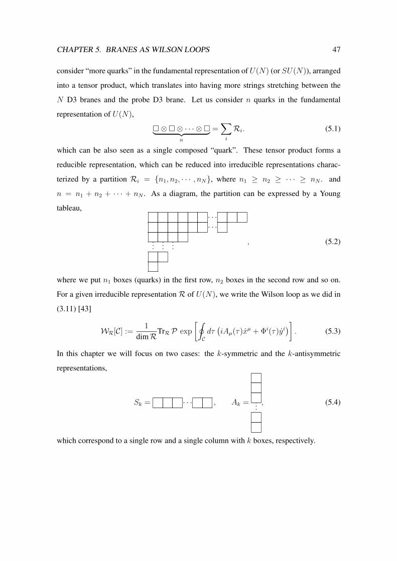
CHAPTER 5. BRANES AS WILSON LOOPS 47
consider “more quarks” in the fundamental representation of U(N) (or SU(N)), arranged
into a tensor product, which translates into having more strings stretching between the
N D3 branes and the probe D3 brane. Let us consider n quarks in the fundamental
representation of U(N),
⊗⊗ · · · ⊗︸ ︷︷ ︸n
=∑i
Ri. (5.1)
which can be also seen as a single composed “quark”. These tensor product forms a
reducible representation, which can be reduced into irreducible representations charac-
terized by a partition Ri = n1, n2, · · · , nN, where n1 ≥ n2 ≥ · · · ≥ nN . and
n = n1 + n2 + · · · + nN . As a diagram, the partition can be expressed by a Young
tableau,· · ·· · ·
.........
, (5.2)
where we put n1 boxes (quarks) in the first row, n2 boxes in the second row and so on.
For a given irreducible representation R of U(N), we write the Wilson loop as we did in
(3.11) [43]
WR[C] :=1
dimRTrRP exp
[∮Cdτ(iAµ(τ)xµ + Φi(τ)yi
)]. (5.3)
In this chapter we will focus on two cases: the k-symmetric and the k-antisymmetric
representations,
Sk = · · · , Ak = ..., (5.4)
which correspond to a single row and a single column with k boxes, respectively.

CHAPTER 5. BRANES AS WILSON LOOPS 48
5.1 Wilson loops in k-symmetric and k-antisymmetric rep-
resentations
In principle, to compute the expectation value of the Wilson loop we must calculate the
path integral
〈WR〉 =
∫DX e−S[X]WR∫DX e−S[X]
, (5.5)
where X denotes the fields of U(N) SYM theory. As we saw before, Erickson, Semenoff
and Zarembo [27], Drukker and Gross [28] proposed and proved, respectively, that the
expectation value of the Wilson loop in fundamental representation can be exactly calcu-
lated by summing ladder diagrams, and that this can be represented by a matrix model.
The matrix model was proved to be Gaussian by Pestun [39].
Since the matrix model is independent of the representation of U(N), we consider
Z =
∫DM exp
(−2N
λTrM2
), (5.6)
whereM is aN×N Hermitian matrix which transforms in theR representation of U(N)
(see [43,45], two important references). In the eigenvalue basis,M = diag (λ1, λ2, · · · , λN),
the partition function is (3.55)
Z =
∫ N∏i=1
dλi∏i<j
(λi − λj)2 exp
(−2N
λ
∑i
λ2i
). (5.7)
The expectation value of the Wilson loop is (see (3.42))
〈WR〉 =1
dimR⟨TreM
⟩, (5.8)
where we replace dim = N → dimR, in general. After diagonalization we can write
1
dimR⟨TreM
⟩=
1
dimR〈SR
(eλ1 , eλ2 , · · · , eλN
)〉, (5.9)
where SR(eλ1 , eλ2 , · · · , eλN
)is the Schur polynomial associated to the representation
R [24] (see [105] for details). Thus,
〈WR〉 =1
dimR1
Z
∫ N∏i=1
dλi∏i<j
(λi − λj)2SR(eλ1 , eλ2 , · · · , eλN
)exp
(−2N
λ
∑i
λ2i
).
(5.10)
For the symmetric and antisymmetric cases (5.4) with k-boxes, the Schur polynomials are
the following [106, 107]:
CHAPTER 5. BRANES AS WILSON LOOPS 49
• k-symmetric
SSk(eλ1 , eλ2 , · · · , eλN
)= hk
(eλ1 , eλ2 , · · · , eλN
), (5.11)
where hk is the kth complete symmetric polynomial, the sum of all monomials of
total degree k in expλi,
hk =∑i=k
expλi. (5.12)
The generating function for hk is
H(t) =∑k≥0
hktk =
N∏i=1
1
(1− teλi)=
1
det (1− teM)= FS(t), (5.13)
which can be inverted as
hk =1
2πi
∮dtFS(t)
tk+1, (5.14)
where t ∈ C.
• k-antisymmetric
SAk(eλ1 , eλ2 , · · · , eλN
)= ek
(eλ1 , eλ2 , · · · , eλN
), (5.15)
where ek is the kth elementary symmetric polynomial, the sum of all products of k
distinct variables expλi,
ek =∑
1≤i1<i2<···<ik≤N
exp (λi1 + λi2 + · · ·+ λik) . (5.16)
The generating function for ek is
E(t) =∑k≥0
ektk =
N∏i=1
(1 + teλi
). (5.17)
We can redefine E(t) as [45]
FA(t) = tNE
(1
t
)=∑k≥0
ektN−k =
N∏i=1
(t+ eλi
)= det
(t+ eM
), (5.18)
which can be inverted as
ek =1
2πi
∮dtFA(t)
tN−k+1. (5.19)

CHAPTER 5. BRANES AS WILSON LOOPS 50
The strategy in [43] was to compute the expectation value of the generating function
instead of the Wilson loop’s
〈FA,S(t)〉 =1
Z
∫ N∏i=1
dλi∏
1≤i<j≤N
(λi − λj)2FS,A(t) exp
(−2N
λ
∑i
λ2i
). (5.20)
The expectation value of the Wilson loop can be then calculated by
〈WS,A〉 =1
dim[S,A]
∮dt
2πi〈FS,A(t)〉 ×
1
tk+1 for SS
1tN−k+1 for SA
. (5.21)
The dimensions of the rank k symmetric and antisymmetric representations are, respec-
tively,
dim[S] =(N + k − 1)!
k!(N − 1)!, dim[A] =
N !
k!(N − k)!. (5.22)
The path integral can be rewritten as
〈FS,A(t)〉 =1
Z
∫ N∏i=1
dλi exp (−SS,A [λi]) , (5.23)
where
SS,A =2N
λ
∑i
λ2i −
∑i<j
log(λi − λj)2 +N∑i=1
+ log(1− teλi
)for SS
− log(t+ eλi
)for SA
. (5.24)
The first two terms are of order N2 and the last one is of order N , so at large N the first
two terms will dominate. So the expectation value for the generating functions will be
〈FS(t)〉 = 〈exp(Tr log
[t+ eM
])〉 → exp
(−N
∫ +√λ
−√λ
dx ρ(x) log (1− tex)
), (5.25)
and
〈FA(t)〉 = 〈exp(−Tr log
[1− teM
])〉 → exp
(N
∫ +√λ
−√λ
dx ρ(x) log (t+ ex)
). (5.26)
where ρ (x) was defined in (3.51) in subsection 3.2.1.
At large N , the circular Wilson loop is given by (5.8), where
• k-symmetric
⟨TrSke
M⟩
=
∮dt
2πi
1
tk+1exp
(−N
∫ +√λ
−√λ
dx ρ(x) log (1− tex)
). (5.27)

CHAPTER 5. BRANES AS WILSON LOOPS 51
• k-antisymmetric
⟨TrAke
M⟩
=
∮dt
2πi
1
tk+1exp
(N
∫ +√λ
−√λ
dx ρ(x) log (1 + tex)
), (5.28)
where we absorbed the factor t−N into the exponent and changed t→ 1/t.
Therefore, we can write both results as
⟨TrSk,Ake
M⟩
=
∮dt
2πi
1
tk+1exp
(∓N
∫ +√λ
−√λ
dx ρ(x) log (1∓ tex)
). (5.29)
where the − sign corresponds to the symmetric representation, and the + one to the
antisymmetric. Notice that this is the saddle point approximation we reviewed in subsec-
tion 3.2.1.
5.1.1 The large N ∼ k limit
We have already considered the largeN limit, which reduced (5.10) to computing residues
in (5.29). It is interesting to take also the limit when the number of boxes, the number of
“quarks”, is large. Let us define,
f =k
N, (5.30)
which is kept fixed, and change
t = e√λz, (5.31)
to write (5.29) as
⟨TrSk,Ake
M⟩
=
√λ
2πi
∫C
dz exp
[∓N
(2
π
∫ +1
−1
dx√
1− x2 log(
1∓ e−√λ(x−z)
)± f√λz
)].
(5.32)
Now t = 0 is mapped to z → −∞, and t→∞ to z →∞.
In the large N limit, the integral is dominated by the saddle point, whose equation is
2
π
∫ +1
−1
dx
√1− x2
1∓ e√λ(x−z)
± f = 0, (5.33)
which is an equation in z. In order to compare with the supergravity result, we need to
take λ→∞.

CHAPTER 5. BRANES AS WILSON LOOPS 52
Let us review the corresponding results for the symmetric and antisymmetric cases. At
largeN , (5.32) can be evaluated using the saddle point method when we choose the upper
sign (see [43, 108] and also [41])
〈WS〉 = exp[2N(κ√
1 + κ2 + sinh−1 κ)], κ =
k√λ
4N. (5.34)
which is the expectation value of a Wilson loop in the symmetric representation.
It was computed also in [43,108] that, in the antisymmetric representation, the Wilson
loop is
〈WA〉 = exp
(2N
3π
√λ sin3 θk
), (5.35)
where θk satisfies
πf = θk −1
2sin 2θk. (5.36)
1/N corrections were studied in [66, 109, 110].
Let us see next how these results appear in the corresponding gravity context.
5.2 D-branes and holography
We saw that the expectation value of a Wilson loops in the fundamental representation
of U(N) (or SU(N)) corresponds to calculating the minimal area of the worldsheet of
an open string ending on a D3 brane probing N D3 branes. For higher representations,
one could think that the expectation value of the Wilson loop should correspond to having
more (fundamental) strings attached to the boundary ofAdS. But calculating the minimal
area of coincident worldsheets is a daunting task due to the complicated geometry.
It was found, for first time, in [111] that a bunch of fundamental strings ending on
branes are described better by another brane! This was later confirmed in [37, 38, 50,
65]. To be precise, let us consider k fundamental strings. Calculating the minimal area
would involve the evaluation of the string action containing string corrections since the k
worldsheets could interact and develop conical singularities and branch cuts. A horrible
collective worldsheet! Each string carries a unit of “electric flux” which is communicated
to the brane through the B-field (see [86,112] for the basics). Now, k fundamental strings
will insert k units of electric field to the probe D3 brane. Following [111], we can consider

CHAPTER 5. BRANES AS WILSON LOOPS 53
instead a “string-equivalent“D-brane carrying k units of electric field on its worldvolume.
The dynamics of this brane is given by the Dirac-Born-Infeld action.
In [37, 38] it was proved that 1/2 BPS Wilson loops of N = 4 SYM in symmetric
and antisymmetric representations of SU(N) can be described by D3 and D5 branes,
respectively, carrying k units of fundamental string charge, which in their worldvolume
action means to insert a Chern-Simons term.
As we know, a circular or straight line Wilson operator breaks one-half of the super-
conformal symmetries of N = 4 SYM. Just for recalling: in order for the Wilson loop
to be supersymmetric, each point in the loop must preserves supersymmetry, it leads to
the condition x = 0. This is satisfied by the straight line loop and, by conformal trans-
formation, by the circular loop. The line, or the circle, breaks the SO(4, 2) × SO(6)
(bosonic) isometry of N = 4 into SO(2, 1) × SO(3) × SO(5): conformal transforma-
tions along the line and rotations. For higher representations, since, in spacetime, the
loops is the same as in the fundamental case, the symmetries that must be preserved are
still SO(2, 1)× SO(3)× SO(5) or SU(1, 1)× SU(2)× SO(5).
5.2.1 D5k-brane and the k-antisymmetric representation
Let us consider a D5 brane probing N D3 branes in flat space. The configuration in flat
space can be expressed as (see [37, 38] and [86])
0 1 2 3 4 5 6 7 8 9
D3 X X X X
D5 X X X X X X
The effect of the D5 brane on the four-dimensional worldvolume theory ofN D3 branes is
to insert a codimension three defect. This perturbations correspond to the (3, 5) and (5, 3)
string states, i.e. strings connecting the D5 with the D3. These new degrees of freedom
are localized in the defect. The (5, 5) strings are not dynamical, but they are important
to identify the D5 brane with the Wilson loop in the antisymmetric representation. As
explained in [37, 38], the D5 branes inserts a defect term in the partition function of
N = 4 theory that includes fermionic fields due to the endpoints of the (3, 5) and (5, 3)
strings, transforming in the fundamental representation of U(N). Also, since the D5 is

CHAPTER 5. BRANES AS WILSON LOOPS 54
charged, a Chern-Simons term must be included, which brings the electric charge of the
D5 into the D3 worldvolume as well as the interaction between it and the defect fields.
As better explained in the references, integrating out those defect states from the partition
function has the effect of inserting into the N = 4 path integral a Wilson loop in the
k-antisymmetric representation, for k ≤ N . It results that the charge of the D5 we add
corresponds to the number of strings endpoints or fermionic states on the D3 branes.
Here, we will follow some details of the calculations in [65] and [113] (reviewed in
[41]), where it was computed and proved that indeed D5 branes can be used to compute
the circular Wilson loop in the antisymmetric representation. Let us consider the AdS5 ×
S5 space as a fibration of two-dimensional space with AdS2×S2×S4 fiber, in which the
SU(1, 1)× SU(2)× SO(5) isometry is explicit.
ds2 = cosh2 u ds2AdS2
+du2+sinh2 u ds2S2 +dθ2+sin2 θ dΩ2
4 , 0 ≤ u , 0 ≤ θ ≤ π, (5.37)
with
ds2AdS2
= dξ2 + sinh2 ξ dψ2 , ds2S2 = dϑ2 + sin2 ϑ dφ2, (5.38)
where the worldvolume coordinates of the D5 brane are taken to be ξ, ψ, θ1, · · · , θ4
(static gauge). The Wilson loop is located at u = 0, ξ → ∞; so u = u (ξ).1 The action
for the D5 brane in this background is given by
SD5 = T5
∫d6ξ√
det (G+ F )− iT6
∫F ∧ C4. (5.39)
Let us consider that the D5 brane wraps S4, so the θ angles are fixed θ = θk. The C4
background field is
C4 = 4
(u
8− 1
32sinh 4u
)volAdS2 ∧ volS2 −
(3
2θ − sin 2θ +
1
8sin 4θ
)volS4 . (5.40)
Taking the ansatz u = 0 and θ = θk constant, and F = Fψξdψ ∧ dξ, the action for the D5
brane is
SD5 =2N
3π
√λ
∫dξ sinh ξ sin4 θ
√1 +
4π2
λ
F 2ψξ
sinh2 ξ
+4iN
3
∫dξ Fψξ
(3
2θk − sin 2θk +
1
8sin 4θk
), (5.41)
1Notice that ξ is the radial coordinate of the internal AdS2 space.

CHAPTER 5. BRANES AS WILSON LOOPS 55
where TD5 = N√λ/8π2 and volS4 = 8π2/3. Since the worldvolume gauge field, Aξ,
does not appear explicitly in the action, its corresponding conjugate momentum iΠ is
conserved (constant and equal to the electric charge),
Π = −i 1
2π
δLδFψξ
=2N
3π
E sin4 θk√1− E2
+2N
3π
(3
2θk − sin 2θk +
1
8sin 4θk
)= k, (5.42)
with
E = −2πi√λ
Fψξsinh ξ
. (5.43)
We set Π = k because of the fundamental string charge goes into the brane as electric
charge. If E = cos θk, then Fψξ = i√λ sinh ξ cos θk/2π,
θk − sin θk cos θk = πk
N≤ π ⇒ k ≤ N. (5.44)
The boundary contribution which takes into account the effect of the boundary ofAdS can
be computed [32, 65, 113]. Plugging the solution back to (5.41) and adding the boundary
term2 we get
SD5 + Sbdy,A = −2N
3π
√λ sin3 θk. (5.45)
The expectation value of the Wilson loop in the antisymmetric representation is
〈WAk〉 = exp2N
3π
√λ sin3 θk, (5.46)
the same result obtained by Hartnoll and Kumar we wrote in (5.35). Now, when k N
the angle θk is small, so we can approximate θ3k = 3πk/2N and
〈WAk〉 = exp2N
3π
√λθ3
k = ek√λ, (5.47)
or
〈WAk〉 ∼ 〈W〉k. (5.48)
Which is the expected result, representing k independent fundamental strings attached to
the D3 brane.
There is also an interesting detail with our result, the k-antisymmetric and (N − k)-
antisymmetric representations, where k ≤ N , are related by the change θk → π − θk,
which means Fψξ → −Fψξ, the complex conjugation of the electric field. Under this
change, the Wilson loop is invariant.2This boundary term must be at ξ, since this is the radial coordinate.

CHAPTER 5. BRANES AS WILSON LOOPS 56
5.2.2 D3k-brane and the k-symmetric representation
It was shown also in [37, 38] that the configuration for a D3 brane probing N D3 branes
corresponding to the k-symmetric representation of U(N) can be obtained by bosoniza-
tion of the fermionic field χ in the defect theory. This partition function inserts a Wilson
loop in the k-symmetric representation in N = 4 SYM theory, so we expect that duality
allows us to compute the expected value also in the gravity side in the D3 brane descrip-
tion. Actually, the derivation of the symmetric representation was re-shown in [38] by
following the same method in [37] for the D5 brane. k, again, represents the number of
string ending on the D3 stack. An important difference from the D5 case is that, in this
case, the electric charge is arbitrary, so k can take any value, even k > N .
In order to see how the D3 brane description actually works, we will follow [41,50] to
calculate the circular Wilson loop in the symmetric representation. The AdS5 × S5 space
can be written as
ds2 =1
y2
(dy2 + dr2
1 + r21dψ
2 + dr22 + r2
2dφ2)
+ dΩ25. (5.49)
The circular loop is located at r1 = a, r2 = 0 and z → 0. In order to exhibit the
SU(1, 1)× SU(2)× SO(5) symmetry, we change variables,
r1 =a cos η
cosh ρ− sinh ρ cos θ, r2 =
a sinh η sin θ
cosh ρ− sinh ρ cos θ, y =
a sin η
cosh ρ− sinh ρ cos θ,
(5.50)
such that the metric becomes
ds2 =1
sin2 η
(dη2 + cos2 η dψ2 + dρ2 + sinh2 ρ
(dθ2 + sin2 θ dφ2
))+ dΩ2
5, (5.51)
where 0 ≤ ρ, 0 ≤ θ ≤ π and 0 ≤ η ≤ π/2. In this metric the Wilson loop is located at
η = ρ = 0. We go to static gauge in which the worldvolume coordinates are ψ, ρ, θ, φ,
and the brane sits at a fixed point ΘI on S5. The remaining coordinate, η, will be seen
as a worldvolume scalar field η = η(ρ). There is also a gauge field, which is chosen to be
only electric, Fψρ. The four-form potential is, in terms of the old metric (5.49),
C4 =r1r2
y4dr1 ∧ dψ ∧ dr2 ∧ dφ, (5.52)
and can be written in the new coordinates (5.50). Dynamics of the D3 brane is given by

CHAPTER 5. BRANES AS WILSON LOOPS 57
the DBI action and the corresponding Wess-Zumino term.
SD3 = 2N
∫dρdθ
sin θ sinh2 ρ
sin4 η
√cos2 η (1 + η′2) + (2πα′)2 sin4 ηF 2
ψρ
−2N
∫dρdθ
cos η sin θ sinh2 ρ
sin4 η
(cos η + η′ sin η
sinh ρ− cosh ρ cos θ
cosh ρ− sinh ρ cos θ
).
(5.53)
Solutions to the equations of motion are
sin η = κ−1 sinh ρ , Fψρ =ikλ
8πN sinh2 ρ, (5.54)
where
Π = −i 1
2π
δLδFψρ
= k =4Nκ√λ
(5.55)
is the constant conjugate momentum associated toAψ(ρ), the electric field, i.e. the electric
charge or fundamental string charge dissolved on the D3 brane. By plugging this solution
back into the action we can calculate the on-shell action,
SonshellD3 = 2N
(κ√
1 + κ2 − sinh−1 κ), (5.56)
which is exactly finite. Even though we found a non-divergent action and naively we
computed the expectation value of the circular Wilson loop, we need to do the Legendre
transform as required and hope it does not produce a divergence. There are two boundary
terms
Sbdy,η = limη0→0− 1
2π
∫dψη
δLδη′
∣∣∣∣η0
= −4Nκ
η0
, (5.57)
and
Sbdy,A = limη0→0− i
2π
∫dψdρΠFψρ = −4Nκ
√1 + κ2 +
4Nκ
η0
. (5.58)
Thus, the regularized action is
SonshellD3 + Sbdy,η + Sbdy,A = −2N
(κ√
1 + κ2 + sinh−1 κ). (5.59)
The expectation value of the circular Wilson loop is then
〈WSk〉 = exp 2N(κ√
1 + κ2 + sinh−1 κ), (5.60)
which is precisely the matrix model result in (5.34). At small k and λ N2, the last
expression reduces to
〈WSk〉 ∼ ek√λ = 〈W〉k. (5.61)

CHAPTER 5. BRANES AS WILSON LOOPS 58
The last result coincides with 〈WAk〉 at small k,
limk→1〈WSk〉 = lim
k→1〈WAk〉 = 〈W〉k. (5.62)
For example,
〈W 〉 ' 〈W 〉 ' 〈W〉〈W〉, (5.63)
where two fundamental strings produces a circular Wilson loop separately.
But, what happens when k N? This is not allowed in the antisymmetric case but
only in the symmetric. In this regime the brane we considered backreacts on the geometry
and deform the AdS5×S5 space, forming the so-called bubbling geometries (see [71–73]
for details).
As we said before, to consider k fundamental strings to describe the k-representation
of the circular Wilson loop, would lead to handle complicated and singular geometries.
The k ≈ N limit, in which we dissolve the k strings worldsheets into a brane is convenient
because it produces the expected AdS/CFT results, and then it encodes the interactions
between the coincident strings and allows to have all non-planar contributions to the ex-
pectation value of the higher rank Wilson loop.
Two kinds of branes were considered in order to describe, in this case, circular Wil-
son loops in the k-symmetric and k-antisymmetric representations of U(N) (with N
large): D3 and D5 branes with k units of charge. Those brane descriptions satisfied the
SO(2, 1)×SO(3)×SO(5) symmetry of the Wilson loop in the gauge theory as an isom-
etry of their induced geometries. Their worldvolumes are: AdS2 × S2 and AdS2 × S4,
for the D3 and the D5. We can see that the D3 branes is entirely embedded into AdS5 but
not the D5 which has its S4 part inside S5, so it preserves SO(5).
It is important to mention that we have assumed some results from the string world-
sheet results given in the last chapter. Remember that, in order to describe a Wilson loop
at the boundary of AdS5 × S5, we minimize the string worldsheet area which, in turn,
yields the BPS condition for the loop as required by supersymmetry. Here we considered
a brane as the “effective“ behavior of k worldsheets, and assume that the minimal area
condition became the onshell regularized action of the brane. It was proved in [114] that
the worldvolume field on the probe brane attached to the Wilson loop at the AdS boundary
are constrained by the BPS condition, as expected, since the loop does not change.

CHAPTER 5. BRANES AS WILSON LOOPS 59
5.3 Beyond the leading order
The last results correspond to the N → ∞ and λ → ∞ regime. Let us go back to the
result of [28], in which the circular Wilson loop in the fundamental representation of
U(N) was computed in the matrix model for any N, λ
〈Wladders〉 =
⟨1
NTreM
⟩=
1
NL1N−1
(− λ
4N
)exp
(λ
8N
), (5.64)
which can be expanded in powers of 1/N and Bessel functions In
〈Wladders〉 =2√λI1
(√λ)
+λ
48N2I2
(√λ)
+λ2
1280N4I4
(√λ)
+ · · · . (5.65)
When N, λ→∞,
〈Wladders〉 ≈ e√λ. (5.66)
Let us consider the k-symmetric Wilson loop result. We saw that, at small k,
〈WSk〉 ≈ 〈Wladders〉k ≈ ek√λ. (5.67)
So we can take (5.64), and change λ→ k2λ
〈WSk〉 =
⟨1
NTrekM
⟩=
1
NL1N−1
(−k
2λ
4N
)exp
(k2λ
8N
), (5.68)
or
〈WSk〉 =
⟨1
NTrekM
⟩=
1
NL1N−1
(−4Nκ2
)exp
(2Nκ2
), (5.69)
where k√λ = 4Nκ. Laguerre polynomials satisfy the differential equation,
xLkn(x)′′
+ (k + 1− x)Lkn(x)′+ nLkn(x) = 0, (5.70)
which leads to an equation for 〈WSk〉 [50]
[κ∂2
κ + 3∂κ − 16N2κ(1 + κ2
)]〈WSk〉 = 0. (5.71)
If we set 〈WSk〉 = exp (−NF), then
(F ′)2 − 1
κN(κF ′′ + 3F ′)− 16
(1 + κ2
)= 0. (5.72)
If we consider k√λ ∼ κN 1 since k ∼ N 1 and λ 1, (5.72) becomes
dFdκ
= ±4√
1 + κ2, (5.73)

CHAPTER 5. BRANES AS WILSON LOOPS 60
whose solution is
F = F0 ± 2(κ√
1 + κ2 + sinh−1 κ), (5.74)
which coincides with (5.60) when F0 = 0 and we choose the minus sign. We can also
solve (5.72) without eliminating the 1/κN term [114],
F = −2(κ√
1 + κ2 + sinh−1 κ)
+1
2N
(lnκ3√
1 + κ2 + ln(32πN3
))+O
(1
N2
).
(5.75)
A similar result was obtained by Faraggi et al. in [109],
F = −2(κ√
1 + κ2 + sinh−1 κ)− 1
2Nln
κ3
√1 + κ2
. (5.76)
Another result appeared in [66],
F = −2(κ√
1 + κ2 + sinh−1 κ)
+1
2Nln
κ3
√1 + κ2
+1
Nln 4√λ. (5.77)
Notice that the second term differs by a sign and a constant of the result given in the last
expression, and also by an extra term. On the gravity side [115] (see also [116, 117], it
was obtained
FD3 = −2(κ√
1 + κ2 + sinh−1 κ)
+1
2Nln
κ3
√1 + κ2
. (5.78)
We notice that the 1/N corrections are slightly different in both sides, and even in the
same side. The disagreement between results could be due to subtle effects in the matrix
model, or backreaction of the probe branes in the background geometry [41].
Similiar results for the antisymmetric case, and also a recent discovery of a relation
between both symmetric and antisymmetric representations are given in [67–70,118,119].
5.4 Rectangular tableau and the need of a nonabelian
DBI action
In this section we will present an original, even though unpublished, work in which we
explore higher representations called rectangular that allow to extend our study to include
the so called nonabelian DBI action for probe branes. Let us consider the following Young

CHAPTER 5. BRANES AS WILSON LOOPS 61
tableaux
Rvert =
`
k Rhor =
k
`. (5.79)
As said in [37, 38], Rvert is dual to a set of ` coincident D5 branes in AdS5 × S5, while
Rhor corresponds to ` D3 branes in AdS5 × S5. This is expected, we can think Rvert and
Rhor as an arrangement of ` symmetric and antisymmetric representations, respectively;
those which correspond to D3s and D5s. In this description we also need to have `
k ∼ N in both cases in order to not have backreaction in the geometry, i.e. that the
presence of the branes does not modify severely the original AdS5 × S5 background.
Dynamics of these probes would then be given by the so-called Nonabelian Dirac-Born-
Infeld (NADBI) action [75–77, 120, 121], the generalized form of the well-known DBI
action for a single brane moving on a background.
Let us have a taste of how these rectangular tableaux become complicated.
5.4.1 Vertical rectangular tableau
A vertical rectangular tableau should correspond to a group of D5 probes in AdS5 × S5.
From (5.10), we see that the Wilson loop insertion is represented by the Schur function
〈WR〉 =1
dimR1
Z
∫ N∏i=1
dλi∏i<j
(λi − λj)2SR(eλ1 , eλ2 , · · · , eλN
)exp
(−2N
λ
∑i
λ2i
),
(5.80)
and in the case of the vertical (antisymmetric) tableau, we can express the Schur function
as the determinant of a N × N composed by elementary symmetric polynomials (5.15)
[105],
SR = |eλi−i+j| =
∣∣∣∣∣∣∣∣∣∣∣∣
eλ1 eλ1+1 · · · eλ`+`−1
eλ2−1 eλ2 · · ·...
. . .
eλ`−`+1 eλ`
∣∣∣∣∣∣∣∣∣∣∣∣, (5.81)

CHAPTER 5. BRANES AS WILSON LOOPS 62
where i = 1, · · · , N and λi are eigenvalues. This is the so-called second Jacobi-Trudi
identity [106]. Now, if λ`+1 = · · · = λλN = 0, the determinant simplifies to the determi-
nant of a `× ` matrix. Let us work with the simplest case, ` = 2, thus
SR = e2k − ek+1ek−1. (5.82)
So, we need to compute 〈ek+1ek−1〉. By using the generating functions of the elementary
symmetric polynomials we have
〈emen〉 =1
(2πi)2
∮dt
tN−m+1
∮ds
sN−n+1〈FA(t)FA(s)〉. (5.83)
The expectation values can be calculated by
〈FA(t)FA(s)〉 =1
Z
∫ N∏i=1
dλi exp (−SA(t, s)) , (5.84)
with
SA(t, s) =2N
λ
∑i
λ2i−∑i<j
log(λi−λj)2−N∑i=1
log(t+ eλi
)−
N∑i=1
log(s+ eλi
). (5.85)
The first two terms dominate since they are of order N2, the Gaussian model, while the
last two enter as insertions since they are of order N . Therefore, in the large N limit the
eigenvalue distribution is governed by the Wigner semi-circle law, thus
〈FA(t)FA(s)〉 → exp
(N
∫ +√λ
−√λ
dx ρ(x)(
log (t+ ex) + log (s+ ex)))
= 〈FA(t)〉〈FA(s)〉.
(5.86)
It means that
〈emen〉 = 〈em〉〈en〉. (5.87)
Since
〈WAk〉 =1
dimAk〈ek〉, (5.88)
we can write
〈WRvert〉`=2 =1
dimRvert
((dimAk〈WAk〉)
2 − dimAk+1dimAk−1〈WAk+1〉〈WAk−1
〉),
(5.89)
which is a determinant that can be generalized for any ` as
〈WRvert〉` =1
dimRvert|dimAk−i+j〈WAk−i+j〉|, (5.90)
CHAPTER 5. BRANES AS WILSON LOOPS 63
with ` k ∼ N . dimRvert of the vertical tableau (5.79) can be computed by induction
from the dimAk, a single column tableau, and it is given by
dimRvert (`, k) =∏i=1
(N − 1 + i)!(`− i)!(N − k − 1 + 1)!(k + `− i)!
, (5.91)
where ` ≥ 1, and for ` = 1 we see that dimRvert (1, k) = dimAk = N !k!(N−k)!
, as expected.
For ` = 2, we get
dimRvert (2, k) =N !(N + 1)!
(N − k)!(k + 1)!(N − k + 1)!k!. (5.92)
In the gravity side, as we learned, we have to consider two D5 branes as probes in the
AdS5 × S5 geometry. Also, as we mentioned above, higher representations in the gauge
theory side requires more than one branes whose dynamics is given by the not well-
defined nonabelian DBI action. Unfortunately, we have not developed computations in the
gravity side in this case, but we developed some ideas for the horizontal Young tableau.
5.4.2 Horizontal rectangular tableau
In the case of the horizontal (symmetric) tableau, which corresponds to a D3 branes prob-
ingAdS5×S5, we can express the Schur function in (5.80) as the determinant of aN×N ,
composed by complete (homogeneous) symmetric polynomials,
SR = |hλi−i+j| =
∣∣∣∣∣∣∣∣∣∣∣∣
hλ1 hλ1+1 · · · hλ`+`−1
hλ2−1 hλ2 · · ·...
. . .
hλ`−`+1 hλ`
∣∣∣∣∣∣∣∣∣∣∣∣, (5.93)
where i = 1, · · · , N and λi are eigenvalues. This is the so-called first Jacobi-Trudi iden-
tity [106]. Now, if λ`+1 = · · · = λλN = 0, the determinant simplifies to the determinant
of a `× ` matrix. Let us work with the simplest case, ` = 2 with λi = k, thus
SR = h2k − hk+1hk−1. (5.94)
So again, we need to compute 〈hk+1hk−1〉. In the same way we did it before,
〈hmhn〉 =1
(2πi)2
∮dt
tm+1
∮ds
sn+1〈FS(t)FS(s)〉. (5.95)
CHAPTER 5. BRANES AS WILSON LOOPS 64
The expectation values can be calculated by
〈FS(t)FS(s)〉 =1
Z
∫ N∏i=1
dλi exp (−SS(t, s)) , (5.96)
with
SS(t, s) =2N
λ
∑i
λ2i −
∑i<j
log(λi − λj)2 +N∑i=1
log(1− teλi
)+
N∑i=1
log(1− seλi
).
(5.97)
In the large N limit, again,
〈FS(t)FS(s)〉 → exp
(−N
∫+√λ
−√λ
dx ρ(x)(
log (1− tex) + log (1− sex)))
= 〈FS(t)〉〈FS(s)〉,
(5.98)
then,
〈hmhn〉 = 〈hm〉〈hn〉. (5.99)
From
〈WSk〉 =1
dimSk〈hk〉, (5.100)
we conclude that
〈WRhor〉`=2 =1
dimRhor
((dimSk〈WSk〉)
2 − dimSk+1dimSk−1〈WSk+1〉〈WSk−1
〉),
(5.101)
which is a determinant that can be generalized, again, for any ` as
〈WRhor〉` =1
dimRhor|dimSk−i+j〈WSk−i+j〉|, (5.102)
with ` k ∼ N . dimRhor of the horizontal tableau (5.79) can be computed by induction
from the dimSk, a single row tableau, giving
dimRhor =∏i=1
(N + k − i)!(`− i)!(N − i)!(k + `− i)!
, (5.103)
where ` ≥ 1, and for ` = 1 we see that dimRhor = dimSk = (N+k−1)!k!(N−1)!
, again, as expected.
For ` = 2, we obtain
dimRvert =(N + k − 1)!(N + k − 2)!
(N − 1)!(k + 1)!(N − 2)!k!. (5.104)
We will do some further computations in this case. Let us remember that
〈WSk〉 = exp 2N(κ√
1 + κ2 + sinh−1 κ), κ =
k√λ
4N, (5.105)

CHAPTER 5. BRANES AS WILSON LOOPS 65
which should be obtained in the gravity side by considering D3 branes in the AdS5 × S5
background. Moreover, we saw in (5.78) that the first corrected action, and the expectation
value is
〈WSκ〉 =
√κ3
√1 + κ2
exp(
2N(κ√
1 + κ2 + sinh−1 κ))
=
√κ3
√1 + κ2
〈WSk〉N→∞.
(5.106)
The factor in front of 〈WSk〉N→∞ in the last result contains the 1/N correction. Since
k ∼ N (5.102) would vanish if N → ∞, so we need to consider corrections and then
(5.106). Since
(k ± 1)√λ
4N= κ±
√λ
4N→ κ(1± ε) , ε ∼ 1
N 1, (5.107)
the nonabelian nature can be extracted from 1/N corrections. The expectation value we
want to compute is
〈WRhor〉`=2 =1
dimRhor|dimSk+i−j〈Wκ+(i−j)εκ〉|. (5.108)
From (5.101), by using dimSk = (N+k−1)!k!(N−1)!
, we can see that
dimSk+1dimSk−1 = (dimSk)2 (N + k)k
(N + k − 1)(k + 1). (5.109)
If we fix k/N = q, we can expand the last result for large k, and get
dimSk+1dimSk−1 = (dimSk)2
(1− 1
k(1 + q)
). (5.110)
So we can see that there is an effect of order 1/k only looking at the dimension of the
representations. We can compute 〈WRhor〉`=2, by inserting the different dimensions and
the result (5.106), and get
〈WRhor〉`=2 =(〈WSk〉N→∞
)2(
1 + u(κ) +1
kv(κ)
), (5.111)
where u(κ) and v(κ) are functions to be determined and compared with the gravity result.3
We can write the last result as
〈WRhor〉`=2 = exp(
4N(κ√
1 + κ2 + sinh−1 κ))(
1 + u(κ) +1
kv(κ)
). (5.112)
3We have not obtained a reliable result for these functions because we need to take better care of the
expansions we perform, but we expect that the behavior to be the one we wrote above. A result appeared
recently [122] where an approximate expression for the expansion of the factor in front of the squared
expression of the horizontal rectangular Wilson loop was obtained.
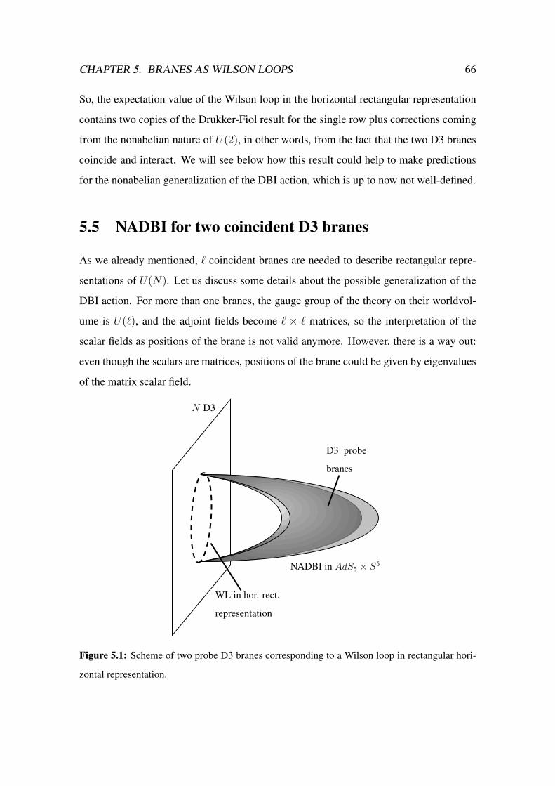
CHAPTER 5. BRANES AS WILSON LOOPS 66
So, the expectation value of the Wilson loop in the horizontal rectangular representation
contains two copies of the Drukker-Fiol result for the single row plus corrections coming
from the nonabelian nature of U(2), in other words, from the fact that the two D3 branes
coincide and interact. We will see below how this result could help to make predictions
for the nonabelian generalization of the DBI action, which is up to now not well-defined.
5.5 NADBI for two coincident D3 branes
As we already mentioned, ` coincident branes are needed to describe rectangular repre-
sentations of U(N). Let us discuss some details about the possible generalization of the
DBI action. For more than one branes, the gauge group of the theory on their worldvol-
ume is U(`), and the adjoint fields become ` × ` matrices, so the interpretation of the
scalar fields as positions of the brane is not valid anymore. However, there is a way out:
even though the scalars are matrices, positions of the brane could be given by eigenvalues
of the matrix scalar field.
D3 probe
branes
N D3
WL in hor. rect.
representation
NADBI in AdS5 × S5
Figure 5.1: Scheme of two probe D3 branes corresponding to a Wilson loop in rectangular hori-
zontal representation.
CHAPTER 5. BRANES AS WILSON LOOPS 67
Let us start by explaining the case of the DBI action for one single brane, a D3. The
action for a Dp-brane is
SDBI = −Tp∫dp+1ξe−φ
√−det [P [G+B]ab + 2πα′Fab]. (5.113)
Interactions with the background gauge fields are given by the Wess-Zumino term
SWZ = µp
∫P[∑
C(n)eB]e2πα′F = µp
∫P[C(n) ∧ (1 +B + · · · )
](1 + 2πα′F + · · · ) .
(5.114)
HereC(n) represents the n-form RR potential,B is the NSNS two-form potential, F = dA
where Aa is a U(1) field, and P [· · · ] denotes the pullback of the bulk spacetime fields to
the (p+ 1)-dimensional worldvolume of the Dp-brane,
P [E]ab = Eµν∂xµ
∂σa∂xν
∂σb= Eab + 2πα′Eia∂bΦ
i + 2πα′Eib∂aΦi + (2πα′)
2Eij∂aΦ
i∂bΦj.
(5.115)
The brane charge is defined as the charge under C(p+1), in which µp = ±Tp. In general,
the WZ term allows us to couple the Dp-brane to another RR potentials with lower form
degree than p+ 1. The last action, in the same way the Nambu-Goto for the fundamental
string, represents the proper volume swept out by the Dp-brane. If we go to the static
gauge σa = xa, with a = 0, 1, · · · , p, the other coordinates, xi, with i = p + 1, · · · , 9,
correspond to scalar fields in the worldvolume theory
xi(σ) = 2πα′Φi(σ). (5.116)
The square root in the DBI action resums an infinite series of stringy corrections coming
from the fact that this is an effective action which arises through integrating out massive
modes in string theory.
Now let us consider ` parallel branes. Strings stretching between them become mass-
less when branes approach each other, then Aa = A(n)a T n where T n are `2 Hermitian
generators of U(`) and n = 1, · · · , `2 − 1, and U(1) becomes U(`). The field strength is
now
Fab = ∂aAb − ∂bAa + i [Aa, Ab] . (5.117)
The scalars Φi also transform in the adjoint of U(`), with
DaΦi = ∂aΦ
i + i[Aa,Φ
i]. (5.118)

CHAPTER 5. BRANES AS WILSON LOOPS 68
Since scalars are now matrices, as we mentioned above, they cannot represent positions
of the branes in the transverse space.
It was suggested in [123], that for general non-commuting scalars, positions are given
by eigenvalues. It was proposed by Myers in [75] (and reviewed in [76, 77]) by using
T-duality on the DBI action of a D9-brane that the action for ` Dp-branes is
SDBI = −TDp∫dp+1σ STr(g)
(e−φ√
detMab detQij
), (5.119)
where the superscript (g) means trace over the gauge group, and
Mab = P[Eab + Eai
(Q−1 − δ
)ijEjb
]+ λFab, (5.120)
and
Qij = δij + iλ
[Φi,Φk
]Ekj , λ = 2πα′, (5.121)
with
EMN = GMN +BMN , (5.122)
and
Fab = ∂aAb − ∂bAa + i [Aa, Ab] . (5.123)
To incorporate the nonabelian gauge symmetry of the action, Tseytlin [120, 121], sug-
gested the symmetrized trace “STr” in front of the action (see some general properties
in [121]). This trace is necessary to remove the ambiguity in the ordering of the products
of the terms inside the action. The standard prescription instructs us to expand the square
root in powers of λ and take the trace over all possible orderings because it is not clear
how to take this symmetrized trace without expanding the square root:
STr(g) (T n1T n2 · · ·T nK ) =1
K!Tr (T n1T n2 · · ·T nK + permutations) . (5.124)
The WZ term [75, 77]
SWZ = TD3
∫STr(g)
(P[ei(2πα
′)iΦiΦC(4)]∧ e(2πα′)F
), (5.125)
will be a generalization of the WZ term in (5.114), where iΦ is an interior product which
reduces the form degree by −1. The nonabelian pullback is defined as
P [E]ab = Eab + λEiaDbΦi + λEibDaΦ
i + λ2EijDaΦiDbΦ
j. (5.126)

CHAPTER 5. BRANES AS WILSON LOOPS 69
The metric can be written as
ds2
L2= Gabdx
adxb +Gijdxidxj , Gai = 0. (5.127)
Let us take p = 3 and BMN = φ = 0. The non-abelian pullback is [77] (some terms
vanish because Gia = 0)
P [Gab] = Gab + λ2GijDaΦiDbΦ
j , xi = λΦi, (5.128)
and
P[Gai
(Q−1 − δ
)ijGjb
]= λ2Gki
(Q−1 − δ
)ijGjlDaΦ
kDbΦl, (5.129)
where
DaΦi = ∂aΦ
i + i[Aa,Φ
i]
(5.130)
is necessary to preserve gauge symmetry. Then,
SDBI = −TD3
∫d4σ STr(g)
(√detMab
√detQi
j
), TD3 = N/2π2L4, (5.131)
Mab = Gab + λ2(Gij +Gik
(Q−1 − δ
)klGlj
)DaΦ
iDbΦj + λFab. (5.132)
Since
(Q−1 − δ)ij = −iλ[Φi,Φj
], λ 1, (5.133)
then
Mab = Gab + λ2(Gij − iλ
[Φk,Φl
]GkiGlj
)DaΦ
iDbΦj + λFab, (5.134)
or
Mab = Gab + λFab + λ2DaΦiDbΦ
jGij − iλ3[Φk,Φl
]DaΦ
iDbΦjGkiGlj. (5.135)
The background fields are functionals of the nonabelian scalars. After fixing the static
gauge (5.127), the metric Gab in the D-brane action would be given by a nonabelian
Taylor expansion [75–77]
Gab = exp[λΦi∂xi ]Gab(xa, xi)|xi=0
= Gab(xa, 0) + λΦi∂xiGab(x
a, 0) + λ2ΦiΦj∂xi∂xjGab(xa, 0) + · · ·
. (5.136)

CHAPTER 5. BRANES AS WILSON LOOPS 70
5.5.1 The U(2) case
In this section we explore further the NADBI and try to make comparisons with the matrix
models results. Let us consider ` = 2, then the gauge field on the D3 brane probe world-
volume is U(2); the gauge field is Aa = A(n)a T n with a = 0, 1, 2, 3 and (n) = 0, 1, 2, 3
counts the generators of U(2) (the 2 × 2 identity and the SU(2) generators). The scalar
fields are Φi = Φi (n)T n with i = 1, · · · , 6. Notice now that we actually have “too many”
scalars because they are matrices, they do not longer describe positions.
Let us explore the case of two probe D3 branes in AdS5 × S5. The metric is
ds2
L2=
1
sin2 η
(dη2 + cos2 η dψ2 + dρ2 + sinh2 ρ (dθ2 + sin2 θ dφ2)
), (5.137)
where ρ ∈ [0,∞), θ ∈ [0, π), 0 ≤ ψ, φ ≤ 2π and η ∈ [0, π/2]. In this coordinate system
the boundary is located at η = 0 (and also at ρ → ∞). The circular loop is located at
η = ρ = 0. We take ψ, ρ, θ, φ as the brane world-volume coordinates. The embedding
function (transverse coordinate) is η = η(ρ) [50]. In the nonabelian extension of the DBI
action, we must promote the transverse coordinate to a transverse scalar field
η(ρ)→ λΦ(ρ) , (5.138)
where Φ(ρ) is a 2 × 2 matrix. The other five scalars are related to the S5 part of the
background, but we do not need to worry about them if we conveniently fix a point on
S5 to be the north pole of the sphere, so we set them to zero. With only one scalar
field Φ in our problem, the non-abelian DBI action will simplify drastically because all
commutators [Φi,Φj] vanish.
With these simplifications the non-abelian DBI action becomes
SDBI = −TD3
∫d4σ STr(g)
√detMab, (5.139)
where
Mab = Gab + λFab + λ2DaΦiDbΦ
jGij. (5.140)
Note that the components of the pullback are now 2× 2 matrices. In particular, the metric
components are now viewed as functionals of the scalars
GMN(x)→ GMN [Φi] . (5.141)

CHAPTER 5. BRANES AS WILSON LOOPS 71
In principle, this transition should be done using the so called non-abelian Taylor expan-
sion (5.136), but we will follow an alternative approach using the properties of the Pauli
matrices, as we will describe below. After doing that, we need to evaluate the determinant
in the DBI action (5.139). For our embedding it has the form
detMµν = (MψψMρρ −MψρMρψ)MθθMφφ , (5.142)
where
Mψψ = Gψψ − λ2 [Aψ,Φ]2Gηη,
Mψρ = −λA′ψ + iλ2 [Aψ,Φ] Φ′Gηη,
Mρψ = λA′ψ + iλ2 [Aψ,Φ] Φ′Gηη,
Mρρ = Gρρ + λ2 (Φ′)2Gηη,
Mθθ = Gθθ,
Mφφ = Gφφ . (5.143)
After promoting the embedding function to a matrix (η → λΦ) we also need to promote
GMN to matrices, that now are functionals of Φ. We take the Pauli matrices and the
identity as the generators of U(2): T a = 1/2 I, 1/2~σ. So the scalar field has the
following form
ΦaTa =
1
2
Φ0 + Φ3 Φ1 − iΦ2
Φ1 + iΦ2 Φ0 − Φ3
, (5.144)
whose eigenvalues (which describe the positions of the branes [123]) are
λ1,2 = Φ0 − |~Φ|,Φ0 + |~Φ| , |~Φ| =√
Φ21 + Φ2
2 + Φ23. (5.145)
For coincident branes λ1 = λ2, so |~Φ| = 0, then Φ = 12Φ0I. 4
In the metric background (5.137) we have sines and cosines. Writing them as expo-
nentials and using the properties of the Pauli matrices we obtain
sin(λΦ) = a1I + a2(Φ · ~σ),
cos(λΦ) = b1I + b2(Φ · ~σ), (5.146)
4This choice allows to have only derivatives of A in the action, so a conserved momentum.
CHAPTER 5. BRANES AS WILSON LOOPS 72
wherea1 = sin(λ2Φ0
)cos(λ2|~Φ|)
a2 = cos(λ2Φ0
)sin(λ2|~Φ|) ,
b1 = cos(λ2Φ0
)cos(λ2|~Φ|)
b2 = − sin(λ2Φ0
)sin(λ2|~Φ|) , Φ =
~Φ
|~Φ|.
(5.147)
With the above expressions we can compute the metric components. Explicitly, we get
Gηη[Φ]
L2=
1
sin2 λΦ=
2− 2 cosλΦ0 cosλ|~Φ|(cosλΦ0 − cosλ|~Φ|)2
I− 2 sinλΦ0 sinλ|~Φ|(cosλΦ0 − cosλ|~Φ|)2
(Φ · ~σ) ,
Gψψ[Φ]
L2=
cos2 λΦ
sin2 λΦ=
2− cos 2λΦ0 − cos 2λ|~Φ|2(cosλΦ0 − cosλ|~Φ|)2
I− 2 sinλΦ0 sinλ|~Φ|(cosλΦ0 − cosλ|~Φ|)2
(Φ · ~σ) .
(5.148)
The other metric components are proportional to Gηη, namely
Gρρ = Gηη, Gθθ = sinh2 ρGηη, Gφφ = sinh2 ρ sin2 θ Gηη . (5.149)
Note that all metric components commute with each other and with Φ. We saw that
for coincident branes we can take Φ = 12Φ0I, and then η = λ
2Φ0I. With this choice,
everything that appears in the DBI action commutes, thus we do not need to worry about
any ambiguity and the symmetrized trace is simply a regular trace. Let us chooseAψ(ρ) =
A(0)ψ (ρ)I + ~Aψ(ρ) · ~σ just like in [50]. Then, the determinant (5.142) is
√detMab =
√AI +B
(~A′ψ · ~σ
)sinh2 ρ sin θ
sin2 λΦ0
2
. (5.150)
Since the Pauli matrices do not appear as products, there is only one term, so we do not
need to symmetrize the square root:
STr√
detMab = Tr√
detMab. (5.151)
The formula of the trace of the determinant of a 2× 2 matrix implies that
Tr√
detMab =√
2sinh2 ρ sin θ
sin2 η
√A+
√A2 −B2|~Fρψ|2, (5.152)
with
A =cos2 η (1 + η′2)
sin4 η+ λ2
(F
(0) 2ρψ + |~Fρψ|2
)(5.153)
B = λ2F(0) 2ρψ . (5.154)

CHAPTER 5. BRANES AS WILSON LOOPS 73
Back to the DBI action, we write
SDBI = −√
2TD3
∫d4σ
sinh2 ρ sin θ
sin2 η
√A+
√A2 −B2|~Fρψ|2. (5.155)
The WZ part is the one given in Drukker and Fiol [50], but multiplied by 2 due to the
matrix nature of the variable η
SWZ = −4N
∫dρ dθ
cos η sin θ sinh2 ρ
sin4 η
(cos η + η′ sin η
sinh ρ− cosh ρ cos θ
cosh ρ− sinh ρ cos θ
).
(5.156)
It is important to notice that when ~Fρψ = 0, we get the abelian action of Drukker and
Fiol multiplied by 2, as expected. So, the nonabelian nature of our system is contained in
the off-diagonal terms of Fρψ. Since making them to vanish breaks the U(2) symmetry to
U(1)× U(1), they are related to the off-diagonal terms of Φ, ~Φ, by T-duality [75].
Since we have only considered that the gauge field on the two D3 brane system get
nonabelian effects, leaving the scalar field duplicated due to the matrix nature of the field,
we can take the result in [50] and deform it to include this effect.
The ansatz that includes the solution of [50] is
η(ρ) = sin−1(κ−1 sinh ρ
)F
(0)ρψ =
iκ(1 + ε)√λ
2π sinh2 ρ
|~Fρψ| = εκ√λ
2π sinh2 ρ, (5.157)
where ε 1 is a parameter that allows us to insert the nonabelian nature. We can see from
the action that there are four conserved quantities associated to the gauge fields charges.
In the abelian case, where we only have F (0)ρψ , the conserved momentum k0 corresponds to
the fundamental string charge on the brane. In this case, we have two branes so we expect
to have two conserved quantities equal to the fundamental string charges on each brane,
but we have four momenta. After inserting (5.157) into (5.155) and (5.156), we get
k(0) =8Nκ√λ
+8Nε√λ
(1 + κ2)
κ
|~k| = 8Nε√λ
(1 + κ2)
κ+
24Nε2 (1 + κ2)
κ3√λ
, (5.158)
CHAPTER 5. BRANES AS WILSON LOOPS 74
where |~k| =(k(1))2
+(k(2))2
+(k(3))2, and ε2 = ε21 + ε22 + ε23. If we write the 2 × 2
momentum matrix as k = k(0)I + ~k · ~σ, its eigenvalues are
λ1 =8Nκ√λ− 24Nε2 (1 + κ2)
κ3√λ
= 2k + · · · , (5.159)
λ2 =8Nκ√λ
+24Nε2 (1 + κ2)
κ3√λ
+16Nε (1 + κ2)
κ√λ
= 2k + · · · . (5.160)
In the same way, the conserved momentum in the abelian case is equal to the number
of the strings (and then the fundamental string charge) attached to the brane, this two
eigenvalues must correspond to the number of strings attached to each branes. Thus, we
can expect that for U(`) for any `, the `× ` matrix momentum with ` eigenvalues which
can be interpreted as the number of strings attached to each brane. Back to our problem,
we are studying the rectangular horizontal tableau, so we impose that λ1 = λ2, which
leads to a form for ε,
ε = −κ2
3 1. (5.161)
So, we expect κ to be small. This fact could lead to think that κN is not large anymore,
which we considered before when we included a subleading term in (5.75). This particular
value of ε, leads to write
λ1 = λ2 =8Nκ√λ− 8Nκ (1 + κ2)
3√λ
= 2k − · · · , (5.162)
which should be the number of strings attached to each brane. On the other hand, if we
compute the equations of motion and plug our ansatz in them, by expanding in ε up to
order ε4 we can “solve“ the equations for ε, and get
ε = −4κ2
15 1. (5.163)
Which is slightly different than our ε for equal momenta, but not too much. We can see
that ε in (5.161) ”solves“ the equation of motion up to order κ8, so we can close the
equations of motion and have equal momenta. Now, we need to add the corresponding
boundary terms in the same way it was done in [32,50]. In this case we have five boundary
terms, one associated with η and the others corresponding to the conserved charges
Πη =1
2π
δLδη
, iΠ(0) =1
2π
δLδF
(0)ρψ
= k(0) and Π(i) =1
2π
δLδF
(i)ρψ
= k(i). (5.164)

CHAPTER 5. BRANES AS WILSON LOOPS 75
If we take the ansatz and plug it back into the action S = SDBI +SWZ , we get the onshell
action
SonshellD3 = 4N
(κ√
1 + κ2 − sinh−1 κ)
+ 8Nεκ√
1 + κ2 +64N2ε2κ
η0
. (5.165)
Notice how we have nonabelian effects containing an IR divergence. The boundary terms
are,
Sbdy,η = − limη0→0
∫dψηΠη
∣∣η0
= −8Nκ
η0
− 8Nε
κη0
, (5.166)
and
Sbdy,A(0) = − limη0→0
∫dψdρ iΠ(0)F
(0)ψρ
∣∣η0
= −8Nκ√
1 + κ2+8Nκ
η0
−8Nε√
1 + κ2
κ+
8Nε
κη0
,
(5.167)∑i
Sbdy,A(i) = − limη0→0
∫dψdρΠ(i)F
(i)ψρ
∣∣η0
=8Nε2
κ+
8Nε2
κη0
. (5.168)
Then, the regularized worldvolume is
Stot = SonshellD3 + Sbdy,η + Sbdy,A(0) +
∑i
Sbdy,A(i) , (5.169)
thus,
Stot = −4N(κ√
1 + κ2 + sinh−1 κ)
+ 8Nεκ√
1 + κ2− 8Nε√
1 + κ2
κ+
8Nε2
κ+
8Nε2
κη0
.
(5.170)
Notice that the first term in the last result corresponds to 2SDrukker-Fiol plus corrections and
an unwanted still divergent term 5. We can write the last result as in (5.112)
〈WRhor〉`=2 = exp(
4N(κ√
1 + κ2 + sinh−1 κ))(
1 + 8Nεκ+8Nε√
1 + κ2
κ
)(5.171)
In this chapter we tried to use the DBI action written by Myers in its exact form to try to
match with the gauge theory result in (5.112). Both results are quite new, and in principle
could be different because we are working with a deformation of the Drukker-Fiol result
and, in general, with expansions.
It is important to mention that we worked with the compact form of the NADBI action
proposed by Myers, which is known to not capture the full IR physics (small α′). Let5It was remarked that a better understanding of this divergences is needed in order to explain if those
cancel each other or if it is due to our ansatz that they appear. This is open and ongoing.

CHAPTER 5. BRANES AS WILSON LOOPS 76
us say some words about it. In the same way the abelian action can be expanded to see
how it contains the abelian Maxwell theory plus nonlinear corrections, we can expand
the nonabelian action (5.113) and (5.114) and get terms over all orders of Fab, DaΦi
and [Φi,Φj], but this expansion actually matches with string theory only up to fourth
order in F . At sixth order, symmetrized trace will lead to produce commutators between
F ’s [77, 120, 121], they in turn will introduce derivatives of F leading to an ambiguity.
Reviews about higher order corrections can be found in [124–127].
It would be interesting to get to the bottom of these ambiguities and produce a suc-
cessfull match between these quantities on the gauge theory side and on the gravity side.

Chapter 6
Wilson loop correlator in holography:
defects and phase transition(s)
If instead of the expectation value of a single Wilson loop, one wanted to compute the cor-
relator between two loops, the relevant string surface would be the one connecting the two
different contours. This is similar to a well-known (solved) problem called the Plateau’s
problem, in which one has to determine the shape of a thin soap film stretched between
two rings lying on parallel planes (see [51] and referenced textbooks therein). Modifying
the geometry (radii and distance) of these two rings introduces a phase diagram: there
are critical values for the parameters that allow to go from the “catenoid” solution to the
so-called “Goldschmidt” solution, which corresponds to two separated “domes”. When
the two rings are separated beyond a certain critical value, the catenoid solution becomes
unstable and breaks into the Goldschmidt one. Similarly, in the case of the Wilson loop,
the string world-sheet describes a catenoid-like solution until, at certain values of the
radii of the loops and the distance, it becomes energetically unfavored with respect to the
Goldschmidt-like solution. This transition is called a Gross-Ooguri phase transition [48].
The discontinuous solution corresponds in this case to two minimal surfaces inAdS, each
attached to a different loop. These minimal surfaces are the onshell regularized actions
with each loop as boundary.
The expectation value of a Wilson loop in the fundamental representation was reviewed
in chapter 3. By looking at the result from localization, (3.64), we see that it does not
depend neither on the radius of the loop nor on its distance with respect to the origin. This
77

CHAPTER 6. WILSON LOOP CORRELATORS IN HOLOGRAPHY 78
can be seen also from the definition itself in (3.11), if we now consider
xµ = (R cos s, R sin s, L, 0) , (6.1)
the expectation value of the Wilson loop does not change.
If we consider now two disconnected (separated) and independent loops, say at x = L
and x = L + h, the total action is trivially given by twice the value above, because the
result does not depend on the position in x (x3 in the four-dimensional space)
S0 = −2√λ. (6.2)
As we will see, this is not the case when a defect is introduced. The position of the loops
with respect to the defect is going to add a parameter to the system and make things more
interesting.
An interesting setup that has received some recent attention in holography [15, 16]
is the one in which a defect is introduced in the gauge theory. This defect is typically
obtained by considering systems of intersecting branes [15]. In particular, intersecting
D3 and D5 branes along the x0, x1, x2-directions allow to construct three-dimensional
defects inside the four-dimensional world-volume of the N D3 branes corresponding to
theN = 4 SYM directions. The end result is that there are two different gauge groups on
each side of the defect brane (see [15] and [63, 128] for recent reviews). This is because
n D3 branes now end on the D5 defect, so on one side we have the usual SU(N) and on
the other side we have SU(N − n).

CHAPTER 6. WILSON LOOP CORRELATORS IN HOLOGRAPHY 79
N D3
D5
defect
N-n D3
SU(N)
SU(N − n)
interface
(boundary)
x0,1,2
x3
y1,2,3
Figure 6.1: Scheme of the construction of the DCFT due to the intersection of a D5 branes with
N D3 branes. For our study we will focus only on the SU(N) side (x3 > 0).
0 1 2 3 4 5 6 7 8 9
N D3 × × × ×
D5 × × × × × ×
Table 6.1: Brane configuration of the D3-D5 system.
In the string theory side, the solution corresponding to a single D5 wall inside AdS5×
S5 was obtained [60] by considering that the D5 brane introduces a ”magnetic” two-form
flux that couples with the four-form of the D3 branes and integrates on a S2 ⊂ S5. The
expectation value of a single Wilson loop in this case was calculated [63]. In this case, the
minimal world-sheet surface is attached to the loop and ends on the defect. The presence
of the defect introduces new boundary conditions for the string: the usual ones along the
loop and the ones that ensure that the world-sheet surface ends on the defect.

CHAPTER 6. WILSON LOOP CORRELATORS IN HOLOGRAPHY 80
y
x3
x0,1,2
D5
y = x3/κ
S2 ⊂ S5
θ = π/2
S5
×
n
Figure 6.2: Scheme of the solution of a D5 (probe) defect in AdS5 × S5.
In this chapter, we compute the Wilson loop correlator in the presence of a D5 defect
from holography. We study the Gross-Ooguri phase transition in this geometry, investi-
gating in detail how this transition depends on the (numerous) parameters of the setting.
We compare this case with the case without any defect present and observe that the defect
allows the connected surface to survive at larger values of the distance. The Gross-Ooguri
phase transition is still present but now it depends on more parameters, those coming from
the defect.
In section 6.1 we review the Wilson loop correlator, in which two Wilson loops in
the fundamental representation are connected by a catenoid-like solution. We extend the
analysis of [129] by considering different radii and plot the behavior of the connected
solution, and its limiting parameters and the phase transition to two disconnected Wilson
loops without defect. In Appendix A we study the holographic symmetric/fundamental
Wilson loop which correspond to the solution connecting a a D3 brane and a loop. This
follows the study in [78] in which the antisymmetric/fundamental correlator was studied.
In section 6.2 we review the connected fundamental/fundamental correlator when polar
angles in S5 are considered. In section 6.3 we review the case of Wilson loops ending
on a D5 brane defect as studied in [63, 64]. We will consider two loops ending on the
defect as the disconnected phase instead of the two Wilson loops without the defect. In

CHAPTER 6. WILSON LOOP CORRELATORS IN HOLOGRAPHY 81
section 6.4 we study the phase transition from the connected catenoid-like solution to
the disconnected loops ending on the defect and discover that the presence of the defect
allows a longer connected phase of the loop at certain values of the parameters.
6.1 Two connected Wilson loops with ∆φ = 0
The connected correlator of two concentric (fundamental) Wilson loops, with radii R1
and R2 and separated by a distance h, was initially studied in [52, 53, 79, 130] with no
separation in S5, and later reviewed in [58] where it was considered also a separation
in S5. It is given by the action of a string attached to the two circles C1 and C2 at the
boundary of AdS5
〈W (C1)W (C2)〉conn = exp (−Sconn) . (6.3)
The Nambu-Goto action that describes the world-sheet area is [53]
Sconn =
√λ
2π
∫dτdσ
√det g, (6.4)
with the background metric
ds2 =1
y2
(dy2 + dx2
0 + dr2 + r2dϕ2 + dx2)
+ dφ2, (6.5)
and the world-sheet coordinates τ = ϕ ∈ [0, 2π] and σ = x, so that1
Sconn =√λ
∫ L+h
L
dxr
y2
√1 + r′2 + y′2. (6.6)
In this ansatz, the coordinates r and y have been taken to depend on x (the prime denotes
a derivative w.r.t. x). The corresponding equations of motion are
r′′ − r
k2y4= 0 , y′′ +
2r2
k2y5= 0, (6.7)
where
k =r
y2
1√1 + r′2 + y′2
(6.8)
is a constant of motion coming from the independence of the Lagrangian on x.2 Then, the
action becomes
Sconn =
√λ
k
∫ L+h
L
dxr2
y4. (6.9)
1Notice we have not considered the internal angle in S5. This case was considered in [58].2k is Kx in [58].

CHAPTER 6. WILSON LOOP CORRELATORS IN HOLOGRAPHY 82
The boundary conditions we require are
y (L) = 0 = y (L+ h) , (6.10)
r (L) = R2 , r (L+ h) = R1. (6.11)
Notice that these expression are the sames as in [52, 53, 79, 129] and also in [58]. These
conditions come from the configuration of the loops: the first loop, with radius R2, is
located at x = L; and the second loop, with radius R1, is located at x = L + h. Both
loops are located at the boundary of AdS, so we require that at x = L and x = L + h,
y = 0. By combining the equations of motion (6.7) and (6.8), we get
r2 + y2 + (x+ c)2 = a2 , c = c− L, (6.12)
where the constants a and c are determined by the boundary conditions
c =R2
2 −R21
2h− h
2, a2 = c2 +R2
2. (6.13)
Here we have introduced a shifted constant c to define c in the same way as [52, 53]. The
reparametrization
r =
√a2 − (x+ c)2 cos θ (x) , y =
√a2 − (x+ c)2 sin θ (x) (6.14)
allows us to write (6.8) as
dθ
dx= ± a
a2 − (x+ c)2
√cos2 θ − k2a2 sin4 θ
ka sin2 θ, (6.15)
where θ (x) ∈ [0, π/2] satisfies the boundary conditions (see (6.10))
θ (L) = 0 = θ (L+ h) . (6.16)
The function θ grows (plus sign in (6.15)) up to some maximum θ0 in x = x0, for L ≤
x < x0, and then decreases (minus sign in (6.15)) for x0 < x ≤ L+h. Thus, the integrals
to consider are∫ θ(x0)=θ0
θ(L)=0
dθka sin2 θ√
cos2 θ − k2a2 sin4 θ= +
∫ x0
L
a
a2 − (x+ c)2 (6.17)
and ∫ θ(L+h)=0
θ(x0)=θ0
dθka sin2 θ√
cos2 θ − k2a2 sin4 θ= −
∫ L+h
x0
a
a2 − (x+ c)2 . (6.18)

CHAPTER 6. WILSON LOOP CORRELATORS IN HOLOGRAPHY 83
The left hand side of these integrals is the same so we add them. The maximum of θ, θ0,
occurs when θ′ (x0) = 0 in (6.15). We can write then
θ0 (ka) = arccos
(√4k2a2 + 1− 1
2ka
), (6.19)
where θ (x0) = θ0. Since the angular integral is the same on both sides we define
F (ka) =
∫ θ0
0
dθka sin2 θ√
cos2 θ − k2a2 sin4 θ=
1
4lna+ h+ c
a− h− c− a+ c
a− c, (6.20)
where we have integrated separately L ≤ x ≤ x0 and x0 ≤ x ≤ L + h. Notice that
ka becomes an important geometric parameter to control the behavior of the connected
solution.
The right hand side of (6.20) is independent of L, because of the choice of constants
in (6.13) that allows us to write F just like in [53]. The integral in (6.20) can be written
as in [129]
F (ka) =
∫ θ0
0
dθka sin2 θ√
cos2 θ − k2a2 sin4 θ=
1
2
∫ 1
t0
dt
√1− t√
−t (t− β+) (t− β−), (6.21)
where we defined the change of variable t = cos2 θ, and
β± =(1 + 2k2a2)±
√1 + 4k2a2
2k2a2= 1 +
1
2k2a2±√
1 + 4k2a2
2k2a2, (6.22)
where β+ = 1/β−. Also, notice that
t0 = cos2 θ0 =
(√4k2a2 + 1− 1
2ka
)2
= 1 +1
2k2a2−√
1 + 4k2a2
2k2a2= β−, (6.23)
so (6.21) becomes
F (ka) =1
2
∫ 1
β−
dt
√1− t√
−t (t− β+) (t− β−). (6.24)
(6.24) can be written in terms of elliptic integrals (see 255.21 in [131]; see also [102]).
Thus, 3
F (ka) =β+ − 1√β+ − β−
(Π
(1− β−β+ − β−
,(1− β−) β+
(β+ − β−)
)−K
((1− β−) β+
(β+ − β−)
)). (6.25)
From the right hand side of (6.20) we have
F (R1, R2, h) =1
4lna+ h+ c
a− h− c− a+ c
a− c, (6.26)
3This expression is the same as the one given in eq. (21) in [58].

CHAPTER 6. WILSON LOOP CORRELATORS IN HOLOGRAPHY 84
so, by replacing c and a from (6.13), we get
F (R1, R2, h) =1
2ln
R21 +R2
2 + h2 +√
(R22 −R2
1)2
+ h4 + 2h2 (R21 +R2
2)
2R1R2
,
(6.27)
or
h = R2
√2α(1 + 2 sinh2F
)− α2 − 1, (6.28)
where we defined R1 = αR2 and a was defined in (6.13). From (6.28) we see that there
is a maximum value of h,
hmax = R2 sinh 2F , (6.29)
when
α = 1 + 2 sinh2F ≥ 1. (6.30)
Notice that F was defined in two ways: in (6.25) and (6.27), in terms of ka and R1, R2
and h, respectively. But we know that a is defined also in terms of R1, R2 and h (6.13),
or in terms of α and h if we fix R2 = 1. In principle, k, as defined in (6.8), could take
any value, but now we know it is connected to the geometry by F , it is useful to solve and
plot (6.28)
h = R2
√2α(1 + 2 sinh2F (k, α,R2, h)
)− α2 − 1, (6.31)
to show how the geometry, i.e α and h, imposes values on k or viceversa.
Notice, from (6.28), or (6.31), that h is obviously invariant under the exchange of
R1 → R2, i.e. α → 1/α. We understand this “symmetry” geometrically as the fact that
the connected solution looks the same under exchange of radii.
In Figure 6.3 we show how the integration parameter controls the allowed values of
h. For R1 = R2 we reproduce the plot in [129] (black curve), where, in general they
study the finite temperature case (see also [132]). There we see that the maximum value
of the distance between the loops, hmax, changes if we now change the ratio between
the radii, α = R1/R2, around the values that gave α = 1. Although in Figure 6.3 we
considered five pairs of values for the radii, only three of them appears. This is due to the
obvious symmetry under α → 1/α we saw before in (6.31). We also see that there is an
explicit maximum for k except for equal radii, α = 1. This is interesting because we see
how restricted is the geometry of the solution even in this simple case. This maximum

CHAPTER 6. WILSON LOOP CORRELATORS IN HOLOGRAPHY 85
becomes infinite as α→ 1, so, the α = 1 curve becomes a limit for the allowed values of
k and h.
Figure 6.3: Behavior of the integration parameter k with the geometric parameters, R1, R2 and
h. We see that, for a given pair of radii, there is an exchange symmetry due to the form of the
connected solution. Also, for each pair of radii, there is a maximum value of h and k.
From Figure 6.3 we see that only for α ≈ 1, we can set k → ∞. In Figure 6.4 we
see how hmax changes as we increase the radii with α = 1. This is quite obvious because
the larger the radii the larger the allowed distance between the circles for the connected
solution. We could vary the radii around α = 1, for each pair of them, to see how every
curve acts as a limit for the allowed values of k and h.

CHAPTER 6. WILSON LOOP CORRELATORS IN HOLOGRAPHY 86
Figure 6.4: Behavior of the integration parameter k with the geometric parameters, R1, R2 and
h. In this case we show the k − h curve for increasing R1 = R2 values.
In general, we see that k and h depict an allowed region, outside of which the con-
nected solution ceases to exist. This same behavior will be also clear for the action, as we
will see below.
6.1.1 Evaluating the action
From (6.14) and (6.15), the action (6.9) becomes
Sconn =
√λ
ka
∫ L+h
L
dxa
a2 − (x+ c)2
cos2 θ
sin4 θ= 2√λ
∫ θ0
0
dθcot2 θ√
cos2 θ − k2a2 sin4 θ,
(6.32)
where the factor of 2 comes from including the two branches of θ.
This action is actually divergent. From (6.10) and (6.14), we see in (6.16) that we
must regularize now for θ at x = L and x = L + h. Thus, from (6.14), we introduce the
regulator ε as
θ (L) = arctanε
R1
≈ ε
R1
,
θ (L+ h) = arctanε
R2
≈ ε
R2
. (6.33)

CHAPTER 6. WILSON LOOP CORRELATORS IN HOLOGRAPHY 87
Because of this, the action (6.32) must be written as
Sconn =√λ
∫ θ0
ε/R1
dθcot2 θ√
cos2 θ − k2a2 sin4 θ+√λ
∫ θ0
ε/R2
dθcot2 θ√
cos2 θ − k2a2 sin4 θ. (6.34)
Let us work first with a generic radius, R, to understand how to regularize the action:
Sconn =√λ
∫ θ0
ε/R
cot2 θ√cos2 θ − k2a2 sin4 θ
. (6.35)
Under the redefinition t = cos2 θ, (6.35) becomes
Sconn =
√λ
2ka
∫ β−
cos2 ε/R
dt
√−t
(t− 1)√
(β− − t) (t− 1) (t− β+)=
√λ
2kaI (ka) , (6.36)
which can expressed as in 255.04 of [131]
I (ka) =
(A−BB − C
)g
w′2(w′2u1 − E
(ϕ,w2
)+ dnu1 tnu1
), (6.37)
with
D = β+ , C = 1 , y = cosε
R, B = β− , A = 0 . (6.38)
With these values
ϕ = arcsin
√cos2 ε/R− β−
(1− β−) cos2 ε/R= arcsin
(1 +
β−1− β−
ε2
R2
),
w2 = 1− w′2 =(1− β−) β+
(β+ − β−), g =
2√β+ − β−
, (6.39)
where β± were defined in (6.22). If ε = 0, then ϕ = π/2 and u1 = F (π/2, w2) =
K (w2) = K. Since this is not the case, we expand around u = K instead.
If we naively evaluate (6.37) at u1 = K (w2) we see that it diverges, the divergence
coming from tnu = snu/cnu. Expanding dnu tnu ≈ −1/ (u−K). We need to know
u−K in terms of ε/R, so we expand snu around u = K and compare with the expansion
in (6.39)
snu ≈ 1− 1
2w′2 (u−K)2 = sinϕ ≈ 1 +
β−1− β−
ε2
R2, (6.40)
from which we discover that
(u−K) ≈ 1
w′
√β−
1− β−ε
R. (6.41)

CHAPTER 6. WILSON LOOP CORRELATORS IN HOLOGRAPHY 88
Replacing the divergent term by its approximation when ε→ 0 we get
Sconn = 2√λR
ε+(1 + 4k2a2
)1/4 ((1− w2
)K(w2)− E
(w2)). (6.42)
Now applying (6.42) to the case of different radii, we get
Sconn = 2√λR1 +R2
ε+ 2
(1 + 4k2a2
)1/4 ((1− w2
)K(w2)− E
(w2)). (6.43)
The regularized action is then
Sconn = 2√λ(1 + 4k2a2
)1/4 ((1− w2
)K(w2)− E
(w2)). (6.44)
Notice that when ka = 0, β− = 0 then w = 1. Since E (1) = 1,
Sconn = −2√λ, (6.45)
which corresponds precisely to the case of two disconnected loops without defect. We
can see this behavior in Figure 6.5. The action in (6.44) does not depend explicitly on
the radii, R1 and R2, and the distance between loops, h, but on ka. These geometric
parameters are encoded in F by (6.27).
In Figure 6.5, we plot the connected action Sconn as a function of h and see that there
are several maxima corresponding to the same behavior of theF function with ka. We see
three regions: the region below the dotted line, i.e the stable disconnected solution; the
region above the dotted line but below the cusp, i.e the metastable solution, in which the
disconnected (without defect in this case) solution is favored; and the unstable solution
that touches the disconnected solution from above when ka → 0 and goes to the cusp
from the left. This cusp corresponds to the maximum value for the distance between
the loops, hmax, beyond which the connected solution does not exist. From Figure 6.5
we also see the well-known Gross-Ooguri phase transition, in which the disconnected
solution becomes energentically favored with respect to the connected solution. As the
figure shows, it happens at a distance, h0 < hmax, so before the connected solution ceases
to exist.
We also notice that the α = 1 curve becomes a limiting curve for the pair (R1, R2).
As we saw before, in (6.28) and Figure 6.3, the symmetry under the exchange of radii
(R1, R2) → (R2, R1), which geometrically was understood due to the form of the con-
nected solution, leads to the curves with α and 1/α being the same. This means that the
connected solution preserves the area under this exchange of radii.

CHAPTER 6. WILSON LOOP CORRELATORS IN HOLOGRAPHY 89
From Figure 6.6 we see the same behavior as in Figure 6.4: if we increase the radii, in
particular with α = 1, the connected stable distance, h0, also increases.
Figure 6.5: Connected solution parametrized by ka. For different values of the radii and α, we
see that there is a two-branch structure in the connected action due to the behavior of h with k.
We see also the usual (Gross-Ooguri) phase transition to the disconnected action, S0/√λ = −2,
described in [48, 51, 54], at some value h0 < hmax.

CHAPTER 6. WILSON LOOP CORRELATORS IN HOLOGRAPHY 90
Figure 6.6: Connected solution parametrized by ka. For increasing values of the radii, in particu-
lar with α = 1, the distance for the Gross-Ooguri phase transition also increases.
6.2 Two connected Wilson loops with ∆φ 6= 0
Let us consider now the same case as in section 6.1 but now with a separation in S5 as
was considered recently in [58]. The action now is
Sconn =√λ
∫ L+h
L
dxr
y2
√1 + r′2 + y′2 + y2φ′2. (6.46)
The corresponding equations of motion are now
r′′ − r
k2y4= 0 , y′′ +
2r2
k2y5− `2
k2y3= 0, (6.47)
where now we have two constants of motion:
k =r
y2√
1 + r′2 + y′2 + y2φ′2, ` =
rφ′√1 + r′2 + y′2 + y2φ′2
(6.48)
are constants of motion coming from the independence of the Lagrangian on x and φ.4
Then, the action becomes the same as (6.9). The boundary conditions we require are the
same as 6.10 and 6.11. These conditions come from the configuration of the loops: the4k and ` are Kx and Kφ in [58].

CHAPTER 6. WILSON LOOP CORRELATORS IN HOLOGRAPHY 91
first loop, with radius R2, is located at x = L; and the second loop, with radius R1, is
located at x = L + h. Both loops are located at the boundary of AdS, so we require that
at x = L and x = L+ h, y = 0. By combining the equations of motion (6.47) and (6.48),
we get, again,
r2 + y2 + (x+ c)2 = a2 , c = c− L, (6.49)
where the constants a and c are determined by the boundary conditions
c =R2
2 −R21
2h− h
2, a2 = c2 +R2
2. (6.50)
Here we have introduced a shifted constant c as in section 6.1. The reparametrization
r =
√a2 − (x+ c)2 cos θ (x) , y =
√a2 − (x+ c)2 sin θ (x) (6.51)
allows us to write (6.48) as
dθ
dx= ± a
a2 − (x+ c)2
√cos2 θ − k2a2 sin4 θ − `2 sin2 θ
ka sin2 θ, (6.52)
where θ (x) ∈ [0, π/2] satisfies the boundary conditions (see (6.10))
θ (L) = 0 = θ (L+ h) . (6.53)
The maximum value of θ, θ0, can be written as
s = sin2 θ0 =
√4k2a2 + (1 + `2)2 − (1 + `2)
2k2a2. (6.54)
So 0 ≤ s ≤ 1. This produces a similar angular integral as in (6.55)∫ θ0
0
dθka sin2 θ√
cos2 θ − k2a2 sin4 θ − `2 sin2 θ=
1
4lna+ h+ c
a− h− c− a+ c
a− c. (6.55)
The l.h.s of (6.55) can be written as
F (s, t) =
∫ 1
0
dz
√st z2√
(1− z2) (1− sz2) (1 + tz2), t = k2a2s2. (6.56)
where z = sin θ/√s. The internal separation (see Figure 6.7) ca be written as
γ = ∆φ =
∫ L+h
L
dx φ′ =
∫ L+h
L
dx`
k
1(a2 − (x+ c− L)2) sin2 θ
(6.57)
or
γ (s, t) =
∫ 1
0
dz2√
1− s− t√(1− z2) (1− sz2) (1 + tz2)
. (6.58)
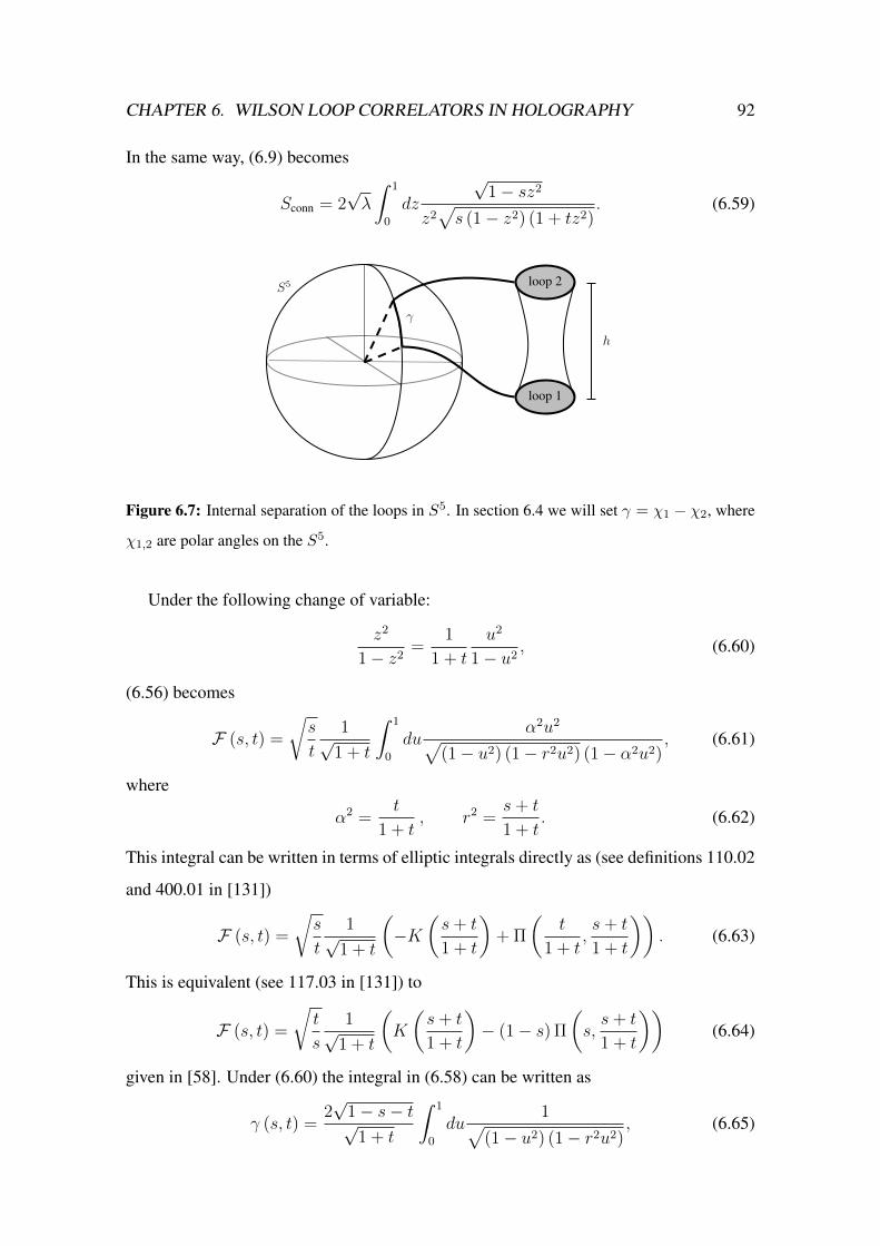
CHAPTER 6. WILSON LOOP CORRELATORS IN HOLOGRAPHY 92
In the same way, (6.9) becomes
Sconn = 2√λ
∫ 1
0
dz
√1− sz2
z2√s (1− z2) (1 + tz2)
. (6.59)
loop 2
loop 1
γ
h
S5
Figure 6.7: Internal separation of the loops in S5. In section 6.4 we will set γ = χ1 − χ2, where
χ1,2 are polar angles on the S5.
Under the following change of variable:
z2
1− z2=
1
1 + t
u2
1− u2, (6.60)
(6.56) becomes
F (s, t) =
√s
t
1√1 + t
∫ 1
0
duα2u2√
(1− u2) (1− r2u2) (1− α2u2), (6.61)
where
α2 =t
1 + t, r2 =
s+ t
1 + t. (6.62)
This integral can be written in terms of elliptic integrals directly as (see definitions 110.02
and 400.01 in [131])
F (s, t) =
√s
t
1√1 + t
(−K
(s+ t
1 + t
)+ Π
(t
1 + t,s+ t
1 + t
)). (6.63)
This is equivalent (see 117.03 in [131]) to
F (s, t) =
√t
s
1√1 + t
(K
(s+ t
1 + t
)− (1− s) Π
(s,s+ t
1 + t
))(6.64)
given in [58]. Under (6.60) the integral in (6.58) can be written as
γ (s, t) =2√
1− s− t√1 + t
∫ 1
0
du1√
(1− u2) (1− r2u2), (6.65)

CHAPTER 6. WILSON LOOP CORRELATORS IN HOLOGRAPHY 93
which corresponds to the definition 110.02 in [131], so
γ (s, t) =2√
1− s− t√1 + t
K
(s+ t
1 + t
). (6.66)
This implies that s+ t ≤ 1. The action (6.59) becomes
Sconn =2√λ√s
1√1 + t
∫ 1
ε
du
√1− α2u2
u2√
1− u2=
2√λ√s
1√1 + t
I (s, t) , (6.67)
where we have considered the regulator ε → 0. This integral in (6.67) can be written as
220.12 of [131]
I (s, t) = α
∫ 1
ε
du
√p2 − u2
u2√
1− u2= α
g
q2
((1− q2
)u1 − E
(ϕ, q2
)+ dnu1 tnu1
), (6.68)
where
α2 =s+ t
1 + t, p2 =
1
α2, q2 =
1
p2, g =
1
q, sinϕ =
√p2 (1− ε2)
p2 − ε2≈ 1−1
2
(1− q2
)ε2.
(6.69)
This means that ϕ ≈ π/2, thus u1 ≈ K (q2). Around u1 ≈ K,
sn ≈ 1− 1
2
(1− q2
)(u−K)2 . (6.70)
Moreover,
dnu1 tnu1 ≈ −1
u−K= −1
ε. (6.71)
This is the divergent part of the action because the other terms were not divergent for
u1 → K. The regularized integral now is
I reg (s, t) = (1− s)K(q2)− (1 + t)E
(q2). (6.72)
Finally,
Sregconn =
2√λ√s
1√1 + t
((1− s)K
(s+ t
1 + t
)− (1 + t)E
(s+ t
1 + t
))(6.73)
just like in [58]. From (6.66) we see that we can go to the ∆φ = 0 case in section 6.1
when s+ t = 1 which precisely corresponds to ` = 0.
Let us now analyse how the parameters s and t control the physical parameters (dis-
tance between loops and internal separation) and the action. In Figure 6.8, we plot curves
for constant γ and h/R, in this for R1 = R2 = R. We also plotted the Sconn/√λ = −2

CHAPTER 6. WILSON LOOP CORRELATORS IN HOLOGRAPHY 94
curve (dashed black line) that separates the connected and disconnected regions (see Fig-
ure 2 in [58]). For different values of γ and h/R we can see, just like in [58], that there are
intersections between γ and h/R; this indicates that for a fixed value of γ, two values of
h/R are possible; but as h/R grows intersections coalesce (see for example h/R ≈ 0.80
for γ ≈ π/2 in Figure 6.8). For h/R ' 0.8, for example h/R ≈ 0.9, there is no inter-
section so there is no connected solution. It is important to notice that, in general, when
we have these two intersections it is the one above the dotted black line that matters. This
corresponds to the dominant solution whose action is below Sconn/√λ = −2. Notice also
that for γ ≈ π we can have a connected solution only for h/R→ 0, and for γ ≈ 0 we are
limited by h/R ≈ 1.
Figure 6.8: s-t curves for different fixed values of γ and h/R. The black dotted line separates the
connected region from the disconnected one, representing the GO transition limit.
In Figure 6.9 we see how the action behaves as we increase the internal separation γ. In
particular, when R1 = R2 we see that as we increase γ the GO phase transition occurs at
lower distance. Notice there that when set γ = 0 (as studied in section 6.1), the transition
distance h/R goes to its maximum value, in this case, h/R ≈ 0.91 (see [29, 52, 129]).
Conversely, if we go to γ = π we see that the critical distance decreases and goes to
h/R = 0, i.e. the action is larger. We also see that the action has two branches, i.e. at

CHAPTER 6. WILSON LOOP CORRELATORS IN HOLOGRAPHY 95
fixed angle and distance there are two values for the action, two contributions; one of
them can be called dominant or leading, and the other sub-dominant.
Figure 6.9: Behavior of the action for differente values of the internal separation γ withR1 = R2.
As we decrese γ we reach the maximum value of the critical distance.
How does the action behave for α ≤ 1? If now the radii are different we expect the
allowed distance before the GO transition to decrease. Moreover, as we saw in Figure 6.9
the critical distance also decreases as we increase γ. In Figure 6.10 we show precisely
how hc behaves with α = R1/R2, in particular with R2 = 1.
In Figure 6.11 we plot the behavior of the action when γ = 0 but for α ≤ 1. As
mentioned before, for different radii the connected solution breaks before the equal radii
case, and also becomes energentically unfavorable with respect to the disconnected loops.

CHAPTER 6. WILSON LOOP CORRELATORS IN HOLOGRAPHY 96
Figure 6.10: Behavior of the critical distance hc with α = R1 when R2 = 1. Notice the highest
value of hc ≈ 0.91 when α = 1.

CHAPTER 6. WILSON LOOP CORRELATORS IN HOLOGRAPHY 97
Figure 6.11: Behavior of the action for γ = 0 with R2 = 1, so α = R1. Notice how the
critical distance for the GO transition decreases as we decrease α, and that for α = 1 we again get
hc/R ≈ 0.91. This plot is similar to the one in Figure 6.5.
As reviewed in this section, there is an interesting behavior when we connect two
Wilson loops: at certain distance the correlator ”prefers” (energetically) to separate into
two “domes”. This always happens before the critical distance in which the correlator
itself breaks and ceases to exist. It was argued in [48,49,52] that in the metastable region
of the distance, between hc and the maximum value when it breaks, the radius of the
connecting cylinder (i.e. the correlator) becomes of the order of the string length. After
that, when we keep separating, quantum fluctuations of the surfaces start to support the
worldsheet against the total collapse, so the two loops would be “connected” by a thin
tube of a string scale. Thus, the correlator does not completely vanish but is mediated by
the supergraviton exchange between the loops. Here lies the importance of the study of
the holographic Wilson loops correlators: correlators in the strong coupling regime could
give hints of glueballs in QCD (see [133,134], and also [26]). Correlator of Wilson loops

CHAPTER 6. WILSON LOOP CORRELATORS IN HOLOGRAPHY 98
where also studied perturbatively in [55, 56] and in the matrix model in [63, 122].
loop 1
loop 1
loop 2
loop 2
graviton
exchange
connected
solution
Sconn < Sdisc
Sconn > Sdisc
Figure 6.12: Scheme of the GO phase transition. The minimal worldsheet area connecting the
loops becomes larger that the sum of the minimal area of two domes. The connected solution
becomes energetically unfavorable.
6.3 Disconnected case with the defect
As we saw before, the usual phase transition, without the defect, occurs when the action
for the connected solution becomes, at some values of the parameters, equal or greater
than the action corresponding to two separated loops, so that it becomes favoured with
respect to the connected solution, Sconn ≥ S0. As we saw from Figure 6.5, this transition
occurs before the connected action becomes unstable: h0 < hmax. The case we want to
study here is how the transition behaves when we add a defect D5 brane, i.e. a wall that
divides the space into two parts, as described in [60].
Let us consider the Wilson loop in the presence of a D5 defect wrapping an AdS4×S2
subspace of AdS5 × S5 [63]. In this case, only one endpoint of the string describing the
Wilson loop lies at the boundary of AdS5, so one set of conditions are the same as the
case with no defect. The other set of conditions come from the fact that the string does go
into AdS5 and ends on the defect.
CHAPTER 6. WILSON LOOP CORRELATORS IN HOLOGRAPHY 99
The AdS space metric is given in (6.5). The S5 is
ds2S5 = dθ2 + sin2 θds2
S2 + cos2 θds2S2 (6.74)
where S2 and S2 are two 2-spheres: S2 is wrapped by D5 and S2 is its complementary in
S5. The solution of the probe D5 in AdS5 was found in [60] 5
y =1
κx , F = −κ volS2 , θ =
π
2, (6.75)
where κ represents the inclination of the D5 in the x − y plane. Also, κ is associated to
the number of D3 branes ending on the D5, n, by
κ =πn√λ. (6.76)
A fundamental string stretching from the boundary ofAdS5, y = 0, to the D5 is described
by the Polyakov action
Sdisc =
√λ
4π
∫dτdσ
1
y2
(y′2 + r′2 + r2 + x′2 + y2θ′2
), (6.77)
where the ansatz
φ = τ , y = y (σ) , r = r (σ) , x = x (σ) , θ = θ (σ) (6.78)
was used. Notice that now we have not considered x = σ because of (6.75). The equations
of motion are
x′ = −cy2 , θ′ = m, (6.79)
where c ≥ 0 and m ≥ 0 are constants of motion, and the minus sign in front of the
equation of x is because of the expected behavior of the solution in the x− y plane. Also,
we take c > 0 because we want that x decreases with σ. The equations of motion for y
and r are
yy′′ + r′2 + r2 − y′2 + c2y4 = 0 , yr′′ − 2r′y′ − yr = 0. (6.80)
The Virasoro constraint is
y′2 + r′2 + c2y4 + y2m2 − r2 = 0. (6.81)5Here we set x3 = x for simplicity.

CHAPTER 6. WILSON LOOP CORRELATORS IN HOLOGRAPHY 100
In order for the string to end on the D5, we impose that [60]
C1 ≡ y′ (σ) + κx (σ) = 0 , C3 ≡ r′ (σ) = 0,
C2 ≡ y (σ)− 1
κx (σ) = 0 , θ (σ) =
π
2, (6.82)
where σ is maximum value of the σ coordinate. Let us suppose that the loop is located at
x = L, and has radius R. At σ = 0 the string endpoint is at the boundary of AdS5, so
y (0) = 0 , r (0) = R,
x (0) = L , θ (0) = χ. (6.83)
The equation for θ is easy to solve:
θ (σ) = mσ + χ. (6.84)
From (6.82) we can determine the “size” of the string:
σ =1
m
(π2− χ
). (6.85)
If we define (see [64], where these calculations were done)
g (σ) =r (σ)
y (σ), h (σ) =
1
y (σ), (6.86)
Combining (6.80) and (6.81) gives two separated equations: one only for g (σ),
g′′ (σ)
g (σ)= 1−m2 + 2g2 (σ) , (6.87)
andh′′ (σ)
h (σ)= 2g2 (σ)−m2. (6.88)
(6.87) can be easily solved to get (see [135])
g (σ) =
√m2 − 1
k2 + 1ns
(√m2 − 1
k2 + 1σ, k2
), (6.89)
where k2 is the elliptic modulus of the Jacobi elliptic function. Near σ → 0 we see that
g (σ)→ 1/σ. This can be also inferred from the definition (6.86). Notice that
g (0) =r (0)
y (0)→∞. (6.90)

CHAPTER 6. WILSON LOOP CORRELATORS IN HOLOGRAPHY 101
which is in agreement with (6.83). Let us follow [64] and write the first equation in (6.87)
as
g′2 (σ) +(m2 − 1
)g2 (σ)− g4 (σ) = −ε0 −m2, (6.91)
since it does not depend explicitly on σ. Here, −ε0 − m2 is a convenient integration
constant. Moreover, by considering that h (σ) has the following form
h (σ) =√
1 + g2 (σ)z (σ) , (6.92)
we can rewrite, with help of (6.87) and (6.91), (6.88) as(g2 (σ) + 1
) (2g (σ) g′ (σ) z′ (σ) +
(g2 (σ) + 1
)z′′ (σ)
)− ε0z (σ) = 0. (6.93)
If we multiply (6.93) by 2z′ (σ) and integrate in σ, we get(g2 (σ) + 1
)2z′2 (σ)− ε0z
2 (σ) + ζ0 = 0, (6.94)
where ζ0 is an integration constant that can be fixed by rewriting the Virasoro constraint
(6.81) in terms of g (z) and z (σ), and with (6.91). The result is(g2 (σ) + 1
)2z′2 (σ)− ε0z
2 (σ) + c2 = 0, (6.95)
from which ζ0 = c2. From (6.95) we also see that ε0 ≥ 0. The last equation can be solved
by
z (σ) =c√ε0
cosh (v (σ)− η) , (6.96)
if we define
v′ (σ) =
√ε0
1 + g2 (σ)(6.97)
with v (0) = 0 and η being an integration constant. From (6.86) we can write that
y (σ) =
√ε0
c
1√1 + g2 (σ)
sech (v (σ)− η) ,
r (σ) =
√ε0
c
g (σ)√1 + g2 (σ)
sech (v (σ)− η) . (6.98)
From (6.79),
x′ = −√ε0
cv′ (σ) sech2 (v (σ)− η) , (6.99)
which can be integrated:
x (σ) = x0 −√ε0
ctanh (v (σ)− η) . (6.100)

CHAPTER 6. WILSON LOOP CORRELATORS IN HOLOGRAPHY 102
Let us impose the boundary conditions (6.83). r (0) = R becomes
R =
√ε0
csech η ⇒ c =
√ε0
Rsech η. (6.101)
x (0) = L, on the other hand, becomes
L = x0 +R sinh η ⇒ x0 = L−R sinh η. (6.102)
A clever way to impose the boundary conditions on the D5 brane (6.82) is to impose a
combination of them, sinceCi = 0 then∑
iAiCi = 0, [64]. With (6.98), the combination:
κcC1 +1
y (σ)C2 +
r (σ)
y2 (σ)C3 = 0 ⇒ −cx0 = 0. (6.103)
This helps to find thatL
R= sinh η, (6.104)
now in terms of L and R, geometric parameters. From C3 = 0 we have,
√ε0g (σ) tanh (η − v (σ)) + g′ (σ) = 0 ⇒ η = v (σ) + tanh−1
(− 1√ε0
g′ (σ)
g (σ)
)(6.105)
The last result allows to eliminate v (σ)−η from C1 = 0 and C2 = 0 in (6.82) with (6.98).
Both boundary conditions lead to the same equation for κ, the flux,
κ = −√
1 + g2 (σ)g′ (σ)√ε0g2 (σ)− g′2 (σ)
, (6.106)
where κ ≥ 0 since it is the flux due to the D5 defect. We can use (6.91) to eliminate
g′2 (σ) in the denominator of (6.106) to get
κ = − g′ (σ)√m2 + ε0 − g2 (σ)
. (6.107)
Let us write (6.98) and (6.100) by using (6.101),
y = R cosh η1√
1 + g2 (σ)sech (v (σ)− η) ,
r = R cosh ηg (σ)√
1 + g2 (σ)sech (v (σ)− η) ,
x = −R cosh η tanh (v (σ)− η) . (6.108)
Now, since v (σ) is given by (6.97), we need an explicit form for g (σ). We can write
(6.91) as
g′2 (σ) =(g2 − α+
) (g2 − α−
), (6.109)

CHAPTER 6. WILSON LOOP CORRELATORS IN HOLOGRAPHY 103
with
α± =1
2
(m2 − 1±
√(m2 + 1)2 + 4ε0
). (6.110)
We can write (6.109) as
±∫ g
∞
dg√(g2 − α+) (g2 − α−)
= σ, (6.111)
from which we choose the minus sign in order to have σ ≥ 0. This integral can we solved
in terms of Jacobi elliptic function ns (see 130.10 in [131]). As a result we get
g (σ) =√α+ ns
(√α+σ,
α−α+
). (6.112)
If we compare the last result with (6.89),
k2 =α−α+
=m2 − 1−
√(m2 + 1)2 + 4ε0
m2 − 1 +√
(m2 + 1)2 + 4ε0
. (6.113)
since k < 1. This allows to write
ε0 = −(k2 +m2) (m2k2 + 1)
(k2 + 1)2 . (6.114)
We can also write c2 from (6.101) in terms of k2,
c2 = −(k2 +m2) (m2k2 + 1)
(k2 + 1)2 (L2 +R2). (6.115)
We need ε0 ≥ 0, and also that α+ ≥ 0 to have g (σ) real. This leads to 6
region (A) −1 ≤ k2 ≤ 0 m2 ≥ − 1
k2,
region (B) −∞ < k2 ≤ −1 m2 ≤ − 1
k2.
(6.116)
6ε0 ≥ 0 actually produces four regions of parameters but we choose only those that lead to real g (σ).

CHAPTER 6. WILSON LOOP CORRELATORS IN HOLOGRAPHY 104
Figure 6.13: Allowed values of k2 and m2 for ε0 ≥ 0. Only those values of k2 and m2 that
leads to g (σ) be real are selected. They depict two different regions: A and B. The black curve
represents m2 = −1/k2 (or c = 0).
From (6.115) we see that c = 07 at the intersection of both regions,
m2 = − 1
k2. (6.117)
We can write (6.112) as
g (σ) =
√m2 − 1
k2 + 1ns
(√m2 − 1
k2 + 1σ, k2
). (6.118)
as expected.
Since κ ≥ 0, from (6.107) we need that g′ (σ) ≤ 0 and
g2 (σ) ≤ −k2 (m2 − 1)2
(k2 + 1)2 . (6.119)
From g′ (σ) ≤ 0 we deduce that
0 ≤ σ ≤ σmax with σmax =
√k2 + 1
m2 − 1K(k2). (6.120)
7This case was solved in [63].

CHAPTER 6. WILSON LOOP CORRELATORS IN HOLOGRAPHY 105
From (6.85) we find
x ≤ K (k2)(π2− χ
) , (6.121)
where it was defined
x =
√m2 − 1
m2 (k2 + 1). (6.122)
From (6.116) we get the same range for x for both regions, so
1 ≤ x ≤ K (k2)(π2− χ
) . (6.123)
As said in [64], in region A, by construction, x is always less or equal to 1/√k2 + 1.
Then, from (6.121), we have
1 ≤ x ≤ Min
(1√
k2 + 1,K (k2)(π2− χ
)) . (6.124)
It is necessary that the admisible interval of x is not empty. If k2 = tanα, α ∈[−π
2, 0].
This is shown in Figure 6.14.
Figure 6.14: This plot shows the allowed values of χ and α. There also appear separated regions
A and B. The black curve corresponds to χ = π2 − K
(k2)
(or x = 1, so m2 = −1/k2, then
c = 0). Also, χ = 0 is allowed only when k2 = 0 (and then m2 →∞) in region A. This leads to
σ → 0 (no solution).
CHAPTER 6. WILSON LOOP CORRELATORS IN HOLOGRAPHY 106
Moreover, (6.119) can be written as
cn2(x(π
2− χ
), k2)≤ − 1
k2
(1− 1
x2
). (6.125)
The r.h.s of (6.125) takes values between 0 and 1 in both regions A and B. Let us consider
the lower bound of the last relation,
cn2(x0
(π2− χ
), k2)
= − 1
k2
(1− 1
x20
). (6.126)
Since x0 ≥ 1, this reduces the interval of x to be
region (A) 1 ≤ x0 ≤ x ≤ Min
(1√
k2 + 1,K (k2)(π2− χ
)) ,region (B) 1 ≤ x0 ≤ x ≤ K (k2)(
π2− χ
) .(6.127)
On the other hand, (6.107) can be written, by using (6.118), as
κ2 =x2 cn2 (w, k2) dn2 (w, k2)
(k2x2 cn2 (w, k2) + x2 − 1) sn2 (w, k2), (6.128)
where w = x (π/2− χ) =√nσ. It is possible to see that when w = K (k2), so x =
K (k2) / (π/2− χ), then κ = 0. If χ → π/2, x could be greater than 1/√k2 + 1 and
then go out the allowed values in region A. In general, we cannot find an x inside A that
allows small κ for χ→ π/2.

CHAPTER 6. WILSON LOOP CORRELATORS IN HOLOGRAPHY 107
Figure 6.15: Values of x that lie outside region A (green) when K(k2)/ (π/2− χ) ≥
1/√k2 + 1. Critical values (αc, χc) when κ = 0 (blue). The region A (blue) enlarges as we
increase κ. The blue curve represents xc = 1/√
1 + k2c .
In Figure 6.15, the blue curve has m2 → ∞; since it must converge to the same point
(0, 0), we can say that the blue curve also represents c = 0. The χ = π/2 line corresponds
to k2 → −∞, this leads to c2 → −m2; since c2 cannot be negative, m2 = 0. Thus, the
total allowed region, both A and B, is surrounded by c = 0 (the case solved in [63]).
As said in [64], we can fix χ and κ and study how the region A changes as we increase
k2. Let xc = 1/√k2c + 1 be the critical value of x that solves (6.128) in A. For k2 ≥ k2
c
there is no solution for κ. From (6.128),
sn
((π/2− χ)√k2 + 1
, k2
)≥
√2√
k2 + 1 +√
(k2 − 1)2 − 4k2κ2
, (6.129)

CHAPTER 6. WILSON LOOP CORRELATORS IN HOLOGRAPHY 108
or
χ ≤ π
2−√k2 + 1 sn−1
√
2√k2 + 1 +
√(k2 − 1)2 − 4k2κ2
, k2
. (6.130)
These values ensure that the l.h.s of (6.128) is less than a fixed κ2. Also, from (6.130),
we can find, at fixed κ and χ, the critical value of k2 (in region A) above which there is
no solution. It was shown in [64] that as we increase κ2 the allowed values of k2 also
increase (see also Figure 6.16). In Figure 6.15 this can be seen as the expansion of the
region A (blue).
Figure 6.16: Expansion of the allowed region of parameters as we increase κ. Notice how k2c goes
to zero as we enlarge region A. Thus, when κ → ∞, k2 can be zero at any value of χ ∈[0, π2
].
Each curve for fixed κ is given by the equality in (6.130)
So, for larger values of κ we can access larger values in region A. When κ → ∞,
region A enlarges to its maximum. In general, χ and κ control the limits of k2.

CHAPTER 6. WILSON LOOP CORRELATORS IN HOLOGRAPHY 109
6.3.1 Evaluating the action
Back to the action (6.77), we can write it onshell as
Sdisc =√λ
∫ σ
0
dσr2
y2. (6.131)
From (6.108) we get
Sdisc =√λ
∫ σ
0
dσg2 (σ) =√λ
∫ σ
0
dσ n ns2(√
nσ, k2), (6.132)
where n = m2−1k2+1
. This integral can be solved in terms of elliptic function (see 362.01
in [131]),
Sdisc =√λn(√
nσ − E(am(√
nσ), k2)− dn
(√nσ, k2
)cs(√
nσ, k2)) ∣∣∣∣σ=σ
σ=0
. (6.133)
The last result is divergent at σ = 0. We also assume that σ > 0, so k2 < k2c and the
action is non-vanishing. As usual, let us introduce the regulator σ = ε with ε → 0. With
this, the evaluated action becomes
Sdisc =√λn(w − E
(am (w) , k2
)− dn
(w, k2
)cs(w, k2
))+
√λ
ε, (6.134)
which, without the O (1/ε) term, corresponds to the onshell action.
On the other hand, if we derivate (6.105) w.r.t σ, then combine with (6.97) and finally
integrate, we get an expression corresponding to the definition of the incomplete elliptic
integral of the third kind (see 400.01 [131]). Then, we find
η =
√− (1 + n)
(1
n+ k2
)Π(am(w, k2
),−k2n, k2
), (6.135)
where w = x (π/2− χ) =√nσ. Thus,
L
R= sinh η, (6.136)
so η ≥ 0. From (6.105) we can say that at k2c , for which m2 →∞ and then σ → 0, η, and
thus L/R, goes to zero. This gives an interpretation to the critical value k2c : the value for
which the Wilson loop touches the defect [64].

CHAPTER 6. WILSON LOOP CORRELATORS IN HOLOGRAPHY 110
Figure 6.17: Behavior of L/R with k2 for χ = π/2−K (−0.95) ≈ 0.25. Notice that as k2 → k2c ,
the critical value for each κ2, L/R→ 0, as expected.
From Figure 6.17, we can see that L/R is not always monotonic. There are certain
values of κ2 in which L/R has a maximum [64]. This leads to having two values of k2
for one L/R. In Figure 6.18 and Figure 6.19 we can see, for fixed values of χ, that an
increasing flux also increases the critical distance Lc/R for the Gross-Ooguri-like transi-
tion and the maximum value of L/R for the solution to exist. We also see that decreasing
the angle also decreases the critical value of Lc/R.
When the transition occurs the minimal area of the string worldsheet attached to the
boundary and to the defect becomes larger than the minimal area of the string worldsheet
ending only on the boundary and forming a dome surface because. This configuration is
energentically preferred with respect to the one ending on the D5 (see Figure 6.20).

CHAPTER 6. WILSON LOOP CORRELATORS IN HOLOGRAPHY 111
Figure 6.18: Behavior of Sdisc with L/R for different values of the flux κ2 at χ ≈ 0.25. We
can see that the distance for the GO-like transition, when the curves cross S0, the action in (6.2),
increases as we increase the flux κ.

CHAPTER 6. WILSON LOOP CORRELATORS IN HOLOGRAPHY 112
Figure 6.19: Behavior of Sdisc with L/R for different values of the flux κ2 at χ ≈ 0.12. We can
see here that for a lower value of χ, all critical distances for the GO-like transition decrease. Also,
notice that for this choice of χ there is only branch for the action.

CHAPTER 6. WILSON LOOP CORRELATORS IN HOLOGRAPHY 113
D5 defect
Sdefect
S0 = −√λ
loop
κ
χ
R
S5
Figure 6.20: Behavior of Sdisc, the action of the worldsheet attached to the D5 defect and its
comparison with the “dome”. This is the GO-like transition studied in [64]. In this case χ ≤ π/2
because the D5 defect is located at χ = π/2 in S5.
6.4 Phase transition in the presence of the defect
In this section we will explore the case in which we have two Wilson loops separated by a
distance along x3 in the presence of a D5 defect. The correlator of these loops will be the
same as in section 6.2, in which we reviewed the correlator of two Wilson loops with radii
R1 andR2, separated by a distance h along x3 and by an internal angle γ. At some critical
value of the distance the area of the worldsheet stretching between the loops becomes
greater than the total area of two independent loops forming the usual dome in AdS5, and
thus a phase transition occurs. This critical distance is controlled by the internal angle and
the radii as can be seen in Figure 6.9 and Figure 6.11. Also, the connected correlator has
a maximum distance before ceasing to exist and, as we saw, this happens always before
they are becoming energentically unfavored with respect to the domes. In the presence

CHAPTER 6. WILSON LOOP CORRELATORS IN HOLOGRAPHY 114
of a D5 defect we must take care now if the corresponding minimal area connecting the
loops becomes larger than the total area of the two loops. These loops could either both
end on the defect or only one of them or both form domes. This behavior is now controlled
by more parameters: the radii R1 and R2, the distance with respect to the defect, L, the
relative distance between the loops, h, the internal angles χ1 and χ2, and the flux due to
the defect, κ.
As a starting situation we consider that the two loops have equal radii R1 = R2 = R;
and that the first one is placed at L/R with respect to the defect and the second one is at
(L+ h) /R. With this we fix the minimal string worldsheet of the first loop and then the
total action will depend only on h/R. For the second loop we have,
h
R(χ1, χ2, κ) = −L
R(χ2, κ) + sinh η (χ1, κ) , (6.137)
and the total action is
Sdisc
(h
R, γ, κ
)= S
(1)disc
(L+ h
R, χ1, κ
)+ S
(2)disc
(L
R, χ2, κ
), (6.138)
where the upper indices correspond to the actions of first and second loops, respectively,
and with S(2)disc
(LR, χ2, κ
)fixed at certain value of L/R for which the loop is connected to
the defect. We also took R1 = R2 = R in order to control the transition only with L/R,
h/R, κ and γ = χ1 − χ2.
We will fix the first loop at a distance L/R for which its action S(2)disc < −
√λ, and leave
the relative distance h/R free in S(1)disc.
In Figure 6.21, we see how the action corresponding to two Wilson loops behaves in
terms of their relative separation h/R. There we have fixed the first loop to be always
connected to the defect so we can see at which value of h/R the second loop forms a
dome.
As we learned from Figure 6.9 and Figure 6.11, the minimal worldsheet connecting
two Wilson loops has maximum values for γ → 0 (coincident loops in S5) and α → 1
(equal radii). In Figure 6.21, we chose χ1 ≈ 0.25, R1 = R2 = R, and plotted the total
disconnected action for three different values of parameters for the fixed loop.

CHAPTER 6. WILSON LOOP CORRELATORS IN HOLOGRAPHY 115
Figure 6.21: Behavior of two separated Wilson loops in the presence of a D5 defect with κ2 = 2
with χ1 ≈ 0.25. We have fixed the second loop for different values of parameters. Remember the
GO-like transition occurs at −1+S(2)disc, so hc/R ≈ 0.05− 0.1, so most of Sdisc correspond to one
loop attached to the D5 and the other one not attached. For lower values of κ2 the maximal value
of h/R decreases.
In Figure 6.21 we considered two cases in which the second loop is attached to the
D5 brane and one in which it is not (green). For the first two cases we considered also
different internal angles, one of them being equal to our choice of χ1, so γ = 0. Notice
that for h/R→ 0 we reduce to
Sdisc (0, γ, κ) = S(1)disc
(L
R, χ1, κ
)+ S
(2)disc
(L
R, χ2, κ
), (6.139)
in which for χ1 = χ2 ≈ 0.25 we reduce to 2S(2)disc
√λ ≈ −3.2. In general, we show a

CHAPTER 6. WILSON LOOP CORRELATORS IN HOLOGRAPHY 116
scheme in Figure 6.22.
loop 2 loop 1
D5 defect
S(2)disc S
(1)disc
S0 = −√λ
Figure 6.22: Two separated loops with the same radii. The first loop keeps fixed on the D5. Each
loop can take different positions in S5. We must take care on the second loop since its distance
(L+ h)/R could allow the GO-like transition: Sdisc (hc/R, γ, κ) = −√λ+ S
(2)disc (L/R, χ2, κ).
In Figure 6.23 and Figure 6.24, we see for χ1 = χ2 ≈ 0.25, the comparison between
the minimal string worldsheet connecting two loops of equal radii separated by a distance
h (red) compared with the total action of two independent loops where one of them is
fixed to have S(2)disc/√λ = −2 and S(2)
disc/√λ = −3, respectively, so it ends on the D5 in
three cases: κ2 = 4, 6, 10. When total action Sdisc/√λ = −3 and Sdisc/
√λ = −4, the first
loop forms a dome since its action S(1)disc/√λ = −1. This is the GO-like transition [64]. As
we increase the flux the GO transition occurs at lower distances because the inclination
of the defect increases. For lower values of the flux the connected solution does not see
the defect and the GO transition occurs at h/R ≈ 0.9 as usual.

CHAPTER 6. WILSON LOOP CORRELATORS IN HOLOGRAPHY 117
Figure 6.23: Behavior of Sconn compared to Sdisc for γ = 0 in S5 and S(2)disc/√λ = −2 for different
values of κ. GO transition from connected to attached-dome configuration.

CHAPTER 6. WILSON LOOP CORRELATORS IN HOLOGRAPHY 118
Figure 6.24: Behavior of Sconn compared to Sdisc for γ = 0 in S5 and S(2)disc/√λ = −3 for different
values of κ. GO transition from connected to attached-attached configuration.
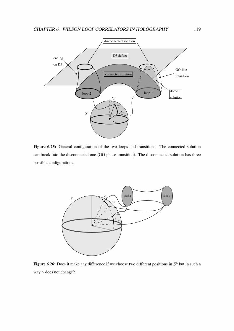
CHAPTER 6. WILSON LOOP CORRELATORS IN HOLOGRAPHY 119
loop 2 loop 1
D5 defect
connected solutionGO-like
transition
ending
on D5
disconnected solution
dome
solution
S5χ1
χ2
γ
Figure 6.25: General configuration of the two loops and transitions. The connected solution
can break into the disconnected one (GO phase transition). The disconnected solution has three
possible configurations.
γ
γ
loop 2 loop 1S5
χ′2
χ2
χ′1
χ1
Figure 6.26: Does it make any difference if we choose two different positions in S5 but in such a
way γ does not change?

CHAPTER 6. WILSON LOOP CORRELATORS IN HOLOGRAPHY 120
Figure 6.27: GO phase transition for two cases with the same separation in S5, γ ≈ 0.13 and
S(2)disc/√λ = −3.
In Figure 6.27, we see, for κ2 = 6, that if the two loops are not placed in the same
positions in S5 but their separation is the same the critical distance for the GO transition
increases for the loops placed at lower polar positions in S5.
There are now several parameters we could manipulate in order to control the tran-
sitions: L/R, h/R, χ and κ. And, if we choose different radii, also R1/R2 will be a
parameter. We could choose the first loop ending on the defect, either near the the dis-
tance for which the minimal surface becomes a dome or not. If the second loop ”sees” the
defect or not depends on this choice. Also, different internal angles would lead to move
the critical values for the transitions. The general setup is given in Figure 6.25.
Chapter 7
Results and outlook
There are now techniques that allow to test the AdS/CFT conjecture exactly, i.e to have
results that can be compared on the weak/strong coupling on the opposite sides of the
duality. In particular, a largely studied observable in gauge theory is the Wilson operator.
In this case, by using localization, on the gauge side and probe branes on the gravity side,
exact results were obtained. The strong coupling expansion of these results can then be
successfully compared with a dual gravity computation based on minimal string surfaces
in AdS, attached to the loop on the AdS boundary. If instead of the expectation value of a
single Wilson loop, one wanted to compute the correlator between two loops holographi-
cally, the relevant string worldsheet surface would be the one connecting the two different
contours. Modifying the geometry of these two rings introduces a phase diagram in which
there are critical values for the parameters that separate the catenoid solution and the
Goldschmidt solution. When the two rings are separated beyond a certain critical value,
the catenoid solution becomes unstable and breaks into the Goldschmidt one. Similarly,
in the case of the Wilson loop, the string worldsheet describes a catenoid-like solution
until, at certain values of the radii of the loops and the distance, it becomes energetically
unfavored with respect to the Goldschmidt-like solution. This is called a Gross-Ooguri
(GO) phase transition. The discontinuous (broken catenoid) solution corresponds, in this
case, to two minimized “dome“ surfaces in AdS, each attached to a different loop, i.e two
separated Wilson loops. These minimal surfaces are the usual onshell regularized actions
with each loop as boundary. On the gauge theory side, the correlator of two Wilson loops
is studied and it is found that there exist an analogous GO transition. An interesting setup
121

CHAPTER 7. RESULTS AND OUTLOOK 122
that was the focus of this work is the one in which a defect is introduced in the gauge
theory. This defect is typically obtained by considering systems of intersecting branes. In
particular, intersecting D3 and D5 branes along three of the four worldvolume directions
allows to construct three-dimensional defects inside the N = 4 worldvolume of the N
D3 branes. The end result is that there are two different gauge groups on each side of the
defect brane. This is because k D3 branes now end on the D5 defect, so on one side we
have the usual SU(N) and on the other side we have SU(N − k). On the string theory
side, the solution corresponding to a single D5 wall insideAdS5×S5 is computed by con-
sidering that the D5 brane is along three directions in AdS5 and two in S5. This reduces
the allowed symmetries in both parts; in particular, the conformal symmetry of AdS5 and
the isometries of S5. The minimal worldsheet surface is attached to the loop and ends on
the defect. The presence of the defect introduces then new boundary conditions for the
string: the usual ones along the loop and the ones that ensure that the worldsheet surface
end on the defect. But it could happen that the string worldsheet does not touch the defect,
or energetically prefers not to end on it and form a dome instead. Thus, this situation is
very rich in parameters. This work is recent and ongoing. We studied the Wilson loop
correlator in the presence of a D5 defect on the string theory side and the Gross-Ooguri
phase transition in this geometry. We investigated in detail how this transition depends
on the parameters of the setting: radii and separation of the loops, distance with respect
to the defect and inclination of it, and we compared this case with the case without defect
and observed that the defect modifies the GO transition region.
Since the latter was solved by considering the connected solution of a single world-
sheet attached to two loops, and its transition into two separated minimal worldsheet
surfaces; the gauge dual of this correlator will correspond to the expectation value of two
Wilson loops in the fundamental representations. The work in the gauge theory side was
already started for the correlator without the defect of two concentric loops. Also, Wil-
son loops in defect gauge theory were also computed and are still studied. We leave as
a future work to study also correlators in defect field theory by using well-defined tech-
niques in field theory such as perturbative expansion and localization. As we mentioned
above, the duality was tested also for higher representations, which on the string side,
correspond to putting probe branes in the string background. Thus, for the N = 4 SYM

CHAPTER 7. RESULTS AND OUTLOOK 123
theory, it was found that, in particular, a Wilson loop in the symmetric representations
corresponds to a D3 probe in AdS5 × S5; and that the antisymmetric representation case
to a D5 probe instead, both with the loop as boundary. In general, for an arbitrary high
representation, the dual string description is in terms of bubbling geometries. Here, the
string background is strongly deformed by the high number of branes in it. So, it is also
interesting to extend the study of correlators of fundamental Wilson loops in defect field
theory to corrrelators of symmetric/antisymmetric Wilson loops now in the presence of
defects. If we consider one of the string attached to the loop as before but the other one
attached now to a D3 brane, this is the case of a Wilson loop correlator for mixed repre-
sentations; in particular, we setup the symmetric/fundamental correlator in Appendix A.
The antisymmetric/fundamental case, involving a D5 brane as boundary of one end of the
string was studied before.
Another interesting route to follow is the finite temperature case. So , there are many
routes to follow, firstly, to find the corresponding solution of the finite temperature case
in the presence of a defect, and later to consider the correlator of two Wilson loops in that
case. This should reduce to the known results at zero temperature and, at some values of
the paremeters, to the zero temperature case without defect. Another route we want to
follow is to consider adding parameters that deform the string background without losing
the solvability of the model. These directly come from the so-called integrable deforma-
tions in which we can consider to put Wilson loops, i.e. to try to find the minimal surface
of the string worldsheet [136, 137]. These deformed string backgrounds correspond to
non-commutative quantum field theories which are also largely studied. Independently of
the AdS/CFT correspondence, Wilson loops in non-commutative field theories were stud-
ied since the beginning of the AdS/CFT times [18, 19, 138], and recently in [139]. Thus,
we are also interested in studying the correlator of Wilson loops to make progress and
predictions that will be comparable with their corresponding string dual. These studies
can help to deepen and enrich our understanding of AdS/CFT correspondence.
Appendix A
Symmetric/fundamental Wilson loop
correlator
In this section we study the correlator between two Wilson loops, one in the fundamental
and the other in the symmetric representation.1 We already know that the fundamental
representation corresponds to taking a string and that the symmetric representation corre-
sponds to taking a D3 brane. We discover that, after a suitable choice of coordinates, the
presence of the D3 brane introduces new boundary conditions parameterized by κ. We
study how the Gross-Ooguri phase transition behaves in this case, and how it reduces to
the fundamental/fundamental case.1The antisymmetric/fundamental case was studied in [78] and the antisymmetric/antisymmetric case
in [79].
124

APPENDIX A. SYMMETRIC/FUNDAMENTAL WILSON LOOP CORRELATOR125
D3 brane
Connected solutionloop 2 loop 1
dome solution
Figure A.1: Schematic behavior of the connected solution for the holographic symmet-
ric/fundamental Wilson loop correlator. Since the D3 brane is much heavier that the fundamental
string, the D3 brane is not deformed and only sets new boundary conditions.
The Drukker-Fiol solution was found by using
ds2
L2=
1
sin2 η
(dη2 + cos2 ηdψ2 + dρ2 + sinh2 ρ
(dθ2 + sin2 θdφ2
)), (A.1)
as the AdS5 metric. Here 0 ≤ ρ, 0 ≤ θ ≤ π and 0 ≤ η ≤ π/2. The solution for a D3
brane is given by
sinh ρ = κ sin η , Fψρ =iκ√λ
2π sinh2 ρ, κ =
k√λ
4N. (A.2)
The solution is attached to the circle on the AdS boundary at ρ = 0, and corresponds to a
Wilson loop in the symmetric representation.
The loop at the boundary appears from the original form of the AdS metric,
ds2
L2=
1
y2
(dy2 + dr2
1 + r21dψ
2 + dr22 + r2
2dφ2)
(A.3)
with
r1 =R cos η
cosh ρ− sinh ρ cos θ, r2 =
R sinh ρ sin θ
cosh ρ− sinh ρ cos θ, y =
R sin η
cosh ρ− sinh ρ cos θ.
(A.4)
with x3 = r2 cosφ and x4 = r2 sinφ. The original condition for the loop is r1 = R with
y = 0. Thus,
r21 + y2 =
R2
(cosh ρ− sinh ρ cos θ)2 ⇒ r1 = R if ρ = 0. (A.5)

APPENDIX A. SYMMETRIC/FUNDAMENTAL WILSON LOOP CORRELATOR126
Now let us consider a string worldsheet whose first boundary is attached to the D3 brane
and its second boundary is attached to the loop on the AdS boundary. Let the worldsheet
coordinates be (σ, ψ). Let σ = σ0 be the boundary on the brane, whereas σ = σ1 be the
boundary at the loop with σ0 < σ1.
Let us consider the ansatz
η = η (σ) , ρ = ρ (σ) , θ = 0. (A.6)
This ansatz makes r2 = 0, so x3, x4 = 0, which does not allow to study the correlator of
Wilson loops separated in x3. We could choose instead,
η = η (σ) , ρ = ρ (σ) , θ = π/2 , φ = 0, (A.7)
which implies x4 = 0 and
x3 (σ) = r2 = R tanh ρ (σ) (A.8)
and
r1 (σ) =R cos η (σ)
cosh ρ (σ), y (σ) =
R sin η (σ)
cosh ρ (σ). (A.9)
The boundary conditions are:
• σ = σ0 (string attached at the boundary loop)
ρ (σ0) = η (σ0) = 0 ⇒ r1 = R1 = R , y = 0 x3 = 0; (A.10)
• σ = σ1 (string attached to the D3 brane + ansatz)
ρ (σ1) = ρ0 = sinh−1 (κ sin η (σ1)) = sinh−1 (κ sin η0)
x3 (σ1) = h0 −R tanh ρ0 = h (ρ0)
r1 (σ1) =R cos η0
cosh ρ0
=R√κ2 − sinh2 ρ0
κ cosh ρ0
= R2 (ρ0)
y (σ1) =R sin η0
cosh ρ0
=R tanh ρ0
κ=h (ρ0)
κ. (A.11)
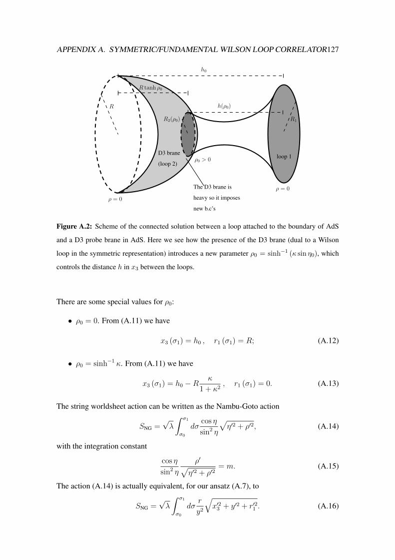
APPENDIX A. SYMMETRIC/FUNDAMENTAL WILSON LOOP CORRELATOR127
R tanh ρ0
h(ρ0)R
R1R2(ρ0)
ρ0 > 0
ρ = 0
ρ = 0
h0
D3 brane
(loop 2)loop 1
The D3 brane is
heavy so it imposes
new b.c’s
Figure A.2: Scheme of the connected solution between a loop attached to the boundary of AdS
and a D3 probe brane in AdS. Here we see how the presence of the D3 brane (dual to a Wilson
loop in the symmetric representation) introduces a new parameter ρ0 = sinh−1 (κ sin η0), which
controls the distance h in x3 between the loops.
There are some special values for ρ0:
• ρ0 = 0. From (A.11) we have
x3 (σ1) = h0 , r1 (σ1) = R; (A.12)
• ρ0 = sinh−1 κ. From (A.11) we have
x3 (σ1) = h0 −Rκ
1 + κ2, r1 (σ1) = 0. (A.13)
The string worldsheet action can be written as the Nambu-Goto action
SNG =√λ
∫ σ1
σ0
dσcos η
sin2 η
√η′2 + ρ′2, (A.14)
with the integration constant
cos η
sin2 η
ρ′√η′2 + ρ′2
= m. (A.15)
The action (A.14) is actually equivalent, for our ansatz (A.7), to
SNG =√λ
∫ σ1
σ0
dσr
y2
√x′23 + y′2 + r′21 . (A.16)

APPENDIX A. SYMMETRIC/FUNDAMENTAL WILSON LOOP CORRELATOR128
This is the usual action in AdS as studied in [52]. Let us choose now σ = x3 = x and
rename r1 = r, thus the action becomes
Sconn =√λ
∫ h=R tanh(κ sin η0)
0
dxr
y2
√1 + y′2 + r′2. (A.17)
There is also a boundary term due to the gauge field at σ = σ1 (see [78])
Sbdy,1 = i
∫σ=σ1
A+constant = iAψ (σ0)+constant =√λ
(√
1 + κ2 −√
1 + κ2 sin2 η0
sin η0
).
(A.18)
The constant is chosen so that this boundary term vanishes at η0 = π/2 where the bound-
ary of the worldsheet shrinks to a point (and ρ0 = sinh−1 κ).
If ρ0 → 0
Sbdy,1 =√λ√
1 + κ2 −√λκ
ρ0
. (A.19)
Thus, let us just take the expression for the (usual) connected correlator between two
Wilson loops, with radii R1 = R and R2 = R2 (ρ0), separated by a distance h = h (ρ0)
in x3 of AdS:
Sconn = 2√λR +R2 (ρ0)
ε (ρ0)+ 2
(1 + 4τ 2
)1/4 ((1− w2
)K(w2)− E
(w2)). (A.20)
Here w = w (τ), where τ = ma is a geometrical parameter, with
m =r
y2
1√1 + r′2 + y′2
, (A.21)
and
a2 =
(R2
2 −R21
2h− h
2
)2
+R22. (A.22)
We know that the divergent part of (A.20) comes from evaluating the action with a cutoff
in y at the two sides of the connected solution which end at y = 0. So we can translate
this term to the coordinates we are using. From (A.10) and (A.11) with ρ0 → 0
Sconn = 4√λκ
ρ0
+ 2(1 + 4τ 2
)1/4 ((1− w2
)K(w2)− E
(w2)), (A.23)
where w = w (τ). If we add (A.19) with ρ0 → 0 and, we get
Sonshellconn = 3
√λκ
ρ0
+ 2√λ(1 + 4τ 2
)1/4 ((1− w2
)K(w2)− E
(w2))
+√λ√
1 + κ2
(A.24)

APPENDIX A. SYMMETRIC/FUNDAMENTAL WILSON LOOP CORRELATOR129
We still have a divergent term that we must totally eliminate by a suitable Legendre trans-
form. Let us take instead the finite part of the action as being regularized
Sregconn = 2
√λ(1 + 4τ 2
)1/4 ((1− w2
)K(w2)− E
(w2))
+√λ√
1 + κ2 (A.25)
The parameter τ = ma, where a = a (ρ0), parametrizes F = F (τ). But now we have
h0 −R tanh ρ0 = R2
√2α(1 + 2 sinh2F (τ)
)− α2 − 1, (A.26)
where α = R/R2. In this case,
α =κ cosh ρ0√κ2 − sinh2 ρ0
(A.27)
which becomes 1 when ρ0 = 0. Moreover, in this case, we also have
h0 = 2 sinhF (ma) , a2 = 1 +h0
4. (A.28)
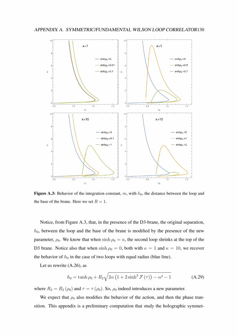
APPENDIX A. SYMMETRIC/FUNDAMENTAL WILSON LOOP CORRELATOR130
Figure A.3: Behavior of the integration constant, m, with h0, the distance between the loop and
the base of the brane. Here we set R = 1.
Notice, from Figure A.3, that, in the presence of the D3-brane, the original separation,
h0, between the loop and the base of the brane is modified by the presence of the new
parameter, ρ0. We know that when sinh ρ0 = κ, the second loop shrinks at the top of the
D3 brane. Notice also that when sinh ρ0 = 0, both with κ = 1 and κ = 10, we recover
the behavior of h0 in the case of two loops with equal radius (blue line).
Let us rewrite (A.26), as
h0 = tanh ρ0 +R2
√2α(1 + 2 sinh2F (τ)
)− α2 − 1 (A.29)
where R2 = R2 (ρ0) and τ = τ (ρ0). So, ρ0 indeed introduces a new parameter.
We expect that ρ0 also modifies the behavior of the action, and then the phase tran-
sition. This appendix is a preliminary computation that study the holographic symmet-

APPENDIX A. SYMMETRIC/FUNDAMENTAL WILSON LOOP CORRELATOR131
ric/fundamental Wilson loop correlator. Since it is a preliminary computation, next step
will be to do plots for the action of the connected correlator and to compare with the
disconnected case, which in this case will be
Sdisc = −2N(κ√
1 + κ2 + sinh−1 κ)−√λ. (A.30)

Appendix B
Perturbative computation of the Wilson
loop correlator in DCFT
In this appendix we start computing the correlator between two Wilson loops in defect
conformal field theory (DCFT). As said in [60,140,141], the one-point functions of gauge
invariant operators can be non-vanishing in the presence of a defect. In this case, three of
the six scalars acquire a non-vanishing vev. This is called fuzzy-funnel solution,
〈Φi〉 = − 1
x3
ti ⊕ 0(N−n)×(N−n) , x3 > 0, (B.1)
where ti, i = 4, 5, 6 are generators of the n-dimensional irreducible representation of
SU(2), i.e. n× n matrices satisfying the SU(2) algebra.
Let us consider the Wilson loop operator as defined in (3.3) and the connected corre-
lator of two circular Wilson loops [58],
〈W (C1, C2)〉c = 〈W (C1)W (C2)〉 − 〈W (C1)〉〈W (C2)〉, (B.2)
where C1 and C2 are concentric circles of radii R1 and R2, respectively, separated by a
distance h along x3. In addition, they are oppositelly oriented in space and separated in
S5,
C1 : xµ (τ) = (R1 cos τ,+R1 sin τ, L, 0) , ni (τ) = (0, 0, sinχ1, 0, 0, cosχ1) ,
C2 : yµ (τ) = (R2 cos τ,−R2 sin τ, L+ h, 0) , ni (τ) = (0, 0, sinχ2, 0, 0, cosχ2) ,
(B.3)
132

APPENDIX B. PERTURBATIVE COMPUTATION 133
where we have shifted the parametrization to include the parameter L, the distance
with respect to the defect, and χ1,2 ∈[0, π
2
]. With this parametrization we get 1
W (C1) =1
NTrP exp
(R1
∫ 2π
0
dτ[−iA1 sin τ + iA2 cos τ − sinχ1Φ
(1)3 − cosχ1Φ6
]),
W (C2) =1
NTrP exp
(R2
∫ 2π
0
dτ[−iA1 sin τ − iA2 cos τ − sinχ2Φ
(2)3 − cosχ2Φ6
]).
(B.4)
We can study the leading order in λ = g2N 1 by starting with the Feynman gauge
〈ΦaiΦ
bj〉 =
λ
4π2N
δabδij
(x− y)2 , 〈AaµAbν〉 =λ
4π2N
δabδµν
(x− y)2 . (B.5)
The second term of (B.2) was calculated in [58] for each factor, but we must worry about
the two different positions of the loops, L and L+ h.
We define the classical propagator between points on different loops as
U cl (α, β) = P exp
∫ β
α
dτ Acl (τ) , Acl (τ) = − sinχ〈Φ3〉cl, (B.6)
where
〈Φ3〉(1)cl =
sinχ1
L+ ht3 , 〈Φ3〉(2)
cl =sinχ2
Lt3, (B.7)
then
U cl (α, β) = exp
([β sinχ1
L+ h− α sinχ2
L
]t3
). (B.8)
Figure B.1: Planar diagrams, rainbow (same circle) and ladder (circle to circle), for the case
without defect [58].
1We chose a minus sign in front of the term involving the scalars as in [63].

APPENDIX B. PERTURBATIVE COMPUTATION 134
0 2π
2π0
loop 1
loop 2
lollipop
tadpole
Figure B.2: Scheme of the 1-loop ladder contributions to the Wilson loop correlator in DCFT.
In Figure B.1 we recall the the planar diagrams for the case without defect. The rain-
bow propagator is a constant, and the ladder can be computed without considering the vev
of Φ3,
〈W (C1, C2)〉(0)c =
λ
8π2
∫ 2π
0
dα
∫ 2π
0
dβcos (α− β) + cos (χ1 − χ2)
coshw − cos (α− β), (B.9)
where
coshw =R2
1 +R22 + h2
2R1R2
(B.10)
In Figure B.2 we see the contributions at 1-loop to ladder diagram, the tadpole and
lollipop diagrams (see [140]) due to the defect. These contribute at the same order in λ 2
with
〈W (C1, C2)〉defectc =
∫ 2π
0
dα
∫ 2π
α
dβ 〈U cl (0, α)A (α)U cl (α, β)A (β)U cl (β, 2π)〉
(B.11)
corresponding to the tadpole diagram.
We leave the continuation of this study for a future work. This will involve results
given in [58, 59, 63] and will be similar to the ones in [128].
2Lollipop contribution results to vanish. [141]

Bibliography
[1] M. Green, J. Schwarz, and E. Witten, Superstring Theory: Vol 1,2. Cambridge
Monographs on Mathematical Physics, Cambridge University Press, 1988.
[2] J. Polchinski, “Introduction to Gauge/Gravity Duality,” in Proceedings, Theoreti-
cal Advanced Study Institute in Elementary Particle Physics (TASI 2010). String
Theory and Its Applications: From meV to the Planck Scale: Boulder, Colorado,
USA, June 1-25, 2010, pp. 3–46, 2010. 1010.6134.
[3] O. Aharony, S. S. Gubser, J. M. Maldacena, H. Ooguri, and Y. Oz, “Large N field
theories, string theory and gravity,” Phys. Rept., vol. 323, pp. 183–386, 2000. hep-
th/9905111.
[4] I. R. Klebanov, “TASI lectures: Introduction to the AdS / CFT correspondence,”
in Strings, branes and gravity. Proceedings, Theoretical Advanced Study Insti-
tute, TASI’99, Boulder, USA, May 31-June 25, 1999, pp. 615–650, 2000. hep-
th/0009139.
[5] E. D’Hoker and D. Z. Freedman, “Supersymmetric gauge theories and the AdS
/ CFT correspondence,” in Strings, Branes and Extra Dimensions: TASI 2001:
Proceedings, pp. 3–158, 2002. hep-th/0201253.
[6] M. Ammon and J. Erdmenger, Gauge/Gravity Duality. Cambridge University
Press, 2015.
[7] H. Nastase, Introduction to AdS/CFT Correspondence. Cambridge University
Press, 2015.
135

BIBLIOGRAPHY 136
[8] E. Witten, “Anti-de Sitter space and holography,” Adv. Theor. Math. Phys., vol. 2,
pp. 253–291, 1998. hep-th/9802150.
[9] S. S. Gubser, I. R. Klebanov, and A. M. Polyakov, “Gauge theory correlators
from noncritical string theory,” Phys. Lett., vol. B428, pp. 105–114, 1998. hep-
th/9802109.
[10] J. M. Maldacena, “The Large N limit of superconformal field theories and super-
gravity,” Int. J. Theor. Phys., vol. 38, pp. 1113–1133, 1999. hep-th/9711200.
[11] O. Aharony, O. Bergman, D. L. Jafferis, and J. Maldacena, “N=6 superconformal
Chern-Simons-matter theories, M2-branes and their gravity duals,” JHEP, vol. 10,
p. 091, 2008. 0806.1218.
[12] I. R. Klebanov and E. Witten, “Superconformal field theory on three-branes at
a Calabi-Yau singularity,” Nucl. Phys., vol. B536, pp. 199–218, 1998. hep-
th/9807080.
[13] M. J. Strassler, “The Duality cascade,” in Progress in string theory. Proceedings,
Summer School, TASI 2003, Boulder, USA, June 2-27, 2003, pp. 419–510, 2005.
hep-th/0505153.
[14] F. C. Fernandez, D-branes in Supersymmetric Backgrounds. PhD thesis, Santiago
de Compostela U., 2008. 0804.4878.
[15] A. Karch and L. Randall, “Open and closed string interpretation of SUSY CFT’s
on branes with boundaries,” JHEP, vol. 06, p. 063, 2001. hep-th/0105132.
[16] O. DeWolfe, D. Z. Freedman, and H. Ooguri, “Holography and defect conformal
field theories,” Phys. Rev., vol. D66, p. 025009, 2002. hep-th/0111135.
[17] I. Kirsch, “Generalizations of the AdS / CFT correspondence,” Fortsch. Phys.,
vol. 52, pp. 727–826, 2004. hep-th/0406274.
[18] J. M. Maldacena and J. G. Russo, “Large N limit of noncommutative gauge theo-
ries,” JHEP, vol. 09, p. 025, 1999. hep-th/9908134.

BIBLIOGRAPHY 137
[19] A. Hashimoto and N. Itzhaki, “Noncommutative Yang-Mills and the AdS / CFT
correspondence,” Phys. Lett., vol. B465, pp. 142–147, 1999. hep-th/9907166.
[20] J.-i. Sakamoto, Integrable deformations of string sigma models and generalized
supergravity. PhD thesis, Kyoto U., 2019. 1904.12827.
[21] P. H. Ginsparg, “Matrix models of 2-d gravity,” in Trieste HEP Cosmol.1991:785-
826, pp. 785–826, 1991. hep-th/9112013.
[22] R. Dijkgraaf and C. Vafa, “Matrix models, topological strings, and supersymmetric
gauge theories,” Nucl. Phys., vol. B644, pp. 3–20, 2002. hep-th/0206255.
[23] M. Marino, “Les Houches lectures on matrix models and topological strings,”
2004. hep-th/0410165.
[24] M. Marino, Chern-Simons Theory, Matrix Models, and Topological Strings. Inter-
national series of monographs on physics, Clarendon Press, 2005.
[25] M. Peskin and D. Schroeder, An Introduction To Quantum Field Theory. Frontiers
in physics, Westview Press, 1995.
[26] M. Shifman, Advanced Topics in Quantum Field Theory: A Lecture Course. Ad-
vanced Topics in Quantum Field Theory: A Lecture Course, Cambridge University
Press, 2012.
[27] J. K. Erickson, G. W. Semenoff, and K. Zarembo, “Wilson loops in N = 4 super-
symmetric Yang-Mills theory,” Nucl. Phys., vol. B582, pp. 155–175, 2000. hep-
th/0003055.
[28] N. Drukker and D. J. Gross, “An Exact prediction of N = 4 SUSYM theory for
string theory,” J. Math. Phys., vol. 42, pp. 2896–2914, 2001. hep-th/0010274.
[29] G. W. Semenoff and K. Zarembo, “Wilson loops in SYM theory: From weak to
strong coupling,” Nucl. Phys. Proc. Suppl., vol. 108, pp. 106–112, 2002. hep-
th/0202156.
[30] J. M. Maldacena, “Wilson loops in large N field theories,” Phys. Rev. Lett., vol. 80,
pp. 4859–4862, 1998. hep-th/9803002.

BIBLIOGRAPHY 138
[31] S.-J. Rey and J.-T. Yee, “Macroscopic strings as heavy quarks in large N gauge
theory and anti-de Sitter supergravity,” Eur. Phys. J., vol. C22, pp. 379–394, 2001.
hep-th/9803001.
[32] N. Drukker, D. J. Gross, and H. Ooguri, “Wilson loops and minimal surfaces,”
Phys. Rev., vol. D60, p. 125006, 1999. hep-th/9904191.
[33] H. Ooguri, “Wilson loops in large N theories,” Class. Quant. Grav., vol. 17,
pp. 1225–1233, 2000. hep-th/9909040.
[34] N. Drukker, D. J. Gross, and A. A. Tseytlin, “Green-Schwarz string in AdS5× S5:
Semiclassical partition function,” JHEP, vol. 04, p. 021, 2000. hep-th/0001204.
[35] H. Ooguri, J. Rahmfeld, H. Robins, and J. Tannenhauser, “Holography in super-
space,” JHEP, vol. 07, p. 045, 2000. hep-th/0007104.
[36] K. Zarembo, “Supersymmetric Wilson loops,” Nucl. Phys., vol. B643, pp. 157–
171, 2002. hep-th/0205160.
[37] J. Gomis and F. Passerini, “Wilson Loops as D3-Branes,” JHEP, vol. 01, p. 097,
2007. hep-th/0612022.
[38] J. Gomis and F. Passerini, “Holographic Wilson Loops,” JHEP, vol. 08, p. 074,
2006. hep-th/0604007.
[39] V. Pestun, “Localization of gauge theory on a four-sphere and supersymmetric Wil-
son loops,” Commun. Math. Phys., vol. 313, pp. 71–129, 2012. hep-th/0712.2824.
[40] K. Hosomichi, “The localization principle in SUSY gauge theories,” PTEP,
vol. 2015, no. 11, p. 11B101, 2015. hep-th/1502.04543.
[41] K. Zarembo, “Localization and AdS/CFT Correspondence,” J. Phys., vol. A50,
no. 44, p. 443011, 2017. hep-th/1608.02963.
[42] V. Pestun et al., “Localization techniques in quantum field theories,” J. Phys.,
vol. A50, no. 44, p. 440301, 2017. hep-th/1608.02952.

BIBLIOGRAPHY 139
[43] S. A. Hartnoll and S. P. Kumar, “Higher rank Wilson loops from a matrix model,”
JHEP, vol. 08, p. 026, 2006. hep-th/0605027.
[44] J. Gomis, S. Matsuura, T. Okuda, and D. Trancanelli, “Wilson loop correlators at
strong coupling: From matrices to bubbling geometries,” JHEP, vol. 08, p. 068,
2008. 0807.3330.
[45] B. Fiol and G. Torrents, “Exact results for Wilson loops in arbitrary representa-
tions,” JHEP, vol. 01, p. 020, 2014. hep-th/1311.2058.
[46] A. Cohen, G. Moore, P. Nelson, and J. Polchinski, “An off-shell propagator for
string theory,” Nuclear Physics B, vol. 267, no. 1, pp. 143 – 157, 1986.
[47] A. Marshakov, “The path integral representation of the fermionic string propaga-
tor,” Nuclear Physics B, vol. 312, no. 1, pp. 178 – 196, 1989.
[48] D. J. Gross and H. Ooguri, “Aspects of large N gauge theory dynamics as seen by
string theory,” Phys. Rev., vol. D58, p. 106002, 1998. hep-th/9805129.
[49] D. Berenstein, R. Corrado, W. Fischler, and J. Maldacena, “The Operator Product
Expansion for Wilson Loops and Surfaces in the Large N Limit,” 1998. hep-
th/9809188.
[50] N. Drukker and B. Fiol, “All-genus calculation of Wilson loops using D-branes,”
JHEP, vol. 02, p. 010, 2005. hep-th/0501109.
[51] S. D. Avramis, K. Sfetsos, and K. Siampos, “Stability of strings dual to flux tubes
between static quarks in N = 4 SYM,” Nucl. Phys., vol. B769, pp. 44–78, 2007.
hep-th/0612139.
[52] K. Zarembo, “Wilson loop correlator in the AdS / CFT correspondence,” Phys.
Lett., vol. B459, pp. 527–534, 1999. hep-th/9904149.
[53] P. Olesen and K. Zarembo, “Phase transition in Wilson loop correlator from AdS /
CFT correspondence,” 2000. hep-th/0009210.
[54] K. Zarembo, “String breaking from ladder diagrams in SYM theory,” JHEP,
vol. 03, p. 042, 2001. hep-th/0103058.

BIBLIOGRAPHY 140
[55] G. Arutyunov, J. Plefka, and M. Staudacher, “Limiting geometries of two circular
Maldacena-Wilson loop operators,” JHEP, vol. 12, p. 014, 2001. hep-th/0111290.
[56] J. Plefka and M. Staudacher, “Two loops to two loops in N=4 supersymmetric
Yang-Mills theory,” JHEP, vol. 09, p. 031, 2001. hep-th/0108182.
[57] G. W. Semenoff and K. Zarembo, “More exact predictions of SUSYM for string
theory,” Nucl. Phys., vol. B616, pp. 34–46, 2001. hep-th/0106015.
[58] D. H. Correa, P. Pisani, and A. Rios Fukelman, “Ladder Limit for Correlators of
Wilson Loops,” JHEP, vol. 05, p. 168, 2018. 1803.02153.
[59] D. Correa, P. Pisani, A. Rios Fukelman, and K. Zarembo, “Dyson equations for
correlators of Wilson loops,” JHEP, vol. 12, p. 100, 2018. 1811.03552.
[60] K. Nagasaki, H. Tanida, and S. Yamaguchi, “Holographic Interface-Particle Poten-
tial,” JHEP, vol. 01, p. 139, 2012. 1109.1927.
[61] E. D’Hoker, J. Estes, and M. Gutperle, “Exact half-BPS Type IIB interface solu-
tions. I. Local solution and supersymmetric Janus,” JHEP, vol. 06, p. 021, 2007.
0705.0022.
[62] E. D’Hoker, J. Estes, and M. Gutperle, “Exact half-BPS Type IIB interface solu-
tions. II. Flux solutions and multi-Janus,” JHEP, vol. 06, p. 022, 2007.
[63] J. Aguilera-Damia, D. H. Correa, and V. I. Giraldo-Rivera, “Circular Wilson loops
in defect Conformal Field Theory,” JHEP, vol. 03, p. 023, 2017. 1612.07991.
[64] S. Bonansea, S. Davoli, L. Griguolo, and D. Seminara, “The fate of the circular
Wilson loop inN = 4 SYM with defect: phase transition, double scaling limit and
OPE expansion.” To appear, 2019.
[65] S. Yamaguchi, “Wilson loops of anti-symmetric representation and D5-branes,”
JHEP, vol. 05, p. 037, 2006. hep-th/0603208.
[66] X. Chen-Lin, “Symmetric Wilson Loops beyond leading order,” SciPost Phys.,
vol. 1, no. 2, p. 013, 2016. hep-th/1610.02914.

BIBLIOGRAPHY 141
[67] J. Gordon, “Antisymmetric Wilson loops in N = 4 SYM beyond the planar limit,”
JHEP, vol. 01, p. 107, 2018. 1708.05778.
[68] K. Okuyama, “Phase Transition of Anti-Symmetric Wilson Loops inN = 4 SYM,”
JHEP, vol. 12, p. 125, 2017. 1709.04166.
[69] A. F. Canazas Garay, A. Faraggi, and W. Muck, “Antisymmetric Wilson loops in
N = 4 SYM: from exact results to non-planar corrections,” JHEP, vol. 08, p. 149,
2018. 1807.04052.
[70] A. F. Canazas Garay, A. Faraggi, and W. Muck, “Note on generating functions
and connected correlators of 1/2-BPS Wilson loops in N = 4 SYM theory,” 2019.
1906.03816.
[71] H. Lin, O. Lunin, and J. M. Maldacena, “Bubbling AdS space and 1/2 BPS geome-
tries,” JHEP, vol. 10, p. 025, 2004. hep-th/0409174.
[72] S. Yamaguchi, “Bubbling geometries for half BPS Wilson lines,” Int. J. Mod. Phys.,
vol. A22, pp. 1353–1374, 2007. hep-th/0601089.
[73] T. Okuda and D. Trancanelli, “Spectral curves, emergent geometry, and bubbling
solutions for Wilson loops,” JHEP, vol. 09, p. 050, 2008. hep-th/0806.4191.
[74] J. Aguilera-Damia, D. H. Correa, F. Fucito, V. I. Giraldo-Rivera, J. F. Morales,
and L. A. Pando Zayas, “Strings in Bubbling Geometries and Dual Wilson Loop
Correlators,” JHEP, vol. 12, p. 109, 2017. 1709.03569.
[75] R. C. Myers, “Dielectric branes,” JHEP, vol. 12, p. 022, 1999. hep-th/9910053.
[76] R. C. Myers, “NonAbelian D-branes and noncommutative geometry,” Int. J. Mod.
Phys., vol. A16, pp. 956–965, 2001. hep-th/0106178.
[77] R. C. Myers, “NonAbelian phenomena on D branes,” Class. Quant. Grav., vol. 20,
pp. S347–S372, 2003. hep-th/0303072.
[78] T.-S. Tai and S. Yamaguchi, “Correlator of Fundamental and Anti-symmetric Wil-
son loops in AdS/CFT Correspondence,” JHEP, vol. 02, p. 035, 2007. hep-
th/0610275.

BIBLIOGRAPHY 142
[79] C. Ahn, “Two circular Wilson loops and marginal deformations,” 2006. hep-
th/0606073.
[80] S. De Haro, D. R. Mayerson, and J. N. Butterfield, “Conceptual Aspects of
Gauge/Gravity Duality,” Found. Phys., vol. 46, no. 11, pp. 1381–1425, 2016. hep-
th/1509.09231.
[81] S. De Haro, “Dualities and Emergent Gravity: Gauge/Gravity Duality,” Stud. Hist.
Phil. Sci., vol. B59, pp. 109–125, 2017. 1501.06162.
[82] D. Rickles, “A philosopher looks at string dualities,” Studies in History and Phi-
losophy of Science Part B: Studies in History and Philosophy of Modern Physics,
vol. 42, no. 1, pp. 54 – 67, 2011.
[83] D. Rickles, “Dual theories: ‘same but different’ or ‘different but same’?,” Studies
in History and Philosophy of Science Part B: Studies in History and Philosophy of
Modern Physics, vol. 59, pp. 62 – 67, 2017. Dualities in Physics.
[84] J. Polchinski, String Theory: Vol 1,2. Cambridge Monographs on Mathematical
Physics, Cambridge University Press, 1998.
[85] J. Polchinski, “Dirichlet Branes and Ramond-Ramond charges,” Phys. Rev. Lett.,
vol. 75, pp. 4724–4727, 1995. hep-th/9510017.
[86] C. Johnson, D-Branes. Cambridge Monographs on Mathematical Physics, Cam-
bridge University Press, 2006.
[87] J. Dai, R. G. Leigh, and J. Polchinski, “New Connections Between String Theo-
ries,” Mod. Phys. Lett., vol. A4, pp. 2073–2083, 1989.
[88] G. ’t Hooft, “A Planar Diagram Theory for Strong Interactions,” Nucl. Phys.,
vol. B72, p. 461, 1974. [,337(1973)].
[89] M. A. Shifman, “Nonperturbative dynamics in supersymmetric gauge theories,”
Prog. Part. Nucl. Phys., vol. 39, pp. 1–116, 1997. hep-th/9704114.
[90] K. G. Wilson, “Confinement of quarks,” Phys. Rev. D, vol. 10, pp. 2445–2459, Oct
1974.

BIBLIOGRAPHY 143
[91] K.-I. Kondo, “Existence of confinement phase in quantum electrodynamics,” Phys.
Rev., vol. D58, p. 085013, 1998. hep-th/9803133.
[92] L. F. Alday and J. Maldacena, “Comments on gluon scattering amplitudes via
AdS/CFT,” JHEP, vol. 11, p. 068, 2007. 0710.1060.
[93] J. Polchinski and J. Sully, “Wilson Loop Renormalization Group Flows,” JHEP,
vol. 10, p. 059, 2011. 1104.5077.
[94] M. Beccaria, S. Giombi, and A. Tseytlin, “Non-supersymmetric Wilson loop in N
= 4 SYM and defect 1d CFT,” JHEP, vol. 03, p. 131, 2018. 1712.06874.
[95] M. Beccaria and A. A. Tseytlin, “On non-supersymmetric generalizations of the
Wilson-Maldacena loops in N = 4 SYM,” Nucl. Phys., vol. B934, pp. 466–497,
2018. 1804.02179.
[96] R. Blumenhagen and E. Plauschinn, Introduction to Conformal Field Theory: With
Applications to String Theory. Lecture Notes in Physics, Springer Berlin Heidel-
berg, 2009.
[97] P. Di Francesco, P. H. Ginsparg, and J. Zinn-Justin, “2-D Gravity and random ma-
trices,” Phys. Rept., vol. 254, pp. 1–133, 1995. hep-th/9306153.
[98] E. Brezin, C. Itzykson, G. Parisi, and J. B. Zuber, “Planar diagrams,” Communica-
tions in Mathematical Physics, vol. 59, no. 1, pp. 35–51, 1978.
[99] S. Coleman, “1/N,” in Aspects of Symmetry: Selected Erice Lectures, pp. 351–402,
Cambridge: Cambridge University Press, 008 1985.
[100] M. L. Mehta, “A method of integration over matrix variables,” Communications in
Mathematical Physics, vol. 79, no. 3, pp. 327–340, 1981.
[101] D. V. H. Kuraoka, “Supersymmetric Wilson loops in the AdS/CFT correspon-
dence,” Master’s thesis, Instituto de Fısica, University of Sao Paulo, Sao Paulo
- Brazil, 2013.
[102] I. Gradshteyn and I. Ryzhik, Table of Integrals, Series, and Products. Elsevier
Science, 2007.

BIBLIOGRAPHY 144
[103] B. Assel, D. Martelli, S. Murthy, and D. Yokoyama, “Localization of supersym-
metric field theories on non-compact hyperbolic three-manifolds,” JHEP, vol. 03,
p. 095, 2017. 1609.08071.
[104] A. M. Polyakov and V. S. Rychkov, “Gauge field strings duality and the loop equa-
tion,” Nucl. Phys., vol. B581, pp. 116–134, 2000. hep-th/000210.
[105] W. Fulton and J. Harris, Representation Theory: A First Course. Graduate Texts in
Mathematics, Springer New York, 2013.
[106] W. Fulton, Young Tableaux: With Applications to Representation Theory and Ge-
ometry. Cambridge: Cambridge University Press, 12 1996.
[107] I. Macdonald, Symmetric Functions and Hall Polynomials. Oxford classic texts in
the physical sciences, Clarendon Press, 1998.
[108] K. Okuyama and G. W. Semenoff, “Wilson loops in N=4 SYM and fermion
droplets,” JHEP, vol. 06, p. 057, 2006. hep-th/0604209.
[109] A. Faraggi, J. T. Liu, L. A. Pando Zayas, and G. Zhang, “One-loop structure of
higher rank Wilson loops in AdS/CFT,” Phys. Lett., vol. B740, pp. 218–221, 2015.
hep-th/1409.3187.
[110] M. Horikoshi and K. Okuyama, “α′-expansion of Anti-Symmetric Wilson Loops
in N = 4 SYM from Fermi Gas,” PTEP, vol. 2016, no. 11, p. 113B05, 2016.
hep-th/1607.01498.
[111] C. G. Callan and J. M. Maldacena, “Brane death and dynamics from the Born-
Infeld action,” Nucl. Phys., vol. B513, pp. 198–212, 1998. hep-th/9708147.
[112] B. Zwiebach, A First Course in String Theory. Cambridge University Press, 2009.
[113] S. Giombi, R. Ricci, and D. Trancanelli, “Operator product expansion of higher
rank Wilson loops from D-branes and matrix models,” JHEP, vol. 10, p. 045, 2006.
hep-th/0608077.

BIBLIOGRAPHY 145
[114] S. Kawamoto, T. Kuroki, and A. Miwa, “Boundary condition for D-brane from
Wilson loop, and gravitational interpretation of eigenvalue in matrix model
in AdS/CFT correspondence,” Phys. Rev., vol. D79, p. 126010, 2009. hep-
th/0812.4229.
[115] E. I. Buchbinder and A. A. Tseytlin, “1/N correction in the D3-brane description of
a circular Wilson loop at strong coupling,” Phys. Rev., vol. D89, no. 12, p. 126008,
2014. hep-th/1404.4952.
[116] A. Faraggi and L. A. Pando Zayas, “The Spectrum of Excitations of Holographic
Wilson Loops,” JHEP, vol. 05, p. 018, 2011. hep-th/1101.5145.
[117] A. Faraggi, W. Mueck, and L. A. Pando Zayas, “One-loop Effective Action of the
Holographic Antisymmetric Wilson Loop,” Phys. Rev., vol. D85, p. 106015, 2012.
hep-th/1112.5028.
[118] K. Okuyama, “Connected correlator of 1/2 BPS Wilson loops in N = 4 SYM,”
JHEP, vol. 10, p. 037, 2018. 1808.10161.
[119] B. Fiol, J. Martınez-Montoya, and A. Rios Fukelman, “Wilson loops in terms of
color invariants,” JHEP, vol. 05, p. 202, 2019. 1812.06890.
[120] A. A. Tseytlin, “On nonAbelian generalization of Born-Infeld action in string the-
ory,” Nucl. Phys., vol. B501, pp. 41–52, 1997. hep-th/9701125.
[121] A. A. Tseytlin, “Born-Infeld action, supersymmetry and string theory,” pp. 417–
452, 1999. hep-th/9908105.
[122] E. Sysoeva, “Wilson loop and its correlators in the limit of large coupling constant,”
Nucl. Phys., vol. B936, pp. 383–399, 2018. 1803.00649.
[123] W. Taylor, “Lectures on D-branes, gauge theory and M(atrices),” in 2nd Trieste
Conference on Duality in String Theory Trieste, Italy, June 16-20, 1997, pp. 192–
271, 1997. hep-th/9801182.

BIBLIOGRAPHY 146
[124] P. Bain, “On the nonAbelian Born-Infeld action,” in Proceedings, NATO Advanced
Study Institute on Progress in String Theory and M-Theory: Cargese, France, May
24-June 5, 1999, pp. 313–317, 1999. hep-th/9909154.
[125] N. Wyllard, “Derivative corrections to D-brane actions with constant background
fields,” Nucl. Phys., vol. B598, pp. 247–275, 2001. hep-th/0008125.
[126] A. Sevrin, J. Troost, and W. Troost, “The nonAbelian Born-Infeld action at order
F 6,” Nucl. Phys., vol. B603, pp. 389–412, 2001. hep-th/0101192.
[127] P. Koerber and A. Sevrin, “The NonAbelian D-brane effective action through order
α4,” JHEP, vol. 10, p. 046, 2002. hep-th/0208044.
[128] M. Preti, D. Trancanelli, and E. Vescovi, “Quark-antiquark potential in defect con-
formal field theory,” JHEP, vol. 10, p. 079, 2017. 1708.04884.
[129] H. Kim, D. K. Park, S. Tamarian, and H. J. W. Muller-Kirsten, “Gross-Ooguri
phase transition at zero and finite temperature: Two circular Wilson loop case,”
JHEP, vol. 03, p. 003, 2001. hep-th/0101235.
[130] N. Drukker and B. Fiol, “On the integrability of Wilson loops in AdS5×S5: Some
periodic ansatze,” JHEP, vol. 01, p. 056, 2006. hep-th/0506058.
[131] P. F. Byrd and M. D. Friedman, Handbook of elliptic integrals for engineers
and scientists. Grundlehren der mathematischen Wissenschaften, Springer-Verlag,
1971.
[132] T.-S. Tai, “Two Polyakov loop correlators from D5-branes at finite temperature,”
Prog. Theor. Phys., vol. 118, pp. 97–107, 2007. hep-th/0701006.
[133] J. Nian and H. J. Pirner, “Wilson Loop-Loop Correlators in AdS/QCD,” Nucl.
Phys., vol. A833, pp. 119–137, 2010. 0908.1330.
[134] A. Armoni, M. Piai, and A. Teimouri, “Correlators of Circular Wilson Loops from
Holography,” Phys. Rev., vol. D88, no. 6, p. 066008, 2013. 1307.7773.
[135] E. W. Weisstein, “JacobiNS. From MathWorld—A Wolfram Web Resource.”
http://functions.wolfram.com/EllipticFunctions/JacobiNS/13/ShowAll.html.

BIBLIOGRAPHY 147
[136] C.-S. Chu and D. Giataganas, “Near BPS Wilson Loop in beta-deformed Theories,”
JHEP, vol. 10, p. 108, 2007. 0708.0797.
[137] T. Kameyama and K. Yoshida, “Generalized quark-antiquark potentials from a
q-deformed AdS5×S5 background,” PTEP, vol. 2016, no. 6, p. 063B01, 2016.
1602.06786.
[138] N. Ishibashi, S. Iso, H. Kawai, and Y. Kitazawa, “Wilson loops in noncommutative
Yang-Mills,” Nucl. Phys., vol. B573, pp. 573–593, 2000. hep-th/9910004.
[139] Y. Bea, N. Jokela, A. Ponni, and A. V. Ramallo, “Noncommutative massive un-
quenched ABJM,” Int. J. Mod. Phys., vol. A33, no. 14n15, p. 1850078, 2018.
1712.03285.
[140] M. de Leeuw, A. C. Ipsen, C. Kristjansen, and M. Wilhelm, “One-loop Wilson
loops and the particle-interface potential in AdS/dCFT,” Phys. Lett., vol. B768,
pp. 192–197, 2017. 1608.04754.
[141] I. Buhl-Mortensen, M. de Leeuw, A. C. Ipsen, C. Kristjansen, and M. Wilhelm,
“One-loop one-point functions in gauge-gravity dualities with defects,” Phys. Rev.
Lett., vol. 117, no. 23, p. 231603, 2016. 1606.01886.