universidad complutense de madrid - …eprints.ucm.es/8366/1/t30704.pdf · doctor of philosophy ......
TRANSCRIPT

UNIVERSIDAD COMPLUTENSE DE MADRID
FACULTAD DE INFORMÁTICA Departamento de Arquitectura de Computadores y Automática
CONFIGURATION AND DATA SCHEDULING TECHNIQUES FOR EXECUTING DYNAMIC
APPLICATIONS ONTO MULTICONTEXT RECONFIGURABLE SYSTEMS
MEMORIA PARA OPTAR AL GRADO DE DOCTOR
PRESENTADA POR
Fredy Alexander Rivera Vélez
Bajo la dirección de los doctores Marcos Sánchez-Élez y Nader Bagherzadeh
Madrid, 2009
• ISBN: 978-84-692-1099-4 © Fredy Alexander Rivera Vélez, 2008

Universidad Complutense de Madrid
Departamento de Arquitectura de Computadores y Automatica
Tecnicas de Planificacion de Configuraciones
y Datos para la Ejecucion de Aplicaciones
Dinamicas en Sistemas Reconfigurables
Multi-Contexto
Configuration and Data Scheduling Techniques
for Executing Dynamic Applications
onto Multicontext Reconfigurable Systems
Tesis Doctoral
Fredy Alexander Rivera Velez
2008


Tecnicas de Planificacion de Configuraciones
y Datos para la Ejecucion de Aplicaciones
Dinamicas en Sistemas Reconfigurables
Multi-Contexto
Configuration and Data Scheduling Techniques
for Executing Dynamic Applications
onto Multicontext Reconfigurable Systems
by
Fredy Alexander Rivera Velez
Dissertation
Presented to the Facultad de Informatica of theUniversidad Complutense de Madrid
in Partial Fulfillmentof the Requirements
for the Degree of
Doctor of Philosophy
Universidad Complutense de Madrid
Departamento de Arquitectura deComputadores y Automatica
May 2008


Tecnicas de Planificacion de Configu-raciones y Datos para la Ejecucionde Aplicaciones Dinamicas en SistemasReconfigurables Multi-Contexto
Memoria presentada por Fredy Alexander RiveraVelez para optar al grado de Doctor por la Univer-sidad Complutense de Madrid, realizada bajo la di-reccion de Marcos Sanchez-Elez (DACyA, Universi-dad Complutense de Madrid) y Nader Bagherzadeh(EECS, University of California, Irvine).
Configuration and Data SchedulingTechniques for Executing DynamicApplications onto Multicontext Re-configurable Systems
Dissertation presented by Fredy Alexander RiveraVelez to the Universidad Complutense de Madrid inpartial fulfillment of the requirements for the degree ofDoctor of Philosophy. This work has been supervisedby Marcos Sanchez-Elez (DACyA, Universidad Com-plutense de Madrid) and Nader Bagherzadeh (EECS,University of California, Irvine).
Madrid, Mayo de 2008.

This work has been supported by the Comision Interministerial de Cien-cia y Tecnologıa from the Spanish government under research grants CICYTTIC2002-00750 and CICYT TIN2005-05619.

A mis padres y hermano
A mi Esposa


El Corazon Al Sur
Nacı en un barrio donde el lujo fue un albur,por eso tengo el corazon mirando al sur.Mi viejo fue una abeja en la colmena,las manos limpias, el alma buena...Y en esa infancia, la templanza me forjo,despues la vida mil caminos me tendio,y supe del magnate y del tahur,por eso tengo el corazon mirando al sur.
Mi barrio fue una planta de jazmın,la sombra de mi vieja en el jardın,la dulce fiesta de las cosas mas sencillasy la paz en la gramilla de cara al sol.Mi barrio fue mi gente que no esta,las cosas que ya nunca volveran,si desde el dıa en que me fuicon la emocion y con la cruz,yo se que tengo el corazon mirando al sur!
La geografıa de mi barrio llevo en mı,sera por eso que del todo no me fui:la esquina, el almacen, el piberıo...lo reconozco... son algo mıo...Ahora se que la distancia no es realy me descubro en ese punto cardinal,volviendo a la ninez desde la luzteniendo siempre el corazon mirando al sur.
Letra y musica de Eladia Blasquez


Agradecimientos
Esta frase ratifica que la presente seccion se dedica a los agradecimientos,
con la siguiente organizacion. El segundo y tercer parrafos contienen mi re-
conocimiento a los directores de este trabajo. El cuarto parrafo se ocupa de
quien fue mi directora de tesis en un comienzo. Un breve mensaje para los di-
rectores del grupo de investigacion esta incluıdo en el quinto parrafo. El saludo
de gratitud del sexto parrafo esta dirigido a algunas de las personas con las
que me he cruzado en este largo camino y de las que guardo algun tipo de
recuerdo, por lo general bueno. Estos agradecimientos se cierran en el septimo
parrafo.
Quiero expresar mis mas sinceros agradecimientos a Marcos Sanchez-Elez,
de quien siempre he recibido la orientacion inmediata y precisa a lo largo del
desarrollo de esta tesis. Agradezco su apoyo, confianza, paciencia y, en especial,
amistad. Sigue tu rumbo que algun dıa seras un hombre del renacimiento.
I would also like to thank Prof. Nader Bagherzadeh at UC Irvine for his
advising. Thanks for the continuous guidance, help and support. I have learnt
a lot and really enjoyed my research stay at UCI. We also have shared good
times in Madrid. All the best, Nader.
Otra persona a la quiero agradecer es Milagros Fernandez, quien me en-
camino por esta lınea de investigacion al unirme al Departamento. Sus consejos
oportunos durante la primera mitad de mi tesis fueron de un valor inestimable
para mi formacion investigadora.
Tambien agradezco a Roman Hermida por el interes que ha demostrado y
el seguimiento que ha hecho de mi trabajo. Ası mismo, agradezco a Francisco
Tirado el haberme permitido incorporarme al Departamento mediante una
beca FPI.
Hago mencion ahora de las personas con las que he compartido experien-
cias a lo largo de estos anos. Mi primera companera de despacho, Guadalupe,
quien desde aquellos primeros dıas y hasta hoy no ha dejado de maravillarme
con su forma de ser. Sara, cuya generosidad es solo una muestra de sus grandes
cualidades como persona. Jose, gran crıtico de todas las artes y fan de Eighth
Wonder, quien siempre te contagia de alegrıa con su risa estruendosa. Recuer-

da, Jose, “los zombies de 28 Semanas Despues no son zombies, son infecta-
dos”. Merecen tambien mi aprecio y respeto Nacho Gomez, Javi Resano, Dani
“El Rojo”, Raquel, Sonia, Juan Carlos, Inma, Silvia, Daniel Mozos, Katia,
Manu, con quienes he compartido comidas, partidos de futbol, dıas de San
Patricio, viajes, cenas, congresos, francachelas, pelıculas, discusiones tecnicas,
irrelevantes y existenciales. Agradezco tambien a Mari Cruz, con quien com-
partı charlas, cafes y paseos en California que hicieron mas agradable mi paso
por allı.
Por ultimo, dejo unas palabras de agradecimiento, que siempre seran pocas,
para los amigos que conservo al otro lado del oceano, habitando sobre las verdes
montanas de los Andes que cruzan mi entranable y contradictoria Locombia.
Ana, Alejo, Landon: gracias por todo el animo y apoyo que me han brindado,
ası como por todos los buenos momentos compartidos durante mis breves visi-
tas. A mis padres tambien doy las gracias porque lo que soy como persona se lo
debo a ellos. Para terminar, agradezco a la persona que ha vivido y sufrido esta
tesis con la misma intensidad que yo: Negrura mıa, gracias por comprender el
inutil gusto que desde siempre he tenido por aprender cosas de dudoso valor.
Si no supiera de tu presencia en mi vida, no tendrıa la ilusion que hoy me
llena.
Madrid, Mayo de 2008.

“Te levantas, te das vuelta y miras, y entonces decıs:
¿Pero esto lo hice yo?”
Rayuela, capıtulo 83.


Contents
1. Introduction 1
1.1. Reconfigurable computing systems . . . . . . . . . . . . . . . . 2
1.1.1. Characteristics of reconfigurable computing systems . . 3
1.1.2. Fine-grained reconfigurable systems . . . . . . . . . . . 5
1.1.3. Coarse-grained reconfigurable systems . . . . . . . . . 7
1.2. Target applications . . . . . . . . . . . . . . . . . . . . . . . . 9
1.3. Objectives of this thesis . . . . . . . . . . . . . . . . . . . . . 11
1.4. Background and related work . . . . . . . . . . . . . . . . . . 12
1.4.1. Static scheduling for reconfigurable architectures . . . . 12
1.4.2. Dynamic scheduling for reconfigurable architectures . . 22
1.4.3. Configuration and data prefetching . . . . . . . . . . . 27
1.5. Organization of this thesis . . . . . . . . . . . . . . . . . . . . 31
2. Coarse-Grain Multicontext Reconfigurable Architectures 33
2.1. Examples of coarse-grain reconfigurable architectures . . . . . 34
2.1.1. The MATRIX architecture . . . . . . . . . . . . . . . . 34
2.1.2. The REMARC array processor . . . . . . . . . . . . . 35
2.1.3. The eXtreme Processing Platform (XPP) . . . . . . . . 37
2.1.4. Montium tile processor . . . . . . . . . . . . . . . . . . 39
2.1.5. The Pleiades architecture . . . . . . . . . . . . . . . . 40
2.1.6. Silicon Hive’s processor template . . . . . . . . . . . . 42
2.2. The MorphoSys reconfigurable architecture . . . . . . . . . . . 43
2.2.1. MorphoSys model . . . . . . . . . . . . . . . . . . . . . 44
2.3. The MorphoSys M2 implementation . . . . . . . . . . . . . . 47
i

Contents
2.3.1. M2 organization . . . . . . . . . . . . . . . . . . . . . 48
2.3.2. Reconfigurable Cell architecture . . . . . . . . . . . . . 49
2.3.3. RC Array organization and interconnection . . . . . . . 51
2.3.4. Context Memory . . . . . . . . . . . . . . . . . . . . . 53
2.3.5. TinyRISC processor . . . . . . . . . . . . . . . . . . . 54
2.3.6. Data interface components . . . . . . . . . . . . . . . . 56
2.4. MorphoSys reconfigurability . . . . . . . . . . . . . . . . . . . 60
2.5. MorphoSys operation flow . . . . . . . . . . . . . . . . . . . . 60
2.6. Operation autonomy of Reconfigurable Cells . . . . . . . . . . 64
2.7. MorphoSys vs. Other architectures . . . . . . . . . . . . . . . 66
2.8. Conclusions . . . . . . . . . . . . . . . . . . . . . . . . . . . . 70
3. Application modeling and compilation framework 73
3.1. Characteristics of target applications . . . . . . . . . . . . . . 74
3.2. Application modeling . . . . . . . . . . . . . . . . . . . . . . . 76
3.2.1. Conditional constructs classification . . . . . . . . . . . 77
3.2.2. Examples of modeled applications . . . . . . . . . . . . 79
3.3. Conditional branches overhead in SIMD reconfigurable archi-
tectures . . . . . . . . . . . . . . . . . . . . . . . . . . . . . . 84
3.4. Mapping of conditional constructs onto MorphoSys . . . . . . 85
3.4.1. Mapping of if-then-else constructs . . . . . . . . . . . . 86
3.4.2. Mapping of iterative constructs . . . . . . . . . . . . . 86
3.5. MorphoSys task-level execution model . . . . . . . . . . . . . 87
3.6. Contexts and data transfers overhead associated to a condi-
tional branch . . . . . . . . . . . . . . . . . . . . . . . . . . . 91
3.7. Compilation framework . . . . . . . . . . . . . . . . . . . . . . 92
3.7.1. Application kernel description . . . . . . . . . . . . . . 93
3.7.2. Kernel information extractor . . . . . . . . . . . . . . . 94
3.7.3. Application profiling . . . . . . . . . . . . . . . . . . . 95
3.7.4. Application clustering . . . . . . . . . . . . . . . . . . 95
3.7.5. Task scheduling . . . . . . . . . . . . . . . . . . . . . . 96
3.7.6. Data and context scheduling . . . . . . . . . . . . . . . 97
3.7.7. Dynamic scheduling support . . . . . . . . . . . . . . . 97
ii

Contents
3.8. Conclusions . . . . . . . . . . . . . . . . . . . . . . . . . . . . 98
4. Compile-time Scheduling Approach 101
4.1. Off-line scheduling overview . . . . . . . . . . . . . . . . . . . 102
4.2. Application clustering . . . . . . . . . . . . . . . . . . . . . . 104
4.2.1. Exploration algorithm . . . . . . . . . . . . . . . . . . 104
4.2.2. Cluster feasibility . . . . . . . . . . . . . . . . . . . . . 107
4.2.3. Cluster bounding check . . . . . . . . . . . . . . . . . . 108
4.3. Cluster scheduling . . . . . . . . . . . . . . . . . . . . . . . . 108
4.3.1. Non-overlapped transfers time estimation . . . . . . . . 110
4.3.2. Cluster scheduling of if-then-else constructs . . . . . . 113
4.3.3. Cluster scheduling of iterative constructs . . . . . . . . 115
4.4. Experimental results . . . . . . . . . . . . . . . . . . . . . . . 118
4.5. Conclusions . . . . . . . . . . . . . . . . . . . . . . . . . . . . 133
5. Runtime Scheduling Approach 135
5.1. Dynamic context scheduling . . . . . . . . . . . . . . . . . . . 136
5.1.1. Runtime context switch technique . . . . . . . . . . . . 136
5.1.2. Experimental results . . . . . . . . . . . . . . . . . . . 142
5.2. Data coherence . . . . . . . . . . . . . . . . . . . . . . . . . . 145
5.2.1. SIMD data coherent mapping scheme . . . . . . . . . . 149
5.3. Dynamic data scheduling . . . . . . . . . . . . . . . . . . . . . 152
5.3.1. Data prefetch mechanisms . . . . . . . . . . . . . . . . 154
5.3.2. Pareto multi-objective optimization . . . . . . . . . . . 156
5.3.3. Power/performance trade-off . . . . . . . . . . . . . . . 158
5.3.4. Implementation of a data prefetch scheme for 3D image
applications . . . . . . . . . . . . . . . . . . . . . . . . 160
5.3.5. Experimental results . . . . . . . . . . . . . . . . . . . 166
5.4. Conclusions . . . . . . . . . . . . . . . . . . . . . . . . . . . . 169
6. Conclusions 171
6.1. Main contributions . . . . . . . . . . . . . . . . . . . . . . . . 174
6.2. Future work . . . . . . . . . . . . . . . . . . . . . . . . . . . . 177
6.3. List of publications . . . . . . . . . . . . . . . . . . . . . . . . 179
iii

Contents
A. Resumen en Espanol I
A.1. Introduccion . . . . . . . . . . . . . . . . . . . . . . . . . . . . i
A.1.1. Objetivos de esta tesis . . . . . . . . . . . . . . . . . . iii
A.1.2. Trabajo relacionado . . . . . . . . . . . . . . . . . . . . iv
A.2. Arquitectura objetivo . . . . . . . . . . . . . . . . . . . . . . . iv
A.3. Modelado de aplicaciones y entorno de compilacion . . . . . . vi
A.3.1. Construcciones condicionales . . . . . . . . . . . . . . . viii
A.3.2. Entorno de compilacion . . . . . . . . . . . . . . . . . x
A.4. Planificacion en tiempo de compilacion . . . . . . . . . . . . . xii
A.4.1. Particionamiento de la aplicacion . . . . . . . . . . . . xii
A.4.2. Planificacion de clusters . . . . . . . . . . . . . . . . . xvi
A.5. Planificacion en tiempo de ejecucion . . . . . . . . . . . . . . . xxiii
A.5.1. Planificacion dinamica de configuraciones . . . . . . . . xxiii
A.5.2. Coherencia de datos . . . . . . . . . . . . . . . . . . . xxvi
A.5.3. Planificacion dinamica de datos . . . . . . . . . . . . . xxvii
A.6. Conclusiones . . . . . . . . . . . . . . . . . . . . . . . . . . . . xxxi
A.7. Publicaciones . . . . . . . . . . . . . . . . . . . . . . . . . . . xxxiv
Bibliography XXXVII
List of Figures XLIX
List of Tables LIII
iv

Chapter 1
Introduction
We are witnessing a large growth in the amount of research being addressed
worldwide into field programmable logic and its related technologies. As the
electronic world shifts to mobile devices [KPPR00] [Rab00] [MP03], recon-
figurable systems emerge as a new paradigm for satisfying the simultaneous
demand for application performance and flexibility [WVC03].
Reconfigurable computing systems [GK89] represent an intermediate ap-
proach between general-purpose and application specific systems. General-
purpose processors (microprocessors and digital signal processors, among oth-
ers) are the most used computing platforms. The same hardware can be used
for executing a large class of applications. It is the broad application domain
which limits the performance that can be achieved using general-purpose pro-
cessors, because their design is not conceived to speedup a particular applica-
tion. Application specific integrated circuits (ASICs) represent an alternative
solution to overcome the performance issues of general-purpose processors.
ASICs are optimally designed to execute a specific application and, hence,
each ASIC has superior performance when it executes that application. Since
ASICs have a fixed functionality, any post-design optimizations and upgrades
in features and algorithms are not permitted.
Reconfigurable computers potentially achieve a similar performance to that
of customized hardware, while maintaining a similar flexibility to that of gen-
eral purpose machines. Reconfigurable computing fundamental principle is
1

Chapter 1. Introduction
Application Specific Integrated
Circuits
Reconfigurable Hardware
Application Specific Integrated Processors
Digital Signal Processors
General-Purpose Processors E
ffici
ency
(P
erfo
rman
ce, A
rea,
Pow
er
cons
umpt
ion)
Flexibility
Figure 1.1: Comparison between computation platforms
that the hardware organization, functionality and/or interconnections may be
customized after fabrication. Figure 1.1 shows a graphic comparison of im-
plementation technologies in terms of efficiency (performance, area and power
consumption) versus flexibility. Reconfigurable computing represents an im-
portant implementation alternative since it fills the gap between ASICs and
microprocessors. The reconfiguration capability of the hardware enables its
adaptation for specific computations in each application to achieve higher per-
formance compared to general-purpose processors.
Reconfigurable architectures consist of an array of logic blocks and an in-
terconnection network. The functionality and the interconnection of the logic
blocks can be modified by means of multiple programmable configuration bits.
The availability of increasingly large number of transistors [ITR06] has enabled
the integration of reconfigurable logic with other components (host processors,
memory, etc.) on system-on-chip (SoC) architectures, combining a wide range
of complex functions on a single die [MP03]. This allows to build high-end
architectures capable of executing a wide set of applications.
1.1. Reconfigurable computing systems
The fundamental differences between reconfigurable computing systems
and traditional computing systems can be summarized as follows: Rather than
temporally sequencing through a shared computational unit, reconfigurable
2

1.1. Reconfigurable computing systems
computers process data by spatially distributing the computations through
the available hardware (Spatial computation). The functionality of the recon-
figurable units and the interconnection network can be adapted at runtime
by means of a reconfiguration mechanism (Reconfigurable data-path). The
computational units process data based on a local configuration (Distributed
control). The required resources for computation, such as functional units and
memory, are distributed throughout the device (Distributed resources).
Reconfigurable computing systems use to couple a general-purpose micro-
processor to the reconfigurable component onto the same chip. Typically, the
computation-intensive parts of the applications are mapped onto the large
number of distributed and reconfigurable functional units, while the sequen-
tial parts of the applications, as well as the memory and I/O operations are
performed by the host processor. This mapping provides superior performance
in many applications compared to mapping onto general-purpose processors.
1.1.1. Characteristics of reconfigurable computing
systems
There are a set of criteria that are frequently used to characterize the
design of a reconfigurable system. These criteria are: granularity, depth of
programmability, reconfigurability, computation model and system interface.
These terms are very useful in classifying reconfigurable systems.
⋆ Granularity
This refers to the data size of the operations performed by the processing
elements in the reconfigurable component (or Reconfigurable Processing
Unit, RPU) of a system. A RPU is a logic block having both config-
urable functionality and interconnection. In fine-grain systems, process-
ing elements in the RPU are typically logic gates, flip-flops and look-up
tables. These processing elements operate at the bit level, implementing
logic functions. FPGAs are examples of fine-grain granularity because
they operate at the bit level [MSHA+97] [Hau98] [VH98]. On the other
hand, in coarse-grain systems, processing elements in the RPU may con-
tain complete functional units, like ALUs and/or multipliers that oper-
3

Chapter 1. Introduction
ate upon multiple-bit words, typically from 8- to 32-bit, as in [MD96],
[WTS+97], [MO98], and [TAJ00].
⋆ Depth of programmability
This describes the number of configuration programs (or contexts) stored
in the RPU. In single context systems, only one context resides in the
RPU as in [HFHK04] and [VBR+96]. Therefore, the functionality of
the RPU is limited to the context currently loaded. In order to execute
a different application or function, the context has to be reloaded. In
multiple context systems, several contexts reside simultaneously in the
RPU as in [HW97] and [SLL+00]. The presence of multiple contexts
allows the execution of different tasks simply by changing the operating
context without having to reload the configuration program.
⋆ Reconfigurability
In order to execute different functions, a RPU may need to be frequently
reconfigured. Reconfiguration is the process of reloading configuration
programs (contexts). This process may be either static when the execu-
tion is interrupted to be performed or dynamic when it is performed in
parallel with execution. Single context RPUs usually have static recon-
figuration, since there is only one context that cannot be simultaneously
changed and executed as in [HFHK04] and [VBR+96]. Therefore, RPUs
having multiple contexts are candidates for dynamic reconfiguration. If
a RPU can can still execute a part of its context, while the other part
is being changed, it is said that it supports partial reconfiguration as
in the Xilinx Virtex 5 FPGAs [Xil08]. This feature helps to reduce the
reconfiguration overhead.
⋆ Computation model
Reconfigurable systems may follow different computation models and
their architectures may be organized in different schemes. Several sys-
tems follow the uniprocessor model, in which the RPU is organized
as a general-purpose processor with a single data-path as in [HW97],
[TCE+95], [WC96] and [HFHK04]. In some architectures the RPU acts
4

1.1. Reconfigurable computing systems
as a coprocessor of the host processor, while in other ones it can be inte-
grated into the pipeline of the host processor. In other systems, the RPU
may have multiple processing streams operating in SIMD or MIMD style
such as in [SLL+00], [MO98], [MD96], [Abn01] and [LBH+03]. Some sys-
tems may also be organized according to the VLIW computation model
as in [BEM+03] and [SH02].
⋆ System interface
A reconfigurable system may have either a remote or a local interface.
When the RPU is organized as a separate element from the host processor
and is located on a separate chip or silicon die, the reconfigurable system
has a remote interface. A local interface means that the host processor
and the RPU reside on the same chip.
After characterizing the reconfigurable computing systems, the following
two subsections deal with their classification in terms of granularity, i.e. fine-
grain and coarse-grain reconfigurable systems.
1.1.2. Fine-grained reconfigurable systems
In fine-grain systems, processing elements operate at the bit level. FPGAs
are examples of fine-grain granularity because they operate at the bit level.
FPGAs [RESV93] can be visualized as programmable logic embedded in a
programmable interconnect. FPGAs are composed of three fundamental com-
ponents: logic blocks, I/O blocks, and programmable routing. A circuit is
implemented in an FPGA by programming each logic block to implement a
small portion of the logic required by the circuit, and each of the I/O blocks
to act as either an input pad or an output pad, as required by the circuit.
The programmable routing is configured to make all the necessary connec-
tions among logic blocks, and from logic blocks to I/O blocks. The functional
complexity of the logic blocks was simple Boolean functions in early designs
[BR96]. Nowadays, it is possible to have larger, complex logic blocks able to
perform arithmetic operations upon multiple bits [Xil08].
Earlier FPGA-based reconfigurable systems were single context devices and
5

Chapter 1. Introduction
they only supported static reconfiguration. Any change to a configuration of
these FPGAs required a complete reprogramming of the entire chip. This
was tolerated because hardware changes were required at a relative slow rate
(hours or days). Later, new application domains required multiple planes
of configuration to be available in order to switch between them to increase
system performance. Dynamic reconfiguration also was required to increase
system performance by using highly optimized circuits that are loaded and
unloaded dynamically during the system operation. In some cases, only a part
of the device requires modification. In order to do that, partial reconfiguration
allows to specify the target location of the configuration data for selective
reconfiguration of the device.
Below we include a brief summary of some relevant fine-grained FPGA-
based reconfigurable systems, highlighting their characteristics related to the
previous aspects. For a detailed architectural survey of FPGAs and related
systems, the interested reader can refer to [MSHA+97], [Hau98] and [VH98].
Dynamically Programmable Gate Arrays (DPGAs) contains multiple con-
figuration memory resources to store several configurations for the fixed com-
puting and interconnect resources [TCE+95]. DPGA has a multiple context
programmability and supports dynamic reconfiguration. Garp [HW97] be-
longs to the family of reconfigurable coprocessors. In the Garp architecture,
the FPGA acts as a slave computational unit on the same die as the host
processor. The reconfigurable hardware is used to speedup operations when
possible, while the main processor takes care of all other computations. Garp
has a multiple context programmability and supports static reconfiguration.
The Chimaera system [HFHK04] integrates a reconfigurable functional unit
(RFU) into the pipeline of a superscalar processor. The RFU implements ap-
plication specific operations. The Chimaera has a single context programma-
bility and supports static reconfiguration. Some other examples of fine-grain
reconfigurable systems are OneChip [WC96], DISC [WH95], and 3D-FPGA
[CLV01]. In the commercial field, most recent Xilinx devices contain, besides
fine-grain resources, hard Intellectual Property (IP) blocks as DSPs, or embed-
ded processors. The Virtex 5 family [Xil08] provides the newest most powerful
features among Xilinx FPGAs. Virtex 5 devices supports partial reconfigu-
6

1.1. Reconfigurable computing systems
ration. Altera [Alt07], Actel [Act07], Atmel [Atm07], Lattice [Lat07], among
others, are companies that also provides FPGA chips and development boards.
Splash 2 [ABD92] and Programmable Active Memory (PAM) DECPeRLe-
1 [VBR+96] were the first multi-FPGA systems. Splash 2 is a multi-FPGA
parallel computer containing an inter-FPGA crossbar interconnecting for data
transfers and broadcast. Splash 2 has a multiple context programmability
for interconnection and supports static reconfiguration. DECPeRLe-1 system
contains arrangements of FPGA processors in a 2-D mesh with memory de-
vices aligned along the array perimeter. This system was designed to create
the architectural appearance of a functional memory for a host microproces-
sor. DECPeRLe-1 has a single context programmability and supports static
reconfiguration.
Although fine-grain architectures with building blocks of 1-bit to 4-bit are
highly reconfigurable, the system exhibits low efficiency when it comes to more
specific tasks. For example, if an 16-bit adder is implemented in a fine-grain
system, it will be inefficient compared to a coarse-grained system composed
by an array of 16-bit adders, when performing an addition-intensive task. In
addition to that, an 16-bit adder will occupy more space in the fine-grain
implementation. Coarse-grained systems have emerge in order to deal with
applications demanding a larger computational granularity.
1.1.3. Coarse-grained reconfigurable systems
In coarse-grain systems, processing elements in the RPU may contain com-
plete functional units that operate upon multiple-bit words. In this systems
the reconfiguration of processing elements and interconnections is performed
at word-level. Due to their coarse-grain granularity, when they are used to im-
plement word-level operators and fixed data-paths, coarse-grain reconfigurable
systems offer higher performance, reduced reconfiguration overhead, better
area utilization, and low power consumption than the fine-grain ones [KR07].
Although the development of a coarse-grained architecture to be used in any
application is an unrealistic goal [TSV07], if we focus on a specific application
domain and exploit its special features, the design of coarse-grain reconfig-
7
Chapter 1. Introduction
urable systems is affordable. This purpose was followed by Lee et al. [LCD03b]
and Mei et al. [MLM+05]. Both teams have suggested generic coarse-grained
reconfigurable templates. These templates can be used as a model for design
space exploration and application mapping. Below are detailed the common
and relevant features of these generic reconfigurable architecture templates:
⋆ The architecture consists of identical processing elements placed in a
regular array with programmable interconnections between them and a
high speed memory interface.
⋆ The array of processing elements and the interconnection network have a
direct data transfer path with the main processor to enable quick trans-
fers of variables, parameters and results.
⋆ Each processing element is similar to the data-path of a conventional
microprocessor composed of functional units (ALUs and/or multipliers)
and storage units (register file, local RAM).
⋆ Processing elements interconnection network is defined at different hier-
archical levels: nearest neighbor connectivity, row/column connectivity,
group connectivity, for example.
Matrix [MD96], RAW [WTS+97], Remarc [MO98] and Chameleon [TAJ00]
are coarse-grain architectures that have these features. Our target architec-
ture, MorphoSys [SLL+00], also fits into these templates. A wider survey
of coarse-grained reconfigurable architectures and an in-depth description of
MorphoSys are presented in Chapter 2.
Since this thesis is focused on developing a compilation framework opti-
mized for coarse-grained multicontext reconfigurable architectures, any recon-
figurable architecture having the same features that those described above is
a good candidate to apply the compilation techniques described in this the-
sis. In particular, we have used MorphoSys as a target architecture since it
presents the same features that any coarse-grained multicontext architecture,
and we have also developed several applications and tools that facilitate the
8

1.2. Target applications
debugging process of the proposed compilation framework. Some other re-
search efforts that have also used these templates for design space exploration
and application mapping are the following ones: Network topology exploration
and interconnect-aware mapping of applications are done in [BGD+04b] and
[BGD+04a]. Application mapping focused on the memory bandwidth bottle-
neck is studied in [DGG05a] and [DGG05b]. Control dependency of programs
is tackle in [RSEFB05] and [LKJ+04]. Different techniques for application
mapping are proposed in [PFKM06] and [BS06].
The application of our compilation proposals and hardware enhancements
to other architectures is possible although it could not be immediate. Morpho-
Sys, and the other cited coarse-grained architectures, have the same problems
to deal with dynamic applications. Our solution could be potentially applied
to any of these architectures considering their inner details.
1.2. Target applications
Current and future applications are characterized by different features and
demands. The majority of contemporary applications, for example, DSP and
multimedia applications, are characterized by the presence of computationally-
and data-intensive algorithms. Also, high speed and throughput are frequently
needed since they are subjected to real-time constraints. Moreover, due to the
wide spread of portable devices, low-power consumption becomes relevant. As
the needs of the customers change rapidly and new standards appear, systems
must be flexible enough to satisfy new requirements. This can be achieved by
changing (reconfiguring) the functionality of the system in the field, according
to the needs of each application. However, the reconfiguration of the systems
must be accomplished without introducing large penalties in terms of per-
formance. Recent coarse-grained reconfigurable architectures have abundant
parallel computational resources and functional flexibility, features that turn
them into unbeatable candidates to implement this class of applications.
Static applications have been so far analyzed. When they are considered,
all relevant information is well-known at compilation time, and so they can
be near-optimally scheduled prior to execution [MKF+01]. Opposite to these
9

Chapter 1. Introduction
applications, there is a growing class of applications which are characterized
by dynamic workload, data-intensive computation, and hard real-time con-
straints. We refer to them as dynamic applications. Some examples of these
dynamic applications are multimedia applications (audio and video encod-
ing/decoding systems running AC3, ADPCM, MPEG2, H.261 or JPEG), 3D
image processing applications (ray tracing, rendering), wireless applications
(GSM, CDMA), etc. Task-, instruction-, and data-parallelism are available at
different levels in these dynamic applications. Also, they are often limited by
bandwidth because of the large volume of data they use to process. Some ap-
plications operate on sequences of ordered data (streams), while another ones
have non-regular data access patterns. User activity and data dependencies
produce a highly uncertain program flow for these applications at runtime.
ME MC DCT Q IQ IDCT IMC
6 6 6 6 6 6
396
Figure 1.2: MPEG2 encoder
Target applications can be easily modeled by a data dependency-based
task graph. Our purpose is to describe the applications by means of a Data-
Flow Graph (DFG). A DFG is a graph which represents a data dependencies
between a number of operations. For instance, the MPEG2 encoder (see Fig-
ure 1.2) [MPE96] is composed by the kernel sequence Motion Estimation (ME),
Motion Compensation (MC), Discrete Cosine Transform (DCT), Quantization
(Q), Inverse Quantization (IQ), Inverse Discrete Cosine Transform (IDCT) and
Inverse Motion Compensation (IMC), which is repeated 396 times in Morpho-
Sys to process an input image [Mae00]. In the case of the MPEG2 encoder,
the program flow is well-known at compilation time. After executing a kernel,
we know the next one to be executed, independently of the input data, i.e.
the specific image.
However, in the new class of applications on which reconfigurable systems
are targeted, the next kernel to be executed most of the times depends directly
on the input data, or user activity, so it is decided at runtime. Then, this
10
1.3. Objectives of this thesis
class of applications exhibit a dynamic program flow that can be modeled by
means of the conditional execution of tasks. To deal with this feature, we have
added control dependencies to the DFG, in such a way that some tasks are
executed depending on the result of a previous task. We have adopted the
hybrid control and data flow graph (CDFG), since it embeds all control and
sequencing information explicitly within the DFG. In the CDFG, two tasks
are joined by an edge if there is a data and/or control dependency between
them. Edges directly linking tasks represent data dependencies, and edges
linking tasks through a conditional branch represent control dependencies. In
the case of a control dependency, the task located after the conditional branch
is executed depending on the result of the task located before the conditional
branch.
1.3. Objectives of this thesis
This thesis deals with the scheduling of dynamic applications onto a multi-
context coarse-grained reconfigurable architecture. The MorphoSys reconfig-
urable system is used as target architecture. Initially, the problem seemed to
be solved because the applications usually implemented had a behavior that
can be known at compilation time, and several static compilation frameworks
were developed. However, in the last few years, a new class of applications
have appeared which operate in dynamically changing scenarios because of
user activity and data dependencies. They must be able of reacting to new
runtime conditions, and are subjected to real-time constraints, since the user
has to be sense of interactivity. Furthermore, reconfigurable platforms are
proposed in the last years as part of mobile systems to improve performance,
then low-power consumption is becoming relevant.
The program flow, that is needed configurations and their associated input
data, of these dynamic applications is only known at runtime. If next config-
uration to process is not immediately available in the on-chip memory of the
reconfigurable component, as well as its input data, a computation stall oc-
curs. The dynamic behavior of these new applications demands a modification
of the compilation tools developed for multicontext architectures. Compila-
11

Chapter 1. Introduction
tion framework for dynamic applications should include a context and data
pre-fetching technique to hide latencies because of context and data unavail-
ability.
There is an additional issue. Concurrent processing of an application on
a reconfigurable architecture means that each processing element processes a
subset of input data. Following the single instruction stream / multiple data
stream (SIMD) style, used in most reconfigurable systems, this concurrent
processing leads to a problem when the dynamic behavior of the mapped
applications demands the execution of different tasks at the same time.
In summary, our goal is to map dynamic applications in order to
execute them onto SIMD multicontext reconfigurable architectures,
by means of an efficient scheduling of configurations and data, look-
ing for the minimization of both the number of clock cycles and
power required to complete the application.
1.4. Background and related work
This section gives an overview of the related work for this thesis. Thus, it is
divided into three topics. First, previous research efforts in the area of compile-
time scheduling algorithms for coarse-grained reconfigurable architectures are
described. Second, some publications addressing the runtime scheduling of
applications for embedded systems and coarse-grained reconfigurable archi-
tectures are summarized. Third, we explain several works on configuration
and data prefetching for reconfigurable architectures. Obviously, this section
is not an exhaustive survey of algorithms and methods for reconfigurable com-
puting but a concise summary of relevant previous works. For the interested
reader, some publications present wider surveys on these topics [BP02] [CH02]
[Har01] [SVKS01].
1.4.1. Static scheduling for reconfigurable architectures
Below we summarize some research approaches that are focused on the
scheduling of applications onto reconfigurable architectures at compilation
12

1.4. Background and related work
time. This summary includes fundamental mapping approaches as loop map-
ping, temporal partitioning, and hardware/software co-design techniques. It
also includes a brief overview of complete compilation environments for several
reconfigurable systems.
⋆ Loop mapping for reconfigurable architectures
One of the first scheduling approaches for coarse-grained reconfigurable
architectures was focused on loop mapping. This is because the appli-
cations usually implemented on these architectures consist of loops that
are repeated a great number of times. For example, the kernel sequence
of MPEG2 is repeated 396 times when it is executed on MorphoSys.
The works by Mei et al. [MVV+02] and Lee et al. [LCD03b] are focused
on exploiting loop-level parallelism on coarse-grained architectures. Mei
et al. use a modulo scheduling algorithm [MVV+03b], a software pipelin-
ing technique used in instruction-level parallelism (ILP) processors such
as VLIW to improve parallelism by executing different loop iterations in
parallel. The objective of modulo scheduling is to engineer a schedule for
one iteration of the loop such that this same schedule is repeated at reg-
ular intervals with respect to intra- and inter-iteration dependency and
resource constraints. Lee et al. employ a two-step approach [LCD03a]:
first, they cluster the operations of a given loop to generate line-level
placements, and then they combine the line placements at the plane
level. Their approach generates high performance pipelines for a given
loop body so that consecutive iterations of the loop can be consecutively
executed on those pipelines.
Bondalapati also worked on loop mapping for reconfigurable architec-
tures. In [Bon01] an approach to map nested loops by using a combi-
nation of pipelining, parallelization, and a technique called data context
switching is described. This work is focused on mapping nested loop
computations that have loop carried dependencies, except in the outer
loop. In the first phase, the inner loops are transformed into a pipelined
data-path. Loop unrolling can provide additional instructions for more
13

Chapter 1. Introduction
ILP, but requiring more memory bandwidth for executing each instruc-
tion. Loops can be parallelized by replicating the hardware mapping and
executing a subset of the iterations on each replicated pipeline. Data
context switching overcomes the limit on the hardware resources. Each
iteration of the outermost loop defines a different data context. Each
data context differs in the data inputs that are used in the computa-
tion. By using data context memories, multiple versions of the pipeline
computing on distinct data sets are simulated. Data context switching
uses the embedded and distributed local memory to store the context
information and retrieve it at appropriate cycles in the computation,
interleaving the execution of the iteration of the loops.
Huang and Malik [HM02] proposed a methodology for the design of appli-
cation specific coprocessors that use dynamically reconfigurable coarse-
grained logic. Their methodology is supported by an architectural model
consisting of a master processor and a reconfigurable coprocessor shar-
ing the same memory subsystem. In the first step in the methodology,
the computationally intensive loops in the application are identified. For
each such loop a custom data-path is designed to maximize parallelism.
Data-paths designed for different loops are then combined into a single
reconfigurable data-path coprocessor. The coprocessor switches between
the individual data-paths by changing the connections between the func-
tional units using the programmable interconnect. To extract kernel
loops they use the IMPACT compiler [CMC+91]. Only the most exe-
cuted innermost loops are mapped. IMPACT delivers an intermediate
representation in a meta assembly language for these loops. The custom
data-paths are obtained by means of a direct mapping in which each
software instruction corresponds to one functional unit in the hardware.
To pipeline the execution, registers are inserted in the data-path in order
to chain functional units. Data dependencies between loop iterations are
handle by means of delays or bypasses.
All previously cited works are focused on speeding up the execution of
loops. They exploit instruction- and data-level parallelism at compile-
14

1.4. Background and related work
time. These methods represent low-level techniques that can be applied
after applying a scheduling at a task-level. Our algorithms work at the
task-level, also providing low-level support for configuration and data
scheduling. We propose compile-time scheduling algorithms that can be
adapted according to the runtime conditions.
⋆ Retargetable compiler for a dynamically reconfigurable embed-
ded system (DRESC)
Mei et al. presented a retargetable compiler called DRESC (Dynamically
Reconfigurable Embedded System Compiler) [MVV+02]. This compiler
has as target platform an architecture template that includes a tightly
coupled VLIW processor and a coarse-grained reconfigurable architec-
ture (CGRA) [MVV+03a]. The VLIW processor consist of several func-
tional units connected together through a multi-port register file. The
CGRA is composed of a number of reconfigurable cells which basically
comprise functional units and register files. To remove the control flow
inside loops, the reconfigurable cell functional units support predicated
operations. The architecture template does not impose any constraint
on the internal organization of the reconfigurable cells, and interconnect.
The CGRA is intended to efficiently execute data flow-like kernels in a
highly parallel way, while the VLIW processor executes the remaining
parts of the application. The VLIW processor and the CGRA performs
tasks exclusively.
In the DRESC compilation flow, a design starts from a C language
description of the application. Focused on execution time and possi-
ble speedup, the profiling and partitioning step identifies the candidate
computation-intensive loops for mapping into the CGRA. The next step
heavily relies on the IMPACT compiler [CMC+91] as front end to parse
C code and perform analysis and optimizations. IMPACT emits an
intermediate representation which serves as input for scheduling. Simul-
taneously with these early compilation steps, the architecture is param-
eterized using a high level of abstraction in order to obtain an internal
graph representation of it. A modulo scheduling algorithm [Rau94] that
15

Chapter 1. Introduction
takes the intermediate representation and the architecture representa-
tion as inputs is applied. The task of modulo scheduling is to map the
program graph to the architecture graph and try to achieve optimal per-
formance while respecting all dependencies. This is done by executing
multiple iterations of the same loop in parallel. DRESC finally generates
scheduled code for both the CGRA and the VLIW processor.
The CGRA on which this compiler is targeted is intended to execute data
flow-like kernels in a highly parallel way by means of a software pipelining
technique. However, it is not clear how the control flow instructions
linking the computation-intensive loops selected to be mapped onto the
CGRA are handled.
⋆ Compilation approach for a dynamically reconfigurable ALU
array (DRAA)
Lee et al. [LCD03b] proposed a flow for mapping loops onto a generic
architecture template called Dynamically Reconfigurable ALU Array
(DRAA). The DRAA places identical processing elements (PEs) in a 2D
array, with regular interconnections among them, and a high-bandwidth
memory interface. The DRAA template is described at three levels: the
PE microarchitecture level, which defines the PE data-path, supported
opcodes and timing; the line level architecture, which defines the ded-
icated connections, global buses and specialized interconnections; and
the reconfigurable plane architecture level, which defines reconfiguration
related parameters as configuration memory size and dynamic reloading
overhead.
To achieve maximal throughput, their approach generates high perfor-
mance pipelines for a given loop body so that consecutive iterations of
the loop can be consecutively executed on those pipelines. The pipelines
are generated from microoperation trees (expression trees with microop-
erations as nodes), representing the loop body through the three levels
described above.
A PE-level operation is defined as an microoperation that can be im-
16

1.4. Background and related work
plemented with a single configuration of a PE. The PE-level mapping
process generates PE-level operation trees in which the nodes represent
PE-level operations. After the PE-level mapping is the line-level map-
ping, which groups the PE-level operation nodes and places them on each
line. The plane-level mapping links together the line placements gener-
ated in the line-level mapping, on the 2D plane of PEs. By reducing the
effective number of memory operations, the application’s performance is
boosted. The opportunity for memory operation sharing comes from the
data reuse pattern in loops of DSP algorithms. When several PEs share
a memory bus or one memory operation, less resources are employed.
Saved resources can be used to execute other iterations in parallel to
increase performance.
This approach provides an interesting way to map applications on a
generic reconfigurable architecture template, as it is our purpose. How-
ever, our methodology works at a higher level of abstraction, by consid-
ering that more complex tasks are executed within a loop, as in the case
of the MPEG2 decoder, for example.
⋆ Application mapping for the Montium architecture
Guo et al. [GSB+05] introduces a method to map applications onto the
Montium [HS03] tile processor. The organization within a Montium pro-
cessor tile is very regular and resembles a VLIW architecture. A single
Montium tile includes five identical ALUs to exploit spatial concurrency,
a high-bandwidth memory interface made of ten local memories moti-
vated by the locality of reference principle, an instruction decoding block
where the configurable instructions are stored, a simple sequencer that
controls the entire tile processor, and a communication and configuration
unit which implements the interface with the world outside the tile (For a
wider description of the Montium architecture refer to Subsection 2.1.4).
The goal of these authors is to map DSP programs written in C language
onto a single Montium tile looking for the minimization of clock cycles
once they are executed. Their compilation process is decomposed into
four phases: translation, clustering, scheduling, and resource allocation.
17

Chapter 1. Introduction
In the translation phase, the input C program is translated into a Control
Data Flow Graph (CDFG) which feeds the following phase. In the clus-
tering phase, the CDFG is partitioned into clusters and mapped to an
unbounded number of fully connected ALUs. A cluster corresponds to a
possible configuration of an ALU data-path. In the scheduling phase, the
graph obtained from the clustering phase is scheduled taking the num-
ber of ALUs (five in their case) into account. Their scheduling algorithm
tries to minimize the number of distinct ALU configurations in the tile.
In the resource allocation phase, the scheduled graph is mapped onto the
resources where locality of reference is exploited, taking into account the
register banks and local memories sizes, as well as the number of buses
of the crossbar.
Although the application is compiled looking for the minimization of
execution time, large computation stalls can be expected when the ap-
plication program includes conditional constructs which destinations are
only known at runtime. These computation stalls are produced for the
lack of appropriate configuration and data within a tile processor when
a control flow instruction is performed. Our methodology tries to an-
ticipate the destination of a conditional construct in order to load the
appropriate configuration and data in advance, looking for the reduction
of computation stalls.
⋆ Temporal partitioning and scheduling
Purna and Bhatia [PB99] presented algorithms for temporal partitioning
and scheduling data-flow graphs (DFGs) for reconfigurable computers.
Their work lies in hardware implementations of applications that have
logic requirements that greatly exceeds the logic capacity of the recon-
figurable computer. They proposed a temporal partitioning that divides
the design into mutually exclusive, limited size segments such that the
logic requirement for implementing a segment is less than or equal to the
logic capacity of the reconfigurable computer. Such temporal segments
are scheduled for execution in proper order to ensure correct overall ex-
ecution.
18

1.4. Background and related work
In their design flow an application is represented by a DFG having nodes,
edges, weights, and delays. The nodes represent functional operations,
the weights represent the size of the logic, and the delays represent the
delay of the function. The edges represent data dependencies between
the nodes of the graph. Temporal partitioning is performed under area
constraints. Its goal is to divide the initial DFG into segments such
that the size of each segment is less than or equal to the size of the
reconfigurable computer. In addition, all the segments must have an
acyclic precedence relation in order to respect the dependencies between
the nodes. Hence, a node can be executed if all its predecessors have
already been executed.
Every node of the DFG is assigned with an ASAP level, which represents
the depth of the node respect to the primary inputs. Two partitioning
algorithms were designed by the authors. The level-based partition-
ing algorithm tries to achieve maximum possible parallelism, thereby
decreasing the delay. The cluster-based partitioning algorithm tries to
minimize the communication overhead by sacrificing the parallelism, and
increasing the delay. The bigger degree of parallelism, the bigger com-
munication overhead for satisfying the data dependencies between the
partitions. Their trade-off is to extract maximum performance from the
available resources. They apply both partitioning algorithms to study
the trade-off between decreasing the delay of the partition and the com-
munication overheads associated with such parallelism. Once the appli-
cation is partitioned, it is scheduled onto the reconfigurable hardware
satisfying both the precedence relation, and the data dependencies be-
tween the partitions.
Similarly, our methodology starts by partitioning the application in such
a way that a set of tasks are assigned to the same set of the on-chip
memory. However, once these authors have partitioned the application,
immediately it is scheduled onto the reconfigurable hardware satisfying
the precedence relations determined at compilation-time. In the case of
dynamic precedence relations, large computation stalls can be expected
19

Chapter 1. Introduction
while the reconfigurable hardware is re-scheduled in order to satisfy the
dynamically changing precedence relations.
⋆ Co-design for dynamically reconfigurable architectures
Chatha and Vemuri [CV99] presented a technique for automatic mapping
of an application to an heterogeneous architecture which contain a soft-
ware processor, a dynamically reconfigurable coprocessor, and memory
elements.
The application is described as a task graph indicating data dependen-
cies. Each node of the task graph may contain loops and control flow con-
structs. The objective of the algorithm is to map the task graph onto the
dynamically reconfigurable co-design architecture looking for the mini-
mization of the execution time, and satisfying hardware area constraints.
However, they only reconfigure the entire hardware coprocessor at time,
and do not consider partial reconfiguration. The presented algorithm in-
tegrates the hardware-software partitioning, temporal partitioning, and
scheduling stages. To map a task graph, the tasks are partitioned be-
tween hardware and software. Then, hardware tasks are assigned to
time exclusive temporal segments (temporal partitioning). Later, tasks
are scheduled on hardware and software processors. Reconfiguration of
hardware processor are also scheduled, as well as the inter-processor and
intra-processor communication through shared memory and local mem-
ory, respectively.
Although these authors claim that each node of the task graph may con-
tain control flow constructs, their mapping proposal are performed at
the task-level. No further information is provided in order clarify how
the control flow constructs within a task are mapped onto the hardware
coprocessor. Our methodology also propose a kernel-level approach for
scheduling, but including configuration and data management for appli-
cations containing dynamic control flows.
20

1.4. Background and related work
⋆ Task scheduling and context and data management. Previous
MorphoSys compilation framework
Maestre et al. [MKF+01] developed a seminal work to automate the de-
sign process for a multicontext reconfigurable architecture. Their work is
focused on two different aspects: kernel scheduling, and context schedul-
ing and allocation. Their purpose is the exploitation of the architectural
features so that the reconfiguration impact on latency is minimized. Mor-
phoSys [SLL+00] was employed as target architecture in order to test the
scheduling proposals. Both tasks were integrated in the first compilation
framework of the MorphoSys architecture.
The target applications of this work are described by a data-flow graph,
whose nodes are kernels. Edges represent data dependencies. The goal of
the kernel scheduler is to find the optimal kernel sequence to minimize the
execution time. Kernel scheduling is guided by three optimization cri-
teria: (1) context reloading minimization, (2) data reuse maximization,
and (3) computation and context/data transfer overlapping maximiza-
tion. Kernel scheduling is performed by first partitioning the application
into sets of kernels that can be scheduled independently of the rest of
the application. Since optimization criteria are conflicting and the num-
ber of possible partitions could be huge, the authors define a way to
estimate and bound the quality of a partition based on its performance.
The quality of the partition is estimated without performing scheduling,
and represents a lower bound for the execution time. Any partition is
only feasible when the size of its input data fits into the on-chip memory.
The kernel scheduler generates a sequence of kernels which have to be
scheduled. Context and data scheduling is a crucial task its which goal is
to achieve the degree of performance that the kernel scheduler assumes.
As the kernel scheduler does, the context and data scheduler, and al-
locator maximize the overlapping of context and data transfers with
computation, so that the execution time is minimized. To distribute the
overlapping time between context and data transfers, data movements
use as much time as they need, and the free time (if available) is used by
21

Chapter 1. Introduction
context loading. The context scheduler selects the context words that
can stay in the on-chip memory over several iterations, and the context
words that have to be loaded, so that the context loads that do not over-
lap with computation are minimized. Context allocator decide where to
place each context word, so that memory fragmentation is minimized.
Maestre does not develop the data scheduler and allocator. This work
was done by Sanchez-Elez et al. [SEFHB05]. These authors schedule
data from an ordered set of partitions (sequence of kernels), given their
data sizes and a memory hierarchy. The data scheduling benefits from
the data reuse between partitions: results produced by one partition can
be used as input data for a subsequent partition. The data scheduler
minimizes data transfers. It transfers between the on-chip and the main
memories, only the required input data and the output results of the
application, keeping the intermediate results, if possible, in the on-chip
memory.
It is important to notice that both Maestre as well as Sanchez-Elez deal
with a class of applications in which context and data requests and their
sizes are well known before execution. This enables all the possible
optimizations to be performed at compilation time. Their algorithms
and methods do not give acceptable results once they are applied on
dynamic applications, i.e applications containing highly data-dependent
program flows, as those we are considering in this thesis.
1.4.2. Dynamic scheduling for reconfigurable
architectures
The works described above are focused on static scheduling of applications
which cannot completely solve the problem of executing applications under
runtime changing scenarios. Below we summarize some research efforts that
deal with dynamic program flows. These approaches range from architectural
support for dynamic scheduling to dynamic reconfiguration management, and
dynamic ordering of tasks.
22

1.4. Background and related work
⋆ Microarchitecture support for dynamic scheduling
Noguera and Badia [NB04] presented an approach to the problem of non-
preemptive multitasking on reconfigurable architectures, which is based
on implementing a microarchitecture support for dynamic scheduling,
containing a hardware-based configuration prefetching unit.
Their work is targeted on a heterogeneous architecture including a a
general-purpose processor, and array of dynamic reconfigurable logic
(DRL) blocks, and shared memory resources. Each DRL block can be
independently configured. The architecture supports multiple configu-
rations running concurrently.
They proposed a hardware-software co-design methodology for dynami-
cally reconfigurable systems which is divided into three stages: applica-
tion stage, static stage, and dynamic stage. The application stage is fo-
cused on the system specification. The static stage includes four phases:
extraction, estimation, hardware-software partitioning, and hardware
and software synthesis. The extraction phase obtains the task graph
representation from the system specification, including the dependencies
between tasks and their priorities. This phase also identifies independent
tasks that are mutually exclusive (resembling the temporal partitioning
proposed by Purna and Bhatia which was outlined above). The estima-
tion phase provides information about delay and area to the following
phase. This information is obtained by applying high-level synthesis
and profiling tools. The hardware-software partitioning phase decides
which tasks will be executed in reconfigurable hardware and which in
software. The dynamic scheduling results highly depend on the quality
of the hardware-software partitioning, which helps to reduce the runtime
reconfiguration overhead. The dynamic stage includes execution schedul-
ing and DRL multicontext scheduling. Both of them run in parallel and
base their functionality on events found in the event stream, i.e. tasks
that are ready to be executed because all their dependencies have been
completed. The execution scheduler and the DRL multicontext sched-
uler algorithms are mapped to hardware, implementing the multitasking
23

Chapter 1. Introduction
support unit which stores the event stream. Tasks are executed in the
DRL blocks or in the CPU, and their execution is triggered by the mul-
titasking support unit. By observing a number of events in advance, the
execution scheduler assigns events to functional units and decides their
execution order. The DRL multicontext scheduler is used to minimize
the reconfiguration overhead. It is in charge of deciding which DRL block
must be reconfigured, and which reconfiguration context (task) must be
loaded in the DRL block. Dynamic scheduler attempts to minimize the
reconfiguration overhead by overlapping the execution
⋆ Dynamic reconfiguration management
Resano et al. [RMVC05] developed a reconfiguration manager to reduce
the reconfiguration overhead for highly dynamic applications with very
tight deadlines. Their target platform is a heterogeneous multi-processor
platform that includes one or more instruction set processors (ISPs), re-
configurable processing units (RPUs), and ASICs. This platform adopts
network-on-chip interconnection model (ICN) [MBV+02] for the recon-
figurable units. This ICN model partitions a FPGA into an array of
identical tiles that serve as RPUs. Each RPU can accommodate one
task. Task loading onto an RPU can be performed while the other tasks
continues normal execution.
The reconfiguration manager runs under a hybrid runtime scheduling en-
vironment called task concurrency management (TCM). This scheduling
is split into two phases: design time, and runtime. At design time the
scheduler explores the design space for each task and generate a small
set of schedules with different energy-performance trade offs. At runtime
the scheduler selects the most suitable schedule for each task from all the
schedules determined at design time. Two different techniques are per-
formed both at design time and runtime: prefetching and replacement.
Design time prefetching tags each node of a task graph with a weight
that represents how critical that node’s execution is. An initial schedule
is obtained by performing an as-late-as-possible scheduling. Runtime
prefetching uses the initial schedule and applies on it a heuristic based
24

1.4. Background and related work
on list scheduling. According to the number of configurations ready for
loading, runtime prefetching selects the configuration with the highest
weight. After the runtime scheduler selects the schedule, it identifies the
tasks that are currently located in the FPGA and are reusable. With
this information, the runtime replacement algorithm creates a replace-
ment list on which those tasks that will be executed sooner are always
at the beginning of the list.
This work is focused on reducing the reconfiguration overhead for fine-
grained reconfigurable architectures. This is achieved by prefetching the
critical configuration based on a wighted list. However, this technique
need to be supported for a data prefetching technique that provides ap-
propriate data to the configurations loaded in advance. Our dynamic
scheduling algorithms selects configurations and data to be loaded in
advance according to the runtime condition, looking for the reduction of
the computation stalls produced by configurations and data unavailabil-
ity.
⋆ Dynamic mapping and ordering tasks
Yang and Catthoor [YC04] addressed the problem of task mapping and
ordering under performance/cost trade-offs. They deal with embedded
real-time applications with large amounts of instruction- and data-level
parallelism, which have to be mapped onto a multi-processor platform,
typically containing several reconfigurable and programmable compo-
nents (general-purpose processor, DSP or ASIP), on-chip memory, I/O
and other ASICs.
Performance/cost trade-off exploration is translated to a Pareto-based
optimization problem [YC03]. The Pareto-optimal concept comes from
multiobjective optimization problems, where more than one conflicting
optimization objectives exists. A solution is Pareto-optimal when it is
optimal in at least one optimization objective direction. Their approach
explores the potentially available design space at design time but defer
the selection step till run time, i.e. the system cost function is optimized
25
Chapter 1. Introduction
at runtime based on pre-computed performance-cost Pareto curves, sat-
isfying the real-time constraints.
In their design methodology, the applications are represented as a set of
concurrent thread frames (TFs) that exhibits a single thread of control.
Each of these TFs consists of many thread nodes (TNs) that can be
looked at as an independent and schedulable code section.
Scheduling is done in two phases. Given a thread frame, the design time
scheduler explores all the different mapping and ordering possibilities,
and generates a Pareto-optimal set, where every point represents a dif-
ferent mapping and ordering combination. The runtime scheduler works
at the granularity of thread frames. It considers all actives thread frames,
trying to satisfy their time constraints while minimizing the system cost.
After the runtime scheduler selects a Pareto point, it decides the execu-
tion order of the thread nodes and on which processor to execute them.
To allows new thread frames to come and join the running applications
at any moment, the authors have wrapped every thread frame into an
object, which contains an initializer, a scheduler and a specific TF data
structure. The scheduler keeps a set of function pointers. Every Pareto
point just means a different set of values of these pointers. Whenever a
new TF enters the system, its initializer is first called to register itself
to the system. Then for a given Pareto point, the scheduler resets its
pointer to the desired TNs in the appropriate order. The runtime sys-
tem modules runs like a middleware layer which separates the application
from the lower level RTOS.
This work deals with applications that have to be mapped on a multi-
processor platform. In the case of a large number of processors in this
architecture, an important overhead can be expected for the runtime
scheduler because the processor assignment is more complex. In addi-
tion, no control flow instructions are considered to be placed within a
thread node.
26

1.4. Background and related work
1.4.3. Configuration and data prefetching
As it has been described along this chapter, one of the main issues in the
scheduling problem for reconfigurable architectures lies on the reconfiguration
and data transfers. Below, we summarize several works in this field.
⋆ Configuration prefetching for partial reconfiguration
Li and Hauck [LH02] proposed configuration prefetching techniques for
reducing the reconfiguration overhead by overlapping the configuration
loading with computation. They investigated various techniques includ-
ing static configuration prefetching, dynamic configuration prefetching,
and hybrid prefetching. Their work is based on the Relocation + De-
fragmentation (R+D) FPGA model [CCKH00] to further improve the
hardware utilization. The relocation allows the final placement of a
configuration within the FPGA to be determined at runtime, while de-
fragmentation provides a method to consolidate unused area within a
FPGA during runtime without unloading useful configurations.
Static prefetching is a compiler-based approach that inserts prefetch in-
structions after performing control flow and data flow analysis based on
profile information and data access patterns. Dynamic prefetching de-
termines and dispatches prefetches at runtime, using more data access
information to make accurate predictions. Hybrid prefetching combines
the strong points of both approaches.
Static configuration prefetching starts computing the potential penalties
for a set of prefetches at each node of the control flow graph. Then, the
algorithm determines the configurations that need to be prefetched at
each instruction node based on the penalties calculated in the previous
phase. Prefetches are generated under the restriction of the size of the
chip. Later, the algorithm trims the redundant prefetches generated in
the previous stage. Termination instructions are also inserted.
Dynamic configuration prefetching is based on a Markov model in which
the occurrence of a future state depends on the immediately preced-
ing state, and only on it. In order to find good candidates to prefetch,
27

Chapter 1. Introduction
Markov prefetching updates the probability of each transition using the
currently available access information. After the execution of a hard-
ware task, the dynamic prefetching algorithm sorts the probabilities and
selects the first candidate. Then, the algorithm issues prefetch requests
for each candidate that is not currently on-chip.
The hybrid configuration prefetching integrates the static prefetching
with the dynamic one to avoid mispredictions. The static prefetches
are used to correct the wrong predictions determined by the dynamic
prefetching, as can occur for the transitions jumping out of a loop.
We also applies a prefetching approach, this includes both configura-
tion and data. Configuration and data prefetching are initially guided
by the static scheduler according to the application profiling, and then
is adapted during the execution by a very simple runtime monitor.
Qu et al. [QSN06] proposed a configuration model to enable configura-
tion parallelism in order to reduce configuration latency. Their approach
consists of dividing the configuration SRAM into sections in such a way
that multiple sections can be accessed in parallel by multiple configura-
tion controllers. Each configuration SRAM section its attached to a pro-
grammable logic making a tile. The complete device consists of a number
of continuously connected homogeneous tiles. A crossbar connection is
used to connect the configuration SRAMs of the tiles to a number of par-
allel configuration controllers. The authors defined a prefetch scheduling
to load tasks whenever there are tiles and configuration controllers avail-
able, instead of tasks become ready. The tasks are modeled as directed
acyclic graphs and scheduling is performed at design time. The tasks are
scheduled by means of a priority function which determines the urgency
of execution of a task, how much benefit a task can get if its configuration
immediately starts, and how many additional configurations have to be
delayed if configuration of the task cannot stat immediately. This work
does not include a runtime scheduling stage. In addition, it is highly
specialized on a device model having multiple configuration controllers.
Lee et al. [LYC02] presented a method for runtime reconfiguration
28

1.4. Background and related work
scheduling in reconfigurable SoC design to hide the reconfiguration la-
tency. Their work is based on a formal model of computation, hierar-
chical FSM with synchronous data flow (HFSM-SDF). The basic idea
consists of knowing the exact order of required configurations during
runtime. To obtain the exact order of configurations, the authors ex-
ploit the inherent property of HFSM-SDF that the execution order of
SDF actors can be determined before the execution of state transition of
top FSM. For each transition of top FSM, they compute the exact order
of configurations in a ready configuration queue by traversing the hierar-
chical FSM. Then, with the queue, a runtime reconfiguration scheduler
launches configuration fetches as early as possible during the execution
of state transition of top FSM. This work highly depends on the model
of computation. However, the authors do not deal with the problem of
data supplying for the early fetched configurations. Our work considers
the data required by a prefetched task.
⋆ Data prefetching
Data prefetching is a technique that has been proposed for hiding the
latency of main memory access. Rather than wait for a cache miss to
initiate a memory fetch, data prefetching anticipates such misses and
issues a fetch to the memory system in advance to the actual memory
reference. To be effective, data prefetching must be timely, useful, and
introduce little overhead. Prefetch strategies are diverse, and no single
strategy has yet been proposed that provides optimal performance. All
approaches have their own design trade-offs. For a complete survey of
data prefetch mechanisms in general-purpose systems, we refer to the
work published by Vanderwiel and Lilja [VL00].
Chai et al. [CCE+05] proposed a flexible memory subsystem for stream
computation which uses stream units to move stream data between mem-
ory and processors. The stream units prefetch and align data based on
stream descriptors [CBK+06], a mechanism that allows programmers
to indicate data movement explicitly by describing their memory ac-
cess patterns. The memory subsystem builds upon configurable stream
29

Chapter 1. Introduction
units that move data while computation is performed. The stream units
are specialized DMA units that are optimized for stream data transfer.
They rely on a set of stream descriptors, which define the memory access
pattern, to prefetch and align data in the order required by the comput-
ing platform. Stream units take advantage of available bandwidth by
prefetching data before it is needed. Stream computation is very popu-
lar in the multimedia domain. However, there is a class of applications
which data accesses are not regular and the streaming memory hierarchy
could not be enough to provide data to the computing platform in an ef-
ficient manner. Our target architecture also includes an on-chip memory
for streaming applications. In this work, we have added a new on-chip
memory in order to handle non-streaming data access patterns.
Vuletic et al. [VPI04] presented an operating system (OS) module that
monitors reconfigurable coprocessors, predicts their future memory ac-
cesses, and performs memory prefetching accordingly. Their goal is
to hide memory to memory communication latency. Their OS-based
prefetching is applied to the Virtual Memory Window (VMW), which
enables the coprocessors to share the virtual memory address space with
user applications. The technique presented in this work is essentially a
dynamic software technique that uses a hardware support to detect co-
processors memory access patterns. During a VMW-based coprocessor
execution, the OS sleeps for a significant amount of time. During idle
time, the VMW manager surveys the execution of the coprocessor and
anticipate its future requests. During coprocessor operation, the Win-
dow Management Unit (WMU) informs the manager about the pages
accessed by the coprocessor. Based on this information, the manager
predicts future activities of the coprocessor and schedule prefetch-based
loads of virtual memory pages. The WMU provides hardware support
for the translation of the coprocessor virtual address and for accessing
the window memory. The only input to the predictor are miss addresses
and access page numbers. The predictor assumes that for each miss a
new stream is detected, and it schedules a speculative prefetch for the
page following the missing one. This technique can be effectively applied
30

1.5. Organization of this thesis
on streaming applications having a large spatial locality of coprocessor
memory accesses. However, for non-streaming applications the predictor
should be highly improved. Our data prefetch technique is also a soft-
ware approach with a lightweight hardware support, and is focused on
non-streaming applications.
The first work on data prefetching targeted on the MorphoSys archi-
tecture was done by Venkataramani [VNK+03]. This research work
addressed the problem of compiling a program written in a high-level
language, SA-C, to the coarse-grained architecture, MorphoSys. The
compiler handles issues concerning data streaming and caching in or-
der to minimize data transfers overhead. It uses a simple strategy to
prefetch data, in order to overlap most data fetching and storing with
computation. Later, Sanchez-Elez et al. [SEFHB05] proposed a data
scheduler and allocator for the MorphoSys architecture. This scheduler
benefits from the data reuse between sequence of kernels, minimizing
data transfers by keeping the intermediate results, if possible, in the
on-chip memory. However, both cited works deal with a class of ap-
plications in which data requests and their sizes are well known before
execution. This enables all the possible optimizations to be performed
at compilation time. Results are not good once these techniques are ap-
plied on dynamic applications, as those we are considering. Our purpose
is to hide the latency of data accesses by overlapping computation with
memory accesses, looking for a reduction in overall execution time. This
is done by taking benefit of the architectural features combined with a
data prefetch heuristic.
1.5. Organization of this thesis
The rest of this dissertation is organized as follows:
⋆ Chapter 2 presents a brief summary of some relevant coarse-grained
reconfigurable systems developed by academy and industry, as well as
an in-depth description of our target architecture, MorphoSys. The op-
31

Chapter 1. Introduction
eration autonomy of MorphoSys processing elements, which is funda-
mental to support our scheduling proposals, is also explained. Before
to close this chapter, a concise comparison of MorphoSys with other
coarse-grained reconfigurable architectures is made.
⋆ Chapter 3 describes how the target applications are modeled in order to
be mapped onto the architecture. The MorphoSys compilation frame-
work is also introduced. Special attention is deserved to the static and
dynamic scheduling stages of the compilation framework, which are those
on which this thesis is focused.
⋆ Chapter 4 presents the off-line scheduling algorithms which are firstly
applied on the applications to be executed onto coarse-grained recon-
figurable architectures. These algorithms include application clustering
algorithms, off-line time penalty estimators, and cluster serialization al-
gorithms.
⋆ Chapter 5 presents the runtime scheduling technique we have developed,
including its hardware support. Runtime monitors to dynamically adapt
the execution to the current runtime conditions are explained. Data
prefetching schemes are also described in this chapter.
⋆ Chapter 6 highlights the major contributions of our work and concludes
this dissertation. Future work is also addressed at the end of this chapter.
⋆ Appendix A includes a Spanish summary of this dissertation, in compli-
ance with the regulations of the Universidad Complutense de Madrid.
32

Chapter 2
Coarse-Grain Multicontext
Reconfigurable Architectures
In Chapter 1, the terms to describe the essential features of reconfigurable
systems were summarized. Also, it was highlighted how these terms are useful
in defining and classifying the architecture of a reconfigurable system. In
general, it is desirable to have a system with multiple context planes, dynamic
reconfiguration and a local interface. The granularity and computation model
should be chosen according to the target application characteristics.
The main goal of this chapter is to present an in-depth description of our
target architecture, MorphoSys. Since coarse-grained reconfigurable systems
have been built upon common ideas and concepts, first of all, we include a brief
summary of some relevant coarse-grained systems developed by academy and
industry that may help to put in perspective our target architecture. Then,
a high-level description of MorphoSys is presented, according to the reconfig-
urable computing systems properties analyzed in Chapter 1. We have worked
with the second implementation of MorphoSys. Therefore, the limitations
of the first implementation are summarized, and the architectural improve-
ments introduced in this thesis are highlighted along the architecture’s second
implementation description. In addition to the architectural organization of
MorphoSys, its reconfiguration qualities and operation flow are included. A
complete section is dedicated to the operation autonomy of MorphoSys pro-
33

Chapter 2. Coarse-Grain Multicontext Reconfigurable Architectures
cessing elements, which is fundamental to support our scheduling proposals.
Before to close this chapter, a concise comparison of MorphoSys with other
coarse-grained reconfigurable architectures is made.
2.1. Examples of coarse-grain reconfigurable
architectures
According to the granularity of configuration, reconfigurable systems are
classified into two categories, namely, fine- and coarse-grain reconfigurable sys-
tems. This section presents a representative set of coarse-grain reconfigurable
architectures that have been proposed in the literature by both academy and
industry in order to put in perspective our target architecture.
2.1.1. The MATRIX architecture
MATRIX [MD96] was developed jointly by Ethan Mirsky and Andre De-
Hon at the Massachusetts Institute of Technology. These authors introduced
MATRIX as a novel, general-purpose computing architecture which does not
take a pre-fabrication stand on the assignment of space, distribution, and
control for instructions. Rather, MATRIX allows the user or application to
determine the actual organization and deployment of resources as needed.
MATRIX is based on an uniform array of primitive elements and intercon-
nect which can implement instruction, control, and data functions. A single
integrated memory and computing element can serve as an instruction store,
data store, data-path element, or control element.
A concrete MATRIX microarchitecture consists of an array of identical,
8-bit primitive data-path elements interconnected by a configurable network.
Each data-path element or Basic Functional Unit (BFU) contains a 256×8-bit
memory, an 8-bit ALU and multiply unit, and reduction control logic including
a 20×8 NOR plane (see Figure 2.1). The network is hierarchical, supporting
three levels of interconnect.
The BFU is designed to be the basic processing and configuration ele-
ment. It unifies resources used since the BFU can serve as instruction memory
34

2.1. Examples of coarse-grain reconfigurable architectures
Figure 2.1: MATRIX Basic Functional Unit (BFU)
for controlling ALU, memory, or interconnect functions; read/write memory
for storage and retiming of data; byte slice of a register-file-ALU combination;
and independent ALU function. The interconnect distribution resembles tradi-
tional FPGA interconnect. Unlike traditional FPGA interconnect, MATRIX
has the option to dynamically switch network connections. A collection of
BFUs may be configured for operation in SIMD, MIMD or VLIW fashion.
MATRIX flexibility is provided by means of a multilevel configuration
scheme. Traditional “instructions” direct the behavior of data-path and net-
work elements on a cycle-by-cycle basis. Metaconfiguration data configures
the device behavior at a more primitive level defining the architectural orga-
nization for a computation.
2.1.2. The REMARC array processor
The Reconfigurable Array Multimedia Coprocessor (REMARC) [MO98]
was developed by the Stanford University and is designed to accelerate multi-
media applications. REMARC is a reconfigurable coprocessor that is tightly
coupled to a main RISC processor and consists of a global control unit and 64
programmable logic units called nano-processors.
REMARC is intended for working as a coprocessor for an extended MIPS
processor. The main processor issues instructions to REMARC wich executes
them. REMARC allows to define and configure specialized instructions for a
35
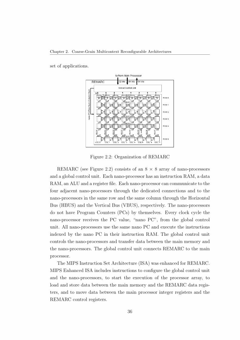
Chapter 2. Coarse-Grain Multicontext Reconfigurable Architectures
set of applications.
Figure 2.2: Organization of REMARC
REMARC (see Figure 2.2) consists of an 8 × 8 array of nano-processors
and a global control unit. Each nano-processor has an instruction RAM, a data
RAM, an ALU and a register file. Each nano-processor can communicate to the
four adjacent nano-processors through the dedicated connections and to the
nano-processors in the same row and the same column through the Horizontal
Bus (HBUS) and the Vertical Bus (VBUS), respectively. The nano-processors
do not have Program Counters (PCs) by themselves. Every clock cycle the
nano-processor receives the PC value, “nano PC”, from the global control
unit. All nano-processors use the same nano PC and execute the instructions
indexed by the nano PC in their instruction RAM. The global control unit
controls the nano-processors and transfer data between the main memory and
the nano-processors. The global control unit connects REMARC to the main
processor.
The MIPS Instruction Set Architecture (ISA) was enhanced for REMARC.
MIPS Enhanced ISA includes instructions to configure the global control unit
and the nano-processors, to start the execution of the processor array, to
load and store data between the main memory and the REMARC data regis-
ters, and to move data between the main processor integer registers and the
REMARC control registers.
36
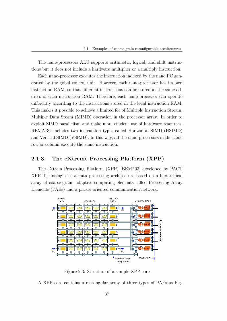
2.1. Examples of coarse-grain reconfigurable architectures
The nano-processors ALU supports arithmetic, logical, and shift instruc-
tions but it does not include a hardware multiplier or a multiply instruction.
Each nano-processor executes the instruction indexed by the nano PC gen-
erated by the gobal control unit. However, each nano-processor has its own
instruction RAM, so that different instructions can be stored at the same ad-
dress of each instruction RAM. Therefore, each nano-processor can operate
differently according to the instructions stored in the local instruction RAM.
This makes it possible to achieve a limited for of Multiple Instruction Stream,
Multiple Data Sream (MIMD) operation in the processor array. In order to
exploit SIMD parallelism and make more efficient use of hardware resources,
REMARC includes two instruction types called Horizontal SIMD (HSIMD)
and Vertical SIMD (VSIMD). In this way, all the nano-processors in the same
row or column execute the same instruction.
2.1.3. The eXtreme Processing Platform (XPP)
The eXtrem Processing Platform (XPP) [BEM+03] developed by PACT
XPP Technologies is a data processing architecture based on a hierarchical
array of coarse-grain, adaptive computing elements called Processing Array
Elements (PAEs) and a packet-oriented communication network.
Figure 2.3: Structure of a sample XPP core
A XPP core contains a rectangular array of three types of PAEs as Fig-
37

Chapter 2. Coarse-Grain Multicontext Reconfigurable Architectures
ure 2.3 illustrates. Those in the center of the array are ALU-PAEs. To the
left and right side of the ALU-PAEs are RAM-PAEs with I/O. Finally, at
the right side of the array, there is a column of Function PAEs (FNC-PAEs).
ALU-PAEs and RAM-PAEs comprise the data-flow array which is dedicated
to the efficient processing of high bandwidth data streams. FNC-PAEs are
VLIW-like general-purpose processors dedicated to the control flow and se-
quential sections of the applications. All elements are communicated via a
packet-oriented network.
Regular streaming algorithms like filters or transforms are implemented on
the data-flow array. Flow graphs of arbitrary shape can be directly mapped
to ALU objects. The nodes of the flow graph are mapped on the PAEs and
the edges are mapped on the data network, resulting in a parallel, pipelined
implementation. PAEs can be configured in parallel while neighboring PAEs
are processing data. Entire applications can run independently on different
parts of the array. Reconfiguration can be triggered by a controlling FNC-PAE
or even by special event signals originating within the data-flow array, enabling
self-reconfiguring designs. By utilizing protocols implemented in hardware,
data and event packets are used to process, generate, decompose and merge
streams of data.
The configuration executed on a XPP core is stored in configuration regis-
ters distributed throughout the XPP data-flow array. Configuration registers
store configuration words which control the functionality of the XPP objects,
i.e. which opcodes are executed by an ALU, the connections between ALUs,
memories and registers, etc. A configuration word consists of an address (i.e.
the PAE row and column number and the number of the register within the
PAE) and a value which is written to the configuration register being ad-
dressed. This addressing scheme allows to configure PAEs individually and
independently. An entire configuration word is sent to the data-flow array in
each clock cycle through a dedicated configuration bus. To load an entire con-
figuration, all configuration words are sequentially sent, cycle by cycle. Only
the XPP objects which are part of a reconfiguration need to be reconfigured
(partial reconfiguration). Several completely independent partial reconfigura-
tions, i.e. configurations not sharing any resources, can be loaded to a XPP
38

2.1. Examples of coarse-grain reconfigurable architectures
data-flow array and execute concurrently. These configurations represent in-
dependent tasks operating on their own memories or data streams.
2.1.4. Montium tile processor
The Montium tile processor [HS03] was initially designed under the Chame-
leon project at the Univertity of Twente. The Montium tile acts as a coarse-
grain reconfigurable component in the Chameleon SoC [SKW+07], which is
specially designed for mobile computing. This SoC contains a general-purpose
processor (ARM core), a bit-level reconfigurable part (FPGA) and several
word-level reconfigurable parts (Montium tiles).
Figure 2.4: Montium tile processor
A single Montium tile processor is depiected in Figure 2.4. The hardware
organization within a tile is very regular and resembles a VLIW architecture.
However, the control structure of the Montium is very different. A relative
simple sequencer controls the entire tile processor. The sequencer selects con-
figurable tile instructions that are stored in the instruction decoding block.
The five identical ALUs (ALU1 · · · ALU5) in a tile exploit spatial con-
currency. This parallelism demands a very high memory bandwidth, which is
obtained by having ten local memories (M01 · · · M10) in parallel. The small
39

Chapter 2. Coarse-Grain Multicontext Reconfigurable Architectures
local memories are also motivated by the principle of locality. The ALU input
registers provide an even more local level of storage. The Montium has a data-
path width of 16-bits and supports both integer and fixed-point arithmetic.
An Address Generation Unit (AGU, not shown in Figure 2.4) accompanies
each memory. The AGU can generate the typical memory access patterns
found in common DSP algorithms, for example, incremental, decremental,
and bit-reversal addressing. It is also possible to use the memory as a look-up
table for complicated functions which cannot be calculated using an ALU. A
memory can be used for both integer and fixed-point look-ups.
The communication and configuration unit implements the interface with
the world outside the tile. The interconnect provides flexible routing within a
tile. The configuration of the interconnect can change every clock cycle. There
are ten buses that are used for inter-ALU communication. These buses are
called global buses. The span of global buses is only within a single tile. The
communication and configuration unit is also connected to the global buses.
It uses global buses to access local memories and to handle data in streaming
algorithms.
The reconfigurable elements within the Montium are the sequencer, in-
struction decoding block, and AGUs. Their functionality can be changed at
runtime. The Montium is programmed in two steps. In the first step, AGUs
are configured and a limited set of instructions is defined by configuring the
instruction decoding block. Then, the sequencer is instructed to sequentially
select the required instructions.
2.1.5. The Pleiades architecture
The Pleiades architecture [Abn01] was developed by the University of Cali-
fornia at Berkeley and is focused on the digital signal processing domain. The
Pleiades architecture is based on the template shown in Figure 2.5.
The architecture template consists of a control processor (a general-purpose
microprocessor core) surrounded by a heterogeneous array of autonomous,
special-purpose satellite processors. All processors in the system communi-
cate over a reconfigurable communication network that can be configured to
40

2.1. Examples of coarse-grain reconfigurable architectures
Figure 2.5: The Pleiades architecture template
create the required communication patterns. All computation and communi-
cation activities are coordinated via a distributed data-driven control mecha-
nism. The dominant, energy-intensive computational kernels of a given DSP
algorithm are implemented on the satellite processors as a set of independent,
concurrent threads of computation. The rest of the algorithm, which is not
compute-intensive, is executed on the control processor. The computational
demand on the control processor is minimal, as its main task is to config-
ure satellite processors and the communication network (via the configuration
bus), to execute the non-intensive parts of a given algorithm, and to manage
overall control flow of the algorithm.
In the model of computation used in the Pleiades architecture template,
a given application implemented on a domain-specific processor consists of a
set of concurrent communicating processes that run on the various hardware
resources of the processor and are managed by the control processor. The con-
trol processor configures available satellite processors and the communication
network at runtime to construct the dataflow graph corresponding to a given
computational kernel directly in hardware. In the configured hardware struc-
ture, the satellite processors correspond to the nodes of the dataflow graph,
and the links through the communication network correspond to the arcs of
the dataflow graph. Each arc in the dataflow graph is assigned a dedicated
link through the communication network. The underlying details and the ba-
41

Chapter 2. Coarse-Grain Multicontext Reconfigurable Architectures
sic parameters of the various computational DSP kernels are accommodated
at runtime by the reconfigurability of the satellite processors and the commu-
nication network. The type and number of satellite processors can vary and
depend on the properties of the particular application domain. They can be
fixed components, e. g. memories, address generators, multiply-accumulate
processors, add-compare-select processors, or reconfigurable data-paths.
The functionality of each hardware resource, be it a satellite processor or
a switch in the communication network, is specified by the configuration state
of that resource, a collection of bits that instruct the hardware resource what
to do. The configuration state of each hardware resource is stored locally in
a suitable storage element. Thus, storage for the configuration states of hard-
ware resources of a processor are distributed throughout the system. These
configuration states are in the memory map of the control processor and are
accessed by the control processor through the reconfiguration bus, which is an
extension of the address/data/control bus of the control processor.
2.1.6. Silicon Hive’s processor template
Silicon Hive, a Philips Electronics spin-out, designs a scalable and modular
architecture template [LBH+03] which can be seen as an approach to design
programmable custom logic by replacing fixed-function units within a SoC
with programmable ones.
Figure 2.6: Hierarchy of Silicon Hive’s processor cell template
The Silicon Hive processor template has a fully hierarchical structure as
is depicted in Figure 2.6. A core consists of multiple cells, each of which
42

2.2. The MorphoSys reconfigurable architecture
having its own thread of control. Cells can have streaming interfaces, which
allow the cells to be interconnected. For scalability reasons, usually a nearest-
neighbor interconnect strategy is chosen, leading to a mesh structure. A cell
has a controller (CTRL), a configuration memory and multiple Processing
and Storage Elements (PSEs). Cell’s controller is much less complex than
traditional RISC or VLIW processors and is in charge of stepping through
the program code. A cell may contains a set of DSP modules in order to
provide specific algorithmic support. A PSE comprises multiple Issue Slots
(ISs), Register Files (RFs), Interconnect Networks (INs), and optionally local
memory storage (MEM). Issue Slots basically consist of multiple Function
Units (FUs). The program word contains exactly one operation per IS. This
means that in every clock cycle one operation per Issue Slot can be fired.
Maximum parallelism of a cell depends on the number of issue slots. FU
instantiation depends on the operations that must be supported. Interconnect
networks route the data from the outputs of ISs into the RFs and from the
RFs into the inputs of ISs. The designs of the INs are such that the RFs
are connected to FUs on a need-to-have basis. This reduces the input/output
ports of the RFs to a minimum.
All data-path features are visible to and controlled by the compiler, in or-
der to actually benefit from available parallelism. A cell is a fully-operational
processor capable of computing complete algorithms. Typically, one applica-
tion function at a time is mapped onto the matrix of PSEs. The more PSEs
are present, the more the function can be mapped in space, in a data-flow
manner.
2.2. The MorphoSys reconfigurable
architecture
The MorphoSys architecture has been designed by researches in the Univer-
sity of California at Irvine, and is targeted on data- and computation-intensive
applications with inherent parallelism and high throughput requirements. The
MorphoSys architecture is widely described because is the architecture on
43

Chapter 2. Coarse-Grain Multicontext Reconfigurable Architectures
which we have tested our proposals. However, our ideas are enough general
to be applied on different coarse-grained reconfigurable architectures. This
statement is backed up by the fact that most of the existing coarse-grained
reconfigurable architectures have similar characteristics, as it was explained in
Chapter 1.
The MorphoSys architecture gathers together all the features that describe
a coarse-grained reconfigurable template (refer to Subsection 1.1.3), and there-
fore, it can be employed as an experimental framework in order to prove the
quality of any scheduling proposal for coarse-grained reconfigurable systems,
as it is our purpose. In the next subsection, first of all, a high-level description
of our target architecture is done.
2.2.1. MorphoSys model
There are three major design principles that helped to define the Morpho-
Sys model. These design principles are concerned with defining the system
blocks, data interface and other system issues. They are outlined as follows:
⋆ Integration of the general-purpose processor with the RPU
Some computation-intensive applications, such as video games that em-
ploys advanced 3-D graphics, are turning into mainstream applications.
However, they used to be implemented on ASICs. Therefore, it is impor-
tant to integrate the capability to execute these demanding applications
into systems used for mainstream applications. The problem is that
complete applications cannot be performed in real-time by a stand-alone
general-purpose processor because of the data- and/or computation-
intensive nature of these applications. This fact motivates the use of a
RPU in conjunction with a general-purpose processor. The RPU will be
in charge of processing the data- and/or computation-intensive applica-
tion sub-tasks. This idea has been well stablished by many reconfigurable
systems [HW97], [MO98], [MVV+03a] and [HFHK04].
⋆ High-bandwidth data interface
Adequate computing resources are not enough to execute data-intensive
44

2.2. The MorphoSys reconfigurable architecture
applications, if there is not sufficient memory bandwidth. In the case
of data interface bottlenecks, performance is degraded because many
computation resources may be idle for long periods while waiting for
data. This fact enforces the implementation of a data interface with a
high-bandwidth, in order to successfully execute data- and computation-
intensive applications within real-time constraints.
⋆ System-on-Chip concept
The System-on-Chip concept provides a conceptually simple solution to
the widely known limitations of off-chip I/O processing. Modern VLSI
fabrication technologies have made possible to integrate up to one billion
transistors on one die, enabling the practical realization of the System-
on-Chip concept.
In the case of MorphoSys, all important components are present on the
same die. Without this feature, it is quite possible that off-chip I/O
processing limitations be more relevant than the data transfers and pro-
cessing advantanges obtained from the combination of RPU and high-
bandwidth data interface.
Based on the above design considerations, an integrated architecture was
proposed for MorphoSys as Figure 2.7 shows [Sin00].
Figure 2.7: MorphoSys integrated architecture model
45

Chapter 2. Coarse-Grain Multicontext Reconfigurable Architectures
The Morphosys architecture has three major component blocks, namely,
the reconfigurable processor array, the general-purpose processor and the high-
bandwidth data interface. Also, there is an instruction/data cache for the
main processor, and a system bus that interfaces with the external memory.
The architecture integrates the reconfigurable component with a general-
purpose microprocessor in the same chip. The data interface enables fast
data transfers to hide the latency of data transfers between the reconfigurable
component and the external memory. All components, except the external
memory, are present on the same chip as depicted by the outer dashed line in
Figure 2.7.
The three major components communicate with each other as well as with
the external memory through the system bus. In addition, the reconfigurable
array has a direct high-bandwidth bus to the data interface unit.
The features of the MorphoSys main components are briefly described as
follows:
⋆ Reconfigurable processor array has multiple number of processing
elements organized in an array. The multiplicity of processing elements
is focused on computation-intensive applications by enabling their spa-
tial mapping. An important performance gaining will be derived from
the presence of a large number of computing elements. The array in-
terconnections can be reconfigured and the configuration information is
also stored within this component.
⋆ General-purpose processor controls the entire system and is similar
to a typical microprocessor. It can execute the sequential parts of ap-
plications and also perform I/O tasks. The processor’s instruction set
architecture is slightly different from that of an ordinary processor, in
order to implement control and communication with the reconfigurable
array and the data interface.
⋆ Data interface enables fast data transfers between the external mem-
ory and the reconfigurable processor array. It basically consists of data
buffers communicated through a high-bandwidth bus with the reconfig-
46

2.3. The MorphoSys M2 implementation
urable array. These buffers and their control component transfer appli-
cation data from the external memory to themselves, in order to quickly
provide data to the reconfigurable array through the high-bandwidth
link. This interface is controlled by both the general-purpose processor
and the reconfigurable array.
The MorphoSys architecture aims to handle data- and computation-in-
tensive applications usign a large number of processing elements, and the
reconfiguration capability of its interconnection and functionality. The high-
bandwidth data interface is used for satisfying high throughput requirements
of the applications. Depending on the implementation, the features of different
MorphoSys components are completely defined. A detailed description of the
specific MorphoSys implementation we have used is provided in the following
section.
2.3. The MorphoSys M2 implementation
M2 is the second implementation of the MorphoSys architecture. This sec-
tion presents an overview of the system organization, components description,
reconfiguration capability and system operation flow.
The first MorphoSys M1 implementation [SLL+00] showed to support
many different application domains as data encryption, video compression and
target recognition. However, some other applications demand architectural
enhancements in different aspects in order to be succesfully mapped. These
enhancements include simple extensions to already present functions, as well
as entirely new functions. Architectural enhancements have been introduced
in order to improve the data interface components, and the reconfigurable pro-
cessor array functionality and autonomy, and have been proposed by different
project members [Kam03], [SE04], and [Pan05]. It is important to note that
the underlying MorphoSys model has always prevailed.
The second MorphoSys M2 implementation is the architecture we have
used to evaluate our scheduling proposals. When compared to the M1 im-
plementation, MorphoSys M2 introduces an improved architecture in order to
47

Chapter 2. Coarse-Grain Multicontext Reconfigurable Architectures
support a new application domain characterized by a highly dynamic program
flow, and irregular data accesses. Some of the architectural improvements in-
troduced in this thesis with respect to the first MorphoSys M1 implementation
are highlighted along this section.
2.3.1. M2 organization
Figure 2.8 illustrates the MorphoSys M2 implementation at a block level.
The Reconfigurable Cell Array (RC Array) and the Context Memory consti-
tute the reconfigurable processing block described in Figure 2.7. The RC
Array consists of 64 Reconfigurable Cells (RCs) organized in an 8 × 8 array.
The Reconfigurable Cell is the basic processing element of MorphoSys. The
configuration program (context) for the RC Array is provided by the Context
Memory.
Figure 2.8: MorphoSys M2 block diagram
The TinyRISC processor is a 32-bit RISC processor which handles the se-
quential parts of applications and controls the system operation. The processor
has an on-chip intruction/data cache linked to an off-chip main memory.
The Frame Buffer, the Reconfigurable Cell Addressable Buffer and the
DMA controller comprise the data interface of the RC Array to the off-chip
main memory. The Frame Buffer and the RC Addressable Buffer stores ap-
plication data that is transferred to the RC Array through a high-bandwidth
48

2.3. The MorphoSys M2 implementation
data bus. The DMA controller coordinates all data transfers to/from the data
buffers and to the Context Memory.
The next subsections describes the detailed implementation of the Recon-
figurable Cell, its functionality, the organization of the RC Array interconnec-
tion network, the Context Memory design, the TinyRISC architecture, and
the data interface organization.
2.3.2. Reconfigurable Cell architecture
The Reconfigurable Cell is the basic unit of the RC Array. The RC ar-
chitecture is similar to the data-path of a conventional microprocessor with a
32-bit operand size. Each RC comprises a Context Register, two input multi-
plexers, an ALU-multiplier, a shift unit, an output register, a register file and
a local bank of RAM as Figure 2.9 shows. The M1 implementation included
a 16-bit Reconfigurable Cell data-path, but it showed to be insufficient for
some image processing applications. Hence, it was necessary to implement an
improved RC model with a 32-bit data-path.
··· ···
··· ···
···
ALU+MULT
MUX_A MUX_B
Data Buffers Inter / Intra
Quadrant RCs
SHIFT
Output Register
Neighboring RCs
Con
text
Reg
iste
r
Con
text
Wor
d fr
om C
onte
xt M
emor
y
Address Decoder R
F0
···
RF1
5
RC RAM
DM
A C
ontr
olle
r
Data Buffers
To Data Buffers and other RCs
constant
Figure 2.9: Reconfigurable Cell architecture
Context Register : This 32-bit register provides the control bits for the com-
ponents inside each RC. The 32-bit value stored in the Context Register is the
context word for configuring each RC. This context word specifies the func-
49

Chapter 2. Coarse-Grain Multicontext Reconfigurable Architectures
tion for the ALU-multiplier, the inputs to be selected from the multiplexers,
the amount and direction for the shift unit, and the register for storing the
result. The context word can also provides an 8-bit constant data value to the
ALU-multiplier.
ALU-multiplier : This is the main component of the Reconfigurable Cell
and includes a 32 × 32 integer multiplier, and a 32-bit integer ALU. This func-
tional unit has three input ports, two of them coming from the input multi-
plexers and the third one being a 8-bit constant value coming from the context
word stored in the Context Register. The multiply-accumulate (MAC) opera-
tion is one of the most frequent operation in DSP and multimedia applications.
Therefore, the RC performs the MAC operation by adding the multiplication
result to the value stored in the RC output register. This output register is
then 32-bit wide. The functions of the ALU-multiplier include standard logic
and arithmetic operations, single-cycle multiply-accumulate and absolute value
computation. The ALU-multiplier function is defined by an opcode included
in the context word stored in the Context Register.
Shift unit : This operates on 32-bit data and is mainly used to scale and fix
the precision after MAC or multiplication operations, based on the numerical
representation of the input data. This unit is also controlled by the context
word.
Register file: This comprises sixteen 32-bit register. The context word
specifies the register to which the result of a computation is written.
RC RAM : The presence of a local memory bank within each RC helps
to reduce data transfers among main memory and data buffers. The RC
RAM can store constants which prevail over several iterations such as some
functions demand (DSP filters, for example). Also, some applications require a
recursive processing of independent data sets on each RC. The RC RAM stores
intermediate data until the final result is obtained and transferred to main
memory. The RC RAM load and store operations are performed from/to the
data buffers. The TinyRISC orders data movements via the DMA controller
by using specific instructions. The elements of the register file are used as
base address registers. The address decoder tranlates the register content to
address the RC RAM. Actual operation (read or write) on the RC RAM, as
50

2.3. The MorphoSys M2 implementation
well as the number of data elements to be moved, are signaled by the DMA
controller.
Multiplexer A: MUX A is a 32-bit input multiplexer which supplies the
left operand to the ALU-multiplier unit. This multiplexer has inputs from
the data buffers, from the adjoining RCs in the RC Array, from RCs in other
quadrants (each quadrant is 4 × 4 group of RCs), and from the RC register
file. The control bits for this multiplexer are provided by the context word
stored in the Context Register.
Multiplexer B : MUX B is a 32-bit input multiplexer which supplies the
right operand to the ALU-multiplier unit. This multiplexer has inputs from
the RC register file, from the adjoining RCs, and from the data buffers. The
control bits for this multiplexer are provided by the context word stored in the
Context Register.
2.3.3. RC Array organization and interconnection
The 8 × 8 RC Array consists of four quadrants, QUAD 0 to QUAD 3,
where each quadrant is a group of 4 × 4 RCs, as Figure 2.10 depicts.
Figure 2.10: RC Array organization and interconnection
The context word is broadcasted from the Context Memory to the RC
51

Chapter 2. Coarse-Grain Multicontext Reconfigurable Architectures
Array along the rows or columns. Therefore, the RC Array operates in SIMD
style, with a set (row or column) of RCs receiving the same instruction (context
word) but operating on different data.
The RC Array has a three-level reconfigurable interconnection network, as
it is explained below.
Nearest neighbor connectivity : A 2-D mesh provides nearest neighbor con-
nectivity for the RCs. This connectivity is illustrated by the bold lines between
every two neighboring RCs in Figure 2.10.
Intra-quadrant connectivity : Within any quadrant, each RC can access the
output of any other RC in its row as well as in its column. This connectivity
is depicted by the dashed lines in each quadrant in Figure 2.10.
Inter-quadrant connectivity : There are data buses between adjacent quad-
rants, called express lanes, that runs across rows and columns, in both direc-
tions. These express lanes transfer data from an RC of one quadrant to one
up to four RCs of an adjoining quadrant. Figure 2.11 shows express lanes for
one column and one row of the RC Array.
Figure 2.11: Column and row express lanes
Besides this interconnection network, there are three more buses in the RC
Array.
The first one is the context bus which carries the context word coming
from the Context Memory to the Context Register within each RC. This bus
has two parts, the column context bus and the row context bus. The column
52

2.3. The MorphoSys M2 implementation
context bus provides context words to the eight columns of the RC Array for
column-wise operation. Each column receives a 32-bit context word. The row
context bus transports context words for the rows of the RC Array for row-wise
operation. Each row is provided with a 32-bit context word.
The second bus is the data buffers (Frame Buffer and RC Addressable
Buffer) - RC Array data bus. This data bus also has two parts. One provides
data from the data buffers to the RC Array and is called the operand bus, while
the second part writes out data from the RC Array to the data buffers and is
called the result bus. These buses are designed to provide and write out data
in a column-wise manner. Therefore, data can be concurrently loaded into all
the eight RCs of one of the eight columns of the RC Array, in only one clock
cycle. The first part of the bus carries a maximum of two 32-bit operands to
each RC of any one column of the RC Array, and is therefore 512 bits wide.
The second part of the bus is half as wide as the first part, and can write out
32-bit result values from each RC of any one column of the RC Array.
The third bus is the data bus to TinyRISC. This 32-bit bus provides data
from one of the eight RCs of the first row of the RC Array to the TinyRISC
processor. This bus is used to communicate data to the TinyRISC from the
RC Array by writing the data value to a RC in the first row.
2.3.4. Context Memory
The Context Memory stores the context words used for configuring the
functionality of the RCs as well as the interconnection network. The Context
Memory provides, cycle by cycle, one context word to the Context Register of
each RC.
The Context Memory is organized in two blocks, the column block and the
row block. Each block has eight sets, with each set corresponding to a row or
column of the RC Array. Each set stores sixteen 32-bit context words.
The column block stores the context words for column-wise operation of
the RC Array. Similarly, the row block stores the context words for row-wise
operation of the RC Array.
The RC Array configuration plane is the set of context words to configure
53

Chapter 2. Coarse-Grain Multicontext Reconfigurable Architectures
the entire RC Array for one clock cycle. This comprises eight context words
(one from each set) from a row or column block, for a configuration plane size
of 256 bits.
The depth of programmability of the Context Memory enables dynamic
reloading of context. While some of the context words are being used to con-
figure the RC Array execution, the inactive context words can be replaced by
new context words, without interrupting the system operation. This dynamic
reconfiguration allows the reduction of the reconfiguration latency.
Since MorphoSys is focused on regular and data-parallel applications, each
context word is broadcasted to a complete row or column of RCs. There are
two broadcasting modes, the row broadcast and the column broadcast, corre-
sponding to row-wise and column-wise operation of the RC Array, respectively.
Every clock cycle, each set of the row or column block of the Context Memory
broadcasts a context word to its associated row or column in the RC Array.
Since there are eight RCs in a row or column, all eight of these share the same
context word. Thus, all RCs in the same row (column) perform the same op-
eration but process different data, providing a SIMD style for the RC Array
operation. These modes of context broadcast are motivated by the fact that
the inherent data-parallelism of the target applications allows the spatial dis-
tribution of the computation to achive a linear speedup over general-purpose
processors.
By broadcasting the same context word to eight RCs (in a row or column),
the overhead of loading and storing context words can be reduced. Also, more
configuration planes can be stored for a fixed Context Memory size than if a
separate context word were used for each RC.
2.3.5. TinyRISC processor
The TinyRISC is the MorphoSys control processor. It is a 32-bit RISC
processor with four pipeline stages based on the design presented in [ACG+92].
The TinyRISC controls the execution of the RC Array, and provides con-
trol signals to the Context Memory and the data interface. It also performs
the sequential parts of applications while the RC Array handles data-parallel
54

2.3. The MorphoSys M2 implementation
operations.
In order to perform all the above tasks in an efficient manner, TinyRISC
ISA was modified. Special instructions were added to initiate loading of con-
text program into the Context Memory, initiate data transfers between main
memory, Frame Buffer, RC Addressable Buffer and RC RAM, execute RC
Array with specific context, and write back results. These instructions are
summarized in Table 2.1. For a detailed description of these special instruc-
tions along with the specific formats, refer to [Sin00].
Table 2.1: TinyRISC instructions for MorphoSys
Mnemonic Description of operation
LDCTXT Initiate loading of context program into theContext Memory
LDFB, STFB Initiate data transfer between main memoryand data buffers
CBCAST Context broadcast. Execute context (fromContext Memory) in the RC Array (row orcolumn mode)
SBCB Single bank, context broadcast. Execute RCArray with specific context (row/column),load one operand from data buffers into RCArray column
DBCBC Double bank, column broadcast. Execute RCArray with specific context (column mode),load two operands from data buffers into RCArray
DBCBR Double bank, row broadcast. Execute RC Ar-ray with specific context (row mode), load twooperands from data buffers into RC Array
WFB Write data from RC Array column to specifiedaddress in data buffers
WFBI Write data from RC Array column to databuffers (immediate address)
RCRISC Write data from an RC in the first row of theRC Array to the TinyRISC register file
55

Chapter 2. Coarse-Grain Multicontext Reconfigurable Architectures
2.3.6. Data interface components
This subsection describes the third major component of MorphoSys, the
data interface. It consists of the data buffers, namely, the Frame Buffer and
the RC Addressable Buffer, and the DMA controller.
Data buffers store application data to be used by the RC Array, provide
this data in an efficient manner to the RC Array elements, and store the results
after the data have been processed by the RC Array. Data buffers are internal
data memories similar to a random access memory in nature and operation.
However, each data buffer has its own particularities, as it is explained below.
⋆ Frame Buffer
The Frame Buffer (FB) is divided into two sets, called Set 0 and Set 1
as shown in Figure 2.12.
Ban
k A
···
Ban
k B
···
Set
0
Ban
k A
···
···
Set
1
Ban
k B
Operand Bus
To RC Array
A
B
A
B
A
B
A
B
A
B
A
B
A
B
A
B
Result Bus
From RC Array
Figure 2.12: Frame Buffer organization
The FB has a two set organization to provide overlapping of computation
with data transfers. At any given time, one set of the FB provides data
to the RC Array and also receives processed data from the RC Array.
Concurrently, the other set stores previously processed data into the off-
chip main memory through the DMA controller and loads fresh data
56

2.3. The MorphoSys M2 implementation
from the main memory for the next round of computations. This fact
helps to prevent the latency of data I/O operations that can affect the
system performance.
Each set of the FB is further subdivided into two banks, Bank A and
Bank B. Each bank stores 512 rows of eight 32-bit words. Therefore,
the entire FB has 1024 × 16 words (64 KBytes). Data operands are
carried from the FB to the RC Array through the operand bus (see Sub-
section 2.3.3). Each bank drives half of the operand bus enabling the
concurrent access of both banks to the RC Array. Data transfers are
performed on an interleaved basis, in which the operand bus carries data
from the FB banks in the order A0−B0−A1−B1− . . .−A7−B7, where
An and Bn denote the nth word from Bank A and Bank B, respectively
(see Figure 2.12). Each cell in an RC Array column receives two words
of data, one from Bank A and the other from Bank B. This operation
mode is appropriate for image processing applications involving template
matching, that compare two 32-bit operands. The result bus (see Sub-
section 2.3.3) can transfer eight 32-bit words of computation results (one
word from each RC in a column) to either bank of the FB.
The output data of a FB bank is a contiguous sequence of eight words
starting from a particular word of a specific bank. This makes the FB
perfectly suitable to be used on applications with high spatial proximity
of memory accesses such as streaming applications and image processing
applications. However, there are some more application classes with low
spatial locality and the use of the FB on its own would represent an
important overhead.
The first implementation of MorphoSys, M1 [SLL+00], only included
the Frame Buffer as data buffer. Since applications with low spatial
locality turn into a relevant application domain for the architecture, for
the second implementation, MorphoSys M2, a new data buffer was added
in order to handle irregular memory access patterns. This data buffer is
the RC Addressable Buffer and is explained below.
57
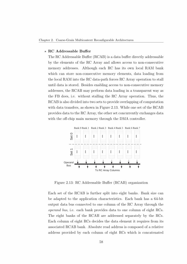
Chapter 2. Coarse-Grain Multicontext Reconfigurable Architectures
⋆ RC Addressable Buffer
The RC Addressable Buffer (RCAB) is a data buffer directly addressable
by the elements of the RC Array and allows access to non-consecutive
memory addresses. Although each RC has its own local RAM bank
which can store non-consecutive memory elements, data loading from
the local RAM into the RC data-path forces RC Array operation to stall
until data is stored. Besides enabling access to non-consecutive memory
addresses, the RCAB may perform data loading in a transparent way as
the FB does, i.e. without stalling the RC Array operation. Thus, the
RCAB is also divided into two sets to provide overlapping of computation
with data transfers, as shown in Figure 2.13. While one set of the RCAB
provides data to the RC Array, the other set concurrently exchanges data
with the off-chip main memory through the DMA controller.
···
···
Bank 0 Bank 1
···
···
Bank 2 Bank 3
···
···
Bank 4 Bank 5 ··
·
···
Bank 6 Bank 7
···
···
···
···
···
···
···
···
Set
0
Set
1
To RC Array Columns
Operand Bus
Figure 2.13: RC Addressable Buffer (RCAB) organization
Each set of the RCAB is further split into eight banks. Bank size can
be adapted to the application characteristics. Each bank has a 64-bit
output data bus connected to one column of the RC Array through the
operand bus, i.e. each bank provides data to one column of eight RCs.
The eight banks of the RCAB are addressed separately by the RCs.
Each column of eight RCs decides the data element it requires from its
associated RCAB bank. Absolute read address is composed of a relative
address provided by each column of eight RCs which is concatenated
58

2.3. The MorphoSys M2 implementation
with bits provided by the TinyRISC processor. The number of bits of
the read address bus depends on the implemented RCAB size.
⋆ DMA Controller
Along with data buffers, the DMA controller completes MorphoSys data
interface. The DMA controller performs data transfers between off-chip
main memory and MorphoSys M2 chip, and is under the control of the
TinyRISC processor. TinyRISC provides information such as the type
of operation (load/store), starting addresses in the main memory, Frame
Buffer, RC Addressable Buffer, or Context Memory and the number of
bytes to be transferred.
The DMA controller is in charge of loading the configuration program
from memory to the Context Memory. This is performed before the
execution of the RC Array, or sometimes even during its execution. The
TinyRISC sets the DMA controller to perform transfer of context words
from main memory to the Context Memory by means of the LDCTXT
instruction.
The DMA controller is also in charge of loading application data from
main memory to the data buffers, i. e. Frame Buffer and RC Addressable
Buffer. This is performed once the context words have been loaded into
the Context Memory. TinyRISC sets the DMA controller to perform the
data loading through the LDFB instruction.
After the RC Array has finished processing of application data, and
written it back to the Frame Buffer, this data is transferred to the main
memory by the DMA controller which is signaled by the STFB TinyRISC
instruction.
At this point, all the different components of the MorphoSys M2 imple-
mentation have been outlined. The following section describes the MorphoSys
reconfiguration capabilities.
59

Chapter 2. Coarse-Grain Multicontext Reconfigurable Architectures
2.4. MorphoSys reconfigurability
MorphoSys has two basic forms of reconfiguration, namely, interconnect
reconfiguration and functional reconfiguration. Both forms of reconfiguration
are implemented through the context word.
The interconnect reconfiguration is based on the presence of two multi-
plexers in each Reconfigurable Cell as shown in Figure 2.9. Each multiplexer
has inputs coming from different RCs in the same quadrant, and also from
the inter-quadrant horizontal and vertical express lanes. The control bits of
the input multiplexers are provided by the context word and determine the
connectivity for each clock cycle operation.
Similarly, the functional reconfiguration depends on the control bits pro-
vided by the context word. These control bits specify the arithmetic or logical
operation performed by the functional units within each RC.
A context word coming from the Context Memory is provided to the Con-
text Register of each RC every clock cycle. Since there are multiple configura-
tion planes in the Context Memory (see Subsection 2.3.4), a different configu-
ration plane can be used every cycle, without stopping the system operation,
thus exhibiting a dynamic nature.
In addition, more context words can be loaded into the Context Memory
while the RC Array is operating on previously loaded context words. This
operation is performed by the DMA controller (see Subsection 2.3.6) and can
take place without stalling the RC Array execution. Therefore, ideally, there
is no time lost for reconfiguring the RC Array.
Thanks to its reconfiguration capabilities, MorphoSys is a multicontext
reconfigurable architecture supporting one cycle dynamic reconfiguration.
2.5. MorphoSys operation flow
This section illustrates the typical operation of MorphoSys M2 for execut-
ing applications. M2 operation is controlled by the enhanced TinyRISC pro-
cessor which signals the DMA controller to initiate loading of Context Memory
and data buffers, and ultimately causes the computation to be performed by
60

2.5. MorphoSys operation flow
the RC Array.
For executing applications on MorphoSys M2, the application may be par-
titioned into sequential and parallel parts. The TinyRISC is in charge of ex-
ecuting sequential parts, i.e. general-purpose operations without parallelism,
while data-parallel parts of the application are assigned to the RC Array.
Prior to start the execution it is necessary to collect the TinyRISC instruc-
tion program, the RC Array configuration program and the application data.
The TinyRISC instruction program controls the RC Array execution and also
performs sequential operations on the TinyRISC. The RC Array configuration
program is the set of context words representing the RC Array computations
required for the given application which has to be stored in the Context Mem-
ory. The application data refers to the data required for processing by the
application (images frames, for example).
The TinyRISC instruction sequence follows a specific pattern to enable the
overlapping of data and context transfers with RC Array computation. This
is essential for maximizing application throughput.
An example of application execution pattern for optimum system perfor-
mance is depicted in Figure 2.14 and is explained as follows:
CBCAST , etc LDFB
Issue LDCTXT
Issue LDFB
CBCAST , etc STFB , LDFB
CBCAST , etc LDCTXT
CBCAST , etc LDCTXT
TinyRISC
Context to RC Array
Load new context
Idle Context to RC
Array Reload context
Reload context
Context Memory
Compute Idle Idle
Data to RC Array
Idle Load new
data Write out results,
load new data Data to RC
Array Idle
Load new data
Idle Idle Data to RC Array Idle Data to RC
Array
RC Array
FB Set 0
FB Set 1
Compute Compute Compute
Execution sequence
Figure 2.14: MorphoSys operation flow
⋆ First, the instruction LDCTXT is executed by the TinyRISC to load
context program into the Context Memory. This operation is performed
through the DMA controller.
61
Chapter 2. Coarse-Grain Multicontext Reconfigurable Architectures
⋆ Next, the LDFB is executed by the TinyRISC to load computation data
into the FB set 0. This operation is performed through the DMA con-
troller. This data can be accesses by the RC Array in subsequent cycles.
⋆ Later, the TinyRISC issues one of the RC Array execution instructions,
such as CBCAST, SBCB, etc (see Table 2.1). These instructions specify
the particular context (among multiple context words in Context Mem-
ory) to be executed by the RC Array. RC Array computation accesses
to data from the previously loaded FB set 0.
⋆ While the RC Array executes the instructions previously issued, the
TinyRISC issues a single instruction, LDFB, for loading the FB set 1.
This instruction signals the DMA controller to load the required data, for
the next round of computations, into the FB set 1 (while data from the
FB set 0 is being used by the RC Array). Alternatively, the TinyRISC
may issue a LDCTXT instruction to reload inactive parts of the Context
Memory. Either of these transfers happens concurrently with the RC
Array computation. The shaded regions of Figure 2.14 shows the overlap
of computations with data transfers and context reloads.
⋆ Once all the data in the FB set 0 has been processed, the TinyRISC issues
one of the RC Array execution instructions. Now, RC Array computation
accesses to data from the FB set 1. Immediately after, the TinyRISC
may issue the instructions STFB and LDFB to store data from the FB
set 0 into off-chip memory and load new computation data into this FB
set.
The last two items are repeated till the application concludes. At this
moment, the final step consists of storing the processed data from the FB into
main memory (if it is needed).
The previously described MorphoSys execution pattern summarizes the
ideal scenario for maximizing application throughput. However, there are
some issues and constraints that degrade the performance.
According to the MorphoSys execution model, prior to execute a set of
contexts in the RC Array, they must be loaded into the Context Memory, as
62

2.5. MorphoSys operation flow
well as the data on which they will operate must be loaded into one of the
data buffers. While data is processed in the RC Array, the TinyRISC can
order the loading of new data for the next round of computations. However,
applications usually executed in MorphoSys process high volumes of data, and
it is possible that not all the required data can be loaded in parallel with the
RC Array operation. In those cases, the RC Array computation is stalled till
the required data are loaded into the data buffers. This fact motivates the
development of a scheduling methodology that looks for the minimization of
these RC Array computation stalls. This problem is the main topic of this
work and is widely explained in the next chapter.
RC Array computation stalls also appears due to the MorphoSys SIMD
computational model. In order to exploit data parallelism, the same instruc-
tion operates on multiple data. TinyRISC processor is in charge of performing
global branches that affects the entire RC Array. This is valid when the branch
decision is taken by the TinyRISC processor, and all the elements of the RC
Array perform the same branch designated by the main processor. However,
not all the applications on which MorphoSys is targeted follow the previous
scheme. In fact, some applications exhibit a high dependency on the input
data. This input data dependency is due to the presence of parallel condi-
tional constructs instead of the global ones, as it was explained some lines
above. Since each Reconfigurable Cell is processing independent input data
subsets, it is possible that in the presence of a conditional branch, different
RCs demand the execution of different branch targets. In order to execute
different branch targets in the SIMD RC Array, not all the burden of eval-
uating branches must be performed by the TinyRISC. Instead of that, some
operation autonomy must be provided to the individual Reconfigurable Cells,
as it is explained below.
63

Chapter 2. Coarse-Grain Multicontext Reconfigurable Architectures
2.6. Operation autonomy of Reconfigurable
Cells
The SIMD computational model enables one instruction operating on mul-
tiple data at time. Its goal is to exploit parallelism in data streams. For that
purpose, SIMD architectures incorporate an array of processing elements that
are centrally controlled by a master processor. In the case of MorphoSys, the
array of processing elements correspond to the RC Array, and the TinyRISC
is the master processor. The TinyRISC fetches instructions and broadcasts
contexts to the RC Array.
On a pure SIMD architecture, the individual processing elements have no
local control over any parameter of the execution, and their computations are
uniform and regular over the processor array [Nar93]. Pure SIMD architec-
tures have a global program control flow. In the presence of global conditional
constructs (if-then-else, for example), master processor is responsible for per-
forming global branches that affects the entire processor array.
However, applications having a global control flow are not predominant.
Most of the applications on which MorphoSys was targeted do not fit into this
category. Instead of global conditional constructs handled by the main pro-
cessor, MorphoSys mainly deals with applications containing conditional con-
structs which are derived from data dependencies in their program flow, that
would be handle by each RC. Conditional constructs refers to constructs that
would be encoded in each processing element in the form of data-dependent
branches. According to the MorphoSys SIMD model of computation, each
Reconfigurable Cell is processing independent input data subsets, so it is pos-
sible that in the presence of conditional constructs, different RCs demand the
execution of different paths. However, in the first MorphoSys M1 implementa-
tion, the RCs do not implement branches because they do not have a program
counter. In MorphoSys M1, control is centralized by the TinyRISC processor
which performs global branches that affect the entire RC Array. In order to
efficiently implement the parallel conditional constructs on MorphoSys, some
operation autonomy must be provided to the individual RCs. RC operation
autonomy refers to its capability to participate in a computation step or ab-
64

2.6. Operation autonomy of Reconfigurable Cells
stain from it based on a local condition. This a type of control on instruction
selection named Autonomous SIMD (ASIMD).
To solve this problem, MorphoSys M2 introduces a new set of contexts
called pseudo-branches [APB02], which are supported by an extra hardware
added to the RC architecture. The pseudo-branches enable to conditionally
nullify blocks of code starting at the branch instruction and ending at the target
position, independently of the instructions inside that block of code. In this
way, the TinyRISC is relieved from the burden represented by the evaluation
of the branch target of each RC, because the branches are emulated by the
individual RCs. The implementation and operation of the pseudo-branches
are explained below.
A pseudo-branch context was created to emulate branch behavior. The
pseudo-branch context includes a branch condition (greater than, equal, etc.)
and a destination (target) tag added by the programmer as in normal assembly
code. Later, the assembler assigns a 5-bit code to each different tag. Thus, up
to 31 different tags are supported to enable the encoding of complex conditional
constructs (code 0 is reserved).
An end-branch context was also created to be the pseudo-branch target.
The end-branch context is a modified version of the NOP instruction. Since
there were some unused bits in the NOP instruction, five of them are now used
as a tag field to implement the end-branch context. Any conditional structure
starts with a pseudo-branch context and finishes with an end-branch context,
both having the same tag.
A 1-bit register (Sleep/Awake Flag) was added to each RC. Normally this
flag is in the awake mode, which means that the RC is able to execute contexts.
When a pseudo-branch appears, the RC evaluates the condition included on it.
If the condition is true (branch taken), then the branch tag field is copied to
a Tag Register inside the RC, and the Sleep/Awake flag is set to sleep mode,
nullifying all the contexts (inserting NOPs) until the RC is returned to the
awake mode. The flag is returned to the awake mode when the content of the
Tag Register and the target tag existing in the end-branch context (modified
NOP instruction) are the same.
Each RC is then provided with a 5-bit register called Tag Register (TReg).
65

Chapter 2. Coarse-Grain Multicontext Reconfigurable Architectures
This register stores the branch tag field when a pseudo-branch is taken and
operates as it was explained above.
Figure 2.15 shows how the pseudo-branches work. There is only one context
stream broadcasted by the TinyRISC. Each RC evaluates the branch condi-
tion included on the pseudo-branch and end-branch contexts and proceeds
according to its current state and the content of its Tag Register.
RC i
pBra cc T1 context a ... pBra cc T2 ... context k pBra T1 eBra T2 context m context n eBra T1
TagReg i
00000 00000 00000 00010 00010 00010 00010 00010 00000 00000 00000
Sleep/ Awake
1 1 1 1 0 0 0 1 1 1 1
RC j
pBra cc T1 context a ... pBra cc T2 ... context k pBra T1 eBra T2 context m context n eBra T1
TagReg j
00000 00001 00001 00001 00001 00001 00001 00001 00001 00001 00000
Sleep/ Awake
1 0 0 0 0 0 0 0 0 0 1
Description
RCj branches, RCi does not RCj nullifies, RCi executes RCi is awake, RCj is asleep RCi branches RCi and RCj are asleep RCi and RCj are asleep RCi and RCj are asleep RCi wakes up, RCj is asleep RCi is awake, RCj is asleep RCi is awake, RCj is asleep RCi is awake, RCj wakes up
RC i , RC j : Reconfigurable Cells i and j , respectively pBra cc : pseudo branch context. cc specifies conditions as greater or equal, minus, etc. eBra : end branch context TReg : Tag register ( T1 : 00001 , T2 : 00010 ) pBranch taken: pBranch not taken:
Figure 2.15: Example of pseudo-branches operation in two RCs
The Sleep/Awake flag is also used for power saving in each RC. When in
the sleep mode, all combinational blocks of the RC have their power disabled,
except for the instruction decoder.
Pseudo-branches are relevant because it allows to efficiently map data-
dependent conditional constructions using SIMD instruction streams without
the intervention of the TinyRISC processor.
2.7. MorphoSys vs. Other architectures
At the beginning of this chapter a set of coarse-grained reconfigurable ar-
chitectures were described, and in the preceding sections the MorphoSys archi-
tecture was detailed. This section compares and contrasts the main features
of Morphosys with those of cited reconfigurable systems.
66
2.7. MorphoSys vs. Other architectures
According to flexibility, MorphoSys can be classified as an Application
Domain-Specific System (ADSS) [TSV07]. The design of MorphoSys compo-
nents is based on the multimedia and digital signal processing domain needs.
MorphoSys architecture is characterized by generality and regularity. Gen-
erality means that the architecture includes more than the required number
and types of processing units and interconnections for implementing a class of
applications in order to suit future needs. Regularity means that the resources
(processing elements and interconnections) are organized in regular structures.
This is motivated by the fact that the kernels implemented by the architecture
exhibit regularity. Thanks to these generality and regularity feature, Morpho-
Sys can be used to implement any application of its domain. As well as Mor-
phoSys, the MATRIX architecture (Subsection 2.1.1), the REMARC array
processor (Subsection 2.1.2), the eXtreme Processing Platform (XPP) (Sub-
section 2.1.3), the Montium tile processor (Subsection 2.1.4), and the Silicon
Hive processor (Subsection 2.1.6) can also be classified as Application Domain-
Specific Systems, although the MATRIX architectures has a wider application
scope. On the other hand, the Pleiades architecture (Subsection 2.1.5) can
be classified, in terms of flexibility, as an Application Class-Specific System
(ACSS) [TSV07]. It means that it has been designed to support only a prede-
fined set of applications having limited reconfigurability. It can be configured
to implement only the considered set of applications and not all the applica-
tions of the domain. Pleiades’ satellite processors are designed to implement
specific tasks with high performance and low energy consumption, sacrifying
the flexibility.
Comparing ADSSs and ACSSs, the latter ones exhibit reduced flexibility
and better performance. ACSSs are useful for cases where the exact algorithms
are known in advance, and it is critical to meet design constraints, and no ad-
ditional flexibility is required. ADSSs (MorphoSys among them) are designed
looking for the implementation of a wide set applications of certain application
domain.
In terms of design issues, ACSSs consist of a fixed number and type of
programmable interconnections and processinng elements usually organized
in not so regular structures. Their interconnection networks only offer the
67

Chapter 2. Coarse-Grain Multicontext Reconfigurable Architectures
required flexibility so that the processing elements can communicate each other
according to the needs of the applications. In contrast to ACSSs, ADSSs
aim at implementing the applications of a whole domain. This imposes the
development of a generic and flexible architecture. The organization and the
number of processing elements, the operations that are supported by each
processing element, as well as the interconnection network, must be enough
general to support a wider application range.
A detailed comparison of MorphoSys with other cited coarse-grained re-
configurable architectures is summarized in Table 2.2.
Table 2.2: MorphoSys compared with other coarse grain systems
Computational
natureReconfiguration
Interconnection
network
Application
domain
MorphoSys SIMD Every clock cycle Mesh-based Digital signal pro-cessing and multi-media
MATRIX[MD96]
SIMD, MIMD,VLIW
Every clock cycle Mesh-based General-purposecomputing
REMARC[MO98]
SIMD, limitedMIMD
Every clock cycle Mesh-based Multimedia
XPP[BEM+03]
VLIW-like within aPAE
Every clock cycle Packet-orientedcommunicationnetwork
Mobile communi-cations
Montium[HS03]
VLIW-like within atile
Every clock cycle Mesh-based Mobile computing
Pleiades[Abn01]
MIMD with a con-trol processor
Every clock cycle Data-driven com-munication net-work
Digital signal pro-cessing
SiliconHive[LBH+03]
MIMD Every clock cycle Mesh-based Digital signal pro-cessing and multi-media
MorphoSys SIMD computational nature allows it to configure the entire RC
Array by broadcasting a context plane, which makes it more straightforward
than the VLIW-like and MIMD computational models that other systems may
have. XPP and Montium have a VLIW-like control processor to configure their
functionality and interconnection at the Processing Array Element (PAE)- and
tile-level, respectively. However, a XPP device can contain several Processing
Array Clusters (PACs), i.e. rectangular arrays of PAEs. Likewise, Montium
tiles are usually integrated whithin a System-On-Chip. Pleaides architecture
has a control processor surrounded by a heterogeneous array of autonomous
68
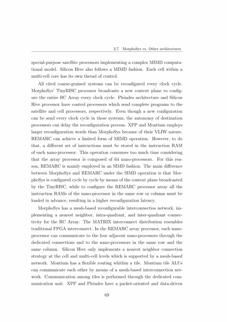
2.7. MorphoSys vs. Other architectures
special-purpose satellite processors implementing a complex MIMD computa-
tional model. Silicon Hive also follows a MIMD fashion. Each cell within a
multi-cell core has its own thread of control.
All cited coarse-grained systems can be reconfigured every clock cycle.
MorphoSys’ TinyRISC processor broadcasts a new context plane to config-
ure the entire RC Array every clock cycle. Pleiades architecture and Silicon
Hive processor have control processors which send complete programs to the
satellite and cell processors, respectively. Even though a new configuration
can be send every clock cycle in these systems, the autonomy of destination
processors can delay the reconfiguration process. XPP and Montium employs
larger reconfiguration words than MorphoSys because of their VLIW nature.
REMARC can achieve a limited form of MIMD operation. However, to do
that, a different set of instructions must be stored in the instruction RAM
of each nano-processor. This operation consumes too much time considering
that the array processor is composed of 64 nano-processors. For this rea-
son, REMARC is mainly employed in an SIMD fashion. The main difference
between MorphoSys and REMARC under the SIMD operation is that Mor-
phoSys is configured cycle by cycle by means of the context plane broadcasted
by the TinyRISC, while to configure the REMARC processor array all the
instruction RAMs of the nano-processor in the same row or column must be
loaded in advance, resulting in a higher reconfiguration latency.
MorphoSys has a mesh-based reconfigurable interconnectios network, im-
plementing a nearest neighbor, intra-quadrant, and inter-quadrant connec-
tivity for the RC Array. The MATRIX interconnect distribution resembles
traditional FPGA interconnect. In the REMARC array processor, each nano-
processor can communicate to the four adjacent nano-processors through the
dedicated connections and to the nano-processors in the same row and the
same column. Silicon Hive only implements a nearest neighbor connection
strategy at the cell and multi-cell levels which is supported by a mesh-based
network. Montium has a flexible routing whithin a tile. Montium tile ALUs
can communicate each other by means of a mesh-based interconnection net-
work. Communication among tiles is performed through the dedicated com-
munication unit. XPP and Pleiades have a packet-oriented and data-driven
69

Chapter 2. Coarse-Grain Multicontext Reconfigurable Architectures
communication networks, respectively. Dedicated links are established accord-
ing to the application needs in both architectures.
MorphoSys, the MATRIX architecure, the REMARC array processor, the
eXtreme Processing Platform (XPP), the Montium tile processor, and the
Silicon Hive processor are classified as Application Domain-Specific Systems.
On the other hand, the Pleiades architecture is classified as an Application
Class-Specific System. MorphoSys, MATRIX, REMARC, XPP, Montium and
Silicon Hive can be used to implement any application of their domains, thanks
to their generality and regularity features. On the other hand, the Pleiades
architecture can be configured to implement only a specific set of applications
and not all the applications of the domain.
2.8. Conclusions
This chapter introduced our target architecture, MorphoSys. Some coarse-
grained reconfigurable systems were also introduced in order to provide a wider
perspective of the architecture field. Coarse-grained reconfigurable systems
have been built upon common ideas and concepts. In order to obtain an
important throughput, it is desirable to have a system with multiple context
planes, dynamic reconfiguration capability and local interface. Other specific
features of each architecture stem from the application domain on which they
are targeted, and on the knowledge and expertise of designers.
MorphoSys architecture is targeted for data- and computation-intensive ap-
plications with inherent parallelism and high throughput requirements. Mor-
phoSys integrates a general-purpose processor with a reconfigurable processing
unit. Those computing resources are backed up by a high-bandwidth data in-
terface. All components are present in the same die to avoid limitation of
off-chip I/O processing. MorphoSys processing elements are organized in a
2D array. Their functionality and interconnection can be reconfigured every
clock cycle. TinyRISC processor is in charge of controlling the whole sys-
tem. Sequential parts of the applications are executed by the TinyRISC while
the data-parallel parts are mapped onto the array. MorphoSys has a SIMD
computational model that enables it to execute one instruction over multiple
70

2.8. Conclusions
data at time. Under the SIMD style, individual RCs lack of some operation
autonomy, because they have no local control over any parameter of the execu-
tion. To solve this problem, MorphoSys introduces a new set of contexts called
pseudo-branches. The pseudo-branches enable to conditionally nullify blocks
of code starting at the pseudo-branch context and ending at the end-branch
context, independently of the instructions inside that block of code. Each RC
evaluates the branch condition included on the pseudo-branch and end-branch
contexts, and participates in computations or abstains from them based on a
local condition.
71


Chapter 3
Application modeling and
compilation framework
In Chapter 2 we have presented an in-depth description of our target ar-
chitecture, MorphoSys, detailing the architectural improvements introduced
in this work in order to support our scheduling proposals, whose are in part
explained in this chapter. MorphoSys reconfiguration capabilities were also in-
cluded, as well as its low-level operation flow. Complementing that work, this
chapter presents the architecture operation from a higher level of abstraction,
the application point of view. The target applications are presented in rela-
tion with their high-level handling in order to map them onto the MorphoSys
architecture.
Recently, coarse-grained reconfigurable systems have targeted on a new
class of applications. So, we first identify the characteristics of this new class
of applications. Then, we explain how they are modeled in order to be mapped
onto the MorphoSys architecture. According to these characteristics, and the
developed mapping scheme, different overheads appear. We discuss these over-
heads and propose some solutions to overcome them.
This thesis is focused on the scheduling of dynamic applications onto a
coarse-grained multicontext reconfigurable architecture. This work is centered
on the development of both off-line and dynamic scheduling techniques to han-
dle the dynamic characteristics of the target applications. Existing MorphoSys
73

Chapter 3. Application modeling and compilation framework
compilation framework is only focused on static applications mapping. So, we
have improved its off-line scheduling stage, and introduced a novel runtime
scheduling support in order to efficiently execute dynamic applications. In
this chapter we present an overall description of this enhanced compilation
framework.
3.1. Characteristics of target applications
The majority of contemporary applications, for example, DSP and multi-
media applications, are characterized by the presence of computationally- and
data-intensive tasks, demanding high throughput since they are also subjected
to tight real-time constraints. We refer to this kind of tasks as kernels. Our
work is based on the characterization of these kernels in such a way that any
application can be represented as a sequence of kernels. In contemporary ap-
plications the way in which these kernels are executed is highly influenced by
the changing customer needs change rapidly, and the rising of new standards.
So, systems must be flexible enough to satisfy new requirements. According
to the characteristics presented in previous chapters, reconfigurable computing
becomes an interesting alternative to implement these types of applications.
Its high degree of runtime flexibility allows to adapt its functionality according
to the user interaction and the intrinsic dynamic behavior of the applications.
Static applications are easily modeled by a data dependency-based task
graph, namely a data-flow graph (DFG). A DFG is a graph which represents
data dependencies between a number of tasks. It is a directed graph whose ver-
tex set has an one-to-one correspondence with the set of tasks, and whose set of
directed edges is in correspondence with the transfers of data from one task to
another one. For instance, the MPEG-2 encoder [MPE96] is composed by the
kernel 1 sequence Motion Estimation (ME), Motion Compensation (MC), Dis-
crete Cosine Transform (DCT), Quantization (Q), Inverse Quantization (IQ),
Inverse Discrete Cosine Transform (IDCT) and Inverse Motion Compensation
(IMC), which is repeated 396 times in MorphoSys to process an input image
1In this work, we use the terms kernel and task indistinctly
74

3.1. Characteristics of target applications
(see Figure 3.1). In the MPEG-2 encoder not all the kernels are executed the
same number of times in each outer loop iteration [Mae00]. This is because
the first kernel (ME) processes a block of data six times larger than the one
processed by the remaining kernels. In order to have an uniform data flow
size through the kernels, the remaining kernels iterate six times each. For
this application, the program flow is well-known at compilation time. After
executing a kernel, we know the next one to be executed, independently of
the input data, i.e. the specific image. Then, all the scheduling issues can
be addressed at compilation time to obtain a code optimized for its execution
onto the MorphoSys architecture.
ME MC DCT Q IQ IDCT IMC
6 6 6 6 6 6
396
Figure 3.1: MPEG-2 encoder
Opposite to the static applications, where all relevant information is well-
known at compilation time (and so they can be near-optimally scheduled prior
to execution), we are targeting on a growing class of applications which are
characterized by dynamic workload, data-intensive computation, and hard
real-time constraints. We refer to them as dynamic applications. Some ex-
amples of these dynamic applications are in multimedia (audio and video en-
coding/decoding systems running AC3, ADPCM, MPEG2, H.261 or JPEG),
3D image processing (ray-tracing, rendering), and wireless (GSM, CDMA)
domains. Some applications operate on sequences of ordered data (streams),
while another ones have non-regular data access patterns. User activity and
data dependencies produce an unpredictable program flow for this class of
applications at runtime.
In dynamic applications, the next kernel to be executed most of the times
depends directly on input data, or user activity, so it is decided at runtime.
Then, our target applications exhibit a dynamic program flow that we model
by means of the conditional execution of kernels. To deal with this feature, we
have added control dependencies to the DFG, in such a way that some kernels
75

Chapter 3. Application modeling and compilation framework
are executed or not depending on the result of a previous kernel. There are
several graph representations that can help us to reflect the structure of these
applications [GDWL94], [dM94]. We have adopted the hybrid control and
data flow graph (CDFG) since it embeds all control and sequencing informa-
tion explicitly within the same graph. This approach extends DFGs further by
introducing branching vertices that represent operations that evaluate condi-
tional clauses. From a branching vertex a set of alternative paths are derived.
When a branching vertex appears in a CDFG, the kernel located after the
branching vertex is executed depending on the result of the kernel located
before the branching vertex, as it is widely explained in the next section.
3.2. Application modeling
In our approach, the applications are specified at a coarse level of granu-
larity by a task graph G(K,E), where K = {ki; i = 0, 1, 2, . . . , n} is the set of
nodes (kernels) of the graph, and E = {(ki, kj); i, j = 0, 1, 2, . . . , n} is the set
of directed edges which is in correspondence with the transfer of data from a
kernel to another one. The task graph is a CDFG which besides data depen-
dencies also represents control dependencies between a number of functions.
The set of nodes of the graph is in one-to-one correspondence with the set
of kernels representing coarse-grained computations, e.g. DCT, IDCT in the
case of MPEG-2. For each kernel ki ∈ K, we know its execution time on the
reconfigurable unit, t(ki), its input data and results size, s(di + ri), and its
configuration size, s(ci). Data and configuration sizes can also be expressed in
terms of time, according to the bandwidth of the corresponding data interface
component. In such a way, the input data and results transfer time is denoted
by t(di + ri), and the configuration loading time is denoted by t(ci). Elements
(ki, kj) ∈ E represent those kernel pairs such that kernel kj follows directly ki
for any i, j = 0, 1, 2, . . . , n. Set E reflects data dependencies, that is when an
input of a kernel is the result of another kernel, and the former kernel depends
on the latter. Kernel ki is called a predecessor of kj when there is a path (or
an edge) with tail ki and head kj. Similarly, kernel ki is a successor of kj
when there is a path (or an edge) with tail kj and head ki. It is important
76

3.2. Application modeling
to notice that a kernel is fired (it may begin execution) only when input data
and configurations are ready.
3.2.1. Conditional constructs classification
Control-flow information can also be represented graphically. The simplest
way is to extend further DFGs by introducing branching vertices that represent
operations that evaluate conditional clauses. A branching vertex is the tail of
a set of alternative paths, corresponding to the possible branches. Figure 3.2
shows two examples of dynamic applications represented as CDFGs. We use a
diamond in the CDFG to indicate a branching vertex. The branching vertex
is modeled by a branching clause. In both cases, CDFGs represent a block
of code which is executed many times, N , to completely process the input
data of the application. The presence of a branching clause in a CDFG results
in two possible constructs, according to the branch destination possibilities:
branching and iterative contructs.
K 1
K 2
K 3
CB
N
True
False
(a)
K 1 K 2 CB
N
True
False
(b)
Figure 3.2: Examples of task graphs
⋆ Branching constructs
Branching constructs can be modeled by a branching clause and branch-
ing bodies. A branching body is a set of kernels that are selected accord-
ing to the value of the branching clause. There are as many branching
bodies as the possible values of the branching clause, and their execution
is mutually exclusive. Branching is modeled by associating a sequence
of kernels with each branching body and a link vertex with the branch
clause. The link vertex models the operation of evaluating the clause
and taking the branch decision. The diamond in the CDFG shown in
77
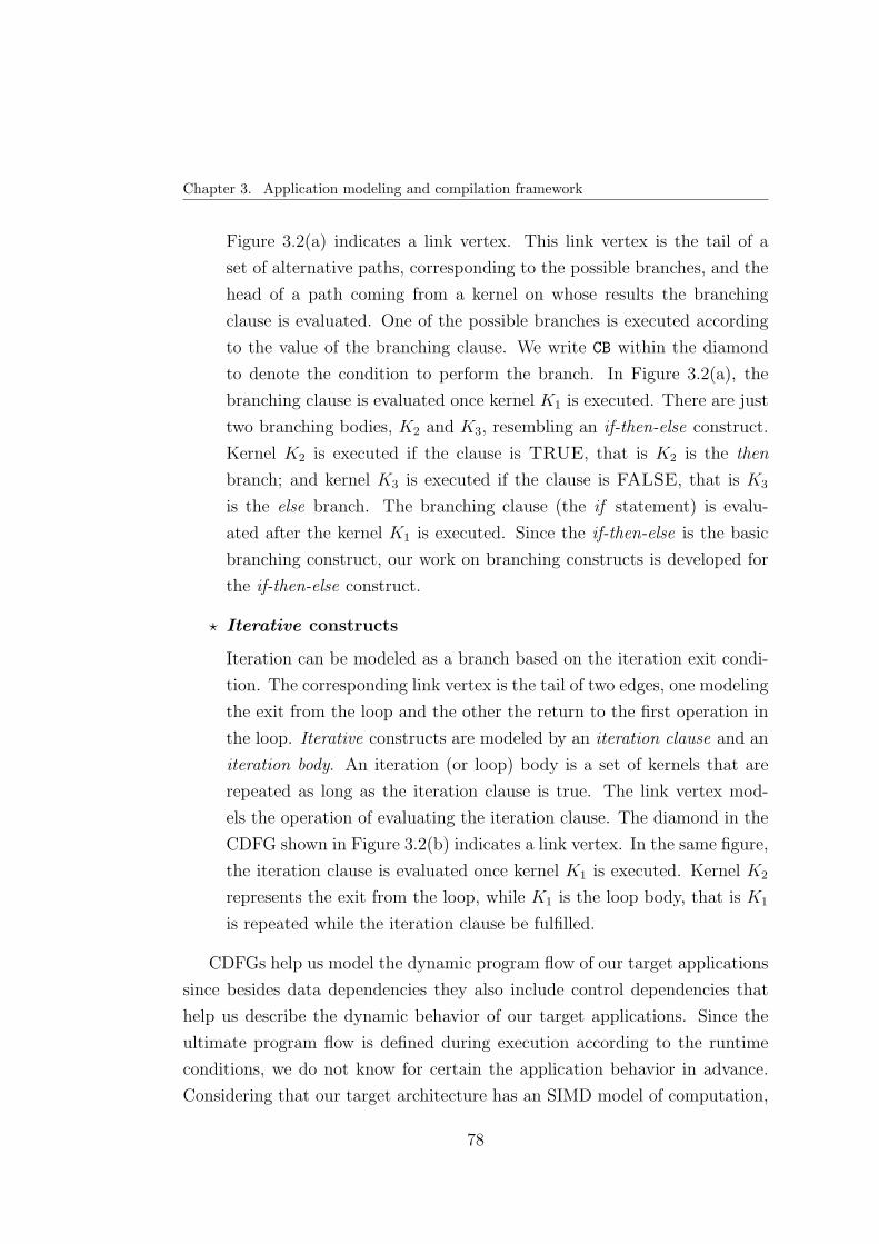
Chapter 3. Application modeling and compilation framework
Figure 3.2(a) indicates a link vertex. This link vertex is the tail of a
set of alternative paths, corresponding to the possible branches, and the
head of a path coming from a kernel on whose results the branching
clause is evaluated. One of the possible branches is executed according
to the value of the branching clause. We write CB within the diamond
to denote the condition to perform the branch. In Figure 3.2(a), the
branching clause is evaluated once kernel K1 is executed. There are just
two branching bodies, K2 and K3, resembling an if-then-else construct.
Kernel K2 is executed if the clause is TRUE, that is K2 is the then
branch; and kernel K3 is executed if the clause is FALSE, that is K3
is the else branch. The branching clause (the if statement) is evalu-
ated after the kernel K1 is executed. Since the if-then-else is the basic
branching construct, our work on branching constructs is developed for
the if-then-else construct.
⋆ Iterative constructs
Iteration can be modeled as a branch based on the iteration exit condi-
tion. The corresponding link vertex is the tail of two edges, one modeling
the exit from the loop and the other the return to the first operation in
the loop. Iterative constructs are modeled by an iteration clause and an
iteration body. An iteration (or loop) body is a set of kernels that are
repeated as long as the iteration clause is true. The link vertex mod-
els the operation of evaluating the iteration clause. The diamond in the
CDFG shown in Figure 3.2(b) indicates a link vertex. In the same figure,
the iteration clause is evaluated once kernel K1 is executed. Kernel K2
represents the exit from the loop, while K1 is the loop body, that is K1
is repeated while the iteration clause be fulfilled.
CDFGs help us model the dynamic program flow of our target applications
since besides data dependencies they also include control dependencies that
help us describe the dynamic behavior of our target applications. Since the
ultimate program flow is defined during execution according to the runtime
conditions, we do not know for certain the application behavior in advance.
Considering that our target architecture has an SIMD model of computation,
78

3.2. Application modeling
while an application is processed it is possible to have different RCs with
different branch targets, resulting in a relevant issue that is discussed in detail
in Section 3.3. Moreover, the uncertainty about the ultimate kernel sequence
demanded by the applications also implies that we are not aware of the context
and data required by each kernel. This yields to the possibility of increasing
the application latency when context and data are not provided at the right
time. A detailed description of this problem is presented in Section 3.6.
The next subsection shows how two real applications are modeled in order
to be mapped onto the MorphoSys architecture.
3.2.2. Examples of modeled applications
In Section 3.1 we showed that the MPEG-2 encoder is a kind of static
application, where all relevant information is well-known at compilation time,
and so, it can be near-optimally scheduled prior to execution. However, our
target applications have an uncertain program flow, because the next kernel to
be executed most of the times depends directly on the input data processing,
or user activity, so it is decided at runtime. Now, we introduce two exam-
ples of target applications in the field of 3D image processing, both of them
exhibiting a highly dynamic program flow. These applications are ray-tracing
and rendering. Our purpose is to illustrate how they are modeled by means of
CDFGs including the conditional execution of kernels.
Ray-tracing
Ray-tracing [Gla89] is a global illumination based rendering method that
works by simulating how photons travel in real world. It traces rays of light
from the eye back through the image plane into the scene. Then the rays are
tested against all objects in the scene to determine if they intersect any objects.
If the ray does not intersect any object, then that pixel has the background
color. If the ray hits an object, in the intersection point several types of rays
are spawned (see Figure 3.3):
⋆ Shadow rays are generated by shooting rays from the point to all the
light sources. If this shadow ray hits another object before it hits a light
79

Chapter 3. Application modeling and compilation framework
Figure 3.3: Ray-tracing
source, then the first intersection point is in the shadow of the second
object. This means that only the ambient term for that light source is
counted for the final color.
⋆ Reflection rays are generated according to the reflective properties of the
object. If the reflected ray hits an object then a local illumination model
is applied at the point of intersection and the result is carried back to
the first intersection point.
⋆ Refraction rays are generated if the object is transparent. As with the
reflected ray, if the refracted ray hits an object then a local illumination
model is applied at the point of intersection and the result is carried
back to the first intersection point.
Reflected rays can generate other reflected rays that can generate other
reflected rays, and so on. Thus, the ray-tracing works recursively.
Shading / Secondary rays
generation
Octree traversal
Eye rays generation
Ray-object intersection
Leaf node?
Hit? True True
Figure 3.4: CDFG to describe the ray-tracing application
The ray tracer works as a streaming process split into four kernels: eye ray
generation, data structure traversal, ray-object intersection, and shading, in-
80
3.2. Application modeling
cluding secondary rays generation. Ray-tracing extended CDFG is illustrated
in Figure 3.4. The eye rays generator kernel produces a set of viewing rays.
Each viewing ray is a single ray corresponding to a pixel in the image. The
traversal kernel is fed by the set of rays produced by the eye ray generator.
As an efficient data structure to store the scene geometry we have chosen an
octree [Gla84]. The octree traversal kernel takes rays through the octree until
the ray encounters a node containing objects, that is until the ray reaches a
leaf node. This conditional iteration over the octree traversal kernel is con-
trolled by an iteration clause that is illustrated by the leaf node diamond in the
CDFG. Once the ray reaches a leaf node, the ray and object data are passed
to the intersection kernel. The intersection kernel is responsible for testing ray
intersections with all the objects contained in the node. If ray-object inter-
section occurs (there is a hit) in that node, the ray and the object that are
hit are ready for shading. If there is not a hit, the ray is passed back to the
traversal kernel and the search for nodes containing objects continues. The
shading kernel calculates a color. If a ray processing finishes at this hit, then
the color of the associated pixel is written. If secondary rays are considered,
they may be generated by the shading kernel and passed back to the traversal
kernel.
We have mapped the ray-tracing application onto the MorphoSys archi-
tecture trying to maximize the available parallelism of the application. Our
purpose is to process one ray per reconfigurable cell of the RC Array. Referring
to Figure 3.3, remember that a ray corresponds to a pixel of the screen. This
means that there are 64 different rays being concurrently processed in the RC
Array at a time. To illustrate one of the mapping issues, lets imagine the 64
rays simultaneously traversing the octree structure. According to the geome-
try of the scene, to the spatial objects distribution, and to the direction of the
ray, it is impossible to know how many times one ray will process the octree
traversal kernel, before to demand the execution of the intersection kernel. In
fact, it is highly probable that different rays not demand the execution of the
octree traversal kernel the same number of times. Considering the SIMD com-
putational model of our target architecture, these issues represent a serious
challenge to successfully map the application.
81

Chapter 3. Application modeling and compilation framework
Graphics pipeline (Rendering)
We have implemented a graphics pipeline [Wat00] which takes a descrip-
tion of a scene in three-dimensional space and map it into a two-dimensional
projection on the view surface (the screen). The processes involved in the
graphics pipeline are geometric and algorithmic. Since we have considered
the case of polygon mesh models (polygon objects are by far the most com-
mon representational form in computer graphics), geometric processes involve
operations on the vertices of polygons (transforming the vertices from one co-
ordinate space to another or discarding polygons that cannot be seen from the
point of view, for example). Algorithmic processes refer to rendering processes
that involve operations like shading and texture mapping and are more costly
than the geometric operations. The extended DFG representing the graphics
pipeline is shown in Figure 3.5. The overall process is a transformation of the
object representation from a three-dimensional space into a two-dimensional
space. The input to the graphics pipeline is a list of polygons and the output
is a colour for each pixel onto which each polygon projects on the screen.
3D Scene
Vertices sorting
Edge pixels
Z-Buffer Line pixels
Z-Buffer Interior pixels?
Line finished?
True
True
Figure 3.5: CDFG to describe the rendering application
The rendering of a scene is done in a scan line order, where the segments
of all polygons in that scene which cross a given scan line are rendered, be-
fore moving on to the next scan line. Pixels in the interior of polygon are
shaded using an incremental shading scheme, and their depth is evaluated
by interpolation from the z values of the polygon vertices after the viewing
transformations has been applied. The Z-buffer algorithm [Wat70] is a hidden
surface removal algorithm that is equivalent to a search through the z values
of each interior polygon point, to find that point with the minimum z value.
This search is implemented by using a Z-buffer that holds for a current point
82

3.2. Application modeling
the smallest z value so far encountered. During the processing of a polygon we
write the intensity of a point into the buffer depending on whether the depth
z, of the current point, is less than the depth so far encountered as recorded
in the Z-buffer.
The first kernel of the graphics pipeline sorts the vertices of the polygons
representing the 3D scene by using one of its coordinates in order to facilitate
the shading process. Then, according to the scan line algorithm, edge pixels
are shaded and stored in the Z-buffer. Later, interior pixels, if any (see the
“Interior pixels?” diamond in the DFG), are shaded and stored in the Z-
buffer, until the given scan line is finished (see the “Line finished?” diamond
in the DFG), and the next scan line is started.
We have mapped the rendering application onto the MorphoSys architec-
ture trying to maximize the exploitation of the abundant parallel resources.
We have developed an implementation in which the polygons representing the
3D scene are triangles. Our purpose is to process one triangle per reconfig-
urable cell of the RC Array. This means the parallel execution of 64 triangles
of different sizes on the RC Array. A problem arise because the triangles si-
multaneously processed are very different from each other. This means that
after extracting 64 triangles from the 3D scene, it is highly probable that they
have different number of lines to be drawn, as well as different number of pixels
per line. Therefore, the number of times that the “Edge pixels?” and “Line
pixels?” kernels are executed for every triangle is unknown in advance. This
is one of the issues that may be effectively handled to successfully map the
application onto the target architecture.
To close this section, we can say that existing static compilation frame-
works can not efficiently map these highly dynamic applications because of
their uncertain program flow. Therefore, it is necessary to introduce a new
scheduling process in order to achieve an efficient mapping of them. Prior to
do that, we discuss different overheads produced by the characteristics of both,
the applications and the target architecture.
83

Chapter 3. Application modeling and compilation framework
3.3. CBs overhead in SIMD reconfigurable
architectures
The well-known multicontext reconfigurable architectures Matrix [MD96],
Remarc [MO98], and MorphoSys [SLL+00] have an SIMD model of compu-
tation. This means that all their processing elements must execute the same
configuration at time, that is the same kernel, over independent subsets of in-
put data. However, in the presence of a CB, it is highly probable that several
RCs inside the RC Array demand the execution of different kernels.
An execution scenario perfectly suited for the SIMD computational model
corresponds to the case in which the entire RC Array is required to process the
same kernel at time. Hence, the program flow follows the same path and the
branch decisions are taken globally for the entire RC Array. However, this is
a few probable scenario because all RCs are processing independent subsets of
input data and their evolution can be different according to the characteristics
of the application.
A more realistic scenario implies, for example, as Figure 3.2(b) shows, that
after executing kernel K1 some RCs demand the execution of kernel K2, while
the other ones demand the execution of kernel K1 again. This situation is not
compatible with the SIMD model of computation. Just one of the possible
program flow paths must be executed on the RCs that have required it, while
the remaining ones should be stalled and their associated kernel execution
should be postponed. It is necessary to define a methodology in order to
determine how to proceed when different program paths appear inside the RC
Array after evaluating a CB. This means, it is necessary to decide the next
kernel to be executed. Moreover, this decision should be preferably taken
without main processor action, because in other case the processor has to
check the 64 RC branch destinations, surely increasing the execution time.
Having this goal in mind, we have provided some operation autonomy to the
individual RCs, in order to relieve as much as possible the main processor of
the burden represented by the evaluation of the branch destination of each RC.
This solution represented an architectural enhancement and was explained in
Section 2.6. In the next section we describe how the operation autonomy of the
84

3.4. Mapping of conditional constructs onto MorphoSys
individual RCs helps to effectively implement the kernel serialization, without
main processor action.
3.4. Mapping of conditional constructs onto
MorphoSys
In this section we show how the MorphoSys architectural enhancements in-
troduced in Section 2.6 helps to relieve as much as possible the main processor
of the burden represented by the evaluation of the branch target of individual
RCs.
Our target applications contain conditional constructs which are derived
from data dependencies in their program flow, that should be handled by each
RC. Conditional constructs refers to those constructs that would be encoded in
each RC in the form of data-dependent branches. Since each MorphoSys RC is
processing independent input data subsets, it is possible that in the presence of
conditional constructs, different RCs demand the execution of different branch
targets. However, RCs do not implement branches because they do not have
a program counter.
In Section 2.6 we have introduced a new set of contexts called pseudo-
branches, which are supported by an extra hardware added to the RC archi-
tecture. The pseudo-branches give to the RCs the capability to participate in
a computation step or abstain from it based on a local condition, eliminating
the centralized control initally performed by the Tiny RISC processor. The
pseudo-branches enable to conditionally nullify blocks of code starting at the
branch instruction and ending at the target position, independently of the in-
structions inside that block of code. In this way, the TinyRISC is relieved
from the burden represented by the evaluation of the branch target of each
RC, because the branches are emulated by the individual RCs.
In the next two subsections we show how the pseudo-branches are used
in order to map onto the target architecture the two conditional constructs
described in Subsection 3.2.1.
85

Chapter 3. Application modeling and compilation framework
3.4.1. Mapping of if-then-else constructs
The if-then-else construct is a particular case of the branching construct
described in Subsection 3.2.1. Referring to Figure 3.2(a), after executing the
kernel K1 and evaluating the branching clause, we could decide executing K3
over the RCs that require it. Then, we would execute K2 over the other RCs.
For that purpose we use the pseudo-branch contexts as is explained below.
The pseudo-branch contexts added to execute the if-then-else construct
of Figure 3.2(a) are shown in Figure 3.6. The CB is emulated by the pBracc
Label_k2 context. Those RCs meeting the “cc” condition 2 (those that require
the execution of K2) will copy the branch label Label_k2 into their label
register, and then they are set to sleep mode. The remaining (awake) RCs
execute K3 contexts. After K3 execution, these active RCs will copy the
branch label Label_k3 into their label register by means of the unconditional
pBra Label_k3 context, and so they are set to sleep mode. The RCs that
were labeled with Label_k2 are set to awake mode by the endBra Label_k2
context. These RCs now execute the kernel K2 contexts. Finally, the endBra
Label_k3 context sets to awake mode the RCs labeled with Label_k3. From
this moment, the entire RC Array is awake and ready to execute the following
kernels. It is important to notice that the main processor does not take part
in making the branch decision. The processor is just in charge of issuing the
contexts to be executed by the RC Array. The decision to go to sleep is taken
locally inside each RC.
3.4.2. Mapping of iterative constructs
Referring to Figure 3.2(b), after executing the kernel K1 and evaluating
the branching clause, we could decide executing K1 over the RCs that still
require it. Only once all iterations over K1 are completed, K2 is executed. In
this case, the pseudo-branches alone are not enough to handle the conditional
branch, and the main processor must take part on it to define when the entire
RC Array demands the execution of kernel K2. Figure 3.7(a) shows a pseudo-
code excerpt from the main processor instructions. The processor loads the
2“cc” specifies conditions such as MI-minus, GE-greater or equal, and so on
86
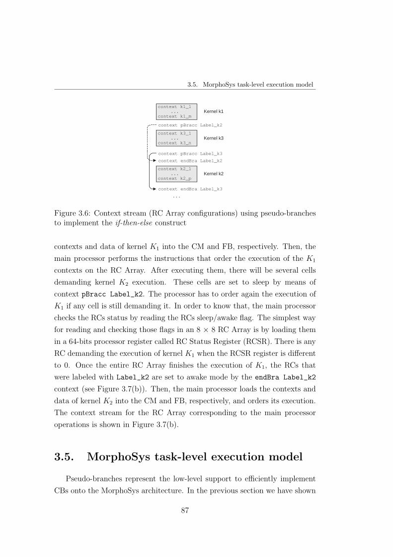
3.5. MorphoSys task-level execution model
context k1_1 ...
context k1_m
context pBracc Label_k2
Kernel k1
context k3_1 ...
context k3_n
context pBracc Label_k3
context endBra Label_k2
context k2_1 ...
context k2_p
context endBra Label_k3
...
Kernel k3
Kernel k2
Figure 3.6: Context stream (RC Array configurations) using pseudo-branchesto implement the if-then-else construct
contexts and data of kernel K1 into the CM and FB, respectively. Then, the
main processor performs the instructions that order the execution of the K1
contexts on the RC Array. After executing them, there will be several cells
demanding kernel K2 execution. These cells are set to sleep by means of
context pBracc Label_k2. The processor has to order again the execution of
K1 if any cell is still demanding it. In order to know that, the main processor
checks the RCs status by reading the RCs sleep/awake flag. The simplest way
for reading and checking those flags in an 8 × 8 RC Array is by loading them
in a 64-bits processor register called RC Status Register (RCSR). There is any
RC demanding the execution of kernel K1 when the RCSR register is different
to 0. Once the entire RC Array finishes the execution of K1, the RCs that
were labeled with Label_k2 are set to awake mode by the endBra Label_k2
context (see Figure 3.7(b)). Then, the main processor loads the contexts and
data of kernel K2 into the CM and FB, respectively, and orders its execution.
The context stream for the RC Array corresponding to the main processor
operations is shown in Figure 3.7(b).
3.5. MorphoSys task-level execution model
Pseudo-branches represent the low-level support to efficiently implement
CBs onto the MorphoSys architecture. In the previous section we have shown
87

Chapter 3. Application modeling and compilation framework
k1_loop: load k1 configurations in CM load k1 data in FB execute context k1_1 // ... // k1 contexts execute context k1_m //
execute context pBracc Label_k2
// Check RCs status if (r_stat != 0) then jump to k1_loop
execute context endBra Label_k2
k2_begin: load k2 configurations in CM load k2 data in FB execute context k2_1 // ... // k2 contexts execute context k2_p // ...
(a)
context k1_1 ... context k1_m
context pBracc Label_k2
// The decision to execute the // following contexts is made // by the main processor in // this point
context endBra Label_k2
context k2_1 ... context k2_p
...
Kernel k1
Kernel k2
(b)
Figure 3.7: Pseudo-code instruction flow for main processor and the corre-sponding context stream to implement the iterative construct
how the pseudo-branches operate within the context stream issued by the main
processor. Individual RCs decide either participating in a computation or ab-
staining from it according to their current status, defined by the previously
issued pseudo-branch contexts. In this section we complement the previous
approach by considering the data and context transfers associated to the exe-
cution of a sequence of kernels. Our purpose is to explain how the applications
are executed onto the MorphoSys architecture, starting from a CDFG defini-
tion for them. We describe the MorphoSys execution model at a task-level
granularity, complementing the MorhoSys operation flow described in Sec-
tion 2.5. Prior to illustrate the MorphoSys execution model, it is important
to remind the main operation features of our target architecture:
⋆ The RC Array follows the SIMD model of computation.
⋆ While input data and contexts are not available in the on-chip memories,
the RC Array can not start to execute the corresponding task.
⋆ MorphoSys supports single-cycle dynamic reconfiguration (without in-
terruption of RC Array execution).
88

3.5. MorphoSys task-level execution model
⋆ The CM is divided into two sets (column-CM and row-CM) which are
indistinctly used. During the time when the application is configured
through column-contexts, we can access the row-contexts, and vice versa.
⋆ The FB is organized into two sets. Using these two sets alternatively, the
computation of the RC Array can overlap the load and store operations
of the FB.
⋆ The DMA controller can not handle simultaneous transfers of data and
contexts.
We describe the MorphoSys execution model by means of a time diagram
(Figure 3.8(b)), which corresponds to the time spent in context and data
transfers to the CM and the FB, respectively, as well as in kernel computation,
for the application shown in Figure 3.8(a).
K 1
K 2
K 3
K 4 K 5
N
(a)
CM
FB(0)
FB(1)
RC Array K 1 j K 2
j
r 5 j-1 d 3
j
c 3 j
r 1 j r 2
j
c 4 j
K 4 j
d 4 j
K 3 j
r 3 j d 5
j
c 5 j
K 5 j
r 4 j d 1
j d 2 j
c 1 j+1
kc 2 kc 3 kc 4 kc 5
c 2 j+1
time
X i j : Variable X of kernel i , iteration j
K : Kernel computation time kc : Time available to overlap context transfer and computation c : Context transfer time d, r : data and results transfers time
Computations stalls
No transfers
(b)
Figure 3.8: Application’s CDFG and the corresponding execution model ontothe MorphoSys architecture
Figure 3.8(b) represents the jth iteration of the outer loop, then superscript
j refers to the jth iteration. The computation of the kernels can be overlapped
89

Chapter 3. Application modeling and compilation framework
with data and contexts transfers of the current, previous, or next kernel it-
erations. Then, for example, kernels K1 and K2 operate over data stored in
the FB set 0. While kernels K1 and K2 are consecutively executed on the RC
Array, the results of K5 from the previous iteration (rj−15 ), and the input data
of K3 for the current iteration (dj3) are transferred between the main memory
and the FB set 1. K3 execution can not be started until its corresponding
contexts, c3, are loaded into the CM, producing a computation stall of the RC
Array. K4 execution only starts once its input data reside in the FB set 1,
despite that its contexts were available before. In the case of a kernel requiring
data from both FB sets, as can occur for kernel K4, data residing in one FB
set must be transferred to the FB set on which K4 will operate. With respect
to the data coming from main memory, it is possible to perform replicated
loading into the FB sets in order to satisfy data dependencies. In all cases,
the MorphoSys task-level execution model takes into account the total time
spent in data and results transfers, including both the potential moving of data
between FB sets, and the replicated loading of input data from main memory.
Contexts loading can overlap with kernel computation during the intervals
kc, in which the RC Array does not access the CM. Actually, this interval is
not continuous but it is represented in this way to simplify the figure. The kc
time interval is the sum of the time available in one CM set (row or column)
while the other is being accessed, and the time spent by the main processor in
general purpose operations. It is important to remind that data and contexts
transfers can be overlapped with computations, but simultaneous transfers of
data and contexts are not supported by the architecture.
It is important to notice that kernels K1 and K2 are consecutively executed
on the RC Array and they operate over data stored in the same FB set. This
means that we can compute those kernels as a set, since we can transfer their
data and contexts jointly. Moreover, while data is being transferred from main
memory to the FB set, the RC Array cannot access this FB set until all data
are transferred. So, the execution of kernels K1 and K2 cannot be started
until all their data are transferred. In this case, kernels K1 and K2 make a
cluster. A cluster is defined as a set of kernels which its consecutive execution
is assigned to the same FB set. The concept of partitioning an application into
90
3.6. Contexts and data transfers overhead associated to a conditional branch
kernels that are then grouped into clusters is used in previous task scheduling
proposals [MKF+01]. Kernels are grouped in clusters in such a way that the
data reuse and the overlapping of context and data with computation are
maximized. This allows to obtain groups of kernels that can be scheduled
independently of the rest of the application, achieving the minimum execution
time once the context and data transfers are scheduled. The concept of cluster
is discussed in detail in the next chapter because it is the core of our kernel
scheduling proposal.
Although in Figure 3.8 the sequence of kernels to be executed is well-
known, the total execution time can be larger than the kernel computation
time because of data and configuration transfers latency. This is because of
the contraints imposed by the architecture and the characteristics of the target
applications. Optimal scheduling of data and configurations transfers is even
more critical when the next kernel to be executed is unknown in advance, as
occurs in the applications we are considering. In the next section, we explain
the execution overhead associated to the data and configuration transfers.
3.6. Contexts and data transfers overhead
associated to a CB
For a sequence of kernels it is necessary to schedule the context and data
transfers. This is a critical issue when we try to execute dynamic applications
because of the uncertainty about the next kernel (contexts) to execute, and
the input data it requires. In this thesis we propose solutions for this problem.
These solutions are described in detail in the next chapter but in this section
we give an introduction to the problem.
While data and contexts of a kernel are not available in the on-chip memo-
ries, the RC Array can not start to execute it, resulting in a computation stall.
The possibility of overlapping data and contexts transfers with computations
can be used to load data and contexts required by the next kernel in advance.
This is possible thanks to the FB organization. By using the two FB sets
alternatively, the computation of the RC Array can overlap the load and store
91

Chapter 3. Application modeling and compilation framework
operations of the FB. The problem is that the next kernel to be executed is
just known after testing the CB.
An important performance gain could be obtained by preloading the cor-
rect data and contexts before they are required. Rather than wait the CB
instruction testing to define the next kernel to be processed, speculative load-
ing of data and contexts can help to reduce the performance penalization
because of computation stalls. This speculative loading must be timely, use-
ful, and introduce little overhead. Some clues about the program flow of the
application can be obtained by subjecting it to an exhaustive profiling. CBs
behavior can be characterized by observing and recording the execution of the
application under a wide range of runtime scenarios. Application’s profile can
help to identify the most feasible branch destinations under certain conditions
and guide the speculative loading of data and contexts. Our purpose is to
initially execute the application using an estimation of the configurations and
data required after a CB in order to loaded in advance. This estimation is
given by the application’s profiling results. As the execution of the applica-
tion evolves, the CB behavior can change (remember that the CB models input
data dependencies or user activity), and so different configurations and data
would be required. A runtime monitor will be provided in order to adapt the
configurations and data preloading to the evolving runtime conditions. These
solutions make part of our compilation framework and are described in detail
in chapters 4 and 5. In the next section we introduce the complete compilation
framework, highlighting the different static and dynamic schedulig techniques
we propose.
3.7. Compilation framework
This thesis is about the scheduling of dynamic applications onto a coarse-
grained multicontext reconfigurable architecture. The MorphoSys reconfig-
urable system is used as target architecture. This work is focused on the off-
line and the dynamic scheduling stages of the MorphoSys compilation frame-
work. Previous efforts were only focused on static applications mapping, with-
out taking into consideration the conditional execution of tasks. As we have
92

3.7. Compilation framework
demonstrated along this chapter, SIMD reconfigurable architectures can han-
dle conditional branches. Therefore, new scheduling techniques to deal with
the dynamic applications characteristics can be proposed. We follow that pur-
pose. The scheduling techniques we propose are focused on decreasing the
number of cycles required to complete the application, and are described in
Chapters 4 and 5. Our scheduling proposals have been conceived to be inte-
grated within the complete MorphoSys compilation framework, wich defines
the input information and the goals of every stage. In fact, our scheduling
algorithms helps to generalize the static compilation framework previously
developed [MKF+01], by providing effective support to map dynamic appli-
cations. In this section we present an overall description of this compilation
framework.
Context Set 3 Context Set 2
Context Set 1
Data Set 3 Data Set 2
DataSet 1
Application kernel description
Kernel library
Static Scheduling
Kernel information extractor
Application profiling
Application clustering
Data and context scheduling
Testbench library
Task scheduling
SIMD execution
Runtime monitor
Load
Runtime monitor
Adjust
DCS
DDS
DCS : Dynamic Context Scheduling DDS : Dynamic Data Scheduling
...
...
Dynamic Scheduling
Figure 3.9: Compilation framework
3.7.1. Application kernel description
An overview of the compilation framework is shown in Figure 3.9. It is
a library-based approach. The application description is provided in C code,
and it is written in terms of kernels. Remember that a kernel represents a
93

Chapter 3. Application modeling and compilation framework
coarse-grained computation, e.g. DCT, IDCT, and that applications are mod-
eled as a sequence of interrelated kernels by means of a CDFG which models
the dynamic behavior of the application by including conditional branches.
The Kernel Library stores the code that specifies not only the functionality of
each kernel, but also their mapping onto the reconfigurable units. This map-
ping was initially performed by hand (refer to [Sin00] for some examples), and
later automated [VNK+03], making the MorphoSys architecture available to
the application programmer. This approach enables the reuse of kernels (for
example, DCT kernel is widely used in the field of audio and video processing),
and the design modularity. In this way, the application development cycle is
reduced. In fact, the design process can be translated to a graphical environ-
ment in which the applications are described my means of kernels linked each
other according to their data and control dependencies. Additionally, global
optimizations may be exploited more easily at the kernel level.
3.7.2. Kernel information extractor
The first stage of the compilation framework consists of extracting the in-
formation. The Kernel Information Extractor generates from the kernels input
code and the application’s CDFG all the parameters that feed the following
stages. Information as execution time, context and input data sizes for each
kernel are extracted from the kernel library. From the application’s CDFG
representation the kernel information extractor extracts the data dependen-
cies among kernels, the number of iterations of static loops, the data reuse
among kernels, and identifies the branch instructions and the possible branch
destinations. Data reuse refers to the data that may be used by different
kernels. By keeping these data in the on-chip memory, no data reloading is
necessary. Thus, if some kernels use data that are produced by other kernel,
the former kernels reuse these data. In the case of static applications, the ker-
nel information extractor provides all the relevant information to perform a
near-optimal scheduling. However, when dynamic applications are considered,
the information provided by the kernel information extractor may be com-
plemented with some more information about the dynamic behavior of the
94
3.7. Compilation framework
applications. This information is obtained through the application profiling.
3.7.3. Application profiling
The Application Profiling observes and records the application behavior
under a wide range of runtime scenarios. Profiling is an approach for finding
profitable context and data speculation opportunities within an application.
The objective of application profiling can be accomplished in many ways with
different accuracy and difficulty. Profiling utilities consist of functions with
statistics gathering code. These utilities can gather information about mem-
ory references and branch behavior. These information is collected for a wide
range of runtime scenarios, which are stored in the Testbench Library. Appli-
cation profiling helps to know the behavior of the application under certain
dynamic conditions, going beyond the worst-case analysis. Since the appli-
cation profiling is performed at compilation time, it makes part of the Static
Scheduling stage.
Although this thesis is not focused on developing an infrastructure for ap-
plication profiling, the interested reader can refer to [Con97] for an example of
memory dependencies profiling, and to [WPS+04] for a profiling approach to
expose memory access regularities. We have developed an application profiler
for the ray-tracing application to evaluate the compilation framework, includ-
ing a large set of 3D scenarios to test the application. This profiler helps us
to identify most common branch destinations as the ray traverses the data
structure (see Figure 3.4), as well as the most probable input data for the next
iteration.
Information provided by the application profiling is combined with the ker-
nel information extractor output to feed the following stages of the compilation
framework.
3.7.4. Application clustering
The Application clustering stage refers to the partitioning of the applica-
tion into clusters, which are sequences of kernels fulfilling particular conditions.
95

Chapter 3. Application modeling and compilation framework
The term cluster was initially used in the Static Kernel Scheduler (SKS) de-
veloped by Maestre et al. [MKF+01]. The SKS performs context transfers in
advance to reduce the computation stalls. This scheduler is focused on de-
terministic applications whose execution sequences do not depend on runtime
conditions. Its purpose is to determine a linear sequence of kernels with the
minimal execution time. This is achieved by partitioning the application into
sets of kernels called clusters. A cluster is defined as a set of kernels which
consecutive execution is assigned to the same FB set. Kernels are grouped in
clusters in such a way that the data reuse and the overlapping of context and
data transfers with computation are maximized. This allows to obtain groups
of kernels that can be scheduled independently of the rest of the application,
achieving the minimum execution time once the context and data transfers are
scheduled. Obviously, results are very poor when the SKS is applied on our
target applications. The presence of CBs demands the revision of the parti-
tioning algorithm to overcome the problems related to the dynamic program
flow.
3.7.5. Task scheduling
The Task Scheduling process consists of the cluster serialization and is
performed after the application clustering. The task scheduler explores the
design space to find a sequence of clusters that minimizes the overall execu-
tion time. Although each application imposes some constraints in the program
flow, and considering the presence of CBs, there may be a lot of valid cluster
sequences with different execution times. This design space is explored by the
task scheduler in order to find the cluster sequences with the minimum time
penalty. Task scheduling is guided by the following three criteria to reduce
the execution time: (1) Minimization of context reloading; (2) Maximiza-
tion of data reuse; and (3) Maximization of the overlapping of computation
with data/context transfers. Previous goals look for the reduction of mem-
ory latency since the data and context transfers are mainly performed during
computation, allowing a reduction of the execution stalls because of the CBs.
Task scheduling is performed at compilation time. So, many different clusters
96
3.7. Compilation framework
sequences can be evaluated in order to collect a set of solutions having differ-
ent execution times. This set of solutions serves to select an initial solution
and helps to adapt the execution of the application for different performance
constraints, by selecting a specific cluster sequence from this set of solutions
according to the runtime conditions.
In summary, the task scheduling looks for the sequence of clusters with the
minimum time penalty represented by computation stalls. The computation
stalls during the execution of a cluster are related to the operations that cannot
be overlapped with kernel computations, i.e. the non-overlapped transfers of
context and data. Once the sequence of kernels with the minimum execution
time is determined by the task scheduler, context and data transfers should
be completely scheduled.
3.7.6. Data and context scheduling
In the previous stage we have determined a sequence of clusters that po-
tentially has the minimum execution time. During that stage the detailed
scheduling of data and context transfers is no accurate, but it is an estimation
based on the information for each kernel. Until the data and context are not
completely scheduled, the execution time is no accurate. The goal of the Data
and Context Scheduling stage is to define when to perform the data and con-
text transfers, and on which bank of the FB or CM, respectively. So, at this
stage we refer to scheduling as the process of scheduling and allocating the
data and context transfers. This scheduling is performed based on the input
data size of each kernel and on the available time to overlap data transfers with
computations. It looks for the minimization of the non-overlapped transfers
of context and data with computation. Since this work was successfully done
by Sanchez-Elez et al. [SEFHB05], we will make use of their data scheduler
and allocator, with minimal modifications.
3.7.7. Dynamic scheduling support
After and initial solution has been selected in order to guarantee certain
initial performance constraints, the sequence of clusters is translated to as-
97

Chapter 3. Application modeling and compilation framework
sembly instructions for the TinyRISC processor. This assembly code contains
accurate information about all the events scheduled in the previous stages. In
the case of static applications, this code performs data and context transfers,
as well as orders their execution, in specific times. All the memory references to
context and data are the same for each execution of the application. However,
as we have explained, this is not the case of dynamic applications, where data
dependencies and user activity make the context and data required unknown
in advance.
We have introduce Dynamic Context and Data Schedulers by means of run-
time monitors that indicate if the constraints, in terms of time and power, are
being met during the execution. If this is not the case, they can load another
possible cluster sequence, found it by the task scheduler at compilation time,
in order to reduce the execution time. We also develop a selective prefetch
policy that helps to avoid performance degradation within a power budget.
Both runtime monitors implementation are described in Chapter 5.
3.8. Conclusions
In this chapter we have described how the applications are modeled in or-
der to be mapped onto the target architecture, MorphoSys. Opposite to the
static applications, where all relevant information is well-known at compila-
tion time (and so they can be near-optimally scheduled prior to execution),
we are targeting a growing class of applications which are characterized by dy-
namic workload, data-intensive computation, and hard real-time constraints.
Static applications use to be modeled by a data dependency-based task graph,
namely a Data Flow Graph (DFG). However, this type of DFG is not enough
to efficiently model and map dynamic applications. Then, we model the dy-
namic program flow of our target applications by means of the conditional
execution of tasks. To deal with this feature, we have adopted the hybrid con-
trol and data flow graph (CDFG), since it embeds all control and sequencing
information explicitly within the same graph, in such a way that some tasks
are executed depending on the result of a previous task. In our approach, the
applications are specified at a coarse level of granularity by a CDFG which be-
98
3.8. Conclusions
sides data dependencies also represents control dependencies among a number
of functions. The presence of a conditional statement in a program flow allows
us to classify the derived conditional constructs according to the branch desti-
nation possibilities (if-then-else, and iterative constructs) in order to facilitate
their mapping. I have showed how two real highly dynamic applications (ray-
tracing and rendering) are modeled in order to be mapped onto MorphoSys.
It is well-known that in SIMD reconfigurable architectures all processing
elements must execute the same configuration at time, i.e. the same kernel,
over independent subsets of input data. However, in the presence of a CB, it is
highly probable that several RCs inside the RC Array demand the execution
of different kernels. Since our purpose is to minimize the number of cycles
required to complete the application, it is necessary to define a methodology
in order to determine how to proceed when different program paths appear
inside the RC Array after evaluating a CB. Moreover, this decision should be
preferably taken without main processor action, because in other case the pro-
cessor has to check the 64 RC branch destinations, surely increasing the time
penalty. Having this goal in mind, we have provided some operation autonomy
to the individual RCs, in order to relieve as much as possible the main pro-
cessor of the burden represented by the evaluation of the branch destination
of each RC. A new set of contexts called pseudo-branches were introduced,
which are supported by an extra hardware added to the RC architecture. The
pseudo-branches give to the RCs the capability to participate in a computation
step or abstain from it based on a local condition, eliminating the centralized
control initally performed by the Tiny RISC processor. The pseudo-branches
enable it to conditionally nullify blocks of code, independent of the instruc-
tions inside that block of code. In this way, the TinyRISC is relieved from
the burden represented by the evaluation of the branch target for each RC,
because the branches are emulated by the individual RCs. I have shown how
the pseudo-branches are used in order to map onto the target architecture the
two conditional construct (if-then-else, and iterative constructs).
We have explained how the applications are executed onto the Morpho-
Sys architecture starting from a CDFG definition for them. The MorphoSys
task-level execution model helps to introduce the problem of data and context
99
Chapter 3. Application modeling and compilation framework
transfers, since the total execution time can be larger than the kernel computa-
tion time because of data and configuration transfers latency. This is because
of the contraints imposed by the architecture and the characteristics of the
target applications. Optimal scheduling of data and configurations transfers is
even more critical when the next kernel to be executed is unknown in advance,
as occurs in the applications we are considering.
To explain how we face this set of problems, we have described the ex-
tended MorphoSys compilation framework. Previous efforts were only focused
on static applications mapping. Therefore, new scheduling techniques that
can handle the dynamic applications characteristics are proposed. They all
are focused on decreasing the number of cycles required to complete the ap-
plication. In fact, the proposed scheduling algorithms help to generalize the
static compilation framework previously developed in [MKF+01], by providing
effective support to map dynamic applications. This work is focused on the off-
line and dynamic scheduling stages of the MorphoSys compilation framework.
The main contributions lie on the application description in order to support
the mapping of dynamic applications, as well as on the application clustering,
and static and dynamic context and data scheduling stages. In this chapter,
we have presented an overall description of this compilation framework. The
underlying algorithms are explained in the next two chapters.
100

Chapter 4
Compile-time Scheduling
Approach
According to the compilation framework described in the previous chapter,
any application to be mapped is described in C code and modeled as a sequence
of interrelated kernels by means of a Control Data Flow Graph (CDFG). The
CDFG models the dynamic behavior of the application by including condi-
tional branches (CBs). The kernel information extractor generates from the
kernels input code and the application’s CDFG all the parameters that feed the
following stages. The information provided by the kernel information extractor
is complemented with some more information about the dynamic behavior of
the application. This information is obtained after subjecting the application
to an exhaustive profiling. Once all this information is gathered, the schedul-
ing process is performed. The first step in the scheduling process consists of an
off-line scheduling approach. It starts by partitioning the application into clus-
ters, and then performing the cluster serialization. This cluster serialization
generates a sequence of clusters which is initially executed, and then refined at
runtime by the dynamic scheduling support. In this chapter we described the
main issues and challenges of cluster partitioning and serialization because of
the presence of CBs modeling the dynamic behavior of the target applications.
101
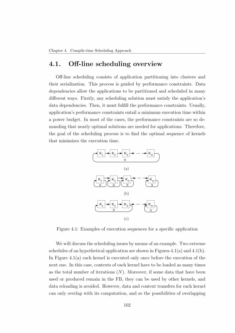
Chapter 4. Compile-time Scheduling Approach
4.1. Off-line scheduling overview
Off-line scheduling consists of application partitioning into clusters and
their serialization. This process is guided by performance constraints. Data
dependencies allow the applications to be partitioned and scheduled in many
different ways. Firstly, any scheduling solution must satisfy the application’s
data dependencies. Then, it must fulfill the performance constraints. Usually,
application’s performance constraints entail a minimum execution time within
a power budget. In most of the cases, the performance constraints are so de-
manding that nearly optimal solutions are needed for applications. Therefore,
the goal of the scheduling process is to find the optimal sequence of kernels
that minimizes the execution time.
K 1 K 2 K 3 K m
N
(a)
K 1 K 2 K 3 K m
N N N N
(b)
K 1 K 2 K 3 K m
N N
(c)
Figure 4.1: Examples of execution sequences for a specific application
We will discuss the scheduling issues by means of an example. Two extreme
schedules of an hypothetical application are shown in Figures 4.1(a) and 4.1(b).
In Figure 4.1(a) each kernel is executed only once before the execution of the
next one. In this case, contexts of each kernel have to be loaded as many times
as the total number of iterations (N). Moreover, if some data that have been
used or produced remain in the FB, they can be used by other kernels, and
data reloading is avoided. However, data and context transfers for each kernel
can only overlap with its computation, and so the possibilities of overlapping
102

4.1. Off-line scheduling overview
are minimal. In Figure 4.1(b) each kernel is executed N times before executing
the next one. In this case, contexts of each kernel have to be loaded only once.
However, as the size of data produced and used by a kernel is likely to exceed
the internal memory size, data reuse may be low. Furthermore, data transfers
for a kernel can potentially overlap with computation of any other kernel,
and so possibilities of overlapping are maximal. Optimal scheduling solution
remains between these two extreme alternatives. Intermediate solutions (see
Figure 4.1(c)) can be obtained, if the application is partitioned into set of
kernels that can be scheduled independently of the rest of the application. We
refer to one of these set of kernels as a cluster. It is clear that the scheduling
process is guided by the following three optimization criteria:
1. Minimization of context reloading.
2. Maximization of data reuse.
3. Maximization of the overlapping of computation with data and context
transfers.
The scheduling of kernels within a partition goes beyond the simple kernel
ordering. In architectures with multiple memory sets such as MorphoSys, the
scheduling of kernels can be viewed as an assigment of computations to these
memory sets. The assigments influence the reuse of data among kernels, as
well as the possible overlapping of computation and data transfers. As was
explained in Section 3.5, two kernels operating over different FB sets cannot
reuse data, whereas they can overlap the computations for one of them with
data transfers for the other one. We use the term cluster to designate a
group of kernels that are consecutively executed and assigned to the same
FB set. Furthermore, clusters can be scheduled independently of the rest of
the application, achieving the minimum execution time once the context and
data transfers are scheduled. So, scheduling is highly influenced by cluster
generation.
103
Chapter 4. Compile-time Scheduling Approach
4.2. Application clustering
The optimization criteria described in the previous section are conflicting
because of the execution model constrains explained in Section 3.5. Therefore,
it is necessary to perform an exhaustive search in order to find the optimal
solution, which would imply generation of all possible partitions, and then
scheduling of every cluster of the partition. It is obvious that this approach
will not be efficient. Based on the characteristics of our target applications
and on how we model them, we impose some constraints in the partitioning
process in order to make it affordable. This is done by pruning the search
space in such a way that is not necessary to schedule all possible partitions.
Only the quality of a few selected partition candidates is estimated.
In [MKF+01], Maestre et al. presented a Static Kernel Scheduler (SKS)
that performs cluster generation to reduce computation stalls. This scheduler
is focused on deterministic applications whose program flows do not depend
on runtime conditions. Obviously, results are very poor when this SKS is
applied on our target applications. Although static scheduling solution could
be applied on dynamic applications under certain conditions, it is based on
a typical execution scenario (the worst case scenario, mainly), reducing the
possibilities of optimization. Also, it cannot be dynamically adapted to satisfy
the performance constraints. The presence of CBs in the model of our target
applications demands a new partitioning algorithm to overcome the problems
related to dynamic program flows. We have conceived this new partitioning
algorithm, by redefining the cluster generation concept and developing a new
exploration algorithm.
4.2.1. Exploration algorithm
We will discuss the cluster generation issues by means of the examples in-
cluded in Figure 4.2. Figures 4.2(a) and 4.2(b) show two applications. Given
an application, described by means of a CDFG, it can be partitioned in many
different ways. One of the desirable properties of the exploration algorithm
is the potential generation of any possible solution. It ensures that the opti-
mal solution can always be found. Hence, we propose a recursive algorithm
104

4.2. Application clustering
with backtracking. The partitioning process starts with the whole application
which is the initial solution. Partitioning of this initial solution will allow all
possible partitions (clusters) to be visited. According to the existing cluster
definition, the presence of CBs inside a partition could create inconsistencies.
For example, a partition including a CB implies that sometimes (depending on
the branch destination) not all the kernels forming the partition are executed.
K 1 K 2
K 3 K 4
CB
K 5
K 6
1 2
3 4
5 2
2
Application 1
(a)
K 1 K 2 K 3 K 4 CB K 5 K 6
1
2 3
4
4 5
4
Application 2
(b)
K 1 K 2
K 3 K 4
CB
K 5
K 6
5
(c)
K 1 K 2 K 3 K 4 CB K 5 K 6
4
4 1
2 4
(d)
K 1 K 2
K 3 K 4
CB
K 5
K 6
5
2
2
2
(e)
K 1 K 2 K 3 K 4 CB K 5 K 6
1
3
(f)
Figure 4.2: Two dynamic applications and some examples of their partitioninginto clusters
The exploration procedure is implemented as follows:
⋆ Each edge of the CDFG is numbered in ascending order according to
the amount of data reuse between the kernels linked by that edge. If
data reuse is the same for several edges, any order is valid, but numbers
are not repeated. Edges coming to, and emerging from, a CB share the
same number. Application’s numbered CDFG represents the root node
of the exploration tree. Figures 4.2(a) and 4.2(b) show two applications’
numbered CDFGs. Figure 4.3 shows the exploration tree for the appli-
cation shown in Figure 4.2(a). The root node P1 represents the whole
105

Chapter 4. Compile-time Scheduling Approach
application corresponding to the initial partitioning solution.
⋆ Then, edges are removed in ascending order to create possible clusters.
New child-nodes are created as different edges are removed. The proce-
dure continues removing edges to create new child-nodes from the previ-
ous one. Edge removing is performed in ascending order but not strictly
in a consecutive way. The only constraint is that at a given node of the
exploration tree, edge i can not be removed if previously any edge j such
as j > i has been removed. Thus, we ensure that there is not any child-
node containing the same partition. For instance, in Figure 4.2(c) edges
1, 2, 3 and 4 were consecutively removed. This partition corresponds to
the node P5 of the exploration tree shown in Figure 4.3. Note that if the
exploration tree is visited from the top to any leaf (refer to Figure 4.3),
it is not possible to find a descending edge sequence. This fact guar-
antees that each solution is generated only once. This process results
in the formation of groups of kernels that have no joining edges. Each
separated group of kernels forms a potential cluster which feasibility has
to be checked, as it is explained below.
P 3
P 2
P 1
P 7 P 4 P 9
P 5 P 6 P 8
...
1
2
3
4
4 5
5 5
2 Removed edges
P 13 P 10 P 15
P 11
P 12
4
5
P 14
5
4 5 3
Figure 4.3: Example of exploration tree
106

4.2. Application clustering
4.2.2. Cluster feasibility
Not all the partitions found by the exploration algorithm are candidates
to be scheduled. A feasibility checking is performed in order to prune the
search space even more. This feasibility checking refers to data dependencies
fulfillment and to CBs handling, and it is based on the following constraints:
⋆ Data dependencies must be fulfilled within a cluster and among clusters
in such a way that the cluster can be handled independently of the
rest of the application. For instance, Figure 4.2(c) represents a feasible
partition although the cluster formed by K5 and K6 needs the results
of another cluster, that one formed by K4, because there is at least one
cluster serialization fulfilling those data dependencies. In Figure 4.2(e)
edges 1, 3 and 4 were consecutively removed, creating a non-feasible
partition because the execution of the cluster formed by K4 needs the
results produced by the cluster formed by kernels K2, K3, K5 and K6,
but at the same time, the later cluster requires the results of the cluster
formed by K4. Then, data dependencies are not fulfilled, and this is a
non-feasible partition. This partition corresponds to the node P11 of the
exploration tree shown in Figure 4.3.
⋆ When a partition includes a CB, we can guarantee that this partition
is feasible only if both branch destinations belong to the same cluster
in which the branch condition is tested. This constraint also looks for
data dependencies fulfilling. For example, Figure 4.2(d) represents a
non-feasible partition since the CB, which is in the middle of a cluster,
has as possible destinations K3 and K5, and K3 does not make part of
the cluster formed by K4 and K5. In addition, when the branch is taken,
cluster formed by K4 and K5 is not completely executed because the
execution of a kernel belonging to other cluster is required.
⋆ A kernel, which is a branch destination, can be in any cluster when all
the kernels belonging to that cluster are executed after the branch follows
that thread. For example, Figure 4.2(d) shows a non-feasible partition
since from the subset {K1, K2, K3} only K3 is demanded for execution
107

Chapter 4. Compile-time Scheduling Approach
after the branch is taken; and Figure 4.2(f) shows a feasible one since
either of the whole subsets {K3, K4} or {K5} is executed after the CB.
The last two conditions ensure that never more than the required data and
configurations are transferred to the on-chip memories of the reconfigurable
system.
4.2.3. Cluster bounding check
The goal of partitioning process is to find a set of clusters whose input data
and results size fit in one set of the internal memory (FB). When the data and
results of one cluster fit in the FB, further partitioning of that cluster does
not improve the execution time, as Maestre demonstrates in [MKF+01]. For
example, the subset {K5, K6} in Figure 4.2(c) could eventually be further par-
titioned, but the exploration tree shown in Figure 4.3 shows that this partition
(P5) is a leaf node, and it is not further partitioned. This is because the input
data and results of the subset {K5, K6} fit in one set of the FB.
Once the application has been partitioned, clusters must be ordered for ex-
ecution. This must be done satisfying the data dependencies as it is explained
below.
4.3. Cluster scheduling
Cluster scheduling makes part of the task scheduling stage of the compila-
tion framework. It consists of the cluster serialization and is performed after
the application clustering. This process is still guided for the three criteria ex-
plained in Section 4.1. Those criteria look for the reduction of memory traffic
since their purpose is to mainly perform data, results and context transfers
during computation.
Clusters are joined by an edge if there is a data and/or control dependency
between them. Edges directly linking clusters represent data dependencies,
and edges linking clusters through a CB represent control dependencies. Our
purpose is to define a cluster sequence in such a way that the execution stalls
because of data and context unavailability produced by the CBs are minimized.
108

4.3. Cluster scheduling
As was explained in Section 3.5, the execution model of the architecture
imposes the following constraints that must be taken into account to perform
the cluster scheduling:
1. Only one kernel can be executed at a time.
2. Input data and contexts should be loaded before cluster execution.
3. Results are written-back after cluster execution.
4. Data movements can be overlapped with computations when they are
performed in different FB sets.
5. Context loading over row/columns can be overlapped with computations
over column/rows.
6. Simultaneous transfers of context and data are not allowed.
It is clear that at least a configuration plane of its context set should reside
in the CM before to start the execution of a cluster. In the case of the input
data of a cluster, they must be loaded into on-chip memory before its execution
starts. Note that the bounding check of the application clustering algorithm
refers to the size of a FB set. That bounding check forces the input data of a
cluster to always fit into a FB set. Since overlapping can be exploited when
computations and data transfers are performed in different FB sets, this can
be achieved by forcing the execution of consecutive clusters over different FB
sets.
In summary, cluster scheduling looks for the sequence of clusters with min-
imum time penalty represented by computation stalls. Computation stalls
during the execution of a cluster are related to those operations that cannot
be overlapped with kernel computations, i.e. non-overlapped transfers of data,
results and contexts. Therefore, cluster scheduling purpose is to firstly quan-
tify those non-overlapped transfers in terms of time. This is done as follows:
109
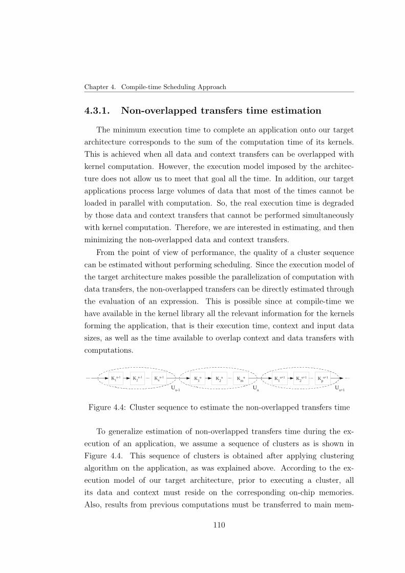
Chapter 4. Compile-time Scheduling Approach
4.3.1. Non-overlapped transfers time estimation
The minimum execution time to complete an application onto our target
architecture corresponds to the sum of the computation time of its kernels.
This is achieved when all data and context transfers can be overlapped with
kernel computation. However, the execution model imposed by the architec-
ture does not allow us to meet that goal all the time. In addition, our target
applications process large volumes of data that most of the times cannot be
loaded in parallel with computation. So, the real execution time is degraded
by those data and context transfers that cannot be performed simultaneously
with kernel computation. Therefore, we are interested in estimating, and then
minimizing the non-overlapped data and context transfers.
From the point of view of performance, the quality of a cluster sequence
can be estimated without performing scheduling. Since the execution model of
the target architecture makes possible the parallelization of computation with
data transfers, the non-overlapped transfers can be directly estimated through
the evaluation of an expression. This is possible since at compile-time we
have available in the kernel library all the relevant information for the kernels
forming the application, that is their execution time, context and input data
sizes, as well as the time available to overlap context and data transfers with
computations.
K 1 u-1 K 2
u-1 K n u-1
U u-1
K 1 u K 2
u K m u
U u
K 1 u+1 K 2
u+1 K p u+1
U u+1
Figure 4.4: Cluster sequence to estimate the non-overlapped transfers time
To generalize estimation of non-overlapped transfers time during the ex-
ecution of an application, we assume a sequence of clusters as is shown in
Figure 4.4. This sequence of clusters is obtained after applying clustering
algorithm on the application, as was explained above. According to the ex-
ecution model of our target architecture, prior to executing a cluster, all
its data and context must reside on the corresponding on-chip memories.
Also, results from previous computations must be transferred to main mem-
110

4.3. Cluster scheduling
ory. These transfers must be performed in parallel with kernel computation
whenever possible. When not all the tranfers are overlapped with computa-
tion, those non-overlapped transfers represents the time penalty associated
to the cluster execution. Let Uu = {ku1 , . . . , ku
m} be the cluster that is being
executed; Uu−1 = {ku−11 , . . . , ku−1
n } be the cluster previously executed; and
Uu+1 = {ku+11 , . . . , ku+1
p } be the next cluster to be executed. Then, the time
of non-overlapped transfers during the execution of cluster Uu, tnon−ovlp(Uu),
produced by the non-overlapped transfers of its contexts, the input data of the
cluster Uu+1 and the results of cluster Uu−1, is calculated using (4.1), (4.2),
and (4.3).
tnon−ovlp(Uu) =∑
∀i∈u∀j∈u+1∀l∈u−1
[t(du+1j + ru−1
l ) + t(cui ) − t(ku
i )],
if∑
∀i∈u t(cui ) <
∑∀i∈u t(kcu
i )
and∑
∀i∈u t(kui ) <
∑∀i∈u
∀j∈u+1∀l∈u−1
[t(du+1j + ru−1
l ) + t(cui )]
(4.1)
tnon−ovlp(Uu) =∑
∀i∈u∀j∈u+1∀l∈u−1
[t(du+1j + ru−1
l ) + t(cui ) − t(ku
i )],
if∑
∀i∈u t(cui ) >
∑∀i∈u t(kcu
i )
and∑
∀i∈u t(kui ) <
∑∀i∈u
∀j∈u+1∀l∈u−1
[t(du+1j + ru−1
l ) + t(kcui )]
(4.2)
tnon−ovlp(Uu) =∑
∀i∈u[t(cui ) − t(kcu
i )],if
∑∀i∈u t(cu
i ) >∑
∀i∈u t(kcui )
and∑
∀i∈u t(kui ) >
∑∀i∈u
∀j∈u+1∀l∈u−1
[t(du+1j + ru−1
l ) + t(kcui )]
(4.3)
Wherein t(kui ) is the computation time of kernel ki of cluster Uu on the
RC Array; t(cui ) is the transfer time of the contexts of kernel ki of cluster Uu
from main memory to the CM; t(du+1j + ru−1
l ) is the transfer time of data of
kernel kj of cluster Uu+1, and results of kernel kl of cluster Uu−1 from/to main
memory to/from the FB; and t(kcui ) is the portion of computation time of
kernel ki of cluster Uu that can be overlapped with contexts loading. All those
quantities were introduced in the execution model of our target architecture
111

Chapter 4. Compile-time Scheduling Approach
in Section 3.5.
Contexts and data sizes as well as the execution times of kernels are known
at compile-time once the application is described by means of a CDFG at a
kernel level, and they are stored in the kernel library. Equations (4.1), (4.2),
and (4.3) describe, respectively, the following three possible cases:
1. Context loading is completely overlapped with computation, and the
non-overlapped transfers time only accounts for data and results trans-
fers, as Figure 4.5(a) depicts.
2. Contexts, data and results transfers are not completely overlapped with
computation, as Figure 4.5(b) shows.
3. Data and results transfers are completely overlapped with computation
but not context loading, as it is illustrated in Figure 4.5(c).
context loading
context overlapping
cluster computation
data and results transfers
time
(a)
context overlapping
cluster computation
data and results transfers
time
context loading
Non-overlapped transfers
(b)
context overlapping
cluster computation
data and results transfers
time
context loading
(c)
Figure 4.5: Time diagrams highlighting the non-overlapped transfers
Following next, we include a detailed description of the Equations (4.1),
(4.2), and (4.3), according to the execution model of the architecture. The
computation time of the cluster Uu is the sum of the execution time of its
kernels, and it is estimated as∑
∀i∈u t(kui ). This quantity corresponds to the
cluster computation time depicted in Figure 4.5. According to the execution
model of our target architecture, while cluster Uu is being executed, the input
data for the next cluster Uu+1 must be loaded into the on-chip memory, and
the results of the previous cluster Uu−1 must be transferred to main memory.
The time consumed by both tasks is estimated as∑
∀j∈u+1∀l∈u−1
[t(du+1j + ru−1
l )].
This quantity corresponds to the data and results transfers time illustrated
112

4.3. Cluster scheduling
in Figure 4.5. For the sake of simplicity for time estimation, and as Maestre
demonstrates in [MKF+01], we assume that while the cluster Uu is being ex-
ecuted, its contexts are loaded into the CM. The time consumed by this task
is estimated as∑
∀i∈u t(cui ). This quantity corresponds to the context loading
time depicted in Figure 4.5. The time available to overlap context loading with
kernel computation is the sum of the corresponding time windows available for
each kernel, and it is estimated to be∑
∀i∈u t(kcui ). This quantity corresponds
to the context overlapping time illustrated in Figure 4.5.
Moreover, our target applications have a highly dynamic program flow
which we model by means of CBs. The uncertainty in the program flow pro-
duced by data dependencies and user activity potentially results in a per-
formance degrading because of computation stalls associated to a CB. This
computation stalls are time consumed while context and data are loaded into
the on-chip memories when they have not been loaded in advance. Our pur-
pose is to initially define a cluster sequence with the minimum computation
stalls. This estimation is performed at compile-time but it will be refined at
runtime as it is explained in the next chapter.
As it was described in Subsection 3.2.1, CBs are classified into two different
categories, if-then-else and iterative constructs. We generalize both categories
by substituting each kernel by sequences of kernels grouped into clusters. The
cluster scheduler, which is based on the previously estimated non-overlapped
transfers time, is applied to these two generalized cluster organizations as
follows.
4.3.2. Cluster scheduling of if-then-else constructs
Each kernel from Figure 3.2(a) is substituted by a sequence of kernels
grouped into clusters resulting in the generalized if-then-else construct shown
in Figure 4.6. Our purpose is to show how the cluster scheduling is performed
for this generalized construct.
When an if-then-else construct appears, some RCs require the execution of
kernels on the then-branch whereas the remaining ones require the execution
of kernels on the else-branch. In order to process the two branches onto the
113

Chapter 4. Compile-time Scheduling Approach
K 1 if K 2
if CB K m if
K 1 then K 2
then K n then
K 1 else K 2
else K p else
U if
U then
U else
Figure 4.6: If-then-else construct generalization
SIMD architecture, they must be serialized, as it was explained in the pre-
vious chapter. Cluster scheduling performs this serialization looking for the
minimum time penalty. For the if-then-else constructs, this time penalty is
represented by the non-overlapped transfers of data and context, as it was
explained in the previous subsection.
Referring to Figure 4.6, in the if-then-else construct the execution se-
quences can be Uif → Uthen → Uelse or Uif → Uelse → Uthen. However, each
branch could be constituted by more than one cluster and then, the number
of possible execution sequences would be large. It is clear that those clusters
located in different branches do not share results. So, in order to promote the
data and results reuse among clusters, the cluster scheduling algorithm assigns
those clusters belonging to the then-branch to one FB set, while clusters of
the else-branch are assigned to the other FB set. Our goal is that while a
cluster is being executed, data and configurations for a cluster located in the
other branch are simultaneously transferred. This fact significantly reduces
the search space. This means that just the first cluster to be executed has
to be decided, and then the remaining ones are allocated taking into account
the branch they belong to, in such a way that the clusters of each branch are
alternatively executed.
The cluster scheduler is applied on if-then-else constructs (see Figure 4.6)
as follows. Let Uif = {kif1 , . . . , kif
m} be the cluster on which the condition is
evaluated; Uthen = {kthen1 , . . . , kthen
n } be the cluster executed if the condition
is true, Uelse = {kelse1 , . . . , kelse
p } be the cluster executed if the condition is
not fulfilled; TPif→then be the time penalty represented by the non-overlapped
transfers during the execution of cluster Uif when the execution of cluster
114

4.3. Cluster scheduling
Uthen is expected; and TPif→else be the time penalty represented by the non-
overlapped transfers during the execution of cluster Uif when the execution
of cluster Uelse is expected. The cluster scheduling algorithm for if-then-else
constructs is outlined in Algorithm 1.
Input: Clusters Uif , Uthen, and Uelse
Output: Scheduled cluster sequenceTPif→then = tnon−ovlp(Uif → Uthen);TPif→else = tnon−ovlp(Uif → Uelse);if TPif→then < TPif→else then
CSCH(Uif → Uthen → Uelse);endelse
CSCH(Uif → Uelse → Uthen);end
Algorithm 1: Algorithm for cluster scheduling of if-then-else constructs
Inputs of the scheduling algorithm for if-then-else constructs are clusters
linked by the CB, Uif , Uthen, and Uelse, as Figure 4.6 shows. Each possible
branch corresponds to a cluster sequence. So, the time penalty for each clus-
ter sequence is computed. Equations (4.1), (4.2), and (4.3) are used by the
cluster scheduling algorithm to estimate the terms TPif→then and TPif→else,
as tnon−ovlp(Uif → Uthen) and tnon−ovlp(Uif → Uelse), respectively, since in this
case the time penalty is because of the non-overlapped transfers of data and
contexts. By means of these time penalties, we find the sequence with the min-
imum non-overlapped transfers time. Once the cluster sequence to ultimately
map is determined, the kernels are mapped onto the architecture, by using
the function CSCH. This function takes as input the cluster sequence, and
performs context and data scheduling, according to the algorithms developed
in [MKF+01], and [SEFHB05], and as was explained in Section 3.4.
4.3.3. Cluster scheduling of iterative constructs
Each kernel from Figure 3.2(b) is substituted by a sequence of kernels
grouped into clusters resulting in the generalized iterative construct shown in
115

Chapter 4. Compile-time Scheduling Approach
Figure 4.7. Our purpose is to show how the cluster scheduling is performed
for this generalized construct.
K 1 b K 2
b K n b
U b
K 1 1 K 2
1 K m 1
U 1
CB K 1 f K 2
f K p f
U f
N
Figure 4.7: Iterative construct generalization
In Figure 4.7, the cluster U1 is the cluster on which the branch condition
is evaluated, cluster Ub is the cluster executed if the branch condition is true,
that is the target cluster when the backward branch is taken, and Uf is the
cluster executed if the branch condition is not fulfilled, that is the target cluster
when the branch is not taken. We assume that the loop body is formed by a
cluster sequence started by the cluster Ub and finished by the cluster U1, with
a determined number of clusters in between.
Considering Figure 4.7, cluster scheduling algorithm will select U1 → Ub
(the taken branch sequence) as the expected cluster sequence to map when the
time penalty for that sequence is lower than the time penalty for the sequence
U1 → Uf (the not taken branch sequence). Unlike if-then-else constructs
where the time penalty is only because of non-overlapped transfers, in iterative
constructs the time penalty also depends on an extra stall time. If the cluster
sequence to map is U1 → Ub, the time penalty is because of the non-overlapped
transfers of the sequence U1 → Ub, since they are consecutively scheduled,
and the stall time produced by data and contexts transfers when cluster Uf is
required, since these data and context transfer are only transferred on-demand.
The stall time (tstall), produced when the cluster actually executed (Uu) is
not the expected one, is estimated using (4.4). This stall time exists because
the data and contexts of the cluster Uu were not previously loaded.
tstall(Uu) =∑
∀i∈u
[t(cui ) + t(du
i )] (4.4)
Where t(cui ) is the context loading time, and t(du
i ) is the input data loading
time of kernel ki of cluster Uu. Equation (4.4) sums those quantities for the
116
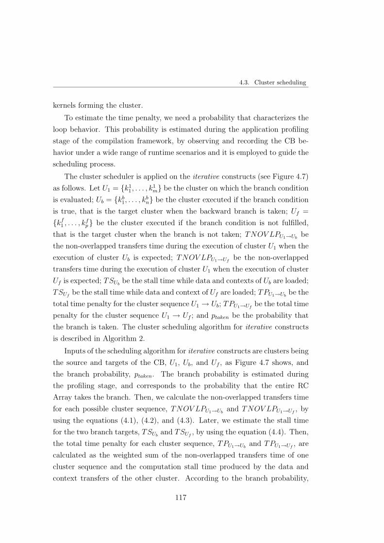
4.3. Cluster scheduling
kernels forming the cluster.
To estimate the time penalty, we need a probability that characterizes the
loop behavior. This probability is estimated during the application profiling
stage of the compilation framework, by observing and recording the CB be-
havior under a wide range of runtime scenarios and it is employed to guide the
scheduling process.
The cluster scheduler is applied on the iterative constructs (see Figure 4.7)
as follows. Let U1 = {k11, . . . , k
1m} be the cluster on which the branch condition
is evaluated; Ub = {kb1, . . . , k
bn} be the cluster executed if the branch condition
is true, that is the target cluster when the backward branch is taken; Uf =
{kf1 , . . . , kf
p} be the cluster executed if the branch condition is not fulfilled,
that is the target cluster when the branch is not taken; TNOV LPU1→Ubbe
the non-overlapped transfers time during the execution of cluster U1 when the
execution of cluster Ub is expected; TNOV LPU1→Ufbe the non-overlapped
transfers time during the execution of cluster U1 when the execution of cluster
Uf is expected; TSUbbe the stall time while data and contexts of Ub are loaded;
TSUfbe the stall time while data and context of Uf are loaded; TPU1→Ub
be the
total time penalty for the cluster sequence U1 → Ub; TPU1→Ufbe the total time
penalty for the cluster sequence U1 → Uf ; and ptaken be the probability that
the branch is taken. The cluster scheduling algorithm for iterative constructs
is described in Algorithm 2.
Inputs of the scheduling algorithm for iterative constructs are clusters being
the source and targets of the CB, U1, Ub, and Uf , as Figure 4.7 shows, and
the branch probability, ptaken. The branch probability is estimated during
the profiling stage, and corresponds to the probability that the entire RC
Array takes the branch. Then, we calculate the non-overlapped transfers time
for each possible cluster sequence, TNOV LPU1→Uband TNOV LPU1→Uf
, by
using the equations (4.1), (4.2), and (4.3). Later, we estimate the stall time
for the two branch targets, TSUband TSUf
, by using the equation (4.4). Then,
the total time penalty for each cluster sequence, TPU1→Uband TPU1→Uf
, are
calculated as the weighted sum of the non-overlapped transfers time of one
cluster sequence and the computation stall time produced by the data and
context transfers of the other cluster. According to the branch probability,
117

Chapter 4. Compile-time Scheduling Approach
Input: Clusters U1, Ub, Uf , and ptaken
Output: Scheduled cluster sequenceTNOV LPU1→Ub
= tnon−ovlp(U1 → Ub);TNOV LPU1→Uf
= tnon−ovlp(U1 → Uf );TSUb
= tstall(Ub);TSUf
= tstall(Uf );TPU1→Ub
= TNOV LPU1→Ub/ (1 − ptaken) + TSUf
;TPU1→Uf
= TNOV LPU1→Uf+ TSUb
/ (1 − ptaken);
if TPU1→Ub< TPU1→Uf
thenCSCH(U1 → Ub);
endelse
CSCH(U1 → Uf );end
Algorithm 2: Algorithm for cluster scheduling of iterative constructs
under a static scenario, the loop body is executed 1/(1 − ptaken) times per
one execution of the cluster Uf . The cluster sequence with the minimum time
penalty is selected to be mapped. Once the cluster sequence to ultimately
map is determined, the kernels are mapped onto the architecture, by using
the function CSCH. This function takes as input the cluster sequence, and
performs context and data scheduling, according to the algorithms developed
in [MKF+01], and [SEFHB05], and as was explained in Section 3.4.
4.4. Experimental results
We have applied the cluster scheduler to different synthetic experiments
(SEs), and to an interactive ray tracing application running on the MorphoSys
architecture. Our experimental framework executes applications on the target
architecture and delivers the execution and stall times. Synthetic experiments
modeling if-then-else and iterative constructs are generated within reasonable
boundaries for kernel computation time, and context, data and results trans-
fers time. Their purpose is to cover a wide range of feasible applications that
could be executed on the target architecture. Furthermore, some synthetic
experiments are more complex than typical applications to test the schedul-
118
4.4. Experimental results
ing algorithms under extreme conditions. Ray-tracing applications having an
iterative construct are real experiments that generates images from 3D scene
models.
Thirty different synthetic experiments (SE1 to SE30) having an if-then-else
construct in their CDFG are tested. All these synthetic experiments are firstly
partitioned into clusters, and then the clusters are scheduled. To test the qual-
ity of the clustering and scheduling algorithms, we have modeled the synthetic
experiments with different cluster bounding checks (see Subsection 4.2.3) in
mind. This means we have modeled the synthetic experiments targeting the
architecture with different FB sizes.
If-then-else synthetic experiments SE1 to SE10 are partitioned with a FB
set size of 16 KB as cluster bounding check, which corresponds to half of the
FB size used in the MorphoSys M2 implementation, as it was explained in
Subsection 2.3.6. Table 4.1 summarizes the results of applying the clustering
algorithm on the synthetic experiments SE1 to SE10.
In Table 4.1, second and third columns summarize the characteristics of
the cluster located before the CB, that is the cluster on which the condition
is evaluated. Second column corresponds to the number of kernels within the
cluster. Third column collects the total kernel execution time, the total context
loading time, and the total data and results transfers time for the cluster, all
of them expressed in clock cycles. Fourth and fifth columns, and sixth and
seventh columns summarize the characteristics of the then and else branches,
respectively. To make lighter the tables not all the information of the clusters
is outlined. For each branch, these columns include the number of clusters
in the branch, the average number of kernels per cluster in the branch, the
average context loading time per cluster, the average kernel execution time
per cluster, the average context loading time per cluster, and the average data
and results transfers time per cluster.
For synthetic experiments SE1 to SE10, the number of kernels of the cluster
acting as the if statement ranges from 1 to 9, and the number of clusters in
the then and else branches ranges from 1 to 6. Table 4.1 summarizes average
quantities for the clusters located in both branches. The maximum number of
kernels in a branch reaches 36 for the synthetic experiment SE5, which has 6
119

Chapter 4. Compile-time Scheduling Approach
Table 4.1: Application clustering results (if-then-else constructs) for a FB setsize of 16 KB
Before CB (IF) THEN Branch ELSE Branch
NK
P
t(ki) /P
t(ci) /P
t(di + ri)
(cc)
NC /
AKPC
AP
t(ki) /
AP
t(ci) /
AP
t(di + ri)
(cc)
NC /
AKPC
AP
t(ki) /
AP
t(ci) /
AP
t(di + ri)
(cc)
SE1 42384 / 338 /
8743 / 7
2106 / 258 /
9736 / 5
2346 / 224 /
930
SE2 82196 / 305 /
9065 / 6
1902 / 216 /
9612 / 4
1894 / 350 /
932
SE3 92060 / 184 /
9964 / 7
2094 / 239 /
9791 / 8
2196 / 305 /
906
SE4 41404 / 363 /
9906 / 5
2183 / 231 /
9073 / 5
2048 / 314 /
952
SE5 12971 / 215 /
10161 / 8
2196 / 305 /
9066 / 6
2059 / 304 /
933
SE6 51953 / 393 /
8442 / 6
2061 / 235 /
10075 / 4
2443 / 274 /
909
SE7 42384 / 338 /
8741 / 9
2060 / 184 /
9964 / 6
2073 / 208 /
1000
SE8 82196 / 305 /
9065 / 5
2135 / 234 /
9752 / 7
2146 / 241 /
897
SE9 92060 / 184 /
9963 / 3
2623 / 155 /
9445 / 4
2038 / 275 /
952
SE10 51953 / 393 /
8444 / 5
2020 / 295 /
9144 / 6
2129 / 240 /
928
NK: Number of kernels in the cluster;P
t(Ki): Total kernel execution time for thecluster;
P
t(ci): Total context loading time for the cluster;P
t(di + ri): Total dataand results transfers time for the cluster; NC: Number of clusters in the branch;AKPC: Average number of kernels per cluster in the branch; A
P
t(Ki): Averagekernel execution time per cluster; A
P
t(ci): Average context loading time per cluster;A
P
t(di + ri): Average data and results transfers time per cluster; cc: Clock cycles.
clusters in the else branch, and an average of 6 kernels per cluster.
If-then-else synthetic experiments SE11 to SE20 are partitioned with a
FB set size of 32 KB as cluster bounding check, which corresponds to the
FB size used in the MorphoSys M2 implementation. Remember that the FB
is organized into two sets of the same size (see Subsection 2.3.6). Table 4.2
summarizes the results of applying clustering algorithm on the synthetic ex-
periments SE11 to SE20.
For synthetic experiments SE11 to SE20, the number of kernels of the
cluster acting as the if statement ranges from 1 to 4, and the number of
120
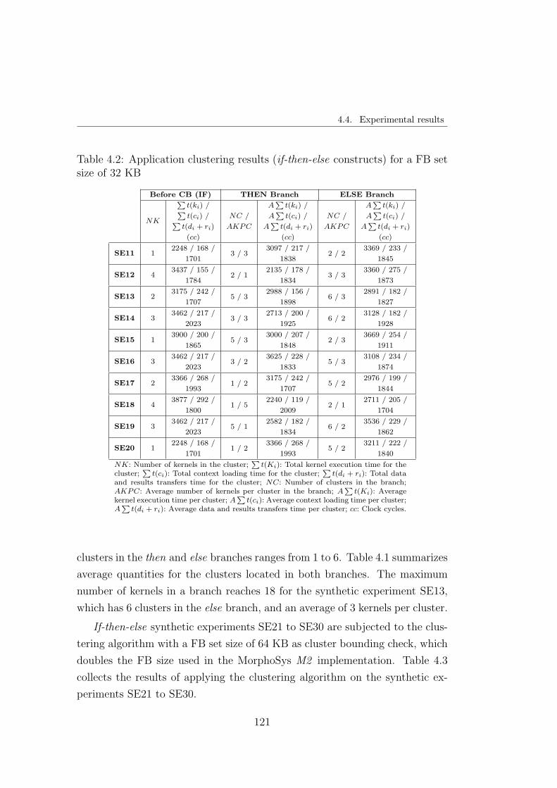
4.4. Experimental results
Table 4.2: Application clustering results (if-then-else constructs) for a FB setsize of 32 KB
Before CB (IF) THEN Branch ELSE Branch
NK
P
t(ki) /P
t(ci) /P
t(di + ri)
(cc)
NC /
AKPC
AP
t(ki) /
AP
t(ci) /
AP
t(di + ri)
(cc)
NC /
AKPC
AP
t(ki) /
AP
t(ci) /
AP
t(di + ri)
(cc)
SE11 12248 / 168 /
17013 / 3
3097 / 217 /
18382 / 2
3369 / 233 /
1845
SE12 43437 / 155 /
17842 / 1
2135 / 178 /
18343 / 3
3360 / 275 /
1873
SE13 23175 / 242 /
17075 / 3
2988 / 156 /
18986 / 3
2891 / 182 /
1827
SE14 33462 / 217 /
20233 / 3
2713 / 200 /
19256 / 2
3128 / 182 /
1928
SE15 13900 / 200 /
18655 / 3
3000 / 207 /
18482 / 3
3669 / 254 /
1911
SE16 33462 / 217 /
20233 / 2
3625 / 228 /
18335 / 3
3108 / 234 /
1874
SE17 23366 / 268 /
19931 / 2
3175 / 242 /
17075 / 2
2976 / 199 /
1844
SE18 43877 / 292 /
18001 / 5
2240 / 119 /
20092 / 1
2711 / 205 /
1704
SE19 33462 / 217 /
20235 / 1
2582 / 182 /
18346 / 2
3536 / 229 /
1862
SE20 12248 / 168 /
17011 / 2
3366 / 268 /
19935 / 2
3211 / 222 /
1840
NK: Number of kernels in the cluster;P
t(Ki): Total kernel execution time for thecluster;
P
t(ci): Total context loading time for the cluster;P
t(di + ri): Total dataand results transfers time for the cluster; NC: Number of clusters in the branch;AKPC: Average number of kernels per cluster in the branch; A
P
t(Ki): Averagekernel execution time per cluster; A
P
t(ci): Average context loading time per cluster;A
P
t(di + ri): Average data and results transfers time per cluster; cc: Clock cycles.
clusters in the then and else branches ranges from 1 to 6. Table 4.1 summarizes
average quantities for the clusters located in both branches. The maximum
number of kernels in a branch reaches 18 for the synthetic experiment SE13,
which has 6 clusters in the else branch, and an average of 3 kernels per cluster.
If-then-else synthetic experiments SE21 to SE30 are subjected to the clus-
tering algorithm with a FB set size of 64 KB as cluster bounding check, which
doubles the FB size used in the MorphoSys M2 implementation. Table 4.3
collects the results of applying the clustering algorithm on the synthetic ex-
periments SE21 to SE30.
121
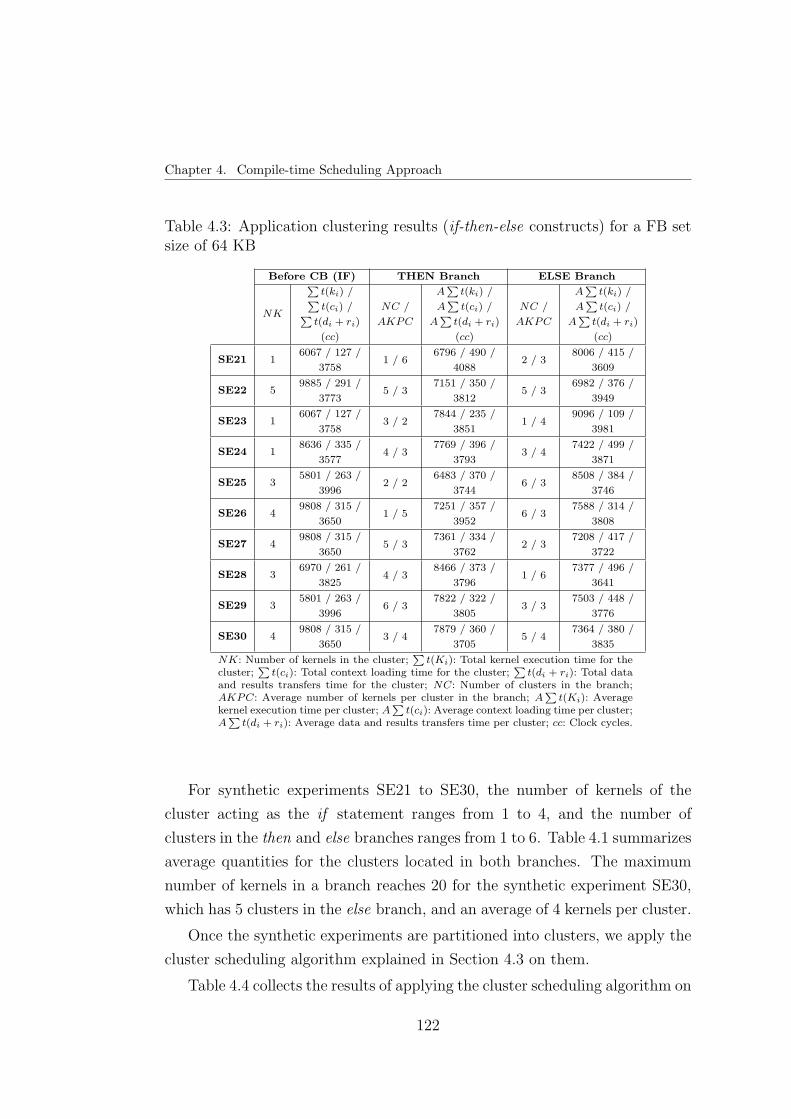
Chapter 4. Compile-time Scheduling Approach
Table 4.3: Application clustering results (if-then-else constructs) for a FB setsize of 64 KB
Before CB (IF) THEN Branch ELSE Branch
NK
P
t(ki) /P
t(ci) /P
t(di + ri)
(cc)
NC /
AKPC
AP
t(ki) /
AP
t(ci) /
AP
t(di + ri)
(cc)
NC /
AKPC
AP
t(ki) /
AP
t(ci) /
AP
t(di + ri)
(cc)
SE21 16067 / 127 /
37581 / 6
6796 / 490 /
40882 / 3
8006 / 415 /
3609
SE22 59885 / 291 /
37735 / 3
7151 / 350 /
38125 / 3
6982 / 376 /
3949
SE23 16067 / 127 /
37583 / 2
7844 / 235 /
38511 / 4
9096 / 109 /
3981
SE24 18636 / 335 /
35774 / 3
7769 / 396 /
37933 / 4
7422 / 499 /
3871
SE25 35801 / 263 /
39962 / 2
6483 / 370 /
37446 / 3
8508 / 384 /
3746
SE26 49808 / 315 /
36501 / 5
7251 / 357 /
39526 / 3
7588 / 314 /
3808
SE27 49808 / 315 /
36505 / 3
7361 / 334 /
37622 / 3
7208 / 417 /
3722
SE28 36970 / 261 /
38254 / 3
8466 / 373 /
37961 / 6
7377 / 496 /
3641
SE29 35801 / 263 /
39966 / 3
7822 / 322 /
38053 / 3
7503 / 448 /
3776
SE30 49808 / 315 /
36503 / 4
7879 / 360 /
37055 / 4
7364 / 380 /
3835
NK: Number of kernels in the cluster;P
t(Ki): Total kernel execution time for thecluster;
P
t(ci): Total context loading time for the cluster;P
t(di + ri): Total dataand results transfers time for the cluster; NC: Number of clusters in the branch;AKPC: Average number of kernels per cluster in the branch; A
P
t(Ki): Averagekernel execution time per cluster; A
P
t(ci): Average context loading time per cluster;A
P
t(di + ri): Average data and results transfers time per cluster; cc: Clock cycles.
For synthetic experiments SE21 to SE30, the number of kernels of the
cluster acting as the if statement ranges from 1 to 4, and the number of
clusters in the then and else branches ranges from 1 to 6. Table 4.1 summarizes
average quantities for the clusters located in both branches. The maximum
number of kernels in a branch reaches 20 for the synthetic experiment SE30,
which has 5 clusters in the else branch, and an average of 4 kernels per cluster.
Once the synthetic experiments are partitioned into clusters, we apply the
cluster scheduling algorithm explained in Section 4.3 on them.
Table 4.4 collects the results of applying the cluster scheduling algorithm on
122

4.4. Experimental results
the if-then-else synthetic experiments SE1 to SE10 whose cluster partitioning
results are summarized in Table 4.1.
Table 4.4: Cluster scheduling results (if-then-else constructs) for a FB set sizeof 16 KB
Scheduled Cluster Scheduler Non-Scheduled Relative Time
Branch ET (cc) ST (cc) ET (cc) ST (cc) Saving (%)
SE1 else 24459 1677 34641 11859 29.39
SE2 then 16791 1295 24977 9481 32.77
SE3 then 13614 979 19786 7151 31.19
SE4 then 22511 1864 32489 11842 30.71
SE5 else 19111 1590 27390 9869 30.23
SE6 then 19691 1398 27931 9638 29.50
SE7 then 13574 837 20002 7265 32.14
SE8 else 18322 1157 26668 9503 31.30
SE9 then 21572 1452 30729 10609 29.80
SE10 else 20046 1494 29096 10544 31.10
ET : Execution time; ST : Stall time; cc: Clock cycles
In Table 4.4, second column shows the branch which has been firstly sched-
uled, that is the branch with the minimum non-overlapped transfers. Third
and fourth columns show the execution time and the stall time once the ap-
plication is scheduled and executed using our algorithms. Fifth and sixth
columns illustrate the execution time and the stall time once the application
is executed without performing scheduling. Non-scheduled execution means
that data and contexts transfers are non-overlapped since they are performed
as they are required. Seventh column shows the relative time saving delivered
by our approach when is compared to the non-scheduled execution.
Experimental results correspond to the execution and stall times obtained
by the cluster scheduling algorithm. Execution time obtained by the cluster
scheduling algorithm is compared to a non-scheduled execution of the exper-
iments. For synthetic experiments SE1 to SE10, the average relative time
saving is 31%. Relative time savings delivered by the cluster scheduling algo-
rithm for synthetic experiments SE1 to SE10 are depicted in Figure 4.8.
Table 4.5 collects the results of applying the cluster scheduling algorithm on
the if-then-else synthetic experiments SE11 to SE20 whose cluster partitioning
results are summarized in Table 4.2.
123
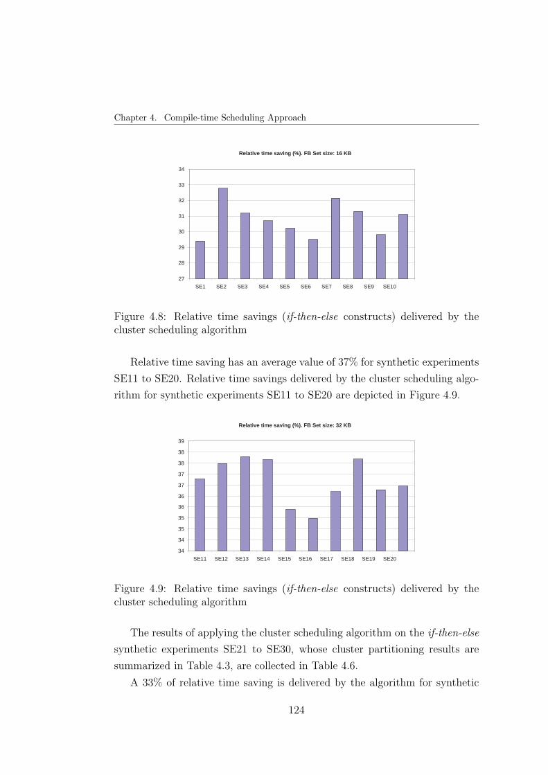
Chapter 4. Compile-time Scheduling Approach
Relative time saving (%). FB Set size: 16 KB
27
28
29
30
31
32
33
34
SE1 SE2 SE3 SE4 SE5 SE6 SE7 SE8 SE9 SE10
Figure 4.8: Relative time savings (if-then-else constructs) delivered by thecluster scheduling algorithm
Relative time saving has an average value of 37% for synthetic experiments
SE11 to SE20. Relative time savings delivered by the cluster scheduling algo-
rithm for synthetic experiments SE11 to SE20 are depicted in Figure 4.9.
Relative time saving (%). FB Set size: 32 KB
34
34
35
35
36
36
37
37
38
38
39
SE11 SE12 SE13 SE14 SE15 SE16 SE17 SE18 SE19 SE20
Figure 4.9: Relative time savings (if-then-else constructs) delivered by thecluster scheduling algorithm
The results of applying the cluster scheduling algorithm on the if-then-else
synthetic experiments SE21 to SE30, whose cluster partitioning results are
summarized in Table 4.3, are collected in Table 4.6.
A 33% of relative time saving is delivered by the algorithm for synthetic
124

4.4. Experimental results
Table 4.5: Cluster scheduling results (if-then-else constructs) for a FB set sizeof 32 KB
Scheduled Cluster Scheduler Non-Scheduled Relative Time
Branch ET (cc) ST (cc) ET (cc) ST (cc) Saving (%)
SE11 then 19311 1032 30546 12267 36.78
SE12 then 18880 1091 30200 12411 37.48
SE13 then 37254 1789 59894 24429 37.80
SE14 then 32025 1652 51361 20988 37.65
SE15 then 27648 1407 42792 16551 35.39
SE16 else 31558 1680 48544 18666 34.99
SE17 else 22623 1201 35460 14038 36.20
SE18 then 12199 659 19578 8038 37.69
SE19 else 39813 2221 62485 24893 36.28
SE20 else 23052 1379 36276 14603 36.45
ET : Execution time; ST : Stall time; cc: Clock cycles
experiments SE21 to SE30. Relative time savings delivered by the cluster
scheduling algorithm for synthetic experiments SE21 to SE30 are depicted in
Figure 4.10.
Relative time saving (%). FB Set size: 64 KB
30
30
31
31
32
32
33
33
34
34
35
SE21 SE22 SE23 SE24 SE25 SE26 SE27 SE28 SE29 SE30
Figure 4.10: Relative time savings (if-then-else constructs) delivered by thecluster scheduling algorithm
Figure 4.11 shows the relative reduction of the non-overlapped transfers
delivered by the cluster scheduling algorithm once it is applied on the if-then-
else constructs, compared to a non-scheduled execution of the experiments.
Non-overlapped transfers are reduced by the cluster scheduling algorithm an
125

Chapter 4. Compile-time Scheduling Approach
Table 4.6: Cluster scheduling results (if-then-else constructs) for a FB set sizeof 64 KB
Scheduled Cluster Scheduler Non-Scheduled Relative Time
Branch ET (cc) ST (cc) ET (cc) ST (cc) Saving (%)
SE21 then 30461 1585 45473 16597 33.01
SE22 else 83700 3146 127083 46529 34.14
SE23 else 39489 793 59111 20415 33.20
SE24 then 64866 2885 95915 33934 32.37
SE25 else 72662 2844 107228 37410 32.24
SE26 then 64759 2172 96209 33622 32.69
SE27 then 63205 2173 94054 33022 32.80
SE28 then 50288 2076 73001 24789 31.11
SE29 then 78212 2967 116658 41413 32.96
SE30 else 72849 2580 107633 37364 32.32
ET : Execution time; ST : Stall time; cc: Clock cycles
average of 81% with respect to the non-scheduled execution of the synthetic
experiments. This means that data and contexts required by the kernels are
mainly transferred in parallel with computation once the cluster scheduling
algorithm is applied.
To evaluate how the cluster scheduling algorithm works on iterative con-
structs, we initially have modeled ten more synthetic experiments (SE31 to
SE40). Then, we have applied the cluster scheduling algorithm on a set of
ray-tracing experiments, whose include iterative constructs in their CDFG
(refer to Section 3.2). All synthetic experiments are firstly partitioned into
clusters.
Iterative synthetic experiments SE31 to SE40 are partitioned with a FB
set size of 32 KB as cluster bounding check, which corresponds to the FB used
in the MorphoSys M2 implementation. These synthetic experiments are more
complex than typical applications in order to test the scheduling algorithms
under extreme conditions. Table 4.7 summarizes the results of applying the
clustering algorithm on the synthetic experiments SE31 to SE40.
In Table 4.7, second and third columns summarize the branch probability
and the number of iterations of the outer loop to complete the application,
respectively. Fourth and fifth columns, and sixth and seventh columns sum-
marize the characteristics of the taken and not-taken branches, respectively.
126

4.4. Experimental results
Non-overlapped transfers reduction (%)
76
78
80
82
84
86
88
90
92
94
96
98
SE
1 S
E2
SE
3 S
E4
SE
5 S
E6
SE
7 S
E8
SE
9 S
E10
S
E11
S
E12
S
E13
S
E14
S
E15
S
E16
S
E17
S
E18
S
E19
S
E20
S
E21
S
E22
S
E23
S
E24
S
E25
S
E26
S
E27
S
E28
S
E29
S
E30
FB Set: 16KB FB Set: 32KB FB Set: 64KB
Figure 4.11: Relative reduction of the non-overlapped transfers (if-then-elseconstructs) delivered by the cluster scheduling algorithm
To make lighter the tables not all the information of the clusters is outlined.
For each branch, these columns include the number of clusters in the branch,
the average number of kernels per cluster in the branch, the average context
loading time per cluster, the average kernel execution time per cluster, the
average context loading time per cluster, and the average data and results
transfers time per cluster.
For synthetic experiments SE31 to SE40, the branch probability models
applications having a trend to performing the branch most of the times (prob-
ability near to 1), and applications having a trend to not performing the branch
(probability just over 0). The number of application iterations is over hun-
dreds, as occurs in the case of the MPEG-2 encoder [Mae00]. The number of
clusters in the taken branch ranges from 2 to 10.
Once the synthetic experiments are partitioned into clusters, we apply the
cluster scheduling algorithm explained in Section 4.3 on them.
Table 4.8 summarizes the results of applying the cluster scheduling algo-
rithm on the synthetic experiments SE31 to SE40 whose cluster partitioning
127

Chapter 4. Compile-time Scheduling Approach
Table 4.7: Application clustering results (iterative constructs) for a FB setsize of 32 KB
TAKEN branch NOT-TAKEN branch
ptaken
Application
iterations
NC /
AKPC
AP
t(ki) /
AP
t(ci) /
AP
t(di + ri)
(cc)
NC /
AKPC
AP
t(ki) /
AP
t(ci) /
AP
t(di + ri)
(cc)
SE31 0.5 821 5 / 22945 / 227 /
18121 / 1
2706 / 97 /
1844
SE32 0.3 728 7 / 22927 / 180 /
18711 / 2
3366 / 268 /
1993
SE33 0.4 783 3 / 23304 / 236 /
17991 / 3
3462 / 217 /
2023
SE34 0.1 371 10 / 23091 / 206 /
18601 / 4
3877 / 292 /
1800
SE35 0.7 699 2 / 13074 / 184 /
17831 / 1
3900 / 200 /
1865
SE36 0.2 672 6 / 23121 / 206 /
18671 / 3
3462 / 217 /
2023
SE37 0.6 321 2 / 23369 / 233 /
18451 / 4
3877 / 292 /
1800
SE38 0.8 720 3 / 23074 / 218 /
17781 / 1
2706 / 97 /
1844
SE39 0.3 166 7 / 23217 / 225 /
18611 / 5
2240 / 119 /
2009
SE40 0.1 844 8 / 22979 / 202 /
18781 / 1
3900 / 200 /
1865
NC: Number of clusters in the branch; AKPC: Average number of kernels per clusterin the branch; A
P
t(Ki): Average kernel execution time per cluster; AP
t(ci): Averagecontext loading time per cluster; A
P
t(di + ri): Average data and results transfers timeper cluster; cc: Clock cycles.
results are summarized in Table 4.7.
In Table 4.8, second column shows the branch which has been firstly sched-
uled, that is the branch with the minimum time penalty. Third and fourth
columns show the execution time and the stall time once the application is
scheduled and executed using our algorithms. Fifth and sixth columns illus-
trate the execution time and the stall time once the application is executed
without performing scheduling. Seventh column shows the relative time saving
delivered by our approach when is compared to the non-scheduled execution.
Experimental results correspond to the execution and stall times obtained
by the cluster scheduling algorithm. Execution time obtained by the cluster
128

4.4. Experimental results
Table 4.8: Cluster scheduling results (iterative constructs) for a FB set size of32 KB
Cluster Scheduler Non-Scheduled
Scheduled
Branch
ET
(cc × 107)
ST
(cc × 107)
ET
(cc × 107)
ST
(cc × 107)
Time
Saving (%)
SE31 taken 2.98 3.41 4.66 2.02 36.01
SE32 taken 2.67 0.29 4.18 1.80 36.13
SE33 taken 1.84 0.27 2.70 1.13 31.95
SE34 taken 1.84 0.27 2.42 1.00 24.20
SE35 taken 1.93 0.23 2.90 1.19 33.23
SE36 taken 2.05 0.25 3.13 1.32 34.31
SE37 taken 7.73 0.11 1.13 0.46 31.55
SE38 taken 3.87 0.36 5.97 2.46 35.18
SE39 taken 0.65 0.07 0.99 0.41 34.78
SE40 taken 2.88 0.32 4.47 1.91 35.53
ET : Execution time; ST : Stall time; cc: Clock cycles
scheduling algorithm is compared to a non-scheduled execution of the exper-
iments. Non-scheduled execution means that data and contexts transfers are
non-overlapped since they are performed as they are required. For synthetic
experiments SE31 to SE40, the average relative time saving is 33%. Rela-
tive time savings delivered by the cluster scheduling algorithm for synthetic
experiments SE31 to SE40 are depicted in Figure 4.12.
Relative time saving (%). FB Set size: 32 KB
0
5
10
15
20
25
30
35
40
SE31 SE32 SE33 SE34 SE35 SE36 SE37 SE38 SE39 SE40
Figure 4.12: Relative time savings (iterative constructs) delivered by the clus-ter scheduling algorithm
The relative reduction of the non-overlapped transfers delivered by the
129

Chapter 4. Compile-time Scheduling Approach
cluster scheduling algorithm once it is applied on the iterative constructs,
compared to a non-scheduled execution of the experiments, is shown in Fig-
ure 4.13.
Non-overlapped transfers reduction (%). FB Set size: 32 KB
66
68
70
72
74
76
78
80
82
84
86
88
SE31 SE32 SE33 SE34 SE35 SE36 SE37 SE38 SE39 SE40
Figure 4.13: Relative reduction of the non-overlapped transfers (iterative con-structs) delivered by the cluster scheduling algorithm
We have applied the cluster scheduling algorithm on a set of ray-tracing ex-
periments, RT1 to RT5, that includes iterative constructs in their CDFG (refer
to Section 3.2). Ray-tracing experiments use an octree [LZ06] as acceleration
data structure to store the scene geometry. An octree is a hierarchical spatial
subdivision data structure that begins with an axis parallel bounding box of
the scene (the root of the tree) and proceeds to construct a tree. Each node
that does not meet the termination criteria is subdivided into eight congruent
child sub-nodes. The scene surface is modeled as a collection of triangles.
Table 4.9 summarizes the ray-tracing experiments setup. Ray-tracing ex-
periments RT1 to RT5 differs among them in the octree depth. This allows us
to have different branch probabilities for the experiments. A deeper octree a
larger number of leaf nodes. This means that the octree traversal kernel has
to be executed a large number of times in a deep octree before to reach a leaf
node, where the ray-object intersection is evaluated.
In Table 4.9, second column shows the branch probability (which is related
to the octree depth). Third, fourth and fith columns summarize the char-
acteristics of the octree traversal kernel. Sixth, seventh and eighth columns
130

4.4. Experimental results
Table 4.9: Ray-tracing experiments setup
OCTREE INTERSECTION
Branch
probability
P
t(ki)
(cc)
P
t(ci)
(cc)
P
t(di + ri)
(cc)
P
t(ki)
(cc)
P
t(ci)
(cc)
P
t(di + ri)
(cc)
RT1 0.800 52 208 240 52 208 384
RT2 0.833 52 208 240 104 208 528
RT3 0.857 52 208 240 156 208 672
RT4 0.875 52 208 240 208 208 816
RT5 0.889 52 208 240 260 208 960P
t(Ki): Total kernel execution time;P
t(ci): Total context loading time;P
t(di + ri): Totaldata and results transfers time; cc: Clock cycles.
summarize the characteristics of the ray-object intersection kernel (refer to
Section 3.2 and Figure 3.4). Ray-object intersection kernel has different char-
acteristics in each ray-tracing experiment because of a different number of
objects is allowed to be processed at a leaf node.
Table 4.10 summarizes the results of applying the cluster scheduling algo-
rithm on the ray-tracing experiments RT1 to RT5.
Table 4.10: Ray-tracing cluster scheduling results
Cluster Scheduler Non-Scheduled
Scheduled
Branch
ET
(cc × 106)
ST
(cc × 106)
ET
(cc × 106)
ST
(cc × 106)
Time
Saving (%)
RT1 Octree 2.95 2.63 4.02 5.28 26.49
RT2 Octree 3.61 3.18 5.13 6.72 29.65
RT3 Octree 4.27 3.74 6.33 8.29 32.60
RT4 Octree 4.93 4.29 7.63 9.98 35.34
RT5 Octree 5.60 4.85 9.01 11.80 37.87
ET : Execution time; ST : Stall time; cc: Clock cycles
In Table 4.10, second column shows the branch which has been firstly
scheduled, that is the branch with the minimum time penalty. Third and
fourth columns show the execution time and the stall time once the application
is scheduled and executed using our algorithms. Fifth and sixth columns
illustrate the execution time and the stall time once the application is executed
without performing scheduling. Non-scheduled execution means that data and
contexts transfers are non-overlapped since they are performed as they are
131
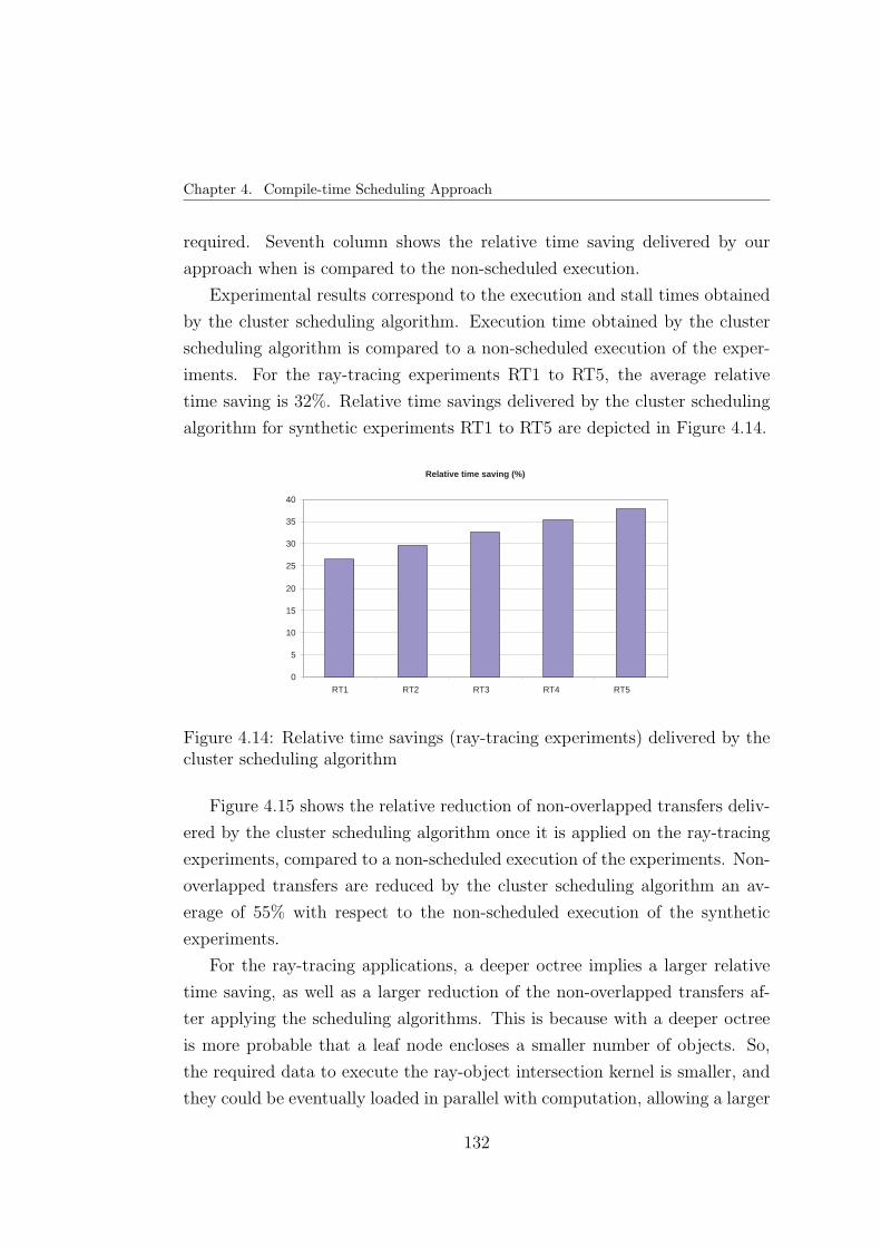
Chapter 4. Compile-time Scheduling Approach
required. Seventh column shows the relative time saving delivered by our
approach when is compared to the non-scheduled execution.
Experimental results correspond to the execution and stall times obtained
by the cluster scheduling algorithm. Execution time obtained by the cluster
scheduling algorithm is compared to a non-scheduled execution of the exper-
iments. For the ray-tracing experiments RT1 to RT5, the average relative
time saving is 32%. Relative time savings delivered by the cluster scheduling
algorithm for synthetic experiments RT1 to RT5 are depicted in Figure 4.14.
Relative time saving (%)
0
5
10
15
20
25
30
35
40
RT1 RT2 RT3 RT4 RT5
Figure 4.14: Relative time savings (ray-tracing experiments) delivered by thecluster scheduling algorithm
Figure 4.15 shows the relative reduction of non-overlapped transfers deliv-
ered by the cluster scheduling algorithm once it is applied on the ray-tracing
experiments, compared to a non-scheduled execution of the experiments. Non-
overlapped transfers are reduced by the cluster scheduling algorithm an av-
erage of 55% with respect to the non-scheduled execution of the synthetic
experiments.
For the ray-tracing applications, a deeper octree implies a larger relative
time saving, as well as a larger reduction of the non-overlapped transfers af-
ter applying the scheduling algorithms. This is because with a deeper octree
is more probable that a leaf node encloses a smaller number of objects. So,
the required data to execute the ray-object intersection kernel is smaller, and
they could be eventually loaded in parallel with computation, allowing a larger
132

4.5. Conclusions
Non-overlapped transfers reduction (%)
44
46
48
50
52
54
56
58
60
RT1 RT2 RT3 RT4 RT5
Figure 4.15: Relative reduction of the non-overlapped transfers (ray-tracingexperiments) delivered by the cluster scheduling algorithm
reduction of the non-overlapped data transfers, and consequently a larger rel-
ative time saving.
4.5. Conclusions
In this chapter we have described the compile-time scheduling approach.
Starting from a CDFG modeling the application, we have partitioned it into
clusters, and then we have serialized the execution of those clusters. This
cluster serialization generates a sequence of clusters which is initially executed,
and then refined at runtime by the dynamic scheduling support we propose in
the next chapter.
By partitioning the application into clusters we can perform the scheduling
process at a cluster-level, since a cluster can be scheduled independently of the
rest of the application. Application clustering and scheduling are focused on
the reduction of the non-overlapped transfers, that is the reduction of data and
contexts transfers latency. This goal is achieved following three criteria: min-
imization of context reloading, maximization of data reuse, and maximization
of the overlapping of data and contexts transfers with computation. Accord-
ing to the application domain, the search space is large. In the same way, the
optimization criteria are conflicting. So, we have imposed some constraints in
133

Chapter 4. Compile-time Scheduling Approach
the application partitioning to make it affordable. By redefining the cluster
generation to take into account the existence of conditional branches, we have
proposed a new clustering algorithm. This clustering algorithm generates sets
of kernels that are assigned to the same FB set and are consecutively executed.
Once the application is partitioned into clusters, they can be scheduled.
Cluster scheduling looks for the sequence of clusters with the minimum time
penalty represented by computation stalls. The uncertainty in the program
flow produced by control and data dependencies, and user activity results in
a performance degradation because of computation stalls associated to a con-
ditional branch. For both conditional constructs (if-then-else and iterative
constructs), we have proposed scheduling algorithms that minimize the com-
putation stalls based on the information provided by the earlier stages of the
compilation framework.
The proposed compile-time scheduling algorithms reduce the computation
stalls due to the existence of CBs by performing an effective exploration of the
design space of possible task sequences.
Obtained experimental results for the two possible conditional constructs
demonstrate the impact of the clustering and scheduling algorithms on the
overall execution time which is an important factor in interactive applications
subjected to real-time constraints. In some applications the static schedul-
ing approach is not enough to guarantee high performance. To refine the
compile-time scheduling solution developed in the current chapter, we propose
a runtime scheduling support. This dynamic scheduling support monitors the
execution of the application and adapts it to meet the power-performance
constraints, as it is explained in the following chapter.
134
Chapter 5
Runtime Scheduling Approach
In Chapter 4 we have described the static scheduling approach that is the
first scheduling step in the compilation framework. Static scheduling starts
by partitioning the application into clusters, and then performing the cluster
serialization. This cluster serialization generates a sequence of clusters which
is initially executed. This static scheduling approach is based on an off-line
estimation of the execution time, looking for the minimization of the non-
overlapped data transfers and computation stalls.
Considering the characteristics of our target applications, we know that
their runtime behavior can vary from the typical execution scenario estimated
at compile-time. In most of the cases this situation results in a performance
degradation. Our purpose is to provide a runtime support that helps to adapt
the application to the variable runtime conditions, according to a power and
performance budget.
One component of this runtime support consists of a runtime context switch
technique that tracks the behavior of the application around the conditional
branches (CBs), and decides when it is necessary to re-schedule the cluster
sequence around them. Because of the data dependecies and the large amount
of data that the target applications use to process, data management comes
up as a relevant issue. Data transfers have an associated power cost when they
are performed. It is desirable to keep at minimum level the data transfers to
save power. Specially when the actual input data of the applications comes
135

Chapter 5. Runtime Scheduling Approach
from a huge data set, and it is only known at runtime. This situation implies
a power/performance trade-off. We analyze this power/performance trade-
off by using the Pareto-optimal concept, and propose a data prefetch policies
that dynamically helps to meet performance contraints within a power budget.
Moreover, based on the data coherence of the applications, we propose a SIMD
data coherent execution model at the RC Array level in order to effectively
map the CBs at runtime.
5.1. Dynamic context scheduling
Conditional branch behavior is estimated during the static scheduling stage
of the compilation framework by means of an exhaustive profiling. Execution
of the application can show acceptable results when it runs under similar
conditions to those used to perform the off-line scheduling. However, this is
not always the case. Then, the scheduling should be tuned at runtime to meet
performance constraints.
5.1.1. Runtime context switch technique
Along the execution of an application, runtime conditions vary from the
typical scenario used to perform the static scheduling. Our purpose is to
develop a runtime support that allows us to adapt the execution of the appli-
cation to avoid performance degradation. This runtime support consists of a
context switch technique that tracks the behavior of the application around
the CBs, and decides when it is necessary to re-schedule the cluster sequence
around them.
We illustrate our runtime context switch technique by means of the ren-
dering application running onto the MorphoSys architecture. The rendering
application CDFG is shown in Figure 5.1.
The Line pixels and Z-buffer kernels draw one pixel of a line and store
it into the z-buffer, respectively, and they iterates until the line has been
completed and stored. The length of the line determines the number of times
that this kernel sequence is repeated. But the triangles composing an image
136

5.1. Dynamic context scheduling
3D Scene
Vertices sorting
Edge pixels
Z-Buffer Line pixels
Z-Buffer Interior pixels?
Line finished?
True
True
Figure 5.1: CDFG to describe the rendering application
have very different sizes, and the length of the lines forming a triangle are not
the same. As Figure 5.2 shows, line i has a different length when compared
to line j. Hence, the branch probability of the CB labeled as “Line finished?”
dynamically ranges from almost 0 (when few line pixels must be drawn) to
almost 1 (when the line is very long).
Edge pixels
Line pixels
Line i
Line j
x
y
Figure 5.2: The variable length of the lines implies a variable branch proba-bility
Since the branch probability varies during the execution because of the va-
riety of polygons composing a 3D scene, we have developed a dynamic context
scheduler that helps to adapt the execution to the current runtime conditions.
This dynamic context scheduler is based on a runtime monitor that switch
among precomputed configurations. These configurations are obtained during
the static scheduling stages of the compilation framework.
As it was explained in Section 4.3, the presence of a CB implies two pos-
sible program flows. The goal of the static cluster scheduling approach is to
determine a cluster sequence to be initially executed. This cluster sequence
is determined under a set of conditions defining a typical execution scenario
which is estimated during the previous application profiling stage, and we refer
137

Chapter 5. Runtime Scheduling Approach
to it as the Initial configuration. This initial configuration has the minimum
time penalty represented by computation stalls. The other possible cluster
sequence is not initially employed but it is actually computed and stored. We
refer to it as the Complementary configuration. Clearly, the complementary
configuration has a larger time penalty for the initially assumed execution
scenario.
Figure 5.3 shows the time penalty delivered by the static cluster scheduling
algorithm, versus the taken branch probability. Cluster scheduling was applied
around the CB labeled as “Line finished?” (see Figure 5.1). In this figure the
taken branch sequence corresponds to the sequence Line pixels - Z-buffer -
Line pixels, and the not-taken branch sequence corresponds to the sequence
Line pixels - Z-buffer - Edge pixels. We observe that the two plots intersect
each other in one point. We refer to the probability value of this point as the
cross-point probability, and it is highlighted in the figure. To the left of the
cross-point probability, the not-taken branch sequence delivers the minimum
time penalty. However, beyond the cross-point probability, it is the taken
banch sequence which delivers the minimum time penalty.
Taken Branch
Sequence
Not Taken Branch
Sequence
80
110
140
170
200
230
260
0,05 0,25 0,45 0,65 0,85
Taken branch probability
Tim
e p
enal
ty (
Clo
ck c
ycle
s)
Cross-point Probability
Figure 5.3: Time penalty against taken branch probability
Let’s assume that after passing the application through the profiling stage,
it determines a taken branch probability value of 0.4 to characterize a typ-
ical execution scenario around the CB labeled as “Line finished?”. Then,
we apply the static scheduling algorithm to found that the cluster sequence
138

5.1. Dynamic context scheduling
with the minimum time penalty for that execution scenario corresponds to
the not-taken branch sequence, as Figure 5.3 depicts. This means that the
initial configuration is the sequence Line pixels - Z-buffer - Edge pixels, while
the complementary configuration is the sequence Line pixels - Z-buffer - Line
pixels.
However, while the application is running the taken branch probability can
dynamically increase beyond the cross-point probability. This can occurs when
the line that is being drawn is long enough. Then, there will be a performance
degradation because the initially scheduled cluster sequence does not delivers
the minimum time penalty for the new runtime conditions. Our purpose is to
detect this situation and order the loading of the complementary configuration
(in this case, the configuration associated to the taken branch) in order to keep
at a minimum level the time penalty under the new runtime conditions.
The implementation of the dynamic context scheduler has a mixed hard-
ware/software approach. The software part is executed by the TinyRISC pro-
cessor, and it is supported by a minimal hardware addition. Its algorithmic
implementation is summarized in the Algorithm 3 box, and it works as follows.
Both, the Initial configuration and the Complementary configuration are com-
puted by the static cluster scheduling algorithm, and they are stored in main
memory. Initially, the application starts running the Initial configuration. This
initial configuration consists of the data and context scheduling around the CB
for a pre-determined execution scenario. That execution scenario is modeled
by a static taken branch probability. For each CB in the application’s control
and data flow graph (CDFG), we add to the TinyRISC processor a saturated
counter [Smi81]. Our purpose is to use the counter to know the number of
times that the branch has been taken. Before starting to execute the applica-
tion, counters are initialized to zero. While the application is running, every
time a branch is taken, the corresponding counter value is increased by one.
Then, the new counter value is compared to the cross-point probability. If the
counter equals the cross-point probability, TinyRISC processor orders loading
the Complementary configuration from main memory into the CM. The cross-
point probability corresponds to the intersection point of the two plots, as it
is depicted in Figure 5.3. When the current counter equals the cross-point
139
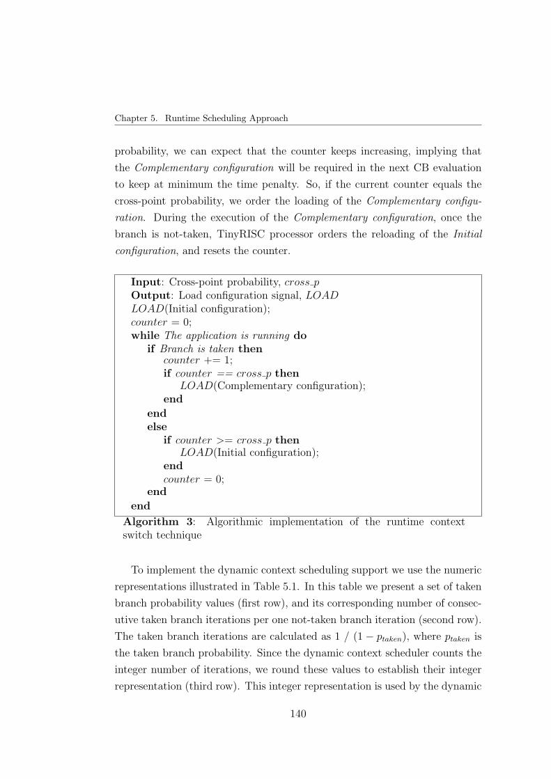
Chapter 5. Runtime Scheduling Approach
probability, we can expect that the counter keeps increasing, implying that
the Complementary configuration will be required in the next CB evaluation
to keep at minimum the time penalty. So, if the current counter equals the
cross-point probability, we order the loading of the Complementary configu-
ration. During the execution of the Complementary configuration, once the
branch is not-taken, TinyRISC processor orders the reloading of the Initial
configuration, and resets the counter.
Input: Cross-point probability, cross pOutput: Load configuration signal, LOADLOAD(Initial configuration);counter = 0;while The application is running do
if Branch is taken thencounter += 1;if counter == cross p then
LOAD(Complementary configuration);end
endelse
if counter >= cross p thenLOAD(Initial configuration);
endcounter = 0;
end
end
Algorithm 3: Algorithmic implementation of the runtime contextswitch technique
To implement the dynamic context scheduling support we use the numeric
representations illustrated in Table 5.1. In this table we present a set of taken
branch probability values (first row), and its corresponding number of consec-
utive taken branch iterations per one not-taken branch iteration (second row).
The taken branch iterations are calculated as 1 / (1 − ptaken), where ptaken is
the taken branch probability. Since the dynamic context scheduler counts the
integer number of iterations, we round these values to establish their integer
representation (third row). This integer representation is used by the dynamic
140

5.1. Dynamic context scheduling
context scheduler to perform the comparisons between the counter and the
cross-point probability in Algorithm 3. For instance, a cross-point probability
of 0.7 is represented by an integer value of 4. This means, for the example
illustrated in Figure 5.3, that if the branch is taken four times, the counter
has a value of four, equaling the cross-point probability, and demanding the
loading of the complementary configuration.
Table 5.1: Integer representation of different branch probabilities
Taken branch probability < 0.5 0.5 0.6 0.7 0.8 0.9
Taken branch iterations < 2 2 2.5 3.3 5 10
Integer representation 1 2 3 4 5 10
The previous description of the runtime context switch was focused on the
rendering application. However, it can be applied on any application where the
branch probability can dynamically vary. For instance, let’s consider the ray-
tracing application based on an octree structure (see Figure 5.4). The taken
branch probability of the CB labeled as “Leaf node?” dynamically changes as
we traverse the octree structure. If the octree is balanced, we can expect that
the leaf nodes are in the deeper level. So, as we go deep down the octree, the
probability of finding a lead nodes increases. For instance, if we are traversing a
full and balanced octree with two levels of subdivision, after the first iteration
of the octree traversal kernel (over the root node), we know that non-leaf
nodes will be found, implying a taken branch probability of 1. Later, after
the second iteration of the octree traversal kernel, we know that leaf nodes
will visited, implying a taken branch probability of 0. However, if the octree
were unbalanced, after the first iteration of the octree traversal kernel we can
visit leaf or non-leaf nodes, and the taken branch probability will have a value
between 0 and 1. In summary, when the octree structure is well-defined at
compile-time, we can characterize the taken branch probability behavior as we
traverse the octree, and use this analysis to feed the runtime context switch
technique to load the configuration that guarantees the minimum time penalty
for the current runtime conditions.
141

Chapter 5. Runtime Scheduling Approach
Shading / Secondary rays
generation
Octree traversal
Eye rays generation
Ray-object intersection
Leaf node?
Hit? True True
Figure 5.4: CDFG to describe the ray-tracing application
5.1.2. Experimental results
We have implemented the runtime context switch technique in a render-
ing application running onto the MorphoSys architecture. Our experimental
framework executes the application and delivers the execution time.
We have tested four different rendering experiments, REN1 to REN4, to
render four standard models in the computer graphics field. Table 5.2 shows
our experiment setup, including the number of triangles of the 3D scenes.
Table 5.2: Experiments to be rendered while applying the runtime contextswitch technique
Experiment 3D Scene Number of Triangles
REN1 Sphere 320
REN2 Teapot 2256
REN3 Rabbit 69451
REN4 Horse 96966
The runtime context switch technique was implemented on both CBs: “In-
terior pixels?” and “Line finished?” (see Figure 5.1). After applying the clus-
tering algorithm described in the previous chapter, we found the time penalty
as a function of the taken branch probability for the two CBs. Figures 5.5(a)
and 5.5(b) show the time penalty versus the taken branch probability for the
CBs labeled as “Interior pixels?” and “Line finished?”, respectively.
Tables 5.3 and 5.4 summarize the experimental results after executing the
rendering experiments using the runtime context switch technique. Both ta-
bles show the taken branch probability estimated during the profiling stage,
and used at compile-time to define the kernel sequence around the CBs to
be initially executed. Runtime results include the number of configuration
142
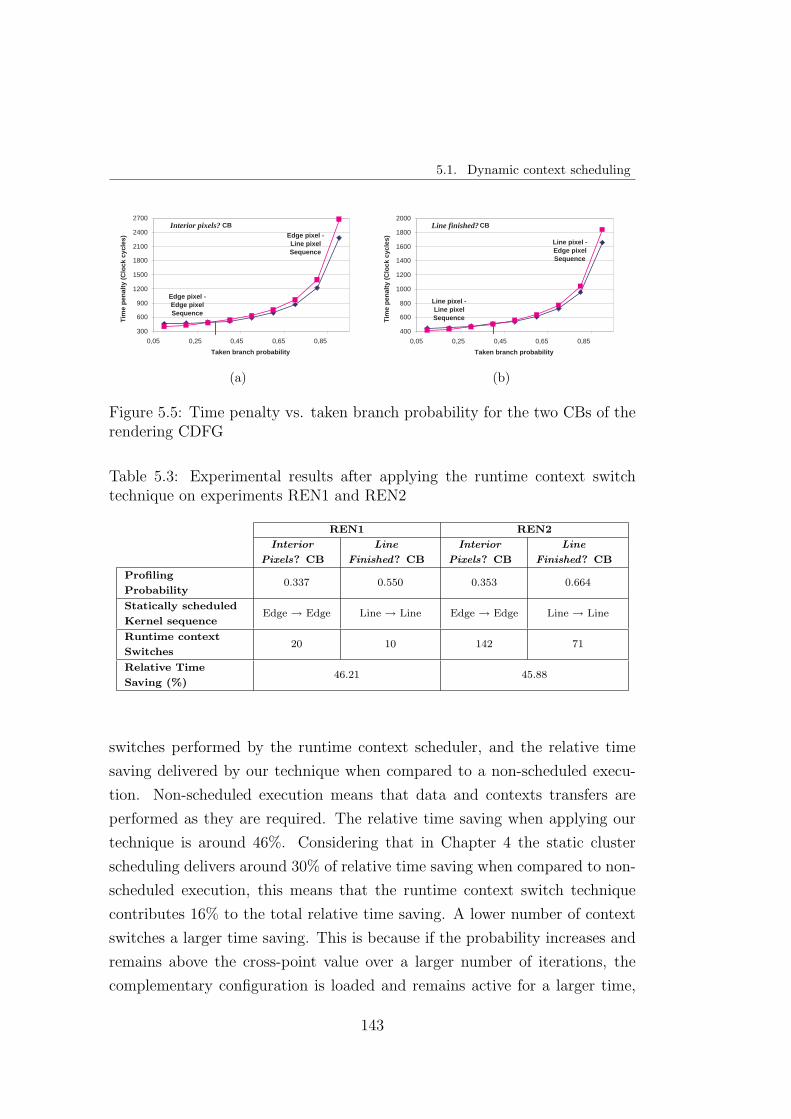
5.1. Dynamic context scheduling
Edge pixel - Edge pixel Sequence
Edge pixel - Line pixel Sequence
300
600
900
1200
1500
1800
2100
2400
2700
0,05 0,25 0,45 0,65 0,85
Taken branch probability
Tim
e p
enal
ty (
Clo
ck c
ycle
s)
Interior pixels? CB
(a)
Line pixel - Line pixel Sequence
Line pixel - Edge pixel Sequence
400
600
800
1000
1200
1400
1600
1800
2000
0,05 0,25 0,45 0,65 0,85
Taken branch probability
Tim
e p
enal
ty (
Clo
ck c
ycle
s)
Line finished? CB
(b)
Figure 5.5: Time penalty vs. taken branch probability for the two CBs of therendering CDFG
Table 5.3: Experimental results after applying the runtime context switchtechnique on experiments REN1 and REN2
REN1 REN2
Interior
Pixels? CB
Line
Finished? CB
Interior
Pixels? CB
Line
Finished? CB
Profiling
Probability0.337 0.550 0.353 0.664
Statically scheduled
Kernel sequenceEdge → Edge Line → Line Edge → Edge Line → Line
Runtime context
Switches20 10 142 71
Relative Time
Saving (%)46.21 45.88
switches performed by the runtime context scheduler, and the relative time
saving delivered by our technique when compared to a non-scheduled execu-
tion. Non-scheduled execution means that data and contexts transfers are
performed as they are required. The relative time saving when applying our
technique is around 46%. Considering that in Chapter 4 the static cluster
scheduling delivers around 30% of relative time saving when compared to non-
scheduled execution, this means that the runtime context switch technique
contributes 16% to the total relative time saving. A lower number of context
switches a larger time saving. This is because if the probability increases and
remains above the cross-point value over a larger number of iterations, the
complementary configuration is loaded and remains active for a larger time,
143

Chapter 5. Runtime Scheduling Approach
Table 5.4: Experimental results after applying the runtime context switchtechnique on experiments REN3 and REN4
REN3 REN4
Interior
Pixels? CB
Line
Finished? CB
Interior
Pixels? CB
Line
Finished? CB
Profiling
Probability0.342 0.669 0.353 0.668
Statically scheduled
Kernel sequenceEdge → Edge Line → Line Edge → Edge Line → Line
Runtime context
Switches4283 2170 6042 3030
Relative Time
Saving (%)45.92 45.79
45,60
45,80
46,00
46,20
46,40
REN1 REN2 REN3 REN4
Rel
ativ
e ti
me
savi
ng
(%
)
Figure 5.6: Relative time savings delivered by the runtime context switchtechnique
keeping at minimal the time penalty for the current runtime conditions. How-
ever, a minor impact after applying the runtime context switch technique can
be expected when the branch probability goes up and down the cross-point
probability often. This means that in the rendering experiments, the runtime
context switch technique applied on the CB labeles as “Line finished?” gives
the main contribution to the relative time saving because it has a lower num-
ber of context switches. This is because to render a triangle we need to draw
line pixels more often than only edge pixels. Figure 5.6 depicts the relative
time saving achieved by the runtime context switch technique.
Figure 5.7 depicts the 3D scenes obtained with our experiments.
144

5.2. Data coherence
(a) REN1: Sphere (b) REN2: Teapot
(c) REN3: Stanford rabbit (d) REN4: Horse(Top view)
Figure 5.7: 3D scenes obtained by the rendering application through the ex-periments
5.2. Data coherence
Concurrent processing of an application onto any SIMD reconfigurable ar-
chitecture means that each RC processes an independent subset of a larger
input data stream. Depending on the application characteristics, and consid-
ering that there are sixty-four RCs working in parallel, several of them can
require different data sets widely scattered in external memory, turning the
data supply to the RCs into a key issue. The lack of spatial locality potentially
derived from this situation can produce an important amount of processing
stalls because of the external memory delay overhead. However, our target
application domain exhibits a considerable degree of data coherence that can
facilitate us the data supply.
Data coherence [GP89] means that several RCs present the same memory
145

Chapter 5. Runtime Scheduling Approach
access pattern while the application is being executed. Hence, a coherent
group of RCs requires the same data sets and accesses the same memory
addresses. Data coherence is relevant because it impacts on the number of
memory accesses. When several RCs are demanding data widely scattered in
external memory, these data cannot be loaded in a streaming way and several
memory references may be resolved and performed. For instance, in 3D virtual
applications an important degree of data coherence can be expected because
neighboring pixels color is obtained after processing similar data since they
cover a reduced image region. Concurrent processing of non-adjacent pixels
results in a relatively large memory delay overhead. Therefore, Concurrent
processing of neighboring pixel blocks on the RC Array is highly desirable
because of the potential for exploiting data coherence [RSEF+04a].
For an N × N RC Array having the features of our target architecture
(each context word is broadcasted to a complete row or column of RCs, as it
was explained in Subsection 2.3.4), there are three possible coherent schemes
as Figure 5.8 illustrates.
1. All N × N RCs are assumed to be data coherent (Figure 5.8(a)).
2. M groups of K ×N RCs are data coherent, where M ×K is equal to N
(Figure 5.8(b)).
3. N groups of 1 × N RCs are data coherent (Figure 5.8(c)).
(a) (b) (c)
Figure 5.8: Possible data coherence schemes for an N × N RC Array
Although the data coherence illustrated in Figure 5.8 is column-based, data
coherence can also be assumed in a row-basis. In the figure only a 4 × 4 RC
Array is used for the sake of simplicity.
146

5.2. Data coherence
Option (1) requires the smallest memory bandwidth because the entire RC
Array exhibits the same memory access pattern, that is the same data set is
loaded for all the RCs in the array. On the other hand, Option (3) requires the
largest memory bandwidth because each row/column of RCs requires different
data sets. So, Option (1) should be chosen whenever the application allows it.
However, finding N ×N RCs being data coherent is really difficult for a larger
value of N . The number of data coherent RCs is usually small. According to
the SIMD model of computation of our target architecture, Option (3) is well
suited for it. Option (3) is interpreted as all the RCs in the same row/column
being data coherent. It is clear that the case of N groups of 1×N RCs being
data coherent can be easily extrapolated to the K × N and N × N cases. In
the Option (3), each group of N RCs (one row/column) is assumed to be data
coherent, and the N groups of 1×N RCs are allowed to process different data
sets. Finding N RCs being data coherent is more realistic when the value of
N is not too large.
Data coherence relevance is easily understood by means of the ray-tracing
application running onto the MorphoSys architecture (see Figure 5.4). Let’s
assume a ray-tracing application based on an octree. The octree is used as an
acceleration data structure to store the scene geometry. As it was explained
in Section 3.2, to draw a pixel in the screen a ray of light is traced from the
viewer through the pixel into the 3D scene. To determine if a ray intersects
with any objects in the scene, the ray must tested on each object. Considering
that a simple scene can be made of thousands of objects, this task can be
very expensive. By dividing the space in single cubic elements (voxels), it is
possible to define a hierarchical data structure describing how the objects are
distributed through out the 3D space occupied by the scene. An octree [LZ06]
is a rooted tree so that every internal node has eight children. Every node in the
tree corresponds to a cube in the physical space, as shown in Figure 5.9. Then,
the octree is a hierarchical spatial subdivision data structure that begins with
an axis parallel bounding box of the scene (the root of the tree) and proceeds
to construct a tree. Each node that does not meet the termination criteria
is subdivided into eight congruent child sub-nodes. Each child represents one
octant of its parent. The octree leaves store lists of objects (or, rather, pointers
147

Chapter 5. Runtime Scheduling Approach
to objects). The termination criteria for the octree construction can be the
maximum depth reached, or a determined number of objects ocuppying the
node. In this way, the objects intersected by a ray are encountered as we
track a ray through the octree. This requires no exhaustive search through
the whole collection of objects and is a much faster strategy.
Figure 5.9: An example of an octree
Our purpose is to completely process one ray (pixel) per RC. Each ray
traverses the octree structure looking for leaf nodes where objects reside. Then,
the ray is tested against all objects in the leaf to determine if they intersect
any object. If the ray does not intersect any object, then that pixel has the
background color. If the ray hits an object, in the intersection point several
types of rays are spawned. The octree traversal kernel implements a top-down
method in which the ray trace starts at the root node, and recurses down into
those nodes and leaves that are traversed by the ray. To process a ray against
an octree node, both the ray and the node geometry data may be loaded into
the RC. After processing a node, a child node to be visited is found. Since
there are sixty-four different rays concurrently traversing the octree structure,
in the worst case scenario, once the current node processing is finished, sixty-
four child nodes information may be loaded into the on-chip memory. This
situation represents an important memory bottleneck. However, if the rays
being concurrently processed corresponds to a reduced image region, we can
expect that they traverse the octree in a similar way, that is they will visit the
148

5.2. Data coherence
same nodes at same time, because the rays are pointing to the same region in
3D space. An ideal scenario occurs when all the sixty-four rays traverse the
octree in the same way. This ideal scenario corresponds to the data coherent
model illustrated in Figure 5.8(a), where all the N ×N RCs require the same
data set, that is the same node geometry information. A more realistic scenario
is represented by a smaller number of data coherent RCs. According to the
SIMD model of computation of our target architecture, we assume a 1 × N
column data coherent model, as it is illustrated in Figure 5.8(c). This means
that all the RCs in the same column are assumed to be data coherent, that
is each column will require the same dat set, and N diferent data sets will be
concurrently processed on the RC Array. This data coherent model applied to
the ray-tracing application means that there will be eight different nodes (one
per column of the RC Array) being concurrently tested against sixty-four rays.
In this way the memory overhead is make lighter because the amount of data
to load is reduced, and performance gain can be still obtained because most
of our target applications exhibits a considerable degree of data coherence. In
the next subsection we describe the implementation of a mapping scheme that
is based on the SIMD model of computation and on the 1 × N column data
coherent model.
5.2.1. SIMD data coherent mapping scheme
Static scheduling approach determines the cluster sequence to be initially
executed. This cluster sequence is determined by modeling the CB behavior by
means of a branch probability that is obtained through an exhaustive profiling.
This branch probability models the case in which the entire RC Array performs
the branch. However, at runtime, the branch can be handled and performed in
many different ways. This is because the RC Array is concurrently processing
independent data subsets and, in the presence of a CB, the individual RCs
eventually do not need to perform the branch at the same time. Our solution
represents a runtime CB mapping scheme that works at the RC Array level
based on the SIMD model of computation, and the data coherence model, as
it is explained below.
149

Chapter 5. Runtime Scheduling Approach
As it was explained in Section 5.2, we have assumed a 1×N column data
coherent model, as it is illustrated in Figure 5.8(c), because it allows us to
exploit all the parallel capabilities of our SIMD target architecture. In this
model all the RCs in the same column are assumed to be data coherent, that
is each column will require the same dat set, and N different data sets will
be concurrently processed on the RC Array. We illustrate the runtime CB
mapping scheme by means of the ray-tracing implementation running onto
the MorphoSys architecture (see Figure 5.4).
In the ray-tracing implementation there are N ×N rays being concurrently
processed on the RC Array, that is one ray per RC. According to the data
coherent model, there are N data coherent groups of N RCs. This means that
there are N groups of N rays with a coherent behavior, one coherent group
per column of the RC Array. Hence, each coherent group of rays will visit
the same nodes of the octree. Then, there will be N different nodes being
concurrently tested against N × N rays on the RC Array. Initially, all rays
are processed by the octree traversal kernel against the root node data. This
gives us the next nodes to visit in the next depth-level of the octree. The
rays information is provided to the RCs from the FB, since it prevails over the
execution of the octree traversal and ray-object intersection kernels until the
pixel is drawn. However, the node information must be renewed after every
octree traversal execution, because new nodes are visited. Since there are N
different nodes being concurrently processed, at least N new nodes information
must be provided for the next octree traversal execution, at least one node per
column.
We use the RC Addressable Buffer (RCAB) (refer to Subsection 2.3.6) to
manage data coherence. As the FB, the RCAB is also divided into two sets to
provide overlapping of computation with data transfers. While one set of the
RCAB provides data to the RC Array, the other set concurrently exchanges
data with the off-chip main memory through the DMA controller. Each set
of the RCAB is further split into eight banks. Each bank provides data to
one column of eight RCs. This means that each bank corresponds to a data
coherent group of 1×8 RCs. In fact, the RCAB is introduced, besides to allow
accessing non-consecutive memory addresses, to exploit data coherence.
150

5.2. Data coherence
After executing the octree traversal kernel, since each column is processing
N different rays against the same node stored in the associated RCAB bank,
it is also possible that the N rays do not have enough data coherence, visiting
different nodes in the next kernel execution. Since all visited nodes must be
processed, we test N rays against all of them, one per kernel execution. In
order to keep the trace of the nodes to be processed, we use a software stack for
each data coherent column of the RC Array [SEDT+03]. TinyRISC processor
is in charge of controlling these software stacks. After every execution of the
octree traversal kernel on the RC Array, the TinyRISC processor puts into the
corresponding stack the nodes to be visited by the rays in each data coherent
column of the RC Array. It is important to notice that after executing the
octree traversal kernel the following cases can occur:
1. All found nodes in every data coherent column are non-leaf nodes de-
manding once again the execution of the octree traversal kernel.
2. At least one of the data coherent columns reaches a leaf node demanding
the execution of the ray-object intersection kernel.
As we have said, TinyRISC processor puts into the corresponding stacks
the found nodes. Prior to the next RC Array execution, TinyRISC processor
gets a node from each stack. If all the N extracted nodes are in the first
case, octree traversal algorithm keeps on executing, and the branch to the
ray-object intersection kernel is not performed. If at least one of the extracted
nodes is a leaf node, we need to decide the kernel to be executed because the
octree traversal and ray-object intersection kernels cannot be simultaneously
executed on the RC Array. We implement a runtime CB mapping scheme to
take this decision, consisting of a simple routine executed by the TinyRISC
processor that works as follows:
⋆ The octree traversal kernel is continuously executed on the N data co-
herent columns. Every time an RC reaches a lead node, that RC is
stalled and the lead processing is postponed. Once there are N post-
poned leaves, one per column of the RC Array, the octree traversal ker-
nel stops, and the ray-object intersection kernel starts. This means that
151

Chapter 5. Runtime Scheduling Approach
the ray-object intersection kernel is only executed once all data coher-
ent columns have found a leaf. The octree traversal kernel execution is
continued while there are no postponed leaves in all the columns of the
RC Array. Once the octree traversal kernel iterations have been com-
pleted, all the possible postponed leaves are processed by the ray-object
intersection kernel.
Summarizing the SIMD data coherent mapping scheme, we claim that in
the presence of a CB, the branch is performed by the entire RC Array when
there is one RC per data coherent column demanding the branch. In this
way, the entire RC Array executes the kernel associated to the branch target.
In any other case, the kernel on which the branch condition is evaluated is
continuously executed.
Based on the data coherence model and on the SIMD data coherent ex-
ecution, in the following section we analyze the case of data scheduling at
runtime.
5.3. Dynamic data scheduling
As it was explained in Section 3.2, each kernel of a CDFG representing
an application operates on a fixed-size input data. However, according to the
characteristics of our target applications, the input data of a kernel at a given
time is only a fraction of a larger data set, and depends on runtime conditions.
Even though the input data size of a kernel is well-known once it is coded, in
the case of dynamic applications the specific input data set is only known at
runtime, because it depends on previous results, or user activity. Furthermore,
demanded input data must be chosen among a larger data set. If all the pos-
sible input data set can be loaded in advance, kernel input data resides in the
on-chip memories (Frame Buffer or RC Addressable Buffer) just in time to be
processed. However, most of the times this is impracticable because of the size
of all the possible input data set, and the memory bandwidth. The selection
of the fraction of the possible input data to be loaded in advance represents
a relevant issue because it has a considerable impact on performance. When
152

5.3. Dynamic data scheduling
preloaded data contains the required input data, no computation stalls are
produced. In other case, computation is stalled while required data are loaded
into the FB. A larger preloaded data set, a smaller probability of computation
stalls because of data unavailability. This implies a trade-off between power
and performance. The power refers to the power consumed by data transfers,
and the performance refers to the execution time of the application. To deal
with these issues, we make use of the data coherence and other characteristics
of our target applications. Data coherence helps to efficiently prune the possi-
ble input data set in order to select a specific data subset to be preloaded, and
also reduces the number of data transfers. Thus, if we minimize the number
of data transfers, we reduce the power consumed by them, and by preloading
the correct data subset the performance is boosted, because the number of
computation stalls is also reduced.
Let’s use again as illustrative example the ray-tracing application based
on an octree data structure. The octree traversal kernel computes the nodes
traversed by the ray in a recursive way. This means that after processing a
ray at a given node, in the next step, only one node among eight different
possible nodes will be visited. This node is only known after the current node
processing is finished. To avoid computation stalls, the information of the
subsequent node has to be loaded in advance. This is possible by preloading
all the eight child nodes information. However, this fact has a larger impact on
power and performance because the information of eight nodes is transferred
but only one of them is actually processed, increasing the power consumption
produced by useless data transfers, and the time required to perform all data
loading. According to the charactertistics of the ray-tracing application and
the octree structure, a data prefetch policy can be defined. By means of
an effective data prefetch policy a number of child nodes is selected to be
preloaded to improve performance and to save power. Below we explain the
main data prefetch mechanisms and illustrate our implementation.
153

Chapter 5. Runtime Scheduling Approach
5.3.1. Data prefetch mechanisms
The use of cache memory hierarchies is a widely spread technique for reduc-
ing the memory access latency. The use of large cache hierarchies has proven
to be effective in reducing the average memory access penalty for programs
that show a high degree of locality in their addressing patterns. The quality
of cache utilization depends on the memory fecth policy it uses. The three
existing prefetch policies operation [VL00] can be explained according to our
problem as follows. Let’s assume that our purpose is to execute the sequence
of kernels K1, K2, K3, and K4 considering that we do not know the data they
need in advance.
By means of the on-demand fetch policy, the input data of a kernel is trans-
ferred into the FB from main memory only after the RC Array has requested it
and found it absent from the FB. This situation is illustrated in Figure 5.10(a)
where computation, including memory references, are represented by the up-
per time line while main memory access time is represented by the lower time
line. In this figure, the data sets associated to memory references rf2, rf3,
and rf4, performed by the kernels K2, K3, and K4, respectively, are not found
in the FB and must therefore be loaded from main memory. The RC Array
will be stalled while it waits for the corresponding data set to be loaded. Once
the data is loaded into the FB from main memory, the RC Array computation
may proceed. From the point of view of power consumed by data transfers,
on-demand fetch policy is the better solution because only needed data is
transferred. However, in terms of performance, on-demand policy takes longer
to complete an application because there is a computation stall for every data
set needed by a kernel.
Many of these FB misses can be avoided if a data prefetch operation is in-
troduced. Rather than waiting for a FB miss to perform a memory fetch, data
prefetching anticipates such misses and issues a fetch to the memory system
in advance of the actual memory reference. It is desirable that this prefetch
proceeds in parallel with RC Array computation. Ideally, the prefetch will
complete just in time for the RC Array to access the needed data in the FB
without stalling the RC Array. Data prefetch is initiated by an explicit load
154
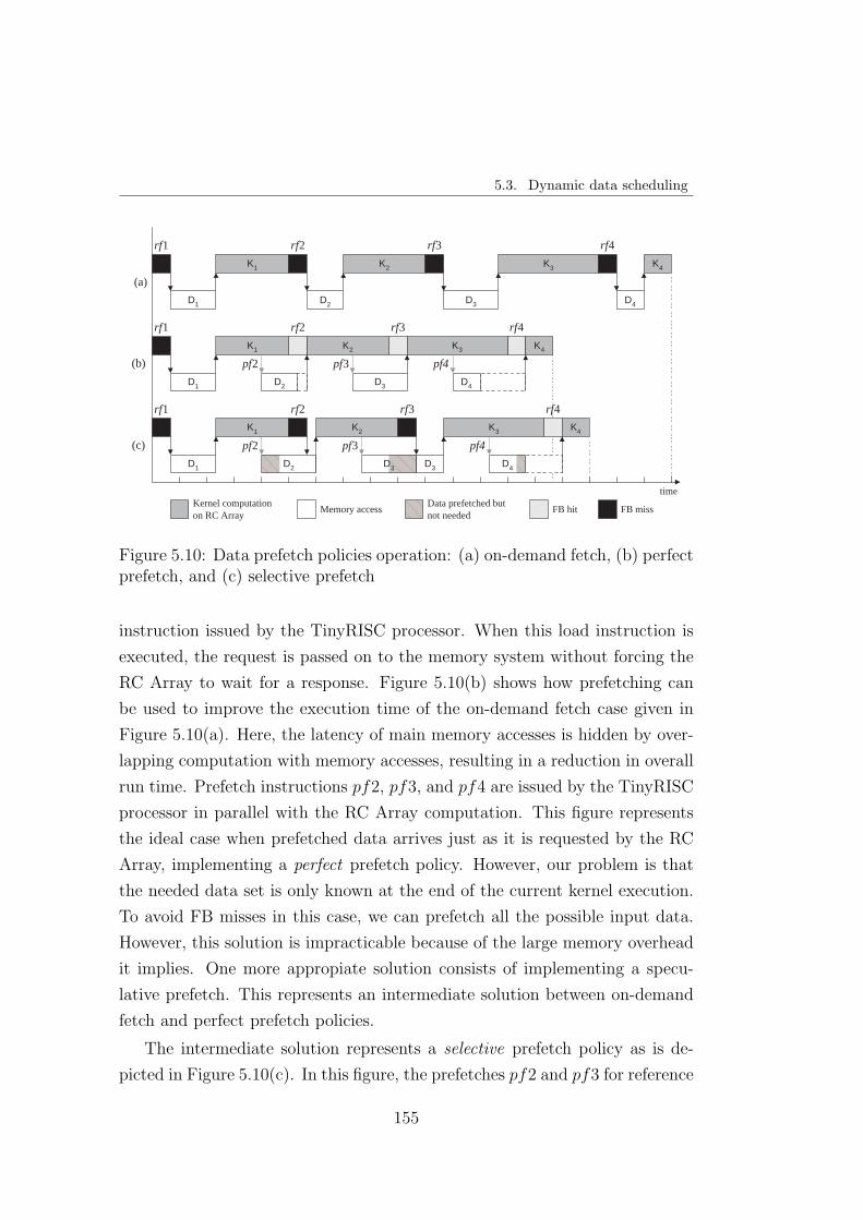
5.3. Dynamic data scheduling�����K 1
D 1
Kernel computation on RC Array
time
(a)
(b)
K 2
D 2
rf 2
K 3
D 3
rf 3
K 4
D 4
rf 4
K 1
D 1 D 2
rf 1
pf 2
K 2
rf 2
D 3
rf 3
pf 3
K 3
pf4
D 4
K 4
(c)
rf 4
K 1
D 1 D 2
rf 1
pf 2
K 2
rf 2 rf 3
pf 3
K 3
pf4
D 4
K 4
D 3 D 3
rf 4
Memory access FB hit FB miss ��Data prefetched but not needed
rf 1
Figure 5.10: Data prefetch policies operation: (a) on-demand fetch, (b) perfectprefetch, and (c) selective prefetch
instruction issued by the TinyRISC processor. When this load instruction is
executed, the request is passed on to the memory system without forcing the
RC Array to wait for a response. Figure 5.10(b) shows how prefetching can
be used to improve the execution time of the on-demand fetch case given in
Figure 5.10(a). Here, the latency of main memory accesses is hidden by over-
lapping computation with memory accesses, resulting in a reduction in overall
run time. Prefetch instructions pf2, pf3, and pf4 are issued by the TinyRISC
processor in parallel with the RC Array computation. This figure represents
the ideal case when prefetched data arrives just as it is requested by the RC
Array, implementing a perfect prefetch policy. However, our problem is that
the needed data set is only known at the end of the current kernel execution.
To avoid FB misses in this case, we can prefetch all the possible input data.
However, this solution is impracticable because of the large memory overhead
it implies. One more appropiate solution consists of implementing a specu-
lative prefetch. This represents an intermediate solution between on-demand
fetch and perfect prefetch policies.
The intermediate solution represents a selective prefetch policy as is de-
picted in Figure 5.10(c). In this figure, the prefetches pf2 and pf3 for reference
155

Chapter 5. Runtime Scheduling Approach
rf2 and rf3 are not enough to avoid RC Array computation stalls because
they do not include all the required data by kernels K2 and K3, that is the
speculation is not correct. Since the initially prefetched data sets are not the
complete data sets needed by the kernels, a computation stall is produced
while the remaining needed data is fetched into the FB. Note that the data
set for reference rf4 arrives early enough to hide all of the memory latency,
although not all of them are actually processed. This example illustrates main
issues when trying to conceive a selective prefetch policy for our target appli-
cations. Since the actually needed data set is part of a larger data set, and
it is also unknown in advance, the prefetch must not be just in time but also
accurate to avoid FB misses. As can be seen in Figure 5.10, selective prefetch
boosts performance but not for free. Power consumption is proportional to
the size of the prefetched data set. Depending on the power budget a deter-
mined size of data can be prefetched, and the performace gain is defined by
the FB hit rate, that is by the accuracy of the data speculation. In summary,
selective prefetch implies a power/performance trade-off. Prefetched data set
size may be selected for maximixing FB hit rate and minimizing computation
stalls, while power consumed by data tranfers fits into the application’s power
budget. Therefore, the application must be configured to meet varied power
and performace requirements. Pareto-based optimization is an effective way
to represent and explore this trade-off.
5.3.2. Pareto multi-objective optimization
The Pareto-optimal concept [OR94] is applied on multi-objective optimiza-
tion problems, where more than one conflicting optimization objectives exist.
Multi-objective design methods can be seen as a way for generating design
alternatives that vary along some sets of the solution space that are known to
be “good solutions”. A solution can be considered Pareto-optimal if there is
no other solution that performs at least as well on every objective and strictly
better on at least one objective. That is, a Pareto-optimal solution cannot be
improved upon without hurting at least one of the objectives. A solution is
not Pareto-optimal if one objective can be improved without degrading any
156
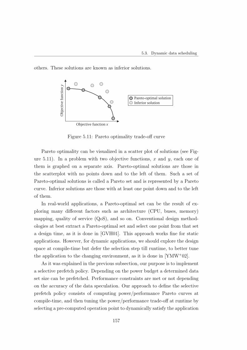
5.3. Dynamic data scheduling
others. These solutions are known as inferior solutions.
Objective function x
Obj
ectiv
e fu
nctio
n y
Pareto-optimal solution Inferior solution
Figure 5.11: Pareto optimality trade-off curve
Pareto optimality can be visualized in a scatter plot of solutions (see Fig-
ure 5.11). In a problem with two objective functions, x and y, each one of
them is graphed on a separate axis. Pareto-optimal solutions are those in
the scatterplot with no points down and to the left of them. Such a set of
Pareto-optimal solutions is called a Pareto set and is represented by a Pareto
curve. Inferior solutions are those with at least one point down and to the left
of them.
In real-world applications, a Pareto-optimal set can be the result of ex-
ploring many different factors such as architecture (CPU, buses, memory)
mapping, quality of service (QoS), and so on. Conventional design method-
ologies at best extract a Pareto-optimal set and select one point from that set
a design time, as it is done in [GVH01]. This approach works fine for static
applications. However, for dynamic applications, we should explore the design
space at compile-time but defer the selection step till runtime, to better tune
the application to the changing environment, as it is done in [YMW+02].
As it was explained in the previous subsection, our purpose is to implement
a selective prefetch policy. Depending on the power budget a determined data
set size can be prefetched. Performance constraints are met or not depending
on the accuracy of the data speculation. Our approach to define the selective
prefetch policy consists of computing power/performance Pareto curves at
compile-time, and then tuning the power/performance trade-off at runtime by
selecting a pre-computed operation point to dynamically satisfy the application
157

Chapter 5. Runtime Scheduling Approach
constraints. In the next subsection we describe how the power/performance
trade-off is explored by using the Pareto-optimal concept.
5.3.3. Power/performance trade-off
Our target applications are modeled in such a way that at compile-time the
input data size of every kernel is well-known. However, the specific input data
set is only determined at runtime among a larger data set. By implement-
ing a prefetch mechanism a performance boost is obtained, although paying
a power cost. As was explained above, factors that define power/performance
trade-off are size of the prefetched data set and the hit rate. The larger
prefetched data set, the larger hit rate (if the speculation is good enough),
as well as the higher power consumption because of data transfers. Since the
ultimate power/performance trade-off of an application is only known at run-
time, we do not know the best data size to be prefetched in advance. Instead
of obtaining just one solution, our purpose is to generate a set of solutions
representing different power/performance trade-offs. This is done by means
of the Pareto-optimal concept. Initially, a Pareto curve is obtained. This
Pareto curve collects Pareto points representing different power/performance
trade-offs. During the execution of the application, depending on the runtime
conditions, a Pareto point is selected to define a data size to prefetch.
Let’s assume a ray-tracing application based on an octree (see Figure 5.4)
to show how the Pareto curve is obtained. After a ray is processed against a
given node by the octree traversal kernel, eight different child nodes can be
visited. However, only one (or none) of them will be processed in the next
kernel execution (actually, the next node to be executed could be a sibling
of the current node). Hence, we can prefetch the information of one to eight
child nodes plus one to eight sibling nodes. During the profiling stage, or
according to the characteristics of the application, different data subsets to be
prefetched are observed in order to evaluate the hit rate for all of them. Those
data subsets have specific sizes and a power cost to be transferred. For each
data subset to be prefetched, execution time and power consumption, because
of data transfers are estimated to explore the power/performance trade-off. In
158

5.3. Dynamic data scheduling
this way, the Pareto curve is obtained. Figure 5.12 depicts the Pareto curve
for the ray-tracing application.
9% 18%
45%
27%
620
640
660
680
130 150 170 190 210 230
Power per 32-bits word access (x10 3 )
Tim
e (C
lock
Cyc
les)
Figure 5.12: Pareto curve illustrating the power/performance trade-off for theray-tracing application
Figure 5.12 shows how much power is consumed by the data transfers in
order to meet a performance constraint. The points highlighted on the curve
represent different sizes of prefetched data as a fraction of all the possible input
data. As we have claimed, a larger data subset implies a larger hit rate that
is reflected on a performance boost, and on a higher power consumption. A
determined data subset size can be selected to be prefetched in order to meet a
power/performance trade-off. For instance, let’s assume we have to complete
the application in 670 clock cycles (see the dashed line in Figure 5.12). Hence,
we can prefetch 27% of all the possible input data that allows us to complete
the application in 660 clock cycles. If the performance constraint is later
relaxed, that is the application must be completed in a longer time, then we
can prefetch 18% of all the possible input data that allows us to complete the
application in around 690 clock cycles, with a lower power cost. It also can
occur that the performance constraint is tighter, and we need to prefetch 45%
of all the possible input data to reduce the execution time. In this case we
pay a higher power cost to meet the performance constraint. Depending on
the runtime conditions we can move upward or downward the Pareto curve to
reach a specific power/performance trade-off.
Let’s assume that we can increase the memory bandwidth between the
159

Chapter 5. Runtime Scheduling Approach
on-chip data buffers and main memory. In this way, we can load more data
in the same clock cycle. In this case, the y–axis will be contracted because
the performance will be boosted, while the x–axis will be expanded and the
Pareto curve will look flatter. At any rate, the power/performance trade-off
still exists.
In our approach, we obtain the Pareto curve at compile-time. Pareto curve
collects different data sizes to be prefetched and their corresponding power
costs. The profiling stage of the compilation framework defines a Pareto point
for a typical execution scenario to start running the application. This Pareto
point determines a power/performance trade-off, represented by a specific data
size to be prefetched. Along application’s code, we introduce software check-
points in order to track the application’s performance. Once the application
is running, software checkpoints indicate to the TinyRISC processor if per-
formance constrainsts are being met. If not, TinyRISC selects a new Pareto
point and modifies the data prefetch scheme by increasing the size of the data
to be prefetched. This means moving downward the Pareto curve, implying
a higher power consumption. However, data size to be prefetched can only
be increased if its power consumption does not exceed the application’s power
budget. TinyRISC can also reduce the size of the prefetched data when the
execution time of the application is below the performance contraints. This
implies moving upward the Pareto curve, relaxing both execution time and
power consumption.
In the next subsection we explain how a selective prefetch policy is imple-
mented for a ray-tracing application. Based on the characteristics of the target
application, we define the size as well as the heuristic to choose the specific
subset of input data to be prefetched, in order to meet power and performance
contraints.
5.3.4. Implementation of a data prefetch scheme for 3D
image applications
As it was explained above, the input data for an execution a kernel of our
target applications is only a fraction a larger data set. Although both data
160

5.3. Dynamic data scheduling
sizes are well known at compilation time, the dynamic behavior of our target
applications does not allow to know the actual input data set until executing
the prior kernel. In this subsection we present the data prefetch policy we have
developed for 3D image applications. This data prefetch policy is based on the
geometric characteristics of the ray-tracing application we have implemented
onto the MorphoSys architecture.
The ray-tracing implementation (see Figure 5.4) is based on a octree data
structure which is traversed by the ray to draw one pixel on the screen. The
octree traversal kernel implements a top-down method in which the ray trace
starts at the root node, and recurses down into those nodes and leaves that
are traversed by the ray. This means that after processing the ray at a given
node, in the next step only one node among eight different possible nodes will
be visited. By implementing a perfect prefetch policy, computation stalls can
be avoided. Perfect prefetch consists of loading all eight child nodes of the
current node in advance. However, this fact has a larger impact on power and
performance. Power consumption is incremented because the information of
eight nodes is transferred but only one of them is actually required. Perfor-
mance is degraded because the loading of eight nodes information demands a
large memory delay. Since the main memory to FB bandwidth is limited, the
loading of eight nodes information are mainly performed as non-overlapped
data transfers. Our purpose is to implement a selective prefetch policy in
which only some nodes are prefetched. In this way some performance gain
is obtained because prefetched data are mainly transferred in parallel with
the octree traversal kernel computation, at a reduced power cost. The octree
traversal kernel is in charge of tracking rays through the octree structure. Since
the selective prefetch policy is derived from the particularities of the octree
traversing, we firstly explain the octree traversal kernel implementation.
Octree traversal kernel
The octree traversal kernel implements a top-down method, related to other
parametric octree traversal [RUL00], as follows. The idea is to work with the
parametric representation of the ray to decide which children of a node must
161

Chapter 5. Runtime Scheduling Approach
be visited. Let the ray be given by:
−→x = −→p + t−→d (5.1)
where −→p is the view point,−→d is the unit length direction vector, and t is
the parameter; and a voxel v by
[xl, xh] × [yl, yh] × [zl, zh] (5.2)
If we have the line parameters of the intersection of the ray with the borders
of a node, then the line intervals half-way in between (see Figure 5.13) are
computed by:
tmα =1
2(tlα + thα), α ∈ {x, y, z} (5.3)
In order to determine the order in which subnodes should be traversed,
we first need to determine at which plane the ray enters the current voxel by
using Table 5.5.
Next, we determine the first subnode to be visited (the entry node) by
using Table 5.6, following the numbering scheme illustrated in Figure 5.14.
In Table 5.6, the first column is the entry plane determined in the previous
step. The third column contains a factor to be added in order to determine
the first subnode to be visited: initially assuming that the entry node 0, if one
or both of the conditions of the second column hold, then the corresponding
quantity as indicated by the third column should be added.
Finally, in order to obtain the exact path followed by the ray, it is necessary
to compute the plane where the ray leaves each of the visited subnodes, which
makes possible to obtain the next subnode to be visited. The exit plane is
obtained using Table 5.7.
Table 5.8 gives the next visited subnode given the current subnode and the
exit plane. The entries labeled with “exit” means the exit plane of the ray for
the current subnode. For example, if the entry node is 0, the nodes that can
be visited are 4, 2 and 1, depending on the exit plane. From node number 5,
162
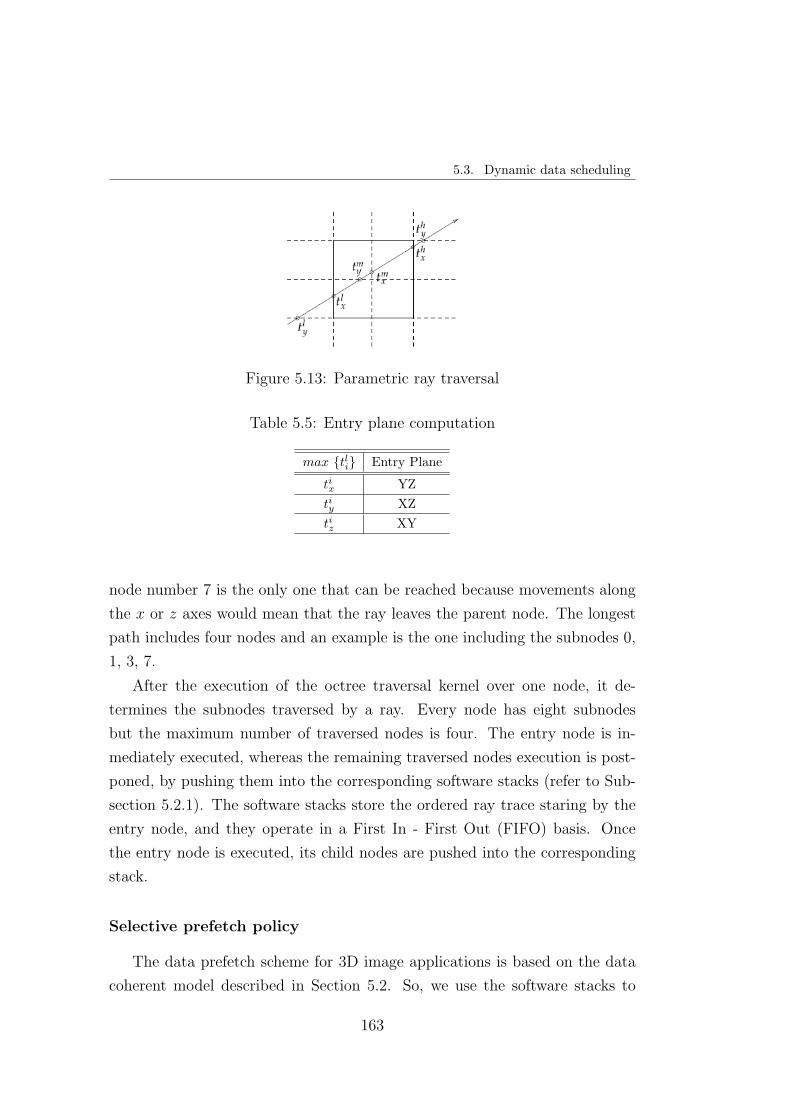
5.3. Dynamic data scheduling
Figure 5.13: Parametric ray traversal
Table 5.5: Entry plane computation
max {tli} Entry Plane
tix YZ
tiy XZ
tiz XY
node number 7 is the only one that can be reached because movements along
the x or z axes would mean that the ray leaves the parent node. The longest
path includes four nodes and an example is the one including the subnodes 0,
1, 3, 7.
After the execution of the octree traversal kernel over one node, it de-
termines the subnodes traversed by a ray. Every node has eight subnodes
but the maximum number of traversed nodes is four. The entry node is in-
mediately executed, whereas the remaining traversed nodes execution is post-
poned, by pushing them into the corresponding software stacks (refer to Sub-
section 5.2.1). The software stacks store the ordered ray trace staring by the
entry node, and they operate in a First In - First Out (FIFO) basis. Once
the entry node is executed, its child nodes are pushed into the corresponding
stack.
Selective prefetch policy
The data prefetch scheme for 3D image applications is based on the data
coherent model described in Section 5.2. So, we use the software stacks to
163

Chapter 5. Runtime Scheduling Approach
x
y
z
0 4
2 6
3
7
5
Figure 5.14: Octree nodes numbering scheme (The hidden node has number1)
Table 5.6: First subnode computation
Entry Plane Condition Factor to add
XYtmz < tlx 1
tmy < tlx 2
XZtmx < tly 1
tmz < tly 4
YZtmy < tlx 2
tmz < tlx 4
store the ray trace of each column of the RC Array. For the sake of clarity, we
analyze the data prefetch scheme just for a column of the RC Array. At a given
octree depth level, after executing the octree traversal kernel over a node, we
know the next child nodes to be traversed. Let’s assume that after processing
the root node, the ray traverse the nodes 0, 2, 6, and 7. These nodes are
pushed into the corresponding software stack in that order. Since the entry
node 0 is firstly processed, we can anticipate its child nodes according to its
next sibling node, 2. By using the octree nodes numbering scheme depicted in
Figure 5.14, if a ray traverses from node 0 towards its sibling node 2, before
the ray enters to node 2, it surely visites at least one of the node 0’s children
0.2, 0.3, 0.6, and 0.7. So, our purpose is to prefetch the information of these
child nodes. Based on the geometric properties of the octree structure, and
on its nodes numbering scheme, we build Table 5.9. This table gives the child
nodes of the first traversed node (nodei) that can be prefetched, according to
164
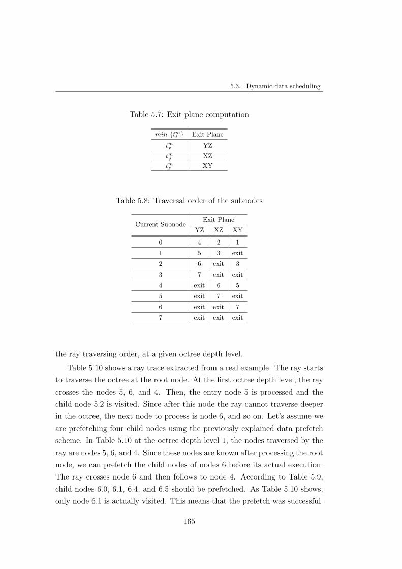
5.3. Dynamic data scheduling
Table 5.7: Exit plane computation
min {tmi } Exit Plane
tmx YZ
tmy XZ
tmz XY
Table 5.8: Traversal order of the subnodes
Current SubnodeExit Plane
YZ XZ XY
0 4 2 1
1 5 3 exit
2 6 exit 3
3 7 exit exit
4 exit 6 5
5 exit 7 exit
6 exit exit 7
7 exit exit exit
the ray traversing order, at a given octree depth level.
Table 5.10 shows a ray trace extracted from a real example. The ray starts
to traverse the octree at the root node. At the first octree depth level, the ray
crosses the nodes 5, 6, and 4. Then, the entry node 5 is processed and the
child node 5.2 is visited. Since after this node the ray cannot traverse deeper
in the octree, the next node to process is node 6, and so on. Let’s assume we
are prefetching four child nodes using the previously explained data prefetch
scheme. In Table 5.10 at the octree depth level 1, the nodes traversed by the
ray are nodes 5, 6, and 4. Since these nodes are known after processing the root
node, we can prefetch the child nodes of nodes 6 before its actual execution.
The ray crosses node 6 and then follows to node 4. According to Table 5.9,
child nodes 6.0, 6.1, 6.4, and 6.5 should be prefetched. As Table 5.10 shows,
only node 6.1 is actually visited. This means that the prefetch was successful.
165

Chapter 5. Runtime Scheduling Approach
Table 5.9: Child nodes to be prefetched according to the traversing order ofsibling nodes
nodei+1
nodei 0 1 2 3 4 5 6 7
0 - 1, 3, 5, 7 2, 3, 6, 7 3, 7 4, 5, 6, 7 5, 7 6, 7 7
1 0, 2, 4, 6 - 2, 6 2, 3, 6, 7 4, 6 4, 5, 6, 7 6 6, 7
2 0, 1, 4, 5 1, 5 - 1, 3, 5, 7 4, 5 5 4, 5, 6, 7 5 7
3 0, 4 0, 1, 4, 5 0, 2, 4, 6 - 4 4, 5 4, 6 4, 5, 6, 7
4 0, 1, 2, 3 1, 3 2, 3 3 - 1, 3, 5, 7 2, 3, 6, 7 3, 7
5 0, 2 0, 1, 2, 3 2 2, 3 0, 2, 4, 6 - 2, 6 2, 3, 6, 7
6 0, 1 1 0, 1, 2, 3 1, 3 0, 1, 4, 5 1, 5 - 1, 3, 5, 7
7 0 0, 1 0, 2 0, 1, 2, 3 0, 4 0, 1, 4, 5 0, 2, 4, 6 -
Note that we have prefetched the information of four nodes. So, we have
incur in an extra power consumption. However, we have saved power when
compared to prefetching all eight child nodes information. In addition, the
hit allow us to improve performance and avoid computation stalls due to data
unavailability.
Table 5.10: Example of a ray trace through an octree
Octree depth Nodes traversed by the ray
0 root
1 5 6 4
2 5.2 6.1 4.3
3 5.2.6 5.2.4 6.1.5 4.3.7 4.3.5 4.3.6 4.3.4
4
4.3.7.6 4.3.5.6 4.3.6.7 4.3.4.7
4.3.7.4 4.3.6.5 4.3.4.6
4.3.6.4
4.3.6.6
5.3.5. Experimental results
We have applied the previously explained data prefetch scheme on a ray-
tracing application running onto the MorphoSys architecture. Our experimen-
tal framework executes the application and delivers the execution time, as well
as the number of 32-bit words transferred to the on-chip memories, which help
166

5.3. Dynamic data scheduling
us to estimate the power consumed by those data transfers.
We have tested different experimental setups. Our purpose is to process the
same 3D scene with different octree depths, and screen sizes. A deeper octree,
a larger data structure to traverse. A larger screen means more algorithm
iterations because the RC Array can only process 8 × 8 pixels at time. In
all experiments one sibling node is prefetched. The number of child nodes
to preload are two and four. When two child nodes are prefetched, they are
randomly selected from the prefetch table (see Table 5.9).
Table 5.11 summarizes the experimental results when prefetching one sib-
ling node, and two child nodes. Three screen sizes were used, and three dif-
ferent octree structures storing the 3D scene were employed.
Table 5.11: Experimental results for prefetching one sibling and two childnodes
Screen size (Pixels) 32 × 32 64 × 64 128 × 128
Octree depth⋆ Oc1 Oc2 Oc3 Oc1 Oc2 Oc3 Oc1 Oc2 Oc3
Hit rate (%) 52 53 55 53 55 57 53 55 55
Time growth
Selective /
Perfect Prefetch (%)
6.32 6.80 7.21 10.20 10.84 11.32 13.80 17.20 19.65
Power Saving
Selective /
Perfect Prefetch (%)
58.31 59.03 60.02 58.91 59.30 60.98 59.43 60.02 61.56
⋆Oc3 > Oc2 > Oc1
By prefetching one sibling and two child nodes, an average hit rate of
54 percent is achieved, allowing to speed up the application just 6% above
the execution time delivered by using a perfect data prefetch policy. When
considering the power consumption, this prefetch scheme reduces the power
consumed by data transfers in 59 percent with respect to a perfect prefetch
policy. The same results are depicted in Figure 5.15.
Table 5.12 summarizes the experimental results when prefetching one sib-
ling node, and four child nodes. Three different octree structures storing the
3D scene were employed, as well as three different screen sizes.
By prefetching one sibling and four child nodes, an average hit rate of 73
percent is achieved, allowing to speed up the application just above the execu-
167

Chapter 5. Runtime Scheduling Approach
0
4
8
12
16
20
Oc1 Oc2 Oc3 Oc1 Oc2 Oc3 Oc1 Oc2 Oc3
32 × 32 64 × 64 128 × 128
Screen size
Rel
ativ
e ti
me
gro
wth
(%
)
(a)
56
58
60
62
Oc1 Oc2 Oc3 Oc1 Oc2 Oc3 Oc1 Oc2 Oc3
32 × 32 64 × 64 128 × 128
Screen size
Rel
ativ
e p
ow
er s
avin
g (
%)
(b)
Figure 5.15: Experimental results after prefetching one sibling and two childnodes
Table 5.12: Experimental results for prefetching one sibling and four childnodes
Screen size (Pixels) 32 × 32 64 × 64 128 × 128
Octree depth⋆ Oc1 Oc2 Oc3 Oc1 Oc2 Oc3 Oc1 Oc2 Oc3
Hit rate (%) 77 72 70 75 74 72 74 73 73
Time growth
Selective /
Perfect Prefetch (%)
3.22 2.01 1.98 2.15 1.41 1.23 1.40 0.98 0.56
Power Saving
Selective /
Perfect Prefetch (%)
38.10 35.41 34.67 37.97 36.51 34.87 38.18 36.97 35.20
⋆Oc3 > Oc2 > Oc1
tion time delivered by using a perfect data prefetch policy. When considering
the power consumption, this prefetch scheme reduces the power consumed by
data transfers in 36 percent with respect to a perfect prefetch policy. The
same results are depicted in Figure 5.16.
In the case of one sibling and two child nodes prefetch scheme, obtained
hit rate allows reducing the power consumption considerably, but it cannot be
enough because of the minor reduction in execution time. In the case of one
sibling and four child nodes prefetch scheme, a greater hit rate allows reducing
the execution time although power saving is not as larger as with the previous
scheme. Here we observe the power/performance trade-off we have explained
in Subsection 5.3.3.
168

5.4. Conclusions
0
0,5
1
1,5
2
2,5
3
3,5
Oc1 Oc2 Oc3 Oc1 Oc2 Oc3 Oc1 Oc2 Oc3
32 × 32 64 × 64 128 × 128
Screen size
Rel
ativ
e ti
me
gro
wth
(%
)
(a)
32
34
36
38
Oc1 Oc2 Oc3 Oc1 Oc2 Oc3 Oc1 Oc2 Oc3
32 × 32 64 × 64 128 × 128
Screen size
Rel
ativ
e p
ow
er s
avin
g (
%)
(b)
Figure 5.16: Experimental results after prefetching one sibling and four childnodes
5.4. Conclusions
In this chapter we have described the runtime scheduling approach. The
dynamic characteristics of our target applications demonstrates that the static
scheduling approach is not enough to satisfy the performance constraints. In
our compilation framework, we have subjected the application to an exhaustive
profiling in order to define a typical execution scenario to start running the
application. Profiling results feed the static and dynamic scheduling stages. At
compile-time, the time penalties for all the possible cluster sequences around a
CB are estimated as a function of the taken branch probability. The dynamic
behavior produced by data dependencies and user activity is modeled by means
of a branch probability. To avoid performance degradation, we have developed
a runtime support that allows us to adapt the execution of the application to
the new runtime conditions. This runtime support consists of a context switch
technique that tracks the behavior of the application around the CBs, and
decides when it is necessary to re-schedule the cluster sequence around them.
According to the experimental results, by applying the runtime context switch
we contribute 16% more to the total relative time saving, which is around 46%.
We have used the data coherence concept to exploit the parallel capabilities
of our target architecture. Since there are N ×N RCs processing independent
data subsets, data supply comes up as a key issue. If all RCs are requiring data
widely scattered in main memory, this situation surely produces a considerable
169

Chapter 5. Runtime Scheduling Approach
amount of computation stalls because of the external memory overhead. By
adopting a data coherent model, memory accesses can be reduced because it
can be expected that several groups of RCs require data with some degree of
spatial locality, facilitating the data supply and allowing a performance gain.
Input data of target applications’ kernels are only known at runtime and
considered as part of a large data set. If it were possible to prefetch all possible
input data set, a large power cost will result, with no performance degrada-
tion. However, this is impracticable. We must be able to prefetch a selected
fraction of all possible input data set, in such a way that the power con-
sumption is reduced while not too much performance degradation is obtained.
This implies the implementation of a selective data prefetch policy. The se-
lective data prefetch policy is associated to a power/performance trade-off.
The quality of the data prefetch is determined by its hit rate, that helps to
avoid performance degradation, and by the power consumed by the data tran-
fers it performs. A larger prefetched data subset, a higher power cosst. We
have explored this power/performance trade-off for the application by using
the Pareto-optimal concept. At compile-time, we obtain the Pareto curve that
collects Pareto points. A Pareto point represents a specific power/performance
trade-off. During the execution of the application, a Pareto point is selected to
meet performance contraints within a power budget. The Pareto point estab-
lishes a determined size of input data subset to be prefetched, knowing that
the hit rate depends on the quality of the heuristic implemented to select the
input data subset to prefetch among all possible input data. By using the se-
lective data prefetch scheme, the execution time of the ray-tracing application
is just 6% above the execution time obtained when all the possible input data
is prefetched, but reducing till 59% the power because of data transfers with
respect to the same perfect prefetch.
170

Chapter 6
Conclusions
The majority of contemporary applications (DSP, multimedia, wireless)
are characterized by the presence of computationally- and data-intensive al-
gorithms. Also, high speed and throughput are frequently needed since they
are subjected to real time constraints. Moreover, due to the wide spread of
portable devices, low-power consumption becomes relevant.
Reconfigurable systems emerged as a new paradigm for satisfying the si-
multaneous demand for application performance and flexibility. Recent coarse-
grained reconfigurable architectures have abundant parallel resources and func-
tional flexibility, features that turn them into unbeatable candidates to imple-
ment this class of applications.
Scheduling techniques are crucial for the future of coarse-grained recon-
figurable architectures. Powerful architectural features are not enough to effi-
ciently execute applications if they are not usefully exploited. A lot of work has
been done in static compilation for reconfigurable architectures. When static
applications are considered, all relevant information is available at compile-
time, and so they can be near-optimally scheduled prior to execution. How-
ever, we are targeting a new class of applications which are characterized
by dynamic workload, data-intensive computation, and hard real-time con-
straints. The program flow of these applications highly depends on runtime
conditions such as input data and user activity. The scheduling proposals
presented in this thesis have been conceived to be integrated within the com-
171
Chapter 6. Conclusions
plete MorphoSys compilation framework. In fact, these scheduling algorithms
help to generalize the previously developed static compilation framework, by
providing effective support to map dynamic applications.
This thesis attempts to provide a way to model the dynamic behavior of
the target applications, and to propose an scheduling approach to implement
them onto the MorphoSys reconfigurable system.
Static applications use to be modeled by a data dependency-based task
graph, namely a data-flow graph (DFG). However, this kind of DFG is not
enough to model the target applications. We model the dynamic program
flow of these applications by means of the conditional execution of tasks. To
deal with this feature, we have adopted the hybrid control and data flow
graph (CDFG) since it embeds all control and sequencing information explic-
itly within the same graph. Besides data dependencies, a CDFG also repre-
sents control dependencies between a number of kernels. Since a kernel is a
computationally- and data-intensive task, in our approach the applications are
specified at a coarse level of granularity as a sequence of kernels.
The scheduling techniques developed in this thesis are focused on decreas-
ing the number of clock cycles required to complete the application, in order
to meet performance constraints within a power budget. This scheduling ap-
proach has two components: a static component, and a dynamic one.
At compile-time, the application is partitioned into clusters, and the ex-
ecution of those clusters is serialized. This cluster serialization generates a
sequence of clusters which is initially executed, and then refined at runtime
by the dynamic scheduling support. By partitioning the application into clus-
ters we can perform the scheduling process at cluster-level, since a cluster
can be scheduled independently of the rest of the application. Application
clustering and scheduling are focused on the reduction of the non-overlapped
transfers, that is the reduction of data and contexts transfers latency. This
goal is achieved following three criteria: minimization of context reloading,
maximization of data reuse, and maximization of the overlapping of data and
contexts transfers with computation. These three optimization criteria are
conflicting. To solve this problem we impose some constraints in the applica-
tion partitioning by redefining the cluster generation procedure to take into
172

account the existence of conditional branches.
Once the application is partitioned into clusters, they are serialized. This
serialization is performed according to the conditional construct dereived from
the presence of a conditional branch. In the case of branching contructs (if-
then-else), the scheduling algorithm minimizes the non-overlapped data and
contexts transfers. In the case of iterative constructs, the scheduling algo-
rithm minimizes both the non-overlapped data and contexts transfers, and
the computation stalls. These static scheduling algorithms are based on the
information provided by the earlier stages of the compilation framework.
The dynamic characteristics of the target applications demonstrates that
the previous static scheduling approach is not enough to satisfy the perfor-
mance constraints. The uncertainty in the program flow produced by control
and data dependencies, as well as the user activity results in a performance
degradation because of computation stalls associated to a conditional branch.
The compilation framework subjects the application to an exhaustive profiling
in order to define a typical execution scenario to start running the application.
Profiling results feed the scheduling process. The dynamic behavior produced
by data dependencies and user activity is modeled by means of a branch proba-
bility. At compile-time, the time penalties for all the possible cluster sequences
around a conditional branch are estimated as a function of the taken branch
probability.
To avoid performance degradation because of the dynamic nature of the
application, we have developed a runtime support that allows us to adapt the
execution of the application to the runtime conditions. This runtime support
consists of a context switch technique that tracks the behavior of the appli-
cation around the conditional branches, and decides when it is necessary to
re-schedule the cluster sequence.
The data coherence concept is used to exploit the parallel capabilities of
the target architecture. Since there are N × N RCs processing independent
data subsets, data supply comes up as a key issue. If all RCs are requiring data
widely scattered in main memory, this situation surely produces a considerable
amount of computation stalls because of the external memory overhead. By
adopting a data coherent model, memory accesses can be reduced, because it
173

Chapter 6. Conclusions
can be expected that several groups of RCs require data with some degree of
spatial locality, facilitating the data supply and allowing a performance gain.
Input data of kernels are only known at runtime and considered as part
of a larger data set. If it is possible to prefetch all the possible input data,
no performance degradation exists, but due to its high power cost, this is
usually impracticable. Hence, we must be able to prefetch a selected fraction
of the possible input data, in such a way that the power consumption is re-
duced while not too much performance degradation is obtained. This goal can
be achieved by applying a selective data prefetch policy. The selective data
prefetch policy is associated to a power/performance trade-off. The quality of
the data prefetch is determined by its hit rate, that helps to avoid performance
degradation, and by the power consumed by the data tranfers it performs.
The larger prefetched data subset, the higher power cost. We explore this
power/performance trade-off for the application by using the Pareto-optimal
concept. At compile-time, the Pareto curve that collects Pareto points is
obtained. A Pareto point represents a specific power/performance trade-off.
During the execution of the application, a Pareto point is selected to meet
performance contraints within a power budget. The Pareto point adjust the
size of the input data to prefetch, knowing that the hit rate depends on the
quality of the heuristic implemented to select the input data subset among
all possible input data. We also have developed a complete selective prefetch
policy for 3D image applications.
6.1. Main contributions
The main contributions of this thesis can be summarized as follows:
⋆ Application modeling: In dynamic applications the next kernel to be
executed depends directly on input data, or user activity, and it is de-
cided at runtime. Then, dynamic program flow is modeled by means of
the conditional execution of kernels. We have adopted the hybrid control
and data flow graph (CDFG) since it embeds all control and sequencing
information within the same graph. We have added branching vertices
174

6.1. Main contributions
representing operations that evaluate conditional clauses into the appli-
cation data-flow graph to model data and control dependencies.
⋆ Application clustering: By partitioning the application into clusters
we can perform the scheduling process at a cluster-level, since a cluster
can be scheduled independently of the rest of the application. We have
developed a novel clustering algorithm following the constraints imposed
by the cluster definition and the application modeling. Clustering algo-
rithm consists of an exploration algorithm that efficiently prunes the
search space and generates the potential clusters. Then, potential clus-
ters are subjected to a feasibility check to detect whose of them fit into
the cluster definition and satisfy data dependencies.
⋆ Off-line scheduling: From the application modeling and clustering, we
have proposed static scheduling algorithms to start executing dynamic
applications. These static scheduling algorithms employ profiling infor-
mation. By subjecting dynamic applications to an exhaustive profiling,
their dynamic behavior can be characterized. Application profiling de-
termines the behavior of conditional clauses, and the configurations and
data needed under certain conditions. Static algorithms serialize the
clusters minimizing the computation stalls due to data and context un-
availability. Static serialization configures a typical execution scenario
to start running the application. After applying our static scheduling al-
gorithms on real ray-tracing experiments, a 33% of average relative time
saving is obtained respect to a non-scheduled version of the experiments.
Non-overlapped data and contexts transfers are reduced an average of
55% for the same experiments.
⋆ Runtime scheduling: Dynamic scheduling support is in charge of
tracking the behavior of the application while is being executed, and
tune it to the runtime conditions. By using the developed runtime con-
text switch technique, TinyRISC processor is able to decide when to
order re-scheduling the cluster sequence around a conditional branch
in order to keep at minimum the time penalty. Relative time saving
175
Chapter 6. Conclusions
obtained with the runtime context switch is around 46% respect to a
non-scheduled version of the application (30% of that speedup is due to
the static scheduling, and 16% to the runtime context switch technique).
Speculative data loading is implemented to improve performance. This
is a key point because the actual input data of the applications is only
known at runtime. The larger preloaded data set, the smaller probability
of computation stalls because of data unavailability. This implies a trade-
off between power and performance. The power refers to the power
consumed by data transfers, and the performance refers to the execution
time of the application. Since the ultimate power/performance trade-
off of an application is only known at runtime, we do not know the
best data size to be prefetched in advance. Instead of obtaining just
one solution, we generate a set of solutions at compile-time representing
different power/performance trade-offs by means of a Pareto curve. Once
the application is running, TinyRISC selects a Pareto point according to
the runtime conditions. After applying this selective prefetch policy for
3D image applications, the execution time is just 2% above the execution
time obtained with a perfect prefetch. Power consumption due to data
tranfers is also reduced up to 73% respect to the power consumed with
a perfect prefetch.
⋆ Compilation framework: The scheduling proposals collected in this
thesis have been conceived to be integrated within the previous Morpho-
Sys compilation framework in such a way that it can deal with dynamic
applications. With our contributions on application modeling, applica-
tion profiling, and application clustering for dynamic applications, as
well as with the new algorithms to schedule conditional constructs at
compile-time, and the runtime scheduling support to adapt the execution
of the application to the runtime conditions within a power/performance
trade-off, MorphoSys is able to efficiently implement dynamic applica-
tions.
176

6.2. Future work
6.2. Future work
Several computation- and data-intensive algorithms have been successfully
implemented onto MorphoSys. However, when trying to map some algorithms,
relevant shortcomings of MorphoSys are identified:
⋆ MorphoSys highly depends on the central controlling processor. RC Ar-
ray is tightly coupled to the TinyRISC processor. Every instruction to
be executed by each RC is directly determined by this controlling proces-
sor. RC Array-shared memory is also under direct control of the central
processor. These dependences on the controlling processor may easily
result in poor RC utilization, and eventually performance degradation.
⋆ Data and instruction broadcast to the RC Array, and also some inter-RC
communication are performed over global buses. However, this type of
signal path cannot be easily scaled as hypothetical MorphoSys utilizes
larger RC arrays. In addition, wire delay is becoming a major constraint
in the implementation of large processors. Therefore, MorphoSys is not
easily scalable.
⋆ Memory hierarchy in MorphoSys has to be improved for the growing RC
Array, as a global data memory and a global instruction memory cannot
efficiently exploit the possible spatial and temporal localities. Although
the introduction of the RCA Buffer allows the execution of non-streaming
data intensive applications, memory hierarchy of MorphoSys is still a
rigid bottleneck.
⋆ Concurrent kernels are not supported by MorphoSys, resulting in either
performance degradation or much complicated interfacing between sev-
eral single-kernel engines.
A Macro-pipelined Reconfigurable System (MaRS) [TBKD04] is being de-
veloped at UC-Irvine as an attempt to relax the above concerns. Hence, MaRS
is an advanced sucessor of MorphoSys. Its purpose is to provide a break-
through computing engine for efficient mapping of highly parallel data- and/or
computation-intensive wireless communication and multimedia applications.
177

Chapter 6. Conclusions
Figure 6.1: Top level MaRS
The backbone of MaRS is a 2D mesh of 32-bit processing elements (PEs).
Each PE is comprised of a router and an execution unit (EU). A number of
PEs may be bound together as a macro-pipeline stage. Then, several macro-
pipelines may operate at the same time executing different kernels, tailoring
the system to the intended application, as shown in Figure 6.1. These macro-
pipelines are reconfigurable in terms of shape and number of participating
PEs.
The PEs are interconnected through channels. All data processing tasks are
performed by the EU. The router is in charge of directing the ongoing traffic
toward the corresponding destination PEs. The incoming data/instructions
are also absorbed by the router once they reach destination. The router also
lets the locally generated blocks enter and then ripple through the network to
reach destination.
MaRS is targeted at large concurrent kernels. As the very first example
of application mapping, let’s consider the ray-tracing application. In this ap-
plication, the octree traversing kernel is not a data-streaming task, and has
little spatial and temporal localities, demanding a high-memory bandwidth.
Furthermore, a large octree prevents it from being an on-chip resident, and
this represents a further memory bandwidth requirement. Therefore, while
the corresponding high computation demand can be satisfied by the on-chip
computing resources, the high memory bandwidth has to be thoroughly stud-
ied to avoid performance degradations, as it was demonstrated while mapping
178

6.3. List of publications
the ray-tracing application onto MorphoSys, where a data coherent model was
assumed, and non-streaming buffers were introduced to achieve acceptable
performance results. An approach to overcome this problem with MaRS is to
sufficiently shorten the octree to reach an acceptable off-chip memory band-
width, at the cost of some computation overhead, which can be tolerated by
the sufficient computing resources in MaRS.
Since the MaRS architecture is still being developed at UCI, there is a
lot of work to do on compilation support. For a sophisticated system such
as MaRS, proper compilation tools are indispensable. Beyond an assembler
and a cycle-accurate simulator that are being simultaneously developed, we
intend to contribute in application mapping. As it was demonstrated by our
work with MorphoSys, application mapping allows to identify the architec-
ture’s shortcomings and strengths that enable a better architecture exploita-
tion. Application mapping for MaRS is very different to that performed for
MorphoSys because of their models of computation. MaRS follows a multiple
instruction stream - multiple data stream (MIMD). Therefore, task-level par-
allelism can be massively exploited. It is necessary to develope methodologies
for resources allocation, data and instructions scheduling, and multiple kernel
interfacing. Data and instructions scheduling is also a big issue in MaRS be-
cause the program flow and data requirements of the target applications are
only known at runtime. Then, it is necessary to propose techniques to provide
data and instructions to the processing elements with the minimal latency.
6.3. List of publications
This is a list of publications that have been produced during my research:
1. F. Rivera, M. Sanchez-Elez, R. Hermida, and N. Bagherzadeh. Schedul-
ing methodology for conditional execution of kernels onto multi-context
reconfigurable architectures. IET Computers & Digital Techniques,
2(3):199–213, May 2008.
179
Chapter 6. Conclusions
2. F. Rivera, M. Sanchez-Elez, and N. Bagherzadeh. Configuration and
data scheduling for executing dynamic applications onto multi-context
reconfigurable architectures. In Proc. Intl. Conf. on Engineering of Re-
configurable Systems and Algorithms (ERSA), pages 85–91, June 2007.
3. F. Rivera, M. Sanchez-Elez, M. Fernandez, R. Hermida, and N. Bagher-
zadeh. Configuration scheduling for conditional branch execution onto
multi-context reconfigurable architectures. In Proc. Intl. Conf. on Field
Programmable Logic and Applications (FPL), pages 589–596, August
2006.
4. J. Davila, A. de Torres, J. Sanchez, M. Sanchez-Elez, N. Bagherzadeh,
and F. Rivera. Design and implementation of a rendering algorithm in
a SIMD reconfigurable architecture (MorphoSys). In Proc. Design, Au-
tomation and Test in Europe Conference and Exhibition (DATE), pages
52–57, March 2006.
5. F. Rivera, M. Sanchez-Elez, M. Fernandez, and N. Bagherzadeh. An
approach to execute conditional branches onto SIMD multi-context re-
configurable architectures. In Proc. Euromicro Conference on Digital
System Design (DSD), pages 396–402, August 2005.
6. F. Rivera, M. Sanchez-Elez, M. Fernandez, R. Hermida, and N. Bagher-
zadeh. Low power data prefetch for 3D image applications on coarse-
grain reconfigurable architectures. In Proc. Intl. Parallel and Distributed
Processing Symposium (IPDPS), page 171, April 2005.
7. F. Rivera, M. Sanchez-Elez, M. Fernandez, R. Hermida, and N. Ba-
gherzadeh. Efficient mapping of hierarchical trees on coarse-grain re-
configurable architectures. In Proc. Intl. Conf. on Hardware/Software
Codesign and System Synthesis (CODES+ISSS), pages 30–35, Septem-
ber 2004.
8. F. Rivera, M. Sanchez-Elez, M. Fernandez, R. Hermida, and N. Bagher-
zadeh. Ejecucion paralela de arboles jerarquicos en arquitecturas recon-
figurables de grano grueso. In Actas de las XV Jornadas de Paralelismo,
pages 126–131, September 2004.
180

Apendice A
Resumen en Espanol
En cumplimiento del Artıculo 4 de la normativa de la Universidad Com-
plutense de Madrid que regula los estudios universitarios oficiales de postgrado,
se presenta a continuacion un resumen en espanol de la presente tesis que in-
cluye la introduccion, objetivos, principales aportaciones y conclusiones del
trabajo realizado.
A.1. Introduccion
A medida que el mercado electronico se orienta hacia los dispositivos mo-
viles [KPPR00] [Rab00] [MP03], los sistemas reconfigurables surgen como un
nuevo paradigma para satisfacer las exigencias, tanto de rendimiento como de
flexibilidad [WVC03].
Los sistemas de computacion reconfigurable representan una solucion a
medio camino entre los sistemas de proposito general y los de aplicacion
especıfica. Ellos pueden lograr un rendimiento similar al del hardware de
proposito especıfico, conservando mucha de la flexibilidad de los sistemas de
proposito general. El principio fundamental de la computacion reconfigura-
ble es que la organizacion del hardware, su funcionalidad e interconexionado
pueden modificarse despues de su fabricacion.
Los sistemas de computacion reconfigurable suelen acoplar un procesador
de proposito general a un modulo reconfigurable en el mismo chip. Normal-
i

Apendice A. Resumen en Espanol
mente, las partes de las aplicaciones con mas exigencia computacional se sin-
tetizan sobre el modulo reconfigurable, mientras que las partes secuenciales de
las aplicaciones son ejecutadas por el procesador principal.
Los sistemas reconfigurables se clasifican segun su granularidad en dos
tipos: de grano fino y de grano grueso. Los sistemas de grano fino [MSHA+97]
[Hau98] [VH98] operan a nivel de bit, mientras que los de grano grueso [MD96]
[WTS+97] [MO98] [TAJ00] operan sobre palabras de varios bits. Gracias a su
granularidad, cuando se emplean para implementar operadores a nivel de pala-
bra y rutas de datos, los sistemas de grano grueso ofrecen un mejor rendimien-
to, menor latencia de reconfiguracion, mejor aprovechamiento de recursos y
menor consumo de potencia que los de grano fino [KR07].
Las aplicaciones objetivo de este trabajo se caracterizan por la presencia
de algoritmos complejos para el procesamiento masivo de datos, que se deben
ejecutar en tiempos estrictos y con bajo consumo de potencia. La cantidad de
datos a procesar, ası como las configuraciones necesarias para ello, hacen de la
planificacion de sus transferencias una tarea crıtica para la ejecucion eficiente
de las aplicaciones objetivo. En estas aplicaciones la siguiente tarea a ejecutar
depende muchas veces de los datos de entrada o de la interaccion del usuario
y, por lo tanto solo se conoce en tiempo de ejecucion. La incertidumbre en
el flujo de programa obliga a modelar las aplicaciones mediante la ejecucion
condicional de tareas. El dinamismo del flujo de programa representa un pro-
blema debido a que las configuraciones y datos necesarios para operar no se
conocen sino en tiempo de ejecucion, lo que puede incrementar la latencia de la
aplicacion si tardan mucho en llevarse a las memorias internas. Una manera de
reducir la latencia de las aplicaciones sera a traves de la planificacion cuidadosa
de las transferencias de configuraciones y datos, que en muchos casos se haran
de manera especulativa. Sin embargo, sera necesario prestar atencion al tamano
de los datos a precargar de manera que el consumo de potencia debido a las
transferencias de datos no se dispare.
ii

A.1. Introduccion
A.1.1. Objetivos de esta tesis
Esta tesis versa sobre la planificacion de aplicaciones dinamicas en ar-
quitecturas reconfigurables multi-contexto. Nuestra arquitectura objetivo es
MorphoSys, un sistema multi-contexto de grano grueso. Los entornos de com-
pilacion existentes arrojan resultados casi optimos cuando se usan en aplica-
ciones estaticas [MKF+01]. Sin embargo, las aplicaciones actuales de las que
se estan empezando a ocupar los sistemas reconfigurables no son estaticas. Por
el contrario, las aplicaciones de nuestro interes operan en entornos dinamicos
debido a la interaccion del usuario y a dependencias de datos. La aplicacion
debe ser capaz de responder a condiciones de ejecucion variables, sabiendo que
existen restricciones de tiempo real. Ademas, en los ultimos anos las platafor-
mas reconfigurables se estan integrando en sistemas moviles para incrementar
el rendimiento, por lo que el diseno enfocado al bajo consumo es muy impor-
tante.
El comportamiento dinamico de las aplicaciones objetivo hace que tanto
las configuraciones como los datos requeridos solo se conozcan en tiempo de
ejecucion. Mientras las configuraciones y los datos no esten disponibles en las
memorias internas el sistema no puede proceder con la ejecucion. Por lo tanto,
es necesario desarrollar un entorno de trabajo que permita reducir al maximo
las paradas de ejecucion mediante una planificacion eficiente de las transfe-
rencias de configuraciones y datos. Tecnicas como la carga especulativa seran
utiles para reducir la latencia de configuraciones y datos. Por otra parte, el
procesamiento concurrente de una aplicacion significa que cada elemento de
procesamiento se encarga de un subconjunto de los datos de entrada. Bajo el
modelo de computacion SIMD, que es el mas comun en arquitecturas recon-
figurables, el procesamiento concurrente generara problemas cuando diferentes
elementos de procesamiento requieran la ejecucion de tareas diferentes. Se re-
quiere, entonces, una metodologıa que permita resolver el problema con la
menor penalizacion posible en tiempo de ejecucion y consumo de potencia.
De acuerdo con lo anterior, el objetivo de esta tesis se resume ası: desa-
rrollar tecnicas de modelado y sıntesis que permitan ejecutar apli-
caciones dinamicas en arquitecturas reconfigurables multi-contexto
iii
Apendice A. Resumen en Espanol
SIMD, mediante la planificacion eficiente de configuraciones y datos,
buscando reducir el tiempo y la potencia necesarios para completar
la aplicacion.
A.1.2. Trabajo relacionado
Los primeros trabajos de sıntesis de aplicaciones para arquitecturas de
grano grueso fueron herramientas en tiempo de compilacion para aplicaciones
estaticas que aprovechaban el paralelismo a nivel de bucle [Bon01] [MVV+02]
[LCD03b]. Varios entornos de compilacion estaticos se desarrollaron para ar-
quitecturas especıficas como Montium [GSB+05] y MorphoSys [MKF+01].
Para la ejecucion de aplicaciones dinamicas se han propuesto soluciones ar-
quitectonicas [NB04], y algorıtmicas [RMVC05] para reducir la latencia de
las configuraciones. La planificacion de aplicaciones dinamicas se aborda en
[YC04] mediante la exploracion de un compromiso entre el rendimiento y la
potencia. La precarga de datos se ha intentado a nivel de sistema operativo
[VPI04], y mediante jerarquıas de memoria especıficas [CCE+05].
A.2. Arquitectura objetivo
La arquitectura objetivo de esta tesis pertenece a las denominadas arqui-
tecturas reconfigurables de grano grueso. Lee [LCD03b] y Mei [MLM+05] han
propuesto arquitecturas genericas de grano grueso que pueden usarse como
modelos para la exploracion del espacio de diseno y la sıntesis de aplicaciones.
De ellas se puede concluir que las caracterısticas que debe reunir una arquitec-
tura de grano grueso son las siguientes: (1) Debe estar formada por elementos
de procesamiento identicos dispuestos de manera regular, con interconexiones
programables entre ellos y una interfaz de memoria de gran ancho de banda.
(2) El conjunto de elementos de procesamiento y la red de interconexion deben
tener una comunicacion directa con el procesador para facilitar la transferencia
de datos, parametros y resultados. (3) Cada elemento de procesamiento debe
estar compuesto de unidades funcionales (ALUs, multiplicadores) y unidades
de almacenamiento (banco de registros, RAM local), y la red de interconexion
iv

A.2. Arquitectura objetivo
se debe definir a diferentes niveles de jerarquıa.
Matrix [MD96], RAW [WTS+97], Remarc [MO98] y Chameleon [TAJ00]
son arquitecturas que poseen estas caracterısticas. Nuestra arquitectura obje-
tivo, MorphoSys, tambien se ajusta a este modelo. Por lo tanto, las propuestas
que aquı se presentan se pueden aplicar en arquitecturas que compartan las
mismas cualidades.
La primera implementacion de MophoSys fue M1 [SLL+00]. Sobre ella se
sintetizaron con exito aplicaciones de encriptacion de datos, compresion de
vıdeo y reconocimiento de objetivos. Sin embargo, otro tipo de aplicaciones
requerıan de nuevas funcionalidades para ser sintetizadas. Las mejoras que se
han introducido en [Kam03], [SE04] y [Pan05], junto a las que se proponen en
este trabajo, hacen parte de la segunda implementacion de MorphoSys, deno-
minada M2, que es la arquitectura sobre la que se han evaluado las propuestas
de planificacion de esta tesis.
Figura A.1: Diagrama de bloques de MorphoSys M2
El componente principal de MorphoSys M2 (Figura A.1) es el modulo
reconfigurable, que consiste en una matriz de 8 × 8 celdas reconfigurables
(RC Array) y una Memoria de Contextos (CM). Cada celda reconfigurable
(RC) es similar a la ruta de datos de un procesador convencional de 32 bits,
y puede realizar las operaciones aritmeticas y logicas habituales, ası como
multiplicaciones de 32 × 32 bits. Los bits de control para los componentes
de cada RC se almacenan mediante una palabra de contexto en su Registro de
Contexto. La palabra de contexto es suministrada por la Memoria de Contexto
en modo de filas o columnas. Por lo tanto, la matriz de RCs opera en modo
v

Apendice A. Resumen en Espanol
SIMD, de tal manera que cada fila/columna de RCs recibe la misma palabra
de contexto pero opera sobre conjuntos diferentes de datos. La Memoria de
Contextos puede proporcionar una nueva palabra de contexto por ciclo de
reloj a cada registro de contexto, mediante la cual se especifica la conectividad
entre RCs y las operaciones a realizar por las unidades funcionales de cada
RC. La interfaz de datos con la memoria principal se implementa mediante
dos memorias internas de datos (FB y RCAB) y un controlador DMA. El
controlador DMA carga las configuraciones en la Memoria de Contexto, al
igual que los datos en las memorias internas de datos. La memoria de datos
FB esta organizada en dos conjuntos de manera que la matriz de RCs puede
operar sobre uno de ellos, mientras sobre el otro se realizan transferencias
a traves del controlador DMA. La memoria FB es util para aplicaciones del
tipo streaming, o con gran localidad espacial de datos. La memoria RCAB fue
introducida en MorphoSys M2 para manejar patrones irregulares de acceso a
memoria. Como la memoria FB, la RCAB esta dividida en dos conjuntos para
permitir el solapamiento de transferencias con la ejecucion. Cada conjunto de
la memoria RCAB esta dividido a su vez en ocho bancos de manera que cada
uno ellos esta conectado a una columna de la matriz de RCs. Cada columna
de ocho RCs decide cuales datos necesita de su correspondiente banco de la
memoria RCAB. Aunque el controlador DMA permite las transferencias de
datos en paralelo con la ejecucion, las transferencias simultaneas de datos y
contextos no son posibles. El procesador TinyRISC controla la ejecucion del
modulo reconfigurable y proporciona las senales de control para la Memoria de
Contexto y la interfaz de datos. Tambien se encarga de las partes sequenciales
de las aplicaciones, mientras que el modulo reconfigurable se encarga de las
operaciones paralelas.
A.3. Modelado de aplicaciones y entorno de
compilacion
Las aplicaciones objetivo de este trabajo se caracterizan por incluir tareas
de procesamiento masivo de datos sujetas a restricciones de tiempo real. A
vi

A.3. Modelado de aplicaciones y entorno de compilacion
estas tareas les denominaremos kernels. Por lo tanto, una aplicacion se repre-
sentara como una secuencia de kernels. Las aplicaciones estaticas se pueden
modelar mediante un Grafo de Flujo de Datos (DFG), que representa las de-
pendencias de datos entre un grupo de kernels. Por ejemplo, la Figura A.2
muestra la sequencia de kernels del codificador MPEG-2 [MPE96], la cual se
ejecuta 396 veces en MorphoSys para procesar una imagen. Esta aplicacion
posee un flujo de programa conocido en tiempo de compilacion: despues de
ejecutar un kernel se sabe cual se va a ejecutar enseguida sin importar cuales
sean los datos de entrada. Por lo tanto, en tiempo de compilacion se puede
lograr una planificacion casi optima.
ME MC DCT Q IQ IDCT IMC
6 6 6 6 6 6
396
Figura A.2: Codificador MPEG-2
Sin embargo, este trabajo esta enfocado en otro tipo de aplicaciones carac-
terizadas por una carga de trabajo dinamica, procesamiento masivo de datos y
restricciones de tiempo real. Nos referimos a ellas como aplicaciones dinamicas.
Aplicaciones de este tipo se pueden encontrar en multimedia, procesamiento
de imagenes en 3D, y comunicaciones inalambricas. En estas aplicaciones el
siguiente kernel a ejecutar depende directamente de los datos de entrada o de
la interaccion del usuario y, por lo tanto, solo se define en tiempo de ejecucion.
Por consiguiente, poseen un flujo de programa dinamico, el cual se modela me-
diante la ejecucion condicional de kernels. Para ello se agregan dependencias
de control al DFG, de tal manera que un kernel se ejecuta o no dependiendo de
los resultados del kernel que le antecede. Para modelar el caracter dinamico de
estas aplicaciones empleamos el Grafo de Flujo de Datos y Control (CDFG),
que permite incluir explıcitamente toda la informacion de secuenciamiento y
control en el mismo grafo.
vii

Apendice A. Resumen en Espanol
A.3.1. Construcciones condicionales
La informacion de control de flujo en el CDFG se indica mediante un bloque
condicional que representa una operacion que evalua una proposicion condi-
cional. El bloque condicional se representa como un rombo con la etiqueta CB
(conditional branch) en cada CDFG. De la presencia de este bloque condi-
cional se derivan dos estructuras condicionales basicas, como se muestra en la
Figura A.3.
K 1
K 2
K 3
CB
N
True
False
(a)
K 1 K 2 CB
N
True
False
(b)
Figura A.3: Estructuras condicionales basicas
La Figura A.3(a) corresponde a una estructura if-then-else, en la cual el
destino del salto posee dos alternativas, diferentes al kernel sobre el que se ha
evaluado la condicion. La Figura A.3(b) corresponde a una estructura iterativa,
en la que se produce la ejecucion reiterada de un kernel.
El uso de CDFGs permite modelar el flujo dinamico de programa. Como
este flujo solo se define en tiempo de ejecucion, surgen dos problemas. El
primero se debe a que durante la ejecucion de una aplicacion es posible que
diferentes RCs dentro del modulo reconfigurable tengan diferentes destinos de
salto. Por lo tanto, es necesario proponer una solucion que se adapte al modelo
SIMD de la arquitectura. El otro problema se relaciona con el suministro de
datos y configuraciones al modulo reconfigurable. Como el siguiente kernel
a ejecutar solo se conoce en tiempo de ejecucion, es posible que la latencia
de la aplicacion crezca considerablemente si los datos y configuraciones no se
suministran eficazmente. Es necesario, entonces, proponer una solucion para
proveer datos y configuraciones.
viii

A.3. Modelado de aplicaciones y entorno de compilacion
Sıntesis de construcciones condicionales
Cuando las RCs poseen diferentes destinos de salto, el modelo SIMD obliga
a seguir un unico hilo de programa, postergando la ejecucion del otro. Para
decidir cual hilo se ejecuta y cual se posterga, lo ideal es que el procesador
principal no intervenga y que sean las mismas RCs quienes decidan que hacer.
Para ello se ha dotado a las RCs de cierta autonomıa de operacion, de tal ma-
nera que el TinyRISC intervenga lo menos posible en la evaluacion del destino
de salto de las RCs. En MorphoSys M2 se ha introducido un nuevo tipo de
contextos denominado pseudo-branches [APB02]. Los pseudo-branches emulan
saltos dentro de las RCs, inhibiendo la ejecucion de bloques de contextos a par-
tir del contexto pseudo-branch y hasta el contexto end-branch. La operacion de
estos contextos es ası: cada RC posee un flag sleep/awake que indica si se en-
cuentra en disposicion de ejecutar contextos o no. Un contexto pseudo-branch
incluye una condicion de salto (mayor que, igual, etc.) y una etiqueta de desti-
no. Cuando aparece un contexto pseudo-branch, cada RC evalua su condicion
de salto. Si la condicion se cumple (salto tomado), la etiqueta de destino del
contexto pseudo-branch se copia en el registro de etiqueta de la RC, y el flag
sleep/awake se limpia de tal manera que la RC queda inactiva, absteniendose
de ejecutar contextos hasta que vuelva a estar activa. Un contexto end-branch
incluye una etiqueta que marca el destino de un salto. Cuando una RC se
encuentra inactiva, esta a la espera de un contexto end-branch que posea una
etiqueta igual a aquella almacenada en su registro de etiqueta. Cuando esto
ocurre, la RC vuelve a estar activa y lista para ejecutar contextos. De esta
manera, el TinyRISC ordena la ejecucion de una serie de contextos, y son las
mismas RCs quienes deciden cuales de ellos deben ejecutar. Ası, es posible
ejecutar saltos condicionales dentro del modelo SIMD sin la intervencion del
procesador principal.
Latencia de las transferencias de datos y contextos
El modelo de ejecucion de la arquitectura impone que el modulo reconfi-
gurable no puede operar hasta que los datos y las configuraciones correspon-
dientes no se encuentren en sus memorias internas. Sin embargo, en las apli-
ix

Apendice A. Resumen en Espanol
caciones dinamicas el siguiente kernel a ejecutar y sus datos de entrada solo
se conocen en tiempo de ejecucion, por lo que su ejecucion puede retrasarse
mientras los datos y configuraciones requeridos son cargados en las memo-
rias internas. Para reducir la latencia de la aplicacion se puede aprovechar la
posibilidad de solapar la operacion del modulo reconfigurable con las transfe-
rencias de datos y contextos. En lugar de esperar a que se conozcan los datos y
contextos requeridos, es posible realizar una carga especulativa de ellos de tal
manera que se mitigue la penalizacion debida a las paradas de ejecucion. En
este trabajo se proponen tecnicas para la carga anticipada de datos y contextos
basadas en informacion obtenida mediante perfiles de la aplicacion.
A.3.2. Entorno de compilacion
El proposito de este trabajo es aportar tecnicas de planificacion que permi-
tan la ejecucion eficiente de aplicaciones dinamicas sobre MorphoSys. Nuestras
propuestas permiten generalizar el entorno de compilacion desarrollado pre-
viamente en [MKF+01], como se muestra en la Figura A.4.
Context Set 3 Context Set 2
Context Set 1
Data Set 3 Data Set 2
DataSet 1
Application kernel description
Kernel library
Static Scheduling
Kernel information extractor
Application profiling
Application clustering
Data and context scheduling
Testbench library
Task scheduling
SIMD execution
Runtime monitor
Load
Runtime monitor
Adjust
DCS
DDS
DCS : Dynamic Context Scheduling DDS : Dynamic Data Scheduling
...
...
Dynamic Scheduling
Figura A.4: Entorno de compilacion de MorphoSys
En el entorno de compilacion de MorphoSys, las aplicaciones se describen
x

A.3. Modelado de aplicaciones y entorno de compilacion
como secuencias de kernels interrelacionados por medio de un CDFG que mo-
dela el comportamiento dinamico de la aplicacion. La biblioteca de kernels
(Kernel library) almacena el codigo que contiene no solo la funcionalidad de
cada kernel sino su implementacion en el modulo reconfigurable. El extractor
de informacion (Kernel information extractor) genera a partir de la codificaci-
on de los kernels y el CDFG todos los parametros que alimentan las siguientes
etapas de compilacion. De la biblioteca de los kernels se extraen el tiempo
de ejecucion y el tamano de datos y contextos de cada kernel. Del CDFG se
extraen las dependencias y la reutilizacion de datos entre kernels, el numero
de iteraciones de bucles estaticos, y se identifican las instrucciones de salto
y sus posibles destinos. Mientras que para las aplicaciones estaticas esta in-
formacion puede ser suficiente para lograr una planificacion optima, para las
aplicaciones dinamicas es necesario complementarla con informacion acerca de
su comportamiento dinamico. Para ello se obtienen perfiles de la aplicacion
(Application profiling) en los cuales se observa y registra su comportamiento
en un amplio rango de escenarios de ejecucion, los cuales hacen parte de la
biblioteca de testbench. Mediante los perfiles de la aplicacion es posible reunir
informacion acerca de las referencias a memoria y el comportamiento de los
saltos, ası como de los datos y contextos que pueden reportar algun beneficio
en terminos de rendimiento cuando sean cargados especulativamente.
Mediante el particionamiento de la aplicacion (Application clustering) se
busca obtener grupos de kernels que puedan ser planificados independiente-
mente del resto de la aplicacion. Para ello se usa el concepto de cluster in-
troducido en [MKF+01]. Un cluster se define como un grupo de kernels cuya
ejecucion consecutiva se asigna al mismo conjunto del FB. El particionamiento
de la aplicacion en clusters se hace mediante un algoritmo de exploracion que
busca maximizar la reutilizacion de datos y el solapamiento de las transferen-
cias de datos y contextos con la computacion del modulo reconfigurable. La
planificacion de tareas (Task scheduling) se refiere a la serializacion de los clus-
ters. Esta planificacion explora el espacio de diseno y halla una sequencia de
clusters que minimiza el tiempo de ejecucion de la aplicacion. Una vez esta se-
cuencia se ha obtenido, se planifican los datos y contextos con precision (Static
data and context scheduling), indicando que datos y contextos se cargan, y en
xi

Apendice A. Resumen en Espanol
que conjuntos del FB y la CM.
El proposito de la planificacion estatica es obtener una solucion inicial que
garantice un determinado rendimiento en un escenario especıfico. Sin embargo,
el comportamiento de la aplicacion varıa en tiempo de ejecucion y sera nece-
sario ajustar la planificacion para seguir garantizando las cotas de rendimiento
y consumo de potencia. Con este objetivo se implementan monitores en tiem-
po de ejecucion que indican cuando es necesario cambiar la configuracion que
se ejecuta actualmente por otra que permita alcanzar la meta de rendimiento,
ası como modificar el patron de datos que se esta cargando por otro con el que
la penalizacion temporal sea inferior (Dynamic data and context scheduling).
A.4. Planificacion en tiempo de compilacion
Cualquier solucion de planificacion debe, primero, satisfacer las dependen-
cias de datos de la aplicacion, y luego lograr un tiempo de ejecucion mınimo
dentro de unas restricciones de consumo de potencia. Para facilitar la planifica-
cion, la aplicacion se divide en grupos de kernels (clusters) que pueden tratarse
de manera independiente. Por lo tanto, la planificacion estara influenciada por
la generacion de los clusters.
A.4.1. Particionamiento de la aplicacion
Encontrar una solucion optima demanda la realizacion de una busqueda
exhaustiva, lo que podrıa implicar la generacion de todas las particiones posi-
bles y su planificacion para luego ser evaluadas. Considerando la forma en que
se modelan las aplicaciones y las caracterısticas de la arquitectura, se impone
un conjunto de restricciones que hacen mas asequible el particionamiento. Esto
se logra reduciendo el espacio de busqueda de tal manera que no es necesario
planificar todas las particiones, y solamente se evalua la calidad de unos pocos
candidatos. En este trabajo se concibe una tecnica nueva de particionamien-
to que redefine la generacion de clusters y desarrolla un nuevo algoritmo de
exploracion.
xii

A.4. Planificacion en tiempo de compilacion
Algoritmo de exploracion
Para discutir la generacion de clusters se usaran las Figuras A.5(a) y A.5(b)
que ilustran los CDFGs de dos aplicaciones. En el proceso de particionamiento,
la aplicacion completa es la solucion inicial. Como se ha dicho, un cluster es
un grupo de kernels cuya ejecucion consecutiva se asigna al mismo banco del
FB. El particionamiento tiene que realizarse siguiendo esta definicion y a su
vez considerando la presencia de saltos condicionales (CBs) en el CDFG de la
aplicacion. Primero se generaran los clusters y luego se evaluara su factibilidad.
El algoritmo de exploracion para general los clusters funciona ası:
K 1 K 2
K 3 K 4
CB
K 5
K 6
1 2
3 4
5 2
2
Application 1
(a)
K 1 K 2 K 3 K 4 CB K 5 K 6
1
2 3
4
4 5
4
Application 2
(b)
K 1 K 2
K 3 K 4
CB
K 5
K 6
5
(c)
K 1 K 2 K 3 K 4 CB K 5 K 6
4
4 1
2 4
(d)
K 1 K 2
K 3 K 4
CB
K 5
K 6
5
2
2
2
(e)
K 1 K 2 K 3 K 4 CB K 5 K 6
1
3
(f)
Figura A.5: Dos aplicaciones dinamicas y algunos ejemplos de su particion enclusters
⋆ Los enlaces del CDFG se numeran en orden ascendente de acuerdo con
la cantidad de datos reutilizados entre los kernels conectados por cada
uno de ellos. Si la cantidad de datos reutilizados por varios enlaces es la
misma, cualquier orden es valido mientras los numeros no se repitan. A
los enlaces que llegan a, o salen de un CB se les asigna el mismo numero.
xiii

Apendice A. Resumen en Espanol
El CDFG numerado de la aplicacion representa el nodo raız del arbol de
exploracion, como se muestra en las Figuras A.5(a) y A.5(b).
⋆ Luego, los enlaces se eliminan en orden ascendente para crear nuevas
particiones. Cada nueva particion es un nuevo nodo del arbol de explo-
racion. Los enlaces se eliminan en orden ascendente pero no estrictamente
consecutivo. La unica restriccion es que en un nodo dado del arbol de ex-
ploracion, el enlace i no puede eliminarse si previamente cualquier enlace
j, tal que j > i, ha sido removido. Ası se asegura que no hay ningun nodo
hijo que contenga la misma particion. Por ejemplo, en la Figura A.5(c)
se han eliminado consecutivamente los enlaces 1, 2, 3 y 4. Notese que si
el arbol de exploracion se recorre de arriba abajo, no es posible hallar
una secuencia descendente. Este hecho garantiza que cada solucion se
genera una sola vez. Mediante este proceso se forman grupos de kernels
disjuntos. Cada grupo de kernels forma un cluster cuya factibilidad tiene
que ser evaluada.
Factibilidad de los clusters
No todas las particiones halladas por el algoritmo de exploracion son can-
didatas para planificarse. Es necesario realizar una prueba de factibilidad para
podar aun mas el espacio de diseno. Esta prueba de factibilidad esta relaciona-
da con la satisfaccion de las dependencias de datos y con el tratamiento de los
saltos condicionales, y se rige por las siguientes restricciones:
⋆ Las dependencias de datos deben satisfacerse dentro de cada cluster y
entre clusters de tal manera que cada cluster pueda ser tratado inde-
pendientemente del resto de la aplicacion. Por ejemplo, la Figura A.5(c)
muestra un particion factible porque aunque el cluster formado por K5
y K6 necesite de los resultados del cluster formado por K4, existe una
serializacion que satisface las dependencias de datos. La Figura A.5(e)
representa una particion que no es factible porque el cluster formado por
K4 necesita los resultados producidos por el cluster formado por K2, K3,
K5 y K6, pero a la vez este ultimo cluster necesita los resultados de K4.
xiv

A.4. Planificacion en tiempo de compilacion
⋆ Cuando una particion contiene un CB, se puede garantizar que es una
particion factible solo si ambos destinos del salto pertenecen al mismo
cluster en el que se evalua la condicion de salto. Por ejemplo, la Figu-
ra A.5(d) representa una particion no factible ya que el CB tiene como
posibles destinos a K3 y K5, y K3 no hace parte del cluster formado por
K4 y K5. Ademas, cuando el salto se toma, el cluster formado por K4 y
K5 no se ejecuta por completo porque en medio de ellos se requiere la
ejecucion de un kernel perteniciente a otro cluster.
⋆ Un kernel que es destino de un salto puede estar en cualquier cluster
cuando todos los kernels pertenecientes a ese mismo cluster son ejecu-
tados una vez el salto sigue esa rama. Por ejemplo, la Figura A.5(d)
muestra una particion no factible ya que del cluster formado por K1,
K2 y K3 solo se require la ejecucion de K3 despues de tomar el salto;
mientras que la Figura A.5(f) muestra una particion factible ya que en-
tre el cluster formado por K3 y K4, o el cluster formado por K5, solo se
ejecutara uno despues de evaluar el salto.
Las dos ultimas restricciones aseguran, ademas, que a las memorias internas
solo seran transferidos los datos y configuraciones estrictamente requeridos
para la ejecucion.
Criterio de terminacion del algoritmo de exploracion
El objetivo del algoritmo de particionamiento es encontrar un conjunto de
clusters cuyos datos de entrada y resultados quepan en un conjunto del FB.
Cuando los datos y resultados de un cluster se ajustan a un conjunto del FB,
continuar con el proceso de particion no producira ninguna mejora en el tiempo
de ejecucion del cluster, como esta demostrado en [MKF+01]. Por ejemplo, el
cluster formado por K5 y K6 podrıa ser dividido, pero si sus datos se ajustan
al tamano de un conjunto del FB no sera necesario hacerlo.
Una vez se ha particionado la aplicacion, los clusters deben ser ordena-
dos para su ejecucion. Esto se hace satisfaciendo las dependencias de datos y
buscando minimizar el tiempo de ejecucion.
xv

Apendice A. Resumen en Espanol
A.4.2. Planificacion de clusters
Por planificacion de clusters se entiende la serializacion de clusters que se
realiza despues del particionamiento. Este proceso de planificacion esta guiado
por tres criterios de optimizacion: (1) Minimizacion de la recarga de contex-
tos. (2) Maximizacion de la reutilizacion de datos. (3) Maximizacion del sola-
pamiento de la computacion del modulo reconfigurable con las transferencias
de datos y contextos.
El modelo de ejecucion de la arquitectura impone las siguientes restric-
ciones que deben ser tomadas en cuenta para realizar la serializacion de clus-
ters: (1) Solo se puede ejecutar un kernel a la vez en el modulo reconfigurable.
(2) Los datos y contextos deben residir en las memorias internas antes de la
ejecucion del cluster. (3) Los resultados se almacenan despues de ejecutar el
cluster. (4) Los movimientos de datos se pueden solapar con computaciones
cuando se realizan sobre conjuntos complementarios del FB. (5) Las cargas
de contextos se pueden solapar con la computacion cuando se realizan sobre
conjuntos complementarios de la CM. (6) Las transferencias simultaneas de
datos y contextos no estan permitidas.
Mediante la serializacion de los clusters se busca una secuencia de clus-
ters con la mınima penalizacion temporal representada por las paradas de
computacion. Las paradas de computacion durante la ejecucion de un cluster
estan relacionadas con las operaciones que no pueden solaparse con la ejecu-
cion de kernels en el modulo reconfigurable. Es decir, las paradas de ejecucion
se reducen a aquellas transferencias no solapadas de datos y contextos. Por lo
tanto, primero se estimaran las transferencias no solapadas durante la ejecu-
cion de un cluster.
Estimacion de las transferencias no solapadas
El tiempo de ejecucion de una aplicacion es, en el mejor de los casos, la suma
de los tiempos de computacion de los kernels que la componen. Sin embargo,
el gran volumen de datos que suelen procesar las aplicaciones objetivo, junto a
las restricciones arquitectonicas no permiten alcanzar esa meta. El verdadero
tiempo de ejecucion esta influido por las transferencias de datos y contextos
xvi

A.4. Planificacion en tiempo de compilacion
que no se pueden realizar en paralelo con la computacion de kernels.
Desde el punto de vista del rendimiento, la calidad de una secuencia de
cluster se puede estimar sin tener que realizar la planificacion detallada de
sus datos y contextos. Esto es posible ya que en la biblioteca de kernels
esta disponible toda la informacion relevante de los kernels que componen
la aplicacion, como sus tiempos de ejecucion y los tamanos de sus datos y
contextos, ası como los tiempos disponibles para solapar la transferencias de
datos y contextos con la ejecucion, de acuerdo con el modelo arquitectonico.
tnon−ovlp(Uu) =∑
∀i∈u∀j∈u+1∀l∈u−1
[t(du+1j + ru−1
l ) + t(cui ) − t(ku
i )],
if∑
∀i∈u t(cui ) <
∑∀i∈u t(kcu
i )
and∑
∀i∈u t(kui ) <
∑∀i∈u
∀j∈u+1∀l∈u−1
[t(du+1j + ru−1
l ) + t(cui )]
(A.1)
tnon−ovlp(Uu) =∑
∀i∈u∀j∈u+1∀l∈u−1
[t(du+1j + ru−1
l ) + t(cui ) − t(ku
i )],
if∑
∀i∈u t(cui ) >
∑∀i∈u t(kcu
i )
and∑
∀i∈u t(kui ) <
∑∀i∈u
∀j∈u+1∀l∈u−1
[t(du+1j + ru−1
l ) + t(kcui )]
(A.2)
tnon−ovlp(Uu) =∑
∀i∈u[t(cui ) − t(kcu
i )],if
∑∀i∈u t(cu
i ) >∑
∀i∈u t(kcui )
and∑
∀i∈u t(kui ) >
∑∀i∈u
∀j∈u+1∀l∈u−1
[t(du+1j + ru−1
l ) + t(kcui )]
(A.3)
Para estimar las transferencias no solapadas de datos y contextos durante
la ejecucion de un cluster se asumira una sequencia arbitraria de tres clus-
ters como sigue. Sea Uu = {ku1 , . . . , ku
m} el cluster que se esta ejecutando,
Uu−1 = {ku−11 , . . . , ku−1
n } el cluster que se ejecuto previamente, y Uu+1 =
{ku+11 , . . . , ku+1
p } el siguiente cluster a ejecutar. Las transferencias no sola-
padas durante la ejecucion del cluster Uu, tnon−ovlp(Uu), son producidas por las
transferencias no solapadas de sus contextos, los datos de entrada del cluster
Uu+1, y los resultados del cluster Uu−1, y se calculan mediante (A.1), (A.2) y
xvii

Apendice A. Resumen en Espanol
(A.3).
En donde t(kui ) es el tiempo de ejecucion del kernel ki del cluster Uu en
el modulo reconfigurable; t(cui ) es el tiempo de carga de los contextos del
kernel ki del cluster Uu desde memoria principal; t(du+1j + ru−1
l ) es el tiempo
de transferencia de datos del kernel kj del cluster Uu+1, y los resultados del
kernel kl del cluster Uu−1 desde/hacia memoria principal hacia/desde el FB; y
t(kcui ) es la fraccion de tiempo de computacion del kernel ki del cluster Uu que
puede solaparse con cargas de contextos. Todas estas cantidades se encuentran
disponibles en la biblioteca de kernels en tiempo de compilacion.
Las ecuaciones (A.1), (A.2) y (A.3) describen, respectivamente, los tres
casos siguientes: (1) La carga de contextos se solapa completamente con la
ejecucion, y las transferencias no solapadas se deben solo a transferencias de
datos y resultados. (2) Las transferencias de contextos, datos y resultados no se
pueden solapar completamente con la ejecucion. (3) Las transferencias de datos
y resultados se solapan completamente con la ejecucion, y las transferencias
no solapadas se deben solo a carga de contextos.
El proposito de la planificacion de clusters en tiempo de compilacion es es-
tablecer una secuencia de kernels que posea el mınimo numero de paradas de
computacion bajo un escenario de ejecucion especıfico que es determinado por
el perfil de la aplicacion. Como las aplicaciones objetivo poseen un compor-
tamiento dinamico que se modela mediante saltos condicionales, de acuerdo
con el tipo de construccion condicional la planificacion de clusters se realiza
de la siguiente manera.
Planificacion de construcciones if-then-else
Cuando aparece una construccion if-then-else, algunas RCs requeriran la
ejecucion de la rama then mientras que las restantes requeriran la ejecucion de
la rama else. En este caso la planificacion de clusters se encarga de serializar
la ejecucion de ambas ramas buscando la mınima penalizacion temporal. Es
evidente que aquellos clusters ubicados en ramas diferentes no comparten re-
sultados. Por lo tanto, para aprovechar la reutilizacion de datos entre clusters,
el algoritmo de planificacion asigna los clusters de la rama then a un conjunto
xviii

A.4. Planificacion en tiempo de compilacion
del FB, y los clusters de la rama else al otro conjunto del FB. El proposito es
que mientras se ejecuta el cluster de una rama, simultaneamente se transfieran
los datos y contextos de un cluster de la otra.
El planificador de clusters se aplica a las construcciones if-then-else ası.
Sea Uif = {kif1 , . . . , kif
m} el cluster sobre el que se evalua la condicion de
salto; Uthen = {kthen1 , . . . , kthen
n } el cluster a ejecutar si la condicion es cierta;
Uelse = {kelse1 , . . . , kelse
p } el cluster a ejecutar si la condicion es falsa; TPif→then
la penalizacion temporal representada por las transferencias no solapadas du-
rante la ejecucion del cluster Uif cuando se espera la ejecucion del cluster
Uthen; y TPif→else la penalizacion temporal representada por las transferencias
no solapadas durante la ejecucion del cluster Uif cuando se espera la ejecucion
del cluster Uelse.
Las penalizaciones temporales se estiman usando (A.4) y (A.5), que a su
vez se valen de (A.1), (A.2) y (A.3) ya que en este caso la penalizacion temporal
se debe solo a las transferencias no solapadas de datos y contextos.
TPif→then = tnon−ovlp(Uif → Uthen) (A.4)
TPif→else = tnon−ovlp(Uif → Uelse) (A.5)
Por medio de estas penalizaciones se determina la secuencia de clusters
alrededor del salto condicional con el menor tiempo de tranferencias no so-
lapadas. Una vez se conoce esta secuencia, los kernels se sintetizan sobre la
arquitectura usando los algoritmos desarrollados en [MKF+01] y [SEFHB05],
quienes planifican los datos y los contextos con detalle.
Planificacion de construcciones iterativas
En las contrucciones iterativas el numero de veces que se ejecutan los clus-
ters que forman el cuerpo del bucle depende de las condiciones presentes en
tiempo de ejecucion. Considerando la Figura A.3(b), nuestro algoritmo de
planificacion de clusters elige la secuencia K1 → K1 (la secuencia del salto
tomado) como la secuencia a planificar cuando la penalizacion temporal para
ella es inferior a la penalizacion temporal de la secuencia K1 → K2 (la se-
xix
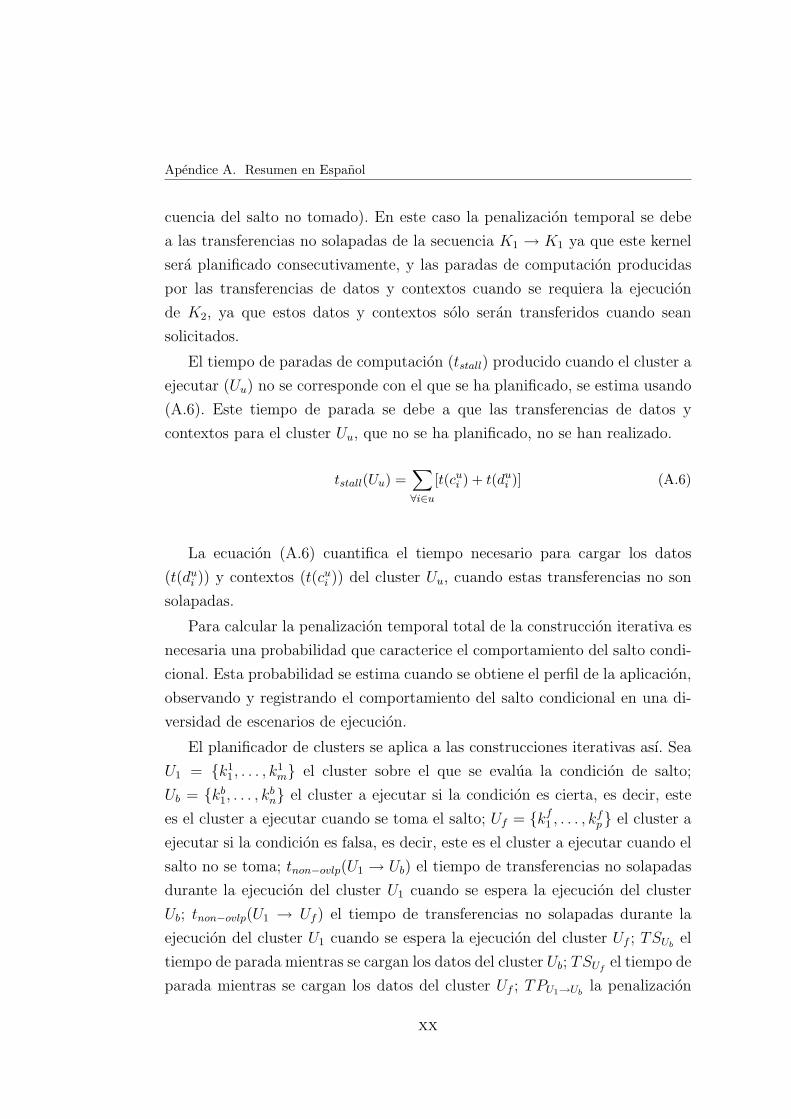
Apendice A. Resumen en Espanol
cuencia del salto no tomado). En este caso la penalizacion temporal se debe
a las transferencias no solapadas de la secuencia K1 → K1 ya que este kernel
sera planificado consecutivamente, y las paradas de computacion producidas
por las transferencias de datos y contextos cuando se requiera la ejecucion
de K2, ya que estos datos y contextos solo seran transferidos cuando sean
solicitados.
El tiempo de paradas de computacion (tstall) producido cuando el cluster a
ejecutar (Uu) no se corresponde con el que se ha planificado, se estima usando
(A.6). Este tiempo de parada se debe a que las transferencias de datos y
contextos para el cluster Uu, que no se ha planificado, no se han realizado.
tstall(Uu) =∑
∀i∈u
[t(cui ) + t(du
i )] (A.6)
La ecuacion (A.6) cuantifica el tiempo necesario para cargar los datos
(t(dui )) y contextos (t(cu
i )) del cluster Uu, cuando estas transferencias no son
solapadas.
Para calcular la penalizacion temporal total de la construccion iterativa es
necesaria una probabilidad que caracterice el comportamiento del salto condi-
cional. Esta probabilidad se estima cuando se obtiene el perfil de la aplicacion,
observando y registrando el comportamiento del salto condicional en una di-
versidad de escenarios de ejecucion.
El planificador de clusters se aplica a las construcciones iterativas ası. Sea
U1 = {k11, . . . , k
1m} el cluster sobre el que se evalua la condicion de salto;
Ub = {kb1, . . . , k
bn} el cluster a ejecutar si la condicion es cierta, es decir, este
es el cluster a ejecutar cuando se toma el salto; Uf = {kf1 , . . . , kf
p} el cluster a
ejecutar si la condicion es falsa, es decir, este es el cluster a ejecutar cuando el
salto no se toma; tnon−ovlp(U1 → Ub) el tiempo de transferencias no solapadas
durante la ejecucion del cluster U1 cuando se espera la ejecucion del cluster
Ub; tnon−ovlp(U1 → Uf ) el tiempo de transferencias no solapadas durante la
ejecucion del cluster U1 cuando se espera la ejecucion del cluster Uf ; TSUbel
tiempo de parada mientras se cargan los datos del cluster Ub; TSUfel tiempo de
parada mientras se cargan los datos del cluster Uf ; TPU1→Ubla penalizacion
xx

A.4. Planificacion en tiempo de compilacion
temporal total de la secuencia U1 → Ub; TPU1→Ufla penalizacion temporal
total de la secuencia U1 → Uf ; y ptaken la probabilidad de tomar el salto.
Los tiempos de parada de computacion se calculan mediante (A.7) y (A.8),
que se valen a su vez de (A.6).
TSUb= tstall(Ub) (A.7)
TSUf= tstall(Uf ) (A.8)
Las penalizaciones temporales totales se calculan como la suma pondera-
da del tiempo de transferencias no solapadas de una secuencia de clusters, y
el tiempo de parada de computacion de la otra secuencia, como se muestra
en (A.9) y (A.10). De acuerdo con la probabilidad de salto, en un escenario
estatico, el cuerpo del bucle se ejecuta 1/(1− ptaken) veces por cada ejecucion
del cluster Uf .
TPU1→Ub= tnon−ovlp(U1 → Ub)/(1 − ptaken) + TSUf
(A.9)
TPU1→Uf= tnon−ovlp(U1 → Uf ) + TSUb
/(1 − ptaken) (A.10)
Por medio de estas penalizaciones se determina la secuencia de clusters
alrededor del salto condicional con el menor tiempo de tranferencias no sola-
padas y paradas de computacion. Una vez se conoce esta secuencia, los ker-
nels se sintetizan sobre la arquitectura usando los algoritmos desarrollados
en [MKF+01] y [SEFHB05], quienes planifican los datos y los contextos con
detalle.
Resultados experimentales
Para evaluar el planificador de clusters se han usado experimentos sinteticos
y la aplicacion de ray-tracing [Gla89] ejecutandose sobre MorphoSys (ver Figu-
ra A.6). Los experimentos sinteticos son lo suficientemente diversos para cubrir
un amplio rango de posibles aplicaciones. Ray-tracing es una aplicacion real
que genera imagenes de gran realismo a partir de modelos geometricos en 3D.
xxi

Apendice A. Resumen en Espanol
De los experimentos sinteticos, 30 de ellos poseen construcciones if-then-
else en su CDFG, y 10 de ellos poseen construcciones iterativas. Todos los
experimentos sinteticos han sido sometidos inicialmente al algoritmo de parti-
cionamiento y luego se han planificado. Los experimentos if-then-else se han
particionado usando diferentes criterios de terminacion, es decir, se han usado
diferentes tamanos de FB con el fin de evaluar los posibles beneficios. De ray-
tracing, que posee construcciones iterativas en su CDFG como se muestra en
la Figura A.6, se han desarrollado 5 experimentos. Estos experimentos usan
un octree como estructura de datos para almacenar la geometrıa de la esce-
na. Un octree [LZ06] es un arbol en el que cada nodo posee ocho hijos. Cada
nodo corresponde a un cubo en el espacio. Las hojas del arbol almacenan los
objetos que conforman la escena. Los experimentos evaluados difieren en la
profundidad del octree.
Shading / Secondary rays
generation
Octree traversal
Eye rays generation
Ray-object intersection
Leaf node?
Hit? True True
Figura A.6: CDFG de la aplicacion de ray-tracing
Para los experimentos sinteticos, el planificador de clusters permite mejorar
el tiempo de ejecucion en un 35 % como promedio respecto a una version de los
experimentos sin planificar, es decir, aquella en la que los datos y los contextos
se transfieren cuando se solicitan. Ası mismo, el planificador de clusters permite
reducir las transferencias no solapadas de datos y contextos en un 81 % como
promedio, respecto a una version de los experimentos sin planificar.
Para los experimentos de ray-tracing, la mejora en el tiempo de ejecucion
que logra el planificador de clusters es un 32 % como promedio, respecto a una
version de los experimentos sin planificar. De la misma manera, la reduccion
de las transferencias no solapadas de datos y contextos despues de aplicar el
planificador de clusters es 55 % como promedio.
xxii
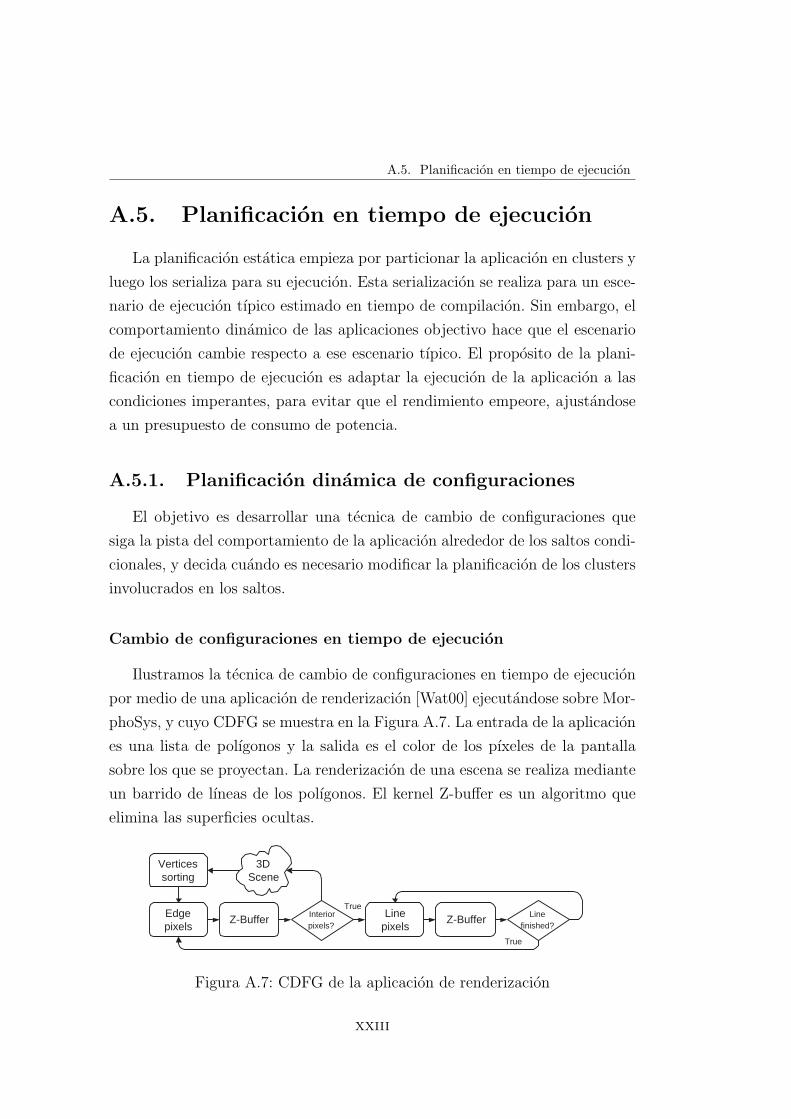
A.5. Planificacion en tiempo de ejecucion
A.5. Planificacion en tiempo de ejecucion
La planificacion estatica empieza por particionar la aplicacion en clusters y
luego los serializa para su ejecucion. Esta serializacion se realiza para un esce-
nario de ejecucion tıpico estimado en tiempo de compilacion. Sin embargo, el
comportamiento dinamico de las aplicaciones objectivo hace que el escenario
de ejecucion cambie respecto a ese escenario tıpico. El proposito de la plani-
ficacion en tiempo de ejecucion es adaptar la ejecucion de la aplicacion a las
condiciones imperantes, para evitar que el rendimiento empeore, ajustandose
a un presupuesto de consumo de potencia.
A.5.1. Planificacion dinamica de configuraciones
El objetivo es desarrollar una tecnica de cambio de configuraciones que
siga la pista del comportamiento de la aplicacion alrededor de los saltos condi-
cionales, y decida cuando es necesario modificar la planificacion de los clusters
involucrados en los saltos.
Cambio de configuraciones en tiempo de ejecucion
Ilustramos la tecnica de cambio de configuraciones en tiempo de ejecucion
por medio de una aplicacion de renderizacion [Wat00] ejecutandose sobre Mor-
phoSys, y cuyo CDFG se muestra en la Figura A.7. La entrada de la aplicacion
es una lista de polıgonos y la salida es el color de los pıxeles de la pantalla
sobre los que se proyectan. La renderizacion de una escena se realiza mediante
un barrido de lıneas de los polıgonos. El kernel Z-buffer es un algoritmo que
elimina las superficies ocultas.
3D Scene
Vertices sorting
Edge pixels
Z-Buffer Line pixels
Z-Buffer Interior pixels?
Line finished?
True
True
Figura A.7: CDFG de la aplicacion de renderizacion
xxiii

Apendice A. Resumen en Espanol
El kernel Line pixels dibuja un pıxel de una lınea y lo pasa al Z-buffer,
operacion que se repite hasta que la lınea se completa. La longitud de la lınea
determina el numero de veces que esta secuencia se repite. Pero los polıgonos
que componen una escena son muy diferentes entre sı y la longitud de las lıneas
a dibujar no son siempre las mismas. Por ejemplo, en la Figura A.8 la lınea i
posee una longitud diferente a la lınea j. Por lo tanto, la probabilidad del salto
condicional etiquetado como “Line finished?” varıa dinamicamente desde casi
0 (cuando se dibujan pocos pıxeles de lınea) hasta casi 1 (cuando la lınea es
muy larga).
Edge pixels
Line pixels
Line i
Line j
x
y
Figura A.8: Las lıneas de diferente longitud implican una probabilidad de saltovariable
La presencia de un salto condicional implica dos flujos de programa posi-
bles. La planificacion estatica determina una secuencia de clusters que se eje-
cuta inicialmente. A esta planificacion se le llamara Configuracion Inicial. Esta
configuracion inicial posee la mınima penalizacion temporal para el escenario
tıpico que define el perfil de la aplicacion. La otra secuencia posible, que no
se ejecuta en un comienzo porque posee una mayor penalizacion temporal
para el escenario tıpico, igualmente se planifica y almacena. A esta segunda
planificacion se le llamara Configuracion Complementaria.
La Figura A.9 muestra la penalizacion temporal del planificador estatico
como funcion de la probabilidad de salto. En este caso la planificacion de
clusters se ha realizado alrededor del salto condicional etiquetado como “Line
finished?”. La secuencia del salto tomado (Taken branch sequence) corresponde
a la secuencia Line pixels - Z-buffer - Line pixels, y la secuencia del salto no
tomado (Not taken branch sequence) corresponde a la secuencia Line pixels -
Z-buffer - Edge pixels. Las dos curvas intersectan en un punto, cuyo valor de
xxiv

A.5. Planificacion en tiempo de ejecucion
probabilidad se denomina probabilidad de cruce (cross-point probability). A la
izquierda de la probabilidad de cruce, la secuencia del salto no tomado posee la
mınima penalizacion temporal, y hacia la derecha de este valor es la secuencia
del salto tomado la que posee la mınima penalizacion temporal.
Taken Branch
Sequence
Not Taken Branch
Sequence
80
110
140
170
200
230
260
0,05 0,25 0,45 0,65 0,85
Taken branch probability
Tim
e p
enal
ty (
Clo
ck c
ycle
s)
Cross-point Probability
Figura A.9: Penalizacion temporal contra la probabilidad de tomar el salto
Como la probabilidad de salto puede cambiar dinamicamente, el objetivo
es detectar la situacion en la cual su valor sobrepasa la probabilidad de cruce y
ordenar el cambio de configuracion, de tal manera que la penalizacion temporal
sea siempre mınima.
La implementacion del planificador dinamico de configuraciones es como
sigue. En tiempo de compilacion se determinan y almacenan las configura-
ciones inicial y complementaria. La aplicacion comienza a ejecutarse con la
configuracion inicial. Por cada salto condicional del CDFG se agrega un con-
tador saturado al TinyRISC. El contador registrara el numero de veces que el
salto se toma. Al iniciar la ejecucion el contador tiene un valor de cero, pero
cada vez que se tome el salto se incrementa en uno. El valor del contador se
compara con la probabilidad de cruce. Si la iguala, el TinyRISC ordena la car-
ga de la configuracion complementaria en la CM. Cuando el valor del contador
iguale la probabilidad de cruce se puede esperar que el contador se siga incre-
mentando, lo que implica que en la proxima evaluacion del salto se requerira la
configuracion complementaria si se quiere mantener la penalizacion temporal
al mınimo. Durante la ejecucion de la configuracion complementaria, una vez
xxv

Apendice A. Resumen en Espanol
el salto no se toma, el TinyRISC ordena la recarga de la configuracion inicial
y pone el contador a cero.
Aunque la explicacion de la planificacion dinamica de configuraciones se
realizo con la aplicacion de renderizacion, puede aplicarse a cualquier apli-
cacion de la que se pueda obtener una caracterizacion del comportamiento de
la probabilidad de salto.
Resultados experimentales
Para evaluar la planificacion dinamica de configuraciones se han implemen-
tado cuatro experimentos de renderizacion que representan cuatro modelos
estandar de la computacion grafica. El tiempo de ejecucion se mejora en un
46 % como promedio respecto a una version de los experimentos sin planificar,
es decir, aquella en la que los datos y los contextos se transfieren solo cuando se
solicitan. Considerando que con la planificacion estatica se lograba un 30 % de
mejora en el tiempo de ejecucion, la planificacion dinamica de configuraciones
aporta un 16 % mas de mejora.
A.5.2. Coherencia de datos
Considerando que en MorphoSys hay 64 RCs operando en paralelo, muchas
de ellas pueden requerir datos bastante dispersos en memoria principal. Es-
ta falta de localidad espacial puede significar una gran cantidad de paradas
de ejecucion mientras la carga de datos se realiza. Sin embargo, si las aplica-
ciones poseen algun grado de coherencia de datos y se elige un modelo para
implementarla, las paradas de ejecucion se pueden reducir.
La coherencia de datos [GP89] significa que varias RCs presentan el mismo
patron de acceso a memoria a medida que se ejecuta la aplicacion. Por ejemplo,
en las aplicaciones graficas de 3D es normal encontrar gran coherencia de datos
porque los colores de pıxeles vecinos se obtienen despues de procesar datos si-
milares ya que cubren una pequena region del espacio. El modelo de coherencia
elegido se adapta al estilo SIMD de la arquitectura, y se explicara mediante la
aplicacion de ray-tracing (ver Figura A.6).
El objetivo es procesar completamente un rayo (pıxel) en cada RC. Por
xxvi

A.5. Planificacion en tiempo de ejecucion
lo tanto, despues de ejecutar el kernel Octree traversal sobre 64 rayos, en el
peor de los casos cada rayo visitara un nodo diferente y para la siguiente
ejecucion del kernel debera cargarse la informacion de 64 nodos hijos. Sin
embargo, si los rayos que se procesan en paralelo cubren un region reducida
del espacio, se puede esperar que recorran el arbol de manera similar. De las
posibilidades existentes y de acuerdo con el modelo SIMD de la arquitectura, se
ha asumido que todas los RCs de la misma columna del modulo reconfigurable
son coherentes. Esto significa que cada columna procesara el mismo nodo, por
lo que en todo el modulo reconfigurable se procesaran ocho nodos diferentes.
Por lo tanto, al comienzo de la aplicacion se carga la informacion de 64 rayos,
uno por RC, que permaneceran en las RCs hasta que se procesen por completo.
Para cada ejecucion del kernel Octree traversal se cargaran ocho nodos, uno
por columna. De esta manera se reduce la latencia de memoria porque se
reduce el numero de datos a cargar, mientras que aun se obtienen mejoras en
el rendimiento gracias a que las aplicaciones poseen un grado importante de
coherencia de datos.
El concepto de coherencia de datos es usado tambien en la implementacion
de un esquema de precarga de datos, como se explica mas adelante.
A.5.3. Planificacion dinamica de datos
Una caracterıstica de los kernels es que poseen un tamano de datos de en-
trada fijo. Sin embargo, en nuestras aplicaciones objetivo, los datos de entrada
de un kernel se eligen entre un conjunto mas grande de posibles datos de en-
trada, de acuerdo con las condiciones de ejecucion. Si fuese posible cargar de
manera anticipada todo el conjunto de posibles datos de entrada de un kernel,
este podrıa iniciar su ejecucion de inmediato, sin parar la ejecucion. Pero esto
suele ser impracticable por el tamano del conjunto de posibles datos de entrada
y la limitacion en el ancho de banda. Una alternativa consiste en precargar un
grupo de datos, de tal manera que si los solicitados por el kernel para su eje-
cucion se encuentran entre ellos no se producen paradas de ejecucion. Cuanto
mas grande sea el grupo de datos a precargar, menor sera la posibilidad de te-
ner paradas de ejecucion. Esto implica un compromiso rendimiento/potencia.
xxvii

Apendice A. Resumen en Espanol
El rendimiento se refiere al tiempo de ejecucion de la aplicacion, y la potencia
a la potencia consumida por las transferencias de datos.
Si los datos precargados son los correctos, el rendimiento sera incrementado
porque se reducen las paradas de ejecucion. Dependiendo del presupuesto de
potencia, un tamano determinado de datos podra ser precargado, y la mejora
en rendimiento dependera de la precision al elegir los datos a precargar. La
ejecucion de la aplicacion se podra configurar para que se ajuste a diferentes
requisitos de rendimiento y potencia. La exploracion de este compromiso se
realiza mediante el concepto de optimizacion de Pareto.
Compromiso rendimiento/potencia
El concepto de optimizacion de Pareto [OR94] se aplica en problemas en
los que existen conflictos de optimizacion entre variables. Una solucion se con-
sidera optima si no se puede mejorar sin afectar ninguna de las otras que se
busca optimizar.
Suponiendo la ejecucion de la aplicacion de ray-tracing basada en octree
sobre MorphoSys, despues de procesar un rayo contra la informacion de un
nodo se pueden visitar ocho nodos hijos. En tiempo de compilacion se ha
probado a precargar un numero diferente de nodos hijos para evaluar su aporte
en la mejora de rendimiento. Por cada tamano de datos precargados se obtiene
el tiempo de ejecucion y el consumo de potencia debido a las transferencias de
datos. De esta manera se construye una curva de Pareto para la aplicacion de
ray-tracing como se muestra en la Figura A.10.
En esta figura se puede ver cuanta potencia se consume para ajustarse a
una meta de rendimiento. Los puntos destacados en la curva corresponden
a diferentes tamanos de datos precargados, expresados como una fraccion del
conjunto de posibles datos de entrada. Un tamano mayor de datos precargados
representa un incremento mayor en el rendimiento, y tambien un consumo
mayor de potencia.
Como el compromiso rendimiento/potencia requerido solo se conoce en
tiempo de ejecucion, el objetivo es obtener un grupo de soluciones con diferen-
tes compromisos rendimiento/potencia (curva de Pareto) en tiempo de com-
xxviii

A.5. Planificacion en tiempo de ejecucion
9% 18%
45%
27%
620
640
660
680
130 150 170 190 210 230
Power per 32-bits word access (x10 3 )
Tim
e (C
lock
Cyc
les)
Figura A.10: Curva de Pareto que ilustra el compromiso entre rendimiento ypotencia para la aplicacion de ray-tracing
pilacion, y luego elegir el mas adecuado en tiempo de ejecucion. La aplicacion
comienza a ejecutarse con un compromiso rendimiento/potencia sugerido por
su perfil. Una vez se esta ejecutando, el TinyRISC se encarga de verificar si las
metas de rendimiento se estan alcanzando, mediante la evaluacion de check-
points introducidos en el programa. Si no es ası, el TinyRISC selecciona otro
punto de la curva de Pareto que incrementa el tamano de los datos a precargar
de tal manera que se pueda elevar el rendimiento. Sin embargo, el tamano de
los datos a precargar se puede incrementar solo si el presupuesto de potencia
lo permite.
La mejora en el rendimiento producida por la precarga de datos se debe a la
tasa de aciertos que logra, la misma que depende de la calidad de la eleccion de
los datos a precargar. Para definir el esquema de seleccion de datos a precargar
es necesario estudiar con detalle la aplicacion y valerse de sus particularidades,
como se explica en la siguiente subseccion.
Implementacion de un esquema de precarga de datos para graficos
de 3D
El siguiente esquema de precarga de datos esta basado en las caracterısticas
geometricas de ray-tracing. Esta aplicacion se basa en un octree, cuyo esquema
de numeracion de nodos se muestra en la Figura A.11.
xxix

Apendice A. Resumen en Espanol
x
y
z
0 4
2 6
3
7
5
Figura A.11: Numeracion de nodos del octree (El nodo oculto es el numero 1)
El octree es atravesado por el rayo para dibujar un pıxel en la pantalla.
El kernel Octree traversal (ver Figura A.6) se encarga de recorrer el arbol
de arriba abajo hasta llegar a una hoja que es donde residen los objetos que
componen la imagen. Despues de ejecutar el kernel Octree traversal sobre un
nodo, se determinan los subnodos atravesados por el rayo. Cada nodo posee
ocho hijos pero solo un maximo de cuatro nodos sera atravesado por el rayo
[RUL00].
El esquema de precarga de datos se basa en el modelo de coherencia de
datos descrito anteriormente. Para implementarlo se usan stacks para almace-
nar la trayectoria del rayo por cada columna del modulo reconfigurable. Una
vez el kernel Octree traversal determina, en orden, los nodos que atraviesa el
rayo en un nivel de profundidad del octree, estos se almacenan en el stack co-
rrespondiente que opera en modo FIFO (First In - First Out), de manera que
el nodo de entrada sera el primero en procesarse. Para definir los subnodos a
precargar se toman dos nodos hermanos almacenados consecutivamente en el
stack, nodei y nodei+1, respectivamente, y se usa la Tabla A.1 para definir los
hijos de nodei a precargar. Por ejemplo, si en un nivel determinado del octree,
el rayo cruza los nodos 6 y 4, despues de procesar el nodo de entrada 6, sus
nodos hijos a precargar seran 0, 1, 4 y 5, ya que el nodo que sigue en su mismo
nivel es el 4.
xxx

A.6. Conclusiones
Tabla A.1: Nodos hijos a precargar de acuerdo con el orden de nodos visitados
nodei+1
nodei 0 1 2 3 4 5 6 7
0 - 1, 3, 5, 7 2, 3, 6, 7 3, 7 4, 5, 6, 7 5, 7 6, 7 7
1 0, 2, 4, 6 - 2, 6 2, 3, 6, 7 4, 6 4, 5, 6, 7 6 6, 7
2 0, 1, 4, 5 1, 5 - 1, 3, 5, 7 4, 5 5 4, 5, 6, 7 5 7
3 0, 4 0, 1, 4, 5 0, 2, 4, 6 - 4 4, 5 4, 6 4, 5, 6, 7
4 0, 1, 2, 3 1, 3 2, 3 3 - 1, 3, 5, 7 2, 3, 6, 7 3, 7
5 0, 2 0, 1, 2, 3 2 2, 3 0, 2, 4, 6 - 2, 6 2, 3, 6, 7
6 0, 1 1 0, 1, 2, 3 1, 3 0, 1, 4, 5 1, 5 - 1, 3, 5, 7
7 0 0, 1 0, 2 0, 1, 2, 3 0, 4 0, 1, 4, 5 0, 2, 4, 6 -
Resultados experimentales
Para evaluar el esquema de precarga de datos para aplicaciones graficas
de 3D se han implementado seis experimentos de ray-tracing en los cuales la
misma escena se construye con diferentes profundidades de arbol y tamanos
de pantalla. En todos los experimentos siempre se precarga un nodo hermano
del actual, y el numero de hijos a precargar es de dos y cuatro. Cuando se
precargan un hermano y dos hijos se logra una tasa de aciertos de 54 % como
promedio, lo que significa que el tiempo de ejecucion esta un 6% por encima
del tiempo que se obtendrıa si se precargaran todos los nodos hijos. Para esta
misma configuracion el consumo de potencia se reduce un 59 % como promedio
respecto a la precarga de todos los nodos hijos. Mediante la precarga de un
nodo hermano y cuatro hijos se logra una tasa de aciertos del 73 %, lo que se
traduce en un tiempo de ejecucion que es un 2 % mas del tiempo de ejecucion
cuando se realiza una precarga de todos los nodos hijos. Para esta misma
configuracion el consumo de potencia se reduce un 36 % respecto a la precarga
de todos los nodos hijos.
A.6. Conclusiones
Los sistemas reconfigurables surgen como un nuevo paradigma para satis-
facer la demanda simultanea de rendimiento y flexibilidad que poseen las apli-
xxxi
Apendice A. Resumen en Espanol
caciones actuales. Sin embargo, la abundancia de recursos computacionales y
la flexibilidad funcional de los sistemas reconfigurables no son suficientes para
garantizar su futuro. Son las tecnicas de compilacion (de planificacion entre
ellas) quienes permiten ejecutar eficientemente las aplicaciones, aprovechando
al maximo los recursos disponibles. Se han publicado muchos trabajos sobre
planificacion estatica para sistemas reconfigurables. Sin embargo, las aplica-
ciones actuales estan lejos de ser estaticas. Estas aplicaciones se caracterizan
por tener flujos dinamicos de programa que dependen de los datos de entrada
o de la interaccion del usuario, procesan grandes cantidades de datos y estan
sometidas a restricciones de tiempo real.
Las tecnicas de planificacion para aplicaciones dinamicas propuestas en
este trabajo se concibieron para integrarse en el entorno de compilacion de
MorphoSys, de tal manera que los algoritmos de planificacion presentados per-
miten generalizarlo, ofreciendo el soporte necesario para sintetizar aplicaciones
dinamicas sobre MorphoSys.
Para modelar el comportamiento dinamico de las aplicaciones objetivo se
considera la ejecucion condicional de tareas. Para ello se ha adoptado el grafo
de flujo de datos y control (CDFG) que permite incluir explıcitamente toda la
informacion de secuenciamiento y control en el mismo grafo.
Las tecnicas de planificacion propuestas buscan reducir el numero de ciclos
de reloj necesarios para ejecutar una aplicacion, con el objetivo de cumplir
una meta de rendimiento dentro de un presupuesto de consumo de potencia.
Estas tecnicas se dividen en estaticas y dinamicas.
En tiempo de compilacion, las aplicaciones se particionan en clusters. Para
realizar la particion de la aplicacion en clusters se ha desarrollado un nuevo
algoritmo de particionamiento que tiene en cuenta la presencia de saltos condi-
cionales en el CDFG. Una vez se han obtenido los clusters, se serializan para la
ejecucion. La serializacion de clusters en tiempo de compilacion determina una
secuencia de clusters con las mınimas paradas de computacion, de acuerdo con
un escenario de ejecucion tipo que se obtiene mediante un estudio del perfil de
la aplicacion a sintetizar.
Las caracterısticas dinamicas de las aplicaciones objetivo demuestran que la
planificacion estatica no es suficiente para lograr las metas de rendimiento. El
xxxii

A.6. Conclusiones
comportamiento dinamico de la aplicacion debido a las dependencias de datos
y a la interaccion del usuario se han modelado mediante una probabilidad
de salto. Como esta probabilidad varıa durante la ejecucion, para evitar la
perdida de rendimiento se ha desarrollado una tecnica que permite seguir la
pista del comportamiento de la aplicacion alrededor de un salto condicional,
de tal manera que puede ordenar, en tiempo de ejecucion, la carga de una
nueva secuencia de clusters alrededor del salto que garantice el mınimo valor
de paradas de computacion para las condiciones de ejecucion imperantes.
Los datos de entrada de las tareas que componen una aplicacion solo se
conocen en tiempo de ejecucion y hacen parte de un conjunto mas grande de
datos posibles. Si se pudieran cargar todo los datos posibles de entrada de un
kernel, no habrıan paradas de ejecucion producidas por la falta de datos en la
memoria interna, aunque el consumo de potencia debido a las transferencias de
datos serıa elevado. Como esto no es practico, es necesario realizar una carga
especulativa de una fraccion del conjunto de datos posibles de entrada para
que el consumo de potencia no se dispare, y aun se pueda evitar una perdida
de rendimiento. Esto implica la implementacion de un esquema de precarga
selectiva de datos, que tiene asociado un compromiso entre la potencia y el
rendimiento. La calidad del esquema de precarga se determina por su tasa
de aciertos que permite evitar la perdida de rendimiento, y por la potencia
consumida por las transferencias de datos. Para explorar el compromiso entre
potencia y rendimiento se usado el concepto de Pareto. En tiempo de compi-
lacion se obtiene una curva de Pareto para las variables involucradas. Cada
punto de esta curva representa un compromiso potencia/rendimiento especıfi-
co. Durante la ejecucion de la aplicacion, se elige un punto de esta curva para
satisfacer las restricciones de rendimiento dentro de un presupuesto de poten-
cia. Cada punto de la curva tiene asociado un tamano del subconjunto de datos
que se debe precargar, sabiendo que la tasa de aciertos esta determinada por
la calidad de la heurıstica empleada para elegir este subconjunto de datos de
entre todos los posibles.
Los resultados experimentales obtenidos demuestran las bondades de los
algoritmos de planificacion propuestos. Mediante el uso de los algoritmos de
planificacion estatica, y las tecnicas de tiempo de ejecucion de cambio de con-
xxxiii

Apendice A. Resumen en Espanol
texto y carga anticipada de datos en aplicaciones reales como ray-tracing basa-
da en octree, es posible lograr un tiempo de ejecucion que es solo un 2 % mas
que el tiempo de ejecucion obtenido cuando se implementa una precarga per-
fecta de datos. Para este mismo caso, el consumo de potencia despues de aplicar
nuestras tecnicas se reduce en un 36 % respecto a una ejecucion basada en una
precarga perfecta de datos.
A.7. Publicaciones
Las siguientes son las publicaciones que se han producido a partir del pre-
sente trabajo:
1. F. Rivera, M. Sanchez-Elez, R. Hermida, and N. Bagherzadeh. Schedul-
ing methodology for conditional execution of kernels onto multi-context
reconfigurable architectures. IET Computers & Digital Techniques,
2(3):199–213, May 2008.
2. F. Rivera, M. Sanchez-Elez, and N. Bagherzadeh. Configuration and
data scheduling for executing dynamic applications onto multi-context
reconfigurable architectures. In Proc. Intl. Conf. on Engineering of Re-
configurable Systems and Algorithms (ERSA), pages 85–91, June 2007.
3. F. Rivera, M. Sanchez-Elez, M. Fernandez, R. Hermida, and N. Bagher-
zadeh. Configuration scheduling for conditional branch execution onto
multi-context reconfigurable architectures. In Proc. Intl. Conf. on Field
Programmable Logic and Applications (FPL), pages 589–596, August
2006.
4. J. Davila, A. de Torres, J. Sanchez, M. Sanchez-Elez, N. Bagherzadeh,
and F. Rivera. Design and implementation of a rendering algorithm in
a SIMD reconfigurable architecture (MorphoSys). In Proc. Design, Au-
tomation and Test in Europe Conference and Exhibition (DATE), pages
52–57, March 2006.
xxxiv
A.7. Publicaciones
5. F. Rivera, M. Sanchez-Elez, M. Fernandez, and N. Bagherzadeh. An
approach to execute conditional branches onto SIMD multi-context re-
configurable architectures. In Proc. Euromicro Conference on Digital
System Design (DSD), pages 396–402, August 2005.
6. F. Rivera, M. Sanchez-Elez, M. Fernandez, R. Hermida, and N. Bagher-
zadeh. Low power data prefetch for 3D image applications on coarse-
grain reconfigurable architectures. In Proc. Intl. Parallel and Distributed
Processing Symposium (IPDPS), page 171, April 2005.
7. F. Rivera, M. Sanchez-Elez, M. Fernandez, R. Hermida, and N. Ba-
gherzadeh. Efficient mapping of hierarchical trees on coarse-grain re-
configurable architectures. In Proc. Intl. Conf. on Hardware/Software
Codesign and System Synthesis (CODES+ISSS), pages 30–35, Septem-
ber 2004.
8. F. Rivera, M. Sanchez-Elez, M. Fernandez, R. Hermida, and N. Bagher-
zadeh. Ejecucion paralela de arboles jerarquicos en arquitecturas recon-
figurables de grano grueso. In Actas de las XV Jornadas de Paralelismo,
pages 126–131, September 2004.
xxxv


Bibliography
[ABD92] J. Arnold, D. Buell, and E. Davis. Splash 2. In Proc. ACMSymp. on Parallel Algorithms and Architectures, pages 316–322,June 1992.
[Abn01] A. Abnous. Low-Power Domain-Specific Processors for DigitalSignal Processing. PhD thesis, EECS Department, University ofCalifornia, Berkeley, 2001.
[ACG+92] A. Abnous, C. Christensen, J. Gray, J. Lenell, A. Naylor, andN. Bagherzadeh. Design and implementation of TinyRISC mi-croprocessor. Microprocessors and Microsystems, 16(4):187–194,1992.
[Act07] Actel Devices, http://www.actel.com/products/devices.aspx,2007.
[Alt07] Altera Devices, http://www.altera.com/products/devices, 2007.
[APB02] M. Anido, A. Paar, and N. Bagherzadeh. A novel method forimproving the operation autonomy of SIMD processing elements.In Proc. Symp. on Integrated Circuits and Systems Design, pages49–54, sep 2002.
[Atm07] Atmel FPGAs Devices, http://www.atmel.com/products/fpga,2007.
[BEM+03] V. Baumgarte, G. Ehlers, F. May, A. Nuckel, M. Vorbach, andM. Weinhardt. PACT XPP - A self-reconfigurable data process-ing architecture. The Journal of Supercomputing, 26(2):167–184,September 2003.
[BGD+04a] N. Bansal, S. Gupta, N. Dutt, A. Nicolau, and R. Gupta.Interconnect-aware mapping of applications to coarse-grain re-configurable architectures. In Proc. Intl. Conf. on Field Pro-
xxxvii
Bibliography
grammable Logic and Applications (FPL), pages 891–899, August2004.
[BGD+04b] N. Bansal, S. Gupta, N. Dutt, A. Nicolau, and R. Gupta. Net-work topology exploration of mesh-based coarse-grain reconfig-urable architectures. In Proc. Design, Automation and Testin Europe Conference and Exhibition (DATE), pages 474–479,February 2004.
[Bon01] K. Bondalapati. Parallelizing DSP nested loops on reconfigurablearchitectures using data context switching. In Proc. Design andAutomation Conference (DAC), pages 273–276, June 2001.
[BP02] K. Bondalapati and V. Prasanna. Reconfigurable computing sys-tems. Proc. IEEE, 90(7):1201–1217, July 2002.
[BR96] S. Brown and J. Rose. FPGA and CPLD architectures: A tuto-rial. IEEE Des. Test. Comput., 13(2):42–57, 1996.
[BS06] J. Braunes and R. Spallek. A compiler-oriented architecture de-scription for reconfigurable systems. In Proc. Intl. Workshop Re-configurable Computing: Architectures and Applications (ARC),pages 443–448, March 2006.
[CBK+06] S. Chai, N. Bellas, G. Kujawa, T. Ziomek, L. Dawson, T. Scam-inaci, M. Dwyer, and D. Linzmeier. Reconfigurable streamingarchitectures for embedded smart cameras. In Proc. Conf. onComputer Vision and Pattern Recognition Workshop, pages 122–122, June 2006.
[CCE+05] S. Chai, S. Chiricescu, R. Essick, B. Lucas, P. May, K. Moat,J. Norris, M. Schuette, and A. Lopez-Lagunas. Streaming pro-cessors for next-generation mobile imaging applications. IEEECommun. Mag., 43(12):81–89, December 2005.
[CCKH00] K. Compton, J. Cooley, S. Knol, and S. Hauck. Configurationrelocation and defragmentation for reconfigurable computing. InProc. IEEE Symp. on Field-Programmable Custom ComputingMachines (FCCM), pages 279–280, April 2000.
[CH02] K. Compton and S. Hauck. Reconfigurable computing: A surveyof systems and software. ACM Computing Surveys, 34(2):171–210, June 2002.
xxxviii
Bibliography
[CLV01] S. Chiricescu, M. Leeser, and M. Vai. Design and analysis ofa dynamically reconfigurable three-dimensional FPGA. IEEETrans. VLSI Syst., 9(1):186–196, February 2001.
[CMC+91] P. Chang, S. Mahlke, W. Chen, N. Warter, and W. Hwu.IMPACT: An architectural framework for multiple-instruction-issue processors. In Proc. Intl. Symp. on Computer Architecture(ISCA), pages 266–275, May 1991.
[Con97] D. Connors. Memory profiling for directing data speculative op-timizations and scheduling. Master’s thesis, University of Illinois,Urbana-Champaing, 1997.
[CV99] K. Chatha and R. Vemuri. Hardware-software codesign for dy-namically reconfigurable architectures. In Proc. Intl. Conf. onField Programmable Logic and Applications (FPL), pages 175–185, August 1999.
[DdTS+06] J. Davila, A. de Torres, J. Sanchez, M. Sanchez-Elez, N. Bagher-zadeh, and F. Rivera. Design and implementation of a renderingalgorithm in a SIMD reconfigurable architecture (MorphoSys).In Proc. Design, Automation and Test in Europe Conference andExhibition (DATE), pages 52–57, March 2006.
[DGG05a] G. Dimitroulakos, M. Galanis, and C. Goutis. Alleviating thedata memory bandwidth bottleneck in coarse-grained reconfig-urable arrays. In Proc. Intl. Conf. on Application-Specific Sys-tems, Architecture Processors (ASAP), pages 161–168, July 2005.
[DGG05b] G. Dimitroulakos, M. Galanis, and C. Goutis. A compiler methodfor memory-conscious mapping of applications on coarse-grainedreconfigurable architectures. In Proc. Intl. Parallel and Dis-tributed Processing Symposium (IPDPS), page 160, April 2005.
[dM94] G. de Micheli. Synthesis and optimization of digital circuits.McGraw-Hill, 1994.
[GDWL94] D. Gajski, N. Dutt, A. Wu, and S. Lin. High-level synthesis:introduction to chip and system design. Kluwer Academic Pub-lishers, 1994.
[GK89] J. Gray and T. Kean. Configurable hardware: A new paradigmfor computation. In Proc. Decennial CalTech Conference onVLSI, pages 277–293, March 1989.
xxxix

Bibliography
[Gla84] A. Glassner. Space subdivision for fast ray tracing. IEEE Com-put. Graph. Appl., 4(10):15–22, October 1984.
[Gla89] A. Glassner. An Introduction to Ray Tracing. Academic Press,1989.
[GP89] S. Green and D. Paddon. Exploiting coherence for multiprocessorray tracing. IEEE Comput. Graph. Appl., 9(6):12–26, November1989.
[GSB+05] Y. Guo, G. Smit, H. Broersma, M. Rosien, P. Heysters, andT. Krol. Mapping applications to a coarse grain reconfigurablesystem. In P. Lysaght and W. Rosenstiel, editors, New Algo-rithms, Architectures and Applications for Reconfigurable Com-puting, pages 93–103. Springer, 2005.
[GVH01] T. Givargis, F. Vahid, and J. Henkel. System-level explorationfor pareto-optimal configurations in parameterized systems-on-a-chip. In Proc. Intl. Conf. on Computer-Aided Design (ICCAD),pages 25–30, November 2001.
[Har01] R. Hartenstein. A decade of reconfigurable computing: a vision-ary retrospective. In Proc. Design, Automation and Test in Eu-rope Conference and Exhibition (DATE), pages 642–649, March2001.
[Hau98] S. Hauck. The roles of fpgas in reprogrammable systems. Proc.IEEE, 86(4):615–638, April 1998.
[HFHK04] S. Hauck, T. Fry, M. Hosler, and J. Kao. The Chimaera reconfig-urable functional unit. IEEE Trans. VLSI Syst., 12(2):206–217,February 2004.
[HM02] Z. Huang and S. Malik. Exploiting operation level parallelismthrough dynamically reconfigurable datapaths. In Proc. Designand Automation Conference (DAC), pages 337–342, June 2002.
[HS03] P. Heysters and G. Smit. Mapping of DSP algorithms on theMONTIUM architecture. In Proc. Reconfigurable ArchitecturesWorkshop (RAW), page 180, April 2003.
[HW97] J. Hauser and J. Wawrzynek. Garp: A MIPS processor witha reconfigurable coprocessor. In Proc. IEEE Symp. on Field-Programmable Custom Computing Machines (FCCM), pages 12–21, April 1997.
xl

Bibliography
[ITR06] International Technology Roadmap forSemiconductors ITRS 2006 Update,http://www.itrs.net/links/2006update/2006updatefinal.htm,2006.
[Kam03] A. Kamalizad. Several DVB-T cores mapping into MorphoSysarchitecture. Master’s thesis, EECS Department, University ofCalifornia, Irvine, 2003.
[KPPR00] F. Koushanfar, V. Prabhu, M. Potkonjak, and J. Rabaey. Pro-cessors for mobile applications. In Proc. Intl. Conf. on ComputerDesign (ICCD), pages 603–608, September 2000.
[KR07] I. Kuon and J. Rose. Measuring the gap between FPGAs andASICs. IEEE Trans. Computer-Aided Design, 26(2):203–215,February 2007.
[Lat07] Lattice FPGAs Devices, http://www.latticesemi.com/products/fpga, 2007.
[LBH+03] J. Leijten, G. Burns, J. Huisken, E. Waterlander, and A. vanWei. AVISPA: A massively parallel reconfigurable accelerator. InProc. Intl. Symp. on System-On-Chip, pages 165–168, November2003.
[LCD03a] J. Lee, K. Choi, and N. Dutt. An algorithm for mapping loopsonto coarse-grained reconfigurable architectures. In Proc. ACMConf. on Language, Compiler, and Tool Support for EmbeddedSystems (LCTES), pages 183–188, July 2003.
[LCD03b] J. Lee, K. Choi, and N. Dutt. Compilation approach for coarse-grained reconfigurable architectures. IEEE Des. Test. Comput.,20(1):26–33, January 2003.
[LH02] Z. Li and S. Hauck. Configuration prefetching techniques for par-tial reconfigurable coprocessor with relocation and defragmenta-tion. In Proc. ACM Intl. Symp. on Field Programmable GateArrays (FPGA), pages 187–195, February 2002.
[LKJ+04] J. Lee, Y. Kim, J. Jung, S. Kang, and K. Choi. Reconfigurablealu array architecture with conditional execution. In Proc. Intl.SoC Design Conference (ISOCC), October 2004.
xli
Bibliography
[LYC02] S. Lee, S. Yoo, and K. Choi. Reconfigurable SoC design withhierarchical FSM and synchronous dataflow model. In Proc. Intl.Conf. on Hardware Software Codesign (CODES), pages 199–204,May 2002.
[LZ06] E. Langetepe and G. Zachmann. Geometric Data Structures forComputer Graphics. A. K. Peters Ltd., 2006.
[Mae00] R. Maestre. Estrategias de Planificacion para Sistemas Re-configurables Multi-Contexto. PhD thesis, Depto. Arquitecturade Computadores y Automatica, Universidad Complutense deMadrid, 2000.
[MBV+02] T. Marescaux, A. Bartic, D. Verkest, S. Vernalde, and R. Lauw-ereins. Interconnection networks enable fine-grain dynamicmulti-tasking on FPGAs. In Proc. Intl. Conf. on FieldProgrammable Logic and Applications (FPL), pages 741–763,September 2002.
[MD96] E. Mirsky and A. DeHon. MATRIX: A reconfigurable computingarchitecture with configurable instruction distribution and de-ployable resources. In Proc. IEEE Symp. on Field-ProgrammableCustom Computing Machines (FCCM), pages 157–166, April1996.
[MKF+01] R. Maestre, F. Kurdahi, M. Fernandez, R. Hermida, and N. Ba-gherzadeh. A framework for reconfigurable computing: Taskscheduling and context management. IEEE Trans. VLSI Syst.,9(6):858–873, December 2001.
[MLM+05] B. Mei, A. Lambrechts, J. Mignolet, D. Verkest, and R. Lauw-ereins. Architecture exploration for a reconfigurable architecturetemplate. IEEE Des. Test. Comput., 22(2):90–101, March 2005.
[MO98] T. Miyamori and U. Olukotun. A quantitative analysis of re-configurable coprocessors for multimedia applications. In Proc.IEEE Symp. on Field-Programmable Custom Computing Ma-chines (FCCM), pages 2–11, April 1998.
[MP03] P. Magarshack and P. Paulin. System-on-chip beyond thenanometer wall. In Proc. Design and Automation Conference(DAC), pages 419–424, June 2003.
xlii

Bibliography
[MPE96] ISO/IEC 13818. Generic coding of moving pictures and associ-ated audio information (MPEG-2), 1996.
[MSHA+97] W. Mangione-Smith, B. Hutchings, D. Andrews, A. DeHon,C. Ebeling, R. Hartenstein, O. Mencer, J. Morris, K. Palem,V. Prasanna, and H. Spaanenburg. Seeking solutions in con-figurable computing. IEEE Computer, 30(12):38–43, December1997.
[MVV+02] B. Mei, S. Vernalde, D. Verkest, H. De Man, and R. Lauwere-ins. DRESC: A retargetable compiler for coarse-grained reconfig-urable architectures. In Proc. Intl. Conf. on Field ProgrammableTechnology (FPT), pages 166–173, 2002.
[MVV+03a] B. Mei, S. Vernalde, D. Verkest, H. de Man, and R. Lauwereins.ADRES: An architecture with tightly coupled VLIW processorand coarse-grained reconfigurable matrix. In Proc. Intl. Conf. onField Programmable Logic and Applications (FPL), pages 61–70,September 2003.
[MVV+03b] B. Mei, S. Vernalde, D. Verkest, H. de Man, and R. Lauwere-ins. Exploiting loop-level parallelism on coarse-grained recon-figurable architectures using modulo scheduling. In Proc. De-sign, Automation and Test in Europe Conference and Exhibition(DATE), pages 296–301, March 2003.
[Nar93] P. Narayanan. Processor autonomy on SIMD architectures. InProc. Intl. Conf. on Supercomputing (ICS), pages 127–136, 1993.
[NB04] J. Noguera and R. Badia. Multitasking on reconfigurable ar-chitectures: Microarchitecture support and dynamic scheduling.ACM Trans. on Embedded Computing Systems, 3(2):385–406,May 2004.
[OR94] M. Osborne and A. Rubinstein. A Course in Game Theory. MITPress, July 1994.
[Pan05] C. Pan. Streaming Computing Platform Design: DVB-T Imple-mentation on a Reconfigurable Architecture. PhD thesis, EECSDepartment, University of California, Irvine, 2005.
[PB99] K. Purna and D. Bhatia. Temporal partitioning and schedul-ing data flow graphs for reconfigurable computers. IEEE Trans.Comput., 48(6):579–590, June 1999.
xliii

Bibliography
[PFKM06] H. Park, K. Fan, M. Kudlur, and S. Mahlke. Modulo graphembedding: mapping applications onto coarse-grained reconfig-urable architectures. In Proc. Intl. Conf. on Compilers, Architec-ture and Synthesis for Embedded Systems (CASES), pages 136–146, October 2006.
[QSN06] Y. Qu, J. Soininen, and J. Nurmi. A parallel configuration modelfor reducing the run-time reconfiguration overhead. In Proc. De-sign, Automation and Test in Europe Conference and Exhibition(DATE), pages 965–969, March 2006.
[Rab00] J. Rabaey. Low-power silicon architectures for wireless commu-nications. In Proc. Asian and South Pacific Design and Automa-tion Conference (ASP-DAC), pages 377–380, June 2000.
[Rau94] B. Rau. Iterative modulo scheduling: an algorithm for softwarepipelining loops. In Proc. Intl. Symp. on Microarchitecture, pages63–74, November 1994.
[RESV93] J. Rose, A. El Gamal, and A. Sangiovanni-Vincentelli. Architec-ture of field-programmable gate arrays. Proc. IEEE, 81(7):1013–1029, July 1993.
[RMVC05] J. Resano, D. Mozos, D. Verkest, and F. Catthoor. A reconfigu-ration manager for dynamically reconfigurable hardware. IEEEDes. Test. Comput., 22(5):452–460, September 2005.
[RSEB07] F. Rivera, M. Sanchez-Elez, and N. Bagherzadeh. Configura-tion and data scheduling for executing dynamic applicationsonto multi-context reconfigurable architectures. In Proc. Intl.Conf. on Engineering of Reconfigurable Systems and Algorithms(ERSA), pages 85–91, June 2007.
[RSEF+04a] F. Rivera, M. Sanchez-Elez, M. Fernandez, R. Hermida,and N. Bagherzadeh. Efficient mapping of hierarchical treeson coarse-grain reconfigurable architectures. In Proc. Intl.Conf. on Hardware/Software Codesign and System Synthesis(CODES+ISSS), pages 30–35, September 2004.
[RSEF+04b] F. Rivera, M. Sanchez-Elez, M. Fernandez, R. Hermida, andN. Bagherzadeh. Ejecucion paralela de arboles jerarquicos enarquitecturas reconfigurables de grano grueso. In Actas de lasXV Jornadas de Paralelismo, pages 126–131, September 2004.
xliv

Bibliography
[RSEF+05] F. Rivera, M. Sanchez-Elez, M. Fernandez, R. Hermida, andN. Bagherzadeh. Low power data prefetch for 3D image applica-tions on coarse-grain reconfigurable architectures. In Proc. Intl.Parallel and Distributed Processing Symposium (IPDPS), page171, April 2005.
[RSEF+06] F. Rivera, M. Sanchez-Elez, M. Fernandez, R. Hermida, andN. Bagherzadeh. Configuration scheduling for conditional branchexecution onto multi-context reconfigurable architectures. InProc. Intl. Conf. on Field Programmable Logic and Applications(FPL), pages 589–596, August 2006.
[RSEFB05] F. Rivera, M. Sanchez-Elez, M. Fernandez, and N. Bagherzadeh.An approach to execute conditional branches onto SIMD multi-context reconfigurable architectures. In Proc. Euromicro Con-ference on Digital System Design (DSD), pages 396–402, August2005.
[RSEHB08] F. Rivera, M. Sanchez-Elez, R. Hermida, and N. Bagherzadeh.Scheduling methodology for conditional execution of kernels ontomulti-context reconfigurable architectures. IET Computers &Digital Techniques, 2(3):199–213, May 2008.
[RUL00] J. Revelles, C. Urena, and M. Lastra. An efficient parametricalgorithm for octree traversal. In Proc. Intl. Conf. in Central Eu-rope on Computer Graphics, Visualization and Interactive DigitalMedia, pages 212–219, February 2000.
[SE04] M. Sanchez-Elez. Gestion de la Planificacion de Datos enSistemas Reconfigurables Multi-Contexto Orientada a Baja En-ergıa. PhD thesis, Depto. Arquitectura de Computadores y Au-tomatica, Universidad Complutense de Madrid, 2004.
[SEDT+03] M. Sanchez-Elez, H. Du, N. Tabrizi, Y. Lung, M. Fernandez, andN. Bahgerzadeh. Algorithm optimizations and mapping schemesfor interactive ray tracing on a reconfigurable architecture. Com-puter & Graphics, 27(5):701–713, October 2003.
[SEFHB05] M. Sanchez-Elez, M. Fernandez, R. Hermida, and N. Bagherza-deh. A low energy data management for multi-context recon-figurable architectures. In P. Lysaght and W. Rosenstiel, edi-tors, New Algorithms, Architectures and Applications for Recon-figurable Computing, pages 145–155. Springer, 2005.
xlv

Bibliography
[SH02] G. Smit and P. Havinga. Dynamic reconfiguration in mobilesystems. In Proc. Intl. Conf. on Field Programmable Logic andApplications (FPL), pages 171–181, September 2002.
[Sin00] H. Singh. Reconfigurable Architectures for Multimedia and Data-Parallel Application Domains. PhD thesis, EECS Department,University of California, Irvine, 2000.
[SKW+07] G. Smit, A. Kokkeler, P. Wolkotte, P. Holzenspies, M. van deBurgwal, and P. Heysters. The Chameleon architecture forstreaming DSP applications. EURASIP Journal on EmbeddedSystems, 2007:78082–78091, 2007.
[SLL+00] H. Singh, M. Lee, G. Lu, F. Kurdahi, N. Bagherzadeh, andE. Chaves. MorphoSys: An integrated reconfigurable systemfor data-parallel and computation-intensive applications. IEEETrans. Comput., 49(5):465–481, May 2000.
[Smi81] J. Smith. A study of branch prediction strategies. In Proc. Intl.Symp. on Computer Architecture (ISCA), pages 135–148, May1981.
[SVKS01] P. Schaumont, I. Verbauwhede, K. Keutzer, and M. Sarrafzadeh.A quick safari through the reconfiguration jungle. In Proc. Designand Automation Conference (DAC), pages 172–177, June 2001.
[TAJ00] X. Tang, M. Aalsma, and R. Jou. A compiler directed approachto hiding configuration latency in chameleon processors. In Proc.Intl. Conf. on Field Programmable Logic and Applications (FPL),pages 29–38, August 2000.
[TBKD04] N. Tabrizi, N. Bagherzadeh, A. Kamalizad, and H. Du. MaRS: Amacro-pipelined reconfigurable system. In Proc. Conf. on Com-puting Frontiers, pages 343–349, April 2004.
[TCE+95] E. Tau, D. Chen, I. Eslick, J. Brown, and A. DeHon. A first gen-eration DPGA implementation. In Proc. Third Canadian Work-shop of Field-Programmable Devices, pages 138–143, May 1995.
[TSV07] G. Theodoridis, D. Soudris, and S. Vassiliadis. A survey ofcoarse-grain reconfigurable architectures and CAD tools. InS. Vassiliadis and D. Soudris, editors, Fine- and Coarse-GrainReconfigurable Computing, pages 89–149. Springer, 2007.
xlvi

Bibliography
[VBR+96] J. Vuillemin, P. Bertin, D. Roncin, M. Shand, H. Touati, andP. Boucard. Programmable active memories: reconfigurable sys-tems come of age. IEEE Trans. VLSI Syst., 4(1):56–69, March1996.
[VH98] J. Villasenor and B. Hutchings. The flexibility of configurablecomputing. IEEE Signal Processing Mag., 15(5):67–84, Septem-ber 1998.
[VL00] S. Vanderwiel and D. Lilja. Data prefetch mechanisms. ACMComputing Surveys, 32(2):174–199, June 2000.
[VNK+03] G. Venkataramani, W. Najjar, F. Kurdahi, N. Bagherzadeh,W. Bohm, and J. Hammes. Automatic compilation to a coarse-grained reconfigurable system-on-chip. ACM Trans. on Embed-ded Computing Systems, 2(4):560–589, November 2003.
[VPI04] M. Vuletic, L. Pozzi, and P. Ienne. Dynamic prefetching in thevirtual memory window of portable reconfigurable coprocessors.In Proc. Intl. Conf. on Field Programmable Logic and Applica-tions (FPL), pages 596–605, August 2004.
[Wat70] G. Watkins. A real time visible surface algorithm. PhD thesis,University of Utah, 1970.
[Wat00] A. Watt. 3D Computer Graphics. Addison-Wesley, 2000.
[WC96] R. Wittig and P. Chow. OneChip: an FPGA processor with re-configurable logic. In Proc. IEEE Symp. on Field-ProgrammableCustom Computing Machines (FCCM), pages 126–135, April1996.
[WH95] M. Wirthlin and B. Hutchings. A dynamic instruction set com-puter. In Proc. IEEE Symp. on Field-Programmable CustomComputing Machines (FCCM), pages 99–107, April 1995.
[WPS+04] Q. Wu, A. Pyatakov, A. Spiridonov, R. Easwaran, D. Clark, andD. August. Exposing memory access regularities using object-relative memory profiling. In Proc. Intl. Symp. on Code Gener-ation and Optimization (CGO), pages 315–323, March 2004.
[WTS+97] E. Waingold, M. Taylor, D. Srikrishna, V. Sarkar, W. Lee, V. Lee,J. Kim, M. Frank, P. Finch, R. Barua, J. Babb, S. Amarasinghe,and A. Agarwal. Baring it all to software: RAW machines. IEEEComputer, 30(9):86–93, September 1997.
xlvii
Bibliography
[WVC03] S. Wong, S. Vassiliadis, and S. Cotofana. Future directions of pro-grammable and reconfigurable embedded processors. In S. Bhat-tacharyya, E. Deprettere, and J. Teich, editors, Domain-SpecificProcessors: Systems, Architectures, Modeling, and Simulation,pages 235–149. CRC Press, 2003.
[Xil08] Xilinx Virtex Series, http://www.xilinx.com/products/siliconsolutions/fpgas/virtex/index.htm, 2008.
[YC03] P. Yang and F. Catthoor. Pareto-optimization-based run-time task scheduling for embedded systems. In Proc. Intl.Conf. on Hardware/Software Codesign and System Synthesis(CODES+ISSS), pages 120–125, October 2003.
[YC04] P. Yang and F. Catthoor. Dynamic mapping and ordering tasksof embedded real-time systems on multiprocessor platforms. InProc. Intl. Workshop on Software and Compilers for EmbeddedSystems (SCOPES), pages 167–181, September 2004.
[YMW+02] P. Yang, P. Marchal, C. Wong, S. Himpe, F. Catthoor, P. David,J. Vounckx, and R. Lauwereins. Managing dynamic concurrenttasks in embedded real-time multimedia systems. In Proc. Intl.Conf. on System Synthesis (ISSS), pages 112–119, October 2002.
xlviii

List of Figures
1.1. Comparison between computation platforms . . . . . . . . . . 21.2. MPEG2 encoder . . . . . . . . . . . . . . . . . . . . . . . . . 10
2.1. MATRIX Basic Functional Unit (BFU) . . . . . . . . . . . . . 352.2. Organization of REMARC . . . . . . . . . . . . . . . . . . . . 362.3. Structure of a sample XPP core . . . . . . . . . . . . . . . . . 372.4. Montium tile processor . . . . . . . . . . . . . . . . . . . . . . 392.5. The Pleiades architecture template . . . . . . . . . . . . . . . 412.6. Hierarchy of Silicon Hive’s processor cell template . . . . . . . 422.7. MorphoSys integrated architecture model . . . . . . . . . . . . 452.8. MorphoSys M2 block diagram . . . . . . . . . . . . . . . . . . 482.9. Reconfigurable Cell architecture . . . . . . . . . . . . . . . . . 492.10. RC Array organization and interconnection . . . . . . . . . . . 512.11. Column and row express lanes . . . . . . . . . . . . . . . . . . 522.12. Frame Buffer organization . . . . . . . . . . . . . . . . . . . . 562.13. RC Addressable Buffer (RCAB) organization . . . . . . . . . . 582.14. MorphoSys operation flow . . . . . . . . . . . . . . . . . . . . 612.15. Example of pseudo-branches operation in two RCs . . . . . . . 66
3.1. MPEG-2 encoder . . . . . . . . . . . . . . . . . . . . . . . . . 753.2. Examples of task graphs . . . . . . . . . . . . . . . . . . . . . 773.3. Ray-tracing . . . . . . . . . . . . . . . . . . . . . . . . . . . . 803.4. CDFG to describe the ray-tracing application . . . . . . . . . 803.5. CDFG to describe the rendering application . . . . . . . . . . 823.6. Context stream using pseudo-branches to implement the if-
then-else construct . . . . . . . . . . . . . . . . . . . . . . . . 873.7. Pseudo-code instruction flow for main processor and the corre-
sponding context stream to implement the iterative construct 883.8. Application’s CDFG and the corresponding execution model
onto the MorphoSys architecture . . . . . . . . . . . . . . . . 893.9. Compilation framework . . . . . . . . . . . . . . . . . . . . . . 93
xlix

List of Figures
4.1. Examples of execution sequences for a specific application . . . 1024.2. Two dynamic applications and some examples of their parti-
tioning into clusters . . . . . . . . . . . . . . . . . . . . . . . . 1054.3. Example of exploration tree . . . . . . . . . . . . . . . . . . . 1064.4. Cluster sequence to estimate the non-overlapped transfers time 1104.5. Time diagrams highlighting the non-overlapped transfers . . . 1124.6. If-then-else construct generalization . . . . . . . . . . . . . . . 1144.7. Iterative construct generalization . . . . . . . . . . . . . . . . 1164.8. Relative time savings (if-then-else constructs) delivered by the
cluster scheduling algorithm . . . . . . . . . . . . . . . . . . . 1244.9. Relative time savings (if-then-else constructs) delivered by the
cluster scheduling algorithm . . . . . . . . . . . . . . . . . . . 1244.10. Relative time savings (if-then-else constructs) delivered by the
cluster scheduling algorithm . . . . . . . . . . . . . . . . . . . 1254.11. Relative reduction of the non-overlapped transfers (if-then-else
constructs) delivered by the cluster scheduling algorithm . . . 1274.12. Relative time savings (iterative constructs) delivered by the
cluster scheduling algorithm . . . . . . . . . . . . . . . . . . . 1294.13. Relative reduction of the non-overlapped transfers (iterative
constructs) delivered by the cluster scheduling algorithm . . . 1304.14. Relative time savings (ray-tracing experiments) delivered by the
cluster scheduling algorithm . . . . . . . . . . . . . . . . . . . 1324.15. Relative reduction of the non-overlapped transfers (ray-tracing
experiments) delivered by the cluster scheduling algorithm . . 133
5.1. CDFG to describe the rendering application . . . . . . . . . . 1375.2. The variable length of the lines implies a variable branch prob-
ability . . . . . . . . . . . . . . . . . . . . . . . . . . . . . . . 1375.3. Time penalty against taken branch probability . . . . . . . . . 1385.4. CDFG to describe the ray-tracing application . . . . . . . . . 1425.5. Time penalty vs. taken branch probability for the two CBs of
the rendering CDFG . . . . . . . . . . . . . . . . . . . . . . . 1435.6. Relative time savings delivered by the runtime context switch
technique . . . . . . . . . . . . . . . . . . . . . . . . . . . . . 1445.7. 3D scenes obtained by the rendering application through the
experiments . . . . . . . . . . . . . . . . . . . . . . . . . . . . 1455.8. Possible data coherence schemes for an N × N RC Array . . . 1465.9. An example of an octree . . . . . . . . . . . . . . . . . . . . . 1485.10. Data prefetch policies operation: (a) on-demand fetch, (b) per-
fect prefetch, and (c) selective prefetch . . . . . . . . . . . . . 1555.11. Pareto optimality trade-off curve . . . . . . . . . . . . . . . . 157
l
List of Figures
5.12. Pareto curve illustrating the power/performance trade-off forthe ray-tracing application . . . . . . . . . . . . . . . . . . . . 159
5.13. Parametric ray traversal . . . . . . . . . . . . . . . . . . . . . 1635.14. Octree nodes numbering scheme (The hidden node has number
1) . . . . . . . . . . . . . . . . . . . . . . . . . . . . . . . . . . 1645.15. Experimental results after prefetching one sibling and two child
nodes . . . . . . . . . . . . . . . . . . . . . . . . . . . . . . . . 1685.16. Experimental results after prefetching one sibling and four child
nodes . . . . . . . . . . . . . . . . . . . . . . . . . . . . . . . . 169
6.1. Top level MaRS . . . . . . . . . . . . . . . . . . . . . . . . . . 178
A.1. Diagrama de bloques de MorphoSys M2 . . . . . . . . . . . . v
A.2. Codificador MPEG-2 . . . . . . . . . . . . . . . . . . . . . . . vii
A.3. Estructuras condicionales basicas . . . . . . . . . . . . . . . . viii
A.4. Entorno de compilacion de MorphoSys . . . . . . . . . . . . . x
A.5. Dos aplicaciones dinamicas y algunos ejemplos de su particionen clusters . . . . . . . . . . . . . . . . . . . . . . . . . . . . . xiii
A.6. CDFG de la aplicacion de ray-tracing . . . . . . . . . . . . . . xxii
A.7. CDFG de la aplicacion de renderizacion . . . . . . . . . . . . . xxiii
A.8. Las lıneas de diferente longitud implican una probabilidad desalto variable . . . . . . . . . . . . . . . . . . . . . . . . . . . xxiv
A.9. Penalizacion temporal contra la probabilidad de tomar el salto xxv
A.10.Curva de Pareto que ilustra el compromiso entre rendimiento ypotencia para la aplicacion de ray-tracing . . . . . . . . . . . . xxix
A.11.Numeracion de nodos del octree (El nodo oculto es el numero 1) xxx
li


List of Tables
2.1. TinyRISC instructions for MorphoSys . . . . . . . . . . . . . . 552.2. MorphoSys compared with other coarse grain systems . . . . . 68
4.1. Application clustering results (if-then-else constructs) for a FBset size of 16 KB . . . . . . . . . . . . . . . . . . . . . . . . . 120
4.2. Application clustering results (if-then-else constructs) for a FBset size of 32 KB . . . . . . . . . . . . . . . . . . . . . . . . . 121
4.3. Application clustering results (if-then-else constructs) for a FBset size of 64 KB . . . . . . . . . . . . . . . . . . . . . . . . . 122
4.4. Cluster scheduling results (if-then-else constructs) for a FB setsize of 16 KB . . . . . . . . . . . . . . . . . . . . . . . . . . . 123
4.5. Cluster scheduling results (if-then-else constructs) for a FB setsize of 32 KB . . . . . . . . . . . . . . . . . . . . . . . . . . . 125
4.6. Cluster scheduling results (if-then-else constructs) for a FB setsize of 64 KB . . . . . . . . . . . . . . . . . . . . . . . . . . . 126
4.7. Application clustering results (iterative constructs) for a FB setsize of 32 KB . . . . . . . . . . . . . . . . . . . . . . . . . . . 128
4.8. Cluster scheduling results (iterative constructs) for a FB set sizeof 32 KB . . . . . . . . . . . . . . . . . . . . . . . . . . . . . . 129
4.9. Ray-tracing experiments setup . . . . . . . . . . . . . . . . . . 1314.10. Ray-tracing cluster scheduling results . . . . . . . . . . . . . . 131
5.1. Integer representation of different branch probabilities . . . . . 1415.2. Experiments to be rendered while applying the runtime context
switch technique . . . . . . . . . . . . . . . . . . . . . . . . . 1425.3. Experimental results after applying the runtime context switch
technique on experiments REN1 and REN2 . . . . . . . . . . 1435.4. Experimental results after applying the runtime context switch
technique on experiments REN3 and REN4 . . . . . . . . . . 1445.5. Entry plane computation . . . . . . . . . . . . . . . . . . . . . 1635.6. First subnode computation . . . . . . . . . . . . . . . . . . . . 164
liii

List of Tables
5.7. Exit plane computation . . . . . . . . . . . . . . . . . . . . . . 1655.8. Traversal order of the subnodes . . . . . . . . . . . . . . . . . 1655.9. Child nodes to be prefetched according to the traversing order
of sibling nodes . . . . . . . . . . . . . . . . . . . . . . . . . . 1665.10. Example of a ray trace through an octree . . . . . . . . . . . . 1665.11. Experimental results for prefetching one sibling and two child
nodes . . . . . . . . . . . . . . . . . . . . . . . . . . . . . . . . 1675.12. Experimental results for prefetching one sibling and four child
nodes . . . . . . . . . . . . . . . . . . . . . . . . . . . . . . . . 168
A.1. Esquema de precarga de nodos . . . . . . . . . . . . . . . . . . xxxi
liv

Vuelvo Al Sur
Vuelvo al Sur,como se vuelve siempre al amor,vuelvo a vos,con mi deseo, con mi temor.
Llevo el Sur,como un destino del corazon,soy del Sur,como los aires del bandoneon.
Sueno el Sur,inmensa luna, cielo al reves,busco el Sur,el tiempo abierto, y su despues.
Quiero al Sur,su buena gente, su dignidad,siento el Sur,como tu cuerpo en la intimidad.
Te quiero Sur,Sur, te quiero.
Vuelvo al Sur,como se vuelve siempre al amor,vuelvo a vos,con mi deseo, con mi temor.
Quiero al Sur,su buena gente, su dignidad,siento el Sur,como tu cuerpo en la intimidad.
Vuelvo al Sur,llevo el Sur,te quiero Sur,te quiero Sur...
Letra de Fernando SolanasMusica de Astor Piazzolla