unit i: digital image fundamentals part -a …€¦ · unit – i: digital image fundamentals part...

UNIT – I: DIGITAL IMAGE FUNDAMENTALS

PART -A (2 Marks)

1. Define Image?[AUC NOV 2012] An image may be defined as two dimensional light intensity function f(x, y)where x and y denote spatial co-ordinate and the amplitude or value of f at any point (x, y) is called intensity or grayscale or brightness of the image at that point. 2. What is Dynamic Range? The range of values spanned by the gray scale is called dynamic range of an image. Image will have high contrast, if the dynamic range is high and image will have dull washed out gray look if the dynamic range is low. 3. Define Brightness? [AUC NOV2011] Brightness of an object is the perceived luminance of the surround. Two objects with different surroundings would have identical luminance but different brightness. 4. Define Tapered Quantization? If gray levels in a certain range occur frequently while others occurs rarely, the quantization levels are finely spaced in this range and coarsely spaced outside of it. This method is sometimes called Tapered Quantization. 5. What do you meant by Gray level? [AUC NOV 2012] Gray level refers to a scalar measure of intensity that ranges from black to grays and finally to white. 6. What do you meant by Color model? [AUC APR 2013] A Color model is a specification of 3D-coordinates system and a subspace within that system where each color is represented by a single point. 7. List the hardware oriented color models? [AUC APR 2012] 1. RGB model 2. CMY model 3. YIQ model 4. HSI model 8. What is Hue of saturation? [AUC NOV 2012 APR 2013] Hue is a color attribute that describes a pure color where saturation gives a measure of the degree to which a pure color is diluted by white light. 9. List the applications of color models? [AUC NOV 2011] 1. RGB model--- used for color monitor & color video camera 2. CMY model---used for color printing 3. HIS model----used for color image processing4. YIQ model---used for color picture transmission 10. What is Chromatic Adoption? The hue of a perceived color depends on the adoption of the viewer. For example, the American Flag will not immediately appear red, white, and blue of the viewer has been subjected to high intensity red light before viewing the flag. The color of the flag will appear to shift in hue toward the red component cyan. 11. Define Resolutions? [AUC NOV 2012] Resolution is defined as the smallest number of discernible detail in an image. Spatial resolution is the smallest discernible detail in an image and gray level resolution refers to the smallest discernible change is gray level.

12. What is meant by pixel? [AUC NOV 2009] A digital image is composed of a finite number of elements each of which has a particular location or value. These elements are referred to as pixels or image elements or picture elements or pels elements. 13. Define Digital image? [AUC NOV 2010] When x, y and the amplitude values of f all are finite discrete quantities , we call the image digital image. 14. What are the steps involved in DIP? [AUC NOV 2013] 1. Image Acquisition 2. Preprocessing 3. Segmentation 4. Representation and Description 5. Recognition and Interpretation 15. What is recognition and Interpretation? [AUC NOV 2010] Recognition means is a process that assigns a label to an object based on the information provided by its descriptors. Interpretation means assigning meaning to a recognized object. 16. Specify the elements of DIP system? [AUC APR 2011] 1. Image Acquisition 2. Storage 3. Processing 4. Display 17. Explain the categories of digital storage? 1. Short term storage for use during processing. 2. Online storage for relatively fast recall. 3. Archical storage for infrequent access. 18. What are the types of light receptors? The two types of light receptors are 1. Cones and 2. Rods 19. Differentiate photopic and scotopic vision? Photopic vision Scotopic vision 1. The human being can resolve the fine details with these cones because each one is connected to its own nerve end. 2. This is also known as bright light vision. Several rods are connected to one nerve end. So it gives the overall picture of the image. This is also known as thin light vision. 20. How cones and rods are distributed in retina? In each eye, cones are in the range 6-7 million and rods are in the range 75-150 million. 21. Define subjective brightness and brightness adaptation? Subjective brightness means intensity as preserved by the human visual system. Brightness adaptation means the human visual system can operate only from scotopic to glare limit. It cannot operate over the range simultaneously. It accomplishes this large variation by changes in its overall intensity. 22. Define weber ratio The ratio of increment of illumination to background of illumination is called as weber ratio.(ie) _i/i If the ratio (_i/i) is small, then small percentage of change in intensity is needed (ie) good brightness adaptation. If the ratio (_i/i) is large , then large percentage of change in intensity is needed (ie) poor brightness adaptation.

23. What is meant by machband effect? Machband effect means the intensity of the stripes is constant. Therefore it preserves the brightness pattern near the boundaries, these bands are called as machband effect. 24. What is simultaneous contrast? The region reserved brightness not depend on its intensity but also on its background. All centre square have same intensity. However they appear to the eye to become darker as the background becomes lighter. 25. What is meant by illumination and reflectance? Illumination is the amount of source light incident on the scene. It is represented as i(x, y). Reflectance is the amount of light reflected by the object in the scene. It is represented by r(x, y). 26. Define sampling and quantization[AUC NOV 2013] Sampling means digitizing the co-ordinate value (x, y). Quantization means digitizing the amplitude value. 27. Find the number of bits required to store a 256 X 256 image with 32 gray levels? 32 gray levels = 25 = 5 bits 256 * 256 * 5 = 327680 bits. 28. Write the expression to find the number of bits to store a digital image? The number of bits required to store a digital image is b=M X N X k When M=N, this equation becomes b=N^2k 30. What do you meant by Zooming of digital images? Zooming may be viewed as over sampling. It involves the creation of new pixel locations and the assignment of gray levels to those new locations. 31. What do you meant by shrinking of digital images? Shrinking may be viewed as under sampling. To shrink an image by one half, we delete every row and column. To reduce possible aliasing effect, it is a good idea to blue an image slightly before shrinking it. 32. Write short notes on neighbors of a pixel. The pixel p at co-ordinates (x, y) has 4 neighbors (ie) 2 horizontal and 2 vertical neighbors whose co-ordinates is given by (x+1, y), (x-1,y), (x,y-1), (x, y+1). This is called as direct neighbors. It is denoted by N4(P) Four diagonal neighbors of p have co-ordinates (x+1, y+1), (x+1,y-1), (x-1, y-1), (x-1, y+1). It is denoted by ND(4). Eight neighbors of p denoted by N8(P) is a combination of 4 direct neighbors and 4 diagonal neighbors. 33. Explain the types of connectivity. 1. 4 connectivity 2. 8 connectivity 3. M connectivity (mixed connectivity) 34. What is meant by path? Path from pixel p with co-ordinates (x, y) to pixel q with co-ordinates (s,t) is a sequence of distinct pixels with co-ordinates.

35. Give the formula for calculating D4 and D8 distance. D4 distance ( city block distance) is defined by D4(p, q) = |x-s| + |y-t| D8 distance(chess board distance) is defined by D8(p, q) = max(|x-s|, |y-t|). 36. What is geometric transformation? Transformation is used to alter the co-ordinate description of image. The basic geometric transformations are 1. Image translation 2. Scaling 3. Image rotation 37. What is image translation and scaling? Image translation means reposition the image from one co-ordinate location to another along straight line path. Scaling is used to alter the size of the object or image (ie) a co-ordinate system is scaled by a factor. 38. What is the need for transform? The need for transform is most of the signals or images are time domain signal (ie) signals can be measured with a function of time. This representation is not always best. For most image processing applications anyone of the mathematical transformation are applied to the signal or images to obtain further information from that signal. 39. Define the term Luminance? Luminance measured in lumens (lm), gives a measure of the amount of energy an observer perceiver from a light source. 40. What is Image Transform? An image can be expanded in terms of a discrete set of basis arrays called basis images. These basis images can be generated by unitary matrices. Alternatively, a given NxN image can be viewed as an N^2x1 vectors. An image transform provides a set of coordinates or basis vectors for vector space. 41. What are the applications of transform. 1) To reduce band width 2) To reduce redundancy 3) To extract feature. 42. Give the Conditions for perfect transform? Transpose of matrix = Inverse of a matrix. Orthoganality. 43. What are the properties of unitary transform? 1) Determinant and the Eigen values of a unitary matrix have unity magnitude 2) the entropy of a random vector is preserved under a unitary Transformation 3) Since the entropy is a measure of average information, this means information is preserved under a unitary transformation. 44. Define fourier transform pair?

The fourier transform of f(x) denoted by F(u) is defined by F(u)= _ f(x) e-j2_ux dx ----------------(1)

-

The inverse fourier transform of f(x) is defined by f(x)= _F(u) ej2_ux dx --------------------(2)

- The equations (1) and (2) are known as fourier transform pair.

45. Define fourier spectrum and spectral density? Fourier spectrum is defined as F(u) = |F(u)| e j_(u) Where |F(u)| = R2(u)+I2(u) _(u) = tan-1(I(u)/R(u)) Spectral density is defined by p(u) = |F(u)|2 p(u) = R2(u)+I2(u) 46. Give the relation for 1-D discrete fourier transform pair? [AUC NOV 2012] The discrete fourier transform is defined by n-1 F(u) = 1/N _ f(x) e –j2_ux/N x=0 The inverse discrete fourier transform is given by n-1 f(x) = _ F(u) e j2_ux/N x=0 These equations are known as discrete fourier transform pair. 47. Specify the properties of 2D fourier transform. [AUC NOV 2011] The properties are 1. Separability 2. Translation 3. Periodicity and conjugate symmetry 4. Rotation 5. Distributivity and scaling 6. Average value 7. Laplacian 8. Convolution and correlation 9. sampling 48. Explain separability property in 2D fourier transform The advantage of separable property is that F(u, v) and f(x, y) can be obtained by successive application of 1D fourier transform or its inverse. n-1 F(u, v) =1/N _ F(x, v) e –j2_ux/N x=0 Where n-1 F(x, v)=N[1/N _ f(x, y) e –j2_vy/N y=0 49. Properties of twiddle factor. 1. Periodicity WN^(K+N)= WN^K 2. Symmetry WN^(K+N/2)= -WN^K 50. Give the Properties of one-dimensional DFT 1. The DFT and unitary DFT matrices are symmetric. 2. The extensions of the DFT and unitary DFT of a sequence and their inverse transforms are periodic with period N. 3. The DFT or unitary DFT of a real sequence is conjugate symmetric about N/2. 51. Give the Properties of two-dimensional DFT 1. Symmetric 2. Periodic extensions 3. Sampled Fourier transform 4. Conjugate symmetry.

52. What is meant by convolution? The convolution of 2 functions is defined by

f(x)*g(x) = f( ) .g(x- ) d

where is the dummy variable 53. State convolution theorem for 1D If f(x) has a fourier transform F(u) and g(x) has a fourier transform G(u) then f(x)*g(x) has a fourier transform F(u).G(u). Convolution in x domain can be obtained by taking the inverse fourier transform of the product F(u).G(u). Convolution in frequency domain reduces the multiplication in the x domain F(x).g(x) _ F(u)* G(u) These 2 results are referred to the convolution theorem. 54. What is wrap around error? The individual periods of the convolution will overlap and referred to as wrap around error 55. Give the formula for correlation of 1D continuous function. The correlation of 2 continuous functions f(x) and g(x) is defined by

f(x) o g(x) = f*( ) g(x+ ) d 56. What are the properties of Haar transform? [AUC NOV 2011] 1. Haar transform is real and orthogonal. 2. Haar transform is a very fast transform 3. Haar transform has very poor energy compaction for images 4. The basic vectors of Haar matrix sequensly ordered. 57. What are the Properties of Slant transform? [AUC NOV 2012] 1. Slant transform is real and orthogonal. 2. Slant transform is a fast transform 3. Slant transform has very good energy compaction for images 4. The basic vectors of Slant matrix are not sequensely ordered. 58. Specify the properties of forward transformation kernel? The forward transformation kernel is said to be separable if g(x, y, u, v) g(x, y, u, v) = g1(x, u).g2(y, v) The forward transformation kernel is symmetric if g1 is functionally equal to g2 g(x, y, u, v) = g1(x, u). g1(y,v) 59. Define fast Walsh transform. The Walsh transform is defined by n-1 x-1 w(u) = 1/N _ f(x) _ (-1) bi(x).bn-1-i (u) x=0 i=0 60. Give the relation for 1-D DCT. The 1-D DCT is, N-1 C(u)=_(u)_ f(x) cos[((2x+1)u_)/2N] where u=0,1,2,….N-1 X=0 N-1 Inverse f(x)= _ _(u) c(u) cos[((2x+1) u_)/2N] where x=0,1,2,…N-1 V=0 61.Write slant transform matrix SN. SN = 1/_2 62. Define Haar transform. [AUC NOV 2013] The Haar transform can be expressed in matrix form as, T=HFH Where F = N X N image matrix H = N X N transformation matrixT = resulting N X N transform.

Digital Image Processing Unit‐I

1. What is meant by Digital Image Processing? Explain how digital images can

be represented?

An image may be defined as a two-dimensional function, f(x, y), where x and y are spatial (plane)

coordinates, and the amplitude of f at any pair of coordinates (x, y) is called the intensity or gray

level of the image at that point. When x, y, and the amplitude values of f are all finite, discrete

quantities, we call the image a digital image. The field of digital image processing refers to

processing digital images by means of a digital computer. Note that a digital image is composed of

a finite number of elements, each of which has a particular location and value. These elements are

referred to as picture elements, image elements, pels, and pixels. Pixel is the term most widely

used to denote the elements of a digital image.

Vision is the most advanced of our senses, so it is not surprising that images play

the single most important role in human perception. However, unlike humans, who are limited to

the visual band of the electromagnetic (EM) spectrum, imaging machines cover almost the entire

EM spectrum, ranging from gamma to radio waves. They can operate on images generated by

sources that humans are not accustomed to associating with images. These include ultra-sound,

electron microscopy, and computer-generated images. Thus, digital image processing

encompasses a wide and varied field of applications. There is no general agreement among

authors regarding where image processing stops and other related areas, such as image analysis

and computer vision, start. Sometimes a distinction is made by defining image processing as a

discipline in which both the input and output of a process are images. We believe this to be a

limiting and somewhat artificial boundary. For example, under this definition, even the trivial task

of computing the average intensity of an image (which yields a single number) would not be

considered an image processing operation. On the other hand, there are fields such as computer

vision whose ultimate goal is to use computers to emulate human vision, including learning and

being able to make inferences and take actions based on visual inputs. This area itself is a branch

of artificial intelligence (AI) whose objective is to emulate human intelligence. The field of AI is

in its earliest stages of infancy in terms of development, with progress having been much slower

than originally anticipated. The area of image analysis (also called image understanding) is in

between image processing and computer vision.

There are no clear-cut boundaries in the continuum from image processing

at one end to computer vision at the other. However, one useful paradigm is to consider three

types of computerized processes in this continuum: low-, mid-, and high-level processes. Low-

level processes involve primitive operations such as image preprocessing to reduce noise, contrast

enhancement, and image sharpening. A low-level process is characterized by the fact that both its

inputs and outputs are images. Mid-level processing on images involves tasks such as

segmentation (partitioning an image into regions or objects), description of those objects to reduce

them to a form suitable for computer processing, and classification (recognition) of individual

objects. A mid-level process is characterized by the fact that its inputs generally are


images, but its outputs are attributes extracted from those images (e.g., edges, contours, and the

identity of individual objects). Finally, higher-level processing involves “making sense” of an

ensemble of recognized objects, as in image analysis, and, at the far end of the continuum,

performing the cognitive functions normally associated with vision and, in addition, encompasses

processes that extract attributes from images, up to and including the recognition of individual

objects. As a simple illustration to clarify these concepts, consider the area of automated analysis

of text. The processes of acquiring an image of the area containing the text, preprocessing that

image, extracting (segmenting) the individual characters, describing the characters in a form

suitable for computer processing, and recognizing those individual characters are in the scope of

what we call digital image processing.

Representing Digital Images:

We will use two principal ways to represent digital images. Assume that an image f(x, y) is

sampled so that the resulting digital image has M rows and N columns. The values of the

coordinates (x, y) now become discrete quantities. For notational clarity and convenience, we shall

use integer values for these discrete coordinates. Thus, the values of the coordinates at the origin

are (x, y) = (0, 0). The next coordinate values along the first row of the image are represented as

(x, y) = (0, 1). It is important to keep in mind that the notation (0, 1) is used to signify the second

sample along the first row. It does not mean that these are the actual values of physical coordinates

when the image was sampled. Figure 1 shows the coordinate convention used.

Fig 1 Coordinate convention used to represent digital images


The notation introduced in the preceding paragraph allows us to write the complete M*N digital

image in the following compact matrix form:

The right side of this equation is by definition a digital image. Each element of this matrix array is

called an image element, picture element, pixel, or pel.

2. What are the fundamental steps in Digital Image Processing? [AUC NOV 2012]

Fundamental Steps in Digital Image Processing:

Image acquisition is the first process shown in Fig.2. Note that acquisition could be as simple as

being given an image that is already in digital form. Generally, the image acquisition stage

involves preprocessing, such as scaling.

Image enhancement is among the simplest and most appealing areas of digital image processing.

Basically, the idea behind enhancement techniques is to bring out detail that is obscured, or simply

to highlight certain features of interest in an image. A familiar example of enhancement is when

we increase the contrast of an image because “it looks better.” It is important to keep in mind that

enhancement is a very subjective area of image processing.

Image restoration is an area that also deals with improving the appearance of an image. However,

unlike enhancement, which is subjective, image restoration is objective, in the sense that

restoration techniques tend to be based on mathematical or probabilistic models of image

degradation. Enhancement, on the other hand, is based on human subjective preferences regarding

what constitutes a “good” enhancement result.

Color image processing is an area that has been gaining in importance because of the significant

increase in the use of digital images over the Internet.


Fig.2. Fundamental steps in Digital Image Processing

Wavelets are the foundation for representing images in various degrees of resolution.

Compression, as the name implies, deals with techniques for reducing the storage required to save

an image, or the bandwidth required to transmit it. Although storage technology has improved

significantly over the past decade, the same cannot be said for transmission capacity. This is true

particularly in uses of the Internet, which are characterized by significant pictorial content. Image

compression is familiar (perhaps inadvertently) to most users of computers in the form of image

file extensions, such as the jpg file extension used in the JPEG (Joint Photographic Experts Group)

image compression standard.

Morphological processing deals with tools for extracting image components that are useful in the

representation and description of shape.

Segmentation procedures partition an image into its constituent parts or objects. In general,

autonomous segmentation is one of the most difficult tasks in digital image processing. A rugged

segmentation procedure brings the process a long way toward successful solution of imaging

problems that require objects to be identified individually. On the other hand, weak or erratic

segmentation algorithms almost always guarantee eventual failure. In general, the more accurate

the segmentation, the more likely recognition is to succeed.


Representation and description almost always follow the output of a segmentation stage, which

usually is raw pixel data, constituting either the boundary of a region (i.e., the set of pixels

separating one image region from another) or all the points in the region itself. In either case,

converting the data to a form suitable for computer processing is necessary. The first decision that

must be made is whether the data should be represented as a boundary or as a complete region.

Boundary representation is appropriate when the focus is on external shape characteristics, such as

corners and inflections. Regional representation is appropriate when the focus is on internal

properties, such as texture or skeletal shape. In some applications, these representations

complement each other. Choosing a representation is only part of the solution for transforming

raw data into a form suitable for subsequent computer processing. A method must also be

specified for describing the data so that features of interest are highlighted. Description, also

called feature selection, deals with extracting attributes that result in some quantitative

information of interest or are basic for differentiating one class of objects from another.

Recognition is the process that assigns a label (e.g., “vehicle”) to an object based on its

descriptors. We conclude our coverage of digital image processing with the development of

methods for recognition of individual objects.

3. What are the components of an Image Processing System? [AUC NOV 2012 , APR 2013]

Components of an Image Processing System:

As recently as the mid-1980s, numerous models of image processing systems being sold

throughout the world were rather substantial peripheral devices that attached to equally substantial

host computers. Late in the 1980s and early in the 1990s, the market shifted to image processing

hardware in the form of single boards designed to be compatible with industry standard buses and

to fit into engineering workstation cabinets and personal computers. In addition to lowering costs,

this market shift also served as a catalyst for a significant number of new companies whose

specialty is the development of software written specifically for image processing.

Although large-scale image processing systems still are being sold for massive

imaging applications, such as processing of satellite images, the trend continues toward

miniaturizing and blending of general-purpose small computers with specialized image processing

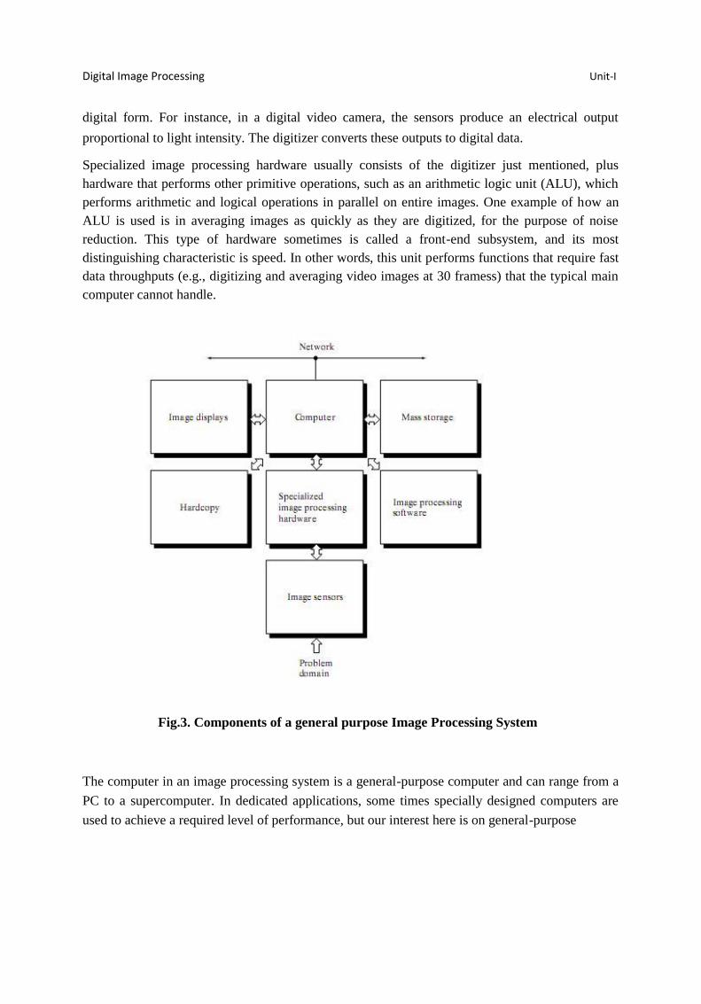
hardware. Figure 3 shows the basic components comprising a typical general-purpose system used

for digital image processing. The function of each component is discussed in the following

paragraphs, starting with image sensing.

With reference to sensing, two elements are required to acquire digital images. The first is a

physical device that is sensitive to the energy radiated by the object we wish to image. The

second, called a digitizer, is a device for converting the output of the physical sensing device into


digital form. For instance, in a digital video camera, the sensors produce an electrical output

proportional to light intensity. The digitizer converts these outputs to digital data.

Specialized image processing hardware usually consists of the digitizer just mentioned, plus

hardware that performs other primitive operations, such as an arithmetic logic unit (ALU), which

performs arithmetic and logical operations in parallel on entire images. One example of how an

ALU is used is in averaging images as quickly as they are digitized, for the purpose of noise

reduction. This type of hardware sometimes is called a front-end subsystem, and its most

distinguishing characteristic is speed. In other words, this unit performs functions that require fast

data throughputs (e.g., digitizing and averaging video images at 30 framess) that the typical main

computer cannot handle.

Fig.3. Components of a general purpose Image Processing System

The computer in an image processing system is a general-purpose computer and can range from a

PC to a supercomputer. In dedicated applications, some times specially designed computers are

used to achieve a required level of performance, but our interest here is on general-purpose


image processing systems. In these systems, almost any well-equipped PC-type machine is

suitable for offline image processing tasks.

Software for image processing consists of specialized modules that perform specific tasks. A well-

designed package also includes the capability for the user to write code that, as a minimum,

utilizes the specialized modules. More sophisticated software packages allow the integration of

those modules and general-purpose software commands from at least one computer language.

Mass storage capability is a must in image processing applications. An image of size 1024*1024

pixels, in which the intensity of each pixel is an 8-bit quantity, requires one megabyte of storage

space if the image is not compressed. When dealing with thousands, or even millions, of images,

providing adequate storage in an image processing system can be a challenge. Digital storage for

image processing applications falls into three principal categories: (1) short-term storage for use

during processing, (2) on-line storage for relatively fast re-call, and (3) archival storage,

characterized by infrequent access. Storage is measured in bytes (eight bits), Kbytes (one thousand

bytes), Mbytes (one million bytes), Gbytes (meaning giga, or one billion, bytes), and Tbytes

(meaning tera, or one trillion, bytes). One method of providing short-term storage is computer

memory. Another is by specialized boards, called frame buffers, that store one or more images and

can be accessed rapidly, usually at video rates (e.g., at 30 complete images per second).The latter

method allows virtually instantaneous image zoom, as well as scroll (vertical shifts) and pan

(horizontal shifts). Frame buffers usually are housed in the specialized image processing hardware

unit shown in Fig.3.Online storage generally takes the form of magnetic disks or optical-media

storage. The key factor characterizing on-line storage is frequent access to the stored data. Finally,

archival storage is characterized by massive storage requirements but infrequent need for access.

Magnetic tapes and optical disks housed in “jukeboxes” are the usual media for archival

applications.

Image displays in use today are mainly color (preferably flat screen) TV monitors. Monitors are

driven by the outputs of image and graphics display cards that are an integral part of the computer

system. Seldom are there requirements for image display applications that cannot be met by

display cards available commercially as part of the computer system. In some cases, it is necessary

to have stereo displays, and these are implemented in the form of headgear containing two small

displays embedded in goggles worn by the user.

Hardcopy devices for recording images include laser printers, film cameras, heat-sensitive

devices, inkjet units, and digital units, such as optical and CD-ROM disks. Film provides the

highest possible resolution, but paper is the obvious medium of choice for written material. For

presentations, images are displayed on film transparencies or in a digital medium if image

projection equipment is used. The latter approach is gaining acceptance as the standard for image

presentations.

www.jntuworld.com


Networking is almost a default function in any computer system in use today. Because of the large

amount of data inherent in image processing applications, the key consideration in image

transmission is bandwidth. In dedicated networks, this typically is not a problem, but

communications with remote sites via the Internet are not always as efficient. Fortunately, this

situation is improving quickly as a result of optical fiber and other broadband technologies.

4. Explain about elements of visual perception. [AUC NOV 2013]

Elements of Visual Perception:

Although the digital image processing field is built on a foundation of mathematical and

probabilistic formulations, human intuition and analysis play a central role in the choice of one

technique versus another, and this choice often is made based on subjective, visual judgments.

(1) Structure of the Human Eye:

Figure 4.1 shows a simplified horizontal cross section of the human eye. The eye is nearly a

sphere, with an average diameter of approximately 20 mm. Three membranes enclose the eye: the

cornea and sclera outer cover; the choroid; and the retina. The cornea is a tough, transparent tissue

that covers the anterior surface of the eye. Continuous with the cornea, the sclera is an opaque

membrane that encloses the remainder of the optic globe. The choroid lies directly below the

sclera. This membrane contains a network of blood vessels that serve as the major source of

nutrition to the eye. Even superficial injury to the choroid, often not deemed serious, can lead to

severe eye damage as a result of inflammation that restricts blood flow. The choroid coat is

heavily pigmented and hence helps to reduce the amount of extraneous light entering the eye and

the backscatter within the optical globe. At its anterior extreme, the choroid is divided into the

ciliary body and the iris diaphragm. The latter contracts or expands to control the amount of light

that enters the eye. The central opening of the iris (the pupil) varies in diameter from

approximately 2 to 8 mm. The front of the iris contains the visible pigment of the eye, whereas the

back contains a black pigment.

The lens is made up of concentric layers of fibrous cells and is suspended by fibers that attach to

the ciliary body. It contains 60 to 70%water, about 6%fat, and more protein than any other tissue

in the eye. The lens is colored by a slightly yellow pigmentation that increases with age. In

extreme cases, excessive clouding of the lens, caused by the affliction commonly referred to as

cataracts, can lead to poor color discrimination and loss of clear vision. The lens absorbs

approximately 8% of the visible light spectrum, with relatively higher absorption at shorter

wavelengths. Both infrared and ultraviolet light are absorbed appreciably by proteins within the

lens structure and, in excessive amounts, can damage the eye.


Fig.4.1 Simplified diagram of a cross section of the human eye.

The innermost membrane of the eye is the retina, which lines the inside of the wall’s entire

posterior portion. When the eye is properly focused, light from an object outside the eye is imaged

on the retina. Pattern vision is afforded by the distribution of discrete light receptors over the

surface of the retina. There are two classes of receptors: cones and rods. The cones in each eye

number between 6 and 7 million. They are located primarily in the central portion of the


retina, called the fovea, and are highly sensitive to color. Humans can resolve fine details with

these cones largely because each one is connected to its own nerve end. Muscles controlling the

eye rotate the eyeball until the image of an object of interest falls on the fovea. Cone vision is

called photopic or bright-light vision. The number of rods is much larger: Some 75 to 150 million

are distributed over the retinal surface. The larger area of distribution and the fact that several rods

are connected to a single nerve end reduce the amount of detail discernible by these receptors.

Rods serve to give a general, overall picture of the field of view. They are not involved in color

vision and are sensitive to low levels of illumination. For example, objects that appear brightly

colored in daylight when seen by moonlight appear as colorless forms because only the rods are

stimulated. This phenomenon is known as scotopic or dim-light vision.

(2) Image Formation in the Eye:

The principal difference between the lens of the eye and an ordinary optical lens is that the former

is flexible. As illustrated in Fig. 4.1, the radius of curvature of the anterior surface of the lens is

greater than the radius of its posterior surface. The shape of the lens is controlled by tension in the

fibers of the ciliary body. To focus on distant objects, the controlling muscles cause the lens to be

relatively flattened. Similarly, these muscles allow the lens to become thicker in order to focus on

objects near the eye. The distance between the center of the lens and the retina (called the focal

length) varies from approximately 17 mm to about 14 mm, as the refractive power of the lens

increases from its minimum to its maximum. When the eye

Fig.4.2. Graphical representation of the eye looking at a palm tree Point C is the optical

center of the lens.

focuses on an object farther away than about 3 m, the lens exhibits its lowest refractive power.

When the eye focuses on a nearby object, the lens is most strongly refractive. This information


makes it easy to calculate the size of the retinal image of any object. In Fig. 4.2, for example, the

observer is looking at a tree 15 m high at a distance of 100 m. If h is the height in mm of that

object in the retinal image, the geometry of Fig.4.2 yields 15/100=h/17 or h=2.55mm. The retinal

image is reflected primarily in the area of the fovea. Perception then takes place by the relative

excitation of light receptors, which transform radiant energy into electrical impulses that are

ultimately decoded by the brain.

(3)Brightness Adaptation and Discrimination:

Because digital images are displayed as a discrete set of intensities, the eye’s ability to

discriminate between different intensity levels is an important consideration in presenting image-

processing results. The range of light intensity levels to which the human visual system can adapt

is enormous—on the order of 1010

—from the scotopic threshold to the glare limit. Experimental

evidence indicates that subjective brightness (intensity as perceived by the human visual system)

is a logarithmic function of the light intensity incident on the eye. Figure 4.3, a plot of light

intensity versus subjective brightness, illustrates this characteristic. The long solid curve

represents the range of intensities to which the visual system can adapt. In photopic vision alone,

the range is about 106. The transition from scotopic to photopic vision is gradual over the

approximate range from 0.001 to 0.1 millilambert (–3 to –1 mL in the log scale), as the double

branches of the adaptation curve in this range show.

Fig.4.3. Range of Subjective brightness sensations showing a particular adaptation level.


The essential point in interpreting the impressive dynamic range depicted in Fig.4.3 is that the

visual system cannot operate over such a range simultaneously. Rather, it accomplishes this large

variation by changes in its overall sensitivity, a phenomenon known as brightness adaptation. The

total range of distinct intensity levels it can discriminate simultaneously is rather small when

compared with the total adaptation range. For any given set of conditions, the current sensitivity

level of the visual system is called the brightness adaptation level, which may correspond, for

example, to brightness Ba in Fig. 4.3. The short intersecting curve represents the range of

subjective brightness that the eye can perceive when adapted to this level. This range is rather

restricted, having a level Bb at and below which all stimuli are perceived as indistinguishable

blacks. The upper (dashed) portion of the curve is not actually restricted but, if extended too far,

loses its meaning because much higher intensities would simply raise the adaptation level higher

than Ba.

5. Explain the process of image acquisition.

Image Sensing and Acquisition:

The types of images in which we are interested are generated by the combination of an

“illumination” source and the reflection or absorption of energy from that source by the elements

of the “scene” being imaged. We enclose illumination and scene in quotes to emphasize the fact

that they are considerably more general than the familiar situation in which a visible light source

illuminates a common everyday 3-D (three-dimensional) scene. For example, the illumination

may originate from a source of electromagnetic energy such as radar, infrared, or X-ray energy.

But, as noted earlier, it could originate from less traditional sources, such as ultrasound or even a

computer-generated illumination pattern.

Similarly, the scene elements could be familiar objects, but they can just as easily be molecules,

buried rock formations, or a human brain. We could even image a source, such as acquiring

images of the sun. Depending on the nature of the source, illumination energy is reflected from, or

transmitted through, objects. An example in the first category is light reflected from a planar

surface. An example in the second category is when X-rays pass through a patient’s body for the

purpose of generating a diagnostic X-ray film. In some applications, the reflected or transmitted

energy is focused onto a photo converter (e.g., a phosphor screen), which converts the energy into

visible light. Electron microscopy and some applications of gamma imaging use this approach.

Figure 5.1 shows the three principal sensor arrangements used to transform illumination energy

into digital images. The idea is simple: Incoming energy is transformed into a voltage by the

combination of input electrical power and sensor material that is responsive to the particular type

of energy being detected. The output voltage waveform is the response of the sensor(s), and a

digital quantity is obtained from each sensor by digitizing its response.


Fig.5.1 (a) Single imaging Sensor (b) Line sensor (c) Array sensor

(1)Image Acquisition Using a Single Sensor:

Figure 5.1 (a) shows the components of a single sensor. Perhaps the most familiar sensor of this

type is the photodiode, which is constructed of silicon materials and whose output voltage

waveform is proportional to light. The use of a filter in front of a sensor improves selectivity. For

example, a green (pass) filter in front of a light sensor favors light in the green band of the color


spectrum. As a consequence, the sensor output will be stronger for green light than for other

components in the visible spectrum.

In order to generate a 2-D image using a single sensor, there has to be relative displacements in

both the x- and y-directions between the sensor and the area to be imaged. Figure 5.2 shows an

arrangement used in high-precision scanning, where a film negative is mounted onto a drum

whose mechanical rotation provides displacement in one dimension. The single sensor is mounted

on a lead screw that provides motion in the perpendicular direction. Since mechanical motion can

be controlled with high precision, this method is an inexpensive (but slow) way to obtain high-

resolution images. Other similar mechanical arrangements use a flat bed, with the sensor moving

in two linear directions. These types of mechanical digitizers sometimes are referred to as

microdensitometers.

Fig.5.2. Combining a single sensor with motion to generate a 2-D image

(2) Image Acquisition Using Sensor Strips:

A geometry that is used much more frequently than single sensors consists of an in-line

arrangement of sensors in the form of a sensor strip, as Fig. 5.1 (b) shows. The strip provides

imaging elements in one direction. Motion perpendicular to the strip provides imaging in the other

direction, as shown in Fig. 5.3 (a).This is the type of arrangement used in most flat bed scanners.

Sensing devices with 4000 or more in-line sensors are possible. In-line sensors are used routinely

in airborne imaging applications, in which the imaging system is mounted on an aircraft that flies

at a constant altitude and speed over the geographical area to be imaged. One-dimensional

imaging sensor strips that respond to various bands of the electromagnetic spectrum are mounted

perpendicular to the direction of flight. The imaging strip gives one line of an image


at a time, and the motion of the strip completes the other dimension of a two-dimensional image.

Lenses or other focusing schemes are used to project the area to be scanned onto the sensors.

Sensor strips mounted in a ring configuration are used in medical and industrial imaging to obtain

cross-sectional (“slice”) images of 3-D objects, as Fig. 5.3 (b) shows. A rotating X-ray source

provides illumination and the portion of the sensors opposite the source collect the X-ray energy

that pass through the object (the sensors obviously have to be sensitive to X-ray energy).This is

the basis for medical and industrial computerized axial tomography (CAT). It is important to note

that the output of the sensors must be processed by reconstruction algorithms whose objective is to

transform the sensed data into meaningful cross-sectional images.

In other words, images are not obtained directly from the sensors by motion alone; they require

extensive processing. A 3-D digital volume consisting of stacked images is generated as the object

is moved in a direction perpendicular to the sensor ring. Other modalities of imaging based on the

CAT principle include magnetic resonance imaging (MRI) and positron emission tomography

(PET).The illumination sources, sensors, and types of images are different, but conceptually they

are very similar to the basic imaging approach shown in Fig. 5.3 (b).

Fig.5.3 (a) Image acquisition using a linear sensor strip (b) Image acquisition using a

circular sensor strip.


(3) Image Acquisition Using Sensor Arrays:

Figure 5.1 (c) shows individual sensors arranged in the form of a 2-D array. Numerous

electromagnetic and some ultrasonic sensing devices frequently are arranged in an array format.

This is also the predominant arrangement found in digital cameras. A typical sensor for these

cameras is a CCD array, which can be manufactured with a broad range of sensing properties and

can be packaged in rugged arrays of 4000 * 4000 elements or more. CCD sensors are used widely

in digital cameras and other light sensing instruments. The response of each sensor is proportional

to the integral of the light energy projected onto the surface of the sensor, a property that is used in

astronomical and other applications requiring low noise images. Noise reduction is achieved by

letting the sensor integrate the input light signal over minutes or even hours. Since the sensor array

shown in Fig. 5.4 (c) is two dimensional, its key advantage is that a complete image can be

obtained by focusing the energy pattern onto the surface of the array. The principal manner in

which array sensors are used is shown in Fig.5.4. This figure shows the energy from an

illumination source being reflected from a scene element, but, as mentioned at the beginning of

this section, the energy also could be transmitted through the scene elements. The first function

performed by the imaging system shown in Fig.5.4 (c) is to collect the incoming energy and focus

it onto an image plane. If the illumination is light, the front end of the imaging system is a lens,

which projects the viewed scene onto the lens focal plane, as Fig. 2.15(d) shows. The sensor array,

which is coincident with the focal plane, produces outputs proportional to the integral of the light

received at each sensor. Digital and analog circuitry sweep these outputs and converts them to a

video signal, which is then digitized by another section of the imaging system. The output is a

digital image, as shown diagrammatically in Fig. 5.4 (e).


Fig.5.4 An example of the digital image acquisition process (a) Energy (“illumination”)

source (b) An element of a scene (c) Imaging system (d) Projection of the scene onto the

image plane (e) Digitized image

6. Explain about image sampling and quantization process. [AUC APR 2013]

Image Sampling and Quantization:

The output of most sensors is a continuous voltage waveform whose amplitude and spatial

behavior are related to the physical phenomenon being sensed. To create a digital image, we need

to convert the continuous sensed data into digital form. This involves two processes: sampling and

quantization.

Basic Concepts in Sampling and Quantization:

The basic idea behind sampling and quantization is illustrated in Fig.6.1. Figure 6.1(a) shows a

continuous image, f(x, y), that we want to convert to digital form. An image may be continuous

with respect to the x- and y-coordinates, and also in amplitude. To convert it to digital form, we

have to sample the function in both coordinates and in amplitude. Digitizing the coordinate values

is called sampling. Digitizing the amplitude values is called quantization.

The one-dimensional function shown in Fig.6.1 (b) is a plot of amplitude (gray level) values of the

continuous image along the line segment AB in Fig. 6.1(a).The random variations are due to

image noise. To sample this function, we take equally spaced samples along line AB, as shown in

Fig.6.1 (c).The location of each sample is given by a vertical tick mark in the bottom part of the

figure. The samples are shown as small white squares superimposed on the function. The set of

these discrete locations gives the sampled function. However, the values of the samples still span

(vertically) a continuous range of gray-level values. In order to form a digital function, the gray-

level values also must be converted (quantized) into discrete quantities. The right side of Fig. 6.1

(c) shows the gray-level scale divided into eight discrete levels, ranging from black to white. The

vertical tick marks indicate the specific value assigned to each of the eight gray levels. The

continuous gray levels are quantized simply by assigning one of the eight discrete gray levels to

each sample. The assignment is made depending on the vertical proximity of a sample to a vertical

tick mark. The digital samples resulting from both sampling and quantization are shown in Fig.6.1

(d). Starting at the top of the image and carrying out this procedure line by line produces a two-

dimensional digital image.

Sampling in the manner just described assumes that we have a continuous image in both

coordinate directions as well as in amplitude. In practice, the method of sampling is determined by

the sensor arrangement used to generate the image. When an image is generated by a single


sensing element combined with mechanical motion, as in Fig. 2.13, the output of the sensor is

quantized in the manner described above. However, sampling is accomplished by selecting the

number of individual mechanical increments at which we activate the sensor to collect data.

Mechanical motion can be made very exact so, in principle; there is almost no limit as to how fine

we can sample an image. However, practical limits are established by imperfections in the optics

used to focus on the

Fig.6.1. Generating a digital image (a) Continuous image (b) A scan line from A to Bin the

continuous image, used to illustrate the concepts of sampling and quantization (c) Sampling

and quantization. (d) Digital scan line


sensor an illumination spot that is inconsistent with the fine resolution achievable with mechanical

displacements. When a sensing strip is used for image acquisition, the number of sensors in the

strip establishes the sampling limitations in one image direction. Mechanical motion in the other

direction can be controlled more accurately, but it makes little sense to try to achieve sampling

density in one direction that exceeds the sampling limits established by the number of sensors in

the other. Quantization of the sensor outputs completes the process of generating a digital image.

When a sensing array is used for image acquisition, there is no motion and the number of sensors

in the array establishes the limits of sampling in both directions. Figure 6.2 illustrates this concept.

Figure 6.2 (a) shows a continuous image projected onto the plane of an array sensor. Figure 6.2 (b)

shows the image after sampling and quantization. Clearly, the quality of a digital image is

determined to a large degree by the number of samples and discrete gray levels used in sampling

and quantization.

Fig.6.2. (a) Continuos image projected onto a sensor array (b) Result of image

sampling and quantization.


7. Define spatial and gray level resolution. Explain about isopreference curves.

Spatial and Gray-Level Resolution:

Sampling is the principal factor determining the spatial resolution of an image. Basically, spatial

resolution is the smallest discernible detail in an image. Suppose that we construct a chart with

vertical lines of width W, with the space between the lines also having width W.A line pair

consists of one such line and its adjacent space. Thus, the width of a line pair is 2W, and there are

1/2Wline pairs per unit distance. A widely used definition of resolution is simply the smallest

number of discernible line pairs per unit distance; for example, 100 line pairs per millimeter.

Gray-level resolution similarly refers to the smallest discernible change in gray level. We have

considerable discretion regarding the number of samples used to generate a digital image, but this

is not true for the number of gray levels. Due to hardware considerations, the number of gray

levels is usually an integer power of 2.

The most common number is 8 bits, with 16 bits being used in some applications where

enhancement of specific gray-level ranges is necessary. Sometimes we find systems that can

digitize the gray levels of an image with 10 or 12 bit of accuracy, but these are the exception

rather than the rule. When an actual measure of physical resolution relating pixels and the level of

detail they resolve in the original scene are not necessary, it is not uncommon to refer to an L-

level digital image of size M*N as having a spatial resolution of M*N pixels and a gray-level

resolution of L levels.

Fig.7.1. A 1024*1024, 8-bit image subsampled down to size 32*32 pixels The number of

allowable gray levels was kept at 256.


The subsampling was accomplished by deleting the appropriate number of rows and columns

from the original image. For example, the 512*512 image was obtained by deleting every other

row and column from the 1024*1024 image. The 256*256 image was generated by deleting every

other row and column in the 512*512 image, and so on. The number of allowed gray levels was

kept at 256. These images show the dimensional proportions between various sampling densities,

but their size differences make it difficult to see the effects resulting from a reduction in the

number of samples. The simplest way to compare these effects is to bring all the subsampled

images up to size 1024*1024 by row and column pixel replication. The results are shown in Figs.

7.2 (b) through (f). Figure7.2 (a) is the same 1024*1024, 256-level image shown in Fig.7.1; it is

repeated to facilitate comparisons.

Fig. 7.2 (a) 1024*1024, 8-bit image (b) 512*512 image resampled into 1024*1024 pixels by

row and column duplication (c) through (f) 256*256, 128*128, 64*64, and 32*32 images

resampled into 1024*1024 pixels


Compare Fig. 7.2(a) with the 512*512 image in Fig. 7.2(b) and note that it is virtually impossible

to tell these two images apart. The level of detail lost is simply too fine to be seen on the printed

page at the scale in which these images are shown. Next, the 256*256 image in Fig. 7.2(c) shows a

very slight fine checkerboard pattern in the borders between flower petals and the black back-

ground. A slightly more pronounced graininess throughout the image also is beginning to appear.

These effects are much more visible in the 128*128 image in Fig. 7.2(d), and they become

pronounced in the 64*64 and 32*32 images in Figs. 7.2 (e) and (f), respectively.

In the next example, we keep the number of samples constant and reduce the number of gray

levels from 256 to 2, in integer powers of 2.Figure 7.3(a) is a 452*374 CAT projection image,

displayed with k=8 (256 gray levels). Images such as this are obtained by fixing the X-ray source

in one position, thus producing a 2-D image in any desired direction. Projection images are used

as guides to set up the parameters for a CAT scanner, including tilt, number of slices, and range.

Figures 7.3(b) through (h) were obtained by reducing the number of bits from k=7 to k=1 while

keeping the spatial resolution constant at 452*374 pixels. The 256-, 128-, and 64-level images are

visually identical for all practical purposes. The 32-level image shown in Fig. 7.3 (d), however,

has an almost imperceptible set of very fine ridge like structures in areas of smooth gray levels

(particularly in the skull).This effect, caused by the use of an insufficient number of gray levels in

smooth areas of a digital image, is called false contouring, so called because the ridges resemble

topographic contours in a map. False contouring generally is quite visible in images displayed

using 16 or less uniformly spaced gray levels, as the images in Figs. 7.3(e) through (h) show.


Fig. 7.3 (a) 452*374, 256-level image (b)–(d) Image displayed in 128, 64, and 32 gray levels,

while keeping the spatial resolution constant (e)–(g) Image displayed in 16, 8, 4, and 2 gray

levels.


As a very rough rule of thumb, and assuming powers of 2 for convenience, images of size

256*256 pixels and 64 gray levels are about the smallest images that can be expected to be

reasonably free of objectionable sampling checker-boards and false contouring.

The results in Examples 7.2 and 7.3 illustrate the effects produced on image quality by varying N

and k independently. However, these results only partially answer the question of how varying N

and k affect images because we have not considered yet any relationships that might exist between

these two parameters.

An early study by Huang [1965] attempted to quantify experimentally the effects on image quality

produced by varying N and k simultaneously. The experiment consisted of a set of subjective

tests. Images similar to those shown in Fig.7.4 were used. The woman’s face is representative of

an image with relatively little detail; the picture of the cameraman contains an intermediate

amount of detail; and the crowd picture contains, by comparison, a large amount of detail. Sets of

these three types of images were generated by varying N and k, and observers were then asked to

rank them according to their subjective quality. Results were summarized in the form of so-called

isopreference curves in the Nk-plane (Fig.7.5 shows average isopreference curves representative

of curves corresponding to the images shown in Fig. 7.4).Each point in the Nk-plane represents an

image having values of N and k equal to the coordinates of that point.

Fig.7.4 (a) Image with a low level of detail (b) Image with a medium level of detail (c) Image

with a relatively large amount of detail

Points lying on an isopreference curve correspond to images of equal subjective quality. It was

found in the course of the experiments that the isopreference curves tended to shift right and

upward, but their shapes in each of the three image categories were similar to those shown in


Fig. 7.5. This is not unexpected, since a shift up and right in the curves simply means larger values

for N and k, which implies better picture quality.

Fig.7.5. Representative isopreference curves for the three types of images in Fig.7.4

The key point of interest in the context of the present discussion is that isopreference curves tend

to become more vertical as the detail in the image increases. This result suggests that for images

with a large amount of detail only a few gray levels may be needed. For example, the

isopreference curve in Fig.7.5 corresponding to the crowd is nearly vertical. This indicates that,

for a fixed value of N, the perceived quality for this type of image is nearly independent of the

number of gray levels used. It is also of interest to note that perceived quality in the other two

image categories remained the same in some intervals in which the spatial resolution was

increased, but the number of gray levels actually decreased. The most likely reason for this result

is that a decrease in k tends to increase the apparent contrast of an image, a visual effect that

humans often perceive as improved quality in an image.


8. Explain about Aliasing and Moire patterns.

Aliasing and Moiré Patterns:

Functions whose area under the curve is finite can be represented in terms of sines and cosines of

various frequencies. The sine/cosine component with the highest frequency determines the highest

“frequency content” of the function. Suppose that this highest frequency is finite and that the

function is of unlimited duration (these functions are called band-limited functions).Then, the

Shannon sampling theorem [Brace well (1995)] tells us that, if the function is sampled at a rate

equal to or greater than twice its highest frequency, it is possible to recover completely the

original function from its samples. If the function is undersampled, then a phenomenon called

aliasing corrupts the sampled image. The corruption is in the form of additional frequency

components being introduced into the sampled function. These are called aliased frequencies.

Note that the sampling rate in images is the number of samples taken (in both spatial directions)

per unit distance.

As it turns out, except for a special case discussed in the following paragraph, it is impossible to

satisfy the sampling theorem in practice. We can only work with sampled data that are finite in

duration. We can model the process of converting a function of unlimited duration into a function

of finite duration simply by multiplying the unlimited function by a “gating function” that is

valued 1 for some interval and 0 elsewhere. Unfortunately, this function itself has frequency

components that extend to infinity. Thus, the very act of limiting the duration of a band-limited

function causes it to cease being band limited, which causes it to violate the key condition of the

sampling theorem. The principal approach for reducing the aliasing effects on an image is to

reduce its high-frequency components by blurring the image prior to sampling. However, aliasing

is always present in a sampled image. The effect of aliased frequencies can be seen under the right

conditions in the form of so called Moiré patterns.

There is one special case of significant importance in which a function of infinite duration can be

sampled over a finite interval without violating the sampling theorem. When a function is

periodic, it may be sampled at a rate equal to or exceeding twice its highest frequency and it is

possible to recover the function from its samples provided that the sampling captures exactly an

integer number of periods of the function. This special case allows us to illustrate vividly the

Moiré effect. Figure 8 shows two identical periodic patterns of equally spaced vertical bars,

rotated in opposite directions and then superimposed on each other by multiplying the two images.

A Moiré pattern, caused by a breakup of the periodicity, is seen in Fig.8 as a 2-D sinusoidal

(aliased) waveform (which looks like a corrugated tin roof) running in a vertical direction. A

similar pattern can appear when images are digitized (e.g., scanned) from a printed page, which

consists of periodic ink dots.


Fig.8. Illustration of the Moiré pattern effect

9. Explain about the basic relationships and distance measures between pixels

in a digital image.

Neighbors of a Pixel:

A pixel p at coordinates (x, y) has four horizontal and vertical neighbors whose coordinates are

given by (x+1, y), (x-1, y), (x, y+1), (x, y-1). This set of pixels, called the 4-neighbors of p, is

denoted by N4 (p). Each pixel is a unit distance from (x, y), and some of the neighbors of p lie

outside the digital image if (x, y) is on the border of the image.

The four diagonal neighbors of p have coordinates (x+1, y+1), (x+1, y-1), (x-1, y+1), (x-1, y-1)

and are denoted by ND (p). These points, together with the 4-neighbors, are called the 8-neighbors

of p, denoted by N8 (p). As before, some of the points in ND (p) and N8 (p) fall outside the image

if (x, y) is on the border of the image.


Connectivity:

Connectivity between pixels is a fundamental concept that simplifies the definition of numerous

digital image concepts, such as regions and boundaries. To establish if two pixels are connected, it

must be determined if they are neighbors and if their gray levels satisfy a specified criterion of

similarity (say, if their gray levels are equal). For instance, in a binary image with values 0 and 1,

two pixels may be 4-neighbors, but they are said to be connected only if they have the same value.

Let V be the set of gray-level values used to define adjacency. In a binary image, V={1} if we are

referring to adjacency of pixels with value 1. In a grayscale image, the idea is the same, but set V

typically contains more elements. For example, in the adjacency of pixels with a range of possible

gray-level values 0 to 255, set V could be any subset of these 256 values. We consider three types

of adjacency:

(a) 4-adjacency. Two pixels p and q with values from V are 4-adjacent if q is in the set N4 (p).

(b) 8-adjacency. Two pixels p and q with values from V are 8-adjacent if q is in the set N8 (p).

(c) m-adjacency (mixed adjacency).Two pixels p and q with values from V are m-adjacent if

(i) q is in N4 (p), or

(ii) q is in ND (p) and the set has no pixels whose values are from V.

Mixed adjacency is a modification of 8-adjacency. It is introduced to eliminate the ambiguities

that often arise when 8-adjacency is used. For example, consider the pixel arrangement shown in

Fig.9 (a) for V= {1}.The three pixels at the top of Fig.9 (b) show multiple (ambiguous) 8-

adjacency, as indicated by the dashed lines. This ambiguity is removed by using m-adjacency, as

shown in Fig. 9 (c).Two image subsets S1 and S2 are adjacent if some pixel in S1 is adjacent to

some pixel in S2. It is understood here and in the following definitions that adjacent means 4-, 8-,

or m-adjacent. A (digital) path (or curve) from pixel p with coordinates (x, y) to pixel q with

coordinates (s, t) is a sequence of distinct pixels with coordinates

where and pixels are adjacent for

. In this case, n is the length of the path. If (xo, yo) = (xn, yn), the path is a closed

path. We can define 4-, 8-, or m-paths depending on the type of adjacency specified. For example,

the paths shown in Fig. 9 (b) between the northeast and southeast points are 8-paths, and the path

in Fig. 9 (c) is an m-path. Note the absence of ambiguity in the m-path. Let S represent a subset of

pixels in an image. Two pixels p and q are said to be connected in S if there


exists a path between them consisting entirely of pixels in S. For any pixel p in S, the set of pixels

that are connected to it in S is called a connected component of S. If it only has one connected

component, then set S is called a connected set.

Let R be a subset of pixels in an image. We call R a region of the image if R is a connected set.

The boundary (also called border or contour) of a region R is the set of pixels in the region that

have one or more neighbors that are not in R. If R happens to be an entire image (which we recall

is a rectangular set of pixels), then its boundary is defined as the set of pixels in the first and last

rows and columns of the image. This extra definition is required because an image has no

neighbors beyond its border. Normally, when we refer to a region, we are referring to a subset

Fig.9 (a) Arrangement of pixels; (b) pixels that are 8-adjacent (shown dashed) to the center

pixel; (c) m-adjacency

of an image, and any pixels in the boundary of the region that happen to coincide with the border

of the image are included implicitly as part of the region boundary.

Distance Measures:

For pixels p, q, and z, with coordinates (x, y), (s, t), and (v, w), respectively, D is a distance

function or metric if

The Euclidean distance between p and q is defined as


For this distance measure, the pixels having a distance less than or equal to some value r from(x,

y) are the points contained in a disk of radius r centered at (x, y).

The D4 distance (also called city-block distance) between p and q is defined as

In this case, the pixels having a D4 distance from (x, y) less than or equal to some value r form a

diamond centered at (x, y). For example, the pixels with D4 distance ≤ 2 from (x, y) (the center

point) form the following contours of constant distance:

The pixels with D4 =1 are the 4-neighbors of (x, y).

The D8 distance (also called chessboard distance) between p and q is defined as

In this case, the pixels with D8 distance from(x, y) less than or equal to some value r form a square

centered at (x, y). For example, the pixels with D8 distance ≤ 2 from(x, y) (the center point) form

the following contours of constant distance:


The pixels with D8=1 are the 8-neighbors of (x, y). Note that the D4 and D8 distances between p

and q are independent of any paths that might exist between the points because these distances

involve only the coordinates of the points. If we elect to consider m-adjacency, however, the Dm

distance between two points is defined as the shortest m-path between the points. In this case, the

distance between two pixels will depend on the values of the pixels along the path, as well as the

values of their neighbors. For instance, consider the following arrangement of pixels and assume

that p, p2 , and p4 have value 1 and that p1 and p3 can have a value of 0 or 1:

Suppose that we consider adjacency of pixels valued 1 (i.e. = {1}). If p1 and p3 are 0, the length of

the shortest m-path (the Dm distance) between p and p4 is 2. If p1 is 1, then p2 and p will no

longer be m-adjacent (see the definition of m-adjacency) and the length of the shortest m-path

becomes 3 (the path goes through the points pp1p2p4). Similar comments apply if p3 is 1 (and p1

is 0); in this case, the length of the shortest m-path also is 3. Finally, if both p1 and p3 are 1 the

length of the shortest m-path between p and p4 is 4. In this case, the path goes through the

sequence of points pp1p2p3p4.

10. Write about perspective image transformation.

A perspective transformation (also called an imaging transformation) projects 3D points onto a

plane. Perspective transformations play a central role in image processing because they provide an

approximation to the manner in which an image is formed by viewing a 3D world. These

transformations are fundamentally different, because they are nonlinear in that they involve

division by coordinate values.

Figure 10 shows a model of the image formation process. The camera coordinate system (x, y, z)

has the image plane coincident with the xy plane and the optical axis (established by the center of

the lens) along the z axis. Thus the center of the image plane is at the origin, and the centre of the

lens is at coordinates (0.0, λ). If the camera is in focus for distant objects, λ is the focal length of

the lens. Here the assumption is that the camera coordinate system is aligned with the world

coordinate system (X, Y, Z).

Digital I mage Proces sing Unit‐I

Let (X, Y, Z) be t he world coordinates of any point in a 3-D s cene, as sh own in the Fig. 10. We

assume throughout the follow ing discuss ion that Z> λ; that is all points o f interest li e in front o f

the lens . The first step is to ob tain a relationship that gives the c oordinates (x, y) of the

projection of the point (X. Y , Z) onto the image plane. This is easily accomplished by the use of

simila r triangles. With ref erence to Fig. 10,

Fig.10 Basic model of the im aging pro cess The ca mera coordinate syst em (x, y, z) is

aligned with the world coordinate sy stem (X, Y , Z)

Where the negativ e signs in front of X an d Y indicat e that image points are actually in verted,

as the geometry of Fig.10 shows.

The image-plane coordinates of the projected 3-D p oint follow directly from above eq uations


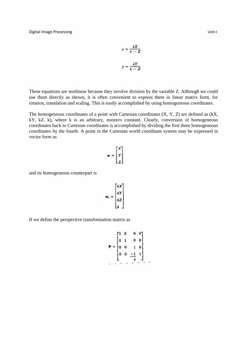
These equations are nonlinear because they involve division by the variable Z. Although we could

use them directly as shown, it is often convenient to express them in linear matrix form, for

rotation, translation and scaling. This is easily accomplished by using homogeneous coordinates.

The homogeneous coordinates of a point with Cartesian coordinates (X, Y, Z) are defined as (kX,

kY, kZ. k), where k is an arbitrary, nonzero constant. Clearly, conversion of homogeneous

coordinates back to Cartesian coordinates is accomplished by dividing the first three homogeneous

coordinates by the fourth. A point in the Cartesian world coordinate system may be expressed in

vector form as

and its homogeneous counterpart is

If we define the perspective transformation matrix as


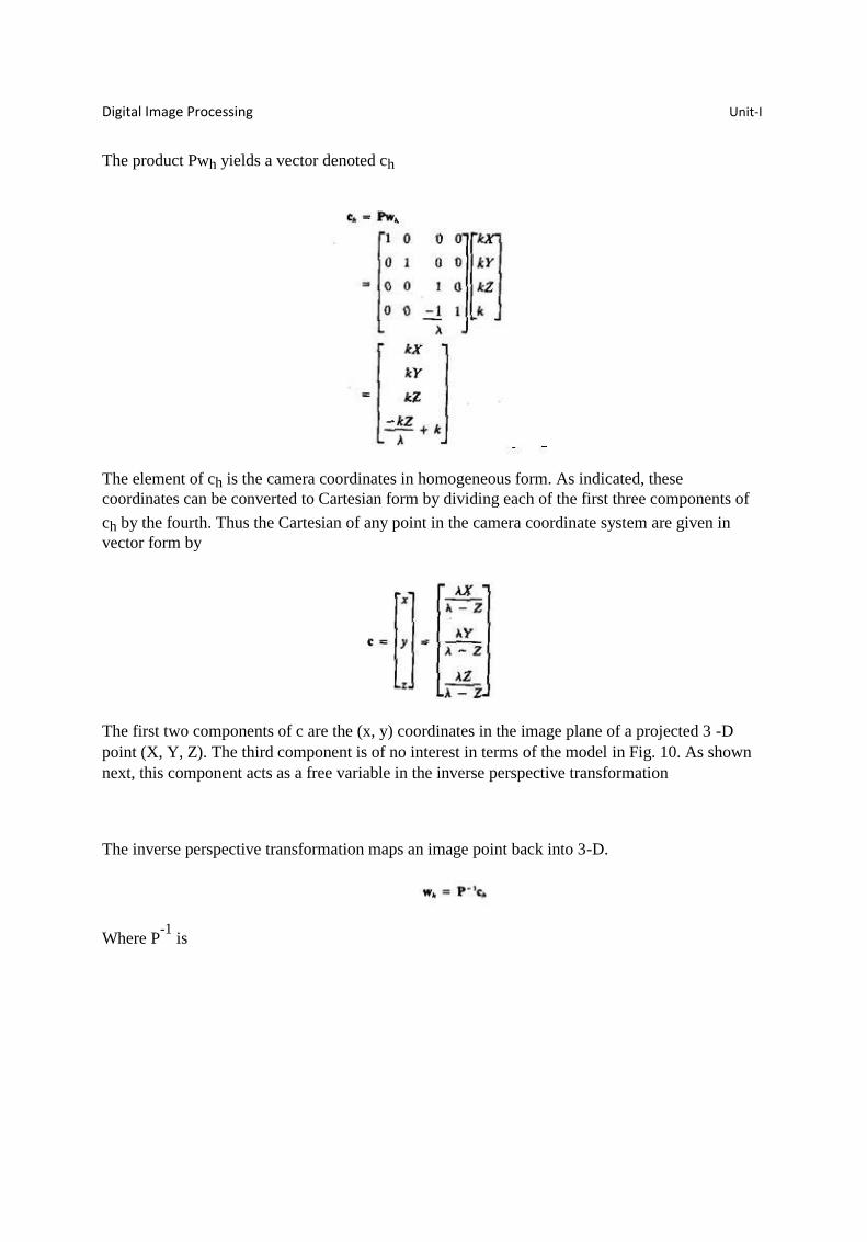
The product Pwh yields a vector denoted ch

The element of ch is the camera coordinates in homogeneous form. As indicated, these

coordinates can be converted to Cartesian form by dividing each of the first three components of

ch by the fourth. Thus the Cartesian of any point in the camera coordinate system are given in

vector form by

The first two components of c are the (x, y) coordinates in the image plane of a projected 3 -D

point (X, Y, Z). The third component is of no interest in terms of the model in Fig. 10. As shown

next, this component acts as a free variable in the inverse perspective transformation

The inverse perspective transformation maps an image point back into 3-D.

Where P-1

is


Suppose that an image point has coordinates (xo, yo, 0), where the 0 in the z location simply

indicates that the image plane is located at z = 0. This point may be expressed in homogeneous

vector form as

or, in Cartesian coordinates

This result obviously is unexpected because it gives Z = 0 for any 3-D point. The problem here is caused by mapping a 3-D scene onto the image plane, which is a many-to-one transformation. The

image point (x0, y 0) corresponds to the set of collinear 3-D points that lie on the line passing

through (xo, yo, 0) and (0, 0, λ). The equation of this line in the world coordinate system; that is,


Equations above show that unless something is known about the 3-D point that generated an image point (for example, its Z coordinate) it is not possible to completely recover the 3-D point from its image. This observation, which certainly is not unexpected, can be used to formulate the

inverse perspective transformation by using the z component of ch as a free variable instead of 0.

Thus, by letting

It thus follows

which upon conversion to Cartesian coordinate gives

In other words, treating z as a free variable yields the equations


Solving for z in terms of Z in the last equation and substituting in the first two expressions yields

which agrees with the observation that revering a 3-D point from its image by means of the

inverse perspective transformation requires knowledge of at least one of the world coordinates of

the point.

11. Define Fourier Transform and its inverse.

Let f(x) be a continuous function of a real variable x. The Fourier transform of f(x) is

defined by the equation

Where j = √-1

Given F(u), f(x) can be obtained by using the inverse Fourier transform

The Fourier transform exists if f(x) is continuous and integrable and F(u) is integrable.

The Fourier transform of a real function, is generally complex,

F(u) = R(u) + jI(u)

Where R(u) and I(u) are the real and imiginary components of F(u). F(u) can be expressed in

exponential form as

F(u) = │F(u)│ejØ(u)

where

│F(u)│ = [R2(u) + I

2(u)]

1/2

and

Ø (u, v) = tan-1

[ I (u, v)/R (u, v) ]

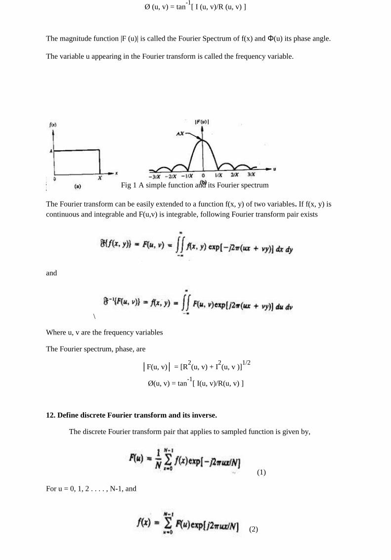
The magnitude function |F (u)| is called the Fourier Spectrum of f(x) and Φ(u) its phase angle.

The variable u appearing in the Fourier transform is called the frequency variable.

Fig 1 A simple function and its Fourier spectrum

The Fourier transform can be easily extended to a function f(x, y) of two variables. If f(x, y) is

continuous and integrable and F(u,v) is integrable, following Fourier transform pair exists

and

\

Where u, v are the frequency variables

The Fourier spectrum, phase, are

│F(u, v)│ = [R2(u, v) + I

2(u, v )]

1/2

Ø(u, v) = tan-1

[ I(u, v)/R(u, v) ]

12. Define discrete Fourier transform and its inverse.

The discrete Fourier transform pair that applies to sampled function is given by,

(1)

For u = 0, 1, 2 . . . . , N-1, and

(2)

For x = 0, 1, 2 . . . ., N-1.

In the two variable case the discrete Fourier transform pair is

For u = 0, 1, 2 . . . , M-1, v = 0, 1, 2 . . . , N - 1, and

For x = 0, 1, 2 . . . , M-1, y = 0, 1, 2 . . . , N-1.

If M = N, then discrete Fourier transform pair is

For u, v = 0, 1, 2 . . . , N – 1, and

For x, y = 0, 1, 2 . . . , N – 1

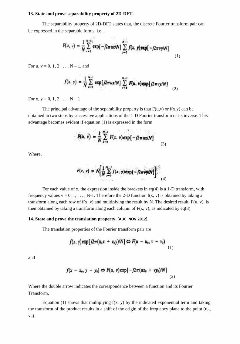
13. State and prove separability property of 2D-DFT.

The separability property of 2D-DFT states that, the discrete Fourier transform pair can

be expressed in the separable forms. i.e. ,

(1)

For u, v = 0, 1, 2 . . . , N – 1, and

(2)

For x, y = 0, 1, 2 . . . , N – 1

The principal advantage of the separability property is that F(u,v) or f(x,y) can be

obtained in two steps by successive applications of the 1-D Fourier transform or its inverse. This

advantage becomes evident if equation (1) is expressed in the form

(3)

Where,

(4)

For each value of x, the expression inside the brackets in eq(4) is a 1-D transform, with

frequency values v = 0, 1, . . . , N-1. Therefore the 2-D function f(x, v) is obtained by taking a

transform along each row of f(x, y) and multiplying the result by N. The desired result, F(u, v), is

then obtained by taking a transform along each column of F(x, v), as indicated by eq(3)

14. State and prove the translation property. [AUC NOV 2012]

The translation properties of the Fourier transform pair are

(1)

and

(2)

Where the double arrow indicates the correspondence between a function and its Fourier

Transform,

Equation (1) shows that multiplying f(x, y) by the indicated exponential term and taking

the transform of the product results in a shift of the origin of the frequency plane to the point (uo,

vo).

Consider the equation (1) with uo = vo = N/2 or

exp[j2Π(uox + voy)/N] = ejΠ(x + y)

= (-1)(x + y)

and

f(x, y)(-1)x +y

F(u – N/2, v – N/2)

Thus the origin of the Fourier transform of f(x, y) can be moved to the center of its corresponding

N x N frequency square simply by multiplying f(x, y) by (-1)x+y

. In the one variable case this

shift reduces to multiplication of f(x) by the term (-1)x. Note from equation (2) that a shift in f(x,

y) does not affect the magnitude of its Fourier transform as,

15. State distributivity and scaling property.

Distributivity:

From the definition of the continuous or discrete transform pair,

and, in general,

In other words, the Fourier transform and its inverse are distributive over addition but not over

multiplication.

Scaling:

For two scalars a and b,

af (x, y) aF(u, v)

16. Explain the basic principle of Hotelling transform.

Hotelling transform:

The basic principle of hotelling transform is the statistical properties of vector

representation. Consider a population of random vectors of the form,

And the mean vector of the population is defined as the expected value of x i.e.,

mx = E{x}

The suffix m represents that the mean is associated with the population of x vectors. The

expected value of a vector or matrix is obtained by taking the expected value of each elememt.

The covariance matrix Cx in terms of x and mx is given as

Cx = E{(x-mx) (x-mx)T

}

T denotes the transpose operation. Since, x is n dimensional, {(x-mx) (x-mx)T

} will be of

n x n dimension. The covariance matrix is real and symmetric. If elements xi and xj are

uncorrelated, their covariance is zero and, therefore, cij = cji = 0.

For M vector samples from a random population, the mean vector and covariance matrix

can be approximated from the samples by

and

6. Write about Slant transform. [AUC NOV 2011]

The Slant transform matrix of order N x N is the recursive expression Sn is given by

Where Im is the identity matrix of order M x M, and

The coefficients are

and

The slant transform for N = 4 will be

17. What are the properties of Slant transform? [AUC NOV 2012 , APR 2013]

Properties of Slant transform

(i) The slant transform is real and orthogonal.

S = S*

S-1

= ST

(d) The slant transform is fast, it can be implemented in (N log2N) operations on an N x 1 vector.

(e) The energy deal for images in this transform is rated in very good to excellent range.

(f) The mean vectors for slant transform matrix S are not sequentially ordered for n ≥ 3.

8. Define discrete cosine transform.

The 1-D discrete cosine transform is defined as

For u = 0, 1, 2, . . , N-1. Similarly the inverse DCT is defined as

For u = 0, 1, 2, . . , N-1

Where α is

The corresponding 2-D DCT pair is

For u, v = 0, 1, 2, . . , N-1, and

For x, y= 0, 1, 2, . . , N-1

18. Explain about Haar transform. [AUC NOV 2013]

The Haar transform is based on the Haar functions, hk(z), which are defined over the

continuous, closed interval z ε [0, 1], and for k = 0, 1, 2 . . . , N-1, where N = 2n. The first step in

generating the Haar transform is to note that the integer k can be decomposed uniquely as

k = 2p + q - 1

where 0 ≤ p ≤ n-1, q = 0 or 1 for p = 0, and 1 ≤ q ≤ 2p for p ≠ 0. For example, if N = 4, k, q, p

have following values

The Haar functions are defined as

for z ε [0, 1] ……. (1)

and

These results allow derivation of Haar transformation matrices of order N x N by formation of the

ith row of a Haar matrix from elements oh hi(z) for z = 0/N, 1/N, . . . , (N-1)/N. For instance, when

N = 2, the first row of the 2 x 2 Haar matrix is computed by using ho(z) with z = 0/2, 1/2. From

equation (1) , ho(z) is equal to 1/ , independent of z, so the first row of the matrix has two

identical 1/ elements. Similarly row is computed. The 2 x 2 Haar matrix is

Similarly matrix for N = 4 is

19. What are the properties of Haar transform. [AUC NOV 2011]

Properties of Haar transform:

(j) The Haar transform is real and orthogonal.

(k) The Haar transform is very fast. It can implement O(n) operations on an N x 1 vector.

(l) The mean vectors of the Haar matrix are sequentially ordered.

(m) It has a poor energy deal for images.

11. Write a short notes on Hadamard transform.

1-D forward kernel for hadamard transform is

Expression for the 1-D forward Hadamard transform is

Where N = 2n and u has values in the range 0, 1, . . . , N-1.

1-D inverse kernel for hadamard transform is

Expression for the 1-D inverse Hadamard transform is

The 2-D kernels are given by the relations

and

2-D Hadamard transform pair is given by following equations

Values of the 1-D hadamard transform kernel for N = 8 is

The Hadamard matrix of lowest order N = 2 is

If HN represents the matrix of order N, the recursive relationship is given by

Where H2N is the Hadamard matrix of order 2N and N = 2n

12. Write about Walsh transform.

The discrete Walsh transform of a function f (x), denoted W(u), is given by

Walsh transform kernel is symmetric matrix having orthogonal rows and columns. These

properties, which hold in general, lead to an inverse kernel given by

Thus the inverse Walsh transform is given by

The 2-D forward and inverse Walsh kernels are given by

and

Thus the forward and inverse Walsh transforms for 2-D are given by

and

The Walsh Transform kernels are seperable and symmetric, because

Values of the 1-D walsh transform kernel for N = 8 is

unit i: digital image fundamentals part -a …€¦ · unit – i: digital image fundamentals part...

Documents