unit i 1) data structure structure... · 2019-12-19 · 2. an algorithm is an ordered finite set of...

1

UNIT – I

1) Data structure:

1. Data structure is a way of collecting and organising data in such a way that we can perform

operations on these data in an effective way.

2. Data structures refer to data and representation of data objects within a program, that is, the

implementation of structured relationships.

3. A data structure is a collection of atomic and composite data types into a set with defined

relationships. By structure, we mean a set of rules that holds the data together.

4. In brief, a data structure is

1. a combination of elements, each of which is either as a data type or another data structure and

2. a set of associations or relationships (structures) involving the combined elements.

5. A data structure is a set of domains D, a set of functions F, and a set of axioms A. The triple

structure (D, F, A) denotes the data structure with the following elements:

Domain (D) This is the range of values that the data may have.

Functions (F) This is the set of operations for the data. We must specify a set of operations for a

data structure to operate on.

Axioms (A) This is a set of rules with which the different operations belonging to F can

actually be implemented.

an example of a data structure of an integer.

Here, the data structure d = Integer Integer

Domain D = {Integer, Boolean}

Set of functions F = {zero, ifzero, add, increment}

Set of axioms A = {

ifzero(zero()) true;

ifzero(increment(zero()) false

add(zero(), x) x

add(increment(x), y) = increment(add(x, y))

equal(increment(x), increment(y) = equal(x, y)

}

end Integer

Abstract Data Type

Abstraction allows us to focusing on logical properties of data and actions rather than on the

implementation details.

Logical properties refer to the ‗what‘ and

implementation details refer to the‗how‘.

Data abstraction is the separation of logical properties of the data from details of how

the data is represented. Procedural abstraction means separation of the logical properties

of action from implementation. Procedural abstraction and data abstraction are closely

related as operations within the ADTs are procedural abstractions. An ADT encompasses

both procedural as well as data abstraction; the set of operations are defined for any data

type that might make up the set of values. includes declaration of data, implementation of

operations,and encapsulation of data and operations.

Consider the concept of a queue. At least three data structures will support a queue.

We can use an array, a linked list, or a fle. If we place our queue in an ADT, users should

2

not be aware of the structure we use. As long as they can enqueue (insert) and dequeue

(retrieve) data, how we store the data should make no difference.

2) TYPES OF DATA STRUCTURES

Various types of data structures are as follows:

1. primitive and non-primitive

2. linear and non-linear

3. static and dynamic

4. persistent and ephemeral

5. sequential and direct access

1 Primitive and Non-primitive Data structures

Primitive data structures defne a set of primitive elements that do not involve any other

elements as its subparts —for example, data structures defned for integers and characters. These

are generally primary or built-in data types in programming languages.

Non-primitive data structures are those that define a set of derived elements such as

arrays,Class and structures

2 Linear and Non-linear Data structures

Data structures are classified as linear and non-linear. A data structure is said to be linear

if its elements form a sequence or a linear list. In a linear data structure, every data element has a

unique successor and predecessor. There are two basic ways of representing

linear structures in memory. One way is to have the relationship between the elements by

means of pointers (links), called linked lists. The other way is using sequential organization, that

is, arrays.

Non-linear data structures are used to represent the data containing hierarchical or

network relationship among the elements. Trees and graphs are examples of non-linear

data structures. In non-linear data structures, every data element may have more than one

predecessor as well as successor. Elements do not form any particular linear sequence.

3. static and Dynamic Data structures

A data structure is referred to as a static data structure if it is created before program execution

begins (also called during compilation time). An array is a static data structure.

A data structure that is created at run-time is called dynamic data structure. The variables of this

type are not always referenced by a user-defned name. These are accessed indirectly using their

addresses through pointers.

A linked list is a dynamic data structure when realized using dynamic memory management and

pointers, whereas an array is a static data structure. Non-linear data structures are generally

implemented in the same way as linked lists. Hence, trees and graphs

can be implemented as dynamic data structures.

4 Persistent and Ephemeral Data structures

There are two versions of a data structure namely the recently modified data structure and the

previous version

A data structure that supports operations on the most recent version as well as the

previous version is termed as a persistent data structure.

An ephemeral data structure is one that supports operations only on the most recent

version.

3

5. Sequential Access and Direct Access Data structures

This classification is with respect to the access operations associated with data structures.

Sequential access means that to access the nth element, we must access the preceding

(n 1) data elements. A linked list is a sequential access data structure. Direct access means that

any element can be accessed without accessing its predecessor or successor; we can directly

access the nth element. An array is an example of a direct access data structure.

3) INTRODUCTION TO ALGORITHMS:

Def:

1. Algorithm is a step by step process to get a solution to the given problem.

2. An algorithm is an ordered finite set of unambiguous and effective steps that

produces a result and terminates.

Each algorithm includes steps for

1. Input,

2. Processing, and

3. Output.

Characteristics of Algorithms:

The characteristics of algorithms are:

1. Input: An algorithm is supplied with zero or more external quantities as input.

2. Output: An algorithm must produce a result, that is, an output.

3. Unambiguous steps: Each step in an algorithm must be clear and unambiguous. This

helps the person or computer following the steps to take a definite action.

4. Finiteness: An algorithm must halt. Hence, it must have finite number of steps.

5. Effectiveness: Every instruction must be sufficiently basic, to be executed easily.

Algorithm Design Tools: Pseudo code and Flowchart:

The two popular tools used in the representation of algorithms are the following:

1. Pseudocode

2. Flowchart

1. PSEUDOCODE:

An algorithm can be written in any of the natural languages such as English, German,

French, etc. One of the commonly used tools to define algorithms is the pseudocode.

A pseudocode is an English-like presentation of the code required for an algorithm. It is

partly English and partly computer language structure code. The structure code is nothing but

syntax constructs of a programming language

Pseudocode Notations

Pseudocode is a precise description of a solution as compared to a flowchart. To get a

complete description of the solution with respect to problem defnition, pre–post conditions and

4

return value details are to be included in the algorithm header. In addition,

information about the variables used and the purpose are to be viewed clearly. To help

anyone get all this information at a glance, the pseudocode uses various notations such

as header, purpose, pre–post conditions, return, variables, statement numbers, and sub

algorithms.

Ex:

Algorithm sort(ref A<integer>, val N<integer>)

Pre array A to be sorted

Post sorted array A

Return None

1.if(N < 1) goto step (4)

2.M = N - 1

3.For I = 1 to M do

For J = I + 1 to N do

begin

if(A(I)> A(J))

then

begin

Fundamental concepts 15

T = A(I)

A(I) = A(J)

A(J) = T

end

end if

end

4.stop

2. FLOWCHARTS

A very effective tool to show the logic flow of a program is the flowchart. A flowchart is

a pictorial representation of an algorithm. It hides all the details of an algorithm by giving a

picture it shows how the algorithm flows from beginning to end. In a programming environment,

it can be used to design a complete program or just a part of the program. The primary purpose

of a flowchart is to show the design of the algorithm. At the same time, it relieves the

programmers from the syntax and details of a programming language while allowing them to

concentrate on the details of the problem to be solved. This is in contrast to another

programming design tool, the pseudocode, which provides a textual design solution.

5

The above flow chart describes the process of reading, adding, printing three numbers, and printing the

result.

ANALYSIS OF ALGORITHMS:

Algorithms heavily depend on the organization of data. There can be several ways to

organize data and/or write algorithms for a given problem. The difficulty lies in deciding which

algorithm is the best. We can compare one algorithm with the other and choose the best. For

comparison, we need to analyse the algorithms. Analysis involves measuring the performance of an

algorithm. Performance is measured in terms of the following parameters:

1. Programmer’s time complexity —Very rarely taken into account as it is to be paid for once

2. Time complexity —The amount of time taken by an algorithm to perform the intended task

3. Space complexity—The amount of memory needed to perform the task.

1. Space Complexity

Space complexity is the amount of computer memory required during program execution as a

function of the input size. Space complexity measurement, which is the space

requirement of an algorithm, can be performed at two different times:

1. Compile time

2. Run time

Compile Time Space Complexity

Compile time space complexity is defined as the storage requirement of a program at compile time.

This storage requirement can be computed during compile time. The storage needed by the program at

compile time can be determined by summing up the storage size of each variable using declaration

statements.

Space complexity Space needed at compile time

This includes memory requirement before execution starts.

6

Run-time Space Complexity

If the program is recursive or uses dynamic variables or dynamic data structures, then

there is a need to determine space complexity at run-time. In general, this dynamic storage

size is dependent on some parameters used in a program. It is difficult to estimate

memory requirement accurately, as it is also determined by the efficiency of compiler.

Memory requirement is the summation of the program space, data space, and stack space.

Program space This is the memory occupied by the program itself.

Data space This is the memory occupied by data members such as constants and

variables.

Stack space This is the stack memory needed to save the function‘s run-time

environment while another function is called. This cannot be accurately estimated

since it depends on the run-time call stack, which can depend on the program‘s data

set. This memory space is crucially important for recursive functions.

2. Time Complexity

Time complexity is the time taken by a program , that is, the sum of its compile

and execution times. This is system-dependent. Another way to compute it is to count the

number of algorithm steps. An algorithm step is a syntactically or semantically meaningful segment of a

program.

Best, Worst, and Average Cases

The best case complexity of an algorithm is the function defined by the minimum number of steps taken

on any instance of size n.

The worst case complexity of an algorithm is the function defined by the maximum number of steps

taken on any instance of size n.

The average case complexity of an algorithm is the function defined by an average number of steps

taken on any instance of size n.

7

LINEAR DATA STRUCTURE USING ARRAYS:

1. Array is a group of similar elements that shares a common name and stores in continuous

memory locations.

2. Arrays are the most general and easy to use of all the data structures. An array as a data

structure is defined as a set of pairs (index, value) such that with each index, a value

is associated.

index—indicates the location of an element in an array

value—indicates the actual value of that data element

3. An array is a finite ordered collection of homogeneous data elements that provides direct access

to any of its elements.

Finite The number of elements in an array is finite or limited.

Ordered collection The arrangement of all the elements in an array is very specific, that is, every

element has a particular ranking in the array.

Homogeneous All the elements of an array should be of the same data type.

Declaration of an array in C.

int A[20];

This statement will allocate a memory space to store 20 integer elements, and the name assigned to the

array is A.

char Name[20];

Similarly, this statement will create an array Name that can store 20 character data type elements in it.

The common terms associated with arrays are as follows:

1.Size of array The maximum number of elements that would be stored in an array is the size of that

array. It is also the length of that array. Arrays are static data structures because once the size of an

array is defined, it cannot be changed after compilation. For the array Name, the size is 20.

2.Base The base address of an array is the memory location where the first element of an array is

stored. It is decided at the time of execution of a program. The value of this base address varies at every

program execution as it is decided at the run-time. It cannot be decided or defined even by a

programmer.

3.Data type of array The data type of an array indicates the data type of elements stored in that array.

4.Index A user or a programmer can access the elements of an array by using subscripts such as

Name[0], Name[1], ..., Name[i]. This subscript is called the index of an element. It indicates the

relative position of every element in the array with respect to its frst element. Often, an array is also

referred to as subscripted variable.

5.Range of index If N is the size of an array, then in C, the range of index is 0 (N 1) (whereas for

languages such as Pascal it could be some integer, say, lower bound (LB) to upper bound (UB), e.g., 2 to

n 1 or 3 to n 4). The range is language dependent.

8

MEMORY REPRESENTATION AND ADDRESS CALCULATION:

A computer‘s memory can be considered as one long list of bits grouped together into bytes and/or

words. Each one of them can be referred to just one location so as to avoid machine dependent details,

that is, whether memory is structured with a one-byte, two-byte, or n byte word. In addition, the

addressing scheme varies with each computer such as byte addressable or word addressable. During

compilation, the appropriate number of locations is allocated for the array. The mechanism for allocating

memory is much dependant on a language. Regardless of machine and language dependency, when the

space is actually allocated, the location of an entire block of memory is referenced by the base address of

the first location. The remaining elements are stored sequentially at a fixed distance apart, say, by a

constant C. So if the ith element is mapped into a memory location of address x, then the(i 1)th element

is mapped into the memory location with address (x C) . Here, C depends on the size of the element,

that is, the number of locations required per element, and also on the addressing of these locations.

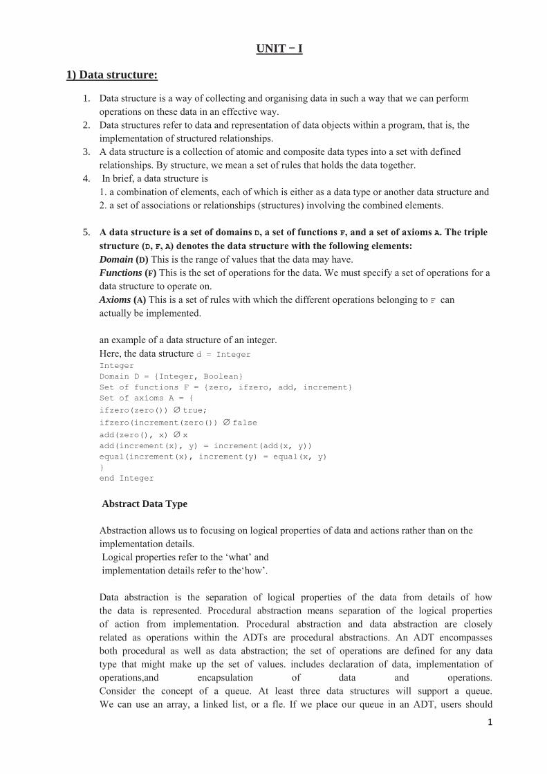
The address of the ith element is calculated by the following formula:

(Base address) (Offset of ith element from base address)

Here, base address is the address of the first element where array storage starts. In Fig,, the base address

is x and the offset is computed as

Offset of ith element (Number of elements before ith element) X(Size of each element)

Address of A[i] Base I XSize of element

Assuming the size of the element as one memory location, the memory representation

is shown in Fig

9

Most of the languages use the base address plus offset for addressing. This way of addressing helps in

direct access to an element with bounded time O(1) for access. In brief, the Array_A[N] is implemented

as follows:

1. Array_A is the name of the object/structure and is associated with a base (starting) address in

memory.

2. The [N] notation specifes the number of array elements from the beginning (offset), which starts at

zero.

3. The address of the ith element is then computed as base i (Size of element), where Size of element

depends on the data type.

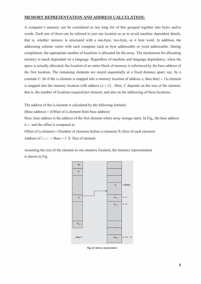
The index, address, and values are shown in Fig. 2.5 for an array of six real numbers.

CLASS ARRAY

The array ADT can support various operations such as traversal, sorting, searching, insertion, deletion,

merging, and block movement. Some of these operations are detailed in Program

class Array

{

private:

int MaxSize;

int A[20];

int Size;

public:

Array() // constructor

{

MaxSize = 20;

Size = 0;

}

void Read_Array();

void Display(); // Traverse_Forward()

void Traverse_Backward();

void Insert(int Location, int Element);

void Delete(int Location);

int Search(int Element);

};

10

void Array :: Read_Array()

{

int i, N;

cout << "Enter size of array";

cin >> N;

if(N > MaxSize)

{

cout << "Array of this size cannot be created";

cout << "Maximum size is" << MaxSize;

return;

}

else

{

for(i = 0; i < N; i++)

{

cin >> A[i];

}

Size = N;

}

}

void Array :: Display()

{

int i;

for(i = 0; i < Size; i++)

cout << A[i] << "\t";

cout << endl;

}

void Array :: Traverse_Backward()

{

int i;

for(i = Size - 1; i >= 0; i--)

cout << A[i] << "\t"; cout << endl;

}

int Array :: Search(int Element)

{

int i;

for(i = 0; i < Size - 1; i++)

{

if(Element == A[i])

return(i);

}

return(-1);

}

void Array :: Insert(int Location, int Element)

{

int i;

if(Size >= MaxSize)

{

cout << "Sorry, Array Overfl ow";

return;

}

for(i = Size - 1; i >= Location - 1; i--)

{

A[i + 1] = A[i]; // shifting element to right by

1 position

}

A[Location - 1] = Element;

Size = Size + 1;

}

11

void Array :: Delete(int Location)

{

int i;

for(i = Location; i < Size; i++)

{

A[i - 1] = A[i];

// shifting elements to the left by 1 position

}

A[Size - 1] = 0;

// Store 0 at the last location to mark it empty

Size = Size - 1;

}

void main()

{

Array A;

A.Read_Array();

A.Display(); // Traverse_Forward()

A.Traverse_Backward();

A.Insert(3, 66); // insert at position 3

A.Display();

cout << endl;

A.Delete(3); // delete 4th element

A.Display();

cout << endl;

cout << A.Search(66);

cout << A.Search(3);

}

Two-dimensional Arrays

A two-dimensional array A of dimension m Xn is a collection of m Xn elements in which each element

is identifed by a pair of indices [i, j], where in general, 1 i m and 1 j n. For the C/Clanguages

this range is 0 i m and 0 j n. A two-dimensional array has m rows and n columns. The best

example of two-dimensional arrays is the most popular mathematical entity, matrix.

Memory Representation of Two-dimensional Arrays

Let us consider a two-dimensional array A of dimension m Xn. Though the array is multidimensional, it

is usually stored in memory as a one-dimensional array. A multidimensional array is represented in

memory as a sequence of m Xn consecutive memory locations.

The elements of a multidimensional array can be stored in the memory as

1. Row-major representation or

2. Column-major representation

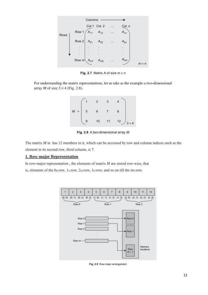
Figure shows matrix A of size m Xn.

12

The matrix M in has 12 members in it, which can be accessed by row and column indices such as the

element in its second row, third column, is 7.

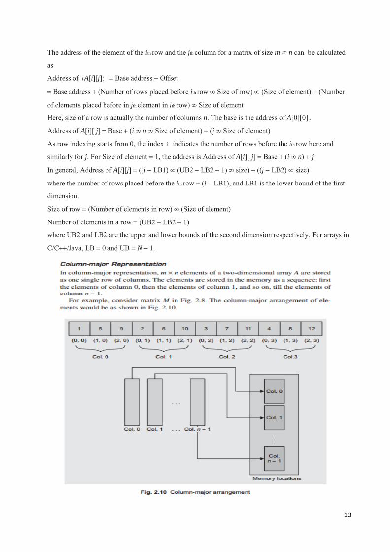
1. Row-major Representation

In row-major representation , the elements of matrix M are stored row-wise, that

is, elements of the 0th row, 1st row, 2nd row, 3rd row, and so on till the mth row.

13

The address of the element of the ith row and the jth column for a matrix of size m n can be calculated

as

Address of (A[i][j]) Base address Offset

Base address (Number of rows placed before ith row Size of row) (Size of element) (Number

of elements placed before in jth element in ith row) Size of element

Here, size of a row is actually the number of columns n. The base is the address of A[0][0].

Address of A[i][ j] Base (i n Size of element) (j Size of element)

As row indexing starts from 0, the index i indicates the number of rows before the ith row here and

similarly for j. For Size of element 1, the address is Address of A[i][ j] Base (i n) j

In general, Address of A[i][j] ((i LB1) (UB2 LB2 1) size) ((j LB2) size)

where the number of rows placed before the ith row (i LB1), and LB1 is the lower bound of the first

dimension.

Size of row (Number of elements in row) (Size of element)

Number of elements in a row (UB2 LB2 1)

where UB2 and LB2 are the upper and lower bounds of the second dimension respectively. For arrays in

C/C/Java, LB 0 and UB N 1.

14

The address of A[i][ j] is computed as Address of (A[i][j]) Base address Offset

Base address (Number of columns placed before jth column size of column) (Size of element)

(Number of elements placed before in ith element in ith row) Size of element

Here, the size of the column is the number of rows, that is, m. If the base is the address

of A[0][0], then

Address of A[i][j] Base (j m Size of element) (i Size of element)

For Size of element = 1, the address is

Address of A[i][j] for column-major arrangement Base (j m) i

In general, for column-major arrangement, the address of the element of the ith row and the jth column is

Address of (A[i][ j] ((j LB2) (UB1 LB1 1) size) ((i LB1) size)

n-dimensional Arrays

An n-dimensional m 1 m2 m3 ... mn array A is a collection of m1 m2 m3 … mn

elements in which each element is specifed by a list of n integers such as k1, k2, … kn

called subscripts where 0 k1 m1 1, 0 k2 m2 1, …, 0 kn mn 1. The element

of array A with subscripts k1, k2, …, kn is denoted by A[k1][k2]…[kn].

\

16

Program:

Class String

{

private:

char Str[];

public:

String() {}

int Length();

void Concat(String B);

int Substring(String S);

};

int String :: Length()

{

int length = 0, i;

for(i = 0; Str[i] != ‟\0‟; i++)

length++;

return(length);

}

17

void String :: Concat(String B)

{

int len_A, i, j;

// To concatenate B to A we need to traverse

// string A till the end

for(i = 0; Str[i] != „\0‟; i++);

len_A = i;

// Let us concatenate B to A now

for(i = len_A, j = 0; B.Str[j] != „\0‟; j++,i++)

{

Str [i] = B.Str[j];

}

Str[i] = „\0‟;

}

String String :: Copy()

{

String B;

int i;

for(i = 0; Str[i] != „\0‟; i++)

B.Str[i] = Str[i];

B.Str[i] = „\0‟; // Append the termination character

return B;

}

String String :: Copy_Reverse()

{

int i, l, Len_A;

for(l = 0; Str[l] != „\0‟; l++);

Len_A = l--

for(i = l, j = 0; i >= 0; i--, j++)

B.Str[j] = Str[i];

B.Str[j] = „\0‟; //Append termination character

return B;

}

void String :: Rev_String()

{

int i, len = 0;

char t;

for(len = 0; Str[len] !=„\0‟,len++);

for(i = 0, j = len - 1; i != j; i++, j--)

{

t = Str[i]; Str[i] = Str[j]; Str[j] = t;

}

}

int String :: Str_cmp(String A, String B)

{

int i = 0;

if (A.Length() != B.Length())

return(0);

18

while

(A.Str[i] == B.Str[i] && A.Str[i] != „\0‟ && B.Str[i] != „\0‟)

++ i;

if(A.Str[i] == „\0‟ && B.Str[i] == „\0‟)

return(1);

else

return(0);

}

CONCEPT OF ORDERED LIST

Ordered list is the most common and frequently used data object. Linear elements of an ordered list are

related with each other in a particular order or sequence. The following are some examples of ordered

lists.

1. Odd numbers less than or equal to 15 = {1, 3, 5, 7, 9, 11, 13, 15}

2. Months = {January, February, March, April, May, June, July, August, September,

October, November, December}

3. Colors of the rainbow = {Violet, Indigo, Blue, Green, Yellow, Orange, Red}

There are many basic operations that can be performed on the ordered list. The following list states

them:

1. Find the length of the list.

2. Traverse the list from left to right or from right to left.

3. Access the ith element in the list.

4. Update (Overwrite) the value at the ith position.

5. Insert an element at the ith location.

6. Delete an element at the ith position.

Arrays are the most common data structures that can be used for representing an ordered list.

In an ordered list, members of the list follow some specific sequence. We need to select the best suitable

data structure to perform these operations efficiently. The best possible way to organize them is in an

array. Let L be the list; L {a0, a1, a2, ..., an-1} having n elements.

If we store this list in an array, say list[n], then we can store the ith element at the ith location (index) of

the list. This representation would store a0 at list[0], a1 at list[1], and so on, sequentially as ai and ai+1 at

the ith and (i+1)th locations.

19

PROS AND CONS OF ARRAYS

Characteristics

1. An array is a finite ordered collection of homogeneous data elements.

2. In an array, successive elements are stored at a fixed distance apart.

3. An array is defined as a set of pairs—index and value.

4. An array allows direct access to any element.

5. In an array, insertion and deletion of elements in-between positions require data movement.

6. An array provides static allocation, which means the space allocation done once during the compile

time cannot be changed during run-time.

Advantages

1. Arrays permit efficient random access in constant time 0(1).

2. Arrays are most appropriate for storing a fixed amount of data and also for high frequency of data

retrievals as data can be accessed directly.

3. Arrays are among the most compact data structures; if we store 100 integers in an array, it takes only

as much space as the 100 integers, and no more (unlike a linked list in which each data element has an

additional link field).

4. Arrays are well known in applications such as searching, hash tables, matrix operations, and sorting.

5. Wherever there is a direct mapping between the elements and their position, such as an ordered list,

arrays are the most suitable data structures.

6. Ordered lists such as polynomials are most efficiently handled using arrays.

7. Arrays are useful to form the basis for several complex data structures such as heaps and hash tables

and can be used to represent strings, stacks, and queues.

Disadvantages

1. Arrays provide static memory management. Hence, during execution, the size can neither be grown

nor shrunk.

2. There is a solution to handle the problem, that is, to declare the array of some arbitrarily maximum

size. This leads to two other problems:

(a) In future, if the user still needs to exceed this limit, it is not possible.

(b) Higher the maximum, the more is the memory wastage because very often, many locations remain

unused but still allocated (reserved) for the program. This leads to poor utilization of space.

3. Static allocation in an array is a problem associated with implementation in many programming

languages except a few such as JAVA.

4. An array is inefficient when often data is inserted or deleted as insertion or deletion of an element in

an array needs a lot of data movement.

6. A drawback due to the simplicity of arrays is the possibility of referencing a nonexistent element by

using an index outside the valid range. This is known as exceeding

the array bounds.

20

Stacks

Stack is a linear data structure which contains one open end and one closed end.

Insertion and deletion is done at a single end. It follows LIFO (Last in First Out).i.e. the

element which enters last deleted first. Elements may be added to or removed from only

one end, called the top of a stack.

A stack is defined as a restricted list where all insertions and deletions are made only

at one end, the top. Each stack abstract data type (ADT) has a data member, commonly

named as top, which points to the topmost element in the stack. There are two basic

operations push and pop that can be performed on a stack; insertion of an element in

the stack is called push and deletion of an element from the stack is called pop. In

stacks, we cannot access data elements from any intermediate positions other than the

top position.

c top

b

a

Primitive Operations:

The three basic stack operations are push, pop, and getTop. Besides these, there

are some more operations that can be implemented on a stack such as

stack_initialization, stack_empty, and stack_full. The stack_initialization operation

prepares the stack for use and sets it to a vacant state. The stack_empty operation simply

tests whether the stack is empty. The stack_empty operation is useful as a safeguard

against an attempt to pop an element from an empty stack. Popping an empty stack is an

error condition. The stack_empty condition is also termed stack underflow. we need to

check the stack_full condition before doing push because pushing an element in a full

stack is also an error condition. Such a stack full condition is called stack overflow.

Another stack operation is GetTop. This returns the top element of the stack without

actually popping it. A few more stack operations include traversing the stack, counting

the total number of elements in the stack, and copying the stack.

21

Stack operations

1. Push—inserts an element on the top of the stack

2. Pop—deletes an element from the top of the stack

3. GetTop—reads (only reading, not deleting) an element from the top of the stack

4. Stack_initialization—sets up the stack in an empty condition

5. Empty—checks whether the stack is empty

6. Full—checks whether the stack is full

1. Push

The push operation inserts an element on the top of the stack. The recently added

element is always at the top of the stack.

diagram

When there is no space to accommodate the new element on the stack, the stack is

said to be full. If the operation push is performed when the stack is full, it is said

to be in overflow state, that is, no element can be added when the stack is full.

The push operation modifies the top

2. Pop

The pop operation deletes an element from the top of the stack and returns the

same to the user. It modifies the stack so that the next element becomes the top

element

diagram

When there is no element available on the stack, the stack is said to be empty. If

pop is performed when the stack is empty, then the stack is said to be in an

underflowstate

3. GetTop

The getTop operation gives information about the topmost element and returns

the element on the top of the stack. In this operation, only a copy of the element,

which is at the top of the stack, is returned.

Daiagram

22

STACK ABSTRACT DATA TYPE (ADT):

The following five functions comprise a functional definition of a stack:

1. Create(S)—creates an empty stack

2. Push(i, S)—inserts the element i on the stack S and returns the modifed stack

3. Pop(S)—removes the topmost element from the stack S and returns the modifed stack

4. GetTop(S)—returns the topmost element of stack S

5. Is_Empty(S)—returns true if S is empty, otherwise returns false

However, when we choose to represent a stack, it must be possible to build these operations. the

structure stack.

ADT Stack(element)

1. Declare Create() Æ stack

2. push(element, stack) Æ stack

3. pop(stack) Æ stack

4. getTop(stack) Æ element

5. Is_Empty(stack) Æ Boolean;

6. for all S Œ stack, e Œ element, Let

7. Is_Empty(Create) = true

8. Is_Empty(push(e, S)) = false 9. pop(Create()) = error

10. pop(push(e,S)) = S

11. getTop(Create) = error

12. getTop(push(e, S)) = e

13. end

14. end stack

The five functions with their domains and ranges are declared in lines 1 through 5.

Lines 6 through 13 are the set of axioms that describe how the functions are related.

Lines 10 and 12 are important because they define the LIFO behavior of the stack.

To implement the ADT stack in C++, the operations are often implemented as functions to

provide data abstraction. A program that uses stacks would access the stacks only through

these functions and would not be concerned about the implementation.

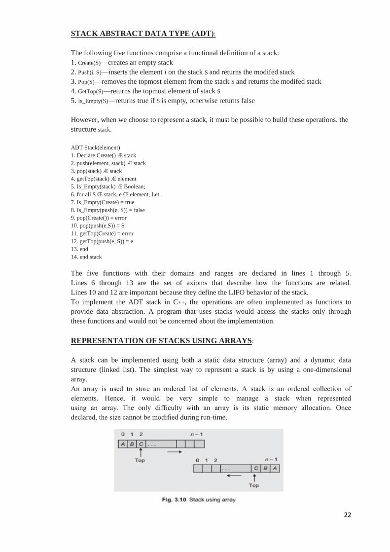
REPRESENTATION OF STACKS USING ARRAYS:

A stack can be implemented using both a static data structure (array) and a dynamic data

structure (linked list). The simplest way to represent a stack is by using a one-dimensional

array.

An array is used to store an ordered list of elements. A stack is an ordered collection of

elements. Hence, it would be very simple to manage a stack when represented

using an array. The only difficulty with an array is its static memory allocation. Once

declared, the size cannot be modified during run-time.

23

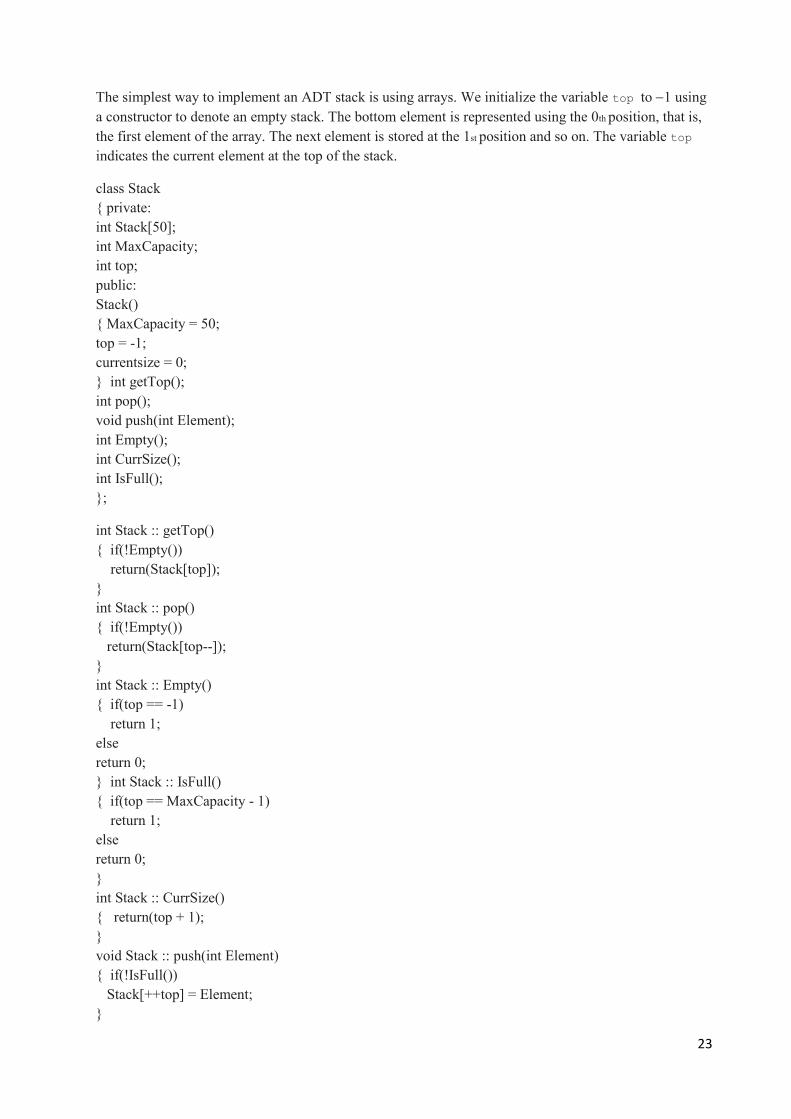
The simplest way to implement an ADT stack is using arrays. We initialize the variable top to 1 using

a constructor to denote an empty stack. The bottom element is represented using the 0th position, that is,

the first element of the array. The next element is stored at the 1st position and so on. The variable top

indicates the current element at the top of the stack.

class Stack

{ private:

int Stack[50];

int MaxCapacity;

int top;

public:

Stack()

{ MaxCapacity = 50;

top = -1;

currentsize = 0;

} int getTop();

int pop();

void push(int Element);

int Empty();

int CurrSize();

int IsFull();

};

int Stack :: getTop()

{ if(!Empty())

return(Stack[top]);

}

int Stack :: pop()

{ if(!Empty())

return(Stack[top--]);

}

int Stack :: Empty()

{ if(top == -1)

return 1;

else

return 0;

} int Stack :: IsFull()

{ if(top == MaxCapacity - 1)

return 1;

else

return 0;

}

int Stack :: CurrSize()

{ return(top + 1);

}

void Stack :: push(int Element)

{ if(!IsFull())

Stack[++top] = Element;

}

24

void main()

{

Stack S;

S.pop();

S.push(1);

S.push(2);

cout << S.getTop() << endl;

cout << S.pop() << endl;

cout << S.pop() << endl;

}

APPLICATIONS OF STACK

The stack data structure is used in a wide range of applications. A few of them are the following:

1. Converting infix expression to postfx and prefix expressions

2. Evaluating the postfix expression

3. Checking well-formed (nested) parenthesis

4. Reversing a string

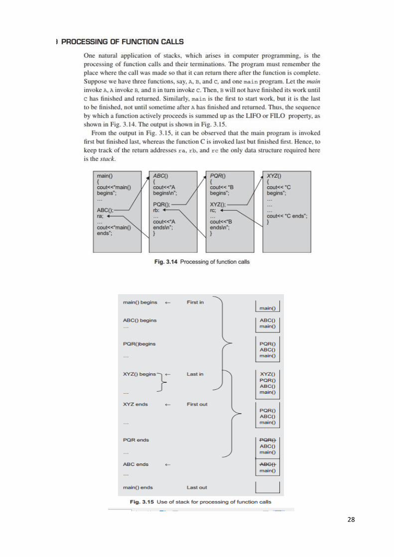
5. Processing function calls

6. Parsing (analyse the structure) of computer programs

7. Simulating recursion

8. In computations such as decimal to binary conversion

9. In backtracking algorithms (often used in optimizations and in games)

Expression evaluation:

Expression is combination of operators, operands and constants. When there are more than one

operator in the expression, evaluating the expression becomes complex. Which operator needs to

evaluate first and which evaluates next?

To fix the order of evaluation each operator is assigned with some priority. So high priority operators

evaluates first next the low priority operators evaluate. If there is same priority operators more than

one in the expression then we need to follow the associativity left to right or right to left. If there are

parentheses (brackets) in the expression then the first priority is given to the operation in the

parenthesis.

Operators priority

Exponentiation (^), Unary (+), Unary (-), and not (~)

Multiplication (X), and division (/) 2

Addition (+), and subtraction (-)

Relational operators

Logical AND 5

Logical OR 6

X A/B ^ C D XE A XC

By using priorities and associativity rules, the expression X is rewritten as

X A/(B ^ C) (DXE) (A XC)

We manually evaluate the innermost expression first

25

Still the question remains as to how a compiler can accept such an expression and

produce the correct code. The solution is to rework on the expression to a form called the

postfix notation.

Infix, prefix, and postfix notations:

The Polish Mathematician Han Lukasiewicz suggested a notation called Polish notation,

which gives two alternatives to represent an arithmetic expression, namely the postfix

and prefix notations.

The conventional way of writing the expression is called infix, because the binary operators occur

between the operands, and unary operators precede their operand. For example, the expression ((A B)

C)/D is an infix expression. In postfix notation, the operator is written after its operands, whereas in

prefix notation, the operator precedes its operands.

Ex:

Convert the following expression to its postfix and prefix notations:

X = A/B ^ C + D X E - A X C

Solution By applying the rules of priority and associativity, this expression can be written in the

following form:

X = ((A/(B ^ C)) + (D X E) - (A X C))

It can be reworked to get its equivalent postfix and prefix expressions.

Postfix: ABC ^/ DE X + AC X

Prefix: -+/ A ^ BC X DE X AC

Postfix Expression Evaluation

The postfix expression may be evaluated by making a left-to-right scan, stacking operands, and

evaluating operators using the correct number from the stack as operands

and again placing the result onto the stack. This evaluation process is much simpler

than attempting a direct evaluation from the infix notation. This process continues

till the stack is not empty or on occurrence of the character #, which denotes the end

of the expression.

Algorithm lists the steps involved in the evaluation of the postfix expression E. 1. Let E denote the postfix expression

2. Let Stack denote the stack data structure to be used & let Top = -1

3. while(1) do

begin

X = get_next_token(E) // Token is an operator, operand, or delimiter

if(X = #) {end of expression}

then return

if(X is an operand)

then push(X) onto Stack

else {X is operator}

begin

OP1 = pop() from Stack

OP2 = pop() from Stack

26

Tmp = evaluate(OP1, X, OP2)

push(Tmp) on Stack

end

{If X is operator then pop the correct number of operands from stack for operator X.

Perform the operation and push the result, if any, onto the stack}

end

4. Stop

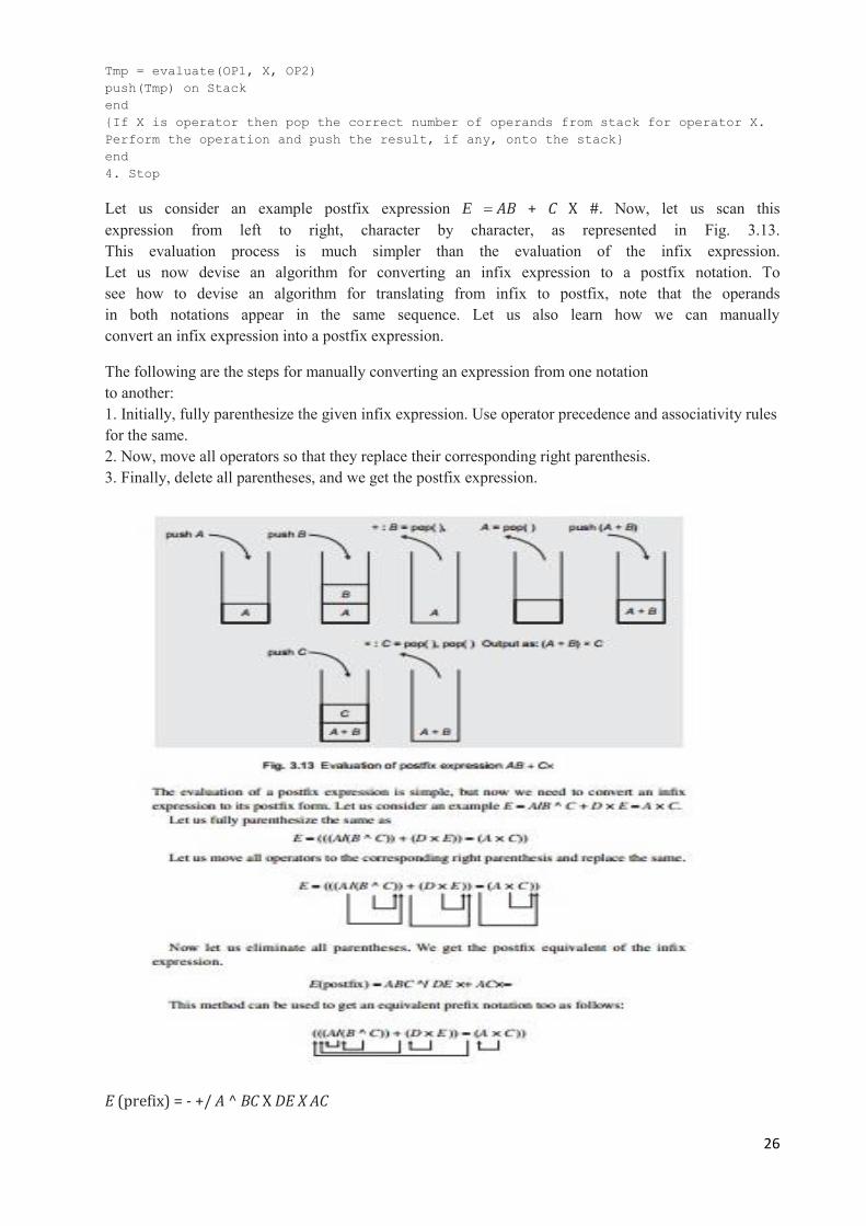
Let us consider an example postfix expression E AB + C X #. Now, let us scan this

expression from left to right, character by character, as represented in Fig. 3.13.

This evaluation process is much simpler than the evaluation of the infix expression.

Let us now devise an algorithm for converting an infix expression to a postfix notation. To

see how to devise an algorithm for translating from infix to postfix, note that the operands

in both notations appear in the same sequence. Let us also learn how we can manually

convert an infix expression into a postfix expression.

The following are the steps for manually converting an expression from one notation

to another:

1. Initially, fully parenthesize the given infix expression. Use operator precedence and associativity rules

for the same.

2. Now, move all operators so that they replace their corresponding right parenthesis.

3. Finally, delete all parentheses, and we get the postfix expression.

E (prefix) = - +/ A ^ BC X DE X AC

27

Infx to Postfx Conversion

Algorithm illustrates the infx to postfx conversion.

1. Scan expression E from left to right, character by character, till

character is „#‟

ch = get_next_token(E)

2. while(ch != ‟#‟}

if(ch = ‟)‟) then ch = pop()

while(ch !=„(‟)

Display ch

ch = pop()

end while

if(ch = operand) display the same

if(ch = operator) then

if(ICP > ISP) then push(ch)

else

while(ICP <= ISP)

pop the operator and display it

end while

ch = get_next_token(E)

end while

3. if(ch = #) then while(!emptystack()) pop and display

4. Stop

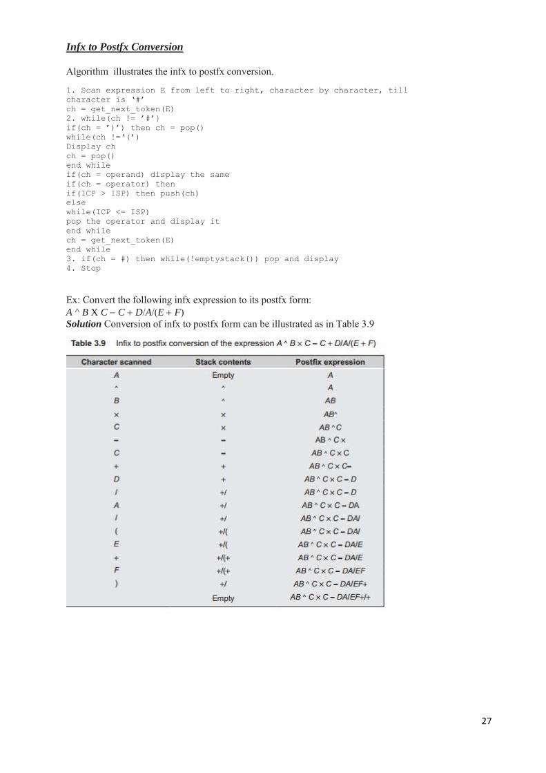
Ex: Convert the following infx expression to its postfx form:

A ^ B XC C D/A/(E F)

Solution Conversion of infx to postfx form can be illustrated as in Table 3.9

29

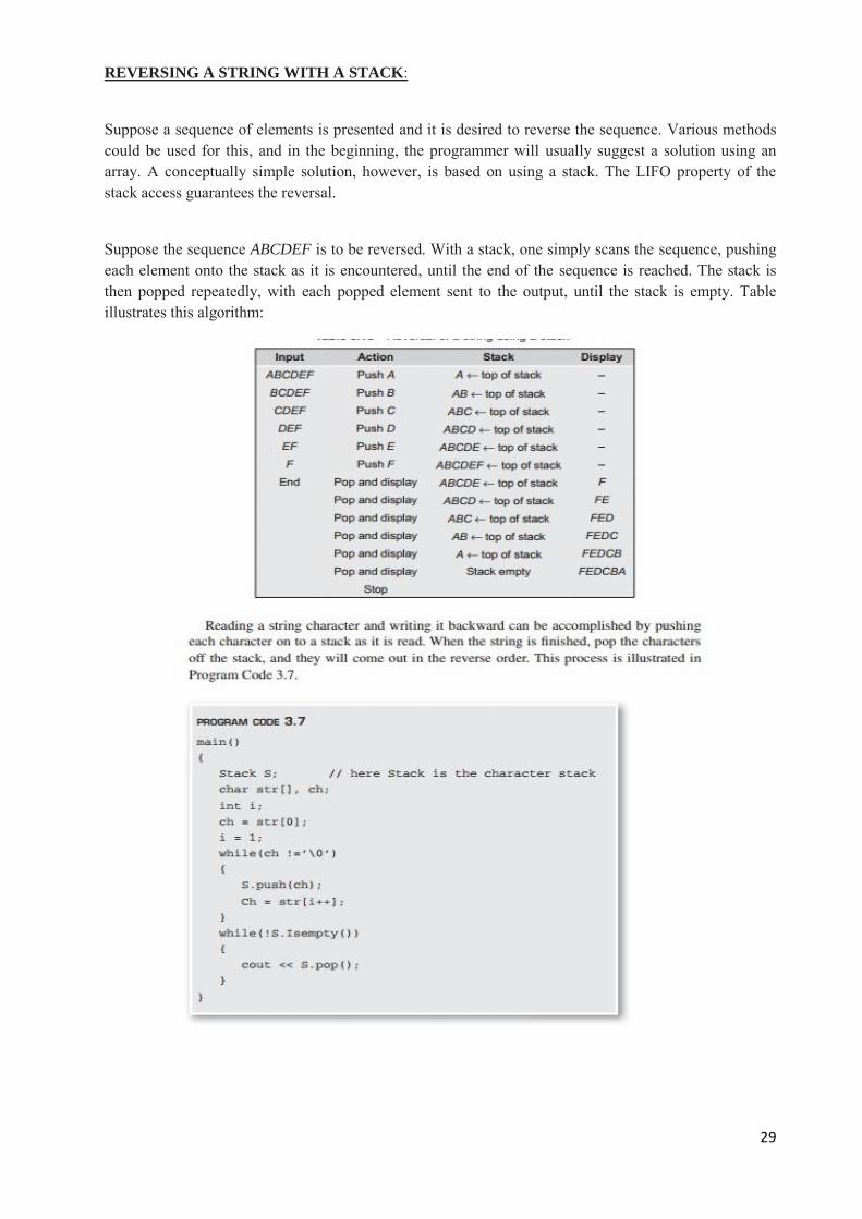
REVERSING A STRING WITH A STACK:

Suppose a sequence of elements is presented and it is desired to reverse the sequence. Various methods

could be used for this, and in the beginning, the programmer will usually suggest a solution using an

array. A conceptually simple solution, however, is based on using a stack. The LIFO property of the

stack access guarantees the reversal.

Suppose the sequence ABCDEF is to be reversed. With a stack, one simply scans the sequence, pushing

each element onto the stack as it is encountered, until the end of the sequence is reached. The stack is

then popped repeatedly, with each popped element sent to the output, until the stack is empty. Table

illustrates this algorithm:

30

CHECKING CORRECTNESS OF WELL-FORMED PARENTHESES

Consider a mathematical expression that includes several sets of nested parentheses. For example,

Z ((X X ((X Y/J 2)) Y)/3).

To ensure that the parentheses are nested correctly, we need to check that

1. There are equal numbers of right and left parentheses

2. Every right parenthesis is preceded by a matching left parenthesis

Expressions such as ((X Y) or (X Y)) violate condition 1, and expressions such as

(X Y) ( or (X Y))(A B) violate condition 2.

To solve this problem, let us define the parentheses count at a particular point in an expression as the

number of left parenthesis minus the number of right parenthesis that have been encountered in the left-

to-right scanning of the expression at that particular point. The two conditions that must hold if the

parentheses in an expression form an admissible pattern are as follows:

1. The parenthesis count at each point in the expression is non-negative.

2. The parenthesis count at the end of the expression is 0.

A stack may also be used to keep track of the parentheses count. Whenever a left parenthesis is

encountered, it is pushed onto the stack, and whenever a right parenthesis is encountered, the stack is

examined. If the stack is empty, then the string is declared to be invalid. In addition, when the end of the

string is reached, the stack must be empty; otherwise, the string is declared to be invalid.

31

UNIT- II

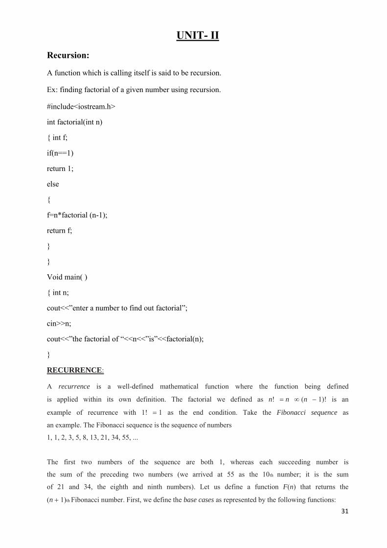
Recursion:

A function which is calling itself is said to be recursion.

Ex: finding factorial of a given number using recursion.

#include<iostream.h>

int factorial(int n)

{ int f;

if(n==1)

return 1;

else

{

f=n*factorial (n-1);

return f;

}

}

Void main( )

{ int n;

cout<<‖enter a number to find out factorial‖;

cin>>n;

cout<<‖the factorial of ―<<n<<‖is‖<<factorial(n);

}

RECURRENCE:

A recurrence is a well-defined mathematical function where the function being defined

is applied within its own definition. The factorial we defined as n! n (n 1)! is an

example of recurrence with 1! 1 as the end condition. Take the Fibonacci sequence as

an example. The Fibonacci sequence is the sequence of numbers

1, 1, 2, 3, 5, 8, 13, 21, 34, 55, ...

The first two numbers of the sequence are both 1, whereas each succeeding number is

the sum of the preceding two numbers (we arrived at 55 as the 10th number; it is the sum

of 21 and 34, the eighth and ninth numbers). Let us define a function F(n) that returns the

(n 1)th Fibonacci number. First, we define the base cases as represented by the following functions:

32

F(1) 1 and

F(2) 1

Now, we consider the other numbers. To get the (n 1)th Fibonacci number, we just add the nth and the

(n 1)th Fibonacci numbers. F(n) F(n 1) F(n 2) This function F is called recurrence since it

computes the nth value in terms of (n 1)th and (n 2)th Fibonacci values. The problems that can be

described using recurrence are easily expressed as recursive functions in programming.

The process of recursion occurs when a function calls itself. Recursion is useful in situations where

solving one or more smaller versions of the same problem can solve the problem. Computing the value

of three to the fourth power can be considered as

34 3 X 3

3

Three cubed can be defined as 33 3 X 3

2

Three squared is 32 3 X 3

1

Finally, 3 3 X 3

0 = 3 X 1

The recurrence for this computation is M n X M

n-1

USE OF STACK IN RECURSION:

The stack is a special area of memory where temporary variables are stored. It acts on the LIFO

principle. The following program code explains how recursive functions use the stack.

if(n <= 1)

return 1;

else

return n * Factorial(n - 1);

Let n 3; that is, let us compute the value of 3!, which is 3 X 2 X 1 = 6. When the function is called f

or the first time, n holds the value 3, so the else statement is executed. The function knows the value of

n but not of Factorial(n - 1), so it pushes n (value 3) onto the stack and calls itself for the second

time with the value 2. This time, the else statement is again executed, and n (value 2) is pushed onto

the stack as the function calls itself for the third time with the value 1. now, the if statement is executed

and as n 1, the function returns 1. Since the value of Factorial(1) is now known, it reverts to its

second execution by popping the last value 2 from the stack and multiplying it by 1. This operation gives

the value of Factorial(2), so the function reverts to its first execution by popping the next value 3 from

the stack and multiplying it with the factorial, giving the value 6, which the function finally returns.

From this example, we notice the following:

1. The Factorial() function in Program Code 4.2 runs three times for n 3, out of which it calls itself

two times. The number of times a function calls itself is known as the recursive depth of that function.

2. Each time the function calls itself, it stores one or more variables on the stack. Since stacks hold a

limited amount of memory, the functions with a high recursive depth may crash because of non-

33

availability of memory. Such a situation is known as stack overflow.

3. Recursive functions usually have (and in fact should have) a terminating (or end) condition. The

Factorial() function in Program stops calling itself when n 1.

4. All recursive functions go through two distinct phases. The frst phase, winding, occurs when the

function calls itself and pushes values onto the stack. The second phase, unwinding, occurs when the

function pops values from the stack, usually after the end condition.

Variants of recursion:

The recursive functions are categorized as direct, indirect, linear, tree, and tail recursions. Recursion may

have any one of the following forms:

1. A function calls itself.

2. A function calls another function which in turn calls the caller function.

3. The function call is part of the same processing instruction that makes a recursive function call.

A few more terms that are used with respect to recursion are explained in the following section.

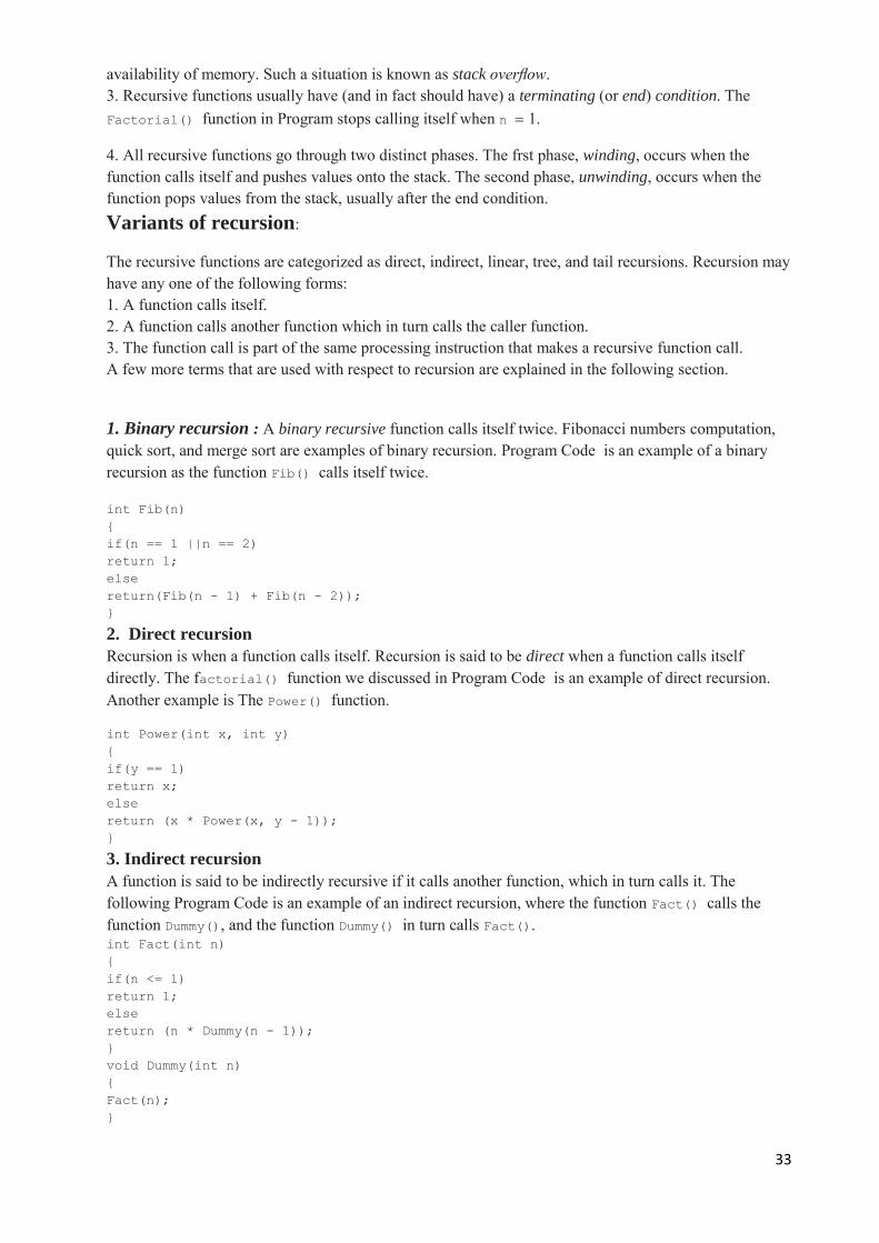
1. Binary recursion : A binary recursive function calls itself twice. Fibonacci numbers computation,

quick sort, and merge sort are examples of binary recursion. Program Code is an example of a binary

recursion as the function Fib() calls itself twice.

int Fib(n)

{

if(n == 1 ||n == 2)

return 1;

else

return(Fib(n - 1) + Fib(n - 2));

}

2. Direct recursion

Recursion is when a function calls itself. Recursion is said to be direct when a function calls itself

directly. The factorial() function we discussed in Program Code is an example of direct recursion.

Another example is The Power() function.

int Power(int x, int y)

{

if(y == 1)

return x;

else

return (x * Power(x, y - 1));

}

3. Indirect recursion

A function is said to be indirectly recursive if it calls another function, which in turn calls it. The

following Program Code is an example of an indirect recursion, where the function Fact() calls the

function Dummy(), and the function Dummy() in turn calls Fact(). int Fact(int n)

{

if(n <= 1)

return 1;

else

return (n * Dummy(n - 1));

}

void Dummy(int n)

{

Fact(n);

}

34

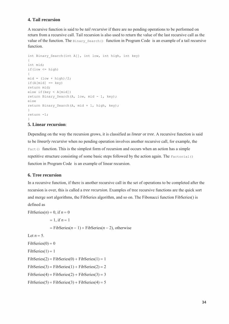
4. Tail recursion

A recursive function is said to be tail recursive if there are no pending operations to be performed on

return from a recursive call. Tail recursion is also used to return the value of the last recursive call as the

value of the function. The Binary_Search() function in Program Code is an example of a tail recursive

function.

int Binary_Search(int A[], int low, int high, int key)

{

int mid;

if(low <= high)

{

mid = (low + high)/2;

if(A[mid] == key)

return mid;

else if(key < A[mid])

return Binary_Search(A, low, mid - 1, key);

else

return Binary_Search(A, mid + 1, high, key);

}

return -1;

}

5. Linear recursion:

Depending on the way the recursion grows, it is classified as linear or tree. A recursive function is said

to be linearly recursive when no pending operation involves another recursive call, for example, the

Fact() function. This is the simplest form of recursion and occurs when an action has a simple

repetitive structure consisting of some basic steps followed by the action again. The Factorial()

function in Program Code is an example of linear recursion.

6. Tree recursion

In a recursive function, if there is another recursive call in the set of operations to be completed after the

recursion is over, this is called a tree recursion. Examples of tree recursive functions are the quick sort

and merge sort algorithms, the FibSeries algorithm, and so on. The Fibonacci function FibSeries() is

defined as

FibSeries(n) 0, if n 0

1, if n 1

FibSeries(n 1) FibSeries(n 2), otherwise

Let n 5.

FibSeries(0) 0

FibSeries(1) 1

FibSeries(2) FibSeries(0) FibSeries(1) 1




35

Figure demonstrates this explanation for n 4.

36

4. n 1

Now execute statement 1, which returns 1.

5. Pop the contents and n 2, so now the expression becomes 2 1.

6. Now, n 3 after popping the top of the stack contents. Therefore, the expression is 3 2 1.

7. After popping the top of the stack contents applying n 4, the expression is 4 3 2 1 24.

8. After popping the top of the stack contents, we get to know that the stack is empty, and the answer is

4! 24.

At the end condition, when no more recursive calls are made, the following steps are performed:

1. If the stack is empty, then execute a normal return.

2. Otherwise, pop the stack frame, that is, take the values of all the parameters that are on

the top of the stack and assign these values to the corresponding variables.

3. Use the return address to locate the place where the call was made.

4. Execute all the statements from that place (address) where the call was made.

5. Go to step 1

ITERATION VERSUS RECURSION:

Recursion is a top–down approach of problem solving. It divides the problem into pieces or selects one

key step, postponing the rest. On the other hand, iteration is more of a bottom–up approach. It begins

with what is known and from this constructs the solution step by step. It is hard to say that the non-

recursive version is better than the recursive one or vice versa. However, a few languages do not support

writing recursive code, such as FORTRAN or COBOL. The non-recursive version is more effcient as the

overhead of parameter passing in most compilers is heavy.

Demerits of recursive algorithms

1. Many programming languages do not support recursion

2. Even though mathematical functions can be easily implemented using recursion, it is always at the

cost of additional execution time and memory space.

Demerits of iterative Methods

1. Iterative code is not readable and hence not easy to understand.

2. In iterative techniques, looping of statements is necessary and needs a complex logic.

3. The iterations may result in a lengthy code.

37

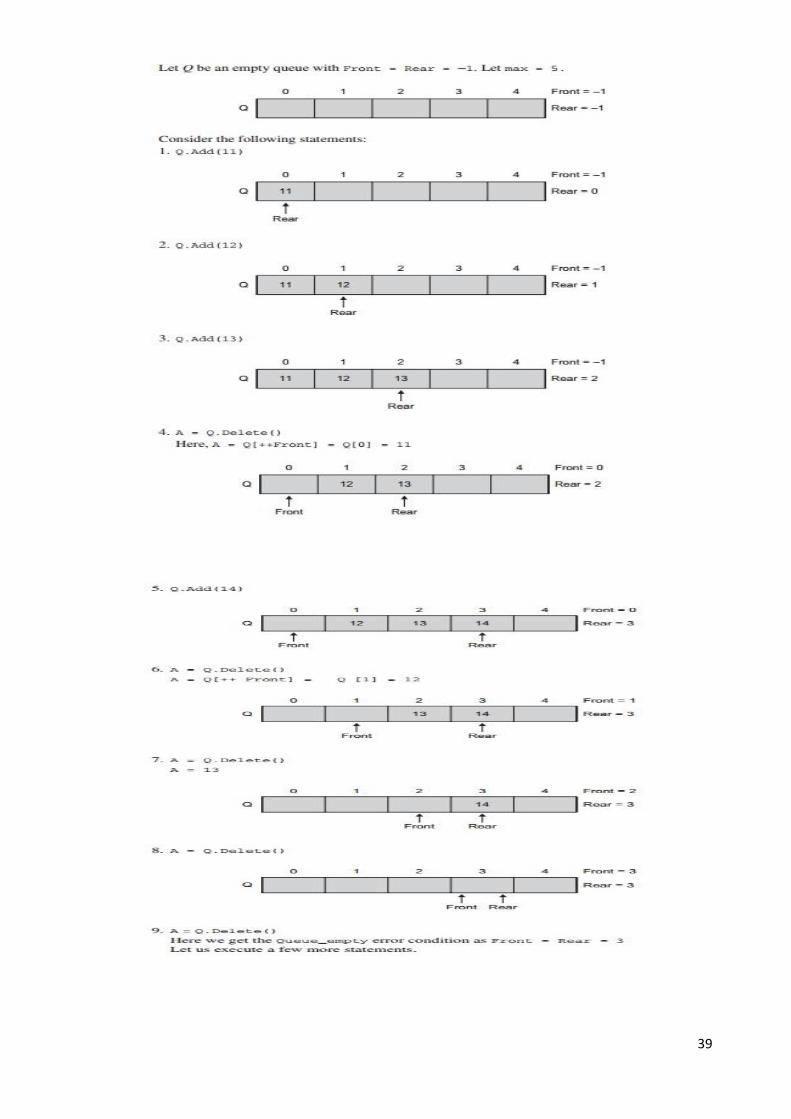
QUEUES:

Queue is a Linear Data Structure which has two open ends. The data entered and deleted from

two different ends. The end at which data is inserted is called the rear and that from which it is deleted

is called the front. Queue is a first in first out (FIFO) or last in last out (LILO) structure.

Primitive operations:

1.Create This operation should create an empty queue. Here max is the maximum initial size that is

defned. #defne max 50

int Queue[max];

int Front = Rear = -1;

2. Is_Empty This operation checks whether the queue is empty or not. This is confirmed by comparing

the values of Front and Rear. If Front = Rear, then Is_Empty returns true, else returns false. bool Is_Empty()

{ if(Front == Rear)

return 1; else

return 0;

}

3. Is_Full: before insertion, the queue must be checked for the Queue_Full state. When Rear points to

the last location of the array, it indicates that the queue is fullbool Is_Full() { if(Rear == max - 1)

return 1;

else

return 0;

}

4. Add This operation adds an element in the queue if it is not full. As Rear points to the last element of

the queue, the new element is added at the (rear 1)th location. void Add(int Element)

{ if(Is_Full())

cout << “Error, Queue is full”;

else

Queue[++Rear] = Element;

}

5. Delete This operation deletes an element from the front of the queue and sets Front to point to the

next element. Front can be initialized to one position less than the actual front. We should first

increment the value of Front and then remove the element. int Delete()

{ if(Is_Empty())

cout << “Sorry, queue is Empty”;

else

return(Queue[++Front]);

}

6. getFront The operation getFront returns the element at the front, but unlike delete, this does not

update the value of Front. int getFront()

{ if(Is_Empty())

cout << “Sorry, queue is Empty”; else

return(Queue[Front + 1]);

}

38

Queue ADT:

The basic operations performed on the queue include adding and deleting an element, traversing the

queue, checking whether the queue is full or empty, and fnding who is at the front and who is at the rear

ends.

A minimal set of operations on a queue is as follows:

1. create()—creates an empty queue, Q

2. add(i,Q)—adds the element i to the rear end of the queue, Q and returns the new queue

3. delete(Q)—takes out an element from the front end of the queue and returns the resulting queue

4. getFront(Q)—returns the element that is at the front position of the queue

5. Is_Empty(Q)—returns true if the queue is empty; otherwise returns false

The complete specification for the queue ADT is given in Algorithm

class queue(element)

declare create() queue

add(element, queue) -> queue

delete(queue) queue

getFront(queue) queue

Is_Empty(queue) Boolean;

For all Q Equeue, i E element let

Is_Empty(create()) = true

Is_Empty(add(i,Q)) = false

delete(create()) = error

delete(add(i,Q)) =

if Is_Empty(Q) then create

else add(i, delete(Q))

getFront(create) = error

getFront(add(i, Q)) =

if Is_Empty(Q) then i

else getFront(Q)

end

end queue

Since a queue is a linear data structure, it can be implemented using either arrays or linked lists

40

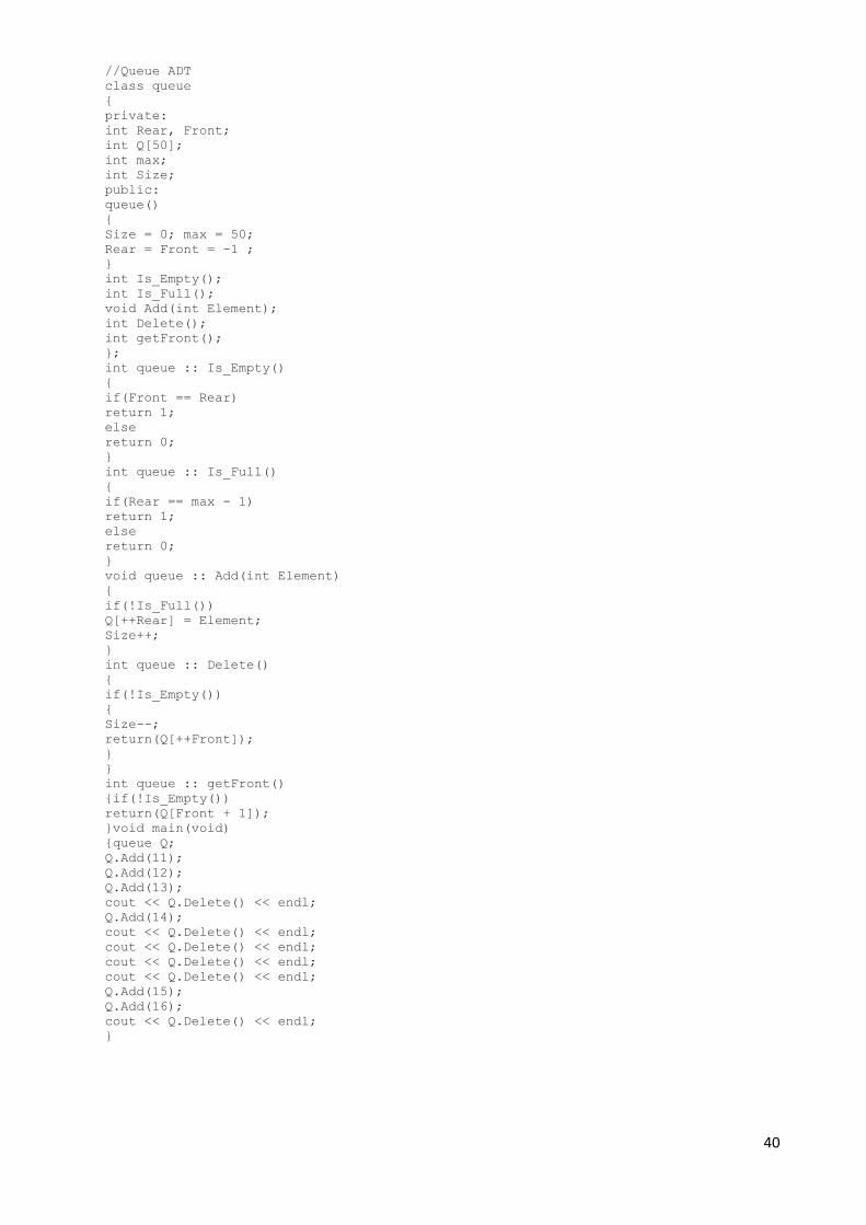
//Queue ADT

class queue

{

private:

int Rear, Front;

int Q[50];

int max;

int Size;

public:

queue()

{

Size = 0; max = 50;

Rear = Front = -1 ;

}

int Is_Empty();

int Is_Full();

void Add(int Element);

int Delete();

int getFront();

};

int queue :: Is_Empty()

{

if(Front == Rear)

return 1;

else

return 0;

}

int queue :: Is_Full()

{

if(Rear == max - 1)

return 1;

else

return 0;

}

void queue :: Add(int Element) {

if(!Is_Full())

Q[++Rear] = Element;

Size++;

}

int queue :: Delete()

{

if(!Is_Empty())

{

Size--;

return(Q[++Front]);

}

}

int queue :: getFront()

{if(!Is_Empty())

return(Q[Front + 1]);

}void main(void)

{queue Q;

Q.Add(11);

Q.Add(12);

Q.Add(13);

cout << Q.Delete() << endl;

Q.Add(14);





Q.Add(15);

Q.Add(16);


}

41

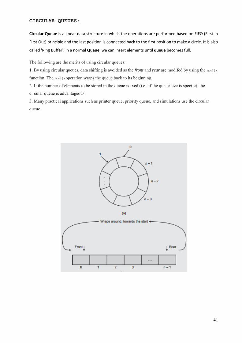
CIRCULAR QUEUES:

Circular Queue is a linear data structure in which the operations are performed based on FIFO (First In

First Out) principle and the last position is connected back to the first position to make a circle. It is also

called 'Ring Buffer'. In a normal Queue, we can insert elements until queue becomes full.

The following are the merits of using circular queues:

1. By using circular queues, data shifting is avoided as the front and rear are modifed by using the mod()

function. The mod()operation wraps the queue back to its beginning.

2. If the number of elements to be stored in the queue is fxed (i.e., if the queue size is specifc), the

circular queue is advantageous.

3. Many practical applications such as printer queue, priority queue, and simulations use the circular

queue.

42

#include<iostream.h>

class Cqueue

{ private:

int Rear, Front;

int Queue[50];

int Max;

int Size;

public:

Cqueue() {Size = 0; Max = 50; Rear = Front = -1;}

int Empty();

int Full();

void Add(int Element);

int Delete();

int getFront();

};

int Cqueue :: Empty()

{ if(Front == Rear)

return 1;

else

return 0;

}

int Cqueue :: Full()

{ if(Rear == Front)

return 1;

else

return 0;

}

void Cqueue :: Add(int Element)

{ if(!Full())

Rear = (Rear + 1) % Max;

Queue[Rear] = Element;

Size++;

}

int Cqueue :: Delete()

{ if(!Empty())

Front = (Front + 1) % Max;

Size--;

return(Queue[Front]);

}

int Cqueue :: getFront()

{ int Temp;

if(!Empty())

Temp = (Front + 1) % Max;

return(Queue[Temp]);

}

void main(void)

{ Cqueue Q;

Q.Add(11);

43

Q.Add(12);

Q.Add(13);


Q.Add(14);





Q.Add(15);

Q.Add(16);


}

DEQUE:

The word deque is a short form of double-ended queue. It is pronounced as ‗deck‘. Deque defines a data

structure where elements can be added or deleted at either the front end or the rear end, but no changes

can be made elsewhere in the list. Thus, deque is a generalization of both a stack and a queue. It supports

both stack-like and queue-like capabilities. It is a sequential container that is optimized for fast index-

based access and efficient insertion at either of its ends. Deque can be implemented as either a

continuous deque or as a linked deque. Figure shows the representation of a deque.

The deque ADT combines the characteristics of stacks and queues. Similar to stacks

and queues, a deque permits the elements to be accessed only at the ends. However, a

deque allows elements to be added at and removed from either end. We can refer to the

operations supported by the deque as EnqueueFront, EnqueueRear, DequeueFront,

and DequeueRear. When we complete a formal description of the deque and then implement it using a

dynamic, linked implementation, we can use it to implement both stacks

and queues, thus achieving signifcant code reuse.

The following are the four operations associated with deque:

1. EnqueueFront()—adds elements at the front end of the queue

2. EnqueueRear()—adds elements at the rear end of the queue

3. DequeueFront()—deletes elements from the front end of the queue

4. DequeueRear()—deletes elements from the rear end of the queue

For stack implementation using deque, EnqueueFront and DequeueFront are used as

push and pop functions, respectively.

44

LINKED LIST

A linked list is an ordered collection of data in which each element (node) contains a minimum

of two values, data and link(s) to its successor (and/or predecessor). A list with one link field using

which every element is associated to its successor is known as a singly linked list (SLL). In a linked list,

before adding any element to the list, a memory space for that node must be allocated. A link is made

from each item to the next item in the list as shown in Fig.

Each node of the linked list has at least the following two elements:

1. The data member(s) being stored in the list.s

2. A pointer or link to the next element in the list.

The last node in the list contains a null pointer

Linked List terminology

The following terms are commonly used in discussions about linked lists:

Header node: A header node is a special node that is attached at the beginning of the Linked list. This

header node may contain special information (metadata) about the linked list as shown in Fig

This special information could be the total number of nodes in the list, date of creation, type, and so on.

The header node may or may not be identical to the data nodes.

45

Data node: The list contains data nodes that store the data members and link(s) to its predecessor

(and/or successor).

Head pointer: The variable (or handle), which represents the list, is simply a pointer to the node at the

head of the list. A linked list must always have at least one pointer pointing to the first node (head) of the

list. This pointer is necessary because it is the only way to access the further links in the list. This pointer

is often called head pointer, because a linked list may contain a dummy node attached at the start

position called the header node.

Tail pointer: Similar to the head pointer that points to the first node of a linked list, we may have a

pointer pointing to the last node of a linked list called the tail pointer.

Header node: Tail pointer Similar to the head pointer that points to the first node of a linked list, we

may have a pointer pointing to the last node of a linked list called the tail pointer.

Primitive Operations

The following are basic operations associated with the linked list as a data structure:

1. Creating an empty list

2. Inserting a node

3. Deleting a node

4. Traversing the list

Some more operations, which are based on the basic operations, are as follows:

5. Searching a node

6. Updating a node

7. Printing the node or list

8. Counting the length of the list

9. Reversing the list

10. Sorting the list using pointer manipulation

11. Concatenating two lists

12. Merging two sorted lists into a third sorted list

In addition, operations such as merging the second sorted list into the first sorted list and many more are

possible by the use of these operations.

46

REPRESENTATION OF LINKED LISTS USING ARRAYS:

1. REPRESENTATION OF LINKED LISTS:

Let L be a set of names of months of the year.

L {Jan, Feb, Mar, Apr, May, Jun, Jul, Aug, Sep, Oct, Nov, Dec}

Here, L is an ordered set. The linked organization of this list using arrays is shown in Fig. The elements

of the list are stored in the one-dimensional array, Data. The elements are not stored in the same order as

in the set L. They are also not stored in a continuous block of locations. Note that the data elements are

allowed to be stored anywhere in the array, in any order.

To maintain the sequence, the second array, Link, is added. The values in this array are the links to each

successive element. Here, the list starts at the 10th location of the array.

Let the variable Head denote the start of the list.

L {Jan, Feb, Mar, Apr, May, Jun, Jul, Aug, Sep, Oct, Nov, Dec}

Here, Head = 10 and Data[Head] = Jan.

Let us get the second element. The location where the second element is stored t is Link[Head] =

Link[10]. Hence, Data[Link[Head]] = Data[Link[10]] = Data[3] = Feb. Let us get the third data

element through the second element. Data[Link[3]] = Data[8] = Mar, and so on. Continuing in this

manner, we can list all the members in the sequence. The link value of the last element is set to 1 to

represent the end of the list. Figure 6.6 shows the same representation as in Fig. 6.5 but in a different

manner.

47

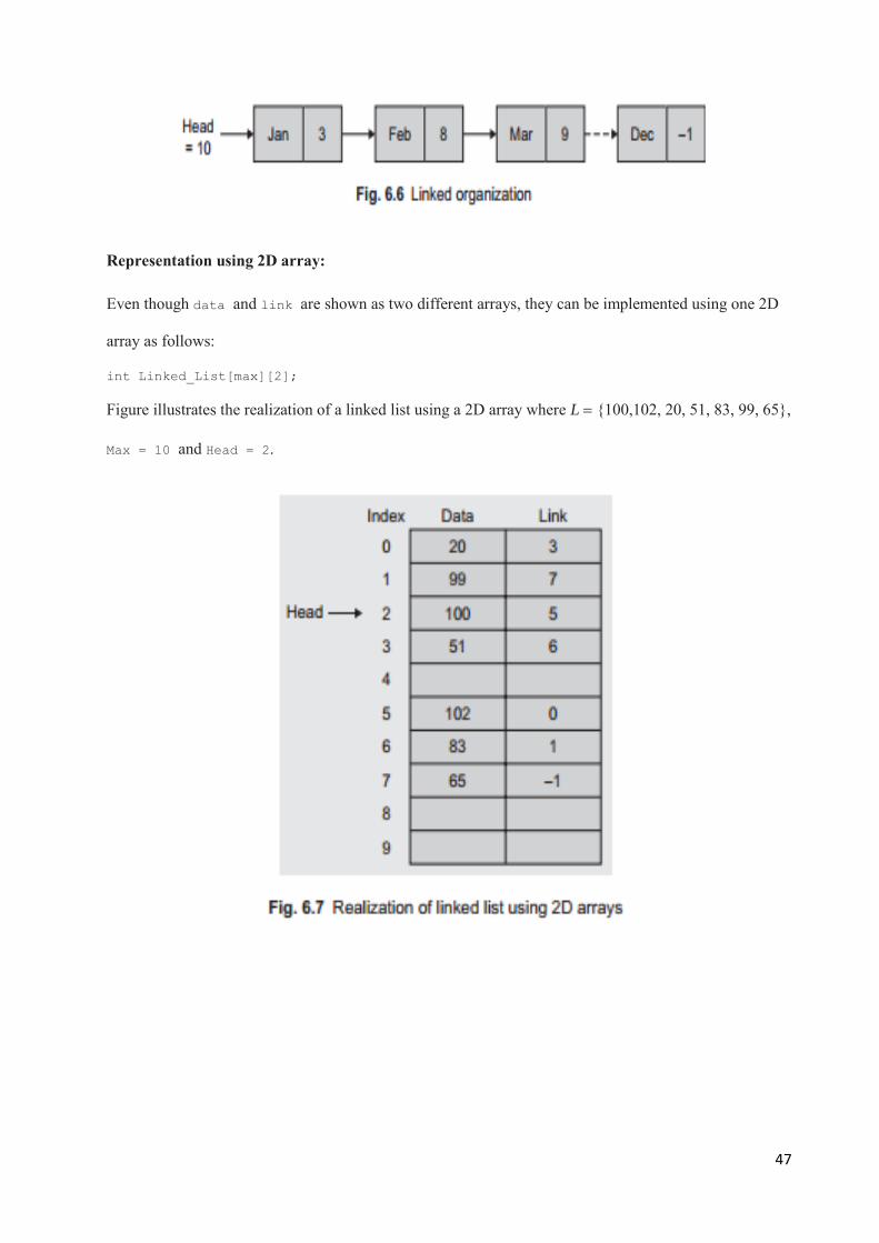
Representation using 2D array:

Even though data and link are shown as two different arrays, they can be implemented using one 2D

array as follows:

int Linked_List[max][2];

Figure illustrates the realization of a linked list using a 2D array where L {100,102, 20, 51, 83, 99, 65},

Max = 10 and Head = 2.

48

Linked List ADT:

#include<iostream>

using namespace std;

class Node

{

public :

int data;

Node *link;

};

class Llist

{

private:

Node *Head,*Tail;

public:

Llist()

{

Head = NULL;

}

void Create();

void Display();

Node* GetNode();

void Append(Node* NewNode);

void Insert_at_Pos( Node *NewNode, int

position);

void DeleteNode(int del_position);

void sort();

};

void Llist::sort()

{ Node *ptr,*s;

int value;

if(Head==NULL)

{cout<<"the list is

empty"<<endl;

}

ptr=Head;

while (ptr != NULL)

{

for (s=ptr->link;s !=NULL;s = s->link)

{

if (ptr->data > s->data)

{

value = ptr->data;

ptr->data = s->data;

s->data = value;

}

}

ptr = ptr->link;

}

}

void Llist :: Create()

{

char ans;

Node *NewNode;

while(1)

{

cout << "Any more nodes to be added

(Y/N)";

cin >> ans;

if(ans == 'n') break;

NewNode = GetNode();

Append(NewNode);

}

}

void Llist :: Append(Node* NewNode)

{

if(Head == NULL)

{

Head = NewNode;

Tail = NewNode;

}

else

{

Tail->link = NewNode;

Tail = NewNode;

}

}

Node* Llist :: GetNode()

{

Node *Newnode;

Newnode = new Node;

cin >> Newnode->data;

Newnode->link = NULL;

return(Newnode);

}

void Llist :: Display()

{

Node *temp = Head;

if(temp == NULL)

cout << "Empty List";

else

{

while(temp != NULL)

{

cout << temp->data << "\t";

temp = temp->link;

}

}

cout << endl;

}

void Llist :: DeleteNode(int pos)

{

int count = 1, flag = 1;

Node *curr, *temp;

temp = Head;

if(pos == 1)

{

Head = Head->link;

delete temp;

}

else

{

while(count != pos - 1)

{

temp = temp->link;

if(temp == NULL)

{

flag = 0; break;

}

count++;

}

if(flag == 1)

{

curr = temp->link;

temp->link = curr->link;

delete curr;

}

else

cout << "Position not found" << endl;

}

}

void Llist :: Insert( Node *NewNode,

int position)

{

Node *temp = Head;

int count = 1,flag = 1;

if(position == 1)

NewNode->link = temp;

Head = NewNode; // update head

}

else

49

{

while(count != position - 1)

{

temp = temp->link;

if(temp == NULL)

{

flag = 0; break;

}

count ++;

}

if(flag == 1)

{

NewNode->link = temp->link;

temp->link = NewNode;

}

else

cout << "Position not found" << endl;

}

}

void Llist::search()

{

int value,pos=0;

bool flag=false;

if(Head==NULL)

{

cout<<"list is empty";

return;

}

cout<<"enter the value to be

searched";

cin>>value;

Node *n=Head;

while(n!=NULL)

{

pos++;

if(n->data==value)

{flag= true;

cout<<"element"<<value<<"i

s found at

position"<<pos<<endl;

}

n=n->link;

}

if(!flag)

cout<<"element"<<value<<"not found in

the list"<<endl;

}

int main()

{

Node *NewNode;

Llist L1;

L1.Create();

L1.Display();

L1.sort();

L1.Display();

NewNode=L1.GetNode();

L1.Insert(NewNode,2);

L1.Display();

L1.DeleteNode(2);

L1.Display();

}

50

LINKED LIST VARIANTS:

Linked list can be classified as follows

1. Singly linked list

2. Doubly linked list

1) Single linked list: A linked list in which every node has one link f eld, to provide information

about where the next node of the list is, is called as singly linked list (SLL). It has no knowledge

about where the previous node lies in the memory. In SLL, we can traverse only in one direction.

We have no way to go to the ith node from (i 1)th node, unless the list is traversed

again from the first node

2) Double Linked List

In a doubly linked list (DLL), each node has two link fields to store information about the one to the

next and also about the one ahead of the node. Hence, each node has knowledge of its successor and

also its predecessor. In DLL, from every node, the list can be traversed in both the directions.

Both SSL and DLL may or may not contain a header node. The one with a header node is explicitly

mentioned in the title as a header-SLL and a header-DLL. These are also called as singly linked list with

header node and doubly linked list with header node.

II. The other classification of linked lists based on their method of traversing is

1. Linear linked list

2. Circular linked list

1. Linear Linked List:

The linear linked list having only 1 way traversing all the elements in the list can be accessed by

traversing from the first node of the list.

2. Circular Linked list:

In linear linked list it is not possible to traverse the list from the last node or to reach any of the

nodes that precede any node. To overcome this disadvantages the link field of the last node can be

set to point to the first node rather than the Null. Such a linked list is called as circular linked list.

51

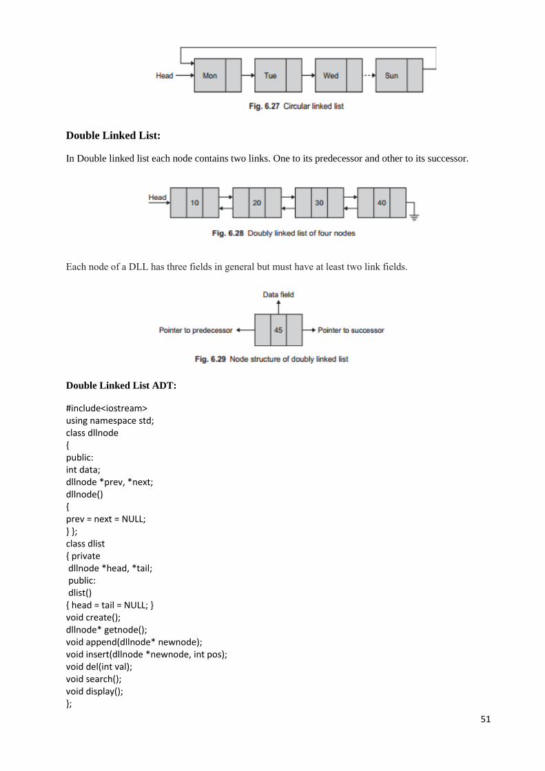
Double Linked List:

In Double linked list each node contains two links. One to its predecessor and other to its successor.

Each node of a DLL has three fields in general but must have at least two link fields.

Double Linked List ADT:

#include<iostream> using namespace std; class dllnode { public: int data; dllnode *prev, *next; dllnode() { prev = next = NULL; } }; class dlist { private dllnode *head, *tail; public: dlist() { head = tail = NULL; } void create(); dllnode* getnode(); void append(dllnode* newnode); void insert(dllnode *newnode, int pos); void del(int val); void search(); void display(); };

52

dllnode* dlist :: getnode() { dllnode *newnode; newnode = new dllnode; cout << "Enter Data"; cin >> newnode->data; newnode->next = newnode->prev = NULL; return(newnode); } void dlist :: append(dllnode* newnode) { if(head == NULL) { head = newnode; tail = newnode; } else { tail->next = newnode; newnode->prev = tail; tail = newnode; } } void dlist :: create() { char ans; dllnode *newnode; while(1) { cout << "Any more nodes to be added (Y/N)"; cin >> ans; if(ans == 'n') break; newnode = getnode(); append(newnode); } } void dlist :: insert(dllnode* newnode, int pos) { dllnode *temp = head; int count = 1,flag=1; if(head==NULL) head=tail=newnode; else if(pos == 1) { newnode->next = head; head->prev = newnode; head = newnode; } else { while(count != pos) { temp = temp->next; if(temp == NULL)

{ flag=0;break; } count++; } if(flag == 1) { (temp->prev)->next = newnode; newnode->prev = temp->prev; temp->prev = newnode; newnode->next=temp; } else cout << "The node position is not found" << endl; } } void dlist :: del(int val) { dllnode *curr, *temp; curr = head; while(curr!=NULL) { if(curr->data == val) break; curr = curr->next; } if(curr != NULL) { if(curr == head) { head = head->next; head->prev = NULL; delete curr; } else { if(temp == tail) { tail = temp->prev; (temp->prev)->next = NULL; delete temp; } else { (curr->prev)->next = curr->next; (curr->next)->prev = curr->prev; delete curr; } } if(head == NULL) { tail = NULL;

53

} } else cout << "Node to be deleted is not found \n"; } void dlist::search() { int value,pos=0; bool flag=false; if(head==NULL) { cout<<"list is empty"; return; } cout<<"enter the value to be searched"; cin>>value; dllnode *n=head; while(n!=NULL) { pos++; if(n->data==value) {flag= true; cout<<"element"<<value<<"is found at position"<<pos<<endl; } n=n->next; } if(!flag) cout<<"element"<<value<<"not found in the list"<<endl; } void dlist :: display() { dllnode *temp = head; if(temp == NULL) cout << "Empty List"; else { while(temp != NULL) { cout << temp->data << "\t"; temp = temp->next; } } cout << endl; } int main() { dllnode *newnode; int val; dlist d; d.create();

d.display(); newnode=d.getnode(); d.insert(newnode,3); d.display(); cout<<"enter element to be deleted"; cin>>val; d.del(val); d.display(); d.search(); }

54

CIRCULAR LINKED LIST:

In a singly linear list, the last nodes link field is set to Null. Instead of that, store the address of the first

node of the list in that link field. This change will make the last node point to the first node of the list.

Such a linked list is called circular linked list . From any node in such a list, it is possible to reach to any

other node in the list. We need not traverse the list again right from the first node.

1. Singly circular linked list:

In a singly circular list, the pointer head points to the first node of the list. From the last node, we can

access the first node. Remember that we cannot access the last node through the header node. We have

access to only the first node. We need to traverse the whole list to reach to the last node.

CIRCULAR LINKED LIST WITH HEADER NODE:

Suppose we want to insert a new node at the front of this list. We have to change the link field of the last

node. In addition, we have to traverse the whole list to reach the last node as the link field of the last

node is also to be updated. Hence, it is convenient if the head pointer points to the last node rather than

the header node, which is the first node of the list.

55

2. DOUBLY CIRCULAR LINKED LIST:

APPLICATION OF LINKED LIST—GARBAGE COLLECTION:

To be able to reuse this memory, the memory allocator will usually link the freed blocks together in a

free list by writing pointers to the next free block in the block itself. An external free list pointer points to

the first block in the free list. When a new block of memory is requested, the allocator will generally

scan the free list looking for a free block of suitable size and delete it from the free list (relinking the free

list around the deleted block).

One of the components of an operating system is the memory management module. This module

maintains a list, which consists of unused memory cells. This list very often requires the operations to be

performed on the list, such as insert, delete, and search (traversal). Such a list implemented as a

linked organization is called the list of available space, free storage list, or the free pool. Suppose some

memory block is freed by the program. The space available can be used for future use. One way to do so

is to add the blocks in the free pool. For good memory utilization, the operating system periodically

collects all the free blocks and inserts into the free pool. Any technique that does this collection is called

garbage collection. Garbage collection usually takes place in two phases. In

general, garbage collection takes place when either overflow or underflow occurs

Overflow Some times, a new data node is to be inserted into data structure, but there is

no available space, that is, free pool is empty. This situation is called overfl ow.

Underfl ow This refers to the situation where the programmer wants to delete a node from the empty list.

56

STACK ADT BY USING LINKED LIST: #include<iostream> using namespace std; class node { public: int data; node *link; }; class stack { private: node *top; int Size; int isempty(); public: stack() { top = NULL; Size = 0; } int gettop(); int pop(); void push( int Element); void display(); }; int stack :: isempty() { if(top == NULL) return 1; else return 0; } int stack :: gettop() { if(!isempty()) return(top->data); } void stack :: push(int value) { node * newnode; newnode = new node; newnode->data = value; newnode->link = NULL; newnode->link = top; top = newnode; } int stack :: pop() { node * tmp = top; int data = top->data; if(!isempty()) { top = top->link;

delete tmp; return(data); } } void stack :: display() { node *temp = top; if(temp == NULL) cout << "Empty List"; else { while(temp != NULL) { cout << temp->data << "\t"; temp = temp->link; } } cout << endl; } int main() { stack S; S.push(5); S.push(6); S.display(); cout << "top element is "<<S.gettop()<<endl; cout << "deleted element"<<S.pop()<<endl; S.display(); S.push(7); S.display(); }

57

QUEUE ADT BY USING LINKED LIST #include<iostream> using namespace std; class node { public: int data; node *link; }; class queue { node *front, *rear; int isempty(); public: queue() { front = rear= NULL; } void add( int element); int del(); int getfront(); void display(); }; int queue :: isempty() { if(front == NULL) return 1; else return 0; } int queue :: getfront() { if(!isempty()) return(front->data); } Void queue :: add(int x) { node *newnode; newnode = new node; newnode->data = x; newnode->link = NULL; if(rear == NULL) { front = newnode; rear = newnode; } else { rear->link = newnode; rear = newnode; } }

int queue :: del() { int temp; node *current = NULL; if(!isempty()) { temp = front->data; current = front; front = front->link; delete current; if(front == NULL) rear = NULL; return(temp); } } void queue::display() { node *temp= front; if(temp==NULL) cout<<"queue is empty"; else { while(temp != NULL) { cout << temp->data << "\t"; temp = temp->link; } } cout << endl; } int main() { queue q; q.add(11); q.add(12); q.add(13); q.display(); cout <<"deleted element" <<q.del() << endl; q.display(); q.add(14); q.display(); cout << "deleted element"<<q.del() << endl; q.display(); cout <<"front element is"<< q.getfront() << endl; }

58

UNIT - III

TREES:

1) A tree is non – linear, hierarchical Data Structure.

2) A tree is a finite non empty set if elements. It is an abstract model of a hierarchical structure

consists of nodes with a parent- child relation.

3) A tree T is defined recursively as follows:

1. A set of zero items is a tree, called the empty tree (or null tree).

2. If T1, T2, ..., Tn are n trees for n> 0 and Ris a node, then the set T containing R and the trees

T1,T2, .., Tn are a tree. Within T, R is called the root of T, and T1, T2,.. Tn are called subtrees.

Tree Terminology

Root: node without parent (A)

Subtree: tree consisting of a node and its descendants

Siblings: nodes share the same parent (B,C,D) (E,F) (I,J,K) (G,H)

Internal node: node with at least one child (A, B, C, F)

LEAVES(External node): node without children (E, I, J, K, G, H, D)

Ancestors of a node: parent, grandparent, grand-grandparent, etc.

Descendant of a node: child, grandchild, grand-grandchild, etc.

Depth of a node: number of ancestors

Height of a tree: maximum depth of any node (3)

Degree of a node: the number of its children

Degree of a tree: the maximum number of its node.

59

Representation of a General Tree

We can use either a sequential organization or a linked organization for representing a tree. If we wish to

use a generalized linked list, then a node must have a varying number of felds depending upon the

number of branches. However, it is simpler to use algorithms for the data where the node size is fxed.

For a fxed size node, we can use a node with data and pointer felds as in a generalized linked list.

TYPES OF TREES

1. Free tree: A free tree is a connected, acyclic graph. It is an undirected graph. It has no node

designated as a root. As it is connected, any node can be reached from any other node through a

unique path. The tree in Fig. is an example of a free tree.

60

2. Rooted tree: Unlike free tree, a rooted tree is a directed graph where one node is designated as root,

whose incoming degree is zero, whereas for all other nodes, the incoming degree is one

3.Ordered tree : In many applications, the relative order of the nodes at any particular level assumes

some signifcance. It is easy to impose an order on the nodes at a level by referring to a particular node as

the frst node, to another node as the second, and so on. Such ordering can be done from left to right

(Fig.). Just like nodes at each level, we can prescribe order to edges. If in a directed tree, an ordering of a

node at each level is prescribed, then such a tree is called an ordered tree.

1. Regular tree A tree where each branch node vertex has the same outdegree is called a regular

tree. If in a directed tree, the outdegree of every node is less than or equal to m, then the tree is

called an m-ary tree. If the outdegree of every node is exactly equal to m (the branch nodes) or

zero (the leaf nodes), then the tree is called a regular m-ary tree.

2. Binary tree A binary tree is a special form of tree. Each and every node in the binary tree

contains 2 or lessthan 2 children except leaf nodes.

Partial Binary tree: Each and every node in the tree contains lessthan 2 children except leaf

nodes.

Full Binary tree: Each and every node in the tree (Except Leaf nodes) contains

exactly 2 nodes is called Full Binary tree.

3. Complete Binary tree: A Binary Tree is said to be a Complete Binary Tree if all its levels except the

last level have the maximum number of possible nodes, and all the nodes of the last level appear as far

left as possible. In a complete binary tree, all the leaf nodes are at the last and the second last level, and

the levels are flled from left to right

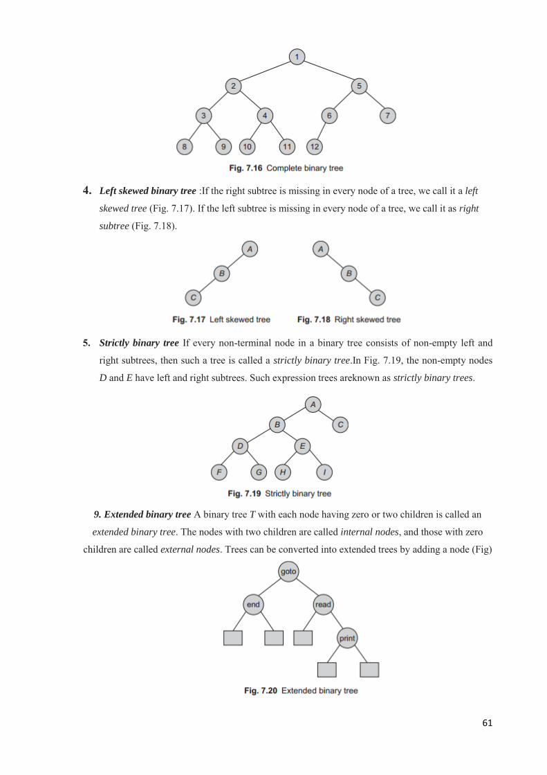
61

4. Left skewed binary tree :If the right subtree is missing in every node of a tree, we call it a left

skewed tree (Fig. 7.17). If the left subtree is missing in every node of a tree, we call it as right

subtree (Fig. 7.18).

5. Strictly binary tree If every non-terminal node in a binary tree consists of non-empty left and

right subtrees, then such a tree is called a strictly binary tree.In Fig. 7.19, the non-empty nodes

D and E have left and right subtrees. Such expression trees areknown as strictly binary trees.

9. Extended binary tree A binary tree T with each node having zero or two children is called an

extended binary tree. The nodes with two children are called internal nodes, and those with zero

children are called external nodes. Trees can be converted into extended trees by adding a node (Fig)

62

BINARY TREE ABSTRACT DATA TYPE( ADT):

We have defined a binary tree. Let us now define it as an abstract data type (ADT), which includes a list

of operations that process it.

ADT btree

1. Declare create()Æbtree

2. makebtree(btree, element, btree)Æbtree

3. isEmpty(btree)Æboolean

4. leftchild(btree)Æbtree

5. rightchild(btree)Æbtree

6. data(btree)Æelement

7. for all l,r Œbtree, e Œelement, Let

8. isEmpty(create) = true

9. isEmpty(makebtree(l,e,r)) = false

10. leftchild(create()) = error

11. rightchild(create()) = error

12. leftchild(makebtree(l,e,r)) = l

13. rightchild(makebtree(l,e,r)) = r

14. data(makebtree(l,e,r)) = e

15. end

end btree

Operations on binary tree :The basic operations on a binary tree can be as listed as follows:

1. Creation—Creating an empty binary tree to which the ‘root’ points

2. Traversal—Visiting all the nodes in a binary tree

3. Deletion—Deleting a node from a non-empty binary tree

4. Insertion—Inserting a node into an existing (may be empty) binary tree

5. Merge—Merging two binary trees

6. Copy—Copying a binary tree

7. Compare—Comparing two binary trees

8. Finding a replica or mirror of a binary tree

63

BINARY TREE ADT CLASS:

class TreeNode

{

public:

char Data;

TreeNode *Lchild;

TreeNode *Rchild;

};

class BinaryTree

{

private:

TreeNode *Root;

public:

BinaryTree() {Root = Null;

}

TreeNode *GetNode();

void InsertNode(TreeNode*);

void DeleteNode(TreeNode*);

void Postorder(TreeNode*);

void Inorder(TreeNode*);

void Preorder(TreeNode*);

TreeNode *TreeCopy();

void Mirror();

int TreeHeight(TreeNode*);

int CountLeaf(TreeNode*);

int CountNode(TreeNode*);

void BFS_Tree();

void DFS_Tree();

TreeNode *Create_Btree_InandPre_Traversal(char

preorder[max], char inorder[max]);

void Po storder_Non_Recursive(void);

void Inorder_Non_Recursive();

void Preorder_Non_Recursive();

int BTree_Equal( BinaryTree, BinaryTree);

TreeNode *TreeCopy(TreeNode*); void Mirror(TreeNode*);

};

64

REPRESENTATION OF A BINARY TREE

Array implementation of Binary Trees

This representation of binary trees using an array seems to be the easiest. Certainly, it can be used for all

binary trees. However, such a representation has certain drawbacks. In most of the representations, there

will be a lot of unused space. For complete binary trees, the representation seems to be good as no space

in an array is wasted between the nodes. Certainly, the space is wasted as we generally declare an array

of some arbitrary maximum limit. From the examples, we can make out that for the skewed tree,

however, less than half of the array is only used and more is left unused. In the worst case, a skewed tree

of depth k will require 2k+1 1 locations of array, and occupy just a few of them.

65

Linked implementation of Binary Trees

Binary tree has a natural implementation in a linked storage. In a linked organization, we wish that all

the nodes should be allocated dynamically. Hence, we need each node with data and link felds. Each

node of a binary tree has both a left and a right subtree. Each node will have three felds—Lchild, Data,

and Rchild. Pictorially, this node is shown in Fig. .

A node does not provide information about the parent node. However, it is still adequate for most of the

applications. If needed, the fourth parent feld can be included. The binary tree in Fig. 7.28 will have the

linked representation as in Fig. 7.29. The root of the tree is stored in the data member root of the tree.

This data member provides an access pointer to the tree.

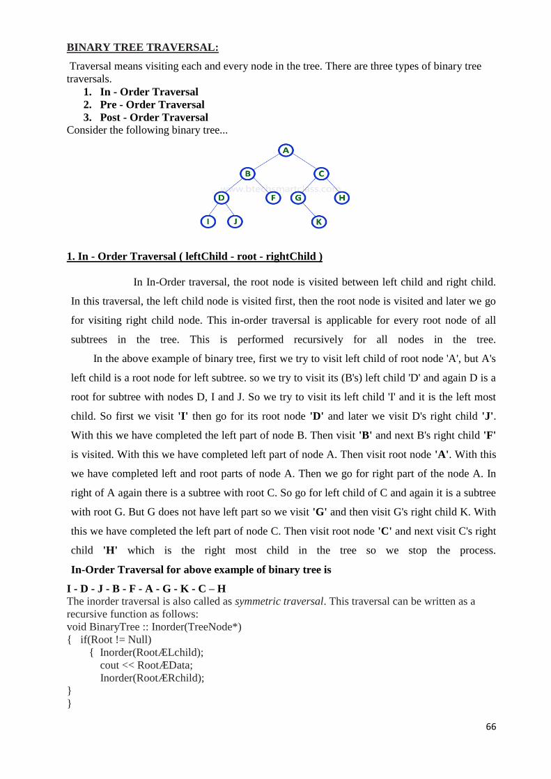
66

BINARY TREE TRAVERSAL:

Traversal means visiting each and every node in the tree. There are three types of binary tree

traversals.

1. In - Order Traversal

2. Pre - Order Traversal

3. Post - Order Traversal

Consider the following binary tree...

1. In - Order Traversal ( leftChild - root - rightChild )

In In-Order traversal, the root node is visited between left child and right child.

In this traversal, the left child node is visited first, then the root node is visited and later we go

for visiting right child node. This in-order traversal is applicable for every root node of all

subtrees in the tree. This is performed recursively for all nodes in the tree.

In the above example of binary tree, first we try to visit left child of root node 'A', but A's

left child is a root node for left subtree. so we try to visit its (B's) left child 'D' and again D is a

root for subtree with nodes D, I and J. So we try to visit its left child 'I' and it is the left most

child. So first we visit 'I' then go for its root node 'D' and later we visit D's right child 'J'.

With this we have completed the left part of node B. Then visit 'B' and next B's right child 'F'

is visited. With this we have completed left part of node A. Then visit root node 'A'. With this

we have completed left and root parts of node A. Then we go for right part of the node A. In

right of A again there is a subtree with root C. So go for left child of C and again it is a subtree

with root G. But G does not have left part so we visit 'G' and then visit G's right child K. With

this we have completed the left part of node C. Then visit root node 'C' and next visit C's right

child 'H' which is the right most child in the tree so we stop the process.

In-Order Traversal for above example of binary tree is

I - D - J - B - F - A - G - K - C – H

The inorder traversal is also called as symmetric traversal. This traversal can be written as a

recursive function as follows:

void BinaryTree :: Inorder(TreeNode*)

{ if(Root != Null)

{ Inorder(RootÆLchild);

cout << RootÆData;

Inorder(RootÆRchild);

}

}

67

2. Pre - Order Traversal ( root - leftChild - rightChild )

In Pre-Order traversal, the root node is visited before left child and right child nodes. In this

traversal, the root node is visited first, then its left child and later its right child. This pre-order

traversal is applicable for every root node of all subtrees in the tree.

In the above example of binary tree, first we visit root node 'A' then visit its left child 'B'

which is a root for D and F. So we visit B's left child 'D' and again D is a root for I and J. So we

visit D's left child 'I' which is the left most child. So next we go for visiting D's right child 'J'.

With this we have completed root, left and right parts of node D and root, left parts of node B.

Next visit B's right child 'F'. With this we have completed root and left parts of node A. So we

go for A's right child 'C' which is a root node for G and H. After visiting C, we go for its left

child 'G' which is a root for node K. So next we visit left of G, but it does not have left child so

we go for G's right child 'K'. With this we have completed node C's root and left parts. Next

visit C's right child 'H' which is the right most child in the tree. So we stop the process.

Pre-Order Traversal for above example binary tree is

A - B - D - I - J - F - C - G - K – H

The Preorder() function can be written as both recursive and non recursive.

void BinaryTree :: Preorder(TreeNode*)

{ if(Root != Null)

{ cout << Root->Data;

Preorder(Root->Lchild);

Preorder(Root->Rchild);

}

}

2. Post - Order Traversal ( leftChild - rightChild - root )

In Post-Order traversal, the root node is visited after left child and right child. In this

traversal, left child node is visited first, then its right child and then its root node. This is

recursively performed until the right most node is visited.

Here we have visited in the order of I - J - D - F - B - K - G - H - C - A using Post-Order

Traversal.

Post-Order Traversal for above example binary tree is

I - J - D - F - B - K - G - H - C – A

void BinaryTree :: Postorder(TreeNode*)

{

if(Root != Null)

{

cout << Root->Data;

Postorder(Root->Lchild);

Postorder(Root->Rchild);

}

}

68

BINARY SEARCH TREE

Binary Search Tree, is a node-based binary tree data structure which has the following

Properties:

The left subtree of a node contains only nodes with keys less than the node’s key.

The right subtree of a node contains only nodes with keys greater than the node’s key.

The left and right subtree each must also be a binary search tree.

There must be no duplicate nodes.

EX:

Applications of binary trees

Binary Search Tree - Used in many search applications where data is constantly

entering/leaving, such as the map and set objects in many languages' libraries.

Binary Space Partition - Used in almost every 3D video game to determine what

objects need to be rendered.

Binary Tries - Used in almost every high-bandwidth router for storing router-tables.

Hash Trees - used in p2p programs and specialized image-signatures in which a hash

needs to be verified, but the whole file is not available.

Heaps - Used in implementing efficient priority-queues, which in turn are used for

scheduling processes in many operating systems, Quality-of-Service in routers, and A*

(path-finding algorithm used in AI applications, including robotics and video games).

Also used in heap-sort.

Huffman Coding Tree (Chip Uni) - used in compression algorithms, such as those

used by the .jpeg and .mp3 file-formats.

GGM Trees - Used in cryptographic applications to generate a tree of pseudo-random

numbers.

Syntax Tree - Constructed by compilers and (implicitly) calculators to parse

expressions.

Treap - Randomized data structure used in wireless networking and memory allocation.

T-tree - Though most databases use some form of B-tree to store data on the drive,

databases which keep all (most) their data in memory often use T-trees to do so.

http://en.wikipedia.org/wiki/Binary_search_tree

http://en.wikipedia.org/wiki/Binary_space_partitioning

http://en.wikipedia.org/wiki/Radix_tree

http://en.wikipedia.org/wiki/Hash_tree

http://en.wikipedia.org/wiki/Heap_(data_structure)

http://en.wikipedia.org/wiki/Huffman_coding

https://stackoverflow.com/questions/2130416/what-are-the-applications-of-binary-trees/2174096#2174096

http://www.wisdom.weizmann.ac.il/~/oded/ggm.html

http://en.wikipedia.org/wiki/Abstract_syntax_tree

http://en.wikipedia.org/wiki/Treap

http://en.wikipedia.org/wiki/T-tree

69

GRAPHS:

Graph is a collection of vertices and arcs which connects vertices in the graph

Graph is a collection of nodes and edges which connects nodes in the graph

Generally, a graph G is represented as G = ( V , E ), where V is set of vertices and E is set of

edges.

Example

The following is a graph with 5 vertices and 7 edges.

This graph G can be defined as G = ( V , E )

Where V = {A,B,C,D,E} and E = {(A,B),(A,C)(A,D),(B,D),(C,D),(B,E),(E,D)}.

Graph Terminology

We use the following terms in graph data structure...

Vertex

A individual data element of a graph is called as Vertex. Vertex is also known as node. In

above example graph, A, B, C, D & E are known as vertices.

Edge

An edge is a connecting link between two vertices. Edge is also known as Arc. An edge is

represented as (startingVertex, endingVertex). For example, in above graph, the link between

vertices A and B is represented as (A,B). In above example graph, there are 7 edges (i.e., (A,B),

(A,C), (A,D), (B,D), (B,E), (C,D), (D,E)).

Edges are three types.

1. Undirected Edge - An undirected egde is a bidirectional edge. If there is a undirected

edge between vertices A and B then edge (A , B) is equal to edge (B , A).

2. Directed Edge - A directed egde is a unidirectional edge. If there is a directed edge

between vertices A and B then edge (A , B) is not equal to edge (B , A).

3. Weighted Edge - A weighted egde is an edge with cost on it.

Undirected Graph

A graph with only undirected edges is said to be undirected graph.

Directed Graph

A graph with only directed edges is said to be directed graph.

Mixed Graph

A graph with undirected and directed edges is said to be mixed graph.

70

End vertices or Endpoints

The two vertices joined by an edge are called the end vertices (or endpoints) of the edge.

Origin

If an edge is directed, its first endpoint is said to be origin of it.

Destination

If an edge is directed, its first endpoint is said to be origin of it and the other endpoint is said to

be the destination of the edge.

Adjacent

If there is an edge between vertices A and B then both A and B are said to be adjacent. In other

words, Two vertices A and B are said to be adjacent if there is an edge whose end vertices are A

and B.

Incident

An edge is said to be incident on a vertex if the vertex is one of the endpoints of that edge.

Outgoing Edge

A directed edge is said to be outgoing edge on its orign vertex.

Incoming Edge

A directed edge is said to be incoming edge on its destination vertex.

Degree

Total number of edges connected to a vertex is said to be degree of that vertex.

Indegree

Total number of incoming edges connected to a vertex is said to be indegree of that vertex.

Outdegree

Total number of outgoing edges connected to a vertex is said to be outdegree of that vertex.

Parallel edges or Multiple edges

If there are two undirected edges to have the same end vertices, and for two directed edges to

have the same origin and the same destination. Such edges are called parallel edges or multiple

edges.

Self-loop

An edge (undirected or directed) is a self-loop if its two endpoints coincide.

Simple Graph

A graph is said to be simple if there are no parallel and self-loop edges.

Path

A path is a sequence of alternating vertices and edges that starts at a vertex and ends at a vertex

such that each edge is incident to its predecessor and successor vertex.

71

GRAPH ABSTRACT DATA TYPE:

Graphs as non-linear data structures represent the relationship among data elements, having more than

one predecessor and/or successor. A graph G is a collection of nodes (vertices) and arcs joining a pair of

the nodes (edges). Edges between two vertices represent the relationship between them. For finite

graphs, V and E are finite. We can denote the graph as G = (V, E).

Let us define the graph ADT. We need to specify both sets of vertices and edges. Basic operations

include creating a graph, inserting and deleting a vertex, inserting and deleting an edge, traversing a

graph, and a few others.

A graph is a set of vertices and edges {V, E} and can be declared as follows:

graph

create()Graph

insert_vertex(Graph, v)Graph

delete_vertex(Graph, v)Graph

insert_edge(Graph, u, v)Graph

delete_edge(Graph, u, v)Graph

is_empty(Graph)Boolean;

end graph

These are the primitive operations that are needed for storing and processing a graph.

Create

The create operation provides the appropriate framework for the processing of graphs. The

create() function is used to create an empty graph. An empty graph has both V and E as null

sets. The empty graph has the total number of vertices and edges as zero. However, while

implementing, we should have V as a non-empty set and E as an empty set as the mathematical

notation normally requires the set of vertices to be non-empty.

Insert Vertex

The insert vertex operation inserts a new vertex into a graph and returns the modified graph. When the

vertex is added, it is isolated as it is not connected to any of the vertices in the graph through an edge. If

the added vertex is related with one (or more) vertices in the graph, then the respective edge(s) are to be

inserted. Figure 8.1(a) shows a graph G(V, E), where V {a, b, c} and E {(a, b), (a, c), (b, c)}, and the

resultant graph after inserting the node d. The resultant graph G is shown in Fig. 8.1(b). It shows the

inserted vertex with resultant V {a, b, c, d}. We can show the adjacency relation with other vertices by

adding the edge. So now, E would be E {(a, b), (a, c), (b, c), (b, d)} as shown in Fig.

72

Is_empty:

The is empty operation checks whether the graph is empty and returns true if empty else returns false.

An empty graph is one where the set V is a null set. These are the basic operations on graphs, and a few

more include getting the set of adjacent nodes of a vertex or an edge and traversing a graph. Checking

the adjacency between vertices means verifying the relationship between them, and the relationship is

maintained using a suitable data structure.

Delete Vertex

The delete vertex operation deletes a vertex and all the incident edges on that vertex and returns the

modified graph. Figure 8.2(a) shows a graph G(V, E)

where V = {a, b, c, d} and E = {(a, b), (a, c), (b, c), (b, d)},

and the resultant graph after deleting the node c is shown in

Fig. 8.2(b)with V = {a, b, d} and E = {(a, b), (b, d)}.

Insert Edge

The insert edge operation adds an edge incident between two vertices. In an undirected graph, for adding

an edge, the two vertices u and v are to be specified, and for a directed graph along with vertices, the

start vertex and the end vertex should be known Figure 8.3(a)

shows a graph G(V, E) where V = {a, b, c, d} and

E = {(a, b), (a, c), (b, c), (b, d)} and the resultant

graph after inserting the edge (c, d) is shown in Fig. 8.3(b)

with V = {a, b, c, d}and E = {(a, b), (a, c), (b, c), (b, d), (c, d)}.

Delete Edge

The delete edge operation removes one edge from the graph. Let the graph G be G(V, E). Now,

deleting the edge (u, v) from G deletes the edge incident between

vertices u and v and keeps the incident vertices u, v.

Figure 8.4(a) shows a graph G(V, E) where V= {a, b, c, d}

and E = {(a, b),(a, c), (b, c), (b, d)} The resultant graph after

deleting the edge (b, d) is shown in Fig. 8.4(b) with V = {a, b, c, d}

and E = {(a, b), (a, c), (b, c)}

Graph traversal is also known as searching through a graph.

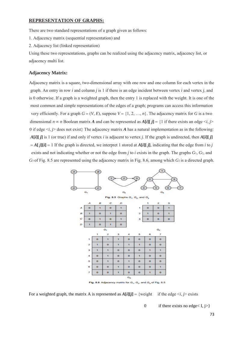
73

REPRESENTATION OF GRAPHS:

There are two standard representations of a graph given as follows:

1. Adjacency matrix (sequential representation) and

2. Adjacency list (linked representation)

Using these two representations, graphs can be realized using the adjacency matrix, adjacency list, or

adjacency multi list.

Adjacency Matrix:

Adjacency matrix is a square, two-dimensional array with one row and one column for each vertex in the

graph. An entry in row i and column j is 1 if there is an edge incident between vertex i and vertex j, and

is 0 otherwise. If a graph is a weighted graph, then the entry 1 is replaced with the weight. It is one of the

most common and simple representations of the edges of a graph; programs can access this information

very efficiently. For a graph G (V, E), suppose V {1, 2, …, n}. The adjacency matrix for G is a two

dimensional n n Boolean matrix A and can be represented as A[i][ j] {1 if there exists an edge <i, j>

0 if edge <i, j> does not exist} The adjacency matrix A has a natural implementation as in the following:

A[i][ j] is 1 (or true) if and only if vertex i is adjacent to vertex j. If the graph is undirected, then A[i][ j]

A[ j][i] 1 If the graph is directed, we interpret 1 stored at A[i][ j], indicating that the edge from i to j

exists and not indicating whether or not the edge from j to i exists in the graph. The graphs G1, G2, and

G3 of Fig. 8.5 are represented using the adjacency matrix in Fig. 8.6, among which G2 is a directed graph.

For a weighted graph, the matrix A is represented as A[i][j] {weight if the edge <i, j> exists

0 if there exists no edge< I, j>}

74

Here, weight is the label associated with the edge of the graph. For example, Figs 8.7(a) and (b) show the

weighted graph and its associated adjacency matrix.

ADJACENCY LIST:

In this representation, the n rows of the adjacency list are represented as n-linked lists, one list per vertex

of the graph. The adjacency list for a vertex i is a list of all vertices adjacent to it. One way of achieving

this is to go for an array of pointers, one per vertex. For example, we can represent the graph G by an

array Head, where Head[i] is a pointer to the adjacency list of vertex i. For list, each node of the list has

at least two fields: vertex and link. The vertex field contains the vertex id, and the link field stores a

pointer to the next node that stores another vertex adjacent to i. Figure 8.8(b) shows an adjacency list

representation for a directed graph in Fig.

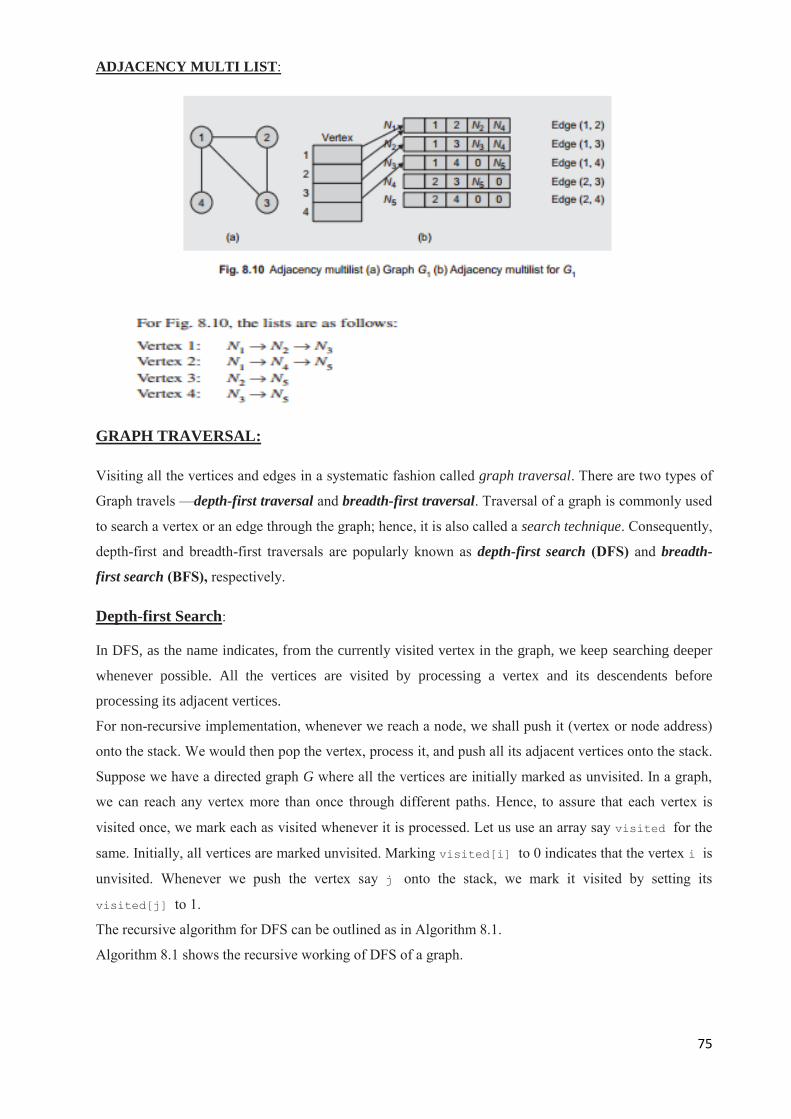
75

ADJACENCY MULTI LIST:

GRAPH TRAVERSAL:

Visiting all the vertices and edges in a systematic fashion called graph traversal. There are two types of

Graph travels —depth-first traversal and breadth-first traversal. Traversal of a graph is commonly used

to search a vertex or an edge through the graph; hence, it is also called a search technique. Consequently,

depth-first and breadth-first traversals are popularly known as depth-first search (DFS) and breadth-

first search (BFS), respectively.

Depth-first Search:

In DFS, as the name indicates, from the currently visited vertex in the graph, we keep searching deeper

whenever possible. All the vertices are visited by processing a vertex and its descendents before

processing its adjacent vertices.

For non-recursive implementation, whenever we reach a node, we shall push it (vertex or node address)

onto the stack. We would then pop the vertex, process it, and push all its adjacent vertices onto the stack.

Suppose we have a directed graph G where all the vertices are initially marked as unvisited. In a graph,

we can reach any vertex more than once through different paths. Hence, to assure that each vertex is

visited once, we mark each as visited whenever it is processed. Let us use an array say visited for the

same. Initially, all vertices are marked unvisited. Marking visited[i] to 0 indicates that the vertex i is

unvisited. Whenever we push the vertex say j onto the stack, we mark it visited by setting its

visited[j] to 1.

The recursive algorithm for DFS can be outlined as in Algorithm 8.1.

Algorithm 8.1 shows the recursive working of DFS of a graph.

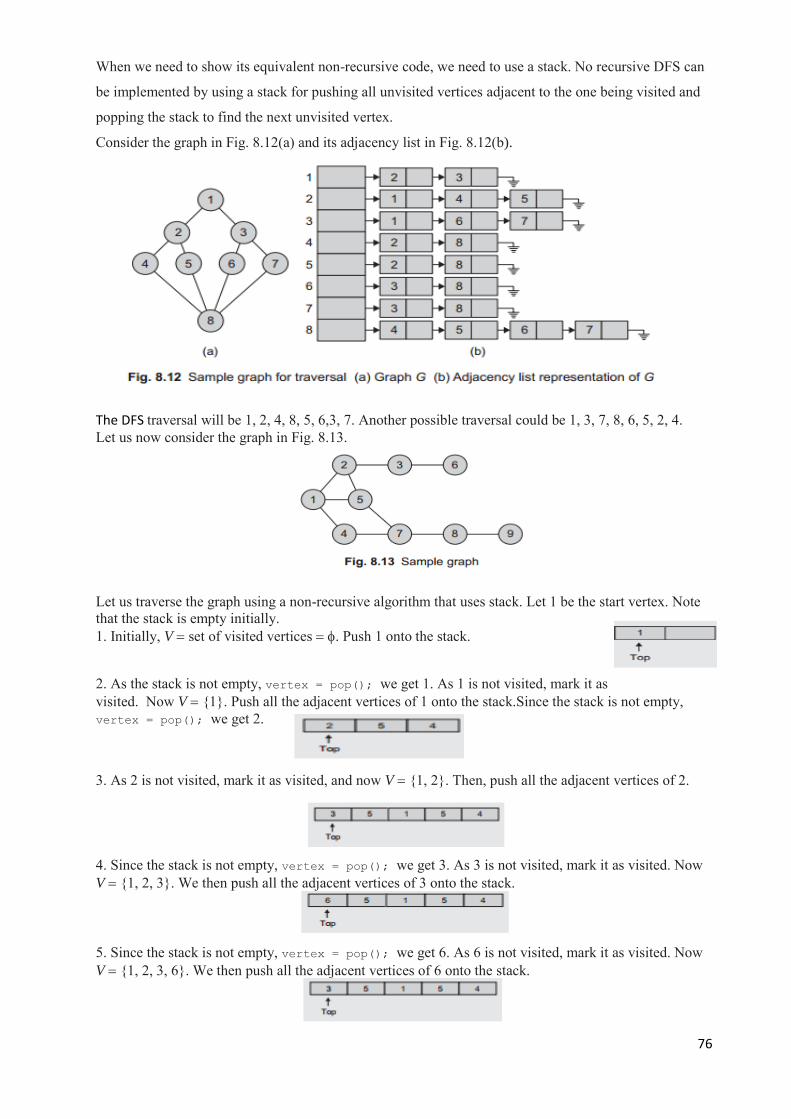
76

When we need to show its equivalent non-recursive code, we need to use a stack. No recursive DFS can

be implemented by using a stack for pushing all unvisited vertices adjacent to the one being visited and

popping the stack to find the next unvisited vertex.

Consider the graph in Fig. 8.12(a) and its adjacency list in Fig. 8.12(b).

The DFS traversal will be 1, 2, 4, 8, 5, 6,3, 7. Another possible traversal could be 1, 3, 7, 8, 6, 5, 2, 4.

Let us now consider the graph in Fig. 8.13.

Let us traverse the graph using a non-recursive algorithm that uses stack. Let 1 be the start vertex. Note

that the stack is empty initially.

1. Initially, V set of visited vertices . Push 1 onto the stack.

2. As the stack is not empty, vertex = pop(); we get 1. As 1 is not visited, mark it as

visited. Now V {1}. Push all the adjacent vertices of 1 onto the stack.Since the stack is not empty,

vertex = pop(); we get 2.

3. As 2 is not visited, mark it as visited, and now V {1, 2}. Then, push all the adjacent vertices of 2.

4. Since the stack is not empty, vertex = pop(); we get 3. As 3 is not visited, mark it as visited. Now

V {1, 2, 3}. We then push all the adjacent vertices of 3 onto the stack.

5. Since the stack is not empty, vertex = pop(); we get 6. As 6 is not visited, mark it as visited. Now

V {1, 2, 3, 6}. We then push all the adjacent vertices of 6 onto the stack.

77

6. Since the stack is not empty, vertex = pop();we get 3. As 3 is visited, pop again vertex = pop();

we then get 5. As 5 is not visited, mark it as visited. Now V {1, 2, 3, 6, 5}. Push all the adjacent

vertices onto the stack.

7. As the stack is not empty, vertex=pop();we get 7, which is not visited. Hence, V {1, 2, 3, 6, 5, 7};

we now push all the adjacent vertices of 7 onto the stack.

8. As the stack is not empty, vertex=pop();we get 8,which is not visited. Hence {1, 2, 3, 6, 5, 7, 8}.

Push all the adjacent vertices of 8 onto the stack.

9. As the stack is not empty, vertex =pop()7, which is visited; vertex=pop()9, which is not visited.

Hence, V = {1, 2, 3, 6, 5, 7, 8, 9}. Push all the adjacent vertices of 9 onto the stack.

10. As the stack is not empty, vertex = pop()8, which is visited; so again vertex=pop()4, which is

not visited. Hence, V {1, 2, 3, 6, 5, 7, 8, 9, 4}. Push all the adjacent vertices of 4 onto the stack.

11. The stack is not empty. So the following operations yield:

vertex = pop() we get 7, visited








12. The stack is now empty, Hence, we stop. The set V {1, 2, 3, 6, 5, 7, 8, 9, 4} represents the order in

which they are visited. Hence, the DFS of the graph (Fig. 8.13) gives the sequence as 1, 2, 3, 6, 5, 7, 8, 9,

and 4. This is shown in Fig. 8.14.

78

Breadth-first Search:

Another systematic way of visiting the vertices is the breadth-first search (BFS). The BFS differs from

DFS in a way that all the unvisited vertices adjacent to i are visited after visiting the start vertex i and

marking it visited. Next, the unvisited vertices adjacent to these vertices are visited and so on until the

entire graph has been traversed. The approach is called ‗breadth-first‘ because from the vertex i that we

visit, we search as broadly as possible by next visiting all the vertices adjacent to i. For example, the

BFS of the graph of Fig. 8.13 results in visiting the nodes in the following order: 1, 2, 3, 4, 5, 6, 7, and 8.

This search algorithm uses a queue to store the vertices of each level of the graph as and when they are

visited. These vertices are then taken out from the queue in sequence, that is, first in first out (FIFO), and

their adjacent vertices are visited until all the vertices have been visited.

Let us traverse the graph using a non-recursive algorithm that uses a queue. Let 1 be the start vertex.

Initially, the queue is empty, and the initial set of visited vertices, V .

1. Add 1 to the queue. Mark 1 as visited. V {1}.

2. As the queue is not empty, vertex = delete() from queue, and we get 1. Add all the un-visited

adjacent vertices of 1 to the queue. In addition, mark them as visited. Now, V {1, 2, 5, 4}

3. As the queue is not empty, vertex = delete() and we get 2. Add all the adjacent, un-visited

vertices of 2 to the queue and mark them as visited. Now V {1, 2, 5, 4, 3}.

4. As the queue is not empty, vertex = delete() from queue, and we get 5. Now, add all the adjacent,

un-visited vertices adjacent to 5 to the queue and mark them as visited. Now, V {1, 2, 5, 4, 3, 7}.

5. As the queue is not empty, vertex = delete() from queue, and we get 4. Now, add all the adjacent,

not visited vertices adjacent to 4 to the queue. The vertices 1 and 7 are adjacent to 4 and hence are

already visited. Now the next element we get from the queue is 3. Now, we add all the un-visited

vertices adjacent to 3 to the queue, making V {1, 2, 5, 4, 3, 7, 6}

6. As the queue is not empty, vertex = delete() and we get 7. Add all the adjacent, unvisited

vertices of 7 to the queue and mark them as visited. Now, V {1, 2, 5, 4, 3, 7, 6, 8}

79

7. As the queue is not empty, vertex = delete(), and we get 6. Then, add all the un-visited adjacent

vertices of 6 to the queue and mark them as visited. Now V {1, 2, 5, 4, 3, 7, 6, 8}

8. As queue is not empty, vertex = delete() and we get 8. Add its adjacent un-visited vertices to the

queue and mark them as visited. V {1, 2, 5, 4, 3, 7, 6, 8, 9}.

9. As the queue is not empty, vertex = delete() 9. Here, note that no adjacent vertices of 9 are un-

visited. 10. As the queue is empty, we stop. The sequence in which the vertices are visited by the BFS is

1, 2, 5, 4, 3, 7, 6, 8, 9 This is represented in Fig. 8.18.

SPANNING TREE:

DEF: A tree is a connected graph with no cycles. A spanning tree is a sub-graph of G that has all

vertices of G and is a tree. A minimum spanning tree of a weighted graph G is the spanning tree of G

whose edges sum to minimum weight. There can be more than one minimum spanning tree for a graph.

Figure 8.19 shows a graph, one of its spanning trees, and a minimum spanning tree.

There are two popular methods used to compute the minimum spanning tree of a graph is

1. Prim‘s algorithm

2. Kruskal‘s algorithm

1) Prim’s algorithm:

Prim's algorithm is a greedy algorithm that finds a minimum spanning tree for a weighted undirected

graph. This means it finds a subset of the edges that forms a tree that includes every vertex, where the

total weight of all the edges in the tree is minimized.

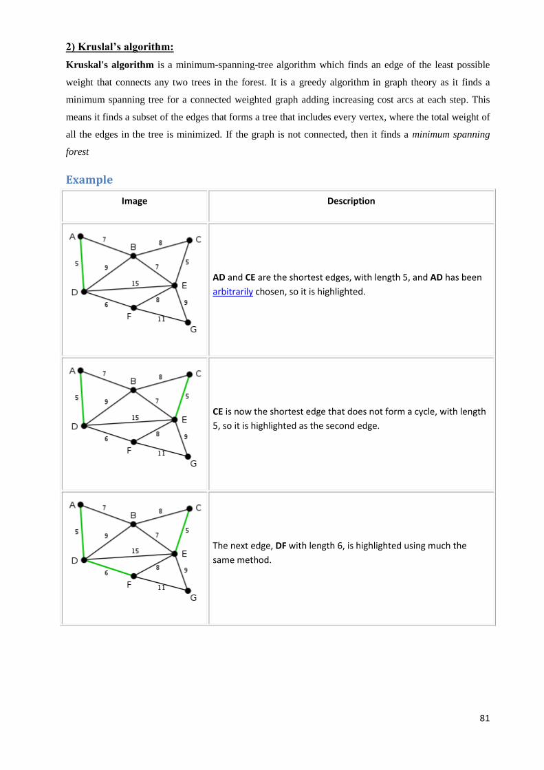
81

2) Kruslal’s algorithm:

Kruskal's algorithm is a minimum-spanning-tree algorithm which finds an edge of the least possible

weight that connects any two trees in the forest. It is a greedy algorithm in graph theory as it finds a

minimum spanning tree for a connected weighted graph adding increasing cost arcs at each step. This

means it finds a subset of the edges that forms a tree that includes every vertex, where the total weight of

all the edges in the tree is minimized. If the graph is not connected, then it finds a minimum spanning

forest

Example

Image Description

AD and CE are the shortest edges, with length 5, and AD has been

arbitrarily chosen, so it is highlighted.

CE is now the shortest edge that does not form a cycle, with length

5, so it is highlighted as the second edge.

The next edge, DF with length 6, is highlighted using much the

same method.

https://en.wikipedia.org/wiki/Minimum_spanning_tree#Algorithms

https://en.wikipedia.org/wiki/Greedy_algorithm

https://en.wikipedia.org/wiki/Graph_theory

https://en.wikipedia.org/wiki/Minimum_spanning_tree

https://en.wikipedia.org/wiki/Connectivity_(graph_theory)

https://en.wikipedia.org/wiki/Glossary_of_graph_theory#Weighted_graphs_and_networks

https://en.wikipedia.org/wiki/Edge_(graph_theory)

https://en.wikipedia.org/wiki/Vertex_(graph_theory)

https://en.wikipedia.org/wiki/Arbitrary

https://en.wikipedia.org/wiki/File:Kruskal_Algorithm_1.svg



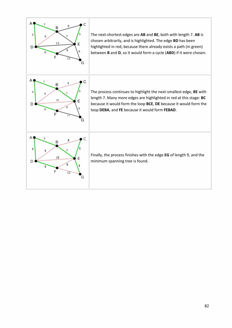
82

The next-shortest edges are AB and BE, both with length 7. AB is

chosen arbitrarily, and is highlighted. The edge BD has been

highlighted in red, because there already exists a path (in green)

between B and D, so it would form a cycle (ABD) if it were chosen.

The process continues to highlight the next-smallest edge, BE with

length 7. Many more edges are highlighted in red at this stage: BC

because it would form the loop BCE, DE because it would form the

loop DEBA, and FE because it would form FEBAD.

Finally, the process finishes with the edge EG of length 9, and the

minimum spanning tree is found.




83

HASHING:

Def:

Hashing is a method of directly computing the address of the record with the help of a key by using a

suitable mathematical function called the hash function. A hash table is an array-based structure used to

store <key, information> pairs.

Hashing is the process of indexing and retrieving element (data) in a data structure to provide faster way

of finding the element using the hash key.

Hash Table:

Hash table is an array which maps a key (data) into the datastructure with the help of hash function

such that insertion, deletion and search operations can be performed with constant time complexity

Hash Function:

Hash function is a function that maps a key in the range [0 to Max - 1], the result of which is used as an

index (or address) in the hash table for storing and retrieving records

One more way to define a hash function is as the function that transforms a key into an address.

The address generated by a hashing function is called the home address. All home addresses refer to a

particular area of the memory called the prime area.

Basic concept of hashing and hash table is shown in the following figure...

Bucket :A bucket is an index position in a hash table that can store more than one record. Tables 11.1

and 11.2 show a bucket of size 1 and size 2, respectively. When the same index is mapped with two

keys, both the records are stored in the same bucket. The assumption is that the buckets are equal in size.

84

Probe: Each action of address calculation and check for success is called as a probe.

Collision: The result of two keys hashing into the same address is called collision.

Synonym: Keys that hash to the same address are called synonyms.

Overflow: The result of many keys hashing to a single address and lack of room in the bucket is known

as an overflow. Collision and overflow are synonymous when the bucket is of size 1.

Open or external hashing When we allow records to be stored in potentially unlimited space, it is

called as open or external hashing.

Closed or internal hashing When we use fixed space for storage eventually limiting the number of

records to be stored, it is called as closed or internal hashing.

Hash function Hash function is an arithmetic function that transforms a key into an address which is

used for storing and retrieving a record.

Perfect hash function The hash function that transforms different keys into different addresses is

called a perfect hash function. The worth of a hash function depends on how well it avoids collision.

HASH FUNCTIONS:

To store a record in a hash table, a hash function is applied to the key of the record being stored,

returning an index within the range of the hash table. The record is stored at that index position, if it is

empty. With direct addressing, a record with key K is stored in slot K. With hashing, this record is stored

at the location Hash(K), where Hash(K) is the function. The hash function Hash(K) is used to compute

the slot for the key K.

Good Hash Function

A good hash function is one which satisfies the assumption. that any given record is equally likely to

hash into any of the slots, independent of whether any other record has been already hashed to it or not.

This assumption is known as simple uniform hashing.

Features of a Good Hashing Function

1. Addresses generated from the key are uniformly and randomly distributed.

2. Small variations in the value of the key will cause large variations in the record

addresses to distribute records (with similar keys) evenly.

3. The hashing function must minimize the occurrence of collision.

85

There are many methods of implementing hash functions:

1. Division Method

One of the required features of the hash function is that the resultant index must be within the table index

range. One simple choice for a hash function is to use the modulus division indicated as MOD (the

operator % in C/C). The function MOD returns the remainder when the first parameter is divided by

the second parameter. The result is negative only if the first parameter is negative and the parameters

must be integers. The function returns an integer. If any parameter is NULL, the result is NULL.

Hash(Key) Key % M Key is divided by some number M, and the remainder is used as the hash

address.

2. Multiplication Method:

3. Extraction Method

4. Mid-square Hashing

5. Folding Technique

6. Rotation

7. Universal Hashing

COLLISION RESOLUTION STRATEGIES:

No hash function is perfect. If Hash(Key1) Hash(Key2), then Key1 and Key2 are synonyms and if

bucket size is 1, we say that collision has occurred. As a consequence, we have to store the record Key2

at some other location. A search is made for a bucket in which a record is stored containing Key2, using

one of the several collision resolution strategies. The collision resolution strategies are as follows:

1. Open addressing

(a) Linear probing

(b) Quadratic probing

(c) Double hashing

(d) Key offset

2. Separate chaining (or linked list)

3. Bucket hashing (defers collision but does not prevent it)

The most important factors to be taken care of to avoid collision are the table size and choice of the hash

function.

86

UNIT –IV

SEARCHING:

Search is a process of finding a value in a list of values. In other words, searching is the process

of locating given value position in a list of values.

Linear Search (Sequential Search):

Linear search algorithm finds given element in a list of elements with O(n) time complexity where n is

total number of elements in the list. This search process starts comparing of search element with the first

element in the list. If both are matching then results with element found otherwise search element is

compared with next element in the list. If both are matched, then the result is "element found".

Otherwise, repeat the same with the next element in the list until search element is compared with last

element in the list, if that last element also doesn't match, then the result is "Element not found in the

list". That means, the search element is compared with element by element in the list.

Linear search is implemented using following steps...

Step 1: Read the search element from the user

Step 2: Compare, the search element with the first element in the list.

Step 3: If both are matching, then display "Given element found!!!" and terminate the function

Step 4: If both are not matching, then compare search element with the next element in the list.

Step 5: Repeat steps 3 and 4 until the search element is compared with the last element in the

list.

Step 6: If the last element in the list is also doesn't match, then display "Element not found!!!"

and terminate the function.

Example

Consider the following list of element and search element...

87

Linear Search Program

#include<iostream>


int main()

{ int list[]={10,20,40,30,50};

int size,i,s;

size= sizeof(list)/sizeof(list[0]);

cout<<"Enter the element to be Search";

cin>>s;

for(i = 0; i < size; i++)

{

if(s == list[i])

{

cout<<"Element is found at posdition"<<i+1;

break;

}

}

if(i == size)

cout<<"Given element is not found in the list!!!";

}

88

Binary Search:

Binary search algorithm finds given element in a list of elements with O(log n) time complexity where n

is total number of elements in the list. The binary search algorithm can be used with only sorted list of

element. That means, binary search can be used only with list of element which are already arranged in a

order. The binary search can not be used for list of element which are in random order. This search

process starts comparing of the search element with the middle element in the list. If both are matched,

then the result is "element found". Otherwise, we check whether the search element is smaller or larger

than the middle element in the list. If the search element is smaller, then we repeat the same process for

left sublist of the middle element. If the search element is larger, then we repeat the same process for

right sublist of the middle element. We repeat this process until we find the search element in the list or

until we left with a sublist of only one element. And if that element also doesn't match with the search

element, then the result is "Element not found in the list".

Binary search is implemented using following steps...

Step 1: Read the search element from the user

Step 2: Find the middle element in the sorted list

Step 3: Compare, the search element with the middle element in the sorted list.

Step 4: If both are matching, then display "Given element found!!!" and terminate the function

Step 5: If both are not matching, then check whether the search element is smaller or larger

than middle element.

Step 6: If the search element is smaller than middle element, then repeat steps 2, 3, 4 and 5 for

the left sublist of the middle element.

Step 7: If the search element is larger than middle element, then repeat steps 2, 3, 4 and 5 for

the right sublist of the middle element.

Step 8: Repeat the same process until we find the search element in the list or until sublist

contains only one element.

Step 9: If that element also doesn't match with the search element, then display "Element not

found in the list!!!" and terminate the function.

Example

Consider the following list of element and search element...

90

Binary Search Program #include<iostream>


int main()

{

int list[] = {10,20,30,40,50,60,70,80,80,100};

int first, last, middle, size, i, s;

size= sizeof(list)/sizeof(list[0]);

cout<<"Enter the element to be Search";

cin>>s;

first = 0;

last = size - 1;

middle = (first+last)/2;

while (first <= last)

{

if (list[middle] < s)

first = middle + 1;

else if (list[middle] == s)

{

cout<<"Element is found at posdition"<<middle+1;

break;

}

else

last = middle - 1;

middle = (first + last)/2;

}

if (first > last)

cout<<"Given element is not found in the list!!!";

}

SORTING:

Arranging the elements in a list in either ascending or descending order is called sorting. There are

several types of sorting techniques:

1. Bubble Sort:

Bubble sort is also known as exchange sort. Bubble sort is a simplest sorting algorithm. In

bubble sort algorithm array is traversed from 0 to the length-1 index of the array and compared

one element to the next element and swap values in between if the next element is less than the

previous element. In other words, bubble sorting algorithm compare two values and put the

largest value at largest index. The algorithm follow the same steps repeatedly until the values of

array is sorted.

Working of bubble sort algorithm: Say we have an array unsorted A[0],A[1],A[2]................ A[n-1] and A[n] as input. Then the

following steps are followed by bubble sort algorithm to sort the values of an array.

1.Compare A[0] and A[1] .

2.If A[0]>A[1] then Swap A[0] and A[1].

3.Take next A[1] and A[2].

4.Comapre these values.

5.If A[1]>A[2] then swap A[1] and A[2]

...............................................................

at last compare A[n-1] and A[n]. If A[n-1]>A[n] then swap A[n-1] and A[n]. As we see the

highest value is reached at nth

position. At next iteration leave nth

value. Then apply the same

steps repeatedly on A[0],A[1],A[2]................ A[n-1] elements repeatedly until the values of

array is sorted.

91

Ex:

12 9 4 99 120 1 3 10

The basic steps followed by algorithm:-

In the first step compare first two values 12 and 9.

12 9 4 99 120 1 3 10

As 12>9 then we have to swap these values

Then the new sequence will be

9 12 4 99 120 1 3 10

In next step take next two values 12 and 4

9 12 4 99 120 1 3 10

Compare these two values .As 12>4 then we have to swap these values.

Then the new sequence will be

9 4 12 99 120 1 3 10

We have to follow similar steps up to end of array. e.g.

9 4 12 99 120 1 3 10

9 4 12 99 120 1 3 10

9 4 12 99 1 120 3 10

9 4 12 99 1 120 3 10

9 4 12 99 1 3 120 10

9 4 12 99 1 3 10 120

When we reached at last index .Then restart same steps unlit the data is not sorted.

The output of this example will be : 1 3 4 9 10 12 99 120

Program :

#include<iostream>


void bubblesrt( int a[], int n )

{

int i, j,t=0;

for(i = 0; i < n; i++)

for(j = 1; j < (n-i); j++)

if(a[j-1] > a[j])

{

t = a[j-1];

a[j-1]=a[j];

a[j]=t;

}

}

int main()

{

int i,size;

int array[] = {12,9,4,99,120,1,3,10};

size=sizeof(array)/sizeof(array[i]);

cout<<"Values Before sorting:"<<endl;


cout<< array[i]<<" ";

cout<<endl;

bubblesrt(array, size);

cout<<"Values after sorting:"<<endl;



}

92

Insertion Sort: Insertion sorting algorithm is similar to bubble sort. But insertion sort is more efficient than

bubble sort because in insertion sort the elements comparisons are less as compare to bubble

sort. In insertion sorting algorithm compare the value until all the prior elements are lesser than

compared value is not found. This mean that the all previous values are lesser than compared

value. This algorithm is more efficient than the bubble sort .Insertion sort is a good choice for

small values and for nearly-sorted values.

Code description:

In insertion sorting take the element form left assign value into a variable. Then compare the value with

previous values. Put value so that values must be lesser than the previous values. Then assign

next value to a variable and follow the same steps relatively until the comparison not reached to end of

array.

Ex:

Program: #include<iostream>


void insertionsrt(int array[], int n)

{ int i,j;

for (i = 1; i < n; i++)

{

int j = i;

int B = array[i];

while ((j > 0) && (array[j-1] > B))

{

array[j] = array[j-1];

j--;

}

array[j] = B;

}

}

93

int main()

{

int i,size;

int array[] = {12,9,4,99,120,1,3,10};

size=sizeof(array)/sizeof(array[0]);




cout<<endl;

insertionsrt(array, size);




}

Selection Sort: In selection sorting algorithm, find the minimum value in the array then swap it first position. In

next step leave the first value and find the minimum value within remaining values. Then swap

it with the value of minimum index position. Sort the remaining values by using same steps.

Selection sort is probably the most intuitive sorting algorithm to invent.

Code description:

In selection sort algorithm to find the minimum value in the array. First assign minimum index in key

(index_of_min=x). Then find the minimum value and assign the index of minimum value in key

(index_of_min=y). Then swap the minimum value with the value of minimum index.

At next iteration leave the value of minimum index position and sort the remaining values by following

same steps.

Working of the selection sort :

Say we have an array unsorted A[0],A[1],A[2]................ A[n-1] and A[n] as input. Then the

following steps are followed by selection sort algorithm to sort the values of an array . (Say we

have a key index_of_min that indicate the position of minimum value)

1. Initially variable index_of_min=0;

2.Find the minimum value in the unsorted array.

3. Assign the index of the minimum value into index_of_min variable.

4. Swap minimum value to first position.

5. Sort the remaining values of array (excluding the first value).

94

The code of the program :

#include<iostream> using namespace std; void selectionsort(int array[], int n) { int x,indexofmin; for(x=0; x<n; x++) { indexofmin = x; for(int y=x; y<n; y++) if(array[indexofmin]>array[y]) indexofmin = y; int temp = array[x]; array[x] = array[indexofmin]; array[indexofmin] = temp; } } int main() { int array[] = {12,9,4,99,120,1,3,10}; int i,size; size=sizeof(array)/sizeof(array[0]); cout<<"Values Before sorting:"<<endl; for(i = 0; i < size; i++) cout<< array[i]<<" "; cout<<endl; selectionsort(array, size); cout<<"Values after sorting:"<<endl; for(i = 0; i < size; i++) cout<< array[i]<<" "; }

Quick Sort:

Quick sort is a comparison sort. The working of quick sort algorithm is depending on a divide-

and-conquer strategy. A divide and conquer strategy is dividing an array into two sub-arrays.

Quick sort is one of the fastest and simplest sorting algorithm.

Code description:

In quick sort algorithm pick an element from array of elements. This element is

called the pivot. Then compare the the values from left to right until a greater element is find

then swap the values. Again start comparison from right with pivot. When lesser element is find

then swap the values. Follow the same steps until all elements which are less than the pivot

come before the pivot and all elements greater than the pivot come after it. After this

partitioning, the pivot is in its last position. This is called the partition operation. Recursively

sort the sub-array of lesser elements and the sub-array of greater elements.

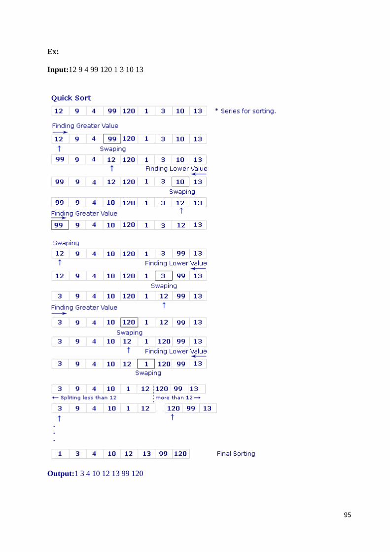
95

Ex:

Input:12 9 4 99 120 1 3 10 13

Output:1 3 4 10 12 13 99 120

96

Program:

#include<iostream> using namespace std; void quicksort(int array[],int low, int n) { int mid,t; int lo = low; int hi = n; if (lo >= n) return; mid = array[(lo + hi) / 2]; while (lo < hi) { while (lo<hi && array[lo] < mid) lo++; while (lo<hi && array[hi] > mid) hi--; if (lo < hi) { t = array[lo]; array[lo] = array[hi]; array[hi] = t; } } if (hi < lo) { int t = hi; hi = lo; lo = t; } quicksort(array, low, lo); quicksort(array, lo == low ? lo+1 : lo, n); } int main() { int array[] = {12,9,4,99,120,1,3,10,13}; int i,size; size=sizeof(array)/sizeof(array[0]); cout<<"Values Before sorting:"<<endl; for(i = 0; i < size; i++) cout<< array[i]<<" "; cout<<endl; quicksort(array,0,size-1); cout<<"Values after sorting:"<<endl; for(i = 0; i < size; i++) cout<< array[i]<<" "; }

Merge Sort:

Like QuickSort, Merge Sort is a Divide and Conquer algorithm. It divides input array in two halves, calls

itself for the two halves and then merges the two sorted halves. The merge() function is used for

merging two halves. The merge(arr, l, m, r) is key process that assumes that arr[l..m] and arr[m+1..r] are

sorted and merges the two sorted sub-arrays into one.

http://quiz.geeksforgeeks.org/quick-sort/

http://www.geeksforgeeks.org/divide-and-conquer-set-1-find-closest-pair-of-points/

97

The following diagram from shows the complete merge sort process for an example array {38, 27, 43, 3,

9, 82, 10}. The array is recursively divided in two halves till the size becomes 1. Once the size becomes

1, the merge processes comes into action and starts merging arrays back till the complete array is

merged.

Ex:

Program: #include <iostream> using namespace std; void Merge(int *a, int low, int high, int mid) { int i, j, k, temp[high-low+1]; i = low; k = 0; j = mid + 1; while (i <= mid && j <= high) { if (a[i] < a[j]) { temp[k] = a[i]; k++; i++; } else { temp[k] = a[j]; k++; j++; } } while (i <= mid) { temp[k] = a[i]; k++; i++; } while (j <= high) { temp[k] = a[j]; k++; j++; } for (i = low; i <= high; i++) a[i] = temp[i-low]; }

98

void MergeSort(int *a, int low, int high) { int mid; if (low < high) { mid=(low+high)/2; MergeSort(a, low, mid); MergeSort(a, mid+1, high); Merge(a, low, high, mid); } } int main() { int array[] = {12,9,4,99,120,1,3,10,13}; int i,size; size=sizeof(array)/sizeof(array[0]); cout<<"Values Before sorting:"<<endl; for(i = 0; i < size; i++) cout<< array[i]<<" "; cout<<endl; MergeSort(array,0,size-1); cout<<"Values after sorting:"<<endl; for(i = 0; i < size; i++) cout<< array[i]<<" "; }

Comparisons of sorting techniques:

99

Heaps:

BASIC CONCEPTS:

Def:

A heap is a binary tree having the following properties:

1. It is a complete binary tree, that is, each level of the tree is completely filled, except the bottom

level, where it is filled from left to right.

2. It satisfies the heap-order property , that is, the key value of each node is greater than

or equal to the key value of its children, or the key value of each node is lesser than or

equal to the key value of its children.

All the binary trees of Fig. 12.1 are heaps, whereas the binary trees of Fig. 12.2 are not. The second

condition is violated in Fig. 12.2(a) as the content of the child node 80 is greater than its parent node 70.

The first condition is violated in Fig. 12.2(b) as at level 2, 30 has a right child but no left child, that is, at

this level, it should be filled from left to right.

Min-heap and Max-heap

Min-heap

The structure shown in Fig. 12.3 is called min-heap. In min-heap, the key value of each node is lesser

than or equal to the key value of its children. In addition, every path from root to leaf should be sorted in

ascending order.

Figure 12.4 is an example of a min-heap.

100

Max-heap

A max-heap is where the key value of a node is greater than or equal to the key value of its children. In

general, whenever the term ‗heap‘ is used by itself, it refers to a max-heap as shown in Fig. 12.5.

In addition, every path from the root to leaf should be sorted in descending order. Figure 12.6 is an

example of a max-heap.

IMPLEMENTATION OF HEAP:

To implement heaps using array is an easy task. We simply number the nodes in the heap from top to

bottom, number the nodes on each level from left to right, and store the ith node in the ith location of the

array.

The root of the tree is stored at index 0, its left child at

index 1, its right child at index 2, and so on.

For example, consider Fig 12.7.

Figure 12.8 shows the corresponding array representation of the heap.

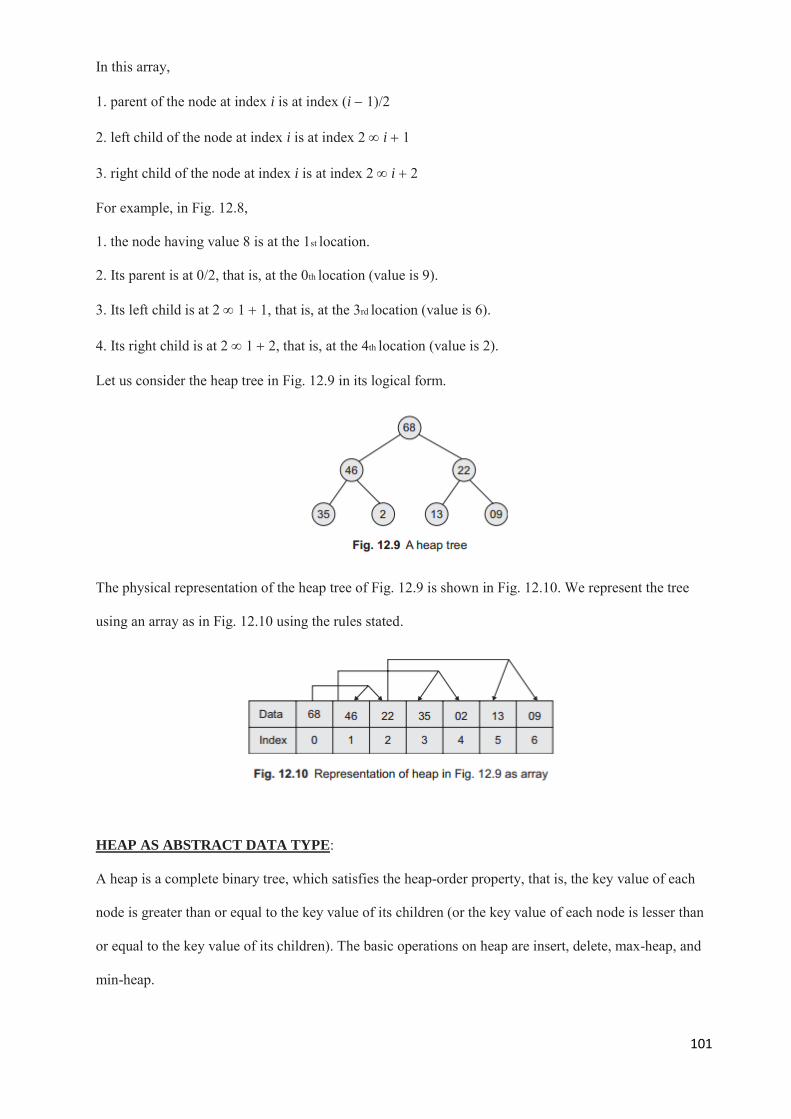
101

In this array,

1. parent of the node at index i is at index (i 1)/2

2. left child of the node at index i is at index 2 i 1

3. right child of the node at index i is at index 2 i 2

For example, in Fig. 12.8,

1. the node having value 8 is at the 1st location.

2. Its parent is at 0/2, that is, at the 0th location (value is 9).

3. Its left child is at 2 1 1, that is, at the 3rd location (value is 6).

4. Its right child is at 2 1 2, that is, at the 4th location (value is 2).

Let us consider the heap tree in Fig. 12.9 in its logical form.

The physical representation of the heap tree of Fig. 12.9 is shown in Fig. 12.10. We represent the tree

using an array as in Fig. 12.10 using the rules stated.

HEAP AS ABSTRACT DATA TYPE:

A heap is a complete binary tree, which satisfies the heap-order property, that is, the key value of each

node is greater than or equal to the key value of its children (or the key value of each node is lesser than

or equal to the key value of its children). The basic operations on heap are insert, delete, max-heap, and

min-heap.

102

ADT Heap

1.Create()Heap

2.Insert(Heap, Data)Heap

3.DeleteMaxVal(Heap)Heap

4.ReHeapDown(Heap, Child)Heap

5.ReHeapUp(Heap, Root)Heap

End

The Cclass declaration for this ADT is as follows:

class HeapNode

{

int A[max];

int n; //No. of elements heap contains

};

class Heap

{

private:

HeapNode *Root;

void ReHeapUp(int i);

void ReHeapDown(int i);

public:

Heap();

{

for(int i = 0; i < max; i++)

A[i] = 0;

}

void Create();

void Insert(int i);

void DeleteMaxVal();

};

103

Heap Sort: #include <iostream>


void MaxHeapify(int a[], int i, int n)

{

int j, temp;

temp = a[i];

j = 2*i;

while (j <= n)

{

if (j < n && a[j+1] > a[j])

j = j+1;

if (temp > a[j])

break;

else if (temp <= a[j])

{

a[j/2] = a[j];

j = 2*j;

}

}

a[j/2] = temp;

return;

}

void HeapSort(int a[], int n)

{

int i, temp;

for (i = n; i >= 2; i--)

{

temp = a[i];

a[i] = a[1];

a[1] = temp;

MaxHeapify(a, 1, i - 1);

}

}

void Build_MaxHeap(int a[], int n)

{

int i;

for(i = n/2; i >= 1; i--)

MaxHeapify(a, i, n);

}

int main()

{

int n, i,size;

int array[] = {12,9,4,99,120,1,3,10,13};

size=sizeof(array)/sizeof(array[0]);




cout<<endl;

Build_MaxHeap(array, size-1);

HeapSort(array, size-1);




}

unit i 1) data structure structure... · 2019-12-19 · 2. an algorithm is an ordered finite set of...

Documents