unit 3 cpu scheduling algorithms - notes milenge · operating systems unit 3 sikkim manipal...
TRANSCRIPT
Operating Systems Unit 3
Sikkim Manipal University Page No. 37
Unit 3 CPU Scheduling Algorithms
Structure
3.1 Introduction
Objectives
3.2 Basic Concepts of Scheduling.
CPU-I/O Burst Cycle.
CPU Scheduler.
Preemptive/non preemptive scheduling.
Dispatcher
Scheduling Criteria
3.3 Scheduling Algorithms
First come First Served Scheduling
Shortest-Job-First Scheduling
Priority Scheduling.
Round-Robin Scheduling
Multilevel Queue Scheduling
Multilevel Feedback Queue Scheduling
Multiple-Processor Scheduling
Real-Time Scheduling
3.4 Evaluation of CPU Scheduling Algorithms.
Deterministic Modeling
Queuing Models
Simulations
Implementation
3.5 Summary
3.6 Terminal Questions
3.7 Answers
Operating Systems Unit 3
Sikkim Manipal University Page No. 38
3.1 Introduction
The CPU scheduler selects a process from among the ready processes to
execute on the CPU. CPU scheduling is the basis for multi-programmed
operating systems. CPU utilization increases by switching the CPU among
ready processes instead of waiting for each process to terminate before
executing the next.
The idea of multi-programming could be described as follows: A process is
executed by the CPU until it completes or goes for an I/O. In simple systems
with no multi-programming, the CPU is idle till the process completes the I/O
and restarts execution. With multiprogramming, many ready processes are
maintained in memory. So when CPU becomes idle as in the case above,
the operating system switches to execute another process each time a
current process goes into a wait for I/O.
Scheduling is a fundamental operating-system function. Almost all computer
resources are scheduled before use. The CPU is, of course, one of the
primary computer resources. Thus, its scheduling is central to operating-
system design.
Objectives:
At the end of this unit, you will be able to understand:
Basic Scheduling Concepts, Different Scheduling algorithms, and Evolution
of these algorithms.
3.2 Basic concepts of Scheduling
3.2.1 CPU- I/O Burst Cycle
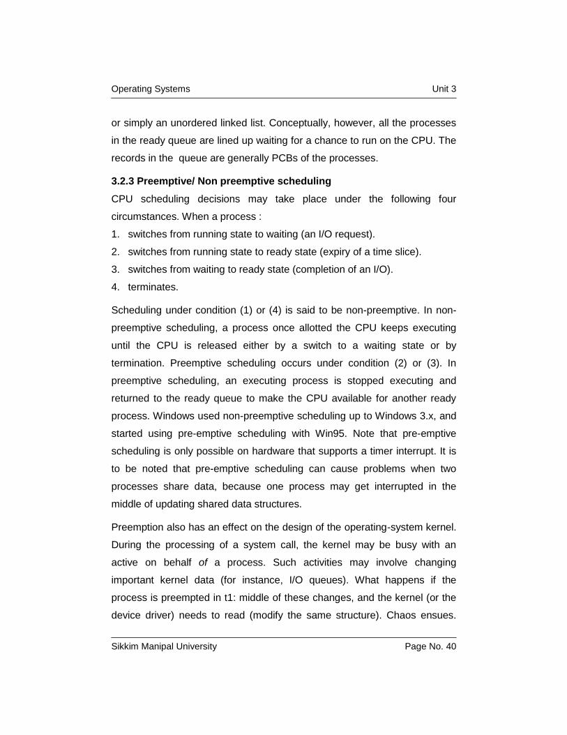
Process execution consists of alternate CPU execution and I/O wait. A cycle
of these two events repeats till the process completes execution (Figure 3.1).
Process execution begins with a CPU burst followed by an I/O burst and
then another CPU burst and so on. Eventually, a CPU burst will terminate
Operating Systems Unit 3
Sikkim Manipal University Page No. 39
the execution. An I/O bound job will have short CPU bursts and a CPU
bound job will have long CPU bursts.
:
:
Load memory
Add to memory CPU burst
Read from file
I/O burst
Load memory
Make increment CPU burst
Write into file
I/O burst
Load memory
Add to memory CPU burst
Read from file
I/O burst
:
:
Figure 3.1: CPU and I/O bursts
3.2.2 CPU Scheduler
Whenever the CPU becomes idle, the operating system must select one of
the processes in the ready queue to be executed. The short-term scheduler
(or CPU scheduler) carries out the selection process. The scheduler selects
from among the processes in memory that are ready to execute, and
allocates the CPU to one of them.
Note that the ready queue is not necessarily a first-in, first-out (FIFO) queue.
As we shall see when we consider the various scheduling algorithms, a
ready queue may be implemented as a FIFO queue, a priority queue, a tree,
Wait for I/O
Wait for I/O
Wait for I/O
Operating Systems Unit 3
Sikkim Manipal University Page No. 40
or simply an unordered linked list. Conceptually, however, all the processes
in the ready queue are lined up waiting for a chance to run on the CPU. The
records in the queue are generally PCBs of the processes.
3.2.3 Preemptive/ Non preemptive scheduling
CPU scheduling decisions may take place under the following four
circumstances. When a process :
1. switches from running state to waiting (an I/O request).
2. switches from running state to ready state (expiry of a time slice).
3. switches from waiting to ready state (completion of an I/O).
4. terminates.
Scheduling under condition (1) or (4) is said to be non-preemptive. In non-
preemptive scheduling, a process once allotted the CPU keeps executing
until the CPU is released either by a switch to a waiting state or by
termination. Preemptive scheduling occurs under condition (2) or (3). In
preemptive scheduling, an executing process is stopped executing and
returned to the ready queue to make the CPU available for another ready
process. Windows used non-preemptive scheduling up to Windows 3.x, and
started using pre-emptive scheduling with Win95. Note that pre-emptive
scheduling is only possible on hardware that supports a timer interrupt. It is
to be noted that pre-emptive scheduling can cause problems when two
processes share data, because one process may get interrupted in the
middle of updating shared data structures.
Preemption also has an effect on the design of the operating-system kernel.
During the processing of a system call, the kernel may be busy with an
active on behalf of a process. Such activities may involve changing
important kernel data (for instance, I/O queues). What happens if the
process is preempted in t1: middle of these changes, and the kernel (or the
device driver) needs to read (modify the same structure). Chaos ensues.
Operating Systems Unit 3
Sikkim Manipal University Page No. 41
Some operating systems, including most versions of UNIX, deal with this
problem by waiting either for a system call to complete, or for an I/O block to
take place, before doing a context switch. This scheme ensures that the
kernel structure is simple, since the kernel will not preempt a process while
the kernel data structures are in an inconsistent state. Unfortunately, this
kernel execution model is a poor one for supporting real-time computing and
multiprocessing.
3.2.4 Dispatcher
Another component involved in the CPU scheduling function is the
dispatcher. The dispatcher is the module that gives control of the CPU to the
process selected by the short-term scheduler. This function involves:
Switching context
Switching to user mode
Jumping to the proper location in the user program to restart that
program
The dispatcher should be as fast as possible, given that it is invoked during
every process switch. The time it takes for the dispatcher to stop one
process and start another running is known as the dispatch latency.
3.2.5 Scheduling Criteria
Many algorithms exist for CPU scheduling. Various criteria have been
suggested for comparing these CPU scheduling algorithms. Common
criteria include:
1. CPU utilization: We want to keep the CPU as busy as possible. CPU
utilization may range from 0% to 100% ideally. In real systems it ranges,
from 40% for a lightly loaded systems to 90% for heavily loaded systems.
2. Throughput: Number of processes completed per time unit is
throughput. For long processes may be of the order of one process per
Operating Systems Unit 3
Sikkim Manipal University Page No. 42
hour whereas in case of short processes, throughput may be 10 or 12
processes per second.
3. Turnaround time: The interval of time between submission and
completion of a process is called turnaround time. It includes execution
time and waiting time.
4. Waiting time: Sum of all the times spent by a process at different
instances waiting in the ready queue is called waiting time.
5. Response time: In an interactive process the user is using some output
generated while the process continues to generate new results. Instead
of using the turnaround time that gives the difference between time of
submission and time of completion, response time is sometimes used.
Response time is thus the difference between time of submission and
the time the first response occurs.
Desirable features include maximum CPU utilization, throughput and
minimum turnaround time, waiting time and response time.
3.3 Scheduling Algorithms
Scheduling algorithms differ in the manner in which the CPU selects a
process in the ready queue for execution. In this section, we have described
several of these algorithms.
3.3.1 First Come First Served scheduling algorithm
This is one of the very brute force algorithms. A process that requests for
the CPU first is allocated the CPU first. Hence, the name first come first
serve. The FCFS algorithm is implemented by using a first-in-first-out (FIFO)
queue structure for the ready queue. This queue has a head and a tail.
When a process joins the ready queue its PCB is linked to the tail of the
FIFO queue. When the CPU is idle, the process at the head of the FIFO
queue is allocated the CPU and deleted from the queue.
Operating Systems Unit 3
Sikkim Manipal University Page No. 43
Even though the algorithm is simple, the average waiting is often quite long
and varies substantially if the CPU burst times vary greatly, as seen in the
following example.
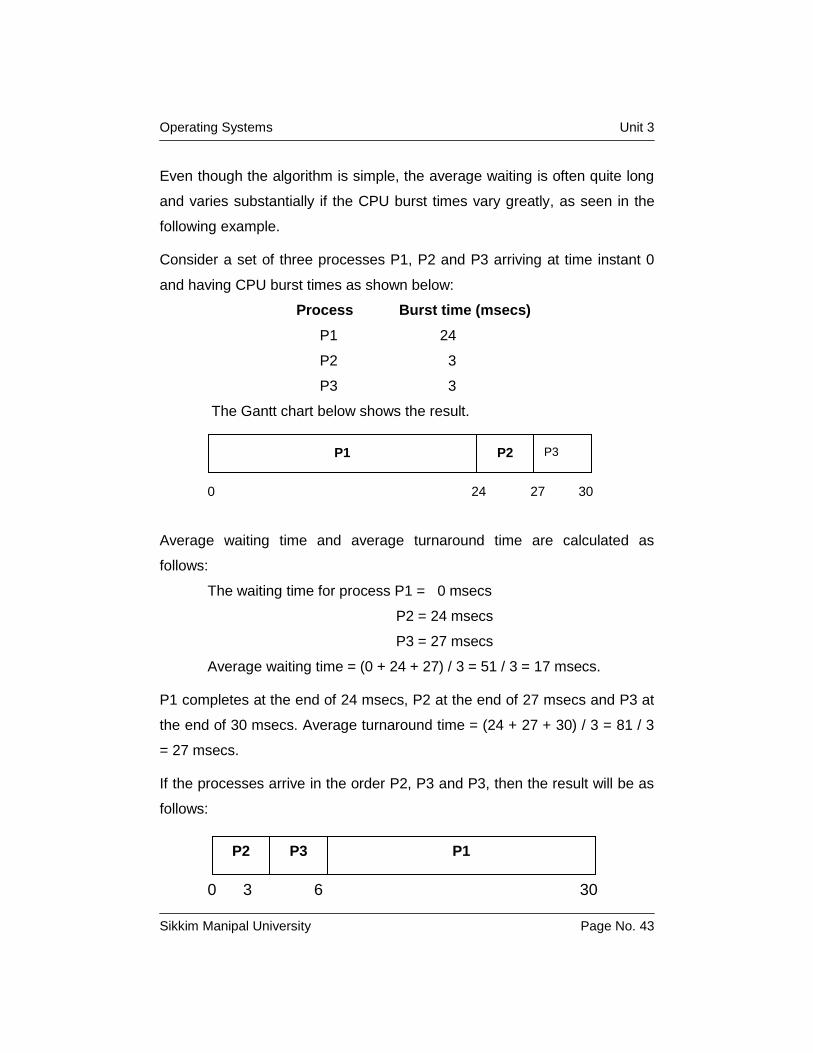
Consider a set of three processes P1, P2 and P3 arriving at time instant 0
and having CPU burst times as shown below:
Process Burst time (msecs)
P1 24
P2 3
P3 3
The Gantt chart below shows the result.
0 24 27 30
Average waiting time and average turnaround time are calculated as
follows:
The waiting time for process P1 = 0 msecs
P2 = 24 msecs
P3 = 27 msecs
Average waiting time = (0 + 24 + 27) / 3 = 51 / 3 = 17 msecs.
P1 completes at the end of 24 msecs, P2 at the end of 27 msecs and P3 at
the end of 30 msecs. Average turnaround time = (24 + 27 + 30) / 3 = 81 / 3
= 27 msecs.
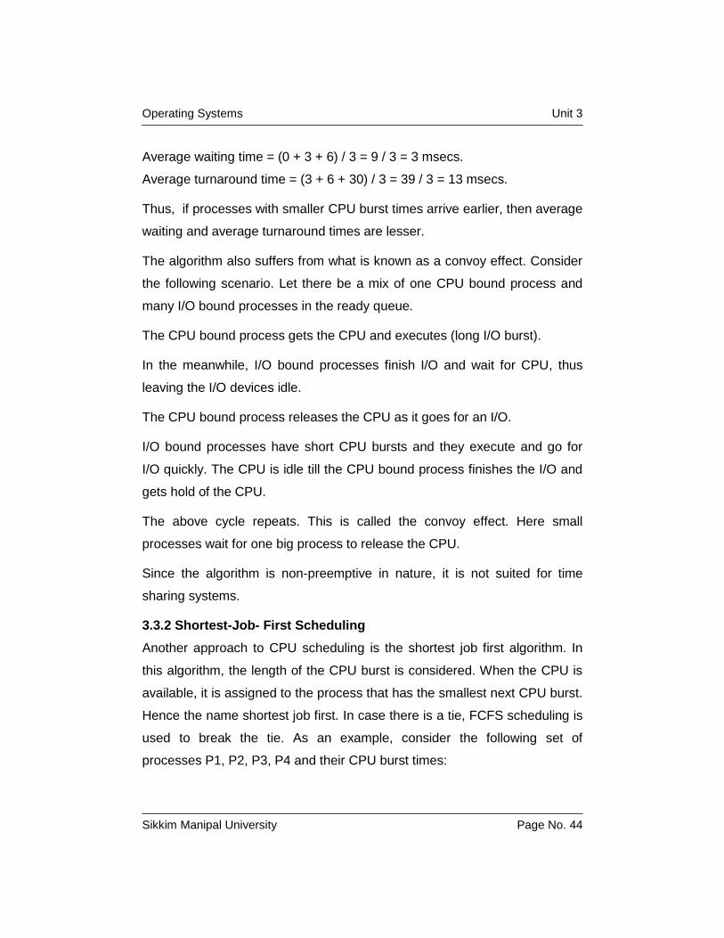
If the processes arrive in the order P2, P3 and P3, then the result will be as
follows:
0 3 6 30
P1 P2 P3
P1 P2 P3
Operating Systems Unit 3
Sikkim Manipal University Page No. 44
Average waiting time = (0 + 3 + 6) / 3 = 9 / 3 = 3 msecs.
Average turnaround time = (3 + 6 + 30) / 3 = 39 / 3 = 13 msecs.
Thus, if processes with smaller CPU burst times arrive earlier, then average
waiting and average turnaround times are lesser.
The algorithm also suffers from what is known as a convoy effect. Consider
the following scenario. Let there be a mix of one CPU bound process and
many I/O bound processes in the ready queue.
The CPU bound process gets the CPU and executes (long I/O burst).
In the meanwhile, I/O bound processes finish I/O and wait for CPU, thus
leaving the I/O devices idle.
The CPU bound process releases the CPU as it goes for an I/O.
I/O bound processes have short CPU bursts and they execute and go for
I/O quickly. The CPU is idle till the CPU bound process finishes the I/O and
gets hold of the CPU.
The above cycle repeats. This is called the convoy effect. Here small
processes wait for one big process to release the CPU.
Since the algorithm is non-preemptive in nature, it is not suited for time
sharing systems.
3.3.2 Shortest-Job- First Scheduling
Another approach to CPU scheduling is the shortest job first algorithm. In
this algorithm, the length of the CPU burst is considered. When the CPU is
available, it is assigned to the process that has the smallest next CPU burst.
Hence the name shortest job first. In case there is a tie, FCFS scheduling is
used to break the tie. As an example, consider the following set of
processes P1, P2, P3, P4 and their CPU burst times:
Operating Systems Unit 3
Sikkim Manipal University Page No. 45
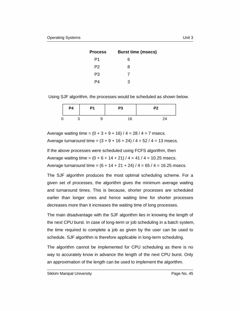
Process Burst time (msecs)
P1 6
P2 8
P3 7
P4 3
Using SJF algorithm, the processes would be scheduled as shown below.
0 3 9 16 24
Average waiting time = (0 + 3 + 9 + 16) / 4 = 28 / 4 = 7 msecs.
Average turnaround time = (3 + 9 + 16 + 24) / 4 = 52 / 4 = 13 msecs.
If the above processes were scheduled using FCFS algorithm, then
Average waiting time = (0 + 6 + 14 + 21) / 4 = 41 / 4 = 10.25 msecs.
Average turnaround time = (6 + 14 + 21 + 24) / 4 = 65 / 4 = 16.25 msecs.
The SJF algorithm produces the most optimal scheduling scheme. For a
given set of processes, the algorithm gives the minimum average waiting
and turnaround times. This is because, shorter processes are scheduled
earlier than longer ones and hence waiting time for shorter processes
decreases more than it increases the waiting time of long processes.
The main disadvantage with the SJF algorithm lies in knowing the length of
the next CPU burst. In case of long-term or job scheduling in a batch system,
the time required to complete a job as given by the user can be used to
schedule. SJF algorithm is therefore applicable in long-term scheduling.
The algorithm cannot be implemented for CPU scheduling as there is no
way to accurately know in advance the length of the next CPU burst. Only
an approximation of the length can be used to implement the algorithm.
P4 P1 P2 P3
Operating Systems Unit 3
Sikkim Manipal University Page No. 46
But the SJF scheduling algorithm is provably optimal and thus serves as a
benchmark to compare other CPU scheduling algorithms.
SJF algorithm could be either preemptive or non-preemptive. If a new
process joins the ready queue with a shorter next CPU burst then what is
remaining of the current executing process, then the CPU is allocated to the
new process. In case of non-preemptive scheduling, the current executing
process is not preempted and the new process gets the next chance, it
being the process with the shortest next CPU burst.
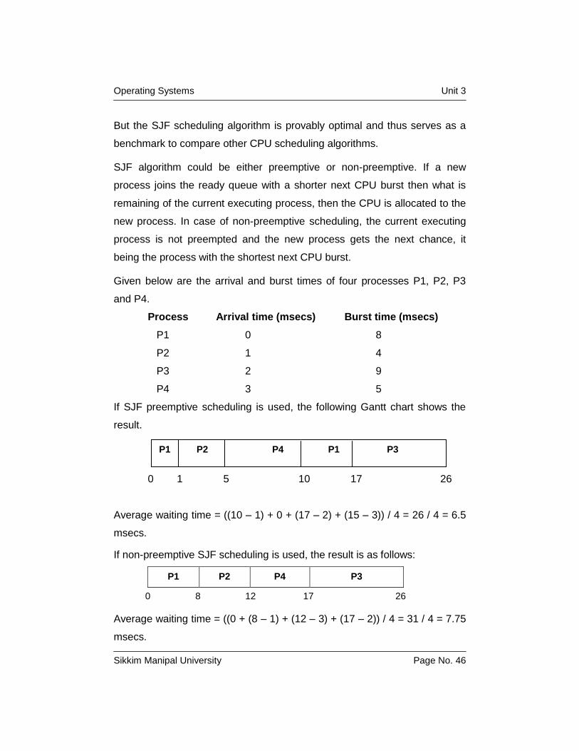
Given below are the arrival and burst times of four processes P1, P2, P3
and P4.
Process Arrival time (msecs) Burst time (msecs)
P1 0 8
P2 1 4
P3 2 9
P4 3 5
If SJF preemptive scheduling is used, the following Gantt chart shows the
result.
0 1 5 10 17 26
Average waiting time = ((10 – 1) + 0 + (17 – 2) + (15 – 3)) / 4 = 26 / 4 = 6.5
msecs.
If non-preemptive SJF scheduling is used, the result is as follows:
P1 P2 P4 P3
0 8 12 17 26
Average waiting time = ((0 + (8 – 1) + (12 – 3) + (17 – 2)) / 4 = 31 / 4 = 7.75
msecs.
P1 P2 P4 P1 P3
Operating Systems Unit 3
Sikkim Manipal University Page No. 47
3.3.3 Priority Scheduling
In priority scheduling each process can be associated with a priority. CPU is
allocated to the process having the highest priority. Hence the name priority.
Equal priority processes are scheduled according to FCFS algorithm.
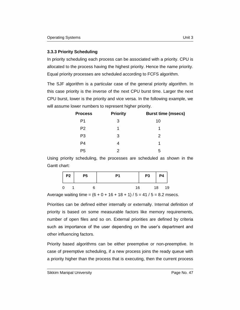
The SJF algorithm is a particular case of the general priority algorithm. In
this case priority is the inverse of the next CPU burst time. Larger the next
CPU burst, lower is the priority and vice versa. In the following example, we
will assume lower numbers to represent higher priority.
Process Priority Burst time (msecs)
P1 3 10
P2 1 1
P3 3 2
P4 4 1
P5 2 5
Using priority scheduling, the processes are scheduled as shown in the
Gantt chart:
0 1 6 16 18 19
Average waiting time = (6 + 0 + 16 + 18 + 1) / 5 = 41 / 5 = 8.2 msecs.
Priorities can be defined either internally or externally. Internal definition of
priority is based on some measurable factors like memory requirements,
number of open files and so on. External priorities are defined by criteria
such as importance of the user depending on the user’s department and
other influencing factors.
Priority based algorithms can be either preemptive or non-preemptive. In
case of preemptive scheduling, if a new process joins the ready queue with
a priority higher than the process that is executing, then the current process
P2 P1 P5 P3 P4
Operating Systems Unit 3
Sikkim Manipal University Page No. 48
is preempted and CPU allocated to the new process. But in case of non-
preemptive algorithm, the new process having highest priority from among
the ready processes, is allocated the CPU only after the current process
gives up the CPU.
Starvation or indefinite blocking is one of the major disadvantages of priority
scheduling. Every process is associated with a priority. In a heavily loaded
system, low priority processes in the ready queue are starved or never get a
chance to execute. This is because there is always a higher priority process
ahead of them in the ready queue.
A solution to starvation is aging. Aging is a concept where the priority of a
process waiting in the ready queue is increased gradually. Eventually even
the lowest priority process ages to attain the highest priority at which time it
gets a chance to execute on the CPU.
3.3.4 Round-Robin Scheduling
The round-robin CPU scheduling algorithm is basically a preemptive
scheduling algorithm designed for time-sharing systems. One unit of time is
called a time slice(Quantum). Duration of a time slice may range between
10 msecs and about 100 msecs. The CPU scheduler allocates to each
process in the ready queue one time slice at a time in a round-robin fashion.
Hence the name round-robin.
The ready queue in this case is a FIFO queue with new processes joining
the tail of the queue. The CPU scheduler picks processes from the head of
the queue for allocating the CPU. The first process at the head of the queue
gets to execute on the CPU at the start of the current time slice and is
deleted from the ready queue. The process allocated the CPU may have the
current CPU burst either equal to the time slice or smaller than the time slice
or greater than the time slice. In the first two cases, the current process will
release the CPU on its own and thereby the next process in the ready

Operating Systems Unit 3
Sikkim Manipal University Page No. 49
queue will be allocated the CPU for the next time slice. In the third case, the
current process is preempted, stops executing, goes back and joins the
ready queue at the tail thereby making way for the next process.
Consider the same example explained under FCFS algorithm.
Process Burst time (msecs)
P1 24
P2 3
P3 3
Let the duration of a time slice be 4 msecs, which is to say CPU
switches between processes every 4 msecs in a round-robin fashion. The
Gantt chart below shows the scheduling of processes.
0 4 7 10 14 18 22 26 30
Average waiting time = (4 + 7 + (10 – 4)) / 3 = 17/ 3 = 5.66 msecs.
If there are 5 processes in the ready queue that is n = 5, and one time slice
is defined to be 20 msecs that is q = 20, then each process will get 20
msecs or one time slice every 100 msecs. Each process will never wait for
more than (n – 1) x q time units.
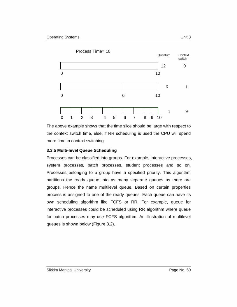
The performance of the RR algorithm is very much dependent on the length
of the time slice. If the duration of the time slice is indefinitely large then the
RR algorithm is the same as FCFS algorithm. If the time slice is too small,
then the performance of the algorithm deteriorates because of the effect of
frequent context switching. A comparison of time slices of varying duration
and the context switches they generate on only one process of 10 time units
is shown below..
P1 P2 P3 P1 P1 P1 P1 P1
Operating Systems Unit 3
Sikkim Manipal University Page No. 50
Process Time= 10
12 0
0 10
0 6 10
0 1 2 3 4 5 6 7 8 9 10
The above example shows that the time slice should be large with respect to
the context switch time, else, if RR scheduling is used the CPU will spend
more time in context switching.
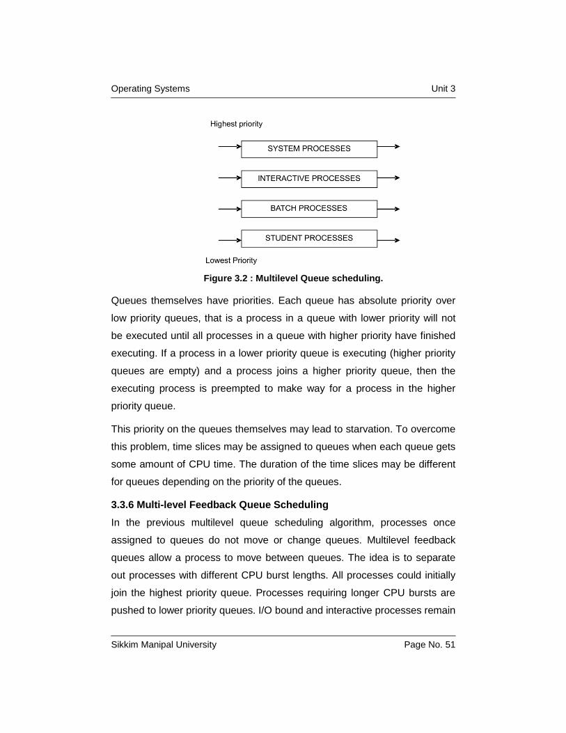
3.3.5 Multi-level Queue Scheduling
Processes can be classified into groups. For example, interactive processes,
system processes, batch processes, student processes and so on.
Processes belonging to a group have a specified priority. This algorithm
partitions the ready queue into as many separate queues as there are
groups. Hence the name multilevel queue. Based on certain properties
process is assigned to one of the ready queues. Each queue can have its
own scheduling algorithm like FCFS or RR. For example, queue for
interactive processes could be scheduled using RR algorithm where queue
for batch processes may use FCFS algorithm. An illustration of multilevel
queues is shown below (Figure 3.2).
Quantum Context switch
6 1
9 1
Operating Systems Unit 3
Sikkim Manipal University Page No. 51
Figure 3.2 : Multilevel Queue scheduling.
Queues themselves have priorities. Each queue has absolute priority over
low priority queues, that is a process in a queue with lower priority will not
be executed until all processes in a queue with higher priority have finished
executing. If a process in a lower priority queue is executing (higher priority
queues are empty) and a process joins a higher priority queue, then the
executing process is preempted to make way for a process in the higher
priority queue.
This priority on the queues themselves may lead to starvation. To overcome
this problem, time slices may be assigned to queues when each queue gets
some amount of CPU time. The duration of the time slices may be different
for queues depending on the priority of the queues.
3.3.6 Multi-level Feedback Queue Scheduling
In the previous multilevel queue scheduling algorithm, processes once
assigned to queues do not move or change queues. Multilevel feedback
queues allow a process to move between queues. The idea is to separate
out processes with different CPU burst lengths. All processes could initially
join the highest priority queue. Processes requiring longer CPU bursts are
pushed to lower priority queues. I/O bound and interactive processes remain
Operating Systems Unit 3
Sikkim Manipal University Page No. 52
in higher priority queues. Aging could be considered to move processes
from lower priority queues to higher priority to avoid starvation. An
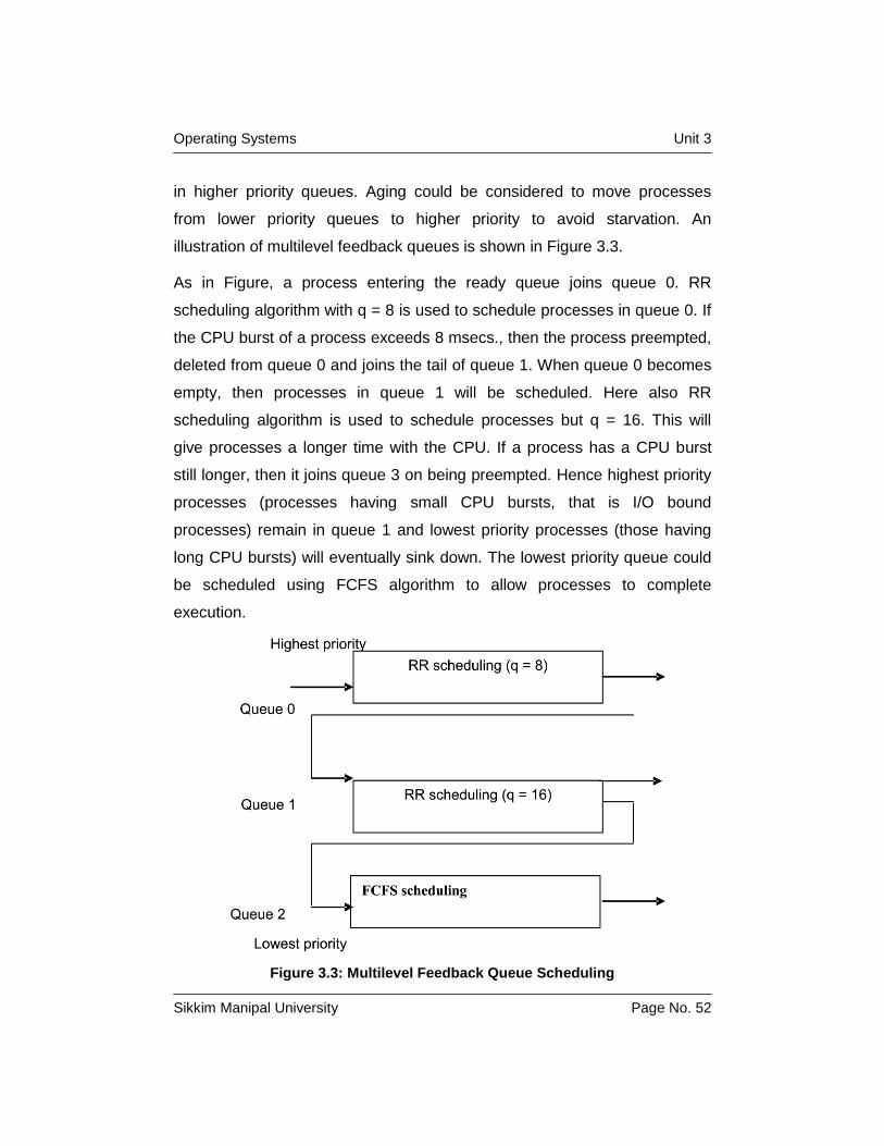
illustration of multilevel feedback queues is shown in Figure 3.3.
As in Figure, a process entering the ready queue joins queue 0. RR
scheduling algorithm with q = 8 is used to schedule processes in queue 0. If
the CPU burst of a process exceeds 8 msecs., then the process preempted,
deleted from queue 0 and joins the tail of queue 1. When queue 0 becomes
empty, then processes in queue 1 will be scheduled. Here also RR
scheduling algorithm is used to schedule processes but q = 16. This will
give processes a longer time with the CPU. If a process has a CPU burst
still longer, then it joins queue 3 on being preempted. Hence highest priority
processes (processes having small CPU bursts, that is I/O bound
processes) remain in queue 1 and lowest priority processes (those having
long CPU bursts) will eventually sink down. The lowest priority queue could
be scheduled using FCFS algorithm to allow processes to complete
execution.
Figure 3.3: Multilevel Feedback Queue Scheduling
Operating Systems Unit 3
Sikkim Manipal University Page No. 53
Multilevel feedback scheduler will have to consider parameters such as
number of queues, scheduling algorithm for each queue, criteria for
upgrading a process to a higher priority queue, criteria for downgrading a
process to a lower priority queue and also the queue to which a process
initially enters.
3.3.7 Multiple- Processor Scheduling
When multiple processors are available, then the scheduling gets more
complicated, because now there is more than one CPU which must be kept
busy and in effective use at all times. Multi-processor systems may be
heterogeneous, (different kinds of CPUs), or homogenous, (all the same
kind of CPU). This book will restrict its discussion to homogenous systems.
In homogenous systems any available processor can then be used to run
any processes in the queue. Even within homogenous multiprocessor,
there are sometimes limitations on scheduling. Consider a system with an
I/O device attached to a private bus of one processor. Processes wishing to
use that device must be scheduled to run on that processor, otherwise the
device would not be available.
If several identical processors are available, then load sharing can occur. It
would be possible to provide a separate queue for each processor. In this
case, however one processor could be idle, with an empty queue, while
another processor was very busy. To prevent this situation, we use a
common ready queue. All processes go into one queue and are scheduled
onto any available processor.
In such scheme, one of two scheduling approaches may be used. In one
approach, each processor is self –scheduling,. Each processor examines
the common ready queue and selects a process to execute. We must
ensure that two processors do not choose the same process, and that
processes are not lost from the queue. The other approach avoids this
Operating Systems Unit 3
Sikkim Manipal University Page No. 54
problem by appointing one processor as scheduler for other processors,
thus creating a master-slave structure.
Some systems carry this structure one step further, by having all scheduling
decisions, I/O processing, and other system activities handled by one single
processor- the master server. The other processors only execute user code.
This asymmetric multiprocessing is far simpler than symmetric
multiprocessing, because only one processor accesses the system data
structures, alleviating the need for data sharing.
3.3.8 Real-Time Scheduling
In unit 1 we gave an overview of real-time operating systems. Here we
continue the discussion by describing the scheduling facility needed to
support real-time computing within a general purpose computer system.
Real-time computing is divided into two types. Hard real-time systems and
soft real-time systems. Hard real time systems are required to complete a
critical task within a guaranteed amount of time. A process is submitted
along with a statement of the amount of time in which it needs to complete
or perform I/O. The scheduler then either admits the process, guaranteeing
that the process will complete on time, or rejects the request as impossible.
This is known as resource reservation. Such a guarantee requires that the
scheduler knows exactly how long each type of operating system function
takes to perform, and therefore each operation must be guaranteed to take
a maximum amount of time. Such a guarantee is impossible in a system
with secondary storage or virtual memory, because these subsystems
cause unavoidable and unforeseeable variation in the amount of time to
execute a particular process. Therefore, hard real-time systems are
composed of special purpose software running on hardware dedicated to
their critical process, and lack the functionality of modern computers and
operating systems.
Operating Systems Unit 3
Sikkim Manipal University Page No. 55
Soft real-time computing is less restrictive. It requires that critical processes
receive priority over less fortunate ones. Implementing soft real-time
functionality requires careful design of the scheduler and related aspects of
the operating system. First, the system must have priority scheduling, and
real-time processes must have the highest priority. The priority of real-time
processes must not degrade over time, even though the priority of non-real
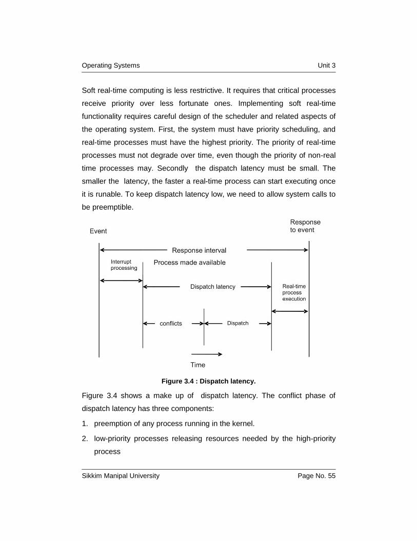
time processes may. Secondly the dispatch latency must be small. The
smaller the latency, the faster a real-time process can start executing once
it is runable. To keep dispatch latency low, we need to allow system calls to
be preemptible.
Figure 3.4 : Dispatch latency.
Figure 3.4 shows a make up of dispatch latency. The conflict phase of
dispatch latency has three components:
1. preemption of any process running in the kernel.
2. low-priority processes releasing resources needed by the high-priority
process
Operating Systems Unit 3
Sikkim Manipal University Page No. 56
3. context switching from the current process to the high-priority process.
As an example in Solaris 2, the dispatch latency with preemption disabled is
over 100 milliseconds. However, the dispatch latency with preemption
enabled is usually to 2 milliseconds.
3.4 Evaluation of CPU Scheduling Algorithms
We have many scheduling algorithms, each with its own parameters. As a
result, selecting an algorithm can be difficult. To select an algorithm first we
must define, the criteria on which we can select the best algorithm. These
criteria may include several measures, such as:
Maximize CPU utilization under the constraint that the maximum
response time is 1 second.
Maximize throughput such that turnaround time is (on average) linearly
proportional to total execution time.
Once the selection criteria have been defined, we use one of the
following different evaluation methods.
3.4.1 Deterministic Modeling
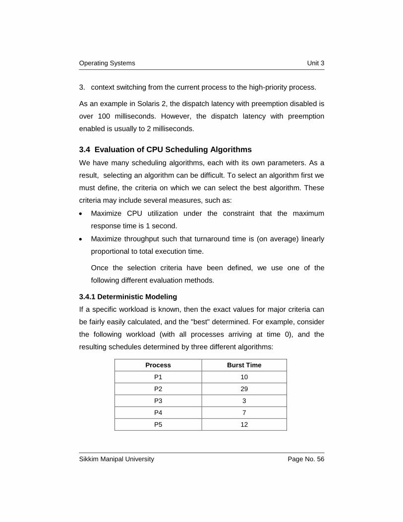
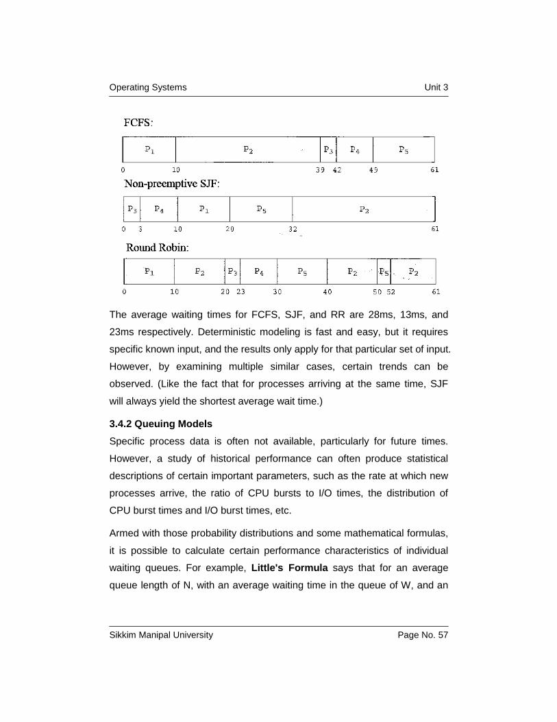
If a specific workload is known, then the exact values for major criteria can
be fairly easily calculated, and the "best" determined. For example, consider
the following workload (with all processes arriving at time 0), and the
resulting schedules determined by three different algorithms:
Process Burst Time
P1 10
P2 29
P3 3
P4 7
P5 12
Operating Systems Unit 3
Sikkim Manipal University Page No. 57
The average waiting times for FCFS, SJF, and RR are 28ms, 13ms, and
23ms respectively. Deterministic modeling is fast and easy, but it requires
specific known input, and the results only apply for that particular set of input.
However, by examining multiple similar cases, certain trends can be
observed. (Like the fact that for processes arriving at the same time, SJF
will always yield the shortest average wait time.)
3.4.2 Queuing Models
Specific process data is often not available, particularly for future times.
However, a study of historical performance can often produce statistical
descriptions of certain important parameters, such as the rate at which new
processes arrive, the ratio of CPU bursts to I/O times, the distribution of
CPU burst times and I/O burst times, etc.
Armed with those probability distributions and some mathematical formulas,
it is possible to calculate certain performance characteristics of individual
waiting queues. For example, Little's Formula says that for an average
queue length of N, with an average waiting time in the queue of W, and an
Operating Systems Unit 3
Sikkim Manipal University Page No. 58
average arrival of new jobs in the queue of Lambda, the these three terms
can be related by:
N = Lambda * W
Queuing models treat the computer as a network of interconnected queues,
each of which is described by its probability distribution statistics and
formulas such as Little's formula. Unfortunately real systems and modern
scheduling algorithms are so complex as to make the mathematics
intractable in many cases with real systems.
3.4.3 Simulations
Another approach is to run computer simulations of the different proposed
algorithms (and adjustment parameters) under different load conditions, and
to analyze the results to determine the "best" choice of operation for a
particular load pattern. Operating conditions for simulations are often
randomly generated using distribution functions similar to those described
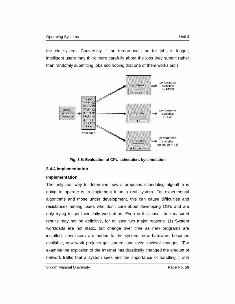
above. A better alternative when possible is to generate trace tapes, by
monitoring and logging the performance of a real system under typical
expected work loads. These are better because they provide a more
accurate picture of system loads, and also because they allow multiple
simulations to be run with the identical process load, and not just statistically
equivalent loads. A compromise is to randomly determine system loads and
then save the results into a file, so that all simulations can be run against
identical randomly determined system loads.
Although trace tapes provide more accurate input information, they can be
difficult and expensive to collect and store, and their use increases the
complexity of the simulations significantly. There are also some questions
as to whether the future performance of the new system will really match the
past performance of the old system. (If the system runs faster, users may
take fewer coffee breaks, and submit more processes per hour than under
Operating Systems Unit 3
Sikkim Manipal University Page No. 59
the old system. Conversely if the turnaround time for jobs is longer,
intelligent users may think more carefully about the jobs they submit rather
than randomly submitting jobs and hoping that one of them works out.)
Fig. 3.5: Evaluation of CPU schedulers by simulation
3.4.4 Implementation
Implementation
The only real way to determine how a proposed scheduling algorithm is
going to operate is to implement it on a real system. For experimental
algorithms and those under development, this can cause difficulties and
resistances among users who don't care about developing OS’s and are
only trying to get their daily work done. Even in this case, the measured
results may not be definitive, for at least two major reasons: (1) System
workloads are not static, but change over time as new programs are
installed, new users are added to the system, new hardware becomes
available, new work projects get started, and even societal changes. (For
example the explosion of the Internet has drastically changed the amount of
network traffic that a system sees and the importance of handling it with
Operating Systems Unit 3
Sikkim Manipal University Page No. 60
rapid response times.) (2) As mentioned above, changing the scheduling
system may have an impact on the workload and the ways in which users
use the system.
Most modern systems provide some capability for the system administrator
to adjust scheduling parameters, either on the fly or as the result of a reboot
or a kernel rebuild.
3.5 Summary
In this chapter we have discussed CPU scheduling. The long-term
scheduler provides a proper mix of CPU-I/O bound jobs for execution. The
short-term scheduler has to schedule these processes for execution.
Scheduling can either be preemptive or non-preemptive. If preemptive, then
an executing process can be stopped and returned to ready state to make
the CPU available for another ready process. But if non-preemptive
scheduling is used then a process once allotted the CPU keeps executing
until either the process goes into wait state because of an I/O or it has
completed execution. Different scheduling algorithms have been discussed.
First-come, first-served (FCFS) scheduling is the simplest scheduling
algorithm, but it can cause short processes to wait for very long processes.
Shortest-Job-First (SJF) scheduling is provably optimal, providing the
shortest average waiting time. Implementing SJF scheduling is difficult
because predicting the length of the next CPU burst is difficult. The SJF
algorithm is a special case of the general priority-scheduling algorithm,
which simply allocates the CPU to the highest-priority process. Both priority
and SJF scheduling may suffer from starvation. Aging is a technique to
prevent starvation. Round robin (RR) scheduling is more appropriate for a
time-shared (inter-active) system. RR scheduling allocates the CPU to the
first process in the ready queue for q time units, where q is the time
Operating Systems Unit 3
Sikkim Manipal University Page No. 61
quantum. After q time units, if the process has not relinquished the CPU, it is
preempted and the process is put at the tail of the ready queue.
Multilevel queue algorithms allow different algorithms to be used for various
classes of processes. The most common is a foreground interactive queue,
which uses RR scheduling, and a background batch queue, which uses FC
scheduling. Multilevel feedback queues allow processes to moves from one
queue to another. Finally, we also discussed various algorithm evaluation
models.
Self Assessment Questions
1. ______________ selects a process from among the ready processes to
execute on the CPU.
2. The time taken by the Dispatcher to stop one process and start another
running is known as _________________.
3. The interval of time between submission and completion of a process is
called _____________.
4. A solution to starvation is _____________.
5. __________ systems are required to complete a critical task within a
guaranteed amount of time.
3.6 Terminal Questions
1. Explain Preemptive and Non-preemptive scheduling approaches.
2. Discuss First come First served scheduling algorithm.
3. What are the Drawbacks of Shortest-Job- First Scheduling algorithm?
4. Why are Round-Robin Scheduling algorithm designed for time-sharing
systems? Explain.
5. Write a note on Multi-level Queue Scheduling.
6. Write a note on Dispatch Latency.
Operating Systems Unit 3
Sikkim Manipal University Page No. 62
7. Explain any two evaluation methods used for the evaluation of
scheduling algorithms.
3.7 Answers to Self Assessment Questions and Terminal
Questions
Answers to Self Assessment Questions
1. CPU Schedular
2. Dispatch Latency
3. Turnaround time
4. Aging
5 . Hard real time.
Answers to Terminal Questions.
1. Refer section 3.2.3
2. Refer section 3.3.1
3. Refer section 3.3.2
4. Refer section 3.3.4
5. Refer section 3.3.5
6. Refer section 3.3.8
7. Refer section 3.4