unit 2 macro
TRANSCRIPT

7/27/2019 Unit 2 Macro
http://slidepdf.com/reader/full/unit-2-macro 1/35
CHAPTER 7 THE CLASSICAL MODELTHE KEYNESIAN REJOINDER
There are several alternative theories or models available to explain the way macro-economiesfunction with different implications for government economic policy. There is far moredisagreement in this area of macroeconomics than we ever saw in microeconomics – this is whydifferent analysts in government and the media say completely contradictory things about whatthe government should do even if they agree about the current state of the economy. We willexamine each of the major economic theories that has influenced economic thought and/or government policy in the US over the course of the last 100 years.
In the late 1800s and early 1900s American economic theory in both microeconomics andmacroeconomics was dominated by Classical theory. Classical economic theory largely camefrom the study of individual market behavior in microeconomics and its macroeconomic theorywas based on the contention that market based economies are just an amalgamation of individualmarkets and, therefore, the same behavioral patterns prevail. Classical economics viewedmarkets as incredibly powerful and efficient mechanisms that could not be improved upon by anyintervention; as a consequence, they strongly urged laissez-faire policy by the government – thatthe government should leave the economy alone and let it work properly.
The Assumptions of the Classical Model
An economic model is based on certain conditions or assumptions; it is important to examinethese to understand why the theory makes the conclusions that it does. The assumptions of amodel function as its foundation and flaws in the foundation undermine the structural integrity of
the building. Flaws in a model’s assumptions undermine the accuracy of the model itself. Themain assumptions of the Classical model are as follows.
Markets are highly competitive: If markets are highly competitive, than no one can hold amarket off its full employment equilibrium. Firms competing with each other will have to makethe best product they can for the lowest acceptable price – any firm trying to take advantage of consumers by selling an inferior product for an inflated price will just lose its customers to other firms. Price will, therefore, always reflect the minimum efficient cost of making the good. Aslong as consumer benefit is high enough to justify paying for the good, they will keep buying itand we will keep making it. Consequently, if individual markets do this, all the markets together will - we will make the socially optimal level of production, i.e. full employment.
Wages and prices are completely flexible: Wages and prices will rapidly adjust to reflectsupply and demand in the labor and goods markets. If producers are making more output thanconsumers want, price will simply fall until the quantity demanded and quantity supplied for goods are equal. If workers are unable to find enough jobs, wages will simply fall until thequantity demanded and quantity supplied for labor are equal. Wages and prices adjust to keep thefull employment level of goods selling and the full employment level of labor working.Furthermore, this adjustment is so rapid that an economy left alone will not experience anysignificant period of unemployment or falling production. This adjustment process is one of the powerful self-correcting mechanisms in the Classical model.
45

7/27/2019 Unit 2 Macro
http://slidepdf.com/reader/full/unit-2-macro 2/35
Savings will always equal investment: The act of producing national output also generatesnational income and the national income is used to buy the national output. These two valuesmust be equal since the value produced always belongs to someone (consider them GDP by theexpenditures approach and GDP by the cost/income approach – with no measurement error thetwo would always be equal). So as long as the national income spent is equal to the nationaloutput available, there will not be unsold goods or unfulfilled demand. The Classical economists
said that it always will, a belief presented as Say’s Law – supply creates its own demand – the actof making national output will always generate the right amount of income to buy the output. Wecan, therefore, sustain the economy at full employment.
=
Some people pointed out a potential problem – consumers do not spend their entire income theysave part of it – won’t that cause the amount of national income spent to be too small to buy allthe output we have made? No, the Classical economists said, because businesses don’t intend tosell all their output to consumers anyway. To keep the analysis simple, imagine the economyonly has consumers and businesses in it so there is only consumer spending or consumption(C)and business spending or investment (I). When businesses invest, what they are actually doing iswithholding goods and services from the household sector – they are keeping part of nationaloutput to themselves. When consumers save, they are withholding purchasing power from the business sector – they are keeping part of national income to themselves. As long as businessinvestment is equal to consumer saving, we will still see the economy maintain equilibrium at fullemployment.
Savings
90%
10%
Suppose that business withhold 10% of the value produced for their own uses, leaving 90%available for consumers. If consumers withhold 10% of value earned for savings, leaving 90%available to buy goods and services, then we have a balance between quantity of national outputdemanded and quantity supplied. Consumers will buy all the output available to them and businesses take the remaining – both sides achieved the share of national output they were tryingto acquire. There is no reason for production or employment to shift.This sets up the situation where consumption and investment automatically correct for each other,maintaining the economy at the natural rate of output. Suppose that full employment equilibrium
46
Nat’lOutput
Nat’lIncome
Investment
90%
10%
7/27/2019 Unit 2 Macro
http://slidepdf.com/reader/full/unit-2-macro 3/35
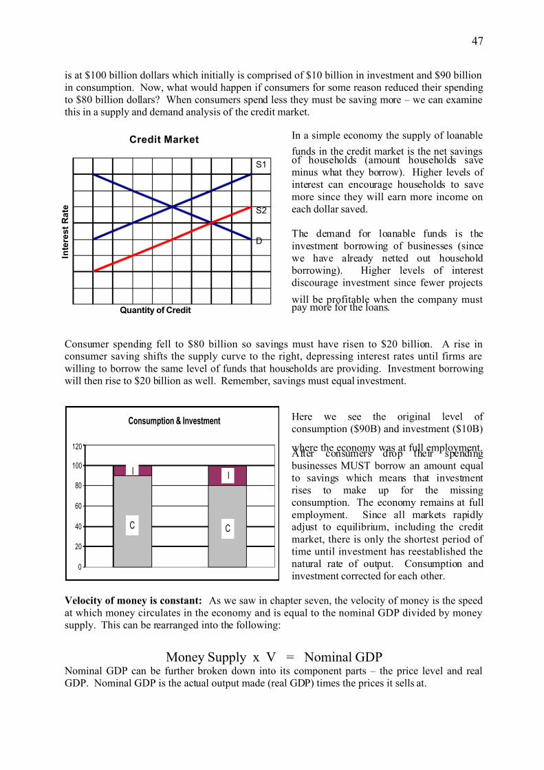
is at $100 billion dollars which initially is comprised of $10 billion in investment and $90 billionin consumption. Now, what would happen if consumers for some reason reduced their spendingto $80 billion dollars? When consumers spend less they must be saving more – we can examinethis in a supply and demand analysis of the credit market.
In a simple economy the supply of loanable
funds in the credit market is the net savingsof households (amount households saveminus what they borrow). Higher levels of interest can encourage households to savemore since they will earn more income oneach dollar saved.
The demand for loanable funds is theinvestment borrowing of businesses (sincewe have already netted out household borrowing). Higher levels of interestdiscourage investment since fewer projects
will be profitable when the company must pay more for the loans.
Consumer spending fell to $80 billion so savings must have risen to $20 billion. A rise inconsumer saving shifts the supply curve to the right, depressing interest rates until firms arewilling to borrow the same level of funds that households are providing. Investment borrowingwill then rise to $20 billion as well. Remember, savings must equal investment.
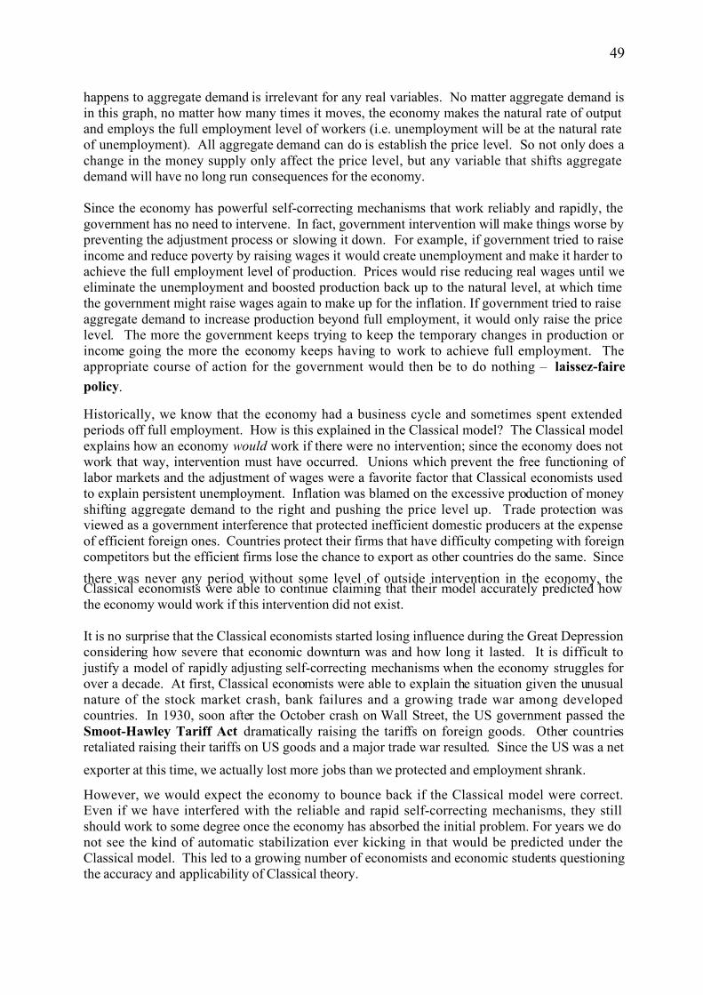
Here we see the original level of consumption ($90B) and investment ($10B)
where the economy was at full employment.After consumers drop their spending businesses MUST borrow an amount equalto savings which means that investmentrises to make up for the missingconsumption. The economy remains at fullemployment. Since all markets rapidlyadjust to equilibrium, including the creditmarket, there is only the shortest period of time until investment has reestablished thenatural rate of output. Consumption andinvestment corrected for each other.
Velocity of money is constant: As we saw in chapter seven, the velocity of money is the speedat which money circulates in the economy and is equal to the nominal GDP divided by moneysupply. This can be rearranged into the following:
Money Supply x V = Nominal GDP Nominal GDP can be further broken down into its component parts – the price level and realGDP. Nominal GDP is the actual output made (real GDP) times the prices it sells at.
47
Consumption & Investment
12
0
20
40
60
80
100
120
C C
II
Credit Market
Quantity of Credit
I n t e r e s t R a t e
D
S1
S2

7/27/2019 Unit 2 Macro
http://slidepdf.com/reader/full/unit-2-macro 4/35
Money Supply x V = P x Y
If the velocity of money is a constant, then the only way nominal GDP can change is if the moneysupply changes first. This is known as the quantity theory of money – the quantity or supply of
money determines nominal GDP. Attempts to use fiscal policy to change real GDP (Y) will failsince fiscal policy cannot change the value of the left-hand side of the equation. If the publicsector takes a larger slice of an economic pie that is not changing in value, then the private sector must take a smaller piece. Fiscal policy is cancelled by opposite changes in private sector spending – perfect crowding out. Note that when the government increased its share of nationaloutput from $15 billion to $30, billion the private sector share fell equal to that increase.
Furthermore, monetary is also ineffective at adjusting real GDP; if the economy adjusts so rapidlythat the real GDP is continually at the natural rate of output, then the only effect of a change inthe money supply is a change in the price level. We can see this another way using the aggregatesupply and demand model.
Implications of Assumptions
If all markets are competitive while wagesand prices are flexible, then the economywill be rapidly pushed to full employment just as a single market is rapidly pushed toequilibrium. When there are unsoldgoods, output prices will fall; when thereare unemployed workers, wages will falluntil the natural rate of output is reached.
This means the aggregate supply curve inthe economy is a vertical line (completelyinelastic) set at the natural rate of output – any deviation in the economy is verytemporary and is fixed quickly by our self-correcting mechanisms.Since aggregate supply is perfectlyinelastic for all but the shortest time, what
48
Aggregate Supply
P r i c e
L e
v e l
AS
NRO
Public vs. Private Sector
85
15
Public vs. Private Sector
30
7070
7/27/2019 Unit 2 Macro
http://slidepdf.com/reader/full/unit-2-macro 5/35
happens to aggregate demand is irrelevant for any real variables. No matter aggregate demand isin this graph, no matter how many times it moves, the economy makes the natural rate of outputand employs the full employment level of workers (i.e. unemployment will be at the natural rateof unemployment). All aggregate demand can do is establish the price level. So not only does achange in the money supply only affect the price level, but any variable that shifts aggregatedemand will have no long run consequences for the economy.
Since the economy has powerful self-correcting mechanisms that work reliably and rapidly, thegovernment has no need to intervene. In fact, government intervention will make things worse by preventing the adjustment process or slowing it down. For example, if government tried to raiseincome and reduce poverty by raising wages it would create unemployment and make it harder toachieve the full employment level of production. Prices would rise reducing real wages until weeliminate the unemployment and boosted production back up to the natural level, at which timethe government might raise wages again to make up for the inflation. If government tried to raiseaggregate demand to increase production beyond full employment, it would only raise the pricelevel. The more the government keeps trying to keep the temporary changes in production or income going the more the economy keeps having to work to achieve full employment. Theappropriate course of action for the government would then be to do nothing – laissez-faire
policy.
Historically, we know that the economy had a business cycle and sometimes spent extended periods off full employment. How is this explained in the Classical model? The Classical modelexplains how an economy would work if there were no intervention; since the economy does notwork that way, intervention must have occurred. Unions which prevent the free functioning of labor markets and the adjustment of wages were a favorite factor that Classical economists usedto explain persistent unemployment. Inflation was blamed on the excessive production of moneyshifting aggregate demand to the right and pushing the price level up. Trade protection wasviewed as a government interference that protected inefficient domestic producers at the expenseof efficient foreign ones. Countries protect their firms that have difficulty competing with foreigncompetitors but the efficient firms lose the chance to export as other countries do the same. Since
there was never any period without some level of outside intervention in the economy, theClassical economists were able to continue claiming that their model accurately predicted howthe economy would work if this intervention did not exist.
It is no surprise that the Classical economists started losing influence during the Great Depressionconsidering how severe that economic downturn was and how long it lasted. It is difficult to justify a model of rapidly adjusting self-correcting mechanisms when the economy struggles for over a decade. At first, Classical economists were able to explain the situation given the unusualnature of the stock market crash, bank failures and a growing trade war among developedcountries. In 1930, soon after the October crash on Wall Street, the US government passed theSmoot-Hawley Tariff Act dramatically raising the tariffs on foreign goods. Other countriesretaliated raising their tariffs on US goods and a major trade war resulted. Since the US was a net
exporter at this time, we actually lost more jobs than we protected and employment shrank.
However, we would expect the economy to bounce back if the Classical model were correct.Even if we have interfered with the reliable and rapid self-correcting mechanisms, they stillshould work to some degree once the economy has absorbed the initial problem. For years we donot see the kind of automatic stabilization ever kicking in that would be predicted under theClassical model. This led to a growing number of economists and economic students questioningthe accuracy and applicability of Classical theory.
49

7/27/2019 Unit 2 Macro
http://slidepdf.com/reader/full/unit-2-macro 6/35
The Keynesian Answer
During the 1930s a British economist, John Maynard Keynes, answered the assumptions of theClassical model point by point. His position was that the Classical model was flawed from the beginning by inappropriate assumptions; if you can deny the assumptions, the model falls apart.Let’s examine the Keynesian rejoinder to each of the Classical assumptions. Bear in mind thatsome of the arguments presented may not have been the work of John Maynard Keynes himself, but rather that of some of his students and later followers. The Keynesian model evolves over anumber of years from the publication of Keynes original work.
Many markets are not very competitive: Keynes argued that there are powerful oligopoliesand monopolies in an industrial economy and that their domination was growing. Companieswith this kind of market power can artificially restrict production in order to boost price. As alarger and larger part of the economy is found in these industries, a larger and larger part of theeconomy will not demonstrate a full employment level of production. Furthermore, someemployers will not be in competitive labor markets and can hold wages artificially lowwithholding income from consumers so that they are unable to buy full employment output.
Wages and prices are not flexible – they are “sticky” – particularly downward: Wages and prices do not rapidly adjust to reflect supply and demand for a variety of reasons.
Contracts: Companies often sign contracts with employees and suppliers – these contracts mean that the company cannot lower the prices it pays for inputs and is, therefore, unwilling to cut the price of their output. It is harder to lower wages and prices since theseller is more motivated to fight a downward move than anupward one.
Menu Costs: It costs a company money to change its prices – someone has to
change the information in the computer, someone has to changethe prices on the shelf or the individual tags, any “hard copy”that contains prices has to be reprinted, etc. These are calledmenu costs (when a restaurant changes prices it must reprint themenu). These make a company reluctant to change prices unlessthey feel the change is not temporary. Obviously, companies areless reluctant to raise price than lower it.
Implicit Agreements: Whether in the labor market or a goods market, both buyers andsellers have an interest in stability over volatility. Workers wanta dependable level of income not one that fluctuates with everyshift in supply and demand. Firms want a predictable level of
cost not one that fluctuates with every shift in supply anddemand. Firms don’t want to constantly fluctuate price becauseconsumers will learn to wait for the price drops. Consumerswant predictable prices both so they can anticipate expenses andto save time – they don’t want to constantly be looking at where prices are best this week. Consequently, we tend to accept thatwages and prices stay up somewhat when business is weak, butdon’t rise that much when business is strong.
50
7/27/2019 Unit 2 Macro
http://slidepdf.com/reader/full/unit-2-macro 7/35
If wages and prices are somewhat “sticky” and rise more easily than they fall, then we will haveat least a temporary problem in the economy, especially in the downward direction. Firmschange production and employment rather than wages and prices. When there is a drop inaggregate demand, far from self-correcting, the trend intensifies – falling demand for goods andservices leads to layoffs and production cuts. As workers lose jobs they cut their spending – eventhe workers who are still employed will spend less out of concern for future job cuts. As
consumer spending drops, more companies layoff even more workers. The economy will cometo an equilibrium far below full employment and remain there for an extended period of time.Since wages and prices are most sticky in the downward direction, the economy is more prone toentering recessions than booms.
There are no forces to make supply equal intended investment at full employment levels:
While savings must equal investment, Keynes pointed out that there is no reason that savings willequal intended investment at levels necessary to support full employment. Intended investment
refers to what businesses planned to invest in their business – desired changes in asset levels.Let’s see why the difference is important.
When we looked at Classical economics, we had a situation where full employment was $100
billion, made up of $90 in consumer spending (savings is $10 billion) and $10 billion in businessinvestment. When consumer spending fell to $80 billion (saving rose to $20 billion), businessinvestment rose to $20 billion and we remained at full employment. Now let’s break investmentdown into intended and unintended levels and see the effect it has on economic events.
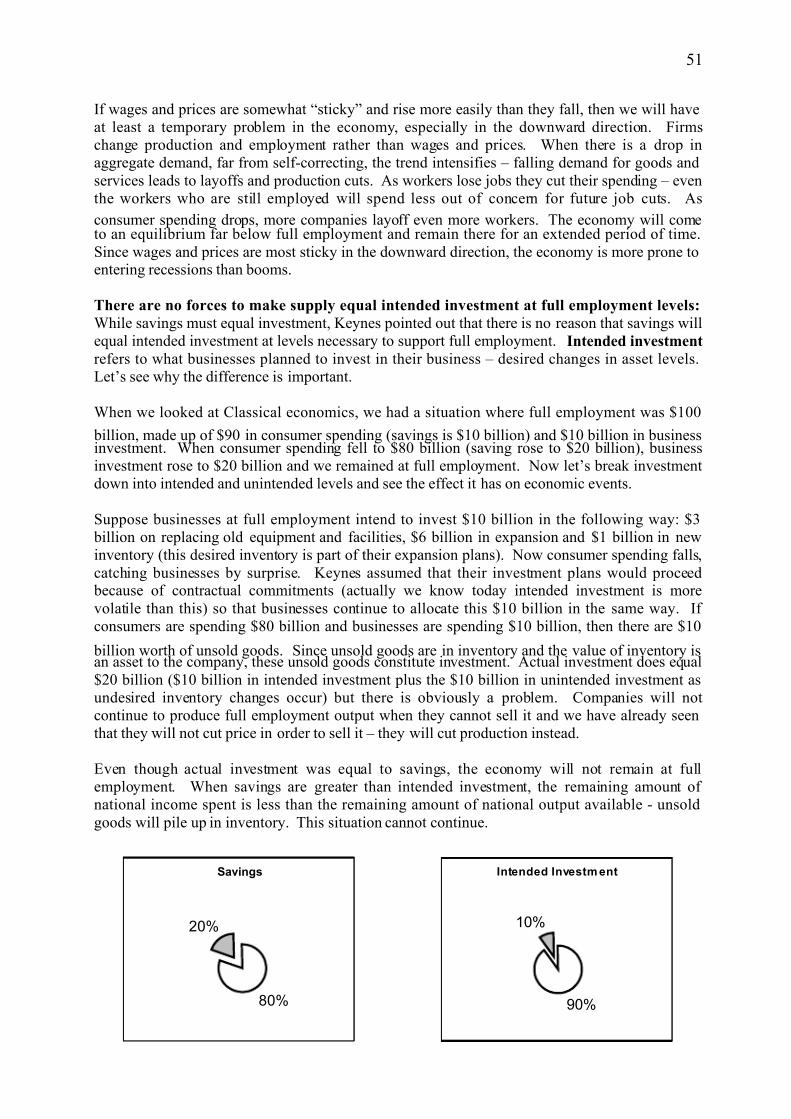
Suppose businesses at full employment intend to invest $10 billion in the following way: $3 billion on replacing old equipment and facilities, $6 billion in expansion and $1 billion in newinventory (this desired inventory is part of their expansion plans). Now consumer spending falls,catching businesses by surprise. Keynes assumed that their investment plans would proceed because of contractual commitments (actually we know today intended investment is morevolatile than this) so that businesses continue to allocate this $10 billion in the same way. If consumers are spending $80 billion and businesses are spending $10 billion, then there are $10
billion worth of unsold goods. Since unsold goods are in inventory and the value of inventory isan asset to the company, these unsold goods constitute investment. Actual investment does equal$20 billion ($10 billion in intended investment plus the $10 billion in unintended investment asundesired inventory changes occur) but there is obviously a problem. Companies will notcontinue to produce full employment output when they cannot sell it and we have already seenthat they will not cut price in order to sell it – they will cut production instead.
Even though actual investment was equal to savings, the economy will not remain at fullemployment. When savings are greater than intended investment, the remaining amount of national income spent is less than the remaining amount of national output available - unsoldgoods will pile up in inventory. This situation cannot continue.
51
Savings
80%
20%
Intended Investm ent
90%
10%

7/27/2019 Unit 2 Macro
http://slidepdf.com/reader/full/unit-2-macro 8/35
Consumption and investment nolonger correct for each other, evenif intended investment doesn’tfall. When C originally fell, businesses saw no reason toincrease intended investment
since they can’t sell currentoutput. We will see layoffs anddrops in production, but ashouseholds lose income, they cutconsumption more and theeconomy moves further awayfrom full employment.
If anything, firms will cutintended investment as theeconomy worsens which wouldincrease the drop off seen in the
graph to the left.
For full employment to exist saving and intended investment must be equal when GDP is at fullemployment levels and the Keynesians said there is no reason to expect that to happen. In theClassical model interest rates brought savings and investment together, but the Keynesians believe that interest rates largely lose their power as the economy moves off full employment. If the economy has dropped significantly below full employment so that companies cannot sell alltheir output and workers are losing jobs, low interest rates will be relatively powerless toencourage either group to increase their borrowing and spending. If the economy has sped upsignificantly above full employment so that companies are seeing continually rising revenue and profits while workers are able to get good jobs and overtime, high interest rates may not be
sufficient to discourage either to slow their borrowing and spending.
The velocity of money fluctuates: The Keynesians believe that the velocity of money moveswith the economy and against the money supply all other things equal. When the economy isstrong, people, businesses and financial institutions move money more rapidly and aggressively – they are less inclined to hold it for long periods of time. When the economy is weak, people, businesses and financial institutions move money more slowly and cautiously – they are moreinclined to hold it for long periods of time.
Money Supply x V = P x Y
Since V fluctuates with Y, if the Fed pumps additional money into the financial system, it will
have little affect on real GDP (Y) unless people, businesses and financial institutions have theconfidence and opportunities to lend, borrow and spend. If the money supply rises, but banks arereluctant to lend it while people and businesses have little incentive to borrow and spend, then thevelocity of money will just slow down, negating the effect of the policy. Fiscal policy on theother hand will now work – since V fluctuates a change in fiscal policy can cause both sides of the equation to rise. Fiscal stimulus can raise real GDP (Y) on the right hand side of the equation because as the fiscal policy works the velocity of money on the left hand side is rising as well.
52
Consumption and Investment
0
20
40
60
80
100
120
CC
C
I
I
I

7/27/2019 Unit 2 Macro
http://slidepdf.com/reader/full/unit-2-macro 9/35
Crowding out will no longer be a problem since when government takes a larger piece of theeconomic pie, it causes total output to rise as well and there is more pie to go around. Privatesector spending may drop by a very small amount (by $1 billion below) but for the most part, theadditional government consumption of goods and services is filled by the expanded production.
The nature of the velocity of money is one of the main differences between Keynesian policy andthose that hold opposing theories – it drives the controversies over the nature of monetary and
fiscal policy. If velocity is constant or almost constant, then fiscal policy is very weak whilemonetary policy has a lot of power, at least over nominal measures. If velocity is variable, thenfiscal policy is very powerful while monetary policy is fairly weak. We are not able to answer this by examining the historical data – the velocity of money is not completely constant but itsvariability is limited. The analysis is further complicated by the fact that the stability of V variesdepending on the time period looked at and the money aggregate used. V is less stable for M1and more stable for M2.
How much variation is needed for the Keynesian view to still work? Keynesians argue that evensmall variations in V are sufficient since the money supply is so enormous (even a small changemultiplied against a large base can have a significant effect). Some other economists say thatvariations in V are too small and that crowding out will be a significant problem.
Implications of Assumptions
If many markets are not competitive whilewages and prices are not flexible for anextended time, then the economy canremain off the natural rate of output for prolonged periods of time. When there areunsold goods, production rather than output prices will fall, employment rather than
wages will fall.
This gives us the aggregate supply curvewe saw in chapter four – the shape is driven by the fact that some wages and prices areless sticky than others and, in general, areless sticky upward than downward.
53
Public vs. Private Sector
85
15
Public vs. Private Sector
84
30
Short-run Aggregate Supply
National Output
P r i c e L e v e l
AS

7/27/2019 Unit 2 Macro
http://slidepdf.com/reader/full/unit-2-macro 10/35
This aggregate supply curve is a more sophisticated and realistic version of the originalKeynesian AS curve and contains three distinct areas. In the horizontal range we see that as theeconomy contracts, the price level drops very little and the main impact is on production (and,therefore, employment). Since wages and prices are more prone to downward stickyness, theeconomy has room to fall far below full employment. In the vertical range we see that as theeconomy booms, the price level starts changing much faster – this is because wages and prices
are less sticky in the upward direction. There is still a little stickyness so that the economy canrise above full employment production.
Since the economy lacks rapid and reliable self-correcting mechanisms, it is possible for theeconomy to become “stuck” far off full employment (especially below full employment) for verylong periods of time. It is clear why this model gained acceptability during the Great Depressionsince it reflected the economy of the time – one far below full employment for years. If the private sector does not have the ability to turn the economy around, then it is the necessary role of the government to do so. Government not only has the ability to stabilize the economy, it has theresponsibility to do so. It is unacceptable to allow people, households, businesses to suffer long period of falling income, sales, profits – a financial blow from which many will never recover – when the government can shift aggregate demand in order to restore the natural rate of output
more quickly and reliably than the economy could on its own.
We will develop the extended technical Keynesian model and use it for predicting the necessarygovernment policy to achieve full employment in the next chapter.
Journal Topics: Complete the following assignment:
Write a 3 page paper comparing the two theories using at least two sources.
54

7/27/2019 Unit 2 Macro
http://slidepdf.com/reader/full/unit-2-macro 11/35
CHAPTER 8 THE KEYNESIAN CROSS
The technical Keynsian model, known as the Keynesian cross, can be presented in differentformats – tabular, graphical or algebraic – but is always going to show the relationship between
the components of aggregate demand and the final equilibrium output of an economy. TheKeynesian cross is used to estimate how changes in aggregate demand affect the final equilibriumlevel of production and, therefore, the necessary government action to achieve full employment.The model comes in more and less sophisticated versions – we will use only the basic modelwhich is based on: 1) a closed economy, i.e. no exports or imports, 2) “sticky” wages and prices, 3) only consumption is affected by GDP, and 4) Real GDP is both national output andthe income of households.
Aggregate Demand or Aggregate Expenditures represents the value spent on goods and servicesin an economy, and since this economy is closed will equal C + I + G (consumption plusinvestment plus government purchases). We will start by modeling consumption – the maindeterminant of consumer spending is consumer income (more sophisticated models include other
variables but the largest determinant is income). When the government gathers spending andincome data for consumers, we observe a pattern or correlation between the two variables -consumption and income have a positive correlation – the more income consumers have thehigher their spending will be. We can summarize the typical or general relationship betweenincome and spending either as a line or a formula (remember from math any line can berepresented as a formula in slope/intercept form). This “summary” is known as theconsumption function.
The Consumption Function
The points on the graph to the leftrepresent the differing observations of consumer spending found at differentincome levels. A graph showing thiskind of set of points is known as ascattergram.
When given a set of suchobservations, a computer can calculatethe “typical” relationship between thetwo variables by fitting a line into thescattering of points. This line
minimizes the total distance betweenthe line and all the points. This line isthe consumption function.
Since we have assumed that national income (GDP) is also the income of households, thisconsumption data also tells us something about savings. What households do not spend musthave been saved. Therefore, if a GDP of $700 billion is associated with a consumption level of $680 billion, then net household savings must have been $20 billion.
55
Consumption Function
0.00
100.00
200.00
300.00
400.00
500.00
600.00
700.00
800.00
100 200 300 400 500 600 700National Income

7/27/2019 Unit 2 Macro
http://slidepdf.com/reader/full/unit-2-macro 12/35
The consumption function is typically graphed but it could also be represented in a table or as analgebraic formula.
Here we see some points along theconsumption function which represent
the typical level of consumption to beexpected at certain GDP levels. For example, when GDP is $400 billion,consumption averages $410 billion;since consumers are spending more thantheir income, savings is negative.
These points could also be representedas entry in a table. The five individual points to the left are also represented inthe table below. We could add a line tothe table and calculate household
savings as well.
GDP 300 400 500 600 700
C 320.00 410.00 500.00 590.00 680.00
Sn -20 -10 0 10 20
Note that we have no observations for extremely low levels of GDP – even in the depths of theGreat Depression GDP was no where near 0. In order to find the algebraic formula for theconsumption function, we need to extrapolate from the relationship we do see. Imagine that the
existing data does not vary in pattern as we work backwards to non-observed GDP levels – thiscan be thought of as extending the line or table back to the left.
When we extend the consumptionfunction to the left, we see that when theline intersects the Y axis (in other wordsGDP is zero), there is still someconsumption occurring. This level of consumption is independent of the levelof income and is known as autonomous
consumption.
Consumers also spend a percent of income in addition to the autonomousconsumption. This spending isdetermined by the level of income and isknown as induced consumption. This proportion of income spent in addition isthe slope of the consumption functionand is known as the marginal
propensity to consume.
56
Consumption Function
0.00
100.00
200.00
300.00
400.00
500.00
600.00
700.00
800.00
100 200 300 400 500 600 700
National Income
Consumption Function
0.00
100.00
200.00
300.00
400.00
500.00
600.00
700.00
800.00
0 100 200 300 400 500 600 700

7/27/2019 Unit 2 Macro
http://slidepdf.com/reader/full/unit-2-macro 13/35
We can also work backwards with the tabular information and in fact this is usually moreaccurate given the difficulties of precision with a graph.
GDP 0 100 200 300 400 500 600 700
C 50.00 140.00 230.00 320.00 410.00 500.00 590.00 680.00
Since every column demonstrates a $100 billion dollar difference in GDP, we just add columns backward until GDP reaches 0. Since each column represents a $90 billion dollar difference inconsumption, we just continue that relationship until we reach the GDP of 0. This starting levelof consumption is our autonomous consumption. To derive the formula for the consumptionfunction we need both autonomous and induced consumption – to find induced consumption weneed the marginal propensity to consume.
MPC =income
nconsumptio
∆
∆or
Y
C
∆
∆
In our problem we see that this equals:
MPC =Y
C
∆
∆=
100
90or .9
People are spending 90% of their income in addition to the starting level of autonomousconsumption. In fact, this is close to the traditional historical MPC for American consumers (inthe last generation it is a bit higher than in previous years). Since any line can be represented as aformula in slope/intercept form and autonomous consumption is the intercept while the MPC isthe slope, the formula for the consumption function is:
C = 50 + .9Y
Aggregate Expenditures
Keynes, himself, did not really use aggregate supply and demand to model the behavior of amarket economy. He did not use GDP and the price level as his axes, instead he uses GDP andspending or aggregate expenditures. In a closed economy (no net exports) spending would be C+ I + G; note that this is the closed economy version of the aggregate demand model. Since weare not using the price level as a variable (prices and wages are sticky)and aggregate demandrelates spending to the price level, Keynes named this measure aggregate expenditures.
Keynes treated the other two components of aggregate expenditures or aggregate demand ascompletely autonomous – independent of the level of GDP. Lacking good information oninvestment, Keynes assumed that businesses would be caught by surprise when consumersfluctuated their spending – in other words, that intended investment would tend to remain thesame, at least for awhile, as businesses were contractually tied to investment projects. Likewise,the government would have its spending already budgeted and contracted, therefore, would notchange its policies without the passage of new legislation. While these are not accurateassumptions, using them does not undermine the validity of the model’s conclusions – if Keynes’
57

7/27/2019 Unit 2 Macro
http://slidepdf.com/reader/full/unit-2-macro 14/35
model shows the economy is unstable with stable investment, then if business investment actuallyfluctuates with the economy as consumption does, the economy is even more unstable, not less.Keynes’ assertion about the short-run instability of the economy is not challenged by theobservation that business investment is not stable. If government policy is necessary to stabilizethe economy, it does not matter that some of that policy is actually built into the system to runautomatically, government policy is still necessary. For the moment, we will continue to hold the
simple Keynesian assumptions.
To calculate aggregate expenditures (AE), we need to add our autonomous investment andgovernment purchases to consumption. Again, this can be done on the table, the graph or in theformula. Let us start with no government participation.
GDP 0 100 200 300 400 500 600 700
C 50.00 140.00 230.00 320.00 410.00 500.00 590.00 680.00
I 10 10 10 10 10 10 10 10
G 0 0 0 0 0 0 0 0
AE 60 150 240 330 420 510 600 690
Equilibrium is found where aggregate demand equals aggregate supply – here where the amount people are trying to buy equals what is available to be purchased. Only at a GDP level of 600 isthe value being made (GDP or Aggregate Supply) equal to the value being bought (AE or Aggregate Demand). This is our equilibrium, but we were only able to see it because it occurredon the table – if equilibrium had been between our observations, we would not be able to find it.
The AE curve starts at atthe autonomous spending(here 60) and rises at therate of the MPC (here .9).
The gray line is the 45-degree line and representsall the points where AEequals GDP. Every oneof these points is a potential equilibrium.
Any economy must be onthe 45-degree line. Thiseconomy is on its AEcurve. The only placewhere both is true iswhere the lines intersect – that is equilibrium. Thisis the Keynesian Cross.
Notice that it can bedifficult to see theequilibrium point on thegraph.
58
Keynesian Cross
0.00
100.00
200.00
300.00
400.00
500.00
600.00
700.00
800.00
900.00
0 100 200 300 400 500 600 700 800
GDP or AS
A E o
r A

7/27/2019 Unit 2 Macro
http://slidepdf.com/reader/full/unit-2-macro 15/35
It is easiest to calculate the equilibrium level of GDP, changes in the equilibrium GDP and theeffect of government policies using the algebraic model. We have the formula for consumptionas well as the autonomous levels of investment and government purchases. This will allow us tofind the formula for AE.
C = 50 + .9Y AE = 60 + .9YI = 10 Y = 60 + .9YG = 0 .1Y = 60
Y = 600AE = 60 + .9Y
Once we have the formula for AE we want to solve for the value of national income (Y) whereaggregate demand (AE) equals aggregate supply (GDP). Very quickly, we can find that thisoccurs when GDP or Y is 600.
Changes in Equilibrium – The Multiplier
When one of the components of AE changes its spending behavior, then the equilibrium level of GDP will also change. Suppose that a new technology is invented and businesses raise their investment to 15 as they buy the new equipment.
C = 50 + .9Y AE = 65 + .9YI = 15 Y = 65 + .9YG = 0 .1Y = 65
Y = 650
AE = 65 + .9Y
Notice that equilibrium output rose by much more than the initial change in investment. This is because of induced consumption. When businesses spent $5 billion more, it meant $5 billionmore in income for some households who then raised their spending by 90% of that $5 billion,causing consumer spending to rise by $4.5 billion. But this means that other households havenow seen their income rise by $4.5 billion and will raise their spending by 90% of that or $4.05 billion. This causes a further rise in household income and yet another rise in consumer spending, and so forth. We have set off a chain reaction of spending – a self-perpetuating cycle. Note that each time consumers raise their spending they increase it by a smaller amount sinceonly 90% of the change in income goes to spending. Eventually, the cycle breaks down and we
can see the final effect on total spending. This can be represented in a flow chart.
∆SInitialChange in Final EffectAutonomous ∆ Y ∆C on Eq. GDPSpending
59
7/27/2019 Unit 2 Macro
http://slidepdf.com/reader/full/unit-2-macro 16/35
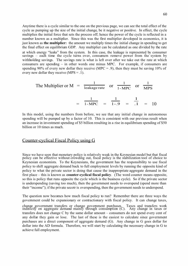
Anytime there is a cycle similar to the one on the previous page, we can see the total effect of thecycle as pumping up the size of the initial change, be it negative or positive. In effect, the cyclemultiplies the initial force that sets the process off; hence the power of the cycle is reflected in anumber known as a multiplier. Since this was the first multiplier developed in economics, it is just known as the multiplier: the amount we multiply times the initial change in spending to getthe final effect on equilibrium GDP. Any multiplier can be calculated as one divided by the rate
at which energy “leaks” from the system. In this case, the leakage is represented by consumer savings – each time the cycle turns over, consumers remove power from the system bywithholding savings. The savings rate is what is left over after we take out the rate at whichconsumers are spending – in other words one minus MPC. For example, if consumers arespending 90% of every new dollar they receive (MPC = .9), then they must be saving 10% of every new dollar they receive (MPS = .1).
The Multiplier or M =rateleakage
1or
MPC-1
1or
MPS
1
= MPC-1
1
= .9-1
1
= .1
1
= 10
In this model, using the numbers from before, we see that any initial change in autonomousspending will be pumped up by a factor of 10. This is consistent with our previous result whenan increase in investment spending of $5 billion resulting in a rise in equilibrium spending of $50 billion or 10 times as much.
Counter-cyclical Fiscal Policy using G
Since we have seen that monetary policy is relatively weak in the Keynesian model but that fiscal policy can be effective without crowding out, fiscal policy is the stabilization tool of choice toKeynesian economists. To the Keynesians, the government has the responsibility to use fiscal policy to shift aggregate demand back to full employment levels by running the opposite kind of policy to what the private sector is doing that cause the inappropriate aggregate demand in thefirst place – this is known as counter-cyclical fiscal policy. (The word counter means opposite,so this is policy that runs opposite the cycle which is the business cycle). So if the private sector is underspending (saving too much), then the government needs to overspend (spend more thantheir “income”); if the private secotr is overspending, then the government needs to underspend.
The question now becomes how much fiscal policy to run? Remember there are three ways thegovernment could be expansionary or contractionary with fiscal policy. It can change taxes,
change government transfers or change government purchases. Taxes and transfers work indirectly on aggregate demand mainly through consumption (C). Any change in taxes or transfers does not change C by the same dollar amount – consumers do not spend every cent of any dollar they gain or lose. The last of these is the easiest to calculate since government purchases are a direct component of aggregate demand (G). Any change in G goes dollar for dollar into the AD formula. Therefore, we will start by calculating the necessary change in G toachieve full employment.
60

7/27/2019 Unit 2 Macro
http://slidepdf.com/reader/full/unit-2-macro 17/35
C + I + G + Xn = AD and each of these components has an autonomous level of spending. In thesimple Keynesian model Xn does not exist while both I and G are completely autonomous. Therelationship between autonomous spending is:
Autonomous spending x multiplier = equilibrium Y
Which means that a change in autonomous spending will translate to a change in equilibrium Y by the formula:
Δ Autonomous spending x multiplier = Δ equilibrium Y
If we know what equilibrium Y is, in other words, we know the actual level of GDP the economyis stuck at, and we have a target GDP we want the economy to achieve – our estimate of fullemployment, then we know the amount by which we need equilibrium Y to change. Plug thatnumber in on the right hand side of the equation, plug the multiplier in and you can solve for thenecessary change in autonomous spending. In the case of government purchases that is your
answer, since G is part of autonomous spending.
Back in the first example of calculating equilibrium GDP, we had an equilibrium Y of $600 billion and a multiplier of 10. Suppose that full employment GDP is at $700 billion. How muchwould government purchases (G which is currently zero) have to change to achieve fullemployment?
Δ Autonomous spending x multiplier = Δ equilibrium YΔG x 10 = $100 billion
ΔG = $ 10 billion
Let’s test that and see if it works. If we change government purchases by 10 when they wereoriginally 0 then G will now be 10. This gives us a new AD or AE formula of:
C = 50 + .9Y AE = 70 + .9YI = 10 Y = 70 + .9YG = 10 .1Y = 70
Y = 700AE = 70 + .9Y
The new level of government purchases supports a level of economic activity consistent with fullemployment, i.e. the policy worked. Notice that when we increased government purchases
nothing happened to the formulas for either C or I. In other words, there was no crowding out.This is because the Keynesians believe that the velocity of money changes; since spending by the private sector has slowed, the velocity of money has slowed. As the government taps thesluggish flow of money, borrowing funds that are unused or slow in being used, the governmentspeeds up the velocity of money and, therefore, there is no reason for the C or I functions tochange. This is true as long as the government borrows to fund its expansionary fiscal policies – debt/bond financing. The situation will be different if the government uses tax financing – raises taxes to pay for its fiscal policies. Tax financing will change the consumption function(assuming we use income taxes) since consumers now have less income to spend.
61

7/27/2019 Unit 2 Macro
http://slidepdf.com/reader/full/unit-2-macro 18/35
Suppose the government consistently runs a balanced budget so that increases in G requireincreases in taxes and decreases in G require decreases in taxes. Now we are changing twocomponents of aggregate demand and changing them in the opposite direction – if G rises causinga tax increase, C will fall. The fall in C will cancel out the rise in G to some degree. Let’sidentify how much of the original rise in G actually impacts the economy using the number in thecurrent example. We just raised G by $10 billion when we used debt/bond financing. What
would happen if we raised G by $10 billion when using tax financing?
Increase G by $10 billionIncrease Taxes by $10 billionHousehold income falls $10 billionConsumption falls $ 9 billion (Δ income times the MPC = -$10 billion x .9)Δ autonomous spending $ 1 billion (G up $10 billion while C down $9 billion)
90% of the change in G was cancelled by an opposite change in C so that only 10% actuallymakes it through to affect autonomous spending. The MPC represents the proportion of thechange in G that is cancelled by the opposite change in C; 1-MPC represents the proportion of the change in G that is NOT cancelled by the opposite change in C and makes it to autonomous
spending.
multiplier x Δ Auto. spending = Δ equilibrium Ymultiplier x (1-MPC) Δ G = Δ equilibrium Y1/(1-MPC) x (1-MPC) Δ G = Δ equilibrium Y(1-MPC)/(1-MPC) x Δ G = Δ equilibrium Y
Δ G = Δ equilibrium Y
In the simple Keynesian model, (1-MPC)/(1-MPC) is sometimes referred to as the balanced
budget multiplier since it is what we multiply by the change in G to get the change in
equilibrium output. The balanced budget multiplier in the simple Keynesian model is alwaysequal to one – whatever the government wants to happen to equilibrium Y that’s what they haveto do to government purchases.
Since tax financing results in crowding outand means the government has to fluctuateits tax and spending programs more fromyear to year, the Keynesians reject taxfinancing. Instead they want thegovernment to balance the budget over the business cycle – running deficits and borrowing the money during recessionswhile running surpluses and paying the
debt off during booms. The surplusesshould roughly cancel the deficits - this isknown as balancing the budget over the
business cycle. (It does not quite work that well, because of downward stickywages and prices the economy is more prone to recessions than booms sosurpluses will not be large enough andfrequent enough to pay the deficits off).
62
Balancing the Budget Over the
Business Cycle
BalancedBuget at
Full EmpDeficit
Surplus
7/27/2019 Unit 2 Macro
http://slidepdf.com/reader/full/unit-2-macro 19/35
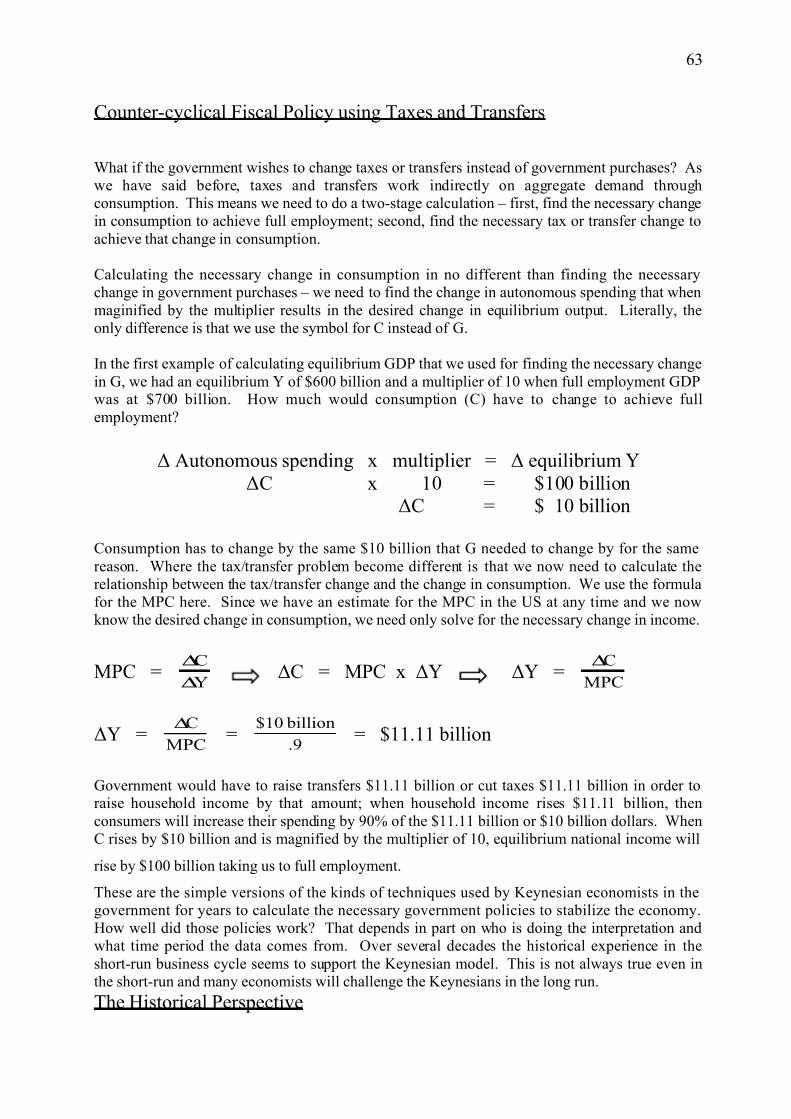
Counter-cyclical Fiscal Policy using Taxes and Transfers
What if the government wishes to change taxes or transfers instead of government purchases? Aswe have said before, taxes and transfers work indirectly on aggregate demand throughconsumption. This means we need to do a two-stage calculation – first, find the necessary changein consumption to achieve full employment; second, find the necessary tax or transfer change toachieve that change in consumption.
Calculating the necessary change in consumption in no different than finding the necessarychange in government purchases – we need to find the change in autonomous spending that whenmaginified by the multiplier results in the desired change in equilibrium output. Literally, theonly difference is that we use the symbol for C instead of G.
In the first example of calculating equilibrium GDP that we used for finding the necessary changein G, we had an equilibrium Y of $600 billion and a multiplier of 10 when full employment GDPwas at $700 billion. How much would consumption (C) have to change to achieve fullemployment?
Δ Autonomous spending x multiplier = Δ equilibrium YΔC x 10 = $100 billion
ΔC = $ 10 billion
Consumption has to change by the same $10 billion that G needed to change by for the samereason. Where the tax/transfer problem become different is that we now need to calculate therelationship between the tax/transfer change and the change in consumption. We use the formulafor the MPC here. Since we have an estimate for the MPC in the US at any time and we nowknow the desired change in consumption, we need only solve for the necessary change in income.
MPC =Y
C
∆
∆ΔC = MPC x ΔY ΔY =
MPC
C∆
ΔY =MPC
C∆=
.9
billion$10= $11.11 billion
Government would have to raise transfers $11.11 billion or cut taxes $11.11 billion in order toraise household income by that amount; when household income rises $11.11 billion, thenconsumers will increase their spending by 90% of the $11.11 billion or $10 billion dollars. WhenC rises by $10 billion and is magnified by the multiplier of 10, equilibrium national income will
rise by $100 billion taking us to full employment.
These are the simple versions of the kinds of techniques used by Keynesian economists in thegovernment for years to calculate the necessary government policies to stabilize the economy.How well did those policies work? That depends in part on who is doing the interpretation andwhat time period the data comes from. Over several decades the historical experience in theshort-run business cycle seems to support the Keynesian model. This is not always true even inthe short-run and many economists will challenge the Keynesians in the long run.
The Historical Perspective
63
7/27/2019 Unit 2 Macro
http://slidepdf.com/reader/full/unit-2-macro 20/35
During the 1930s the US government started using fiscal policy to try to improve the economyduring the Great Depression – we spent money on government projects to provide jobs, such asthe TVA building dams, the WPA constructing government buildings, the National Park system buying land and building lodges, paths, bridges, etc. Although large by standards of the day, the
spending of the 1930s was woefully modest relative to the depths of the economic downturn – theKeynesian model recommended far larger fiscal policies than government was willing to enactduring that time. As the Keynesian model would predict the economy improved but extremelyslowly. During the Presidential campaign of 1936, Roosevelt promised to start moving back to a balanced budget since the economy was modestly improving, raising taxes and cutting spending.As the Keynesian model would predict, in 1937 the economy took another drop as did the stock market. Finally, in the early days of WWII, the US government had the justification it needed torun the size of spending programs the Keynesians advocated – military spending for the war. Asthe government spent millions that it borrowed from the public in the form of war bonds, theeconomy soared out of the Depression the way the Keynesian model predicted. This convincedmost of a generation of young economists that the Keynesian model had solved the riddle of the business cycle and had handed government the policy tools it needed to stabilize the economy.
Over the next couple of decades the US government used the appropriate Keynesian fiscal policywhenever the economy seemed to be developing a problem and it appeared to be successful. Inaddition, we set up our tax and transfer programs to rise and fall with economic activity whichresults in some Keynesian policy being run without the need for new legislation – these areknown as automatic stabilizers. Since we have tied taxes to the level of income, sales and profits, when the economy is weak, tax revenue automatically falls. Since we have tied mosttransfer programs to the level of income, when the economy is weak, spending on transfersautomatically rises. This eliminates much of the lag problem with fiscal policy. There is fairlygood data during this time period to support the Keynesian contention that the business cycle hadimproved – that economic downturns were milder and less frequent compared to the days beforegovernment intervention. As we will see in the next chapter, opposing economists argue that
other factors could cause this and that the pattern of stability is missing in the 1970s and early1980s. They also argue that what appears to be true in the short-run does not occur in the long-run, especially the relationship between AD and real GDP as well as unemployment and inflation.
Aggregate demand in the short-run pushes real GDP up and down – this is the heart of the business cycle. While Keynes believed that consumption was the volatile component of aggregate demand, modern Keynesians are more likely to blame investment. Investmentspending is much more responsive to changes in economic activity than the level of economicactivity. While consumers keep spending if their income is high but slowing down in growth, businesses tend to slow down their spending if not cut it when their sales and profits slow even if they are still high. After all, business investment spending builds future capacity so we needincreasing sales to support creating more capacity than we are using now. Businesses pick up
changes in economic activity and adjust their spending accordingly, which intensifies the initialsmall economic trend. A slowdown in growth becomes slower and slower and possibly adownturn. This is known as the accelerator principle – business investment takes the beginningof a trend and “speeds” it up – often providing the turning point of the business cycle. Other thanadjusting the mechanism that causes the instability of aggregate demand, the basic conclusionsremain the same – fluctuating aggregate demand in an environment of sticky wages and priceswill push the economy off full employment and cause short-run ups and downs in real GDP.Just as there is very good short-run data that real GDP fluctuates with Aggregate Demand, thereis very good short-run data that unemployment and inflation move in the opposite direction.
64
7/27/2019 Unit 2 Macro
http://slidepdf.com/reader/full/unit-2-macro 21/35
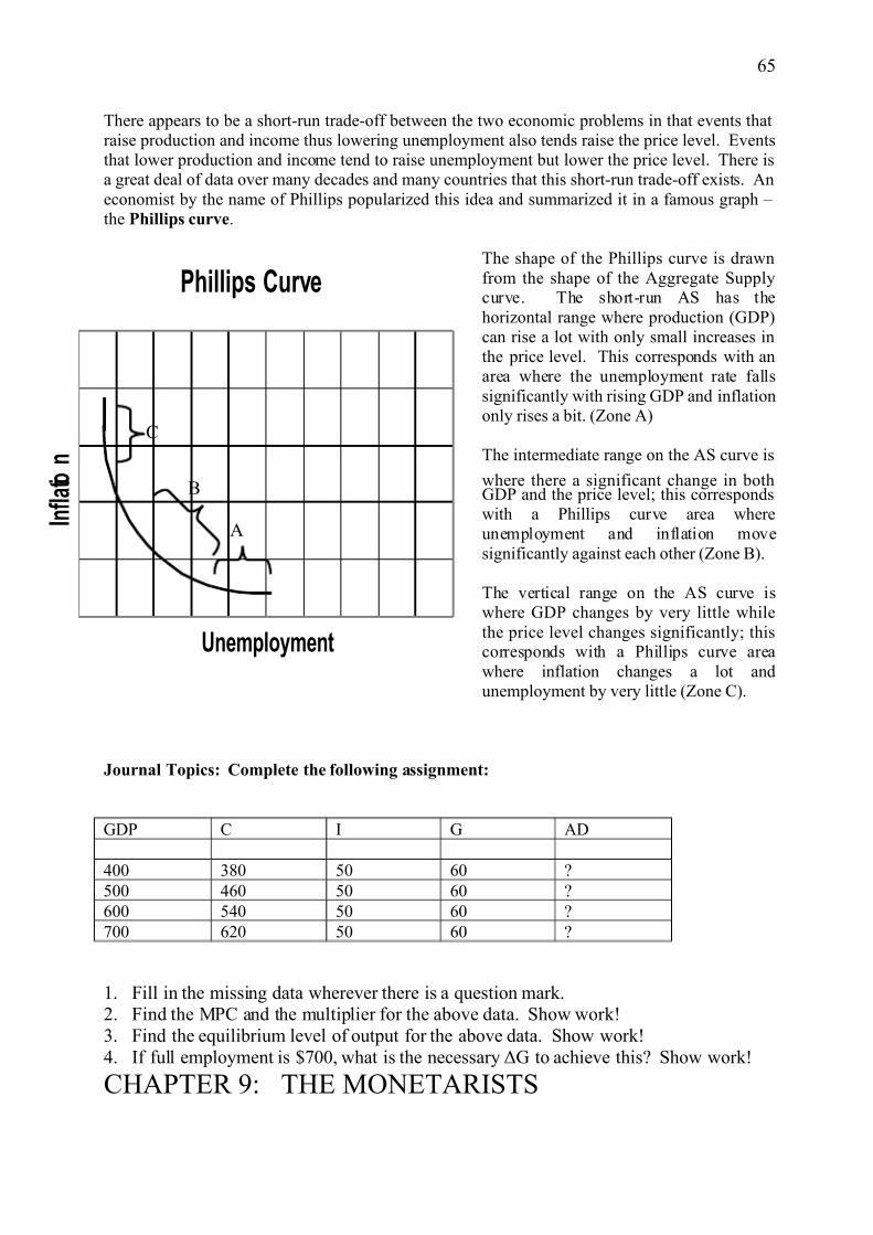
There appears to be a short-run trade-off between the two economic problems in that events thatraise production and income thus lowering unemployment also tends raise the price level. Eventsthat lower production and income tend to raise unemployment but lower the price level. There isa great deal of data over many decades and many countries that this short-run trade-off exists. Aneconomist by the name of Phillips popularized this idea and summarized it in a famous graph – the Phillips curve.
The shape of the Phillips curve is drawnfrom the shape of the Aggregate Supplycurve. The short-run AS has thehorizontal range where production (GDP)can rise a lot with only small increases inthe price level. This corresponds with anarea where the unemployment rate fallssignificantly with rising GDP and inflationonly rises a bit. (Zone A)
The intermediate range on the AS curve is
where there a significant change in bothGDP and the price level; this correspondswith a Phillips curve area whereunemployment and inflation movesignificantly against each other (Zone B).
The vertical range on the AS curve iswhere GDP changes by very little whilethe price level changes significantly; thiscorresponds with a Phillips curve areawhere inflation changes a lot andunemployment by very little (Zone C).
Journal Topics: Complete the following assignment:
GDP C I G AD
400 380 50 60 ?
500 460 50 60 ?
600 540 50 60 ?
700 620 50 60 ?
1. Fill in the missing data wherever there is a question mark.2. Find the MPC and the multiplier for the above data. Show work!3. Find the equilibrium level of output for the above data. Show work!4. If full employment is $700, what is the necessary ΔG to achieve this? Show work!
CHAPTER 9: THE MONETARISTS
65
Phillips Curve
Unemployment
I n f l a t i o
n
A
B
C
7/27/2019 Unit 2 Macro
http://slidepdf.com/reader/full/unit-2-macro 22/35
Just as Keynesian economics began to supersede Classical theory as the latter appeared unable toexplain the events of the 1930s, Keynesian economics was challenged when it appeared not to fitthe economy of the 1970s. The Keynesian model claimed that an unstable aggregate demand
caused the instability of market economies; excessive aggregate demand and inflation causing booms and insufficient aggregate demand and unemployment causing recessions. The solutionwas then to correct the fluctuations of the private market with the opposite government policy – slowing aggregate demand during a boom and raising aggregate demand during a recession.
In the 1970s the US experienced a period of rising inflation and unemployment simultaneously;this did not fit the Keynesian model. Shifts in aggregate demand cause inflation andunemployment to move in the opposite direction, not together. Keynesian policy had nosuggestions for the current economic woes either; one uses expansionary policy to fightunemployment at the cost of worsening inflation or one uses contractionary policy to fightinflation at the cost of worsening unemployment. Since the Keynesians did not seem to have animmediate explanation or solution, people began to explore other options. Since the 1950s a
small group of macroeconomists, led by Milton Friedman, had challenged Keynesian economicthought, but since the latter appeared to work so well, they had not been able to influenceeconomic theory or government policy significantly. Now the theory seemed worth a closer look.
The Assumptions of the Monetarist Model
Markets are competitive enough: The Classical economists had said that if markets werehighly competitive, then no one could hold a market off its full employment equilibrium. Pricewill, therefore, always reflect the minimum efficient cost of making the good. As long asconsumer benefit is high enough to justify paying for the good, they will keep buying it and we
will keep making it. Consequently, if individual markets do this, all the markets together will -we will make the socially optimal level of production, i.e. full employment. The Keynesians hadclaimed that does not occur because there are many noncompetitive markets dominated by powerful oligopolies and monopolies. The Monetarists claimed that while markets are not ascompetitive as the Classical economists had assumed, they are more competitive than theKeynesians were willing to admit, particularly with anti-trust law and a more open internationaltrade adding competition. In general, a firm will only be temporarily able to hold a market off its potential production level and then new firms will enter pushing production up and prices down.
Wages and prices are flexible enough: The Classical economists said that wages and priceswill rapidly adjust to keep the full employment level of goods selling and the full employmentlevel of labor working. Furthermore, this adjustment is so rapid that an economy left alone will
not experience any significant period of unemployment or falling production. The Keynesianscountered that wages and prices are inflexible particularly in the downward direction,undermining this self-correction mechanism. The Monetarists asserted that while wages and prices are “sticky” in the short-run, they become flexible in a reasonable period of time. They point out that many wages and prices are not hampered by contracts and that most contracts areopen for renegotiation within a 12 to 18 month period. Consequently, the economy will startcorrecting itself in this time, which is about the same time it takes stabilization policy to work.
66

7/27/2019 Unit 2 Macro
http://slidepdf.com/reader/full/unit-2-macro 23/35
Savings will generally equal intended investment at full employment levels if the
government maintains the appropriate quantity of money: The monetarists argued thatmoney is an asset that competes with other assets like land, stocks, gold etc. Money has theadvantages of being liquid – so it’s available for emergencies – and stable in value – it does notgo up and down each day in worth like the other assets mentioned can (it only erodes over timewith inflation). Money has the disadvantages that it does not appreciate in value over time like
the others and it generates little or no income – money in the bank earns little interest if any andcash earns none. Consequently, Friedman claimed that people wish to keep only a portion of their wealth in money form and that this portion remains relatively constant over time. If this iscorrect, then if government maintains the appropriate level of money people can be depended onto convert approximately the needed amount into either goods and services or other assets. Evenif someone were to buy gold, stock or land they have now given someone else more money thanthey wish to hold in money form and they will have to convert it. Eventually, enough will beconverted into goods and services.
Changes in spending on goods and services by one component of aggregate demand will shift theallotment of money assets so that someone is holding more money than they wish. Some other component of aggregate demand will end up correcting for the initial shift in spending. This
process can take awhile, so once again, the Monetarists are looking at a 12 to 18 month period for the economy to start stabilizing itself unlike the Classical economists who saw this processoperating almost immediately. The Monetarist contention is that the economy’s self-correctingmechanisms work reliably, although not rapidly, and since government fiscal and monetary policy also take 12-18 months to work, we are better off letting the market economy correct itself.
Velocity of money is relatively stable: As we have seen, the velocity of money is the speed atwhich money circulates in the economy and is equal to the nominal GDP divided by moneysupply. Nominal GDP is the price level times real GDP.
Money Supply x V = Nominal GDP = P x Y
If the velocity of money is relatively stable, then nominal GDP is primarily driven by the moneysupply. This is a modified version of the quantity theory of money – the quantity or supply of money determines nominal GDP. Attempts to use fiscal policy to change real GDP (Y) will not be significant in shifting aggregate demand since fiscal policy cannot change the value of the left-hand side of the equation by any significant amount. If the public sector takes a larger slice of aneconomic pie that is not changing much in value, then the private sector must take a smaller piece. Fiscal policy is still largely cancelled by opposite changes in private sector spending – crowding out just as it was in the Classical model.
67
Public vs. Private Sector
85
15
Public vs. Private Sector
72
30

7/27/2019 Unit 2 Macro
http://slidepdf.com/reader/full/unit-2-macro 24/35
In contrast, monetary policy has important implications for real GDP and unemployment.
Money Supply x V = Nominal GDP = P x Y
Since the price level is “sticky” in the short-run Monetarist model, it is important that the
government maintain the appropriate level of money in order to insure that real GDP (Y) is asstable as possible. Remember that potential GDP grows over time with new technology, population growth, new resources etc. While we do not know the growth of potential GDP per se, we do know that actual real GDP grows at a 2-3% rate per year, therefore, the potential must be growing at that rate or higher. This is only the average annual growth, actual potential GDPgrowth will vary from year to year since technology and new resource discoveries are irregular in pace. This suggests that the money supply needs to grow at a similar rate in order to maintain fullemployment. If the money supply grows faster, then we will see inflation in the long run equal tothe excess growth of the money supply. If the money supply grows slower, then we will see realGDP slow from its growth path or even fall causing unemployment in the short run. While pricesand wages are flexible in the long run and will adjust until whatever money supply we have issufficient to support the natural rate of output, there will be a lag period before this adjustment
occurs. Both of these outcomes are undesirable and avoidable.
Since we will not be able to even estimate the actual growth in the natural rate of output untilafter the fact, and monetary policy takes 12-18 months to work beyond that, Friedman claimedthe government should not use feedback policy – where policy is set by economic conditions andthen adjusted as the economy reacts to the policy. Friedman claimed that this will create asituation where the government was causing tomorrows problem today by fighting yesterday’sdilemma. Instead, Friedman claims that the most stable policy would be to use a fixed-rule
policy – where policy is set once at a regular rate that never varies with the state of the economy.In the case of monetary policy the Monetarist fixed rule was the monetary rule – that the Fedshould increase the money supply at a set rate (Friedman said 3% per year) every year regardlessof economic conditions. When the economy steams ahead a bit faster than its average long-run
growth path, there will be too little money in the economy and production will slow for a while;when the economy lags behind a bit from its average long-run growth path, there will be toomuch money in the economy and prices will rise for a while, but no other strategy keeps themoney supply as close to the necessary level as much of the time. Friedman said that themonetary rule would not eliminate the business cycle but would make recessions less frequent,shorter and milder when they do occur.
Implications of Assumptions
If all markets are competitive enough while wages and prices are sticky in the short run though
flexible enough in the long run, then the economy will be pushed to full employment, but only inabout 12-18 months. This means that a Keynesian style Aggregate Supply curve can exist in theshort-run - there will be a business cycle.
Short-run shifts in aggregate demand result in temporary and unsustainable changes in real GDP,eventually as wages and prices adjust to the new aggregate demand conditions, the short-runaggregate supply curve shifts to push the economy back to the natural rate of output. In areasonable period of time, the economy will face the vertical AS curve set at the natural rate of output just as in the Classical model – the difference is the time delay.
68
7/27/2019 Unit 2 Macro
http://slidepdf.com/reader/full/unit-2-macro 25/35
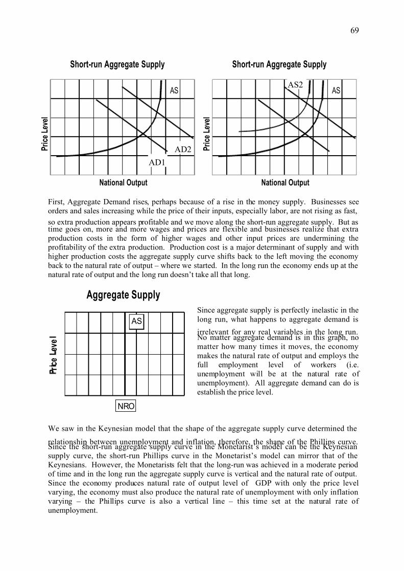
First, Aggregate Demand rises, perhaps because of a rise in the money supply. Businesses seeorders and sales increasing while the price of their inputs, especially labor, are not rising as fast,
so extra production appears profitable and we move along the short-run aggregate supply. But astime goes on, more and more wages and prices are flexible and businesses realize that extra production costs in the form of higher wages and other input prices are undermining the profitability of the extra production. Production cost is a major determinant of supply and withhigher production costs the aggregate supply curve shifts back to the left moving the economy back to the natural rate of output – where we started. In the long run the economy ends up at thenatural rate of output and the long run doesn’t take all that long.
Since aggregate supply is perfectly inelastic in thelong run, what happens to aggregate demand is
irrelevant for any real variables in the long run. No matter aggregate demand is in this graph, nomatter how many times it moves, the economymakes the natural rate of output and employs thefull employment level of workers (i.e.unemployment will be at the natural rate of unemployment). All aggregate demand can do isestablish the price level.
We saw in the Keynesian model that the shape of the aggregate supply curve determined the
relationship between unemployment and inflation, therefore, the shape of the Phillips curve.Since the short-run aggregate supply curve in the Monetarist’s model can be the Keynesiansupply curve, the short-run Phillips curve in the Monetarist’s model can mirror that of theKeynesians. However, the Monetarists felt that the long-run was achieved in a moderate periodof time and in the long run the aggregate supply curve is vertical and the natural rate of output.Since the economy produces natural rate of output level of GDP with only the price levelvarying, the economy must also produce the natural rate of unemployment with only inflationvarying – the Phillips curve is also a vertical line – this time set at the natural rate of unemployment.
69
Aggregate Supply
r c e
e v e
AS
NRO
Short-run Aggregate Supply
National Output
P r i c e
L e v e l
AS
AD1
AD2
Short-run Aggregate Supply
National Output
P r i c e
L e v e l
ASAS2

7/27/2019 Unit 2 Macro
http://slidepdf.com/reader/full/unit-2-macro 26/35
Since the economy has reliable self-correcting mechanisms to push us to the natural rate of outputand the natural rate of unemployment, and these mechanisms while not rapid, work at least asquickly as government policy, the government has no need to intervene. In fact, governmentintervention could make things worse by continually setting up the next economic problem. For example, if the economy were experiencing a short-run contractionary gap and government triedto raise aggregate demand and lower unemployment, by the time the government policy would be
working the economy has already started to correct itself The government policy on top of theself-correcting mechanisms would end up pushing the economy too far in the other direction,setting off a short-run expansionary gap. By the time the government realizes that inflation has become a problem and enacts contractionary policy, the economy’s self-correcting mechanismsare again beginning to work. The government policy on top of the economy’s adjustments would push the economy too far back in the opposite direction into another recession. Friedmanclaimed that the government’s attempt to use feedback stabilization policy, in fact, destabilizesthe economy. The appropriate course of action for the government would then be to follow aneutral fixed policy rule conducive to the support of the natural rate of output.
The Keynesian/Monetarist debate: So who’s right anyway?
During the 1970s and into the 80s, the field of economics was dominated by the debate betweenthe Keynesians and Monetarists over the nature of the economy. By the mid80s a pair of journalarticles appeared each written by a key supporter of one of the theories conceding that the other side had some valid points (“We are all Keynesians now” and “We are all Monetarists now”). Itappears that the economy is more stable than the original Keynesian model suggested – that mostwages and prices do become more flexible in a reasonable period of time and the quantity of money is highly correlated with the price level of an economy. Most recessions last 2 years or less from top to bottom and back up again; however, we do know that the economy hasoccasionally remained significantly off full employment far longer than the Monetarist modelwould suggest possible or reasonable (over 10 years during the Great Depression). We also know
that the economy reacted to changes in fiscal policy during the Great Depression in a manner consistent with the Keynesian model and that the economy appears to respond faster to fiscal policy than monetary when the economy is far below full employment. Monetary policy appearsfar more successful than fiscal at controlling the problem of inflation. The velocity of money is atricky subject, since the velocity of M1 shows far less stability than the velocity of M2, whileeven the velocity of M2 has been less stable in the last 20 years than in the several decades beforethat. When velocity fluctuates, it does so as predicted by the Keynesian model.
In general, there is a certain amount of support for each theory. The Monetarists appear to bemore successful at explaining the long run economic patterns of the US economy, as well as howthe economy behaves in the more usual times of being close to the natural rate of output. TheKeynesians appear to be more successful at explaining how an economy responds to being
pushed far off full employment, suggesting that the self-correction mechanisms may stall once acertain critical level of economic activity has been reached. Some Keynesians have claimed thatthe US economy has been more stable since the government started using stabilization policy;however, that could also be the result of a better regulated banking and financial system, the shiftof the US economy from manufacturing to a more service and information processing economy(the first is more prone to large shifts in production and employment) and the greater internationaleconomy providing a stabilizing force (in a global economy weak demand in the US can becountered by stronger demand from abroad).
70
7/27/2019 Unit 2 Macro
http://slidepdf.com/reader/full/unit-2-macro 27/35
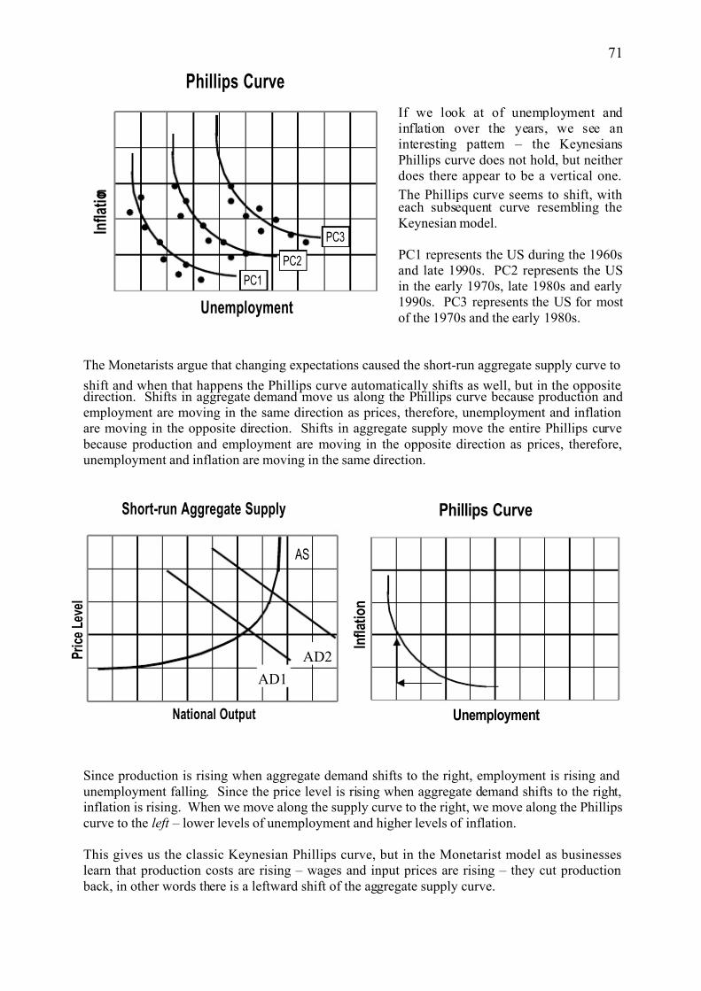
If we look at of unemployment andinflation over the years, we see aninteresting pattern – the KeynesiansPhillips curve does not hold, but neither does there appear to be a vertical one.
The Phillips curve seems to shift, witheach subsequent curve resembling theKeynesian model.
PC1 represents the US during the 1960sand late 1990s. PC2 represents the USin the early 1970s, late 1980s and early1990s. PC3 represents the US for mostof the 1970s and the early 1980s.
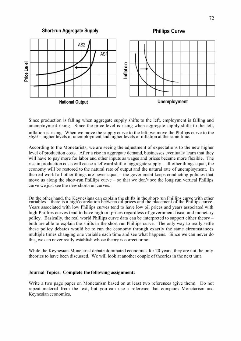
The Monetarists argue that changing expectations caused the short-run aggregate supply curve to
shift and when that happens the Phillips curve automatically shifts as well, but in the oppositedirection. Shifts in aggregate demand move us along the Phillips curve because production andemployment are moving in the same direction as prices, therefore, unemployment and inflationare moving in the opposite direction. Shifts in aggregate supply move the entire Phillips curve because production and employment are moving in the opposite direction as prices, therefore,unemployment and inflation are moving in the same direction.
Since production is rising when aggregate demand shifts to the right, employment is rising andunemployment falling. Since the price level is rising when aggregate demand shifts to the right,inflation is rising. When we move along the supply curve to the right, we move along the Phillipscurve to the left – lower levels of unemployment and higher levels of inflation.
This gives us the classic Keynesian Phillips curve, but in the Monetarist model as businesseslearn that production costs are rising – wages and input prices are rising – they cut production back, in other words there is a leftward shift of the aggregate supply curve.
71
Phillips Curve
Unemployment
I n f l a t i o n
PC1
PC2
PC3
Short-run Aggregate Supply
National Output
P r i c e
L e v e l
AS
AD1
AD2
Phillips Curve
Unemployment
I n f l a t i o n
7/27/2019 Unit 2 Macro
http://slidepdf.com/reader/full/unit-2-macro 28/35
Since production is falling when aggregate supply shifts to the left, employment is falling andunemployment rising. Since the price level is rising when aggregate supply shifts to the left,
inflation is rising. When we move the supply curve to the left, we move the Phillips curve to theright – higher levels of unemployment and higher levels of inflation at the same time.
According to the Monetarists, we are seeing the adjustment of expectations to the new higher level of production costs. After a rise in aggregate demand, businesses eventually learn that theywill have to pay more for labor and other inputs as wages and prices become more flexible. Therise in production costs will cause a leftward shift of aggregate supply – all other things equal, theeconomy will be restored to the natural rate of output and the natural rate of unemployment. Inthe real world all other things are never equal – the government keeps conducting policies thatmove us along the short-run Phillips curve – so that we don’t see the long run vertical Phillipscurve we just see the new short-run curves.
On the other hand, the Keynesians can explain the shifts in the short-run Phillips curve with other variables – there is a high correlation between oil prices and the placement of the Phillips curve.Years associated with low Phillips curves tend to have low oil prices and years associated withhigh Phillips curves tend to have high oil prices regardless of government fiscal and monetary policy. Basically, the real world Phillips curve data can be interpreted to support either theory – both are able to explain the shifts in the short-run Phillips curve. The only way to really settlethese policy debates would be to run the economy through exactly the same circumstancesmultiple times changing one variable each time and see what happens. Since we can never dothis, we can never really establish whose theory is correct or not.
While the Keynesian-Monetarist debate dominated economics for 20 years, they are not the onlytheories to have been discussed. We will look at another couple of theories in the next unit.
Journal Topics: Complete the following assignment:
Write a two page paper on Monetarism based on at least two references (give them). Do notrepeat material from the text, but you can use a reference that compares Monetarism andKeynesian economics.
72
Phillips Curve
Unemployment
I n f l a t i o n
Short-run Aggregate Supply
National Output
P r i c e L e v e l
AS1
AS2
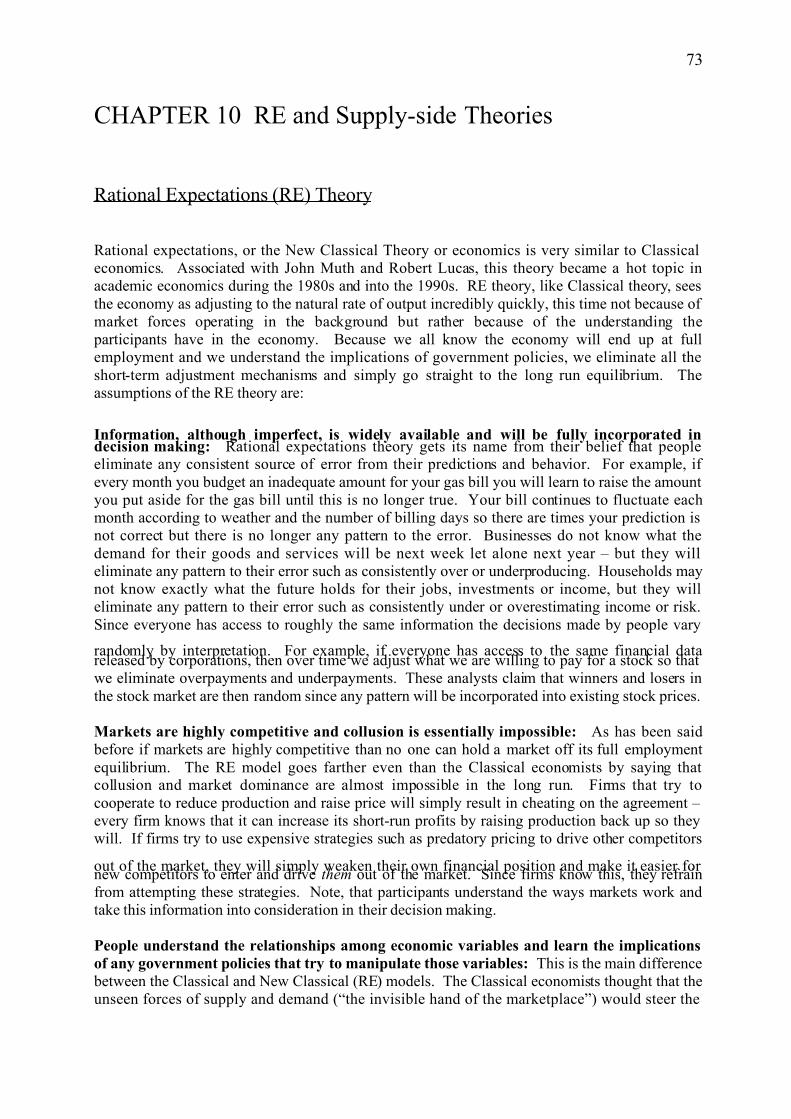
7/27/2019 Unit 2 Macro
http://slidepdf.com/reader/full/unit-2-macro 29/35
CHAPTER 10 RE and Supply-side Theories
Rational Expectations (RE) Theory
Rational expectations, or the New Classical Theory or economics is very similar to Classicaleconomics. Associated with John Muth and Robert Lucas, this theory became a hot topic inacademic economics during the 1980s and into the 1990s. RE theory, like Classical theory, seesthe economy as adjusting to the natural rate of output incredibly quickly, this time not because of market forces operating in the background but rather because of the understanding the participants have in the economy. Because we all know the economy will end up at fullemployment and we understand the implications of government policies, we eliminate all theshort-term adjustment mechanisms and simply go straight to the long run equilibrium. Theassumptions of the RE theory are:
Information, although imperfect, is widely available and will be fully incorporated indecision making: Rational expectations theory gets its name from their belief that peopleeliminate any consistent source of error from their predictions and behavior. For example, if every month you budget an inadequate amount for your gas bill you will learn to raise the amountyou put aside for the gas bill until this is no longer true. Your bill continues to fluctuate eachmonth according to weather and the number of billing days so there are times your prediction isnot correct but there is no longer any pattern to the error. Businesses do not know what thedemand for their goods and services will be next week let alone next year – but they willeliminate any pattern to their error such as consistently over or underproducing. Households maynot know exactly what the future holds for their jobs, investments or income, but they willeliminate any pattern to their error such as consistently under or overestimating income or risk.Since everyone has access to roughly the same information the decisions made by people vary
randomly by interpretation. For example, if everyone has access to the same financial datareleased by corporations, then over time we adjust what we are willing to pay for a stock so thatwe eliminate overpayments and underpayments. These analysts claim that winners and losers inthe stock market are then random since any pattern will be incorporated into existing stock prices.
Markets are highly competitive and collusion is essentially impossible: As has been said before if markets are highly competitive than no one can hold a market off its full employmentequilibrium. The RE model goes farther even than the Classical economists by saying thatcollusion and market dominance are almost impossible in the long run. Firms that try tocooperate to reduce production and raise price will simply result in cheating on the agreement – every firm knows that it can increase its short-run profits by raising production back up so theywill. If firms try to use expensive strategies such as predatory pricing to drive other competitors
out of the market, they will simply weaken their own financial position and make it easier for new competitors to enter and drive them out of the market. Since firms know this, they refrainfrom attempting these strategies. Note, that participants understand the ways markets work andtake this information into consideration in their decision making.
People understand the relationships among economic variables and learn the implications
of any government policies that try to manipulate those variables: This is the main difference between the Classical and New Classical (RE) models. The Classical economists thought that theunseen forces of supply and demand (“the invisible hand of the marketplace”) would steer the
73

7/27/2019 Unit 2 Macro
http://slidepdf.com/reader/full/unit-2-macro 30/35
economy to socially optimal outcomes in micro markets and full employment in macro marketsas individuals pursued their individual interests. This happens without the understanding of the participants who are unknowingly pushed by competition and self-interest. The RE theorists feltthat we achieved socially optimal outcomes in micro markets and full employment in macromarkets because as individuals we understand the economic forces at work and that thisunderstanding plays an important role in the rapid achievement of these outcomes. Remember,
that people incorporate any information in their decision making – the RE theorists feel thatindividuals in an economy learn the processes at work and then anticipate them. For example,since people “know” that a current deficit means the government will need more money in thefuture to pay the interest on the national debt in addition to repaying the bonds they “know” thatthis will mean the need for higher taxes or lower spending in the future. Consequently, they willnot increase their spending today, rather they will save more money to cover the future problemsthey anticipate. The policies used by the government will not even stimulate aggregate demandin the short-run because we understand their consequences.
Wages and prices are completely flexible: RE theorists argue that buyers and sellers of goods,services and labor will constantly renegotiate prices based upon their understanding of economicforces. For example, since people “know” that excessive money growth causes future inflation as
soon as they see excessive money growth they start raising their prices and wage demands tocompensate for the coming inflation. Wages and prices do not display any “stickyness” they arerapidly renegotiated. If there is inadequate money to support full employment at the current pricelevel everyone knows that the price level will fall in the future so they renegotiate wages and prices today to preserve jobs and sales. Since we “know” that in the long run the economy willend up at the natural rate of output we agree to adjust wages and prices today to keep theeconomy there in the short-run as well. Only unanticipated events or events with unknownconsequences (because we have never seen them before) will be able to disrupt the economy evenin the short-run.
Implications of Assumptions
Since all markets are operating on the firms’knowledge that excessive prices throughmarket dominance or cooperation merely brings in new competitors, said excessive prices will not occur. Firms will knowinglyset production at the socially optimal level.As long as outside factors remain equal, thefirms and, therefore, the economy, willdeviate from the natural rate of output only by random error.
Short-run shifts in aggregate demand resultin immediate adjustments in aggregatesupply that push the economy back to thenatural rate of output, as everyoneimmediately adjusts wages and prices tosupport full employment. Even in the short-run, the aggregate supply curve is vertical aslong as there are no unanticipated changes in
74
Aggregate Supply
P r i c e L
e v e l
AS
NRO
7/27/2019 Unit 2 Macro
http://slidepdf.com/reader/full/unit-2-macro 31/35
outside variables. By this logic the Phillips curve is also vertical with only random variationsfrom the natural rate of unemployment, again, as long as there are no unanticipated changes inoutside variables.
If this is true then how do we explain the business cycle? Clearly, there are times in the economythat the economy moves farther and farther away from full employment, stabilizes and then
moves back closer and closer to full employment. That is not a random pattern of economicactivity. A group of RE theorists derived their explanation of the cyclical pattern of economicactivity – the real business cycle model.
The real business cycle model states that changes in exogenous factors that temporarily or permanently shift the natural rate of output are responsible for the ups and downs of GDP.Mainly, it is shifts in technology or resource availability that create the short-run fluctuations ineconomic activity. A rise in the availability of resources such as oil and/or a rise in technologywould shift aggregate supply to the right - resulting in lower prices and a higher natural rate of output while the Phillips curve would shift to the left – resulting in lower inflation and a lower natural rate of unemployment. A disruption in the availability of resources such as oil and/or adrop in capacity due to loss of technology or facilities would shift aggregate supply to the left -
resulting in higher prices and a lower natural rate of output while the Phillips curve would shift tothe right – resulting in higher inflation and a higher natural rate of unemployment.
The problem is that relatively few business cycle phases in US history can be linked to exogenousfactors shifting – the booming economy of the late 1990s and the stagnant economy of the late1970s are relatively rare examples of cycles created by shifts in resource availability and/or technology. Most business cycles in US history clearly originate with aggregate demand notaggregate supply. If aggregate supply is shifting then unemployment and inflation will move inthe SAME direction – if aggregate demand is shifting then they will move in the OPPOSITEdirection. In most business cycles we see them clearly move in the opposite direction.
In my opinion, RE theory is too dependent on the technical development of their models and the
mathematics involved and too unresponsive to empirical data and experiences. We do not seerapid renegotiations of wages and prices in the real world, we do not see consumers taking thefuture consequences of current government economic policies into consideration when makingdecisions, and we do not see random variations on GDP, employment and prices in the absence of real world variables shifting. I believe the Monetarists have a much more defensible conservativemacroeconomic model.
Supply-side Economics
A relatively small group of economists in the late 1970s and 1980s also suggested that the
business cycle was the result of fluctuating aggregate supply, however, their opinion was thatgovernment policies were responsible for disrupting the aggregate supply of the economy. Theyargued that the government had created a environment that was hostile to business and successand encouraged waste and inefficiency, resulting in a leftward shift of the aggregate supply curve.A leftward shift in aggregate supply results in higher unemployment and inflation at the sametime and this was their explanation of the stagflation of the 1970s. This theory was never widelyaccepted in economics, although it was embraced by conservative politicians and served as thefoundation of Ronald Reagan’s economic policies (Reaganomics).
75

7/27/2019 Unit 2 Macro
http://slidepdf.com/reader/full/unit-2-macro 32/35
According to the supply-siders, liberal government policies during the late 1960s and early 1970sreduced production and employment in the US by over-taxation (especially of businesses) andover-regulation. These excessive taxes and regulations raise the cost of production for American businesses and cause them to reduce their production and hiring. Individuals who worked hard,acquired additional training or education and raised their wages found themselves in higher tax brackets where they lost a larger percent of their income to the government. This discouraged
people from pursuing these activities which are valuable to the economy and society. In addition,the government was said to encourage waste and inefficiency by rewarding nonproductive behavior – the tax code gave big write-offs for excessive costs and entitlement programs“rewarded” people for choosing not to work or acquire skills by giving them benefits such aswelfare and food stamps. In general, the government was said to have created a skewed incentivesystem with productive behavior being punished and discouraged while unproductive behavior was reward and encouraged.
The Supply-side solution to this was to reduce taxes, especially on businesses and upper incomegroups, reduce government regulations on industry and reduce entitlement spending. I’m sureyou can see why this theory resonated with political conservatives. While many conservativeeconomists were sympathetic to some of the claims of the supply-siders, their theory was largely
rejected in the field of economics because of the extremes they took their claims to. The mostcontroversial aspect of the supply-side model was their view of the relationship betweengovernment tax rates and tax revenue.
The Laffer Curve
Arthur Laffer was the predominate supply-side economist at this time, and he made the rather extreme claim that the government could cut tax rates without losing any money, in fact, if anything, they were likely to receive higher tax revenue after cutting tax rates. This view was NOT supported by the empirical evidence on tax elasticity at the time. Tax revenue is the product
of the tax rate and the number of units being taxed (tax base).
Tax Rev = Tax Rate x Tax base
So that if the government has a 40¢ a gallon tax on gasoline and 10 million gallons of gas aresold, then the government will collect $4 million dollars in tax revenue. All other things equal,the tax rate and the tax base will move in the opposite direction – if the government raises the taxrate it discourages the production or consumption of the good being taxed. The degree to which production or consumption falls depends on the responsiveness of the people being taxed.
The more consumers keep buying a product even though it is now more expensive, the more producers will keep making it. Consequently, the tax base will decrease less than the tax ratewent up and the tax revenue will move with the tax rate. If people tend to keep working eventhough their income tax has risen then the tax base falls less than the tax rate went up and the taxrevenue will again move with the tax rate.
The less consumers keep buying a product because it is now more expensive, the less producerswill keep making it. Consequently, the tax base will decrease more than the tax rate went up andthe tax revenue will move with the tax base. If people tend not to keep working because their
76

7/27/2019 Unit 2 Macro
http://slidepdf.com/reader/full/unit-2-macro 33/35
income tax has risen then the tax base falls more than the tax rate went up and the tax revenuewill again move with the tax base.
When the tax rate is 0%, then clearly thegovernment will take in $0. But, noticethat the government also takes in $0 whenthe tax rate is 100%. Will people work or
open businesses if the government took 100% of their income or profits? No!
At lower tax rates the tax base does notshrink very much as tax rates rise. Peoplewill not change behavior very much whenvery low tax rates rise to low tax rates.
At higher tax rates the tax base shrinkssignificantly as tax rates rise. People willchange behavior a lot when high tax rates become very high tax rates. These are
known as prohibitive taxes – tax rates sohigh they reduce tax revenue.
In the late 1970s, Laffer claimed that the US was on the right hand side of this graph – that our tax rates were prohibitive. If this were true, then a cut in government taxes would eventuallyraise tax revenue or at least leave it about the same. The stimulus does not work immediately, because it will take time for businesses to expand their productive capacity; it takes time to buildnew factories, order new equipment, hire and train new workers, etc. The supply-siders claimedthat in about 3-5 years the government tax cut would pay for itself or better. Mainstreameconomists denied that the US was in the zone of prohibitive taxes; all our data suggested that wewere somewhere to the left of the graph, perhaps approaching the maximum tax revenue at worst.
The Reagan tax cuts in the early 1980s were largely influenced by the supply-siders though thefinal version of the tax cuts was more of an across the board cut than originally proposed. Giventhat the US economy was in a severe recession at the time, economists and politicians argued howmuch the tax cut operated as a Keynesian tax cut and how much it operated as a Supply-side one.The same groups argued over how much the large budget deficits of the 1980s were a result of the recession and how much the result of Reagan’s economic policies.
A Tax Cut By Any Other Name
The Keynesians wanted a tax cut during the recession of 1980-82, the Supply-siders wanted a tax
cut during the recession of 1980-82 – how are the two positions different? Supply-sideeconomists saw large differences between their tax cuts and those of their theoretical
To whom do we give the tax cut? Keynesian tax cuts were either across the board (for political purposes) or aimed at the lower 50% of the income distribution (because these are the people thatrespond most to an income change). Supply-side tax cuts were aimed primarily at businesses andupper income households because those are the individuals most likely to invest the money in the business sector thus creating new production capacity.
77
LAFFER CURVE
Tax rate
T a x R e v e n u e
0% 100%

7/27/2019 Unit 2 Macro
http://slidepdf.com/reader/full/unit-2-macro 34/35
Which curve shifts? Keynesian tax cuts were aimed at increasing the aggregate demand curve by shifting consumption – an increase in aggregate demand, aote, raises both real GDP and the price level. A supply-side tax cut is aimed at increasing the aggregate supply curve by increasinginvestment to build more capacity – an increase in aggregate supply, aote, raises real GDP butlowers the price level. Since investment is also part of the aggregate demand curve, aggregatedemand will also rise, but the supply-siders said that it will not rise more than aggregate supply,
therefore, the most that will happen is the price level will remain constant – a supply-side tax cutis non-inflationary.
Effect on the national debt: A Keynesian tax cut creates a ongoing deficit that will persist untilthe economy overheats and the government reverses policy raising taxes. Since recessions are
more frequent and more severe that booms, this means that the national debt over time graduallyincreases. A supply-side tax cut, it was claimed, would only create a very temporary deficit thatlasts until the business sector expands production sufficiently to move us up and to the left on theLaffer curve. At this point the deficit disappears, in fact, the economy is likely to move into asurplus that can be used to pay off past debt or used to spend on other government programs.
The supply-side economists felt that their policy was clearly superior to that of the Keynesians.This entire argument is based upon two principles both working – that businesses and highincome households invest their tax cut in building productive capacity (as opposed to CEO bonuses or European vacations) and that tax elasticity is elastic – i.e. tax revenue moves with thetax base not the tax rate. Our real world experience suggests that the former is only partially trueand that the latter has not been true at all for the US at any time.
Many economists concluded that our experiences during the 1980s have proven supply-sidetheory wrong but this overstates the clarity of the evidence. During the 1980s the government ranenormous budget deficits that remained high even after the US economy started recovering fromthe recession of 1980-82. Part of this was due to the severity of the recession and how long ittook to climb back to previous production levels, part was due to the increases in militaryspending, part was due to the extremely high interest rates coming from the contractionary policyof the Federal Reserve and part to the tax cuts themselves. While economists disagree over howmuch of the resulting government debt was due to the tax cut, one thing is clear – there was a
78
Keynesian Tax Cut
GDP
P r i c e
L e v e l
AS
AD2
AD1
A
B
Supply-side Tax Cut
GDP
P r i c e
L e v e l
AS1
AS2
AD2
AD1
A B

7/27/2019 Unit 2 Macro
http://slidepdf.com/reader/full/unit-2-macro 35/35
large shift in aggregate demand because of this tax cut – much larger than the shift in aggregatesupply. The lesson is not clear, however, since the Reagan tax cuts were not entirely supply side – they were much more across the board than the supply-siders had wanted – more across the board then the Reagan administration had wanted.
The US economy started booming in the mid 1990s and some supply-siders have claimed that
this is the result of the tax cuts during the 1980s. If the lag time for capacity is more like 5 yearsinstead of 3-5 years and the creation of capacity was delayed because of the Fed’s high interestrates and then the recession of 1990-91, it would be possible that the supply-side stimulus did notsignificantly impact the US economy until the mid 1990s. Most economists believe that the boom of the 1990s was really the result of low oil prices, high productivity coming fromtechnology and greater efficiency due to rising international trade, but proving it is another matter.
Journal Topics: Complete the following assignment
Find two web pages on each theory and write a one page summary of the 2 web pages for each
theory.
79