UNIT 14 MEASURES OF DISPERSION

Structure

14.1 introduction

Objectives

Meaning of Dispersion

Importance. of the Measures of Dispersion

Concept of Range

Concept of Quartile Deviation

14.6.1 Calculation of Quartile Deviation 14.6.2 Interpreta6ion of Quartile Deviation

Concept of Percentiles

14.7.1 Calculation of Percentiles 14.7.2 lnterpretation of Percentiles 14.7.3 Limitations of Percentiles

Concept of Mean Deviation

14.8.1 Calculation of Mean Deviation 14.8.2 Interpretation of Mean Deviation

Concept of Standard Deviation

14.9.1 Calculation of Standard Deviation 14.9.2 Interpretation of Standard Deviation

14.10 Use of Standard Deviation, Quartile Deviation and Percentiles in Classroom Situation

14.12 Unit-end Exercies

14.13 Points for Discussion

14.14 Answers to Check Your Progress

14.15 Suggested Readings

14.1 INTRODUCTION

In Unit 12 and 13 of this Block, you have studied about the 'Tabulation and Graphical Representation of Data' and the 'Measures of Central Tendency'. Measures of central tendency can describe only one of the important characteristics of a given distribution i.e. the measures of location or the value of the variate around which the distribution may centre. Another important characteristic of the distribution is its variability. It is equally necessary to know about the variability of data, which may be concentrated or scattered around the measures of cehtra~ tendency.

In the present unit, you are.going to study about the meaning and the importance of the measures of variability or dispersion, calculation and interpretation of these measures and the use of these measures in the actual classroom situation. Yau wouM then be in a better position to teach these to your students.

'

-- - 14.2 OBJECTIVES --- - After going through this unit, you will be able to:

und~erstand the concept of dispersion;

diffkrentiate between the measures of central tendency and the rrieasures of dispersion; 40

state the importance of the measures of dispersion;

define quanile deviation 'Q' in your own words;

calculate 'Q' for given data;

interpret the value of 'Q' obtained by you;

+ define and calculate the specified percentiles;

interpret the percentile obtained by you;

define mean deviation in your own words;

calculate mean deviation for ungrouped, as we11 as gmuped data;

interpret the mean deviation obtained by you;

define standard deviation 'd in your own words; d

calculate 'o' from ungrouped, as well as from grmpd data;

interpret the index of 'a', calculated by you;

use appropriate measure of dispersion in classram situation for the improvement of teaching-learning process.

14.3 II~EAIWNG OF DISPERSION

The measures of central tendency give one p i n t re~esentation of t k diai$ution bere tk decrsion making requires more than this information. For exampEe, let us consider the performance of the two groups of children in a mathematics test. The sores obtained by tk children are as follows :

GroupA: 8, 12,11,12,10,&~9,11,12,10,8,10,9, ~0,112,8,f8,9,10,TII.

Group B : 15,2, 8, I2,4, 17,20,6,2, E8, 16, 4 3, 9,6, I@ 15, 17,9, 11.

By computing means, you will notice thaf the average performance of the children of both rk groups is the same, which is 10.0. However, if y m go rhaogh the scores & a i d by the children s f the two groups, you will find that in Group A, no child has less than 8 ar m e ihm 12 marks, while in G r ~ u p B, there are many chiidren getting less titan 8 sr m e tkm I2 - marks. Actually, the scores vary frm O to 20 in Group B. The two groups are m cmprsbk in terms of homog&eity. Group A is hmoger~ews, while G r q B is wte k a ( ~ o g m o u ~ ~ This information regarding the variability d data is not revealed by the measure of sentraI tendency. The property which denaes the extent to which she values are dispersed a- the central value is called dispersion. Dispersion is also known as spread, scatter or variability.

Measures of dispersion, provide a quantitative m m r e ofthe v;rriabiIi:y of vdues. Just as the measure of central tendency is a point on the scale of mawement, the: measwe of dispersion i s also a distance dong the scale of measwemnt. The measms of dispersion in cmm use are Range, Quartile Deviaaion, Mean Deviation and S t d a d Deviation.

Measures of Central Tendency can be used to &scribe a d campre different data, &H thew dcr no1 give information about its variability. The varkbi9lty of dasa reveals much more than what the measure of central tmdency alone can do. Tfre masure of ddiqmsisn provides a quantitative index of ,fk degree of v;rrislion arrtang a parriedar set of values cw sexes. For compirri~g the relative &gra ofvariability with r e p ~ d to some trait ammg the indivirdwis in two or more groups, the measure of diqersion of the trait in a& group is needed. The quantitative ~ndices required far camprison purposes stPauld 6e available in dams of the same unit. The measure of dispersion, especidfy ek deviation, is required for m y 41

N Measures of Dispersion being that for the median we consider - cases, while t'or the Q1 and 4 3 we have to take

- 2

N 3N -and - cases respectively. 4 4

Let us consider the following example :

Example 1 : The scores obtained by 36 students of a class in mathematics are shown in the table. ~ i n d the quartile deviation of the scores.

Table 14.1

Scores f c f

In column 1 , we have taken Scores, in column 2, we have taken the frequency, and in colu~nn 3. cumulative frequencies starting from the bottom have been written.

N 36 Here N = 36, so for Q1 we have to take -=-=9 cases and for 4 3 we have to take

4 4

- ---= 36 27 cases: By looking into column 3, cf = 9 will be included in C155-59, whose 3N 4 4

real limits are 54.5 - 59.5. So Ql would lie in the interval 54.5 - 59.5. The value of Ql is to

be computed as fol l~ws :

For calculating 43, cf = 27 will be included in CI 65-69, whose real limits are 64.5 - 69.5. So

Q3 would lie in the interval 64.5 - 69.5 and its value is to he computed as follows':

Q3 - Q1 65.50 - 55.93 - 9.57 - Thus, Q=-- -- 2 2 2

Siatistierl Techniques of Analysis 14.6.2 Interpretation of Quartile Deviation

Let us first discuss the use and limitations of quartile deviation as a measure of dispersion. Quartile deviation is easy to calculate and interpret. It is independent of the extreme values, so it is more representative and reliable than range. Wherever median is preferred as a measure of cenrral tendency, quartile deviation is preferred as measure of dispersion. However, like median, quartile deviation is not amenable to algebraic treatment, as it does not take into consideration all the values of the distribution.

While interpreting the value of quartile deviation it is better to have the values of Median, Q1 and Q3, alongwith Q. If the value of Q is more, then the dispersion will be more, but again the value depends on the scale of measurement. Two values of Q are to be compared only if the scale used is the same. Q measured for scores out of 20 cannot be compared directly with Q for scbres out of 50. If median and Q are known, we can say that 50% of the cases lie between 'Median - Q' and 'Median + Q'. These are the middle 50% of the cases. Here, we come to know about the range of only the middle 50% of the cases. How the lower 25% .of the cases and the upper 25% of the cases are distributed, is not known through this measure. Sometimes, the extreme cases or values are not known, in which case the only alternative available to us is to compute median and quartile deviation as the measures of central tendency and dispersion. Through median and quartiles we can infer about the symmetry or skewness of the distribution. Let ud therefore, get some idea of symmetrical and skewed distributions.

Symaetrical and Skewed Distributions : A distribution is said to be symmetrical when the frequencies are symmetrically distributed around the measure of central tendency. In other words, we can say that the distribution is symmetrical if the values at equal distance on the two sides of the measure of central tendency have equal frequencies.

Example 2 : Find whether the given distribution is symmetrical or not.

-

Score 0 1 2 3 4 5 6 7 8 9 10

Frequency 1 2 2 4 5 8 5 4 2 2 1

Here Ihe measure of central tendency, mean as well as median, is 5. If we start comparing the frequencies of the values on the two sides of 5, we find that the values 4 and 6,3 and 7,2 and 8, 1 and 9, 0 and 10 have the same number of frequencies. So the distribution is perfectly ~ymmetrical.

En a symmetrical distribution, mean and median are equal and median lies at an equal distance from the two quartiles i.e. Q3 - Median = Median - Q 1 .

If a distribution is not symmetric, then the departure from the symmetry refers to its skewness. Skewness indicates that the curve is turned more towards one side than the other. So the curve will have a longer tail on one side. The skewness is said to be positive if the longer tail is on the right side and it is said to be negative if the longer tail is on the left side. The following figurks, show the appearance of a positively skewed curve and a negatively skewed curve.

Fig. 14.1

(a) Pclsitively skewed (h) Negatively skewed

For a positively skewed curve, ,.r (Q3 -Median) is greater than (Median - Q1)

' For a negatively skewed curve,

(Q3 - Median) is less than (Median - Q1)

.. ------ --. 1 .'.i.Gt- % o:tr ~ ~ ~ v g r c ~ s s I

' I ; 1 , ~ ~ J : ~ ! I ~ ~ ~ ~ :j:!;t;\:i<:< : ~ : ~ < i L . ~ ~ . ~ , ~ ~ ~ ~ ? ~ : ..IL ., .;, :. :

i 1

I i IIL.~ ! I , $ . \k~:~,i~.,~~\.i ;?I!L! ~ . ~ , i : i i ( : i l ~ $ : 1.d \k.,.x:%t.2i ,.'!iz \ I - , > I

. . . . . . . . . . . . . . . . . . . . . . . . . . . . . . . . . . . . . . . . . . . . . . . . . . . . . . . . . . . . . . . . . . . . . . . . . . . . . . . . . . . . . . . . . . . I . . . . . . . . . . . . . . . . . . . . . . . . . . . . . . . . . . . . . . . . . . . . . . . . . . . . . i

t

I . . . . . . . . . . . . . . . . . . . . . . . . . . . . . . . . . . . . . . . . . . . . . . . . . . . . . . . . . . .

I f

i .." -- ..------ I I

- 1.4.7 CONCEPT OF PERCENTILES In case of median, total frequency is divi'ded into two equal parts ; in the case of quartiles, total !requency is divided into four equal parts; similarly in case of percentiles, total frequency is - . divided inlo 100 equal parts. Percentiles are denoted by P,, P,, P, ........ P ,,,,. 'Thus, percentiles inay be defined as those values of the variate which dlvide the total frequency into 100 equal parts. So, there are 1 percent of the cases below the point P,, 2 percent of the cases below the point P, and so on. As discussed earlier, Median is represented by PC,> and the two quartiles Q1 - ,, and Q3 are represented by P,, and P,, respectively. Similarly. first, second, third, .........., ninth

.......... deciles are represented by P ,,,, P,,, P ,,,, P,, respectively.

14.7.1 Calculation of Percentiles

I For calCulating the values of percentiles, we have to find the points on the scale of measurement I upto which the specified percent of cases lie. The process of calculating the percentiles wherein

we takc into consideration the specified percent of cases is similar to that of calculating the qua~tiles. Thus,

and so on.

Example 3 : Let us find out P,,, and P,,, for the data given In Table 14.1. It shows the scores

ohtained by 36 students of a class in mathematics. Here N = 36, so for computing P ,,, we have

I ON tc: take - or 3.6 cases. The cf against 45 - 49 1s 2 and against 50 - 54 l t IS 7. So 3.6 cases

1 00 would lie upto a point between 49.5 and 54.5 Thus,

Measures of Dispersion

Statistical Techniques of Analysis 20N For computing P?,, we have to take -or 7.2 cases.

l o o

The cf against 50 - 54 is 7 and against 55 - 59 is 14. So 7.2 cases would lie upto a point between 54.5 and 59.5. Now I

7.3 -7 : P2,) = 54.5 + -=--x 5 7

I = 54.5 + - 7

= 54.5 + 0.14 .

= 54.64

In Unit 12, you have learnt to draw a cumulative frequency curve and ogive, wherein alongwith cumulative:frequency, the cu~nulative percentage has been used on Y-axis. With the help of the Ogive, you can directly find the values of different percentiles without computing them.

14.7.2 Interpretation of Percentiles

Percentiles dre more frequently used in testing and interpreting test scores. For any standardised tests, percentile norms are reported with the test, so that the obtained test results may be interpreted droperly. If the percentile rank of an individual is 60, we come to know that 60% of the studebts have scored less ihan that individual. If only the score of an individual is given, it is difficult to judge the performance. It can be judged only with reference to a particular group. However, with the help of the cumulative percentage curve, we can find the percentile rank of that ihdividual and judge the performance on that basis,

14.7.3 Limitations of Percentiles

The mastery of an individual is not judged by the use of percenliles, as the same person in a poor group will show better rank and in an excellent group will show comparatively poorer rank. Also, as in casc of simple ranks the difference in percentile ranks at different intervals are not equal. !As an example, P ,,,,, - P,,, is not comparable to P,,, - P ,,,. The position of a student on total achievement cannot be calculated from percentiles given in several tests.

14.8 CONCEPT OF MEAN DEVIATION

The distance of a score from a central point is called a deviation. The simplest way to take into consideraqion the variation of all the values in a distribution is to find the mean of all the deviations of tlbese values from a selected point of central tendency. Usually, the deviation is taken from t1re:mean of the distribution. The avcrage of the deviations of all values from the arithmetic meah is known as mean deviation or average deviation.

The measure o t central tendency is such a point on the scale of measurement on both sides of which there are a number of values. So, the deviations from this point, will be in opposite directions, both positivc and negative. If the score is denotcd by X, and the mean by M, then X-M denotes the deviation of scores from the mean. The deviation, where mean is greater than the scorc, will be negative. By definition of the mean, as measure of central tendency, the algebraic suln of all thcse deviations will come out to be zero, as the deviations on both the

sides are equal.! To avoid this problem, the absolute values of these deviations, i.e. IX - MI irrespective of tlleil- sign is taken into consideration. Thus,

CIX - MI Mean Deviation =

N .

Where X is the scorc, M is [he mean and N is the total frequency.

14.8.1 Calculation of Mean ~eviation

In Unit 13, you vent through some examples for calculation of means. Let us consider the 4h

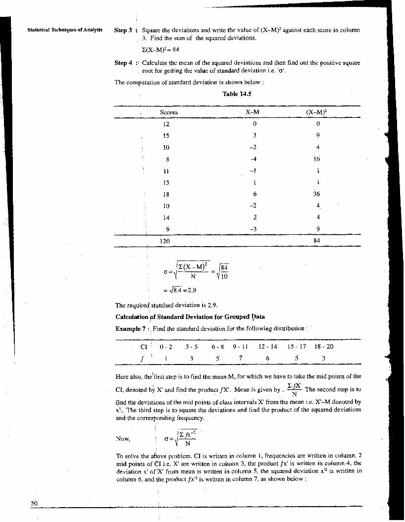
Statistical Techniques of Analysis Step 3 :, Square the deviations and write the value of (X-M)2 against each score in column 3. Find the sum of the squared deviations.

Step 4 : Calculate the mean of the squared deviations and then find out the positive square root for getting the value of standard deviation i.e. '0'.

The computation of standard deviation is shown below :

Table 14.5

Scores X-M (X-M)'

12 0 0

The requiredl standard deviation is 2.9.

Calculation bf Standard Deviation for Grouped Data

Example 7 : Find the standard deviation for the following distribution :

Here also, thelfirst step is to find the mean M, for which we have to take the mid points of the

Zfl The second step is to CI, denoted bp X' and find the product fX'. Mean is given by . - N

(ind the deviations of the mid points of class intervals X' from the mean i.e. X'-M denoted by X " \ ~ h e third step is to square the deviations and find the product of the squared deviations and the corresponding frequency.

Now, N

To solve the a k v e problem, CI is written in column 1, frequencies are written in column, 2 mid points of TI i.e. X' are written in column 3, the product fx' is written in column 4, the deviation x' of lX' from mean is wr~tten in column 5 , the squared deviation xtZ is written in column 6, and the product f ~ ' ~ is written in column 7, as shown below :

Table 14.6

Mid Point

CI f x' fx' xi ' X 12 jx'2

Total 30 333 674.70

c f X' 333 Mean =-=-=I 1.1 N 30

So, the deviations of the mid points are to be taken from 11.1.

= 1 / m = 4 . 7 4

Thus, the required standard deviation is 4.74.

Here, you must have observed that the deviations from the actual mean results in decimals and the values of x'' and f X" are difficult t0,calculate. In order to avoid this problem we follow a short-cut method for calculating standard deviation. In this method, instead of taking the deviations from actual mean, we take deviations from assumed mean. As a result, the formula for finding the standard deviation also changes to :

i 4- =-x NXfd - Xfd N

Here, i is the length of each class interval, N is the total number of cases and is the deviation of mid-point from the Assumed Mean, divided by the length of CI. This method is also known as Step Deviation Method.

Step Deviation Method for the Calculation of Standard Deviation

In this method. in column 1, we write the CI; in column 2, we write the frequency; in column

X' -AM 3, we write the values of d, where d = . ; in column 4, we write the product fd, and in 1

column 5, we write the value of fd2, as shown below

Measures of Dispersion

1

Statistical Techniques of Analysis

Total 30 11 79

Here Assumed Mean is the mid-point of the CI 9- 11 i.e. 10, so the deviations have been taken from 10 and divided by 3, the length of CI.

Now, O = ~ J ~ N

Here also o = 4.74

14,9.2 Interpretation of Standard Deviation

Let us first consider the use and limitations of Standard Deviation as a measure of dispersion. Standard Deviation is the most widely used and important measure of dispersion. It occupies a central position in statistics. Like mean deviation, it is based on all the values of the distribution. Here, the signs of deviations are not disregarded, instead they are eliminated by squaring each of the deviations. It is the master measure of variability as it is amenable to algebraic treatment and is used in correlational work and in further statistical analyses. The only limitation is that, the extreme values affect it to a large extent. For interpreting the value of the measure of dispersion we must understand that greater the value of 'o ' the more scattered are the scores from the mean.

As in the case of mean deviation, the interpretation of standard deviation requires the values of M and N for consideration.

In exaqples 6 and 7, the required values o r ? , mean and N are as follows :

- Example 6

Example 7 11.1 4.74 30 I

Here, the dispersion is more in example 7 as compared to example 6. It means the values are more soatiered in example 7, as compared to the values of example 6.

- B-=-mw"T- I Me;lsums of Dispersion

14.10 USE OF STANDARD DEVIATION, QUARTILE DEVIATION AND PERCENTILES IN CLASSROOM SITUATION

In classroom situations, we are required to use statistics frequently. However, in such a situation, either the teacher avoids computing the required statistic or computes the simplest measure of central tendency and dispersion without bothering for the suitability of these measures for the given distribution. A teacher should use the statistic when required and it should be appropriate for the situation.

While reporting the progress of the child, the teacher simply reports the subject-wise m a k s in an examination. No other information is provided with reference to the performance of the children of the class. To avoid this situation, teacher can prepare the individual profiles of the children in terms of their percentile ranks. These profiles can be reported to their parents; they will be able to understand the position of their child in the class.

Example 8 : The scores of a student of class IX in the annual examination are reported as follows :

- - -

Subject : English Hindi Maths Science Soc. St Total

Max. Marks 100 100 100 100 100 500

Marks obtained 55 60 70 63 58 306

From the above data, it is difficult to have an objective assessment. We can simply see the percentage of achievement in each of the subjects and in the total. However, if the teacher provides subject-wise PRs alongwith marks obtained, it will be more meaningful. For this, individual's PRs reported are as follows :

Subject : English Hindi Maths Science Soc. St Total !

PRs P o Ps4 P~~ Pss P53 Pss

Total number of students in class are 44.

Here, one understands the relative position of the individual in the group, for each of the subject. Further, individuals can be compared with earlier and later performance, if reported in this way.

The measure of dispersion helps the teacher to know about the variability in the class and plan the individualised instruction to suit the deprived and the intelligent children.

Statistical Techniques Analysis For comparison of individual scores, the best way is to convert the obtained scores into the standard scores and for comparing two different distributions in terms of their variability, the coefficient of the variation may be used. The standared score and the coefficient of variation is being discussed in the following section.

Standard Scores

If the mean and SD of a set of values is known, then the given score may be expressed as deviation from the mean as a multiple of SD. Such a score is called standard score or Z score.

X-M z=- a

Standatd scores are amenable to all algebraic treatment, as these scores are represented in the form of Ratio Scales of measurement. Any two scores are comparable when converted into standard scores. If the raw scores of different subjects are converted into standard scores, we can calculate the composite scores also.

The Coefficient of Variation

When two series or distributions are kxpressed in the same unit and have approximately same

average value then the a s of the two series/distributions may be compared directly. But if the units are different or the average value of the two distributions differ to a large extent then direct comparison may not give the true picture.

Example 9 : The heights of students of class VIII A have been measured in inches, while those of class VIII B have been measured in cms. The standard deviations for the two groups are as follows :

Class 0

VIII A 5

VIII B 12

These two a s cannot be compared directly, unless these are converted to the same unit or in any other form not involving unit.

For this we need another measure of variability that is independent of unit and takes averages into consideration. Such a measure is the co-efficient of variation or relative standard deviation and is expressed as a percentage.

As CV is the ratio of two quantities, a and M, having the same unit, it is independent of unit. It also provides a value relative to mean.

Exceptional variation : In educational situations CV less than 5% or more than 35% would raise doubts regarding accuracy of computation of means and SDs, or the appropriate measures may not have been computed. For such cases, special analysis and interpretation is needed.

14.11 LET US SUM UP

The property which denotes the extent to which the values are spread about the central value is called dispersion.

The measure of dispersion is a distance along the scale of measurement.

Commonly used measures of dispersion are Range, Quartile Deviation, Mean Deviation add standard Deviation. The simplest measure is Range and the most trust worthy measure is Standard Deviation.

Standard Deviation is required for further statistical computations.

Before computing the measure of dispersion it is desirable to see the suitability of the

54 measure to a given situation.

Measures of Dispersion

Statistical Techniques of Analysis 14.lb SUGGI 1

ESTED READINGS 1 Blombners, P. and Lindquist, E.F. (1959), Elementary Statistical Methods, Houghton Mifflih Company, Boston.

Garrett, H.E.(1956), Elementary Statistics. Longmans, Green & Co., New York.

Guilford, J.P. (1965), Fundamental Statistics in Psychology and Education, McGraw Hill Book Company, New York.

Hannagan, T.J. (1982), Mastering Statistics, The Macmillan Press Ltd., Surrey.

Lindgren, B.W. (1975), Basic Ideas of Statistics, Macmillan Publishing Co. Inc.,New York. I Tate, M.W. (1955), Statistjcs in Education, The Macmillan Company, New York. 1 Walkeq, H.M. and Lev, J. (1965), Elementary Statistical Methods, Oxford & IBH Publishing Co., Chlcutta.

Wine, R.L. (1976), Beginning Statistics, Winthrop Publishers Inc., Massachusetts. 7