UNIT : 1 1. CLASSIFICATION OF RADIO TRANSMITTERS ON THE BASES OF TYPE OF

SERVICE INVOLVED:

1) Radio Telegraph Transmitters:

A radio telegraph transmitter transmits stele graph signals from one radio

station to another radio station. It may use either amplitude modulation or frequency

modulation. When point-to-point radio communication is involved, the transmitting antennas

are highly directive so that the electromagnetic energy is beamed into a narrow beam directed

towards the receiving antenna at the receiving radio station.

2) Television Transmitters:

Television broadcast requires two transmitters one for transmission of

picture and the other for transmission of sound. Both operate in very high frequency of in

ultra-high frequency rang. The picture transmitter is amplitude modulated by the picture signal

occupying a band of about 5 5MHz Vestigial transmission is used i.e. one full sideband

and only a vestige or a part (about 0 75 MHZ) of the other sideband together with the carrier

are radiated from the transmitting aerial. The total bandwidth occupied by one television

channel is about 7 MHz The sound carrier is frequency modulated.

3) Radar Transmitter:

Radar (abbreviation for Radio Detection and Ranging) may be of two

types:

(i) Pulse Radar and (ii) C.W. (Continuous Wave Radar). Pulse radar transmitter uses pulse modulation of carrier. It uses high output power typically

100 kW peak and operates at microwave frequencies typically 3000 MHz (10 cm

wavelength) or 10,000 MHz (3 cm wavelength). The C.W. radar transmitter may use

frequency modulation of the carrier voltage or may utilize Doppler Effect.

4) Navigation Transmitters:

A number of navigational aids using special types of radio

transmitters and receivers are used these days for sea and air navigation. Also radio aids are

used for blind landing of aircrafts. Typical radio aids of landing are (a) I.L.S. (Instrumental

Landing System) and (b) G.C.A. (Ground Controlled Approach). In addition to these,

several other radio means are provided at airport for surveillance. Accordingly, a large

number of radio transmitter of varied types, frequency and power are required depending upon

the operation desired.

CLASSIFICATION OF RADIO TRANSMITTERS ON THE BASES OF

CARRIER FREQUENCY

1) Long Wave Transmitters:

These transmitters operate on long waves i e on frequencies below 300

kHz. Such long wave radio transmitters are used for broadcast in temperate countries, where

atmospheric disturbances on long waves are not severe. Since long wave radio signals

travel along the surface of earth and are rapidly attenuated, for reasonably high signal

strength at the distant receiving aerial, the carrier power radiated from the transmitting

aerial must be very large typically 100 kW or more.

2) Medium Wave Transmitters:

These transmitters operate on frequencies in the range of 550 to 1650

kHz and are usually used for broadcast. Hence the band of frequency extending from 550 to

1650 kHz is commonly referred to as the Broadcast Band. The carrier power may vary from as

low as 5 kW to as high as 500 to 1000kW.

3) Short Wave Transmitters:

These transmitters operate on frequencies in the short wave range of 3 to

30MHz. In practice, frequencies beyond 24 MHz’ are not used. Ionosphere propagation of

electromagnetic waves takes place at such short waves. The attenuation of radio waves

travelling from the transmitting aerial to the distant receiving aerial though the ionosphere is

small Hence carrier power required to be radiated from the transmitting aerial is small. For

national broadcast the carrier power used may vary from about 1 to 10 kW For overseas

broadcast certain amount of beaming of power is required to be done But in spite of such a

beaming of energy; because of the large distance involved, the carrier power generally used is

10 to 1 00 kW. For radio telephone working over long distances on short waves, highly

directive transmitting and receiving antennas are used so that carrier power required may be

relatively small; of the order of 5 kW or so.

Block diagram of AM transmitter AM Transmitter:

Transmitters that transmit AM signals are known as AM transmitters.

These transmitters are used in medium wave (MW) and short wave (SW) frequency bands for

AM broadcast. The MW band has frequencies between 550 KHz and 1650 KHz, and the

SW band has frequencies ranging from 3 MHz to 30 MHz The two types of AM

transmitters that are used based on their transmitting powers are:

· High Level · Low Level High level transmitters use high level modulation, and low level transmitters use low level

modulation. The choice between the two modulation schemes depends on the

transmitting power of the AM transmitter. In broadcast transmitters, where the

transmitting power may be of the order of kilowatts, high level modulation is employed. In

low power transmitters, where only a few watts of transmitting power are required, low level

modulation is used.

High-Level and Low-Level Transmitters Below figures show the block diagram of high-level and low-level transmitters. The basic

difference between the two transmitters is the power amplification of the carrier and

modulating signals.

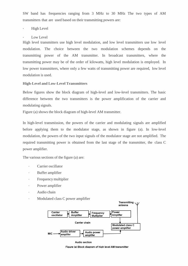
Figure (a) shows the block diagram of high-level AM transmitter.

In high-level transmission, the powers of the carrier and modulating signals are amplified

before applying them to the modulator stage, as shown in figure (a). In low-level

modulation, the powers of the two input signals of the modulator stage are not amplified. The

required transmitting power is obtained from the last stage of the transmitter, the class C

power amplifier.

The various sections of the figure (a) are:

· Carrier oscillator

· Buffer amplifier

· Frequency multiplier

· Power amplifier

· Audio chain

· Modulated class C power amplifier

Carrier oscillator The carrier oscillator generates the carrier signal, which lies in the RF range. The frequency

of the carrier is always very high. Because it is very difficult to generate high frequencies

with good frequency stability, the carrier oscillator generates a sub multiple with the required

carrier frequency. This sub multiple frequency is multiplied by the frequency multiplier

stage to get the required carrier frequency. Further, a crystal oscillator can be used in this

stage to generate a low frequency carrier with the best frequency stability. The frequency

multiplier stage then increases the frequency of the carrier to its required value.

Buffer Amplifier The purpose of the buffer amplifier is twofold. It first matches the output impedance of the

carrier oscillator with the input impedance of the frequency multiplier, the next stage of the

carrier oscillator. It then isolates the carrier oscillator and frequency multiplier.

This is required so that the multiplier does not draw a large current from the carrier

oscillator. If this occurs, the frequency of the carrier oscillator will not remain stable.

Frequency Multiplier The sub-multiple frequency of the carrier signal, generated by the carrier oscillator, is now

applied to the frequency multiplier through the buffer amplifier. This stage is also known as

harmonic generator. The frequency multiplier generates higher harmonics of carrier oscillator

frequency. The frequency multiplier is a tuned circuit that can be tuned to the requisite carrier

frequency that is to be transmitted.

Power Amplifier The power of the carrier signal is then amplified in the power amplifier stage. This is the basic

requirement of a high-level transmitter. A class C power amplifier gives high power current

pulses of the carrier signal at its output.

Audio Chain The audio signal to be transmitted is obtained from the microphone, as shown in figure (a).

The audio driver amplifier amplifies the voltage of this signal. This amplification is

necessary to drive the audio power amplifier. Next, a class A or a class B power amplifier

amplifies the power of the audio signal.

Modulated Class C Amplifier This is the output stage of the transmitter. The modulating audio signal and the carrier

signal, after power amplification, are applied to this modulating stage. The modulation takes

place at this stage. The class C amplifier also amplifies the power of the AM signal to the

reacquired transmitting power. This signal is finally passed to the antenna., which radiates the

signal into space of transmission.

Figure shows the block diagram of a low-level AM transmitter.

The low-level AM transmitter shown in the figure (b) is similar to a high-level transmitter,

except that the powers of the carrier and audio signals are not amplified. These two

signals are directly applied to the modulated class C power amplifier.

Modulation takes place at the stage, and the power of the modulated signal is amplified to

the required transmitting power level. The transmitting antenna then transmits the signal.

FM transmitter The following image shows the block diagram of the FM transmitter and the required

components of the FM transmitter are; microphone, audio pre amplifier, modulator,

oscillator, RF- amplifier and antenna. There are two frequencies in the FM signal, first one is

carrier frequency and the other one is audio frequency. The audio frequency is used to

modulate the carrier frequency. The FM signal is obtained by differing the carrier frequency

by allowing the AF. The FM transistor consists of oscillator to produce the RF signal.

Block Diagram of FM Transmitter:

The following circuit diagram shows the FM transmitter circuit and the required electrical

and electronic components for this circuit is the power supply of 9V, resistor, capacitor,

trimmer capacitor, inductor, mic, transmitter, and antenna. Let us consider the microphone to

understand the sound signals and inside the mic there is a presence of capacitive sensor. It

produces according to the vibration to the change of air pressure and the AC signal.

The formation of the oscillating tank circuit can be done through the transistor of 2N3904 by

using the inductor and variable capacitor. The transistor used in this circuit is an NPN

transistor used for general purpose amplification. If the current is passed at the inductor L1

and variable capacitor, then the tank circuit will oscillate at the resonant carrier

frequency of the FM modulation. The negative feedback will be the capacitor C2 to the

oscillating tank circuit.

To generate the radio frequency carrier waves the FM transmitter circuit requires an

oscillator. The tank circuit is derived from the LC circuit to store the energy for

oscillations. The input audio signal from the mic penetrated to the base of the transistor,

which modulates the LC tank circuit carrier frequency in FM format. The variable capacitor

is used to change the resonant frequency for fine modification to the FM frequency

band. The modulated signal from the antenna is radiated as radio waves at the FM frequency

band and the antenna is nothing but copper wire of 20cm long and 24 gauge. In this circuit

the length of the antenna should be significant and here you can use the 25-27 inches long

copper wire of the antenna.

UNIT-2

SUPER HETERODYNE RECEIVER There are some key circuit blocks that form the basic super heterodyne receiver. Although

more complicated receivers can be made, the basic circuit is widely used – further blocks

can add improved performance or additional functionality and their operation within the

whole receiver is normally easy to determine once the basic block diagram is understood.

• RF tuning & amplification: This RF stage within the overall block diagram for the

receiver provides initial tuning to remove the image signal. It also provides some

amplification. If noise performance for the receiver is important, then this stage will

be designed for optimum noise performance. This RF amplifier circuit block will also

increase the signal level so that the noise introduced by later stages is at a lower level

in comparison to the wanted signal.

• Local oscillator: The local oscillator circuit block can take a variety of forms. Early

receivers used free running local oscillators. Today most receivers use frequency

synthesizers, normally based around phase locked loops. These provide much

greater levels of stability and enable frequencies to be programmed in a variety of

ways.

• Mixer: Both the local oscillator and incoming signal enter this block within the

super heterodyne receiver. The wanted signal is converted to the intermediate

frequency.

• IF amplifier & filter: This super heterodyne receiver block provides the majority of

gain and selectivity. High performance filters like crystal filters may be used,

although LC or ceramic filters may be used within domestic radios.

• Demodulator: The super heterodyne receiver block diagram only shows one

demodulator, but in reality radios may have one or more demodulators dependent upon

the type of signals being receiver.

• Audio amplifier: Once demodulated, the recovered audio is applied to an audio

amplifier block to be amplified to the required level for loudspeakers or

headphones. Alternatively, the recovered modulation may be used for other

applications whereupon it is processed in the required way by a specific circuit

block.

Super heterodyne receiver block diagram Signals enter the receiver from the antenna and are applied to the RF amplifier where they

are tuned to remove the image signal and also reduce the general level of unwanted signals on

other frequencies that are not required.

The signals are then applied to the mixer along with the local oscillator where the wanted

signal is converted down to the intermediate frequency. Here significant levels of

amplification are applied and the signals are filtered. This filtering selects signals on one

channel against those on the next. It is much larger than that employed in the front end. The

advantage of the IF filter as opposed to RF filtering is that the filter can be designed for a

fixed frequency. This allows for much better tuning. Variable filters are never able to provide

the same level of selectivity that can be provided by fixed frequency ones.

Once filtered the next block in the super heterodyne receiver is the demodulator. This could

be for amplitude modulation, single sideband, frequency modulation, or indeed any form of

modulation. It is also possible to switch different demodulators in according to the mode

being received.

The final element in the super heterodyne receiver block diagram is shown as an audio

amplifier, although this could be any form of circuit block that is used to process or

amplified the demodulated signal.

Block diagram summary

The diagram above shows a very basic version of the superhot or super heterodyne

receiver. Many sets these days are far more complicated. Some superhot radios have more

than one frequency conversion, and other areas of additional circuitry to provide the required

levels of performance.

However, the basic super heterodyne concept remains the same, using the idea of mixing the

incoming signal with a locally generated oscillation to convert the signals to a new

frequency

The parameters of the AM Receivers Are Sensitivity, Selectivity, Fidelity, Image

frequency rejection etc. some of which are explained below:

1. Selectively

• The selectivity of an AM receiver is defined as its ability to accept or select the

desired band of frequency and reject all other unwanted frequencies which can be

interfering signals.

• Adjacent channel rejection of the receiver can be obtained from the selectivity

parameter.

• Response of IF section, mixer and RF section considerably contribute towards

selectivity.

• The signal bandwidth should be narrow for better selectivity.

• Graphically selectivity can be represented as a curve shown in Fig1. Below, which

depicts the attenuation offered to the unwanted signals around the tuned frequency.

2. Fidelity

• Fidelity of a receiver is its ability to reproduce the exact replica of the transmitted

signals at the receiver output.

• For better fidelity, the amplifier must pass high bandwidth signals to amplify the

frequencies of the outermost sidebands, while for better selectivity the signal

should have narrow bandwidth. Thus a tradeoff is made between selectivity and

fidelity.

• Low frequency response of IF amplifier determines fidelity at the lower

modulating frequencies while high frequency response of the IF amplifier

determines fidelity at the higher modulating frequencies.

3. Sensitivity

• Sensitivity of a receiver is its ability to identify and amplify weak signals at the

receiver output.

• It is often defined in terms of voltage that must be applied to the input terminals of

the receiver to produce a standard output power which is measured at the output

terminals.

• The higher value of receiver gain ensures smaller input signal necessary to

produce the desired output power.

• Thus a receiver with good sensitivity will detect minimum RF signal at the input and

still produce utilizable demodulated signal.

• Sensitivity is also known as receiver threshold.

• It is expressed in microvolts or decibels.

• Sensitivity of the receiver mostly depends on the gain of IF amplifier.

• It can be improved by reducing the noise level and bandwidth of the receiver.

• Sensitivity can be graphically represented as a curve shown in Fig2. Below, which

depicts that sensitivity varies over the tuning band.

4. Double spotting

• Double spotting is a condition where the same desired signal is detected at two

nearby points on the receiver tuning dial.

• One point is the desired point while the other is called the spurious or image point.

• It can be used to determine the IF of an unknown receiver.

• Poor front-end selectivity and inadequate image frequency rejection leads to

double spotting.

• Double spotting is undesirable since the strong signal might mask and overpower the

weak signal at the spurious point in the frequency spectrum.

• Double spotting can be counter acted by improving the selectivity of RF amplifier and

increasing the value of IF.

• Consider an incoming strong signal of 1000 kHz and local oscillator tuned at 1455

kHz. Thus a signal of 455 kHz is produced at the output of the mixer which is the IF

frequency.

Now consider the same signal but with 545 kHz tuned local oscillator. Again we get 455 kHz

signal at the output.

Therefore, the same 1000 kHz signal will appear at 1455 kHz as well as 545 kHz on the

receiver dial and the image will not get rejected. This is known as Double spotting

phenomenon.

• It is also known as adjacent channel selectivity. In radio, the image rejection ratio, or image frequency rejection ratio, is the ratio of (a) the

intermediate-frequency (IF) signal level produced by the desired input frequency to

(b) that produced by the image frequency. The image rejection ratio is usually expressed in

dB when the image rejection ratio is measured, the input signal levels of the desired and

image frequencies must be equal for the measurement to be meaningful.

Selection of IF freq.

The choice of an IF frequency is one of those design trade-offs.

The lower the IF frequency used, the easier it is to achieve a narrow bandwidth to obtain good

selectivity in the receiver and the greater the IF stage gain. On the other hand, the higher the

IF, the further removed the image frequency is from the signal frequency and hence the better

the image rejection.

One problem of the problems of a super heterodyne receiver, is its ability to pick up a

second or image frequency that is twice the intermediate frequency away from the signal

frequency.

For example, if we have a signal frequency of 1 MHz which is mixed with an IF of 455 kHz. A

second or image signal, with a frequency equal to 1 MHz plus (2 x 455) kHz or 1.910 MHz,

can also mix with the 1.455 MHz to produce the 455 kHz.

The choice of IF is also affected by the selectivity of the RF end of the receiver. If the

receiver has a number of RF stages, it is better able to reject an image signal close to the

signal frequency and hence a lower IF channel can be tolerated. This is why modern rigs have

2 or even 3 IF stages.

The chosen IF frequency should be free from radio interference. Standard intermediate

frequencies have been established and these are kept dear of signal channel allocation.

As you have noted, 455 KHz is a common IF. This is because broadcasters settled on this as a

standard frequency during the broadcast AM days.

From a design point of view 455KHz it leads to poor image response when used above 10

MHz One commonly used IF for shortwave receivers is 1.600 MHz and this gives a much

improved image response for the HF spectrum. Ham band SSB HF transceivers have

commonly used 9 MHz as a receiver intermediate frequency

This frequency is a little high for ordinary tuned circuits to achieve the narrow bandwidth

needed in speech communication, however, when used with ceramic crystal filter networks

it leads to good results.

Some recent amateur transceivers use intermediate frequencies slightly below 9 MHz A

frequency of 8.830 MHz can be found in various Kenwood transceivers and a frequency of

8.987.5 MHz in some Yaesu transceivers. This change could possibly be to avoid the

second harmonic of the IF falling too near the edge of the 17m WARC band

Simple & Delayed AGC Automatic gain control (AGC) is a mechanism wherein the overall gain of the radio

receiver is automatically varied according to the changing strength of the received signal. This

is done to maintain the output at a constant level. If the gain is not varied as per the input

signal, consider a stronger input signal, then the signal might probably be distorted with some

of the amplifiers reaching saturation level. AGC is applied to the RF, IF and mixer stages,

which also helps in improving the dynamic range of the receiver antenna to 60-100 dB by

adjusting the gain of the various stages in the radio receiver. The AGC derives dc bias

voltage from the part of the detected signal to apply to the RF, IF and mixer stages to control

their gains. The Trans conductance and hence the gain of the devices used in these stages of

the receiver depends on the applied bias voltage or current. When the overall signal level

increases, the value of the applied AGC bias increase leading to the decrease in the gain of the

controlled stages. When there is no signal or signal with low value, there is minimum AGC

bias which results in amplifier generating maximum gain. AGC facilitates tuning to varying

signal strength stations providing a constant output. AGC smoothens the amplitude variations

of the input signal and the gain control does not have to be recalibrated every time the receiver

is tuned from station to station. An AGC which is not designed correctly can lead to

considerable distortion to a smooth signal.

There are two types of AGC circuits:

• Simple AGC: the gain control mechanism is active for high as well as low value of

carrier voltage.

• Delayed AGC: AGC bias is not applied to the amplifiers until signal strength crosses a

predetermined level, after which AGC bias is applied.

FM RECEIVER RF section

• Consists of a pre-selector and an amplifier

• Pre-selector is a broad-tuned band pass filter with an adjustable center frequency used

to reject unwanted radio frequency and to reduce the noise bandwidth.

• RF amplifier determines the sensitivity of the receiver and a predominant factor in determining the noise figure for the receiver.

Mixer/converter section

• Consists of a radio-frequency oscillator and a mixer.

• Choice of oscillator depends on the stability and accuracy desired. • Mixer is a nonlinear device to convert radio frequency to intermediate frequencies (i.e.

heterodyning process).

The shape of the envelope, the bandwidth and the original information contained

in the envelope remains unchanged although the carrier and sideband frequencies are

translated from RF to IF.

IF section

• Consists of a series of IF amplifiers and band pass filters to achieve most of the

receiver gain and selectivity.

• The IF is always lower than the RF because it is easier and less expensive to

construct high-gain, stable amplifiers for low frequency signals.

• IF amplifiers are also less likely to oscillate than their RF counterparts. Detector section

• To convert the IF signals back to the original source information (demodulation).

• Can be as simple as a single diode or as complex as a PLL or balanced demodulator.

Audio amplifier section

• Comprises several cascaded audio amplifiers and one or more speakers AGC (Automatic Gain Control)

• Adjust the IF amplifier gain according to signal level (to the average amplitude

signal almost constant).

• AGC is a system by means of which the overall gain of radio receiver is varied

automatically with the variations in the strength of received signals, to maintain the

output constant.

• AGC circuit is used to adjust and stabilize the frequency of local oscillator.

Types of AGC –No AGC, Simple AGC, Delayed AGC.

Communication receiver The receiving antenna intercepts the electromagnetic radiations and converts them into RF

voltage. The RF signal is then applied to the RF amplifier through the antenna coupling,

network, which matches the impedances of the antenna and the RE amplifier. The RF

amplifier amplifies this signal, which lies in the frequency range of 2 - 30 MHz The

amplified signal is fed to the first mixer, where it is mixed with the locally generated

signal. The frequency of the local oscillator, f01 is 650 kHz above the frequency the

receiver signal, fs. Thus, the frequency range of the first local oscillator is (fs + 650 kHz).

The first local oscillator and the RF amplifier are ganged together to generate the correct

oscillator frequency.

The mixer circuit generates an IF signal whose frequency is 650 kHz. This IF signal is

amplified by the first IF amplifier. After amplification, the IF signal is given to the second

mixer, which mixes this signal with another locally generated signal generated by the

second oscillator. The frequency of the second local oscillator is fixed at 500 kHz. As this

frequency is fixed, a crystal oscillator is used in this stage to have good frequency stability. The

second mixer generates the second IF signal. The value of the second IF frequency is 150

kHz, as it

is the

difference

between the

first IF

frequency (650

kHz) and the

second

local oscillator

frequency (500

kHz). The

frequency of

the second IF frequency is kept below the usual IF frequency of the AM receiver which is 455

kHz. The frequency of the first IF signal is kept above 455 kHz, up to a value of 650 kHz.

With this arrangement, the communication receiver has the advantages of both low and high

IF frequency. This technique of using two frequencies is known as double conversion.

The second IF signal is now applied to the second IF amplifier, which amplifies it to the

required value so that the signal is satisfactorily detected. The detector stage demodulates the

received signal and gives its output as the modulating signal, which is an audio signal.

This audio signal is then amplified by the audio stages which consist of the audio driver

amplifier and the audio output power amplifier. The audio signal is then given to the

speaker, which produces the sound. To control the gains of the amplifiers of the system, AGC

is employed. The AGC voltage is used to keep the volume of the receiver constant to the level

set by the listener. The output of the second IF amplifier is also given to the AGC detector, as

shown in Figure (a). The AGC detector produces a dc voltage, called the AGC bias voltage,

which is proportion to the carrier strength of the received signal. The signal is also

amplified by the AG amplifier before being detected to generate the AGC bias voltage. The

AGC bias Voltage generated is applied to the RF amplifier and first IF amplifier, to

control their gains. In addition to the above-mentioned sections of the AM communication

receiver, communication receiver has additional features that described next. Seat

Frequency Oscillator (BFO) Communication receivers can also receive telegraphic signals

that use Morse code, which is a pulse modulated RF carrier signal. Morse code is

transmitted as dots, dashes, and spaces. These are distinguished by different carrier

frequencies with constant amplitude. A normal diode detector used in an AM system is not

capable of distinguishing the presence or absence of a carrier signal, which is the usual

technique to transmit Morse code. For example, the absence of a carrier signal may represent a

space in the Morse code. To detect Morse code, a simple LC oscillator, which generates a

constant frequency of 1 KHz or 400 Hz above or below the second IF frequency, is provided

in the system. The LC oscillator is known as the BFO.. The output of the BFO is applied to

the second IF amplifier as its second input. The second IF signal and the output of the BFO

together generate whistles that indicate the presence of a dot, a dash, or a space. A switch is

provided in the receiver to select the option of receiving an audio signal or a telegraph signal.

This switch is in the off position when telegraph signals are not received. This provision is

known as variable selectivity.

Squelch or Muting When the communication transmitter does not transmit any signal, the

receiver receives only the noise present at its input. A good quality communication receiver

can amplify this noise to produce a very loud noise from the speaker. The main reason

behind this loud noise is that the AGC bias voltage which is proportion to the carrier

strength is absent. In the absence of the RF signal. Thus, the gains of the RF and IF amplifiers

are not controlled, and they provide maximum to the noise. The communication receivers

used by police, ambulances, and coast guard radio stations are continuously operated. In these

receivers, it is necessary to control the noise level in the absence of a carrier signal, as it will

irritate the user. This is done by providing a Squelch or muting circuit in the system. The

output of the AGC detector is also applied to the squelch circuit, as shown in Figure (a). In

the absence of a carrier, the AGC detector does not generate the AGC bias voltage. The

squelch circuit, in this condition, cuts off the audio amplifier stages to block the noise signal

to the speaker. As soon as the carrier signal is received, the AGC voltage is generated and the

audio amplifiers work as normal. Metering (Tuning Indicator) Tuning indicator is provided

in the receiver so that the operator knows if the receiver is tuned to the correct signal

frequency. This process is also called metering of the strength of the received signal. The

tuning indicator is either a set of light emitting diodes (LEDs) or an electronic meter, called

an S-Meter. When the receiver is tuned to the correct signal frequency, both the side bands

of the received signal are well accommodated and the detector generates a dc component.

This dc component is proportional to the received carrier strength. The tuning indicator uses

the dc component to indicate the strength of the received signal. The receiver is tuned

until the tuning indicator indicates the maximum possible value for the desired tuned

signal. Double Conversion in the double conversion technique, two intermediate

frequencies are generated instead of then single intermediate frequency used in commercial

AM receivers. In addition, this technique uses two local oscillators and two mixers, as shown

in Figure (a). The first local oscillator is a variable frequency oscillator that can generate an

IF frequency of 650 kHz. It is ganged with the RF amplifier to generate the correct local

oscillator frequency so that the mixer gives an output 650 kHz.

Receiver RF Transmitter Level Transmitter Frequency Transmitter Amplifier

Circuit Diagram

The second local oscillator is a crystal oscillator that generates a fixed frequency signal of 500

kHz. Therefore, the input to the second mixed is also a fixed IF frequency, and hence there is

no need for a variable local oscillator frequency. The second mixer generates an IF signal at

150 kHz. The two basic reasons for double conversion are: • It provides advantages of

having both higher and lower IF frequencies. • It provides a higher image frequency

rejection. Due to these reasons, double conversion has become popular in communication

receivers. Another technique called up-conversion, explained next, also though to get better

selectivity of the receiver. Up-Conversion The conversion technique generates an IF with a

frequency above the signal frequency. In conversion, IF frequency may have a value of 40

MHz for a signal frequency hand of 2-30 MHz The local oscillator frequency in this case will

be (fs + 40 MHz). In AM receivers, IF frequency is kept lower than the signal frequency: This

lower signal is used because capacitors and inductors arc available for selectivity networks,

called filters, at lower frequencies. The invention of crystal and ceramic filters at very high

frequencies provides an opportunity to adopt IF frequency higher than the signal

frequencies. Thus, the up-conversion technique has become very popular in

communication receivers due to the availability of good filters operated at higher

frequencies.

UNIT-3

EM spectrum The electromagnetic spectrum

is the range of frequencies

(the spectrum) of

electromagnetic radiation and

their respective wavelengths

and photon energies.

The electromagnetic spectrum

covers electromagnetic waves

with frequencies ranging

from below one hertz to

above 1025 hertz,

corresponding to wavelengths

from thousands of kilometres

down to a fraction of the size

of an atomic nucleus. This

frequency range is divided

into separate bands, and the

electromagnetic waves within

each frequency band are

called by different names;

beginning at the low

frequency (long wavelength)

end of the

spectrum these are: radio waves, microwaves, infrared, visible light, ultraviolet, X-rays,

and gamma rays at the high-frequency (short wavelength) end. The electromagnetic waves in

each of these bands have different characteristics, such as how they are produced, how they

interact with matter, and their practical applications. The limit for long wavelengths is the size

of the universe itself, while it is thought that the short wavelength limit is in the vicinity of

the Planck length. Gamma rays, X-rays, and high ultraviolet are classified as ionizing radiation

as their photons have enough energy to ionize atoms, causing chemical reactions. Exposure to

these rays can be a health hazard, causing radiation sickness, DNA damage and cancer.

Radiation of visible light wavelengths and lower are called nonionizing radiation as they

cannot cause these effects.

In most of the frequency bands above, a technique called spectroscopy can be used to

physically separate waves of different frequencies, producing a spectrum showing the

constituent frequencies. Spectroscopy is used to study the interactions of electromagnetic

waves with matter. Other technological uses are described under electromagnetic radiation.

The radiation pattern of a dipole antenna is of particular importance.

The radiation pattern reflects the 'sensitivity' of the antenna in different directions and a

knowledge of this allows the antenna to be orientated in the optimum direction to ensure the

required performance.

Radiation pattern and polar diagram The radiation pattern of any antenna can be plotted. This is plotted onto a polar diagram. A

polar diagram is a plot that indicates the magnitude of the response in any direction.

At the centre of the diagram is a point of referred to as the origin. This is surrounded by a

curve whose radius at any given point is proportional to the magnitude of the property

measured in the direction of that point.

Antenna polar diagram concept Polar diagrams are used for plotting the radiation patterns of antennas as well as other

applications like measuring the sensitivity of microphones in different directions, etc.

The radiation pattern shown on a polar diagram is taken to be that of the plane in which the

diagram plot itself. For a dipole it is possible to look at both the along the axis of the antenna

and also at right angles to it. Normally these would be either vertical or horizontal planes.

One fundamental fact about antenna radiation patterns and polar diagrams is that the

receiving pattern, i.e. the receiving sensitivity as a function of direction is identical to the far-

field radiation pattern of the antenna when used for transmitting. This results from the

reciprocity theorem of electromagnetics. Accordingly, the radiation patterns the antenna

can be viewed as either transmitting or receiving, whichever is more convenient.

Half wave dipole radiation pattern The radiation pattern of a half wave dipole antenna that the direction of maximum

sensitivity or radiation is at right angles to the axis of the RF antenna. The radiation falls to

zero along the axis of the RF antenna as might be expected.

Radiation pattern of a half wave dipole antenna in free space

In a three dimensional plot, the radiation pattern envelope for points of equal radiation

intensity for a doughnut type shape, with the axis of the antenna passing through the hole in the

centre of the doughnut.

Radiation patterns for multiple half wavelength dipoles If the length of the dipole antenna is changed from a half wavelength, then the radiation

pattern is altered. As the length of the antenna is extended it can be seen that the familiar

figure of eight pattern changes to give main lobes and a few side lobes. The main lobes

move progressively towards the axis of the antenna as the length increases.

Polarization of waves Polarization, also called wave polarization, is an expression of the orientation of the lines of

electric flux in an electromagnetic field (EM field). Polarization can be constant -- that is,

existing in a particular orientation at all times, or it can rotate with each wave cycle.

Polarization is important in wireless communications systems. The physical orientation of a

wireless antenna corresponds to the polarization of the radio waves received or

transmitted by that antenna. Thus, a vertical antenna receives and emits vertically polarized

waves, and a horizontal antenna receives or emits horizontally polarized waves. The best

short-range communications are obtained when the transmitting and receiving (source and

destination) antennas have the same polarization. The least efficient short-range

communications usually take place when the two antennas are at right angles (for example,

one horizontal and one vertical). Over long distances, the atmosphere can cause the

polarization of a radio wave to fluctuate, so the distinction between horizontal and vertical

becomes less significant.

Some wireless antennas transmit and receive EM waves whose polarization rotates 360

degrees with each complete wave cycle. This type of polarization, called elliptical or

circular polarization, can be either clockwise or counter clockwise. The best

communications results are obtained when the transmitting and receiving antennas have the

same sense of polarization (both clockwise or both counter clockwise). The worst

communications usually take place when the two antennas radiate and receive in the

opposite sense (one clockwise and the other counter clockwise).

Polarization affects the propagation of EM fields at infrared (IR), visible, ultraviolet (UV), and

even X-ray wavelength s. In ordinary visible light, there are numerous wave components at

random polarization angles. When such light is passed through a special filter, the filter

blocks all light except that having a certain polarization. When two polarizing filters are

placed so a ray of light passes through them both, the amount of light transmitted depends on

the angle of the polarizing filters with respect to each other. The most light is transmitted

when the two filters are oriented so they polarize light in the same direction. The least light

is transmitted when the filters are oriented at right angles to each other.

Point source Radio wave sources which are smaller than one radio wavelength are also generally

treated as point sources. Radio emissions generated by a fixed electrical circuit are

usually polarized, producing anisotropic radiation. If the propagating medium is lossless,

however, the radiant power in the radio waves at a given distance will still vary as the

inverse square of the distance if the angle remains constant to the source polarization.

Directive gain or directivity Is a different measure which does not take an antenna's electrical efficiency into account? This

term is sometimes more relevant in the case of a receiving antenna where one is concerned

mainly with the ability of an antenna to receive signals from one direction while rejecting

interfering signals coming from a different direction.

Power gain Power gain (or simply gain) is a unit less measure that combines an antenna's efficiency

Antenna and directivity D.

G = E antenna. D Aperture

In electromagnetics and antenna theory, antenna aperture, effective area, or receiving cross

section, is a measure of how effective an antenna is at receiving the power of

electromagnetic radiation (such as radio waves). The aperture is defined as the area,

oriented perpendicular to the direction of an incoming electromagnetic wave, which

would intercept the same amount of power from that wave as is produced by the antenna

receiving it. At any point, a beam of electromagnetic radiation has an irradiance or power flux

density (PFD) which is the amount of energy passing through a unit area of one square

meter

Effective aperture

The effective antenna aperture/area is a theoretical value which is a measure of how

effective an antenna is at receiving power. The effective aperture/area can be calculated by

knowing the gain of the receiving antenna.

Where, Ae = Effective Antenna Aperture

λ = Wavelength = C/F (where f = frequency, C = speed of light) G=

Antenna gain (Linear Value)

Radiation Pattern The energy radiated by an antenna is represented by the Radiation pattern of the antenna.

Radiation Patterns are diagrammatical representations of the distribution of radiated energy

into space, as a function of direction.

The radiation patterns can be field patterns or power patterns. The field patterns are plotted as a function of electric and magnetic fields. They are

plotted on logarithmic scale.

The power patterns are plotted as a function of square of the magnitude of electric and

magnetic fields. They are plotted on logarithmic or commonly on dB scale.

Beam width In a radio antenna pattern, the half power beam width is the angle between the half-

power (-3 dB) points of the main lobe, when referenced to the peak effective radiated

power of the main lobe. See beam diameter. Beam width is usually but not always

expressed in degrees and for the horizontal plane.

Radiation resistance is that part of an antenna's feed point resistance that is caused by the

radiation of electromagnetic waves from the antenna, as opposed to loss resistance (also

called ohmic resistance) which generally causes the antenna to heat up. The total of radiation

resistance and loss resistance is the electrical resistance of the antenna.

Radiation resistance The radiation resistance is determined by the geometry of the antenna, where loss

resistance is primarily determined by the materials of which it is made. While the energy lost

by ohmic resistance is converted to heat, the energy lost by radiation resistance is converted

to electromagnetic radiation.

Radiation resistance is caused by the radiation reaction of the conduction electrons in the

antenna.

Half wave dipole

The dipole antenna is cut and bent for effective radiation. The length of the total wire,

which is being used as a dipole, equals half of the wavelength (i.e., l = λ/2). Such an

antenna is called as half-wave dipole antenna. This is the most widely used antenna

because of its advantages. It is also known as Hertz antenna.

Frequency range

The range of frequency in which half-wave dipole operates is around 3 KHz to 300GHz.

This is mostly used in radio receivers.

Construction & Working of Half-Wave Dipole

It is a normal dipole antenna, where the frequency of its operation is half of its

wavelength. Hence, it is called as half-wave dipole antenna.

The edge of the dipole has maximum voltage. This voltage is alternating (AC) in nature. At

the positive peak of the voltage, the electrons tend to move in one direction and at the

negative peak, the electrons move in the other direction. This can be explained by the

figures given below.

The figures given above show the working of a half-wave dipole.

• Fig 1 shows the dipole when the charges induced are in positive half cycle. Now the

electrons tend to move towards the charge.

• Fig 2 shows the dipole with negative charges induced. The electrons here tend to

move away from the dipole.

• Fig 3 shows the dipole with next positive half cycle. Hence, the electrons again

move towards the charge.

The cumulative effect of this produces a varying field effect which gets radiated in the

same pattern produced on it. Hence, the output would be an effective radiation following the

cycles of the output voltage pattern. Thus, a half-wave dipole radiates effectively.

The above figure shows the current distribution in half wave dipole. The directivity of half

wave dipole is 2.15dBi, which is reasonably good. Where, ‘I’ represents the isotropic

radiation.

Radiation Pattern

The radiation pattern of this half-wave dipole is Omni-directional in the H-plane. It is

desirable for many applications such as mobile communications, radio receivers etc.

The above figure indicates the radiation pattern of a half wave dipole in both H-plane and

V-plane.

The radius of the dipole does not affect its input impedance in this half wave dipole,

because the length of this dipole is half wave and it is the first resonant length. An

antenna works effectively at its resonant frequency, which occurs at its resonant

length.

Advantages

The following are the advantages of half-wave dipole antenna −

• Input impedance is not sensitive.

• Matches well with transmission line impedance.

• Has reasonable length.

• Length of the antenna matches with size and directivity.

Disadvantages

The following are the disadvantages of half-wave dipole antenna −

• Not much effective due to single element.

• It can work better only with a combination. Applications

The following are the applications of half-wave dipole antenna −

• Used in radio receivers.

• Used in television receivers.

• When employed with others, used for wide variety of applications.

Medium wave antenna

These antennas have been developed in order to cover mobile systems needs as well as the

emergency service of temporary MW AM broadcasting. They can also be used as

stationary antennas for services in the MW broadcasting range. The whole antenna

system comprises: antenna, matching unit and a coaxial feeder line. The antenna consists of a

grounded vertical tower with six folded wires spaced in 60 degrees around the tower. The folds

are tied together on the ring at the base of the antenna. The matching unit is designed so

that it can match transmitter output to the antenna input impedance over the whole MW

band. All components are placed in a weatherproof Al-box that makes it ready for immediate

service.

A flexible coaxial cable is used as a connection between the transmitter and the antenna

matching unit, especially in case of mobile application. The ground screen consists of 60

copper wires equispaced around the tower. Each folded Unipolar Antenna is designed to

withstand nominal radiating power +125 % amplitude modulation in the frequency range

525 to 1605 kHz.

A Folded Unipolar Antenna has the following advantages in comparison with series fed and

top-loaded antennas:

• greater radiation resistance

• greater bandwidth of overall system

• no base insulator required, hence, the tower is at ground potential for lighting

protection

• no lighting chokes or transformers are required when tower lights are used

• better stability in inclement weather Folded dipole antenna

In its basic form the folded dipole antenna consists of a basic dipole with an added

conductor connecting the two ends together to make a complete loop of wire or other

conductor. As the ends appear to be folded back, the antenna is called a folded dipole.

The basic format for the folded dipole aerial is shown below. As can be seen from this it is a

balanced antenna, like the standard dipole, although it can be fed with unbalanced feeder

provided that a balun of some form is used to transform from an unbalanced to balance feed

structure.

Half wave dipole antenna The folded dipole antenna uses an extra wire connecting both ends of the previous dipole as

shown. Often this is achieved by using a wire or rod of the same diameter for all

sections of the antenna, but this is not always the case.

Also the wires or rods are typically equi-spaced along the length of the parallel elements. This

can be achieved in a number of ways. Often for VHF or UHF antennas the rigidity of the

elements is sufficient, but at lower frequencies spacers may need to be employed. To

keep the wires apart. Obviously if they are not insulated it is imperative to keep them from

shorting. In some instances, flat feeder can be used.

Half-wave folded dipole antenna

One of the main reasons for using the folded dipole aerial is the increase in feed impedance

that it provides. If the conductors in the main dipole and the second or "fold" conductor are

the same diameter, then it is found that there is a fourfold increase (i.e. two squared) in the feed

impedance. In free space, this gives an increase in feed impedance from 73Ω to around

300Ω ohms. Additionally, the RF antenna has a wider bandwidth.

Loop antenna A loop antenna is a radio antenna consisting of a loop or coil of wire, tubing, or other

electrical conductor usually fed by a balanced source or feeding a balanced load. Within this

physical description there are two distinct antenna types. The large self-resonant loop

antenna has a circumference close to one wavelength of the operating frequency and so is

resonant at that frequency. This category also includes smaller loops 5% to 30% of a

wavelength in circumference, which use a capacitor to make them resonant. These

antennas are used for both transmission and reception. In contrast, small loop antennas less

than 1% of a wavelength in size are very inefficient radiators, and so are only used for

reception. An example is the ferrite (loop stick) antenna used in most AM broadcast radios.

Loop antennas have a dipole radiation pattern; they are most sensitive to radio

waves in two broad lobes in opposite directions, 180° apart. Due to this directional

pattern they are used for radio direction finding (RDF), to locate the position of a

transmitter.

Radiation Pattern The radiation pattern of these antennas will be same as that of short horizontal dipole

antenna.

The radiation pattern for small, high-efficiency loop antennas is shown in the figure given

above. The radiation patterns for different angles of looping are also illustrated clearly in the

figure. The tangent line at 0° indicates vertical polarization, whereas the line with 90° indicates

horizontal polarization.

Advantages The following are the advantages of Loop antenna −

• Compact in size

• High directivity

Disadvantages

• The following are the disadvantages of Loop antenna −

• Impedance matching may not be always good

• Has very high resonance quality factor

Applications

• The following are the applications of Loop antenna −

• Used in RFID devices

• Used in MF, HF and Short wave receivers

• Used in Aircraft receivers for direction finding

• Used in UHF transmitters

Yagi Antenna / Yagi-Uda Antenna The Yagi antenna or Yagi-Uda antenna / aerial is one of the most successful RF antenna

designs for directive antenna applications. The Yagi or Yagi-Uda antenna is used in a wide

variety of applications where an RF antenna design with gain and directivity is required. The

Yagi has become particularly popular for television reception, but it is also used in very

many other domestic and commercial applications where an RF antenna is needed that has

gain and directivity. Not only is the gain of the Yagi antenna important as it enables

better levels of signal to noise ratio to be achieved, but also the directivity can be

used to reduce interference levels by focussing the transmitted power on areas where it is

needed, or receiving signals best from where the emanate.

Yagi antenna - the basics

The Yagi antenna design has a dipole as the main radiating or driven element. Further

'parasitic' elements are added which are not directly connected to the driven element.

These parasitic elements within the Yagi antenna pick up power from the dipole and re-

radiate it. The phase is in such a manner that it affects the properties of the RF antenna as a

whole, causing power to be focussed in one particular direction and removed from others.

The parasitic elements of the Yagi antenna operate by re-radiating their signals in a

slightly different phase to that of the driven element. In this way the signal is reinforced in

some directions and cancelled out in others. It is found that the amplitude and phase of the

current that is induced in the parasitic elements is dependent upon their length and the

spacing between them and the dipole or driven element.

There are three types of element within a Yagi antenna:

• Driven element: The driven element is the Yagi antenna element to which power is

applied. It is normally a half wave dipole or often a folded dipole.

• Reflector: The Yagi antenna will generally only have one reflector. This is behind the

main driven element, i.e. the side away from the direction of maximum sensitivity.

Further reflectors behind the first one adds little to the performance. However, many

designs use reflectors consisting of a reflecting plate, or a series of parallel rods simulating

a reflecting plate. This gives a slight improvement in performance, reducing the level of

radiation or pick-up from behind the antenna, i.e. in the backwards direction.

Typically, a reflector will add around 4 or 5 dB of gain in the forward direction.

• Director: There may be none, one of more reflectors in the Yagi antenna. The

director or directors are placed in front of the driven element, i.e. in the direction of

maximum sensitivity. Typically, each director will add around 1 dB of gain in the

forward direction, although this level reduces as the number of director’s

increases.

The antenna exhibits a directional pattern consisting of a main forward lobe and a

number of spurious side lobes. The main one of these is the reverse lobe caused by

radiation in the direction of the reflector. The antenna can be optimised to either reduce this

or produce the maximum level of forward gain. Unfortunately, the two do not coincide

exactly and a compromise on the performance has to be made depending upon the

application.

Yagi antenna advantages

• The Yagi antenna offers many advantages for its use. The antenna provides many

advantages in a number of applications:

• Antenna has gain allowing lower strength signals to be received.

• Yagi antenna has directivity enabling interference levels to be minimised.

• Straightforward construction. - The Yagi antenna allows all constructional

elements to be made from rods simplifying construction.

• The construction enables the antenna to be mounted easily on vertical and other poles

with standard mechanical fixings

The Yagi antenna also has a number of disadvantages that need to be considered.

• For high gain levels the antenna becomes very long

• Gain limited to around 20dB or so for a single antenna The Yagi antenna is a particularly useful form of RF antenna design. It is widely used in

applications where an RF antenna design is required to provide gain and directivity. In this

way the optimum transmission and reception conditions can be obtained.

Ferrite rod antenna The ferrite rod antenna is a form of RF antenna design that is almost universally used in

portable transistor broadcast receivers as well as many hi-fi tuners where reception on the

long, medium and possibly the short wave bands is required.

Ferrite rod antennas are also being used increasingly in wireless applications in areas such

as RFID. Here the volumes of antennas required can be huge. The antennas also need

to be compact and effective, making ferrite rod antennas an ideal solution. Ferrite rod

antenna basics

As the name suggests the antenna consists of a rod made of ferrite, an iron based magnetic

material. A coil is would around the ferrite rod and this is brought to resonance using a

variable tuning capacitor contained within the radio circuitry itself and in this way the

antenna can be tuned to resonance. As the antenna is tuned it usually forms the RF tuning

circuit for the receiver, enabling both functions to be combined within the same

components, thereby reducing the number of components and hence the cost of the set.

Typical ferrite rod antenna assembly used in a portable radio The ferrite rod antenna operates using the high permeability of the ferrite material and in its

basic form this may be thought of as "concentrating" the magnetic component of the radio

waves. This is brought about by the high permeability μ of the ferrite.

The fact that this RF antenna uses the magnetic component of the radio signals in this way

means that the antenna is directive. It operates best only when the magnetic lines of force fall

in line with the antenna. This occurs when it is at right angles to the direction of the

transmitter. This means that the antenna has a null position where the signal level is at a

minimum when the antenna is in line with the direction of the transmitter.

Operation of a ferrite rod antenna Ferrite rod antenna performance

This form of RF antenna design is very convenient for portable applications, but its

efficiency is much less than that of a larger RF antenna. The performance of the ferrite also

limits the frequency response. Normally this type of RF antenna design is only

effective on the long and medium wave bands, but it is sometimes used for lower

frequencies in the short wave bands although the performance is significantly degraded,

mainly arising from the losses in the ferrite. This limits their operation normally to

frequencies up to 2 or 3 MHz

Ferrite rod antennas are normally only used for receiving. They are rarely used for

transmitting anything above low levels of power in view of their poor efficiency. It any

reasonable levels of power were fed into them they would soon become very hot and there

would be a high likelihood that they would be destroyed. Nevertheless, they can be used as a

very compact form of transmitting antenna for applications where efficiency is not an issue

and where power levels are very low. As they are very much more compact

than other forms of low or medium frequency RF antenna, this can be an advantage, and as a

result they are being used in applications such as RFID.

Broadside Array

The broadside array is defined as “the radiation pattern's direction is perpendicular or

broadside to the array axis”.

It uses the dipole elements that are fed in phase and separated by the one-half wave

length. A broadside array is a type of antenna array which is used to radiate the energy in

specific direction to make better transmission. It is a bidirectional array which can send and

receive process at both ends (sending and receiving end).

The front view of the broadside array is shown below.

The side view of the broadside array is shown below.

From this Figure 1, the broadside array is at extreme right angle direction to the array

plane. However, due to pattern cancellation in the path joining at the centre, the radiation

pattern is too less.

Radiation pattern:

There are different types antenna array present. Each have their own radiation pattern. The

broadside array's pattern is drawn.

This pattern is at right angles to the plane and is bi-directional. The radiation beam has very

narrow pattern and has high gain.

End fire array

The physical arrangement of end-fire array is same as that of the broad side array. The

magnitude of currents in each element is same, but there is a phase difference between these

currents. This induction of energy differs in each element, which can be understood by

the following diagram.

The above figure shows the end-fire array in top and side views respectively.

There is no radiation in the right angles to the plane of the array because of cancellation. The

first and third elements are fed out of phase and therefore cancel each other’s radiation.

Similarly, second and fourth are fed out of phase, to get cancelled.

The usual dipole spacing will be λ/4 or 3λ/4. This arrangement not only helps to avoid the

radiation perpendicular to the antenna plane, but also helps the radiated energy get diverted

to the direction of radiation of the whole array. Hence, the minor lobes are

avoided and the directivity is increased. The beam becomes narrower with the increased

elements.

Radiation Pattern

The Radiation pattern of end-fire array is uni-directional. A major lobe occurs at one end,

where maximum radiation is present, while the minor lobes represent the losses.

The figure explains the radiation pattern of an end-fire array. Figure 1 is the radiation

pattern for a single array, while figures 2, 3, and 4 represent the radiation pattern for

multiple arrays.

End-fire Array Vs Broad Side Array

We have studied both the arrays. Let us try to compare the end-fire and broad side

arrays, along with their characteristics.

The figure illustrates the radiation pattern of end-fire array and broad side array.

• Both, the end fire array and broad side array, are linear and are resonant, as they

consist of resonant elements.

• Due to resonance, both the arrays display narrower beam and high directivity.

• Both of these arrays are used in transmission purposes.

• Neither of them is used for reception, because the necessity of covering a range of

frequencies is needed for any kind of reception.

Rhombic antenna

The Rhombic Antenna is an equilateral parallelogram shaped antenna. Generally, it has two

opposite acute angles. The tilt angle, θ is approximately equal to 90° minus the angle of major

lobe. Rhombic antenna works under the principle of travelling wave radiator. It is arranged

in the form of a rhombus or diamond shape and suspended horizontally above the surface

of the earth.

Frequency Range

The frequency range of operation of a rhombic antenna is around 3MHz to 300MHz. This

antenna works in HF and VHF ranges.

Constructionof Rhombic Antenna

Rhombic antenna can be regarded as two V-shaped antennas connected end-to-end to form

obtuse angles. Due to its simplicity and ease of construction, it has many uses −

• In HF transmission and reception

• Commercial point-to-point communication

The construction of the rhombic antenna is in the form a rhombus, as shown in the figure.

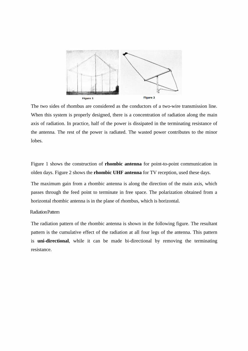
The two sides of rhombus are considered as the conductors of a two-wire transmission line.

When this system is properly designed, there is a concentration of radiation along the main

axis of radiation. In practice, half of the power is dissipated in the terminating resistance of

the antenna. The rest of the power is radiated. The wasted power contributes to the minor

lobes.

Figure 1 shows the construction of rhombic antenna for point-to-point communication in

olden days. Figure 2 shows the rhombic UHF antenna for TV reception, used these days.

The maximum gain from a rhombic antenna is along the direction of the main axis, which

passes through the feed point to terminate in free space. The polarization obtained from a

horizontal rhombic antenna is in the plane of rhombus, which is horizontal.

Radiation Pattern

The radiation pattern of the rhombic antenna is shown in the following figure. The resultant

pattern is the cumulative effect of the radiation at all four legs of the antenna. This pattern

is uni-directional, while it can be made bi-directional by removing the terminating

resistance.

The main disadvantage of rhombic antenna is that the portions of the radiation, which do

not combine with the main lobe, result in considerable side lobes having both horizontal and

vertical polarization.

Advantages

The following are the advantages of rhombic antenna −

• Input impedance and radiation pattern are relatively constant

• Multiple rhombic antennas can be connected

• Simple and effective transmission Disadvantages

The following are the disadvantages of rhombic antenna −

• Wastage of power in terminating resistor

• Requirement of large space

• Reduced transmission efficiency

Applications

The following are the applications of rhombic antenna −

• Used in HF communications

• Used in Long distance sky wave propagations

• Used in point-to-point communications

Another method of using long wire is by bending and making the wire into a loop shaped

pattern and observing its radiational parameters. This type of antennas is termed as loop

antennas.

Parabolic antenna A parabolic antenna is an antenna that uses a parabolic reflector, a curved surface with the

cross-sectional shape of a parabola, to direct the radio waves. The most common form is

shaped like a dish and is popularly called a dish antenna or parabolic dish. The main

advantage of a parabolic antenna is that it has high directivity. It functions similarly to a

searchlight or flashlight reflector to direct the radio waves in a narrow beam, or receive

radio waves from one particular direction only. Parabolic antennas have some of the highest

gains, meaning that they can produce the narrowest beam widths, of any antenna type. In

order to achieve narrow beam widths, the parabolic reflector must be much larger than the

wavelength of the radio waves used, so parabolic antennas are used in the high frequency part

of the radio spectrum, at UHF and microwave (SHF) frequencies, at which the

wavelengths are small enough that conveniently-sized reflectors can be used.

Parabolic antennas are used as high-gain antennas for point-to-point communications, in

applications such as microwave relay links that carry telephone and television signals

between nearby cities, wireless WAN/LAN links for data communications, satellite

communications and spacecraft communication antennas. They are also used in radio

telescopes.

The other large use of parabolic antennas is for radar antennas, in which there is a need to

transmit a narrow beam of radio waves to locate objects like ships, airplanes, and guided

missiles, and often for weather detection. With the advent of home satellite television

receivers, parabolic antennas have become a common feature of the landscapes of

modern countries.

The parabolic antenna was invented by German physicist Heinrich Hertz during his

discovery of radio waves in 1887. He used cylindrical parabolic reflectors with spark-

excited dipole antennas at their focus for both transmitting and receiving during his

historic experiments.

UNIT-4

Surface Waves

These are the principle waves used in AM, FM and TV broadcast. Objects such as buildings,

hills, ground conductivity, etc. have a significant impact on their strength. Surface waves

are usually vertically polarized with the electric field lines in contact with the earth.

Refraction

Because of refraction, the radio horizon is larger than the optical horizon by about 4/3. The

typical maximum direct wave transmission distance (in km) is dependent on the height of

the transmitting and receiving antennas (in meters):

However, the atmospheric conditions can have a dramatic effect on the amount of refraction.

Super Refraction

In super refraction, the rays bend more than normal thus shortening the radio horizon. This

phenomenon occurs when temperature increases but moisture decreases with

height. Paradoxically, in some cases, the radio wave can travel over enormous distances. It

can be reflected by the earth, rebroadcast and super refracted again.

Sub refraction

In sub refraction, the rays bend less than normal. This phenomenon occurs when temperature

decreases but moisture increases with height. In extreme cases, the radio signal may be

refracted out into space.

Space Waves

These waves occur within the lower 20 km of the atmosphere, and are comprised of a

direct and reflected wave. The radio waves having high frequencies are basically called as

space waves. These waves have the ability to propagate through atmosphere, from

transmitter antenna to receiver antenna. These waves can travel directly or can travel after

reflecting from earth’s surface to the troposphere surface of earth. So, it is also called

as Tropospheric Propagation. In the diagram of medium wave propagation, c shows the

space wave propagation. Basically the technique of space wave propagation is used in

bands having very high frequencies. E.g. V.H.F. band, U.H.F band etc. At such higher

frequencies the other wave propagation techniques like sky wave propagation, ground wave

propagation can’t work. Only space wave propagation is left which can handle frequency

waves of higher frequencies. The other name of space wave propagation is line of sight

propagation. There are some limitations of space wave propagation.

1. These waves are limited to the curvature of the earth. 2. These waves have line of sight propagation, means their propagation is along the line of sight

distance.

The line of sight distance is that exact distance at which both the sender and receiver

antenna are in sight of each other. So, from the above line it is clear that if we want to

increase the transmission distance then this can be done by simply extending the heights of

both the sender as well as the receiver antenna. This type of propagation is used

basically in radar and television communication.

The frequency range for television signals is nearly 80 to 200 MHz these waves are not

reflected by the ionosphere of the earth. The property of following the earth’s curvature is

also missing in these waves. So, for the propagation of television signal, geostationary

satellites are used. The satellites complete the task of reflecting television signals towards earth.

If we need greater transmission, then we have to build extremely tall antennas.

Direct Wave This is generally a line of sight transmission, however, because of atmospheric refraction the

range extends slightly beyond the horizon.

Ground Reflected Wave Radio waves may strike the earth, and bounce off. The strength of the reflection depends on

local conditions. The received radio signal can cancel out if the direct and reflected waves

arrive with the same relative strength and 180o out of phase with each other.

Horizontally polarized waves are reflected with almost the same intensity but with an 180o

phase reversal.

Vertically polarized waves generally reflect less than half of the incident energy. If the

angle of incidence is greater than 10o there is very little change in phase angle.

Sky Waves These waves head out to space but are reflected or refracted back by the ionosphere. The

height of the ionosphere ranges from 50 to 1,000 km. Radio waves are refracted by the

ionized gas created by solar radiation. The amount of ionization depends on the time of day,

season and the position in the 11-year sun spot cycle. The specific radio frequency refracted

is a function of electron density and launch angle. A communication channel thousands of

kilometres long can be established by successive reflections at the earth’s surface and in the

upper atmosphere. This ionosphere propagation takes place mainly in

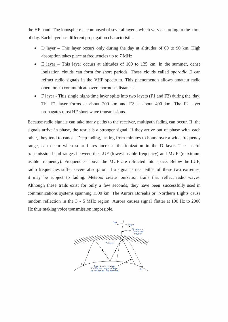
the HF band. The ionosphere is composed of several layers, which vary according to the time

of day. Each layer has different propagation characteristics:

• D layer – This layer occurs only during the day at altitudes of 60 to 90 km. High

absorption takes place at frequencies up to 7 MHz

• E layer – This layer occurs at altitudes of 100 to 125 km. In the summer, dense

ionization clouds can form for short periods. These clouds called sporadic E can

refract radio signals in the VHF spectrum. This phenomenon allows amateur radio

operators to communicate over enormous distances.

• F layer - This single night-time layer splits into two layers (F1 and F2) during the day.

The F1 layer forms at about 200 km and F2 at about 400 km. The F2 layer

propagates most HF short-wave transmissions.

Because radio signals can take many paths to the receiver, multipath fading can occur. If the

signals arrive in phase, the result is a stronger signal. If they arrive out of phase with each

other, they tend to cancel. Deep fading, lasting from minutes to hours over a wide frequency

range, can occur when solar flares increase the ionization in the D layer. The useful

transmission band ranges between the LUF (lowest usable frequency) and MUF (maximum

usable frequency). Frequencies above the MUF are refracted into space. Below the LUF,

radio frequencies suffer severe absorption. If a signal is near either of these two extremes,

it may be subject to fading. Meteors create ionization trails that reflect radio waves.

Although these trails exist for only a few seconds, they have been successfully used in

communications systems spanning 1500 km. The Aurora Borealis or Northern Lights cause

random reflection in the 3 - 5 MHz region. Aurora causes signal flutter at 100 Hz to 2000

Hz thus making voice transmission impossible.

Ionosphere

The ionosphere is the ionized part of Earth's upper atmosphere, from about 60 km (37 mi) to

1,000 km (620 mi) altitude, a region that includes the thermosphere and parts of the

mesosphere and exosphere. The ionosphere is ionized by solar radiation. It plays an

important role in atmospheric electricity and forms the inner edge of the magnetosphere. It has

practical importance because, among other functions, it influences radio propagation to

distant places on the Earth.

In the process of propagation of a wave, there are few terms which we come across quite

often. Let us discuss about these terms one by one.

Virtual Height

When a wave is refracted, it is bent down gradually, but not sharply. However, the path of

incident wave and reflected wave are same if it is reflected from a surface located at a greater

height of this layer. Such a greater height is termed as virtual height.

The figure clearly distinguishes the virtual height (height of wave, supposed to be reflected)

and actual height (the refracted height). If the virtual height is known, the angle of incidence

can be found.

Critical Frequency

Critical frequency for a layer determines the highest frequency that will be returned down

to the earth by that layer, after having been beamed by the transmitter, straight up into the

sky.

The rate of ionization density, when changed conveniently through the layers, the wave will

be bent downwards. The maximum frequency that gets bent and reaches the receiver station

with minimum attenuation, can be termed as critical frequency. This is denoted by fc.

Multi-path

For the frequencies above 30 MHz, the sky wave propagation exists. Signal multipath is the

common problem for the propagation of electromagnetic waves going through Sky wave.

The wave, which is reflected from the ionosphere, can be called as a hop or skip. There can

be a number of hops for the signal as it may move back and forth from the ionosphere and

earth surface many times. Such a movement of signal can be termed as multipath.

The above figure shows an example of multi-path propagation. Multipath propagation is a

term, which describes the multiple paths a signal travels to reach the destination. These

paths include a number of hops. The paths may be the results of reflection,

refraction or even diffraction. Finally, when the signal from such different paths gets to the

receiver, it carries propagation delay, additional noise, and phase differences etc., which

decrease the quality of the received output.

Fading

The decrease in the quality of the signal can be termed as fading. This happens because of

atmospheric effects or reflections due to multipath.

Fading refers to the variation of the signal strength with respect to time/distance. It is

widely prevalent in wireless transmissions. The most common causes of fading in the

wireless environment are multipath propagation and mobility (of objects as well as the

communicating devices).

Skip Distance

The measurable distance on the surface of the Earth from transmitter to receiver, where the

signal reflected from the ionosphere can reach the receiver with minimum hops or skips, is

known as skip distance.

Maximum Usable Frequency(MUF)

The Maximum Usable Frequency (MUF) is the highest frequency delivered by the

transmitter regardless of the power of the transmitter. The highest frequency, which is

reflected from the ionosphere to the receiver is called as critical frequency, fc.

Optimum Working Frequency(OWF)

The frequency, which is being used mostly for a particular transmission and which has been

predicted to be used over a particular period of time, over a path, is termed as Optimum

Working Frequency (OWF).

Inter Symbol Interference

Inter symbol interference (ISI) occurs more commonly in communication system. This is

the main reason for signal multipath also. When signals arrive at the receiving stations via

different propagation paths, they cancel out each other, which is known as the

phenomenon of signal fading. Here, it should be remembered that the signals cancel out

themselves in vector way.

Skin Depth

Electromagnetic waves are not suitable for underwater propagations. However, they can

propagate under water provided we make the frequency of propagation extremely low. The

attenuation of electromagnetic waves under water is expressed in terms of skin

depth. Skin depth is defined as the distance at which the signal is attenuated by 1/e. It is a

measure of depth to which an EM wave can penetrate. Skin depth is represented as δ (delta).

Duct Propagation

At a height of around 50 mts from the troposphere, a phenomenon exists; the temperature

increases with the height. In this region of troposphere, the higher frequencies or

microwave frequencies tend to refract back into the Earth’s atmosphere, instead of shooting

into ionosphere, to reflect. These waves propagate around the curvature of the earth even

up to a distance of 1000km.

This refraction goes on continuing in this region of troposphere. This can be termed as

Super refraction or Duct propagation.

The above image shows the process of Duct Propagation. The main requirement for the duct

formation is the temperature inversion. The increase of temperature with height, rather than

the decrease in the temperature is known as the phenomenon of temperature inversion.

We have discussed the important parameters, which we come across in wave

propagation. The waves of higher frequencies are transmitted and received using this wave

propagation technique.

UNIT: 5

Basics: How do Satellites Work

Two Stations on Earth want to communicate through radio broadcast but are too far

away to use conventional means.

The two stations can use a satellite as a relay station for their communication

One Earth Station sends a transmission to the satellite. This is called a Uplink.

The satellite Transponder converts the signal and sends it down to the second earth

station. This is called a Downlink.

The advantages of satellite communication over terrestrial communication are:

The coverage area of a satellite greatly exceeds that of a terrestrial system.

Transmission cost of a satellite is independent of the distance from the center of

the coverage area.

Satellite to Satellite communication is very precise.

Higher Bandwidths are available for use.

The disadvantages of satellite communication:

Launching satellites into orbit is costly.

Satellite bandwidth is gradually becoming used up.

There is a larger propagation delay in satellite communication than in terrestrial

communication.

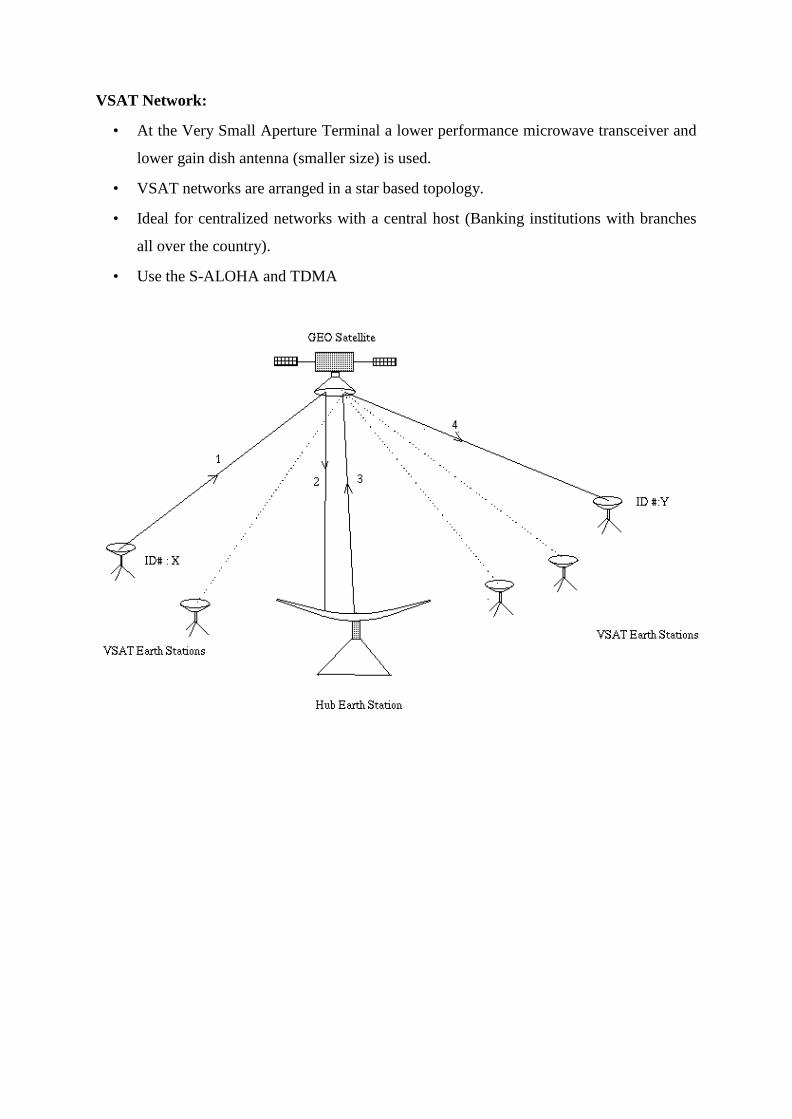
VSAT Network:

• At the Very Small Aperture Terminal a lower performance microwave transceiver and

lower gain dish antenna (smaller size) is used.

• VSAT networks are arranged in a star based topology.

• Ideal for centralized networks with a central host (Banking institutions with branches

all over the country).

• Use the S-ALOHA and TDMA