Uniqueness in the inverse scattering problem in a piecewise homogeneous medium

This article has been downloaded from IOPscience. Please scroll down to see the full text article.

2010 Inverse Problems 26 015002

(http://iopscience.iop.org/0266-5611/26/1/015002)

Download details:

IP Address: 128.143.22.132

The article was downloaded on 02/03/2013 at 10:55

Please note that terms and conditions apply.

View the table of contents for this issue, or go to the journal homepage for more

Home Search Collections Journals About Contact us My IOPscience

IOP PUBLISHING INVERSE PROBLEMS

Inverse Problems 26 (2010) 015002 (14pp) doi:10.1088/0266-5611/26/1/015002

Uniqueness in the inverse scattering problem in apiecewise homogeneous medium

Xiaodong Liu, Bo Zhang and Guanghui Hu

LSEC and Institute of Applied Mathematics, AMSS, Chinese Academy of Sciences,Beijing 100190, People’s Republic of China

E-mail: lxd230@163.com, b.zhang@amt.ac.cn and huguanghui@amss.ac.cn

Received 20 May 2009, in final form 26 August 2009Published 11 December 2009Online at stacks.iop.org/IP/26/015002

AbstractThe scattering of time-harmonic acoustic plane waves by an impenetrableobstacle in a piecewise homogeneous medium is considered. Havingestablished the well posedness of the direct problem by the variational method,we prove a uniqueness result for the inverse problem, that is, the uniquedetermination of the obstacle and its boundary condition from a knowledgeof the far-field pattern for incident plane waves. The proof is based on ageneralization of the mixed reciprocity relation.

1. Introduction

In this paper, we consider the problem of scattering of time-harmonic acoustic plane wavesby an impenetrable obstacle surrounded by a piecewise homogeneous medium. In practicalapplications, the background might not be homogeneous and then must be modeled as alayered medium. A medium of this type that is a nested body consisting of a finite numberof homogeneous layers occurs in various areas of applications such as radar, remote sensing,geophysics and nondestructive testing.

Let � denote the piecewise homogeneous medium which is a bounded and closed subsetof R

n (n = 2, 3) with a C2 boundary S0. Let �0 be the exterior region of �, that is,�0 = R

n\� (n = 2, 3). The interior of � is divided by means of closed and nonintersectingC2 surfaces Sj (j = 1, 2, . . . , N) into subsets (layers) �j (j = 1, 2, . . . , N + 1) with∂�j−1

⋂∂�j = Sj−1 (j = 1, 2, . . . , N + 1). The regions �j (j = 0, 1, . . . , N) are

homogeneous media. The region �N+1 is the impenetrable obstacle.We now give a brief description of the direct and inverse scattering problem.The propagation of time-harmonic acoustic waves in a piecewise homogeneous isotropic

medium in Rn (n = 2, 3) is modeled by the reduced wave equation or Helmholtz equation

with boundary conditions on their interfaces:

�u + k2j u = 0 in �j, j = 0, 1, . . . , N, (1.1)

0266-5611/10/015002+14$30.00 © 2010 IOP Publishing Ltd Printed in the UK 1

Inverse Problems 26 (2010) 015002 X Liu et al

u+ = u−,∂u+

∂ν= λj

∂u−∂ν

on Sj , j = 0, 1, . . . , N − 1, (1.2)

where ν is the unit outward normal to the boundary Sj, u+,∂u+∂ν

(u−,

∂u−∂ν

)denote the limit

of u, ∂u∂ν

on the surface Sj from the exterior (interior) of Sj and λj represents the nonnegativeconstant across the surface Sj (j = 0, 1, . . . , N − 1). Here, u denotes the complex-valuedspace-dependent part of the time-harmonic acoustic wave u(x)e−iωt and kj is the positivewave number given by kj = ωj/cj in terms of the frequency ωj and the sound speed cj in thecorresponding region �j (j = 0, 1, . . . , N). The distinct wave numbers kj (j = 0, 1, . . . , N)

correspond to the fact that the background medium consists of several physically differentmaterials. On these surfaces Sj (j = 0, 1, . . . , N − 1), the so-called transmission conditions(1.2) are imposed, which represent the continuity of the medium and equilibrium of the forcesacting on it. On the boundary SN of the obstacle �N+1 the total wave u has to satisfy a boundarycondition of the form

B(u) = 0 on SN . (1.3)

For a sound-soft obstacle the pressure of the total wave vanishes on the boundary, so aDirichlet boundary condition

B(u) := u on SN

is imposed. Similarly, the scattering from a sound-hard obstacle leads to a Neumann boundarycondition

B(u) := ∂u

∂νon SN

since the normal velocity of the total acoustic wave vanishes on the boundary. More generaland realistic boundary conditions are to allow that the normal velocity on the boundary isproportional to the excess pressure on the boundary, which leads to an impedance boundarycondition of the form

B(u) := ∂u

∂ν+ iλu on SN

with a nonnegative continuous function λ. Henceforth, we shall use B(u) = 0 to representeither of the above three types or mixed type of boundary conditions on SN. In the regionR

n\�N+1 (n = 2, 3), the total wave u is the superposition of the given incident plane waveui(x) = eik0x·d and the scattered wave us(x) which is required to satisfy the Sommerfeldradiation condition

limr→∞ r

n−12

(∂us

∂r− ik0u

s

)= 0 (1.4)

uniformly in all directions x/|x|, where r = |x|. It physically implies that energy is transportedto infinity and it is an important ingredient in ensuring that the physically correct solution ofthe scattering problem is selected. The well posedness (existence, uniqueness and stability)of the direct problem for a sound-soft obstacle using the theory of generalized solutions hasbeen studied by Athanasiadis and Stratis [2]. However, it is not suitable for our later use, thatis, the proof of the uniqueness result in the inverse problem. Therefore, following Cakoni andColton [3] and Mclean [19], we will give a new proof and consider a general mixed boundaryvalue problem in section 2. Moreover, it is known that us(x) has the following asymptotic

2

Inverse Problems 26 (2010) 015002 X Liu et al

representation:

us(x, d) = eik0|x|

|x| n−12

{u∞(x, d) + O

(1

|x|)}

as |x| → ∞ (1.5)

uniformly for all directions x := x/|x|, where the function u∞(x, d) defined on the unit sphereS is known as the far-field pattern with x and d denoting, respectively, the observation directionand the incident direction. By analyticity, the far-field pattern is completely determined onthe whole unit sphere S by only knowing it on some open subset S∗ of S [8]. Therefore, allthe uniqueness results carry over to the case of limited aperture problems where the far-fieldpattern is only known on some open subset S∗ of S. Without loss of generality, we can assumethat the far-field data are given on the whole unit sphere S, that is, in every possible observationdirection.

The inverse problem we consider in this paper is, given the wave numbers kj (j =0, 1, . . . , N), the nonnegative constants λj (j = 0, 1, . . . , N − 1) and the far-field patternu∞(x, d) for all incident plane waves with incident direction d ∈ S, to determine the locationand shape of the obstacle �N+1 and its boundary condition. As usual in most of the inverseproblems, the first question to ask in this context is the identifiability, that is, whether anobstacle can be identified from a knowledge of the far-field pattern. Mathematically, theidentifiability is the uniqueness issue which is of theoretical interest and is required in orderto proceed to efficient numerical methods of solutions.

In the last 30 years, both the inverse scattering problem in a homogeneous medium (i.e.N = 0) and the inverse medium problem have obtained great development in the theoreticaland numerical aspects. We refer to the monographs [8, 14, 23] and the references therein fora comprehensive discussion. As far as we know, there are few uniqueness results for inverseobstacle scattering in a piecewise homogeneous medium. When the obstacle is penetrable(with transmission boundary conditions), Athanasiadis, Ramm and Stratis [1] and Yan [25]proved that the obstacle is determined uniquely by the corresponding far-field pattern based onan orthogonality result [23]. Yan and Pang [26] gave a proof of uniqueness of the sound-softobstacle based on Schiffer’s idea. But their method cannot be extended to other boundaryconditions. They also gave a result for the case of a sound-hard obstacle in a two-layeredbackground medium in [22] using a generalization of Schiffer’s method. However, theirmethod is hard to be extended to the case of a multilayered background medium and seemsunreasonable to require the interior wave number to be in an interval.

There are few results on uniqueness in determining an obstacle or a medium buried inan inhomogeneous medium. In 1998, Kirsch and Paivarinta [15] proved that a sound-softobstacle or a penetrable inhomogeneous medium can be uniquely determined if the outsideinhomogeneity is known in advance. In the same year, Hahner [13] showed that both the sound-soft obstacle and the outside inhomogeneous medium in 2D can be uniquely determined by thefar-field patterns corresponding to all incident plane waves with an interval of wave numbers.Recently in [20], the authors showed that an obstacle buried in a known inhomogeneousmedium can be determined from measurements of the far field at a fixed wave number withouta priori knowledge of the boundary condition.

In recent years a new version of the linear sampling method based on the reciprocity gapfunctional has been developed for the numerical recovery of the shape of an obstacle or aninhomogeneous medium immersed in a two-layered background medium in the case when thenonnegative constants λ0 = 1 (see, e.g. [4–7, 10, 11] and the references therein). In particular,in [10], Cristo and Sun also proved that the obstacle and the surface impedance can be uniquelydetermined by the near field on ∂� for all point sources on the boundary of a box containing �.It should be pointed out that, recently in [24], Yaman presented a numerical method based on

3

Inverse Problems 26 (2010) 015002 X Liu et al

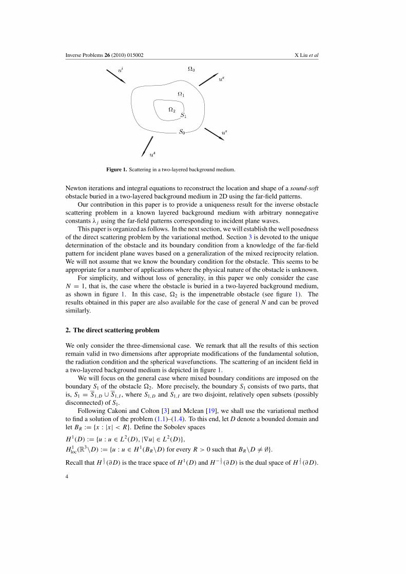
Figure 1. Scattering in a two-layered background medium.

Newton iterations and integral equations to reconstruct the location and shape of a sound-softobstacle buried in a two-layered background medium in 2D using the far-field patterns.

Our contribution in this paper is to provide a uniqueness result for the inverse obstaclescattering problem in a known layered background medium with arbitrary nonnegativeconstants λj using the far-field patterns corresponding to incident plane waves.

This paper is organized as follows. In the next section, we will establish the well posednessof the direct scattering problem by the variational method. Section 3 is devoted to the uniquedetermination of the obstacle and its boundary condition from a knowledge of the far-fieldpattern for incident plane waves based on a generalization of the mixed reciprocity relation.We will not assume that we know the boundary condition for the obstacle. This seems to beappropriate for a number of applications where the physical nature of the obstacle is unknown.

For simplicity, and without loss of generality, in this paper we only consider the caseN = 1, that is, the case where the obstacle is buried in a two-layered background medium,as shown in figure 1. In this case, �2 is the impenetrable obstacle (see figure 1). Theresults obtained in this paper are also available for the case of general N and can be provedsimilarly.

2. The direct scattering problem

We only consider the three-dimensional case. We remark that all the results of this sectionremain valid in two dimensions after appropriate modifications of the fundamental solution,the radiation condition and the spherical wavefunctions. The scattering of an incident field ina two-layered background medium is depicted in figure 1.

We will focus on the general case where mixed boundary conditions are imposed on theboundary S1 of the obstacle �2. More precisely, the boundary S1 consists of two parts, thatis, S1 = S1,D ∪ S1,I , where S1,D and S1,I are two disjoint, relatively open subsets (possiblydisconnected) of S1.

Following Cakoni and Colton [3] and Mclean [19], we shall use the variational methodto find a solution of the problem (1.1)–(1.4). To this end, let D denote a bounded domain andlet BR := {x : |x| < R}. Define the Sobolev spaces

H 1(D) := {u : u ∈ L2(D), |∇u| ∈ L2(D)},H 1

loc(R3\D) := {u : u ∈ H 1(BR\D) for every R > 0 such that BR\D �= ∅}.

Recall that H12 (∂D) is the trace space of H 1(D) and H− 1

2 (∂D) is the dual space of H12 (∂D).

4

Inverse Problems 26 (2010) 015002 X Liu et al

In order to study the mixed boundary value problem, we need the following Sobolevspaces on an open part of the boundary. We refer the reader to [19] for a systematic treatment.

Let � be an open subset of the boundary ∂D. Define

H12 (�) := {

u|� : u ∈ H12 (∂D)

}, H

12 (�) := {

u ∈ H12 (∂D) : supp(u) ⊆ �

}.

Both H12 (�) and H

12 (�) are Hilbert spaces equipped with the restriction of the inner product

of H12 (∂D). Hence, we can define the corresponding dual spaces

H− 12 (�) := (

H12 (�)

)′ = the dual space of H12 (�),

H− 12 (�) := (

H12 (�)

)′ = the dual space of H12 (�).

It can be shown (cf theorem A4 in [19]) that there exists a bounded extension operatorτ : H

12 (�) → H

12 (∂D). An important property of H

12 (�) is that the extension by zero to the

whole boundary ∂D of u ∈ H12 (�) is in H

12 (∂D) and the extension operator is bounded from

H12 (�) to H

12 (∂D). Based on these results, we can identify the dual spaces as follows:

H− 12 (�) := {u|� : u ∈ H− 1

2 (∂D)}, H− 12 (�) := {u ∈ H− 1

2 (∂D) : supp(u) ⊆ �}.Thus, the duality pairing can be explained as

H− 1

2 (�)〈v, u〉

H12 (�)

=H

− 12 (∂D)

〈v, u〉H

12 (∂D)

,

H− 1

2 (�)〈v, u〉

H12 (�)

=H

− 12 (∂D)

〈v, u〉H

12 (∂D)

,

where u ∈ H12 (∂D) is the extension by zero of u ∈ H

12 (�) and v ∈ H− 1

2 (∂D) is the extensionby zero of v ∈ H− 1

2 (�).Consider the mixed boundary value problem: given h ∈ L2(�1), g ∈ H− 1

2 (S0),f ∈ H

12 (S1,D) and p ∈ H− 1

2 (S1,I ), find u ∈ H 1(�1) ∩ H 1loc(�0) such that

�u + k20u = 0 in �0, (2.1)

�u + k21u = h in �1, (2.2)

u+ = u−,∂u+

∂ν− λ0

∂u−

∂ν= g on S0, (2.3)

u = f on S1,D, (2.4)

∂u

∂ν+ iλu = p on S1,I , (2.5)

limr→∞ r

(∂u

∂r− ik0u

)= 0 (2.6)

where r = |x|, kj (j = 0, 1) are positive wave numbers, λ0 is a nonnegative constant and λ isa nonnegative continuous impedance function. Here, equations (2.1) and (2.2) are understoodin a distributional sense and the boundary conditions (2.3)–(2.5) are understood in the tracesense.

Remark 2.1. The case S1,I = ∅ corresponds to a sound-soft obstacle, and the caseS1,D = ∅, λ = 0 corresponds to a sound-hard obstacle.

Remark 2.2. The acoustic scattering of the incident plane wave ui = eik0x·d is a particular caseof the problem (2.1)–(2.6). In particular, the scattered field us satisfies the problem (2.1)–(2.6)with u = us, h = (

k20 −k2

1

)ui |�1 , g = (λ0−1) ∂ui

∂ν|S0 , f = −ui |S1,D

and p = (− ∂ui

∂ν−iλui

)∣∣S1,I

.

5

Inverse Problems 26 (2010) 015002 X Liu et al

Theorem 2.3. The boundary value problem (2.1)–(2.6) admits at most one solution.

Proof. Clearly, it is enough to show that u vanishes identically for the homogeneous boundaryvalue problem (2.1)–(2.6), that is, u = 0 if f = g = h = p = 0. Choose a large ball BR

centered at the origin such that � ⊂ BR . Applying Green’s first theorem over BR\�, weobtain that ∫

∂BR

u∂u

∂νds =

∫BR\�

(u�u + |∇u|2) dx +∫

S0

u∂u

∂νds.

Using Green’s first theorem over �1 again and taking into account the transmission conditions(2.3) and the boundary conditions (2.4) and (2.5), we have∫

∂BR

u∂u

∂νds =

∫BR\�

(u�u + |∇u|2) dx + λ0

∫�1

(u�u + |∇u|2) dx + iλ0

∫S1,I

λ|u|2 ds. (2.7)

Using equations (2.1) and (2.2) and taking the imaginary part of (2.7) we have, on noting thatk2

0, k21, λ0 are nonnegative real numbers and λ is a nonnegative continuous function, that

�∫

∂BR

u∂u

∂νds = λ0

∫S1,I

λ|u|2 ds � 0.

Thus, by Rellich’s lemma [8], it follows that u = 0 in R3\BR . By the unique continuation

principle, we have u = 0 in �0. Holmgren’s uniqueness theorem [16] implies that u = 0 inR

3\�2, which completes the proof of the theorem. �

The boundary value problems arising in scattering theory are formulated in unboundeddomains. In order to solve such problems by the variational method, we need to write themas an equivalent problem in a bounded domain. Choose a ball BR centered at the origin largeenough such that the domain � is contained in the ball and define the Dirichlet to Neumannoperator

T : w → ∂w

∂νon ∂BR

which maps w to ∂w∂ν

where w solves the exterior Dirichlet problem for the Helmholtz equation�w + k2

0w = 0 in R3\BR with the Dirichlet boundary data w|∂BR

= w. Since BR is a ball,then, by separating variables, we can find a solution to the exterior Dirichlet problem outsideBR in the form of a series expansion involving Hankel functions. Based on this result thefollowing important properties of the Dirichlet to Neumann operator can be established (see[8, p 116–117] or [3, theorem 5.20] for details).

Lemma 2.4. The Dirichlet to Neumann operator T is a bounded linear operator fromH

12 (∂BR) to H− 1

2 (∂BR). Furthermore, there exists a bounded operator T0 : H12 (∂BR) →

H− 12 (∂BR) satisfying that

−∫

∂BR

T0ww ds � C‖w‖2

H12 (∂BR)

for some constant C > 0 such that T − T0 : H12 (∂BR) → H− 1

2 (∂BR) is compact.

We now reformulate the problem (2.1)–(2.6) as follows: given h ∈ L2(�1), g ∈ H− 12 (S0),

f ∈ H12 (S1,D) and p ∈ H− 1

2 (S1,I ), find u ∈ H 1(�1) ∩ H 1(BR\�) satisfying (2.1)–(2.5) andthe equation

∂u

∂ν= T u on ∂BR. (2.8)

6

Inverse Problems 26 (2010) 015002 X Liu et al

In exactly the same way as in the proof of lemma 5.22 in [3] one can show that asolution u to the problem (2.1)–(2.5) and (2.8) can be extended to a solution to the scatteringproblem (2.1)–(2.6) and conversely, for a solution u to the scattering problem (2.1)–(2.6), u,restricted to BR\�2, solves the problem (2.1)–(2.5) and (2.8). Therefore, by theorem 2.3, theproblem (2.1)–(2.5) and (2.8) has at most one solution. We now have the following result onthe well posedness of the problem (2.1)–(2.5) and (2.8).

Theorem 2.5. Let h ∈ L2(�1), g ∈ H− 12 (S0), f ∈ H

12 (S1,D) and p ∈ H− 1

2 (S1,I ). Then theproblem (2.1)–(2.5) and (2.8) has a unique solution u ∈ H 1(�1) ∩ H 1(BR\�) satisfying that

‖u‖H 1(�1) + ‖u‖H 1(BR\�) � C(‖f ‖

H12 (S1,D)

+ ‖p‖H

− 12 (S1,I )

+ ‖h‖L2(�1) + ‖g‖H

− 12 (S0)

)(2.9)

with a positive constant C independent of h, g, p and f .

Proof. Let f ∈ H12 (S1) be the extension of the Dirichlet data f ∈ H

12 (S1,D) satisfying

that ‖f ‖H

12 (S1)

� C‖f ‖H

12 (S1,D)

with C independent of f and let u0 ∈ H 1(BR\�2) be such

that u0 = f on S1, u0 = 0 on ∂BR and ‖u0‖H 1(BR\�2) � C‖f ‖H

12 (S1)

(this is possible in

view of theorem 3.37 in [19]). Then for every solution u to the problem (2.1)–(2.5) and (2.8),w = u − u0 is in the Sobolev space H 1

0 (BR\�2, S1,D) defined by

H 10 (BR\�2, S1,D) := {w ∈ H 1(BR\�2) : w = 0 on S1,D}.

Multiplying equations (2.1) and (2.2) by a test function ϕ ∈ H 10 (BR\�2, S1,D), integrating

by parts and using the boundary conditions on S1, S0, ∂BR , we obtain the following variationalformulation for the problem (2.1)–(2.5) and (2.8): find w ∈ H 1

0 (BR\�2, S1,D) such that

a(w, ϕ) = −a(u0, ϕ) + b(ϕ) ∀ϕ ∈ H 10 (BR\�2, S1,D) (2.10)

where, for v, ϕ ∈ H 10 (BR\�2, S1,D),

a(v, ϕ) = λ0

∫�1

(∇v · ∇ϕ − k21vϕ

)dx +

∫BR\�

(∇v · ∇ϕ − k20vϕ

)dx

−∫

∂BR

T vϕ ds − iλ0

∫S1,I

λvϕ ds,

b(ϕ) = −λ0

∫�1

hϕ dx −∫

S0

gϕ ds − λ0

∫S1,I

pϕ ds.

We write a = a1 + a2 with

a1(v, ϕ) = λ0

∫�1

(∇v · ∇ϕ + vϕ) dx +∫

BR\�(∇v · ∇ϕ + vϕ) dx

−∫

∂BR

T0vϕ ds − iλ0

∫S1,I

λvϕ ds

and

a2(v, ϕ) = −λ0(1 + k2

1

) ∫�1

vϕ dx − (1 + k2

0

) ∫BR\�

vϕ dx −∫

∂BR

(T − T0)vϕ ds,

where T0 is the operator defined in lemma 2.4. By the boundedness of T0 and the trace theorem,a1 is bounded. On the other hand, for all w ∈ H 1

0 (BR\�2, S1,D),

�a1(w,w) � min(λ0, 1)‖w‖2H 1

0 (BR\�2,S1,D)−

∫∂BR

T0ww ds

� min(λ0, 1)‖w‖2H 1

0 (BR\�2,S1,D)+ C‖w‖2

H12 (∂BR)

� min(λ0, 1)‖w‖2H 1

0 (BR\�2,S1,D),

7

Inverse Problems 26 (2010) 015002 X Liu et al

that is, a1 is strictly coercive. By the compactness of T − T0 and Rellich’s selection theorem(that is, the compact imbedding of H 1

0 (BR\�2, S1,D) into L2(BR\�2)), it follows that a2

is compact. The Lax–Milgram theorem implies that there exists a bijective bounded linearoperator A : H 1

0 (BR\�2, S1,D) → H 10 (BR\�2, S1,D) satisfying that

a1(w, ϕ) = (Aw, ϕ) for all ϕ ∈ H 10 (BR\�2, S1,D).

By the Riesz representation theorem, there exists a bounded linear operatorB:H 1

0 (BR\�2, S1,D) → H 10 (BR\�2, S1,D) such that

a2(w, ϕ) = (Bw, ϕ) for all ϕ ∈ H 10 (BR\�2, S1,D).

By the Riesz representation theorem again, one can find v ∈ H 10 (BR\�2, S1,D) such that

F(ϕ) := −a(u0, ϕ) + b(ϕ) = (v, ϕ) for all ϕ ∈ H 10 (BR\�2, S1,D).

Thus, the variational formulation (2.10) is equivalent to the problem:

Find w ∈ H 10 (BR\�2, S1,D) such that Aw + Bw = v, (2.11)

where A is bounded and strictly coercive and B is compact. The Riesz–Fredholm theoryand the uniqueness result (theorem 2.3) imply that the problem (2.11) or equivalently theproblem (2.10) has a unique solution. The estimate (2.9) follows from the fact that, by a dualityargument, ‖v‖H 1

0 (BR\�2,S1,D) = ‖F‖ is bounded by ‖p‖H

− 12 (S1,I )

, ‖h‖L2(�1), ‖g‖H

− 12 (S0)

and

‖u0‖H 1(BR\�2) which in turn is bounded by ‖f ‖H

12 (S1,D)

. �

3. The inverse scattering problem

To establish the uniqueness result for the inverse scattering problem as mentioned in theintroduction, we need a generalization of the mixed reciprocity relation.

The scattering of incident plane waves in a two-layered background medium can beformulated as follows:

�u + k20u = 0 in �0, (3.1)

�u + k21u = 0 in �1, (3.2)

u+ = u−,∂u+

∂ν= λ0

∂u−∂ν

on S0, (3.3)

B(u) = 0 on S1, (3.4)

u = ui + us in �0 ∪ �1, (3.5)

limr→∞ r

n−12

(∂us

∂r− ik0u

s

)= 0, r = |x|, (3.6)

with positive wave numbers kj (j = 0, 1) and the nonnegative constant λ0.Recall that the fundamental solution of the Helmholtz equation is given by

�(x, y) =

⎧⎪⎪⎨⎪⎪⎩eik0|x−y|

4π |x − y| for x, y ∈ R3, x �= y,

i

4H 1

0 (k0|x − y|) for x, y ∈ R2, x �= y,

where H 10 is the Hanker function of the first kind of order zero.

As incident fields ui, plane waves and point sources are of special interest. Denote byus(·, d) the scattered field for an incident plane wave ui(·, d) with the incident direction d ∈ S

8

Inverse Problems 26 (2010) 015002 X Liu et al

and by u∞(·, d) the corresponding far-field pattern. The scattered field for an incident pointsource �(·, z) with the source point z ∈ R

n is denoted by us(·; z) and the correspondingfar-field pattern by �∞(·, z).Remark 3.1. The trivial field u = 0 is not a solution of the scattering problem in the casewhen the incident field is a point source �(·, z) with the source point z ∈ R

n—although itsatisfies the radiation condition (since the incident field does). This is because in this case thescattered field us(·; z) = −�(·, z) has a singularity at the source point z ∈ R

n, contradictingto the fact that the scattered field has no singularities. In fact, in this case, equation (3.1)or (3.2) above should hold in �0\{z} or �1\{z} depending on where the source point z is(cf (3.17) in lemma 3.5 below).

For the mixed reciprocity relation we need the constant

γn =

⎧⎪⎪⎨⎪⎪⎩1

4π, n = 3,

eiπ/4

√8k0π

, n = 2

depending on the dimension n.

Lemma 3.2. (Mixed reciprocity relation.) For the scattering of plane waves ui(·, d) withd ∈ S and point sources �(·, z) from an obstacle �2 we have

�∞(x, z) ={

γnus(z,−x), z ∈ �0, x ∈ S,

λ0γnus(z,−x) + (λ0 − 1)γnu

i(z,−x), z ∈ �1, x ∈ S.

Remark 3.3. The proof for the case of an obstacle in a homogeneous medium (i.e. the case� = �2) can be found in [17] or [21].

Proof. By Green’s second theorem and the Sommerfeld radiation condition we have that∫S0

(us

+(y; z)∂us

+(y, d)

∂ν(y)− us

+(y, d)∂us

+(y; z)

∂ν(y)

)ds(y) = 0 (3.7)

for z ∈ �0 ∪ �1 and d ∈ S. Using theorem 2.5 in [8], we obtain the representation

�∞(x, z) = γn

∫S0

(us

+(y; z)∂e−ik0x·y

∂ν(y)− e−ik0x·y ∂us

+(y; z)

∂ν(y)

)ds(y) (3.8)

for z ∈ �0 ∪ �1 and x ∈ S.

We first consider the case z ∈ �0. Adding equation (3.8) to equation (3.7) multipliedby γn and with d replaced by −x to equation (3.8) we obtain, with the help of the boundarycondition on S0 and Green’s second theorem, that for z ∈ �0, x ∈ S,

�∞(x, z) = γn

∫S0

(us

+(y; z)∂u+(y,−x)

∂ν(y)− u+(y,−x)

∂us+(y; z)

∂ν(y)

)ds(y)

= λ0γn

∫S1

(us

+(y; z)∂u+(y,−x)

∂ν(y)− u+(y,−x)

∂us+(y; z)

∂ν(y)

)ds(y)

+ λ0γn

∫�1

((k2

1 − k20

)�(y, z)u(y,−x)

)dy

+ (1 − λ0)γn

∫S0

(u−(y,−x)

∂�(y, z)

∂ν(y)

)ds(y). (3.9)

9

Inverse Problems 26 (2010) 015002 X Liu et al

Green’s second theorem gives that for z ∈ �0 and x ∈ S

γn

∫S0

(ui(y,−x)

∂�(z, y)

∂ν(y)− �(z, y)

∂ui(y,−x)

∂ν(y)

)ds(y) = 0. (3.10)

Using Green’s formula (see theorem 2.4 in [8]) we have

γnus(z,−x) = γn

∫S0

(us

+(y,−x)∂�(z, y)

∂ν(y)− �(z, y)

∂us+(y,−x)

∂ν(y)

)ds(y) (3.11)

for z ∈ �0 and x ∈ S. Adding (3.10) to equation (3.11) we deduce, with the help of theboundary condition on S0 and Green’s second theorem, that

γnus(z,−x) = γn

∫S0

(u+(y,−x)

∂�(z, y)

∂ν(y)− �(z, y)

∂u+(y,−x)

∂ν(y)

)ds(y)

= λ0γn

∫S1

(u+(y,−x)

∂�(z, y)

∂ν(y)− �(z, y)

∂u+(y,−x)

∂ν(y)

)ds(y)

+ λ0γn

∫�1

((k2

1 − k20

)�(y, z)u(y,−x)

)dy

+ (1 − λ0)γn

∫S0

(u−(y,−x)

∂�(y, z)

∂ν(y)

)ds(y) (3.12)

for z ∈ �0 and x ∈ S. It is easy to see that the last two terms on the right-hand side (rhs) of(3.9) and (3.12) coincide. By the boundary condition on S1, the first terms on the rhs of (3.9)and (3.12) coincide, so �∞(x, z) = γnu

s(z,−x) for all z ∈ �0, x ∈ S.

We now consider the case z ∈ �1. Adding equation (3.8) to equation (3.7) multiplied byγn and with d replaced by −x to equation (3.8) and using the boundary condition on S0 andGreen’s second theorem yield that

�∞(x, z) = γn

∫S0

(us

+(y; z)∂u+(y,−x)

∂ν(y)− u+(y,−x)

∂us+(y; z)

∂ν(y)

)ds(y).

We circumscribe the point z ∈ �1 with a sphere �(z; ε) := {y ∈ Rn : |y − z| = ε} contained

in �1. Applying Green’s second theorem in the domain �1,ε := {y ∈ �1 : |y − z| > ε} andtaking into account the boundary condition on S0 we obtain that

�∞(x, z) = λ0γn

∫S1

(us

+(y; z)∂u+(y,−x)

∂ν(y)− u+(y,−x)

∂us+(y; z)

∂ν(y)

)ds(y)

+ λ0γn

∫�(z;ε)

(us(y; z)

∂u(y,−x)

∂ν(y)− u(y,−x)

∂us(y; z)

∂ν(y)

)ds(y)

+ λ0γn

∫�1,ε

((k2

1 − k20

)�(y, z)u(y,−x)

)dy

+ (1 − λ0)γn

∫S0

(u−(y,−x)

∂�(y, z)

∂ν(y)

)ds(y) (3.13)

for z ∈ �1 and x ∈ S. By the well posedness of the direct problem and the interior ellipticregularity (see section 6.3.1 in [12]), u(·,−x) ∈ C∞(�1) and us(·; z) ∈ H 2(V ) for anycompact subset V of �1. Thus, there is a sequence εj such that εj → 0 and∫

�(z;εj )

(|us(y; z)|2 + |∇us(y; z)|2) ds(y) → 0

as j → ∞. This together with the Cauchy–Schwarz inequality implies that the integral on�(z; ε) with ε = εj tends to 0 as j → ∞. By passing to the limit j → ∞ in (3.13) with

10

Inverse Problems 26 (2010) 015002 X Liu et al

ε = εj we have

�∞(x, z) = λ0γn

∫S1

(us

+(y; z)∂u+(y,−x)

∂ν(y)− u+(y,−x)

∂us+(y; z)

∂ν(y)

)ds(y)

+ λ0γn

∫�1

((k2

1 − k20

)�(y, z)u(y,−x)

)dy

+ (1 − λ0)γn

∫S0

(u−(y,−x)

∂�(y, z)

∂ν(y)

)ds(y). (3.14)

The volume integral exists as an improper integral since its integrand is weakly singular.On the other hand, with the help of Green’s formula (see theorem 2.1 in [8]), we have

u(z,−x) =∫

S0

(�(z, y)

∂u−(y,−x)

∂ν(y)− u−(y,−x)

∂�(z, y)

∂ν(y)

)ds(y)

−∫

S1

(�(z, y)

∂u+(y,−x)

∂ν(y)− u+(y,−x)

∂�(z, y)

∂ν(y)

)ds(y)

+∫

�1

((k2

1 − k20

)�(z, y)u(y,−x)

)dy. (3.15)

It follows from (3.14) and (3.15) together with the boundary conditions on S0 and S1 andGreen’s second theorem that

�∞(x, z) − λ0γnu(z,−x) = γn

∫S0

(�(z, y)

∂u+(y,−x)

∂ν(y)− u+(y,−x)

∂�(z, y)

∂ν(y)

)ds(y)

= γn

∫S0

(�(z, y)

∂ui(y,−x)

∂ν(y)− ui(y,−x)

∂�(z, y)

∂ν(y)

)ds(y)

+ γn

∫S0

(�(z, y)

∂us+(y,−x)

∂ν(y)− us

+(y,−x)∂�(z, y)

∂ν(y)

)ds(y)

= −γnui(z,−x).

This implies that �∞(x, z) = λ0γnus(z,−x) + (λ0 − 1)γnu

i(z,−x) for all z ∈ �1, x ∈ S.

�

Remark 3.4. For the case of an (N + 1)-layered background medium, it is easy to deducethat

�∞(x, z) ={γnu

s(z,−x), z ∈ �0, x ∈ S,

λ0λ1 · · · λN−1γnus(z,−x) + (λ0λ1 · · · λN−1 − 1)γnu

i(z,−x), z ∈ �N, x ∈ S.

Lemma 3.5. For n = 2 or 3 and for �2, �2 ⊂ � let G be the unbounded component of

Rn\(�2 ∪ �2) and let u∞(x, d) = u∞(x, d) for all x, d ∈ S with u∞(x, d) being the far-field

pattern of the scattered field us(x, d) corresponding to the obstacle �2 and the same incidentplane wave ui(x, d). For z1 ∈ � ∩ G let us = us(x; z1) be the unique solution of the problem

�us + k20u

s = 0 in �0, (3.16)

�us + k21u

s = (k2

0 − k21

)�(x, z1) in �1\{z1}, (3.17)

us+ = us

−,∂us

+

∂ν− λ0

∂us−

∂ν= (λ0 − 1)

∂�(x, z1)

∂νon S0, (3.18)

B(us) = −B(�(x, z1)) on S1, (3.19)

11

Inverse Problems 26 (2010) 015002 X Liu et al

limr→∞ r

n−12

(∂us

∂r− ik0u

s

)= 0. (3.20)

Assume that us = us(x; z1) is the unique solution of the problem (3.16)–(3.20) with �2 replaced

by �2 and �1 replaced by �1 := �\�2. Then we have

us(x; z1) = us(x; z1), x ∈ G. (3.21)

Remark 3.6. By theorem 2.5, the problem (3.16)–(3.20) has a unique solution.

Proof. By Rellich’s lemma [8], the assumption u∞(x, d) = u∞(x, d) for all x, d ∈ S

implies that

us(x, d) = us(x, d),∂us(x, d)

∂ν= ∂us(x, d)

∂ν, x ∈ S0, d ∈ S.

Using Holmgren’s uniqueness theorem [16], we obtain that us(z1, d) = us(z1, d) forz1 ∈ � ∩ G, d ∈ S. For the far-field pattern of incident point sources we have by lemma 3.2that

�∞(d, z1) = �∞(d, z1), z1 ∈ � ∩ G, d ∈ S.

Thus, Rellich’s lemma [8] gives

us(x; z1) = us(x; z1),∂us(x; z1)

∂ν= ∂us(x; z1)

∂ν, x ∈ S0, z1 ∈ � ∩ G.

From Holmgren’s uniqueness theorem [16] it is derived that

us(x; z1) = us(x; z1), x ∈ � ∩ G, z1 ∈ � ∩ G,

which yields the desired result (3.21). �

Using the generalized mixed reciprocity relation (lemma 3.2) and lemma 3.5, the followinguniqueness result can be proved following Colton and Kress [9] and Kress [18].

Theorem 3.7. Assume that �2 and �2 are two obstacles with boundary conditions B andB, respectively, for the same piecewise homogeneous background medium. If the far-fieldpatterns of the scattered fields for the same incident plane wave ui(x) = eik0x·d coincide ata fixed frequency for all incident direction d ∈ S and observation direction x ∈ S, then�2 = �2, B = B.

Proof. Let G be the unbounded component of Rn\(�2 ∪ �2). Assume that �2 �= �2. Then,

without loss of generality, we may assume that there exists z0 ∈ ∂�2 ∩ (Rn\�2). Chooseh > 0 such that the sequence

zj := z0 +h

jν(z0), j = 1, 2, . . . ,

is contained in � ∩ G, where ν(z0) is the outward normal to ∂�2 at z0. Consider thesolution to the problem (3.16)–(3.20) with z1 replaced by zj . By lemma 3.5 we have that

us(x; zj ) = us(x; zj ), x ∈ G\{zj }. Since z0 has a positive distance from �2, we concludefrom the well posedness of the direct scattering problem that there exists C > 0 such that

|B(us(z0; zj ))| � C

uniformly for j � 1. On the other hand, by the boundary condition on ∂�2,

|B(us(z0; zj ))| = |B(us(z0; zj ))| = |−B(�(z0, zj ))| → ∞as j → ∞. This is a contradiction, which implies that �2 = �2.

12

Inverse Problems 26 (2010) 015002 X Liu et al

We now assume that the boundary conditions are different, that is B �= B. First, forthe case of impedance boundary conditions we assume that we have two different continuousimpedance functions λ �= λ. Then from the conditions

∂u

∂ν+ iλu = 0,

∂u

∂ν+ iλu = 0 on S1,

we obtain that

(λ − λ)u = 0 on S1.

Therefore, on the open set � := {x ∈ S1 : λ �= λ} we have that ∂u∂ν

= u = 0. Then Holmgren’suniqueness theorem [16] implies that the total field u = ui + us = 0. The scattered field us

tends to zero uniformly at infinity while the incident plane wave has modulus 1 everywhere.Thus, the modulus of the total field tends to 1. This leads to a contradiction, giving that λ = λ.The case for other boundary conditions can be dealt with similarly. �

Acknowledgments

This work was partly supported by the Chinese Academy of Sciences through the HundredTalents Program and by the NNSF of China under grant No 10671201. The authors would liketo thank the referees for their invaluable comments which helped improve the presentation ofthe paper.

References

[1] Athanasiadis C, Ramm A G and Stratis I G 1998 Inverse acoustic scattering by a layered obstacle InverseProblem, Tomography and Image Processing (New York: Plenum) pp 1–8

[2] Athanasiadis C and Stratis I G 1996 On some elliptic transmission problems Ann. Pol. Math. 63 137–54[3] Cakoni F and Colton D 2006 Qualitative Methods in Inverse Scattering Theory: An Introduction (Berlin:

Springer)[4] Cakoni F and Colton D 2006 Target identification of buried coated objects Comput. Appl. Math. 25 269–88[5] Cakoni F, Fares M B and Haddar H 2006 Analysis of two linear sampling method applied to electromagnetic

imaging of buried objects Inverse Problems 22 845–67[6] Cakoni F and Haddar H 2007 Identification of partially coated anisotropic buried objects using electromagnetic

Cauchy data J. Integral Equ. Appl. 19 359–89[7] Colton D and Haddar H 2005 An application of the reciprocity gap functional to inverse scattering theory Inverse

Problems 21 383–98[8] Colton D and Kress R 1998 Inverse Acoustic and Electromagnetic Scattering Theory 2nd edn (Berlin: Springer)[9] Colton D and Kress R 2006 Using fundamental solutions in inverse scattering Inverse Problems 22 R49–66

[10] Cristo M Di and Sun J 2006 An inverse scattering problem for a partially coated buried obstacle InverseProblems 22 2331–50

[11] Di Cristo M and Sun J 2007 The determination of the support and surface conductivity of a partially coatedburied object Inverse Problems 23 1161–79

[12] Evans L C 1998 Partial Differential Equations (Providence, RI: American Mathematical Society)[13] Hahner P 1998 A uniqueness theorem for an inverse scattering problem in an exterior domain SIAM J. Math.

Anal. 29 1118–28[14] Isakov V 2006 Inverse Problems for Partial Differential Equations 2nd edn (Berlin: Springer)[15] Kirsch A and Paivarinta L 1998 On recovering obstacles inside inhomogeneities Math. Methods Appl.

Sci. 21 619–51[16] Kress R 2001 Acoustic scattering: specific theoretical tools Scattering ed R Pike and P Sabatier (London:

Academic) pp 37–51[17] Kress R 2001 Acoustic scattering: scattering by obstacles Scattering ed R Pike and P Sabatier (London:

Academic) pp 52–73[18] Kress R 2007 Uniqueness and numerical methods in inverse obstacle scattering Inverse Problems in Applied

Sciences-Towards Breakthrough (J. Physics: Conference Series vol 73) ed J Cheng et al 012003

13

Inverse Problems 26 (2010) 015002 X Liu et al

[19] Mclean W 2000 Strongly Elliptic Systems and Boundary Integral Equation (Cambridge: Cambridge UniversityPress)

[20] Nachman A, Paivarinta L and Teirlila A 2007 On imaging obstacle inside inhomogeneous media J. Funct.Anal. 252 490–516

[21] Potthast R 2001 Point Sources and Multipoles in Inverse Scattering Theory (London: Chapman and Hall/CRC)[22] Pang P Y H and Yan G 2001 Uniqueness of inverse scattering problem for a penetrable obstacle with rigid core

Appl. Math. Lett. 14 155–8[23] Ramm A G 1992 Multidimensional Inverse Scattering Problems (New York: Longman Scientific & Wiley)[24] Yaman F 2009 Location and shape reconstruction of sound soft obstacle buried in penetrable cylinders Inverse

Problems 25 065005[25] Yan G 2004 Inverse scattering by a multilayered obstacle Comput. Math. Appl. 48 1801–10[26] Yan G and Pang P Y H 1998 Inverse obstacle scattering with two scatterers Appl. Anal. 70 35–43

14