arX

iv:1

309.

4656

v1 [

mat

h.ST

] 1

8 Se

p 20

13

The Annals of Statistics

2013, Vol. 41, No. 1, 1716–1741DOI: 10.1214/13-AOS1123c© Institute of Mathematical Statistics, 2013

UNIFORMLY MOST POWERFUL BAYESIAN TESTS

By Valen E. Johnson1

Texas A&M University

Uniformly most powerful tests are statistical hypothesis tests thatprovide the greatest power against a fixed null hypothesis among alltests of a given size. In this article, the notion of uniformly most pow-erful tests is extended to the Bayesian setting by defining uniformlymost powerful Bayesian tests to be tests that maximize the proba-bility that the Bayes factor, in favor of the alternative hypothesis,exceeds a specified threshold. Like their classical counterpart, uni-formly most powerful Bayesian tests are most easily defined in one-parameter exponential family models, although extensions outside ofthis class are possible. The connection between uniformly most pow-erful tests and uniformly most powerful Bayesian tests can be usedto provide an approximate calibration between p-values and Bayesfactors. Finally, issues regarding the strong dependence of resultingBayes factors and p-values on sample size are discussed.

1. Introduction. Uniformly most powerful tests (UMPTs) were proposedby Neyman and Pearson in a series of articles published nearly a century ago[e.g., Neyman and Pearson (1928, 1933); see Lehmann and Romano (2005)for a comprehensive review of the subsequent literature]. They are defined asstatistical hypothesis tests that provide the greatest power among all testsof a given size. The goal of this article is to extend the classical notion ofUMPTs to the Bayesian paradigm through the definition of uniformly mostpowerful Bayesian tests (UMPBTs) as tests that maximize the probabilitythat the Bayes factor against a fixed null hypothesis exceeds a specifiedthreshold. This extension is important from several perspectives.

From a classical perspective, the outcome of a hypothesis test is a deci-sion either to reject the null hypothesis or not to reject the null hypothesis.

Received August 2012; revised April 2013.1Supported by Award Number R01 CA158113 from the National Cancer Institute.AMS 2000 subject classifications. 62A01, 62F03, 62F05, 62F15.Key words and phrases. Bayes factor, Jeffreys–Lindley paradox, objective Bayes, one-

parameter exponential family model, Neyman–Pearson lemma, nonlocal prior density,uniformly most powerful test, Higgs boson.

This is an electronic reprint of the original article published by theInstitute of Mathematical Statistics in The Annals of Statistics,2013, Vol. 41, No. 1, 1716–1741. This reprint differs from the original inpagination and typographic detail.

1

2 V. E. JOHNSON

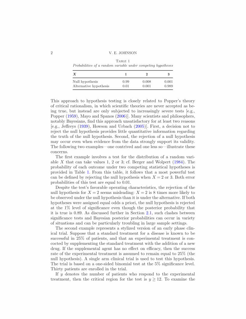
Table 1

Probabilities of a random variable under competing hypotheses

X 1 2 3

Null hypothesis 0.99 0.008 0.001Alternative hypothesis 0.01 0.001 0.989

This approach to hypothesis testing is closely related to Popper’s theoryof critical rationalism, in which scientific theories are never accepted as be-ing true, but instead are only subjected to increasingly severe tests [e.g.,Popper (1959), Mayo and Spanos (2006)]. Many scientists and philosophers,notably Bayesians, find this approach unsatisfactory for at least two reasons[e.g., Jeffreys (1939), Howson and Urbach (2005)]. First, a decision not toreject the null hypothesis provides little quantitative information regardingthe truth of the null hypothesis. Second, the rejection of a null hypothesismay occur even when evidence from the data strongly support its validity.The following two examples—one contrived and one less so—illustrate theseconcerns.

The first example involves a test for the distribution of a random vari-able X that can take values 1, 2 or 3; cf. Berger and Wolpert (1984). Theprobability of each outcome under two competing statistical hypotheses isprovided in Table 1. From this table, it follows that a most powerful testcan be defined by rejecting the null hypothesis when X = 2 or 3. Both errorprobabilities of this test are equal to 0.01.

Despite the test’s favorable operating characteristics, the rejection of thenull hypothesis for X = 2 seems misleading: X = 2 is 8 times more likely tobe observed under the null hypothesis than it is under the alternative. If bothhypotheses were assigned equal odds a priori, the null hypothesis is rejectedat the 1% level of significance even though the posterior probability thatit is true is 0.89. As discussed further in Section 2.1, such clashes betweensignificance tests and Bayesian posterior probabilities can occur in varietyof situations and can be particularly troubling in large sample settings.

The second example represents a stylized version of an early phase clin-ical trial. Suppose that a standard treatment for a disease is known to besuccessful in 25% of patients, and that an experimental treatment is con-cocted by supplementing the standard treatment with the addition of a newdrug. If the supplemental agent has no effect on efficacy, then the successrate of the experimental treatment is assumed to remain equal to 25% (thenull hypothesis). A single arm clinical trial is used to test this hypothesis.The trial is based on a one-sided binomial test at the 5% significance level.Thirty patients are enrolled in the trial.

If y denotes the number of patients who respond to the experimentaltreatment, then the critical region for the test is y ≥ 12. To examine the

UNIFORMLY MOST POWERFUL BAYESIAN TESTS 3

properties of this test, suppose first that y = 12, so that the null hypothesisis rejected at the 5% level. In this case, the minimum likelihood ratio infavor of the null hypothesis is obtained by setting the success rate under thealternative hypothesis to 12/30 = 0.40 (in which case the power of the testis 0.57). That is, if the new treatment’s success rate were defined a priori tobe 0.4, then the likelihood ratio in favor of the null hypothesis would be

Lmin =0.25120.7518

0.4120.618= 0.197.(1)

For any other alternative hypothesis, the likelihood ratio in favor of the nullhypothesis would be larger than 0.197 [e.g., Edwards, Lindman and Savage(1963)]. If equal odds are assigned to the null and alternative hypothesis,then the posterior probability of the null hypothesis is at least 16.5%. Inthis case, the null hypothesis is rejected at the 5% level of significance eventhough the data support it. And, of course, the posterior probability of thenull hypothesis would be substantially higher if one accounted for the factthat a vast majority of early phase clinical trials fail.

Conversely, suppose now that the trial data provide clear support of thenull hypothesis, with only 7 successes observed during the trial. In this case,the null hypothesis is not rejected at the 5% level, but this fact conveys littleinformation regarding the relative support that the null hypothesis received.If the alternative hypothesis asserts, as before, that the success rate of thenew treatment is 0.4, then the likelihood ratio in favor of the null hypothesisis 6.31; that is, the data favor the null hypothesis with approximately 6:1odds. If equal prior odds are assumed between the two hypotheses, then theposterior probability of the null hypothesis is 0.863. Under the assumption ofclinical equipoise, the prior odds assigned to the two hypotheses are assumedto be equal, which means the only controversial aspect of reporting such oddsis the specification of the alternative hypothesis.

For frequentists, the most important aspect of the methodology reportedin this article may be that it provides a connection between frequentistand Bayesian testing procedures. In one-parameter exponential family mod-els with monotone likelihood ratios, for example, it is possible to define aUMPBT with the same rejection region as a UMPT. This means that aBayesian using a UMPBT and a frequentist conducting a significance testwill make identical decisions on the basis of the observed data, which sug-gests that either interpretation of the test may be invoked. That is, a decisionto reject the null hypothesis at a specified significance level occurs only whenthe Bayes factor in favor of the alternative hypothesis exceeds a specifiedevidence level. This fact provides a remedy to the two primary deficienciesof classical significance tests—their inability to quantify evidence in favor ofthe null hypothesis when the null hypothesis is not rejected, and their ten-dency to exaggerate evidence against the null when it is. Having determined

4 V. E. JOHNSON

the corresponding UMPBT, Bayes factors can be used to provide a simplesummary of the evidence in favor of each hypothesis.

For Bayesians, UMPBTs represent a new objective Bayesian test, at leastwhen objective Bayesian methods are interpreted in the broad sense. AsBerger (2006) notes, “there is no unanimity as to the definition of objectiveBayesian analysis. . . ” and “many Bayesians object to the label ‘objectiveBayes,”’ preferring other labels such as “noninformative, reference, default,conventional and nonsubjective.” Within this context, UMPBTs provide anew form of default, nonsubjective Bayesian tests in which the alternativehypothesis is determined so as to maximize the probability that a Bayes fac-tor exceeds a specified threshold. This threshold can be specified either by adefault value—say 10 or 100—or, as indicated in the preceding discussion,determined so as to produce a Bayesian test that has the same rejection re-gion as a classical UMPT. In the latter case, UMPBTs provide an objectiveBayesian testing procedure that can be used to translate the results of clas-sical significance tests into Bayes factors and posterior model probabilities.By so doing, UMPBTs may prove instrumental in convincing scientists thatcommonly-used levels of statistical significance do not provide “significant”evidence against rejected null hypotheses.

Subjective Bayesian methods have long provided scientists with a formalmechanism for assessing the probability that a standard theory is true. Un-fortunately, subjective Bayesian testing procedures have not been—and willlikely never be—generally accepted by the scientific community. In mosttesting problems, the range of scientific opinion regarding the magnitude ofviolations from a standard theory is simply too large to make the report of asingle, subjective Bayes factor worthwhile. Furthermore, scientific journalshave demonstrated an unwillingness to replace the report of a single p-valuewith a range of subjectively determined Bayes factors or posterior modelprobabilities.

Given this reality, subjective Bayesians may find UMPBTs useful for com-municating the results of Bayesian tests to non-Bayesians, even when aUMPBT is only one of several Bayesian tests that are reported. By re-ducing the controversy regarding the specification of prior densities on pa-rameter values under individual hypotheses, UMPBTs can also be used tofocus attention on the specification of prior probabilities on the hypothesesthemselves. In the clinical trial example described above, for example, thevalue of the success probability specified under the alternative hypothesismay be less important in modeling posterior model probabilities than incor-porating information regarding the outcomes of previous trials on relatedsupplements. Such would be the case if numerous previous trials of similaragents had failed to provide evidence of increased treatment efficacy.

UMPBTs possess certain favorable properties not shared by other objec-tive Bayesian methods. For instance, most objective Bayesian tests implicitly

UNIFORMLY MOST POWERFUL BAYESIAN TESTS 5

define local alternative prior densities on model parameters under the alter-native hypothesis [e.g., Jeffreys (1939), O’Hagan (1995), Berger and Pericchi(1996)]. As demonstrated in Johnson and Rossell (2010), however, the use oflocal alternative priors makes it difficult to accumulate evidence in favor ofa true null hypothesis. This means that many objective Bayesian methodsare only marginally better than classical significance tests in summarizingevidence in favor of the null hypothesis. For small to moderate sample sizes,UMPBTs produce alternative hypotheses that correspond to nonlocal al-ternative prior densities, which means that they are able to provide morebalanced summaries of evidence collected in favor of true null and true al-ternative hypotheses.

UMPBTs also possess certain unfavorable properties. Like many objec-tive Bayesian methods, UMPBTs can violate the likelihood principle, andtheir behavior in large sample settings can lead to inconsistency if evidencethresholds are held constant. And the alternative hypotheses generated byUMPBTs are neither vague nor noninformative. Further comments and dis-cussion regarding these issues are provided below.

In order to define UMPBTs, it useful to first review basic properties ofBayesian hypothesis tests. In contrast to classical statistical hypothesis tests,Bayesian hypothesis tests are based on comparisons of the posterior prob-abilities assigned to competing hypotheses. In parametric tests, competinghypotheses are characterized by the prior densities that they impose on theparameters that define a sampling density shared by both hypotheses. Suchtests comprise the focus of this article. Specifically, it is assumed throughoutthat the posterior odds between two hypotheses H1 and H0 can be expressedas

P(H1 | x)P(H0 | x)

=m1(x)

m0(x)× p(H1)

p(H0),(2)

where BF10(x) =m1(x)/m0(x) is the Bayes factor between hypotheses H1

and H0,

mi(x) =

∫

Θ

f(x | θ)πi(θ |Hi)dθ(3)

is the marginal density of the data under hypothesis Hi, f(x | θ) is thesampling density of data x given θ, πi(θ | Hi) is the prior density on θ

under Hi and p(Hi) is the prior probability assigned to hypothesis Hi, fori= 0,1. The marginal prior density for θ is thus

π(θ) = π0(θ |H0)P (H0) + π1(θ |H1)p(H1).

When there is no possibility of confusion, πi(θ |Hi) will be denoted moresimply by πi(θ). The parameter space is denoted by Θ and the sample spaceby X . The logarithm of the Bayes factor is called the weight of evidence. All

6 V. E. JOHNSON

densities are assumed to be defined with respect to an appropriate underly-ing measure (e.g., Lebesgue or counting measure).

Finally, assume that one hypothesis—the null hypothesis H0—is fixed onthe basis of scientific considerations, and that the difficulty in construct-ing a Bayesian hypothesis test arises from the requirement to specify analternative hypothesis. This assumption mirrors the situation encounteredin classical hypothesis tests in which the null hypothesis is known, but noalternative hypothesis is defined. In the clinical trial example, for instance,the null hypothesis corresponds to the assumption that the success proba-bility of the new treatment equals that of the standard treatment, but thereis no obvious value (or prior probability density) that should be assigned tothe treatment’s success probability under the alternative hypothesis that itis better than the standard of care.

With these assumptions and definitions in place, it is worthwhile to re-view a property of Bayes factors that pertains when the prior density defin-ing an alternative hypothesis is misspecified. Let πt(θ |H1) = πt(θ) denotethe “true” prior density on θ under the assumption that the alternativehypothesis is true, and let mt(x) denote the resulting marginal density ofthe data. In general πt(θ) is not known, but it is still possible to comparethe properties of the weight of evidence that would be obtained by usingthe true prior density under the alternative hypothesis to those that wouldbe obtained using some other prior density. From a frequentist perspective,πt might represent a point mass concentrated on the true, but unknown,data generating parameter. From a Bayesian perspective, πt might repre-sent a summary of existing knowledge regarding θ before an experiment isconducted. Because πt is not available, suppose that π1(θ |H1) = π1(θ) isinstead used to represent the prior density, again under the assumption thatthe alternative hypothesis is true. Then it follows from Gibbs’s inequalitythat

∫

X

mt(x) log

[

mt(x)

m0(x)

]

dx−∫

X

mt(x) log

[

m1(x)

m0(x)

]

dx

=

∫

X

mt(x) log

[

mt(x)

m1(x)

]

dx

≥ 0.

That is,∫

X

mt(x) log

[

mt(x)

m0(x)

]

dx≥∫

X

mt(x) log

[

m1(x)

m0(x)

]

dx,(4)

which means that the expected weight of evidence in favor of the alternativehypothesis is always decreased when π1(θ) differs from πt(θ) (on a set withmeasure greater than 0). In general, the UMPBTs described below will thus

UNIFORMLY MOST POWERFUL BAYESIAN TESTS 7

decrease the average weight of evidence obtained in favor of a true alter-native hypothesis. In other words, the weight of evidence reported from aUMPBT will tend to underestimate the actual weight of evidence providedby an experiment in favor of a true alternative hypothesis.

Like classical statistical hypothesis tests, the tangible consequence of aBayesian hypothesis test is often the rejection of one hypothesis, say H0,in favor of the second, say H1. In a Bayesian test, the null hypothesis isrejected if the posterior probability of H1 exceeds a certain threshold. Giventhe prior odds between the hypotheses, this is equivalent to determining athreshold, say γ, over which the Bayes factor between H1 and H0 must fallin order to reject H0 in favor of H1. It is therefore of some practical interestto determine alternative hypotheses that maximize the probability that theBayes factor from a test exceeds a specified threshold.

With this motivation and notation in place, a UMPBT(γ) may be formallydefined as follows.

Definition. A uniformly most powerful Bayesian test for evidence thresh-old γ > 0 in favor of the alternative hypothesis H1 against a fixed null hy-pothesis H0, denoted by UMPBT(γ), is a Bayesian hypothesis test in whichthe Bayes factor for the test satisfies the following inequality for any θt ∈Θand for all alternative hypotheses H2 :θ ∼ π2(θ):

Pθt[BF10(x)> γ]≥Pθt

[BF20(x)> γ].(5)

In other words, the UMPBT(γ) is a Bayesian test for which the alternativehypothesis is specified so as to maximize the probability that the Bayesfactor BF10(x) exceeds the evidence threshold γ for all possible values ofthe data generating parameter θt.

The remainder of this article is organized as follows. In the next section,UMPBTs are described for one-parameter exponential family models. Asin the case of UMPTs, a general prescription for constructing UMPBTs isavailable only within this class of densities. Specific techniques for definingUMPBTs or approximate UMPBTs outside of this class are described laterin Sections 4 and 5. In applying UMPBTs to one parameter exponentialfamily models, an approximate equivalence between type I errors for UMPTsand the Bayes factors obtained from UMPBTs is exposed.

In Section 3, UMPBTs are applied in two canonical testing situations:the test of a binomial proportion, and the test of a normal mean. These twotests are perhaps the most common tests used by practitioners of statistics.The binomial test is illustrated in the context of a clinical trial, while thenormal mean test is applied to evaluate evidence reported in support of theHiggs boson. Section 4 describes several settings outside of one parameterexponential family models for which UMPBTs exist. These include cases in

8 V. E. JOHNSON

which the nuisance parameters under the null and alternative hypothesiscan be considered to be equal (though unknown), and situations in which itis possible to marginalize over nuisance parameters to obtain expressions fordata densities that are similar to those obtained in one-parameter exponen-tial family models. Section 5 describes approximations to UMPBTs obtainedby specifying alternative hypotheses that depend on data through statisticsthat are ancillary to the parameter of interest. Concluding comments appearin Section 6.

2. One-parameter exponential family models. Assume that {x1, . . . ,xn} ≡ x are i.i.d. with a sampling density (or probability mass functionin the case of discrete data) of the form

f(x | θ) = h(x) exp[η(θ)T (x)−A(θ)],(6)

where T (x), h(x), η(θ) and A(θ) are known functions, and η(θ) is monotonic.Consider a one-sided test of a point null hypothesis H0 : θ = θ0 against anarbitrary alternative hypothesis. Let γ denote the evidence threshold for aUMPBT(γ), and assume that the value of θ0 is fixed.

Lemma 1. Assume the conditions of the previous paragraph pertain, anddefine gγ(θ, θ0) according to

gγ(θ, θ0) =log(γ) + n[A(θ)−A(θ0)]

η(θ)− η(θ0).(7)

In addition, define u to be 1 or −1 according to whether η(θ) is monoton-ically increasing or decreasing, respectively, and define v to be either 1 or−1 according to whether the alternative hypothesis requires θ to be greaterthan or less than θ0, respectively. Then a UMPBT(γ) can be obtained byrestricting the support of π1(θ) to values of θ that belong to the set

argminθ

uvgγ(θ, θ0).(8)

Proof. Consider the case in which the alternative hypothesis requiresθ to be greater than θ0 and η(θ) is increasing (so that uv = 1), and let θtdenote the true (i.e., data-generating) parameter for x under (6). Considerfirst simple alternatives for which the prior on θ is a point mass at θ1. Then

Pθt(BF10 > γ) =Pθt [log(BF10)> log(γ)](9)

=Pθt

{

n∑

i=1

T (xi)>log(γ) + n[A(θ1)−A(θ0)]

η(θ1)− η(θ0)

}

.

It follows that the probability in (9) achieves its maximum value when theright-hand side of the inequality is minimized, regardless of the distributionof∑

T (xi).

UNIFORMLY MOST POWERFUL BAYESIAN TESTS 9

Now consider composite alternative hypotheses, and define an indicatorfunction s according to

s(x, θ) = Ind

(

exp

{

[η(θ)− η(θ0)]n∑

i=1

T (xi)− n[A(θ)−A(θ0)]

}

> γ

)

.(10)

Let θ∗ be a value that minimizes gγ(θ, θ0). Then it follows from (9) that

s(x, θ)≤ s(x, θ∗) for all x.(11)

This implies that∫

Θ

s(x, θ)π(θ)dθ ≤ s(x, θ∗)(12)

for all probability densities π(θ). It follows that

Pθt(BF10 > γ) =

∫

X

s(x, θ)f(x | θt)dx(13)

is maximized by a prior that concentrates its mass on the set for whichgγ(θ, θ0) is minimized.

The proof for other values of (u, v) follows by noting that the direction ofthe inequality in (9) changes according to the sign of η(θ1)− η(θ0). �

It should be noted that in some cases the values of θ that maximizePθt(BF10 > γ) are not unique. This might happen if, for instance, no valueof the sufficient statistic obtained from the experiment could produce aBayes factor that exceeded the γ threshold. For example, it would not bepossible to obtain a Bayes factor of 10 against a null hypothesis that abinomial success probability was 0.5 based on a sample of size n = 1. Inthat case, the probability of exceeding the threshold is 0 for all values of thesuccess probability, and a unique UMPBT does not exist. More generally, ifT (x) is discrete, then many values of θ1 might produce equivalent tests. Anillustration of this phenomenon is provided in the first example.

2.1. Large sample properties of UMPBTs. Asymptotic properties ofUMPBTs can most easily be examined for tests of point null hypothesesfor a canonical parameter in one-parameter exponential families. Two prop-erties of UMPBTs in this setting are described in the following lemma.

Lemma 2. Let X1, . . . ,Xn represent a random sample drawn from adensity expressible in the form (6) with η(θ) = θ, and consider a test ofthe precise null hypothesis H0 : θ = θ0. Suppose that A(θ) has three boundedderivatives in a neighborhood of θ0, and let θ∗ denote a value of θ that definesa UMPBT(γ) test and satisfies

dgγ(θ∗, θ0)

dθ= 0.(14)

10 V. E. JOHNSON

Then the following statements apply:

(1) For some t ∈ (θ0, θ∗),

|θ∗ − θ0|=√

2 log(γ)

nA′′(t).(15)

(2) Under the null hypothesis,

log(BF10)→N(− log(γ),2 log(γ)) as n→∞.(16)

Proof. The first statement follows immediately from (14) by expandingA(θ) in a Taylor series around θ∗. The second statement follows by notingthat the weight of evidence can be expressed as

log(BF10) = (θ∗ − θ0)

n∑

i=1

T (xi)− n[A(θ∗)−A(θ0)].

Expanding in a Taylor series around θ0 leads to

log(BF10) =

√

2 log(γ)

nA′′(t)

[

n∑

i=1

T (xi)− nA′(θ0)−n

2A′′(θ0)

√

2 log(γ)

nA′′(t)

]

+ ε,(17)

where ε represents a term of order O(n−1/2). From properties of exponentialfamily models, it is known that

Eθ0 [T (xi)] =A′(θ0) and Varθ0(T (xi)) =A′′(θ0).

Because A(θ) has three bounded derivatives in a neighborhood of θ0, [A′(t)−

A′(θ0)] and [A′′(t)−A′′(θ0)] are order O(n−1/2), and the statement followsby application of the central limit theorem. �

Equation (15) shows that the difference |θ∗ − θ0| is O(n−1/2) when theevidence threshold γ is held constant as a function of n. In classical terms,this implies that alternative hypotheses defined by UMPBTs represent Pit-man sequences of local alternatives [Pitman (1949)]. This fact, in conjunc-tion with (16), exposes an interesting behavior of UMPBTs in large sam-ple settings, particularly when viewed from the context of the Jeffreys–Lindley paradox [Jeffreys (1939), Lindley (1957); see also Robert, Chopinand Rousseau (2009)].

The Jeffreys–Lindley paradox (JLP) arises as an incongruity betweenBayesian and classical hypothesis tests of a point null hypothesis. To un-derstand the paradox, suppose that the prior distribution for a parameterof interest under the alternative hypothesis is uniform on an interval I con-taining the null value θ0, and that the prior probability assigned to the nullhypothesis is π1. If π1 is bounded away from 0, then it is possible for the

UNIFORMLY MOST POWERFUL BAYESIAN TESTS 11

null hypothesis to be rejected in an α-level significance test even when theposterior probability assigned to the null hypothesis exceeds 1−α. Thus, theanomalous behavior exhibited in the example of Table 1, in which the nullhypothesis was rejected in a significance test while being supported by thedata, is characteristic of a more general phenomenon that may occur even inlarge sample settings. To see that the null hypothesis can be rejected evenwhen the posterior odds are in its favor, note that for sufficiently large nthe width of I will be large relative to the posterior standard deviation of θunder the alternative hypothesis. Data that are not “too far” from fθ0 maytherefore be much more likely to have arisen from the null hypothesis thanfrom a density fθ when θ is drawn uniformly from I . At the same time, thevalue of the test statistic based on the data may appear extreme given thatfθ0 pertains.

For moderate values of γ, the second statement in Lemma 2 shows thatthe weight of evidence obtained from a UMPBT is unlikely to provide strongevidence in favor of either hypothesis when the null hypothesis is true. Whenγ = 4, for instance, an approximate 95% confidence interval for the weightof evidence extends only between (−4.65,1.88), no matter how large n is.Thus, the posterior probability of the null hypothesis does not converge to1 as the sample size grows. The null hypothesis is never fully accepted—northe alternative rejected—when the evidence threshold is held constant as nincreases.

This large sample behavior of UMPBTs with fixed evidence thresholdsis, in a certain sense, similar to the JLP. When the null hypothesis is trueand n is large, the probability of rejecting the null hypothesis at a fixedlevel of significance remains constant at the specified level of significance.For instance, the null hypothesis is rejected 5% of the time in a standard5% significance test when the null hypothesis is true, regardless of how largethe sample size is. Similarly, when γ = 4, the probability that the weightof evidence in favor of the alternative hypothesis will be greater than 0converges to 0.20 as n becomes large. Like the significance test, there remainsa nonzero probability that the alternative hypothesis will be favored by theUMPBT even when the null hypothesis is true, regardless of how large n is.

On a related note, Rousseau (2007) has demonstrated that a point nullhypothesis may be used as a convenient mathematical approximation tointerval hypotheses of the form (θ0 − ε, θ0 + ε) if ε is sufficiently small. Herresults suggest that such an approximation is valid only if ε < o(n). Thefact that UMPBT alternatives decrease at a rate of O(n−1/2) suggests thatUMPBTs may be used to test small interval hypotheses around θ0, providedthat the width of the interval satisfies the constraints provided by Rousseau.

Further comments regarding the asymptotic properties of UMPBTs ap-pear in the discussion section.

12 V. E. JOHNSON

3. Examples. Tests of simple hypotheses in one-parameter exponentialfamily models continue to be the most common statistical hypothesis testsused by practitioners. These tests play a central role in many science, tech-nology and business applications. In addition, the distributions of many teststatistics are asymptotically distributed as standard normal deviates, whichmeans that UMPBTs can be applied to obtain Bayes factors based on teststatistics [Johnson (2005)]. This section illustrates the use of UMPBT testsin two archetypical examples; the first involves the test of a binomial successprobability, and the second the test of the value of a parameter estimate thatis assumed to be approximately normally distributed.

3.1. Test of binomial success probability. Suppose x∼Bin(n,p), and con-sider the test of a null hypothesis H0 :p= p0 versus an alternative hypothesisH1 :p > p0. Assume that an evidence threshold of γ is desired for the test;that is, the alternative hypothesis is accepted if BF10 > γ.

From Lemma 1, the UMPBT(γ) is defined by finding p1 that satisfiesp1 > p0 and

p1 = argminp

log(γ)− n[log(1− p)− log(1− p0)]

log[p/(1− p)]− log[p0/(1− p0)].(18)

Although this equation cannot be solved in closed form, its solution canbe found easily using optimization functions available in most statisticalprograms.

3.1.1. Phase II clinical trials with binary outcomes. To illustrate theresulting test in a real-world application that involves small sample sizes,consider a one-arm Phase II trial of a new drug intended to improve theresponse rate to a disease from the standard-of-care rate of p0 = 0.3. Supposealso that budget and time constraints limit the number of patients that canbe accrued in the trial to n = 10, and suppose that the new drug will bepursued only if the odds that it offers an improvement over the standard ofcare are at least 3:1. Taking γ = 3, it follows from (18) that the UMPBTalternative is defined by taking H1 :p1 = 0.525. At this value of p1, the Bayesfactor BF10 in favor of H1 exceeds 3 whenever 6 or more of the 10 patientsenrolled in the trial respond to treatment.

A plot of the probability that BF10 exceeds 3 as function of the trueresponse rate p appears in Figure 1. For comparison, also plotted in thisfigure (dashed curve) is the probability that BF10 exceeds 3 when p1 is setto the data-generating parameter, that is, when p1 = pt.

Figure 1 shows that the probability that BF10 exceeds 3 when calculatedunder the true alternative hypothesis is significantly smaller than it is un-der the UMPBT alternative for values of p < 0.4 and for values of p > 0.78.Indeed, for values of p < 0.334, there is no chance that BF10 will exceed 3.

UNIFORMLY MOST POWERFUL BAYESIAN TESTS 13

Fig. 1. Probability that the Bayes factor exceeds 3 plotted against the data-generating pa-rameter. The solid curve shows the probability of exceeding 3 for the UMPBT. The dashedcurve displays this probability when the Bayes factor is calculated using the data-generatingparameter.

This is so because (0.334/0.30)x remains less than 3.0 for all x ≤ 10. Thedecrease in the probability that the Bayes factor exceeds 3 for large values ofp stems from the relatively small probability that these models assign to theobservation of intermediate values of x. For example, when p= 0.8, the prob-ability of observing 6 out 10 successes is only 0.088, while the correspondingprobability under H0 is 0.037. Thus BF10 = 2.39, and the evidence in favorof the true success probability does not exceed 3. That is, the discontinu-ity in the dashed curve at p≈ 0.7 occurs because the Bayes factor for thistest is not greater than 3 when x= 6. Similarly, the other discontinuities inthe dashed curve occur when the rejection region for the Bayesian test (i.e.,values of x for which the Bayes factor is greater than 3) excludes anotherimmediate value of x. The dashed and solid curves agree for all Bayesiantests that produce Bayes factors that exceed 3 for all values of x≥ 6.

It is also interesting to note that the solid curve depicted in Figure 1represents the power curve for an approximate 5% one-sided significancetest of the null hypothesis that p= 0.3 [note that P0.3(X ≥ 6) = 0.047]. Thisrejection region for the 5% significance test also corresponds to the regionfor which the Bayes factor corresponding to the UMPBT(γ) exceeds γ for

14 V. E. JOHNSON

Fig. 2. Expected weight of evidence produced by a UMPBT(γ) against a null hypothesisthat p0 = 0.3 when the sample size is n= 10 (solid curve), versus the expected weight ofevidence observed using the data-generating success probability at the alternative hypothesis(dashed curve). The data-generating parameter value is displayed on the horizontal axis.

all values of γ ∈ (2.36,6.82). If equal prior probabilities are assigned to H0

and H1, this suggests that a p-value of 0.05 for this test corresponds roughlyto the assignment of a posterior probability between (1.0/7.82,1.0/3.36) =(0.13,0.30) to the null hypothesis. This range of values for the posteriorprobability of the null hypothesis is in approximate agreement with valuessuggested by other authors, for example, Berger and Sellke (1987).

This example also indicates that a UMPBT can result in large type Ierrors if the threshold γ is chosen to be too small. For instance, taking γ = 2in this example would lead to type I errors that were larger than 0.05.

It is important to note that the UMPBT does not provide a test thatmaximizes the expected weight of evidence, as equation (4) demonstrates.This point is illustrated in Figure 2, which depicts the expected weight ofevidence obtained in favor of H1 by a solid curve as the data-generatingsuccess probability is varied in (0.3,1.0). For comparison, the dashed curveshows the expected weight of evidence obtained as a function of the true pa-rameter value. As predicted by the inequality in (4), on average the UMPBTprovides less evidence in favor of the true alternative hypothesis for all valuesof p ∈ (0.3,1.0) except p= 0.525, the UMPBT value.

UNIFORMLY MOST POWERFUL BAYESIAN TESTS 15

3.2. Test of normal mean, σ2 known. Suppose xi, i= 1, . . . , n are i.i.d.N(µ,σ2) with σ2 known. The null hypothesis is H0 :µ= µ0, and the alter-native hypothesis is accepted if BF10 > γ. Assuming that the alternativehypothesis takes the form H1 :µ= µ1 in a one-sided test, it follows that

log(BF10) =n

σ2

[

x(µ1 − µ0) +1

2(µ2

0 − µ21)

]

.(19)

If the data-generating parameter is µt, the probability that BF10 is greaterthan γ can be written as

Pµt

[

(µ1 − µ0)x>σ2 log(γ)

n− 1

2(µ2

0 − µ21)

]

.(20)

If µ1 > µ0, then the UMPBT(γ) value of µ1 satisfies

argminµ1

σ2 log(γ)

n(µ1 − µ0)+

1

2(µ0 + µ1).(21)

Conversely, if µ1 <µ0, then optimal value of µ1 satisfies

argminµ1

σ2 log(γ)

n(µ1 − µ0)+

1

2(µ0 + µ1).(22)

It follows that the UMPBT(γ) value for µ1 is given by

µ1 = µ0 ± σ

√

2 log γ

n,(23)

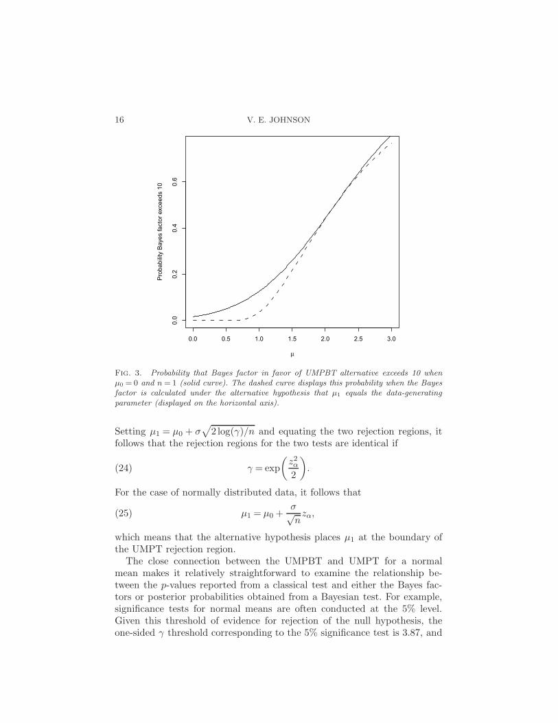
depending on whether µ1 > µ0 or µ1 <µ0.Figure 3 depicts the probability that the Bayes factor exceeds γ = 10 when

testing a null hypothesis that µ= 0 based on a single, standard normal ob-servation (i.e., n= 1, σ2 = 1). In this case, the UMPBT(10) is obtained bytaking µ1 = 2.146. For comparison, the probability that the Bayes factor ex-ceeds 10 when the alternative is defined to be the data-generating parameteris depicted by the dashed curve in the plot.

UMPBTs can also be used to interpret the evidence obtained from clas-sical UMPTs. In a classical one-sided test of a normal mean with knownvariance, the null hypothesis is rejected if

x > µ0 + zασ√n,

where α is the level of the test designed to detect µ1 >µ0. In the UMPBT,from (19)–(20) it follows that the null hypothesis is rejected if

x >σ2 log(γ)

n(µ1 − µ0)+

1

2(µ1 + µ0).

16 V. E. JOHNSON

Fig. 3. Probability that Bayes factor in favor of UMPBT alternative exceeds 10 whenµ0 = 0 and n= 1 (solid curve). The dashed curve displays this probability when the Bayesfactor is calculated under the alternative hypothesis that µ1 equals the data-generatingparameter (displayed on the horizontal axis).

Setting µ1 = µ0 + σ√

2 log(γ)/n and equating the two rejection regions, itfollows that the rejection regions for the two tests are identical if

γ = exp

(

z2α2

)

.(24)

For the case of normally distributed data, it follows that

µ1 = µ0 +σ√nzα,(25)

which means that the alternative hypothesis places µ1 at the boundary ofthe UMPT rejection region.

The close connection between the UMPBT and UMPT for a normalmean makes it relatively straightforward to examine the relationship be-tween the p-values reported from a classical test and either the Bayes fac-tors or posterior probabilities obtained from a Bayesian test. For example,significance tests for normal means are often conducted at the 5% level.Given this threshold of evidence for rejection of the null hypothesis, theone-sided γ threshold corresponding to the 5% significance test is 3.87, and

UNIFORMLY MOST POWERFUL BAYESIAN TESTS 17

Fig. 4. Correspondence between p-values and posterior model probabilities for a UMPBTtest derived from a 5% test. This plot assumes equal prior probabilities were assigned tothe null and alternative hypotheses. Note that both axes are displayed on the logarithmicscale.

the UMPBT alternative is µ1 = µ0 + 1.645σ/√n. If we assume that equal

prior probabilities are assigned to the null and alternative hypotheses, thena correspondence between p-values and posterior probabilities assigned tothe null hypothesis is easy to establish. This correspondence is depicted inFigure 4. For instance, this figure shows that a p-value of 0.01 correspondsto the assignment of posterior probability 0.08 to the null hypothesis.

3.2.1. Evaluating evidence for the Higgs boson. On July 4, 2012, scien-tists at CERN made the following announcement:

We observe in our data clear signs of a new particle, at the level of 5 sigma, inthe mass region around 126 gigaelectronvolts (GeV). (http://press.web.cern.ch/press/PressReleases/Releases2012/PR17.12E.html).

In very simplified terms, the 5 sigma claim can be explained by fitting amodel for a Poisson mean that had the following approximate form:

µ(x) = exp(a0 + a1x+ a2x2) + sφ(x;m,w).

Here, x denotes mass in GeV, {ai} denote nuisance parameters that modelbackground events, s denotes signal above background, m denotes the mass

18 V. E. JOHNSON

of a new particle, w denotes a convolution parameter and φ(x;m,w) de-notes a Gaussian density centered on m with standard deviation w [Prosper(2012)]. Poisson events collected from a series of high energy experimentsconducted in the Large Hadron Collider (LHC) at CERN provide the datato estimate the parameters in this stylized model. The background param-eters {ai} are considered nuisance parameters. Interest, of course, focuseson testing whether s > 0 at a mass location m. The null hypothesis is thats= 0 for all m.

The accepted criterion for declaring the discovery of a new particle in thefield of particle physics is the 5 sigma rule, which in this case requires that theestimate of s be 5 standard errors from 0 (http://public.web.cern.ch/public/).

Calculation of a Bayes factor based on the original mass spectrum datais complicated by the fact that prior distributions for the nuisance param-eters {ai}, m, and w are either not available or are not agreed upon. Forthis reason, it is more straightforward to compute a Bayes factor for thesedata based on the test statistic z = s/ se(s) where s denotes the maximumlikelihood estimate of s and se(s) its standard error [Johnson (2005, 2008)].To perform this test, assume that under the null hypothesis z has a stan-dard normal distribution, and that under the alternative hypothesis z has anormal distribution with mean µ and variance 1.

In this context, the 5 sigma rule for declaring a new particle discoverymeans that a new discovery can only be declared if the test statistic z > 5.Using equation (24) to match the rejection region of the classical significancetest to a UMPBT(γ) implies that the corresponding evidence threshold isγ = exp(12.5) ≈ 27,000. In other words, a Bayes factor of approximatelyγ = exp(12.5) ≈ 27,000 corresponds to the 5 sigma rule required to acceptthe alternative hypothesis that a new particle has been found.

It follows from the discussion following equation (25) that the alternativehypothesis for the UMPBT alternative is µ1 = 5. This value is calculatedunder the assumption that the test statistic z has a standard normal dis-tribution under the null hypothesis [i.e., σ = 1 and n = 1 in (23)]. If theobserved value of z was exactly 5, then the Bayes factor in favor of a newparticle would be approximately 27,000. If the observed value was, say 5.1,then the Bayes factor would be exp(−0.5[0.12−5.12]) = 44,000. These valuessuggest very strong evidence in favor of a new particle, but perhaps not asmuch evidence as might be inferred by nonstatisticians by the report of ap-value of 3× 10−7.

There are, of course, a number of important caveats that should be con-sidered when interpreting the outcome of this analysis. This analysis as-sumes that an experiment with a fixed endpoint was conducted, and thatthe UMPBT value of the Poisson rate at 126 GeV was of physical signifi-cance. Referring to (23) and noting that the asymptotic standard error ofz decreases at rate

√n, it follows that the UMPBT alternative hypothesis

favored by this analysis is O(n−1/2). For sufficiently large n, systematic er-

UNIFORMLY MOST POWERFUL BAYESIAN TESTS 19

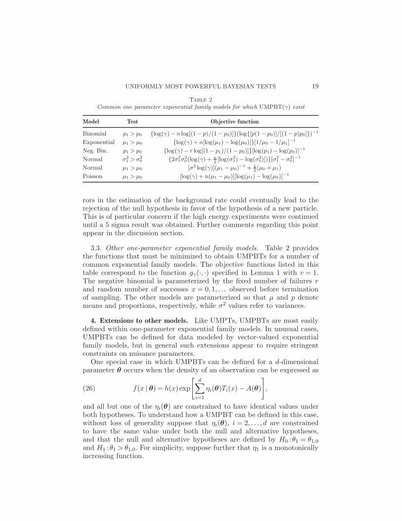
Table 2

Common one parameter exponential family models for which UMPBT(γ) exist

Model Test Objective function

Binomial p1 > p0 {log(γ)− n log[(1− p)/(1− p0)]}(log{[p(1− p0)]/[(1− p)p0]})−1

Exponential µ1 > µ0 {log(γ) + n[log(µ1)− log(µ0)]}[1/µ0 − 1/µ1]−1

Neg. Bin. p1 > p0 {log(γ)− r log[(1− p1)/(1− p0)]}[log(p1)− log(p0)]−1

Normal σ21 > σ2

0 {2σ21σ

20(log(γ) +

n

2[log(σ2

1)− log(σ20)])}[σ

21 − σ2

0 ]−1

Normal µ1 > µ0 [σ2 log(γ)](µ1 − µ0)−1 + 1

2(µ0 + µ1)

Poisson µ1 > µ0 [log(γ) + n(µ1 − µ0)][log(µ1)− log(µ0)]−1

rors in the estimation of the background rate could eventually lead to therejection of the null hypothesis in favor of the hypothesis of a new particle.This is of particular concern if the high energy experiments were continueduntil a 5 sigma result was obtained. Further comments regarding this pointappear in the discussion section.

3.3. Other one-parameter exponential family models. Table 2 providesthe functions that must be minimized to obtain UMPBTs for a number ofcommon exponential family models. The objective functions listed in thistable correspond to the function gγ(·, ·) specified in Lemma 1 with v = 1.The negative binomial is parameterized by the fixed number of failures rand random number of successes x = 0,1, . . . observed before terminationof sampling. The other models are parameterized so that µ and p denotemeans and proportions, respectively, while σ2 values refer to variances.

4. Extensions to other models. Like UMPTs, UMPBTs are most easilydefined within one-parameter exponential family models. In unusual cases,UMPBTs can be defined for data modeled by vector-valued exponentialfamily models, but in general such extensions appear to require stringentconstraints on nuisance parameters.

One special case in which UMPBTs can be defined for a d-dimensionalparameter θ occurs when the density of an observation can be expressed as

f(x | θ) = h(x) exp

[

d∑

i=1

ηi(θ)Ti(x)−A(θ)

]

,(26)

and all but one of the ηi(θ) are constrained to have identical values underboth hypotheses. To understand how a UMPBT can be defined in this case,without loss of generality suppose that ηi(θ), i = 2, . . . , d are constrainedto have the same value under both the null and alternative hypotheses,and that the null and alternative hypotheses are defined by H0 : θ1 = θ1,0and H1 : θ1 > θ1,0. For simplicity, suppose further that η1 is a monotonicallyincreasing function.

20 V. E. JOHNSON

As in Lemma 1, consider first simple alternative hypotheses expressibleas H1 : θ1 = θ1,1. Let θ0 = (θ1,0, . . . , θd,0)

′ and θ1 = (θ1,1, . . . , θd,1)′. It follows

that the probability that the logarithm of the Bayes factor exceeds a thresh-old log(γ) can be expressed as

P[log(BF10)> log(γ)]

=P{[η1(θ1,1)− η1(θ1,0)]T1(x)− [A(θ1)−A(θ0)]> log(γ)}(27)

=P

[

T1(x)>log(γ) + [A(θ1)−A(θ0)]

[η1(θ1,1)− η1(θ1,0)]

]

.

The probability in (27) is maximized by minimizing the right-hand sideof the inequality. The extension to composite alternative hypotheses followsthe logic described in inequalities (11)–(13), which shows that UMPBT(γ)tests can be obtained in this setting by choosing the prior distribution of θ1

under the alternative hypotheses so that it concentrates its mass on the set

argminθ

log(γ) + [A(θ1)−A(θ0)]

[η1(θ1,1)− η1(θ1,0)],(28)

while maintaining the constraint that the values of ηi(θ) are equal underboth hypotheses. Similar constructions apply if η1 is monotonically decreas-ing, or if the alternative hypothesis specifies that θ1,0 < θ0,0.

More practically useful extensions of UMPBTs can be obtained when it ispossible to integrate out nuisance parameters in order to obtain a marginaldensity for the parameter of interest that falls within the class of exponen-tial family of models. An important example of this type occurs in testingwhether a regression coefficient in a linear model is zero.

4.1. Test of linear regression coefficient, σ2 known. Suppose that

y∼N(Xβ, σ2In),(29)

where σ2 is known, y is an n × 1 observation vector, X an n × p designmatrix of full column rank and β = (β1, . . . , βp)

′ denotes a p× 1 regressionparameter. The null hypothesis is defined as H0 :βp = 0. For concreteness,suppose that interest focuses on testing whether βp > 0, and that underboth the null and alternative hypotheses, the prior density on the first p− 1components of β is a multivariate normal distribution with mean vector 0

and covariance matrix σ2Σ. Then the marginal density of y under H0 is

m0(y) = (2πσ2)−n/2|Σ|−1/2|F|−1/2 exp

(

− R

2σ2

)

,(30)

where

F=X′

−pX−p +Σ−1, H=X−pF−1X′

−p, R= y′(In −H)′y,(31)

and X−p is the matrix consisting of the first p− 1 columns of X.

UNIFORMLY MOST POWERFUL BAYESIAN TESTS 21

Let βp∗ denote the value of βp under the alternative hypothesis H1 thatdefines the UMPBT(γ), and let xp denote the pth column of X. Then themarginal density of y under H1 is

m1(y) =m0(y)× exp

{

− 1

2σ2[βp∗

2x′

p(In−H)xp−2βp∗x′

p(In−H)y]

}

.(32)

It follows that the probability that the Bayes factor BF10 exceeds γ canbe expressed as

P

[

x′

p(In −H)y>σ2 log(γ)

βp∗+

1

2βp∗x

′

p(In −H)xp

]

,(33)

which is maximized by minimizing the right-hand side of the inequality. TheUMPBT(γ) is thus obtained by taking

βp∗ =

√

2σ2 log(γ)

x′p(In −H)xp

.(34)

The corresponding one-sided test of βp < 0 is obtained by reversing the signof βp∗ in (34).

Because this expression for the UMPBT assumes that σ2 is known, it isnot of great practical significance by itself. However, this result may guidethe specification of alternative models in, for example, model selection al-gorithms in which the priors on regression coefficients are specified condi-tionally on the value of σ2. For example, the mode of the nonlocal priorsdescribed in Johnson and Rossell (2012) might be set to the UMPBT valuesafter determining an appropriate value of γ based on both the sample sizen and number of potential covariates p.

5. Approximations to UMPBTs using data-dependent alternatives. Insome situations—most notably in linear models with unknown variances—data dependent alternative hypotheses can be defined to obtain tests thatare approximately uniformly most powerful in maximizing the probabilitythat a Bayes factor exceeds a threshold. This strategy is only attractivewhen the statistics used to define the alternative hypothesis are ancillary tothe parameter of interest.

5.1. Test of normal mean, σ2 unknown. Suppose that xi, i= 1, . . . , n, arei.i.d. N(µ,σ2), that σ2 is unknown and that the null hypothesis is H0 :µ=µ0. For convenience, assume further that the prior distribution on σ2 is aninverse gamma distribution with parameters α and λ under both the nulland alternative hypotheses.

To obtain an approximate UMPBT(γ), first marginalize over σ2 in bothmodels. Noting that (1+a/t)t → ea, it follows that the Bayes factor in favor

22 V. E. JOHNSON

of the alternative hypothesis satisfies

BF10(x) =

[∑ni=1(xi − µ0)

2 + 2λ∑n

i=1(xi − µ1)2 + 2λ

]n/2+α

(35)

≈[

1 + (x− µ0)2/s2

1 + (x− µ1)2/s2

]n/2+α

(36)

≈ exp

{

− n

2s2[(x− µ1)

2 − (x− µ0)2]

}

,(37)

where

s2 =

∑ni=1(xi − x)2 +2λ

n+ 2α.(38)

The expression for the Bayes factor in (37) reduces to (19) if σ2 is replacedby s2. This implies that an approximate, but data-dependent UMPBT al-ternative hypothesis can be specified by taking

µ1 = µ0 ± s

√

2 log γ

n,(39)

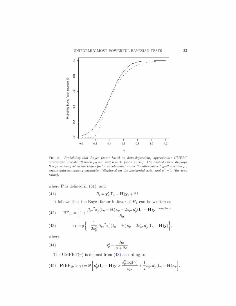
depending on whether µ1 > µ0 or µ1 <µ0.Figure 5 depicts the probability that the Bayes factor exceeds γ = 10 when

testing a null hypothesis that µ= 0 based on an independent sample of sizen = 30 normal observations with unit variance (σ2 = 1) and using (39) toset the value of µ1 under the alternative hypothesis. For comparison, theprobability that the Bayes factor exceeds 10 when the alternative is definedby taking σ2 = 1 and µ1 to be the data-generating parameter is depicted bythe dashed curve in the plot. Interestingly, the data-dependent, approximateUMPBT(10) provides a higher probability of producing a Bayes factor thatexceeds 10 than do alternatives fixed at the data generating parameters.

5.2. Test of linear regression coefficient, σ2 unknown. As final example,suppose that the sampling model of Section 4.1 holds, but assume now thatthe observational variance σ2 is unknown and assumed under both hypothe-ses to be drawn from an inverse gamma distribution with parameters α andλ. Also assume that the prior distribution for the first p−1 components of β,given σ2, is a multivariate normal distribution with mean 0 and covariancematrix σ2Σ. As before, assume that H0 :βp = 0. Our goal is to determine avalue βp∗ so that H1 :βp = βp∗ is the UMPBT(γ) under the constraint thatβp > 0.

Define y1 = y− xpβp∗ and let y0 = y. By integrating with respect to theprior densities on σ2 and the first p − 1 components of β, the marginaldensity of the data under hypothesis i, i= 0,1 can be expressed as

mi(y) = 2απ−n/2|Σ|−1/2 λα

Γ(α)Γ(n/2 + α)|F|−1/2R

−n/2−αi ,(40)

UNIFORMLY MOST POWERFUL BAYESIAN TESTS 23

Fig. 5. Probability that Bayes factor based on data-dependent, approximate UMPBTalternative exceeds 10 when µ0 = 0 and n = 30 (solid curve). The dashed curve displaysthis probability when the Bayes factor is calculated under the alternative hypothesis that µ1

equals data-generating parameter (displayed on the horizontal axis) and σ2 = 1 (the truevalue).

where F is defined in (31), and

Ri = y′

i(In −H)yi + 2λ.(41)

It follows that the Bayes factor in favor of H1 can be written as

BF10 =

[

1 +βp∗

2x′p(In −H)xp − 2βp∗x

′p(In −H)y

R0

]

−n/2−α

(42)

≈ exp

{

− 1

2s2p[βp∗

2x′

p(In −H)xp − 2βp∗x′

p(In −H)y]

}

,(43)

where

s2p =R0

n+ 2α.(44)

The UMPBT(γ) is defined from (43) according to

P(BF10 > γ) =P

[

x′

p(In −H)y>s2p log(γ)

βp∗+

1

2βp∗x

′

p(In −H)xp

]

.(45)

24 V. E. JOHNSON

Minimizing the right-hand side of the last inequality with respect to βp∗results in

βp∗ =

√

2s2p log(γ)

x′p(In −H)xp

.(46)

This expression is consistent with the result obtained in the known vari-ance case, but with s2p substituted for σ2.

6. Discussion. The major contributions of this paper are the definition ofUMPBTs and the explicit description of UMPBTs for regular one-parameterexponential family models. The existence of UMPBTs for exponential familymodels is important because these tests represent the most common hypoth-esis tests conducted by practitioners. The availability of UMPBTs for thesemodels means that these tests can be used to interpret test results in termsof Bayes factors and posterior model probabilities in a wide range of scien-tific settings. The utility of these tests is further enhanced by the connectionbetween UMPBTs and UMPTs that have the same rejection region. Thisconnection makes it trivial to simultaneously report both the p-value froma test and the corresponding Bayes factor.

The simultaneous report of default Bayes factors and p-values may playa pivotal role in dispelling the perception held by many scientists that ap-value of 0.05 corresponds to “significant” evidence against the null hy-pothesis. The preceding sections contain examples in which this level ofsignificance favors the alternative hypothesis by odds of only 3 or 4 to 1.Because few researchers would regard such odds as strong evidence in favorof a new theory, the use of UMPBTs and the report of Bayes factors basedupon them may lead to more realistic interpretations of evidence obtainedfrom scientific studies.

The large sample properties of UMPBTs described in Section 2.1 deservefurther comment. From Lemma 2, it follows that the expected weight ofevidence in favor of a true null hypothesis in an exponential family modelconverges to log(γ) as the sample size n tends to infinity. In other words, theevidence threshold γ represents an approximate bound on the evidence thatcan be collected in favor of the null hypothesis. This implies that γ must beincreased with n in order to obtain a consistent sequence of tests.

Several criteria might be used for selecting a value for γ in large samplesettings. One criterion can be inferred from the first statement of Lemma 2,where it is shown that the difference between the tested parameter’s valueunder the null and alternative hypotheses is proportional to [log(γ)/n]1/2.For this difference to be a constant—as it would be in a subjective Bayesiantest—log(γ) must be proportional to n, or γ = exp(cn) for some c > 0. Thissuggests that an appropriate value for c might be determined by calibrating

UNIFORMLY MOST POWERFUL BAYESIAN TESTS 25

the weight of evidence against an accepted threshold/sample size combina-tion. For example, if an evidence threshold of 4 were accepted as the standardthreshold for tests conducted with a sample size of 100, then c might be setto log(4)/100 = 0.0139. This value of c leads to an evidence threshold ofγ = 16 for sample sizes of 200, a threshold of 64 for sample sizes of 300, etc.From (24), the significance levels for corresponding z-tests would be 5%, 1%and 0.2%, respectively.

The requirement to increase γ to achieve consistent tests in large sam-ples also provides insight into the performance of standard frequentist andsubjective Bayesian tests in large sample settings. The exponential growthrate of γ required to maintain a fixed alternative hypothesis suggests thatthe weight of evidence should be considered against the backdrop of samplesize, even in Bayesian tests. This is particularly important in goodness-of-fittesting where small deviations from a model may be tolerable. In such set-tings, even moderately large Bayes factors against the null hypotheses maynot be scientifically important when they are based on very large samplesizes.

From a frequentist perspective, the use of UMPBTs in large sample set-tings can provide insight into the deviations from null hypotheses when theyare (inevitably) detected. For instance, suppose that a one-sided 1% test hasbeen conducted to determine if the mean of normal data is 0, and that thetest is rejected with a p-value of 0.001 based on a sample size of 10,000.From (24), the implied evidence threshold for the test is γ = 15, and thealternative hypothesis that has been implicitly tested with the UMPBT isthat µ = 0.023σ. Based on the observation of x= 0.031σ, the Bayes factorin favor of this alternative is 88.5. Although there are strong odds againstthe null, the scientific importance of this outcome may be tempered by thefact that the alternative hypothesis that was supported against the nullrepresents a standardized effect size of only 2.3%.

This article has focused on the specification of UMPBTs for one-sidedalternatives. A simple extension of these tests to two-sided alternatives canbe obtained by assuming that the alternative hypothesis is represented bytwo equally-weighted point masses located at the UMPBT values determinedfor one-sided tests. The Bayes factors for such tests can be written as

P

[

0.5ml(x) + 0.5mh(x)

m0(x)> γ

]

,(47)

where ml and mh denote marginal densities corresponding to one-sidedUMPBTs. Letting m∗(x) = max(ml(x),mh(x)) for the data actually ob-served, and assuming that the favored marginal density dominates the other,it follows that

P

[

0.5ml(x) + 0.5mh(x)

m0(x)> γ

]

≈P

[

m∗(x)

m0(x)> 2γ

]

.(48)

26 V. E. JOHNSON

Thus, an approximate two-sided UMPBT(γ) can be defined by specifyingan alternative hypothesis that equally concentrates its mass on the two one-sided UMPBT(2γ) tests.

Additional research is needed to identify classes of models and testingcontexts for which UMPBTs can be defined. The UMPBTs described inthis article primarily involve tests of point null hypotheses, or tests thatcan be reduced to a test of a point null hypothesis after marginalizing overnuisance parameters. Whether UMPBTs can be defined in more generalsettings remains an open question.

Acknowledgments. The author thanks an Associate Editor and two ref-erees for numerous comments that improved this article. Article content issolely the responsibility of the author and does not necessarily represent theofficial views of the National Cancer Institute or the National Institutes ofHealth.

REFERENCES

Berger, J. (2006). The case for objective Bayesian analysis. Bayesian Anal. 1 385–402.MR2221271

Berger, J. O. and Pericchi, L. R. (1996). The intrinsic Bayes factor for model selectionand prediction. J. Amer. Statist. Assoc. 91 109–122. MR1394065

Berger, J. O. and Sellke, T. (1987). Testing a point null hypothesis: Irreconcilabilityof P values and evidence. J. Amer. Statist. Assoc. 82 112–122.

Berger, J. O. and Wolpert, R. L. (1984). The Likelihood Principle. Institute of Mathe-matical Statistics Lecture Notes—Monograph Series 6. IMS, Hayward, CA. MR0773665

Edwards, W., Lindman, H. and Savage, L. (1963). Bayesian statistical inference forpsychological research. Psychological Review 70 193–242.

Howson, C. and Urbach, P. (2005). Scientific Reasoning: The Bayesian Approach, 3rded. Open Court, Chicago, IL.

Jeffreys, H. (1939). Theory of Probability. Cambridge Univ. Press, Cambridge.Johnson, V. E. (2005). Bayes factors based on test statistics. J. R. Stat. Soc. Ser. B

Stat. Methodol. 67 689–701. MR2210687Johnson, V. E. (2008). Properties of Bayes factors based on test statistics. Scand. J.

Stat. 35 354–368. MR2418746Johnson, V. E. and Rossell, D. (2010). On the use of non-local prior densities

in Bayesian hypothesis tests. J. R. Stat. Soc. Ser. B Stat. Methodol. 72 143–170.MR2830762

Johnson, V. E. and Rossell, D. (2012). Bayesian model selection in high-dimensionalsettings. J. Amer. Statist. Assoc. 107 649–660. MR2980074

Lehmann, E. L. and Romano, J. P. (2005). Testing Statistical Hypotheses, 3rd ed.Springer, New York. MR2135927

Lindley, D. (1957). A statistical paradox. Biometrika 44 187–192.Mayo, D. G. and Spanos, A. (2006). Severe testing as a basic concept in a Neyman–

Pearson philosophy of induction. British J. Philos. Sci. 57 323–357. MR2249183Neyman, J. and Pearson, E. (1928). On the use and interpretation of certain test criteria

for purposes of statistical inference. Biometrika 20A 175–240.

UNIFORMLY MOST POWERFUL BAYESIAN TESTS 27

Neyman, J. and Pearson, E. (1933). On the problem of the most efficient tests ofstatistical hypotheses. Philos. Trans. R. Soc. Lond. Ser. A Math. Phys. Eng. Sci. 231289–337.

O’Hagan, A. (1995). Fractional Bayes factors for model comparison. J. R. Stat. Soc. Ser.B Stat. Methodol. 57 99–118.

Pitman, E. (1949). Lecture Notes on Nonparametric Statistical Inference. Columbia Univ.,New York.

Popper, K. R. (1959). The Logic of Scientific Discovery. Hutchinson, London.MR0107593

Prosper (2012). Personal communication to news@bayesian.org.Robert, C. P., Chopin, N. and Rousseau, J. (2009). Harold Jeffreys’s theory of prob-

ability revisited. Statist. Sci. 24 141–172. MR2655841Rousseau, J. (2007). Approximating interval hypothesis: p-values and Bayes factors. In

Proceedings of the 2006 Valencia Conference (J. Bernardo, M. Bayarri, J. Berger,A. Dawid, D. Heckerman, A. Smith and M. West, eds.) 1–27. Oxford Univ. Press,Oxford.

Department of Statistics

Texas A&M University

3143 TAMU

College Station, Texas 77843-3143

USA

E-mail: vjohnson@stat.tamu.edu