unified wave model for progressive waves in finite water depth shijun liao ( 廖世俊 ) state key...
TRANSCRIPT

Unified Wave Model for Progressive Waves in Finite Water Depth
Shijun LIAO (廖世俊 )
State Key Lab of Ocean Engineering
Shanghai Jiaotong University, China
Oct. 27th 2014Celebrating Tony’s 60th birthday Anniversary
Tony, happy 60th birthday!

Outline
1. Motivations2. Unified Wave Model (UWM)3. UWM: Smooth Waves4. UWM: Peaked Waves5. Conclusions and discussions
1. Motivations
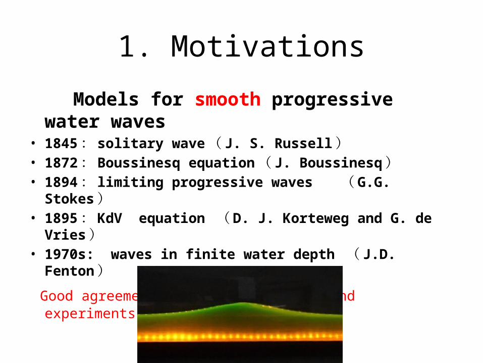
Models for smooth progressive water waves• 1845: solitary wave( J. S. Russell)• 1872: Boussinesq equation( J.
Boussinesq)• 1894: limiting progressive waves (G.G.
Stokes)• 1895: KdV equation (D. J. Korteweg and
G. de Vries)• 1970s: waves in finite water depth ( J.D.
Fenton) Good agreement between wave models and experiments

1. Motivations
• Cammasa-Holm equation (PRL,1993) :
with a peaked solitary wave:
where is a constant related to the critical phase speed of shallow water waves

1. Motivations
• Mathematically, the CH equation is integrable and bi-Hamiltonian, thus possesses an infinite number of conservation laws in involution (Camassa-Holm,1993);
• Physically, unlike the KdV equation and Boussinesq equation, the CH equation can model phenomena of soliton interaction and wave breaking (Constantin, 2000)
• A few researchers even believed that ‘‘it has the potential to become the new master equation for shallow water wave theory’’ (Fuchssteiner, 1996)

1. Motivations
Some open questionsHow about finite water depth?How about exact wave equations?Are the peaked solitary waves consistent with the
smooth waves in theory?Why can we not observe them in experiments?Can we gain more information so as to observe
the peaked/cusped waves in experiments?

2. Unified Wave Model (UWM)
• Smooth waves: infinitely differentiable everywhere
Reason: solutions of Laplace equation are infinitely differentiable everywhere.
• Peaked solitary waves: non-smooth at crest ! How to handle such kind of non-smoothness?
2. Unified Wave Model (UWM) Consider a progressive surface gravity wave propagating on a
horizontal bottom with a constant phase speed c and a permanent form in a finite water depth D. We solve the problem in the frame moving with the phase speed c.
• Assume that the wave elevation has a symmetry about the crest
at x = 0;
• Assume that, in the domain x > 0 and x < 0, the fluid is inviscid and incompressible, the flow is irrotational, and surface tension is neglected;
• However, the flow at x = 0 is not absolutely necessary to be irrotational.

2. Unified Wave Model (UWM)
(1) Symmetry:
which leads to the boundary conditions
for both of the smooth and peaked waves.
So, we need governing equations and free surface conditions only in the domain
(a) (x),u(x, z) are continuous at x = 0
(b) v(0, z) 0, since v(0, z) v(0, z)
0 x

2. Unified Wave Model (UWM)
(2) Equations in the domain
with free surface boundary conditions
bottom condition:
open boundary condition:
periodic waves:
solitary waves:
0 x

2. Unified Wave Model (UWM)
Mathematically, Laplace equation (with bottom condition) has two kinds of solutions:
(1) traditional base function
corresponding to smooth waves
(2) evanescent base function (Massel, 1983)
corresponding to peaked solitary waves

3. UWM: smooth waves
The smooth potential function
automatically satisfy all symmetry conditions
Therefore, all traditional smooth propagating waves can be derived in the frame of the Unified Wave Model (UWM)
It also supports the correctness of the UWM in mathematics.
(x, z) bn cosh nk(z 1 sin(nkx)n1

4. UWM: peaked waves
The velocity potential of peaked waves
does not automatically satisfy the symmetry
and the restrict condition
Therefore, the restricted condition
must be enforced to be satisfied
(x, z) an cos nk(z 1) exp( nkx), x 0n1
4. UWM: peaked waves
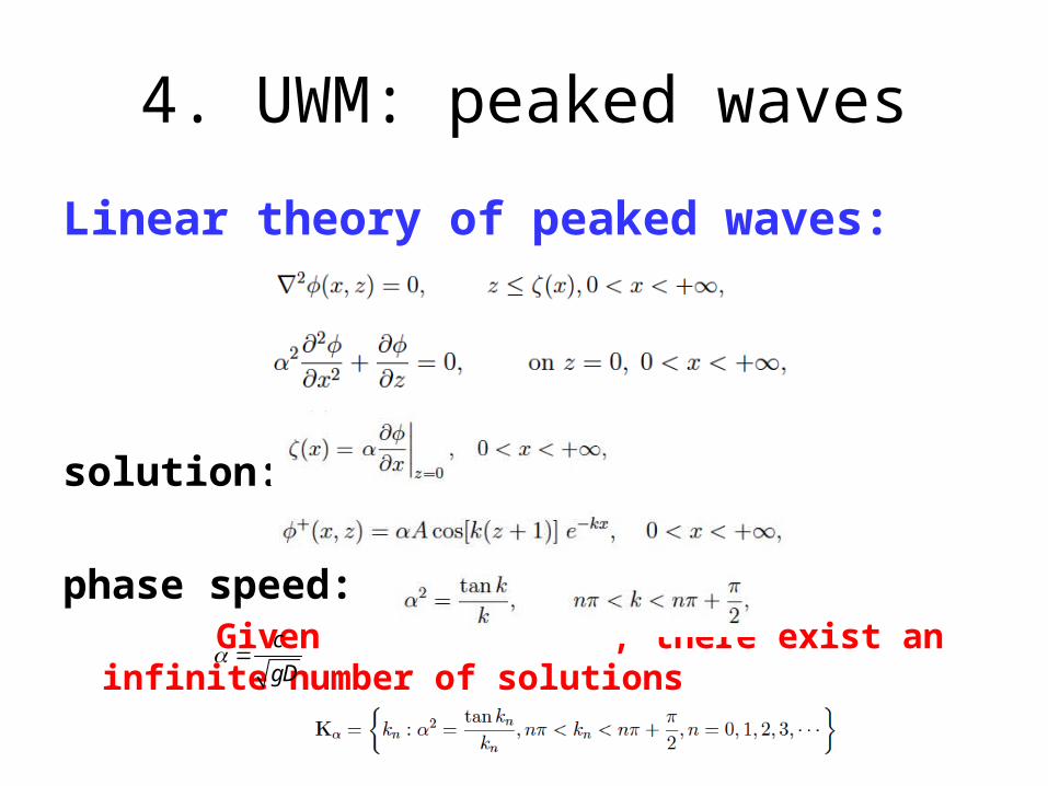
Linear theory of peaked waves:
solution:
phase speed: Given , there exist an infinite number of solutions
c
gD

4. UWM: peaked waves
Linear theory of peaked wavesSurface elevation: Camassa-Holm’s peaked wave is only a special
case of our peaked solitary waves ! This indicatesthat the UWMis reasonable

4. UWM: peaked waves
G.G. Stokes (1894): The smooth propagating periodic waves tend
to have a corner crest at the limiting wave amplitude, and thus become non-smooth.
Thus, non-smooth waves are acceptable in the
frame of inviscid fluid.

4. UWM: peaked waves
Linear theory of peaked waves
Velcoity:
(1) increases from surface to bottom, and is continuous at x = 0
(2) decreases from surface to bottom, and is discontinuous at x = 0, say,
Thus, the condition is enforced.
u(x, z)
v(x, z)
v(0, z) 0
4. UWM: peaked waves
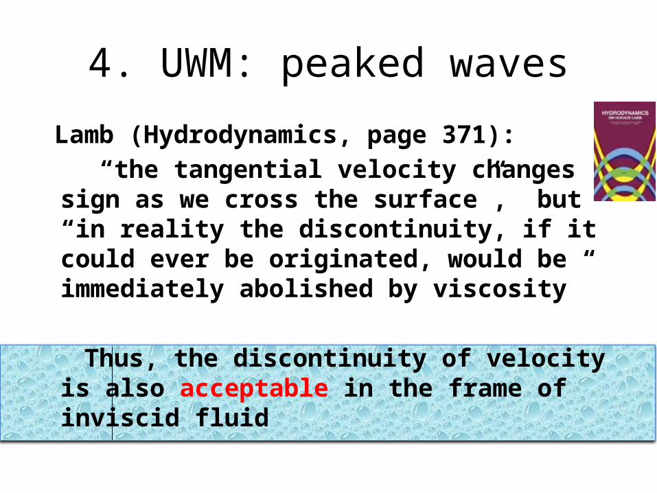
Lamb (Hydrodynamics, page 371): “the tangential velocity changes
sign as we cross the surface”, but “in reality the discontinuity, if it could ever be originated, would be immediately abolished by viscosity”
Thus, the discontinuity of velocity is also acceptable in the frame of inviscid fluid

Kinetic energy distribution
Smooth periodic waves
• Decays exponentially from surface to bottom
• varies periodically in the x direction
Peaked waves
• keeps constant from surface to bottom
• Decays exponentially in the x direction

4. UWM: peaked waves
Nonlinear theory of peaked waves
with fully nonlinear surface conditions
the bottom condition
and other conditions

4. UWM: peaked waves
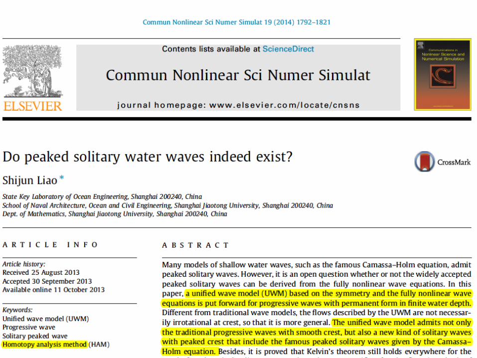
Nonlinear theory of peaked wavesThese nonlinear PDEs are solved by means of
homotopy analysis method (HAM)
Advantages of the HAM:• Independent of physical small parameters• Guarantee of convergence
Applications of the HAM
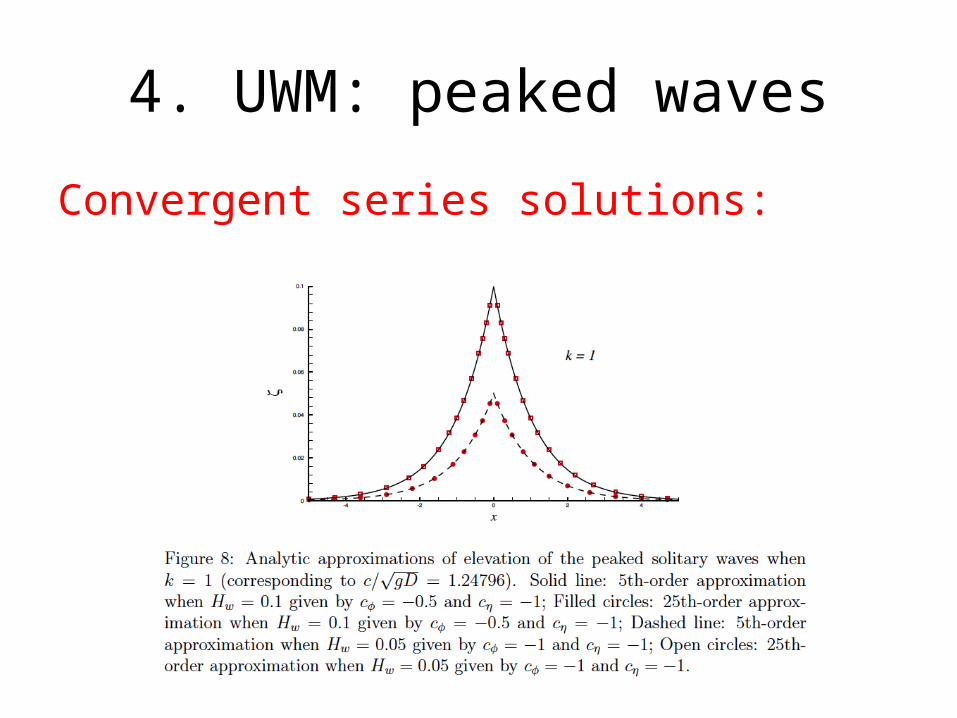
4. UWM: peaked waves
Convergent series solutions:
4. UWM: peaked waves

4. UWM: peaked waves
Nonlinear theory of peaked waves • The phase speed of peaked waves has nothing
to do with wave height, say, the peaked waves are non-dispersive!
• The kinetic energy is almost the same from surface to bottom
• There exists the velocity discontinuity at crest

Comparison of smooth and peaked waves
Smooth waves
• Smooth everywhere• Dispersive• Kinetic energy decays
exponentially from surface to bottom
Peaked waves
• Non-smooth at crest• Non-dispersive• Kinetic energy is almost
the same from surface to bottom
A new theoretical explanation to rogue wave
The rogue wave can suddenly appear on ocean even when “the weather was good, with clear skies and glassy swells”, as reported by Graham (2000) and Kharif (2003).
A new explanation: Peaked solitary waves with small wave height
and different phase speed may suddenly create a rogue wave somewhere, since they are non-dispersive

Relation between peaked and cusped waves
Using the non-dispersive property of peaked waves, it is proved that a cusped solitary wave is consist of an infinite number of peaked solitary waves

5. Conclusions and discussions
(1) The UWM gives not only the traditional smooth progressive waves but also the famous Camassa-Holm’s peaked waves
Therefore, the UAM is reasonable and more general from mathematical viewpoint

5. Conclusions and discussions
(2) The UWM admits not only smooth progressive waves but also peaked/cusped solitray waves in finite water depth
Therefore, the peaked/cusped solitray waves are consistent with smooth waves

5. Conclusions and discussions
(3) The peaked solitary waves have many unusual characteristics:
• Phase speed is independent of wave height (non-dispersive)
• Kinetic energy is almost the same from surface to bottom
• Velocity discontinuity at crest
These information are helpful for possible experimental observations of them in future.

5. Conclusions and discussions
(4) Using the non-dispersive property of peaked solitary waves,
(a) a simple but elegant relationship between peaked and cusped waves is given,
(b)a new theoretical explanation of rogue wave is suggested.

5. Conclusions and discussions
Models for progressive water waves• 1845: solitary wave( J. S. Russell)• 1872: Boussinesq equation( J. Boussinesq)• 1894: limiting progressive waves (G.G. Stokes)• 1895:KdV equation (D. J. Korteweg and G. de Vries)• 1970s: waves in finite water depth ( J.D. Fenton)• 1993: Camassa-Holm equation (Camassa and Holm)• 2014: Unified Wave Model (UWM)
UWM can describe the smooth and
non-smooth progressive waves of all previous models in shallow and finite depth of water!
Tony, happy 60’s Birthday
Anniversary!
Thank You!