unified credit-equity modeling - math.unice.frpatras/creditrisk2009/nice_mendoza.pdf · recent...
TRANSCRIPT

Unified Credit-Equity Modeling
Rafael Mendoza-ArriagaBased on joint research with: Vadim Linetsky and Peter Carr
The University of Texas at AustinMcCombs School of Business (IROM)
Recent Advancements in the Theory and Practice of CreditDerivativesNice, France
September 28-30, 2009
Rafael Mendoza (McCombs) Unified Credit-Equity Modeling Credit Risk 2009 1 / 1

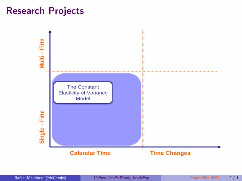
Research Projects
Mul
ti –
Firm
Sin
gle
–Fi
rm
Time ChangesCalendar Time
Rafael Mendoza (McCombs) Unified Credit-Equity Modeling Credit Risk 2009 2 / 1
Research Projects
Mul
ti –
Firm
Sin
gle
–Fi
rm
Time ChangesCalendar Time
The Constant Elasticity of Variance
Model
Rafael Mendoza (McCombs) Unified Credit-Equity Modeling Credit Risk 2009 2 / 1
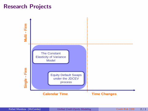
Research Projects
Mul
ti –
Firm
Sin
gle
–Fi
rm
Time ChangesCalendar Time
The Constant Elasticity of Variance
Model
Equity Default Swaps under the JDCEV
process
Rafael Mendoza (McCombs) Unified Credit-Equity Modeling Credit Risk 2009 2 / 1

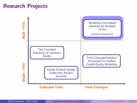
Research Projects
Mul
ti –
Firm
Sin
gle
–Fi
rm
Time ChangesCalendar Time
The Constant Elasticity of Variance
Model
Equity Default Swaps under the JDCEV
process
Time Changed Markov Processes in Unified
Credit-Equity Modeling
Rafael Mendoza (McCombs) Unified Credit-Equity Modeling Credit Risk 2009 2 / 1
Research Projects
Mul
ti –
Firm
Sin
gle
–Fi
rm
Time ChangesCalendar Time
The Constant Elasticity of Variance
Model
Equity Default Swaps under the JDCEV
process
Time Changed Markov Processes in Unified
Credit-Equity Modeling
Modeling Correlated Defaults by Multiple
Firms
(Future Research)
Rafael Mendoza (McCombs) Unified Credit-Equity Modeling Credit Risk 2009 2 / 1

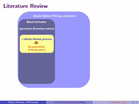
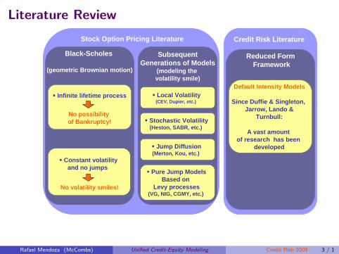
Literature Review
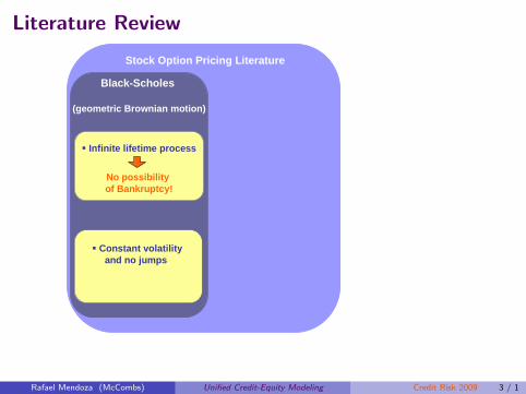
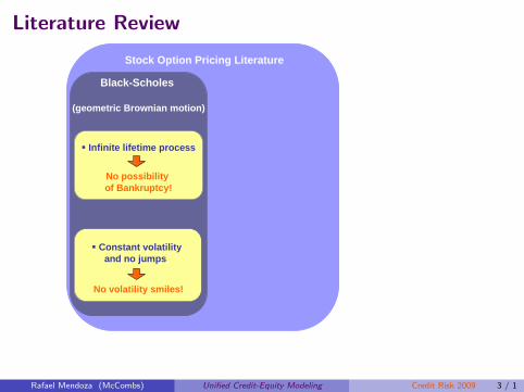
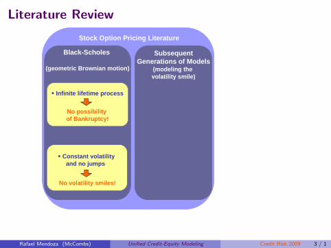
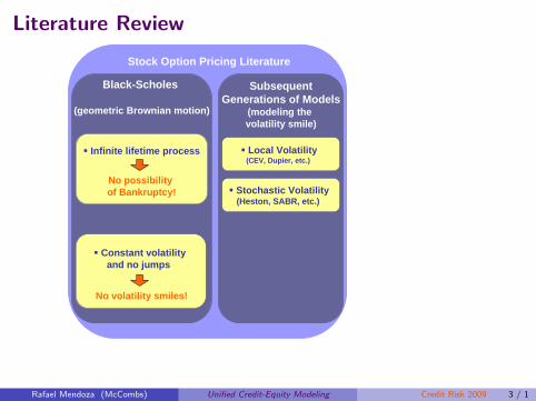
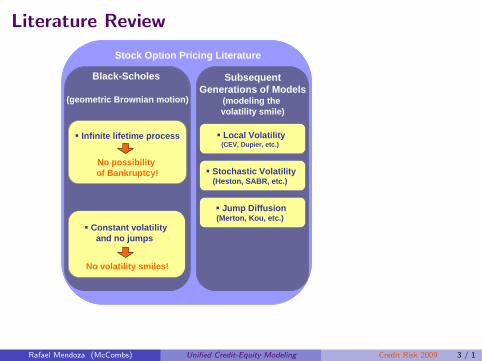
Stock Option Pricing Literature
Black-Scholes
(geometric Brownian motion)
Rafael Mendoza (McCombs) Unified Credit-Equity Modeling Credit Risk 2009 3 / 1

Literature Review
Stock Option Pricing Literature
Black-Scholes
(geometric Brownian motion)
� Infinite lifetime process
Rafael Mendoza (McCombs) Unified Credit-Equity Modeling Credit Risk 2009 3 / 1
Literature Review
Stock Option Pricing Literature
Black-Scholes
(geometric Brownian motion)
� Infinite lifetime process
No possibility of Bankruptcy!
Rafael Mendoza (McCombs) Unified Credit-Equity Modeling Credit Risk 2009 3 / 1
Literature Review
Stock Option Pricing Literature
Black-Scholes
(geometric Brownian motion)
� Infinite lifetime process
No possibility of Bankruptcy!
� Constant volatilityand no jumps
Rafael Mendoza (McCombs) Unified Credit-Equity Modeling Credit Risk 2009 3 / 1
Literature Review
Stock Option Pricing Literature
Black-Scholes
(geometric Brownian motion)
� Infinite lifetime process
No possibility of Bankruptcy!
� Constant volatilityand no jumps
No volatility smiles!
Rafael Mendoza (McCombs) Unified Credit-Equity Modeling Credit Risk 2009 3 / 1
Literature Review
Stock Option Pricing Literature
Black-Scholes
(geometric Brownian motion)
� Infinite lifetime process
No possibility of Bankruptcy!
� Constant volatilityand no jumps
No volatility smiles!
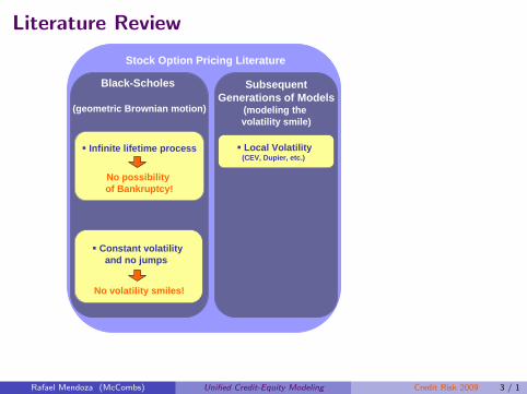
SubsequentGenerations of Models
(modeling the volatility smile)
Rafael Mendoza (McCombs) Unified Credit-Equity Modeling Credit Risk 2009 3 / 1
Literature Review
Stock Option Pricing Literature
Black-Scholes
(geometric Brownian motion)
� Infinite lifetime process
No possibility of Bankruptcy!
� Constant volatilityand no jumps
No volatility smiles!
SubsequentGenerations of Models
(modeling the volatility smile)
� Local Volatility(CEV, Dupier, etc.)
� Stochastic Volatility(Heston, SABR, etc.)
� Jump Diffusion(Merton, Kou, etc.)
Rafael Mendoza (McCombs) Unified Credit-Equity Modeling Credit Risk 2009 3 / 1

Literature Review
Stock Option Pricing Literature
Black-Scholes
(geometric Brownian motion)
� Infinite lifetime process
No possibility of Bankruptcy!
� Constant volatilityand no jumps
No volatility smiles!
SubsequentGenerations of Models
(modeling the volatility smile)
� Local Volatility(CEV, Dupier, etc.)
� Stochastic Volatility(Heston, SABR, etc.)
� Jump Diffusion(Merton, Kou, etc.)
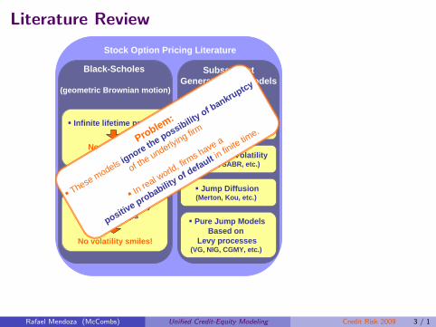
� Pure Jump ModelsBased on
Levy processes(VG, NIG, CGMY, etc.)
Rafael Mendoza (McCombs) Unified Credit-Equity Modeling Credit Risk 2009 3 / 1
Literature Review
Stock Option Pricing Literature
Black-Scholes
(geometric Brownian motion)
� Infinite lifetime process
No possibility of Bankruptcy!
� Constant volatilityand no jumps
No volatility smiles!
SubsequentGenerations of Models
(modeling the volatility smile)
� Local Volatility(CEV, Dupier, etc.)
� Stochastic Volatility(Heston, SABR, etc.)
� Jump Diffusion(Merton, Kou, etc.)
� Pure Jump ModelsBased on
Levy processes(VG, NIG, CGMY, etc.)
Problem:
� These models ignore th
e possibility of b
ankruptcy
of the underlying firm
� In real w
orld, firms have a
positive probabilit
y of default in fin
ite time.
Rafael Mendoza (McCombs) Unified Credit-Equity Modeling Credit Risk 2009 3 / 1
Literature Review
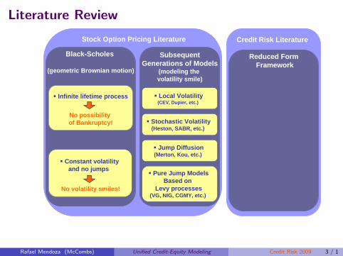
Stock Option Pricing Literature Credit Risk Literature
Black-Scholes
(geometric Brownian motion)
� Infinite lifetime process
No possibility of Bankruptcy!
� Constant volatilityand no jumps
No volatility smiles!
SubsequentGenerations of Models
(modeling the volatility smile)
� Local Volatility(CEV, Dupier, etc.)
� Stochastic Volatility(Heston, SABR, etc.)
� Jump Diffusion(Merton, Kou, etc.)
� Pure Jump ModelsBased on
Levy processes(VG, NIG, CGMY, etc.)
Reduced Form Framework
Rafael Mendoza (McCombs) Unified Credit-Equity Modeling Credit Risk 2009 3 / 1
Literature Review
Stock Option Pricing Literature Credit Risk Literature
Black-Scholes
(geometric Brownian motion)
� Infinite lifetime process
No possibility of Bankruptcy!
� Constant volatilityand no jumps
No volatility smiles!
SubsequentGenerations of Models
(modeling the volatility smile)
� Local Volatility(CEV, Dupier, etc.)
� Stochastic Volatility(Heston, SABR, etc.)
� Jump Diffusion(Merton, Kou, etc.)
� Pure Jump ModelsBased on
Levy processes(VG, NIG, CGMY, etc.)
Reduced Form Framework
Default Intensity Models
Since Duffie & Singleton, Jarrow, Lando &
Turnbull:
A vast amount of research has been
developed
Rafael Mendoza (McCombs) Unified Credit-Equity Modeling Credit Risk 2009 3 / 1
Literature Review
Stock Option Pricing Literature Credit Risk Literature
Black-Scholes
(geometric Brownian motion)
� Infinite lifetime process
No possibility of Bankruptcy!
� Constant volatilityand no jumps
No volatility smiles!
SubsequentGenerations of Models
(modeling the volatility smile)
� Local Volatility(CEV, Dupier, etc.)
� Stochastic Volatility(Heston, SABR, etc.)
� Jump Diffusion(Merton, Kou, etc.)
� Pure Jump ModelsBased on
Levy processes(VG, NIG, CGMY, etc.)
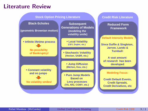
Reduced Form Framework
Modeling Focus:
Credit Default Events,Credit Spreads,
Credit Derivatives, etc
Default Intensity Models
Since Duffie & Singleton, Jarrow, Lando &
Turnbull:
A vast amount of research has been
developed
Rafael Mendoza (McCombs) Unified Credit-Equity Modeling Credit Risk 2009 3 / 1
Literature Review
Stock Option Pricing Literature Credit Risk Literature
Black-Scholes
(geometric Brownian motion)
� Infinite lifetime process
No possibility of Bankruptcy!
� Constant volatilityand no jumps
No volatility smiles!
SubsequentGenerations of Models
(modeling the volatility smile)
� Local Volatility(CEV, Dupier, etc.)
� Stochastic Volatility(Heston, SABR, etc.)
� Jump Diffusion(Merton, Kou, etc.)
� Pure Jump ModelsBased on
Levy processes(VG, NIG, CGMY, etc.)
Reduced Form Framework
Modeling Focus:
Credit Default Events,Credit Spreads,
Credit Derivatives, etc
Default Intensity Models
Since Duffie & Singleton, Jarrow, Lando &
Turnbull:
A vast amount of research has been
developed
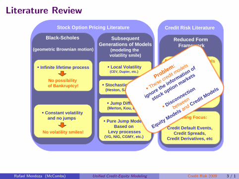
Problem:
� These credit models
ignore the inform
ation of
stock option markets
� Disconnection
between
Equity Models and Credit Models
Rafael Mendoza (McCombs) Unified Credit-Equity Modeling Credit Risk 2009 3 / 1
Literature Review
Stock Option Pricing Literature Credit Risk Literature
Black-Scholes
(geometric Brownian motion)
� Infinite lifetime process
No possibility of Bankruptcy!
� Constant volatilityand no jumps
No volatility smiles!
SubsequentGenerations of Models
(modeling the volatility smile)
� Local Volatility(CEV, Dupier, etc.)
� Stochastic Volatility(Heston, SABR, etc.)
� Jump Diffusion(Merton, Kou, etc.)
� Pure Jump ModelsBased on
Levy processes(VG, NIG, CGMY, etc.)
Reduced Form Framework
Modeling Focus:
Credit Default Events,Credit Spreads,
Credit Derivatives, etc
Default Intensity Models
Since Duffie & Singleton, Jarrow, Lando &
Turnbull:
A vast amount of research has been
developed
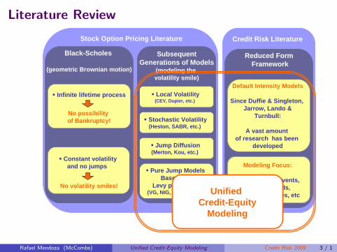
Unified Credit-Equity
Modeling
Rafael Mendoza (McCombs) Unified Credit-Equity Modeling Credit Risk 2009 3 / 1
Motivating Example
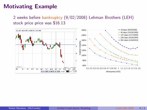
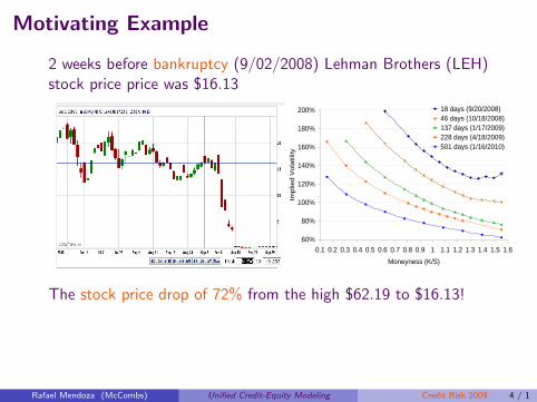
2 weeks before bankruptcy (9/02/2008) Lehman Brothers (LEH)stock price price was $16.13
60%
80%
100%
120%
140%
160%
180%
200%
0.1 0.2 0.3 0.4 0.5 0.6 0.7 0.8 0.9 1 1.1 1.2 1.3 1.4 1.5 1.6
Moneyness (K/S)
Imp
lied
Vo
latil
ity
18 days (9/20/2008)46 days (10/18/2008)137 days (1/17/2009)228 days (4/18/2009)501 days (1/16/2010)
The stock price drop of 72% from the high $62.19 to $16.13!
Open Interest on Put contracts with strike prices K = 2.5 USD
Maturing on 4/18/2009 (228 days) were 1529 contractsMaturing on 1/16/2010 (501 days) were 2791 contracts
Rafael Mendoza (McCombs) Unified Credit-Equity Modeling Credit Risk 2009 4 / 1
Motivating Example
2 weeks before bankruptcy (9/02/2008) Lehman Brothers (LEH)stock price price was $16.13
60%
80%
100%
120%
140%
160%
180%
200%
0.1 0.2 0.3 0.4 0.5 0.6 0.7 0.8 0.9 1 1.1 1.2 1.3 1.4 1.5 1.6
Moneyness (K/S)
Imp
lied
Vo
latil
ity
18 days (9/20/2008)46 days (10/18/2008)137 days (1/17/2009)228 days (4/18/2009)501 days (1/16/2010)
The stock price drop of 72% from the high $62.19 to $16.13!
Open Interest on Put contracts with strike prices K = 2.5 USD
Maturing on 4/18/2009 (228 days) were 1529 contractsMaturing on 1/16/2010 (501 days) were 2791 contracts
Rafael Mendoza (McCombs) Unified Credit-Equity Modeling Credit Risk 2009 4 / 1
The Case for the Next Generation of UnifiedCredit-Equity Models
Put options provide default protection. Deep out-of-the-money putsare essentially credit derivatives which close the link between equityand credit products.
Pricing of equity derivatives should take into account the possibility ofbankruptcy of the underlying firm.
Possibility of default contributes to the implied volatility skew in stockoptions.
Rafael Mendoza (McCombs) Unified Credit-Equity Modeling Credit Risk 2009 5 / 1

Research Goals
Unified Credit –Equity Framework
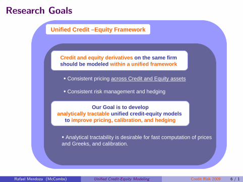
Credit and equity derivatives on the same firm should be modeled within a unified framework
� Consistent pricing across Credit and Equity assets
� Consistent risk management and hedging
Rafael Mendoza (McCombs) Unified Credit-Equity Modeling Credit Risk 2009 6 / 1
Research Goals
Unified Credit –Equity Framework
Credit and equity derivatives on the same firm should be modeled within a unified framework
� Consistent pricing across Credit and Equity assets
� Consistent risk management and hedging
Our Goal is to developanalytically tractable unified credit-equity models
to improve pricing, calibration, and hedging
� Analytical tractability is desirable for fast computation of prices and Greeks, and calibration.
Rafael Mendoza (McCombs) Unified Credit-Equity Modeling Credit Risk 2009 6 / 1

Our Contributions
We introduce a new analytically tractable class of credit-equitymodels.
Our model architecture is based on applying random time changes toMarkov diffusion processes to create new processes with desiredproperties.
We model the stock price as a time changed Markov process withstate-dependent jumps, stochastic volatility, and default intensity(stock drops to zero in default).
For the first time in the literature, we present state-dependent jumpsthat exhibit the leverage effect:
As stock price falls V arrival rates of large jumps increaseAs stock price rises V arrival rate of large jumps decrease
Rafael Mendoza (McCombs) Unified Credit-Equity Modeling Credit Risk 2009 7 / 1

Our Contributions
We introduce a new analytically tractable class of credit-equitymodels.
Our model architecture is based on applying random time changes toMarkov diffusion processes to create new processes with desiredproperties.
We model the stock price as a time changed Markov process withstate-dependent jumps, stochastic volatility, and default intensity(stock drops to zero in default).
For the first time in the literature, we present state-dependent jumpsthat exhibit the leverage effect:
As stock price falls V arrival rates of large jumps increase
As stock price rises V arrival rate of large jumps decrease
Rafael Mendoza (McCombs) Unified Credit-Equity Modeling Credit Risk 2009 7 / 1
Our Contributions
We introduce a new analytically tractable class of credit-equitymodels.
Our model architecture is based on applying random time changes toMarkov diffusion processes to create new processes with desiredproperties.
We model the stock price as a time changed Markov process withstate-dependent jumps, stochastic volatility, and default intensity(stock drops to zero in default).
For the first time in the literature, we present state-dependent jumpsthat exhibit the leverage effect:
As stock price falls V arrival rates of large jumps increaseAs stock price rises V arrival rate of large jumps decrease
Rafael Mendoza (McCombs) Unified Credit-Equity Modeling Credit Risk 2009 7 / 1
Our Contributions (cont.)
In our model architecture, time changes of diffusions have the followingeffects:
Levy subordinator time change induces jumps with state-dependentLevy measure, including the possibility of a jump-to-default (stockdrops to zero).
Time integral of an activity rate process induces stochastic volatilityin the diffusion dynamics, the Levy measure, and default intensity.
Rafael Mendoza (McCombs) Unified Credit-Equity Modeling Credit Risk 2009 8 / 1
Unifying Credit-Equity Models
The Jump to Default Extended Diffusions (JDED)
Before moving on to use time changes to construct models with jumps andstochastic volatility, we review the Jump-to-Default Extended Diffusionframework (JDED)
Rafael Mendoza (McCombs) Unified Credit-Equity Modeling Credit Risk 2009 9 / 1
Jump to Default Extended Diffusions (JDED)
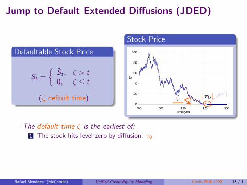
.Defaultable Stock Price..
.
. ..
.
.
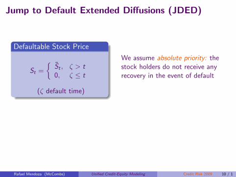
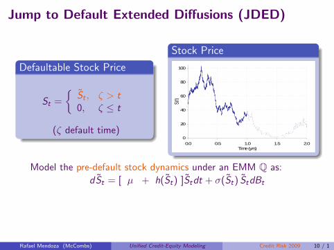
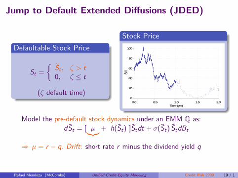
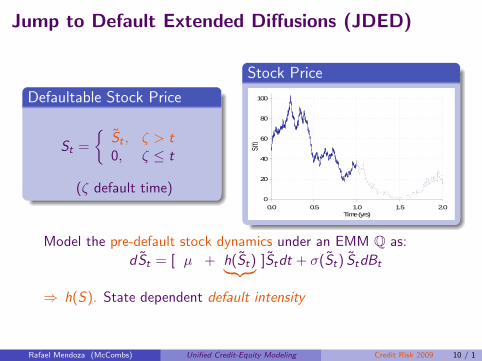
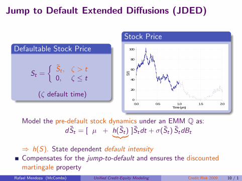
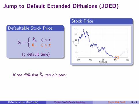
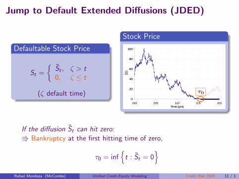
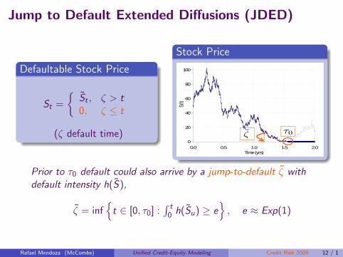
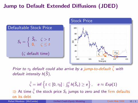
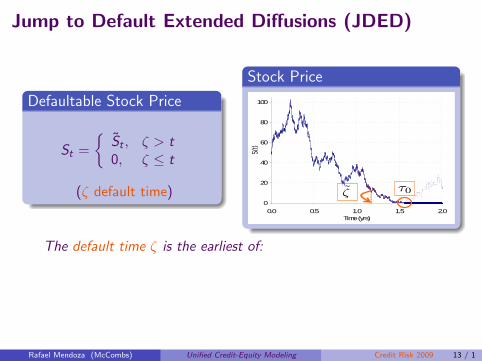
St =
{St , ζ > t0, ζ ≤ t
(ζ default time)
We assume absolute priority: thestock holders do not receive anyrecovery in the event of default
Compensates for the jump-to-default and ensures the discountedmartingale property
Rafael Mendoza (McCombs) Unified Credit-Equity Modeling Credit Risk 2009 10 / 1
Jump to Default Extended Diffusions (JDED)
.Defaultable Stock Price..
.
. ..
.
.
St =
{St , ζ > t0, ζ ≤ t
(ζ default time)
.Stock Price..
.
. ..
.
.
0
20
40
60
80
100
0.0 0.5 1.0 1.5 2.0Time (yrs)
S(t)
Model the pre-default stock dynamics under an EMM Q as:
dSt = [ µ︸︷︷︸+ h(St) ]Stdt + σ(St) StdBt
⇒ µ = r − q. Drift: short rate r minus the dividend yield q
Compensates for the jump-to-default and ensures the discountedmartingale property
Rafael Mendoza (McCombs) Unified Credit-Equity Modeling Credit Risk 2009 10 / 1

Jump to Default Extended Diffusions (JDED)
.Defaultable Stock Price..
.
. ..
.
.
St =
{St , ζ > t0, ζ ≤ t
(ζ default time)
.Stock Price..
.
. ..
.
.
0
20
40
60
80
100
0.0 0.5 1.0 1.5 2.0Time (yrs)
S(t)
Model the pre-default stock dynamics under an EMM Q as:
dSt = [ µ︸︷︷︸+ h(St) ]Stdt + σ(St)︸ ︷︷ ︸ StdBt
⇒ σ(S). State dependent volatility
Compensates for the jump-to-default and ensures the discountedmartingale property
Rafael Mendoza (McCombs) Unified Credit-Equity Modeling Credit Risk 2009 10 / 1
Jump to Default Extended Diffusions (JDED)
.Defaultable Stock Price..
.
. ..
.
.
St =
{St , ζ > t0, ζ ≤ t
(ζ default time)
.Stock Price..
.
. ..
.
.
0
20
40
60
80
100
0.0 0.5 1.0 1.5 2.0Time (yrs)
S(t)
Model the pre-default stock dynamics under an EMM Q as:
dSt = [ µ︸︷︷︸+ h(St)︸ ︷︷ ︸ ]Stdt + σ(St) StdBt
⇒ h(S). State dependent default intensity
Compensates for the jump-to-default and ensures the discountedmartingale property
Rafael Mendoza (McCombs) Unified Credit-Equity Modeling Credit Risk 2009 10 / 1
Jump to Default Extended Diffusions (JDED)
.Defaultable Stock Price..
.
. ..
.
.
St =
{St , ζ > t0, ζ ≤ t
(ζ default time)
.Stock Price..
.
. ..
.
.
0
20
40
60
80
100
0.0 0.5 1.0 1.5 2.0Time (yrs)
S(t)
Model the pre-default stock dynamics under an EMM Q as:
dSt = [ µ︸︷︷︸+ h(St)︸ ︷︷ ︸ ]Stdt + σ(St) StdBt
⇒ h(S). State dependent default intensityCompensates for the jump-to-default and ensures the discountedmartingale property
Rafael Mendoza (McCombs) Unified Credit-Equity Modeling Credit Risk 2009 10 / 1
Jump to Default Extended Diffusions (JDED)
.Defaultable Stock Price..
.
. ..
.
.
St =
{St , ζ > t0, ζ ≤ t
(ζ default time)
.Stock Price..
.
. ..
.
.
0
20
40
60
80
100
0.0 0.5 1.0 1.5 2.0Time (yrs)
S(t)
If the diffusion St can hit zero:
V Bankruptcy at the first hitting time of zero,
τ0 = inf{
t : St = 0}
Rafael Mendoza (McCombs) Unified Credit-Equity Modeling Credit Risk 2009 11 / 1
Jump to Default Extended Diffusions (JDED)
.Defaultable Stock Price..
.
. ..
.
.
St =
{St , ζ > t0, ζ ≤ t
(ζ default time)
.Stock Price..
.
. ..
.
.
0
20
40
60
80
100
0.0 0.5 1.0 1.5 2.0Time (yrs)
S(t)
τ0
If the diffusion St can hit zero:
V Bankruptcy at the first hitting time of zero,
τ0 = inf{
t : St = 0}
Rafael Mendoza (McCombs) Unified Credit-Equity Modeling Credit Risk 2009 11 / 1
Jump to Default Extended Diffusions (JDED)
.Defaultable Stock Price..
.
. ..
.
.
St =
{St , ζ > t0, ζ ≤ t
(ζ default time)
.Stock Price..
.
. ..
.
.
0
20
40
60
80
100
0.0 0.5 1.0 1.5 2.0Time (yrs)
S(t)
τ0ζ
Prior to τ0 default could also arrive by a jump-to-default ζ withdefault intensity h(S),
ζ = inf{
t ∈ [0, τ0] :∫ t0 h(Su) ≥ e
}, e ≈ Exp(1)
V At time ζ the stock price St jumps to zero and the firm defaultson its debt
Rafael Mendoza (McCombs) Unified Credit-Equity Modeling Credit Risk 2009 12 / 1
Jump to Default Extended Diffusions (JDED)
.Defaultable Stock Price..
.
. ..
.
.
St =
{St , ζ > t0, ζ ≤ t
(ζ default time)
.Stock Price..
.
. ..
.
.
0
20
40
60
80
100
0.0 0.5 1.0 1.5 2.0Time (yrs)
S(t)
τ0ζ
The default time ζ is the earliest of:
1 The stock hits level zero by diffusion: τ0
2 The stock jumps to zero from a positive value: ζ
ζ = min(ζ, τ0
)
Rafael Mendoza (McCombs) Unified Credit-Equity Modeling Credit Risk 2009 13 / 1
Jump to Default Extended Diffusions (JDED)
.Defaultable Stock Price..
.
. ..
.
.
St =
{St , ζ > t0, ζ ≤ t
(ζ default time)
.Stock Price..
.
. ..
.
.
0
20
40
60
80
100
0.0 0.5 1.0 1.5 2.0Time (yrs)
S(t)
τ0ζ
The default time ζ is the earliest of:1 The stock hits level zero by diffusion: τ0
2 The stock jumps to zero from a positive value: ζ
ζ = min(ζ, τ0
)
Rafael Mendoza (McCombs) Unified Credit-Equity Modeling Credit Risk 2009 13 / 1

Jump to Default Extended Diffusions (JDED)
.Defaultable Stock Price..
.
. ..
.
.
St =
{St , ζ > t0, ζ ≤ t
(ζ default time)
.Stock Price..
.
. ..
.
.
0
20
40
60
80
100
0.0 0.5 1.0 1.5 2.0Time (yrs)
S(t)
τ0ζ
Default Time ζ:ζ = min
(
ζ , τ0)
The default time ζ is the earliest of:1 The stock hits level zero by diffusion: τ0
2 The stock jumps to zero from a positive value: ζ
ζ = min(ζ, τ0
)Rafael Mendoza (McCombs) Unified Credit-Equity Modeling Credit Risk 2009 13 / 1
Contingent Claims
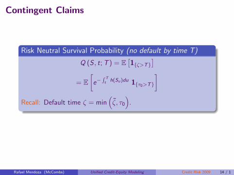
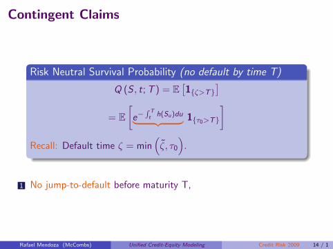
.Risk Neutral Survival Probability (no default by time T)..
.
. ..
.
.
Q (S , t; T ) = E[1{ζ>T}
]= E
[e−
R Tt h(Su)du︸ ︷︷ ︸ 1{τ0>T}︸ ︷︷ ︸
]Recall: Default time ζ = min
(ζ, τ0
).
1 No jump-to-default before maturity T,
2 Diffusion does not hit zero before maturity T.
Rafael Mendoza (McCombs) Unified Credit-Equity Modeling Credit Risk 2009 14 / 1
Contingent Claims
.Risk Neutral Survival Probability (no default by time T)..
.
. ..
.
.
Q (S , t; T ) = E[1{ζ>T}
]= E
[e−
R Tt h(Su)du︸ ︷︷ ︸ 1{τ0>T}︸ ︷︷ ︸
]Recall: Default time ζ = min
(ζ, τ0
).
1 No jump-to-default before maturity T,
2 Diffusion does not hit zero before maturity T.
Rafael Mendoza (McCombs) Unified Credit-Equity Modeling Credit Risk 2009 14 / 1
Contingent Claims
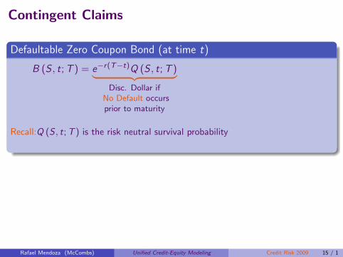
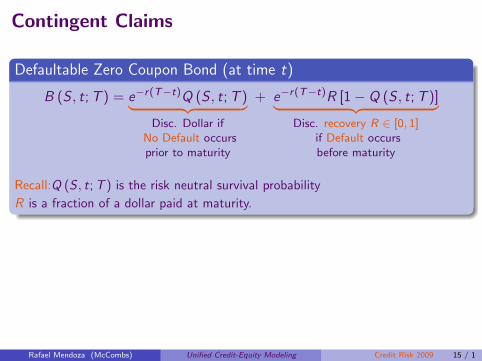
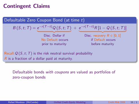
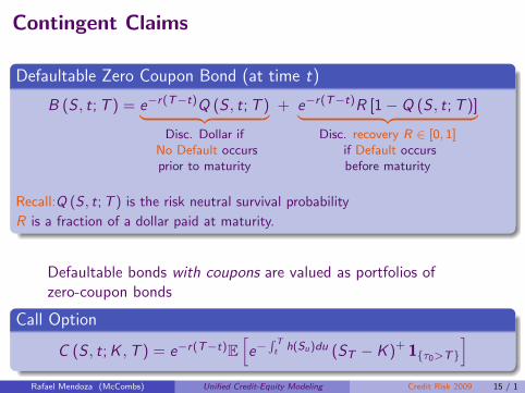
.Defaultable Zero Coupon Bond (at time t)..
.
. ..
.
.
B (S , t;T ) = e−r(T−t)Q (S , t;T )︸ ︷︷ ︸Disc. Dollar if
No Default occursprior to maturity
+ e−r(T−t)R [1 − Q (S , t; T )]︸ ︷︷ ︸Disc. recovery R ∈ [0, 1]
if Default occursbefore maturity T
Recall:Q (S , t; T ) is the risk neutral survival probability
R is a fraction of a dollar paid at maturity.
Defaultable bonds with coupons are valued as portfolios ofzero-coupon bonds
.Call Option..
.
. ..
.
.
C (S , t; K , T ) = e−r(T−t)E[e−
R Tt h(Su)du (ST − K )+ 1{τ0>T}
]
Rafael Mendoza (McCombs) Unified Credit-Equity Modeling Credit Risk 2009 15 / 1
Contingent Claims
.Defaultable Zero Coupon Bond (at time t)..
.
. ..
.
.
B (S , t; T ) = e−r(T−t)Q (S , t;T )︸ ︷︷ ︸Disc. Dollar if
No Default occursprior to maturity
+ e−r(T−t)R [1 − Q (S , t; T )]︸ ︷︷ ︸Disc. recovery R ∈ [0, 1]
if Default occursbefore maturity
Recall:Q (S , t; T ) is the risk neutral survival probability
R is a fraction of a dollar paid at maturity.
Defaultable bonds with coupons are valued as portfolios ofzero-coupon bonds
.Call Option..
.
. ..
.
.
C (S , t; K , T ) = e−r(T−t)E[e−
R Tt h(Su)du (ST − K )+ 1{τ0>T}
]Rafael Mendoza (McCombs) Unified Credit-Equity Modeling Credit Risk 2009 15 / 1
Contingent Claims
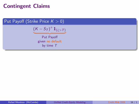
.Put Payoff (Strike Price K > 0)..
.
. ..
.
.
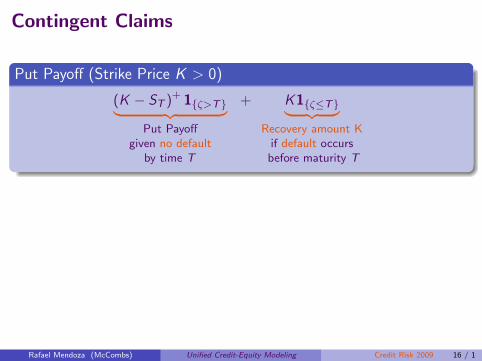
(K − ST )+ 1{ζ>T}︸ ︷︷ ︸Put Payoff
given no defaultby time T
+ K1{ζ≤T}︸ ︷︷ ︸Recovery amount K
if default occursbefore maturity T
.Put Option Price..
.
. ..
.
.
P (S , t; K , T ) = e−r(T−t)E[e−
R Tt h(Su)du (K − ST )+ 1{τ0>T}
]+ Ke−r(T−t) [1 − Q (S , t; T )]
NOTE. A default claim is embedded in the Put Option
Rafael Mendoza (McCombs) Unified Credit-Equity Modeling Credit Risk 2009 16 / 1
Contingent Claims
.Put Payoff (Strike Price K > 0)..
.
. ..
.
.
(K − ST )+ 1{ζ>T}︸ ︷︷ ︸Put Payoff
given no defaultby time T
+ K1{ζ≤T}︸ ︷︷ ︸Recovery amount K
if default occursbefore maturity T
.Put Option Price..
.
. ..
.
.
P (S , t; K , T ) = e−r(T−t)E[e−
R Tt h(Su)du (K − ST )+ 1{τ0>T}
]+ Ke−r(T−t) [1 − Q (S , t; T )]
NOTE. A default claim is embedded in the Put Option
Rafael Mendoza (McCombs) Unified Credit-Equity Modeling Credit Risk 2009 16 / 1
Jump-to-Default Extended Constant Elasticity ofVariance (JDCEV) Model
.The JDCEV process (Carr and Linetsky (2006))..
.
. ..
.
.
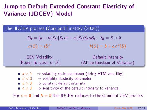
dSt = [µ + h(St)]St dt + σ(St)St dBt , S0 = S > 0
σ(S) = aSβ
CEV Volatility(Power function of S)
h(S) = b + c σ2(S)
Default Intensity(Affine function of Variance)
a > 0 ⇒ volatility scale parameter (fixing ATM volatility)β < 0 ⇒ volatility elasticity parameterb ≥ 0 ⇒ constant default intensityc ≥ 0 ⇒ sensitivity of the default intensity to variance
For c = 0 and b = 0 the JDCEV reduces to the standard CEV process
Rafael Mendoza (McCombs) Unified Credit-Equity Modeling Credit Risk 2009 17 / 1
Jump-to-Default Extended Constant Elasticity ofVariance (JDCEV) Model
.The JDCEV process (Carr and Linetsky (2006))..
.
. ..
.
.
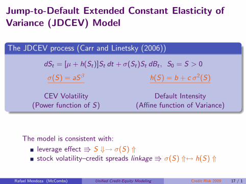
dSt = [µ + h(St)]St dt + σ(St)St dBt , S0 = S > 0
σ(S) = aSβ
CEV Volatility(Power function of S)
h(S) = b + c σ2(S)
Default Intensity(Affine function of Variance)
The model is consistent with:
leverage effect V S ⇓→ σ(S) ⇑stock volatility–credit spreads linkage V σ(S) ⇑↔ h(S) ⇑
Rafael Mendoza (McCombs) Unified Credit-Equity Modeling Credit Risk 2009 17 / 1

An Application of Jump to Default ExtendedDiffusions (JDED)
Equity Default Swaps under the JDCEV Model
Rafael Mendoza (McCombs) Unified Credit-Equity Modeling Credit Risk 2009 18 / 1
Equity Default Swaps (EDS)
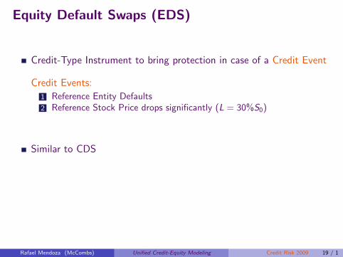
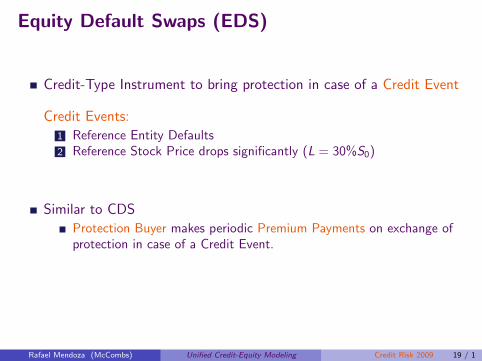
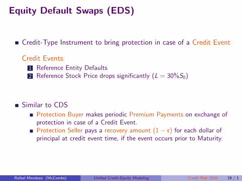
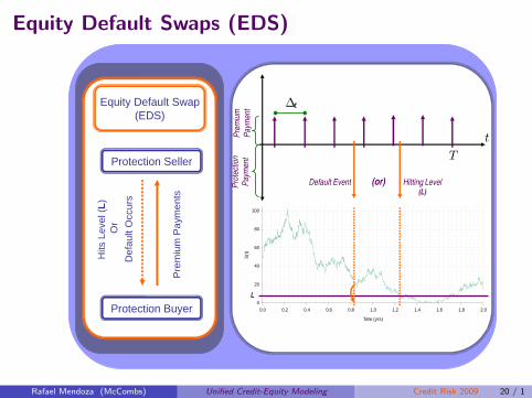
Credit-Type Instrument to bring protection in case of a Credit Event
Credit Events:
1 Reference Entity Defaults2 Reference Stock Price drops significantly (L = 30%S0)
Similar to CDS
Protection Buyer makes periodic Premium Payments on exchange ofprotection in case of a Credit Event.Protection Seller pays a recovery amount (1 − r) for each dollar ofprincipal at credit event time, if the event occurs prior to Maturity.
Rafael Mendoza (McCombs) Unified Credit-Equity Modeling Credit Risk 2009 19 / 1

Equity Default Swaps (EDS)
Credit-Type Instrument to bring protection in case of a Credit Event
Credit Events:
1 Reference Entity Defaults
2 Reference Stock Price drops significantly (L = 30%S0)
Similar to CDS
Protection Buyer makes periodic Premium Payments on exchange ofprotection in case of a Credit Event.Protection Seller pays a recovery amount (1 − r) for each dollar ofprincipal at credit event time, if the event occurs prior to Maturity.
Rafael Mendoza (McCombs) Unified Credit-Equity Modeling Credit Risk 2009 19 / 1

Equity Default Swaps (EDS)
Credit-Type Instrument to bring protection in case of a Credit Event
Credit Events:
1 Reference Entity Defaults2 Reference Stock Price drops significantly (L = 30%S0)
Similar to CDS
Protection Buyer makes periodic Premium Payments on exchange ofprotection in case of a Credit Event.Protection Seller pays a recovery amount (1 − r) for each dollar ofprincipal at credit event time, if the event occurs prior to Maturity.
Rafael Mendoza (McCombs) Unified Credit-Equity Modeling Credit Risk 2009 19 / 1
Equity Default Swaps (EDS)
Credit-Type Instrument to bring protection in case of a Credit Event
Credit Events:
1 Reference Entity Defaults2 Reference Stock Price drops significantly (L = 30%S0)
Similar to CDS
Protection Buyer makes periodic Premium Payments on exchange ofprotection in case of a Credit Event.
Protection Seller pays a recovery amount (1 − r) for each dollar ofprincipal at credit event time, if the event occurs prior to Maturity.
Rafael Mendoza (McCombs) Unified Credit-Equity Modeling Credit Risk 2009 19 / 1
Equity Default Swaps (EDS)
Credit-Type Instrument to bring protection in case of a Credit Event
Credit Events:
1 Reference Entity Defaults2 Reference Stock Price drops significantly (L = 30%S0)
Similar to CDS
Protection Buyer makes periodic Premium Payments on exchange ofprotection in case of a Credit Event.Protection Seller pays a recovery amount (1 − r) for each dollar ofprincipal at credit event time, if the event occurs prior to Maturity.
Rafael Mendoza (McCombs) Unified Credit-Equity Modeling Credit Risk 2009 19 / 1
Equity Default Swaps (EDS)
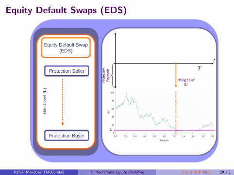
Equity Default Swap(EDS)
Protection Seller
Protection Buyer
Hits
Lev
el (
L)
tT
0
20
40
60
80
100
0.0 0.2 0.4 0.6 0.8 1.0 1.2 1.4 1.6 1.8 2.0
Time (yrs)
S(t
)
Hitting Level(L)
L
Pro
tect
ion
Pay
men
t
Rafael Mendoza (McCombs) Unified Credit-Equity Modeling Credit Risk 2009 20 / 1

Equity Default Swaps (EDS)
Equity Default Swap(EDS)
Protection Seller
Protection Buyer
Def
ault
Occ
urs
Hits
Lev
el (
L)
Or
tT
0
20
40
60
80
100
0.0 0.2 0.4 0.6 0.8 1.0 1.2 1.4 1.6 1.8 2.0
Time (yrs)
S(t
)
Hitting Level(L)
Default Event
L
Pro
tect
ion
Pay
men
t
(or)
Rafael Mendoza (McCombs) Unified Credit-Equity Modeling Credit Risk 2009 20 / 1
Equity Default Swaps (EDS)
Equity Default Swap(EDS)
Protection Seller
Protection Buyer
Def
ault
Occ
urs
Hits
Lev
el (
L)
Or
∆t
tT
0
20
40
60
80
100
0.0 0.2 0.4 0.6 0.8 1.0 1.2 1.4 1.6 1.8 2.0
Time (yrs)
S(t
)
Hitting Level(L)
Default Event
L
Pre
miu
m
Pay
men
t
Pro
tect
ion
Pay
men
t
(or)P
rem
ium
Pay
men
ts+
Acc
rued
Inte
rest
Rafael Mendoza (McCombs) Unified Credit-Equity Modeling Credit Risk 2009 20 / 1
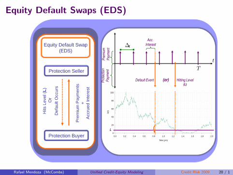
Equity Default Swaps (EDS)
Equity Default Swap(EDS)
Protection Seller
Protection Buyer
Def
ault
Occ
urs
Hits
Lev
el (
L)
Or
∆t
tT
0
20
40
60
80
100
0.0 0.2 0.4 0.6 0.8 1.0 1.2 1.4 1.6 1.8 2.0
Time (yrs)
S(t
)
Hitting Level(L)
Default Event
Acc.
Interest
L
Pre
miu
m
Pay
men
t
Pro
tect
ion
Pay
men
t
(or)P
rem
ium
Pay
men
ts+
Acc
rued
Inte
rest
Rafael Mendoza (McCombs) Unified Credit-Equity Modeling Credit Risk 2009 20 / 1
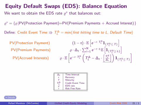
Equity Default Swaps (EDS): Balance EquationWe want to obtain the EDS rate ϱ∗ that balances out:
ϱ∗ = {ϱ |PV(Protection Payment)=PV(Premium Payments + Accrued Interest)}
Define: Credit Event Time V T∆L = min{first hitting time to L, Default Time}
PV(Protection Payment) (1 − r) · E[e−r ·T∆
L 1{T∆L ≤T}
]PV(Premium Payments) ϱ · ∆t ·
∑Ni=1 e−r · ti E
[1{T∆
L ≥ ti}
]PV(Accrued Interests) ϱ · E
[e−r ·T∆
L
(T∆
L − ∆t ·[
T∆L
∆t
])1{T∆
L ≤T}
]
∆t Time Intervalr RecoveryT Maturity
T∆L Credit Event Timeϱ EDS rater Risk Free Rate
.. Details
Rafael Mendoza (McCombs) Unified Credit-Equity Modeling Credit Risk 2009 21 / 1
Equity Default Swaps (EDS)
Advantages of EDS over CDS
Transparency on which an EDS payoff is triggered. It is easy to knowwhether a firm stock price has crossed a lower threshold (L)
Using the Stock Price as the state variable to determine a creditevent allows investors to have a Exposure to Firms for which CDS arenot usually traded.(as in the case of firms with high yield debt)
EDS closes the gap between equity and credit instruments since it isstructurally similar to the credit default swap.
Rafael Mendoza (McCombs) Unified Credit-Equity Modeling Credit Risk 2009 22 / 1
Time-Changing the Jump to Default ExtendedDiffusions (JDED)
Under the jump-to-default extended diffusion framework (includingJDCEV), the pre-default stock process evolves continuously and mayexperience a single jump to default.
Our contribution is to construct far-reaching extensions byintroducing jumps and stochastic volatility by means of time-changes
Rafael Mendoza (McCombs) Unified Credit-Equity Modeling Credit Risk 2009 23 / 1

Time-Changing the Jump to Default ExtendedDiffusions (JDED)
“Time Changes of Markov Processes in Credit-Equity Modeling”
Rafael Mendoza (McCombs) Unified Credit-Equity Modeling Credit Risk 2009 24 / 1

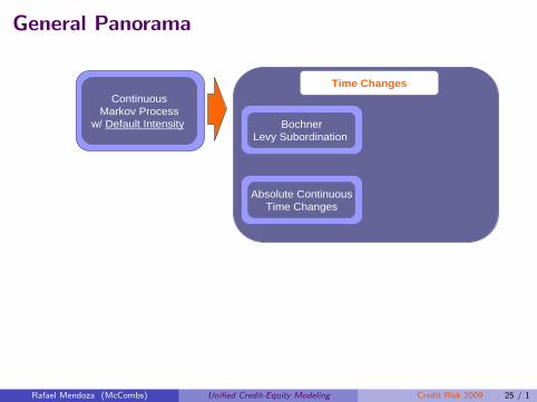
General Panorama
ContinuousMarkov Process
w/ Default Intensity
Rafael Mendoza (McCombs) Unified Credit-Equity Modeling Credit Risk 2009 25 / 1
General Panorama
ContinuousMarkov Process
w/ Default Intensity BochnerLevy Subordination
Time Changes
Absolute ContinuousTime Changes
Rafael Mendoza (McCombs) Unified Credit-Equity Modeling Credit Risk 2009 25 / 1
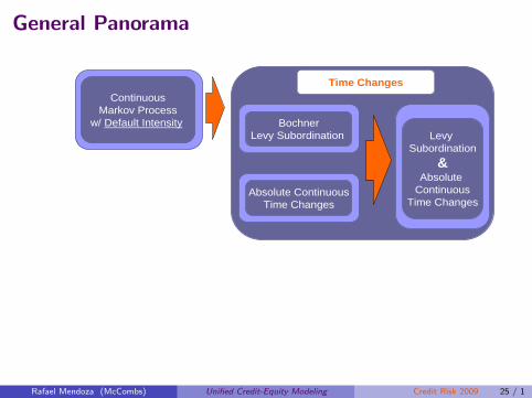
General Panorama
ContinuousMarkov Process
w/ Default Intensity BochnerLevy Subordination
Absolute ContinuousTime Changes
Levy Subordination
&Absolute
ContinuousTime Changes
Time Changes
Rafael Mendoza (McCombs) Unified Credit-Equity Modeling Credit Risk 2009 25 / 1
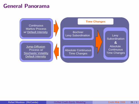
General Panorama
ContinuousMarkov Process
w/ Default Intensity
Jump-Diffusion Process w/
Stochastic VolatilityDefault Intensity
BochnerLevy Subordination
Absolute ContinuousTime Changes
Levy Subordination
&Absolute
ContinuousTime Changes
Time Changes
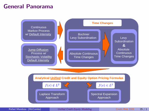
Analytical Unified Credit and Equity Option Pricing Formulas
Rafael Mendoza (McCombs) Unified Credit-Equity Modeling Credit Risk 2009 25 / 1
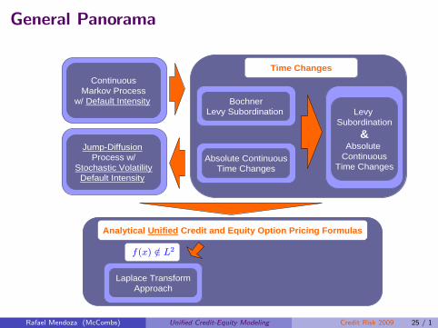
General Panorama
ContinuousMarkov Process
w/ Default Intensity
Jump-Diffusion Process w/
Stochastic VolatilityDefault Intensity
BochnerLevy Subordination
Absolute ContinuousTime Changes
Levy Subordination
&Absolute
ContinuousTime Changes
Analytical Unified Credit and Equity Option Pricing Formulas
Laplace TransformApproach
f(x) /∈ L2
Time Changes
Rafael Mendoza (McCombs) Unified Credit-Equity Modeling Credit Risk 2009 25 / 1
General Panorama
Analytical Unified Credit and Equity Option Pricing Formulas
ContinuousMarkov Process
w/ Default Intensity
Jump-Diffusion Process w/
Stochastic VolatilityDefault Intensity
BochnerLevy Subordination
Absolute ContinuousTime Changes
Levy Subordination
&Absolute
ContinuousTime Changes
Laplace TransformApproach
Spectral ExpansionApproach
f(x) /∈ L2 f(x) ∈ L2
Time Changes
Rafael Mendoza (McCombs) Unified Credit-Equity Modeling Credit Risk 2009 25 / 1
Time-Changed Process Yt = XTt
.Time Changed Process Construction..
.
. ..
.
.
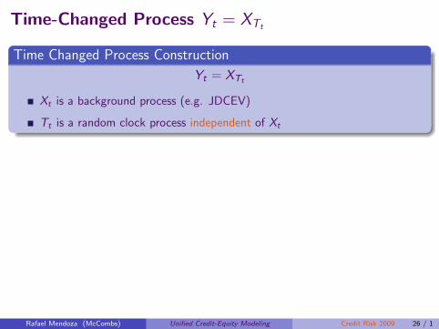
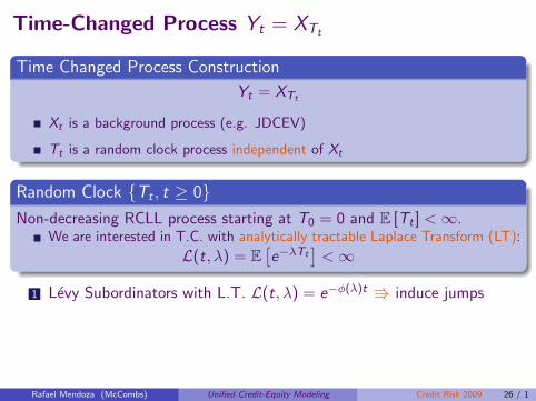
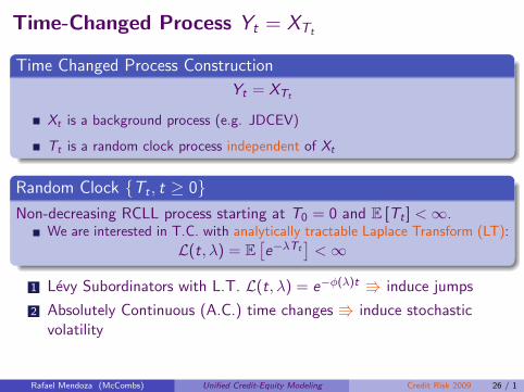
Yt = XTt
Xt is a background process (e.g. JDCEV)
Tt is a random clock process independent of Xt
.Random Clock {Tt , t ≥ 0}..
.
. ..
.
.
Non-decreasing RCLL process starting at T0 = 0 and E [Tt ] < ∞.We are interested in T.C. with analytically tractable Laplace Transform (LT):
L(t, λ) = E[e−λTt
]< ∞
1 Levy Subordinators with L.T. L(t, λ) = e−ϕ(λ)t V induce jumps
2 Absolutely Continuous (A.C.) time changes V induce stochasticvolatility
3 Composite Time Changes V induce jumps & stochastic volatility
Rafael Mendoza (McCombs) Unified Credit-Equity Modeling Credit Risk 2009 26 / 1

Time-Changed Process Yt = XTt
.Time Changed Process Construction..
.
. ..
.
.
Yt = XTt
Xt is a background process (e.g. JDCEV)
Tt is a random clock process independent of Xt
.Random Clock {Tt , t ≥ 0}..
.
. ..
.
.
Non-decreasing RCLL process starting at T0 = 0 and E [Tt ] < ∞.We are interested in T.C. with analytically tractable Laplace Transform (LT):
L(t, λ) = E[e−λTt
]< ∞
1 Levy Subordinators with L.T. L(t, λ) = e−ϕ(λ)t V induce jumps
2 Absolutely Continuous (A.C.) time changes V induce stochasticvolatility
3 Composite Time Changes V induce jumps & stochastic volatility
Rafael Mendoza (McCombs) Unified Credit-Equity Modeling Credit Risk 2009 26 / 1

Illustration of Levy Subordinators.
Y = XTt where Xt = Bt and Tt = t+ Compound Poisson Processwith Exponential Jumps
..
.
. ..
.
.
Time Changed Process Y(t)=X(T(t))
-0.1
0
0.1
0.2
0.3
0.4
0.5
0.6
0 0.1 0.2 0.3 0.4 0.5 0.6 0.7 0.8 0.9 1 1.1 1.2 1.3 1.4 1.5 1.6 1.7
Time (t)
Y(t)=
X (T
(t))
Background Process X(t)
-0.1
0
0.1
0.2
0.3
0.4
0.5
0.6
0 0.1 0.2 0.3 0.4 0.5 0.6 0.7 0.8 0.9 1 1.1 1.2 1.3 1.4 1.5 1.6 1.7
Time T(t)
X(t)
Time Process
0
0.2
0.4
0.6
0.8
1
1.2
1.4
1.6
1.8
2
0 0.1 0.2 0.3 0.4 0.5 0.6 0.7 0.8 0.9 1Time t
Time T
(t)
When jump in T (t) arrives, the clock skips ahead, and time-changed process is
generated by cutting out the corresponding piece of the diffusion sample path in
which T (t) skips ahead. Jumps arriving at (expected) time intervals 1/α = 1/4 yrs. of (expected) jump size
1/η = 0.1 yrs.Rafael Mendoza (McCombs) Unified Credit-Equity Modeling Credit Risk 2009 27 / 1
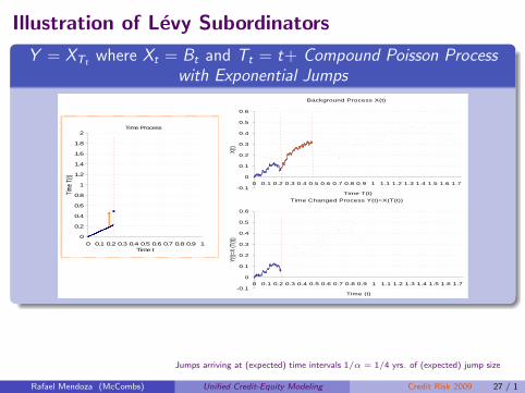
Illustration of Levy Subordinators.
Y = XTt where Xt = Bt and Tt = t+ Compound Poisson Processwith Exponential Jumps
..
.
. ..
.
.
Time Process
0
0.2
0.4
0.6
0.8
1
1.2
1.4
1.6
1.8
2
0 0.1 0.2 0.3 0.4 0.5 0.6 0.7 0.8 0.9 1Time t
Time T
(t)
Background Process X(t)
-0.1
0
0.1
0.2
0.3
0.4
0.5
0.6
0 0.1 0.2 0.3 0.4 0.5 0.6 0.7 0.8 0.9 1 1.1 1.2 1.3 1.4 1.5 1.6 1.7
Time T(t)
X(t)
Time Changed Process Y(t)=X(T(t))
-0.1
0
0.1
0.2
0.3
0.4
0.5
0.6
0 0.1 0.2 0.3 0.4 0.5 0.6 0.7 0.8 0.9 1 1.1 1.2 1.3 1.4 1.5 1.6 1.7
Time (t)
Y(t)=
X (T
(t))
When jump in T (t) arrives, the clock skips ahead, and time-changed process is
generated by cutting out the corresponding piece of the diffusion sample path in
which T (t) skips ahead. Jumps arriving at (expected) time intervals 1/α = 1/4 yrs. of (expected) jump size
1/η = 0.1 yrs.Rafael Mendoza (McCombs) Unified Credit-Equity Modeling Credit Risk 2009 27 / 1
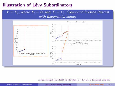
Illustration of Levy Subordinators.
Y = XTt where Xt = Bt and Tt = t+ Compound Poisson Processwith Exponential Jumps
..
.
. ..
.
.
Time Process
0
0.2
0.4
0.6
0.8
1
1.2
1.4
1.6
1.8
2
0 0.1 0.2 0.3 0.4 0.5 0.6 0.7 0.8 0.9 1Time t
Time T
(t)
Background Process X(t)
-0.1
0
0.1
0.2
0.3
0.4
0.5
0.6
0 0.1 0.2 0.3 0.4 0.5 0.6 0.7 0.8 0.9 1 1.1 1.2 1.3 1.4 1.5 1.6 1.7
Time T(t)
X(t)
Time Changed Process Y(t)=X(T(t))
-0.1
0
0.1
0.2
0.3
0.4
0.5
0.6
0 0.1 0.2 0.3 0.4 0.5 0.6 0.7 0.8 0.9 1 1.1 1.2 1.3 1.4 1.5 1.6 1.7
Time (t)
Y(t)=
X (T
(t))
When jump in T (t) arrives, the clock skips ahead, and time-changed process is
generated by cutting out the corresponding piece of the diffusion sample path in
which T (t) skips ahead. Jumps arriving at (expected) time intervals 1/α = 1/4 yrs. of (expected) jump size
1/η = 0.1 yrs.Rafael Mendoza (McCombs) Unified Credit-Equity Modeling Credit Risk 2009 27 / 1

Illustration of Levy Subordinators.
Y = XTt where Xt = Bt and Tt = t+ Compound Poisson Processwith Exponential Jumps
..
.
. ..
.
.
Background Process X(t)
-0.1
0
0.1
0.2
0.3
0.4
0.5
0.6
0 0.1 0.2 0.3 0.4 0.5 0.6 0.7 0.8 0.9 1 1.1 1.2 1.3 1.4 1.5 1.6 1.7
Time T(t)
X(t)
Time Changed Process Y(t)=X(T(t))
-0.1
0
0.1
0.2
0.3
0.4
0.5
0.6
0 0.1 0.2 0.3 0.4 0.5 0.6 0.7 0.8 0.9 1 1.1 1.2 1.3 1.4 1.5 1.6 1.7
Time (t)
Y(t)=
X (T
(t))
Time Process
0
0.2
0.4
0.6
0.8
1
1.2
1.4
1.6
1.8
2
0 0.1 0.2 0.3 0.4 0.5 0.6 0.7 0.8 0.9 1Time t
Time T
(t)
When jump in T (t) arrives, the clock skips ahead, and time-changed process is
generated by cutting out the corresponding piece of the diffusion sample path in
which T (t) skips ahead. Jumps arriving at (expected) time intervals 1/α = 1/4 yrs. of (expected) jump size
1/η = 0.1 yrs.Rafael Mendoza (McCombs) Unified Credit-Equity Modeling Credit Risk 2009 27 / 1
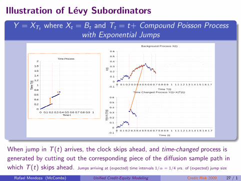
Illustration of Levy Subordinators.
Y = XTt where Xt = Bt and Tt = t+ Compound Poisson Processwith Exponential Jumps
..
.
. ..
.
.
Time Changed Process Y(t)=X(T(t))
-0.1
0
0.1
0.2
0.3
0.4
0.5
0.6
0 0.1 0.2 0.3 0.4 0.5 0.6 0.7 0.8 0.9 1 1.1 1.2 1.3 1.4 1.5 1.6 1.7
Time (t)
Y(t)=
X (T
(t))
Time Process
0
0.2
0.4
0.6
0.8
1
1.2
1.4
1.6
1.8
2
0 0.1 0.2 0.3 0.4 0.5 0.6 0.7 0.8 0.9 1Time t
Time T
(t)
Background Process X(t)
-0.1
0
0.1
0.2
0.3
0.4
0.5
0.6
0 0.1 0.2 0.3 0.4 0.5 0.6 0.7 0.8 0.9 1 1.1 1.2 1.3 1.4 1.5 1.6 1.7
Time T(t)
X(t)
When jump in T (t) arrives, the clock skips ahead, and time-changed process is
generated by cutting out the corresponding piece of the diffusion sample path in
which T (t) skips ahead. Jumps arriving at (expected) time intervals 1/α = 1/4 yrs. of (expected) jump size
1/η = 0.1 yrs.Rafael Mendoza (McCombs) Unified Credit-Equity Modeling Credit Risk 2009 27 / 1
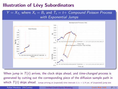
Illustration of Levy Subordinators.
Y = XTt where Xt = Bt and Tt = t+ Compound Poisson Processwith Exponential Jumps
..
.
. ..
.
.
Background Process X(t)
-0.1
0
0.1
0.2
0.3
0.4
0.5
0.6
0 0.1 0.2 0.3 0.4 0.5 0.6 0.7 0.8 0.9 1 1.1 1.2 1.3 1.4 1.5 1.6 1.7
Time T(t)
X(t)
Time Process
0
0.2
0.4
0.6
0.8
1
1.2
1.4
1.6
1.8
2
0 0.1 0.2 0.3 0.4 0.5 0.6 0.7 0.8 0.9 1Time t
Time T
(t)
Time Changed Process Y(t)=X(T(t))
-0.1
0
0.1
0.2
0.3
0.4
0.5
0.6
0 0.1 0.2 0.3 0.4 0.5 0.6 0.7 0.8 0.9 1 1.1 1.2 1.3 1.4 1.5 1.6 1.7
Time (t)
Y(t)=
X (T
(t))
When jump in T (t) arrives, the clock skips ahead, and time-changed process is
generated by cutting out the corresponding piece of the diffusion sample path in
which T (t) skips ahead. Jumps arriving at (expected) time intervals 1/α = 1/4 yrs. of (expected) jump size
1/η = 0.1 yrs.Rafael Mendoza (McCombs) Unified Credit-Equity Modeling Credit Risk 2009 27 / 1

Illustration of Levy Subordinators.
Y = XTt where Xt = Bt and Tt = t+ Compound Poisson Processwith Exponential Jumps
..
.
. ..
.
.
Background Process X(t)
-0.1
0
0.1
0.2
0.3
0.4
0.5
0.6
0 0.1 0.2 0.3 0.4 0.5 0.6 0.7 0.8 0.9 1 1.1 1.2 1.3 1.4 1.5 1.6 1.7
Time T(t)
X(t)
Time Changed Process Y(t)=X(T(t))
-0.1
0
0.1
0.2
0.3
0.4
0.5
0.6
0 0.1 0.2 0.3 0.4 0.5 0.6 0.7 0.8 0.9 1 1.1 1.2 1.3 1.4 1.5 1.6 1.7
Time (t)
Y(t)=
X (T
(t))
Time Process
0
0.2
0.4
0.6
0.8
1
1.2
1.4
1.6
1.8
2
0 0.1 0.2 0.3 0.4 0.5 0.6 0.7 0.8 0.9 1Time t
Time T
(t)
When jump in T (t) arrives, the clock skips ahead, and time-changed process is
generated by cutting out the corresponding piece of the diffusion sample path in
which T (t) skips ahead. Jumps arriving at (expected) time intervals 1/α = 1/4 yrs. of (expected) jump size
1/η = 0.1 yrs.Rafael Mendoza (McCombs) Unified Credit-Equity Modeling Credit Risk 2009 27 / 1
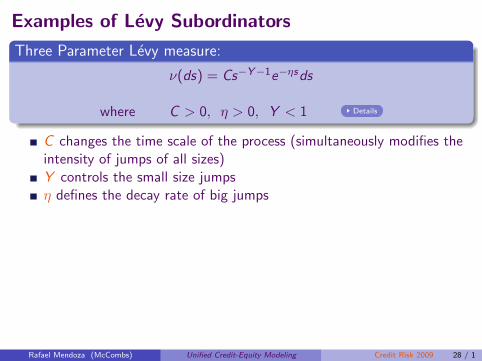
Examples of Levy Subordinators.Three Parameter Levy measure:..
.
. ..
.
.
ν(ds) = Cs−Y−1e−ηsds
where C > 0, η > 0, Y < 1 .. Details
C changes the time scale of the process (simultaneously modifies theintensity of jumps of all sizes)Y controls the small size jumpsη defines the decay rate of big jumps
.Levy-Khintchine formula..
.
. ..
.
.
L(t, λ) = e−ϕ(λ)t
where ϕ(λ) =
γλ − CΓ(−Y )[(λ + η)Y − ηY ], Y = 0
γλ + C ln(1 + λ/η), Y = 0
Rafael Mendoza (McCombs) Unified Credit-Equity Modeling Credit Risk 2009 28 / 1
Absolutely Continuous Time Changes
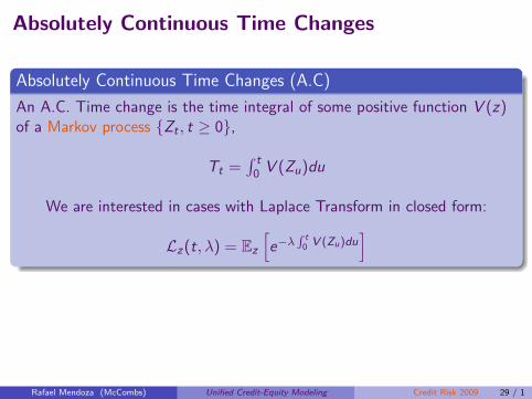
.Absolutely Continuous Time Changes (A.C)..
.
. ..
.
.
An A.C. Time change is the time integral of some positive function V (z)of a Markov process {Zt , t ≥ 0},
Tt =∫ t0 V (Zu)du
We are interested in cases with Laplace Transform in closed form:
Lz(t, λ) = Ez
[e−λ
R t0 V (Zu)du
]
Example: The Cox-Ingersoll-Ross (CIR) process:
dVt = κ(θ − Vt)dt + σV
√VtdWt
with V0 = v > 0, rate of mean reversion κ > 0, long-run level θ > 0,and volatility σV > 0.
Rafael Mendoza (McCombs) Unified Credit-Equity Modeling Credit Risk 2009 29 / 1

Absolutely Continuous Time Changes
.Absolutely Continuous Time Changes (A.C)..
.
. ..
.
.
An A.C. Time change is the time integral of some positive function V (z)of a Markov process {Zt , t ≥ 0},
Tt =∫ t0 V (Zu)du
We are interested in cases with Laplace Transform in closed form:
Lz(t, λ) = Ez
[e−λ
R t0 V (Zu)du
]Example: The Cox-Ingersoll-Ross (CIR) process:
dVt = κ(θ − Vt)dt + σV
√VtdWt
with V0 = v > 0, rate of mean reversion κ > 0, long-run level θ > 0,and volatility σV > 0.
Rafael Mendoza (McCombs) Unified Credit-Equity Modeling Credit Risk 2009 29 / 1

Absolutely Continuous Time Changes
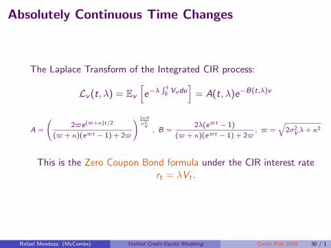
The Laplace Transform of the Integrated CIR process:
Lv (t, λ) = Ev
[e−λ
R t0 Vudu
]= A(t, λ)e−B(t,λ)v
A =
2ϖe(ϖ+κ)t/2
(ϖ + κ)(eϖt − 1) + 2ϖ
!
2κθ
σ2V
, B =2λ(eϖt − 1)
(ϖ + κ)(eϖt − 1) + 2ϖ, ϖ =
q
2σ2V λ + κ2
This is the Zero Coupon Bond formula under the CIR interest ratert = λVt .
Rafael Mendoza (McCombs) Unified Credit-Equity Modeling Credit Risk 2009 30 / 1
Absolutely Continuous Time Changes
The Laplace Transform of the Integrated CIR process:
Lv (t, λ) = Ev
[e−λ
R t0 Vudu
]= A(t, λ)e−B(t,λ)v
A =
2ϖe(ϖ+κ)t/2
(ϖ + κ)(eϖt − 1) + 2ϖ
!
2κθ
σ2V
, B =2λ(eϖt − 1)
(ϖ + κ)(eϖt − 1) + 2ϖ, ϖ =
q
2σ2V λ + κ2
This is the Zero Coupon Bond formula under the CIR interest ratert = λVt .
Rafael Mendoza (McCombs) Unified Credit-Equity Modeling Credit Risk 2009 30 / 1

Illustration of Absolutely Continuous Time Changes
.CIR parameters κ = 7, θ = 2, V0 = 0.5 and σv =
√2
..
.
. ..
.
.
P ro c e s s e s X ( t) v s Y ( t)= X (T ( t))
-0 .1
0
0 .1
0 .2
0 .3
0 .4
0 .5
0 0 .1 0 .2 0 .3 0 .4 0 .5 0 .6 0 .7 0 .8 0 .9 1 1 .1
T im e ( t)
X ( t)
CIR Process
0
0.5
1
1.5
2
2.5
3
0 0.1 0.2 0.3 0.4 0.5 0.6 0.7 0.8 0.9 1Time (t)
V(t)
Time Process
0
0.1
0.2
0.3
0.4
0.5
0.6
0.7
0.8
0.9
1
0 0.1 0.2 0.3 0.4 0.5 0.6 0.7 0.8 0.9 1Time t
Time T
(t)
Time speeds up or slows down based on the amount of new informationarriving and the amount trading (trading time)
Rafael Mendoza (McCombs) Unified Credit-Equity Modeling Credit Risk 2009 31 / 1
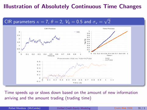
Illustration of Absolutely Continuous Time Changes
.CIR parameters κ = 7, θ = 2, V0 = 0.5 and σv =
√2
..
.
. ..
.
.
CIR Process
0
0.5
1
1.5
2
2.5
3
0 0.1 0.2 0.3 0.4 0.5 0.6 0.7 0.8 0.9 1Time (t)
V(t)
Time Process
0
0.1
0.2
0.3
0.4
0.5
0.6
0.7
0.8
0.9
1
0 0.1 0.2 0.3 0.4 0.5 0.6 0.7 0.8 0.9 1Time t
Time T
(t)
P ro c e s s e s X ( t) v s Y (t)= X (T ( t) )
-0 .1
0
0 .1
0 .2
0 .3
0 .4
0 .5
0 0 .1 0 .2 0 .3 0 .4 0 .5 0 .6 0 .7 0 .8 0 .9 1 1 .1
T im e ( t)
X ( t)X (T (t) )
Time speeds up or slows down based on the amount of new informationarriving and the amount trading (trading time)
Rafael Mendoza (McCombs) Unified Credit-Equity Modeling Credit Risk 2009 31 / 1
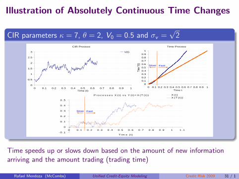
Illustration of Absolutely Continuous Time Changes
.CIR parameters κ = 7, θ = 2, V0 = 0.5 and σv =
√2
..
.
. ..
.
.
Time Process
0
0.1
0.2
0.3
0.4
0.5
0.6
0.7
0.8
0.9
1
0 0.1 0.2 0.3 0.4 0.5 0.6 0.7 0.8 0.9 1Time t
Time T
(t)
P ro c e s s e s X ( t) v s Y (t)= X (T ( t) )
-0 .1
0
0 .1
0 .2
0 .3
0 .4
0 .5
0 0 .1 0 .2 0 .3 0 .4 0 .5 0 .6 0 .7 0 .8 0 .9 1 1 .1
T im e ( t)
X ( t)X (T (t) )
Slow Fast
Slow Fast
CIR Process
0
0.5
1
1.5
2
2.5
3
0 0.1 0.2 0.3 0.4 0.5 0.6 0.7 0.8 0.9 1Time (t)
V(t)
Time speeds up or slows down based on the amount of new informationarriving and the amount trading (trading time)
Rafael Mendoza (McCombs) Unified Credit-Equity Modeling Credit Risk 2009 31 / 1
Composite Time Changes
.Composite Time Changes..
.
. ..
.
.
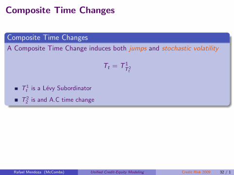
A Composite Time Change induces both jumps and stochastic volatility
Tt = T 1T 2
t
T 1t is a Levy Subordinator
T 22 is and A.C time change
.Laplace Transform of the Composite Time Change..
.
. ..
.
.
It is obtained by first conditioning w.r.t. the A.C. time change
E[e−λTt ] = E[e−T 2t ϕ(λ)] = Lz(t, ϕ(λ))
Rafael Mendoza (McCombs) Unified Credit-Equity Modeling Credit Risk 2009 32 / 1

Composite Time Changes
.Composite Time Changes..
.
. ..
.
.
A Composite Time Change induces both jumps and stochastic volatility
Tt = T 1T 2
t
T 1t is a Levy Subordinator
T 22 is and A.C time change
.Laplace Transform of the Composite Time Change..
.
. ..
.
.
It is obtained by first conditioning w.r.t. the A.C. time change
E[e−λTt ] = E[e−T 2t ϕ(λ)] = Lz(t, ϕ(λ))
Rafael Mendoza (McCombs) Unified Credit-Equity Modeling Credit Risk 2009 32 / 1

Quick Summary
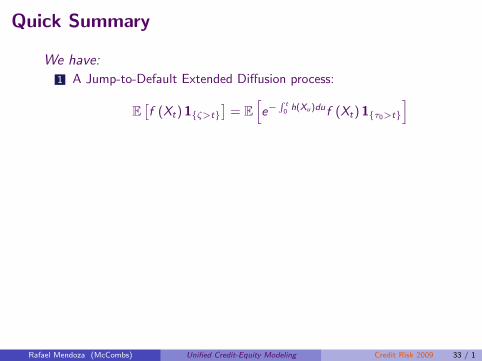
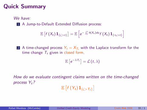
We have:
1 A Jump-to-Default Extended Diffusion process:
E[f (Xt) 1{ζ>t}
]= E
[e−
R t0
h(Xu)duf (Xt) 1{τ0>t}
]2 A time-changed process Yt = XTt with the Laplace transform for the
time change Tt given in closed form,
E[e−λTt
]= L (t, λ)
How do we evaluate contingent claims written on the time-changedprocess Yt?
E[f (Yt) 1{ζ>Tt}
]
Rafael Mendoza (McCombs) Unified Credit-Equity Modeling Credit Risk 2009 33 / 1
Quick Summary
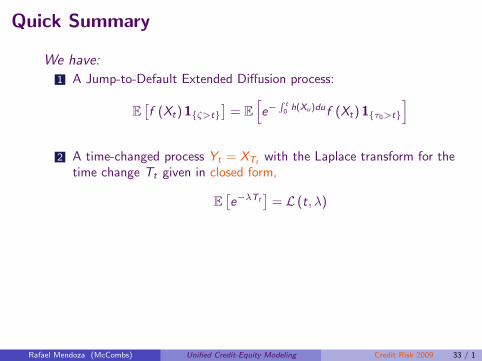
We have:
1 A Jump-to-Default Extended Diffusion process:
E[f (Xt) 1{ζ>t}
]= E
[e−
R t0
h(Xu)duf (Xt) 1{τ0>t}
]
2 A time-changed process Yt = XTt with the Laplace transform for thetime change Tt given in closed form,
E[e−λTt
]= L (t, λ)
How do we evaluate contingent claims written on the time-changedprocess Yt?
E[f (Yt) 1{ζ>Tt}
]
Rafael Mendoza (McCombs) Unified Credit-Equity Modeling Credit Risk 2009 33 / 1
Quick Summary
We have:
1 A Jump-to-Default Extended Diffusion process:
E[f (Xt) 1{ζ>t}
]= E
[e−
R t0
h(Xu)duf (Xt) 1{τ0>t}
]2 A time-changed process Yt = XTt with the Laplace transform for the
time change Tt given in closed form,
E[e−λTt
]= L (t, λ)
How do we evaluate contingent claims written on the time-changedprocess Yt?
E[f (Yt) 1{ζ>Tt}
]
Rafael Mendoza (McCombs) Unified Credit-Equity Modeling Credit Risk 2009 33 / 1
Quick Summary
We have:
1 A Jump-to-Default Extended Diffusion process:
E[f (Xt) 1{ζ>t}
]= E
[e−
R t0
h(Xu)duf (Xt) 1{τ0>t}
]2 A time-changed process Yt = XTt with the Laplace transform for the
time change Tt given in closed form,
E[e−λTt
]= L (t, λ)
How do we evaluate contingent claims written on the time-changedprocess Yt?
E[f (Yt) 1{ζ>Tt}
]
Rafael Mendoza (McCombs) Unified Credit-Equity Modeling Credit Risk 2009 33 / 1
Contingent Claims for the Time-Changed Process
.Valuing contingent claims written on Yt = XTt..
.
. ..
.
.
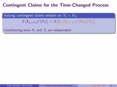
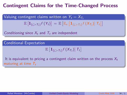
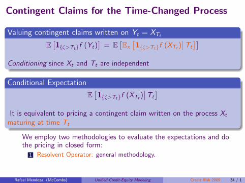
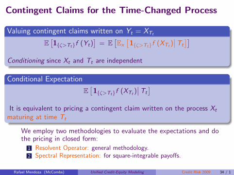
E[1{ζ>Tt}f (Yt)
]= E
[Ex
[1{ζ>Tt}f (XTt )
∣∣Tt
]]Conditioning since Xt and Tt are independent
.Conditional Expectation..
.
. ..
.
.
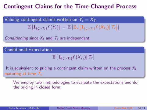
E[1{ζ>Tt}f (XTt )
∣∣Tt
]It is equivalent to pricing a contingent claim written on the process Xt
maturing at time Tt
We employ two methodologies to evaluate the expectations and dothe pricing in closed form:
1 Resolvent Operator: general methodology.2 Spectral Representation: for square-integrable payoffs.
Rafael Mendoza (McCombs) Unified Credit-Equity Modeling Credit Risk 2009 34 / 1
Contingent Claims for the Time-Changed Process
.Valuing contingent claims written on Yt = XTt..
.
. ..
.
.
E[1{ζ>Tt}f (Yt)
]= E
[Ex
[1{ζ>Tt}f (XTt )
∣∣Tt
]]Conditioning since Xt and Tt are independent
.Conditional Expectation..
.
. ..
.
.
E[1{ζ>Tt}f (XTt )
∣∣Tt
]It is equivalent to pricing a contingent claim written on the process Xt
maturing at time Tt
We employ two methodologies to evaluate the expectations and dothe pricing in closed form:
1 Resolvent Operator: general methodology.
2 Spectral Representation: for square-integrable payoffs.
Rafael Mendoza (McCombs) Unified Credit-Equity Modeling Credit Risk 2009 34 / 1
Contingent Claims for the Time-Changed Process
.Valuing contingent claims written on Yt = XTt..
.
. ..
.
.
E[1{ζ>Tt}f (Yt)
]= E
[Ex
[1{ζ>Tt}f (XTt )
∣∣Tt
]]Conditioning since Xt and Tt are independent
.Conditional Expectation..
.
. ..
.
.
E[1{ζ>Tt}f (XTt )
∣∣Tt
]It is equivalent to pricing a contingent claim written on the process Xt
maturing at time Tt
We employ two methodologies to evaluate the expectations and dothe pricing in closed form:
1 Resolvent Operator: general methodology.2 Spectral Representation: for square-integrable payoffs.
Rafael Mendoza (McCombs) Unified Credit-Equity Modeling Credit Risk 2009 34 / 1
Resolvent Operator
.Resolvent Operator:..
.
. ..
.
.
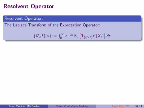
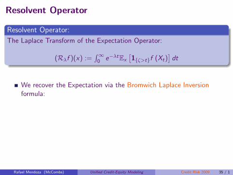
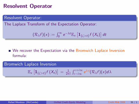
The Laplace Transform of the Expectation Operator:
(Rλf )(x) :=∫∞0 e−λtEx
[1{ζ>t}f (Xt)
]dt
We recover the Expectation via the Bromwich Laplace Inversionformula:
.Bromwich Laplace Inversion..
.
. ..
.
.
Ex
[1{ζ>t}f (Xt)
]= 1
2πi
∫ ϵ+i∞ϵ−i∞ eλ t(Rλf )(x)dλ
NOTE. The time t enters in this expression only through theexponential eλ t
Rafael Mendoza (McCombs) Unified Credit-Equity Modeling Credit Risk 2009 35 / 1
Resolvent Operator
.Resolvent Operator:..
.
. ..
.
.
The Laplace Transform of the Expectation Operator:
(Rλf )(x) :=∫∞0 e−λtEx
[1{ζ>t}f (Xt)
]dt
We recover the Expectation via the Bromwich Laplace Inversionformula:
.Bromwich Laplace Inversion..
.
. ..
.
.
Ex
[1{ζ>t}f (Xt)
]= 1
2πi
∫ ϵ+i∞ϵ−i∞ eλ t(Rλf )(x)dλ
NOTE. The time t enters in this expression only through theexponential eλ t
Rafael Mendoza (McCombs) Unified Credit-Equity Modeling Credit Risk 2009 35 / 1
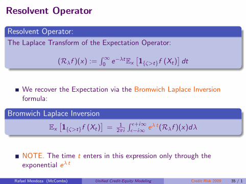
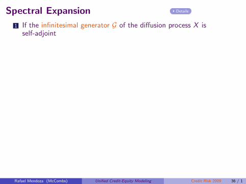
Spectral Expansion .. Details
1 If the infinitesimal generator G of the diffusion process X isself-adjoint
If X is a 1D diffusion process then G is self-adjoint inH = L2 ((0,∞), m) with respect to the speed measure m(dx)
2 If f ∈ HVThen we can use the Spectral Representation Theorem in order toobtain the Expectation
.Eigenfunction Expansion (when the spectrum of G is discrete):..
.
. ..
.
.
Ex
[1{ζ>t}f (Xt)
]=∑∞
n=1 e−λn tcnφn(x)
where cn = ⟨f , φ⟩ are the expansion coefficients and, λn are theeigenvalues, φn(x) the eigenfunctions solving Gφn(x) = λnφn(x)
NOTE. The time t enters in this expression only through theexponential e−λn t
Rafael Mendoza (McCombs) Unified Credit-Equity Modeling Credit Risk 2009 36 / 1
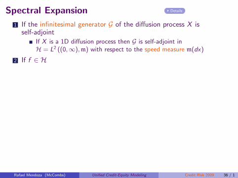
Spectral Expansion .. Details
1 If the infinitesimal generator G of the diffusion process X isself-adjoint
If X is a 1D diffusion process then G is self-adjoint inH = L2 ((0,∞), m) with respect to the speed measure m(dx)
2 If f ∈ H
VThen we can use the Spectral Representation Theorem in order toobtain the Expectation
.Eigenfunction Expansion (when the spectrum of G is discrete):..
.
. ..
.
.
Ex
[1{ζ>t}f (Xt)
]=∑∞
n=1 e−λn tcnφn(x)
where cn = ⟨f , φ⟩ are the expansion coefficients and, λn are theeigenvalues, φn(x) the eigenfunctions solving Gφn(x) = λnφn(x)
NOTE. The time t enters in this expression only through theexponential e−λn t
Rafael Mendoza (McCombs) Unified Credit-Equity Modeling Credit Risk 2009 36 / 1
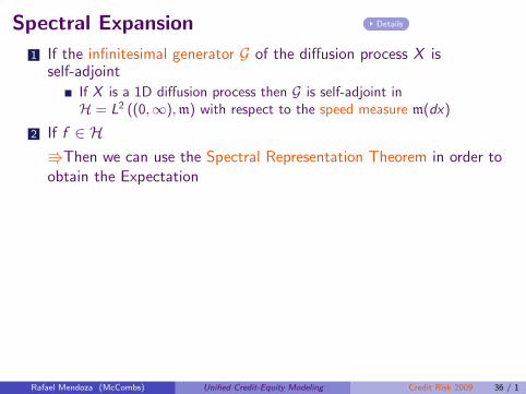
Spectral Expansion .. Details
1 If the infinitesimal generator G of the diffusion process X isself-adjoint
If X is a 1D diffusion process then G is self-adjoint inH = L2 ((0,∞), m) with respect to the speed measure m(dx)
2 If f ∈ HVThen we can use the Spectral Representation Theorem in order toobtain the Expectation
.Eigenfunction Expansion (when the spectrum of G is discrete):..
.
. ..
.
.
Ex
[1{ζ>t}f (Xt)
]=∑∞
n=1 e−λn tcnφn(x)
where cn = ⟨f , φ⟩ are the expansion coefficients and, λn are theeigenvalues, φn(x) the eigenfunctions solving Gφn(x) = λnφn(x)
NOTE. The time t enters in this expression only through theexponential e−λn t
Rafael Mendoza (McCombs) Unified Credit-Equity Modeling Credit Risk 2009 36 / 1
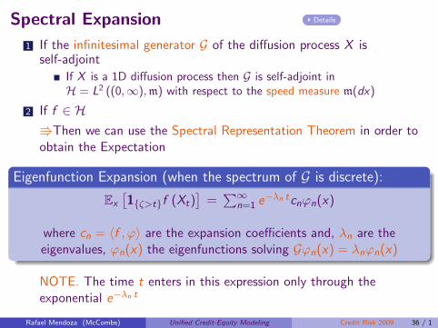
Spectral Expansion .. Details
1 If the infinitesimal generator G of the diffusion process X isself-adjoint
If X is a 1D diffusion process then G is self-adjoint inH = L2 ((0,∞), m) with respect to the speed measure m(dx)
2 If f ∈ HVThen we can use the Spectral Representation Theorem in order toobtain the Expectation
.Eigenfunction Expansion (when the spectrum of G is discrete):..
.
. ..
.
.
Ex
[1{ζ>t}f (Xt)
]=∑∞
n=1 e−λn tcnφn(x)
where cn = ⟨f , φ⟩ are the expansion coefficients and, λn are theeigenvalues, φn(x) the eigenfunctions solving Gφn(x) = λnφn(x)
NOTE. The time t enters in this expression only through theexponential e−λn t
Rafael Mendoza (McCombs) Unified Credit-Equity Modeling Credit Risk 2009 36 / 1
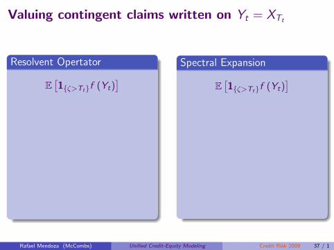
Valuing contingent claims written on Yt = XTt
.Resolvent Opertator..
.
. ..
.
.
E[1{ζ>Tt}f (Yt)
]
= E[Ex
[1{ζ>Tt}f (XTt )
∣∣Tt
]]= E
[∫ ϵ+i∞ϵ−i∞ eλ Tt (Rλf )(x) dλ
2πi
]=∫ ϵ+i∞ϵ−i∞ E
[eλ Tt
](Rλf )(x) dλ
2πi
=∫ ϵ+i∞ϵ−i∞ L(t,−λ)(Rλf )(x) dλ
2πi
.Spectral Expansion..
.
. ..
.
.
E[1{ζ>Tt}f (Yt)
]
= E[Ex
[1{ζ>Tt}f (XTt )
∣∣Tt
]]= E
[∑∞n=1 e−λn Ttcnφn(x)
]=∑∞
n=1 E[e−λn Tt
]cnφn(x)
=∑∞
n=1 L(t, λn)cnφn(x)
Rafael Mendoza (McCombs) Unified Credit-Equity Modeling Credit Risk 2009 37 / 1
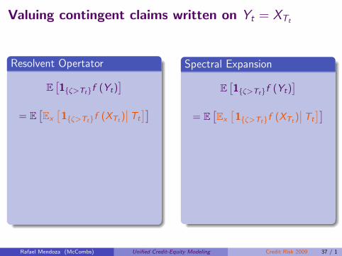
Valuing contingent claims written on Yt = XTt
.Resolvent Opertator..
.
. ..
.
.
E[1{ζ>Tt}f (Yt)
]= E
[Ex
[1{ζ>Tt}f (XTt )
∣∣Tt
]]
= E[∫ ϵ+i∞
ϵ−i∞ eλ Tt (Rλf )(x) dλ2πi
]=∫ ϵ+i∞ϵ−i∞ E
[eλ Tt
](Rλf )(x) dλ
2πi
=∫ ϵ+i∞ϵ−i∞ L(t,−λ)(Rλf )(x) dλ
2πi
.Spectral Expansion..
.
. ..
.
.
E[1{ζ>Tt}f (Yt)
]= E
[Ex
[1{ζ>Tt}f (XTt )
∣∣Tt
]]
= E[∑∞
n=1 e−λn Ttcnφn(x)]
=∑∞
n=1 E[e−λn Tt
]cnφn(x)
=∑∞
n=1 L(t, λn)cnφn(x)
Rafael Mendoza (McCombs) Unified Credit-Equity Modeling Credit Risk 2009 37 / 1

Valuing contingent claims written on Yt = XTt
.Resolvent Opertator..
.
. ..
.
.
E[1{ζ>Tt}f (Yt)
]= E
[Ex
[1{ζ>Tt}f (XTt )
∣∣Tt
]]= E
[∫ ϵ+i∞ϵ−i∞ eλ Tt (Rλf )(x) dλ
2πi
]
=∫ ϵ+i∞ϵ−i∞ E
[eλ Tt
](Rλf )(x) dλ
2πi
=∫ ϵ+i∞ϵ−i∞ L(t,−λ)(Rλf )(x) dλ
2πi
.Spectral Expansion..
.
. ..
.
.
E[1{ζ>Tt}f (Yt)
]= E
[Ex
[1{ζ>Tt}f (XTt )
∣∣Tt
]]= E
[∑∞n=1 e−λn Ttcnφn(x)
]
=∑∞
n=1 E[e−λn Tt
]cnφn(x)
=∑∞
n=1 L(t, λn)cnφn(x)
Rafael Mendoza (McCombs) Unified Credit-Equity Modeling Credit Risk 2009 37 / 1

Valuing contingent claims written on Yt = XTt
.Resolvent Opertator..
.
. ..
.
.
E[1{ζ>Tt}f (Yt)
]= E
[Ex
[1{ζ>Tt}f (XTt )
∣∣Tt
]]= E
[∫ ϵ+i∞ϵ−i∞ eλ Tt (Rλf )(x) dλ
2πi
]=∫ ϵ+i∞ϵ−i∞ E
[eλ Tt
](Rλf )(x) dλ
2πi
=∫ ϵ+i∞ϵ−i∞ L(t,−λ)(Rλf )(x) dλ
2πi
.Spectral Expansion..
.
. ..
.
.
E[1{ζ>Tt}f (Yt)
]= E
[Ex
[1{ζ>Tt}f (XTt )
∣∣Tt
]]= E
[∑∞n=1 e−λn Ttcnφn(x)
]=∑∞
n=1 E[e−λn Tt
]cnφn(x)
=∑∞
n=1 L(t, λn)cnφn(x)
Rafael Mendoza (McCombs) Unified Credit-Equity Modeling Credit Risk 2009 37 / 1
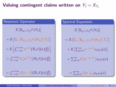
Valuing contingent claims written on Yt = XTt
.Resolvent Opertator..
.
. ..
.
.
E[1{ζ>Tt}f (Yt)
]= E
[Ex
[1{ζ>Tt}f (XTt )
∣∣Tt
]]= E
[∫ ϵ+i∞ϵ−i∞ eλ Tt (Rλf )(x) dλ
2πi
]=∫ ϵ+i∞ϵ−i∞ E
[eλ Tt
](Rλf )(x) dλ
2πi
=∫ ϵ+i∞ϵ−i∞ L(t,−λ)(Rλf )(x) dλ
2πi
.Spectral Expansion..
.
. ..
.
.
E[1{ζ>Tt}f (Yt)
]= E
[Ex
[1{ζ>Tt}f (XTt )
∣∣Tt
]]= E
[∑∞n=1 e−λn Ttcnφn(x)
]=∑∞
n=1 E[e−λn Tt
]cnφn(x)
=∑∞
n=1 L(t, λn)cnφn(x)
Rafael Mendoza (McCombs) Unified Credit-Equity Modeling Credit Risk 2009 37 / 1

A new class of Credit-Equity Models withstate-dependent jumps, S.V. and default intensity.Model Architecture for the Defaultable Stock..
.
. ..
.
.
St = 1{t<τd}eρtXTt .
Xt V Jump-to-Default Extended Diffusion; e.g. JDCEV Process:
dXt = [µ + h(Xt)]Xt dt + σ(Xt)Xt dBt , X0 = x > 0,σ(x) = axβ, h(x) = b + c σ2(x)
Tt V Random Clock: Levy Subordinator, A.C. Time Change, orComposite T.C.
ρ V Compensation Parameter (discounted martingale) .. Details
τd V Default Time
If ζ = min(τ0, ζ) is the lifetime of X , thenτd = inf{t ≥ 0 : ζ ≤ Tt}
At τd the stock drops to zero (Bankruptcy)
Rafael Mendoza (McCombs) Unified Credit-Equity Modeling Credit Risk 2009 38 / 1
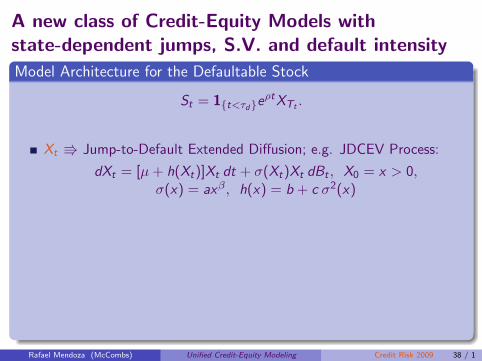
A new class of Credit-Equity Models withstate-dependent jumps, S.V. and default intensity.Model Architecture for the Defaultable Stock..
.
. ..
.
.
St = 1{t<τd}eρtXTt .
Xt V Jump-to-Default Extended Diffusion; e.g. JDCEV Process:
dXt = [µ + h(Xt)]Xt dt + σ(Xt)Xt dBt , X0 = x > 0,σ(x) = axβ , h(x) = b + c σ2(x)
Tt V Random Clock: Levy Subordinator, A.C. Time Change, orComposite T.C.
ρ V Compensation Parameter (discounted martingale) .. Details
τd V Default Time
If ζ = min(τ0, ζ) is the lifetime of X , thenτd = inf{t ≥ 0 : ζ ≤ Tt}
At τd the stock drops to zero (Bankruptcy)
Rafael Mendoza (McCombs) Unified Credit-Equity Modeling Credit Risk 2009 38 / 1
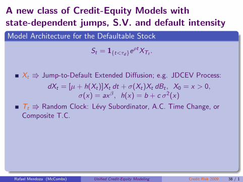
A new class of Credit-Equity Models withstate-dependent jumps, S.V. and default intensity.Model Architecture for the Defaultable Stock..
.
. ..
.
.
St = 1{t<τd}eρtXTt .
Xt V Jump-to-Default Extended Diffusion; e.g. JDCEV Process:
dXt = [µ + h(Xt)]Xt dt + σ(Xt)Xt dBt , X0 = x > 0,σ(x) = axβ , h(x) = b + c σ2(x)
Tt V Random Clock: Levy Subordinator, A.C. Time Change, orComposite T.C.
ρ V Compensation Parameter (discounted martingale) .. Details
τd V Default Time
If ζ = min(τ0, ζ) is the lifetime of X , thenτd = inf{t ≥ 0 : ζ ≤ Tt}
At τd the stock drops to zero (Bankruptcy)
Rafael Mendoza (McCombs) Unified Credit-Equity Modeling Credit Risk 2009 38 / 1
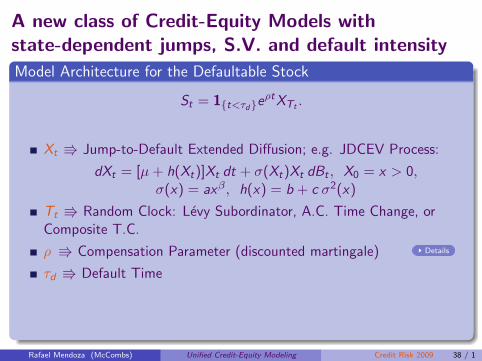
A new class of Credit-Equity Models withstate-dependent jumps, S.V. and default intensity.Model Architecture for the Defaultable Stock..
.
. ..
.
.
St = 1{t<τd}eρtXTt .
Xt V Jump-to-Default Extended Diffusion; e.g. JDCEV Process:
dXt = [µ + h(Xt)]Xt dt + σ(Xt)Xt dBt , X0 = x > 0,σ(x) = axβ , h(x) = b + c σ2(x)
Tt V Random Clock: Levy Subordinator, A.C. Time Change, orComposite T.C.
ρ V Compensation Parameter (discounted martingale) .. Details
τd V Default Time
If ζ = min(τ0, ζ) is the lifetime of X , thenτd = inf{t ≥ 0 : ζ ≤ Tt}
At τd the stock drops to zero (Bankruptcy)
Rafael Mendoza (McCombs) Unified Credit-Equity Modeling Credit Risk 2009 38 / 1
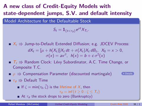
A new class of Credit-Equity Models withstate-dependent jumps, S.V. and default intensity.Model Architecture for the Defaultable Stock..
.
. ..
.
.
St = 1{t<τd}eρtXTt .
Xt V Jump-to-Default Extended Diffusion; e.g. JDCEV Process:
dXt = [µ + h(Xt)]Xt dt + σ(Xt)Xt dBt , X0 = x > 0,σ(x) = axβ , h(x) = b + c σ2(x)
Tt V Random Clock: Levy Subordinator, A.C. Time Change, orComposite T.C.
ρ V Compensation Parameter (discounted martingale) .. Details
τd V Default Time
If ζ = min(τ0, ζ) is the lifetime of X , thenτd = inf{t ≥ 0 : ζ ≤ Tt}
At τd the stock drops to zero (Bankruptcy)
Rafael Mendoza (McCombs) Unified Credit-Equity Modeling Credit Risk 2009 38 / 1

Survival Probability and Defaultable Zero Bonds
.Survival Probability..
.
. ..
.
.
Q(τd > t) = Q(ζ > Tt)
=∑∞
n=0 L (t, (b + ωn))Γ(1+c/|β|)Γ(n+1/(2|β|))Γ(ν+1)Γ(1/(2|β|))n!
×A1
2|β| xe−Ax−2β
1F1(1 − n + c/|β|, ν + 1, Ax−2β)
.. Details
Where 1F1(a, b, z) is the Kummer Confluent Hypergeometric function;and ω = 2|β|(µ + b), ν = 1+2c
2|β| , and A = µ+ba2|β| .
.Defaultable Zero Coupon Bond..
.
. ..
.
.
BR(x , t) = e−rtQ(τd > t) + Re−rt [1 − Q(τd > t)]Recovery fraction R ∈ [0, 1]
Rafael Mendoza (McCombs) Unified Credit-Equity Modeling Credit Risk 2009 39 / 1
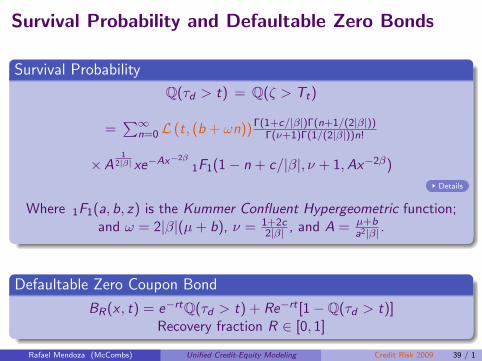
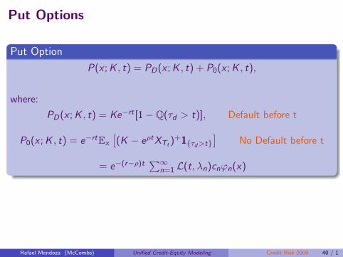
Put Options
.Put Option..
.
. ..
.
.
P(x ; K , t) = PD(x ; K , t) + P0(x ; K , t),
where:
PD(x ; K , t) = Ke−rt [1 − Q(τd > t)], Default before t
P0(x ; K , t) = e−rtEx
[(K − eρtXTt )
+1{τd>t}]
No Default before t
= e−(r−ρ)t∑∞
n=1 L(t, λn)cnφn(x)
The default claim PD(x ;K , t) is directly calculated from the SurvivalProbability Q(τd > t) previously computed
The claim, P0(x ; K , t), is calculated by means of the SpectralExpansion since f (x) = (K − x)+ ∈ L2 ((0,∞), m)
Rafael Mendoza (McCombs) Unified Credit-Equity Modeling Credit Risk 2009 40 / 1
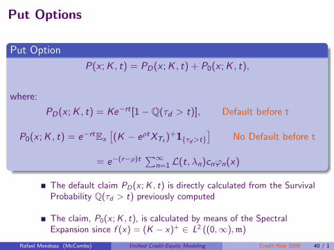
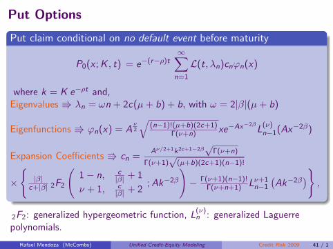
Put Options.Put claim conditional on no default event before maturity..
.
. ..
.
.
P0(x ; K , t) = e−(r−ρ)t∞∑
n=1
L(t, λn)cnφn(x)
where k = K e−ρt and,Eigenvalues V λn = ωn + 2c(µ + b) + b, with ω = 2|β|(µ + b)
Eigenfunctions V φn(x) = Aν2
√(n−1)!(µ+b)(2c+1)
Γ(ν+n) xe−Ax−2βL
(ν)n−1(Ax−2β)
Expansion Coefficients V cn =Aν/2+1k2c+1−2β
√Γ(ν+n)
Γ(ν+1)√
(µ+b)(2c+1)(n−1)!
×
{|β|
c+|β| 2F2
(1 − n, c
|β| + 1
ν + 1, c|β| + 2
; Ak−2β
)− Γ(ν+1)(n−1)!
Γ(ν+n+1) Lν+1n−1
(Ak−2β
)},
2F2: generalized hypergeometric function, L(ν)n : generalized Laguerre
polynomials.
Rafael Mendoza (McCombs) Unified Credit-Equity Modeling Credit Risk 2009 41 / 1

Numerical Examples
Assume a background process {Xt , t > 0} following a JDCEV, and acomposite time change Inverse Gaussian Process & CIR:
.Parameters..
.
. ..
.
.
JDCEV
S 50
CIR
V 1a 10 θ 1β −1 σV 1c 0.5 κ 4b 0.01
IGγ 0
r 0.05 η 8
q 0 C 2√
2/π
Note that γ = 0, thus the time changed process is a pure jumpprocess!
Rafael Mendoza (McCombs) Unified Credit-Equity Modeling Credit Risk 2009 42 / 1

Infinitesimal Generator of the Time ChangedProcess (Yt = XTt
, Vt)
Gf (x , v) =
γv
(1
2a2x2β+2 ∂2f
∂x2(x , v) + (b + ca2x2β)x
∂f
∂x(x , v) − (b + c2a2x2β)f (x , v)
)︸ ︷︷ ︸
Gx f (x ,v) JDCEV’s infinitesimal generator
+v
(∫(0,∞)
(f (y , v) − f (x , v))π(x , y)dy − k (x) f (x , v)
)︸ ︷︷ ︸
R
0,∞(Ps f −f )ν(ds) Subordination component
+σ2
V
2v
∂2f
∂v2(x , v) + κ(θ − v)
∂f
∂v(x , v)︸ ︷︷ ︸
Gv f (x ,v) CIR’s infinitesimal generator
State dependent jump measure π(x , y) =∫(0,∞) p(s; x , y)ν(ds)
Additional killing rate k(x) =∫(0,∞) Ps(x , {0})ν(ds) .. Details
Rafael Mendoza (McCombs) Unified Credit-Equity Modeling Credit Risk 2009 43 / 1
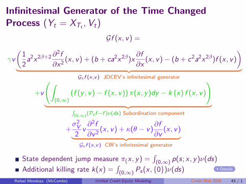
Infinitesimal Generator of the Time ChangedProcess (Yt = XTt
, Vt)
Gf (x , v) =
γv
(1
2a2x2β+2 ∂2f
∂x2(x , v) + (b + ca2x2β)x
∂f
∂x(x , v) − (b + c2a2x2β)f (x , v)
)︸ ︷︷ ︸
Gx f (x ,v) JDCEV’s infinitesimal generator
+v
(∫(0,∞)
(f (y , v) − f (x , v))π(x , y)dy − k (x) f (x , v)
)︸ ︷︷ ︸
R
(0,∞)(Ps f −f )ν(ds) Subordination component
+σ2
V
2v
∂2f
∂v2(x , v) + κ(θ − v)
∂f
∂v(x , v)︸ ︷︷ ︸
Gv f (x ,v) CIR’s infinitesimal generator
State dependent jump measure π(x , y) =∫(0,∞) p(s; x , y)ν(ds)
Additional killing rate k(x) =∫(0,∞) Ps(x , {0})ν(ds) .. Details
Rafael Mendoza (McCombs) Unified Credit-Equity Modeling Credit Risk 2009 43 / 1
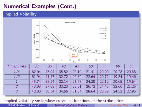
Numerical Examples (Cont.).Implied Volatility..
.
. ..
.
.
Implied Volatility
13%
25%
37%
49%
61%
30 35 40 45 50 55 60 65Strike
Impl
ied
Vol
atilit
y
1/4
1/2
1
2
3
ATMVolatility
Time/Strike 30 35 40 45 50 55 60 65
1/4 62.04 47.94 35.52 26.19 21.41 20.09 20.28 20.881/2 51.94 41.47 32.72 26.39 22.64 20.72 19.84 19.461 45.74 38.24 32.14 27.53 24.30 22.12 20.65 19.642 43.03 37.68 33.23 29.61 26.72 24.45 22.66 21.253 42.80 38.34 34.55 31.34 28.64 26.39 24.52 22.96
Implied volatility smile/skew curves as functions of the strike price.Current stock price level is 50, ATM volatility σ = aSβ = 20%Rafael Mendoza (McCombs) Unified Credit-Equity Modeling Credit Risk 2009 44 / 1
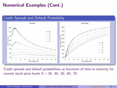
Numerical Examples (Cont.)
.Credit Spreads and Default Probability..
.
. ..
.
.
Credit Spreads
1.5%
2.5%
3.5%
4.5%
5.5%
6.5%
7.5%
8.5%
0 5 10 15 20 25 30 35 40 45 50Time to maturity (years)
Cre
dit s
pre
ads
30
40
50
60
70
Default Probability
0.0%
10.0%
20.0%
30.0%
40.0%
50.0%
60.0%
70.0%
80.0%
0 5 10 15 20 25 30 35 40 45 50Time to maturity (years)
Pro
bability
of defa
ult
30
40
50
60
70
Credit spreads and default probabilities as functions of time to maturity forcurrent stock price levels S = 30, 40, 50, 60, 70.
Rafael Mendoza (McCombs) Unified Credit-Equity Modeling Credit Risk 2009 45 / 1

Summary of Features and Practical Benefits of OurModeling Framework
Our Stock price is a jump-diffusion process with stochastic volatilityand default intensity,
The Default intensity explicitly depends on the stock price andvolatility
The leverage effect is introduced in the diffusion and in jumpscomponents - as the stock falls, the diffusion volatility and arrivalrates of large jumps increase
Rafael Mendoza (McCombs) Unified Credit-Equity Modeling Credit Risk 2009 46 / 1
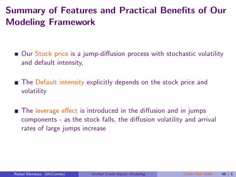

Summary of Features and Practical Benefits of OurModeling Framework (cont.)
Stochastic volatility affects the diffusion and jump components
Unified credit-equity framework V consistency in the pricing andhedging of credit and equity derivatives
We obtain analytical solutions V faster computation of prices andGreeks, and faster calibration
.. Finish
Rafael Mendoza (McCombs) Unified Credit-Equity Modeling Credit Risk 2009 47 / 1

Questions?
Thank you!
Rafael Mendoza (McCombs) Unified Credit-Equity Modeling Credit Risk 2009 48 / 1

Appendix

Appendix
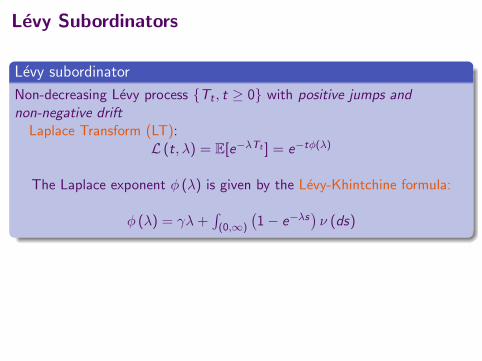
Levy Subordinators
.Levy subordinator..
.
. ..
.
.
Non-decreasing Levy process {Tt , t ≥ 0} with positive jumps andnon-negative drift
Laplace Transform (LT):L (t, λ) = E[e−λTt ] = e−tϕ(λ)
The Laplace exponent ϕ (λ) is given by the Levy-Khintchine formula:
ϕ (λ) = γλ +∫(0,∞)
(1 − e−λs
)ν (ds)
γ ≥ 0 V positive drift
ν (ds) V Levy measure which satisfies∫
(0,∞)(s ∧ 1) ν (ds) < ∞
transition probability πt (ds) is obtained by:∫[0,∞) e−λsπ (ds) = e−tϕ(λ)
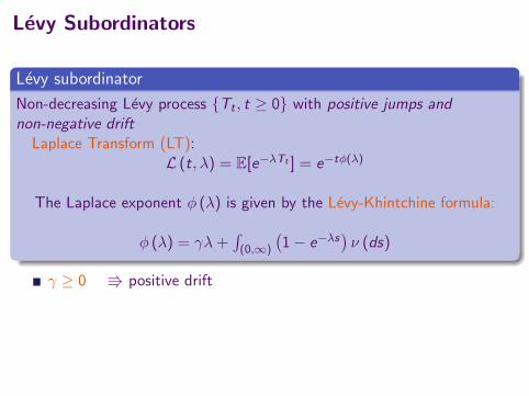
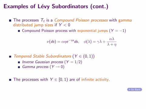
Examples of Levy Subordinators (cont.)
The processes Tt is a Compound Poisson processes with gammadistributed jump sizes if Y < 0
Compound Poisson process with exponential jumps (Y = −1)
ν(ds) = αηe−ηsds, ϕ(λ) = γλ +αλ
λ + η
Tempered Stable Subordinators (Y ∈ (0, 1))
Inverse Gaussian process (Y = 1/2)Gamma process (Y → 0)
The processes with Y ∈ [0, 1) are of infinite activity.
.. Go Back

Appendix
.. Go Back
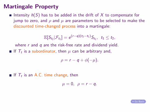
Martingale Property
Intensity h(S) has to be added in the drift of X to compensate forjump to zero, and ρ and µ are parameters to be selected to make thediscounted time-changed process into a martingale:
E[St2 |Ft1 ] = e(r−q)(t2−t1)St1 , t1 ≤ t2,
where r and q are the risk-free rate and dividend yield.
If Tt is a subordinator, then µ can be arbitrary and,
ρ = r − q + ϕ(−µ).
If Tt is an A.C. time change, then
µ = 0, ρ = r − q.
.. Go Back

Appendix
.. Go Back
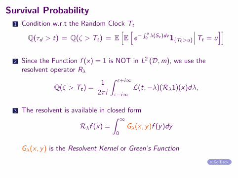
Survival Probability
1 Condition w.r.t the Random Clock Tt
Q(τd > t) = Q(ζ > Tt) = E[E[e−
R u0 λ(Sv )dv1{T0>u}
∣∣∣Tt = u]]
2 Since the Function f (x) = 1 is NOT in L2 (D, m), we use theresolvent operator Rλ
Q(ζ > Tt) =1
2πi
∫ ε+i∞
ε−i∞L(t,−λ)(Rλ1)(x)dλ,
3 The resolvent is available in closed form
Rλf (x) =
∫ ∞
0Gλ(x , y)f (y)dy
Gλ(x , y) is the Resolvent Kernel or Green’s Function
.. Go Back
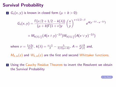
Survival Probability
4 Gλ(x , y) is known in closed form (µ + b > 0):
Gλ(x , y) =Γ(ν/2 + 1/2 − k(λ))
(µ + b)Γ(1 + ν)y
(x
y
)c+1/2−β
eA(y−2β−x−2β)
×Mk(λ), ν2(A(x ∧ y)−2β)Wk(λ), ν
2(A(x ∨ y)−2β)
where ν = 1+2c2|β| , k(λ) = ν−1
2 − λ2|β|(µ+b) , A = µ+b
a2|β| and,
Mk,m(z) and Wk,m(z) are the first and second Whittaker functions.
5 Using the Cauchy Residue Theorem to invert the Resolvent we obtainthe Survival Probability
.. Go Back

Appendix
.. Go Back
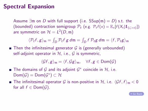
Spectral Expansion
Assume ∃m on D with full support (i.e. SSup(m) = D) s.t. the(bounded) contraction semigroup Pt (e.g. Pt f (x) = Ex [f (Xt)1{ζ>t}])
are symmetric on H = L2(D, m)
⟨Pt f , g⟩m =∫D Pt f g dm =
∫D f Ptg dm = ⟨f ,Ptg⟩m
Then the infinitesimal generator G is (generally unbounded)self-adjoint operator in H, i.e., G is symmetric,
⟨Gf , g⟩m = ⟨f ,Gg⟩m, ∀f , g ∈ Dom(G)
The domains of G and its adjoint G∗ coincide in H, i.e.Dom(G) = Dom(G∗) ⊂ HThe infinitesimal operator G is non-positive in H, i.e. ⟨Gf , f ⟩m < 0for all f ∈ Dom(G).
.. Go Back
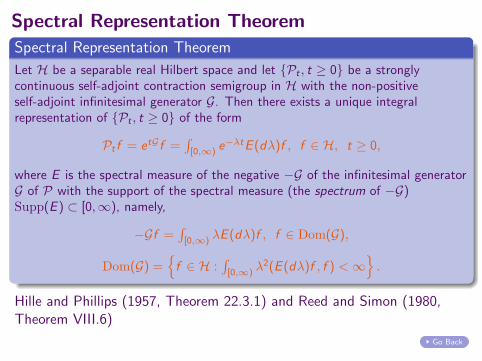
Spectral Representation Theorem.Spectral Representation Theorem..
.
. ..
.
.
Let H be a separable real Hilbert space and let {Pt , t ≥ 0} be a stronglycontinuous self-adjoint contraction semigroup in H with the non-positiveself-adjoint infinitesimal generator G. Then there exists a unique integralrepresentation of {Pt , t ≥ 0} of the form
Pt f = etGf =∫[0,∞)
e−λtE (dλ)f , f ∈ H, t ≥ 0,
where E is the spectral measure of the negative −G of the infinitesimal generatorG of P with the support of the spectral measure (the spectrum of −G)Supp(E ) ⊂ [0,∞), namely,
−Gf =∫[0,∞)
λE (dλ)f , f ∈ Dom(G),
Dom(G) ={
f ∈ H :∫[0,∞)
λ2(E (dλ)f , f ) < ∞}
.
Hille and Phillips (1957, Theorem 22.3.1) and Reed and Simon (1980,Theorem VIII.6)
.. Go Back
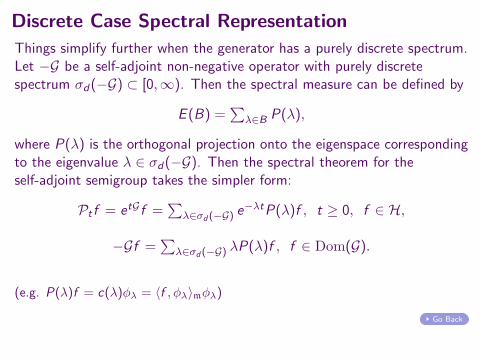
Discrete Case Spectral Representation
Things simplify further when the generator has a purely discrete spectrum.Let −G be a self-adjoint non-negative operator with purely discretespectrum σd(−G) ⊂ [0,∞). Then the spectral measure can be defined by
E (B) =∑
λ∈B P(λ),
where P(λ) is the orthogonal projection onto the eigenspace correspondingto the eigenvalue λ ∈ σd(−G). Then the spectral theorem for theself-adjoint semigroup takes the simpler form:
Pt f = etGf =∑
λ∈σd (−G) e−λtP(λ)f , t ≥ 0, f ∈ H,
−Gf =∑
λ∈σd (−G) λP(λ)f , f ∈ Dom(G).
(e.g. P(λ)f = c(λ)ϕλ = ⟨f , ϕλ⟩mϕλ)
.. Go Back

Appendix
.. Go Back

Notes on Calibration and the Implied Measure(Cont & Tankov, 2004)
Exponential Levy and jump-diffusion models correspond to incompletemarket models
V No perfect hedges can be foundV The (equivalent) martingale measure cannot be defined in a uniqueway
Any arbitrage-free market prices of securities can be represented asdiscounted conditional expectations w.r.t. a risk-neutral measure Qunder which discounted asset prices are martingales
V Model Calibration. Find a risk-neutral model Q which matches theprices of the observed market prices V{i∈I}(S) of securities i ∈ I attime t = 0,
∀i ∈ I , Vi (S) = e−rti EQ[f (Sti )]
.. Go Back
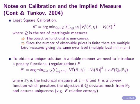
Notes on Calibration and the Implied Measure(Cont & Tankov, 2004)
Least Square Calibration.
θ∗ = arg minQθ∈Q∑
i∈I ωi
∣∣V θi (S , ti ) − Vi (S)
∣∣2where Q is the set of martingale measures
V The objective functional is non-convex.V Since the number of observable prices is finite there are multipleLevy measures giving the same error level (multiple local minimum)
To obtain a unique solution in a stable manner we need to introducea penalty functional (regularization) F
θ∗ = arg minQθ∈Q∑
i∈I ωi
∣∣V θi (S , ti ) − Vi (S)
∣∣2 + αF (Qθ|P0)
where P0 is the historical measure at t = 0 and F is a convexfunction which penalizes the objective if Q deviates much from P0
and ensures uniqueness (v.g. F relative entropy)
.. Go Back

Appendix
.. Go Back
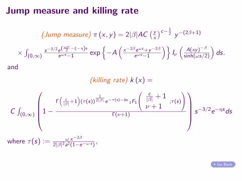
Jump measure and killing rate
(Jump measure) π (x , y) = 2|β|AC( y
x
)c− 12 y−(2β+1)
×∫(0,∞)
s−3/2e(ων2 −ξ−η)s
eωs−1 exp{−A
(x−2βeωs+y−2β
eωs−1
)}Iν(
A(xy)−β
sinh(ωs/2)
)ds.
and
(killing rate) k (x) =
C∫(0,∞)
1 −Γ“
c|β|+1
”
(τ(s))1
2|β| e−τ(s)−bs1F1
0
@
c|β| + 1
ν + 1;τ(s)
1
A
Γ(ν+1)
s−3/2e−ηsds
where τ(s) := ω x−2β
2|β|2a2(1−e−ω s),
.. Go Back

Appendix
.. Go Back

Appendix
.. Go Back

Protection Payment under JDCEV
PV(Protection Payment) = (1 − r) Eh
e−r· T∆L 1{T∆
L≤T}
i
= (1 − r)
8
>
>
>
<
>
>
>
:
E»
e−r· TL−R TL0 h(Xu)du1{TL≤T}
–
| {z }
Diffusion Term
+R T0 e−r· u E
h
e−R u0 h(Xv )dvh (Xu) 1{TL> u}
i
du| {z }
Jump Term
9
>
>
>
=
>
>
>
;
Recall that the first hitting time to L is given by TL = inf {t : Xt = L},and that the first jump time to ∆ is given by
ζ = inf{
t ∈ [0,∞] :∫ t
0h (Xu) du ≥ e
}The default intensity is the power function:
h(Xt) = b + ca2X 2βt
Notice. Since e is an exponentially distributed r.v. with unit mean, then
P[ζ > t] = e−R t
0h(Xu)du and P[ζ < t] =
∫ t
0h (Xv ) e−
R v0
h(Xu)dudv
Rafael Mendoza (McCombs) Unified Credit-Equity Modeling Credit Risk 2009 40 / 1
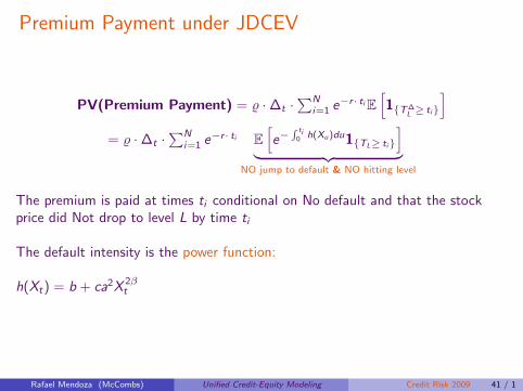
Premium Payment under JDCEV
PV(Premium Payment) = ϱ · ∆t ·∑N
i=1 e−r · ti E[1{T∆
L ≥ ti}
]= ϱ · ∆t ·
∑Ni=1 e−r · ti E
[e−
R ti0 h(Xu)du1{TL≥ ti}
]︸ ︷︷ ︸
NO jump to default & NO hitting level
The premium is paid at times ti conditional on No default and that the stockprice did Not drop to level L by time ti
The default intensity is the power function:
h(Xt) = b + ca2X 2βt
Rafael Mendoza (McCombs) Unified Credit-Equity Modeling Credit Risk 2009 41 / 1
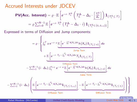
Accrued Interests under JDCEV
PV(Acc. Interest) = ϱ · E[e−r ·T∆
L
(T∆
L − ∆t ·[
T∆L
∆t
])1{T∆
L ≤T}
]= ϱ
∑N−1i=0 E
[e−r ·T∆
L
(T∆
L − ∆t · i)1{T∆
L ∈ (ti ,ti+1)}
]Expressed in terms of Diffusion and Jump components:
= ϱ ·
8
>
>
>
<
>
>
>
:
R T0 u e−r· u E
h
e−R u0 h(Xv )dvh (Xu) 1{TL≥ u}
i
| {z }
Jump Term
du
+ E»
e−r·TL−R TL0 h(Xu)duTL1{TL≤T}
–
| {z }
Diffusion Term
−PN−1
i=1 (i · ∆t)R ti+1ti
e−r· u Eh
e−R u0 h(Xv )dvh (Xu) 1{TL≥ u}
i
| {z }
Jump Term
du
−PN−1
i=1 (i · ∆t)
0
B
B
B
@
E»
e−r· TL−R TL0 h(Xu)du1{TL≤ ti+1}
–
| {z }
Diffusion Term
−E»
e−r· TL−R TL0 h(Xu)du1{TL≤ ti}
–
| {z }
Diffusion Term
1
C
C
C
A
9
>
>
>
=
>
>
>
;
.. Go BackRafael Mendoza (McCombs) Unified Credit-Equity Modeling Credit Risk 2009 42 / 1
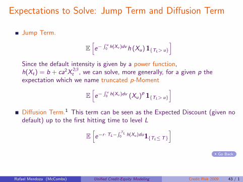
Expectations to Solve: Jump Term and Diffusion Term
Jump Term.
E[e−
R u0
h(Xv )dvh (Xu) 1{TL> u}
]Since the default intensity is given by a power function,h(Xt) = b + ca2X 2β
t , we can solve, more generally, for a given p theexpectation which we name truncated p-Moment
E[e−
R u0
h(Xv )dv (Xu)p 1{TL> u}
]Diffusion Term.1 This term can be seen as the Expected Discount (given nodefault) up to the first hitting time to level L
E[e−r ·TL−
R TL0 h(Xu)du1{TL≤T}
].. Go Back
Rafael Mendoza (McCombs) Unified Credit-Equity Modeling Credit Risk 2009 43 / 1
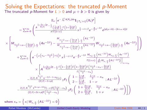
Solving the Expectations: the truncated p-MomentThe truncated p-Moment for L > 0 and µ + b > 0 is given by
Ex
h
e−R t0 h(Xu)du1{TL>t}(Xt)p
i
=P∞
n=0
0
@
A1−2c−2p
4|β| − 12
“
1−p2|β|
”
nΓ
“
1+ 2c+p2|β|
”
n! Γ(1+ν)x
12−c+βe−
A2
x−2βe(p(µ+b)−(b+ω n))t
×
2
6
4
M ν−12
+n−“
2c+p2|β|
”
, ν2
`
Ax−2β´
−M
ν−12
+n−„
2c+p2|β|
«
, ν2
“
A L−2β”
Wν−1
2+n−
„
2c+p2|β|
«
, ν2
(A L−2β)W ν−1
2+n−
“
2c+p2|β|
”
, ν2
`
Ax−2β´
3
7
5
1
C
A
+P∞
n=1
0
B
@
e−
“
ω“
κn− ν−12
”
+ξ”
tx
12−c+βe−
A2
x−2β Mκn, ν2
“
A L−2β”
Wκn, ν2
“
Ax−2β”
Γ(1+ν)
»
ddκ
Wκ, ν2(A L−2β)
–
˛
˛
˛
˛
κ=κn
×"
A1−2c−2p
4|β| − 12
Γ“
1− 1−p2|β|
”
Γ“
1+ 2c+p2|β|
”
Γ“
ν−12
−κn− 2c+p2|β|
”
Γ“
1−ν2
−κn
”
− 2|β|A1−ν
2 L−2β−1+pΓ(ν)(2|β|−1+p) 2F2
1 − 1−p2|β| ,
1−ν2
− κn
2 − 1−p2|β| , 1 − ν
; AL−2β
!
− 2|β|A1+ν
2 L2c+p−2βΓ(−ν)Γ( 1+ν2
−κn)(2|β|+2c+p)Γ
“
1−ν2
−κn
” 2F2
1 + 2c+p2|β| , 1+ν
2− κn
2 + 2c+p2|β| , 1 + ν
;A L−2β
!#!
where κn =n
κ|Wκ, ν2
`
AL−2β´
= 0o
Rafael Mendoza (McCombs) Unified Credit-Equity Modeling Credit Risk 2009 44 / 1

Solving the Expectations: the truncated p-Moment
The truncated p-Moment for L = 0 (CDS case) and µ + b > 0 is given by
Ex
[e−
R t0
h(Xu)du1{TL>t}(Xt)p]
=∑∞
n=0
A1−2c−2p
4|β| − 12 ( 1−p
2|β| )nΓ(1+ 2c+p
2|β| )n! Γ(1+ν) x
12−c+βe−
A2 x−2β
e(p(µ+b)−(b+ω n))t
×M ν−12 +n−( 2c+p
2|β| ), ν2
(Ax−2β
)where κn =
{κ|Wκ, ν
2
(AL−2β
)= 0}
Rafael Mendoza (McCombs) Unified Credit-Equity Modeling Credit Risk 2009 45 / 1

Solving the Expectations: Diffusion Term
The Diffusion Term
Ex
[e−r ·TL−
R TL0 h(Xu)du1{TL≤T}
]=(
xL
) 12−c+β
eϵ A2 (x
−2β−L−2β)×[W
ϵ 1−ν2
− r+ξω
, ν2(Ax−2β)
Wϵ 1−ν
2− r+ξ
ω, ν
2(AL−2β)
+∑∞
n=1ω e
−(ω(κn−ϵ 1−ν2 )+r+ξ)T
(ω(κn−ϵ 1−ν2 )+r+ξ)
Wκn, ν2(Ax−2β)
h
∂∂κ Wκ, ν
2(AL−2β)
i
˛
˛
˛
κ=κn
]
Rafael Mendoza (McCombs) Unified Credit-Equity Modeling Credit Risk 2009 46 / 1
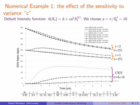
Numerical Example 1: the effect of the sensitivity tovariance “c”Default Intensity function: h(Xt) = b + ca2X 2β
t . We choose a = σ/Sβ0 = 10
0
50
100
150
200
250
300
350
400
450
500
0 1 2 3 4 5 6 7 8 9 10
Time (years)
Spr
eads
(bp
s)
CDS (vol.=20%, c=0, b=0%)
EDS (L=30%S, vol.=20%, c=0, b=0%)
EDS (L=50%S, vol.=20%, c=0, b=0%)
CDS (vol.=20%, c=1, b=2%)
EDS (L=30%S, vol.=20%, c=1, b=2%)
EDS (L=50%S, vol.=20%, c=1, b=2%)
CDS (vol.=20%, c=2, b=2%)
EDS (L=30%S, vol.=20%, c=2, b=2%)
EDS (L=50%S, vol.=20%, c=2, b=2%)
c=2b=2%c=1b=2%
CEVc=b=0
ED
S R
ates
(bp
s)
Time (yrs)∆t r L S0 r q b c β σ0.25 0.5 {0, 15, 25} 50 0.05 0 {0, 0.02} {0, 1, 2} -1 0.20
Rafael Mendoza (McCombs) Unified Credit-Equity Modeling Credit Risk 2009 47 / 1
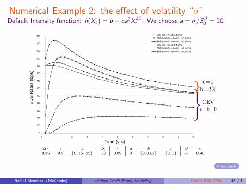
Numerical Example 2: the effect of volatility “σ”Default Intensity function: h(Xt) = b + ca2X 2β
t . We choose a = σ/Sβ0 = 20
0
100
200
300
400
500
600
700
800
900
1000
1100
1200
1300
0 1 2 3 4 5 6 7 8 9 10
Time (years)
Spr
eds
(bps
)CDS (vol.=40%, c=0, b=0%)
EDS (L=30%S, vol.=40%, c=0, b=0%)
EDS (L=50%S, vol.=40%, c=0, b=0%)
CDS (vol.=40%, c=1, b=2%)
EDS (L=30%S, vol.=40%, c=1, b=2%)
EDS (L=50%S, vol.=40%, c=1, b=2%)
CEVc=b=0
c=1b=2%
ED
S R
ates
(bp
s)
Time (yrs)∆t r L S0 r q b c β σ0.25 0.5 {0, 15, 25} 50 0.05 0 {0, 0.02} {0, 1} -1 0.40
.. Go Back
Rafael Mendoza (McCombs) Unified Credit-Equity Modeling Credit Risk 2009 48 / 1