Understanding the Fundamental

Mechanisms of a Dynamic Micro-bubble

Generator for Water Processing and

Cleaning Applications

by

Palaniappan Arumugam

A thesis submitted in conformity with the requirements for

the degree of Master of Applied Science

Graduate Department of Mechanical and Industrial

Engineering University of Toronto

© Copyright by Palaniappan Arumugam 2015

ii

Understanding the Fundamental Mechanisms of a

Dynamic Micro-bubble Generator for Water Processing

and Cleaning Applications

Abstract

The micro-bubble technology in water is widely known and effectively used, but the

fundamental mechanisms of the micro-bubble generation and characteristics are not clearly

established. To better the understanding, extensive literature survey coupled with theoretical and

experimental bubble size estimations and volumetric mass transfer rate calculations were carried

out. Observed multitude of increase in the volumetric mass transfer rate is essentially due to the

specific interfacial area rather than the liquid mass transfer co-efficient. This signifies the

effectiveness of pressurized dissolution type over its counterparts. A second set of experiments

were focussed on particle size analysis using Bluewave particle size analyzer. Measurements for

bubble size distribution were made alongside two cases of surfactant addition, tween20 at

concentrations of 10mM and 1mM. The effect of surfactant on bubble dynamics and stabilization

is interpreted and the axial rise distance hence the rise velocity are computed for both

experimental and theoretical data.

Palaniappan Arumugam

Master of Applied Science

Department of Mechanical and Industrial Engineering

University of Toronto

2015

iii

Acknowledgments

To begin with, I would like to place my utmost gratitude to my supervisor Professor

Chul B. Park who has been a true motivation and a bundle of knowledge to draw inspiration

from. I treasure my time at the Micro-cellular Plastics Manufacturing Laboratory (MPML) under

his able guidance.

I extend my gratitude to the M.A.Sc committee members, Professor Hani Naguib and

Professor Amy Bilton.

My friends and fellow researchers never failed to impress me with their wit and I thank

them for being kind towards me and ably contributing to my research in one way or another.

Special mention goes to Lun Howe Mark for his efforts in helping me through some critical

stages of research and Piyapong Buahom for his support in helping me organize my thesis.

I greatly appreciate the technical correspondence from The Korean Institute of Materials

and Machinery (KIMM) in the matters of Microbubble Generator and its system design.

My warm regards to Mr. Rey Tesoro from the technical marketing division of Betatek

Inc. for his genuine assistance with particle sizing measurements.

I also thank Miss. Kara Kim and Cesar Sanchez from the Department of Mechanical and

Industrial Engineering at the University of Toronto for their valuable support in purchase and

ordering assistance.

My Masters defense wouldn’t have been a reality if not for the support from my family

back home in India. I owe them each step of my progress.

iv

Table of Contents

Abstract .......................................................................................................................................... ii

Acknowledgments ........................................................................................................................ iii

List of Tables ............................................................................................................................... vii

List of Figures ............................................................................................................................. viii

CHAPTER 1. INTRODUCTION .................................................................................................1

1.1 Microbubble technology in Water ..................................................................................1

1.2 Interfacial Tension ..........................................................................................................1

1.3 Micro-bubbles: Properties and Significance ...................................................................2

1.3.1 Long Residence Time of Micro Bubbles ................……………………………3

1.3.2 Self-Pressurizing Effect……………………………………. ..............................5

1.3.3 Large Interfacial Area…………………………………………………..............6

1.3.4 Zeta Potential……………………………………………………………. ..........7

1.3.5 Bubble Growth and Shrinkage………………………………………… ............8

1.4 Scope of Research… .....................................................................................................10

1.5 Organization of the Thesis. ...........................................................................................11

CHAPTER 2. LITERATURE REVIEW AND THEORETICAL BACKGROUND ............12

2.1 Generation Technology of Micro-bubbles in Water………………………… .............12

2.1.1 Pressurized Dissolution (decompression)……………….…………….............12

2.1.2 Venturi-type (cavitation)…………………………………………… ...............13

v

2.1.3 Spiral Liquid flow type (rotatory type)………………………………… .........15

2.1.4 Ejector type (complex pressure profile)……………………………… ............15

2.2 Comparison of different Micro-bubble Generators…………………………. ..............17

2.3 Flotation………………………………………………………………………. ............19

2.4 References on Micro-bubble Modelling and Simulation……………………. .............21

2.4.1 Dimensionless Numbers………………………………………….…… ...........21

2.5 Applications: Overview…………………………….………………………. ...............23

2.5.1: Ozonation of Micro-bubbles…………………………………………. ...........24

CHAPTER 3. EXPERIMENTAL APPROACH- PART 1…………………………...............26

3.1 Experimental Set-up………………………………………………………. .................26

3.1.1 Micro-bubble Generation Break Down………………………………. ............26

3.2 Theoretical Bubble Size Estimation……………………………………… ..................29

3.2.1: Experimental Conditions………………….………………………… .............30

3.2.2: Varying the Pressure…………………………………………………. ....................31

3.3 Dissolved Oxygen………………………………………………………… .................32

3.4 Volumetric Mass Transfer Co-efficient……………………………………….............35

3.4.1 Superficial Gas Velocity………………………………………………............37

3.4.2 Gas Hold-up…………………………………………………………… ..........39

3.4.3 Specific Interfacial Area………………………………………………. ...........39

CHAPTER 4. PARTICLE SIZE ANALYSIS………………………………………… ...........42

4.1 Particle Size Measurement Methods………………………………………. ................42

vi

4.1.1 Interpretation of Size Measurement Results…………………………..............45

4.2 Bubble Distribution: Initial Characterization………….…………………… ...............47

4.3 Bubble Coalescence……………………………………………….…………..............49

4.3.1 Surfactants……………………………………………………………. ............50

4.3.1.1 Critical Micelle Concentration (CMC)………………………..............52

4.3.1.2 Choice of Surfactant…………….……………………………. ............53

4.3.1.3 Polysorbate-20……………………………………………………. ......55

4.4 Observations………….…………………………………….………………. ...............61

CHAPTER 5. SUMMARY AND FUTURE WORK…………………………………….........65

5.1 State of the Art Application…………………………………………………… ...........65

5.2 Future Work……………………………………………………………………...........69

References………………………………………………………….……………………. ...........71

Appendix A……………………………………………………….……………………… ..........79

vii

List of Tables

CHAPTER 3:

Table 3.1: Theoretical bubble size estimation ...............................................................................32

Table 3.2: Comparison of D.O levels ............................................................................................35

Table 3.3: D.O variation as a function of time...............................................................................36

Table 3.4: Volumetric mass transfer co-efficient...........................................................................37

Table 3.5: Specific Interfacial Area and Liquid phase mass transfer co-efficient .........................39

CHAPTER 4

Table 4.1: Bubble Size Distribution at 3 Bar Pressure ..................................................................47

Table 4.2: Experimental Cases.......................................................................................................56

Table 4.3: Bubble Size Distribution: Case1: 10-4M Tween20 .......................................................57

Table 4.4: Bubble Size Distribution: Case2: 10-3M Tween20 .......................................................59

viii

List of Figures

CHAPTER 1

Figure 1.1: Components of a microbubble.......................................................................................3

Figure 1.2: Bubble Rise Velocity.....................................................................................................4

Figure 1.3: Young Laplace law ........................................................................................................5

Figure 1.4: Macro and Micro Bubbles .............................................................................................7

Figure 1.5: Bubble Shrinkage ..........................................................................................................9

Figure 1.6: Zeta Potential Variation.................................................................................................9

CHAPTER 2

Figure 2.1: Pressurized dissolution type micro-bubble generator..................................................13

Figure 2.2: Venturi flow combined with De laval nozzle condition..............................................14

Figure 2.3: Swirl liquid flow type micro-bubble generator ...........................................................16

Figure 2.4: MBG systems (a) Venturi-type micro-bubble generator (b) Ejector-type

micro-bubble generator ..............................................................................................16

Figure 2.5: Sadatomi Model of MBG ............................................................................................17

Figure 2.6: Effect of gas distributors on gas hold up .....................................................................18

Figure 2.7: Bubble size distributions for floatation process ..........................................................20

Figure 2.8: Mechanism of Ozone generation .................................................................................24

CHAPTER 3

Figure 3.1: MBG Schematic ..........................................................................................................26

ix

Figure 3.2: Micro-Bubble Generator (MBG) set-up ......................................................................27

Figure 3.3: a: Connections inside the MBG, b: Mixing chamber part design ...............................28

Figure 3.4: MBG outlet design ......................................................................................................28

Figure 3.5: Water quality chart ......................................................................................................30

Figure 3.6: MBG with acrylic column ...........................................................................................31

Figure 3.7: Effect of Pressure on a: bubble size, b: D.O. levels ....................................................33

Figure 3.8: Comparison between (a) Macro-bubble Generator- Air-stone (top) and

(b) Microbubble Generator (bottom) ......................................................................... 34

Figure 3.9: D.O. VS Time ..............................................................................................................36

Figure 3.10: Rate of Change of D.O Concentration ......................................................................37

Figure 3.11: Effect of Superficial gas velocity on volumetric mass transfer co-efficient .............38

Figure 3.12: Effect of Superficial gas velocity on Specific Interfacial Area .................................40

Figure 3.13: Effect of Superficial gas velocity on liquid phase mass transfer co-efficient ...........40

CHAPTER 4

Figure 4.1: Comparison of Refractive index..................................................................................42

Figure 4.2: Particle Size Analyzer .................................................................................................43

Figure 4.3: Particle image analyzer................................................................................................43

Figure 2.4: Experimental Set-up ....................................................................................................45

Figure 4.5: Understanding Volume and Number based distribution .............................................46

Figure 4.6: Volume based size distribution (top), Number based size distribution (bottom) ........46

Figure 4.7: Bubble size distribution at 3 bar ..................................................................................48

Figure 4.8: Bubble Coalescence Phenomenon...............................................................................49

x

Figure 4.9: Micro-foam Generator .................................................................................................50

Figure 4.10: Colloidal Gas Aphrons ..............................................................................................51

Figure 4.11: Cell wall depletion.....................................................................................................52

Figure 4.12: Structure of a surfactant.............................................................................................53

Figure 4.13: Classification of Surfactants ......................................................................................54

Figure 4.14: Polysorbate-20 ...........................................................................................................55

Figure 4.15: Bubble size distribution: Case 1 ................................................................................58

Figure 4.16: Bubble size distribution: Case 2 ................................................................................60

Figure 4.17: Bubble size distribution for each case .......................................................................62

Figure 4.18: Bubble axial rise ........................................................................................................62

Figure 4.19: Rise velocity of bubbles for the initial case without surfactant.................................63

Figure 4.20: Rise velocity of bubbles with surfactant, Case 1.......................................................64

Figure 4.21: Rise velocity of bubbles with surfactant, Case 2.......................................................64

CHAPTER 5:

Figure 5.1: Deposits on an OLED Processing Glass .....................................................................66

Figure 5.2: Ozone microbubble generation assembly....................................................................67

Figure 5.3: Cleaning Procedure (a) Hot bath, (b) Initial Brushing, (c) MBG Ozonation Cleaning,

(d) Fine Brushing, (e) 2nd Ozonation ...........................................................................68

Figure 5.4: Rubber Coupling Attachment ......................................................................................70

Figure 5.5: Optical chamber...........................................................................................................70

1

Chapter 1

INTRODUCTION

1.1 Microbubble technology in Water

The interface of liquid with other two states of matter, particularly with gases where a

liquid is in direct contact with a gas or in equilibrium with its vapor, is ubiquitous and can be

associated with quite a number of naturally occurring phenomenon. Some classic examples

include foams, free liquid surfaces, ocean waves, etc.

Air bubbles within the surface of water follows the liquid-gas interface paradigm. Water,

incompressible in general, is given compressible properties with the addition of a gas and the

flow follows the two phase regime.

1.2 Interfacial Tension

To facilitate better understanding of studies involving a liquid-gas interface, knowledge

of certain properties is necessary. One among them is the interfacial tension. Interfacial tension

plays an important role in the stability of a colloid. Though interfacial tension and surface

tension are used interchangeably, interfacial tension differs from surface tension in the fact that

adhesive forces at the interface of the two fluids are the dominant factors in the former whereas

cohesive forces between molecules of the same fluid are dominant in the latter. This also touches

on the basics of single phase and two phase systems.

2

Surface tension effect can be demonstrated by the meniscus formation on a water surface

where the cohesive forces between the water molecules cause an inward ‘pull’ on the surface of

the water. On the other hand interfacial tension in an air-water system can be visualized as a

balance of forces at the interface of an air bubble in water. To attain a perfect balance, the

cohesive forces of water molecules should be nullified by the internal pressure of the air bubble

[1].

1.3 Microbubbles: Properties and Significance

Micro-bubbles hold multiple definitions in the field of water technology and are generally

defined as bubbles in the size range of several tens of micrometers. However, other definitions

include bubbles less than 50 microns in diameter [2-4]; less than 100 microns in diameter [5-6]

and bubbles with diameter in the range of 10-60 microns. Some specific applications of micro-

bubbles are referred in [5-15] and elaborated in a later part of the report including untouched

grounds like drag reduction using micro-bubbles [16]. Meanwhile, nano-bubbles are defined as

those bubbles with diameter less than 200 nanometers [2].

Figure 1.1 shows a schematic of micro-bubbles which is segmented into three sections

viz. the gas phase, the aqueous liquid phase, and the shell, separating the two distinct phases.

In case of an air–water system, the core is filled with air (gas phase) and the liquid phase

is water with surfactants or similar nano-particles capable of adhering to the shell and

constituting a part of the micro-bubble.

3

1.3.1 Longer Residence Time of Micro-Bubbles:

Foremost significance of micro gas bubbles inside water is their very low rising velocity.

Microbubbles produced inside the surface of water present a different pattern of growth and

collapse mechanism in comparison to macro-bubbles (range from millimeters to several

centimeters). A graphical comparison of rising velocity of different sizes of bubbles is as shown

in Figure 1.2 adopted from [17] and is observed that as the bubble size and rise velocity share a

direct proportionality which is ascertained by Stokes equation of rise velocity. Rising velocity, as

represented by Stokes law is given by:

S= (1/18)*(ρl- ρg)*g*d2/µ (1-1)

Figure 1.1: Components of a microbubble

4

where ρl is the density of liquid, ρg is the density of the gas, g is the acceleration due to gravity, d

is the equivalent bubble diameter and µ is the dynamic viscosity of the liquid. However the

formulation is characterized by assumption which considers every bubble to be an isolated

sphere devoid of collisions and coalescence during its ascension. Conformable similarity was

observed in the theoretical and experimental rise velocities.

The low rising speed can also be realized in terms of two kinds of forces, namely

the body force, Fb, which is a long range force and the surface force which is a short range force.

Fb = (ρwater- ρair) * Volume = (ρwater- ρair) *4/3**R3 (1-2)

Fs = K * Surface Area = K*4**R

2 (1-3)

Faxial = Fs +/- Fb = Fs (1+/- Fb / Fs) (1-4)

Faxial = 4**R2

(K +/- (ρwater- ρair) *1/3*R) (1-5)

Figure 1.2: Bubble rise velocity [17]

5

The term (ρwater- ρair)/(3K) R loses significance as R decreases. Therefore, Eq (1-5) is reduced to:

Faxial Fs = K*4**R2 (1-6)

As the bubbles decrease in size, their volumes decrease and hence the magnitude of the

body force, compared to the surface force, decreases - a low body force implies a low rising

speed. Though the local surface force decreases, the cumulative surface force tends to be high

due to the enlarged surface area, and hence, the surface force plays the predominant role and

effects the change in rising velocity.

Besides the increased surface to volume characteristic, micro-bubble encompass several

other significance as to follow.

1.3.2 Self-Pressurizing Effect:

The fundamental equation governing the bubble growth phenomenon is given by the

Young-Laplace law which relates the pressure difference across a static liquid and gas interface

to the size of the bubbles as illustrated in Figure 1.3.

Figure 1.3: Young Laplace law

6

The Young-Laplace equation is the simplified form of Rayleigh-Plesset Equation which

corresponds to the dynamic case and is given by:

(1-7)

where PB(t) and P∞(t) represent the pressure inside the bubble and ambient liquid pressure

respectively, R is the bubble size, S is the surface tension of the liquid, ρL is the liquid density

and vL is the kinematic viscosity of the liquid. With water being inviscid, the pressure force

should counteract the interface force to account for the stability of the bubble in the ambient

liquid. For microbubbles residing in water, the pressure difference across the interface is many

folds greater than macro-bubbles and the bubbles present a self-pressurizing effect due to

combined effect of low rising velocity and shrinkage due to increased dissolution [18].

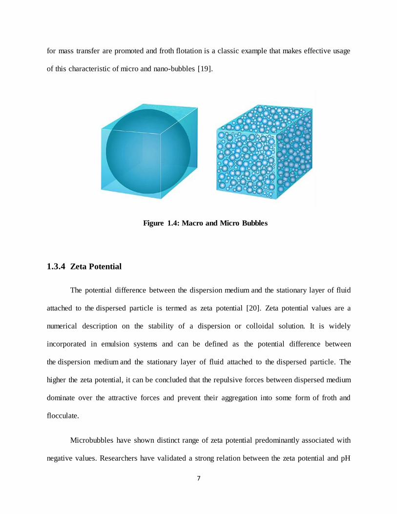
1.3.3 Large interfacial area

The increase in available surface area of the micro-bubbles for the same volume of a

macro-bubble is significant and this can be visualized by computing the ratio of surface area to

volume of a perfect sphere as follows: (assumption that every bubble is a perfect sphere)

Surface area= 4*π*r2

(1-8)

Volume=4/3*π*r3 (1-9)

Surface Area: Volume = 3/r (1-10)

This relation lays emphasis on the fact that as the bubbles decrease in size, an increased

surface area is made available for the same volume as represented in Figure 1.4. This way, sites

7

for mass transfer are promoted and froth flotation is a classic example that makes effective usage

of this characteristic of micro and nano-bubbles [19].

Figure 1.4: Macro and Micro Bubbles

1.3.4 Zeta Potential

The potential difference between the dispersion medium and the stationary layer of fluid

attached to the dispersed particle is termed as zeta potential [20]. Zeta potential values are a

numerical description on the stability of a dispersion or colloidal solution. It is widely

incorporated in emulsion systems and can be defined as the potential difference between

the dispersion medium and the stationary layer of fluid attached to the dispersed particle. The

higher the zeta potential, it can be concluded that the repulsive forces between dispersed medium

dominate over the attractive forces and prevent their aggregation into some form of froth and

flocculate.

Microbubbles have shown distinct range of zeta potential predominantly associated with

negative values. Researchers have validated a strong relation between the zeta potential and pH

8

values of the solution used along with addition of different surfactants. The negative values are

related to the ionic concentrations. Literature [21] reports a detailed study on zeta potential

variations for an air and water microbubble system evaluated through different techniques with

varying experimental conditions.

1.3.5 Bubble growth and shrinkage

Every bubble is characterized by a critical radius, rc which is the radius as given by the

simplified Young-Laplace equation. Bubbles smaller than the rc tend to decrease in size and vice

versa. During coalescence when bubbles merge, the newly formed bubble radius becomes larger

than the critical radius and inward diffusion of gas occurs as bubble begins to grow and becomes

a macro bubble.

As aforementioned, microbubbles have a very low rising velocity which increases the

residence time inside the water or appropriate liquid. A case of air/water microbubble system

elaborating the phenomenon of slow rising velocity of microbubbles and shrinkage within the

surface has been reported in [18]. A plot of zeta potential of microbubbles for different sizes on

the shrinking scale reveals negative value of zeta potential increase with decreasing size of the

micro-bubbles.

The buoyant force on the microbubble initiates minute levels of diffusion and onset of

shrinking during its ascension. On the contrary to milli-bubbles and centi-bubbles which rise to

the surface of water and burst, microbubbles collapse underneath and this phenomenon has been

identified to generate free radicals inside water [13] and the gradual shrinkage over time is

represented in Figure 1.5. Free radicals have unpaired valence electrons which puts them highly

reactive.

9

Figure 1.5: Bubble Shrinkage [13]

However free radical generation requires a dynamic stimulus like ultrasound or

cavitation. Generation of free radical with microbubbles is suspected to be a cumulative effect of

the shrinkage mechanism coupled with high negative values of zeta potentials as denoted in

Figure 1.6 and increased concentration of ions at the surface of microbubbles.

Figure 1.6: Zeta Potential Variation [13]

10

1.4 Scope of Research

Micro and nano-bubble generation technology in water is among the Cardinal areas of

research interest with plentiful industrial purposes. With the ever increasing need for potable

water, significant time and money are being invested in attending to the need. Albeit the

innumerous applications and commercialization, profound knowledge of the underlying

fundamental processes is limited in resource [1]. Treatment of water is one of the most

significant applications of the micro and nano-bubble Generation technology as it withholds a

blooming prospective and has been demanding more attention, especially in the recent past [2-4].

A number of micro-bubble technologies have been effectively used for various

applications. It appears that if the bubble size is reduced to the nano-level, the impact will be

significantly higher. Prevalence of nano-bubble technology in water is almost nil in the current

scenario. With a sound background and well-rounded facility for micro-cellular foaming

technology at the University of Toronto, motivation to extend the conceptual similarities to

bubbles in water is pursued.

The long term scope of this study is to develop a nano-bubble generation technology in

water and explore possible applications. Meanwhile, the short term objective which is precisely

the scope of this study is broken down as follows:

i. To comprehend the present scenario in micro-bubble generation technology

through extensive literature survey.

ii. Characterization of the micro-bubble generator (MBG), developed by Korea

Institute of Materials and Machinery (KIMM).

iii. Estimation of the mass transfer co-efficient and evaluation of its significance

11

iv. To investigate the role of particles (surfactants) and their influence on bubble

growth and shrinkage mechanisms.

1.5 Organization of the Thesis

Chapter 1 gives a brief introduction to micro-bubble technology in water detailing the

basic equations governing the bubble dynamics in water. The significance of micro-bubbles with

appropriate comparison to macro-bubbles is presented. The long and short term objectives of this

study are also stated.

Chapter 2 covers the literature survey on different micro-bubble generation technologies

and their performance analyses. Four basic micro-bubble generation technologies are discussed

in detail in addition to similar models with minor design modifications.

Chapter 3 explains the experimental procedures including the estimation of bubble-size

distribution both theoretically and experimentally and the dissolved oxygen levels of different

bubble generators. The volumetric mass transfer co-efficient is evaluated as a function of

superficial gas velocity and comparisons are made with similar literature.

Chapter 4 deals with the effect of Tween-20, a non-ionic surfactant, on the bubble

dynamics and the apparent coalescence phenomenon is explained. Particle size distribution

charts based on volumetric size-distribution are presented. Rise distance estimation is made for

each case with and without surfactant and an individual rise velocity plot is made for the same.

Chapter 5 summarises the results and concludes with motivations and suggestions to

carry the research forward in the near future. A very brief insight to optical tracking of the micro-

bubbles and the efforts undertaken is also presented.

12

Chapter 2

LITERATURE REVIEW AND BACKGROUND

2.1 Generation Technology of Micro-bubbles in Water

In context of the increasing demand and commercialization of wastewater purification

systems and the like, several technologies are available to generate microbubbles in water.

Bubbles are conventionally produced in a liquid, by following two ideologies:

i. Introducing the gas at a given flow rate into the stationary liquid.

ii. Dissolving the gas into the liquid and forcing the gas-liquid mixture to a state of

turbulence either by mechanical/hydraulic means to generate bubbles.

Four fundamental technologies can be identified as the base for micro-bubble generation

and other modern technologies are looked upon as structural modifications of one of the four.

The four basic microbubble generation technologies in water are discussed in the following

section.

2.1.1 Pressurized dissolution (decompression)

The pressurized dissolution type microbubble generation system bases its physics into the

Henry’s law which relates the concentration of a gas to its partial pressure. Henry’s law is

formulated as:

p = khc (2-1)

13

where p is the partial pressure of the gas, c is the concentration and kh is the henry’s constant. In

other words, henry’s law states more gas can be dissolved into a solution at a higher pressure.

This empirical practice is utilized in a pressurized dissolution microbubble generator where

pressurized air is introduced into a water tank. Due to the subsequent drastic drop in pressure of

the supersaturated air, air is expelled as microbubbles in to the water stream. Figure 2.1

illustrates this principle.

Figure 2.1: Pressurized dissolution type micro-bubble generator [3]

2.1.2 Venturi-type (cavitation)

A venturi based microbubble generation system makes use of the famous continuity

equation which states the conservation of mass. The mass flow rate in and out of any system

ought to be equal unless there is a discharge of energy midway either in the form of a chemical

reaction or leakage. The venturi tube with its three unique sections viz. the converging inlet,

suction throat and diverging outlet constitute the system. Water feeds in through the inlet and as

the section converges to a minimum area at the throat, a low pressure zone is created and gas

(air) is sucked in through the suction manifold. The two phase flow of water along with the gas

14

traverse the remaining section of the venture tube where bubbles are generated due to the shear

forces encountered in the diverging part.

However this method is only effective in producing bubbles of the order of millimeter

and not micro or nano-sized bubbles. In addition to the cavitation or gas injection principles,

acoustic characteristics of the fluid flow given by the de laval nozzle underlies the phenomenon.

Despite water being incompressible, the two phase flow adds compressibility parameters to be

taken into account.

Figure 2.2: Venturi flow combined with De laval nozzle condition

Choking at the tubule section is an essential condition for attainment of an accelerated

flow during the downstream of the flow. The flow in the converging section is essentially

subsonic while at the throat, choking which is reaching a Mach number of 1 shall be reached.

This becomes mandatory because only when a supersonic field is created at the diverging

section, microbubbles are formed due to the shear from shock waves set up in that section [22].

15

2.1.3 Spiral liquid flow type (rotatory type)

The spiral liquid flow type or swirl type microbubble generator is one of the commonly

used and well patented technology [23] famous with Japanese researchers. The principle is

simple and follows that as water is fed into a cylindrical tank and made to flow in a spiral pattern

traversing the inner circumference of the cylinder, a central core of reduced pressure is created

akin to a whirlpool. Gas (air) is sucked in from an aperture on the bottom of the tank. The water

together with the air that is sucked in is sheared at the top producing microbubbles. A

diagrammatic representation on the principle is shown in Figure 2.3.

2.1.4 Ejector type (complex pressure profile):

The ejector type microbubble generator is predominantly similar to the venture tube

microbubble generator but discerns in the design as the converging and diverging sections are

replaced with rectangular designs but the governing principle of inverse proportionality between

pressure and velocity holds good as in venturi case. Though not the first choice, the ejector type

has been used in several comparisons with counterparts [24]. Figure 2.4b represents the ejector

type bubble generator mechanism.

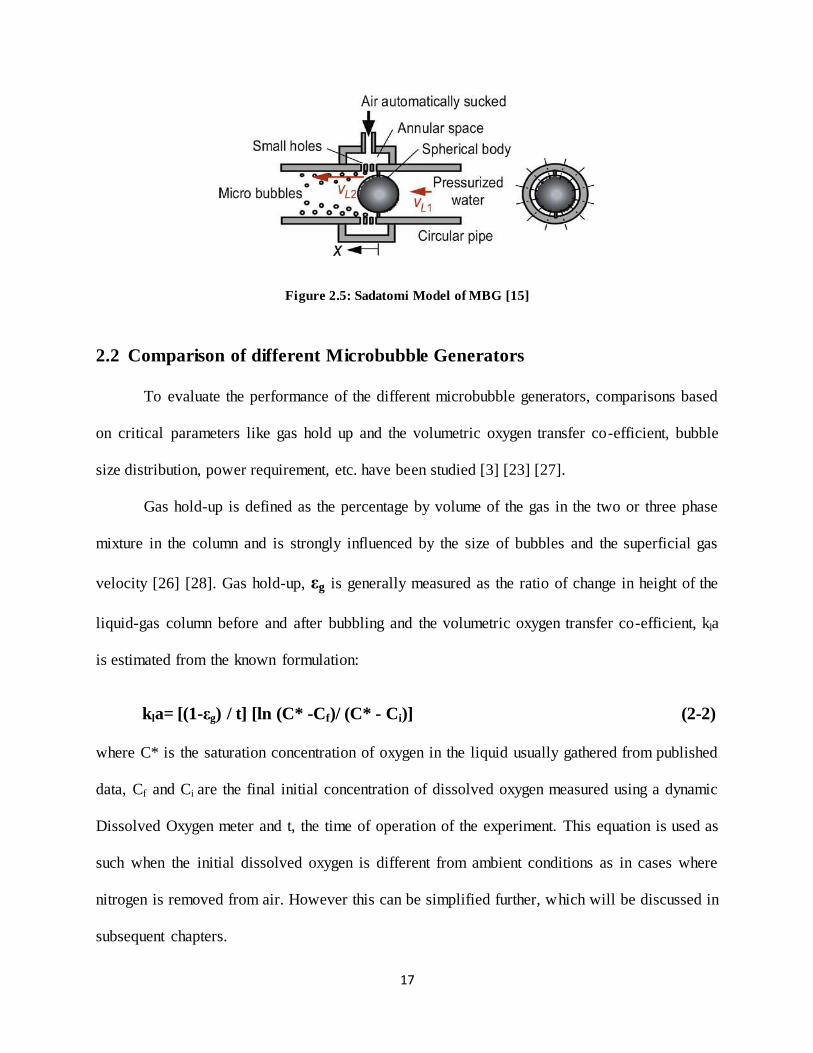
In addition to systems designed based on the four basic microbubble generation

technology, spargers or an array of the same are also used in generation of micro-sized bubbles

[25]. Other microbubble generation technologies and designs like the one developed by

Sadatomi et al. [15] is a structural modification of the conventional venturi tube. It enlists a

spherical body at mid-way through a rectangular section which encloses the water flow as shown

in figure 2.5. The spherical body helps create the necessary pressure drop across the gas aperture

to suck in gas and shear it along with the water to produce microbubbles at the exit section.

16

Another unique design of a modern microbubble generator is the one proposed by

Hasegawa et al. [26] which bases it’s working on the principle of Kelvin Helmholtz Instability

that describes the turbulent transitions in a fluid flow when two fluids of different density at

different velocities come into contact of each other. A wave is a classic example of the

phenomenon where wind blows over the sea water. The design includes slits carved at specific

angles that serve as the shearing site.

Figure 2.3: Swirl liquid flow type micro-bubble generator [21]

Figure 2.4: (a) Venturi-type micro-bubble generator (b) Ejector-type micro-bubble generator [3]

(a) (b)

17

Figure 2.5: Sadatomi Model of MBG [15]

2.2 Comparison of different Microbubble Generators

To evaluate the performance of the different microbubble generators, comparisons based

on critical parameters like gas hold up and the volumetric oxygen transfer co-efficient, bubble

size distribution, power requirement, etc. have been studied [3] [23] [27].

Gas hold-up is defined as the percentage by volume of the gas in the two or three phase

mixture in the column and is strongly influenced by the size of bubbles and the superficial gas

velocity [26] [28]. Gas hold-up, εg is generally measured as the ratio of change in height of the

liquid-gas column before and after bubbling and the volumetric oxygen transfer co-efficient, kla

is estimated from the known formulation:

kla= [(1-εg) / t] [ln (C* -Cf)/ (C* - Ci)] (2-2)

where C* is the saturation concentration of oxygen in the liquid usually gathered from published

data, Cf and Ci are the final initial concentration of dissolved oxygen measured using a dynamic

Dissolved Oxygen meter and t, the time of operation of the experiment. This equation is used as

such when the initial dissolved oxygen is different from ambient conditions as in cases where

nitrogen is removed from air. However this can be simplified further, which will be discussed in

subsequent chapters.

18

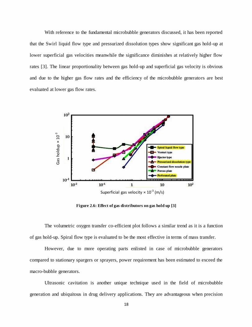
With reference to the fundamental microbubble generators discussed, it has been reported

that the Swirl liquid flow type and pressurized dissolution types show significant gas hold-up at

lower superficial gas velocities meanwhile the significance diminishes at relatively higher flow

rates [3]. The linear proportionality between gas hold-up and superficial gas velocity is obvious

and due to the higher gas flow rates and the efficiency of the microbubble generators are best

evaluated at lower gas flow rates.

Figure 2.6: Effect of gas distributors on gas hold up [3]

The volumetric oxygen transfer co-efficient plot follows a similar trend as it is a function

of gas hold-up. Spiral flow type is evaluated to be the most effective in terms of mass transfer.

However, due to more operating parts enlisted in case of microbubble generators

compared to stationary spargers or sprayers, power requirement has been estimated to exceed the

macro-bubble generators.

Ultrasonic cavitation is another unique technique used in the field of microbubble

generation and ubiquitous in drug delivery applications. They are advantageous when precision

Gas

ho

ldup

× 1

0-3

Superficial gas velocity × 10-3 (m/s)

19

is required however applicability to industrial scale is dubious owing to the cost involved in

operation. A comparison between a microbubble generator operated based on sonication and a

similar driven my mechanical agitation was carried out [30] to evaluate the performance.

Sonication operated equipment generated bubbles of very fine sizes, large interfacial area

and especially lower critical radius which meant the bubbles are more stable and procrastinate

immediate shrinkage. The experimentation also involved selection of kinds of surfactants but

predominant focus was on the type of bubble generation mechanism rather than the surface

active agents.

2.3 Flotation

Flotation is a separation treatment process that uses small bubbles to remove low-density

particulates from potable water and wastewater. Flotation is used as an alternative to

sedimentation for removing low-density materials like clays or algae. Flotation, based on the

method of bubble generation, can be classified as:

Electro-flotation

Dissolved air flotation (DAF)

Dispersed air flotation

Microbubble generation using technologies like electro-flotation and electrostatic-

spraying are industrially favored due to continuous operation where electricity is used to produce

bubbles inside the surface of water. Bubbles of H2, are formed at the cathode and bubbles of O2

at the anode. This method generates bubble diameters ranging from 22 to 50 um, depending on

the experimental conditions and follows the reaction:

20

H2O 2H+ + 1/2 O2(g)+2e

- at Anode( +) (2-3)

2H20 + 2e - 2OH

- +H2(g) at Cathode(-) (2-4)

In electrostatic spraying [31], an electrically charged capillary serves as an electrode

producing bubbles at its tip that is immersed in water. A comparison of the two electrically

stimulated methods with conventional pressurized dissolution (dissolved air flotation) for bubble

size distributions reveal that pressurized dissolution has the narrowest distribution with an

average bubble size of 40 microns while Electrostatic spraying showcased a wide distribution as

depicted in figure 2.7. The very reason behind the scattered size range is due to the high voltages

applied during experimentation aiming for smaller bubble size and at such high voltages, bubble

formation at the tip is said to be incurred with corona discharge [32] and the eventual difference

in sizes of bubbles produced.

Figure 2.7 Bubble size distributions for floatation process [32]

21

2.4 References on Microbubble Modelling and Simulation

A good handful of works have been documented in both theoretical and experimental

modelling of microbubbles in liquids [33-35]. However majority of the literatures deal with cases

where a single bubble is tracked through in a liquid column. Some touch the concept of bubble

swarm [35-38] but modelling such cases proves to be less significant due to the increased

magnitude of assumptions henceforth eventually digressing from the case on hand. Nonetheless,

the field of microbubble technology is taken up as a major research domain in the recent years

with more concentration on the experimental front with advancements in visualization

technologies.

2.4.1 Dimensionless Numbers:

In addition to governing equations such as Navier stoke’s equation, continuity condition,

momentum equations and the like, dimensionless numbers are an inevitable part to modelling by

a solver. Some of the common dimensionless numbers are discussed as below:

Reynolds number, the ratio of inertial force to viscous force, describes the force chiefly

governing the fluid flow. Flow through large pipes is a common example where the Reynolds

number is high.

Meanwhile, Weber number, the ratio between inertial force and surface tension force, is

more comprehensive in the context of interfacial fluid dynamics.

Re = ρ u d / μ (2-5)

We = ρ v2d / σ (2-6)

where ρ is the density of the liquid, u is the liquid velocity and the exit, d is the size of the

bubble, μ is the dynamic viscosity of the liquid and σ is the surface tension.

22

To give a furthermore insight to Weber number, [39] puts into words what Weber

number means and their significance on monodisperse microbubble jets. A stable bubble

distribution is hard to attain at very low Weber numbers and a nominal range of 1< We < 40

ensures a stable dispersion. Also, this is complimented by [40] which reports that no stable

microbubble conditions is observed at a Weber number less than 8 and the maximum can go to

few hundreds, in regards to microjets. These conclusions throw light on the fact that the inertial

forces shall always govern the fluid dynamics relative to the surface tension.

For microbubbles in water, the particle Reynolds number, Rep which uses the bubble size

in the Reynolds number formulation in place of the water outlet diameter, has to be low enough

for assumptions used in flow modelling to hold good.

In addition to the basic dimensionless numbers in fluid dynamics, two dimensionless

numbers namely Morton Number and Eotvos Number are grouped together in simulation

experiments to characterize the structural significance of bubbles in a liquid medium.

Morton number is given by:

Mo = gμc4Δρ/ρc

2σ

3 (2-7)

Eotvos number is given by:

Eo= Δρ g L2 / σ (2-8)

The Bond number is a very slight variation of the Eotvos number but used interchangeably.

Bond Number is given by:

Bo= ρ a L2

/ σ (2-9)

Where σ is the surface tension of the liquid,

Δρ is the difference in density between the liquid and gas

L is the characteristic length scale (radius of a drop)

23

g is the acceleration due to gravity

μc is the viscosity of the liquid

ρc is the density of the liquid

In simulation experiments, it has been observed that bubbles coalesce readily in liquids

with low Morton number and cluster in liquid with high Morton number [41] and can be

visualized directly in terms of viscosity and surface tension forces. Conclusion that high Morton

number liquid is more favorable for effective mass transfer compared to low Morton number

liquids is proposed.

2.5 Applications: Overview

Besides water potability, the micro-bubble generation technology in water is enlisted in the

following:

i. Aqua-life culture: fish and oyster farming [7]

ii. Industrial cleaning: in processing of industrial effluents [8] and sterilization [9]

iii. Agriculture: removal of residual food pesticides [10]

iv. In medicine: drug delivery to human organs, diagnosis using ultrasonic cavitation

v. Pollution control: prevent growth of blue-green algae in water bodies [11] absorption of

CO2 gas [12].

vi. Separation process: treatment of oil/water emulsion [13]; gas liquid contactors and algal

separation [14].

In addition, for free radical generation [15] and they fit in specific applications such as

reduction of drag force in a pipe flow [16].

24

2.5.1 Ozonation of Microbubbles:

Ozone is one of the commonly known and powerful disinfectants that are associated

water purification as they attach to the cell walls of bacteria and immobilize them rendering them

inactive. Almost every commercial water treatment plant has an ozonation unit installed however

Ozonation aided by microbubble technology is a rare occurrence in the present scenario.

Figure 2.8: Mechanism of Ozone generation

Research interests to generate ozone microbubbles for a spectrum of applications are

ongoing. However ozone is sparingly soluble in water and ozonation of water hasn’t been as

successful and efficient as it was thought to be owing to constraints like poor mass transfer rates

and unused quantities of ozone trapped within the water [17] [42]. Critical parameters that

influence solubility of ozone into water include the mixing characteristics of the gas-liquid

contactor, the process of ozone decay inside water along with the bubble density and size [31].

Microbubble ozonation of water using a commercially patented ozone microbubble

generator to study its effect on sludge solubilization was undertaken and compared it to a bubble

contactor [14]. 80% inactivation of microorganisms was achieved in conformity to a meagre

25

50% inactivation using a bubble contactor in addition multifold increase in Total and Soluble

Chemical Oxygen demands (SCOD).

Also Zimmerman et al. [17] recently came up with a novel design that incorporates an

oscillating air lift technology into the bio-reactor system to effectively generate ozone

microbubbles with appreciable mass transfer rates.

Reports on effective removal of different strains of bacteria have been published and

finds intense practice in food processing sector [43-45].

An Electro-static ozonation reactor based on Electrostatic spraying was developed [31]

and evaluated for mass transfer of ozone but at higher voltage levels the results failed to conform

owing to pressure fluctuations and poor controllability of the system.

26

Chapter 3

3. Experimental Approach: Part 1

3.1 Experimental set-up:

The microbubble generation technology used in our study is of the pressurized

dissolution type. A schematic of our system is as shown below in Figure 3.1.

Figure 3.1: MBG Schematic

As a general base, water from the city of toronto is used, delivered through internal

plumbing to the pump incorporated in the micro-bubble generator. Compressed air is also

supplied to the system from internal gas lines. The micro-bubble generation system is of a

dynamic nature where we have two mobile phases compared to single mobile phase. The main

aspect that separates the micro-bubble generator from other counterparts is the bubble number

density characterized by a bubble swarm. The solution is rendered milky white due to the

presence of innumerous bubbles and this can be realised in Figure 3.8 as discussed in later part of

this section. For this very reason, characterization of the system using optical imaging isn’t

pursued rather a dynamic particle size analysis is carried out.

3.1.1 Micro-bubble generation break-down:

Step 1: Process water is sent into the mixing chamber through a pump assembly

27

Step 2: Gas (i.e) air compressed at 100 psi is dissolved in the water inside the mixing chamber at

different gas flow rates.

Step 3: The air-water mixture enters a pressure reducing valve which can be viewed as a

convergent nozzle and exits as air micro-bubbles in water.

Step 4: The final two phase flow is collected in a custom-built water column for further

observations.

Flow meters to regulate the water and gas flow rates are added to the system in addition

to an emergency stop switch and a pressure gauge which gives the pressure inside the system

before it’s released to ambient conditions.

An experimental system of micro-bubble generator (MBG) has been set up with the

assistance of the KIMM. All the components of the micro-bubble generator were manufactured

by the EMT Plus, Korea (Jong-Gu Yim, emt4466@naver.com, +82-10-4466-0173) but all the

electronic and electric systems were replaced by Canadian ones to satisfy the CSA approval.

Figure 3.2, 3.3 and 3.4 show images of the MBG system-front view, internal assembly and outlet

part design respectively.

Figure 3.2: Micro-Bubble Generator (MBG) set-up

28

Figure 3.3: a: Connections inside the MBG, b: Mixing chamber part design

Figure 3.4: MBG outlet design

a b

29

3.2 Theoretical Bubble size estimation:

The bubble size was theoretically predicted using basic experimental data. Micro-bubbles

provide a milky-white color to the water, as supported by the findings in [46]. The theoretical

bubble size measurement was performed based on the observed clearance time after aeration for

a fixed time period. Subsequent aerations of 10 minutes were carried out and the mean was

evaluated. All the known values are fit into Stoke’s equation to predict the diameter of a single

air micro-bubble in water.

Assumptions made in this calculation are as follows:

1. The micro-bubble is a perfect sphere devoid of any irregularities in shape.

2. Each bubble follows the same ascension path.

3. There is no coalescence and if at all there is any, their influence on the overall

averaged diameter is negligible.

4. The rise velocity is unidirectional and directed along the ordinate.

Stoke’s equation:

Rising velocity, S=(1/18)*(ρ*g*d2

)/µ (3-1)

Hadamard-Rybczynski equation:

Rising Velocity, S=(1/12)*(ρ*g*d2

)/µ (3-2)

The deviation of stoke’s equation from the latter is by a constant of 18/12 which is 1.5.

For simplicity purpose and to have a referential comparison to similar works, stoke’s equation is

used going forward.

30

3.2.1 Experimental Conditions:

Temperatures- Ambient: 20 ͦC, Water : 12 ͦC

Water- Dynamic Viscosity (at T): 0.001 kg/ms

o Density: 1000 kg/m3

o Diaphragm Pump: 4.0 lpm (~1.1 gpm) at 80 psi (5.5 bar)

o Dissolved Oxygen: 6.40 mg/L

Gas: Compressed air @ 100psi

Flow rate for D.O. measurements: 2.5 lpm @ 3.2 bar

Water quality:

Figure 3.5: Water quality chart

Industrial water constitutes numerous dissolved solids which influence its quality.

Salinity is a measure of the mass of dissolved salts in a given mass of solution. Salinity is to be

known to effectively determine the dissolved oxygen saturation limit of the water being used. At

a temperature of 20 ͦC and a conductivity of 318 micro-Siemens/cm,

Salinity = 0.17 ppt ~0.20 ppt (3-3)

The acrylic column shown in figure 3.6 was custom built with a 22x22 cm2base standing

80 cm tall sealed at the edges using acrylic cement. Acrylic was preferred over glass for their

31

transparency and flexibility. The sheets were of ¼ inch thickness each and such thin walls

promote the viewing reducing the travel time through the medium.

Figure 3.6: MBG with acrylic column

3.2.2 Varying the Pressure:

System Pressure, as indicated on the Pressure gauge is the pressure difference from the

point just upstream the pressure reducing valve and the MBG exit to ambient conditions.

Pressure can be varied two ways,

1. By tightening or loosening a screw at the MBG outlet which influences the pressure at

which the air-water mixture gets released to the exit point of the pressure reducing valve.

The bubble size estimate shown in Table 3.1 is based on this.

32

2. By varying the mass flow rate of the gas. This way, more fluid is forced to exit for the

same operating conditions thereby increasing the pressure or vice versa.

In our experimentations for bubble size estimations, gas flow rate was fixed and the

pressure variations where brought about in the former way. Whereas for dissolved oxygen

measurements where mass flow rate of gas becomes a variable, the pressure variations were

based on this.

Table 3.1: Theoretical bubble size estimation

3.3 Dissolved Oxygen:

In addition to the bubble size prediction, Dissolved Oxygen (D.O.) measurement was

performed. D.O. can be defined as the amount of oxygen dissolved in water expressed in mg/L

(or) % saturation.

% Saturation = (D.O. / Saturation Level) × 100 (3-4)

D.O. varies inversely with the temperature, salt concentration and altitude implying the

colder the water, the higher is its capacity to hold gas. In the field of aquaculture, D.O. levels are

of prime importance [5] as plant and animals breeding in water require appropriate amounts of

No Pressure (bar) Clearance Time (s) Bubble Superficial

Rising Velocity (mm/s)

Bubble Size (µm)

1 2.6 34 1.617 54.481

2 3.8 65 0.846 39.403

3 4.4 85 0.647 34.456

4 5.2 111 0.495 30.152

33

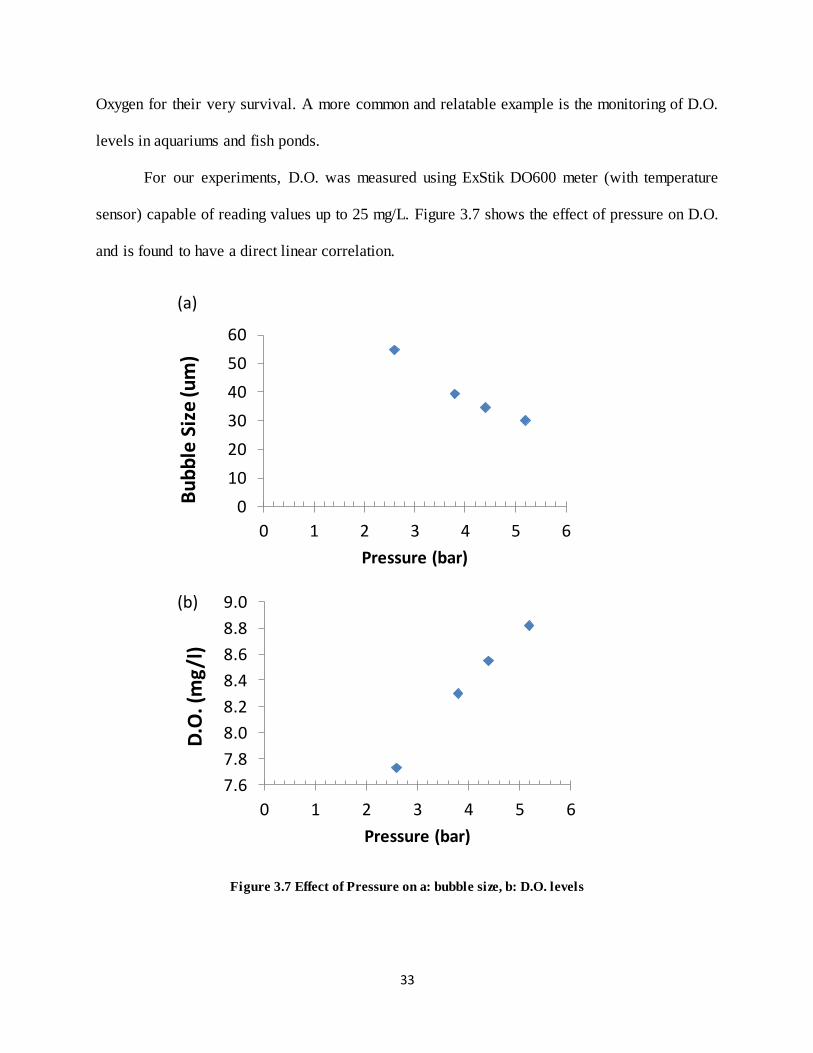
Oxygen for their very survival. A more common and relatable example is the monitoring of D.O.

levels in aquariums and fish ponds.

For our experiments, D.O. was measured using ExStik DO600 meter (with temperature

sensor) capable of reading values up to 25 mg/L. Figure 3.7 shows the effect of pressure on D.O.

and is found to have a direct linear correlation.

Figure 3.7 Effect of Pressure on a: bubble size, b: D.O. levels

0

10

20

30

40

50

60

0 1 2 3 4 5 6

Bu

bb

le S

ize

(um

)

Pressure (bar)

(a)

7.6

7.8

8.0

8.2

8.4

8.6

8.8

9.0

0 1 2 3 4 5 6

D.O

. (m

g/l

)

Pressure (bar)

(b)

34

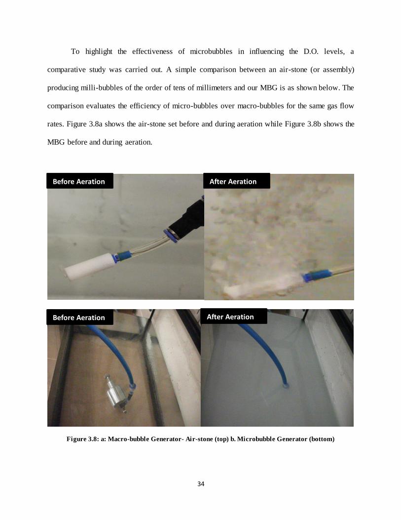
To highlight the effectiveness of microbubbles in influencing the D.O. levels, a

comparative study was carried out. A simple comparison between an air-stone (or assembly)

producing milli-bubbles of the order of tens of millimeters and our MBG is as shown below. The

comparison evaluates the efficiency of micro-bubbles over macro-bubbles for the same gas flow

rates. Figure 3.8a shows the air-stone set before and during aeration while Figure 3.8b shows the

MBG before and during aeration.

Figure 3.8: a: Macro-bubble Generator- Air-stone (top) b. Microbubble Generator (bottom)

Before Aeration After Aeration

Before Aeration After Aeration

35

Table 3.2: Comparison of D.O levels

No. Pressure

(bar)

Dissolved Oxygen (mg/L)

Micro-bubble Generator Macro-bubble Generator

1 0 5.67 5.67

2 2.6 7.73 5.9

3 3.8 8.30 5.77

4 4.4 8.55 6.19

5 5.2 8.82 6.2

3.4 Volumetric Mass Transfer Co-efficient:

To quantize the effect of liquid phase mass transfer, kla, the volumetric mass transfer co-

efficient is estimated from the equation which is applicable where there is no biological

consumption of oxygen [47]:

dC/dt = kLa (Cs – C) (3-5)

where: dC/dt is the rate of change of oxygen content

C is the D.O. concentration at time t

Cs is the saturation concentration

kLa can be estimated through different physical and chemical means. Here, we make use of the

D.O. concentration gradient measured using the D.O. meter and plug in all the known values into

equation (3-5). Subsequently, kLa is evaluated by plotting the natural log of (Cs-C) as a function

of time and kLa is obtained as the slope of the curve as shown from the Figures 3.9 and 3.10

respectively. Equations (3-6) and (3-7) give us the kLa value for two different pressures or gas

flow rates.

36

Table 3.3: D.O. variation as a function of time

System

Pressure

(bar)

Gas flow rate

(10-4 m3/min)

Time

(minutes)

D.O.

(mg/L)

% Saturation Saturation Limit

(mg/L)

2.8 3 0 5.7 46.36 At 20 ͦC,

0.20 PSU*: 9.040

For (inlet pressure =

1.38 psi)

12.295

3 6.2 50.42

6 6.9 56.12

9 8.18 66.53

12 8.32 67.66

4.2 8.5 0 5.7 46.36 12.295

3 6.35 51.64

6 8.01 65.14

9 8.57 69.71

12 9.43 76.7

Figure 3.9: D.O. Vs Time

5.0

6.0

7.0

8.0

9.0

10.0

0 2 4 6 8 10 12

C (

mg/l)

Time (min)

P=4.2 Bar (UofT)

P=2.8 Bar (UofT)

D

.O.

37

Figure 3.10: Rate of Change of D.O. Concentration

For 4.2 bar ln(Cs-C) = -0.0712t + 1.9253 (3-6)

For 2.8 bar ln(Cs-C) = -0.0468t + 1.9159 (3-7)

3.4.1 Superficial Gas Velocity:

In the context of two-phase flows, superficial velocity of each phase is defined as the

ratio of volumetric flow rate of that phase to the total cross-sectional area under consideration

[48]. It’s also sometimes referred to as volumetric flux. It can be interpreted as the velocity of the

single phase in the absence of the other or in other words the influence of one phase on the other

is considered negligible.

jphase = Qphase/Across-section (3-8)

R² = 0.945

R² = 0.9793

0.8

1.0

1.2

1.4

1.6

1.8

2.0

0 2 4 6 8 10 12

ln(C

s-C

)

t (min)

2.8 bar4.2 barLinear (2.8 bar)Linear (4.2 bar)

38

For our experiments, a rectangular tank column was used in contrast to cylindrical

columns. The reason being the pressure at which our system is operated is sufficiently low and

doesn’t necessitate a smooth column. Also, with rectangular columns distortions in bubble image

is minimized when compared to cylindrical columns. Cross sectional area of the column, Across-

section = .0484 m2

Table 3.4: Volumetric mass transfer co-efficient

No. Gas flow rate

(10-4 m3/min)

Superficial Gas Velocity

(10-4m/s)

kLa

(1/s)

1 3 1.01 0.0468

2 8.5 2.93 0.0712

Figure 3.11: Effect of Superficial gas velocity on volumetric mass transfer co-efficient

0

0.02

0.04

0.06

0.08

0 0.0002 0.0004 0.0006 0.0008

kla

(1

/s)

jG (m/s)

Tap Water [49]

Sea Water [49]

Tap Water-Experimental

39

3.4.2 Gas Hold-up:

Gas hold-up is the measure of percentage volume of gas in the mixture. It is evaluated by

observing the rise in the fluid column before and after aeration. In a static liquid column the

measurement is straight forward whereas in a dynamic liquid column measurements have to be

timed. Gas hold up is given by:

ε= A2(z2-z1)/ a

2(z2) (3-9)

where A is the cross-sectional area of the fluid column

z2 and z1 are the heights of the fluid column with and without aeration, respectively.

3.4.3 Specific Interfacial Area:

To elaborate the multitude of increase in the volumetric mass transfer co-efficient, kla, we

calculated the specific interfacial area.

The interfacial area per unit volume, a, is calculated using the formula:

a= 6ε/db (3-10)

where ε is the gas hold up (void fraction)

db is the average bubble diameter

The specific interfacial area alongside the gas hold-up for specific gas flow rates are

tabulated as shown below in Table 3.5.

Table 3.5: Specific Interfacial Area and Liquid phase mass transfer co-efficient

Gas flow rate

(10-4m3/s)

Gas hold up, ε Specific Interfacial area, a (103m-1) kl (10-5m/s)

3 .074 8.880 0.527

8.5 0.193 33 0.216

40

The values are plotted individually as a function of superficial gas velocity and compared

with [49] as follows:

Figure 3.12: Effect of Superficial gas velocity on Specific Interfacial Area

Figure 3.13: Effect of Superficial gas velocity on liquid phase mass transfer co-efficient

1

10

100

1000

10000

100000

0 0.0002 0.0004 0.0006 0.0008 0.001

a (m

-1)

jG (m/s)

Tap Water [49]

Sea Water [49]

Tap Water-Experimental

0.000001

0.00001

0.0001

0.001

0.01

0.1

1

0 0.0002 0.0004 0.0006 0.0008 0.001

k l (

m/s

)

jG (m/s)

Tap Water [49]

Sea Water [49]

Tap Water-Experimental

41

From the Figures 3.12 and 3.13, it is evident that the exponential increase of volumetric

mass transfer rates in our experiments is attributed to the bubble size. This emphasizes that the

smaller the bubble, the higher is the volumetric mass transfer rates. The liquid phase mass

transfer co-efficient didn’t show any significant improvement in our experiments and this trend

is similar to correlations made by [50]. Although, the quality of tap water might vary, the values

are large enough to sufficiently base the interpretation on bubble sizes and interfacial area. It’s

also supported by the fact that sea water [49] is bound to have higher total dissolved solids

compared to tap water, at any instance.

42

Chapter 4

Particle Size Analysis

4.1: Particle Size Measurement Methods

With regular CCD cameras, the ability to distinguish between particles and air bubbles of

similar size is overlooked. However, the effectiveness of characterization can improved with the

aid of particle size analyzers. Refractive indices of different medium are compared in Figure 4.1.

Some of the most common means of particle size measurement include: Optical

microscopy, Laser diffraction, Electro-impedance volumetric zone sensing (ES) and the like.

Laser diffraction is amongst the chief size measurement technologies on the contemporary scene

and is capable of recording finer sized particles in comparison to counterparts [51], though there

is an accusation that additional stresses are placed on the particles in such technologies during

the actual measurement process unlike optical microscopy.

Figure 4.1: Comparison of Refractive index

43

Principle: Laser Diffraction method

Range : 0.08 um-1,400 um

Figure 4.2: Particle Size Analyzer

Principle : Dynamic Optical Microscope

Range : 1 um-2,000 um

Figure 4.3: Particle image analyzer

44

The Particle size analyzer used in out experiments is the Microtrac Bluewave Particle

size Analyzer capable of measuring 0.01 to 2000 microns. The Microtrac Bluewave complies

with or exceeds ISO 13320-1 particle size analysis- light diffraction methods.

It is designed to work using the tri-laser technology but with the advancement of blue

laser diodes in place of two red lasers. Blue laser diodes are of higher sensitivity owing to the

shorter wavelengths and provide better particle size measurement in the micron and sub-micron

range.

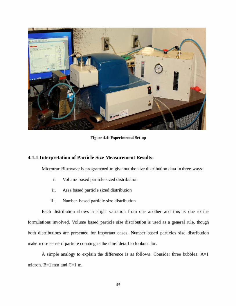
In retrospect, putting the analyzer to effect right away had its difficulties. Bubbles in

general are neither lasting nor rigid as in case of particles. So minimal handling becomes a

necessity for accurate measurements and subsequent interpretation. Our MBG outlet, as seen

from fig- , has a cylindrical assembly through which the micro-bubbles dispersed in water flow

outward and are collected. Meanwhile, the inlet to the particle size analyzer had a very narrow

opening with almost no room for additional mounts or tubing.

Originally, the samples (mostly particles dispersed in a liquid) are collected in a sampling

vessel and poured into the unit called SDC which has an internal circulating mechanism to

deliver the sample at the laser juncture and recirculate for multiple readings of the same sample.

But the dead volume is quite large, especially when dealing with bubble measurement. Then

came in the part called USVR which is basically a station with a small rotating spindle to force

the sample directly for size measurement. This way the dead volume in between bubble

generation and size measurement is made minimal.

Also to minimalize sample handling a direct connection was made between the USVR

and MBG outlet using a rubber coupling with SS clamps as seen from fig. that closed the MBG

outlet from the outside and delivered the bubbles directly into the cup of USVR.

45

Figure 4.4: Experimental Set-up

4.1.1 Interpretation of Particle Size Measurement Results:

Microtrac Bluewave is programmed to give out the size distribution data in three ways:

i. Volume based particle sized distribution

ii. Area based particle sized distribution

iii. Number based particle size distribution

Each distribution shows a slight variation from one another and this is due to the

formulations involved. Volume based particle size distribution is used as a general rule, though

both distributions are presented for important cases. Number based particles size distribution

make more sense if particle counting is the chief detail to lookout for.

A simple analogy to explain the difference is as follows: Consider three bubbles: A=1

micron, B=1 mm and C=1 m.

46

Figure 4.5: Understanding Volume and Number based distribution

In a container holding these three bubbles, a number size distribution will display each

particle to be one third of the total (1:1:1). A volume distribution will display C to occupy a

bigger space with B and A following in the volume hierarchy (3:2:1). Volume distribution is

more comprehensive individually but when combined with number distribution, more precise

analysis could be made, more so in the context of bubble swarm.

An example from present situation is as given below in Figure 4.5:

Figure 4.6: Volume based size distribution (top), Number based size distribution (bottom)

47

Looking at the top distribution in Figure 4.6, it is natural to assume the following:

i. The average bubble size is in the range 5-50 microns

ii. The milli-bubble population isn’t negligible completely

iii. Very few large bubbles are also traced

Now, if we take a look at the number based size distribution, the milli-bubble population

that were encountered in interpreting the former size distribution seem to be negligible,

apparently.

Depending primarily on number based size distribution isn’t acceptable due to the fact

that the values for number based distribution base their correlation on volume based distribution.

However, supplementing the volume based distribution with number based distribution for result

interpretation provides an invariably better perspective.

4.2 Bubble Distribution: Initial Characterization

Experimental Conditions are same as aforementioned in case of theoretical bubble size

estimation to enable comparison at a later stage of this study. Figure 4.7 shows the volumetric

bubble size distribution for a system pressure of 3 bar.

Table 4.1: Bubble Size Distribution at 3 bar Pressure

Pressure

(bar)

Cycle Time (s) Mean Bubble Size

(um)

Smallest bubble

size (um)

3 1 10 24.5 6.28

3 2 20 162.5 79.98

3 3 30 351.5 199.2

3 4 40 436.7 216.3

48

The time recorded on top of each bubble size distributions is the time interval between

successive measurements (i.e) the time since the bubble was generated.

Figure 4.7: Bubble size distribution at 3 bar

It can be seen in Figure 4.7, by the end of 10 seconds, the distribution is spread over a

little in the range 5-100 microns with multiple peaks around 20 microns and a sub-region around

1000 microns.

As time progresses or in other words, as the bubbles rise, there is shift in the curve as the

peak moves towards a larger bubble size range and the sub-region at 1000 microns are getting

bigger. This trend steadies with time and by the end of the fourth run at 40s, the micro-bubble

range has vanished and the milli-bubbles are getting populated. An important cause for this shift

in bubble size distribution over time is attributed to coalescence.

49

4.3 Bubble Coalescence:

Coalescence can be described as the process by which two or more bubbles come in

contact with each other to form a new bubble (i.e) collide with each other resulting in merging.

Coalescence is seen as naturally occurring and induced at times. It is mostly an undesirable

phenomenon as the result is detrimental in terms of:

i. Low bubble generator efficiency,

ii. Uneven bubble size distribution

iii. Improper heat and mass transfer.

Coalescence of bubbles can be visualized as similar to those of droplets [52]. As collision

is the onset of any coalescence, the efficiency of the collision determines the possibility of

coalescence. Bubble coalescence can be segmented into different individual stages as represented

in the Figure 4.8.Two individual gas bubbles approaching each other squeeze a layer of liquid in

between them. This liquid film gradually decreases in thickness and as a critical thickness is

reached, the layer ruptures giving way to coalescence [53-54].

Collision of bubbles occurs due to one of the three factors viz. turbulence, buoyancy and

laminar shear.

Figure 4.8: Bubble Coalescence Phenomenon

50

One of the key alternatives to reduce if not prevent the coalescence is by using

surfactants. Though electricity can be used to greater effectiveness to well disperse the solution,

the cost associated with it is not viable for industrial-scale accommodation.

4.3.1 Surfactants

Surface activating agents abbreviated as surfactants are compounds that comprise of

hydrophilic and hydrophobic elements built into the same structure. They are primarily used to

reduce to the surface (interface) tension of a liquid and may be of anionic, cationic or non-ionic

types.

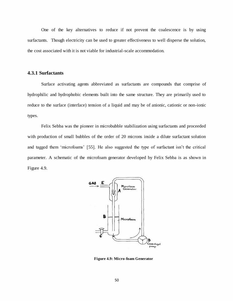
Felix Sebba was the pioneer in microbubble stabilization using surfactants and proceeded

with production of small bubbles of the order of 20 microns inside a dilute surfactant solution

and tagged them ‘microfoams’ [55]. He also suggested the type of surfactant isn’t the critical

parameter. A schematic of the microfoam generator developed by Felix Sebba is as shown in

Figure 4.9.

Figure 4.9: Micro-foam Generator

51

Surfactants play an important role in stabilizing the microbubbles and preventing their

shrinkage and eventual collapse under the surface of water. Surfactants, especially bio-

surfactants find an increasing demand in the field of medicine and instrumentation where

stabilization of drugs and lipids of the order of microns are required. Surfactants are more

efficient and microbubbles stability is more pronounced at a higher pH value [56].

In the following years, following advancements of technology, a more convincing

explanation than ‘microfoams’ was developed and the FAD ‘colloidal gas aphrons’ (CGA)

which refers to microbubbles covered with a surfactant shell which in turn is composed of two

layers of alternating hydrophilic and hydrophobic tails, came into reference as represented in

Figure 4.10. Studies on the properties and significance of the CGA for applications like protein

recovery and similar were made by [57-58]. It was interpreted that stability of the CGA varied

proportionally with the concentration of surfactant but inversely with the salt concentration in the

liquid. However, on contrary to [56], effect of pH was not signified then.

Figure 4.10: Colloidal Gas Aphrons

52

4.3.1.1 Critical Micelle Concentration (CMC):

The quantity of surfactants that go into the solution is a parameter to take note of as

beyond a certain level known as the critical micelle concentration, excess surfactant molecules

accumulate to form micelles and no further change in the surface tension of the liquid shall occur

beyond this critical point.

However, for stabilizing micro-bubbles excess of surfactant concentration that is well

over the CMC is required [59-60].

It is known that the thinning of the surfactant particles on the adjacent surfaces of two

approaching bubbles is responsible for cell opening by increasing the surface area. This is

illustrated in Figure 4.11. However, if the bubbles are not stretched, the existing surfactant

particles will effectively suppress the bubble coalescence. Or in other words, the outward

diffusion of gas from the bubbles should not be strong enough to disperse the surfactant

molecules on its surface.

Figure 4.11: Cell wall depletion

53

Most of the early researchers have focussed on stabilizing a single large bubble in a

quiescent liquid with Davidson et al. [61] being one among the popular, then. With micro-bubble

technology being a relatively new and commercially blooming field, effective suppression of

coalescence especially in a dynamic medium is a critical issue to be dealt.

Micro-bubbles have excellent self-pressurizing effect which can be combined with the

coalescence suppression application of surfactant to enhance the efficiency of the bubble

generator.

4.3.1.2 Choice of Surfactant:

Most surfactants have a tail, hydrophobic or lipophilic, made of a hydrocarbon chain in one form

or the other. Aromatic groups and ether are common in medical sector. The structure of a

surfactant molecule is as shown in Figure 4.12.

Figure 4.12: Structure of a surfactant

54

Surfactants are broadly classified into three categories based on the charge on their polar

head group as follow:

1. Non-ionic

2. Cationic

3. Anionic

As their names indicate, non-ionic surfactants carry no charge on their polar head;

Cationic surfactants have a positively charged head and anionic surfactants carry a negative

charge on their head as schematically shown in Figure 4.13.

Figure 4.13: Classification of Surfactants

In addition to the charge, the balance between the head group and tail group in terms of

percentage is an important parameter to be noted as it determines the property of the product

[62]. This is referred to as the ‘hydrophile-lipophile balance’ (H-P-B) and ready-to-use equations

have been formulated to calculate the value in a mixture [63]. HPB equations are more prevalent

in the emulsion industry where oil or particle size stabilization is primary.

55

4.3.1.3 Polysorbate-20:

As mentioned in [18], bubbles carry a small negative charge at their interface and

addition of charged surfactants would require additional monitoring as they combine more than

one effect to influence the bubble dynamics.

Polysorbate-20, known by brand name, Tween-20 is the selected non-ionic surfactant for

our experiments. The foremost character is its non-ionic property which nullifies the effect of

any electrical charges on the interface.

Structure of Polysorbate20 encompasses the water soluble chains and aromatic links in

their tail as represented in Figure 4.14 as follows:

Figure 4.14: Polysorbate-20

The HPB number for Tween-20 is 16.7 which makes them soluble in water. The higher

the value on a HPB scale of 1-18, the better is its solubility in water.

Tween-20 has been used in the context of stabilizing bubbles in air-water interface [64,

65]. It is reported that increasing the concentration of surfactant slightly affects the stabilization

56

positively which is speculated to be due to packaging at the bubble interface but large amounts

prove detrimental [65]. The use of tween-20 to stabilize micro-bubbles hasn’t been well

documented in literatures and if at all, they follow batch type processes [66]. Key aspects like

non-ionic property ease of availability and limited literatures in the field of micro-bubble

generation technology especially dynamic bubble generation methods.

Tween-20 is a yellow viscous liquid giving a yellowish solution when added to water. It

has a molecular weight of 1228 g/mole. Molecular-biology grades of tween-20 were purchased

from med-store at the University of Toronto in bottles of 500 ml.

Two molecular concentrations of Tween-20 are tested in our experiments, both well

above its CMC. CMC value of Critical Micelle Concentration: 8.04×10−5 M at 21 °C

Molecular Concentration are linked by the dormula:

C = (m/V) * (1/M.W) (4-1)

Where: m is the mass of the solute (tween-20)

V is the volume of the solution (Water)

M.W is the molecular weight.

Table 4.2: Experimental Cases

Case Surfactant Concentration of Surfactant

(M)

1 Tween-20 10-4

2 Tween-20 10-3

57

Table 4.3: Bubble Size Distribution: Case1: 10-4

M Tween20

Pressure (bar) Cycle Time (s) Mean Bubble Size (um) Smallest bubble size (um)

3 1 10 63.97 33.21

3 2 20 63.06 37.54

3 3 30 66.45 37.84

3 4 40 96.76 53.23

3 5 50 103 56.12

3 6 60 116 61.60

3 7 70 114.9 55.83

3 8 80 136.9 58.45

A third case for a much higher concentration of 10-2 M was tested but the MBG started

foaming at the outlet making the flow unsteady to be run through the particle size analyzer for

size characterization measurements.

White foamy agglomerates that were produced at the 10-2 M tween-20 concentration are

essentially due to the excess of surfactant molecules in the solution that started precipitating due

to the sudden pressure release. Similar occurrence were noted when the pressure was increased

even for lower concentrations. This helps us understand that there is a threshold to operate the

MBG to effectively make use of the surfactant.

Henceforth, the MBG was operated at pressures no greater than 3.2 bar (fluctuating

between 3 to 3.2 bar). Also to be seen is the concentration of Tween-20, which is to be kept

above the CMC but below 10mM.

These two cases are then compared with the initial characterization made at the same

pressure of 3 bar but without the surfactant. It’s to be noted that addition of surfactant only

affects the bubble dynamics and not the flow itself. Hence no pressure or flow rate changes were

encountered in the experimentation as a direct effect of surfactant addition.

58

Fig

ure 4

.15

: B

ub

ble

siz

e d

istr

ibu

tio

n:

Ca

se 1

59

Table 4.4: Bubble Size Distribution: Case2: 10-3

M Tween20

Pressure (bar) Cycle Time (s) Mean Bubble Size (um) Smallest bubble size (um)

3 1 10 68.47 30.51

3 2 20 51.07 22.01

3 3 30 57.25 25.90

3 4 40 62.83 28.43

3 5 50 67.45 30.25

3 6 60 70.22 33.34

3 7 70 72.51 34.26

3 8 80 82.93 34.25

3 9 90 150.8 57.62

A slight dip in the size of the bubble after 10 seconds is observed. This is speculated due

to the delay in reaching steady state conditions to produce microbubbles. The volume based

bubble size distribution charts are as shown in Figure 4.16 below.

60

Fig

ure 4

.16

: B

ub

ble

siz

e d

istr

ibu

tio

n :

Ca

se 2

61

4.4 Observations:

It’s observed that the surfactant addition positively affects the micro-bubble as the

bubbles are prevented from sharp increase in their sizes as opposed to the initial case. However,

the presence of outward diffusion happens to be prevalent though at a reduced scale.

Rise velocities can be predicted using stoke’s equation but axial rise distance cannot be

accurately estimated as there’s no correlation of change in size of the bubble over time. A 40um

bubble is predicted to rise at 1 mm/s but during the rise the shape and size of the bubble are

getting altered. This makes comparing our rise velocity calculations to stoke’s rise velocity less

meaningful. However the time dependence is coupled to the rise velocity equation to estimate the

axial rise distance as follows:

L1= ∫ Vdt + L0 (4-5)

Where L1 and L0 are the final and initial distance respectively, V is the rise velocity and dt is the

time interval. Also shown in Figure 4.18 is a comparison of axial rise distance of bubble as a

function of time. The values are calculated by fitting the values into the following equations for

each case

Initial Case, without surfactant: y = 0.1561x2 + 5.3005x (4-2)

Case 1: y = 0.0006x3 - 0.0853x

2 + 4.8326x (4-3)

Case 2: y = 0.001x3 - 0.1361x

2 + 5.4296x (4-4)

Figure 4.17 shows the effects of surfactants on the bubble size as a function of time.

62

Figure 4.17: Bubble size distribution for each case

Figure 4.18: Bubble Axial Rise

63

From the plot Figure 4.18, an air micro-bubble in water without any surfactant added to

the solution will have moved an axial distance of 7.62 mm from the point of generation in 10

seconds. However this distance is made half by surfactant addition, for either case. The effect of

molecular concentration of tween-20 isn’t commendable at the onset or early stages. However,

the stabilization of bubble or prevention of coalescence is gradually amplified as the two

surfactant curves show divergence as time increases gradually.

Another important aspect to be noted is in a dynamic bubble generation system as ours,

bubbles are constantly generated at the bottom and an older bubble is always affected by a newer

one as it passes on a thrust force to the former. This invariably affects the rise distance and this

justifies our results as they show a sharp increase during the onset and the curves flatten

gradually over time.

These equations are also used to estimate the individual rise velocities for each case as

shown in Figure 4.19-4.21

Figure 4.19: Rise velocity of bubbles for the initial case without surfactant

1

10

100

1000

0 10 20 30 40 50 60 70

Ris

e V

elo

city (

mm

/s)

Bubble size,d (um)

Without Surfactant

64

Figure 4.20: Rise velocity of bubbles with surfactant, Case 1

Figure 4.21: Rise velocity of bubbles with surfactant, Case 2

1

10

100

0 50 100 150

Ris

e V

elo

city (

mm

/s)

Bubble size,d (um)

With surfactant, Case 1

1

10

100

0 50 100 150 200

Ris

e V

elo

city (

mm

/s)

Bubble size,d (um)

With surfactant, Case 2

65

Chapter 5

Summary and Future Work

With bubble characterization experiments discussed in earlier chapters of this work,

bubble growth mechanisms and analysis of critical variables viz. size of the micro-bubble, mass

flow rate of gas, rise velocity of micro-bubbles, surface interactions and several other

characteristics are better understood in the context of micro-bubble technology.

One of the major portions of this work throws light on the influence of a non-ionic

surfactant Tween-20 on the properties of air microbubbles in water. As discussed in the

introductory chapter, the surfaces of micro-bubbles carry a slight negative charge and addition of

ionic or zwitteronic surfactants can open up potential applications. In addition, ionic surfactants

are capable of improving the zeta potential property of micro-bubbles too.

Despite the aforementioned facets, ionic surfactants cause a number of phenomena to

occur at the interface thereby singling out the individual effect requires advanced measuring and

recording technology. This investigation shall also disclose the shrinking properties of micro-

bubbles. A commercial and one of a kind application of the pressurized dissolution type MBG

used in our experiments is described as follows.

5.1 State of the art application:

A state of the art application using the MBG is the cleaning of Organic Light emitting

diode (OLED). Cleaning OLED is a daunting task if only brushes and similar mechanized scrubs

are deployed as they have the potential to deteriorate the sensitivity of the photovoltaic cells [67].

Ultrasounds are used for the purpose [68] albeit the facility and cost requirements being high.

Micro-bubbles can be cost-effectively used to serve the cause and substitute for other OLED

cleaning technologies.

66

Figure 5.1 shows an image of a OLED processing glass covered with deposits that are to

be cleaned. MBG used in our experimentation was deployed to wash this glass using ozone

micro-bubbles. The cleaning was carried out at KIMM’s Korean site with specifically assembled

ozone generation module as represented in Figure 5.2.

Figure 5.1: Deposits on an OLED Processing Glass

The MBG was operated at the maximum system pressure so that the bubbles generated

are of the smallest size range at relatively larger bubble density as supported by [59].

The air/water ratio is always maintained below 10-15 % as increasing the gas flow rates

hinder the generation of smaller sized bubbles. The cleaning was done as a five step process

represented in Figure 5.3 and listed in the order as follows:

Step 1: Hot water soaking.

Step 2: Brushing to remove relatively larger dirt particles.

Step 3: Ozone purifying, where the actual MBG is utilized in the process of cleaning.

Step 4: Fine brushing to remove any dust or sticky substances and to expose the effect of

MBG ozonation.

Step 5: Second Ozone purifying before the part can be put to use.

67

Fig

ure 5

.2:

Ozo

ne m

icrob

ub

ble

gen

era

tion

ass

emb

ly

68

Figure 5.3: Cleaning Procedure a: Hot bath, b: Initial Brushing, c: MBG Ozonation Cleaning,

d: Fine Brushing, e: 2nd

Ozonation

a b c

d e

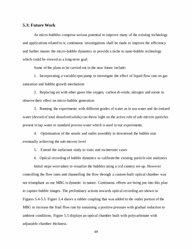
69

5.3: Future Work

As micro-bubbles comprise serious potential to improve many of the existing technology

and applications related to it, continuous investigations shall be made to improve the efficiency

and further master the micro-bubble dynamics to provide a niche to nano-bubble technology

which could be viewed as a long-term goal.

Some of the plans to be carried out in the near future include:

1. Incorporating a variable rpm pump to investigate the effect of liquid flow rate on gas

saturation and bubble growth mechanism

2. Replacing air with other gases like oxygen, carbon di-oxide, nitrogen and ozone to

observe their effect on micro-bubble generation

3. Running the experiments with different grades of water as in sea water and de-ionized

water (devoid of total dissolved solids) can throw light on the active role of sub-micron particles

present in tap water or standard process water which is used in our experiments.

4. Optimization of the nozzle and outlet assembly to downtrend the bubble size

eventually achieving the sub-micron level

5. Extend the surfactant study to ionic and zwitteronic cases

6. Optical recording of bubble dynamics to calibrate the existing particle size analyzers

Initial steps were taken to visualize the bubbles using a ccd camera set-up. However

controlling the flow rates and channelling the flow through a custom-built optical chamber was

not triumphant as our MBG is dynamic in nature. Continuous efforts are being put into this plan

to capture bubble images. The preliminary actions towards optical recording are shown in

Figures 5.4-5.5. Figure 5.4 shows a rubber coupling that was added to the outlet portion of the

MBG to increase the final flow rate by sustaining a positive pressure with gradual reduction to

ambient conditions. Figure 5.5 displays an optical chamber built with polycarbonate with

adjustable chamber thickness.

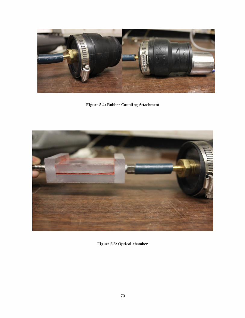
70

Figure 5.4: Rubber Coupling Attachment

Figure 5.5: Optical chamber

71

References:

[1] Tesař, V. (2014). "Shape oscillation of microbubbles." Chemical Engineering Journal 235:

368-378

[2] Agarwal, A., W. J. Ng, et al. (2011). "Principle and applications of microbubble and

nanobubble technology for water treatment." Chemosphere 84: 1175-1180.

[3] Terasaka, K., A. Hirabayashi, et al. (2011). "Development of microbubble aerator for waste

water treatment using aerobic activated sludge." Chemical Engineering Science 66: 3172-

3179.

[4] Khuntia, S., S. K. Majumder, et al. (2013). "Removal of Ammonia from Water using

Ozone Microbubbles." Industrial and Engineering Chemistry Research 52: 318-326.

[5] Srithongouthai, S., A. Endo, et al. (2006). "Control of dissolved oxygen levels of water in

net pens for fish farming by a microscopic bubble generating system." Fisheries Science

72: 485-493.

[6] Sumikura, M., et al. "Ozone micro-bubble disinfection method for wastewater reuse

system." Water Science & Technology 56.5 (2007): 53-61.

[7] James D. Englehardt, "Identifying Promising Hazardous Waste Reduction

Technologies", Journal of Environmental Engineering, 120, pp. 513-526, 1994

[8] Ikeura, H., F. Kobayashi, et al. (2011). "Removal of residual pesticide, fenitrothion, in

vegetables by using ozone microbubbles generated by different methods." Journal of Food

Engineering 103: 345-349.

72

[9] Nakashima, T., Kobayashi, Y. and Hirata, Y. 2012. Method to Exterminate Blue-Green

Algae in a Large Pond and To Improve Plant Growth by Micro-Nano Bubbles in Activated

Water. Acta Hort. (ISHS) 938:391-400

[10] Serizawa, Akimi, et al. "Laminarization of micro-bubble containing milky bubbly flow in a

pipe." Proceedings of 3rd European-Japanese Two-Phase Flow Group Meeting. 2003.

[11] van der Waarden, M. (1958). "Stability of emulsions of water in mineral oils containing

asphaltenes." Kolloid-Zeitschrift 156(2): 116-122.

[12] Rijk, S. E. D., J. H. J. M. V. D. Graaf, et al. (1994). "Bubble Size In Flotation Thickening."

Water Research 28(2): 465-473.

[13] Takahashi, M.; Chiba, K. & Li, P. (2007). Free-Radical Generation from Collapsing

Microbubbles in the Absence of a Dynamic Stimulus

Journal of Physical Chemistry 111: 1343-1347

[14] Chu, L.-B., S.-T. Yan, et al. (2008). "Enhanced sludge solubilization by microbubble

ozonation." Chemosphere 72: 205-212.

[15] Sadatomi, M., A. Kawahara, et al. (2007). "An advanced microbubble generator and its

application to a newly developed bubble-jet-type air-lift pump." Multiphase Science and

Technology 19(4): 323-342.

[16] Shatat, Mohammed ME, et al. "Drag Reduction Effects of Micro-Bubbles in Straight and

Helical Pipes." Journal of Fluid Science and Technology 4.1 (2009): 156-167.

[17] Zimmerman, W. B., V. Tesar, et al. (2008). "Microbubble Generation." Recent Patents on

Engineering 2: 1-8.

73

[18] Takahashi, M., T. Kawamura, et al. (2003). "Effect of shrinking microbubble on gas

hydrate formation." Journal of Physical Chemistry 107(10): 2171-2173.

[19] Féris, L. A., S. C. W. Gallina, et al. (2000). "Optimizing dissolved air flotation design

system." Brazilian Journal of Chemical Engineering 17: 549-556.

[20] Steinhart, M. (2004), Physics and Chemistry of Interfaces. By Hans-Jürgen Butt, Karlheinz

Graf, and Michael Kappl. Angew. Chem. Int. Ed., 43

[21] Oliveira, C. and J. Rubio (2011). "Zeta potential of single and polymer-coated

microbubbles using an adapted microelectrophoresis technique." International Journal of

Mineral Processing 98(1–2): 118-123.

[22] Yoshida, A., O. Takahashi, et al. (2008). "Water Purification using adsorption

characteristics of microbubbles." Japanese Journal of Applied Physics 47: 6574-6577.

[23] Ohnari, H. (2009). Swirling type micro-bubble generating system, Google Patents.

[24] Nakatake Y, Watanabe T, Eguchi T. Characteristic of the minute air bubbles into the gas

oil and mileage reduction of the diesel engine e comparison of an ejector type and

pressurized dissolution-type, Latest Technology 2 of Micro and Nano-Bubbles

2010;2(2):124e8 [in Japanese].

[25] Loubiere, K. and G. Hebard (2003). "Bubble formation from a flexible hole submergerd in

an inviscid liquid." Chemical Engineering Science 58: 135-148.

[26] H.Hasegawa, Y. Nagasaka and H. kataoka (2008). “Electrical Potential of Microbubble

Generated by Shear Flow in Pipe with Slits”, Fluid Dynamics Research, 40: 554-564

[27] S.E.Burns, S.Yiacoumi, et al. (1997). "Microbubble generation for environmental and

industrial separations." Separation and Purification Technology 11: 221-232.

74

[28] Shah, Y. T., Kelkar, B. G., Godbole, S. P. and Deckwer, W.-D. (1982), Design parameters

estimations for bubble column reactors. AIChE J., 28: 353–379

[29] Moshtari, B., E. G. Babakhani, et al. (2009). "EXPERIMENTAL STUDY OF GAS

HOLD-UP AND BUBBLE BEHAVIOR IN GAS –LIQUID BUBBLE COLUMN."

Petroleum and Coal.

[30] Xu, Q., M. Nakajima, et al. (2008). "A comparative study of microbubble generation by

mechanical agitation and sonication." Innovative Food Science & Emerging Technologies

9(4): 489-494.

[31] Shin, W.-T., A. Mirmiran, et al. (1999). "Ozonation using microbubbles formed by electric

fields." Separation and Purification Technology 15(3): 271-282

[32] Ptasinski, K.J., Geurts, F.L.S., Staring, A.J.P.M., Heesch, E.J.M. van & Kerkhof, P.J.A.M.

(1995). Formation of small bubbles in an electric field. Separation Science and

Technology, 30(10), 2127-2144

[33] Roghair, I., Y. M. Lau, et al. (2011). "On the drag force of bubbles in bubble swarms at

intermediate and high Reynolds numbers." Chemical Engineering Science 66(14): 3204-

3211.

[34] Azad, M. A. K., and Sultana R. Syeda. "A Numerical Model for Bubble Size Distribution

in Turbulent Gas-Liquid Dispersion." Journal of Chemical Engineering 24 (2006): 25-34.

[35] Roghair, I., M. Van Sint Annaland, et al. (2013). "Drag force and clustering in bubble

swarms." AIChE Journal 59(5): 1791-1800.

[36] Christian, Cinnamon M., E. G. Paterson, and Arnold A. Fontaine. Modeling Laser-

Generated Cavitation Bubbles. Diss. Pennsylvania State University, 2012.

75

[37] Bunner, B., & Tryggvason, G. (2002). Dynamics of homogeneous bubbly flows part 1. rise

velocity and microstructure of the bubbles. Journal of Fluid Mechanics, 466, 17-52.

[38] Deen, N., Mudde, R., Kuipers, J., Zehner, P. and Kraume, M. 2010. Bubble Columns.

Ullmann's Encyclopedia of Industrial Chemistry.

[39] Talu, E. (2007). Lipid-stabilized monodisperse microbubbles produced by flow focusing

for use as ultrasound contrast agents and targeted drug delivery, ProQuest.

[40] Ganán-Calvo, A. M. (2004). "Perfectly monodisperse microbubbling by capillary flow

focusing: An alternate physical description and universal scaling." Physical Review E

69(2): 027301.

[41] Smolianski, A., H. Haario, et al. (2008). "Numerical study of dynamics of single bubbles

and bubble swarms." Applied Mathematical Modelling 32(5): 641-659.

[42] Xu, P., M.-L. Janex, et al. (2002). "Wastewater disinfection by ozone: main parameters for

process design." Water Research 36(4): 1043-1055.

[43] Fukumoto, Y., Hashizume, K., & Nishimura, Y. (2010). Development of Supply System of

Microbubble Ozonated Water in Agriculture. Horticulture Environment and

Biotechnology, 51(1), 21-27.

[44] Wu, J., T. Luan, et al. (2007). "Removal of residual pesticides on vegetable using ozonated

water." Food Control 18(5): 466-472.

[45] Ikeura, H., Kobayashi, F., & Tamaki, M. (2013). Ozone microbubble treatment at various

water temperatures for the removal of residual pesticides with negligible effects on the

physical properties of lettuce and cherry tomatoes. Journal of Food Science, 78(2), T350-

T355

76

[46] Kobayashi, D., Y. Hayashida, et al. (2011). "Agglomeration and rapid ascent of

microbubbles by ultrasonic irradiation." Ultrasonics Sonochemistry 18(5): 1193-1196.

[47] Garcia-Ochoa, F. and E. Gomez (2009). "Bioreactor scale-up and oxygen transfer rate in

microbial processes: An overview." Biotechnology Advances 27(2): 153-176.

[48] Faghri, A., and Zhang, Y., 2006, Transport Phenomena in Multiphase Systems, Elsevier

Inc.

[49] Kawahara, A., M. Sadatomi, et al. (2009). "Prediction of micro-bubble dissolution

characteristics in water and seawater." Experimental Thermal and Fluid Science 33(5):

883-894.

[50] Calderbank, P. H. and M. B. Moo-Young, “The Continuous Phase Heat and Mass-Transfer

Properties of Dispersion”, Chem. Eng. Sci.16, 39–54 (1961).

[51] Sennoga, C. A., J. S. M. Yeh, et al. (2012). "Evaluation of Methods for Sizing and

Counting of Ultrasound Contrast Agents." Ultrasound in Medicine & Biology 38(5): 834-

845.

[52] M. Dhainaut (2002). "Literature study on observations and experiments on coalescence and

breakup of bubbles and drops," NTNU - Dept. of Chemical Engineering

[53] Postema, M., P. Marmottant, et al. (2004). "Ultrasound-induced microbubble coalescence."

Ultrasound in Medicine & Biology 30(10): 1337-1344.

[54] Prince, M. J. and Blanch, H. W. (1990), Bubble coalescence and break-up in air-sparged

bubble columns. AIChE J., 36: 1485–1499

[55] Sebba, F. (1971). "Microfoams—an unexploited colloid system." Journal of Colloid and

Interface Science 35(4): 643-646.

77

[56] Feng, W.; Singhal, N.; Swift, S. (2009). Drainage mechanism of microbubble dispersion

and factors influencing its stability. J. Colloid Interface Sci.337: 548–554

[57] Sebba, F. (1987). Foams and biliquid foams, aphrons. Chichester [West Sussex]: Wiley.

[58] Jauregi, P., S. Gilmour, et al. (1997). "Characterisation of colloidal gas aphrons for

subsequent use for protein recovery." The Chemical Engineering Journal and the

Biochemical Engineering Journal 65(1): 1-11.

[59] Parhizkar, M., M. Edirisinghe, et al. (2015). "The effect of surfactant type and

concentration on the size and stability of microbubbles produced in a capillary embedded

T-junction device." RSC Advances 5(14): 10751-10762.

[60] Sajjadi, B., M. K. Moraveji, et al. (2010). "Investigation of surfactant effect on the

operational characteristics of a packed bed Internal Loop Airlift Reactor." World Appl Sci J

11: 1004-1014.

[61] Davidson, J. F. and B. O. G. Schuler (1960). "Bubble formation at an orifice in a viscous

liquid." Transactions of the Institution of Chemical Engineers 38: 105-115.

[62] Griffin WC; Calculation of HLB Values of Non-Ionic Surfactants, Journal of the Society of

Cosmetic Chemists; 1954. Vol. 5, pp 249-235

[63] Required HLB Equation”; Journal of Dispersion Science and Technology; 1990. Vol. 11

(1), pp 83 — 91.

[64] Maedeh Asari, Faramarz Hormozi, Effects of Surfactant on Bubble Size Distribution and

Gas Hold-up in a Bubble Column, American Journal of Chemical Engineering. Vol. 1, No.

2, 2013, pp. 50-58. doi: 10.11648/j.ajche.20130102.14

78

[65] Söderberg, I., E. Dickinson, et al. (2003). "Coalescence stability of gas bubbles subjected to

rapid pressure change at a planar air/water interface." Colloids and Surfaces B:

Biointerfaces 30(3): 237-248.

[66] Wan, J., S. Veerapaneni, et al. (2001). "Generation of stable microbubbles and their

transport through porous media." Water Resources Research 37(5): 1173-1182.

[67] Lee, M. W., S. Chicot, et al. (2014). "Study of the Light Coupling Efficiency of OLEDs

Using a Nanostructured Glass Substrate." Journal of Nanoscience 2014: 4.

[68] Wang, Z. B., M. G. Helander, et al. (2011). "Unlocking the full potential of organic light-

emitting diodes on flexible plastic." Nat Photon 5(12): 753-757.

79

Appendix A

Salinity Calculation Equation:

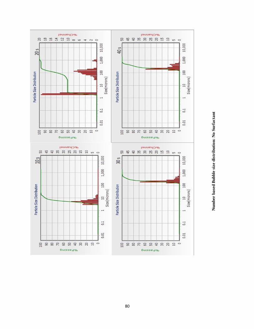
80

Nu

mb

er b

ase

d B

ub

ble

siz

e d

istr

ibu

tio

n:

No

Su

rfa

cta

nt

81

Nu

mb

er b

ase

d B

ub

ble

siz

e d

istr

ibu

tio

n:

Ca

se 1

82

Nu

mb

er b

ase

d B

ub

ble

siz

e d

istr

ibu

tio

n:

Ca

se 2