Understanding the evolution of two species of highly migratory cetacean at multiple scales and the potential value of a mechanistic approach

Francine Kershaw

Submitted in partial fulfillment of the requirements for the degree of Doctor of Philosophy in the

Graduate School of Arts and Sciences

COLUMBIA UNIVERSITY

2015

 

 

© 2015

Francine Kershaw

All Rights Reserved

 

 

ABSTRACT

Understanding the evolution of two species of highly migratory cetacean at multiple scales

and the potential value of a mechanistic approach

Francine Kershaw

An improved understanding of how behavior influences the genetic structure of populations

would offer insight into the inextricable link between ecological processes and evolutionary

patterns. This dissertation aims to demonstrate the need to consider behavior alongside genetics

by examining the population genetic structure of two species of highly migratory cetacean across

multiple scales and presenting an exploration of some potential lines of enquiry into the

behavioral mechanisms underlying the patterns of genetic population structure observed.

The first empirical chapter presents a population genetic analysis conducted on a data set

of new and existing samples of Bryde’s whale (Balaenoptera edeni spp.) collected from the

Western and Central Indo-Pacific and the Northwest Pacific Ocean. Levels of evolutionary

divergence between two subspecies (B. e. brydei and B. e. edeni) and the degree of population

structure present within each subspecies were explored. The subsequent three empirical chapters

represent a series of population- and individual-level genetic analyses on a data set of more than

4,000 individual humpback whales (Megaptera novaengliae) sampled from across the South

Atlantic and Western and Northern Indian Oceans over two decades. Patterns of genetic

population structure and connectivity between breeding populations are examined across the

region, and are complemented by an assessment of genetic structure on shared feeding areas for

these populations in the Southern Ocean.

 

 

Collectively, these studies demonstrate that a hierarchy of behavioral processes operating

at different spatial scales is likely influencing patterns of genetic population structure in highly

migratory baleen whales. Notably, for humpback whales, the widely assumed model of maternal

fidelity to feeding areas and natal philopatry to breeding areas was found not to be applicable at

all spatial scales. From an applied perspective, the complex population patterns observed are not

currently accounted for in current management designation and recommendations for applying

these findings to the management and protection of these species are presented.

As these empirical studies highlight the importance of behavior as a potential mechanism

for shaping the genetic structure of species, the final chapter offers a research prospectus

describing how behavioral and genetic data may be integrated using new individual-based

modeling techniques to integrate data and information from the fields of behavioral ecology and

population genetics.

 

i      

TABLE OF CONTENTS

LIST  OF  TABLES                                                  iii  LIST  OF  FIGURES                                                                  v  

INTRODUCTION 1

CHAPTER ONE: Population differentiation of 2 forms of Bryde’s whales in the Indian and Pacific Oceans 6

ABSTRACT 7 INTRODUCTION 8 MATERIALS AND METHODS 10 RESULTS 15 DISCUSSION 18 TABLES AND FIGURES 25 SUPPORTING INFORMATION 30

CHAPTER TWO: Multiple processes drive genetic structure of humpback whale (Megaptera novaeangliae) populations across spatial scales 35

ABSTRACT 36 INTRODUCTION 37 MATERIALS AND METHODS 39 RESULTS 44 DISCUSSION 48 TABLES AND FIGURES 56 SUPPORTING INFORMATION 65

CHAPTER THREE: Humpback whale (Megaptera novaeangliae) populations show extensive and complex mixing on feeding areas in the South Atlantic and Western Indian oceans 73

ABSTRACT 74 INTRODUCTION 75 MATERIALS AND METHODS 79 RESULTS 86 DISCUSSION 89 TABLES AND FIGURES 101 SUPPORTING INFORMATION 106

CHAPTER FOUR: Philopatry and sex-biased dispersal shapes humpback whale (Megaptera novaeangliae) population structure at multiple scales 119 ABSTRACT 120 INTRODUCTION 121 MATERIALS AND METHODS 124

 

ii    

RESULTS 127 DISCUSSION 128 TABLES AND FIGURES 137

CHAPTER FIVE: Achieving a mechanistic understanding of genetic population structure 140 ABSTRACT 141 INTRODUCTION 143 THE INTEGRATION OF BEHAVIOR 146 DEVELOPING IBMS FOR HIGHLY MIGRATORY SPECIES 147 TECHNIQUES FOR MODEL DEVELOPMENT 157 CONCLUSIONS 161 TABLES AND FIGURES 163

SYNTHESIS 169

REFERENCES 176

 

iii    

LIST OF TABLES

CHAPTER ONE

1. Genetic diversity indices for B. e. brydei and B. e. edeni haplotypes 25

2. Pairwise FST and ϕST values for B. e. brydei and B. e. edeni 26

S1. Details of new Bryde’s whale samples 30

S2. Table of corresponding accession numbers for haplotypes 32

CHAPTER TWO

1. Sample location, size, and diversity indices for nine microsatellite loci 56

2. Analysis of hierarchical variance (AMOVA) results 57

3. Significance values for pairwise fixation indices for FST and Jost’s D 58

S1. Pairwise fixation index values FST, RST, and Jost’s D 68

CHAPTER THREE

1. Genetic diversity for the mitochondrial control region and microsatellite loci 101

2. Genetic differentiation of feeding area boundary sets for mtDNA 102

3. Genetic differentiation of feeding area boundary sets for microsatellites 103

S1. Genetic diversity of the mitochondrial control region and microsatellite loci 107

S2. Genetic differentiation of four alternative boundary sets for mtDNA 108

S3. Genetic differentiation of four alternative boundary sets for microsatellites 112

S4. Genetic diversity of the seven feeding areas included in the haplotype comparison 116

 

iv    

CHAPTER FOUR

1. Sex and date of genotypic matches 137

CHAPTER FIVE

1. Overview of the lessons that can be transferred from existing case studies 163

 

v      

LIST OF FIGURES

CHAPTER ONE

1. Study region and approximate sampling locations 27

2. Phylogenetic reconstruction of mtDNA control region haplotypes 28

S1. Haplotype network of B. e. brydei and B. e. edeni 34

CHAPTER TWO

1. Sampling locations of the humpback whale breeding stocks and substocks 59

2. Distribution of 3 genetic clusters estimated using STRUCTURE 60

3. Discriminant analysis of principle components (DAPC) scatterplots 61

4. Magnitude and directionality of historic gene flow 62

5. Estimated number of migrants per generation (Nem) 64

S1. Mean LnP(K) and Delta K (ΔK) plots for the STRUCTURE outputs 69

S2. Distribution of 4 genetic clusters estimated using STRUCTURE 70

S3. Distribution of individual reassignment by the DAPC 71

S4. Magnitude and directionality of contemporary gene flow 72

CHAPTER THREE

1. The longitudinal boundaries of the 14 feeding areas defined by IWC AH1 104

2. Proportion of individuals allocated to the six breeding stocks by the MSA 105

S1. Mean Ln(P|K) and Delta K (ΔK) plots for the STRUCTURE outputs for K=1-7 117

S2. Distribution of genetic clusters for a) K=2 and b) K=3 118

 

vi    

CHAPTER FOUR

1. Sampling locations and Interchange index values between BSB and BSC 138

2. Return index (Ri) values for BSB1, BSB2, and BSC3 139

CHAPTER FIVE

1. Conceptual diagram of an integrated individual-based model (IBM) 166

2. How an IBM can be used to understand mechanisms influencing genetic patterns 167

 

vii    

ACKNOWLEDGEMENTS

Foremost, I would like to acknowledge my advisor, Dr. Howard C. Rosenbaum, for his guidance

and support, and his unwavering belief that I would succeed. I appreciate both the trust he placed

in me to pursue my own path while also acting as a compass when I felt that I was losing my

way. I am truly grateful for his mentorship and friendship throughout these five years and look

forward to the continued work we are planning together.

Special thanks to my committee for their thoughtful input and encouragement: Dr.

Eleanor Sterling, Dr. George Amato, Dr. Martin Mendez, and Prof. Shahid Naeem. I greatly

appreciate the interest and enthusiasm that each member has shown for my research throughout

my studies, both in idea and final form. I would like to thank the members of my comprehensive

examining committee, Prof. Don Melnick, Dr. Rob DeSalle, again to Dr. Eleanor Sterling. I

extend particular gratitude to Dr. Rob DeSalle for his teaching and mentorship in the first years

of my studies.

I am deeply grateful to the members of the Sackler Lab for Comparative Genomics at the

American Museum of Natural History, and particularly to Rebecca Hersch and Stephen

Gaughran for their one-on-one guidance in the laboratory. I am appreciative of the time and

patience they afforded to me while juggling many other equally important projects, as well as

their enthusiasm for the work we were undertaking. I would also like to extend thanks to Dr.

Mary Blair from the Museum’s Center for Biodiversity and Conservation for her generous

support, mentorship, and encouragement throughout my studies; masterfully balancing scientific

excellence with a passion for conservation, she has represented an important role model to me

and many other students.

 

viii    

I would like to thank all the members of the Ocean Giants Program at the Wildlife

Conservation Society (WCS) that have contributed to my research and made me feel a welcome

part of the team – it was only fitting that they should share my first experience of watching

whales. Particular thanks go to Tim Collins and Dr. Salvatore Cerchio, who I greatly appreciate

for taking the time to impart their knowledge of these amazing animals and for always showing

genuine interest in my research. This project would not have been possible without their work,

and that of the WCS field teams and collaborators, collecting the more than four thousand

samples included in these studies. I am also indebted to Dr. Robert L. Brownell Jr. for imparting

his extensive knowledge of cetacean taxonomy and helping me unravel the complexities of

Bryde’s whales.

I am indebted to Dr. Rita Amaral for her generous mentorship, friendship, and

partnership on a number of collaborative projects. I also extend much appreciation to Dr.

Melinda Rekdahl for our many engaging conversations regarding interdisciplinary approaches to

combining genetic and acoustics, and for her guidance, support, and friendship during my final

two years. I’m grateful to Hannah Jaris for imparting her expertise of genomics and being a close

friend during her time in the Rosenbaum lab. It was also was my pleasure to mentor Charlotte

Tisch whose diligent work matching genotypes formed the basis of the fourth chapter of this

dissertation. Thanks go to Dr. Inês Carvalho for her support and for imparting her knowledge of

humpback whale population genetics, and also to Dr. Sara Maxwell for her encouragement and

mentorship.

Many thanks go to the members of the Sterling-Ginsberg lab group and in particular to

Dr. Eleanor Sterling and Dr. Joshua Ginsberg for creating an engaging academic community

centered upon advancing conservation research. I am indebted to all the members of the lab for

 

ix    

feedback on my dissertation throughout my time at Columbia. I am also incredibly grateful to the

amount of encouragement and feedback I have received from all the members the Department of

Ecology, Evolution, and Environmental Biology at Columbia University.

I am blessed to have the friendship of Nicole Mihnovets, Rae Wynn-Grant, and Megan

Cattau – it has, and will always be, true love. I am grateful to Yili Lim, Camilo Sanin, and

Natalia Rossi, for five years of encouragement and friendship. I’m also deeply thankful to Vivian

Valencia – I couldn’t have asked for better company as we approached the finish line together.

Much appreciation is also extended to the board members of the Columbia University Family

Support Network (CUFSN); it has been a privilege to work alongside a team of such dedicated

students who tirelessly and voluntarily contribute their time to improving resources for all

families at Columbia University.

Finally, this would not have been possible without the love and support of my friends and

family. To Susan Abbott, Michelle Harrison, and Mark Siddall, who have remained my dear

friends through everything even though I moved many miles away. Finally, I extend deep

gratitude and love to my parents, Christine Hey and Martin Kershaw - thank you for continual

support and encouragement to pursue my dreams.

 

x      

DEDICATION

I dedicate this work to my grandparents, Jack and Vera Barnes, who always believed I could do

anything, who taught me that the most important thing is to appreciate your life and those you

share it with, and who nurtured my love for nature in their beautiful garden, be it in the potting

shed, feeding the birds and squirrels, or delighting at the occasional hedgehog. I miss them both

dearly.

  1  

 

INTRODUCTION

Behavior is too important to be left to psychologists.

-­‐ Donald Redfield Griffin

Genetic population structure is commonly observed in wild populations and arises from

variation in the spatial and temporal distribution and movement of individual organisms, which

over evolutionary meaningful timescales results in the systematic variation of population allele

frequencies across space and time (Jones & Wang 2012). Population structure is therefore, at

least in part, driven by complex behaviors operating at the level of the individual organism. An

improved understanding of how behavior influences the genetic structure of populations would

offer insight into the inextricable link between ecological processes and evolutionary patterns,

enabling the interpretation of the mechanisms underlying existing genetic patterns, the

forecasting of how these patterns may change in the future (Blair & Melnick 2012) and, in the

long-term, may facilitate predictions of the evolutionary trajectories of species (Li et al. 2012).

Highly migratory species exhibit a wide range of complex behaviors capable of

influencing their genetic population structure at multiple scales. Population-level fidelity to

breeding and feeding sites has proven to be an important driver of genetic isolation between

populations for a number of migratory species. There is increasing evidence, however, that

genetic structure within populations is driven by subtle, and sometimes socially driven,

differences in dispersal and migratory behaviors that form barriers to gene flow. This behavioral

partitioning within a population may, for example, be linked to differences in the timing of

migration on the basis of age, sex, or reproductive status (Sonsthagen et al. 2009), habitat and

  2  

 

foraging specializations of certain individuals (Rayner et al. 2011; Hoye et al. 2012), or different

social strategies (Andrews et al. 2010).

The properties inherent to different molecular markers enable the testing of explicit

hypotheses regarding how behavior may be influencing genetic patterns. When dispersal is

biased towards one sex, uniparentally inherited markers would be expected to show incongruent

patterns of genetic structure. For example, the general pattern of female philopatry and male-

dispersal observed in mammals (Greenwood 1980) is reflected in strong geographic structuring

of the maternally inherited mitochondrial DNA (mtDNA), but not the paternally inherited Y-

chromosome haplotypes or autosomal markers (Avise 2004). By considering markers with

differing mutation rates and coalescence times, one can also discriminate between the timing of

dispersal events. For instance, rapidly mutating nuclear microsatellite loci can be informative of

recent dispersal and movements of individuals, whereas more slowly evolving mtDNA markers

provide insight into population differentiation and connectivity on historic timescales (Avise

2004).

The ensuing four data chapters examine the genetic structure of two species of highly

migratory baleen whale at the subspecies, population, and individual scales, and explore some

potential lines of enquiry into the mechanisms (i.e. processes) underlying the patterns observed.

Akin to all baleen whales, both the Bryde’s whale (Balaenoptera edeni spp.) and the humpback

whale (Megaptera novaeangliae) display significant behavioral complexity and plasticity, and

recent studies have unveiled corresponding elaborate genetic architectures, the behavioral drivers

of which appear to vary at different scales (e.g. Kanda et al. 2007; Rosenbaum et al. 2009).

Thus, baleen whales represent an interesting and relevant test bed for questions concerning how

behavior may influence the evolutionary patterns of highly migratory species.

  3  

 

From an applied perspective, the elucidation of population-level management units for

these two species is of utmost importance given that baleen whales are in recovery from

significant commercial exploitation and illegal Soviet whaling (Rocha et al. 2015) and some,

including the Bryde’s whale, remain a target of scientific whaling by Japan (Kanda et al. 2007).

These species also are vulnerable to a range of contemporary anthropogenic stressors, such as

disturbance to their acoustic environment, increased shipping and pollution (Rosenbaum et al.

2014), and the indirect effects of a changing climate (Ramp et al. 2015). The interpretation of the

genetic analyses conducted in each of the four data chapters therefore also explicitly informs

species management. In addition, the geographic regions from which the samples used in these

studies were collected, namely the South Atlantic Ocean, Western and Northern Indian Oceans,

and the Southern Ocean, are relatively understudied and so this body of work represents an

important contribution to the global understanding of these species.

Chapter One (published as Kershaw et al. 2013 in the Journal of Heredity) presents

subspecies- and population-level analyses for two forms of Bryde’s whale (B. e. brydei and B. e.

edeni) using mtDNA control region sequences from 56 new samples from Oman, the Maldives,

and Bangladesh, and published sequences originating from Java and the Northwest Pacific. This

chapter combines nine diagnostic characters identified in the mtDNA control region with a

phylogenetic analysis based on maximum parsimony to explore the degree of differentiation

between the two forms of Bryde’s whale. Genetic diversity and differentiation indices, and a

reconstructed haplotype network, are then used to assess population-level genetic structure

within each of the two forms. Subsequently, ecological differences between the two forms that

may be driving their genetic differentiation are considered.

  4  

 

Chapters Two, Three, and Four focus exclusively on a data set comprising more than

4,000 humpback whales sampled in the South Atlantic, Western and Northern Indian, and

Southern Oceans over more than two decades. This data set represents samples from seven

breeding populations and sub-populations identified across the region, and which are managed

by the International Whaling Commission (IWC) as the following “breeding stocks (BS)” and

“substocks”: BSA, located off Albrohos Bank, Brazil; BSB1, a breeding population in the Gulf

of Guinea; BSB2, a group of feeding and migrating individuals off west South Africa; BSC1, off

east South Africa and Mozambique; BSC2, located in the vicinity of the Mayotte and Geyser,

and the Comoros Islands; BSC3, that breeds off northeast Madagascar; and the non-migratory

Arabian Sea Humpback Whale (ASHW) population sampled from the Gulf of Aden, Oman.

Chapter Two examines the genetic diversity and population structure of seven putative

breeding stocks and substocks present in the region using nine microsatellite loci. Genetic

differentiation is assessed both with and without a priori designation of population units, and

gene flow is estimated using maximum likelihood and Bayesian approaches, providing insights

into population connectivity on historic and contemporary temporal scales. For all analyses, sex-

specific differences are explicitly explored. The results of these analyses are compared and

contrasted to those of a parallel study employing a 486 bp consensus sequence of the

mitochondrial control region (Rosenbaum et al. 2009). Chapter Three assesses the relative

contribution and degree of mixing of seven humpback whale breeding stocks and substocks to

shared feeding areas in the Southern Ocean. First, feeding areas are defined using a sensitivity

analysis based on genetic differentiation indices. A mixed stock analysis is then conducted using

ten microsatellite loci and the distribution of haplotypes across feeding areas is examined using a

371 bp consensus sequence of the mitochondrial control region. Genetic diversity is also

  5  

 

assessed for both molecular markers. Chapter Four, the final data-based chapter, presents a

genotypic matching analysis using ten microsatellite loci and two quantitative indices to examine

sex-specific differences of fidelity to breeding areas, dispersal between breeding areas, and

connectivity between breeding areas and feeding grounds, at the individual level.

The preceding four chapters illustrate that the development of a multidisciplinary

approach combining the fields of behavioral ecology and population genetics is necessary to

developing a mechanistic understanding of genetic population patterns (Habel et al. 2015). The

fifth and final chapter therefore presents a literature review and research prospectus for

advancing multidisciplinary approaches for the integration of data from the fields of population

genetics and behavioral ecology using individual-based models (IBMs) as an analytical platform.

Chapter Five first reviews recent advances in the field of IBM development that have resulted in

these models becoming useful platforms for the integration of data on individual behavior,

environmental factors, and genetics. Subsequently, lessons from a variety of applied case studies

are synthesized to guide future model implementation, parameterization, and validation, with a

particular focus on systems that are generally lacking in rich data sets or where the ability to

ground truth model outputs is often not feasible, such as for the majority of highly migratory

species.

  6  

 

CHAPTER ONE

Population differentiation of 2 forms of Bryde’s whales in the Indian and Pacific Oceans FRANCINE KERSHAW, MATTHEW S. LESLIE, TIM COLLINS, RUBAIYAT M. MANSUR, BRIAN D. SMITH, GIANNA MINTON, ROBERT BALDWIN, RICHARD G. LEDUC, CHARLES ANDERSON, ROBERT L. BROWNELL JR., and HOWARD C. ROSENBAUM. Published as Journal of Heredity (2013) 104, 755-764.

  7  

 

ABSTRACT

Accurate identification of units for conservation is particularly challenging for marine species as

obvious barriers to gene flow are generally lacking. Bryde’s whales (Balaenoptera spp.) are

subject to multiple human-mediated stressors, including fisheries bycatch, ship strikes, and

scientific whaling by Japan. For effective management, a clear understanding of how populations

of each Bryde’s whale species/subspecies are genetically structured across their range is

required. We conducted a population-level analysis of mtDNA control region sequences with 56

new samples from Oman, Maldives, and Bangladesh, plus published sequences from off Java

and the Northwest Pacific. Nine diagnostic characters in the mitochondrial control region and a

maximum parsimony phylogenetic analysis identified 2 genetically recognized subspecies of

Bryde’s whale: the larger, offshore form, B. edeni brydei, and the smaller, coastal form, B. e.

edeni. Genetic diversity and differentiation indices, combined with a reconstructed maximum

parsimony haplotype network, indicate strong differences in the genetic diversity and population

structure within each subspecies. Discrete population units are identified for B. e. brydei in the

Maldives, Java, and the Northwest Pacific, and for B. e. edeni between the Northern Indian

Ocean (Oman and Bangladesh) and the coastal waters of Japan.

  8  

 

INTRODUCTION

Barriers to gene flow for cetaceans are rarely evident in marine environments (Mendez et al.

2010) meaning that discrimination of lower-level conservation units is challenging, as

geographic distribution is not an appropriate proxy for isolation. Genetics can be a powerful tool

for discriminating among incipient species and geographical forms, as well as distinct

demographically independent populations that are experiencing levels of gene flow too high for

local adaptation to occur (Taylor 2005). Notable examples of population-level delineations in

baleen whales using genetics include humpback whales (Megaptera novaeangliae) in the North

Pacific (Baker et al. 1998), North Atlantic (Stevick et al. 2006), Arabian Sea, and South Atlantic

and Indian Oceans (Rosenbaum et al. 2009), and blue whales (Balaenoptera musculus) in the

Southern Hemisphere (LeDuc et al. 2007).

Despite these advances, the taxonomy and population structure of many cetaceans remain

unresolved. The implications of the existence of undetected conservation units at species and

distinct population levels are disquieting, especially for taxonomic groups hunted under scientific

permit from the International Whaling Commission, or those recovering from commercial

whaling (Clapham et al. 2008). There is also the potential for the specialized habitat

requirements of distinct lineages to be obscured by being aggregated within larger taxonomic

groups. This issue is particularly consequential when lower-level conservation units inhabit areas

that can be potentially affected by human activities, such as fisheries interactions and

hydrocarbon exploration and development.

Well over a century has passed since the Bryde’s whale (Balaenoptera edeni) was first

described, but the phylogeny of this species complex is still unresolved (Perrin & Brownell

2007). While the nomenclature is unsettled because the species genetics of the holotype

  9  

 

specimen of B. edeni has not yet been determined, 2 subspecies are provisionally recognized by

their genetics: a larger pelagic form, B. edeni brydei, with a circumglobal distribution in tropical

and subtropical waters of the Pacific, Atlantic, and Indian Oceans, and a smaller nearshore form,

B. e. edeni, in the Indo-Pacific region (Committee on Taxonomy 2011). However, others have

recognized 2 species rather than subspecies (B. brydei and B. edeni; Kanda et al. 2007; Kato &

Perrin 2009; Sasaki et al. 2006; Wada et al. 2003). For the purposes of maintaining consistency

with current nomenclature (Committee on Taxonomy 2011), we refer to the subspecies B. edeni

brydei and B. e. edeni, or “large-form” and “small-form”.

A single-species designation of Bryde’s whales was broadly accepted until the 1990s.

Recently, however, it was discovered that populations in several parts of the range exhibit

differences in body size, including a larger offshore form (i.e. B. e. brydei) and 1 or more

smaller, predominantly coastal forms (i.e. B. e. edeni; Best 1997, 2001; Penry et al. 2011; Perrin

& Brownell 2007; Perrin et al. 1996). A new species, B. omurai, representing a separate ancient

lineage within the Balaenopteridae clade (Sasaki et al. 2006), was also recently described in the

Indo-Pacific region (Wada et al. 2003). As Bryde’s whales were previously subjected to

commercial exploitation and remain a target of scientific whaling by Japan (Kanda et al. 2007),

the ability to distinguish Bryde’s whale taxa and elucidate their respective genetic population

structure is required to avoid overexploitation, develop effective conservation plans, and prevent

the loss of irreplaceable evolutionary lineages.

Here, we build upon previous research by combining new genetic samples of Bryde’s

whales from 3 previously unsampled locations across the Northern Indian Ocean (NIO) with

previously published data on samples from the Central Indo-Pacific region and Northwest Pacific

Ocean (Kanda et al. 2007; Yoshida & Kato 1999). Through the integration of these data sets, we

  10  

 

provide additional insights into the Bryde’s whale phylogeny that supports the existing

classification of the 2 taxonomic units (here treated as subspecies): B. e. brydei (large-form) and

B. e. edeni (small-form). We then make population-level inferences across the region, which

provide an important baseline for understanding the genetic diversity and spatial structure of

Bryde’s whale populations; information that is vital for effective conservation and management.

MATERIALS AND METHODS

Samples and molecular methods

A total of 409 samples originating from across the Western and Central Indo-Pacific, and the

Northwest Pacific Ocean were used for the current study, including those previously published

(Kanda et al. 2007; Yoshida & Kato 1999). The study region is defined following the Marine

Ecoregions of the World (MEOW) schema developed by Spalding et al. (2007) and encompasses

the Western Indo-Pacific Realm eastwards from the Somali/Arabian Province, the Central Indo-

Pacific Realm, and the Warm Temperate Northwest Pacific Province nested within the

Temperate North Pacific Realm (Fig. 1). Our dataset includes 56 newly collected samples from

Bangladesh, the Maldives, and Oman (see Table S1 for details). 30 samples were from biopsies

of whales in Bangladesh (BAN). Of these, 29 were sampled from the rim of the Swatch-of-No-

Ground (SoNG) submarine canyon and 1 originated from a stranding at Cox’s Bazaar in

southeast Bangladesh. Previously unpublished data for the mtDNA control region were obtained

for 8 whales sampled off the Maldives (MAL) and 18 individuals stranded or struck by ships

along the coast of Oman (OMA). These new genetic data were combined with mitochondrial

haplotypes from the south of Java (JAV, n=27), the coastal waters of Japan (COJ, n=16), and

  11  

 

with a large dataset from the Northwest Pacific (NWP, n=310; ACCN: EF068013-048,

EF068060-063, Kanda et al. 2007; ACCN: AF146378-388, Yoshida & Kato 1999).

Total genomic DNA was extracted following procedures outlined in the QIAamp Tissue

Kit (QiaGen). A 407bp consensus fragment of the mtDNA control region was amplified using

Polymerase Chain Reaction (PCR), with primers Dlp 1.5 and Dlp 5 (Baker et al. 1993).

Reactions of 25 µL total volume, containing 21.0 µL H20, 1.0 µL of each primer at 10µM

concentration, 1 Illustra (tm) PuReTaq (tm) Ready-To-Go (tm) PCR Bead (GE Healthcare), and

2.0 µL DNA template were conducted using an Eppendorf Gradient Mastercycler (94˚C for 4

min, followed by 30 cycles of 94˚C for 45 s, 54˚C for 45 s, and 72˚C for 45 s, and a final

extension step at 72˚C for 10 min). Amplified PCR products were purified using Agencourt

AMPure XP (Agencourt Bioscience) and sequenced with dye-labeled (BigDye ver 3.1 (tm);

Applied Biosystems, Inc.) terminators in both directions. Sequence data were collected using a

3730xl DNA Analyzer (Applied Biosystems, Inc.). Geneious ver 5.3.5 (Biomatters Ltd. 2010)

was used to edit and create consensus sequences for the forward and reverse reads.

Analytical approach

In fulfillment of data archiving guidelines (Baker 2013), we have deposited the primary data

underlying these analyses with Dryad.

Identification of species and subspecies

To identify which Bryde’s whale species or subspecies were present in our sample, we selected

mtDNA control region reference sequences for B. e. brydei (large-form; ACCN: AB201259,

AP006469), B. e. edeni (small-form; ACCN: AB201258), and B. omurai (ACCN: AB201256-7),

  12  

 

based on the phylogenetic analysis by Sasaki et al. (2006). Sasaki et al. (2006) attempted to

phylogenetically verify specimens used in previous studies and obtained new specimens for each

taxon that adhered to the classification defined by Wada et al. (2003). As all 3 of these taxa were

phylogenetically distinct, and while their correspondence to ‘small’ and ‘large’ forms requires

further work, we consider these sequences to represent the most reliable and consistent reference

for defining the species and subspecies in this study. We recognize that this situation could

change if the genetic identity of the B. edeni holotype is ever determined. Balaenoptera physalus

(ACCN: NC_001321.1) was selected as the outgroup for the phylogenetic analysis given its

basal evolutionary relationship to the Bryde’s whale complex (Sasaki et al. 2006).

We identified the species and subspecies in our sample using characteristic attribute (CA)

diagnosis (Lowenstein et al. 2009; Sarkar et al. 2002). We accepted the phylogeny of the

species/subspecies as described by Sasaki et al. (2006) and aligned the reference sequences using

ClustalW (Higgins et al. 1994) under default settings in MEGA5 (Tamura et al. 2011), and

trimmed to the consensus 299bp mitochondrial control region (bp position 15545-15843 in the

mtDNA genome of B. e. edeni [ACCN: AB201258]). To construct a character-based key, we

visually inspected the reference sequences for variable sites that could serve as diagnostics for

the three taxa (sensu Lowenstein et al. 2009). We then aligned our unknown sequences to the

chosen reference sequences and used the CAs to identify the species and subspecies present in

the unknown sample.

Phylogenetic analysis

Sequences were collapsed to haplotypes using DnaSP ver 5 (Librado & Rosaz 2009). Unique

haplotypes were combined with the outgroup B. physalus and a single B. omurai reference

  13  

 

sequence (ACCN: AB201256), and aligned using ClustalW (Higgins et al. 1994) under default

settings in MEGA5 (Tamura et al. 2011). The resulting 304bp alignment (including gaps) was

used to estimate lineage relationships using maximum parsimony (Fitch 1971). Maximum

parsimony analysis was conducted in PAUP ver 4.0b10 (Swofford 2002) with 1,000 bootstrap

replicates using a heuristic search strategy with tree-bisection-reconnection (TBR) branch

swapping, random taxon addition with 100 repetitions and one tree held at each step, and a

maximum of 1,000 trees saved per replicate in order to decrease the time needed to run large

bootstrap replicates (Sessa et al. 2012). The resulting bootstrap 50% majority-rule consensus tree

was edited using Figtree ver 1.3.1 (Rambaut 2009).

Genetic diversity indices

For the statistical analyses, haplotypes of B. e. brydei and B. e. edeni were treated separately

based on the outcome of the taxon identification and phylogeny, and only sampling regions

where n>5 were included to enable statistical inference. Samples were grouped based on their

geographic sampling site using DnaSP ver 5 (Librado & Rosaz 2009). Genetic diversity indices

(number of haplotypes, haplotype diversity, nucleotide diversity with Jukes-Cantor correction,

and average number of pairwise nucleotide differences among sequences) were calculated in

DnaSP for the total sample and for each geographic region (when n>5). To further explore the

genetic diversity of the newly sequenced samples of B. e. edeni from Oman (n=16) and

Bangladesh (n=29), diversity indices were separately calculated for the consensus 407bp

fragment of the mitochondrial control region (bp position 15500-15906 in the mtDNA genome

of B. e. edeni [ACCN: AB201258]).

  14  

 

Population-level genetic structure

The Java and Northwest Pacific haplotype frequencies (Kanda et al. 2007; Yoshida & Kato

1999) were combined with the new haplotype frequencies from the Northern Indian Ocean. Tests

of genetic differentiation between sampling locations (when n>5) were conducted in Arlequin

ver 3.5 (Excoffier & Lischer 2010) for B. e. brydei and B. e. edeni, respectively. A heterogeneity

test for haplotype frequencies was calculated using Fisher’s exact test of population

differentiation (implemented with 10,000 Markov chain steps and 1,000 dememorization steps)

at the 0.05 significance level. Pairwise genetic differentiation between sampling sites was

calculated using haplotype frequencies (FST) with 1000 permutations at the 0.05 significance

level (Weir & Cockerham 1984) in Arlequin ver 3.5 (Excoffier & Lischer 2010). Pairwise

genetic distances were calculated in PAUP ver 4.0b10 (Swofford, 2002) assuming the HKY85

model of nucleotide substitution as selected according to the corrected Akaike information

criterion (cAIC) implemented in jModelTest ver 2.1 (Darriba et al. 2012). Levels of genetic

divergence between samples were then calculated with the fixation index (ΦST) (Excoffier et al.

1992) in Arlequin ver 3.5 using the distance matrix computed in PAUP. Significance of ΦST for

all possible pairwise population comparisons was assessed using 1000 permutations at the 0.05

significance level.

Haplotype network

The dataset for the haplotype network comprised the consensus 299 bp control region

sequences for B. e. brydei and B. e. edeni, representing 48 haplotypes and 348 samples

(including sampling regions with n<5). The alignment was converted to Roehl data format

(.RDF) using DnaSP. Median-Joining haplotype networks (Bandelt et al. 1999), both with and

  15  

 

without maximum parsimony post-processing (Mardulyn 2012), were calculated using

NETWORK ver 4.6.0.0 (Fluxus Technology Ltd. 1999-2010) with ε=0 and all variable sites

weighted equally. Median-Joining networks have been recommended over maximum parsimony

approaches in intra-specific studies as they capture a greater degree of ambiguity, thus enabling

more realistic interpretations (Cassens et al. 2005).

RESULTS

Presence of Bryde’s whale species and subspecies

Phylogenetic reconstruction of available references sequences for B. e. brydei, B. e. edeni, B.

omurai, relative to the outgroup B. physalus, identified 9 characteristic attributes (CAs) that were

diagnostic of the 4 taxa within the 299 bp consensus region. Sequences from our 56 samples

matched closely those of B. e. brydei or B. e. edeni, sharing all CAs with one or the other of

these taxa. None of the samples matched the known mtDNA sequence of B. omurai, or any other

species. These taxon-specific (species or subspecies) clades were supported by the maximum

parsimony bootstrap 50% majority-rule consensus tree based on 41 parsimony informative

characters (Fig. 2). Bootstrap values for the 2 clades were high (100% for both clades; Fig. 2)

and support previous work that has identified the 2 subspecies as sister taxa (Sasaki et al. 2006).

Samples identified as B. e. brydei and B. e. edeni were therefore treated separately for

subsequent diversity and population-level analyses.

Genetic diversity

The genetic analysis of the mtDNA control region resulted in the identification of 45 unique

haplotypes (H1-H45) for B. e. brydei that were derived from 348 sequences with 34 polymorphic

  16  

 

sites (2 singletons, 32 parsimony informative) in the 297bp control region (following the removal

of gaps and missing data). For sampling locations where n>5, B. e. brydei (n=348) was identified

at 3 sampling locations: the Maldives (n=8), south of Java (n=27) and offshore in the Northwest

Pacific (n=310). In addition, 2 individuals were sampled on the coast of Oman, and 1 individual

was sampled from a ship strike offshore of Bangladesh. Genetic diversity (Table 1) was

relatively high (Hd: 0.845; π(JC): 0.01319; k: 3.821) and was generally comparable between

samples; the Maldives exhibited a relatively lower k value likely related to small sample size,

and the south of Java sample exhibited a relatively lower Hd value.

In contrast, B. e. edeni showed remarkably low genetic diversity with only 3 haplotypes

derived in the 299 bp control region from 61 sequences (3 parsimony informative sites) (Hd:

0.391; π(JC): 0.00371; k: 1.095; Table 1). For sampling locations where n>5, B. e. edeni (n=61)

was identified at 3 sampling locations: Bangladesh (n=29), Oman (n=16) and coast of Japan

(n=16). Notably, no genetic diversity was found among the Bangladesh and Oman samples as all

45 individuals shared a single haplotype for the 299 bp fragment. 3 haplotypes were identified in

the coast of Japan sample, 1 of which was identical to the haplotype identified in Bangladesh and

Oman. When diversity analyses were conducted on the larger 407bp consensus fragment of the

mtDNA control region of the new Oman and Bangladesh samples, we identified 1 additional B.

e. edeni haplotype in the Oman sample (H49; data not shown).

Overall, 4 new haplotypes were identified for B. e. brydei (H01, H06, H07, H44; ACCN:

JX090150-52, KC261305) and 1 new haplotype was identified for B. e. edeni (H49; ACCN:

KC561138). The remaining haplotypes for B. e. brydei and B. e. edeni have been previously

found and presented in other studies (Kanda et al. 2007; Yoshida & Kato 1999; see Table S2).

  17  

 

Population structure

Median-Joining networks showed comparable results irrespective of whether or not maximum

parsimony (MP) post-processing was included. As expected, the Median-Joining network

without MP post-processing captured a larger number of inferred nodes and reticulations

(Cassens et al. 2005; Mardulyn 2012). However, as the fundamental relationships between

haplotypes were not affected, only the more parsimonious network with MP post-processing is

shown (Fig. S1).

For the 44 haplotypes identified as B. e. brydei, two main clusters are apparent: the

Northern Indian Ocean (Oman, Maldives, Bangladesh) and the Northwest Pacific. Haplotypes

from off Java are represented across the network (Figs. 2, S1). 2 clusters, NIO and coastal Japan

respectively, are also evident for B. e. edeni. However, a single individual from the coast of

Japan was found to share a NIO haplotype (H46). B. e. brydei comprised 11.1% of the total

sample in Oman, 100% of the samples in the Maldives, 4.4% of the Bangladesh sample (the

single individual sampled from an offshore ship strike), and 100% of the samples from off Java

and the Northwest Pacific. In contrast, B. e. edeni was only sampled close to the coastline,

comprising 88.9% of the Oman sample, 96.6% in Bangladesh, and 100% in the coastal Japan

(Figs. 2, S1).

For B. e. brydei, pairwise FST and ΦST values (Table 2) were highly significant between all

sampling sites (P<0.001) indicating that populations in the Maldives, off Java, and the Northwest

Pacific can be considered genetically distinct populations. In contrast, for B. e. edeni pairwise

FST and ΦST results showed no significant genetic differentiation between Bangladesh and Oman

(FST: 0.000, p>0.05; ΦST:0.000, p>0.05). However, highly significant differentiation was found

between the coast of Japan and Bangladesh (FST: 0.866, p<0.001; ΦST:0.923, p<0.001), as well as

  18  

 

Oman (FST: 0.817, p<0.001; ΦST:0.893, p<0.001). 1 haplotype (H46) was shared between all 3

sampling locations, and is possibly indicative of some unquantifiable degree of gene flow across

the region or the retention of ancestral polymorphism (Figs. 2, S1).

DISCUSSION

Our phylogenetic analyses of the mtDNA control region are consistent with previous taxonomic

groupings recognized for the subspecies B. e. brydei and B. e. edeni. Our results provide novel

insights into the breadth of the distribution of these subspecies across the Western and Central

Indo-Pacific, and the warm temperate Northwest Pacific, and elucidate genetic patterns at the

population level. The striking differences between the 2 forms indicated by these analyses, and

when considered alongside previously identified morphological and behavioral differences,

support the designation of each form as a separate species or subspecies.

Taxon identification and divergence

Using phylogenetic analyses, we confirmed evolutionary divergence in the mitochondrial DNA

of Bryde’s whale subspecies within our sample: the offshore, large-form, B. e. brydei, and the

coastal, small-form, B. e. edeni, as previously reported by Kanda et al. (2007) and Sasaki et al.

(2006). Due to the limited information available for these taxa, we rely solely on the best

available genetic data to define the species and subspecies in our study. Reference sequences

should ideally be based on verified voucher specimens that offer corollary information (e.g.

morphological data) for taxon designation (Reeves et al. 2004), and we recognize this is a

limitation of our study; independent classification using morphological data is required for

formal taxonomic classification (DeSalle et al. 2005; Reeves et al. 2004).

  19  

 

Individual genetic loci, like morphological characters, do not necessarily reflect the true

phylogenetic history; the gene tree is not always consistent or congruent with the species tree

(Page & Charleston 1997). This has been previously demonstrated in Bryde’s whales by Sasaki

et al. (2006) who found inconsistencies in the phylogenetic relationships between B. e. brydei, B.

e. edeni, and B. borealis dependent upon the mitochondrial molecular marker employed.

Therefore, the phylogeny we identified is likely to be, at least in part, a function of the single

mtDNA marker used in the analysis. Future analyses utilizing larger fragments of the

mitochondrial genome alongside additional nuclear markers are likely to further resolve the

phylogenetic relationships of the Bryde’s whale species complex (Morin et al. 2010; Sharma et

al. 2012).

Morphological, behavioral, and geographic information indicate strong differences

between the 2 subspecies. This differentiation is not only of ecological and evolutionary interest,

but is also of critical importance for informing the conservation and management of these

whales. Size differences and temporal reproductive phase shifts have been recorded in historical

whaling data (Mikhalev 2000). Observations of habitat partitioning (i.e. coastal vs. offshore)

between the 2 subspecies (Best 2001) indicate the existence of an ecological barrier to gene flow,

which may have acted as the mechanism for divergence. These findings are corroborated by field

observations of a putative population of coastal small-form whales off South Africa (Best 2001;

Penry et al. 2011), however the genetic identity of this group still needs to be confirmed. The

present study provides further evidence by showing that B. e. brydei appears to have a more

cosmopolitan distribution in both coastal and offshore areas, likely due to greater mobility and

offshore habitat use. In contrast, B. e. edeni was only sampled close to the coast of Japan

  20  

 

indicating that the coastal waters of the Northwest Pacific may represent their eastern and

northern range extent in the North Pacific.

The original 9 specimens of B. omurai were from the Solomon Sea (n=6) in 1976, off

Cocos Islands (n=2) in 1978, and Tsunoshima (34˚21’N, 130˚52’E), Sea of Japan, Japan (n=1) in

1998 (Wada et al. 2003). More recently additional specimens have been reported from southern

Japan, Taiwan, Philippines, and Thailand (the westernmost specimen of B. omurai from the

Andaman Sea). However, the identification of these new specimens of B. omurai is based solely

on their morphology and not genetics (Yamada et al. 2006, 2008). Omura’s whale and B. edeni,

therefore, appear to be sympatric in parts of their range off southern Japan, Taiwan, and off

Thailand in the Andaman Sea. This sympatry may also occur in the waters around Cocos Islands

in the eastern central Indian Ocean where two specimens of B. omurai were taken under a special

research permit in the late 1970s (Wada & Numachi 1991). The exact details of any habitat

sympatry are unknown because all the whales from Japan, Taiwan, and Thailand are based on

stranded specimens. The lack of B. omurai in our sample adds support to the western limit of this

species in the Eastern Indian Ocean is the Andaman Sea, off the western coast of the Malay

Peninsula (Yamada et al. 2008; Yamada 2009).

Population-level diversity and structure

The genetic structure observed for B. e. brydei indicates 3 discrete populations experiencing very

little gene flow in the Maldives, off Java, and the Northwest Pacific. We note, however, that the

small sample size for the Maldives (n=8) limits the statistical inference that can be made

regarding this potential ‘population’ and precludes a definitive conclusion. Given the potential

consequences of not recognizing a genetically differentiated group in a species subject to

  21  

 

continued hunting, we chose to include the Maldives as a separate population unit in this study as

a precautionary measure with the view to informing management.

The population identity of the whales off Java is not clear, as 3 of the 5 haplotypes were

also identified within the Maldives sample (n=1) and the Northwest Pacific sample (n=2),

indicating contemporary or historic gene flow. Interestingly, the Java population also exhibits

much lower genetic diversity (Hd=0.396) than either the Maldives (Hd=0.750) or the Northwest

Pacific (Hd=0.810), suggesting that the population may be small and subject to the effects of

genetic drift, perhaps due to the lower ocean productivity found in this region (Longhurst 2007).

2 whales sampled in Oman were identified as B. e. brydei, suggesting that another discrete

population may exist in the Arabian Sea, or that the population identified in the Maldives may

have a broader geographical range than detected by this analysis. Historical Soviet whaling

records report large aggregations of both large- and small-form Bryde’s whales in the Gulf of

Aden (Mikhalev 2000), indicating that this may indeed be an important part of the range for both

of these taxa. Increased genetic sampling in this region will be crucial in delineating population

boundaries for management purposes.

In marked contrast to B. e. brydei, extremely low degrees of genetic diversity (Hd=0.391)

and population structure were found for B. e. edeni across the NIO, at a scale not before seen in

baleen whales (e.g. Rosenbaum et al. 2000; Patenaude et al. 2007). Only a single haplotype

(Figs. 2, S1; H46) was shared between the 45 individuals sampled in Bangladesh (Hd=0.000)

and Oman (Hd=0.000) when the 299 bp consensus sequence was examined. As only 1 additional

haplotype was identified in Oman (when the larger 407 bp fragment of the control region was

considered), these low levels of diversity are likely not fully explained by the limited length of

the marker used in our study. Notably, no further diversity was found within the Bangladesh

  22  

 

sample, indicating that levels of genetic diversity can still be considered unusually low for this

subspecies.

We observed strong population structure between the Northern Indian Ocean populations

of both B. e. brydei and B. e. edeni compared to those in the Northwest Pacific and in the coastal

waters of Japan (Table 2; FST and ΦST have significance values of p<0.001 for all comparisons).

This is consistent with the biogeographic barrier imposed by the peninsulas and islands of

Thailand, Malaysia, and Indonesia. However, the shared haplotype between Java and the

Northwest Pacific for B. e. brydei (Figs. 2, S1; H39), and between the Northern Indian Ocean

and coast of Japan for B. e. edeni (Figs. 2, S1; H46), provides evidence of inter-oceanic

exchange, at least historically, within populations of both taxa. Given our small sample size, it

can be assumed that we underestimate the actual rates of genetic exchange between the Northern

Indian Ocean and the Northwest Pacific, thus implying a porous barrier to long-range

movements.

Conclusion

Evidence from phylogenetic analyses, and corroborating morphological and behavioral studies,

supports the presence of 2 taxonomic units of Bryde’s whale across the Western and Central

Indo-Pacific, and the Northwest Pacific Ocean. The distinctiveness of the 2 subspecies confirms

the need to designate each taxon as a separate conservation unit with specific management

recommendations for each. Bryde’s whales are vulnerable to fisheries bycatch and ship strikes

across the study region (Bijukumar et al. 2012), and are currently subject to scientific whaling by

Japan in the western North Pacific. There is also the potential impact of hydrocarbon exploration

and development in coastal waters. Given these stressors, there is a clear need to implement

  23  

 

effective management measures that are fully informed by better defining conservation units at

the species and population-level using molecular information.

Strong genetic differences were found at the population-level within B. e. brydei and B. e.

edeni. We found significant differentiation among populations of B. e. brydei in the Maldives,

Java, and in the offshore Northwest Pacific, and B. e. edeni off Oman and Bangladesh in the

Northern Indian Ocean, and in the coastal waters of southern Japan. We therefore suggest that

each population be considered an independent conservation unit for management purposes. The

Arabian Sea may also represent an important priority for management given bycatch and ship

strikes of these whales in the region, and the catches of 849 Bryde’s whales during the mid-

1960s, which based on their total lengths would likely be B. e. brydei (Mikhalev 2000). This is a

priority for future research as it cannot yet be determined if the whale populations in the Arabian

Sea are independent of the Maldives unit identified in this study. Additional genetic sampling is

therefore urgently needed in the Arabian Sea and the Maldives, as well as coastal Southeast Asia,

particularly along the Malay Peninsula and in the Gulf of Thailand (Perrin & Brownell 2007).

In addition, bi-parentally inherited, neutral microsatellite markers and single-nucleotide

polymorphisms identified by high throughput sequencing techniques represent powerful future

tools to complement population-level mtDNA analyses. Longer mtDNA sequences are likely to

provide greater resolution of haplotypes and more informative estimates of genetic diversity and

population differences, as indicated by our identification of an additional B. e. edeni haplotype in

Oman. It will also be important to collect additional morphological information to validate the

findings of phylogenetic and population genetic studies. Photographic documentation of

individuals during biopsy sampling and the collection of morphological information from future

ship strikes in the Indian Ocean represent two opportunistic methods to gather additional data.

  24  

 

The application of these new data will enable the finer-scale, spatio-temporal analyses essential

for ensuring appropriate management and persistence of these whales (Dale & Von Schantz

2007; Gaines et al. 2005).

  25  

 

TABLES AND FIGURES

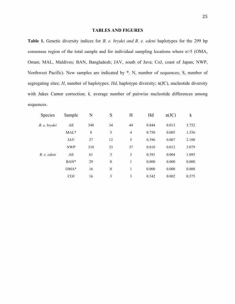
Table 1. Genetic diversity indices for B. e. brydei and B. e. edeni haplotypes for the 299 bp

consensus region of the total sample and for individual sampling locations where n>5 (OMA,

Oman; MAL, Maldives; BAN, Bangladesh; JAV, south of Java; CoJ, coast of Japan; NWP,

Northwest Pacific). New samples are indicated by *. N, number of sequences; S, number of

segregating sites; H, number of haplotypes; Hd, haplotype diversity; π(JC), nucleotide diversity

with Jukes Cantor correction; k, average number of pairwise nucleotide differences among

sequences.

Species Sample N S H Hd π(JC) k

B. e. brydei All 348 34 44 0.844 0.013 3.752

MAL* 8 3 4 0.750 0.005 1.536

JAV 27 12 5 0.396 0.007 2.108

NWP 310 33 37 0.810 0.012 3.079

B. e. edeni All 61 3 3 0.391 0.004 1.095

BAN* 29 0 1 0.000 0.000 0.000

OMA* 16 0 1 0.000 0.000 0.000

COJ 16 3 3 0.342 0.002 0.575

  26  

 

Table 2. Pairwise FST and ϕST values for B. e. brydei and B. e. edeni for each sampling location

where n>5 (OMA, Oman; MAL, Maldives; BAN, Bangladesh; JAV, south of Java; CoJ, coast of

Japan; NWP, Northwest Pacific). FST values are shown above the diagonal, ϕST results are shown

below the diagonal. Significance values are indicated as ***, p<0.001 assessed using 1000

permutations at the 0.05 significance level in Arlequin ver 3.5 (Excoffier & Lischer 2010).

B. e. brydei MAL JAV NWP

MAL - 0.479***

0.211***

JAV 0.561*** - 0.334***

NWP 0.564*** 0.452*** -

B. e. edeni BAN OMA COJ

BAN - 0.000

0.866***

OMA 0.000 - 0.818***

COJ 0.923*** 0.893*** -

  27  

 

Fig. 1. Schematic illustrating the extent of the study region and approximate sampling locations

shaded in gray: OMA, Oman; MAL, Maldives; BAN, Bangladesh; JAV, south of Java CoJ, coast

of Japan; NWP, Northwest Pacific. New samples were collected from Oman, the Maldives, and

Bangladesh. Existing samples had been previously collected from south of Java, coast of Japan,

and Northwest Pacific (Kanda et al. 2007; Yoshida & Kato 1999). The eastern portion of the

schematic (JAV, COJ, NWP) was adapted from Kanda et al. (2007) and Yoshida & Kato (1999).

  28  

 

  29  

 

Fig. 2. Phylogenetic reconstruction of mtDNA control region haplotypes of Bryde’s whales

sampled from across the Western and Central Indo-Pacific, and Northwest Pacific Ocean. The

bootstrap 50% majority-rule consensus parsimony tree is shown with bootstrap values supporting

phylogenetic differentiation of haplotypes identified as B. e. brydei and B. e. edeni. The 9

characteristic attributes (CAs) used to identify the taxa are shown to the immediate right of the

tree. Nucleotide positions correspond to the B. e. brydei mitochondrial genome positions 15477-

16410 (ACCN: AB201259). Positions 15609, 15616, and 15769 diagnose the B. e. brydei

subspecies. Positions 15592, 15681, 15722, and 15726 diagnose the B. e. edeni subspecies. *

represents conserved nucleotides in relation to the outgroup, B. physalus. H, haplotype number;

N, sample size; and sampling location (i.e. OMA, Oman; MAL, Maldives; BAN, Bangladesh;

JAV, south of Java; CoJ, coast of Japan; NWP, Northwest Pacific), are shown adjacent to the

termini in the table to the far right. See Table S2 for details of haplotype accession numbers.

  30  

 

SUPPORTING INFORMATION

Table S1. Details of new Bryde’s whale samples. Sample ID corresponds to original field

sample code managed by the American Museum of Natural History. Taxon was designated as a

result of the phylogenetic analysis carried out in the current study. Sampling sites are as follows:

BAN, Swatch-of-No-Ground, Bangladesh; BAN (CB), Cox’s Bazaar, Bangladesh; MAL,

Maldives; OMA, Oman. Latitude and Longitude are in decimal degrees; N, North; E, East. Body

length is given in meters or, if this information wasn’t available, as life history stage. Sex is

coded as: M, male; F, female. ND, no data.

Sample ID Taxon Sampling Site

Latitude (N)

Longitude (E)

Body Length

Sex Sampling Method

Sample Type

163808 B. e. brydei BAN (CB) 22.28961 91.75449 Adult M Necropsy Muscle 163866 B. e. edeni BAN 21.31197 89.48166 >12m M Biopsy dart Skin 163867 B. e. edeni BAN 21.31197 89.48166 >12m F Biopsy dart Skin 163882 B. e. edeni BAN 21.28040 89.38474 >12m F Biopsy dart Skin 163883 B. e. edeni BAN 21.28040 89.38474 >12m F Biopsy dart Skin 163884 B. e. edeni BAN 21.31197 89.48166 >12m F Biopsy dart Skin 163886 B. e. edeni BAN 21.31197 89.48166 >12m M Biopsy dart Skin 163889 B. e. edeni BAN 21.31197 89.48166 >12m F Biopsy dart Skin 163890 B. e. edeni BAN 21.31197 89.48166 >12m ND Biopsy dart Skin 163891 B. e. edeni BAN 21.31197 89.48166 >12m M Biopsy dart Skin 163892 B. e. edeni BAN 21.26533 89.50288 >12m M Biopsy dart Skin 163898 B. e. edeni BAN 21.31197 89.48166 >12m F Biopsy dart Skin 163904 B. e. edeni BAN 21.31197 89.48166 >12m M Biopsy dart Skin 163906 B. e. edeni BAN 21.31197 89.48166 >12m F Biopsy dart Skin 163907 B. e. edeni BAN 21.28040 89.38474 >12m F Biopsy dart Skin 163908 B. e. edeni BAN 21.30150 89.39712 >12m F Biopsy dart Skin 163910 B. e. edeni BAN 21.40125 89.55322 >12m F Biopsy dart Skin 163914 B. e. edeni BAN 21.31197 89.48166 >12m F Biopsy dart Skin 163916 B. e. edeni BAN 21.31197 89.48166 >12m M Biopsy dart Skin 163917 B. e. edeni BAN 21.27628 89.56635 >12m F Biopsy dart Skin 163926 B. e. edeni BAN 21.40125 89.55322 >12m F Biopsy dart Skin 163927 B. e. edeni BAN 21.32390 89.45966 >12m M Biopsy dart Skin 163932 B. e. edeni BAN 21.27213 89.41471 >12m ND Biopsy dart Skin 163935 B. e. edeni BAN 21.26533 89.50288 >12m ND Biopsy dart Skin 163938 B. e. edeni BAN 21.40860 89.55837 >12m M Biopsy dart Skin 163939 B. e. edeni BAN 21.33016 89.48374 >12m ND Biopsy dart Skin 163940 B. e. edeni BAN 21.31197 89.48166 >12m M Biopsy dart Skin 163942 B. e. edeni BAN 21.31197 89.48166 >12m F Biopsy dart Skin 163954 B. e. edeni BAN 21.65188 89.23253 >12m ND Necropsy Skin 163957 B. e. edeni BAN 21.27213 89.41471 >12m ND Biopsy dart Skin 980409-01 B. e. brydei MAL 7.18333 72.56861 12-13m ND Biopsy dart Skin 980419-01 B. e. brydei MAL 3.35000 73.70222 12-14m ND Biopsy dart Skin 980419-02 B. e. brydei MAL 3.25111 73.71916 10-12m ND Biopsy dart Skin

  31  

 

980419-03 B. e. brydei MAL 3.25000 73.71666 12-14m ND Biopsy dart Skin 980420-01 B. e. brydei MAL 3.25000 73.58333 12-14m ND Biopsy dart Skin 980420-02 B. e. brydei MAL 3.25000 73.58333 12-14m ND Biopsy dart Skin 980420-03 B. e. brydei MAL 3.25000 73.58333 12-14m ND Biopsy dart Skin 980420-04 B. e. brydei MAL 3.25000 73.58333 12-14m ND Biopsy dart Skin 19-03-01-01 B. e. brydei OMA 16.94411 54.01592 13m ND Necropsy Skin,

Muscle 21-03-02-01 B. e. brydei OMA 20.40445 58.53280 ND ND Necropsy Muscle 06-03-01-01 B. e. edeni OMA 21.05246 58.84517 13m ND Necropsy Muscle 11-03-01-01 B. e. edeni OMA 23.61126 58.31159 12m ND Necropsy ND 12-06-01-05 B. e. edeni OMA 19.52770 57.69620 ND ND Necropsy Tissue 12-10-00-02 B. e. edeni OMA 20.52110 58.69620 ND ND Necropsy Tissue 14-03-01-02 B. e. edeni OMA 20.38003 58.32083 13.5m ND Necropsy Skin 15-03-01-01 B. e. edeni OMA 23.55497 58.71840 11m ND Necropsy ND 17-10-00-02 B. e. edeni OMA ND ND ND ND Direct Skin

(slough) 28-02-01-01 B. e. edeni OMA 23.63945 58.49132 ND ND Necropsy Skin 27-10-01-05 B. e. edeni OMA ND ND ND ND Necropsy Skin,

Tissue 30-11-00-06 B. e. edeni OMA 20.43272 57.99270 ND ND Necropsy Tissue 31-10-02-01 B. e. edeni OMA 19.43962 57.98106 Juvenile ND Necropsy Skin Bah001 B. e. edeni OMA 20.37000 58.26733 Juvenile? ND Necropsy Tissue Bah003 B. e. edeni OMA 20.35033 58.43700 Adult ND Necropsy Tissue Bah006 B. e. edeni OMA 20.33667 58.41667 12m ND Necropsy Muscle Mas002 B. e. edeni OMA 20.43467 58.71217 14.1m ND Necropsy Skin,

Tissue Mas003 B. e. edeni OMA 20.17367 58.65900 ND ND Necropsy Tissue

  32  

 

Table S2. Table of corresponding accession (ACCN) numbers for haplotypes H01-H49 included

in the study. From the 299 bp mitochondrial consensus sequence (bp position 15545-15843 in

the mtDNA genome of B. e. edeni [ACCN: AB201258]), H01-H45 were identified as B. e.

brydei, and H46-H48 were identified as B. e. edeni. The B. e. edeni haplotype H49 was identified

from the 407 bp consensus sequence (bp position 15500-15906 in the mtDNA genome of B. e.

edeni [ACCN: AB201258]). The total number of individuals (N) for each haplotype is shown

and, when two accession numbers are listed, the number of individuals represented by each is

indicated in parentheses. * indicates the five new haplotypes described by the current study. The

remaining forty-four haplotypes have been previously described and published (Kanda et al.

2007; Yoshida & Kato 1999). For details of haplotype frequencies across sampling locations, see

Fig. 2 of the main article.

B. e. brydei Haplotype N ACCN 1 ACCN 2 H01 5 JX090150* H02 2 EF068036 H03 1 EF068044 H04 2 EF068046 H05 4 EF068061 H06 1 JX090151* H07 1 KC261305* H08 9 EF068013 H09 2 EF068019 H10 4 EF068014 H11 11 EF068030 H12 1 EF068063 H13 5 EF068015 H14 3 EF068032 H15 28 EF068016 (26) AF146385 (2) H16 1 EF068017 H17 6 EF068020 (5) AF146384 (1) H18 3 EF068045 H19 3 EF068040 H20 1 EF068025 H21 7 EF068031 H22 3 EF068033 H23 4 EF068038 H24 5 EF068041 H25 1 AF146386 H26 6 EF068037

  33  

 

H27 1 EF068039 H28 34 EF068018 (33) AF146382 (1) H29 1 EF068021 H30 126 EF068022 (120) AF146381 (6)

H31 5 EF068023 (4) AF146383 (1)

H32 1 EF068043 H33 11 EF068024 H34 7 EF068027 H35 5 EF068028 H36 1 EF068029 H37 4 EF068034 H38 2 EF068035 H39 3 EF068048 (2) AF146388 (1) H40 1 EF068047 H41 22 EF068060 (19) AF146387 (3) H42 1 EF068062 H43 1 EF068026 H44 2 JX090152* H45 1 EF068042 B. e. edeni Haplotype N ACCN 1 ACCN 2 H46 46 AF146379 H47 13 AF146380 H48 2 AF146378 H49 (407 bp consensus sequence)

5 KC561138*

  34  

 

Fig. S1. Haplotype network of B. e. brydei (N=348) and B. e. edeni (N=61) mtDNA control

region sequences created using a median-joining algorithm (Bandelt et al. 1999) with maximum

parsimony post-processing implemented in NETWORK ver 4.6.0.0 (Fluxus Technology Ltd.

1999-2010) with ε=0 and all variable sites weighted equally. Haplotypes are labelled

sequentially H01-H48: H01-H45 represent B. e. brydei clustered on the left side of the network;

H46-H48 represent B. e. edeni on the right side of the network. Nodes are shaded according to

sampling location (see inset: OMA, Oman; MAL, Maldives; BAN, Bangladesh; JAV, south of

Java; CoJ, coast of Japan; NWP, Northwest Pacific). Size of the node corresponds to the

frequency of that haplotype among sampled individuals. Internal nodes represent reconstructed

median haplotypes. Notches represent nucleotide differences between haplotypes.

  35  

 

CHAPTER TWO

Multiple processes drive genetic structure of humpback whale (Megaptera novaeangliae) populations across spatial scales FRANCINE KERSHAW, INÊS CARVALHO, CRISTINA POMILLA, PETER B. BEST, KEN P. FINDLAY, SALVATORE CERCHIO, TIM COLLINS, MARCIA H. ENGEL, GIANNA MINTON, PETER ERSTS, JACO BARENDSE, DEON P. G. H. KOTZE, YVETTE RAZAFINDRAKOTO, SOLANGE NGOUESSONO, MIKE MEŸER, MEREDITH THORTON, and HOWARD C. ROSENBAUM.

  36  

 

ABSTRACT

Elucidating patterns of population structure for species with complex life histories, as well as

disentangling the processes driving such patterns, remains a significant challenge that requires an

integrative analytical approach. Humpback whale (Megaptera novaeangliae) populations display

complex genetic structures that have not been fully resolved at all spatial scales. We generated a

data set of nine microsatellite loci representing the most robust sampling of “breeding stocks”

across the South Atlantic and western Indian Oceans in order to assess genetic diversity, test for

genetic differentiation between putative populations, and simulate the number of genetic clusters

without a priori population information. We estimated rates of gene flow using maximum

likelihood and Bayesian approaches. Our results reveal that patterns of humpback whale

population structure vary at different spatial scales. At the ocean basin scale, structure is

governed chiefly by geographic distance, female fidelity to breeding areas and male-biased gene

flow. At scales within ocean basins, signals of genetic structure exist but are often less evident

due to high levels of gene flow for both males and females. Our findings suggest these complex

population patterns may not be fully or currently accounted for in management designations,

which may have ramifications for assessments of the current status and continued protections for

populations still undergoing recovery from commercial whaling.

  37  

 

INTRODUCTION

The field of molecular ecology has contributed significant insights into patterns of population

structure for a broad range of terrestrial and marine species (e.g. Wang et al. 2009; Mendez et al.

2010; Kormann et al. 2012). However, understanding patterns of population structure for species

with complex life histories, and the processes driving those patterns, remains a significant

challenge. Genetic population structure (i.e. the spatial and temporal distribution of allele

frequencies) may be influenced by a variety of interacting processes, including behavioral and

ecological responses (Andrews et al. 2010; Piou & Prévost, 2012), environmental conditions

(Kormann et al. 2012), and microevolutionary factors such as genetic drift and gene flow

(Gaggiotti et al. 2009); all of which operate against a background of phylogeographic history

(Muscarella et al. 2011). Disentangling the processes influencing population patterns therefore

requires an integrative analytical approach (Gaggiotti et al. 2009).

The genetic architecture of migratory species is often complex due to the evolution of

behaviors related to reliance on ephemeral patches of breeding and foraging habitat, such as

group cohesion and hysteresis (or “memory”) effects (Guttal & Couzin 2010). At regional scales,

population-level fidelity to breeding and feeding areas may be a primary driver of genetic

structure in these species (Guttal & Couzin 2010); however, at local scales there may be a more

nuanced interplay of processes. For instance, genetic divergence between colonies of Cook’s

petrel (Pterodroma cookii) was linked to segregation of different populations during the non-

breeding season due to habitat specialization (Rayner et al. 2011), and spinner dolphins (Stenella

longirostris) exhibit two alternative social strategies associated with different levels of gene flow

between social groups (Andrews et al. 2010). Synthesizing findings from multiple molecular

markers is of great utility in shedding light on how patterns of population structure may be

  38  

 

influenced by processes operating across different spatial and temporal scales (Amaral et al.

2012a,b).

One of the best-studied migratory marine species is the humpback whale (Megaptera

novaeangliae), which migrates annually from low-latitude breeding areas to high-latitude

feeding areas (Gambell, 1976). Humpback whale genetic structure at the ocean basin scale is

driven by a combination of maternal fidelity to feeding areas and natal philopatry to breeding

areas (Baker et al. 1998, 2013). Patterns of migratory fidelity result from the close dependency

of a first-year calf on its mother during the first complete annual migration, and thus vertical

cultural transmission of migratory route and destinations (Baker et al. 1987; Alter et al. 2009;

Valenzuela et al. 2009; Baker et al. 2013; Barendse et al. 2013). This mechanism of information

transfer from mother to calf contrasts with natal philopatry in the majority of other migratory

marine species, such as sea turtles and sharks, which is likely driven by environmental cues or

genetic inheritance (Shamblin et al. 2012; Baker et al. 2013; Feldheim et al. 2014). However, as

observed for other migratory baleen whale species in both hemispheres (Alter et al. 2012;

Kershaw et al. 2013), genetic studies of humpback whales continue to reveal more complex

structure at finer spatial scales than accounted for in current stock designations (e.g. Rosenbaum

et al. 2009; Schmitt et al. 2013; Carvalho et al. 2014), indicating that other behavioral

mechanisms may be driving humpback whale genetic structure at these scales.

In the South Atlantic and western Indian Ocean, four demographically discrete humpback

whale “breeding stocks” (BS) are managed by the International Whaling Commission (IWC) in

the southwest Atlantic, southeast Atlantic, southwest Indian Ocean, and northern Indian Ocean

(BSA, BSB, BSC, and ASHW, respectively; Fig. 1). BSA shows relatively little diversity or

genetic substructure (Cypriano-Souza et al. 2010), however, direct movements and song

  39  

 

similarity between BSA and BSB indicate some degree of broad-scale connectivity (Darling &

Sousa-Lima 2005; Stevick et al. 2011). BSB is partitioned into two substocks; BSB1 breeds in

the Gulf of Guinea and BSB2 represents a genetically distinctive group that feeds and migrates

off the coast of west South Africa (Rosenbaum et al. 2009; Carvalho et al. 2014). Differences in

levels of migrant exchange and records of individual movements between the four substocks of

BSC (BSC1-C4) suggest genetic structure may be more complex than currently considered

(Rosenbaum et al. 2009; Ersts et al. 2011; Fossett et al. 2014). The Arabian Sea humpback

whale (ASHW) population is the only known non-migratory population globally and is known to

be small (approximately 80-200 individuals) and extremely isolated (Minton et al. 2011; Pomilla

& Amaral et al. 2014).

A complete understanding of patterns of humpback whale population structure using

multiple molecular markers, and the potential processes underlying those patterns, has therefore

not yet been achieved at multiple spatial scales. To help address these ecological and

evolutionary questions, we present an analysis of an extensive microsatellite data set to further

elucidate population genetic patterns across the south Atlantic and southwestern and northern

Indian Ocean. To better understand the potential processes underlying population patterns at

different scales, we partition our analyses to undertake a detailed investigation of the influence of

sex on dispersal and site fidelity.

MATERIALS AND METHODS

Laboratory protocols

Sample collection, DNA Extraction and Sex Determination

  40  

 

A total of 3,575 humpback whale genetic samples originating from multi-year collections across

ten sampling locations were used in this study (Table 1, Fig. 1). Skin tissues were mostly

obtained using biopsy darts (Lambertson 1987), but also from sloughed skin and stranded

specimens. Samples were preserved in 95% Ethanol or salt saturated 20% Dimethyl Sulfoxide

solution (DMSO) and later stored at –20ºC until processed. Total genomic DNA was extracted

from the tissue samples using proteinase K digestion, followed by a standard Phenol/Chloroform

extraction method (Sambrook et al. 1989) or using QIAamp Tissue Kit (QiaGen) following

manufacturer’s protocol. Sex determination was either carried out by Polymerase Chain Reaction

(PCR) amplifications followed by TaqI digestion of the ZFX/ZFY region of the sex

chromosomes (Palsbøll et al. 1992), or using multiplex PCR amplification of the ZFX/ZFY sex

linked gene (Berube & Palsbøll 1996).

Microsatellite molecular analyses

Samples were genotyped at 10 microsatellite loci proven to be polymorphic for this species:

GATA028, GATA053, GATA417 (Palsbøll et al. 1997), 199/200, 417/418, 464/465 (Schlotterer

et al. 1991), EV1Pm, EV37Mn, EV94Mn, EV96Mn (Valsecchi & Amos 1996). The 5’-end of

the forward primer from each locus was labeled with a fluorescent tag (HEX, 6-FAM, and TET,

Qiagen-Operon; NED, Applied Biosystems, Inc). PCRs were carried out in a 20µl volume with

the following conditions: 50mM KCl, 10mM Tris-HCl pH8.8, 2.5-3.5mM MgCl2, 200µM of

each dNTP, 0.4µM of each primer, and 0.025 U/µl Taq Gold polymerase (Perkin-Elmer).

Amplifications were completed in an Eppendorf Gradient Mastercycler, after optimization of

published annealing temperatures and profiles. PCR products were loaded with the addition of an

internal standard ladder (GS600 LIZ, ABI) on a 3730xl DNA Analyzer (Applied Biosystems,

  41  

 

Inc). Microsatellite alleles were identified by their sizes in base pairs using the software

GENEMAPPER v4.0 software (ABI). Specific guidelines were used during laboratory work and

scoring procedures to reduce genotyping errors (Supporting Information).

Data analysis

Diversity estimates

Genetic diversity was measured as the mean number of alleles per locus (K), observed

heterozygosity (Ho), and expected heterozygosity (HE) under Hardy-Weinberg assumptions (Nei

1987) using the program Cervus v3.0 (Kalinowski et al. 2007). Departure of loci from Hardy-

Weinberg (HW) assumptions was tested using Cervus and genotypic disequilibrium (GD)

between pairs of loci was assessed using FSTAT v1.2 (Goudet 1995). Significance levels

(p=0.05) for departure from HW and GD were corrected for multiple comparisons with

Bonferroni correction (Rice 1998).

Analysis of population structure

To test for spatial structure, samples were grouped into seven putative populations,

corresponding to the breeding stocks and substocks delineated by the International Whaling

Commission (IWC) (Table 1, Fig. 1). To explore the presence of sex-biased dispersal, we

partitioned the data set into male and female subsamples and conducted the analyses described

below on all three data partitions.

Pairwise genetic differentiation was estimated by counting the number of different alleles

between two genotypes, the equivalent of estimating weighted FST over all loci (Weir &

Cockerham 1984), and by counting the sum of the square number of repeat differences between

  42  

 

two haplotypes, the equivalent of estimating RST (Slatkin 1995). Estimations were made from

1,000 permutations at the 0.05 significance level using Arlequin v3.5 (Excoffier & Lischer

2010). The statistic Jost’s D (Jost 2008), was estimated using the DEMEtics package (Gerlach et

al. 2010) in R. Jost’s D has been shown to produce a more accurate measure of differentiation

when using highly polymorphic microsatellite loci (Jost 2008). An analysis of molecular

variance (AMOVA) (Excoffier et al. 1992) was conducted in Arlequin v 3.5 to assess

hierarchical population structure. F- and R-statistics were computed at three levels that

considered differences i) among breeding stocks, ii) among substocks within breeding stocks,

and iii) within substocks. Estimations were made from 1,000 permutations at the 0.05

significance level.

To infer the number of genetic clusters in our data set without a priori designation of

populations, we analyzed individual multilocus genotypes using the program STRUCTURE

v2.3.3 (Pritchard et al. 2000), via the University of Oslo Bioportal (Kumar et al. 2009). We

performed 5 independent iterations of K=2–10 for 5,000,000 Markov Chain Monte Carlo

(MCMC) generations with a 500,000 burn-in period, assuming correlated allele frequencies

(gamma distribution with mean 0.01 and standard deviation 0.05). Separate runs were performed

with and without admixture and a sample location prior (LOCPRIOR). A two-cluster scenario

was chosen as the minimum number because when population structure is expected to be low the

scenario K=1 may be disproportionately favored, reducing the likelihood of all other scenarios to

zero and resulting in a loss of overall resolution (Pomilla 2005). We selected the most probable

value of K based on the average maximum estimated log-likelihood of P(X|K) and the ΔK

method (Evanno et al. 2005), where optimum K has the highest rate of change in log probability

in the data between successive K values (i.e. ΔK). All calculations were conducted using

  43  

 

STRUCTURE Harvester (Earl & VonHolt 2012). Clusters were aligned using CLUMPP v 1.1.2

(Jakobsson & Rosenberg 2007) and graphically displayed using the program DISTRUCT v 1.1

(Rosenberg 2004).

To validate the results of the genetic distance and Bayesian clustering analyses, we

performed a discriminant analysis of principle components (DAPC) (Jombart et al. 2010) on

individual allele frequencies using the adegenet package in R (Jombart 2008; Supporting

Information). DAPC has been shown to recover complex patterns of population subdivision and

has proved robust to deviations from HW equilibrium and GD because it does not rely on an

underlying genetic model (Jombart et al. 2010). To assess the genetic distinctiveness of each

breeding stock, the proportion of correct reassignment of each individual to its putative

population was computed (Supporting Information).

Measures of migration rates and gene flow

We estimated relative effective population size (θ) and levels of historical gene flow (M=m/µ),

where m represents the immigration rate and µ the mutation rate, using the maximum likelihood

algorithm implemented in MIGRATE v3.5.1 (Beerli & Felsenstein 2001). To address the issue of

unequal sample sizes between locations, we chose to sub-sample our data set prior to analysis

(Beerli 1998; Supporting Information). We used Brownian motion approximation to obtain

initial parameter values and implemented a complete pairwise migration matrix model of gene

flow between all breeding stocks. The final Markov chain scheme consisted of: 20 short chain

searches (50,000 trees sampled, 500 trees recorded) followed by 3 long chain searches

(5,000,000 trees sampled, 50,000 trees recorded) after a burn-in period of 10,000 genealogies.

  44  

 

The final long chain searches were averaged over ten independent runs and across subsamples.

To aid visualization, results were transformed: NemT = ((1-(1/Nem)2)*100.

We estimated the magnitude and direction of contemporary gene flow among populations

using BayesAss v 3.0 (Wilson & Rannala 2003). To address inconsistencies in the results from

initial runs, we again elected to sub-sample our data set (Supporting Information). Apart from the

mixing parameters, all other options were left at their default settings (Supporting Information).

The final Markov chain scheme comprised 50,000,000 iterations including a 2,500,000 burn-in

period, and a sampling rate of 100. Results were averaged over the five independent runs, and

across both random subsamples, if convergence was achieved.

RESULTS

Sample description

The 3,575 genetic samples analyzed were determined to represent 3,188 different whales

(hereafter, “total sample”; Table 1). Average probability of identity (PID) for the total sample was

small enough to exclude duplicate individuals with high confidence (PID = 1.95x10-12; PID(sibs) =

9.2x10-5; reciprocal of sample size = 2.5x10-4). Sex was determined for 3,046 individuals, 1,978

males and 1,067 females, resulting in an overall proportion of 1.8:1 males to females (Table 1).

Proportionally greater numbers of males were sampled within most breeding stocks, likely due to

a sampling bias resulting from breeding behavior differences between the sexes (Smith et al.

1999). Conversely, there were almost equal numbers of males and females sampled within

BSB2, and a strong female bias in BSC2, with more than three times the number of females

sampled than males (Table 1).

  45  

 

Genetic Diversity

All ten microsatellites were highly polymorphic, ranging from 4 alleles per locus (EV1Pm) to 28

(GATA417). No significant differences were found between the observed heterozygosity (Ho)

and the expected heterozygosity (He) under Hardy-Weinberg assumptions. Two loci, GATA028

and GATA053, were insignificant GD (p<0.01). The least polymorphic locus, GATA053, was

removed from subsequent analyses (Weir 1990). Values of observed and expected

heterozygosity were relatively high across all breeding stocks (Ho=0.702-0.742; He=0.678-0.738)

and the mean number of alleles per locus ranged from 6.44 (ASHW) to 12.89 (BSB1), although

Oman was an outlier with 6.44 while the Southern Hemisphere stocks ranged from 10.11 (BSA)

to 12.89 (BSB1; Table 1). Diversity estimates for BSB2 (n=204, k=11.33) and BSC1 (n=203,

k=12.00) were disproportionately high relative to sample size.

Population structure

The AMOVA showed that genetic variance was best explained within the substock level for all

sample partitions (for total, males, and females, FST=0.003, p<0.001; Table 2). Significant

variation was also observed for the total sample among substocks within breeding stocks

(FST=0.001, p<0.01). Significant variation among breeding stocks (i.e. the highest level of

organization) was found only for females (FST=0.003, p<0.003).

Pairwise FST estimates ranged from 0 to 0.065, RST from 0 to 0.088, and Jost’s D from 0

to 0.181 (Table S1). ASHW proved the most highly differentiated across all fixation indices and

partitions and BSA showed high genetic differentiation from other Southern Hemisphere stocks

for FST; however, results for BSA were more variable for Jost’s D (Table 3). BSB1 also showed

strong differentiation from all other breeding stocks for FST in the total sample, a result generally

  46  

 

supported by Jost’s D; however, this relationship is less pronounced when segregated by sex

(Table 3). The relationships between BSB2 and the substocks of BSC are less clear. BSB2 is

significantly differentiated from BSC1 for FST, and Jost’s D suggests this is driven by the female

sample (Table 3). For males, BSB2 was significantly differentiated from BSC2 and BSC3 but

only for FST (Table 3). Within BSC, BSC1 and BSC3 showed significant differentiation for the

total sample, which appears to be driven by females. All other comparisons between BSB2 and

BSC, and within BSC, were not significant for any indices (Table 3; Table S1).

Genetic structure based on individual allele frequencies without a priori designation of

populations was only detected by STRUCTURE when a location prior was used with correlated

allele frequencies and no admixture. The ln P(K) and ΔK values did not clearly discriminate

whether the optimal number of clusters was K=3 or K=4 (Fig. S1). However, the individual

assignment plots clearly show K=3 (Fig. 2) as the most likely for all data partitions (see Fig. S2

for K=4 plots). The clusters primarily correspond to the South Atlantic (BSA and BSB1),

western Indian Ocean (BSC), and the northern Indian Ocean (ASHW; Fig. 2a-c). BSB2 appears

more genetically similar to BSC than to BSB1 for all data partitions. BSA does not appear

substantially different in composition from BSB1 for the total sample or for males; however, it

does appear to be less admixed for females. The assignment plots also show evidence of

population substructure within BSC when sampling location is considered (Fig. 2). The males

sampled from southwest Madagascar, for example, appear to be highly differentiated from those

sampled in northeast Madagascar (Fig. 2). Attempts to identify the number of genetic clusters

using the DAPC failed.

The first two principle components of the DAPC analysis explained 94.18% of the

variance in allele frequencies for the total sample (118 PCs retained), 68.61% for the male

  47  

 

sample (115 PCs retained), and only 29.98% for the female sample (43 PCs retained, Fig. 3). For

the total sample, the first principle component shows separation between breeding stocks that

reflects their longitudinal distribution, at least for BSA, BSB1, and ASHW; the remaining

breeding stocks show a significant degree of overlap (Fig. 3a). The second principle component

clearly shows the differentiation of ASHW. The longitudinal gradient is not clear for the male

sample (Fig. 3b), however BSB2 also shows some separation on PC2 in addition to ASHW. The

strongest differentiation of ASHW is observed on PC1 for females (Fig. 3c), whereas PC2

describes the longitudinal separation of BSA and BSB1.

The proportion of individuals correctly assigned to their original putative breeding stock

by the DAPC was highest for BSB1 (65-67%), BSC3 (54-68%), driven primarily by the much

larger sample from northeast Madagascar, and ASHW (65-74%; Fig. 3d-f). Despite its

geographic distance from the other breeding stocks, BSA showed relatively low reassignment

success (20-30%). Reassignment to BSB2 (2-9%), BSC1 (3-7%), and BSC2 (5-35%) performed

particularly poorly. Individuals from the breeding stocks and substocks with the smaller sample

sizes were primarily assigned to the much larger BSB1 and BSC3 samples regardless of

sampling locality (Fig. S3).

Gene flow estimation

Historical gene flow (Nem) was estimated to occur to some degree between all pairwise breeding

stock comparisons with little bias in directionality of movements (Fig. 4a-c). For the total

sample, migration estimates ranged from NemT=1.553 (BSB1 to ASHW) to NemT=22.345 (BSC2

to BSC3, Fig. 4a). The highest estimates occurred from BSB2 to BSB1 and BSC, and also within

BSC. Estimates for ASHW were the lowest of all comparisons; however, some estimates

  48  

 

between ASHW and BSC remained NemT>10. BSA showed relatively high exchange for all

comparisons apart from ASHW. For males, estimates ranged from NemT=0.391 (BSC2 to

ASHW) to NemT=23.341 (BSC3 to BSC1, Fig. 4b) and approximated the same pattern as the

total sample; however, a stronger westward bias was evident for some comparisons. For females,

estimates ranged from NemT=0.148 (BSA to ASHW) to NemT=24.618 (BSC1 to BSC2, Fig. 4c)

with high rates of multidirectional exchange (NemT≈20) estimated between BSB and BSC (Fig.

4b-c). Notably, westward exchange for females from BSC3 to BSC2 was more than three times

that of males (female NemT=27.565; male NemT=7.669). Overall, females showed less exchange

between BSA and the other breeding stocks than males (Fig. 4c).

Levels of contemporary gene flow (proportion of migrants, M) estimated using BayesAss

were less informative as many of the pairwise comparisons did not achieve convergence: ~31%

for the total sample, ~33% for males, and ~40% for females (Fig. S4a-c). For the total sample, M

ranged from M=2.710-3 (BSB2 to BSC2) to M=29.710-3 (BSB2 to BSB1, Fig. S4a). Comparisons

of BSA with all other breeding stocks indicate an eastward bias in migration. Estimates for males

were generally higher than females (Fig. S4b-c) with directional gene flow being more evident,

notably from BSC2 to BSC3 (M=13510-3). Estimates for females support a strong eastward bias

from BSA to the other breeding stocks, particularly for BSA to BSB1, with an eastward estimate

~58 times that of the westward (Fig. S4c).

DISCUSSION

Hierarchical assessment of population structure influences

This first examination of the diversity and differentiation of nine microsatellite loci for more than

3,000 individual humpback whales from across the South Atlantic and western Indian Ocean

suggests that a hierarchy of processes is likely to be driving patterns of genetic population

  49  

 

structure at different spatial scales. Such a hierarchy reflects the interplay between

phylogeographic and ecological processes evident in other behaviorally complex mammals

(Wolf et al. 2007; Vanderwaal et al. 2014). In general, our findings support the current model of

maternal fidelity to feeding areas and natal philopatry to breeding areas as the primary driver of

population genetic structure (Palsbøll et al. 1995; Baker et al. 1998, 2013). Previous

examinations of the distribution of humpback whale mtDNA haplotypes at the sub-regional scale

(i.e. BSA-C, ASHW) indicated strong differentiation between humpback whale breeding stocks

for females and less so for males, supporting a model of maternally-directed philopatry to

breeding areas, due to culturally transmitted hysteresis (or “memory”) of specific locations,

combined with male-biased gene flow (Palsbøll et al. 1995; Rosenbaum et al. 2009; Baker et al.

1998, 2013). These patterns are similar to those observed for the southern right whale

(Eubalaena australis; Carroll et al. 2011), where combined genetic and isotope analyses indicate

site-fidelity to feeding areas is culturally transmitted along matrilineal lines, providing a

mechanism for maintaining genetic population structure (Valenzuela et al. 2009; Vighi et al.

2014).

Despite the overall congruence of our data, we find it difficult to entirely generalize this

model either within or across all spatial scales. At regional scales across ocean basins, processes

of isolation by distance (Wright 1943) and phylogeographic history appear to be the primary

drivers of genetic structure. Breeding stocks showed some differentiation along the longitudinal

axis consistent with a model of isolation by distance and previous studies suggesting the long-

term isolation of ASHW (Minton et al. 2011; Pomilla & Amaral et al. 2014). Both BSA and

BSB1 appear distinct from BSB2 and the substocks of BSC, and the ASHW population is clearly

isolated (Fig. 3). Pairwise comparisons of genetic differentiation for nine nuclear introns also

  50  

 

revealed regional population structure between Brazil, Gabon, and Madagascar (Ruegg et al.

2013). However, our data indicate that even at broad spatial scales there may be additional

factors influencing genetic structure: historic and contemporary gene flow estimates for females

between BSA and BSB and BSC (Fig. 4c,f), in concert with real-time dispersal records (Stevick

et al. 2011), suggest that long-distance movements by females should be afforded more

consideration.

Transitioning to local scales (i.e. within breeding stocks) we observed additional

divergence from this model as complex patterns of isolation and connectivity appeared as the

norm, suggesting an array of interacting processes may be responsible for driving population

patterns at these scales. The large data set of genotyped individuals included in our analysis

enabled the detection of low levels of interchange for both sexes not previously quantifiable from

examination of haplotype frequencies alone (due to the inadequate power to detect low levels of

gene flow (i.e. <100 migrants per generation); Baker et al. 2013) and so provides additional

resolution to the population sub-structure previously observed within Breeding Stocks B and C

(Rosenbaum et al. 2009; Carvalho et al. 2014).

Effect of spatio-temporal variation in migratory behavior on population substructure

Genetic evidence supports the existence of two demographically discrete substocks (i.e. BSB1

and BSB2) off West Africa; however, an alternative hypothesis proposes that BSB1 and BSB2

represent two temporal ‘ends’ of a single population (BSB) widely distributed in space and time

(Van Waerebeek et al. 2013; Carvalho et al. 2014; Rosenbaum et al. 2014). In our study, we

detected significant genetic differentiation between BSB1 and BSB2 for the total sample for FST

and Jost’s D (p<0.05), however neither the male or female partitions were found to be significant

  51  

 

(Table 3). Previous analysis of mtDNA haplotype frequencies support the genetic differentiation

of BSB1 and BSB2 for females, but not for males (Rosenbaum et al. 2009), and combined

analysis of mtDNA and microsatellites provide evidence of spatial and/or temporal segregation

between the two substocks, and indicate subtle temporal population sub-structuring based on sex

(Carvalho et al. 2014). This may, at least in part, be related to different migratory groups

undertaking coastal versus oceanic routes to and from the breeding areas off Gabon (Elwen et al.

2014; Rosenbaum et al. 2014). The fact that our pairwise comparisons did not detect significant

differentiation for males and females between BSB1 and BSB2 may be a result of our sampling

scheme not accounting for these fine-scale differences in the distribution of different, and

potentially genetically distinct, groups in the region over the course of the breeding season.

The observed genetic differentiation of BSB2 may also be explained by its apparent

connectivity with BSC1 off East South Africa, as demonstrated by our findings that BSB2 is

more genetically similar to BSC than BSB1, and for males in particular (Fig. 2). Our results

demonstrate that BSB2 exhibits high genetic diversity relative to its size (Table 1), a high level

of admixture (Fig. 2), and low reassignment probabilities (Fig. 3a-c), all of which are consistent

with a migratory population comprising whales from different breeding stocks, including BSC1.

While the lack of differentiation observed between BSB2 and BSC1 may be due to retained

shared ancestral polymorphism (Rosenbaum et al. 2009), increasing evidence for contemporary

exchange between populations on the west and east coasts of Africa suggests recent inter-oceanic

migration (Pomilla & Rosenbaum 2005; Rosenbaum et al. 2009; Carvalho et al. 2014), and

genotypic matches have revealed direct connectivity between BSB2 and BSC1 and BSC3, and

between feeding areas associated with BSB and BSC in the Antarctic (IWC 2009; Amaral & Loo

et al. in review; Kershaw et al. unpublished data).

  52  

 

Migratory overlap and sex-specific differences drive genetic complexity

Substock-scale genetic patterns of structure and connectivity for Breeding Stock C appear to be

highly complex and challenging to generalize in terms of maternal and paternal influence or

directionality. Significant genetic differentiation was found between BSC1 and BSC3 for the

total sample (FST = 0.001; p<0.05), and this difference appears to be driven by the female data

set (Jost’s D = 0.001; p<0.05; Table 3). In contrast, no significant genetic differentiation was

detected between BSC1 and BSC2, or between BSC2 and BSC3 (Table 3). However, we did

detect subtle differences between these patterns for males and females. No differentiation was

detected for males between any of the BSC substocks, supporting the general model of male-

biased gene-flow between populations that would result in the erosion of signals of genetic

differentiation. However, estimates of historical gene flow showed no clear pattern in

directionality and were found to be particularly high for females, calling the general model of

maternally-driven natal philopatry to breeding areas into dispute (Fig. 4a-c; Palsbøll et al. 1995;

Baker et al. 1998, 2013). Genotypic matching results also suggest high levels of exchange

between BSC1-C3 for both females and males (Kershaw et al. unpublished data).

It is possible that the BSC substocks have diverged from one another relatively recently

or may have remained consistently ‘fluid’ (Marko & Hart 2011). This latter suggestion is

consistent with previous hypotheses regarding the presence of three migratory streams within the

southwestern Indian Ocean, one along the east coast of southern Africa (BSC1), one along the

Madagascar ridge (BSC3), and possibly a third through the central Mozambique Channel (BSC2;

Best et al. 1998). It is possible, however, that this third stream comprises wide-ranging animals

from coastal Africa and Madagascar (Best et al. 1998). Our findings of the lack of genetic

  53  

 

differentiation between BSC1 and BSC2, and BSC2 and BSC3, combined with high gene flow

estimates, support the assertion that BSC2 may represent a mixed migratory stream of wide-

ranging animals from BSC1 and BSC3. Recent photo-identification studies (Ersts et al. 2011),

satellite telemetry data (Fossette et al. 2014), and genotypic matches (Kershaw et al. unpublished

data) show that there is indeed considerable movement between BSC2 and BSC3, which are

geographically close to one another relative to distances humpback whales are capable of

travelling. In addition, long-distance movements between northeastern Madagascar (BSC3) and

coasts of Kenya and Somalia in northern BSC1 appear more frequent than previously supposed,

and may even represent a second, more northern migratory stream between BSC1 and BSC3.

Photographic recaptures also suggest relatively substantial interchange between BSC3 and BSC4

(Dulau-Drouot et al. unpublished data), but levels of genetic connectivity have yet to be

assessed. These findings call into question the delineation of substock boundaries in the

southwestern Indian Ocean (Ersts et al. 2011). A similar scenario exists for humpback

populations in the Hawaiian Archipelago and within the wintering region off the coast of Mexico

(Cerchio et al. 1998, Calambokidis et al. 2011).

Importantly, we detected additional genetic structure within BSC3 indicating that further

discrete demographic units may be present. The small sample of males (n=17) from the

southwest of Madagascar (BSC3) shows greater levels of admixture than the large number of

whales sampled in Antongil Bay to the north (Fig. 3). A number of factors apart from population

structure could be driving these observed differences in allele frequencies between sampling

locations, such as non-representative sampling from different years or disparities in sample size

(Marko & Hart 2011). So, until larger, more representative samples are available, conclusions

drawn from these results should be considered with caution. However, given our increasing

  54  

 

understanding of the behavioral complexity (e.g. alternative migration routes) of humpback

whale populations in this region and others (Cerchio et al. 1998; Ersts et al. 2011; Carvalho et al.

2014; Rosenbaum et al. 2014), further investigation into the genetic structure of the BSC

substocks appears to be warranted.

Implications for management at multiple scales

Our findings indicate an array of ecological drivers are likely responsible for the complex

patterns of genetic structure observed within breeding substocks. Further investigation and

syntheses of studies of population genetic structure, individual relatedness, environmental

conditions, and behavioral ecology will be necessary to disentangle which processes are

operating at each hierarchical spatial scale. The regional genetic structure detected by the

microsatellite analyses presented here, and previous studies of nuclear introns (Ruegg et al.

2013) and the mitochondrial control region (Rosenbaum et al. 2009), is generally consistent with

current designations of Breeding Stocks A, B, C, and ASHW, by the International Whaling

Commission. Furthermore, in light of the extreme isolation and regional distinctiveness of

ASHW, and increasing levels of anthropogenic development occurring in the Arabian Sea, our

findings support recommendations that this population be attributed international conservation

priority (Pomilla & Amaral et al. 2014).

Our results for BSB and BSC provide the most definitive evidence to date that the IWC

substocks should be treated as hypotheses only, and a precautionary approach should be taken

toward the management of whale populations in this region until the number of demographically

discrete population units is resolved (Rosenbaum et al. submitted). Efforts to accurately elucidate

discrete management units and understand their connectivity for this species are particularly

  55  

 

germane as the current listing status for the humpback whale as “endangered” under the

Endangered Species Act (ESA) is under review (Bettridge et al. 2012). Given the range of

contemporary anthropogenic impacts potentially affecting whale populations and important

breeding habitat (Rosenbaum et al. 2014), the accurate identification of demographically discrete

populations is paramount to the effective management of this species, which is still undergoing

recovery from commercial whaling.

  56  

 

TABLES AND FIGURES

Table 1. Sample location, size, and diversity indices for nine microsatellite loci across breeding

grounds, migratory corridors, and feeding grounds of humpback whales sampled in the South

Atlantic and Western Indian Ocean. STP, Sao Tome & Principe; N, sample size; M, number of

males; F, number of females; K, mean number of alleles per locus; Ho, observed heterozygosity;

He, expected heterozygosity. The sum of the number of males and females does not always

match the sample size. Duplicate samples have been removed.

Breeding Ground Breeding Stock N M F M: F Years K Ho He

(A) Southwestern Atlantic Ocean

Abrolhos, Brazil 50 30 20 1.5:1 1997-98 10.11 0.702 0.715

(B) Southeastern Atlantic Ocean

(B1) Gabon, STP, Cabinda 1395 826 421 2:1 1999-2006 12.89 0.732 0.735

(B2) West South Africa 204 95 103 1: 1.1 1990, 93, 95 11.33 0.740 0.737

2000-2009

(C) Southwestern Indian Ocean

(C1) Mozambique & East South Africa 203 112 81 1.4:1 1991 12.00 0.742 0.738

1997-2005

(C2) Mayotte & Geyser, Comoros 75 17 55 1: 3.2 1997-2003 10.44 0.723 0.735

(C3) Madagascar 1227 842 373 2.3:1 1994 12.78 0.731 0.729

1996-2006

(X) Northern Indian Ocean

Oman 34 20 14 1.4:1 2001-2002 6.44 0.706 0.678

  57  

 

Table 2. Analysis of hierarchical variance (AMOVA) results obtained using F- and R-statistics

at three levels for the total sample (n=3,188), and males (n=1,978) and females (n=1,067)

separately. Bold type indicates statistical significance at *p<0.05, **p<0.01, ***p<0.001.

Sample Source of variation % var F-statistics % var R-statistics

Total Among breeding stocks 0.24 FCT = 0.0024 0.32 RCT = 0.0032

Among substocks 0.08 FSC = 0.0008** - 0.01 RSC = -0.0001

within breeding stocks

Within substocks 99.68 FST = 0.0032*** 99.69 RST = 0.0031***

Male Among breeding stocks 0.27 FCT = 0.0027 0.42 RCT = 0.0043

Among substocks 0.01 FSC = 0.0001 - 0.12 RSC = -0.0012

within breeding stocks

Within substocks 99.72 FST = 0.0028*** 99.70 RST = 0.0030*

Female Among breeding stocks 0.31 FCT = 0.0031* 0.22 RCT = 0.0022

Among substocks 0.02 FSC = 0.0002 0.05 RSC = 0.0005

within breeding stocks

Within substocks 99.67 FST = 0.0033*** 99.73 RST = 0.0027

  58  

 

Table 3. Significance values for pairwise fixation indices obtained between humpback whale

breeding stocks and substocks for FST and Jost’s D. FST values are shown above the diagonal,

Jost’s D below the diagonal. Results are shown for the total sample (n=3,188), and males

(n=1,978) and females (n=1,067), separately. * indicates statistical significance at *p<0.05,

**p<0.01, ***p<0.001. Estimations of significance were made from 1,000 permutations at the

0.05 significance level. Shaded FST values indicate a statistically significant result for

mitochondrial DNA data, adapted from Rosenbaum et al. (2009). See Table S1 for fixation index

values and RST results.

Total A B1 B2 C1 C2 C3 X

A - ** ** *** *** *** ***

B1 ns - * *** * *** ***

B2 ** * - * ns ns ***

C1 ** ** ns - ns * ***

C2 ns ns ns ns - ns ***

C3 ** ** ns ns ns - ***

X ** ** ** ** ** ** -

Male A B1 B2 C1 C2 C3 X

A - * * * ns * ***

B1 ns - ns * ns * ***

B2 ns ns - ns * *** ***

C1 ns * ns - ns ns ***

C2 ns ns ns ns - ns ***

C3 * *** ns ns ns - ***

X *** *** *** *** *** *** -

Female A B1 B2 C1 C2 C3 X

A - ns * * * * ***

B1 ns - ns ns ns * ***

B2 * ns - ns ns ns ***

C1 * ns * - ns ns ***

C2 ns ns ns ns - ns ***

C3 ** *** ns * ns - ***

X *** *** *** *** *** *** -

  59  

 

Fig. 1. Map showing sampling locations for the humpback whale breeding stocks and substocks

analyzed in this study. The location of breeding stocks and substocks are indicated by white

shading and labeled in parentheses. Sampling locations are indicated by stars and labeled as

follows: B, Abrolhos Bank, Brazil; G, comprising samples from Iguela and Gamba, Gabon,

Cabinda region, Angola, and São Tomé & Príncipe; WZA, Cape Columbine, West South Africa;

EZA, Richard’s Bay, East South Africa; M, comprising samples from Cabo Inhaca and

Mozambique Island, Mozambique; MY, Mayotte and Geyser-Zelee, Comoros Archipelago; SM,

Tulear/Ft Dauphin, Southwest Madagascar; NM, Antongil Bay, Northeast Madagascar; O, Gulf

of Masirah and Dhofar, Oman.

  60  

 

Fig. 2. Distribution of 3 genetic clusters estimated using STRUCTURE for a) the total sample, b)

males, and c) females. Vertical lines are partitioned into colored segments showing the

proportion of each individual assigned to each K cluster. Breeding stocks are indicated above

each figure and sampling locations are below.

  61  

 

Fig. 3. Discriminant analysis of principle components (DAPC) scatterplots showing the genetic

structure between humpback whale breeding stocks for a) the total sample, b) males, and c)

females. Key describes the colors attributed to each breeding stock and substock. Eigenvalues for

each PC axis are shown (PC1, vertical; PC2, horizontal). The number of PCA axes retained in

each DAPC analyses is shown in the bottom-right inset (black bars). Bar charts show the

proportion of reassignment of each individual to its original putative breeding stock (group).

  62  

 

  63  

 

Fig. 4. Magnitude and directionality of historic gene flow between breeding stocks. The historic

estimated number of migrants per generation (NemT) exchanged between breeding stocks is

shown for a) the total sample; b) males; and c) females, as estimated using MIGRATE. Asterisks

highlight key results discussed in the main text.

  64  

 

Fig. 5. Estimated number of migrants per generation (Nem) exchanged between neighboring

breeding stocks and substocks and using MIGRATE for nuclear microsatellites (this study) and

mitochondrial DNA, adapted from Rosenbaum et al. (2009). a) Average estimates of Nem for

mtDNA for the total sample; b-d) estimates of theta and Nem (standard deviation shown in

parentheses) for microsatellites for the total sample, and male and female data partitions. Bold

arrows indicate directional bias in migration. Results were not transformed.

  65  

 

SUPPORTING INFORMATION

Procedure for checking genotype errors

First, automation was introduced whenever possible during PCR setup and manipulation of

genomic DNA or PCR products. Negative controls were run at the PCR step to control for

exogenous contamination. Two reference samples of known allele size were added to each

amplification and subsequent analyses to standardize scoring. Scoring was automated in

GENEMAPPER, and allele sizing was successively checked by hand. Samples that yielded

ambiguous allele peaks were repeated a second time. Genotyping error was checked for the

samples by re-amplifying and re-typing 15% of the total, chosen at random. In order to detect

errors in our dataset, such as identifying possible non-amplified alleles (null alleles), large allele

dropout and scoring errors due to stutter peaks we used the programs DROPOUT v1.3

(McKelvey and Schwartz 2005) and MICRO-CHECKER v.2.2.3 (Van Oosterhout et al. 2004).

Overall, 10 cases of allele dropout were detected and solved by duplicate genotyping.

Overview of Discriminant Analysis of Principle Components (DAPC) methodology

The following overview has been adapted from Jombart et al. (2010). Principle Component

Analysis (PCA) enables the identification of genetic structures in very large data sets within

negligible computational time and the absence of assumptions about the underlying population

genetics model. However, PCA does not provide group assessment and would require a priori

definition of clusters to study population structure. In contrast, Discriminant Analysis (DA) is a

multivariate method that defines a model in which genetic variation is partitioned into a between-

group and a within-group component, and which maximizes the first while minimizing the

second. This method therefore provides the best discrimination of individuals into pre-defined

  66  

 

groups. However, DA requires the number of variables (alleles) to be less than the number of

observations (individuals) and assumes uncorrelated variables.

Discriminant Analysis of Principle Components (DAPC) is a new method developed by

Jombart et al. (2010) that relies on data transformation using PCA as a prior step to DA, which

ensures that the variable submitted to the DA are perfectly uncorrelated, and that their number is

less than that of analyzed individuals. The method assigns individuals to clusters and provides a

visual assessment of between-population genetic structure. When group priors are unknown, the

method employs K-means clustering of principle components to identify groups of individuals.

The best-supported number of clusters is assessed using the Bayesian Information Criteria (BIC).

Selection of number of PC axes retained in DAPC

The number of PC axes that explain the largest amount of total genetic variability in the data set

while achieving the best discrimination between populations was determined using the

optima.a.score function. All discriminant analyses (DA) axes were retained to capture the

maximum amount of variability within the data set (Warmuth et al. 2012).

Sequential K-means clustering in DAPC

The number of genetic clusters in the data set was estimated without a priori population

information using sequential K-means clustering (Legendre & Legendre 1998; see

Supplementary Materials). The Bayesian Information Criterion (BIC) was used to determine the

optimal number of clusters by selecting the value of K after which the BIC either increased or

decreased by a minimal amount (Warmuth et al. 2012). Structure was also tested for each

sequential value of K for K = 1 - 20 by examining individual assignment plots.

  67  

 

Sub-sampling protocol for MIGRATE

Given the large number of individuals in our sample, their unequal distribution among

populations, and the fact that including more individuals does not necessarily improve estimates

but only increases computation time due to the augmented complexity of the genealogies (Beerli

1998), we chose to sub-sample our data set prior to analysis. The data set was randomly sub-

sampled without replacement so that a maximum of 50 samples were included for each

population (Pomilla 2005). We checked the consistency of results between repeated runs for two

different sub-sets of data.

Sub-sampling protocol for BAYESASS

Due to inconsistencies in the results from initial runs, which seemed to be due to the

disproportionate sample size of BSB1 and BSC3, we randomly sub-sampled these two

populations without replacement resulting in 150 individuals from each population being

included in the final data set. The analysis was conducted on two different random sub-sets and

the results were compared for consistency.

Selection of mixing parameters for BAYESASS analysis

Short MCMC chains were conducted (0.08% completion) to determine appropriate values for the

mixing parameters for allele frequencies (ΔA), inbreeding coefficients (ΔF), and migration rates

(ΔM). Mixing parameters were chosen so that acceptance rates remained within the optimal range

of 20-60% (Rannala 2007). Final mixing parameter values for each data partition were as

follows: total sample, ΔA=0.3, ΔF=0.4, ΔM=0.2; male and female samples, ΔA=0.6, ΔF=0.8,

ΔM=0.4.

  68  

 

Table S1. Pairwise fixation index values obtained between humpback whale breeding stocks and

substocks for FST, RST, and Jost’s D. Values are shown for the total sample, and males and

females, separately. * indicates statistical significance at *p<0.05, **p<0.01, ***p<0.001.

Total Male Female

FST RST Jost’s D FST RST Jost’s D FST RST Jost’s D

A/B1 0.004** 0.001 0.011 0.004* 0.001 0.008 0.004 -0.002 0.018

A/B2 0.007** 0.003 0.026** 0.005* -0.001 0.013 0.008* 0.006 0.040*

A/C1 0.008*** 0.002 0.027** 0.006* 0.006 0.012 0.009* 0.000 0.030*

A/C2 0.010*** 0.004 0.024 0.008 0.012 -0.001 0.009* 0.002 0.021

A/C3 0.007*** 0.006 0.025** 0.005* 0.006 0.012* 0.007* 0.001 0.038**

A/X 0.055*** 0.076*** 0.161** 0.044*** 0.088*** 0.119*** 0.065*** 0.056* 0.181***

B1/B2 0.001* 0.000 0.005* 0.001 -0.002 0.000 0.000 -0.001 0.001

B1/C1 0.002*** 0.000 0.010** 0.002* -0.001 0.005* 0.001 0.008* 0.006

B1/C2 0.002* 0.004 0.005 0.001 0.006 -0.009 0.000 0.001 -0.004

B1/C3 0.001*** 0.001* 0.006** 0.001* 0.001 0.005*** 0.001* 0.001 0.006***

B1/X 0.046*** 0.056*** 0.155** 0.041*** 0.062** 0.107*** 0.049*** 0.033* 0.175***

B2/C1 0.001* 0.000 0.007 0.000 -0.003 -0.004 0.002 0.007 0.009*

B2/C2 0.002 0.003 0.008 -0.002* 0.006 -0.019 0.000 -0.002 0.005

B2/C3 0.000 0.000 0.002 -0.001*** -0.001 -0.004 0.000 -0.001 0.004

B2/X 0.045*** 0.056*** 0.151** 0.041*** 0.063** 0.100*** 0.044*** 0.030 0.158***

C1/C2 0.002 0.000 0.004 -0.001 0.009 -0.017 -0.001 -0.001 -0.006

C1/C3 0.001* 0.000 0.002 0.000 -0.001 -0.002 0.001 0.004 0.008*

C1/X 0.037*** 0.048*** 0.125** 0.034*** 0.070*** 0.080*** 0.038*** 0.012 0.131***

C2/C3 0.001 0.001 0.002 -0.001 0.003 -0.013 0.000 -0.002 -0.003

C2/X 0.047*** 0.025* 0.135** 0.048*** 0.013 0.102*** 0.046*** 0.004 0.145***

C3/X 0.044*** 0.047*** 0.144** 0.034*** 0.054** 0.099*** 0.000*** 0.025 0.154***

                         

  69  

 

Fig. S1. Mean LnP(K) and Delta K (ΔK) plots for the STRUCTURE outputs for the a) total

sample, b) males, and c) females. For mean LnP(K), variance is indicated by error bars.

  70  

 

Fig. S2. Distribution of 4 genetic clusters estimated using STRUCTURE for a) the total sample,

b) males, and c) females. Vertical lines are partitioned into colored segments showing the

proportion of each individual assigned to each K. Breeding stocks are indicated above each

figure and sampling locations are below (B, Brazil; G, Gabon; A, Angola; WZA, West South

Africa; EZA, East South Africa; M, Mozambique; My, Mayotte & Comoros; SM, South

Madagascar; NM, North Madagascar; O, Oman).

  71  

 

Fig. S3. Distribution of individual reassignment of each breeding stock and substock by the

DAPC.

  72  

 

Fig. S4. Magnitude and directionality of contemporary gene flow as estimated using BayesAss.

The estimated proportion of migrants from one population to another are shown for a) the total

sample; b) males; and c) females. Note the varying magnitudes of M for each data partition on

the horizontal axes. Left bars indicate a westerly migration direction between the two breeding

stocks; right bars indicate an easterly direction. Results were transformed to aid visualization

(see Materials and Methods).

   

  73  

 

CHAPTER THREE

Humpback whale (Megaptera novaeangliae) populations show extensive and complex mixing on feeding areas in the South Atlantic and Western Indian Oceans FRANCINE KERSHAW, ANA RITA AMARAL and HOWARD C. ROSENBAUM.

  74  

 

ABSTRACT

Elucidating the population structure of migratory species requires an understanding of how life

history influences population genetic patterns across space and time. This information is

essential for the appropriate delineation of management units for species of conservation

concern. To determine the relative contribution of humpback whale breeding stocks in the South

Atlantic and Western Indian Ocean to shared feeding areas off Antarctica, we conducted a mixed

stock analysis (MSA) using ten nuclear microsatellite loci for 340 individuals sampled across

seven feeding areas and a baseline data set of 2,772 individuals sampled on breeding grounds.

We used a 371 bp consensus sequence of the mitochondrial (mtDNA) control region to assess

the distribution of haplotypes across feeding areas and genetic diversity was assessed for both

markers. The MSA demonstrated almost equal representation of the breeding stocks and

substocks across all feeding areas with the exception of Breeding Substock B1, which

consistently represented the greatest proportion of the allocation, particularly in the feeding area

comprising the A/B Margin and B Nucleus. We identified 128 unique haplotypes that were also

evenly distributed across feeding areas. Collectively, the relatively high levels of genetic

diversity, the allocation of samples to breeding stocks by the MSA, and the distribution of

haplotypes, support previous findings of complex patterns of fidelity to feeding areas and

extensive mixing of different populations across the Southern Ocean. This study highlights that

assessments of population structure for migratory species require an integrative approach

encompassing genetic, behavioral, and environmental data from across their geographic range.

  75  

 

INTRODUCTION

Elucidating patterns of genetic structure of populations provides insights into the ecological and

evolutionary processes influencing those patterns, and is essential for the appropriate delineation

of management units for species of conservation concern (DeSalle & Amato 2004). This task is

particularly challenging for migratory species as demographically discrete populations exhibit

ontogenetic shifts between breeding and feeding areas over large geographic scales (Bolker et al.

2007). Migratory patterns can range from simple, where the entire population exhibits strong

connectivity by moving between only two sites (one at either end of the migration route), to

complex, where several distinct populations at one end of the migration are weakly connected to,

and mix in unknown ways at, the other (Bolker et al. 2007). Many migratory cetaceans, such as

baleen whales, adhere to this latter scenario of connectivity. For these species, genetically

distinct populations (or “stocks”) are geographically isolated during the breeding season and

migrate to a temporary mixed assemblage during a separate feeding season (Hoezel 1998).

Improved understanding of how the migratory cycle influences genetic population structure

would be informative from both an evolutionary perspective and for species management

(Valenzuela et al. 2009; Sremba et al. 2012; Constantine et al. 2014).

The ability to allocate individuals to their original breeding population is a necessary step

when attempting to assess how population structure is influenced by migration, particularly if

demographically discrete populations overlap in some geographic regions. The method of Mixed

Stock Analysis (MSA) is a useful analytical tool capable of directly assessing the degree of

mixing of individuals from genetically distinct populations in a given area (Manel et al. 2005;

Pella & Masuda 2005). MSA uses population-level genetic allele frequency data and either a

maximum likelihood or Bayesian statistical framework to estimate the fraction of the individuals

  76  

 

in a mixed stock that originate from each of a set of source (or “baseline”) populations (Pella &

Milner 1987; Bolker et al. 2007). This method also allows for the estimation of relative

exploitation, mortality, and harvest rates (Wennevik et al. 2008), and has been applied to

management questions pertaining to a range of migratory marine taxa, including Atlantic cod

(Wennevik et al. 2008), sea turtles (Bowen et al. 2007; Clusa et al. 2014), and humpback whales

(Schmitt et al. 2014).

Humpback whales (Megaptera novaeangliae) migrate annually from low-latitude

breeding areas to high-latitude feeding areas (Gambell 1976) and populations are genetically

structured due to a combination of natal philopatry to breeding areas and maternal fidelity to

feeding areas (Baker et al. 1998, 2013). In the Southern Hemisphere, humpback whales form

genetically distinct populations in geographically isolated coastal breeding areas that are

managed as separate “breeding stocks” by the International Whaling Commission (IWC), an

intergovernmental organization charged with the conservation of whales and the management of

whaling (IWC 2007). These distinct breeding populations converge on shared sub-Antarctic and

Antarctic feeding areas that were the site of heavy industrial and illegal whaling during the 20th

Century (Cotte & Guinet 2011). Based on catch records corrected for heavy illegal Soviet

whaling that continued until 1973, almost 216,000 humpback whales are estimated to have been

killed by pelagic whaling operations on Antarctic feeding areas after 1900 (Rocha et al. 2015).

Assessing the impact of whaling on humpback whale populations and monitoring their

subsequent recovery is therefore of key management interest.

In the Southern Ocean, the IWC recognizes six circumpolar Management Areas (I-VI)

using longitudinal boundaries that approximate feeding aggregations of the large baleen whale

species, including the seven humpback whale breeding stocks (BS) A-G defined for the Southern

  77  

 

Hemisphere (IWC 2011). The Management Areas are used by the IWC to divide catch data of

humpback whales for feeding grounds reported by the whaling industry in order to inform

estimates of historical abundance and post-whaling recovery of the associated breeding stock.

Division of a large number of catches using inaccurate longitudinal boundaries, therefore

resulting in the assignment of a feeding aggregation to the incorrect breeding stock, can directly

impact the evaluation of current population recovery estimates. Given this caveat, the number

and boundaries of the feeding areas have been reviewed and modified several times as new

information has emerged. An alternative hypothesis “Allocation Hypothesis 1” (hereafter,

“AH1”) was recently proposed that better accounts for the biology and behavior of the species

(IWC 2010). AH1 comprises “Nuclear” areas, where 100% of catches are allocated to the

associated breeding stock, and “Margin” areas, where 50% of catches are allocated to the

adjacent stocks to the east and west (IWC 2010; Fig. 1).

The distribution and degree of mixing of the seven different breeding stocks and

substocks on feeding areas remains unclear, however. Direct connectivity is supported for BSA

and BSG to Management Areas II (60°W-0°) and I (120°W-60°W), respectively (Zerbini et al.

2006; Cypriano-Souza et al. 2010; Horton et al. 2011; IWC 2012, 2013; Fig. 1). In accordance,

whales in Area I have been found to be genetically differentiated from all other areas (Amaral &

Loo et al. in review). However, photo identification (Stevick et al. 2013) and acoustic (Darling

& Sousa-Lima 2005) studies suggest a low level of mixing between BSA and other distant

breeding stocks.

The remaining five breeding stocks show more complex patterns; likely compounded by

the fact that population substructure within some of these stocks is still being resolved

(Rosenbaum et al. submitted). The most recent genetic data suggest that there is some stock

  78  

 

structure in the eastern South Atlantic: whales that overwinter in the greater Gulf of Guinea

(termed Breeding Substock B1, “BSB1”) differ genetically from the smaller group (~510

individuals; Barendse et al. 2011) sampled while feeding and migrating off the west coast of

South Africa (termed BSB2; Carvalho et al. 2014). While satellite telemetry data indicate some

individuals from BSB1 migrate to feeding areas directly south (Rosenbaum et al. 2014), BSB1

and BSB2 have been found to show significant genetic differentiation from the Nucleus feeding

areas of both BSB (10°W-10°E) and BSC (30°E-60°E) and, for BSB2, the B/C Margin (10°E-

30°E; Fig. 1). These findings broadly indicate a high degree of mixing and low fidelity to

feeding areas for BSB (IWC 2011).

BSC in the Western Indian Ocean is currently divided into four substocks (BSC1-C4),

although considerable historic and contemporary interchange between the substocks is evident

(Rosenbaum et al. 2009; Ersts et al. 2011; Fossette et al. 2014; Kershaw et al. in prep; Dulau-

Drouot et al. unpublished data). BSC is broadly associated with Management Area III, which has

been found to show significant differentiation from adjacent Areas I, II and IV (Amaral & Loo et

al. in review). Assessments of population structure show that BSC1-C3 exhibit significant

genetic differentiation from the BSB Nucleus feeding area but not the BSB/BSC Margin or BSC

Nucleus (IWC 2011). Satellite tracked animals off BSC2 have also been observed to move

southeastward towards the French sub-Antarctic Islands and Area III (0°-70°E) (IWC 2013).

Collectively, these findings indicate general support for the feeding area designation for BSC

under AH1 (IWC 2010).

For BSD located off western Australia, BSE1 off eastern Australia, and BSE2-E3 and

BSF1-2 located in the western Pacific islands of Oceania, haplotype distribution analyses and

MSA employing mtDNA haplotypes and nuclear microsatellite markers suggest complex

  79  

 

patterns of fidelity and mixing similar to that of BSB and BSC (Robbins et al. 2011; Schmitt et

al. 2014).

Even in light of existing research, few data exist to fully assess the significance of mixing

of Southern Hemisphere breeding stocks and substocks on feeding areas and further information,

particularly from feeding grounds associated with BSB and BSC, is needed (Amaral & Loo et al.

in review). Here, we present a mixed stock analysis based on nuclear microsatellite data and an

analysis of mitochondrial haplotype distributions to determine the relative contribution of

humpback whale Breeding Stocks A, B, and C, and the substocks therein, to the composition of

feeding areas designated under AH1, and to assess levels of mixing of different breeding stocks

and substocks on these feeding areas. This work has direct relevance for informing estimates of

pre-exploitation population sizes and assessments of recovery from whaling.

MATERIALS AND METHODS

Sample information

The feeding area (i.e. “mixture”) data set comprises 340 individuals sampled in the Antarctic

(south of 60ºS) and sub-Antarctic (between 45ºS and 60ºS; Amaral & Loo et al. in review). The

samples were collected during two major research efforts: the IWC’s International Decade of

Cetacean Research (IDCR) and Southern Ocean Whale Ecosystem Research (SOWER) cruises,

and opportunistic collections by Southern Ocean - Global Oceans Ecosystems dynamics

(GLOBEC) cruises during surveys along the Antarctic Peninsula in 2002. For further details of

sample collection see Amaral & Loo et al. (in review). GPS data was used to allocate samples to

one of 14 feeding areas (with the exception of G/A, where n=0), defined by AH1 to be

geographically associated with the seven genetically distinct breeding stocks (BSA-G) in the

  80  

 

Southern Hemisphere (Fig. 1; Table 1). This allocation of samples does not confirm connectivity

between breeding and feeding grounds nor does it suggest distinct populations.

The breeding area (i.e. “baseline”) data set comprises a total of 2,772 individuals

originating from multi-year collections from the South Atlantic and Western Indian Ocean: BSA

located off Abrolhos Bank in Brazil (n=38), BSB located off West Africa, comprising BSB1

(n=1226) and BSB2 (n=176), and BSC located in the southwest Indian Ocean, comprising BSC1

(n=182), located off east South Africa and Mozambique, BSC2 (n=61) in the vicinity of Mayotte

& the Comoros, and BSC3 (n=1089), located off Madagascar (Rosenbaum et al. 2009; Kershaw

et al. in prep). No genetic data are available for BSC4. Only those individuals with both

mitochondrial and microsatellite loci were included in this study (Table S1).

Laboratory protocols

DNA extraction and sex determination

Total genomic DNA was extracted from the tissue samples using proteinase K digestion,

followed by a standard Phenol/Chloroform extraction method (Sambrook et al. 1989), or using

QIAamp Tissue Kit (QiaGen) following the manufacturer’s protocol. Sex determination was

either carried out by polymerase chain reaction (PCR) amplifications followed by TaqI digestion

of the ZFX/ZFY region of the sex chromosomes (Palsbøll et al. 1992), or using multiplex PCR

amplification of the ZFX/ZFY sex linked gene (Bérubé & Palsbøll 1996).

Mitochondrial sequencing

A 550 bp fragment of the mitochondrial DNA (mtDNA) control region was amplified by

polymerase chain reaction (PCR) using the primers light strand Dlp 1.5 and heavy strand Dlp 5

  81  

 

(Baker et al. 1993). Reactions of 25 mL total volume containing 50 mM KCl, 10 mM Tris-HCl

pH 8.8, 2.5 mM MgCl2, 200 mM of each dNTP, 1.0 mM of each primer, and 0.05 U ml-1 Taq

polymerase (Perkin-Elmer) were conducted under the following conditions: initial denaturing at

94°C for 2 min, followed by 35 cycles of 94°C denaturing for 45 s, 54°C annealing for 45 s, and

72°C extension for 45 s. Amplified PCR products were cycle sequenced with dye-labeled

terminators using conditions recommended by the manufacturer (Applied Biosystems, Inc).

Sequence reactions were analyzed using an ABI 3700 or 3730 DNA Analyzer (Applied

Biosystems, Inc).

Microsatellite molecular analysis

A set of ten microsatellite loci, which have proven to be polymorphic in humpback whales, was

selected for this study: 199/200, 417/418, 464/465 (Schlotterer et al. 1991); EV1Pm, EV37Mn,

EV94Mn, EV96Mn (Valsecchi & Amos 1996); and GATA028, GATA053, GATA417 (Palsbøll

et al. 1997). The 5’-end of the forward primer from each locus was labeled with a fluorescent tag

(HEX and 6-FAM, QIAGEN-Operon; NED, Applied Biosystems, Inc). PCRs were carried out in

10mL or 20mL total volume containing: 50 mM KCl, 10 mM Tris-HCl pH 8.8, 2.5 - 3.5 mM

MgCl2, 200 mM of each dNTP, 0.4 mM of each primer, and 0.025 U mL-1 Taq Gold polymerase

(Perkin-Elmer). Amplifications were completed for most samples, after optimization of

published annealing temperatures and profiles. PCR products were loaded with the addition of an

internal standard ladder (GenScan-500 ROX or GenScan-600 LIZ, Applied Biosystems, Inc) on

an ABI 3700 or ABI 3730 DNA analyzer (Applied Biosystems, Inc). Microsatellite alleles were

identified by their sizes in base pairs using GENOTYPER software v. 2.1 and GENEMAPPER

software v. 4.1 (Applied Biosystems, Inc).

  82  

 

Error checking and duplicate samples

Specific guidelines were used during laboratory work and scoring procedures to reduce

genotyping errors. First, automation was introduced whenever possible during PCR setup and

manipulation of genomic DNA or PCR products. Negative controls were run at the PCR step to

control for exogenous contamination. Two reference samples of known allele size were added to

each amplification and subsequent analyses to standardize scoring. Scoring was automated in

GENEMAPPER and allele sizing was successively checked by hand. Samples that yielded

ambiguous allele peaks were repeated a second time. Genotyping error was checked for the

samples by re-amplifying and re-typing 15% of the total, chosen at random. In order to detect

errors in our dataset, such as identifying possible non-amplified alleles (null alleles), large allele

dropout and scoring errors due to stutter peaks we used the programs DROPOUT v. 1.3

(McKelvey & Schwartz 2005) and MICRO-CHECKER v. 2.2.3 (Van Oosterhout et al. 2004).

Duplicate samples were identified from microsatellite genotype identity using Cervus v.

3.0 (Kalinowski et al. 2007). The probability of different individuals and siblings sharing the

same genotype by chance (Probability of Identity, PID, and PID for siblings, PID(sibs), respectively)

were estimated using Cervus (Kalinowski et al. 2007). The reciprocal of the sample size was

used as the arbitrary cut-off below which the probability values are sufficiently small to conclude

that matching genotypes belong to the same individual (Peakall et al. 2006). Duplicate samples

were removed from subsequent analysis.

Data analysis

Sensitivity analysis to define feeding areas

  83  

 

As samples were unevenly distributed across feeding areas and often low or, in one case, absent

within areas, it was necessary to group the samples prior to conducting the mixed stock analysis.

A sensitivity analysis was conducted to define the most biologically meaningful longitudinal

boundaries for the groupings. Samples were first grouped into the 14 putative core and boundary

areas defined by AH1 (Fig. 1), and then were re-grouped into four alternative boundary “sets” of

either six or seven areas (Tables S2, S3).

Mitochondrial DNA sequences were aligned using ClustalW (Higgins et al. 1994) under

default settings in MEGA5 (Tamura et al. 2011) and were trimmed to the 472 bp consensus

region (bp positions 15484-15955 in the mtDNA genome of M. novaeangliae [ACCN:

AP006467.1]). Pairwise genetic differentiation between feeding area groupings was calculated

using overall differences in haplotype frequencies (FST) with 10,000 permutations at the 0.05

significance level (Weir & Cockerham 1984) in Arlequin ver 3.5 (Excoffier & Lischer 2010).

Levels of genetic divergence between samples were calculated with the fixation index (ΦST),

which takes into account the relationships between haplotypes based on molecular distance

(Excoffier et al. 1992), using the distance matrix inferred from the data in Arlequin v. 3.5

(Excoffier & Lischer 2010). Significance of ΦST for all possible pairwise population comparisons

was assessed using 10 000 permutations at the 0.05 significance level.

For the microsatellite data set, pairwise genetic differentiation was estimated by counting

the number of different alleles between two genotypes, the equivalent of estimating weighted FST

over all loci (Weir & Cockerham 1984). Estimations were made from 10,000 permutations at the

0.05 significance level using Arlequin v. 3.5 (Excoffier & Lischer 2010). The statistic Jost’s D

(Jost 2008) was estimated using the DEMEtics package (Gerlach et al. 2010) in R. Jost’s D has

  84  

 

been shown to produce a more accurate measure of differentiation when using highly

polymorphic loci (Jost 2008).

The final boundary set was selected based on congruence in levels of genetic

differentiation between the two molecular markers and to account for variation in sample size.

Genetic diversity estimates for feeding areas

The 472 bp mitochondrial control region consensus sequences were collapsed to haplotypes and

samples were grouped based on the feeding areas defined by the sensitivity analysis using DnaSP

v. 5 (Librado & Rosaz 2009). Genetic diversity indices (number of haplotypes, haplotype

diversity, nucleotide diversity with Jukes-Cantor correction, and average number of pairwise

nucleotide differences among sequences) were calculated in DnaSP for the total sample and for

each feeding area. Genetic diversity for microsatellite data was measured as the mean number of

alleles per locus (K), observed heterozygosity (HO), and expected heterozygosity (HE) under

Hardy-Weinberg assumptions (Nei 1987) using the program Arlequin v. 3.5 (Excoffier &

Lischer 2010). Departure of loci from Hardy-Weinberg (HW) assumptions was tested using

Cervus and genotypic disequilibrium (GD) between pairs of loci was assessed using FSTAT v.

1.2 (Goudet 1995).

Stock composition on feeding areas

The mixed stock analysis (MSA) was implemented using the Statistical Program for Analyzing

Mixtures (SPAM v. 3.7b; Alaska Department of Fish and Game 2003), which is based on

maximum likelihood. As the goal of the analysis is to inform management decisions regarding

the contemporary use of feeding areas by breeding stocks and substocks, only the microsatellite

  85  

 

data set was used for the MSA due to their rapid mutation rate and bi-parental mode of

inheritance. The analysis was carried out separately for each of the seven feeding areas defined

by the sensitivity analysis, estimating the proportion allocation of the samples to each of the six

breeding stocks and substocks. To account for the number of zeros in any particular region’s

allelic distribution (i.e. not all of the alleles in the feeding area data sets were represented in the

baseline), the Bayesian Pella-Masuda model was implemented in the estimation mode. This

method assumes that the absence of an allele from the baseline data set is rare in the baseline

rather than nonexistent (Koljonen et al. 2005). The analysis was carried out with 100 bootstrap

replicates, two random seeds, and a genotypic tolerance of 1.0x10-55.

In addition to the MSA, the distribution of mtDNA control region haplotypes across

feeding areas and breeding stocks and substocks was examined. Mitochondrial DNA sequences

were aligned using ClustalW (Higgins et al. 1994) under default settings in MEGA5 (Tamura et

al. 2011) and were trimmed to the 371 bp consensus region (bp positions 15559-15930 in the

mtDNA genome of M. novaeangliae [ACCN: AP006467.1]). Sequences were collapsed to

haplotypes and samples were grouped based on breeding and feeding area, using DnaSP v. 5

(Librado & Rosaz 2009). The presence or absence of breeding area haplotypes on each of the

seven feeding areas was then quantified.

To infer the number of genetic clusters in the feeding area data set without a priori

designation of populations, we analyzed individual multilocus genotypes using the program

STRUCTURE v. 2.3.3 (Pritchard et al. 2000). We performed 5 independent iterations of K=1-7

(to account for BSA-BSG) for 5,000,000 Markov Chain Monte Carlo (MCMC) generations with

a 500,000 burn-in period, assuming correlated allele frequencies (gamma distribution with mean

0.01 and standard deviation 0.05). Following a series of initial test runs using alternative

  86  

 

parameter sets, we selected the final parameter set based on the fact that it was the only

combination of parameters that achieved convergence for the summary statistics α, F, the

divergence distances among populations Di,j, and the maximum likelihood scores. The final

parameter set was therefore performed with no admixture and without a sample location prior

(LOCPRIOR). We selected the most probable value of K based on the average maximum

estimated log-likelihood of P(X|K) and the ΔK method (Evanno et al. 2005), where optimum K

has the highest rate of change in log probability in the data between successive K values (i.e.

ΔK), and the probability distribution of individual assignments. All calculations were conducted

using STRUCTURE Harvester (Earl & VonHolt 2012). Clusters were aligned using CLUMPP v.

1.1.2 (Jakobsson & Rosenberg 2007) and graphically displayed using DISTRUCT v. 1.1

(Rosenberg 2004).

RESULTS

Sensitivity analysis to define feeding areas

Examination of the genetic differentiation indices for the four alternative boundary sets (see

Supporting Information) used in the sensitivity analysis led to the designation of seven feeding

areas: the BSA core area (A), the margin area for BSA and BSB, and the BSB core area (A/B-B),

the BSB and BSC margin area (B/C), the core area for BSC (C), the margin area for BSC and

BSD, and the BSD core area (C/D-D), the core and margin areas for BSE and BSF (D/E-E-F-

F/G), and the core and margin area for BSG and BSA (G-G/A).

Genetic diversity estimates for feeding areas

  87  

 

The genetic analysis of the mtDNA control region across the seven feeding areas defined by the

sensitivity analysis resulted in the identification of 110 unique haplotypes derived from the total

sample of 340 sequences with 71 polymorphic sites (Hd=0.976; π(JC)=0.020). Levels of genetic

diversity were generally high across all feeding areas, the highest diversity being observed for

area A/B-B (n=112; H=52; Hd=0.969; π(JC)=0.020) and the lowest for area A (n=21; H=14;

Hd=0.919; π(JC)=0.20). Levels of diversity generally corresponded to sample size; however,

feeding area G-G/A demonstrated relatively low diversity considering its sample size was one of

the highest (n=50; H=24; Hd=0.927; π(JC)=0.018).

All ten microsatellites were highly polymorphic, with a mean number of alleles ranging

from 8.3 in feeding area A to 11.4 in feeding area A/B-B (Table 1). No significant differences

were found between the observed heterozygosity (HO) and the expected heterozygosity (HE)

under Hardy-Weinberg assumptions. Values of observed and expected heterozygosity were

relatively high across all feeding areas (HO=0.725-0.750; HE=0.717-0.756).

Stock composition on feeding areas

The MSA demonstrated representation of all six breeding stocks across each of the seven feeding

areas tested (Fig. 2). Individuals sampled from all feeding areas were allocated to BSA, with the

highest proportion allocated to feeding area A (10.00%; 90% CI=0.00-17.00) and the lowest

proportion to area A/B-B (3.00%; 90% CI=0.00-15.00). Allocation proportions to BSA across

the remaining feeding areas were relatively even, ranging between 5.00% and 7.00%.

BSB1 consistently represented the breeding substock with the highest representation in

all feeding areas, with the highest proportion allocated in A/B-B (53.00%; 90% CI=7.00-94.00)

and the lowest proportion allocated in feeding area G-G/A (9.00%; 90% CI=1.00-26.00).

  88  

 

Feeding area A/B-B also showed particularly low levels of allocation to all other breeding stocks

and substocks than any other feeding area, apart from for BSC2. A high proportion of individuals

from feeding area A to the west were also allocated to BSB1 (26.00%; 90% CI=6.00-87.00) and

from the non-adjacent feeding area C/D-D to the east (24.00%; 90% CI=2.00-76.00).

For feeding areas A and G-G/A, individuals were allocated to BSB2 and the substocks of

BSC with relatively equal distribution. Notably for BSB2, feeding area A/B-B showed the lowest

proportion allocation (3.00%; 90% CI=0.00-15.00) in contrast with the adjacent feeding area A

to the west that showed the highest proportion (11.00%; 90% CI=0.00-17.00). Slightly greater

representation of BSB2 was estimated for feeding area B/C to the east (6.00%; 90% CI=0.00-

14.00). Notably, BSC2 showed proportionally higher allocation than the other BSC substocks in

four of the feeding areas: A/B-B (10.00%; 90% CI=0.00-19.00), C (10.00%; 90% CI=1.00-

32.00), C/D-D (11.00%; 90% CI=0.00-38.00), and D/E-E-F-F/G (15.00%; 90% CI=0.00-50.00).

In contrast, more similar estimates were observed for BSC1 and BSC3; however, allocation to

BSC3 was found to be slightly lower in feeding areas A/B-B, B/C, C/D-D and D/E-E-F-F/G.

The genetic analysis of the 341 bp consensus sequence of the mtDNA control region

across the combined data set of six breeding stocks and substocks and seven feeding areas

resulted in the identification of 128 unique haplotypes derived from the total sample of 3,112

sequences with 61 polymorphic sites (Hd=0.972; π(JC)=0.019; Tables S1, S4). The mtDNA

haplotypes identified for each of the six breeding stocks and substocks were relatively evenly

distributed across the seven feeding areas (Fig. 1). However, feeding area A showed the lowest

proportion of haplotypes from BSA (2.70%) compared to the other six feeding areas (6.09-

9.68%; Fig. 1). In contrast to the MSA results, the elevated allocation to BSB1 was not reflected

in the distribution of haplotypes for any feeding area. Similarly, greater representation of

  89  

 

haplotypes from BSC2 compared to BSC1 and BSC3 was not observed. Feeding areas A, C/D-

D, D/E-E-F-F/G, and G-G/A, included a number of haplotypes (N=5, 3, 7, 11, respectively) that

were not identified in the six breeding stocks and substocks, possibly indicating the presence of

individuals from unsampled breeding locations.

Genetic structure based on individual allele frequencies without a priori designation of

populations was suggested by ln(P|K) and ΔK values produced by STRUCTURE as K=3 (Fig.

S1). However, no population structure was distinguishable from the individual assignment plots

(Fig. S2), leading to the conclusion that K=1.

DISCUSSION

Genetic structure of BSA-C on feeding areas

The lack of geographic structuring of mtDNA haplotypes (Fig. 1) and individual genotypes (Fig.

S2) on feeding areas observed here and in previous studies (Amaral & Loo et al. in review)

indicate shared evolutionary lineages across the Southern Hemisphere and support the recent

proposal to designate this group as a separate subspecies (Jackson et al. 2014). At the regional

scale of the South Atlantic and western Indian Ocean (i.e. BSA-C), the genetic diversity and

differentiation analyses, allocation of samples to breeding stocks and substocks by the MSA, and

the distribution of haplotypes, indicate that breeding stocks exhibit different patterns of fidelity

and mixing on feeding areas in the Southern Ocean. This may indicate differences in the timing

of colonization events and establishment of feeding areas, contemporary mixing of different

breeding stocks and substocks (Amaral & Loo et al. in review), and the genetic impact of

industrial whaling (Jackson et al. 2008).

  90  

 

Feeding area A showed the lowest levels of genetic diversity (Table 1) and the highest

proportion of individuals were allocated to BSA by the MSA (Fig. 2). In addition, the adjacent

feeding area to the east comprising the A/B Margin and B Nucleus (A/B-B) showed the least

representation of individuals from BSA (Fig. 2), indicating that there may be a ‘break’ in the

distribution of BSA individuals at the boundary between feeding areas A and A/B-B. This is

supported by the significant differentiation of feeding area A from other feeding areas based on

mtDNA (Table 2), although this on not reflected in the analysis of haplotype distributions that

indicates that feeding A has the lowest proportion of haplotypes found for BSA (Fig. 1). These

findings therefore show some support for the previous evidence of direct connectivity between

BSA and its corresponding Nucleus feeding area encompassing the region from approximately

50°-20°W (Zerbini et al. 2006; Cypriano-Souza et al. 2010; Horton et al. 2011; IWC 2012,

2013).

BSB1 consistently showed the highest representation in all feeding areas for the MSA,

with a markedly greater proportion allocated to the A/B-B feeding area (Fig. 2). Given that

BSB1 is the only breeding component within BSB (as BSB2 comprises migratory and feeding

animals), this finding may indicate that the westward Margin and Nucleus areas for BSB

represent the primary feeding aggregation for this breeding stock, as currently hypothesized.

Levels of genetic differentiation between the A/B-B and B/C feeding areas were found to be

significant for nuclear markers (Table 3) but not for the haplotype data (Table 2), suggesting that

male fidelity to the A/B-B feeding area may be driving the genetic structure observed. This

contrasts with previous evidence of maternally-driven genetic structure on some feeding areas

(Amaral & Loo et al. in review).

  91  

 

A previous examination of population structure across all feeding areas in the Southern

Ocean based on mitochondrial and microsatellite data detected significant genetic differentiation

of IWC Management Area II (60°W-0°), which directly overlaps with the A/B-B feeding area in

this study (20°W-10°E; Amaral & Loo et al. in review), and Management Area III (0°-70°E),

that approximately corresponds with part of feeding area A/B-B, the B/C Margin (10°E-30°E)

and the C Nucleus (30°E-60°E; Amaral & Loo et al. in review). While our results support

significant differentiation between adjacent feeding areas A/B-B and B/C for nuclear markers

(Table 3) they did not support differentiation between non-adjacent areas A/B-B and C for

nuclear or mitochondrial data (Tables 2, 3). These differences appear to be related to the

longitudinal boundaries used to define Management Areas compared to feeding areas,

particularly from 20°W to 30°E. As Management Area III overlaps with part of feeding area

A/B-B and entirely with feeding areas B/C and C, the high contribution of BSB1 individuals to

feeding area A/B-B may therefore be influencing the genetic distinctiveness of Management

Area III found by Amaral, Loo and colleagues (in review), as opposed to it being driven by the

genetic structure of BSC on feeding areas, of which we found little evidence.

All other feeding areas, and in particular C/D-D, also showed disproportionately high

allocation to BSB1 by the MSA (Fig. 2). This pattern may result from the fact that the sample

size of BSB1 is very large (n=1,226) compared to other breeding stocks and substocks (n=<200).

The allelic composition of BSB1 is therefore overrepresented in the baseline sample used for the

MSA, which may potentially result in inflated levels of allocation to this substock. However, the

fact that the sample size of BSC3 is comparable (n=1,089) but does not show similar levels of

over-representation indicates that differing degrees of population structure and mixing are likely

to be at least a contributing driver of the signal for BSB1.

  92  

 

In contrast, BSB2 and the substocks of BSC showed relatively even allocation and

haplotype distribution among feeding areas (Figs. 1 and 2). Studies of the genetic structure of

these substocks demonstrate high levels of complexity (Rosenbaum et al. 2009; Kershaw et al. in

prep). While the whales observed feeding and migrating off west South Africa (BSB2) likely

comprise a component of the BSB1 substock undertaking a coastal migration from breeding

areas in the Gulf of Guinea to feeding areas in the Sub-Antarctic and Southern Ocean (Barendse

et al. 2013; Carvalho et al. 2014; Rosenbaum et al. 2014), genetic evidence suggests that BSB2

and BSC1 also have high levels of connectivity (Kershaw et al. in prep). In addition, genotypic

matches have revealed direct connectivity between BSB2 and both BSC1 and BSC3, and

between feeding areas associated with BSB and BSC in the Antarctic (IWC 2009; Kershaw et al.

unpublished data). The low allocation to BSB2 for feeding areas A/B-B and B/C, and the higher

allocation to feeding areas further east, support the eastward mixing of BSB2 with the BSC

substocks demonstrated by these previous studies.

Within BSC, significant differentiation has been found between BSC1 off the east coast

of southern Africa and BSC3 in the vicinity of the Madagascar ridge for mitochondrial

(Rosenbaum et al. 2009) and microsatellite data (Kershaw et al. in prep); however, no significant

genetic structure has been detected between BSC2 located in the Mozambique channel, and

either BSC1 or BSC3 (Rosenbaum et al. 2009; Kershaw et al. in prep). Genotypic matches

suggest, however, that contemporary exchange does occur between all three substocks (Kershaw

et al. unpublished data). These genetic findings, in combination with corollary evidence from

photo-identification (Ersts et al. 2011) and satellite telemetry data (Fossette et al. 2014), indicate

that BSC2 in fact represents a migratory stream comprising wide-ranging animals from coastal

Africa and Madagascar (Best et al. 1998). The proportionally higher allocation of individuals to

  93  

 

BSC2 compared to BSC1 and BSC3 in four of the feeding areas (Fig. 2) may also be indicative

that BSC2 comprises individuals from multiple breeding substocks. The low proportion of

samples allocated to BSC3 despite its larger samples size may be due to the genetic similarity of

the BSC2 and BSC3 baseline, meaning individuals on feeding areas that originate from BSC3

may be being incorrectly allocated to BSC2 by the MSA.

Environmental drivers of population structure on feeding areas

Our results suggest that humpback whales from geographically separate and genetically distinct

breeding stocks and substocks converge and significantly mix with one another on feeding areas.

Our work also supports long distance movements on feeding areas as a plausible mechanism for

individuals switching, either temporarily or permanently, between breeding stocks (Rosenbaum

et al. 2009; Stevick et al. 2013). The patterns of structure on feeding areas may be attributed to

complex life history and behavior, and oceanographic features that influence prey distribution,

such as primary productivity and seasonal sea ice dynamics (Friedlaender et al. 2010; Cotte &

Guinet 2011; Amaral & Loo et al. in review), as is evident in other baleen whale species (Wada

& Numachi 1991; Hoezel 1998; Sremba et al. 2012).

During the summer, Southern Hemisphere humpback whales feed almost exclusively on

Antarctic krill (Euphausia superba; Murase et al. 2002) and are thought to target certain habitat

features that promote prey abundance, such as banks, canyons, and the sea ice margin

(Friedlaender et al. 2010; Cotte & Guinet 2011). Summer sea ice, rather than prey abundance,

has been identified as the dominant parameter predicting catch abundance (Cotte & Guinet

2011), indicating that whales target sea-ice habitat not simply in relation to overall krill

abundance or density, but perhaps due to its influence on the ‘patchiness’ of prey distribution

  94  

 

(Cotte & Guinet 2011). Whales are also often associated with habitats characterized by high

levels of primary productivity, such as banks and canyons, and variable frontal systems such as

the Antarctic polar front (Stevick et al. 2006). Seasonal and inter-annual variability of these

oceanographic features, for example changes in the distribution and dynamics of sea ice (Thiele

et al. 2004), are likely to lead to spatial and temporal changes in prey distribution and abundance

(Croll et al. 1998). Highly mobile species likely have the capacity to respond behaviorally to

these changes by adapting their movements within and between feeding areas (Stevick et al.

2003). It would therefore be expected that greater longitudinal movements, and thus higher

levels of mixing, would occur in regions where prey distribution was more variable.

The most recent estimate of post-larval krill biomass for the entire Southern Ocean was

379 million tons (Atkinson et al. 2008) and more than 50% of this biomass is contained within

the Atlantic sector, which has been confirmed as the region with the highest densities of krill in

the Southern Ocean (Atkinson 2004). Due the large geographic expanse of the Atlantic sector

(3.94 million km2) however, the maximum density of krill (7.6 million tons/km2) is markedly

lower than the sectors proximate to the Antarctic Peninsula (Peninsula = 131.0 million tons/km2;

South Orkneys = 64.5 million tons/km2; South Georgia = 151.0 million tons/km2) (Nicol et al.

2000). The differences in maximum krill density between these two regions may provide an

explanation for the recorded fidelity of BSA and BSG to reliable feeding areas with high krill

densities off the Antarctic Peninsula (Zerbini et al. 2006; Cypriano-Souza et al. 2010; Horton et

al. 2011; IWC 2012, 2013), compared to individuals from BSB and BSC (IWC 2011) that are

feeding in lower density krill areas and may need to undertake long-distance longitudinal

movements to maximize feeding opportunities. Maximum krill density in the Southwest Indian

Ocean is estimated to be 2.3 million tons/km2 (Nicol et al. 2000) and may drive individuals from

  95  

 

BSC westwards to exploit the greater feeding opportunities of the Atlantic sector. Prey

distribution may therefore be one of the drivers maintaining genetic connectivity between BSB

and BSC as individuals mix on feeding areas and potentially switch between breeding areas

(Rosenbaum et al. 2009; Stevick et al. 2013).

The genetic signature of whaling

The hunting of almost a quarter of a million humpback whales on sub-Antarctic and Antarctic

feeding areas (Rocha et al. 2015) is likely to have reduced levels of genetic diversity in

contemporary populations and therefore should be considered in the interpretation of

assessments on population structure (Schultz et al. 2009). In a bottlenecked population, rare

alleles are the first to be lost, lowering the mean number of alleles per locus (Schultz et al. 2009).

Heterozygosity, on the other hand, is less affected, resulting in a transient excess of

heterozygosity relative to that expected given the resulting number of alleles (Cornuet & Luikart

1996). Generally, a bottleneck must persist over several generations to impact heterozygosity

significantly (Schultz et al. 2009). Given the long generation time of humpback whale, high

levels of heterozygosity are expected to be observed in the bottlenecked population and therefore

belie the impact of whaling on the erosion of genetic diversity through the loss of rare alleles.

The loss of rare alleles would increase the genetic similarity of humpback whale

populations that would have been previously distinguishable by private alleles. This could result

in a similar genetic signature to that of historic or contemporary migration of individuals

between different populations and potentially inflate perceived levels of connectivity. Therefore,

disentangling the effects of each process is necessary to fully determine the extent to which

contemporary migration and mixing is influencing connectivity of humpback whale populations.

  96  

 

While such an analysis is beyond the scope of this study, methods based on Bayesian and

coalescent-based simulations offer a useful framework for reconstructing historic baselines of

genetic diversity and exploring how these may have been influenced by a range of factors, such

as whaling and demographic changes (e.g. Alter et al. 2007; Jackson et al. 2008). Emerging

genomic sequencing technologies combined with sequential Markov coalescent-based or

Bayesian ABC approaches offer additional flexibility and complexity to these approaches

(Palsbøll et al. 2013).

Limitations of the mixed stock analysis

The results of the MSA support previous evidence for mixing of different breeding stocks and

substocks on feeding areas; however, the levels of mixing occurred at unexpectedly high levels

(i.e. almost equal representation of some breeding stocks and substocks across all feeding areas

tested). While these results may have been influenced by the presence of shared evolutionary

lineages, a number of analytical factors that may have influenced the results need to be

evaluated, including the power of the genetic data set, the size and distribution of samples, and

the constraints inherent to the MSA statistical framework (Bowen et al. 2007).

We elected to use 10 microsatellite markers previously found to be highly polymorphic

for humpback whales for the MSA given that their rapid mutation rate and bi-parental mode of

inheritance makes them well suited to addressing management questions on a contemporary

timescale (Avise 1995). However, it has been questioned whether microsatellite data have

adequate power compared to mtDNA sequence data to be useful for MSA in humpback whales

(Schmitt et al. 2014). Our genetic differentiation analyses for mtDNA and microsatellite data

sets (Table 2 and 3, respectively), demonstrate a loss of some discriminatory power between

  97  

 

feeding areas for FST when ten microsatellites were used compared to the 472 bp consensus

sequence of the mtDNA control region. However, a comparison of nucleotide-level

differentiation (i.e. ΦST; Table 2) and the fraction of allelic variation among groupings (i.e. Jost’s

D; Table 3) shows little difference in levels of statistical significance, indicating that the two

markers show some consistency. In addition, the analysis of haplotype distribution (Fig. 1)

supports the finding of the MSA that high levels of mixing occur across all feeding areas. We

therefore consider the data set used for the MSA to have adequate discriminatory power and

advocate for the use of nuclear data in similar analyses for species that demonstrate sex-biased

dispersal, which may go undetected by mtDNA analyses alone due to its uniparental nature of

inheritance (Avise 1995).

Sampling effects can also influence the accuracy and precision of MSA; for example, if

sampling of the baseline populations is not exhaustive or if sample sizes are low or unevenly

distributed (Bowen et al. 2007). The opportunistic nature of sampling baleen whales, particularly

on remote feeding areas of the Southern Ocean, leads to generally small sample sizes that are

aggregated spatially and temporally. Simulations demonstrate that sample size of the source

populations directly correlates with the accuracy of population identification by the MSA

(Schmitt et al. 2014). The size of the samples used in our study for the source population and

mixture data sets in most cases are relatively small, particularly for feeding areas (<200

individuals is recommended by Schmitt et al. (2014); Tables 1 and S1). Moreover, SPAM has

been found to overestimate the predicted accuracy and precision of the MSA by resampling from

the baseline with replacement, particularly for closely related populations (Anderson et al. 2008;

Schmitt et al. 2014). An additional consideration is that sampling location only indicates where

an individual is present at the time the sample was collected. For highly mobile species it cannot

  98  

 

be assumed that the sampling location corresponds to a feeding location (i.e. an individual may

be in transit) or that an individual would return to that same location over time. These biases may

have resulted in overestimates of mixing by the MSA and haplotype analyses, as the true location

of the major feeding aggregations is not being captured.

MSA generally assume that the source samples and allele frequency estimates are

representative of the populations present in the mixture, and therefore do not take account of

unrepresentative baseline samples and alleles or omitted source populations (Schmitt et al.

2014). Given the biases inherent in sampling baleen whales, the absence of alleles in the mixed

sample or in the baseline data set may be a key factor influencing the results (Wennevik et al.

2008). Feeding areas A, C/D-D, D/E-E-F-F/G, and G-G/A included a number of haplotypes that

were not identified in the breeding stocks and substock data set (Fig. 1). This finding may be due

to incomplete sampling of individuals on breeding areas and the geographical distribution of

these unidentified haplotypes likely reflects the absence of samples from BSD-G in the analysis.

While we included the Pella-Masuda option in SPAM to adjust for alleles that may exist but

were not sampled in the baseline (Alaska Department of Fish & Game 2003), there is no way to

systematically account for the possibility of individuals from unsampled stocks and substocks

being present in the mixture (Schmitt et al. 2014).

We conducted separate analyses for each feeding area (i.e. mixed stock) and this “many-

to-one” (sensu Bolker et al. 2007) approach may have limited the findings of our analysis. As

previous research demonstrates, humpback whales may visit a number of breeding areas and

feeding grounds, meaning that a “many-to-many” (sensu Bolker et al. 2007) analysis, capable of

simultaneously estimating the origins and destinations of individuals in a metapopulation made

up of multiple source populations and multiple mixed stocks (Bolker et al. 2007), may be more

  99  

 

appropriate. Hierarchical Bayesian models may offer a useful framework for future “many-to-

many” MSA for humpback whales (Bolker et al. 2007).

Recommendations for future research

Our findings demonstrate that patterns of population structure of Southern Hemisphere

humpback whales on feeding areas are markedly different than on breeding areas and show that

mixing of different breeding stocks and substocks occur at high levels and to differing degrees.

Given the constraints related to analytical power, sample size, and model structure, further

research is needed to discriminate the mixing of breeding stocks and substocks on feeding areas

to ensure the accurate assessment of historical abundance, the impact of whaling on genetic

diversity, and population recovery. Including existing samples from the remaining Southern

Hemisphere breeding stocks would provide more robust estimates of circumpolar population

structure by reducing the likelihood of missing alleles in the baseline. Increased genetic sampling

in underrepresented feeding areas would also be beneficial; however, the significant resources

required for sampling may be prohibitive. Increasing the power of the genetic data set may

represent a more feasible option. Application of genomic data would improve estimates of

allocation and mixing on feeding areas, and would increase the resolution of the source

populations to which samples are allocated. In addition, implementing a many-to-many model

framework using a hierarchical Bayesian modeling approach (Bolker et al. 2007) may also lead

to more accurate estimates, as it is better able to reflect the behavior of the species. As genetic

evidence suggests latitudinal variation in the distribution of BSB whales in the Antarctic (IWC

2011), feeding area fidelity and mixing for areas defined by different latitude should also be

explored in further detail. Additionally, models of habitat suitability and physiology (e.g. energy

  100  

 

requirements) may prove a useful complementary tool for predicting whale movements, and

therefore the extent of mixing of different breeding stocks and substocks (Friedlaender et al.

2011; Braithwaite et al. 2015). In sum, assessments of population structure for migratory species

require an integrative approach encompassing genetic, behavioral, and environmental data.

 

  101  

 

TABLES AND FIGURES

Table 1. Genetic diversity based on a 472 bp consensus region of the mitochondrial control

region and 10 microsatellite loci for the total sample and the seven feeding areas defined by the

sensitivity analysis. N, sample size; S, number of segregating sites; H, number of haplotypes;

Hd, haplotype diversity; π(JC), nucleotide diversity with Jukes-Cantor correction; K, mean

number of alleles; HE, expected heterozygosity; HO, observed heterozygosity.

Area N MtDNA Microsatellites

S H Hd π(JC) K HE HO

Total 340 71 110 0.976 0.020 12.9 0.741 0.732

A 21 32 14 0.919 0.020 8.3 0.728 0.743

A/B-B 112 52 53 0.969 0.020 11.4 0.753 0.743

B/C 35 44 28 0.978 0.020 8.8 0.718 0.731

C 37 43 25 0.971 0.019 9.3 0.727 0.735

C/D-D 41 44 27 0.977 0.020 9.5 0.756 0.750

D/E-E-F-F/G 44 41 26 0.968 0.020 9.6 0.717 0.745

G-G/A 50 35 25 0.927 0.018 8.8 0.725 0.725

  102  

 

Table 2. Genetic differentiation between the final feeding area boundary sets for the 472 bp

consensus sequence of the mtDNA control region. FST values are shown below the diagonal and

ΦST above the diagonal. * indicates statistical significance at 0.05*, 0.01**, 0.001***.

Estimations of significance were made from 10,000 permutations at the 0.05 significance level.

A A/B-B B/C C C/D-D D/E-E-F-F/G

G-G/A

A - 0.038* 0.026 0.041* 0.028 0.075** 0.011

A/B-B 0.044*** - 0.001 0.006 0.007 0.037** 0.021*

B/C 0.037** -0.004 - -0.003 -0.018 0.001 0.013

C 0.050*** 0.002 -0.001 - -0.005 0.040* 0.034*

C/D-D 0.044*** 0.006 -0.003 0.004 - 0.004 0.019

D/E-E-F- F/G

0.042*** 0.014** 0.003 0.021** 0.004 - 0.050**

G-G/A -0.004 0.036*** 0.029** 0.039*** 0.035*** 0.032*** -

  103  

 

Table 3. Genetic differentiation between the final feeding area boundary sets for the ten

microsatellite loci. FST values are shown below the diagonal and Jost’s D above the diagonal. *

indicates statistical significance at 0.05*, 0.01**, 0.001***. Estimations of significance were

made from 10,000 permutations at the 0.05 significance level.

A A/B-B B/C C C/D-D D/E-E-F-F/G G-G/A

A - 0.036** -0.000 0.001 0.006 0.023* -0.028

A/B-B 0.004 - 0.020** 0.005 0.008 0.034*** 0.045***

B/C -0.001 0.004* - -0.002 0.004 0.038** 0.027**

C -0.002 -0.001 0.000 - -0.002 0.016 0.015

C/D-D -0.001 0.002 -0.001 -0.001 - -0.001 0.014

D/E-E-F- F/G 0.001 0.005** 0.008* 0.002 -0.000 - 0.021*

G-G/A -0.006 0.010*** 0.008** 0.002 0.004 0.006* -

  104  

 

Fig. 1. Map of the longitudinal boundaries of the 14 feeding areas defined by IWC Allocation

Hypothesis 1 (“AH1”; IWC 2010; light gray, Nucleus regions; dark gray, Margin regions).

Longitudinal Boundaries of the six IWC Management Areas (Areas I-VI; IWC 2011) are shown

in the outlined boxes. Note that all feeding areas occur south of 60°S and Areas I-VI are shown

north of 60°S for visualization purposes only. Pie charts represent the distribution of haplotypes

across feeding areas. Haplotypes present in multiple breeding areas are counted once for each

area.

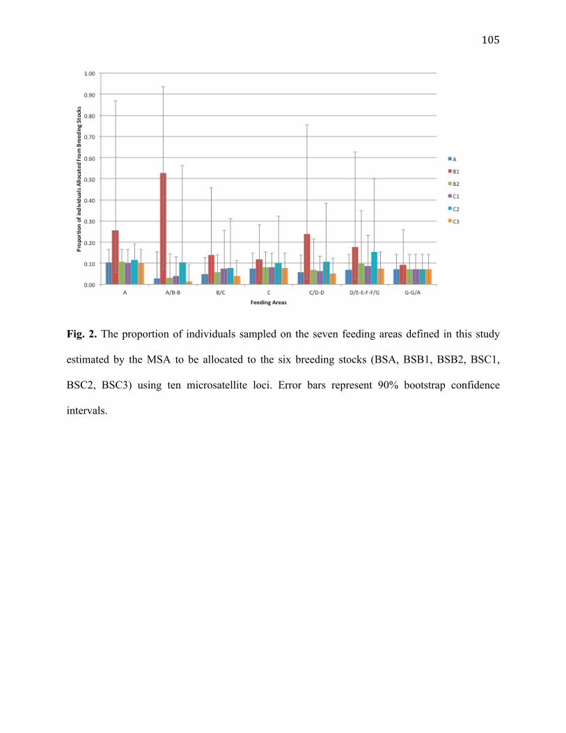
  105  

 

Fig. 2. The proportion of individuals sampled on the seven feeding areas defined in this study

estimated by the MSA to be allocated to the six breeding stocks (BSA, BSB1, BSB2, BSC1,

BSC2, BSC3) using ten microsatellite loci. Error bars represent 90% bootstrap confidence

intervals.

  106  

 

SUPPORTING INFORMATION

Sensitivity analysis to define feeding areas

The BSA core area showed significant differentiation (p<0.001) from almost all other groups,

including A/B-B, for the mtDNA data set (Table S2a-d) and so was designated as a single

grouping. Significant differentiation of A was less evident in the microsatellite data set, however

the separation of A from A/B was still supported by the Jost’s D statistic (Table S3b).

Aggregating A/B with the core area B resulted in no loss of resolution for mtDNA or

microsatellite data set (Table S2; S3). For the mtDNA data set, B/C showed no significant

differentiation from C-D-E-F, however C and C-C/D was found to be significantly differentiated

from the areas designated for E and F, indicating that using C or C-C/D would provide additional

resolution than B/C-C (Tables S2a; S2d). However, the microsatellite data set demonstrated the

opposite, with B/C showing significant differentiation from E-F at both FST and Jost’s D,

whereas C and C-C/D did not show differentiation from any other stock (Tables S3a; S3d). As

samples sizes were adequate across the boundary and core areas for B and C, the B/C boundary

area, C core area, and the C/D-D boundary and core area were designated as separate groupings.

Little resolution was found within the core and boundary areas corresponding to the BSE and

BSF stocks and substocks (Tables S2; S3), resulting in the designation of a single large area

comprising D/E-E-F-F/G. Finally, the core area for G and the G/A boundary (n=0) were

aggregated as designated as a separate area due to the significant differentiation from most other

areas for both the mtDNA and microsatellite data sets (Tables S2; S3).

  107  

 

Table S1. Genetic diversity based on a 371 bp consensus sequence of the mitochondrial control

region and 10 microsatellite loci for the total feeding sample and the six breeding stocks and

substocks included in the baseline data set and the haplotype comparison of breeding and feeding

areas. N, sample size; S, number of segregating sites; H, number of haplotypes; Hd, haplotype

diversity; π(JC), nucleotide diversity with Jukes-Cantor correction; K, mean number of alleles;

HE, expected heterozygosity; HO, observed heterozygosity.

Stock N MtDNA Microsatellites

S H Hd π(JC) K HE HO

Total BS 2772 60 107 0.972 0.019 14.0 0.743

BSA 38 25 18 0.946 0.017 9.4 0.724 0.718

BSB1 1226 55 89 0.965 0.019 13.0 0.745 0.742

BSB2 176 44 54 0.966 0.019 11.1 0.746 0.761

BSC1 182 43 55 0.968 0.018 11.7 0.747 0.750

BSC2 61 34 30 0.969 0.019 10.2 0.736 0.723

BSC3 1089 47 78 0.970 0.019 12.6 0.739 0.742

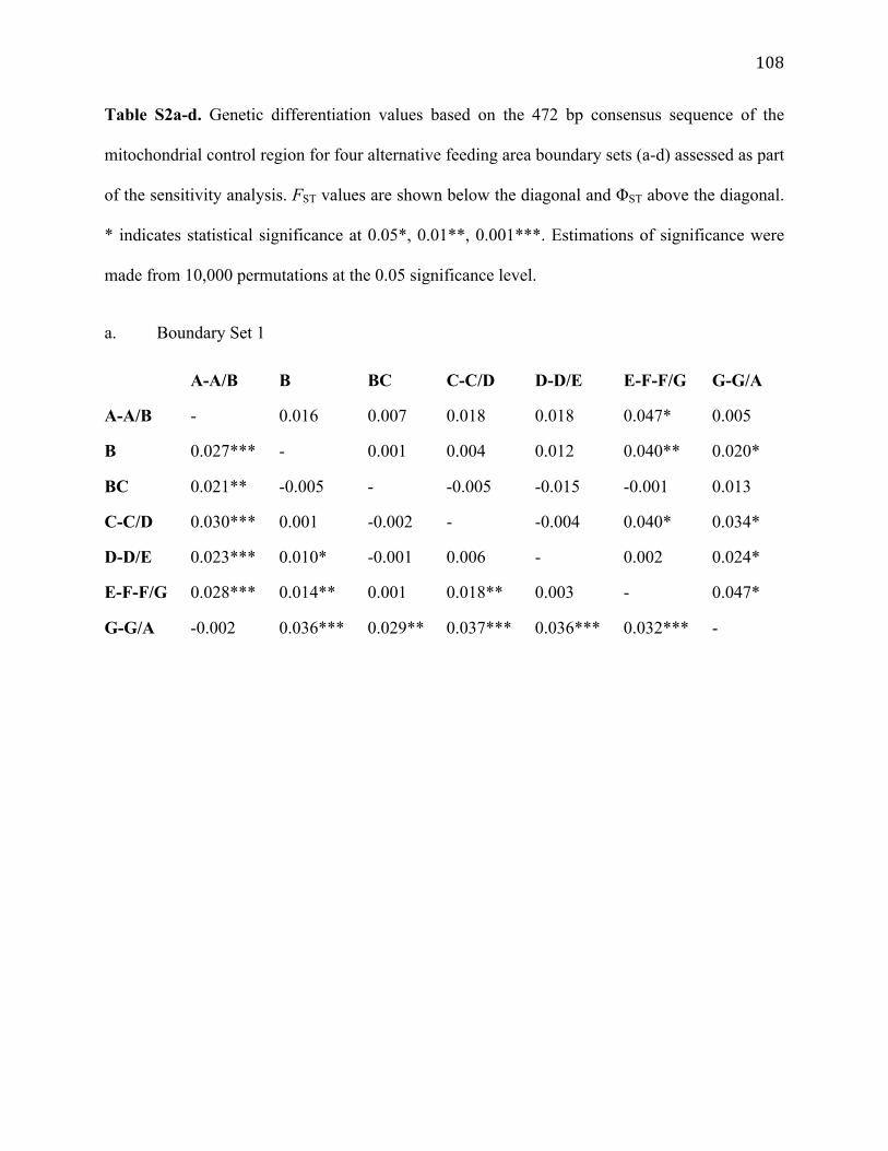
  108  

 

Table S2a-d. Genetic differentiation values based on the 472 bp consensus sequence of the

mitochondrial control region for four alternative feeding area boundary sets (a-d) assessed as part

of the sensitivity analysis. FST values are shown below the diagonal and ΦST above the diagonal.

* indicates statistical significance at 0.05*, 0.01**, 0.001***. Estimations of significance were

made from 10,000 permutations at the 0.05 significance level.

a. Boundary Set 1

A-A/B B BC C-C/D D-D/E E-F-F/G G-G/A

A-A/B - 0.016 0.007 0.018 0.018 0.047* 0.005

B 0.027*** - 0.001 0.004 0.012 0.040** 0.020*

BC 0.021** -0.005 - -0.005 -0.015 -0.001 0.013

C-C/D 0.030*** 0.001 -0.002 - -0.004 0.040* 0.034*

D-D/E 0.023*** 0.010* -0.001 0.006 - 0.002 0.024*

E-F-F/G 0.028*** 0.014** 0.001 0.018** 0.003 - 0.047*

G-G/A -0.002 0.036*** 0.029** 0.037*** 0.036*** 0.032*** -

  109  

 

b. Boundary Set 2

A A/B-B B/C C-C/D D-D/E E-F-F/G G-G/A

A - 0.038* 0.026 0.041* 0.038* 0.070** 0.012

A/B-B 0.044*** - 0.001 0.004 0.011 0.039** 0.021*

B/C 0.037** -0.004 - -0.005 -0.015 0.001 0.013

C-C/D 0.049*** 0.001 -0.002 - -0.005 0.040* 0.034*

D-D/E 0.042*** 0.009* -0.001 0.006 - 0.002 0.024*

E-F-F/G 0.045*** 0.013** 0.001 0.018** 0.003 - 0.047*

G-G/A -0.004 0.036*** 0.029** 0.037*** 0.036*** 0.032*** -

  110  

 

c. Boundary Set 3

A-A/B B B/C-C C/D-D D/E-E-F-F/G G-G/A

A-A/B - 0.016 0.014 0.011 0.050* 0.005

B 0.027*** - 0.004 0.007 0.039** 0.020*

B/C-C 0.026** -0.001 - -0.011 -0.022* 0.023*

C/D-D 0.026*** 0.006 0.001 - -0.004 0.019

D/E-E-F-F/G 0.026*** 0.014** 0.013** 0.004 - 0.050**

G-G/A -0.002 0.036*** 0.034** 0.035*** 0.032*** -

  111  

 

d. Boundary Set 4

A-A/B B B/C C C/D-D-D/E E-F-F/G G-G/A

A-A/B - 0.016 0.007 0.018 0.019 0.047* 0.005

B 0.027*** - 0.001 0.006 0.011 0.040** 0.020*

B/C 0.021** -0.005 - -0.003 -0.014 -0.001 0.013

C 0.030*** 0.003 -0.001 - -0.002 0.044* 0.034*

C/D-D-D/E 0.023*** 0.007* -0.002 0.006 - 0.004 0.026*

E-F-F/G 0.028*** 0.014** 0.001 0.021** 0.003 - 0.047*

G-G/A -0.002 0.036*** 0.029** 0.039*** 0.034*** 0.032*** -

  112  

 

Table S3a-d: Genetic differentiation values based on ten microsatellite loci for four alternative

feeding area boundary sets (a-d) assessed as part of the sensitivity analysis. FST values are shown

below the diagonal and Jost’s D above the diagonal. * indicates statistical significance at 0.05*,

0.01**, 0.001***. Estimations of significance were made from 10,000 permutations at the 0.05

significance level.

a. Boundary Set 1

A-A/B B B/C D-D/E D-D/E E-F-F/G G-G/A

A-A/B - 0.009 -0.009 -0.020 -0.013 0.012 -0.015

B 0.000 - 0.020* 0.001 0.013 0.040** 0.043**

BC -0.004 0.004* - -0.005 0.006 0.034** 0.027**

C-C/D -0.005 -0.001 -0.001 - -0.006 0.008 0.011

D-D/E -0.003 0.003 0.001 -0.002 - 0.007 0.017*

E-F-F/G 0.001 0.053** 0.008* 0.000 0.001 - 0.022*

G-G/A -0.002 0.009*** 0.008** 0.001 0.005* 0.005* -

  113  

 

b. Boundary Set 2

A A/B-B B/C C-C/D D-D/E E-F-F/G G-G/A

A - 0.036** -0.000 -0.003 0.010 0.024 -0.028

A/B-B 0.004 - 0.020** 0.000 0.011 0.040** 0.045**

B/C -0.001 0.004* - -0.005 0.007 0.034** 0.027**

C-C/D -0.004 -0.001 -0.001 - -0.006 0.008 0.011

D-D/E 0.000 0.002 0.001 -0.002 - 0.007 0.017*

E-F-F/G 0.001 0.006** 0.008* 0.000 0.001 - 0.022*

G-G/A -0.006 0.010*** 0.008** 0.001 0.005* 0.005* -

  114  

 

c. Boundary Set 3

A-A/B B B/C-C C/D-D D/E-E-F-F/G G-G/A

A-A/B - 0.009 -0.013 -0.013 0.005 -0.015

B 0.000 - 0.011* 0.009* 0.036** 0.043**

B/C-C -0.004 0.002 - -0.008 0.023* 0.020*

C/D-D -0.003 0.002 -0.001 - 0.001 0.014

D/E-E-F-F/G 0.000 0.005** 0.005* -0.001 - 0.021*

G-G/A -0.003 0.009*** 0.005* 0.004 0.006* -

  115  

 

d. Boundary Set 4

A-A/B B B/C C C/D-D-D/E E-F-F/G G-G/A

A-A/B - 0.009 -0.009 -0.017 -0.011 0.012 -0.015

B 0.000 - 0.029* 0.007 0.012* 0.040** 0.043**

B/C -0.004 0.004* - -0.002 -0.009 0.034** 0.027*

C -0.004 -0.000 0.000 - -0.004 0.015 0.015

C/D-D-D/E -0.003 0.003* 0.001 0.001 - 0.006 0.018*

E-F-F/G 0.001 0.005** 0.008* 0.002 0.001 - 0.022*

G-G/A -0.003 0.009*** 0.008** 0.002 0.005* 0.005* -

  116  

 

Table S4: Genetic diversity based on a 371 bp consensus sequence of the mitochondrial control

region for the seven feeding areas included in the haplotype comparison of breeding and feeding

areas. N, sample size; S, number of segregating sites; H, number of haplotypes; Hd, haplotype

diversity; π(JC), nucleotide diversity with Jukes-Cantor correction.

Feeding Area N MtDNA

S H Hd π(JC)

Total 340 53 91 0.971 0.019

A 21 22 14 0.919 0.017

A/B-B 112 40 45 0.959 0.019

B/C 35 32 27 0.976 0.019

C 37 30 23 0.964 0.017

C/D-D 41 31 26 0.974 0.020

D/E-E-F-F/G 44 28 23 0.950 0.018

G-G/A 50 25 23 0.925 0.017

  117  

 

 Fig. S1. Mean Ln(P|K) and Delta K (ΔK) plots for the STRUCTURE outputs for K=1-7.

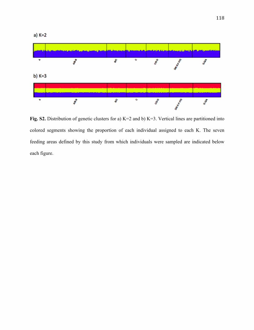
  118  

 

Fig. S2. Distribution of genetic clusters for a) K=2 and b) K=3. Vertical lines are partitioned into

colored segments showing the proportion of each individual assigned to each K. The seven

feeding areas defined by this study from which individuals were sampled are indicated below

each figure.

  119  

 

CHAPTER FOUR

Philopatry and sex-biased dispersal shapes humpback whale population structure at multiple scales FRANCINE KERSHAW, CHARLOTTE TISCH and HOWARD C. ROSENBAUM.

  120  

 

ABSTRACT

Sex-specific differences in philopatry and dispersal have direct influence on the genetic structure

of populations. To better understand the influence of these behaviors on the population structure

of humpback whales, we present a genotypic matching (i.e. genetic capture-recapture) analysis

for 3,814 individual whales, genotyped at 10 microsatellite loci from breeding stocks and

substocks in the South Atlantic (BSA, BSB1-2), the western and northern Indian Ocean (BSC1-

3, ASHW), and Antarctic feeding areas. We used a ‘return index’ (Ri) and ‘interchange index’ (I)

to assess breeding area fidelity and movements between different areas and recorded recaptures

between breeding and feeding areas. Site fidelity was observed for 182 individuals recorded at

the same breeding area in at least two years, and BSB2 showed the highest Ri values overall. 17

individuals were identified in different breeding areas and interchange was highest between

substocks in the same region, however long-distance movements were observed for four males

between BSB and BSC. Mixing of individuals from BSB and BSC on feeding grounds was

evident. At the regional scale (i.e. between breeding stocks), our results generally support a

model of female philopatry and male-biased dispersal as the primary driver of population

structure in this species. At the local scale (i.e. within breeding stocks), substocks BSB2 and

BSC1-3 experience high levels of contemporary interchange, supporting the high gene flow

estimates previously observed at the population-level. Our findings highlight the importance of

understanding current demographic exchange and incorporating this information into the

delineation of population management units.

  121  

 

INTRODUCTION

The demographic process of dispersal, or any movement of individuals or propagules with

potential consequences for gene flow across space (Ronce 2007), is an important factor

influencing the structure of populations (Johnson & Gaines 1990). Dispersal is a complex, multi-

causal process and the timing and frequency of dispersal events result from a combination of

resource dynamics, evolution of life history traits, and inter-individual variation in dispersal

tendencies (Cote et al. 2010; Baguette et al. 2012). In mammals, the majority of species exhibit

male-biased dispersal and female philopatry, likely as a mechanism for females to avoid

inbreeding with related males and the potentially high cost of dispersal (Bonte et al. 2012;

Clutton-Brock & Lucas 2012). Instances of female-biased dispersal do occur however, likely due

to both competitive avoidance for resources and breeding opportunities, and the need to find

unrelated partners (Clutton-Brock & Lucas 2012). In other species, males and females remain in

the same population but show mating preferences for individuals from different social groups

(Amos et al. 1993).

Population-level genetic analyses can be used to tease apart some of these patterns, for

example, by examining variation in gene flow for males and females, and by contrasting

maternally-inherited (i.e. mitochondrial) and bi-parentally inherited (i.e. nuclear) molecular

markers (Avise 2000; Tosi et al. 2003). A number of constraints inherent in population genetic

analyses, however, pose challenges to understanding how current demographic processes are

shaping populations on a timescale relevant for management. Results only reflect historic

patterns due to the genetic signature being scaled to the coalescence time of the molecular

marker used (Avise 2000). It also is challenging to tease apart signals of true genetic

distinctiveness from shared ancestral polymorphism due to recent divergence (Edwards & Beerli

  122  

 

2000; Bulgin et al. 2003). Individual-level genetic analyses, for example, assignment tests or

genotype matching methods, offer a useful complement to population-level studies as they can

provide insights into direct movements of individuals between two populations or between

sampling locations (Lukacs & Burnham 2005; Blair & Melnick 2012). These methods are

therefore capable of providing information on prevalence of philopatry, the rate of current

interchange between two populations, movement capabilities of individuals, and habitat use,

among others. Together, population- and individual-level genetic studies can provide a more

comprehensive understanding of population structure and the demographic processes driving the

patterns observed (Lowe & Allendorf 2010).

The humpback whale (Megaptera novaeangliae) is a baleen species that migrates

annually from low-latitude breeding areas to high-latitude feeding areas (Gambell 1976). Akin to

many wide-ranging mammals (Greenwood 1980), humpback whale population structure is

driven primarily by a combination of maternal fidelity to feeding areas and natal philopatry to

breeding areas, with low-levels of male-biased gene flow (Palsbøll et al. 1995; Baker et al. 1998;

2013; Rosenbaum et al. 2009). This behavior has led to the species being managed by the

International Whaling Commission (IWC) as demographically discrete breeding populations, or

“breeding stocks (BS)”, and it has recently been suggested that populations in different ocean

basins be afforded sub-specific status (Jackson et al. 2014). In the South Atlantic and Western

and Northern Indian Oceans, there are four stocks termed BSA, BSB, and BSC, and the non-

migratory Arabian Sea humpback whale (ASHW). Population sub-structure has been observed

within BSB and BSC and has led to the management of two separate breeding “substocks”

within BSB (i.e. BSB1, a breeding population in the Gulf of Guinea, and BSB2, a genetically

  123  

 

distinct group observed to migrate and feed off West South Africa) and four substocks within

BSC (i.e. BSC1-BSC4) (Fig. 1a).

While natal fidelity plays a predominant role in driving population structure, rare

instances of long-distance interchange do occur between breeding stocks and ocean basins. The

first inter-oceanic migration was documented for two animals marked off eastern Australia in

1954-1955 and killed off western Australia in 1959 (Chittleborough 1965). Direct connectivity

of a single individual has been recorded between BSA off Brazil and the distant BSC in the

Western Indian Ocean (Stevick et al. 2013), and song similarity between BSA and BSB in the

eastern South Atlantic has been observed (Darling & Sousa-Lima 2005). Gene flow between

BSB and BSC is also apparent (Best et al. 1998; Pomilla & Rosenbaum 2005; Rosenbaum et al.

2009), although direct exchange between the west and east coast of South Africa (i.e. BSB2 and

BSC1, respectively) appears limited (Carvalho 2011). At the breeding substock scale, however,

the model of maternal fidelity and male-biased dispersal is not generally supported (Kershaw et

al. in prep) as higher magnitudes of gene flow and complex patterns of isolation and connectivity

occur for both sexes (Rosenbaum et al. 2009; Carvalho et al. 2014; Kershaw et al. in prep).

Southern Hemisphere breeding stocks and substocks converge on shared sub-Antarctic

and Antarctic feeding areas (Gambell 1976). It is generally assumed that temporary or permanent

interchange between breeding stocks occurs as a result of long-distance longitudinal movements

on feeding areas (Rosenbaum et al. 2009). Studies suggest that there are marked differences

between the behaviors of different breeding stocks in terms of feeding area fidelity and the

frequency and extent of longitudinal movements (e.g. Schmitt et al. 2014; Amaral & Loo et al. in

review; Kershaw et al. unpublished data). For example, BSA demonstrates strong fidelity to

discrete feeding areas (Zerbini et al. 2006; Cypriano-Souza et al. 2010; IWC 2012, 2013),

  124  

 

despite evidence of low levels of long-distance interchange (Darling & Sousa-Lima 2005;

Stevick et al. 2013). In contrast, BSB and BSC demonstrate lower levels of fidelity and a higher

degree of mixing, although significant genetic differentiation does occur between some feeding

areas (IWC 2011; Amaral & Loo et al. in review; Kershaw et al. unpublished data). Given the

implications for assessments of stock recovery from industrial and illegal Soviet whaling, there is

an ongoing need to define the location of major feeding aggregations and the degree of mixing

between different breeding stocks and substocks (IWC 2010).

To complement existing population-level genetic studies, we present a genotypic

matching analysis for more than 4,000 genotyped samples, spanning more than two decades of

research, from the seven different breeding areas in the South Atlantic and Western and Northern

Indian Oceans, and feeding areas in the Southern Ocean. We assess a) the degree of site fidelity

of individuals to breeding areas in different years, b) the rate of interchange between different

breeding areas, and c) connectivity between breeding areas and feeding areas, as defined by IWC

Allocation Hypothesis 1 (IWC 2010; Fig. 1a).

MATERIALS AND METHODS

Sample information

A total of 4,360 humpback whale genetic samples originating from multi-year collections across

seven breeding areas and Antarctic feeding areas were used in this study (Fig. 1a). No samples

were available for BSC4. Skin tissues were mostly obtained using biopsy darts (Lambertson

1987), but also from sloughed skin and stranded specimens. Total genomic DNA was extracted

and samples were sexed using ZFX/ZFY markers following Rosenbaum et al. (2009). Samples

were genotyped at 10 microsatellite loci proven to be polymorphic for this species: GATA028,

  125  

 

GATA053, GATA417 (Palsbøll et al. 1997), 199/200, 417/418, 464/465 (Schlötterer et al.

1991), EV1Pm, EV37Mn, EV94Mn, EV96Mn (Valsecchi & Amos 1996) following the

protocols described in Carvalho and colleagues (2014).

Identifying genotypic matches

Duplicate samples were identified from microsatellite genotype identity for 9 or 10 loci using

Cervus v3.0 (Kalinowski et al. 2007). The probability of different individuals and siblings

sharing the same genotype by chance (Probability of Identity, PID, and PID for siblings, PID(sibs),

respectively) were estimated using Cervus (Kalinowski et al. 2007). The reciprocal of the sample

size was used as the arbitrary cut-off below which the probability values are sufficiently small to

conclude that matching genotypes belong to the same individual (Peakall et al. 2006).

Duplicate samples identified in the same breeding area during the same year were

assumed to be individuals mistakenly resampled in the field and were therefore removed from

subsequent analysis. Genotypic matches of individuals identified in the same breeding area in

different years were used as an indicator of site fidelity. The number of and year of each

resighting, and the sex of the individual were recorded for each breeding area. To better

understand connectivity between breeding and feeding areas, genotypic matches were recorded

for individuals found both on breeding areas and the Antarctic feeding areas defined by IWC

Allocation Hypothesis 1 (IWC 2010; Fig. 1a).

Site fidelity and interchange indices

  126  

 

To quantify the relative rate of site fidelity for each breeding area, a ‘return index’ (Ri) was

calculated following Carvalho (2011). The return index was calculated for each year that

sampling was undertaken in a particular location:

Ri = [Mi / (Ai * Bi)] * 1000

Where:

Ai = number of genetically identified whales in all the years before year x for breeding area i

Bi = number of genetically identified whales in year x for breeding area i

Mi = number of genetically identified whales in the previous years and resighted in year x

To quantify the relative rate of interchange between breeding areas, an ‘interchange index’ (I)

was calculated following Carvalho (2011):

I = [Mi,j / (ai * aj )] * 1000

Where:

Ai = number of genetically identified whales in breeding area i

Aj = number of genetically identified whales in breeding area j

Mi,j = number of genetically identified whales in both regions

Both indices are considered to be zero when there are no genotypic matches (i.e. when M = 0)

within (for Ri) or between breeding areas (for I).

  127  

 

RESULTS

Sample information

The 4,360 genetic samples analyzed were determined to represent 3,814 different whales (Fig.

1a). Average probability of identity (PID) for the total sample was small enough to identify

duplicate individuals with high confidence (PID = 1.92x10-12; PID(sibs) = 9.2x10-5; reciprocal of

sample size = 2.6x10-4). Sex was determined for 3,590 individuals, 2,267 males and 1,323

females, resulting in an overall proportion of 1.7:1 males to females.

Fidelity to breeding areas

A total of 182 individuals (123 males; 57 females; 2.5:1 sex ratio) were resighted across five

breeding areas in at least one year (BSA, n=1; BSB1, n=79; BSB2, n=33; BSC2, n=2; BSC3,

n=67; Table S1). The number of times an individual was resighted within a breeding area ranged

from 1 to 3 years. Breeding area fidelity, defined by the return index (Ri), ranged from 0.660–

44.444 and this range varied notably between breeding areas (BSA, Ri=2.083, number of years

(Ny) = 1; BSB1, Ri=0.000-0.116, Ny=8; BSB2, Ri=0.000-44.444, Ny=14; BSC2, Ri=0.870-

10.4167, Ny=2; BSC3, Ri=0.000-0.945, Ny=11; Fig. 2). For breeding areas where Ny>1, BSB2

showed consistently higher values of Ri (Fig. 2b), followed by BSC3 and BSB1 (Fig. 2a, c).

Interchange between breeding areas

A total of 17 individuals (10 males; 7 females; 1.4:1 sex ratio) showed genotypic matches with

more than one breeding area either in the same year (n=3) or different years (n=14). Interchange

occurred primarily between breeding areas in the same region (BSB, n=7; BSC, n=6), and all

interchange observed in the same year occurred between BSB1 and BSB2. Long-distance

  128  

 

movements were observed between BSB and BSC (n=4). All four of these individuals were

male. No interchange was observed for BSA or ASHW. The interchange index (I) ranged from

0.001–0.046 resulting in a change in magnitude of 1x-45.783x, with the highest I value observed

between BSC2 and BSC3, and the lowest between BSB1 and BSC3 (Fig. 1b).

Connectivity between breeding and feeding areas

Genotypic matches for 7 individuals (4 males; 3 females) were recorded between breeding areas

and feeding grounds in the Southern Ocean (Table 1). Six individuals were observed within the

nucleus feeding area for BSB designated under IWC Allocation Hypothesis 1, however, only

three of these individuals were sampled in the BSB breeding area. The remaining matches

comprised two females sampled in BSC1 and one male sampled in BSC3. One male sampled in

BSC3 was matched to an individual sampled in the nucleus feeding area for BSC.

DISCUSSION

Fidelity to breeding areas

Genotypic matches confirm that humpback whales show fidelity to breeding areas and also, in

the case of BSB2, to feeding areas and migratory routes. Counter to expectations that site fidelity

would be observed to a greater extent for females due to maternal philopatry, our results

demonstrate a skew towards males (sex ratio 2.5:1), above that observed for the total sample (sex

ratio 1.7:1). While the skew in sex ratio may be influenced by sampling effects, for example, if

there is temporal variation when different sexes arrive at a breeding location (Carvalho et al.

2014), our results suggest that males are at least as likely as females to return to the same area to

breed in multiple years. Male fidelity has also been observed more frequently than females both

  129  

 

intraseasonally and interannually on breeding grounds in Hawaii (Craig & Herman 1997) and

New Caledonia (Garrigue et al. 2001), and a male-biased distribution is common to humpback

whale wintering grounds worldwide (Herman et al. 2011).

The pattern of male-biased fidelity may be due to male seasonal residency on breeding

areas exceeding female residency on average, perhaps due to continued searching strategy by for

mates, whereas females tend to depart the breeding area once impregnated (Herman et al. 2011).

In the absence of feeding or predation pressure on breeding grounds, sexual selection is the

primary force shaping the breeding behavior of the species (Cerchio et al. 2005), which adheres

to a mating system of male dominance polygyny (Emlen & Oring 1977) and displays the features

of a ‘floating lek’ (Clapham 1996) involving the establishment of dominance rankings among

singing males that are temporarily resident in a specific location (Clapham 1996; Cerchio et al.

2005). The existence of a dominance hierarchy and associated lekking behavior among male

humpback whales is supported by observations of a reproductive skew suggesting that certain

males may have slightly greater reproductive success, although this may be the product of

several alternative mating strategies rather than singing alone (Cerchio et al. 2005).

The highest return index values were observed for BSB2, supporting previous genetic

and photo-identification evidence of long-term fidelity to this area (Barendse et al. 2011;

Carvalho 2011; Fig. 2b). This finding suggests that migratory and feeding behavior may also be

conserved, perhaps as a result of vertical cultural transmission of migration routes and

destinations between mother and calf (Alter et al. 2009; Valenzuela et al. 2009; Barendse et al.

2013). In contrast to BSB1 and BSC3, we observed a slight bias towards females (12 males, 21

females) in the genotypic matches for BSB2, possibly due to the samples being collected during

  130  

 

the southern migration of whales from the BSB1 breeding area and therefore comprising a larger

proportion of impregnated females and mother-calf pairs (Carvalho 2011; Herman et al. 2011).

On the east coast of Africa, BSC1 provides an interesting contrast to BSB2. Similar to

BSB2, the southern portion of BSC1, from Mozambique Island (15°S) to Cape Agulhas

(~34.5°S) is considered primarily a migratory route towards breeding areas north of

Mozambique Island to at least the southern border of Tanzania (4°S) (Findlay et al. 1994; Banks

2013). Unlike BSB2, however, no genotypic matches were found within BSC1 in multiple years

in this study or in previous work (Carvalho 2011). One explanation for the lack of matches for

BSC1 is that animals show lower levels of fidelity to the southern portion of BSC1 than to BSB2

indicating that whales in this region exhibit different behavior to those off the west coast.

Alternatively, animals may be more rapidly moving through the region towards breeding areas

north of Mozambique Island, thereby reducing the likelihood of being resampled (Carvalho

2011; Banks 2013). Observations of the timing of migrating whales (Best et al. 1998), greater

swim speeds, and very few observations of opportunistic feeding (Banks 2013) off east South

Africa suggest that, if behavioral differences are a contributing to the lower the number of

individual recaptures for BSC1 than BSB2, this latter scenario may be the most likely.

However, a number of factors related to sampling bias cannot be overlooked as a possible

explanation for the differences observed. The estimated population size of BSB2 is

approximately 510 individuals (95% CI: 230-790; Barendse et al. 2011) and therefore comprises

many fewer animals than BSC1 currently estimated at 7,035 (90% CI: 5,742-8,824; IWC 2010).

Therefore, even if site fidelity between the two locations is comparable, the likelihood of

resampling the same individual is considerably lower in BSC1 than BSB2. Moreover, the

geographic expanse of the range of BSC1 is significantly greater than BSB2, that likely only

  131  

 

comprises whales undertaking a coastal migration route south of Namibia (i.e. south of 23°S)

(Elwen et al. 2014) and for which samples were collected in one location off west South Africa

(~33°S). Use of larger geographic areas by individuals would be expected to result in shorter

occupancy times in a given location and therefore fewer opportunities for sampling the same

individual would be expected (Banks 2013).

Humpback whale migratory behavior appears to be relatively plastic and individuals have

been observed to delay or change their migration in order to exploit productive feeding areas

(Gales et al. unpublished data). The difference in migratory behavior observed for BSB2

compared to BSC1, if real, may therefore be explained by oceanographic conditions (Carvalho

2011). The waters of west South Africa are rich in nutrients as a result of the Benguela Current

system and an extensive coastal upwelling system (Ansorge & Lutjeharms 2007). This region

therefore represents a persistent feeding area for many species, including southern right whales

(Eubalaena australis; Best & Schell 1996) and Bryde’s whales (Balaenoptera edeni; Penry et al.

2011). No similar upwelling system is found off the east South African coast. It is therefore

likely that BSB2 whales show increased residence time and long-term fidelity to the waters off

West Africa given the presence of a stable food source, whereas whales from BSC1 travel

directly to breeding areas in order to conserve energy during the migration (Carvalho 2011).

Interchange between different breeding areas

The rate of interchange between BSB1 and BSB2 was relatively high (n=7; I=0.018;

magnitude=17.8) and included all individuals matched in the same year, indicating that BSB2

comprises at least a portion of the animals migrating south from BSB1. This rate of interchange

is also supported by the photo-identification of three different individuals at both locations

  132  

 

(Barendse et al. 2011). Satellite telemetry data suggests that whales breeding in the Gulf of

Guinea may take at least two separate migratory routes to Southern Ocean feeding areas, one

close to the coast and another offshore (Rosenbaum et al. 2014). The high levels of interchange

we observed for BSB1 and BSB2 may be representative of this division, with BSB2 whales

representing the inshore migrants, and provide additional support to the assumption that

migratory routes are also conserved across generations. Notwithstanding the evidence of

interchange demonstrated here, significant genetic differentiation has been found between BSB1

and BSB2 at the population level (Rosenbaum et al. 2009; Carvalho et al. 2014; Kershaw et al.

in prep). This indicates that the individuals recorded in both BSB1 and BSB2 may not be

contributing genetically to both populations but rather are only traveling through or utilizing

habitat in both regions, as would be expected given that BSB2 represents a migratory corridor

and feeding area (Best et al. 1998).

High levels of gene flow have been observed between the three substocks of BSC

(Rosenbaum et al. 2009; Kershaw et al. in prep) and our results suggest that current interchange

may play a significant role in driving this connectivity, although the effect of retained ancestral

polymorphism cannot be discounted. Interchange was highest between substocks BSC2 and

BSC3 (Fig. 1b), and one female was found to switch from BSC2 to BSC3 and back to BSC2

over a period of 6 years. Photo-identification studies (Ersts et al. 2011) and satellite tracking data

(Fossette et al. 2014; Cerchio et al. unpublished data) also show considerable movement

between BSC2 and BSC3, which are in relatively close geographic proximity. We also observed

interchange, although to a lesser degree, between BSC1 and BSC3 (Fig. 1b), supporting

suggestions that a northern migratory stream may be present between the east coast of Africa

(BSC1) and northeastern Madagascar (BSC3) (Cerchio et al. unpublished data). Despite

  133  

 

relatively high gene flow estimates between BSC1 and BSC2 (Rosenbaum et al. 2009; Kershaw

et al. in prep), no direct interchange was detected.

Long-distance movements were observed between BSB1 and BSC3 and, for the first

time, between BSB2 and BSC1 (Fig. 1b). All individuals were male, supporting the general

model of long-distance male dispersal (Baker et al. 1998, 2013). That these are the first records

of connectivity between BSB2 and BSC1 (Banks et al. 2011) is surprising given their geographic

proximity and indicates that more complex behavioral drivers, such as the influence of different

oceanographic conditions on fidelity and migratory behavior, may be maintaining the isolation of

these two substocks (Carvalho 2011). Previously recorded genotypic matches between BSB1 and

BSC3 (Pomilla & Rosenbaum 2005) and estimates of gene flow based on mtDNA (Rosenbaum

et al. 2009) have suggested a westward bias in movements from BSC to BSB. This westward

bias was not supported by gene flow estimates based on nuclear microsatellite data (Kershaw et

al. in prep) however, and our results show both eastward and westward movement of males

between BSB2 and BSC1.

Despite previous evidence of rare interchange between the western South Atlantic and the

eastern South Atlantic and Western Indian Ocean (Darling & Sousa-Lima 2005; Stevick et al.

2013), we found no genotypic matches between BSA and any other breeding stock. This was not

unexpected as BSA shows significant genetic differentiation from other stocks at the population-

level (Rosenbaum et al. 2009; Kershaw et al. in prep), likely due to the population being isolated

by geographic distance from stocks in the eastern South Atlantic; although may also have been

influenced by the relatively small sample size for BSA. The lack of interchange we observed for

ASHW in consistent with this breeding stock being non-migratory and extremely isolated from

  134  

 

other stocks and substocks in the Western Indian Ocean (Minton et al. 2011; Pomilla & Amaral

et al. 2014).

Connectivity between breeding and feeding areas

The seven genotypic matches we recorded between breeding and feeding areas support existing

evidence for a high degree of mixing of individuals from BSB and BSC on feeding areas (IWC

2011; Amaral & Loo et al. in review; Kershaw et al. unpublished data). Of the six genotypic

matches observed within the B “Nucleus” feeding area (where 100% animals are allocated to

BSB; IWC 2010), three were matched to individuals sampled within BSB and three to BSC

(Table 1). While the single match between the C Nucleus region and one individual sampled in

BSC3 cannot provide insights into mixing within the C Nucleus, it does confirm direct

connectivity between these two locations (Table 1).

The B Nucleus region therefore appears to be a shared feeding area for animals from

BSB1 and BSC. This finding is supported by genetic data showing that Management Area II

(60°W-0°), which in part overlaps with the B Nucleus (10°W-10°E), has little significant

differentiation from other Management Areas across the Southern Ocean (Amaral & Loo et al. in

review), apart from the eastward adjacent Management Area III (0°-70°E) that encompasses the

C Nucleus feeding area (30°E-60°E) (Amaral & Loo et al. in review). However, a direct

comparison of the B and C Nucleus regions indicates that they are not significantly differentiated

(Kershaw et al. unpublished data). These contrasting findings indicate that genetic differentiation

is sensitive to the longitudinal boundaries used to divide the feeding areas associated with BSB

and BSC, particularly between 20°W and 30°E. In additional to longitudinal boundaries, genetic

  135  

 

evidence suggests latitudinal variation in the distribution of BSB whales in the Antarctic (IWC

2011) indicating that this should also be explored in future studies.

Given the relatively small sample sizes for feeding areas used in this study, our results

suggest that individuals from BSB and BSC may commonly mix in the B Nucleus feeding area.

This is supported by satellite telemetry data for individuals tagged off west South Africa that

demonstrate wide westward (~15°W) and eastward (~40°E) movements on sub-Antarctic and

Antarctic feeding areas (Seakamale et al. 2015). Evidence suggests that baleen whales are

capable of significant behavioral plasticity with regards to environmental variability, including

opportunistic feeding during migration (Gales et al. unpublished data) and adjusting the timing

of their seasonal migration to feeding areas in response to climate-change driven shifts in prey

availability (Ramp et al. 2015). On feeding areas, these species are often associated with habitats

characterized by high krill abundance and density, such as banks and canyons, the sea-ice edge,

and variable frontal systems such as the Antarctic polar front (Wada & Numachi 1991; Hoezel

1998; Stevick et al. 2006; Sremba et al. 2012). Seasonal and inter-annual variability of these

oceanographic features, for example changes in the distribution and dynamics of sea ice (Thiele

et al. 2004), are likely to lead to spatial and temporal changes in prey distribution and abundance

(Croll et al. 1998). For example, inter-breeding area movements by humpback whales between

eastern and western Australia has been associated with the atypical distribution of prey during

the intervening feeding season (Chittleborough 1959), and the first documented movement of an

individual humpback whale between the eastern South Pacific breeding stock off Ecuador (BSG)

and BSA in the western South Atlantic coincided with a particularly strong El Nino Southern

Oscillation (ENSO) event (Stevick et al. 2013). ENSO events affect the entire food web in the

eastern South Pacific and may also extend into polar regions, potentially leading whales to

  136  

 

forage in atypical locations or move more widely in search of prey (Stevick et al. 2013). It would

therefore be expected that greater longitudinal movements and higher levels of mixing would

occur in regions where prey distribution was less dense and more variable, as is the case in the

Atlantic and Southwest Indian Ocean sectors of the Southern Ocean (Nicol et al. 2000).

Management implications

This individual-level analysis has provided important insights into the contemporary drivers of

the genetic structure and connectivity of the humpback whale breeding stocks and substocks

managed by the IWC in the South Atlantic and Western and Northern Indian Oceans. At the

regional scale (i.e. between breeding stocks), the observed fidelity to breeding areas and the low

levels of long-distance interchange between breeding stocks echo the findings of population-

level genetic studies (Rosenbaum et al. 2009; Kershaw et al. in prep) that show general support

for the designation of the four breeding stocks (BSA-C, ASHW) by the IWC. At the local scale

(i.e. within breeding stocks), the high levels of interchange observed between BSB2 and BSC,

and between each of the BSC substocks , corroborates estimates of high gene flow for both sexes

between these substocks at the population level (Kershaw et al. in prep). Our findings indicate

that the high estimates of gene flow at the population-level are, at least in part, the result of

ongoing demographic exchange rather than as a product of historic connectivity or shared

ancestral polymorphism. This work highlights the importance of current research into

understanding current demographic exchange using multiple methods and incorporating this

information into the delineation of population management units.

 

  137  

 

TABLES AND FIGURES

Table 1. Sex and date of genotypic matches found between breeding areas and Antarctic feeding

areas as defined by IWC Allocation Hypothesis I. *indicates matches identified in IWC (2009).

Individual Sex Breeding area Date Feeding area Date

1* M BSC3 2000 B Nucleus 2006

2* M BSB1 2001 B Nucleus 2006

3 M BSB1 2002 B Nucleus 1998

4 F BSC1 2003 B Nucleus 2006

5 F BSB1 2003, 2005 B Nucleus 2007

6* F BSC1 2004 B Nucleus 1997

7 M BSC3 2004 C Nucleus 1999

  138  

 

Fig. 1. a) Location and sample sizes of the seven breeding stocks and substocks, and their

associated “Nucleus” and “Margin” feeding areas; b) Interchange index (I) values between

Breeding Stocks B and C. Magnitudes are shown in parentheses and reflected in the width of the

arrow. Gray arrows indicate potential connections but where no interchange (I=0) was observed

in the sample.

  139  

 

Fig. 2. Return index (Ri) values for a) BSB1, b) BSB2, and c) BSC3, for the entire duration of

sampling for this study. Note the different scales for Ri for each breeding area. Ri values can only

be calculated from the second year of sampling onward. Asterisks indicate years where no

sampling was carried out.

  140  

 

CHAPTER FIVE

Achieving a mechanistic understanding of genetic population structure FRANCINE KERSHAW and HOWARD C. ROSENBAUM

  141  

 

ABSTRACT

The ability to identify and quantify the multiple factors influencing genetic population structure

would offer mechanistic insights into how ecological processes are linked to evolutionary

patterns. New methods in individual-based modeling enable such investigations by providing a

flexible platform upon which behavioral, environmental, and genetic data can be integrated.

Here, we present a research prospectus for developing individual-based models (IBMs) capable

of advancing our understanding of the interactions between ecology and genetic architecture. We

focus on highly migratory species (HMS) due to their diverse range of genetic population

structures resulting from complex interactions between life history and environmental

conditions. We begin by reviewing recent advances in the field of IBM development, which have

resulted in this approach now offering a framework for the integration of individual movement

behavior with environmental and genetic data. To guide model implementation, we transfer

lessons from a number of applied case studies of recently developed IBMs from a variety of

fields. We first provide examples of how genetic parameters, such as genetic diversity, within-

population variation, and genetic connectivity, may be included in an IBM framework. We then

consider the integration of parameters for physiological condition and life history stage, which

may directly influence an individual’s dispersal or breeding behavior. We discuss how

environmental conditions, which may play an important role in determining when and where an

individual chooses to move, can be incorporated. The use of multiple gridded environmental data

sets enable models to account for the temporal dynamism of natural systems, and also allows for

the testing of the relative influence of different environmental parameters at different spatial

scales. We subsequently describe methods for simulating the movement behavior of individuals

to enhance biological realism. The challenge of developing models for HMS is their potential

  142  

 

complexity, and so we present a number of recent advances in model parameterization and

validation, which will enable the development of IBMs in the absence of rich data sets or where

the systematic ground truthing of model outputs is not feasible; both of which represent key

constraints when developing models for HMS. Finally, we emphasize the utility of developing

IBMs for data poor species. As IBMs are not constrained by existing knowledge of the system

they therefore represent a useful tool to explore and generate hypotheses regarding the

mechanistic processes underlying observed patterns. They also offer an alternative to impractical

field studies and are therefore particularly useful for studies of HMS, which are logistically

challenging to study throughout the entirety of their range. We conclude that, while achieving a

mechanistic understanding of patterns of genetic population structure still represents a significant

challenge, new modeling techniques are now capable of facilitating a cautious yet concerted

effort towards establishing a solid foundation for this field of research.

  143  

 

INTRODUCTION

The ability to identify and quantify the behavioral drivers of genetic population structure would

offer unique insights into questions concerning how ecological processes are mechanistically

linked to evolutionary patterns. Genetic population structure is commonly observed in wild

populations and arises from variation in the spatial and temporal distribution and movement of

individual organisms, which over evolutionary meaningful timescales results in systematic

variation in population allele frequencies through space and time (Jones & Wang 2012).

Population structure is driven by complex interactions between processes operating at the level

of the individual organism, including behavioral responses to internal state (Piou & Prévost

2012), ecological factors (Andrews et al., 2010), environmental conditions (Schunter et al. 2011;

Kormann et al. 2012), and micro-evolutionary factors, such as genetic drift and gene flow

(Gaggiotti et al. 2009); all of which operate within the broader context of historical

phylogeography (Scoble & Lowe 2010; Muscarella et al. 2011).

Identifying and quantifying the relative influence of each type of process is fundamental

to gaining an understanding of the mechanisms underlying patterns of genetic structure and

connectivity observed in natural populations. Such an understanding would not only enable our

interpretation of the mechanisms underlying existing genetic patterns, but also enable us to

forecast how these patterns may change in the future (Blair & Melnick 2012). In the long term,

these insights may also facilitate our ability to predict evolutionary trajectories at the species-

level (Li et al. 2012). Achieving such a task will require a research prospectus that fully

integrates behavioral, environmental, and genetic data.

As the burgeoning field of landscape genetics (Manel & Holderegger 2013) and the

growing field of seascape genetics (e.g. Galindo et al. 2010; Mendez et al. 2010, 2011; Selkoe et

  144  

 

al. 2010; Amaral et al. 2012a,b; Treml et al. 2012) demonstrate, our understanding of how the

environment shapes genetic population structure continues to broaden. It is becoming

increasingly apparent, however, that focusing on environmental influence alone is inadequate to

fully explain the genetic patterns observed for certain species that may select for particular

habitat types but are able to tolerate a wide range of environmental conditions. In these cases,

population boundaries do not always align with environmental boundaries.

Population-level fidelity to breeding and feeding sites, for example, is an important driver

of genetic structure for a number of migratory species. For instance, humpback whale

populations in the Southern Hemisphere are genetically structured as a result of strong site

fidelity to winter breeding areas in the tropics and summer feeding areas in the nutrient rich

Southern Ocean (Rosenbaum et al. 2009; Ruegg et al. 2013). Within regions, however, there is

increasing evidence that population structure is driven by subtle, socially driven dispersal and

migratory behaviors. Fine-scale differences in measures of population substructure across time

provide evidence for temporal segregation on the basis of age, sex, and reproductive status

(Rosenbaum et al. 2013; Carvahlo et al. 2014). A similar scenario exists within the migratory

corridor of the Pacific common eider, which breeds along twelve barrier islands in the Beaufort

Sea. Here, nesting location is likely determined by female philopatry that, in turn, is correlated

with time of arrival following migration (Sonsthagen et al. 2009). Due to the strong hysteresis

(or ‘memory’) effects (Guttal & Couzin 2010) associated with philopatry, species that exhibit

strong fidelity to core habitats may be particularly sensitive to anthropogenic impact and

environmental change. Populations may fail to recolonize suitable habitat following local

extirpation (Clapham et al. 2008) or may be unable to respond to shifts in prey distribution by

  145  

 

finding and switching to new feeding areas, resulting in an increased risk of malnutrition and

demographic decline (Leaper et al. 2006).

Behavioral partitioning within populations has also been noted as an important driver of

genetic structure (Taylor & Friesen 2012). For example, genetic divergence between colonies of

Cook’s petrel has been linked to segregation of different populations during the non-breeding

season due to habitat specialization (Rayner et al. 2011). Similar partitioning has been observed

at the individual level in the highly migratory Bewick swan, where current and future

reproductive success was found to correlate with individual foraging specializations along a

terrestrial-aquatic gradient (Hoye et al. 2012). Social dynamics may also play an important role.

In the Hawaiian archipelago, spinner dolphins exhibit two different social strategies, stable

versus dynamic group membership, which are associated with low and high levels of gene flow,

respectively (Andrews et al. 2010).

Integration of behavioral factors into studies of the mechanisms driving the genetic

population structures of these species therefore proves essential. The central goal of this review

is to provide an overview of the emerging field of individual-based modeling (IBM), which is

capable of supporting the necessary integration of behavioral, environmental, and genetic data

(Grimm & Railsback 2011). We focus on describing these approaches in the context of

understanding the mechanisms underlying patterns of genetic population structure in highly

migratory species (HMS) due to their often complex genetic structures, driven not only by

environmental influences, but also innate and learned behaviors, life history stages, and

conspecific interactions. As many of the case studies herein demonstrate (Table 1), however,

these approaches are widely applicable to investigate the behavioral mechanisms underlying

patterns of genetic population structure in any marine or terrestrial species.

  146  

 

THE INTEGRATION OF BEHAVIOR

The multitude of examples described in the Introduction demonstrate that it is essential for

individual-based behavioral ecology to be considered in attempts to quantify the different

mechanisms underlying patterns of genetic population structure in HMS. Challenges of data

limitation and computational power have impeded our ability to meet this need in the past;

however, recent advances in individual-based (or “agent-based”) modeling now offer a

framework for the integration of individual movement behavior with environmental and genetic

data (Epperson et al. 2010; Grimm & Railsback 2011).

Individual- (or “agent-“) based models (IBMs) follow the fitness-maximizing behavior of

individuals and enable the prediction of population-level consequences (e.g. rates of gene flow)

(Grimm & Railsback 2011). Computer simulations can be used to model discrete individuals

within a population, including components of the individual’s life cycle, variation among

individuals, interactions between individuals, and the dynamics of the resources they use (Fig. 1;

Stillman & Goss-Custard 2010). In contrast to other types of deterministic models, IBM’s are

based on the concept of emergence, where behavior is not imposed by programmed empirical

rules, but rather emerges from the model based on the simulated individual’s behavioral

decisions determined by the set of fitness-maximizing decision rules (Stillman & Goss-Custard

2010; Grimm & Railsback 2011). IBMs are therefore not constrained by existing knowledge of

the system and represent a useful tool to explore and generate hypotheses regarding the

mechanistic processes underlying observed patterns (Grimm & Railsback 2011). They also offer

an alternative to impractical field studies by representing “virtual experiments” (Tamburino &

  147  

 

Bravo 2013), which are particularly useful for studies of HMS that are logistically challenging to

study throughout the entirety of their range.

Complexity is an important feature of IBMs, as it is their ability to synthesize a broad

range of knowledge that can lead to previously unforeseen emergent properties (Piou & Prévost

2012). Early IBMs had little standardization of model code or structure, leading to criticisms of

opacity and over-complexity (Topping et al. 2010). The recent publication of an Overview,

Design concepts, and Details (ODD) protocol offers a framework for standardizing published

descriptions of individual-based models (Grimm et al. 2010). The application of ODD has been

shown to improve the rigor of model formulation and helps make the theoretical foundations of

large models more visible, therefore improving their reproducibility (Grimm et al. 2010). In

addition, the ‘pattern-oriented modeling’ (POM) strategy of Grimm and Railsback (2012) offers

model development guidelines that explicitly account for the multi-criteria design, selection, and

calibration of models of complex systems. This approach makes the selection and use of

modeled patterns more explicit and rigorous, thus facilitating the development of models that

have appropriate levels of complexity and predictive ability (Grimm & Railsback 2012).

DEVELOPING IBMS FOR HIGHLY MIGRATORY SPECIES

Capturing the complex behaviors of HMS within an IBM is not a simple task, and it will likely

be infeasible to parameterize all relevant behaviors. These challenges are exacerbated by general

scarcity of data and information for HMS throughout all stages of their life history. There is good

reason for optimism, however, at least for developing IBMs for better-known species. In our

view, the goal of developing IBMs for HMS should not necessarily be to fully replicate the

system, but rather to develop a useful hypothesis-generating tool for exploring the possible

  148  

 

mechanisms underlying the genetic structure of populations. Below, we outline some ways to

approach the task of developing IBMs for explaining the genetic population structures of HMS.

We also present a number of case studies that transfer lessons from recently developed IBMs in

the wider field of ecology and evolution to address questions concerning HMS specifically (see

Table 1).

(1) Integrating genetics and evolutionary history

IBMs are now being used to explicitly explore interactions between ecological (co-occurrence of

individuals in space and time) and evolutionary (reproductive interactions between individuals

and micro-evolutionary processes) paradigms (Frank & Baret 2013). Advances in the field of

individual-based genetics (Planes & Lemur 2011) enables modeled individuals to be

parameterized with genotypic information, providing a useful baseline for explorations into the

effects of mutation, genetic drift, migration, and natural selection on the genetic composition of a

modeled population (Piou & Prévost 2012; Frank & Baret 2013). Recently, the terms “demo-

genetic” and “eco-genetic” have been adopted to describe IBMs specifically aimed at

understanding the relative importance of population genetics and quantitative genetics,

respectively, on life history traits and population dynamics (Piou & Prévost 2012; Frank & Baret

2013).

(a) Understanding the genetic diversity of populations

The genetic structure of populations reflects the distribution of genetic diversity across different

groups of individuals (Jones & Wang 2012). IBMs that account for both the demography and

genealogy of a population can be used to elucidate the mechanisms underlying observed levels

  149  

 

genetic diversity, such as isolation and/or a reduction in population size (Kekkonen et al. 2012).

Further, such models can be used to simulate a population’s historic diversity, or project how it

may change in the future. For example, Kekkonen and colleagues (2012) developed an

individual-based population genetic model to explore whether the relatively high level of genetic

diversity in a population of white-tailed deer could be understood based on historical information

that the founder population comprised only four individuals (Kekkonen et al. 2012). This

information appeared to be conflicting as the level of genetic diversity for a population with such

a small number of founders would usually be expected to be extremely low. However, observed

levels of heterozygosity were found to be concordant with the model’s predictions based on the

recorded founding population, suggesting that a small number of founders does not necessarily

cause a significant reduction in heterozygosity in iteroparous species (Kekkonen et al. 2012).

The ability to simulate the potential processes leading to observed levels of genetic

diversity is particularly useful for migratory species that have been subjected to commercial

harvest. Alter and colleagues (2012) employed a similar combined demographic and

genealogical modelling approach within an Approximate Bayesian Computation (ABC)

framework to estimate the pre-whaling population size of the eastern Pacific gray whale, a

species heavily impacted by commercial hunting in the 19th and 20th centuries. The model

estimated the pre-whaling population to be three to five times its current size and supported a

single bottleneck coincident with the height of the whaling activity for this species, countering

claims of an earlier bottleneck driven by climatic factors (Alter et al. 2012). IBMs may help

refine this type of population-level model by incorporating individual-level information into the

demographic parameters, leading to more realistic simulations of population dynamics. Where

information is more limited, IBMs represent a useful tool to explore potential processes driving

  150  

 

observed levels of genetic diversity. In a recent study on Bryde’s whales (Balaenoptera edeni),

the level of genetic diversity for the subspecies B. e. edeni was relatively low compared to that

generally observed in Balaenopterids (Kershaw et al. 2013). IBMs could be used to simulate a

range of different scenarios to elucidate whether this low level of diversity is the result of a small

founding population, historic whaling activity, or a selective sweep. The application of IBMs in

this way would be particularly useful for understanding the long-term trajectory of the genetic

diversity of HMS that are recovering from commercial hunting (Ruegg et al. 2013) or to gain

insights into possible isolating mechanisms leading to sympatric speciation (Amaral et al.

2012b).

(b) Accounting for within-population variation: time-selection

Studies into the genetic structure of populations continue to reveal increasing levels of

complexity, often resulting from inter-individual behavioral differences within the same

population. In some highly migratory species, there is evidence of plasticity in the timing of

different life history stages among individuals (Conklin et al. 2013; Rosenbaum et al. 2013).

These inter-individual differences in the timing of migration, or “time-selection” (Conklin et al.

2013), represent one of the mechanisms capable of driving fine-scale temporal population

genetic structure and also reflect the capacity of a species to respond evolutionarily to

environmental change (Reed et al. 2010).

Examples of variation in time-selection occur across a diverse range of taxa. New

Zealand bar-tailed godwits undertake one of the longest recorded annual migrations, departing

from New Zealand in the austral summer to breed in Alaska between May and July (Conklin et

al. 2013). In a two-year study, Conklin and colleagues (2013) observed that the timing of pre-

  151  

 

breeding movements was conserved across the population, indicating increased fitness benefits

of a time-constrained northern migration. In contrast, post-breeding movements exhibited much

greater inter-individual variation, with departure from breeding grounds representing the most

variable annual movement; however, at the individual level, godwits maintained relatively

consistent timing of these post-breeding movements across years (Conklin et al. 2013). High

heterogeneity in the timing of migratory movements has also been observed in the population of

humpback whales that breed off the west coast of Africa. Satellite telemetry data demonstrate

that, within the same time period, groups of whales are either still migrating north, residing in a

breeding area, or have commenced their southbound migration to feeding grounds (Rosenbaum

et al. 2013). This variation is reflected in the genetic structure of the population (Rosenbaum et

al. 2009).

IBMs offer great utility for incorporating complex life history parameters into

simulations of genetic population structure and quantitative genetic responses to environmental

change. To understand how the population structure of salmonids may be affected by variation in

life history stages, Piou & Prévost (2012) developed an integrative demo-genetic IBM. The

model realistically captures the complex life cycle of the Atlantic salmon, including the timing of

maturation and resulting commencement of the oceanic migration, and also accounts for

environmental factors during each migratory stage, such as river and ocean climate. The model’s

structure incorporates both individual variability and potential microevolution of life histories,

enabling the parsing of microevolutionary processes and plastic responses, and therefore

allowing explorations into how the population structure of salmonids could be modified as a

result of to environmental change (Piou & Prévost 2012).

  152  

 

(c) The nuances of genetic connectivity

Quantifying how different habitats may facilitate and constrain dispersal, and therefore gene

flow, has been a key focus of landscape genetics (Wang et al. 2009; Landguth et al. 2010a; Zhu

et al. 2010). The application of circuit theory to this question has enabled exploration into how

different habitats may pose resistance to gene flow and provided a means to spatially map likely

dispersal pathways (i.e. those of ‘least resistance’) across the landscape (Blair & Melnick 2012).

However, dispersal models that only consider environmental resistance remain relatively

simplistic. For example, long distance dispersal events across habitat generally perceived as

‘resistant’ may play a significant role in maintaining genetic connectivity (Berkman et al. 2013),

even if such events occur only rarely (Landguth et al. 2010b). Individuals may also choose to

disperse as a result of physiological (Domeier et al. 2012; Burns et al. 2013) or socially-

mediated factors, resulting in groups dispersing based on the movement decisions of other

individuals within their social network, rather than the condition of the surrounding environment

(Premo & Hublin 2009; Guttal & Couzin 2010).

Integrating IBMs into existing habitat resistance frameworks offers an opportunity to

explore these complexities in more detail. Hargrove and Westervelt (2012) developed a modified

Pathway Analysis Through Habitat (PATH) computer simulation model to identify the essential

mechanisms that determine animal migration corridors. The model converts expert knowledge

about habitat patch locations, and individual-based information on the energetic cost of traversal

and probability of mortality associated with non-habitat, into information about the relative

connectivity of all pairs of habitat patches and the most favored pathways (Hargrove &

Westervelt 2012).

  153  

 

Simulated individuals can also be attributed with parameters relating to conspecific

interactions that determine socially influenced movement behaviors. Using IBM simulations,

Guttal and Couzin (2010) demonstrated that generally only a small proportion of the population

(i.e. the “leaders”) actively acquire the information that determines dispersal movements from

their environment, or retain the memories of previous dispersal routes. Rather, the majority of

individuals exhibit socially facilitated movement behavior through their attraction to “leaders”

(Guttal & Couzin, 2010). This type of model would be particularly useful for investigating the

structure of migratory species, where only a few individuals may lead their characteristic

collective, long-distance migrations.

To understand how these behaviors directly affect levels of genetic connectivity,

genotypic information can be assigned to each simulated individual and used to generate a

simulated genetic data set that could be analyzed and directly compared with observed measures

of gene flow (Frank & Baret 2013). Moreover, genetic sub-models that account for other

evolutionary forces that influence population differentiation (e.g. drift, mutation, divergence

time) can be embedded, providing a more complete understanding of the population genetic

relationships observed (Marko & Hart 2011).

The spatiality of individual-based models means that resulting maps of genetic

connectivity are useful for defining population boundaries to inform species-based management,

particularly in terms of protected area network planning and the designation of habitat corridors

(Klein et al. 2009; Decout et al. 2012; Hargrove & Westervelt 2012). Further, by integrating

models of genetic population structure and connectivity with a quantitative genetic framework,

insights can be gained into both genetic and plastic responses to environmental change, serving

  154  

 

to inform the adaptive management of species influenced by climatic change (Piou & Prévost

2012).

(2) Accounting for physiological condition and life history

Important physiological influences on HMS population genetic structure may include, although

are certainly not limited to, decisions related to internal state (e.g. physiological condition, life-

history stage, evolutionary history and cultural memory) and inter-individual interactions (e.g.

cohesiveness of kin-groups, competition, mate-selection). For example, an individual may make

the decision to migrate to feeding grounds before its energetic resources fall below the threshold

of the energetic requirements of the journey (Moriguchi et al. 2010). The age and sex of the

individual may influence dispersal behavior, perhaps due to competitive or social interactions

with conspecifics (Domeier et al. 2012; Burns et al. 2013). An individual may make decisions

based on those of other members of its kingroup or social network (Guttal & Couzin 2010). If

these groups were conserved through time, such cohesiveness may be reflected in the genetic

substructure of the population (Rosenbaum et al. 2009; Carvahlo et al. 2014). Alternatively, an

individual may simply memorize and consistently make the same decision (Burns et al. 2013).

Simulated individuals can be programmed with submodels (Grimm & Railsback 2011)

that have the description of the physiological condition and life history stage embedded within

them; essentially, the individual-based model enables mathematical submodels to take on spatial

form and behavior (Vincenot et al. 2011). Submodels can comprise deterministic (i.e. modeled

using mathematical functions) or stochastic elements (i.e. drawn from a pre-set probability

distribution) (Hedger et al. 2013). For example, Hedger and colleagues (2013) used a

combination of approaches to simulate salmon population abundance within a river in western-

  155  

 

central Norway (Hedger et al. 2013). Parameters such as recruitment and weekly growth were

derived deterministically, whereas individual characteristics (e.g. sex, body mass, growth

variation) and return from at-sea migration were derived probabilistically (Hedger et al., 2013).

A hybrid of individual-based and System Dynamics (SD) modeling (i.e. models based on

ordinary differential equations) can be also be used. It has been suggested that SD submodels

may be better suited to handle a given task (e.g. modeling energetic balance, demographic

processes, etc.) or simply may offer a way to streamline the model (Vincenot et al. 2011).

(3) Integrating the environment

Environmental cues (e.g. seasonal prey distribution, presence of breeding habitat, barriers to

dispersal resulting from environmental gradients) may also play an important role in determining

when and where an individual chooses to move (Friedlaender et al. 2011; Visser et al. 2011;

Bailleul et al. 2012). A number of individual-based modeling platforms (e.g. NetLogo) allow the

direct importation of grids of spatial environmental data, with which individuals can also be

programmed to interact. Railsback and Johnson (2011) simulated the foraging habitat selection

of populations of migratory birds to investigate how land use and habitat diversity affect the

ability of migratory bird populations to suppress an insect pest on Jamaican coffee farms

(Railsback & Johnson 2011). Within the modeled study region, birds selected which neighboring

grid cell they would move to (i.e. forage from) based on its environmental ‘quality’, as defined

by the supply of the pest insect and other arthropod food (Railsback & Johnson 2011). In a more

complex application, Guichard and colleagues (2012) modeled spatio-temporal patterns of

invasive moth dispersal behavior by combining appetitive and pheromone anemotaxis (i.e.

oriented movement) in response to wind, temperature, and pheromone conditions (Guichard et

  156  

 

al. 2012). Simulated individuals of HMS might be expected to consistently move towards grid

cells with higher values of primary productivity in order to maximize fitness by exploiting more

abundant food resources (Doniol-Valcroze et al. 2012). Alternatively, individuals could be

programmed to avoid steep gradients in environmental conditions that correlate with genetic

discontinuities and thus may represent physical barriers to dispersal (e.g. for coastal cetacean

species; Mendez et al. 2010).

(4) Simulating movement behavior

If insights into the spatial and temporal patterns of gene flow are sought, then once the decision

to move (e.g. to migrate to feeding grounds) has been made by a simulated individual, additional

submodels would be required to parameterize how the individual moves to the chosen location.

Accurately representing movement behavior, particularly those relating to dispersal or that are

consistent among kingroups or subpopulations, is important for understanding patterns of gene

flow and, as a result, population structure.

Movement submodels range from simple stochastic or random walk simulators (Palmer

et al. 2011; Yackulic et al. 2011), to more realistic state-space models that partition movements

into multimodal behavioral states (e.g. searching vs. transiting) based on the distribution of

turning angles (Breed et al. 2012), to models that also account for the sensory perception of the

individual to environmental conditions (Guichard et al. 2012). Simple versions of these latter

models founded upon random walk and Brownian motion, including least-cost path and habitat

resistance analyses, are commonplace in the field of landscape genetics (Landguth et al. 2010a;

Palmer et al. 2011; Koen et al. 2012); however, their application in marine systems is currently

limited. Akin to submodels for physiological condition and life history, movement submodels

  157  

 

can be programmed and embedded within simulated individuals. Movement submodels can also

interact with other types of submodel within the same individual (e.g. different habitat selection

by adult and juvenile life stages), or other individuals in the population (e.g. to correlate

movements of parents and offspring).

When selecting a movement submodel the shape of the environmental gradient and the

specific biological mechanism underpinning the behavior for the species of interest needs to be

considered (Watkins & Rose 2013). Realistically modeling animal movement is very challenging

due to a lack of knowledge of the underlying mechanisms and insufficient calibration data at the

scale of interest (Watkins & Rose 2013); both of these issues are pertinent for HMS. The

distance at which the individual can perceive environmental conditions (i.e. how many

neighboring grid cells should a simulated individual base its decision upon) is a key point of

consideration (Fletcher & Sieving 2010). The transfer of social information may also be an

important factor, particularly for highly migratory populations in which the majority of

individuals may be spatially naïve and make movement decisions solely in relation to the

movements of a few ‘leader’ individuals (Guttal & Couzin 2010; Simpson & Sword 2010). In

addition, a single movement submodel might not suffice at all scales of analysis (e.g. local

movements on a breeding or feeding ground compared to long-distance migrations to and from

these critical habitats); in this case, multi-scalar analyses represent a useful approach for

identifying submodel inconsistencies (Yackulic et al. 2011).

TECHNIQUES FOR MODEL DEVELOPMENT

(1) Parameterizing IBMs for HMS

  158  

 

The challenge of developing models for HMS is their potential complexity; however, the process

of parameterization promotes simplicity as the model that reproduces the observed pattern with a

minimal set of parameters is considered to be optimal (Grimm & Railsback 2011). The influence

of each model parameter on the modeled pattern can then be explored through sensitivity

analysis (Grimm & Railsback 2011). Parameters are generally derived from a combination of

information from published literature and empirical observations; however, acquiring enough

information to parameterize the model is a significant challenge for many species.

Recent advances in model calibration tools that build on the fitness-maximizing

principles of individual-based models offer a possible solution for a lack of calibration data. For

example, Watkins and Rose (2013) proved that genetic algorithms (GAs) could be successfully

used to calibrate a variety of movement models. A GA adjusts the values of a set of model

parameters through selection, mutation, and recombination of a population of parameter vectors

over the course of many simulated ‘generations’, with the goal of maximizing high fitness

movement in a particular training environment (Watkins & Rose 2013). The GAs were found to

effectively explore parameter space and consistently identify parameter values that produced

high fitness (Watkins & Rose 2013). For a model of invasive moth dispersal, Guichard and

colleagues (2012) successfully used GAs to explore the ranges of different parameters and to fit

the final parameters on four model replicates (Guichard et al. 2012). Alternatively, a Bayesian

approach to sensitivity analysis can be implemented. Parry and colleagues (2012) introduced a

new methodology (Bayesian Analysis of Computer Code Outputs, BACCO) to rigorously

analyze the sensitivity of an IBM’s parameters. By making use of the general property that

model outputs of interest tend to be smooth functions of their inputs, BACCO offers significant

efficiency gains over typical Monte Carlo (MC) methods, as each model run can be evenly

  159  

 

dispersed through the input parameter space and information from each run is used more

efficiently (Parry et al. 2012).

Due to the data limitations, it is likely that individual-based models will initially be

developed for the species with the richest body of qualitative and quantitative data. Yet, it is

important to note that for species depauperate in information, individual-based models can be

very useful as an explorative tool to understand how different parameters and parameter values

may be contributing towards any observed ecological or genetic pattern of interest. Indeed, one

of the first stages in developing a model is to generate as many hypotheses as possible on what

mechanisms might be important in driving the patterns in the study system (Grimm & Railsback

2011); as such, the process of developing individual-based models offers, in itself, a useful

framework for thinking about the mechanisms driving complex systems.

(2) Validating mechanistic models of population structure

Following the successful parameterization of the IBM, the model can then be implemented and

used to explicitly test hypotheses of the mechanistic underpinnings of observed genetic

population patterns. Validating the results of such models, however, can pose a significant

challenge. How can the modeler be sure that the processes quantified by the model truly reflect

the processes occurring in the natural study population? This problem is particularly pertinent for

non-model and wide-ranging organisms such as HMS, where detailed physiological and

ecological is rarely available, and would require manipulative laboratory experiments and long-

term field observations. Rather, for these species, the process of model validation will, by

necessity, require the interdisciplinary examination of multiple lines of evidence (e.g. expert

  160  

 

assessments, field observations, genetic data, and satellite telemetry). Even then, it is likely that

gaps will exist and highlight areas for future research.

There are, however, at least two increasingly available data sources that may act useful

starting points for model validation: genetic and satellite telemetry data. Models developed for

the purpose of understanding an observed genetic pattern are built on the assumption that

population level genetic data (e.g. genetic distances such as FST, migration rates, etc.) already

exist for the population of interest. The facility of IBMs to assign genetic information to each

simulated individual essentially provides the modeler with the ability to construct a parallel

simulated genetic data set that can be directly compared with the data set from the natural

population (Fig. 2). This means that the same genetic analysis that was carried out for study

population can be conducted on the simulated population. If the simulated data set reproduces

the same genetic patterns as observed in the natural population then this would provide at least

partial model validation (i.e. the model is successfully reproducing the genetic patterns observed

in the natural population).

Satellite telemetry studies are increasingly being carried out for highly migratory species

and offer detailed insights into movement behaviors at both the inter-and intra-individual level

(Klassen et al. 2010; Block et al. 2011; Costa et al. 2012). Specific locations of animal

movements are useful for model validation across multiple scales. At local scales, information

such as turning angles (as facilitated by state-space models) and collective behaviors can be used

to fine-tune the movement submodels embedded within simulated individuals (Breed et al.

2012). At larger scales, satellite telemetry may elucidate behavioral differences between groups

of individuals within the same population, providing evidence of spatial and temporal variation

that may be directly influencing genetic patterns (e.g. Rosenbaum et al. 2014; Carvahlo et al.

  161  

 

2014). It should be noted, however, that as satellite telemetry data can only ever provide a

snapshot of the behaviors of the few sampled individuals within the population, generalizations

of the observed behaviors to the population-level should be carried out with due caution. It is

here that genetic data, which provides insights into broader population patterns, represents a

useful complement to satellite telemetry studies; together, this information provides at least a

useful starting point for validating IBMs for HMS.

CONCLUSIONS

(1) Achieving a mechanistic understanding of patterns of genetic population structure

represents a significant challenge; however, new individual-based modeling (IBM)

techniques are now capable of facilitating a cautious yet concerted effort towards

establishing a solid foundation for this field of research.

(2) Combined use of behavioral information, genetic markers, spatial data on marked

animals, and population simulations, within an IBM framework, offers an improved

understanding of the ecological and behavioral mechanisms that drive population

complexity; knowledge that is essential for effective species- and ecosystem-based

management.

(3) Initially, analyses will be restricted to data-rich species, however it will be important to

test how informative the resulting models are for other highly migratory species and

biodiversity more generally. In order to overcome current data limitations, a concerted

effort to routinely gather and analyze genetic data, as well as information on animal

movements and social behavior, at multiple spatial and temporal scales both within and

outside critical habitats, is required. Notwithstanding this need, IBMs offer a useful

  162  

 

hypothesis-generating tool for investigating and testing possible parameters that may be

influencing observed evolutionary patterns in lesser-known species.

(4) In a conservation and management context, this work is particularly pertinent as

consideration of evolutionary information is notably absent from international policy

mechanisms driving protection initiatives, particularly in the marine realm (Klein et al.

2009; Sagarin et al. 2009; Laikre et al. 2010). Individual-based models also represent an

important education tool (Rebaudo et al. 2011) for students, evolutionary biologists, and

other stakeholders involved in natural resource management.

  163  

 

TABLES AND FIGURES

Table 1. Overview of the lessons that can be transferred from existing case studies for the

development of individual-based models (IBMs) for highly migratory species (HMS). The table

lists a brief summary of the IBM approach undertaken by the case study and the ways in which

this approach can by applied to the development of IBMs for HMS.

Case study Summary of IBM approach Application to developing IBMs for HMS Frank & Baret (2013)

Demo-genetic model to study the medium term impacts of human activities (i.e. migration barriers, stocking) on a population of brown trout.

Genotypic data were assigned to each simulated individual to examine the following demo-genetic output indicators: annual evolution of trout abundances, inbreeding coefficients (FIS), and fixation indices (FST).

Demo-genetic IBMs enable an exploration into the importance of population genetics on life history traits and population dynamics.

Assignment of genotypic data to simulated individuals can result in the generation of a simulated genetic data set that can be analyzed and directly compared with a data set derived from the ‘real’ study population.

Enables an exploration into the effects of mutation, genetic drift, migration, and natural selection, on the genetic composition of a modeled population, and how these effects may be altered by a range of different scenarios (e.g. climate, disturbance, etc.).

Guichard et al. (2012)

Modeled the spatio-temporal patterns of invasive model dispersal by combining appetitive and pheromone anemotaxis (oriented movement) in response to wind, temperature, and pheromone conditions.

Simulated individuals may be programmed to behave/move in response to environmental gradients (e.g. net primary productivity, sea surface temperature, oceanographic current systems). Gradients may also be used to model social behaviors (e.g. maximum distance from a “leader” individual during migration (see Guttal & Couzin, 2010).

Guttal & Couzin (2010)

Simulated social interactions and showed that generally only a small proportion of the population (i.e. “leaders”) actively acquire the information that determines dispersal movements. Rather, the majority of individuals exhibit socially-facilitated movement behavior through their attraction to “leaders”.

Modelling alternative social interaction scenarios (e.g. minimum number of “leaders” required to maintain a migratory connection, strength of attraction to “leaders”). The conservation of social- or kin-groups through time would be expected to be reflected in the genetic substructure of the population.

  164  

 

Hargrove & Westervelt (2012)

Developed a modified Pathway Analysis Through Habitat (PATH) simulation model to identify essential mechanisms that determine the location of migration corridors.

PATH integrates expert knowledge of habitat patch locations with individual-based information on the energetic cost of habitat traversal and probability of mortality, to quantify the relative connectivity between habitat patches.

Maps of connectivity between habitat patches are useful for understanding the likely spatial and temporal distribution of individuals as a result of short-term movements decisions, as well as longer-term patterns of genetic connectivity. Such maps are useful for species-based management (e.g. protected area network planning, designation of habitat corridors, etc.).

Understanding the mechanisms underlying these patterns also enables the prediction of how the distribution of populations and species, and their genetic architecture, may be altered by forecasted environmental change.

Hedger et al. (2013)

Modeled the complete life cycle of the Atlantic salmon (Salmo salar) to estimate population abundance using a spatially explicit IBM that combined deterministic (i.e. based on mathematical functions) and stochastic (i.e. based on a pre-set probability distribution) elements.

Using a combination of deterministic and stochastic elements can produce a more realistic IBM capable of including both deterministic parameters when empirical data is most appropriate/available (e.g. recruitment, growth rate), and stochastic parameters when there is greater uncertainty or the process being modeled is stochastic by nature (e.g. return to breeding grounds following long-distance migration).

Kekkonen et al. (2012)

Developed an individual-based population genetics model to explore whether the current levels of heterozygosity in a population of white-tailed deer could be understood based on recorded size of the founder population.

Identifying the processes most likely underlying observed levels of genetic diversity would be useful in discriminating between mechanisms such as the size of the founder population, a selective sweep, or commercial harvesting (e.g. historic whaling activity).

For data rich species, IBMs can be used to refine population-level demographic models (e.g. Alter et al. 2012), leading to more realistic simulations of population dynamics and more accurate estimations of pre-harvest population size.

Piou & Prévost (2012)

Developed an integrative eco-demo-genetic IBM to understand how the population structure of salmonids may be affected by variation in life-history stages. The model’s structure incorporates both individual variability and potential microeveolution of life histories, enabling the parsing of microevolutionary processes and plastic responses. The model therefore allows exploration into how the

Integrating models of genetic population structure and connectivity within a quantitative genetic IBM framework (i.e. eco-genetic IBM), enables insights into both genetic and plastic responses to environmental change, and serves to inform the adaptive management of HMS influenced by climate change.

  165  

 

population structure of salmonids could be modified as a result of environmental change.

Premo & Hublin (2009)

Simulated cultural and environmental influences on the genetic diversity and population structure of Pleistocene hominins.

Identified that dipersal was due to socially-mediated factors, as groups dispersed based on the movement decisions of other individuals within their social network, rather than the conditions of the surrounding environment.

Modelling the relative influence of social interactions and environmental conditions may provide insights into the extent to which a HMS will be affected by a changing climate.

The composition and conservation of social- or kin-groups through time would be expected to be reflected in, and so explain, the genetic substructure of the population.

Railsback & Johnson (2011)

Simulated the foraging habitat selection of populations of migratory birds to investigate how land use and habitat diversity affect the ability of migratory bird populations to suppress an insect pest on a Jamaican coffee farm.

Within the modeled study region, birds selected which neighboring grid cell they would move to (i.e. forage from) based on its environmental ‘quality’, defined by the supply of pest insect and other arthropod food.

Simulated individuals may be programmed to behave/move in response to environmental or social gradients (e.g. food availability, presence of a “leader” individual).

For lesser known HMS, IBMs can be used to understand what parameters may be useful in defining “environmental quality”, and important component in planning place-based protection and management efforts (e.g. marine protected areas).

Rebaudo et al. (2011)

Modeled the human-induced spread of an invasive insect pest in the agricultural landscape of the tropical Andes.

The model was then used as an effective educational tool to train farmer communities facing pest risks.

IBMs represent an important education tool for students, evolutionary biologists, and other stakeholders involved in research and management of HMS. In particular, the spatiality of map-based IBMs may be particularly useful in the process of marine spatial planning and marine protected area network design, and for simulating and assessing the impact of alternative management scenarios on HMS.

Stillman & Goss-Custard (2010)

Review a number of IBMs developed for coastal sea birds aimed at simulating components of an individual’s life cycle, variation among individuals interactions between individuals, and the dynamics of the resources they use.

HMS exhibit complex life histories and significant inter-individual variation in behavior within the same population. IBMs enable explorations into how this individual-level complexity may influence the simulated individual’s behavioral decisions by varying a defined set of fitness-maximizing decision rules.

Tamburino & Bravo (2013)

Developed the IBM “Wonderforest” to understand patterns of mast seeding by mice at the forest-scale. IBMs offer alternatives to impractical field studies by representing “virtual experiments”.

“Virtual experiments” are particularly useful for studies of HMS, that are often logistically challenging to study directly, at least through the entirety of their range.

  166  

 

Fig. 1. Conceptual diagram showing potential layers of an integrated individual based model. An

individual (black circle) is parameterized first with genetic data and then with a range of

submodels that provide the fitness-maximizing ‘rules’ that influence the individuals emergent

behavior during the model run (e.g. physiological condition, movement behavior, life history

stage, and social status (e.g. “leader” or “follower”)). Individuals are also parameterized to

interact with other individual within the model. Spatial IBMs can incorporated ‘gridded’ data

defining information duch as environmental gradients (e.g. habitat suitability). These grids can

be static or temporally dynamic (T1, T2, T3…Tn) to capture variation in the system through time

(e.g. seasonal shifts in food distribution).

  167  

 

Fig. 2. Diagram showing the work flow for how an individual-based model can be used to

understand the mechanisms influencing the genetic patterns in an observed (‘real’) population.

Genetic data is collected from the observed population and is used, in addition to behavioral

data, to parameterize individuals in a simulated population within an IBM. Following model

parameterization and validation, the model runs will produce a parallel, simulated population

genetic data set that can be analyzed in the same way at the data set for the observed population.

The results for the observed population and the simulated population can then be directly

compared. If the data sets are not concordant then the model parameters can be adjusted and the

process repeated. When concordance is reached (i.e. when the model is successfully reproducing

  168  

 

the genetic patterns observed in the ‘real’ population), the modeller can conclude that the

parameter values in the model may potentially reflect those mechanisms influencing the genetic

structure of the observed population.

 

  169  

 

SYNTHESIS

The preceding four empirical chapters present new information on the genetic population

structure of two species of highly migratory baleen whale across multiple scales. These chapters

reveal complex genetic architecture for both species and explore some of the potential influences

of behavior in shaping their evolution. The findings presented in this dissertation also directly

inform the management and protection of these species. This work therefore highlights the need

to integrate behavioral and genetic information, and offers guidance on how this might be

achieved using new individual-based modeling techniques. This final synthesis serves to

highlight the main findings of the presented studies and evaluate their influence on future

research.

The phylogenetic analysis presented in Chapter One (Kershaw et al. 2013) confirms the

evolutionary divergence in the mitochondrial DNA of two subspecies of Bryde’s whale: B. e.

edeni and B. e. brydei. Observations of morphological differences and habitat partitioning (i.e.

the coastal distribution of the smaller B. e. edeni vs. the cosmopolitan offshore distribution of the

larger B. e. brydei) between the two subspecies (Perrin et al. 1996; Best 1997, 2001; Perrin &

Brownell 2007; Penry et al. 2011) raise the possibility that these behavioral differences may

have resulted in an ecological barrier to gene flow, acting as the mechanism for evolutionary

divergence. Striking differences were also found between the two subspecies in relation to their

respective genetic population structures, with B. e. edeni showing remarkably low levels of

genetic diversity and differentiation in comparison to the high diversity and significant structure

observed for B. e. brydei. The distinctiveness of the two taxa confirms the need to designate each

as a separate conservation unit and develop taxon-specific management recommendations.

  170  

 

The population genetic analyses conducted in Chapters Two and Three, and the

individual-level analysis carried out in Chapter Four, represent an examination of the genetic

population structure of the humpback whale (M. novaeangliae) across four major breeding areas

(BSA-C, ASHW) in the Southern Hemisphere and afford consideration to the behaviors that may

be driving patterns observed.

Chapter Two presents the first examination of the diversity and differentiation of nuclear

microsatellite loci for the more than 3,000 individual humpback whales across the region. This

work provides a direct comparison with the findings of a parallel study that employed a 486 bp

sequence of the mitochondrial control region (Rosenbaum et al. 2009). The results of this chapter

suggest that a hierarchy of ecological processes operating across spatial scales is likely driving

patterns of genetic structure observed. The widely accepted model of maternal fidelity to feeding

areas and natal philopatry to breeding areas as the primary driver of population genetic structure

(Baker et al. 2013) was generally supported by this study; however, this model was found not to

be generalizable at all spatial scales. Notably, at the substock scale, the tendency towards male-

biased dispersal diminishes and high levels of gene flow with no clear pattern in directionality

are observed for both sexes.

Chapter Three extends the study presented in Chapter Two by examining the population

structure on feeding areas shared by BSA-C in the Southern Ocean, and the degree of

connectivity of each breeding stock to their hypothesized corresponding feeding area (IWC

2010). Collectively, high levels of genetic diversity, the allocation of samples to breeding stocks

by the MSA, and the distribution of haplotypes, indicate complex levels of fidelity to feeding

areas and extensive mixing of different populations across the Southern Ocean. These findings

agree with corollary evidence based on a range of data types (Pomilla & Rosenbaum 2005;

  171  

 

Pomilla et al. 2006; Razafindrakoto et al. 2001; Amaral & Loo et al. in review). The results also

provide additional support for the hypothesis that long distance movements on feeding areas are

a plausible mechanism for individuals switching between breeding stocks, either temporarily or

permanently, to an extent that would result in the low levels of gene flow observed between

geographically distant populations in Chapter Two and by Rosenbaum and colleagues (2009).

A number of constraints inherent in the population-level genetic analyses presented in the

previous two chapters pose challenges to understanding how current demographic processes are

shaping populations on a timescale relevant for management. The individual-level genotypic

matching analysis described in Chapter Four therefore offers a useful complement Chapters Two

and Three by providing insights into the degree of fidelity to sampling locations across time, and

direct movements of individuals between two populations, on a contemporary timescale.

Chapter Four confirms that humpback whales show fidelity to breeding areas and also, at

least in the case of BSB2, to feeding areas and migratory routes. Counter to expectations that site

fidelity would be observed to a greater extent for females (Baker et al. 2013), the results echo

previous findings (Craig & Herman 1997; Garrigue et al. 2001; Herman et al. 2011) that

demonstrate a skew towards males, suggesting males are at least as likely, if not more so, to

return to the same breeding area in multiple years. Long-distance movements were observed

between breeding stocks for four males (Rosenbaum et al. 2009); however, interchange between

the substocks of the same breeding stock was more common and was found to occur for both

sexes. Connectivity to feeding areas was also observed and supports mixing of individuals from

BSB and BSC on the Nucleus region for BSB (where 100% of whales are assumed to originate

from BSB), therefore support the patterns of population structure on feeding areas observed in

Chapter Three.

  172  

 

A synthesis of the findings of Chapters Two, Three, and Four support the primary

conclusion of Chapter Two that there is a hierarchy of processes operating at different spatial

scales that influence patterns of genetic population structure in humpback whales. At regional

spatial scales (i.e. between breeding stocks), maternal fidelity to feeding areas and natal

philopatry to breeding areas represents the primary driver of structure, reinforced by the

mechanism of isolation by distance between the most geographically distant stocks (e.g. BSA

compared to BSB and BSC). Chapters Two, Three, and Four indicate that the low levels of gene

flow observed between breeding stocks appear to be primarily driven by long-distance male

dispersal events, as predicted under the model of male-biased dispersal; however, it should be

noted that that previous studies have also recorded movements of females between breeding

stocks (e.g. Stevick et al. 2013).

The high degree of mixing on feeding areas observed in Chapter Three, at least for some

breeding stocks, provides support for the hypothesis that gene flow between adjacent and non-

adjacent breeding stocks may result from long-distance longitudinal movements across feeding

areas (Rosenbaum et al. 2009). It has been suggested that the notable behavioral plasticity in

feeding area fidelity and extent of mixing of different breeding stocks, as observed in this chapter

and other studies (Schmitt 2014; Amaral & Loo et al. in review), may have evolved in relation to

differences in the variability of prey distribution in some regions of the Southern Ocean

(Friedlaender et al. 2010; Cotte & Guinet 2011; Stevick et al. 2013).

At local spatial scales (i.e. between breeding substocks), the influence of maternal fidelity

and male-biased dispersal appears to diminish as both males and females show high levels of

fidelity, gene flow, and interchange. The different processes operating at this scale may be

attributed to social complexity within populations of this species, such as temporal segregation of

  173  

 

dispersal based on life history parameters (Carvalho et al. 2014), habitat preferences of breeding

females (Barendse et al. 2013), and social organization (Barendse et al. 2010), among others.

Further research employing more powerful genetic data sets is needed to better elucidate these

subtle levels of population sub-structure. In addition, the integration of genetic data with other

types of information, such as acoustics, habitat suitability, photographic capture-recaptures, and

satellite telemetry, among others, will be essential to disentangling the multiple behavioral and

other ecological processes underlying these patterns.

From an applied perspective, the complex population patterns observed for humpback

whales in this dissertation are not currently accounted for in management designations by the

IWC. At the regional scale, this research shows general support for the designation of the four

breeding stocks included in these studies (BSA-C, ASHW) by the IWC. However, the more

complex relationships observed within BSB and BSC suggest that the IWC substocks do not

truly reflect the number and boundaries of demographically discrete population units and support

previous suggestions that the IWC substocks should be treated as hypotheses only (Rosenbaum

et al., submitted). Moreover, the distribution and mixing of humpback whale breeding stocks on

feeding areas do not fully support the boundaries designated by the IWC as corresponding to

BSB and BSC (IWC 2010). The incongruence between the current IWC management units and

genetic population units need to be addressed to ensure accurate assessments of the current status

of these populations, which are still undergoing recovery from commercial whaling.

Through four empirical chapters, this dissertation suggests that behavior is an important

mechanism shaping the genetic architecture of populations of highly migratory species, thereby

presenting a strong rationale for advancing interdisciplinary approaches aimed at uniting the

fields of behavioral ecology and population genetics. Similar efforts aimed at integrating genetic

  174  

 

and environmental data in a theoretical and applied context have already been made, as

embodied by the field of seascape genetics (Selkoe et al. 2008; Kershaw & Rosenbaum 2014;

Mendez et al. 2014). The literature review presented in Chapter Five offers a methodological

contribution on how such an interdisciplinary approach could be achieved through the use of

individual-based models as an analytical platform upon which to integrate behavioral,

environmental, and genetic data, and to explicitly test hypotheses regarding the mechanisms

underlying patterns of genetic population structure. Notwithstanding the need for rigorous

parameterization and validation procedures, Chapter Five highlights how IBMs can represent a

useful tool for studies of highly migratory species, counter to assumptions that they are of limited

use for data poor species. Notably, IBMs are not constrained by existing knowledge of the

system and therefore provide a flexible framework for exploring and generating hypotheses

regarding the mechanistic processes underlying observed patterns. Moreover, they offer an

alternative to impractical field studies and so are particularly useful for species that are

logistically challenging to study throughout the entirety of their range.

In conclusion, the empirical studies in this dissertation address a gap in knowledge

regarding the genetic population structure of two highly migratory baleen whales across multiple

scales. This body of work secondarily presents an exploration into the role that behavior may

play in influencing genetic population patterns and, in doing so, highlights the importance of

considering behavioral information alongside genetic data in efforts to understand the evolution

of species with complex social structures (i.e. when ecological relationships, included related

communication and cognition, varies considerably within a species; Whitehead 1997), and to

better manage and protect them. The final chapter and literature review proposes that new

individual-based modeling techniques may be used to facilitate a cautious yet concerted effort

  175  

 

towards this objective. This dissertation is presented in the hope that it will inform current efforts

to unite behavioral and genetic research and contribute to the methodological advancements

necessary to realize this goal.

 

  176  

 

REFERENCES

Alaska Department of Fish and Game (2003) SPAM version 3.7: Addendum II to user's guide for

version 3.2. Division of Commercial Fisheries, Gene Conservation Laboratory, Special

Publication No. 15, Anchorage, Alaska, USA

Alter SE, Rynes E & Palumbi SR (2007) DNA evidence for historic population size and past

ecosystem impacts of gray whales. Proceedings of the National Academy of Sciences,

104, 15162-15167.

Alter SE, Ramirez SF, Nigenda S, et al. (2009) Mitochondrial and nuclear genetic variation

across calving lagoons in eastern North Pacific gray whales (Eschrichtius robustus).

Journal of Heredity, 100, 34-46.

Alter SE, Newsome SD & Palumbi SR (2012) Pre-whaling genetic diversity and population

ecology in eastern pacific gray whales: insights from ancient dna and stable isotopes.

PLoS ONE, 7, e35039.

Alter SE, Rosenbaum HC, Postma LD, et al. (2012) Gene flow on ice: the role of sea ice and

whaling in shaping Holarctic genetic diversity and population differentiation in bowhead

whales (Balaena mysticetus). Ecology and Evolution, 2, 2895–911.

Amaral AR, Beheregaray LB, Bilgmann K, et al. (2012a) Influences of past climatic changes on

historical population structure and demography of a cosmopolitan marine predator, the

common dolphin (genus Delphinus). Molecular Ecology, 21, 4854-4871.

Amaral AR, Beheregaray LB, Bilgmann K, et al. (2012b) Seascape genetics of a globally

distributed, highly mobile marine mammal: the short-beaked common dolphin (genus

Delphinus). PLoS ONE, 7, e31482.

  177  

 

Amaral AR, Loo J, Jarris H, et al. Complex population structure uncovered in feeding

aggregations of humpback whales in the Southern Oceans. Marine Biology, in review.

Amos B, Schlötterer C & Tautz D (1993) Social structure of pilot whales revealed by analytical

DNA profiling. Science, 260, 670-672.

Anderson EC, Waples RS & Kalinowski ST (2008) An improved method for predicting the

accuracy of genetic stock identification. Canadian Journal of Fisheries and Aquatic

Sciences, 65, 1475-1486.

Andrews KR, Karczmarski L, Au WW, et al. (2010) Rolling stones and stable homes: social

structure, habitat diversity and population genetics of the Hawaiian spinner dolphin

(Stenella longirostris). Molecular Ecology 19, 737-748.

Ansorge IJ & Lutjeharms JRE (2007) The influence of the Antarctic circumpolar current on the

oceanographic setting of a sub-Antarctic island. Proceedings of the Royal Society of

Tasmania, 141, 59-66.

Atkinson AA, Seigel V, Pakhomov E & Rothery P (2004) Long-term decline in krill stock and

increase in salps within the Southern Ocean. Nature, 432, 100-103.

Atkinson A, Siegel V, Pakhomov EA, et al. (2008) Oceanic circumpolar habitats of Antarctic

krill. Marine Ecology Progress Series, 362, 1-23.

Avise JC (1995) Mitochondrial DNA polymorphism and a connection between genetics and

demography of relevance to conservation. Conservation Biology, 9, 686-690.

Avise JC (2000) Phylogeography: the history and formation of species. Cambridge: Harvard

University Press.

Avise JC (2004) Molecular markers, natural history, and evolution (2nd ed.). Sunderland:

Sinauer Associates.

  178  

 

Baguette M, Blanchet S, Legrand D, et al. (2012) Individual dispersal, landscape connectivity

and ecological networks. Biological Reviews, 88, 310-326.

Bailleul F, Lesage V, Power M, et al. (2012) Migration phenology of beluga whales in a

changing arctic. Climate Research, 53, 169–178.

Baker CS (2013) Journal of Heredity adopts joint data archiving policy. Journal of Heredity,

104, 1.

Baker CS, Perry A & Herman LM (1987) Reproductive histories of female humpback whales

Megaptera novaeangliae in the North Pacific. Marine Ecology Progress Series, 41, 103-

114.

Baker CS, Perry A, Bannister JL, et al. (1993) Abundant mitochondrial DNA variation and

world-wide population structure in humpback whales. Proceedings of the National

Academy of Sciences, 90, 8239-8243.

Baker CS, Flores-Gonzalez L, Abernethy B, et al. (1998) Mitochondrial DNA variation and

maternal gene flow among humpback whales of the Southern Hemisphere. Marine

Mammal Science, 14, 721–737.

Baker CS, Medrano-Gonzalez L, Calambokidis J, et al. (1998) Population structure of nuclear

and mitochondrial DNA variation among humpback whales in the North Pacific.

Molecular Ecology, 7, 695-707.

Baker CS, Steel D, Calambokidis J, et al. (2013) Strong maternal fidelity and natal philopatry

shape genetic structure in North Pacific humpback whales. Marine Ecology Progress

Series, 494, 291-306.

Bandelt H-J, Forster P & Rohl A (1999) Median-joining networks for inferring intraspecific

phylogenies. Molecular Biology and Evolution, 16, 37-48.

  179  

 

Banks A (2013) The seasonal movements and dynamics of migrating humpback whales off the

east coast of Africa. Ph.D. Thesis, University of St. Andrews, Scotland.

Barendse J, Best PB, Thornton M, et al. (2010) Migration redefined? Seasonality, movements

and group composition of humpback whales Megaptera novaeangliae off the west coast

of South Africa. African Journal of Marine Science, 33, 353-373.

Barendse J, Best PB, Thornton M, et al. (2011) Transit station or destination? Attendance

patterns, regional movement, and population estimate of humpback whales Megaptera

novaeangliae off west South Africa based on photographic and genotypic matching.

African Journal of Marine Science, 33, 353-373.

Barendse J, Best PB, Carvalho I, et al. (2013). Mother knows best: Occurrence and associations

of resighted humpback whales suggest maternally derived fidelity to a southern

hemisphere coastal feeding ground. PLoS ONE, 8, e81238.

Beerli P (1998) Estimation of migration rates and population sizes in geographically structured

populations. In: Advances in moelcular ecology (Ed. G. Carvalho). NATO Science Series

A: Life Sciences, IOS Press, Amsterdam, pp291-303.

Beerli P & Felsenstein J (2001) Maximum likelihood estimation of a migration matrix and

effective populaton sizes in n subpopulations by using a coalescent approach.

Proceedings of the National Academy of Sciences of the United States of America, 98,

4563–4568.

Berkman LK, Nielsen CK, Roy CL & Heist EJ (2013) Resistance is futile: effects of landscape

features on gene flow of the northern bobwhite. Conservation Genetics, 14, 323–332.

Berube M & Palsbøll PJ (1996) Identification of sex in cetaceans by multiplexing with three

ZFX and ZFY specific primers. Molecular Ecology, 5, 283–287.

  180  

 

Best PB (1997) Two allopatric forms of Bryde’s whale off south Africa. Report of the

International Whaling Commission, 39, 363-369.

Best PB (2001) Distribution and population separation of Bryde’s whale Balaenoptera edeni off

southern Africa. Marine Ecology Progress Series, 220, 277-289.

Best PB & Schell DM (1996) Stable isotopes in southern right whale (Eubalaena australis)

baleen as indicators of seasonal movements, feeding and growth. Marine Biology, 124,

483-494.

Best PB, Findlay KP, Sekiguchi K, et al. (1998) Winter distribution and possible migration

routes of humpback whales (Megaptera novaeangliae) in the southwest Indian Ocean.

Marine Ecology Progress Series, 162, 287-299.

Bettridge S, Baker C, Barlow J, et al. (2012) DRAFT: Status review of the humpback whale

(Megaptera novaeangliae) under the Endangered Species Act. Available from the

National Marine Fisheries Service, Office of Protected Resources, 1315 East-West

Highway, 13th Floor, Silver Spring, Maryland 20910.

Bijukumar A, Jijith SS, Suresh Kumar U & George S (2012) DNA barcoding of the Bryde’s

whale Balaenoptera edeni Anderson (Cetacea: Balaenopteridae) washed ashore along

Kerala coast, India. Journal of Threatened Taxa, 4, 2436-2443.

Blair ME & Melnick DJ (2012) Scale-dependent effects of a heterogeneous landscape on genetic

differentiation in the Central American squirrel monkey. PLoS ONE, 7, e43027.

Block BA, Jonsen ID, Jorgensen SJ, et al. (2011) Tracking apex marine predator movements in a

dynamic ocean. Nature, 475, 86–90.

Bolker BM, Okuyama T, Bjorndal KA & Bolten AB (2007) Incorporating multiple mixed stocks

in mixed stock analysis: 'many-to-many' analyses. Molecular Ecology, 16, 685-695.

  181  

 

Bonte D, Van Dyck H, Bullock JM, et al. (2012) Costs of dispersal. Biological Reviews, 87, 290-

312.

Bowen BW, Grant WS, Hillis-Starr Z, et al. (2007) Mixed-stock analysis reveals the migrations

of juvenile hawksbill turtles (Eretmochelys imbricata) in the Caribbean Sea. Molecular

Ecology, 16, 49-60.

Braithwaite JE, Meeuwig JJ & Hipsey MR (2015) Optimal migration energetics of humpback

whales and the implications of disturbance. Conservation Physiology, 3, cov001.

Breed GA, Costa DP, Robinson PW, et al. (2012) State-space methods for better inference of

behavioral dynamics in tracked animals. Ecological Modelling 235–236, 49–58.

Bulgin NL, Gibbs HL, Vickery P, et al. (2003) Ancestral polymoprhisms in genetic markers

obscure detection of evolutionarily distinct populations in the endangered Florida

grasshopper sparrow (Ammodramus savannarum floridanus). Molecular Ecology, 12,

831-844.

Burns D, Brooks L, Clapham P & Harrison P (2013) Between-year synchrony in migratory

timing of individual humpback whales, megaptera novaeangliae. Marine Mammal

Science, 29, 228–235.

Calambokidis J, Steiger GH, Straley JM, et al. (2001) Movements and population structure og

humpback whales in the North Pacific. Marine Mammal Science, 17, 769-794.

Carroll E, Patenaude N, Alexander A, et al. (2011) Population strcuture and individual

movement of southern right whales around New Zealand and Australia. Marine Ecology

Progress Series, 432, 257-268.

Carvalho I (2011) Population structure of humpback whales (Megaptera novaeangliae) in west

coast of Africa. Ph.D. Thesis, University of Algarve, Portugal.

  182  

 

Carvalho I, Loo J, Collins T, et al. (2014) Does temporal and spatial segregation explain the

complex population structure of humpback whales on the coast of West Africa? Marine

Biology, 161, 805-819.

Cassens I, Mardulyn P & Milinkovitch MC (2005) Evaluating intraspecific “network”

construction methods using simulated sequence data: Do existing algorithms outperform

the Global Maximum Parsimony Approach? Systematic Biology, 54, 363-372.

Cerchio S, Gabriele CM, Herman LM & Norris T (1998) Movements of humpback whales

between Kauai and Hawaii: implications for population structure and abundance

estimation in the Hawaiian Islands. Marine Ecology Progress Series, 175, 13-22.

Cerchio S, Jakobsen JK, Cholewiak DM, et al. (2005) Paternity in humpback whales, Megaptera

novaeangliae: assessing polygyny and skew in male reproductive success. Animal

Behaviour, 70, 267-277.

Chittleborough RG (1959) Intermingling of two populations of humpback whales. Norsk

Hvalfangsttid, 48, 510-521.

Chittleborough RG (1965) Dynamics of two populations of the humpback whale, Megaptera

novaeangliae (Borowski). Austrailian Journal of Marine & Freshwater Research, 16, 33-

128.

Clapham PJ (1996) The social and reproductive biology of Humpback Whales: an ecological

perspective. Mammal Review, 26, 27-49.

Clapham PJ, Agular A & Hatch LT (2008) Determining spatial and temporal scales for

management: lessons from whaling. Marine Mammal Science, 24, 183-201.

Clutton-Brock TH & Lukas D (2012) The evolution of social philopatry and dispersal in female

mammals. Molecular Ecology, 21, 472-492.

  183  

 

Clusa N, Carreras C, Pascual M, et al. (2014) Fine-scale distribution of juvenile Atlantic and

Mediterranean loggerhead turtles (Caretta caretta) in the Mediterranean Sea. Marine

Biology, 161, 509-519.

Committee on Taxonomy (2011) List of marine mammal species and subspecies. [cited 2012

May 16]. Available from: http://www.marinemammalscience.org.

Conklin JR, Battley PF & Potter MA (2013) Absolute consistency: individual versus population

variation in annual-cycle schedules of a long-distance migrant bird. PLoS ONE, 8,

e54535.

Constantine R, Steel D, Allen J, et al. (2014) Remote Antarctic feeding ground important for east

Australian humpback whales. Marine Biology, 161, 1087-1093.

Cornuet JM & Luikart G (1996) Description and power analysis of two tests for detecting recent

population bottlenecks from allele frequency data. Genetics, 144, 2001-2014.

Costa DP, Breed GA & Robinson PW (2012) New insights into pelagic migrations: implications

for ecology and conservation. Annual Review of Ecology, Evolution, and Systematics, 43,

73–96.

Cote J, Clobert J, Brodin T, et al. (2010) Personality-dependent dispersal: characterization,

ontogeny and consequences for spatially structured populations. Philosophical

Transactions B, 365, 4065-4076.

Cotte C & Guinet C (2011) The importance of a seasonal sea ice zone and krill density in the

historical abundance of humpback whale catches in the Southern Ocean. Journal of

Cetacean Research & Management, (Special Issue) 3, 101-106.

  184  

 

Craig AS & Herman LM (1997) Sex differences in site fidelity and migration of humpback

whales (Megaptera novaeangliae) to the Hawaiian Islands. Canadian Journal of Zoology,

75, 1923-1933.

Croll DA, Tershy BR, Hewitt R, et al. (1998) An integrated approach to the foraging ecology of

marine birds and mammals. Deep-Sea Research Part II: Topical Studies in

Oceanography, 45, 1353–1371.

Cypriano-Souza AL, Fernandez GP, Lima-Rosa CA, et al. (2010) Microsatellite Genetic

Characterization of the Humpback Whale (Megaptera novaeangliae) Breeding Ground

off Brazil (Breeding Stock A). Journal of Heredity, 101, 189–200.

Dale J & Von Schantz M (2007) From genes to genomes: concepts and applications of DNA

technology. West Sussex, UK: John Wiley & Sons Ltd.

Darling J & Sousa-Lima R (2005) Songs indicate interaction between humpback whale

(Megaptera novaeangliae) populations in the western and eastern South Atlantic Ocean.

Marine Mammal Science, 21, 557–566.

Darriba D, Taboada GL, Doallo R & Posada D (2012) JModelTest 2: more models, new

heuristics and parallel computing. Nature Methods, 9, 772.

Decout S, Manel S, Miaud C & Luque S (2012) Integrative approach for landscape-based graph

connectivity analysis: a case study with the common frog (rana temporaria) in human-

dominated landscapes. Landscape Ecology, 27, 267–279.

DeSalle R & Amato G (2004) The expansion of conservation genetics. Nature Reviews Genetics,

5, 702-712.

DeSalle R, Egan MG & Siddall M (2005) The unholy trinity: taxonomy, species delimitation and

DNA barcoding. Philosophical Transactions of the Royal Society B, 360, 1905-1916.

  185  

 

Domeier ML, Nasby-Lucas N & Lam CH (2012) Fine scale habitat use by white sharks at

guadalupe island, mexico. In: Domeier ML (Ed.) Global perspectives on the biology and

life history of the great white shark. CRC Press.

Doniol-Valcroze T, Lesange V, Giard J & Michaud R (2012) Challenges in marine mammal

habitat modelling: evidence of multiple foraging habitats from the identification of

feeding events in blue whales. Endangered Species Research, 17, 255–268.

Earl DA & VonHolt BM (2012) STRUCTURE HARVESTER: a website and program for

visualizing STRUCTURE output and implementing the Evanno method. Conservation

Genetics Resources, 4, 359–361.

Edwards SV & Beerli P (2000) Perspective: gene divergence, population divergence, and the

variation in coalescence time in phylogeographic studies. Evolution, 54, 1839-1854.

Elwen SH, Tonachella N, Barendse J, et al. (2014) Humpback whales off Namibia: occurrence,

seasonality and a regional comparison of photographic catalogs and scarring. Journal of

Mammalogy, 95, 1064-1076.

Emlen ST & Oring LW (1977) Ecology, sexual selection and the evolution of mating systems.

Science, 197, 215-223.

Epperson BK, McTae BH, Scribner K, et al. (2010) Utility of computer simulations in landscape

genetics. Molecular ecology, 19, 3549–3564.

Ersts PJ, Pomilla C, Kiszka J, et al. (2011) Observations of individual humpback whales utilising

multiple migratory destinations in the south-western Indian Ocean. African Journal of

Marine Science, 33, 333-338.

Evanno G, Regnaut S, & Goudet J (2005) Detecting the number of clusters of individuals using

the software STRUCTURE: a simulation study. Molecular ecology, 14, 2611–20.

  186  

 

Excoffier L, Smouse PE & Quattro JM (1992) Analysis of molecular variance inferred from

metric distances among DNA haplotypes: Application to human mitochondrial DNA

restriction data. Genetics, 131, 479-491.

Excoffier L & Lischer HEL (2010) Arlequin suite ver 3.5: A new series of programs to perform

population genetics analysis under Linux and Windows. Molecular Ecology Resources,

10, 564-567.

Feldheim KA, Gruber SH, DiBattista JD, et al. (2014) Two decades of genetic profiling yields

first evidence of natal philopatry and long-term fidelity to parturition sites in sharks.

Molecular Ecology, 23, 110-117.

Findlay KP, Best PB, Peddemors VM, et al. (1994). The distribution and abundance of

humpback whales on their southern and central Mozambique winter grounds. Report of

the International Whaling Commission, 44, 311-320.

Fitch WM (1971) Toward defining the course of evolution: minimum change for specific tree

topology. Systematic Zoology, 20, 406-416.

Fletcher RJJ & Sieving KE (2010) Social-information use in heterogeneous landscapes: a

prospectus. Condor, 112, 225–234.

Fluxus Technology Ltd. (1999-2010) NETWORK ver 4.6.0.0. [cited 2012 February 10].

Available from: http://www.fluxus-engineering.com.

Fossette S, Heide-Jørgensen M-P, Jensen MV, et al. (2014) Humpback whale (Megaptera

novaeangliae) post breeding dispersal and southward migration in the western Indian

Ocean. Journal of Experimental Marine Biology and Ecology, 450, 6-14.

Frank BM & Baret PV (2013) Simulating brown trout demogenetics in a river/nursery brook

system: the individual-based model demgentrout. Ecological modelling 248, 184–202.

  187  

 

Friedlaender AS, Johnston DW, Fraser WR et al. (2011). Ecological niche modeling of

sympatric krill predators around Marguerite Bay, Western Antarctic Peninsula. Deep-Sea

Research Part II: Topical Studies in Oceanography, 58, 1729-1740.

Gaggiotti OE, Bekkevold D, Jørgensen HBH, et al. (2009) Disentangling the effects of

evolutionary, demographic, and environmental factors influencing the genetic structure of

natural populations: Atlantic herring as a case study. Evolution, 63, 2939-2951.

Gaines CA, Hare MP, Beck SE & Rosenbaum HC (2005) Nuclear markers confirm taxonomic

status and relationships among highly endangered and closely related right whale species.

Proceedings of the Royal Society B: Biological Sciences, 272, 533-542.

Galindo HM, Pfeiffer-Herbert AS, McManus MA, et al. (2010). Seascape genetics along a steep

cline: using genetic patterns to test predictions of marine larval dispersal. Molecular

ecology, 19, 3692–3707.

Gambell R (1976) World whale stocks. Mammal Review, 6, 41–53.

Garrigue CA, Greaves J & Chambellant M (2001) Characteristics of the New Caledonian

humpback whale population. Memoirs of the Queensland Museum, 47, 539-546.

Gerlach G, Jueterbock A, Kraemer P, et al. (2010) Calculations of population differentiation

based on G(ST) and D: forget G(ST) but not all of statistics! Molecular Ecology, 19,

3845–3852.

Goudet J (1995) Fstat version 1.2: a computer program to calculate Fstatistics. Journal of

Heredity, 86, 485–486.

Greenwood PJ (1980) Mating systems, philopatry and dispersal in birds and mammals. Animal

Behavior, 28, 1140-1162.

  188  

 

Grimm V & Railsback SF (2011) Agent-based and individual-based modeling: a practical

introduction. Princeton University Press.

Grimm V & Railsback SF (2012) Pattern-oriented modelling: a “multi-scope” for predictive

systems ecology. Philosophical Transactions of the Royal Society of London B:

Biological Sciences, 367, 298–310.

Grimm V, Berger U, DeAngelis DL, et al. (2010) The odd protocol: a review and first update.

Ecological Modelling, 221, 2760–2768.

Guichard S, Kriticos DJ, Leriche A, et al. (2012) Individual-based modelling of moth dispersal

to improve biosecurity incursion response. Journal of Applied Ecology, 49, 287–296.

Guttal V & Couzin ID (2010) Social interactions, information use, and the evolution of collective

migration. Proceedings of the National Academy of Sciences, 107, 16172-16177.

Habel JC, Zachos FE, Dapporto L, Rödder D, Radespiel U, Tellier A & Schmitt T (2015).

Population genetics revisited – towards a multidisciplinary research field. Biological

Journal of the Linnean Society, in press.

Hargrove WW & Westervelt JD (2012) Ecologist-developed spatially-explicit dynamic

landscape models. In: Westervelt JD & Cohen GL (Eds.) Ecologist-developed spatially

explicit dynamic landscape models, modeling dynamic systems. Springer: USA.

Hedger RD, Sundt-Hansen LE, Forseth T (2013) Modelling the complete life-cycle of atlantic

salmon (Salmo salar l.) Using a spatially explicit individual-based approach. Ecological

Modelling, 248, 119–129.

Herman LM, Pack AA, Rose K, et al. (2011) Resightings of humpback whales in Hawaiian

waters over spans of 10-32 years: Site fidelity, sex ratios, calving rates, female

  189  

 

demographics, and the dynamics of social and behavioral roles of individuals. Marine

Mammal Science, 27, 736-768.

Higgins D, Thompson J, Gibson T, et al. (1994) CLUSTAL W: improving the sensitivity of

progressive multiple sequence alignment through sequence weighting penalties and

weight matrix choice. Nucleic Acids Research, 22, 4673-4680.

Hoelzel AR (1998) Genetic Structure of Cetacean Populations in Sympatry, Parapatry, and

Mixed Assemblages: Implications for Conservation Policy. Journal of Heredity, 89, 451–

458.

Horton TW, Holdaway RN, Zerbini AN, et al. (2011) Straight as an arrow: humpback whales

swim constant course tracks during long-distance migration. Biology Letters, 7, 674-679.

Hoye BJ, Hahn S, Nolet BA & Klassen M (2012). Habitat use throughout migration: linking

individual consistency, prior breeding success and future breeding potential. Journal of

Animal Ecology 81, 657-666.

IWC (2007) Annex H: report of the sub-committee on other Southern Hemisphere Whale Stocks.

Journal of Cetacean Research and Management, 8, 188–209.

IWC (2009) Annex H: report of the sub-committee on other Southern Hemisphere Whale Stocks.

Journal of Cetacean Research and Management, 11, 220-247.

IWC (2010) Annex H: report of the sub-committee on other Southern Hemisphere Whale Stocks.

Journal of Cetacean Research and Management, 11(2), 218–251.

IWC (2011) Annex H: report of the sub-committee on other Southern Hemisphere Whale Stocks.

Journal of Cetacean Research and Management, 12, 203–226.

IWC (2012) Annex H: report of the sub-committee on other Southern Hemisphere Whale Stocks.

Journal of Cetacean Research and Management, 13(Suppl.), 1-73.

  190  

 

IWC (2013) Annex H: report of the sub-committee on other Southern Hemisphere Whale Stocks.

Journal of Cetacean Research and Management, 14(Suppl.), 1-86.

Jackson JA, Patenaude NJ, Carroll EL & Baker CS (2008) How few whales were there after

whaling? Inference from contemporary mtDNA diversity. Molecular Ecology, 17, 236-

251.

Jackson JA, Steel DJ, Beerli P, et al. (2014) Global diversity and oceanic divergence of

humpback whales (Megaptera novaeangliae). Proceedings of the Royal Society B:

Biological Sciences, 281, 20133222.

Jakobsson M & Rosenberg NA (2007) CLUMPP: a cluster matching and permutation program

for dealing with label switching and multimodality in analysis of population structure.

Bioinformatics, 23, 1801–1806.

Johnson ML & Gaines MS (1990) Evolution of dispersal: Theoretical models and empirical tests

using birds and mammals. Annual Review of Ecology and Systematics, 21, 449-480.

Jombart T (2008) adegenet: a R package for the multivariate analysis of genetic markers.

Bioinformatics, 24, 1403–1405.

Jombart T, Devillard S & Balloux F (2010) Discriminant analysis of principal components: a

new method for the analysis of genetically structured populations. BMC Genetics, 11, 94.

Jones OR & Wang J (2012). A comparison of four methods for detecting weak genetic structure

from marker data. Ecology and Evolution 2, 1048-1055.

Jost L (2008) G(ST) and its relatives do not measure differentiation. Molecular Ecology, 17,

4015–4026.

  191  

 

Kalinowski ST, Taper ML & Marshall TC (2007) Revising how the computer program CERVUS

accommodates genotyping error increases success in paternity assignment. Molecular

Ecology, 16, 1099–1106.

Kanda N, Goto M, Kato H, et al. (2007) Population genetic structure of Bryde’s whales

(Balaenoptera brydei) at the inter-oceanic and trans-equatorial levels. Conservation

Genetics, 8, 853-864.

Kato H & Perrin WF (2009) Bryde’s whales Balaenopter edeni/brydei. In: Perrin WF, Würsig B,

Thewissen JGM, editors. Encyclopedia of marine mammals. Amsterdam: Academic

Press.

Kekkonen J, Wikström M & Brommer JE (2012) Heterozygosity in an isolated population of a

large mammal founded by four individuals is predicted by an individual-based genetic

model. PLoS ONE, 7, e43482.

Kershaw F & Rosenbaum HC (2014) Ten years lost at sea: response to Manel and Holderegger.

Trends in Ecology and Evolution, 29, 69-70.

Kershaw F, Leslie MS, Collins T, et al. (2013) Population differentiation of 2 forms of Bryde’s

whales in the Indian and Pacific Oceans. Journal of Heredity, 104:755-764.

Kershaw F, Carvalho I, Pomilla C, et al. Multiple processes drive genetic structure of humpback

whale (Megaptera novaeangliae) populations across spatial scales. In prep.

Klaassen RHG, Strandberg R, Hake M, et al. (2010) Loop migration in adult marsh harriers

circus aeruginosus, as revealed by satellite telemetry. Journal of Avian Biology, 41, 200–

207.

Klein C, Wilson K, Watts M, et al. (2009) Incorporating ecological and evolutionary processes

into continental-scale conservation planning. Ecological Applications, 19, 206–17.

  192  

 

Koen EL, Bowman J & Walpole AA (2012) The effect of cost surface parameterization on

landscape resistance estimates. Molecular Ecology Resources, 12, 686–96.

Koljonen ML, Pella JJ & Masuda M (2005) Classical individual assignments versus mixture

modeling to estimate stock proportions in Atlantic salmon (Salmo salar) catches from

DNA microsatellite data. Canadian Journal of Fisheries and Aquatic Sciences, 62, 2143–

2158.

Kormann U, Gugerli F, Ray N, et al. (2012) Parsimony-based pedigree analysis and individual-

based landscape genetics suggest topography to restrict dispersal and connectivity in the

endangered capercaillie. Biological Conservation, 152, 241-252.

Kumar S, Skjæveland A, Orr RJS, et al. (2009) AIR: A batch-oriented web program package for

construction of supermatrices ready for phylogenomic analyses. BMC Bioinformatics, 10,

357.

Laikre L, Allendorf FW, Aroner LC, et al. (2010) Neglect of genetic diversity in the

implementation of the convention on biological diversity. Conservation Biology, 24, 86–

88.

Lambertson RH (1987) A biopsy system for large whales and its use for cytogenetics. Journal of

Mammalogy, 68, 443–445.

Landguth EL, Cushman SA, Murphy MA & Luikart G (2010a) Relationships between migration

rates and landscape resistance assessed using individual-based simulations. Molecular

Ecology Resources, 10, 854–862.

Landguth EL, Cushman SA, Schwartz MK, et al. (2010b). Quantifying the lag time to detect

barriers in landscape genetics. Molecular Ecology, 19, 4179–4191.

  193  

 

Leaper R, Cooke J, Trathan P, et al. (2006) Global climate drives southern right whale

(Eubalaena australis) population dynamics. Biology Letters, 2, 289–92.

LeDuc RG, Dizon AE, Goto M, et al. (2007) Patterns of genetic variation in Southern

Hemisphere blue whales and the use of assignment test to detect mixing on the feeding

grounds. Journal of Cetacean Research & Management, 9, 73-80.

Legendre P, Legendre L (1998) Numerical ecology, 20. Elsevier.

Li Z, Zou J, Mao K, et al. (2011) Population genetic evidence for complex evolutionary histories

of four high altitude juniper species in the Qinghai-Tibetan Plateau. Evolution, 66-3, 831-

845.

Librado P & Rozas J (2009) DnaSP ver 5: A software for comprehensive analysis of DNA

polymorphism data. Bioinformatics, 25, 1451-1452.

Longhurst A (2007) Ecological geography of the sea, second edition. Oxford: Elsevier.

Lowe WH & Allendorf FW (2010) What can genetics tell us about population connectivity?

Molecular Ecology, 19, 3038-3051.

Lowenstein JH, Amato G & Kolokotronis S. (2009) The real maccoyii: identifying tuna sushi

with DNA barcodes – contrasting characteristic attributes and genetic distances. PLoS

ONE, 4, e7866.

Lukacs PM & Burnham KP (2005) Review of capture-recapture methods applicable to

nonivasive genetic sampling. Molecular Ecology, 14, 3909-3919.

Manel S, Gaggiotti OE & Waples RS (2005) Assignment methods: matching biological

questions with appropriate techniques. Trends in Ecology & Evolution, 20, 136-142.

Manel S & Holderegger R (2013). Ten years of landscape genetics. Trends in Ecology &

Evolution, 28, 614-621.

  194  

 

Mardulyn P (2012) Trees and/or networks to display intraspecific DNA sequence variation?

Molecular Ecology, 21, 3385-3390.

Marko PB & Hart MW (2011) The complex analytical landscape of gene flow inference. Trends

in Ecology & Evolution, 26, 448–456.

McKelvey KS, Schwartz MK (2005) DROPOUT: a program to identify problem loci and

samples for noninvasive genetic samples in a capture mark-recapture framework.

Molecular Ecology Notes, 5, 716-718.

Mendez M, Rosenbaum HC, Subramaniam A, et al. (2010) Isolation by environmental distance

in mobile marine species: molecular ecology of franciscana dolphins at their southern

range. Molecular Ecology, 19, 2212-2228.

Mendez M, Subramaniam A, Collins T, et al. (2011) Molecular ecology meets remote sensing:

environmental drivers to population structure of humpback dolphins in the western indian

ocean. Heredity, 107, 349-361.

Mendez M, Kershaw F, Palumbi S, Pinsky M, Ray C, Rosenbaum H & Subramaniam A (2014).

Marine Spatial Planning 2.0: genes and satellites to conserve seascape dynamics. Aquatic

Conservation: Marine and Freshwater Ecosystems, 24, 742-744.

Mikhalev YA (2000) Whaling in the Arabian Sea by the whaling fleets Slava and Sovetskaya

Ukraina. In: Zemsky VA, Yablokov AV, editors. Soviet whaling data [1949-1979].

Moscow: Center for Russian Environmental Policy, Marine Mammal Council.

Minton G, Collins T, Findlay K, et al. (2011) Seasonal distribution, abundance, habitat use and

population identity of humpback whales in Oman. Journal of Cetacean Research and

Management, Special Issue, 186–198.

  195  

 

Moriguchi S, Amano T, Ushiyama K, et al. (2010) Seasonal and sexual differences in migration

timing and fat deposition in the greater white-fronted goose. Ornithological Science, 9,

75–82.

Morin PA, Archer FI, Foote AD, et al. (2010) Complete mitochondrial genome phylogeographic

analysis of killer whales (Orcinus orca) indicates multiple species. Genome Research, 20,

908-916.

Murase H, Matsuoka K, Ichii T & S Nishiwaki (2002) Relationship between the distribution of

euphausiids and baleen whales in the Antarctic (35E-145W). Polar Biology, 25, 135-145.

Muscarella RA, Murray KL, Ortt D, et al. (2011) Exploring demographic, physical, and

historical explanations for the genetic structure of two lineages of Greater Antillean bats.

PLoS One, 6, e17704.

Nei M (1987) Molecular Evolutionary Genetics. Columbia University Press.

Nicol S, Constable AJ & Pauly T (2000) Estimates of circumpolar abundance of Antarctic krill

based on recent acoustic density measurements. CCAMLR Science, 7, 87-99.

Page RDM & Charleston MA (1997) From gene to organismal phylogeny: reconciled trees and

the gene tree/species tree problem. Molecular Phylogenetics & Evolution, 7, 231-240.

Palmer SCF, Coulon A & Travis JMJ (2011) Introducing a “stochastic movement simulator” for

estimating habitat connectivity. Methods in Ecology and Evolution, 2, 258–268.

Palsbøll PJ, Vader A, Bakke I & Raafat El-Gewely M (1992) Determination of gender in

cetaceans by the polymerase chain reaction. Canadian Journal of Zoology, 70, 2166–

2170.

  196  

 

Palsbøll PJ, Clapham PJ, Mattila DK, et al. (1995) Distribution of mtDNA haplotypes in North

Atlantic humpoback whales: the influence of behaviour on population structure. Marine

Ecology Progress Series, 116, 1-10.

Palsbøll PJ, Bérubé M, Larsen AH & Jørgensen H (1997) Primers for the amplification of tri-

and tetramer microsatellite loci in baleen whales. Molecular Ecology, 6, 983–985.

Palsbøll PJ, Peery MZ, Olsen MT, Beissinger SR, Bérubé M (2013) Inferring recent historic

abundance from current genetic diversity. Molecular Ecology, 22, 22-40.

Parry HR, Topping CJ, Kennedy MC, et al. (2012) A bayesian sensitivity analysis applied to an

agent-based model of bird population response to landscape change. Environmental

Modelling & Software, 45, 104-115.

Patenaude NJ, Portway VA, Schaeff CM, et al. (2007) Mitochondrial DNA diversity and

population structure among southern Right whales (Eubalaena australis). Journal of

Heredity, 98, 147-157.

Peakall R, Ebert D, Cunningham R & Lindenmayer D (2006) Mark-recapture by genetic tagging

reveals restricted movements by bush rats (Rattus fuscipes) in a fragmented landscape.

Journal of Zoology, 268, 207–216.

Pella JJ & Masuda M (2005) Classical discriminant analysis, classification of individuals, and

source population composition of mixtures. In Cadrin SX, Friedland KD, Waldman Stock

JR (eds) Stock Identification Methods: Applications in Fishery Science. Elsevier

Academic Press, Burlington, Massachusetts.

Pella JJ & Milner GB (1987) Use of genetic markers in stock composition analysis. In Ryman N

& Utter F (eds) Population genetics and fishery management. University of Washington

Press, Seattle.

  197  

 

Penry GS, Cockroft VG & Hammond P (2011) Seasonal fluctuations in occurrence of inshore

Bryde’s whales in Plettenberg Bay, South Africa, with notes on feeding and multispecies

associations. African Journal of Marine Science, 33, 403-414.

Perrin WF & Brownell Jr. RL (2007) Proposed updates to the List of Recognised Species of

Cetaceans. Paper SC/59/O15 presented to the International Whaling Commission, 1-4.

Perrin WF, Dolar MLL & Ortega E (1996) Osteological comparison of Bryde’s whales from the

Philippines with specimens from other regions. Report to the International Whaling

Commission, 46, 409-413.

Piou C & Prévost E (2012) A demo-genetic individual-based model for Atlantic salmon

populations: Model structure, parameterization and sensitivity. Ecological Modelling,

231, 37-52.

Planes S & Lemer S (2011) Individual-based analysis opens new insights into understanding

population structure and animal behaviour. Molecular Ecology, 20, 187–189.

Pomilla C (2005) Genetic structure of humpback whale (Megaptera novaeangliae) populations

on Southern Hemisphere wintering grounds, Ph.D. Thesis, New York University.

Pomilla C & Rosenbaum HC (2005) Against the current: an inter-oceanic whale migration event.

Biology letters, 1, 476–9.

Pomilla C, Amaral AR, Collins T, et al. (2014) The world’s most isolated and distinct whale

whale population? Humpback whales of the Arabian Sea. PLoS ONE, 9, e114162.

Premo LS & Hublin JJ (2009) Culture, population structure, and low genetic diversity in

pleistocene hominins. Proceedings of the National Academy of Sciences, 106, 33–7.

Pritchard JK, Stephens M & Donnelly P (2000) Inference of population structure using

multilocus genotype data. Genetics, 155, 945–959.

  198  

 

Railsback SF & Johnson MD (2011) Pattern-oriented modeling of bird foraging and pest control

in coffee farms. Ecological Modelling, 222, 3305–3319.

Rambaut A (2009) Figtree: Tree Figure Drawing Tool, Version 1.3.1. Institut of Evolutionary

Biology, University of Edinburgh.

Ramp C, Delarue J, Palsbøll PJ, et al. (2015) Adapting to a warmer ocean – seasonal shift of

baleen whale movements over three decades. PLoS ONE, 10, e0121374.

Rayner MJ, Hauber ME, Steeves TE, et al. (2011) Contemporary and historical separation of

transequatorial migration between genetically distinct seabird populations. Nature

Communications, 2, 332.

Razafindrakoto Y, Rosenbaum HC & Helweg D (2001) First description of humpback whale

song from Antongil Bay, Madagascar. Marine Mammal Science, 17, 180-186.

Rebaudo F, Crespo-Pérez V, Silvain J-F & Dangles O (2011) Agent-based modeling of human-

induced spread of invasive species in agricultural landscapes: insights from the potato

moth in ecuador. Journal of Artificial Societies and Social Simulation, 14, 7–29.

Reed TE, Waples RS, Schindler DE, et al. (2010) Phenotypic plasticity and population viability:

the importance of environmental predictability. Proceedings of the Royal Society B:

Biological Sciences, 277, 3391–3400.

Reeves RR, Perrin WF, Taylor BL, et al. (2004) Report of the workshop on shortcomings of

cetacean taxonomy in relation to needs of conservation and management, April 30-May

2, 2004, La Jolla, California. NOAA Technical Memorandum, NOAA-NMFS-SWFSC-

363, 59-60.

Rice DW (1998) Marine mammals of the world: systematics and distribution. Special

Publication Number 4. Society for Marine Mammalogy. Allen Press.

  199  

 

Robbins J, Dalla Rosa L, Allen J, et al. (2011) Return movement of a humpback whale between

the Antarctic Peninsula and American Samoa: a seasonal migration record. Endangered

Species Research, 13, 117–121.

Rocha Jr. RC, Clapham PJ & Ivashchenko YV (2015) Emptying the oceans: a summary of

industrial whaling catches in the 20th Century. Marine Fisheries Review 76, 37-48.

Ronce O (2007) How does it feel to be like a rolling stone? Ten questions about dispersal

evolution. Annual Review of Ecology, Evolution, and Systematics, 38, 231-253.

Rosenbaum HC, Egan MG, Clapham PJ, et al. (2000) Utility of North Atlantic right whale

museum specimens for assessing changes in genetic diversity. Conservation Biology, 14,

1837-1842.

Rosenbaum HC, Pomilla C, Mendez M, et al. (2009) Population structure of humpback whales

from their breeding grounds in the South Atlantic and Indian Oceans. PLoS ONE, 4,

e7318.

Rosenbaum HC, Maxwell S, Kershaw F & Mate B (2014). Long-range movement of humpback

whales and their overlap with anthropogenic activity in the South Atlantic Ocean.

Conservation Biology 28, 604-615.

Rosenbaum HC, Mendez M, Kershaw F, et al. Complex genetic structure informs management

of a highly migratory whale at multiple scales. Submitted.

Rosenberg NA (2004) DISTRUCT: a program for the graphical display of population structure.

Molecular Ecology Notes, 4, 137–138.

Ruegg K, Rosenbaum HC, Anderson EC, et al. (2013) Long-term population size of the North

Atlantic humpback whale within the context of worldwide population structure.

Conservation Genetics, 14, 103–114.

  200  

 

Sagarin R, Carlsson J, Duval M, et al. (2009) Bringing molecular tools into environmental

resource management: untangling the molecules to policy pathway. PLoS Biology, 7,

e1000069.

Sambrook J, Fritsch EF & Maniatis T (1989) Molecular cloning: a laboratory manual, 2nd

edition. Cold Spring Harbor Laboratory Press, New York.

Sarkar IN, Thornton JW, Planet PJ, et al. (2002) An automated phylogenetic key for classifying

homeoboxes. Molecular Phylogenetics & Evolution, 24, 388-399.

Sasaki T, Nikaido M, Wada S, et al. (2006) Balaenoptera omurai is a newly discovered baleen

whale that represents an ancient evolutionary lineage. Molecular Phylogenetics &

Evolution, 41, 40-52.

Schlo tterer C, Amos B & Tautz D (1991) Conservation of polymorphic simple sequence loci in

cetacean species. Nature, 354, 63–65.

Schmitt NT, Double MC, Jarman SN, et al. (2013) Low levels of genetic differentiation

characterize Australian humpback whale (Megaptera novaeangliae) populations. Marine

Mammal Science, 30, 221-241.

Schmitt NT, Double MC, Baker S, et al. (2014) Mixed-stock analysis of humpback whales

(Megaptera novaeangliae) on Antarctic feeding grounds. Journal of Cetacean Research

and Management, 14, 141-157.

Schultz JK, Baker JD, Toonen RJ & Bowen BW (2009). Extremely low genetic diversity in the

endangered Hawaiian monk seal (Monachus schauinslandi). Journal of Heredity, 100,

25-33.

  201  

 

Schunter C, Carreras-Carbonall J, MacPherson E, et al. (2011) Matching genetics with

oceanography  : directional gene flow in a mediterranean fish species. Molecular Ecology,

20, 5167–5181.

Scoble J & Lowe AJ (2010) A case for incorporating phylogeography and landscape genetics

into species distribution modelling approaches to improve climate adaptation and

conservation planning. Diversity and Distributions, 16, 343–353.

Selkoe KA, Watson JR, White C, et al. (2010) Taking the chaos out of genetic patchiness:

seascape genetics reveals ecological and oceanographic drivers of genetic patterns in

three temperate reef species. Molecular Ecology, 19, 3708–3726.

Sessa EB, Zimmer EA & Givnish TJ (2012) Phylogeny, divergence times, and historical

biogeography of New World Dryopteris (Dryopteridaceae). American Journal of Botany,

99, 730-750.

Shamblin BM, Bjorndal KA, Bolten AB, et al. (2012) Mitogenomic sequences better resolve

stock structure of southern Greater Caribbean green turtle rookeries. Mole cular Ecology,

21, 2330-2340.

Sharma R, Goosens B, Kun-Rodrigues C, et al. (2012) Two different high throughput

sequencing approaches identify thousands of de novo genomic markers for the

genetically depleted Bornean elephant. PLoS ONE, 7, e49533.

Simpson SJ & Sword GA (2010) Evolving migration. Proceedings of the National Academy of

Sciences, 107, 16753–16754.

Slatkin M (1995) A measure of population subdivision based on microsatellite allele frequencies.

Genetics, 139, 457–462.

  202  

 

Smith TD, Allen J, Clapham PJ, et al. (1999) An ocean-basin-wide mark-recapture study of

north Atlantic humpback whale (Megaptera novaeangliae). Marine Mammal Science, 15,

1-32.

Sonsthagen SA, Talbot SL, Lanctot RB, Scribner KT & McCracken KG (2009). Hierarchical

spatial genetic structure of common eiders (Somateria mollissima) breeding along a

migratory corridor. The Auk 126, 744-754.

Spalding M, Fox HE, Allen GR, et al. (2007) Marine ecoregions of the world: A

bioregionalization of coastal and shelf areas. Bioscience, 57, 573-583.

Sremba AL, Hancock-Hanser B, Branch TA, et al. (2012) Circumpolar diversity and geographic

differentiation of mtDNA in the critically endangered Antarctic blue whale

(Balaenoptera musculus intermedia). PLoS ONE, 7, e32579.

Stevick PT, Allen J, Clapham PJ, et al. (2003) North Atlantic humpback whale abundance and

rate of increase four decades after protection from whaling. Marine Ecology Progress

Series, 258, 263-273.

Stevick PT, Aguayo A, Allen J, et al. (2004) Migrations of individually identified humpback

whales between the Antarctic Peninsula and South America. Journal of Cetacean

Research and Management, 6, 109–113.

Stevick PT, Allen J, Clapham PJ, et al. (2006) Population spatial structuring on the feeding

grounds in North Atlantic humpback whales (Megaptera novaeangliae). Journal of

Zoology, 270, 244-255.

Stevick PT, Neves MC, Johansen F et al. (2011) A quarter of a world away: female humpback

whale moves 10,000 km between breeding areas. Biology letters, 7, 299–302.

  203  

 

Stevick PT, Allen JM, Engel MH, et al. (2013) Inter-oceanic movement of an adult female

humpback whale between Pacific and Atlantic breeding grounds off South America.

Journal of Cetacean Research and Management, 13, 159–162.

Stillman RA & Goss-Custard JD (2010) Individual-based ecology of coastal birds. Biological

Reviews, 85, 413–34.

Swofford DL (2002) PAUP*. Phylogenetic Analysis Using Parsimony (*and other methods).

Sunderland, MA: Sinauer Associates.

Tamburino L & Bravo G (2013) Mice in wonderforest: understanding mast seeding through

individual-based modelling. Ecological Modelling, 250, 34–44.

Tamura K, Peerson D, Peterson N, et al. (2011) MEGA5: Molecular Evolutionary Genetics

Analysis using Maximum Likelihood, Evolutionary Distance, and Maximum Parsimony

Methods. Molecular Biology and Evolution (In press).

Taylor B (2005) Identifying units to conserve. In: Reynolds JE, Perrin WF, Reeves RR, et al.

(Eds.) Marine mammal research, conservation beyond crisis. Baltimore, MD: John

Hopkins University Press.

Taylor S & Friesen V (2012) Use of molecular genetics for understanding seabird evolution,

ecology and conservation. Marine Ecology Progress Series, 451, 285–304.

Thiele D, Chester ET, Moore SE, et al. (2004) Seasonal variability in whale encounters in the

Western Antarctic Peninsula. Deep Sea Research Part II: Topical Studies in

Oceanography, 51, 2311–2325.

Topping CJ, Høye T & Olesen CR (2010) Opening the black box—development, testing and

documentation of a mechanistically rich agent-based model. Ecological Modelling, 221,

245–255.

  204  

 

Tosi AJ, Morales JC & Melnick DJ (2003) Paternal, maternal, and biparental molecular markers

provide unique windows onto the evolutionary history of macaque monkeys. Evolution,

57, 1419-1435.

Treml EA, Roberts JJ, Chao Y, et al. (2012) Reproductive output and duration of the pelagic

larval stage determine seascape-wide connectivity of marine populations. Integrative and

Comparative Biology, 52, 525–37.

Valenzuela LO, Sironi M, Rowntree VJ, et al. (2009) Isotopic and genetic evidence for culturally

inherited site fidelity to feeding grounds in southern right whales (Eubalaena australis).

Molecular Ecology, 18, 782-791.

Valsecchi E & Amos W (1996) Microsatellite markers for the study of cetacean populations.

Molecular Ecology, 5, 151–156.

VanderWaal KL, Wang H, McCowan B, et al. (2014) Multilevel social organization and space

use in reticulated giraffe (Giraffa camelopardalis). Behavioral Ecology, 25, 17-26.

Van Oosterhout C, Hutchinson WF, Wills DP, Shipley P (2004) MICRO-CHECKER: Software

for identifying and correcting genotyping errors in microsatellite data. Molecular Ecology

Notes, 4, 535-538.

Van Waerebeek K, Djiba A, Krakstad J, et al. (2013) New evidence for a South Atlantic stock of

humpback whales wintering on the Northwest African continental shelf: short

communication. African Zoology, 48, 177–186.

Vincenot CE, Giannino F, Rietkerk M, et al. (2011) Theoretical considerations on the combined

use of system dynamics and individual-based modelling in ecology. Ecological

Modelling, 222, 210–218.

  205  

 

Visser F, Hartman KL, Pierce GJ, et al. (2011). Timing of migratory baleen whales at the azores

in relation to the north atlantic spring bloom. Marine Ecology Progress Series, 440, 267–

279.

Wada S & Numachi K (1991) Allozyme analyses of genetic differentiation among populations

and species of the Balaenoptera. Report to the International Whaling Commission, 13

(special issue), 125-154.

Wada S, Oishi M & Yamada TK (2003) A newly discovered species of living baleen whale.

Nature, 426, 278-281.

Wang, IJ, Savage, WK & Shaffer, HB (2009) Landscape genetics and least-cost path analysis

reveal unexpected dispersal routes in the California tiger salamander (Ambystoma

californiense). Molecular Ecology 18, 1365–1374.

Warmuth V, Eriksson A, Bower MA, et al. (2012) Reconstructing the origin and spread of horse

domestication in the Eurasian steppe. Proceedings of the National Academy of Sciences,

109, 8202–8206.

Watkins KS & Rose KA (2013) Evaluating the performance of individual-based animal

movement models in novel environments. Ecological Modelling, 250, 214–234.

Weir (1990) Genetic data analysis. Methods for discrete population genetic data. Sunderland,

MA: Sinauer Associates, Inc., 377 pp.

Weir BS & Cockerham CC (1984) Estimating F-statistics for the analysis of population structure.

Evolution, 38, 1358-1370.

Wennevik V, Jørstad KE, Dahle G & Fevolden S-E (2008) Mixed stock analysis and the power

of different classes of molecular markers in discriminating coastal and oceanic Atlantic

  206  

 

cod (Gadus morhua L.) on the Lofoten spawning grounds, Northern Norway.

Hydrobiologia, 606, 7-25.

Whitehead H (1997) Analysing animal social structure. Animal Behaviour, 53, 1053-1067.

Wilson GA & Rannala B (2003) Bayesian inference of recent migration rates using multilocus

genotypes. Genetics, 163, 1177–1191.

Wolf JBW, Mawdsley D, Trillmich, et al. (2007) Social structure in a colonial mammal:

unravelling hidden structural layers and their foundations by network analysis. Animal

Behaviour, 74, 1293-1302.

Wright S (1943) Isolation by Distance. Genetics, 28, 114–138.

Xu SZ, Kobak CJ & Smouse PE (1994) Constrained least-squares estimation of mixed

population stock composition from MtDNA haplotype frequency data. Canadian Journal

of Fisheries and Aquatic Sciences, 51, 417–425.

Yackulic C, Blake S, Deem S, et al. (2011) One size does not fit all: flexible models are required

to understand animal movements across scales. Journal of Animal Ecology, 80, 1088–

1096.

Yamada TK (2009) Balaenoptera omurai. In: Ohdachi SD, Ishibashi Y, Iwasa MA & Saitoh T

(Eds.) The wild mammals of Japan. Kyoto, Japan: Shoukadoh.

Yamada TK, Chou L-S, Chantrapornsyl S, et al. (2006) Middle sized Balaenopterid whale

specimens (Cetacea: Balaenopteridae) preserved at several institutions in Taiwan,

Thailand, and India. Memorandum of the National Science Museum of Tokyo, 44, 1-10.

Yamada TK, Kakuda T & Tajima Y (2008) Middle sized balaenopterid whale specimens in the

Philippines and Indonesia. Memorandum of the National Science Museum of Tokyo, 45,

75-83.

  207  

 

Yoshida H & Kato H (1999) Phylogenetic relationships of Bryde’s whales in the Western North

Pacific and adjacent waters inferred from mitochondrial DNA sequences. Marine

Mammal Science, 15, 1269-1286.

Zerbini A, Andriolo A, Heide-Jørgensen MP, et al. (2006) Satellite-monitored movements of

humpback whales Megaptera novaeangliae in the Southwest Atlantic Ocean. Marine

Ecology Progress Series, 313, 295–304.

Zhu L, Zhan X, Meng T, et al. (2010) Landscape features influence gene flow as measured by

cost-distance and genetic analyses: a case study for giant pandas in daxiangling and

xiaoxiangling mountains. BMC Genetics, 11, 72.