Understanding of Relation Structures of Graphical Modelsby Lower Secondary Students

Onne van Buuren1,2 & André Heck1 & Ton Ellermeijer3

Published online: 25 June 2015# The Author(s) 2015. This article is published with open access at Springerlink.com

Abstract A learning path has been developed on system dynamical graphical modelling,integrated into the Dutch lower secondary physics curriculum. As part of the developmentalresearch for this learning path, students’ understanding of the relation structures shown in thediagrams of graphical system dynamics based models has been investigated. One of our mainfindings is that only some students understand these structures correctly. Reality-basedinterpretation of the diagrams can conceal an incorrect understanding of diagram structures.As a result, students seemingly have no problems interpreting the diagrams until they are askedto construct a graphical model. Misconceptions have been identified that are the consequenceof the fact that the equations are not clearly communicated by the diagrams or because theicons used in the diagrams mislead novice modellers. Suggestions are made for improvements.

Keywords Physics education .Modelling . Computational modelling . Graphical modelling .

System dynamics

Introduction

There are several reasons for introducing computer modelling in secondary education. It fitsthe goal of letting students develop scientific literacy. As citizens, students must learn about thepossibilities and limitations of computer models, as future professionals, they should learn how

Res Sci Educ (2016) 46:633–666DOI 10.1007/s11165-015-9474-x

* Onne van BuurenO.P.M.vanBuuren@UvA.nl

André HeckA.J.P.Heck@uva.nl

Ton EllermeijerTon@cma-science.nl

1 Korteweg-de Vries Institute, University of Amsterdam, PO Box 94248, 1090 GE Amsterdam,The Netherlands

2 Haags Montessori Lyceum, The Hague, The Netherlands3 Foundation CMA, A.J. Ernststraat 169, 1083 GT Amsterdam, The Netherlands

to use and construct models. In addition, computer modelling enhances science education inthe sense that it enables students to study subjects that are more realistic than the scholarlyproblems found in textbooks. With computer models, subjects can be studied that have acomplexity surpassing the mathematical capabilities of the students. The importance ofcomputer modelling for education was already recognised in the eighties of the twentiethcentury (see, for instance, Ogborn and Wong 1984). Computer modelling became formallypart of the Dutch upper secondary physics curriculum in 1991. Though, a concrete imple-mentation of a complete, well-designed and thoroughly tested learning path on quantitativecomputational modelling into the physics curriculum did not yet exist in 2008 (Lijnse 2008).Therefore, we started a design research project in which such a learning path was developedand tested in school practice.

As Schecker (1998) points out, computer modelling requires a new way of thinking whichtakes considerable time to learn. Also, for computer modelling, many abilities are required,such as the ability to interpret a realistic situation in terms of physical quantities, competencieswith respect to formulas and variables, graphs, and the use of a computer modelling environ-ment, and competencies with respect to the evaluation of models. Hmelo-Silver and Azevedo(2006) note that the complexity of modelling includes the amount of domain content to bemodelled, the granularity of the model depiction required by the modelling task, the level ofabstractness of the model representation, the affordances available to the students, anddifficulties of students in perceiving and understanding model output. The cognitive load fordevelopment of the required abilities is by its nature high for students. In order to diminish thisload, it may be advantageous to start with a modelling learning path early in a student’s schoolcareer, in which all these competencies can be developed in a well-balanced way, instead oftreating computer modelling as a stand-alone instructional unit at upper secondary level. Anearly start gives students more time to get used to modelling. Getting used to this new way ofthinking might also be easier for young children than accommodating to models and modellingat a later stage. Another advantage of starting early is that computer modelling offers new waysof teaching and learning physics that may be more effective than traditional instruction. It maybe more efficient if the modelling learning path and the standard physics curriculum are welltuned to each other. Therefore, we decided to start the learning path from the initial phase ofphysics education (age, 13–14 years) and to completely integrate modelling into the curricu-lum, with a focus on computer modelling.

One of many decisions that had to be made for the design of the modelling learning path isthe choice of a modelling approach. We chose the graphical system dynamics approachdeveloped by Forrester (1961), because of its wide range of applications to phenomena thatcan be modelled as systems whose states change over time. Henceforth, we refer to thisapproach as ‘graphical modelling’. Several computer environments exist in which this ap-proach has been implemented. Examples are STELLA (Steed 1992), Model-It (Jackson et al.1996), Co-Lab (Van Joolingen et al. 2005) and Coach (Heck et al. 2009b). These systems offeralternative ways of specifying a model with varying degree of black-box to glass-boxexploration and modelling, and with various levels of instructional support and scaffolding,but they all adhere to the same basic principle: the students specify models drawn as graphicalstructures that can be executed (simulated). We selected the Coach environment because it isone of the few integrated computer learning and multimedia authoring environments in whichcomputer modelling can be combined with measurements through video and/or sensors, andwith computer animation. The use of only one computer learning environment for multiplepurposes reduces cognitive load for novice learners. The combination of experimentation and

634 Res Sci Educ (2016) 46:633–666

modelling is expected to help students in making connections between the concrete realisticsituations that are modelled and the more abstract models and model output (Sander et al.2002). The implementations of graphical modelling in Coach and in STELLA are similar inmost aspects. A practical advantage is that Coach is available at the majority of Dutchsecondary schools.

Our choice for graphical modelling is also rooted in theories of cognition and instructionaldesign, and in research on systems thinking. Characteristics of system thinking includeperceiving a system as something consisting of many elements that interact with each other,understanding that a change of one element in a system may result in changes in otherelements or even the whole system, and embracing that the relatively simple behaviour ofindividual elements may be aggregated through some mechanism (e.g. cause and effects) toexplain the system at the collective level (Wilensky and Resnick 1999). System thinkers claimthat this approach promotes and supports the causal reasoning skills of students. From amathematical perspective, the elements of a system are variables that are related either by semiquantitative relationships (e.g. as variable t increases, variable x decreases) or by quantitativerelationships, i.e. mathematical equations (e.g. difference equations and direct relations). In agraphical model, the variables and relationships between variables are visually represented as asystem of icons in a diagram. Several researchers (e.g. Niedderer et al. 1991) have suggestedthat the visual representations in graphical models provide students with an opportunity toexpress their own conceptual understanding of physical phenomena and can help to shift thefocus from learning and working with mathematical formulas to more qualitative conceptualreasoning. The graphical model can serve as a representation of an internal (mental) model of amodeller and it provides a means for communication and analysis. According to Fuchs (2008),graphical modelling reflects fundamental aspects of figurative human thought and thereforesupports analogical reasoning. He considers graphical modelling as easy and powerful enoughto lend itself to explicit modelling in classroom. From the perspective of cognitive load theory(Sweller 1994; Sweller et al. 1998, 2011; Van Merrienboer and Sweller 2005), which relatesproblem and presentation formats to learning processes, cognitive load, and transfer, success ofgraphical modelling can be attributed to the assumption that the use of a graphical externalrepresentation supports the off-loading of working-memory and allows the freed workingmemory to be used for learning.

Research has shown that students using an environment for graphical modelling can reasonqualitatively and intuitively about systems (Doerr 1996), and graphical modelling seems to beeffective for learning to reason with complex structures (Van Borkulo 2009). Schecker (1998)reports that half of his students after a mechanics course with STELLAwere able to construct aqualitative causal reasoning chain on a new subject. Mandinach and Cline (1996) note positiveeffects of modelling on students’ cognitive and motivational processes. Kurtz dos Santos et al.(1997) report transfer from one modelled domain to another. All this gives ample support forthe advice of Savelsbergh (2008) to consider graphical modelling as an appropriate candidatefor a modelling approach in the renewed Dutch secondary science curricula.

However, Löhner (2005) reports that, in spite of the claims of proponents of modellingapproaches, evidence to support the claims of learning by modelling is still scarce, especiallywhen it comes to experimental studies. Graphical modelling is still not without problems ineducation practice. Several authors report on difficulties that students have, especially whendesigning or adapting graphical models (Tinker 1993; Bliss 1994; Kurtz dos Santos andOgborn 1994; Sins et al. 2005; Lane 2008; Westra 2008; Van Borkulo 2009; Ormel 2010).Groesser (2012b) points out that the information provided by system dynamics models can

Res Sci Educ (2016) 46:633–666 635

only benefit students who are familiar with system dynamics methodology and who are thusable to read and interpret graphical models. It is not clear yet if the hiding of mathematicaldetails in the graphical approach, often seen as an advantage in the modelling process, actuallyis effective. Many research studies report on obstacles that students encounter in graphicalmodelling, but few focus on the question of how diagrams and icons are actually understood(Doerr 1996; Lane 2008) and which icons best convey the nature of the variables (Lane 2008).In this paper, we intend to fill this gap.

In the design of the modelling learning path for lower secondary physics students, wehave addressed as many known difficulties and obstacles that students may encounter intheir first steps into graphical modelling. The instructional design has been guided byprinciples of cognitive load theory. According to this theory, the cognitive load of alearning task consists of three parts: (1) intrinsic load of the subject matter, which cannotbe altered by instructional methods, (2) extraneous load that reflects the effort to processthe instruction, and (3) germane load that reflects the effort for the acquisition ofschemas that can be stored in long-term memory and reduce working memory load(Sweller et al. 1998). Goal of our instructional design is to reduce extraneous cognitiveload and optimize intrinsic and germane load. Because of the high complexity ofmodelling, the segmenting principle is a fundamental part of our instructional approach(Mayer and Moreno 2010). We applied this principle by subdividing the learning path infive intertwined partial learning paths, on (1) the computer environment, (2) graphs, (3)formulas and variables, (4) graphical models, and (5) evaluation and general nature ofmodels. In this paper, we focus on only one particular aspect of only the fourth partialpath, namely, on how students understand the relation structures shown in the diagramsof graphical system dynamics based models. We consider a correct understanding ofthese structures as a necessary (but not sufficient) condition for understanding graphicalmodels and modelling (cf. Morgan 2001); the step from understanding of the structuretowards an understanding of entire models goes beyond the scope of this paper. Insubsequent sections, we discuss approaches to graphical modelling, our research meth-odology, the design and implementation of our learning path on graphical modelling, andresearch outcomes.

Graphical Models and Graphical Modelling

General Description

In Fig. 1, an example of a graphical model is shown; it is about the motion of an object fallingthrough air. The graphical equivalent of a difference equation is the combination of a ‘stockvariable’, represented by a rectangle, and one or more ‘flow variables’, represented as ‘thick’arrows. The terms ‘stock’ and ‘flow’ are used because the diagrams often can be understoodmetaphorically as flows into or out of a stock (‘inflows’ and ‘outflows’). Each stock needs aninitial value, as a starting point for numerical integration. Variables that are not explicitly partof a difference equation are referred to as ‘auxiliary variables’ and are represented by circularicons. Apart from difference equations, direct relations appear in the models. By a directrelation, we mean a mathematical relationship between symbolized quantities in which at leastone quantity can be isolated and written as a closed form expression of the other quantities.The direct relations must be entered explicitly into the computer environment, otherwise a run

636 Res Sci Educ (2016) 46:633–666

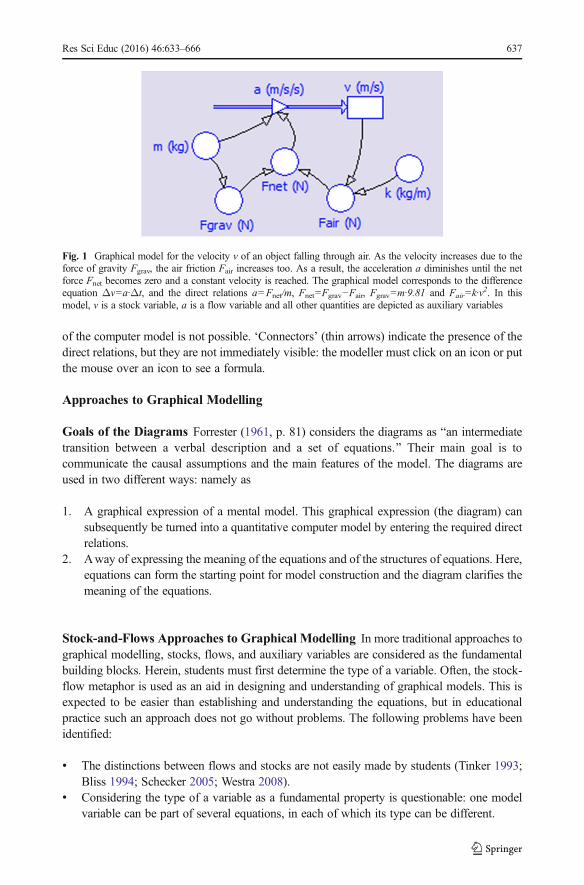
of the computer model is not possible. ‘Connectors’ (thin arrows) indicate the presence of thedirect relations, but they are not immediately visible: the modeller must click on an icon or putthe mouse over an icon to see a formula.

Approaches to Graphical Modelling

Goals of the Diagrams Forrester (1961, p. 81) considers the diagrams as Ban intermediatetransition between a verbal description and a set of equations.^ Their main goal is tocommunicate the causal assumptions and the main features of the model. The diagrams areused in two different ways: namely as

1. A graphical expression of a mental model. This graphical expression (the diagram) cansubsequently be turned into a quantitative computer model by entering the required directrelations.

2. Away of expressing the meaning of the equations and of the structures of equations. Here,equations can form the starting point for model construction and the diagram clarifies themeaning of the equations.

Stock-and-Flows Approaches to Graphical Modelling In more traditional approaches tographical modelling, stocks, flows, and auxiliary variables are considered as the fundamentalbuilding blocks. Herein, students must first determine the type of a variable. Often, the stock-flow metaphor is used as an aid in designing and understanding of graphical models. This isexpected to be easier than establishing and understanding the equations, but in educationalpractice such an approach does not go without problems. The following problems have beenidentified:

& The distinctions between flows and stocks are not easily made by students (Tinker 1993;Bliss 1994; Schecker 2005; Westra 2008).

& Considering the type of a variable as a fundamental property is questionable: one modelvariable can be part of several equations, in each of which its type can be different.

Fig. 1 Graphical model for the velocity v of an object falling through air. As the velocity increases due to theforce of gravity Fgrav, the air friction Fair increases too. As a result, the acceleration a diminishes until the netforce Fnet becomes zero and a constant velocity is reached. The graphical model corresponds to the differenceequation Δv=a·Δt, and the direct relations a=Fnet/m, Fnet=Fgrav−Fair, Fgrav=m·9.81 and Fair=k·v

2. In thismodel, v is a stock variable, a is a flow variable and all other quantities are depicted as auxiliary variables

Res Sci Educ (2016) 46:633–666 637

& According to Bliss (1994), the representation of the rate of change of a variable as itselfanother variable is problematic for students of age 12–14 years. When not confident of thisidea, students cannot express themselves with stock-flow diagrams.

& Students of age 16–18 years tend to use objects, events, and processes instead of truevariables (in the sense of measurable properties) when trying to conceptualize theirmodels, although this seems to depend on the problem that is modelled (Kurtz dos Santosand Ogborn 1994).

& Not all students have sufficient prior knowledge of the flow of a fluid through avalve and its accumulation in a tank to understand this as a metaphor for stock-flowdiagrams (Tinker 1993).

& After an instruction based on this metaphor, the stock-flow diagrams are not yet easilygrasped by many a student (Tinker 1993; Sins et al. 2005; Lane 2008).

& The stock-flow metaphor is not very useful for modelling dynamics, as it is hard toimagine ‘position’ as a stock where ‘velocity’ accumulates (Tinker 1993).

& Even if the use of differential equations can be circumvented, the use of directrelations cannot be avoided. Lower secondary students can have difficulty usingthese relations if they do not have the required notions of variable and formula (VanBuuren et al. 2012).

& Students may think that variables only depend on variables to which they are directlylinked (Van Buuren et al. 2011).

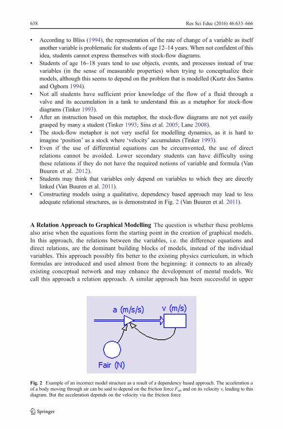
& Constructing models using a qualitative, dependency based approach may lead to lessadequate relational structures, as is demonstrated in Fig. 2 (Van Buuren et al. 2011).

A Relation Approach to Graphical Modelling The question is whether these problemsalso arise when the equations form the starting point in the creation of graphical models.In this approach, the relations between the variables, i.e. the difference equations anddirect relations, are the dominant building blocks of models, instead of the individualvariables. This approach possibly fits better to the existing physics curriculum, in whichformulas are introduced and used almost from the beginning: it connects to an alreadyexisting conceptual network and may enhance the development of mental models. Wecall this approach a relation approach. A similar approach has been successful in upper

Fig. 2 Example of an incorrect model structure as a result of a dependency based approach. The acceleration aof a body moving through air can be said to depend on the friction force Fair and on its velocity v, leading to thisdiagram. But the acceleration depends on the velocity via the friction force

638 Res Sci Educ (2016) 46:633–666

secondary mathematics education (Heck et al. 2009a). Central to the relation approachare the link between a difference equation and a stock-flow diagram, and the interpre-tation of connectors as indicating structures of direct relations.

Interpretation of Diagrams

In order to find out to what extent students are able to interpret the diagrams, first, we reflect onwhat exactly can be derived from the diagrams. In the diagrams, two different subsystems areused: a subsystem representing direct relations and a subsystem representing differenceequations.

Subsystem 1: relation structures formed by connectors.

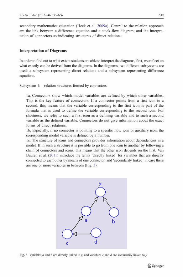
1a. Connectors show which model variables are defined by which other variables.This is the key feature of connectors. If a connector points from a first icon to asecond, this means that the variable corresponding to the first icon is part of theformula that is used to define the variable corresponding to the second icon. Forshortness, we refer to such a first icon as a defining variable and to such a secondvariable as the defined variable. Connectors do not give information about the exactforms of direct relations.1b. Especially, if no connector is pointing to a specific flow icon or auxiliary icon, thecorresponding model variable is defined by a number.1c. The structure of icons and connectors provides information about dependencies in amodel. If in such a structure it is possible to go from one icon to another by following achain of connectors and icons, this means that the other icon depends on the first. VanBuuren et al. (2011) introduce the terms ‘directly linked’ for variables that are directlyconnected to each other by means of one connector, and ‘secondarily linked’ in case thereare one or more variables in between (Fig. 3).

Fig. 3 Variables a and b are directly linked to y, and variables c and d are secondarily linked to y

Res Sci Educ (2016) 46:633–666 639

Subsystem 2: stock-flow diagrams.

2a. A difference equation can be translated into a stock-flow diagram, and vice versa,under the condition that the modeller knows which variable is the independent variable(the variable of integration, usually time).2b. Because graphical models are essentially about numerical integration and not differ-entiation, the relation structure in stock-flow diagrams is always the same: the stockdepends on the flows that are connected to it, but a flow does not need to depend onthe stock. The value of a stock also depends on previous values of the stock. The flowsdetermine the change of the stock.

Even in a relation approach, students may still have difficulties interpreting the diagrams:

– In physics and mathematics, formulas can be inverted at will, to calculate each of itscomponents, depending on which components are given in advance. But in a graphicalmodel, a formula is used to calculate only one of its components. Which component iscalculated is completely determined by the model structure. This is not straightforward;students may think that they are free to choose which component is calculated by theformula (Van Buuren et al. 2011). Thus, students may have difficulty understanding points1a, 2a and 2b. We refer to this as the ‘relation inversion conception’.

– An error that may follow from this relation inversion conception is the use of circulardefinitions: within one model, one direct relation is used twice. For example, students maydefine the acceleration a as Fnet/m while simultaneously defining Fnet as m·a (Van Buurenet al. 2011).

Main Research Question and Research Methodology

The main research question is

How do students understand the relation structures used in graphical system dynamicsbased modelling after a relation-based instruction?

The term understanding is operationalised as being able to derive the information providedby the diagrams as described in BInterpretation of Diagrams^ section and to construct orextend graphical models on the basis of given formulas.

We applied an educational design research approach (Van den Akker et al. 2006): instruc-tional materials were designed, tested in classroom and redesigned in several cycles. Theresearch had an explorative character. The reason is that graphical modelling with youngstudents being fully integrated into the entire lower secondary physics curriculum, is new, to thebest of our knowledge. We applied several research instruments to monitor the learningprocesses. Data sources were audio-recorded participatory observations during the lessonsand in-class impromptu interviews, student results of modelling tasks (writings, computerresults, and screen recordings) and regular tests. We did not feel a need for applying theclassical instrument of in-depth interviews from a representative sample because research wascarried out in Montessori education, in which learning processes of students are permanentlymonitored and in-class impromptu interviews are common. The students’ answers to the

640 Res Sci Educ (2016) 46:633–666

regular test questions about all aspects of the diagrams are the primary sources for answeringthe research question. Answers of a student within one test can be expected to be coherent.This qualitative coherence gives insight in to the students’ understanding and is thereforestudied. The students’ answers are listed and analysed on the basis of three criteria: (1) whichsubsystem is addressed? (2) what is the type of the relation between the model variables? and(3) is it an interpretation or construction question?

In line with BInterpretation of Diagrams^ section, the subsystem can be either the structureformed by connectors or the stock-flow diagram. Because these subsystems are not necessarilydisjoint, in the analysis, we also pay attention to the effects of combining the subsystems. Thetype of relation between model variables is described in terms of occurrence of variables indefinitions and in terms of dependency between variables. For relation structures formed byconnectors, this means the distinction between directly and secondarily linked relations; forstock-flow diagrams, this means the translation from a stock-flow diagram into a differenceequation and the dependency of (the change of) the stock on the connected flows. Thecombination of subsystems also makes a clear distinction between difference equation anddirect relation important.

The other sources of data are used to increase trustworthiness of the findings. Thequantification of the quality of the student answers was used in each developmental cycle toimprove the instructional design. It is not applied to measure the progress in students’performance by statistical methods. The main reason is that, in our setting, the students werestimulated to collaborate and the teachers were still learning how to deal with unexpectedstudent obstacles. In this realistic setting, student results can be expected to be mutuallydependent to a certain degree; therefore, the validity of statistical analysis is questionable.

Design of the Partial Learning Path and Overview of the Implementation

Design Considerations

The instructional design has been guided by principles of cognitive load theory to reduceextraneous cognitive load and optimize intrinsic and germane load for novice learners toenable development of deeper understanding (see Plass et al. 2010). Here are a few ways wehave attempted to reduce the cognitive load: we subdivided tasks and contents into manage-able chunks (segmenting principle). We gradually increased the number of elements in thegraphical model that the students were able to manage (sequencing principle). Studentsreceived worked examples and partially completed problems to go through for initial cognitiveskill acquisition (worked-example and completion principle). We provided students with priorinstruction about behaviour of complex system’s components before presenting the wholesystem (pretraining principle). We let students work with examples from various physics andnon-physics subjects (the variable examples principle).

Results from field testing of pilot versions of the learning path were also used for thedesign. Changes based on early classroom experiments are the following:

& Because of the importance of difference equations as fundamental building blocks, Δ-notation was used almost directly from the start of the learning path. This was actually arecommendation of students confronted with a change in notation at a later stage. Theydeclared that using Δ-notation from the beginning would be easier and less confusing.

Res Sci Educ (2016) 46:633–666 641

& Because lower secondary students’ notions of formula and variable turned out to beinsufficient for graphical modelling (Van Buuren et al. 2012), students get operationaldefinitions of formula and variable in an early stage, before the formal introduction of thetwo subsystems used in the diagrams.

& Because of students’ difficulties with finding a construction order (Van Buuren et al.2011), we offered them a general construction plan for graphical models based on therelation approach in accordance with the goal-free principle. We advised them to

1. Collect or establish all formulas for the situation to be modelled.2. Create the stock-flow diagrams corresponding to the difference equations.3. Proceed with defining the variables in the diagram that have not yet been defined.

For step 3, it was important that students understood that the stock-flow diagram automat-ically determined the difference equation by which the stock was defined, but that all flowsneeded to be defined explicitly, by entering a direct relation. Also, students must understandthat circular definitions are not allowed.

& In order to diminish cognitive load, both subsystems were not introduced simultaneously,but separately, in successive modules in the learning path. Eventually, students must learnto combine both sub systems. A pilot study with a group of 23 students, indicated that thiswas difficult for the students to achieve. This followed clearly from their answers to themultiple choice questions described in Fig. 4. After an instruction in which both subsys-tems were explained, none of these students selected both correct options.

Overview of the Design and Implementation of the Partial Learning Pathon Graphical Models

In the design, six phases are distinguished, labelled 1 to 6.

1. Orientation phase. In this phase, students are provided with several direct relations anddifference equations; Δ-notation is used from the beginning. They also get acquaintedwith basic features of the computer learning environment and orientate themselves withnumerical integration. Learning goals in this phase are orientation and learning-to-use,rather than understanding at a structural level.

2. Pretraining phase. All elements that are prerequisites for understanding diagrams and theirrelationship with formulas are introduced one by one at a more formal level.

Fig. 4 Choose the two options that can correspond to the diagrams. Options B and F are correct

642 Res Sci Educ (2016) 46:633–666

3. First structural introduction phase. In this phase, the focus is on subsystem 1, the structuresformed by connectors. It starts with the introduction of the key feature of connectors (seeBInterpretation of Diagrams^ section).

4. Intermediate phase. For an understanding of graphical models, an understanding of thedistinction between difference equations and direct relations (or ‘Δ-formulas’ and ‘directformulas’, as they are called in the instructional materials) is required. Therefore, in thisphase, both types of formulas are introduced formally, making use of examples taken frompreceding parts in the learning path.

5. Second structural introduction phase. The relationship between stock-flow diagrams anddifference equations is clarified in a more structural way, and the two subsystems arecoupled.

6. Final phase. The general construction plan is introduced and used by the students toconstruct a more extended model in the computer learning environment, based on a givenset of equations.

The principle setup of the partial learning path on graphical models and the distribution ofthe phases over the modules of the physics curriculum is outlined in Table 1.

Overview of the Relation Approach in de Modules Sound and Force and Movement

In this paper, the focus is on the structural introduction phases. This concerns the modules inSound and Force and Movement. The phenomena that are modelled, sound beats and fallingwith air resistance, are typical examples with a high level of reality that usually are not part ofthe lower secondary physics curriculum because the mathematics surpasses the students’traditional mathematical capabilities.

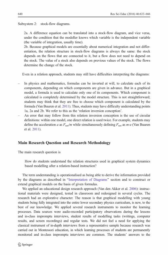
Design of the Module Sound For the formal introduction of the subsystem based on directrelations and formed by connectors (subsystem 1), to minimise extraneous load, we need amodel that consists of direct relations only and contains no stocks and flows. A model forsound beats caused by two tuning forks with slightly different frequencies meets this require-ment. It concerns the addition of two sinusoids. In this context of functions, the independentvariable t (time) must appear explicitly and is displayed by a special icon. Because the sinefunction has not yet been introduced to the students in mathematics class at this stage of thecurriculum, it is introduced as ‘some mathematical function’ of time, frequency, and ampli-tude, and it is mainly represented as a graph. First, students explore this function graphically,using a simulation driven by the model shown in Fig. 5. This figure is also used to introduceauxiliary variables and to explain the key feature of connectors.

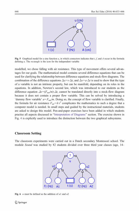
Hereafter, students practise with the role of connectors in exercises on problems of variablefields inside and outside physics (variable examples principle). In these exercises, also a fewstock and flow variables appear, but only as defining, respectively, defined variables. Figure 6is used to explain dependencies: although f1, f2, A1, A2 and t are not explicitly part of theformula for u, they do have a direct influence on u. This means that u depends on these fivevariables. Finally, students must search and enter a suitable formula for u in terms of u1 and u2.

Design of the Module Force and Movement In the module Force and Movement, thesubsystem based on difference equations and formed by stock-flow diagrams (subsystem 2) isintroduced formally, and finally, both subsystems are combined. As phenomenon to be

Res Sci Educ (2016) 46:633–666 643

Tab

le1

Overview

ofthedistributio

nof

thedesign

ofthepartiallearning

path

ongraphicalmodelsover

thecurriculum

Phase

Content

regardingtheunderstandingof

graphicalmodels

Period

aandphysicssubjects

1.Orientatio

nphase

-Firstdirectrelatio

ns-FirstΔ-formulas

-Mainfeatures

ofthecomputerlearning

environm

ent

-Firstuseof

agraphicalmodel

-Initialvalueforastock

-Num

ericalintegration,

roleof

thetim

estep

Firstyear:Density,k

inem

atics,staticforce,

energy

andpower

2.Pretrainingphase

-Introductionof

stock-flow

diagramsandqualitativ

estock-flow

thinking

-Inflow

sandoutflows

-Orientatio

non

therelatio

nbetweenstock-flow

diagram

andΔ-formula

-Operatio

naldefinitionof

form

ula

-Introductionof

adirectrelatio

nin

acomputerlearning

environm

ent

-Operatio

nalintroductio

nof

constant

andof

variableas

varyingquantity

-RelationbetweenΔ-formulaandstock-flow

diagram

-Processof

numericalintegrationin

case

ofafeedback

mechanism

-Use

ofadirectrelationin

agraphicalcomputermodel

-Firstconnector

End

offirstyear,firstmonthsof

second

year:

Energyandpower,resistanceandconductiv

ity,

vacuum

pump

3.Firststructuralintroductio

nphase

-Auxiliaryvariables

-Connectorsandtheirrelatio

nto

thedefinitio

nsof

modelvariables

(the

keyfeatureof

connectors)

-Secondarily

linkedvariablesanddependencies

-Flow

sboth

asdefining

variablesandas

definedvariables

-Stocks

asdefining

variables

-Introductionof

theindependentvariable(tim

e)-Explicituseof

theindependentvariablein

amodelform

ula

Half-way

second

year:So

und

4.Interm

ediatephase

-Fo

rmalintroductio

nof

thedistinctionbetweendifference

equations

anddirectrelatio

nsLastmonthsof

second

year:Fo

rceand

movem

ent(dynam

ics)

5.Secondstructural

introductio

nphase

-Dependencyin

stock-flow

diagrams

-Mathematicalmeaning

ofoutflow

-Differences

betweenstock-flow

diagramsandstructures

form

edby

connectors

-Po

ssibly

twofold(orthreefold)

rolesof

avariable;coupleddifference

equations;

dummyvariables

644 Res Sci Educ (2016) 46:633–666

Tab

le1

(contin

ued)

Phase

Content

regardingtheunderstandingof

graphicalmodels

Period

aandphysicssubjects

-Adaptationof

adifference

equationto

graphicalmodellin

gby

splittingup

into

anew

difference

equationandadirectrelatio

n

6.Finalphase

-Generalconstructio

nplan

-Constructionof

amoreextended

modelbasedon

givenequations

aThe

firstyear

ofthephysicscurriculum

isthesecond

year

ofsecondaryeducationin

theNetherlands

(age,1

3–14

years)

Res Sci Educ (2016) 46:633–666 645

modelled, we chose falling with air resistance. This type of movement offers several advan-tages for our goals. The mathematical model contains several difference equations that can beused for clarifying the relationship between difference equations and stock-flow diagrams. Thecombination of the difference equationsΔx=v·Δt, andΔv=a·Δt is used to show that the typeof a variable is not an intrinsic property, but can be manifold, depending on its roles in theequations. In addition, Newton’s second law, which was introduced to our students as thedifference equation Δv=(Fnet/m)·Δt, cannot be translated directly into a stock-flow diagrambecause it does not contain a proper flow variable. This can be solved by introducing a‘dummy flow variable’ a=Fnet/m. Doing so, the concept of flow variable is clarified. Finally,the formula for air resistance Fair=k·v

2 complicates the mathematics to such a degree that acomputer model is needed. In small steps and guided by the instructional materials, studentsare asked to design this model. Pen-and-paper exercises have been added in which studentspractise all aspects discussed in BInterpretation of Diagrams^ section. The exercise shown inFig. 4 is explicitly used to introduce the distinction between the two graphical subsystems.

Classroom Setting

The classroom experiments were carried out in a Dutch secondary Montessori school. Themodule Sound was studied by 82 students divided over three third year classes (age, 14–

Fig. 6 u must be defined as the addition of u1 and u2

Fig. 5 Graphical model for a sine function u, in which connectors indicates that t, f, and A occur in the formuladefining u. The rectangle is the icon for the independent variable

646 Res Sci Educ (2016) 46:633–666

15 years). In two of these classes, the first author of this paper was the teacher. A third classwas taught by an experienced teacher who had also participated as a teacher at an earlier stageof the project. Because of cancelled lessons, this class did not finish the other module, Forceand Movement. Therefore, the research related to this module was only carried out in the othertwo classes (57 students). Classes consisted of mixed groups of students, preparing for seniorgeneral secondary education and pre-university education. Near the end of the third year ofsecondary education, all students in the Netherlands must have chosen a study profile, i.e. arather fixed combination of examination subjects for upper secondary level. Motivation ofstudents not applying for a science profile often declines. At this Montessori school, it leads toa diminishing number of students participating in the tests towards the end of the year. As aconsequence, in the test results of Force and Movement, there is probably a bias towards hardworking and motivated students. Presumably, the aptitude for science of this group of studentsis more comparable with students who have chosen a science profile with average third yearlower secondary groups.

Students are to some extent allowed to work at their own pace and to postpone a test untilthey are ready for it. They are allowed to redo a test if they fail the first time. Test results of thefirst attempts are used for research purposes, for pragmatic reasons and to avoid a bias towardsgood results.

We received 67 final tests of Sound and 27 final tests of Force and Movement. There weremore than 3 months between these final tests.

Test Question of the Module Sound

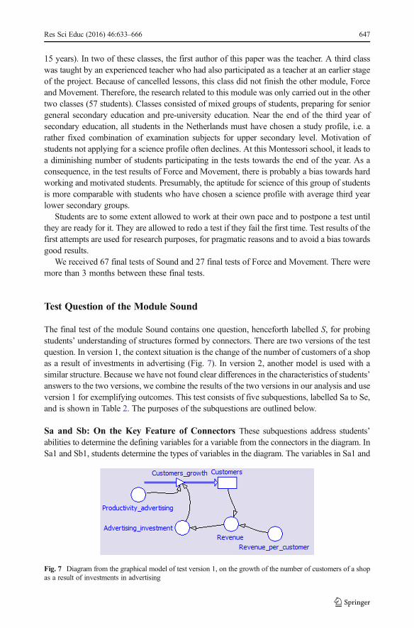
The final test of the module Sound contains one question, henceforth labelled S, for probingstudents’ understanding of structures formed by connectors. There are two versions of the testquestion. In version 1, the context situation is the change of the number of customers of a shopas a result of investments in advertising (Fig. 7). In version 2, another model is used with asimilar structure. Because we have not found clear differences in the characteristics of students’answers to the two versions, we combine the results of the two versions in our analysis and useversion 1 for exemplifying outcomes. This test consists of five subquestions, labelled Sa to Se,and is shown in Table 2. The purposes of the subquestions are outlined below.

Sa and Sb: On the Key Feature of Connectors These subquestions address students’abilities to determine the defining variables for a variable from the connectors in the diagram. InSa1 and Sb1, students determine the types of variables in the diagram. The variables in Sa1 and

Fig. 7 Diagram from the graphical model of test version 1, on the growth of the number of customers of a shopas a result of investments in advertising

Res Sci Educ (2016) 46:633–666 647

Sb1 are defined by a formula and by a number (i.e. a constant), respectively. In case studentshave chosen for ‘formula’, the defining variables must be determined. In order to investigatewhether students regard auxiliary variables as different from stocks with respect to connectors,both an auxiliary variable and a stock variable are part of the formula in Sa1. A student isconsidered to understand the key feature of connectors if (s)he correctly answers both Sa2 andSb2. All subsequent’ answers are analysed in relation to the answers to Sa2 and Sb2.

Sc and Sd: On Dependencies of Secondarily Linked Variables These subquestionsprobe the students’ understanding of dependencies as indicated by the structures of connectorsand icons. In both subquestions, the chain of connectors ends in the same flow variable. Thestarting point is different: in Sc, it is an auxiliary variable and in Sd, it is a stock variable, thechange of which is determined by the flow variable. By comparing students’ answers to thesetwo subquestions, we want to study effects of mixing the subsystems.

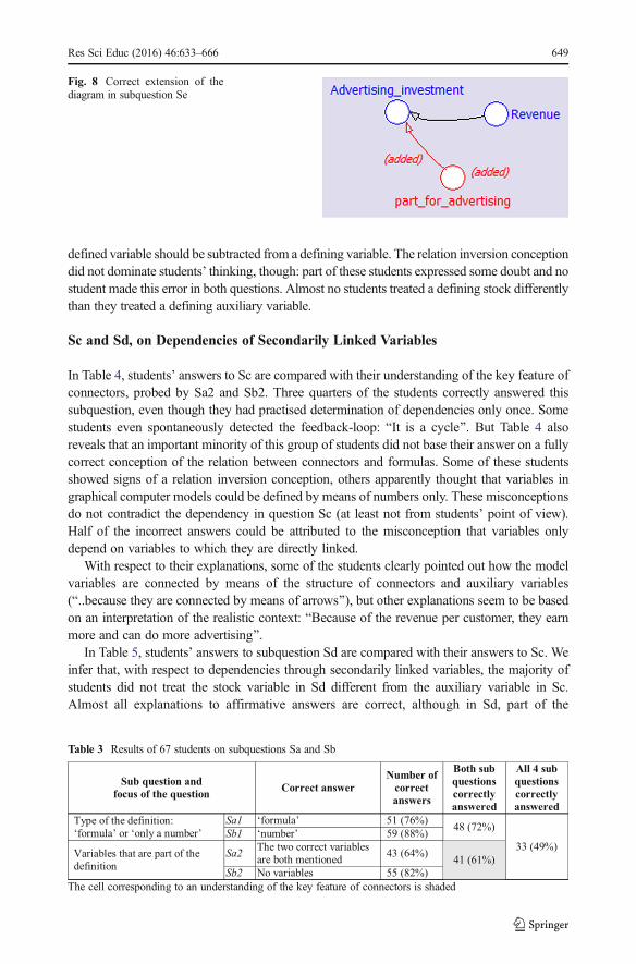
Se: On Formula-based Construction of Structures of Connectors and AuxiliaryVariables In this subquestion students are asked to incorporate a new direct relation intothe graphical model. The essential part of the correct answer is shown in Fig. 8.

Outcomes of the Test Question of the Module Sound

Sa and Sb, on the Key Feature of Connectors

The number of correct answers to subquestions Sa and Sb are listed in Table 3. It shows thathalf of the students correctly answered all four subquestions and that about 61 % understoodthe key feature of connectors. Some students clearly based their answers on the diagram (bystatements such as Bbecause there are two auxiliary variable arrows pointing to the smallsphere for Revenue^), but for many answers, it is not possible to distinguish whether thestudents based their answer on the diagram or on the realistic context situation. We found eightindications (12% of all students) of the relation inversion conception described in BInterpretationof Diagrams^ section. These students probably thought that a defined variable could also appearin the definition of one of its defining variables; some students even answered that a

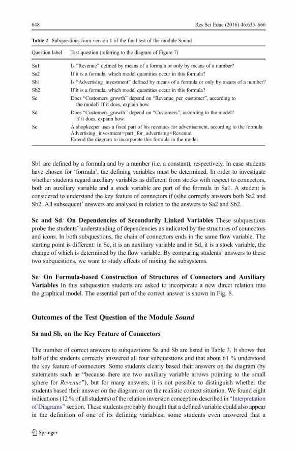
Table 2 Subquestions from version 1 of the final test of the module Sound

Question label Test question (referring to the diagram of Figure 7)

Sa1 Is BRevenue^ defined by means of a formula or only by means of a number?

Sa2 If it is a formula, which model quantities occur in this formula?

Sb1 Is BAdvertising_investment^ defined by means of a formula or only by means of a number?

Sb2 If it is a formula, which model quantities occur in this formula?

Sc Does BCustomers_growth^ depend on BRevenue_per_customer^, according tothe model? If it does, explain how.

Sd Does BCustomers_growth^ depend on BCustomers^, according to the model?If it does, explain how.

Se A shopkeeper uses a fixed part of his revenues for advertisement, according to the formulaAdvertising_investment=part_for_advertising×Revenue.Extend the diagram to incorporate this formula in the model.

648 Res Sci Educ (2016) 46:633–666

defined variable should be subtracted from a defining variable. The relation inversion conceptiondid not dominate students’ thinking, though: part of these students expressed some doubt and nostudent made this error in both questions. Almost no students treated a defining stock differentlythan they treated a defining auxiliary variable.

Sc and Sd, on Dependencies of Secondarily Linked Variables

In Table 4, students’ answers to Sc are compared with their understanding of the key feature ofconnectors, probed by Sa2 and Sb2. Three quarters of the students correctly answered thissubquestion, even though they had practised determination of dependencies only once. Somestudents even spontaneously detected the feedback-loop: BIt is a cycle^. But Table 4 alsoreveals that an important minority of this group of students did not base their answer on a fullycorrect conception of the relation between connectors and formulas. Some of these studentsshowed signs of a relation inversion conception, others apparently thought that variables ingraphical computer models could be defined by means of numbers only. These misconceptionsdo not contradict the dependency in question Sc (at least not from students’ point of view).Half of the incorrect answers could be attributed to the misconception that variables onlydepend on variables to which they are directly linked.

With respect to their explanations, some of the students clearly pointed out how the modelvariables are connected by means of the structure of connectors and auxiliary variables(B..because they are connected by means of arrows^), but other explanations seem to be basedon an interpretation of the realistic context: BBecause of the revenue per customer, they earnmore and can do more advertising^.

In Table 5, students’ answers to subquestion Sd are compared with their answers to Sc. Weinfer that, with respect to dependencies through secondarily linked variables, the majority ofstudents did not treat the stock variable in Sd different from the auxiliary variable in Sc.Almost all explanations to affirmative answers are correct, although in Sd, part of the

Table 3 Results of 67 students on subquestions Sa and Sb

Sub question and

focus of the questionCorrect answer

Number of

correct

answers

Both sub

questions

correctly

answered

All 4 sub

questions

correctly

answered

Type of the definition:

‘formula’ or ‘only a number’

Sa1 ‘formula’ 51 (76%)48 (72%)

33 (49%)

Sb1 ‘number’ 59 (88%)

Variables that are part of the

definition

Sa2 The two correct variables

are both mentioned43 (64%)

41 (61%)

Sb2 No variables 55 (82%)

The cell corresponding to an understanding of the key feature of connectors is shaded

Fig. 8 Correct extension of thediagram in subquestion Se

Res Sci Educ (2016) 46:633–666 649

explanations are based on an understanding of the realistic context. Students’ answers andargumentations show that the presence of a stock-flow diagram in the test question has beenconfusing for approximately a quarter of the students. There are two ways the stock-flowdiagram may have influenced the students:

1. The stock-flow diagram, or the corresponding realistic situation, may have dominated thestudents’ perception. The perception that the stock depends on the flow and not vice-versacan clearly be found in the explanations of some of the students who considered the flowas depending on the auxiliary variable (in Sc), but not on the stock variable (in Sd). Thisstudent referred to the direction of the flow Customers_growth in Figure 7: “No,Customers_growth goes to Customers^. In other words, Customers_growth has influenceon Customers (and not vice versa). It is possible that more students held this opinion; theothers gave no clear explanation. Inspection of the students’ answers to question Sa2, inwhich the stock is a defining variable, reveals that this perception is not caused by anincorrect understanding of the key feature of connectors.

2. Four affirmative answers to question Sd were based on inversion of the stock-flowrelationship.

Se, on Formula-Based Construction of Structures of Connectors and AuxiliaryVariables

In Table 6, students’ answers to subquestion Se are compared with their answers to thesubquestions probing the understanding of the key feature of connectors. Question Se isanswered correctly by almost half of all students, but a quarter of these correct answers are

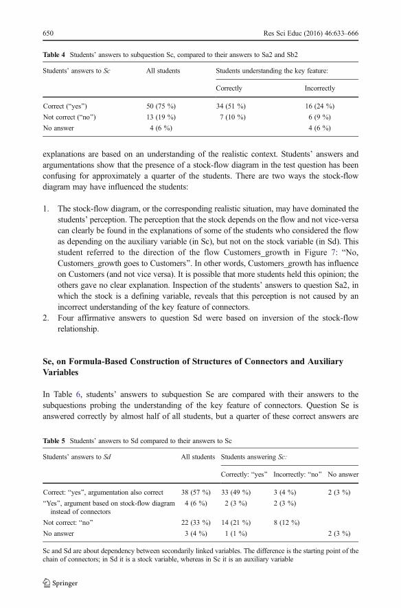
Table 4 Students’ answers to subquestion Sc, compared to their answers to Sa2 and Sb2

Students’ answers to Sc All students Students understanding the key feature:

Correctly Incorrectly

Correct (Byes^) 50 (75 %) 34 (51 %) 16 (24 %)

Not correct (Bno^) 13 (19 %) 7 (10 %) 6 (9 %)

No answer 4 (6 %) 4 (6 %)

Table 5 Students’ answers to Sd compared to their answers to Sc

Students’ answers to Sd All students Students answering Sc:

Correctly: Byes^ Incorrectly: Bno^ No answer

Correct: Byes^, argumentation also correct 38 (57 %) 33 (49 %) 3 (4 %) 2 (3 %)

BYes^, argument based on stock-flow diagraminstead of connectors

4 (6 %) 2 (3 %) 2 (3 %)

Not correct: Bno^ 22 (33 %) 14 (21 %) 8 (12 %)

No answer 3 (4 %) 1 (1 %) 2 (3 %)

Sc and Sd are about dependency between secondarily linked variables. The difference is the starting point of thechain of connectors; in Sd it is a stock variable, whereas in Sc it is an auxiliary variable

650 Res Sci Educ (2016) 46:633–666

most likely based on an incorrect understanding of connectors. Most students answers fromthis quarter show signs of the relation inversion conception or of the conception that ingraphical models only numbers are used to define variables.

Other students correctly translated the direct relation into a model structure, but added anextra connector. The most frequent addition (Fig. 9) may have been based on students’interpretation of the corresponding realistic situation, in which it would make sense to calculatepart_for_advertising from Revenue. Apparently, these students understood how connectorscorrespond to direct relations, but they also added a reality-based element. Some students gavethe incorrect answer shown in Fig. 10. Here, the diagram seems to be viewed as a flow chartfor the money.

Summary of the Outcomes of the Test Question from the Module Sound

Approximately half of the students correctly answered all questions about structures formed byconnectors. Per item, the scores were somewhat better. Apparently, many students had a basicunderstanding of the key feature of connectors. Also, many students correctly understooddependencies. Only 10 % of all students considered secondarily linked variables as notdependent on each other. Only a minority of students had been troubled by the presence ofa stock-flow diagram in a chain of connectors. Constructing (part of) a model was the mostdifficult task. The outcomes of the subquestions also show that students arrived at correctconclusions with respect to model structure without having a complete understanding of theunderlying concepts, using alternative conceptions:

– Students used their understanding of the realistic context and did not interpret the diagramstructure.

– Students holding a relation inversion conception arrived at correct answers to almost allquestions.

Table 6 Students’ answers to subquestion Se compared to their answers to Sa2 and Sb2

Studens’ answers to Se All students Students understanding the key feature:

Correctly Incorrectly

Correct (see Fig. 8) 31 (46 %) 23 (34 %) 8 (12 %)

Correct + extra connector 12 (18 %) 9 (13 %) 3 (4 %)

Not correct 13 (19 %) 5 (7 %) 8 (12 %)

No answer 11 (16 %) 4 (6 %) 7 (10 %)

Fig. 9 A frequent answer tosubquestion Se. This diagram isin accordance with the direct rela-tion that must be added, but also anextra connector is drawn

Res Sci Educ (2016) 46:633–666 651

– The misconception by students that all model variables may only be defined by numbersdid not lead them to incorrect conclusions regarding dependencies.

Test Questions from the Module Force and Movement

Three test questions, F1, F2, and F3, have been designed. F1 probes the interpretation of adiagram. Its structure is similar to the test question in Sound. F2 and F3 are constructionquestions. Purposes of the questions are outlined in below subsections.

Test Question F1, on the Interpretation of Diagrams

Question F1 consists of four subquestions. In subquestions F1a to F1c, students must deriveinformation about the definitions of three model variables from the diagram in Fig. 11.Students’ understanding of dependencies is investigated in F1d.

Subquestions F1a, F1b, and F1c, on the Definitions of Model Variables In F1a to F1cthe focus is on students’ interpretations of stock-flow diagrams and on effects of mixing stock-flow diagrams and structures of connectors.

– In F1a, the defined variable is an outflow of a stock-flow diagram (H_decrease in Fig. 11).This outflow must be defined by a direct relation consisting of an auxiliary variable, astock variable from a second stock-flow diagram, and the stock-variable from its ownstock-flow diagram. This combination has been chosen to find out to what extent studentsare confused by the stock-flow diagram which the outflow is part of.

– In F1b, the defined variable is an auxiliary variable that is defined by a number.

Fig. 10 Example of an incorrectanswer to subquestion Se from testversion 1

Fig. 11 Diagram from test question F1. Subquestions are about the encircled model variables

652 Res Sci Educ (2016) 46:633–666

– In F1c, the defined variable is the stock from the stock-flow diagram used in F1a (Haresin Fig. 11). The question is whether students realise that in the formula defining thechange of the stock only both its flows and the time step can appear. This stock is alsodirectly linked to three other model variables. A question for research is to what extentstudents are confused by the presence of these other variables.

Subquestion F1d, on the Dependency of a Stock on its Outflow In subquestion F1d,students are asked whether the stock Foxes in Fig. 11 depends on the constant auxiliaryvariable F_mortality_factor and to explain their answers. These variables are secondarilylinked, with the outflow of the stock as an intermediate variable. This subquestion has beendesigned to investigate:

1. Whether students consider a stock variable as dependent on its outflow(s). The differencebetween F1c and F1d is that in F1c, students are asked about the definition of the stock,whereas F1d is about dependency. In F1d, the relation between stock and flow is one oftwo relations linking the auxiliary variable F_mortality_factor secondarily to the stockFoxes. Students’ explanations are also analysed with respect to the misconception thatvariables do not depend on each other in case they are not directly linked.

2. To what extent students base their answer on the graphical model, and to what extent theirunderstanding of the realistic context is involved.

Test Question F2, on Formula-based Construction of Diagrams

The students’ ability to construct a diagram for a given system of formulas is investigated. Theformulas are a difference equation containing one flow variable and a direct relation definingthis flow, in the context of electrical circuits.

Test Question F3, on the Construction of a Graphical Model for a Realistic Situation

This question is designed to probe to what extent students are able to construct simple versionsof both types of formulas (direct relations and difference equations) for a given contextsituation, and to investigate how their ability to construct these formulas relates to their abilityto construct the diagram for the realistic situation. The context is forestry. The correctdifference equation contains two flow variables, of which the inflow is a constant and theoutflow depends on the stock variable. Students are asked to construct this difference equation(F3a), the direct relation for one of the flow variables (F3b), and the diagram (F3c).

Outcomes of the Test Questions of the Module Force and Movement

F1, on the Interpretation of Diagrams

F1a to F1c, on the Definitions of Model Variables

To subquestion F1b, about the model variable that must be defined by a number only, 89 % of allstudents’ answers are correct. Occasionally, signs of a relation inversion conception can be detected.

Res Sci Educ (2016) 46:633–666 653

Results on questions F1a and F1c are shown in Tables 7 and 8, respectively. Only a verysmall number of students incorrectly thought that the model variables in these questions aredefined by numbers, but many of the other students had problems with the designation of theseformulas. Misnaming occurred more often in the case of a formula defining a flow than in thecase of a formula defining a stock. Apparently, students are tempted to call any formula that involvesa flow or a stock a difference equation. But in graphical modelling, flows can only be defined bydirect relations or numbers, and stocks are always defined by means of difference equations.

Table 7 shows that a majority (70 %) of the students understand the key feature ofconnectors in spite of problems with designation. Table 8 shows that understanding the relationstructure of stock-flow diagrams is more problematic: merely 41 % of all students correctlymentioned both flow variables as being part of the definition for the stock variable in testquestion F1c. An important error is mentioning the inflow, but not the outflow. We thought oftwo reasons for the alternative conception that a stock is not influenced by its outflow(s). Thefirst reason is diagram-based: students may be confused by the similarity between flow iconsand connectors, because both are represented by arrows. The second reason may be thatstudents think that an outflow does not have an influence on a stock. In answers to otherquestions, students often only discuss increases of variables and rarely mention decreases. Ifthis is what students really think, then their answers on test questions F1d and F3 should alsoindicate this, however, we only found one indication of a student thinking that outflow doesnot have an influence on a stock.

Furthermore, no students mentioned time or a time step as part of the formula defining thestock. Other student errors in test question F1c were the reversion of the connectors linked tothe stock variable and confusion of ‘dependency’ with ‘being part of a formula’ for constantsthat are directly connected to some part of the stock-flow diagram.

Table 7 Student answers to test question F1a

Model variables that appear in the definitiona

Type of definitiona Correct Incorrect Total

)%11( 3)%11( 3rebmuN

Direct relation 11 (41%) 2 (7%) 13 (48%)

Difference equation 8 (30%) 3 (11%) 11 (41%)

)%001( 72)%03( 8)%07( 91latoT

In F1a, students must name the type of definition of a flow variable (H_decrease in Fig. 11). The correct type ofdefinition is direct relation. They must also write down the defining variables. These are the stocks Hares andFoxes, and the constant auxiliary H_decrease_factor. The cell corresponding to the completely correct answer isshadeda According to the students

Table 8 Student answers to test question F1c

Model variables that appear in the definition of the stocka

Type of definitiona only both flows inflow, but no outflow otherwise incorrect Total

)%7(2)%7(2rebmuN

Direct relation 2 ( 7%) 4 (15%) 2 (7%) 8 (30%)

Difference equation 9 (33%) 5 (19%) 3 (11%) 17 (63%)

)%001(72)%62(7)%33(9)%14(11latoT

In F1c, students are asked to name the type of definition of a stock variable (Hares in Fig. 11). The correct type isdifference equation. They are also asked for the defining variables. These are the flows H_decrease andH_increase (the time or the time step was not mentioned by students). The cell corresponding to the completelycorrect answer is shadeda According to the students

654 Res Sci Educ (2016) 46:633–666

F1d, on the Dependency of a Stock on its Outflow

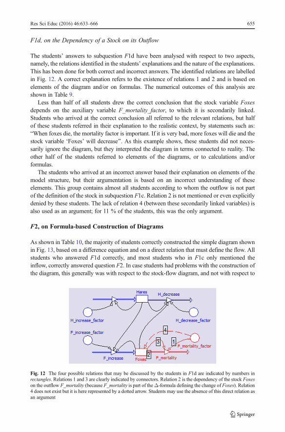
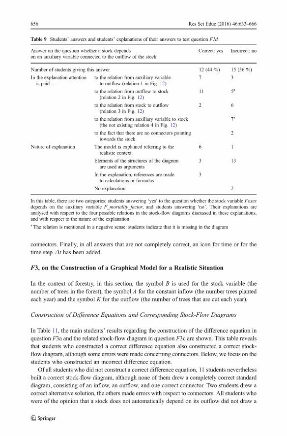
The students’ answers to subquestion F1d have been analysed with respect to two aspects,namely, the relations identified in the students’ explanations and the nature of the explanations.This has been done for both correct and incorrect answers. The identified relations are labelledin Fig. 12. A correct explanation refers to the existence of relations 1 and 2 and is based onelements of the diagram and/or on formulas. The numerical outcomes of this analysis areshown in Table 9.

Less than half of all students drew the correct conclusion that the stock variable Foxesdepends on the auxiliary variable F_mortality_factor, to which it is secondarily linked.Students who arrived at the correct conclusion all referred to the relevant relations, but halfof these students referred in their explanation to the realistic context, by statements such as:BWhen foxes die, the mortality factor is important. If it is very bad, more foxes will die and thestock variable ‘Foxes’ will decrease^. As this example shows, these students did not neces-sarily ignore the diagram, but they interpreted the diagram in terms connected to reality. Theother half of the students referred to elements of the diagrams, or to calculations and/orformulas.

The students who arrived at an incorrect answer based their explanation on elements of themodel structure, but their argumentation is based on an incorrect understanding of theseelements. This group contains almost all students according to whom the outflow is not partof the definition of the stock in subquestion F1c. Relation 2 is not mentioned or even explicitlydenied by these students. The lack of relation 4 (between these secondarily linked variables) isalso used as an argument; for 11 % of the students, this was the only argument.

F2, on Formula-based Construction of Diagrams

As shown in Table 10, the majority of students correctly constructed the simple diagram shownin Fig. 13, based on a difference equation and on a direct relation that must define the flow. Allstudents who answered F1d correctly, and most students who in F1c only mentioned theinflow, correctly answered question F2. In case students had problems with the construction ofthe diagram, this generally was with respect to the stock-flow diagram, and not with respect to

Fig. 12 The four possible relations that may be discussed by the students in F1d are indicated by numbers inrectangles. Relations 1 and 3 are clearly indicated by connectors. Relation 2 is the dependency of the stock Foxeson the outflow F_mortality (because F_mortality is part of theΔ-formula defining the change of Foxes). Relation4 does not exist but it is here represented by a dotted arrow. Students may use the absence of this direct relation asan argument

Res Sci Educ (2016) 46:633–666 655

connectors. Finally, in all answers that are not completely correct, an icon for time or for thetime step Δt has been added.

F3, on the Construction of a Graphical Model for a Realistic Situation

In the context of forestry, in this section, the symbol B is used for the stock variable (thenumber of trees in the forest), the symbol A for the constant inflow (the number trees plantedeach year) and the symbol K for the outflow (the number of trees that are cut each year).

Construction of Difference Equations and Corresponding Stock-Flow Diagrams

In Table 11, the main students’ results regarding the construction of the difference equation inquestion F3a and the related stock-flow diagram in question F3c are shown. This table revealsthat students who constructed a correct difference equation also constructed a correct stock-flow diagram, although some errors were made concerning connectors. Below, we focus on thestudents who constructed an incorrect difference equation.

Of all students who did not construct a correct difference equation, 11 students neverthelessbuilt a correct stock-flow diagram, although none of them drew a completely correct standarddiagram, consisting of an inflow, an outflow, and one correct connector. Two students drew acorrect alternative solution, the others made errors with respect to connectors. All students whowere of the opinion that a stock does not automatically depend on its outflow did not draw a

Table 9 Students’ answers and students’ explanations of their answers to test question F1d

Answer on the question whether a stock dependson an auxiliary variable connected to the outflow of the stock

Correct: yes Incorrect: no

Number of students giving this answer 12 (44 %) 15 (56 %)

In the explanation attentionis paid …

to the relation from auxiliary variableto outflow (relation 1 in Fig. 12)

7 3

to the relation from outflow to stock(relation 2 in Fig. 12)

11 5a

to the relation from stock to outflow(relation 3 in Fig. 12)

2 6

to the relation from auxiliary variable to stock(the not existing relation 4 in Fig. 12)

7a

to the fact that there are no connectors pointingtowards the stock

2

Nature of explanation The model is explained referring to therealistic context

6 1

Elements of the structures of the diagramare used as arguments

3 13

In the explanation, references are madeto calculations or formulas

3

No explanation 2

In this table, there are two categories: students answering ‘yes’ to the question whether the stock variable Foxesdepends on the auxiliary variable F_mortality_factor, and students answering ‘no’. Their explanations areanalysed with respect to the four possible relations in the stock-flow diagrams discussed in these explanations,and with respect to the nature of the explanationa The relation is mentioned in a negative sense: students indicate that it is missing in the diagram

656 Res Sci Educ (2016) 46:633–666

completely correct standard diagram. Apparently, this alternative conception has influencedthe construction of the diagrams, but in different ways. Analysis of the errors in the differenceequations gives more insight. Some errors do not necessarily hinder the construction of thestock-flow diagram. Such errors are the exclusion of Δt from the difference equation and theincorporation of an initial value into the difference equation. Remaining questions are how toexplain why most of these students made errors with respect to connectors, and how to explainthat students who left out a variable for the outflow or the inflow from the difference equationstill could construct a correct stock-flow diagram or alternative diagram. Plausible explana-tions are found by considering consequences of the conception that the stock does not dependon the outflow. In case the difference equation in question F3a contains the variable for theoutflow, from this point of view, there is a conflict that can be solved in two ways:

1. By constructing an alternative solution without using an icon for the outflow, as in Fig. 142. Incorrectly, by adding a connector from the outflow to the stock, which should indicate

that the stock depends on the outflow, as in Fig. 15

We found several examples of both approaches in the students’ work. Another consequenceof the conception that the stock does not depend on the outflow may be that the variable for theoutflow should not appear in the difference equation. We found a few examples of suchdifference equations created by students. These students drew an outflow but also added aconnector to the diagram in a way similar to Fig. 15, or they did not draw a diagram at all.

Most of the students who did not construct a correct stock-flow diagram in question F3 alsodid not construct a correct stock-flow diagram in question F2. A common error was theaddition of an icon to the diagram for the time step in question F2. Further analysis withrespect the time step Δt reveals the following:

– When asked to construct a diagram for a given difference equation in question F2, 30 % ofall students (incorrectly) added an icon for Δt.

– When asked to construct the difference equation for a realistic situation in question F3a,33 % of all students (incorrectly) left out Δt of the equation.

– But when asked to construct a diagram for a realistic situation in question F3c, 85 % of allstudents constructed a diagram without an icon for time or time step. This seems to be aslightly better result. Indeed, one of the arguments in favour of graphical modelling ineducation is that an understanding of difference equations can be circumvented. In

Table 10 Students’ results on test question F2

Quality of the drawn model diagram Number of studentsa

Completely correct 19 (70 %)

Direct relation correctly represented 24 (89 %)

Correct stock-flow diagram for the difference equation. 20 (74 %)

Completely incorrect answers 2 (7 %)

Answers containing an icon for time or time step 8 (30 %)

Students were asked to draw a graphical diagram based on two given formulas: a difference equation and a directrelationa 100 % corresponds to 27 students

Res Sci Educ (2016) 46:633–666 657

addition, the fact that in question F1c no student mentions time as one of the variables thatappear in the formula defining a stock-variable, may mean that students correctly do notconsider time as a causal agent, as is suggested by Kurtz dos Santos and Ogborn (1994).But our results indicate that a reality based construction of a stock-flow diagram may wellconceal an incorrect understanding of the role of time and time step. Students may evennot think of the role of time at all.

Construction of Direct Relations and Corresponding use of Connectors

In question F3b, the formula for the number of trees cut each year (K) must be constructed bythe students. It is given to be 20 % of the number of trees (B). The correct answer is a simpledirect relation involving B.

Main outcomes with respect to the construction of this direct relation and the relatedstructure of connectors in the diagram in question F3c are shown in Table 12. Half of theconstructed direct relations are completely correct. When minor errors, such as calculationerrors, and errors concerning a less adequate conception of variable and formula are ignored,we can state that 78 % of all students realised that K is a function of B.

Approximately, one third of the students drew a diagram in which the structure ofconnectors can be considered as consistent with their answer to question F3b. This numberof consistent diagrams is far less than in question F2. Apparently, question F3, in which thestock-flow diagram and the structure of connectors are more closely intertwined, is moredifficult. As outlined in the section BConstruction of Difference Equations and CorrespondingStock-Flow Diagrams^, an important cause for incorrect structures of connectors is the fact thatK in question F3 is an outflow. The influence of the realistic context situation seems to be a

Fig. 13 Correct diagram to the formulas ΔQ=I·Δt and I=U/R in test question F2

Table 11 Quality of the constructed difference equation in question F3a versus the quality of the constructedstock-flow diagram in question F3c

F3a: constructed difference equation F3c: constructed stock-flow diagram

Correct (or correct alternative diagram) Incorrect or no answer

Correct 9 (33 %) 0 (0 %)

Incorrect 11 (41 %) 7 (26 %)

658 Res Sci Educ (2016) 46:633–666

cause for another error: 19 % of the students drew a connector from the stock B to the inflow,although this inflow was given to be constant. An alternative explanation for this incorrectconnector is that students merely have copied elements from the diagram of question F1.

Summary of the Outcomes of the Test Questions from the Module Forceand Movement

Results confirm that most of the students understand the subsystem formed by connectors andare not troubled by the effects due to mixing of this subsystem with stock-flow diagrams. Avast majority can correctly determine defining variables and can construct simple diagrams asfar as it concerns connectors. Only a few students’ answers show signs of relation inversion.

Students have more difficulty with the relation between stock-flow diagrams and differenceequations. There are two main misconceptions. The first is that students do not sufficientlyunderstand the role of the time step. As a consequence, they forget that the time step is part ofthe difference equation or they add an icon for time or time step when a difference equationmust be converted to a stock-flow diagram. The second alternative conception, held by aquarter of the students, is that a stock variable does not depend on its outflow. A consequenceis that students, trying to deal with this conception, make errors with connectors. The mainreason for this alternative conception is the fact that flows and connectors both are representedas arrows. Students insufficiently appreciate that both types of arrows have completely

Fig. 14 Answer to question F3c of a student who in “F1a to F1c, on the Definitions of Model Variables” sectionwas of opinion that a stock does not depend on an outflow. The only flow in this diagram is an inflow, and whatshould have been an outflow (“K”) is represented by an auxiliary icon which is linked to this inflow. Apart fromthe fact that the connectors are not represented as arrows, this diagram is correct

Fig. 15 Diagram to question F3c of a student who in “F1a to F1c, on the Definitions of Model Variables”section was of opinion that a stock does not automatically depend on an outflow. Erroneously, a superfluous (andincorrect) connector is drawn from the outflow (“K”) to the stock (“B”) to indicate that in this case the stockdepends on the outflow

Res Sci Educ (2016) 46:633–666 659

different meanings. This can be considered as an effect of mixing the subsystems. Anothereffect of mixing may be that students are tempted to call any formula that involves a flow adifference equation. Finally, students have problems with the role of initial values. In spite ofthese problems, results are promising.

From students’ explanations to their answers, we conclude that students who involved therealistic context in their explanations more often correctly identified dependencies betweenvariables than students who based their answers only on the structure of the diagram. Thismakes it difficult to distinguish what students are understanding when they correctly answerquestions concerning a model: the diagram or reality. All students who use mathematics-basedexplanations gave correct answers, but only a few used this type of explanation.

Conclusions and Discussion

The research question addresses students’ understanding of relations structures in graphicalmodelling after relation-based instruction. In this section, we summarise our answer withregard to three aspects: students’ understanding of structures formed by connectors, students’understanding of stock-flow diagrams, and the influence of the realistic situation on students’reasoning and understanding. We position our instructional design and research findings withrespect to approaches and outcomes reported in literature. We briefly discuss why traditionalapproaches seemingly are successful when students work with models but often fail whenstudents must construct models themselves. We also discuss the validity of the researchoutcomes and make recommendations for future design.

Students’ Understanding

Students’ Understanding of Structures Formed by Connectors and DirectRelations Traditional approaches to graphical modelling often use causal reasoning todescribe model relations and dependency of model variables (cf., Groesser 2012a). Ourresearch shows that a relation approach is an alternative effective way to teach young studentsto interpret the structures of graphical models formed by connectors and construct suchstructures. We found that, in this approach, dependency visualised by chains of connectorscan be understood bymany students too, although some of them arrive at correct conclusions by

Table 12 Consistency of the constructed direct relation and the constructed diagram in question F3

Constructed direct relation as definition for K (F3b) Consistency of the diagram as answer to F3c withthe direct relation of F3b

Quality Number ofstudents

Consistent Not completelyconsistent

Nodiagram

Correct function of B 14 (52 %) 7 7

Function of B, containing minor errors 4 (15 %) 1 3

Function of the initial value of B instead of B 3 (11 %) 1 2

Function of another variable or more variables 5 (19 %) 1 3 1

No answer 1 (4 %) 1

Total 27 (100 %) 10 (37 %) 15 (56 %) 2 (8 %)

660 Res Sci Educ (2016) 46:633–666

reality-based reasoning instead of (or together with) diagram-based reasoning, or by usingalternative conceptions. Identified alternative conceptions are the relation inversion conceptionand the conception that in a model only numbers are required, and not formulas involvingvariables. Such misconceptions can easily be left unnoticed in an approach in which littleattention is paid to the mathematical meaning of the relations. Only 10 % of all participants inthis study still think that there is no dependency between secondarily linked variables. Theeffects on students’ understanding also hold when a stock is incorporated at the beginning of achain of connectors and a flow at the end. Only occasionally, students incorrectly ignored such achain in favour of the one-step relation between a flow and corresponding stock.

Students’ Understanding of Stock-Flow Diagrams and Difference Equations Intraditional approaches to graphical modelling, model conceptualisation usually starts withthe determination of stocks and flows straight from the realistic situation. Difference equationsare seldom introduced. This is a fundamental difference with a relation approach, in whichmodel conceptualisation consists of two steps: the determination of the required equations forthe realistic situation, and equation-based construction of the diagrams. We claim that arelation approach circumvents some of the well-known difficulties with traditional stock-flow approaches listed in the section BApproaches to Graphical Modelling^. These are thedifficulties with distinguishing stocks and flows, and obstacles related to the stock-flowmetaphor. This does not mean that all known problems with graphical modelling have beensolved yet, but these problems do not stay underneath the radar and can be explicitly addressedin instruction.

In a relation approach, in the context of physics, the determination of the differenceequations usually is not problematic because many of these difference equations are well-known and are part of the physics curriculum anyway. They form an appropriate starting pointfor the majority of students. Results with respect to equation-based construction of stock-flowdiagrams are promising. Moreover, our research indicates that many of these young studentscan also construct a simple difference equation for a new context situation. But there stillremains some student difficulties that must be solved with equation-based construction ofstock-flow diagrams.

Two of these difficulties can be considered a consequence of the fact that the differenceequations are not clearly visualised in the stock-flow diagrams. The first difficulty is that someof the students are not fully aware of the presence of the time step Δt in the differenceequation. This lack of awareness can be left unnoticed in cases where students are asked toconstruct a stock-flow diagram for a realistic situation without creating a difference equation,as is common practice in traditional approaches. The second difficulty concerns the role of theinitial value with respect to the difference equation. This role is not made clear by the diagramsor the dialog window for defining a stock. The fact that for a stock only the number for theinitial value must be entered may even contribute to the misconception that a stock is notdefined by a formula at all (Van Buuren et al. 2012). One goal of the diagrams is communi-cating the model to people with less mathematics education (cf., Lane 2008), where anunderstanding of difference equations would not be required. This may be true in case thesepeople only have to interpret the graphical models, or listen to a modeller explaining themodel, but the diagrams do not sufficiently communicate the equations for (some of the)novice modellers who are expected to learn to construct models themselves.

A third difficulty is the misconception that a stock does not depend on its outflows. Themain reason for this misconception is that both flows and connectors are represented as arrows.

Res Sci Educ (2016) 46:633–666 661

This conception, of considering the arrows of the flows in the same way as the connectors, has beenexplicitly addressed in the instructional materials (Refer to BOverview of the Relation Approach inde Modules Sound and Force and Movement^) but, apparently, is not easily changed.

The question is how these difficulties can be overcome. Segmenting the learning materialmay have been effective for understanding the subsystem formed by connectors alone, but isapparently not sufficient for teaching students how to understand entire diagrams. From theperspective of cognitive load theory, the diagrams must be considered as high elementinteractivity material (cf., Sweller 1994). The links between the elements of the diagramsand their mathematical counterparts are deliberately not visualised in system dynamics toolsfor the purpose of allowing modellers to focus on the main structures of the model. Such linksmay be redundant for experienced modellers, but for novice learners they are not, as Groesser(2012b) points out and as our results confirm. By not presenting the graphical elements andmathematical counterparts simultaneously, extraneous load is increased (split-attention effect).We think that this extraneous load can be diminished by improving the design of the modellinglearning environment.

Influence of the Realistic Situation on Students’ Reasoning and Understanding Inthe section BOutcomes of the Test Question of the Module Sound^, part of the explanations ofthe students of their answers seem to be based on reality instead of on the diagram. In BF1d, onthe Dependency of a Stock on its Outflow ,̂ it is shown that students who referred to reality intheir explanations more often arrived at the correct conclusion about the dependencies ofvariables than students who based their explanation only on their (incorrect) understanding ofthe diagram. Apparently, there are two ways for students to understand a model for a realsituation: one is based on the diagram structure, the other on the real situation. This makes itdifficult to distinguish what students actually understand when they answer questions about themodel correctly: the model or the real situation. In the cases we have investigated, we suspectthat the students have used their knowledge of reality and some logic to correct theirinterpretation of the diagrams. We noted that some of the students constructed a stock-flowdiagram directly from reality more successfully than they constructed a difference equationfrom reality or a stock-flow diagram from a difference equation. However, this seeminglycorrect reality based construction of a stock-flow diagram may conceal an incorrect under-standing of graphical models. This phenomenon may help to explain findings of research insystem dynamics modelling hitherto, that modelling activities seem to be successful only untilstudents are asked to construct parts of graphical models without assistance (Westra 2008; VanBorkulo 2009). Communication of the causal assumptions and the main features of themathematical model are supposed to be the main purposes of the diagrams. The diagramsapparently are helpful for students to organise their thoughts on reality in a way more or lesssimilar to concept maps. But this strength of the diagrams is at the same time a weakness.Students do not need to fully understand the diagrams for interpreting them. The icons can beinterpreted in several ways. An ‘arrow’ can have at least three different meanings: (1)indicating relationship; (2) representing a flow variable, in which case the arrow givesinformation on the sign of the flow variable in the difference equation for the stock; or, (3)incorrectly, suggesting a direction on a flow chart. Because these arrows are not adequatelylabelled, they can easily be misinterpreted by novice modellers. This shows some resemblancewith concept mapping. Hilbert and Renkl (2008) found that the concept-map characteristicsthat relate most to learning outcomes are the number of correctly labelled and unlabeled links.Here, it also seems to be important for learning that the type of relationship between the

662 Res Sci Educ (2016) 46:633–666

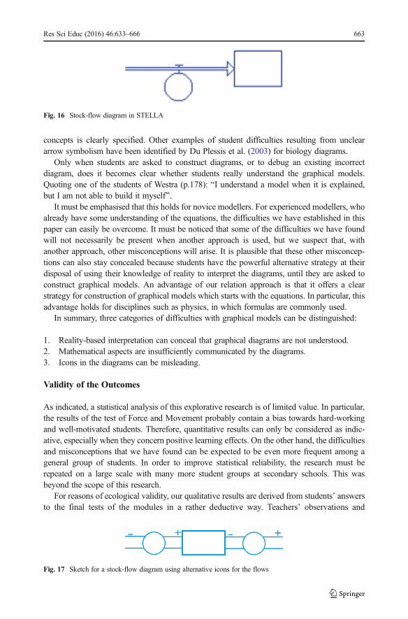
concepts is clearly specified. Other examples of student difficulties resulting from uncleararrow symbolism have been identified by Du Plessis et al. (2003) for biology diagrams.

Only when students are asked to construct diagrams, or to debug an existing incorrectdiagram, does it becomes clear whether students really understand the graphical models.Quoting one of the students of Westra (p.178): BI understand a model when it is explained,but I am not able to build it myself^.

It must be emphasised that this holds for novice modellers. For experienced modellers, whoalready have some understanding of the equations, the difficulties we have established in thispaper can easily be overcome. It must be noticed that some of the difficulties we have foundwill not necessarily be present when another approach is used, but we suspect that, withanother approach, other misconceptions will arise. It is plausible that these other misconcep-tions can also stay concealed because students have the powerful alternative strategy at theirdisposal of using their knowledge of reality to interpret the diagrams, until they are asked toconstruct graphical models. An advantage of our relation approach is that it offers a clearstrategy for construction of graphical models which starts with the equations. In particular, thisadvantage holds for disciplines such as physics, in which formulas are commonly used.

In summary, three categories of difficulties with graphical models can be distinguished:

1. Reality-based interpretation can conceal that graphical diagrams are not understood.2. Mathematical aspects are insufficiently communicated by the diagrams.3. Icons in the diagrams can be misleading.

Validity of the Outcomes

As indicated, a statistical analysis of this explorative research is of limited value. In particular,the results of the test of Force and Movement probably contain a bias towards hard-workingand well-motivated students. Therefore, quantitative results can only be considered as indic-ative, especially when they concern positive learning effects. On the other hand, the difficultiesand misconceptions that we have found can be expected to be even more frequent among ageneral group of students. In order to improve statistical reliability, the research must berepeated on a large scale with many more student groups at secondary schools. This wasbeyond the scope of this research.

For reasons of ecological validity, our qualitative results are derived from students’ answersto the final tests of the modules in a rather deductive way. Teachers’ observations and

Fig. 16 Stock-flow diagram in STELLA

Fig. 17 Sketch for a stock-flow diagram using alternative icons for the flows

Res Sci Educ (2016) 46:633–666 663

impromptu interviews are in agreement with this deduction. The conclusions are plausible, butseparate in-depth interviews may strengthen them. This can be done in follow-up research.

Recommendations for Future Instructional Design

The relation between stock-flow diagrams and difference equations should be made clear fornovice modellers. This might be done by showing the difference equation in the dialog windowfor the stock. Another possibility is to show the students how the diagram can be translated into atext-based model at an early stage of the modelling learning path. In Coach 6, an option isavailable for this translation. But, probably, the most effective is the implementation of an optioninto the modelling software to permanently show all equations to the relevant icons, because thiswould diminish the split-attention effect and therefore would reduce extraneous cognitive load fornovice modellers. This is possible in Simulation Insight (see, for example, Rogers 2008), but inthis modelling environment, all variables are represented by rectangular icons, linked bymeans ofconnectors. The type of a formula is not expressed by the structure of the icons.

We also recommend adaptation of the icons for the flow variables. There exist severalimplementations of system dynamics based graphical modelling. According to Lane (2000),there are at least three or four widely used symbols for flow variables, all taking the form of valveor regulator symbols on the flows, which are indicated by double or thick arrows. In themodellingenvironmentModus, arrows for both the inflows and outflows are oriented from the flow variableto the stock (Klieme andMaichle 1991). Thismay prevent the conception that an outflow does notinfluence the stock, but does not yet clarify the relation between difference equations andstock-flow diagrams. In our opinion, a suitable flow icon should fulfil two conditions:

1. The only difference between an auxiliary variable and a flow variable is that the latter ispart of a difference equation. In all other respects, flow variables and auxiliary variablesare treated the same in the diagrams. Therefore, we recommend to use more similar icons.In Fig. 16, this similarity is already clearer.

2. Icons for flows should differ more from the icons for connectors. A question is whetherflow icons should be arrow-like. From the perspective of a relation approach, a tube-likesymbol in which flow directions are indicated by means of a + or − sign, as sketched inFig. 17, or by means of a word (in or out), might be an alternative.

Acknowledgments This research project has been funded by the Foundation VO Haaglanden.

Conflict of Interest The authors declare that they have no conflict of interest.

Open AccessThis article is distributed under the terms of the Creative Commons Attribution 4.0 InternationalLicense (http://creativecommons.org/licenses/by/4.0/), which permits unrestricted use, distribution, and repro-duction in any medium, provided you give appropriate credit to the original author(s) and the source, provide alink to the Creative Commons license, and indicate if changes were made.

References

Bliss, J. (1994). Causality and common sense reasoning. In H. Mellar, J. Bliss, R. Boohan, J. Ogborn, & C.Tompsett (Eds.), Learning with artificial worlds: Computer-based modelling in the curriculum. London:The Falmer Press.

664 Res Sci Educ (2016) 46:633–666

Doerr, H. M. (1996). Stella ten years later: a review of the literature. International Journal of Computers forMathematical Learning, 1(2), 201–224.

Du Plessis, L., Anderson, T. R., & Grayson, D. J. (2003). Student difficulties with the use of arrow symbolism inbiological diagrams. In J. Lewis, A. Magro, & L. Simonneaux (Eds.), Biology education for the real world:student–teacher–citizen (pp. 89–103). Toulouse: Ecole Nationale de formation agronomique.

Forrester, J. W. (1961). Industrial dynamics. Cambridge: MIT Press.Fuchs, H. U. (2008). System dynamics modeling in fluids, electricity, heat, and motion examples, practical

experience, and philosophy. In E. van den Berg, T. Ellermeijer, & O. Slooten (Eds.), Modelling in physicsand physics education (pp. 166–187). Amsterdam: University of Amsterdam.

Groesser, S. N. (2012a). Mental model of dynamic systems. In Encyclopedia of the sciences of learning (pp.2195–2200). New York: Springer.

Groesser, S. N. (2012b). Model-based learning with system dynamics. In Encyclopedia of the sciences oflearning (pp. 2303–2307). New York: Springer.

Heck, A., Houwing, H., & de Beurs, C. (2009a). An e-class in action: experiences with ICT-intensive teaching andlearning of discrete dynamical models at secondary school. Electronic Journal of e-Learning, 7(1), 41–53.

Heck, A., Kedzierska, E., & Ellermeijer, T. (2009b). Design and implementation of an integrated computerworking environment for doing mathematics and science. Journal of Computers in Mathematics and ScienceTeaching, 28(2), 147–161.

Hilbert, T. S., & Renkl, A. (2008). Concept mapping as a follow-up strategy to learning from texts: whatcharacterizes good and poor mappers? Instructional Science, 36(1), 53–73.

Hmelo-Silver, C. E., & Azevedo, R. (2006). Understanding complex systems: some core challenges. Journal ofthe Learning Sciences, 15(1), 53–61.

Jackson, S. L., Stratford, S. J., Krajcik, J., & Soloway, E. (1996). A Learner-Centered Tool for Students BuildingModels. Communications of the ACM, 39(4), 49.

Klieme, E., & Maichle, U. (1991). Erprobung eines Systems zur Modellbildung und Simulation im Unterricht. InP. Gorny (ed.), Informatik und Schule 1991 (pp. 251–258). Berlin Heidelberg: Springer .

Kurtz dos Santos, A. C., & Ogborn, J. (1994). Sixth form students’ ability to engage in computational modelling.Journal of Computer Assisted Learning, 10(3), 182–200.

Kurtz dos Santos, A. C., Thielo, M. R., & Kleer, A. A. (1997). Students modelling environmental issues. Journalof Computer Assisted Learning, 13(1), 35–47.

Lane, D. C. (2000). Diagramming conventions in system dynamics. The Journal of the Operational ResearchSociety, 51(2), 241–245.

Lane, D. C. (2008). The emergence and use of diagramming in system dynamics: a critical account. SystemsResearch and Behavioral Science, 25(1), 3–23.

Lijnse, P. (2008). Models of/for teaching modeling. In E. Van den Berg, T. Ellermeijer, & O. Slooten(Eds.), Modelling in physics and physics education (pp. 20–33). Amsterdam: University ofAmsterdam.

Löhner, S. (2005). Computer Based Modeling Tasks: the Role Of External Representation. (Doctoral thesis,University of Amsterdam). Amsterdam: University of Amsterdam.

Mandinach, E. B., & Cline, H. F. (1996). Classroom dynamics: the impact of a technology-basedcurriculum innovation on teaching and learning. Journal of Educational Computing Research,14(1), 83–102.

Mayer, R. E., & Moreno, R. (2010). Techniques that reduce extraneous cognitive load and manage intrinsiccognitive load during multimedia learning. In J. L. Plass, R. Moreno, & R. Brünken (Eds.), Cognitive loadtheory (pp. 131–152). New York: Cambridge University Press.

Morgan, M. S. (2001). Models, stories and the economic world. Journal of Economic Methodology, 8(3), 361–384. doi:10.1080/13501780110078972.

Niedderer, H., Schecker, H., & Bethge, T. (1991). The role of computer-aided modelling in learning physics.Journal of Computer Assisted Learning, 7(2), 84–95.

Ogborn, J., & Wong, D. (1984). A microcomputer dynamical modelling system. Physics Education, 19(3), 138–142.

Ormel, B. (2010). Scientific modelling of dynamical systems; towards a pedagogical theory for secondaryeducation (Doctoral thesis, University of Utrecht). Utrecht: CDβ Press.

Plass, J. L., Moreno, R., & Brünken, R. (Eds.). (2010). Cognitive load theory. New York: Cambridge University Press.Rogers, L. (2008). Motivating teachers and pupils to engage with modeling. In E. van den Berg, T. Ellermeijer, &

O. Slooten (Eds.), Modelling in physics and physics education (pp. 101–114). Amsterdam: University ofAmsterdam.

Sander, F., Schecker, H., & Niedderer, H. (2002). Computer tools in the lab—Effects linking theory andexperiment. In D. Psillos & H. Niedderer (Eds.), Teaching and learning in the science laboratory (pp.219–230). Netherlands: Springer.

Res Sci Educ (2016) 46:633–666 665

Savelsbergh, E. (Ed.). (2008). Modelleren en computermodellen in de β-vakken: Advies aan de gezamenlijke β-vernieuwingscommissies. Utrecht: FISME.

Schecker, H. (1998). Physik - Modellieren. Stuttgart: Ernst Klett Verlag.Schecker, H. (2005). Learning mechanics with modelling systems. In Proceedings of the Fifth International

ESERA Conference on Contributions of Research to Enhancing Students’ Interest in Learning Science.Barcelona.

Sins, P., Savelsbergh, E. R., & Van Joolingen, W. R. (2005). The difficult process of scientific modelling: ananalysis of novices’ reasoning during computer-based modelling. International Journal of ScienceEducation, 27(14), 1695–1721.

Steed, M. (1992). Stella, a simulation construction kit: cognitive process and educational implications. Journal ofComputers in Mathematics and Science Teaching, 11(1), 39–52.

Sweller, J. (1994). Cognitive load theory, learning difficulty, and instructional design. Learning and Instruction,4(4), 295–312.

Sweller, J., Van Merrienboer, J. J., & Paas, F. G. (1998). Cognitive architecture and instructional design.Educational Psychology Review, 10(3), 251–296.

Sweller, J., Ayres, P., & Kalyuga, S. (2011). Cognitive load theory (Vol. 1). New York: Springer.Tinker, R. (1993). Modelling and theory building: technology in support of student theorizing. In D. L. Ferguson

(Ed.), Advanced educational technologies for mathematics and science (pp. 93–114). Berlin: Springer.Van Borkulo, S. P. (2009). The assessment of learning outcomes of computer modeling in secondary science

education (Doctoral thesis, Twente University). Twente University.Van Buuren, O., Uylings, P., & Ellermeijer, T. (2011). A modelling learning path, integrated in the secondary

school curriculum, starting from the initial phases of physics education. In Proceedings GIREP-ICPE-MPTLConference 2010, Teaching and Learning Physics Today: Challenges. Reims.

Van Buuren, O., Uylings, P., & Ellermeijer, T. (2012). The use of formulas by lower level secondary schoolstudents when building computer models. In A. Lindell, A.-L. Kähkönen, & J. Viiri (Eds.), ProceedingsGIREP-EPEC Conference 2011, Physics Alive (pp. 140–149). Jyvaskyla: University of Jyväskylä.

Van den Akker, J., Gravemeijer, K., McKenney, S., & Nieveen, N. (Eds.). (2006). Educational design research.London: Routledge.

Van Joolingen, W. R., de Jong, T., Lazonder, A. W., Savelsbergh, E. R., & Manlove, S. (2005). Co-Lab: researchand development of an online learning environment for collaborative scientific discovery learning.Computers in Human Behavior, 21(4), 671–688.

Van Merrienboer, J. J., & Sweller, J. (2005). Cognitive load theory and complex learning: recent developmentsand future directions. Educational Psychology Review, 17(2), 147–177.

Westra, R. (2008). Learning and teaching ecosystem behaviour in secondary education (Doctoral thesis,University of Utrecht). Utrecht: CDβ Press.

Wilensky, U., & Resnick, M. (1999). Thinking in levels: a dynamic systems approach to making sense of theworld. Journal of Science Education and Technology, 8(1), 3–19.

666 Res Sci Educ (2016) 46:633–666