understanding mri: basic mr physics for...

Understanding MRI: basic MR physics for physiciansStuart Currie,1 Nigel Hoggard,1 Ian J Craven,1 Marios Hadjivassiliou,2

Iain D Wilkinson1

1Academic Unit of Radiology,University of Sheffield, RoyalHallamshire Hospital, Sheffield,UK2Department of Neurology,Royal Hallamshire Hospital,Sheffield, UK

Correspondence toDr Stuart Currie, AcademicUnit of Radiology, University ofSheffield, Floor C, RoyalHallamshire Hospital,Glossop Road, SheffieldS10 2JF, UK;[email protected]

Received 24 July 2012Revised 9 August 2012Accepted 14 November 2012Published Online First7 December 2012

To cite: Currie S,Hoggard N, Craven IJ, et al.Postgrad Med J2013;89:209–223.

ABSTRACTMore frequently hospital clinicians are reviewing imagesfrom MR studies of their patients before seeking formalradiological opinion. This practice is driven by amultitude of factors, including an increased demandplaced on hospital services, the wide availability of thepicture archiving and communication system, timepressures for patient treatment (eg, in the managementof acute stroke) and an inherent desire for the clinicianto learn. Knowledge of the basic physical principlesbehind MRI is essential for correct image interpretation.This article, written for the general hospital physician,describes the basic physics of MRI taking into accountthe machinery, contrast weighting, spin- and gradient-echo techniques and pertinent safety issues. Examplesprovided are primarily referenced to neuroradiologyreflecting the subspecialty for which MR currently hasthe greatest clinical application.

INTRODUCTIONFor years, access to images from MR studies waslimited to the reporting radiologist with cliniciansseeing them briefly at multidisciplinary team meet-ings. That has now changed, largely due to theintroduction of the picture archiving and communi-cation system. More frequently, clinicians reviewMRI before seeking specialist radiological opinion.However, knowledge of the basic physical princi-ples underlying MRI acquisition is fundamental toimage interpretation.This article, written for the general hospital

physician, describes the basic physics of MRI takinginto account the machinery, contrast weighting,spin- and gradient-echo techniques and pertinentsafety issues. Examples provided are primarilyreferenced to neuroradiology reflecting the subspe-cialty for which MR currently has the greatest clin-ical application.

THE EQUIPMENTThe MR system comprises two main groups ofequipment. The first is the control centre, which ispositioned where the operator sits. The controlcentre houses the ‘host’ computer with its graphicaluser interface. Its associated electronics and poweramplifiers are usually situated in an adjacent roomand connect to the second equipment group. Thissecond group of equipment is housed within themachine in which the patient lies. It contains theparts of the MR system that generate and receivethe MR signal and include a set of main magnetcoils, three gradient coils, shim coils and an integralradiofrequency (RF) transmitter coil1 (figure 1).Due to the necessary use of RF electromagneticwaves or radio waves (see below), the room thatcontains this second set of equipment needs to

keep potential sources of electromagnetic noise outand its own RF in. This is achieved by enclosingthe magnet and its associated coils within a special,copper-lined examination room, forming what thePhysics community calls a Faraday shield.

MagnetsRecall the principles of the Maxwell equations thatindicate that when an electric current flows througha wire, a magnetic field is induced around the wire.Resistance to the flow of the electric current can bereduced to negligible levels if a special metal con-ductor is cooled substantially. In this situation,lower resistance allows the use of high electric cur-rents to produce high-strength magnetic fields, withlittle heat disposition. This principle is employed inthe generation of superconducting magnets: thetype of magnet typically used in clinical MRsystems. The main magnet coils, made of a super-conducting metal-alloy, are cooled (close to abso-lute zero, ∼4°K or −269°C) using expensivecryogenic liquid helium.2

The main magnet coils generate a strong, con-stant magnetic field (B0) to which the patient isexposed. The strength of the magnetic field is mea-sured in units of Tesla, (T). One Tesla is equivalentto approximately 20 000 times the earth’s magneticfield. Currently, most clinical MR systems aresuperconducting and operate at 1.5 T or 3 T. Fieldstrengths reaching 9.4 T have been used in humanimaging, albeit typically in research.

Gradient coilsThe MR system uses a set coordinates to define thedirection of the magnetic field. Gradient coilsrepresenting the three orthogonal directions (x, yand z) lie concentric to each other within the mainmagnet (figure 1). They are not supercooled andoperate relatively close to room temperature. Eachgradient coil is capable of generating a magneticfield in the same direction as B0, but with astrength that changes with position along the x, yor z directions, depending on which gradient coil isused. The magnetic field generated by the gradientcoils is superimposed on top of B0 so that the mainmagnetic field strength varies along the direction ofthe applied gradient field (figure 2).

RF coilsRF coils, so named because the frequency of elec-tromagnetic energy generated by them lies withinthe megahertz range, are mounted inside the gradi-ent coils and lie concentric to them and to eachother. They may be thought of as the ‘antenna’ ofthe MRI system and accordingly they have twomain purposes: to transmit RF energy to the tissue

Editor’s choiceScan to access more

free content

Currie S, et al. Postgrad Med J 2013;89:209–223. doi:10.1136/postgradmedj-2012-131342 209

Review

on 2 June 2018 by guest. Protected by copyright.

http://pmj.bm

j.com/

Postgrad M

ed J: first published as 10.1136/postgradmedj-2012-131342 on 7 D

ecember 2012. D

ownloaded from

http://pmj.bmj.com/

of interest and to receive the induced RF signal back from thetissue of interest.2

Some RF coils perform the dual role of transmission andreception of RF energy whereas others transmit or receive only.For neuroimaging, a separate RF receiver coil that is tailored tomaximise the signal from the brain is usually applied around thepatient’s head to detect the emitted MR signals.

The RF field is also referred to as the B1 field. When switchedon, the B1 field combines with B0 to generate MR signals thatare spatially localised and encoded by the gradient magneticfields to create an MRI.1 The output signal picked up by thereceive coil is digitised and then sent to a reconstruction com-puter processor to yield the image after complex mathematicalmanipulation.3

Shim coilsLocalisation of the MR signal requires good homogeneitywithin the local magnetic field. In other words, the moreuniform the magnetic field the better. However, placement ofan object (including a patient) within the main B0 field createslocal susceptibility effects and reduces homogeneity. Shimmingrefers to adjustments made to the magnet to improve its

homogeneity. Shimming can be passive or active. Passive shim-ming is achieved during magnet installation by placing sheets orlittle coins of metal at certain locations at the edge of themagnet bore (close to where the RF and gradient coils lie).Active shimming provides additional field correction around anobject of interest through the use of shim coils, which are acti-vated by electric currents controlled by the host computer,under the guidance of the scanner application software and theoperator. Homogeneity of and hence variation in B0 is quotedin parts per million (ppm), that is, a fraction, of the static mag-netic field over a specified spherical volume. For a 1 T systemwith a homogeneity of 1 ppm over 40 cm, no two points within20 cm of isocenter differ by more than 0.000001 T.4

OBTAINING MR SIGNALSOrigin of the MR signal: protons and ‘little bar magnets’The primary origin of the MR signal used to generate almost allclinical images comes from hydrogen nuclei. Hydrogen nucleiconsist of a single proton that carries a positive electrical charge.The proton is constantly spinning and so the positive chargespins around with it. Recall that a moving electrical charge iscalled a current and that an electrical current generates a mag-netic field. Thus, protons have their own magnetic fields andbehave like little bar magnets (figure 3).

The magnetic field for each proton is known as a magneticmoment. Magnetic moments are normally randomly orientated.However, when an external magnetic field (B0) is applied theyalign either with (parallel) or against (antiparallel) the externalfield. The preferred state of alignment is the one that requiresthe least energy: that is, parallel to B0. Accordingly moreprotons align with B0 than against it. The difference in thenumber of protons aligning parallel and antiparallel to B0 is

Figure 3 Protons possess a positive charge and are constantlyspinning around their own axes. This generates a magnetic fieldmaking protons similar to bar magnets. This figure is only reproducedin colour in the online version.

Figure 1 Schematic demonstratingthe relative positions of the differentmagnet coils comprising the MRmachine. The patient is positionedwithin the bore of the machine and issurrounded by coils that lie concentricto each other and in the followingorder (from furthest to closest to thepatient): main magnet coils, gradientcoils and radiofrequency (RF) coils. Forneuroimaging, a further RF coil isplaced around the patient’s head toimprove signal to noise ratio.

Figure 2 Image shown depicts the generation of a gradient in B0 inthe Z direction. For a standard clinical MR system, this is accomplishedusing two coils in which the current flowing through them runs inopposite directions to each other (the so-called Maxwell pair type). Themagnetic field at the centre of one coil adds to the B0 field while themagnetic field at the centre of the other subtracts from B0, thuscreating a gradient in the B0 field.

29 X and Y gradient coils (not shown)generally have a figure-8 configuration. (These designs have started tobe superseded by ‘thumb-print’ designs, which produce the desiredgradients over the patient, but minimise any interfering field interactingwith the main magnet’s coils and containers.)

210 Currie S, et al. Postgrad Med J 2013;89:209–223. doi:10.1136/postgradmedj-2012-131342

Review


http://pmj.bm

j.com/

Postgrad M


ecember 2012. D

ownloaded from

http://pmj.bmj.com/

typically very small but ultimately depends on the strength of B0

as well as the temperature of the sample. As a rough estimate,for about 10 million protons aligning parallel to B0, there areapproximately 10 000 007 aligning antiparallel to the externalmagnetic field.5

PrecessionWhen put in an external static magnetic field, the overall effecton a group of protons (that individually are aligned either paral-lel or antiparallel to B0) means that the group of spins classicallymove in a particular way called precession. Precession can belikened to the movement of a spinning top. When spun, the topwobbles but does not fall over and the axes of the top circlesform a cone shape (figure 4).

The speed of precession, that is, how many times the protonsprecess per second, is measured as the precession frequency(also named the Larmor frequency, ω0, in MHz) and determinedby the Larmor equation:

v0 ¼ gB0

γ Is a constant for a particular nuclear species (eg hydrogen)termed the gyromagnetic ratio. Its value for the proton is42.6 MHz/T. The Larmor equation indicates that precession fre-quency is proportional to the strength of the magnetic field.

Longitudinal magnetisationProtons precessing parallel to B0 begin to cancel each other outin all directions bar one: the direction of the z-axis, along B0

(figure 5A). The result is a sum magnetic field or sum magnet-isation, often given the symbol M, with the value M0. It is char-acteristically shown as a vector. As this sum magnetisationparallels the external magnetic field it is also referred to as lon-gitudinal magnetisation (figure 5B).

The patient essentially becomes a magnet with a magneticvector aligned with B0. The magnetic force of the patient (as itstands) cannot be measured as it is in the same direction as theexternal field. What is required is a magnetisation that lies at anangle to B0.

RF pulses and transverse magnetisationWith the patient in the magnet and possessing longitudinal mag-netisation, RF pulses are switched on and off. The purpose ofthe RF pulse is to disturb the protons so that they fall out ofalignment with B0. This disturbance occurs through the transfer-ence of energy from the RF pulse to the protons. This can onlyoccur when the RF pulse has the same frequency as the preces-sional frequency of the protons, a phenomenon called reson-ance; hence the term magnetic resonance imaging.5 Accordingly,RF pulses are set at the Larmor frequency.

The activation of an RF pulse has two main effects on theprotons. First, some protons gain energy and move to the

Figure 4 When exposed to an external magnetic field, protonsprecess. The movement of precession can be likened to the wobblingmotion seen when a spinning top is spun. The handle of the spinningtop follows a circular path. This figure is only reproduced in colour inthe online version.

Figure 5 Longitudinal magnetisation. For simplicity protons are nowshown as vectors. (A) The magnetic moments of protons precessing inthe external magnetic field begin to cancel each other out. Opposingprotons A and A0 and B and B0 ‘neutralise’ each other leaving a netnumber of protons lying parallel to B0. Protons precessing parallel to B0also begin to cancel each other out. C (pointing to the left) and C0(pointing to the right) oppose and neutralise each other. This occurs inall directions bar one: the direction of the z-axis, along B0. The result isa sum magnetic field that is typically depicted as a vector (B). Thisfigure is only reproduced in colour in the online version.


Review


http://pmj.bm

j.com/

Postgrad M


ecember 2012. D

ownloaded from

http://pmj.bmj.com/

higher energy state of being antiparallel to B0. Consequently,opposing ‘little bar magnets’ (those parallel and antiparallel toB0) once again cancel each other out, resulting in a reduction inoverall longitudinal magnetisation. Second, the RF pulse causesthe protons to move in phase (ie, in the same direction, at thesame time) with each other rather than in random directions.The result is transverse magnetisation in which a new magnetisa-tion vector is created in the x–y plane and moves in line withthe precessing protons at the Larmor frequency.

The transverse magnetisation vector is a moving magneticfield (rotating at the Larmor frequency) and, as such, if a con-ductive receiver coil is placed in proximity, an alternatingvoltage will be induced across it. This in turn generates an elec-trical current, which can be picked up (like an antenna wouldpick up radio waves) forming an MR signal. As soon as the RFpulse is switched off the protons start to fall out of phase witheach other and also return to a lower energy state, that is, theprotons relax. Relaxation occurs in two different ways.Transverse magnetisation begins to disappear, a process calledtransverse (or T2 (‘Time’ 2)) relaxation and the longitudinal

magnetisation starts to return to its original value, a processtermed longitudinal (or T1 (‘Time’ 1)) relaxation (figure 6).

T1 relaxation and T1 valuesT1 relaxation is the process whereby protons exchange energywith their surroundings to return to their lower energy state andin doing cause the restoration of longitudinal magnetisation.The rate at which this occurs is dependent on the tumbling rateof the molecule in which the proton resides. Tumbling ratedescribes the rate of molecular motion. As molecules tumblethey generate a fluctuating magnetic field to which protons inneighbouring molecules are subjected. Energy exchange (andtherefore T1 relaxation) is more favourable when this fluctuat-ing magnetic field is close to the Larmor frequency.

Different molecules have different tumbling rates and as aresult they also differ in their efficiency at T1 relaxation. Freewater (unbound/unrestricted) has a small molecular size andtumbles much too quickly to be effective at T1 relaxation.Similarly, hydrogen protons bound to large macromolecules (eg,membrane lipids) tumble very slowly and also demonstrate low

Figure 6 Recovery of longitudinalmagnetisation following a 90°radiofrequency (RF) pulse. (A) Protonsaligned with B0 produce a sum vectorwith longitudinal magnetisation. (B)When an RF pulse is switched onlongitudinal magnetisation decreasesand transverse magnetisationpropagates. Alternatively, it can besaid that the sum magnetisation ‘tilts’to the side. An RF pulse that abolisheslongitudinal magnetisation to zerowhile inducing transversemagnetisation is called a 90°(saturation) pulse as the summagnetisation vector is seen to tilt orflip 90°. Immediately following an RFpulse, protons precess in phase in thetransverse plane, depicted by a singlevector (arrow) in the lower circle. (C)After the 90° RF pulse, protons fall outof phase (now multiple vectors in thelower circle), transverse magnetisationdecreases and longitudinalmagnetisation begins to recover.During this process, the whole systemcontinues precessing and so the sumvector takes a spiralling motion (D).Recovery of longitudinal magnetisationis termed T1 relaxation and loss oftransverse magnetisation is called T2relaxation. This figure is onlyreproduced in colour in the onlineversion.


Review


http://pmj.bm

j.com/

Postgrad M


ecember 2012. D

ownloaded from

http://pmj.bmj.com/

efficiency at T1 relaxation. Accordingly, both free water(4000 msec) and bound hydrogen have relatively long T1 relax-ation times. Conversely, when water is partially bound (to pro-teins for example) its tumbling rate can be slowed to a ratemore in line with the Larmor frequency. As a result, the T1value of bound or structured water is much less than free water(∼400–800 msec).4 6 Fat typically has a short T1 value. This isbecause the carbon bonds at the ends of the fatty acids have fre-quencies near the Larmor frequency, allowing effective energytransfer.5

As T1 relaxation requires an exchange of energy betweenprotons and their surroundings it is also termed spin–latticerelaxation. The term lattice is a throwback to early nuclear MRstudies in solids, in which the external environment was literallya crystalline lattice of molecules.4

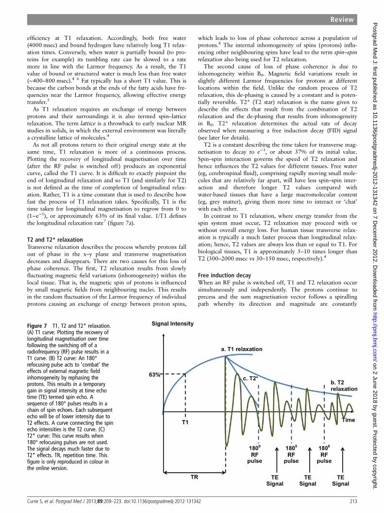
As not all protons return to their original energy state at thesame time, T1 relaxation is more of a continuous process.Plotting the recovery of longitudinal magnetisation over time(after the RF pulse is switched off) produces an exponentialcurve, called the T1 curve. It is difficult to exactly pinpoint theend of longitudinal relaxation and so T1 (and similarly for T2)is not defined as the time of completion of longitudinal relax-ation. Rather, T1 is a time constant that is used to describe howfast the process of T1 relaxation takes. Specifically, T1 is thetime taken for longitudinal magnetisation to regrow from 0 to(1−e−1), or approximately 63% of its final value. 1/T1 definesthe longitudinal relaxation rate7 (figure 7a).

T2 and T2* relaxationTransverse relaxation describes the process whereby protons fallout of phase in the x–y plane and transverse magnetisationdecreases and disappears. There are two causes for this loss ofphase coherence. The first, T2 relaxation results from slowlyfluctuating magnetic field variations (inhomogeneity) within thelocal tissue. That is, the magnetic spin of protons is influencedby small magnetic fields from neighbouring nuclei. This resultsin the random fluctuation of the Larmor frequency of individualprotons causing an exchange of energy between proton spins,

which leads to loss of phase coherence across a population ofprotons.8 The internal inhomogeneity of spins (protons) influ-encing other neighbouring spins have lead to the term spin–spinrelaxation also being used for T2 relaxation.

The second cause of loss of phase coherence is due toinhomogeneity within B0. Magnetic field variations result inslightly different Larmor frequencies for protons at differentlocations within the field. Unlike the random process of T2relaxation, this de-phasing is caused by a constant and is poten-tially reversible. T2* (T2 star) relaxation is the name given todescribe the effects that result from the combination of T2relaxation and the de-phasing that results from inhomogeneityin B0. T2* relaxation determines the actual rate of decayobserved when measuring a free induction decay (FID) signal(see later for details).

T2 is a constant describing the time taken for transverse mag-netisation to decay to e−1, or about 37% of its initial value.Spin–spin interaction governs the speed of T2 relaxation andhence influences the T2 values for different tissues. Free water(eg, cerebrospinal fluid), comprising rapidly moving small mole-cules that are relatively far apart, will have less spin–spin inter-action and therefore longer T2 values compared withwater-based tissues that have a large macromolecular content(eg, grey matter), giving them more time to interact or ‘chat’with each other.

In contrast to T1 relaxation, where energy transfer from thespin system must occur, T2 relaxation may proceed with orwithout overall energy loss. For human tissue transverse relax-ation is typically a much faster process than longitudinal relax-ation; hence, T2 values are always less than or equal to T1. Forbiological tissues, T1 is approximately 5–10 times longer thanT2 (300–2000 msec vs 30–150 msec, respectively).4

Free induction decayWhen an RF pulse is switched off, T1 and T2 relaxation occursimultaneously and independently. The protons continue toprecess and the sum magnetisation vector follows a spirallingpath whereby its direction and magnitude are constantly

Figure 7 T1, T2 and T2* relaxation.(A) T1 curve: Plotting the recovery oflongitudinal magnetisation over timefollowing the switching off of aradiofrequency (RF) pulse results in aT1 curve. (B) T2 curve: An 180°refocusing pulse acts to ‘combat’ theeffects of external magnetic fieldinhomogeneity by rephasing theprotons. This results in a temporarygain in signal intensity at time echotime (TE) termed spin echo. Asequence of 180° pulses results in achain of spin echoes. Each subsequentecho will be of lower intensity due toT2 effects. A curve connecting the spinecho intensities is the T2 curve. (C)T2* curve: This curve results when180° refocusing pulses are not used.The signal decays much faster due toT2* effects. TR, repetition time. Thisfigure is only reproduced in colour inthe online version.


Review


http://pmj.bm

j.com/

Postgrad M


ecember 2012. D

ownloaded from

http://pmj.bmj.com/

changing. Hence, an electrical signal is generated in a suitablereceiver coil. The MR signal generated from the spiralling summagnetisation vector is termed FID. It has its greatest magnitudeimmediately after the RF pulse is switched off and thendecreases as both relaxation processes occur. It also has a con-stant frequency (resonant frequency) and consequently the FIDsignal takes the form of a sine wave with a rapidly decayingenvelope (figure 8).

An FID is most commonly depicted with a 90° pulse but a RFpulse of any flip angle can create an FID because some compo-nents of the longitudinal magnetisation are always tipped intothe transverse plane. Theoretically, a 180° RF pulse shouldrefrain from generating an FID. However, in practice, all 180°pulses are imperfect and produce FID signals.4

FID is subjected to further disruption (de-phasing) by themagnetic field gradients that are used to localise and encode theMR signal. Consequently the signal generated by FID is notusually measured in MRI. Instead, it is common practice to gen-erate and measure the MR signal in the form of an echo: typic-ally a spin echo (SE) or a gradient echo (GRE). Echoes can beappreciated by considering how T1- and T2-weighted imagesare formed.

T1-weighted imagesContrast between tissues allows adjacent structures to be differ-entiated from one another. Contrast is determined by signalintensities, which in turn are governed (at least partly) by theT1 and T2 relaxation times of tissues within an image. Animage in which the difference in signal intensity between tissuesis predominantly due to differences in tissue T1 relaxation timeis called a T1-weighted image. T1-weighted images are gener-ated predominantly by manipulating the time between two RFexcitation pulses, the so-called repetition time (TR) (figure 9).

The preceding example was simplified for ease of understand-ing. It should be appreciated that many parameters influence

signal intensity and hence tissue contrast but in the exampleused T1 had the greatest influence. Contrast in images obtainedat long TR will not be influenced by T1 but instead may beinfluenced by differences in the T2 or proton density of thetissues in question. Factors that influence MR signal intensityare listed in the box.

T2-weighted imagesRecall that protons lose phase coherence following an RF pulseas a result of spin–spin interactions within the tissues (T2 relax-ation) and because of inhomogeneity within the local static mag-netic field (T2* relaxation). De-phasing caused by T2 relaxationis a random, irreversible process whereas the de-phasing causedby magnetic field inhomogeneity is potentially reversible.1

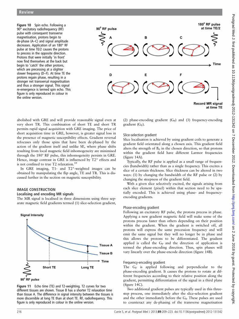
Application of an 180° RF pulse following an initial 90° RFpulse rotates the protons through 180°, effectively making theprotons ‘turn around’ and precess, still in the x–y plane, but inthe opposite direction. Local field inhomogeneity remains andprotons with a slightly faster Larmor frequency begin to catchup with slower protons. Eventually the protons come back intophase, which results in an increase in the amplitude of the MRsignal. Maximum signal amplitude is reached at the echo time(TE). To achieve maximal signal, the 180° RF pulse must beapplied at time TE/2. As the protons (spins) bounce back orecho following the application of the 180° RF refocusing pulse,the signal obtained is given the name SE (figure 10). Continuedinhomogeneity in the static magnetic field means that protonswill continue to lose phase coherence following an 180° RFrefocusing pulse; however, it is possible to repeat the 180° RFrefocusing pulse and obtain further SEs. Over time, the ampli-tude from each SE will decrease due to T2 effects. A curve con-necting the SE intensities is called the T2 curve. T2* curve isthe curve that results if 180° RF refocusing pulses are not used,that is, a curve that depicts the de-phasing caused by T2* effects(figure 7b and c).

Tissues have different T2 values. Brain for example has ashorter T2 than cerebrospinal fluid. TE is the time intervalbetween the 90° RF pulse and the SE. It is one of the para-meters whose value can be chosen by the operator of the MRmachine in order to influence the signal intensities (hence con-trast) between tissues. A much stronger signal is received whenshort TE (as opposed to long TE) is employed. However, atshort TE (eg, <30 msec), differences in T2 have little influenceon tissue contrast. Accordingly, T2-weighted images of the brainare obtained at long TE (eg, 80 msec) (figure 11).

A heavily T2-weighted image could be obtained at longer TEbut loss of MR signal would impact on the signal to noise ratiomaking images potentially subdiagnostic.

Factors influencing SE contrast and weightingImaging parameters influencing the MR signal in the SEsequence include TE and TR. Values for both of these para-meters are purposely chosen by the operator in order to influ-ence the tissue weighting of the image. Short TR and short TEgenerates a T1-weighted image; short TR allows differences inlongitudinal magnetisation to develop before the next 90° exci-tation pulse while short TE limits the T2 effects. Long TR andlong TE produces a predominantly T2-weighted image; longTR allows recovery of longitudinal magnetisation (thus limitingT1 effects) while at long TE T2 effects become pronounced. Adifferent type of image is produced at long TR and short TE.Long TR and short TE limit T1 and T2 effects, respectively.When this occurs, the signal is predominantly influenced by theproton density of the tissues (figure 12A–C).

Figure 8 Free induction decay. Transverse magnetisation (with allprotons rotating in phase) is at its greatest following an initial 90°excitatory radiofrequency (RF) pulse. Its amplitude (along with signalintensity) then decreases as the protons begin to lose phase coherence.The resultant decay signal is termed free induction decay. This figure isonly reproduced in colour in the online version.


Review


http://pmj.bm

j.com/

Postgrad M


ecember 2012. D

ownloaded from

http://pmj.bmj.com/

It should be appreciated that the choice of imaging para-meters for all MRI sequences can influence the sensitivity of thetest for the pathology in question. For example, the sensitivityfor the detection of lesions in multiple sclerosis is dependent onTE (lesion visibility decreases with increasing TE).9

Gradient echoSE sequences with their relatively long TR and TE are time con-suming. This limits the number of patients who can be scanned

in a session and also risks movement artefact by a restlesspatient. Conversely, GRE sequences, which replace the 180°refocusing RF pulse with magnetic field gradients, are relativelyshort. However, they do produce different contrasts. Magneticfield gradients produce a change in field strength and thus achange in Larmor frequency along a particular direction.Application of a gradient pulse after an initial RF pulse causesprotons to rapidly de-phase along the direction of the gradientresulting in rapid decline in the FID signal. This loss of phasecoherence can be reversed by applying a second magnetic fieldgradient with a slope of equal amplitude but in opposite direc-tion to the first. As a result, protons move back into phase andreturn a signal called GRE. TE is the time taken between thebeginning of FID (ie, generation of transverse magnetisation)following the initial RF pulse to the point at which the GREreaches its maximum amplitude (figure 13).

Differences between SE and GRESeveral differences exist between the two techniques. First, TEcan be shorter with GRE as only one RF pulse is used. Second,GRE sequences are typically used with low flip angle excitations(eg, 5°–40°) as opposed to the 90° flip angle used in SE. As aconsequence, longitudinal magnetisation is not completely

Figure 9 Repetition time (TR) andT1-weighting. Consider the followingexample in which two tissues, fat andfluid are being imaged where fat hasshorter transverse and longitudinalrelaxation times than fluid. An initial 90°radiofrequency (RF) pulse is switched onand off, time passes (TR), a second 90°RF pulse is switched on and off, MRsignal is then sampled and an image isgenerated. As MR signal samplingoccurs after the switching off of thesecond RF pulse, the signal intensity willbe determined by the amount oftransverse magnetisation at that point.This in turn will be governed by thevalue of longitudinal magnetisation ofthe two tissues immediately before thesecond 90° RF pulse is switched on.Choosing a long TR (eg, 1500 msec)would allow the tissues to recover theirlongitudinal magnetisation fully with noappreciable difference in the value oflongitudinal magnetisation existingbetween the tissues. In this situation, theapplication of a second RF pulse withsubsequent MR signal sampling wouldresult in no discernible difference in MRsignal between the tissues as thetransverse magnetisation values for thetissues are essentially equal (A) (ie, nosignal contrast). Choosing a short TR(20 msec) means that at the time ofapplying a second 90° RF pulse tissueswith a long T1 (fluid) will show lessrecovery in longitudinal magnetisationthan tissues with a short T1 (fat). Thetissues will possess different transversemagnetisation values (B) and, thus, willgenerate different signal intensities andallow greater contrast betweentissues (C). This figure is only reproducedin colour in the online version.

Box 1 Factors that influence MR signal intensity

▸ Proton density▸ T1▸ T2▸ Flow (eg, blood flow)▸ Pulse sequence▸ Repetition time▸ Echo time▸ Inversion time▸ Magnetic susceptibility (including contrast media)


Review


http://pmj.bm

j.com/

Postgrad M


ecember 2012. D

ownloaded from

http://pmj.bmj.com/

abolished with GRE and will provide reasonable signal even atvery short TR. This combination of short TE and short TRpermits rapid signal acquisition with GRE imaging. The price ofshort acquisition time in GRE, however, is greater signal loss inthe presence of magnetic susceptibility effects. Gradient reversalrefocuses only those spins that have been de-phased by theaction of the gradient itself and unlike SE, where phase shiftsresulting from local magnetic field inhomogeneity are minimisedthrough the 180° RF pulse, this inhomogeneity persists in GRE.Hence, image contrast in GRE is influenced by T2* effects andis not confined to true T2 relaxation.10

In GRE imaging, T1- and T2*-weighted images can beobtained by manipulating the flip angle, TE and TR. This is dis-cussed further in the section on magnetic susceptibility.

IMAGE CONSTRUCTIONLocalising and encoding MR signalsThe MR signal is localised in three dimensions using three sep-arate magnetic field gradients termed (1) slice-selection gradient,

(2) phase-encoding gradient (GP) and (3) frequency-encodinggradient (GF).

Slice-selection gradientSlice localisation is achieved by using gradient coils to generate agradient field orientated along a chosen axis. This gradient fieldalters the strength of B0 in the chosen direction, so that protonswithin the gradient field have different Larmor frequencies(figure 14A).

Typically, the RF pulse is applied as a small range of frequen-cies (bandwidth) rather than as a single frequency. This excites aslice of a certain thickness. Slice thickness can be altered in twoways: (1) by changing the bandwidth of the RF pulse or (2) bychanging the steepness of the gradient field.

With a given slice selectively excited, the signals arising fromeach slice element (pixel) within that section need to be spa-tially encoded. This is achieved using phase- and frequency-encoding gradients.

Phase-encoding gradientFollowing an excitatory RF pulse, the protons precess in phase.Applying a new gradient magnetic field will make some of theprotons precess faster than others depending on their positionwithin the gradient. When the gradient is switched off, allprotons will express the same precession frequency and willemit the same signal but they will no longer be in phase andthis allows the protons to be differentiated. The gradientapplied is called the GP and the direction of application istermed the phase-encoding direction. Thus, spin phases willvary linearly over the phase-encode direction (figure 14B).

Frequency-encoding gradientThe GF is applied following and perpendicular to thephase-encoding gradient. It causes the protons to rotate at dif-ferent frequencies according to their relative position along thegradient, permitting differentiation of the signal in a third plane(figure 14C).

Two additional gradient pulses are typically used in this three-step process, one immediately after the slice-selection gradientand the other immediately before the GF. These pulses are usedto counteract any de-phasing of the transverse magnetisation

Figure 10 Spin echo. Following a90° excitatory radiofrequency (RF)pulse with consequent transversemagnetisation, protons begin tode-phase (A–C) and signal amplitudedecreases. Application of an 180° RFpulse at time TE/2 causes the protonsto precess in the opposite direction.Protons that were initially ‘in front’now find themselves at the back butbegin to ‘catch’ the other protons,which are precessing at a slighterslower frequency (D–F). At time TE theprotons regain phase, resulting in astronger net transversal magnetisationand thus a stronger signal. This signalre-emergence is termed spin echo. Thisfigure is only reproduced in colour inthe online version.

Figure 11 Echo time (TE) and T2-weighting. T2 curves for twodifferent tissues are shown. Tissue B has a shorter T2 relaxation timethan tissue A. The difference in signal intensity between the tissues ismore discernible at long TE than at short TE. RF, radiofrequency. Thisfigure is only reproduced in colour in the online version.


Review


http://pmj.bm

j.com/

Postgrad M


ecember 2012. D

ownloaded from

http://pmj.bmj.com/

that may be caused by the imaging gradients and ensures thatmaximum echo (sampling signal) is achieved.

It should be emphasised that RF pulses excite all protons in aslice simultaneously and that a single echo signal is recordedfrom the entire slice for one phase-encoding step. Thus, toacquire sufficient phase-encoding information for a signal to beassigned to each location within the slice, the pulse sequence(comprising slice selection, frequency encoding and phase encod-ing) is repeated many times. During each repetition, the sameslice selection and frequency encoding are performed but thestrength of the phase-encoding gradient is increased by equalincrements. Each repetition of the phase-encoding step generatesa signal echo that is digitised and stored in a raw data matrixcalled ‘k-space’. Data points in k-space represent the spatial fre-quencies content of an MRI. Data in k-space are converted intoan image using a mathematical tool called a Fourier transform.

IMAGE ACQUISITION TIMEAs each phase-encoding step requires a new pulse sequence thetotal image acquisition time will depend on the product of TR(time interval between pulse sequences) and NP (number ofphase-encoding steps). Conventional pulse sequences such as SEand GRE acquire only one phase-encoding step (one line ofk-space) per TR, making the image acquisition time consider-ably long. This limitation is overcome by faster imaging techni-ques that acquire multiple lines of k-space per TR. The so-calledTurbo (or fast) SE and GRE techniques are now commonplacein MRI.

Turbo SEThe turbo SE (TSE) sequence applies multiple 180° pulses afteran initial 90° pulse (as opposed to the single 180° pulse used in

a conventional SE sequence). Each 180° pulse generates anecho, which (after phase encoding) is used to fill a new line ofk-space. The number of 180° refocusing pulses (and, thus, thenumber of echoes generated) during one TR of the TSEsequence is termed the echo train length (ETL), echo factor orturbo factor. ETL specifies the factor by which the pulsesequence is accelerated (eg, an ETL of 16 means that the TSEsequence is 16 times faster than a conventional SE sequence).

The signal amplitude of each successive echo generated by theTSE sequence will be smaller than the last by way of T2 decayeffects. The echoes will also have different TEs. This means thatin the traditional sense, a single TE does not exist for the TSEsequence. Instead, an effective TE or pseudo TE is ascribed.The effective TE is defined as that of the echo, which isacquired closest to the centre of k-space (with the smallest GP)as this is the echo that has the greatest influence on imagecontrast.1

Echo-planar imagingEcho-planar imaging (EPI) is a fast MRI technique in which therapid oscillation of high-amplitude gradients is used to generatemultiple GREs per TR. In single-shot EPI all of thephase-encoding steps are acquired in a single TR. Multi-shotEPI uses a few TRs to acquire all phase-encoding steps.

3D encodingAlthough the selection of a set of slices encodes data in all threedimensions in space, the slice thickness (often several milli-metres) is often much greater than the inplane pixel resolution(often <1 mm). The initial slice-encoding step can be replacedby a further (termed secondary) phase-encoding iteration, alongwhat was the slice-encoding direction. Instead of a set of slices

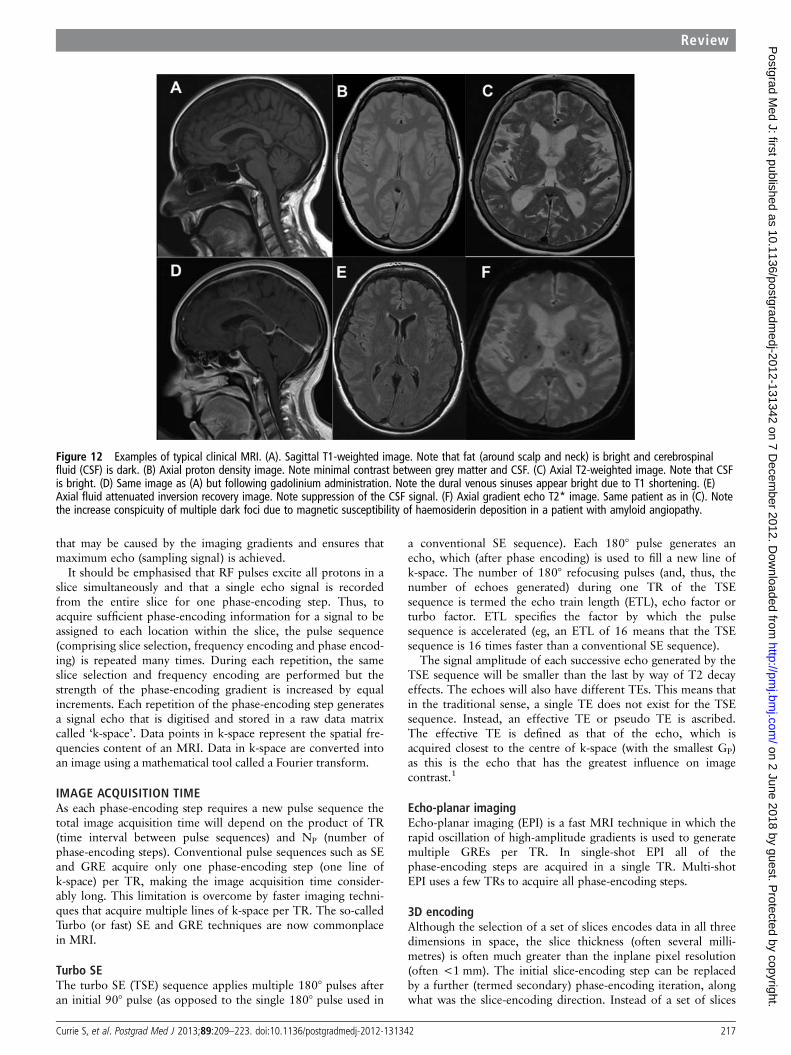
Figure 12 Examples of typical clinical MRI. (A). Sagittal T1-weighted image. Note that fat (around scalp and neck) is bright and cerebrospinalfluid (CSF) is dark. (B) Axial proton density image. Note minimal contrast between grey matter and CSF. (C) Axial T2-weighted image. Note that CSFis bright. (D) Same image as (A) but following gadolinium administration. Note the dural venous sinuses appear bright due to T1 shortening. (E)Axial fluid attenuated inversion recovery image. Note suppression of the CSF signal. (F) Axial gradient echo T2* image. Same patient as in (C). Notethe increase conspicuity of multiple dark foci due to magnetic susceptibility of haemosiderin deposition in a patient with amyloid angiopathy.


Review


http://pmj.bm

j.com/

Postgrad M


ecember 2012. D

ownloaded from

http://pmj.bmj.com/

(that may include slice gaps!), the inclusion of secondary phaseencoding often produces a true 3D dataset comprised of voxels(3D pixels) whose dimensions can be <1 mm×1 mm×1 mm.This is often useful when user manipulation of data in all threeperpendicular or oblique planes is necessary (eg, for intraopera-tive surgical guidance). Performing more phase-encoding stepshas a cost: time. As a result, the majority of true 3D sequencestend to be GREs with short TR or TSEs with high ETLfactors.11

MAGNETIC SUSCEPTIBILITYMagnetic susceptibility describes the extent to which a substancebecomes magnetised when placed in an external magnetic field.It results primarily from the interaction between electronswithin the substance and the external magnetic field. More spe-cifically, orbital and delocalised electrons within the substanceproduce circulating currents in response to the field. These cur-rents generate internal magnetisation (Mi) within the substancethat either augments or opposes the local external magneticfield.4 The result is either positive susceptibility, whereby themagnetic field local to the substance is increased, or negativesusceptibility in which the magnetic field local to the substanceis decreased. Substances with negative susceptibility are termeddiamagnetic; those with positive susceptibility are calledparamagnetic.

Most biological tissues including water cause very weak dia-magnetism and as such induce negligible susceptibility effects.Conversely, matter such as iron, nickel and cobalt show extreme

positive susceptibility and are termed ferromagnetic.Superparamagnetic is used to describe a substance with positivemagnetic susceptibility that lies between paramagnetism andferromagnetism (eg, small ferrous sulphate particles).

Intravenous contrastGadolinium, a rare-earth metal and paramagnetic substance, isused as an intravenous MR contrast medium. Its strong para-magnetic properties result from the numerous unpaired elec-trons that exist within its inner shells. These unpaired electronscan interact with adjacent resonating protons and cause theprotons to relax more rapidly. This results in a shortening ofboth longitudinal and transverse relaxation with consequentreduction in the T1 and T2 values of the tissues in which itaccumulates. This is depicted by an increase in signal inT1-weighted images and a decrease in signal in T2-weightedimages. In practice, the signal increase detected on T1-weightedimaging is better appreciated than any corresponding signaldecrease in T2-weighted imaging and makes T1-weightedimaging the method of choice for intravenous contrast studies.Furthermore, as gadolinium-based contrast agents shorten T1, itis possible to also shorten TR and, hence, reduce overall scantime (figure 12D).

Exploiting magnetic susceptibility using GRE imagingSusceptibility differences among tissues and materials are moreconspicuous on T2*-weighted GRE rather than SE imaging(recall that susceptibility differences promote magnetic fieldinhomogeneity that result in faster T2* relaxation, leading tosignal intensity loss on GRE images; conversely, the 180°refocusing pulse in SE compensates for this). GRE sequencescan be made more sensitive to T2* decay through the manipula-tion of imaging parameters such as TR, TE and the flip angle.As T2* decay commences with the excitation pulse and pro-gresses with time, a longer TE will result in greater signal loss.A low flip angle reduces the influence T1 has on the subjectmatter (as longitudinal magnetisation remains close to the fullyrelaxed state) and allows the T2* effects to dominate. Similarly,T1 effects are limited with a long TR. Hence, T2* GREimaging is obtained at long TE, long TR and low flip angle. T2*sensitivity also increases with field strength and voxel size.12

T2*-weighted sequences are particularly useful in the detectionof haemorrhage and blood products (deoxyhaemoglobin, meth-aemoglobin and haemosiderin are paramagnetic). Various path-ologies may be detected using this imaging modality includingarteriovenous malformations, cavernomas, superficial siderosis,intraparenchymal/intratumoural haemorrhage and amyloidangiopathy (figure 12F). The literature also supports the use ofT2*-weighted imaging for the differentiation of vestibularschwannomas from meningiomas as in most schwannomas,microhaemorrhages can be detected.13

OTHER FACTORS THAT MAY INFLUENCE SIGNALINTENSITYTI: the inversion recovery sequenceThe inversion recovery sequence uses a 180° pulse followed bya 90° pulse. The 180° pulse inverts longitudinal magnetisationso that the sum magnetisation aligns antiparallel to B0.Following the 180° pulse, the inverted longitudinal magnetisa-tion begins to shorten and return to its original position.Application of a 90° pulse causes the longitudinal magnetisationto flip to the transverse plane and allows a signal to be recorded.The strength of the signal is dependent on the magnitude oflongitudinal magnetisation just before the 90° pulse was applied.

Figure 13 Gradient echo. An excitatory radiofrequency (RF) pulsecauses transverse magnetisation and initiation of a free induction decaysignal. This signal rapidly de-phases following the application of amagnetic field gradient. Application of a second magnetic fieldgradient with a slope of equal amplitude but in opposite direction tothe first causes some rephasing. The signal increases again at time TEto a maximal signal termed a gradient echo. The maximum amplitudeof the gradient echo is dependent on the specified TE and the T2*relaxation rate of the tissues in question. This figure is only reproducedin colour in the online version.


Review


http://pmj.bm

j.com/

Postgrad M


ecember 2012. D

ownloaded from

http://pmj.bmj.com/

Figure 14 Image construction. (A) Step 1: Slice selection. A slice-selecting gradient (GS) is applied at the same time as the excitatoryradiofrequency (RF) pulse. In this example, the brain is being imaged and GS is applied along the z-axis, parallel with B0. This means that differentcross sections of the brain experience magnetic fields of differing strength. Accordingly protons will precess at different Larmor frequenciesdepending on their position along the gradient. Selecting an RF pulse (or range of RF pulse frequencies) that matches the Larmor frequency of theprotons will determine the slice location. (B) Step 2: Phase encoding. Protons are in phase after the RF pulse is applied. Applying a phase-encodinggradient along the y-axis causes the protons to increase their speed of precession relative to the strength of the magnetic field to which they areexposed. In this example, speed increases from top to bottom. This is depicted on the right of the schematic, which shows rows of protons withdifferent precession speeds. When the gradient is switched off, all protons are once again exposed to the same magnetic field and as such theyhave the same frequency; only now, they are out of phase. (It may help to think of the protons giving of the same signal frequency but at differenttimes.) (C) Step 3: Frequency encoding. A further magnetic field frequency-encoding gradient is applied to help differentiate the signal from differentprotons by way of differing frequencies. In this example, the protons from the bottom row in step 2 (above) have been exposed to a gradientapplied along the x-axis. While the protons are in phase, they now have different frequencies, allowing their differentiation in the third (x) plane.During the frequency-encoding step, the signal is measured (digitally sampled) at time TE, the point of maximal signal. The signal comprises a rangeof frequencies (or bandwidth) that correspond to the Larmor frequencies of the proton magnetic moments at their different locations along thegradient.1 In this example, the orientation of the three gradients defined a slice perpendicular to the z-axis. Different slice orientations can beachieved by allocating the gradients to a different axis. Combining gradients along two or more axes for each localisation task allows angled slicesto be obtained. This figure is only reproduced in colour in the online version.


Review


http://pmj.bm

j.com/

Postgrad M


ecember 2012. D

ownloaded from

http://pmj.bmj.com/

Hence, the signal obtained by inversion recovery is dependenton the T1 properties of the tissues being examined. Inversiontime (TI) is the time interval between the 180° and the 90°pulses (figure 15A).

Following the 180° pulse there will be a time when longitu-dinal magnetisation passes through the transverse plane.Application of a 90° pulse at this point will result in a signalvoid (the protons will be flipped out of the orientation at whichtheir signal can be recorded). Accordingly, this point is termedthe null point. Knowledge of the null point for a particulartissue can be used to suppress the signal from that tissue (figure15B). Fluid attenuated inversion recovery (FLAIR) sequencesare frequently used in neuroimaging to suppress the signal fromcerebrospinal fluid (figure 12D). This has the particular advan-tage of making periventricular lesions much more conspicuous.As a further bonus, the combination of long TE and a TI canprovide both T2-weighted contrast (aiding the delineation of,for example, ischaemia or inflammation) and T1-weighted con-trast (showing gadolinium-chelate deposition where there is aleaky blood–brain barrier). Gadolinium enhanced FLAIRsequences are being used with increasing frequency in neurosci-ence centres. They can be particularly useful in the detection ofsubtle tumours or for assessing multiple sclerosis. Short TIinversion recovery is used commonly throughout radiology sub-specialties to suppress fat signal. Other fat-suppression techni-ques are available.14

FlowWhen imaging a slice through a vessel containing flowing blood,the blood within the slice at the time of an excitatory RF pulsewill be influenced by the radiowave. However, by the time the

MR signal is sampled, the blood influenced by the radiowavewill have been replaced by blood flowing into the slice that hasnot undergone magnetisation. Thus, no signal will be obtainedfrom the vessel and it will appear black on the image: theso-called flow-void phenomenon.

This is not the only way in which flow influences signal inten-sity and merely constitutes an introduction as in reality thesubject is far more complex. For example, a signal may still beobtained from vessels that contain slow flowing blood and thisto the inexperienced looking at a single sequence of images maybe interpreted as thrombosis. Detailed articles describing MRIin relation to flow and articles relating to MRI artefacts can befound in the literature.15 16

FINALLY, A WORD ON SAFETYSafety issues regarding clinical MRI can be broadly divided intothose that result from the exposure to magnetic fields and thoseresulting from intravenous contrast administration.

Exposure to magnetic fieldsEach of the three types of magnetic field (static, gradient andRF) that the patient is exposed to during an examination carriesa potential risk to patient safety. With regard to the static mag-netic field (B0), the main safety issue involves the attraction offerromagnetic material towards the magnet. Material external tothe patient (such as keys or coins) may become projectileswithin the scanning room, putting the patient and staff (andmachinery) at risk of being hit. Static magnetic fields can alsoexert mechanical forces on ferromagnetic components withinimplanted medical devices such as pacemakers, aneurysmal clipsand cardiac defibrillators. Devices may rotate or dislodge,

Figure 15 Inversion recovery.(A) Inversion of the sum longitudinalmagnetisation vector following an180° radiofrequency (RF) pulse.A further 90° RF pulse flips therecovering sum vector into thetransverse plane allowing a signal tobe obtained. The magnitude of thesignal is dependent on the amount ofT1 recovery that had occurred beforethe 90° pulse and, hence, on theinversion time (time between the 180°and 90° pulses). (B) T1 relaxationcurves for fat and water demonstratingthe recovery of longitudinalmagnetisation following an 180° RFpulse. Application of a 90° RF pulse atthe null point leads to signalsuppression of a chosen tissue. Thisfigure is only reproduced in colour inthe online version.


Review


http://pmj.bm

j.com/

Postgrad M


ecember 2012. D

ownloaded from

http://pmj.bmj.com/

potentially resulting in serious patient harm.17 Higher staticmagnetic fields lead to greater forces on ferromagnetic materi-als.18 Control of access to the magnet room is crucial in mini-mising associated risks.

Excessive noise and potential auditory damage are the mainconcerns with gradient fields. Rapid alterations of currentswithin the gradient coils, in the presence of a strong magneticfield, generate significant force. This force acts upon the gradi-ent coils and manifests as loud tapping or knocking sounds.19

Temporary hearing loss has been reported using conventionalsequences.20 Due to the risk of damage caused by acoustic noiseit is common practice for the patient to wear protective earwear (often headphones and earplugs). Gradient magnetic fieldsalso have the potential to induce voltages on pacing wires thatmay cause oversensing and undersensing. Excitation of periph-eral nerves has also been reported.21

RF pulses may lead to local tissue heating through the dissipa-tion of energy. Typically this is negligible (<1°C) in clinicalimaging but is potentially serious in patients with implantabledevices. A pacemaker lead, for example, may act as an antennaand concentrate RF energy, resulting in dramatic local heating,tissue damage and cardiac dysfunction.22

A devise must have undergone prior testing within MR elec-tromagnetic fields for it to be deemed safe. Booklets listing MRcompatible objects/devises are available and are typically held inthe MR scanner room. More and more MR compatible medicaldevices and equipment are being generated. Most tertiarycentres now have MR-safe anaesthetic equipment and recentstudies have reported favourably on the early outcome of MRcompatible pacemakers.17

Intravenous contrast agentsGadolinium-based contrast agents are generally well tolerated. Arecent study suggests an adverse reaction rate of 0.46%.23 Arare but serious complication that may occur in patients withsevere renal impairment is nephrogenic systemic fibrosis.24

Although a systemic condition, cutaneous manifestations tend todominate with a lower-limb cellulitic-like picture occurringearly. Painful and pruritic, plaque-like ‘woody’ induration of theskin occurs later in the course of the disease with the legs morecommonly affected than the arms and torso. The face isspared.25 These cutaneous manifestations may lead to contrac-tures and limit mobility. nephrogenic systemic fibrosis may alsoaffect the liver, lungs, muscles, heart and nerves.26 Death ratemay be as high as 28%.27 Despite ongoing research the exactmechanisms underlying the condition remain unclear. No uni-versally effective treatment has been identified and prevention(mainly through limiting the use of high-dose gadolinium-basedcontrast agents and/or maximising renal function in patientswith renal failure) represents current recommendations.25

Anaphylaxis resulting from gadolinium-based contrast agentsis rare, with an estimated incidence of 0.02%.23 28 29 This com-pares favourably to the incidence with iodinated contrast mediaused with CT (0.03%–0.16%).29 Patients with a pre-existingallergy to other contrast agents (such as iodine) may confer agreater risk of anaphylaxis to gadolium-based contrast agents,thus highlighting the need for a thorough screening question-naire prior to any contrast administration.23 25

Pregnancy and breast feedingLarge doses of gadolinium-based contrast agents have been shownto cause postimplantation fetal loss, retarded development,increased locomotive activity and skeletal and visceral abnormal-ities in animal experiments.19 Any deleterious effects to humans

are unconfirmed. However, gadolinium-based contrast agents cancross the placenta and appear in the fetal bladder from where theyare excreted but enter the fetal system again through the swallow-ing of amniotic fluid. This makes it difficult to ascertain exact fetalhalf-life measurements for these agents.30 Currently, it is recom-mended that gadolinium-based contrast should only be adminis-tered after careful risk–benefit assessment.25

The amount of contrast absorbed by an infant’s gastrointes-tinal tract following breast feeding is believed to be negligible(<1% of the recommended intravenous infant dose) and assuch no additional precautions are thought necessary for breast-feeding mothers.31 Some centres advise informed consent,however, with an option to stop breast feeding (with continuedexpression and discarding of the milk) for 24 h following mater-nal administration.31

SUMMARYThis article has outlined the fundamental physical principlesinvolved in clinical MRI. Key imaging parameters and sequenceshave been described, including their influence on image contrastand acquisition time. Important safety issues have also beenaddressed.

Main messages

▸ More frequently hospital clinicians are reviewing imagesfrom MR studies of their patients before seeking formalradiological opinion.

▸ Knowledge of the basic physical principles behind MRI isessential for correct image interpretation.

▸ The use of MRI as an investigative tool will only increase inclinical medicine.

Current research questions

▸ Can advanced MR imaging techniques fulfill their potentialas specific and sensitive biomarkers of disease?

▸ Will new image reconstruction algorithms (that move onfrom the simple Fourier transform) generate improved,artifact-free images that can be applied in clinical radiology?

Key references

▸ Elster A. Questions and answers in magnetic resonanceimaging. St Louis: Mosby-Year Book, 1994.

▸ Chavhan GB, Babyn PS, Thomas B, et al. Principles,techniques, and applications of T2*-based MR imaging andits special applications. Radiographics 2009;29:1433–49.

▸ Bley TA, Wieben O, Francois CJ, et al. Fat and watermagnetic resonance imaging. J Magn Reson Imaging2010;31:4–18.

▸ Ivancevic MK, Geerts L, Weadock WJ, et al. Technicalprinciples of MR angiography methods. Magn ResonImaging Clin N Am 2009;17:1–11.

▸ Coskun O. Magnetic resonance imaging and safety aspects.Toxicol Ind Health 2011;27:307–13.


Review


http://pmj.bm

j.com/

Postgrad M


ecember 2012. D

ownloaded from

http://pmj.bmj.com/

MULTIPLE CHOICE QUESTIONS (TRUE (T)/FALSE (F);ANSWERS AFTER THE REFERENCES)1.A. The room housing the MR machine is typically lined with

copper?B. Clinical MR systems typically use superconducting magnets?C. The main magnetic coils generate a strong constant magnetic

field referred to as B1?D. Gradient coils are cooled, close to absolute zero, using cryo-

genic liquid helium?E. Shim coils are used to reduce inhomogeneity?2.A. When placed in an external magnetic field protons move in

a particular way called precession?B. The speed of precession is determined by the Larmor

equation?C. The Larmor equation indicates that precession frequency is

proportional to magnetic field strength?D. Longitudinal magnetisation refers to a sum magnetisation

that parallels the external magnetic field?E. Longitudinal magnetisation can be directly measured to

create an MR signal?3.A. Activation of a 90° radiofrequency pulse flips the sum mag-

netisation vector to the right creating transversemagnetisation?

B. T1 relaxation is the process whereby protons exchangeenergy with their surroundings to return to their lowerenergy state and in so doing cause the restoration of trans-verse magnetisation?

C. T2 relaxation results from inhomogeneity within the localtissue?

D. T2* relaxation determines the actual rate of decay observedwhen measuring a free induction decay signal?

E. T2 is a constant describing the time taken for transversemagnetisation to decay to about 63% of its initial value?

4.A. Short TR and short TE generate a predominantly

T1-weighted image?B. Long TR and long TE produce a predominantly

T2-weighted image?C. Short TR and long TE are used to generate a proton density

image?D. Spin echo sequences generally have greater magnetic suscep-

tibility effects than gradient echo sequences?E. Gradient echo sequences use a 90° saturation pulse followed

by a 180° refocusing pulse?5.A. Substances with negative magnetic susceptibility are termed

paramagnetic?B. Iron is termed ferromagnetic because of its extreme negative

magnetic susceptibility?C. The signal obtained by inversion recovery is dependent on

the T1 properties of the tissues being examined?D. Excessive noise and potential auditory damage are the main

concerns with radiofrequency coils?E. Gadolinium-based contrast agents have an adverse reaction

rate of about 0.5%?

Contributors SC: concept design, literature review, manuscript drafting, manuscriptrevision. NH and IDW: concept design, manuscript revision. IJC and MH: manuscriptrevision.

Funding None.

Competing interests None.

Provenance and peer review Not commissioned; externally peer reviewed.

REFERENCES1 Ridgway JP. Cardiovascular magnetic resonance physics for clinicians: part I.

J Cardiovasc Magn Reson 2010;12:71.2 Jacobs MA, Ibrahim TS, Ouwerkerk R. AAPM/RSNA physics tutorials for residents:

MR imaging: brief overview and emerging applications. Radiographics2007;27:1213–29.

3 Hahn EL. Spin Echoes. Phys Rev 1950;80:580–94.4 Elster A. Questions and answers in magnetic resonance imaging. St Louis:

Mosby-Year Book, 1994.5 Schild H. MRI made easy. Berlin: Schering, 1990.6 Smith H, Ranello F. A non-mathematical approach to basic MRI. Madison, Wis:

Medical Physics Publishing, 1989.7 Bloch F. Nuclear induction. Phys Rev 1946;70:460.8 Fullerton G. Physiologic basis of magnetic relaxation. In: Stark D, Bradley W, eds.

Magnetic resonance imaging. 2nd edn. St Louis: Mosby-Year Book, 1992: 88–108.9 Pikus L, Woo JH, Wolf RL, et al. Artificial multiple sclerosis lesions on simulated

FLAIR brain MR images: echo time and observer performance in detection.Radiology 2006;239:238–45.

10 Winkler ML, Ortendahl DA, Mills TC, et al. Characteristics of partial flip angle andgradient reversal MR imaging. Radiology 1988;166(1 Pt 1):17–26.

11 Mugler JP III, Brookeman JR. Three-dimensional magnetization-prepared rapidgradient-echo imaging (3D MP RAGE). Magn Reson Med 1990;15:152–7.

12 Chavhan GB, Babyn PS, Thomas B, et al. Principles, techniques, and applications ofT2*-based MR imaging and its special applications. Radiographics2009;29:1433–49.

13 Thamburaj K, Radhakrishnan VV, Thomas B, et al. Intratumoral microhemorrhageson T2*-weighted gradient-echo imaging helps differentiate vestibular schwannomafrom meningioma. AJNR Am J Neuroradiol 2008;29:552–7.

14 Bley TA, Wieben O, Francois CJ, et al. Fat and water magnetic resonance imaging.J Magn Reson Imaging 2010;31:4–18.

15 Ivancevic MK, Geerts L, Weadock WJ, et al. Technical principles of MR angiographymethods. Magn Reson Imaging Clin N Am 2009;17:1–11.

16 Morelli JN, Runge VM, Ai F, et al. An image-based approach to understanding thephysics of MR artifacts. Radiographics 2011;31:849–66.

17 Jung W, Zvereva V, Hajredini B, et al. Initial experience with magnetic resonanceimaging-safe pacemakers : a review. J Interv Card Electrophysiol 2011;32:213–19.

18 Pamboucas C, Nihoyannopoulos P. Cardiovascular magnetic resonance at 3 Tesla:advantages, limitations and clinical potential. Hellenic J Cardiol 2006;47:170–73.

19 Coskun O. Magnetic resonance imaging and safety aspects. Toxicol Ind Health2011;27:307–13.

20 Chakeres DW, de Vocht F. Static magnetic field effects on human subjects related tomagnetic resonance imaging systems. Prog Biophys Mol Biol 2005;87:255–65.

21 Pamboucas CA, Rokas SG. Clinical safety of cardiovascular magnetic resonance:cardiovascular devices and contrast agents. Hellenic J Cardiol 2008;49:352–6.

22 Baikoussis NG, Apostolakis E, Papakonstantinou NA, et al. Safety of magneticresonance imaging in patients with implanted cardiac prostheses and metalliccardiovascular electronic devices. Ann Thorac Surg 2011;91:2006–11.

23 Li A, Wong CS, Wong MK, et al. Acute adverse reactions to magnetic resonancecontrast media—gadolinium chelates. Br J Radiol 2006;79:368–71.

24 Cowper SE, Robin HS, Steinberg SM, et al. Scleromyxoedema-like cutaneousdiseases in renal-dialysis patients. Lancet 2000;356:1000–1.

25 Gauden AJ, Phal PM, Drummond KJ. MRI safety: nephrogenic systemic fibrosis andother risks. J Clin Neurosci 2010;17:1097–104.

26 Gibson SE, Farver CF, Prayson RA. Multiorgan involvement in nephrogenic fibrosingdermopathy: an autopsy case and review of the literature. Arch Pathol Lab Med2006;130:209–12.

27 Mendoza FA, Artlett CM, Sandorfi N, et al. Description of 12 cases of nephrogenicfibrosing dermopathy and review of the literature. Semin Arthritis Rheum2006;35:238–49.

28 Murphy KJ, Brunberg JA, Cohan RH. Adverse reactions to gadolinium contrastmedia: a review of 36 cases. AJR Am J Roentgenol 1996;167:847–9.

29 Caro JJ, Trindade E, McGregor M. The cost-effectiveness of replacing high-osmolalitywith low-osmolality contrast media. AJR Am J Roentgenol 1992;159:869–74.

30 Shellock F, Kanal E. Bioeffects and safety of MR procedures. In: Edelman R,Hesselink J, Zlatkin M, eds. Clinical magnetic resonance imaging. Philadelphia: W.B.Saunders, 1996: 429.

31 Webb JA, Thomsen HS, Morcos SK. The use of iodinated and gadolinium contrastmedia during pregnancy and lactation. Eur Radiol 2005;15:1234–40.


Review


http://pmj.bm

j.com/

Postgrad M


ecember 2012. D

ownloaded from

http://pmj.bmj.com/

ANSWERS

1.A. TB. TC. F - B0D. F - main magnetE. T2.A. TB. TC. TD. TE. F - need transverse magnetisation3.A. TB. F - longitudinal magnetisation

C. TD. TE. F - 37%4.A. TB. TC. F - long TR, short TED. F - fewerE. F - this is SE5.A. F - diamagneticB. F - because of its extreme positive magnetic susceptibilityC. T - but also provides T2 contrast because of long TED. F - gradient coilsE. T


Review


http://pmj.bm

j.com/

Postgrad M


ecember 2012. D

ownloaded from

http://pmj.bmj.com/

understanding mri: basic mr physics for...

Documents