SANDIA REPORT

SAND2003-3490 Unlimited Release Printed September 2003 Understanding Metal Vaporization from Laser Welding

Phillip W. Fuerschbach, Jerome T. Norris, Xuili He and Tarasankar DebRoy

Prepared by Sandia National Laboratories Albuquerque, New Mexico 87185 and Livermore, California 94550 Sandia is a multiprogram laboratory operated by Sandia Corporation, a Lockheed Martin Company, for the United States Department of Energy’s National Nuclear Security Administration under Contract DE-AC04-94AL85000. Approved for public release; further dissemination unlimited.

Issued by Sandia National Laboratories, operated for the United States Department of Energy by Sandia Corporation.

NOTICE: This report was prepared as an account of work sponsored by an agency of the United States Government. Neither the United States Government, nor any agency thereof, nor any of their employees, nor any of their contractors, subcontractors, or their employees, make any warranty, express or implied, or assume any legal liability or responsibility for the accuracy, completeness, or usefulness of any information, apparatus, product, or process disclosed, or represent that its use would not infringe privately owned rights. Reference herein to any specific commercial product, process, or service by trade name, trademark, manufacturer, or otherwise, does not necessarily constitute or imply its endorsement, recommendation, or favoring by the United States Government, any agency thereof, or any of their contractors or subcontractors. The views and opinions expressed herein do not necessarily state or reflect those of the United States Government, any agency thereof, or any of their contractors. Printed in the United States of America. This report has been reproduced directly from the best available copy. Available to DOE and DOE contractors from

U.S. Department of Energy Office of Scientific and Technical Information P.O. Box 62 Oak Ridge, TN 37831 Telephone: (865)576-8401 Facsimile: (865)576-5728 E-Mail: reports@adonis.osti.gov Online ordering: http://www.doe.gov/bridge

Available to the public from

U.S. Department of Commerce National Technical Information Service 5285 Port Royal Rd Springfield, VA 22161 Telephone: (800)553-6847 Facsimile: (703)605-6900 E-Mail: orders@ntis.fedworld.gov Online order: http://www.ntis.gov/help/ordermethods.asp?loc=7-4-0#online

2

SAND2003-3490 Unlimited Release

Printed September 2003

Understanding Metal Vaporization from Laser Welding

Phillip W. Fuerschbach and Jerome T. Norris Joining and Coating Department

Sandia National Laboratories P.O. Box 5800

Albuquerque, NM 87185-0889

Xuili He and Tarasankar DebRoy Department of Materials Science and Engineering

The Pennsylvania State University University Park, PA 16802-5006

Abstract The production of metal vapor as a consequence of high intensity laser irradiation is a serious concern in laser welding. Despite the widespread use of lasers in manufacturing, little fundamental understanding of laser/material interaction in the weld pool exists. Laser welding experiments on 304 stainless steel have been completed which have advanced our fundamental understanding of the magnitude and the parameter dependence of metal vaporization in laser spot welding. Calculations using a three-dimensional, transient, numerical model were used to compare with the experimental results. Convection played a very important role in the heat transfer especially towards the end of the laser pulse. The peak temperatures and velocities increased significantly with the laser power density. The liquid flow is mainly driven by the surface tension and to a much less extent, by the buoyancy force. Heat transfer by conduction is important when the liquid velocity is small at the beginning of the pulse and during weld pool solidification. The effective temperature determined from the vapor composition was found to be close to the numerically computed peak temperature at the weld pool surface. At very high power densities, the computed temperatures at the weld pool surface were found to be higher than the boiling point of 304 stainless steel. As a result, vaporization of alloying elements resulted from both total pressure and concentration gradients. The calculations showed that the vaporization was concentrated in a small region under the laser beam where the temperature was very high.

3

Table of Contents Abstract……………………………………………………………...……………………3 List of Figures…………………………………………….………………………………6 List of Tables.……………………………………………………….……………………8 Introduction…………………….……………………………………...…………………9 Section 1. Heat transfer and fluid flow during laser spot welding of 304 stainless steel …….…………………………………………………………….………………….11

1.1. Introduction…………………………………………………….……………11 1.2. Experimental procedure…………………….….………………...……….…12 1.3. Mathematical formulation..……………..…..…………………...……….…13

1.3.1. Governing equations……………………………….…………...…13 1.3.2. Boundary conditions..……………….………………………….…14 1.3.3. Discretization of governing equations…….………………………15 1.3.4. Grid spacings and time steps.………….……………………….…15 1.3.5. Convergence criteria..…………………………………………..…16

1.4. Results and discussion……………………..………...……………...………17 1.4.1.Comparison between the calculated and experimental results….…17 1.4.2.Temperture and velocity fields ..…………….………………….…18 1.4.3. Weld thermal cycle………………………………………………..19 1.4.4.Rate of convection from dimensionless numbers……………….…21 1.4.5.Evaluation of mushy zone……………………….…….…………..23 1.4.6.Solidification..…… ………………………………..………………25 1.4.7.Comparison of laser spot welding with GTA spot welding and GTA linear welding…………………………………………………...……….28

1.5. Conclusions…………..…………………………….…………...……..….…29 1.6. References..…………..………………...…………..…………...………...…29

Section 2. Probing Temperature during Laser Spot Welding from Vapor Composition and Modeling……………………………………………………………31

2.1. Introduction………………...…………………………………….…………31 2.2. Experimental procedure………………………..………………...…………32 2.3. Mathematical formulation.………………….………………………………34 2.4. Results and discussion..…………………….……………..…………...……38 2.5. Conclusions……………….……..………………………………..…………46 2.6. References..……….……..…………………………...……………...………47

4

Section 3. Alloying Element Vaporization during Laser Spot Welding of Stainless Steel……………………………………………………………………………………..48

3.1. Introduction………………………..….………………………….………….48 3.2. Experimental procedure………...………………………………………..….50 3.3. Mathematical formulation.……………………………...………………...…50

3.3.1 Transient temperature profile..…….……………….………………50 3.3.2. Vaporization due to concentration gradient.….…………..…….…51 3.3.3. Vaporization due to pressure gradient.…….……………….…..…52 3.3.4. Over-all vaporization rate & weight loss due to vaporization….…54

3.4. Results and discussion..……………….…………..……………...…………55 3.4.1 Computed temperature fields & weld pool geometry..….…………55 3.4.2. Mass loss…………………………………………….………….…59

3.5. Conclusions……………….…………………………………...………….…65 3.6. References.…….…………...…………………………………...……...……66

Report Summary..………………………………………………………………………67 Acknowledgments……………………………………………………....………………68 Appendix………………………………………………………………………………...69 Distribution………………………………………………………...……………………70

5

List of Figures Figure 1.1 Experimental and calculated weld pool cross sections for laser power of

1967 W and pulse duration of 3 ms.……………………….…….…...….17 Figure 1.2 The experimental and calculate results of effects of laser power density on

(a) the weld pool diameter and (b) the weld pool depth…………....……18 Figure 1.3 Computed temperature and velocity fields at different times: (a) t = 1 ms,

(b) t = 3ms, (c) t = 4ms, (d) t = 4.5 ms and (e) t = 5 ms………….……...19 Figure 1.4 Weld thermal cycles at different locations: (a) top surface and (b) cross

section………………………………….………………………………...20 Figure 1.5 The variation of maximum Peclet number with time………………..….22 Figure 1.6 Evolution of the mushy zone size during laser spot welding……………24 Figure 1.7 Distribution of temperature at the pool top surface at various solidification

Times…………………………………………………………………….24 Figure 1.8 Distance between the mushy zone/solid front and weld center as a function

of time……………………………………………………………………25 Figure 1.9 The value of G, R, G/R along 0° and 90° planes at the mushy zone-solid

interface as a function of time: 530 W and 4.0 ms………………………26 Figure 1.10 The value of G, R, G/R along 0° and 90° planes at the mushy zone-solid

interface as a function of time: 1967 W and 3.0 ms……..………………27 Figure 2.1 A schematic diagram of the experimental setup.………..………....….…33 Figure 2.2 Equilibrium vapor pressures of the four alloying elements.……....…….39

Figure 2.3 Measured weight percent of (a) Fe, (b) Mn, (c) Cr in vapor composition with laser power density. The triangles represent the original data and the circles show best fit……………………………………………...….……40

Figure 2.4 The ratio of calculated vaporization rates of (a) Fe and Mn and (b) Cr and Mn as a function of temperature………..……………………...………...40

Figure 2.5 Temperature values calculated from the ratio of vapor flux. The power density is defined as the ratio of power and laser beam area. .………..…41

Figure 2.6 Experimental and calculated weld pool cross sections. Laser power: 1067 W and pulse duration: 3 ms. (a) Beam radius: 0.325 mm and (b) Beam radius: 0.466 mm……………………………………………...…....……41

Figure 2.7 The effects of laser power density on (a) the weld pool depth, and (b) weld pool width. Laser power: 1967 W, and pulse duration: 3.0 ms. The power density is defined as the ratio of power and laser beam area…….....……42

Figure 2.8 The variation of D/W with laser power density. Laser power: 1967 W and pulse duration: 3.0 ms...………..……….…...…………………....…...…43

Figure 2.9 Computed temperature and velocity fields at different times: (a) t = 1 ms, (b) t = 2 ms, (c) t = 4 ms, (d) t = 4.5 ms, and (e) t = 5 ms. Laser power: 530 W, pulse duration: 4.0 ms, and spot radius: 0.171 mm. ……………44

Figure 2.10 Weld thermal cycles at different locations on the top surface of weld pool…………………………...……..………...…………………....……44

Figure 2.11 The variation of peak temperature on the weld pool surface with laser power density. ………………………………...…………………....……45

6

Figure 3.1 A schematic diagram of the velocity distribution functions in the Knudsen layer and in adjacent regions……………………………………………..52

Figure 3.2 Computed temperature and velocity fields at different times: (a) t = 1 ms, (b) t = 3 ms and (c) t = 5 ms……………………………………………..55

Figure 3.3 Computed weld thermal cycles at various locations on the top surface of the weld pool…………………………………………………………….56

Figure 3.4 The variation of Peclet number with time: 1967 W 3.0 ms……………..57 Figure 3.5 The effect of laser power density on (a) the computed peak power and (b)

the computed maximum velocity………………………………………..57 Figure 3.6 Experimental and calculated weld pool cross sections…………………..58 Figure 3.7 Distribution of temperature and vapor fluxes of various elements at the

weld pool surface after 3.0 ms………………………………………..59-60 Figure 3.8 Weight percent of different elements in vapor composition……………..60 Figure 3.9 Experimental and computed concentrations of (a) Fe and (b) Cr in the

vapor……………………………………………………………………..61 Figure 3.10 The calculated vaporization loss is compared with measured mass loss for

different power densities…………………………………………………63 Figure 3.11 Recoil and surface tension forces as a function of time………………….64 Figure 3.12 Particles of stainless steel, ejected form the weld pool, were captured on

the inner surface of a both end open quartz tube placed co-axial with the laser beam during spot welding……………………………………….…65

7

List of tables Table 1.1 The experimental conditions……………………………………………..13 Table 1.2 Data used in calculations……………………………………………..16-17 Table 1.3 Comparison of laser spot welding variables with FTA linear welding and

GTA spot welding……………...………………………………………...28 Table 2.1 Welding parameters……………………..……………………………….33 Table 2.2 Data used in calculations……………………………………………..36-37 Table 2.3 Temperatures calculated from vapor compositions and numerical model

……………………………………………………………………………46 Table 3.1 Data used in calculations………………………………………………...51 Table 3.2 Calculated and experimental weld pool dimensions for different welding

conditions………………………………………………………………...58 Table 3.3 The experimentally determined and calculated vapor composition for

different welding conditions……………………………………………..61 Table 3.4 The calculated mass loss due to evaporation is compared with the

experimentally determined mass loss for different welding conditions…62

8

Introduction Laser spot welding is widely used for precision joining of nuclear weapon components and other high reliability devices. The production of metal vapor as a consequence of high intensity laser irradiation is a serious concern in cleanrooms, where contamination of adjacent components, ejection of metal particulates, creation of void defects in the fusion zone, and significant loss of high vapor pressure alloying elements are all negative consequences of metal vaporization. Despite the widespread use of laser welding, little fundamental understanding of laser/material interaction in the weld pool exists. Without this fundamental understanding, optimization models cannot be applied to mitigate vaporization problems. This report contains three distinct analytical investigations which each serve to improve our understanding of metal vaporization from laser welding. In section 1, the evolution of temperature and velocity fields during laser spot welding of 304 stainless steel was studied using a transient, heat transfer and fluid flow model based on the solution of the equations of conservation of mass, momentum and energy in the weld pool. The weld pool geometry, weld thermal cycles and various solidification parameters were calculated. The fusion zone geometry, calculated from the transient heat transfer and fluid flow model, was in good agreement with the corresponding experimentally measured values for various welding conditions. Dimensional analysis was used to understand the importance of heat transfer by conduction and convection and the roles of various driving forces for convection in the weld pool. During solidification, the mushy zone grew at a rapid rate and the maximum size of the mushy zone was reached when the pure liquid region vanished. The solidification rate of the mushy zone/solid interface was shown to increase while the temperature gradient in the mushy zone at this interface decreased as solidification of the weld pool progressed. The heating and cooling rates, temperature gradient and the solidification rate at the mushy zone/solid interface for laser spot welding were much higher than those for the moving and spot gas tungsten arc welding. In section 2, measurement of weld pool temperature during laser spot welding was investigated. Composition of the metal vapor from the weld pool was determined by condensing a portion of the vapor on the inner surface of an open ended quartz tube which was mounted perpendicular to the sample surface and co-axial with the laser beam. It was found that iron, chromium and manganese were the main metallic species in the vapor phase. The concentrations of Fe and Cr in the vapor increased slightly while the concentration of Mn in the vapor decreased somewhat with the increase in power density. The vapor composition was used to determine an effective temperature of the weld pool. A transient, three-dimensional numerical heat transfer and fluid flow model based on the solution of the equations of conservation of mass, momentum and energy was used to calculate the temperature and velocity fields in the weld pool as a function of time. The experimentally determined geometry of the spot welds agreed well with that determined from the computed temperature field. The effective temperature determined from the vapor composition was found to be close to the numerically computed peak temperature at the weld pool surface. Because of the short process duration and other serious problems in the direct measurement of temperature during laser spot welding, estimating

9

approximate values of peak temperature from metal vapor composition is particularly valuable. In section 3, alloying element loss from the weld pool during laser spot welding of stainless steel was investigated experimentally and theoretically. The experimental work involved determination of work-piece weight loss and metal vapor composition for various welding conditions. The transient temperature and velocity fields in the weld pool were numerically simulated. The vaporization rates of the alloying elements were modeled using the computed temperature profiles. The fusion zone geometry could be predicted from the transient heat transfer and fluid flow model for various welding conditions. The laser power and the pulse duration were the most important variables in determining the transient temperature profiles. The velocity of the liquid metal in the weld pool increased with time during heating and convection played an increasingly important role in the heat transfer. The peak temperature and velocity increased significantly with laser power density and pulse duration. At very high power densities, the computed temperatures were higher than the boiling point of 304 stainless steel. As a result, the evaporation of alloying elements was caused by both the total pressure and the concentration gradients. The calculations showed that the vaporization occurred mainly from a small region under the laser beam where the temperatures were very high. The computed vapor loss was found to be lower than the measured mass loss because of the ejection of the tiny metal droplets owing to the recoil force exerted by the metal vapors. The ejection of metal droplets has been predicted by computations and verified by experiments.

10

Section 1. Heat transfer and fluid flow during laser spot welding of 304 stainless steel

1.1. Introduction Pulse Nd:YAG spot welds are widely used for assembly and closure of high reliability electrical and electronic packages for the telecommunications, defense, aerospace, and medical industries. Laser spot welding has an important advantage for these applications because it can deliver a minimum amount of energy to very small components with high precision. Laser spot welds behave very differently from their moving weld counterparts because the temperature profiles never reach a steady state and the heating and cooling rates for these welds are much higher than those of linear welds. Laser spot welds are characterized by small weld pool size, rapid changes of temperature and very short duration of the process. These characteristics make physical measurements of important parameters such as temperature and velocity fields, solidification rate and thermal cycles during laser spot welding very difficult. These parameters are important because the weld pool convection patterns and the heating and cooling rates determine the geometry, composition, structure and the resulting properties of the spot welds. In recent decades, numerical calculations of heat transfer and fluid flow have been utilized to understand the evolution of temperature and velocity fields and, weld geometry that cannot be obtained otherwise. However, most of these studies were concerned with arc welds where the time scale is of the order of several seconds. The time scale is much shorter for laser spot welding. The heat transfer and fluid flow during laser spot welding still remain to be investigated to understand how the velocity and temperature fields evolve during heating and cooling and how the mushy zone region behaves. Such a computationally intensive investigation, requiring use of fine grids and very small time steps has now become practical because of recent advances in the computational hardware and software. Several models have been developed to predict the temperature and velocity fields in the weld pool during laser welding. Cline and Anthony1 studied the effects of laser spot size, velocity and power level on the temperature distribution, cooling rate and depth of melting of 304 stainless steel. However, the convection in the weld pool was not considered in the model. Mazumder and Steen2 developed a numerical model of the continuous laser welding process considering heat conduction. The finite difference technique was used. Frewin and Scott3 used a finite element model of the heat flow during pulsed laser beam welding. The transient temperature profiles and the dimensions of fusion zone and HAZ were calculated. Katayama and Mizutani4 developed a heat conduction and solidification model considering the effects of microsegregation and latent heat. Recently, Chang and Na5 applied the finite element method and neural network to study laser spot welding of 304 stainless steel. This combined model could be effectively applied for the prediction of bead shapes of laser spot welding. In summary, transport phenomena based numerical models have been successful in revealing special

11

features in transient spot welding processes such as the transient nature of the solidification rate.6,7 A numerical model to simulate heat transfer and fluid flow during steady and transient fusion welding has been developed and refined during the past 20 years at Penn State. The model has been used to calculate weld pool geometry, temperature and velocity fields during welding of pure iron, 8,9 stainless steel,10-13 low alloy steel,14,15 aluminum alloy16 and titanium alloy17 under different welding conditions. Calculations were done for both moving and stationary heat sources and for laser beam as well as arc welding. The computed temperature fields were useful for the calculation of vaporization rates of alloying elements,8-11,16 weld metal microstructure,9,15 inclusion characteristics,14 grain growth,17 phase transformation kinetics18 and concentrations of dissolved gases in the weld metal.19,20 In this study, a transient numerical model was used to understand heat transfer and fluid flow during laser spot welding of 304 stainless steel. Surface tension and buoyancy forces were considered for the calculation of transient weld pool convection. Very fine grids and small time steps were used to achieve accuracy in the calculations. The calculated weld pool dimensions were compared with the corresponding measured values to validate the model. Dimensional analysis was carried out to understand the significance of the various driving forces for the liquid pool convection. The behavior of the mushy zone, i.e., the solid-liquid two phase region, during heating and cooling were investigated. Results also revealed information about the important solidification parameters R, the solidification rate, and G, the temperature gradient in the mushy zone at the mushy zone/solid front as a function of time. These data are useful for determining the solidification morphology and the scale of the solidification substructure. This work demonstrates that the application of numerical transport phenomena can significantly add to the quantitative knowledge base in fusion welding.

1.2. Experimental procedure Multiple 304 stainless steel pulse Nd:YAG laser spot welds were produced at the Sandia National Laboratories. The steel had the following composition: 1 wt% Mn, 18.1 wt% Cr, 8.6 wt% Ni, 0.012 wt% P, 0.003 wt% S, and balance Fe. A Raytheon SS 525 laser was used for laser spot welding with pulse energies between 2.1 J and 5.9 J, and pulse durations of 3.0 ms and 4.0 ms. For each combination of energy and duration, the laser beam was defocused to different extents to obtain various spot diameters and power densities. By controlling the beam shutter, individual spot welds from the pulsed laser beam were made on 3 by 10 by 17 mm EDM wire cut samples. Up to 15 individual spot welds were made on each of the samples. Laser spot size was measured with 50 µm Kapton film using the method described elsewhere.21 Supplementary argon shielding of plate surface during welding was provided to reduce oxide formation and for protection of the lens. Longitudinal metallographic cross-section measurements through several collinear welds for each plate were averaged to determine weld pool width and depth. The experimental conditions are indicated in Table 1.

12

Table 1. The experimental conditions

Material 304 stainless steel Pulse energy 2.1, 3.2, 5.9 J Pulse power 0.53, 1.0, 1.9 kW Pulse duration 3.0, 4.0 ms Spot radius 0.159 – 0.57 mm Spot welds 15 per sample Shielding gas Argon

1.3. MATHEMATICAL FORMULATION 1.3.1. Governing equations Because of the axisymmetric nature of spot welding,6,12,22 the governing equations can be solved in a two-dimensional system to calculate the temperature and velocity fields. However, since the heat transfer and fluid flow model is also used for the calculations of welding with a moving heat source which is a three dimensional problem, the same transient, three-dimensional, heat transfer and fluid flow model was used for the laser spot welding. An incompressible, laminar and Newtonian liquid flow is assumed in the weld pool. The following equations were solved with appropriate boundary conditions. Mass conservation:

0)V( =⋅∇ (1) Momentum conservation:

1SP)V()VV(tV)(

+∇−∇µ⋅∇+⋅∇ρ−=∂

∂ρ (2)

where ρ is the density, t is the time, V is the velocity, P is the pressure, µ is the viscosity and S1 is the source terms in momentum equation which is expressed as:

( )( ) ( ref3

L

2L

diff1 TTgVBf

f1CSS −βρ++

−−= ) (3)

where Sdiff is a source term representing viscous diffusion which originates from writing the momentum equations in a general form.23 For the x-component of the momentum equation, the source term Sdiff can be expressed as:

⎟⎠⎞

⎜⎝⎛

∂∂

µ∂∂

+⎟⎟⎠

⎞⎜⎜⎝

⎛∂

∂µ

∂∂

+⎟⎠⎞

⎜⎝⎛

∂∂

µ∂∂

=x

Vzx

Vyx

Vx

S zyxdiffx (4)

13

The second term in the right side in equation (3) represents the frictional dissipation of momentum in the mushy zone according to Carman-Kozeny equation for flow through porous media,24,25 fL is the liquid fraction, B is a very small positive number introduced to avoid division by zero, C represents mushy zone morphology and is usually a large number to force the velocity in the solid zone to be zero, β is the thermal expansion coefficient of the liquid, T is the temperature, and Tref is the reference temperature. Energy conservation:

2p

ShCk)Vh(

t)h(

+⎟⎟⎠

⎞⎜⎜⎝

⎛∇⋅∇+ρ⋅−∇=

∂ρ∂ (5)

where h is the sensible heat, k is the thermal conductivity, Cp is the specific heat and S2 is the source term in energy equation which is expressed as:

)HV(tHS2 ∆⋅∇ρ−

∂∆∂

ρ−= (6)

where ∆H is the latent heat. 1.3.2. Boundary conditions A 3D Cartesian coordinate system is used in the calculation, while only half of the work piece is considered since the weld is symmetrical about the weld center line. The input heat on the top surface is assumed to have Gaussian distribution and given as:26

( )

⎟⎟⎠

⎞⎜⎜⎝

⎛ +−

η= 2

b

22

2b

in ryxfexp

rfQH (7)

where f is the heat distribution factor, Q is the laser power, η is the absorption coefficient, rb is the beam radius. For laser welding, distribution factor f is taken as27 3.0. Laser power and beam radius were experimentally measured. The reported values of the absorption coefficient vary significantly.28-31 For example, Cremers, Lewis and Korzekwa28 indicated absorption coefficient of Nd:YAG laser in 316 stainless steel in the range of 0.21 to 0.62. The absorption coefficient has been related to the substrate resistivity and the wavelength of the laser radiation by the following relation:31

2/32/1

006.00667.0365.0)T( ⎟⎠⎞

⎜⎝⎛

λα

+⎟⎠⎞

⎜⎝⎛

λα

−⎟⎠⎞

⎜⎝⎛

λα

=η (8)

where λ is the wavelength, α is the electrical resistivity of the materials. The average electrical resistivity of 304 stainless steel is 80 µΩ-cm,32 and the wavelength of Nd:YAG

14

laser is 1.064 µm. Substituting these values into equation (8), the absorption coefficient is obtained as 0.27, which is the value taken in the calculations reported in this paper. The temperature and velocity boundary conditions used in the calculations are the same as those used in the GTA spot welding. Since these conditions are fairly straightforward and they have been explicitly defined in a recent paper.33

1.3.3. Discretization of governing equations The governing equations were discretized using the control volume method, where a whole rectangular computational domain was divided into small rectangular control volumes. A scalar grid point was located at the center of each control volume, storing the values for scalar variables such as pressure and enthalpy. In order to ensure the stability of numerical calculation, velocity components were arranged on different grid points, staggered with respect to scalar grid points. In another word, velocity components were calculated for the points that lie on the faces of the control volumes. Thus, the control volumes for scalars were different from those for the vectors. Discretized equations for a variable were formulated by integrating the corresponding governing equation over the 3-D control volumes. The final discretized equation takes the following form:23

VSaaaaaaaa U

0P

0PBBTTSSNNWWEEPP ∆+φ+φ+φ+φ+φ+φ+φ=φ (9)

where subscript P represents a given grid point, while subscripts E, W, N, S, T, B represent the east, west, north, south, top and bottom neighbors of the given grid point P, respectively. The symbol φ represents a dependant variable such as velocity or enthalpy, a is the coefficient calculated based on the power law scheme, ∆V is the volume of the control volume, and are the coefficient and value of the dependant variable at the previous time step, respectively. S

0Pa 0

PφU is the constant part of the source term S, which can

be expressed as:

PPU SSS φ+= (10) The coefficient is defined as: Pa

VSaaaaaaaa P

0PBTSNWEP ∆+++++++= (11)

The governing equations were then solved iteratively on a line-by-line basis using a Tri-Diagonal Matrix Algorithm (TDMA). The detailed procedure to solve the equations is described in reference 23. 1.3.4. Grid spacings and time steps A very fine grid system and small time step were used to improve the computation accuracy. A typical grid system used in this paper contained 83 × 45 × 60 grid points, and

15

the corresponding computational domain had dimensions of 30 mm in length, 15 mm in width and 15 mm in depth. Spatially non-uniform grids were used for maximum resolution of variables. A finer grid spacing was used near the heat source. The minimum grid space along the x, y and z directions were about 17, 17 and 10 µm, respectively. The time step used in the heating part was 0.05 ms, while the time step for the cooling part was 0.005 ms to obtain more accurate results. 1.3.5. Convergence criteria In the present model, two convergence criteria are used, i.e., residuals and heat balance. The residuals for velocities and enthalpy are defined as:

∑

∑φ

φ−∆+φ+φ+φ+φ+φ+φ+φ

=

domainP

domainP

P

U0P

0PBBTTSSNNWWEE

aVSaaaaaaa

R (12)

Convergence was assumed when the value of R in equation (12) reached ≤ 10-4. In addition, the following heat balance criterion for the convergence of the computed temperature profiles was also checked.

onaccumulatiheat output heat total

inputheat net +

=θ (13)

Upon convergence, heat balance ratio θ should be very close to 1. In the present study, the convergence criterion used was 0.999 ≤θ ≤1.001. The data used for calculations21,32,34-

36 are presented in Table 2.

Table 2. Data used in calculations [21, 32, 34-36].

Property/parameter Value

Density of liquid metal (gm cm-3) 7.2

Absorption coefficient 0.27

Effective viscosity (gm cm-1 s-1) 1

Solidus temperature (K) 1697

Liquidus temperature (K) 1727

Enthalpy of solid at melting point (cal gm-1) 286.6

Enthalpy of liquid at melting point (cal gm-1) 300.0

Specific heat of solid (cal gm-1 K-1) 0.17

16

Specific heat of liquid (cal gm-1 K-1) 0.20

Thermal conductivity of solid

(cal cm-1 s-1 K-1)

0.046

Effective thermal conductivity of liquid

(cal cm-1 s-1 K-1)

0.50

Temperature coefficient of surface tension

(dynes cm-1 K-1)

-0.43

Coefficient of thermal expansion 1.96e-5

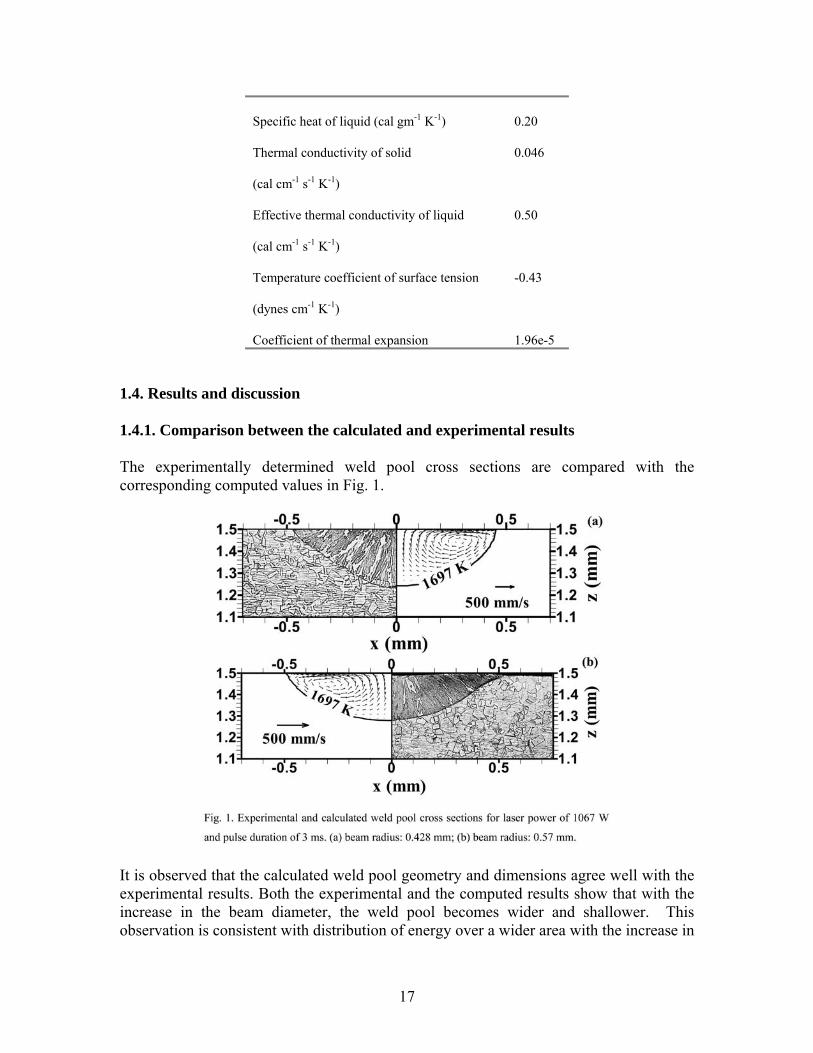
1.4. Results and discussion 1.4.1. Comparison between the calculated and experimental results The experimentally determined weld pool cross sections are compared with the corresponding computed values in Fig. 1.

It is observed that the calculated weld pool geometry and dimensions agree well with the experimental results. Both the experimental and the computed results show that with the increase in the beam diameter, the weld pool becomes wider and shallower. This observation is consistent with distribution of energy over a wider area with the increase in

17

the beam diameter. Since the temperature coefficient of surface tension is negative, the molten metal on the surface flows from the center to the periphery of the pool. As a result, the convection in the weld pool aids in the transport of heat from the middle to the periphery of the weld pool. The role of convection in the heat transfer will be discussed in more details later in this paper. The experimental values of weld pool depth and width for various laser power densities agreed well with the corresponding calculated values as shown in Fig. 2. The fair agreement indicates validity of the transient heat transfer and fluid flow model.

1.4.2. Temperature and velocity fields Figs. 3(a) through 3(e) show the computed temperature and velocity fields as a function of time. The contour values in the figures represent temperatures in K. In the initial period, the weld pool expands rapidly in size and the temperatures and velocities increase with time. At the end of the pulse, the peak temperature drops and the weld pool shrinks rapidly, as shown in Figs. 3(d) and 3(e). The liquid flow during heating is mainly driven by surface tension force and to a much less extent by the buoyancy force. This matter will be discussed more fully using dimensionless numbers. The calculations show that the

18

weld pool solidifies completely in about 1.7 ms after the laser pulse is switched off. The maximum velocity in the weld pool is about 95 cm/s, while at the time of 5.0 ms (1.0 ms after the laser is switched off), the maximum velocity is still about 0.4 cm/s driven mainly by inertia.

A two-phase solid-liquid mushy zone exists in the thin region between the solidus (1697 K) and liquidus (1727 K) isotherms. The size of this zone is very small during heating as shown in Figs 3(a) through 3(c). At the end of the pulse, the size of the mushy zone increases significantly as can be observed from Figs. 3(d) and 3(e). The evolution of mushy zone during laser spot welding is discussed in detail in a later section. 1.4.3. Weld thermal cycle Fig. 4 shows the changes in the computed temperatures at various monitoring locations. The monitoring locations 2, 3 and 4 are at 0.1 mm distance from the weld center but at

19

0°, 45°, and 90° planes, respectively. Similarly, monitoring locations 5, 6 and 7 are at 0.2 mm from the weld center along 0°, 45°, and 90° planes, respectively. The results indicate that initially the heating rate in the weld pool is very fast. With the increase in temperature, the heating rate decreases gradually until the laser is switched off. When the solidification starts, the temperature decreases quickly until it is close to the liquidus temperature. At this temperature, there is a plateau in the thermal cycle curves indicating very low cooling rate due to the release of the latent heat of fusion, as discussed in the next section. When the weld pool cools below the liquidus temperature, the temperature decreases gradually.

The peak temperatures and the heating rates vary significantly depending on the location. Similarly, the cooling rates above the liquidus temperature vary significantly. However, as the weld metal cools, the spatial variation of the cooling rates decreases. When the temperature drops below the solidus temperature, the variation of the cooling rate becomes small due to nearly constant outward heat loss from all locations of the weld. Thus, the spatial variation of the microstructure is expected to be small in the weld metal, except in certain special steels whose microstructures are highly sensitive to cooling rate.

20

From Fig. 4, it can also be seen that the thermal cycles at locations equidistant from the weld center show considerable variation. At the top surface, i.e., x-y plane, the shape of the weld pool is close to a circle. As a result, the temperatures at different locations equidistant to the weld center are the same. However, in the x-z plane, the temperatures at the 0° plane, represented by curve 2 are higher than those at the 90° plane represented by curve 4 although both locations are at a distance of 0.1 mm from the location of the laser beam axis. This variation is mainly due to the shallow pool geometry which increases the temperature gradient along the 90° plane in comparison with the 0° plane. The average temperature gradient in the weld pool at the 90° location is higher than that at the 0° plane since the weld pool is shallow and wide. For locations at the same distance to the weld center, the higher the average temperature gradient, the lower the temperature. Therefore, at locations equidistant from the weld center, the temperatures at the 0° plane are the highest and those at the 90° plane are the lowest. A similar observation was also made by Wei et al.33 while studying GTA spot welding . 1.4.4. Role of convection from dimensionless numbers Relative importance of heat transfer by conduction and convection In the weld pool, heat is transported by a combination of convection and conduction. The relative importance of convection and conduction in the overall transport of heat can be evaluated from the value of Peclet number, Pe, which is defined by:

kLCu

Pe Rpρ= (14)

where u is the average velocity, LR is the characteristic length taken as the pool radius at the top surface of weld pool, ρ, Cp and k have been defined earlier. When Pe is less than one, the heat transport within the weld pool occurs primarily by conduction. When Pe is much higher than 1, the primary mechanism of heat transfer is convection. For spot welding, the value of Peclet number is a function of time since both u and LR depend on time. Fig. 5 shows the change of maximum Peclet number with time in the weld pool. It can be seen that at the beginning of pulse cycle, the Peclet number is low and conduction is the primary mechanism of heat transfer. With time, the Peclet number increases and convection becomes the more important heat transport mechanism in the weld pool. When the pulse is switched off, the Peclet number drops to a very low value very quickly and conduction becomes the main mechanism of heat transfer again due to rapid decrease in velocity.

21

Relative importance of different driving forces Several dimensionless numbers have been used in the literature to determine the relative importance of different driving forces in the weld pool. 37 The ratio of buoyancy force to viscous force is determined by Grashof number:

2

23b TLgGrµ

ρ∆β= (15)

where g is the gravitational acceleration, β is the thermal expansion coefficient, ∆T is the temperature difference between the peak pool temperature and solidus temperature and Lb is a characteristic length for the buoyancy force in the liquid pool which is approximated by one eighth of the pool radius.37 Surface tension Reynolds number, Ma, is used to describe the ratio of surface tension gradient force to viscous force, and is calculated as:

2

R TTL

Maµ

∂∂γ

∆ρ= (16)

Using the physical properties listed in Table 2 and the experimental conditions of Fig. 3, Gr and Ma at t = 4 ms (i.e., just before the laser is switched off) are calculated as follows:

42

23

5

1065.31

2.71400410256.01096.1980

Gr −

−

×=××⎟

⎠⎞

⎜⎝⎛ ×××

= (17)

96.1101

43.014000256.02.7Ma 2 =×××

= (18)

22

The relative importance of the primary driving forces can be judged by the combination of these dimensionless numbers. The ratio of surface tension force to buoyancy force is expressed as:

54b/s 1004.3

1065.396.110

GrMaR ×=

×== − (19)

Therefore, it can be expected that the liquid flow is mainly driven by Marangoni convection and to a much less extent by the buoyancy force.

Order of magnitude of maximum velocity in the weld pool Since the surface tension force is the dominant driving force for convection in the weld pool, the order of the maximal velocity can be approximated by:38

2/12/1

2/12/3

m 664.0W

dydT

dTdu

µργ

≈ (20)

where dT/dy is the average temperature gradient in the weld pool, W is the weld pool radius and the other variables have been defined before. Substituting corresponding value, we can get

s/cm 1.8412.7664.0

0256.0102.043.0u3/2

2/12/1

2/15

m =⎟⎟⎠

⎞⎜⎜⎝

⎛××

×××≈ (21)

This value is in good agreement with that calculated using the 3-D transient heat transfer and fluid flow model, where the maximum velocity at t = 4 ms was found to be about 95 cm/s. The foregoing dimensional analysis provided insights about the weld pool development during spot welding. It should be noted that these order of magnitude analyses cannot provide accurate and detailed information about the spot welding processes, which requires numerical calculation with very fine grids and small time steps.

1.4.5. Evolution of mushy zone The Evolution of mushy zone size during the laser spot welding is shown in Fig. 6. During heating, the liquidus and solidus isotherms are very close and the resulting size of mushy zone is very small. After the pulse is switched off, the mushy zone expands initially and the maximum size of the mushy zone is reached when the pure liquid region diminishes. The size of the mushy zone then decreases as solidification proceeds further.

23

The initial expansion of the mushy zone size could be explained by considering the effect of the latent heat of fusion. When the temperature is higher than the liquidus temperature, the heat loss is accompanied by a decrease in temperature. As the temperature drops between the liquidus and solidus temperatures, the heat loss comes mainly from the release of the latent heat of fusion and the temperature decrease is very slow. As a result, the liquidus isotherm moves faster than the solidus isotherm until the pure liquid region vanishes and the entire weld pool is transformed to mushy region. The evolution of the mushy zone during solidification is demonstrated more clearly in Fig. 7. As shown in this figure, the pure liquid region disappears in about 0.8 ms after the solidification starts and the mushy zone exists for about another 0.9 ms before the weld pool solidifies completely. The existence of a large mushy region is a unique feature of the solidification during spot welding.7,33

24

1.4.6. Solidification During the rapid solidification of the weld pool, the critical parameters in determining the fusion zone microstructure are temperature gradient (G), solidification growth rate (R), undercooling (∆T) and alloy composition. Undercooling, ∆T, indicates how far a liquid alloy of given composition is cooled below its equilibrium liquidus temperature. Since weld solidification proceeds from the preexisting solid substrate, only undercooling associated with growth is important. The undercooling is comprised of contributions from thermal, constitutional, kinetic and solid curvature effects.38 In this study, in order to simplify the calculations, no undercooling is considered. The solidification parameters were calculated by considering only the heat transfer and fluid flow in the weld pool. In other words, the equilibrium liquidus isotherm is assumed to represent the liquid/mushy zone boundary, while the equilibrium solidus isotherm was assumed to be the mushy zone/solid boundary. Fig. 8 shows distances of the mushy zone/solid interface to the weld center as a function of time for two laser power densities (cases A and B). The symbols, D0 and D90 represent the distances at 0° and 90° planes corresponding to the half-width and the depth of the weld pool.

It is observed that for case A, D0 and D90 are very close to each other, while for case B, D0 is twice that of D90 due to the use of larger beam radius. From this figure, the solidification rate, defined as the rate at which the mushy zone/solid interface in the weld pool advances, can be calculated as the slopes of distance versus time. Figs. 9 and 10 show the four important parameters of solidification, temperature gradient (G), solidification rate (R) and their combinations GR and G/R as a function of the time at the 0° and 90° planes for cases A and B, respectively. The temperature gradients, G0 and G90, are evaluated in the mushy zone at the mushy zone/solid interface. The figures show that G0 and G90 at both planes decrease with time, while the solidification rates at both planes increase with time. The maximum solidification rate is reached when the weld pool

25

solidifies completely. In order to understand the solidification phenomena, let us consider the following heat balance equation:33

LfGkGk

dtdrR

L

LLSS −== (22)

where GS and GL are the temperature gradient in solid and mushy zone at the mushy zone/solid interface, respectively, ks and kl are the thermal conductivities in the solid and the liquid, respectively, and fL is the liquid fraction. As shown in Fig. 7, GL drops more rapidly than GS during solidification. Furthermore, decreases with time as the solidification progressed. As a result, the solidification rate increases with time, which is indicated in Figs 9(b) and 10(b).

Lf

The solidification rate, R, and temperature gradient, G, are important in the combined forms G/R and GR (cooling rate). As shown in Figs. 9(c) and 10(c), the solidification parameter G/R decreases with time, since G decreases while R increases with time. The solid-liquid interface stability factor, G/R, is related to the solidification morphology. As the value of G/R increases, the interface morphology changes from equiaxed-dendritic, to cellular-dendritic, to cellular grains.39 As the solidification progresses from the mushy

26

zone/solid front to the weld center, the mushy zone/solid interface has the maximum temperature gradient and minimum solidification growth rate. While for the weld center, the situation is completely different. It has the minimum temperature gradient and maximum solidification rate. Therefore, the value of G/R decreases from the fusion line to the weld center. As a result, we may expect a cellular type of microstructure close to the fusion line, an equiaxed-dendritic microstructure at the pool center, and a cellular-dendritic microstructure between these two regions. The solidification parameter GR is useful as it influences the scale of the solidified substructure. Since G decreases and R increases with time, the change of the value of GR with time depends on the magnitude of G and R and how the rates of G and R change with time. In laser spot welding, because of high temperature gradient and small weld pool geometry, the order of G is much larger than the order of R. So the change of GR with time mostly depends on the change of G with time, that is, the cooling rate decreases with time during solidafication. This is different from GTA spot welding, as discussed in the next section.

Furthermore, the solidification parameters vary with the locations in the weld pool. The computed values of these parameters are shown in Figs. 9 and 10 for 0° and 90° planes. This difference in solidification parameter is relative to the difference of weld pool geometry. From Fig. 8, D0 is very close to D90 for case A, while for case B, D0 is much

27

larger than D90. As a result, for case A, the values of these four parameters along 0° and 90° planes are very similar, while for case B, there are significant differences of these four parameters between 0° and 90° planes. As discussed before, the value of average temperature gradient at the 90° location is the higher than that at the 0° plane. It should be noted that the validation of the numerical model was limited to the weld pool geometry. The calculated solidification parameters have not been validated by comparing with the corresponding experimental results in 304 stainless steel laser spot welds. Calculations presented here indicate aspects of solidification in a qualitative manner, since the focus here was the examination of the results of the transient heat transfer and fluid flow model. Furthermore, the solidification process investigated in the present model is governed only by the transfer of heat. An accurate prediction of the weld pool solidification will require consideration of both the thermodynamics and kinetics of solidification.

1.4.7. Comparison of laser spot welding with GTA spot welding and GTA linear welding

Laser spot welding is characterized by a much shorter time span than the GTA spot welding or GTA linear welding. As a result, the temperature gradients in the work piece and its heating and cooling rates are significantly different in the three processes. The computed values of spatial and the temporal variations of temperature for the three welding processes are compared in Table 3. The laser spot welding is characterized by higher power intensity, higher peak temperature and smaller weld pool size. As a result, the heating and cooling rate, temperature gradient and the solidification rate in the weld

28

pool are much higher than those in GTA linear and spot welding. The computed results in Table 3 indicate that during laser spot welding, the maximum temperature gradient in the weld pool can reach to 12,560 K/mm and the maximum solidification rate can be as high as 800 mm/s. For a typical GTA spot welding of 1005 steel, the maximum temperature gradient in the weld pool is about 430 K/mm and solidification rate of 30 mm/s. More important, the cooling rate in the laser spot welding is significantly higher than the GTA welding. Therefore, it is possible to obtain the different solidification substructures in the fusion zone depending on the welding process. The computed results in Table 3 provide a good understanding of the relative values of important parameters for the three welding processes. However, the results must be used with caution, since the temperature gradients and the cooling rates presented in Table 3 depend strongly on the welding parameters.

1.5. Conclusions

1) The fusion zone geometry, calculated from the transient heat transfer and fluid flow model, was in good agreement with the corresponding experimentally measured values for various laser spot welding conditions. During heating, the heating rate varies significantly at different locations. As the weld pool cools below the solidus temperature, the spatial variation of cooling rates decreases.

2) The liquid flow is mainly driven by the surface tension and to a much less extent, by the buoyancy force. Liquid metal convection significantly affects heat transfer in the weld pool towards the end of the pulse. Heat transfer by conduction is important when the liquid velocity is small at the beginning of the pulse and during weld pool solidification.

3) The size of the mushy zone, i.e., liquid + solid two-phase region, grows significantly with time during solidification and the maximum size of the mushy zone is reached when the pure liquid region vanishes. This behavior can be explained from the heat transfer consideration taking into account the latent heat of fusion.

4) The temperature gradients (G) in the mushy zone at the mushy zone/solid interface decrease with the solidification time. The solidification rate (R) of the mushy zone/solid interface increases with time. The combination of solidification parameters G and R, i.e., G/R and GR, were quantitatively calculated in laser spot welding of 304 stainless steel.

5) For laser spot welding, the heating and cooling rate, temperature gradient and the solidification rate in the weld pool were much larger than those for GTA linear welding and GTA spot welding.

1.6. References

[1] Cline H E and Anthony T R 1977 J. Appl. Phys. 48 3895 [2] Mazumder J and Steen W M 1980 J. Appl. Phys. 51 941 [3] Frewin M R and Scott D A 1999 Welding J. 78 15s [4] Katayama S, Mizutani M and Matsunawa A 1997 Sci. and Technol. of Welding and

Joining 2 1

29

[5] Chang W S and Na S J 2001 Metall. Trans. B 32B 723 [6] Oreper G M, Szekely J and Eager T W 1986 Metall. Trans. B 17B 735 [7] Betram L A 1993 J. Eng. Mater. Technol. 115 24 [8] Sahoo P, Collur M M and DebRoy T 1988 Metall. Trans. B 19B 967 [9] Paul A and DebRoy T 1988 Metall. Trans. B 19B 851 [10] P. A. A. Khan and T. DebRoy 1984 Metall. Trans. B 15B 641 [11] Collar A M M, Paul A and DebRoy T 1987 Metall. Trans. B 18B 733 [12] Zacharia T, David S A, Vitek J M and DebRoy T 1989 Welding J 68 499s[13] Mundra K and DebRoy T 1993 Metall. Trans. B 24B 145 [14] Hong T, DebRoy T, Babu S S and David S A 2000 Metall. Trans. B 31B 161 [15] Mundra K, DebRoy T, Babu S S and David S A 1997 Welding J 76 163s [16] Zhao H and DebRoy T 2001 Metall. Trans. B 32B, 163 [17] Yang Z, Sista S, Elmer J W and DebRoy T 2000 Acta Materialia 48 4813 [18] Zhang W, Elmer J W and DebRoy T 2002 Materials Science and Engineering A333 320 [19] Mundra K, Blackburn J M and DebRoy T 1997 Sci. and Technol. of Welding and

Joining 2 174 [20] Palmer T A and DebRoy T 2000 Metall. Trans. B 31B 1371 [21] Fuerschbach P W and Norris J T 2002 Beam characterization for Nd:YAG spot

welding lasers, presented at ICALEO 2002, Scottsdale, AZ [22] Zacharia T, David S A, Vitek J M and DebRoy T 1989 Welding J. 68 510s [23] Patankar S V 1980 Numerical Heat Transfer and Fluid Flow (New York:

Hemisphere Publishing Corporation) [24] Voller V R and Prakash C 1987 Int. J. Heat Mass Transfer 30 1709 [25] Brent A D, Voller V R and Reid K J 1988 Numer. Heat Transfer 13 297 [26] Tsai N S and Eagar T W 1985 Metall. Trans. B 16B 841 [27] Chan C L, Zehr R, Mazumder J and Chen M M 1986 Modelling and Control of

Casting and Welding Processes, edited by Kou S and Mehrabian R, pp 229 [28] Cremers D A, Lewis G K and Korzekwa D R 1991 Welding J. 70 159s [29] Pitscheneder W 2001 Ph. D thesis, The University of Leoben [30] Ready J F 2001 LIA Handbook of Laser Materials Processing (Orlando: Magnolia

Publishing) [31] Bramson M A 1968 Infrared Radiation: a Handbook for Applications (New York:

Plenum Press) [32] Peckner D and Bernstein I M 1977 Handbook of Stainless Steels (New York:

McGraw-Hill Book Company) [33] Zhang W, Roy G G, Elmer J W and DebRoy T 2003 Modeling of heat transfer and

fluid flow during GTA spot welding of 1005 steel J. Appl. Phys (in press, to appear in March 2003)

[34] Davis J R 1998 Metals Handbook (ASM International, Materials Park, OH). [35] 1994 ASM Specialty Handbook. Stainless Steel (ASM International, Materials Park, OH) [36] 1990 Metals handbook. Volume 1. Properties and Selection: Ion, steels, and high-

performance alloys (ASM International, Materials Park, OH) [37] Yang Z 2000 Ph. D. thesis The Pennsylvania State University [38] DebRoy T and David S A 1995 Rev. Mod. Phys. 67, 85

30

[39] Grong Ø 1997 Metallurgical Modeling of Welding, 2nd ed. (London: The Institute of Materials)

Section 2. Probing Temperature during Laser Spot Welding from Vapor Composition and Modeling

2.1. Introduction Laser spot welding is characterized by the highly transient nature and very short duration of the process. The welding is often completed in a few milliseconds and the heating and cooling rates attained are many times higher than those typical in steady-state linear laser welding process.1 Knowledge of temperature and velocity fields, solidification rate and thermal cycles are important to determine the geometry, composition, structure and the resulting properties of the spot welds.1,2 Understanding the formation of non-equilibrium phases and solidification cracking based on fundamental principles requires knowledge of the heating and cooling rates. Experimental measurements of temperature and velocity fields during laser spot welding are difficult because of the insufficient time for measurement and the highly transient nature of the welding process. In addition, the weld pool is often covered by a metal vapor plume. Because of these difficulties, no generally available technique has been developed to date to measure temperature and velocity fields in the weld pool during laser spot welding. During high energy laser beam welding of important engineering alloys, the metal in the weld pool can be heated to very high temperatures and significant vaporization of volatile alloying elements often takes place from the weld pool surface.3-12 The loss of alloying elements can result in significant changes in the microstructure and degradation of mechanical properties of weldments. During welding of stainless steels, the main constituents of the metal vapor are iron, manganese, chromium and nickel.9,11-13 In high manganese stainless steels, such as AISI 201, iron and manganese are the prominent vapor species in the welding environment. In order to minimize the mass loss during high power laser welding, it is necessary to quantitatively understand the role of various factors that affect the alloying element vaporization. The most important factors in determining the rate of vaporization of different elements are the temperature distribution on the surface and the weld metal chemical composition. During laser welding, a strong spatial gradient of temperature exists on the weld pool surface. The resulting gradient of surface tension is the main driving force for the strong recirculating flow of molten metal in the weld pool.14-16 In addition, the buoyancy force resulting from the spatial variation of density also contributes to the motion of the weld pool, although to a much lesser extent than the surface tension gradient. Because of the strong recirculating flow, the weld pool can be reasonably assumed to be well mixed and compositionally homogeneous. For a weld pool of known composition, the vaporization

31

rates of various alloying elements are strongly affected by the surface temperatures. Since the middle region of the weld pool surface is at a much higher temperature than the periphery, it is fair to expect that much of the vaporized species originate from the middle of the weld pool surface. Since the relative rates of vaporization of two alloying elements are determined by the local temperature, the measured vapor composition can provide a rough idea of the peak temperature at the weld pool surface. In recent decades, numerical models have been developed to understand the heat transfer and fluid flow during welding. These models have been widely utilized to quantitatively understand thermal cycles and fusion zone geometry.17-25 Results from the heat transfer and fluid flow study have also been used to study weld metal phase composition,26-28 inclusion structure,29-31 grain structure,32-34 and for prevention of porosity in welds.35

However, most of these studies were focused on linear steady state welds and not on very short duration laser spot welds. Although a limited number of investigations of spot welds have been undertaken in the past, the time scales studied were much longer than the typical few milliseconds involved in laser spot welds. A detailed experimental and theoretical study of laser spot welding has not been undertaken. In this paper, recent theoretical and experimental research to estimate weld pool temperatures are described. A transient, three-dimensional numerical heat transfer and fluid flow model based on the solution of the equations of conservation of mass, momentum and energy was used to calculate the temperature and velocity fields in the weld pool as a function of time. The effects of spatial variation of surface tension and buoyancy were considered to determine the weld pool convection as a function of time. Very fine grids and small time steps were used to achieve accuracy in the calculations. The model was tested by comparing the experimentally determined geometry of the spot welds with those obtained from the computed temperature fields. Composition of the metal vapor from the weld pool was determined by condensing a portion of the vapor on the inner surface of a both end open quartz tube which was mounted perpendicular to the sample surface and co-axial with the laser beam. The vapor composition was used to determine an effective temperature of the weld pool for various welding conditions. This technique is shown to be a useful method to determine rough values of peak temperature during laser spot welding. No other reliable method for the estimation of peak temperature during laser spot welding has emerged so far because of the very short duration and highly transient nature of the laser spot welding process. 2.2. Experimental procedure Several 304 stainless steel laser spot welds were fabricated at the Sandia National Laboratories. The alloy composition was: 1 wt% Mn, 18.1 wt% Cr, 8.6 wt% Ni, 0.69 wt% Si, 0.046 wt% C, 0.012 wt% P, 0.003 wt% S, and balance Fe. A schematic diagram of the experimental set-up is presented in Fig. 1.

32

Fig. 1: A schematic diagram of the experimental setup. During laser spot welding, a cylindrical 6 mm inner diameter by 25 mm long , open ended quartz tube was placed co-axial to the laser beam and right above the 304 stainless steel samples. The vaporized elements were collected as condensation on the interior surface of the tube. A Raytheon SS 525 pulsed Nd:YAG laser was used for laser spot welding with pulse energies of 2.12 J and 3.19 J and pulse durations of 4.0 ms and 3.0 ms, respectively. The laser beam was focused inside the quartz tube with a 100 mm focal length lens. For each combination of energy and duration, the laser beam was defocused to different extents to obtain various spot diameters and power densities. To increase the amount of vapor condensate collected , 50 individual spot welds were made on each of the 3 by 10 by 17 mm samples.. The spot welds were made in ambient air since it was impractical to provide inert gas shielding inside the quartz tube for each spot weld. The experimental parameters are indicated in Table I.

Table 1. Welding Parameters

Sample number

Pulse energy

(J)

Beam radius (mm)

Power density

(W/mm2)

Pulse duration

(ms) E 2.12 0.289 2020 4

B/F 2.12 0.247 2765 4

C 2.12 0.227 3274 4

D 2.12 0.171 5769 4

G 3.19 0.326 3185 3

A 3.19 0.28 4317 3 The quartz tube samples were examined using the JEOL 8600 Electron Microprobe X-ray Analyzer to determine the vapor composition. The evaporation products had the consistency of fine dust. The quartz tubes were broken and a suitable fragment from each experiment was mounted to expose the deposit. Due to the geometry of the samples and their highly porous nature, the probe was not operated in an automated mode. Instead a series of spot measurements of the K-values (count rate ratios of unknown to standards)

33

were made on each sample. The K value measurements were converted to approximate oxide ratios and averaged together for each sample. 2.3. Mathematical formulation Assumptions: The weld metal was assumed to be incompressible, Newtonian fluid. Constant thermophysical properties were used for the calculations and the variation of absorption coefficient of the laser by the stainless steel at different temperatures was ignored for simplicity.

Governing equations: Because of the axisymmetric nature of the spot welding, the governing equations can be solved in two-dimensions to calculate the temperature and velocity fields. However, since the model is also used for welding with a moving heat source, a transient, three-dimensional, heat transfer and fluid flow model was used for the laser spot welding. The following momentum conservation equation was solved:36

( )

ji

j

ii

jij Sxu

xxuu

tu

+⎟⎟⎠

⎞⎜⎜⎝

⎛∂∂

µ∂∂

=∂

∂ρ+

∂∂

ρ (1)

where ρ is the density, t is the time, xi is the distance along the i = 1, 2 and 3 directions, uj is the velocity component along the j direction, µ is the effective viscosity, and Sj is the source term for the jth momentum equation and is given as:

( )refj3L

2L

j

j

jjj TTgu

Bf)f1(C

xu

xxpS −βρ+⎟⎟

⎠

⎞⎜⎜⎝

⎛

+−

−⎟⎟⎠

⎞⎜⎜⎝

⎛

∂∂

µ∂∂

+∂∂

−= (2)

where p is the pressure, fL is the liquid fraction, B is a constant introduced to avoid division by zero, C (=1.6×104) is a constant that takes into account mushy zone morphology, β is the coefficient of volume expansion and Tref is a reference temperature. The third term on the right hand side (RHS) represents the frictional dissipation in the mushy zone according to the Carman-Kozeny equation for flow through a porous media.37,38 The value of the effective viscosity in equation (1) is a property of the specific welding system and not an inherent property of the liquid metal. Typical values of effective viscosity are much higher than that of the molecular viscosity.24,25 The higher value is important, since it allows accurate modeling of the high rates of transport of momentum in systems with strong fluctuating velocities that are inevitable in small weld pools with very strong convection currents. The pressure field was obtained by solving the following continuity equation simultaneously with the momentum equation:

34

( ) 0xu

i

i =∂ρ∂ (3)

The total enthalpy H is represented by a sum of sensible heat h and latent heat content ∆H, i.e., where , CHhH ∆+= ∫= dTCh p p is the specific heat, T is the temperature,

, L is the latent heat of fusion and the liquid fraction fLfH L=∆ L is assumed to vary linearly with temperature in the mushy zone:

⎪⎪⎩

⎪⎪⎨

⎧

<

≤≤−−

>

=

S

LSSL

S

L

L

TT0

TTTTTTT

TT1

f (4)

where TL and TS are the liquidus and solidus temperature, respectively. The thermal energy transport in the weld work piece can be expressed by the following modified energy equation:2,23

( )⎟⎟⎠

⎞⎜⎜⎝

⎛

∂∂

∂∂

=∂

∂ρ+

∂∂

ρipii

i

xh

Ck

xxhu

th

i

i

x)Hu(

t)H(

∂∆∂

ρ−∂∆∂

ρ− (5)

where k is the thermal conductivity. In the liquid region, the value of the thermal conductivity in equation (5) is taken as the effective thermal conductivity which is a property of the specific welding system and not an inherent property of the liquid metal. Typical values of effective thermal conductivity are much higher than that of the thermal conductivity of the liquid. The higher value is important, since it allows accurate modeling of the high rates of transport of heat in systems with strong fluctuating velocities that are inevitable in small weld pools with very strong convection currents.24,25

The weld top surface is assumed to be flat. The velocity boundary condition is given as:2

0wyT

dTdf

zv

xT

dTdf

zu

L

L

=∂∂γ

=∂∂

µ

∂∂γ

=∂∂

µ

(6)

where u, v and w are the velocity components along the x, y and z directions, respectively, and dγ/dT is the temperature coefficient of surface tension. As shown in this equation, the u and v velocities are determined from the Marangoni effect. The w velocity is equal to zero since there is no flow of liquid metal perpendicular to the pool top surface. The heat flux at the top surface is given as:

35

( ) )T(ThTTσεr

)yf(xexpπrfQη

zTk ac

4a

42

b

22

2b

−−−−⎟⎟⎠

⎞⎜⎜⎝

⎛ +−=

∂∂ (7)

where f is the power density distribution factor, Q is the total energy of the heat source, η is the absorption coefficient, rb is the heat source radius, σ is the Stefan-Boltzmann constant, hc is the heat transfer coefficient, and Ta is the ambient temperature. The first term on the right hand side is the heat input from the heat source. The second and third terms represent the heat loss by radiation and convection, respectively. For laser welding, laser power density distribution factor f is taken as39 3.0. Laser power and beam radius were experimentally measured. The reported values of the absorption coefficient vary significantly.40-42 For example, Cremers, Lewis and Korzekwa40 indicated absorption coefficient of Nd:YAG laser in 316 stainless steel in the range of 0.21 to 0.62. The absorption coefficient has been related to the substrate resistivity and the wavelength of the laser radiation by the following relation.42

2/32/1

006.00667.0365.0)T( ⎟⎠⎞

⎜⎝⎛

λα

+⎟⎠⎞

⎜⎝⎛

λα

−⎟⎠⎞

⎜⎝⎛

λα

=η (8)

where λ is the wavelength (cm), α is the electrical resistivity of the materials (Ω-cm). the average electrical resistivity of 304 stainless steel is 80 µΩ-cm,43 and the wavelength of Nd:YAG laser is 1.064 µm. Substituting these values into equation (8), the absorption coefficient is obtained as 0.27, which is the value taken in the calculations reported in this paper. The data used for calculations43-47 are presented in Table 2.

Table 2 Data used for calculations[43-47]

Property/Parameter Value

Density of liquid metal (kg/m3) 7.2 × 103

Absorption coefficient 0.27

Effective viscosity (kg/m-sec) 0.1

Solidus temperature (K) 1697

Liquidus temperature (K) 1727

Enthalpy of solid at melting point (J/kg) 1.20 × 106

Enthalpy of liquid at melting point (J/kg) 1.26 × 106

Specific heat of solid (J/kg-K) 711.8

Specific heat of liquid (J/kg-K) 837.4

Thermal conductivity of solid (J/m-sec-K) 19.26

36

Effective thermal conductivity of liquid (J/m-sec-K) 209.3

Temperature coefficient of surface tension ( N/m-K) -0.43 × 10-3

Coefficient of thermal expansion 1.96 × 10-5

The boundary conditions are defined as zero flux across the symmetric surface as:

0yw,0v,0

yu

=∂∂

==∂∂ (9)

0yh

=∂∂ (10)

At all other surfaces, temperatures are set at ambient temperature and the velocities are set to be zero. The governing equations were discretized and solved iteratively on a line-by-line basis using a Tri-Diagonal Matrix Algorithm. The detailed procedure to solve the equations is described in the literature.36 After obtaining the values of the sensible enthalpy, h, on computational domain, temperature can be expressed as:

( ) ( )

⎪⎪⎪⎪

⎩

⎪⎪⎪⎪

⎨

⎧

≥−

+

<<

−×+=−−

−+=

−+

≤−

+

=

calpl

calliquid

calmelt

solidliquidlsolidsolidliquidmeltcal

meltsolid

pa

meltsolid

meltps

meltsolid

HhforC

HhT

HhHfor

TTfTTTHH

HhT

CHh

T

HhforCHh

T

T (11)

where Tsolid and Tliquid are the solidus and liquidus temperatures of the material, respectively. Hmelt is the total enthalpies at the liquidus temperatures, Cps and Cpl are the specific heat of solid and liquid, respectively, fl is the liquid fraction. The specific heat, Cpa, in the mushy zone was calculated by:

2/)CC(C plpspa += (12) Hcal is given as:

)TT(CHH solidliquidpameltcal −×+= (13)

2.4. Results and discussion

37

The local evaporation flux of an alloying element based on the Langmuir equation is expressed as:48

RTM2P

Ji

ii

π

λ= (14)

where Ji is the vaporization flux of the element i, λ is positive constant with a maximum value of 1 that accounts for the inevitable condensation of a portion of the vaporized atoms on the surface at pressures higher than perfect vacuum, Pi is the vapor pressure of i over the liquid, Mi is molecular weight of the vaporizing element i, R is the gas constant and T is the temperature. At pressures close to atmospheric pressure, the value of λ cannot be estimated from fundamental principles. The lack of knowledge of λ poses a problem in the application of Langmuir equation for quantitative calculation of the vaporization rates of individual alloying elements. However, since the relative vaporization rates of any two alloying elements is independent of λ , Langmuir equation can be used for predicting the relative vaporization rates of various alloying elements:

21

i

j

j

i

j

i

MM

PP

JJ

⎟⎟⎠

⎞⎜⎜⎝

⎛= (15)

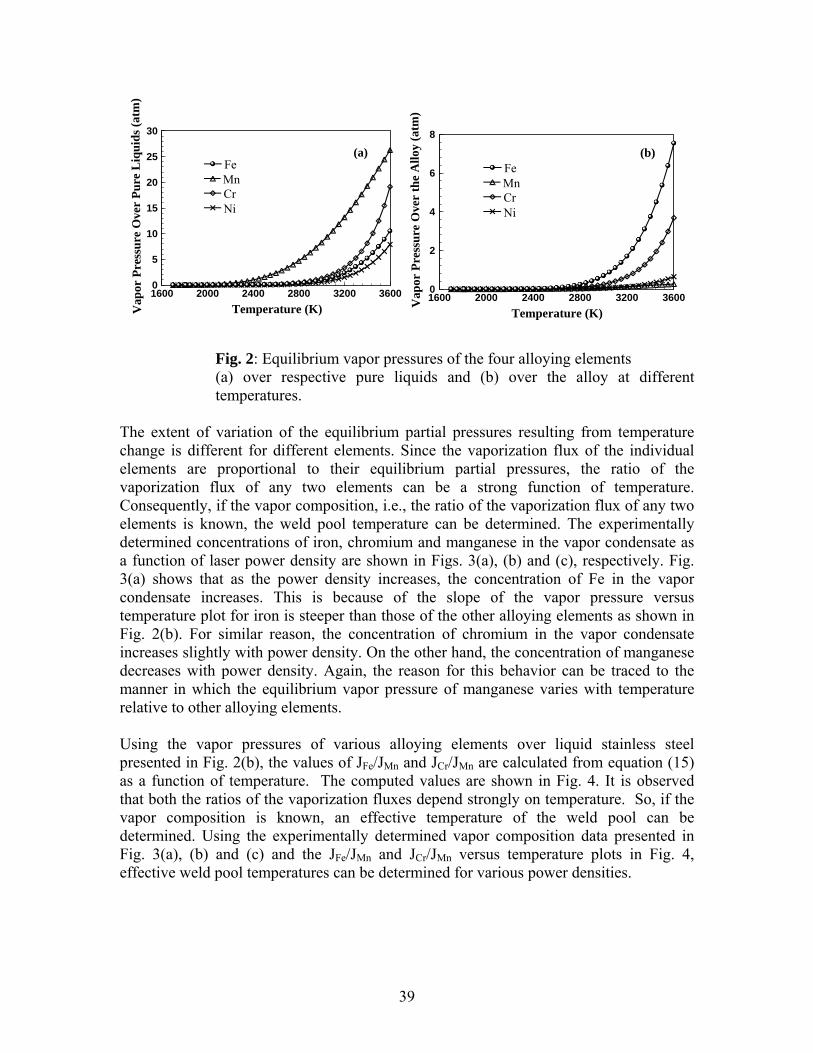
The equilibrium partial pressure Pi over the alloy depends upon the composition and the temperature of the weld metal. The vapor pressures of the alloying elements over pure liquids are presented in Fig. 2(a) and those over 304 stainless steel are shown in Fig. 2(b). The equilibrium vapor pressure data used in the calculations are presented in the Appendix. It can be seen from Fig 2(a) that among the four alloying elements, manganese has the highest vapor pressure over its pure liquid in the entire temperature range studied. However, its vapor pressure over the alloy is lower than those of iron and chromium, as observed from Fig. 2(b). This is because manganese only accounts for 1.0 wt % in 304 stainless steel while iron and chromium are present at 72.3 and 18.1 wt%, respectively. It can be seen from Fig. 2(b) that over liquid stainless steel, iron is the dominant vaporizing species, followed by chromium and manganese. The vapor pressure of nickel over the alloy is very low. Vapor pressures of all the alloying elements are strong functions of temperature.

38

1600 2000 2400 2800 3200 3600Temperature (K)

0

5

10

15

20

25

30V

apor

Pre

ssur

e O

ver

Pure

Liq

uids

(atm

)

y

y

y

y

FeMnCrNi

(a)

1600 2000 2400 2800 3200 3600Temperature (K)

0

2

4

6

8

Vap

or P

ress

ure

Ove

r th

e A

lloy

(atm

)

y

y

y

y

FeMnCrNi

(b)

Fig. 2: Equilibrium vapor pressures of the four alloying elements (a) over respective pure liquids and (b) over the alloy at different temperatures.

The extent of variation of the equilibrium partial pressures resulting from temperature change is different for different elements. Since the vaporization flux of the individual elements are proportional to their equilibrium partial pressures, the ratio of the vaporization flux of any two elements can be a strong function of temperature. Consequently, if the vapor composition, i.e., the ratio of the vaporization flux of any two elements is known, the weld pool temperature can be determined. The experimentally determined concentrations of iron, chromium and manganese in the vapor condensate as a function of laser power density are shown in Figs. 3(a), (b) and (c), respectively. Fig. 3(a) shows that as the power density increases, the concentration of Fe in the vapor condensate increases. This is because of the slope of the vapor pressure versus temperature plot for iron is steeper than those of the other alloying elements as shown in Fig. 2(b). For similar reason, the concentration of chromium in the vapor condensate increases slightly with power density. On the other hand, the concentration of manganese decreases with power density. Again, the reason for this behavior can be traced to the manner in which the equilibrium vapor pressure of manganese varies with temperature relative to other alloying elements. Using the vapor pressures of various alloying elements over liquid stainless steel presented in Fig. 2(b), the values of JFe/JMn and JCr/JMn are calculated from equation (15) as a function of temperature. The computed values are shown in Fig. 4. It is observed that both the ratios of the vaporization fluxes depend strongly on temperature. So, if the vapor composition is known, an effective temperature of the weld pool can be determined. Using the experimentally determined vapor composition data presented in Fig. 3(a), (b) and (c) and the JFe/JMn and JCr/JMn versus temperature plots in Fig. 4, effective weld pool temperatures can be determined for various power densities.

39

2000 3000 4000 5000 6000Power Density (W/mm2)

0

20

40

60

80

100

Con

cent

ratio

n of

Fe(

g) (w

t%)

(a)

2000 3000 4000 5000 6000Power Density (W/mm 2)

0

20

40

60

Con

cent

ratio

n of

Mn(

g) (w

t%)

(b)

2000 3000 4000 5000 6000Power Density (W/mm2)

0

20

40

60

Con

cent

ratio

n of

Cr(

g) (w

t%)

(c)

Fig. 3: Measured weight percent of (a) Fe, (b) Mn, (c) Cr in vapor composition with laser power density. The triangles represent the original data and the circles show best fit.

1600 2000 2400 2800 3200 3600Temperature (K)

0

5

10

15

20

25

30

J Fe/

J Mn

(a)

1600 2000 2400 2800 3200 3600Temperature (K)

0

4

8

12

16

20

J Cr/

J Mn

(b)

Fig. 4: The ratio of calculated vaporization rates of (a) Fe and Mn and (b) Cr and Mn as a function of temperature.

The results are shown in Fig. 5. It can be observed that the temperatures calculated from JFe/JMn are in good agreement with those obtained from JCr/JMn indicating that the estimated effective temperatures are independent of the choice of element pairs.

40

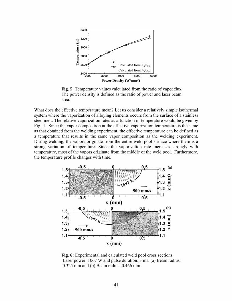
2000 3000 4000 5000 6000Power Density (W/mm2)

2400

2600

2800

3000

3200

3400

Tem

pera

ture

(K)

y

y

Calculated from JFe/JMn

Calculated from JCr/JMn

Fig. 5: Temperature values calculated from the ratio of vapor flux. The power density is defined as the ratio of power and laser beam area.

What does the effective temperature mean? Let us consider a relatively simple isothermal system where the vaporization of alloying elements occurs from the surface of a stainless steel melt. The relative vaporization rates as a function of temperature would be given by Fig. 4. Since the vapor composition at the effective vaporization temperature is the same as that obtained from the welding experiment, the effective temperature can be defined as a temperature that results in the same vapor composition as the welding experiment. During welding, the vapors originate from the entire weld pool surface where there is a strong variation of temperature. Since the vaporization rate increases strongly with temperature, most of the vapors originate from the middle of the weld pool. Furthermore, the temperature profile changes with time.

Fig. 6: Experimental and calculated weld pool cross sections. Laser power: 1067 W and pulse duration: 3 ms. (a) Beam radius: 0.325 mm and (b) Beam radius: 0.466 mm.

41

It will be shown later in this paper that for the conditions of the experiments described the surface temperature change is most pronounced in the first millisecond. The changes in temperature slows down considerably after that time. As a result most of the vapor comes from the later portion of the thermal cycle when the temperature is fairly close to the value at the end of the pulse. In short, since much of the vapor originates from the middle of the weld pool surface and towards the end of the pulse, the effective temperature is expected to be fairly close to the peak temperature. The experimentally determined weld pool cross sections are compared with the corresponding numerically computed values in Fig. 6. It is observed that the calculated weld pool geometry and dimensions agree well with the experimental results. The good agreement indicates the validity of the transient heat transfer and fluid flow model. The experimental and calculated values of weld pool depth and width for various laser power densities are presented in Fig. 7.

1000 2000 3000 4000 5000 6000Power Density (W/mm2)

0

0.2

0.4

0.6

0.8

1

Pene

trat

ion

Dep

th (m

m)

y

y

Calculated valueExperimental value

(a)

1000 2000 3000 4000 5000 6000Power Density (W/mm2)

0

0.5

1

1.5

2

Wel

d Po

ol W

idth

(mm

)y

y

Calculated valueExperimental value

(b)

Fig. 7: The effects of laser power density on (a) weld pool Depth and (b) weld pool width. Laser power: 1967 W, and pulse duration: 3.0 ms. The power density is defined as the ratio of powerand laser beam area.

The total power was kept constant at 1967 W while the beam radius was varied to obtain different power densities. It can be seen that the calculated weld pool depth and width show good agreement with the experimental results at low power densities. However, at high power densities, there is some difference between the calculated and the experimental values of the weld pool depth. In order to understand the reason for the discrepancy, the experimental ratio of weld pool depth to half-width is presented in Fig. 8. It is observed that the ratio varied between 0.4 to 0.7 at power densities below 3500 W/mm2 while this value increased to over 1.0 at higher power densities. Weld pool depths higher than the half-width are often obtained when the surface of the weld pool is significantly depressed from its nearly flat position. Such depressions are common at high power densities, because the high vapor flux exerts significant recoil force on the weld pool surface. In extreme cases, when the recoil force exceeds the surface tension force, fine metal droplets are ejected from the weld pool. Significant loss of mass due to vaporization and metal particle ejection can occur at high power densities.13 However, the difference between the experimental and the computed values of weld pool depth at

42

power density higher than 3500 W/mm2 is consistent with the mass loss due to vaporization and particle ejection. At lower power densities, experimentally measured and computed values of weld pool depth and width agree better with the corresponding measured values.

1000 2000 3000 4000 5000 6000Power Density (W/mm2)

0

0.3

0.6

0.9

1.2

1.5

D/W

W

D

Fig. 8: The variation of D/W with laser power density. Laser power: 1967 W and pulse duration: 3.0 ms.

Figs. 9(a) through 9(e) show the computed temperature and velocity fields as a function of time. The liquid metal motion in the weld pool is driven mainly by the surface tension force and to a much lower extent by the buoyancy force. Because of the negative values of the temperature coefficient of surface tension, the surface tension drives the liquid metal from the center to the periphery at the top surface of the weld pool. As a result, the weld pool becomes wide and shallow. During the initial period of laser spot welding, the weld pool grows rapidly in size and the temperature and velocity of liquid increase with time. At the end of the pulse, the peak temperature and velocity of liquid drops and the weld pool shrinks rapidly. The maximum velocity of liquid in the weld pool is 0.86 m/s. After 5.0 ms, i.e., 1.0 ms after the laser is switched off, the maximum velocity is still about 4.1 mm/s, which is driven mainly by inertia.

1.2

1.3

1.4

1.5

z(m

m)

-0.4 -0.3 -0.2 -0.1 0 0.1 0.2 0.3 0.4

x (mm)0

0.2

0.4y (mm

)

1000 K1727 K

2300 K

2700 K

600 mm/s1.2

1.3

1.4

1.5

z(m

m)

-0.4 -0.3 -0.2 -0.1 0 0.1 0.2 0.3 0.4

x (mm)0

0.2

0.4y (mm

)

1000 K1727 K

2300 K2900 K

600 mm/s

(a) (b)

43

1.2

1.3

1.4

1.5

z(m

m)

-0.4 -0.3 -0.2 -0.1 0 0.1 0.2 0.3 0.4

x (mm)0

0.2

0.4y (mm

)

1000 K1727 K

2300 K

2900 K

600 mm/s1.2

1.3

1.4

1.5

z(m

m)

-0.4 -0.3 -0.2 -0.1 0 0.1 0.2 0.3 0.4

x (mm)0

0.2

0.4y (mm

)

1000 K

1727 K

1760 K

600 mm/s

1697 K

mushy zone

(c) (d)

1.2

1.3

1.4

1.5

z(m

m)

-0.4 -0.3 -0.2 -0.1 0 0.1 0.2 0.3 0.4

x (mm)0

0.2

0.4y (mm)

1000 K

1400 K

600 mm/s

1697 K

mushy zone

(e)

Fig. 9: Computed temperature and velocity fields at different times: (a) t = 1 ms, (b) t = 2 ms, (c) t = 4 ms, (d) t = 4.5 ms, and (e) t = 5 ms. Laser power: 530 W, pulse duration: 4.0 ms, and spot radius: 0.171 mm.

A two-phase solid-liquid mushy zone exists in the thin region between the solidus (1697 K) and liquidus (1727 K) temperatures. The size of this zone is very small during heating (as shown in Figs. 9(a) through 9(c)). After the pulse is switched off, the mushy zone begins to expand (shown in Figs. 9(d) and 9(e)), which could be explained by considering the effect of the latent heat of fusion.

0 2 4 6 8 10 12Time (ms)

500

1000

1500

2000

2500

3000

3500

Tem

pera

ture

(K) 1

2

3

Solidus Temperat

x

y °

S

1Top su face

L3

Fig. 10: Weld thermal cycles at different locationssurface of weld pool. Distance from the weld cente2: 0.058 mm; 3: 0.125 mm, as shown in the small fsolid horizontal line indicates solidus temperature.530 W, pulse duration: 4.0 ms, and beam radius: 0

44

0

°

90

2

r

14

ure

on the top r: 1: 0.0 mm; igure. The Laser power: .171 mm.

When the temperature is higher than the liquidus temperature, the heat loss is accompanied by the decrease in temperature. As the temperature drops between the liquidus and solidus temperatures, the heat loss comes mainly from the release of the latent heat of fusion and the temperature decrease is very slow. The existence of mushy zone has significant effect on the final solidified microstructure. Fig. 10 shows changes in the computed temperatures at three selected locations as a function of time. These locations represent distances of 0, 0.085 and 0.125 mm, respectively from the location of the heat source, as shown in the small figure. The results indicate that the peak temperatures and the heating rates at different locations vary significantly. The weld pool solidifies completely in about 1.66 ms after the laser pulse is switched off. After the solidification starts, the temperature decreases quickly until it is close to the liquidus temperature. At this temperature, there is a plateau in the thermal cycle curves indicating very low cooling rate due to the release of the latent heat of fusion. Depending on the position, the cooling rates above the liquidus temperature vary significantly. However, as the weld metal cools, the spatial variation of the cooling rates decreases. In the 1073 to 873 K range, the variation of the cooling rate with temperature is small due to nearly constant outward heat loss from all locations of the weld. Thus, in steels where the final microstructure is determined by the cooling rate through this temperature range, the spatial variation of the microstructure is expected to be small.

2000 3000 4000 5000 6000Power Density (W/mm 2)

2000

2400

2800

3200

3600

Peak

Tem

pera

ture

(K)

y

y4.0 ms pulse, 530 W3.0 ms pulse, 1063 W

Fig. 11: The variation of peak temperature on the weld pool surface with laser power density.

The variation of the computed peak temperature with power density is shown in Fig. 11. The peak temperature represents the highest values on the weld pool surface at the end of the pulse. It is also observed from this figure that for the same power energy and same pulse duration, a higher pulse density results in higher peak temperature. The comparison of peak temperature calculated from the numerical heat transfer and fluid flow model with the effective weld pool temperature estimated from the vapor composition is shown in Table 3. It can be seen that the temperatures from the model are in fair agreement with the effective temperatures determined from the vapor composition. Thus, the vapor composition can provide a useful estimate of the weld pool peak temperature.

45

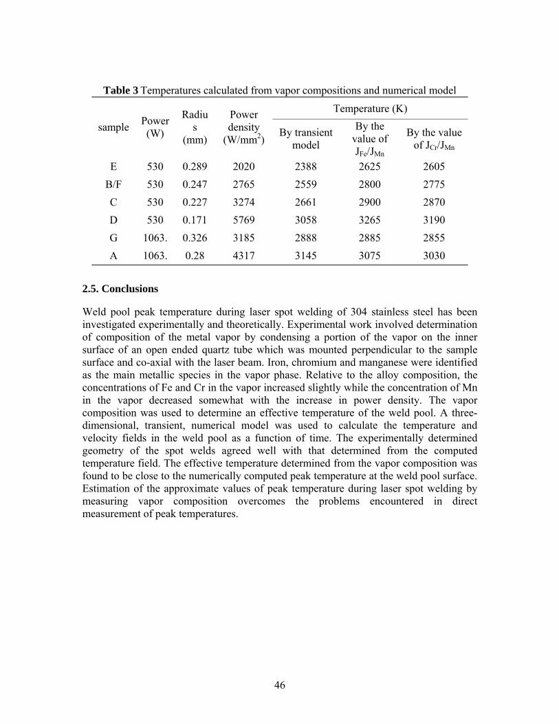
Table 3 Temperatures calculated from vapor compositions and numerical model

Temperature (K)

sample Power (W)

Radius

(mm)

Power density

(W/mm2) By transient

model

By the value of JFe/JMn

By the value of JCr/JMn

E 530 0.289 2020 2388 2625 2605 B/F 530 0.247 2765 2559 2800 2775 C 530 0.227 3274 2661 2900 2870 D 530 0.171 5769 3058 3265 3190 G 1063. 0.326 3185 2888 2885 2855 A 1063. 0.28 4317 3145 3075 3030

2.5. Conclusions Weld pool peak temperature during laser spot welding of 304 stainless steel has been investigated experimentally and theoretically. Experimental work involved determination of composition of the metal vapor by condensing a portion of the vapor on the inner surface of an open ended quartz tube which was mounted perpendicular to the sample surface and co-axial with the laser beam. Iron, chromium and manganese were identified as the main metallic species in the vapor phase. Relative to the alloy composition, the concentrations of Fe and Cr in the vapor increased slightly while the concentration of Mn in the vapor decreased somewhat with the increase in power density. The vapor composition was used to determine an effective temperature of the weld pool. A three-dimensional, transient, numerical model was used to calculate the temperature and velocity fields in the weld pool as a function of time. The experimentally determined geometry of the spot welds agreed well with that determined from the computed temperature field. The effective temperature determined from the vapor composition was found to be close to the numerically computed peak temperature at the weld pool surface. Estimation of the approximate values of peak temperature during laser spot welding by measuring vapor composition overcomes the problems encountered in direct measurement of peak temperatures.

46

2.6. References

1X. He, P. W. Fuerschbach and T. DebRoy, Journal of Physics, D: Applied Physics 36, 1388 (2003). 2W. Zhang, G. Roy, J. Elmer and T. DebRoy, J Appl Phys. 93(5), 3022 (2003). 3A. Block-Bolten and T. W. Eager, Metall. Trans. B 15B, 461 (1984). 4G. J. Dunn, C.D. Allemand and T. W. Eagar, Metall. Trans. 17A(10), 1863 (1986). 5G. J. Dunn and T. W. Eagar, Metall. Trans. 17A(10), 1871 (1986). 6A. Blake and J. Mazumder, J. Engineering for Industry 107, 275 (1985). 7D. W. Moon and E. A. Metzbower, Welding J. 62, 53s (1983). 8M. J. Cieslak and P. W. Fuerschbach, Metall. Trans. B 19B, 319 (1988). 9K. Mundra and T. DebRoy, Metall. Trans. B 24B, 145 (1993). 10H. Zhao and T. DebRoy, Metall. Trans. B 32B, 163 (2001). 11P. A. A. Khan and T. DebRoy, Metall. Trans. B 15B, 641 (1984). 12M. M. Collur, A. Paul, and T. DebRoy, Metall. Trans. B 18B, 733 (1987). 13S. Basu and T. DebRoy, J Appl Phys. 72(8), 3317 (1992). 14S. A. David and T. DebRoy, Science 257, 497 (1992). 15T. DebRoy and S. A. David, Rev. Mod. Phys. 67, 85 (1995). 16H. Zhao, D. R. White, and T. DebRoy, Int. Mater. Rev. 44, 238 (1999). 17G. M. Oreper, J. Szekely, and T. W. Eager, Metall. Trans. B 17B, 735 (1986). 18S. Kou and D. K. Sun, Metall. Trans. A 16A, 203 (1985). 19S. Kou and Y.H. Wang, Metall. Trans. A 17A, 2271 (1986). 20M. C. Tsai and S. Kou, Int. J. for Numerical Methods in Fluids 9, 1503 (1989). 21S. Kou, Welding J. 65(3), S63 (1986). 22C. Chan, J. Mazumder, and M.M. Chen, Metall. Trans. A 15A, 2175 (1984). 23 K. Mundra, T. DebRoy, and K. M. Kelkar, Numer. Heat Transfer 29, 115 (1996). 24W. Pitscheneder, T. DebRoy, K. Mundra, and R. Ebner, Welding J. 75(3), 71s (1996). 25A. Paul and T. DebRoy, Metall. Trans. B, 19B, 851 (1988). . 26Z. Yang and T. DebRoy: Sci. Tech. Welding and Joining 2(2), 53 (1997). 27Z. Yang and T. DebRoy, Metall. Trans. B 30B, 483 (1999). 28W. Zhang, J. W. Elmer, and T. DebRoy, Mater. Sci. Eng. A 333, 320 (2002). 29T. Hong, W. Pitscheneder, and T. DebRoy: Sci. Tech. Welding and Joining 3(1), 33

(1998). 30T. Hong and T. DebRoy, Metall. Trans. B 34B, 267 (2003). 31T. Hong and T. DebRoy, Ironmaking and Steelmaking 28(6), 450 (2001). 32 S. Sista, and T. DebRoy, Metall. Trans. B 32B, 1195 (2001). 33Z. Yang, S. Sista, J. W. Elmer, and T. DebRoy: Acta Materialia 48(20), 4813 (2000). 34S. Sista, Z. Yang and T. DebRoy, Metall. Trans. B 31B, 529 (2000). 35H. Zhao and T. DebRoy, J. Appl. Phys. 35(12), 10089 (2003). 36S. V. Patankar. Numerical Heat Transfer and Fluid Flow (Hemisphere Publishing Corporation, New York, 1980). 37V. R. Voller and C. Prakash, Int. J. Heat Mass Transfer 30, 1709 (1987). 38A. D. Brent, V. R. Voller, and K. J. Reid, Numer. Heat Transfer 13, 297 (1988). 39C. L. Chan, R. Zehr, J. Mazumder, and M. M. Chen, in Modeling and Control of Casting and Welding Processes, S. Kou and R. Mehrabian, Editor, TMS, PA, p.229.(1986).

47

40D. A. Cremers, G. K. Lewis, and D. R. Korzekwa, Welding J. 70, 159s (1991). 41J. F. Ready. LIA Handbook of Laser Materials Processing (Magnolia Publishing, Orlando, 2001). 42M. A. Bramson. Infrared Radiation: a Handbook for Applications, (Plenum Press, New York, 1968). 43D. Peckner and I. M. Bernstein. Handbook of Stainless Steels (McGraw-Hill Book Company, New York, 1977). 44P. W. Fuerschbach and J. T. Norris, "Beam Characterization for Nd:YAG Spot Welding Lasers," presented at ICALEO 2002, Scottsdale, AZ, 2002. 45J. R. Davis. Metals Handbook (ASM International, Materials Park, OH, 1998). 46ASM Specialty Handbook. Stainless Steel (ASM International, Materials Park, OH, 1994). 47Metals handbook. Volume 1. Properties and Selection: Ion, steels, and high-performance alloys (ASM International, Materials Park, OH, 1990). 48F. D. Richardson. Physical Chemistry of Melts in Metallurgy (Academic Press, London, 1974). 49R. Hultgren, P. D. Desai, D. T. Hawkins, M. Gleiser, K. K. Kelley, and D. D. Wagman. Selected Values of the Thermodynamic Properties of the Elements (ASM International, Materials Park, OH, 1973). 50R. E. Honig and D. A. Kramer. Physicochemical Measurements in Metal Research (Interscience Publishers, New York, 1970). 51C. L. Yaws. Handbook of vapor pressure. Houston: Gulf Pub. Co., c1994 52C. B. Alcock, V. P. Itkin and M. K. Horrigan. Canadian Metallurgical Quarterly. 23, 309 (1984).

Section 3. Alloying Element Vaporization during Laser Spot Welding of Stainless Steel

3.1. Introduction

During laser welding of many important engineering alloys, pronounced vaporization of volatile alloying elements takes place from the weld pool surface when the weld pool temperatures are very high.1-16 When this temperature is higher than the boiling point, the pressures at the weld pool surface can be greater than the ambient pressure. This excess pressure provides a driving force for the vaporization. The loss of alloying elements can result in significant changes in the microstructure and degradation of mechanical properties of weldments.9-14 Moon and Metzbower9 investigated the change of properties of aluminum alloy before and after welding using a CO2 laser with He gas shield. They found that the tensile properties of the welds were inferior to the base metal, mainly because of magnesium depletion, loss of strain hardened structure, and porosity. Cieslak and Fuerschbach10 investigated the property change of aluminum alloys 5456 and 5086. They found that the hardness of weld metal was lower than the base metal due to the magnesium vaporization. The loss of hardness was attributed to a reduction in the solid

48

solution strengthening effect as a result of lower magnesium concentration. In the electronics industry, where components are often processed in a clean room environment, discharge of metal vapors is not acceptable. During laser assisted joining of components, evaporation of alloying elements needs to be minimized. Therefore, quantitative understanding of the evaporation of alloying elements is important in the welding of engineering alloys. During welding of stainless steel, the main constituents of the metal vapor are iron, manganese, chromium and nickel.8,12-15 In the high manganese stainless steel, such as AISI 201, iron and manganese were the prominent vapor species in the welding environment. In order to have a quantitative understanding of vaporization of weld metal, a comprehensive model is needed. Anisimov17 and Knight18 derived expressions for the vapor temperature, density, velocity and the extent of condensation by solving the equations of conservation of mass, momentum and energy in a thin layer adjacent to the liquid-vapor interface, known as the Knudsen layer. Their approach has been incorporated into vaporization models11,12 to calculate the laser-induced vaporization rate. When the weld pool temperatures are very high, the escaping vapor exerts a large recoil force on the weld pool surface and, as a consequence, tiny liquid metal particles may be expelled from the weld pool. Thus, in addition to vaporization of alloying elements, ejection of metal particles may also take place when a high power laser beam is used for welding. The expulsion of liquid metal is not acceptable during welding, since the metal loss can adversely affect the weld geometry and weldment properties. Expulsion of liquid metal has also been reported in the literature.19-22 Chun and Rose19 irradiated an aluminum target with a Nd-doped glass laser and found that as much as 90% of the material lost was removed from the molten pool as liquid. The fraction of material lost as liquid depended on the laser pulse characteristics and material properties. Von Allmen21 suggested that the vapor pressure acts like a piston on the liquid weld pool and forces liquid metal out of the cavity. Basu and DebRoy22 examined the conditions for the initiation of liquid-metal expulsion during laser irradiation experimentally and theoretically. They proposed that when the vapor recoil force exceeds the surface tension force of the liquid metal at the periphery of the weld pool, liquid expulsion takes place. The work presented in this article was conducted to quantitatively understand the vaporization rate of alloying elements during laser spot welding. The temperature field used to calculate the vaporization rate was obtained from a well tested comprehensive 3-D transient numerical model. 11-15,23-29 Using the computed temperature fields, vapor composition and total mass loss due to vaporization of various alloying elements resulting from both concentration and pressure driven transport were calculated. The experimentally determined weld pool dimensions, vapor composition and overall vaporization loss were compared with the corresponding modeling results. The possibility of metal expulsion was also examined experimentally and theoretically.

49

3.2. Experimental procedure Several 304 stainless steel welds were fabricated at the Sandia National Laboratories. The steel had the following composition: 1 wt% Mn, 18.1 wt% Cr, 8.6 wt% Ni, 0.69 wt% Si, 0.046 wt% C, 0.012 wt% P, 0.003 wt% S, and balance Fe. A Raytheon SS 525 pulsed Nd:YAG laser was used for laser spot welding with pulse energies of 2.1 J, 3.2 J and 5.9 J and pulse durations of 4.0 ms and 3.0 ms, respectively. No temporal pulse shaping was employed. The laser beam was focused inside the quartz tube with a 100 mm focal length lens. For each combination of energy and duration, the laser beam was defocused to different extents to obtain various spot diameters and power densities. Individual spot welds from a pulsed laser beam were made on 3 by 10 by 17 mm EDM wire cut samples. Up to 15 individual spot welds were made on each of the samples. Laser spot size was measured with 50 µm Kapton film using the method described elsewhere.30 Longitudinal metallographic cross-section measurements through several collinear welds for each plate were averaged to determine weld pool width and depth. The mass loss was experimentally determined by weighing each specimen before and after welding with a Metler MT5 micro-balance. To increase the accuracy of the weight loss measurements, the reported mass loss per pulse is the average of the fifteen spot welds made on each sample. In order to determine the concentration of various alloying elements in the vapor, during laser spot welding, a cylindrical 6 mm inner diameter by 25 mm long, open ended quartz tube was placed co-axial to the laser beam and right above the 304 stainless steel samples. The vaporized elements were collected as condensation on the interior surface of the tube. The quartz tube samples were examined using the JEOL 8600 Electron Microprobe X-ray Analyzer to determine the vapor composition. The evaporation products had the consistency of fine dust. The quartz tubes were broken and a suitable fragment from each experiment was mounted to expose the deposit. Due to the geometry of the samples and their highly porous nature, the probe was not operated in an automated mode. Instead a series of spot measurements of the K-values (count rate ratios of unknown to standards) were made on each sample. The K value measurements were converted to approximate oxide ratios and averaged together for each sample.

3.3. Mathematical modeling 3.3.1 Transient temperature profiles A well tested, transient heat transfer and fluid flow model was used to calculate the temperature and velocity fields in the weld pool both during heating and cooling. The assumptions, model framework and the solution procedure have been described in details in recent papers23,24 and are not repeated here. The computed temperature fields as a function of time were then used to calculate the vaporization rates of alloying elements. The data used for calculations30-34 are presented in Table 1.

50

Table 1. Data used in calculations.

3.3.2 Vaporization due to concentration gradient At the weld pool surface, the concentrations of the alloying elements in the vapor are higher than those in the bulk shielding gas. The vaporization flux of element i, Jc,i , can be defined as:

⎟⎟⎠

⎞⎜⎜⎝

⎛−= b

il

0ii

ii,gi,c CRT

PaMKJ (1)

where Kg,i is the mass transfer coefficient of element i, Mi is the molecular weight of the element i, ai is the activity of element i in the liquid metal, is the equilibrium vapor pressure of element i over its pure liquid, R is the gas constant, T

0iP

l is the temperature (K) at the weld pool surface and is obtained from the transient heat transfer and fluid flow model, Ci

b is the concentration of element i in the shielding gas. Since the concentration of element i in the shielding gas, Ci

b, is significantly lower than the concentration at the weld pool surface, Ci

b can be neglected. The mass transfer coefficient between the weld pool surface and the shielding gas is calculated from the graphical results of Schlunder and Gniclinski35 for a jet impinging on a flat surface and is given by:

⎥⎥⎦

⎤

⎢⎢⎣

⎡⎟⎠⎞

⎜⎝⎛+−⎟⎟

⎠

⎞⎜⎜⎝

⎛+= −

23

5.055.0i

5.042.0

i,g dr10x71.7

dr108.0483.0

200Re1

dDRePr2K (2)

51

where Pr is Prandtl number, Re is the Reynolds number at the nozzle exit, Di is the average diffusivity of element i in the shielding gas at average temperature Tav, d is the diameter of the nozzle, and r is the radial distance on the weld pool surface. 3.3.3 Vaporization due to pressure gradient During laser welding, the peak temperature reached on the weld pool surface often exceeds the boiling point of the alloy. As a result, the vapor pressure at the weld pool surface can be higher than the ambient pressure, and the excess pressure provides a driving force for the vapor to move away from the surface. Therefore, the convective flux of the vaporized elements, driven by the excess pressure is an important contributor to the overall vaporization flux.

Fig. 1 A schematic diagram of the velocity distribution functions

in the Knudsen layer and in adjacent regions The velocity distribution functions of the vapor molecules, f1, f2, and f3, escaping from the weld pool surface at various locations are shown schematically in Fig. 1. On the weld pool surface, the molecules cannot travel in the negative direction, and as a consequence, the velocity distribution is half-Maxwellian. The velocity varies from 0 to + . Close to the weld pool, there exists a space of several mean free paths length, known as the Knudsen layer, at the outer edge of which the velocity distribution just reaches the equilibrium distribution. A portion of the vaporized material condenses on the liquid surface. The rate of condensation was taken into account in the model.

∞

The temperature Tv, density ρv, pressure Pv and the mean velocity u of the vapor, at the edge of the Knudsen layer can be related to temperature Tl, density ρl, and pressure Pl of the vapor at the liquid surface by treating the Knudsen layer as a gasdynamic discontinuity. Anisimov17 and Knight18 derived expressions for the vapor temperature, density, velocity and the extent of condensation across the Knudsen layer by solving the equations of conservation of mass, momentum and translational kinetic energy, using the velocity distribution functions presented in Fig. 1. The derived jump conditions across the Knudsen layer are given by:

52

2

v

v

2

v

v

l

v

2m

11

2m

11

1TT

⎥⎥

⎦

⎤

⎢⎢

⎣

⎡

+γ−γ

π−⎟⎟⎠

⎞⎜⎜⎝

⎛+γ−γ

π+= (3)

where m = u/ 2R Tv v , Rv = R/Mv, R is the gas constant, Mv is the average molecular weight of the vapor, γv is the ratio of specific heat of the vapor, which is treated as a monatomic gas.

( ) ( )[ ]merfcme1TT

21mmerfce

21m

TT 22 m

v

lm2

v

l

l

v π−+⎥⎦

⎤⎢⎣

⎡π

−⎟⎠⎞

⎜⎝⎛ +=

ρρ

(4)

where erfc is the complimentary error function. The condensation factor β can be given by

( )v

l

v

lm

v

l2

TTe

TTm1m2

2

ρρ

⎥⎦

⎤⎢⎣

⎡π−+=β (5)

The density, ρl , can be computed from Pl and Tl assuming that the vapor behaves like an ideal gas. The equilibrium vapor pressure, Pl, at the weld pool surface is obtained from the equilibrium vapor pressure-temperature relationships of the various alloying elements:

∑=

=n

1i

0iil PaP (6)

and Mv, the average molecular weight of the vapor is given by:

∑=

=n

1i l

0ii

iv PPaMM (7)

where ai is the activity of element i in the weld pool, is the equilibrium vapor pressure of pure element i at temperature T

0iP

l, and Mi is the molecular weight of element i. There are four unknowns in equations (3) through (5), namely, Tv, γv, β and m. Therefore, it is necessary to have an additional equation to have unique values of these variables. The necessary equation is obtained by applying Rankine-Hugoniot relation36 to relate the pressure at the edge of the Knudsen layer to the ambient conditions:

⎥⎥

⎦

⎤

⎢⎢

⎣

⎡

⎟⎟⎠

⎞⎜⎜⎝

⎛Γ

+γ++Γ

+γΓγ+=

2gg

gl

2

g

l M4

11M

41

M1PP

PP (8)

53

where Pg and P2 are the pressures in front of and behind the wavefront, respectively, P2 = Pv, γg is the ratio of specific heats for shielding gas, and Γ = γ γv v v g g gR T R T/ . The Mach number, M, is related to m by the following relation:

m M v=γ2

(9)

The Mach number M and the density ρv, obtained by solving Equations (3) through (9), can be used to calculate the vaporization flux due to pressure gradient at the weld pool surface corresponding to a local surface temperature Tl:

MSJ vp ρ= (10)

where S is the speed of sound in the vapor at temperature Tv. Since the rate of vaporization of an alloying element is proportional to its partial pressure over the weld pool, its flux, JP,i, due to pressure gradient can be given by:

pv

i

l

0i

ii,p JMM

PPaJ = (11)

3.3.4. Overall vaporization rate and weight loss due to vaporization The total vaporization flux for element i is the sum of diffusion driven and pressure driven vapor fluxes and can be given by:

i.pi,ci JJJ += (12)

The vaporization rate of element i is obtained by integrating the vapor flux over the entire weld pool surface, and the total vaporization rate of all the elements is given by:

∑∫∫∑==

==n

1i si

n

1ii dxdyJGG (13)

where s indicates the weld pool surface. The total weight loss of element i can be calculated by:

∑∫∫ ∆=∆t s

ii tdxdyJW (14)

where ∆t is the time step.

54

3.4 Results and discussion 3.4.1. Computed temperature fields and weld pool geometry

Fig. 2 Computed temperature and velocity fields at different times: (a) t = 1 ms, (b) t = 3 ms and (c) t = 5 ms. Laser poser: 1967 W, pulse duration: 3.0 ms and spot radius: 0.428 mm.

Figs. 2(a) through 2(c) show the computed temperature and velocity fields as a function of time. The liquid metal motion in the weld pool is driven mainly by the surface tension force and to a much lower extent by the buoyancy force. Because of the negative values of the temperature coefficient of surface tension, the surface tension drives the liquid metal from the center to the periphery at the top surface of the weld pool. As a result, the weld pool becomes wide and shallow. During the initial period of laser spot welding, the weld pool grows rapidly in size and the temperatures increase with time. After the laser is switched off, the temperatures decrease rapidly and consequently, the weld pool begins to shrink. The maximum velocity of liquid in the weld pool is 0.73 m/s after 3 ms. This velocity decreases rapidly after the laser is switched off. The maximum velocity is reduced to 4.5 mm/s 2.0 ms after the laser is switched off. The computed results show that it takes about 3.55 ms after the power is switched off for the weld pool to solidify completely.

55

Fig. 3 Computed weld thermal cycles at various locations on the top surface of the weld pool. Distance from the weld center: 1: 0.0 mm; 2: 0.125 mm; 3: 0.175 mm; 4: 0.225 mm, as shown in the small figure. The solid horizontal lines indicates solidus temperature. Laser power: 1967 W, pulse duration: 3.0 ms and beam radius: 0.428 mm

Fig. 3 shows changes in the computed temperatures at various monitoring locations, which are indicated as points 1, 2, 3, and 4 in the small figure. These locations represent distances of 0, 0.125, 0.175, and 0.225 mm from the axis of the laser beam, as shown in the figure. There are several special features of interest. First, the temperatures reach very high values near the laser beam axis. It is to be noted that the peak temperature can exceed the boiling point of the alloy, i.e., the equilibrium vapor pressure at the liquid surface can be higher than one atmosphere. Second, the computed results also indicate that the heating rates vary significantly depending on the location. Finally, as the weld metal cools, the spatial variation of the cooling rates within the solid metal is much smaller than the spatial variation in the heating rates. These features of temperature and the temperature distribution at the weld pool surface are of interest in examining the vaporization of alloying elements from the weld pool. In the weld pool, heat is transported by a combination of convection and conduction mechanisms. The relative importance of convection and conduction in the overall transport of heat can be evaluated from the value of Peclet number, Pe, which is defined by:

kLCu

Pe Rpρ= (15)

where u is the velocity, ρ is the density, Cp is the specific heat, LR is the characteristic length taken as the pool radius at the top surface of weld pool, and k is the thermal conductivity. When Pe is less than one, the heat transport within the weld pool occurs primarily by conduction.

56

Fig. 4 The variation of Peclet number with time. Laser power: 1967 W, pulse duration: 3.0 ms and beam radius

When Pe is much higher than 1, the convective heat transport is the primary mechanism of heat transfer. Fig. 4 shows the change of Peclet number with time. It can be seen that at the beginning of pulse cycle, the Peclet number is low and conduction is the primary mechanism of heat transfer.

Fig. 5 The effects of laser power density on (a) the computed peak

temperature and (b) the computed maximum velocity. Laser power: 1967, pulse duration: 3.0 ms.

With time, the Peclet number increases and convection becomes the more important heat transport mechanism in the weld pool. When the pulse is switched off, the Peclet number drops to a very low value very quickly and conduction becomes the main mechanism of heat transfer again. The variation of peak temperature and maximum velocity with power density is shown in Fig. 5. Both the peak temperature and the maximum velocity represent the highest values in the weld pool at the end of the pulse. The high maximum velocity at high power densities means a more dominant role of convection at high power densities.

57

Fig. 6 Experimental and calculated weld pool cross sections. (a) laser power: 1967 W, pulse duration: 3 ms and beam radius: 0.521 mm; (b) laser power: 1507 W, pulse duration: 4 ms and beam radius: 0.389 mm.

The experimentally determined weld pool cross sections are compared with the corresponding computed values under two welding conditions in Fig. 6. It is observed that the calculated weld pool geometry and dimensions agree well with the experimental results. At various other laser power densities, experimentally measured and computed values of weld pool depth and width are presented in Table 2. The total power was kept constant at 530 W while the beam radius was varied to obtain different power densities. It can be seen that the calculated weld pool depth and width show fair agreement with the experimental results. Table 2. Calculated and experimental weld pool dimensions

for different welding conditions

58

3.4.2. Mass loss Because the weld pool surface temperatures reach high values, pronounced evaporation of alloying elements takes place during high power laser spot welding. Fig. 7 shows the computed temperature distribution and various vapor fluxes at the weld pool surface after 3.0 ms. The total vapor flux is the sum of the fluxes of individual alloying elements resulting from both pressure driven and concentration difference driven fluxes. The results show that the distribution patterns of vapor fluxes are similar to the surface temperature profiles. This similarity is anticipated since the vapor fluxes are strongly affected by temperature. The primary driving force for vaporization is the total pressure gradient at temperatures higher than the boiling point. At lower temperatures, the vapor flux is driven mainly by diffusion in the gas phase outside the liquid pool. The calculated results show that most of the vaporization occurs from a small region near the center of the beam-work piece interaction zone where the weld pool surface temperatures are very high as observed from Fig. 7(a). The diameter of this active region is approximately 0.6 mm as can be observed from Figs. 7(b) through (h). This dimension is comparable but somewhat smaller than the diameter of the laser beam at the focal point.

59

Fig. 7 Distribution of temperature and vapor fluxes of various elements at the weld pool surface after 3.0 ms. Laser power: 1967 W, pulse duration: 3.0 ms and beam radius: 0.428 mm.

From the computed vapor fluxes presented in Fig. 7(e) through 7(h), it can be seen that iron is the dominant vaporizing species, followed by chromium and manganese. The equilibrium vapor pressure data used for the calculations are presented in the Appendix. Although manganese has the highest vapor pressure over its pure liquid, its concentration in 304 stainless steel is much lower than those of iron and chromium. Manganese only accounts for 1.0% of the stainless steel composition while iron and chromium are present at 72.3% and 18.1%, respectively. The lower concentration results in the lower vapor flux of manganese compared to iron and chromium over 304 stainless steel.

Fig 8 Weight percent of different elements in vapor composition. (a) laser power: 1064 W, pulse duration: 3.0 ms and beam radius: 0.28 mm; (b) laser power: 530 W, pulse duration: 4.0 ms and beam radius: 0.171 mm.

The vapor composition was also determined from the experiments. The concentrations of different elements in the vapor obtained from both experiments and calculations are presented in Fig 8. Iron and chromium were the main vaporizing species. It is also observed that the calculated concentrations of various vaporizing species agree well with those obtained from measurements.

60

Fig. 9 Experimental and computed concentrations of (a) Fe and (b) Cr in the vapor.

The experimentally determined and the calculated concentrations of different alloying elements in the vapor are presented in Table 3 for various welding conditions. The change in the concentrations of the main vaporizing species, i.e., iron and chromium, with power density is shown in Fig. 9. Generally, as the power density increases, the concentration of iron in the vapor increases. This is mainly because of the slope of the vapor pressure versus temperature plot for iron is steeper than those of the other alloying elements. For similar reason, the concentration of chromium in the vapor condensate increases slightly with power density. Table 3. Experimentally determined and calculated vapor

compositions for different welding conditions.

The calculated mass loss due to evaporation is compared with the experimental results of mass loss at various power densities in Fig. 10. Some additional results are also presented in Table 4 for completeness. As the laser power density increases, the temperature at the weld pool surface exceeds the boiling point of the steel. As a result, the total vaporization loss increases significantly due to pressure driven vaporization. However, it can be observed that the experimental weight loss is always higher than the computed mass loss due to vaporization. There are two possible reasons for this discrepancy. First, in a complex modeling effort such as the present research, the accuracy of the modeling

61

results must be carefully considered. In other words, a possibility that all of the mass loss is attributable to the vaporization of alloying elements and the model chronically underpredicts the vaporization loss cannot be ruled out. Second, it is conceivable that in addition to vaporization, mass loss also occurs due to ejection of metal droplets. Both these possibilities are examined next. Table 4. Calculated mass loss due to evaporation is compared

with the experimentally determined mass loss for different welding conditions.

The computed vaporization rates may be lower than the actual values because of several reasons. First, the computed temperatures on the weld pool surface may be lower than the actual values. Second, the computed weld pool surface area considered in the calculations is lower than the true surface area. Third, the vaporization model used in the calculations may underpredict the vaporization rate for the conditions of the current experiments. First, let us consider the possibility that the computed surface temperatures are lower than the actual temperatures prevailing at the surface. It has been established in several previous studies that during laser welding, most of the vapors originate from the center of the weld pool surface11,12. So, for the purpose of this inquiry, the magnitude of the computed peak temperature should be a good parameter to examine. The computed values of peak temperatures for all experiments are presented in Table 4. The highest computed peak temperature listed in this table is 3628 K which is about 600 K higher than the boiling point of the alloy.

62

Fig 10 Calculated vaporization loss is compared with measured mass loss for different power densities: (a) laser power: 1067 W, pulse duration: 3.0 ms; (b) laser power: 1967 W, pulse duration: 3.0 ms.

Although temperatures higher than the boiling point have been reported in the literature,11,12,37-39 the reported temperatures are not significantly different from the boiling points for power densities close to about 106 watts/cm2. Therefore, the value of 3628 K, if deemed inaccurate for the sake of argument, can only be higher than the actual value. Furthermore, Table 4 shows that even a temperature as high as 3628 K would not result in a vaporization rate necessary to account for all the mass loss due to vaporization. Therefore, the difference between the calculated and the experimental mass loss cannot be attributed to the lower computed temperatures. Second, let us examine the role of the weld pool surface area. When the recoil force of the vapors is significant, considerable depression of the weld pool free surface can result and the true surface area of the weld pool can be significantly higher than the nominal, flat, undeformed surface area. However, the deformation of the surface area can only account for roughly 5 to 20% increase of the surface area for typical surface deformation. The data in Table 4 shows that the computed mass loss is significantly lower than the experimentally determined mass loss for most situations and that typical errors in the surface area cannot explain the difference. Third, the accuracy of the evaporation rate calculation must also be examined. The evaporation model has been adapted from the works of Anisimov17 and Knight.18 The same model has been extensively applied to calculate the laser induced vaporization rates of alloying elements.11,12,39 In each case, the computed vaporization rate was comparable to the corresponding experimental data. So, the difference between the computed vaporization loss and the experimental mass loss cannot be attributed to the inaccuracies resulting from the evaporation model. It is also worth noting that the experimentally measured mass loss indicated in Table 4, if totally attributed to vaporization, demands unrealistically high values of vaporization rate. For example, let us consider the experiment with 0.159 mm radius laser beam having 530 W power applied for 4 ms. The total mass loss was found to be 15.6 microgram. If the entire mass loss is attributed to vaporization, the vaporization rate can be readily estimated. If we assume that roughly 1 ms was needed for the initial heating, the average vaporization rate is calculated as 5.2 mg/s. For the welding of stainless steel with a comparable power density beam, an overall vaporization rate of about 1 mg/s has been reported.13 Thus, the experimental value of mass loss is far too high to be explained by vaporization alone.

63

A possible reason for the observed discrepancy between the experimental weight loss and the calculated vaporization loss is that only a portion of the mass loss occurs due to evaporation and the remainder of the loss must be attributed to some other mechanism. Therefore, the possibility of ejection of the tiny metal droplets from the weld pool owing to the recoil force exerted by the metal vapors was examined.

Fig 11 Recoil and surface tensio forces as a funtion of time. Laser power: 1067 W, pulse duration: 3.0 ms and beam radius: 0.225 mm

Expulsion of metal drops takes place when the vapor recoil force exceeds the surface tension force of the liquid metal at the periphery of the weld pool.39 The vapor recoil force Fr and the surface tension force at the periphery Fs can be expressed by:

(16) ∫ ∆π= Br

0r dr)r(Pr2F

σπ= 0s r2F (17) where rB is the radial distance at which the surface temperature reaches the boiling point, ∆P(r) is the difference between the local equilibrium vapor pressure and the atmosphere pressure and is the function of radial distance from the beam axis, r0 is the radial distance at which the temperature is equal to the melting point, σ is the surface tension coefficient at the melting point. Fig. 11 shows the computed values of these two forces during welding. As the temperature increases with time, the equilibrium vapor pressure and the resulting recoil force increases significantly. At about 1.4 ms after the start of the pulse, the two forces are roughly equal. Further heating results in higher recoil force than the surface tension force. When the recoil force exceeds the surface tension force, ejection of metal droplets is anticipated. To verify the model prediction of metal droplet ejection, a few experiments were conducted where both end open quartz tubes were placed co-axial to the laser beam and right above the 304 stainless steel sample during the laser spot welding. The interior surface of the tube was examined after the experiments. Fig. 12 shows the presence of metal vapor and tiny metal droplets on the interior wall of a quartz tube. Three small droplets can be seen in this macrograph. Clearly, mass loss is

64

contributed by both vaporization of alloying elements as well as the ejection of metal droplets.

Fig. 12 Particles of 304 stainless steel, effected from the weld pool, were captured on the inner surface of a both end open quartz tube place co-axial with the laser beam during spot welding. Laser power: 1967 W, pulse duration: 3.0 ms and beam radius: 0.379 mm

3.5. Conclusions Loss of alloying elements from the weld pool during laser spot welding of stainless steel was investigated experimentally and theoretically. The experiments involved measurements of weight loss resulting from welding and analysis of the chemical composition of the vapor by condensing a portion of it on the inner surface of a both end open quartz tube. The theoretical work involved numerical modeling of transient temperature and velocity fields in the weldment and calculation of the vaporization rate of the alloying elements using the computed temperature profiles. The fusion zone geometry could be predicted from the transient heat transfer and fluid flow model for various welding conditions. In the range of variables investigated, the laser power and the pulse duration were the most important variables in determining the temperature profile. During heating, temperatures and velocities increased with time and convection played an increasingly important role in the heat transfer within the weld pool. The peak temperatures and velocities increased significantly with the laser power density. At very high power densities, the computed temperatures at the weld pool surface were found to be higher than the boiling point of 304 stainless steel. As a result, vaporization of alloying elements resulted from both total pressure and concentration gradients. The calculations showed that the vaporization was concentrated in a small region under the laser beam where the temperature was very high. The computed vapor loss was found to be lower than the measured mass loss because of the ejection of the tiny metal droplets owing to the recoil force exerted by the metal vapors. The ejection of metal droplets was predicted by computations and verified by experiments.

65

3.6. References 1S. A. David and T. DebRoy, Science 257, 497 (1992). 2G. J. Dunn, C.D. Allemand and T. W. Eagar, Metall. Trans., 17A(10), 1863 (1986). 3G. J. Dunn and T. W. Eagar, Metall. Trans., 17A(10), 1871 (1986). 4A. Blake and J. Mazumder, J. Engineering for Industry 107, 275 (1985). 5P. Sahoo, M. M. Collur and T. DebRoy, Metall.Trans.B 19B, 967(1988). 6K. Mundra, J. M. Blackburn and T. DebRoy, Sci.Technol.Weld.Joining 2, 174 (1997). 7T. A. Palmer and T. DebRoy Metall.Trans.B 31B, 1371 (2000). 8M. M. Collur, A. Paul, and T. DebRoy, Metall. Trans. B 18B, 733 (1987). 9D. W. Moon and E. A. Metzbower, Welding J. 62, 53s (1983). 10M. J. Cieslak and P. W. Fuerschbach, Metall. Trans. B 19B, 319 (1988). 11H. Zhao and T. DebRoy, Metall. Trans. B 32B, 163 (2001). 12K. Mundra and T. DebRoy, Metall. Trans. B 24B, 145 (1993). 13P. A. A. Khan, T. DebRoy, and S. A. David, Welding J. Res. Suppl. 67, 1s (1988). 14P. A. A. Khan and T. DebRoy, Metall. Trans. B 15B, 641 (1984) 15K. Mundra and T. DebRoy, Welding J. Res. Suppl. 72, 1s (1993). 16A. Block-bolten and T. W. Eager, Metall. Trans. B 15B, 461 (1984). 17S. I. Anisimov and A. Kh. Rakhmatulina, Soviet Physics – JETP 37, 441 (1973). 18C. J. Knight, AIAA J. 17, 519 (1979). 19M. K. Chun and K. Rose, J. Appl. Phys. 11, 614 (1970). 20M. P. Graham, H. W. Kerr, and D. C. Weckman, Proceedings of the SPIE – The International Society for Optical Engineering 2703, 170 (1996). 21M. von Allmen, J. Appl. Phys. 47, 5460 (1976). 22S. Basu and T. DebRoy, J. Appl. Phys. 72, 3317 (1992). 23X. He, P. W. Fuerschbach and T. DebRoy, J.of Phy., D: Appl. Phys. 36, 1388 (2003). 24W. Zhang, G. Roy, J. Elmer and T. DebRoy, J Appl Phys, 93(5), 3022 (2003). 25T. Zacharia, S. A. David, J. M. Vitek, and T. DebRoy, Welding J 68, 499s (1989). 26T. Zacharia, S. A. David, J. M. Vitek, and T. DebRoy, Welding J 68, 510s (1989). 27Z. Yang, S. Sista, J. W. Elmer and T. DebRoy, Acta Mater. 48, 4813 (2000). 28T. Hong, T. DebRoy, S. S. Babu and S. A. David, Metall.Trans.B 31B, 161 (2000). 29W. Zhang, J. W. Elmer and T. DebRoy, Mater.Sci.Eng. A333, 320 (2002). 30P. W. Fuerschbach and J. T. Norris, Beam Characterization for Nd:YAG Spot Welding Lasers, (Scottsdale, AZ, 2002). 31D. Peckner and I. M. Bernstein. Handbook of Stainless Steels (McGraw-Hill Book Company, New York, 1977). 32J. R. Davis. Metals Handbook (ASM International, Materials Park, OH, 1998). 33ASM Specialty Handbook. Stainless Steel (ASM International, Materials Park, OH, 1994). 34Metals handbook. Volume 1. Properties and Selection: Ion, steels, and high-performance alloys (ASM International, Materials Park, OH, 1990). 35E. U. Schlunder and V. Gniclinski, Chem. Ing. Technol 39, 578 (1967). 36W. G. Vincenti and C. H. Kruger. Introduction to Physical Gas Dynamics (Wiley, New York, 1965). 37C. L. Chan and J. Mazumdar, J. Appl. Phys. 62, 4579 (1987). 38M. vonAllmen, Laser Beam Interaction with Materials (Springer, 1987), p. 161.

66

39T. DebRoy, S. Basu, and K. Mundra, J. Appl. Phys. 70, 1313 (1991). 40R. Hultgren, P. D. Desai, D. T. Hawkins, M. Gleiser, K. K. Kelley, and D. D. Wagman. Selected Values of the Thermodynamic Properties of the Elements (ASM International, Materials Park, OH, 1973). 41R. E. Honig and D. A. Kramer. Physicochemical Measurements in Metal Research (Interscience Publishers, New York, 1970 -517), p. 505. 42C. L. Yaws. Handbook of vapor pressure. Houston: Gulf Pub. Co., c1994 43C. B. Alcock, V. P. Itkin and M. K. Horrigan. Canadian Metallurgical Quarterly. 23, 309 (1984).

Report Summary

Successful development of a comprehensive analytical model required that both the incident laser beam parameters and the experimental results be accurately determined. Loss of alloying elements from the weld pool during laser spot welding was examined through accurate mass loss measurements and microprobe analysis of the chemical composition of the vapor. Longitudinal metallographic cross-section measurements through several collinear laser spot welds were examined to determine fusion zone dimensions. The measured vapor composition was employed in an analytical expression to determine an effective temperature of the weld pool. A three-dimensional, transient, numerical model was used to calculate the temperature and velocity fields in the weld pool as a function of time. Results from the analytical model enabled an insightful examination of the responses inside the laser spot weld pool. The fusion zone geometry was in good agreement with the corresponding experimentally measured values for various laser spot welding conditions. During heating, the heating rate varies significantly at different locations, temperatures and velocities increased with time, and convection played a very important role in the heat transfer especially towards the end of the laser pulse.. The peak temperatures and velocities increased significantly with the laser power density. The liquid flow is mainly driven by the surface tension and to a much less extent, by the buoyancy force. Heat transfer by conduction is important when the liquid velocity is small at the beginning of the pulse and during weld pool solidification. The size of the mushy zone, i.e., liquid + solid two-phase region, grows significantly with time during solidification and the maximum size of the mushy zone is reached when the pure liquid region vanishes. The temperature gradients (G) in the mushy zone at the mushy zone/solid interface decrease with the solidification time. The solidification rate (R) of the mushy zone/solid interface increases with time. The effective temperature determined from the vapor composition was found to be close to the numerically computed peak temperature at the weld pool surface. At very high power densities, the computed temperatures at the weld pool surface were found to be higher than the boiling point of 304 stainless steel. As a result, vaporization of alloying elements resulted from both total pressure and concentration gradients. The calculations

67

showed that the vaporization was concentrated in a small region under the laser beam where the temperature was very high. The computed vapor loss was found to be lower than the measured mass loss because of the ejection of the tiny metal droplets owing to the recoil force exerted by the metal vapors. The ejection of metal droplets was predicted by computations and verified by experiments.

Acknowledgments This work was performed at Sandia National Laboratories, which is a multiprogram laboratory operated by Sandia Corporation, a Lockheed Martin Company, for the United States Department of Energy’s National Nuclear Security Administration under contract DE-AC04-94AL85000. The computational work was supported by a grant from the U.S. Department of Energy, Office of Basic Energy Sciences, Division of Materials Sciences, under grant number DE-FGO2-01ER45900. The authors would like to thank Alice Kilgo and Paul Hlava for their help with the experimental measurements. In addition the authors would like to thank Wei Zhang, Amit Kumar, Yajun Fan, Amitava De, Saurabh Mishra, and Cheolhee Kim for their comments on parts of the manuscript.

68

Appendix

Equilibrium vapor pressure data used for the calculations The equilibrium vapor pressures of the various vaporizing species over pure liquid were calculated using the following equations.40-43 In these equations, the vapor pressure is expressed in atm and the temperature is in K.

213-9-40Fe T101.9086T102.7182-T0.62549log-

T1101.9538-11.5549)760Plog( ×+××=×

609.12T110503.1T10-5.58)10013.1Plog( 4450

Mn +×−×=×× −−

077.87T10381.8T1029.9Tlog658.33T110-13.505)10013.1Plog( 273350

Cr −×+×−+×=×× −−

T120765-6.666Plog 0

Ni =

Assuming that the solution is ideal at high temperatures, the equilibrium vapor pressures of the various species over the alloy can be expressed as:

0iii PXP =

where Xi is the mole fraction of element i in the alloy, is the equilibrium vapor pressure of element i over the pure liquid.

0iP

69

Distribution

3 MS 0889 P. W. Fuerschbach, 01833 1 MS 0889 J. T. Norris, 01833 1 MS 0889 M. F. Smith, 01833 1 MS 0834 R. A. Roach, 09114 1 MS 0834 J. E. Johannes, 09114 1 MS 0323 LDRD office, 01011 1 MS 9018 Central Technical Files, 8945-1 2 MS 0899 Technical Library, 9616 1 The Pennsylvania State University Xuili He 212 Steidle Building University Park, PA 16802-5006 1 The Pennsylvania State University Tarasankar DebRoy 212 Steidle Building University Park, PA 16802-5006

70