UNDERSTANDING FINANCIAL FRAGILITY: THE ROLES OF

OPACITY, FIRE SALES, AND SOVEREIGN DEBT

by

RYUICHIRO IZUMI

A dissertation submitted to the

School of Graduate Studies

Rutgers, The State University of New Jersey

In partial fulfillment of the requirements

For the degree of

Doctor of Philosophy

Graduate Program in Economics

Written under the direction of

Todd Keister

And approved by

New Brunswick, New Jersey

October, 2019

c© 2019

Ryuichiro Izumi

ALL RIGHTS RESERVED

ABSTRACT OF THE DISSERTATION

Understanding Financial Fragility: The Roles of Opacity, Fire Sales, and

Sovereign Debt

By RYUICHIRO IZUMI

Dissertation Director:

Todd Keister

This dissertation studies fragility-enhancing economic mechanisms and how government

policy can promote - or may inadvertently undermine - the stability of the financial

system. It is composed of three separate essays that investigate this question in the

context of particular aspects of the recent global financial crisis: the opacity of assets,

fire sales, and the link between banking and sovereign debt crises. Each of these chapters

aims to inform an ongoing policy debate about appropriate changes to financial policy

and regulation.

In Chapter 1, I study how the opacity, or complexity, of banks’ assets affects financial

stability and asks when the level of opacity should be regulated. An important feature of

the global financial crisis was widespread “runs” in which depositors and other creditors

withdrew funds from a variety of shadow banking arrangements that invested in complex

assets that were difficult to value, especially once financial markets became stressed.

Some policy makers have argued that this type of opacity makes runs more likely and

should be prohibited by regulation. Others have argued that opacity plays a useful role

by making the value of a bank’s liabilities less sensitive to information and therefore

more liquid. This chapter asks: What is the optimal degree of opacity in the financial

ii

system? To answer this question, I analyze a version of the Diamond and Dybvig (1983)

model of financial intermediation with financial markets and fundamental uncertainty

as in Allen and Gale (1998). I add the ability of a bank to make its assets opaque

in the sense that it will take time to discern the true value of the assets. Until the

true state is known, the bank’s assets will trade in financial markets based on their

expected payoff. By choosing the level of opacity, the bank determines how many of

its depositors will be paid while its assets remain information insensitive in this sense.

In other words, opacity of the bank’s assets offers an insurance benefit in the spirit

of the classic Hirshleifer (1971) effect. However, I show that this type of opacity also

has a cost in terms of financial stability. In particular, a higher level of opacity makes

the bank more fragile in the sense that it introduces equilibria in which a self-fulfilling

bank run is more likely to occur. In choosing the level of opacity for its assets, I show

that a bank faces a trade-off between providing insurance to more of its depositors and

increasing its susceptibility to a self-fulfilling run. If depositors can accurately observe

the bank’s opacity choice before depositing their funds, competition will drive banks

to choose the optimal level. If, however, depositors are unable to observe this choice,

banks will have an incentive to become overly opaque and regulation to limit opacity

would improve welfare.

In Chapter 2, which is a joint work with Yang Li, we study whether policies that aim

to mitigate “fire-sales”, in which assets are sold at prices well below their fundamental

value, actually promote financial stability. Fire-sales were an important contributing

factor in the global financial crisis. After the crisis, policy makers aimed to prevent

future fire-sales by requiring banks to hold sufficient liquid assets to survive distressed

periods without selling illiquid assets. However, forcing banks to hold larger amounts

of liquid assets entails an opportunity cost in terms of lost opportunities of illiquid

and profitable investments. We study whether the opportunity costs associated with

liquidity regulation worsens financial fragility and derive the optimal level of liquidity

regulation. We construct a model in which banks choose a portfolio of liquid and illiquid

assets, anticipating that a bank run may occur and force the bank to sell illiquid assets.

When banks have to sell more illiquid assets, the price will fall further (a fire-sale).

iii

We show that banks choose to hold a larger amount of illiquid assets than is socially

optimal. Liquidity regulation can correct this fire-sale externality. However, we find

a striking result: in some cases, liquidity regulation worsens financial fragility in the

sense that it introduces equilibria in which a self-fulfilling bank run is more likely to

occur. The reason is that when banks are allowed to hold fewer high-return, illiquid

assets, they tend to offer a lower repayment to depositors who remain invested which,

in turn, can increase the incentive for depositors to withdraw early. As a result, policy

makers must balance the desire to correct the fire-sale externality against the increased

fragility that liquidity regulation may bring.

In Chapter 3, I study whether government guarantees or liquidity regulation are

a more effective way to prevent financial crises when these policies interact with the

government’s fiscal position. A government guarantee is a popular policy to mitigate

banking panics. However, there was a lot of criticism about the taxpayer money used

to bail out the banks in the global financial crisis. Recent reforms in the U.S. and

Europe move in the direction of restricting the ability of the public sector to provide

guarantees in a future crisis and to instead introduce tighter financial regulations. I

contribute to this discussion by considering the negative feedback loop between the

fiscal position of the government and the health of the banking sector. The fiscal

cost of guarantees may hurt sovereign debt sustainability, and an unsustainable debt

undermines the effectiveness of guarantees, as occurred in Greece, Iceland, Ireland and

Italy in the recent crisis. This chapter asks: Are government guarantees or financial

regulation a more effective way to prevent banking crises in the presence of the negative

feedback loop? To answer this question, I construct a version of Diamond and Dybvig

(1983) model of financial intermediation in which the government issues, and may

default on, debt. Banks hold some of this debt, which ties their health to that of

the government. The government’s tax revenue, in turn, depends on the quantity of

investment that banks are able to finance. Without any policy, this economy is fragile in

the sense that a self-fulfilling bank run occurs in an equilibrium. I compare government

guarantees, liquidity regulation, and a combination of these policies to find the best

way to eliminate this equilibrium. This comparison given the negative feedback loop is

iv

novel in the literature. I show that each policy adversely affects the government’s fiscal

position through revenue and/or expenditure, which in turn determines the effectiveness

of each policy. I show that the guarantee tends to be effective in preventing banking

crises when the return on long-term investment is high and when the government’s initial

debt is small. In some cases, the combination of guarantees and liquidity regulation

is needed to prevent crises. In other cases, liquidity regulation alone is effective and

adding guarantees would make the financial system fragile.

v

Acknowledgements

I first and foremost would like to thank my advisor, Todd Keister, for his extraordinary

mentoring, constant encouragement and thoughtful guidance. This dissertation would

undoubtedly not have been possible without his boundless support. I am also deeply

grateful to Roberto Chang and Tomas Sjostrom, not only for being supportive mem-

bers of my dissertation committee, but also for providing insightful suggestions and

encouragement throughout my studies. My discussions with them have substantially

improved the quality of this work. In addition, I am indebted to my outside committee

member, Dr. Alexandros Vardoulakis, from the Federal Reserve Board of Governors,

for providing valuable suggestions and feedback.

During my studies at Rutgers, I have greatly benefited from and enjoyed my inter-

actions with many faculty members. In particular, Eugene White and Hugh Rockoff

enlightened me on how banking history and theory are complementary to one another,

and guided me into the world of financial history. Colin Campbell and Oriol Carbonell-

Nicolau have generously spent their time with me to discuss various forms of games and

equilibria. Ira Gang taught me the importance of academic networks and gave me much

emotional support over coffee. I am also indebted to Diego Anzoategui, Douglas Blair,

Zhifeng Cai, Jennifer Hunt, Roger Klein, John Landon-Lane, Bruce Mizrach, Daijiro

Okada and Xiye Yang. Additionally, I am grateful to the staff members, especially

Linda Zullinger and Debbie Holman, for their heartening support.

I have been fortunate enough to have received support from outside of the Rutgers

community as well. I owe lots of thanks to Toni Ahnert, Yu Awaya, Nobuhiro Kiyotaki

and Shengxing Zhang for their suggestions on this work. Ippei Shibata and Hiroaki

Miyamoto, my co-authors on the project I worked on at the IMF, generously trained

me in empirical analyses. Daniel Hardy, Hiroko Oura and Murtaza Syed also provided

support to my project during my time at the IMF. Eri Ikeda, Ayumu Ken Kikkawa,

Nick Mader, and Jorge Mondragon are Ph.D. students at other institutions who have

been great friends and helped motivate me to work on this dissertation.

vi

I am deeply indebted to my brothers and sisters in my academic family: Yang Li,

Yuliyan Mitkov, Hyeon Ok Lee, Yan Xue and Yu Xiao. I cannot express enough how

largely my intellectual progress has been owed to them. I also would like to express my

gratitude to a number of graduate students at Rutgers for making my adventures much

more enjoyable along the way: Wukuang Cun, Freddy Rojas Cama, Mingmian Cheng,

Ning Li, Geoffrey Clarke, Maria Sole Pagliari, Yixiao Jiang, Weiqi Xiong, Suwei Luo,

Yuanting Wu, Xuesong Huang, Humberto Martinez Beltran, Monica Mogollon Plazas,

and visiting scholars Stefano Condrelli, Simon Amrein, and Alain Naef.

Finally, I would like to express my deepest gratitude to my family. My parents have

always respected my dreams and encouraged me to pursue my goals, even when this

meant being away from them for long stretches of time. My last acknowledgement goes

to my fiance, Akari Armatas, who has given me unbounded love and endless support.

vii

Table of Contents

Abstract . . . . . . . . . . . . . . . . . . . . . . . . . . . . . . . . . . . . . . . . ii

Acknowledgements . . . . . . . . . . . . . . . . . . . . . . . . . . . . . . . . . vi

List of Figures . . . . . . . . . . . . . . . . . . . . . . . . . . . . . . . . . . . . xi

1. Opacity: Insurance and Fragility . . . . . . . . . . . . . . . . . . . . . . 1

1.1. Introduction . . . . . . . . . . . . . . . . . . . . . . . . . . . . . . . . . . 1

1.2. The Model . . . . . . . . . . . . . . . . . . . . . . . . . . . . . . . . . . 6

1.2.1. The environment . . . . . . . . . . . . . . . . . . . . . . . . . . . 6

1.2.2. Decentralized economy . . . . . . . . . . . . . . . . . . . . . . . . 8

1.2.3. Timeline . . . . . . . . . . . . . . . . . . . . . . . . . . . . . . . . 10

1.2.4. Financial autarky . . . . . . . . . . . . . . . . . . . . . . . . . . . 12

1.2.5. The full information allocation . . . . . . . . . . . . . . . . . . . 12

1.2.6. Withdrawal game . . . . . . . . . . . . . . . . . . . . . . . . . . . 14

1.2.7. Banking problem . . . . . . . . . . . . . . . . . . . . . . . . . . . 14

1.2.8. Discussion . . . . . . . . . . . . . . . . . . . . . . . . . . . . . . . 15

1.3. Equilibrium in the withdrawal game . . . . . . . . . . . . . . . . . . . . 15

1.3.1. The best-response allocation . . . . . . . . . . . . . . . . . . . . 16

1.3.2. Equilibrium bank runs . . . . . . . . . . . . . . . . . . . . . . . . 17

1.3.3. The impact of opacity . . . . . . . . . . . . . . . . . . . . . . . . 19

1.3.4. Discussion . . . . . . . . . . . . . . . . . . . . . . . . . . . . . . . 21

1.4. Optimal opacity . . . . . . . . . . . . . . . . . . . . . . . . . . . . . . . 23

1.4.1. Worst scenario . . . . . . . . . . . . . . . . . . . . . . . . . . . . 23

1.4.2. Banking problem . . . . . . . . . . . . . . . . . . . . . . . . . . . 24

1.4.3. Optimal opacity . . . . . . . . . . . . . . . . . . . . . . . . . . . 24

1.4.4. Comparison with the autarky . . . . . . . . . . . . . . . . . . . . 26

1.4.5. Discussion . . . . . . . . . . . . . . . . . . . . . . . . . . . . . . . 26

viii

1.5. Regulating opacity . . . . . . . . . . . . . . . . . . . . . . . . . . . . . . 27

1.5.1. Modified withdrawal game . . . . . . . . . . . . . . . . . . . . . . 27

1.5.2. The best response allocation . . . . . . . . . . . . . . . . . . . . 27

1.5.3. Roles of policy . . . . . . . . . . . . . . . . . . . . . . . . . . . . 28

1.6. Conclusion . . . . . . . . . . . . . . . . . . . . . . . . . . . . . . . . . . 29

2. Financial Stability and Fire-sales . . . . . . . . . . . . . . . . . . . . . . 32

2.1. Introduction . . . . . . . . . . . . . . . . . . . . . . . . . . . . . . . . . . 32

2.2. The model . . . . . . . . . . . . . . . . . . . . . . . . . . . . . . . . . . . 34

2.2.1. The environment . . . . . . . . . . . . . . . . . . . . . . . . . . . 34

2.2.2. Financial crises . . . . . . . . . . . . . . . . . . . . . . . . . . . . 36

2.3. Equilibrium and financial fragility . . . . . . . . . . . . . . . . . . . . . 37

2.3.1. The best-response allocation . . . . . . . . . . . . . . . . . . . . 37

2.3.2. Market clearing price . . . . . . . . . . . . . . . . . . . . . . . . . 41

2.3.3. Fragility . . . . . . . . . . . . . . . . . . . . . . . . . . . . . . . . 43

2.4. Market liquidity and financial fragility . . . . . . . . . . . . . . . . . . . 44

2.4.1. Intuition . . . . . . . . . . . . . . . . . . . . . . . . . . . . . . . . 45

2.5. Liquidity regulation . . . . . . . . . . . . . . . . . . . . . . . . . . . . . 46

2.5.1. Given η . . . . . . . . . . . . . . . . . . . . . . . . . . . . . . . . 47

2.5.2. Optimal η . . . . . . . . . . . . . . . . . . . . . . . . . . . . . . . 48

2.6. Conclusion . . . . . . . . . . . . . . . . . . . . . . . . . . . . . . . . . . 50

3. Financial Stability with Sovereign Debt . . . . . . . . . . . . . . . . . . 51

3.1. Introduction . . . . . . . . . . . . . . . . . . . . . . . . . . . . . . . . . . 51

3.2. The Model . . . . . . . . . . . . . . . . . . . . . . . . . . . . . . . . . . 54

3.2.1. The environment . . . . . . . . . . . . . . . . . . . . . . . . . . . 54

3.2.2. Financial crisis . . . . . . . . . . . . . . . . . . . . . . . . . . . . 56

3.2.3. Timeline . . . . . . . . . . . . . . . . . . . . . . . . . . . . . . . . 57

3.3. Equilibria without policy . . . . . . . . . . . . . . . . . . . . . . . . . . 57

3.3.1. The no-run equilibrium . . . . . . . . . . . . . . . . . . . . . . . 58

ix

3.3.2. Bank run . . . . . . . . . . . . . . . . . . . . . . . . . . . . . . . 61

3.3.3. Discussion . . . . . . . . . . . . . . . . . . . . . . . . . . . . . . . 63

3.4. Policies . . . . . . . . . . . . . . . . . . . . . . . . . . . . . . . . . . . . 64

3.4.1. Government guarantees . . . . . . . . . . . . . . . . . . . . . . . 64

3.4.2. Liquidity regulation . . . . . . . . . . . . . . . . . . . . . . . . . 68

3.4.3. Policy mix . . . . . . . . . . . . . . . . . . . . . . . . . . . . . . . 74

3.4.4. Discussion . . . . . . . . . . . . . . . . . . . . . . . . . . . . . . . 77

3.5. Concluding remarks . . . . . . . . . . . . . . . . . . . . . . . . . . . . . 79

Appendix A. Supplemental Materials for Chapter 1 . . . . . . . . . . . . 81

A.1. Expected individual consumption . . . . . . . . . . . . . . . . . . . . . . 81

A.2. Full solution to the bank’s problem (Section 1.3.1) . . . . . . . . . . . . 81

A.3. Proofs for selected results . . . . . . . . . . . . . . . . . . . . . . . . . . 82

Appendix B. Supplemental Materials for Chapter 2 . . . . . . . . . . . . 90

B.1. Equilibrium preliminaries . . . . . . . . . . . . . . . . . . . . . . . . . . 90

B.1.1. The best-response allocation of the bank given p . . . . . . . . . 90

B.1.2. Market clearing condition . . . . . . . . . . . . . . . . . . . . . . 93

B.2. Proofs of selected results . . . . . . . . . . . . . . . . . . . . . . . . . . . 94

Appendix C. Supplemental Materials for Chapter 3 . . . . . . . . . . . . 96

C.1. Proofs for selected results . . . . . . . . . . . . . . . . . . . . . . . . . . 96

Bibliography . . . . . . . . . . . . . . . . . . . . . . . . . . . . . . . . . . . . . 98

x

List of Figures

1.1. Timeline . . . . . . . . . . . . . . . . . . . . . . . . . . . . . . . . . . . . 11

1.2. Numerical example: q over θ . . . . . . . . . . . . . . . . . . . . . . . . 21

1.3. Numerical example: Welfare . . . . . . . . . . . . . . . . . . . . . . . . . 25

2.1. The set of bank’s best response to strategy profile (2.1) . . . . . . . . . 40

2.2. The market clearing price of the long asset . . . . . . . . . . . . . . . . 41

2.3. The impact of q on the market clearing price p∗ . . . . . . . . . . . . . . 42

2.4. The impact of ws on the measure of fragility . . . . . . . . . . . . . . . 44

2.5. The impact of ws on c1/c2β . . . . . . . . . . . . . . . . . . . . . . . . . 45

2.6. Imposing liquidity regulation for a given η . . . . . . . . . . . . . . . . . 48

2.7. The impact of η on q . . . . . . . . . . . . . . . . . . . . . . . . . . . . . 49

2.8. The impact of ws on the optimal policy rate . . . . . . . . . . . . . . . . 50

3.1. Timeline . . . . . . . . . . . . . . . . . . . . . . . . . . . . . . . . . . . . 57

3.2. Effectiveness of the guarantee . . . . . . . . . . . . . . . . . . . . . . . . 67

3.3. Effectiveness of liquidity regulation . . . . . . . . . . . . . . . . . . . . . 73

3.4. Effectiveness of the combination of the two policies . . . . . . . . . . . . 77

xi

1

Chapter 1

Opacity: Insurance and Fragility

1.1 Introduction

A decade ago, the economy was in the midst of the global financial crisis. An impor-

tant feature of this crisis was widespread runs in which depositors and other creditors

withdrew funds from a variety of shadow banking arrangements.1 One such arrange-

ment was Asset-Backed Commercial Paper (ABCP) conduits, some of which invested

funds into complex assets that were difficult to assess in a timely manner. This type

of opacity is blamed for causing or at least exacerbating the global financial crisis. The

Dodd-Frank Wall Street Reform and Consumer Protection Act was introduced in 2010

to “to promote the financial stability of the United States by improving accountability

and transparency in the financial system.” Subsequently, new rules were stipulated,

for example, stronger prudential standards for financial firms that use derivatives and

a prohibition on commercial banks from sponsoring and investing hedge funds. It is,

however, said that banks have been historically and purposefully opaque. The opac-

ity enables banks to issue information insensitive liabilities by keeping asset qualities

unknown and isolating the valuation of liabilities from the risk of assets.2 Doing so

allows bank liabilities to be a stable median of exchange and a store of value. This

role of opacity is an important feature not only of traditional commercial banks but

also of shadow banks.3 For example, an ABCP conduit issues information insensitive

liabilities in the form of commercial paper backed by Asset Backed Securities, Mortgage

Backed Securities or derivatives that may be highly complex and risky. This disparity

between these two views raises a fundamental question: Should the banking system be

transparent or opaque?

1See Gorton and Metrick (2012) for further details.

2See Gorton and Metrick (2012), Holmstrm (2015) and Dang et al. (2017).

3Gorton et al. (2012) show that the main provider of these information insensitive instruments hasshifted from commercial banks issuing demand deposits to shadow banks.

2

This paper addresses the question by constructing a version of the Diamond and

Dybvig (1983) model of financial intermediation that illustrates the costs and benefits

of opacity in a unified framework. In particular, I study an environment with financial

markets and fundamental uncertainty as in Allen and Gale (1998) and with limited

commitment as in Ennis and Keister (2009). I add the ability of a bank to make its

assets opaque in the sense that it will take time to discern the true value of the assets.

Until the true state is known, the bank’s assets will trade in financial markets based

on their expected payoff. By choosing the level of opacity, the bank determines how

many of its depositors will be paid while its assets remain information insensitive in this

sense. The bank’s assets mature in the long-term and yield the realized return, which

implies that the bank’s repayments to its creditors in the long-term are necessarily

contingent on the realized return. Opacity, therefore, can make the bank’s liabilities

information insensitive only in the short-term. This fact, in turn, affects depositors’

decisions on when to withdraw. In this model, I show that opacity of a bank’s assets

is way of providing insurance to the bank’s depositors. At the same time, however, it

may worsen financial fragility. I use this model to derive the optimal level of opacity

and discuss the conditions under which regulation that limits opacity is desirable.

Opacity here can, in practice, be interpreted as the complexity of the bank’s asset.

Derivatives and asset backed securities tend to be more complex and harder to assess

and even financial firms themselves may have difficulty assessing their asset qualities.4

For this reason, I assume symmetric information: neither the bank nor depositors

and outside investors have information on the asset quality during the information

insensitive period.5 Complexity differs even among this class of assets by how it is

structured, and hence I assume the choice of opacity is a continuous variable.

I begin my analysis by showing that opacity generates a risk-sharing opportunity

in the spirit of the classic Hirshleifer (1971) effect. The asset price depends on the

4Ben Bernanke, the chair of Federal Reserve Board at that time, testified that “Financial firmssometimes found it quite difficult to fully assess their own net derivatives exposures... The associateduncertainties helped fuel losses of confidence that contributed importantly to the liquidity problems”in September 2010.

5There are papers supposing asymmetric information such that bank has more information. See ,for instance, Bouvard et al. (2015), Monnet and Quintin (2017) or Faria-e Castro et al. (2017).

3

expected asset return until the realized return is known and, hence, opacity provides

depositors with insurance against fundamental uncertainty. In other words, opacity

allows the bank to transfer the asset-return risk from risk-averse depositors to risk-

neutral investors. A higher level of opacity insures more depositors from the uncertainty

in the short-term. The repayments made to depositors who wait to withdraw are made

using matured assets and, hence, are still exposed to uncertainty. My first contribution

is to discover a novel mechanism through this type of insurance raises the possibility of a

self-fulfilling bank run. The insurance offered by opacity is available only to depositors

who withdraw before the asset returns are known. This limited distribution of insurance

enhances depositors’ incentive to withdraw early and, as a result, a bank run is more

likely to occur.

My second contribution is to derive the optimal level of opacity. In choosing a level

of opacity, the bank faces a trade-off between providing insurance and increasing the

run susceptibility. The optimal level of opacity depends on the extent to which outside

investors discount future consumption and on the volatility of asset returns. When the

asset returns are more volatile, the insurance is more beneficial and a higher level of

opacity is optimal. My third contribution is to show that when the choice of opacity is

unobservable by depositors, regulating opacity can improve the allocation of resources

and financial stability. Depositors may have difficulty evaluating the details of complex

structures of derivatives or asset backed securities. I find that, in this case, the bank will

choose the highest possible level of opacity. As a result, the associated expected utility

of depositors will be lower and fragility will be higher than the optimal. Introducing

a regulatory limit on opacity can then improve welfare. This analysis provides a novel

justification for regulating opacity.

Related literature: My paper contributes to a growing literature on opacity and

financial stability. My paper is the first to study how opacity itself makes depositors

more likely to panic and to show that higher opacity is always worse for financial sta-

bility. Existing studies on opacity in theoretical models of bank runs or roll-over risk

conclude that opacity enhances or has mixed effects on financial stability. Key dif-

ferences in these papers are the assumption of asymmetric information and the focus

4

on information-driven bank runs. My paper studies an environment with symmetric

information and it is the opacity itself that increases the run susceptibility. Parlatore

(2015) builds a global game model of bank runs based on Goldstein and Pauzner (2005)

and shows that transparency increases the economy’s vulnerability to bank runs. She

interprets the precision of private signals about fundamentals as opacity. In her envi-

ronment, transparency means precise information about the fundamental state, which

enhances the strategic complementarity of depositors’ withdrawal decisions. She shows

that a lower precision reduces the risk of bank runs by removing possible coordination

incentives. Chen and Hasan (2006, 2008) build a model with two banks in which their

investment returns are random but correlated. Depositors receive a signal and condi-

tion their withdrawal decision on the quality of this signal. Their results show that

transparency raises run incentives and destabilizes the banking system. Bouvard et al.

(2015) and Ahnert and Nelson (2016) study the rollover behavior of a bank’s creditors

in a global game and show that opacity has mixed effects on financial stability.

My analysis also contributes to a growing literature on information and risk-sharing

in financial intermediation. This paper is the first to discover that opacity itself in-

creases financial fragility. My paper shares the idea that opacity provides insurance

with Kaplan (2006) and Dang et al. (2017). Kaplan (2006) extends Diamond and Dy-

bvig (1983) to include risky investment and compares two types of deposit contracts:

the middle-period repayments are contingent (transparent) or non-contingent (opaque)

on the realization. In contrast, I measure opacity by the time it takes to verify asset

returns and, hence, the degree of opacity is continuous. He shows that non-contingent

contract generates risk-sharing effects. The idea that less information can improve wel-

fare originated in Hirshleifer (1971). A key assumption of Kaplan’s paper is that bank

runs are costlessly prevented by policy makers with commitment. My paper studies an

environment with limited commitment and, hence, partial runs possibly occur. Dang

et al. (2017) study effects of opacity on roll-over behavior in a model of financial inter-

mediation. They show that a bank can provide a fixed amount of goods, safe liquidity,

independently from the realized return of its assets if the returns are unobservable, or

opaque. My paper shares the idea of Hirshleifer effects with these papers, but goes

5

further in studying how this insurance affects not only the allocation of resources but

also financial fragility. Also, I introduce financial markets where the bank can liquidate

its projects as in Allen and Gale (1998), and the opacity affects the liquidation value.

Kaplan (2006) and Dang et al. (2017) do not have mechanisms that opacity affects

liquidation value of assets. I will show that this asset price is a source of the Hirshleifer

effect but also a source of bank runs.

The idea that opacity enhances financial stability is often studied with risk-taking

behavior of banks. Jungherr (2018) characterizes the optimal level of opacity in an

environment where opacity reduces the risk of bank runs but encourages banks to take

excess risk. He shows that, when asset returns are correlated, banks choose higher

opacity than the socially optimal level in order to hide information about their portfo-

lio. Cordella and Yeyati (1998), Hyytinen and Takalo (2002) and Moreno and Takalo

(2016) also show that transparency may enhance the bank’s risk-taking and increases

the chance of a bank failure. Shapiro and Skeie (2015) study the optimal disclosure

about bailout policies in resolving a bank. A higher willingness of bailouts reduces run

incentives of depositors but leads to risker behavior of the bank. In my model, the bank

does not have a portfolio choice and the bank’s risk-taking is not the source of fragility.

Adverse selection is another and growing idea in studying opacity, together with

runs. Faria-e Castro et al. (2017) model disclosure by combining the ideas of bank runs,

competitive financial markets as in Allen and Gale (1998) and the Bayesian persuasion

approach developed by Kamenica and Gentzkow (2011). My paper also combines the

idea of bank runs and competitive financial markets but supposes symmetric infor-

mation. They study how asymmetric information drives adverse selection in financial

markets but disclosure negatively affects runs or roll-over risk, characterizing the opti-

mal use of disclosure. My paper also introduces a financial market in which bank can

trade its assets, but one of the key assumption of the paper is that the assets will be

traded at a discounted pooling price.

Opacity is an popular idea in discussions of disclosing stress test results as well.

Goldstein and Sapra (2014) review this literature and show that opacity is preferred

in a majority of studies. Goldstein and Leitner (2015) emphasize the Hirshleifer effect

6

to characterize the optimal information disclosure. Alvarez and Barlevy (2015) study

a mandatory disclosure of bank’s balance sheet in an environment where banks are

inter-connected. They show that the mandatory disclosure of a bank’s balance sheet

may reassure not only its creditors but also other banks’ creditors by reducing concerns

of contagion, but it loses an opportunity of risk-sharing. These works suppose that a

regulator or bank have more information about bank’s assets, whereas my paper studies

an environment of symmetric information.

The rest of paper is organized as follows: Section 1.2 introduces the model environ-

ment and the definition of equilibrium and financial fragility. Section 1.3 derives the

equilibrium condition for a bank run and analyzes the effect of increasing opacity on

financial fragility. Section 1.4 characterizes the optimal level of opacity subject to the

trade-off between risk-sharing and fragility. I study the case where the choice of opacity

is unobservable in Section 1.5 and then conclude.

1.2 The Model

The analysis is based on a version of Diamond and Dybvig (1983) augmented to include

a choice regarding the transparency of a bank’s asset. The model also includes financial

markets to trade assets as in Allen and Gale (1998) and the limited commitment features

of Ennis and Keister (2010). This section describes the model environment including

agents, technologies, financial markets and information structure.

1.2.1 The environment

Depositors: There are three periods, labeled t = 0, 1, 2, and a continuum of depositors,

indexed by i ∈ [0, 1]. Each depositor has preferences given by

u(ci1, ci2;ωi) =

(ci1 + ωici2)1−γ

1− γ(1.1)

where cit expresses consumption of the good in period t. The coefficient of relative

risk aversion γ is greater than 1. The parameter ωi is a binominal random variable

with support Ω ≡ 0, 1, which is realized in period 1 and privately observed by each

depositor. If ωi = 1, depositor i is patient, while she is impatient if ωi = 0. Each

7

depositor is chosen to be impatient with a known probability π ∈ (0, 1), and the fraction

of impatient depositors in each location is equal to π.

Technology: Each depositor is endowed with one unit of good at the beginning

of period 0. There is a single, constant-returns-to-scale technology for transforming

this endowment into consumption in the last period. A unit of the good invested in

period 0, called a project, matures at period 2 and yields a random return Rj where

j ∈ J = b, g. A project yields Rg with probability ng and Rb < Rg with probability

nb = 1− ng. The return realizes at the beginning of period 1.

Investors: The project can be securitized and traded in period 1 as asset, in a

competitive asset market, and a large number of wealthy risk-neutral investors may

purchase them. These investors have endowments in period 1 and preferences are given

by

g(cf1 , cf2 ; ρ) ≡ cf1 + ρcf2 , (1.2)

where cft is the period-t consumption of investor f . The parameter ρ < 1 captures

differences in preferences of investors relative to depositors. Investors’ endowments are

large enough that their preferences are never constrained. This setup implies that,

given an expected return ER and information at hand, the asset is valued as p = ρER

by these investors.

Financial intermediation: The investment technology is operated at a central

location, in which depositors pool and invest resources together in period 0 to insure

individual liquidity uncertainty. This intermediation technology can be interpreted as

financial intermediary, or bank. At the beginning of period 1, each depositor learns her

type and either contacts the bank to withdraw funds at period 1 or waits until period

2 to withdraw. Depositors are isolated from each others in period 1 and 2, and they

cannot engage in trade. Upon withdrawal, a depositor must consume immediately what

is given. Repayments follow a sequential service constraint as in Wallace (1988) and

Peck and Shell (2003). Depositors who choose to withdraw in period 1 are assumed

to arrive in random order and each repayment is made sequentially. Similarly to Peck

and Shell (2003), when making her choice, a depositor does not know her position in

the order of withdrawals.

8

Bank opacity: The bank can make its securitized assets opaque in the sense that

it will take time to reveal the realization. A degree of opacity of its assets is determined

in period 0, denoted by θ ∈ [0, π], and this degree of opacity is known to depositors.

The opacity is measured by the time length to reveal the realization of asset returns

in period 1, and the time is measured by a number of withdrawals. Therefore, before

θ withdrawals, nobody knows the realization of Rj . After θ withdrawals, everybody

know the realization.

1.2.2 Decentralized economy

The intermediation technology is operated by a large number of banks. Banks be-

have competitively and act to maximize the expected utility of their depositors at all

times. In period 0, having deposits a bank securitizes its project with choosing a de-

gree of opacity θ anticipating subsequent events, and this chosen degree of opacity is

common knowledge. Actual amounts of payments will depend on a non-cooperative

simultaneous-move game in which the bank chooses a repayment strategy and deposi-

tors choose a withdrawal strategy at the beginning of period 1. The bank anticipates

an equilibrium path to be played in this game to determine the degree of opacity in

period 0.

Limited commitment: Each can anticipate that a fraction π of its depositors will

be impatient, but does not observe whether a given depositor is patient or impatient.

Payments are, therefore, contingent not on a depositor’s type but on the other available

information at the time of the withdrawal. At π withdrawals, the bank can make

inference about whether any patient depositor has withdrawn or not. A bank run is

defined as withdrawals by a positive measure of patient depositors. The bank reacts to

a run as it recognizes the run is underway and I assume the run stops at this point as

in Ennis and Keister (2009), which can be interpreted as that bank’s reaction restores

confidence in the bank.6 The way the bank reacts has lack of commitment and the

6This reaction can be, for example, a resolution with haircut. This assumption can be generalizedby having more rounds of coordination failure. See Ennis and Keister (2010) for the details. Havingmultiple coordination failure, however, does not change main mechanisms in this model and resultsremain unchanged qualitatively.

9

bank allocates remaining consumption efficiently: The bank makes repayments to the

remaining impatient depositors after π withdrawals in case of runs. This assumption

of no-commitment is crucial to prohibit banks to prevent self-fulfilling runs by a time-

inconsistent policy.7

Repayment plan: The bank sets a state-contingent repayment plan by the begin-

ning of period 1. The repayment made by bank in period 1 can be summarized by a

function

c : [0, π + π(1− π)]× b, g 7→ R2+ (1.3)

where the number cj(µ) is the payment to µ-th depositor withdrawing at period 1 in

state j and µ ∈ [0, π + π(1 − π)]. The opacity in sequential service implies cb(µ) =

cg(µ) for µ = [0, θ]. In case of runs, some patient depositors withdraw in the first

π withdrawals. Although runs stop at the π-th withdrawal, there are still π(1 − π)

impatient depositors who will need to withdraw in period 1. Remaining withdrawal is

made to these impatient depositors, and payments made in period 1 will be at most a

fraction π+ π(1− π) of depositors. The remaining patient depositors who have chosen

to withdraw at period 1 are convinced to wait until period 2 at this point. In period 2,

the payment to these remaining patient depositor will be made by equally dividing the

matured projects. The repayment plan in period 1 is subject to feasibility constraints

such that

∫ π+π(1−π)

0cj(µ)dµ ≤ θpu + (π − θ)pj ,∀j, (1.4)

where pu is the discounted expected return of asset such that pu = nbpb + ngpg. The

asset trades at the price pu before and at the price pj after θ withdrawals.

Withdrawal plan: Depositors decide a contingent withdrawal plan at the same

7Diamond and Dybvig (1983) shows that by pre-committing to a payment schedule, e.g. depositfreeze, banks could prevent equilibrium bank runs. However, suspending payments and giving zeroconsumption to remaining impatient depositors after a fraction π of depositors have withdrawn aretime-inconsistent in the spirit of Kydland and Prescott (1977). Ennis and Keister (2009), on the otherhand, show that bank runs can occur in equilibrium if banks fail to commit to their initial paymentschedules.

10

time when the bank makes decision. A depositor’s withdrawal plan is conditioned on

both her type and an extrinsic sunspot variable s ∈ S = [0, 1] that are unobservable to

bank.8 Let yi denote the withdrawal strategy for depositor i such that

yi : Ω× S 7→ 0, 1,

where yi(ωi, s) = 0 corresponds to withdrawal in period 1 and yi(ωi, s) = 1 corresponds

to withdrawal in period 2. A bank run, therefore, occurs if yi(1, s) = 0 for a positive

measure of patient depositors. Let y denote the profile of withdrawal plans for all

depositors.

Expected payoffs: Given θ, the strategies (c, y) determine a level of consumption

that each depositor receives at every possible cases as a function of her position of

withdrawal order. Rewriting (1.1) so that (ci1, ci2) are a function of θ, the depositor i’s

preferences are contingent on both ωi and θ such that u(ci1, ci2;ωi, θ). Let v(c, (yi, y−i), θ)

denote the expected utility of depositor i as a function of her chosen strategy yi, that

is

vi(c, y; θ) = E[u(ci1, ci2;ωi, θ)], (1.5)

where the expectation E is over ωi and her position in the order of withdrawals.9 The

bank determines the repayment plan to maximize the expected utility of depositors:

U(c, y; θ) =

∫ 1

0vi(c, yi; θ)di. (1.6)

The bank chooses θ to maximize the depositors’ expected utilities by anticipating its

effects on the equilibrium to be played in the game.

1.2.3 Timeline

The timing is summarized in Figure 1. In period 0, depositors deposit their endowments

with the bank, the bank chooses opacity, and the period ends. This choice of opacity

8See, for example, the discussion in Diamond and Dybvig (1983), Cooper and Ross (1998) and Peckand Shell (2003).

9See Appendix for a explicit expression for (ci1, ci2).

11

immediately becomes public information. At the beginning of period 1, each depositor

makes a contingent withdrawal plan whether to contact her bank for withdrawal at

period 1 or wait on her type and sunspot state. At the same time, bank sets a contingent

repayment plan on the realization of sunspot state and fundamental state. After they

make contingent plans, the state of the world is realized. Depositors learn their type ωi

and the realized sunspot state, and make actions accordingly to the plan. Depositors

who have chosen to withdraw at period 1 are randomly assigned positions in the queue at

the bank. The bank begins redeeming deposits withdrawn by depositors from the front

of the line sequentially. To make these repayments, the bank sells assets in the financial

market. These assets are valued by investors according to their payoff. Agents observe

the asset quality after the θ-th withdrawal, after which assets are vakued according

to the realized fundamental. Observing the realized fundamental state, the amount of

repayment is modified accordingly to the repayment plan. At the π-th withdrawal, the

bank infers the realization of sunspot state by whether an additional withdrawal occurs

or not, and the amount of repayment become modified. The withdrawal by a patient

depositor (bank run) stops at π withdrawals, and hence a further withdrawal can occur

only by the remaining impatient depositors. At period 2, all projects mature and bank

repays remaining depositors.

Figure 1.1: Timeline

12

1.2.4 Financial autarky

In absence of the banking system, a depositor places her endowment directly into a

project. An individual depositor has no choice on opacity because opacity can only be

created by a bank, which is more elaborately organized entity. An individual in autarky

is, therefore, exposed to idiosyncratic risk. Goods are obtained in period 1 through asset

trading and prices are determined at the financial market. Investors purchase assets in

whatever quantity depositors desire at price pj = ρRj . A depositor, therefore, consumes

ρRj if she is impatient and consumes Rj if she is patient. A depositor’s expected utility

in financial autarky will be defined as

WA = Σj=g,bnjπu(pj) + (1− π)u(Rj). (1.7)

1.2.5 The full information allocation

I first characterize the problem of a benevolent banking authority who can observe

depositors’ types and can control both the bank’s opacity choice, the withdrawal deci-

sions of depositors and the bank’s payments. The authority, however, can not observe

the realization of fundamental state until θ withdrawals and can not direct the choices

of investors. The objective of this authority is to maximize the expected utilities of

depositors. The authority chooses the level of opacity θ and how much and at which

period each depositor consumes based upon their types subject to the sequential ser-

vice constraint. I call the allocation characterized by this problem the full information

allocation.

The full information allocation would give consumption to impatient depositors at pe-

riod 1 and to patient depositors at period 2. Let c1 denote the level of consumption

given to θ impatient depositors, c1j the level to the other impatient depositors in the

fundamental state j, and c2j the level to patient depositors in the fundamental state j.

The authority chooses (θ, c1, c1j , c2jj=b,g) to solve.

max[θ,c1,c1j ,c2jj=b,g ]

θu(c1) + Σjnj

[(π − θ)u(c1j) + (1− π)u(c2j)

](1.8)

13

subject to

θc1

pu+ (π − θ)c1j

pj+ (1− π)

c2j

Rj= 1, ∀j. (1.9)

where (pu, pg, pb) represents the price of the asset sold in the market in different situa-

tions: pu is the price before the fundamental state revealed and pj is the price in state

j after the state revealed. Before the fundamental state is revealed, the price will be

determined at a discounted value of an expected return pu = nbpb + ngpg. Notice that

the optimal arrangement has the feature that θ impatient depositors receive c1 and the

remaining impatient depositors receive goods contingent on the fundamental state. All

of patient depositors are exposed to the uncertainty on fundamental state.

Letting λh denote the multiplier on the constraint in the fundamental state j, the

solution to this problem is characterized by the following first-order conditions.

u(c1)− ngu(c1g)− nbu(c1b) ≥c1

pu(λg + λb)−

c1g

pgλg −

c1b

pbλb (1.10)

λg + λb = puu′(c1) (1.11)

λg = ngpgu′(c1g) = ngRgu

′(c2g) (1.12)

λb = nbpbu′(c1b) = nbRbu

′(c2b). (1.13)

The last two equations show that patient depositors are expected to consume more

than impatient ones in each fundamental state j. It is, however, not immediately clear

about relations among other variables. Combining these first-order conditions with the

resource constraint, I establish the following proposition:

Proposition 1.1. The full information allocation involves full opacity θ = π.

which means that opacity is set at the maximal and all impatient depositors receive

c1. This result reflects that the opacity provides depositors with insurance against

the fundamental uncertainty and, therefore, more opacity always increases welfare. I

will below examine its effect on financial fragility and characterize the optimal level

of opacity under a trade-off between creating insurance opportunities and worsening

financial fragility.

14

1.2.6 Withdrawal game

Depositors and the bank choose their withdrawal strategies and a repayment plan,

respectively, at the same time in period 1. In this simultaneous move game, a depositor’s

strategy is yi in maximizing v(c, (yi, y−i); θ) and the bank’s strategy is c in maximizing

U(c, y; θ). An equilibrium of this game is then defined as follows:

Definition 1.1. Given θ, an equilibrium of the withdrawal game is profile of strategies

(c∗, y∗) such that

1. vi(c∗, (y∗i (s), y

∗−i(s)); θ) ≥ vi(c∗, (yi(s), y∗−i(s)); θ) for all s, for all yi, for all i

2. U(c∗, y∗(s); θ) ≥ U(c, y∗(s); θ) for all c

Notice that the bank takes the strategies of depositors as given and chooses a best

response to these strategies, and a change in c does not influence the behavior of

depositors. However, the payoffs of this game depend on θ. Let Y(θ) denote the

set of equilibria of the game associated with the choice θ such that

Y(θ) = (c∗, y∗) θ. (1.14)

1.2.7 Banking problem

My interest is in how the interaction between depositors’ withdrawal decisions and the

bank’s repayment plan depends on the level of opacity θ. The bank chooses the level

of opacity in period 0 to maximize the expected utility of depositors. Notice that the

function (1.6) depends on θ. The bank chooses θ by anticipating equilibrium outcomes

in the withdrawal game and this choice of θ is immediately observable to depositors.

The bank’s problem is, therefore,

maxθ U(c, y; θ (c, y) ∈ Y(θ)). (1.15)

15

1.2.8 Discussion

The result in Proposition 1.1 has a common feature with Kaplan (2006) and Dang

et al. (2017) such that uncertainty about asset returns provides an opportunity of risk-

sharing. Impatient depositor receives a level of consumption c1 that is independent of

the realized return of her bank’s asset. In other words, the opacity indeed assures that

the value of short-term debt a bank produces is information insensitive. This result

supports the view that the bank should enhance opacity. I will, however, show that

opacity has a cost in financial fragility and the optimal level of opacity is not trivial. The

opacity certainly provides the insurance by transferring risk from risk-averse depositors

to risk-neutral investors, but transfers the risk only of the first θ depositors withdrawing

in period 1. Therefore, the degree of opacity influences the expected payoff of depositors

who withdraw in period 1.

1.3 Equilibrium in the withdrawal game

In this section, I study equilibrium in the withdrawal game given the bank’s choice of

opacity and show how opacity affects equilibrium. I am interested in the probability

capturing the existence of an equilibrium in which bank run occurs. A standard way

in the literature is studying the condition such that the following strategy profile is a

part of equilibrium.10 Denote yi(ωi, s) be q-strategy profile such that

yi(ωi, s; q) =

ωi

0

if s

≥

<

q for some q ∈ [0, 1],∀i. (1.16)

In this strategy profile, impatient depositors withdraw at period 1 and patient depos-

itors withdraw at period 2 if the realized sunspot state is s < q, but both types of

depositors withdraw at period 1 if the sunspot state s ≥ q. Notice that, since s is

uniformly distributed on [0, 1], the value q is the probability of a run associated with

this strategy profile. I first derive conditions under which a run equilibrium exists by (i)

studying the bank’s best response to this q-strategy profile and (ii) verifying whether

this profile is part of equilibrium.

10See, for example, Cooper and Ross (1998), Peck and Shell (2003) and Ennis and Keister (2010).

16

1.3.1 The best-response allocation

In period 1, the bank makes a repayment plan c, which pays c1 to the first θ depositors

and contingent amounts after θ withdrawals. At the θ-th withdrawal, the fundamental

state is revealed to every agent and the bank switches to pay an amount c1j to each

of the following withdrawal until the π-th withdrawals in state j. Once π withdrawals

have occurred, the bank will be able to infer the sunspot state by observing whether an

additional withdrawal is requested at this point or not. At this point, all uncertainty

has been resoled and the bank gives a common amount cR1j to the remaining impatient

depositors in state j. Letting πs be the remaining impatient depositors, the profile (1.16)

generates πs≥q = 0 and πs<q = π(1 − π). Additionally, each of the remaining patient

depositors will receive a common amount cN2j if s ≥ q and cR2j if s < q in state j. Given

θ and q, I will below characterize these consumption levels (c1, c1j , cN1j , c

N2j , c

R2jj=b,g)

to solve:

max[c1,c1j ,cN1j ,cN2j ,cR2jj=b,g ]

θu(c1) + Σjnj

[(π − θ)u(c1j) + (1− q)(1− π)u(cN2j)

+ q(1− π)[πu(cR1j) + (1− π)u(cR2j)]]

(1.17)

subject to

(1− π)cN2jRj

= 1− θ c1

pu− (π − θ)c1j

pj, (1.18)

π(1− π)cR1jpj

+ (1− π)2cR2jRj

= 1− θ c1

pu− (π − θ)c1j

pj,∀h. (1.19)

Notice, in sunspot state s < q, that the bank must continue to serve the additional

π(1 − π) depositors after π withdrawals at period 1. The right hand side of each

constraint implies remaining resources at the π-th withdrawals. The solution satisfies

the following first-order conditions.

u′(c1) = ngpgpuu′(c1g) + nb

pbpuu′(c1b) (1.20)

u′(c1j) =Rjpj(1− q)u′(cN2j) + qu′(cR2j) (1.21)

u′(cR1j) =Rjpju′(cR2j), ∀j. (1.22)

Notice that cβ1j < cβ2j always holds, but other relations especially between c1 and cβ2j

depend on θ and q. The best-response allocation to profile (1.16) is summarized by the

17

vector

A(θ, q) ≡ c1, c1j , cN1j , c

N2j , c

R2jj=b,g (1.23)

that solves the problem (1.17) and is characterized by conditions above. Finally, this

best-response allocation has the following feature:

Lemma 1.1. U(c∗, y(q); θ) is decreasing in q.

The intuition behind this lemma is that the bank anticipates that runs are more

likely to occur and becomes more cautious as q increases. The bank allocates less

consumption into period 1 and more consumption into period 2. This lemma implies

that the bank’s precautionary behavior has to distort the allocation.

1.3.2 Equilibrium bank runs

I now study whether the q-strategy profile is a part of an equilibrium in the withdrawal

game given θ and thus the financial system is stable or fragile. The profile is sometimes

a part of equilibrium, whether or not it is depends on q. I will find what values of q,

given θ, make profile (1.16) to be an equilibrium. Let Q be a set of q such that

Q(θ) = q : y(q) ∈ Y(θ). (1.24)

Since impatient depositors do not value any consumption at period 2, they strictly

prefer to withdraw at period 1. I only have to consider the actions of patient depositors

to find the set Q(θ). Patient depositors receive cN2j or cR2j depending on the sunspot state

s and the fundamental state j if she waits until period 2. She receives, however, c1 or

c1j in any sunspot state in the fundamental state j if she withdraws in period 1. There

can be, therefore, two conditions corresponding to each sunspot state to characterize

the set Q(θ). I first study the upper bound of the set such that

q = argmaxq ∈ Q(θ), (1.25)

by comparing expected payoffs by actions in the sunspot state s < q as in Keister (2016)

18

and Li (2017). The expected payoffs by withdrawing in period 1 or 2 are respectively

Eu(c1k) =θ

πu(c1) +

(1− θ

π

)Σjnju(c1j) (1.26)

Eu(cN2j) = Σjnju(cN2j) (1.27)

Eu(cR2j) = Σjnju(cR2j) (1.28)

where k denotes her position in the order of withdrawals. From (1.20)-(1.22), it is

straightforward to show that Eu(c1k), Eu(cN2j) and Eu(cR2j) depend on q in the following

way:

Lemma 1.2. The best-response allocation A(θ, q) satisfies that:

1. Eu(c1k) is monotonically decreasing in q,

2. Eu(cN2j) and Eu(cR2j) are monotonically increasing in q

The intuition behind this lemma is that the bank becomes more conservative as q

increases and give less consumption to early withdrawals in t = 1. The threshold q

satisfies Eu(c1k) = Eu(cR2j), and this lemma assures that there always exists an unique

value of q. When q > q, withdrawing in period 1 is not a best response. If q = 1, there

is always an equilibrium in which a patient depositor certainly withdraw in period 1 in

any sunspot state such that yi(ωi, s) = 0 for all i for all s.

Proposition 1.2. There is an equilibrium in which bank run certainly occurs if and

only if q = 1.

I now turn my attention to the greatest lower bound of q such that

q = argminq ∈ Q(θ), (1.29)

by solving for q such that Eu(cN2j) = Eu(c1k) holds. Lemma 1.2 assures that there always

exists an unique value for q as well. This threshold value q is the minimum value of q in

which patient depositors prefer to wait until period 2 when all other patient depositors

wait until period 2. When q is small, the bank becomes aggressive to give consumption

in period 1, and patient depositors may withdraw in period 1 whatever the sunspot

state is. This threshold q has the following feature:

19

Proposition 1.3. There is an equilibrium in which no bank run occurs if and only if

q = 0.

This proposition means that a no-run strategy profile, such that yi(ωi, s) = ωi for all

i for all s, is a part of equilibrium if and only if q = 0.11 Finally, q and q have the

following feature.

Proposition 1.4. q

=

>

0 if and only if q

<

=

1.

This proposition means that there are two cases: (i) when q = 0, there always exists a

no-run equilibrium and co-exists with equilibria in which runs occur with probability

q ≤ q and (ii) when q > 0, there always exists an equilibrium in which runs certainly

occur and co-exists with equilibria in which runs occur with probability q > q. Since

my interest is the susceptibility to runs, the following analysis focuses on q as a measure

of fragility to study an impact of opacity on a banking panic.

1.3.3 The impact of opacity

I now ask the following question: how does an increase in the opacity affect finan-

cial fragility measured by q? The first θ withdrawals made by selling risky assets at

discounted expected values pu, and hence these withdrawals are isolated from the fun-

damental uncertainty (Hirschleifer effects). By doing so, the bank transfers risks of the

asset from risk-averse depositors to risk-neutral investors for the first θ withdrawals in

period 1. It is worth emphasizing that a higher θ benefits those who withdraw after θ

withdrawals in period 1 or withdraw in period 2. The bank can insure more deposi-

tors from the fundamental uncertainty through opacity, and hence the shadow price of

giving consumption to these depositors decreases. As the opacity increases, the bank

reduces the amount of goods c1 and increase amounts of goods payments after θ. The

opacity, therefore, benefits patient depositors as well even if they withdraw in period

2. However, these patient depositors are still exposed to the fundamental uncertainty.

11In Ennis and Keister (2010), Li (2017) and many others, the value of q is always at 0 and a no-run

equilibrium always exists. See Subsection 1.3.4 for further discussion.

20

By withdrawing at period 1, a patient depositor can be isolated from the uncertainty if

she arrives early enough. The possibility to get an insurance against the fundamental

uncertainty depends on θ. Higher θ means that a patient depositor has a higher chance

of arriving at the bank before the state is investigated and of getting the insurance.

When θ is sufficiently high, joining a run becomes more profitable than waiting until

period 2 although returns at period 1 are relatively smaller than period 2 by ρ. As

θ further increases, the incentive to join a run becomes even stronger and financial

fragility keep growing.

Proposition 1.5. q is monotonically increasing in θ.

This result is illustrated in Figure 1.2, which depicts q as a function of θ in the horizontal

axis given (γ, π, n,Rg, Rb, ρ) = (2, 0.5, 0.5, 2, 1, 0.9). Notice that q remains at zero for a

while as θ increases, which implies that the chance of obtaining the insurance against

the fundamental uncertainty is sufficiently low for a patient depositor. Joining a run

is, therefore, too risky for her because she has a high chance of receiving cR1j which is

exposed to the fundamental uncertainty and is even smaller than cR2j . As θ increases,

an attempt to obtain the insurance becomes more attractive and an incentive to join a

run becomes higher.

Proposition 1.6. Given θ, the financial fragility q rises when

• risk-aversion γ increases,

• the relativity of returns over periods ρ increases,

• the gap of returns between fundamental states (Rg −Rb) increases,

• the fundamental state is more uncertain (when n is closer to 12).

This proposition shows how key parameters govern benefits and costs of insurances.

The relativity of returns, which captures what fraction the asset is discounted at period

1, show the cost of insurance, implying that a patient depositor has to give up a part

of returns to obtain the insurance. It is straightforward that higher costs discourage

her from joining a run, and hence effects of opacity on fragility is diminished. All

21

Figure 1.2: Numerical example: q over θ

other parameters determine the incentive to insure the fundamental uncertainty. When

the asset return is highly volatile, or when a depositor is more risk-averse, the opacity

further raises the incentive to join a run and worsens financial fragility even more.

1.3.4 Discussion

It is worth noting that a run can be rational even if an expected amount of goods

repaid at period 2 is larger than the one of goods repaid before θ at period 1 such that

c1 < EcR2j . When ρ is small, this inequality is more likely to hold because the price of

asset is low. There exists cases such that c1 < EcR2j but Eu(c1k) ≥ Eu(cR2j), which is

attributed to the insurance benefits. This is also the reason why the full information

allocation is not incentive compatible in some cases, which is q > 0. In Diamond

and Dybvig (1983), Cooper and Ross (1998), Ennis and Keister (2010) and others,

the full information allocation is always incentive compatible, which can be translated

into q = 0. Peck and Shell (2003) and Shell and Zhang (2018) introduce a preference

parameter in such a way that patient depositors value short-term consumption more

22

and show that the full information allocation is not implementable in some cases. These

cases correspond to q > 0.

The negative effect of opacity on financial fragility is not caused by the risk-sharing

itself but by its distribution. Notice that depositors, who arrive before θ-th withdrawals,

receive the insurance benefits. I have assumed that bank can not sell assets at a pooling

price more than necessary to redeem demanded repayments. It is possible to generalize

this assumption so that the bank could sell more assets than necessary to redeem

demanded repayments before the state is verified. In an extreme case, the bank would

sell all assets before any withdrawal occur. It seems, however, reasonable to assume

that selling assets takes a time. It is hard to tell which of selling assets and redeeming

repayments is quicker. Gorton and Metrick (2012) discuss that the recent financial crisis

was a run on the repo market, and then repo transactions could be even faster than

redemption at a counter deposit. Unless bank can sell all assets before θ withdrawals,

some of bank’s assets are still exposed to the uncertainty. And then, this generalization

does not change my results qualitatively.

In relation to the literature, proposition 1.5 disputes their conclusion that opacity

helps financial stability. This opposing result comes mainly from a difference of the

assumption about the depositors’ withdrawal decision. In their models, depositors

make a withdrawal decision after they receive partial or full information about the

realization of asset returns. In other words, bank runs in their models are information-

driven. My model allows depositors to make a withdrawal decision before they learn

the realization of the fundamental state. This environment enables me to study self-

fulfilling bank runs together with the opacity that have been missed in the literature.

This distinction between information-driven runs and self-fulfilling runs explains the

difference in the results. Existing results focus on the information-driven runs and

show that opacity helps financial stability by preventing depositors to identify unsound

banks. I propose the new channel from the opacity to financial fragility: The opacity

raises the susceptibility to self-fulfilling runs.

23

1.4 Optimal opacity

In this section, I study a bank’s choice of the degree of opacity in period 0. When the

bank chooses θ, it is creating a withdrawal game based on that level of opacity. The

bank must form a belief about which equilibrium of the withdrawal game will be played

for each possible value of θ. I suppose that the bank expects the worst equilibrium in

the sense of welfare associated with that value of θ to be played. By doing so, I will

find the solution in the banking problem choosing the degree of opacity.

1.4.1 Worst scenario

A bank faces uncertainty about the specification of the realized sunspot variable and

hence the run susceptibility. I suppose that the bank minimizes losses in the worst case

over the set Q(θ). In other words, the bank chooses θ by maxθminq∈Q(θ) U(c∗, y(q); θ).

It is straightforward to show that the worst scenario in the welfare sense is q and hence

q ∈ argmin U(c∗, y∗; θ). Recall that a run equilibrium exists if and only if q ≤ q and

that the expected utility of depositors U(c, y; θ, q), evaluated at A(θ, q), is decreasing

in q.

Recall that the expected utility of depositors (1.6) is the function of (c, y) given θ.

In this approach, (c, y), and hence the function U , are determined by (θ, q(θ)). Defining

W(θ, q(θ)) such that

W(θ, q(θ)) = U(c∗(θ), y(q(θ)); θ). (1.30)

The solution to this problem characterize an equilibrium in this overall economy to-

gether with the strategy profiles in the withdrawal game to be played upon the choice

θ.

Definition 1.2. An equilibrium with an observable degree of opacity is 3-tuple (c∗, y∗, θ∗)

such that

1. (c∗, y∗) ∈ Y(θ∗)

2. θ∗ ∈ argmaxW(θ, q(θ)).

24

1.4.2 Banking problem

The bank chooses θ ∈ [0, π] to maximize the ex-ante welfare of depositors such that

max W(θ, q(θ)). (1.31)

The first argument captures the direct effect of opacity, which is providing insurance.

The second argument shows the indirect effect, which is a worse financial fragility. The

optimal level of opacity will be determined under the trade-off between insurance and

raising. I will below discuss characteristics of the optimal level of opacity.

1.4.3 Optimal opacity

I characterize the optimal level of θ. A higher level of opacity means that more deposi-

tors can get the insurance c1 instead of c1j , which is preferable to risk-averse depositors.

It, however, increases financial fragility q.

In determining the optimal opacity, the channel to transmit the cost of opacity into

the welfare is qθ. In some cases, an increment θ does not increase q(θ) and the highest

opacity will be optimal. This case can occur, for example, when the project returns are

largely discounted by investors such that ρ is very low, which implies that an increase

of θ does not make a run attractive enough. In other cases, the optimal level of θ is at

an interior solution θ or at the other corner solution (θ = 0).

Proposition 1.7. For some parameter values, θ∗ < π.

This result is illustrated in Figure 1.3, which depicts the welfare along θ given the

same parameter set (γ, π, n,Rg, Rb, ρ) = (2, 0.5, 0.5, 2, 1, 0.9) to Figure 1.2. The benefit

of risk-sharing raises the welfare when θ is small, but eventually q begins to increase

and leads to mis-allocation as θ increases. At some point, this cost of mis-allocation

dominates the risk-sharing benefits and diminishes the welfare. The optimal level of

opacity is pinned down by balancing this trade-off.

I now specify γ = 2 to see determinants of θ in a closed-form solution. The following

two propositions show how the optimal level is pinned down in case of γ = 2.

25

Figure 1.3: Numerical example: Welfare

Proposition 1.8. When γ = 2, the optimal level of θ is,

θ∗ = min

π,π

12 ρ

14 (∆pu)

12 [π(1− π) + (1− π)2ρ

12

12 − πρ

−12

12 ]

1− (∆pu)12

, (1.32)

where ∆ ≡ ngp−1g + nbp

−1b .

Proposition 1.9. When γ = 2, the optimal opacity becomes larger when

• the discount rate ρ increases

• the gap of returns between fundamental states (Rg −Rb) increases,

• the fundamental state is more uncertain (when n is closer to 12).

Intuition for the last two bullet points is simple. When the asset returns are more

uncertain, the bank has higher incentives to raise opacity to insure the fundamental

uncertainty. Effects of ρ will explained through the incentive mechanism of depositors.

A higher ρ reduces opportunity costs associated by runs and hence costs of bank runs,

which raises the optimal level of opacity. The maximum opacity θ∗ = π will be efficient,

26

particularly when ρ is sufficiently large such that bank runs are much less costly even

if it occurs.

1.4.4 Comparison with the autarky

This banking system provides insurances against uncertainty at the individual prefer-

ences and the fundamental state. Diamond and Dybvig (1983) study the former role of

bank, and Cooper and Ross (1998) imply that, in some cases, the susceptibility to runs

undermines the benefits of this role. My analysis has shown that the bank’s second role

strengthens benefits of the banking system but also costs of fragility. I now study if

there exists a case in which the banking system is dominated by the financial autarky.

On top of that the bank insures the individual liquidity shock, it now chooses θ to

insure the fundamental uncertainty subject to a higher run susceptibility.

Proposition 1.10. W(θ) >WA for any value of θ.

This proposition shows that the banking system always implements a better allocation

than the financial autarky when the bank chooses opacity θ by the robust control view.

If the susceptibility of runs is high, the bank chooses a lower opacity to reduce incentives

of runs.

1.4.5 Discussion

These results do not deny the role of bank’s short-term debt as safe liquidity, but show

why bank as secret keepers is more susceptible to runs. This paper proposes that, in

some cases, only very short-term debts should be information insensitive and that the

other short-term debts should have the risk, which limits the amount of information

insensitive liabilities produced by banks. The optimal amount will depend on a situation

surrounding the bank, for example how uncertain and risky its project is (γ, n,Rg, Rb)

and the discount rate of investors (ρ).

27

1.5 Regulating opacity

I have supposed that the level of opacity is observable to depositors. However, it may

not be easy to know how opaque the bank’s assets especially in case of structured assets

like derivatives. Now suppose instead that depositors do not observe the level of opacity

chosen by her bank. The depositors chooses, therefore, a withdrawal decision without

any information on θ, and the bank’s choice on θ does not directly affect the depositors’

behavior.

1.5.1 Modified withdrawal game

In this environment, the bank’s choice on θ becomes a part of withdrawal game. In

this simultaneous-move game, the bank chooses (c, θ) at the same time to maximize

U(c, y, θ). Depositors choose yi as before to maximize vi(c, y, θ). An equilibrium of this

game is defined as follows:

Definition 1.3. An equilibrium of the modified withdrawal game is profile of strategies

(c∗∗, y∗∗, θ∗∗) such that

1. vi(c∗∗, (y∗∗i (s), y∗∗−i(s)), θ∗∗) ≥ vi(c

∗∗, (yi(s), y∗∗−i(s)), θ

∗∗) for all s, for all yi, for

all i

2. U(c∗∗, y∗∗(s), θ∗∗) ≥ U(c, y∗∗(s), θ) for all c and for all θ

1.5.2 The best response allocation

Similarly to Section 1.3.1, I consider the strategy profile (1.16) and study the best

response of the bank. Given q, I will below characterize the optimal level of θ and these

consumption levels (θ, c1, c1j , cN1j , c

N2j , c

R2jj=b,g) to solve:

max[θ,c1,c1j ,cN1j ,cN2j ,cR2jj=b,g ]

θu(c1) + Σjnj

[(π − θ)u(c1j) + (1− q)(1− π)u(cN2j)

+ q(1− π)[πu(cR1j) + (1− π)u(cR2j)]]

(1.33)

28

subject to

(1− π)cN2jRj

= 1− θ c1

pu− (π − θ)c1j

pj, (1.34)

π(1− π)cR1jpj

+ (1− π)2cR2jRj

= 1− θ c1

pu− (π − θ)c1j

pj,∀h. (1.35)

Only difference from Section 1.3.1 is that θ is now a one of the choice variables. The

solution to this problem is characterized by the first-order conditions (1.20)-(1.22) and

the following first-order condition of θ:

u(c1)− c1u′(c1) ≥ (1− n)u(c1g)− c1gu

′(c1g)+ nu(c1b)− c1bu′(c1b). (1.36)

By these conditions, I can establish the following proposition:

Proposition 1.11. Conditioned on y(q)∀q, the bank’s conditional dominant strategy is

θ = π.

The solution has, therefore, the feature that θ is at the corner solution. The intuition

behind this result is that the bank has an incentive to raise θ as much as possible

because it generates risk-sharing opportunities without directly influencing the behavior

of depositors. The solution of this problem, then, corresponds to A(π, q).

The strategy profile (1.16) is a part of equilibrium when q ∈ Q(π). Following Section

1.4, I consider the worst scenario over the possible q. As in Lemma 1.1, the best

response allocation characterized above has a feature that U(c∗, y, π) is decreasing in

q. Therefore, the worst scenario corresponds to q. The expected utility of depositors

is, therefore, W(θ, q(π)).

1.5.3 Roles of policy

The regulator may improve the welfare by regulating opacity in the case that θ is

unobservable. Suppose that the regulator places an upper bound on θ. Letting θ be

this upper bound, suppose that the government imposes a regulation that θ ≤ θ = θ∗

and lets everyone know it, then depositors will expect their bank to choose θ∗. The

outcome of this model is the same as the one in Section 1.4.

29

Proposition 1.12. When θ is unobservable, regulating θ ≤ θ∗ improves the expected

utility of depositors up to the same level to the case θ is observable.

This regulation would correspond in practice to a restriction on asset types or structures

that bank can invest in. When the optimal level of opacity is lower, this regulation is

more likely to improve welfare. Proposition 1.9 implies that that is when asset returns

are less uncertain or when bank can liquidate their assets at higher prices relative to

its (expected) fundamental values.

The regulation may be operated flexibly over business cycle, because the parame-

ters that I discussed would vary over cycle. For example, if the gap of returns is higher

(lower) in times of booms (recessions), the restriction should be counter-cyclically tight-

ened and transparency should be more enhanced at the time of recessions.

1.6 Conclusion

I have presented a model of financial intermediation in which opacity, measured by a

time to verify a fundamental state, not only creates risk-sharing opportunities but also

raises incentives of joining a run. The benefit of risk-sharing is available only before

the state is verified and not distributed to depositors withdrawing later. A higher

opacity increases the probability that a patient depositor could arrive before the state

is verified and thus raises expected payoffs by joining a run. The incentive becomes even

stronger when asset returns are more uncertain or when bank can liquidate their assets

at higher prices relative to its (expected) fundamental values. By having risk dominance

as a equilibrium selection mechanism, I have characterized the optimal level of opacity

under the trade-off between risk-sharing effects and runs. A higher opacity is efficient

when asset returns are volatile or when liquidation values of assets are higher relative to

its (expected) fundamental values. Finally, I discussed roles of policy by supposing that

all bank experience a run with the same probability. My analyses explained why and

how transparency should be enhanced by policies. A lack of policy intervention may

lead to excessive opacity and raise the susceptibility to runs. I found that regulation on

opacity would restrict the choice or opacity taxes would reduce the distortive incentives

30

so that the constrained efficient allocation could be implemented.

These results show that Hirschleifer effects are accompanied by financial fragility,

because the insurance benefits would not be distributed evenly to depositors. Dang

et al. (2017) discuss that opacity is necessary for banks to produce safe liquidity, but

my finding shows that depositors are more likely to panic by opacity. That is, the

bank’s function of creating money-like securities has a trade-off with financial fragility.

In order to provide such securities stably, bank may create risky liquidity as well.

This series of results propose the optimal level of opacity and necessity of restricting

a choice of opacity given an economic environment. I may interpret the banking system

facing a higher volatile assets (or more risky) as a shadow bank and the one facing a

lower volatile assets (or less risky) as a traditional commercial bank. My results, then,

imply that a shadow bank should choose a higher opacity by sacrificing a higher run

susceptibility, and that a traditional commercial bank should choose a lower opacity

by enhancing stability. My analysis, furthermore, have shown that a commercial bank

tends to choose inefficiently higher opacity worsening financial fragility. My discussion,

then, provides rationales to restrict a traditional bank on choosing opacity but not to

restrict a shadow bank. The view of Dang et al. (2017) supports both type of banks

to have a higher opacity, but I may suggest that a traditional commercial bank should

not have a high level of opacity and be restricted by the government.

I conclude by noting potentially promising directions for future researches. Firstly,

government guarantees are a popular policy to prevent banking panics and may com-

plement the provision of safe liquidity. However, guarantees in bad times may distort

banks’ incentives and also there could be various formulations of guarantees. It is,

then, not clear how guarantees interplay with opacity and what scheme of guarantees

is efficient. Secondly, investors may discount the uncertainty of asset returns. When

they can not distinguish banks having good or bad assets, adverse selection problem

may arise and asset prices may be severely discounted until the returns are verified. A

lower pooling price reduces risk-sharing benefits but also incentives of joining a run.

It is ambiguous which of these competing effects dominate the other. Furthermore, an

associated pecuniary externality would call for roles of another policy. Studies on these

31

extensions would be an interesting future research.

32

Chapter 2

Financial Stability and Fire-sales

2.1 Introduction

The fundamental role of banks is to accept short-term deposits and make longer-term

loans. However, this process of maturity transformation exposes them to liquidity risk.

During times of financial stress, such as the global financial crisis 2007-2009, banks need

to have a sufficient buffer of liquid assets to be able to meet rapid and large withdrawals

of funds, motivated by depositors’ own funding needs as well as their concern about

banks’ solvency.

When markets become illiquid, making it difficult to sell assets or to fund them,

financial intermediaries can be subjected to extreme stress as their ability to continue

to fund their assets is impaired, which can lead to fire sales. In addition, insufficient

liquidity of banks may accelerate the withdrawal demand of depositors, which will in

turn cause a run on banks.

Banks may, of course, avoid fire sales if they have a sufficiently large amount of liq-

uidity. Holding the precautionary excess liquidity would mitigate the losses associated

with the fire-sales, but the more liquid portfolio would decrease the value of banks’

resources caused by the sharp drop on the amount of investment. In this study, we ask

how the asset price and banks’ behavior interact.

Moreover, in the bad times, outside funds are limited. This fact will affect banks’

prudent behavior. For instance, if the market liquidity is sufficient to purchase the

banks’ asset, the market-clearing price will be still at the fundamental value. Thus,

there is no difference between holding excess liquidity and not. On the other hand, if

the liquidity of the outsider is not enough to clear the market for bank sales at the

fundamental value, then, it is optimal for banks to hold excess liquidity as the price

is sufficiently low. We attempt to analyze the impact of market liquidity on banks’

behavior and on the financial stability.

33

The potential role for policy tools in the environment studied here would come

from banks’ losses from the fire-sales in the event of a crisis. Following the recent

global financial crisis, the Basel Committee on Banking Supervision has proposed a

new liquidity standard for banks, called the liquidity coverage ratio (LCR), as part

of the Basel III accords. The primary objective of the LCR is to promote the short-

term resilience of banks’ funding liquidity by ensuring that they hold sufficient liquid

assets to survive a significant stress scenario lasting for 30 days. Therefore, we will

discuss whether policy makers should adopt an ex ante policy to resolve limited market

liquidity.

Our analysis is based on a modern version of the Diamond and Dybvig (1983) model

with the following features. As in Cooper and Ross (1998), there are two assets and

banks face a non-trivial portfolio choice. Banks make this choice taking into account the

probability of run by depositors. We also incorporate the limited commitment approach

of Ennis and Keister (2009, 2010), which removes the contracting restrictions imposed

by Cooper and Ross (1998) while capturing the idea that banks are unable to commit

to follow a particular course of action in the event of a crisis. As in Allen and Gale

(1998) and many others, we assume there exist ex ante identical outside speculators

who may purchase the long asset from banks.

This paper is closely related to Li (2017), which studies a version of Diamond and

Dybvig (1983) model with two-assets and limited commitment but with directly liqui-

dating the assets for a fixed return during a run and hence no market-determined price.

In that paper, policies that lower the term premium can either increase or decrease

financial fragility, and that this relationship can be complex. In our paper, exploring

how the policy maker use macroprudential tools such as the Liquidity Coverage Ratio

in the Basel III accords to alter the relationships studied in Li (2017).

In this model, we first focused on the question of how changes in the market liquidity

influence financial fragility. We show that a higher level of market liquidity may either

increase or decrease the degree of financial fragility. Indeed, when the market liquidity

is scarce, an increase in this liquidity leads to make the bank more susceptible to a

run since the bank tends to hold a more illiquid portfolio and provides higher early

34

payments. We next consider a regulatory-policy regime in which a planner imposes

a liquidity regulation on banks’ asset holding. Such a regime can reliably promote

financial stability in some cases but may also lead to undesirable results in others.

2.2 The model

In this section, we construct a version of the model that is close to Li (2017). we begin

by describing the physical environment and the basic elements of the model and then

define financial stability in this environment.

2.2.1 The environment

We consider an economy with three periods indexed by t = 0, 1, 2. The economy is

populated by a [0, 1] continuum of ex ante identical depositors, indexed by i. We

suppose that each depositor has preferences of the following CRRA form:

u (c1, c2;ωi) =(c1 + ωic2)1−γ

1− γ.

As in Diamond and Dybvig (1983), the coefficient of relative risk-aversion γ is

assumed to be greater than one. The ct represents consumption in period t = 1, 2

and the parameter ωi is a binomial random variable with support Ω ≡ 0, 1. With

probability π a depositor is impatient (i.e. ωi = 0) and only values consumption in

period 1; with probability 1−π she is patient and values the sum of period-1 and period-

2 consumption. A depositor’s type ωi (impatient or patient) is private information and

is revealed to her at the beginning of period 1. We assume that the fraction of depositors

in the population who will be impatient is also π due to a law of large numbers.

In period 0, depositors are each endowed with one unit of all-purpose good that can

be used for consumption or investment. There are two kinds of assets, a short-term,

liquid asset and a long-term, illiquid asset, each representing a constant-returns-to-

scale investment technology. The short asset is represented by a storage technology

that allows one unit of the good placed in period t (t = 0, 1) to be converted into 1 unit

of the good in period t+ 1. The long asset is represented by an investment technology

that allows one unit of the good in period 0 to be converted into R > 1 units of the

35

good in period 2. If the long asset is traded in period 1, the price p is determined by

the market liquidity and the bank’s behavior.

At the beginning of period 0, depositors pool their resources and set up a bank

to insure themselves against individual liquidity risk. In period 1, upon learning her

preference type, each depositor chooses either to withdraw her funds in period 1 or to

wait until period 2. Those depositors who contact the bank in period 1 arrive one at

a time in the order given by their index i. This index is private information and the

bank only observes that a depositor has arrived to withdraw. Under this sequential

service constraint, as in Wallace (1988, 1990), the bank determines the payment to

each withdrawing depositor based on the number of withdrawals that have been made

so far. There is no restriction on these payments; the bank can freely choose the amount

received by each depositor when she withdraws. Depositors do not observe the bank’s

payments made to other depositors, but they can infer the chosen values in equilibrium.

As in Ennis and Keister (2009, 2010), the bank cannot pre-commit to future actions,

which implies that the bank must always serve depositors optimally depending on the

current situation. The objective of the bank is to maximize welfare measured by the

equal-weighted sum of depositors’ expected utilities,

W =

∫ 1

0E [u (c1(i), c2(i);ωi)] di.

We follow Peck and Shell (2003) and many others in introducing an extrinsic

“sunspot” signal on which depositors can base their withdrawal decisions. The economy

will be in one of two states, s ∈ S ≡ α, β with probabilities 1 − q, q. Depositors

observe the realization of the state of nature at the beginning of period 1. The bank

does not observe the sunspot state and must infer it based on the observed withdrawal

behavior. If the bank observes the state simultaneously, it will always choose to give

more consumption to depositors who wait to withdraw. Thus, for a crisis to arise in

this setting, it must be the case that the bank must uncertain about the state of nature.

As in Allen and Gale (1998), we suppose that there is a competitive market for

liquidating the illiquid asset for price p. The participants in the asset market are

the banks, who use it to obtain liquidity, and a large number of wealthy, risk neutral

36

speculators. The speculators hold some endowments ws in order to purchase the illiquid

assets when the banks sell off assets at t = 1 and they value consumption at t = 2 only.

In order for the asset price to be effectively determined by the market, the following

condition must be satisfied.

Assumption 2.1. ws < π(1− π)R1−1/γ [πR1−1/γ + (1− π)]−2.

This assumption implies that the market liquidity is always scarce such that the

bank will hold precautionary liquidity to mitigate the effect of fire-sale. It also raises

the question of how the policy maker imposes a prudential liquidity regulation on the

bank to promote the asset price. If this inequality were reversed, the market price could

be equal to the fundamental level and hence there would be no fire-sale and no need

for liquidity regulation. In what follows, we shall restrict attention to the above case.

2.2.2 Financial crises

After observing her own preference type ωi and the state s, each depositor can choose

either to withdraw in period 1 or to wait until period 2. A withdrawal strategy is a

function

yi : Ω× S → 0, 1,

where yi = 0 corresponds to withdrawing at t = 1 and yi = 1 corresponds to withdraw-

ing at t = 2. Let y denote a profile of withdrawal strategies for all depositors. In this

game, an equilibrium is a strategy profile for all depositors, together with strategies for

the bank and the cleared asset market, such that every agent is best responding to the

strategies of others.

Notice that there is always a “good” equilibrium in which depositors withdraw early

only if they are impatient. Since no runs occur in this equilibrium, this implements the

first-best allocation of resources. The question of interest is whether there exist other,

inferior equilibria in which some patient depositors run by withdrawing early. Without

loss of generality, we assume a run only occurs in state β. In order to allow a run to

occur with non-trivial probability, we assign the value of q strictly between 0 and 1. All

impatient depositors will clearly choose to withdraw in period 1, since they receive no

37

utility from consuming in period 2. The interesting question is how patient depositors

will behave in state β.

Note that there cannot be a full run on the financial system. If a bank expected

all of its depositors to withdraw early with certainty, its best response would be to

give each depositor her initial deposit back when she withdraws. An individual patient

depositor would then have no incentive to run; she would prefer that the bank keeps her

funds until maturity and earn higher payoff. Thus, we study the following partial-run

strategy profile for depositors:

yi(ωi, α) = ωi for all i, and

yi(ωi, β) =

0

ωi

for

i ≤ π

i > π

.(2.1)

Under this profile, each patient depositor with i ≤ π chooses to withdraw early in

state β. Notice that after a fraction π of depositors has been served, the run stops

and all remaining patient depositors wait to withdraw in period 2. We show below

that once the bank has inferred the sunspot state from the flow of withdrawals, patient

depositors no longer have an incentive to withdraw early and the run must stop. The

following definition provides the notion of financial fragility that we use in the paper.

Definition 2.1. A banking system is said to be fragile if the strategy profile (2.1) is

part of an equilibrium; otherwise the banking system is said to be stable.

2.3 Equilibrium and financial fragility

In this section, we first derive the bank’s best response to profile (2.1) taking the price

p as given. We then verify whether the withdrawals strategy profile is part of an

equilibrium and hence whether the banking system is fragile.

2.3.1 The best-response allocation

The bank takes one unit of the good from each depositor in period 0 and invests

it in a portfolio consisting of x units of the long asset and 1 − x units of the short

asset. The bank is initially unable to make any inference about the state of nature

38

and chooses to give the same level of consumption c1 to each withdrawing depositor

with i ≤ π. Once π withdrawals have taken place, the bank will be able to infer the

state of nature by observing whether or not withdrawals stop at this point. It will use

this information to calculate the fraction of its remaining depositors who are impatient,

which we denote πs. (Notice that (2.1) generates πα = 0 and πβ = π.) Since all

uncertainty has been resolved, the bank will choose to give a common amount c1s to

each (impatient) depositor who withdraws after the run has stopped. In addition, each

of the remaining patient depositors will receive a common amount c2s from the bank’s

remaining resources when she withdraws in period 2. Given bank’s portfolio choice

(1 − x, x), which was made in period 0, these common amounts c1, c1β, c2α, and c2β

will be chosen to solve:

maxx,c1,c1β ,c2α,c2β

πu(c1) + (1− q)(1−π)u(c2α) + q(1−π) [πu(c1β) + (1− π)u(c2β)] . (2.2)

We can simplify the constraint set for this problem by first noting that it will never

be optimal for the bank to sell any of the long assets in state α. In such a case, the

bank could provide more consumption to all depositors by holding more of the short

asset and less of the long asset. Similarly, the assumption R > 1 implies that it will

never be optimal for the bank to hold units of the short asset over two periods in state

β. The bank may, however, hold units of the short asset until t = 2 in state α, and it

may choose to meet additional early withdrawal demand by selling investment in state

β. Thus, we can write bank’s resource constraints as follows

πc1 ≤ (1− x),

(1− π)c2α = Rx+ (1− x− πc1),

(1− x− πc1) ≤ (1− π)πc1β,

(1− π)2c2β = Rx− 1

p [(1− π)πc1β − (1− x− πc1)].

The first constraint says that the consumption of the first π depositors to withdraw

will always come from the resources placed into storage. This constraint may or may

not hold with equality at the solution. The second constraint says that in state α, the

remaining patient depositors will consume all of the bank’s matured investment plus

39

any resources held in storage for two periods. The third constraint reflects the fact

that additional period-1 payments may come from selling investment, since all of the

resources in storage have already been depleted. The last constraint is the standard

pro rata division of remaining resources that determines the payment in period 2.

The above analysis establishes that this solution to the problem (2.2) will lie in one

of the three cases identified in Table 1.

State α

no excess liquidity excess liquidity

fire-sale Case I Case II

State β

no fire-sale Case III

In Case I, the bank does not hold excess liquidity for the purpose of providing

funds to depositors in the event of a run, and hence it will sell investment to provide

additional period-1 payments. It is, of course, possible that the bank responds to a run

by selling investment, even though it holds excess liquidity, which corresponds to Case

II. In Case III, the additional early payments come only from the resources in storage

without selling investment if a crisis occurs. Notice that the bank will never choose to

be in the case where there is no excess liquidity and no fire-sale. In such a case, the

resources in storage have already been paid out to the first π depositors who withdrew.

Thus, the impatient depositors with i > π who have not yet been served would receive

no consumption in state β.

The best-response allocation to profile (2.1) given the price p is summarized by the

vector A∗ ≡x∗, c∗1, c

∗2α, c

∗1β, c

∗2β

that solves the problem (2.2). The explicit derivation

of this allocation is given in Appendix A. The next result shows when the best-response

allocation A∗ lies in each of the different cases in Table 1. For notational convenience,

we define the following constants, which depend only on parameter values.

pl = p ∈ (0, 1)|(1− p)[π + (1− π)(R/p)1/γ ]γ = (1/q − 1)(R− 1),

pu = p ∈ (0, 1)|(1− p)[π(R/p) + (1− π)(R/p)1/γ ]γ = (1/q − 1)(R− 1).

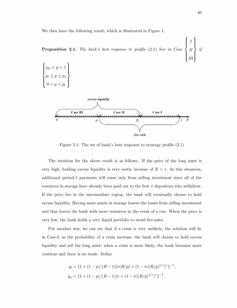
40

We then have the following result, which is illustrated in Figure 1.

Proposition 2.1. The bank’s best response to profile (2.1) lies in Case

I

II

III

if

pu < p < 1

pl ≤ p ≤ pu

0 < p < pl

.

Figure 2.1: The set of bank’s best response to strategy profile (2.1)

The intuition for the above result is as follows. If the price of the long asset is

very high, holding excess liquidity is very costly because of R > 1. In this situation,

additional period-1 payments will come only from selling investment since all of the

resources in storage have already been paid out to the first π depositors who withdrew.

If the price lies in the intermediate region, the bank will eventually choose to hold

excess liquidity. Having more assets in storage lowers the losses from selling investment

and thus leaves the bank with more resources in the event of a run. When the price is

very low, the bank holds a very liquid portfolio to avoid fire-sales.

Put another way, we can see that if a crisis is very unlikely, the solution will lie

in Case-I; as the probability of a crisis increase, the bank will choose to hold excess

liquidity and sell the long asset; when a crisis is more likely, the bank becomes more

cautious and there is no trade. Define

ql = 1 + (1− p)/(R− 1)[π(R/p) + (1− π)(R/p)1/γ ]γ−1,

qu = 1 + (1− p)/(R− 1)[π + (1− π)(R/p)1/γ ]γ−1.

41

We then have the following Corollary.

Corollary 2.1. The bank’s best response to profile (2.1) lies in Case

I

II

III

if

0 < q < ql

ql ≤ q ≤ qu

qu < q < 1

.

2.3.2 Market clearing price

Now, we turn to the asset market. The price p is determined by demand and supply.

The supply of the long asset comes from the bank who wants to liquidate some of its

illiquid assets in order to serve early withdrawing depositors in bad times. The demand

for the long asset comes from the speculator who inelastically purchase bank’s holdings

of the long asset since it wants to consume until date 2. The asset demand is ws/p and

the asset supply depends on cases identified in Table 1. In Case I, there is no excess

liquidity, the supply is equal to the additional period-1 payment (1 − π)πc1β over p,

we call it LI/p. In Case II, the supply is equal to the additional period-1 payments

(1− π)πc1β minus the excess liquidity 1− x− πc1 and then over p, we call it LII/p. In

Case III, there is no trade among the bank and the outside speculator. Note that the

implicit price of long asset will be determined by ws and L if we multiply both demand

and supply by p, where L is measured in unit of goods at t = 1. The patterns of LI

and LII is hence described by the following result and Figure 2.

Proposition 2.2. The amount of liquidity obtained by the bank L is strictly increasing

in p in both Cases I and II.

Figure 2.2: The market clearing price of the long asset

42

As we pointed out in Corollary 1, the best response of the bank to (2.1) involves

holding excess liquidity and/or fire-sale depending on the probability of crisis. Com-

bining the above discussion, we have the effect of bank run on the market clearing price

p∗, which is the point of intersection of the demand and supply curve.

Proposition 2.3. Given ws, γ, π,R, these exists a unique qc ∈ (0, 1) such that the

market clearing price p∗ is strictly

decreasing

increasing

in q if q

<> qc.

We now intuitively explain this pattern. First, recall that if bank run occurs less

likely then there is no excess liquidity and the price level is high corresponding to Case

I; as the probability of crisis increases, the bank chooses to holds excess liquidity and

the price level is low corresponding to Case II.

Figure 2.3: The impact of q on the market clearing price p∗

Recall next that when the solution lies in Case-I, the payments to the first π with-

drawals is exactly equal to the storage, that is, πc1 = 1 − x. In this case, the bank

needs to obtain the liquidity to serve the continual withdrawing depositors, that is

LI = (1− π)πc1β. Thus, the bank will sell more long assets as the crisis becomes more

likely. When the solution lies in Case-II, we know that excess liquidity is equal to the

storage minus the early payments to the first π depositors, that is 1−x−πc1. Now the

bank use the liquidity purchased from the speculator plus the excess liquidity to meet

the extra withdrawal demand, that is, LII = (1− π)πc1β − (1− x− πc1). In this case,

the bank thus sell less long assets and holds more excess liquidity as q increases since

it becomes more conservative.

43

Therefore, the curve LI is strictly increasing in q but LII is strictly decreasing in q.

Holding ws fixed, an increase in q moves the curve LI out and drags the market-clearing

price p∗ down; but this increase causes the LII to move in and arises the p∗ as depicted

in Figure 3.

2.3.3 Fragility

We now verify whether the strategy profile in (2.1) is part of an equilibrium and hence

whether the banking system is fragile. Recall that an impatient depositor will al-

ways strictly prefer to withdraw early whatever payment she receives, since she values

period-1 consumption only. Therefore, we only need to consider the actions of patient

depositors. Once the withdrawals pass π, the bank knows a run occurs, it is able to

implement the first-best continuation allocation. Thus, a patient depositor with i > π

prefers to wait in state β. For patient depositors with i ≤ π, consider separately each

of the two possible sunspot states. In state α, a patient depositor will strictly prefer

to wait as specified in (1). In state β, a patient depositor with i ≤ π receives c1 if she

joins the run and c2β if she leaves her funds in the banking system. The discussion

above establishes that the profile (2.1) emerges as part of an equilibrium if and only if

the allocation satisfies c∗1 ≥ c∗2β.

It is straightforward to show that c∗1/c∗2β is strictly decreasing in q since the bank

becomes conservative as the probability of crisis increases. We follow Li (2017) in

measuring the susceptibility of the banking system to a run. Define q to be maximum

probability with which a run can occur in equilibrium.

Definition 2.2. Given (γ, π, ws, R), let q be the maximum value of q such that c∗1 ≥ c∗2βholds. If c∗1 ≥ c∗2β does not hold for any value of q, then define q = 0.

If the probability of a run exceeds this cutoff value, the bank will become sufficiently

cautious that running is no longer an equilibrium behavior for depositors. This cutoff

value provides a natural measure of financial fragility; if a change in parameter values

decreases the maximum probability of a run equilibrium, we say that it makes the

banking system less fragile or more stable.

44

2.4 Market liquidity and financial fragility

We now turn our attention to the relationship between the market liquidity ws and

the measure of financial fragility q. One might assume that an increase in the market

liquidity would mitigate the effects of fire-sales and then promote the financial stability.

In what follows, however, we show that this relationship is non-monotone: a small

increase in the market liquidity may increase the susceptibility of banks to a run even

if the market liquidity is scarce, but a larger increase may make the banking system

more stable.

Proposition 2.4. If q lies in

Case I

Case II

, then q is strictly

decreasing

increasing

in ws.

Figure 2.4: The impact of ws on the measure of fragility

Figure 4 shows that q will lie in Cases I and II depending on parameter values.

When the market liquidity is limited or when the market clearing price is relatively

low, c1 > c2β always holds in Case I since the amount of remaining resources is small;

and the ratio c1/c2β crosses 1 after the bank has chose to hold excess liquidity, which

corresponds to Case II. When the market liquidity is rich, or when the market clearing

price is high, c1 < c2β always holds in Cases II and the ratio c1/c2β falls below 1 while

the solution is in Case I, as described in Figure 4.

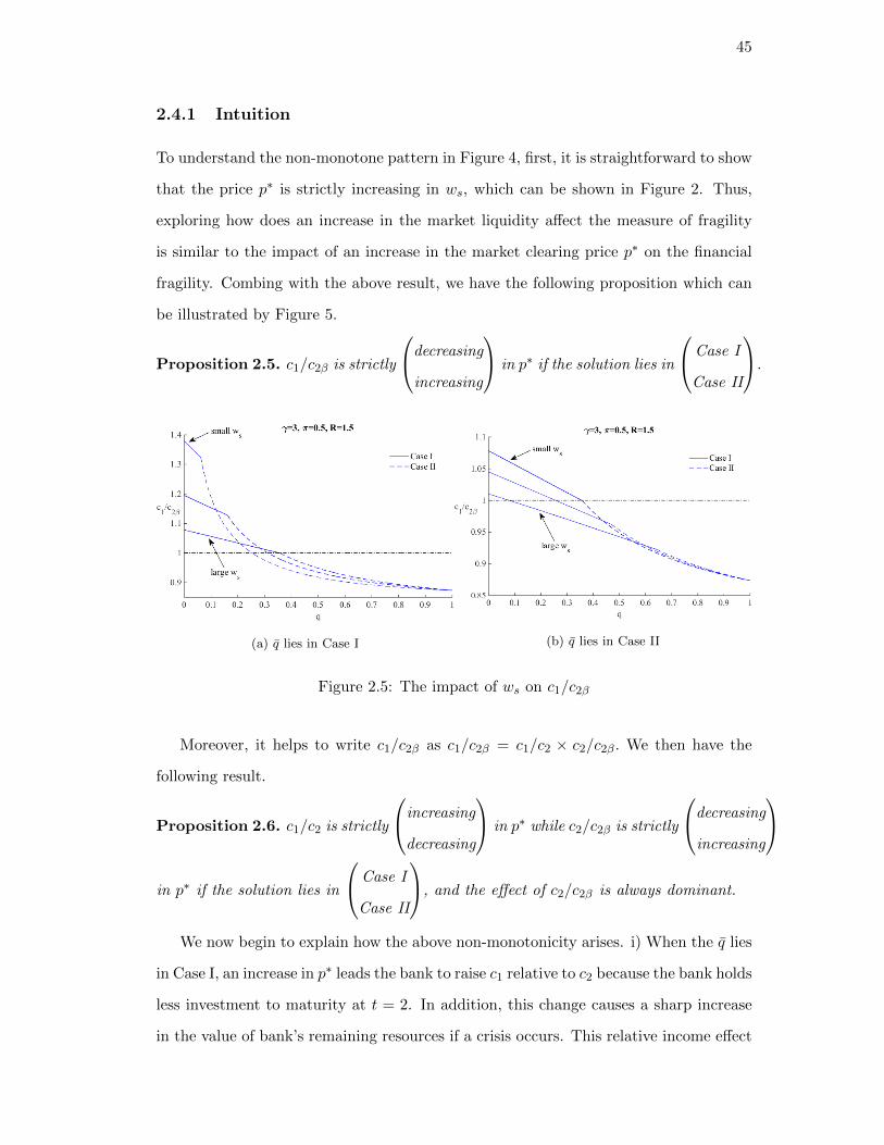
45

2.4.1 Intuition

To understand the non-monotone pattern in Figure 4, first, it is straightforward to show

that the price p∗ is strictly increasing in ws, which can be shown in Figure 2. Thus,

exploring how does an increase in the market liquidity affect the measure of fragility

is similar to the impact of an increase in the market clearing price p∗ on the financial

fragility. Combing with the above result, we have the following proposition which can

be illustrated by Figure 5.

Proposition 2.5. c1/c2β is strictly

decreasing

increasing

in p∗ if the solution lies in

Case I

Case II

.

(a) q lies in Case I (b) q lies in Case II

Figure 2.5: The impact of ws on c1/c2β

Moreover, it helps to write c1/c2β as c1/c2β = c1/c2 × c2/c2β. We then have the

following result.

Proposition 2.6. c1/c2 is strictly

increasing

decreasing

in p∗ while c2/c2β is strictly

decreasing

increasing

in p∗ if the solution lies in

Case I

Case II

, and the effect of c2/c2β is always dominant.

We now begin to explain how the above non-monotonicity arises. i) When the q lies

in Case I, an increase in p∗ leads the bank to raise c1 relative to c2 because the bank holds

less investment to maturity at t = 2. In addition, this change causes a sharp increase

in the value of bank’s remaining resources if a crisis occurs. This relative income effect

46

decreases the spread between between the payments to the late-withdrawing depositors

in good times and in bad times (c2α/c2β. ii) When the q lies in Case II, an increase in p∗

now will decrease c1 relative to c2 because the bank holds less excess liquidity. At the

same time, the bank increases the spread between (c2α/c2β because less investment is

held to maturity in bad times. Moreover, the relative income effects is always dominant

in both Cases I and II. As a result, such an increase in p∗ leads to a non-monotone

patter since this effect changes as the solutions lies in different cases. Therefore, the

net effect of an increase in market liquidity on stability is thus ambiguous.

2.5 Liquidity regulation

As we pointed out above, when the market liquidity is scarce, an increase in this liq-

uidity makes the bank more susceptible to a run since the bank tends to hold a more

illiquid portfolio and provides higher early payments. We next consider a regulatory-

policy regimes that attempts to eliminate the negative effects associated with fire-sales.

Suppose a benevolent planner could control the operations of the bank and the specu-

lator. This planner allocates resources to maximize the sum of all investors’ utilities.

We allows the policy maker to place a minimum liquidity requirement on banks’ asset

holdings.

The Basel III framework includes the Liquidity Coverage Ratio (LCR), which re-

quires each bank to hold high-quality liquid assets (HQLA) at least equal to its total

net cash outflows (NCOF) over a 30-day period under a stress scenario:

LCR =HQLA

NCOF≥ 100%.

In the context of our model, a bank’s stock of high-quality liquid assets is equal to

1−x, that is the liquid asset held in the bank’s portfolios. Total expected cash outflows

are calculated by multiplying the bank’s short-term debts πc1 by the rates at which

they are expected to run off in the stress scenario specified by supervisors. Letting η

denote the runoff rate assigned to short-term debts, and the LCR constraint for the

model can be written as

1− x ≥ ηπc1, (2.3)

47

which resembles the Basel III Liquidity Coverage Ratio.

2.5.1 Given η

We first consider the case in which the run off rate η is given. Now, the bank solves

the problem (2.2) subjected to the extra constraint (2.3). Note that this problem is

the same as before if η ≤ 1 since the first resource constraint πc1 ≤ (1− x) makes the

liquidity constraint trivial. Thus, we focus on the case with η > 1. It is straightforward

to show that the solution will alway lie in Case II and the first order condition is

[(1−q)Ru′(c2)+qRu′(c1β)−(1−q)u′(c2)−qu′(c2β)] = [u′(c1)−(1−q)u′(c2)−qu′(c1β)]/η = µ,

where the first term represents the benefit from investing one more unit of long asset

and the second term is the corresponding cost of decreasing early payment. Here, µ

is Lagrangian multiplier on the LCR constraint (2.3) and it is equal to zero when the

liquidity constraint is not binding.

Recall that the bank will hold excess liquidity and then the market clearing condi-

tions yields:

ws = LII = [(1− π)πc1β − (1− x− πc1)].

Combining the first order condition, we have the market clearing price p∗ and the best-

response allocation A∗. As in the previous section, the financial system will be fragile

under the regime with liquidity regulation if and only if c1 < c2 and c1 ≥ c2β. We next

investigate the impact of the market liquidity on the measure of financial fragility and

have the following proposition.

Proposition 2.7. For a given η, the financial system under the regime with liquidity

regulation becomes more fragile in some economies.

The result in Proposition 7 is established in Figure 6 which adds the pattern of q

under the regime with liquidity regulation for a given run off rate η = 1.1 to Figure 4.

When the market liquidity is scarce, imposing the liquidity regulation is trivial since the

bank has already chosen to hold sufficient liquidity. As the market liquidity increases,

the bank becomes risky and the financial fragility arises under the regime with no

48

regulation but forcing the bank to continue to hold enough liquidity will promote the

stability when the liquidity regulation is imposed. When the marker liquidity is rich,

keep imposing liquidity regulation will lead the bank to increase the early payment.

This effect may become the source of deteriorating stability.

Figure 2.6: Imposing liquidity regulation for a given η

2.5.2 Optimal η

In this section, we begin by analyzing how the financial fragility evolves with respect to

an increase in the runoff rate η holding other parameters fixed. Our next result shows

that imposing a strong liquidity regulation may increase q.

Proposition 2.8. Given ws, γ, π,R, increase the runoff rate η in some economies where

the liquidity constraint is binding may make the financial system more fragile.

This proposition is established in panel (a) of Figure 7 which shows that when the

market liquidity is limited imposing a stronger liquidity regulation may increase the

fragility q. By changing the policy parameter η, the liquidity constraint is not binding

when η is either small or large. In these cases, q remains the same level under the regime

with no regulation. When the liquidity constraint is binding, imposing a strict binding

minimum liquidity holdings will not be optimal, as shown in panel (a). However, when

the market liquidity is large, it can be optimal for the policymaker to select a high

binding minimum, as shown in panel (b).

49

(a) small ws (b) large ws

Figure 2.7: The impact of η on q

It is worth noting that when the market liquidity is 0.1, setting η = 1.175 will obtain

the most stable financial system from the robust-control type of view, as shown in panel

(b) of Figure. We next assume the policymaker is able to choose the runoff rate η that

minimizes the measure of financial fragility q for different level of market liquidity ws.

It is worth emphasizing that when imposing the liquidity regulation arises the fragility

compared to the regime with no regulation, we set the optimal parameter value η. Our

next numerical example shows that what the optimal policy parameter η∗ is associated

with the most stable financial system measure by q∗ as ws increases.

In the economy with γ = 3, π = 0.5, R = 1.5, adding liquidity regulation generates a

considerably lower threshold value for run equilibrium compared to the regime with no

regulation (see Figure 4), because the policymaker now requires the bank to hold a fairly

liquid portfolio and, as a result, make the financial system more stable. In addition,

note that when the market liquidity is limited imposing the liquidity regulation makes

the financial system more fragile. We hence set η∗ = 1, as depicted in panel (b) of

Figure 8. In this case, the bank holds more resources in reserves as a provision against

undesirable outcomes even if there is no regulation. Once the policy maker requires

the bank to hold more liquidity, the bank will alter its deposit contracts to provide a

higher payoff to depositors who withdraw early as a best response. This effect tends to

make the financial system more fragile by increasing the incentive of patient depositors

to join the run.

50

(a) q∗ (b) η∗

Figure 2.8: The impact of ws on the optimal policy rate

2.6 Conclusion

In a two-asset version of the Diamond and Dybvig (1983) model with limited commit-

ment and market determined asset price, we first established the relationship between

the market liquidity and the financial fragility. Our results showed that a higher level of

market liquidity may either increase or decrease the degree of financial fragility. Indeed,

when the market liquidity is scarce, an increase in this liquidity leads to make the bank

more susceptible to a run since the bank tends to hold a more illiquid portfolio and

provides higher early payments. We next introduced a liquidity regulation imposed on

banks’ asset holding. Such a regime, in some economies, can reliably promote finan-

cial stability. Paradoxically, we have indicated that an increase in the market liquidity

might also increase the financial fragility even if the liquidity regulation is in place.

51

Chapter 3

Financial Stability with Sovereign Debt

3.1 Introduction

The recent financial crisis has triggered various reforms in financial systems. There

has been much discussion and controversy over whether policy makers should expand

government guarantees of the banking system, cut back on these guarantees and focus

on financial regulation, or combine guarantees with new regulations. As emphasized by

Gorton (2010), a government guarantee in the form of deposit insurance ended the type

of banking panics that the U.S. had suffered prior to 1933. However, the Dodd-Frank

Wall Street Reform and Consumer Protection Act moves in the opposite direction,

introducing regulatory reforms “to protect the American taxpayer by ending bailouts”

and restrict the ability of the public sector in the U.S. to provide guarantees in a future

crisis. In this paper, I ask whether government guarantees, financial regulation, or a

combination of these two policies is most effective at preventing financial crises.

Government guarantees are costly. A sizable literature focuses on the moral hazard

problem associated with guarantees, in which the anticipation of government support

in bad times distorts the incentives of financial intermediaries.1 The Irish financial cri-

sis in 2008 illustrates another important cost: guarantees may undermine the solvency

of government. When the Irish government announced it would guarantee banks’ de-

posits on September 30, 2008, it took on a liability that was potentially three times

the size of annual GDP. Anticipated difficulties of financing this guarantee undermined

its credibility, and the cost of credit default swaps increased for both banks and the

government.2 This example shows the fiscal cost of guarantees may hurt the sovereign

debt sustainability, and an unsustainable debt undermines the effectiveness of guaran-

tees. Ways to prevent or mitigate this negative feedback loop have been a key focus of

1See, for example, Kareken and Wallace (1978), Gale and Vives (2002), Rancire and Tornell (2016),and Keister (2016).

2Further details can be found in IMF (2015).

52

policy makers after the crisis.3

In this paper, I study not only guarantees (as in Konig et al. (2014) and Leonello

(2018)), but also financial regulation and the combination of these policies when there

is a negative feedback loop between the government and banking sector. I specify

the transmission channel from banking sector to the government as tax revenue and

guarantees. The tax revenue channel has been either ignored (Konig et al. (2014) and

Leonello (2018)), or assumed to be irrelevant from banks’ lending (Cooper and Nikolov),

to study self-fulfilling bank runs. This channel creates a negative feedback loop between

banking and sovereign crises even in the absence of guarantees. My model is the first

to study liquidity regulation and the interaction between regulation and guarantees.

Are guarantees, financial regulation or a combination of these policies the best

way to promote financial stability given this loop? I address this question in a model

of financial intermediation based on a version of the classic model of Diamond and

Dybvig (1983) extended to include a government that issues, and may default on, debt.

Intermediaries invest in a combination of government bonds and long-term projects,

and these projects are a source of tax revenue for the government when they mature.

As in Diamond and Dybvig (1983) and many others, intermediaries conduct maturity

transformation and are potentially susceptible to a self-fulfilling run by depositors. The

government and banking sector are linked in two ways:

1. Tax revenue: taxes on matured investment financed by intermediaries are an

important source of revenue for the government.

2. Bond price: intermediaries hold government bonds and changes in the price of

these bonds affect their solvency.

My analysis begins by studying equilibrium outcomes when there are no guarantees

or regulation, which I call the no-policy regime. If depositors run on the banking system,

3IMF managing director Christine Lagarde mentioned “We must break the vicious cycle of bankshurting sovereigns and sovereigns hurting banks” in her speech of January 2012, and Governor IgnazioVisco of the Bank of Italy said “An intensely debated topic in the context of possible further financialreforms... concerns possible actions to address the negative loop between sovereign and bank risk.” inhis speech of May 2016.

53

banks liquidate projects to redeem withdrawals. If enough depositors withdraw, the

banks will be forced to liquidate all of their projects, which implies the government has

no tax base and is unable to repay its bonds. I show that, in the no-policy regime, the

financial system is always vulnerable to a run and a run always causes the government

to default on its debt.

I then introduce three different policy regimes into this model and ask under what

conditions each regime eliminates the bank run equilibrium. The first regime is a

government guarantee of deposits in the banking system. The role of this guarantee

is to prevent liquidation of long-term investment and, in the process, to preserve the

tax base. However, its effectiveness depends on whether the government will be able

to pay off the debt used to finance the guarantee. I find the guarantee tends to be

effective when the return on long-term investment is high and when the government’s

initial debt is small. The guarantee becomes a third linkage between the government

and banking sector:

3. Guarantees: the government may make transfers on the occasion of a bank’s

liquidity shortage, increasing the government expenditures.

The second policy regime is a type of liquidity regulation that requires banks to

have a minimum level of liquid assets relative to expected short-term outflows. When

this requirement binds, a bank must shift its portfolio away from profitable projects and

toward bonds. This regulation may prevent a run, but may also distort the allocation

and can even cause default if it is too tight. I find the regulation tends to be more

effective than the guarantee at preventing financial crises when the return on long-term

investment is low, while the guarantee is likely to be more effective when this return is

high. In some cases, both policies are effective at preventing a run. In these cases, the

guarantee implements a better allocation because it does not distort banks’ choices.

I examine the combination of these two policies as the third policy regime. Liquidity

regulation may complement the guarantee, because it requires banks to have a larger

amount of bonds and to reduce their short-term outflows. The banks can redeem some

54

extra withdrawals using the returns from their bond holdings without liquidating long-

term projects. Furthermore, liquidity regulation lowers short-term liabilities, which

decreases the obligations faced by the government in the event of a run. The combi-

nation of these two policies is needed to prevent a run in some cases. In other cases,

liquidity regulation alone is effective and adding guarantees would make the financial

system fragile.

The remainder of the paper is organized as follows: Section 3.2 introduces the envi-

ronment and defines financial stability and fragility. In Section 3.3, I present equilibrium

outcomes without policy, and I study equilibria given different policy regimes in Section

3.4. I offer some concluding remarks in Section 5.

3.2 The Model

The analysis is based on a version of Diamond and Dybvig (1983) model augmented

to include a government that issues and may default on debt. I introduce a financial

market in which the bonds are traded. This section describes the basic elements of the

model.

3.2.1 The environment

There are three periods, labeled t = 0, 1, 2, and a continuum of depositors indexed by

i ∈ [0, 1]. Each depositor has preferences given by

U(c1, c2;ωi, δ,1G) = u(c1 + ωic2)− 1Dδ,

where ct is the consumption of goods in period t. The function u is assumed to be

logarithmic. The parameter ωi is a binominal random variable with support Ω ≡ 0, 1,

which is realized in period 1 and privately observed by the depositors. If ωi = 1,

depositor i is patient, while she is impatient if ωi = 0. Each depositor is chosen to be

impatient with a known probability π ∈ (0, 1), and the fraction of impatient depositors

is also equal to π. The other component of the preferences is the welfare loss associated

with a sovereign default. The indicator function 1D takes the value 1 if the government

55

defaults and 0 otherwise, and δ captures the level of loss. I assume δ is sufficiently large

such that a default should be avoided at any cost if possible.4

Technologies: Depositors are each endowed with one unit of all-purpose good

which can be used for consumption or investment at the beginning of period 0. There

is a single, constant-returns-to-scale technology for transforming this endowment into

consumption in the last period. A unit of the good invested in period 0, called a project,

yields with R > 1 in period 2 or r < 1 in period 1, where r represents the liquidation

value.

Government: The government must finance a given level of expenditure in period

0. This expenditure can be interpreted as initial debt, and is denoted by d0 > 0. The

government issues bonds to raise funds in period 0, and levies taxes on matured projects

in period 2 to repay the bonds. The matured projects can be interpreted as output of

the economy.

Bond market and Investors: The government bonds can be traded in both

periods 0 and 1 at price qt for t = 0, 1. Depositors and deep-pocketed risk neutral

investors have access to the market. A continuum of identical investors of mass 1 has

preferences denoted by

vj(cf,j2 ) ≡ cf,j2 ,

where cf,j2 is the period-2 consumption of investor j ∈ [0, 1]. The investors have an

outside option which pays a return R∗ ≥ 1 in period 2.

Financial intermediation: Depositors pool their resources to form a bank in order

to insure against liquidity risk, as in Diamond and Dybvig (1983) and many others. This

representative bank behaves competitively in the sense of taking the returns on assets as

given and invests in a combination of projects and government bonds. Each depositor

can either contact her bank to withdraw funds in period 1 or wait until the final period to

withdraw. Depositors are isolated from each others in period 1 and 2, and they cannot

trade with each other. Upon withdrawing, the depositor must consume what is given

4A government default would negatively affect the credibility, institutions, public safety or infras-tructure in an economy. This default cost captures all such negative effects. The default cost in utilityis a standard way to incorporate default costs in the literature of sovereign default. See, for example,Bianchi et al. (2018), Arellano and Bai (2017) and Bolton and Jeanne (2007).

56

immediately. Repayments follow a sequential service constraint (Wallace (1988)), and

the order of a depositor’s arrival at the central location is randomly determined after

they decide to withdraw. Therefore, each depositor learns her type at the beginning of

period 1 and decides whether to contact the central location or not. Once a depositor

decides to make contact, she learns her position in the queue of depositors to withdraw.

3.2.2 Financial crisis

Withdrawal: Depositors may condition their withdrawal decision on an extrinsic

sunspot signal s ∈ S = α, β. This “sunspot” variable is realized at the beginning

of period 1 and is observable to depositors and investors, but unobservable to banks. A

depositor’s withdrawal decision depends on both her type and the sunspot signal. Let

yi denote the withdrawal strategy for depositor i such that

yi : Ω× S 7→ 0, 1,

where yi(ωi, s) = 0 corresponds to withdrawal in period 1 and yi(ωi, s) = 1 corresponds

to withdrawal in period 2. Impatient depositors, where ωi = 0, always withdraw in

period 1 (yi(0, s) = 0).

I will say that the financial system is fragile if there exists an equilibrium in which

all depositors choose to withdraw in period 1 in some sunspot state. Without any loss

of generality, I let s = β denote the bad state in which a run potentially occurs. I refer

to s = α as the good state.

Definition 3.1. The financial system is said to be fragile if there exists an equilibrium

strategy profile with yi(1, β) = 0 for all i; otherwise the financial system is said to be

stable.

I assume that the probability agents assign to the bad sunspot state in period 0

is zero. This assumption is a useful and common simplification in the literatures on

banking and other financial crises.5 The occurrence and timing of a financial crisis is

5See, for example, Diamond and Dybvig (1983), Chang and Velasco (2000), and Ennis and Keister(2009).

57

notoriously difficult to predict, and there is evidence that the risks of such events are

effectively overlooked by private agents in good times.

3.2.3 Timeline

The timing is summarized in Figure 1. In period 0, depositors deposit their endowments

with the bank in each central location. The government issues the bonds to investors

and banks through the bond market, in order to repay the initial debt. The bank divides

the resources deposited by the depositors between bonds and projects, and the period

ends. At the beginning of period 1, depositors learn their type ωi and the sunspot

state, and choose whether to withdraw in period 1 or wait. Withdrawing depositors

then begin to arrive one at a time at their banks and are served as they arrive. To

finance these withdrawals, a bank sells bonds to investors and may liquidate projects.

In period 2, the government levies taxes on matured projects and repays its bonds.

Banks then repay the remaining depositors.

Figure 3.1: Timeline

3.3 Equilibria without policy

I begin the analysis by studying equilibrium with no government guarantee or liquidity

regulation. Given the self-fulfilling nature of a run in this model, there always exists a

“good” equilibrium in which patient depositors withdraw in period 2. I will first derive

the allocation in this no-run equilibrium. As is standard in Diamond and Dybvig (1983),

this allocation will be equivalent to the full information efficient allocation. I will then

58

look for another equilibrium in which patient depositors withdraw in period 1.

3.3.1 The no-run equilibrium

Suppose, in period 0, banks expect impatient depositors to always withdraw in period

1 and patient depositors to always withdraw in period 2. Based on this expectation,

banks then decide the portfolio structure and payment schedule (c1, c2) in period 0. Let

x denote the fraction of the total assets placed into project investment; the remaining

(1− x) is invested in government bonds.

In order for the government to be able to repay its debt in the good state, the

following condition must be satisfied.

Assumption 3.1. d0 ≤ (1−π)(R−R∗)R∗ .

As I show below, this assumption guarantees that investing in the project yields a higher

after-tax return at t = 2 than holding bonds. In other words, with the tax rate in the

good state τα ∈ [0, 1], this assumption guarantees that R(1− τα) ≥ 1q0

holds in the no-

run equilibrium. If this assumption were not satisfied, there would be no equilibrium

in which a positive amount of projects could mature, leaving the government zero tax

revenue. As a result, anticipating that the government would be unable to repay any

bonds in period 2, no agent would purchase government bonds in period 0 and 1. The

government would then be unable to raise enough revenue to repay its initial debt

and would default on its initial debt in period 0. However, because my interest is to

analyze the effects of different policies on debt sustainability, I will only focus on cases

in which the government can repay its debt in the good state. A sovereign default can

be triggered only by a bank run, and does not happen without a run in this model.

Definition 3.2. There is a sovereign default if the government is unable to repay debt

fully under an equilibrium strategy profile with yi(1, β) = 0.

Bond price: Investors play an important role in determining the price of bonds

through their arbitrage between the bonds and the outside option. In period 0, investors

and banks expect that the bad state, in which runs occur, will not be realized with

probability one, yielding

59

q0 =1

R∗. (3.1)

The bond price in periods 0 and period 1 and 2 will remain at this level if the good

state realizes, meaning

q0 = q1,g. (3.2)

Deposit contract: By Assumption 3.1 and the arbitrage conditions (3.1) and

(3.2), banks will not liquidate any illiquid assets in the good state, because selling

bonds would be more profitable than liquidating projects. Likewise, they will not keep

any bond until period 2 in the good state. A bank chooses (c1, c2, x) to maximize the

expected utility of its depositors such that

maxc1,c2,x πu( c1) + (1− π)u( c2), (3.3)

subject to

πc1 = (1− x)q1,g

q0, (3.4)

(1− π)c2 = xR(1− τα), (3.5)

c1 ≥ 0, c2 ≥ 0, and 0 ≤ x ≤ 1. (3.6)

The first constraint states that the consumption of impatient depositors in the good

state always comes from the returns from bonds. The second constraint states that

the bank redeems withdrawals by patient depositors in the good state through returns

from projects.

The solution to this problem is characterized by the first-order condition

u′(c1)

u′(c2)= R(1− τα)

( q0

q1,g

)= R(1− τα)

>1

q0

= R∗.

60

The second and last equalities follow from equations (3.1) and (3.2), and the inequality

is implied by Assumption 3.1. Notice that c∗2 > c∗1 necessarily holds, because R∗ > 1.

Patient depositors consume more than impatient ones. Under the logarithmic utility

function for depositors, the optimal level of project investment is exactly equal to the

fraction of patient depositors such as x∗ = 1 − π. The deposit contract is, therefore,

given by

c∗1 = 1 and c∗2 = R(1− τα). (3.7)

Tax rate: The government levies taxes on matured projects in period 2 to repay

the exact amount of outstanding debt. The tax rate in the good state will be

τα =

︷︸︸︷d0

1

q0

outstanding debt

Rx∗︸︷︷︸tax base

. (3.8)

The period-0 bond price in the numerator captures the funding cost for the government.

Therefore, the contract can be solved in closed form,

c∗1 = 1 and c∗2 = R− d0R∗

1− π. (3.9)

Withdrawal strategy: Banks are able to repay (c∗1, c∗2) as long as patient deposi-

tors withdraw in period 2 and impatient depositors withdraw in period 1. Since c∗2 > c∗1,

there is an equilibrium in which impatient depositors withdraw in period 1 and patient

ones withdraw in period 2, meaning

yi(ωi, g) = ωi. (3.10)

Then, Assumption 3.1 implies that the government is able to levy taxes sufficiently to

repay the debt. The tax rate is determined by (3.8), and the bonds are traded at the

price (3.1) and (3.2). It is straightforward to show that the consumption allocation

in this no-run equilibrium specified in (3.9) is equal to the full information efficient

allocation in this environment.

61

3.3.2 Bank run

I will now examine whether there exists an equilibrium in which patient depositors

instead choose to withdraw in period 1. If this withdrawal happens, banks exhaust

their bond holdings and are forced to liquidate projects to redeem the extra withdrawals.

Let ` be the amount of liquidation needed to accommodate such withdrawals, which

increases as more patient depositors withdraw in period 1.

Preliminaries: Liquidation reduces the number of projects that can mature in

period 2, shrinking the tax base. The government must raise the tax rate to be able

to repay its debt, and the after-tax return from projects will decrease correspondingly.

Let τβ denote the tax rate in the bad state. If there is an equilibrium in which a run

occurs and banks have to liquidate projects, τβ represents the corresponding tax rate.

If this tax rate is high enough, banks will find it profitable to liquidate their projects

and hold government bonds instead, since the proceeds on these bonds are not taxed.

This is true regardless of how many depositors are attempting to withdraw from the

bank.

Assumption 3.2. Banks liquidate all projects and purchase additional bonds if R(1−

τβ) < rR∗

Note that the return from bonds is 1q1

= R∗ which appears on the right hand side of the

inequality. This inequality suggests that government bonds yield higher returns than

keeping the projects invested despite the bank having to pay liquidation costs. Under

this assumption, the maximum tax rate in which the banks keep projects invested is

τβ = 1− rR∗

R. (3.11)

Withdrawal strategy: Consider the following strategy profile for depositors,

yi(ωi, β) = 0. (3.12)

Under this profile, both impatient and patient depositors withdraw in period 1, and

a bank run occurs. This is an unexpected event to the banks, in which they must

liquidate projects to keep paying c∗1. The amount of liquidation will be

62

` = (1− π)c∗1r. (3.13)

The remaining project is x∗ − `, and the bank will run out of assets if x∗ − ` < 0.

Evaluating at the solution to the problem characterized by (3.3), (3.4), (3.5) and (3.6),

I see that banks will always exhaust the assets with this profile because

x∗ − ` = (1− π)− (1− π)1

r< 0. (3.14)

The tax rate associated with this profile is

τβ =d0

1q0

R(x∗ − `)= +∞.

Notice that banks always liquidate all projects before all depositors have been served,

because τβ < +∞.

The negative feedback loop: Since τβ < τβ, the government has no base on which

to levy taxes and is unable to fulfill the debt in period 2, which leads to a sovereign

default. Investors anticipate this inability to repay and reduce their demand for bonds

to zero, meaning that nobody will purchase bonds from banks in period 1, meaning

q1,β = 0.

Banks must then liquidate further projects. The amount of liquidation which banks

need to redeem all withdrawals under the sovereign default is

`′ =c∗1,sr

=1

r,

which is larger than `. The negative feedback loop through the government thus raises

the necessary amount of liquidation. The banks will run out all of their assets before

period 2 because 0 > x∗−` > x∗−`′. The banks keep paying c∗1 to redeem withdrawals,

and pay nothing once they run out of funds. The probability of a depositor arriving at

her bank before the bank runs out of the assets is

p = minrx∗

c∗1, 1.

63

A patient depositor, therefore, has a chance to receive positive consumption if she were

to withdraw in period 1. However, she receives zero for certain if she were to wait until

period 2.

Equilibrium and fragility: The above analysis establishes the behavior of the

government and banks under the strategy profile (3.12). I now ask whether the strategy

profile can indeed be an equilibrium and hence whether the financial system is fragile

or stable. Recall that an impatient depositor will always strictly prefer to withdraw in

period 1 because she values period-1 consumption only, so only the actions of patient

depositors need to be considered. Banks are unable to repay withdrawals by both

impatient and patient depositors in period 1 because banks run out of funds before

period 2 as 0 > x∗− ` > x∗− `′. A patient depositor prefers a chance to receive positive

consumption over receiving zero for certain, and hence I can construct an equilibrium

in which depositors follow (3.12).

Proposition 3.1. The financial system is always fragile under the no-policy regime

Notice that a sovereign default always occurs in the bad state because the banks liqui-

date all projects and the government has zero tax revenue.

3.3.3 Discussion

Tax exempted bond: The assumption that the government does not levy taxes on

government bonds is an essential ingredient for financial fragility in this environment.

If I were to instead allow the government to freely tax bold holdings, it would be able

to directly reduce its liabilities to bond holders without repaying them. In other words,

taxing bond holdings would effectively allow the government to indirectly default on

its obligations, either partially or in full. In the extreme case of a 100% tax rate on

gross returns from the bonds, the government’s repayment and the debt holders’ tax

payment offset each other, and the government has zero net payment to debt holders.

My assumption that the government cannot tax bond holdings is equivalent to assuming

that the default cost δ applies regardless of whether the default reflects a failure to repay

or a direct confiscation of the bonds through taxation.

64

Alternatively, the government may levy taxes on net returns from bonds. However,

the net return must at least equal the risk-free rate R∗ because of the arbitrage con-

ditions (3.1) and (3.2). As long as the risk-free rate is not very high, and the taxes

on net return from these bonds would not help the government revenue much. Costs

to implement such taxes can even be higher than additional tax revenue from bond

returns.

In practice, many countries and states exempt interest on government bonds from

taxation as documented in Norregaard (1997). In addition to the high cost of adminis-

tration, administrative difficulties in implementing taxes on international debt holders

may also be responsible for such exemptions.

This assumption has been commonly used in several pieces of literature, to discuss

correlated risks between government and banks (see, for example, Acharya and Rajan

(2013) and Acharya et al. (2014)) or to discuss sovereign default (see, for example,

Cuadra et al. (2010), Schabert (2010) and Scholl (2017)).

3.4 Policies

In this section, I study equilibrium outcomes under the three different policy regimes. I

derive and compare conditions under which each policy regime is effective in stabilizing

the banking system.

3.4.1 Government guarantees

Suppose that the government guarantees deposits to prevent bank runs in bad times,

reassuring the depositors that their banks will repay them. Such guarantees are made

through transfers from the government to the banks when banks face the necessity of

costly liquidation. By doing so, banks can avoid liquidating projects as long as the

government makes the transfer. The government finances this expenditure by issuing

additional bonds, and repays these bonds in period 2 together with the bonds issued in

period 0.

65

Deposit contract: The government implements deposit guarantees in bad times,

but this scheme does not affect the deposit contract and bank’s portfolio choice in

period 0 because the bad state is not ex-ante expected. The contract follows the efficient

allocation (3.9), and the bond price will be at the levels (3.1) and (3.2).

An equilibrium in the good state remains unchanged with consumption levels at

(c∗1, c∗2), and there is no actual transfer from government. Depositors follow the with-

drawal strategy (3.10), meaning they follow their types to decide withdrawal timing.

Run strategy: Now consider the strategy profile (3.12) in the bad state. Banks

first serve π withdrawals by selling the government bonds, then the government helps

banks to redeem extra withdrawals through transfers. The total amount of transfer will

be

bDG = (1− π)c∗1 = (1− π). (3.15)

where (1−π) is the number of remaining depositors withdrawing in period 1. To make

these transfers, the government issues new bonds in the market and investors may

purchase them. The government has to pay an interest rate of 1q1

as funding costs. The

investors will buy these newly issued bonds if they anticipate the government can fulfill

its debt in period 2. The outstanding government debt in period 2 will be

d01

qDG0

+ b1

qDG1,β

.

Correspondingly, the tax rate will be

τDGβ =d0

1qDG0

+ bDG 1qDG1,β

Rx∗. (3.16)

In the case that the government can repay all debt in period 2, investors trade the

bonds under the arbitrage against the outside option, anticipating the government will

pay it back,

qDG1,β =1

R∗. (3.17)

66

The government is able to guarantee the deposit if the tax rate is below the threshold

level (3.11), τDGβ ≤ τβ, under the bond price (3.17). While the government finances

the amount (3.15) to serve all extra withdrawals, the banks still have projects as assets

and are able to repay more in period 2 than in period 1 because c∗2 > c∗1. A patient

depositor is better off deviating to wait until period 2, and the strategy profile (3.12) is

not in an equilibrium. Therefore, the deposit guarantee eliminates the equilibrium in

which a bank run occurs, given that the government can defray the expenditure.

Run equilibrium: The government, however, may not be able to pay the debt

back in period 2, meaning that τDGβ > τβ. Investors will then anticipate that the

government will default on its debt in period 2, and do not purchase bonds in period

1, meaning

qDG1,β = 0.

In such a case, the government is unable to raise any funds to make a transfer to the

banks, and the banks must liquidate projects to serve withdrawal demands in period 1.

The banks will exhaust their projects as the liquidation is costly and τDGβ = +∞ > τβ.

The banks repay c∗1 before p withdrawal and 0 otherwise, and will repay 0 in period 2.

A patient depositor prefers to withdraw in period 1 because she has a chance to receive

positive consumption by doing so and would receive zero for certain if she were to wait

until period 2. I can therefore construct an equilibrium with the strategy profile (3.12).

Effectiveness: The guarantee can eliminate the run equilibrium without distortion

and actual expenditures if it is effective. Its effectiveness, however, depends on whether

the government can raise funds or not. In other words, there exists a bank run equi-

librium if and only if the government is unable to finance the guarantee, the ability for

the government to finance guarantees is in turn dependent on whether the government

can levy sufficient taxes to repay the bonds in period 2. Recall that τDG2,β denotes the

equilibrium tax rate in the bad state. The condition for stability is then formulated as

follows.

Proposition 3.2. The financial system is

fragile

stable

if τDG2,β

>

≤

τβ

67

Figure 3.2: Effectiveness of the guarantee

This proposition implies that once the necessary tax rate exceeds the threshold, the

government no longer has a sufficient tax base to fulfill its debt, rendering its guarantee

ineffective. By rewriting the condition in Proposition 3.2 with parameters only, I can

derive the condition for the stability of a financial system as

d0 ≤ (1− π)(R

R∗− 1− r). (3.18)

The government guarantee becomes more effective in removing the run equilibrium

as project returns (R) increase and as the initial debt levels decrease (d0). The intuition

behind this condition is that a larger amount of production will expand the tax base for

the government, and higher debt levels will minimize leeway for other expenditures. Let

d0DG

represent the maximum level of initial debt that can be supported in the guarantee

regime that satisfies condition (3.18). According to condition 3.18, d0DG

increases as

project returns increase. These results are illustrated in Figure (3.2), where the colored

region represents when the guarantee eliminates the run equilibrium. The horizontal

axis represents levels of pre-tax returns (R), and the vertical axis corresponds to the

initial debt level (d0). The remaining parameters follow (r, π,R∗) = (0.7, 0.4, 1.1).

As for the remaining parameters, outside return (R∗), liquidation value (r) and

68

the fraction of impatient depositors (π) reduce the effectiveness of the guarantee and

decrease d0DG

. Higher outside returns lead to lower bond prices, causing banks to

shift their assets from their projects to bonds earlier, and as a result the maximum tax

rate that the government can implement (τβ) will decrease. Additionally, lower bond

prices mean higher funding costs for the government. The liquidation value affects the

maximum tax rate the government can set, because doing so makes it more beneficial

for banks to liquidate the projects.

My interest is how this set of parameters compares to the stable sets under the other

policy regimes. In the next subsections, I turn to the study of the other policy regimes

and derive their conditions for stability.

3.4.2 Liquidity regulation

The idea of liquidity regulation is to force banks to hold more liquid assets than a

particular level. An example of such liquidity regulation is the Liquidity Coverage

Ratio (LCR) regulation which is newly installed in the Basel III accord. According to

this regulation, banks are required to hold enough high quality liquid assets (HQLA)

to cover their net cash outflows over the next 30 calendar days (NCOF) in a stress

scenario. The LCR requirement is

LCR =HQLA

NCOF≥ 1.

Regulation in the model: The LCR regulation would create a buffer for banks to

deal with extra withdrawals in period 1 if it binds. In period 0, the banks are required to

hold a quantity of government bonds (HQLA) equal to their net cash outflows (NCOF),

which I take to be a fraction ξ of their total short-term obligations c1. The parameter ξ

is a policy choice that reflects the severity of the stress scenario chosen by policy makers.

A bank then chooses (c1, c2, x, θ) to maximize the weighted utility of depositors (3.3)

subject to

69

πc1 = θq1,g

q0(3.19)

(1− π)c2 = xR(1− τα) + (1− x− θ) 1

q0(3.20)

c1 ≥ 0, c2 ≥ 0, and, 0 ≤ θ ≤ 1− x, 0 ≤ x ≤ 1, (3.21)

and the LCR constraint

ξc1 ≤ (1− x),

where θ represents the amount of the government bonds which the bank sells in period

1. I express the optimal level of choices in this problem by (cLCR1 , cLCR2 , xLCR, θLCR). I

also suppose that policy makers can tighten the regulation only enough to ensure a tax

base to levy sufficient taxes to repay its debt. The regulation may reduce the quantity

of project investments by banks, leading to higher tax rates. Policy makers have to

make sure that the after-tax return from projects is sufficiently large to incentivize

banks to invest in projects. The maximum level of regulation ξ, then, must satisfy

R(1− τα(xLCR(ξ))) = R∗.

A higher ξ than this threshold level raise tax rates and makes investments in long-term

projects less profitable than holding government bonds both in period 1 and 2. In such

a case, banks will not invest in projects and a necessary tax base will not be assured,

rendering the government unable to repay its bonds even in the good state.

The LCR constraint will be slack if ξ < π, in which case the solution (3.9) is

implemented. Otherwise, the equilibrium allocation satisfies

u′(cLCR1 )

u′(cLCR2 )=ξR(1− τLCRα )− ξ 1

qLCR0+ π 1

qLCR1,g

π.

Assumption 3.1 and ξ < ξ imply that the government can levy sufficient taxes in period

2 in the good state, and that bond prices will be at levels (3.1) and (3.2). Given the

logarithmic utility function for u(·), the equilibrium allocation under the LCR regulation

70

will be

cLCR1 =πR(1− τLCRα )

ξR(1− τLCRα )−R∗(ξ − π)and cLCR2 = R(1− τLCRα ). (3.22)

The amount of project investment and the amount of bonds that banks sell in period

1 will be respectively

xLCR = 1− ξπR(1− τLCRα )

ξR(1− τLCRα )−R∗(ξ − π)and θLCR =

π2R(1− τLCRα )

ξR(1− τLCRα )−R∗(ξ − π).

(3.23)

The tax rate is determined by rule (3.8), where the amount of project investments

(xLCR) depends on the tax rate. While there can be multiple equilibrium tax rates,

I suppose that the government chooses the lowest tax rate among those satisfying the

rule in order to implement the higher weighted utility of depositors.

Recall that all of cLCR1 , cLCR2 and xLCR are dependent on ξ in addition to τα.

Lemma 3.1. The depositors’ utility and the amount of project investments decrease

as LCR regulation (ξ) is tightened.

Banks must give up some opportunities to invest in projects by having required liquidity,

and hence have less returns to repay. Policy makers choose the lowest ξ if there is more

than one ξ capable of making the economy stable, in order to implement the higher

weighted utility of depositors.

This allocation implies cLCR2 > cLCR1 for any value of ξ as

cLCR1 ≤ c∗1 = 1 < R∗ < R(1− τα) = cLCR2 .

In the good state, there will be an equilibrium with the withdrawal strategy (3.10), the

bond prices (qLCR0 , qLCR1,g ), and the consumption levels (cLCR1 , cLCR2 ).

Run strategy: Under this regulation, banks hold excess liquidity, meaning they

hold more liquidity than necessary to repay impatient depositors. I consider the with-

drawal strategy (3.12) in this environment.

The excess liquidity enables banks to redeem extra withdrawals without costly liq-

uidation. The number of depositors which the banks can repay with returns from bonds

will be

71

γLCR =1− xLCR − θLCR

cLCR1

= ξ − π,

where (1 − xLCR − θLCR) shows the amount of excess liquidity. However, banks will

eventually run out of the bonds to sell eventually, and they try to redeem remaining

withdrawals by liquidation. The amount of necessary liquidation will be

`LCR = (1− π − γLCR)cLCR1

r= (1− ξ)c

LCR1

r.

The bank’s ability to redeem these additional withdrawals depends on whether they

can pay the contracted repayment to all depositors by liquidation in period 1: (xLCR−

`LCR). The tax rate is determined at

τLCRβ =d0

1q0

R(xLCR − `LCR). (3.24)

When banks liquidate all projects, this tax rate will diverge to infinity. However,

Assumption 3.2 implies that the maximum tax rate in which the government can im-

plement is less than positive infinity. Therefore, the condition in which the government

does not default is

τLCRβ ≤ τβ, (3.25)

which implies the bank’s solvency condition such that

xLCR − `LCR ≥ 0. (3.26)

Suppose that condition (3.25) holds, and that the government will never default on

its debt. In such a case, the bond price will be

qLCR1,β =1

R∗.

The banks will still have a positive amount of assets after serving all withdrawals in

period 1. In this situation, a depositor i is better off by deviating from the profile

(3.12), and this strategy profile will not be in an equilibrium.

72

I now consider the case in which condition (3.25) does not hold, where the govern-

ment is unable to repay its debt. In this case, investors anticipate the default and the

bond price will be

qLCR1,β = 0.

The necessary liquidation to serve the withdrawals increases as the bonds are worthless

as

`′ =cLCR1

∗

r.

This suggests that banks must serve all withdrawals by liquidating their projects. The

banks will eventually run out funds in period 1 as (xLCR − `′) < (xLCR − `) < 0, and

will not be able to repay any withdrawals in period 2. Letting pLCR = min rxLCRcLCR1

, 1

be the probability for a depositor to arrive at her bank before the bank runs out of the

assets given the regulation. Similarly to the analyses in the no-policy regime and the

guarantee regime, a patient depositor prefers to withdraw in period 1 because she has a

chance to receive positive consumption. Therefore, the strategy profile (3.12) is a part

of an equilibrium if and only if the other inequality in the condition (3.25) holds.

Effectiveness: Liquidity regulation prevents bank runs if it is effective, and its

effectiveness in turn depends on whether the excess liquidity is sufficient to avoid the

critical level of liquidation. If the necessary liquidation exceeds the critical level, bond

prices drop and banks are unable to serve all withdrawal demands through the negative

feedback loop. In other words, the tax rate associated with the necessary liquidation

should be lower than the threshold tax rate in order for the financial system to be

stable. If there exists ξ ≤ ξ such that the tax rate after necessary liquidation is below

the threshold level, policy makers can prevent bank runs through liquidity regulation.

Proposition 3.3. The financial system is

fragile

stable

if τLCR2β

>

≤

τβ for any ξ ≤ ξ.

Note that the equilibrium tax rate in the bad state τLCR2,β is a function of ξ. The

73

Figure 3.3: Effectiveness of liquidity regulation

condition for the financial system to be stable can be rewritten as, for any ξ ≤ ξ,

d0 ≤(

1− ξλR(1− τα)

ξR(1− τα)−R∗(ξ − λ)

)(R− rR∗ + 1−ξ

ξ

R∗

)−(

(1− ξ)(R− rR∗)rξR∗

). (3.27)

where the tax rate (τα) is obtained through the tax rule (3.8) with xLCR. I denote the

maximum level of initial debt that can be supported in the liquidity regulation regime

that satisfies the equality in condition 3.27 as d0LCR

.

Figure 3.3 depicts this result given the same parameter set as the guarantee regime.

The categories labeled on each region indicate which policies can be implemented to

eliminate fragility in those economies. For instance, for any economy in the regions

labeled as “Liquidity regulation” or “Guarantees or Liquidity regulation”, there exists

ξ ≤ ξ such that it satisfies condition (3.27), meaning that economy can be stabilized

by liquidity regulation. In this numerical example, the set of economies that can be

stabilized by guarantees is, then, a strict subset of the economies that can be stabilized

by liquidity regulation.

When the return on long-term investment is high and when government’s initial

debt is small, regulation effectively makes the deposit contract run-proof, requiring

banks to have a larger amount of bonds and to reduce expected short-term outflows.

74

The value of these bonds depends on whether the government can repay them. Having

higher returns on investment and lower initial debt helps government repay the bonds,

and banks can redeem some extra withdrawals from returns from the bonds without

liquidating long-term projects, as d0LCR

increases as R increases.

In the next subsection, I turn to the study of the combination of these two policies,

and discuss how they interact with each other.

3.4.3 Policy mix

Policy makers may consider adopting liquidity regulation and government guarantees

together. Banks would be required to hold some level of liquid assets according to the

regulation, and the government would make transfers to the banks once they deplete

their liquid assets.

Deposit contract: In period 0, banks face an identical problem to the liquidity

regulation regime because, like in the liquidity regulation regime, the bad state is not

expected to occur. The deposit contract and efficient allocation will be equal to the ones

in the liquidity regulation regime (3.22) associated with the portfolio choices (3.23).

Additionally, an equilibrium in the good state would be completed with the with-

drawal strategy (3.10) and with the bond prices at levels (3.1) and (3.2).

Run strategy: I now consider the strategy profile (3.12) in the bad state given this

environment. After serving π withdrawals, banks would still have government bonds

to serve further withdrawals, and can redeem withdrawals without any liquidation for

up to γLCR withdrawals, analogous to the liquidity regulation regime. Once the banks

exhaust the government bonds, the government begins to make transfers in order to

avoid liquidation. The necessary amount to prevent liquidation is

bMIX = (1− ξ)cLCR1 .

Notice that this necessary amount of transfers is smaller than bDG. This is not only

because (π−ξ) depositors are served through the excess liquidity, but also because banks

make a safer deposit contract under liquidity regulation. Thus, liquidity regulation

75

diminishes the necessary amount of transfers per depositor in the guarantee. Banks will

pay less in the good state, and have opportunity costs, while it will be less costly for

the government to rescue the banks. Intuitively, because the size of banks is suppressed

by the regulation, problems in the smaller banks would be easier to resolve.

However, it is unclear whether the tax rate would be lower than that of the guarantee

regime, because regulation reduces the tax base,

τMIXβ =

d01

qMIX0

+ bMIX 1qMIX1,β

RxLCR. (3.28)

Suppose then that the government has a sufficient tax base to implement τMIXβ , and

that the bond price in the bad state is

qMIX1,β =

1

R∗. (3.29)

In this case, the government can guarantee all withdrawals after ξ withdrawals if

τMIXβ ≤ τβ given the bond price (3.29). Similarly to the guarantee regime, patient

depositors are better off deviating from the strategy profile (3.12) in order to receive

the leftovers. The combination of policies, then, eliminates the run equilibrium if the

government can raise funds for the transfer.

Run equilibrium: The government may not be able to implement a tax rate below

the threshold, resulting in τMIXβ > τβ given the bond price (3.29). Anticipating the

default, investors will not purchase bonds from banks, and hence

qMIX1,β = 0.

Banks are then forced to redeem withdrawals by liquidating projects in period 1. As

in the liquidity regulation regime, the banks eventually run out of projects to liquidate

before period 2. I can then construct an equilibrium with the strategy profile (3.12), in

which patient depositors will bank run in the bad state.

Effectiveness: Liquidity regulation constrains banks to invest less in projects, re-

sulting in a reduction of the tax base. However, it reduces the fiscal cost to guarantee

76

deposits. Then, the policy combination may or may not help the government guaran-

tees, and its effectiveness depends on whether the government can finance the expenses.

Proposition 3.4. The financial system is

fragile

stable

if τMIX

2,β

>

≤

τβ for any ξ ≤ ξ

where the equilibrium tax rate in the bad state τMIX2,β is a function of ξ. Note that this

proposition is equivalent to Proposition 3.2 if ξ ≤ π, because the liquidity regulation

does not bind the bank’s behavior. This condition for the financial system to be stable

can be rewritten as; for any ξ ≤ ξ,

d0 ≤(

1− ξλR(1− τα)

ξR(1− τα)−R∗(ξ − λ)

)(R

R∗− r +

1− ξξ

)−(

1− ξξ

). (3.30)

where the tax rate (τα) is obtained through the tax rule (3.8) with xLCR. Let d0MIX

satisfy the equality in condition (3.30) and represent the maximum level of initial debt

that can be supported in the policy mix regime. The set of economies that can be

stabilized by guarantees is a strict subset of the economies that can be stabilized by a

policy mix.

Lemma 3.2. For any parameter sets, d0MIX

> d0DG

.

This result is illustrated in Figure 3.4. For any economy in the region labeled as “Policy

mix” or “Any”, there exists ξ ≤ ξ satisfying condition (3.30), and that economy will

become stable by combining both the guarantee and liquidity regulation.

While these two policies may be lacking individually, in certain situations, they may

complement each other in a way that makes them effective when used in combination.

Liquidity regulation lowers short-term liabilities, decreasing government liabilities in

the event of a run. As project returns increase, and as initial debt levels decrease,

weaker regulation can eliminate fragility. Intuitively, higher project returns and smaller

initial debt levels give the government more room to guarantee deposits. As regulation

continues to grow weaker, it will eventually become slack, and the economy will be able

to eliminate fragility solely by the guarantee.

Now that I have examined the three policy regimes, I will discuss these results in the

context of the literature and compare them to one another in the following subsection.

77

Figure 3.4: Effectiveness of the combination of the two policies

3.4.4 Discussion

By analyzing the three different policy regimes, I was able to derive the conditions for

each regime to be effective in eliminating fragility. In contrast to Diamond and Dybvig

(1983), my results show that government guarantees may not eliminate the run equi-

librium given the possibility of bank runs causing sovereign default. These results are

consistent with those in Konig et al. (2014) and Leonello (2018). Government guar-

antees are effective if condition (3.18) is satisfied, for instance, in economies with high

returns and low debt, but will be ineffective if the return decreases or debt increases.

In addition, I have demonstrated the government guarantees may be complemented by

liquidity regulation, and that the combination of these two policies is needed to prevent

a run in some cases.

If liquidity regulation eliminates the run equilibrium, such a contract is said to be

a run-proof contract. Cooper and Ross (1998) show that it is possible for banks to

form a no-run contract without financial regulation, but in this model, banks can make

the no-run contract only if liquidity regulation is adopted by policy makers.6 However,

6This is because banks expect the bad state will not happen in this model. In Cooper and Ross(1998), banks expect a positive probability of the bad state to occur.

78

policy makers cannot require banks to make a no-run contract by liquidity regulation

if it hurts the tax base critically (ξ > ξ). I show that policy makers may be still able

to regulate banks to form a no-run contract through combination of regulation and

guarantees, depending on parameters.

Proposition 3.5. d0LCR

≥<

d0MIX

as R2

≤>

rR∗.

In both the policy mix and liquidity regulation regime, regulation constrains the

amount of projects invested, lowering the tax base. Additionally, the policy mix regime

has the funding cost (R∗) to serve a depositor to make transfers to the banks as well.

Regulation allows banks to liquidate projects if necessary, which shrinks the tax base

(R−rR∗

r ). These costs vary upon parameters, and the lower the cost, the less runs

undermine debt sustainability. A policy with a sufficiently low fiscal cost can isolate the

debt sustainability from runs and may be effective in eliminating the run equilibrium.

Hence, this proposition shows that a policy regime with a lower fiscal cost can tolerate

higher levels of the government debt given a set of other parameters than the other

regime.

Proposition 3.6. Suppose d0 < min(d0LCR

, d0MIX

) is satisfied, thenLiquidity regulation

Policy mix

implements higher depositors’ utility if R

2

≤>

rR∗.

Regulation, however, entails welfare loss because it reduces the amounts of bank’s

repayment. From a welfare perspective, guarantees will be the most preferable if con-

dition (3.18) is satisfied. Otherwise, a policy regime that can get rid of fragility with

a weaker regulation implements better welfare.7 Proposition 3.6 establishes that an

effective policy regime with a lower fiscal cost just needs a weaker regulation.

Numerical example: These results can be discussed through Figure 3.4 in which

an economy in a colored region satisfies at least one of the conditions to be stable.

All of the three policy regimes are effective in economies with high returns and low

debt. If the return decreases or the debt level increases, guarantees becomes ineffective

7Recall that I have assumed a sufficiently large default cost (δ) such that a fragile financial systemis strictly worse than a stable one in a welfare perspective.

79

whereas liquidity regulation and the policy mix remain effective. In economies with

high returns and high debt levels, only the policy mix is effective. Conversely, liquidity

regulation is the only solution to eliminate fragility in economies with low returns and

low debt levels. The policy mix can support higher levels of initial debt if the return

is high, otherwise liquidity regulation can sustain higher levels of initial debt. At the

point where the boundaries of the liquidity regulation regime and the policy mix regime

cross, these two regimes need the same level of regulation to be effective and achieve

the same consumption allocation. An economy outside the colored region cannot be

stable by any of the policies. Such an economy either has multiple equilibria or does

not have any equilibrium in which the government is able to repay its debt.

3.5 Concluding remarks

I have studied the effectiveness of government guarantees, liquidity regulation and a

combination of these two policies in stabilizing the banking system given the negative

feedback loop between banks and the government. To evaluate the fiscal costs of these

policies, I have extended the model of Diamond and Dybvig (1983) to include a govern-

ment that issues and may default on its debt. Additionally, my model has three linkages

between banks and government: tax revenue, guarantees and government bond prices.

I have found that an economy is always fragile under the no-policy regime, and that

policies are not always effective in eliminating fragility. Both guarantees and liquidity

regulation have negative effects on debt sustainability, either through expenditures or

revenue. The effectiveness of the policies is restricted by debt sustainability, and an

ineffective policy will result in a banking crisis with sovereign default.

I have derived the conditions for each policy to be effective in eliminating fragility,

and have shown that liquidity regulation complements guarantees by reducing the fiscal

costs of the guarantee. This is because regulation requires banks to hold excess liquidity

and lower the amount of short-term outflows. When guarantees are ineffective, either

liquidity regulation alone or a combination of these two policies may be most effective

depending on their costs, in particular, the government’s funding costs to serve a de-

positor and the losses of tax base associated with a run. Regulation is more likely to

80

be effective than the policy mix in economies with low liquidation costs, high funding

costs and low project returns. In contrast, the policy mix is more likely to be effective

in economies with high liquidation costs, low funding costs and high project returns.

81

Appendix A

Supplemental Materials for Chapter 1

A.1 Expected individual consumption

I here denote the expected individual consumption explicitly. Suppose a measure Ψ of

patient depositors follow run strategy such that

Ψ(y) =

∫ 1

01(yi(1,s<q)=0)di.

If yi(ωi, s) = ωi,

ci1 =(1− q)

(θ

πu(c1) +

(1− θ

π

)(ngu(cN1g) + nbu(cN1b)

))

+ q

[θ

π + Ψ(1− π)u(c1) +

π − θπ + Ψ(1− π)

(ngu(c1g) + nbu(c1b)

)

+

(1− π

π + Ψ(1− π)

)(ngu(cR1g) + nbu(cR1b)

)],

ci2 =(1− q)(ngu(cN2g) + nbu(cN2b)

)+ q

(ngu(cR2g) + nbu(cR2b)

).

If yi(ωi, s) =

ωi

0

if s

≥

<

q,

ci1 =(1− q)

(θ

πu(c1) +

(1− θ

π

)(ngu(cN1g) + nbu(cN1b)

))

+ q

[θ

π + Ψ(1− π)u(c1) +

π − θπ + Ψ(1− π)

(ngu(c1g) + nbu(c1b)

)],

ci2 =(1− q)(ngu(cN2g) + nbu(cN2b)

)+ q

(1− π

π + Ψ(1− π)

)(ngu(cR2g) + nbu(cR2b)

).

A.2 Full solution to the bank’s problem (Section 1.3.1)

I here summarize the full characterization of the solution to the banking problem.

Through constraints (1.18)-(1.19) and the first-order conditions (1.20)-(1.22), it is

straightforward to derive each consumption variables given θ as below.

82

c1(θ) =pu

θ + η( ∆

p1−γu

)1γ

(A.1)

c1j(θ) =pj(1− θ c1pu )

η, (A.2)

cN2j(θ) =Rj(1− θ c1pu )(Λ

1γ

η )

η, (A.3)

cR1j(θ) =ph(1− θ c1pu )(Λ

1γ

η )

π(1− π) + (1− π)2(1ρ)

1−γγ

, (A.4)

cR2j(θ) =ph(1− θ c1pu )(Λ

1γ

η )

π(1− π) + (1− π)2(1ρ)

1−γγ

(1

ρ

) 1γ

,∀h ∈ b, g (A.5)

where

η =(π − θ) + Λ1γ > 0,

∆ =ngp1−γg + nbp

1−γb > 0,

Λ =(1− q)

(1− π)

(1

ρ

) 1−γγγ

+ q

π(1− π) + (1− π)2

(1

ρ

) 1−γγγ

> 0.

The last inequality implies the first inequality because its first term is positive (θ ∈

[0, π]).

A.3 Proofs for selected results

Proposition 1.1. Recall the set of constraints (1.9) and the associated first-order con-

ditions (1.11)-(1.13). I combine them to reduce the maximization problem to the max-

imization problem of θ:

maxθ∈[0,θ]1

1− γp1−γu

(θ +

(∆

p1−γu

) 1γ

(π − θ) + (1− π)

(1

ρ

) 1−γγ)γ

.

83

If the solution to this problem has an interior solution, condition (1.10) binds. Other-

wise, it is slack. Taking derivative of θ, I obtain(γ

1− γ

)︸ ︷︷ ︸negative

p1−γu

θ

(1−

(∆

p1−γu

) 1γ)

+

π + (1− π)

(1

ρ

) 1−γγ(

∆

p1−γu

) 1γγ−1

︸ ︷︷ ︸positive

×(

1−(

∆

p1−γu

) 1γ)

︸ ︷︷ ︸negative

> 0

where (∆

p1−γu

)=

(ngp

1−γg + nbp

1−γb

(ngpg + nbpb)1−γ

)> 1.

Therefore, the objective function is monotonically increasing in θ, and θ is at the corner

solution.

Lemma 1.1. The bank’s best response to y(θ) is summarized in the vector A(θ, q) in

which each consumption variable is derived in Section A.2. Substituting (A.1)-(A.5)

into the objective function (1.17), I can derive the objective function U(c∗, y(q); θ) as a

function of θ such that

U(c∗, y(q); θ) =

(1

1− γ

)p1−γu

θ

(1−

(∆

p1−γu

) 1γ)

+ (π + Λ1γ )

(∆

p1−γu

) 1γγ

(A.6)

where (η,∆) follows the notation in Section A.2. Taking a derivative of θ,

∂U(c∗, y(q); θ)

∂θ=

(γ

1− γ

)︸ ︷︷ ︸negative

p1−γu

θ

(1−

(∆

p1−γu

) 1γ)

+ (π + Λ1γ )

γ−1

︸ ︷︷ ︸positive

×

(1−

(∆

p1−γu

) 1γ)

︸ ︷︷ ︸negative

> 0.

The second group becomes straightforward if it is written as

θ

(1−

(∆

p1−γu

) 1γ)

+ (π + Λ1γ ) = θ + η

(∆

p1−γu

) 1γ

> 0.

The third sign is implied by the risk-aversion such that(∆

p1−γu

)=

(ngp

1−γg + nbp

1−γb

(ngpg + nbpb)1−γ

)> 1.

84

Lemma 1.2. I first show that the expected payoff (1.26) is monotonically decreasing in

q. Recall the expected payoff in period 1:

Eu(c1k) =θ

πu(c1) +

(1− θ

π

)Σjnju(c1j)

=

(1

1− γ

)θ

πp1−γu

(1

θ + η(

∆

p1−γu

) 1γ

)1−γ+

(1− θ

π

)∆

( (∆

p1−γu

) 1γ

θ + η(

∆

p1−γu

) 1γ

)1−γ

Taking a derivative of θ,

∂Eu(c1k)

∂q=(−1)

(1

θ + η(

∆

p1−γu

) 1γ

)1−γ( ∆

p1−γu

) 1γθ

πp1−γu +

(1− θ

π

)∆

(∆

p1−γu

) 1γ

︸ ︷︷ ︸positive

× ∂η

∂q︸︷︷︸positive

< 0.

The positive sign of ∂η∂q is because

π(1− π) + (1− π)2

(1

ρ

) 1−γγ>

(1− π)

(1

ρ

) 1−γγ. (A.7)

Similarly, I next show that the expected payoff (1.28) is monotonically increasing in q.

Letting A = 1

π(1−π)+(1−π)2( 1ρ

)1−γγ

(1ρ)

1γ ,

∂Eu(cR2j)

∂q= ∆A1−γ

(∆

p1−γu

) 1−γγ

(1

θ + η(

∆

p1−γu

) 1γ

)−γΛ

1−2γγ ·

(∆

p1−γu

) 1γ

∆∂η

∂q+

(1

θ + η(

∆

p1−γu

) 1γ

)(1

γ

)∂Λ

∂q

> 0.

where all of the terms are positive.

Proposition 1.2. When q = 1, for any value of qin[0, 1], Eu(c1k) ≥ Eu(cR2j) holds. Notice

that q-strategy profile with q = 1 is equivalent to a strategy profile yi(ωi; s) = 0 ∀s, ∀i

that is a certain run strategy profile. Therefore, there exists an equilibrium in which

bank run certainly occurs when q = 1. When q < 1, Eu(c1k) ≥ Eu(cR2j) holds for

q ≤ q < 1 by definition. Then, q-strategy profile with q = 1 is not a part of equilibrium

and hence there does not exist an equilibrium in which runs certainty occur.

85

Proposition 1.3. When q = 0, for any value of qin[0, 1], Eu(c1k) ≤ Eu(cN2j) holds. Notice

that q-strategy profile with q = 0 is equivalent to a strategy profile yi(ωi; s) = ωi ∀s, ∀i

that is a no-run strategy profile. Therefore, there exists an equilibrium in which no

bank run occurs when q = 0. When q > 0, Eu(c1k) ≤ Eu(cN2j) holds for q ≥ q > 0 by

definition. Then, q-strategy profile with q = 0 is not a part of equilibrium and hence

there does not exist an equilibrium in which no run occurs.

Proposition 1.4. I first find q such that Eu(c1k) = Eu(cR2j) holds. Equating Eu(c1k) and

Eu(cR2j),θ

π+

(1− θ

π

)(∆

p1−γu

) 1γ γ

1−γπ(1− π) + (1− π)2

(1

ρ

) 1−γγ

γ( ∆

p1−γu

) −11−γ

ρ = Λ.

By substituting Λ and solving for q,

q =

θπ +

(1− θ

π

)(∆

p1−γu

) 1γ γ

1−γπ(1− π) + (1− π)2

(1ρ

) 1−γγγ( ∆

p1−γu

) −11−γ ρ−

(1− π)( 1

ρ )1−γγ

γπ(1− π) + (1− π)2

(1ρ

) 1−γγγ − (1− π)( 1

ρ )1−γγγ

(A.8)

Similarly, I derive q such that Eu(c1k) = Eu(cN2j) holds. Equating Eu(c1k) and Eu(cN2j),θ

π+

(1− θ

π

)(∆

p1−γu

) 1γ γ

1−γ(1− π)γ

(∆

p1−γu

) −11−γ

ρ = Λ. (A.9)

By substituting Λ and solving for q,

q =

θπ +

(1− θ

π

)(∆

p1−γu

) 1γ γ

1−γ (1− π)γ(

∆

p1−γu

) −11−γ ργ −

(1− π)(1

ρ)1−γγ

γπ(1− π) + (1− π)2

(1ρ

) 1−γγγ − (1− π)(1

ρ)1−γγγ

Conditions q

≤>

1 and q

≥<

0 reduce to the same condition

θ

π+

(1− θ

π

)(∆

p1−γu

) 1γ γ

1−γ(

∆

p1−γu

) −11−γ

ρ

≥<

1. (A.10)

Proposition 1.5. I below find ∂q∂θ by differentiating (A.8) w.r.t θ. Notice that the de-

nominator of (A.8) is positive and θ appears only in the first term of the numerator.

86

Differentiating q by θ gives:

∂q

∂θ=

γ

1− γ︸ ︷︷ ︸negative

(1

π

)(1−

(∆

p1−γu

) 1γ)

θ

π+

(1− θ

π

)(∆

p1−γu

) 1γ 1

1−γχ︸ ︷︷ ︸

positive

, (A.11)

where χ =

π(1−π)+(1−π)2

(1ρ

) 1−γγγ(

∆

p1−γu

) −11−γ

ρπ(1−π)+(1−π)2

(1ρ

) 1−γγγ−

(1−π)( 1ρ

)1−γγγ > 0.

Proposition 1.6. Recall the explicit form of q(θ):

q =

θπ +

(1− θ

π

)(∆

p1−γu

) 1γ γ

1−γπ(1− π) + (1− π)2

(1ρ

) 1−γγγ( ∆

p1−γu

) −11−γ ρ−

(1− π)( 1

ρ )1−γγ

γπ(1− π) + (1− π)2

(1ρ

) 1−γγγ − (1− π)( 1

ρ )1−γγγ

When (Rg − Rb) increases, n is closer to 12 , or γ increases, the relevant term is only

the first term of the numerator. Each of these changes raises a benefit of risk-sharing

as ∆

p1−γu

decreases, which pushes q. Parameters ρ and γ have effects on the risk-sharing

between good and bad fundamental states and the risk-sharing between period 1 and

period 2, and hence they appear every terms. Suppose γ or ρ increase, then effects on

q depend onθπ +

(1− θ

π

)(∆

p1−γu

) 1γ γ

1−γ p1−γu ∆

−11−γ ρ. Notice that this term also increases

as γ or ρ increase, and thus q increases.

Proposition 1.7. Recall the expected utility (A.6), I take the derivative of θ to solve for

θ∗:

∂U(c∗, y(q(θ)); θ)

∂θ=γp1−γ

u

1− γ

(θ + η

(∆

p1−γu

) 1γ)γ−1

1 +

(∆

p1−γu

) 1γ ∂η

∂θ

.

The optimal level of opacity is, then, θ∗ = minπ, θ such that

−γx(θ)2

1−γ + Cx(θ)γ

1−γ + 1 = 0 (A.12)

where

x(θ) =( ∆

P 1−γu

) 1γ

+( θπ

)(1−

( ∆

P 1−γu

) 1γ)

(A.13)

∆ = ngp1−γg + nbp

1−γb (A.14)

C = p1−γγ

u ∆−1

γ(1−γ) ρ1γ

π(1− π) + (1− π)2

(1

ρ

) 1−γγ( ∆

P 1−γu

) 1γ

(A.15)

Notice that this solution does not have a closed-form solution. Given a parameter set

(γ, π, n,Rg, Rb, ρ) = (2, 0.5, 0.5, 2, 1, 0.9), θ∗ < π as shown in Figure 1.3. When γ = 2,

this solution has a closed-form and it is illustrated in Proposition 1.8.

87

Proposition 1.8. Suppose γ = 2. Then, the expected utility (A.6) can be written as:

U(c∗, y(q(θ)); θ) =p−1u

1− γ

(θ(1− a0) +

(a0 +

(a0 + (1− a0)

θ

π

)−1

a1 + a0π

)2),

where

a0 = (∆pu)12

a1 = ∆puρ12 π(1− π) + (1− π)2ρ

12 .

Taking a derivative, I derive θ∗ such that ∂U(c∗,y(q(θ));θ)∂θ = 0 as below.

0 = (1− a0)

π

(a0 + (1− a0)

θ∗

π

)+ a1

(a0 + (1− a0)

θ∗

π

)−1×

1− a1

π

(a0 + (1− a0)

θ∗

π

)−2⇒ θ∗ =

π12 ρ

14 (∆pu)

12 [π(1− π) + (1− π)2ρ

12

12 − πρ

−12

12 ]

1− (∆pu)12

Proposition 1.9. I prove this result by taking a derivative of each component:.

• the discount rate ρ:

Since ∆pu =(ng

1pg

+ nb1pb

)(ngpg + nbpb

)=(ng

1Rg

+ nb1Rb

)(ngRg + nbRb

), ρ

is relevant only in the numerator. Each term in the numerator increases as ρ

increases and hence θ∗ is increasing in ρ.

• the difference of returns over state (Rg −Rb):

These parameters affect θ∗ through ∆pu. An increase of the difference of returns

raises ∆pu =(ng

1pg

+ nb1pb

)(ngpg + nbpb

), and hence θ∗ increases.

• the probability of asset being good n: Similarly to the case (Rg − Rb), a change

of n affects ∆pu. When n becomes closer to 12 , this term ∆pu increases as the

fundamental uncertainty is more uncertain. Correspondingly, the optimal level of

opacity θ∗ increases.

88

Proposition 1.10. I begin this proof by finding the threshold value of q such that

q such that W(0, q) =WA. (A.16)

RecallW(0, q) = U(c∗, y(q); θ) and the expected utility (A.6). Equating (A.6) and (1.7)

and solving for q, I obtain

q =

(π + (1− π)

(1ρ

)1−γ) 1γ − π

γ −(1− π)(1ρ)

1−γγ

γπ(1− π) + (1− π)2

(1ρ

) 1−γγγ − (1− π)(1

ρ)1−γγγ .

Because ρ < 1, q(0) < q holds for any parameter sets. By Lemma 1.1,

W(0, q(0)) >W(0, q) =WA.

Therefore, W(θ, q(θ)) ≥ W(0, q(0)).

Proposition 1.11. I first characterize the solution to the modified banking problem. The

objective function (1.33) and the set of constraints (1.34)-(1.35) remain unchanged from

the bank’s problem in Section 1.4, but here is one more choice variable θ. The solution is

characterized by the resource constraint (1.34)-(1.35), the first-order conditions (1.20)-

(1.22) and (1.36). Combining these equation, I characterize optimal consumption levels

by θ and I formulate the optimization problem as a function of θ:

U(c∗∗(θ), y(q), θ) = maxθ∈[0,π]p1−γu

1− γ

(θ + η

(∆

p1−γu

) 1γ)γ.

If the first-order condition (1.36) binds, this problem has an interior solution. Other-

wise, it has a corner solution for θ. I differentiate this objective function by θ:

∂U(c∗∗(θ), y(q), θ)

∂θ=

γ

1− γ︸ ︷︷ ︸negative

p1−γu

(θ + η

(∆

p1−γu

) 1γ)γ−1

︸ ︷︷ ︸positive

(1−

(∆

p1−γu

) 1γ)

︸ ︷︷ ︸negative

, (A.17)

where the sign of the second last and last group are implied by Proof of Lemma 1.

Therefore, U(c∗∗(θ), y(q), θ) is monotonically increasing in θ given y(q)∀q. The optimal

level of θ will be at the maximum level θ∗∗ = π.

Proposition 1.12. By Proof of Proposition 10, θ∗∗ in this environment is a corner solu-

tion. By limiting the bank’s choice set from [0, π] to [0, θ∗], θ∗∗ is still a corner solution

89

but at the same level to θ∗. Since the objective function and the set of constraints

are the same to Section 1.4, the expected utility of depositors are equivalent to the θ

observable case with θ = π. Then, W(θ∗, q(θ∗)) ≥ W(π, q(π)).

90

Appendix B

Supplemental Materials for Chapter 2

B.1 Equilibrium preliminaries

In this appendix, we first derive the best response of the bank to the strategy profile

(2.1) given the asset price p and then very whether the asset market is clear. The

expressions derived here are used in the proofs of the propositions given in Appendix

B.2.

B.1.1 The best-response allocation of the bank given p

Given the asset price p, the bank chooses (x, c1, c1β, c2, c2β) to solve the problem (2.2)

πu(c1) + (1− q)(1− π)u(c2) + q(1− π)[πu(c1β) + (1− π)u(C2β)]

subject to the following resources constraints

πc1 ≤ 1− x,

(1− π)c2 = Rx+ 1− x− πc1,

(1− π)πc1β ≥ 1− x− πc1,

(1− π)2c2β = Rx− 1p [(1− π)πc1β − (1− x− πc1)].

Let µ1, µ2, µ1β, µ2β be the Lagrangian multipliers on the above resource constraints, the

first order conditions with respect to (x, c1, c1β, c2, c2β) are:

−µ1 + (R− 1)µ2 + µ1β + (R−R/p)µ2β = 0,

πu′(c1)− πµ1 − πµ2 + πµ1β − π(R/p)µ2β = 0,

q(1− π)πu′(c1β) + (1− π)πµ1β − (1− π)π(R/p)µ2β = 0,

(1− q)(1− π)u′(c2)− (1− π)µ2 = 0,

q(1− π)2u′(c2β)− (1− π)2µ2β = 0.

91

The allocation will lie in different cases, depending on the value of p given the other

parameters (γ, π,R, q). I define

pl = p ∈ (0, 1)|(1− p)[π + (1− π)(R/p)1/γ ]γ = (1/q − 1)(R− 1),

pu = p ∈ (0, 1)|(1− p)[π(R/p) + (1− π)(R/p)1/γ ]γ = (1/q − 1)(R− 1).

Case I: If pu < p < 1, then there is no excess liquidity (i.e. µ1 > 0), fire-sale occurs

(i.e. µ1β = 0), and the solution is given by:

πc1 = 1− x, (B.1)

(1− π)c2 = Rx, (B.2)

c1β/c2β = (R/p)−1/γ < 1, (B.3)

c1β = px/[(1− π)π + (1− π)2(R/p)1/γ−1], (B.4)

u′(c1) = µ1 + µ2 + (R/p)µ2β = (1− q)Ru′(c2) + qRu′(c2β) = Rµ2 +Rµ2β, (B.5)

c1 =(π + (1− π)(1− q)R1−γ + q[πp1/γ−1 + (1− π)R1/γ−1]γ1/γ

)−1, (B.6)

x =(

1 + π/(1− π)R(1− q)R+ qR[π(R/p)1−1/γ + (1− π)]γ−1/γ)−1

,

(B.7)

c1/c2 = (1− q)R+ qR[π(R/p)1−1/γ + (1− π)]γ−1/γ < 1, (B.8)

c2/c2β = π(R/p)1−1/γ + (1− π), (B.9)

c1/c2β = (1− q)R[π(R/p)1−1/γ + (1− π)]−γ + qR−1/γ . (B.10)

Note that if pu < p < 1 which implies that [π(R/p)1−1/γ + (1 − π)]−γ > [q(R/p −

R)]/[(1 − q)(R − 1)]. Combined this condition with the equations (8) and (12), we

have (1 − q)(R − 1)u′(c2) > q(R/p − R)u′(c2β) which implies µ1 > 0. In addition, the

equation (10) means that 0 < x < 1 holds which in turn implies c1β > 0 according to the

equation (7). Combined with the equation (4), we have (1− π)πc1β > 1− x− πc1 = 0.

Thus, if pu < p < 1 then the solution satisfies µ1 > 0 and µ1β = 0 (i.e. the bank will

sell the long asset and will not hold excess liquidity).

It is worth emphasizing that c1β < c2β and c1 < c2 always hold if the solution lies

in Case I. As a result, the equilibrium allocation will be in Case I if cI1 ≥ cI2β holds.

92

Case II: If pl ≤ p ≤ pu, then there is excess liquidity (i.e. µ1 = 0), fire-sale occurs (i.e.

µ1β = 0), and the solution is given by:

(1− π)c2 = Rx+ 1− x− πc1, (B.11)

c1β/c2β = (R/p)−1/γ < 1, (B.12)

c1β = px/[(1− π)π + (1− π)2(R/p)1/γ−1], (B.13)

u′(c1) = (1− q)u′(c2) + qu′(c1β) = (1− q)Ru′(c2) + qRu′(c2β), (B.14)

c1 = π + (1− π)[(R− p)/(1− p)]1/γ−1(1− q)1/γ

+ (1− π)[π + (1− π)(R/p)1/γ−1][(R− p)/(R− 1)]1/γ−1q1/γ−1, (B.15)

x = [π + (1− π)[(R− p)/(1− p)]1/γ(1− q)1/γ ]c1 − 1/(R− 1), (B.16)

c1/c2 = [(1− q)(R− p)/(1− p)]−1/γ < 1 as long as p ≥ pl, (B.17)

c2/c2β = [q/(1− q) · (R/p) · (1− p)/(R− 1)]−1/γ , (B.18)

c1/c2β = [q · (R/p) · (R− p)/(R− 1)]−1/γ . (B.19)

Note that if pl ≤ p ≤ pu which implies that πc1 ≤ 1− x and (1− π)πc1β ≥ 1− x− πc1

hold, which in turn implies µ1 = 0 and µ1β = 0 (i.e. the bank will sell the long asset

and hold excess liquidity). It is worth emphasizing that c1β < c2β and c1 < c2 always

hold if the solution lies in Case II. As a result, the equilibrium allocation will be in

Case II if cII1 ≥ cII2β holds.

Case III: If 0 < p < pl, then there is excess liquidity (i.e. µ1 = 0), but no fire-sale

occurs (i.e. µ1β > 0), and the solution is given by:

93

(1− π)c2 = Rx+ 1− x− πc1, (B.20)

(1− π)πc1β = 1− x− πc1, (B.21)

(1− π)2c2β = Rx, (B.22)

µ1β = q(R/p)u′(c2β − qu′(c1β) = q(R/p−R)u′(c2β)− (1− q)(R− 1)u′(c2),

(B.23)

u′(c1) = (1− q)u′(c2) + qu′(c1β) = (1− q)Ru′(c2) + qRu′(c2β), (B.24)

c1β/c2β = c1β/c2β|(1− q)(R− 1)[πc1β/c2β + (1− π)]−γ − q(c1β/c2β)−γ + qR = 0

= [R+ (1− q)/q(R− 1)(c2/c2β)−γ ]−1/γ < 1, (B.25)

c1/c2 = (1− q)R+ qR[πc1β/c2β + (1− π)]γ−1/γ < 1 since c1β/c2β < 1,

(B.26)

c2/c2β = πc1β/c2β + (1− π) < 1 since c1β/c2β < 1. (B.27)

Note first that c1β/c2β is strictly decreasing in p. The condition p < pl hence implies

c1β/c2β > (R/p)−1/γ . Combined with the equation (26), we then have µ1β > 0 holds.

In addition, the equation (24) means that πc1 < 1 − x. It is worth emphasizing that

c1β < c2β, c1 < c2, and c2 < c2β. Combined with these conditions, we have c2β > c2 >

c1. Thus, the equilibrium allocation will never be in Case III.

B.1.2 Market clearing condition

As we discussed in the text, there is a representative speculator who purchases the long

asset from the bank and the bank sell it for obtaining liquidity to meet early withdrawal

demand. In equilibrium, the asset market is clear, that is, L = ws.

Case I: When the solution lies in Case I, the liquidity obtained by the bank is LI =

π(1− π)c1β. Using the equations we derived in Appendix B.1.1, LI is given by:

LI = π(1− π) · (p/R)1/γ · (1− q)R[π(R/p)1−1/γ + (1− π)]−γ + qR1/γ · c1.

where c1 is given by (9). It is straightforward to show c1 is strictly increasing in p, and

both the second and third term in the right-hand side of the above equation are strictly

increasing in p. Thus, LI is strictly increasing in p when the solution lies in Case I.

94

Case II: When the solution lies in Case II, the liquidity obtained by the bank is

LII = π(1− π)c1β − (1− x− πc1). Using the equations we derived in Appendix B.1.1,

LII is given by:

LII = ∆ · c1 −R/(R− 1), where c1 is given by (18) and

∆ = π + π(1− π)[(R− p)/(R− 1)]1/γq1/γ

+ [π + (1− π)[(R− p)/(1− p)]1/γ(1− q)1/γ ]/(R− 1).

Differentiating c1 and ∆ with respect to p, and the derivative of these expressions are

given by:

dc1/dp ∝ (1/q − 1)− (1− p)/(R− 1)[π + (1− π)(R/p)1/γ ]γ ,

d∆/dp ∝ 1 + [π + (1− p)1+1/γ/(R− 1)1/γ ]γ−1 − q.

It is straightforward to show that both c.1/dp and d∆/dp are positive as long as pl ≤

p ≤ pu. Thus, LII is strictly increasing in p when the solution lies in Case II.

Case III: When the solution lies in Case III, the bank is conservative that no fire-sale

occurs by holding sufficient excess liquidity. In this case, LIII = 0 and hence the asset

market is not clear.

Taken together, the market clearing price p∗ is unique determined by the condition

L = ws. In addition, if p∗ ∈ (pu, 1) then the solution lies in Case I and if p∗ ∈ [pl, pu]

then the solution lies in Case II. It is worth emphasizing that p∗ is always less than one

by Assumption 1 and that LIp→pu = LIIp=pu and LIIp→pl = LIII = 0 hold.

B.2 Proofs of selected results

Proposition 2.3. This proof can be divided into four steps. First, differentiating LI

with respect to q, the derivative of LI has the same sign of the derivative of c1β, which

is given by dc1β/dq ∝ [π(R/p)1−1/γ + (1 − π)]γ − 1 > 0. Second, the derivative of LII

with respect to q is given by dLII/dq ∝ pdx/dq−(1−π)2(p/R)·dc2β/dq. Recall that the

level of x is determined by the equation (19) in Appendix B.1.1, it is straightforward

to show that x is strictly decreasing in q. In addition, recall that c1 is given by the

equation (18) and differentiating c1 with respect to q, we have dc1/dq ∝ q − 1 + (1−

95

p)/(R−1)[π+(1−π)(R/p)1/γ−−1]γ/(1−γ)−1. Using the condition pl ≤ p ≤ pu, we have

dc1/dq < 0. We next differentiate c2β with respect to q, the derivative is given by

dc2β/dq ∝ −[(1− p)dx/dq + πdc1/dq]

. Combined the derivative of x and c1, we then have we have dc2β/dq > 0, which in

turn implies that LII is strictly decreasing in q.

Third, it is straightforward to show both pl and pu are strictly increasing q. Finally,

we define qc = 1 + (1 − pc)/(R − 1)[πR/pc + (1 − π)(R/pc)1/γ ]γ−1 such that ws =

LIpc=pu = LIIpc=pu satisfied. Taken together, once q < qc then ws = LI holds and the

market clearing price p∗ is strictly decreasing in q since LI moves out as q increases.

However, once q > qc then ws = LII holds and the market clearing price p∗ is strictly

increasing in q since LII moves in as q increases. These changes are illustrated in Figure

3 in the text.

Proposition 2.5. According to Appendix B.1.1, the value of c1/c2β is given by equation

(13) or (22) depending on which case the solution lies in. When the solution is in Case

I, differentiating the expression of cI1/cI2β with respect to p, we have cI1/c

I2β is strictly

decreasing in p. Similarly, we have cII1 /cII2β is strictly increasing in p. As a result, if

the equilibrium solution lies in Case I, cI1/cI2β is strictly decreasing in p∗; but cII1 /c

II2β is

strictly increasing in p∗ if the equilibrium solution lies in Case II.

In addition, it is straightforward to show that the market clearing price p∗ is strictly

increasing in ws. Recall the definition of q that is the maximum probability q such that

c1/c2β crosses 1, combining Proposition 5, we then have Proposition 4 as desired.

Proposition 2.6. Using the best-response allocation from Appendix B.1.1, we have

cI1/cI2 = (1− q)R+ qR[π(R/p)1−1/γ + (1− π)]γ−1/γ ,

cI2/cI2β = π(R/p)1−1/γ + (1− π),

cII1 /cII2 = [(1− q)(R− p)/(1− p)]−1/γ ,

cII2 /cII2β = [q/(1− q) · (R/p) · (1− p)/(R− 1)]−1/γ .

Differentiating these expressions with respect to p, we have this proposition as desired.

96

Appendix C

Supplemental Materials for Chapter 3

C.1 Proofs for selected results

Lemma 3.1. (i) Amount of project investment

Recall the optimal level of project invested is determined at Equation (3.23). I must

show ∂xLCR

∂ξ < 0 where the tax rate τα is determined at the fixed point in Equation

(3.8).

∂xLCR

∂ξ= − πR(1− τα)

ξR(1− τα)−R∗(ξ − π)+ ξπR(1− τα)

R(1− τα)−R∗

(ξR(1− τα)−R∗(ξ − π))2

= − π2R∗R(1− τα)

(ξR(1− τα)−R∗(ξ − π))2

< 0

Despite τα changes upon ξ, the last inequality always holds because τα ∈ [0, 1].

(ii) Depositors’ utility

∂xLCR

∂ξ < 0 implies that the tax rate must increase to compensate the shrink of the

tax base, leading to∂cLCR2∂ξ < 0. Additionally,

∂cLCR1

∂ξ= −(R(1− τα)−R∗) πR(1− τα)

(ξR(1− τα)−R∗(ξ − π))2

< 0

where (R(1 − τα) − R∗) > 0 is implied by Assumption 3.1 and ξ < /barξ. Both

impatient and patient depositors are therefore worse off by the regulation.

Proposition 3.5. Let d0LCR

and d0MIX

be the maximum levels of initial debts in which

a stable economy can accommodate in the liquidity regulation regime and the policy

mix regime respectively. Equation (3.27) and (3.30) determine these threshold levels

when their equalities hold.

97

The subtraction gives;

d0MIX − d0

LCR=R− rR∗

r−R∗ (C.1)

The liquidity regulation regime could thus tolerate more initial debts than the policy

mix regime if R−rR∗

r −R∗ > 0, or R2 > rR∗, and vice versa.

Proposition 3.6. Suppose a set of parameters satisfies R2 > rR∗. Let d0 = d0

LCR, then

d0MIX

> d0 by Proposition 3.5. Since ∂d0MIX

∂ξ > 0 and ∂d0LCR

∂ξ > 0 ∀ξ ∈ [π, ξ], I get

ξMIX < ξLCR. Lemma 3.1 implies (cMIX1 , cMIX2) > (cLCR1 , cLCR2). An analogy can be

applied to the other inequality.

98

Bibliography

Acharya, V., Drechsler, I., and Schnabl, P. 2014. A pyrrhic victory? bank

bailouts and sovereign credit risk. Journal of Finance 69:2689–2739.

Acharya, V. and Rajan, R. 2013. Sovereign debt, government myopia, and the

financial sector. Review of Financial Studies 26:1526–1560.

Ahnert, T. and Nelson, B. 2016. Opaque Assets and Rollover Risk. Bank of Canada

Staff Working Papers .

Allen, F. and Gale, D. 1998. Optimal financial crises. The Journal of Finance

53:1245–1284.

Alvarez, F. and Barlevy, G. 2015. Mandatory disclosure and financial contagion.

NBER Working Paper .

Arellano, C. and Bai, Y. 2017. Fiscal austerity during debt crises. Economic

Theory 64:657–673.

Bianchi, J., Ottonello, P., and Presno, I. 2018. Fiscal policy, sovereign risk and

unemployment. mimeo .

Bolton, P. and Jeanne, O. 2007. Structuring and restructuring sovereign debt: The

role of a bankruptcy regime. Journal of Political Economy 115:901–924.

Bouvard, M., Chaigneau, P., and Motta, A. D. 2015. Transparency in the

financial system: Rollover risk and crises. The Journal of Finance 70:1805–1837.

Chang, R. and Velasco, A. 2000. Financial fragility and the exchange rate regime.

Journal of Economic Theory 92:1 – 34.

Chen, Y. and Hasan, I. 2006. The transparency of the banking system and the

efficiency of information-based bank runs. Journal of Financial Intermediation 15:307

– 331.

99

Chen, Y. and Hasan, I. 2008. Why do bank runs look like panic? a new explanation.

Journal of Money, Credit and Banking 40:535–546.

Cooper, R. and Nikolov, K. Government debt and banking fragility: the spreading

of strategic uncertainty. International Economic Review 59:1905–1925.

Cooper, R. and Ross, T. 1998. Bank runs: Liquidity costs and investment distor-

tions. Journal of Monetary Economics 41:27–38.

Cordella, T. and Yeyati, E. L. 1998. Public disclosure and bank failures. IMF

Staff Papers 45:110–131.

Cuadra, G., Sanchez, J., and Sapriza, H. 2010. Fiscal policy and default risk in

emerging markets. Review of Economic Dynamics 13:452 – 469.

Dang, T. V., Gorton, G., Holmstrm, B., and Ordoez, G. 2017. Banks as secret

keepers. American Economic Review 107:1005–29.

Diamond, D. and Dybvig, P. 1983. Bank runs, deposit insurance, and liquidity.

Journal of Political Economy 91:401–419.

Ennis, H. and Keister, T. 2009. Bank runs and institutions: The perils of interven-

tion. American Economic Review 99:1588–1607.

Ennis, H. and Keister, T. 2010. Banking panics and policy responses. Journal of

Monetary Economics 57:404 – 419.

Faria-e Castro, M., Martinez, J., and Philippon, T. 2017. Runs versus lemons:

Information disclosure and fiscal capacity. The Review of Economic Studies 84:1683–

1707.

Gale, D. and Vives, X. 2002. Dollarization, bailouts, and the stability of the banking

system. The Quarterly Journal of Economics 117:467–502.

Goldstein, I. and Leitner, Y. 2015. Stress tests and information disclosure. Federal

Reserve Bank of Philadelphia Working Papers .

100

Goldstein, I. and Pauzner, A. 2005. Demand deposit contracts and the probability

of bank runs. The Journal of Finance 60:1293–1327.

Goldstein, I. and Sapra, H. 2014. Should banks’ stress test results be disclosed?

an analysis of the costs and benefits. Foundations and Trends(R) in Finance 8:1–54.

Gorton, G. 2010. Questions and answers about the financial crisis. NBER Working

Paper 15787.

Gorton, G., Lewellen, S., and Metrick, A. 2012. The safe-asset share. The

American Economic Review Papers and Proceedings 102:101–106.

Gorton, G. and Metrick, A. 2012. Securitized banking and the run on repo.

Journal of Financial Economics 104:425–451.

Hirshleifer, J. 1971. The private and social value of information and the reward to

inventive activity. The American Economic Review 61:561–574.

Holmstrm, B. 2015. Understanding the role of debt in the financial system.

Hyytinen, A. and Takalo, T. 2002. Enhancing bank transparency: A re-assessment.

Review of Finance 6:429–445.

IMF 2015. Ireland : Lessons from its recovery from the bank-sovereign loop. IMF

Departmental Paper 15/12.

Jungherr, J. 2018. Bank opacity and financial crises. Journal of Banking and Finance

97:157 – 176.

Kamenica, E. and Gentzkow, M. 2011. Bayesian persuasion. American Economic

Review 101:2590–2615.

Kaplan, T. R. 2006. Why banks should keep secrets. Economic Theory 27:341–357.

Kareken, J. H. and Wallace, N. 1978. Deposit insurance and bank regulation: A

partial-equilibrium exposition. The Journal of Business 51:413–438.

101

Keister, T. 2016. Bailouts and financial fragility. Review of Economic Studies 83:89–

104.

Konig, P., Anand, K., and Heinemann, F. 2014. Guarantees, transparency and

the interdependency between sovereign and bank default risk. Journal of Banking

and Finance 45:321 – 337.

Kydland, F. and Prescott, E. 1977. Rules rather than discretion: The inconsis-

tency of optimal plans. Journal of Political Economy 85:473–491.

Leonello, A. 2018. Government guarantees and the two-way feedback between bank-

ing and sovereign debt crises. Journal of Financial Economics 130:592 – 619.

Li, Y. 2017. Interest rates and financial fragility. Journal of Economic Dynamics and

Control 82:195 – 205.

Monnet, C. and Quintin, E. 2017. Rational opacity. The Review of Financial

Studies 30:4317–4348.

Moreno, D. and Takalo, T. 2016. Optimal bank transparency. Journal of Money,

Credit and Banking 48:203–231.

Norregaard, J. 1997. The tax treatment of government bonds. IMF Working Paper

25.

Parlatore, C. 2015. Transparency and bank runs. mimeo .

Peck, J. and Shell, K. 2003. Equilibrium bank runs. Journal of Political Economy

111:103–123.

Rancire, R. and Tornell, A. 2016. Financial liberalization, debt mismatch, alloca-

tive efficiency, and growth. American Economic Journal: Macroeconomics 8:1–44.

Schabert, A. 2010. Monetary policy under a fiscal theory of sovereign default. Journal

of Economic Theory 145:860 – 868.

Scholl, A. 2017. The dynamics of sovereign default risk and political turnover. Journal

of International Economics 108:37 – 53.

102

Shapiro, J. and Skeie, D. 2015. Information management in banking crises. The

Review of Financial Studies 28:2322–2363.

Shell, K. and Zhang, Y. 2018. Bank runs: The predeposit game. Macroeconomic

Dynamics p. 118.

Wallace, N. 1988. Another attempt to explain an illiquid banking system: the dia-

mond and dybvig model with sequential service taken seriously. Quarterly Review,

1988 Fall:3–16.

Wallace, N. 1990. A banking model in which partial suspension is best. Federal

Reserve Bank of Minneapolis. Quarterly Review-Federal Reserve Bank of Minneapolis

14:11.