understanding and describing tennis...
TRANSCRIPT

Understanding and Describing Tennis Videos
Thesis submitted in partial fulfillmentof the requirements for the degree of
MS by Researchin
Computer Science and Engineering
by
Mohak Kumar Sukhwani201307583
Center for Visual Information TechnologyInternational Institute of Information Technology
Hyderabad - 500 032, INDIAJune 2016

Copyright c© Mohak Kumar Sukhwani, 2016
All Rights Reserved

International Institute of Information TechnologyHyderabad, India
CERTIFICATE
It is certified that the work contained in this thesis, titled “Understanding and Describing Tennis Videos”by Mohak Kumar Sukhwani, has been carried out under my supervision and is not submitted elsewherefor a degree.
Date Adviser: Dr. C.V. Jawahar

To
Family and friends

Acknowledgements
This work is the manifestation of shared vision, determination, commitment, patience, encourage-ment and synergistic contribution of many people. This report would be incomplete without my expres-sion of indebtedness towards them. I have great pleasure in expressing my deep sense of gratitude tomy supervisor, Dr. C.V. Jawahar, for providing his guidance and encouragement at every phase of theproject. His vast experience in this field was of invaluable help to me.
Special mention to Dr. Ravindra Babu Tallamraju, Principal Researcher - Infosys Labs, for his con-stant support and belief. His contribution as a manager, teacher and guide will always remain invaluable.I’m thankful to him for always taking time from his busy schedule to proofread all my research papers.I also take this opportunity to thank all the faculty members at CVIT – Dr. P. J. Narayanan, Dr. AnoopNamboodiri and Dr. Jayanthi Sivaswamy for creating a wonderful environment in CVIT, and CVITadministration Satya, Phani, Rajan and Nandini for helping me on numerous occasions.
I am grateful to Yashaswi Verma for taking keen interest in my work and for his invaluable contribu-tions in form of suggestions and guidance. Thanks to my lab mates and friends at IIIT for keeping mesane and providing feedbacks all throughout my research term – Pritish, Viresh, Aniket, Anand, Suriya,Devendra(Dau), Ajeet(ji), Udit, Praveen, Saurabh, Vijay, Pramod, Koustav, Vishal, Vishakh, Bipin,Anirudh, Arwa, Anurag, Yash and many others. I profusely thank Kumar Vaibhav, Anubhav Agarwaland Tushar Verma for always being there through thick and thin. Last but not the least, I would also liketo wholeheartedly thank my family, for their love and unwavering support in all my endeavours.
v

Abstract
‘Our most advanced machines are like toddlers when it comes to sight.’ 1 When shown a tennisvideo to kid, he mostly probably would blabber words like ‘tennis’, ‘racquet’, ‘ball’ etc. Similar is thecase with present day state-of-art video understanding algorithms. We in this work try to solve one suchmultimedia content analysis problem – ‘How to get machines go beyond object and action recognitionand make them understand lawn tennis video content in a holistic manner ?’. We propose a multi-facetapproach to understand the video content as a whole - (a) Low level Analysis: Identify and isolate courtregions and players (b) Mid Level Understanding: Recognize players actions and activities (c) HighLevel Annotations: Generate detailed summary of event comprising of information from full game play.
Annotating visual content with text has attracted significant attention in recent years. While the focushas been mostly on images, of late few methods have also been proposed for describing videos. Thedescriptions produced by such methods capture the video content at certain level of semantics. However,richer and more meaningful descriptions may be required for such techniques to be useful in real-lifeapplications. We make an attempt towards this goal by focusing on a domain specific setting – lawntennis videos. Given a video shot from a tennis match, we intend to predict detailed (commentary-like)descriptions rather than small captions. Rich descriptions are generated by leveraging a large corpusof human created descriptions harvested from Internet. We evaluate our method on a newly createdtennis video data set comprising of broadcast video recordings of matches from London Olympics2012. Extensive analysis demonstrate that our approach addresses both semantic correctness as wellas readability aspects involved in the task.
Given a test video, we predict a set of action/verb phrases individually for each frame using the fea-tures computed from its neighbourhood. The identified phrases along with additional meta-data are usedto find the best matching description from the commentary corpus. We begin by identifying two playerson the tennis court. Regions obtained after isolating playing court regions assist us in segmenting outthe candidate player regions through background subtraction using thresholding and connected com-ponent analysis. Each candidate foreground region thus obtained is represented using HOG descriptorsover which a SVM classifier is trained to discard non-player foreground regions. The candidate playerregions thus obtained are used to recognize players using using CEDD descriptors and Tanimoto dis-tance. Verb phrases are recognized, by extracting features from each frame of input video using slidingwindow. Since this typically results into multiple firings, non-maximal suppression (NMS) is applied.
1Fei-Fei Li
vi

vii
This removes low-scored responses that are in the neighbourhood of responses with locally maximalconfidence scores. Once we get potential phrases for all windows along with their scores, we removethe independence assumption and smooth the predictions using an energy minimization framework. Forthis, a Markov Random Field (MRF) based model is used which captures dependencies among nearbyphrases. We formulate the task of predicting the final description, as an optimization problem of se-lecting the best sentence among the set of commentary sentences in corpus which covers most numberof unique words in obtained phrase set. We even employ Latent Semantic Indexing (LSI) techniquewhile matching predicted phrases with descriptions and demonstrate its effectiveness over naıve lexicalmatching. The proposed pipeline is benchmarked against state-of-the-art methods. We compare ourperformance with recent methods. Caption generation based approaches achieve significantly low scoreowing to their generic nature. Compared to all the competing methods, our approach consistently pro-vides better performance. We validate that in domain specific settings, rich descriptions can be producedeven with small corpus size.
The thesis introduces a method to understand and describe the contents of lawn tennis videos. Ourapproach illustrates the utility of simultaneous use of vision, language and machine learning techniquesin a domain specific environment to produce human-like descriptions. The method has direct extensionsto other sports and various other domain specific scenarios. With deep learning based approaches be-coming a de-facto standard for any modern machine learning task, we wish to explore them for presenttask in future augmentations. The flexibility and power of such structures have made them outperformother methods in solving some really complex vision problems. Large scale deployments of combi-nation of Convolutional Neural Networks (CNNs) and Recurrent Neural Networks (RNNs) have alreadysurpassed other comparable methods for real time image summarization. We intend to exploit the powerof such combined structures in VIDEO TO TEXT regime and generate real time commentaries for thegame-videos as one of the proposed future extensions.

Contents
Chapter Page
1 Introduction . . . . . . . . . . . . . . . . . . . . . . . . . . . . . . . . . . . . . . . . . . 11.1 Computer Vision and Language Processing . . . . . . . . . . . . . . . . . . . . . . . 21.2 Sports Video Analysis . . . . . . . . . . . . . . . . . . . . . . . . . . . . . . . . . . . 41.3 Contributions . . . . . . . . . . . . . . . . . . . . . . . . . . . . . . . . . . . . . . . 51.4 Thesis Outline . . . . . . . . . . . . . . . . . . . . . . . . . . . . . . . . . . . . . . . 6
2 Background . . . . . . . . . . . . . . . . . . . . . . . . . . . . . . . . . . . . . . . . . . 72.1 Feature Extraction . . . . . . . . . . . . . . . . . . . . . . . . . . . . . . . . . . . . . 7
2.1.1 HOG - Histograms of Oriented Gradients . . . . . . . . . . . . . . . . . . . . 72.1.2 CEDD - Color and Edge Directivity Descriptor . . . . . . . . . . . . . . . . . 82.1.3 Dense Trajectories . . . . . . . . . . . . . . . . . . . . . . . . . . . . . . . . 92.1.4 Text Features . . . . . . . . . . . . . . . . . . . . . . . . . . . . . . . . . . . 10
2.2 Classification . . . . . . . . . . . . . . . . . . . . . . . . . . . . . . . . . . . . . . . 112.2.1 SVM - Support Vector Machines . . . . . . . . . . . . . . . . . . . . . . . . . 12
2.2.1.1 Kernel Mapping: Non-Linear Case . . . . . . . . . . . . . . . . . . 142.2.2 SSVM - Structured Support Vector Machines . . . . . . . . . . . . . . . . . . 142.2.3 Nearest Neighbors . . . . . . . . . . . . . . . . . . . . . . . . . . . . . . . . 15
2.3 Graphical Models - Optimization . . . . . . . . . . . . . . . . . . . . . . . . . . . . . 152.3.1 MRF - Markov Random Fields . . . . . . . . . . . . . . . . . . . . . . . . . . 152.3.2 BP - Belief propagation for Inference . . . . . . . . . . . . . . . . . . . . . . 16
2.4 Retrieval . . . . . . . . . . . . . . . . . . . . . . . . . . . . . . . . . . . . . . . . . . 172.4.1 LSI: Latent Semantic Indexing . . . . . . . . . . . . . . . . . . . . . . . . . . 17
2.5 Evaluation Measures . . . . . . . . . . . . . . . . . . . . . . . . . . . . . . . . . . . 182.5.1 Classification Accuracy . . . . . . . . . . . . . . . . . . . . . . . . . . . . . 182.5.2 BLUE scores . . . . . . . . . . . . . . . . . . . . . . . . . . . . . . . . . . . 192.5.3 Human Evaluation . . . . . . . . . . . . . . . . . . . . . . . . . . . . . . . . 19
3 Problem Statement and Dataset . . . . . . . . . . . . . . . . . . . . . . . . . . . . . . . . 213.1 Introduction . . . . . . . . . . . . . . . . . . . . . . . . . . . . . . . . . . . . . . . . 213.2 Motivation . . . . . . . . . . . . . . . . . . . . . . . . . . . . . . . . . . . . . . . . . 233.3 Dataset . . . . . . . . . . . . . . . . . . . . . . . . . . . . . . . . . . . . . . . . . . 24
4 Action Localization . . . . . . . . . . . . . . . . . . . . . . . . . . . . . . . . . . . . . . 254.1 Introduction . . . . . . . . . . . . . . . . . . . . . . . . . . . . . . . . . . . . . . . . 254.2 Action Localization . . . . . . . . . . . . . . . . . . . . . . . . . . . . . . . . . . . . 26
viii
CONTENTS ix
4.2.1 Court Detection . . . . . . . . . . . . . . . . . . . . . . . . . . . . . . . . . . 264.2.2 Player Detection . . . . . . . . . . . . . . . . . . . . . . . . . . . . . . . . . 274.2.3 Player Recognition . . . . . . . . . . . . . . . . . . . . . . . . . . . . . . . . 28
4.3 Experiments and Results . . . . . . . . . . . . . . . . . . . . . . . . . . . . . . . . . 28
5 Weak Learners for Action recognition . . . . . . . . . . . . . . . . . . . . . . . . . . . . . 305.1 Introduction . . . . . . . . . . . . . . . . . . . . . . . . . . . . . . . . . . . . . . . . 305.2 Learning Action Phrases . . . . . . . . . . . . . . . . . . . . . . . . . . . . . . . . . 31
5.2.1 Supervised Approach . . . . . . . . . . . . . . . . . . . . . . . . . . . . . . . 315.2.1.1 Verb Phrase Prediction and Temporal Smoothing . . . . . . . . . . . 32
5.2.2 Weakly Labelled Semi-Supervised Approach . . . . . . . . . . . . . . . . . . 335.2.2.1 Phrase Extraction and Clustering . . . . . . . . . . . . . . . . . . . 345.2.2.2 Dictionary Learning for Action-Phrase Alignment: Probabilistic La-
bel Consistent KSVD . . . . . . . . . . . . . . . . . . . . . . . . . 355.3 Experiments and Results . . . . . . . . . . . . . . . . . . . . . . . . . . . . . . . . . 38
5.3.1 Supervised Action Learners . . . . . . . . . . . . . . . . . . . . . . . . . . . 385.3.2 Semisupervised Action Learners . . . . . . . . . . . . . . . . . . . . . . . . . 39
5.4 Baselines and comparisons . . . . . . . . . . . . . . . . . . . . . . . . . . . . . . . . 41
6 Commentary Generation . . . . . . . . . . . . . . . . . . . . . . . . . . . . . . . . . . . . 426.1 Introduction . . . . . . . . . . . . . . . . . . . . . . . . . . . . . . . . . . . . . . . . 426.2 Description Prediction . . . . . . . . . . . . . . . . . . . . . . . . . . . . . . . . . . 436.3 Experiments and Results . . . . . . . . . . . . . . . . . . . . . . . . . . . . . . . . . 446.4 Baseline and Comparisons . . . . . . . . . . . . . . . . . . . . . . . . . . . . . . . . 45
6.4.1 Performance of Individual Modules . . . . . . . . . . . . . . . . . . . . . . . 476.5 Human Evaluation . . . . . . . . . . . . . . . . . . . . . . . . . . . . . . . . . . . . 48
7 Conclusions and Future Directions . . . . . . . . . . . . . . . . . . . . . . . . . . . . . . . 497.1 Applications . . . . . . . . . . . . . . . . . . . . . . . . . . . . . . . . . . . . . . . . 49
7.1.1 Search and Retrieval . . . . . . . . . . . . . . . . . . . . . . . . . . . . . . . 497.1.2 Automatic match Summarization . . . . . . . . . . . . . . . . . . . . . . . . 507.1.3 Mine rare-shots . . . . . . . . . . . . . . . . . . . . . . . . . . . . . . . . . . 50
7.2 Future directions . . . . . . . . . . . . . . . . . . . . . . . . . . . . . . . . . . . . . 50
Appendix A: Qualitative auxiliary . . . . . . . . . . . . . . . . . . . . . . . . . . . . . . . 52
Bibliography . . . . . . . . . . . . . . . . . . . . . . . . . . . . . . . . . . . . . . . . . . . . 56

List of Figures
Figure Page
1.1 Sport Analysis in Soccer: Real-time football analysis include automatic game summa-rization, player tracking, highlight extraction etc. . . . . . . . . . . . . . . . . . . . . 2
1.2 Sport Analysis in Ice-Hockey: Player recognition and tracking on field. . . . . . . . . 31.3 Sport Analysis in snooker and volley ball: (Left) Analysis of shot trajectories and stroke
analysis in snooker. (Right) Player identification and action recognition in volley-ball. 31.4 Sport Analysis in Cricket: Temporal segmentation and annotation of actions with se-
mantic descriptions. . . . . . . . . . . . . . . . . . . . . . . . . . . . . . . . . . . . 41.5 For a test video, the description predicted using our approach is dense and human-
like. Above figure demonstrates our approach – a) Player Identification b) Verb PhrasePrediction c) Description Generation . . . . . . . . . . . . . . . . . . . . . . . . . . 5
2.1 Visualization of HOG descriptors: (a) Down Player (b)Up Player (c) No Player . . . . 82.2 CEDD Histogram: Each Image Block feeds successively all the units. Color unit extracts
color information and Texture unit extracts texture information. The CEDD histogramis constituted by 6 regions, determined by the Texture Unit. Each region is constitutedby 24 individual regions, emanating from the Color Unit. . . . . . . . . . . . . . . . . 9
2.3 Dense Trajectories: Feature points are sampled densely for multiple spatial scales andtracking is performed in the corresponding spatial scale over L frames. Trajectory de-scriptors are based on its shape represented by relative point coordinates as well asappearance and motion information over a local neighborhood of N × N pixels alongthe trajectory. The trajectory neighborhood is divided into a spatio-temporal grid of sizenσ × nσ × nτ . . . . . . . . . . . . . . . . . . . . . . . . . . . . . . . . . . . . . . 10
2.4 Belief Propagation : Figure shows an example of a message passing from x1 to x2. Anode passes a message to an adjacent node only when it has received all incoming mes-sages, excluding the message from the destination node to itself. x1 waits for messagesfrom nodes A,B,C,D before sending its message to x2. . . . . . . . . . . . . . . . . 16
3.1 For a test video, the caption generated using an approximation of a state-of- the-artmethod [34], and the description predicted using our approach. Unlike recent methodsthat focus on short and generic captions, we aim at detailed and specific descriptions. . 21
3.2 Trend illustrating saturation of word-level trigram, bigram and unigram counts in do-main specific settings. Emphasized(*) labels indicate corpus of unrestricted tennis text(blogs/news) and remaining labels indicate tennis commentary corpus. Bigram* andTrigram* frequencies are scaled down by a factor of 10 to show the comparison. . . . . 22
x

LIST OF FIGURES xi
3.3 Dataset contents: (a) Annotated-action dataset: short videos aligned with verb phrases.(b) Video commentary dataset: game videos aligned with commentary. . . . . . . . . . 23
3.4 Text Corpus: Glimpse of online scraped commentary text. Each commentary line iscomprised of ‘player names’, ‘dominant shots’ and other details. . . . . . . . . . . . . 24
4.1 Camera motion makes localization a difficult task: (UP) Trajectories with no cameramotion (BELOW) False trajectories due to camera motion . . . . . . . . . . . . . . . 26
4.2 Court detection for various cases: Overlapping structures, lack of prominent field lines(due to lack of contrast) and other occlusions . . . . . . . . . . . . . . . . . . . . . . 27
4.3 Player detection for various success and failure cases. . . . . . . . . . . . . . . . . . 274.4 Retrieving player details: (a) Extracted foreground regions. (b) Visualization of HOG
features for players and non-player regions. (c) Court detection. (d) Player Detection.(d) Some examples of successful and failed player detections. . . . . . . . . . . . . . 28
5.1 Example frames depicting varied actions. Upper frames are shown at the top, and lowerframes at the bottom. Here, upper and lower frames do not correspond to same video. 31
5.2 Effect of using MRF based Temporal Smoothing. Coloured segments represent various‘action phrases’. . . . . . . . . . . . . . . . . . . . . . . . . . . . . . . . . . . . . . . 32
5.3 Semi-Supervised approach: (Input:) Given a collection of tennis videos along with linkedcaptions, (Output:) Our approach generates annotations for constituent frames of each inputvideo. The approach aligns video frames with corresponding ‘action phrases’. Window size of‘two’ assigns similar labels to adjacent two frames. . . . . . . . . . . . . . . . . . . . . . 33
5.4 The proposed approach: Every frame is associated with a corresponding tag which isa collection of similar ‘action phrases’. Both trajectory matrix (Y) and phrase-clustermatrix (H) are stacked together to compute the dictionary. The dictionary is used to gen-erate frame level annotations for the input videos. We represent each group of ‘phrases’by a cluster number. . . . . . . . . . . . . . . . . . . . . . . . . . . . . . . . . . . . . 34
5.5 Parsed dependencies (collapsed and propagated) for an input commentary text. Weonly keep nine selected encodings and discard others to assimilate all possible phraseinformation in the linked sentence. . . . . . . . . . . . . . . . . . . . . . . . . . . . . 35
5.6 Qualitative Result for phrase clustering in semi-supervised regime: (a) Dendrogram ofclusters of all generated phrases (b) Dendrogram of prominent phrases. . . . . . . . . . 36
5.7 Illustration of semi-supervised approach: First two rows correspond to videos and the linkeddescription. The extracted phrases and assigned phrase clusters are shown in next two rows.Last row demonstrates output phrase clusters obtained using proposed approach (Number ofsuch clusters depend on duration of video input) . . . . . . . . . . . . . . . . . . . . . . . 37
5.8 Matrix structure: Considering the sliding window size of ‘n’ frames, a video with mframes (n < m) will constitute (m/n) columns in matrix Y and H; Each column of Ycorresponds to the dense trajectory feature of frames in sliding window and each columnof H represents equal probabilities of phrase cluster labels detected in the input linkedtext (m/n adjacent columns in H are identical). . . . . . . . . . . . . . . . . . . . . . 38
5.9 Correct match v.s. Dictionary sparsity: Initial phrase clusters (computed using only linked de-scription) act as ground truth and are compared to clusters computed using proposed approach. 40
6.1 Distinction between captions and descriptions. We generate more descriptive sentenceswhen compared to present state of art . . . . . . . . . . . . . . . . . . . . . . . . . . 43
xii LIST OF FIGURES
6.2 Illustration of our approach. Input sequence of videos is first translated into a set ofphrases, which are then used to produce the final description. . . . . . . . . . . . . . 44
6.3 Success and failure cases: Example videos along with their descriptions. The ‘ticked’descriptions match with the ground truth, while the ‘crossed’ ones do not. . . . . . . . 46
6.4 Qualitative comparison of output of present state of the art methods: Youtube2Text [22]and RNN [34]. Both [22, 34] work for generic videos and images, we approximatethem for comparisons. . . . . . . . . . . . . . . . . . . . . . . . . . . . . . . . . . . 48
7.1 Future directions: (a) Smart theatrics: Narration generation for dance dramas. (b)Sports [25]: Commentary generation for various sporting events. (c) Cooking Instruc-tions [52]: Automated generation of cooking instructions. . . . . . . . . . . . . . . . 51
A.1 Success Cases: Example videos along with their generated descriptions that are similarto ground truth descriptions . . . . . . . . . . . . . . . . . . . . . . . . . . . . . . . . 53
A.2 Failure Cases: Example videos along with their generated descriptions which fail tomatch with ground truth descriptions. Descriptions in failed category involve wrongaction sequences in descriptions. . . . . . . . . . . . . . . . . . . . . . . . . . . . . . 53
A.3 Annotated-action dataset: Video shots aligned with verb phrases. Every video shot islabelled with two phrases, the upper text correspond to actions of upper player and lowertext to actions of lower player. . . . . . . . . . . . . . . . . . . . . . . . . . . . . . . 54
A.4 Human Evaluations: Testing portal used for human evaluation. Fifteen sets comprisingof six videos each was presented randomly to twenty people with exposure to game oftennis. . . . . . . . . . . . . . . . . . . . . . . . . . . . . . . . . . . . . . . . . . . . 54

List of Tables
Table Page
3.1 Dataset statistics: Our dataset is a culmination of three standalone datasets. Table de-scribes them in detail, along with the roles they play in the experiments. . . . . . . . . 24
4.1 Court and Player Detection: Detections on test videos each with two players on singlecourt. In all we have 710 videos in our test dataset and hence 710× 2 = 1420 players inall. The players thus detected are then identified using recognition module. . . . . . . . 29
5.1 Verb phrase recognition accuracy averaged over top five retrieval. . . . . . . . . . . . . 395.2 Class classification accuracy for frequent phrases. Freq. refers to number of times these
phrases occur in annotated-action dataset and Acc. refers to classification accuracy. . . 395.3 Qualitative Result for assigned clusters: Clusters computed using proposed solution bind tem-
poral information and depend on the length of the video. . . . . . . . . . . . . . . . . . . . 395.4 Impact of harnessing domain relevant cues on verb phrase recognition accuracy. . . . . 41
6.1 Comparison between corpus size and BLEU scores averaged over top five retrieval. B-nstands for n-gram BLEU score. Vector size represent the dimension of tf-idf vector. . . 45
6.2 Detailed comparison with cross-modal retrieval method of [75]. Various distance func-tions are tried and final scores are reported in above table. . . . . . . . . . . . . . . . . 46
6.3 Performance comparison with previous methods using the best performing dictionary.‘Corpus#’ denotes the number of commentary lines, ‘Vocab#’ denotes the dimensional-ity of the textual vocabulary/dictionary and ‘B-n’ means n-gram BLEU score. . . . . . 48
xiii

Chapter 1
Introduction
‘If we want our machines to think, we need
to teach them to see and understand.’Fei-Fei
Li, Stanford AI Lab
WIRED, April’15
‘IN, Winner: Djokovic!!! Monaco goes for a out-wide serve, Djokovic works a backhand return,hard fought rally, Monaco forehand goes outside the court.’ The ease with which a human describesan ongoing game scene (lawn tennis in this case) still remains unmatched with present day state-of-artvision and machine learning algorithms. Multitude of algorithms running behind the scene still find itdifficult to achieve such ‘human like’ details in the text they generate describing the given scene. Thiswork takes a step towards smart vision for ‘videos’ and propose a pipeline comprising of vision, learn-ing and language algorithms to generate descriptions for ‘lawn-tennis’ videos. It is indeed challengingto develop a generic approach for such tasks. We hence are confined to a specific domain and focus ongenerating fine grained and rich descriptions for tennis videos. We address the problem of automaticallygenerating human-like descriptions for unseen videos, given a collection of videos and their correspond-ing human-generated descriptions. Here, we present a method which simultaneously utilizes the visualclues, corpus statistics and the available text to construct final commentary like textual descriptions.
Videos convey visual information of scene bounded by temporal ordering. They tend to hold abun-dance of information which needs to be catered by underlying algorithm to generate natural text. Com-puter vision for long has strived to design such algorithms, with an ultimate goal of generic multimedia(image/video) understanding. To date much of the video understanding has been tackled by object andsubject detection, but it does not cater to holistic needs for full video content. Only a limited content ofvideos are summarized by such approach, leading to ‘machine like’ or ‘robotic’ description generationfor the scene. We tackle the challenge of natural description generation for videos by adding a newdimension of fine-grained action recognition over object and subject recognitions. We present a com-prehensive set of experiments and results to prove the effectiveness of constrained setting on quality of
1

Figure 1.1: Sport Analysis in Soccer: Real-time football analysis include automatic game summariza-tion, player tracking, highlight extraction etc.
descriptions. Ours is a supervised learning method that considers video-text associations to generate thecommentary. We generate richer description for videos through a retrieval based approach.
With the amount of video data growing rapidly on the web, one has to resort to the techniques thatanalyse these videos and index them for human consumption. We need to develop methods that assistus in fine grained video analysis. Such methods should impart semantic meanings and associationsamong identified events in the video and generate better insights for the overall video content. Talkingin terms of text based video understanding, the final descriptions generated for a given video should bea culmination of smaller but related texts (each smaller text describing an event). This project looksat the ways to identify the salient events in a given video, describe them and finally generate a holistictext combining all the event information to describe the full video. We analyse and study various videofeatures and text features to learn the associating models and exploit the complimentary nature of the‘pixels’ in videos and the ‘characters’ in text to generate our final description. The challenges associatedwith our present work can be summarized as – (a) generate a rich vocabulary to create ‘human like’descriptions. (b) use appropriate video features to capture maximum video information. (c) exploitdomain information to reproduce most effective description.
This project has direct significance to various tasks that access videos and their textual descriptionssimultaneously – video search, browsing, question-answer system, commercial applications such astennis coaching (‘virtual assistance’) and societally important applications such as assistance for theblind. Additionally, the outputs of this work, have potential for cross impact on both computer visionand natural language communities.
1.1 Computer Vision and Language Processing
With recent technological advancements we have witnessed a sudden surge in image and video con-tent on-line. Millions of images and more than hundred hours of video get uploaded on daily basis.
2

Figure 1.2: Sport Analysis in Ice-Hockey: Player recognition and tracking on field.
This huge chunk of data is mostly left untagged and unlabelled on web space with no semantic associ-ations. This gives us huge opportunity to discover the automated methods to add semantic descriptionsto available multimedia content. Although there has been much progress in developing theories, modelsand systems in the areas of Natural Language Processing (NLP) and Vision Processing (VP), there hasheretofore been little progress on integrating these two subareas of Artificial Intelligence (AI). We focuson one such integration – we generate commentary like description for lawn tennis videos. Describingthe visual content with natural language labels have attracted large number of people in vision commu-nity. While majority of the work has been done in image domain, works related to video descriptionsare still in nascent stages. However, even for simple videos automatically generating such descriptionsmay be quite complex, thus suggesting the hardness of the problem.
Figure 1.3: Sport Analysis in snooker and volley ball: (Left) Analysis of shot trajectories and strokeanalysis in snooker. (Right) Player identification and action recognition in volley-ball.
3
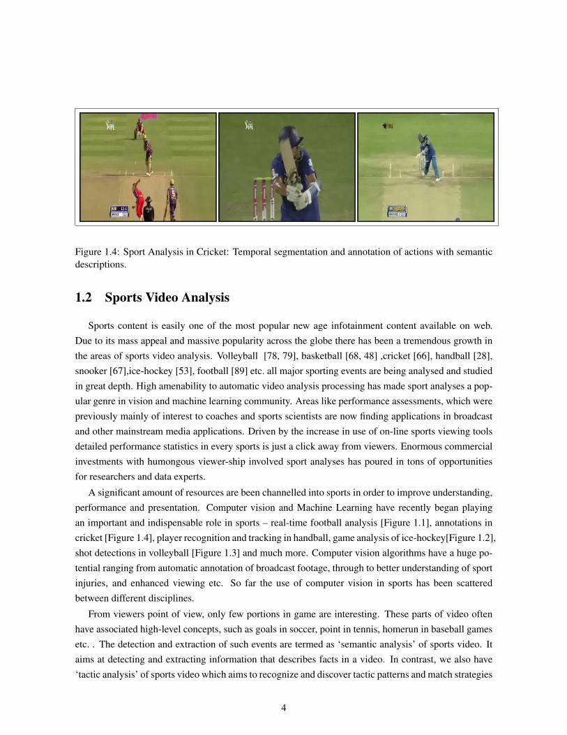
Figure 1.4: Sport Analysis in Cricket: Temporal segmentation and annotation of actions with semanticdescriptions.
1.2 Sports Video Analysis
Sports content is easily one of the most popular new age infotainment content available on web.Due to its mass appeal and massive popularity across the globe there has been a tremendous growth inthe areas of sports video analysis. Volleyball [78, 79], basketball [68, 48] ,cricket [66], handball [28],snooker [67],ice-hockey [53], football [89] etc. all major sporting events are being analysed and studiedin great depth. High amenability to automatic video analysis processing has made sport analyses a pop-ular genre in vision and machine learning community. Areas like performance assessments, which werepreviously mainly of interest to coaches and sports scientists are now finding applications in broadcastand other mainstream media applications. Driven by the increase in use of on-line sports viewing toolsdetailed performance statistics in every sports is just a click away from viewers. Enormous commercialinvestments with humongous viewer-ship involved sport analyses has poured in tons of opportunitiesfor researchers and data experts.
A significant amount of resources are been channelled into sports in order to improve understanding,performance and presentation. Computer vision and Machine Learning have recently began playingan important and indispensable role in sports – real-time football analysis [Figure 1.1], annotations incricket [Figure 1.4], player recognition and tracking in handball, game analysis of ice-hockey[Figure 1.2],shot detections in volleyball [Figure 1.3] and much more. Computer vision algorithms have a huge po-tential ranging from automatic annotation of broadcast footage, through to better understanding of sportinjuries, and enhanced viewing etc. So far the use of computer vision in sports has been scatteredbetween different disciplines.
From viewers point of view, only few portions in game are interesting. These parts of video oftenhave associated high-level concepts, such as goals in soccer, point in tennis, homerun in baseball gamesetc. . The detection and extraction of such events are termed as ‘semantic analysis’ of sports video. Itaims at detecting and extracting information that describes facts in a video. In contrast, we also have‘tactic analysis’ of sports video which aims to recognize and discover tactic patterns and match strategies
4

Figure 1.5: For a test video, the description predicted using our approach is dense and human-like.Above figure demonstrates our approach – a) Player Identification b) Verb Phrase Prediction c) Descrip-tion Generation
in sport videos. This kind of analysis is more focused on coaches and team staff. Computer vision andmachine learning in sports is gradually attracting the attention of large sports associations. Baseballteam ‘Boston Red Sox’ and football club ‘AC Milan’ were among the first few organizations that startedto apply such methodologies for sports analysis. Appropriate use of large amounts of video and otherdata available to sports organizations led to growth of this field. Application of such analysis couldlead to better overall team performance by analysing player behaviors in varied situations, determiningtheir individual impact, revealing the opponent’s tactics and pointing possible weaknesses in play etc.. While the use of advance machine learning, statistics and data mining in decision making is certainlyan improvement over present day semi-automated works but it comes with its own set of challenges andinhibitions. We in our present work focus our attention to understand the game of lawn tennis usingvision based approaches and generate a text ‘commentary’ that best describes the input scene.
1.3 Contributions
We propose an approach which explicitly splits the problem of analysis and understanding lawn ten-nis videos into first ‘action localization’ for player identification followed by ‘verb phrase recognition’for fine grained action classification. A retrieval based approach is thereafter used for final descriptiongeneration. To this end we make following notable contributions:
5

(i) New Dataset: release of a new dataset comprising of over 1000 lawn tennis game and com-mentary aligned videos for public consumption 1. The dataset even comprises of over 400K unalignedcommentary text lines.
(ii) Content Analysis – Player and Court Recognition: use of domain information for action lo-calization and player identification.
(iii) Fine grained action recognition: use of action trajectories for recognizing lawn tennis actionsand representing them with ‘verb phrases’. Our main contributions in this direction are – (a) joint modelto assign video frames into appropriate phrase bins under weak label supervision. (b) probabilistic labelconsistent dictionary learning for sparse modelling and classification.
(iv) Commentary Generation for lawn tennis: use of action phrases for fine grained retrievalwhich assists in creation of florid and verbose commentary text.
We demonstrate that in a domain restrictive setting, limited number of labelled video data is sufficientenough to generate rich descriptions for a new input video. We exploit the untapped potential of group ofpre-trained weak-classifiers and leverage the hidden information of parallel (but related) text to producehuman like descriptions for video inputs.
1.4 Thesis Outline
In our present work, we address the problem of analysing and understanding the contents of an inputlawn tennis video. Chapter 2 introduces the technical background needed for the later sections of thethesis. We begin by formally defining our problem statement in Chapter 3 and introduce a new ‘lawntennis’ dataset. The new dataset has been publicly released for the community. Chapter 4 deals withidentification and localization of active action zones (players), Figure 1.5(a), in the video which actlike a precursor for fine grained action recognition in subsequent chapters. Chapter 5 describes a novel‘verb phrase’ recognition module, Figure 1.5(b). Action verb phrases thus identified are used for finaldescription generation using a retrieval based approach, Figure 1.5(c), in Chapter 6. Chapter 6 also dealsin comparisons with other present state of art methods and demonstrates the effectiveness of our methodover others. We conclude with a short discussion and future directions of our work in Chapter 7
1http://cvit.iiit.ac.in/research/projects/cvit-projects/fine-grained-descriptions-for-domain-specific-videos
6

Chapter 2
Background
In this chapter, we briefly discuss the machine learning, vision and text analysis tools which havebeen used in the thesis. In Section 2.1, we look at the popular linear as well as non-linear featureextraction strategies used for most of the upcoming tasks. Section 2.2, describes various classificationtechniques used for both phrase detections and player identification. The penultimate section describesthe optimization techniques to compute the best commentary text for an input video clip. We end thechapter by describing evaluation techniques used for both quantitative and qualitative analysis.
2.1 Feature Extraction
Feature extraction begins from an initial set of measured data and builds derived values (features)intended to be informative and non-redundant, facilitating the learning and generalization, and in somecases leading to better human interpretations. In (majority of) cases it is related to dimensionality re-duction and involves reducing the amount of resources required to describe a large set of data. Featureextraction is a general term of constructing combinations of the variables to create a succinct represen-tation and to get around the problems of large memory and power requirements while still describingthe data with sufficient accuracy. The extracted features are expected to contain the relevant informa-tion from the input data, so that the desired task can be performed by using this reduced representationinstead of the complete initial data.
2.1.1 HOG - Histograms of Oriented Gradients
Detecting humans in tennis videos is a challenging task owing to the variability in appearances andposes. We need a robust feature set that allows the human form to be discriminated cleanly, even incluttered backgrounds under difficult illumination. Histogram of oriented gradients HOG is a featuredescriptor [11] used to detect objects in computer vision and image processing. The HOG descriptortechnique counts occurrences of gradient orientation in localized portions of an image - detection win-dow, or region of interest. The HOG descriptors are reminiscent of edge orientation histograms SIFT
7

Figure 2.1: Visualization of HOG descriptors: (a) Down Player (b)Up Player (c) No Player
descriptors and shape contexts, but they are computed on a dense grid of uniformly spaced cells andthey use overlapping local contrast normalizations for improved performance.
HOG divides the input image into square cells of size ‘cellSize’, fitting as many cells as possible,filling the image domain from the upper-left corner down to the right one. For each row and column,the last cell is at least half contained in the image. Then the image gradient is computed by usingcentral difference (for colour image the channel with the largest gradient at that pixel is used). Thegradient is assigned to one of 2×numOrientations orientation in the range [0, 2π). Contributions arethen accumulated by using bilinear interpolation to four neigbhour cells, as in Scale Invariant FeatureTransform SIFT. This results in an histogram hd (of dimension 2 × numOrientations) of directedorientations. It accounts for the direction as well as the orientation of the gradient. A second histogramhu of undirected orientations of half the size is obtained by folding hd into two.
Let a block of cell be a 2×2 sub-array of cells. Let the norm of a block be the l2 norm of the stackingof the respective unoriented histogram. Given a HOG cell, four normalisation factors are then obtainedas the inverse of the norm of the four blocks that contain the cell. Each histogram hd is copied four times,normalised using the four different normalisation factors, the four vectors are stacked, saturated at 0.2,and finally stored as the descriptor of the cell. This results in a numOrientations× 4 dimensional celldescriptor. Blocks are visited from left to right and top to bottom when forming the final descriptor.
2.1.2 CEDD - Color and Edge Directivity Descriptor
This feature is called ‘Color and Edge Directivity Descriptor’ and incorporates color and texture in-formation in a histogram. CEDD size is limited to 54 bytes per image, rendering this descriptor suitablefor use in large image databases. One of the most important attribute of the CEDD is the low computa-tional power needed for its extraction.
To make detection resilient to lighting, occlusion and direction our framework extracts monocularcues, viz. color and texture features, from each candidate object and stores in the form of histogram-Color and Edge Directivity Descriptor (CEDD) [6]. The size of histogram is 144 bins with each binrepresented by 3 bits (144 × 3 = 432bits). The histogram is divided into 6 regions, each determinedby the extracted texture information. Each region is further divided into 24 individual sub regions,
8

Figure 2.2: CEDD Histogram: Each Image Block feeds successively all the units. Color unit extractscolor information and Texture unit extracts texture information. The CEDD histogram is constitutedby 6 regions, determined by the Texture Unit. Each region is constituted by 24 individual regions,emanating from the Color Unit.
with each sub region containing color information 6 × 24 = 144. The HSV color channel is providedas input to fuzzy system to obtain color information. The texture information is composed of edgescharacterized as vertical, horizontal, 45o, 135o and non-directional, more details in [6]. This histogramis used as feature vector to describe the candidate object (player candidate regions in present case) andprovided as input to the learning framework, figure 2.2.
2.1.3 Dense Trajectories
In our present work we employ dense trajectories for action recognition [80].The trajectories areobtained by tracking densely sampled points using optical flow fields. The number of tracked pointscan be scaled up easily, as dense flow fields are already computed. Furthermore, global smoothnessconstraints are imposed among the points in dense optical flow fields, which results in more robusttrajectories than tracking or matching points separately. Dense trajectories [80, 81] are extracted formultiple spatial scales, figure 2.3. Feature points are sampled on a grid spaced by W pixels and trackedin each scale separately. Each point in a frame is tracked to the next frame by median filtering in a denseoptical flow field. Once the dense optical flow field is computed, points can be tracked very denselywithout additional cost. Points of subsequent frames are concatenated to form a trajectory. The lengthof a trajectory is limited to L frames to avoid problem of drift. As soon as a trajectory exceeds L, it isremoved from the tracking process. The shape of a trajectory encodes local motion patterns and thusassists in identifying actions.
Motion is the most informative cue for action recognition. It can be due to the action of interest,but also be caused by background or the camera motion. This is inevitable when dealing with realisticactions in uncontrolled settings. To overcome the problem of camera motion, [80] introduced a localdescriptor that focuses on foreground motion. The descriptor extends the motion coding scheme basedon motion boundaries developed in the context of human detection to dense trajectories. Moreover, ingame of ‘lawn tennis’ the camera motion is negligible after the onset of ‘serve’.
9

Figure 2.3: Dense Trajectories: Feature points are sampled densely for multiple spatial scales andtracking is performed in the corresponding spatial scale over L frames. Trajectory descriptors are basedon its shape represented by relative point coordinates as well as appearance and motion information overa local neighborhood of N ×N pixels along the trajectory. The trajectory neighborhood is divided intoa spatio-temporal grid of size nσ × nσ × nτ
The motion information in dense trajectories are included by computing descriptors within a space-time volume around the trajectory. The size of the volume is N × N pixels and L frames. To embedstructure information in the representation, the volume is subdivided into a spatio-temporal grid of size
For each trajectory descriptors comprise of Trajetory, HOG (Histogram of Oriented gradients), HOF
(histograms of optical flow) and MBH (motion boundary histogram). HOG captures static appearanceinformation and HOF, MBH measure motion information based on optical flow. The final dimensionof descriptors are 30 for Trajectory, 96 for HOG, 108 for HOF and 192 for MBH (quantizes derivativesinto horizontal and vertical component - MBHx and MBHy). For both HOF and MBH descriptors, thedense optical flow that is already computed to extract dense trajectories is reused. This makes featurecomputation process very efficient.
2.1.4 Text Features
Text Analysis is a one of the major application field for machine learning algorithms. Most of themachine learning algorithms expect numerical feature vectors with a fixed size rather than the raw textdocuments with variable length. So an essential task to generate such features is core of text processing.Vectorization is the term of the general process of turning a collection of text documents into numericalfeature vectors. This strategy comprising of tokenization, counting and normalization is called the Bagof Words or ‘Bag of n-grams’ representation in text domain. Documents (in our case commentaries andphrases) are described by word occurrences while completely ignoring the relative position informationof the words in the document. Tokenizing refers to giving an integer id for each possible token, for in-stance by using white-spaces and punctuation as token separators. Counting refers to frequency countof the occurrences of tokens in each document. Normalizing and weighting with diminishing impor-tance tokens that occur in the majority of samples and documents is key for text feature computation.
10

In a large text corpus, frequently occurring words (e.g. ‘the’, ‘a’, ‘is’ in English) hence carry verylittle meaningful information about the actual contents of the document. If we were to feed the directcount data directly to a classifier those very frequent terms would shadow the frequencies of rarer yetmore interesting terms. In order to re-weight the count features into floating point values suitable forusage by a classifier it is very common to use the TFIDF transform. Tf means term-frequency whileTFIDF means term-frequency times inverse document-frequency. This was originally a term weightingscheme developed for information retrieval (as a ranking function for search engines results), that hasalso found good use in document classification and clustering.
The term frequency is the term count within a document divided by the number of words in thatdocument ):
tf(t, d) =count(t), t ∈ d
|d|(Term frequency of term t, document d)
A term’s document frequency is the count of documents containing that term divided by the totalnumber of documents (probability of seeing t in a document):
df(t,N) =|{di : t ∈ di, i = 1..N}|
N(Document frequency of t in N documents)
In order to attenuate the TFIDF scores for terms with high document frequencies, we need the doc-ument frequency in the denominator:
tfidf(t, d,N) =tf(t, d)
df(t,N)(First approximation to TFIDF)
This formula is meaningful but gives a poor term score because the document frequency tends toengulf the term frequency in the numerator so we take the log of the denominator first.
tfidf(t, d,N) = tf(t, d)× log(1
df(t,N)) (TFIDF with attenuated document frequency)
To prevent division by 0 errors when a term does not exist in a corpus (e.g., df(t,N) = 0 whenwe pass unknown term(s) t), we add 1 to the denominator. This is similar to additive smoothing andpretends that there is an imaginary document with every unknown word. To keep document frequenciesin [0..1], we can to bump the document count, N , as well.
df(t,N) =|{di : t ∈ di, i = 1..N}|+ 1
N + 1(df with smoothing)
2.2 Classification
The term ‘classification’ in machine learning is the problem of identifying the category (or class) towhich a new observation belongs, on the basis of a training set of data containing observations whose
11

category membership is known. It is considered an instance of supervised learning, i.e. learning wherea training set of correctly identified observations is available. The individual observations are convertedinto a set feature vectors and thereafter classified into respective category using pre-trained models. Analgorithm that implements classification is known as a classifier. Its a mathematical function that mapsinput data to a category.
2.2.1 SVM - Support Vector Machines
Given a setK of training samples from two lineally separable classes P and N: {(xk, yk), k = 1, · · · ,K},where yk ∈ {1,−1} are class labels. We find a hyper-plane in terms of w and b, that linearly separatesthe two classes. For a decision hyper-plane xTw + b = 0 to separate the two classes P (xi, 1) and N(xi,−1), it should satisfy
yi(xTi w + b) ≥ 0
for both xi ∈ P and xi ∈ N . Among all such planes satisfying this condition, we find the optimal onethat separates the two classes with the maximal margin (the distance between the decision plane and theclosest sample points).
The optimal plane should be in the middle of the two classes, so that the distance from the plane tothe closest point on either side is the same. We define two additional planesH+ andH− that are parallelto H0 and go through the point closest to the plane on either side:
xTw + b = 1, and xTw + b = −1
All points xi ∈ P on the positive side satisfy xTi w + b ≥ 1, yi = 1 and all points xi ∈ N on thenegative side satisfy xTi w + b ≤ −1, yi = −1. These can be combined into one inequality:
yi(xTi w + b) ≥ 1, (i = 1, · · · ,m)
The equality holds for those points on the planes H+ or H−. Such points are called support vectors, forwhich xTi w + b = yi i.e., the following holds for all support vectors:
b = yi − xTi w = yi −m∑j=1
αjyj(xTi xj)
Moreover, the distances from the origin to the three planes H−, H0 and H+ are, respectively, |b −1|/||w||, |b|/||w||, and |b + 1|/||w||, and the distances between planes H− and H+ is 2/||w||, whichis to be maximized. Now the problem of finding the optimal decision plane in terms of w and b can beformulated as:
minimize1
2wTw =
1
2||w||2 (objective function)
subject to yi(xTi w + b) ≥ 1, or 1− yi(xTi w + b) ≤ 0, (i = 1, · · · ,m)
12

This QP problem is solved by Lagrange multipliers method to minimize
Lp(w, b, α) =1
2||w||2 +
m∑i=1
αi(1− yi(xTi w + b))
with respect to w, b and the Lagrange coefficients αi ≥ 0 (i = 1, · · · , αm). We let
∂
∂WLp(w, b) = 0,
∂
∂bLp(w, b) = 0
These leads, respectively, to
w =m∑j=1
αjyjxj , andm∑i=1
αiyi = 0
Substituting these two equations back into the expression of L(w, b), we get the dual problem (withrespect to αi) of the above primal problem:
maximize Ld(α) =
m∑i=1
αi −1
2
m∑i=1
m∑j=1
αiαjyiyjxTi ,xj
subject to αi ≥ 0,
m∑i=1
αiyi = 0
Solving this dual problem (an easier problem than the primal one), we get αi, from which w of theoptimal plane can be found. Those points xi on either of the two planes H+ and H− (for which theequality yi(wTxi + b) = 1 holds) are called support vectors and they correspond to positive Lagrangemultipliers αi > 0. The training depends only on the support vectors, while all other samples awayfrom the planes H+ and H− are not important.
For a support vector xi (on the H− or H+ plane), the constrained condition is yi(xTi w + b
)=
1 , (i ∈ sv). Here, sv is a set of all indices of support vectors xi (corresponding to αi > 0). Substituting
w =
m∑j=1
αjyjxj =∑j∈sv
αjyjxj
we getyi(∑j∈sv
αjyjxTi xj + b) = 1
For the optimal weight vector w and optimal b, we have:
||w||2 = wTw =∑i∈sv
αiyixTi
∑j∈sv
αjyjxj =∑i∈sv
αiyi∑j∈sv
αjyjxTi xj
=∑i∈sv
αi(1− yib) =∑i∈sv
αi − b∑i∈sv
αiyi
=∑i∈sv
αi
13

The last equality is due to∑m
i=1 αiyi = 0 shown above. The distance between the two margin planesH+ and H− is 2/||w||, and the margin, the distance between H+ (or H−) and the optimal decisionplane H0, is
1
||w||=
(∑i∈sv
αi
)−1/2
2.2.1.1 Kernel Mapping: Non-Linear Case
The algorithm above converges only for linearly separable data. If the data set is not linearly separa-ble, we can map the samples x into a feature space of higher dimensions:
x −→ φ(x)
in which the classes can be linearly separated. The decision function in the new space becomes:
f(x) = φ(x)Tw + b =m∑j=1
αjyj(φ(x)Tφ(xj)) + b
where w =∑m
j=1 αjyjφ(xj) and b are the parameters of the decision plane in the new space. As thevectors xi appear only in inner products in both the decision function and the learning law, the mappingfunction φ(x) does not need to be explicitly specified. Instead, all we need is the inner product of thevectors in the new space. The function φ(x) is a kernel-induced implicit mapping. A kernel is a functionthat takes two vectors xi and xj as arguments and returns the value of the inner product of their imagesφ(xi) and φ(xj):
K(x1,x2) = φ(x1)Tφ(x2)
As only the inner product of the two vectors in the new space is returned, the dimensionality of the newspace is not important. The learning algorithm in the kernel space can be obtained by replacing all innerproducts in the learning algorithm in the original space with the kernels:
f(x) = φ(x)Tw + b =
m∑j=1
αjyjK(x,xj) + b
The parameter b can be found from any support vectors xi:
b = yi − φ(xi)Tw = yi −
m∑j=1
αjyj(φ(xi)Tφ(xj)) = yi −
m∑j=1
αjyjK(xi,xj)
2.2.2 SSVM - Structured Support Vector Machines
Structured SVM is a Support Vector Machine (SVM) learning algorithm for predicting multivariate orstructured outputs. It performs supervised learning by approximating a mapping using labelled trainingsamples. Unlike the regular SVMs which consider only univariate predictions like in classification andregression, SSVM can predict complex objects like trees, sequences or sets.
14

In the SSVM model, the initial learning model parameters are set and the pattern-label pairs are readwith specific functions. The user defined special constraints are then initialised and then the learningmodel is initialised. After that, a cache of combined feature vectors is created and then the learningprocess begins. The learning process repeatedly iterates over all the examples. For each example,the label associated with most violated constraint for the pattern is found. Then, the feature vectordescribing the relationship between the pattern and the label is computed and the loss is also computedwith loss function. The program determines from feature vector and loss whether the constraint isviolated enough to add it to the model. The program moves on to the next example. At various times(which depend on options set) the program retrains whereupon the iteration results are displayed. In theevent that no constraints were added in iteration, the algorithm either lowers its tolerance or, if minimumtolerance has been reached, ends the learning process.
2.2.3 Nearest Neighbors
Nearest neighbors are one of the most classifiers, possibly because it does not involve any training.This technique simply consists of storing all the labeled training examples and given a test images, thelabel of closest training sample(or majority label of k-neighbors) is assigned to the test image. Nearestneighbors can be easily kernelized or coupled with metric learning. For classification techniques suchas LDA or linear SVM, only a single weight vector needs to be stored per class(in a one-vs-rest setting),however, a nearest neighbor classification strategy typically consists of storing all the training samples.This is one of the major demerits of nearest neighbors.
2.3 Graphical Models - Optimization
A graphical model (in probability theory, statisticsparticularly Bayesian statisticsand machine learn-ing) is a probabilistic model for which a graph expresses the conditional dependence structure betweenrandom variables. PGMs use a graph-based representation as the foundation for encoding a completedistribution over a multi-dimensional space and a graph that is a compact or factorized representation ofa set of independences that hold in the specific distribution.
2.3.1 MRF - Markov Random Fields
A Markov Random Field (MRF) is a graphical model of a joint probability distributions that encodespatial dependencies. It consists of an undirected graph G = (N,E) in which the nodes N representrandom variables. Let XS be the set of random variables associated with the set of nodes S. Then, theedges E encode conditional independence relationships via the following rule: given disjoint subsetsof nodes A, B, and C, is conditionally independent of given if there is no path from any node in A toany node in B that doesn’t pass through a node of C. The neighbour set Nn of a node n is defined tobe the set of nodes that are connected to n via edges in the graph. Given its neighbour set, a node n is
15
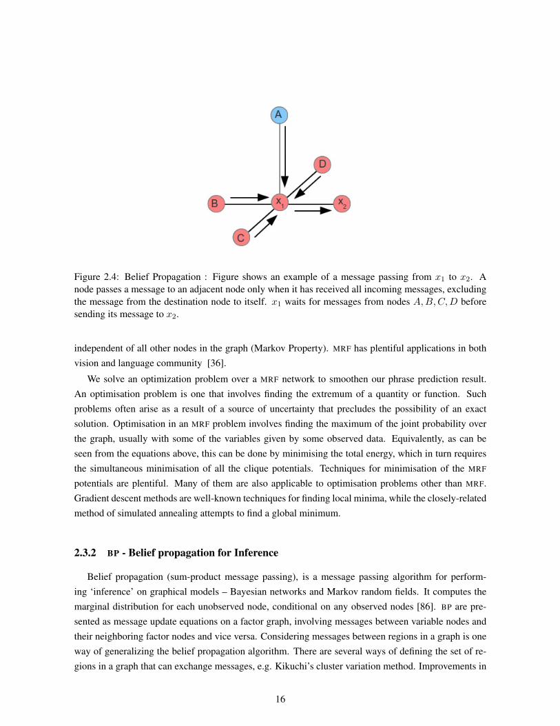
Figure 2.4: Belief Propagation : Figure shows an example of a message passing from x1 to x2. Anode passes a message to an adjacent node only when it has received all incoming messages, excludingthe message from the destination node to itself. x1 waits for messages from nodes A,B,C,D beforesending its message to x2.
independent of all other nodes in the graph (Markov Property). MRF has plentiful applications in bothvision and language community [36].
We solve an optimization problem over a MRF network to smoothen our phrase prediction result.An optimisation problem is one that involves finding the extremum of a quantity or function. Suchproblems often arise as a result of a source of uncertainty that precludes the possibility of an exactsolution. Optimisation in an MRF problem involves finding the maximum of the joint probability overthe graph, usually with some of the variables given by some observed data. Equivalently, as can beseen from the equations above, this can be done by minimising the total energy, which in turn requiresthe simultaneous minimisation of all the clique potentials. Techniques for minimisation of the MRF
potentials are plentiful. Many of them are also applicable to optimisation problems other than MRF.Gradient descent methods are well-known techniques for finding local minima, while the closely-relatedmethod of simulated annealing attempts to find a global minimum.
2.3.2 BP - Belief propagation for Inference
Belief propagation (sum-product message passing), is a message passing algorithm for perform-ing ‘inference’ on graphical models – Bayesian networks and Markov random fields. It computes themarginal distribution for each unobserved node, conditional on any observed nodes [86]. BP are pre-sented as message update equations on a factor graph, involving messages between variable nodes andtheir neighboring factor nodes and vice versa. Considering messages between regions in a graph is oneway of generalizing the belief propagation algorithm. There are several ways of defining the set of re-gions in a graph that can exchange messages, e.g. Kikuchi’s cluster variation method. Improvements in
16

the performance of belief propagation algorithms are achievable by breaking the replicas symmetry inthe distributions of the fields (messages).
The original belief propagation algorithm was proposed by Pearl in 1988 for finding exact marginalson trees. Trees are graphs that contain no loops. It turns out the same algorithm can be applied to generalgraphs, those that contain loops, hence the ‘loopy BP’ [51]. LBP is a message passing algorithm. Anode passes a message to an adjacent node only when it has received all incoming messages, excludingthe message from the destination node to itself. The choice of using cost/penalty or probabilities isdependent on the choice of the MRF energy formulation. LBP is an iterative method. It runs for a fixednumber of iterations or terminate when the change in energy drops below a threshold.
2.4 Retrieval
Information retrieval in general is done by naively matching terms in documents with those of aquery. However, such lexical matching methods can be inaccurate. Since there are usually many waysto express a given concept (synonymy), most words have multiple meanings (polysemy) etc. the endtask doesn’t remain that simple. A robust approach should allow users to retrieve information on thebasis of a conceptual topic or meaning of a document. LSI is one such approach.
2.4.1 LSI: Latent Semantic Indexing
LSI uses linear algebra techniques to learn the conceptual correlations in text collection. It involvesconstructing a weighted term-document matrix, performing a Singular Value Decomposition on thematrix, and using the matrix to identify the concepts contained in the text Latent Semantic Indexing [60]overcomes the problems of lexical matching by using statistically derived conceptual indices instead ofindividual words for retrieval. It assumes underlying or latent structure in word usage that is partiallyobscured by variability in word choice. A truncated singular value decomposition SVD is used toestimate the structure in word usage across documents. Retrieval is then performed using the databaseof singular values and vectors obtained from the truncated SVD.
This technique projects queries and documents into a space with ‘latent’ semantic dimensions. Insuch space, a query and a document can have high cosine similarity even if they do not share anyterms - as long as their terms are semantically similar in a sense. The latent semantic space has fewerdimensions than the original space (which has as many dimensions as terms). LSI is thus a method fordimensionality reduction. Latent semantic indexing is the application of Singular Value Decompositionto a word-by-document matrix. SVD (and hence LSI) is a least-squares method. The projection into thelatent semantic space is chosen such that the representations in the original space are changed as littleas possible when measured by the sum of the squares of the differences.
Textual documents are represented as vectors in a vector space. Each position in a vector representsa term (typically a word), with the value of a position i equal to 0 if the term does not appear in the
17

document, and having a positive value otherwise. Positive values are represented as the log of the totalfrequency in that document weighted by the entropy of the term. As a result, the corpus can be lookedat as a large term-by-document (t × d) matrix X , with each position xij corresponding to the presenceor absence of a term (a row i) in a document (a column j). This matrix is typically very sparse, as mostdocuments contain only a small percentage of the total number of terms seen in the full collection ofdocuments.
The SVD of the t×dmatrix, X , is the product of: TSDT , where T andD are the matrices of the leftand right singular vectors and S is the diagonal matrix of singular values. The diagonal elements of Sare ordered by magnitude, and therefore these matrices can be simplified by setting the smallest k valuesin S to zero. The columns of T andD that correspond to the values of S that were set to zero are deleted.The new product of these simplified three matrices is a matrix X that is an approximation of the term-by-document matrix. This new matrix represents the original relationships as a set of orthogonal factors.When used for retrieval, a query is represented in the same new small space that the document collectionis represented in. This is done by multiplying the transpose of the term vector of the query with matricesT and S−1. Once the query is represented this way, the distance between the query and documents canbe computed using the cosine metric, which represents a numerical similarity measurement betweendocuments. LSI returns the distance between the query and all documents in the collection. Thosedocuments that have higher cosine distance value than some cutoff point are returned as relevant to thequery.
2.5 Evaluation Measures
This section describes various terms/keywords used to measure the effectiveness of our methods.It talks about importance of ‘robust’ evaluations schemes and justifies the harnessing of well knownevaluations techniques for our experiments.
2.5.1 Classification Accuracy
We use classification accuracy for quantifying performance for the phrase recognition tasks. Fordefining classification accuracy, we first define the following quantities
• True Positive(tp):number of correctly classified positive samples.
• True Positive(tn):number of correctly classified negative samples.
• False Positive(fp):number of positive samples misclassified as belonging to the negative class.
• False Negative(fn):number of negative samples misclassified as belonging to the positive class.
Accuracy is defined as
Accuracy =tp+ tn
tp+ tn+ fp+ fn(2.1)
18

2.5.2 BLUE scores
Human evaluations of machine translation are extensive but expensive. Human evaluations can takemonths to finish and involve human labor that can not be reused. BLEU [55] is a method of automaticmachine translation evaluation that is quick, inexpensive, and language-independent, that correlateshighly with human evaluation, and that has little marginal cost per run.
It is a score for evaluating the quality of text which has been generated by any underlying algorithm.Quality is considered to be the correspondence between a machines output and that of a human: ‘thecloser a machine translation is to a professional human translation, the better it is’ – this is the centralidea behind BLEU. Scores are computed for individual sentences comparing them with a set of goodquality reference sentences (ground truths). Scores are then averaged over the whole corpus to reach anestimate of the overall quality of system. Intelligibility or grammatical correctness are not taken intoaccount. BLEU output is a number between 0 and 1. This value indicates how similar the candidate andreference texts are, with values closer to 1 representing more similar texts. BLEU correlates well withhuman judgement, and remains a benchmark for the assessment of many evaluation metric [55]. BLEU
cannot in its present form deal with languages lacking word boundaries.
2.5.3 Human Evaluation
There are several venues where development of machine algorithms can benefit from human involve-ment. Humans can be involved in the task of collecting, labelling and evaluating data. Especially withthe increasing popularity of tools like LabelMe [62] and Amazon Mechanical Turk [38], one finds itvery easy to involve human ‘experts’ in large scale studies. From labelling task in vision to machinetranslations in NLP, micro-task markets, such as Amazon’s Mechanical Turk, offer a potential paradigmfor engaging a large number of users for low time and monetary costs.
Experiments have shown high agreement between Mechanical Turk non-expert annotations and ex-isting gold standard labels provided by expert labels [69]. Using non-expert labels for training machinelearning algorithms can be as effective as using gold standard annotations from experts. Many largelabelling tasks can be effectively designed and carried out in this method at a fraction of the usual ex-pense. The need for efficient, reliable human evaluation of text output has led to the creation of severaljudgement tasks [14]. Evaluations investigating the quality of text output often elicit absolute qualityjudgements such as adequacy or fluency ratings. Several problems are encountered with this approach– annotators have difficulty agreeing on what factors constitute ‘good’ or ‘bad’ quality and are oftenunable to reproduce their own absolute scores. Relative judgement tasks such as ranking address theseproblems by eliminating notions of objective ‘good’ or ‘bad’ of translations in favor of simpler com-parisons. While these tasks show greater agreement between judges, ranking can prove difficult andconfusing when translation hypotheses are nearly identical or contain
Since we did not have control over evaluators involved in AMT, we in our present work use inhouse developed human evaluation schema and use ‘experts’ for evaluations. ‘Experts’ in our case
19

comprise of people with decent lawn-tennis exposure. Experts were asked to give relative scores togenerated descriptions and the final score was obtained by averaging the scores obtained over top fiveretrieval. Utmost care was taken while deciding the experts evaluators involved and we believe this hasstrengthened our evaluations.
20

Chapter 3
Problem Statement and Dataset
We make an attempt towards the goal of creating ‘richer and human-like descriptions’ by focusing ona domain specific setting – lawn tennis videos. For such videos, we aim to predict detailed (commentary-like) descriptions rather than small captions. Figure 3.1 depicts the problem of interest and an exampleresult of our method. It even depicts the difference between a caption and a description. Rich descriptiongeneration demands deep understanding of visual content and their associations with natural text. Thismakes our problem challenging.
3.1 Introduction
The majority of previous work in multimedia recognition has focused on image labeling with a fixedset of visual categories [85, 20]. While closed vocabularies constitute a convenient modeling assump-tion, they are vastly restrictive when compared to the enormous amount of variability that a human cancompose. Other approaches that focus on generating much more dense image descriptions [40, 19]often rely on hard-coded visual concepts and sentence templates, which imposes limits on their vari-ety. Number of approaches have even posed the task as a retrieval problem, and transfer the most most
Figure 3.1: For a test video, the caption generated using an approximation of a state-of- the-artmethod [34], and the description predicted using our approach. Unlike recent methods that focus onshort and generic captions, we aim at detailed and specific descriptions.
21

Figure 3.2: Trend illustrating saturation of word-level trigram, bigram and unigram counts in domainspecific settings. Emphasized(*) labels indicate corpus of unrestricted tennis text (blogs/news) andremaining labels indicate tennis commentary corpus. Bigram* and Trigram* frequencies are scaleddown by a factor of 10 to show the comparison.
compatible annotation in the training set to a test image [29, 19, 70, 54] or where training annotationsare fragmented and stitched together [41, 44]. Several other image caption generating approaches arebased on fixed templates [24, 40, 19, 84] or generative grammars [85, 49]. Much more recent works usecombination of combination of Convolutional Neural Networks (CNNs) and Recurrent Neural Networksto generate image descriptions [34, 47, 76, 37, 16].
One of the earliest works in tennis video analytics [72, 50] focuses on detecting court area and play-ers in significant frames. The relative positions of both the players with respective to court lines and netare used to determine action types. Using special set-ups to detect people, ball, court lines with utmostprecision [56] have been explored by many. Use of audiovisual and textual cues [33] to summarise thegame by set of static representative frames (shot boundaries) has also received considerable attention inpast. None of these works have still focused on creation of ‘text based’ commentaries for lawn-tennis inrealistic settings. Although soccer ‘commentary’ generation has been explored in past by few [77, 73]but the methods described by them are not generic and can not be extended for our case. While Roccouses simulation to track players (robots) and ball, Mike uses soccer server information for same task.Rocco uses template based method to create descriptions. We are keen on generating systems like aboveand generate final output as detailed as [87]. Authors in [87] use discriminative model for action at-tribute detection and use contextual constraints to produce detailed attributes labels. They detect majoraction attributes so as to generate extremely detailed video description.
For the game of tennis, which has a pair of players hitting the ball, actions play the central role. Here,actions are not just simple verbs like ‘running’, ‘walking’, ‘jumping’ etc. as in the early days of actionrecognition but complex and compound phrases like ‘hits a forehand volley’, ‘delivers a backhandreturn’ etc. Although learning such activities add to the complexities of the task, yet they make ourdescriptions diverse and vivid. To further integrate finer details into descriptions, we consider constructs
22

Figure 3.3: Dataset contents: (a) Annotated-action dataset: short videos aligned with verb phrases. (b)Video commentary dataset: game videos aligned with commentary.
that modify the effectiveness of nouns and verbs. Though phrases like ‘hits a nice serve’ ,‘hits a goodserve’ and ‘sizzling serve’ describe similar action, ‘nice’, ‘good’ and ‘sizzling’ add to the intensity ofthat action. We develop a model that learns the effectiveness of such phrases, and builds upon these topredict florid descriptions. Empirical evidences demonstrate that our approach predicts descriptions thatmatch the videos.
Lawn tennis is a racquet sport played either individually against a single opponent (singles), orbetween two teams of two players each (doubles). We restrict our attention to singles. Videos of suchmatches have two players – one in the upper half and the other in the lower half of a video frame. Acomplete tennis match is an amalgamation of sequence of ‘tennis-sets’, each comprising of a sequence of‘tennis-games’ played with service alternating between consecutive sets. A ‘tennis-point’ is the smallestsub-division of match that begins with the start of the service and ends when a scoring criteria is met.We work at this granularity.
3.2 Motivation
We seek to analyse how focusing on a specific domain confines the output space. We compute thecount of unique (word-level) unigrams, bigrams and trigrams in tennis commentaries. Each commentarysentence in the Tennis-text corpus is processed individually using standard Natural Language ToolKit(NLTK) library, and word-level n-gram frequencies of corpus are computed. The ‘frequency’ (count)trends of unigrams, bigrams and trigrams plotted over ‘corpus size’ (number of lines in corpus) aredepicted in Figure 3.2. We compare these with the corresponding frequencies in unrestricted tennis textmined from on-line tennis news, blogs, etc. (denoted by ‘*’ in the figure). It can be observed that in caseof tennis commentary, the frequency of each n-gram saturates well within a small corpus as compared tocorresponding frequencies of unrestricted text. The frequency plots reveal that the vocabulary specificto tennis commentary is indeed small, and sentences are often very similar. Hence, in a domain specificenvironment, we can create rich descriptions even with a limited corpus size.
23

Figure 3.4: Text Corpus: Glimpse of online scraped commentary text. Each commentary line is com-prised of ‘player names’, ‘dominant shots’ and other details.
3.3 Dataset
We use broadcast video recordings for five matches from London Olympics 2012 for our experiments.The videos used are of resolution 640 × 360 at 30 fps. Each video is manually segmented into shotscorresponding to ‘tennis-points’, and is described with a textual commentary obtained from [1]. Thisgives a collection of video segments aligned with corresponding commentaries. In total, there are 710
‘tennis-points’ of average frame length 155. We refer to this collection as ‘Video-commentary’ dataset.This serves as our test dataset and is used for the final evaluation. In addition to this, we create anindependent ‘Annotated-action’ data set comprising 250 short videos (average length of 30 frames)describing player actions with verb phrases. Examples of the verb phrases include ‘serves in the middle’,‘punches a volley’, ‘rushes towards net’, etc. In total, we have 76 action phrases. We use this collectionto train our action classifiers. Figure 3.3 and 3.4 show samples from our dataset. ‘Annotated action’dataset comprises of video shots linked with corresponding action phrases. Figure 6.3 showcases someof the contents of ‘Annotated action’ dataset.
As an additional linguistic resource for creating human readable descriptions, we crawl tennis com-mentaries (with no corresponding videos). This text corpus is built using (human-written) commentaryof 2689 lawn tennis matches played between 2009-14 from [1]. A typical commentary describes theplayers names, prominent shots and the winner of the game. We refer this collection as ‘Tennis-text’.Table 3.1 summarizes the three datasets. Note that all the datasets are independent, with no overlapamong them.
Name Contents Role
Annotated-action 250 action videos and phrases Classification and Training
Video-commentary 710 game videos and commentaries. Testing
Tennis Text 435K commentary lines Dictionary Learning, Evaluation and Retrieval
Table 3.1: Dataset statistics: Our dataset is a culmination of three standalone datasets. Table describesthem in detail, along with the roles they play in the experiments.
24

Chapter 4
Action Localization
Recognition of human actions and activities is one of the most sought out topics in automatic videoanalysis. The two most relevant and related problems in this area are localization and classification ofhuman actions. Much of the learning has been successfully applied to object localization in past, wherethe mapping between an image and an object bounding box can be well captured. Extension of suchapproaches action localization in videos is much more challenging. One needs to predict the locationsof the action patterns both spatially and temporally, i.e., identifying a sequence of bounding boxes thattrack the action in video. The problem becomes intractable due to the exponentially large size of thevideo space enriched with actions. In this chapter we deal with preliminaries and explain how doesdomain restrictions eases the the task of action localization.
4.1 Introduction
While the idea of action localization is not new, it has been applied to video restricted to a staticcameras [30, 88] or videos with simple background with limited clutter [18, 45]. It is easy to applysimpler methods such as background subtraction (to localize actors) in such restricted cases which isnearly an impossible case with moving cameras. Figure 4.1 explains one such scenario. Localizingnatural actions in realistic cluttered videos has been challenging – localizing actions by training anaction-pose specific human detector [43] and use visual words [82] to discriminate actions are slow anddata dependent. We instead use ‘domain knowledge’ to generate a real time solution in our case.
Early work on action recognition [15, 31, 65] in video used sequences with prominent actions,mainly static cameras, simple backgrounds and full bodies visible, as in the KTH [9] and Weizmann[21] datasets. This enabled action classifiers to be explored with variation in the actors and actions, butwithout the added complexity of change of viewpoint, scale, lighting, partial occlusion, complex back-ground etc. Predicting the locations of the action patterns is far more demanding than classification. Inthe case of action classification, which is often the aim in action analysis, sequences with pre-definedtemporal extent are labeled as belonging to one of the action classes. However, for video search andannotation applications, action localization is far more important and acts like a precursor to classifica-
25

Figure 4.1: Camera motion makes localization a difficult task: (UP) Trajectories with no camera motion(BELOW) False trajectories due to camera motion
tion. It enables temporal sequence containing the action to be delimited and also the actor carrying outthe action to be identified, when there are multiple actors in a shot.
We take a similar approach and focus our attention on identifying active action zones. We use anapproach which splits the spatio-temporal action localization into first detecting court area and sub-sequently tracking the players. This determines the spatial localization of the action, followed by atemporal action classification of the computed trajectories, and hence detect and localize the actions intime.
4.2 Action Localization
4.2.1 Court Detection
We begin by identifying/tracking both players on the tennis court. The playing court in lawn tennishas a set of prominent straight white lines, each of which adds meaning to the game in a unique way. Wedetect these lines using the Hough transform and consider only the most prominent lines (by keepinga threshold on length). A bounding-box is created encompassing the set of identified lines, which isthen considered as foreground seed for the GrabCut algorithm [61]. This in turn returns the playingfield as shown in Figure 4.2. We tested our algorithm on the extended dataset of others tournaments
26

Figure 4.2: Court detection for various cases: Overlapping structures, lack of prominent field lines (dueto lack of contrast) and other occlusions
(random videos from youtube.com) to test the robustness of our court detection solutions. Figure 4.2showcases some of success and failure cases.
4.2.2 Player Detection
In a tennis broadcast video background is (nearly) static after the serve begins, and remains the sametill a player wins a point. Based on this, the candidate regions for players are segmented through back-ground subtraction using thresholding and connected component analysis. Each candidate foregroundregion thus obtained is represented using HOG descriptor [10]. To prune away false detections (i.e., non-player regions), multi-class SVM with RBF-kernel is employed distinguishing between ‘upper-player’,‘lower-player’ and ‘no player’ regions. Figure 4.4(b) visualizes HOG features for few examples. Asdone in the case of court detection we tested our algorithm on extended dataset of others tournaments(random videos from youtube.com). Figure 4.3 depicts few unique cases.
Figure 4.3: Player detection for various success and failure cases.
27

(a) (b) (c) (d) (e)
Figure 4.4: Retrieving player details: (a) Extracted foreground regions. (b) Visualization of HOG fea-tures for players and non-player regions. (c) Court detection. (d) Player Detection. (d) Some examplesof successful and failed player detections.
4.2.3 Player Recognition
The detected windows thus obtained are used to recognize players. In any particular tournament (andin general) players often wear similar colored jerseys and depict unique stance during game play, we usethese cues to recognize them. We perceive both color and stance information using CEDD [6] descriptor.This descriptor captures both colour and edge (for stance) information of each detected candidate playerregion. We use Tanimoto distance [6] to build our classifier. Classifier scores averaged over initial tenframes are used to recognize both the players. Figure 4.4(d) highlights the players detected in a frame,and Figure 4.4(e) shows some true and false detections.
4.3 Experiments and Results
There are two players in the game and they are typically in the top and bottom half of the videowhen they play. To process the videos, we begin by tracking both the players on the field. We beginby isolating the playing area from rest of the field using hough lines and grabCut algorithm [61]. Wecreate a bounding box encompassing the set of lines identified. Area inside this box is considered asforeground seed for grabCut algorithm which in turn returns playing field as shown in Figure 4.4(c). Weextract HOG features for each of the candidate foreground regions (identified player regions) so obtainedafter background subtraction and prune away false detections (non-player regions) by using classifierbuilt over HOG features. Thereafter the players are identified using CEDD features. Some of the true andfalse positives detections are depicted in and Figure 4.4(e).
Since major activities during game take place on each side of the net we analyse videos by dividingthem across net. In almost all tennis broadcasts net is at the center of the frame. The upper and lowervideos thus formed are analysed separately in subsequent sections. Note that the activities taking placein these two halts are correlated. We use this larger game structure when we refine the action labels
28

using MRFs. We begin by foreground extraction to identify the players in input video. This step resultsin many potential candidate regions. To prune out the false candidate regions we learn SVM classifier todifferentiate between regions that contain a player from regions that do not contain them. We train thisclassifier using hand labelled examples. Player bounding boxes (for both upper and lower players) wereidentified by randomly drawing bounding boxes across players in video frames of training set. Trainingset comprised of 2432 ‘lower player’, 2421 ‘upper player’ and 13050 ‘no players’ windows. We extractHOG features for each of these candidate bounding boxes and model it as a multi-class classificationproblem for three identified categories.
For recognition purpose we learn classifiers over CEDD features built using 2432 ‘lower players’ and2419 ‘upper players’ windows. Each window is identified by one of the eight unique player names in ourtraining set. We run our player recognition classifier over selected candidate regions generated by theprevious module and predict the player name. Since in any frame we can have only two players we usethis information to suppress left over false positives (if any) by considering only top two classifier scores.Table 4.1 summarize both court detections and player detections results. Our recognition accuracies are0.98 and 0.978 for lower and upper players respectively.
Correct # Actual #
Court 621 710
Player 746 1420
Table 4.1: Court and Player Detection: Detections on test videos each with two players on single court.In all we have 710 videos in our test dataset and hence 710 × 2 = 1420 players in all. The players thusdetected are then identified using recognition module.
29

Chapter 5
Weak Learners for Action recognition
Field of human activity recognition has grown dramatically over last few years. Much of the creditof such growth goes to usage of activity recognition in many high-impact applications such as smartsurveillance, query based video retrieval etc. With advent of new devices and technological advance-ments this growth is destined to grow even more in coming days. The field is no more restricted tolimited set of actions and is gradually moving towards more structured interpretation of complex humanactivities. We describe one such case in this chapter and use recently proposed ‘improved dense trajec-tories’ [81] for action classification. We learn fine grained action classifiers to generate ‘action phrases’.The trajectory features used for classification encode the optical flow based motion information and arerobust to fast irregular motions as well as camera motions. [80, 81]
5.1 Introduction
Action classification has been studied in a variety of settings [9, 18]. Initial attempts used the labo-ratory videos of few well defined actions. Of late, interest has been shifted to the actions captured in thenatural settings like movies [42, 17]. They have even taken help of contextual information [23, 63, 83]and movie scripts [17, 42] as means of weak supervision to describe human actions in videos. In allthese cases, the actions of interest are visually and semantically very different. Some of the recent meth-ods have also started looking into the fine grain classification of human actions. At times when there islow inter-action and high intra-action variability in human actions people have used such approaches todistinguish between subtle variations in actions [59].
Videos were annotated with natural sentences by aligning the parallel scripts available elsewhere [64].However, this was applicable only for a very limited class of videos. In recent years, there has been manysuccessful attempts that created natural language sentences for images and videos without any paralleltextual descriptions. Focus has now shifted from recognizing nouns, verbs to more complex task ofobserving actor-action-object relationships. Niveda et al. [39] generate descriptions for short videosby identifying the best SVO (subject-verb-object) triplet. They determine the likelihood of various SVO
combinations from large corpus and select best among all to generate the sentences. Sergio et al. [22]
30

Figure 5.1: Example frames depicting varied actions. Upper frames are shown at the top, and lowerframes at the bottom. Here, upper and lower frames do not correspond to same video.
extend this for out-of domain actions (not in training set) by generating brief sentences that sum up mainactivity in the video with broader verb and object coverage. Barbu et al. [4] produce rich sequential de-scriptions of video using detection based tracking and body-posture codebook to determine the subject,verb and object.
Our goal is to automatically describe video segments of tennis points in the Video-commentarydataset. We begin by learning phrase classifiers using Annotated-action dataset. Given a test video, wepredict a set of action/verb phrases individually for each frame using the features computed from itsneighbourhood. Since this sequence of labels could be noisy, these are smoothed by introducing priorsin an energy minimization framework. The identified phrases along with additional meta-data (suchas player details) are used to find the best matching description from the Tennis-text dataset. Majoractivities during any tennis game take place on each side of the net, we analyse videos by dividing themacross the net in the subsequent sections (referred as ‘upper’ and ‘lower’ video/frame). In almost alltennis broadcast videos, this net is around the center of a frame, and thus can be easily approximated.
For the game of tennis, which has a pair of players hitting the ball each other, actions are the centralcomponent. Here, actions are not simple verbs like ‘running’, ‘walking’ and ‘jumping’as in the earlydays of action recognition. Many recent methods [39] use verbs in interchangeable fashion to describeactivities in videos (‘hits a forehand return’, ‘delivers a forehand return’). In our case, such richer actionlabels are obtained by mining a large text data and learning the semantic relationships that are ableto differentiate between lesser and more frequent action words [22]. We also add finer details to ourdescriptions by placing constructs that modifies the effectiveness of nouns and verbs in our sentences.‘hits a nice serve’,‘hits a good serve’and ‘sizzling serve’etc. describe similar task yet nice, good andsizzling add to the intensity of similar action. We develop a model that learns effectiveness of phrasesand build upon these phrases to generate descriptions that are florid and verbose.
5.2 Learning Action Phrases
5.2.1 Supervised Approach
We learn phrase classifiers using ‘Annotated-action’ dataset. For representation, we use descriptorsas described in [80], and extract dense trajectory features over space-time volumes (using default pa-
31

Figure 5.2: Effect of using MRF based Temporal Smoothing. Coloured segments represent various‘action phrases’.
rameters). For each trajectory, we use Trajetory, HOG, HOF (histograms of optical flow) [7] and MBH
(motion boundary histogram) [11] descriptors. While HOG captures static appearance information, HOF
and MBH measure motion information based on optical flow. The dimensions of each of these descrip-tors are: 30 for Trajectory, 96 for HOG, 108 for HOF and 192 for MBH. For each descriptor, bag-of-words(BOW) representation is adopted (with vocabulary size 2000). We take square root of each element ina feature vector before computing the codebook (similar to RootSIFT [3]). The final representation isconcatenation of BOW histograms of all the descriptors. Using this, a 1-vs-rest SVM classifier (with RBF
kernel and χ2 distance) is learned for each phrase. In all, we have 76 verb phrases - 39 for upper and 37
for lower player. Figure 6.3 illustrates some examples of player actions.
5.2.1.1 Verb Phrase Prediction and Temporal Smoothing
Given a (test) video, we recognize verb phrase for each frame by extracting features from neighbour-ing frames using sliding window (neighbourhood of size 30 frames). Since this typically results intomultiple firings, non-maximal suppression (NMS) is applied. This removes low-scored responses thatare in the neighbourhood of responses with locally maximal confidence scores. Once we get potentialphrases for all windows along with their scores, we remove the independence assumption and smooththe predictions using an energy minimization framework. For this, a Markov Random Field (MRF) basedmodel is used which captures dependencies among nearby phrases. We add one node for each windowsequentially from left to right and connect these by edges. Each node takes a label from the set of actionphrases. The energy function for nodes ν, neighbourhood N and labels L is:
E =∑p∈ν
Dp(fp) +∑p,q∈N
Vpq(fp, fq) (5.1)
32

Figure 5.3: Semi-Supervised approach: (Input:) Given a collection of tennis videos along with linked captions,(Output:) Our approach generates annotations for constituent frames of each input video. The approach alignsvideo frames with corresponding ‘action phrases’. Window size of ‘two’ assigns similar labels to adjacent twoframes.
Here, Dp(fp) denotes unary phrase selection cost. This is set to 1 − p(lj |xp), where p(lj |xp) isthe SVM score of the phrase label lj for node xp, normalized using the Platt’s method [57]. The termVpq(fp, fq) denotes pairwise phrase cohesion cost associated with two neighbouring nodes xi and xjtaking some phrase label. For each pair of phrases, this is determined by their probability of occurringtogether in the game play, and is computed using frame-wise transition probability. In our case, sincethere are two players, and each player’s shot depends on the other player’s shot and his own previousshot, we consider four probability scores: p(liP1 , ljP1), p(liP1 , ljP2), p(liP2 , ljP2) and p(liP2 , ljP1). Here,p(liP1 , ljP2) refers to the probability of phrase li of player1 and lj of player2 occurring together duringgame play. We compute pairwise cost, 1−p, for each of the four probabilities and solve the minimizationproblem using a loopy belief propagation (BP) algorithm [35].
5.2.2 Weakly Labelled Semi-Supervised Approach
In this section we propose a that method encodes local temporal structure in tennis videos and alignsframes with appropriate find grained annotations ,i.e. ‘phrases’ that best describe the constituent videoframes. Our solution bears resemblance to method [2] that learns sequence of steps to complete certaintasks – discriminative joint clustering scheme is proposed by authors to identify prominent steps fromverbal descriptions and align them to appropriate video frames. We take a step towards weakly labelledsemi-supervised ‘action phrase’ recognition for tennis videos and suggest a unified objective function
33

Figure 5.4: The proposed approach: Every frame is associated with a corresponding tag which is acollection of similar ‘action phrases’. Both trajectory matrix (Y) and phrase-cluster matrix (H) arestacked together to compute the dictionary. The dictionary is used to generate frame level annotationsfor the input videos. We represent each group of ‘phrases’ by a cluster number.
comprising of probabilistic label consistent constraint and classification error. The proposed objectivefunction solved using KSVD yields dictionaries such that local temporal structures of videos bearingsimilar actions have similar action phrases. We use probabilistic label constrained KSVD for learningsparse dictionaries for recognition [32]. The suggested approach utilizes video descriptions at hand tolearn different varied constructs and associates them with actions features extracted from videos. Itextracts various linguistic phrases [26] from available sentences and clusters them into group of seman-tically similar [27] ‘action phrases’, for e.g. phrases like ‘huge rally’ and ‘contested rally’ are part ofone cluster and ‘backhand catches net’ and ‘Serena catches net’ belong to same cluster. The phraseclusters are thereafter used for classifying action features – similar looking actions are labelled withsimilar phrase clusters. A group of semantically similar phrases belong to same ‘phrase clusters’ andgroup of frames encoding similar actions are assigned similar phrase clusters as corresponding labels.
5.2.2.1 Phrase Extraction and Clustering
We automate the process of phrase extraction from given video descriptions using CoreNLP toolkit 1.We use ‘collapsed-coprocessed-dependencies’ [12], i.e. dependencies involving prepositions and con-juncts are collapsed to reflect direct relation between content words. Each sentence is mapped to listof nine distinct types of phrases encoding order preference information – (subject), (object), (sub-ject;verb), (object;verb), (subject;prep;object), (object;prep;object), (attribute;subject), (attribute;object)
1http://nlp.stanford.edu/software/corenlp.shtml
34

Figure 5.5: Parsed dependencies (collapsed and propagated) for an input commentary text. We onlykeep nine selected encodings and discard others to assimilate all possible phrase information in thelinked sentence.
and (verb;prep;object), Figure 5.5. We believe these nine encodings are sufficient to assimilate all pos-sible information in linked sentence. Since generated phrases are targeted to increase overall retrievalefficiency we kept player names en-tact in the extracted phrases.
The extracted phrases are clustered using hierarchical agglomerative clustering using Semantic Tex-tual Similarity (STS) measure described in [27]. In an agglomerative setting each phrase starts with itsown cluster and subsequently the pairs of text clusters are merged as one climbs up the hierarchy. Thesimilarity scores describe the degree of equivalence in the underlying semantics of paired snippets oftext (phrases). The distance metric uses a word similarity feature combining both LSA word similarityand WORDNET knowledge. The text clusters so obtained are visualized using a dendrogram as shownin Figure 5.6
5.2.2.2 Dictionary Learning for Action-Phrase Alignment: Probabilistic Label Consistent KSVD
For action representation, we extract dense trajectory features to describe actions and process themsimilar to previous sections. Given set of videos, we extract action features from both upper and lowerpart of frames (capturing actions of both upper and lower player respectively). Features are computedfrom neighbouring frames using sliding window (neighbourhood of size 30 frames with no overlap).Computed action features (from both halves) when stacked over each other represent the feature vectorof frames in sliding window. We aim to classify stacked action features depended on phrase clusterscomputed in section 5.2.2.1. A compact and discriminative dictionary is learnt for sparse coding whichis thereafter used for classification, 5.6
Let, Y be a matrix of stacked video features (from upper and lower halves) of training videos(collection of N sliding windows). A single training video is represented by consecutive columnsof Y and number of such columns equate to count of sliding windows encompassing whole video.Every column represents feature vector of frames in one sliding window, each of n dimensions, i.e.
35

Figure 5.6: Qualitative Result for phrase clustering in semi-supervised regime: (a) Dendrogram ofclusters of all generated phrases (b) Dendrogram of prominent phrases.
Y = {y1, y2 . . . yN} ∈ Rn×N . We learn a single re-constructive dictionary, D, with K items for sparserepresentation of Y :
< D,X >= arg minD,X‖ Y −DX ‖22, s.t.∀i, ‖ xi ‖0≤ T (5.2)
Here, D = {d1, d2 . . . dK} ∈ Rn×K is the learnt dictionary, X = {x1, x2 . . . xN ∈ RK×N are sparse codes of
Y and T is sparsity constraint factor (each sparse code has fewer than T items). We leverage the supervised infor-
mation (i.e. phrase labels obtained after text clustering) of feature vectors to learn a more efficient dictionary. In
order to make dictionary optimal for classification we include the classification error term in the objective function
for dictionary learning. Similar to [32] we use a linear predictive classifier f(x;W ) = Wx and learn weights,W .
Following objective function for learning a dictionary, encompasses both reconstruction and classification errors:
< D,W,X >= arg minD,W,X
‖ Y −DX ‖22 + ‖ H −WX ‖22, s.t.∀i, ‖ xi ‖0≤ T (5.3)
There is an explicit correspondence between dictionary items and the phrase labels. The term ‖ H −WX ‖22represents classification error, with W being the classifier (weights) parameters. H = {h1, h2 . . . hK} ∈ Rm×N
are the class labels of Y . A video (represented by consecutive columns of Y) can have multiple (extracted)
phrases, so we assign equal probabilities to corresponding phrases to each column of H . Number of columns
depends on number of features columns in Y for each video.
36

Figure 5.7: Illustration of semi-supervised approach: First two rows correspond to videos and the linked de-scription. The extracted phrases and assigned phrase clusters are shown in next two rows. Last row demonstratesoutput phrase clusters obtained using proposed approach (Number of such clusters depend on duration of videoinput)
A video with 90 frames will constitute (90/30)=3 columns (sliding window size: 30 frames) in matrix Y and
H; yi corresponds to stacked dense trajectory feature of 30 frames and hi represents equal probabilities of phrase
labels (all three corresponding columns in H will be identical). hi = [0, 0.33, 0.33, 0, 0.33, . . . , 0, 0] would mean
that phrase identified from linked description belong to phrase clusters 2, 3, 5 (non-zero entries in hi), Figure 5.8.
In such case we assign each phrase cluster an equal probability (1/3 = 0.33). Intuitively this would mean this
video is comprised of these three cluster labels and hence classification error should be minimized with respect to
all three. We use KSVD to find optimal solution for all parameters simultaneously. The objective function can be
re-written as:
< D,W,X >= arg minD,W,X
‖
Y
H
− D
W
X ‖22, s.t.∀i, ‖ xi ‖0≤ T (5.4)
< D,W,X >= arg minD,W,X
‖ Y ∗ −D∗X ‖22, s.t.∀i, ‖ xi ‖0≤ T (5.5)
D∗, is the final dictionary with ‘optimal’ reconstruction and classification error. The learned dictionary makes
sure that the features from same class have similar sparse codes and those from different classes have dissimilar
sparse codes; hence can be used for action classification.
Initialization: To begin with dictionary learning using KSVD, we initialize the parameters D0 and W0 similar
to [32]. We use the multivariate ridge regression, with the quadratic loss and L2 norm regularization. Parameters
used are similar to what suggested in [32].
37

Figure 5.8: Matrix structure: Considering the sliding window size of ‘n’ frames, a video with m frames(n < m) will constitute (m/n) columns in matrix Y and H; Each column of Y corresponds to the densetrajectory feature of frames in sliding window and each column of H represents equal probabilities ofphrase cluster labels detected in the input linked text (m/n adjacent columns in H are identical).
Classification: Both D and W are transformed and normalized usingdk
‖ dk ‖2and
wk‖ wk ‖2
(for every kth col-
umn) before we begin classification. For a test video, we compute sparse representation (xi) of dense trajectories
action features (yi) using modified dictionary, D :
xi = arg minxi
‖ yi − Dxi ‖22, s.t.∀i, ‖ xi ‖0≤ T (5.6)
We use the linear predictive classifier W to estimate the label j (where l ∈ Rm is the class label):
j = arg maxj
(l = Wxi) (5.7)
5.3 Experiments and Results
5.3.1 Supervised Action Learners
For classification experiments we randomly partition our annotated-action dataset into 150 training videos and
100 test videos. We repeat this process for five trials and report average classification accuracy. Labels like ‘hits
a forehand return’, ‘returns a forehand return’, ‘works a forehand return’ etc. are significantly similar in our
case (high correlation between the classes); as a result looking for exact matches could be a strict constraint. We
relax these conditions by looking for label matches which are considerably near rather than exact. Phrase pairs
38

Approach Upper LowerRelaxed 0.869 0.705
Exact 0.770 0.613
Table 5.1: Verb phrase recognition accuracy averaged over top five retrieval.
Class Upper Player Lower PlayerFreq. Acc. Freq. Acc.
waits for ball 64 0.87 44 0.64player focused 30 0.93 30 0.91audience seems enjoying 13 0.33 13 0.25serves a good one 5 0.5 7 0.33crafts a forehand return 8 0.33 8 0.53hits a backhand return 3 0.60 7 0.14
Table 5.2: Class classification accuracy for frequent phrases. Freq. refers to number of times thesephrases occur in annotated-action dataset and Acc. refers to classification accuracy.
having overlapping subtopics have high similarity values when measured by standard cosine similarity. For exact
matches the cosine similarity score is 1 while for relaxed case we consider pairs with cosine similarity score of
more than 0.50. We report our results in Table 5.1, averaged over top five retrievals for both exact and relaxed
matches. We also report average class wise accuracy of frequent classes in Table 5.2. Figure 6.3 illustrates some
actions classes for both upper and lower players. In all we have 76 verb phrases - 39 for upper and 37 for lower
player.
5.3.2 Semisupervised Action Learners
For experiments, we partition dataset into 60% train and 40% test data. The training set is used to learn dictio-
nary and other model parameters. At time of text based phrase clustering we use all available linked descriptions.
Clusters (Only Description) Aligned Clusters (Joint Model)
4,23 4,23,23,23
2,16,26,32,36,43 16,43
4,9,16,23,40 23,4,23,16,4,40,4,16,4,9
23,29,48 23,29
4,15,23,26,29,32 23,32,29,23,15
4,23 23,4,23,23,23,4,23,4,4,23,23,2,2,23,18,23,18,49
Table 5.3: Qualitative Result for assigned clusters: Clusters computed using proposed solution bind temporalinformation and depend on the length of the video.
39

Figure 5.9: Correct match v.s. Dictionary sparsity: Initial phrase clusters (computed using only linked descrip-tion) act as ground truth and are compared to clusters computed using proposed approach.
While extracting phrases from available descriptions we replace all possible words with respective synonyms de-
termined using WordNet synsets [26]. Overall we had 50 phrase clusters during text based phrase clustering –
these clusters determine groups and bin to which a descriptions would belong. Figure 5.7 summarises the steps
involved in our method. We compute action phrases and assign clusters to them as described in section 5.2.2.1.
The assigned clusters in turn act like a ground truth for comparison purpose. One should note that count of
phrases generated and phrase clusters may differ – In video 3 (Fig. 5.7), ‘quick return’ and ‘Williams return re-
turn’ fall into same clusters. We determine output of the proposed system by using learnt classifiers described in
section 5.2.2.2. Number of such assigned phrase clusters depend on the size of the (test) video, which is evident
from all examples shown in Figure 5.7.
To evaluate the temporal localization, we need to have a one-to-one mapping between the identified phrase
clusters in the video and the ground truth alignment. Owing to lack of such data we demonstrate the effectiveness
of proposed system by comparing it with only text based model. Table 5.3 illustrates subtleness involved in the
phrase alignments using a joint model. The clusters obtained using join modelling bind temporal information and
depend on the length of input video which is not the case with text based modelling which depends only on size of
description. We consider clusters computed using only descriptions as ground truth and compare them to clusters
obtained using proposed solution. Figure 5.7 illustrates the match between ground truth and computed clusters –
an overlap of one cluster is considered as a match.
40

ApproachWithout Frame Division With Frame DivisionUpper Lower Upper Lower
Relaxed 0.713 0.636 0.869 0.705
Exact 0.672 0.516 0.770 0.614
Table 5.4: Impact of harnessing domain relevant cues on verb phrase recognition accuracy.
5.4 Baselines and comparisons
Using Domain Specific cues: Compared to a naive use of phrase classifier, our verb phrase classifier performs
better by dividing the frame into upper and lower halves. Table 5.4 summarizes the effects of domain specific
cues, i.e. division across the net.
41

Chapter 6
Commentary Generation
Mere a cursory glance of a video content is sufficient for users to describe it in great depth. However, such
remarkable ability has proven to be an elusive task for present day state of art visual recognition systems and
models. We aim to mimic this unique ‘human ability’ and describe the lawn-tennis video contents using fine-
grained descriptions. The chapter describes the final stage of the proposed pipeline and demonstrates the overall
efficacy of our approach.
6.1 Introduction
With reincarnation of ‘deep learning’ and other neural network based approaches, caption generation for
multimedia content has taken central stage in both vision and language community [34]. Both video [22, 39]
and image [75, 46] annotation generation are present day active field of research – given a multimedia content
the gaol is to create most descriptive and relevant annotation. Some of these methods find most appropriate
phrases/sentence from a database by formulating the problem as a structured output prediction [75]. Another
successful paradigm has been to identify objects (nouns) and actions (verbs), and thereafter construct natural
language sentences using computational linguistic techniques. In case of images [40], objects localized using
precomputed detectors and their spatial arrangements helped in creating meaningful sentences. Videos provide
more reliable information about the verbs in those sentences. For example, one can detect “Human” and “running”
in a video clip, and then form a sentence like “A person is running towards the left”. While such sentences capture
the visual content at certain level of semantics, richer and more meaningful descriptions are required for these
techniques to be useful in diverse applications. We aim of describing the video content similar to the way a
human expert does. For example, “Serena rushes towards left and punches a backhand volley” could have been
far more apt for the same video clip. A commentary is actually more elaborate than this.
We attempt to generate descriptions (rather than captions) for broadcast videos of lawn tennis. Figure 6.1
depicts the problem of interest and an example result of our method. We also depict the difference between the
captions and descriptions for the same video. Richer descriptions demand deeper understanding of the visual
42

Figure 6.1: Distinction between captions and descriptions. We generate more descriptive sentenceswhen compared to present state of art
content. We address this by limiting our attention to a specific domain. Though these videos were captured in
natural setting for human use, they are not diverse like those harvested from youtube [22]. However, the fine
variations in the data and the granularity of the description, make the problem challenging. The actions that
we need to recognise are of finer granularity compared to the popular action recognition tasks. Richer natural
descriptions also demand the sentences to be of higher linguistic quality. We address this by exploiting a large
corpus of human commentaries crawled from a public web site [1].
6.2 Description Prediction
Let, W = {w1, w2, . . . , wn} be set of unique words present in the group of phrases along with player names,
and S = {s1, s2, . . . , sm} be the set of all the sentences in the Tennis-text corpus. Here, each sentence is a separate
and full commentary description. We formulate the task of predicting the final description as an optimization
problem of selecting the best commentary from S that covers as many words as possible. Let, xi be a variable
which is 1 if sentence si is selected, and 0 otherwise. Similarly, let aij be a variable which is 1 if sentence si
contains word wj , and 0 otherwise. A word wj is said to be covered if it is present in the selected sentence
(∑i aijxi = 1). Hence, our objective is to find a sentence that covers as many words as possible:
max∑
i∈{1,2,...,m},j∈{1,2,...,n}
aijxi, s.t.
m∑i=1
xi = 1, ∀aij , xi ∈ {0, 1} (6.1)
43

Figure 6.2: Illustration of our approach. Input sequence of videos is first translated into a set of phrases,which are then used to produce the final description.
In the above formulation, doing naıve lexical matching can be inaccurate as it would consider just the pres-
ence/absence of words, and fail to capture the overall semantics of the text. To address this, we adopt Latent
Semantic Indexing (LSI) [13], and use statistically derived conceptual indices rather than individual words. LSI
assumes an underlying structure in word usage that is partially obscured by variability in word choice. It projects
derived phrases and corpus sentences into a lower dimensional subspace, and addresses the problems of synonymy
(similar meaning words). Figure 6.2 illustrates the steps involved in our method by taking two examples. The verb
phrase prediction and smoothing steps provide a set of relevant phrases. Number of such phrases depend on the
size of the (test) video. This is evident from the second example (right), which is of longer duration and thus has
more phrases predictions. These phrases are used to select the best matching commentary from the Tennis-text
corpus. Since similar events are described by identical descriptions in text corpus, there could be instances where
the retrieved descriptions are same – first example (left) in Figure 6.2.
6.3 Experiments and Results
We use an action classifier similar to that presented in chapter 5. During test time the classifier is evaluated on
every frame by extracting features from neighbourhood of 30 frames. To encode the contextual information into
the classifier they are trained on annotated-action dataset by jittering the clip boundaries. A frame-wise transition
probability is computed from the annotated frames that constitute the videos of Annotated-action classifiers and
is used as pair wise costs to solve MRF using loopy BP implementation of [35]. Using these phrases we build
retrieval system over our corpus using both naive lexical and LSI approach.
44

Corpus # Vector # B-1 B-2 B-3 B-4
100 85 0.3789 0.2348 0.1545 0.0954
500 118 0.4279 0.2510 0.1676 0.1071
1K 126 0.4312 0.2554 0.1689 0.1084
5K 128 0.4578 0.2647 0.1785 0.1111
10K 134 0.4607 0.2754 0.1818 0.1115
30K 140 0.4601 0.2766 0.1821 0.1128
50K 144 0.4612 0.2765 0.1826 0.1136
Table 6.1: Comparison between corpus size and BLEU scores averaged over top five retrieval. B-n standsfor n-gram BLEU score. Vector size represent the dimension of tf-idf vector.
Table 6.3 (left) demonstrates the effect of variations in corpus size on BLEU scores. It can be observed that
the scores saturate soon, which validates our initial premise that in domain specific settings, rich descriptions
can be produced even with small corpus size. In Table 6.3 (right), we compare our performance with some of
the recent methods. Here we observe that caption generation based approaches [22, 34] achieve very low BLEU
score. 1 This attributes to their generic nature, and their current inability to produce detailed descriptions. On
the other hand, cross-modal retrieval approaches [58, 75] perform much better than [22, 34]. Compared to all
the competing methods, our approach consistently provides better performance. The performance improvements
increase as we move towards higher n-grams, with an improvement of around 50% over [75] for 4-gram. These
results confirm the efficacy of our approach in retrieving descriptions that match the semantics of the data much
better than cross-modal retrieval approaches.
6.4 Baseline and Comparisons
The proposed system is benchmarked against state-of-the-art methods from two streams that are popular in
predicting textual descriptions for visual data: description/caption generation and cross-modal description re-
trieval.
(1) Description generation: Since the approaches in this domain are either too generic [22, 39, 34], or designed
for images [34], we evaluate by adapting them to our setting. In both [22, 39], a template-based caption is gen-
erated by considering a triplet of form (SVO). To compare with this setting, we align the best predicted verb
phrase into a template ‘player1 − verbPhrase1 , player2 − verbPhrase2’. Since a verb phrase is a combination
of an action verb and an object, this template resembles the ‘SVO’ selection of [22, 39]. To compare with [34],
we use the publicly available pretrained model and generate captions for key frames in a video. Since this is a
generic approach, the captions generated are nearly similar, and the set of distinct captions is far less than the total
1Recall that [22, 34] work for generic videos and images, we approximate them for comparisons.
45

Figure 6.3: Success and failure cases: Example videos along with their descriptions. The ‘ticked’descriptions match with the ground truth, while the ‘crossed’ ones do not.
number of key-frames. To associate a caption with a video, we pick the one with the highest frequency. Figure,
6.4 showcases the qualitative comparisons with present state of the art methods.
(2) Cross-modal description retrieval: Cross-modal retrieval approaches [58, 75] perform retrieval by match-
ing samples from the input modality with those in the output modality (both of which are represented as feature
vectors). While comparing with [75], we consider the best performing variant of their approach; i.e., the one
that uses projected features with Euclidean distance as loss function. Note that our approach is also based on
retrieving a description; however, it makes explicit use of low-level visual and textual cues unlike cross-modal
retrieval approaches. This difference is also evident from the experimental results, where our approach is shown
to retrieve better descriptions than [58, 75].
(2.1) Extension and detailed comparison [75]:
Method [75] Vector# B-1 B-2 B-3 B-4CCA-Cosine 144 0.4299 0.2414 0.1493 0.0796
CCA-L2 144 0.4219 0.2334 0.1417 0.0747
CCA-L1 144 0.4132 0.2279 0.1356 0.0723
Table 6.2: Detailed comparison with cross-modal retrieval method of [75]. Various distance functionsare tried and final scores are reported in above table.
46

Each video VSi is represented using p-dimensional feature vector xi in space X = <p and each text (com-
mentary) TSi is represented using q-dimensional feature vector yi in space Y = <q . Our objective is to learn a
discriminant function F : X × Y −→ < that can be used to predict optimal output using input output pairs.
y∗ = argmaxy∈Y
F (x, y;w) (6.2)
We make an assumption of F = w.Ψ(x, y); i.e. F is linear function of joint feature representation Ψ(.) of
input-output pair.The task of learning w is formulated as following:
minw,ξ≥0
1
2||w||2 +
C
N
N∑i=1
ξi (6.3)
s.t. w.Ψ(xi, yi) ≥ w.Ψ(xi, y) + ∆(yi, y) − ξi∀i, yεY \{yi} where ||.||2 denotes L2norm, C > 0 controls trade
off between regularization term and loss term,ξi denotes slack variable and ∆(yi, y) is loss function.
Both Ψ(.) and ∆(.) are problem specific. Similar to [75] we define Ψ(x, y) = x ⊗ yε<r, r = p × q. Since
phrases are represented by tfidf (term frequency-inverse document frequency) vectors one of the obvious choice
of loss function would be cosine distance. As cosine distance is not a distance metric, we instead use angular
distance, ∆(yi, y) = 2Π cos−1 (cosSimilarity) as our loss function. We solve the above equation using cutting
plane algorithm [74] which requires efficient computation of the most violated constraint during each iteration.
The following equation describes most violated constraint corresponding to incorrect prediction y:
argmaxy∈Y \{yi}
∆(yi, y) + w.Ψ(xi, y)− w.Ψ(xi, yi) (6.4)
Since, w.Ψ(xi, yi) is constant with respect to y, we have
argmaxy∈Y \{yi}
∆(yi, y) + w.Ψ(xi, y) (6.5)
Under the assumption that a video and its corresponding text are two heterogeneous representation of similar
information we map each representation into maximally correlated vector subspaces using CCA. The results are
reported in Table 6.2.
6.4.1 Performance of Individual Modules
To validate the utility of our design choices, we discuss performance of various modules in this section.
(1) Verb Phrase Recognition: Compared to a straightforward use of state-of-the-art technique [80] to recognize
verbs, our verb phrase recognition module performs better by around 15%. This suggests the utility of harnessing
relevant cues (dividing a frame into two halves) while working in a domain specific environment.
(2) Smoothing Vs. No Smoothing of Verb Phrase Predictions: In practice, using MRF for smoothing phrase
predictions improved average BLEU score from 0.204 to 0.235.
(3) LSI-based Matching Vs. Lexical Matching: Employing LSI technique while matching predicted phrases
with descriptions achieves an average BLEU score of 0.235, whereas naıve lexical matching achieves 0.198.
47

Figure 6.4: Qualitative comparison of output of present state of the art methods: Youtube2Text [22] andRNN [34]. Both [22, 34] work for generic videos and images, we approximate them for comparisons.
Method B-1 B-2 B-3 B-4Guadarrama [22] 0.119 0.021 0.009 0.002
Karpathy [34] 0.135 0.009 0.001 0.001
Rasiwasia [58] 0.409 0.222 0.132 0.070
Verma [75] 0.422 0.233 0.142 0.075
This work 0.461 0.276 0.183 0.114
Table 6.3: Performance comparison with previous methods using the best performing dictionary. ‘Cor-pus#’ denotes the number of commentary lines, ‘Vocab#’ denotes the dimensionality of the textualvocabulary/dictionary and ‘B-n’ means n-gram BLEU score.
6.5 Human Evaluation
We created an online testing portal and asked twenty people with decent tennis exposure to evaluate our
annotations (commentary). Videos were presented in form fifteen sets comprising of six videos each. Every
evaluator was randomly presented (atleast) two sets and asked to rate the text on subjective scale of ‘Perfect ’,
‘Good ’, ‘OK ’, ‘Poor ’, ‘Flawed ’. Participants were asked to give scores for both structure and semantics of
commentary. We converted this on scale of 1-5 with ‘Perfect ’being 5 and ‘Flawed ’being 1 and took average over
both scores. On scale of 5 we scored 2.8 on semantics and 4.7 on structure of the generated descriptions.
48

Chapter 7
Conclusions and Future Directions
We have introduced a novel method for predicting commentary-like descriptions for lawn tennis videos. Our
approach demonstrates the utility of the simultaneous use of vision, language and machine learning techniques in
a domain specific environment to produce semantically rich and human-like descriptions. Though we demonstrate
our method on tennis videos, we believe it is fairly generic and has direct extensions to similar situations where
activities are in a limited context, the linguistic diversity is confined and the description has to be semantically
rich. Similar approaches can be developed for driver assistance systems (for human interface), entertainment
(creating narrations for classical dance performances), commentaries for wide variety of sports (e.g. baseball,
soccer) and many more. Each of these applications need domain specific tracking, recognition modules and a
corpus of examples to generate novel rich descriptions. Our method generates semantically richer descriptions,
and not just captions. This is possibly the first time such a task is being attempted, as far as we are aware
of. Previous methods [22, 39, 46, 54] were interested in annotating images and videos with words, phrases or
captions (simple sentences). Their objective has been primarily to make images and videos searchable, while our
descriptions are aimed at direct human consumption. Our method is novel in the sense that we take advantages of
two complementary approaches that match and retrieve [54, 75] and recognize and synthesize [22, 39, 40].
7.1 Applications
The proposed method is generic and can be adopted to similar situations where activities are in a limited con-
text and the linguistic diversity is confined, however the output description can be semantically rich. Applications
of our solution could range from content based retrieval to real life tennis coaching. In this section we describe
some of the explored applications of the pipeline.
7.1.1 Search and Retrieval
Following the solution in Chapter 6 each video is associated with a set of descriptive tags. We can build a
text-based search engine over these annotated scenes. We perform a standard stop-word detection before indexing
49

the scenes. Our system accepts text queries given by the user and searches through the index to retrieve the
scenes matching the query. The user could thus query for all scenes involving a particular player, or with a
certain outcome. For e.g. a user query of ‘Sharapova all forehand shots’ would result in collection of videos
where Sharapova has hit forehand shot. To retrieve the scenes most suitable to user query, we use standard vector
space models popular in text retrieval. Each annotated scene is considered as a bag-of-words of its corresponding
annotations. The query too is considered as a bag-of-words. Both the scenes and queries are assumed to be points
in a space whose dimensions are given by all unique words (sans stop words) in the annotations. The similarity
between the query and annotation is given by the cosine similarity measure.
7.1.2 Automatic match Summarization
An extension in form of automatic full-match summary is also one of the probable extension. Match sum-
maries or highlights generated by our proposed method have potential to be descriptive and less machine like.
An additional module of automated transitions detection [5, 71] in tennis videos, i.e. shot transition detection to
localize game scenes, would be sufficient to achieve such a goal. Every identified game scene passes through our
‘proposed solution’ in a time-serial manner and the descriptions thus generated summarize the match in totality.
7.1.3 Mine rare-shots
Action trajectories computed for every localized action in Chapter 5 could assist in mining rare and unique
shots from the set of inputs. A joint clustering model [8] learnt over multimedia (video) features and text features
could be designed to isolate rare and unique shots. Sparse clusters generated using co-clustering framework
correspond to rare and unique shots with action phrases linked to them.
7.2 Future directions
Future research extensions of the proposed technique would be application of present work in other video-
text pairs. There are many other video collections, figure 7.1 ,that have parallel text information that are yet to
be exploited for both annotation and retrieval, for example, (a) Smart theatrics: Narration generation for dance
dramas have huge potential of such applications. Any classical dance form narrating a story has a common story
line and plot and hence this domain restriction makes our method apt. (b) Commentary generation [25] for other
sports events like cricket, baseball etc. could be well be generalized using described procedure. (c) Cooking
Instructions [52]: A cooking recipe is one more example of restricted domain. Generally a recipe of a dish tends
to pretty similar hence the problem can be framed as two step process as in our case – generate phrases for
actions like ‘sprinkle salt’, ‘pick pan’ etc. could be generated and later used for full recipe generation. We believe
that annotation and retrieval based pipeline is a stepping stone for multimedia understanding. We showcase the
50

Figure 7.1: Future directions: (a) Smart theatrics: Narration generation for dance dramas. (b)Sports [25]: Commentary generation for various sporting events. (c) Cooking Instructions [52]: Au-tomated generation of cooking instructions.
effectiveness of leveraging parallel text for multimedia understanding and hence take a step towards what Fei-Fei
Li said ‘If we want our machines to think, we need to teach them to see and understand.’
51

Appendix A
Qualitative auxiliary
52

Figure A.1: Success Cases: Example videos along with their generated descriptions that are similar toground truth descriptions
Figure A.2: Failure Cases: Example videos along with their generated descriptions which fail to matchwith ground truth descriptions. Descriptions in failed category involve wrong action sequences in de-scriptions.
53

Figure A.3: Annotated-action dataset: Video shots aligned with verb phrases. Every video shot islabelled with two phrases, the upper text correspond to actions of upper player and lower text to actionsof lower player.
Figure A.4: Human Evaluations: Testing portal used for human evaluation. Fifteen sets comprising ofsix videos each was presented randomly to twenty people with exposure to game of tennis.
54

Related Publications
Mohak Sukhwani, C.V. Jawahar Tennis Vid2Text : Fine-Grained Descriptions for Domain Specific Videos,
Proceedings of the 26th British Machine Vision Conference (BMVC), 07-10 Sep 2015, Swansea, UK.
55

Bibliography
[1] Tennis Earth - webpage. http://www.tennisearth.com/.
[2] J.-B. Alayrac, P. Bojanowski, N. Agrawal, I. Laptev, J. Sivic, and S. Lacoste-Julien. Learning from narrated
instruction videos. In Arxiv 1506.09215, 2015.
[3] R. Arandjelovic and A. Zisserman. Three things everyone should know to improve object retrieval. In
CVPR, 2012.
[4] A. Barbu, A. Bridge, Z. Burchill, D. Coroian, S. J. Dickinson, S. Fidler, A. Michaux, S. Mussman,
S. Narayanaswamy, D. Salvi, L. Schmidt, J. Shangguan, J. M. Siskind, J. W. Waggoner, S. Wang, J. Wei,
Y. Yin, and Z. Zhang. Video in sentences out. In CoRR, 2012.
[5] J. Bescos, G. Cisneros, J. M. Martınez, J. M. Menendez, and J. Cabrera. A unified model for techniques on
video-shot transition detection. In IEEE Transactions on Multimedia, 2005.
[6] S. A. Chatzichristofis and Y. S. Boutalis. Cedd: Color and edge directivity descriptor: A compact descriptor
for image indexing and retrieval. In ICVS, 2008.
[7] R. Chaudhry, A. Ravich, G. Hager, and R. Vidal. Histograms of oriented optical flow and binet-cauchy
kernels on nonlinear dynamical systems for the recognition of human actions. In CVPR, 2009.
[8] X. Chen, A. Ritter, A. Gupta, and T. Mitchell. Sense discovery via co-clustering on images and text. In
CVPR, 2015.
[9] I. L. Christian Schuldt and B. Caputo. Recognizing human actions: A local svm approach. In CVPR, 2004.
[10] N. Dalal and B. Triggs. Histograms of oriented gradients for human detection. In CVPR, 2005.
[11] N. Dalal, B. Triggs, and C. Schmid. Human detection using oriented histograms of flow and appearance. In
ECCV, 2006.
[12] M.-C. De Marneffe and C. D. Manning. The stanford typed dependencies representation. In COLING
Workshop, 2008.
[13] S. Deerwester, S. T. Dumais, G. W. Furnas, T. K. Landauer, and R. Harshman. Indexing by latent semantic
analysis. In JASIST, 1990.
[14] M. Denkowski and A. Lavie. Choosing the right evaluation for machine translation: an examination of
annotator and automatic metric performance on human judgment tasks. In AMTA, 2010.
[15] P. Dollar, V. Rabaud, G. Cottrell, and S. Belongie. Behavior recognition via sparse spatio-temporal features.
In VS-PETS, 2005.
56

[16] J. Donahue, L. A. Hendricks, S. Guadarrama, M. Rohrbach, S. Venugopalan, K. Saenko, and T. Dar-
rell. Long-term recurrent convolutional networks for visual recognition and description. In arXiv preprint
arXiv:1411.4389, 2014.
[17] O. Duchenne, I. Laptev, J. Sivic, F. Bach, and J. Ponce. Automatic annotation of human actions in video. In
ICCV, 2009.
[18] A. A. Efros, A. C. Berg, G. Mori, and J. Malik. Recognizing action at a distance. In ICCV, 2003.
[19] A. Farhadi, M. Hejrati, M. A. Sadeghi, P. Young, C. Rashtchian, J. Hockenmaier, and D. Forsyth. Every
picture tells a story: Generating sentences from images. In ECCV. 2010.
[20] R. Girshick, J. Donahue, T. Darrell, and J. Malik. Rich feature hierarchies for accurate object detection and
semantic segmentation. In CVPR, 2014.
[21] L. Gorelick, M. Blank, E. Shechtman, M. Irani, and R. Basri. Actions as space-time shapes. In ICCV, 2005.
[22] S. Guadarrama, N. Krishnamoorthy, G. Malkarnenkar, S. Venugopalan, R. Mooney, T. Darrell, and
K. Saenko. Youtube2text: Recognizing and describing arbitrary activities using semantic hierarchies and
zero-shot recognition. In ICCV, 2013.
[23] A. Gupta and L. S. Davis. Objects in action: An approach for combining action understanding and object
perception. In CVPR, 2007.
[24] A. Gupta and P. Mannem. From image annotation to image description. In NIPS, 2012.
[25] A. Gupta, P. Srinivasan, J. Shi, and L. S. Davis. Understanding videos, constructing plots learning a visually
grounded storyline model from annotated videos. In CVPR, 2009.
[26] A. Gupta, Y. Verma, and C. Jawahar. Choosing linguistics over vision to describe images. In AAAI, 2012.
[27] L. Han, A. Kashyap, T. Finin, J. Mayfield, and J. Weese. Umbc ebiquity-core: Semantic textual similarity
systems. In *SEM, 2013.
[28] A. Hervieu, P. Bouthemy, and J.-P. L. Cadre. Trajectory-based handball video understanding. In ICIV, 2009.
[29] M. Hodosh, P. Young, and J. Hockenmaier. Framing image description as a ranking task: Data, models and
evaluation metrics. In JAIR, 2013.
[30] Y. Hu, L. Cao, F. Lv, S. Yan, Y. Gong, and T. S. Huang. Action detection in complex scenes with spatial and
temporal ambiguities. In ICCV, 2009.
[31] H. Jhuang, T. Serre, L. Wolf, and T. Poggio. A biologically inspired system for action recognition. In ICCV,
2007.
[32] Z. Jiang, Z. Lin, and L. S. Davis. Learning a discriminative dictionary for sparse coding via label consistent
K-SVD. In CVPR, 2011.
[33] S. S. Kanade and P. M. Patil. Lawn tennis video summarization based on audiovisual and text feature
analysis. In IJCA, 2012.
[34] A. Karpathy and L. Fei-Fei. Deep visual-vemantic alignments for generating image descriptions. In CVPR,
2015.
[35] J. Kim and K. Grauman. Observe locally, infer globally: A space-time mrf for detecting abnormal activities
with incremental updates. In CVPR, 2009.
57

[36] R. Kindermann, J. L. Snell, et al. Markov random fields and their applications. In American Mathematical
Society, 1980.
[37] R. Kiros, R. Salakhutdinov, and R. S. Zemel. Unifying visual-semantic embeddings with multimodal neural
language models. In arXiv preprint arXiv:1411.2539, 2014.
[38] A. Kittur, E. H. Chi, and B. Suh. Crowdsourcing user studies with mechanical turk. In SIGCHI, 2008.
[39] N. Krishnamoorthy, G. Malkarnenkar, R. J. Mooney, K. Saenko, and S. Guadarrama. Generating natural-
language video descriptions using text-mined knowledge. In AAAI, 2013.
[40] G. Kulkarni, V. Premraj, S. Dhar, S. Li, Y. Choi, A. C. Berg, and T. L. Berg. Baby talk: Understanding and
generating image descriptions. In CVPR, 2011.
[41] P. Kuznetsova, V. Ordonez, A. C. Berg, T. L. Berg, and Y. Choi. Collective generation of natural image
descriptions. In ACL, 2012.
[42] I. Laptev, M. Marszałek, C. Schmid, and B. Rozenfeld. Learning realistic human actions from movies. In
CVPR, 2008.
[43] I. Laptev and P. Perez. Retrieving actions in movies. In ICCV, 2007.
[44] S. Li, G. Kulkarni, T. L. Berg, A. C. Berg, and Y. Choi. Composing simple image descriptions using web-
scale n-grams. In ACL, 2011.
[45] W.-L. Lu and J. J. Little. Simultaneous tracking and action recognition using the pca-hog descriptor. In
CRV, 2006.
[46] A. Makadia, V. Pavlovic, and S. Kumar. A new baseline for image annotation. In ECCV, 2008.
[47] J. Mao, W. Xu, Y. Yang, J. Wang, and A. L. Yuille. Explain images with multimodal recurrent neural
networks. In arXiv preprint arXiv:1410.1090, 2014.
[48] B. Markoski, Z. Ivankovic, L. Ratgeber, P. Pecev, and D. Glusac. Application of adaboost algorithm in
basketball player detection. In Acta Polytechnica Hungarica, 2015.
[49] M. Mitchell, X. Han, J. Dodge, A. Mensch, A. Goyal, A. Berg, K. Yamaguchi, T. Berg, K. Stratos, and
H. Daume III. Midge: Generating image descriptions from computer vision detections. In ECACL, 2012.
[50] H. Miyamori and S. Iisaku. Video annotation for content-based retrieval using human behavior analysis and
domain knowledge. In FG, 2000.
[51] K. P. Murphy, Y. Weiss, and M. I. Jordan. Loopy belief propagation for approximate inference: An empirical
study. In UAI, 2013.
[52] B. Ni, V. R. Paramathayalan, and P. Moulin. Multiple granularity analysis for fine-grained action detection.
In CVPR, 2014.
[53] K. Okuma, A. Taleghani, N. De Freitas, J. J. Little, and D. G. Lowe. A boosted pinproceedings filter:
Multitarget detection and tracking. In ECCV, 2004.
[54] V. Ordonez, G. Kulkarni, and T. L. Berg. Im2text: Describing images using 1 million captioned photographs.
In NIPS, 2011.
[55] K. Papineni, S. Roukos, T. Ward, and W.-J. Zhu. Bleu: A method for automatic evaluation of machine
translation. In ACL, 2002.
58

[56] G. Pingali, A. Opalach, and Y. Jean. Ball tracking and virtual replays for innovative tennis broadcasts. In
ICPR, 2000.
[57] J. C. Platt. Probabilistic outputs for support vector machines and comparisons to regularized likelihood
methods. In Advances in Large Margin Classifiers, 2000.
[58] N. Rasiwasia, J. C. Pereira, E. Coviello, G. Doyle, G. R. G. Lanckriet, R. Levy, and N. Vasconcelos. A new
approach to cross-modal multimedia retrieval. In ACM MM, 2010.
[59] M. Rohrbach, S. Amin, M. Andriluka, and B. Schiele. A database for fine grained activity detection of
cooking activities. In CVPR, 2012.
[60] B. Rosario. Latent semantic indexing: An overview. In Techn. rep. INFOSYS, 2000.
[61] C. Rother, V. Kolmogorov, and A. Blake. ”grabcut”: Interactive foreground extraction using iterated graph
cuts. In SIGGRAPH, 2004.
[62] B. C. Russell, A. Torralba, K. P. Murphy, and W. T. Freeman. Labelme: A database and web-based tool for
image annotation. In IJCV, 2008.
[63] M. S. Ryoo and J. Aggarwal. Hierarchical recognition of human activities interacting with objects. In CVPR,
2007.
[64] K. P. Sankar, C. V. Jawahar, and A. Zisserman. Subtitle-free movie to script alignment. In BMVC, 2009.
[65] K. Schindler and L. Van Gool. Action snippets: How many frames does human action recognition require?
In CVPR, 2008.
[66] R. A. Sharma, K. P. Sankar, and C. V. Jawahar. Fine-grain annotation of cricket videos. In ACPR, 2015.
[67] W. Shen and L. Wu. A method of billiard objects detection based on snooker game video. In ICFCC, 2010.
[68] H. B. Shitrit, J. Berclaz, F. Fleuret, , and P. Fua. Tracking multiple people under global appearance con-
straints. In ICCV, 2011.
[69] R. Snow, B. O’Connor, D. Jurafsky, and A. Y. Ng. Cheap and fast—but is it good?: Evaluating non-expert
annotations for natural language tasks. In EMNLP, 2008.
[70] R. Socher, A. Karpathy, Q. V. Le, C. D. Manning, and A. Y. Ng. Grounded compositional semantics for
finding and describing images with sentences. In TACL, 2014.
[71] P. S. Sowjanya and R. Mishrab. Comparison of video shot boundary detection. In Digital Image Processing,
2011.
[72] G. Sudhir, J. Lee, and A. Jain. Automatic classification of tennis video for high-level content-based retrieval.
In International Workshop on content-based access of image and video database, 1998.
[73] K. Tanaka, H. Nakashima, I. Noda, K. Hasida, I. Frank, and H. Matsubara. Mike: an automatic commentary
system for soccer. In ICMS, 1998.
[74] I. Tsochantaridis, T. Hofmann, T. Joachims, and Y. Altun. Support vector machine learning for interdepen-
dent and structured output spaces. In ICML, 2004.
[75] Y. Verma and C. V. Jawahar. Im2text and Text2Im: Associating images and texts for cross-modal retrieval.
In BMVC, 2014.
59

[76] O. Vinyals, A. Toshev, S. Bengio, and D. Erhan. Show and tell: A neural image caption generator. In arXiv
preprint arXiv:1411.4555, 2014.
[77] D. Voelz, E. Andre, G. Herzog, and T. Rist. Rocco: A robocup soccer commentator system. In Proceedings
of RoboCup, 1999.
[78] G. Waltner, T. Mauthner, and H. Bischof. Improved sport activity recognition using spatio-temporal context.
In DVS/GSSS, 2014.
[79] G. Waltner, T. Mauthner, and H. Bischof. Indoor activity detection and recognition for automated sport
games analysis. In AAPR/OAGM, 2014.
[80] H. Wang, A. Klaser, C. Schmid, and C.-L. Liu. Action Recognition by Dense Trajectories. In CVPR, 2011.
[81] H. Wang and C. Schmid. Action recognition with improved trajectories. In ICCV, 2013.
[82] G. Willems, J. H. Becker, T. Tuytelaars, and L. J. Van Gool. Exemplar-based action recognition in video. In
BMVC, 2009.
[83] J. Wu, A. Osuntogun, T. Choudhury, M. Philipose, and J. Rehg. A scalable approach to activity recognition
based on object use. In ICCV, 2007.
[84] Y. Yang, C. L. Teo, H. Daume III, and Y. Aloimonos. Corpus-guided sentence generation of natural images.
In EMNLP, 2011.
[85] M. Yatskar, L. Vanderwende, and L. Zettlemoyer. See no evil, say no evil: Description generation from
densely labeled images. In * SEM 2014, 2014.
[86] J. S. Yedidia, W. T. Freeman, and Y. Weiss. Understanding belief propagation and its generalizations. In
Exploring artificial intelligence in the new millennium, 2003.
[87] X. Yu, C. L. Teo, Y. Yang, C. Fermuller, and Y. Aloimonos. Action attribute detection from sports videos
with contextual constraints. In BMVC, 2013.
[88] J. Yuan, Z. Liu, and Y. Wu. Discriminative subvolume search for efficient action detection. In CVPR, 2009.
[89] G. Zhu, C. Xu, Q. Huang, Y. Rui, S. Jiang, W. Gao, and H. Yao. Event tactic analysis based on broadcast
sports video. In IEEE Transactions on Multimedia, 2009.
60