unconventional monetary policy and international … · unconventional monetary policy and...
TRANSCRIPT

K.7
Unconventional Monetary Policy and International Risk Premia
Rogers, John H., Chiara Scotti, and Jonathan H. Wright
International Finance Discussion Papers Board of Governors of the Federal Reserve System
Number 1172
June 2016
Please cite paper as: Rogers, John H., Chiara Scotti and Jonathan H. Wright (2016). Unconventional Monetary Policy and International Risk Premia International Finance Discussion Papers 1172.
http://dx.doi.org/10.17016/IFDP.2016.1172

Board of Governors of the Federal Reserve System
International Finance Discussion Papers
Number 1172
June 2016
Unconventional Monetary Policy and International Risk Premia
John H. Rogers
Federal Reserve Board
Chiara Scotti
Federal Reserve Board
Jonathan H. Wright
Johns Hopkins
NOTE: International Finance Discussion Papers are preliminary materials circulated to stimulate
discussion and critical comment. References in publications to International Finance Discussion Papers
(other than an acknowledgment that the writer has had access to unpublished material) should be cleared
with the author or authors. Recent IFDPs are available on the Web at www.federalreserve.gov/pubs/ifdp/.
This paper can be downloaded without charge from Social Science Research Network electronic library at
http://www.ssrn.com/.

Unconventional Monetary Policy and International
Risk Premia∗
John H. Rogers† Chiara Scotti‡ Jonathan H. Wright§
May 31, 2016
Abstract
We assess the relationship between monetary policy, foreign exchange risk pre-mia and term premia at the zero lower bound. We estimate a structural VARincluding U.S. and foreign interest rates and exchange rates, and identify mon-etary policy shocks through a method that uses these surprises as the crucial“external instrument” that achieves identification without having to use im-plausible short-run restrictions. This allows us to measure effects of policyshocks on expectations, and hence risk premia. U.S. monetary policy easingshocks lower domestic and foreign bond risk premia, lead to dollar depreciationand lower foreign exchange risk premia. We present some evidence that U.S.monetary policy easing surprises at the ZLB shift options-implied skewness inthe direction of dollar depreciation and also reduce the demand for the liquid-ity of short-term U.S. Treasuries. Both of these channels should lower foreignexchange risk premia.
∗The views expressed in this paper are solely the responsibility of the authors and should not beinterpreted as reflecting the views of the Board of Governors of the Federal Reserve System or ofany other person associated with the Federal Reserve System. We thank Charles Engel for veryhelpful comments on an earlier draft and Mark Berry, Eric English, Qian Li, and J Seymour forvaluable research assistance. All errors are our sole responsibility.†International Finance Division, Federal Reserve Board, Washington DC 20551;
[email protected].‡Division of Financial Stability, Federal Reserve Board, Washington DC 20551;
[email protected].§Department of Economics, Johns Hopkins University, Baltimore MD 21218; [email protected].

1 Introduction
In the wake of the Great Recession, the world’s largest central banks set short term
nominal interest rates to the effective zero lower bound (ZLB) and began adopting
unconventional monetary policies, such as forward guidance and large scale asset
purchases. These policies have renewed interest in the role of monetary policy in
explaining the dynamics of exchange rates, and domestic and foreign interest rates.
By affecting exchange rates and foreign interest rates, monetary policy shifts are a
potential source of unintended spillovers onto other countries (Engel, 2013). Indeed,
these issues are old ones in empirical international finance, predating the recent period
of unconventional monetary policy (Eichenbaum and Evans, 1995; Kim, 2001; Kim
and Roubini, 2000; Faust et al., 2003), but the answers are potentially different at
the ZLB.
A large strand of the literature addresses these questions using a vector autore-
gression (VAR) in interest rates (domestic and foreign) and exchange rates. The iden-
tification of monetary policy shocks is however contentious. Several papers achieve
identification by positing a recursive ordering in which it is assumed that U.S. mone-
tary policy shocks have no immediate effect on foreign interest rates (Eichenbaum and
Evans, 1995; Kim and Roubini, 2000).1 However, there is considerable evidence from
the “event-study” literature showing that global interest rates and exchange rates
respond immediately and substantively to U.S. monetary policy shocks (Andersen et
al., 2003, 2007; Faust et al., 2007; Ehrmann and Fratzscher, 2003, 2005; Bredin et
al., 2010; Hausman and Wongswan, 2011; Rogers et al., 2014; Wright, 2012; Kiley,
2013; Gilchrist et al., 2014). In this paper, we adopt a different and more credible
approach to identification of structural monetary policy shocks in a VAR. We use a
variant of the method of external instruments (Stock and Watson, 2012; Olea et al.,
2013; Gertler and Garadi, 2015; Mertens and Ravn, 2013), where the ordering of the
variables does not matter in identification. This structural VAR then allows us to
trace out the dynamic effects of a monetary policy shock on domestic and foreign
interest rates, as well as exchange rates. As a by-product, we can then compute the
1There are of course exceptions (Faust and Rogers, 2003; Scholl and Uhlig, 2008; Bjornland,2009; Bouakez and Normandin, 2010). Faust and Rogers (2003) first studied these issues using atechnique that allowed a relaxation of such dubious assumptions, Scholl and Uhlig (2008) use arelated sign restrictions procedure, while Bjornland (2009) and Bouakez and Normandin (2010) uselong run zero restrictions and identification through heteroskedasticity, respectively. In all cases,identification works through shocks to the target Fed Funds rate in these pre-ZLB papers.
1

effects of the monetary policy shock on financial market risk premia: the domestic
term premium, the foreign term premium, and the foreign exchange risk premium.
We focus primarily on the effects of U.S. monetary policy shocks, but also include a
brief analysis of the impact of Bank of England, European Central Bank, and Bank
of Japan monetary policy shocks.
This framework gives us a complete picture of the international effects of uncon-
ventional monetary policy on asset prices and risk premia. It is clear that foreign
exchange risk premia are time-varying (Fama, 1984; Engel, 1996), but the existing
empirical results on whether monetary policy surprises affect foreign exchange risk
premia are more mixed (Kim and Roubini, 2000; Faust and Rogers, 2003; Scholl and
Uhlig, 2008; Bjornland, 2009; Bouakez and Normandin, 2010). In other words, it
is clear that uncovered interest parity (UIP) does not hold unconditionally, but the
existing evidence is less clear on whether UIP holds conditional on monetary policy
surprises. We revisit this issue in the context of unconventional monetary policy.
The plan for the remainder of this paper is as follows. In the next section we
describe the data we use in the empirical analysis. In section 3, we describe our VAR
methodology. In section 4, we present empirical results. Section 5 concludes.
2 Data
We use a wide range of financial and macroeconomic data at different frequencies.
To the extent possible, we try to incorporate intradaily information into our analysis.
We measure U.S. monetary policy shocks at the ZLB as in Rogers et al. (2014).
Specifically, the surprise is the change in five-year Treasury futures from 15 minutes
before the time of FOMC announcements to 1 hour 45 minutes afterwards on the
days of FOMC announcements. A positive value of the monetary policy surprise is
normalized to be an expansionary change, i.e., a drop in the yield. These monetary
policy surprises are computed from October 2008 to December 2015, which is the
entire period of the ZLB in the U.S. The dates of the unconventional monetary policy
period correspond to those in Rogers et al. (2014) updated to the end of 2015. There
are 69 FOMC announcements in this period.
In the VAR analysis, we use three-month, five-year and ten-year U.S. zero-coupon
bond yields, the log foreign exchange rate, the three-month and ten-year foreign zero-
coupon bond yields, the log of U.S. employment and core CPI, and the BAA-Treasury
2
spread (a widely-used credit spread (Christiano et al., 2014)). The zero-coupon bond
yields all come from the dataset of Wright (2011), updated to the end of 2015, aug-
mented with Italian zero-coupon bond yields, obtained from the BIS. Exchange rates
are defined throughout as dollars per unit of foreign currency. The VAR is run at
the monthly frequency (using end-of-month data for asset prices), but we have daily
data on the zero-coupon yields and intradaily data on foreign exchange rates, and we
will use these higher-frequency data in identifying our structural VAR, as explained
below. We choose the U.K., euro area, and Japan as our foreign countries. The
sample period is January 1990 to December 2015 (except January 1999 to December
2015 where the euro area is the foreign country).
3 VAR Analysis
We start from an assumption that there is an nx1 vector of monthly variables, Yt
including interest rates and exchange rates, that follows a VAR(p):
A(L)Yt = εt (1)
where εt denote the reduced form forecast errors which are N(0,Σ). All variables are
linearly detrended. We further assume that these reduced form errors can be related
to a set of underlying structural shocks:
εt = Rηt (2)
where ηt is a vector of structural shocks. Partition ηt as (η1t, η′2t)′ where η1t is the
monetary policy shock and η2t is an (n− 1)x1 vector of other shocks. The fact that
the monetary policy shock is ordered first is for notational convenience only. The
ordering of variables is irrelevant as a Choleski decomposition will not be used for
identification.
Our approach to identification instead involves the method of external instru-
ments. We define Zt as the intraday change in a domestic interest rate in a short
window bracketing the time of any monetary policy announcement in month t. Here
our external instrument Zt is the monetary policy surprise described in section 2:
the change in yields on five-year Treasury futures from 15 minutes before the time
of FOMC announcements to 1 hour 45 minutes afterwards on the days of FOMC
3

meetings. In the VAR, if there is no monetary policy announcement in that month,
then Zt = 0. If there are multiple monetary policy announcements, then it is the sum
of the intraday changes bracketing all of those announcements.
We make a number of assumptions. Our first assumption is that Zt is correlated
with the monetary policy shock and uncorrelated with all other structural shocks:
Assumption A1: E(η1tZt) = α and E(η2tZt) = 0.
We further define Wt as a vector of changes in the elements of Yt in daily or intradaily
windows bracketing the time of any monetary policy announcement in month t.2 For
any element of Yt for which daily or intradaily data are not available (i.e. macro
variables), set the corresponding element of Wt to the reduced form shock in εt.
Our second assumption is that any shocks to Yt that occur away from the time of the
monetary policy announcement cannot be correlated with the jump that is associated
with the monetary policy news:
Assumption A2: E(Zt(εt −Wt)) = 0.
Clearly assumption A2 implies that E(ZtWt) = E(Ztεt). In conjunction with as-
sumption A1, it implies that E(ZtWt) = αR1, where R1 is the first column of R. Our
third assumption is a standard sign restriction used by Faust (1998) and Uhlig (2005)
and many others:
Assumption A3: An easing monetary policy surprise cannot contemporaneously
lower prices or employment.
Under these assumptions, R1 is identified only up to scale and sign. We consider a
monetary policy shock that is scaled to lower U.S. five-year yields by 25 basis points.
We estimate the VAR by Bayesian methods, similar to those proposed by Caldara
and Herbst (2016). Write the VAR in equation (1) in the form Y = XB+ ε where X
is Txk, and let B denote the OLS estimate of B (which contains all the parameters
in A(L)). Write the regression of the ith element of Wt on Zt as Wit = γiZt + uit,
where V ar(uit) = ω2i . Define Wi = (Wi1,Wi2, ...WiT )′, γ = (γ1, γ2, ...γn)′ and ω =
(ω1, ω2, ...ωn)′. We use a diffuse prior for {B,Σ} that is proportional to |Σ|−(n+1)/2.
2For some asset prices, we have daily data and so these elements of Wt are constructed as dailychanges summed over all announcement days in the month. For other asset prices, we have intradailydata and so these elements of Wt are constructed as the changes from 15 minutes before the FOMCannouncement to 1 hour 45 minutes afterwards, summed over all announcement days in the month.If there is no FOMC announcement in a given month, the elements of Wt corresponding to any assetprices are all set to zero.
4

The priors for {γi, ω2i }ni=1 are likewise diffuse, proportional to ω−2i . Apart from the
sign restriction, the posterior for the parameters is:
p(B,Σ, γ, ω|D) = p(B,Σ|D)p(γ, ω|B,Σ, D)
∝ |Σ|−(T+n+1)/2 exp(−1
2tr(Σ−1(Y −XB)′(Y −XB)))
Πni=1ω
−T−2i exp(− 1
2ω2i
(Wi − γiZ)′(Wi − γiZ)) (3)
where D denotes the available data (consisting of both Yt and the high-frequency data
in Zt and Wt). We take draws from the posterior in equation (3) from the following
simulation scheme:
1. Draw a proposal for Σ from an inverse-Wishart distribution with parameters
((Y −XB)′(Y −XB), T − k) and for vec(B) from a N(vec(B),Σ⊗ (X ′X)−1).
This is the posterior for the VAR parameters based on Yt alone. Let Σ∗ and B∗
denote these proposals. Accept the proposal with probability:
min(p(B∗,Σ∗, γ, ω)
p(B,Σ, γ, ω), 1).
Otherwise keep the existing draws of Σ and B (Metropolis-Hastings step).
2. Let γi be (Z ′Z)−1Z ′Wi. Draw ω2i from an inverse-Wishart distribution with
parameters ((Wi − Zγi)′(Wi − Zγi), T − 1) for each i from 1 to n. Wi is taken
from high-frequency data if available, or else is calculated as the ith element of
Y −BX.
3. Draw the ith element of R1 from a N(γi, ω2i (Z ′Z)−1) for each i.
4. Normalize R1 to lower U.S. five-year yields by 25 basis points.
5. Reject the draw if it does not satisfy the sign restriction (Assumption A3).
6. Repeat steps 1-5 to build up the posterior distribution, discarding an initial
burnin sample.
This allows us to trace out the effect of the monetary policy shock on Et(Yt+j). The
methodology essentially involves the external instruments approach, but we extend it
5

by using the fact that data at higher-than-monthly frequency are available for some
elements of Yt. Thus, the methodology also draws on the event study approach, as
we use high-frequency data around announcements in both Zt and Wt.3 However,
because we embed this in an identified VAR, we can trace out the full dynamic effect
of the monetary policy shock, not just the instantaneous effect as is standard in the
event-study literature.
We let Yt be a vector of 9 variables: three-month, five-year and ten-year U.S.
zero-coupon bond yields, the log foreign exchange rate, the three-month and ten-
year foreign zero-coupon bond yields, and the log of U.S. employment and core CPI,
and the BAA-Treasury spread. A separate VAR is run for each foreign country:
United Kingdom, euro area, and Japan. For Wt, we observe daily data on the zero-
coupon yields and intradaily data on the foreign exchange rate, and so we construct
the variable Wt as described in footnote 2. The sample period is January 1990 to
December 2015 (except January 1999 to December 2015 where the euro area is the
foreign country). However, because we are interested in the effects of announcements
during the era of unconventional monetary policy, for our external instrument Zt, we
only consider announcements from October 2008 to December 2015—that is steps 2
and 3 of the simulation scheme are run using this subsample alone.
The VAR immediately allows us to trace out the effects of the monetary policy
shock on future values of Yt. But, because expectations can be measured from the
VAR, it also allows us to work out the effects of the monetary policy shock on various
financial market risk premia. These include the domestic term premium, defined as:
TPt(m) = rt(m)− Et(1
m/3Σ
m/3−1i=0 rt+3i(3)), (4)
the foreign term premium, defined as:
TP ∗t (m) = r∗t (m)− Et(1
m/3Σ
m/3−1i=0 r∗t+3i(3)), (5)
and the average annualized foreign exchange risk premium over the next m months,
3The high-frequency data in Wt permits much tighter inference. We could simply use the full vec-tor of reduced form residuals as Wt, and this would be the standard external instruments approach,but the resulting confidence intervals for impulse responses would be much wider.
6

defined as:
FP (m) =1
m/3Σ
m/3−1i=0 [Etr
∗t+3i(3)− Etrt+3i(3) + 400(Etst+3i+3 − Etst+3i)]. (6)
For these definitions, the short rate is a three-month interest rate but the time sub-
scripts refer to months, consistent with the VAR. Examining the dynamic effect of
the monetary policy shock on each of these risk premia gives us additional insight
into the channels by which monetary policy may be effective.
Our paper is related to the large and fast-growing literature on the effects of un-
conventional monetary policy. Authors such as Gagnon et al. (2011), Krishnamurthy
and Vissing-Jorgenson (2011) and Christensen and Rudebusch (2012) have examined
the change in government bond yields and term premia—as estimated by affine term
structure models—on the days of specific unconventional monetary policy announce-
ments. Wright (2012) and Rogers et al. (2014) used a methodology based on identifica-
tion through heteroskedasticity to trace out the effects of monetary policy surprises on
interest rates. Kiley (2013) estimates the one-day effects of monetary policy surprises
on foreign and domestic long-term interest rates and on exchange rates. He defines
the UIP deviation as the hold-to-maturity excess returns on the foreign long bond
over the domestic long bond, i.e. m12
(r∗t (m)−rt(m))+100(Et+mst+m−st). Under the
assumption that m is sufficiently large that the monetary policy surprise has no effect
on Et+mst+m, Kiley (2013) finds that monetary policy surprises do not significantly
affect the UIP deviation defined in this way. The present paper is however the first to
use a vector autoregression identified with external instruments to measure the full
dynamic effects of unconventional monetary policy surprises on foreign and domestic
interest rates, and exchange rates. As a by-product, this then gives us estimates of
the effects of monetary policy surprises on the full set of financial market risk premia
given by equations (4)-(6).
It should also be emphasized that several papers, including Gagnon et al. (2011),
Krishnamurthy and Vissing-Jorgenson (2011) and Christensen and Rudebusch (2012),
have analyzed the effects of specific unconventional monetary policy announcements,
assuming that they were entirely unanticipated by the markets. This is a reasonable
assumption in relation to some announcements, for example during the first phase
of quantitative easing in the United States (QE1). But many other unconventional
monetary policy announcements have been partially anticipated by markets. This
7

is not a problem for our methodology, as long as there is some news coming out in
monetary policy announcements. At the same time, it should be emphasized that the
external instruments methodology used in this paper only identifies monetary policy
up to a scale factor. Also, we do not separate out the effects of monetary policy
operating via forward guidance and asset purchases—rather we are estimating the
total effects of monetary policy news.
4 Empirical Results
First, we check instrument relevance. The “first stage” regression is a regression of
the daily change in five-year yields onto the instrument. The test statistic is 301—far
above the cutoff in the weak instruments literature (Stock and Yogo, 2005; Stock et
al., 2002). Weak instruments are not an issue in this application.
Figure 1 shows the effect of the monetary policy shock on the exchange rate at dif-
ferent horizons (all impulse responses are shown out to 60 months). The figure shows
the posterior median and 68 percent Bayesian posterior intervals, which we henceforth
refer to as the estimates and confidence intervals. The expansionary U.S. monetary
policy shocks cause the dollar to depreciate significantly. The effect tends to wear off
over time, but slowly. Unlike Eichenbaum and Evans (1995) (who considered VARs
with recursive identification), we find no evidence of delayed overshooting. The ex-
change rate effect is significantly positive for at least about a year for all three foreign
currencies—here and henceforth we refer to effects as significantly positive/negative
if the Bayesian confidence interval covers only positive/negative values.
Figure 2 shows the effect of the U.S. monetary policy shock on the foreign interest
rates, both three-month and ten-year. For all three countries, the monetary policy
shock has little effect on three-month yields, but has a significantly negative effect on
ten-year interest rates at short horizons. The finding that monetary policy spillovers
are greatest for longer term interest rates seems unsurprising because the ZLB was
binding in the United Kingdom and Japan for this period, and so no easing action
by the Fed can lower their short rates much further, while the European Central
Bank was close to the ZLB and reached it near the end of the sample. The estimated
instantaneous effect on foreign ten-year interest rates is slightly more than 10 basis
points for the United Kingdom and Germany and a bit less for Japan.
Figure 3 shows the effect of the monetary policy shock on the expected foreign
8
exchange excess returns (FP (m)) at different horizons. The monetary policy shock is
estimated to significantly lower the foreign exchange risk premium, at least at some
horizons, for both the pound and the euro.
Table 1 shows the estimated instantaneous effect of the monetary policy shock on
the ten-year term premium in the United Kingdom, Germany and Japan. The point
estimates of the effects on term premia are roughly the same as the effects on the
ten-year yield—the effect on foreign long bond yields is estimated to be largely due
to term premia. The confidence intervals are wide, but do not bracket zero.
From the VAR results so far, we conclude that U.S. monetary policy easing shocks
depreciate the dollar, lower foreign term premia, and lower foreign exchange risk
premia.
4.1 Analysis of Foreign Exchange Risk Premia
The evidence that we find against conditional UIP is that an easing monetary policy
surprise lowers the foreign exchange risk premium. This is the opposite sign from
what has been found in earlier VAR work (e.g. Eichenbaum and Evans (1995)).
A recent study (International Monetary Fund, 2013) finds that with unconven-
tional monetary policy, surprise easings of U.S. policy shift foreign exchange risk-
reversals in the direction of dollar depreciation. A risk-reversal is an options position
which is long an out-of-the-money call option and short an equivalently out-of-the-
money put option. It is quoted as the annualized implied volatility on the call option
less that on the put option. It is a measure of options-implied skewness.
Motivated by this finding, on all U.S. monetary policy announcement days, we
regressed the change in foreign exchange risk-reversals at various maturities onto
our measure of the U.S. monetary policy surprise, for all 69 FOMC announcement
days from October 2008 to December 2015. The results are shown in Table 2. The
coefficients are significantly positive (at the 5 percent level) for all currency-maturity
pairs. Recall that throughout this paper the foreign exchange rate is defined as
dollars per unit foreign currency. This means that, like International Monetary Fund
(2013), we find that monetary policy easings cause the options market to view the
prospects for future exchange rate changes as being more skewed in the direction of
dollar depreciation. If investors are risk-averse, this in turn might make them want to
shift from dollar-denominated to foreign-currency-denominated assets. As investors
9

cannot all do so, in equilibrium the expected return on foreign-currency assets must
fall. In other words, investors may demand a bigger risk premium to hold currencies
that are more likely to depreciate sharply than to appreciate sharply. If so, and if
unconventional monetary policy easings shift skewness in the direction of sharp dollar
depreciations, it would reduce the foreign currency risk premium. This is at least
consistent with our finding that unconventional easing monetary policy surprises lower
the foreign exchange risk premium. Note that International Monetary Fund (2013)
found this pattern of monetary policy surprise easings leading to options-implied
skewness only for unconventional monetary policy.
This potential explanation for the evidence that we find against UIP conditional
on monetary policy shocks is related to several recent papers that have proposed
a skewness-related interpretation of the unconditional failure of UIP. Brunnermeier
et al. (2009) and Farhi and Gabaix (2014) find that risk-reversals imply that the
distribution of future exchange rate returns is skewed in the direction of depreciation
of high interest currencies. They argue that, as compensation for this risk, investors
demand positive expected returns to induce them to hold high interest currencies,
explaining the unconditional failure of UIP. We are using a similar argument to explain
the failure of UIP conditional on unconventional monetary policy surprises.
Other recent theoretical explanations of the UIP puzzle include Engel (forthcom-
ing) and Backus et al. (2010). Engel argues that it is unlikely that a pure foreign
exchange risk premium could explain the pattern of excess returns that he docu-
ments in a (mostly pre-ZLB) sample period ending in October 2009, and offers a
model based on liquidity returns. Backus et al. (2010) investigate how different spec-
ifications of domestic and foreign Taylor rules for monetary policy can resolve the
UIP puzzle. International Monetary Fund (2013) argues that unconventional mone-
tary policy helped to improve market functioning. Our finding that unconventional
easing surprises lower the foreign exchange risk premium, as we define it, could per-
haps represent diminished demand for the liquidity of short-term U.S. Treasuries amid
improved market functioning.
To consider this possibility further, we took the spread of three-month Eurodollar
rates over corresponding maturity Treasury bill rates, the so-called TED spread as a
measure of market functioning (high values correspond to heightened demand for the
liquidity and safety of Treasury bills). We regressed the change in the TED spread
onto our measure of the U.S. monetary policy surprise for all announcement days
10

from October 2008 to December 20154. We estimate that a U.S. monetary policy
easing surprise (meaning a one percentage point drop in five-year yields bracketing
the FOMC announcement) lowers the TED spread by 0.19 percentage points, with
a t-statistic of 1.65. This is barely significant at the 10 percent level. This repre-
sents suggestive evidence that unconventional easing surprises may lower the foreign
exchange risk premium, as we define it, via diminished demand for the liquidity of
short-term U.S. Treasuries.
4.2 Effects of Monetary Policy on Domestic Term Premia
Our main focus in this paper is on the effects of monetary policy surprises on interna-
tional risk premia, but our methodology also gives estimates of the effects of monetary
policy surprises on domestic term premia. We estimated the effects of monetary pol-
icy surprises on U.S. term premia in the VARs of the previous section. The precise
results of course depend on which foreign country is included, but are qualitatively
similar to each other, and to the results in a VAR that includes no foreign variables.
Consequently, for the purpose of estimating effects on domestic term premia, we re-
port results from a VAR in U.S. three-month, five-year and ten-year interest rates,
the log of employment and core CPI, and the BAA-Treasury spread.
The results are shown in Table 3. The monetary policy shock that lowers the five-
year yield by 25 basis points is estimated to lower the corresponding term premium by
21 basis points, essentially explaining the full drop in yields. Results for the ten-year
term premium are similar.
4.3 Comparison with pre-ZLB era
The methodology that we propose applies in principle to the pre-ZLB era as well.
Indeed, monetary policy in the pre-ZLB and ZLB eras have much in common. Kut-
tner (2001) and Gurkaynak et al. (2005) both show that over the past twenty years,
4In this exercise, care must be taken with regard to the timing at which the asset prices arerecorded. Eurodollar rates are measured at 11am London time, which is very early in the morningin New York. Treasury bill rates are measured at the close of business in the United States. AllFOMC announcements occur between these two times. Consequently, we measure the change in theTED spread bracketing the FOMC announcement as the change in the Eurodollar rate from the dayof the announcement to the day after the announcement less the change in the Treasury bill yieldfrom the day before the announcement to the day of the announcement.
11

FOMC announcements concerning the target federal funds rate have been largely an-
ticipated by the market. Instead, FOMC announcements and communications have
been important mainly because of information that they contain about the future
path of monetary policy. But this is just a form of forward-guidance, although less
explicit than during the ZLB era.
In Figures 4, 5 and 6, we show the estimated effects of the monetary policy shock
on the exchange rate, foreign interest rates, and expected foreign exchange returns,
where the VAR is estimated as before, but the external instrument is the change
in the fourth eurodollar futures contract from 15 minutes before the time of FOMC
announcements to 1 hour 45 minutes afterwards, and the VAR residuals are regressed
on this external instrument over the period from February 1994 to September 2008.
The effects of monetary policy surprises over the pre-ZLB era estimated in Figures
4-6 are generally similar to those in Figures 1-3. A 25 basis point reduction in five-year
yields that is driven by monetary policy leads to dollar depreciation and lower interest
rates abroad. But there are some differences. The point estimates of the exchange
rate effects are smaller in the pre-ZLB sample. Also, in the pre-ZLB sample, three-
month U.K. and Japanese interest rates are significantly lowered. The point estimates
of the effects on foreign ten-year rates are smaller in the pre-ZLB sample. Finally,
there is no statistically significant effect on the foreign exchange risk premium in the
pre-ZLB sample for any of the three currencies.
Table 4 shows the estimated effect of the U.S. monetary policy shock on the
ten-year term premium in the United Kingdom, Germany and Japan in the pre-ZLB
sample. The effect is not statistically significant for Japan, but is significantly negative
for the United Kingdom and Germany. Overall the evidence that U.S. monetary
policy shocks affect foreign term premia seems a little weaker over the pre-ZLB sample.
4.4 Foreign Monetary Policy Surprises
We applied precisely the same methodology to the case where the home country is the
United Kingdom, the euro area or Japan. For the United Kingdom and Japan, the
variables in the VAR, Yt, consist of three-month, five-year and ten-year U.K./Japanese
zero-coupon bond yields, the log foreign exchange rate, the three-month and ten-
year U.S. zero-coupon bond yields, and U.K./Japanese unemployment and log CPI.
The external instruments are now intraday changes in U.K. or Japanese ten-year
12

government bond yields on monetary policy announcement days. The monetary
policy surprise is normalized to lower U.K./Japanese five-year bond yields by 25
basis points. For the euro area, the variables in the VAR consist of three-month, five-
year and ten-year German zero-coupon bond yields, the log foreign exchange rate,
the three-month and ten-year U.S. zero-coupon bond yields, German unemployment
and log CPI, and five-year zero-coupon Italian bond yields. The external instrument
is the spread between Italian and German yields, and the monetary policy shock is
normalized to lower five-year Italian yields by 25 basis points. The somewhat different
treatment of euro area monetary policy surprises is because, over this unusual period,
accommodative actions of the ECB were clearly aimed at lowering government bond
yields such as Italy and other countries whose sovereign bond markets were coming
under significant pressure, rather than German bond yields. As in the U.S. framework,
the sample period is January 1990 to December 2015 for the VAR estimation of the
residuals (except January 1999 to December 2015 for the euro area). For our external
instrument Zt, we only consider announcements during the unconventional monetary
policy period—the dates of U.K., euro-area and Japanese unconventional monetary
policy announcements correspond to those in Rogers et al. (2014) updated to the end
of 2015.5
Figure 7 shows the estimated effects of U.K., euro-area, and Japanese monetary
policy shocks on their respective exchange rates. The Bank of England monetary pol-
icy easing that lowers five-year U.K. yields by 25 basis points is estimated to lead to
pound depreciation viz-a-viz the dollar that is significant for about a year. The ECB
monetary policy easing that lowers Italian five-year yields by 25 basis points leads to a
short-lived but statistically significant appreciation of the euro, while the correspond-
ing Bank of Japan monetary policy easing has no significant exchange rate effect.
The finding that ECB monetary policy easing leads the euro to appreciate may seem
surprising, but recall that the euro was in danger of falling apart for most of our sam-
ple period. This is presumably the reason why actions that lowered Italian-German
spreads, which we interpret as monetary policy easings, led to euro appreciation.
Note that the January 2015 ECB announcement of larger-than-expected quantita-
tive easing was accompanied by euro depreciation, and commentary attributed much
5The unconventional monetary policy announcements are defined as all monetary policy an-nouncements since October 2008, August 2007 and January 2000 for the Bank of England, ECB andBank of Japan, respectively.
13

of the depreciation of the euro in late 2014 to building expectations that the ECB
would embark on a full-blown quantitative easing program. This however came near
the end of our sample when concerns about the viability of the euro had ebbed. We
conjecture that going forward ECB monetary policy easing surprises will lead to euro
depreciation, unless substantial concerns of a disintegration of European monetary
union resume.
Figure 8 shows the estimated effects of U.K., euro-area and Japanese monetary
policy shocks on U.S. interest rates. The U.K. and Japanese monetary policy shocks
significantly lower U.S. ten-year yields for a few quarters. The euro area easing shock
actually raises U.S. yields. Again this is probably because ECB easing shocks raised
the chances of the survival of the euro and reduced safe-haven flows into Treasuries.
Figure 9 shows the estimated effects of U.K., euro area, and Japanese monetary
policy shocks on the foreign exchange risk premium. Foreign monetary policy easings
are estimated to raise the foreign exchange risk premia, but significantly only for
the euro area. These foreign exchange risk premia are defined from the perspective
of the foreign country. For example, the euro area panel shows the effect of the
ECB monetary policy easing on expected future U.S. short rates less expected future
German short rates, adjusted for expected changes in the euro-dollar exchange rate.
From this and our earlier results on the effects of U.S. monetary policy easings, we
can conclude that to the extent that conditional UIP fails, it is that monetary policy
easing shocks anywhere shifts the foreign exchange risk premium in favor of U.S.
interest rates.
Finally, the U.K. monetary policy shock is estimated to lower the ten-year U.K.
term premium by 27 basis points (confidence interval: -30 to -24 basis points). The
ECB monetary policy surprise lowers the ten-year German term premium by 2 basis
points (confidence interval: -4 to -1). The Japanese monetary policy shock is esti-
mated to lower the ten-year Japanese term premium by 30 basis points (confidence
interval: -39 to -24 basis points).
5 Conclusion
We assess the relationship between monetary policy and foreign exchange risk premia
and term premia at the zero lower bound, employing a structural VAR analysis,
using changes in yields in short windows bracketing monetary policy announcements
14

as an external instrument. This represents a different and more credible approach to
identification of structural monetary policy shocks, one that is well-suited to analyzing
policy at the ZLB. We find that U.S. monetary policy easing shocks during the ZLB
period lower domestic and foreign bond risk premia, lead to dollar depreciation and
lower foreign exchange risk premia.
We offer evidence that our findings are consistent with a skewness-related interpre-
tation of the failure of UIP conditional on unconventional monetary policy surprises.
During the ZLB, monetary policy easings shift skewness in the direction of dollar
depreciations. In equilibrium, these should reduce the foreign currency risk premium,
as conventionally defined. We also investigate whether the decline in the foreign ex-
change risk premium could result from a liquidity channel. We find some evidence
that unconventional easing surprises lower the demand for the liquidity of short-term
U.S. Treasuries amid improved market functioning. This too should lower the foreign
exchange risk premium, and is thus consistent with our VAR results.
15

Table 1: Effects of U.S. Monetary Policy Shock on Foreign Ten-Year
Term Premia (in basis points)
Point Estimate Confidence Interval
United Kingdom -12.5 (-14.9,-10.1)
Germany -11.4 (-12.9,-10.1)
Japan -4.1 (-4.7,-3.3)
Notes: The table reports the posterior median and 68% Bayesian confidence intervals for the effects
of a monetary policy shock that lowers the U.S. five-year yield by 25 basis points on the ten-year
term premium in the United Kingdom, Germany and Japan.
Table 2: Effects of U.S. Monetary Policy Shock on Foreign Exchange
Risk Reversals
Risk Reversal Maturity Euro Pound Yen
1 month 1.08∗∗∗ 0.81∗∗ 1.61∗∗
(0.32) (0.32) (0.65)
3 months 1.00∗∗∗ 0.67∗∗ 1.52∗∗
(0.30) (0.26) (0.68)
6 months 0.80∗∗∗ 0.56∗∗ 1.07∗∗
(0.23) (0.23) (0.48)
1 year 0.66∗∗∗ 0.49∗∗ 0.83∗∗
(0.20) (0.22) (0.41)
Notes: We measure monetary policy surprises as minus the intraday changes in the five-year Treasury
futures yield from 15 minutes before FOMC announcements to 1 hour and 45 minutes afterwards—
positive values reflect easing surprises. We then regress the two-day change in 25 delta risk reversals
for each currency (viz-a-viz the dollar) and each maturity on these monetary policy surprises. Mone-
tary policy surprises are measured in percentage points, while risk-reversals represent the differences
in annualized volatility, also in percentage points, implied by out-of-the-money call and put options.
The regression is run over all 69 FOMC announcements from October 2008 to December 2015. The
regressions are run without constants. Robust standard errors are in parentheses. All currencies
are defined as dollars per unit foreign currency, so that a positive coefficient means that a monetary
policy easing changes the options-implied skewness in the direction of dollar depreciation. One, two
and three asterisks denote significance at 10, 5 and 1 percent levels, respectively.
16

Table 3: Effects of U.S. Monetary Policy Shock on Domestic Term
Premia (in basis points)
Point Estimate Confidence Interval
Five-year -21.3 (-22.8,-18.9)
Ten-year -21.6 (-22.7,-20.4)
Notes: The table reports the posterior median and 68% Bayesian confidence intervals for the effects
of a monetary policy shock that lowers the U.S. five-year yield by 25 basis points on the five- and
ten-year U.S. term premium.
Table 4: Effects of U.S. Monetary Policy Shock on Foreign Ten-Year
Term Premia in the pre-ZLB era (in basis points)
Point Estimate Confidence Interval
United Kingdom -9.4 (-12.9,-6.7)
Germany -6.6 (-10.1,-3.3)
Japan -0.9 (-2.5,1.0)
Notes: As for Table 1, except over the pre-ZLB period.
17

Figure 1: Effects of U.S. Monetary Policy Shock on Exchange Rates
10 20 30 40 50 60−0.5
0
0.5
1
1.5Pound
10 20 30 40 50 60−0.5
0
0.5
1
1.5
2Euro
10 20 30 40 50 60−0.5
0
0.5
1
1.5
2
2.5Yen
Note: This figure plots the posterior median effects of a monetary policy shock thatlowers the U.S. five-year yield by 25 basis points on exchange rates (in percentage points,measured as dollars per unit of foreign currency) over the subsequent 60 months. Thedashed lines are Bayesian 68 percent confidence intervals.
18

Figure 2: Effects of U.S. Monetary Policy Shock on Foreign InterestRates
10 20 30 40 50 60−0.2
−0.1
0
0.1
0.2UK: 3−month
10 20 30 40 50 60−0.15
−0.1
−0.05
0
0.05UK: 10−year
10 20 30 40 50 60−0.1
−0.05
0
0.05
0.1Germany: 3−month
10 20 30 40 50 60−0.15
−0.1
−0.05
0
0.05Germany: 10−year
10 20 30 40 50 60−0.06
−0.04
−0.02
0
0.02Japan: 3−month
10 20 30 40 50 60−0.05
0
0.05Japan: 10−year
Note: This figure plots the posterior median effects of a monetary policy shock thatlowers the U.S. five-year yield by 25 basis points on foreign interest rates (in percent-age points) over the subsequent 60 months. The dashed lines are Bayesian 68 percentconfidence intervals.
19

Figure 3: Effects of U.S. Monetary Policy Shock on Foreign ExchangeRisk Premium
10 20 30 40 50 60−2.5
−2
−1.5
−1
−0.5
0Pound
10 20 30 40 50 60−2.5
−2
−1.5
−1
−0.5
0
0.5
1Euro
10 20 30 40 50 60−2
−1.5
−1
−0.5
0
0.5
1Yen
Note: This figure plots the posterior median effects of a monetary policy shock thatlowers the U.S. five-year yield by 25 basis points on the foreign exchange risk premium(as defined in equation (6) in the text, and measured in percentage points) over thesubsequent 60 months. The dashed lines are Bayesian 68 percent confidence intervals.
20

Figure 4: Effects of U.S. Monetary Policy Shock on Exchange Rates:Pre-ZLB Era
10 20 30 40 50 60−0.4
−0.2
0
0.2
0.4
0.6
0.8
1Pound
10 20 30 40 50 60−3
−2
−1
0
1
2
3Euro
10 20 30 40 50 60−1
−0.5
0
0.5
1
1.5Yen
Note: This figure plots the posterior median effects of a monetary policy shock thatlowers the U.S. five-year yield by 25 basis points on exchange rates (in percentage points,measured as dollars per unit of foreign currency) over the subsequent 60 months. Themonetary policy shock is identified over the pre-ZLB period using FOMC-day intradaychanges in the fourth eurodollar futures contract as the external instrument. The dashedlines are Bayesian 68 percent confidence intervals.
21

Figure 5: Effects of U.S. Monetary Policy Shock on Foreign InterestRates: Pre-ZLB Era
10 20 30 40 50 60−0.2
−0.1
0
0.1
0.2UK: 3−month
10 20 30 40 50 60−0.1
−0.05
0
0.05
0.1UK: 10−year
10 20 30 40 50 60−0.2
−0.1
0
0.1
0.2Germany: 3−month
10 20 30 40 50 60−0.2
−0.1
0
0.1
0.2Germany: 10−year
10 20 30 40 50 60−0.1
−0.05
0
0.05
0.1Japan: 3−month
10 20 30 40 50 60−0.1
−0.05
0
0.05
0.1Japan: 10−year
Note: This figure plots the posterior median effects of a monetary policy shock thatlowers the U.S. five-year yield by 25 basis points on foreign interest rates (in percentagepoints) over the subsequent 60 months. The monetary policy shock is identified overthe pre-ZLB period using FOMC-day intraday changes in the fourth eurodollar futurescontract as the external instrument. The dashed lines are Bayesian 68 percent confidenceintervals.
22

Figure 6: Effects of U.S. Monetary Policy Shock on Foreign ExchangeRisk Premium: Pre-ZLB Era
10 20 30 40 50 60−1
−0.5
0
0.5
1Pound
10 20 30 40 50 60−2
−1
0
1
2
3
4Euro
10 20 30 40 50 60−2.5
−2
−1.5
−1
−0.5
0
0.5Yen
Note: This figure plots the posterior median effects of a monetary policy shock thatlowers the U.S. five-year yield by 25 basis points on the foreign exchange risk premium(as defined in the text, and measured in percentage points) over the subsequent 60months. The monetary policy shock is identified over the pre-ZLB period using FOMC-day intraday changes in the fourth eurodollar futures contract as the external instrument.The dashed lines are Bayesian 68 percent confidence intervals.
23

Figure 7: Effects of Non-U.S. Monetary Policy Shocks on Exchange Rates
10 20 30 40 50 60−1.5
−1
−0.5
0
0.5Pound
10 20 30 40 50 60−0.8
−0.6
−0.4
−0.2
0
0.2
0.4
0.6Euro
10 20 30 40 50 60−3
−2
−1
0
1
2
3Yen
Note: This figure plots the posterior median effects of a monetary policy shock thatlowers the U.K., Italian or Japanese five-year yield by 25 basis points on the respectiveexchange rates (in percentage points, measured as unit of foreign currency per dollar)over the subsequent 60 months. The dashed lines are Bayesian 68 percent confidenceintervals.
24

Figure 8: Effects of Non-U.S. Monetary Policy Shocks on U.S. InterestRates
10 20 30 40 50 60−0.1
0
0.1
0.2
0.3UK Shock: 3−month US rates
10 20 30 40 50 60−0.15
−0.1
−0.05
0
0.05UK Shock: 10−year US rates
10 20 30 40 50 60−0.05
0
0.05
0.1
0.15Euro Shock: 3−month US rates
10 20 30 40 50 60−0.05
0
0.05
0.1
0.15Euro Shock: 10−year US rates
10 20 30 40 50 60−0.4
−0.2
0
0.2
0.4Japan Shock: 3−month US rates
10 20 30 40 50 60−0.4
−0.2
0
0.2
0.4Japan Shock: 10−year US rates
Note: This figure plots the posterior median effects of a monetary policy shock thatlowers the U.K., Italian or Japanese five-year yield by 25 basis points on U.S. interestrates over the subsequent 60 months. The dashed lines are Bayesian 68 percent confidenceintervals.
25
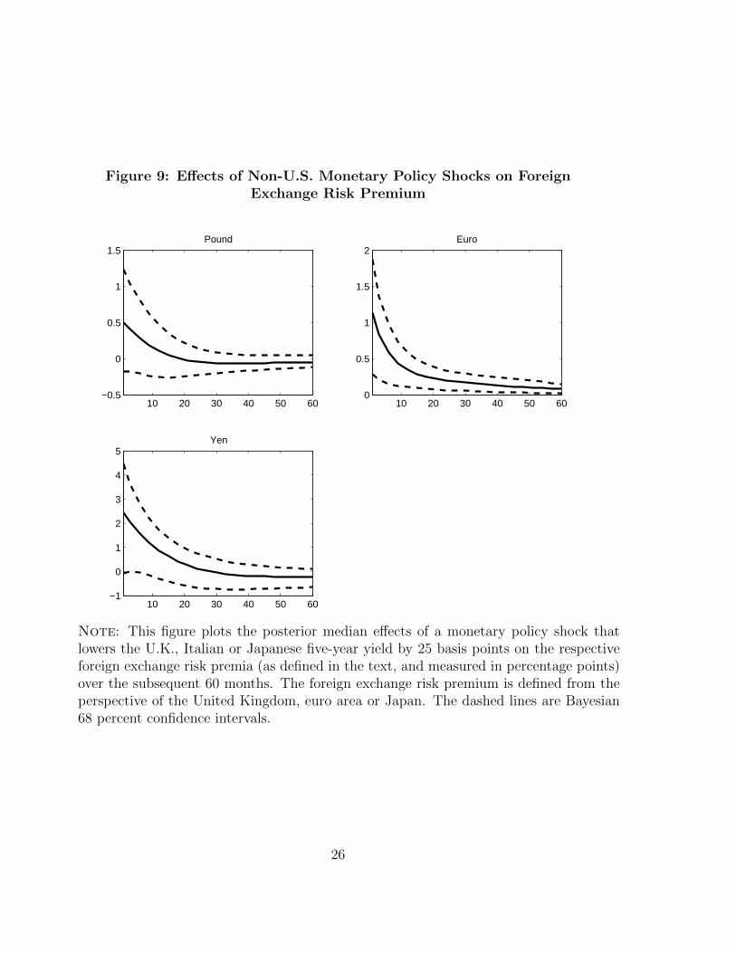
Figure 9: Effects of Non-U.S. Monetary Policy Shocks on ForeignExchange Risk Premium
10 20 30 40 50 60−0.5
0
0.5
1
1.5Pound
10 20 30 40 50 600
0.5
1
1.5
2Euro
10 20 30 40 50 60−1
0
1
2
3
4
5Yen
Note: This figure plots the posterior median effects of a monetary policy shock thatlowers the U.K., Italian or Japanese five-year yield by 25 basis points on the respectiveforeign exchange risk premia (as defined in the text, and measured in percentage points)over the subsequent 60 months. The foreign exchange risk premium is defined from theperspective of the United Kingdom, euro area or Japan. The dashed lines are Bayesian68 percent confidence intervals.
26
References
Andersen, Torben, Tim Bollerslev, Francis X. Diebold, and Clara Vega,
“Micro effects of macro announcements: real-time price discovery in foreign ex-
change,” American Economic Review, 2003, 93, 3862.
, , , and , “Real-time price discovery in global stock, bond and foreign
exchange markets,” Journal of International Economics, 2007, 73, 251277.
Backus, David K., Federico Gavazzoni, Chris Telmer, and Stanley E. Zin,
“Montary Policy and the Uncovered Interest Rate Parity Puzzle,” 2010. NBER
Working Paper 16218.
Bjornland, Hilde C., “Monetary Policy and Exchange Rate Overshooting: Dorn-
busch was Right After All,” Journal of International Economics, 2009, 79.
Bouakez, Hafedh and Michel Normandin, “Fluctuations in the Foreign Ex-
change Market: How Important are Monetary Policy Shocks?,” Journal of Inter-
national Economics, 2010, 81, 139153.
Bredin, Don, Stuart Hyde, and Gerard OReilly, “Monetary Policy Surprises
and International Bond Markets,” Journal of International Money and Finance,
2010, 29, 9881002.
Brunnermeier, Markus, Stefan Nagel, and Lasse Pedersen, “Carry Trades
and Currency Crashes,” NBER Macroeconomics Annual, 2009, 23, 313–347.
Caldara, Dario and Edward Herbst, “Monetary Policy, Real Activity and Credit
Spreads: Evidence from Bayesian Proxy SVARs,” 2016. Working Paper.
Christensen, Jens H.E. and Glenn D. Rudebusch, “The Response of Interest
Rates to US and UK Quantitative Easing,” Economic Journal, 2012, 122, F385–
F414.
Christiano, Lawrence J., Roberto Motto, and Massimo Rostagno, “Risk
Shocks,” American Economic Review, 2014, 104, 27–65.
Ehrmann, Michael and Marcel Fratzscher, “Monetary Policy Announcements
and Money Markets: A Transatlantic Perspective,” International Finance, 2003, 6,
1–20.
27

and , “Equal Size, Equal Role? Interest Rate Interdependence between the
Euro Area and the United States,” Economic Journal, 2005, 115, 930–950.
Eichenbaum, Martin and Charles L. Evans, “Some Empirical Evidence on the
Effects of Shocks to Monetary Policy on Exchange Rates,” Quarterly Journal of
Economics, 1995, 110, 975–1010.
Engel, Charles, “The forward discount anomaly and the risk premium: A survey
of recent evidence,” Journal of Empirical Finance, 1996, 3, 123191.
, “Exchange Rates and Interest Parity,” Handbook of International Economics,
2013.
, American Economic Review, forthcoming. Exchange Rates, Interest Rates, and
the Risk Premium.
Fama, Eugene, “Spot and Forward Exchange Rates,” Journal of Monetary Eco-
nomics, 1984, 14, 319–338.
Farhi, Emmanuel and Xavier Gabaix, “Rare Disasters and Exchange Rates,”
2014. Working Paper.
Faust, Jon, “The Robustness of Identified VAR Conclusions about Money,” Carnegie
Rochester Series on Public Policy, 1998, 49, 207–244.
and John Rogers, “Monetary policy’s role in exchange rate behavior,” Journal
of Monetary Economics, 2003, 50, 1403–1424.
, John H. Rogers, Shing-Yi Wang, and Jonathan H. Wright, “The high-
frequency response of exchange rates and interest rates to macroeconomic an-
nouncements,” Journal of Monetary Economics, 2007, 54, 10511068.
, John Rogers, Eric T. Swanson, and Jonathan H. Wright, “Identifying
the Effects of Monetary Policy on Exchange Rates Using High Frequency Data,”
Journal of the European Economic Association, 2003, 1, 1031–1057.
Gagnon, Joseph, Matthew Raskin, Julie Remache, and Brian Sack, “Large-
Scale Asset Purchases by the Federal Reserve: Did They Work?,” International
Journal of Central Banking, 2011, 7, 3–44.
28

Gertler, Mark and Peter Garadi, “Monetary Policy Surprises, Credit Costs and
Economic Activity,” American Economic Journal: Macroeconomics, 2015, 7, 44–
76.
Gilchrist, Simon, Vivian Yue, and Egon Zakrajsek, “US Monetary Policy and
Foreign Bond Yields,” 2014. Working Paper.
Gurkaynak, Refet S., Brian Sack, and Eric T. Swanson, “Do Actions Speak
Louder Than Words? The Response of Asset Prices to Monetary Policy Actions
and Statements,” International Journal of Central Banking, 2005, 1, 55–93.
Hausman, Joshua and Jon Wongswan, “Global Asset prices and FOMC An-
nouncements,” Journal of International Money and Finance, 2011, 30, 547571.
International Monetary Fund, “Unconventional Monetary Policies—Recent Ex-
perience and Prospects,” 2013.
Kiley, Michael T., “Exchange Rates, Monetary Policy Statements, and Uncovered
Interest Parity: Before and After the Zero Lower Bound,” 2013. Finance and
Economics Discussion Series, 2013-17.
Kim, Soyoung, “International transmission of US monetary policy shocks: Evidence
from VARs,” Journal of Monetary Economics, 2001, 48, 339–372.
and Nouriel Roubini, “Exchange Rate Anomalies in the Industrial Countries:
A Solution with a Structural VAR Approach,” Journal of Monetary Economics,
2000, 45, 561–586.
Krishnamurthy, Arvind and Annette Vissing-Jorgenson, “The Effects of
Quantitative Easing on Long-term Interest Rates,” Brookings Papers on Economic
Activity, 2011, 2, 215–265.
Kuttner, Kenneth, “Monetary Policy Surprises and Interest Rates: Evidence from
the Fed Funds Futures Market,” Journal of Monetary Economics, 2001, 47, 523–
544.
Mertens, Karel and Morten O. Ravn, “The Dynamic Effects of Personal and
Corporate Income Tax Changes in the United States,” American Economic Review,
2013, 103, 1212–1247.
29

Olea, Jose L.M., James H. Stock, and Mark W. Watson, “Inference in Struc-
tural VARs with External Instruments,” 2013. Working Paper.
Rogers, John, Chiara Scotti, and Jonathan H. Wright, “Evaluating Asset-
Market Effects of Unconventional Monetary Policy: A Multi-Country Review,”
Economic Policy, 2014, 29, 3–50.
Scholl, Almuth and Harald Uhlig, “New Evidence on the Puzzles: Results from
Agnostic Identification on Monetary Policy and Exchange Rates,” Journal of In-
ternational Economics, 2008, 76, 113.
Stock, James H. and Mark. W. Watson, “Disentangling the Channels of the
2007-2009 Recession,” Brookings Papers on Economic Activity, 2012, 1, 81–156.
and Motohiro Yogo, “Testing for Weak Instruments in Linear IV Regression,”
in Donald W.K. Andrews and James H. Stock, eds., Identification and Inference
for Econometric Models: Essays in Honor of Thomas Rothenberg, Cambridge Uni-
versity Press 2005.
, Jonathan H. Wright, and Motohiro Yogo, “A Survey of Weak Instruments
and Weak Identification in Generalized Method of Moments,” Journal of Business
and Economic Statistics, 2002, 20, 518–529.
Uhlig, Harald, “What are the Effects of Monetary Policy on Output? Results from
an Agnostic Identification Procedure,” Journal of Monetary Economics, 2005, 52,
381–419.
Wright, Jonathan H., “Term Premia and Inflation Uncertainty: Empirical Evi-
dence from an International Panel Dataset,” American Economic Review, 2011,
101, 1514–1534.
, “What does Monetary Policy do to Long-term Interest Rates at the Zero Lower
Bound?,” Economic Journal, 2012, 122, F447–F466.
30