unclassified 407 325 a d - defense technical information center · navweps report 8354 ... rocket...
TRANSCRIPT

UNCLASSIFIED
"407 325A D - ....
DEFENSE DOCUMENTATION CENTERFOR
SCIENTIFIC AND TECHNICAL INFORMATION
CAMERON STATION, ALEXANDRIA, VIRGINIA
UNCLASSIFIED

NOTICE: When government or other drawings, speci-fications or other data are used for any purposeother than in connection with a definitely relatedgovernment procurement operation, the U. S.Government thereby incurs no responsibility, nor anyobligation whatsoever; and the fact that the Govern-ment may have formulated, furnished, or in any waysupplied the said drawings, specifications, or otherdata is not to be regarded by implication or other-wise as in any manner licensing the holder or anyother person or corporation, or conveying any rightsor permission to manufacture, use or sell anypatented invention that may in any way be relatedthereto.

NAVWEPS REPORT 8354NOTS TP 3241
COPY 5 2
DESCRIPTION OF A CONTROL SYSTEM FORROCKET-MOTOR MASS MEASUREMENT
byLU R. A. Elston
Test Deportment
Released to ASTIA for further disseminatlon .itb
out bimitftion eyond those imposed by Oeur"itVoQut jimitfitionoedb ecrt
regulations.
J ABSTRACT. A technique for determining the mass of large
rocket motors during burning, and an experimental systemdeveloped for use with the NOTS-designed three-component
static-test stand at the Skytop facility, are described.SThe technique involves mounting the rocket motor on
springs and continuously exciting the spring-mass sys-tem at its natural frequency.
The theoretical design of the control system is dis-
cussed and theoretical system-performance characteristicsIare compared with those of the experimental system. Re-
sults of an analog simulation study conducted in two de-grees of freedom are included in the appendix.
Analysis of data from an evaluation test involving the
static firing of a large rocket motor, indicates that a2e accuracy in mass measurement is attainable with the
experimental system. Criteria for the design of an oper-ational system that will produce an accuracy of 1% are
presented.
' /yA U.S. NAVAL ORDNANCE TEST STATION
China Lake, Californiaa• IJune 1963 E :: 1963
STIJUN27
U. S. NAVAL ORDNANCE TEST STATION
AN ACTIVITY OF THE BUREAU OF NAVAL WEAPONS
C. BLENMAN, JR., CAPT., USN WM. B. McLEAN, PH.D. 'VCommander Technical Director
FOREWORD
In the static testing of rocket motors, the prime requirement isto be able to determine accurately the force of the developed thrust.With the advent of large rocket motors it became necessary to test themwith correspondingly large static-test stands having very low naturalfrequencies. However, because of the low-frequency characteristics ofthe test stand, oscillations occurred during irregular burning, thrustbuildup, and termination periods and these extraneous oscillations wererecorded as part of the thrust load-cell data. To separate oscillation-caused data from the thrust data, a data combination system was developed.To use the system it is necessary to know the mass of the oscillatingsystem throughout rocket-motor burning.
This report, issued at the working level, describes a techniquefor determining the mass of a system continuously during rocket-motorburning. It also includes a description of the theoretical developmentof an experimental mass-measuring system, the design and evaluation of aprototype system, results of an analog simulation study, and informationon full-scale testing.
This project was started in the spring of 1959 under Task AssignmentSP 71401-7 and was completed with an evaluation firing in December 1962under Task Assignment SP 71402-8. The report has been reviewed for tech-nical accuracy by Benjamin Glatt, R. W. Murphy, D. P. Ankeney, and C. E.Woods.
R. A. APPLETONReleased under Head, Range Divisionthe authority of
IVAR E. HIGHBERGHead, Test Department
NOTS Technical Publication 3241NAVWEPS Report 8354
Published by ................ ...................... Test DepartmentManuscript ............................................. .. 30/MS-579Collation ...... ................ .Cover, 36 leaves, abstract cardsFirst printing ................... 285 numbered copies
iil

NAVWEPS REPORT 8354
CONTENTS
Introduction ....................... ............................ 1Mass Measurement Technique ................. ..................... 4Experimental System .................... ........................ 8
Phase Determination .................. ....................... 8Force Generator ...................... ......................... 9
System Analysis .................... .......................... .. 15Root Locus Stability Analysis ............. .................. .. 22Performance Characteristics ............. .................... .. 28
Live Motor Firing .................... .......................... 35Conclusions and Recommendations ............... ................... 40
Operational System ................. ......................... 41Appendixes:
A. Analog Simulation .................................. ...43B. Derivation of Equations for Analog Simulation and Analog
Schematic Diagram .............. ....................... ... 54C. Derivation of System Transfer Functions and Phase
Comparator Schematic ............. ...................... .. 61
Figures:
1. Rocket Motor and Thrust Stand Schematic Illustrating BasicThrust Equation ................... ........................ 1
2. NOTS Model II Thrust Stand With Dummy Load ....... ........... 43. Rocket Motor and Thrust Stand Schematic .......... ........... 54. Phase Comparator Logic .................. ................... 85. Rotating Eccentric Weights ................. .................. 96. Block Diagram of the Experimentally Tuned Control System . . . 157. Simplified Block Diagram of the Compensated Control System . . 188. Mag-Amp and Drive Motor Static Characteristics ..... ........ 209. Diagram Showing Further Simplification of the Compensated
Control System .................. ......................... 2110. Block Diagram of the Uncompensated Control System ............ 2211. Root Locus of the Uncompensated System With a Rocket Motor
Carcass in the Stand.......... . ..................... ..2312. Root Locus of the Uncompensated System With a Live ýocket
Motor in the Stand ................ ...................... ..2313. Final Block Diagram of the Compensated Control System With
the Equivalent Series Transfer Function Replacing theMinor Loop .................. ........................ .. 24
14. Root Locus of Minor Loop ................................. .. 2515. Root Locus of the Compensated System With a Rocket Motor
Carcass in the Stand ...................................... 26
iii

NAVWEPS REPORT 8354
16. Root Locus of the Compensated System With a Live RocketMotor in the Stand ........................................ .. 27
17. Experimental System Response as a Function of Time to aSimulated Step Input (Rocket Motor Carcass) .... ........... .. 30
18. Experimental System Response as a Function of Time to aSimulated Step Input (Live Rocket Motor), System Oper-ating as a Straight Sampling Type ...... ................ .. 31
19. Rocket Motor and Stand Displacement as a Function ofFrequency (Rocket Motor Carcass) ......... ................ .. 33
20. Rocket Motor and Stand Displacement as a Function ofFrequency (Live Rocket Motor) ........ .................. .. 34
21. Vibrating Mass as a Function of Burning Time .... .......... .. 3522. Rocket Motor and Stand Displacement as a Function of
Frequency (Rocket Motor Carcass), Analog Simulation ........... 4423. Rocket Motor and Stand Displacement as a Function of Fre-
quency (Live Rocket Motor) Analog Simulation .... .......... .. 4524. System Response as a Function of Time to a Simulated Step
Input (Rocket Motor Carcass), Analog Simulation ............ .. 4725. System Response as a Function of Time to a Simulated Step
Input (Live Rocket Motor), Analog Simulation .... .......... .. 4726. Mass as a Function of Burning Time, Analog Simulation ......... 4927. Vibrating Mass as a Function of Burning Time Computed From
Frequency Data, Analog Simulation ...... ................ .. 4928. Vibrating Mass as a Function of Burning Time With Jetavator
Reaction, Analog Simulation ....... ................... .. 5129. Vibrating Mass as a Function of Burning Time With Jetavator
Reaction, Analog Simulation ....... ................... .. 5130. Phase Angle Response of Spring-Mass System as a Function of
Time, Analog Simulation ............. ..................... 5231. Large Rocket Motor in Three-Component Stand Prior to Firing. . . 66
ACKNOWLEDGMENT
The initial discussions on this mass-measuring technique werecoordinated by H. S. Olson, D. Nelson, and D. P. Ankeney. Theauthor is indebted to them for their technical and managerialassistance in resolving some of the initial problems encoun-tered and for their continued support throughout the develop-ment of this technique.
Further acknowledgment is made of the many other individuals,especially those in the Design and Development Branch of theTest Department, for their direct support in the basic designof the experimental system and for their conscientious effortsin helping to carry the development through to the. successfulcompletion of the evaluation test.
iv

NAVWEPS REPORT 8354
INTRODUCTION
In the static testing of large rocket motors, early test staune,often employed a standard load cell to solve the following simplifiedthrust equation:
T = KX (1)
where
T = thrustK = spring constant of load cellX = spring displacement
It soon became apparent, however, that the necessarily low resonant-translation frequency generally associated with large-scale testing re-sulted in the occurrence of undesirable oscillations or 'ringing' duringthrust buildup and thrust termination. This is the result of the thrustbuildup and termination appearing as approximate step inputs to an under-damped stand load-cell system. To account for these oscillations, thebasic single degree of freedom equation can be used.
Consider the rocket motor and stand illustrated in Fig. 1
LOADýX CELL
FIG. 1. Rocket Motor and Thrust Stand SchematicIllustrating Basic Thrust Equation.
1

NAVWEPS REPORT 8354
Where:
T = developed thrust, lb
K = spring constant of load-cell, lb/ft
C = lumped damping constant, lb-secftb-sec2
M(t) = mass of total moving structure (varies with time), ft
c.g. = center of gravity location (assumed fixed throughout burn-ing)
X = displacement of mass center of gravity
By summing the forces along the translational axis the following equa-tion is obtained:
T = KX + CX + M(t)X (2)
It is noted that this basic equation is a differential equation ofthe second order. As such, with the damping constant C relatively small(as it should be for accurate determination of thrust buildup and termi-nation), a step input or sudden change in thrust will result in largeovershoots and relatively undamped oscillations in X. These oscilla-tions are recorded as part of the load-cell data and, because of theirlow-frequency, they cannot be filtered without sacrificing data resolu-tion. As a solution to this problem NOTS has considered the developmentof a data-combination system which enables the separation of these oscil-lations from the load-cell data.* With this system, data from an accel-erometer mounted with its sensitive axis along the rocket-motor line ofthrust will be combined with the standard load-cell data and, by assuminga linear change in rocket mass during burning (as determined by weighingthe rocket motor before and after burning or as calculated from internalballistics data) the basic thrust equation can be solved. The acceler-ometer data is integrated to obtain X and by estimating C the second termof Eq. (2) can also be included.
While in many routine tests the assumption of a linear change inmass during burning might be useful in applying accelerometer data toobtain accurate thrust determinations, it is not adequate for use with
U. S. Naval Ordnance Test Station. A System for Correcting forSpurious Natural-Frequency Ringing of Rocket Static Thrust Stands, byJ. S. Ward. China Lake, Calif., NOTS, 1 September 1960. (NAVWEPS Re-
port 7569, NOTS TP 2541).
2

NAVWEPS REPORT 8354
propulsion systems in which the propellant mass-burning rate, intention-ally or otherwise, deviates seriously from a constant ialue during burn-ing. Furthermore, it is often desirable to know the mass-burning rateto the same degree of accuracy as that of the thrust at all times duringburning in order to evaluate the changing effects of erosive burning,combustion-chamber free volume, operating pressure, charge deformation,specific thrust, nozzle erosion, propellant composition, etc. Likewise,it is very important to have continuous mass measurement in case of me-chanical failure in the propulsion system since only limited specificthrust and specific impulse data can be obtained from an incomplete testif the mechanical condition of the nozzle and the amount of propellantburned prior to the failure are not known.
In reviewing this problem it was judged that a reasonably sophisti-cated evaluation of test records would provide a significant increase ininformation if a system could be devised for determining rocket mass con-tinuously during a firing. With the high cost of testing large motors,this increased information would create substantial savings in both timeand money during developmental programs.
Two methods which have been used for determining the mass of a burn-ing rocket motor are referred to as the Z Load Cell Method and internalballistics or Pressure Method.
The Z Load Cell Method involves the use of load cells in the thruststand legs to measure the vertical force during burning. If the standand thrust misalignments are known and assumed constant throughout burn-ing, a determination of mass versus time can be made. The overall accu-racy in mass determination is estimated as 5%; however, it is felt thatimproved stand alignments and data reduction techniques may improve thisfigure. Continued investigation into this method is planned.
To use the Pressure Method of determining mass requires that therocket motor chamber pressure be known throughout burning. It is alsonecessary to know the total amount of propellant burned and the throatarea of the nozzle. Using these parameters, calculations of mass burn-ing rates are made. It has been estimated that, due to the difficultyin measuring these parameters and the linearizing assumptions made inconverting the information to mass-burning rates, an accuracy of 5% isthe best attainable with this technique, too.
Using this as a general guideline in determining the feasibilityand usefulness of a particular system, the following technique for thecontinuous measurement of mass has been developed. The horizontal NOTSModel II thrust stand used in Bay I at Skytop (Fig. 2) was selected forsystem development, since it lends itself favorably to this techniqueof mass measurement and since considerable knowledge had been gained ofits operational characteristics.
The NOTS Model II thrust stand was designed with a six-compomentcapability but was used as a three-component stand for this development.
3

NAVWEPS REPORT 8354
FIG. 2. NOTS Model II Thrust Stand With Dummy Load.
An evaluation test of the experimental system and an analog simula-tion study have been conducted. The evaluation test is discussed onpage 35; results of the analog simulation study are given in AppendixA; the derivation of analog simulation equations is presented in Appen-dix B; Appendix C includes the derivation of system transfer functions.
MASS MEASUREMENT TECHNIQUE
The mass of a burning rocket motor is determined by continuouslyexciting the rocket-motor-stand system at its undamped natural frequencywhen supported on springs as shown schematically in Fig. 3. If the vi-brating system is assumed to have a single degree of freedom and slowlyvarying mass then the mass can be calculated throughout burning from thefollowing equation:
M(t)- 2K (3)Wn(t)
4

NAVWEPS REPORT 8354
FIG. 3. Rocket Motor and Thrust Stand Schematic.
where
=undamped natural frequency of vibrating systemfnltjt (variable with burning time)
F(t) = F sinct (sinusoidal force generator), lb
0t 2
o ~lb-sec2M(t) = effective vibrating mass, of
K = lumped spring constant, lb/ft
C = lumped damping constant, lb-sec
Z = vertical displacement of rocket motor center ofgravity, ft
This equation is derived in writing the dynamic equation of motion.Applying Newton's second law to the system of Fig. 3 and assuming a non-changing mass environment, the differential equation of translationalmotion is written:
2F sinwt = M dZ + C dz + KZ (4)dt 2 dt
Applying the LaPlace transform operator, S
s2 + 2 (S) + sCZ(s) (s)
5

NAVWEPS REPORT 8354
solving for Z(S)
(S) ) (s2M + SC + K) (6)Z(s) -- (s 2 (6
rearranging
Fwz F 0 w __ _ __ _
Z(s) 2 2) s2 s
By definition, any linear second-order differential equation can bewritten in terms of two quantities: ý and w .
n
The damping ratio ý is the ratio of the damping that exists in asecond-order system to the critical damping; i.e., the value of dampingresulting in a nonoscillatory response following a step input. The un-damped natural frequency wn is the frequency of oscillation that occursfor zero damping. By definition, then
2ýw C (8)
(2 =K (9)
Rearranging, Eq. (9) then becomes original Eq. (3):
KM=K2
n
Substitution of Eqs. (8) and (9) in Eq. (7) yields
Z F w 1(10)Z(S) M(S2 + w2) (S2 + 2tn S + n2)
Rearranging
6

NAVWEPS REPORT 8354
Z2F0w2 2 12 2 (i(S M(s2+ W2) [(S + nw) + 2(_ -2t
Using the appropriate transform function, the complete solution ofthe displacement of the rocket motor is found to be:
Fo i -nt Z 1Z(t) = 0 sinY'n 1•-•2-)(12)4 4 2~2 2~22•n•-2
M( 1[+W 4_2w 2n +4t 2 n2W ) ffn 1/l - e In n T.1 n
where
2 2
tan -2 W n e
W . 2ý 2 W2 _ 2 + W2
n n n
Considering only the steady-state solution it can be seen that asthe frequency of the exciting force w approaches the undamped naturalfrequency Wn, the phase angle el approaches 90°. In other words, whenthe spring-mass system is oscillating at the undamped natural frequencythe displacement Z lags the exciting force in phase by 900 so that
for
F(t) = F sinwt (13)0
FZ(t) = 2 sin(wt - 900) (14)
2M •w
The problem remaining, then, is to design a control system to main-tain this 90° phase relationship continuously throughout burning. Bymaintaining this relationship, system oscillation at the undamped natu-ral frequency is insured and computations of mass versus burning timecan be made by using Eq. (3).
Gardner, Murray F. and John L. Barnes. Transients in Linear Sys-tems, Vol. 1. New York, Wiley, 1956. Transform pair 1.357, Appendix A.
7

NAVWEPS REPORT 8354
EXPERIMENTAL SYSTEM
PHASE DETERMINATION
The first step in the design of the control system was to devise amethod of sensing the phase relationship of the sinusoidal-force gener-ator exciting function F(t) with that of the spring-supported rocket-motor stand system displacement function Z(t).
The waveforms in Fig. 4 a, which depict the phase relationship be-tween these two functions at an instant in time when the spring-masssystem is oscillating just below the undamped natural frequency, showa phase angle of 800. In orderto detect the phase polarity(i.e., lead or lag, in ref-erence to the desired 900 value) oSIN ,(A)a third waveform is added. This ZK'SIN(wt-80o)(C)waveform, shown in Fig. 4b, isalways leading the exciting func-tion by 90% For the conditionshown (i.e., for the system os-cillating below the undamped nat-ural frequency) it is now possibleto write logic equations relatingthe three waveforms and the 100 FIG.4a
phase error. IF
/ t 7-- F.oS N (W(A)Using Boolean Algebra termi- f K'SIN(wt_8OOI(c)
nology and selecting A,_B,_C to 'LZ(represent positive andA, B, C to I
represent negative values, thefollowing equations are written:
A B C =1 (15)
A B C = 1 (16) FIG. 4b
dFW-F 'COS Wt(B)
where A B C is defined as A F ,--FoSINWt(A)
and B and C.
In the same manner it is A9--Ipossible to write the logicequations for the conditionwherein the spring-mass system BC,,is oscillating above the un-damped natural frequency. As FIG. 4c
illustrated in Fig. 4c, thelogic equations are: FIG. 4. Phase Comparator Logic.
8

NAVWEPS REPORT 8354
A B C 1 (17)
A = 1 (18)
These equations were used in designing the diode logic circuitry(phase comparator), a schematic diagram of which appears in Appendix C.The phase comparator generates an error pulse of constant amplitude withthe width equal to the relative phase error. The pulse is positive fora system-oscillation frequency below the undamped natural frequency andnegative for frequencies above the undamped natural frequency. Sinceone of the four logic equations will be satisfied at each crossover ofthe displacement wave, a digital sensor exists with a sampling rate oftwo samples per cycle. This low sampling rate in a closed-loop systemwill tend to increase system-response time which will generally degradesystem performance. In this experimental system, however, the powertrain has a time constant of approximately 200 millisec and the addi-tional lag introduced by the lowest sampling rate of 20 samples per sec-ond does not appear to be significant. It is apparent that in the designof fully operational systems having power train-time constants consider-ably lower than 200 millisec, techniques for increasing the digital sam-pling rate will have to be devised.
FORCE GENERATOR
The force generator is a mechanical device consisting of two setsof eccentric weights connected through a differential. The arrangementand relative rotation of the weights is shown in Fig. 5.
Set #2
F -FIG. 5. Rotating Eccentric
-- -- -Differentiol Weights. Arrows indicateL -- direction of rotation.
S/ k Set if,_
-11 Y -
W,9

NAVWEPS REPORT 8354
With an individual eccentric weight W1 , a radius of rotation rI andan angular velocity w, the centrifugal inertia force is given by
W1 2F1 = w r (19)
where
F1 = force, lb
W1 = effective weight, lb
rI = radius of rotation, ft
g = gravitational force, 32.2 ft/sec2
S= angular velocity, rad/sec
Since the two weights of each set are coupled together and rotatein opposite directions, the centrifugal inertia force along the x axisis canceled out and a force is generated only along the y axis. Theforce is sinusoidal and has a maximum magnitude which is dependent onthe phase relationship between the two sets of weights. Thus, the ex-citation force is calculated using the following equation:
4 w1 2F1 = -g- r1 w sin(e1 - &2) sinwt (20)
The desired magnitude of force can be generated by selecting theproper phase angle between the two sets of weights with the differential;hence the term sin(e1 -6 2 ).
The magnitude of the force necessary to excite the spring-mass sys-tem at the undamped natural frequency is dependent upon: (1) the accel-eration limitations in the vertical plane of the rocket motor under test,(2) the damping existing in the spring-mass system, and (3) the mass ofthe vibrating system. For the rocket motor and stand assembly beingtested, the following specifications apply:
10

NAVWEPS REPORT 8354
Sprung weight with live rocket motor(propellant unburned) in stand 25,000 lb
Sprung weight with rocket-motor car-cass (propellant burned) in stand 10,ý000 lb
Effective spring constant 3.72x10⁶ lb/ft
Undamped natural frequency (live ,motor in stand) 10.88 cps
Undamped natural frequency (motor ,carcass in stand) 16.88 cps
Damping ratio ý (this ratio was cal-culated using Eq. (22) and esti- 0.01 or 1%
mating Fo, while maintaining a1-g acceleration)
Maximum vertical acceleration 1.0 g
Burning time 60 sec
By taking the second derivative of Eq. (14), the following expres-sion is obtained for the acceleration of the spring-mass system oscil-lating at the undamped natural frequency:
FcoswtZ(t) = •--cst(21)
The vibrating structure (including a first-stage rocket motor) hasa mass of approximately 720 slugs when the rocket motor propellant isunburned and approximately 320 slugs with the rocket motor carcass. Thedamping ratio is small since dash pots have not been added and the onlydamping present (such as propellant flexibility) is that which is inher-ent in the system. ý is estimated at approximately 0.01. Under theseconditions, the magnitude of the exciting force can be computed fromEq. (21).
Maximum acceleration occurs when coswt = 1. Therefore, rewritingEq. (21)
F = 2t2 (22)
Values determined experimentally.
11

NAVWEPS REPORT 8354
and for the conditions above
F = (2)(0.01)(320)(32.2) = 2o6 lb (23)
This value of Fo will result in a 1-g acceleration with a rocketmotor carcass mounted in the stand. Since ý is considered constantthroughout burning, it is apparent that a much larger exciting forcecould be tolerated under live motor conditions. However, since theforce generator differential will not be operated during the test, itis necessary to restrict the maximum force to that indicated in Eq. (23).
It is now possible to calculate the maximum horsepower required todrive the force generator. The power required in the system is the sumof the power needed to provide angular acceleration; to overcome dampingin the spring-mass system, shaker, and drive motor, to counteract thelosses in the gear train; and to compensate for torque feedback due tothe oscillatory motion of the shaker in relation to the drive motor.The maximum horsepower requirement is calculated by:
T = J6 + Bb (unknown) + Tf + gear train losses (unknown) (24)
+ spring-mass damping
and
T f =m [f + (2 + ZO) cose + Zb sine] (25)
where
T = total torque reflected into the drive motor, lb-ft
Tf = feedback torque, lb-ft
o = angular velocity, rad/sec
6 = angular acceleration, rad/sec2
mi = effective shaker unbalance, lb-sec2
S= effective mass lever arm, ft
J = effective system inertia, lb-ft-sec2
The derivation of Eq. (25) is given in Appendix B.
12

NAVWEPS REPORT 8354
To calculate the maximum power required, e and 6 will be assumed tooccur simultaneously and have the following values:
max = 106 rad/sec
6max = 10 rad/sec2
The term e is based on the system being in operation with a rocketmotor carcass in the stand and 0 is based on the maximum transient re-sponse requirement as indicated in the figure shown on page 30.
Since the second and third terms of Eq. (25) have a 90o relation-ship, only the second term need be considered to obtain peak torque.When cose = 1, this equation becomes
Tf mg (16 + Z + Z6 2 ) (26)
where
ml 0.02
I-- 0.096
then
Tf - (0.02)(0.096 x 10 + 32.2 + 0.00287 x 10⁶) 2 2.6 lb-ft
The additional torque required to provide the desired acceleration is
J6-= (lO)(0.71) = 7.1 lb-ft
where
J = 0.71
Then
T = Tf + JO = 2.60 + 7.1 = 9.7 lb-ft total known torque
13

NAVWEPS REPORT 8354
The horsepower transmitted by a shaft making n revolutions perminute under a torque of T lb-ft is
27tn T33,000
(27)
HP = (2g)(16.88)(60)(9"7) -1.8733,000
The horsepower requirement to provide acceleration and to compensate fortorque feedback then, is 1.87. The additional power requirement to over-come spring-mass damping is obtained from the following power equation,where Z is the velocity of the displacement Z and C is the damping con-stant as in Eq. (2):
Power = Z2C (28)
The damping C as determined from Eq. (8) is 680 lb-sec and dis-ft
placement velocity Z is obtained by differentiating Eq. (14); therefore,
Power = (0.304) 2(680) = 63 secsec
HP= 6 3 =0.12550
This results in a total known instantaneous peak power requirementof approximately two horsepower. A drive motor is normally selected byconsidering both the instantaneous and average power requirements. Inthis case, however, the average power dissipated, other than that due todamping, is difficult to ascertain analytically. It has been determinedexperimentally that the average power dissipated is approximately onehorsepower. It appears, therefore, that the selection of the 5-horse-power motor used in this experiment is somewhat conservative and thatimproved response could be realized by carefully selecting a motor justmatching the power requirements.
14

r
NAVWEPS REPORT 8354
SYSTEM ANALYSIS
The block diagram of Fig. 6 represents the complete experimentalcontrol system when it is operating as a relay type with sampling. Thesystem was initially constructed as a straight sampling type (i.e., asshown in Fig. 6, without the flip-flop). Using the sampled data system,a rocket-motor firing was conducted; the results are discussed later inthis report. The system performed satisfactorily; however, in prepara-tion for a second evaluation test it was found that the addition of theflip-flop improved system performance. (It was planned to conduct thesecond test using the configuration shown in Fig. 6; however, this testcould not be conducted because of a rocket motor malfunction which par-tially destroyed the drive motor and shaker.)
SINE-COSINEPOTENTIOMETER
AS SIN 8 A30:,
(REF)AsCos e 51.5 MA (SIAS)
PHAS POWER DRIVE
COMPARATOR FLIPFLOP INTEGRATOR COMPENSATION PRE-AMP - AMP MOTOR
j_ 0, K1 e 2 (s-+i)(s+-) e3 1 A2 e6 K2
S+(S+11K0 J17
DYINAMICS SHAKER (4)
s24,sRwN,- C) A 2 2 -- ---- --'• TC
FIG. 6. Block Diagram of the Experimentally Tuned Control System.
Although the evaluation test was conducted with the system operat-ing as a straight sampling type, it is felt that significant improvementin closed-loop performance was obtained with the addition of the flip-flop and that the analysis should be made for the relay sampling typesystem. No recorded data of the relay-sampling system were obtained be-cause of the rocket-motor malfunction. The system was operated, however,with a rocket-motor carcass in the stand prior to this catastrophe andthe system performance was observed. The significant performance char-acteristics are indicated for comparison on the response curves obtainedwith the straight sampling system.
15
NAVWEPS REPORT 8354
In Fig. 6, comparator No. 1 and the 'sampler' represent the phasecomparator described previously. The phase of the waveform e, represent-ing the exciting force is compared with the phase of the waveform Z r-ep-resenting the displacement of the oscillating spring-mass system. Asampling rate of two samples per cycle has been established. The outputof the sampler is used to trigger a flip-flop which in turn is used asthe error signal for integration. (At least one stage of integrationin addition to that performed by the drive motor is desirable in veloc-ity control since this results in a Type 2 system which exhibits a zerosteady-state error in a simple configuration--i.e., a single loop withcontinuous feedback. A theoretical derivation is given in Chapter 7 ofServomechanism Analysis.*) The addition of the flip-flop changes theservomechanism from a straight sampling type to a relay type with sam-pling.
Usually, the performance characteristics of relay servos are notparticularly favorable; that is, a servo with continuous (proportional)feedback will generally out-perform the relay type. In this case, how-ever, where it is necessary to compare the phase relationship of twosinusoidal waveforms (one of which has a variable amplitude), a practi-cal device for comparing the phase relationship continuously is notreadily available. The phase comparator thus uses diode logic circuitryto produce pulses which are phase dependent at each zero crossover ofthe displacement waveform. The pulses are of constant amplitude buthave a width directly proportional to phase error.
Comparing the system performance during experimental operation,both as a straight sampling type and as a relay type with sampling, itwas found that the relay type exhibited superior characteristics. Withthe relay configuration, it was possible to more-than-double the forward-loop gain of the control system with a consequent improvement in fre-quency response. The steady-state oscillation or limit cycle of theservo system was more pronounced when operated as a relay type; however,the frequency of oscillation was higher, and better response was obtainedfor small step inputs in phase error. It should be noted, however, thatwith the use of highly sophisticated compensating circuitry, a straightsampling system performance, comparable to that of the relay type, couldvery likely be obtained. The compensating circuitry necessary to attainthis result is quite complex making experimental improvement of closed-loop system performance extremely difficult. While on the other hand,the relay system required relatively elementary compensating circuitryand produced the desired result.
From the control system diagrammed in Fig. 6, it is apparent thatseveral nonlinearities exist. (A component is said to be nonlinear ifthe equations describing its dynamics contain terms made up of the pro-duct or quotient of a dependent variable and a time variant coefficient.)The equation describing the spring-mass dynamics is written:
,Thaler, G. J. and R. G. Brown. Servomechanism Analysis. New York,
McGraw-Hill, 1953.
16

NAVWEPS REPORT 8354
F ,(d)2 sinf(t)t = M t) + C +KZ (29)
Since this equation is of the nonlinear type, it cannot be handledby regular LaPlace methods.
The complete solution of the nonlinear system will not be attempted,only the two end points of operation will be considered. That is, thecontrol. system will be analyzed operating first in a nonchanging massenvironment with a rocket motor carcass and then with a live rocket mo-tor mounted in the thrust stand. To simplify and linearize the system,the spring-mass dynamics will be considered analogous to a low-pass fil-ter. That is, the spring-mass system will be considered to introducephase lag and amplitude attenuation in the feedback loop. Data obtainedwith the experimental system and in the analog simulation studies (Ap-pendix A), indicate that a lag in the spring-mass system to simulatedstep inputs exists and that the response curve approaches that of anexponential.
This lag characteristic is described in some detail in NAVWEPSReport 7741* which illustrates that a step change in mass will result inan exponentially rising input error to the control system. The assump-tion has been made here that this lag will also appear when changes indriving-function frequency are experienced and that this lag is in thefeedback path. This assumption is open to considerable discussion; how-ever, it is shown that, with this assumption, reasonable agreement withexperimental data can be obtained. Using the experimentally determinedtime constants, the following transfer functions will be used to simu-late the spring-mass system in the analysis of the two end points ofoperation:
with a rocket motor carcass in the stand
Z 3 (30)
with a live rocket motor in the stand
Z 2 (31)e S +-2
This simplifies the system block diagram to that of Fig. 7.
U. S. Naval Ordnance Test Station. Determination of Rocket-MotorMass by Measurement of the Natural Frequency of a Mass-Spring System, byBenjamin Glatt. China Lake, Calif., NOTS, 15 June 1961. (NAVWEPS Re-port 7741, NOTS TP 2706).
17

NAVWEPS REPORT 8354
FLIP- DRIVESAMPLER FLOP INTEGRATOR COMPENSATION PRE-AMP MAG-AMP MOTOR
FIG. 7. Simplified Block Diagram of the CompensatedControl System.
It should be pointed out that these time constants may be in con-siderable error. As noted in NAVWEPS Report 7741, the time constantsare dependent on the damping and mass of the system at the time the stepchange in mass is initiated. The experimental data were obtained bysuddenly changing the driving-function frequency and observing the lagof the spring-mass system. Since, in this experiment, both the lag ofthe power train and the spring-mass system are combined, some error isevident in the interpolation. It is also noted that, although the timeconstant determined under live-motor conditions compares favorably withthat of the analog study, there is a considerable difference between thetime constant obtained under rocket-motor carcass conditions and thatobtained in the analog study.
In the analog simulation, it was necessary to vary the damping withburning time and to distribute it unequally between front and rear sup-ports to provide the needed coupling to cause pitching and thus repro-duce the disnlacement curves obtained experimentally. It has since beendetermined under system operation that the structural oscillation of thethrust take-out member was also introducing pitching. It is evident,therefore, that the damping used in the analog study for the rocket-motor carcass condition is in error and that the time constant of therocket-motor lag for this condition is also in error.
The speed of the shaker-drive motor is controlled by regulating thearmature current while maintaining a constant field strength. The dy-namic equations pertaining to this type of control are well developed.*
The transfer function of the motor when driving an inertia load and neg-lecting frictional losses is:
Thaler, G. J. and aR. G. Brown. Op. cit., pp. 62-65.
18

NAVWEPS REPORT 8354
K
JR-e= a(32)e6 s(s4)
whereohm-sec
K = motor constant, rad
Ra = motor armature resistance, ohmis
J = total inertia load, ft-lb-sec2
For the system under development, the motor constants K, and Rawere determined experimentally (Appendix C). The transfer function is:
@ K2e S(SlO)
(33)
The magnetic amplifier dynamic characteristics were also determinedexperimentally (Appendix C) and the transfer function is:
e6 A26 2 (34)
5 (S + 10)5
Tachometer feedback is utilized in a minor loop. Since this is avelocity servo, the derivative of the tach or 0 is actually fed backand, since the tach output contains high-frequency components in theform of ripple, a filter is employed with the differentiator. The fil-ter is connected in the feedback circuit of the operational amplifierused as the differentiator; filtering is accomplished since the gain be-comes a function of frequency. The lead circuit is used to reshape thefilter characteristics slightly and to allow optimization of the tachcircuit under operating conditions. Derivation of the transfer functionsappear in Appendix C.
The steady-state transfer function of the mag-amp and drive motoras a unit was obtained experimentally to determine if there were anynonlinearities in this portion of the control system. The curve plottedin Fig. 8 shows the nonlinearity that is present. If the mag-amp anddrive-motor transient characteristics are considered not to change fromthe experimentally obtained values then the analysis of the end pointsof operation can continue by assuming an appropriate change in the for-ward loop gain as dictated by the curve in Fig. 8.
19

NAVWEPS REPORT 8354
45
40ROCKET MOTOR CARCAS IN STAND
A2K2 = 2580
LI VE MOTOR IN STANDA21(2 11I90
30
25
20
15
9 0oi I ID 4 5 IS I? I IS 20 D 29 10 1 2 13 14 15 16 17 is 19 20 21 22
0 (CPS)
FIG. 8. Mag-Amp and Drive Motor Static Characteristics.
Under closed-loop operation it was observed that the control systemexhibited a limit-cycle frequency of approximately one cycle per second.The sampling frequency at the low frequency end (with a live rocket mo-tor mounted in the stand) is about 20 samples per second and about 36samples per second at the high frequency end. Since the sampling rateis at least twenty times the switching rate of the relay (flip-flop), inthis analysis the sampler will be considered to have an infinite fre-quency. That is, the error detector will be considered to be continuous.
The describing function technique for analysis of relay servos isparticularly useful when relays approaching the ideal are used and whenthe system is of a high order. * A linear approximation is made in thefrequency domain by defining a describing function in terms of the Fourierseries for the component response to a sinusoidal input. With an idealrelay, the application of a sinusoidal input will result in a Fourierseries describing the output consisting of the fundamental input and allodd harmonics thereof. The approximation is made with the assumption thatthe relay output consists only of the fundamental sinusoidal input. Forthis to hold, it is necessary that the feedback signal generated by therelay output be a pure sinusoid. Since a relatively high-order systemexists (i.e., one with considerable low-pass filtering), this assumptionappears valid. Since the ideal relay presents zero phase shift, the fol-lowing described transfer function is defined in amplitude only:
,Thaler, G. J. and Marvin P. Pastel. Analysis and Design of Non-
linear Feedback Control Systems. Chapter 4. New York, McGraw-Hill, 1962.
20

NAVWEPS REPORT 8354
Describing function
GD F(A, w) ()
G D A (35)
where
A = amplitude of input sinusoid to cause saturation
F(Aw) = amplitude of output sinusoid
0 = phase angle between input and output functions
For the system under study, assume a maximum input sensitivity Aof 0.1 volt and an output F(Aw) of 30 volts. Then
GD 30 0 10o (36)
The block diagram of the servo system is now reduced to that shownin Fig. 9. It is observed that the effect of the nonlinear componentGD on the control system is to introduce a variable forward loop gain.When large errors and transients exist in the control system the forwardloop gain is minimized since the input A of the describing function,Eq. (35), increases while the output F remains constant. The maximumforward loop gain occurs under steady-state operation when the control-system feedback is just sufficient to trigger the relay (flip-flop).
DESCRIBING INTEGRATOR aFUNCTION COMPENSATION
+S 2 is
LIVE ROCKET MOTOR ROCKET MOTORIN STAND CARCASS IN STAND
1/),- 2 II/y .3
A2K2 = H19O A2 K 2 :2580
FIG. 9. Diagram Showing Further Simplification of theCompensated Control System.
21
NAVWEPS REPORT 8354
ROOT LOCUS STABILITY ANALYSIS
Once the describing function has been defined it is possible toexamine the servo performance by the root locus method. Since the non-linear element is considered to introduce variable gain only, the locusof roots will not be affected and only a single overall curve is requiredto depict servo performance as a function of forward loop gain.
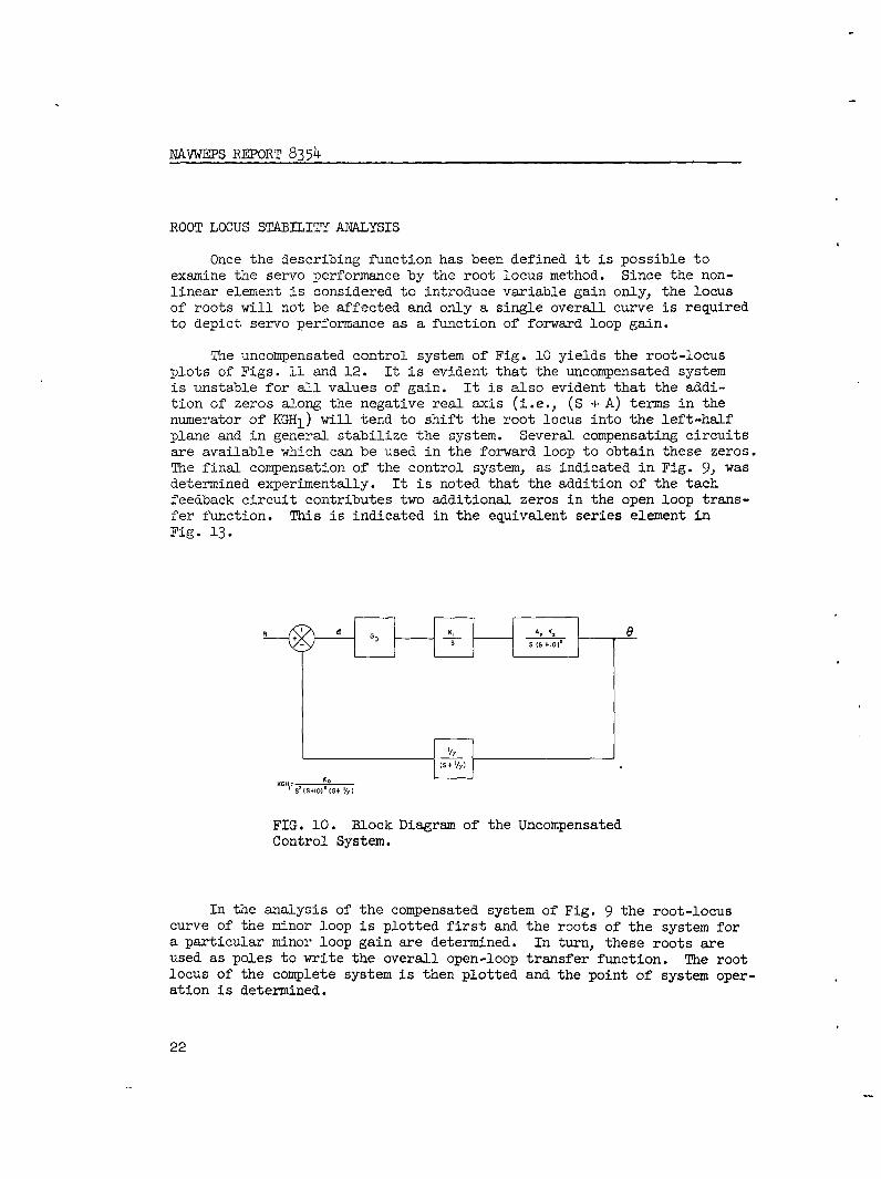
The uncompensated control system of Fig. 10 yields the root-locusplots of Figs. 11 and 12. It is evident that the uncompensated systemis unstable for all values of gain. It is also evident that the addi-tion of zeros along the negative real axis (i.e., (S + A) terms in thenumerator of KGH 1 ) will tend to shift the root locus into the left-halfplane and in general stabilize the system. Several compensating circuitsare available which can be used in the forward loop to obtain these zeros.The final compensation of the control system, as indicated in Fig. 9, wasdetermined experimentally. It is noted that the addition of the tachfeedback circuit contributes two additional zeros in the open loop trans-fer function. This is indicated in the equivalent series element inFig. 13.
S7 S (S +I0),
S4
(S+1O)4
(S+ IVY)
FIG. 10. Block Diagram of the UncompensatedControl System.
In the analysis of the compensated system of Fig. 9 the root-locuscurve of the minor loop is plotted first and the roots of the system fora particular minor loop gain are determined. In turn, these roots areused as poles to write the overall open-loop transfer function. The rootlocus of the complete system is then plotted and the point of system oper-ation is determined.
22

NAVWEPS REPORT -354
KGH1 • .__ •
52 S 3) 1 S- I
2 2 REAL-- - -4 -2 -I
THIS SYSTEM IS UNSTABLE FOR ALL VALUES OF GAIN
SINCE TWO ROOTS WILL ALWAYS BE IN POSITIVEREAL PLANE RESULTING IN POSITIVE EXPONENT
EXPONENTIALS IN THE REAL TIME TRANSFORMATION.
FIG. ii. Root Locus of the Uncompersated System With aRocket Motor Carcass in the Stand.
6
5/
-4
3
I2
KGH - K$2(S+2)(S+10)2
2 2 REAL
-10 -9 -8 -7 -6 -5 -4 -3 -2 -I
THIS SYSTEM IS UNSTABLE FOR ALL VALUES OF GAIN
SINCE TWO ROOTS WILL ALWAYS BE IN POSITIVE 31REAL PLANE RESULTING IN POSITIVE EXPONENTEXPONENTIALS IN THE REAL TIME TRANSFORMATION. I
FIG. 12. Root Locus of the Uncompensated System Witha Live Rocket Motor in the Stand.
23

NAVWEPS REPORT 8354
DESCRIBINGFUNCTION S+IlS+0 ($sS+ II+3s+ )J
MAX Em~
LIVE ROCKET MOTOR ROCKET MOTOR CARCASSIN STAND IN STAND
I/ 2 =/ 3A2 K2 =1190 A2 K2 =2580S, =-10.2 +j 4.0 S 1-I0.4 +j 6.2S2= -10.2- j 4.0 S2 10.4-J 6.2S3=-1.7 +jO.6 S3= 1.6 + {0.7S4= -1-7- j 0.6 S4=- 1-6 - JO.-7
FIG. 13. Final Block Diagram of the Compensated Control SystemWith the Equivalent Series Transfer Function Replacing the MinorLoop.
The system will be analyzed first using the system constants asso-ciated with a rocket motor carcass. The minor open-loop transfer func-tion of Fig. 9 is given as:
KGH•2 28 S(S 4-1) 2(7)(s + 10) 2(s + 2)2
A2K K4 =28
The roots at the point of operation as determined from the locus ofroots shown in Fig. 14 are as follows:
S1 = -lO.4 + j6.2
s2 = -io.4 - j6.2
S3 = - 1.6 + j0.7
S4 = - 1.6 - jO.7
The minor-loop transfer function can now be written as follows:
SA 2AK2 (S + 2)2
14 S(S + 1)(S + s2)(s 3)(s s (38)
24

NAVWEPS REPORT 8354
CARCASS LIVE MOTOR
KGH2 - 28S (S -I) 12.9$ (S+I)(S+ 2)2 (S + 10)2 KGH2 = (S+ 2)2 (S + 0)2
SI SI= -10.4 + j 6.2 SI--10.2 + J 4.0
S2 -10.4 - J 6.2 S2= -10.2 - 14.0
S3:-1.6 -" + 0.7 S3 - -1.7 + 1 0.6
S4 = -1,r 0-.7 S4 - -1.7 -- 0.6
SI 4
3
2
S X
_2 1 I I I I .Z2 A REAL
-12 -II -I -9 -e -7 -6 -5 -4 -3 -2 -- 1
FIG. 14. Root Locus of Minor Loop.
This transfer function can now be handled as a series element inthe outer loop as illustrated in Fig. 13. The outer open-loop transferfunction is written:
0.9 A2K2 (S+l)2 (S+2)2KGHI =
y S (S+l1)(S+50))(S+ ) (Si) (S+S2 )(S+S 3)(S+S 4 )
For the motor carcass condition A2K2 = 2,58o and y = 1/3 seconds.
7000 (S+1) 2(S+2)2 (4o)KGH = 7S(S+50)(S+3)(S+ll)(S+Sl )(S+S2 )(S+S3 )(S+S 4 )
The root-locus plot for this open-loop transfer iw-z ton is shown inFig. 15.
The same procedure is followed in plotting the overall root locuswith a live rocket motor in the stand. Since the minor-loop gain ischanged for this condition, a new KGH2 must be plotted and another setof roots determined. Thus,
25

NAVWEPS REPORT 8354
0z.44
K = 7000-a5.5
APPROXIMATE OPERATING POINT
GH69 2 7000 (S +1I)2
(S - 21) 5
1 (S+II )( S+50)(S+3XS+ 1.6 +JO.7)(S- 1.6 -j 0.7)(S+10.4.j 6.2)(S+ 10.4-1 6.2)
-4
-I 11- -10 -9 -8 --7 -6 -5 -4 -3 -2'V -I2
FIG. 15. Root Locus of the Compensated System With aRocket Motor Carcass in the Stand.
12.9 s(s + 1) (41)(S + 2) 2 (S + 10)2
A2 K2 K4 = 12.9
The roots at the point of operation as determined from the locus of rootsin Fig. 14 are as follows:
S = -10.2 + j4.0
S2 = -10.2 - j4.o
S3 = - 1.7 + j0.6
S4 = - 1.7 - j0.6
The minor-loop transfer function can now be written:
S=T 1190 (s + 2) 2 -7 (42)14 S(S + ST)(S + S2 )(S + S3)(S + S(
This transfer function is now handled as a series element in theouter loop and the following open-loop transfer function is written:
26

NAVWEPS REPORT 8354
KOH, = 2 3340 (s+l)2 (S+2),2 (43)S (s+ll)(s+5o)(s+2)(s+sl)(s+s2 )(s+s3) (s+s4)
The root-locus plot for this open-loop transfer function is shownin Fig. 16. It is interesting to note that the loci of Figs. 15 and 16are dependent only on the linear system. The effect of the variable-gain nonlinearity (describing function) is to move the root positionalong the locus.
7
K=3220 6
APPROXIMATEOPERATING POINT 3
2
I
23" REAL-11 -10 -9 .8 -7 -6 -5 -4 -3 - -
K( 50 3220(S+)2 (S+2)2
KOHI SZ(S+ )(S-50)(SI-2)(S +I.7+J.6)(S+I.7-J.6)(S+IO.2 +j4)(S+IO.2-14)
FIG. 16. Root Locus of the Compensated SystemWith a Live Rocket Motor in the Stand.
In a relay servo system of the type under analysis, maximum gainoccurs under minimum error conditions. It is seen that the roots forthis condition are located at their greatest displacement from the open-loop poles. For a large initial disturbance, such as a step change inmass, the gain is low and the system will exhibit a low natural frequency.It is evident, then, that in this type of servo system the maximum gainoperating point should produce a system damping ratio somewhat lower thanthe nominal value of 0.7. The system under study was experimentallytuned at the high-frequency end point (or in accordance with the rootlocus of Fig. 15). The approximate operating point indicates a dampingratio of 0.44 and an undamped natural frequency of 5.5 rad/sec.
27

NAVWEPS REPORT 8354
It should be pointed out that considerable error may be present inthe calculation of the maximum describing function gain. It is feltthat the experimentally determined threshold sensitivity of the phase-comparator flip-flop configuration may be in error by as much as 50%.An increase in forward-loop gain of this magnitude would greatly in-crease the natural frequency but would tend to make the system unstable.An interesting point in favor of this type of servo system, however, isits ability to operate very near the imaginary axis while maintainingcomplete stability. This is best understood by visualizing the largechange in gain which takes place when the system is oscillating about'the zero error point. At the minimum error pbint the describing func-tion gain is approximately 300. This corresponds to a phase-angle error(i.e., phase angle difference from 900 between the forcing function anddisplacement function) of about 1°. Under maximum error conditions, orat a 1% frequency error, a phase-angle error of about 100 is evident.This reduces the describing function gain to 30. Thus, a total forward-loop gain reduction by a factor of 10 has taken place. This tends tostabilize the system by sluggishly reducing the phase error to zero.
PERFORMANCE CHARACTERISTICS
Because of the rocket-motor malfunction that precluded completionof the second evaluation test, limited data were obtained with the sys-tem operating as a relay type with sampling. The data obtained wereobserved, but not recorded. The steady-state performance characteris-tics were observed using a rocket-motor carcass as the mass environment.The experimental results are interpolated on Fig. 17. Figures 17 and 18also show curves of the experimental results obtained with the systemoperating as used in the first evaluation test; i.e., as a straight sam-pling type.
To obtain the curves of these figures, the control system (straightsampling type) was first operated using a live rocket motor as the massenvironment. A step change in mass was approximated by closing the for-ward loop as the system was oscillating out of resonance with phase er-ror. The system responded to peak overshoot in approximately 1.4 secand settled to within 1% of the undamped natural frequency in about 3sec. The driving-function response for this condition is plotted inFig. 18. A steady-state oscillation about the natural frequency of 1/3cps was observed with an 0.8% maximum deviation from the mean.
With a rocket-motor carcass mounted in the stand, the system re-sponded to peak overshoot in approximately 1.5 sec and settled to within1% of the undamped natural frequency in approximately 2.1 sec. A steady-state oscillation about the natural frequency of 1/2 cps was observedwith a 0.5% maximum deviation from the mean. The driving-function re-sponse for this condition is shown in Fig. 17.
28

NAVWEPS REPORT 8354
It is evident from the curves of Fig. 17 that the system exhibitsimproved transient characteristics when operated as a relay type withsampling and maintains steady-state characteristics comparable to thoseobserved when the system was operated as a straight sampling type. Theroot locus plot of Fig. 16 indicates that the transient-response charac-teristics will be somewhat less desirable with a live rocket motor inthe stand than it was with the rocket-motor carcass due to the lowergain and resonant frequency of the system at the operating point.
Techniques have been developed for theoretically approximating thelimit-cycle frequency and transient response of relay servos.* The tech-nique described in the Analysis and Design of Nonlinear Feedback ControlSystems incorporates the use of the describing function and root-locusplot. An iterative process is involved and although some degree of ac-curacy is attainable, the analysis becomes very laborious in high-ordersystems. In general, for practical purposes, the techniques which havebeen developed for transient analysis of nonlinear servos are limited tothird-order systems or lower. As a very rough approximation, however,it is possible to make the following calculation. Consider the equationgiven for the resonant frequency of a lightly damped second-order system:
Wr= W _ n •;2 (4•4)
In a lightly damped system the transient time from t = 0 to peak over-shoot is approximately equal to one-half cycle of the resonant frequencyoscillation time. Therefore, from the root locus plot in Fig. 15:
wr = 5.5 F1-0.42 (45)
From this
t = 0.7 secP
From Fig. 16:
r = 3.6C1-0.55 , and (46)
t = 1.25 secP
Thaler, G. J. and Marvin P. Pastel. Op. cit., pp. 183-190.
29

NAVWEPS REPORT 8354
- 150
6-100 - 900
0, PHASE ANGLE PLOT OF THE RESPONSE0 FUNCTION LAGGING THE DRIVE FUNCTION,zx -0 SYSTEM OPERATING AS STRAIGHT SAMPLING.
0.
,O. 8 SEC17.4 SYSTEM OPERATING AS STRAIGHT SAMPLING
17.4
A APPROXIMATE PEAK OVERSHOOT TIME OF17.2 SYSTEM OPERATING AS RELAY WITH SAMPLING
PROBABLE CURVE INTERPOLATED-FROM OBSERVED RESPONSE
17.0 '0
016.8- 00 _ iOf, fnI•e8 --.-- °O.6% OF fn
zD 16.6 DRIVING FUNCTION RESPONSE WHEN CLOSING
6 •LOOP WHILE SYSTEM IS OSCILLATING OUT OFRESONANCE
16.4 -THIS SLOPE USED TO COMPUTE APPROXIMATE
MAXIMUM POWER REQUIREMENTS
86 =10 RADS/SEC216.2
16.0 I I I I I0 1 2 3 4 5 6
TIME, SEC
FIG. 17. Experimental System Responseas a Function of Time to a SimulatedStep Input (Rocket Motor Carcass).
30

NAVWEPS REPORT 8354
-150 r-
09
21,
Ldgo0 -10
4 PHASE ANGLE PLOT OF THERESPONSE FUNCTION LAGGING
0.
10.8
0 10.90% OF f
10.8
DRIVING FUNCTION RESPONSEWHEN CLOSING LOOP WHILE
10.7 SYSTEM IS OSCILLATING OUTOF RESONANCE
10.6 1 1 I I0 I 2 3 4 5 6
TIME, SEC
FIG. 18. Experimental System Response as aFunction of Time to a Simulated Step Input(Live Rocket Motor), System Operating as aStraight Sampling Type.
31

NAVWEPS REPORT 8354
A measure of agreement is evident between the value of 0.7 seconds andthe experimental data. It is reasonable to assume that the value of1.25 seconds is equally representable and that the transient responseof the relay type system would also show improvement over the straightsampling type at the low frequency operating point.
In developing a high-order system with relay and other nonlinear-ities, theoretical calculations must be used only as a building block.That is, the theory is used to establish a first approximation from whichcomponents having a wide controllable range of values are designed or se-lected. In system optimization, the root-locus plots become very valu-able in pointing out the compensation needed for improved performance.For instance, several possibilities for further system refinement can belisted from the root locus plots of Figs. 15 and 16. The difference be-tween these plots can be attributed mainly to the change in minor-loopgain in traversing from one operating point to the other. It follows,therefore, that an increase in the minor-loop gain would very probablyimprove system performance even further. The primary restriction to thisis steady-state error and instability both of which are affected by for-ward-loop gain. The main objective is to establish the maximum undampednatural frequency for an allowable steady-state error thus optimizing thesystem's transient response. Modification of the compensating circuit inthe forward loop could be made to shift the root locus more into the neg-ative plane. This would also improve the transient response.
Additional experimental data were obtained to determine the validityof the assumption that a single degree of freedom system existed.
Figure 19 shows a plot of the front and rear displacements of thestand legs into the steel springs with a rocket motor carcass in thestand; Fig. 20 plots the displacement with a live rocket motor in thestand. Although the stand was statically decoupled, it is apparent thata two-degree-of-freedom system existed consisting of two modes--pitchingand translational. A look at the equations for this type of system isrevealing. The equations for a completely coupled two-degree-of-freedomsystem (Appendix B) are as follows:
M(t)Z + (Cf +Cr Z+(Ir Cr-fCf)* + (Kf+Kr)Z + (IrKr -fKf)*
322
-S m2 sinw t (47)
JW +(12 102 +(0) _ Cr + (,e2 K 12 K')7
+ (XrK r-.9f Kf )Z = 0 (48)
32

NAVWEPS REPORT 8354
By statically decoupling the system (i.e., by adjusting K and K sothat X fKf-rKr = 0), the equations are simplified to Eqs.r(49 ) and (50).
The center-of-gravity shift was found experimentally to be small so that2r and 2f remain constant. Therefore,
M(t)Z+(Cf+Cr)Z+(2rCr-8fCf)* + (Kf+Kr)Z 2 mkoosino ot (49)
J(t) '+(2•2C2+. Cr)i + (IrCr-IfCf)Z + (,8Kf++K)9 r 0 (50)
This statically decoupled system is still coupled dynamicallythrough damping, resulting in the data shown in Figs. 19 and 20. Itwas later determined that the thrust takeout member was also contribut-ing a pitching moment.
The major trouble caused by the pitching mode is that at some timeduring burning the pitching-mode frequency is equal to the translationalmode. At this point, phase errors are introduced into the translationalsensors and the control loop will not function properly. Since it wasnot possible during design to compute the actual damping encountered,Figs. 19 and 20 represented the first concrete information obtained ondamping. Despite the knowledge that the existence of a pitching modewould affect the accuracy of the data, the firing was conducted.
0.09 -
0.00 APPROX. Ig AT REAR
0.07 -0 REAR
A FRONT
0.06
0.05 -
S0.04 -
0.03
0.02 -
0.01
10 I1 12 13 14 15 16 17 i s 19
FREQUENCY, CPS
FIG. 19. Rocket Motor and Stand Displacement as a Functionof Frequency (Rocket Motor Carcass).
33

NAVWEPS REPORT 83524
0040
0.040
o REARSFRONT
0.035 5
0030
- 0025
0 00200
0015
O0010
0.005 0
0 I I I95 100 105 1ro 1.5 120 125 13.0
FIG. 20. Rocket Motor arnd StandDisplacement as a Function of Fre-quency (Live Rocket Motor).

NAVWEPS REPORT 8354
LIVE MOTOR FIRING
An evaluation test of the experimental system with the NOTS-designedthree-component static thrust stand was conducted with the firing of alarge rocket motor on 29 June 1962. The system was operated as a straightsampling type. With the live motor mounted in the stand and the mass-measuring system in operation, a natural frequency of 10.88 cps was indi-cated. This reflects a corrected propellant mass (calculated mass minusthe mass of the motor-stand hardware) of approximately 466 slugs or apropellant weight of 15,000 lb. At the end of burning a natural fre-quency of 16.88 cps was indicated--which reflects a motor-stand hardwareweight of approximately 10,000 lb.
The control system remained locked-in throughout burning and thenatural frequency of the spring-mass system during burning was obtained.The first full-scale demonstration of the feasibility of this techniquefor determining mass during burning is shown in a plot of mass versusburning time derived from the natural frequency data (Fig. 21).
26,000 - --- LEGEND- -0-- MASS FROM INTERNAL BALLISTICS
5/% ENVELOPE (ESTIMATED ACCURACY24,000- N OF INTERNAL BALLISTICS DATA)
N MASS FROM FREQUENCY DATA
22000 - CORRECTION FOR PITCHING22•00CN \ \ \N\
20,000 -- •
MN
18,000 -
10,000 -84,0001N
-10 -5 0 5 10 I5 20 25 30 55 40 45 50 50 60 65TIME, SEC
FIG. 21. Vibrating Mass as a Function of Burning Time.
35

NAVWEPS REPORT 8354
It is evident from Fig. 21 that, except for the period from 5 to15 sec during burning, the calculation of mass using natural-frequencyinformation is generally within 2% of the mass as derived from internalballistics or pressure information. The graph was plotted by smoothingor averaging the data to obtain a point for each second of operation.
Several anomalies are apparent in the 5- to 15-sec period of burn-ing. Analysis of the data of the front and rear displacement sensorsindicates that the pitching motion is predominately active during thisstate of operation since the natural frequency of the pitching mode isequal to that of the translational mode during this period. It is ap-parent that the control system is attempting to lock-on the pitchingmode and is thus switching between the pitching and translational motions.The natural frequency of the pitching mode and the natural frequency ofthe translational mode increase with a decrease in mass but the pitchingmode frequency increases at a much lower rate. Therefore, after 15 secof burning, the natural frequency of the pitching mode is sufficientlyseparated from the desired translational natural frequency so that itsinterference with the control system is minimized. Mass calculationsfrom this point to the end of burning, using frequency data, are gener-ally within 2% of the mass plotted from the internal ballistics data.
The pitching motion contributes additional error since the magni-tudes of the displacement sensors, which are located over the front andrear springs, are not equal. Since the waveform representing system re-sponse is obtained by sum-nming the sinusoidal outputs of the sensors, it
,has a phase relationship dependent upon displacement magnitude. Theextent to which this adds to frequency error is not known since true-system response is not readily available from existing data; however, in"a spring-mass system with a very small damping ratio (approximately 0.1%),"a relatively large phase error, say 100, would result in an approximate1% error in the natural frequency and an approximate 2% error in masscalculation.
Another factor associated with the pitching motion which contrib-utes directly to error in calculations of mass is the assumption that
Kf +Kr
M f r (51)
n
This equation describes a spring-mass system with a single degree offreedom. To derive the approximate equation including the pitching mode,consider a spring-mass system with little damping, wherein:
PE
36

NAVWEPS REPORT 8324
½(Kf+Kr) Z2 + ½(4Kf + in2 K)e 2
1 M((uZ )2 + I J(w 2 = 12 n m Jf(n 1
Solving for mass:
(Kf + Kr) Z2 + (;2Kf + rar m 2m
rr2 2 2 (52)
n m m
where
PE = maximum potential energy, lb-ft
KE = maximum kinetic energy, lb-ft
J = inertia, lb-ft-sec2
Xf = distance from c.g. to forward support, ft
I = distance from c.g. to rear support, ftr
Kf = front spring constant, lb/ft
K = rear spring constant, lb/ftrC = front damping, lb-secfrn f t
lb-secC = rear damping, ftr f
Z = maximum vertical displacement, ftm
a = natural frequency vertical plane, rad/sec
e = maximum pitching angle, radm
A rough calculation using quick-look analog data for obtaining 0and estimating a value for J has showm that an error of 2% in mass de-termination is probable if the simplified mass equation is used (seeFig..21 for correction of the two end points).
37

NAVWEPS REPORT 8354
Another possible source of error in the determination of mass isspring nonlinearity. A dynamic spring constant can be derived as follows:
2 = K 2 K1 L
2
whereML = mass of live motor
MB = mass of motor carcass
Rearranging, the equation becomes
K KM K and KL W2MB W
n nn2
and combining terms, gives
K KML MB WJ62 w12
n1 n2
Again rearranging, the equation becomes
M K 1 1)
n nn2
and finally,
K(I) 2 2 (53)
nI n 2
Using the end point frequencies and the change in mass obtained byweighing the rocke} motor before and after burning, a dynamic spring con-stant of 3.72 x 10 lb/ft was obtained. This figure is within approxi-
38

NAVWEPS REPORT 8354
mately 4.5% of the average calculated spring constant of 3.56 x 10⁶ lb/ftobtained using static deflections and known weights in the mass calcula-tions shown in Fig. 21. Although the pitching mode has been neglectedin calculating for K(dy), this magnitude of difference suggests that a
a measure of nonlinearity may exist.
Analysis of the data from this firing in correlation with the analogcomputer study (Appendix A) indicates that the discrepancy in the calcula-tion of mass from actual frequency as compared with internal ballisticsdata can be attributed to the existence of the pitching mode and to themomentary loss of vertical displacement.
_K
It is estimated that using the simplified equation, mass -
n(which neglects the pitching mode) contributed an error of approximately2 in the computation of mass. It should be noted, however, that informa-tion obtained in the simulation study indicated that the pitching modeerror as well as the error in the indicated natural frequency may be dueto an additional form of damping or structural phenomena.
Experimental tests were conducted to determine what types of dampingexisted and if undesirable structural oscillations were present. It wasfound that structural as well as viscous damping existed and that pitch-ing was being introduced by coupling through damping and by the momentsgenerated by the structural oscillation of the thrust take-out member.
Although structural damping adds to the nonlinearities of the system,it is not particularly undesirable in system operation since, in the trans-lational mode, the undamped natural frequency is independent of such damp-ing. It was observed that the natural frequency of the thrust take-outmember was approximately 15 cps. With this relatively low natural fre-quency, the member was being excited through the oscillations in the trans-lational mode. A solution to this problem might be to stiffen the thrusttake-out member (which can be accomplished quite easily) to raise its nat-ural frequency and thus reduce the energy transmitted from the transla-tional mode. The pitching motion further introduced error in the phaserelationship of the displacement waveform. This spurious error in phaserelationship was the result of sensing the unequal translational motionof the rocket motor at the front and rear supports and was reflected inthe control system as true freqency error. The frequency error from thissource (generally spasmodic) is predominately active during the first 15sec of burning. It was observed that the: pitching motion was most activeduring this period when the natural frequency of the pitching mode wasequal to and traversed by the continually increasing natural frequency ofthe spring-mass system.
Momentary loss of vertical displacement resulting both from excessivephase error and contributions from external disturbances caused an over-excitation of the control system. In this state, large magnitudes of os-cillation are introduced and the system approaches instability. These
oscillations are apparent in the 5- to 15-sec period of burning.
39

NAVWTEPS REPORT 8354
CONCLUSIONS AND RECOMMNDATIONS
The theoretical analysis presented in this report gives a reasonableprediction of the mass measurement system performance. As well as provid-ing component design criteria, the root-locus method becomes a convenienttool for field optimization of the system. The nature of the root-locusmethod is such that the time constant of each component is easily obtainedand its affect on the system can be determined. The affect of varioustypes of compensating circuits (i.e., lead, lag, lead-lag, or lag-lead)on the root locus, and hence on the system, can also be conveniently de-termined.
The assumption that the spring-mass nonlinear transfer function canbe replaced with that of a simple RC lag network is not theoretically just-ified. It is clear, however, from the analog studies that a lag does existin the feedback loop due to sudden changes in mass. It is also clear thatthe time response of the lag changes between the two end points of opera-tion. This is probably due to a change in system damping between theseoperating points. A detailed analysis of this lag is described in NAVWEPSReport 7741 (see Bibliography). This report describes an electrical ana-log of the spring-mass system which is designed and constructed. Thebreadboard model is laboratory tested to determine the lag characteristics.
The experimental system, through the successful firing of a largerocket motor, has demonstrated the feasibility of this technique for de-termining the mass of large rocket motors during burning.
The steady-state performance characteristics indicate that the system(straight sampling type) is capable of maintaining a translational oscil-lation within 1% of the undamped natural frequency of the spring-mass sys-tem. A 1% frequency error in a single degree of freedom system will cor-respond to an approximate 2% error in mass measurement. Since the presentmethods of mass determination are considered to have an accuracy of 5%,it is obvious that the new technique will improve accuracies significantly.The main limitation of the experimental system is its inability to respondrapidly to sudden changes in mass burning rates. It is estimated thatsudden mass changes in the order of 1% of the total vibrating mass couldbe detected. Detailed information on the mass burning rates during a periodof irregular burning cannot be obtained because of the smoothing or inte-grating character-istic of the control system.
It is pointed out that this experimental system was developed primar-ily to demonstrate the feasibility of this technique of mass measurement.Considerable improvements can be incorporated into an operational systemto improve steady-state and transient characteristics. Several of theseimprovements are discussed in the following paragraphs.
4o

=WS REPORT 8354
OPERATIONAL SYSTEM
As noted above, the design of an operational control system involvestwo prime considerations: minimization of steady-state error and maximi-zation of frequency (transient) response. The experience gained in thesuccessful operation of the experimental system has provided considerableinsight in the selection of components to adequately meet these two majorobjectives. Following are several suggested improvements for each of themajor experimental system components.
Force Generator
The force generator used in the experimental system was a mechanicaldevice with rotating parts (Fig. 5). Although the device generated afairly smooth sinusoidal waveform some backlash did exist. This backlashappeared minimal and was not considered in the theoretical anaylsis; how-ever, the existence of backlash is certainly undesirable. The force gen-erator was driven with a DC motor which in turn was controlled by a mag-netic amplifier. This relatively long power train results in excessiveresponse lags and ultimately limits the frequency response of the closed-loop system. As an improvement for this portion of the system it is rec-ommended that an electrodynamic shaker be employed. Electrodynamic shak-ers that will fulfill frequency and force output requirements are commer-cially available. In addition to the advantage of generating a smoothundistorted waveform, the main improvement the electrodynamic shaker pro-vides is a large reduction in response time. It is estimated that theresponse times associated with this portion of the experimental systemcould be reduced by a factor of 10 with tile selection of a suitable elec-trodynamic shaker. These shakers are available with both velocity andacceleration feedback so that a closed-loop system similar to that of theexperimental system could be used.
Phase Comparator
The phase comparator used in the experimental system was a samplingdevice in that the phase error was determined at each zero crossover ofthe displacement wave. It is apparent that an improvement in system oper-ation could be realized if a phase comparator were available for a con-tinuous comparison of the phases of two sinusoidal waveforms. Thecomplication is in the design of a phase comparator capable of comparingthe phase relationship of two waveforms, one of which exhibits a variableamplitude. Some methods of low frequency phase detection are describedin a paper by T. F. Bogart, Jr.*
Technical paper dated January 1963 written to fulfill thesis require-ment for a Masters Degree at the University of California, Los Angeles.
41

NAV'TEPS REPORT 8354
Another method of improving this portion of the control system wouldbe to use a sampling phase comparator as was used in the experimental sys-tem and increase the sampling rate. Although the following methods havenot been investigated in detail, this effect might be accomplished throughthe use of frequency multipliers of electronic type or, in the case ofthe sine-cosine potentiometer, through a simple gearing arrangement.
Spring-Mass Dynamics
Although this area has been touched only lightly in this report itremains a very important element in the successful use of this techniqueof mass measurement. The static thrust stand must be designed to meetspecial requirements. The stand must be adjusted in the field to elimin-ate entirely if possible, or to at least minimize, pitching. This wouldenable the use of single degree of freedom theory and much simpler oper-ation. NAVWTEPS Report 8353* describes the design criteria for construc-tion of thrust stands to be used with this technique of mass measurement.
1% System
It is felt that modification of the control system described in thisreport to incorporate the use of an electrodynamic shaker and by carefulthrust-stand design, a system can be developed which will provide for thedetermination of mass to an accuracy of better than 1% and will enablethe extraction of data on instantaneous burning rates during periods ofirregular burning.
U. S. Naval Ordnance Test Station. Design Criteria for LargeAccurate Solid-Propellant Static-Thrust Stands, by D. P. Ankeney and C.E. Woods. China Lake, Calif., NOTS, June 1963. (NAVWEPS Report 8353,NoTS TP 3240).
42

NAVWEPS REPORT 8354
Appendix A
ANALOG SIMULATION
Data analysis of the first evaluation firing using the mass measur-ing system pointed out some apparent anomalies in the data and in thesystem's overall performance. In order to better define system behaviorand to predict minor in-house modifications which could be made to theexperimental system before conducting the second evaluation firing* ananalog computer simulation of the complete system was made. In addition,an investigation to determine system performance under jetavator reactionwas conducted.
ANALOG SETUP
The differential equations describing the spring-mass-force systemwere written in two degrees of freedom (Appendix B) taking the verticalmotion of the c.g. of the rocket motor and the pitching motion of therocket motor about its c.g. into consideration. The equations were ex-tended to include both front and rear vertical-motion sensors (potentiom-eters). To simulate the two-degree of freedom experimental system, thesignals from the sensors were summed to provide one composite signal rep-resenting the vertical displacement of the rocket motor. A schematic ofthe analog simulation is presented in Appendix B.
In setting up the analog computer study it was felt that consider-able valuable information (in addition to that defining general systemcharacteristics) would be obtained if the experimental system were veryaccurately simulated. For instance, the same improved system performanceproduced in the analog simulation by small changes in electrical charac-teristics and minor hardware modifications could also be expected fromthe experimental system by making the same component changes.
The procedure used in attempting to set up the analog computer tosimulate the experimental system accurately was to adjust the basic(experimental or calculated) values of various coefficients in the dif-ferential equations that were known or believed to change during burning
*The second firing was not conducted because of a rocket-motor mal-
function which resulted in partial destruction of the drive motor andshaker.
43

NAVWEPS REPORT 8354
and then try to retrace the vertical displacement-curve data shown inFigs. 19 and 20. To obtain data points for the curves, the system wasoperated open loop and the front and rear rocket-motor displacement wasobserved as the oscillation frequency was varied. The displacementcurves of the final analog setup are shown in Figs. 22 and 23. Figures19 and 22 are curves for a rocket-motor carcass mounted in the stand andFigs. 20 and 23 are curves for a live rocket motor mounted in the stand.In order to reproduce the curves plotted in Figs. 19 and 20 for the ana-log simulation, it was necessary to use time-varying functions for rocket-motor inertia, system damping, and all terms associated with a shift inrocket-motor c.g.
0.105 -
0.090 0 REAR7 FRONT(3 COMMON POINT
0.075 -
i 0.045-
0.0630
0.015 fn.I3.97 CPS
-f.= 17,09 CPS
0 I I I9.5 10.5 11.5 12.5 13.5 14.5 15.5 16.5 17.5 18.5 19.5
FREQUENCY, CPS
FIG. 22. Rocket Motor and Stand Displacement as a Functionof Frequency (Rocket Motor Carcass), Analog Simulation.
44

NAVWEPS REPORT 8354
T0 .072 IN.
0 REAR0.050 ý7 FRONT
(0 COMMON POINT
0.045
0.040
0.035 /
-0.030
S0.025
°0.020/ \
0.015
0,010
0.005
10.75 CP Sn=1.4CP
9.5 10.0 10.5 1110 11.5 12.0 12.5 I1.O
FREOUENCY, CPS
FIG. 23. Rocket Motor and Stand Displacementas a Function of Frequency (Live Rocket Motor)Analog Simulation.
The controlled functions were made to vary linearly with time fromrocket-motor ignition to burnout. Curves of each function versus timeappear in Appendix B. Although the displacement curves are only fairlycomparable to those of the experimental system, they represent the bestsimulation obtainable with the present differential equations. Addi-tional terms would be required to improve the accuracy of simulation.Structural damping, which is amplitude dependent, has been suggestedas a highly probable required term--structural damping was detected inlater experimental tests.
The actual differential equations solved include viscous dampingonly. In the final analcg setup it was necessary to double the systemdamping from ignition to burnout. It was further necessary to reversethe distribution of the system damping between front and rear so thatthe damping in the rear exceeded that in the front. This was necessary
45

NAVWEPS REPORT 8354
in order to reproduce the pitching evident in the experimental data.It has since been determined that the thrust take-out member was alsocontributing to the pitching motion.
Since the differential equations solved include time-varying coeffi-cients, they are considered nonlinear and their degree of similarity tothe experimental system, as compared by vertical displacement curves, isdifficult to ascertain. It was felt however, that the major character-istics of the displacement curves were reproduced and that reasonablesimilarity existed.
To further compare the analog simulation and the experimental sys-tem, all of the components associated with the experimental system weresimulated and tested. Response curves were obtained by monitoring thefrequency of the driving function (motor speed 6) and closing the con-trol loop while the system was oscillating out of resonance. The re-sulting curve indicates the system response to a step input in phaseerror (an approximated step change in mass). Phase error is defined asthe phase difference in degrees between the forcing function and therocket-motor-stand response function minus 900, or:
0e = ef - er - 90°
where ee is the instantaneous phase error, ef is the phase angle of theforcing function with respect to )me reference, and Or is the phaseangle of the rocket-motor-stand response function with respect to thesame reference. The (-90*) is required since Of is leading Or by 900 atthe natural frequency. The analog simulation response curves for thestep input in phase error with a rocket-motor carcass and with a liverocket motor mounted in the stand are shown in Figs. 24 and 25. Figures17 and 18 are curves from the same test conducted experimentally withthe prototype system. The forward-loop gain, the feedback-loop gain, andthe compensating networks of the control system were adjusted in an ef-fort to improve the similarity between the two sets of curves. Figures24 and 25 represent the best simulation attainable using constant con-trol system characteristics; i.e., closed-loop gain and compensating net-works.
It was noted that much better similarity could be obtained (wheneither the rocket-motor carcass or the live rocket motor was mountedin the stand) if the control system characteristics were adjusted undereach condition. This adjustment, however, cannot presently be made inthe field, and it was decided to continue the simulation study using theanalog setup indicated above rather than to attempt to incorporate time-varying functions in the control system.
Considerable difference is apparent between the two sets of responsecurves. The degree of dissimilarity between the analog setup and the ex-perimental system is such that the significance of the analog study willbe limited to applications of a general nature.
46

NAVVWEPS REPORT 8354
16.94 INDICATES 900 LAG IN REFERENCE
16.80
fn
16.66'
1i 6.52
16.38
16.24
16.1o 00 0.5 1.0 1.5 2.0 2.5 3.0 3.5
TIME, SEC
FIG. 24. System Response as a Function of Time to a Simu-lated Step Input (Rocket Motor Carcass), Analog Simulation.
11.31
INDICATES 900 LAG IN REFERENCE
11.15 TO SPR185-MASS SYSTEM
10.99
" 10.83
Q/Z
10.67
10.51
0o s 0. 1. 1. 2. 2. I. I.
TIME, SEC
FIG. 25. System Response as a Function of' Time to a Simu-lated Step Input (Live Rocket Motor), Analog Simulation.
47

NAVWEPS REPORT 8354
COMPUTATION OF MASS
The curve of Fig. 26 is mass versus time and represents the simu-lated linearly changing mass. The curves of Fig. 27 are mass versus timeand were obtained under closed-loop operation by computing mass from con-tinuous knowledge of the driving-function frequency and the spring con-stant of the spring-mass system.
It is noted that very little difference exists between the computedcurves of mass versus time with and without the pitching mode terms.That is, the computed curves of mass versus time obtained when simulat-ing a two-degree-of-freedom spring-mass system are essentially retracedwhen the spring-mass system is simulated in one degree of freedom. Theone-degree-of-freedom simulation was accomplished by eliminating allterms in Eqs. (49) and (50) associated with the pitching angle ?P. Theresulting equation is
M(t)Z + (C + C )(t)2 + (K + Kr)Z = mW2 sino tf r tz (f r 0 0
An Lpproximate 2% error in the mass computation due to rocket motorpitching was expected since this was the error estimated in the live mo-tor test. This error is not apparent in the analog simulation. An ap-preciable amount of pitching was evident in the analog setup which tendsto indicate that pitching does not contribute greatly to frequency error.
It should also be pointed out that it was not possible to excitethe pitching mode when simulating a statically decoupled system. Thatis, when setting the term (lfKf - IrKr) = 0. This tends to indicate thatdamping other than viscous is present or perhaps that coupling is exis-tent through a structural difficiency or through the shift in c.g. Itwas necessary to introduce a relatively large coupling term (.'fKf - 2rKr)
in order to cause pitching and enable the retracing of the displacementcurves of Figs. 22 and 23. The overall accuracy in analog mass computa-tion is improved over the indicated results of the experimental systemin the evaluation firing. The error in mass computation is approximately2% at ignition and decays to essentially zero by the end of burning.
48

JIAVWEPS REPORT 8354
26,000 -
24,000 -
22,000
20,000
18,000
16,000
14,000
12,000
10,000
6,000 - I I I I I I I I I I I-10 -5 0 5 10 1S 20 25 30 35 40 45 50 55 60 65
TIME, SEC
FIG. 26. Mass as a Function of Burning Time, Analog Sim-ulation.
26,000 -_'/ //,- WITH PITCHING MODE
24,00024°° \WITHOUT • '
22,000 - PITCHING MODE
20,000
I-" 18,000 --
16, 000
14,000 --
I12,000
10,000 -- WITH PITCHING MODE
8,0o0 - I I I I I I I I I I II-10 -5 0 5 I0 IS 20 25 30 35 40 45 50 55 60 65
TIME, SEC
FIG. 27. Vibrating Mass as a Function of Burning TimeComputed From Frequency Data, Analog Simulation.

NAVWEPS REPORT 8354
JETAVATOR REACTION
The curves of Figs. 28 and 29 are computed mass versus time withthe system being subjected to jetavator reaction of various frequenciesand waveforms (Appendix B). It was found that the system as simulatedwas essentially unaffected (actually performance was improved) by a sinus-oidal jetavator reaction frequency of 1 or 2 cps. The system became un-stable as the jetavator reaction frequency approached 10 cps (sinusoidal).In each case where instability was observed, it was noted that the con-trol loop remained unaffected and that instability took place throughthe progressive buildup of the vertical displacement. The system againbecame unstable with the application of a square wave jetavator reactionof l-cps frequency. The system was essentially unaffected, however, whensubjected to a triangular waveform with a frequency of 2 cps.
ROCKET-MOTOR LAG
From data obtained with the experimental system, it is apparentthat a lag relative to changes in driving-function frequency exists inthe spring-mass system. It was not known if this lagging effect would besufficient to hinder closed-loop performance under conditions of normalor irregular propellant burning. An investigation was conducted on theanalog system to better define the rocket-motor lag characteristics.The investigation consisted of effecting step changes in mass while hold-ing the oscillation frequency of the driving function constant and ob-serving the phase angle between the spring-mass system and the drivingfunction. The curves in Fig. 30 show phase angle versus time for thetwo conditions; i.e., live and carcass rocket motors mounted in the stand.Comparison of the response curves of Figs. 24 and 25 with those of Fig. 30shows that the response times are approximately the same in each case.While this indicates that the rocket-motor lag in a spring-mass systemmight very well affect overall system performance, it is noted that thesimulated system did perform satisfactorily with the lag.
Although the experimental system is only generally simulated and therocket-motor lag curves do not necessarily reflect field conditions, itis reasonable to assume that this lag does not seriously affect the per-formance of the present experimental system. However, if a degree ofaccuracy better than the presently feasible 2% is to be attained, addi-tional investigation in this area may be necessary.
50

NAVWEPS REPORT 8354
26,000 - BURNING INITIATED
24,000 -
?22,000 - JETAVAT0RS IN
20,000 .
18,000
3 16,000
14,000
12,000
10,000 -
8,000 1-10 -5 0 5 10 15 20 25 30 35 40 45 50 55 60 65
TIME, SEC
FIG. 28. Vibrating Mass as a Function of Burning TimeWith Jetavator Reaction, Analog Simulation.
26,000 i-2 S SI
-- I0 CPS UNSTABLE TRIANGULAR (2 CPS)22,000 -- SIN
20•00SIN (2 CPS)
41,000
SIN (3 CPS)W 1 iv000 J aco A l Sm ao
S' /SIN (10 CPS)12,000
10,000 -
-10 -5 0 5 10 1 5 20 25 30 35 40 45 50 55 60 65
TIME, SEC
FIG. 29. Vibrating Mass as a Function of Burning TimeWith Jetavator Reaction, Analog Simulation.
51-

NAVWEPS REPORT 8354
A ROCKET MOTOR CARCASS PHASE DIFF IS THE ANGLE AT WHICH THE
(DATA GOOD TO GO ONLY) MASS SYSTEM LAGS THE FORCING FUNCTION.
0 LIVE MOTOR THIS PLOT WAS OBTAINED BY INITIATING A
STEP CHANGE IN MASS AT TIME-O ANDHOLDING THE FREQUENCY OF OSCILLATIONCONSTANT (OPEN LOOP)STEP CHANGE- 40 SLUGS
-00 -0
-80 -
-60
-40
- 20
0 0.10 0.20 0.30 0.40 0.50 0.60 0.70 0.80 0.80 1.00
TIME, SEC
FIG. 30. Phase Angle Response of Spring-Mass System as aFunction of Time, Analog Simulation.
SUMMARY
Analog computer simulation of the experimental mass measurement sys-tem was undertaken with the idea that the system could be accurately sim-ulated and that reproduction of experimental data could be made. Detailedchanges could then be made on the analog setup to study and improve systemperformance and, by making the appropriate changes on the experimentalsystem, the same results could be expected.
The effective similarity between the final analog setup and the ex-perimental system was found, however, to be questionable since only partof the data obtained with the experimental system could be reproduced inthe simulation. The data reproduced are of vertical displacement versusfrequency for the two conditions of a rocket-motor carcass and a liverocket motor mounted in the thrust stand. In order to obtain correlationwith experimental data it was necessary to vary, linearly with time dur-ing burning, several of the coefficients of the differential equationssolved. The extent to which some of these coefficients had to be varieddoes not appear to be practical. The conclusion is, then, that the analogsetup must be considered in general terms only and that it cannot be usedfor detailed design studies. Since the analog setup is of the same type
52

NAVWEPS REORT 8354
of system as the experimental system (i.e., velocity-controlled, phase-sensitive) with identical type components, it is reasonable to speculatethat the general system characteristics are also similar.
It should be noted that several tests conducted with the analogsetup have indicated that damping is a critical factor in depicting thesimilarity between the analog setup and the experimental system. Thesetests support a previous theory that structural (amplitude-dependent) aswell as viscous (velocity-sensitive) damping is existent in the experi-mental system. It is reasonable to assume that improved correlation couldbe obtained in a future study by using additional damping terms. Appro-priate terms would also be required to simulate the pitching moment con-tributed by the thrust take-out member.
The following conclusions are based on the preceding discussion andare applied to the experimental system in terms of gross information only.
The vertical frequency characteristic of the closed-loop system(analog setup) to a linearly changing mass is one of controlled symmetri-cal oscillation about the mean or natural frequency. The computer set-up did not produce excessive oscillation during the 5- to 15-sec periodof burning as did the experimental system. This is attributed to theneed for additional terms in the differential equations to cause the ex-cessive pitching apparent in the evaluation test during this period ofburning.
A rocket-motor lag to a step change in mass was apparent in the spring-mass system. The effect of such a lag on the system's performance is small,however, and should not prevent mass determination to an accuracy of 2%.
Jetavator reaction frequencies of 2 cps sinusoidal and triangulardid not adversely affect system performance. The system was unstable,however, when subjected to a jetavator reaction sinusoidal frequency of10 cps and a square wave frequency of 1 cps.
The limited computer time available did not permit an investigation ofsystem component characteristics in relation to their affect on system per-formance nor an investigation of system performance when operated as a re-lay-sampling system (addition of relay in forward loop). Detailed informa-tion of such tests would not be direcly applicable to the experimentalsystem since the analog setup did not exactly simulate the experimentalsystem.
53

NAVWEPS REPORT 8354
Appendix B
DERIVATION OF EQUATIONS FOR ANALOG SIMULATIONAND ANALOG SCI-MATIC DIAGRAM*
SPRING-MASS SYSTEM EQUATIONS
Fl= 10, 000 sin Wlt Fo= mot 0 WO sinfwot
I FT If
Kr Cr C, K,
Rocket Motor Mounted in StandAssume two degrees of freedom
a. Vertical motion of c. g.b. Pitching motion about c. g.
Fo = Force generated by mechanical shakerFl = Force generated by jetavator
From F = ma
M = [mt wo2 sin wot - (Kf + Kr) Z -(Cf+Cr)- (trKr-tfKf). -(514.)
(trCr - 'tfCf) 1 - 10, 000 sin wit]
From T = Ja
J•: [-(f 2 Kf + tr 2 Kr) - (f 2 Cf+ 'r 2 Cr) 0-(-'rKr -tfKf) Z
(55)('t'rCr -4fCf) Z - (tr + 1) 10, 000 sin wit J
*For symbols and variable coefficients used in this appendix, see
pages 57 and 59 ; the analog schematic diagram appears on page 60.
54

NAVWEPS REPORT 8354
MECHANICAL OSCILLATOR EQUATION*
Derivation of the equation of torque reflected into drive motormounted on inertial axis.
z
MCENTER OF ROTATION OF
ECCENTRIC WEIGHTS
r
MOTOR AXIS
Unit Vectors-- L -" -.-
ey, ez, ex
then:
=ez sin 9 + ey tcos 0 (56)
and
6e = t-, sin +e A4cos6 (57)
also
Z = eZ ( Z+ u sin e) (58)
andd
Z -=eZ U- (Z+ tsin 0) (59)..-L --LK10
r =Z + z, (60)
r= Za + (61)
Torque = ý (angular momentum)"- dh
1 T - d- (62)
*This material was reproduced from notes compiled by D. P. Ankeney.
55

NAVWEPS REPORT 8354
-. • .=.h==
h r Xm v (63)
butd-J,
- v = r (64)dt
so:
h = r XXmr (65)sub: 60-61 in 65
h =(Z +t,) Xm (Z + ) (66)
sub: 56-57-58-59 in 66.
h=m[e,• Cos O+ez (Z +,sin X cosO+T(Z+ t sin 9 (67)
Expressing 62 in determinate form
ex ey eZ
O -tcos 0 Z + t sin 8dd
Z- T d d (68)dt 0 t Tt Cos 8 O (Z + t sin 8)
Solution of determinate yields
T =m ei cos6 d(Z+sinP)- t-cos6(Z+tsine)] (69)
or
T=m IZ 'sin 8+CW+ (i +Z 6)cos9 (70)
MOTOR EQUATIONS
Separately excited shunt motor
Em= IaRa+ K1 6 (71)
T = K1 Ia (developed torque) (72)
T = J 0 +B 6+ Tf (required torque) (73)
56
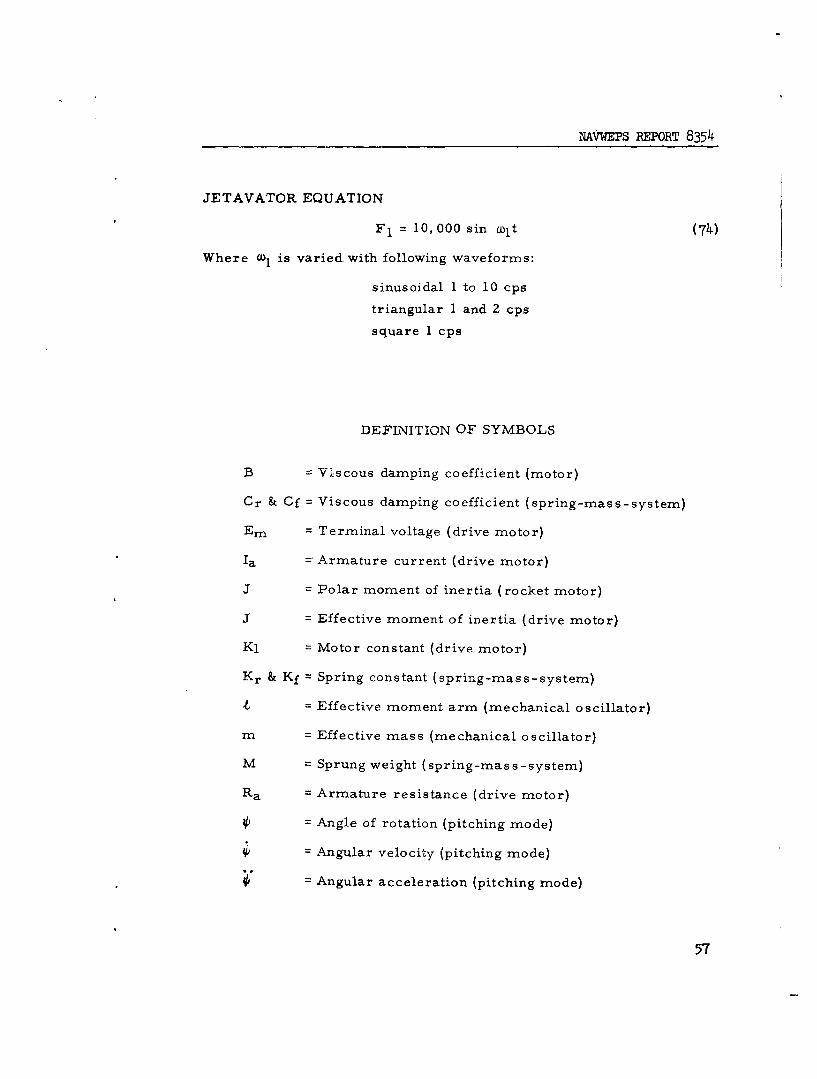
NAVWEPS REPORT 8354
JETAVATOR EQUATION
F 1 = 10, 000 sin ai1t (74)
Where a) is varied with following waveforms:
sinusoidal 1 to 10 cps
triangular 1 and 2 cps
square 1 cps
DEFINITION OF SYMBOLS
B = Viscous damping coefficient (motor)
Cr & Cf = Viscous damping coefficient (spring-mass-system)
Em = Terminal voltage (drive motor)
Ia = Armature current (drive motor)
J = Polar moment of inertia (rocket motor)
= Effective moment of inertia (drive motor)
Kl = Motor constant (drive motor)
Kr & Kf = Spring constant (spring-mass-system)
t = Effective moment arm (mechanical oscillator)
m = Effective mass (mechanical oscillator)
M = Sprung weight (spring-mass-system)
Ra = Armature resistance (drive motor)
= Angle of rotation (pitching mode)
4 = Angular velocity (pitching mode)
= Angular acceleration (pitching mode)
57

NAVWEPS REPORT 8354
Vertical displacement (rocket motor)
= Vertical velocity (rocket motor)
= Vertical acceleration (rocket motor)
S =Angle of rotation (drive motor)
S = Angular velocity (drive motor)
0 Angular acceleration (drive motor)
h = Angular momentum
58

NAvwEPS REPORT 8354
VARIABLE COEFFICIENTS
783.37 11,590
C)c'J
U)u (n (n
I-
LL
320.48 "/7,660I I -
0 60 0 60BURNING TIME, SEC BURNING TIME, SEC
M (t) i (t)
1,125 --.,500
i-
LL 0"I u
0 60 0
.J
500 + 1,5001I II
0 60 0 60BURNING TIME, SEC BURNING TIME, SEC
(CK +Cr) f(t) (Jf rCr-,+Af Cf) f(t)
14 X 105 34,780
U)
-J
IL
7 X 10 5 20,000
I .JI
0 60 0 60BURNING TIME, SEC BURNING TIME, SEC
59

NAvwEPS REPORT 8354
__ .00 10 [>I
0.40 004001
ZsIN I ..4..
..00 -410
I o +-0IN&
-100.0C- 1R CiI 10* II) -

-~ i ~ ~ 4y . -TEQUATIONS SOLVED
I 0 20.A TIME SCALED BY 10
1 o -E10F 007 *..8
SINln.I-O.OOOSIN.,IIJETAVATONRl
.00cs -1 -s
IIN
ourN L1 IS) Tf .0,200- (I .I ItemsAVA+fONNI .
CO SIN N 4 M1 R ..
250 OUT AS 0.0 (5 T- 1
AO (6 -6T
+100 ~ ~ ~ ~ ~ ~ ~ ~ J SIR 8AT -10 I 7 -000NN,(EAAO
0.5 CONTROLBL
0.250 l ON:50
OU IUT,
*104 IN, IANALO SC~h~MAIC DAGRA0. 1 41

iAVWEPS REPORT 8354
Appendix C
DERIVATION OF SYSTEM TRANSFER FUNCTIONSAND PHASE COMPARATOR SCHEMATIC
INTEGRATOR
A high-gain operational azinplifier was used in the following config-uration to provide the integration indicated in Fig. 7.
2Me, -" G e,
OPERATIONAL AMPLIFIER
The transfer function for an operational amplifier* is given as
e 2 Z f.b.
e Z in
where
Z f.b. = feedback impedance
Z in = input impedance
and in LaPlace notation
x 10f0Z f.b. = =
Z in = 2M
then 2
and K1 2
Walter J. Karplus and Walter W. Sorous. Analog Methods. New York,McGraw-Hill, 1959. P. 39.
61

NAVWEPS REPORT 8354
LEAD COMPENSATION
The lead compensation indicated in the forward loop of Fig. 7 hasthe following configuration:
e1 0vM 5 M 1-- 2 . /e,3
e3
is•MOPERATIONAL i13 OO
SAMPLIFIER•- GAIN-]I "=
Using nodal analysis:
i + i +i = 01 2 3
and
i1 = e e)
e° - e 2
2 0 M
e0
3 M
combining
S (e - e2) e e 2 eo10-- + 10 M 1 'M=0
rearranging
eo 2 + = e2 +
62

NAVWEPS REPORT 8354
and
e 0 (S + 1)
e2 (S + 11)
e3- is obtained in the same manner and ise
0 e3 (S + 1)
e 0 s + 50)
from whiche3 (S + 1)2
e2 (S + 11) (S + 50)
MINOR LOOP FEEDBACK
The differentiator and compensation circuitry indicated in theminor loop feedback path of Fig. 7 utilizes an operational amplifierconnected as follows:
.5 M6e in eo
S5. 6 K
MAG-AMPBIAS WINDING 1_17
63

NAVVEPS REPORT 8354
Using the transfer function for operational amplifiers
eo Z f.b.e in Z in
It can be shown that the feedback capacitor in the above sketch used forfiltering the differentiated ripple of the tachometer output, will con-tribute a pole in the overall transfer function at S = -100 and as suchwill not significantly affect the root locus plot. Therefore, the capac-itor will not be included in the following derivation:
el lO M 20 S
e in M(S•+•2)•5M +S
and
e o 0 lM _ 10 (S +1)e, 2 (S +2)
TM + & +
S
so that the final transfer function is
e e1 e1
eo 200 S(S + l)"e in (S + 2
The tachometer constant of 0.3 and the conversion for the 5.6K loadresistor gives a final transfer function of
i7 10.8 x 10⁻³ S(S + 1)e (S + 2)2
K4 = 10.8 x 10⁻³
64

NAVWEPS REPORT 8354
PREAMPLIFIER
The preamplifier indicated in Fig. 7 has the following experimen-tally determined response curve:
16 v - - -R-
MAX. CURRENT REQUIREDe 3
3.33 v - - - MIN. CURRENT REQUIRED
i0 Ms .50msi4
The response characteristic is considered linear over the necessaryrange of operation. The preamp constant is found to be:
"4- = A1 3 x 10⁻³
e 3
SIGNAL SENSORS
The input signals to the phase comparator were obtained with theuse of carbon film potentiometers (see Fig. 31 for approximate hardwarelocation). The sinusoidal signals depicting the driving-function re-sponse and the reference response were obtained by attaching a sine-cosine, continuous-turn potentiometer to the rotating shaft of the forcegenerator. The signal depicting the displacement motion was obtained byattaching the sliding arm of a linear-motion potentiometer to the thruststand leg. Although the sine-cosine unit was adequate in the operationof the experimental system, these units have a relatively short life andshould be replaced with electromagnetic devices in the development of anoperational system.
65

INAVWEPS REPORT 8354
ROCKET MOTO
FIG.~~~~~~~~~~RN 31SUP oce oo he-oPOnTEntSaDProtoUS Firing. (YP
FORC GENRATO
66DIEMT IECSN

NAVWEPS REPORT 8354
DC DRIVE MOTOR
The motor constants, Ra, La, and K, were determined experimentallyusing the procedure described in the literature cited below.* The valueswere found to be:
R = .86 ohms
a
La = 4 ýih (negligible)
K = 1.68 ohm-secondradian
The inertia was listed by the manufacturer for the motor and was calcu-lated for the force generator. The total inertia is
J = .71 ft-lb-sec2
The motor time constant is defined as
R Ja
and is T = .1 secondsm
Since 1/Tm positions the pole in the motor transfer function, the follow-ing expression is obtained, neglecting La:
e S 0e6 S (S + 10)
MAGNETIC AMPLIFIER
The steady-state response curve of the magnetic amplifier and drivemotor was determined as a single unit under operating conditions, seepage 20. The transient response characteristic of the magnetic amplifierwas determined experimentally as shown in the following sketch:
Office of Chief of Ordnance, Dcpartment of' the Army. S-orvechan-isms., Section 4, Power Elements and System Design. Aug5ust 1959. (ORDP20-139).
67

NAVWEPS REPORT 8354
MAG-AMP FIELD Rf
OUTPUT2608 OSCILLOSCOPE
POWER OSC CAMERA
ARMATURE S, RECORDINGOUTPUT R2 R,
In the above setup the fixed resistance Rf is connected to thefield output terminals of the amplifier to simulate the field of thedrive motor. The resistance R1 simulates the motor armature load. Anappropriate resistance was chosen to correspond to 1/2 full load. Withthe mag-amp energized the switch S1 was closed. The load of R2 is thenadded to that of R1 . The resulting transient was recorded and is inter-polated below.
STEPINPUT VRIRz -.0
(VOLTAGEACTUALLY OUTPUT RESPONSE
DECREASES) 06-
.1
SECONDS
The response curve approaches that of an exponential resulting froma pure R, L circuit having a time constant of 0.1 seconds. Thus, thetransfer function is
e6 A2 A 2
i5 (S1,aT) (s +o)
A2 is determined from steady-state characteristics as described on
page 20.
68

+28 i
+286
+28 -
2000
12 K2.9mlOOK
-4 lOOK
+289
20K201 0200 K-4
0 L T-1,01NA-IM0)10
.001~2. Mf N6
SWTHNGIRCUTR DIOD LOI

_____________________________ ____ AVWEPS REPORT 8354
+ 281
II228
+28 1 +2
28+28 M2.M40
67
+288
28 +22+ 8156MA P IFE
OIOO LOI MLFI IVRE SUMMER 8FI FLIPFOP ITGAO
2NI69

NAVWEPS REPORT 8354
BIBLIOGRAPHY
Chestnut, Harold and Robert W. Mayer. Servomechanisms and RegulatingSystem Design, Vol. I. New York, Wiley, 1961.
-- Servomechanisms and Regulating System Design. Vol. II. NewYork, Wiley, 1956.
Cosgriff, Robert Lien. Nonlinear Control Systems. New York, McGraw-Hill,1958.
Gardner, Murray F. and John L. Barnes. Transients in Linear Systems,Vol. I. New York, Wiley, 195b.
Karplus, Walter J. and Walter W. Sorous. Analog Methods. New York,McGraw-Hill, 1959.
Office of Chief of Ordnance, Department of the Army. Servomechanisms,Section 4, Power Elements and System Design. August 1959. (ORDP20-139).
Savant, C. J. Basic Feedback Control System Design. New York, McGraw-Hill, 1958.
Thaler, G. J. and R. G. Brown. Servomechanism Analysis. New York,McGraw-Hill, 1953.
Thaler, G. J. and Marvin P. Pastel. Analysis and Design of NonlinearFeedback Control Systems. New York, McGraw-Hill, 1962.
U. S. Naval Ordnance Test Station. A System for Correcting for SpuriousNatural-Frequency Ringing of Rocket Static Thrust Stands, by J. S.Ward. China Lake, Calif., NOTS, 1 September 1960. (NAVWEPS Report7569, NOTS TP 2541).
-- - Determination of Rocket-Motor Mass by Measurement of the NaturalFrequency of a Mass-Spring System, by Benjamin Glatt. China Lake,Calif., NOTS, 15 June 1961. (NAVWEPS Report 7741, NOTS TP ý706).
-- - Design Cirteria for Large Accurate Solid-Propellant Static-ThrustStands, by D. P. Ankeney and C. E. Woods. China Lake, Calif., NOTS,June 1963. (NAVWEPS Report 8353, NOTS TP 3240).
70

to (L)i R U O O W rd F) .4 4
9 4 D d~' -r 0) rq 10)Q ) 4- t0)u -rd
4) ~ ~ ~ ~ H *H4't4 P "-P-0 P
FA W W 0 0 0bP4~W m Q.a) :t 0
0 4' C 0 - 1x W* 4 to I 0 4-' 00 4) 1 to ri*HU'4' ~ (1 ul 'd. ' H' * U
E- ~ ~ ý 0 0 p ;Hj~-UE4dE4 ~ R*
P P - 0H. 9 '4-) 0C) >20 4 0 q 4-') .0 (L) cc a) 'd 0 C C)-R '' 0)-40 ) r
*) 44)H pO00Q) 0 a)U0
-P () C) 0 4 a) g0CH w -P 0C W ~ 4 A ' t O 4 3 Q)
P0 U QQ~'~f ) C ýpU Q) r~l a) -
E- o' m Pfl qs- -r 5q, - H A
ý,o~~~- H WC drdO, r .HCl) t- r, C Cdro 4- mr- Q)~ U W co* 4 WH
HCCr (0C)' WCiC Pq43I )ý 4-CO 4.3 0 , ~ ' 0 CO.-c ('1)U'
C) 0 ~ 4/2)U CO 4-d-i C O)4 0 C0 U' WdWHO ~0 WHO)-1 P*HO 0 *H' a)0+ )- *Hq * . 0~
0 H 0~ 0 0W4'0 H
., 0 - rd ' t r:- *H I (1) 4 i W~4- rd .M
4 d 0 4 0-04WJ 4-) 0.0 Q)M)
0* WH 0W- + 0 4-3W ~ W '
ri~c 4 -0 I~C 0 H to *- 0 0 0 'rIg ! CF-C )Wrd0 .-1 0 E-4O 4H W rd () PA4 Q
A) M~0 0 0d4 C) 1 0 Q ,0' 4' o0I'd ' 00\ (L) X C) = 4)ý U 4 :
0) Cd (n 4 (L) r ~0) (Y) 4 'H r0 0'4 4C) - t o C)CC) 00 OC -P I C)Q0 rH.4'r0U2 ca w rdH 4r0 0toQ m r
0P~C p~ P~- 0. E-iW H OW a -
0 HU0 (L) C)) 0) 0' U (1 CH) a
*CH 4~\~) 'C -:, *CH ..PU C) A 4-4-3~U (/r 4f rd. ;JZU CjCrbf 4- C)r0 ' +)') U'1 - - 4040 0 0 ,4 '-, E0 53 rd 0 H C r dr4U -- r ,

0~~ *,-44 'li bat) AO 4' 1ýi0
) o4 1a, d o Ic* r. - 4 3ýý,-4 " ,- '0 H q a,- a)-,0C.
a)r J -4 r4-) +3 COlo 4'd 0
r-I ~~ a) toa)
to 0 00 Q 0 0 C~ 4-3 0'd r-- (D43 r-cx 0 p o -P -r rH O 4'0rq 04-
-1 43 q00 4' cd ~Id(L) o.H , 4-34' 4) o lr
00l 0 )0 j
-P 4'H0 t r:rjý
H H 0 2~ 4
Q'O3~d 04C -30 t
4j '(
0 P42' 0~ $4'4 Lf\+3 rFj~~~ ~ ~ ~ bD CCý> 2o P 4l,d t~oc a CYd to cd(1co 0 w o Cd 91 iH C
a) a)rd 0 0-4 V ag * 41)fr~P 4 gg.,4q P44' ~~c '4'a ~ d 0'4,o to 'C'd 4 4 '
INITIAL DISTRIBUTION
9 Chief, Bureau of Naval WeaponsFWAM (1)R-14 (1)RM-3 (1)RM-35 (1)RMMP (1).RM-12 (1)RMMP- 2 41 (1)RmwP-4 (1)RT (1)
10 Special Projects OfficeSp-O0 (1)Sp-O1 (i)Sp-20 (i)Sp-27 (1)Sp-27l (3)Sp-274 (2)Sp-3 (1)
4 Chief of Naval Operations (Operations Evaluation Group)1 Chief of Naval Research (Code 1o4)1 Naval Air Test Center, Patuxent River (Aeronautical Publications
Library)1 Naval Avionics Facility, Indianapolis (Library)1 Naval Explosive Ordnance Disposal Facility, Naval Propellant Plant,
Indian Head1 Naval Propellant Plant, Indian Head1 Naval Weapons Evaluation Facility, Kirtland Air Force Base (Code 401)2 Naval Weapons Services Office1 Operational Test and Evaluation Force2 Bureau of Naval Weapons Branch Representative, Cumberland (SPH)1 Bureau of Naval Weapons Representative, Azusa3 Bureau of Naval Weapons Representative, Sunnyvale (SFL)2 Bureau of Naval Weapons Resident Representative, Bacchus (SPLB)2 Bureau of Naval Weapons Resident Representative, Sacramento (SFLA)1 Air Force Cambridge Research Laboratories, Laurence G. Hanscom Field1 Air Force Flight Test Center, Edwards Air Force Base1 Air Proving Ground Center, Eglin Air Force Base1 Arnold Engineering Development Center, Tullahoma2 National Aeronautics and Space Administration
R. Ziem (1)W. Cohen (i)
1 Allegany Ballistics Laboratory, Cumberland1 Bruce H. Sage Consultant, Pasadena1 Hercules Powder Company, Bacchus Works, Bacchus, Utah1 Inca Engineering Corporation, Pasadena