R-R1?9 253 RESILIENT MODULUS OF FREEZE-TNON AFFECTED GANULAR 1/1SOILS FOR PAVYEMENT DES.. (U) COLD REGIONS RESEARCH AND

UNCLAS ENGINERING LAG HANOVER N D M COLE ET A. FED S7

Z L S IF IED CR R E L- -2 0T'F A A/PN- 4--16-P T -3 FO G/1 3 L

-mhhhhhhhhhhhlsmhhhhhhhmhlm

'~1.0 :lEU,

1I 1.25

/|

DOTIFAAIPM-84116,3 Resilient Modulus of Freeze-ThawAffected Granular Solis for

Program Engineering Pavement Design and Evaluationand Maintenance Service Part 3. Laboratory Tests on Soils fromWashington, D.C. 20591 Albany County Airport

I3iC FILE COPY

N D.M. ColeD.L. Bentley

a') G.D. DurellT.C. Johnson'"

U.S. Army Cold Regions Research andEngineering LaboratoryHanover, New Hampshire 03755-1290

February 1987

This document Is available to the publicthrough the National Technical InformationService, Springfield, Virginia 22161

-DTIC"ELECTE

us ~ TranporttionAPR 2 11987US. D of TrJon E

RN~~ma7 4~kk 2l Wlo 06..

For conversion of SI metric units to U.S./Britishcustomary units of measurement consult ASTMStandard E380, Metric Practice Guide, publishedby the American Society for Testing and Materi-als, 1916 Race St., Philadelphia, Pa. 19103.

NOTICE

This document is disseminated under the spon-sorship of the Department of Transportation inthe Interest of Information exchange. The UnitedStates Government assumes no liability for itscontents or use thereof.

Technical Report Documentation Page1. Report No. 2. Government Accession No. 3. Recipient's Catalog No.

DOT/FAA/PM-84/16,3- t9/T 70Ft4. Title and Subtitle 5. Report Date

RESILIENT MODULUS OF FREEZE-THAW AFFECTED February 1987GRANULAR SOILS FOR PAVEMENT DESIGN AND 6. Performing Organization CodeEVALUATION. Part 3. Laboratory Tests on Soils fromAlbany County Airport S. Performing Organization Report No.

7. Authors)D.M. Cole, D.L. Bentley, G.D. Durell and T.C. Johnson CRREL Report 87-2

9. Performing Organization Name and Address 10. Work Unit No. (TRAIS)

U.S. Army Cold Regions Research andEngineering Laboratory 11. Contract or Gront No.Hanover, New Hampshire 03755-1290 FHWA-8-3-0187

13. Type of Report and Period Covered12. Sponsoring Agency Name and Address

U.S. Department of TransportationFederal Aviation Administration _-_

Program Engineering and Maintenance Service 14. Sponsoring Agency CodeWashington, D.C. 20591 APM-740

15. Supplementary NotesCo-sponsored by: Federal Highway Administration, Washington, D.C.

Office of the Chief of Engineers, U.S. Army, Washington, D.C.

16. Abstract

"b- This is the third in a series of four reports on the laboratory and field testing of a numberof road and airfield subgrades, covering the laboratory repeated-load triaxial testing of fivesoils in the frozen and thawed states and analysis of the resulting resilient modulus measure-ments. The laboratory testing procedures allow simulation of the gradual increase in stiffnessfound in frost-susceptible soils after thawing. The resilient modulus is expressed in a nonlinearmodel in terms of the applied stresses, the soil moisture tension level (for unfrozen soil), theunfrozen water content (for frozen soil) and the dry density. The resilient modulus is about10 GPa for the frozen material at temperatures in the tange of -5 to -8C. The decrease inmodulus with increasing temperature was well-modeled in terms of the unfrozen water content.Upon thaw, the modulus dropped to about 100 MPa and generally increased with increasingconfining stress and decreased with increasing principal stress ratio. The modulus also in-creased with the soil moisture tension level. The resilient Poisson's ratio did not appear tobe a systematic function of any of the test variables.

l417 4tY Words 18. Distribution Statement

Airfied d- Roads This document is available to the publicFreezing-thawing Soil tests through the National Technical Informa-Laboratory tests 'Subgrade solls tion Service, Springfield, Virginia 22161.Repeated-load triaxial tests -

Resilient moduli -19. Security Classif. (of this report) 20. Security Classif. (of this page) 21. No. of Pages 22. Price

Unclassified Unclassified 40 %

Form DOT F 1700.7 (8-72) Reproduction of completed page authorized

PREFACE

This report was prepared by David M. Cole, Research Civil Engineer, Applied ResearchBranch, Experimental Engineering Division; Diane L. Bentley, Research Civil Engineer,Civil Engineering Research Branch, Experimental Engineering Division; Glenn D. Durell,Mechanical Engineering Technician, Engineering and Measurement Services Branch, Tech-nical Services Division, and Thaddeus C. Johnson, Civil Engineer and Chief of the Civil En-gineering Research Branch, Experimental Engineering Division, U.S. Army Cold RegionsResearch and Engineering Laboratory.

This report covers certain aspects of a project partially funded by the Federal HighwayAdministration and the Federal Aviation Administration, and the Office of the Chief of En-gineers through DA Project 4A762730AT42, Design, Construction and Operations Technol-ogy for Cold Regions; Task A2, Soils and Foundations Technology/Cold Regions; WorkUnit 004, Seasonal Change in Strength and Stiffnew of Soils and Base Courses.

The work was done at CRREL and a number of people contributed to the successful con-clusion of this area of the project. The authors acknowledge in particular E. Chamberlainwho was closely involved in equipment development, D. Carbee for his help in specimenpreparation, D. Keller who assisted in field coring and sample preparation, L. Irwin forhelpful discussions of the test results, J. Ingersoll who was responsible for generating themoisture characteristic curves and who assisted in the development of the tensiometer sys-tems, and A. Tice who generated the unfrozen water content data for the test soils.

This report was technically reviewed by E.J. Chamberlain and F. Sayles of CRREL.The contents of this report are not to be used for advertising or promotional purposes. Ci-

tation of brand names does not constitute an official endorsement or approval of the use ofsuch commercial products.

AccessI an For

INTIS GRAMITIC TAB

U113nnouncedJust lfctto0

Dimt ribution/Availability Code,

l~valtl mid/or

Special

' .

CONTENTSPage

Ab s t r a ct........................... ....Prefe.............................. .......Introduction ................................Test sections and materials ............................................ 2Specimen preparation ................................................ 4

Test sodls........................................................ 4Asphalt concrete.................................................. 4

Laboratory testing................................................... 4Soil testing ...................................................... 4Waveforms of applied stress.......................................... 5Asphalt concrete.................................................. 6

Data reduction and analysis............................................ 6Soil ............................................................ 6Asphalt concrete.................................................. 7

Results and discussion ................................................ 7General ......................................................... 7Resilient modulus ................................................. 10

Summary.......................................................... 14Conclusions ....................................................... 14Literature cited ..................................................... IS5Appendix A: Soil moisture tension versus water content for several test soils ........ 17Appendix B: Tabulated results for all tests on frozen and thawed soils ............. 19

ILLUSTRATIONS

Figure1. Albany Airport taxiway profiles .................................... 22. Gradation curves for Albany soils.................................... 33. Load pulse waveforms used in the repeated load triaxial tests ................ S54. Regression analysis results showing modulus versus temperature for various

waveforms for asphalt concrete specimens in repeated load, unconfinedcompression ................................................ 9

5. Regression analysis results showing resilient modulus versus temperature ....... 11 I6. Dependence on moisture tension of k, that characterizes the resilient moduli of

thawed and recovering soils .................................... 127. Resilient modulus versus stress functions for several principal stress ratios ... 13

8. Resilient modulus versus stress function for various levels of moisture tension. . 14

TABLESITable

1. Physical characteristics and classification of the Albany Airport soils......... 4

2. Results of regression analyses-asphalt concrete and test soils from AlbanyUAirport.................................................... 8

3. Additional regression equations for some frozen soils ..................... 94. Average values of resilient Poisson's ratio for the test soils ........... 10

ii.6

Resilient Modulus of Freeze-Thaw Affected Granular Soilsfor Pavement Design and Evaluation

Part 3. Laboratory Tests on Soils from Albany County Airport

D.M. COLE, D.L. BENTLEY, G.D. DURELL AND T.C. JOHNSON

INTRODUCTION flection measurements on the two taxiways andverifies the laboratory-determtined resilient modu-

This is one of four reports that document the lus expressions developed in the present work. Thelaboratory and field test results of an extensive re- verification is accomplished through the use of asearch effort jointly funded by the U.S. Army computer code (called NELAPAY) that carriesCorps of Engineers, the Federal Highway Admin- out a layered elastic analysis of the pavement sys-istration and the Federal Aviation Administra- temn. The program and the verification proceduretion. The project, entitled Full-Scale Field Tests. to have been covered in detail elsewhere (Irwin andEvaluate Frost Action Predictive Techniques, Johnson 1981).called for laboratory testing and field verification Field data on the temperature and moisture ten-of the resilient properties of a number of test soils sion history of the test sections provided the ap-located at Winchendon, Massachusetts (the sub- propriate range of these variables in the labora-ject of Parts 1 and 2 [Cole et al. 1986, Johnson et tory testing. Specimens were first tested in re-al. 1986a] of this series of reports) and Albany, peated-load triaxial compression in the frozenNew York (the subject of this report and Part 4 state, beginning with the lowest temperature, at[Johnson et al. 1986b]). Part I includes detailed several values of axial stress and a single valuedescriptions of the laboratory testing procedures (69.0 kPa) of confining stress. Next, the specimensand methods of data analysis and interpretation, were completely thawed on specially designed tri-Consequently, this report does not dwell on such axial cell bases (see Cole et al. 1986) and tested atmatters, but instead concentrates on the presenta- up to five levels of soil moisture tension. The in-tion and analysis of results from the two taxiways creases in moisture tension were achieved by draw-that we investigated at the Albany County Air- ing water from the specimen via the triaxial cell'sport. drainage system. This procedure simulates the

The objectives of the work call for characteriz- gradual recovery of stiffness experienced by thaw-ing the test soils under a variety of seasonal condi- weakened soils.tions: frozen, thawed and recovered. The first two The repeated-load triaxial testing yields the re-conditions are self-explanatory; "recovered" re- silient modulus, Mr (defined as cyclic stress divid-fers to soil that has drained and possibly consoli- ed by recoverable axial strain), as a function of ap-dated after thawing and has consequently regained plied stresses, temperature (for soils in the frozen(or recovered) the same degree of stiffness it pos- state), moisture tension (for the unfrozen state),sessed prior to the freezing and thawing cycle. The and dry unit weight _Yd where applicable. A simpletesting sequence used in the laboratory work is nonlinear relationship of the formdesigned to simulate the progression of events thatthe soils experience in the field. This process relies Mr= k [f()1k1(I

heavily on the use of soil moisture tension andtemperature as links between laboratory and field is used to represent the test data-k, is generally aIresults. function of #, and in some cases 7~d, and k: isa

Part 4 (Johnson et al. 1986b), the companion to constant. A linear regression technique is used tothis report, presents the results of the surface de- find constants that give the best fit to the test data.

A

-. . . . .- Z

The stress function f(o) is taken as either the moisture tension profiles for each section, whichcommonly used first stress invariant J, (sum of the are presented by Johnson et al. (1986b). Grada-principal stresses) or the ratio J2/rct (ratio of the tion curves for the test soils appear in Figure 2,second stress invariant to the octahedral shear and Table I gives some physical characteristicsstress). The latter function has been examined at and classifications for the soils.length by Cole et al. (1981, 1986). Its usefulness The water table fluctuated seasonally betweenstems from its ability to adequately reflect the ten- 1.5 and 2.0 m at both sites. Frost penetrationdency of many granular soils to exhibit an increas- depths for the periods of observation are given bying modulus with both increasing confining stress Johnson et al. (1986b).(a,) and decreasing principal stress ratio (0 1/o,). Taxiway A consists of a layer of asphalt con-All analyses are carried out in terms of both stress crete, a crushed stone base, a gravelly sand sub-functions for comparison. base and a silty fine sand subgrade. Taxiway B

The reader is referred to Cole et al. (1986) for consists of a badly broken layer of asphalt con-extensive background information on the project crete, an asphalt penetration macadam stone base,in general as well as for details of the laboratory a silty sandy gravel subbase and a silty fine sandtesting methodology. The Albany County Airport subgrade.work closely follows the Winchendon, Massachu- Since the moisture retention characteristics ofsetts, activity with one exception: we tested no these materials are of interest, the moisture ten-field cores from the Albany site. All specimens sion versus water content curves were determinedwere remolded in the laboratory using material for several of the soils in the laboratory. Curvesthat had been remixed according to the original for the Taxiway A base and subbase and the Taxi-gradation specifications for the taxiway sections. way B subgrade appear in Appendix A. The sub-

grades for both taxiways were nearly identical, sothe Taxiway B subgrade curve is assumed valid for

TEST SECTIONS AND MATERIALS Taxiway A as well. We were not able to obtainsuch data for the Taxiway B subbase since it was

Figure 1 gives cross sections of each taxiway. too coarse to test in our cell.Field instrumentation yielded temperature and

TAXIWAY A TAXIWAY BDepth Thickness Thickness Depth(mM) (ram) (mrm) (mm)0 76Asphalt Concrete"0o

Asphalt -6Concrete 330178

12? Subbase330. 305

Subgrode

Bcracked and brokenBase 584

914

Subbase 914

Note: Oron to scale

Subgrode

Figure 1. Albany Airport taxiway profiles.

2

'.l

* '*. _"K

U.S. Std. Sieve Size and No.

3 3/4 4 10 40 200 Hydrometer

100- \ - . I ' I \ '

Je \ i . I I \

- \ \ I I Subgrde

60Ko-I\Subbase

t ,o I I \I ,L404

I~ f , os \

20 I I Io Il~ Ih Il I 'l l

Io I IO Oi 0.l o.o

100 10 1.0 0.1 0.01 0.001Grain Size (mm)

Gravel Sand I SICoarse I Fine IC'rse Medium Fine Silt or Clay

a. Taxiway A.

U.S. Std. Sieve Size and No.

3 3/4 4 10 40 200 Hydrometer

S80- Subbase I Ii I \SubgradeI i I I \ -

60 I I IC

20 4I

0100 10 V0 0.1 0.01 0.001

Grain Size (mm)

I Gravel Sand Slt Of Cloy

Coarsel Fine IC'rse Mediuml Fine I

b. Taxiway B.Figure 2. Gradation curves for Albany soils.

3 %.

Table 1. Physical characteristics and classification of the AlbanyAirport soils.

MaximumUnified Soil size Coefficients Specific

Soil Classification (m) C. C' gravity

Taxiway A subbase SM 19.1 95.8 2.2 2.73Taxiway A subgrade SM 0.42 4.0 1.6 2.67Taxiway B subbase GM 19.1 16.3 0.22 2.68Taxiway B subgrade SM 0.42 2.7 1.2 2.69

SPECIMEN PREPARATION three of the short cores and binding them togetherwith a thin layer of asphalt emulsion. The asphalt

Test soils concrete was tested in the dry state, althoughWe obtained shovel samples of all the layers of moisture content is expected to affect the resilient

material. Since it was impossible to distinguish be- behavior (Johnson et al. 1978).tween the base and subbase materials of TaxiwayB because of the deterioration and insufficientthickness of the base, both layers were sampled LABORATORY TESTINGand tested as a single material.

The various soils were sieved and remixed in the All testing of the soils was carried out in one oflaboratory according to original specifications. two triaxial cells, depending upon specimen size.The coarse-grained materials were compacted in a The asphalt concrete was tested only in uniaxial152-mm-diameter, 305-mm-high mold and were compression. For all laboratory tests, we used anfrozen at a rate of 25 mm/day under open system electro-hydraulic, closed-loop testing machineconditions. These specimens were capped in the operated in LOAD control.manner described by Cole et al. (1986). They did To achieve a steady-state response, 200 loadingnot heave appreciably (i.e., less than 10% of speci- cycles were applied at each combination of axialmen height). The fine-grained subgrade material and radial stress. The Mr values were calculatedwas compacted in a tapered 152-mm-diameter, from a representative cycle near the end of each ,

152-mm-high mold and subjected to the same run.freezing conditions. Once the material was frozen, The test equipment and procedures are fully de-several 51-mm-diameter, 127-mm-long specimens scribed by Cole et al. (1986).were machined from the samples and carefullytrimned prior to testing. Soil testing

Since the frost did not penetrate to the depth of Two triaxial cells, with several unique features,interest insofar as the layered elastic analysis was were designed and built for this testing program.concerned, it was necessary to characterize the The cells differed primarily in size: one accommo- .subgradc in the unfrozen (as well as frozen and dated the 51-mm-diameter specimens while thethawed) state. For this purpose, specimens (51 mm other accommodated the 152-mm-diameter speci-in diameter by 127 mm long) were merely com- mens. The cells featured removable bases, whichpacted to design specifications and tested. facilitated the sequential testing of each specimen,

Additional details of the preparation proce- and built-in tensiometer systems to continuouslydures are given by Cole et al. (1986). monitor soil moisture tension.

Since handling of the frozen specimens present-Asphalt concrete ed no serious problems given adequate coldroom

We were able to obtain usable cores of the as- facilities, a single cell base equipped with a ther-phalt concrete layers for both taxiways. Taxiway mocouple was used for the frozen state tests.A was sufficiently thick to yield 102-mm-diam- However, since many specimens were often ex-eter, 250-mm-long cores, which were easily tremely weak and deformable upon thawing, thetrimmed and tested. The thin asphalt layer of removable cell base concept was developed. ThisTaxiway B, however, made it necessary for us to approach called for designing triaxial cells thatform a specimen of adequate height by stacking could be completely assembled about a specimen

4I1

that was mounted on the cell base. We used up to at three points, equally spaced about the circum-six bases for the small cell and four for the large ference, at midheight on the specimen. The loadcell. In this manner, a number of specimens could was monitored by a miniature load cell, mountedbe tested sequentially without removing them in the triaxial cell, in direct contact with the topfrom their respective cell bases. The major cell cap of the specimen. This load cell also served as acomponents and the deformation and load meas- feedback, controlling the load applied by theuring devices were easily transferred from one testing machine.base to another. Cole et al. (1986) give details of These measurements allowed the calculation ofthis procedure and of the equipment design. both resilient and permanent strains in the axial

The sequential testing approach was used to al- and radial directions, which in turn allowed thelow the maximum amount of testing on each spec- calculation of resilient modulus and resilient Pois-imen and to allow use of the major cell compo- son's ratio (14,).nents while tested specimens were equilibrating atnew moisture tension levels. Simulation of the re- Waveforms of applied stresscovery period after thawing was achieved by alter- The soils were subjected to two loading wave-nately testing and drying each specimen until the forms that correspond to the loading characteris-moisture tension reached the level observed in the tics of the two devices used in the surface deflec-field. At each level of moisture tension, a speci- tion tests done in the field. The waveform simulat-men was subjected to the sequence of confining ing the Repeated-load Plate-Bearing apparatusand nominal deviator stresses given in Cole et al. (designated RPB) was a 1-s-on, 2-s-off pulse. A(1986). The actual deviator stresses at each data 28-ms haversine, repeated every 2 s was used topoint, with slight corrections for the changes in simulate the load pulse produced by the Falling-specimen area, are given in Appendix B. All of the Weight Deflectometer (designated FWD) (Fig. 3).triaxial tests were carried out with a vacuum ap- Throughout the course of this study, we made aplied to the specimen through the drainage system. gradual shift in the field verification work fromThe vacuum level coincided with the desired soil the use of the RPB device to the FWD device. Inmoisture tension level for the test. This was done the Albany County Airport work, we used theto ensure a constant moisture tension level FWD device exclusively, but continued to applythroughout load cycling, the RPB loading waveform in the laboratory test-

Axial deformation was measured on the speci- ing for the sake of continuity with earlier work.men with a system of four Linear Variable Differ- Initial tests indicated that there was no signifi-ential Transformers (LVDTs), which measured cant difference in the modulus determined withthe relative displacement of two circumferentially these two waveforms, so we decided to apply themounted rings. Radial displacement was measured FWD pulse as a rule and spot-check the modulus

Is 2s

FWD

28 mns

Figure 3. Load pulse waveforms used in the repeated load triaxial tests (repeat-ed load plate-bearing apparatus [RPBJ waveform and falling- weight deflect-ometer [FWD] waveform).

%.

periodically with the RPB pulse. Consequently, in cycles for the lower stress levels and within aboutcontrast to Cole et al. (1986) where modulus equa- 50 cycles for the higher stress levels.tions were presented for each waveform separate- The test data were subjected to multiple linearly, the equations presented in this work are applic- regression analysis, the details of which are givenable to both waveforms for all granular materials, in Cole et al. (1986). We employed the simple non-

linear expression given by eq 1 to represent theAsphalt concrete material in the thawed state. The coefficient k.

The asphalt concrete cores were tested at tem- was treated as a function of 4 and 'Yd, where ap-peratures of -10°, 50, 250 and 40*C in uniaxial plicable. The exponent k2 was considered constantcompression. Maximum axial cyclic stresses of ap- for a given material with a given freeze-thaw his-proximately 68.0, 103.0, 136.0, 174.0 and 228.0 tory. Earlier work indicated that k2 does not varykPa were applied under three waveforms, systematically with 4 (Cole et al. 1981).

Axial deformation was measured using LVDTs The analyses employ one of two stress functionsmounted on circumferential clamps. Load was to model the stress dependency of the thawedmeasured by a load cell mounted on the actuator soils: J, the first stress invariant, and J 2 /rct, theof the testing machine. The machine was operated second stress invariant divided by the octahedralin LOAD control, as in the soil tests. shear stress. The former stress function is tradi-

The asphalt concrete tests employed three wave- tional and reflects the tendency of the modulus toforms: the RPB and FWD pulses described earlier increase with increasing bulk stress. However, J, isand a continuous haversine at frequencies of 1, 4 insensitive to the effect of the principal stress ratioand 16 Hz. The latter loading condition was in- a,/a,. It is frequently observed for granular soilscluded for completeness and is according to ASTM that modulus decreases as the principal stress ratioD3497-79T (ASTM 1981). increases. The latter stress function, J/Toct, ad-

dresses the effect of principal stress ratio and thusproves useful in the present analysis.

DATA REDUCTION AND ANALYSIS In a common repeated-load triaxial test, whereo2 = a3 and a, = a3 + ad, the two stress functions

Soil are given as:The frozen state test on a given soil yields an Mr

value for a certain stress level and temperature. J, = ad + 3a, (2)Testing in the thawed or unfrozen states yields anMr value for a given applied stress state and mois- 9o + 6a, adture tension level. Not all of the stress levels given J/roct =(3)

in Cole et al. (1986) could be applied to each speci- N(

men at all values of moisture tension, 4. Since where J, = 01 + 02 + 03

each specimen was tested a number of times, it J2 = G002 + 0203 + 0,,

was important to avoid excessive permanent de- rocI = 1[(o,-2)' +(o-) + (G'-,)2 /2.

formation in the early stages of testing. Conse-quently, the testing of thawed material at low 4 See Cole et al. (1981) for details regarding eq 3. ,,,

values was often terminated before the higher Moisture tension is incorporated in the modulusstress levels were applied. Appendix B gives the ac- expression (eq 1) through the term 1(101.36-4)/tual stress levels z.pplied for each test. In general, '0oA, where 4 is in kilopascals, 4o is a referencenewly thawed specimens (4' = 2 kPa) were tested stress of I kPa, and 101.36 is atmospheric pressureto deviator and confining stress levels of approxi- in kilopascals. For soils in which dry unit weightmately 28 kPa; the associated resilient axial strains varied significantly, the term d/To entered intowere approximately 3 x 10-' to 4 x 10-'. Stiffer the analysis. -o is a reference density of I Mg/m'.specimens were tested to stress levels of approxi- As in Part I of this series (Cole et al. 1986), themately 70 kPa and corresponding strain levels frozen state test data were analyzed in terms of thenear 8 x 10-'. unfrozen water content, W,, normalized to the

As a result of the testing sequence, each speci- total gravimetric water content, WT. The expres-men generated from 50 to 70 data points. Each of sions for W u, are of the formthese data points represents a nominally steady "S.state material response after 200 load cycles. The W = a(-O/o0) -b (4)resilient behavior generally stabilized within 10-20

6

* .,

S°O

where W, is gravimetric water content expressed model the temperature dependency of the resilientas a decimal, a and b are regression constants, 0 is modulus.the temperature in degrees celsius, and 00 is a ref-erence temperature of I C. The expressions for

W, were obtained using the pulsed Nuclear Mag- RESULTS AND DISCUSSIONnetic Resonance (NMR) method* (for additional 0.details, see Cole 1984). The Taxiway A base and Generalsubbase materials were too coarse for testing in Appendix B gives a tabulation of all the labora-the NMR device, so it was necessary to estimate tory test results on the frozen, thawed and unfro-the constants needed in eq 4. The exponent b is the zen soil specimens. The tabulation gives confiningmore important of the two. A value of 0.25, ap- and deviator stress levels, resilient axial and radialproximately in the middle of the range of typical strains, -r, Afr, _Yd, gravimetric moisture contentvalues, proved suitable, producing values of R2 = and i. Temperature is given for all frozen-state0.92 in the resilient modulus regression analyses tests.for each soil in the frozen state. No attempt was Table 2 gives the results of the regression analy-made to account for the physical characteristics of ses for all soils under all test conditions. The as-the soils in the determination. phalt concrete analysis results are also given in

The range of validity of the frozen state tests is Table 2, and the results of the analysis are plottedfrom -5.0' or -8.8°C, depending on soil type, to in Figure 4. These equations produce Mr values inthe completely thawed state. The analysis was ac- megapascals, provided the units of all variablescomplished by including a number of data points are appropriate (see notes, Table 2). Two or morerepresenting the condition of the material upon equations appear for a given soil and state inthaw. Clearly, problems are encountered with eq 4 Table 2. This was done to demonstrate the influ- orif the soil temperature, 0, is set equal to zero. ence of either different stress functions or addi- P,.*

However, this problem vanishes upon the follow- tional terms (i.e., a density term) on the empiricaling consideration. As the temperature of the fro- result. Subsequent work on the verification ofzen soil increases, it eventually reaches a point be- these results using a layered elastic analysis (John-low 0°C at which all the soil water is unfrozen. son et al. 1986b) employs the simplest of theseThe temperature at which the soil is completely equations with the highest R values to represent athawed may be very close to O°C. This is true for given layer.fine-grained soils in general. As a consequence of A change in the procedure used to analyze thethe mathematical formulation, the unfrozen water frozen-state test data resulted in somewhat differ-contem term Wu/ WT goes to I before the tempera- ent constants in the regression equations for theture term goes to 0 and the singularity in eq 2 is frozen soils. The f-ozen state equations given inthus avoided. Temperatures greater than that re- Table 2 are based solely on data points obtainedquired to completely thaw the soil are not mean- from frozen specimens. The highest temperaturesingful in the frozen soil model. Thus, once the soil were in the range of -0.2 ° to -0.5 0C, and strictly I.

is completely thawed, the equations given for the speaking these temperatures define the limit of ap-thawed state are used. The equations for the fro- plicability of the equations. The frozen state equa-zen state give sensible values for modulus when tions in Table 2 were used in the layered elasticthe temperature term goes to unity. However, the analysis of the test sections.expressions are generally stress-independent, and A subsequent analysis provided a means to ex-should be used only for cases where at least some tend the range of applicability of the frozen state %,,%.pore ice is present. equations. This analysis incorporated data points %.N1

from tests performed upon thawing, and thus re- NO

Asphalt concrete suited in regression equations that are valid atThe results of the cyclic uniaxial testing of the temperatures between the limits of the equations

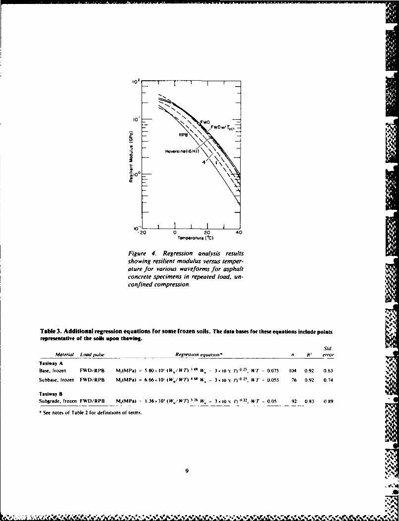
asphalt concrete were analyzed, for each type of in Table 2 and the melting point. These equationswaveform, in terms of temperature, stress and fre- are given in Table 3.quency (for the continuous haversine loading). A The equations in Table 2 appear somewhat dif-second-order expression proved adequate to ferent from the form given in eq 1. The aggrega-

tion of all terms other than the stress functionraised to a power is to be considered as the term k,

Personal communication with A. Tice, CRREL 1984. in eq I. For the thawed soils, then, k, is a function

7

Table 2. Results of regression analyses-asphalt concrete and test soils from Albany Airport (the standard er-ror Is referenced to the natural log of Mr value).

Std. Eq.Material Load pulse Regression equation n R1 error no.

Taaiway AAsphalt/concrete FWD tMr(MPa) = 1.84x 10 exp[-3.80x 10-T-9.14x 10 P ] 88 0.97 0.19 I

RPB M,,(MPa) = 1.01 x 10 exp(-6.50x 10"IT-6.50x 10-'T ] 93 0.98 0.24 2Haversine Mr(MPa) = 1.09x 10 expf-4.75x 10-IT-7.81 x I0'T/L/tij 280 0.97 0.22 3

Thawed base FWD/RPB tM(MPa) = 1.10x l04Lf(V)]'2.of(o)30 222 0.82 0.16 4

M,(MPa) = 4.44x 10'V(0)l' 21 f(a)P" 222 0.82 0.16 5Mr(MPa) = 3.68x lYV()l'ZI.fz(0)o3°f('Yd)3." 222 0.84 0.16 6Mr(MPa) = 2.56xlOLf(h)W-f,(a)s)f(_yd)29° 222 0.82 0.16 7

Frozen base t.M(MPa) = l.89x 10(w/w,) - '2. w,, =3x l0-'(-T)-0 5, w = 0.075 78 0.78 0.66 8Thawed subbase FWD/RPB tMr(MPa) = 2.07 x 10'V(0)1"1-1 fi(a)°'-' 149 0.80 0.20 9

Mr(MPa) = 4.35 x 10'1f()l]-2 .72 f() 0 "3 149 0.80 0.20 10

Mr(MPa) = 1.39x l0'(f(0)P'3t J(a)°*"f(Yd) °° 149 0.82 0.20 IIMr(MPa) = 8.00x10V(v)''Wf()°If(d)Ss 149 0.82 0.19 12

Frozen subbase tM,(MPa) = 8.18x l0o(w./wt)- '02 , Wu = 3x 10-(-7) - .25, wt = 0.055 53 0.70 0.84 13

Non-frozen FWD/RPB tMr(MPa) = 1.34x ID'V(0)j- °' f,(o)0.3 262 0.80 0.80 14subgrade Mr(MPa) = 7.73 x 10'V(4,) - ' ' f,(,) 0

.35 262 0.78 0.17 I5Tuxlway BThawed basel FWD/RPB tMr(MPa) = 5.55 x l0"f(0)]- . "-(O)P" 173 0.69 0.26 16

subbase M (MPa) = 9.67 x 10'f(0,)1 - 3' f,(a)°

'.6

173 0.73 0.24 17

Mr(MPa) = 4.28x l0,V(4)j'3."f,(0)°.7Afvd)S.3$ 173 0.71 0.25 18

Mr(MPa) = 1.56x 100f(O )ef, () 'f(Vd)7 2

173 0.74 0.23 19

Frozen base/subbase tM (MPa) = 1.00x i0(wu/Wt)- '63

. wu = 3 x 10"1(-")-

., w 0.05 92 0.96 0.42 20

Thawed subgrade FWD/RPB rMr(MPa) = 8.76x 10' V(,)]-2.38 f,(o)

0. 293 0.72 0.20 21

Mr(MPa) = 3.36x 10' V(0)1-., f1(o.34 293 0.68 0.21 22 ,

Mr(MPa) = 3.80x 10) -2-36f2(or)

" 21 ft(d)" .0o 293 0.74 0.19 23

Mr(MPa) = 1.35 x 10'i(0)]- '

,o)°'

A(Yd )-3.1 293 0.70 0.20 24

Frozen subgrade Mr(MPa) = 2.66(wu/wt)-' 02f(o)"'1, wu = 3.14x 10"1(- )-0.29, 152 0.82 0.92 25

= 0.29Mr(MPa) = 2.59(wu/wt)-4't f,(o)° ", w, = 3.14 x 10-'(-T) - , 152 0.84 0.85 26

wt = 0.29Mr(MPa) = 3.31 x l1(wuwt)-0.sf,(o)ou- , wu = 3.14x 10-(T)-o 29, 152 0.82 0.92 27

wt = 0.29Nonfrozen subgrade Mr(MPa) = 5.16x 10' f(0)1- " fi(a)0'z ' 278 0.81 0.15 28

M,(MPa) = 5.48 x 10'[f(0)] "2 " f(o)° 26 278 0.72 0.18 29M,(MPa) = 2.49x 10'[(0)1' "fi(0)°zsf(' 278 0.82 0.14 30

NOTES:RPB = repeated-load plate-bearing apparatus waveformFWD = falling-weight deflectometer waveform

= equations used in analysis f(,,) = (101.36-)/,, J, = first stress invariant (kPa)n = number of points = moisture tension (kPa) A = second stress invariant (kPa)RI - coefficient of determination 0o = I kPa rm, = octahedral shear stress (kPa)Mr = resilient modulus (a) = (J,/0) f(vd) =

T = e/eo f'(0) = (J,/rw.)/o o Id = dry unit weight (Mg/m)9 - temperature ('C) fPa) - r,,)/ao ) = I Mg/m'0o = I 'C a = stress (kPa) wu = unfrozen water content (decimal)

&= load waveform frequency (Hz) oo = I kPa wt = total water content (decimal)

a

I.t

)r - -* - ?g . . , ,,,,...,,- .,,- ,8

to,

10o

FW

%° o

\\FWDw/TC,

& RPB

Hoverimn(161Hz)

4

-20 0 20 40Temperature (*C)

Figure 4. Regression analysis resultsshowing resilient modulus versus temper-ature for various waveforms for asphaltconcrete specimens in repeated load, un-confined compression.

Table 3. Additional regression equations for some frozen soils. The data bases for these equations include pointsrepresentative of the soils upon thawing.

Sid.Material Load pulse Regression equation$ n R) error

Taxjiwu A

Base, frozen FWD/RPB Mr(MPa) = 5.80 10' (K'u/ WT) 1u = 3 tO q-T) 0 25, I4T = 0.075 104 0.92 0.63

Subbase, frozen FWD/RPB M,(MPa) = 6.66x 10' (Wu/WT) 4 14 3 Io,(-7) 0 25 , K'T = 0.055 76 0.92 0.74Taidway B

Subgrade, frozen FWD/RPB M,(MPa) = 1.36x 10' (W'TW7) 1 26 i, = 3 t 0 I- T 0 22, WT : 0.05 92 0.83 0.89

See notes of Table 2 for definitions of terms. - ...

%-

9

Table 4. Average values of resilient completely overshadowed by the temperature ef-Poisson's ratio for the test soils. fects that temperature (via the unfrozen water

content term) is the only significant variable in theA, analysis. Inspection of the R 2 values associated

with these equations indicates that the inclusion of

Base 0.33 Base-subbase 0 a stress term only marginally improves the correla-Subbase 0.39 Subgrade 0.35 tion.Subgrade 0.26 As with the soils tested in the earlier phase of

this work (Cole et al. 1986), the resilient deforma-tion was not sufficiently large to produce consis-tently measurable radial deformation in the frozen

of the term f(), and occasionally a function of soil. As a result, we were not able to calculatedry density through the term f(yd). The exponent reliable values for the resilient Poisson's ratio foron the f(o) term is, of course, k,. any of the soils in the frozen state.

As found in Part I of this series, the resilientPoisson's ratio, #r, was not found to be a system- Thawed soilsatic function of any of the test variables. Regres- Upon thaw, virtually all test soils developed asion analyses similar to those performed for the moisture tension level of 2.0 kPa, indicating aresilient moduli yielded unacceptably low values state of less than complete saturation. As notedof R 2, indicating no clear dependency of ,L on any above, these soils were tested at several levels ofof the test variables. Table 4 gives the average moisture tension up to 24 kPa, which was thevalues of Poisson's ratio calculated from all the highest value recorded in the field test sections.thawed-state test results for each soil. The dependency of Mr on moisture tension was

The regression equations generated the curves addressed analytically through the termgiven in this section with certain exceptions, notedbelow. (101.36--t )A4

Resilient modulusThe values of A, ranged from -1.34 to -4.72 for

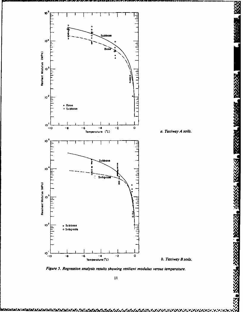
Frozen soil the Taxiway A subgrade and Taxiway B base-sub-Figure 5 shows plots of the regression equations base materials respectively. Most values, however,

for the frozen soils. These equations represent the were in the range of -2.2 to -4.0.data rather well: the R I values range from 0.83 to The influence of the moisture tension term gov-0.92. As can be seen by the form of the equations erns the response of the mathematical model tofor the frozen state, the curvature of these rela- the thaw recovery phase of the soil. All soils exper-tionships is a strong function of the unfrozen ienced an increase in stiffness with increasing #water content versus temperature relationship for level and the absolute value of the exponent A,a particular soil. The modulus of frozen soil can gives a relative indication of how rapidly the stiff-be between two and three orders of magnitude ness increases with 4.higher than that of the same soil in the thawed Figure 6 shows the effect of moisture tensionstate. Some representative data points are also level on the term k,, in eq 1, over the range of 0 toshown in Figure 5. The Taxiway B subgrade was 24 kPa. The curves in Figure 6 were generatedthe only soil to exhibit a significant stress depen- from the regression equations and are shown fordency. The plotted curve is based on representa- the k, values determined for both stress functions.tive values of J for each temperature. As mentioned earlier, and in other work (Cole

The relatively fine-grained subgrade layers have et al. 1986), the stress function J2/7o0 proved verynoticeably lower moduli than the coarse-grained effective in representing the stress sensitivity of abase and subbase layers. The greater unfrozen number of the test soils. We do not yet have suffi-water content of the fine-grained material un- cient data to ascertain why certain soils are moredoubtedly contributes substantially to the lower favorably represented by this function than by thestiffness. Additionally, the Taxiway B subgrade bulk stress model. Consequently, the stress func-was the only soil to exhibit a systematic stress de- tion that best represents a particular data set is em-pendency in the frozen state. The reason for this is ployed in the present work.unclear. Generally, the stress level effects are so .

10

00

300

.0.

102

* easeo Subbase

10-10 -8 -6 -4 -2 0

Temperature 00) a. Taxiway A soils.

0

a.a~4

10~0

10 2 Subbase

0

o Subgrade

101-10 -8 -6 -4 -2 0

Temperature (*C) b. Taxiway B soils.

Figure 5. Regression analysis results showing resilient modulus versus temperature.

1V1

7G ' I i I [ i I [ t

60- -J2 /TOct

50-

kI40-

Subbe Bose

30-.2-(bbose

20--

I0-

0 4 8 12 16 20 244', Moisture Tension (kPa)

a. Taxiway A.7I

60- Base- J2 '/Toct

50- .a Subgrode(unfrozen)

k, 4C-

-- -- Subrode20_ (thwed)

to-

0 4 8 I 2 16 20 24

*, Moisture Tension (kPo)

b. Taxiway B.

Figure 6. Dependence on moisture tension of k, the coefficient of eitherof two stress functions, J, or J2 /rot, that characterizes the resilientmoduli of thawed and recovering soils.

Figure 7 shows Mr versus the two stress func- The only drawback that we have found to datetions for actual test data from the Taxiway A base in using the J/oc t stress function is that it has alayer, 4 = 13.00 kPa. The stress ratio for all test singularity when roct = 0, i.e., in the case of hy-points is indicated. Each grouping of points in drostatic compression. Under most loading cir-Figure 7a corresponds to tests conducted under a cumstances this would present no problem. How-constant confining pressure and increasing devi- ever, in the case where the lateral stresses areator stress levels. The bulk stress, of course, in- greater than the vertical stress in the unloadedcreases as the deviator stress increases, but the re- state, there exists a certain level of applied verticalsuiting increase in stress ratio brings about a de- stress that can, in theory, bring the soil to a hydro-crease in resilient modulus. This systematic varia- static stress state and thus cause the denominatortion of modulus with stress is reduced to virtually in the stress function to go to 0. We are continuingrandom scatter when the data are plotted using the work on this aspect of the analysis with the goal ofJ2/Tct stress function as seen in Figure 7b. developing a similar stress function without the

singularity problem.

12

I iI I iI I I' ir

1.5 -Z 02.0

0

'30

102 10

Jl Stress Function (kPo)

a. J,.

I I i lI I I III I 1 11

21.5 A

. - o 2.0-2.5"3.0

VA

0

Cr

00 103

J, Stress Function (kPo)

Figure 7. Resilient modulus versus stress functions for severalprincipal stress ratios; actual test data on thawed subgrade fromTaxiway B.

Figure 8 shows modulus versus stress function Taxiway A subgrade and the Taxiway B base-sub-for various levels of moisture tension. The curves base materials respectively. The dry unit weight,were generated by eq 9 and 21, respectively, of Yd, varied little through the course of testing. Con- -Table 2. Note that while the stress function expo- sequently, a clear dependency of Mr on -Yd doesnents are similar for these two soils, the exponents not emerge from these data. Occasionally, as inof the moisture tension level terms differ signifi- the case of the thawed Taxiway A base, and thecantly (3.05 versus -1.5). The fact that the thawed thawed Taxiway B base-subbase, inclusion of aTaxiway A subbase is more sensitive to changes in dry unit weight term in the regression analysis im-moisture tension level than the Taxiway A sub- proved the correlation coefficient very slightly.grade is evidenced by the wider spacing of the con- The Taxiway B unfrozen subgrade, however,stant moisture tension level curves, showed a significant improvement in the RI value

The magnitude of the increase in Mr as a result (0.72 to 0.82) by inclusion of the dry unit weightof natural increases in during thaw recovery var- term. Care must be taken in applying the regres-ied from a factor of 1.5 to a factor of 3.5 for the sion equations that contain a _Yd density term. Be-

13

.0

,o" ~ I, I I I~~ f I,

4Jt20 ki

10 %qi.20 kPa

i0

:1k T/WA SUSBASE.THAWED T/ 8 SUGRADE, THED1 1 1

10 112 to101 02 0

J2TtStress Function (kPa)

Figure 8. Resilient modulus versus stress function for various levels of moisture tension inthe Taxiway A subbase and subgrade (curves on left from eq 9 of Table 2; curves on rightfrom eq 21 of Table 2).

cause the dry unit weights in the SI system of units Johnson et al. (1986b), verifies the present resultsare close to unity, they can bring about rather using a layered elastic analysis to predict the sur-large exponents on this term, and substitution of face deflections of the Albany County Airport testvalues outside of the range of the data set may sections.result in unrealistic modulus values.

CONCLUSIONSSUMMARY

From the foregoing test results and analyses, theFrozen- and thawed-soil testing methods and following conclusions may be drawn.

analytical techniques developed in other work 1. For the test conditions of this study, the resil-(Cole et al. 1986) were applied in a study of frost ient modulus, Mr, of the granular soils tested ineffects on pavement materials from the Albany the thawed state is well represented by a simpleCounty Airport. We developed empirical models nonlinear model of the formof the response of the test soils to cyclic loading inthe frozen, thawed and recovered states. The Mr = k, f()k '

P

models give resilient modulus as a function oftemperature (for soils in the frozen state), stress wheref(or) = J, or J,/rostate, soil moisture tension (for unfrozen soils), k, = f(O), a function of moisture tensionand in some cases dry unit weight. k, = constant.

The results of this study are in general agree-ment with our previous work regarding the effects 2. The stress function J2 /Toc was found to ade-of temperature, stress level and soil moisture ten- quately reflect the tendency of the granular soils'sion level on the resilient modulus. Although we moduli to increase with increasing confining stressmeasured Poisson's ratio in all tests, it did not ap- and decrease with increasing principal stress ratio.pear to vary systematically with the quantities af- 3. The increase in stiffness observed subsequentfecting the resilient modulus, and was thus taken to a freeze-thaw cycle can be expressed throughas a constant, the term k, which increases as the soil desatu-

One area of this study indicates that the varia- rates.tions in soil stiffness over a freeze-thaw-recovery 4. The temperature dependence of the resilientcycle can be determined using laboratory test tech- modulus can be expressed through the unfrozenniques. Another area of this study, reported by water content:

14

.'C

M, Irwin, L.H. nod T.C. Johnson (1981) Frost-

Mr -A, affected resilient moduli evaluated with the aid ofnondestructively measured pavement surface de-

where A,,A 2 = constants flections. Paper presented to the TransportationW, = unfrozen water content Research Board task force on nondestructive eval-

Wave = total gravimetric water content. uation of airfield pavements. USA Cold RegionsResearch and Engineering Laboratory, Hanover,

5. Poisson's ratio did not vary systematically N.H., Internal Report 942 (unpublished).with stress or moisture tension level and may con- Johnson, T.C., D.M. Cole and E.J. Chamberlainsequently be taken as a constant. (1978) Influence of freezing and thawing on the re-

6. The variations in soil stiffness throughout a silient properties of a silt soil beneath an asphaltfreeze-thaw-recovery cycle can be simulated in concrete pavement. USA Cold Regions Researchthe laboratory through the use of open system and Engineering Laboratory, Hanover, N.H.,freezing and proper testing methodology. CRREL Report 78-23.

Johnson, T.C., D. Bentley and D. Cole (1986a)Resilient modulus of freeze-thaw affected granu-

LITERATURE CITED lar soils for pavement design and evaluation. Part2. Field validation tests at Winchendon, Massa-

Cole, D.M., L.H. Irwin and T.C. Johnson (1981) chusetts, test sections. USA Cold Regions Re-Effect of freezing and thawing on resilient modu- search and Engineering Laboratory, Hanover,lus of a granular soil exhibiting nonlinear behav- N.H., CRREL Report 86-12. Also U.S. Depart-ior. Transportation Research Board Record 809, ment of Transportation, Federal Aviation Admin-pp. 19-26. istration Report DOT/FAA/PM-84/16,2.Cole, D.M., D. Bentley, G. Durell and T. John. Johnson, T., A. Crowe, M. Erickson and D. Coleson (1986) Resilient modulus of freeze-thaw af- (1986b) Resilient modulus of freeze-thaw affected

fected granular soils for pavement design and granular soils for pavement design and evaluation.

evaluation. Part 1. Laboratory tests on soils from Part 4. Field validation tests at Albany County

Winchendon, Massachusetts, test sections. USA Airport. USA Cold Regions Research and Engi- 5

Cold Regions Research and Engineering Labora- neering Laboratory, Hanover, N.H., CRREL Re-tory, Hanover, N.H., CRREL Report 86-4. Also port 86-13. Also U.S. Department of Transporta-

U.S. Department of Transportation, Federal Avi- tion, Federal Aviation Administration Reportation Administration Report DOT/FAA/PM-84/ DOT/FAA/PM-84/16,4.16,1.

15

APPENDIX A: SOIL MOISTURE TENSION VERSUS WATER CONTENTFOR SEVERAL TEST SOILS

so0 Y.2 16 Mg/rn 3

G,-2.71

60-

0

20-

0 5 20 15% Water (WO)

a. Taxiway A base material.

r d 2.16 Mq/rn3

=.7Mrn

S, .7 d3" *5% G1' 2.71

C

4o 40

20- 20

0 %0 Loe w)%Wtr(t

% ae0(I 20 0 10 20 30

b. Taxi way A subbase material. C. Taxiway B subgrade. I

Figure AlI. Moisture tension versus moisture content.

17

APPENDIX B: TABULATED RESULTS FOR ALL TESTS ON

FROZEN AND THAWED SOILS

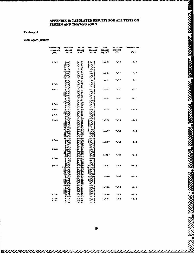
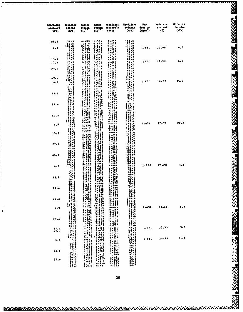
Tuziway A

Base layer, frozen

Confining Deviator AzLal Resilient Dry Moisture Temperaturepressure stress strait modulus densi5 y content

(kPa) (kta) xlO (GPa) (Kg/n ) () (°C)

69.2 66.9 '. 29 23.07 1.892 7.5. -5.'136.9 .64 21.3920. 2. 143 14.46273.7 ,.2?9 11.9234:.6 :.343496.6 ).)43 e.9666.9 r.155 4.!7 7.89. 7.5"136.9 '.S25 4.21206.8 C.%95 2.9b213.7 1.169 2.3466.9 1.'069 1. 4 1.8C 7.5: -0136.9 3.75b 7.36

27.6 40.1 1.172 1.3453.5 1.512 .3566.9 1.951 :.34

69.: 67.5 :.167 6. 1 1.932 7.57 -5.,138.3 1.057 -. 37208.1 1.429 4.85216.0 0.543 5.34344.3 J.686 5.167.5 C.207 1.26 1.932 7.50 -1.C138.0 3.a29 2.61288.5 n.!86 2.35

27.6 4:.5 C.j86 4.7154.0 3.129 4.1867.5 0.214 3.15

69.0 67.5 3.139 4.85 1.932 7.5: -2.?138.3 0.472 2.122C8.5 0.750 2.78

27.6 40.5 0.256 7.2355.2 0.097 5.6967.5 0.139 4.85

69.0 67.5 0.028 24.10 1.932 7.50 -7.8138.0 0.'63 21.90208.5 0.139 15.00276.0 0.216 12.78343.5 0.292 11.76490.7 0.445 11.0368.3 0.059 11.58 1.887 7.50 -5.0

279.5 0.421 6.64347.9 0.579 6.0127.6 69:3 1:45t 122422 3 00 27 10012 1.887 7.50 -1.0

41.0 0.068 6.0354.7 p.108 5.06

0.:161 :1

139.8 0.676 2.07211.2 1.218 1.7368.3 0.244 2.80 1007 7.50 -2.2

139.8 0.623 2.242706 27: 0.041 6.7

21: 0.067 6.125 4 .7 1 1 1 4 4

69.0 18. 0.019 36.03 1.887 7.50 -7.61390 0.050 267.96

211.2 0.125 16.90219.5 0.213 13.12347.9 0.287 12.12196.9 0.500 9.9467.3 0.042 16.04 1.940 7.50 -5.037 00139 9.9108.2 0.208 10.01

275.5 0.292 9.43342.9 0.375 9.14489.0 0.583 8.40

7.3 0.147 4.03 1.940 7.50 -2.2137. 0.581 2.7520:1 0.891 2:34273.5 10311 2.10

27.6 26.9 2.507 0.11 1.940 7.50 -0.213.5 1.253 5.l1

27.6 40.4 3.681 0.11 1.943 7.50 -0.269.0 67.3 3.969 2.17

137.8 7.993 3.17

19 %

V' %/ ,', '', !'% %', ' 'J*,''. 'li' ': . ' % T.' 7,., ." " . ', "".. ' . " " ." " " " .¢ " " ' J. . ,

Base layer, thawed

Confining Deviator Radial Axial Resilient Resilient Dry Moisture Moisture

pressure stress strain strain Poisson's modulus densiSy content tension

(kPa) (kPa) x 10 xl0 ratio (Mra) (Mg/U ) () (kPa)

6.9 .4 443 7 5 . 7 .4 . . 2.^

1C.3 J.75421 .!'. .4.'i13.P -.8 -.444 l.,-tl ;.411 C4.1

2..6 1.442 3.541 .. 4 7 ".I27.b 14.3 -. 49 1 .'?4 1.I 7"

27.9 1.4 . '6.R 3.4 ".112 -.411 6. 7 . .

c .:

1b.9 1~2 1~ .114.2 172 1 . 2 .1

17.2 1... b 2.146 7 66.13.b b.3 -.223 .7' s C4.7

14.2 (!.1 6 :!23.9 '.762 2.469 ' .17 84.&28.3 1.!4C !.41,3 :.!A 41.5 .34.5 1.7e7 4.j44 3.2 C1.2

27.b 14.2 S.59 1.142 J.49 124.226.3 -.994 2.4-8 -. !71 117.641.9 1.343 3.b12 -!71 115.956.6 2.122 5.72 .. 41n 111.7

69.3 34.5 ^.559 1.77b P.-19 194.173.9 1.229 3.47 0.323 194.3

6.9 3.5 2.112 0.253 C.443 136.6 1.98P 4.53 13.C6.9 :.224 1.57: 0.193 121.213.5 2.391 0.961 '.' 106.914.2 O.Z59 1.392 C.40u 111.917.3 5.727 1.772 0.41L 97.5

13.8 6.) :.224 1.411 3.545 168.114.2 G.391 1.013 0.386 140.1

21.0 ..643 1.772 3.36! 118.428.4 0.895 2.4Z6 ;.372 118.034.5 1.174 2.975 C.35 116.1

27.6 14.2 0.168 0.855 0.196 166.028.4 1.447 1.773 0.252 160.142.0 C.783 2.723 0.268 154.156.8 1.341 3.810 0.!53 149.4

69.0 34.5 3.335 1.393 0.243 248.074.0 3.951 3.167 0.300 233.8

6.9 3.5 0.112 C.323 0.367 107.1 1.99! 3.80 24.06.9 C.224 1.647 C.!46 116.910.5 3.336 1.000 0.336 105.014.2 0.503 1.353 0.!72 105.017.3 3.615 1.776 -1.36^ 101.3

13.8 6.9 2.168 0.586 0.286 117.614.2 0.392 1.206 0.325 117.721.0 r.559 1.765 C.317 118.928.4 0.783 2.353 0.33! 120.734.6 C.951 2.765 -.344 125.1

27.6 14.2 0.280 0.7,2 3.399 202.328.4 0.615 1.883 C.327 150.842.0 0.895 2.648 0.!38 158.656.8 1.175 3.646 :.322 155.7

69.0 34.6 0.503 1.589 0.!17 217.674.1 l.jC6 3.237 C.311 228w8

6.9 3.4 C.222 0.500 0.444 68.1 1.887 7.35 2.0 06.8 3.499 1.112 1.449 61.3

10.3 0.944 1.946 0.485 53.114.0 1.332 2.615 0.!19 53.5

13.8 6.8 0.333 0.A9C 2.!74 76.514.4 C.722 1.946 ;.!71 71.b

20.7 1.221 2.896 0.422 71.427.6 14.0 3.416 1.336 7.311 134.7

2.a 0.944 2.FI7 1.326 96.6 %6.9 3.5 .140 1.421 .3 b2.3 1.929 5.40 6.0

6.9 0.392 C.947 3.414 73.111.5 C.616 1.527 Z.4C3 68.814.2 5.896 2.1-6 :.4k5 67.517.3 1.12G 2.475 *.453 72.2

13.8 6.9 1.224 2.737 .5.34 94.C14.2 ..360 1.5P[ 1.!54 qO.221.3 1.Q52 2.423 .. ,:;! A64.82e..4 1.343 !..46 :.i11 57.1

27.6 14.2 q.-36 1.1:t C.!14 128.627.t . .r,9 2-'71 .. 654 1 3.- 1.92 t.41 .

6-), !4.c . 1.7?4 J 1 .

t.9 !.5 -.112 2.343 .7 111.1 I. ' 4.53 13.^t. .2Z4 %6k44 41.1 ^-

1 .5 -.'92 1.1.7. 7b.6

17.3 .ii4 2.217 1.659 7M.113.6 1.11.6 . 45 ; ; L.

14.,e .448 1.1,43 ^.L a821.5 3.72h 2.217 I. ZA n 4.et.

4 l.'.7 2.4.3 -'47 '4j.

34.b 1-58 !.1,37 1 1 .7.,27.6 14.2 ).136 1.,'6 .!16 134.7

2L.4 :.672 2.;i. 91. b 175.342.1 1.11s 3.-73 2.!42 125.551..9 1.568 4. Z* I.71 1 4.7

69.0 34.6 .b14 1.6'.c :.;96 214.974.; 1.127 3.4!4 3.326 216.1

20

.?.

Confining Deviator Radial Axial Resilient Resilient Dry oisture oisturepressure stress strJn strain Polsson's modulus densisy content tension

(kPa) (kpe) x10 - I0 ratio (HPa) (Mg/u ) (1) (kPa)

6.9 3.5 - .21 . 159. 1.946 3.81 2.17.2 .1 0.9 0 0-.28 139.3

13.6 2.253 0.813 -.311 133.G14.3 0.336 1.156 .201 123.717.4 .449 1.5;. .2S9 116.1

13.6 7.0 :.112 0.469 G.239 148.514.3 :.337 1. ; .337 143.j21.1 :.449 1.5C 3.299 141.02d.6 ..73& 2.125 2.344 134.634.8 3.898 2.668 0.334 129.6

27.6 14.3 3.281 0.813 0.346 175.)28.6 3.505 1.753 0.289 163.542.3 2.786 2.563 0.3c7 165.057.2 1.291 3.564 0.362 160.5

69.0 34.8 0.393 1.438 0.273 242.271.5 1.842 3.D64 0.275 233.4

6.9 3.3 0.220 0.485 0.454 69.0 1.94C 7.30 2.06.7 3.550 1.J91 0.504 61.410.2 0.681 1.819 a.48

4 55.9

13.8 1.156 2.427 0.476 56.713.8 6.7 C.330 0.789 0.418 84.9

13.8 0.771 1.699 0.454 80.923.3 1.321 2.731 1.484 74.4

27.6 13.8 0.495 1.153 0.429 119.327.5 C.990 2.733 0.362 110.6

6.9 3.3 0.110 0.485 0.227 69.0 1.950 5.40 6.06.7 0.330 0.970 0.340 69.01C.2 3.495 1.576 0.314 64.513.8 C.771 2.243 0.344 61.316.7 0.990 2.667 0.371 62.8

13.8 21.3 0.771 2.425 .. 318 83.827.5 1.211 3.457 5.350 79.5

27.6 40.6 1.100 3.337 3.33^1 121.855.0 1.706 4.675 0.3 b5 117.6

69.0 33.5 C.358 1.713 O.k11 196.965.8 .825 3.463 3.238 189.9

6.9 3.4 :.055 C.333 0.165 II.C 1.974 4.50 13.0b.7 ^.165 0.b94 0.238 96.9

1 .2 .276 1.356 0.261 96.713.8 .441 1.5LG 0.294 92.116.6 :.552 1.834 0.321 I1.7

13.8 6.7 S.110 0. 83 0.189 115.413.8 7.331 1.333 0.248 1D3.720.4 C.496 1.889 C.263 108.127.6 C.772 2.511 3.3.9 110.533.6 0.992 3.358 D.324 110.3

27.6 13.8 2.221 1.a21 3.221 138.127.6 0.496 1.946 3.255 142.041.8 .772 2.891 L.267 141.255.2 1.269 3.894 0.326 141.9

69.0 33.6 0.331 1.a72 &.Z20 223.872.0 C.772 3.339 0.231 215.8

6.9 3.4 :.355 :.05z C.22Z 134.6 1.974 !.81 24.36.7 :.110 0.5s2 O.i2 134.6

Im.b -.. ,41 1.!53 2.1 12E."13. t.7. 2..4. 151.514.P .L76 ".,' . I 15.t

* 7 "1 I. .12 lIo3

!3.b .772 2.-54 :.z 1,44.127.n 1.8 .221 J.77 -. i44 '177.'.

21.b 1.146 2. 1 1 1'71.t-? 772 2. 34 ,..! 1 171;."

69..* ! .6 '.'06 1.11, 1!: 7 .

79.1 7.027 ".779 .. 2 9.7b.9 . .

2.j5 3. 6 1..5' U

7. .. 138 1.'4 . 51.7I1.6 :..76 2.1 1 4.7

13.t 7. .. 25 1 69.?

14.1 .- t.3 2. 5 G.1 A. I21.3 L.Q I 3. . . 77 65.427.6 14.4 -.225 1.477 .152 7. 4

2b.. '..75 2.,57 :.Z2? 97.36.9 !.5 ^.113 U.417 '.271 k4.1 1.91- 5.40 6.1

7.C 1.2251 -893 3.25. 78.5I1 06 (.!44 1.4b8 .0 71.614.4 -. 563 2.324 Z.27' 71.117.5 ,.789 2.511 0.S15 70.1 %

13.8 7.0 1.169 0.774 3.118 90.614.4 ;.394 1.bJ8 1.245 89.621.3 2.676 2.51 C.27C 85.128.8 1.370 3.396 0.!15 84.8 St35.1 I.b34 #.293 0.581 81.7

27.b 14.4 1.225 1.312 0.171 109.82U.8 Z.b20 2.564 . 42 112.442.b 1. 14 3.580 0.283 119.057.6 1.803 5.075 3.355 113.5

69.0 35.1 0.394 1.792 0.220 195.775.1 1..70 3.866 0.275 193.4

6.9 3.5 0.113 0.363 0.311 97.0 1.931 4.10 13.07.0 &.226 C.754 0.3Cc 93.4

17.7 0.395 1.173 0.337 q1.l14.5 C.565 1.564 0.!61 92.517.6 C.734 2.011 0.365 87.6

13.8 7.0 1.198 2.671 0.295 104.914.5 Z.395 1.341 0.295 107.821.4 Z. 65 1.956 0.289 IC903

29.9 C.303 2.571 3.!51 112.535.2 1.242 3.186 0.390 110.5

21

.0-V

Confining Deviator Radial Axial Resilient Resilient Dry Moisture moisture

pressure strong strain strakn Poisson's modulus densiy content tensio(kPa) (kVa) :16- 10C ratio (MPa) (Mg/rn) 2 (kPa)

27.6 14.5 C.395 1.118 0.353 129.328.9 C.846 2.124 0.!98 136.242.8 1.354 3.186 0.425 134.257.8 1.912 4.195 3.456 137.935.2 0.793 1.734 3.456 2G3.172.3 1.354 3.47c 0.391 2 8.4

69.0 35.2 0.790 1.734 j.456 203.172.3 1.354 3.470 5.391 208.4

6.9 3.5 ----- C.3C8 114.3 1.93' 3.8 24.07.0 L.169 :.672 0.51 1C4.8

10.7 0.282 I.aD7 0.280 106.21,.5 C.395 1.399 0.282 103.*17.6 2.508 1.735 0.293 IG1.513.8 7.t Z.169 1.561 1.32 125.814.5 Z.339 1.175 0.289 123.121.4 S.5c8 1.791 ^.284 119.428.9 0.677 2.406 2.281 121.235.2 C.303 2.41c 1.311 121.4

27.6 14.5 0.282 1.;07 3.280 143.628.9 0.565 2.;15 3.2bO 143.542.8 103 2.7S8 3.!23 152.R57.8 1.242 3.75C C.31 154.3

69.0 35.2 5.452 1.56? 0.288 224.772.3 1.961 3.191 1.201 226.6

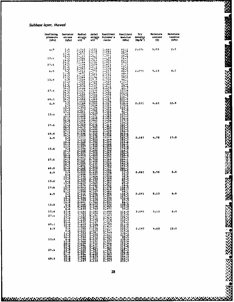
Subbase layer, frozen

Confining Deviator Axial Resilient Dry Moisture Teperaturepressure stress Ott&i modulus densisy content

(10a) (kPs) zldiD (CPa) (Mg/u 0 oC

69.3 136.3 0.342 32.38 2.020 7.50 -5.3236.0 0.083 24.82272.7 3.139 19.6233Q.3 3.264 12.85484.8 ).486 9.98136.3 0.139 3.81 2.020 7.50 -2.226.0 0.361 5.71272.7 C.639 4.27314.3 7073 3.49

27.b 13.3 1.113 3.12 2.02; 7.51 -0.226.7 2.646 1.1341.3 4.184 3.1:

69.3 66.6 6.294 .11136.3 11.230 1.12235.4 I .20 e.22 2 . ;9s 7.1 7 -1 .271. C.417 .52337. .5b% 5.7d69.5 .3-56 12.43 2.19,j 7.51 -.135.9 :.197 1*.01

2S5.4 3.139 14 .7,,271.8 -. 222 12.24338.2 3.250 13.b3483.2 :.361 13.39

6b.4 .31i9 34.97 2.399 7.5 -R.3135.3 5.:51 26.65235.4 C.577 26.68271.8 1.109 24.9453313 1.183 19.79 r493.2 3.295 16.38 %:66.4 3.108 6.15 2.391 7.50 -0.5

135.7 1.257 5.26215.4 3.435 5.37271.8 C.568 4.79338.3 0.811 4.17 .136.1 C.-42 32.40 2.044 7.5 -5.?00. 3 24 7272.2 0O1° 21.78

338.7 0.181 18.71483.8 0.361 13.469° 0069 1 08 2.044 7.50 -1.4

6. .153 a.0 .

205.6 0.333 6.17272.2 0.667 4.08338.7 1.0 1 3.38136.1 0.053 25.66 2.044 7.50 -8.8205.6 0.105 19.56272.2 0.156 17.2333:1 1:1191 11136.1 0.184 7.40 2.040 7.50 -6.505.6 0.316 6.51

7 :160.604 4.95

22

.- oI'

Subbase layer, thawed

Confining Deviator Radial Axial Resilient Resilient Dry Moisture Moisture

pressure stress stra!V strakn Poisson's modulus density content tension(kPa) (la) X0l x10- ratio (MPa) (Mg/ () (kPa)

E3.6 1.14 1.:-(,1 ' .(7 . !3.71.4 2.19 2.44 3.744 33.7

1.1.3 i.Tt 2 2.747 '.. 7& 4t.

27.b 1.3 [.16 1.7:1 &.R 77.96.9 .1 .2.161 .5 3't 9i.5 2.2' e.51 6.3

8.5 ..4 3 :.,2 1. 73.6 1

13.2 1.-35 1. 42 2.656 166.217.3 1.926 2.649 2.c.9 65.!

13.h 6.6 2.22 2.7:b 1.,SL 56.713.7 L.752 I.,jS- ).&73 2,6.j21.3 1.181 2.555 2.521 1 65.127.3 1.926 !.179 . 4 85.9

27.b 13.7 C.5!7 1.119 5.4e, 122.127.3 1.128 2.297 0.491 118.9

6.9 3.4 [.1Z7 0.!53 0.3L3 96.7 2.024 6. 13.06.8 :.269 C.7r6 G.381 96.7

1.2 f.376 I..59 C.355 96.713.7 3.591 1.530 3.386 b9.317.1 0.905 2. CC G.402 85.317.1 3.805 1.941 3.415 87.0

13.8 6.8 C.215 3.471 3.456 145.013.7 0.430 1.177 0.365 116.120.5 O.b06 1.883 0.428 18.827.3 1.181 2.648 0.446 103.2

27.6 13.7 C.322 0.765 1.421 178.627.3 0.752 1.883 0.399 145.141.0 1.449 2.945 3.492 139.154.6 1.987 4.122 0.482 132.5

69.0 34.1 C.591 1.472 0.101 231.968.3 1.235 3.164 0.4G3 222.9

6.9 6.8 0.161 3.514 0.313 133.2 2.035 5.50 24.010.3 0.322 0.857 0.!76 119.813.7 0.484 1.230 3.403 114.117.1 0.645 1.543 0.418 110.9

13.8 6.8 0.161 0.400 0.402 171.113.7 0.484 1.200 0.403 114.123.5 0.645 1.600 3.4C3 128.327.:4 0.968 2.229 0.434 122.834.2 1.344 2.972 1.452 115.1

27.6 13.7 0.269 O.ROO 3.336 171.127.4 C.645 1.772 0.!64 154.541.1 1.075 2.743 0.392 149.754.8 1.612 3.716 3.434 17 4

69.0 34.2 0.484 1.258 0.385 212.962.7 0.967 2.744 3.352 228.6

6.9 3.3 0.327 3667 G.490 49.1 2.044 7.50 2.06.6 0.762 1.455 G.524 45.19.8 1.307 2.243 0.583 43.8

13.8 6.6 1.436 1.273 0.!42 51.513.1 1.389 2.304 3.473 56.919.7 1.960 3.458 1.567 56.9

27.6 13.1 0.654 1.577 0.415 83.1 '26.2 1.525 3.338 D.457 78.6

6.9 3.3 C.081 ^.572 0.142 57.3 2.044 6.50 6.06.6 0.242 1.306 1.185 50.2q.8 C.485 2.141 0.238 48.2

13.1 G.647 2.776 a.233 47.213.8 6.6 0.202 0,980 0.206 66.913.1 C.404 2.J42 3.198 64.2

19.7 0.687 3.186 ;.216 61.727.6 13.1 C.162 1.317 0.124 100.3

26.2 0.566 2.860 0.198 91.76.9 3.5 3.109 0,353 0,309 130.1 2.08C 6.03 13.0

6.8 0.219 0.765 3.286 89.3 ,10.6 E.437 1.236 .54 85.14.1 0.655 1.6f48 G.397 85.717.7 3.874

2 119

1412 83.313.8 6.8 0.164 J.7;6 3.232 96.7

21.2 Z.819 2.11j 3.!87 ICO.0 'a28.2 1.211 3.303 3.40G 94.C A

27.b 14.1 ^.327 1.-,1 '.L27 141.L28.2 :.764 2.79 3 351 129.6

27.c 42.3 1.256 3.3fP 3.574 12-.l 2.0f(5 6.:3 13.156.5 1.474 4.716 ).13 119.7 .'

69.2 !2.9 :.)46 1.6"1 J.2!1 109.'7..b 21.2LI 3.339 .5 i1jQ.'

6. :6 --- 3.2-6 -- 149.5 2.$7J 24.C.8 ,. 2 1 8 0 , 5 3 1 : .4 1 I 1 2 A .5

10.6 C.342 -4H5 2.432 119.714.1 Z.491 1.1L 2.418 119.617.8 1.-46 1. 102 .!43 11 .8

13.8 (.8 2.1J9 L.!I 2.25 128.514.1 Z.-27 1.- 2 .ArR 132.C21.2 j.-61 1.bL2 2.564 128.12b.2 1.e74 2.162 1.411 129.435.3 :.982 2.714 ,.262 13u..

27.6 14.1 r.273 3.9.# O.269 149.523.2 '.546 1.77, -. 223 159.542.3 2.e19 2.555 0.:X8 159.556.5 1.36t 3.540 0.Sb 159.5 a-

69.0 35.3 j.437 1.20h '.?37 271.971.6 C. 47 2.951 2.196 239.1

6.9 3.3 1.220 ;;.572 0.685 58.3 2.32^ 7.53 2.06.7 2.550 1.221 1 .458 55.6

13.1 1.989 2132 45864 47.5

23 'a

%

Confining Deviator Radial Axial Resilient Resilient Dry Moisture Moisture

pressure stress straku straJn Poisson's modulus densiy content tension

(kPa) (kPa) .10- xl 0- ratio (MPa) (Mg/u ) (2) (kP&)

13.8 6.7 C.330 0.948 0.348 70.413.7 0.879 2.074 0.424 66.120.3 1.429 3.383 0.464 65.7

27.6 13.7 0.494 1.482 3.333 92.427.4 1.154 2.966 0.389 92.440.5 2.033 4.453 0.457 91.0

6.9 10.1 ,.604 1.143 0.528 88.6 2.02C 6.50 6.013.7 C.879 1.714 0.513 O.C16.7 1.209 2.286 0.529 73.0

13.8 13.7 0.659 1.315 3.5C1 104.320.3 C.989 1.829 0.541 110.827.4 1.539 2.8G1 0.549 97.933.4 2.633 3.716 0.547 89.8

27.6 13.7 0.385 0.915 0.421 149.827.4 C.879 2.173 0.405 126.141.7 1.t39 3.431 0.449 121.654.8 2.198 4.577 0.480 119.8

69.0 33.4 0.550 1.602 0.343 208.365.5 1.318 3.434 0.384 190.9

6.9 3.4 0.583 0.342 0.243 99.2 2.069 6.00 13.06.8 0.222 0.737 0.301 92.110.3 0.388 1.158 0.335 88.913.9 0.498 1.579 0.315 88.217.0 C.665 2.300 0.332 84.8

13.8 6.8 0.111 0.605 0.183 112.213.9 0.388 1.263 0.307 110.320.6 1.609 1.895 0.321 108.727.9 C.887 2.632 0.337 135.933.9 1.219 3.422 G.356 99.2

27.6 13.9 0.277 1.030 0.271 139.327.9 C.664 2.3Z0 0.332 139.341.2 1.53 3.C31 3.351 137.355.7 1.385 4. 55 0.342 137.5

69.0 33.9 0.610 1.422 0.429 238.672.7 1.607 3.206 0.531 226.8

6.9 3.4 0.355 0.211 0.261 16G.8 2.06' 5.50 24.06.8 0.111 0.474 0.234 143.210.3 ;.222 0.789 0.281 130.513.9 0.332 1.105 C.330 126.117.0 C.443 1.421 G.311 119.4

13.8 6.8 C.111 0.447 ).248 151.813.9 0.305 1.a00 0.305 139.323.6 0.498 1.526 0.326 135.027.9 0.720 2.C53 3.351 135.833.9 G.997 2.474 0.403 137.1

27.6 13.9 0.222 0.842 w.264 165.427.9 0.665 1.737 0.383 160.441.2 1.353 2.632 0.4L0 156.555.7 1.441 3.422 3.421 162.9

69.0 33.9 0.498 1.369 0.364 247.872.7 1.219 3.:02 .4,06 242.2

Subgrade layer, thawed

Confining Deviator Radial Axial Resilient Resilient Dry Moisture Moisture

pressure stress 8trakn straIn Poisson's modulus densiy content tension

(kPa) (kPa) .lO- xlO ratio (HPa) (Mgim ) (2) (kPe)

1!.b 7.3 3.333 1.*6 3.315 te,.2 1.6% 24.60 2.014.3 '.499 1.961 0.;6 71.!22.~ ~9 3.99 19 3 68.627.3 1.165 6.I% 3.3el b5.9

27.o 16.0 0.333 1.434 C.232 -7.627.3 *.o32 3.318 .2

7b 93.6

4.-.4 C.1,99 4.52- 3.21 09.365.; 33S.q .3!3 2.264 ^1417 149.6

7'.3 3.G99 4.4re O.i34 142.1?4.9 1.831 7.953 F.31 132.2104.9 I.597 8.311 3.4. 126.2

13.8 14.C :.499 1.36: 0.167 1-2.9 1.61% 22.q0 6.121.9 L.F32 2.416 3.344 90.428.6 1.165 3.401 0.343 83.b35.0 1..64 4.3w9 0.386 81.2

27.6 26.4 ".632 2.419 i.!44 117.541.5 1.165 3.7s0 C,58 109.156.8 1.997 6.15C G.33' 94.3

69.J 35.0 :.499 1.966 C.2)4 177.97;.; L0.99 4.513 1.232 162.3

104.9 2.163 7.945 G.272 132.3139.8 3.659 10.990 0.333 127.2

13.8 14.0 C.499 1.440 a.347 97.1 1.653 20.70 11.023.8 C.632 2.425 #.343 85.634.9 1.497 4.395 0.341 79.5

27.6 28.4 0.665 2.425 0.274 117.141.5 1.331 4.168 0.319 99.656.8 1.996 6.064 0.329 93.669#9 2:661 7:580 8:351 92:2

69.0 34.9 a0499 1.895 0263 84.4

69.9 0.832 4.548 0.183 153.7164.1 1.996 6.976 0.286 150.2139.8 3.327 10o240 0.325 136.5

13.8 14.0 0.333 4.062 0.314 131.6 1.65C 15.90 21.021.8 0.665 1.669 0.398 130.928.4 3.832 2.276 0.366 124.734.9 0.998 3.035 0.329 115.1

2A

-04%

Conf tin8 Deviator Radial AzJal Resilient Resilient Dry moisture moisturepressure stresmstrt ta.Pjm.a io~1udni oto euo

(kPa) (kba) 10 RIO ratio (MRP) (MG/u) (0) (ka)

27.6 28.4 0:665 1.821 3:365 155.941.5 0.990 3.035 0.329 136.756.8 1.331 4.552 0.292 124.7930 1:I 32,0 0 2 122. 8

69.0 1049 1:115112? 8-165 191.

69.9 0.832 3.794 .21o9 184.210. 8 1.663 6.051 0.258 162.5139.8 2.162 8.349 0.259 167.4

13.8 14.0 .333 1..62 0.314 131.6 1.653 14.83 26.021.8 0.499 1.821 0.274 119.921:8 a.499 2.-49 0.244 136.627.3 0.665 L:M 3.214 112.434.9 0.998 3.&6 0.329 115.1

27.6 28.4 0.499 1.670 0.299 173.c.1.5 C.832 3.036 0.274 136.756.6 1.331 4.327 2.308 126.269.9 1.497 5.466 3.274 127.969.9 1.497 6.073 0.i47 11501

69.0 34.9 :.333 1.673 ;.199 2L9.269.9 3.832 3.568 C.233 I15.91:4.8 1.331 6.273 0.419 172.6104.8 1.331 6.413 0.2J6 162.4139.8 2.162 8.354 C.259 167.3

6.9 3.5 ---- 00.4.9 78.1 1.650 24.23 3.07.0 - -1.46 b6.910.5 0.3!3 1.866 0.17s 56.214.4 Z.25; 2.617 2.096 53.5

13.8 14. - 1.469 74.921.9 C0.333 2.991 0.111 73.221.9 0.333 3065 ,..q 65.126.3 C.533 4.062 Q..68 54.0

69.0 35.0 ----- 2.769 ----- 126.4i.: 2.533 5.612 L.059 124.8

125.0 1.32 A.2!4 .162 127.!

6. .5 1.167 :.3 9 5679 .4 1065c 22.13 a.3

7.3 .333 1.348 ".-47 51.91:.5 -2.60h 2.246 3...-7 40. 7

17.5 E. . .524 .. 4.713.6 0 . . 0 "

0 *

21.0 4.9 4. 1 . 2..'ip.4 1.232 .2 2.2 7 61.!!t. 1.!:6135 5. . 64,Q

27.b 14.; " 033 I. T2 :.170 74.1

. d3 1 6.-41 :.,'4 d5.'69.i ?1.) 1.166 5.244 .222 1!3.!

'',. 231 7.4.9 1. 96 133.4143.3 3.35 10.133 2.!17 133.3

6.9 3.5 ----- ..454 77.8 1 .6! 17.3 17.0

1-5 :.335 1.65C ;.2- 63.614.0 u.5G0 2.1"3 0.;38 66.717.5 0.666 2.6"C4 3.;54 66.7

13.8 7.0 0.167 1.550 3.159 66.714.0 4 0501 1.0)3 -.256 71.s23.8 1.033 2.774 0.33C 74.928.4 1.166 3.749 0.311 75.935.0 1.332 .649 0.2a7 71-3

27.6 14.2 C.333 1.530 3.223 q3.328.4 G.833 3.140 0.265 40.341.6 1.166 4.499 J.259 92.456.9 1.832 5.909 0.305 94.872.0 2.331 7.274 3.!20 96.3

69.0 35.0 0.!00 2.4G0 0.208 145.970.0 0.999 4.499 3.22 155.6

105.0 1.832 6.751 0.271 155.5140.0 2.31 9.373 0.!02 149.4140.0 2.664 9.373 0.84 149.4

6.9 3.5 0.300 116.7 1.651 14.88 26017.5 0.16 2.411 0.277 8297.0 0.11 7 4912110.5 03 3 1. 51 0.246 77

14.0 0.500 1.801 0.278 77.71105 00666 20'GI 0.277 72.9

13.8 7.0 0.167 0.825 0.212 84.914.0 0.333 1.651 0.202 84.820.08 C.666 2.401 0.277 06.628.4 0.833 3.376 0.47 84.335.0 1.166 4.128 0.282 A4.8

27.6 14.0 C.333 1.351 0.246 113.628.4 G.666 2.o52 3.234 09.841.6 C.999 3.903 0.256 136.556.9 1.499 5.404 0.277 105.370.0 1.098 6.755 Z.i96 103.770.0 1.998 6.755 i.296 133.7

69.0 105.0 1.665 5.877 2.283 178.7143.0 2.331 8.634 0.210 162.1

6.9 3.4 0.165 a588 0.261 58.4 1.6!1 24.60 2.06.9 0.495 1.469 0.337 46.8

10.3 0.825 2.d 4 0.!74 46.713.7 1.154 2.943 0.392 4607

13.8 6.9 ^.330 1.330 0.32C 66.713.7 0.659 2.354 0.260 58.320.4 1.319 3.460 J.381 58.9 .9272 1:813 5.013 v0362 5507

27.b 137 0495 1:.769 .28a 77.627.9 1.153 3.686 0.!13 75.627.9 1.153 3.666 3.313 75.64j:1 I.6 t 5.31 0.298 ;:20 57,388 3.421 .

25 2a

Confinin Devitor Radial Axial Resilient Resilait Dry Moisture Moitaure

pressure stress strih troan Polasou'• modulus denslSy coatOnt tension

(iea) (kPa) lo S1O- ratio (lila) (Hag/u) (Z) (kus)

69.0 34.3 0.659 2.586 0.2!5 132.568.5 1:318 5.690 3:232 120.4102.8 2.570 8.5,7 0.290 120.8

6.9 3.4 C.165 £444 0.572 77.2 1.65C 22.90 6.06.9 0.329 1.257 0.262 54.510.3 0.824 1.957 L.413 51.513.7 0.988 2.5. 0.381 52.917.2 1.318 3.1;7 0.424 55.3

13.8 13.7 0.659 2.072 0.316 66.1

13.d 2:.3 0 39 Z.9 4 L.434 48.7 2.65" 22.90 60.27.o 1:565 4.-7: C.-, 69i.434.3 1.J12 5.1cl ;.3sc 66.1

27.6 27.8 :..44 3.1e :,265 89.65b.7 2.141 6.413 C-114 i-1.7 :

bh.5 2.S64 8.148 3.3(-4 F4.1690C 34,3 .Q4 2.L19 19? 136.

122.8 1.I12 1.151 ^.^-2 126.16.9 3.4 :.165 2.247 C.15b 115.4 1.65. 18.53 15.0

6. ,247 C. 64 .z-,6 71.112.3 0.494 1,;A4 .!3! 69.313.3 :.576 2.t77 2.Z77 63.916.7 ,.655 2.671 2,2w7 62.5

13.8 6. .6 i ; .15 7 .

13.3 C.412 1.632 2.2S2 81.4IQ.3 1.6b9 2.!74 0l.75 81.225.7 08 3.339 3.;96 77.C34.3 1.482 4.230 3.351 81.0

27.6 13.7 4.329 1.187 C.277 115.427.8 C.t,24 2.597 0.317 107.2

55 . 1.647 6.308 3.261 88.368.5 C0.988 4.6r2 a.215 148.9

69.0 34.3 C.329 2.375 0:13q 144.368.5 1.88 4.6-2 .215 148.9

102.0 1.647 7.0O2 0.234 145.8137.0 2.635 9.281 0.284 147.6

6.9 6.9 ----- 0.59 .. 115.4 1.65C 15.70 22.31.3 0.329 1.340 0.316 98.813.7 0.412 1.337 0.308 102.517.1 1.659 1.931 0.341 88.7

13.8 . .520 131.811:9 -.329 1.337 3.246 102.520.3 60659 2.154 0.306 94.427.8 0.824 2.971 0.277 93.734.3 1.153 3.62 0.299

27.6 13.7 0329 1.340 316 127.8 0.659 2.154 0.336 129.241.8 0.988 3:862 0.256 108.155.7 1:482 5

348 0:277 104.1

68.5 1.9 6 6.462 0.306 106.069.0 34.3 0:329 2.302 0.143 148.8

68.5 0.980 4.308 0.229 159.1102.8 1.482 6.02 0.243 168.71370 2.470 8.546 0.289 160.3137.0 2.470 8.546 0.289 160.3

6.9 35 . 0.603 58.2 1.650 25.20 1.07.0 0.33 1.357 0.245 51.710.5 0.50 2.263 0.221 46.514.0 0.750 3.018 0.249 46.617.6 1.001 3.774 0.265 46.5

13.8 7.0 0.167 1.132 0.148 62.014.0 0.417 2.264 0.184 62.120.8 0.834 3.472 0.240 60.128.5 1.334 4.908 0.272 58.135.1 1.667 5.666 0.294 61.9

27.6 14.0G .333 1.813 0.184 77.428.5 0.833 3.4C0 0.245 83.941.7 1.167 5:062 0.231 82.3

70 2026.804 0.294 83:970.2 2.667 6.701 3.307 a

69.0 35.1 0.500 2:800 0.179 125.470.2 1.167 5.826 0.200 120.505.3 2.00~ 8.326 0.240 126.5

7.0 0 0' 133 0 .244 1.140. 3.0 098 .7 127.9

6.9 3. 0.606 ----- 57.9 1.650 23.30 5.06.:0 0:333 1:363 0 .02 4 51 5

10.5 0500 2.424 0.226 43.413:2 0.667 3.181 0.21C 41.417.5 1.330 3.938 0.254 44.6

27.6 14.3 0.333 1.667 0.20O 84.228:3 0.667 3.788 a0176 75.341 1.167 5.114 ..22o 81.557.0 10833 6.439 0.28! 88.6

27.6 7i.2 2. 33 7.367 1.317 15.! 1.65. 23.31 5.069.1 35.1 :.50C 2.652 2.018 132.4

73.2 1.167 5.6A4 0.2.5 123.5105.3 1.833 7.959 0.3. 132.3144 2.bzil 13.62: 3. 51 132.2

6.0 3.5 ----- 2.231 ----- 6.1 1.61: 20.70 2I.C7.3 a.167 1.213 0.13 57.910.5 C.333 1:971 2.169 53.4

13.2 C.SIC 2.730 C.1F3 48.217.5 :.667 3.b64 2.167 49.2

13.8 7.3 0167 1.362 0.157 66.1 A14.0 '.333 2.275 3.146 61.720C. C0667 3.412 3 195 61.126.5 1. :0 4.550 30c2l 62.7

27.6 14,3 0.333 1:517 0.220 92.628.5 0:§7 3.412 J.195 83.641.7 10fl 4.929 203 84657.3 1.520 6.W7 1.233 68.5

26.

Confining Deviator Radial Axial Reuifient Resilient Dry Moisture Moisturepressure stress strLA)n strain Poissonta modulus densi~y content tension

(kPa) (kPa) xl0 Xl0 ratio (MPa) (Mg/a ) (1) (kPa)

6.9 3.5 ----- 0.455 77.1 1.65 15.13 25.07.0 ----- 0.910 ----- 77.1

10.5 C.250 1.441 C.173 73.114.0 0.333 1.972 3.169 71.217.5 0.417 2.579 0.162 68.0

13.8 7.0 - .759 92:614.0 1.333 1.744 0.191 80.52u.8 1.503 2.656 0.188 78.528.5 0.750 3.634 0.208 79.135.1 1..00 4.552 00.2

0 77.1

27.6 14.0 :.250 1:366 0:183 102.828.5 1.530 3 .35 0.165 9.041.7 0.833 4.173 0.200 99.957.0 1.333 5.690 3.234 100.270.2 1.667 6.831 0.244 102.8

69.0 35.1 0.417 2.504 0.167 140.270.2 1.000 4.932 0.203 142.3

105.3 1.667 6.831 0.244 154.2140.4 2.167 9.490 0.228 147.9

Taxway B

Subbase layer, frozen

Confining Deviator Axial Resilient Dry Moisture Temperaturepressure stress stral modulus densisy content

(kP() (kPa) z1O (GPa) (Ma/ ) (2) (°C)

69.0 71.5 0.51 14.31 1.976 5.50 -5.i139.8 i 128 13.92211.3 0.192 11.01279.7 0.256 13.93348.0 0.321 13.84497.2 9046 14.3771.5 0.058 12.32 1.976 5.5" -2.0139.8 0.105 13.31211.3 0.186 11.36280.0 0.279 10.04348.0 0.349 9.97497.2 0.535 9.2971.5 0.282 2.53 1.976 5.50 -0.3

139.8 0.693 2.02211.3 1.155 1.83

27.6 219:4 h:81; :61128.0 0.116 2.4141.0 0.193 2.1355.9 0.295 1.9068.4 0.372 1.84

69.0 70.3 0.04 14.65 2.004 5.50 -5.8137.8 0.107 12.8820 : 0.167 12.4627 . .202 13.61342.5 0.238 14.3948.9 0.32 1.5270.3 0.107 6.57 2.004 5.50 -2.0137.6 0.238 5078208.0 0.353 6.2527 .0 0.429 6.41343.0 0.524 6.55489.4 0.691 7.08705 0.163 4.32 2.004 5.50 -0.3

137.6 0.550 2.50

27.6 27.5 0.050 5.5141.6 0.01 5.14

69.0 69.4 0.03 1928 1.965 5.50 -5.0

135.7 0.119 11.4005.1 02:6 00871.4 001 ; 149

337.8 0.333 10.14482.5 0.417 11 7.4: it1:13 1.965 5.50 -2.020. 0?4 t7049271.4 0.321 8.45327 084 8 18

16": 02: .43 1.965 S.50 -0.31 005 47 18 040

27.6 13:3 000 2527. 0:!40:7

6904 6 .65

27

'A172

Subbase layer, thawed

Confining Deviator Radial Axial Resilient Resilient Dry Moisture Moisturepressure stress strain stratn Poisson's modulus densky content tension

(kPa) (k.Pe) xlO X10 ratio (lPa) (MS/u ) (2) (kPa)

0.9 !.5 .3i3 .571 Ef" 1;1.1 2.C7t 5.5 0 2.0

7.3 C.843 1.2!8 :.(81 56.414.5 2.-21 2.6', -. 771 t)4.6

13.6 7.3 1.786 1.259 L.!34 56.3

14.3 1.797 2.3 3 .754 63.121.2 .. 4S .7 3.753 59.2

27.6 14.3 7.7 1.574 :.42b 53.92 .6 1..H5 3.1:1 .113 - .S

42.3 2.357 4.;.97 '.549 98.56.9 3.5 C.112 .3n3 Z.-7 F8.9 2.Cq1 5.13 6.0

I3.5 '.b72 1.22 C.55i o6.314.3 1.Lj? 1.757 0.574 81.1

17.3 1.344 2.136 3.-612 79.C13.8 6.9 :.224 0.7-P C.!16 980C

14.3 :.728 1.415 1.514 03.721.1 1.269 2.iQ4 3.b62 91.b28.5 1.935 3.172 3.631 89.b34.7 2.688 4.247 3.633 81.7

27.6 14.3 C.a34 1.172 &.43' 121.628.5 1.121 2.544 0.478 121.642.1 1.680 3.516 C.478 119.857.0 2.352 4.185 .4bl 116.7

69.3 34.7 0.448 1.563 0.287 221.974.3 1.233 3.666 0.336 202.8

6.9 3.5 3.484 0.293 0.2,7 118.6 2.11 4.80 12.06.9 C.224 C.634 C.353 19.610.5 0.393 1.24 0.334 103.014.3 ..617 1.463 0.422 97.517.4 0.841 1.815 0.466 96.2

13.8 6.9 0.140 0.537 3.261 129.414.3 0.449 1.171 0.383 121.921.1 0.729 1.805 0.404 116.828.5 1.065 2.440 0.436 117.037.7 1.514 3.171 0.477 119.0

27.6 14.3 0.280 0.878 0.319 162.528.5 0.673 1.903 0.354 150.042.2 1.65 2.684 0.397 157.257.1 1.570 3.660 0.429 155.9

69.0 34.7 0.336 1.318 0.255 263.674.4 1.009 3.076 0.328 242.0

6.9 3.5 0.225 154.7 2.107 4.70 11.07.0 0.112 0.450 0.249 154.7

10.6 0.168 0.750 0.224 140.0814.3 0.281 1.050 0.268 136.117.4 0.337 1.300 *0.259 133.8

13.8 7.0 C.356 0.4 0 0.140 174.014.3 0.168 0.850 0.198 168.121.1 0.337 1.350 0.250 156.528.6 0.449 1.800 0:249 158.834.8 0.617 2.250 0.274 154.7

27.6 14.3 0.112 0.700 0.160 204.128.6 0.281 1.400 0.201 204.142.3 0.505 2.201 0.229 192.057.2 C.841 3.C01 0.280 190.5

69.0 34.8 0.168 0.950 0.177 366.374.6 0.505 2.451 0.206 30 4.2

6.9 3.4 0.222 0.439 0.506 77.3 2.080 5.50 2.06.8 0.498 0.927 0.537 73.210.3 0.776 1.464 0530 70.413.9 1.108 2.050 0.540 68.0

13.8 6.8 0.332 0.732 0.454 92.?13.9 0.610 1.563 0.390 89.22.6 1.274 2.442 0.522 10.6

27.6 13.9 0.443 1.172 0.378 118.927.9 1.053 2.541 0.414 109.741.2 1.995 4.157 0.480 99.1

6.9 3.4 0.111 0.286 0.388 118.4 2.091 5.19 6.06.8 0.277 0.619 0.47 109.410.3 0.498 1.600 0.498 102.813.9 C.720 1.429 0.504 97.316.9 0.941 1.762 0.534 96.1

13.8 6.8 0.166 0.5G0 0.332 135.513.9 0.498 1.095 0.455 127.06.6 0.830 1.762 0.471 37.2

13.8 27.8 1.162 2.382 '.488 116.8 2.041 5.10 6.033.9 1.950 2.s54 0.!25 114.6

27.b 1!.9 e.Z32 0.n56 0.!87 162.127.8 C.886 1.926 0.465 145.941.1 1.605 3.098 0.518 132.755.6 2.435 4.147 3.5e7 134.1

69.0 33. C.669 1.526 3.!99 221.672.5 1.500 3.577 0.419 202.8

6.9 3.4 3.^55 C.275 0.2c" 123.1 2.197 4.80 12.06.8 0.222 3.6CC Q.370 112.813.3 0.332 0.95v 049 138.113.9 0.554 1.350 3.41G 103.016.9 C.720 1.73 0..24 99.5

13.8 6.8 0.166 0.530C 0.332 135.413.9 2.388 1.15C 3.337 123.920.5 0.609 1.70 0.358 120.927.8 G.996 2.401 0.415 115.833.8 1.328 2.51 0.466 118.7

27.6 13.9 C0222 0.750 o.296 185.327.8 0.554 1.751 0.316 150.841.1 0.996 2.602 0.383 157.955.6 1.606 3.633 0.446 154.3

69.0 33.8 0.388 1.301 0.298 260.172.5 1.107 3.103 0.357 233.7

28 44

%hArX%

Im

Confiing Deviator Radial Azial Resilient Rellient Dry Moisture Nolsture

Pressure stress atrajo @traina Poisson' m odulus denai~y contant tension(kIPa) (Wa) IlO XlO ratio (Ipa) (Mg/n ) (Z) (klPa)

6.9 3.4 0.055 0.200 0.275 169.4 2.098 4.70 17.00.166 0500 0.332 135.50.249 0.650 0.293 120.9

13.9 0.368 1.150 0.337 121.016.9 0.554 1.400 0.396 121.0

13.8 6.8 0.111 0.425 0.261 159.413.9 0.277 0.900 0.308 1540.620.6 0.471 1.400 0:336 146.927.8 0.720 1.900 0.379 146.533.9 0.941 2.350 0.400 144.2

27.6 13.9 0.166 3.700 0.237 198.727.8 0.443 1.400 0.316 198.841.1 0.775 2.051 0.378 200.655.6 1.107 2.751 0.402 202.3

69.0 33.9 C.27? 1.000 0.277 338.872.6 0.775 2.251 0.344 322.5

6.9 3.3 0.275 0.564 0.488 59.3 2.092 5.50 2.06.7 2.960 1.334 0.720 50.110.1 1.210 2.053 0.589 49.413.7 1.815 2.824 0.643 48.6

13.8 6.7 3.385 0.822 0.468 81.313.7 00824 1.797 0.459 76.420.3 1.430 2.672 0.535 75.9

27.6 13.7 0.495 1.131 0.38 121.427.5 0.990 2.314 0.428 118.740.6 1.870 3.859 0.485 105.2

6.9 3.4 0.110 0.300 0.367 112.4 2.12! 5.10 6.06.7 0.276 0.675 3.409 99.9

10.2 0.552 1.050 0.526 97.513.8 0.773 1.500 0.15 92.316.9 1.350 1.850 0.60 91.1 0"

13.8 6.7 0.221 0.550 0.il2 122.613:8 0.552 1.15C 0.482 120.42005 C0814 1.751 C.505 111092?.5 1.215 2.351 C.517 11 .8

33.7 1.656 3.902 :.552 112.327.6 13.8 0.351 0.826 0.431 167.7

27.7 0.71 1.551 0.463 178.64^09 1.215 2.6L3 0.467 157.355.4 1.878 3.756 0.530 147.5

69.0 33.7 30.552 1.3-2 0.424 259.072.3 1.325 3.057 0.441 2430.3

6.9 3.4 0.155 0.44 3.225 138.7 2.137 4.83 12.06.8 0.138 0.537 0.257 126.110.3 0.277 O0878 1.315 117.013.9 2.387 1.171 3.33, 118.716.9 ^.!53 1.561 ;.!b4 1Z8o4

13.8 6.8 3.138 3.48 3.298 138.713.9 3.277 1. 24 :.;71 135.72 0.5 0.498 1.512 .!2 135.927.8 L.71i 2. 49 L..51 135.7

13.8 33.8 0.941 2.537 J.371 133.4 2.1!7 4.80 12.C27.6 13.9 .221 0732 L.3C2 189.9

27.t :.443 1.560 :.-4 178.241.1 6.775 2.294 %.338 179.15!.b 1.162 3.C26 0.384 183.7

69.: A3.8 0.387 1.171 0.3 289."72.5 C.996 2.68b6 L!71 27L.:

6.9 3.4 C.055 3.195 0.282 174.2 2.14i 4.70 17.06.8 .111 1.439 C.257 154.7

10.3 -.166 0.737 0.235 145.816.5 f.222 Z.927 C.239 150.517.0 0.277 1.171 0.237 145..

13.8 6.8 0.:55 3.390 C.141 174.215.9 0.166 0.854 0.194 163.32-.6 L.277 1.317 .21C 156.627.9 0.388 1.708 0.-27 163.334.0 0.554 2.147 3.258 158.2

27.6 13.9 3.111 0.683 0.163 204.227.9 C.277 1.366 ;.213 204.241.2 G.499 2.098 0.238 196.655.8 1.776 2.782 0.279 200.6

69.0 34.0 0.277 1.171 0.237 290.072.8 0.776 2.538 0.506 286.8

Subgrade layer, frozen

Confining Devlator Axial Resilient Dry Moisture Temperaturepraasura stress strait aodulu density content

(kra) (kPa) zID (Gla) (Ng/u) (2) (°C)

13.8 14.0 0188 0.75 1.339 29.2V -0.220.6 0.313 1.6627.4 0.563 C.49NJo C:698 C.51

27.6 10 02 3.5627.4 0.530 0.5541.6 00813 0.5154.8 1.126 0.49

69.0 102.6 00170 6.04 1.339 29.20 -1.P139.7 C0273 5.12174.6 00375 4.66205.1 0.477 4.30102:1 00034 30.18 1.339 29.20 -5.013 97 0.085 16.44

29

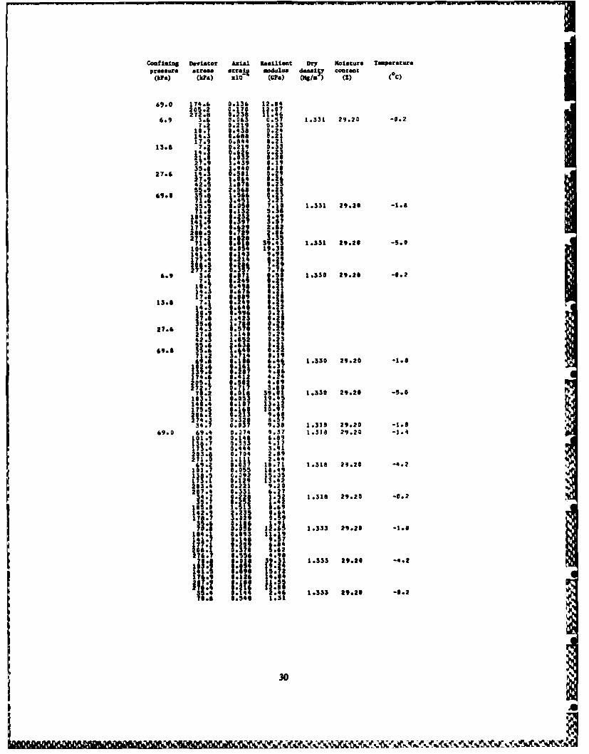
Coufilinsi Deviator ilaI teilllent Dry IHolsture TemperaturePressure Stream utrotl modulus donaiSy content(ka) (kPi) riO (Gin) (M/) () (C)

69.0 174.6 0.136 12:04105 2 01 0 ?02708 0038 146

6.9 3.6 0.063 C057 10331 29.20 -0.2S 0219 0.33

0.438 0.2414.3 0.688 0:2117.N 0.044 0.21

27.9 1.439 0.19

27.6 14.3 096 0 1:1l

I21 1 . aa :

,,. 35. 2a1.9

I., S. so 1.331 29.28 -1.8

174 !! 2h

'" ~:' "" Iii" :1 3 1.330 29.20 -1.8

!!! "'ft1:' i" .3 9.6 -.

2 1.419.45

II:! 001"3.9 . *.i 93 1.33 29.20 -1.8

I !.: h.4* 3.91

1 2038 .80 208

21.0 41,1 1:

5: .29 1~ 1:2 12 a 13.42

203 0.2 9.23

j 2. 2207 0~ .338L : 1.316 29.20 -02

:I0 f, 0 l7 :.3 1.313 29.20 -1.8

.6

138333 29.26 04.2

11:.4 04°° 1:11271.2 !J11 4 .19

a1 0 1 :1 1.330 29.20 -. 2

630

1 19.45

I~4 10. 00:492

00:9 1 914 1 06:89

120 0 002.8

119:2 1-:It 1.318 29.0o -4.211 ll9 N2

6o04;

Ito 0 1:9619 1.333 29.20 -1.8

1i4. : 19 :!! 9!1lll .,, l~li°i 1.333 29.2i -4.2

46 146 1333 9*20 -0.

Subgrade layer, thawed

Coafinla Deviator Radial Axial Reslient Reailient Dry Noiture Moisturepressure stress tr!n strain Poso' a modulus densi~y conteat tenalon

(kba) We~) :1O RIO ratio (lil) (Hg/u ) (Z) We~)

6.9 3.6 .252 1.763 3.032 47.1 1.630 23.80 1..?.2 .151.7: a.2fl 41.:9

1 .7 i.26 2.746 .!37 39.I13.8 7.2 C.136 1.256 0.267 56.P

14.3 f,.757 2.74q ..75 52.r

27.6 14.3 :.421 i.d76 2.,24 76.226.8 1.:09 !.433 o.:63 7C1241.3 2.186 5.85: ^..74 71.6

69.Z 31.7 b?3 2.0Z6 C.23 122.171.4 1.134 6.17!5 -- n1 115.7

6.9 3.6 .169 0.714 1.237 50.8 1.63R 16.20 5.27.3 C.339 1.588 :.213 45.7

1..9 ^.593 2.381 0.249 45.614.5 lo-15 3.497 029: 41.4

17.2 1.185 4.1!4 0.287 41.613.8 7.2 0.169 1.192 3.142 60.7

14.5 .b92 2.3k5 3.248 63.723.8 I.115 3.499 .29C 59.527.1 1.523 5.490 3.299 53.336.2 2.537 6.776 3.374 53.4

27.6 14.5 2.423 1.913 0.221 75.627.1 1.15 3.747 0.271 72.442.9 1.777 5.903 0.301 72.756.4 2.706 7.5:8 C.360 75.2

69.0 36.1 0.676 2.875 0.235 125.672.2 1.691 5.914 0.286 122.2

103.8 2.706 8.328 0.325 124.66.9 3.6 3.C84 0.536 0.157 67.3 1.638 9.38 12.0

7.2 0.253 1.112 0.228 64.910.8 0.422 1.840 0.229 58.714.4 0.675 2.454 0.275 58.717.1 0.844 2.915 0.290 58.6

13.8 7.2 C.168 0.844 C.199 85.214.4 6.506 1.944 0.260 74.020.7 0.675 3068 0:2 67.428.1 1.181 4.141 67.835.9 1.517 5.141 0.295 69.9

27.6 14.4 C.253 1.535 0.165 93.728.1 0.844 3.223 0.262 87.142.6 1.349 4.604 0.293 9M*56.1 2.022 6.450 0.313

69.0 35.9 0.506 2.611 0.194 137.571.8 1.349 5.376 0.251 133.6103.2 2.360 7.688 0.307 134.2

6.9 3.4 ----- 0.364 ----- 93.6 1.638 6.10 17.06.8 0.169 0.889 0.196 76.610.9 0.339 1217 0.210 67.413.2 0.24 2.12 0.194 62417.2 0.678 2.506 0271 68:81q

13.8 6.8 0.169 0.808 0.209 84.213.6 0.339 1.778 0.191 76.520.9 0.593 2.667 0.222 78.327.2 0.932 3.558 0.262 76.434.0 1.101 4.366 0.252 77.9

27.6 13.6 0.254 1:375 8.185 98.927.2 0.593 2.749 0.216 98.940.8 1.316 4.204 0.242 97.655.5 1.524 54662 0.269 98.0

69.0 34.0 0.339 2t386 0.142 142.467.9 1.016 4:531 0.244 149.9106.4 2.0 1 7.448 273 142.914C.3 3.386 9.731 0.348 144.2

6.9 3.6 0.340 0.642 0.530 56.8 1.637 16.20 5.07.3 0.765 1.560 0.490 46.8

10.9 1.360 2.571 0.529 42.614.6 2.038 3.490 0.584 41.817.3 2.294 4.343 0.567 420

13.8 7.3 0.340 1.103 0.308 66.114.6 1.419 2.297 0.444 63.521.0 1.699 3.308 0.514 63.427.3 2.463 4.596 0.536 59.536.4 3.660 6.73 0.603 60.0

27.6 14.6 0.509 1.564 0.325 93.227.3 1.189 3.128 0.383 87.3

27.6 41.J 2.207 4.185 1.461 85.6 1.6Xl 1f.23 5.1

Sb.1 Z.225 6.44A .. 86.469. 36.4 1.764 2.395 1.319 151.9

72.6 2.36 5.160 .!95 141.0114.6 3.225 7.380 0.-37 141.7

6.9 3.4 C.256 2.469 V.546 73.5 1.67 9.30 12.06.9 C.341 .901 '. 41 7..3

10.6 0.597 1.664 3.35a 63.5

13.8 2.768 2.219 3.046 62.117.4 1.222 2.731 3.!74 63.9

13.8 6.9 L.256 C.e54 0.332 63.613.8 0.597 10742 3.333 76.82 :1 :1.22 2.818 J.063 74.927.S 1.449 3.758 0.386 73.334.4 1.789 4.614 0.388 74.5

27.6 13.8 0.20 1.367 3.312 100.627 .937 2.734 a.34 100.643.5 1.704 4.446 0.383 98.055.0 2.386 5.816 0.410 94.6

6.9 3.5 :0.08 0,36 0.237 :6 1.637 6.10 17.0190 0.11 94 0.181 4

6 0428 1.591 .:269 66.82.986 .228 1340 62.2

1 29 0 2.547 174 6.8

- -q - - --- - - - -

Cotining Deviator Radial Axial Resilient Resllient Dry Moisture moisturepressure stresa atrak atrain Polusonas nodulus danalsy content tension

(kPa) (kPa) zlO- IO ratio i4EPa) (Mg/8") (2) (kPa)

13.8 6.9 Z.171 0.819 0.209 84.513.8 0.598 1.729 0.346 600021.2 0.940 2.729 C.344 77.827.6 1.367 3.457 0.395 80.034.6 1.537 4.367 0.352 79.1

27.6 13.8 0.342 1.410 40.243 98.027.6 0.854 2.911 0.293 95.041.5 1.367 4.186 0.327 99.155.3 2.049 5.645 0.363 91.0

69.0 34.6 0598 2.367 0.253 146.069.1 1.452 4.736 0.307 145.9106.0 2.734 7.294 0.375 145.3138.1 3.928 9.496 0.414 145.4

6.9 7.2 0.506 0.996 0.508 72.3 1.634 23.80 1.010.8 0.760 1.828 0.416 59.814.4 1.350 2.831 0.477 50.8

13.8 7.2 0.337 0.832 0.405 86.414., 0 :4 M8 1 915 0490 7518 928.0 2.192 4.508 0.486 62.2

27.6 14.4 0.506 1.419 0.357 101.221:1 1.011 292' 0.604 2.022 4.853 0.41 85.5

6.9 3.7 00332 110.3 1.634 9.30 12.07.3 0.170 0.830 0.205 88.211.0 0.511 1.494 0.342 73.514.6 &.766 1.991 0.385 73.517.4 0.851 2.572 0.331 67.6

13.8 7.3 0.170 0.788 0.216 92.914.6 0.510 1.659 0.!07 88.221.0 0.766 2.531 3.303 83.227.5 1.192 3.320 0.359 82.736.6 1.703 4.650 3.366 78.7

27.6 14.6 0.341 1.162 3.293 126.027.5 C.681 2.492 4.273 110.241.2 1.277 3.988 0.20 103.356.0 1.872 5.570 0.336 100.5

69.0 36.6 C.510 2.162 0.236 169.173.1 1.361 4.825 3.2b2 151.6

109.7 2.127 7.331 0.290 149.66.9 3.4 0.089 0.490 0.182 69.7 1.634 6.10 17.0

6.8 0.169 0.899 C.188 75.911.9 G0.340 1.552 0.219 70.413.6 0.424 1.961 0G.16 69.617.3 0.509 2.533 3.231 680.2

13.8 6.8 0.085 0.817 0.124 83.513.6 0.339 1.634 .2Z7 83.420.9 0.509 2.533 0.201 82.528.4 3.848 3.432 .'47 82.734.1 1.217 4.21.0 C.239 A1.2

27.6 13.6 C.169 1.1:8 .12v 14.227.6 27.3 C.5:9 2.615 ;.195 1:4.2 1.634 6.10 17.C

5b.6 1.272 5.396 .26 1 5.269.0 54.1 L.254 1.963 0.129 17'.E

68.1 L.678 4.253 2.15q 16;.2104.5 1.357 6.547 ).2:7 159.6136.3 2.635 2.375 0.17 573.9

6.9 3.8 0.348 0.666 0.521 57.2 1.62! 23.80 1.07.6 1. 42 1.733 .. 6.1 441.311.4 2.428 2.b86 02.S4 42.4

13.8 7.6 .6c7 1.116 ,.549 68.515.2 1.648 2.608 0.613 56.522.3 3.115 4.762 ;.654 46.7

27.6 15.1 ;.693 1.905 0.364 79.529.6 1.558 3.814 3.4e8 77.644.9 3.805 6.378 0.597 70.4

69.0 37.8 0.951 2.711 0.351 139.475.6 2.249 5.593 J.402 135.1

6.9 3.8 0.173 ..676 3.256 56.2 1.625 13.50 6.07.6 0.780 1.353 0.576 56.111.4 1.387 2.369 0.585 48.015.1 2.077 3.390 0.613 44.7

13.8 7.6 0.346 1.186 0.292 63.915.1 1.212 2.373 0.511 63.821.8 1.991 3.561 0.559 61.128.3 3.285 5:100 0.644 55.5

27.6 15.1 1.692 10700 0.407 88.828.3 1.555 3.400 0.457 83.344.8 2.766 5.616 0.493 79.858.8 4.833 7.682 0.629 76.5

69.0 37.6 0.863 2.561 0.337 146.975.3 2.070 5.637 0.367 133.5

110.4 3.796 8.559 0.444 129.07.7 0.349 0.747 0.467 102.6 1.625 9.30 12.011.5 0.522 1.337 0.390 85.915.3 0.871 1.889 0.46111:1 :44 2.3 2 0.44213.8 630 0414 121,615.3 0.61 1.496 0.408 10 .422.1 1.044 2.363 0.442 95.2

287 1:391 3:3101 00421 86.73802 208 40419 0.472 8.

27.6 15.3 0.348 1.184 0.294 129:128.7 0.870 2.525 0:345 113.545.4 1.740 4.105 0.424 110.659.7 2.607 5.533 0.471 107r8

69.0 380.2 0.783 2.055 0.381 185.876.4 1.739 4.745 0.366 160.9

109.8 2.956 7.127 0.415 154.16.9 7.1 0017 0.465 00372 153.5 1.625 6.10 170

10.9 0.347 0.968 0.358 113.014.3 0.521 1.394 0.374 102.417.1 0.928 1.782 0.521 96.1

32

I~n

Confining Deviator Radial Axial Resilient Resilient Dry Moisture Moisturepressure stress stragn strain Poisson's modulus densi~y content tension

(kPa) (kla) X1O X10 ratio (Pa) ( g/u ) (Z) (kPa)

13.8 14.3 0.434 1.240 0.350 115.121.9 0.781 1.937 0.403 113.026.5 1.041 2.790 0.373 102.335.7 1.476 3.565 0.414 100.1

27.6 14:3 0.347 1007 0.345 141.728.5 C781 2.170 0.36C 131.6

42.8 1.215 3.565 0:341 120.054.7 1.909 4.651 a.413 117.5

69.0 35.6 0520 1.860 0.280 191.771.3 1.215 4.341 0.28G 164.2

109.2 2.515 7.138 0.352 153.06.9 3.8 0.390 98.2 1.53C 9.30 12.0

7.7 C.348 1.341 0.334 73.511.0 0.522 1.648 C0.17 66.814.4 0.871 2.255 0.386 63.717.7 1. 44 2.776 0.376 63.8

13.8 7.2 0.261 0.824 0.317 87.314.3 01.609 1.735 C.351 82.621.5 3.957 2.689 3.35b 80.C28.6 1.391 3.645 0.382 78.635.8 1.913 4.514 0.424 79.3

27.6 14.3 3.348 1.359 C.251 1:3.127.6 28.6 2.956 2.778 3.344 103.1 1.531 9.10 12.,

44.1 1.564 4.167 31.375 116.:54.9 2.26C 5.3S4 1.42: 1Q2.1

69.C 35.8 2.,09 2.384 0.292 171.871.6 1.391 4.343 '.32' 164.8109.7 2.6;6 b.954 2.!75 i57.8

6.9 3.8 .173 0.497 3.348 76.3 1.6,7 23.P3 1.07.b 0.433 1.325 3.327 57.2

11.4 C.693 !.988 3.349 57.215.1 1.126 2.936 3.377 50.7

13.8 7.b 0.173 -. 95 1.174 76.11t .I :.S19 2.11,7 3.241 70.222.3 1.:38 3.322 3.312 67.029.5 1.385 4.406 1.38 65.7

27.6 15.1 5.34f6 1.495 0.231 lCI.929.5 C.865 3.331 0.263 88.744.9 1.817 5.339 3.34C 84.1

69.0 37.8 0.692 2.523 0.276 151.175.6 1.644 5.851 0.2dl 129.3

6.9 7.4 0.!43 0.767 0.447 96.8 1.627 13.50 6.011.1 0.514 1.324 0.394 85.414.8 1.857 1.994 0.433 74.518.1 1.028 2.379 0.432 76.1

13.8 14.8 3.600 1.535 0.391 96.721.8 1.C28 2.456 6.419 88.827.8 1.371 3.226 0.425 86.237.0 2.054 4.459 0.461 83.1

27.6 14.8 90.343 1.230 0.279 120.527.8 0.856 2.460 0.348 113.044.0 1.541 3.999 0.385 110.055.5 2.226 5.388 0.413 103.0

69.0 37.0 0.513 2.001 0.256 185.074.0 1.370 4.314 0.318 171.6

106.3 2.224 6.487 0.343 163.96.9 3.9 0.088 0.368 0.239 105.3 1.607 9.30 12.0

7.7 0.263 0.818 0.322 94.711.6 0.525 1.309 0.401 88.815.5 0.700 1.759 0.398 87.918.4 0875 2.128 0.411 86.4

13.8 7.7 0.175 0.655 0.267 118.215.5 0.525 1.432 0.367 108.122.3 8.788 2:291 0.344 97.229.0 312 3.027 0.433 95838.7 1.925 4:090 0.471 94.5

27.6 15.5 C.350 1.146 0.305 135:029.0 0.700 2.456 0.285 118.144.7 1.400 3.767 0.372 118.758.0 2.099 5.079 0.413 114.2

69.0 37.5 0.525 2.089 0.251 179.372.5 1:400 4:261 0329 170.1111.2 2.623 6.564 0.400 169.4

6.9 3.5 ----- 0.337 102.9 1.607 6.10 17.06.9 0.171 0.675 0.253 102.6

10.6 0.342 1.181 0.290 89.913.8 C.342 1.518 0.225 91.217.1 0:684 1.856 0.369 92.013.8 6.9 0.170 0:675 0.252 102.513.8 0342 1,350 0.253 102.521.2 0.684 2.025 0.!38 104.827.6 0.940 2.700 0.348 102.434.6 1.281 3:544 0.361 97.5

27.6 13.8 0.342 1.181 0.290 117.026.5 0.512 2.194 0.233 120.842.6 1.025 3.375 0.304 126.355.2 1.536 4.558 0:337 121.2

69.0 34.5 0.427 1.941 0.220 177.869.0 1.024 3.884 0.264 177.8105.9 1.964 6.250 0.314 169.4

46

33.

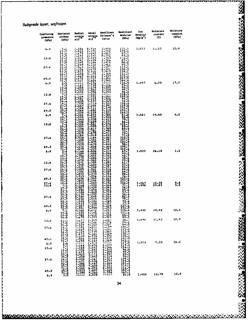
Subgrade layer, unfrozen

Confinin8 Deviator Radial AII Resilient lsilient Dry moisture Molsture

Pressure stress *train :train OcaG*on't modulusl densi~y contet tensgioni4

(kha) (kPa) :10 17 ratio (O0a) (g/S ) () (kPa)

6.9 7.1 .336 0.714 3.471 100.1 1.5!! 1t.13 12.010.7 3.420 1.371 5.!92 100.114.3 :.673 1.643 3.41L 87.r17.9 :.841 2.143 0.!,2 83.3

13.8 14.3 L.t24 1.429 :.!53 112.C21.2 3.641 2.429 0.34h 87.327.9 1.345 3.144 ..4^8 88.835.7 1.849 4.;02 3.462 P9.!

27.6 14.3 2.544 1..72 0.477 133.127.9 10.38 2.t73 0.302 108.342.4 1.512 3.716 0.4C7 114.C5b.? 1.848 5.;"4 J.369 111.371.3 2.687 6.153 0.437 115.8

69.0 35.6 0.672 1.717 0.391 207.571.3 1.511 3.865 0.391 184.4

6.9 3.5 0.296 118.9 1.497 6.80 17.07.0 C.167 C.739 0.226 95.2

10.6 0.250 1.109 0.225 95.214.1 0.333 1.552 0.215 90.717.2 0.501 1.996 3.251 86.0

13.8 7.0 C.592 118.914.1 G.334 1.331 0.251 105.820.9 C.501 2.219 0.226 94.128.6 0.835 3:107 0.269 92.0

27.6 14.1 Z.334 1.110 0.301 1260827.5 0.667 2.294 0.291 119.041.8 1.168 3.111 0N375 134.3

69.0 35.2 0.584 1.852 0.315 190.070.4 1.335 4.154 0.321 169.5

6.0 1:8 0336 0072 0.385 01.8 1.521 14.80 6.006 504 1.235 0.408 86.6

14.3 0.840 2.035 0.413 70.117.8 1008 2.689 0.375 66.3

13. 7.1 0.336 0.581 0.578 122.714.3 0.504 1.599 0.315 89.221.2 1.008 2.617 0.385 00.927.8 1.512 3.781 0.400 13.735.6 2.015 4.875 0.413 73.135.6 2.184 5.019 0.435 71.0

27.6 14.3 0.420 1.164 0.361 122.527.8 1.008 2:581 0.391 107.9

42.3 1.511 4.075 0.371 103.955.7 20519 5.679 0.444 98.1

69.0 35.6 C.672 1.820 0.369 195.771.2 1.679 4.225 0.397 16..6

6.9 3.6 00168 0.526 0.319 67.7 1.523 26.10 1.07.1 0504 1448 0.348 49.210.7 0.756 2.501 0:302 42.714.2 1.175 3.686 0.319 38.617.0 1.678 4.083 0.411 43.5

13.8 14.2 0.671 2.305 0.291 61.721.1 1.342 3.689 0.364 57.227.7 2.011 5.140 0.!91 54.0

27.6 14.2 0.503 1.581 0.318 89.827.7 1.006 3.295 0.305 84.242.2 1.844 5.273 0.350 80055.4 30015 7.256 0.416 76.4

69.0 35.5 0.838 2.309 0.363 153.670.9 1.843 5.146 00358 137.9

27.6 14.0 0.333 1.289 0.258 108.5 1.469 12.30 8.0

13.8 7.1 0.168 1.000 0.168 71.0 1.496 23.80 3.014.2 0587 2.429 0242 58.521.1 1.006 3.858 0.261 54.627.7 1.508 4.860 0.310 57.135.5 2.179 6.293 0.346 56.4

27.6 14.2 0.335 1.645 0.204 86.327.7 0.838 3.5C4 0.239 79.142.1 1.508 5.293 1.285 79.655.4 2.513 7.159 0.351 77.4

69.0 ;5.5 0:587 2.577 0.228 137.670.9 5.299 0.253 133.9

6.9 7.1 0.168 0.672 3.25S 105.4 1.496 10.40 12.010.6 C.335 1..45 0.321 101.614.2 C0502 1.642 .306 86.216.8 0.b 70 2.J91 0.321 80.5

13.a 21.1 ' 2.35 3.2A' de.. 1.496 10.43 12.127.6 1.10k 3.Zb6 3.3,6 84.135.4 1.339 4.163 1.321 84.527 14.1 1.335 1.1 5 .z9q 126.!

27.6 C.669 2.3.C 1.24 115.642.0 1.234 3.735 0.26i 112.455.3 1.673 5.381 0.329 108.77C.7 2.n39 6.728 3.373 105.1

69.G 35.4 :.586 1.944 0.321 181.970.7 1.255 4.337 0.289 163.1

6.9 3.6 -- 3-- C.3t3 . 117.4 1.5 P.30 18.0C

7.1 0.168 0.606 0.277 117.413.8 7.1 :.168 0.662 0.246 104.3

14.2 ;.336 1.443 0.233 98.821.1 0.671 2.273 0.295 92.9

2 :923 3.0C3 0.297 89.535. 1.258 3.942 0.319 90.2

27.6 14.2 0.336 1.661 0.317 134.027.8 0,o71 2.426 0.277 114.542.2 1.006 3.4R7 0.289 121.0 N55.5 1.509 4.859 00311 114.371.0 2:180 6:373 0.342 111.4

69.0 35.5 0.503 1.897 0:265 187.271.0 1.090 4.250 0.256 167.1

6.9 3.5 0.429 81.0 1.456 10.70 12.0

348

Cof Ln DevLator RadLal AxLal Rasillent RasilLent Dry HoLiture Moisturepressure stress strain strain Poion ouu dniy cott tein

(kPea) (kPa) ZO Z raio (MPa) (Mg8m) (Z) (kPa)

7.0 0.786 88.513.8 7.0 0.71% 97.4

13.9 0.332 1.715 0.194 81.120.6 0.584 2.715 0.215 76.027.2 00.13 3.574 0.255 76.0

27.6 13.9 0.332 1.215 0.273 114.527.2 0.664 2.788 0.238 97.441.3 1.162 4.436 0.262 93.1

69.0 34.8 0.664 2.147 0.309 161.969.5 1.660 4.873 0.341 142.7

6.9 3.5 0.357 980.6 1.474 21.30 4.07.0 0.334 1.000 0.334 70.4

10.6 0.500 1.786 0.280 59.114.1 0.835 2.572 00325 54.717.6 1.168 3.431 0.340 51.3

13.8 7.0 0.250 0:715 0.350 98.414.1 0.668 1787 0.374 78.820.9 1.001 3.C03 0.333 69.627.5 1.502 4.05 0.375 68.635.2 2.169 5.295 0.410 66.4

27.6 27.5 1.901 2.647 0.378 103.941.7 1.668 4.008 0.416 104.054.9 2.669 5.732 0.466 95.9

6.9 14.2 1.341 2.649 0.506 53.6 1.489 23.90 3.017.8 1.761 3.384 0.520 52.5

13.8 7.1 0.335 0.736 0.455 96.514.2 0.838 1.913 0.438 74.221.1 1.508 3.691 0.488 68.227.7 2.010 3.27 0.525 72.435.5 3.315 5.07 0.602 70.8

27.6 27.7 1.005 2:04 0.401 110.742.1 1.843 4.125 0.447 102.155.4 2.680 5.307 0.505 104.3

6.9 7.0 00500 1.172 0.427 60.0 1.477 26.70 2.010.5 0.834 1.859 0.449 56.814.1 1.335 2.575 0.518 54.6

13.8 14.1 0.834 1.788 0.466 78.620.9 1.335 3.C6 0.444 69.4

27.6 27.5 1.168 2.578 0.453 1;6.635.2 1.SC1 3.870 0.388 90.9

6.9 1C.6 0.335 0.811 0.413 131.3 1.505 9.30 18.914.2 C.503 1.32 0.487 137.617.3 0.671 1.621 0.414 106.8

13.8 14.2 C.335 10.32 0325 137.621.1 0.671 1.843 3.364 114.427.7 1-o06 2.653 0.379 104.635.5 1.341 3.391 3.095 I4.7

27.6 27.7 C.671 1.319 G.353 144.642.2 1.174 2.949 0.398 143.0

27.6 73.9 2.346 5.6;8 6.41P 12E.t 1.90, 5.30 18.369.0 35.5 :,b67 1.476 :.-96 24L.5

70.9 1.57 3.!Q5 3.371 209.:6.9 !.5 .... 0.20 - - 122.5 1.476 7.10 19.0

7.3 - .b5

2 107.213.5 3.166 1.087 0.153 96.4

13.8 14.0 0.333 1.377 0 .42 101.520.8 C.333 2.174 P.153 95.427.3 :.666 2.899 3.03L 34.234.9 3.832 3.768 0.221 92.7

27.6 14.0 Z.166 1.334 C.127 17.228.4 C.666 2.536 0.263 111.941.5 C.832 4.059 0.2L5 112.254.6 1.165 5.075 3.k33 107.6

6.9 3.5 0.468 75.3 1.496 15.10 6.07.1 0.167 1014 0.165 69.510.6 0.340 1.561 0.218 67.0814.1 0.501 2.185 0.229 64.517.6 0.668 2.731 0.245 64.6

13.8 7.1 0.167 0.936 0.178 75.314.1 0.334 1.795 0.186 78.620.9 0.668 2.653 0.252 78.926.1 1.003 3.590 0.279 72.635.3 1.337 4.528 0.295 77.9

27.6 14.1 0.334 1.483 0.225 95.128.6 0.668 2.967 0.225 96.628.6 0.501 2:967 0.169 96.641.9 1.002 4.374 0.229 95.755.0 1.670 5.859 0.285 93.970.4 2.505 7.431 0.337 94.8

69.0 35.2 0.334 2.190 0.153 160.870.4 1000 4:382 0:228 160.8

6.9 3.5 0.167 0.714 0.234 49.5 1.504 26.40 1.87.1 0.335 1.393 0.240 50.8

10.6 0.502 2.143 0.234 49.514.1 0.837 2.059 0.293 49.517.7 1.171 3.716 0.315 47.6

13.8 7.1 0.167 1.108 0.151 63.814.1 0.669 2.216 0.302 63.821.0 1.003 3.288 0.305 63.8P.06 1.505 4.573 0.329 60.3

35.3 2.006 5.721 0.351 61.827.6 14.1 0.334 1.645 0.203 85.914.1 0.334 1.645 0.203 85.927.6 0.836 3.218 0.260 85.841.9 1.338 4.721 00283 88.955.1 2.005 6.153 0.326 89.6

6.9 3.5 ----- 0.294 120.5 1.509 10.30 12.0 S.7.1 0:168 0.662 0:254 107.1

10.6 0.335 1.103 0.304 96.414.2 0.502 1.618 0.310 87.617.7 0.670 2.059 0,325 86.1

35

L,+.,p'.t

+~ 5% p V % '. .. +% ... I, .' . %''..' '%' VV '.

Confining Deviator Radial Axial Resilient Resilient Dry Moisture Moisture

pressure stress strain strain Poisson's modulus density content tension

(kPa) (kPa) 10 x10 ratio ()Pa) (Ha/a (Z) (kPa)

13.8 7.1 C.168 0.588 0.286 120.514.2 0.335 1.397 0.240 101.521.0 0.670 2.206 0.304 95.327.6 0.837 2.795 0.299 98.935.4 1.172 3.678 0.319 96.2

27.6 14.2 0.168 1.103 0.152 128.427.6 0.502 2.207 0.227 125.342.0 1.004 3.384 0.297 124.255.3 1.506 4.857 0.310 113.970.8 2.175 6.331 0.344 111.8

69.0 35.4 0.335 2.208 0.152 160.170.7 1.004 4.122 0.244 171.6

6.9 10.6 C.334 0.716 0.466 147.6 1.503 6.80 17.014.1 0.417 1.146 0.364 122.917.6 0.417 1.575 3.265 111.8

13.8 14.1 C.334 1.G74 0.311 131.220.9 0.501 1.648 3.!04 126.9 -

28.6 0.835 2.293 3.!64 124.735.2 1.G02 3.297 01.314 IC6.7 I,

27.6 14.1 c.250 0.788 0.!17 178.7 V.27.5 C.667 1.79i .!. 72 153.4.F41.8 1.302 3.298 0.304 126.7

67.2 35.2 .CL 1.5p. C.316 222.7 1.50! 6.80 17.073.4 1.166 3..A3 3.-"1 181.4

6.9 7.1 ?.168 1.224 :.164 69.3 1.52r 14.A3 6.010.6 .!35 1.571 .1! A7.714.2 2.587 -:1,,5 c.:6S 64.517.7 *.d38 2.t68 ..- 61.q

17.7 2.838 2.868 .i9) 61.913.4 7.1 :.168 3.6F8 G.1Q 7q.1

14.2 Z.419 1.644 .227 77.1,21.1 C..70 2.731 0.24C 77.127.7 1.35 3.689 C.272 75.135.5 1.548 4.L46 ;.325 76.3

27.6 14.2 C.251 1.296 .193 10-.327.7 C.67 2.665 ..1 114.^42.1 1.173 4.121 ;.286 1C2.798.8 1.843 5:6J7 u.32

9 176.3

69.0 35.5 1.563 2.872 C.175 123.570.9 1.173 4.652 C.252 152.5

6.9 7.1 0.334 1.143 1.292 61.7 1.517 26.20 1.010.6 3.669 1.714 0.39C 61.8 to14.1 1.03 2.501 0.431 56.5 1.

17.6 1.337 3.145 0.425 56.113.8 7.1 1.167 0.929 0.180 76.0 4

14.1 C.501 1.930 0.26C 73.220.9 1.CQ3 2.664 0.!51 73.3 45

27.6 1.671 4.005 0.417 68.835.3 2.339 5.295 0.442 66.6

27.6 14.1 0.417 1.288 0.324 109.527.5 1.002 2.719 0.369 101.341.9 1.671 4.294 0.389 97.555.0 2.338 5.729 0.408 96.1

6.9 3.5 ----- 0:606 58.37.1 0.335 1.212 0.276 58.3

10.6 0.669 1.895 0.353 55.914.1 0.858 2.425 0.354 58.317.6 1.003 3.184 0.315 55.43.6 0.379 94.2 1.542 10.11 12.07ol 0.168 0.909 0.185 78a510.7 0.336 1.364 0.246 78.514.3 0.504 1.742 0.289 82.017.8 0.672 2.122 0.317 84.1

13.8 7.1 0.168 0.758 0.222 94.214.3 0.336 1.516 0.222 94.221.2 0.588 2.273 0.259 93.227.9 G.841 3.031 0.277 92.035.7 1.177 4.093 0.288 87.2

27.6 14.3 0.336 1.137 0.296 125.6

27.9 0.672 2.426 0.277 114.942.4 1.008 3.866 0.261 109.655.8 1.345 5.05 0.269 111.471.4 2.016 6.829 0.295 104.5

69.0 35.7 C.504 2.200 0.229 162.271.4 1.108 4.b54 0.221 156.7

_ e .

,.

'4

36

:,0 6.2

A facsimile catalog card in Library of Congress MARCformat is reproduced below.

Cole, David M.Resilient Modulus of Freeze-Thaw Affected Granular

Soils for Pavement Design and Evaluation. Part 3: Lab-oratory tests on soils from Albany County Airport / byDavid M. Cole, Diane L. Bentley, Glenn D. Durell andThaddeus C. Johnson. Hanover, N.H.: Cold RegionsResearch and Engineering Laboratory; Springfield, Va.:available from National Technical Information Service,1987.

iii, 40 p., illus.; 28 cm. (CRREL Report 87-2.)Bibliography: p. 15.1. Airfields. 2. Freezing-thawing. 3. Laboratory

tests. 4. Repeated-load triaxial tests. 5. Resilientmoduli. 6. Roads. 7. Soil tests. 8. Subgrade soils.I. Bentley, Diane L. II. Durell, Glenn D. III. Johnson,Thaddeus C. IV. United States. Army. Corps of Engi-neers. V. Cold Regions Research and Engineering Lab-oratory, Hanover, N.H. VI. Series: CRREL Report 87-2.

U. 5. GOVERNMENT PRUN.TIN, OFF 1E: 1987--00-1 0-12,077

* V ~ ~S..:%.,,